Digital Predistortion of Wideband Satellite CommunicationSignals with Reduced Observational Bandwidth and Reduced

Model Order Complexity

Pedro Miguel Brinco de Sousa

Thesis to obtain the Master of Science Degree in

Aerospace Engineering

Examination CommitteeChairperson: Prof. Doutor João Manuel Lage de Miranda LemosSupervisor: Prof. Doutor António José Castelo Branco RodriguesMember of the Committee: Prof. Doutor Rui Miguel Henriques Dias Morgado Dinis

November 2014

ii

Para ela.

Onde quer que esteja.

iii

iv

Acknowledgments

F IRST of all, I would like to appreciate all the dedication, knowledge and support given to me by my supervisor

Pere Gilabert, from the moment in which we first discussed this thesis up until the moment I presented it. I

would also like to address my gratefulness to other people with whom I shared the five months I spent in the Signal

Theory and Communications (TSC) department of Universitat Politecnica de Catalunya, namely Gabriel Montoro

Lopez and my fellow peers who also endured their task of developing a master thesis: Giacomo Pojani and Teng

Wang.

I also appreciate the prompt availability of my supervisor in Portugal, Antonio Rodrigues, in accepting my

thesis proposal and to make the necessary arrangements in order to make it possible.

I would like to show my gratitude for all my friends in Barcelona, especially Ana Hernandez, Basak Anayurt,

Carmen Quevedo, Celeste Miquilena, Ezgi Ustun, Fatih Andic, Misel Gannoum, Wiktor Walasik and all my MAST

colleagues, who all contributed for my growth as an individual by introducing me to their different cultures and

also for making the year I spent in Barcelona unforgettable.

Furthermore, and because five years is a long journey to be fought, I would like to address to my friends at

Instituto Superior Tecnico, namely Ana Vilhena, Andre Cardeira, Joao Andrade, Joao Clemente, Miguel Rita,

Tiago Pinto, Telma Oliveira and all my other Aerospace Engineering Master colleagues. I really appreciate the

motivation and continuous support you gave me, the countless fun we had together and also for making me feel at

home in Lisbon.

I cannot conclude this acknowledgement without referring to the friends I have in Oliveira de Azemeis, my

home-town, and also across the country, each of them giving the best they can, twenty-four-seven, to make me a

better, happier and wiser person. I must highlight some of them: Diogo Costa, Goncalo Almeida, Ines Barbosa,

Ines Ramalho, Isabel Dias, Isabel Magalhaes, Mariana Silva, Manuel Melo, Joao Costa, Joana Pereira, Joana

Raquel, Rafaela Goncalves, Regina Costa and Sara Cruz. Apart from these, I have to acknowledge individually

the person who supported me throughout the hardest days of my life, who stood by me in my biggest challenges

and who was also there to celebrate my conquests, Filipa Almeida, and also the little sister I wish I had, the one I

saw growing up to be the woman she is now and to whom I proudly answered to her countless requests for advice

in order to help her find her way to success and happiness, Carla Almeida.

And last, but not the least, I would like to thank all the support, love and courage given to me by my family,

especially my father Jose and grandparents Angelina and Antonio for raising me the man I am today and for

giving me the opportunity to achieve higher grounds. This appreciation is extended to my godmother Isabel for her

unflagging dedication and support and to my aunt Fatima, my uncle Victor and my cousin Joana without whom I

cannot consider my family complete.

v

vi

Resumo

A S comunicacoes sem fio sao cada vez mais procuradas pelos utilizadores, o que requer uma infraestru-

tura que ofereca capacidade, seguranca e eficiencia a nıveis cada vez maiores. Um dos pontos crıticos

no processo das telecomunicacoes, no que ao hardware diz respeito, e o amplificador de potencia (PA): nao so

e o dispositivo que consome mais potencia na cadeia de transmissao, mas tambem o que apresenta uma carac-

teristica altamente nao-linear e que pode comprometer os requerimentos necessarios ao bom funcionamento das

comunicacoes.

Esta tese aborda a tecnica da pre-distorcao digital (DPD), cujo objectivo e reduzir a influencia da nao-linearidade

introduzida pelo PA no sinal transmitido, e explora duas contribuicoes para esta tecnica que buscam uma maior

eficiencia computacional e economica sem comprometer a capacidade da DPD. A primeira contribuicao foca-se

na realimentacao necessaria para o DPD. Nela procura-se capturar sinais de banda larga usando multiplas capturas

com uma largura de banda reduzida. Na segunda, o objectivo e reduzir o numero de coeficientes necessarios para

a DPD, suprimindo os modos que menos influem na descricao da caracteristica do PA. Adicionalmente, aplicou-se

a tecnica de reducao do PAPR do sinal tendo em vista uma maior eficacia do DPD na linearizacao do sinal.

A campanha experimental, realizada com um dispositivo real, provou que a reducao da largura de banda de

observacao e realizavel. Esta conclusao e apoiada no facto de que foram obtidos resultados similares usando esta

tecnica e usando uma observacao total do espectro do sinal.

Palavras-chave: comunicacoes por satelite, amplificador de potencia, linearizacao, pre-distorcao digi-

tal

vii

viii

Abstract

T HE increase in the demand for wireless communications from the user-end point of view calls for an in-

frastructure that is constantly more capable, reliable and efficient. One of the critical nodes in the telecom-

munications process, from the hardware perspective, is the power amplifier (PA): it is not only the more power-

consuming device in the transmission chain but it also has a highly nonlinear behaviour which can compromise the

well-functioning of the communications infrastructure.

This thesis addresses the digital predistortion (DPD) technique, whose goal is to reduce the nonlinear influence

of the PA in the transmitted signal, and enhances it with two contributions which can allow for a bigger com-

putational and economic efficiency without compromising the effectiveness of DPD. These contributions are the

Reduced Observational Bandwidth and the Reduced Model Order. In the former, the observational path required

for the implementation of the DPD is redesigned to permit the capture of wideband signals using multiple reduced

bandwidth observations. The latter, on the other hand, aims at reducing the number of coefficients needed for DPD

by discarding the less contributive modes of the PA behavioural model. Additionally, the technique of reducing

the signal PAPR is applied in order to seek a more effective predistortion.

The experimental campaign in a real DUT proved that the reduction of the observational bandwidth was feasible

and produced similar results when compared to a full spectrum observation.

Keywords: satellite communications, power amplifier, linearisation, digital predistortion

ix

x

Contents

Acknowledgments . . . . . . . . . . . . . . . . . . . . . . . . . . . . . . . . . . . . . . . . . . . . . . v

Resumo . . . . . . . . . . . . . . . . . . . . . . . . . . . . . . . . . . . . . . . . . . . . . . . . . . . vii

Abstract . . . . . . . . . . . . . . . . . . . . . . . . . . . . . . . . . . . . . . . . . . . . . . . . . . . ix

List of Tables . . . . . . . . . . . . . . . . . . . . . . . . . . . . . . . . . . . . . . . . . . . . . . . . xiii

List of Figures . . . . . . . . . . . . . . . . . . . . . . . . . . . . . . . . . . . . . . . . . . . . . . . . xv

Nomenclature . . . . . . . . . . . . . . . . . . . . . . . . . . . . . . . . . . . . . . . . . . . . . . . . xvii

Glossary . . . . . . . . . . . . . . . . . . . . . . . . . . . . . . . . . . . . . . . . . . . . . . . . . . . xix

1 Introduction 1

1.1 Motivation . . . . . . . . . . . . . . . . . . . . . . . . . . . . . . . . . . . . . . . . . . . . . . . 1

1.2 Objectives and Methodology . . . . . . . . . . . . . . . . . . . . . . . . . . . . . . . . . . . . . 2

1.3 Outline of the Thesis . . . . . . . . . . . . . . . . . . . . . . . . . . . . . . . . . . . . . . . . . 3

2 Problem Statement 5

2.1 Nonlinear Behaviour of a Power Amplifier . . . . . . . . . . . . . . . . . . . . . . . . . . . . . . 5

2.1.1 The Memoryless Complex Power Series Model . . . . . . . . . . . . . . . . . . . . . . . 5

2.1.2 Nonlinear distortion . . . . . . . . . . . . . . . . . . . . . . . . . . . . . . . . . . . . . 6

2.1.3 A quantitative measure of nonlinearity . . . . . . . . . . . . . . . . . . . . . . . . . . . . 8

2.2 Linearity vs. Efficiency . . . . . . . . . . . . . . . . . . . . . . . . . . . . . . . . . . . . . . . . 10

2.3 Memory Effects . . . . . . . . . . . . . . . . . . . . . . . . . . . . . . . . . . . . . . . . . . . . 11

3 Towards Digital Predistortion 13

3.1 System-Level Linearisation Methods . . . . . . . . . . . . . . . . . . . . . . . . . . . . . . . . . 13

3.2 Principles of Digital Predistortion . . . . . . . . . . . . . . . . . . . . . . . . . . . . . . . . . . 15

3.2.1 Model Behaviour . . . . . . . . . . . . . . . . . . . . . . . . . . . . . . . . . . . . . . . 16

3.2.2 Adaptive Implementations . . . . . . . . . . . . . . . . . . . . . . . . . . . . . . . . . . 18

3.3 PAPR Reduction . . . . . . . . . . . . . . . . . . . . . . . . . . . . . . . . . . . . . . . . . . . 21

4 Reduced Observational Bandwidth 23

4.1 Analogue-to-Digital Conversion . . . . . . . . . . . . . . . . . . . . . . . . . . . . . . . . . . . 23

4.2 The Windowing technique . . . . . . . . . . . . . . . . . . . . . . . . . . . . . . . . . . . . . . 24

4.3 Signal Reconstruction . . . . . . . . . . . . . . . . . . . . . . . . . . . . . . . . . . . . . . . . . 25

xi

4.4 Frequency Estimation . . . . . . . . . . . . . . . . . . . . . . . . . . . . . . . . . . . . . . . . . 26

5 Model Order Reduction 29

5.1 Principal Component Analysis . . . . . . . . . . . . . . . . . . . . . . . . . . . . . . . . . . . . 29

6 Experimental Campaign 33

6.1 Experimental Set-up . . . . . . . . . . . . . . . . . . . . . . . . . . . . . . . . . . . . . . . . . 33

6.2 Test Signals . . . . . . . . . . . . . . . . . . . . . . . . . . . . . . . . . . . . . . . . . . . . . . 35

6.3 The ADC Emulation . . . . . . . . . . . . . . . . . . . . . . . . . . . . . . . . . . . . . . . . . 35

6.4 Experimental Results . . . . . . . . . . . . . . . . . . . . . . . . . . . . . . . . . . . . . . . . . 37

7 Conclusions 47

7.1 Achievements . . . . . . . . . . . . . . . . . . . . . . . . . . . . . . . . . . . . . . . . . . . . . 48

7.2 Future Work . . . . . . . . . . . . . . . . . . . . . . . . . . . . . . . . . . . . . . . . . . . . . . 48

Bibliography 51

xii

List of Tables

2.1 Efficiency and Linearity of PA depending on its Operation Class. . . . . . . . . . . . . . . . . . . 10

2.2 Various linearisation techniques . . . . . . . . . . . . . . . . . . . . . . . . . . . . . . . . . . . 11

3.1 NMSE and ACEPR for three Memory Polynomial model configurations. . . . . . . . . . . . . . . 17

3.2 Evolution of NMSE with the reduction of PAPR in a LTE-CA signal with two intra-band non-

contiguous carriers. . . . . . . . . . . . . . . . . . . . . . . . . . . . . . . . . . . . . . . . . . . 22

6.1 Comparison of Full and Reduced Observational Bandwidths in a Single LTE signal. . . . . . . . . 37

6.2 Comparison of Full and Reduced Observational Bandwidths in a LTE-CA Signal. . . . . . . . . . 37

6.3 Effect of the number of estimation coefficients in the DPD in a Single LTE Signal. . . . . . . . . . 38

6.4 Effect of the number of estimation coefficients in the DPD in a LTE-CA Signal. . . . . . . . . . . 38

6.5 Comparison between Time and Frequency Estimation in a Single LTE Signal. . . . . . . . . . . . 39

6.6 Comparison between Time and Frequency Estimation in a LTE-CA Signal. . . . . . . . . . . . . 39

6.7 Evolution of NMSE with the reduction of PAPR used in this experiment, for the Single LTE signal. 40

6.8 Effect of PAPR reduction on the DPD in a Single LTE Signal. . . . . . . . . . . . . . . . . . . . 40

6.9 Evolution of NMSE with the reduction of PAPR used in this experiment, for the LTE-CA signal. . 40

6.10 Effect of PAPR reduction on the DPD in the LTE-CA Signal. . . . . . . . . . . . . . . . . . . . . 41

xiii

xiv

List of Figures

1.1 Iridium communications satellite . . . . . . . . . . . . . . . . . . . . . . . . . . . . . . . . . . . 2

2.1 Ideal and Real behaviours of a Power Amplifier . . . . . . . . . . . . . . . . . . . . . . . . . . . 6

2.2 Output spectra for a third-order memoryless two-tone test . . . . . . . . . . . . . . . . . . . . . . 8

2.3 Output spectra for the linear signal and 3rd and 5th-order IMD products . . . . . . . . . . . . . . . 9

2.4 Example of spectral regrowth in a 5MHz LTE signal. . . . . . . . . . . . . . . . . . . . . . . . . 9

2.5 Sources of the memory effects in a PA . . . . . . . . . . . . . . . . . . . . . . . . . . . . . . . . 12

3.1 Cartesian feedback system . . . . . . . . . . . . . . . . . . . . . . . . . . . . . . . . . . . . . . 14

3.2 Basic confguration and principles of a EER linearizer . . . . . . . . . . . . . . . . . . . . . . . . 14

3.3 Principle of Predistortion. . . . . . . . . . . . . . . . . . . . . . . . . . . . . . . . . . . . . . . . 15

3.4 Input-Output relation of three Memory Polynomial model configurations. . . . . . . . . . . . . . 18

3.5 Direct Learning method for DPD . . . . . . . . . . . . . . . . . . . . . . . . . . . . . . . . . . . 18

3.6 Indirect Learning method for DPD . . . . . . . . . . . . . . . . . . . . . . . . . . . . . . . . . . 20

4.1 Effects of aliasing when sampling a signal. . . . . . . . . . . . . . . . . . . . . . . . . . . . . . . 24

4.2 Input signals and three observational windows . . . . . . . . . . . . . . . . . . . . . . . . . . . . 25

4.3 Scheme of the reduced observational bandwidth windowing technique. . . . . . . . . . . . . . . . 25

4.4 Example of the windowing technique in a LTE signal with 20MHz of bandwidth. . . . . . . . . . 27

5.1 Graphical illustration of principal component analysis. . . . . . . . . . . . . . . . . . . . . . . . 30

6.1 Diagram of the set-up used in the experimental campaign. . . . . . . . . . . . . . . . . . . . . . . 34

6.2 Photograph of the set-up used in the experimental campaign. . . . . . . . . . . . . . . . . . . . . 34

6.3 Signals used in the experimental campaign. . . . . . . . . . . . . . . . . . . . . . . . . . . . . . 35

6.4 Schematic representation of the algorithm used to emulate an ADC. . . . . . . . . . . . . . . . . 36

6.5 Graphical output of the Reduced Observational Bandwidth performance test. . . . . . . . . . . . 42

6.6 Graphical output of the Model Order Analysis test. . . . . . . . . . . . . . . . . . . . . . . . . . 43

6.7 Graphical output of the Time vs. Frequency-estimation test. . . . . . . . . . . . . . . . . . . . . . 44

6.8 Graphical output of the influence of PAPR in DPD. . . . . . . . . . . . . . . . . . . . . . . . . . 45

7.1 Fixed DC vs. Envelope Tracking supply . . . . . . . . . . . . . . . . . . . . . . . . . . . . . . . 48

xv

xvi

Nomenclature

Greek symbols

γ Basis waveform.

λ Step factor, eigenvalue.

Roman symbols

a DPD coefficients.

e Estimated error.

x Estimated PA input.

y Estimated PA output.

G0 Linear gain of the PA.

u Original input vector.

x PA input vector.

y PA output vector.

Subscripts

in Input.

out Output.

Superscripts

H Complex Conjugate.

xvii

xviii

Glossary

ACEPR Adjacent Channel Error Power Ratio

ACLR Adjacent Channel Leakage Ratio

ACPR Adjacent Channel Power Ratio

ADC Analogue-to-Digital Converter

BB Base-band

CDMA2000 Code Division Multiple Access-2000

DAC Digital-to-Analogue Converter

DPD Digital Predistortion

DSP Digital Signal Processor

DVB-T Digital Video Broadcasting - Terrestrial

EER Envelope Elimination and Restoration

FM Frequency Modulation

FPGA Field-Programmable Gate Array

GSM Global System for Mobile Communications

I/Q In-Phase/Quadrature

IF Intermediate Frequency

LO Local Oscillator

LTE-CA LTE with Carrier Aggregation

LTE Long Term Evolution

NMSE Normalised Mean Square Error

PAPR Peak-to-Average Power Ratio

QAM Quadrature Amplitude Modulation

RF Radiofrequency

WiMAX Worldwide Interoperability for Microwave Access

xix

xx

Chapter 1

Introduction

T HIS thesis addresses the problematic of implementing a linearisation technique for power amplifiers in or-

der to improve their efficiency. The technique will be implemented in the frequency domain and using a

feedback path, which is needed for DPD adaptation, with an observational bandwidth which is smaller than the

distorted signal (which suffers an expansion around five times the original bandwidth due to the predistortion), as

well as, a reduced order model. It will be applied to wideband signals, as those used in satellite communications,

and tested in a test-bench with a real device under test.

1.1 Motivation

In the 21st century, telecommunications play a key-role in the daily-life of both people and companies. For exam-

ple, in 2013, the revenues of the global telecommunications industry were reported to be of 5 billion U.S. dollars,

having grown 7% since the previous year. Though representing only 4% of the total revenues, the majority of the

satellite market depends, on the other hand, on the telecommunications business — 53% of the active satellites in

2013 have the sole purpose of governmental and commercial communications [1]. These figures are backed by an

ever bigger — more than 2 thousand million mobile subscribers if only China and India are taken into account and

which is projected to reach 2.7 thousand million by 2017 — and hunger market on a global scale, with wireless

data traffic having reached almost 1.5 thousand millions of Gigabytes in 2012 in the United States alone, a growth

of 70% comparing to 2011, and of 280% in relation to 2010 [2].

The aforementioned figures constitute, per se, a strong evidence that the industry must strive to provide technol-

ogy in order to cope with the growing market and avoid a spectrum crunch that could compromise the broadband

usage. While the duty of the governing institutions is to improve the spectrum management [2], the companies are

required to use their part of the spectrum more efficiently while obeying stricter sets of rules.

The power amplifier (PA) presents itself as a critical point towards the accomplishment of the referred goals:

it is the main source of nonlinearities present in the transmission chain. This effect is relevant as it produces a

spectral regrowth, thus leaking energy into adjacent channels. A common solution to avoid this effect is to drive

the PA far from its compression zone, a technique known as back-off. However, this solution compromises the

efficiency of the PA.

1

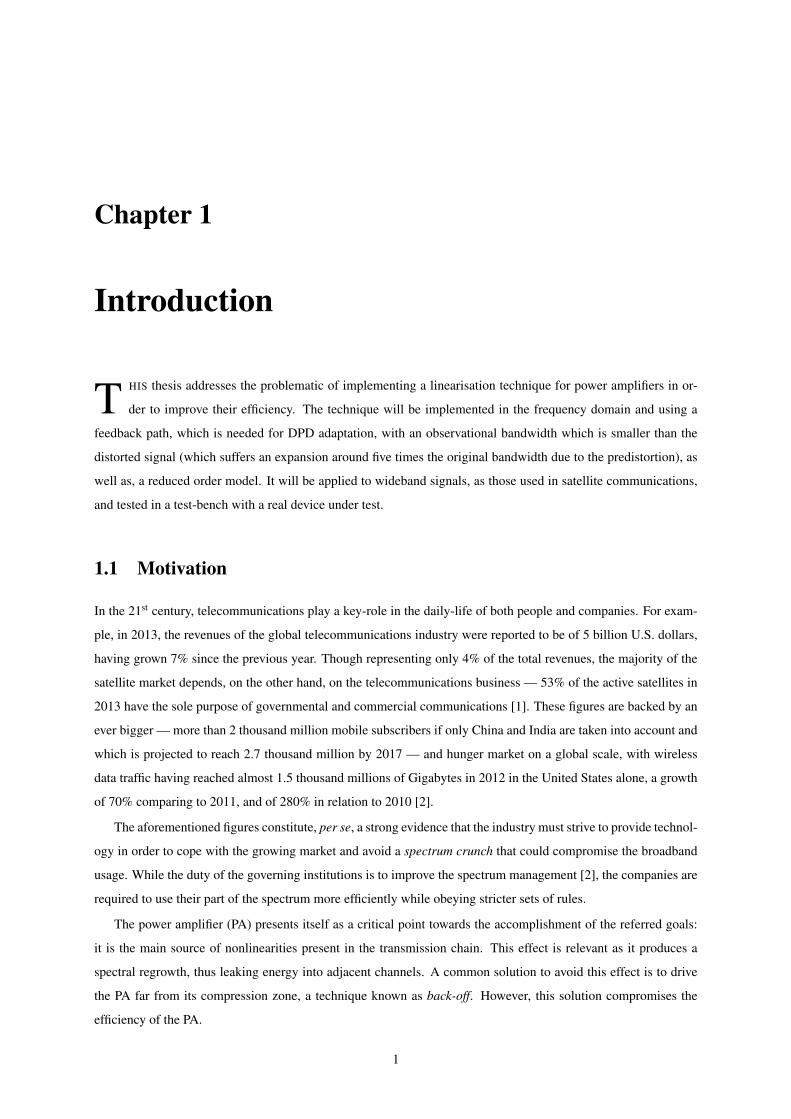
Figure 1.1: Iridium communications satellite

Furthermore, communications standards in use nowadays are usually synonym of high Peak-to-Average Power

Ratio (PAPR) values. In the telephony domain, typical values of PAPR for signals using CDMA2000 standards

are of 10 dB [3]. Other examples of high PAPR can be found in, for example, OFDM-encoded data such as the

802.11a, DVB-T and WiMAX standards in which the values can reach up to 14 dB [4]. This means that the PA

has to be driven very far from its ideal working conditions to be able to cope with the peaks of the signals without

being saturated. Once again, this greatly penalizes the efficiency of the device.

In addition to the high PAPR values, the necessity of high data rates to cope with the traffic demand, leads to

standards of telecommunications imposing greater bandwidths for the carriers: for example, the LTE carriers can

have up to 20 MHz and can also be combined in technologies like carrier aggregation in which five contiguous

carriers can be combined forming an effective bandwidth of 100 MHz [5]. This order of magnitude of the band-

widths, and which tends to increase, brings the necessity of high speed analogue-to-digital converters to recover

the signal for processing, which is not cost-effective.

Finally, the complexity of the PA behaviour usually requires a large and complex mathematical model to

describe it. Due to the fact that the adaptation process is commonly related to a reduction of a quadratic error,

the extraction of the coefficients relies on techniques such as the Least Mean Squares, which can benefit from the

well-conditioning of the matrices.

1.2 Objectives and Methodology

The aim of this M.Sc. thesis is to reduce the bandwidth of the observational path in order to extract the coefficients

of the DPD. This has an impact on the required sampling frequency of the Analogue-to-Digital Converter (ADC),

and thus on its costs and power consumption. Predistortion consists of creating a nonlinear behaviour which is

the inverse of the one generated by the PA and applying it to the input signal, such that the relation between the

input and output signals becomes linear. The specificity of this algorithm lies in the fact that the monitoring of

the signal, which is needed for adapting the predistortion, is accomplished not using all the signal spectra at once,

but rather using a collection of narrower observational bandwidths which allow for the signal to be reconstructed

digitally. This is particularly important if one takes into account the fact that the signal suffers an expansion when

predistorted, which increases its bandwidth up to five times, which require a monitoring of signals with very large

2

bandwidths. Furthermore, the other key-point in this algorithm is reducing the complexity of the model which

describes the PA. These solutions aim to improve computational and monetary efficiency.

To sum up, the objectives can be described as twofold: to perform an intelligent model-order reduction based

on eigenvalue decomposition methods and to use a combination of narrow bandwidth observations to estimate the

digital predistortion (DPD) coefficients. The reduction of the model-order aims at reducing the computational

cost of the digital predistortion by providing matrices which are better conditioned to the adaptation process. On

the other hand, the reduction of the observational bandwidth aims at reducing the sampling rate required for an

ADC to sample a signal with a wide bandwidth, and hence the cost and power consumption of performing this

task, without compromising the DPD capabilities. In order to meet these goals, the approach will consist of the

following steps:

• Read and comprehend the literature inherent to this topic;

• Design the required digital signal processing algorithms;

• Perform preliminary MATLAB-based simulations;

• Test the designed algorithms in an instrumentation-based test-bed with a real device-under-test.

The implementation and testing parts of this thesis will be performed in the Signal Theory and Communications

(TSC) Department of the Universitat Politecnica de Catalunya located in Castelldefels (Barcelona), Spain under

the Erasmus Mundus programme.

1.3 Outline of the Thesis

This thesis is organized in such a way that it follows the chronological order of the developed work, from the

theoretical analysis up to the algorithm testing using a real test-bench.

Chapter 2 presents a theoretical overview of the principles regarding the functioning of a PA. It addresses the

mathematical expressions governing the behaviour of these devices and also the figures of merit used throughout

this thesis.

Chapter 3 starts with a brief overview of some linearisation techniques found in literature. Subsequently, the

digital predistortion technique is presented in more depth together with an improved model to describe the PA

more accurately. Finally, a technique on how to reduce the PAPR of the signals is presented.

In Chapter 4, the approach used to extract the signal using a reduced observational bandwidth is presented, as

well as, the procedure to reconstruct the signal from the various observations. It concludes with a description of the

extraction of DPD coefficients in the frequency domain, taking advantage of the fact that the signal was recovered

in this domain.

Chapter 5 addresses the problematic of reducing the order of the model that describes the PA behaviour and

which is used to estimate the coefficients. A technique based in the principal component analysis theory is pre-

sented to overcome this issue.

In the Chapter 6, the results obtained experimentally are presented along with their analysis.

3

Finally, in Chapter 7, conclusions are drawn from the developed project and considerations on future work that

can be done to improve the discussed topics are listed.

4

Chapter 2

Problem Statement

T HE Power Amplifier is the device that stands on a critical point in the transmission chain: it generates

nonlinearities that can compromise the broadcasting of the signal due to standards violations. On this chapter

the fundamentals of a PA are presented in order to demonstrate the need for a compensation to be made, so as to

guarantee the correct transmission of a signal. It starts with an overview of the nonlinear characteristic inherent to

the power amplifier, followed by an analysis to the trade-off between efficiency and linearity and, finally, there is a

brief description of the memory effects present in a PA and its importance.

2.1 Nonlinear Behaviour of a Power Amplifier

2.1.1 The Memoryless Complex Power Series Model

The PA is usually the last element in the transmission chain and whose role is to amplify a signal in order to drive

the load, which can be an antenna, for most of the telecommunications purposes. This rise in the power of the

signal is necessary in order to guarantee enough power at the reception for the communication to be possible,

despite the losses in the transmission medium.

Ideally, the relation between the input and output signals of the PA would be represented just as a scalar gain.

Let vin(t) be the input signal, then the output would be given by (2.1).

vout(t) = g · vin(t), (2.1)

where g is a scalar gain. This ideal behaviour of a Power Amplifier is shown in Figure 2.1(a). Nonetheless, it

can be observed that, even in the ideal situation, the PA behaviour cannot be described as an infinite line with g : 1

slope, but rather as a line with the referred slope until a point where it becomes a zero-slope line, that is, despite

the increase of the input power, the output power will remain the same. When this situation occurs, the PA is said

to be saturated. Saturation, however, is not an inherent condition of the PA, but rather a function of the load which

is being driven by the PA.

The described behaviour presents itself as nonlinear, emphasizing that a Power Amplifier cannot be described

by a relation like in (2.1). In reality, such an abrupt transition between slopes is also not observed, but rather a

5

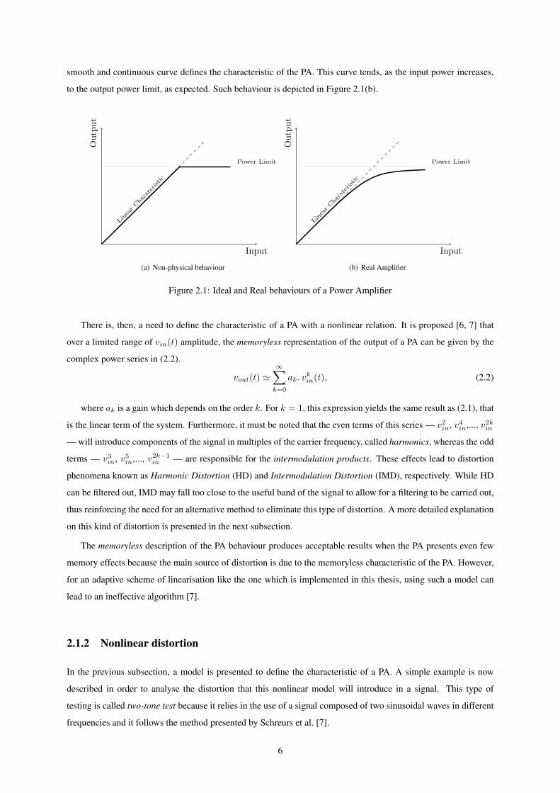
smooth and continuous curve defines the characteristic of the PA. This curve tends, as the input power increases,

to the output power limit, as expected. Such behaviour is depicted in Figure 2.1(b).

Input

Output

LinearCharateristic

Power Limit

(a) Non-physical behaviour

Input

Output

LinearCharateristic

Power Limit

(b) Real Amplifier

Figure 2.1: Ideal and Real behaviours of a Power Amplifier

There is, then, a need to define the characteristic of a PA with a nonlinear relation. It is proposed [6, 7] that

over a limited range of vin(t) amplitude, the memoryless representation of the output of a PA can be given by the

complex power series in (2.2).

vout(t) '∞∑

k=0

ak. vkin(t), (2.2)

where ak is a gain which depends on the order k. For k = 1, this expression yields the same result as (2.1), that

is the linear term of the system. Furthermore, it must be noted that the even terms of this series — v2in, v4in,..., v2kin

— will introduce components of the signal in multiples of the carrier frequency, called harmonics, whereas the odd

terms — v3in, v5in,..., v2k−1in — are responsible for the intermodulation products. These effects lead to distortion

phenomena known as Harmonic Distortion (HD) and Intermodulation Distortion (IMD), respectively. While HD

can be filtered out, IMD may fall too close to the useful band of the signal to allow for a filtering to be carried out,

thus reinforcing the need for an alternative method to eliminate this type of distortion. A more detailed explanation

on this kind of distortion is presented in the next subsection.

The memoryless description of the PA behaviour produces acceptable results when the PA presents even few

memory effects because the main source of distortion is due to the memoryless characteristic of the PA. However,

for an adaptive scheme of linearisation like the one which is implemented in this thesis, using such a model can

lead to an ineffective algorithm [7].

2.1.2 Nonlinear distortion

In the previous subsection, a model is presented to define the characteristic of a PA. A simple example is now

described in order to analyse the distortion that this nonlinear model will introduce in a signal. This type of

testing is called two-tone test because it relies in the use of a signal composed of two sinusoidal waves in different

frequencies and it follows the method presented by Schreurs et al. [7].

6

Let the input signal be defined as

x(t) = A1 cos(ω1t) +A2 cos(ω2t), (2.3)

whereA1 andA2 are the tones’ amplitudes and ω1 and ω2 are their angular frequencies, recalling that ω1 6= ω2.

For simplicity, only a third-order power series is used for this example. Equation (2.2) becomes

vout(t) = a1x(t) + a2x2(t) + a3x

3(t); (2.4)

so, substituting Equation (2.3) into Equation (2.4) yields

vout(t) = a1[A1 cos(ω1t) +A2 cos(ω2t)]

+ a2[A1 cos(ω1t) +A2 cos(ω2t)]2

+ a3[A1 cos(ω1t) +A2 cos(ω2t)]3.

(2.5)

Equation (2.5) can be further expanded and decomposed using trigonometrical relations to yield

vout(t) =a2A

21

2+a2A

22

2

+A1[a1 +3a3A

21

4+

3a3A22

2] cos(ω1t)

+A2[a1 +3a3A

22

4+

3a3A21

2] cos(ω2t)

+a2A

21

2cos(2ω1t) +

a2A22

2cos(2ω2t)

+ a2A1A2[cos((ω2 − ω1)t) + cos((ω2 + ω1)t)]

+a3A

31

4cos(3ω1t) +

a3A32

4cos(3ω2t)

+3a3A

21A2

4[cos((2ω1 + ω2)t) + cos((2ω1 − ω2)t)]

+3a3A

22A1

4[cos((2ω2 + ω1)t) + cos((2ω2 − ω1)t)].

(2.6)

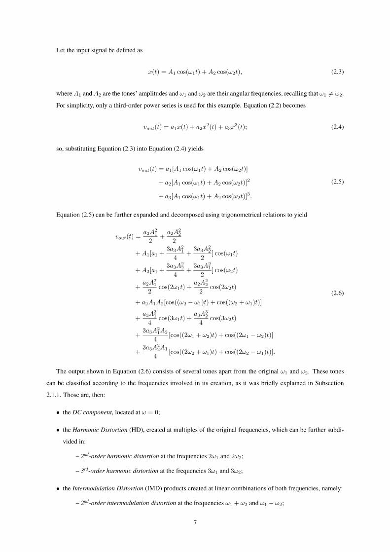
The output shown in Equation (2.6) consists of several tones apart from the original ω1 and ω2. These tones

can be classified according to the frequencies involved in its creation, as it was briefly explained in Subsection

2.1.1. Those are, then:

• the DC component, located at ω = 0;

• the Harmonic Distortion (HD), created at multiples of the original frequencies, which can be further subdi-

vided in:

– 2nd-order harmonic distortion at the frequencies 2ω1 and 2ω2;

– 3rd-order harmonic distortion at the frequencies 3ω1 and 3ω2;

• the Intermodulation Distortion (IMD) products created at linear combinations of both frequencies, namely:

– 2nd-order intermodulation distortion at the frequencies ω1 + ω2 and ω1 − ω2;

7

– 3rd-order intermodulation distortion at the frequencies 2ω1 +ω2, 2ω1−ω2, 2ω2 +ω1 and 2ω2−ω1.

It is evident that an increase in the order of the polynomial used to describe the PA behaviour, will result in an

increase of the harmonic and intermodulation distortion orders.

// // //

Frequency

Power

ω2 − ω1 2ω1 − ω2

ω1 ω2

2ω2 − ω1 2ω1

ω1 + ω2

2ω2 3ω1

2ω1 + ω2 2ω2 + ω1

3ω2

Figure 2.2: Output spectra for a third-order memoryless two-tone test

In Figure 2.2, the spectrum plot of the result obtained in Equation (2.6) is presented, considering that both tones

have the same amplitude, that is, A1 = A2. It must be noted that the third-order IMD products fall very close to

the original frequencies and as the polynomial order is increased, more IMD products will appear surrounding the

two tones, thus making filtering an impractical solution for the removal of this distortion phenomena.

2.1.3 A quantitative measure of nonlinearity

Radiofrequency (RF) signals are far more complex when compared to the simple sinusoidal tones analysed in the

previous subsection. A RF signal can be, usually, decomposed in two distinctive signals:

• the message, which is a band-limited signal that contains the information to be transmitted;

• the carrier, which is a tone at a given frequency at which the message is going to be modulated.

A common example of this technique is the commercial radio, either in Amplitude Modulation (AM) or Fre-

quency Modulation (FM), where the voice, which is a band-limited signal, is modulated at a given frequency before

being transmitted. This carrier frequency is the one that should be selected in the receiver — tuning.

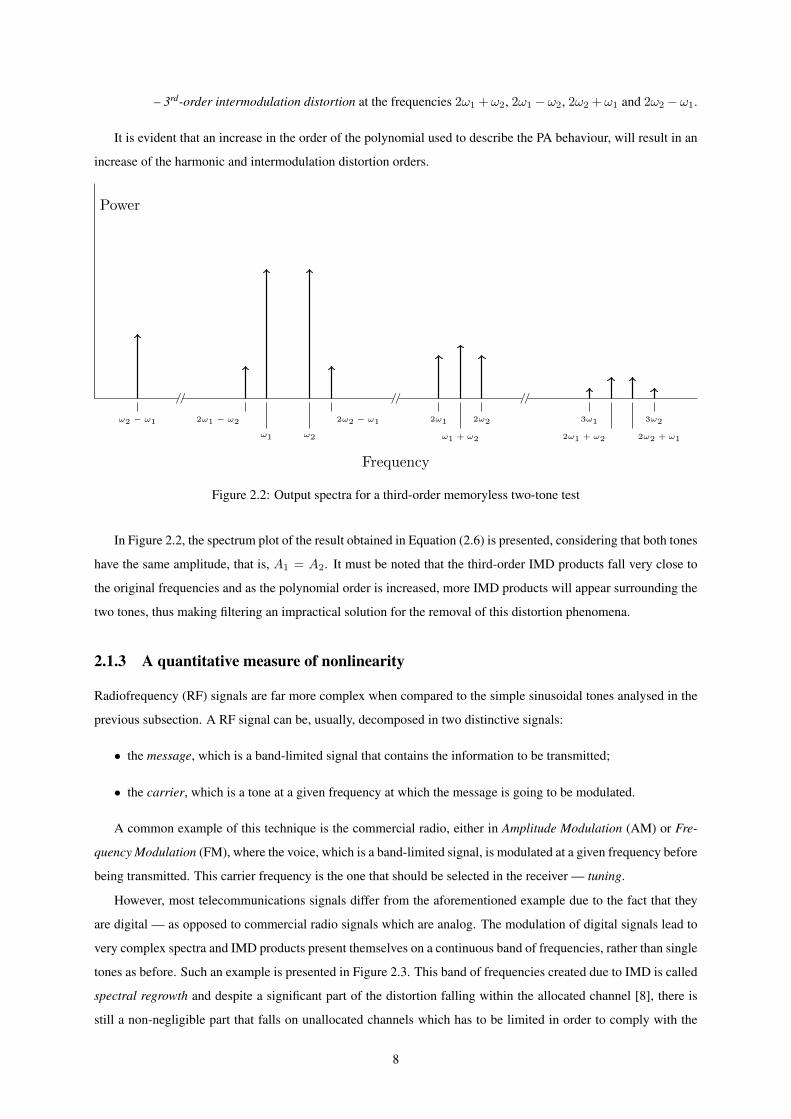
However, most telecommunications signals differ from the aforementioned example due to the fact that they

are digital — as opposed to commercial radio signals which are analog. The modulation of digital signals lead to

very complex spectra and IMD products present themselves on a continuous band of frequencies, rather than single

tones as before. Such an example is presented in Figure 2.3. This band of frequencies created due to IMD is called

spectral regrowth and despite a significant part of the distortion falling within the allocated channel [8], there is

still a non-negligible part that falls on unallocated channels which has to be limited in order to comply with the

8

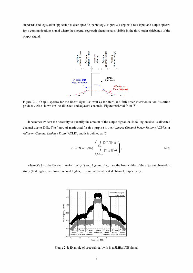
standards and legislation applicable to each specific technology. Figure 2.4 depicts a real input and output spectra

for a communications signal where the spectral regrowth phenomena is visible in the third-order sidebands of the

output signal.

Figure 2.3: Output spectra for the linear signal, as well as the third and fifth-order intermodulation distortionproducts. Also shown are the allocated and adjacent channels. Figure retrieved from [8].

It becomes evident the necessity to quantify the amount of the output signal that is falling outside its allocated

channel due to IMD. The figure-of-merit used for this purpose is the Adjacent Channel Power Ration (ACPR), or

Adjacent Channel Leakage Ratio (ACLR), and it is defined as [7]:

ACPR = 10 log

∫fadj

|Y (f)|2df∫

fchan

|Y (f)|2df

, (2.7)

where Y (f) is the Fourier transform of y(t) and fadj and fchan are the bandwidths of the adjacent channel in

study (first higher, first lower, second higher, . . . ) and of the allocated channel, respectively.

Figure 2.4: Example of spectral regrowth in a 5MHz LTE signal.

9

2.2 Linearity vs. Efficiency

As mentioned in Section 1.1, the PA efficiency is defined as its capacity to transform the power provided as DC

into the power of an output radiofrequency signal. Therefore, the efficiency can be mathematically described as:

η =Pout

PDC[%]. (2.8)

However, the input signal has already some power which is not being taken into account by the Equation (2.8).

A Figure of Merit that overcomes this handicap is known as the Power Added Efficiency (PAE) of a PA, and it is

described by the following relation:

PAE =Pout − Pin

PDC[%]. (2.9)

This relation allows for a more precise quantification of the PA performance in terms of efficiency and should be

used instead of (2.8) whenever the amplifier’s gain is so low that the Pin contribution to Pout cannot be neglected

[6]. Although the PA accounts for a power consumption in the range of 70% [9] to 85% [10] of a common

communications hand-held device, its PAE is usually 50% or less.

Another important consideration regarding the linearity of a PA is its operation class. Amplifiers are usually

classified in seven classes, however, they can be further divided in two separate groups [11]:

• Highly-linear amplifiers (Classes A, AB, B and C) characterized by their linear behaviour and widely used

in mobile communications;

• Highly-efficient amplifiers (Classes D, E and F) which, in turn, present a high efficiency and, therefore, are

used in satellite communications due to the energy constraints observed in this type of communications.

In the first group of classes, the PA behaves like a voltage-controlled current-source, thus creating a current

based on the input signal, hence the linear behaviour. On the other hand, in classes D, E and F, amplifiers behave

like a switch. Such behaviour introduces nonlinearities in the output due to its non-continuous operation but allows

for energy-saving during the time when it is not conducting, which is the reason for their efficiency. On Table 2.1

a comparison between the different classes and their efficiency and linearity is drawn.

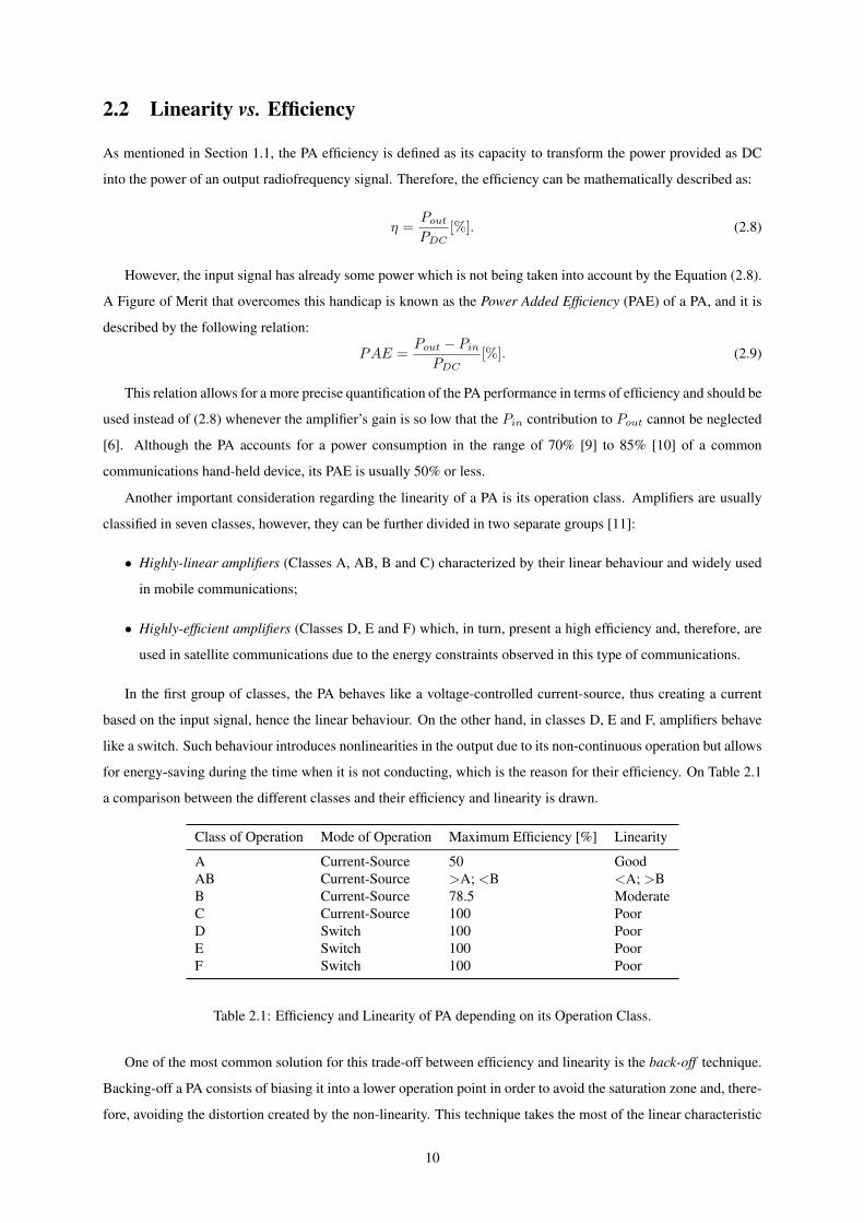
Class of Operation Mode of Operation Maximum Efficiency [%] Linearity

A Current-Source 50 GoodAB Current-Source >A; <B <A; >BB Current-Source 78.5 ModerateC Current-Source 100 PoorD Switch 100 PoorE Switch 100 PoorF Switch 100 Poor

Table 2.1: Efficiency and Linearity of PA depending on its Operation Class.

One of the most common solution for this trade-off between efficiency and linearity is the back-off technique.

Backing-off a PA consists of biasing it into a lower operation point in order to avoid the saturation zone and, there-

fore, avoiding the distortion created by the non-linearity. This technique takes the most of the linear characteristic

10

of the amplifier (recall Figure 2.1). This technique may also appear suggestive for signals which have strong peaks

when compared to its mean value. We can define a Figure of Merit that characterizes this relation in a signal —

the Peak-to-Average Power Ratio (PAPR).

PAPR = 10 log

(Ppeak

Pavg

), (2.10)

where Ppeak is the power of the signal maximum and Pavg is the average power of the signal. Common values

of PAPR are 0 dB for a single-tone, 1.5 dB for a GSM signal and between 10 and 12 dB for a CDMA signal.

However, for most PA, the instantaneous efficiency — the efficiency at one specific output level — reaches its

highest value at the peak output power and lowers as the output diminishes [12]. This means that in order to cope

with signals with large PAPR values, the PA must operate far from its ideal operation point, thus penalizing its

efficiency. As of that, backing-off the amplifier, though suggestive at first impression, presents itself as inefficient.

It becomes clear that linearity and efficiency cannot be fulfilled at the same time, due to their contradictory

characteristics. Linearisation can be seen as a solution to overcome this trade-off. In linearisation, the efficiency

of the PA is exploited at the expense of the linearity. The linear effect is achieved externally to the amplifier

using techniques such as the ones described in Table 2.2 which compares the complexity, efficiency and the main

memory effects that these techniques are sensitive too. A brief overview on memory effects is presented in the next

section.

Complexity Efficiency Main Source of Memory Effects

Cartesian Feedback Moderate High Loop BandwidthFeedforward High Moderate Passive ComponentsEER Moderate High Time delaysRF Predistortion Low High Power AmplifierDigital Predistortion High Moderate PA & BB and IF filters

Table 2.2: Various linearisation techniques. Adapted from [10].

The technique used in this work is the digital predistortion which consists of applying the inverse nonlinear

behaviour of the PA to the input signal. The resulting signal is then sent through the PA, which leads to a linear

relation between the original input and the output. More details on this technique are presented on Chapter 3.

2.3 Memory Effects

Another fundamental aspect that cannot be neglected when dealing with Power Amplifiers is the memory effect.

Memory effect is the dependence of the output in past events. This means that the Equation (2.2) is no longer

valid to describe a PA if one wants to take the memory effects into account. These effects are more discernible in

wideband input signals [13].

Memory effects can be linked with two sources [10]:

• Electrical Memory Effects are associated mainly with the bias circuitry. Though they are designed to present

a high impedance at RF, a non-constant envelope in the input signal will cause impedance changes in the

11

active device which will introduce nonlinearities. Because this effect is a function of the envelope of the

input signal, these type of effects are associated to low frequencies;

• Electrothermal Memory Effects are correlated with the self-heating of the active device due to the temper-

ature changes not occurring instantaneously. Nonetheless, despite all power amplifiers exhibiting thermal

memory effects, these effects can be neglected for frequencies above 1MHz since it is too fast to influence

the temperature in the various components of the device.

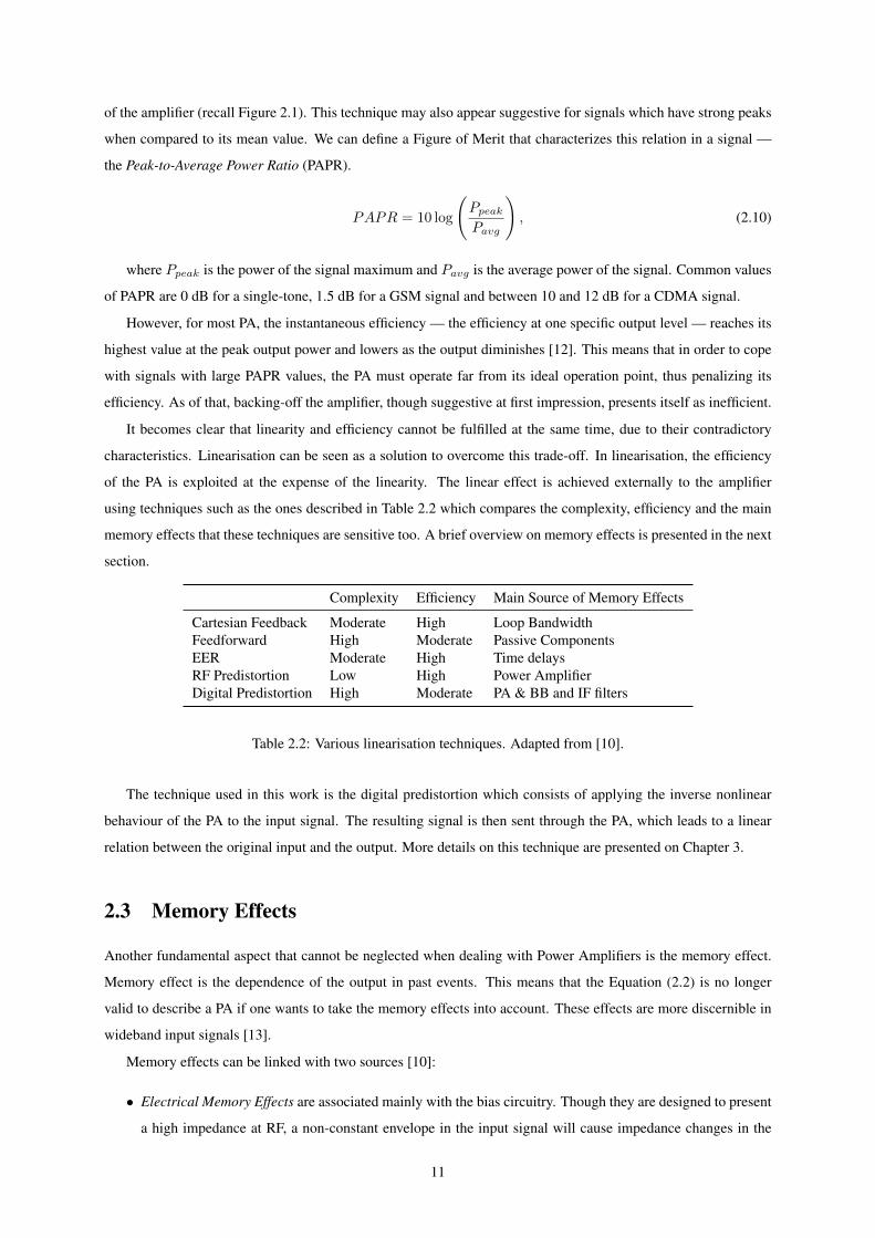
The addition of these effects together with impedance variances, mismatches in the remaining circuitry and

even in the power supply of the transistor contribute to the creation of memory effects in the PA, which make the

output also dependant on past samples of the input. Figure 2.5 depicts the sources of these effects in the PA.

Figure 2.5: Sources of the memory effects in a PA. Figure retrieved from [11].

12

Chapter 3

Towards Digital Predistortion

L INEARISATION of a Power Amplifier can be done at either the circuit or the system levels. Circuit-level

linearisation is more cost effective because it is performed directly to the device, namely the power amplifier.

This makes this type of technique more suitable for the user-end equipments, nonetheless, it is not as effective

in reducing IMD and becomes restrictive to further technology developments. On the other hand, system-level

linearisation is performed at a level where it encompasses all the system — and not only the PA — which leads to

a better distortion-reduction effectiveness, however, at the expense of a higher cost. Due to this reason, system-level

linearisation is mainly applied at wireless backhauling.

We will now concentrate in the linearisation at system-level since it is the one which is covered in this project.

A brief overview is presented on some of the techniques used in this type of linearisation.

3.1 System-Level Linearisation Methods

Feedback techniques

Feedback is one of the classic control techniques in which the output of the signal is used to change parameters

at the input in order to achieve the required goal. For example, the Cartesian Feedback is a technique where the

in-phase and quadrature components of the ouput are separated and compared to the respective components in

the input. This system is depicted on Figure 3.1. Despite this technique being analog and, thus, not requiring

a detailed knowledge of the PA nonlinear characteristic, it is very dependant on the phase alignment between

both components. In the circuit there can be various contributions to a non-zero phase difference between both

components, leading to what is called a phase misalignment which leads to stability issues due to the coupling

between both loops [14]. However, this technique can be used in narrowband signals, as opposed to wideband

signals where it presents stability issues.

Feedforward techniques

The basis for feedforward techniques is quite simple: the output of the signal is reduced to the same level of the

input and a subtraction is performed in order to keep the distortion. This signal is then amplified again to the level

of the PA output and subtracted from it, so the final output becomes just an amplified replica of the input signal

13

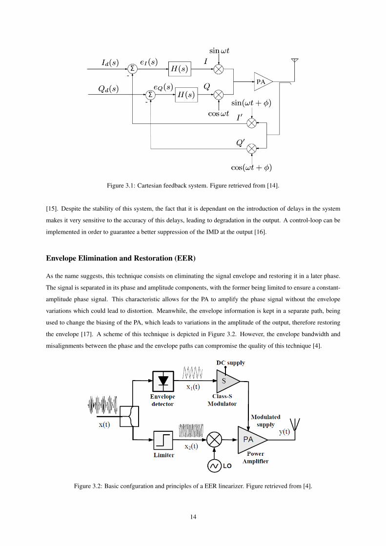
Figure 3.1: Cartesian feedback system. Figure retrieved from [14].

[15]. Despite the stability of this system, the fact that it is dependant on the introduction of delays in the system

makes it very sensitive to the accuracy of this delays, leading to degradation in the output. A control-loop can be

implemented in order to guarantee a better suppression of the IMD at the output [16].

Envelope Elimination and Restoration (EER)

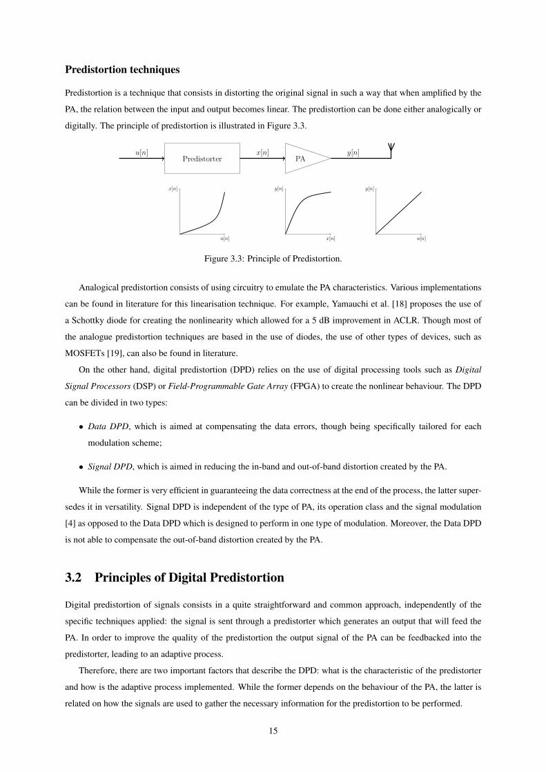
As the name suggests, this technique consists on eliminating the signal envelope and restoring it in a later phase.

The signal is separated in its phase and amplitude components, with the former being limited to ensure a constant-

amplitude phase signal. This characteristic allows for the PA to amplify the phase signal without the envelope

variations which could lead to distortion. Meanwhile, the envelope information is kept in a separate path, being

used to change the biasing of the PA, which leads to variations in the amplitude of the output, therefore restoring

the envelope [17]. A scheme of this technique is depicted in Figure 3.2. However, the envelope bandwidth and

misalignments between the phase and the envelope paths can compromise the quality of this technique [4].

Figure 3.2: Basic confguration and principles of a EER linearizer. Figure retrieved from [4].

14

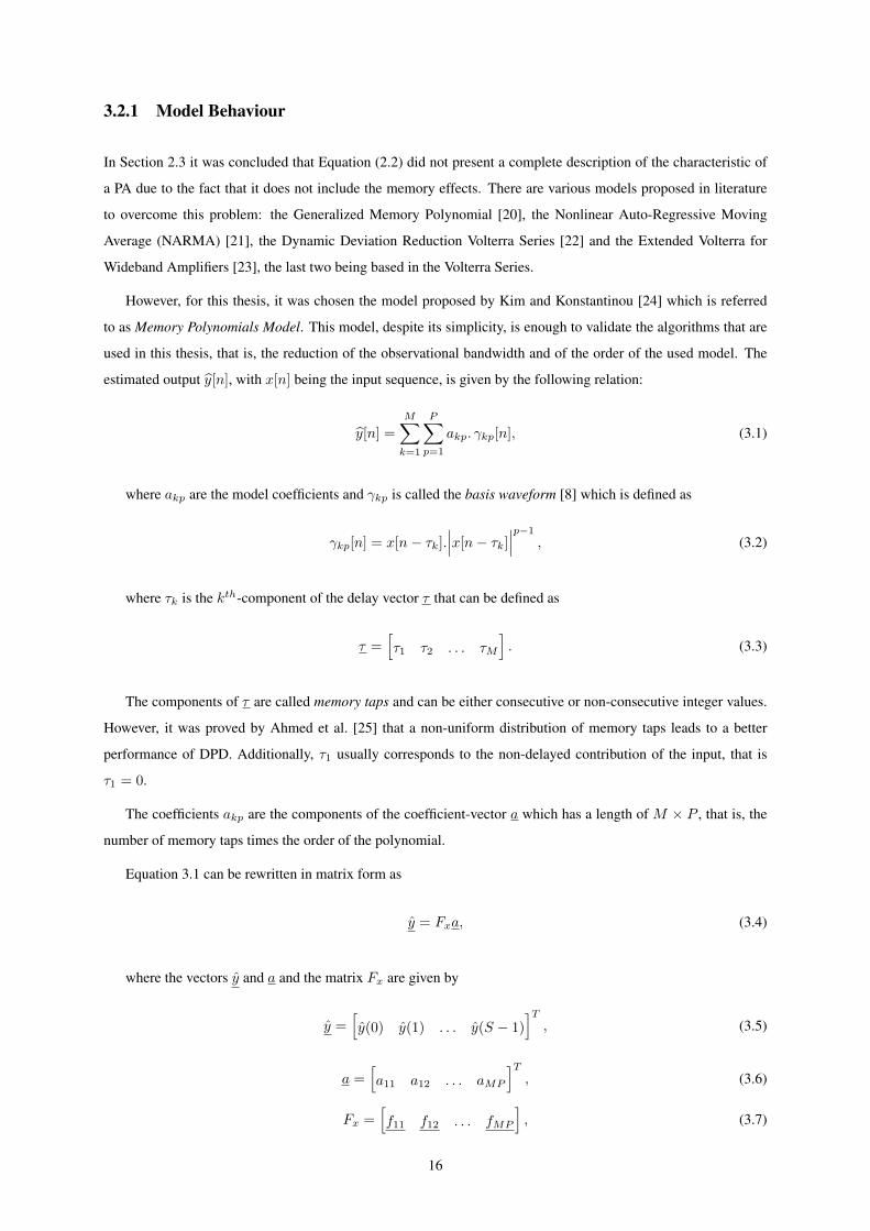
Predistortion techniques

Predistortion is a technique that consists in distorting the original signal in such a way that when amplified by the

PA, the relation between the input and output becomes linear. The predistortion can be done either analogically or

digitally. The principle of predistortion is illustrated in Figure 3.3.

u[n] x[n] y[n]Predistorter PA

x[n]

u[n]

y[n]

x[n]

y[n]

u[n]

Figure 3.3: Principle of Predistortion.

Analogical predistortion consists of using circuitry to emulate the PA characteristics. Various implementations

can be found in literature for this linearisation technique. For example, Yamauchi et al. [18] proposes the use of

a Schottky diode for creating the nonlinearity which allowed for a 5 dB improvement in ACLR. Though most of

the analogue predistortion techniques are based in the use of diodes, the use of other types of devices, such as

MOSFETs [19], can also be found in literature.

On the other hand, digital predistortion (DPD) relies on the use of digital processing tools such as Digital

Signal Processors (DSP) or Field-Programmable Gate Array (FPGA) to create the nonlinear behaviour. The DPD

can be divided in two types:

• Data DPD, which is aimed at compensating the data errors, though being specifically tailored for each

modulation scheme;

• Signal DPD, which is aimed in reducing the in-band and out-of-band distortion created by the PA.

While the former is very efficient in guaranteeing the data correctness at the end of the process, the latter super-

sedes it in versatility. Signal DPD is independent of the type of PA, its operation class and the signal modulation

[4] as opposed to the Data DPD which is designed to perform in one type of modulation. Moreover, the Data DPD

is not able to compensate the out-of-band distortion created by the PA.

3.2 Principles of Digital Predistortion

Digital predistortion of signals consists in a quite straightforward and common approach, independently of the

specific techniques applied: the signal is sent through a predistorter which generates an output that will feed the

PA. In order to improve the quality of the predistortion the output signal of the PA can be feedbacked into the

predistorter, leading to an adaptive process.

Therefore, there are two important factors that describe the DPD: what is the characteristic of the predistorter

and how is the adaptive process implemented. While the former depends on the behaviour of the PA, the latter is

related on how the signals are used to gather the necessary information for the predistortion to be performed.

15

3.2.1 Model Behaviour

In Section 2.3 it was concluded that Equation (2.2) did not present a complete description of the characteristic of

a PA due to the fact that it does not include the memory effects. There are various models proposed in literature

to overcome this problem: the Generalized Memory Polynomial [20], the Nonlinear Auto-Regressive Moving

Average (NARMA) [21], the Dynamic Deviation Reduction Volterra Series [22] and the Extended Volterra for

Wideband Amplifiers [23], the last two being based in the Volterra Series.

However, for this thesis, it was chosen the model proposed by Kim and Konstantinou [24] which is referred

to as Memory Polynomials Model. This model, despite its simplicity, is enough to validate the algorithms that are

used in this thesis, that is, the reduction of the observational bandwidth and of the order of the used model. The

estimated output y[n], with x[n] being the input sequence, is given by the following relation:

y[n] =

M∑

k=1

P∑

p=1

akp. γkp[n], (3.1)

where akp are the model coefficients and γkp is called the basis waveform [8] which is defined as

γkp[n] = x[n− τk].∣∣∣x[n− τk]

∣∣∣p−1

, (3.2)

where τk is the kth-component of the delay vector τ that can be defined as

τ =[τ1 τ2 . . . τM

]. (3.3)

The components of τ are called memory taps and can be either consecutive or non-consecutive integer values.

However, it was proved by Ahmed et al. [25] that a non-uniform distribution of memory taps leads to a better

performance of DPD. Additionally, τ1 usually corresponds to the non-delayed contribution of the input, that is

τ1 = 0.

The coefficients akp are the components of the coefficient-vector a which has a length of M × P , that is, the

number of memory taps times the order of the polynomial.

Equation 3.1 can be rewritten in matrix form as

y = Fxa, (3.4)

where the vectors y and a and the matrix Fx are given by

y =[y(0) y(1) . . . y(S − 1)

]T, (3.5)

a =[a11 a12 . . . aMP

]T, (3.6)

Fx =[f11 f12 . . . fMP

], (3.7)

16

where S is the number of samples and fkp is defined as

fkp =[γkp(0) γkp(1) . . . γkp(S − 1)

]T. (3.8)

The subscript x in the matrix Fx denotes that the basis waveforms used to construct the matrix are generated

using the input signal x[n]. The coefficients a can be obtained using the Least Squares method, whose solution is

given by

a =(FHx Fx

)−1FHx y (3.9)

where (.)H denotes the conjugate transpose of the matrix F .

The models can be evaluated on how accurately they mimic the behaviour of the PA using two Figures of Merit,

the Normalised Mean Square Error (NMSE) and the Adjacent Channel Error Power Ratio(ACEPR), both usually

expressed in dB and which are defined as

NMSE = 10 log

∑Ln=1

∣∣∣yreal[n]− ymod[n]∣∣∣2

∑Ln=1

∣∣∣yreal[n]∣∣∣2

, (3.10)

and

ACEPR = 10 log

∫fadj

∣∣∣Yreal(f)− Ymod(f)∣∣∣2

df

∫fchan

|Yreal(f)|2df

, (3.11)

where yreal[n] and ymod[n] are the outputs of the PA and of the model, respectively, and Yreal(f) and Ymod(f)

their Fourier transform.

In Figure 3.4, there are presented three configurations of the Memory Polynomial model for describing the

behaviour of a PA. It can be observed that an increase in the model order leads to a better characterization of the

non-linear behaviour. Additionally, an increase in the memory taps results in a fattening of the curves.

The data depicted in the Figure 3.4 is presented in Table 3.1. It can be seen that increasing the coefficients will

reduce the NMSE, that is, the difference between the real output and the model output will decrease. In addition,

the ACEPR, that is, the leakage that occurs to the adjacent bandwidths due to the errors of the model also decreases.

Polynomial Memory Coefficients NMSE [dB] ACEPR [dB]

Order Taps Lower Upper

2 1 2 -20.4 -38.66 -38.312 7 14 -33.1 -39.15 -38.575 7 35 -40.1 -52.58 -52.08

Table 3.1: NMSE and ACEPR for three Memory Polynomial model configurations.

17

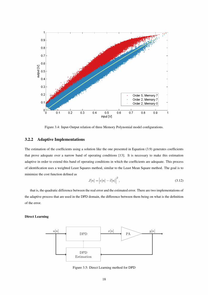
Figure 3.4: Input-Output relation of three Memory Polynomial model configurations.

3.2.2 Adaptive Implementations

The estimation of the coefficients using a solution like the one presented in Equation (3.9) generates coefficients

that prove adequate over a narrow band of operating conditions [13]. It is necessary to make this estimation

adaptive in order to extend this band of operating conditions in which the coefficients are adequate. This process

of identification uses a weighted Least Squares method, similar to the Least Mean Square method. The goal is to

minimize the cost function defined as

J [n] =∣∣∣e[n]− e[n]

∣∣∣2

, (3.12)

that is, the quadratic difference between the real error and the estimated error. There are two implementations of

the adaptive process that are used in the DPD domain, the difference between them being on what is the definition

of the error.

Direct Learning

u[n] x[n] y[n]DPD PA

DPDEstimation

Figure 3.5: Direct Learning method for DPD

18

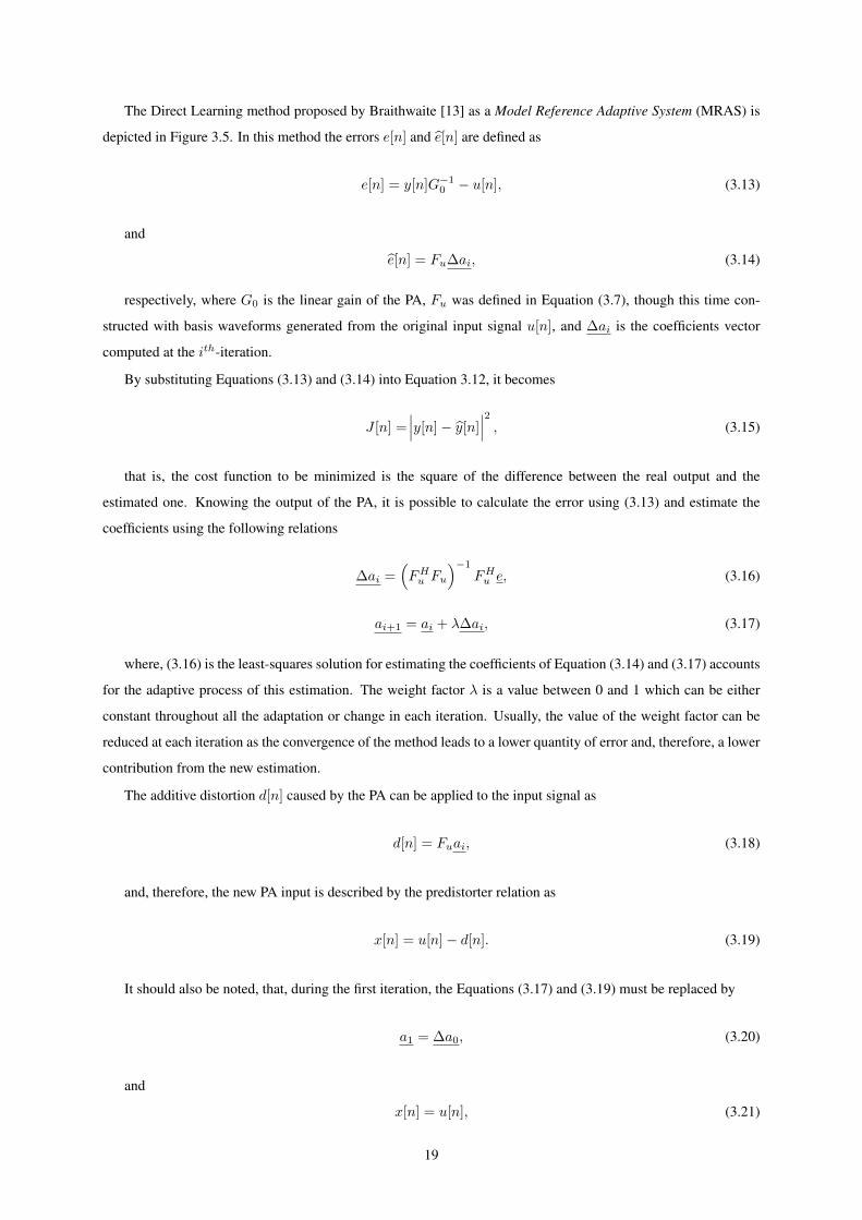
The Direct Learning method proposed by Braithwaite [13] as a Model Reference Adaptive System (MRAS) is

depicted in Figure 3.5. In this method the errors e[n] and e[n] are defined as

e[n] = y[n]G−10 − u[n], (3.13)

and

e[n] = Fu∆ai, (3.14)

respectively, where G0 is the linear gain of the PA, Fu was defined in Equation (3.7), though this time con-

structed with basis waveforms generated from the original input signal u[n], and ∆ai is the coefficients vector

computed at the ith-iteration.

By substituting Equations (3.13) and (3.14) into Equation 3.12, it becomes

J [n] =∣∣∣y[n]− y[n]

∣∣∣2

, (3.15)

that is, the cost function to be minimized is the square of the difference between the real output and the

estimated one. Knowing the output of the PA, it is possible to calculate the error using (3.13) and estimate the

coefficients using the following relations

∆ai =(FHu Fu

)−1FHu e, (3.16)

ai+1 = ai + λ∆ai, (3.17)

where, (3.16) is the least-squares solution for estimating the coefficients of Equation (3.14) and (3.17) accounts

for the adaptive process of this estimation. The weight factor λ is a value between 0 and 1 which can be either

constant throughout all the adaptation or change in each iteration. Usually, the value of the weight factor can be

reduced at each iteration as the convergence of the method leads to a lower quantity of error and, therefore, a lower

contribution from the new estimation.

The additive distortion d[n] caused by the PA can be applied to the input signal as

d[n] = Fuai, (3.18)

and, therefore, the new PA input is described by the predistorter relation as

x[n] = u[n]− d[n]. (3.19)

It should also be noted, that, during the first iteration, the Equations (3.17) and (3.19) must be replaced by

a1 = ∆a0, (3.20)

and

x[n] = u[n], (3.21)

19

respectively, due to the lack of information inherent to this stage of the adaptive process.

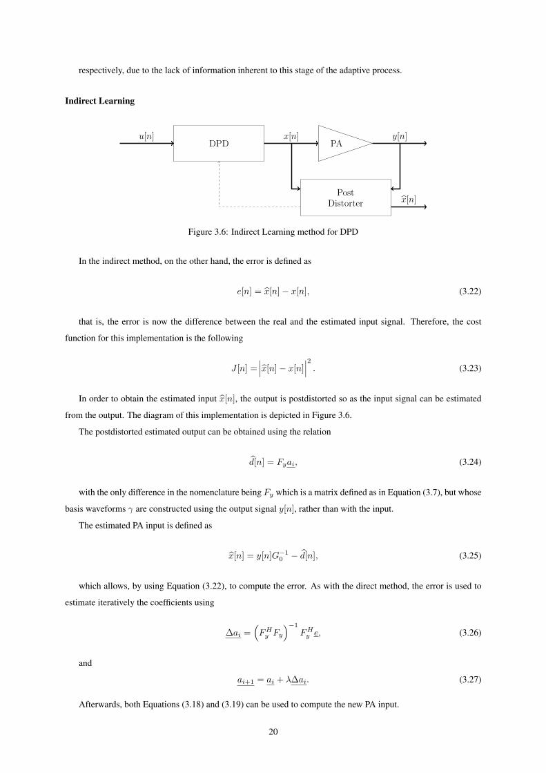
Indirect Learning

u[n] x[n] y[n]DPD PA

PostDistorter x[n]

Figure 3.6: Indirect Learning method for DPD

In the indirect method, on the other hand, the error is defined as

e[n] = x[n]− x[n], (3.22)

that is, the error is now the difference between the real and the estimated input signal. Therefore, the cost

function for this implementation is the following

J [n] =∣∣∣x[n]− x[n]

∣∣∣2

. (3.23)

In order to obtain the estimated input x[n], the output is postdistorted so as the input signal can be estimated

from the output. The diagram of this implementation is depicted in Figure 3.6.

The postdistorted estimated output can be obtained using the relation

d[n] = Fyai, (3.24)

with the only difference in the nomenclature being Fy which is a matrix defined as in Equation (3.7), but whose

basis waveforms γ are constructed using the output signal y[n], rather than with the input.

The estimated PA input is defined as

x[n] = y[n]G−10 − d[n], (3.25)

which allows, by using Equation (3.22), to compute the error. As with the direct method, the error is used to

estimate iteratively the coefficients using

∆ai =(FHy Fy

)−1FHy e, (3.26)

and

ai+1 = ai + λ∆ai. (3.27)

Afterwards, both Equations (3.18) and (3.19) can be used to compute the new PA input.

20

In this adaptive learning process, the starting condition in (3.21) must be kept for the first iteration, as well as,

a1 = 0. (3.28)

Both direct and indirect methods are suitable for performing the estimation of the coefficients for the digital

predistortion. However, and despite the fact that the indirect method is more simple and intuitive, the direct method

presents better results in reducing the ACLR.

3.3 PAPR Reduction

As referred in the Section 2.2 the signals in use for telecommunications nowadays have a high level of PAPR. This

compromises the efficiency of the PA by compressing the output if one wishes to drive the PA as close to saturation

as possible. Therefore, a reduction of the PAPR is usually performed to the input signal u[n] before using it in the

digital predistortion algorithm. Hence, a solution to perform this reduction is to suppress the peaks of the input

signal without compromising the information contained in it. This technique is called Scaled Peak Cancellation

(SPC) [26].

Let us define the clipper pulse c[n] as

c[n] =

A∣∣∣u[n]∣∣∣

if∣∣∣u[n]

∣∣∣ > A

1 if∣∣∣u[n]

∣∣∣ ≤ A, (3.29)

where A is the suppressing threshold. The clipped pulse p[n] is, then, defined as

p[n] = u[n]− u[n] · c[n]. (3.30)

The output of this clipped pulse has to be filtered with a low-pass filter with the same bandwidth as that of the

x[n]. If x[n] is multi band signal, each band has to be filtered individually and then recombined. The PAPR-reduced

signal z[n] is finally obtained with

z[n] = u[n]− α · p[n] ∗ h[n], (3.31)

where h[n] is the impulse response of the filter, ∗ denotes the convolution operation and α is a weight factor

defined as

α =

max

(∣∣∣p[n]∣∣∣)

max

(∣∣∣p[n] ∗ h[n]∣∣∣) . (3.32)

This technique can be implemented repetitively by making u[n] = z[n] at the end of each iteration, leading to

a technique called Repeated Peak Cancellation (RPC).

The drawback of this technique is distorting the information that is contained in the original signal. Hence, a

trade-off has to be guaranteed between reducing the PAPR and maintaining the integrity of the signal. In Table

3.2, a comparison is made between the reduction of the PAPR and the mesured NMSE between the original signal

21

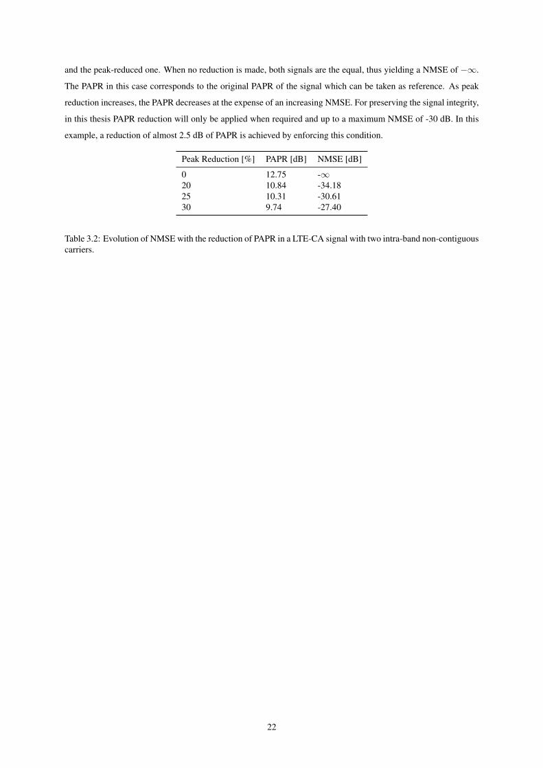
and the peak-reduced one. When no reduction is made, both signals are the equal, thus yielding a NMSE of −∞.

The PAPR in this case corresponds to the original PAPR of the signal which can be taken as reference. As peak

reduction increases, the PAPR decreases at the expense of an increasing NMSE. For preserving the signal integrity,

in this thesis PAPR reduction will only be applied when required and up to a maximum NMSE of -30 dB. In this

example, a reduction of almost 2.5 dB of PAPR is achieved by enforcing this condition.

Peak Reduction [%] PAPR [dB] NMSE [dB]

0 12.75 -∞20 10.84 -34.1825 10.31 -30.6130 9.74 -27.40

Table 3.2: Evolution of NMSE with the reduction of PAPR in a LTE-CA signal with two intra-band non-contiguouscarriers.

22

Chapter 4

Reduced Observational Bandwidth

A S discussed in the Subsection 3.2.2 of the last Chapter, the Digital predistortion relies on the feedback of

the output in order to accomplish the adaptive process. However, due to nowadays’ use of signals that can

reach, for example, 20 MHz of bandwidth in LTE [27], thus leading to a bandwidth of over 100 MHz if there is

the necessity of analysing the leakage up to the channel that is located two bandwidths above or below the carrier

channel (due to the 5th-order IMD products, as explained in Subsection 2.1.3).

4.1 Analogue-to-Digital Conversion

One of the main components of the feedback path in the DPD context is the Analogue-to-Digital Converter,

commonly referred to as ADC. The role of the ADC is to convert the analogue signal, that is sent through the

antenna and also recovered through the feedback path, to a digital signal that can be processed either in a DSP or

in a FPGA.

Despite being characterised by numerous factors such as the resolution, linearity, accuracy or jitter, there is

one that plays an important role in the predistortion application: the sampling frequency or sampling rate. The

sampling rate of an ADC is the rate at which the samples of the analogue signal are captured and converted to

digital. From the sampling theory, the Shannon-Nyquist Theorem states that if a signal has no frequencies higher

than B0 hertz, then it will be completely represented by samples captured 1/(2B0) seconds apart [28]. This

theorem can be translated to a mathematical relation:

fs ≥ 2B0, (4.1)

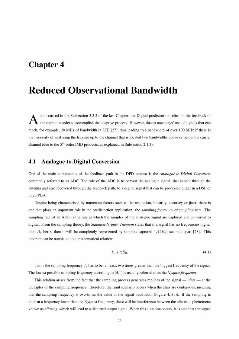
that is the sampling frequency fs has to be, at least, two times greater than the biggest frequency of the signal.

The lowest possible sampling frequency according to (4.1) is usually referred to as the Nyquist frequency.

This relation arises from the fact that the sampling process generates replicas of the signal — alias — at the

multiples of the sampling frequency. Therefore, the limit scenario occurs when the alias are contiguous, meaning

that the sampling frequency is two times the value of the signal bandwidth (Figure 4.1(b)). If the sampling is

done at a frequency lower than the Nyquist frequency, there will be interference between the aliases, a phenomena

known as aliasing, which will lead to a distorted output signal. When this situation occurs, it is said that the signal

23

f

|Y (f)|

0−B B

(a) Spectrum of the original analog signal.

f

|Y (f)|

0−B B fs 2fs−fs−2fs

. . .. . .

(b) Spectrum of the signal sampled at Nyquist frequency.

f

|Y (f)|

0−B B fs 2fs−fs−2fs

. . .. . .

(c) Spectrum of the signal sampled below Nyquist frequency.

Figure 4.1: Effects of aliasing when sampling a signal.

is under-sampled or, more colloquially, that it does not comply with Nyquist theorem (Figure 4.1(c)).

Despite the fact that a low-pass filter with cut-off frequency at fs/2 is the most simple solution used to prevent

the aliasing problem, the discussion of anti-aliasing techniques is outside the scope of this thesis .

The analysis of this problematic leads to the conclusion that, in order to represent a wide bandwidth signal such

as the aforementioned LTE signal with a bandwidth of 20 MHz, and if we take into account the expansion of five

times its bandwidth caused by DPD, then there is a call for an ADC with a sampling rate of, at least, 200 MHz.

As the cost of an ADC is closely related with its performance capabilities, the higher the sampling rate an ADC is

able to work at, the more expensive it is. Therefore, reducing the sampling rate necessary to sample a signal while

at the same time complying with Nyquist, will have a direct economic impact in the predistortion process as it will

allow to save on the power and cost of the ADC.

4.2 The Windowing technique

In order to reduce the bandwidth of a signal, the solution is to hard-limit it in frequency capturing a certain

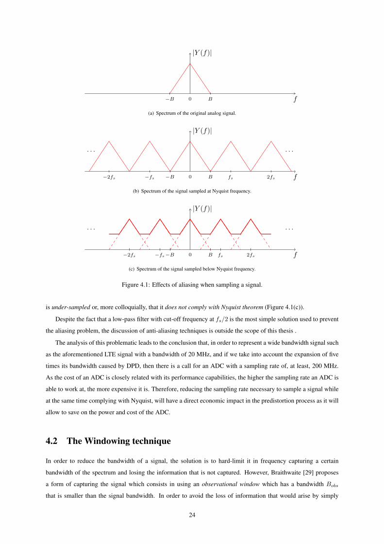
bandwidth of the spectrum and losing the information that is not captured. However, Braithwaite [29] proposes

a form of capturing the signal which consists in using an observational window which has a bandwidth Bobs

that is smaller than the signal bandwidth. In order to avoid the loss of information that would arise by simply

24

limiting the signal, the effective captured bandwidth is increased by up and down converting the signal at different

frequencies so as the area of the spectrum covered by the observational window is different. The use of these

different observations allows for the signal to be reconstructed in the digital domain, relieving the ADC from

sampling at high rates. The principle is depicted in Figure 4.2.

Figure 4.2: Input signals and three observational windows. Figure retrieved from [29].

The hardware principle of this technique combines a tunable local oscillator (LO) followed by a low-pass filter

whose bandwidth isBobs before the signal is sent to the ADC (Figure 4.3). The LO is tuned in order to demodulate

the original signal so as the centre of the observational window is the same as the filter’s.

y(t) y2(t) yf(t) y[n]

L.O.

−Bobs Bobs

H(f)

ADC

Figure 4.3: Scheme of the reduced observational bandwidth windowing technique.

4.3 Signal Reconstruction

Once the signal has been through the ADC, it is in the digital domain, and therefore, it can be submitted to digital

signal processing techniques.

Due to the fact that the signal was converted using observational windows, in the digital domain, the data

consists of several sets of observations which correspond to the windows used. In addition, since the captures were

all made using a filter tuned at the same frequency and with the same bandwidth, the sets constitute a superposition

of the spectra in the frequency domain.

There is a necessity of aligning the different observation spectra to reconstruct the signal spectrum. The first

step of this process is a demodulation to baseband. In the digital domain, it can be substituted for a frequency shift

which avoids the replicas that would appear if a sinusoidal demodulation was made and that could interfere with

the signal. The operation applied to each observation set is defined as

YBB

(ejω)

= YADC

e

j

(ω+

fffs

) , (4.2)

25

where YBB(ejω) and YADC(ejω) are the Discrete-Time Fourier Transforms of yBB [n] and yADC [n], respec-

tively and whose subscripts refer to the signal in baseband and to the signal that is outputted from the ADC, also

respectively. In addition, ff is the observation filter centre frequency and fs is the ADC sampling frequency. In

the time domain, the relation of (4.2) is expressed as

yBB [n] = yADC [n]e−jfffs

n. (4.3)

After the signal is demodulated to baseband, an ideal filtering can be performed to filter out the window more

effectively. This is accomplished by using a low-pass filter, whose cut-off frequency is half the bandwidth of the

observational windows.

The following step towards the reconstruction of the signal is the interpolation. Despite not being necessary

to the reconstruction of the signal, it is done in order to allow for the signal to be compared and aligned with the

input, so that the DPD can be performed.

As mentioned before, the windowing techniques results in that the observation sets, when plotted in the fre-

quency domain, are all located in the same frequency and they all have the same bandwidth. Therefore, there is a

necessity to shift them to their proper position. The knowledge of the centre frequency of each window reduces

this problem to a simple shift of each set to the frequency of its corresponding window. In Figure 4.4(a) an example

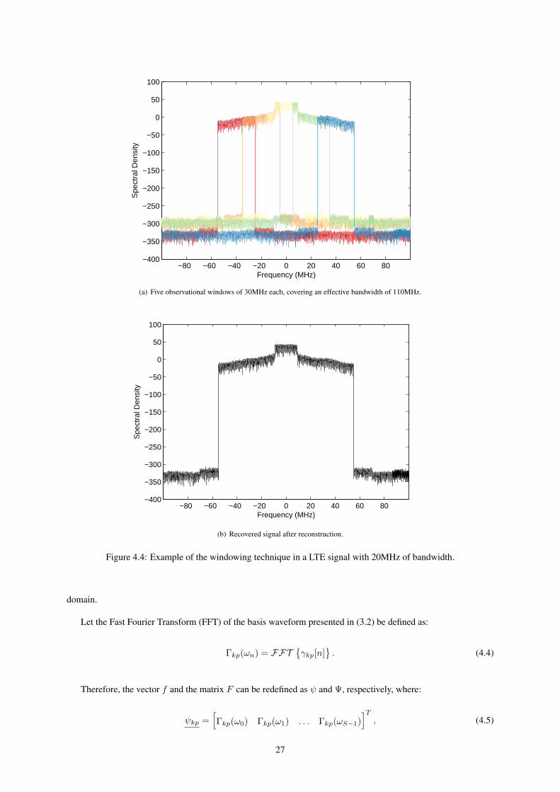
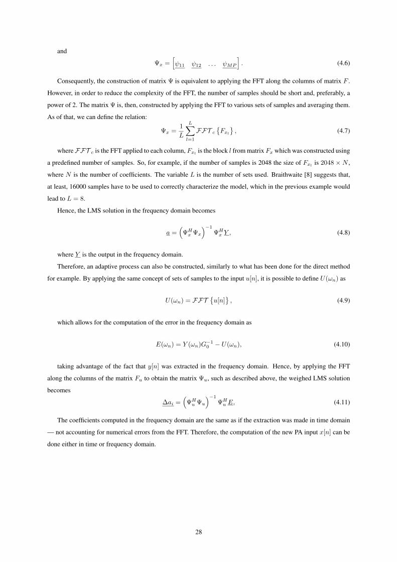
of five observational sets of 30 MHz each is depicted after alignment.

The last step of reconstruction is the merger of the various observations into one signal, which is the recon-

structed output. Although it is a straightforward process because it only implies picking the relevant part of the

spectrum from each observation, the ideal filtering that was previously made creates a discontinuity in the filter

cut-off frequency that has to be avoided when picking the spectrum. This issue is overcome, firstly, by guaran-

teeing that the windows overlap each other when projecting the system, and then by applying an algorithm that

discards the last samples of the window when picking. The implemented algorithm makes the following decisions

regarding the first and last samples to be picked at each set:

• First Sample:

– The first sample of the set, if it is the first set;

– The sample after the last one picked from the previous observation set, if it is not the first set.

• Last Sample:

– The last sample of the set, if it is the last set;

– The sample that is located two samples before the last sample of the window, if it is not the last set.

This last condition guarantees that the aforementioned discontinuity is discarded.The recovered signal is de-

picted on Figure 4.4(b).

4.4 Frequency Estimation

The estimation of the coefficients is proven [8] to be feasible without transforming the signal into the discrete time

domain, which can save computational resources due to the fact that the signal was recovered in the frequency

26

−80 −60 −40 −20 0 20 40 60 80−400

−350

−300

−250

−200

−150

−100

−50

0

50

100

Frequency (MHz)

Spe

ctra

l Den

sity

(a) Five observational windows of 30MHz each, covering an effective bandwidth of 110MHz.

−80 −60 −40 −20 0 20 40 60 80−400

−350

−300

−250

−200

−150

−100

−50

0

50

100

Frequency (MHz)

Spe

ctra

l Den

sity

(b) Recovered signal after reconstruction.

Figure 4.4: Example of the windowing technique in a LTE signal with 20MHz of bandwidth.

domain.

Let the Fast Fourier Transform (FFT) of the basis waveform presented in (3.2) be defined as:

Γkp(ωn) = FFT{γkp[n]

}. (4.4)

Therefore, the vector f and the matrix F can be redefined as ψ and Ψ, respectively, where:

ψkp =[Γkp(ω0) Γkp(ω1) . . . Γkp(ωS−1)

]T, (4.5)

27

and

Ψx =[ψ11 ψ12 . . . ψMP

]. (4.6)

Consequently, the construction of matrix Ψ is equivalent to applying the FFT along the columns of matrix F .

However, in order to reduce the complexity of the FFT, the number of samples should be short and, preferably, a

power of 2. The matrix Ψ is, then, constructed by applying the FFT to various sets of samples and averaging them.

As of that, we can define the relation:

Ψx =1

L

L∑

l=1

FFT c

{Fxl

}, (4.7)

whereFFT c is the FFT applied to each column, Fxlis the block l from matrix Fx which was constructed using

a predefined number of samples. So, for example, if the number of samples is 2048 the size of Fxlis 2048 × N ,

where N is the number of coefficients. The variable L is the number of sets used. Braithwaite [8] suggests that,

at least, 16000 samples have to be used to correctly characterize the model, which in the previous example would

lead to L = 8.

Hence, the LMS solution in the frequency domain becomes

a =(

ΨHx Ψx

)−1ΨH

x Y , (4.8)

where Y is the output in the frequency domain.

Therefore, an adaptive process can also be constructed, similarly to what has been done for the direct method

for example. By applying the same concept of sets of samples to the input u[n], it is possible to define U(ωn) as

U(ωn) = FFT{u[n]

}, (4.9)

which allows for the computation of the error in the frequency domain as

E(ωn) = Y (ωn)G−10 − U(ωn), (4.10)

taking advantage of the fact that y[n] was extracted in the frequency domain. Hence, by applying the FFT

along the columns of the matrix Fu to obtain the matrix Ψu, such as described above, the weighed LMS solution

becomes

∆ai =(

ΨHu Ψu

)−1ΨH

u E, (4.11)

The coefficients computed in the frequency domain are the same as if the extraction was made in time domain

— not accounting for numerical errors from the FFT. Therefore, the computation of the new PA input x[n] can be

done either in time or frequency domain.

28

Chapter 5

Model Order Reduction

I N Chapter 3 we discussed the adaptive methods that allowed for the computation of the DPD coefficients. In

both direct and indirect methods, a matrix F was constructed from the basis waveforms γ generated from the

signal which is used as input in each method. It can be recalled that the size of the matrix F is S ×N , regardless

of the learning method used, and where S is the number of samples used to determine the model and N is the

number of coefficients used for the behavioural model, that is, the number of memory taps times the order of the

polynomial.

However, the number of coefficients used for the model has an effect on the accuracy of the model estimation.

Though the bias of the estimation, that is, the sum of the squared errors between the real output and the model

output, can be reduced by increasing the coefficients, the variance of the estimation increases proportionally to

the ratio between the number of coefficients and the number of samples, which can lead to a degradation of the

estimation [30]. Thus, a low ratio is desirable, with experimental results supporting a number of samples that is, at

least, 20 times the number of coefficients [31].

In order to reduce the aforementioned ratio, two options are obvious: reducing the number of coefficients or

increasing the number of samples. In a cost-saving perspective, the latter is more promising because it can reduce

not only the size of matrices, but also improve its conditioning, both of them leading to a better computational

efficiency.

5.1 Principal Component Analysis

The Principal Component Analysis (PCA) is a statistical technique which allows for the reduction of the dimen-

sions of a given set of variables. This technique consists of an orthogonal transformation in which the original

and possibly correlated variables is transformed to an uncorrelated set, the principal components. These principal

components are ordered in such a way that the variance decreases along them which leads to the fact that the first

few components account for almost the totality of the variance present in all set [32]. In Figure 5.1 a graphi-

cal representation of the PCA method is depicted. The data, represented in the x − y basis can be orthogonally

transformed to the v1 − v2 basis which are the principal components. The eigenvector v1 accounts for the biggest

variability in the data, hence being the biggest eigenvector in modulus.

29

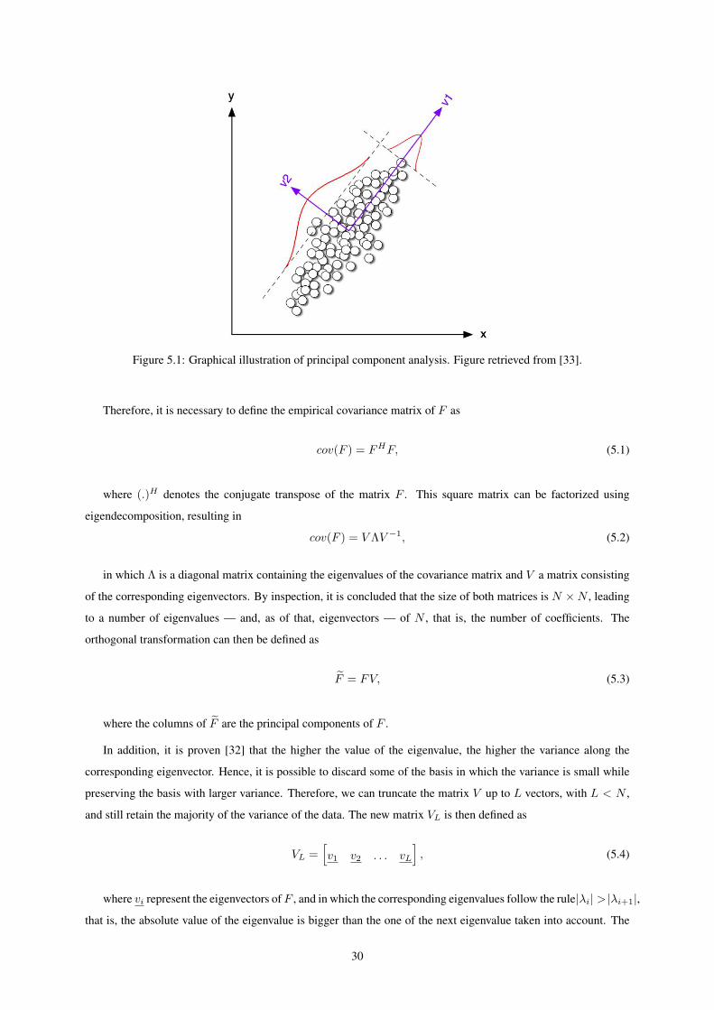
Figure 5.1: Graphical illustration of principal component analysis. Figure retrieved from [33].

Therefore, it is necessary to define the empirical covariance matrix of F as

cov(F ) = FHF, (5.1)

where (.)H denotes the conjugate transpose of the matrix F . This square matrix can be factorized using

eigendecomposition, resulting in

cov(F ) = V ΛV −1, (5.2)

in which Λ is a diagonal matrix containing the eigenvalues of the covariance matrix and V a matrix consisting

of the corresponding eigenvectors. By inspection, it is concluded that the size of both matrices is N ×N , leading

to a number of eigenvalues — and, as of that, eigenvectors — of N , that is, the number of coefficients. The

orthogonal transformation can then be defined as

F = FV, (5.3)

where the columns of F are the principal components of F .

In addition, it is proven [32] that the higher the value of the eigenvalue, the higher the variance along the

corresponding eigenvector. Hence, it is possible to discard some of the basis in which the variance is small while

preserving the basis with larger variance. Therefore, we can truncate the matrix V up to L vectors, with L < N ,

and still retain the majority of the variance of the data. The new matrix VL is then defined as

VL =[v1 v2 . . . vL

], (5.4)

where vi represent the eigenvectors ofF , and in which the corresponding eigenvalues follow the rule|λi| > |λi+1|,that is, the absolute value of the eigenvalue is bigger than the one of the next eigenvalue taken into account. The

30

size of the matrix VL is N × L and the orthogonal relation of (5.3) can be rewritten as

F = FVL, (5.5)

which leads to a matrix F of size S × L, therefore reducing the number of coefficients that will be outputted

to L.

Gilabert et al. [34] proposes the application of this method to the DPD estimation process, proving that a

considerable reduction of the model order can be done without compromising the DPD capabilities.

31

32

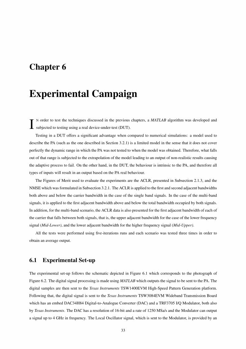
Chapter 6

Experimental Campaign

I N order to test the techniques discussed in the previous chapters, a MATLAB algorithm was developed and

subjected to testing using a real device-under-test (DUT).

Testing in a DUT offers a significant advantage when compared to numerical simulations: a model used to

describe the PA (such as the one described in Section 3.2.1) is a limited model in the sense that it does not cover

perfectly the dynamic range in which the PA was not tested to when the model was obtained. Therefore, what falls

out of that range is subjected to the extrapolation of the model leading to an output of non-realistic results causing

the adaptive process to fail. On the other hand, in the DUT, the behaviour is intrinsic to the PA, and therefore all

types of inputs will result in an output based on the PA real behaviour.

The Figures of Merit used to evaluate the experiments are the ACLR, presented in Subsection 2.1.3, and the

NMSE which was formulated in Subsection 3.2.1. The ACLR is applied to the first and second adjacent bandwidths

both above and below the carrier bandwidth in the case of the single band signals. In the case of the multi-band

signals, it is applied to the first adjacent bandwidth above and below the total bandwidth occupied by both signals.

In addition, for the multi-band scenario, the ACLR data is also presented for the first adjacent bandwidth of each of

the carrier that falls between both signals, that is, the upper adjacent bandwidth for the case of the lower frequency

signal (Mid-Lower), and the lower adjacent bandwidth for the higher frequency signal (Mid-Upper).

All the tests were performed using five-iterations runs and each scenario was tested three times in order to

obtain an average output.

6.1 Experimental Set-up

The experimental set-up follows the schematic depicted in Figure 6.1 which corresponds to the photograph of

Figure 6.2. The digital signal processing is made using MATLAB which outputs the signal to be sent to the PA. The

digital samples are then sent to the Texas Instruments TSW1400EVM High-Speed Pattern Generation platform.

Following that, the digital signal is sent to the Texas Instruments TSW3084EVM Wideband Transmission Board

which has an embed DAC34H84 Digital-to-Analogue Converter (DAC) and a TRF3705 I/Q Modulator, both also

by Texas Instruments. The DAC has a resolution of 16-bit and a rate of 1250 MSa/s and the Modulator can output

a signal up to 4 GHz in frequency. The Local Oscillator signal, which is sent to the Modulator, is provided by an

33

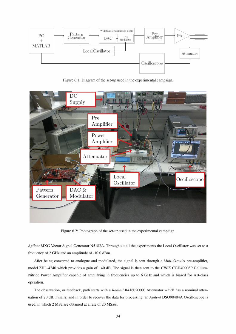
PC+

MATLAB

PatternGenerator

Wideband Transmission Board

DAC I/QModulator

PreAmplifier PA

Attenuator

Oscilloscope

Local Oscillator

Figure 6.1: Diagram of the set-up used in the experimental campaign.

PatternGenerator

DAC &Modulator

LocalOscillator

Oscilloscope

DCSupply

PreAmplifier

PowerAmplifier

Attenuator

Figure 6.2: Photograph of the set-up used in the experimental campaign.

Agilent MXG Vector Signal Generator N5182A. Throughout all the experiments the Local Oscillator was set to a

frequency of 2 GHz and an amplitude of -10.0 dBm.

After being converted to analogue and modulated, the signal is sent through a Mini-Circuits pre-amplifier,

model ZHL-4240 which provides a gain of +40 dB. The signal is then sent to the CREE CGH40006P Gallium-

Nitride Power Amplifier capable of amplifying in frequencies up to 6 GHz and which is biased for AB-class

operation.

The observation, or feedback, path starts with a Radiall R416020000 Attenuator which has a nominal atten-

uation of 20 dB. Finally, and in order to recover the data for processing, an Agilent DSO90404A Oscilloscope is

used, in which 2 MSa are obtained at a rate of 20 MSa/s.

34

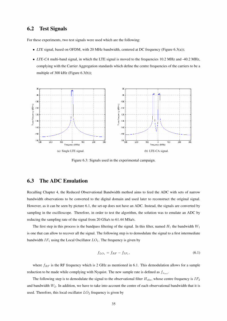
6.2 Test Signals

For these experiments, two test signals were used which are the following:

• LTE signal, based on OFDM, with 20 MHz bandwidth, centered at DC frequency (Figure 6.3(a));

• LTE-CA multi-band signal, in which the LTE signal is moved to the frequencies 10.2 MHz and -40.2 MHz,

complying with the Carrier Aggregation standards which define the centre frequencies of the carriers to be a

multiple of 300 kHz (Figure 6.3(b));

(a) Single LTE signal. (b) LTE-CA signal.

Figure 6.3: Signals used in the experimental campaign.

6.3 The ADC Emulation

Recalling Chapter 4, the Reduced Observational Bandwidth method aims to feed the ADC with sets of narrow

bandwidth observations to be converted to the digital domain and used later to reconstruct the original signal.

However, as it can be seen by picture 6.1, the set-up does not have an ADC. Instead, the signals are converted by

sampling in the oscilloscope. Therefore, in order to test the algorithm, the solution was to emulate an ADC by

reducing the sampling rate of the signal from 20 GSa/s to 61.44 MSa/s.

The first step in this process is the bandpass filtering of the signal. In this filter, named H1 the bandwidth W1

is one that can allow to recover all the signal. The following step is to demodulate the signal to a first intermediate

bandwidth IF1 using the Local Oscillator LO1. The frequency is given by

fLO1= fRF − fIF1

, (6.1)

where fRF is the RF frequency which is 2 GHz as mentioned in 6.1. This demodulation allows for a sample

reduction to be made while complying with Nyquist. The new sample rate is defined as fsint .

The following step is to demodulate the signal to the observational filter Hobs, whose centre frequency is IF2

and bandwidth W2. In addition, we have to take into account the centre of each observational bandwidth that it is

used. Therefore, this local oscillator LO2 frequency is given by

35

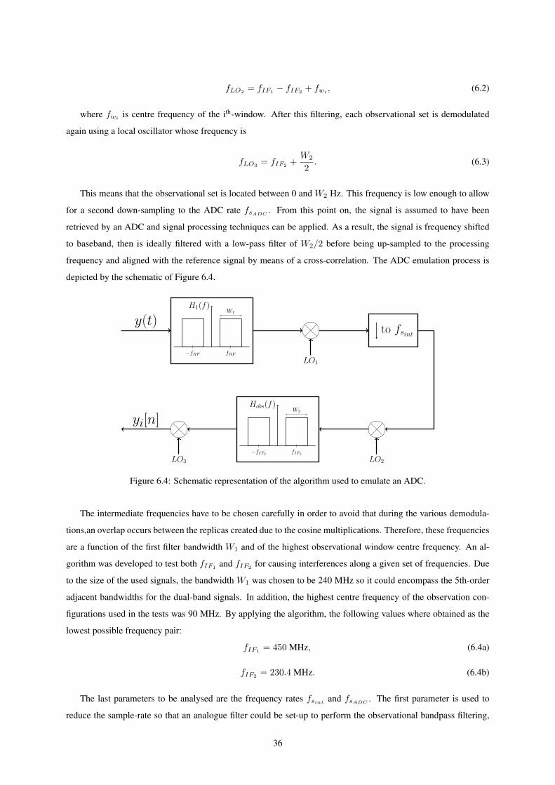
fLO2 = fIF1 − fIF2 + fwi , (6.2)

where fwiis centre frequency of the ith-window. After this filtering, each observational set is demodulated

again using a local oscillator whose frequency is

fLO3 = fIF2 +W2

2. (6.3)

This means that the observational set is located between 0 and W2 Hz. This frequency is low enough to allow

for a second down-sampling to the ADC rate fsADC. From this point on, the signal is assumed to have been

retrieved by an ADC and signal processing techniques can be applied. As a result, the signal is frequency shifted

to baseband, then is ideally filtered with a low-pass filter of W2/2 before being up-sampled to the processing

frequency and aligned with the reference signal by means of a cross-correlation. The ADC emulation process is

depicted by the schematic of Figure 6.4.

y(t)

yi[n]

−fRF fRF

H1(f)W1

LO1

to fsint

LO2

−fIF2 fIF2

Hobs(f)W2

LO3

Figure 6.4: Schematic representation of the algorithm used to emulate an ADC.

The intermediate frequencies have to be chosen carefully in order to avoid that during the various demodula-

tions,an overlap occurs between the replicas created due to the cosine multiplications. Therefore, these frequencies

are a function of the first filter bandwidth W1 and of the highest observational window centre frequency. An al-

gorithm was developed to test both fIF1 and fIF2 for causing interferences along a given set of frequencies. Due

to the size of the used signals, the bandwidth W1 was chosen to be 240 MHz so it could encompass the 5th-order

adjacent bandwidths for the dual-band signals. In addition, the highest centre frequency of the observation con-

figurations used in the tests was 90 MHz. By applying the algorithm, the following values where obtained as the

lowest possible frequency pair:

fIF1 = 450 MHz, (6.4a)

fIF2 = 230.4 MHz. (6.4b)

The last parameters to be analysed are the frequency rates fsintand fsADC

. The first parameter is used to

reduce the sample-rate so that an analogue filter could be set-up to perform the observational bandpass filtering,

36

as a lower sample rate would result in a lower filter order Therefore the down-sampling was chosen to be by a

factor of ten, resulting in the signals being re-sampled at 2 GHz. The second sample-rate is chosen just to comply

with Nyquist criterion, that is, to be equal or greater than 2W2, that is two times the bandwidth of the observation

window. The widest used observation window is of 30 MHz, so 60 MHz is the minimum admissible sample rate.

However, the ADC rate was chosen to be of 61.44 MHz because it is exactly ten times lower than the DAC rate

which is set to 614.4 MHz. In addition, it shall be noted that the processing sample-rate is the same as that of the

DAC.

6.4 Experimental Results

Reduced Observational Bandwidth Performance

On the first part of this experiment, the single LTE signal was used. The test consisted of a comparison between

the third-order (First Sideband) and fifth-order (Second Sideband) ACLR and the NMSE between the original and

captured signal in four scenarios: no DPD performed, a full observational bandwidth, a set of nine observational

windows of 30 MHz each (9W30 configuration) and a set of thirteen observational windows of 20 MHz each

(13W20 configuration). All the recovered signals have a bandwidth of 190 MHz, except in the case of the 13W20

which has 200 MHz. Despite this fact, this does not affect the bandwidths in which the measurements were taken.

The polynomial order was 7 and the memory depth was 11, resulting in 77 coefficients. The results are described

in Table 6.1 and in Figure 6.5(a).

1st Sideband ACLR [dB] 2nd Sideband ACLR [dB] NMSE [dB]Lower Upper Lower Upper

No-DPD -40.95 -41.26 -45.32 -44.01 -23.91Full-OBW -42.10 -42.19 -44.06 -43.93 -24.4013W20 -42.20 -42.06 -43.98 -44.14 -24.299W30 -42.25 -42.11 -44.16 -43.96 -24.21

Table 6.1: Comparison of Full and Reduced Observational Bandwidths in a Single LTE signal.

On the second part, the LTE-CA signal was recovered using two configurations: a full (200 MHz) observational

bandwidth and a reduced observational bandwidth composed of thirteen observation windows of 20 MHz each

(13W20 configuration) spanning a total of 200 MHz. The polynomial order was 11 and the memory depth was 31,

thus yielding 341 coefficients. The results are presented in Table 6.2 and in Figure 6.5(b).

Multi-Carrier ACLR [dB] Single-Carrier ACLR [dB] NMSE [dB]Lower Upper Mid-Lower Mid-Upper

No-DPD -23.70 -22.44 -30.95 -29.88 -16.97Full-OBW -34.92 -29.39 -29.24 -23.05 -20.8413W20 -35.12 -29.40 -29.43 -23.24 -20.91

Table 6.2: Comparison of Full and Reduced Observational Bandwidths in a LTE-CA Signal.

By analysing the data, four things have to be noted:

37

• The predistortion technique using frequency estimation is not very effective in the single band test, as op-

posed to the dual-band where it reduced the intermodulation products;

• The change in the size of the windows tested in the single-band case returned similar results;

• The reduced observational bandwidth and the full-observational bandwidth returned similar results in both

tests;

• The dual-band scenario suffers from distortion created in the I/Q modulator which leads to the existence of

uncorrected areas (between -20 and 0 MHz and between around 25 MHz and 45 MHz). In fact, the area

contiguous to the higher frequency carrier is affected by a spurious at DC, hence the regrowth in that area,

which is not observed anywhere else near the bands.

Model Order Analysis

In this part we sought to test the effect of the model order in the digital predistortion process.

In the first test, the LTE signal was recovered using thirteen windows of 20 MHz each (13W20 configuration)

which covers a bandwidth of 200 MHz. In comparison was the same recovery method using 385 coefficients (poly-

nomial of order 11 and 35 memory taps) and 77 coefficients (order 7 and 11 memory taps). An extra comparison

was made by reducing the model order by a factor of 5, that is, the original 385 were reduced to 77, denoted in the

results by 77*. The results are presented in the Table 6.3 and in the Figure 6.6(a).

Coefficients 1st Sideband ACLR [dB] 2nd Sideband ACLR [dB] NMSE [dB]Lower Upper Lower Upper

No-DPD -40.61 -40.94 -45.14 -43.93 -23.8313W20 385 -41.23 -42.20 -43.66 -43.21 -22.5313W20 77 -43.95 -43.57 -45.13 -45.81 -25.8413W20 77* -44.71 -44.89 -44.91 -44.10 -25.15

Table 6.3: Effect of the number of estimation coefficients in the DPD in a Single LTE Signal.

In the second part, the same experiment was made using the LTE-CA signal and the results are presented in the

Table 6.4 and in the Figure 6.6(b).

Coefficients Multi-Carrier ACLR [dB] Single-Carrier ACLR [dB] NMSE [dB]Lower Upper Mid-Lower Mid-Upper

No-DPD -24.04 -22.80 -30.94 -29.80 -17.0413W20 385 -34.45 -29.36 -20.67 -22.69 -20.6813W20 77 -35.59 -30.65 -30.88 -28.59 -23.7913W20 77* -36.60 -32.52 -32.75 -29.86 -24.59

Table 6.4: Effect of the number of estimation coefficients in the DPD in a LTE-CA Signal.

In this experiment, the tests in which a lower order was used, the DPD proved to be more effective in both

signals. Additionally, in the dual-band scenario, the 77* test performed better than the 77, mainly by reducing the

leakage in the adjacent bands of the carriers.

38

Time vs. Frequency Estimation Methods

In this test, the LTE signal was submitted to DPD estimation in both time (using the direct learning method) and in

frequency. In both cases, there was also considered the model-order reduction with a factor of 20 for comparison.

Therefore, the number of coefficients used was 385 (polynomial of order 11 and 35 memory taps) and the reduction

led to 19 coefficients, denoted as 19*. The results of this test are presented in Table 6.5 and graphically in Figure

6.7(a).

Coefficients 1st Sideband ACLR [dB] 2nd Sideband ACLR [dB] NMSE [dB]Lower Upper Lower Upper

No-DPD -40.61 -40.94 -45.14 -43.93 -23.83

Time Estimation 385 -47.26 -48.26 -48.00 -47.99 -27.2219* -46.41 -47.29 -46.57 -45.95 -27.06

Frequency Estimation 385 -41.23 -42.20 -43.66 -43.21 -22.5319* -44.08 -44.38 -44.82 -45.48 -24.83

Table 6.5: Comparison between Time and Frequency Estimation in a Single LTE Signal.

For the second part of this experiment, the same procedure was applied to the LTE-CA signal, whose results

are described in Table 6.6 and in Figure 6.7(b).

Coefficients Multi-Carrier ACLR [dB] Single-Carrier ACLR [dB] NMSE [dB]Lower Upper Mid-Lower Mid-Upper

No-DPD -24.00 -22.76 -30.85 -29.76 -16.87

Time Estimation 385 -37.06 -33.03 -33.19 -30.99 -25.2019* -33.35 -29.33 -32.53 -30.52 -24.13

Frequency Estimation 385 -34.45 -29.36 -20.67 -22.69 -20.6819* -33.37 -29.55 -32.40 -29.86 -23.73

Table 6.6: Comparison between Time and Frequency Estimation in a LTE-CA Signal.

By looking at the results produced by the Single LTE signal, the first thing to be noted is that the F-385 case

does not prove very effective when compared to the situation without DPD. The other three scenarios effectively

reduced the ACLR values, in special the time-estimated cases which reached 6-7 dB improvement in the first

sideband ACLR and more than 3 dB in the NMSE. The improvement in the second bandwidth was between 1 and

4 dB, whereas the F-385 did not improve the ACLR values.

In the LTE-CA case, despite all scenarios having improved the total bandwidth leakage, the F-385 did not

improve the intra-carrier leakage. As mentioned in the previous tests, this case proved to be sensitive to the I/Q

imbalance, thus leading to a degradation of the referred ACLR. The better performing condition was the T-385,

with the T-19* and F-19* performing very similarly.

To sum up, the time-estimated scenarios provided a better DPD performance than the frequency-estimated

ones, either with a complete set of coefficients or with a reduced set.

39

Contribution of PAPR reduction

In this part of the testing, it was sought to compare the response of the DPD when the signal was subjected to the

PAPR reduction technique described in Section 3.3. Therefore, in the first test, the LTE signal was predistorted,

after its PAPR being reduced. In the Table 6.7, there are described the PAPR values obtained after the reduction, as

well as, the NMSE value comparing the original with the processed signal. In the Table 6.8, the results of the test

are presented. There were used 385 coefficients (polynomial of order 11 and 35 memory taps) which were reduced

by a factor of 20, yielding 19 coefficients. The graphical result of this solution is presented in Figure 6.8(a).

Peak Reduction [%] PAPR [dB] NMSE [dB]

0 10.58 -∞10 9.68 -42.3720 8.69 -34.7625 8.12 -31.61

Table 6.7: Evolution of NMSE with the reduction of PAPR used in this experiment, for the Single LTE signal.

1st Sideband ACLR [dB] 2nd Sideband ACLR [dB] NMSE [dB]Lower Upper Lower Upper

No-DPD -43.76 -44.26 -46.41 -45.72 -24.400%-Reduction -44.14 -44.18 -45.63 -46.74 -23.6510%-Reduction -44.36 -44.38 -45.82 -46.41 -24.3820%-Reduction -44.09 -44.11 -45.10 -45.03 -24.6425%-Reduction -44.08 -44.38 -44.82 -45.48 -24.83

Table 6.8: Effect of PAPR reduction on the DPD in a Single LTE Signal.

Next, the same procedure was applied to the LTE-CA signal. The Table 6.9 presents the evolution of the

NMSE with the reduction of the PAPR, whereas the Table 6.10 presents the results obtained when predistorting

those signals. The graphical result of this solution is displayed in Figure 6.8(b).

Peak Reduction [%] PAPR [dB] NMSE [dB]

0 12.75 -∞10 11.84 -43.2520 10.84 -34.1825 10.30 –30.61

Table 6.9: Evolution of NMSE with the reduction of PAPR used in this experiment, for the LTE-CA signal.

The results for this test have to be analysed more carefully. In fact, only the No-DPD and 0%-reduction cases

can be compared directly in terms of ACLR and NMSE because they correspond to the same situation. All other

cases would have to be compared to the No-DPD case in which the same reduction factor would have been applied.

For example, it can be noted that reducing the PAPR will cause the carrier, and hence the rest of the signal, to have

more power.

However, some conclusions can be drawn from these tests. In the Single LTE test, PAPR reduction did not

40

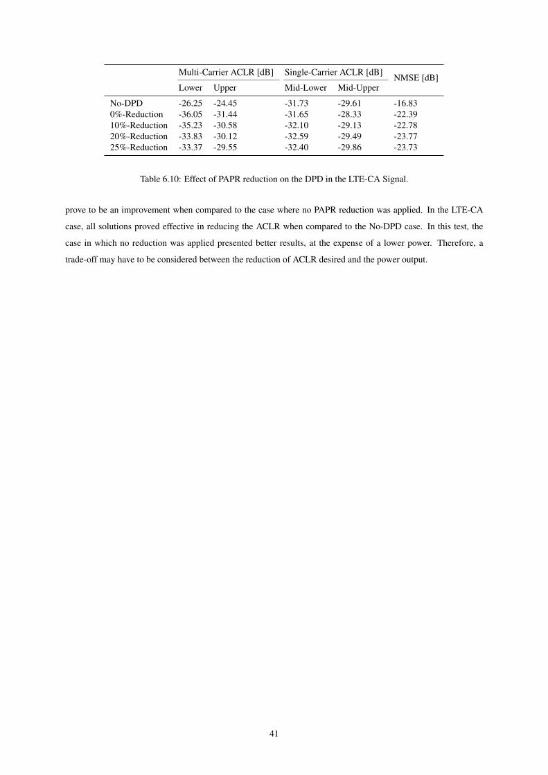
Multi-Carrier ACLR [dB] Single-Carrier ACLR [dB] NMSE [dB]Lower Upper Mid-Lower Mid-Upper

No-DPD -26.25 -24.45 -31.73 -29.61 -16.830%-Reduction -36.05 -31.44 -31.65 -28.33 -22.3910%-Reduction -35.23 -30.58 -32.10 -29.13 -22.7820%-Reduction -33.83 -30.12 -32.59 -29.49 -23.7725%-Reduction -33.37 -29.55 -32.40 -29.86 -23.73

Table 6.10: Effect of PAPR reduction on the DPD in the LTE-CA Signal.

prove to be an improvement when compared to the case where no PAPR reduction was applied. In the LTE-CA

case, all solutions proved effective in reducing the ACLR when compared to the No-DPD case. In this test, the

case in which no reduction was applied presented better results, at the expense of a lower power. Therefore, a

trade-off may have to be considered between the reduction of ACLR desired and the power output.

41

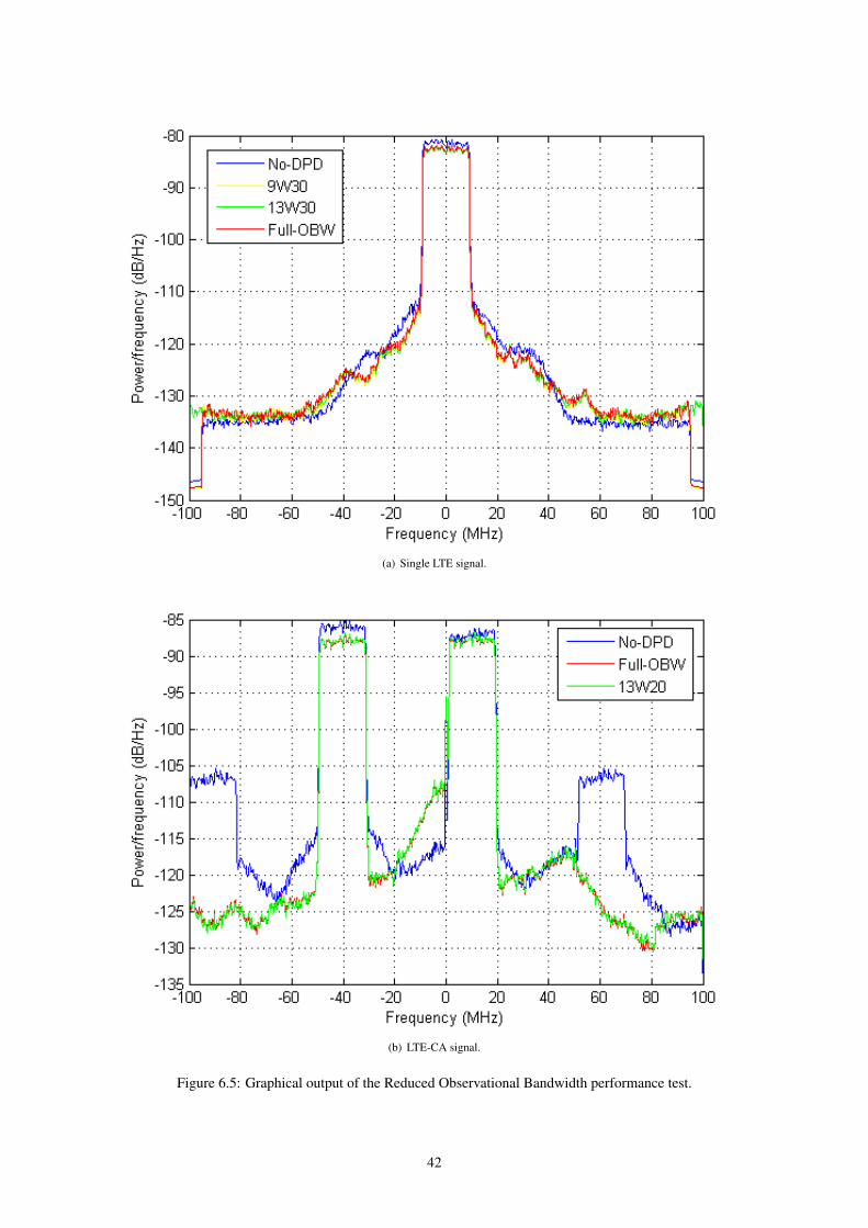
(a) Single LTE signal.

(b) LTE-CA signal.

Figure 6.5: Graphical output of the Reduced Observational Bandwidth performance test.

42

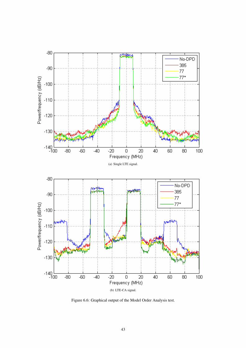
(a) Single LTE signal.

(b) LTE-CA signal.

Figure 6.6: Graphical output of the Model Order Analysis test.

43

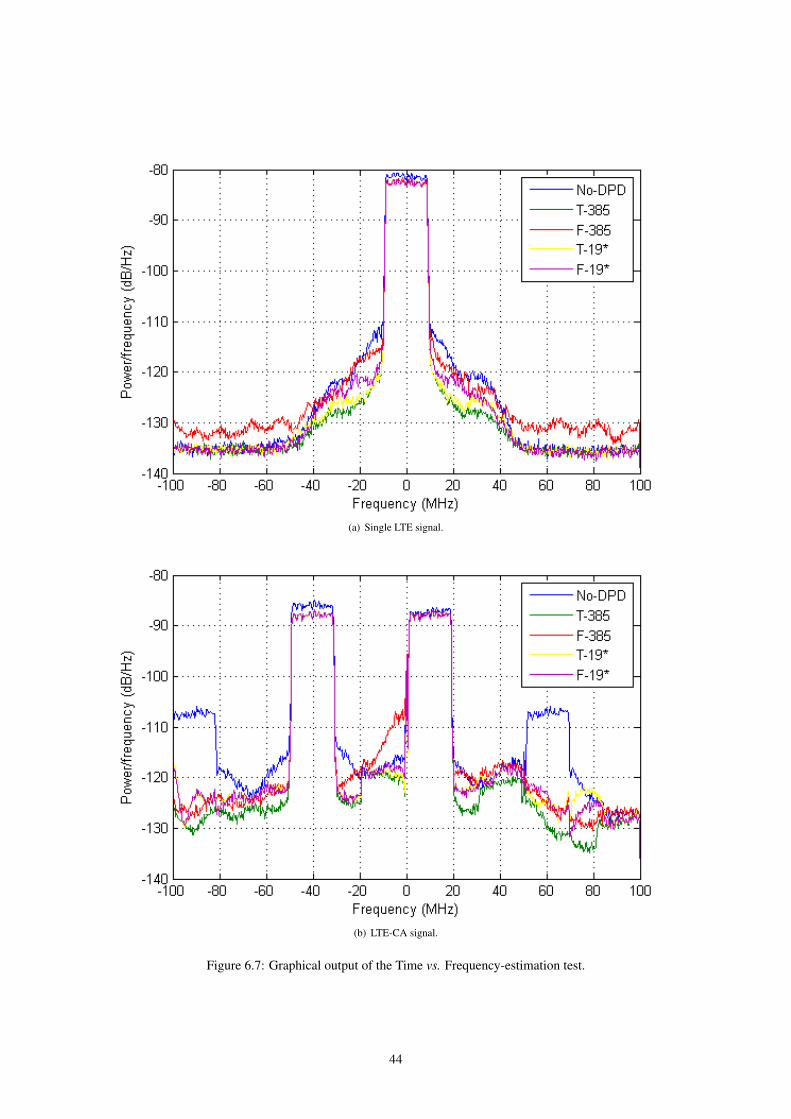
(a) Single LTE signal.

(b) LTE-CA signal.

Figure 6.7: Graphical output of the Time vs. Frequency-estimation test.

44

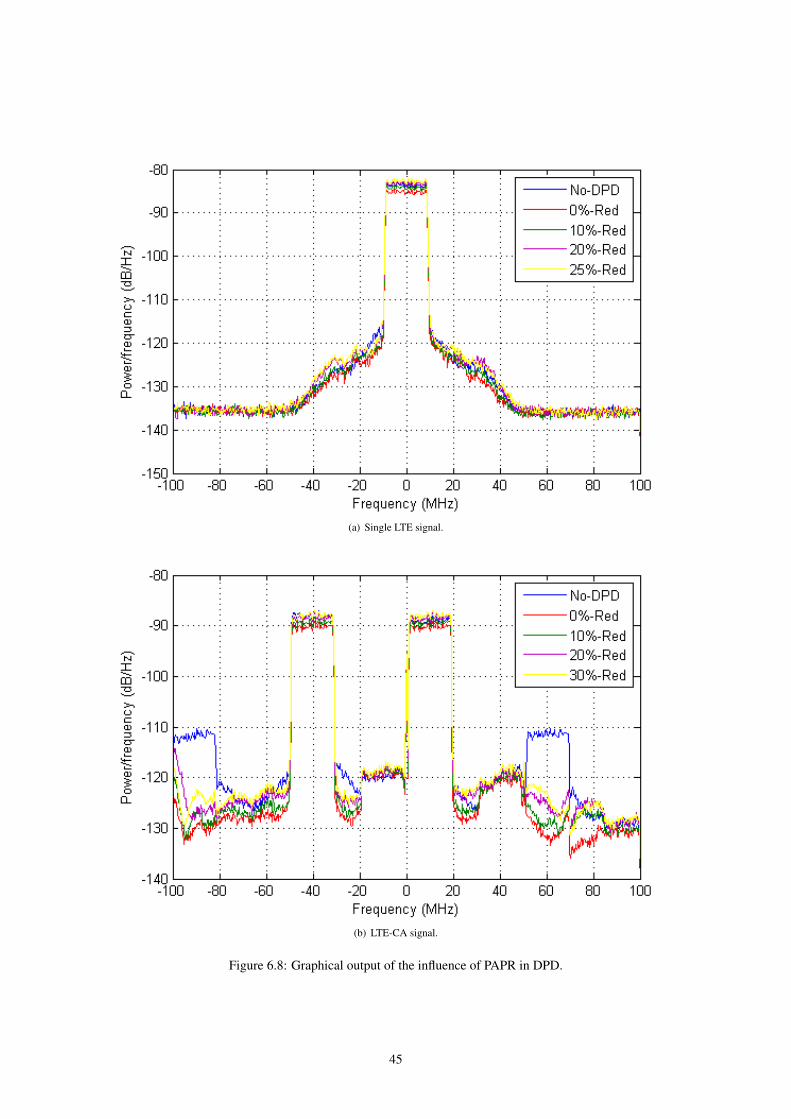
(a) Single LTE signal.

(b) LTE-CA signal.

Figure 6.8: Graphical output of the influence of PAPR in DPD.

45

46

Chapter 7

Conclusions

A FTER the theoretical analysis that was developed throughout the first chapters of this thesis, the experimental

component played an important role in comprehending the real-life applicability of the theory. In addition,

as referred in Chapter 6, using a real DUT allows for a more realistic testing of the hypotheses without being

constrained by the limitations of a numerical model.

However, the tests that were performed did not prove to be very rewarding scientifically, as the results obtained

did not meet some of the expectations that existed when the thesis started. This is mainly due to the fact that fine

adjustments had to be made in the digital predistortion process in order to overcome system issues, such as the

imbalance in the I/Q. Nonetheless, all the topics covered in this dissertation were put to test and some conclusions

can be drawn from the experimental campaign.

First of all, reducing the observational bandwidth of a signal for its recovery has been proved to be as DPD

efficient as when the full spectrum of the signal is recovered. In addition, the method also returned similar results

using different observational bandwidths, provided that the effective area covered by all sets of bandwidths is the

same.

Secondly, the model order reduction returned better or similar results, but only in the frequency-estimation

method. In the time-domain estimation, the full-order model proved to be more efficient.

Moreover, the estimation in frequency did not prove to be as effective as the estimation in the time-domain.

This can be linked to the inefficiency described above for the model-order reduction. The results obtained with

time-domain estimation returned better results than those obtained with frequency estimation. However, a more

complete analysis relating the performance of these two methods together with the model order would have to

be performed in order to establish the degree of dependence of each methods with the number of coefficients. In

addition, the high order frequency-based estimation proved inefficient in overcoming the imbalances caused by the

I/Q modulator that interfered with the signal.

Finally, a direct correlation between the reduction of the PAPR and the efficiency of the DPD could not be

found. Despite this fact, the PAPR was reduced up to 75% of its original value and still an improvement on the

ACLR values was verified when compared to the case where no reduction and no DPD were performed. Therefore,

and without compromising the integrity of the signals, the DPD was proven to be able to perform in PAPR-reduced

signals.

47

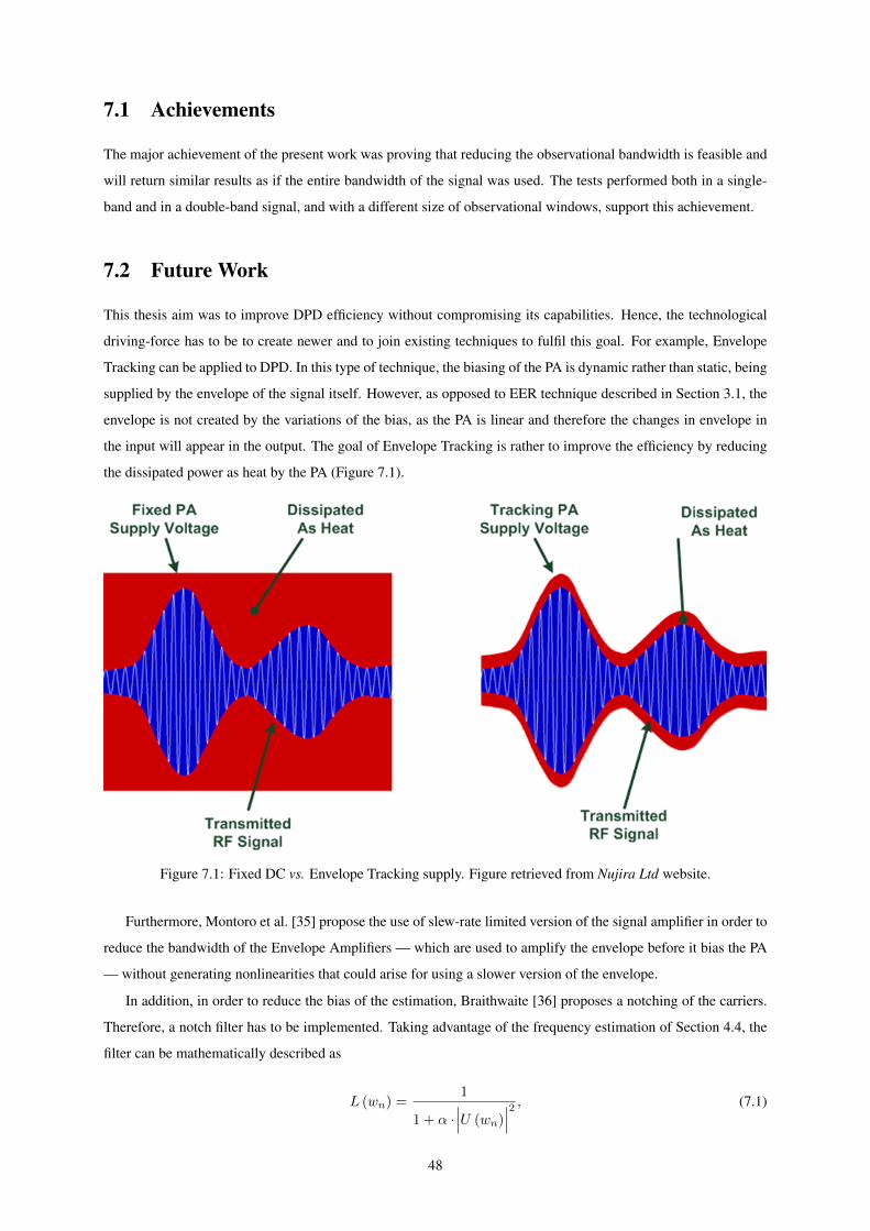
7.1 Achievements

The major achievement of the present work was proving that reducing the observational bandwidth is feasible and

will return similar results as if the entire bandwidth of the signal was used. The tests performed both in a single-

band and in a double-band signal, and with a different size of observational windows, support this achievement.

7.2 Future Work

This thesis aim was to improve DPD efficiency without compromising its capabilities. Hence, the technological

driving-force has to be to create newer and to join existing techniques to fulfil this goal. For example, Envelope

Tracking can be applied to DPD. In this type of technique, the biasing of the PA is dynamic rather than static, being

supplied by the envelope of the signal itself. However, as opposed to EER technique described in Section 3.1, the

envelope is not created by the variations of the bias, as the PA is linear and therefore the changes in envelope in

the input will appear in the output. The goal of Envelope Tracking is rather to improve the efficiency by reducing

the dissipated power as heat by the PA (Figure 7.1).

Figure 7.1: Fixed DC vs. Envelope Tracking supply. Figure retrieved from Nujira Ltd website.

Furthermore, Montoro et al. [35] propose the use of slew-rate limited version of the signal amplifier in order to

reduce the bandwidth of the Envelope Amplifiers — which are used to amplify the envelope before it bias the PA

— without generating nonlinearities that could arise for using a slower version of the envelope.

In addition, in order to reduce the bias of the estimation, Braithwaite [36] proposes a notching of the carriers.

Therefore, a notch filter has to be implemented. Taking advantage of the frequency estimation of Section 4.4, the

filter can be mathematically described as

L (wn) =1

1 + α ·∣∣∣U (wn)

∣∣∣2 , (7.1)

48

where U (wn) is the Fourier transform of u[n] and α is the notching-control parameter. The filtering has to

be applied in both input and output signals so as to achieve coherence for the coefficients extraction. Matrix Ψ

defined in (4.6) can be rewritten as

Ψx =

[L{ψ11

}L{ψ12

}. . . L

{ψMP

}]. (7.2)

By filtering both u[n] and y[n], Equation (4.10) can be redefined as

L{E(ωn)

}= L

{Y (ωn)

}G−10 − L

{U(ωn)

}, (7.3)

which leads to a notch-filtered error signal that can be used to extract the coefficients.

On the other hand, during the practical experiments for this project, we were faced with impairments created by

the I/Q Modulator when processing wideband signals, such as the LTE-CA. The cause of this impairment is related

to the fact that the in-phase and quadrature carriers may not have the same amplitude and the phase difference

between them may not be exactly 90 degrees. These impairments resulted in spurious tones that appeared in the

carrier band. Though it was possible to suppress them manually to a certain level using the Modulator GUI, there

are techniques which can be applied to diminish this effect algorithmically.

Cao et al. [37] propose a non-linear approach to this problematic in order to account for the frequency-

dependant impairments. A modified Memory Polynomial model that accounts for both in-phase and quadrature

components can be used. The output of the Modulator can be defined as

y[n] =

M∑

m=0

N∑

k=0

Q∑

q=0

P∑

p=0

amkqp

(xI [n−m]

)p (xQ[n−m]

)q, (7.4)

where xI and xQ represent the in-phase and quadrature components of the signal. Due to the fact that both

components influence each other, then the error has to be taken account separately and can be defined as

eI [n] = yI − yI , (7.5a)

eQ[n] = yQ − yQ. (7.5b)

From this point, the process can be done iteratively using a method such as the one described for the PA Direct

Learning (Subsection 3.2.2), yielding a set of coefficients for each component. Therefore, the new Modulator input

can be defined as

x[n] ={uI [n]− dI [n]

}+ j

{uQ[n]− dQ[n]

}, (7.6)

where dI/Q[n] is the additive distortion computed in the in-phase and quadrature paths, respectively.

Hence, this implementation can be seen as a predistortion technique applied to the modulator in a similar

manner to what it is done in the PA predistortion. So, the Modulator compensation algorithm can be applied in

a recursive way inside the PA DPD algorithm. However, since it requires the capture and processing of data at

every iteration it may not be efficient to do it at every DPD iteration. A trade-off may be required between the

49

influence one can allow for the I/Q imbalance and the computational time required to correct it. This trade-off may

lead to the option of computing the impairment correction coefficients at the first DPD iteration, or at the first two

iterations to allow for the biggest variations in signal that occur with DPD, and keeping the same coefficients for

the rest of the DPD iterations.

These three techniques described above can be used together with the project developed in this thesis to seek

more efficient predistortion algorithms.

50

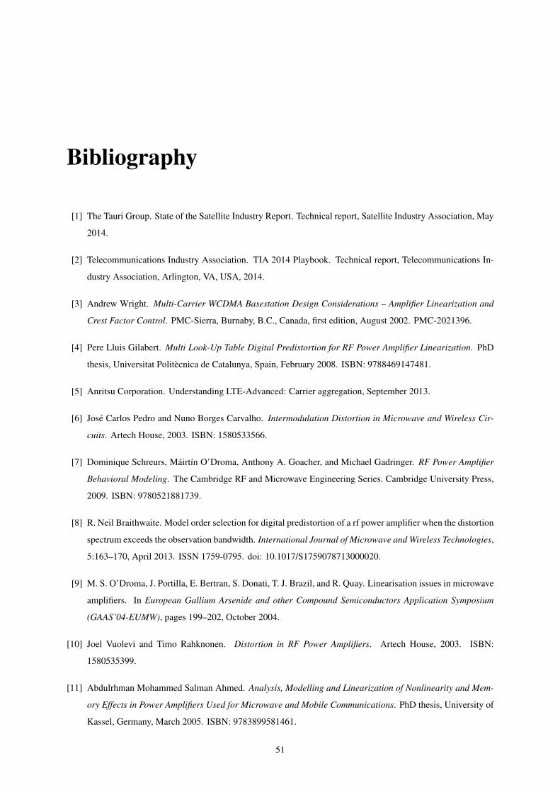
Bibliography

[1] The Tauri Group. State of the Satellite Industry Report. Technical report, Satellite Industry Association, May

2014.

[2] Telecommunications Industry Association. TIA 2014 Playbook. Technical report, Telecommunications In-

dustry Association, Arlington, VA, USA, 2014.

[3] Andrew Wright. Multi-Carrier WCDMA Basestation Design Considerations – Amplifier Linearization and

Crest Factor Control. PMC-Sierra, Burnaby, B.C., Canada, first edition, August 2002. PMC-2021396.

[4] Pere Lluis Gilabert. Multi Look-Up Table Digital Predistortion for RF Power Amplifier Linearization. PhD

thesis, Universitat Politecnica de Catalunya, Spain, February 2008. ISBN: 9788469147481.

[5] Anritsu Corporation. Understanding LTE-Advanced: Carrier aggregation, September 2013.

[6] Jose Carlos Pedro and Nuno Borges Carvalho. Intermodulation Distortion in Microwave and Wireless Cir-

cuits. Artech House, 2003. ISBN: 1580533566.

[7] Dominique Schreurs, Mairtın O’Droma, Anthony A. Goacher, and Michael Gadringer. RF Power Amplifier

Behavioral Modeling. The Cambridge RF and Microwave Engineering Series. Cambridge University Press,

2009. ISBN: 9780521881739.

[8] R. Neil Braithwaite. Model order selection for digital predistortion of a rf power amplifier when the distortion

spectrum exceeds the observation bandwidth. International Journal of Microwave and Wireless Technologies,

5:163–170, April 2013. ISSN 1759-0795. doi: 10.1017/S1759078713000020.

[9] M. S. O’Droma, J. Portilla, E. Bertran, S. Donati, T. J. Brazil, and R. Quay. Linearisation issues in microwave

amplifiers. In European Gallium Arsenide and other Compound Semiconductors Application Symposium

(GAAS’04-EUMW), pages 199–202, October 2004.

[10] Joel Vuolevi and Timo Rahknonen. Distortion in RF Power Amplifiers. Artech House, 2003. ISBN:

1580535399.

[11] Abdulrhman Mohammed Salman Ahmed. Analysis, Modelling and Linearization of Nonlinearity and Mem-

ory Effects in Power Amplifiers Used for Microwave and Mobile Communications. PhD thesis, University of

Kassel, Germany, March 2005. ISBN: 9783899581461.

51

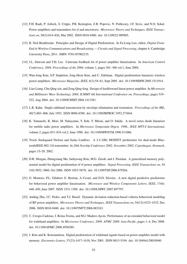
[12] F.H. Raab, P. Asbeck, S. Cripps, P.B. Kenington, Z.B. Popovic, N. Pothecary, J.F. Sevic, and N.O. Sokal.

Power amplifiers and transmitters for rf and microwave. Microwave Theory and Techniques, IEEE Transac-

tions on, 50(3):814–826, Mar 2002. ISSN 0018-9480. doi: 10.1109/22.989965.

[13] R. Neil Braithwaite. Principles and Design of Digital Predistortion. In Fa-Long Luo, editor, Digital Front-

End in Wireless Communications and Broadcasting — Circuits and Signal Processing, chapter 6. Cambridge

University Press, 2011. ISBN: 9781107002135.

[14] J.L. Dawson and T.H. Lee. Cartesian feedback for rf power amplifier linearization. In American Control

Conference, 2004. Proceedings of the 2004, volume 1, pages 361–366 vol.1, June 2004.

[15] Wan-Jong Kim, S.P. Stapleton, Jong-Heon Kim, and C. Edelman. Digital predistortion linearizes wireless

power amplifiers. Microwave Magazine, IEEE, 6(3):54–61, Sept 2005. doi: 10.1109/MMW.2005.1511914.

[16] Liao Liang, Chu Qing-xin, and Zeng Qing-feng. Design of feedforward linear power amplifier. In Microwave

and Millimeter Wave Technology, 2004. ICMMT 4th International Conference on, Proceedings, pages 519–

522, Aug 2004. doi: 10.1109/ICMMT.2004.1411581.

[17] L.R. Kahn. Single-sideband transmission by envelope elimination and restoration. Proceedings of the IRE,

40(7):803–806, July 1952. ISSN 0096-8390. doi: 10.1109/JRPROC.1952.273844.

[18] K. Yamauchi, K. Mori, M. Nakayama, Y. Itoh, Y. Mitsui, and O. Ishida. A novel series diode linearizer

for mobile radio power amplifiers. In Microwave Symposium Digest, 1996., IEEE MTT-S International,

volume 2, pages 831–834 vol.2, June 1996. doi: 10.1109/MWSYM.1996.511066.

[19] Troels Studsgaard Nielsen and Saska Lindfors. A 2.4 GHz MOSFET predistorter for dual-mode Blue-

tooth/IEEE 802.11b transmitter. In 20th Norchip Conference 2002, November 2002, Copenhagen, Denmark,

pages 15–20. 2002.

[20] D.R. Morgan, Zhengxiang Ma, Jaehyeong Kim, M.G. Zierdt, and J. Pastalan. A generalized memory poly-

nomial model for digital predistortion of rf power amplifiers. Signal Processing, IEEE Transactions on, 54

(10):3852–3860, Oct 2006. ISSN 1053-587X. doi: 10.1109/TSP.2006.879264.

[21] G. Montoro, P.L. Gilabert, E. Bertran, A Cesari, and D.D. Silveira. A new digital predictive predistorter

for behavioral power amplifier linearization. Microwave and Wireless Components Letters, IEEE, 17(6):

448–450, June 2007. ISSN 1531-1309. doi: 10.1109/LMWC.2007.897797.

[22] Anding Zhu, J.C. Pedro, and T.J. Brazil. Dynamic deviation reduction-based volterra behavioral modeling

of RF power amplifiers. Microwave Theory and Techniques, IEEE Transactions on, 54(12):4323–4332, Dec

2006. ISSN 0018-9480. doi: 10.1109/TMTT.2006.883243.

[23] C. Crespo-Cadenas, J. Reina-Tosina, and M.J. Madero-Ayora. Performance of an extended behavioral model

for wideband amplifiers. In Microwave Conference, 2008. APMC 2008. Asia-Pacific, pages 1–4, Dec 2008.

doi: 10.1109/APMC.2008.4958289.

[24] J. Kim and K. Konstantinou. Digital predistortion of wideband signals based on power amplifier model with

memory. Electronics Letters, 37(23):1417–1418, Nov 2001. ISSN 0013-5194. doi: 10.1049/el:20010940.

52

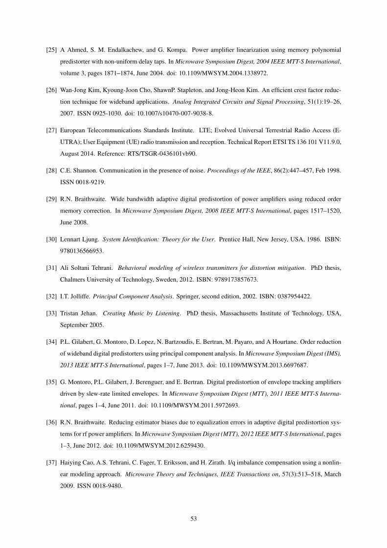
[25] A Ahmed, S. M. Endalkachew, and G. Kompa. Power amplifier linearization using memory polynomial

predistorter with non-uniform delay taps. In Microwave Symposium Digest, 2004 IEEE MTT-S International,

volume 3, pages 1871–1874, June 2004. doi: 10.1109/MWSYM.2004.1338972.

[26] Wan-Jong Kim, Kyoung-Joon Cho, ShawnP. Stapleton, and Jong-Heon Kim. An efficient crest factor reduc-

tion technique for wideband applications. Analog Integrated Circuits and Signal Processing, 51(1):19–26,

2007. ISSN 0925-1030. doi: 10.1007/s10470-007-9038-8.

[27] European Telecommunications Standards Institute. LTE; Evolved Universal Terrestrial Radio Access (E-

UTRA); User Equipment (UE) radio transmission and reception. Technical Report ETSI TS 136 101 V11.9.0,

August 2014. Reference: RTS/TSGR-0436101vb90.

[28] C.E. Shannon. Communication in the presence of noise. Proceedings of the IEEE, 86(2):447–457, Feb 1998.

ISSN 0018-9219.

[29] R.N. Braithwaite. Wide bandwidth adaptive digital predistortion of power amplifiers using reduced order

memory correction. In Microwave Symposium Digest, 2008 IEEE MTT-S International, pages 1517–1520,

June 2008.

[30] Lennart Ljung. System Identification: Theory for the User. Prentice Hall, New Jersey, USA, 1986. ISBN:

9780136566953.

[31] Ali Soltani Tehrani. Behavioral modeling of wireless transmitters for distortion mitigation. PhD thesis,

Chalmers University of Technology, Sweden, 2012. ISBN: 9789173857673.

[32] I.T. Jolliffe. Principal Component Analysis. Springer, second edition, 2002. ISBN: 0387954422.

[33] Tristan Jehan. Creating Music by Listening. PhD thesis, Massachusetts Institute of Technology, USA,

September 2005.

[34] P.L. Gilabert, G. Montoro, D. Lopez, N. Bartzoudis, E. Bertran, M. Payaro, and A Hourtane. Order reduction

of wideband digital predistorters using principal component analysis. In Microwave Symposium Digest (IMS),

2013 IEEE MTT-S International, pages 1–7, June 2013. doi: 10.1109/MWSYM.2013.6697687.

[35] G. Montoro, P.L. Gilabert, J. Berenguer, and E. Bertran. Digital predistortion of envelope tracking amplifiers

driven by slew-rate limited envelopes. In Microwave Symposium Digest (MTT), 2011 IEEE MTT-S Interna-

tional, pages 1–4, June 2011. doi: 10.1109/MWSYM.2011.5972693.

[36] R.N. Braithwaite. Reducing estimator biases due to equalization errors in adaptive digital predistortion sys-

tems for rf power amplifiers. In Microwave Symposium Digest (MTT), 2012 IEEE MTT-S International, pages

1–3, June 2012. doi: 10.1109/MWSYM.2012.6259430.

[37] Haiying Cao, A.S. Tehrani, C. Fager, T. Eriksson, and H. Zirath. I/q imbalance compensation using a nonlin-

ear modeling approach. Microwave Theory and Techniques, IEEE Transactions on, 57(3):513–518, March

2009. ISSN 0018-9480.

53

54