Digital imaging processing 2nd
190
Digital Image Processing Second Edition Rafael C. Gonzalez University of Tennessee Richard E. Woods MedData Interactive Prentice Hall Upper Saddle River, New Jersey 07458
-
Upload
khoatin2007 -
Category
Education
-
view
543 -
download
3
Transcript of Digital imaging processing 2nd

Digital ImageProcessingSecond Edition
Rafael C. GonzalezUniversity of Tennessee
Richard E. WoodsMedData Interactive
Prentice HallUpper Saddle River, New Jersey 07458
GONZFM-i-xxii. 5-10-2001 14:22 Page iii

Library of Congress Cataloging-in-Pubblication Data
Gonzalez, Rafael C.Digital Image Processing / Richard E. Woods
p. cm.Includes bibliographical referencesISBN 0-201-18075-81. Digital Imaging. 2. Digital Techniques. I. Title.
TA1632.G66 2001621.3—dc21 2001035846
CIPVice-President and Editorial Director, ECS: Marcia J. HortonPublisher: Tom RobbinsAssociate Editor: Alice DworkinEditorial Assistant: Jody McDonnellVice President and Director of Production and Manufacturing, ESM: David W. RiccardiExecutive Managing Editor: Vince O’BrienManaging Editor: David A. GeorgeProduction Editor: Rose KernanComposition: Prepare, Inc.Director of Creative Services: Paul BelfantiCreative Director: Carole AnsonArt Director and Cover Designer: Heather ScottArt Editor: Greg DullesManufacturing Manager: Trudy PisciottiManufacturing Buyer: Lisa McDowellSenior Marketing Manager: Jennie Burger
© 2002 by Prentice-Hall, Inc.Upper Saddle River, New Jersey 07458
All rights reserved. No part of this book may be reproduced, in any form or by any means,without permission in writing from the publisher.
The author and publisher of this book have used their best efforts in preparing this book. These effortsinclude the development, research, and testing of the theories and programs to determine theireffectiveness. The author and publisher make no warranty of any kind, expressed or implied, with regard tothese programs or the documentation contained in this book. The author and publisher shall not be liable inany event for incidental or consequential damages in connection with, or arising out of, the furnishing,performance, or use of these programs.
Printed in the United States of America10 9 8 7 6 5 4 3 2 1
ISBN: 0-201-18075-8
Pearson Education Ltd., LondonPearson Education Australia Pty., Limited, SydneyPearson Education Singapore, Pte. Ltd.Pearson Education North Asia Ltd., Hong KongPearson Education Canada, Ltd., TorontoPearson Education de Mexico, S.A. de C.V.Pearson Education—Japan, TokyoPearson Education Malaysia, Pte. Ltd.Pearson Education, Upper Saddle River, New Jersey
GONZFM-i-xxii. 5-10-2001 14:22 Page iv
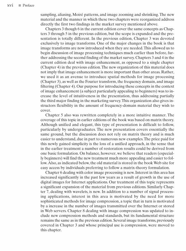
Preface
When something can be read without effort,great effort has gone into its writing.
Enrique Jardiel Poncela
This edition is the most comprehensive revision of Digital Image Processingsince the book first appeared in 1977.As the 1977 and 1987 editions by Gonzalezand Wintz, and the 1992 edition by Gonzalez and Woods, the present edition wasprepared with students and instructors in mind.Thus, the principal objectives ofthe book continue to be to provide an introduction to basic concepts andmethodologies for digital image processing, and to develop a foundation that canbe used as the basis for further study and research in this field.To achieve theseobjectives, we again focused on material that we believe is fundamental andhas a scope of application that is not limited to the solution of specialized prob-lems. The mathematical complexity of the book remains at a level well withinthe grasp of college seniors and first-year graduate students who have intro-ductory preparation in mathematical analysis, vectors, matrices, probability, sta-tistics, and rudimentary computer programming.
The present edition was influenced significantly by a recent market surveyconducted by Prentice Hall. The major findings of this survey were:
1. A need for more motivation in the introductory chapter regarding the spec-trum of applications of digital image processing.
2. A simplification and shortening of material in the early chapters in orderto “get to the subject matter” as quickly as possible.
3. A more intuitive presentation in some areas, such as image transforms andimage restoration.
4. Individual chapter coverage of color image processing, wavelets, and imagemorphology.
5. An increase in the breadth of problems at the end of each chapter.
The reorganization that resulted in this edition is our attempt at providing areasonable degree of balance between rigor in the presentation, the findings ofthe market survey, and suggestions made by students, readers, and colleaguessince the last edition of the book. The major changes made in the book are asfollows.
Chapter 1 was rewritten completely.The main focus of the current treatmentis on examples of areas that use digital image processing. While far from ex-haustive, the examples shown will leave little doubt in the reader’s mind re-garding the breadth of application of digital image processing methodologies.Chapter 2 is totally new also.The focus of the presentation in this chapter is onhow digital images are generated, and on the closely related concepts of
xv
GONZFM-i-xxii. 5-10-2001 14:22 Page xv
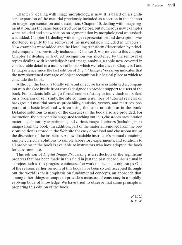
sampling, aliasing, Moiré patterns, and image zooming and shrinking. The newmaterial and the manner in which these two chapters were reorganized addressdirectly the first two findings in the market survey mentioned above.
Chapters 3 though 6 in the current edition cover the same concepts as Chap-ters 3 through 5 in the previous edition, but the scope is expanded and the pre-sentation is totally different. In the previous edition, Chapter 3 was devotedexclusively to image transforms. One of the major changes in the book is thatimage transforms are now introduced when they are needed.This allowed us tobegin discussion of image processing techniques much earlier than before, fur-ther addressing the second finding of the market survey. Chapters 3 and 4 in thecurrent edition deal with image enhancement, as opposed to a single chapter(Chapter 4) in the previous edition.The new organization of this material doesnot imply that image enhancement is more important than other areas. Rather,we used it as an avenue to introduce spatial methods for image processing(Chapter 3), as well as the Fourier transform, the frequency domain, and imagefiltering (Chapter 4). Our purpose for introducing these concepts in the contextof image enhancement (a subject particularly appealing to beginners) was to in-crease the level of intuitiveness in the presentation, thus addressing partiallythe third major finding in the marketing survey.This organization also gives in-structors flexibility in the amount of frequency-domain material they wish tocover.
Chapter 5 also was rewritten completely in a more intuitive manner. Thecoverage of this topic in earlier editions of the book was based on matrix theory.Although unified and elegant, this type of presentation is difficult to follow,particularly by undergraduates. The new presentation covers essentially thesame ground, but the discussion does not rely on matrix theory and is mucheasier to understand, due in part to numerous new examples.The price paid forthis newly gained simplicity is the loss of a unified approach, in the sense thatin the earlier treatment a number of restoration results could be derived fromone basic formulation. On balance, however, we believe that readers (especial-ly beginners) will find the new treatment much more appealing and easier to fol-low.Also, as indicated below, the old material is stored in the book Web site foreasy access by individuals preferring to follow a matrix-theory formulation.
Chapter 6 dealing with color image processing is new. Interest in this area hasincreased significantly in the past few years as a result of growth in the use ofdigital images for Internet applications. Our treatment of this topic representsa significant expansion of the material from previous editions. Similarly Chap-ter 7, dealing with wavelets, is new. In addition to a number of signal process-ing applications, interest in this area is motivated by the need for moresophisticated methods for image compression, a topic that in turn is motivatedby a increase in the number of images transmitted over the Internet or storedin Web servers. Chapter 8 dealing with image compression was updated to in-clude new compression methods and standards, but its fundamental structureremains the same as in the previous edition. Several image transforms, previouslycovered in Chapter 3 and whose principal use is compression, were moved tothis chapter.
xvi � Preface
GONZFM-i-xxii. 5-10-2001 14:22 Page xvi
Chapter 9, dealing with image morphology, is new. It is based on a signifi-cant expansion of the material previously included as a section in the chapteron image representation and description. Chapter 10, dealing with image seg-mentation, has the same basic structure as before, but numerous new exampleswere included and a new section on segmentation by morphological watershedswas added. Chapter 11, dealing with image representation and description, wasshortened slightly by the removal of the material now included in Chapter 9.New examples were added and the Hotelling transform (description by princi-pal components), previously included in Chapter 3, was moved to this chapter.Chapter 12 dealing with object recognition was shortened by the removal oftopics dealing with knowledge-based image analysis, a topic now covered inconsiderable detail in a number of books which we reference in Chapters 1 and12. Experience since the last edition of Digital Image Processing indicates thatthe new, shortened coverage of object recognition is a logical place at which toconclude the book.
Although the book is totally self-contained, we have established a compan-ion web site (see inside front cover) designed to provide support to users of thebook. For students following a formal course of study or individuals embarkedon a program of self study, the site contains a number of tutorial reviews onbackground material such as probability, statistics, vectors, and matrices, pre-pared at a basic level and written using the same notation as in the book.Detailed solutions to many of the exercises in the book also are provided. Forinstruction, the site contains suggested teaching outlines, classroom presentationmaterials, laboratory experiments, and various image databases (including mostimages from the book). In addition, part of the material removed from the pre-vious edition is stored in the Web site for easy download and classroom use, atthe discretion of the instructor.A downloadable instructor’s manual containingsample curricula, solutions to sample laboratory experiments, and solutions toall problems in the book is available to instructors who have adopted the bookfor classroom use.
This edition of Digital Image Processing is a reflection of the significantprogress that has been made in this field in just the past decade. As is usual ina project such as this, progress continues after work on the manuscript stops. Oneof the reasons earlier versions of this book have been so well accepted through-out the world is their emphasis on fundamental concepts, an approach that,among other things, attempts to provide a measure of constancy in a rapidly-evolving body of knowledge. We have tried to observe that same principle inpreparing this edition of the book.
R.C.G.R.E.W.
� Preface xvii
GONZFM-i-xxii. 5-10-2001 14:22 Page xvii

GONZFM-i-xxii. 5-10-2001 14:22 Page xxii

Digital ImageProcessingSecond Edition
Rafael C. GonzalezUniversity of Tennessee
Richard E. WoodsMedData Interactive
Prentice HallUpper Saddle River, New Jersey 07458
GONZFM-i-xxii. 5-10-2001 14:22 Page iii

Library of Congress Cataloging-in-Pubblication Data
Gonzalez, Rafael C.Digital Image Processing / Richard E. Woods
p. cm.Includes bibliographical referencesISBN 0-201-18075-81. Digital Imaging. 2. Digital Techniques. I. Title.
TA1632.G66 2001621.3—dc21 2001035846
CIPVice-President and Editorial Director, ECS: Marcia J. HortonPublisher: Tom RobbinsAssociate Editor: Alice DworkinEditorial Assistant: Jody McDonnellVice President and Director of Production and Manufacturing, ESM: David W. RiccardiExecutive Managing Editor: Vince O’BrienManaging Editor: David A. GeorgeProduction Editor: Rose KernanComposition: Prepare, Inc.Director of Creative Services: Paul BelfantiCreative Director: Carole AnsonArt Director and Cover Designer: Heather ScottArt Editor: Greg DullesManufacturing Manager: Trudy PisciottiManufacturing Buyer: Lisa McDowellSenior Marketing Manager: Jennie Burger
© 2002 by Prentice-Hall, Inc.Upper Saddle River, New Jersey 07458
All rights reserved. No part of this book may be reproduced, in any form or by any means,without permission in writing from the publisher.
The author and publisher of this book have used their best efforts in preparing this book. These effortsinclude the development, research, and testing of the theories and programs to determine theireffectiveness. The author and publisher make no warranty of any kind, expressed or implied, with regard tothese programs or the documentation contained in this book. The author and publisher shall not be liable inany event for incidental or consequential damages in connection with, or arising out of, the furnishing,performance, or use of these programs.
Printed in the United States of America10 9 8 7 6 5 4 3 2 1
ISBN: 0-201-18075-8
Pearson Education Ltd., LondonPearson Education Australia Pty., Limited, SydneyPearson Education Singapore, Pte. Ltd.Pearson Education North Asia Ltd., Hong KongPearson Education Canada, Ltd., TorontoPearson Education de Mexico, S.A. de C.V.Pearson Education—Japan, TokyoPearson Education Malaysia, Pte. Ltd.Pearson Education, Upper Saddle River, New Jersey
GONZFM-i-xxii. 5-10-2001 14:22 Page iv
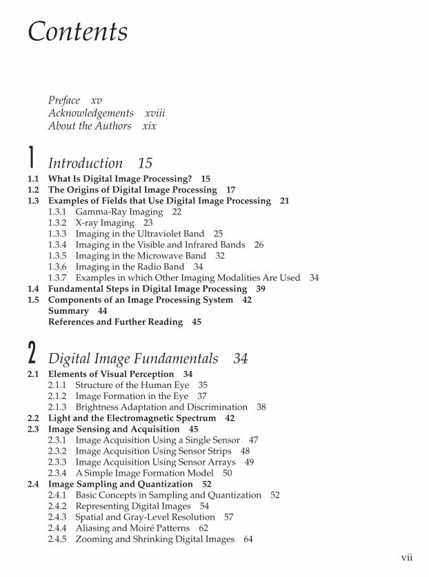
Contents
Preface xvAcknowledgements xviiiAbout the Authors xix
1 Introduction 151.1 What Is Digital Image Processing? 151.2 The Origins of Digital Image Processing 171.3 Examples of Fields that Use Digital Image Processing 21
1.3.1 Gamma-Ray Imaging 221.3.2 X-ray Imaging 231.3.3 Imaging in the Ultraviolet Band 251.3.4 Imaging in the Visible and Infrared Bands 261.3.5 Imaging in the Microwave Band 321.3.6 Imaging in the Radio Band 341.3.7 Examples in which Other Imaging Modalities Are Used 34
1.4 Fundamental Steps in Digital Image Processing 391.5 Components of an Image Processing System 42
Summary 44References and Further Reading 45
2 Digital Image Fundamentals 342.1 Elements of Visual Perception 34
2.1.1 Structure of the Human Eye 352.1.2 Image Formation in the Eye 372.1.3 Brightness Adaptation and Discrimination 38
2.2 Light and the Electromagnetic Spectrum 422.3 Image Sensing and Acquisition 45
2.3.1 Image Acquisition Using a Single Sensor 472.3.2 Image Acquisition Using Sensor Strips 482.3.3 Image Acquisition Using Sensor Arrays 492.3.4 A Simple Image Formation Model 50
2.4 Image Sampling and Quantization 522.4.1 Basic Concepts in Sampling and Quantization 522.4.2 Representing Digital Images 542.4.3 Spatial and Gray-Level Resolution 572.4.4 Aliasing and Moiré Patterns 622.4.5 Zooming and Shrinking Digital Images 64
vii
GONZFM-i-xxii. 5-10-2001 14:22 Page vii
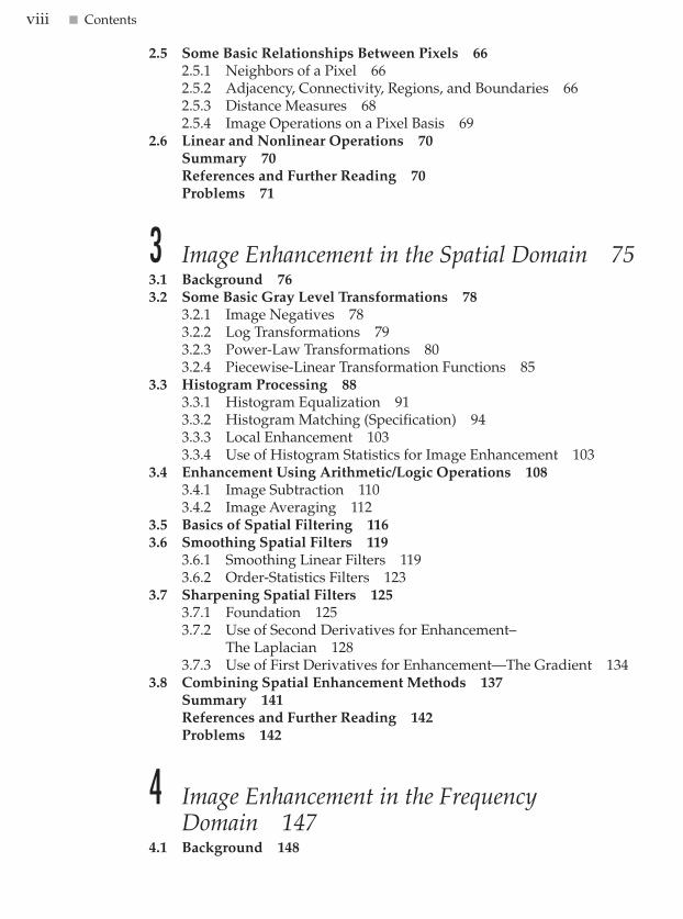
2.5 Some Basic Relationships Between Pixels 662.5.1 Neighbors of a Pixel 662.5.2 Adjacency, Connectivity, Regions, and Boundaries 662.5.3 Distance Measures 682.5.4 Image Operations on a Pixel Basis 69
2.6 Linear and Nonlinear Operations 70Summary 70References and Further Reading 70Problems 71
3 Image Enhancement in the Spatial Domain 753.1 Background 763.2 Some Basic Gray Level Transformations 78
3.2.1 Image Negatives 783.2.2 Log Transformations 793.2.3 Power-Law Transformations 803.2.4 Piecewise-Linear Transformation Functions 85
3.3 Histogram Processing 883.3.1 Histogram Equalization 913.3.2 Histogram Matching (Specification) 943.3.3 Local Enhancement 1033.3.4 Use of Histogram Statistics for Image Enhancement 103
3.4 Enhancement Using Arithmetic/Logic Operations 1083.4.1 Image Subtraction 1103.4.2 Image Averaging 112
3.5 Basics of Spatial Filtering 1163.6 Smoothing Spatial Filters 119
3.6.1 Smoothing Linear Filters 1193.6.2 Order-Statistics Filters 123
3.7 Sharpening Spatial Filters 1253.7.1 Foundation 1253.7.2 Use of Second Derivatives for Enhancement–
The Laplacian 1283.7.3 Use of First Derivatives for Enhancement—The Gradient 134
3.8 Combining Spatial Enhancement Methods 137Summary 141References and Further Reading 142Problems 142
4 Image Enhancement in the Frequency Domain 147
4.1 Background 148
viii � Contents
GONZFM-i-xxii. 5-10-2001 14:22 Page viii
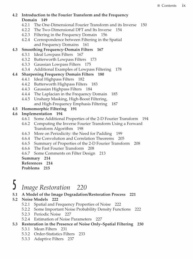
4.2 Introduction to the Fourier Transform and the Frequency Domain 1494.2.1 The One-Dimensional Fourier Transform and its Inverse 1504.2.2 The Two-Dimensional DFT and Its Inverse 1544.2.3 Filtering in the Frequency Domain 1564.2.4 Correspondence between Filtering in the Spatial
and Frequency Domains 1614.3 Smoothing Frequency-Domain Filters 167
4.3.1 Ideal Lowpass Filters 1674.3.2 Butterworth Lowpass Filters 1734.3.3 Gaussian Lowpass Filters 1754.3.4 Additional Examples of Lowpass Filtering 178
4.4 Sharpening Frequency Domain Filters 1804.4.1 Ideal Highpass Filters 1824.4.2 Butterworth Highpass Filters 1834.4.3 Gaussian Highpass Filters 1844.4.4 The Laplacian in the Frequency Domain 1854.4.5 Unsharp Masking, High-Boost Filtering,
and High-Frequency Emphasis Filtering 1874.5 Homomorphic Filtering 1914.6 Implementation 194
4.6.1 Some Additional Properties of the 2-D Fourier Transform 1944.6.2 Computing the Inverse Fourier Transform Using a Forward
Transform Algorithm 1984.6.3 More on Periodicity: the Need for Padding 1994.6.4 The Convolution and Correlation Theorems 2054.6.5 Summary of Properties of the 2-D Fourier Transform 2084.6.6 The Fast Fourier Transform 2084.6.7 Some Comments on Filter Design 213Summary 214References 214Problems 215
5 Image Restoration 2205.1 A Model of the Image Degradation/Restoration Process 2215.2 Noise Models 222
5.2.1 Spatial and Frequency Properties of Noise 2225.2.2 Some Important Noise Probability Density Functions 2225.2.3 Periodic Noise 2275.2.4 Estimation of Noise Parameters 227
5.3 Restoration in the Presence of Noise Only–Spatial Filtering 2305.3.1 Mean Filters 2315.3.2 Order-Statistics Filters 2335.3.3 Adaptive Filters 237
� Contents ix
GONZFM-i-xxii. 5-10-2001 14:22 Page ix
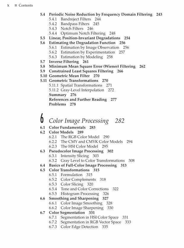
5.4 Periodic Noise Reduction by Frequency Domain Filtering 2435.4.1 Bandreject Filters 2445.4.2 Bandpass Filters 2455.4.3 Notch Filters 2465.4.4 Optimum Notch Filtering 248
5.5 Linear, Position-Invariant Degradations 2545.6 Estimating the Degradation Function 256
5.6.1 Estimation by Image Observation 2565.6.2 Estimation by Experimentation 2575.6.3 Estimation by Modeling 258
5.7 Inverse Filtering 2615.8 Minimum Mean Square Error (Wiener) Filtering 2625.9 Constrained Least Squares Filtering 2665.10 Geometric Mean Filter 2705.11 Geometric Transformations 270
5.11.1 Spatial Transformations 2715.11.2 Gray-Level Interpolation 272Summary 276References and Further Reading 277Problems 278
6 Color Image Processing 2826.1 Color Fundamentals 2836.2 Color Models 289
6.2.1 The RGB Color Model 2906.2.2 The CMY and CMYK Color Models 2946.2.3 The HSI Color Model 295
6.3 Pseudocolor Image Processing 3026.3.1 Intensity Slicing 3036.3.2 Gray Level to Color Transformations 308
6.4 Basics of Full-Color Image Processing 3136.5 Color Transformations 315
6.5.1 Formulation 3156.5.2 Color Complements 3186.5.3 Color Slicing 3206.5.4 Tone and Color Corrections 3226.5.5 Histogram Processing 326
6.6 Smoothing and Sharpening 3276.6.1 Color Image Smoothing 3286.6.2 Color Image Sharpening 330
6.7 Color Segmentation 3316.7.1 Segmentation in HSI Color Space 3316.7.2 Segmentation in RGB Vector Space 3336.7.3 Color Edge Detection 335
x � Contents
GONZFM-i-xxii. 5-10-2001 14:22 Page x
6.8 Noise in Color Images 3396.9 Color Image Compression 342
Summary 343References and Further Reading 344Problems 344
7 Wavelets and Multiresolution Processing 3497.1 Background 350
7.1.1 Image Pyramids 3517.1.2 Subband Coding 3547.1.3 The Haar Transform 360
7.2 Multiresolution Expansions 3637.2.1 Series Expansions 3647.2.2 Scaling Functions 3657.2.3 Wavelet Functions 369
7.3 Wavelet Transforms in One Dimension 3727.3.1 The Wavelet Series Expansions 3727.3.2 The Discrete Wavelet Transform 3757.3.3 The Continuous Wavelet Transform 376
7.4 The Fast Wavelet Transform 3797.5 Wavelet Transforms in Two Dimensions 3867.6 Wavelet Packets 394
Summary 402References and Further Reading 404Problems 404
8 Image Compression 4098.1 Fundamentals 411
8.1.1 Coding Redundancy 4128.1.2 Interpixel Redundancy 4148.1.3 Psychovisual Redundancy 4178.1.4 Fidelity Criteria 419
8.2 Image Compression Models 4218.2.1 The Source Encoder and Decoder 4218.2.2 The Channel Encoder and Decoder 423
8.3 Elements of Information Theory 4248.3.1 Measuring Information 4248.3.2 The Information Channel 4258.3.3 Fundamental Coding Theorems 4308.3.4 Using Information Theory 437
8.4 Error-Free Compression 4408.4.1 Variable-Length Coding 440
� Contents xi
GONZFM-i-xxii. 5-10-2001 14:22 Page xi
8.4.2 LZW Coding 4468.4.3 Bit-Plane Coding 4488.4.4 Lossless Predictive Coding 456
8.5 Lossy Compression 4598.5.1 Lossy Predictive Coding 4598.5.2 Transform Coding 4678.5.3 Wavelet Coding 486
8.6 Image Compression Standards 4928.6.1 Binary Image Compression Standards 4938.6.2 Continuous Tone Still Image Compression Standards 4988.6.3 Video Compression Standards 510Summary 513References and Further Reading 513Problems 514
9 Morphological Image Processing 5199.1 Preliminaries 520
9.1.1 Some Basic Concepts from Set Theory 5209.1.2 Logic Operations Involving Binary Images 522
9.2 Dilation and Erosion 5239.2.1 Dilation 5239.2.2 Erosion 525
9.3 Opening and Closing 5289.4 The Hit-or-Miss Transformation 5329.5 Some Basic Morphological Algorithms 534
9.5.1 Boundary Extraction 5349.5.2 Region Filling 5359.5.3 Extraction of Connected Components 5369.5.4 Convex Hull 5399.5.5 Thinning 5419.5.6 Thickening 5419.5.7 Skeletons 5439.5.8 Pruning 5459.5.9 Summary of Morphological Operations on Binary Images 547
9.6 Extensions to Gray-Scale Images 5509.6.1 Dilation 5509.6.2 Erosion 5529.6.3 Opening and Closing 5549.6.4 Some Applications of Gray-Scale Morphology 556Summary 560References and Further Reading 560Problems 560
xii � Contents
GONZFM-i-xxii. 5-10-2001 14:22 Page xii
10 Image Segmentation 56710.1 Detection of Discontinuities 568
10.1.1 Point Detection 56910.1.2 Line Detection 57010.1.3 Edge Detection 572
10.2 Edge Linking and Boundary Detection 58510.2.1 Local Processing 58510.2.2 Global Processing via the Hough Transform 58710.2.3 Global Processing via Graph-Theoretic Techniques 591
10.3 Thresholding 59510.3.1 Foundation 59510.3.2 The Role of Illumination 59610.3.3 Basic Global Thresholding 59810.3.4 Basic Adaptive Thresholding 60010.3.5 Optimal Global and Adaptive Thresholding 60210.3.6 Use of Boundary Characteristics for Histogram Improvement
and Local Thresholding 60810.3.7 Thresholds Based on Several Variables 611
10.4 Region-Based Segmentation 61210.4.1 Basic Formulation 61210.4.2 Region Growing 61310.4.3 Region Splitting and Merging 615
10.5 Segmentation by Morphological Watersheds 61710.5.1 Basic Concepts 61710.5.2 Dam Construction 62010.5.3 Watershed Segmentation Algorithm 62210.5.4 The Use of Markers 624
10.6 The Use of Motion in Segmentation 62610.6.1 Spatial Techniques 62610.6.2 Frequency Domain Techniques 630Summary 634References and Further Reading 634Problems 636
11 Representation and Description 64311.1 Representation 644
11.1.1 Chain Codes 64411.1.2 Polygonal Approximations 64611.1.3 Signatures 64811.1.4 Boundary Segments 64911.1.5 Skeletons 650
� Contents xiii
GONZFM-i-xxii. 5-10-2001 14:22 Page xiii
11.2 Boundary Descriptors 65311.2.1 Some Simple Descriptors 65311.2.2 Shape Numbers 65411.2.3 Fourier Descriptors 65511.2.4 Statistical Moments 659
11.3 Regional Descriptors 66011.3.1 Some Simple Descriptors 66111.3.2 Topological Descriptors 66111.3.3 Texture 66511.3.4 Moments of Two-Dimensional Functions 672
11.4 Use of Principal Components for Description 67511.5 Relational Descriptors 683
Summary 687References and Further Reading 687Problems 689
12 Object Recognition 69312.1 Patterns and Pattern Classes 69312.2 Recognition Based on Decision-Theoretic Methods 698
12.2.1 Matching 69812.2.2 Optimum Statistical Classifiers 70412.2.3 Neural Networks 712
12.3 Structural Methods 73212.3.1 Matching Shape Numbers 73212.3.2 String Matching 73412.3.3 Syntactic Recognition of Strings 73512.3.4 Syntactic Recognition of Trees 740Summary 750References and Further Reading 750Problems 750
Bibliography 755
Index 779
xiv � Contents
GONZFM-i-xxii. 5-10-2001 14:22 Page xiv

GONZFM-i-xxii. 5-10-2001 14:22 Page xxii
1
1 Introduction
One picture is worth more than ten thousand words.Anonymous
PreviewInterest in digital image processing methods stems from two principal applica-tion areas: improvement of pictorial information for human interpretation; andprocessing of image data for storage, transmission, and representation for au-tonomous machine perception.This chapter has several objectives: (1) to definethe scope of the field that we call image processing; (2) to give a historical per-spective of the origins of this field; (3) to give an idea of the state of the art inimage processing by examining some of the principal areas in which it is ap-plied; (4) to discuss briefly the principal approaches used in digital image pro-cessing; (5) to give an overview of the components contained in a typical,general-purpose image processing system; and (6) to provide direction to thebooks and other literature where image processing work normally is reported.
What Is Digital Image Processing?
An image may be defined as a two-dimensional function, f(x, y), where x andy are spatial (plane) coordinates, and the amplitude of f at any pair of coordi-nates (x, y) is called the intensity or gray level of the image at that point.Whenx, y, and the amplitude values of f are all finite, discrete quantities, we call theimage a digital image. The field of digital image processing refers to processingdigital images by means of a digital computer. Note that a digital image is com-posed of a finite number of elements, each of which has a particular location and
1.1
GONZ01-001-033.II 29-08-2001 14:42 Page 1
2 Chapter 1 � Introduction
value. These elements are referred to as picture elements, image elements, pels,and pixels. Pixel is the term most widely used to denote the elements of a digi-tal image. We consider these definitions in more formal terms in Chapter 2.
Vision is the most advanced of our senses, so it is not surprising that imagesplay the single most important role in human perception. However, unlikehumans, who are limited to the visual band of the electromagnetic (EM) spec-trum, imaging machines cover almost the entire EM spectrum, ranging fromgamma to radio waves. They can operate on images generated by sources thathumans are not accustomed to associating with images. These include ultra-sound, electron microscopy, and computer-generated images.Thus, digital imageprocessing encompasses a wide and varied field of applications.
There is no general agreement among authors regarding where image pro-cessing stops and other related areas, such as image analysis and computer vi-sion, start. Sometimes a distinction is made by defining image processing as adiscipline in which both the input and output of a process are images.We believethis to be a limiting and somewhat artificial boundary. For example, under thisdefinition, even the trivial task of computing the average intensity of an image(which yields a single number) would not be considered an image processing op-eration. On the other hand, there are fields such as computer vision whose ul-timate goal is to use computers to emulate human vision, including learningand being able to make inferences and take actions based on visual inputs.Thisarea itself is a branch of artificial intelligence (AI) whose objective is to emu-late human intelligence.The field of AI is in its earliest stages of infancy in termsof development, with progress having been much slower than originally antic-ipated. The area of image analysis (also called image understanding) is in be-tween image processing and computer vision.
There are no clear-cut boundaries in the continuum from image processingat one end to computer vision at the other. However, one useful paradigm isto consider three types of computerized processes in this continuum: low-,mid-, and high-level processes. Low-level processes involve primitive opera-tions such as image preprocessing to reduce noise, contrast enhancement, andimage sharpening. A low-level process is characterized by the fact that bothits inputs and outputs are images. Mid-level processing on images involvestasks such as segmentation (partitioning an image into regions or objects),description of those objects to reduce them to a form suitable for computerprocessing, and classification (recognition) of individual objects. A mid-levelprocess is characterized by the fact that its inputs generally are images, but itsoutputs are attributes extracted from those images (e.g., edges, contours, andthe identity of individual objects). Finally, higher-level processing involves“making sense” of an ensemble of recognized objects, as in image analysis,and, at the far end of the continuum, performing the cognitive functions nor-mally associated with vision.
Based on the preceding comments, we see that a logical place of overlap be-tween image processing and image analysis is the area of recognition of indi-vidual regions or objects in an image. Thus, what we call in this book digitalimage processing encompasses processes whose inputs and outputs are images
GONZ01-001-033.II 29-08-2001 14:42 Page 2
1.2 � The Origins of Digital Image Processing 3
† References in the Bibliography at the end of the book are listed in alphabetical order by authors’ lastnames.
and, in addition, encompasses processes that extract attributes from images, upto and including the recognition of individual objects. As a simple illustrationto clarify these concepts, consider the area of automated analysis of text. Theprocesses of acquiring an image of the area containing the text, preprocessingthat image, extracting (segmenting) the individual characters, describing thecharacters in a form suitable for computer processing, and recognizing thoseindividual characters are in the scope of what we call digital image processingin this book. Making sense of the content of the page may be viewed as beingin the domain of image analysis and even computer vision, depending on thelevel of complexity implied by the statement “making sense.” As will becomeevident shortly, digital image processing, as we have defined it, is used success-fully in a broad range of areas of exceptional social and economic value.The con-cepts developed in the following chapters are the foundation for the methodsused in those application areas.
The Origins of Digital Image Processing
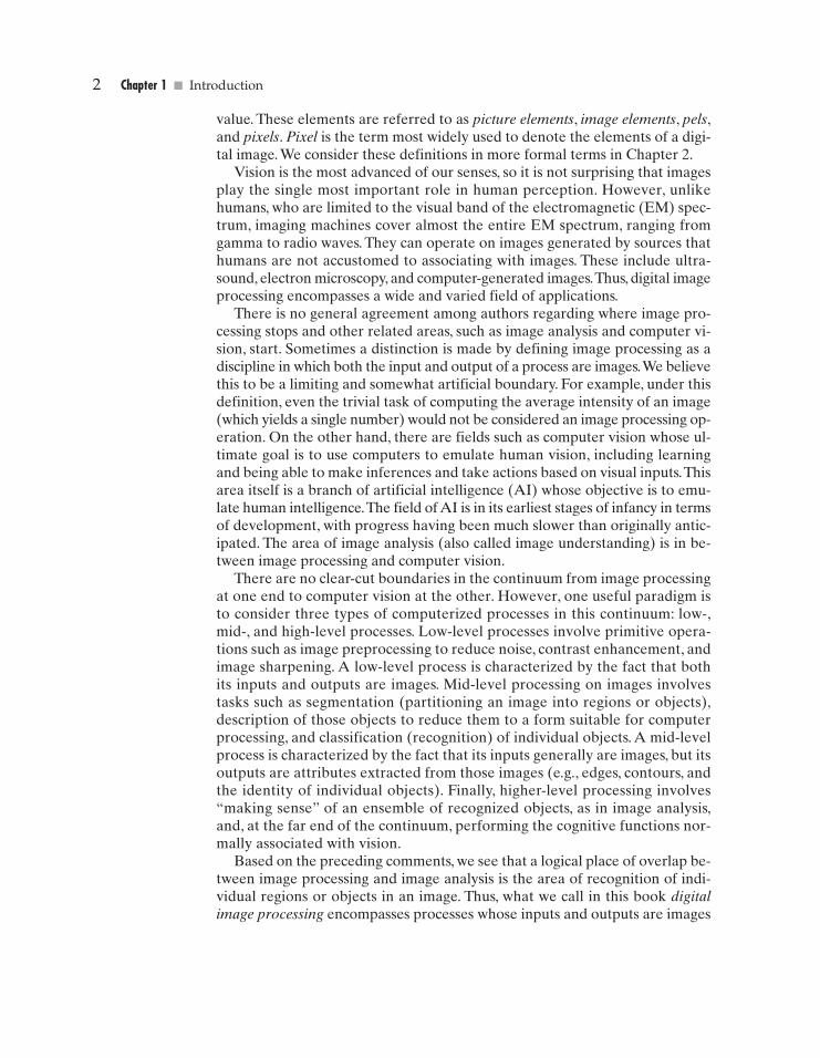
One of the first applications of digital images was in the newspaper industry,when pictures were first sent by submarine cable between London and NewYork. Introduction of the Bartlane cable picture transmission system in theearly 1920s reduced the time required to transport a picture across the Atlanticfrom more than a week to less than three hours. Specialized printing equipmentcoded pictures for cable transmission and then reconstructed them at the re-ceiving end. Figure 1.1 was transmitted in this way and reproduced on a tele-graph printer fitted with typefaces simulating a halftone pattern.
Some of the initial problems in improving the visual quality of these early dig-ital pictures were related to the selection of printing procedures and the distri-bution of intensity levels. The printing method used to obtain Fig. 1.1 wasabandoned toward the end of 1921 in favor of a technique based on photo-graphic reproduction made from tapes perforated at the telegraph receivingterminal. Figure 1.2 shows an image obtained using this method. The improve-ments over Fig. 1.1 are evident, both in tonal quality and in resolution.
1.2
FIGURE 1.1 Adigital pictureproduced in 1921from a coded tapeby a telegraphprinter withspecial type faces.(McFarlane.†)
GONZ01-001-033.II 29-08-2001 14:42 Page 3
4 Chapter 1 � Introduction
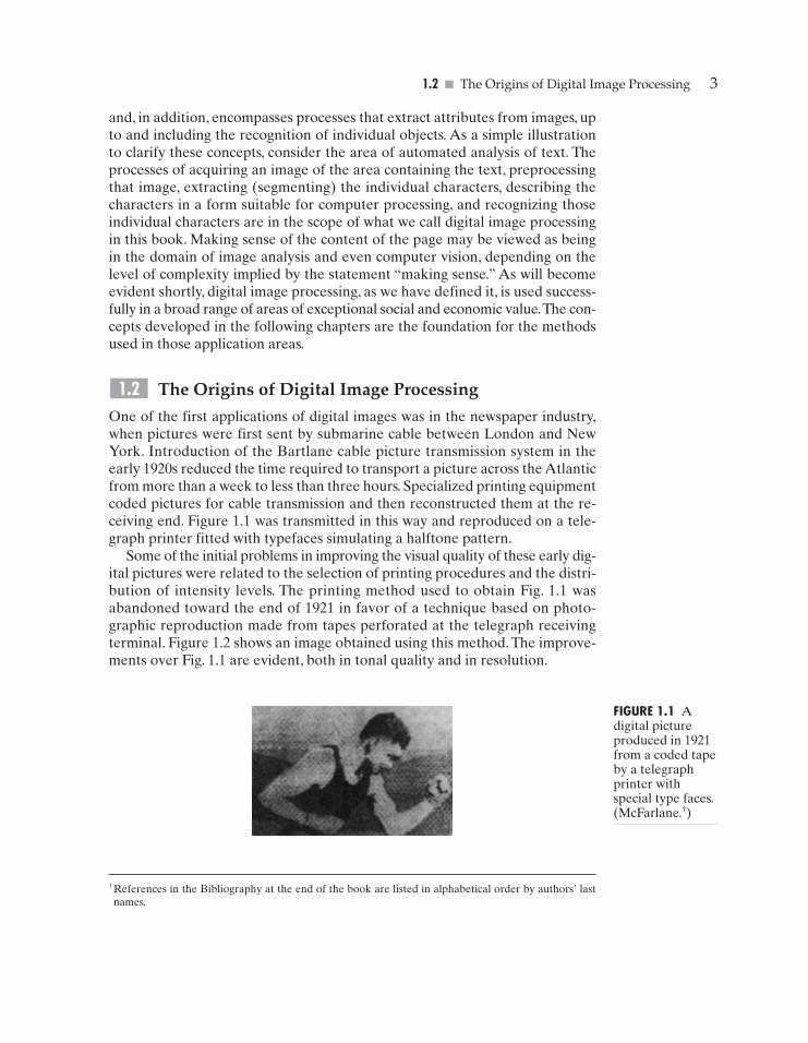
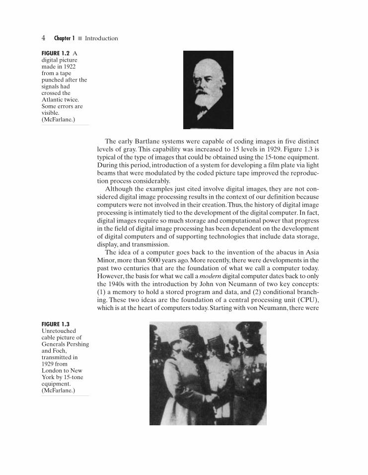
FIGURE 1.3Unretouchedcable picture ofGenerals Pershingand Foch,transmitted in1929 fromLondon to NewYork by 15-toneequipment.(McFarlane.)
The early Bartlane systems were capable of coding images in five distinctlevels of gray. This capability was increased to 15 levels in 1929. Figure 1.3 istypical of the type of images that could be obtained using the 15-tone equipment.During this period, introduction of a system for developing a film plate via lightbeams that were modulated by the coded picture tape improved the reproduc-tion process considerably.
Although the examples just cited involve digital images, they are not con-sidered digital image processing results in the context of our definition becausecomputers were not involved in their creation.Thus, the history of digital imageprocessing is intimately tied to the development of the digital computer. In fact,digital images require so much storage and computational power that progressin the field of digital image processing has been dependent on the developmentof digital computers and of supporting technologies that include data storage,display, and transmission.
The idea of a computer goes back to the invention of the abacus in AsiaMinor, more than 5000 years ago. More recently, there were developments in thepast two centuries that are the foundation of what we call a computer today.However, the basis for what we call a modern digital computer dates back to onlythe 1940s with the introduction by John von Neumann of two key concepts:(1) a memory to hold a stored program and data, and (2) conditional branch-ing. These two ideas are the foundation of a central processing unit (CPU),which is at the heart of computers today. Starting with von Neumann, there were
FIGURE 1.2 Adigital picturemade in 1922from a tapepunched after thesignals hadcrossed theAtlantic twice.Some errors arevisible.(McFarlane.)
GONZ01-001-033.II 29-08-2001 14:42 Page 4
1.2 � The Origins of Digital Image Processing 5
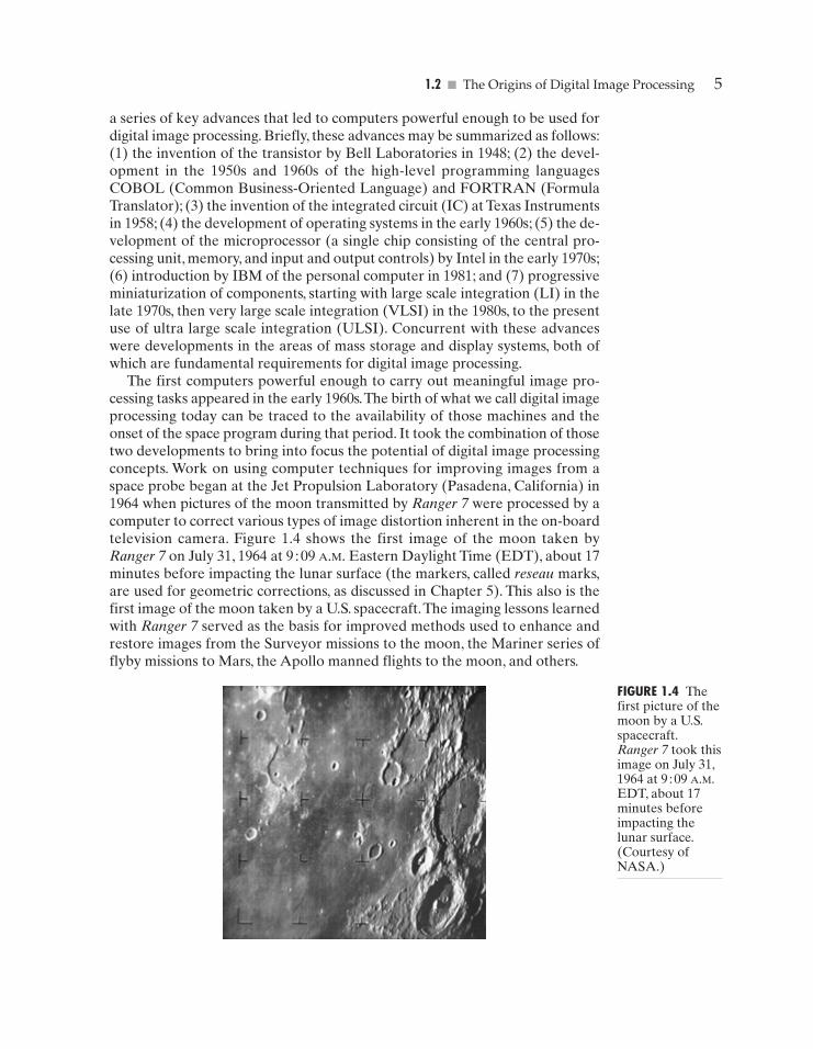
FIGURE 1.4 Thefirst picture of themoon by a U.S.spacecraft.Ranger 7 took thisimage on July 31,1964 at 9 : 09 A.M.EDT, about 17minutes beforeimpacting thelunar surface.(Courtesy ofNASA.)
a series of key advances that led to computers powerful enough to be used fordigital image processing. Briefly, these advances may be summarized as follows:(1) the invention of the transistor by Bell Laboratories in 1948; (2) the devel-opment in the 1950s and 1960s of the high-level programming languagesCOBOL (Common Business-Oriented Language) and FORTRAN (FormulaTranslator); (3) the invention of the integrated circuit (IC) at Texas Instrumentsin 1958; (4) the development of operating systems in the early 1960s; (5) the de-velopment of the microprocessor (a single chip consisting of the central pro-cessing unit, memory, and input and output controls) by Intel in the early 1970s;(6) introduction by IBM of the personal computer in 1981; and (7) progressiveminiaturization of components, starting with large scale integration (LI) in thelate 1970s, then very large scale integration (VLSI) in the 1980s, to the presentuse of ultra large scale integration (ULSI). Concurrent with these advanceswere developments in the areas of mass storage and display systems, both ofwhich are fundamental requirements for digital image processing.
The first computers powerful enough to carry out meaningful image pro-cessing tasks appeared in the early 1960s.The birth of what we call digital imageprocessing today can be traced to the availability of those machines and theonset of the space program during that period. It took the combination of thosetwo developments to bring into focus the potential of digital image processingconcepts. Work on using computer techniques for improving images from aspace probe began at the Jet Propulsion Laboratory (Pasadena, California) in1964 when pictures of the moon transmitted by Ranger 7 were processed by acomputer to correct various types of image distortion inherent in the on-boardtelevision camera. Figure 1.4 shows the first image of the moon taken byRanger 7 on July 31, 1964 at 9 : 09 A.M. Eastern Daylight Time (EDT), about 17minutes before impacting the lunar surface (the markers, called reseau marks,are used for geometric corrections, as discussed in Chapter 5). This also is thefirst image of the moon taken by a U.S. spacecraft.The imaging lessons learnedwith Ranger 7 served as the basis for improved methods used to enhance andrestore images from the Surveyor missions to the moon, the Mariner series offlyby missions to Mars, the Apollo manned flights to the moon, and others.
GONZ01-001-033.II 29-08-2001 14:42 Page 5
6 Chapter 1 � Introduction
In parallel with space applications,digital image processing techniques began inthe late 1960s and early 1970s to be used in medical imaging, remote Earth re-sources observations, and astronomy.The invention in the early 1970s of comput-erized axial tomography (CAT), also called computerized tomography (CT) forshort, is one of the most important events in the application of image processing inmedical diagnosis. Computerized axial tomography is a process in which a ring ofdetectors encircles an object (or patient) and an X-ray source, concentric with thedetector ring, rotates about the object.The X-rays pass through the object and arecollected at the opposite end by the corresponding detectors in the ring. As thesource rotates, this procedure is repeated.Tomography consists of algorithms thatuse the sensed data to construct an image that represents a “slice” through the ob-ject. Motion of the object in a direction perpendicular to the ring of detectors pro-duces a set of such slices, which constitute a three-dimensional (3-D) rendition ofthe inside of the object. Tomography was invented independently by Sir GodfreyN. Hounsfield and Professor Allan M. Cormack, who shared the 1979 Nobel Prizein Medicine for their invention. It is interesting to note that X-rays were discov-ered in 1895 by Wilhelm Conrad Roentgen, for which he received the 1901 NobelPrize for Physics. These two inventions, nearly 100 years apart, led to some of themost active application areas of image processing today.
From the 1960s until the present, the field of image processing has grown vig-orously. In addition to applications in medicine and the space program, digitalimage processing techniques now are used in a broad range of applications. Com-puter procedures are used to enhance the contrast or code the intensity levels intocolor for easier interpretation of X-rays and other images used in industry, medi-cine, and the biological sciences. Geographers use the same or similar techniquesto study pollution patterns from aerial and satellite imagery. Image enhancementand restoration procedures are used to process degraded images of unrecoverableobjects or experimental results too expensive to duplicate. In archeology, imageprocessing methods have successfully restored blurred pictures that were the onlyavailable records of rare artifacts lost or damaged after being photographed. Inphysics and related fields, computer techniques routinely enhance images of ex-periments in areas such as high-energy plasmas and electron microscopy. Similar-ly successful applications of image processing concepts can be found in astronomy,biology, nuclear medicine, law enforcement, defense, and industrial applications.
These examples illustrate processing results intended for human interpreta-tion.The second major area of application of digital image processing techniquesmentioned at the beginning of this chapter is in solving problems dealing withmachine perception. In this case, interest focuses on procedures for extractingfrom an image information in a form suitable for computer processing. Often,this information bears little resemblance to visual features that humans use ininterpreting the content of an image. Examples of the type of information usedin machine perception are statistical moments, Fourier transform coefficients, andmultidimensional distance measures. Typical problems in machine perceptionthat routinely utilize image processing techniques are automatic character recog-nition, industrial machine vision for product assembly and inspection, militaryrecognizance, automatic processing of fingerprints, screening of X-rays and bloodsamples, and machine processing of aerial and satellite imagery for weather
GONZ01-001-033.II 29-08-2001 14:42 Page 6
1.3 � Examples of Fields that Use Digital Image Processing 7
prediction and environmental assessment.The continuing decline in the ratio ofcomputer price to performance and the expansion of networking and commu-nication bandwidth via the World Wide Web and the Internet have created un-precedented opportunities for continued growth of digital image processing.Some of these application areas are illustrated in the following section.
Examples of Fields that Use Digital Image Processing
Today, there is almost no area of technical endeavor that is not impacted insome way by digital image processing. We can cover only a few of these appli-cations in the context and space of the current discussion. However, limited asit is, the material presented in this section will leave no doubt in the reader’smind regarding the breadth and importance of digital image processing. Weshow in this section numerous areas of application, each of which routinely uti-lizes the digital image processing techniques developed in the following chap-ters. Many of the images shown in this section are used later in one or more ofthe examples given in the book. All images shown are digital.
The areas of application of digital image processing are so varied that someform of organization is desirable in attempting to capture the breadth of thisfield. One of the simplest ways to develop a basic understanding of the extent ofimage processing applications is to categorize images according to their source(e.g., visual, X-ray, and so on).The principal energy source for images in use todayis the electromagnetic energy spectrum. Other important sources of energy in-clude acoustic, ultrasonic, and electronic (in the form of electron beams used inelectron microscopy). Synthetic images, used for modeling and visualization, aregenerated by computer. In this section we discuss briefly how images are gener-ated in these various categories and the areas in which they are applied. Meth-ods for converting images into digital form are discussed in the next chapter.
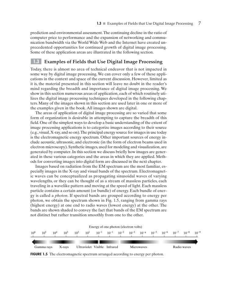
Images based on radiation from the EM spectrum are the most familiar, es-pecially images in the X-ray and visual bands of the spectrum. Electromagnet-ic waves can be conceptualized as propagating sinusoidal waves of varyingwavelengths, or they can be thought of as a stream of massless particles, eachtraveling in a wavelike pattern and moving at the speed of light. Each masslessparticle contains a certain amount (or bundle) of energy. Each bundle of ener-gy is called a photon. If spectral bands are grouped according to energy perphoton, we obtain the spectrum shown in Fig. 1.5, ranging from gamma rays(highest energy) at one end to radio waves (lowest energy) at the other. Thebands are shown shaded to convey the fact that bands of the EM spectrum arenot distinct but rather transition smoothly from one to the other.
1.3
10–910–810–710–610–510–410–310–210–1 10–1101102103104105106
Energy of one photon (electron volts)
Gamma rays X-rays Ultraviolet Visible Infrared Microwaves Radio waves
FIGURE 1.5 The electromagnetic spectrum arranged according to energy per photon.
GONZ01-001-033.II 29-08-2001 14:42 Page 7
8 Chapter 1 � Introduction
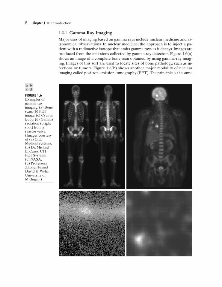
FIGURE 1.6Examples ofgamma-rayimaging. (a) Bonescan. (b) PETimage. (c) CygnusLoop. (d) Gammaradiation (brightspot) from areactor valve.(Images courtesyof (a) G.E.Medical Systems,(b) Dr. MichaelE. Casey, CTIPET Systems,(c) NASA,(d) ProfessorsZhong He andDavid K. Wehe,University ofMichigan.)
1.3.1 Gamma-Ray ImagingMajor uses of imaging based on gamma rays include nuclear medicine and as-tronomical observations. In nuclear medicine, the approach is to inject a pa-tient with a radioactive isotope that emits gamma rays as it decays. Images areproduced from the emissions collected by gamma ray detectors. Figure 1.6(a)shows an image of a complete bone scan obtained by using gamma-ray imag-ing. Images of this sort are used to locate sites of bone pathology, such as in-fections or tumors. Figure 1.6(b) shows another major modality of nuclearimaging called positron emission tomography (PET).The principle is the same
a bc d
GONZ01-001-033.II 29-08-2001 14:42 Page 8
1.3 � Examples of Fields that Use Digital Image Processing 9
as with X-ray tomography, mentioned briefly in Section 1.2. However, insteadof using an external source of X-ray energy, the patient is given a radioactive iso-tope that emits positrons as it decays. When a positron meets an electron, bothare annihilated and two gamma rays are given off.These are detected and a to-mographic image is created using the basic principles of tomography.The imageshown in Fig. 1.6(b) is one sample of a sequence that constitutes a 3-D rendi-tion of the patient. This image shows a tumor in the brain and one in the lung,easily visible as small white masses.
A star in the constellation of Cygnus exploded about 15,000 years ago, gen-erating a superheated stationary gas cloud (known as the Cygnus Loop) thatglows in a spectacular array of colors. Figure 1.6(c) shows the Cygnus Loop im-aged in the gamma-ray band. Unlike the two examples shown in Figs. 1.6(a)and (b), this image was obtained using the natural radiation of the object beingimaged. Finally, Fig. 1.6(d) shows an image of gamma radiation from a valve ina nuclear reactor. An area of strong radiation is seen in the lower, left side ofthe image.
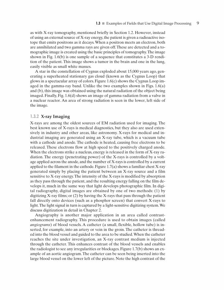
1.3.2 X-ray ImagingX-rays are among the oldest sources of EM radiation used for imaging. Thebest known use of X-rays is medical diagnostics, but they also are used exten-sively in industry and other areas, like astronomy. X-rays for medical and in-dustrial imaging are generated using an X-ray tube, which is a vacuum tubewith a cathode and anode. The cathode is heated, causing free electrons to bereleased. These electrons flow at high speed to the positively charged anode.When the electrons strike a nucleus, energy is released in the form of X-ray ra-diation. The energy (penetrating power) of the X-rays is controlled by a volt-age applied across the anode, and the number of X-rays is controlled by a currentapplied to the filament in the cathode. Figure 1.7(a) shows a familiar chest X-raygenerated simply by placing the patient between an X-ray source and a filmsensitive to X-ray energy.The intensity of the X-rays is modified by absorptionas they pass through the patient, and the resulting energy falling on the film de-velops it, much in the same way that light develops photographic film. In digi-tal radiography, digital images are obtained by one of two methods: (1) bydigitizing X-ray films; or (2) by having the X-rays that pass through the patientfall directly onto devices (such as a phosphor screen) that convert X-rays tolight.The light signal in turn is captured by a light-sensitive digitizing system.Wediscuss digitization in detail in Chapter 2.
Angiography is another major application in an area called contrast-enhancement radiography. This procedure is used to obtain images (calledangiograms) of blood vessels. A catheter (a small, flexible, hollow tube) is in-serted, for example, into an artery or vein in the groin. The catheter is thread-ed into the blood vessel and guided to the area to be studied.When the catheterreaches the site under investigation, an X-ray contrast medium is injectedthrough the catheter. This enhances contrast of the blood vessels and enablesthe radiologist to see any irregularities or blockages. Figure 1.7(b) shows an ex-ample of an aortic angiogram.The catheter can be seen being inserted into thelarge blood vessel on the lower left of the picture. Note the high contrast of the
GONZ01-001-033.II 29-08-2001 14:42 Page 9
10 Chapter 1 � Introduction
FIGURE 1.7 Examples of X-ray imaging. (a) Chest X-ray. (b) Aortic angiogram. (c) HeadCT. (d) Circuit boards. (e) Cygnus Loop. (Images courtesy of (a) and (c) Dr. DavidR. Pickens, Dept. of Radiology & Radiological Sciences,Vanderbilt University MedicalCenter, (b) Dr. Thomas R. Gest, Division of Anatomical Sciences, University of Michi-gan Medical School, (d) Mr. Joseph E. Pascente, Lixi, Inc., and (e) NASA.)
abc
d
e
GONZ01-001-033.II 29-08-2001 14:42 Page 10
1.3 � Examples of Fields that Use Digital Image Processing 11
large vessel as the contrast medium flows up in the direction of the kidneys,which are also visible in the image. As discussed in Chapter 3, angiography is amajor area of digital image processing, where image subtraction is used to en-hance further the blood vessels being studied.
Perhaps the best known of all uses of X-rays in medical imaging is comput-erized axial tomography. Due to their resolution and 3-D capabilities, CATscans revolutionized medicine from the moment they first became available inthe early 1970s.As noted in Section 1.2, each CAT image is a “slice” taken per-pendicularly through the patient. Numerous slices are generated as the patientis moved in a longitudinal direction.The ensemble of such images constitutes a3-D rendition of the inside of the patient, with the longitudinal resolution beingproportional to the number of slice images taken. Figure 1.7(c) shows a typicalhead CAT slice image.
Techniques similar to the ones just discussed, but generally involving higher-energy X-rays, are applicable in industrial processes. Figure 1.7(d) shows anX-ray image of an electronic circuit board. Such images, representative of lit-erally hundreds of industrial applications of X-rays, are used to examine circuitboards for flaws in manufacturing, such as missing components or broken traces.Industrial CAT scans are useful when the parts can be penetrated by X-rays,such as in plastic assemblies, and even large bodies, like solid-propellant rock-et motors. Figure 1.7(e) shows an example of X-ray imaging in astronomy.Thisimage is the Cygnus Loop of Fig. 1.6(c), but imaged this time in the X-ray band.
1.3.3 Imaging in the Ultraviolet BandApplications of ultraviolet “light” are varied. They include lithography, indus-trial inspection, microscopy, lasers, biological imaging, and astronomical obser-vations.We illustrate imaging in this band with examples from microscopy andastronomy.
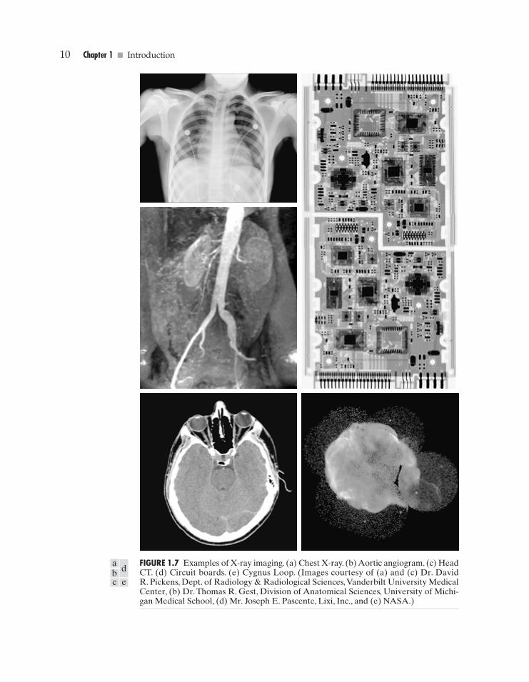
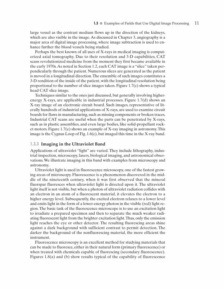
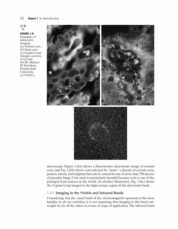
Ultraviolet light is used in fluorescence microscopy, one of the fastest grow-ing areas of microscopy. Fluorescence is a phenomenon discovered in the mid-dle of the nineteenth century, when it was first observed that the mineralfluorspar fluoresces when ultraviolet light is directed upon it. The ultravioletlight itself is not visible, but when a photon of ultraviolet radiation collides withan electron in an atom of a fluorescent material, it elevates the electron to ahigher energy level. Subsequently, the excited electron relaxes to a lower leveland emits light in the form of a lower-energy photon in the visible (red) light re-gion.The basic task of the fluorescence microscope is to use an excitation lightto irradiate a prepared specimen and then to separate the much weaker radi-ating fluorescent light from the brighter excitation light.Thus, only the emissionlight reaches the eye or other detector. The resulting fluorescing areas shineagainst a dark background with sufficient contrast to permit detection. Thedarker the background of the nonfluorescing material, the more efficient theinstrument.
Fluorescence microscopy is an excellent method for studying materials thatcan be made to fluoresce, either in their natural form (primary fluorescence) orwhen treated with chemicals capable of fluorescing (secondary fluorescence).Figures 1.8(a) and (b) show results typical of the capability of fluorescence
GONZ01-001-033.II 29-08-2001 14:42 Page 11
12 Chapter 1 � Introduction
FIGURE 1.8Examples ofultravioletimaging.(a) Normal corn.(b) Smut corn.(c) Cygnus Loop.(Images courtesyof (a) and (b) Dr. MichaelW. Davidson,Florida StateUniversity,(c) NASA.)
microscopy. Figure 1.8(a) shows a fluorescence microscope image of normalcorn, and Fig. 1.8(b) shows corn infected by “smut,” a disease of cereals, corn,grasses, onions, and sorghum that can be caused by any of more than 700 speciesof parasitic fungi. Corn smut is particularly harmful because corn is one of theprincipal food sources in the world. As another illustration, Fig. 1.8(c) showsthe Cygnus Loop imaged in the high-energy region of the ultraviolet band.
1.3.4 Imaging in the Visible and Infrared BandsConsidering that the visual band of the electromagnetic spectrum is the mostfamiliar in all our activities, it is not surprising that imaging in this band out-weighs by far all the others in terms of scope of application. The infrared band
a bc
GONZ01-001-033.II 29-08-2001 14:42 Page 12
1.3 � Examples of Fields that Use Digital Image Processing 13
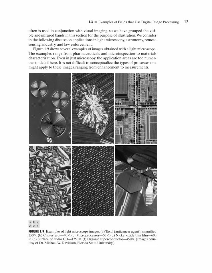
FIGURE 1.9 Examples of light microscopy images. (a) Taxol (anticancer agent), magnified250µ. (b) Cholesterol—40µ. (c) Microprocessor—60µ. (d) Nickel oxide thin film—600µ. (e) Surface of audio CD—1750µ. (f) Organic superconductor—450µ. (Images cour-tesy of Dr. Michael W. Davidson, Florida State University.)
often is used in conjunction with visual imaging, so we have grouped the visi-ble and infrared bands in this section for the purpose of illustration.We considerin the following discussion applications in light microscopy, astronomy, remotesensing, industry, and law enforcement.
Figure 1.9 shows several examples of images obtained with a light microscope.The examples range from pharmaceuticals and microinspection to materialscharacterization. Even in just microscopy, the application areas are too numer-ous to detail here. It is not difficult to conceptualize the types of processes onemight apply to these images, ranging from enhancement to measurements.
a b cd e f
GONZ01-001-033.II 29-08-2001 14:42 Page 13
14 Chapter 1 � Introduction
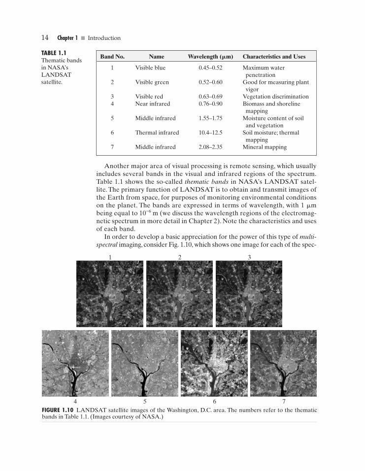
FIGURE 1.10 LANDSAT satellite images of the Washington, D.C. area. The numbers refer to the thematicbands in Table 1.1. (Images courtesy of NASA.)
TABLE 1.1Thematic bands in NASA’sLANDSATsatellite.
Band No. Name Wavelength (�m) Characteristics and Uses
1 Visible blue 0.45–0.52 Maximum water penetration
2 Visible green 0.52–0.60 Good for measuring plant vigor
3 Visible red 0.63–0.69 Vegetation discrimination4 Near infrared 0.76–0.90 Biomass and shoreline
mapping5 Middle infrared 1.55–1.75 Moisture content of soil
and vegetation6 Thermal infrared 10.4–12.5 Soil moisture; thermal
mapping7 Middle infrared 2.08–2.35 Mineral mapping
Another major area of visual processing is remote sensing, which usuallyincludes several bands in the visual and infrared regions of the spectrum.Table 1.1 shows the so-called thematic bands in NASA’s LANDSAT satel-lite. The primary function of LANDSAT is to obtain and transmit images ofthe Earth from space, for purposes of monitoring environmental conditionson the planet. The bands are expressed in terms of wavelength, with 1 �mbeing equal to 10–6 m (we discuss the wavelength regions of the electromag-netic spectrum in more detail in Chapter 2). Note the characteristics and usesof each band.
In order to develop a basic appreciation for the power of this type of multi-spectral imaging, consider Fig. 1.10, which shows one image for each of the spec-
1 2 3
4 5 6 7
GONZ01-001-033.II 29-08-2001 14:42 Page 14

1.3 � Examples of Fields that Use Digital Image Processing 15
FIGURE 1.11Multispectralimage ofHurricaneAndrew taken byNOAA GEOS(GeostationaryEnvironmentalOperationalSatellite) sensors.(Courtesy ofNOAA.)
tral bands in Table 1.1.The area imaged is Washington D.C., which includes fea-tures such as buildings, roads, vegetation, and a major river (the Potomac) goingthough the city. Images of population centers are used routinely (over time) toassess population growth and shift patterns, pollution, and other factors harm-ful to the environment.The differences between visual and infrared image fea-tures are quite noticeable in these images. Observe, for example, how welldefined the river is from its surroundings in Bands 4 and 5.
Weather observation and prediction also are major applications of multi-spectral imaging from satellites. For example, Fig. 1.11 is an image of a hurricanetaken by a National Oceanographic and Atmospheric Administration (NOAA)satellite using sensors in the visible and infrared bands.The eye of the hurricaneis clearly visible in this image.
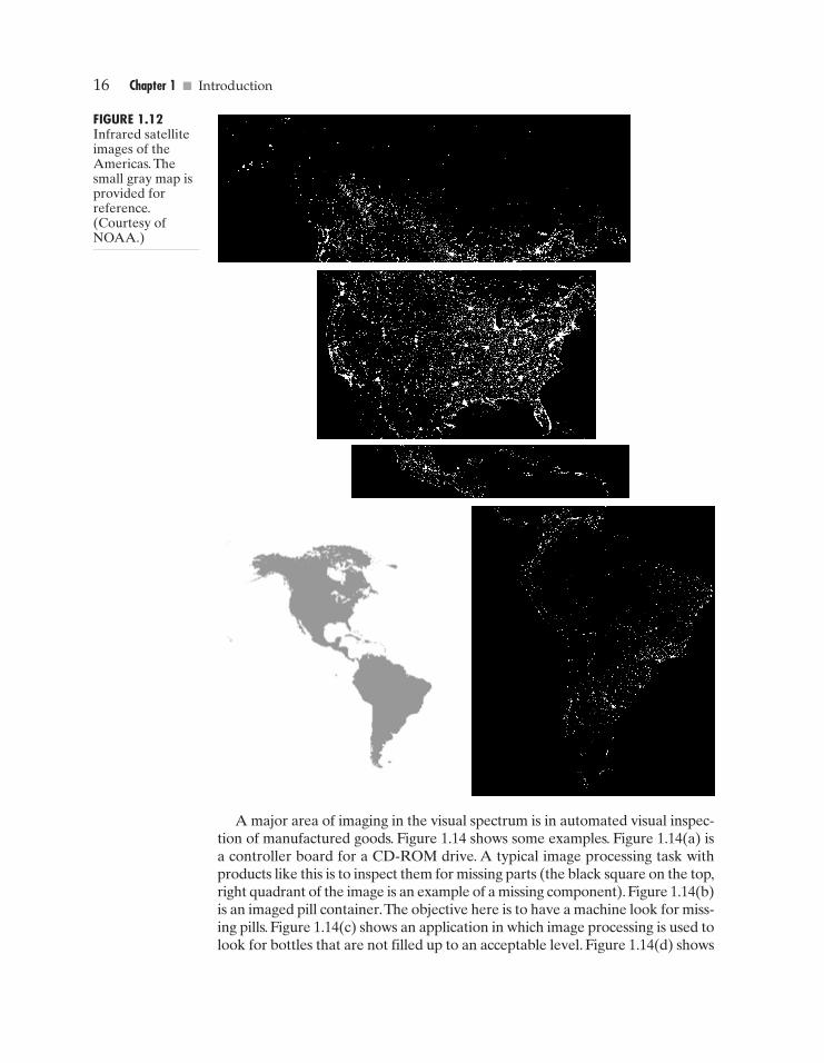
Figures 1.12 and 1.13 show an application of infrared imaging.These imagesare part of the Nighttime Lights of the World data set, which provides a glob-al inventory of human settlements.The images were generated by the infraredimaging system mounted on a NOAA DMSP (Defense Meteorological Satel-lite Program) satellite.The infrared imaging system operates in the band 10.0to 13.4 �m, and has the unique capability to observe faint sources of visible-near infrared emissions present on the Earth’s surface, including cities, towns,villages, gas flares, and fires. Even without formal training in image process-ing, it is not difficult to imagine writing a computer program that would usethese images to estimate the percent of total electrical energy used by variousregions of the world.
GONZ01-001-033.II 29-08-2001 14:42 Page 15
16 Chapter 1 � Introduction
FIGURE 1.12Infrared satelliteimages of theAmericas. Thesmall gray map isprovided forreference.(Courtesy ofNOAA.)
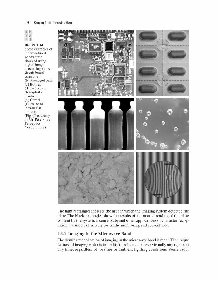
A major area of imaging in the visual spectrum is in automated visual inspec-tion of manufactured goods. Figure 1.14 shows some examples. Figure 1.14(a) isa controller board for a CD-ROM drive. A typical image processing task withproducts like this is to inspect them for missing parts (the black square on the top,right quadrant of the image is an example of a missing component). Figure 1.14(b)is an imaged pill container.The objective here is to have a machine look for miss-ing pills. Figure 1.14(c) shows an application in which image processing is used tolook for bottles that are not filled up to an acceptable level. Figure 1.14(d) shows
GONZ01-001-033.II 29-08-2001 14:42 Page 16
1.3 � Examples of Fields that Use Digital Image Processing 17
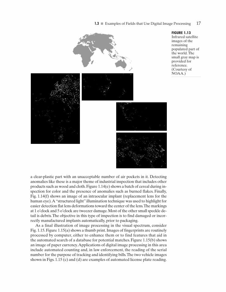
FIGURE 1.13Infrared satelliteimages of theremainingpopulated part ofthe world. Thesmall gray map isprovided forreference.(Courtesy ofNOAA.)
a clear-plastic part with an unacceptable number of air pockets in it. Detectinganomalies like these is a major theme of industrial inspection that includes otherproducts such as wood and cloth. Figure 1.14(e) shows a batch of cereal during in-spection for color and the presence of anomalies such as burned flakes. Finally,Fig. 1.14(f) shows an image of an intraocular implant (replacement lens for thehuman eye).A “structured light” illumination technique was used to highlight foreasier detection flat lens deformations toward the center of the lens.The markingsat 1 o’clock and 5 o’clock are tweezer damage. Most of the other small speckle de-tail is debris.The objective in this type of inspection is to find damaged or incor-rectly manufactured implants automatically, prior to packaging.
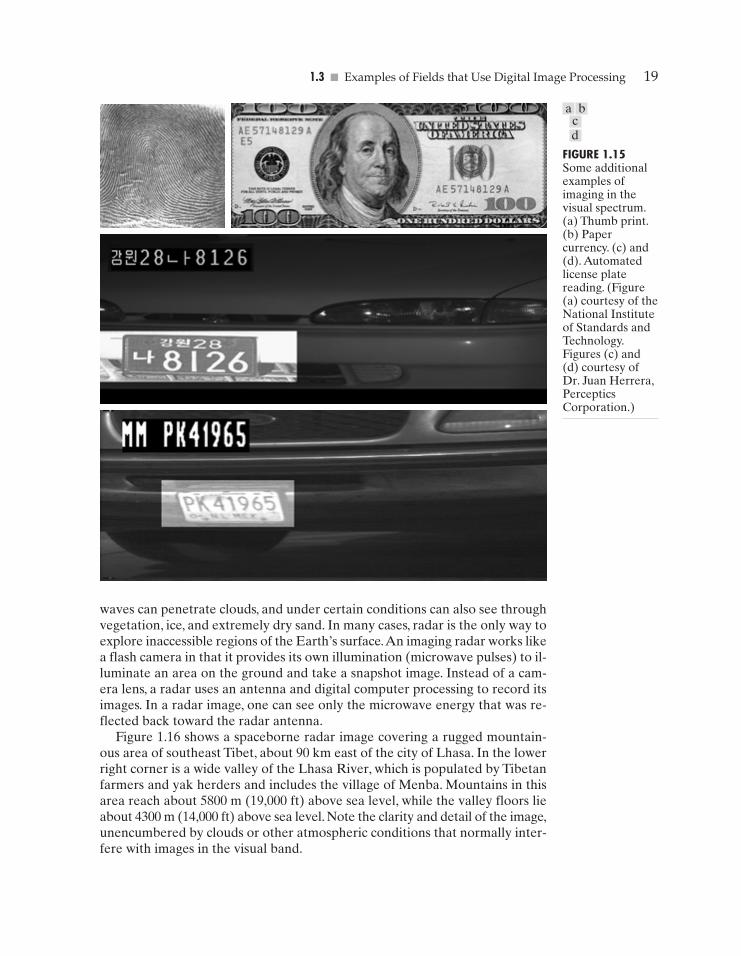
As a final illustration of image processing in the visual spectrum, considerFig. 1.15. Figure 1.15(a) shows a thumb print. Images of fingerprints are routinelyprocessed by computer, either to enhance them or to find features that aid inthe automated search of a database for potential matches. Figure 1.15(b) showsan image of paper currency.Applications of digital image processing in this areainclude automated counting and, in law enforcement, the reading of the serialnumber for the purpose of tracking and identifying bills.The two vehicle imagesshown in Figs. 1.15 (c) and (d) are examples of automated license plate reading.
GONZ01-001-033.II 29-08-2001 14:42 Page 17
18 Chapter 1 � Introduction
FIGURE 1.14Some examples ofmanufacturedgoods oftenchecked usingdigital imageprocessing. (a) Acircuit boardcontroller.(b) Packaged pills.(c) Bottles.(d) Bubbles inclear-plasticproduct.(e) Cereal.(f) Image ofintraocularimplant.(Fig. (f) courtesyof Mr. Pete Sites,PercepticsCorporation.)
The light rectangles indicate the area in which the imaging system detected theplate. The black rectangles show the results of automated reading of the platecontent by the system. License plate and other applications of character recog-nition are used extensively for traffic monitoring and surveillance.
1.3.5 Imaging in the Microwave BandThe dominant application of imaging in the microwave band is radar.The uniquefeature of imaging radar is its ability to collect data over virtually any region atany time, regardless of weather or ambient lighting conditions. Some radar
ace
bdf
GONZ01-001-033.II 29-08-2001 14:42 Page 18
1.3 � Examples of Fields that Use Digital Image Processing 19
FIGURE 1.15Some additionalexamples ofimaging in thevisual spectrum.(a) Thumb print.(b) Papercurrency. (c) and(d). Automatedlicense platereading. (Figure(a) courtesy of theNational Instituteof Standards andTechnology.Figures (c) and(d) courtesy ofDr. Juan Herrera,PercepticsCorporation.)
waves can penetrate clouds, and under certain conditions can also see throughvegetation, ice, and extremely dry sand. In many cases, radar is the only way toexplore inaccessible regions of the Earth’s surface.An imaging radar works likea flash camera in that it provides its own illumination (microwave pulses) to il-luminate an area on the ground and take a snapshot image. Instead of a cam-era lens, a radar uses an antenna and digital computer processing to record itsimages. In a radar image, one can see only the microwave energy that was re-flected back toward the radar antenna.
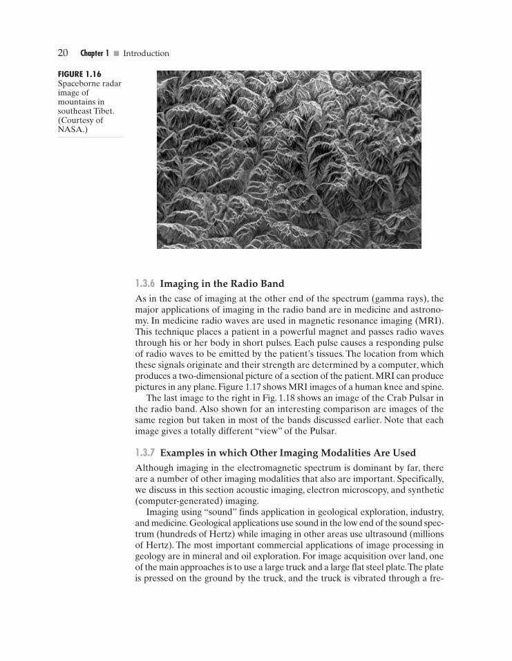
Figure 1.16 shows a spaceborne radar image covering a rugged mountain-ous area of southeast Tibet, about 90 km east of the city of Lhasa. In the lowerright corner is a wide valley of the Lhasa River, which is populated by Tibetanfarmers and yak herders and includes the village of Menba. Mountains in thisarea reach about 5800 m (19,000 ft) above sea level, while the valley floors lieabout 4300 m (14,000 ft) above sea level. Note the clarity and detail of the image,unencumbered by clouds or other atmospheric conditions that normally inter-fere with images in the visual band.
a bcd
GONZ01-001-033.II 29-08-2001 14:42 Page 19
20 Chapter 1 � Introduction
FIGURE 1.16Spaceborne radarimage ofmountains insoutheast Tibet.(Courtesy ofNASA.)
1.3.6 Imaging in the Radio BandAs in the case of imaging at the other end of the spectrum (gamma rays), themajor applications of imaging in the radio band are in medicine and astrono-my. In medicine radio waves are used in magnetic resonance imaging (MRI).This technique places a patient in a powerful magnet and passes radio wavesthrough his or her body in short pulses. Each pulse causes a responding pulseof radio waves to be emitted by the patient’s tissues. The location from whichthese signals originate and their strength are determined by a computer, whichproduces a two-dimensional picture of a section of the patient. MRI can producepictures in any plane. Figure 1.17 shows MRI images of a human knee and spine.
The last image to the right in Fig. 1.18 shows an image of the Crab Pulsar inthe radio band. Also shown for an interesting comparison are images of thesame region but taken in most of the bands discussed earlier. Note that eachimage gives a totally different “view” of the Pulsar.
1.3.7 Examples in which Other Imaging Modalities Are UsedAlthough imaging in the electromagnetic spectrum is dominant by far, thereare a number of other imaging modalities that also are important. Specifically,we discuss in this section acoustic imaging, electron microscopy, and synthetic(computer-generated) imaging.
Imaging using “sound” finds application in geological exploration, industry,and medicine. Geological applications use sound in the low end of the sound spec-trum (hundreds of Hertz) while imaging in other areas use ultrasound (millionsof Hertz). The most important commercial applications of image processing ingeology are in mineral and oil exploration. For image acquisition over land, oneof the main approaches is to use a large truck and a large flat steel plate.The plateis pressed on the ground by the truck, and the truck is vibrated through a fre-
GONZ01-001-033.II 29-08-2001 14:42 Page 20
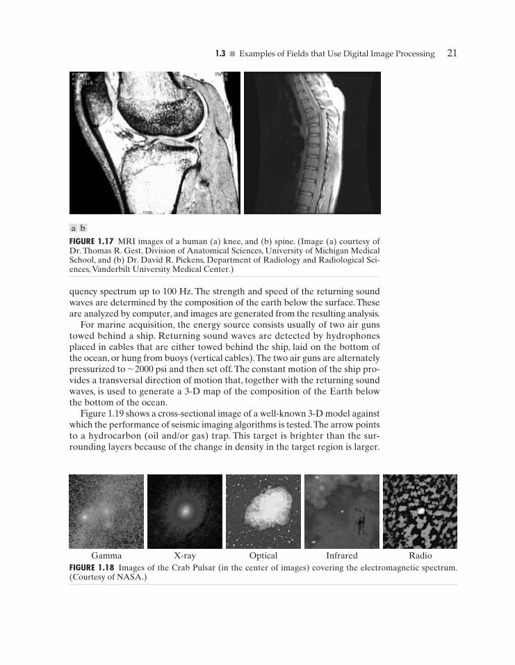
FIGURE 1.18 Images of the Crab Pulsar (in the center of images) covering the electromagnetic spectrum.(Courtesy of NASA.)
1.3 � Examples of Fields that Use Digital Image Processing 21
FIGURE 1.17 MRI images of a human (a) knee, and (b) spine. (Image (a) courtesy ofDr. Thomas R. Gest, Division of Anatomical Sciences, University of Michigan MedicalSchool, and (b) Dr. David R. Pickens, Department of Radiology and Radiological Sci-ences, Vanderbilt University Medical Center.)
quency spectrum up to 100 Hz. The strength and speed of the returning soundwaves are determined by the composition of the earth below the surface. Theseare analyzed by computer, and images are generated from the resulting analysis.
For marine acquisition, the energy source consists usually of two air gunstowed behind a ship. Returning sound waves are detected by hydrophonesplaced in cables that are either towed behind the ship, laid on the bottom ofthe ocean, or hung from buoys (vertical cables).The two air guns are alternatelypressurized to ~2000 psi and then set off. The constant motion of the ship pro-vides a transversal direction of motion that, together with the returning soundwaves, is used to generate a 3-D map of the composition of the Earth belowthe bottom of the ocean.
Figure 1.19 shows a cross-sectional image of a well-known 3-D model againstwhich the performance of seismic imaging algorithms is tested.The arrow pointsto a hydrocarbon (oil and/or gas) trap. This target is brighter than the sur-rounding layers because of the change in density in the target region is larger.
Gamma X-ray Optical Infrared Radio
a b
GONZ01-001-033.II 29-08-2001 14:42 Page 21
22 Chapter 1 � Introduction
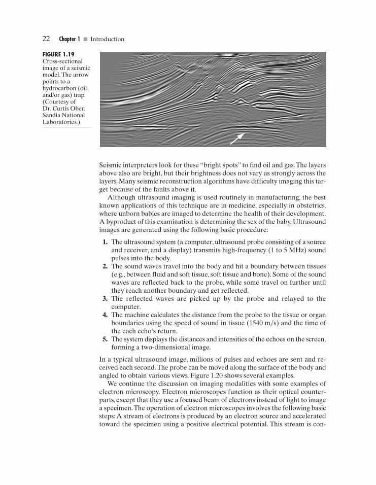
FIGURE 1.19Cross-sectionalimage of a seismicmodel. The arrowpoints to ahydrocarbon (oiland/or gas) trap.(Courtesy of Dr. Curtis Ober,Sandia NationalLaboratories.)
Seismic interpreters look for these “bright spots” to find oil and gas.The layersabove also are bright, but their brightness does not vary as strongly across thelayers. Many seismic reconstruction algorithms have difficulty imaging this tar-get because of the faults above it.
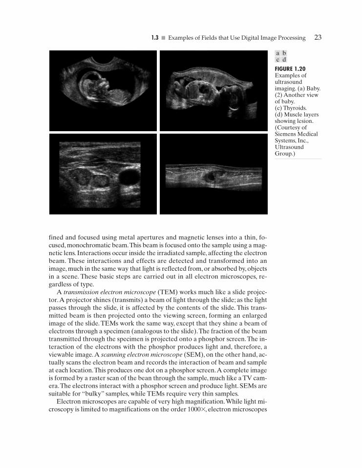
Although ultrasound imaging is used routinely in manufacturing, the bestknown applications of this technique are in medicine, especially in obstetrics,where unborn babies are imaged to determine the health of their development.A byproduct of this examination is determining the sex of the baby. Ultrasoundimages are generated using the following basic procedure:
1. The ultrasound system (a computer, ultrasound probe consisting of a sourceand receiver, and a display) transmits high-frequency (1 to 5 MHz) soundpulses into the body.
2. The sound waves travel into the body and hit a boundary between tissues(e.g., between fluid and soft tissue, soft tissue and bone). Some of the soundwaves are reflected back to the probe, while some travel on further untilthey reach another boundary and get reflected.
3. The reflected waves are picked up by the probe and relayed to thecomputer.
4. The machine calculates the distance from the probe to the tissue or organboundaries using the speed of sound in tissue (1540 m�s) and the time ofthe each echo’s return.
5. The system displays the distances and intensities of the echoes on the screen,forming a two-dimensional image.
In a typical ultrasound image, millions of pulses and echoes are sent and re-ceived each second.The probe can be moved along the surface of the body andangled to obtain various views. Figure 1.20 shows several examples.
We continue the discussion on imaging modalities with some examples ofelectron microscopy. Electron microscopes function as their optical counter-parts, except that they use a focused beam of electrons instead of light to imagea specimen.The operation of electron microscopes involves the following basicsteps: A stream of electrons is produced by an electron source and acceleratedtoward the specimen using a positive electrical potential. This stream is con-
GONZ01-001-033.II 29-08-2001 14:42 Page 22
1.3 � Examples of Fields that Use Digital Image Processing 23
FIGURE 1.20Examples ofultrasoundimaging. (a) Baby.(2) Another viewof baby.(c) Thyroids.(d) Muscle layersshowing lesion.(Courtesy ofSiemens MedicalSystems, Inc.,UltrasoundGroup.)
fined and focused using metal apertures and magnetic lenses into a thin, fo-cused, monochromatic beam.This beam is focused onto the sample using a mag-netic lens. Interactions occur inside the irradiated sample, affecting the electronbeam. These interactions and effects are detected and transformed into animage, much in the same way that light is reflected from, or absorbed by, objectsin a scene. These basic steps are carried out in all electron microscopes, re-gardless of type.
A transmission electron microscope (TEM) works much like a slide projec-tor.A projector shines (transmits) a beam of light through the slide; as the lightpasses through the slide, it is affected by the contents of the slide. This trans-mitted beam is then projected onto the viewing screen, forming an enlargedimage of the slide. TEMs work the same way, except that they shine a beam ofelectrons through a specimen (analogous to the slide).The fraction of the beamtransmitted through the specimen is projected onto a phosphor screen.The in-teraction of the electrons with the phosphor produces light and, therefore, aviewable image.A scanning electron microscope (SEM), on the other hand, ac-tually scans the electron beam and records the interaction of beam and sampleat each location.This produces one dot on a phosphor screen.A complete imageis formed by a raster scan of the bean through the sample, much like a TV cam-era.The electrons interact with a phosphor screen and produce light. SEMs aresuitable for “bulky” samples, while TEMs require very thin samples.
Electron microscopes are capable of very high magnification.While light mi-croscopy is limited to magnifications on the order 1000 *, electron microscopes
a bc d
GONZ01-001-033.II 29-08-2001 14:42 Page 23
24 Chapter 1 � Introduction
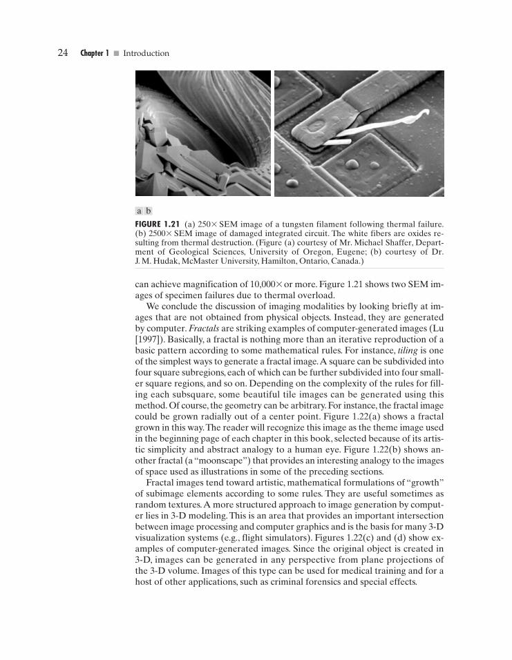
can achieve magnification of 10,000 * or more. Figure 1.21 shows two SEM im-ages of specimen failures due to thermal overload.
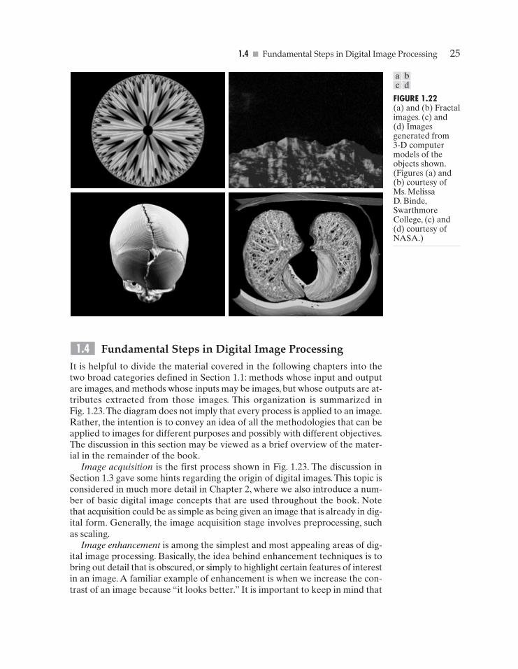
We conclude the discussion of imaging modalities by looking briefly at im-ages that are not obtained from physical objects. Instead, they are generatedby computer. Fractals are striking examples of computer-generated images (Lu[1997]). Basically, a fractal is nothing more than an iterative reproduction of abasic pattern according to some mathematical rules. For instance, tiling is oneof the simplest ways to generate a fractal image.A square can be subdivided intofour square subregions, each of which can be further subdivided into four small-er square regions, and so on. Depending on the complexity of the rules for fill-ing each subsquare, some beautiful tile images can be generated using thismethod. Of course, the geometry can be arbitrary. For instance, the fractal imagecould be grown radially out of a center point. Figure 1.22(a) shows a fractalgrown in this way.The reader will recognize this image as the theme image usedin the beginning page of each chapter in this book, selected because of its artis-tic simplicity and abstract analogy to a human eye. Figure 1.22(b) shows an-other fractal (a “moonscape”) that provides an interesting analogy to the imagesof space used as illustrations in some of the preceding sections.
Fractal images tend toward artistic, mathematical formulations of “growth”of subimage elements according to some rules. They are useful sometimes asrandom textures.A more structured approach to image generation by comput-er lies in 3-D modeling. This is an area that provides an important intersectionbetween image processing and computer graphics and is the basis for many 3-Dvisualization systems (e.g., flight simulators). Figures 1.22(c) and (d) show ex-amples of computer-generated images. Since the original object is created in3-D, images can be generated in any perspective from plane projections ofthe 3-D volume. Images of this type can be used for medical training and for ahost of other applications, such as criminal forensics and special effects.
a b
FIGURE 1.21 (a) 250 * SEM image of a tungsten filament following thermal failure.(b) 2500 * SEM image of damaged integrated circuit. The white fibers are oxides re-sulting from thermal destruction. (Figure (a) courtesy of Mr. Michael Shaffer, Depart-ment of Geological Sciences, University of Oregon, Eugene; (b) courtesy of Dr.J. M. Hudak, McMaster University, Hamilton, Ontario, Canada.)
GONZ01-001-033.II 29-08-2001 14:42 Page 24
1.4 � Fundamental Steps in Digital Image Processing 25
FIGURE 1.22(a) and (b) Fractalimages. (c) and(d) Imagesgenerated from3-D computermodels of theobjects shown.(Figures (a) and(b) courtesy ofMs. MelissaD. Binde,SwarthmoreCollege, (c) and(d) courtesy ofNASA.)
Fundamental Steps in Digital Image Processing
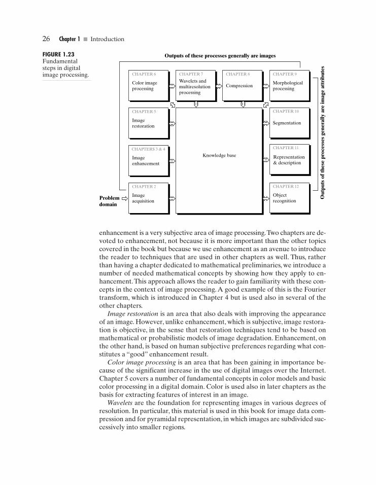
It is helpful to divide the material covered in the following chapters into thetwo broad categories defined in Section 1.1: methods whose input and outputare images, and methods whose inputs may be images, but whose outputs are at-tributes extracted from those images. This organization is summarized inFig. 1.23.The diagram does not imply that every process is applied to an image.Rather, the intention is to convey an idea of all the methodologies that can beapplied to images for different purposes and possibly with different objectives.The discussion in this section may be viewed as a brief overview of the mater-ial in the remainder of the book.
Image acquisition is the first process shown in Fig. 1.23. The discussion inSection 1.3 gave some hints regarding the origin of digital images. This topic isconsidered in much more detail in Chapter 2, where we also introduce a num-ber of basic digital image concepts that are used throughout the book. Notethat acquisition could be as simple as being given an image that is already in dig-ital form. Generally, the image acquisition stage involves preprocessing, suchas scaling.
Image enhancement is among the simplest and most appealing areas of dig-ital image processing. Basically, the idea behind enhancement techniques is tobring out detail that is obscured, or simply to highlight certain features of interestin an image. A familiar example of enhancement is when we increase the con-trast of an image because “it looks better.” It is important to keep in mind that
1.4
a bc d
GONZ01-001-033.II 29-08-2001 14:42 Page 25
26 Chapter 1 � Introduction
Knowledge base
CHAPTER 7
Wavelets andmultiresolutionprocessing
CHAPTER 6
Color imageprocessing
Outputs of these processes generally are images
CHAPTER 5
Imagerestoration
CHAPTERS 3 & 4
Imageenhancement
Problemdomain
Out
puts
of t
hese
pro
cess
es g
ener
ally
are
imag
e at
trib
utes
CHAPTER 8
Compression
CHAPTER 2
Imageacquisition
CHAPTER 9
Morphologicalprocessing
CHAPTER 10
Segmentation
CHAPTER 11
Representation & description
CHAPTER 12
Objectrecognition
FIGURE 1.23Fundamentalsteps in digitalimage processing.
enhancement is a very subjective area of image processing.Two chapters are de-voted to enhancement, not because it is more important than the other topicscovered in the book but because we use enhancement as an avenue to introducethe reader to techniques that are used in other chapters as well. Thus, ratherthan having a chapter dedicated to mathematical preliminaries, we introduce anumber of needed mathematical concepts by showing how they apply to en-hancement.This approach allows the reader to gain familiarity with these con-cepts in the context of image processing. A good example of this is the Fouriertransform, which is introduced in Chapter 4 but is used also in several of theother chapters.
Image restoration is an area that also deals with improving the appearanceof an image. However, unlike enhancement, which is subjective, image restora-tion is objective, in the sense that restoration techniques tend to be based onmathematical or probabilistic models of image degradation. Enhancement, onthe other hand, is based on human subjective preferences regarding what con-stitutes a “good” enhancement result.
Color image processing is an area that has been gaining in importance be-cause of the significant increase in the use of digital images over the Internet.Chapter 5 covers a number of fundamental concepts in color models and basiccolor processing in a digital domain. Color is used also in later chapters as thebasis for extracting features of interest in an image.
Wavelets are the foundation for representing images in various degrees ofresolution. In particular, this material is used in this book for image data com-pression and for pyramidal representation, in which images are subdivided suc-cessively into smaller regions.
GONZ01-001-033.II 29-08-2001 14:42 Page 26
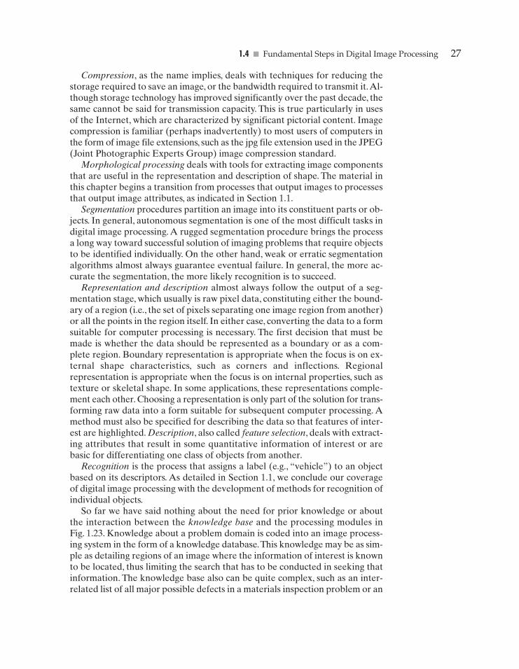
1.4 � Fundamental Steps in Digital Image Processing 27
Compression, as the name implies, deals with techniques for reducing thestorage required to save an image, or the bandwidth required to transmit it.Al-though storage technology has improved significantly over the past decade, thesame cannot be said for transmission capacity. This is true particularly in usesof the Internet, which are characterized by significant pictorial content. Imagecompression is familiar (perhaps inadvertently) to most users of computers inthe form of image file extensions, such as the jpg file extension used in the JPEG(Joint Photographic Experts Group) image compression standard.
Morphological processing deals with tools for extracting image componentsthat are useful in the representation and description of shape. The material inthis chapter begins a transition from processes that output images to processesthat output image attributes, as indicated in Section 1.1.
Segmentation procedures partition an image into its constituent parts or ob-jects. In general, autonomous segmentation is one of the most difficult tasks indigital image processing. A rugged segmentation procedure brings the processa long way toward successful solution of imaging problems that require objectsto be identified individually. On the other hand, weak or erratic segmentationalgorithms almost always guarantee eventual failure. In general, the more ac-curate the segmentation, the more likely recognition is to succeed.
Representation and description almost always follow the output of a seg-mentation stage, which usually is raw pixel data, constituting either the bound-ary of a region (i.e., the set of pixels separating one image region from another)or all the points in the region itself. In either case, converting the data to a formsuitable for computer processing is necessary. The first decision that must bemade is whether the data should be represented as a boundary or as a com-plete region. Boundary representation is appropriate when the focus is on ex-ternal shape characteristics, such as corners and inflections. Regionalrepresentation is appropriate when the focus is on internal properties, such astexture or skeletal shape. In some applications, these representations comple-ment each other. Choosing a representation is only part of the solution for trans-forming raw data into a form suitable for subsequent computer processing. Amethod must also be specified for describing the data so that features of inter-est are highlighted. Description, also called feature selection, deals with extract-ing attributes that result in some quantitative information of interest or arebasic for differentiating one class of objects from another.
Recognition is the process that assigns a label (e.g., “vehicle”) to an objectbased on its descriptors. As detailed in Section 1.1, we conclude our coverageof digital image processing with the development of methods for recognition ofindividual objects.
So far we have said nothing about the need for prior knowledge or aboutthe interaction between the knowledge base and the processing modules inFig. 1.23. Knowledge about a problem domain is coded into an image process-ing system in the form of a knowledge database.This knowledge may be as sim-ple as detailing regions of an image where the information of interest is knownto be located, thus limiting the search that has to be conducted in seeking thatinformation. The knowledge base also can be quite complex, such as an inter-related list of all major possible defects in a materials inspection problem or an
GONZ01-001-033.II 29-08-2001 14:42 Page 27
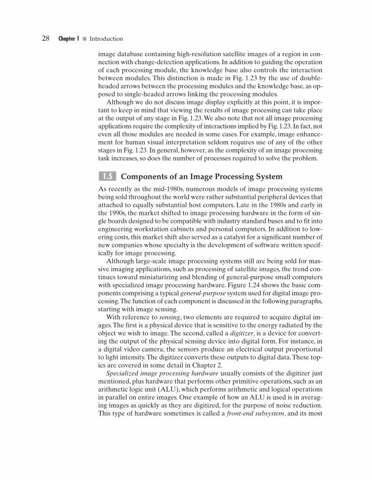
28 Chapter 1 � Introduction
image database containing high-resolution satellite images of a region in con-nection with change-detection applications. In addition to guiding the operationof each processing module, the knowledge base also controls the interactionbetween modules. This distinction is made in Fig. 1.23 by the use of double-headed arrows between the processing modules and the knowledge base, as op-posed to single-headed arrows linking the processing modules.
Although we do not discuss image display explicitly at this point, it is impor-tant to keep in mind that viewing the results of image processing can take placeat the output of any stage in Fig. 1.23.We also note that not all image processingapplications require the complexity of interactions implied by Fig. 1.23. In fact, noteven all those modules are needed in some cases. For example, image enhance-ment for human visual interpretation seldom requires use of any of the otherstages in Fig. 1.23. In general, however, as the complexity of an image processingtask increases, so does the number of processes required to solve the problem.
Components of an Image Processing System
As recently as the mid-1980s, numerous models of image processing systemsbeing sold throughout the world were rather substantial peripheral devices thatattached to equally substantial host computers. Late in the 1980s and early inthe 1990s, the market shifted to image processing hardware in the form of sin-gle boards designed to be compatible with industry standard buses and to fit intoengineering workstation cabinets and personal computers. In addition to low-ering costs, this market shift also served as a catalyst for a significant number ofnew companies whose specialty is the development of software written specif-ically for image processing.
Although large-scale image processing systems still are being sold for mas-sive imaging applications, such as processing of satellite images, the trend con-tinues toward miniaturizing and blending of general-purpose small computerswith specialized image processing hardware. Figure 1.24 shows the basic com-ponents comprising a typical general-purpose system used for digital image pro-cessing.The function of each component is discussed in the following paragraphs,starting with image sensing.
With reference to sensing, two elements are required to acquire digital im-ages.The first is a physical device that is sensitive to the energy radiated by theobject we wish to image. The second, called a digitizer, is a device for convert-ing the output of the physical sensing device into digital form. For instance, ina digital video camera, the sensors produce an electrical output proportionalto light intensity.The digitizer converts these outputs to digital data.These top-ics are covered in some detail in Chapter 2.
Specialized image processing hardware usually consists of the digitizer justmentioned, plus hardware that performs other primitive operations, such as anarithmetic logic unit (ALU), which performs arithmetic and logical operationsin parallel on entire images. One example of how an ALU is used is in averag-ing images as quickly as they are digitized, for the purpose of noise reduction.This type of hardware sometimes is called a front-end subsystem, and its most
1.5
GONZ01-001-033.II 29-08-2001 14:42 Page 28
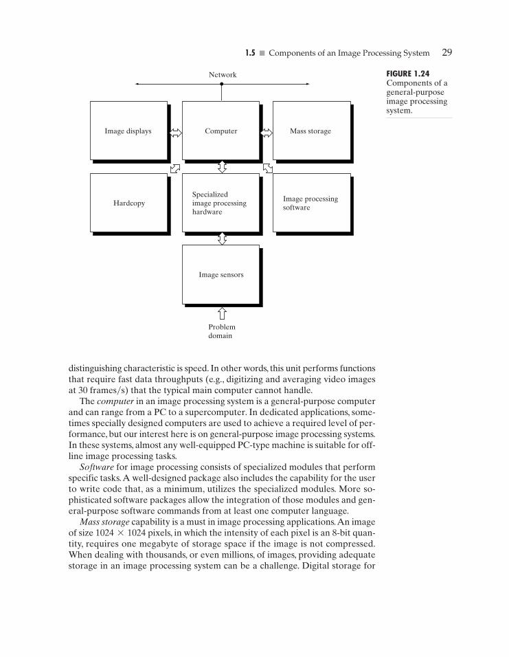
1.5 � Components of an Image Processing System 29
Image displays Computer Mass storage
HardcopySpecializedimage processinghardware
Image sensors
Problemdomain
Image processingsoftware
Network FIGURE 1.24Components of ageneral-purposeimage processingsystem.
distinguishing characteristic is speed. In other words, this unit performs functionsthat require fast data throughputs (e.g., digitizing and averaging video imagesat 30 frames�s) that the typical main computer cannot handle.
The computer in an image processing system is a general-purpose computerand can range from a PC to a supercomputer. In dedicated applications, some-times specially designed computers are used to achieve a required level of per-formance, but our interest here is on general-purpose image processing systems.In these systems, almost any well-equipped PC-type machine is suitable for off-line image processing tasks.
Software for image processing consists of specialized modules that performspecific tasks.A well-designed package also includes the capability for the userto write code that, as a minimum, utilizes the specialized modules. More so-phisticated software packages allow the integration of those modules and gen-eral-purpose software commands from at least one computer language.
Mass storage capability is a must in image processing applications.An imageof size 1024*1024 pixels, in which the intensity of each pixel is an 8-bit quan-tity, requires one megabyte of storage space if the image is not compressed.When dealing with thousands, or even millions, of images, providing adequatestorage in an image processing system can be a challenge. Digital storage for
GONZ01-001-033.II 29-08-2001 14:42 Page 29
30 Chapter 1 � Introduction
image processing applications falls into three principal categories: (1) short-term storage for use during processing, (2) on-line storage for relatively fast re-call, and (3) archival storage, characterized by infrequent access. Storage ismeasured in bytes (eight bits), Kbytes (one thousand bytes), Mbytes (one mil-lion bytes), Gbytes (meaning giga, or one billion, bytes), and Tbytes (meaningtera, or one trillion, bytes).
One method of providing short-term storage is computer memory. Anotheris by specialized boards, called frame buffers, that store one or more images andcan be accessed rapidly, usually at video rates (e.g., at 30 complete images persecond). The latter method allows virtually instantaneous image zoom, as wellas scroll (vertical shifts) and pan (horizontal shifts). Frame buffers usually arehoused in the specialized image processing hardware unit shown in Fig. 1.24. On-line storage generally takes the form of magnetic disks or optical-media stor-age.The key factor characterizing on-line storage is frequent access to the storeddata. Finally, archival storage is characterized by massive storage requirementsbut infrequent need for access. Magnetic tapes and optical disks housed in“jukeboxes” are the usual media for archival applications.
Image displays in use today are mainly color (preferably flat screen) TV mon-itors. Monitors are driven by the outputs of image and graphics display cards thatare an integral part of the computer system. Seldom are there requirements forimage display applications that cannot be met by display cards available com-mercially as part of the computer system. In some cases, it is necessary to havestereo displays, and these are implemented in the form of headgear containingtwo small displays embedded in goggles worn by the user.
Hardcopy devices for recording images include laser printers, film cam-eras, heat-sensitive devices, inkjet units, and digital units, such as optical andCD-ROM disks. Film provides the highest possible resolution, but paper is theobvious medium of choice for written material. For presentations, images are dis-played on film transparencies or in a digital medium if image projection equip-ment is used.The latter approach is gaining acceptance as the standard for imagepresentations.
Networking is almost a default function in any computer system in use today.Because of the large amount of data inherent in image processing applications,the key consideration in image transmission is bandwidth. In dedicated net-works, this typically is not a problem, but communications with remote sites viathe Internet are not always as efficient. Fortunately, this situation is improvingquickly as a result of optical fiber and other broadband technologies.
SummaryThe main purpose of the material presented in this chapter is to provide a sense of per-spective about the origins of digital image processing and, more important, about cur-rent and future areas of application of this technology. Although the coverage of thesetopics in this chapter was necessarily incomplete due to space limitations, it should haveleft the reader with a clear impression of the breadth and practical scope of digital imageprocessing.As we proceed in the following chapters with the development of image pro-cessing theory and applications, numerous examples are provided to keep a clear focus
GONZ01-001-033.II 29-08-2001 14:42 Page 30
� References and Further Reading 31
on the utility and promise of these techniques. Upon concluding the study of the finalchapter, the reader of this book will have arrived at a level of understanding that is thefoundation for most of the work currently underway in this field.
References and Further ReadingReferences at the end of later chapters address specific topics discussed in those chap-ters, and are keyed to the Bibliography at the end of the book. However, in this chapterwe follow a different format in order to summarize in one place a body of journals thatpublish material on image processing and related topics.We also provide a list of booksfrom which the reader can readily develop a historical and current perspective of activ-ities in this field.Thus, the reference material cited in this chapter is intended as a general-purpose, easily accessible guide to the published literature on image processing.
Major refereed journals that publish articles on image processing and related topicsinclude: IEEE Transactions on Image Processing; IEEE Transactions on Pattern Analy-sis and Machine Intelligence; Computer Vision, Graphics, and Image Processing (priorto 1991); Computer Vision and Image Understanding; IEEE Transactions on Systems,Man and Cybernetics; Artificial Intelligence; Pattern Recognition; Pattern RecognitionLetters; Journal of the Optical Society of America (prior to 1984); Journal of the OpticalSociety of America—A: Optics, Image Science and Vision; Optical Engineering; AppliedOptics—Information Processing; IEEE Transactions on Medical Imaging; Journal ofElectronic Imaging; IEEE Transactions on Information Theory; IEEE Transactions onCommunications; IEEE Transactions on Acoustics, Speech and Signal Processing; Pro-ceedings of the IEEE; and issues of the IEEE Transactions on Computers prior to 1980.Publications of the International Society for Optical Engineering (SPIE) also are ofinterest.
The following books, listed in reverse chronological order (with the number of booksbeing biased toward more recent publications), contain material that complements ourtreatment of digital image processing. These books represent an easily accessibleoverview of the area for the past 30 years and were selected to provide a variety of treat-ments.They range from textbooks, which cover foundation material; to handbooks, whichgive an overview of techniques; and finally to edited books, which contain material rep-resentative of current research in the field.
Duda, R. O., Hart, P. E., and Stork, D. G. [2001]. Pattern Classification, 2nd ed., John Wiley& Sons, NY.
Ritter, G. X. and Wilson, J. N. [2001]. Handbook of Computer Vision Algorithms in ImageAlgebra, CRC Press, Boca Raton, FL.
Shapiro, L. G. and Stockman, G. C. [2001]. Computer Vision, Prentice Hall, Upper Sad-dle River, NJ.
Dougherty, E. R. (ed.) [2000]. Random Processes for Image and Signal Processing, IEEEPress, NY.
Etienne, E. K. and Nachtegael, M. (eds.). [2000]. Fuzzy Techniques in Image Processing,Springer-Verlag, NY.
Goutsias, J, Vincent, L., and Bloomberg, D. S. (eds.). [2000]. Mathematical Morphologyand Its Applications to Image and Signal Processing, Kluwer Academic Publishers,Boston, MA.
Mallot, A. H. [2000]. Computational Vision, The MIT Press, Cambridge, MA.
Marchand-Maillet, S. and Sharaiha, Y. M. [2000]. Binary Digital Image Processing: ADiscrete Approach, Academic Press, NY.
GONZ01-001-033.II 29-08-2001 14:42 Page 31
32 Chapter 1 � Introduction
Mitra, S. K. and Sicuranza, G. L. (eds.) [2000]. Nonlinear Image Processing, AcademicPress, NY.
Edelman, S. [1999]. Representation and Recognition in Vision,The MIT Press, Cambridge,MA.
Lillesand,T. M. and Kiefer, R.W. [1999]. Remote Sensing and Image Interpretation, JohnWiley & Sons, NY.
Mather, P. M. [1999]. Computer Processing of Remotely Sensed Images:An Introduction,John Wiley & Sons, NY.
Petrou, M. and Bosdogianni, P. [1999]. Image Processing:The Fundamentals, John Wiley& Sons, UK.
Russ, J. C. [1999]. The Image Processing Handbook, 3rd ed., CRC Press, Boca Raton,FL.
Smirnov, A. [1999]. Processing of Multidimensional Signals, Springer-Verlag, NY.
Sonka, M., Hlavac, V., and Boyle, R. [1999]. Image Processing, Analysis, and ComputerVision, PWS Publishing, NY.
Umbaugh, S. E. [1998]. Computer Vision and Image Processing: A Practical ApproachUsing CVIPtools, Prentice Hall, Upper Saddle River, NJ.
Haskell, B. G. and Netravali,A. N. [1997]. Digital Pictures: Representation, Compression,and Standards, Perseus Publishing, NY.
Jahne, B. [1997]. Digital Image Processing: Concepts, Algorithms, and Scientific Applica-tions, Springer-Verlag, NY.
Castleman, K. R. [1996]. Digital Image Processing, 2nd ed., Prentice Hall, Upper SaddleRiver, NJ.
Geladi, P. and Grahn, H. [1996]. Multivariate Image Analysis, John Wiley & Sons, NY.
Bracewell, R. N. [1995]. Two-Dimensional Imaging, Prentice Hall, Upper SaddleRiver, NJ.
Sid-Ahmed, M. A. [1995]. Image Processing: Theory, Algorithms, and Architectures,McGraw-Hill, NY.
Jain, R., Rangachar, K., and Schunk, B. [1995]. Computer Vision, McGraw-Hill, NY.
Mitiche, A. [1994]. Computational Analysis of Visual Motion, Perseus Publishing, NY.
Baxes, G.A. [1994]. Digital Image Processing: Principles and Applications, John Wiley &Sons, NY.
Gonzalez, R. C. and Woods, R. E. [1992]. Digital Image Processing, Addison-Wesley,Reading, MA.
Haralick, R. M. and Shapiro, L. G. [1992]. Computer and Robot Vision, vols. 1 & 2,Addison-Wesley, Reading, MA.
Pratt, W. K. [1991] Digital Image Processing, 2nd ed., Wiley-Interscience, NY.
Lim, J. S. [1990]. Two-Dimensional Signal and Image Processing, Prentice Hall, UpperSaddle River, NJ.
Jain,A. K. [1989]. Fundamentals of Digital Image Processing, Prentice Hall, Upper SaddleRiver, NJ.
Schalkoff, R. J. [1989]. Digital Image Processing and Computer Vision, John Wiley &Sons, NY.
Giardina, C. R. and Dougherty, E. R. [1988]. Morphological Methods in Image and Sig-nal Processing, Prentice Hall, Upper Saddle River, NJ.
GONZ01-001-033.II 29-08-2001 14:42 Page 32

� References and Further Reading 33
Levine, M. D. [1985]. Vision in Man and Machine, McGraw-Hill, NY.
Serra, J. [1982]. Image Analysis and Mathematical Morphology, Academic Press, NY.
Ballard, D. H. and Brown, C. M. [1982]. Computer Vision, Prentice Hall, Upper SaddleRiver, NJ.
Fu, K. S. [1982]. Syntactic Pattern Recognition and Applications, Prentice Hall, UpperSaddle River, NJ.
Nevatia, R. [1982]. Machine Perception, Prentice Hall, Upper Saddle River, NJ.
Pavlidis, T. [1982]. Algorithms for Graphics and Image Processing, Computer SciencePress, Rockville, MD.
Rosenfeld, R. and Kak, A. C. [1982]. Digital Picture Processing, 2nd ed., vols. 1 & 2,Academic Press, NY.
Hall, E. L. [1979]. Computer Image Processing and Recognition, Academic Press, NY.
Gonzalez, R. C. and Thomason, M. G. [1978]. Syntactic Pattern Recognition: An Intro-duction, Addison-Wesley, Reading, MA.
Andrews, H. C. and Hunt, B. R. [1977]. Digital Image Restoration, Prentice Hall, UpperSaddle River, NJ.
Pavlidis, T. [1977]. Structural Pattern Recognition, Springer-Verlag, NY, 1977.
Tou, J. T. and Gonzalez, R. C. [1974]. Pattern Recognition Principles, Addison-Wesley,Reading, MA, 1974.
Andrews, H. C. [1970]. Computer Techniques in Image Processing, Academic Press, NY.
GONZ01-001-033.II 29-08-2001 14:42 Page 33
34
2 Digital ImageFundamentals
Those who wish to succeed must ask the right preliminary questions.Aristotle
PreviewThe purpose of this chapter is to introduce several concepts related to digital im-ages and some of the notation used throughout the book. Section 2.1 brieflysummarizes the mechanics of the human visual system, including image for-mation in the eye and its capabilities for brightness adaptation and discrimina-tion. Section 2.2 discusses light, other components of the electromagneticspectrum, and their imaging characteristics. Section 2.3 discusses imaging sen-sors and how they are used to generate digital images. Section 2.4 introduces theconcepts of uniform image sampling and gray-level quantization. Additionaltopics discussed in that section include digital image representation, the effectsof varying the number of samples and gray levels in an image, some importantphenomena associated with sampling, and techniques for image zooming andshrinking. Section 2.5 deals with some basic relationships between pixels that areused throughout the book. Finally, Section 2.6 defines the conditions for linearoperations. As noted in that section, linear operators play a central role in thedevelopment of image processing techniques.
Elements of Visual Perception
Although the digital image processing field is built on a foundation of mathe-matical and probabilistic formulations, human intuition and analysis play a cen-tral role in the choice of one technique versus another, and this choice often is
2.1
GONZ02-034-074.II 29-08-2001 13:35 Page 34
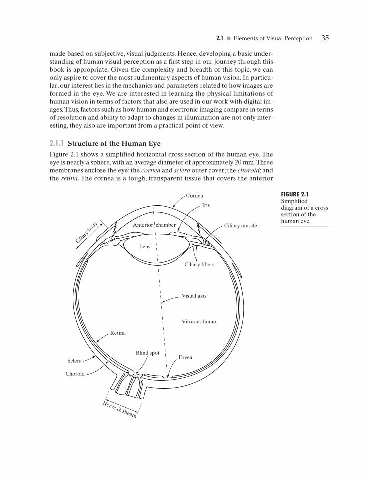
2.1 � Elements of Visual Perception 35
Retina
Blind spot
Sclera
Choroid
Nerve & sheath
Fovea
Vitreous humor
Visual axis
Ciliary fibers
Ciliary muscle
Iris
Cornea
Lens
Anterior chamber
Ciliar
y body
FIGURE 2.1Simplifieddiagram of a crosssection of thehuman eye.
made based on subjective, visual judgments. Hence, developing a basic under-standing of human visual perception as a first step in our journey through thisbook is appropriate. Given the complexity and breadth of this topic, we canonly aspire to cover the most rudimentary aspects of human vision. In particu-lar, our interest lies in the mechanics and parameters related to how images areformed in the eye. We are interested in learning the physical limitations ofhuman vision in terms of factors that also are used in our work with digital im-ages.Thus, factors such as how human and electronic imaging compare in termsof resolution and ability to adapt to changes in illumination are not only inter-esting, they also are important from a practical point of view.
2.1.1 Structure of the Human EyeFigure 2.1 shows a simplified horizontal cross section of the human eye. Theeye is nearly a sphere, with an average diameter of approximately 20 mm.Threemembranes enclose the eye: the cornea and sclera outer cover; the choroid; andthe retina. The cornea is a tough, transparent tissue that covers the anterior
GONZ02-034-074.II 29-08-2001 13:35 Page 35
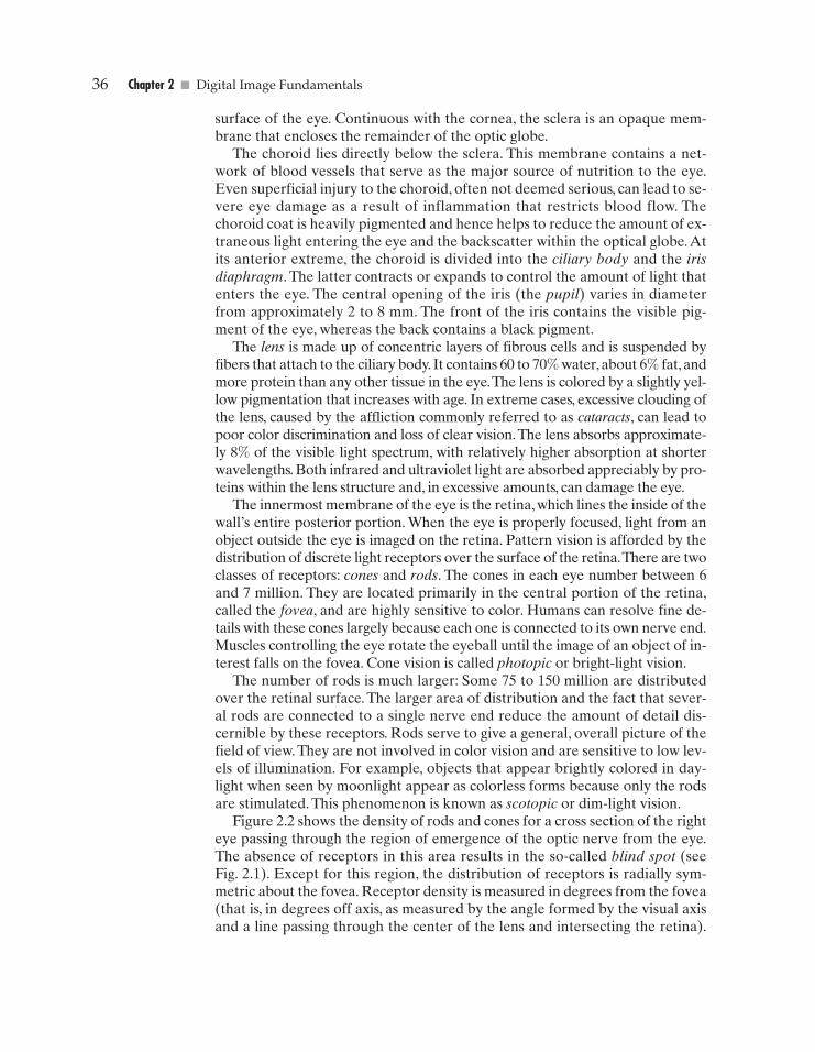
36 Chapter 2 � Digital Image Fundamentals
surface of the eye. Continuous with the cornea, the sclera is an opaque mem-brane that encloses the remainder of the optic globe.
The choroid lies directly below the sclera. This membrane contains a net-work of blood vessels that serve as the major source of nutrition to the eye.Even superficial injury to the choroid, often not deemed serious, can lead to se-vere eye damage as a result of inflammation that restricts blood flow. Thechoroid coat is heavily pigmented and hence helps to reduce the amount of ex-traneous light entering the eye and the backscatter within the optical globe.Atits anterior extreme, the choroid is divided into the ciliary body and the irisdiaphragm. The latter contracts or expands to control the amount of light thatenters the eye. The central opening of the iris (the pupil) varies in diameterfrom approximately 2 to 8 mm. The front of the iris contains the visible pig-ment of the eye, whereas the back contains a black pigment.
The lens is made up of concentric layers of fibrous cells and is suspended byfibers that attach to the ciliary body. It contains 60 to 70% water, about 6% fat, andmore protein than any other tissue in the eye.The lens is colored by a slightly yel-low pigmentation that increases with age. In extreme cases, excessive clouding ofthe lens, caused by the affliction commonly referred to as cataracts, can lead topoor color discrimination and loss of clear vision.The lens absorbs approximate-ly 8% of the visible light spectrum, with relatively higher absorption at shorterwavelengths. Both infrared and ultraviolet light are absorbed appreciably by pro-teins within the lens structure and, in excessive amounts, can damage the eye.
The innermost membrane of the eye is the retina, which lines the inside of thewall’s entire posterior portion. When the eye is properly focused, light from anobject outside the eye is imaged on the retina. Pattern vision is afforded by thedistribution of discrete light receptors over the surface of the retina.There are twoclasses of receptors: cones and rods. The cones in each eye number between 6and 7 million. They are located primarily in the central portion of the retina,called the fovea, and are highly sensitive to color. Humans can resolve fine de-tails with these cones largely because each one is connected to its own nerve end.Muscles controlling the eye rotate the eyeball until the image of an object of in-terest falls on the fovea. Cone vision is called photopic or bright-light vision.
The number of rods is much larger: Some 75 to 150 million are distributedover the retinal surface. The larger area of distribution and the fact that sever-al rods are connected to a single nerve end reduce the amount of detail dis-cernible by these receptors. Rods serve to give a general, overall picture of thefield of view. They are not involved in color vision and are sensitive to low lev-els of illumination. For example, objects that appear brightly colored in day-light when seen by moonlight appear as colorless forms because only the rodsare stimulated. This phenomenon is known as scotopic or dim-light vision.
Figure 2.2 shows the density of rods and cones for a cross section of the righteye passing through the region of emergence of the optic nerve from the eye.The absence of receptors in this area results in the so-called blind spot (seeFig. 2.1). Except for this region, the distribution of receptors is radially sym-metric about the fovea. Receptor density is measured in degrees from the fovea(that is, in degrees off axis, as measured by the angle formed by the visual axisand a line passing through the center of the lens and intersecting the retina).
GONZ02-034-074.II 29-08-2001 13:35 Page 36
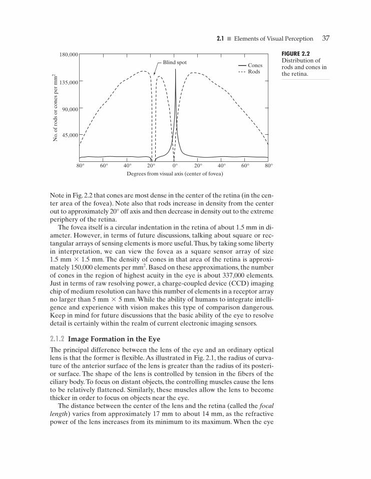
2.1 � Elements of Visual Perception 37
Blind spot ConesRods
No.
of r
ods
or c
ones
per
mm
2
Degrees from visual axis (center of fovea)
180,000
135,000
90,000
45,000
80° 60° 40° 20° 0° 20° 40° 60° 80°
FIGURE 2.2Distribution ofrods and cones inthe retina.
Note in Fig. 2.2 that cones are most dense in the center of the retina (in the cen-ter area of the fovea). Note also that rods increase in density from the centerout to approximately 20° off axis and then decrease in density out to the extremeperiphery of the retina.
The fovea itself is a circular indentation in the retina of about 1.5 mm in di-ameter. However, in terms of future discussions, talking about square or rec-tangular arrays of sensing elements is more useful.Thus, by taking some libertyin interpretation, we can view the fovea as a square sensor array of size1.5 mm*1.5 mm. The density of cones in that area of the retina is approxi-mately 150,000 elements per mm2. Based on these approximations, the numberof cones in the region of highest acuity in the eye is about 337,000 elements.Just in terms of raw resolving power, a charge-coupled device (CCD) imagingchip of medium resolution can have this number of elements in a receptor arrayno larger than 5 mm*5 mm. While the ability of humans to integrate intelli-gence and experience with vision makes this type of comparison dangerous.Keep in mind for future discussions that the basic ability of the eye to resolvedetail is certainly within the realm of current electronic imaging sensors.
2.1.2 Image Formation in the EyeThe principal difference between the lens of the eye and an ordinary opticallens is that the former is flexible. As illustrated in Fig. 2.1, the radius of curva-ture of the anterior surface of the lens is greater than the radius of its posteri-or surface. The shape of the lens is controlled by tension in the fibers of theciliary body. To focus on distant objects, the controlling muscles cause the lensto be relatively flattened. Similarly, these muscles allow the lens to becomethicker in order to focus on objects near the eye.
The distance between the center of the lens and the retina (called the focallength) varies from approximately 17 mm to about 14 mm, as the refractivepower of the lens increases from its minimum to its maximum. When the eye
GONZ02-034-074.II 29-08-2001 13:35 Page 37
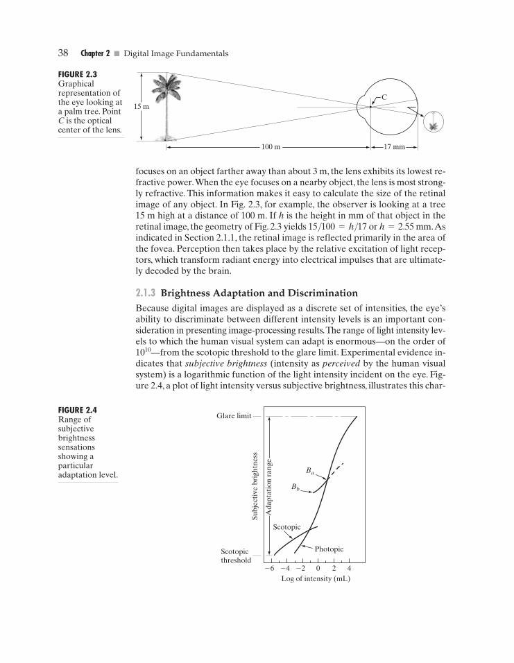
38 Chapter 2 � Digital Image Fundamentals
15 mC
17 mm100 m
FIGURE 2.3Graphicalrepresentation ofthe eye looking ata palm tree. PointC is the opticalcenter of the lens.
focuses on an object farther away than about 3 m, the lens exhibits its lowest re-fractive power.When the eye focuses on a nearby object, the lens is most strong-ly refractive. This information makes it easy to calculate the size of the retinalimage of any object. In Fig. 2.3, for example, the observer is looking at a tree15 m high at a distance of 100 m. If h is the height in mm of that object in theretinal image, the geometry of Fig. 2.3 yields 15/100=h/17 or h=2.55 mm.Asindicated in Section 2.1.1, the retinal image is reflected primarily in the area ofthe fovea. Perception then takes place by the relative excitation of light recep-tors, which transform radiant energy into electrical impulses that are ultimate-ly decoded by the brain.
2.1.3 Brightness Adaptation and DiscriminationBecause digital images are displayed as a discrete set of intensities, the eye’sability to discriminate between different intensity levels is an important con-sideration in presenting image-processing results.The range of light intensity lev-els to which the human visual system can adapt is enormous—on the order of1010—from the scotopic threshold to the glare limit. Experimental evidence in-dicates that subjective brightness (intensity as perceived by the human visualsystem) is a logarithmic function of the light intensity incident on the eye. Fig-ure 2.4, a plot of light intensity versus subjective brightness, illustrates this char-
Glare limit
Subj
ecti
ve b
righ
tnes
s
Ada
ptat
ion
rang
e
Scotopicthreshold
Log of intensity (mL)
Scotopic
Photopic
–6 –4 –2 0 2 4
Ba
Bb
FIGURE 2.4Range ofsubjectivebrightnesssensationsshowing aparticularadaptation level.
GONZ02-034-074.II 29-08-2001 13:35 Page 38
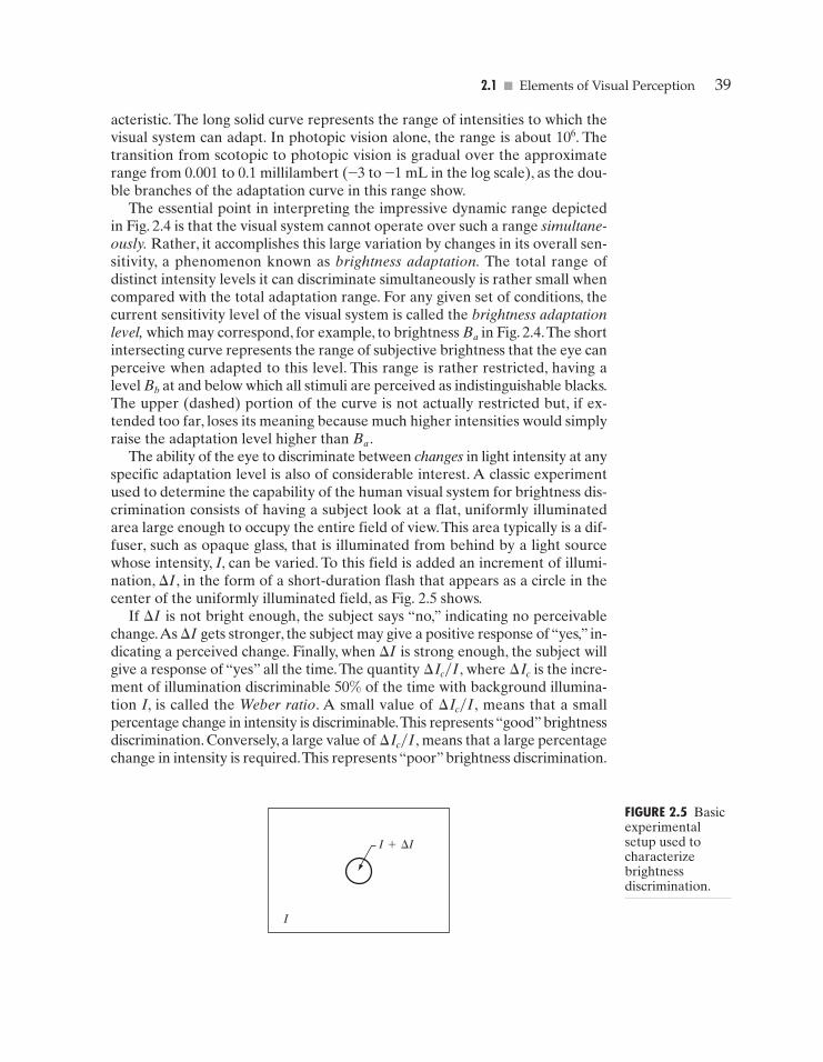
2.1 � Elements of Visual Perception 39
acteristic. The long solid curve represents the range of intensities to which thevisual system can adapt. In photopic vision alone, the range is about 106. Thetransition from scotopic to photopic vision is gradual over the approximaterange from 0.001 to 0.1 millilambert (–3 to –1 mL in the log scale), as the dou-ble branches of the adaptation curve in this range show.
The essential point in interpreting the impressive dynamic range depictedin Fig. 2.4 is that the visual system cannot operate over such a range simultane-ously. Rather, it accomplishes this large variation by changes in its overall sen-sitivity, a phenomenon known as brightness adaptation. The total range ofdistinct intensity levels it can discriminate simultaneously is rather small whencompared with the total adaptation range. For any given set of conditions, thecurrent sensitivity level of the visual system is called the brightness adaptationlevel, which may correspond, for example, to brightness Ba in Fig. 2.4.The shortintersecting curve represents the range of subjective brightness that the eye canperceive when adapted to this level. This range is rather restricted, having alevel Bb at and below which all stimuli are perceived as indistinguishable blacks.The upper (dashed) portion of the curve is not actually restricted but, if ex-tended too far, loses its meaning because much higher intensities would simplyraise the adaptation level higher than Ba .
The ability of the eye to discriminate between changes in light intensity at anyspecific adaptation level is also of considerable interest. A classic experimentused to determine the capability of the human visual system for brightness dis-crimination consists of having a subject look at a flat, uniformly illuminatedarea large enough to occupy the entire field of view.This area typically is a dif-fuser, such as opaque glass, that is illuminated from behind by a light sourcewhose intensity, I, can be varied. To this field is added an increment of illumi-nation, �I, in the form of a short-duration flash that appears as a circle in thecenter of the uniformly illuminated field, as Fig. 2.5 shows.
If �I is not bright enough, the subject says “no,” indicating no perceivablechange.As �I gets stronger, the subject may give a positive response of “yes,” in-dicating a perceived change. Finally, when �I is strong enough, the subject willgive a response of “yes” all the time.The quantity where is the incre-ment of illumination discriminable 50% of the time with background illumina-tion I, is called the Weber ratio. A small value of means that a smallpercentage change in intensity is discriminable.This represents “good” brightnessdiscrimination. Conversely, a large value of means that a large percentagechange in intensity is required.This represents “poor” brightness discrimination.
¢Ic�I,
¢Ic�I,
¢Ic¢Ic�I,
I
I+¢I
FIGURE 2.5 Basicexperimentalsetup used tocharacterizebrightnessdiscrimination.
GONZ02-034-074.II 29-08-2001 13:35 Page 39
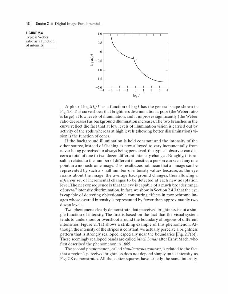
40 Chapter 2 � Digital Image Fundamentals
–1.5
–2.0–4 –3 –2 –1 0
log Ilo
g ¢I
c/I
1 2 3 4
–1.0
–0.5
0.5
1.0
0
FIGURE 2.6Typical Weberratio as a functionof intensity.
A plot of as a function of log I has the general shape shown inFig. 2.6.This curve shows that brightness discrimination is poor (the Weber ratiois large) at low levels of illumination, and it improves significantly (the Weberratio decreases) as background illumination increases.The two branches in thecurve reflect the fact that at low levels of illumination vision is carried out byactivity of the rods, whereas at high levels (showing better discrimination) vi-sion is the function of cones.
If the background illumination is held constant and the intensity of theother source, instead of flashing, is now allowed to vary incrementally fromnever being perceived to always being perceived, the typical observer can dis-cern a total of one to two dozen different intensity changes. Roughly, this re-sult is related to the number of different intensities a person can see at any onepoint in a monochrome image.This result does not mean that an image can berepresented by such a small number of intensity values because, as the eyeroams about the image, the average background changes, thus allowing adifferent set of incremental changes to be detected at each new adaptationlevel. The net consequence is that the eye is capable of a much broader rangeof overall intensity discrimination. In fact, we show in Section 2.4.3 that the eyeis capable of detecting objectionable contouring effects in monochrome im-ages whose overall intensity is represented by fewer than approximately twodozen levels.
Two phenomena clearly demonstrate that perceived brightness is not a sim-ple function of intensity. The first is based on the fact that the visual systemtends to undershoot or overshoot around the boundary of regions of differentintensities. Figure 2.7(a) shows a striking example of this phenomenon. Al-though the intensity of the stripes is constant, we actually perceive a brightnesspattern that is strongly scalloped, especially near the boundaries [Fig. 2.7(b)].These seemingly scalloped bands are called Mach bands after Ernst Mach, whofirst described the phenomenon in 1865.
The second phenomenon, called simultaneous contrast, is related to the factthat a region’s perceived brightness does not depend simply on its intensity, asFig. 2.8 demonstrates. All the center squares have exactly the same intensity.
log ¢Ic�I,
GONZ02-034-074.II 29-08-2001 13:35 Page 40
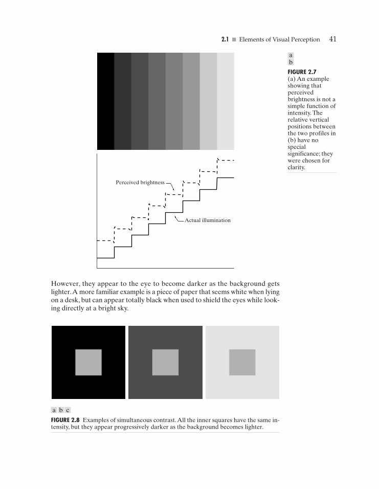
2.1 � Elements of Visual Perception 41
Actual illumination
Perceived brightness
However, they appear to the eye to become darker as the background getslighter.A more familiar example is a piece of paper that seems white when lyingon a desk, but can appear totally black when used to shield the eyes while look-ing directly at a bright sky.
FIGURE 2.7(a) An exampleshowing thatperceivedbrightness is not asimple function ofintensity. Therelative verticalpositions betweenthe two profiles in(b) have nospecialsignificance; theywere chosen forclarity.
ab
FIGURE 2.8 Examples of simultaneous contrast.All the inner squares have the same in-tensity, but they appear progressively darker as the background becomes lighter.
a b c
GONZ02-034-074.II 29-08-2001 13:35 Page 41
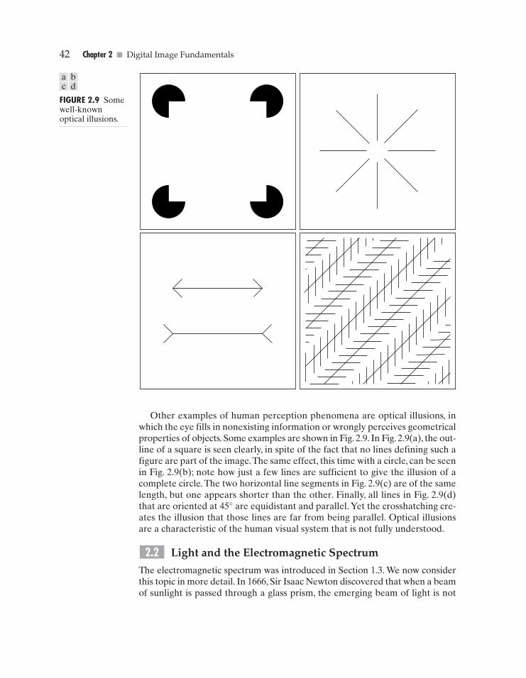
42 Chapter 2 � Digital Image Fundamentals
FIGURE 2.9 Somewell-knownoptical illusions.
a bc d
Other examples of human perception phenomena are optical illusions, inwhich the eye fills in nonexisting information or wrongly perceives geometricalproperties of objects. Some examples are shown in Fig. 2.9. In Fig. 2.9(a), the out-line of a square is seen clearly, in spite of the fact that no lines defining such afigure are part of the image.The same effect, this time with a circle, can be seenin Fig. 2.9(b); note how just a few lines are sufficient to give the illusion of acomplete circle. The two horizontal line segments in Fig. 2.9(c) are of the samelength, but one appears shorter than the other. Finally, all lines in Fig. 2.9(d)that are oriented at 45° are equidistant and parallel. Yet the crosshatching cre-ates the illusion that those lines are far from being parallel. Optical illusionsare a characteristic of the human visual system that is not fully understood.
Light and the Electromagnetic Spectrum
The electromagnetic spectrum was introduced in Section 1.3. We now considerthis topic in more detail. In 1666, Sir Isaac Newton discovered that when a beamof sunlight is passed through a glass prism, the emerging beam of light is not
2.2
GONZ02-034-074.II 29-08-2001 13:35 Page 42
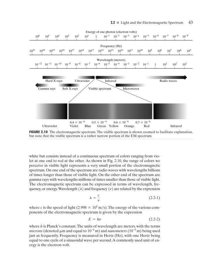
2.2 � Light and the Electromagnetic Spectrum 43
105106107108109101010111012101310141015101610171018101910201021
Frequency (Hz)
10–910–810–710–610–510–410–310–210–11101102103104105106
Energy of one photon (electron volts)
0.4*10–6 0.5*10–6 0.6*10–6 0.7*10–6
103102101110–110–210–310–410–510–610–710–810–910–1010–1110–12Wavelength (meters)
Radio waves
Microwaves
InfraredUltraviolet
Visible spectrumGamma rays Soft X-rays
Hard X-rays
InfraredUltraviolet Violet Blue Green Yellow RedOrange
FIGURE 2.10 The electromagnetic spectrum. The visible spectrum is shown zoomed to facilitate explanation,but note that the visible spectrum is a rather narrow portion of the EM spectrum.
white but consists instead of a continuous spectrum of colors ranging from vio-let at one end to red at the other. As shown in Fig. 2.10, the range of colors weperceive in visible light represents a very small portion of the electromagneticspectrum. On one end of the spectrum are radio waves with wavelengths billionsof times longer than those of visible light. On the other end of the spectrum aregamma rays with wavelengths millions of times smaller than those of visible light.The electromagnetic spectrum can be expressed in terms of wavelength, fre-quency, or energy.Wavelength (l) and frequency (n) are related by the expression
(2.2-1)
where c is the speed of light (2.998*108 m�s).The energy of the various com-ponents of the electromagnetic spectrum is given by the expression
E=hn (2.2-2)
where h is Planck’s constant.The units of wavelength are meters, with the termsmicrons (denoted �m and equal to 10–6 m) and nanometers (10–9 m) being usedjust as frequently. Frequency is measured in Hertz (Hz), with one Hertz beingequal to one cycle of a sinusoidal wave per second.A commonly used unit of en-ergy is the electron-volt.
l =cn
GONZ02-034-074.II 29-08-2001 13:35 Page 43
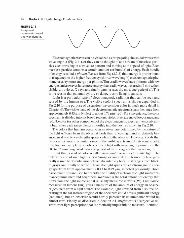
44 Chapter 2 � Digital Image Fundamentals
lFIGURE 2.11Graphicalrepresentation ofone wavelength.
Electromagnetic waves can be visualized as propagating sinusoidal waves withwavelength l (Fig. 2.11), or they can be thought of as a stream of massless parti-cles, each traveling in a wavelike pattern and moving at the speed of light. Eachmassless particle contains a certain amount (or bundle) of energy. Each bundleof energy is called a photon.We see from Eq. (2.2-2) that energy is proportionalto frequency, so the higher-frequency (shorter wavelength) electromagnetic phe-nomena carry more energy per photon.Thus, radio waves have photons with lowenergies, microwaves have more energy than radio waves, infrared still more, thenvisible, ultraviolet, X-rays, and finally gamma rays, the most energetic of all.Thisis the reason that gamma rays are so dangerous to living organisms.
Light is a particular type of electromagnetic radiation that can be seen andsensed by the human eye. The visible (color) spectrum is shown expanded inFig. 2.10 for the purpose of discussion (we consider color in much more detail inChapter 6).The visible band of the electromagnetic spectrum spans the range fromapproximately 0.43 �m (violet) to about 0.79 �m (red).For convenience, the colorspectrum is divided into six broad regions: violet, blue, green, yellow, orange, andred. No color (or other component of the electromagnetic spectrum) ends abrupt-ly, but rather each range blends smoothly into the next, as shown in Fig. 2.10.
The colors that humans perceive in an object are determined by the nature ofthe light reflected from the object. A body that reflects light and is relatively bal-anced in all visible wavelengths appears white to the observer.However,a body thatfavors reflectance in a limited range of the visible spectrum exhibits some shadesof color. For example, green objects reflect light with wavelengths primarily in the500 to 570 nm range while absorbing most of the energy at other wavelengths.
Light that is void of color is called achromatic or monochromatic light. Theonly attribute of such light is its intensity, or amount. The term gray level gen-erally is used to describe monochromatic intensity because it ranges from black,to grays, and finally to white. Chromatic light spans the electromagnetic ener-gy spectrum from approximately 0.43 to 0.79 �m, as noted previously. Threebasic quantities are used to describe the quality of a chromatic light source: ra-diance; luminance; and brightness. Radiance is the total amount of energy thatflows from the light source, and it is usually measured in watts (W). Luminance,measured in lumens (lm), gives a measure of the amount of energy an observ-er perceives from a light source. For example, light emitted from a source op-erating in the far infrared region of the spectrum could have significant energy(radiance), but an observer would hardly perceive it; its luminance would bealmost zero. Finally, as discussed in Section 2.1, brightness is a subjective de-scriptor of light perception that is practically impossible to measure. It embod-
GONZ02-034-074.II 29-08-2001 13:35 Page 44
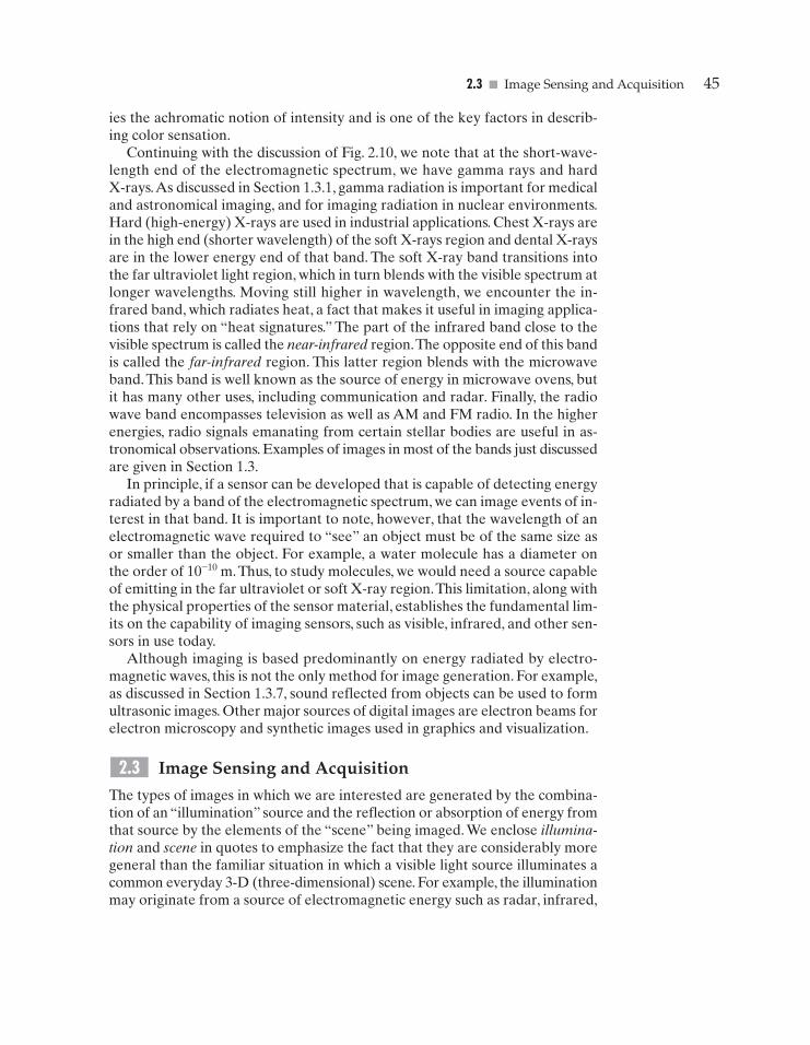
2.3 � Image Sensing and Acquisition 45
ies the achromatic notion of intensity and is one of the key factors in describ-ing color sensation.
Continuing with the discussion of Fig. 2.10, we note that at the short-wave-length end of the electromagnetic spectrum, we have gamma rays and hardX-rays.As discussed in Section 1.3.1, gamma radiation is important for medicaland astronomical imaging, and for imaging radiation in nuclear environments.Hard (high-energy) X-rays are used in industrial applications. Chest X-rays arein the high end (shorter wavelength) of the soft X-rays region and dental X-raysare in the lower energy end of that band. The soft X-ray band transitions intothe far ultraviolet light region, which in turn blends with the visible spectrum atlonger wavelengths. Moving still higher in wavelength, we encounter the in-frared band, which radiates heat, a fact that makes it useful in imaging applica-tions that rely on “heat signatures.” The part of the infrared band close to thevisible spectrum is called the near-infrared region.The opposite end of this bandis called the far-infrared region. This latter region blends with the microwaveband. This band is well known as the source of energy in microwave ovens, butit has many other uses, including communication and radar. Finally, the radiowave band encompasses television as well as AM and FM radio. In the higherenergies, radio signals emanating from certain stellar bodies are useful in as-tronomical observations. Examples of images in most of the bands just discussedare given in Section 1.3.
In principle, if a sensor can be developed that is capable of detecting energyradiated by a band of the electromagnetic spectrum, we can image events of in-terest in that band. It is important to note, however, that the wavelength of anelectromagnetic wave required to “see” an object must be of the same size asor smaller than the object. For example, a water molecule has a diameter onthe order of 10–10 m.Thus, to study molecules, we would need a source capableof emitting in the far ultraviolet or soft X-ray region.This limitation, along withthe physical properties of the sensor material, establishes the fundamental lim-its on the capability of imaging sensors, such as visible, infrared, and other sen-sors in use today.
Although imaging is based predominantly on energy radiated by electro-magnetic waves, this is not the only method for image generation. For example,as discussed in Section 1.3.7, sound reflected from objects can be used to formultrasonic images. Other major sources of digital images are electron beams forelectron microscopy and synthetic images used in graphics and visualization.
Image Sensing and Acquisition
The types of images in which we are interested are generated by the combina-tion of an “illumination” source and the reflection or absorption of energy fromthat source by the elements of the “scene” being imaged. We enclose illumina-tion and scene in quotes to emphasize the fact that they are considerably moregeneral than the familiar situation in which a visible light source illuminates acommon everyday 3-D (three-dimensional) scene. For example, the illuminationmay originate from a source of electromagnetic energy such as radar, infrared,
2.3
GONZ02-034-074.II 29-08-2001 13:35 Page 45
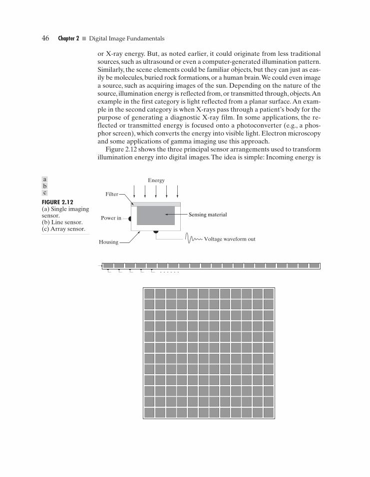
46 Chapter 2 � Digital Image Fundamentals
or X-ray energy. But, as noted earlier, it could originate from less traditionalsources, such as ultrasound or even a computer-generated illumination pattern.Similarly, the scene elements could be familiar objects, but they can just as eas-ily be molecules, buried rock formations, or a human brain.We could even imagea source, such as acquiring images of the sun. Depending on the nature of thesource, illumination energy is reflected from, or transmitted through, objects.Anexample in the first category is light reflected from a planar surface. An exam-ple in the second category is when X-rays pass through a patient’s body for thepurpose of generating a diagnostic X-ray film. In some applications, the re-flected or transmitted energy is focused onto a photoconverter (e.g., a phos-phor screen), which converts the energy into visible light. Electron microscopyand some applications of gamma imaging use this approach.
Figure 2.12 shows the three principal sensor arrangements used to transformillumination energy into digital images. The idea is simple: Incoming energy is
Sensing material
Voltage waveform out
Filter
Energy
Power in
Housing
FIGURE 2.12(a) Single imagingsensor.(b) Line sensor.(c) Array sensor.
abc
GONZ02-034-074.II 29-08-2001 13:35 Page 46
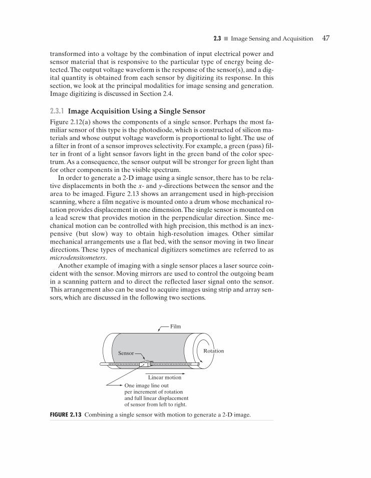
2.3 � Image Sensing and Acquisition 47
Sensor
Linear motion
One image line outper increment of rotationand full linear displacementof sensor from left to right.
Film
Rotation
FIGURE 2.13 Combining a single sensor with motion to generate a 2-D image.
transformed into a voltage by the combination of input electrical power andsensor material that is responsive to the particular type of energy being de-tected.The output voltage waveform is the response of the sensor(s), and a dig-ital quantity is obtained from each sensor by digitizing its response. In thissection, we look at the principal modalities for image sensing and generation.Image digitizing is discussed in Section 2.4.
2.3.1 Image Acquisition Using a Single SensorFigure 2.12(a) shows the components of a single sensor. Perhaps the most fa-miliar sensor of this type is the photodiode, which is constructed of silicon ma-terials and whose output voltage waveform is proportional to light. The use ofa filter in front of a sensor improves selectivity. For example, a green (pass) fil-ter in front of a light sensor favors light in the green band of the color spec-trum.As a consequence, the sensor output will be stronger for green light thanfor other components in the visible spectrum.
In order to generate a 2-D image using a single sensor, there has to be rela-tive displacements in both the x- and y-directions between the sensor and thearea to be imaged. Figure 2.13 shows an arrangement used in high-precisionscanning, where a film negative is mounted onto a drum whose mechanical ro-tation provides displacement in one dimension.The single sensor is mounted ona lead screw that provides motion in the perpendicular direction. Since me-chanical motion can be controlled with high precision, this method is an inex-pensive (but slow) way to obtain high-resolution images. Other similarmechanical arrangements use a flat bed, with the sensor moving in two lineardirections. These types of mechanical digitizers sometimes are referred to asmicrodensitometers.
Another example of imaging with a single sensor places a laser source coin-cident with the sensor. Moving mirrors are used to control the outgoing beamin a scanning pattern and to direct the reflected laser signal onto the sensor.This arrangement also can be used to acquire images using strip and array sen-sors, which are discussed in the following two sections.
GONZ02-034-074.II 29-08-2001 13:35 Page 47
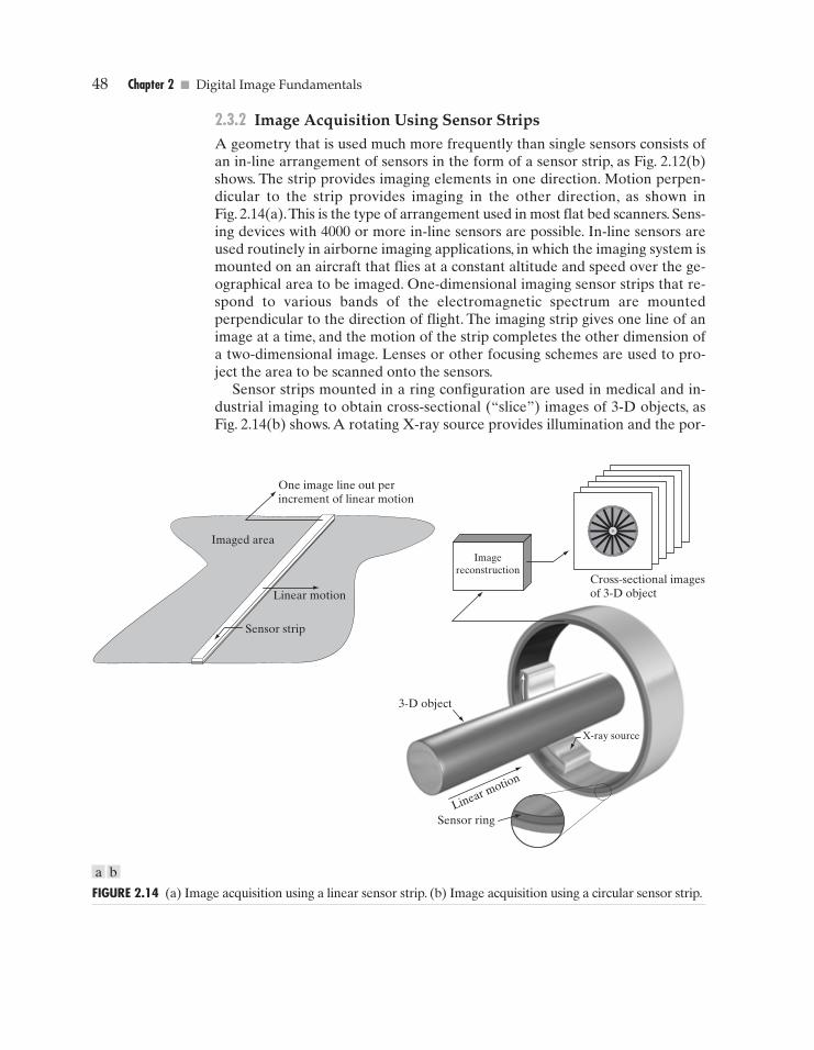
48 Chapter 2 � Digital Image Fundamentals
Imagereconstruction
3-D object
Linear motion
Sensor ring
X-ray source
Sensor strip
Linear motion
Imaged area
One image line out perincrement of linear motion
Cross-sectional imagesof 3-D object
FIGURE 2.14 (a) Image acquisition using a linear sensor strip. (b) Image acquisition using a circular sensor strip.
2.3.2 Image Acquisition Using Sensor StripsA geometry that is used much more frequently than single sensors consists ofan in-line arrangement of sensors in the form of a sensor strip, as Fig. 2.12(b)shows. The strip provides imaging elements in one direction. Motion perpen-dicular to the strip provides imaging in the other direction, as shown inFig. 2.14(a).This is the type of arrangement used in most flat bed scanners. Sens-ing devices with 4000 or more in-line sensors are possible. In-line sensors areused routinely in airborne imaging applications, in which the imaging system ismounted on an aircraft that flies at a constant altitude and speed over the ge-ographical area to be imaged. One-dimensional imaging sensor strips that re-spond to various bands of the electromagnetic spectrum are mountedperpendicular to the direction of flight. The imaging strip gives one line of animage at a time, and the motion of the strip completes the other dimension ofa two-dimensional image. Lenses or other focusing schemes are used to pro-ject the area to be scanned onto the sensors.
Sensor strips mounted in a ring configuration are used in medical and in-dustrial imaging to obtain cross-sectional (“slice”) images of 3-D objects, asFig. 2.14(b) shows. A rotating X-ray source provides illumination and the por-
a b
GONZ02-034-074.II 29-08-2001 13:35 Page 48
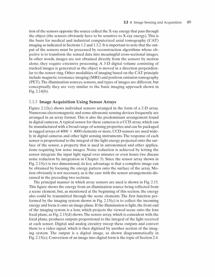
2.3 � Image Sensing and Acquisition 49
tion of the sensors opposite the source collect the X-ray energy that pass throughthe object (the sensors obviously have to be sensitive to X-ray energy). This isthe basis for medical and industrial computerized axial tomography (CAT)imaging as indicated in Sections 1.2 and 1.3.2. It is important to note that the out-put of the sensors must be processed by reconstruction algorithms whose ob-jective is to transform the sensed data into meaningful cross-sectional images.In other words, images are not obtained directly from the sensors by motionalone; they require extensive processing. A 3-D digital volume consisting ofstacked images is generated as the object is moved in a direction perpendicu-lar to the sensor ring. Other modalities of imaging based on the CAT principleinclude magnetic resonance imaging (MRI) and positron emission tomography(PET).The illumination sources, sensors, and types of images are different, butconceptually they are very similar to the basic imaging approach shown inFig. 2.14(b).
2.3.3 Image Acquisition Using Sensor ArraysFigure 2.12(c) shows individual sensors arranged in the form of a 2-D array.Numerous electromagnetic and some ultrasonic sensing devices frequently arearranged in an array format. This is also the predominant arrangement foundin digital cameras.A typical sensor for these cameras is a CCD array, which canbe manufactured with a broad range of sensing properties and can be packagedin rugged arrays of elements or more. CCD sensors are used wide-ly in digital cameras and other light sensing instruments. The response of eachsensor is proportional to the integral of the light energy projected onto the sur-face of the sensor, a property that is used in astronomical and other applica-tions requiring low noise images. Noise reduction is achieved by letting thesensor integrate the input light signal over minutes or even hours (we discussnoise reduction by integration in Chapter 3). Since the sensor array shown inFig. 2.15(c) is two dimensional, its key advantage is that a complete image canbe obtained by focusing the energy pattern onto the surface of the array. Mo-tion obviously is not necessary, as is the case with the sensor arrangements dis-cussed in the preceding two sections.
The principal manner in which array sensors are used is shown in Fig. 2.15.This figure shows the energy from an illumination source being reflected froma scene element, but, as mentioned at the beginning of this section, the energyalso could be transmitted through the scene elements. The first function per-formed by the imaging system shown in Fig. 2.15(c) is to collect the incomingenergy and focus it onto an image plane. If the illumination is light, the front endof the imaging system is a lens, which projects the viewed scene onto the lensfocal plane, as Fig. 2.15(d) shows.The sensor array, which is coincident with thefocal plane, produces outputs proportional to the integral of the light receivedat each sensor. Digital and analog circuitry sweep these outputs and convertthem to a video signal, which is then digitized by another section of the imag-ing system. The output is a digital image, as shown diagrammatically inFig. 2.15(e). Conversion of an image into digital form is the topic of Section 2.4.
4000 * 4000
GONZ02-034-074.II 29-08-2001 13:35 Page 49
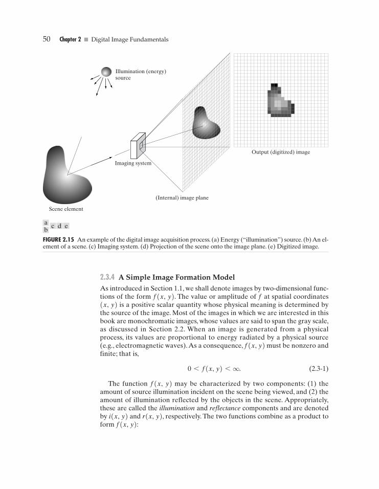
50 Chapter 2 � Digital Image Fundamentals
Illumination (energy)source
Imaging system
(Internal) image plane
Output (digitized) image
Scene element
FIGURE 2.15 An example of the digital image acquisition process. (a) Energy (“illumination”) source. (b) An el-ement of a scene. (c) Imaging system. (d) Projection of the scene onto the image plane. (e) Digitized image.
2.3.4 A Simple Image Formation ModelAs introduced in Section 1.1, we shall denote images by two-dimensional func-tions of the form f(x, y). The value or amplitude of f at spatial coordinates(x, y) is a positive scalar quantity whose physical meaning is determined bythe source of the image. Most of the images in which we are interested in thisbook are monochromatic images, whose values are said to span the gray scale,as discussed in Section 2.2. When an image is generated from a physicalprocess, its values are proportional to energy radiated by a physical source(e.g., electromagnetic waves).As a consequence, f(x, y) must be nonzero andfinite; that is,
0<f(x, y)<q. (2.3-1)
The function f(x, y) may be characterized by two components: (1) theamount of source illumination incident on the scene being viewed, and (2) theamount of illumination reflected by the objects in the scene. Appropriately,these are called the illumination and reflectance components and are denotedby i(x, y) and r(x, y), respectively. The two functions combine as a product toform f(x, y):
ab
c d e
GONZ02-034-074.II 29-08-2001 13:35 Page 50
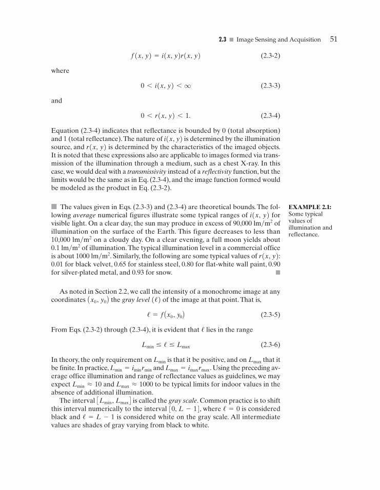
2.3 � Image Sensing and Acquisition 51
f(x, y)=i(x, y)r(x, y) (2.3-2)
where
0<i(x, y)<q (2.3-3)
and
0<r(x, y)<1. (2.3-4)
Equation (2.3-4) indicates that reflectance is bounded by 0 (total absorption)and 1 (total reflectance).The nature of i(x, y) is determined by the illuminationsource, and r(x, y) is determined by the characteristics of the imaged objects.It is noted that these expressions also are applicable to images formed via trans-mission of the illumination through a medium, such as a chest X-ray. In thiscase, we would deal with a transmissivity instead of a reflectivity function, but thelimits would be the same as in Eq. (2.3-4), and the image function formed wouldbe modeled as the product in Eq. (2.3-2).
� The values given in Eqs. (2.3-3) and (2.3-4) are theoretical bounds. The fol-lowing average numerical figures illustrate some typical ranges of i(x, y) forvisible light. On a clear day, the sun may produce in excess of 90,000 lm�m2 ofillumination on the surface of the Earth. This figure decreases to less than10,000 lm�m2 on a cloudy day. On a clear evening, a full moon yields about0.1 lm�m2 of illumination.The typical illumination level in a commercial officeis about 1000 lm�m2. Similarly, the following are some typical values of r(x, y):0.01 for black velvet, 0.65 for stainless steel, 0.80 for flat-white wall paint, 0.90for silver-plated metal, and 0.93 for snow. �
As noted in Section 2.2, we call the intensity of a monochrome image at anycoordinates Ax0, y0 B the gray level (/) of the image at that point. That is,
(2.3-5)
From Eqs. (2.3-2) through (2.3-4), it is evident that / lies in the range
(2.3-6)
In theory, the only requirement on Lmin is that it be positive, and on Lmax that itbe finite. In practice, Lmin=iminrmin and Lmax=imaxrmax. Using the preceding av-erage office illumination and range of reflectance values as guidelines, we mayexpect Lmin≠10 and Lmax≠1000 to be typical limits for indoor values in theabsence of additional illumination.
The interval is called the gray scale. Common practice is to shiftthis interval numerically to the interval [0, L-1], where /=0 is consideredblack and /=L-1 is considered white on the gray scale. All intermediatevalues are shades of gray varying from black to white.
CLmin , Lmax D
Lmin � / � Lmax
/ = fAx0 , y0B
EXAMPLE 2.1:Some typicalvalues ofillumination andreflectance.
GONZ02-034-074.II 29-08-2001 13:35 Page 51
52 Chapter 2 � Digital Image Fundamentals
Image Sampling and Quantization
From the discussion in the preceding section, we see that there are numerousways to acquire images, but our objective in all is the same: to generate digitalimages from sensed data. The output of most sensors is a continuous voltagewaveform whose amplitude and spatial behavior are related to the physicalphenomenon being sensed. To create a digital image, we need to convert thecontinuous sensed data into digital form.This involves two processes: samplingand quantization.
2.4.1 Basic Concepts in Sampling and QuantizationThe basic idea behind sampling and quantization is illustrated in Fig. 2.16. Fig-ure 2.16(a) shows a continuous image, f(x, y), that we want to convert to digi-tal form.An image may be continuous with respect to the x- and y-coordinates,and also in amplitude.To convert it to digital form, we have to sample the func-tion in both coordinates and in amplitude. Digitizing the coordinate values iscalled sampling. Digitizing the amplitude values is called quantization.
The one-dimensional function shown in Fig. 2.16(b) is a plot of amplitude(gray level) values of the continuous image along the line segment AB inFig. 2.16(a).The random variations are due to image noise.To sample this func-tion, we take equally spaced samples along line AB, as shown in Fig. 2.16(c).Thelocation of each sample is given by a vertical tick mark in the bottom part of thefigure.The samples are shown as small white squares superimposed on the func-tion.The set of these discrete locations gives the sampled function. However, thevalues of the samples still span (vertically) a continuous range of gray-level val-ues. In order to form a digital function, the gray-level values also must be con-verted (quantized) into discrete quantities. The right side of Fig. 2.16(c) showsthe gray-level scale divided into eight discrete levels, ranging from black towhite.The vertical tick marks indicate the specific value assigned to each of theeight gray levels. The continuous gray levels are quantized simply by assigningone of the eight discrete gray levels to each sample. The assignment is madedepending on the vertical proximity of a sample to a vertical tick mark. Thedigital samples resulting from both sampling and quantization are shown inFig. 2.16(d). Starting at the top of the image and carrying out this procedureline by line produces a two-dimensional digital image.
Sampling in the manner just described assumes that we have a continuousimage in both coordinate directions as well as in amplitude. In practice, themethod of sampling is determined by the sensor arrangement used to generatethe image. When an image is generated by a single sensing element combinedwith mechanical motion, as in Fig. 2.13, the output of the sensor is quantized inthe manner described above. However, sampling is accomplished by selectingthe number of individual mechanical increments at which we activate the sen-sor to collect data. Mechanical motion can be made very exact so, in principle,there is almost no limit as to how fine we can sample an image. However, prac-tical limits are established by imperfections in the optics used to focus on the
2.4
GONZ02-034-074.II 29-08-2001 13:35 Page 52
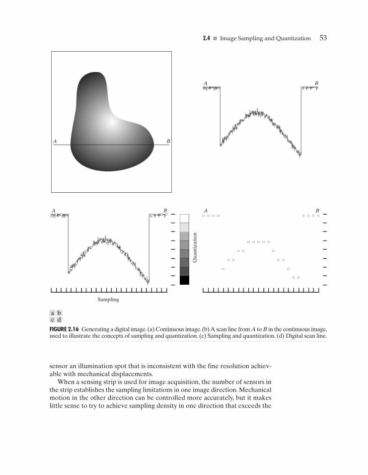
2.4 � Image Sampling and Quantization 53
A B
A B
Sampling
A B A B
Qua
ntiz
atio
n
FIGURE 2.16 Generating a digital image. (a) Continuous image. (b)A scan line from A to B in the continuous image,used to illustrate the concepts of sampling and quantization. (c) Sampling and quantization. (d) Digital scan line.
sensor an illumination spot that is inconsistent with the fine resolution achiev-able with mechanical displacements.
When a sensing strip is used for image acquisition, the number of sensors inthe strip establishes the sampling limitations in one image direction. Mechanicalmotion in the other direction can be controlled more accurately, but it makeslittle sense to try to achieve sampling density in one direction that exceeds the
a bc d
GONZ02-034-074.II 29-08-2001 13:35 Page 53
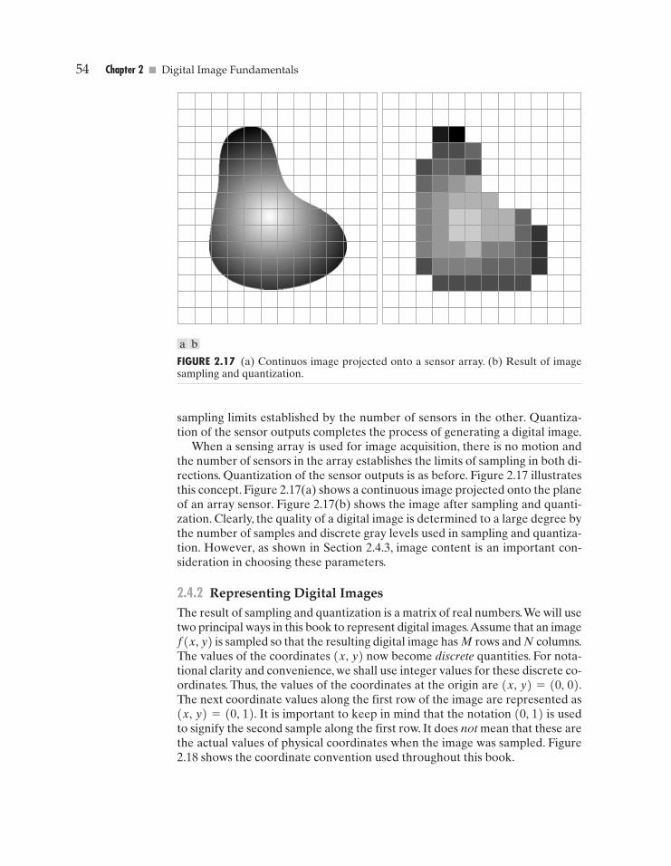
54 Chapter 2 � Digital Image Fundamentals
FIGURE 2.17 (a) Continuos image projected onto a sensor array. (b) Result of imagesampling and quantization.
sampling limits established by the number of sensors in the other. Quantiza-tion of the sensor outputs completes the process of generating a digital image.
When a sensing array is used for image acquisition, there is no motion andthe number of sensors in the array establishes the limits of sampling in both di-rections. Quantization of the sensor outputs is as before. Figure 2.17 illustratesthis concept. Figure 2.17(a) shows a continuous image projected onto the planeof an array sensor. Figure 2.17(b) shows the image after sampling and quanti-zation. Clearly, the quality of a digital image is determined to a large degree bythe number of samples and discrete gray levels used in sampling and quantiza-tion. However, as shown in Section 2.4.3, image content is an important con-sideration in choosing these parameters.
2.4.2 Representing Digital ImagesThe result of sampling and quantization is a matrix of real numbers.We will usetwo principal ways in this book to represent digital images.Assume that an imagef(x, y) is sampled so that the resulting digital image has M rows and N columns.The values of the coordinates (x, y) now become discrete quantities. For nota-tional clarity and convenience, we shall use integer values for these discrete co-ordinates. Thus, the values of the coordinates at the origin are (x, y)=(0, 0).The next coordinate values along the first row of the image are represented as(x, y)=(0, 1). It is important to keep in mind that the notation (0, 1) is usedto signify the second sample along the first row. It does not mean that these arethe actual values of physical coordinates when the image was sampled. Figure2.18 shows the coordinate convention used throughout this book.
a b
GONZ02-034-074.II 29-08-2001 13:35 Page 54
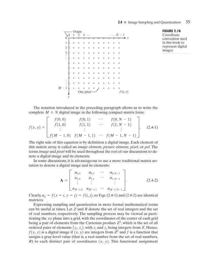
2.4 � Image Sampling and Quantization 55
Origin
00 1 2 3
1
2
3...
.
.
. . .. . .
.M-1
N-1
One pixel
x
y
f (x, y)
FIGURE 2.18Coordinateconvention usedin this book torepresent digitalimages.
The notation introduced in the preceding paragraph allows us to write thecomplete M*N digital image in the following compact matrix form:
(2.4-1)
The right side of this equation is by definition a digital image. Each element ofthis matrix array is called an image element, picture element, pixel, or pel. Theterms image and pixel will be used throughout the rest of our discussions to de-note a digital image and its elements.
In some discussions, it is advantageous to use a more traditional matrix no-tation to denote a digital image and its elements:
(2.4-2)
Clearly, aij=f(x=i, y=j)=f(i, j), so Eqs. (2.4-1) and (2.4-2) are identicalmatrices.
Expressing sampling and quantization in more formal mathematical termscan be useful at times. Let Z and R denote the set of real integers and the setof real numbers, respectively. The sampling process may be viewed as parti-tioning the xy plane into a grid, with the coordinates of the center of each gridbeing a pair of elements from the Cartesian product Z2, which is the set of allordered pairs of elements Azi, zj B , with zi and zj being integers from Z. Hence,f(x, y) is a digital image if (x, y) are integers from Z2 and f is a function thatassigns a gray-level value (that is, a real number from the set of real numbers,R) to each distinct pair of coordinates (x, y). This functional assignment
A = D a0, 0
a1, 0
oaM - 1, 0
a0, 1
a1, 1
oaM - 1, 1
pp
p
a0, N - 1
a1, N - 1
oaM - 1, N - 1
T .
f(x, y) = D f(0, 0)
f(1, 0)
of(M - 1, 0)
f(0, 1)
f(1, 1)
of(M - 1, 1)
pp
p
f(0, N - 1)
f(1, N - 1)
of(M - 1, N - 1)
T .
GONZ02-034-074.II 29-08-2001 13:35 Page 55
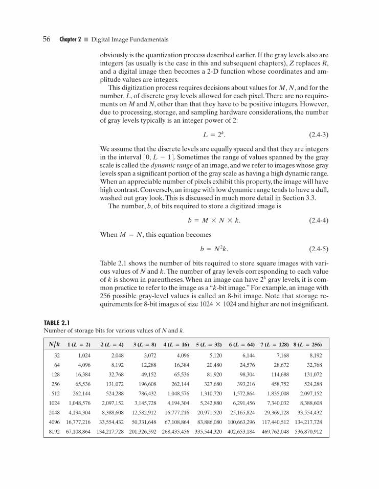
56 Chapter 2 � Digital Image Fundamentals
obviously is the quantization process described earlier. If the gray levels also areintegers (as usually is the case in this and subsequent chapters), Z replaces R,and a digital image then becomes a 2-D function whose coordinates and am-plitude values are integers.
This digitization process requires decisions about values for M, N, and for thenumber, L, of discrete gray levels allowed for each pixel.There are no require-ments on M and N, other than that they have to be positive integers. However,due to processing, storage, and sampling hardware considerations, the numberof gray levels typically is an integer power of 2:
(2.4-3)
We assume that the discrete levels are equally spaced and that they are integersin the interval [0, L-1]. Sometimes the range of values spanned by the grayscale is called the dynamic range of an image, and we refer to images whose graylevels span a significant portion of the gray scale as having a high dynamic range.When an appreciable number of pixels exhibit this property, the image will havehigh contrast. Conversely, an image with low dynamic range tends to have a dull,washed out gray look. This is discussed in much more detail in Section 3.3.
The number, b, of bits required to store a digitized image is
b=M*N*k. (2.4-4)
When M=N, this equation becomes
(2.4-5)
Table 2.1 shows the number of bits required to store square images with vari-ous values of N and k. The number of gray levels corresponding to each valueof k is shown in parentheses. When an image can have 2k gray levels, it is com-mon practice to refer to the image as a “k-bit image.” For example, an image with256 possible gray-level values is called an 8-bit image. Note that storage re-quirements for 8-bit images of size 1024*1024 and higher are not insignificant.
b = N2k.
L = 2k.
1 (L � 2) 2 (L � 4) 3 (L � 8) 4 (L � 16) 5 (L � 32) 6 (L � 64) 7 (L � 128) 8 (L � 256)
32 1,024 2,048 3,072 4,096 5,120 6,144 7,168 8,192
64 4,096 8,192 12,288 16,384 20,480 24,576 28,672 32,768
128 16,384 32,768 49,152 65,536 81,920 98,304 114,688 131,072
256 65,536 131,072 196,608 262,144 327,680 393,216 458,752 524,288
512 262,144 524,288 786,432 1,048,576 1,310,720 1,572,864 1,835,008 2,097,152
1024 1,048,576 2,097,152 3,145,728 4,194,304 5,242,880 6,291,456 7,340,032 8,388,608
2048 4,194,304 8,388,608 12,582,912 16,777,216 20,971,520 25,165,824 29,369,128 33,554,432
4096 16,777,216 33,554,432 50,331,648 67,108,864 83,886,080 100,663,296 117,440,512 134,217,728
8192 67,108,864 134,217,728 201,326,592 268,435,456 335,544,320 402,653,184 469,762,048 536,870,912
N /k
TABLE 2.1Number of storage bits for various values of N and k.
GONZ02-034-074.II 29-08-2001 13:35 Page 56
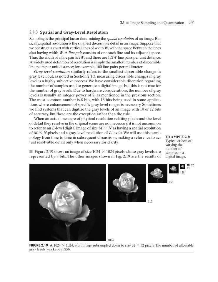
2.4.3 Spatial and Gray-Level ResolutionSampling is the principal factor determining the spatial resolution of an image. Ba-sically, spatial resolution is the smallest discernible detail in an image. Suppose thatwe construct a chart with vertical lines of width W,with the space between the linesalso having width W. A line pair consists of one such line and its adjacent space.Thus, the width of a line pair is 2W, and there are 1/2W line pairs per unit distance.A widely used definition of resolution is simply the smallest number of discernibleline pairs per unit distance; for example, 100 line pairs per millimeter.
Gray-level resolution similarly refers to the smallest discernible change ingray level, but, as noted in Section 2.1.3, measuring discernible changes in graylevel is a highly subjective process. We have considerable discretion regardingthe number of samples used to generate a digital image, but this is not true forthe number of gray levels. Due to hardware considerations, the number of graylevels is usually an integer power of 2, as mentioned in the previous section.The most common number is 8 bits, with 16 bits being used in some applica-tions where enhancement of specific gray-level ranges is necessary. Sometimeswe find systems that can digitize the gray levels of an image with 10 or 12 bitsof accuracy, but these are the exception rather than the rule.
When an actual measure of physical resolution relating pixels and the levelof detail they resolve in the original scene are not necessary, it is not uncommonto refer to an L-level digital image of size M*N as having a spatial resolutionof M*N pixels and a gray-level resolution of L levels.We will use this termi-nology from time to time in subsequent discussions, making a reference to ac-tual resolvable detail only when necessary for clarity.
� Figure 2.19 shows an image of size 1024*1024 pixels whose gray levels arerepresented by 8 bits. The other images shown in Fig. 2.19 are the results of
2.4 � Image Sampling and Quantization 57
1024
512
256
128
6432
FIGURE 2.19 A 1024*1024, 8-bit image subsampled down to size 32*32 pixels. The number of allowablegray levels was kept at 256.
EXAMPLE 2.2:Typical effects ofvarying thenumber ofsamples in adigital image.
GONZ02-034-074.II 29-08-2001 13:35 Page 57
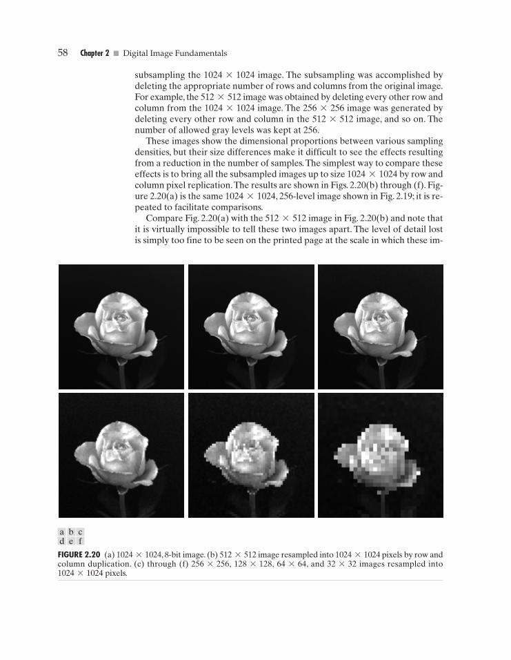
58 Chapter 2 � Digital Image Fundamentals
subsampling the 1024*1024 image. The subsampling was accomplished bydeleting the appropriate number of rows and columns from the original image.For example, the 512*512 image was obtained by deleting every other row andcolumn from the 1024*1024 image. The 256*256 image was generated bydeleting every other row and column in the 512*512 image, and so on. Thenumber of allowed gray levels was kept at 256.
These images show the dimensional proportions between various samplingdensities, but their size differences make it difficult to see the effects resultingfrom a reduction in the number of samples.The simplest way to compare theseeffects is to bring all the subsampled images up to size 1024*1024 by row andcolumn pixel replication.The results are shown in Figs. 2.20(b) through (f). Fig-ure 2.20(a) is the same 1024*1024, 256-level image shown in Fig. 2.19; it is re-peated to facilitate comparisons.
Compare Fig. 2.20(a) with the 512*512 image in Fig. 2.20(b) and note thatit is virtually impossible to tell these two images apart. The level of detail lostis simply too fine to be seen on the printed page at the scale in which these im-
FIGURE 2.20 (a) 1024*1024, 8-bit image. (b) 512*512 image resampled into 1024*1024 pixels by row andcolumn duplication. (c) through (f) 256*256, 128*128, 64*64, and 32*32 images resampled into1024*1024 pixels.
a b cd e f
GONZ02-034-074.II 29-08-2001 13:35 Page 58
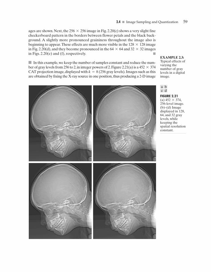
2.4 � Image Sampling and Quantization 59
ages are shown. Next, the 256*256 image in Fig. 2.20(c) shows a very slight finecheckerboard pattern in the borders between flower petals and the black back-ground. A slightly more pronounced graininess throughout the image also isbeginning to appear.These effects are much more visible in the 128*128 imagein Fig. 2.20(d), and they become pronounced in the 64*64 and 32*32 imagesin Figs. 2.20(e) and (f), respectively. �
� In this example, we keep the number of samples constant and reduce the num-ber of gray levels from 256 to 2, in integer powers of 2.Figure 2.21(a) is a 452*374CAT projection image, displayed with k=8 (256 gray levels). Images such as thisare obtained by fixing the X-ray source in one position, thus producing a 2-D image
EXAMPLE 2.3:Typical effects ofvarying thenumber of graylevels in a digitalimage.
FIGURE 2.21(a) 452*374,256-level image.(b)–(d) Imagedisplayed in 128,64, and 32 graylevels, whilekeeping thespatial resolutionconstant.
a bc d
GONZ02-034-074.II 29-08-2001 13:36 Page 59
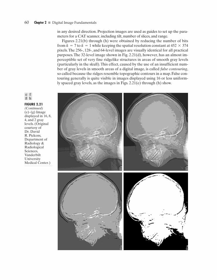
60 Chapter 2 � Digital Image Fundamentals
in any desired direction. Projection images are used as guides to set up the para-meters for a CAT scanner, including tilt, number of slices, and range.
Figures 2.21(b) through (h) were obtained by reducing the number of bitsfrom k=7 to k=1 while keeping the spatial resolution constant at 452*374pixels. The 256-, 128-, and 64-level images are visually identical for all practicalpurposes.The 32-level image shown in Fig. 2.21(d), however, has an almost im-perceptible set of very fine ridgelike structures in areas of smooth gray levels(particularly in the skull).This effect, caused by the use of an insufficient num-ber of gray levels in smooth areas of a digital image, is called false contouring,so called because the ridges resemble topographic contours in a map. False con-touring generally is quite visible in images displayed using 16 or less uniform-ly spaced gray levels, as the images in Figs. 2.21(e) through (h) show.
FIGURE 2.21(Continued)(e)–(g) Imagedisplayed in 16, 8,4, and 2 graylevels. (Originalcourtesy ofDr. DavidR. Pickens,Department ofRadiology &RadiologicalSciences,VanderbiltUniversityMedical Center.)
e fg h
GONZ02-034-074.II 29-08-2001 13:36 Page 60
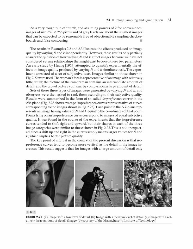
2.4 � Image Sampling and Quantization 61
As a very rough rule of thumb, and assuming powers of 2 for convenience,images of size 256*256 pixels and 64 gray levels are about the smallest imagesthat can be expected to be reasonably free of objectionable sampling checker-boards and false contouring. �
The results in Examples 2.2 and 2.3 illustrate the effects produced on imagequality by varying N and k independently. However, these results only partiallyanswer the question of how varying N and k affect images because we have notconsidered yet any relationships that might exist between these two parameters.An early study by Huang [1965] attempted to quantify experimentally the ef-fects on image quality produced by varying N and k simultaneously.The exper-iment consisted of a set of subjective tests. Images similar to those shown inFig. 2.22 were used.The woman’s face is representative of an image with relativelylittle detail; the picture of the cameraman contains an intermediate amount ofdetail; and the crowd picture contains, by comparison, a large amount of detail.
Sets of these three types of images were generated by varying N and k, andobservers were then asked to rank them according to their subjective quality.Results were summarized in the form of so-called isopreference curves in theNk-plane (Fig. 2.23 shows average isopreference curves representative of curvescorresponding to the images shown in Fig. 2.22). Each point in the Nk-plane rep-resents an image having values of N and k equal to the coordinates of that point.Points lying on an isopreference curve correspond to images of equal subjectivequality. It was found in the course of the experiments that the isopreferencecurves tended to shift right and upward, but their shapes in each of the threeimage categories were similar to those shown in Fig. 2.23. This is not unexpect-ed, since a shift up and right in the curves simply means larger values for N andk, which implies better picture quality.
The key point of interest in the context of the present discussion is that iso-preference curves tend to become more vertical as the detail in the image in-creases. This result suggests that for images with a large amount of detail only
FIGURE 2.22 (a) Image with a low level of detail. (b) Image with a medium level of detail. (c) Image with a rel-atively large amount of detail. (Image (b) courtesy of the Massachusetts Institute of Technology.)
a b c
GONZ02-034-074.II 29-08-2001 13:36 Page 61
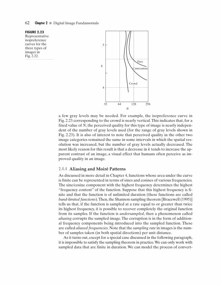
62 Chapter 2 � Digital Image Fundamentals
Face
2561286432
4
5
k
N
Crowd
Cameraman
FIGURE 2.23Representativeisopreferencecurves for thethree types ofimages inFig. 2.22.
a few gray levels may be needed. For example, the isopreference curve inFig. 2.23 corresponding to the crowd is nearly vertical.This indicates that, for afixed value of N, the perceived quality for this type of image is nearly indepen-dent of the number of gray levels used (for the range of gray levels shown inFig. 2.23). It is also of interest to note that perceived quality in the other twoimage categories remained the same in some intervals in which the spatial res-olution was increased, but the number of gray levels actually decreased. Themost likely reason for this result is that a decrease in k tends to increase the ap-parent contrast of an image, a visual effect that humans often perceive as im-proved quality in an image.
2.4.4 Aliasing and Moiré PatternsAs discussed in more detail in Chapter 4, functions whose area under the curveis finite can be represented in terms of sines and cosines of various frequencies.The sine/cosine component with the highest frequency determines the highest“frequency content” of the function. Suppose that this highest frequency is fi-nite and that the function is of unlimited duration (these functions are calledband-limited functions).Then, the Shannon sampling theorem [Bracewell (1995)]tells us that, if the function is sampled at a rate equal to or greater than twiceits highest frequency, it is possible to recover completely the original functionfrom its samples. If the function is undersampled, then a phenomenon calledaliasing corrupts the sampled image. The corruption is in the form of addition-al frequency components being introduced into the sampled function. Theseare called aliased frequencies. Note that the sampling rate in images is the num-ber of samples taken (in both spatial directions) per unit distance.
As it turns out, except for a special case discussed in the following paragraph,it is impossible to satisfy the sampling theorem in practice.We can only work withsampled data that are finite in duration. We can model the process of convert-
GONZ02-034-074.II 29-08-2001 13:36 Page 62
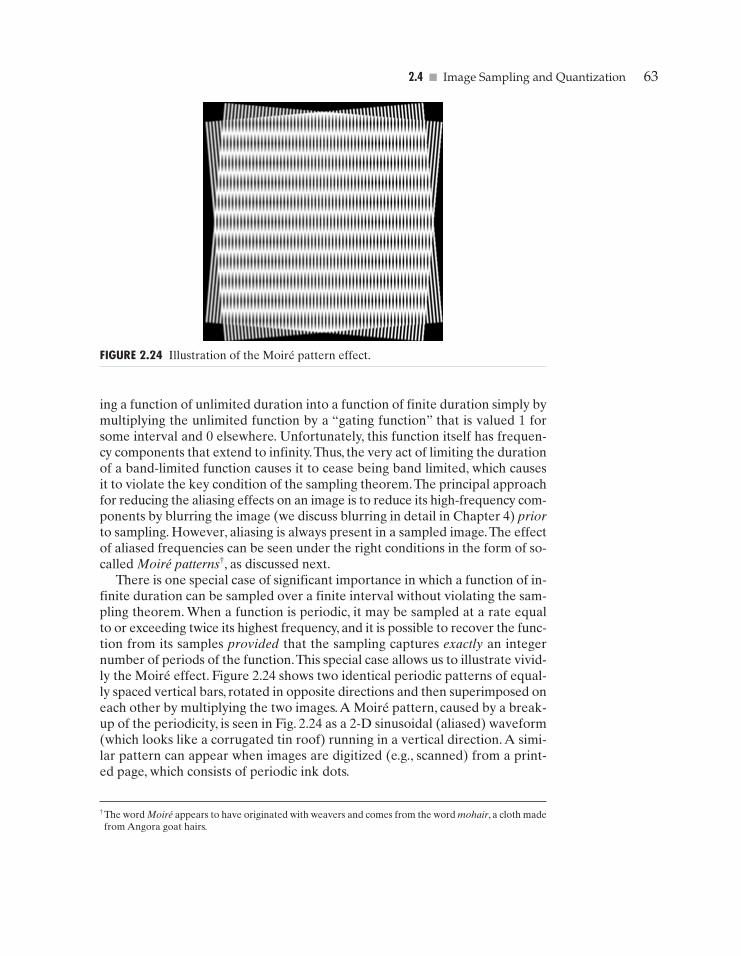
2.4 � Image Sampling and Quantization 63
ing a function of unlimited duration into a function of finite duration simply bymultiplying the unlimited function by a “gating function” that is valued 1 forsome interval and 0 elsewhere. Unfortunately, this function itself has frequen-cy components that extend to infinity.Thus, the very act of limiting the durationof a band-limited function causes it to cease being band limited, which causesit to violate the key condition of the sampling theorem.The principal approachfor reducing the aliasing effects on an image is to reduce its high-frequency com-ponents by blurring the image (we discuss blurring in detail in Chapter 4) priorto sampling. However, aliasing is always present in a sampled image.The effectof aliased frequencies can be seen under the right conditions in the form of so-called Moiré patterns†, as discussed next.
There is one special case of significant importance in which a function of in-finite duration can be sampled over a finite interval without violating the sam-pling theorem. When a function is periodic, it may be sampled at a rate equalto or exceeding twice its highest frequency, and it is possible to recover the func-tion from its samples provided that the sampling captures exactly an integernumber of periods of the function.This special case allows us to illustrate vivid-ly the Moiré effect. Figure 2.24 shows two identical periodic patterns of equal-ly spaced vertical bars, rotated in opposite directions and then superimposed oneach other by multiplying the two images.A Moiré pattern, caused by a break-up of the periodicity, is seen in Fig. 2.24 as a 2-D sinusoidal (aliased) waveform(which looks like a corrugated tin roof) running in a vertical direction. A simi-lar pattern can appear when images are digitized (e.g., scanned) from a print-ed page, which consists of periodic ink dots.
FIGURE 2.24 Illustration of the Moiré pattern effect.
† The word Moiré appears to have originated with weavers and comes from the word mohair, a cloth madefrom Angora goat hairs.
GONZ02-034-074.II 29-08-2001 13:36 Page 63
64 Chapter 2 � Digital Image Fundamentals
2.4.5 Zooming and Shrinking Digital ImagesWe conclude the treatment of sampling and quantization with a brief discussionon how to zoom and shrink a digital image. This topic is related to image sam-pling and quantization because zooming may be viewed as oversampling, whileshrinking may be viewed as undersampling. The key difference between thesetwo operations and sampling and quantizing an original continuous image isthat zooming and shrinking are applied to a digital image.
Zooming requires two steps: the creation of new pixel locations, and theassignment of gray levels to those new locations. Let us start with a simple ex-ample. Suppose that we have an image of size 500*500 pixels and we wantto enlarge it 1.5 times to 750*750 pixels. Conceptually, one of the easiestways to visualize zooming is laying an imaginary 750*750 grid over the orig-inal image. Obviously, the spacing in the grid would be less than one pixel be-cause we are fitting it over a smaller image. In order to perform gray-levelassignment for any point in the overlay, we look for the closest pixel in theoriginal image and assign its gray level to the new pixel in the grid. When weare done with all points in the overlay grid, we simply expand it to the origi-nal specified size to obtain the zoomed image. This method of gray-level as-signment is called nearest neighbor interpolation. (Pixel neighborhoods arediscussed in the next section.)
Pixel replication, the method used to generate Figs. 2.20(b) through (f), is aspecial case of nearest neighbor interpolation. Pixel replication is applicablewhen we want to increase the size of an image an integer number of times. Forinstance, to double the size of an image, we can duplicate each column. Thisdoubles the image size in the horizontal direction.Then, we duplicate each rowof the enlarged image to double the size in the vertical direction.The same pro-cedure is used to enlarge the image by any integer number of times (triple,quadruple, and so on). Duplication is just done the required number of times toachieve the desired size. The gray-level assignment of each pixel is predeter-mined by the fact that new locations are exact duplicates of old locations.
Although nearest neighbor interpolation is fast, it has the undesirable featurethat it produces a checkerboard effect that is particularly objectionable at highfactors of magnification. Figures 2.20(e) and (f) are good examples of this. Aslightly more sophisticated way of accomplishing gray-level assignments isbilinear interpolation using the four nearest neighbors of a point. Let (x¿, y¿)denote the coordinates of a point in the zoomed image (think of it as a point onthe grid described previously), and let v(x¿, y¿) denote the gray level assignedto it. For bilinear interpolation, the assigned gray level is given by
(2.4-6)
where the four coefficients are determined from the four equations in four un-knowns that can be written using the four nearest neighbors of point (x¿, y¿).
Image shrinking is done in a similar manner as just described for zooming.Theequivalent process of pixel replication is row-column deletion.For example,to shrinkan image by one-half,we delete every other row and column.We can use the zoom-ing grid analogy to visualize the concept of shrinking by a noninteger factor,except
v(x¿, y¿) = ax¿ + by¿ + cx¿y¿ + d
GONZ02-034-074.II 29-08-2001 13:36 Page 64
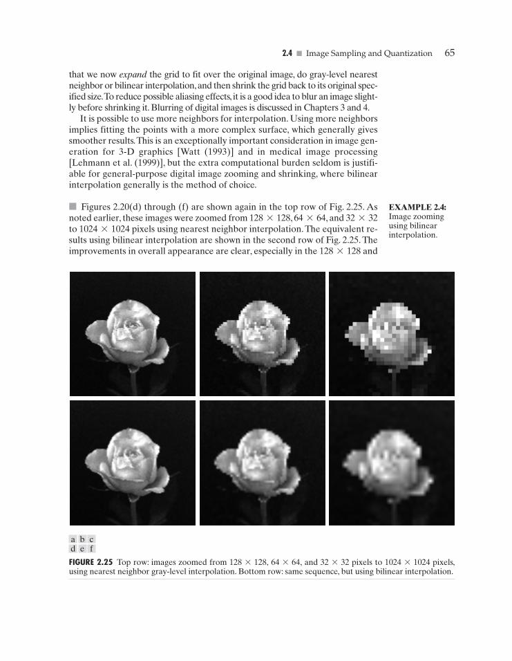
2.4 � Image Sampling and Quantization 65
that we now expand the grid to fit over the original image, do gray-level nearestneighbor or bilinear interpolation,and then shrink the grid back to its original spec-ified size.To reduce possible aliasing effects, it is a good idea to blur an image slight-ly before shrinking it. Blurring of digital images is discussed in Chapters 3 and 4.
It is possible to use more neighbors for interpolation. Using more neighborsimplies fitting the points with a more complex surface, which generally givessmoother results.This is an exceptionally important consideration in image gen-eration for 3-D graphics [Watt (1993)] and in medical image processing[Lehmann et al. (1999)], but the extra computational burden seldom is justifi-able for general-purpose digital image zooming and shrinking, where bilinearinterpolation generally is the method of choice.
� Figures 2.20(d) through (f) are shown again in the top row of Fig. 2.25. Asnoted earlier, these images were zoomed from 128*128, 64*64, and 32*32to 1024*1024 pixels using nearest neighbor interpolation. The equivalent re-sults using bilinear interpolation are shown in the second row of Fig. 2.25. Theimprovements in overall appearance are clear, especially in the 128*128 and
FIGURE 2.25 Top row: images zoomed from 128*128, 64*64, and 32*32 pixels to 1024*1024 pixels,using nearest neighbor gray-level interpolation. Bottom row: same sequence, but using bilinear interpolation.
a b cd e f
EXAMPLE 2.4:Image zoomingusing bilinearinterpolation.
GONZ02-034-074.II 29-08-2001 13:36 Page 65
66 Chapter 2 � Digital Image Fundamentals
64*64 cases.The 32*32 to 1024*1024 image is blurry, but keep in mind thatthis image was zoomed by a factor of 32. In spite of this, the result of bilinearinterpolation shown in Fig. 2.25(f) is a reasonably good rendition of the origi-nal image shape, something that is lost in Fig. 2.25(c). �
Some Basic Relationships Between Pixels
In this section, we consider several important relationships between pixels in adigital image.As mentioned before, an image is denoted by f(x, y).When refer-ring in this section to a particular pixel, we use lowercase letters, such as p and q.
2.5.1 Neighbors of a PixelA pixel p at coordinates (x, y) has four horizontal and vertical neighbors whosecoordinates are given by
(x+1, y), (x-1, y), (x, y+1), (x, y-1)
This set of pixels, called the 4-neighbors of p, is denoted by N4(p). Each pixelis a unit distance from (x, y), and some of the neighbors of p lie outside thedigital image if (x, y) is on the border of the image.
The four diagonal neighbors of p have coordinates
(x+1, y+1), (x+1, y-1), (x-1, y+1), (x-1, y-1)
and are denoted by ND(p). These points, together with the 4-neighbors, arecalled the 8-neighbors of p, denoted by N8(p).As before, some of the points inND(p) and N8(p) fall outside the image if (x, y) is on the border of the image.
2.5.2 Adjacency, Connectivity, Regions, and BoundariesConnectivity between pixels is a fundamental concept that simplifies the defini-tion of numerous digital image concepts, such as regions and boundaries. To es-tablish if two pixels are connected, it must be determined if they are neighbors andif their gray levels satisfy a specified criterion of similarity (say, if their gray lev-els are equal). For instance, in a binary image with values 0 and 1, two pixels maybe 4-neighbors, but they are said to be connected only if they have the same value.
Let V be the set of gray-level values used to define adjacency. In a binaryimage, V={1} if we are referring to adjacency of pixels with value 1. In a gray-scale image, the idea is the same, but set V typically contains more elements. Forexample, in the adjacency of pixels with a range of possible gray-level values 0to 255, set V could be any subset of these 256 values. We consider three typesof adjacency:
(a) 4-adjacency. Two pixels p and q with values from V are 4-adjacent if q isin the set N4(p).
(b) 8-adjacency. Two pixels p and q with values from V are 8-adjacent if q isin the set N8(p).
2.5
GONZ02-034-074.II 29-08-2001 13:36 Page 66
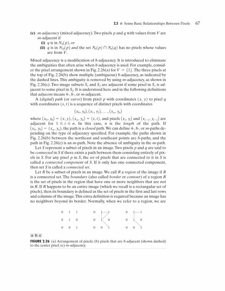
2.5 � Some Basic Relationships Between Pixels 67
(c) m-adjacency (mixed adjacency).Two pixels p and q with values from V arem-adjacent if
(i) q is in N4(p), or(ii) q is in ND(p) and the set has no pixels whose values
are from V.
Mixed adjacency is a modification of 8-adjacency. It is introduced to eliminatethe ambiguities that often arise when 8-adjacency is used. For example, consid-er the pixel arrangement shown in Fig. 2.26(a) for V={1}.The three pixels atthe top of Fig. 2.26(b) show multiple (ambiguous) 8-adjacency, as indicated bythe dashed lines. This ambiguity is removed by using m-adjacency, as shown inFig. 2.26(c). Two image subsets S1 and S2 are adjacent if some pixel in S1 is ad-jacent to some pixel in S2. It is understood here and in the following definitionsthat adjacent means 4-, 8-, or m-adjacent.
A (digital) path (or curve) from pixel p with coordinates (x, y) to pixel qwith coordinates (s, t) is a sequence of distinct pixels with coordinates
where and pixels and areadjacent for 1 � i � n. In this case, n is the length of the path. If
the path is a closed path.We can define 4-, 8-, or m-paths de-pending on the type of adjacency specified. For example, the paths shown inFig. 2.26(b) between the northeast and southeast points are 8-paths, and thepath in Fig. 2.26(c) is an m-path. Note the absence of ambiguity in the m-path.
Let S represent a subset of pixels in an image.Two pixels p and q are said tobe connected in S if there exists a path between them consisting entirely of pix-els in S. For any pixel p in S, the set of pixels that are connected to it in S iscalled a connected component of S. If it only has one connected component,then set S is called a connected set.
Let R be a subset of pixels in an image. We call R a region of the image if Ris a connected set. The boundary (also called border or contour) of a region Ris the set of pixels in the region that have one or more neighbors that are notin R. If R happens to be an entire image (which we recall is a rectangular set ofpixels), then its boundary is defined as the set of pixels in the first and last rowsand columns of the image.This extra definition is required because an image hasno neighbors beyond its border. Normally, when we refer to a region, we are
Ax0 , y0B = (xn , yn),
Axi - 1 , yi - 1BAxi , yiBAxn , ynB = (s, t),Ax0 , y0B = (x, y),
Ax0 , y0B, Ax1 , y1B, p , Axn , ynB
N4(p) ¨ N4(q)
0 1 1
0 1 0
0 0 1
0 1 1
0 1 0
0 0 1
0 1 1
0 1 0
0 0 1
FIGURE 2.26 (a) Arrangement of pixels; (b) pixels that are 8-adjacent (shown dashed)to the center pixel; (c) m-adjacency.
a b c
GONZ02-034-074.II 29-08-2001 13:36 Page 67
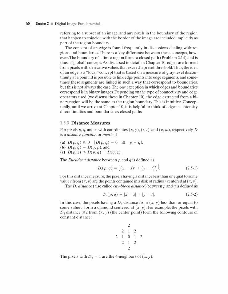
68 Chapter 2 � Digital Image Fundamentals
referring to a subset of an image, and any pixels in the boundary of the regionthat happen to coincide with the border of the image are included implicitly aspart of the region boundary.
The concept of an edge is found frequently in discussions dealing with re-gions and boundaries. There is a key difference between these concepts, how-ever.The boundary of a finite region forms a closed path (Problem 2.14) and isthus a “global” concept.As discussed in detail in Chapter 10, edges are formedfrom pixels with derivative values that exceed a preset threshold.Thus, the ideaof an edge is a “local” concept that is based on a measure of gray-level discon-tinuity at a point. It is possible to link edge points into edge segments, and some-times these segments are linked in such a way that correspond to boundaries,but this is not always the case.The one exception in which edges and boundariescorrespond is in binary images. Depending on the type of connectivity and edgeoperators used (we discuss these in Chapter 10), the edge extracted from a bi-nary region will be the same as the region boundary. This is intuitive. Concep-tually, until we arrive at Chapter 10, it is helpful to think of edges as intensitydiscontinuities and boundaries as closed paths.
2.5.3 Distance MeasuresFor pixels p, q, and z, with coordinates (x, y), (s, t), and (v, w), respectively, Dis a distance function or metric if
(a) D(p, q) � 0 AD(p, q)=0 iff p=q B ,(b) D(p, q)=D(q, p), and(c) D(p, z) � D(p, q)+D(q, z).
The Euclidean distance between p and q is defined as
(2.5-1)
For this distance measure, the pixels having a distance less than or equal to somevalue r from (x, y) are the points contained in a disk of radius r centered at (x, y).
The D4 distance (also called city-block distance) between p and q is defined as
(2.5-2)
In this case, the pixels having a D4 distance from (x, y) less than or equal tosome value r form a diamond centered at (x, y). For example, the pixels withD4 distance �2 from (x, y) (the center point) form the following contours ofconstant distance:
The pixels with D4=1 are the 4-neighbors of (x, y).
2
212
21012
212
2
D4(p, q) = ∑x - s∑ + ∑y - t∑.
De(p, q) = C(x - s)2 + (y - t)2 D
12
.
GONZ02-034-074.II 29-08-2001 13:36 Page 68
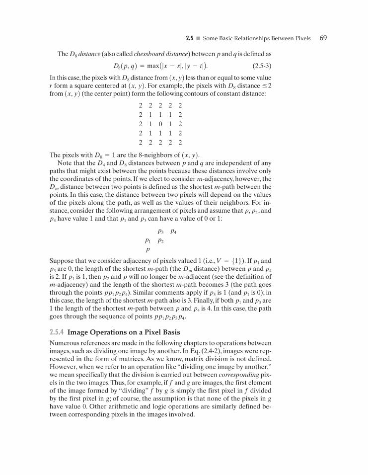
2.5 � Some Basic Relationships Between Pixels 69
The D8 distance (also called chessboard distance) between p and q is defined as
(2.5-3)
In this case, the pixels with D8 distance from (x, y) less than or equal to some valuer form a square centered at (x, y). For example, the pixels with D8 distance �2from (x, y) (the center point) form the following contours of constant distance:
The pixels with D8=1 are the 8-neighbors of (x, y).Note that the D4 and D8 distances between p and q are independent of any
paths that might exist between the points because these distances involve onlythe coordinates of the points. If we elect to consider m-adjacency, however, theDm distance between two points is defined as the shortest m-path between thepoints. In this case, the distance between two pixels will depend on the valuesof the pixels along the path, as well as the values of their neighbors. For in-stance, consider the following arrangement of pixels and assume that p, p2 , andp4 have value 1 and that p1 and p3 can have a value of 0 or 1:
Suppose that we consider adjacency of pixels valued 1 (i.e., V={1}). If p1 andp3 are 0, the length of the shortest m-path (the Dm distance) between p and p4
is 2. If p1 is 1, then p2 and p will no longer be m-adjacent (see the definition ofm-adjacency) and the length of the shortest m-path becomes 3 (the path goesthrough the points ). Similar comments apply if p3 is 1 (and p1 is 0); inthis case, the length of the shortest m-path also is 3. Finally, if both p1 and p3 are1 the length of the shortest m-path between p and p4 is 4. In this case, the pathgoes through the sequence of points
2.5.4 Image Operations on a Pixel BasisNumerous references are made in the following chapters to operations betweenimages, such as dividing one image by another. In Eq. (2.4-2), images were rep-resented in the form of matrices. As we know, matrix division is not defined.However, when we refer to an operation like “dividing one image by another,”we mean specifically that the division is carried out between corresponding pix-els in the two images.Thus, for example, if f and g are images, the first elementof the image formed by “dividing” f by g is simply the first pixel in f dividedby the first pixel in g; of course, the assumption is that none of the pixels in ghave value 0. Other arithmetic and logic operations are similarly defined be-tween corresponding pixels in the images involved.
pp1 p2 p3 p4 .
pp1 p2 p4
p1
p
p3
p2
p4
22222
21112
21012
21112
22222
D8(p, q) = max A∑x - s∑, ∑y - t∑B.
GONZ02-034-074.II 29-08-2001 13:36 Page 69
70 Chapter 2 � Digital Image Fundamentals
Linear and Nonlinear Operations
Let H be an operator whose input and output are images. H is said to be a linearoperator if, for any two images f and g and any two scalars a and b,
(2.6-1)
In other words, the result of applying a linear operator to the sum of two images(that have been multiplied by the constants shown) is identical to applying theoperator to the images individually, multiplying the results by the appropriateconstants, and then adding those results. For example, an operator whose func-tion is to compute the sum of K images is a linear operator. An operator thatcomputes the absolute value of the difference of two images is not. An opera-tor that fails the test of Eq. (2.6-1) is by definition nonlinear.
Linear operations are exceptionally important in image processing becausethey are based on a significant body of well-understood theoretical and practi-cal results.Although nonlinear operations sometimes offer better performance,they are not always predictable, and for the most part are not well understoodtheoretically.
SummaryThe material in this chapter is primarily background information for subsequent dis-cussions. Our treatment of the human visual system, although brief, provides a basic ideaof the capabilities of the eye in perceiving pictorial information. The discussion of lightand the electromagnetic spectrum is fundamental in understanding the origin of themany images we use in this book. Similarly, the image model developed in Section 2.3.4is used in the Chapter 4 as the basis for an image enhancement technique called homo-morphic filtering, and again in Chapter 10 to explain the effect of illumination on theshape of image histograms.
The sampling ideas introduced in Section 2.4 are the foundation for many of the dig-itizing phenomena likely to be encountered in practice. These ideas can be expandedfurther once a basic understanding of frequency content is mastered.A detailed discus-sion of the frequency domain is given in Chapter 4. The concepts of sampling and alias-ing effects also are of importance in the context of image acquisition.
The concepts introduced in Section 2.5 are the basic building blocks for processingtechniques based on pixel neighborhoods. As shown in the following chapter and inChapter 5, neighborhood processing methods are at the core of many image enhance-ment and restoration procedures.When applicable, neighborhood processing is favoredin commercial applications of image processing due to their operational speed and sim-plicity of implementation in hardware and/or firmware. Finally, the concept of a linearoperator and the theoretical and conceptual power associated with it will be used ex-tensively in the following three chapters.
References and Further ReadingAdditional reading for the material in Section 2.1 regarding the structure of the humaneye may be found in Atchison and Smith [2000], and Oyster [1999]. For additional read-ing on visual perception, see Regan [2000] and Gordon [1997].The book by Hubel [1988]and the now classic book by Cornsweet [1970] also are of interest. Born and Wolf [1999]
H(af + bg) = aH(f) + bH(g).
2.6
GONZ02-034-074.II 29-08-2001 13:36 Page 70
�
�
� Problems 71
is a basic reference that discusses light in terms of electromagnetic theory. Electromag-netic energy propagation is covered in some detail by Felsen and Marcuvitz [1994].
The area of image sensing is quite broad and very fast moving. An excellent sourceof information on optical and other imaging sensors is the International Society for Op-tical Engineering (SPIE). The following are representative publications by the SPIE inthis area: Blouke et al. [2001], Hoover and Doty [1996], and Freeman [1987].
The image model presented in Section 2.3.4 is from Oppenheim, Schafer, and Stock-ham [1968].A reference for the illumination and reflectance values used in that sectionis the IES Lighting Handbook [2000]. For additional reading on image sampling andsome of its effects, such as aliasing, see Bracewell [1995]. The early experiments men-tioned in Section 2.4.3 on perceived image quality as a function of sampling and quati-zation were reported by Huang [1965].The issue of reducing the number of samples andgray levels in an image while minimizing the ensuing degradation is still of current in-terest, as exemplified by Papamarkos and Atsalakis [2000]. For further reading on imageshrinking and zooming, see Sid-Ahmed [1995], Unser et al. [1995], Umbaugh [1998], andLehmann et al. [1999]. For further reading on the topics covered in Section 2.5, seeRosenfeld and Kak [1982], Marchand-Maillet and Sharaiha [2000], and Ritter and Wil-son [2001].Additional reading on linear systems in the context of image processing maybe found in Castleman [1996].
Problems2.1 Using the background information provided in Section 2.1, and thinking purely
in geometric terms, estimate the diameter of the smallest printed dot that the eyecan discern if the page on which the dot is printed is 0.2 m away from the eyes.Assume for simplicity that the visual system ceases to detect the dot when theimage of the dot on the fovea becomes smaller than the diameter of one recep-tor (cone) in that area of the retina. Assume further that the fovea can be mod-eled as a square array of dimensions 1.5 mm*1.5 mm, and that the cones andspaces between the cones are distributed uniformly throughout this array.
2.2 When you enter a dark theater on a bright day, it takes an appreciable intervalof time before you can see well enough to find an empty seat. Which of the visu-al processes explained in Section 2.1 is at play in this situation?
2.3 Although it is not shown in Fig. 2.10, alternating current certainly is part of theelectromagnetic spectrum. Commercial alternating current in the United Stateshas a frequency of 60 Hz.What is the wavelength in kilometers of this componentof the spectrum?
2.4 You are hired to design the front end of an imaging system for studying the bound-ary shapes of cells, bacteria, viruses, and protein.The front end consists, in this case,of the illumination source(s) and corresponding imaging camera(s). The diame-ters of circles required to enclose individual specimens in each of these categoriesare 50, 1, 0.1, and 0.01 �m, respectively.
(a) Can you solve the imaging aspects of this problem with a single sensor andcamera? If your answer is yes, specify the illumination wavelength band andthe type of camera needed. Identify the camera as being a color camera, far-infrared camera, or whatever appropriate name corresponds to the illumi-nation source.
(b) If your answer in (a) is no, what type of illumination sources and corre-sponding imaging sensors would you recommend? Specify the light sources
Detailed solutions to theproblems marked with astar can be found in thebook web site. The sitealso contains suggestedprojects based on the ma-terial in this chapter.
See inside front cover
GONZ02-034-074.II 29-08-2001 13:36 Page 71
�
�
72 Chapter 2 � Digital Image Fundamentals
and cameras as requested in part (a). Use the minimum number of illumina-tion sources and cameras needed to solve the problem.
2.5 A CCD camera chip of dimensions 7*7 mm, and having 1024*1024 elements,is focused on a square, flat area, located 0.5 m away. How many line pairs per mmwill this camera be able to resolve? The camera is equipped with a 35-mm lens.(Hint: Model the imaging process as in Fig. 2.3, with the focal length of the cam-era lens substituting for the focal length of the eye.)
2.6 An automobile manufacturer is automating the placement of certain componentson the bumpers of a limited-edition line of sports cars.The components are colorcoordinated, so the robots need to know the color of each car in order to select theappropriate bumper component. Models come in only four colors: blue, green, red,and white.You are hired to propose a solution based on imaging. How would yousolve the problem of automatically determining the color of each car, keeping inmind that cost is the most important consideration in your choice of components?
2.7 Suppose that a flat area with center at is illuminated by a light source withintensity distribution
Assume for simplicity that the reflectance of the area is constant and equal to1.0, and let K=255. If the resulting image is digitized with k bits of intensity res-olution, and the eye can detect an abrupt change of eight shades of intensity be-tween adjacent pixels, what value of k will cause visible false contouring?
2.8 Sketch the image in Problem 2.7 for k=2.
2.9 A common measure of transmission for digital data is the baud rate, defined asthe number of bits transmitted per second. Generally, transmission is accom-plished in packets consisting of a start bit, a byte (8 bits) of information, and a stopbit. Using these facts, answer the following:
(a) How many minutes would it take to transmit a 1024*1024 image with 256gray levels using a 56K baud modem?
(b) What would the time be at 750K baud, a representative speed of a phoneDSL (digital subscriber line) connection?
2.10 High-definition television (HDTV) generates images with a resolution of 1125horizontal TV lines interlaced (where every other line is painted on the tube facein each of two fields, each field being 1�60th of a second in duration).The width-to-height aspect ratio of the images is 16 :9. The fact that the horizontal lines aredistinct fixes the vertical resolution of the images. A company has designed animage capture system that generates digital images from HDTV images.The res-olution of each TV (horizontal) line in their system is in proportion to vertical res-olution, with the proportion being the width-to-height ratio of the images. Eachpixel in the color image has 24 bits of intensity resolution, 8 pixels each for a red,a green, and a blue image.These three “primary” images form a color image. Howmany bits would it take to store a 2-hour HDTV program?
2.11 Consider the two image subsets, S1 and S2, shown in the following figure. ForV={1}, determine whether these two subsets are (a) 4-adjacent, (b) 8-adjacent,or (c) m-adjacent.
i(x, y) = Ke-CAx - x0B2 + Ay - y0B
2D.
Ax0 , y0B
�
GONZ02-034-074.II 29-08-2001 13:36 Page 72
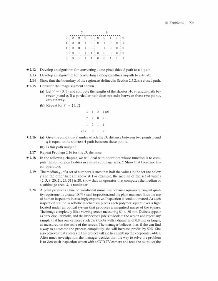
�
�
� Problems 73
2.12 Develop an algorithm for converting a one-pixel-thick 8-path to a 4-path.
2.13 Develop an algorithm for converting a one-pixel-thick m-path to a 4-path.
2.14 Show that the boundary of the region, as defined in Section 2.5.2, is a closed path.
2.15 Consider the image segment shown.
(a) Let V={0, 1} and compute the lengths of the shortest 4-, 8-, and m-path be-tween p and q. If a particular path does not exist between these two points,explain why.
(b) Repeat for V={1, 2}.
2.16 (a) Give the condition(s) under which the D4 distance between two points p andq is equal to the shortest 4-path between these points.
(b) Is this path unique?
2.17 Repeat Problem 2.16 for the D8 distance.
2.18 In the following chapter, we will deal with operators whose function is to com-pute the sum of pixel values in a small subimage area, S. Show that these are lin-ear operators.
2.19 The median, z, of a set of numbers is such that half the values in the set are belowz and the other half are above it. For example, the median of the set of values{2, 3, 8, 20, 21, 25, 31} is 20. Show that an operator that computes the median ofa subimage area, S, is nonlinear.
2.20 A plant produces a line of translucent miniature polymer squares. Stringent qual-ity requirements dictate 100% visual inspection, and the plant manager finds the useof human inspectors increasingly expensive. Inspection is semiautomated.At eachinspection station, a robotic mechanism places each polymer square over a lightlocated under an optical system that produces a magnified image of the square.The image completely fills a viewing screen measuring 80*80 mm. Defects appearas dark circular blobs, and the inspector’s job is to look at the screen and reject anysample that has one or more such dark blobs with a diameter of 0.8 mm or larger,as measured on the scale of the screen. The manager believes that, if she can finda way to automate the process completely, she will increase profits by 50%. Shealso believes that success in this project will aid her climb up the corporate ladder.After much investigation, the manager decides that the way to solve the problemis to view each inspection screen with a CCD TV camera and feed the output of the
3 1 2 1
2 2 0 2
1 2 1 1
1(p)
(q)
0 1 2
0 0 0 0
0 0 1 0
0 0 1 0
0 1 1 1
0
0
1
1
0
0 1 1 1
0 0 1 1
0 1 0 0
1 1 0 0
0 0
0
1
0
0
1
0 0
0 0 1 1
S1 S2
�
�
GONZ02-034-074.II 29-08-2001 13:36 Page 73
74 Chapter 2 � Digital Image Fundamentals
camera into an image processing system capable of detecting the blobs, measuringtheir diameter, and activating the accept/reject buttons previously operated by aninspector. She is able to find a system that can do the job, as long as the smallest de-fect occupies an area of at least 2*2 pixels in the digital image.The manager hiresyou to help her specify the camera and lens system, but requires that you use off-the-shelf components. For the lenses, assume that this constraint means any integermultiple of 25 mm or 35 mm, up to 200 mm. For the cameras, it means resolutionsof 512*512, 1024*1024, or 2048*2048 pixels.The individual imaging elementsin these cameras are squares measuring 8*8 �m, and the spaces between imag-ing elements are 2 �m. For this application, the cameras cost much more than thelenses, so the problem should be solved with the lowest-resolution camera possible,based on the choice of lenses.As a consultant, you are to provide a written recom-mendation, showing in reasonable detail the analysis that led to your conclusion.Use the same imaging geometry suggested in Problem 2.5.
GONZ02-034-074.II 29-08-2001 13:36 Page 74
75
3 Image Enhancement in the Spatial Domain
It makes all the difference whether one sees darknessthrough the light or brightness through the shadows.
David Lindsay
PreviewThe principal objective of enhancement is to process an image so that the re-sult is more suitable than the original image for a specific application.The wordspecific is important, because it establishes at the outset that the techniques dis-cussed in this chapter are very much problem oriented. Thus, for example, amethod that is quite useful for enhancing X-ray images may not necessarily bethe best approach for enhancing pictures of Mars transmitted by a space probe.Regardless of the method used, however, image enhancement is one of the mostinteresting and visually appealing areas of image processing.
Image enhancement approaches fall into two broad categories: spatial domainmethods and frequency domain methods.The term spatial domain refers to theimage plane itself, and approaches in this category are based on direct manipu-lation of pixels in an image. Frequency domain processing techniques are basedon modifying the Fourier transform of an image. Spatial methods are covered inthis chapter, and frequency domain enhancement is discussed in Chapter 4. En-hancement techniques based on various combinations of methods from thesetwo categories are not unusual.We note also that many of the fundamental tech-niques introduced in this chapter in the context of enhancement are used insubsequent chapters for a variety of other image processing applications.
There is no general theory of image enhancement. When an image isprocessed for visual interpretation, the viewer is the ultimate judge of how well
GONZ03-075-146.II 29-08-2001 13:42 Page 75
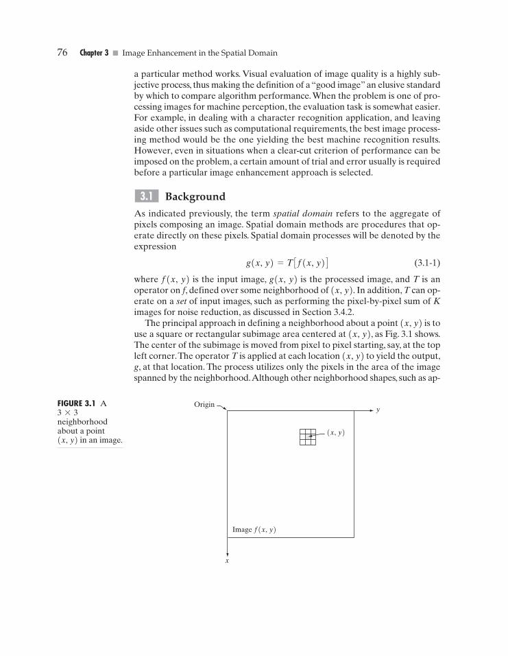
76 Chapter 3 � Image Enhancement in the Spatial Domain
Origin
x
Image f(x, y)
(x, y)
yFIGURE 3.1 A3*3neighborhoodabout a point(x, y) in an image.
a particular method works. Visual evaluation of image quality is a highly sub-jective process, thus making the definition of a “good image” an elusive standardby which to compare algorithm performance.When the problem is one of pro-cessing images for machine perception, the evaluation task is somewhat easier.For example, in dealing with a character recognition application, and leavingaside other issues such as computational requirements, the best image process-ing method would be the one yielding the best machine recognition results.However, even in situations when a clear-cut criterion of performance can beimposed on the problem, a certain amount of trial and error usually is requiredbefore a particular image enhancement approach is selected.
Background
As indicated previously, the term spatial domain refers to the aggregate ofpixels composing an image. Spatial domain methods are procedures that op-erate directly on these pixels. Spatial domain processes will be denoted by theexpression
(3.1-1)
where f(x, y) is the input image, g(x, y) is the processed image, and T is anoperator on f, defined over some neighborhood of (x, y). In addition, T can op-erate on a set of input images, such as performing the pixel-by-pixel sum of Kimages for noise reduction, as discussed in Section 3.4.2.
The principal approach in defining a neighborhood about a point (x, y) is touse a square or rectangular subimage area centered at (x, y), as Fig. 3.1 shows.The center of the subimage is moved from pixel to pixel starting, say, at the topleft corner.The operator T is applied at each location (x, y) to yield the output,g, at that location. The process utilizes only the pixels in the area of the imagespanned by the neighborhood.Although other neighborhood shapes, such as ap-
g(x, y) = T Cf(x, y) D
3.1
GONZ03-075-146.II 29-08-2001 13:42 Page 76
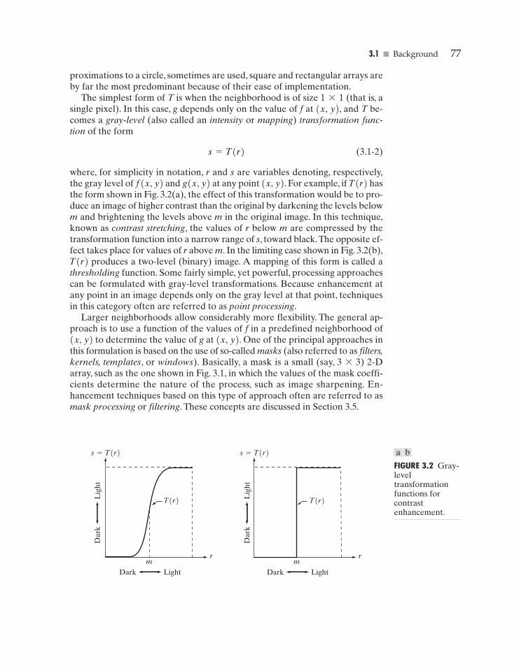
3.1 � Background 77
T(r)T(r)
mr
s=T(r) s=T(r)
Dar
kL
ight
Dar
kL
ight
Dark Lightm
Dark Light
r
FIGURE 3.2 Gray-leveltransformationfunctions forcontrastenhancement.
proximations to a circle, sometimes are used, square and rectangular arrays areby far the most predominant because of their ease of implementation.
The simplest form of T is when the neighborhood is of size 1*1 (that is, asingle pixel). In this case, g depends only on the value of f at (x, y), and T be-comes a gray-level (also called an intensity or mapping) transformation func-tion of the form
(3.1-2)
where, for simplicity in notation, r and s are variables denoting, respectively,the gray level of f(x, y) and g(x, y) at any point (x, y). For example, if T(r) hasthe form shown in Fig. 3.2(a), the effect of this transformation would be to pro-duce an image of higher contrast than the original by darkening the levels belowm and brightening the levels above m in the original image. In this technique,known as contrast stretching, the values of r below m are compressed by thetransformation function into a narrow range of s, toward black.The opposite ef-fect takes place for values of r above m. In the limiting case shown in Fig. 3.2(b),T(r) produces a two-level (binary) image. A mapping of this form is called athresholding function. Some fairly simple, yet powerful, processing approachescan be formulated with gray-level transformations. Because enhancement atany point in an image depends only on the gray level at that point, techniquesin this category often are referred to as point processing.
Larger neighborhoods allow considerably more flexibility. The general ap-proach is to use a function of the values of f in a predefined neighborhood of(x, y) to determine the value of g at (x, y). One of the principal approaches inthis formulation is based on the use of so-called masks (also referred to as filters,kernels, templates, or windows). Basically, a mask is a small (say, 3*3) 2-Darray, such as the one shown in Fig. 3.1, in which the values of the mask coeffi-cients determine the nature of the process, such as image sharpening. En-hancement techniques based on this type of approach often are referred to asmask processing or filtering. These concepts are discussed in Section 3.5.
s = T(r)
a b
GONZ03-075-146.II 29-08-2001 13:42 Page 77
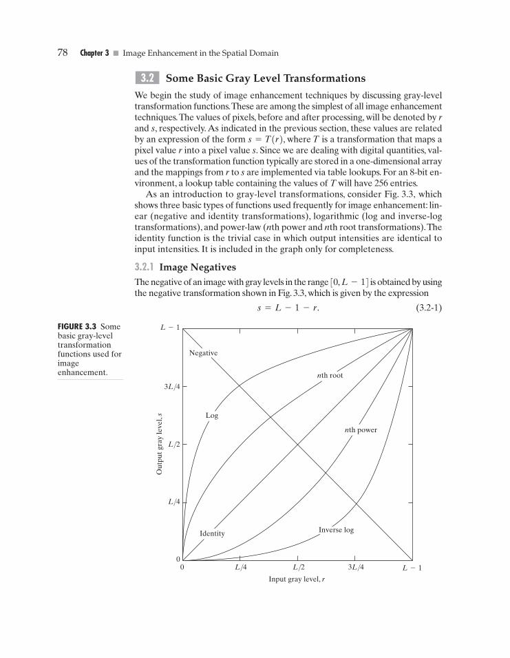
78 Chapter 3 � Image Enhancement in the Spatial Domain
Some Basic Gray Level Transformations
We begin the study of image enhancement techniques by discussing gray-leveltransformation functions.These are among the simplest of all image enhancementtechniques.The values of pixels, before and after processing, will be denoted by rand s, respectively. As indicated in the previous section, these values are relatedby an expression of the form s=T(r), where T is a transformation that maps apixel value r into a pixel value s. Since we are dealing with digital quantities, val-ues of the transformation function typically are stored in a one-dimensional arrayand the mappings from r to s are implemented via table lookups. For an 8-bit en-vironment, a lookup table containing the values of T will have 256 entries.
As an introduction to gray-level transformations, consider Fig. 3.3, whichshows three basic types of functions used frequently for image enhancement: lin-ear (negative and identity transformations), logarithmic (log and inverse-logtransformations), and power-law (nth power and nth root transformations).Theidentity function is the trivial case in which output intensities are identical toinput intensities. It is included in the graph only for completeness.
3.2.1 Image NegativesThe negative of an image with gray levels in the range [0, L-1] is obtained by usingthe negative transformation shown in Fig. 3.3, which is given by the expression
(3.2-1)s = L - 1 - r.
3.2
0
Identity
0L/4
L/4
L/2
L/2
3L/4
3L/4
L-1
L-1
Input gray level, r
Out
put g
ray
leve
l, s Log
Negative
Inverse log
nth power
nth root
FIGURE 3.3 Somebasic gray-leveltransformationfunctions used forimageenhancement.
GONZ03-075-146.II 29-08-2001 13:42 Page 78
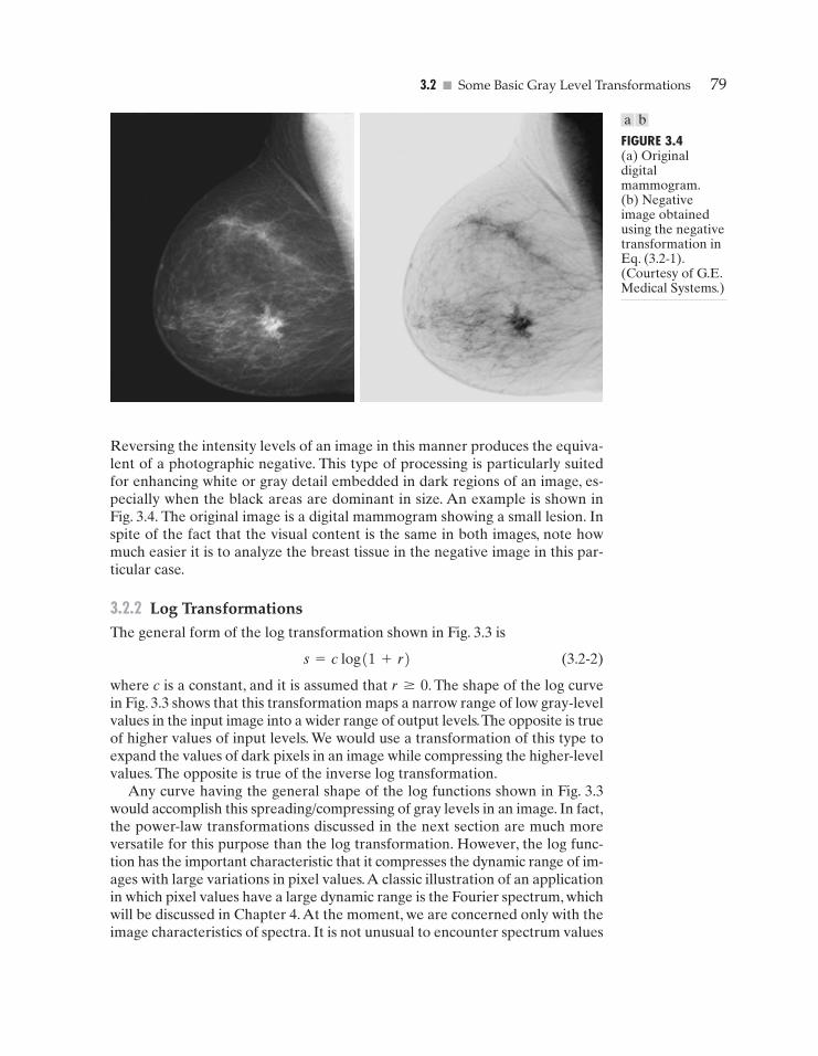
3.2 � Some Basic Gray Level Transformations 79
FIGURE 3.4(a) Originaldigitalmammogram.(b) Negativeimage obtainedusing the negativetransformation inEq. (3.2-1).(Courtesy of G.E.Medical Systems.)
Reversing the intensity levels of an image in this manner produces the equiva-lent of a photographic negative. This type of processing is particularly suitedfor enhancing white or gray detail embedded in dark regions of an image, es-pecially when the black areas are dominant in size. An example is shown inFig. 3.4. The original image is a digital mammogram showing a small lesion. Inspite of the fact that the visual content is the same in both images, note howmuch easier it is to analyze the breast tissue in the negative image in this par-ticular case.
3.2.2 Log TransformationsThe general form of the log transformation shown in Fig. 3.3 is
(3.2-2)
where c is a constant, and it is assumed that r � 0. The shape of the log curvein Fig. 3.3 shows that this transformation maps a narrow range of low gray-levelvalues in the input image into a wider range of output levels.The opposite is trueof higher values of input levels. We would use a transformation of this type toexpand the values of dark pixels in an image while compressing the higher-levelvalues. The opposite is true of the inverse log transformation.
Any curve having the general shape of the log functions shown in Fig. 3.3would accomplish this spreading/compressing of gray levels in an image. In fact,the power-law transformations discussed in the next section are much moreversatile for this purpose than the log transformation. However, the log func-tion has the important characteristic that it compresses the dynamic range of im-ages with large variations in pixel values.A classic illustration of an applicationin which pixel values have a large dynamic range is the Fourier spectrum, whichwill be discussed in Chapter 4.At the moment, we are concerned only with theimage characteristics of spectra. It is not unusual to encounter spectrum values
s = c log (1 + r)
a b
GONZ03-075-146.II 29-08-2001 13:42 Page 79
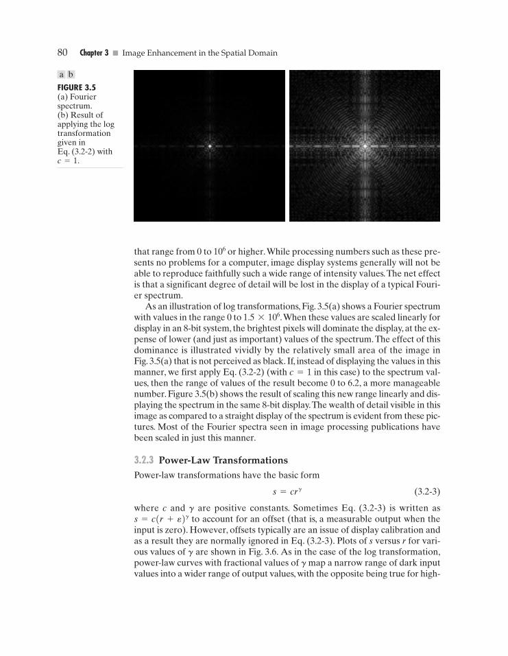
80 Chapter 3 � Image Enhancement in the Spatial Domain
FIGURE 3.5(a) Fourierspectrum.(b) Result ofapplying the logtransformationgiven inEq. (3.2-2) withc=1.
that range from 0 to or higher.While processing numbers such as these pre-sents no problems for a computer, image display systems generally will not beable to reproduce faithfully such a wide range of intensity values.The net effectis that a significant degree of detail will be lost in the display of a typical Fouri-er spectrum.
As an illustration of log transformations, Fig. 3.5(a) shows a Fourier spectrumwith values in the range 0 to 1.5*106.When these values are scaled linearly fordisplay in an 8-bit system, the brightest pixels will dominate the display, at the ex-pense of lower (and just as important) values of the spectrum.The effect of thisdominance is illustrated vividly by the relatively small area of the image inFig. 3.5(a) that is not perceived as black. If, instead of displaying the values in thismanner, we first apply Eq. (3.2-2) (with c=1 in this case) to the spectrum val-ues, then the range of values of the result become 0 to 6.2, a more manageablenumber. Figure 3.5(b) shows the result of scaling this new range linearly and dis-playing the spectrum in the same 8-bit display.The wealth of detail visible in thisimage as compared to a straight display of the spectrum is evident from these pic-tures. Most of the Fourier spectra seen in image processing publications havebeen scaled in just this manner.
3.2.3 Power-Law TransformationsPower-law transformations have the basic form
(3.2-3)
where c and g are positive constants. Sometimes Eq. (3.2-3) is written asto account for an offset (that is, a measurable output when the
input is zero). However, offsets typically are an issue of display calibration andas a result they are normally ignored in Eq. (3.2-3). Plots of s versus r for vari-ous values of g are shown in Fig. 3.6. As in the case of the log transformation,power-law curves with fractional values of gmap a narrow range of dark inputvalues into a wider range of output values, with the opposite being true for high-
s = c(r + e)g
s = crg
106
a b
GONZ03-075-146.II 29-08-2001 13:42 Page 80
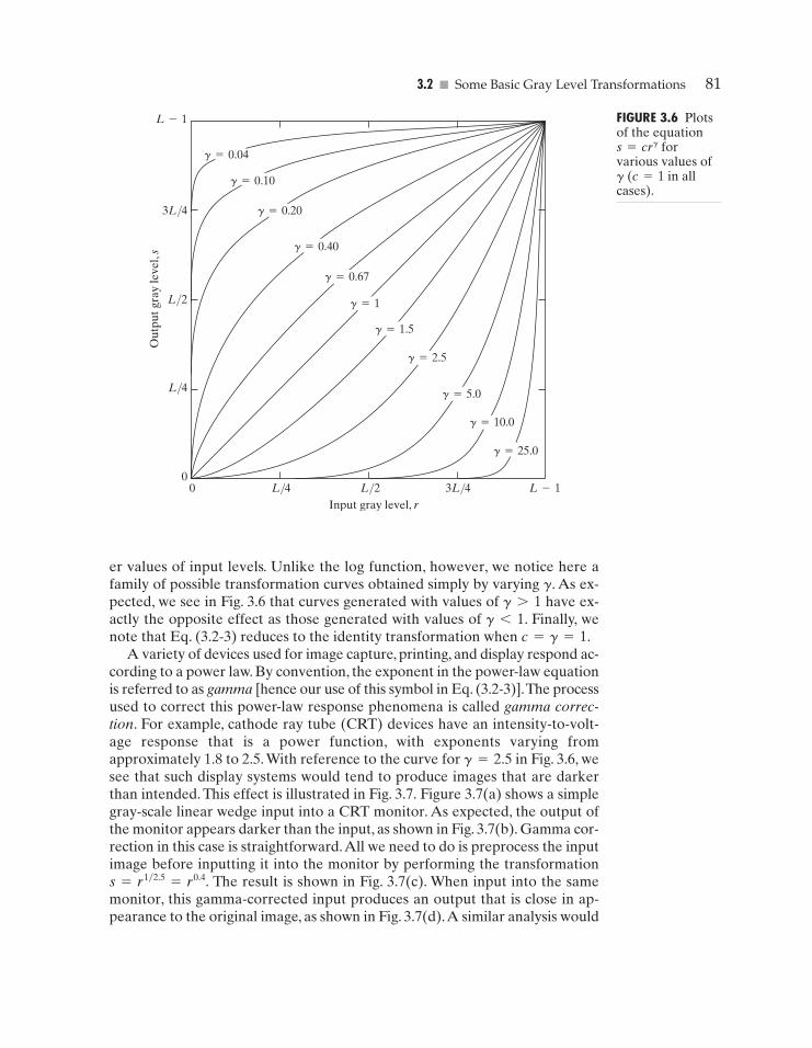
3.2 � Some Basic Gray Level Transformations 81
00
L/4
L/4
L/2
L/2
3L/4
3L/4
L-1
L-1
Input gray level, r
Out
put g
ray
leve
l, s
g=0.04
g=0.10
g=0.20
g=0.40
g=0.67
g=1
g=1.5
g=2.5
g=5.0
g=10.0
g=25.0
FIGURE 3.6 Plotsof the equations=crg forvarious values ofg (c=1 in allcases).
er values of input levels. Unlike the log function, however, we notice here afamily of possible transformation curves obtained simply by varying g. As ex-pected, we see in Fig. 3.6 that curves generated with values of g>1 have ex-actly the opposite effect as those generated with values of g<1. Finally, wenote that Eq. (3.2-3) reduces to the identity transformation when c=g=1.
A variety of devices used for image capture, printing, and display respond ac-cording to a power law. By convention, the exponent in the power-law equationis referred to as gamma [hence our use of this symbol in Eq. (3.2-3)].The processused to correct this power-law response phenomena is called gamma correc-tion. For example, cathode ray tube (CRT) devices have an intensity-to-volt-age response that is a power function, with exponents varying fromapproximately 1.8 to 2.5.With reference to the curve for g=2.5 in Fig. 3.6, wesee that such display systems would tend to produce images that are darkerthan intended. This effect is illustrated in Fig. 3.7. Figure 3.7(a) shows a simplegray-scale linear wedge input into a CRT monitor. As expected, the output ofthe monitor appears darker than the input, as shown in Fig. 3.7(b). Gamma cor-rection in this case is straightforward.All we need to do is preprocess the inputimage before inputting it into the monitor by performing the transformation
The result is shown in Fig. 3.7(c). When input into the samemonitor, this gamma-corrected input produces an output that is close in ap-pearance to the original image, as shown in Fig. 3.7(d).A similar analysis would
s = r1�2.5 = r0.4.
GONZ03-075-146.II 29-08-2001 13:42 Page 81
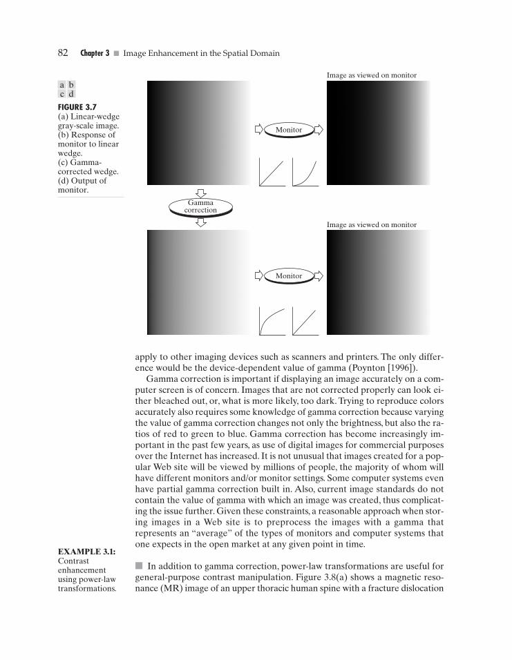
82 Chapter 3 � Image Enhancement in the Spatial Domain
Monitor
Monitor
Gammacorrection
Image as viewed on monitor
Image as viewed on monitor
FIGURE 3.7(a) Linear-wedgegray-scale image.(b) Response ofmonitor to linearwedge.(c) Gamma-corrected wedge.(d) Output ofmonitor.
apply to other imaging devices such as scanners and printers. The only differ-ence would be the device-dependent value of gamma (Poynton [1996]).
Gamma correction is important if displaying an image accurately on a com-puter screen is of concern. Images that are not corrected properly can look ei-ther bleached out, or, what is more likely, too dark. Trying to reproduce colorsaccurately also requires some knowledge of gamma correction because varyingthe value of gamma correction changes not only the brightness, but also the ra-tios of red to green to blue. Gamma correction has become increasingly im-portant in the past few years, as use of digital images for commercial purposesover the Internet has increased. It is not unusual that images created for a pop-ular Web site will be viewed by millions of people, the majority of whom willhave different monitors and/or monitor settings. Some computer systems evenhave partial gamma correction built in. Also, current image standards do notcontain the value of gamma with which an image was created, thus complicat-ing the issue further. Given these constraints, a reasonable approach when stor-ing images in a Web site is to preprocess the images with a gamma thatrepresents an “average” of the types of monitors and computer systems thatone expects in the open market at any given point in time.
� In addition to gamma correction, power-law transformations are useful forgeneral-purpose contrast manipulation. Figure 3.8(a) shows a magnetic reso-nance (MR) image of an upper thoracic human spine with a fracture dislocation
EXAMPLE 3.1:Contrastenhancementusing power-lawtransformations.
a bc d
GONZ03-075-146.II 29-08-2001 13:42 Page 82
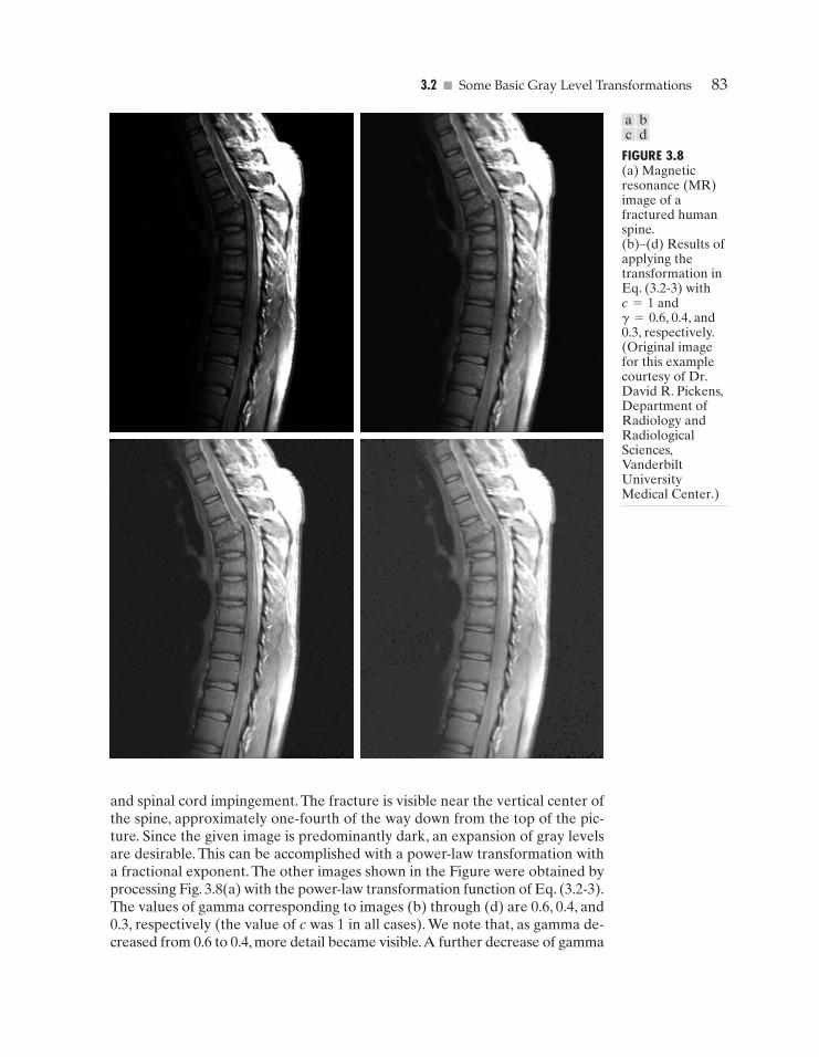
3.2 � Some Basic Gray Level Transformations 83
FIGURE 3.8(a) Magneticresonance (MR)image of afractured humanspine.(b)–(d) Results ofapplying thetransformation inEq. (3.2-3) withc=1 andg=0.6, 0.4, and0.3, respectively.(Original imagefor this examplecourtesy of Dr.David R. Pickens,Department ofRadiology andRadiologicalSciences,VanderbiltUniversityMedical Center.)
and spinal cord impingement. The fracture is visible near the vertical center ofthe spine, approximately one-fourth of the way down from the top of the pic-ture. Since the given image is predominantly dark, an expansion of gray levelsare desirable. This can be accomplished with a power-law transformation witha fractional exponent. The other images shown in the Figure were obtained byprocessing Fig. 3.8(a) with the power-law transformation function of Eq. (3.2-3).The values of gamma corresponding to images (b) through (d) are 0.6, 0.4, and0.3, respectively (the value of c was 1 in all cases). We note that, as gamma de-creased from 0.6 to 0.4, more detail became visible.A further decrease of gamma
a bc d
GONZ03-075-146.II 29-08-2001 13:42 Page 83
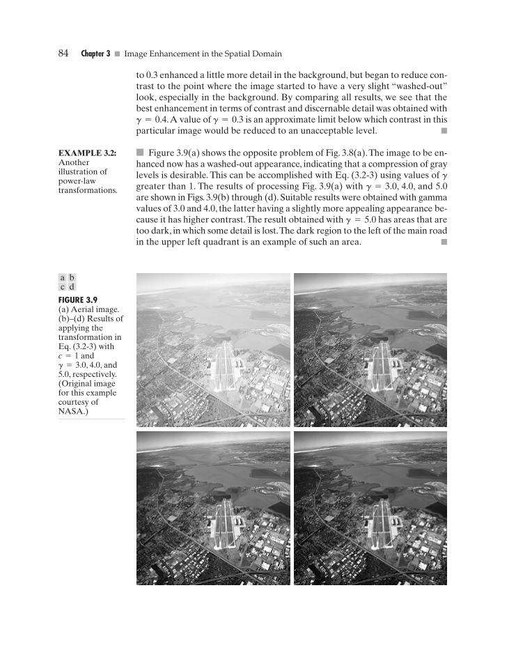
84 Chapter 3 � Image Enhancement in the Spatial Domain
FIGURE 3.9(a) Aerial image.(b)–(d) Results ofapplying thetransformation inEq. (3.2-3) withc=1 andg=3.0, 4.0, and5.0, respectively.(Original imagefor this examplecourtesy ofNASA.)
to 0.3 enhanced a little more detail in the background, but began to reduce con-trast to the point where the image started to have a very slight “washed-out”look, especially in the background. By comparing all results, we see that thebest enhancement in terms of contrast and discernable detail was obtained withg=0.4.A value of g=0.3 is an approximate limit below which contrast in thisparticular image would be reduced to an unacceptable level. �
� Figure 3.9(a) shows the opposite problem of Fig. 3.8(a).The image to be en-hanced now has a washed-out appearance, indicating that a compression of graylevels is desirable. This can be accomplished with Eq. (3.2-3) using values of ggreater than 1. The results of processing Fig. 3.9(a) with g=3.0, 4.0, and 5.0are shown in Figs. 3.9(b) through (d). Suitable results were obtained with gammavalues of 3.0 and 4.0, the latter having a slightly more appealing appearance be-cause it has higher contrast.The result obtained with g=5.0 has areas that aretoo dark, in which some detail is lost.The dark region to the left of the main roadin the upper left quadrant is an example of such an area. �
EXAMPLE 3.2:Anotherillustration ofpower-lawtransformations.
a bc d
GONZ03-075-146.II 29-08-2001 13:42 Page 84
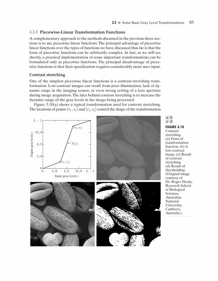
3.2 � Some Basic Gray Level Transformations 85
3.2.4 Piecewise-Linear Transformation FunctionsA complementary approach to the methods discussed in the previous three sec-tions is to use piecewise linear functions. The principal advantage of piecewiselinear functions over the types of functions we have discussed thus far is that theform of piecewise functions can be arbitrarily complex. In fact, as we will seeshortly, a practical implementation of some important transformations can beformulated only as piecewise functions. The principal disadvantage of piece-wise functions is that their specification requires considerably more user input.
Contrast stretching
One of the simplest piecewise linear functions is a contrast-stretching trans-formation. Low-contrast images can result from poor illumination, lack of dy-namic range in the imaging sensor, or even wrong setting of a lens apertureduring image acquisition.The idea behind contrast stretching is to increase thedynamic range of the gray levels in the image being processed.
Figure 3.10(a) shows a typical transformation used for contrast stretching.The locations of points Ar1, s1B and Ar2, s2B control the shape of the transformation
T(r)
(r1, s1)
(r2, s2)
Input gray level, r
Oup
ut g
ray
leve
l, s
00 L/4
L/4
L/2
L/2
3L/4
3L/4
L-1
L-1
FIGURE 3.10Contraststretching.(a) Form oftransformationfunction. (b) Alow-contrastimage. (c) Resultof contraststretching.(d) Result ofthresholding.(Original imagecourtesy ofDr. Roger Heady,Research Schoolof BiologicalSciences,AustralianNationalUniversity,Canberra,Australia.)
a bc d
GONZ03-075-146.II 29-08-2001 13:42 Page 85
86 Chapter 3 � Image Enhancement in the Spatial Domain
function. If r1=s1 and r2=s2 , the transformation is a linear function that pro-duces no changes in gray levels. If r1=r2, s1=0 and s2=L-1, the transfor-mation becomes a thresholding function that creates a binary image, as illustratedin Fig. 3.2(b). Intermediate values of Ar1, s1B and Ar2, s2B produce various degreesof spread in the gray levels of the output image, thus affecting its contrast. Ingeneral, r1 � r2 and s1 � s2 is assumed so that the function is single valued andmonotonically increasing.This condition preserves the order of gray levels, thuspreventing the creation of intensity artifacts in the processed image.
Figure 3.10(b) shows an 8-bit image with low contrast. Fig. 3.10(c) shows theresult of contrast stretching, obtained by setting Ar1 , s1 B= Armin , 0 B andAr2, s2 B=Armax, L-1B where rmin and rmax denote the minimum and maximumgray levels in the image, respectively.Thus, the transformation function stretchedthe levels linearly from their original range to the full range [0, L-1]. Final-ly, Fig. 3.10(d) shows the result of using the thresholding function defined pre-viously, with r1=r2=m, the mean gray level in the image.The original imageon which these results are based is a scanning electron microscope image ofpollen, magnified approximately 700 times.
Gray-level slicing
Highlighting a specific range of gray levels in an image often is desired. Appli-cations include enhancing features such as masses of water in satellite imageryand enhancing flaws in X-ray images.There are several ways of doing level slic-ing, but most of them are variations of two basic themes. One approach is to dis-play a high value for all gray levels in the range of interest and a low value forall other gray levels.This transformation, shown in Fig. 3.11(a), produces a binaryimage.The second approach, based on the transformation shown in Fig. 3.11(b),brightens the desired range of gray levels but preserves the background andgray-level tonalities in the image. Figure 3.11(c) shows a gray-scale image, andFig. 3.11(d) shows the result of using the transformation in Fig. 3.11(a).Variationsof the two transformations shown in Fig. 3.11 are easy to formulate.
Bit-plane slicing
Instead of highlighting gray-level ranges, highlighting the contribution made tototal image appearance by specific bits might be desired. Suppose that eachpixel in an image is represented by 8 bits. Imagine that the image is composedof eight 1-bit planes, ranging from bit-plane 0 for the least significant bit to bit-plane 7 for the most significant bit. In terms of 8-bit bytes, plane 0 contains allthe lowest order bits in the bytes comprising the pixels in the image and plane7 contains all the high-order bits. Figure 3.12 illustrates these ideas, and Fig. 3.14shows the various bit planes for the image shown in Fig. 3.13. Note that thehigher-order bits (especially the top four) contain the majority of the visually sig-nificant data.The other bit planes contribute to more subtle details in the image.Separating a digital image into its bit planes is useful for analyzing the relativeimportance played by each bit of the image, a process that aids in determiningthe adequacy of the number of bits used to quantize each pixel. Also, this typeof decomposition is useful for image compression, as discussed in Chapter 8.
GONZ03-075-146.II 29-08-2001 13:42 Page 86
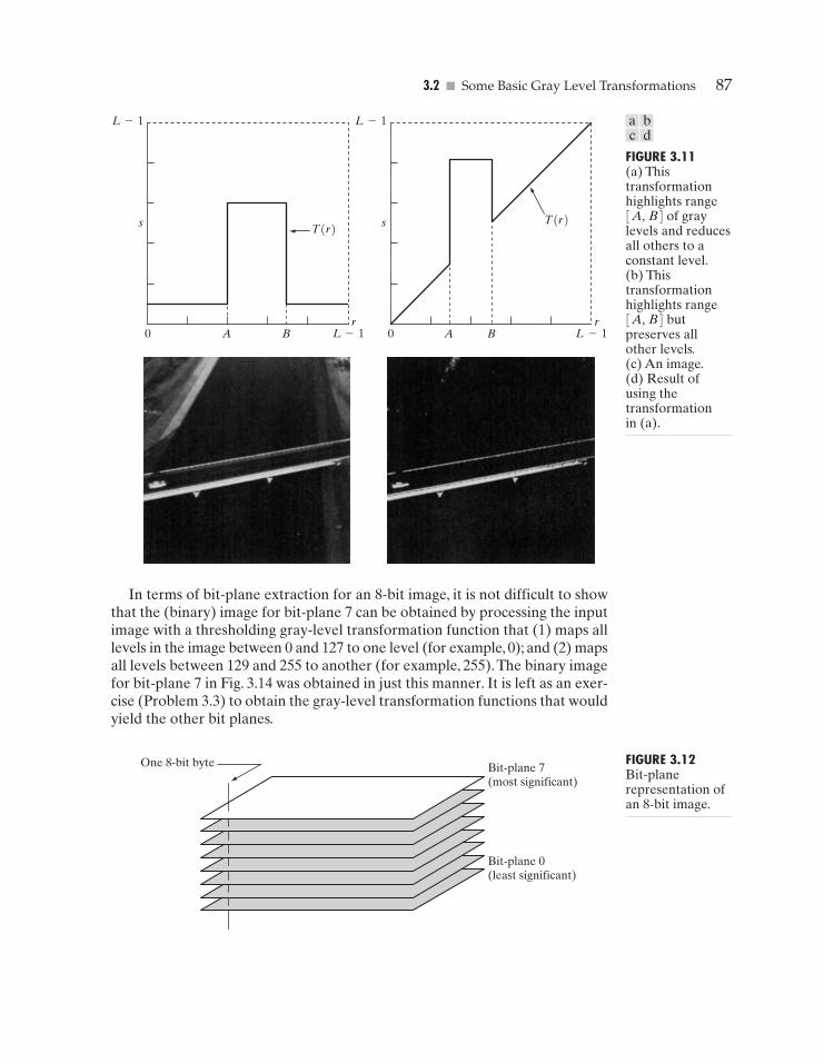
3.2 � Some Basic Gray Level Transformations 87
L-1
L-1
s
r
T(r)
0 A B
L-1
L-1
s
r
T(r)
0 A B
FIGURE 3.11(a) Thistransformationhighlights range[A, B] of graylevels and reducesall others to aconstant level.(b) Thistransformationhighlights range[A, B] butpreserves allother levels.(c) An image.(d) Result ofusing thetransformationin (a).
One 8-bit byte Bit-plane 7(most significant)
Bit-plane 0(least significant)
FIGURE 3.12Bit-planerepresentation ofan 8-bit image.
In terms of bit-plane extraction for an 8-bit image, it is not difficult to showthat the (binary) image for bit-plane 7 can be obtained by processing the inputimage with a thresholding gray-level transformation function that (1) maps alllevels in the image between 0 and 127 to one level (for example, 0); and (2) mapsall levels between 129 and 255 to another (for example, 255).The binary imagefor bit-plane 7 in Fig. 3.14 was obtained in just this manner. It is left as an exer-cise (Problem 3.3) to obtain the gray-level transformation functions that wouldyield the other bit planes.
a bc d
GONZ03-075-146.II 29-08-2001 13:42 Page 87
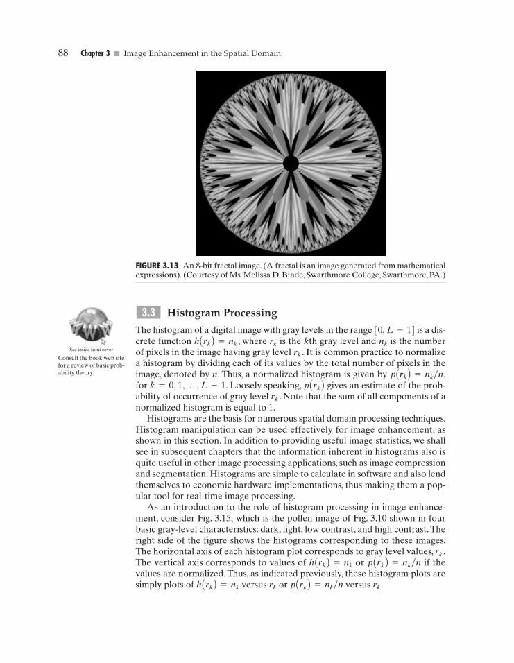
88 Chapter 3 � Image Enhancement in the Spatial Domain
Histogram Processing
The histogram of a digital image with gray levels in the range [0, L-1] is a dis-crete function h Ark B=nk , where rk is the kth gray level and nk is the numberof pixels in the image having gray level rk . It is common practice to normalizea histogram by dividing each of its values by the total number of pixels in theimage, denoted by n. Thus, a normalized histogram is given by p Ark B=nk�n,for k=0, 1, p , L-1. Loosely speaking, p Ark B gives an estimate of the prob-ability of occurrence of gray level rk . Note that the sum of all components of anormalized histogram is equal to 1.
Histograms are the basis for numerous spatial domain processing techniques.Histogram manipulation can be used effectively for image enhancement, asshown in this section. In addition to providing useful image statistics, we shallsee in subsequent chapters that the information inherent in histograms also isquite useful in other image processing applications, such as image compressionand segmentation. Histograms are simple to calculate in software and also lendthemselves to economic hardware implementations, thus making them a pop-ular tool for real-time image processing.
As an introduction to the role of histogram processing in image enhance-ment, consider Fig. 3.15, which is the pollen image of Fig. 3.10 shown in fourbasic gray-level characteristics: dark, light, low contrast, and high contrast. Theright side of the figure shows the histograms corresponding to these images.The horizontal axis of each histogram plot corresponds to gray level values, rk .The vertical axis corresponds to values of h Ark B=nk or p Ark B=nk�n if thevalues are normalized. Thus, as indicated previously, these histogram plots aresimply plots of h Ark B=nk versus rk or p Ark B=nk�n versus rk .
3.3
FIGURE 3.13 An 8-bit fractal image. (A fractal is an image generated from mathematicalexpressions). (Courtesy of Ms. Melissa D. Binde, Swarthmore College, Swarthmore, PA.)
Consult the book web sitefor a review of basic prob-ability theory.
See inside front cover
GONZ03-075-146.II 29-08-2001 13:42 Page 88
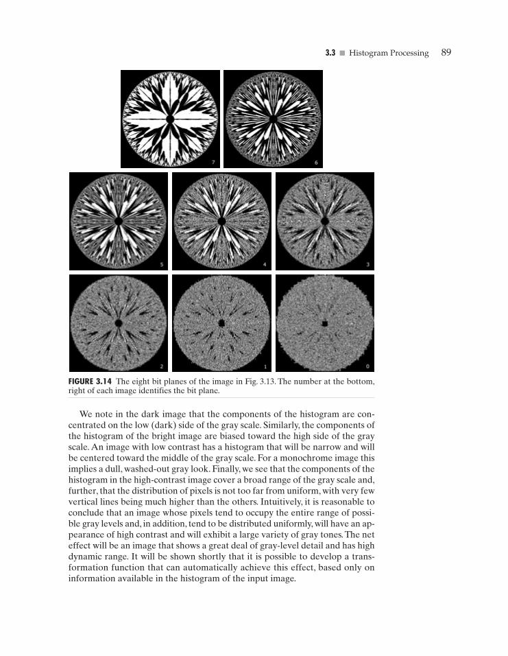
3.3 � Histogram Processing 89
FIGURE 3.14 The eight bit planes of the image in Fig. 3.13. The number at the bottom,right of each image identifies the bit plane.
We note in the dark image that the components of the histogram are con-centrated on the low (dark) side of the gray scale. Similarly, the components ofthe histogram of the bright image are biased toward the high side of the grayscale. An image with low contrast has a histogram that will be narrow and willbe centered toward the middle of the gray scale. For a monochrome image thisimplies a dull, washed-out gray look. Finally, we see that the components of thehistogram in the high-contrast image cover a broad range of the gray scale and,further, that the distribution of pixels is not too far from uniform, with very fewvertical lines being much higher than the others. Intuitively, it is reasonable toconclude that an image whose pixels tend to occupy the entire range of possi-ble gray levels and, in addition, tend to be distributed uniformly, will have an ap-pearance of high contrast and will exhibit a large variety of gray tones.The neteffect will be an image that shows a great deal of gray-level detail and has highdynamic range. It will be shown shortly that it is possible to develop a trans-formation function that can automatically achieve this effect, based only oninformation available in the histogram of the input image.
GONZ03-075-146.II 29-08-2001 13:42 Page 89
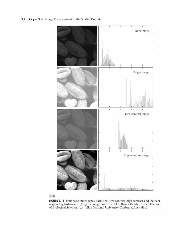
90 Chapter 3 � Image Enhancement in the Spatial Domain
Dark image
Bright image
Low-contrast image
High-contrast image
FIGURE 3.15 Four basic image types: dark, light, low contrast, high contrast, and their cor-responding histograms. (Original image courtesy of Dr. Roger Heady, Research Schoolof Biological Sciences, Australian National University, Canberra, Australia.)
a b
GONZ03-075-146.II 29-08-2001 13:42 Page 90
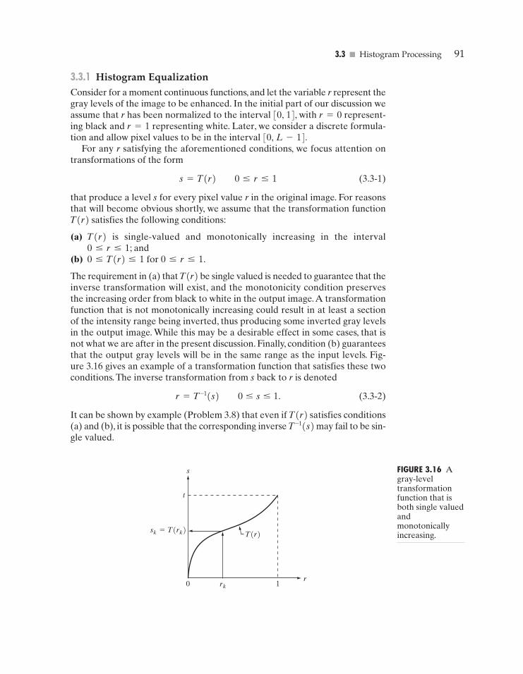
3.3 � Histogram Processing 91
3.3.1 Histogram EqualizationConsider for a moment continuous functions, and let the variable r represent thegray levels of the image to be enhanced. In the initial part of our discussion weassume that r has been normalized to the interval [0, 1], with r=0 represent-ing black and r=1 representing white. Later, we consider a discrete formula-tion and allow pixel values to be in the interval [0, L-1].
For any r satisfying the aforementioned conditions, we focus attention ontransformations of the form
s=T(r) 0 � r � 1 (3.3-1)
that produce a level s for every pixel value r in the original image. For reasonsthat will become obvious shortly, we assume that the transformation functionT(r) satisfies the following conditions:
(a) T(r) is single-valued and monotonically increasing in the interval0 � r � 1; and
(b) 0 � T(r) � 1 for 0 � r � 1.
The requirement in (a) that T(r) be single valued is needed to guarantee that theinverse transformation will exist, and the monotonicity condition preservesthe increasing order from black to white in the output image.A transformationfunction that is not monotonically increasing could result in at least a sectionof the intensity range being inverted, thus producing some inverted gray levelsin the output image. While this may be a desirable effect in some cases, that isnot what we are after in the present discussion. Finally, condition (b) guaranteesthat the output gray levels will be in the same range as the input levels. Fig-ure 3.16 gives an example of a transformation function that satisfies these twoconditions. The inverse transformation from s back to r is denoted
(3.3-2)
It can be shown by example (Problem 3.8) that even if T(r) satisfies conditions(a) and (b), it is possible that the corresponding inverse may fail to be sin-gle valued.
T-1(s)
r = T-1(s) 0 � s � 1.
T(r)
0 rk 1
t
r
s
sk=T(rk)
FIGURE 3.16 Agray-leveltransformationfunction that isboth single valuedandmonotonicallyincreasing.
GONZ03-075-146.II 29-08-2001 13:42 Page 91
92 Chapter 3 � Image Enhancement in the Spatial Domain
The gray levels in an image may be viewed as random variables in the in-terval [0, 1]. One of the most fundamental descriptors of a random variable isits probability density function (PDF). Let pr(r) and ps(s) denote the probabilitydensity functions of random variables r and s, respectively, where the subscriptson p are used to denote that pr and ps are different functions. A basic resultfrom an elementary probability theory is that, if pr(r) and T(r) are known and
satisfies condition (a), then the probability density function ps(s) of thetransformed variable s can be obtained using a rather simple formula:
(3.3-3)
Thus, the probability density function of the transformed variable, s, is deter-mined by the gray-level PDF of the input image and by the chosen transfor-mation function.
A transformation function of particular importance in image processinghas the form
(3.3-4)
where w is a dummy variable of integration.The right side of Eq. (3.3-4) is rec-ognized as the cumulative distribution function (CDF) of random variable r.Since probability density functions are always positive, and recalling that the in-tegral of a function is the area under the function, it follows that this transfor-mation function is single valued and monotonically increasing, and, therefore,satisfies condition (a). Similarly, the integral of a probability density function forvariables in the range [0, 1] also is in the range [0, 1], so condition (b) is satis-fied as well.
Given transformation function T(r), we find ps(s) by applying Eq. (3.3-3).Weknow from basic calculus (Leibniz’s rule) that the derivative of a definite inte-gral with respect to its upper limit is simply the integrand evaluated at that limit.In other words,
(3.3-5)
Substituting this result for dr�ds into Eq. (3.3-3), and keeping in mind that allprobability values are positive, yields
(3.3-6)
= 1 0 � s � 1.
= pr(r) 2 1pr(r)2
ps(s) = pr(r) 2 drds2
= pr(r).
=d
dr c 3
r
0pr(w) dw d
dsdr
=dT(r)
dr
s = T(r) = 3r
0pr(w) dw
ps(s) = pr(r) 2 drds2 .
T-1(s)
GONZ03-075-146.II 29-08-2001 13:42 Page 92
3.3 � Histogram Processing 93
Because ps(s) is a probability density function, it follows that it must be zero out-side the interval [0, 1] in this case because its integral over all values of s mustequal 1. We recognize the form of ps(s) given in Eq. (3.3-6) as a uniform prob-ability density function. Simply stated, we have demonstrated that performingthe transformation function given in Eq. (3.3-4) yields a random variable s char-acterized by a uniform probability density function. It is important to note fromEq. (3.3-4) that T(r) depends on pr(r), but, as indicated by Eq. (3.3-6), the re-sulting ps(s) always is uniform, independent of the form of pr(r).
For discrete values we deal with probabilities and summations instead ofprobability density functions and integrals. The probability of occurrence ofgray level rk in an image is approximated by
(3.3-7)
where, as noted at the beginning of this section, n is the total number of pixelsin the image, nk is the number of pixels that have gray level rk , and L is the totalnumber of possible gray levels in the image. The discrete version of the trans-formation function given in Eq. (3.3-4) is
(3.3-8)
Thus, a processed (output) image is obtained by mapping each pixel with levelrk in the input image into a corresponding pixel with level sk in the output imagevia Eq. (3.3-8). As indicated earlier, a plot of pr Ark B versus rk is called a his-togram. The transformation (mapping) given in Eq. (3.3-8) is called histogramequalization or histogram linearization. It is not difficult to show (Problem 3.9)that the transformation in Eq. (3.3-8) satisfies conditions (a) and (b) stated pre-viously in this section.
Unlike its continuos counterpart, it cannot be proved in general that this dis-crete transformation will produce the discrete equivalent of a uniform proba-bility density function, which would be a uniform histogram. However, as willbe seen shortly, use of Eq. (3.3-8) does have the general tendency of spreadingthe histogram of the input image so that the levels of the histogram-equalizedimage will span a fuller range of the gray scale.
We discussed earlier in this section the many advantages of having gray-levelvalues that cover the entire gray scale. In addition to producing gray levels thathave this tendency, the method just derived has the additional advantage thatit is fully “automatic.” In other words, given an image, the process of histogramequalization consists simply of implementing Eq. (3.3-8), which is based on in-formation that can be extracted directly from the given image, without the needfor further parameter specifications. We note also the simplicity of the compu-tations that would be required to implement the technique.
The inverse transformation from s back to r is denoted by
(3.3-9)rk = T-1AskB k = 0, 1, 2, p , L - 1
= ak
j = 0 nj
n k = 0, 1, 2, p , L - 1.
sk = TArkB = ak
j = 0prArjB
pr(rk) =nk
n k = 0, 1, 2, p , L - 1
GONZ03-075-146.II 29-08-2001 13:42 Page 93
94 Chapter 3 � Image Enhancement in the Spatial Domain
It can be shown (Problem 3.9) that the inverse transformation in Eq. (3.3-9)satisfies conditions (a) and (b) stated previously in this section only if none ofthe levels, rk , k=0, 1, 2, p , L-1, are missing from the input image.Althoughthe inverse transformation is not used in histogram equalization, it plays a cen-tral role in the histogram-matching scheme developed in the next section. Wealso discuss in that section details of how to implement histogram processingtechniques.
� Figure 3.17(a) shows the four images from Fig. 3.15, and Fig. 3.17(b) showsthe result of performing histogram equalization on each of these images.The firstthree results (top to bottom) show significant improvement. As expected, his-togram equalization did not produce a significant visual difference in the fourthimage because the histogram of this image already spans the full spectrum ofthe gray scale. The transformation functions used to generate the images inFig. 3.17(b) are shown in Fig. 3.18. These functions were generated from thehistograms of the original images [see Fig. 3.15(b)] using Eq. (3.3-8). Note thattransformation (4) has a basic linear shape, again indicating that the gray lev-els in the fourth input image are nearly uniformly distributed.As was just noted,we would expect histogram equalization in this case to have negligible effect onthe appearance of the image.
The histograms of the equalized images are shown in Fig. 3.17(c). It is of in-terest to note that, while all these histograms are different, the histogram-equalized images themselves are visually very similar. This is not unexpectedbecause the difference between the images in the left column is simply one ofcontrast, not of content. In other words, since the images have the same content,the increase in contrast resulting from histogram equalization was enough torender any gray-level differences in the resulting images visually indistinguish-able. Given the significant contrast differences of the images in the left column,this example illustrates the power of histogram equalization as an adaptive en-hancement tool. �
3.3.2 Histogram Matching (Specification)As indicated in the preceding discussion, histogram equalization automatical-ly determines a transformation function that seeks to produce an output imagethat has a uniform histogram. When automatic enhancement is desired, this isa good approach because the results from this technique are predictable and themethod is simple to implement. We show in this section that there are applica-tions in which attempting to base enhancement on a uniform histogram is notthe best approach. In particular, it is useful sometimes to be able to specify theshape of the histogram that we wish the processed image to have. The methodused to generate a processed image that has a specified histogram is calledhistogram matching or histogram specification.
Development of the method
Let us return for a moment to continuous gray levels r and z (consideredcontinuous random variables), and let pr(r) and pz(z) denote their corre-sponding continuos probability density functions. In this notation, r and z denote
EXAMPLE 3.3:Histogramequalization.
GONZ03-075-146.II 29-08-2001 13:42 Page 94
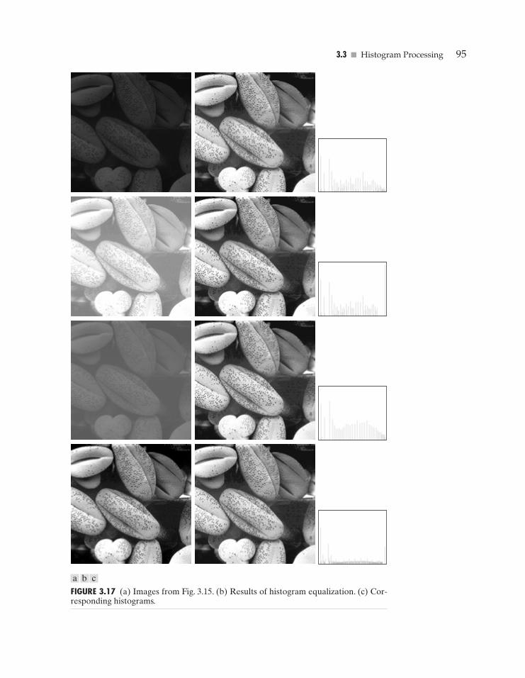
3.3 � Histogram Processing 95
FIGURE 3.17 (a) Images from Fig. 3.15. (b) Results of histogram equalization. (c) Cor-responding histograms.
a b c
GONZ03-075-146.II 29-08-2001 13:42 Page 95
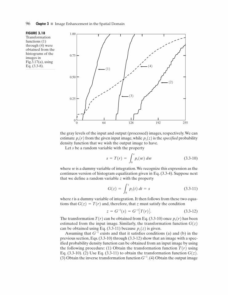
96 Chapter 3 � Image Enhancement in the Spatial Domain
1.00
0.75
0.50
0.25
00 64
(1)
(3)
(2)
(4)
128 192 255
FIGURE 3.18Transformationfunctions (1)through (4) wereobtained from thehistograms of theimages inFig.3.17(a), usingEq. (3.3-8).
the gray levels of the input and output (processed) images, respectively.We canestimate pr(r) from the given input image, while pz(z) is the specified probabilitydensity function that we wish the output image to have.
Let s be a random variable with the property
(3.3-10)
where w is a dummy variable of integration.We recognize this expression as thecontinuos version of histogram equalization given in Eq. (3.3-4). Suppose nextthat we define a random variable z with the property
(3.3-11)
where t is a dummy variable of integration. It then follows from these two equa-tions that G(z)=T(r) and, therefore, that z must satisfy the condition
(3.3-12)
The transformation T(r) can be obtained from Eq. (3.3-10) once pr(r) has beenestimated from the input image. Similarly, the transformation function G(z)can be obtained using Eq. (3.3-11) because pz(z) is given.
Assuming that G–1 exists and that it satisfies conditions (a) and (b) in theprevious section, Eqs. (3.3-10) through (3.3-12) show that an image with a spec-ified probability density function can be obtained from an input image by usingthe following procedure: (1) Obtain the transformation function T(r) usingEq. (3.3-10). (2) Use Eq. (3.3-11) to obtain the transformation function G(z).(3) Obtain the inverse transformation function G–1. (4) Obtain the output image
z = G-1(s) = G-1 CT(r) D .
G(z) = 3z
0pz(t) dt = s
s = T(r) = 3r
0pr(w) dw
GONZ03-075-146.II 29-08-2001 13:42 Page 96
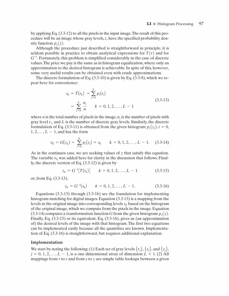
3.3 � Histogram Processing 97
by applying Eq. (3.3-12) to all the pixels in the input image.The result of this pro-cedure will be an image whose gray levels, z, have the specified probability den-sity function pz(z).
Although the procedure just described is straightforward in principle, it isseldom possible in practice to obtain analytical expressions for T(r) and forG–1. Fortunately, this problem is simplified considerably in the case of discretevalues.The price we pay is the same as in histogram equalization, where only anapproximation to the desired histogram is achievable. In spite of this, however,some very useful results can be obtained even with crude approximations.
The discrete formulation of Eq. (3.3-10) is given by Eq. (3.3-8), which we re-peat here for convenience:
(3.3-13)
where n is the total number of pixels in the image, nj is the number of pixels withgray level rj , and L is the number of discrete gray levels. Similarly, the discreteformulation of Eq. (3.3-11) is obtained from the given histogram pz Azi B , i=0,1, 2, p , L-1, and has the form
(3.3-14)
As in the continuos case, we are seeking values of z that satisfy this equation.The variable vk was added here for clarity in the discussion that follows. Final-ly, the discrete version of Eq. (3.3-12) is given by
(3.3-15)
or, from Eq. (3.3-13),
(3.3-16)
Equations (3.3-13) through (3.3-16) are the foundation for implementinghistogram matching for digital images. Equation (3.3-13) is a mapping from thelevels in the original image into corresponding levels sk based on the histogramof the original image, which we compute from the pixels in the image. Equation(3.3-14) computes a transformation function G from the given histogram pz(z).Finally, Eq. (3.3-15) or its equivalent, Eq. (3.3-16), gives us (an approximationof) the desired levels of the image with that histogram. The first two equationscan be implemented easily because all the quantities are known. Implementa-tion of Eq. (3.3-16) is straightforward, but requires additional explanation.
Implementation
We start by noting the following: (1) Each set of gray levels ErjF , EsjF , and EzjF ,j=0, 1, 2, p , L-1, is a one-dimensional array of dimension L*1. (2) Allmappings from r to s and from s to z are simple table lookups between a given
zk = G-1AskB k = 0, 1, 2, p , L - 1.
zk = G-1 CTArkB D k = 0, 1, 2, p , L - 1
vk = GAzkB = ak
i = 0pzAziB = sk k = 0, 1, 2, p , L - 1.
= ak
j = 0 nj
n k = 0, 1, 2, p , L - 1
sk = TArkB = a k
j = 0prArjB
GONZ03-075-146.II 29-08-2001 13:42 Page 97
98 Chapter 3 � Image Enhancement in the Spatial Domain
0 L-10
s
r
1
rk
sk
T(r)
L-1
v
z0 zq
vq
0
1
G(z)
L-1
v
z0 zk
sk
0
1
G(z)
FIGURE 3.19(a) Graphicalinterpretation ofmapping from rk
to sk via T(r).(b) Mapping of zq
to itscorrespondingvalue vq via G(z).(c) Inversemapping from sk
to itscorrespondingvalue of zk .
a bc
pixel value and these arrays. (3) Each of the elements of these arrays, for ex-ample, sk , contains two important pieces of information: The subscript k de-notes the location of the element in the array, and s denotes the value at thatlocation. (4) We need to be concerned only with integer pixel values. For ex-ample, in the case of an 8-bit image, L=256 and the elements of each of thearrays just mentioned are integers between 0 and 255.This implies that we nowwork with gray level values in the interval [0, L-1] instead of the normalizedinterval [0, 1] that we used before to simplify the development of histogramprocessing techniques.
In order to see how histogram matching actually can be implemented, con-sider Fig. 3.19(a), ignoring for a moment the connection shown between thisfigure and Fig. 3.19(c). Figure 3.19(a) shows a hypothetical discrete transfor-mation function s=T(r) obtained from a given image. The first gray level inthe image, r1 , maps to s1 ; the second gray level, r2 , maps to s2 ; the kth level rk
maps to sk ; and so on (the important point here is the ordered correspondencebetween these values). Each value sj in the array is precomputed usingEq. (3.3-13), so the process of mapping simply uses the actual value of a pixelas an index in an array to determine the corresponding value of s. This processis particularly easy because we are dealing with integers. For example, the smapping for an 8-bit pixel with value 127 would be found in the 128th positionin array EsjF (recall that we start at 0) out of the possible 256 positions. If westopped here and mapped the value of each pixel of an input image by the
GONZ03-075-146.II 29-08-2001 13:42 Page 98
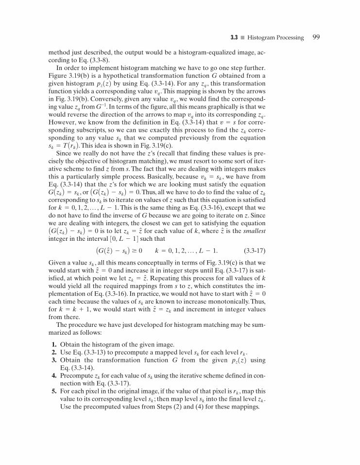
3.3 � Histogram Processing 99
method just described, the output would be a histogram-equalized image, ac-cording to Eq. (3.3-8).
In order to implement histogram matching we have to go one step further.Figure 3.19(b) is a hypothetical transformation function G obtained from agiven histogram pz(z) by using Eq. (3.3-14). For any zq , this transformationfunction yields a corresponding value vq . This mapping is shown by the arrowsin Fig. 3.19(b). Conversely, given any value vq , we would find the correspond-ing value zq from G–1. In terms of the figure, all this means graphically is that wewould reverse the direction of the arrows to map vq into its corresponding zq .However, we know from the definition in Eq. (3.3-14) that v=s for corre-sponding subscripts, so we can use exactly this process to find the zk corre-sponding to any value sk that we computed previously from the equationsk=T Ark B . This idea is shown in Fig. 3.19(c).
Since we really do not have the z’s (recall that finding these values is pre-cisely the objective of histogram matching), we must resort to some sort of iter-ative scheme to find z from s. The fact that we are dealing with integers makesthis a particularly simple process. Basically, because vk=sk , we have fromEq. (3.3-14) that the z’s for which we are looking must satisfy the equationGAzk B=sk , or AGAzk B-skB=0. Thus, all we have to do to find the value of zk
corresponding to sk is to iterate on values of z such that this equation is satisfiedfor k=0, 1, 2, p , L-1. This is the same thing as Eq. (3.3-16), except that wedo not have to find the inverse of G because we are going to iterate on z. Sincewe are dealing with integers, the closest we can get to satisfying the equationAG Azk B-sk B=0 is to let zk= for each value of k, where is the smallestinteger in the interval [0, L-1] such that
(3.3-17)
Given a value sk , all this means conceptually in terms of Fig. 3.19(c) is that wewould start with and increase it in integer steps until Eq. (3.3-17) is sat-isfied, at which point we let Repeating this process for all values of kwould yield all the required mappings from s to z, which constitutes the im-plementation of Eq. (3.3-16). In practice, we would not have to start witheach time because the values of sk are known to increase monotonically. Thus,for k=k+1, we would start with and increment in integer valuesfrom there.
The procedure we have just developed for histogram matching may be sum-marized as follows:
1. Obtain the histogram of the given image.2. Use Eq. (3.3-13) to precompute a mapped level sk for each level rk .3. Obtain the transformation function G from the given pz(z) using
Eq. (3.3-14).4. Precompute zk for each value of sk using the iterative scheme defined in con-
nection with Eq. (3.3-17).5. For each pixel in the original image, if the value of that pixel is rk , map this
value to its corresponding level sk ; then map level sk into the final level zk .Use the precomputed values from Steps (2) and (4) for these mappings.
z = zk
z = 0
zk = z.z = 0
AG(z) - skB � 0 k = 0, 1, 2, p , L - 1.
zz
GONZ03-075-146.II 29-08-2001 13:42 Page 99
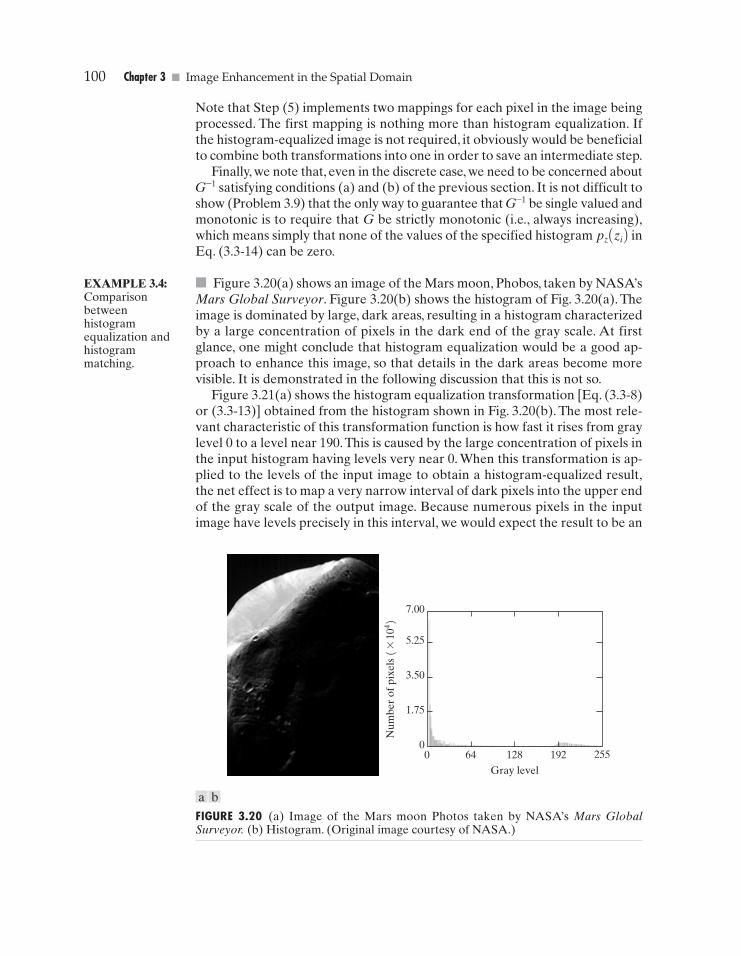
100 Chapter 3 � Image Enhancement in the Spatial Domain
7.00
5.25
3.50
1.75
00 64 128 192 255
Gray level
Num
ber
of p
ixel
s (*
104 )
FIGURE 3.20 (a) Image of the Mars moon Photos taken by NASA’s Mars GlobalSurveyor. (b) Histogram. (Original image courtesy of NASA.)
Note that Step (5) implements two mappings for each pixel in the image beingprocessed. The first mapping is nothing more than histogram equalization. Ifthe histogram-equalized image is not required, it obviously would be beneficialto combine both transformations into one in order to save an intermediate step.
Finally, we note that, even in the discrete case, we need to be concerned aboutG–1 satisfying conditions (a) and (b) of the previous section. It is not difficult toshow (Problem 3.9) that the only way to guarantee that G–1 be single valued andmonotonic is to require that G be strictly monotonic (i.e., always increasing),which means simply that none of the values of the specified histogram pz Azi B inEq. (3.3-14) can be zero.
� Figure 3.20(a) shows an image of the Mars moon, Phobos, taken by NASA’sMars Global Surveyor. Figure 3.20(b) shows the histogram of Fig. 3.20(a). Theimage is dominated by large, dark areas, resulting in a histogram characterizedby a large concentration of pixels in the dark end of the gray scale. At firstglance, one might conclude that histogram equalization would be a good ap-proach to enhance this image, so that details in the dark areas become morevisible. It is demonstrated in the following discussion that this is not so.
Figure 3.21(a) shows the histogram equalization transformation [Eq. (3.3-8)or (3.3-13)] obtained from the histogram shown in Fig. 3.20(b). The most rele-vant characteristic of this transformation function is how fast it rises from graylevel 0 to a level near 190.This is caused by the large concentration of pixels inthe input histogram having levels very near 0. When this transformation is ap-plied to the levels of the input image to obtain a histogram-equalized result,the net effect is to map a very narrow interval of dark pixels into the upper endof the gray scale of the output image. Because numerous pixels in the inputimage have levels precisely in this interval, we would expect the result to be an
EXAMPLE 3.4:Comparisonbetweenhistogramequalization andhistogrammatching.
a b
GONZ03-075-146.II 29-08-2001 13:42 Page 100
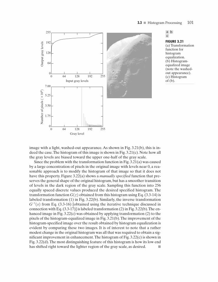
3.3 � Histogram Processing 101
255
192
128
64
00 64 128 192 255
Input gray levels
Out
put g
ray
leve
ls
7.00
5.25
3.50
1.75
00 64 128 192 255
Gray level
Num
ber
of p
ixel
s (*
104 )
FIGURE 3.21(a) Transformationfunction forhistogramequalization.(b) Histogram-equalized image(note the washed-out appearance).(c) Histogram of (b).
image with a light, washed-out appearance. As shown in Fig. 3.21(b), this is in-deed the case.The histogram of this image is shown in Fig. 3.21(c). Note how allthe gray levels are biased toward the upper one-half of the gray scale.
Since the problem with the transformation function in Fig. 3.21(a) was causedby a large concentration of pixels in the original image with levels near 0, a rea-sonable approach is to modify the histogram of that image so that it does nothave this property. Figure 3.22(a) shows a manually specified function that pre-serves the general shape of the original histogram, but has a smoother transitionof levels in the dark region of the gray scale. Sampling this function into 256equally spaced discrete values produced the desired specified histogram. Thetransformation function G(z) obtained from this histogram using Eq. (3.3-14) islabeled transformation (1) in Fig. 3.22(b). Similarly, the inverse transformationG–1(s) from Eq. (3.3-16) [obtained using the iterative technique discussed inconnection with Eq. (3.3-17)] is labeled transformation (2) in Fig. 3.22(b).The en-hanced image in Fig. 3.22(c) was obtained by applying transformation (2) to thepixels of the histogram-equalized image in Fig. 3.21(b).The improvement of thehistogram-specified image over the result obtained by histogram equalization isevident by comparing these two images. It is of interest to note that a rathermodest change in the original histogram was all that was required to obtain a sig-nificant improvement in enhancement.The histogram of Fig. 3.22(c) is shown inFig. 3.22(d).The most distinguishing feature of this histogram is how its low endhas shifted right toward the lighter region of the gray scale, as desired. �
a bc
GONZ03-075-146.II 29-08-2001 13:42 Page 101
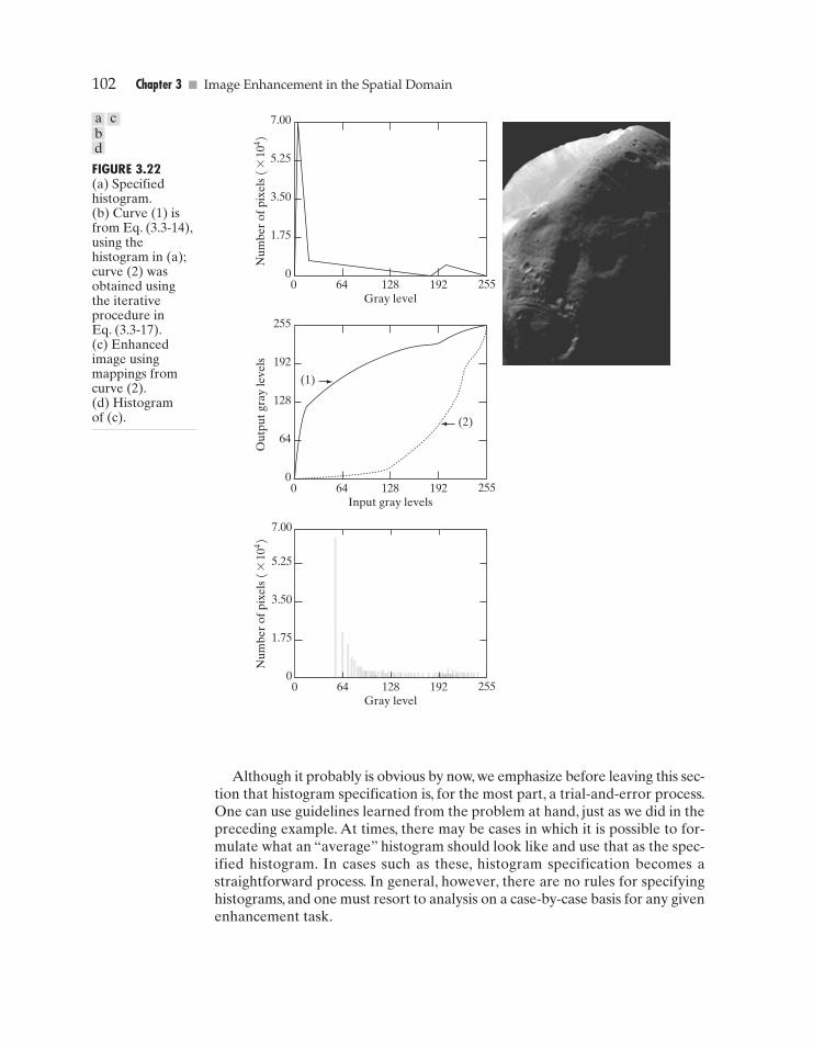
102 Chapter 3 � Image Enhancement in the Spatial Domain
7.00
5.25
3.50
1.75
00 64 128 192 255
Gray level
Num
ber
of p
ixel
s (*
104 )
255
192
128
64
00 64 128 192 255
Input gray levels
Out
put g
ray
leve
ls
(2)
(1)
7.00
5.25
3.50
1.75
00 64 128 192 255
Gray level
Num
ber
of p
ixel
s (*
104 )
FIGURE 3.22(a) Specifiedhistogram.(b) Curve (1) isfrom Eq. (3.3-14),using thehistogram in (a);curve (2) wasobtained usingthe iterativeprocedure inEq. (3.3-17).(c) Enhancedimage usingmappings fromcurve (2).(d) Histogram of (c).
Although it probably is obvious by now, we emphasize before leaving this sec-tion that histogram specification is, for the most part, a trial-and-error process.One can use guidelines learned from the problem at hand, just as we did in thepreceding example. At times, there may be cases in which it is possible to for-mulate what an “average” histogram should look like and use that as the spec-ified histogram. In cases such as these, histogram specification becomes astraightforward process. In general, however, there are no rules for specifyinghistograms, and one must resort to analysis on a case-by-case basis for any givenenhancement task.
a cbd
GONZ03-075-146.II 29-08-2001 13:42 Page 102
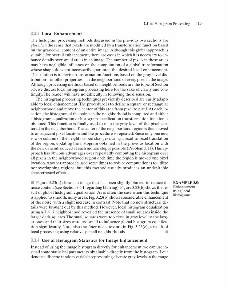
3.3 � Histogram Processing 103
3.3.3 Local EnhancementThe histogram processing methods discussed in the previous two sections areglobal, in the sense that pixels are modified by a transformation function basedon the gray-level content of an entire image. Although this global approach issuitable for overall enhancement, there are cases in which it is necessary to en-hance details over small areas in an image.The number of pixels in these areasmay have negligible influence on the computation of a global transformationwhose shape does not necessarily guarantee the desired local enhancement.The solution is to devise transformation functions based on the gray-level dis-tribution—or other properties—in the neighborhood of every pixel in the image.Although processing methods based on neighborhoods are the topic of Section3.5, we discuss local histogram processing here for the sake of clarity and con-tinuity. The reader will have no difficulty in following the discussion.
The histogram processing techniques previously described are easily adapt-able to local enhancement. The procedure is to define a square or rectangularneighborhood and move the center of this area from pixel to pixel. At each lo-cation, the histogram of the points in the neighborhood is computed and eithera histogram equalization or histogram specification transformation function isobtained. This function is finally used to map the gray level of the pixel cen-tered in the neighborhood.The center of the neighborhood region is then movedto an adjacent pixel location and the procedure is repeated. Since only one newrow or column of the neighborhood changes during a pixel-to-pixel translationof the region, updating the histogram obtained in the previous location withthe new data introduced at each motion step is possible (Problem 3.11).This ap-proach has obvious advantages over repeatedly computing the histogram overall pixels in the neighborhood region each time the region is moved one pixellocation.Another approach used some times to reduce computation is to utilizenonoverlapping regions, but this method usually produces an undesirablecheckerboard effect.
� Figure 3.23(a) shows an image that has been slightly blurred to reduce itsnoise content (see Section 3.6.1 regarding blurring). Figure 3.23(b) shows the re-sult of global histogram equalization. As is often the case when this techniqueis applied to smooth, noisy areas, Fig. 3.23(b) shows considerable enhancementof the noise, with a slight increase in contrast. Note that no new structural de-tails were brought out by this method. However, local histogram equalizationusing a 7*7 neighborhood revealed the presence of small squares inside thelarger dark squares. The small squares were too close in gray level to the larg-er ones, and their sizes were too small to influence global histogram equaliza-tion significantly. Note also the finer noise texture in Fig. 3.23(c), a result oflocal processing using relatively small neighborhoods. �
3.3.4 Use of Histogram Statistics for Image EnhancementInstead of using the image histogram directly for enhancement, we can use in-stead some statistical parameters obtainable directly from the histogram. Let rdenote a discrete random variable representing discrete gray-levels in the range
EXAMPLE 3.5:Enhancementusing localhistograms.
GONZ03-075-146.II 29-08-2001 13:42 Page 103
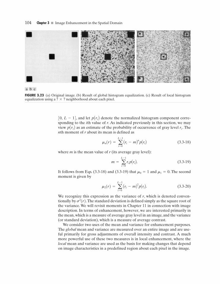
104 Chapter 3 � Image Enhancement in the Spatial Domain
FIGURE 3.23 (a) Original image. (b) Result of global histogram equalization. (c) Result of local histogramequalization using a 7*7 neighborhood about each pixel.
[0, L-1], and let p Ari B denote the normalized histogram component corre-sponding to the ith value of r. As indicated previously in this section, we mayview p Ari B as an estimate of the probability of occurrence of gray level ri . Thenth moment of r about its mean is defined as
(3.3-18)
where m is the mean value of r (its average gray level):
(3.3-19)
It follows from Eqs. (3.3-18) and (3.3-19) that m0=1 and m1=0. The secondmoment is given by
(3.3-20)
We recognize this expression as the variance of r, which is denoted conven-tionally by s2(r).The standard deviation is defined simply as the square root ofthe variance. We will revisit moments in Chapter 11 in connection with imagedescription. In terms of enhancement, however, we are interested primarily inthe mean, which is a measure of average gray level in an image, and the variance(or standard deviation), which is a measure of average contrast.
We consider two uses of the mean and variance for enhancement purposes.The global mean and variance are measured over an entire image and are use-ful primarily for gross adjustments of overall intensity and contrast. A muchmore powerful use of these two measures is in local enhancement, where thelocal mean and variance are used as the basis for making changes that dependon image characteristics in a predefined region about each pixel in the image.
m2(r) = aL - 1
i = 0Ari - mB2pAriB.
m = aL - 1
i = 0ri pAriB.
mn(r) = aL - 1
i = 0Ari - mBnpAriB
a b c
GONZ03-075-146.II 29-08-2001 13:42 Page 104
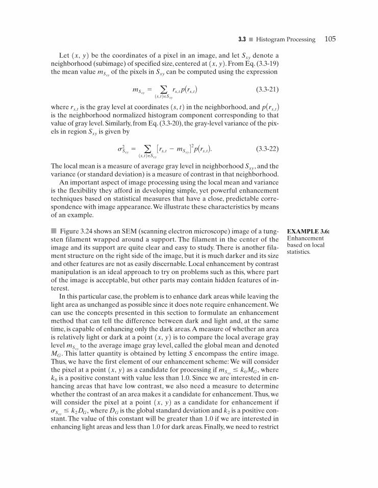
3.3 � Histogram Processing 105
Let (x, y) be the coordinates of a pixel in an image, and let Sxy denote aneighborhood (subimage) of specified size, centered at (x, y). From Eq. (3.3-19)the mean value of the pixels in Sxy can be computed using the expression
(3.3-21)
where rs, t is the gray level at coordinates (s, t) in the neighborhood, and p Ars, t Bis the neighborhood normalized histogram component corresponding to thatvalue of gray level. Similarly, from Eq. (3.3-20), the gray-level variance of the pix-els in region Sxy is given by
(3.3-22)
The local mean is a measure of average gray level in neighborhood Sxy , and thevariance (or standard deviation) is a measure of contrast in that neighborhood.
An important aspect of image processing using the local mean and varianceis the flexibility they afford in developing simple, yet powerful enhancementtechniques based on statistical measures that have a close, predictable corre-spondence with image appearance.We illustrate these characteristics by meansof an example.
� Figure 3.24 shows an SEM (scanning electron microscope) image of a tung-sten filament wrapped around a support. The filament in the center of theimage and its support are quite clear and easy to study. There is another fila-ment structure on the right side of the image, but it is much darker and its sizeand other features are not as easily discernable. Local enhancement by contrastmanipulation is an ideal approach to try on problems such as this, where partof the image is acceptable, but other parts may contain hidden features of in-terest.
In this particular case, the problem is to enhance dark areas while leaving thelight area as unchanged as possible since it does note require enhancement.Wecan use the concepts presented in this section to formulate an enhancementmethod that can tell the difference between dark and light and, at the sametime, is capable of enhancing only the dark areas.A measure of whether an areais relatively light or dark at a point (x, y) is to compare the local average graylevel to the average image gray level, called the global mean and denotedMG . This latter quantity is obtained by letting S encompass the entire image.Thus, we have the first element of our enhancement scheme: We will considerthe pixel at a point (x, y) as a candidate for processing if wherek0 is a positive constant with value less than 1.0. Since we are interested in en-hancing areas that have low contrast, we also need a measure to determinewhether the contrast of an area makes it a candidate for enhancement.Thus, wewill consider the pixel at a point (x, y) as a candidate for enhancement if
where DG is the global standard deviation and k2 is a positive con-stant. The value of this constant will be greater than 1.0 if we are interested inenhancing light areas and less than 1.0 for dark areas. Finally, we need to restrict
sSxy� k2 DG ,
mSxy� k0 MG ,
mSxy
s2Sxy
= a
(s, t)HSxy
Crs, t - mSxyD 2pArs, tB.
mSxy= a
(s, t)HSxy
rs, t pArs, tB
mSxy
EXAMPLE 3.6:Enhancementbased on localstatistics.
GONZ03-075-146.II 29-08-2001 13:42 Page 105
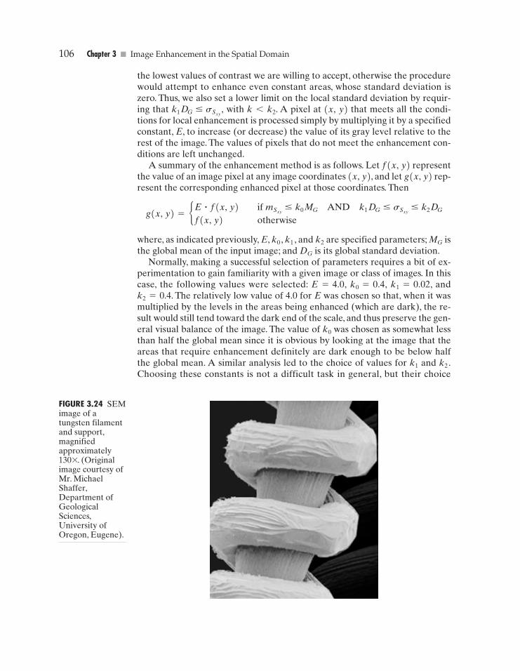
106 Chapter 3 � Image Enhancement in the Spatial Domain
the lowest values of contrast we are willing to accept, otherwise the procedurewould attempt to enhance even constant areas, whose standard deviation iszero. Thus, we also set a lower limit on the local standard deviation by requir-ing that with k<k2. A pixel at (x, y) that meets all the condi-tions for local enhancement is processed simply by multiplying it by a specifiedconstant, E, to increase (or decrease) the value of its gray level relative to therest of the image. The values of pixels that do not meet the enhancement con-ditions are left unchanged.
A summary of the enhancement method is as follows. Let f(x, y) representthe value of an image pixel at any image coordinates (x, y), and let g(x, y) rep-resent the corresponding enhanced pixel at those coordinates. Then
where, as indicated previously, E, k0 , k1 , and k2 are specified parameters; MG isthe global mean of the input image; and DG is its global standard deviation.
Normally, making a successful selection of parameters requires a bit of ex-perimentation to gain familiarity with a given image or class of images. In thiscase, the following values were selected: E=4.0, k0=0.4, k1=0.02, andk2=0.4. The relatively low value of 4.0 for E was chosen so that, when it wasmultiplied by the levels in the areas being enhanced (which are dark), the re-sult would still tend toward the dark end of the scale, and thus preserve the gen-eral visual balance of the image. The value of k0 was chosen as somewhat lessthan half the global mean since it is obvious by looking at the image that theareas that require enhancement definitely are dark enough to be below halfthe global mean. A similar analysis led to the choice of values for k1 and k2 .Choosing these constants is not a difficult task in general, but their choice
g(x, y) = bE � f(x, y)
f(x, y)
if mSxy� k0 MG AND k1 DG � sSxy
� k2 DG
otherwise
k1 DG � sSxy ,
FIGURE 3.24 SEMimage of atungsten filamentand support,magnifiedapproximately130*. (Originalimage courtesy ofMr. MichaelShaffer,Department ofGeologicalSciences,University ofOregon, Eugene).
GONZ03-075-146.II 29-08-2001 13:42 Page 106
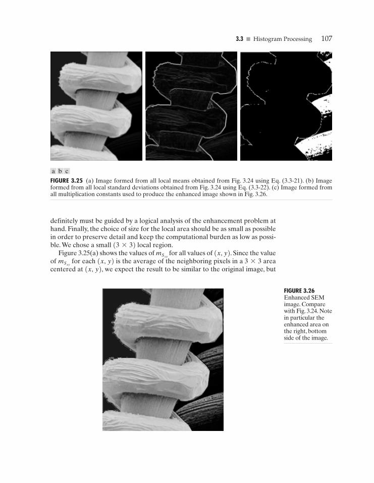
3.3 � Histogram Processing 107
FIGURE 3.25 (a) Image formed from all local means obtained from Fig. 3.24 using Eq. (3.3-21). (b) Imageformed from all local standard deviations obtained from Fig. 3.24 using Eq. (3.3-22). (c) Image formed fromall multiplication constants used to produce the enhanced image shown in Fig. 3.26.
definitely must be guided by a logical analysis of the enhancement problem athand. Finally, the choice of size for the local area should be as small as possiblein order to preserve detail and keep the computational burden as low as possi-ble. We chose a small (3*3) local region.
Figure 3.25(a) shows the values of for all values of (x, y). Since the valueof for each (x, y) is the average of the neighboring pixels in a 3*3 areacentered at (x, y), we expect the result to be similar to the original image, but
mSxy
mSxy
a b c
FIGURE 3.26Enhanced SEMimage. Comparewith Fig. 3.24. Notein particular theenhanced area onthe right, bottomside of the image.
GONZ03-075-146.II 29-08-2001 13:42 Page 107
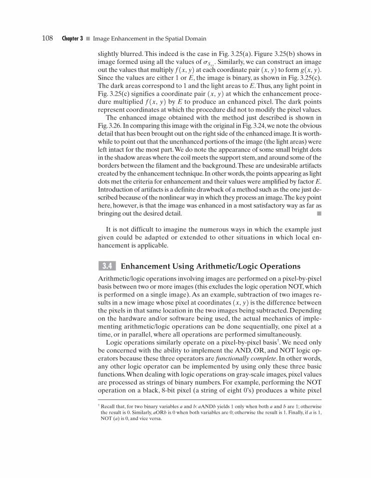
108 Chapter 3 � Image Enhancement in the Spatial Domain
slightly blurred. This indeed is the case in Fig. 3.25(a). Figure 3.25(b) shows inimage formed using all the values of Similarly, we can construct an imageout the values that multiply f(x, y) at each coordinate pair (x, y) to form g(x, y).Since the values are either 1 or E, the image is binary, as shown in Fig. 3.25(c).The dark areas correspond to 1 and the light areas to E.Thus, any light point inFig. 3.25(c) signifies a coordinate pair (x, y) at which the enhancement proce-dure multiplied f(x, y) by E to produce an enhanced pixel. The dark pointsrepresent coordinates at which the procedure did not to modify the pixel values.
The enhanced image obtained with the method just described is shown inFig.3.26. In comparing this image with the original in Fig.3.24,we note the obviousdetail that has been brought out on the right side of the enhanced image.It is worth-while to point out that the unenhanced portions of the image (the light areas) wereleft intact for the most part.We do note the appearance of some small bright dotsin the shadow areas where the coil meets the support stem,and around some of theborders between the filament and the background.These are undesirable artifactscreated by the enhancement technique.In other words,the points appearing as lightdots met the criteria for enhancement and their values were amplified by factor E.Introduction of artifacts is a definite drawback of a method such as the one just de-scribed because of the nonlinear way in which they process an image.The key pointhere, however, is that the image was enhanced in a most satisfactory way as far asbringing out the desired detail. �
It is not difficult to imagine the numerous ways in which the example justgiven could be adapted or extended to other situations in which local en-hancement is applicable.
Enhancement Using Arithmetic/Logic Operations
Arithmetic/logic operations involving images are performed on a pixel-by-pixelbasis between two or more images (this excludes the logic operation NOT, whichis performed on a single image). As an example, subtraction of two images re-sults in a new image whose pixel at coordinates (x, y) is the difference betweenthe pixels in that same location in the two images being subtracted. Dependingon the hardware and/or software being used, the actual mechanics of imple-menting arithmetic/logic operations can be done sequentially, one pixel at atime, or in parallel, where all operations are performed simultaneously.
Logic operations similarly operate on a pixel-by-pixel basis†. We need onlybe concerned with the ability to implement the AND, OR, and NOT logic op-erators because these three operators are functionally complete. In other words,any other logic operator can be implemented by using only these three basicfunctions.When dealing with logic operations on gray-scale images, pixel valuesare processed as strings of binary numbers. For example, performing the NOToperation on a black, 8-bit pixel (a string of eight 0’s) produces a white pixel
3.4
sSxy .
† Recall that, for two binary variables a and b: aANDb yields 1 only when both a and b are 1; otherwisethe result is 0. Similarly, aORb is 0 when both variables are 0; otherwise the result is 1. Finally, if a is 1,NOT (a) is 0, and vice versa.
GONZ03-075-146.II 29-08-2001 13:42 Page 108
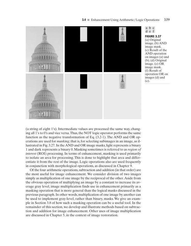
3.4 � Enhancement Using Arithmetic/Logic Operations 109
FIGURE 3.27(a) Originalimage. (b) ANDimage mask.(c) Result of theAND operationon images (a) and(b). (d) Originalimage. (e) ORimage mask.(f) Result ofoperation OR onimages (d) and(e).
(a string of eight 1’s). Intermediate values are processed the same way, chang-ing all 1’s to 0’s and vice versa.Thus, the NOT logic operator performs the samefunction as the negative transformation of Eq. (3.2-1). The AND and OR op-erations are used for masking; that is, for selecting subimages in an image, as il-lustrated in Fig. 3.27. In the AND and OR image masks, light represents a binary1 and dark represents a binary 0. Masking sometimes is referred to as region ofinterest (ROI) processing. In terms of enhancement, masking is used primarilyto isolate an area for processing. This is done to highlight that area and differ-entiate it from the rest of the image. Logic operations also are used frequentlyin conjunction with morphological operations, as discussed in Chapter 9.
Of the four arithmetic operations, subtraction and addition (in that order) arethe most useful for image enhancement. We consider division of two imagessimply as multiplication of one image by the reciprocal of the other.Aside fromthe obvious operation of multiplying an image by a constant to increase its av-erage gray level, image multiplication finds use in enhancement primarily as amasking operation that is more general than the logical masks discussed in theprevious paragraph. In other words, multiplication of one image by another canbe used to implement gray-level, rather than binary, masks. We give an exam-ple in Section 3.8 of how such a masking operation can be a useful tool. In theremainder of this section, we develop and illustrate methods based on subtrac-tion and addition for image enhancement. Other uses of image multiplicationare discussed in Chapter 5, in the context of image restoration.
a b cd e f
GONZ03-075-146.II 29-08-2001 13:42 Page 109
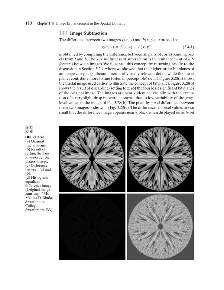
110 Chapter 3 � Image Enhancement in the Spatial Domain
FIGURE 3.28(a) Originalfractal image.(b) Result ofsetting the fourlower-order bitplanes to zero.(c) Differencebetween (a) and(b).(d) Histogram-equalizeddifference image.(Original imagecourtesy of Ms.Melissa D. Binde,SwarthmoreCollege,Swarthmore, PA).
3.4.1 Image SubtractionThe difference between two images f(x, y) and h(x, y), expressed as
(3.4-1)
is obtained by computing the difference between all pairs of corresponding pix-els from f and h. The key usefulness of subtraction is the enhancement of dif-ferences between images. We illustrate this concept by returning briefly to thediscussion in Section 3.2.4, where we showed that the higher-order bit planes ofan image carry a significant amount of visually relevant detail, while the lowerplanes contribute more to fine (often imperceptible) detail. Figure 3.28(a) showsthe fractal image used earlier to illustrate the concept of bit planes. Figure 3.28(b)shows the result of discarding (setting to zero) the four least significant bit planesof the original image. The images are nearly identical visually, with the excep-tion of a very slight drop in overall contrast due to less variability of the gray-level values in the image of Fig. 3.28(b). The pixel-by-pixel difference betweenthese two images is shown in Fig. 3.28(c). The differences in pixel values are sosmall that the difference image appears nearly black when displayed on an 8-bit
g(x, y) = f(x, y) - h(x, y),
a bc d
GONZ03-075-146.II 29-08-2001 13:42 Page 110
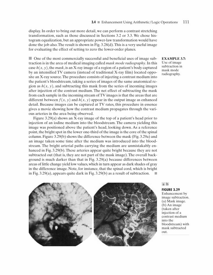
3.4 � Enhancement Using Arithmetic/Logic Operations 111
display. In order to bring out more detail, we can perform a contrast stretchingtransformation, such as those discussed in Sections 3.2 or 3.3. We chose his-togram equalization, but an appropriate power-law transformation would havedone the job also.The result is shown in Fig. 3.28(d).This is a very useful imagefor evaluating the effect of setting to zero the lower-order planes.
� One of the most commercially successful and beneficial uses of image sub-traction is in the area of medical imaging called mask mode radiography. In thiscase h(x, y), the mask, is an X-ray image of a region of a patient’s body capturedby an intensified TV camera (instead of traditional X-ray film) located oppo-site an X-ray source.The procedure consists of injecting a contrast medium intothe patient’s bloodstream, taking a series of images of the same anatomical re-gion as h(x, y), and subtracting this mask from the series of incoming imagesafter injection of the contrast medium. The net effect of subtracting the maskfrom each sample in the incoming stream of TV images is that the areas that aredifferent between f(x, y) and h(x, y) appear in the output image as enhanceddetail. Because images can be captured at TV rates, this procedure in essencegives a movie showing how the contrast medium propagates through the vari-ous arteries in the area being observed.
Figure 3.29(a) shows an X-ray image of the top of a patient’s head prior toinjection of an iodine medium into the bloodstream. The camera yielding thisimage was positioned above the patient’s head, looking down. As a referencepoint, the bright spot in the lower one-third of the image is the core of the spinalcolumn. Figure 3.29(b) shows the difference between the mask (Fig. 3.29a) andan image taken some time after the medium was introduced into the blood-stream. The bright arterial paths carrying the medium are unmistakably en-hanced in Fig. 3.29(b). These arteries appear quite bright because they are notsubtracted out (that is, they are not part of the mask image). The overall back-ground is much darker than that in Fig. 3.29(a) because differences betweenareas of little change yield low values, which in turn appear as dark shades of grayin the difference image. Note, for instance, that the spinal cord, which is brightin Fig. 3.29(a), appears quite dark in Fig. 3.29(b) as a result of subtraction. �
EXAMPLE 3.7:Use of imagesubtraction inmask moderadiography.
FIGURE 3.29Enhancement byimage subtraction.(a) Mask image.(b) An image(taken afterinjection of acontrast mediuminto thebloodstream) withmask subtractedout.
a b
GONZ03-075-146.II 29-08-2001 13:42 Page 111
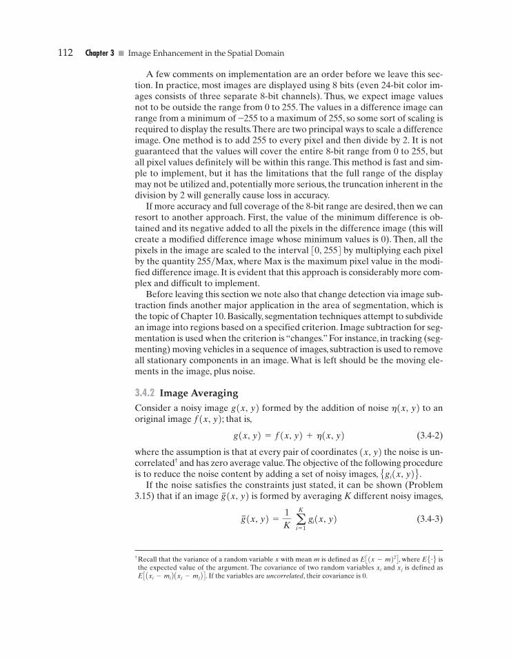
112 Chapter 3 � Image Enhancement in the Spatial Domain
† Recall that the variance of a random variable x with mean m is defined as E C(x-m)2 D , where EE�F isthe expected value of the argument. The covariance of two random variables xi and xj is defined asE C Axi-mi B Axj-mj B D . If the variables are uncorrelated, their covariance is 0.
A few comments on implementation are an order before we leave this sec-tion. In practice, most images are displayed using 8 bits (even 24-bit color im-ages consists of three separate 8-bit channels). Thus, we expect image valuesnot to be outside the range from 0 to 255. The values in a difference image canrange from a minimum of –255 to a maximum of 255, so some sort of scaling isrequired to display the results.There are two principal ways to scale a differenceimage. One method is to add 255 to every pixel and then divide by 2. It is notguaranteed that the values will cover the entire 8-bit range from 0 to 255, butall pixel values definitely will be within this range. This method is fast and sim-ple to implement, but it has the limitations that the full range of the displaymay not be utilized and, potentially more serious, the truncation inherent in thedivision by 2 will generally cause loss in accuracy.
If more accuracy and full coverage of the 8-bit range are desired, then we canresort to another approach. First, the value of the minimum difference is ob-tained and its negative added to all the pixels in the difference image (this willcreate a modified difference image whose minimum values is 0). Then, all thepixels in the image are scaled to the interval [0, 255] by multiplying each pixelby the quantity 255�Max, where Max is the maximum pixel value in the modi-fied difference image. It is evident that this approach is considerably more com-plex and difficult to implement.
Before leaving this section we note also that change detection via image sub-traction finds another major application in the area of segmentation, which isthe topic of Chapter 10. Basically, segmentation techniques attempt to subdividean image into regions based on a specified criterion. Image subtraction for seg-mentation is used when the criterion is “changes.” For instance, in tracking (seg-menting) moving vehicles in a sequence of images, subtraction is used to removeall stationary components in an image. What is left should be the moving ele-ments in the image, plus noise.
3.4.2 Image AveragingConsider a noisy image g(x, y) formed by the addition of noise h(x, y) to anoriginal image f(x, y); that is,
(3.4-2)
where the assumption is that at every pair of coordinates (x, y) the noise is un-correlated† and has zero average value.The objective of the following procedureis to reduce the noise content by adding a set of noisy images, Egi(x, y)F .
If the noise satisfies the constraints just stated, it can be shown (Problem3.15) that if an image is formed by averaging K different noisy images,
(3.4-3)g–(x, y) =1K
aK
i = 1gi(x, y)
g–(x, y)
g(x, y) = f(x, y) + h(x, y)
GONZ03-075-146.II 29-08-2001 13:43 Page 112
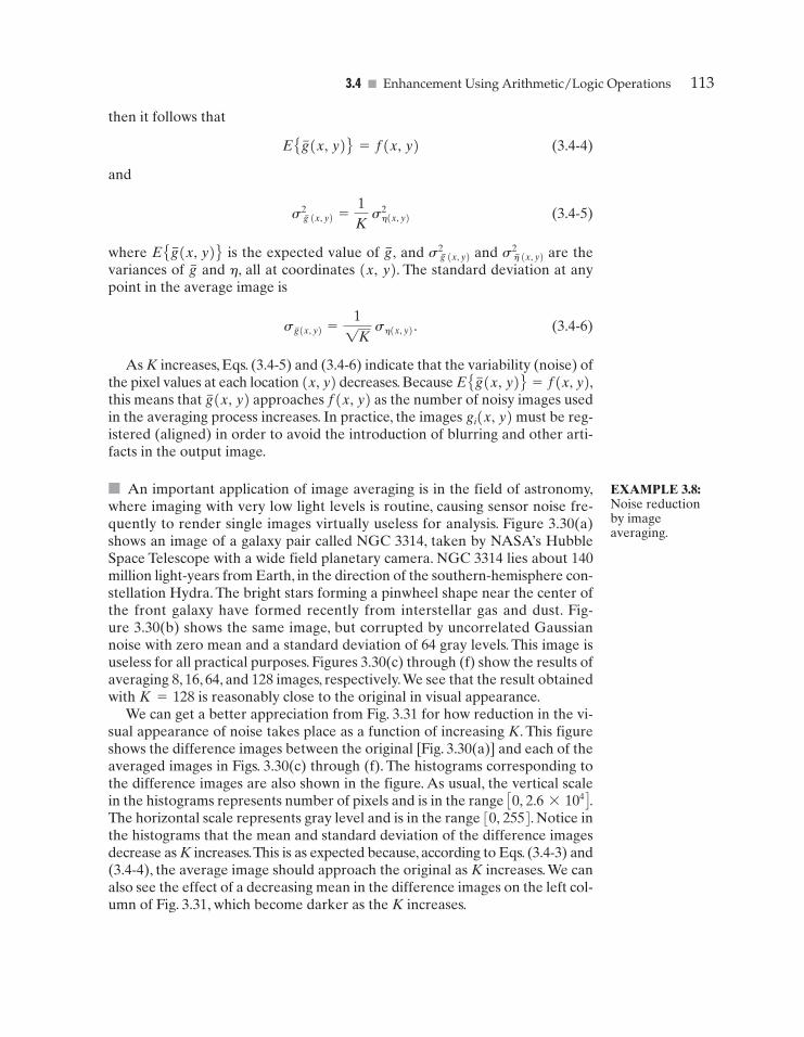
3.4 � Enhancement Using Arithmetic/Logic Operations 113
then it follows that
(3.4-4)
and
(3.4-5)
where is the expected value of and and are thevariances of and h, all at coordinates (x, y). The standard deviation at anypoint in the average image is
(3.4-6)
As K increases, Eqs. (3.4-5) and (3.4-6) indicate that the variability (noise) ofthe pixel values at each location (x, y) decreases. Because = f(x, y),this means that approaches f(x, y) as the number of noisy images usedin the averaging process increases. In practice, the images gi(x, y) must be reg-istered (aligned) in order to avoid the introduction of blurring and other arti-facts in the output image.
� An important application of image averaging is in the field of astronomy,where imaging with very low light levels is routine, causing sensor noise fre-quently to render single images virtually useless for analysis. Figure 3.30(a)shows an image of a galaxy pair called NGC 3314, taken by NASA’s HubbleSpace Telescope with a wide field planetary camera. NGC 3314 lies about 140million light-years from Earth, in the direction of the southern-hemisphere con-stellation Hydra. The bright stars forming a pinwheel shape near the center ofthe front galaxy have formed recently from interstellar gas and dust. Fig-ure 3.30(b) shows the same image, but corrupted by uncorrelated Gaussiannoise with zero mean and a standard deviation of 64 gray levels. This image isuseless for all practical purposes. Figures 3.30(c) through (f) show the results ofaveraging 8, 16, 64, and 128 images, respectively.We see that the result obtainedwith K=128 is reasonably close to the original in visual appearance.
We can get a better appreciation from Fig. 3.31 for how reduction in the vi-sual appearance of noise takes place as a function of increasing K. This figureshows the difference images between the original [Fig. 3.30(a)] and each of theaveraged images in Figs. 3.30(c) through (f). The histograms corresponding tothe difference images are also shown in the figure. As usual, the vertical scalein the histograms represents number of pixels and is in the range C0, 2.6*104 D .The horizontal scale represents gray level and is in the range [0, 255]. Notice inthe histograms that the mean and standard deviation of the difference imagesdecrease as K increases.This is as expected because, according to Eqs. (3.4-3) and(3.4-4), the average image should approach the original as K increases. We canalso see the effect of a decreasing mean in the difference images on the left col-umn of Fig. 3.31, which become darker as the K increases.
g–(x, y)EEg–(x, y)F
sg–(x, y) =11K
sh(x, y) .
g–s2h– (x, y)s2
g– (x, y)g–,EEg–(x, y)F
s2g– (x, y) =
1K
s2h(x, y)
EEg–(x, y)F = f(x, y)
EXAMPLE 3.8:Noise reductionby imageaveraging.
GONZ03-075-146.II 29-08-2001 13:43 Page 113
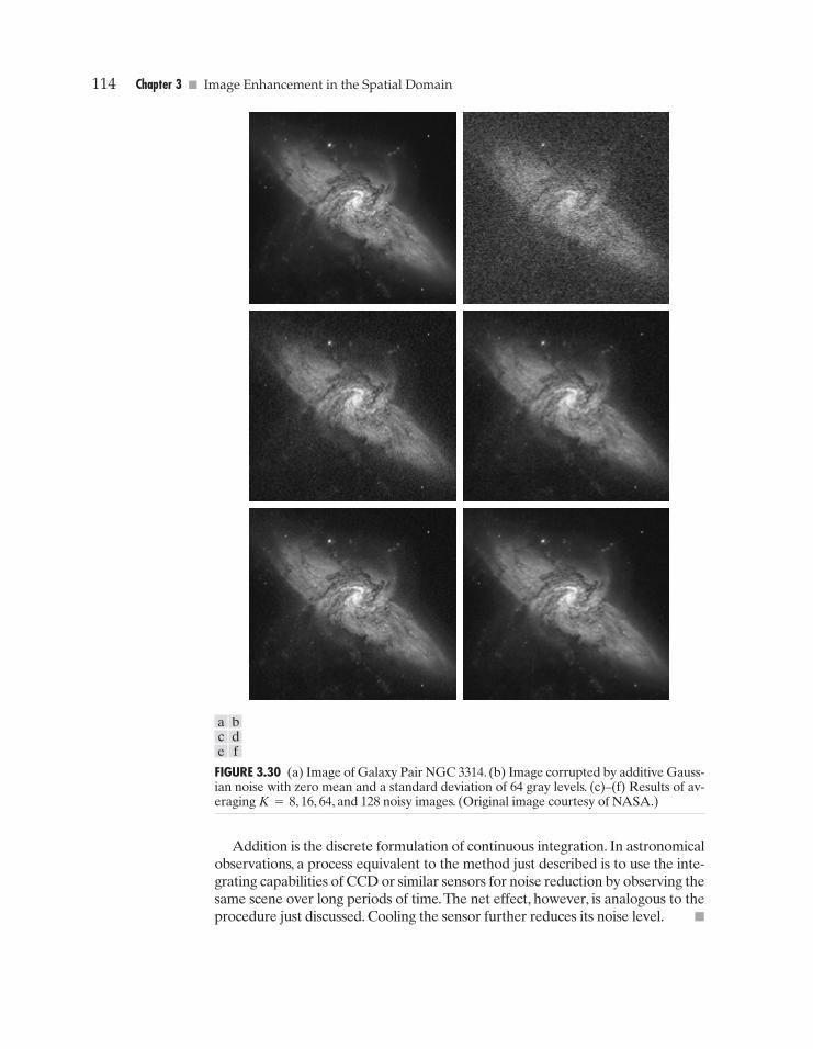
114 Chapter 3 � Image Enhancement in the Spatial Domain
FIGURE 3.30 (a) Image of Galaxy Pair NGC 3314. (b) Image corrupted by additive Gauss-ian noise with zero mean and a standard deviation of 64 gray levels. (c)–(f) Results of av-eraging K=8, 16, 64, and 128 noisy images. (Original image courtesy of NASA.)
Addition is the discrete formulation of continuous integration. In astronomicalobservations, a process equivalent to the method just described is to use the inte-grating capabilities of CCD or similar sensors for noise reduction by observing thesame scene over long periods of time.The net effect, however, is analogous to theprocedure just discussed. Cooling the sensor further reduces its noise level. �
a bce
df
GONZ03-075-146.II 29-08-2001 13:43 Page 114
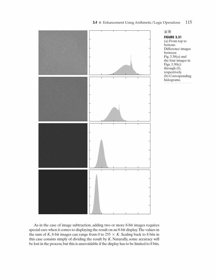
3.4 � Enhancement Using Arithmetic/Logic Operations 115
FIGURE 3.31(a) From top tobottom:Difference imagesbetweenFig. 3.30(a) andthe four images inFigs. 3.30(c)through (f),respectively.(b) Correspondinghistograms.
As in the case of image subtraction, adding two or more 8-bit images requiresspecial care when it comes to displaying the result on an 8-bit display.The values inthe sum of K, 8-bit images can range from 0 to 255*K. Scaling back to 8 bits inthis case consists simply of dividing the result by K. Naturally, some accuracy willbe lost in the process,but this is unavoidable if the display has to be limited to 8 bits.
a b
GONZ03-075-146.II 29-08-2001 13:43 Page 115
116 Chapter 3 � Image Enhancement in the Spatial Domain
It is possible in some implementations of image averaging to have negativevalues when noise is added to an image. In fact, in the example just given, thiswas precisely the case because Gaussian random variables with zero mean andnonzero variance have negative as well as positive values.The images in the ex-ample were scaled using the second scaling method discussed at the end of theprevious section. That is, the minimum value in a given average image was ob-tained and its negative was added to the image. Then all the pixels in the mod-ified image were scaled to the range [0, 255] by multiplying each pixel in themodified image by the quantity 255�Max, where Max was the maximum pixelvalue in that image.
Basics of Spatial Filtering
As mentioned in Section 3.1, some neighborhood operations work with the val-ues of the image pixels in the neighborhood and the corresponding values of asubimage that has the same dimensions as the neighborhood. The subimage iscalled a filter, mask, kernel, template, or window, with the first three terms beingthe most prevalent terminology. The values in a filter subimage are referred toas coefficients, rather than pixels.
The concept of filtering has its roots in the use of the Fourier transform forsignal processing in the so-called frequency domain. This topic is discussed inmore detail in Chapter 4. In the present chapter, we are interested in filteringoperations that are performed directly on the pixels of an image. We use theterm spatial filtering to differentiate this type of process from the more tradi-tional frequency domain filtering.
The mechanics of spatial filtering are illustrated in Fig. 3.32. The process con-sists simply of moving the filter mask from point to point in an image. At eachpoint (x, y), the response of the filter at that point is calculated using a prede-fined relationship. For linear spatial filtering (see Section 2.6 regarding linear-ity), the response is given by a sum of products of the filter coefficients and thecorresponding image pixels in the area spanned by the filter mask. For the 3*3mask shown in Fig. 3.32, the result (or response), R, of linear filtering with thefilter mask at a point (x, y) in the image is
which we see is the sum of products of the mask coefficients with the corre-sponding pixels directly under the mask. Note in particular that the coefficientw(0, 0) coincides with image value f(x, y), indicating that the mask is centeredat (x, y) when the computation of the sum of products takes place. For a maskof size m*n, we assume that m=2a+1 and n=2b+1, where a and b arenonnegative integers. All this says is that our focus in the following discussionwill be on masks of odd sizes, with the smallest meaningful size being 3*3 (weexclude from our discussion the trivial case of a 1*1 mask).
+ w(0, 0)f(x, y) + p + w(1, 0)f(x + 1, y) + w(1, 1)f(x + 1, y + 1),
R = w(-1, -1)f(x - 1, y - 1) + w(-1, 0)f(x - 1, y) + p
3.5
GONZ03-075-146.II 29-08-2001 13:43 Page 116
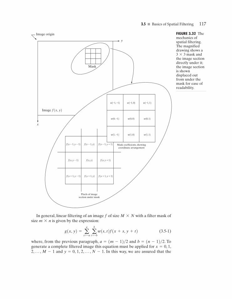
3.5 � Basics of Spatial Filtering 117
y
x
Image origin
Mask
Image f(x, y)
w(–1, –1)
f(x-1, y-1) f(x-1, y) f(x-1, y+1)
f(x, y-1) f(x, y) f(x, y+1)
f(x+1, y-1) f(x+1, y) f(x+1, y+1)
w(–1, 0) w(–1, 1)
w(0, –1) w(0, 0) w(0, 1)
w(1, –1) w(1, 0) w(1, 1)
Mask coefficients, showingcoordinate arrangement
Pixels of imagesection under mask
FIGURE 3.32 Themechanics ofspatial filtering.The magnifieddrawing shows a3*3 mask andthe image sectiondirectly under it;the image sectionis showndisplaced outfrom under themask for ease ofreadability.
In general, linear filtering of an image f of size M*N with a filter mask ofsize m*n is given by the expression:
(3.5-1)
where, from the previous paragraph, a=(m-1)�2 and b=(n-1)�2. Togenerate a complete filtered image this equation must be applied for x=0, 1,2, p , M-1 and y=0, 1, 2, p , N-1. In this way, we are assured that the
g(x, y) = aa
s = -a a
b
t = -bw(s, t)f(x + s, y + t)
GONZ03-075-146.II 29-08-2001 13:43 Page 117
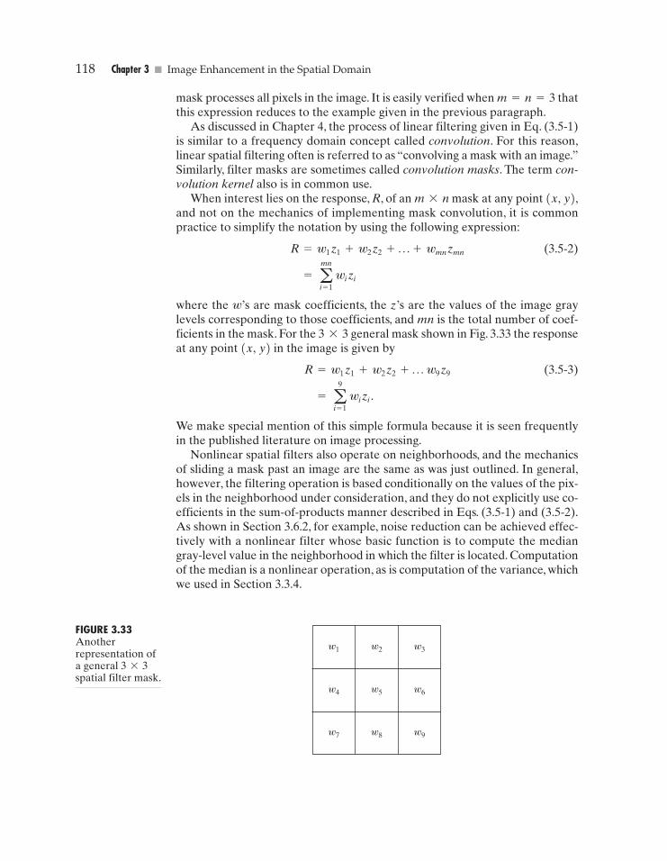
118 Chapter 3 � Image Enhancement in the Spatial Domain
mask processes all pixels in the image. It is easily verified when m=n=3 thatthis expression reduces to the example given in the previous paragraph.
As discussed in Chapter 4, the process of linear filtering given in Eq. (3.5-1)is similar to a frequency domain concept called convolution. For this reason,linear spatial filtering often is referred to as “convolving a mask with an image.”Similarly, filter masks are sometimes called convolution masks. The term con-volution kernel also is in common use.
When interest lies on the response, R, of an m*n mask at any point (x, y),and not on the mechanics of implementing mask convolution, it is commonpractice to simplify the notation by using the following expression:
(3.5-2)
where the w’s are mask coefficients, the z’s are the values of the image graylevels corresponding to those coefficients, and mn is the total number of coef-ficients in the mask. For the 3*3 general mask shown in Fig. 3.33 the responseat any point (x, y) in the image is given by
(3.5-3)
We make special mention of this simple formula because it is seen frequentlyin the published literature on image processing.
Nonlinear spatial filters also operate on neighborhoods, and the mechanicsof sliding a mask past an image are the same as was just outlined. In general,however, the filtering operation is based conditionally on the values of the pix-els in the neighborhood under consideration, and they do not explicitly use co-efficients in the sum-of-products manner described in Eqs. (3.5-1) and (3.5-2).As shown in Section 3.6.2, for example, noise reduction can be achieved effec-tively with a nonlinear filter whose basic function is to compute the mediangray-level value in the neighborhood in which the filter is located. Computationof the median is a nonlinear operation, as is computation of the variance, whichwe used in Section 3.3.4.
= a9
i = 1wi zi .
R = w1 z1 + w2 z2 + p w9 z9
= amn
i = 1wi zi
R = w1 z1 + w2 z2 + p + wmn zmn
w1 w2 w3
w4 w5 w6
w7 w8 w9
FIGURE 3.33Anotherrepresentation ofa general 3*3spatial filter mask.
GONZ03-075-146.II 29-08-2001 13:43 Page 118
3.6 � Smoothing Spatial Filters 119
An important consideration in implementing neighborhood operations forspatial filtering is the issue of what happens when the center of the filter ap-proaches the border of the image. Consider for simplicity a square mask of sizen*n. At least one edge of such a mask will coincide with the border of theimage when the center of the mask is at a distance of (n-1)�2 pixels awayfrom the border of the image. If the center of the mask moves any closer to theborder, one or more rows or columns of the mask will be located outside theimage plane. There are several ways to handle this situation. The simplest is tolimit the excursions of the center of the mask to be at a distance no less than(n-1)�2 pixels from the border. The resulting filtered image will be smallerthan the original, but all the pixels in the filtered imaged will have beenprocessed with the full mask. If the result is required to be the same size as theoriginal, then the approach typically employed is to filter all pixels only with thesection of the mask that is fully contained in the image. With this approach,there will be bands of pixels near the border that will have been processed witha partial filter mask. Other approaches include “padding” the image by addingrows and columns of 0’s (or other constant gray level), or padding by replicat-ing rows or columns.The padding is then stripped off at the end of the process.This keeps the size of the filtered image the same as the original, but the valuesof the padding will have an effect near the edges that becomes more prevalentas the size of the mask increases.The only way to obtain a perfectly filtered re-sult is to accept a somewhat smaller filtered image by limiting the excursions ofthe center of the filter mask to a distance no less than (n-1)�2 pixels from theborder of the original image.
Smoothing Spatial Filters
Smoothing filters are used for blurring and for noise reduction. Blurring is usedin preprocessing steps, such as removal of small details from an image prior to(large) object extraction, and bridging of small gaps in lines or curves. Noisereduction can be accomplished by blurring with a linear filter and also by non-linear filtering.
3.6.1 Smoothing Linear FiltersThe output (response) of a smoothing, linear spatial filter is simply the averageof the pixels contained in the neighborhood of the filter mask. These filterssometimes are called averaging filters. For reasons explained in Chapter 4, theyalso are referred to a lowpass filters.
The idea behind smoothing filters is straightforward. By replacing the valueof every pixel in an image by the average of the gray levels in the neighbor-hood defined by the filter mask, this process results in an image with reduced“sharp” transitions in gray levels. Because random noise typically consists ofsharp transitions in gray levels, the most obvious application of smoothing isnoise reduction. However, edges (which almost always are desirable features ofan image) also are characterized by sharp transitions in gray levels, so averag-ing filters have the undesirable side effect that they blur edges. Another appli-cation of this type of process includes the smoothing of false contours that result
3.6
GONZ03-075-146.II 29-08-2001 13:43 Page 119
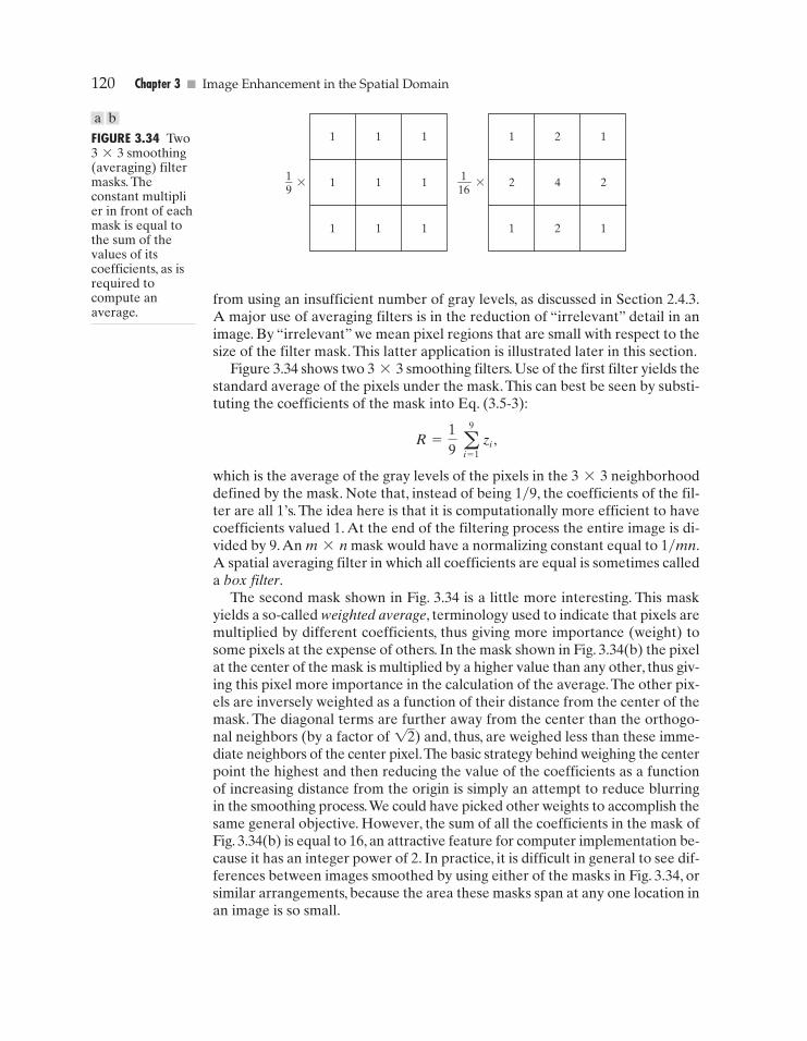
120 Chapter 3 � Image Enhancement in the Spatial Domain
1 1 1
119–* 1
16––*1 1
1 1 1
1 2 1
2 4 2
1 2 1
FIGURE 3.34 Two3*3 smoothing(averaging) filtermasks. Theconstant multiplier in front of eachmask is equal tothe sum of thevalues of itscoefficients, as isrequired tocompute anaverage.
from using an insufficient number of gray levels, as discussed in Section 2.4.3.A major use of averaging filters is in the reduction of “irrelevant” detail in animage. By “irrelevant” we mean pixel regions that are small with respect to thesize of the filter mask. This latter application is illustrated later in this section.
Figure 3.34 shows two 3*3 smoothing filters. Use of the first filter yields thestandard average of the pixels under the mask.This can best be seen by substi-tuting the coefficients of the mask into Eq. (3.5-3):
which is the average of the gray levels of the pixels in the 3*3 neighborhooddefined by the mask. Note that, instead of being 1�9, the coefficients of the fil-ter are all 1’s. The idea here is that it is computationally more efficient to havecoefficients valued 1. At the end of the filtering process the entire image is di-vided by 9.An m*n mask would have a normalizing constant equal to 1�mn.A spatial averaging filter in which all coefficients are equal is sometimes calleda box filter.
The second mask shown in Fig. 3.34 is a little more interesting. This maskyields a so-called weighted average, terminology used to indicate that pixels aremultiplied by different coefficients, thus giving more importance (weight) tosome pixels at the expense of others. In the mask shown in Fig. 3.34(b) the pixelat the center of the mask is multiplied by a higher value than any other, thus giv-ing this pixel more importance in the calculation of the average.The other pix-els are inversely weighted as a function of their distance from the center of themask. The diagonal terms are further away from the center than the orthogo-nal neighbors (by a factor of ) and, thus, are weighed less than these imme-diate neighbors of the center pixel.The basic strategy behind weighing the centerpoint the highest and then reducing the value of the coefficients as a functionof increasing distance from the origin is simply an attempt to reduce blurringin the smoothing process.We could have picked other weights to accomplish thesame general objective. However, the sum of all the coefficients in the mask ofFig. 3.34(b) is equal to 16, an attractive feature for computer implementation be-cause it has an integer power of 2. In practice, it is difficult in general to see dif-ferences between images smoothed by using either of the masks in Fig. 3.34, orsimilar arrangements, because the area these masks span at any one location inan image is so small.
12
R =19
a9
i = 1zi ,
a b
GONZ03-075-146.II 29-08-2001 13:43 Page 120
3.6 � Smoothing Spatial Filters 121
With reference to Eq. (3.5-1), the general implementation for filtering anM*N image with a weighted averaging filter of size m*n (m and n odd) isgiven by the expression
(3.6-1)
The parameters in this equation are as defined in Eq. (3.5-1). As before, it isunderstood that the complete filtered image is obtained by applying Eq. (3.6-1)for x=0, 1, 2, p , M-1 and y=0, 1, 2, p , N-1. The denominator inEq. (3.6-1) is simply the sum of the mask coefficients and, therefore, it is a con-stant that needs to be computed only once.Typically, this scale factor is appliedto all the pixels of the output image after the filtering process is completed.
� The effects of smoothing as a function of filter size are illustrated in Fig. 3.35,which shows an original image and the corresponding smoothed results obtainedusing square averaging filters of sizes n=3, 5, 9, 15, and 35 pixels, respectively.The principal features of these results are as follows: For n=3, we note a gen-eral slight blurring throughout the entire image but, as expected, details thatare of approximately the same size as the filter mask are affected considerablymore. For example, the 3*3 and 5*5 squares, the small letter “a,” and the finegrain noise show significant blurring when compared to the rest of the image.Apositive result is that the noise is less pronounced. Note that the jagged bordersof the characters and gray circles have been pleasingly smoothed.
The result for n=5 is somewhat similar, with a slight further increase inblurring. For n=9 we see considerably more blurring, and the 20% black cir-cle is not nearly as distinct from the background as in the previous three images,illustrating the blending effect that blurring has on objects whose gray levelcontent is close to that of its neighboring pixels. Note the significant furthersmoothing of the noisy rectangles. The results for n=15 and 35 are extremewith respect to the sizes of the objects in the image.This type of excessive blur-ring is generally used to eliminate small objects from an image. For instance, thethree small squares, two of the circles, and most of the noisy rectangle areashave been blended into the background of the image in Fig. 3.35(f). Note alsoin this figure the pronounced black border. This is a result of padding the bor-der of the original image with 0’s (black) and then trimming off the paddedarea. Some of the black was blended into all filtered images, but became trulyobjectionable for the images smoothed with the larger filters. �
As mentioned earlier, an important application of spatial averaging is to bluran image for the purpose getting a gross representation of objects of interest,such that the intensity of smaller objects blends with the background and larg-er objects become “bloblike” and easy to detect. The size of the mask estab-lishes the relative size of the objects that will be blended with the background.As an illustration, consider Fig. 3.36(a), which is an image from the Hubble tele-scope in orbit around the Earth. Figure 3.36(b) shows the result of applying a
g(x, y) =a
a
s = -a a
b
t = -bw(s, t)f(x + s, y + t)
aa
s = -a a
b
t = -bw(s, t)
EXAMPLE 3.9:Image smoothingwith masks ofvarious sizes.
GONZ03-075-146.II 29-08-2001 13:43 Page 121
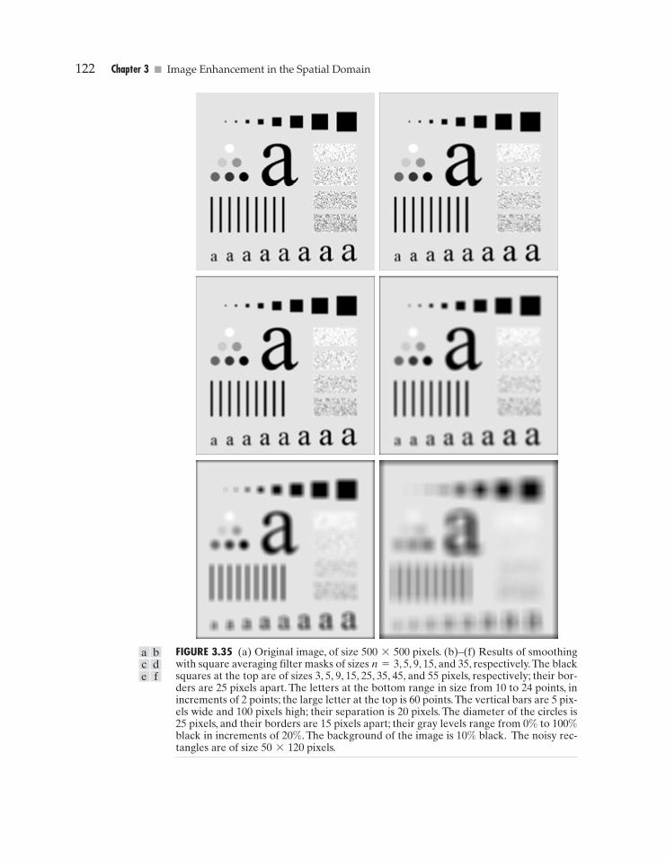
122 Chapter 3 � Image Enhancement in the Spatial Domain
FIGURE 3.35 (a) Original image, of size 500*500 pixels. (b)–(f) Results of smoothingwith square averaging filter masks of sizes n=3, 5, 9, 15, and 35, respectively.The blacksquares at the top are of sizes 3, 5, 9, 15, 25, 35, 45, and 55 pixels, respectively; their bor-ders are 25 pixels apart. The letters at the bottom range in size from 10 to 24 points, inincrements of 2 points; the large letter at the top is 60 points.The vertical bars are 5 pix-els wide and 100 pixels high; their separation is 20 pixels. The diameter of the circles is25 pixels, and their borders are 15 pixels apart; their gray levels range from 0% to 100%black in increments of 20%. The background of the image is 10% black. The noisy rec-tangles are of size 50*120 pixels.
a bce
df
GONZ03-075-146.II 29-08-2001 13:43 Page 122
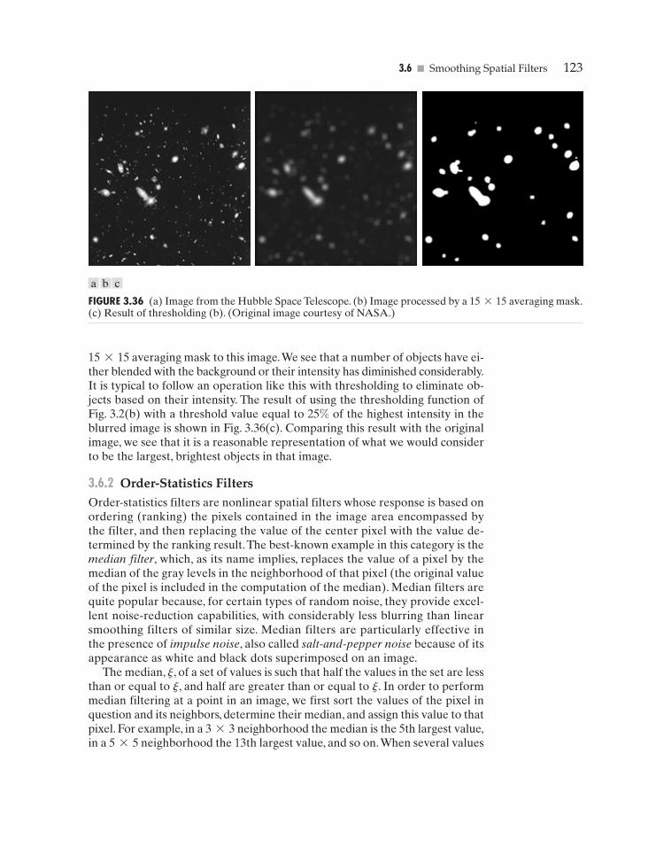
3.6 � Smoothing Spatial Filters 123
FIGURE 3.36 (a) Image from the Hubble Space Telescope. (b) Image processed by a 15*15 averaging mask.(c) Result of thresholding (b). (Original image courtesy of NASA.)
15*15 averaging mask to this image.We see that a number of objects have ei-ther blended with the background or their intensity has diminished considerably.It is typical to follow an operation like this with thresholding to eliminate ob-jects based on their intensity. The result of using the thresholding function ofFig. 3.2(b) with a threshold value equal to 25% of the highest intensity in theblurred image is shown in Fig. 3.36(c). Comparing this result with the originalimage, we see that it is a reasonable representation of what we would considerto be the largest, brightest objects in that image.
3.6.2 Order-Statistics FiltersOrder-statistics filters are nonlinear spatial filters whose response is based onordering (ranking) the pixels contained in the image area encompassed bythe filter, and then replacing the value of the center pixel with the value de-termined by the ranking result.The best-known example in this category is themedian filter, which, as its name implies, replaces the value of a pixel by themedian of the gray levels in the neighborhood of that pixel (the original valueof the pixel is included in the computation of the median). Median filters arequite popular because, for certain types of random noise, they provide excel-lent noise-reduction capabilities, with considerably less blurring than linearsmoothing filters of similar size. Median filters are particularly effective inthe presence of impulse noise, also called salt-and-pepper noise because of itsappearance as white and black dots superimposed on an image.
The median, j, of a set of values is such that half the values in the set are lessthan or equal to j, and half are greater than or equal to j. In order to performmedian filtering at a point in an image, we first sort the values of the pixel inquestion and its neighbors, determine their median, and assign this value to thatpixel. For example, in a 3*3 neighborhood the median is the 5th largest value,in a 5*5 neighborhood the 13th largest value, and so on.When several values
a b c
GONZ03-075-146.II 29-08-2001 13:43 Page 123
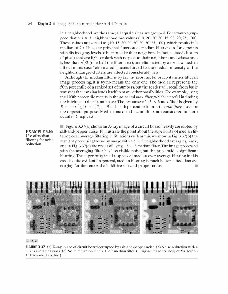
124 Chapter 3 � Image Enhancement in the Spatial Domain
in a neighborhood are the same, all equal values are grouped. For example, sup-pose that a 3*3 neighborhood has values (10, 20, 20, 20, 15, 20, 20, 25, 100).These values are sorted as (10, 15, 20, 20, 20, 20, 20, 25, 100), which results in amedian of 20. Thus, the principal function of median filters is to force pointswith distinct gray levels to be more like their neighbors. In fact, isolated clustersof pixels that are light or dark with respect to their neighbors, and whose areais less than n2�2 (one-half the filter area), are eliminated by an n*n medianfilter. In this case “eliminated” means forced to the median intensity of theneighbors. Larger clusters are affected considerably less.
Although the median filter is by far the most useful order-statistics filter inimage processing, it is by no means the only one. The median represents the50th percentile of a ranked set of numbers, but the reader will recall from basicstatistics that ranking lends itself to many other possibilities. For example, usingthe 100th percentile results in the so-called max filter, which is useful in findingthe brightest points in an image. The response of a 3*3 max filter is given byR=max Ezk |k=1, 2, p , 9F .The 0th percentile filter is the min filter, used forthe opposite purpose. Median, max, and mean filters are considered in moredetail in Chapter 5.
� Figure 3.37(a) shows an X-ray image of a circuit board heavily corrupted bysalt-and-pepper noise.To illustrate the point about the superiority of median fil-tering over average filtering in situations such as this, we show in Fig. 3.37(b) theresult of processing the noisy image with a 3*3 neighborhood averaging mask,and in Fig. 3.37(c) the result of using a 3*3 median filter.The image processedwith the averaging filter has less visible noise, but the price paid is significantblurring. The superiority in all respects of median over average filtering in thiscase is quite evident. In general, median filtering is much better suited than av-eraging for the removal of additive salt-and-pepper noise. �
EXAMPLE 3.10:Use of medianfiltering for noisereduction.
FIGURE 3.37 (a) X-ray image of circuit board corrupted by salt-and-pepper noise. (b) Noise reduction with a3*3 averaging mask. (c) Noise reduction with a 3*3 median filter. (Original image courtesy of Mr. JosephE. Pascente, Lixi, Inc.)
a b c
GONZ03-075-146.II 29-08-2001 13:43 Page 124
3.7 � Sharpening Spatial Filters 125
Sharpening Spatial Filters
The principal objective of sharpening is to highlight fine detail in an image orto enhance detail that has been blurred, either in error or as a natural effect ofa particular method of image acquisition. Uses of image sharpening vary and in-clude applications ranging from electronic printing and medical imaging to in-dustrial inspection and autonomous guidance in military systems.
In the last section, we saw that image blurring could be accomplished in thespatial domain by pixel averaging in a neighborhood. Since averaging is analo-gous to integration, it is logical to conclude that sharpening could be accom-plished by spatial differentiation. This, in fact, is the case, and the discussion inthis section deals with various ways of defining and implementing operators forsharpening by digital differentiation. Fundamentally, the strength of the re-sponse of a derivative operator is proportional to the degree of discontinuity ofthe image at the point at which the operator is applied. Thus, image differenti-ation enhances edges and other discontinuities (such as noise) and deempha-sizes areas with slowly varying gray-level values.
3.7.1 FoundationIn the two sections that follow, we consider in some detail sharpening filters thatare based on first- and second-order derivatives, respectively. Before proceedingwith that discussion, however, we stop to look at some of the fundamental prop-erties of these derivatives in a digital context. To simplify the explanation, wefocus attention on one-dimensional derivatives. In particular, we are interestedin the behavior of these derivatives in areas of constant gray level (flat segments),at the onset and end of discontinuities (step and ramp discontinuities), and alonggray-level ramps.These types of discontinuities can be used to model noise points,lines, and edges in an image. The behavior of derivatives during transitions intoand out of these image features also is of interest.
The derivatives of a digital function are defined in terms of differences.Thereare various ways to define these differences. However, we require that any de-finition we use for a first derivative (1) must be zero in flat segments (areas ofconstant gray-level values); (2) must be nonzero at the onset of a gray-levelstep or ramp; and (3) must be nonzero along ramps. Similarly, any definition ofa second derivative (1) must be zero in flat areas; (2) must be nonzero at theonset and end of a gray-level step or ramp; and (3) must be zero along rampsof constant slope. Since we are dealing with digital quantities whose values arefinite, the maximum possible gray-level change also is finite, and the shortest dis-tance over which that change can occur is between adjacent pixels.
A basic definition of the first-order derivative of a one-dimensional func-tion f(x) is the difference
We used a partial derivative here in order to keep the notation the same aswhen we consider an image function of two variables, f(x, y), at which time we
0f
0x= f(x + 1) - f(x).
3.7
GONZ03-075-146.II 29-08-2001 13:43 Page 125
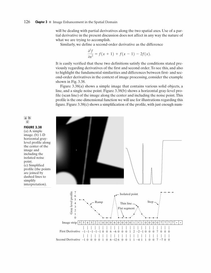
126 Chapter 3 � Image Enhancement in the Spatial Domain
Second Derivative
First Derivative
Image strip
Gra
y le
vel p
rofi
le
5
76543210
5 4 3 2 1 0 0 0 6 0 0 0 0 1 3 1 0 0 0 0 7 7 7
–1 –1 –1 –1 –1 0 0 6 –6 0 0 0 1 2 –2 –1 0 0 0 7 0 0 0
–1 0 0 0 0 1 0 6 –12 6 0 0 1 1 –4 1 1 0 0 7 –7 0 0
7
Ramp
Isolated point
Thin line
Flat segment
Step
FIGURE 3.38(a) A simpleimage. (b) 1-Dhorizontal gray-level profile alongthe center of theimage andincluding theisolated noisepoint.(c) Simplifiedprofile (the pointsare joined bydashed lines tosimplifyinterpretation).
will be dealing with partial derivatives along the two spatial axes. Use of a par-tial derivative in the present discussion does not affect in any way the nature ofwhat we are trying to accomplish.
Similarly, we define a second-order derivative as the difference
It is easily verified that these two definitions satisfy the conditions stated pre-viously regarding derivatives of the first and second order.To see this, and alsoto highlight the fundamental similarities and differences between first- and sec-ond-order derivatives in the context of image processing, consider the exampleshown in Fig. 3.38.
Figure 3.38(a) shows a simple image that contains various solid objects, aline, and a single noise point. Figure 3.38(b) shows a horizontal gray-level pro-file (scan line) of the image along the center and including the noise point.Thisprofile is the one-dimensional function we will use for illustrations regarding thisfigure. Figure 3.38(c) shows a simplification of the profile, with just enough num-
02f
0x2 = f(x + 1) + f(x - 1) - 2f(x).
a bc
GONZ03-075-146.II 29-08-2001 13:43 Page 126
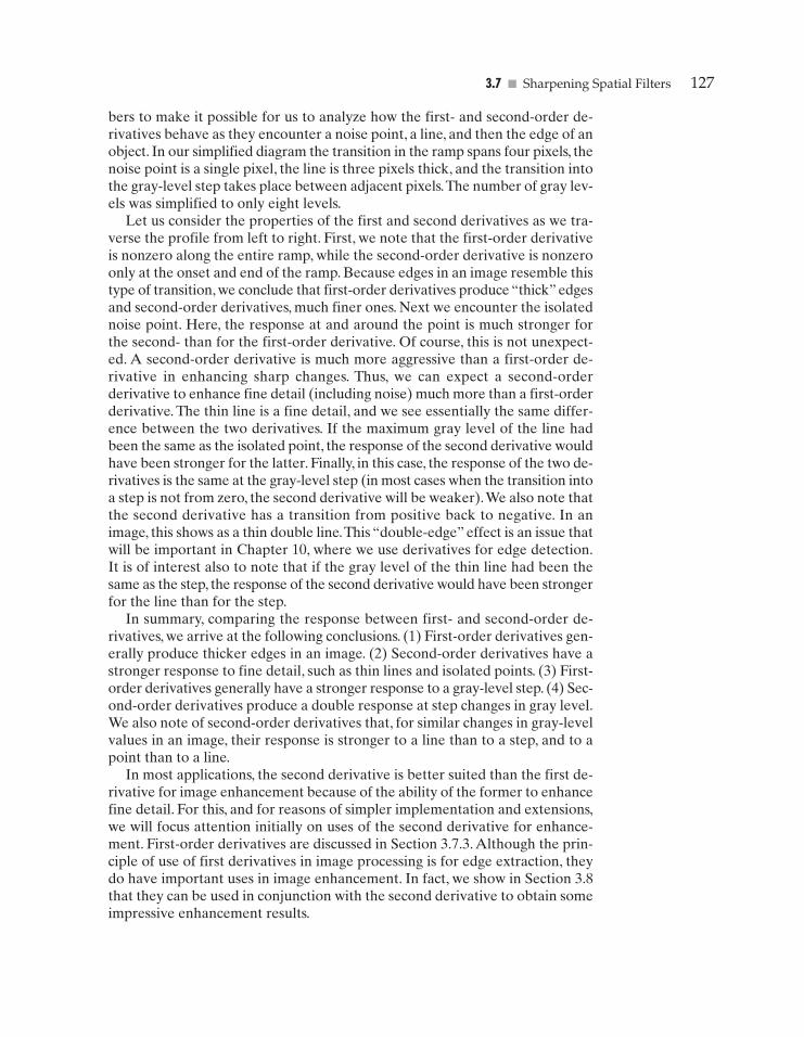
3.7 � Sharpening Spatial Filters 127
bers to make it possible for us to analyze how the first- and second-order de-rivatives behave as they encounter a noise point, a line, and then the edge of anobject. In our simplified diagram the transition in the ramp spans four pixels, thenoise point is a single pixel, the line is three pixels thick, and the transition intothe gray-level step takes place between adjacent pixels.The number of gray lev-els was simplified to only eight levels.
Let us consider the properties of the first and second derivatives as we tra-verse the profile from left to right. First, we note that the first-order derivativeis nonzero along the entire ramp, while the second-order derivative is nonzeroonly at the onset and end of the ramp. Because edges in an image resemble thistype of transition, we conclude that first-order derivatives produce “thick” edgesand second-order derivatives, much finer ones. Next we encounter the isolatednoise point. Here, the response at and around the point is much stronger forthe second- than for the first-order derivative. Of course, this is not unexpect-ed. A second-order derivative is much more aggressive than a first-order de-rivative in enhancing sharp changes. Thus, we can expect a second-orderderivative to enhance fine detail (including noise) much more than a first-orderderivative. The thin line is a fine detail, and we see essentially the same differ-ence between the two derivatives. If the maximum gray level of the line hadbeen the same as the isolated point, the response of the second derivative wouldhave been stronger for the latter. Finally, in this case, the response of the two de-rivatives is the same at the gray-level step (in most cases when the transition intoa step is not from zero, the second derivative will be weaker).We also note thatthe second derivative has a transition from positive back to negative. In animage, this shows as a thin double line.This “double-edge” effect is an issue thatwill be important in Chapter 10, where we use derivatives for edge detection.It is of interest also to note that if the gray level of the thin line had been thesame as the step, the response of the second derivative would have been strongerfor the line than for the step.
In summary, comparing the response between first- and second-order de-rivatives, we arrive at the following conclusions. (1) First-order derivatives gen-erally produce thicker edges in an image. (2) Second-order derivatives have astronger response to fine detail, such as thin lines and isolated points. (3) First-order derivatives generally have a stronger response to a gray-level step. (4) Sec-ond-order derivatives produce a double response at step changes in gray level.We also note of second-order derivatives that, for similar changes in gray-levelvalues in an image, their response is stronger to a line than to a step, and to apoint than to a line.
In most applications, the second derivative is better suited than the first de-rivative for image enhancement because of the ability of the former to enhancefine detail. For this, and for reasons of simpler implementation and extensions,we will focus attention initially on uses of the second derivative for enhance-ment. First-order derivatives are discussed in Section 3.7.3. Although the prin-ciple of use of first derivatives in image processing is for edge extraction, theydo have important uses in image enhancement. In fact, we show in Section 3.8that they can be used in conjunction with the second derivative to obtain someimpressive enhancement results.
GONZ03-075-146.II 29-08-2001 13:43 Page 127
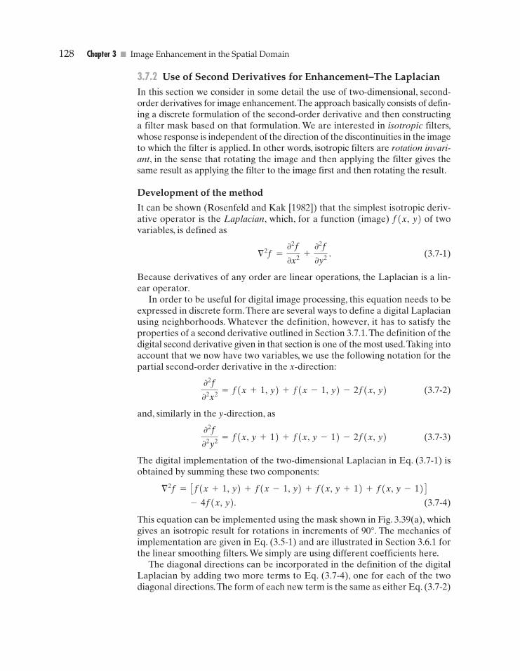
128 Chapter 3 � Image Enhancement in the Spatial Domain
3.7.2 Use of Second Derivatives for Enhancement–The LaplacianIn this section we consider in some detail the use of two-dimensional, second-order derivatives for image enhancement.The approach basically consists of defin-ing a discrete formulation of the second-order derivative and then constructinga filter mask based on that formulation. We are interested in isotropic filters,whose response is independent of the direction of the discontinuities in the imageto which the filter is applied. In other words, isotropic filters are rotation invari-ant, in the sense that rotating the image and then applying the filter gives thesame result as applying the filter to the image first and then rotating the result.
Development of the method
It can be shown (Rosenfeld and Kak [1982]) that the simplest isotropic deriv-ative operator is the Laplacian, which, for a function (image) f(x, y) of twovariables, is defined as
(3.7-1)
Because derivatives of any order are linear operations, the Laplacian is a lin-ear operator.
In order to be useful for digital image processing, this equation needs to beexpressed in discrete form.There are several ways to define a digital Laplacianusing neighborhoods. Whatever the definition, however, it has to satisfy theproperties of a second derivative outlined in Section 3.7.1.The definition of thedigital second derivative given in that section is one of the most used.Taking intoaccount that we now have two variables, we use the following notation for thepartial second-order derivative in the x-direction:
(3.7-2)
and, similarly in the y-direction, as
(3.7-3)
The digital implementation of the two-dimensional Laplacian in Eq. (3.7-1) isobtained by summing these two components:
(3.7-4)
This equation can be implemented using the mask shown in Fig. 3.39(a), whichgives an isotropic result for rotations in increments of 90°. The mechanics ofimplementation are given in Eq. (3.5-1) and are illustrated in Section 3.6.1 forthe linear smoothing filters. We simply are using different coefficients here.
The diagonal directions can be incorporated in the definition of the digitalLaplacian by adding two more terms to Eq. (3.7-4), one for each of the twodiagonal directions.The form of each new term is the same as either Eq. (3.7-2)
- 4f(x, y).
§ 2f = Cf(x + 1, y) + f(x - 1, y) + f(x, y + 1) + f(x, y - 1) D
02f
02y2 = f(x, y + 1) + f(x, y - 1) - 2f(x, y)
02f
02x2 = f(x + 1, y) + f(x - 1, y) - 2f(x, y)
§ 2f =02f
0x2 +02f
0y2 .
GONZ03-075-146.II 29-08-2001 13:43 Page 128
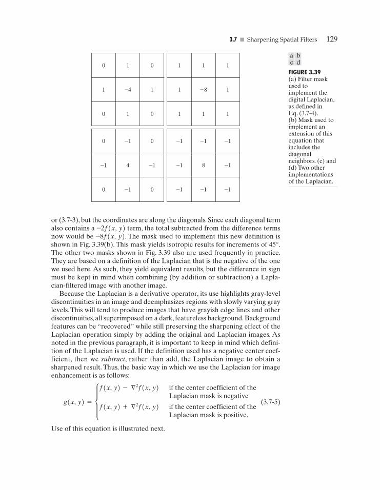
3.7 � Sharpening Spatial Filters 129
0 1 0
1 –4 1
0 1 0
1 1 1
1 –8 1
1 1 1
0 –1 0
–1 4 –1
0 –1 0
–1 –1 –1
–1 8 –1
–1 –1 –1
FIGURE 3.39(a) Filter maskused toimplement thedigital Laplacian,as defined inEq. (3.7-4).(b) Mask used toimplement anextension of thisequation thatincludes thediagonalneighbors. (c) and(d) Two otherimplementationsof the Laplacian.
or (3.7-3), but the coordinates are along the diagonals. Since each diagonal termalso contains a –2f(x, y) term, the total subtracted from the difference termsnow would be –8f(x, y). The mask used to implement this new definition isshown in Fig. 3.39(b). This mask yields isotropic results for increments of 45°.The other two masks shown in Fig. 3.39 also are used frequently in practice.They are based on a definition of the Laplacian that is the negative of the onewe used here. As such, they yield equivalent results, but the difference in signmust be kept in mind when combining (by addition or subtraction) a Lapla-cian-filtered image with another image.
Because the Laplacian is a derivative operator, its use highlights gray-leveldiscontinuities in an image and deemphasizes regions with slowly varying graylevels. This will tend to produce images that have grayish edge lines and otherdiscontinuities, all superimposed on a dark, featureless background. Backgroundfeatures can be “recovered” while still preserving the sharpening effect of theLaplacian operation simply by adding the original and Laplacian images. Asnoted in the previous paragraph, it is important to keep in mind which defini-tion of the Laplacian is used. If the definition used has a negative center coef-ficient, then we subtract, rather than add, the Laplacian image to obtain asharpened result. Thus, the basic way in which we use the Laplacian for imageenhancement is as follows:
(3.7-5)
Use of this equation is illustrated next.
g(x, y) = df(x, y) - § 2f(x, y)
f(x, y) + § 2f(x, y)
if the center coefficient of theLaplacian mask is negative
if the center coefficient of theLaplacian mask is positive.
a bc d
GONZ03-075-146.II 29-08-2001 13:43 Page 129
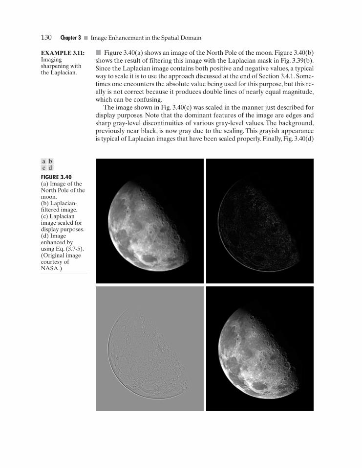
130 Chapter 3 � Image Enhancement in the Spatial Domain
FIGURE 3.40(a) Image of theNorth Pole of themoon.(b) Laplacian-filtered image.(c) Laplacianimage scaled fordisplay purposes.(d) Imageenhanced byusing Eq. (3.7-5).(Original imagecourtesy ofNASA.)
� Figure 3.40(a) shows an image of the North Pole of the moon. Figure 3.40(b)shows the result of filtering this image with the Laplacian mask in Fig. 3.39(b).Since the Laplacian image contains both positive and negative values, a typicalway to scale it is to use the approach discussed at the end of Section 3.4.1. Some-times one encounters the absolute value being used for this purpose, but this re-ally is not correct because it produces double lines of nearly equal magnitude,which can be confusing.
The image shown in Fig. 3.40(c) was scaled in the manner just described fordisplay purposes. Note that the dominant features of the image are edges andsharp gray-level discontinuities of various gray-level values. The background,previously near black, is now gray due to the scaling. This grayish appearanceis typical of Laplacian images that have been scaled properly. Finally, Fig. 3.40(d)
EXAMPLE 3.11:Imagingsharpening withthe Laplacian.
a bc d
GONZ03-075-146.II 29-08-2001 13:43 Page 130
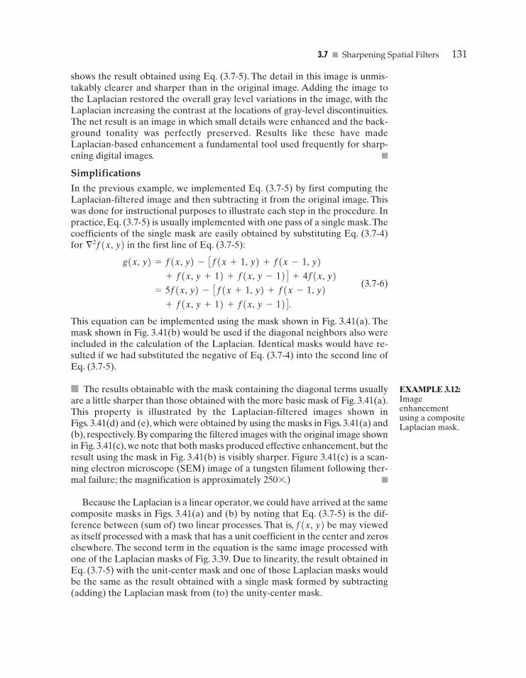
3.7 � Sharpening Spatial Filters 131
shows the result obtained using Eq. (3.7-5). The detail in this image is unmis-takably clearer and sharper than in the original image. Adding the image tothe Laplacian restored the overall gray level variations in the image, with theLaplacian increasing the contrast at the locations of gray-level discontinuities.The net result is an image in which small details were enhanced and the back-ground tonality was perfectly preserved. Results like these have madeLaplacian-based enhancement a fundamental tool used frequently for sharp-ening digital images. �
Simplifications
In the previous example, we implemented Eq. (3.7-5) by first computing theLaplacian-filtered image and then subtracting it from the original image. Thiswas done for instructional purposes to illustrate each step in the procedure. Inpractice, Eq. (3.7-5) is usually implemented with one pass of a single mask.Thecoefficients of the single mask are easily obtained by substituting Eq. (3.7-4)for in the first line of Eq. (3.7-5):
(3.7-6)
This equation can be implemented using the mask shown in Fig. 3.41(a). Themask shown in Fig. 3.41(b) would be used if the diagonal neighbors also wereincluded in the calculation of the Laplacian. Identical masks would have re-sulted if we had substituted the negative of Eq. (3.7-4) into the second line ofEq. (3.7-5).
� The results obtainable with the mask containing the diagonal terms usuallyare a little sharper than those obtained with the more basic mask of Fig. 3.41(a).This property is illustrated by the Laplacian-filtered images shown inFigs. 3.41(d) and (e), which were obtained by using the masks in Figs. 3.41(a) and(b), respectively. By comparing the filtered images with the original image shownin Fig. 3.41(c), we note that both masks produced effective enhancement, but theresult using the mask in Fig. 3.41(b) is visibly sharper. Figure 3.41(c) is a scan-ning electron microscope (SEM) image of a tungsten filament following ther-mal failure; the magnification is approximately 250 *.) �
Because the Laplacian is a linear operator, we could have arrived at the samecomposite masks in Figs. 3.41(a) and (b) by noting that Eq. (3.7-5) is the dif-ference between (sum of) two linear processes. That is, f(x, y) be may viewedas itself processed with a mask that has a unit coefficient in the center and zeroselsewhere. The second term in the equation is the same image processed withone of the Laplacian masks of Fig. 3.39. Due to linearity, the result obtained inEq. (3.7-5) with the unit-center mask and one of those Laplacian masks wouldbe the same as the result obtained with a single mask formed by subtracting(adding) the Laplacian mask from (to) the unity-center mask.
+ f(x, y + 1) + f(x, y - 1) D . = 5f(x, y) - Cf(x + 1, y) + f(x - 1, y)
+ f(x, y + 1) + f(x, y - 1) D + 4f(x, y)
g(x, y) = f(x, y) - Cf(x + 1, y) + f(x - 1, y)
§ 2f(x, y)
EXAMPLE 3.12:Imageenhancementusing a compositeLaplacian mask.
GONZ03-075-146.II 29-08-2001 13:43 Page 131
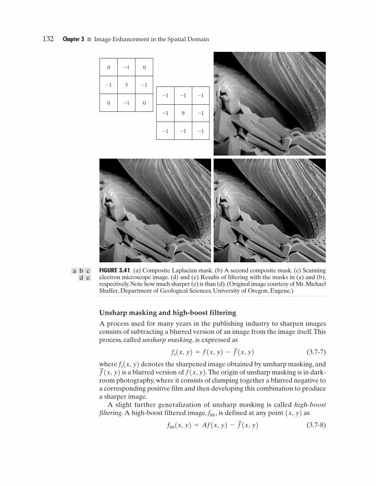
132 Chapter 3 � Image Enhancement in the Spatial Domain
0 –1 0
–1 5 –1
0 –1 0–1 –1 –1
–1 9 –1
–1 –1 –1
FIGURE 3.41 (a) Composite Laplacian mask. (b) A second composite mask. (c) Scanningelectron microscope image. (d) and (e) Results of filtering with the masks in (a) and (b),respectively.Note how much sharper (e) is than (d). (Original image courtesy of Mr.MichaelShaffer, Department of Geological Sciences, University of Oregon, Eugene.)
Unsharp masking and high-boost filtering
A process used for many years in the publishing industry to sharpen imagesconsists of subtracting a blurred version of an image from the image itself.Thisprocess, called unsharp masking, is expressed as
(3.7-7)
where fs(x, y) denotes the sharpened image obtained by unsharp masking, andis a blurred version of f(x, y).The origin of unsharp masking is in dark-
room photography, where it consists of clamping together a blurred negative toa corresponding positive film and then developing this combination to producea sharper image.
A slight further generalization of unsharp masking is called high-boostfiltering. A high-boost filtered image, fhb, is defined at any point (x, y) as
(3.7-8)fhb(x, y) = Af(x, y) - f–
(x, y)
f–
(x, y)
fs(x, y) = f(x, y) - f–
(x, y)
a b cd e
GONZ03-075-146.II 29-08-2001 13:43 Page 132
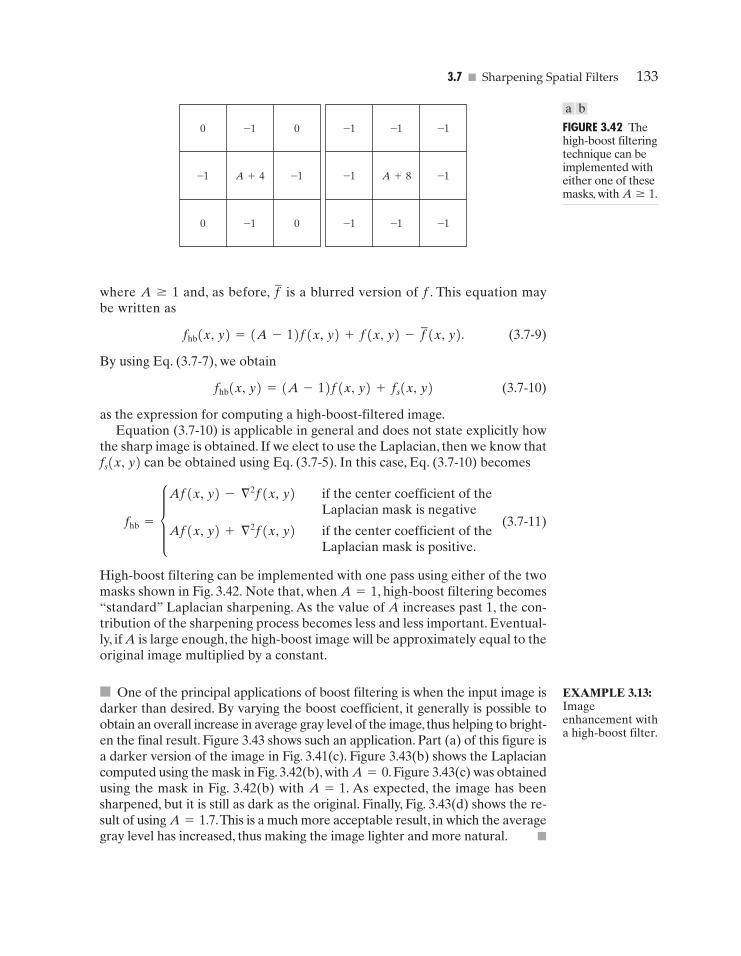
3.7 � Sharpening Spatial Filters 133
0 –1 0
–1 A+4 –1
0 –1 0
–1 –1 –1
–1 A+8 –1
–1 –1 –1
FIGURE 3.42 Thehigh-boost filteringtechnique can beimplemented witheither one of thesemasks, with A � 1.
where A � 1 and, as before, is a blurred version of f. This equation maybe written as
(3.7-9)
By using Eq. (3.7-7), we obtain
(3.7-10)
as the expression for computing a high-boost-filtered image.Equation (3.7-10) is applicable in general and does not state explicitly how
the sharp image is obtained. If we elect to use the Laplacian, then we know thatfs(x, y) can be obtained using Eq. (3.7-5). In this case, Eq. (3.7-10) becomes
(3.7-11)
High-boost filtering can be implemented with one pass using either of the twomasks shown in Fig. 3.42. Note that, when A=1, high-boost filtering becomes“standard” Laplacian sharpening. As the value of A increases past 1, the con-tribution of the sharpening process becomes less and less important. Eventual-ly, if A is large enough, the high-boost image will be approximately equal to theoriginal image multiplied by a constant.
� One of the principal applications of boost filtering is when the input image isdarker than desired. By varying the boost coefficient, it generally is possible toobtain an overall increase in average gray level of the image, thus helping to bright-en the final result. Figure 3.43 shows such an application. Part (a) of this figure isa darker version of the image in Fig. 3.41(c). Figure 3.43(b) shows the Laplaciancomputed using the mask in Fig. 3.42(b), with A=0. Figure 3.43(c) was obtainedusing the mask in Fig. 3.42(b) with A=1. As expected, the image has beensharpened, but it is still as dark as the original. Finally, Fig. 3.43(d) shows the re-sult of using A=1.7.This is a much more acceptable result, in which the averagegray level has increased, thus making the image lighter and more natural. �
fhb = dAf(x, y) - § 2f(x, y)
Af(x, y) + § 2f(x, y)
if the center coefficient of theLaplacian mask is negative
if the center coefficient of theLaplacian mask is positive.
fhb(x, y) = (A - 1)f(x, y) + fs(x, y)
fhb(x, y) = (A - 1)f(x, y) + f(x, y) - f–
(x, y).
f–
EXAMPLE 3.13:Imageenhancement witha high-boost filter.
a b
GONZ03-075-146.II 29-08-2001 13:43 Page 133
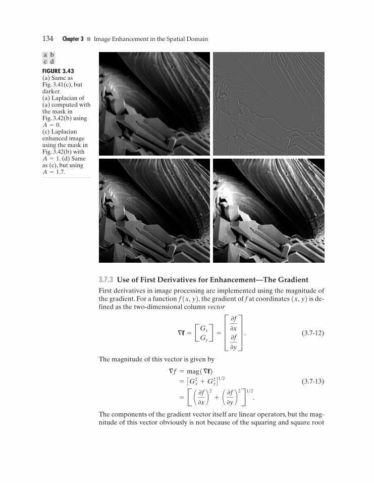
134 Chapter 3 � Image Enhancement in the Spatial Domain
FIGURE 3.43(a) Same asFig. 3.41(c), butdarker.(a) Laplacian of(a) computed withthe mask inFig. 3.42(b) usingA=0.(c) Laplacianenhanced imageusing the mask inFig. 3.42(b) withA=1. (d) Sameas (c), but usingA=1.7.
3.7.3 Use of First Derivatives for Enhancement—The GradientFirst derivatives in image processing are implemented using the magnitude ofthe gradient. For a function f(x, y), the gradient of f at coordinates (x, y) is de-fined as the two-dimensional column vector
(3.7-12)
The magnitude of this vector is given by
(3.7-13)
The components of the gradient vector itself are linear operators, but the mag-nitude of this vector obviously is not because of the squaring and square root
= B a 0f
0xb
2
+ a0f
0yb
2R 1�2
.
= CG2x + G2
y D1�2
§f = mag (§f)
§f = BGx
GyR = D 0f
0x0f
0y
T .
a bc d
GONZ03-075-146.II 29-08-2001 13:43 Page 134
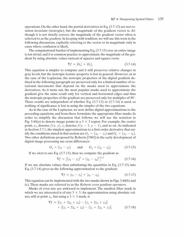
3.7 � Sharpening Spatial Filters 135
operations. On the other hand, the partial derivatives in Eq. (3.7-12) are not ro-tation invariant (isotropic), but the magnitude of the gradient vector is. Al-though it is not strictly correct, the magnitude of the gradient vector often isreferred to as the gradient. In keeping with tradition, we will use this term in thefollowing discussions, explicitly referring to the vector or its magnitude only incases where confusion is likely.
The computational burden of implementing Eq. (3.7-13) over an entire imageis not trivial, and it is common practice to approximate the magnitude of the gra-dient by using absolute values instead of squares and square roots:
(3.7-14)
This equation is simpler to compute and it still preserves relative changes ingray levels, but the isotropic feature property is lost in general. However, as inthe case of the Laplacian, the isotropic properties of the digital gradient de-fined in the following paragraph are preserved only for a limited number of ro-tational increments that depend on the masks used to approximate thederivatives. As it turns out, the most popular masks used to approximate thegradient give the same result only for vertical and horizontal edges and thusthe isotropic properties of the gradient are preserved only for multiples of 90°.These results are independent of whether Eq. (3.7-13) or (3.7-14) is used, sonothing of significance is lost in using the simpler of the two equations.
As in the case of the Laplacian, we now define digital approximations to thepreceding equations, and from there formulate the appropriate filter masks. Inorder to simplify the discussion that follows, we will use the notation inFig. 3.44(a) to denote image points in a 3*3 region. For example, the centerpoint, z5 , denotes f(x, y), z1 denotes f(x-1, y-1), and so on. As indicatedin Section 3.7.1, the simplest approximations to a first-order derivative that sat-isfy the conditions stated in that section are Gx=Az8-z5B and Gy=Az6-z5B .Two other definitions proposed by Roberts [1965] in the early development ofdigital image processing use cross differences:
(3.7-15)
If we elect to use Eq. (3.7-13), then we compute the gradient as
(3.7-16)
If we use absolute values, then substituting the quantities in Eq. (3.7-15) intoEq. (3.7-14) gives us the following approximation to the gradient:
(3.7-17)
This equation can be implemented with the two masks shown in Figs. 3.44(b) and(c). These masks are referred to as the Roberts cross-gradient operators.
Masks of even size are awkward to implement. The smallest filter mask inwhich we are interested is of size 3*3. An approximation using absolute val-ues, still at point z5 , but using a 3*3 mask, is
(3.7-18) + @ Az3 + 2z6 + z9B - Az1 + 2z4 + z7B @ . §f L @ Az7 + 2z8 + z9B - Az1 + 2z2 + z3B @
§f L @z9 - z5 @ + @z8 - z6 @ .
§f = C Az9 - z5B2 + Az8 - z6B
2 D 1�2
Gx = Az9 - z5B and Gy = Az8 - z6B.
§f L @Gx @ + @Gy @ .
GONZ03-075-146.II 29-08-2001 13:43 Page 135
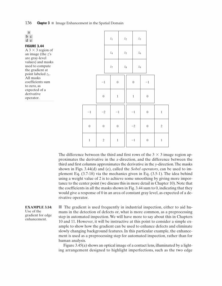
136 Chapter 3 � Image Enhancement in the Spatial Domain
–1 0
0 1
0 –1
1 0
–1 –2 –1
0 0 0
1 2 1
–1 0 1
–2 0 2
–1 0 1
z1 z2 z3
z4 z5 z6
z7 z8 z9
FIGURE 3.44A 3*3 region ofan image (the z’sare gray-levelvalues) and masksused to computethe gradient atpoint labeled z5 .All maskscoefficients sumto zero, asexpected of aderivativeoperator.
The difference between the third and first rows of the 3*3 image region ap-proximates the derivative in the x-direction, and the difference between thethird and first columns approximates the derivative in the y-direction.The masksshown in Figs. 3.44(d) and (e), called the Sobel operators, can be used to im-plement Eq. (3.7-18) via the mechanics given in Eq. (3.5-1). The idea behindusing a weight value of 2 is to achieve some smoothing by giving more impor-tance to the center point (we discuss this in more detail in Chapter 10). Note thatthe coefficients in all the masks shown in Fig. 3.44 sum to 0, indicating that theywould give a response of 0 in an area of constant gray level, as expected of a de-rivative operator.
� The gradient is used frequently in industrial inspection, either to aid hu-mans in the detection of defects or, what is more common, as a preprocessingstep in automated inspection. We will have more to say about this in Chapters10 and 11. However, it will be instructive at this point to consider a simple ex-ample to show how the gradient can be used to enhance defects and eliminateslowly changing background features. In this particular example, the enhance-ment is used as a preprocessing step for automated inspection, rather than forhuman analysis.
Figure 3.45(a) shows an optical image of a contact lens, illuminated by a light-ing arrangement designed to highlight imperfections, such as the two edge
EXAMPLE 3.14:Use of thegradient for edgeenhancement.
b cd e
a
GONZ03-075-146.II 29-08-2001 13:43 Page 136
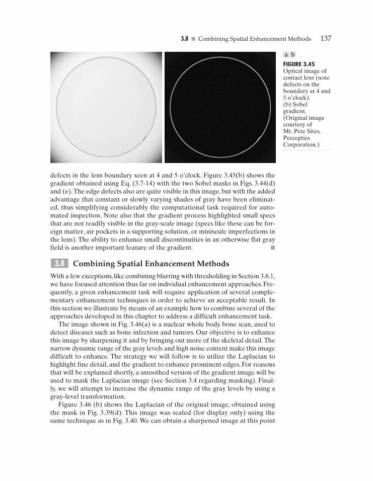
3.8 � Combining Spatial Enhancement Methods 137
FIGURE 3.45Optical image ofcontact lens (notedefects on theboundary at 4 and5 o’clock).(b) Sobelgradient.(Original imagecourtesy ofMr. Pete Sites,PercepticsCorporation.)
a b
defects in the lens boundary seen at 4 and 5 o’clock. Figure 3.45(b) shows thegradient obtained using Eq. (3.7-14) with the two Sobel masks in Figs. 3.44(d)and (e).The edge defects also are quite visible in this image, but with the addedadvantage that constant or slowly varying shades of gray have been eliminat-ed, thus simplifying considerably the computational task required for auto-mated inspection. Note also that the gradient process highlighted small specsthat are not readily visible in the gray-scale image (specs like these can be for-eign matter, air pockets in a supporting solution, or miniscule imperfections inthe lens). The ability to enhance small discontinuities in an otherwise flat grayfield is another important feature of the gradient. �
Combining Spatial Enhancement Methods
With a few exceptions, like combining blurring with thresholding in Section 3.6.1,we have focused attention thus far on individual enhancement approaches. Fre-quently, a given enhancement task will require application of several comple-mentary enhancement techniques in order to achieve an acceptable result. Inthis section we illustrate by means of an example how to combine several of theapproaches developed in this chapter to address a difficult enhancement task.
The image shown in Fig. 3.46(a) is a nuclear whole body bone scan, used todetect diseases such as bone infection and tumors. Our objective is to enhancethis image by sharpening it and by bringing out more of the skeletal detail.Thenarrow dynamic range of the gray levels and high noise content make this imagedifficult to enhance. The strategy we will follow is to utilize the Laplacian tohighlight fine detail, and the gradient to enhance prominent edges. For reasonsthat will be explained shortly, a smoothed version of the gradient image will beused to mask the Laplacian image (see Section 3.4 regarding masking). Final-ly, we will attempt to increase the dynamic range of the gray levels by using agray-level transformation.
Figure 3.46 (b) shows the Laplacian of the original image, obtained usingthe mask in Fig. 3.39(d). This image was scaled (for display only) using thesame technique as in Fig. 3.40. We can obtain a sharpened image at this point
3.8
GONZ03-075-146.II 29-08-2001 13:43 Page 137
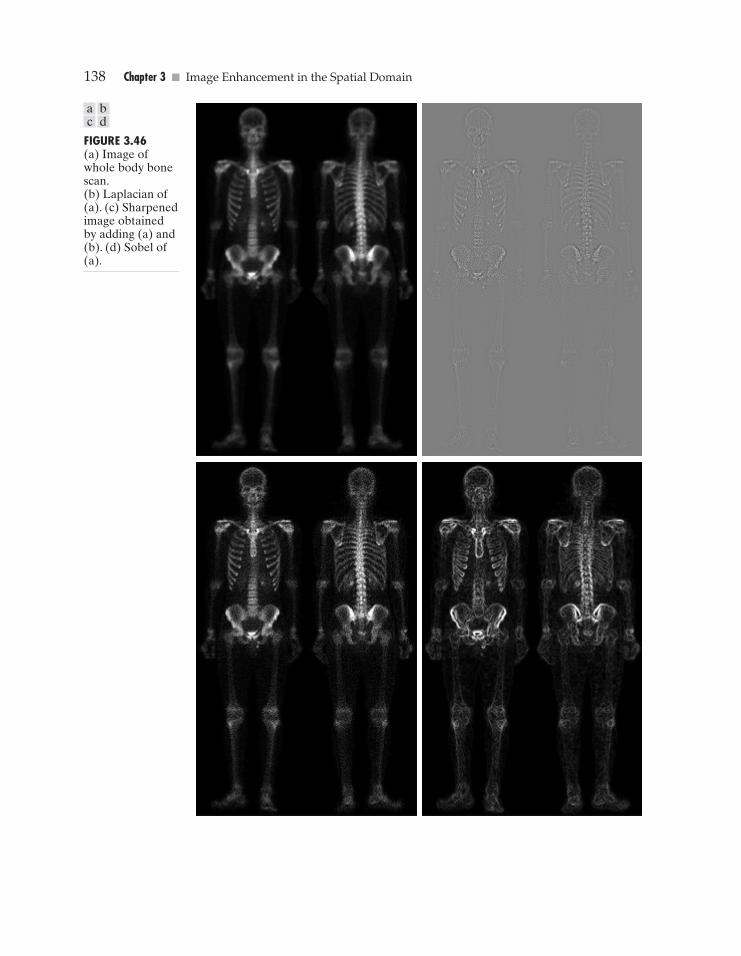
138 Chapter 3 � Image Enhancement in the Spatial Domain
FIGURE 3.46(a) Image ofwhole body bonescan.(b) Laplacian of(a). (c) Sharpenedimage obtainedby adding (a) and(b). (d) Sobel of(a).
a bc d
GONZ03-075-146.II 29-08-2001 13:43 Page 138
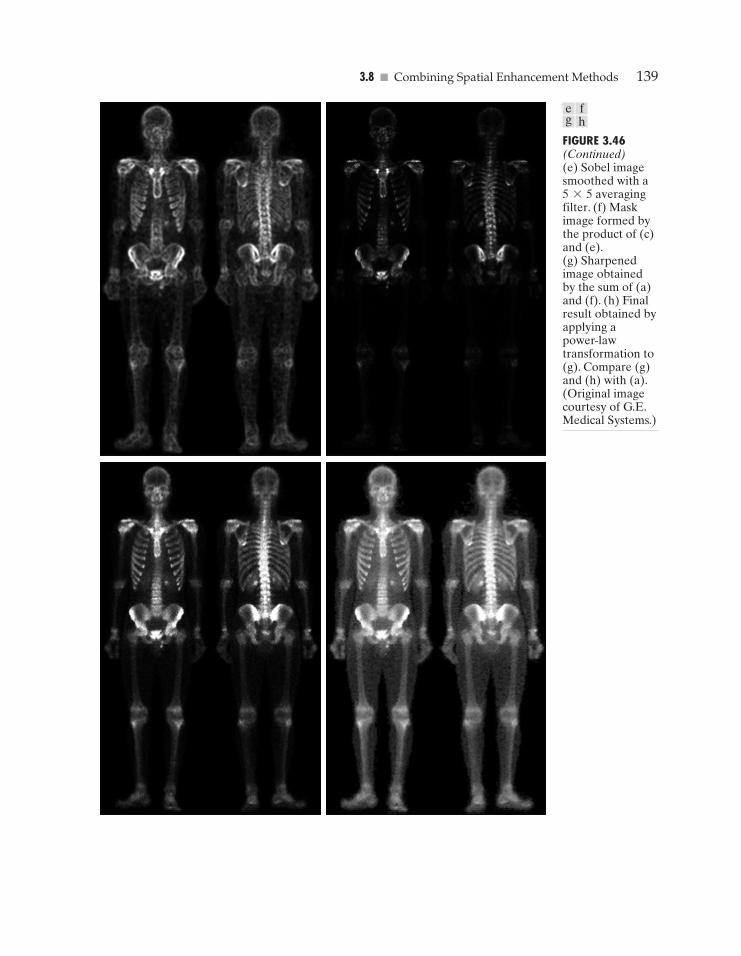
3.8 � Combining Spatial Enhancement Methods 139
FIGURE 3.46(Continued)(e) Sobel imagesmoothed with a5*5 averagingfilter. (f) Maskimage formed bythe product of (c)and (e).(g) Sharpenedimage obtainedby the sum of (a)and (f). (h) Finalresult obtained byapplying a power-lawtransformation to(g). Compare (g)and (h) with (a).(Original imagecourtesy of G.E.Medical Systems.)
e fg h
GONZ03-075-146.II 29-08-2001 13:43 Page 139
140 Chapter 3 � Image Enhancement in the Spatial Domain
simply by adding Figs. 3.46(a) and (b), which are an implementation of thesecond line in Eq. (3.7-5) (we used a mask with a positive center coefficient).Just by looking at the noise level in (b), we would expect a rather noisy sharp-ened image if we added Figs. 3.46(a) and (b), a fact that is confirmed by theresult shown in Fig. 3.46(c). One way that comes immediately to mind to re-duce the noise is to use a median filter. However, median filtering is a non-linear process capable of removing image features. This is unacceptable inmedical image processing.
An alternate approach is to use a mask formed from a smoothed version ofthe gradient of the original image. The motivation behind this is straightfor-ward and is based on the properties of first- and second-order derivatives ex-plained in Section 3.7.1.The Laplacian, being a second-order derivative operator,has the definite advantage that it is superior in enhancing fine detail. Howev-er, this causes it to produce noisier results than the gradient. This noise is mostobjectionable in smooth areas, where it tends to be more visible. The gradienthas a stronger response in areas of significant gray-level transitions (gray-levelramps and steps) than does the Laplacian.The response of the gradient to noiseand fine detail is lower than the Laplacian’s and can be lowered further bysmoothing the gradient with an averaging filter.The idea, then, is to smooth thegradient and multiply it by the Laplacian image. In this context, we may viewthe smoothed gradient as a mask image. The product will preserve details inthe strong areas while reducing noise in the relatively flat areas.This process canbe viewed roughly as combining the best features of the Laplacian and the gra-dient.The result is added to the original to obtain a final sharpened image, andcould even be used in boost filtering.
Figure 3.46(d) shows the Sobel gradient of the original image, computedusing Eq. (3.7-14). Components Gx and Gy were obtained using the masks inFigs. 3.44(d) and (e), respectively. As expected from our discussion in Section3.7.1, edges are much more dominant in this image than in the Laplacian image.The smoothed gradient image shown in Fig. 3.46(e) was obtained by using anaveraging filter of size 5*5. The two gradient images were scaled for displayin the same manner as the two Laplacian images. Because the smallest possiblevalue of a gradient image is 0, the background is black in the scaled gradient im-ages, rather than gray as in the scaled Laplacian.The fact that Figs. 3.46(d) and(e) are much brighter than Fig. 3.46(b) is again evidence that the gradient of animage with significant edge content has values that are higher in general thanin a Laplacian image.
The product of the Laplacian and smoothed-gradient image is shown inFig. 3.46(f). Note the dominance of the strong edges and the relative lack of vis-ible noise, which is the key objective behind masking the Laplacian with asmoothed gradient image.Adding the product image to the original resulted inthe sharpened image shown in Fig. 3.46(g). The significant increase in sharp-ness of detail in this image over the original is evident in most parts of the image,including the ribs, spinal chord, pelvis, and skull.This type of improvement wouldnot have been possible by using the Laplacian or gradient alone.
The sharpening procedure just discussed does not affect in an appreciableway the dynamic range of the gray levels in an image.Thus, the final step in our
GONZ03-075-146.II 29-08-2001 13:43 Page 140
� Summary 141
enhancement task is to increase the dynamic range of the sharpened image.Aswe discussed in some detail in Sections 3.2 and 3.3, there are a number of gray-level transformation functions that can accomplish this objective. We do knowfrom the results in Section 3.3.2 that histogram equalization is not likely to workwell on images that have dark gray-level distributions like our images havehere. Histogram specification could be a solution, but the dark characteristicsof the images with which we are dealing lend themselves much better to a power-law transformation. Since we wish to spread the gray levels, the value of g inEq. (3.2-3) has to be less than 1.After a few trials with this equation we arrivedat the result shown in Fig. 3.46(h), obtained with g=0.5 and c=1. Compar-ing this image with Fig. 3.46(g), we see that significant new detail is visible inFig. 3.46(h). The areas around the wrists, hands, ankles, and feet are good ex-amples of this. The skeletal bone structure also is much more pronounced, in-cluding the arm and leg bones. Note also the faint definition of the outline ofthe body, and of body tissue. Bringing out detail of this nature by expandingthe dynamic range of the gray levels also enhanced noise, but Fig. 3.46(h) rep-resents a significant visual improvement over the original image.
The approach just discussed is representative of the types of processes thatcan be linked in order to achieve results that are not possible with a singletechnique. The way in which the results are used depends on the application.The final user of the type of images shown in this section is likely to be a ra-diologist. For a number of reasons that are beyond the scope of our discussion,physicians are unlikely to rely on enhanced results to arrive at a diagnosis.However, enhanced images are quite useful in highlighting details that canserve as clues for further analysis in the original image or sequence of images.In other areas, the enhanced result may indeed be the final product. Examplesare found in the printing industry, in image-based product inspection, in foren-sics, in microscopy, in surveillance, and in a host of other areas where the prin-cipal objective of enhancement is to obtain an image with a higher content ofvisual detail.
SummaryThe material presented in this chapter is representative of spatial domain techniquescommonly used in practice for image enhancement. This area of image processing isa dynamic field, and new techniques and applications are reported routinely in pro-fessional literature and in new product announcements. For this reason, the topics in-cluded in this chapter were selected for their value as fundamental material thatwould serve as a foundation for understanding the state of the art in enhancementtechniques, as well as for further study in this field. In addition to enhancement, thischapter served the purpose of introducing a number of concepts, such as filtering withspatial masks, that will be used in numerous occasions throughout the remainder ofthe book. In the following chapter, we deal with enhancement from a complemen-tary viewpoint in the frequency domain. Between these two chapters, the reader willhave developed a solid foundation for the terminology and some of the most funda-mental tools used in image processing.The fact that these tools were introduced in thecontext of image enhancement is likely to aid in the understanding of how they op-erate on digital images.
GONZ03-075-146.II 29-08-2001 13:43 Page 141
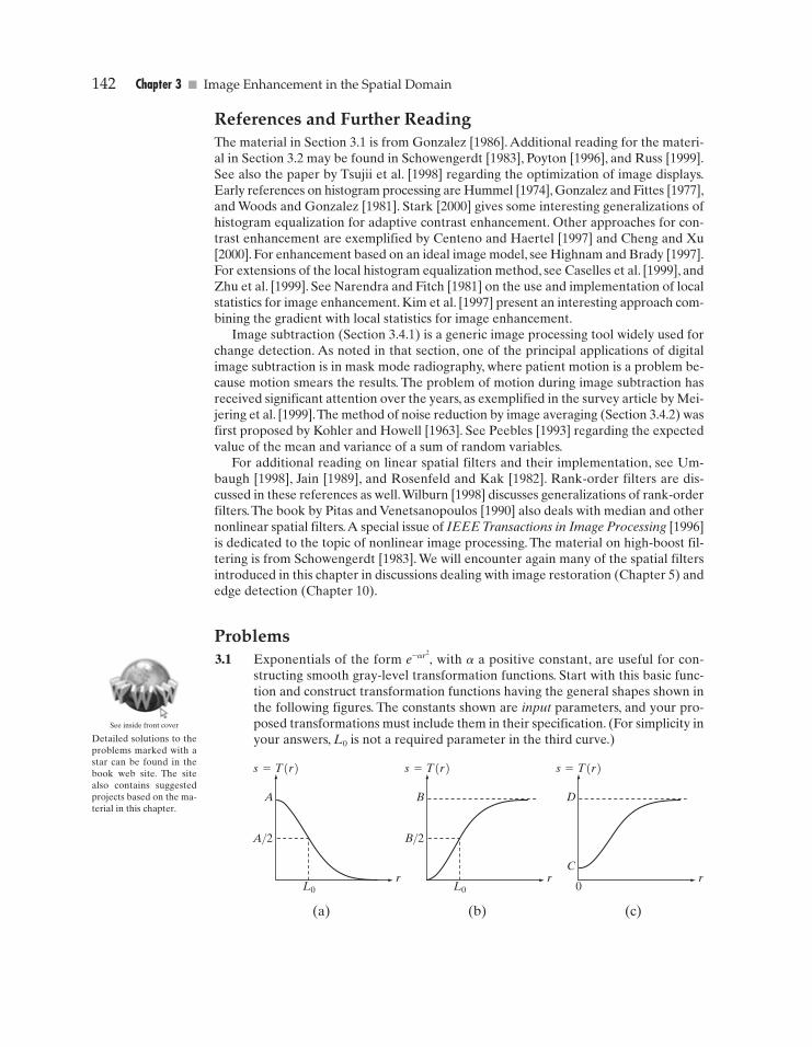
142 Chapter 3 � Image Enhancement in the Spatial Domain
References and Further ReadingThe material in Section 3.1 is from Gonzalez [1986]. Additional reading for the materi-al in Section 3.2 may be found in Schowengerdt [1983], Poyton [1996], and Russ [1999].See also the paper by Tsujii et al. [1998] regarding the optimization of image displays.Early references on histogram processing are Hummel [1974], Gonzalez and Fittes [1977],and Woods and Gonzalez [1981]. Stark [2000] gives some interesting generalizations ofhistogram equalization for adaptive contrast enhancement. Other approaches for con-trast enhancement are exemplified by Centeno and Haertel [1997] and Cheng and Xu[2000]. For enhancement based on an ideal image model, see Highnam and Brady [1997].For extensions of the local histogram equalization method, see Caselles et al. [1999], andZhu et al. [1999]. See Narendra and Fitch [1981] on the use and implementation of localstatistics for image enhancement. Kim et al. [1997] present an interesting approach com-bining the gradient with local statistics for image enhancement.
Image subtraction (Section 3.4.1) is a generic image processing tool widely used forchange detection. As noted in that section, one of the principal applications of digitalimage subtraction is in mask mode radiography, where patient motion is a problem be-cause motion smears the results. The problem of motion during image subtraction hasreceived significant attention over the years, as exemplified in the survey article by Mei-jering et al. [1999].The method of noise reduction by image averaging (Section 3.4.2) wasfirst proposed by Kohler and Howell [1963]. See Peebles [1993] regarding the expectedvalue of the mean and variance of a sum of random variables.
For additional reading on linear spatial filters and their implementation, see Um-baugh [1998], Jain [1989], and Rosenfeld and Kak [1982]. Rank-order filters are dis-cussed in these references as well.Wilburn [1998] discusses generalizations of rank-orderfilters.The book by Pitas and Venetsanopoulos [1990] also deals with median and othernonlinear spatial filters.A special issue of IEEE Transactions in Image Processing [1996]is dedicated to the topic of nonlinear image processing. The material on high-boost fil-tering is from Schowengerdt [1983]. We will encounter again many of the spatial filtersintroduced in this chapter in discussions dealing with image restoration (Chapter 5) andedge detection (Chapter 10).
Problems3.1 Exponentials of the form with a a positive constant, are useful for con-
structing smooth gray-level transformation functions. Start with this basic func-tion and construct transformation functions having the general shapes shown inthe following figures. The constants shown are input parameters, and your pro-posed transformations must include them in their specification. (For simplicity inyour answers, L0 is not a required parameter in the third curve.)
(a) (b) (c)
L0
A
r
s=T(r)
A/2
L0
B
r
s=T(r)
B/2
0
D
Cr
s=T(r)
e-ar2
,
Detailed solutions to theproblems marked with astar can be found in thebook web site. The sitealso contains suggestedprojects based on the ma-terial in this chapter.
See inside front cover
GONZ03-075-146.II 29-08-2001 13:43 Page 142
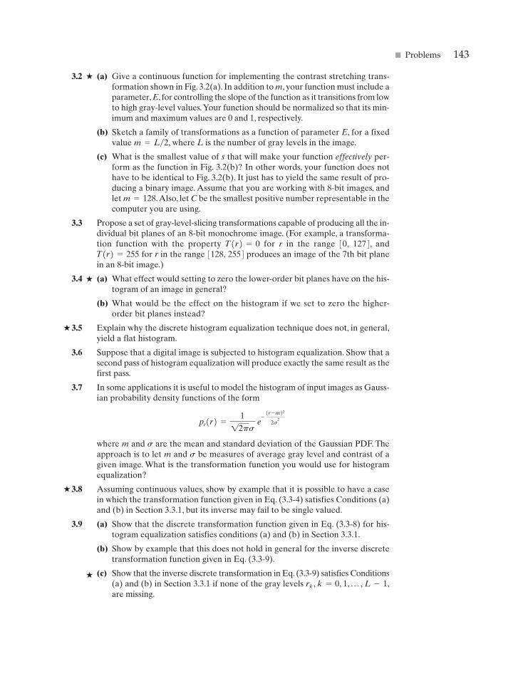
� Problems 143
3.2 (a) Give a continuous function for implementing the contrast stretching trans-formation shown in Fig. 3.2(a). In addition to m, your function must include aparameter,E, for controlling the slope of the function as it transitions from lowto high gray-level values.Your function should be normalized so that its min-imum and maximum values are 0 and 1, respectively.
(b) Sketch a family of transformations as a function of parameter E, for a fixedvalue m=L�2, where L is the number of gray levels in the image.
(c) What is the smallest value of s that will make your function effectively per-form as the function in Fig. 3.2(b)? In other words, your function does nothave to be identical to Fig. 3.2(b). It just has to yield the same result of pro-ducing a binary image. Assume that you are working with 8-bit images, andlet m=128.Also, let C be the smallest positive number representable in thecomputer you are using.
3.3 Propose a set of gray-level-slicing transformations capable of producing all the in-dividual bit planes of an 8-bit monochrome image. (For example, a transforma-tion function with the property T(r)=0 for r in the range [0, 127], andT(r)=255 for r in the range [128, 255] produces an image of the 7th bit planein an 8-bit image.)
3.4 (a) What effect would setting to zero the lower-order bit planes have on the his-togram of an image in general?
(b) What would be the effect on the histogram if we set to zero the higher-order bit planes instead?
3.5 Explain why the discrete histogram equalization technique does not, in general,yield a flat histogram.
3.6 Suppose that a digital image is subjected to histogram equalization. Show that asecond pass of histogram equalization will produce exactly the same result as thefirst pass.
3.7 In some applications it is useful to model the histogram of input images as Gauss-ian probability density functions of the form
where m and s are the mean and standard deviation of the Gaussian PDF. Theapproach is to let m and s be measures of average gray level and contrast of agiven image. What is the transformation function you would use for histogramequalization?
3.8 Assuming continuous values, show by example that it is possible to have a casein which the transformation function given in Eq. (3.3-4) satisfies Conditions (a)and (b) in Section 3.3.1, but its inverse may fail to be single valued.
3.9 (a) Show that the discrete transformation function given in Eq. (3.3-8) for his-togram equalization satisfies conditions (a) and (b) in Section 3.3.1.
(b) Show by example that this does not hold in general for the inverse discretetransformation function given in Eq. (3.3-9).
(c) Show that the inverse discrete transformation in Eq. (3.3-9) satisfies Conditions(a) and (b) in Section 3.3.1 if none of the gray levels rk , k=0, 1, p , L-1,are missing.
pr(r) =112ps
e
-
(r - m)2
2s2
�
�
�
�
�
GONZ03-075-146.II 29-08-2001 13:43 Page 143
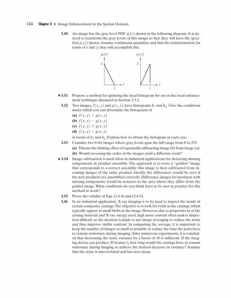
144 Chapter 3 � Image Enhancement in the Spatial Domain
3.10 An image has the gray level PDF pr(r) shown in the following diagram. It is de-sired to transform the gray levels of this image so that they will have the speci-fied pz(z) shown. Assume continuous quantities and find the transformation (interms of r and z) that will accomplish this.
3.11 Propose a method for updating the local histogram for use in the local enhance-ment technique discussed in Section 3.3.3.
3.12 Two images, f(x, y) and g(x, y), have histograms hf and hg . Give the conditionsunder which you can determine the histograms of(a) f(x, y)+g(x, y)
(b) f(x, y)-g(x, y)
(c) f(x, y)*g(x, y)
(d) f(x, y) , g(x, y)
in terms of hf and hg. Explain how to obtain the histogram in each case.3.13 Consider two 8-bit images whose gray levels span the full range from 0 to 255.
(a) Discuss the limiting effect of repeatedly subtracting image (b) from image (a).(b) Would reversing the order of the images yield a different result?
3.14 Image subtraction is used often in industrial applications for detecting missingcomponents in product assembly. The approach is to store a “golden” imagethat corresponds to a correct assembly; this image is then subtracted from in-coming images of the same product. Ideally, the differences would be zero ifthe new products are assembled correctly. Difference images for products withmissing components would be nonzero in the area where they differ from thegolden image. What conditions do you think have to be met in practice for thismethod to work?
3.15 Prove the validity of Eqs. (3.4-4) and (3.4-5).3.16 In an industrial application, X-ray imaging is to be used to inspect the inside of
certain composite castings.The objective is to look for voids in the castings, whichtypically appear as small blobs in the image. However, due to properties in of thecasting material and X-ray energy used, high noise content often makes inspec-tion difficult, so the decision is made to use image averaging to reduce the noiseand thus improve visible contrast. In computing the average, it is important tokeep the number of images as small as possible to reduce the time the parts haveto remain stationary during imaging. After numerous experiments, it is conclud-ed that decreasing the noise variance by a factor of 10 is sufficient. If the imag-ing device can produce 30 frames�s, how long would the castings have to remainstationary during imaging to achieve the desired decrease in variance? Assumethat the noise is uncorrelated and has zero mean.
2
1
2
1
pr(r) pz(z)
r z
�
�
GONZ03-075-146.II 29-08-2001 13:43 Page 144
� Problems 145
3.17 The implementation of linear spatial filters requires moving the center of a maskthroughout an image and, at each location, computing the sum of products of themask coefficients with the corresponding pixels at that location (see Section 3.5).In the case of lowpass filtering, all coefficients are 1, allowing use of a so-calledbox-filter or moving-average algorithm, which consists of updating only the partof the computation that changes from one location to the next.
(a) Formulate such an algorithm for an n*n filter, showing the nature of thecomputations involved and the scanning sequence used for moving the maskaround the image.
(b) The ratio of the number of computations performed by a brute-force imple-mentation to the number of computations performed by the box-filter algo-rithm is called the computational advantage. Obtain the computationaladvantage in this case and plot it as a function of n for n>1.The 1�n2 scalingfactor is common to both approaches, so you need not consider it in obtainingthe computational advantage. Assume that the image has an outer border ofzeros that is thick enough to allow you to ignore border effects in your analysis.
3.18 Discuss the limiting effect of repeatedly applying a 3*3 lowpass spatial filter toa digital image. You may ignore border effects.
3.19 (a) It was stated in Section 3.6.2 that isolated clusters of dark or light (with respectto the background) pixels whose area is less than one-half the area of a medi-an filter are eliminated (forced to the median value of the neighbors) by the fil-ter.Assume a filter of size n*n, with n odd, and explain why this is so.
(b) Consider an image having various sets of pixel clusters.Assume that all pointsin a cluster are lighter or darker than the background (but not both simulta-neously in the same cluster), and that the area of each cluster is less than orequal to n2�2. In terms of n, under what condition would one or more of theseclusters cease to be isolated in the sense described in part (a)?
3.20 (a) Develop a procedure for computing the median of an n*n neighborhood.
(b) Propose a technique for updating the median as the center of the neighbor-hood is moved from pixel to pixel.
3.21 (a) In a character recognition application, text pages are reduced to binary formusing a thresholding transformation function of the form shown in Fig. 3.2(b).This is followed by a procedure that thins the characters until they becomestrings of binary 1’s on a background of 0’s. Due to noise, the binarizationand thinning processes result in broken strings of characters with gaps rang-ing from 1 to 3 pixels. One way to “repair” the gaps is to run an averagingmask over the binary image to blur it, and thus create bridges of nonzero pix-els between gaps. Give the (odd) size of the smallest averaging mask capableof performing this task.
(b) After bridging the gaps, it is desired to threshold the image in order to con-vert it back to binary form. For your answer in (a), what is the minimum valueof the threshold required to accomplish this, without causing the segments tobreak up again?
3.22 The three images shown were blurred using square averaging masks of sizesn=23, 25, and 45, respectively.The vertical bars on the left lower part of (a) and(c) are blurred, but a clear separation exists between them. However, the bars
�
�
�
�
GONZ03-075-146.II 29-08-2001 13:43 Page 145
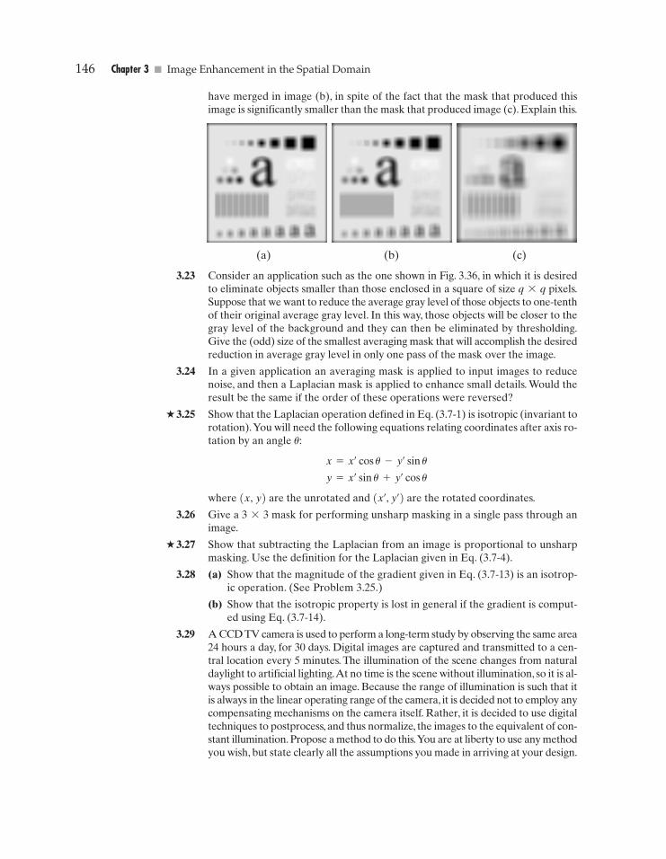
146 Chapter 3 � Image Enhancement in the Spatial Domain
have merged in image (b), in spite of the fact that the mask that produced thisimage is significantly smaller than the mask that produced image (c). Explain this.
3.23 Consider an application such as the one shown in Fig. 3.36, in which it is desiredto eliminate objects smaller than those enclosed in a square of size q*q pixels.Suppose that we want to reduce the average gray level of those objects to one-tenthof their original average gray level. In this way, those objects will be closer to thegray level of the background and they can then be eliminated by thresholding.Give the (odd) size of the smallest averaging mask that will accomplish the desiredreduction in average gray level in only one pass of the mask over the image.
3.24 In a given application an averaging mask is applied to input images to reducenoise, and then a Laplacian mask is applied to enhance small details. Would theresult be the same if the order of these operations were reversed?
3.25 Show that the Laplacian operation defined in Eq. (3.7-1) is isotropic (invariant torotation).You will need the following equations relating coordinates after axis ro-tation by an angle u:
x=x¿ cos u-y¿ sin u
y=x¿ sin u+y¿ cos u
where (x, y) are the unrotated and (x¿, y¿) are the rotated coordinates.
3.26 Give a 3*3 mask for performing unsharp masking in a single pass through animage.
3.27 Show that subtracting the Laplacian from an image is proportional to unsharpmasking. Use the definition for the Laplacian given in Eq. (3.7-4).
3.28 (a) Show that the magnitude of the gradient given in Eq. (3.7-13) is an isotrop-ic operation. (See Problem 3.25.)
(b) Show that the isotropic property is lost in general if the gradient is comput-ed using Eq. (3.7-14).
3.29 A CCD TV camera is used to perform a long-term study by observing the same area24 hours a day, for 30 days. Digital images are captured and transmitted to a cen-tral location every 5 minutes. The illumination of the scene changes from naturaldaylight to artificial lighting.At no time is the scene without illumination, so it is al-ways possible to obtain an image. Because the range of illumination is such that itis always in the linear operating range of the camera, it is decided not to employ anycompensating mechanisms on the camera itself. Rather, it is decided to use digitaltechniques to postprocess, and thus normalize, the images to the equivalent of con-stant illumination. Propose a method to do this.You are at liberty to use any methodyou wish, but state clearly all the assumptions you made in arriving at your design.
(a) (b) (c)
�
�
GONZ03-075-146.II 29-08-2001 14:30 Page 146

Digital Image ProcessingSecond Edition
Instructor’s Manual(Evaluation copy–Contains only representative, partial problem solutions)
Rafael C. GonzalezRichard E. Woods
Prentice Hall
Upper Saddle River, NJ 07458
www.prenhall.com/gonzalezwoods
or
www.imageprocessingbook.com

ii
Revision history
10 9 8 7 6 5 4 3 2 1
Copyright c°19922002 by Rafael C. Gonzalez and Richard E. Woods
PrefaceThis manual contains detailed solutions to all problems in Digital Image Processing, 2nd
Edition. We also include a suggested set of guidelines for using the book, and discuss
the use of computer projects designed to promote a deeper understanding of the subject
matter. The notation used throughout this manual corresponds to the notation used in
the text.
The decision of what material to cover in a course rests with the instructor, and it de
pends on the purpose of the course and the background of the students. We have found
that the course outlines suggested here can be covered comfortably in the time frames
indicated when the course is being taught in an electrical engineering or computer sci
ence curriculum. In each case, no prior exposure to image processing is assumed. We
give suggested guidelines for onesemester courses at the senior and firstyear graduate
levels. It is possible to cover most of the book in a twosemester graduate sequence.
The book was completely revised in this edition, with the purpose not only of updating
the material, but just as important, making the book a better teaching aid. To this
end, the instructor will find the new organization to be much more flexible and better
illustrated. Although the book is self contained, we recommend use of the companion
web site, where the student will find detailed solutions to the problems marked with a
star in the text, review material, suggested projects, and images from the book. One of
the principal reasons for creating the web site was to free the instructor from having to
prepare materials and handouts beyond what is required to teach from the book.
Computer projects such as those described in the web site are an important part of
a course on image processing. These projects give the student handson experience
with algorithm implementation and reinforce the material covered in the classroom.
The projects suggested at the web site can be implemented on almost any reasonably
equipped multiuser or personal computer having a hard copy output device.
1 Introduction
The purpose of this chapter is to present suggested guidelines for teaching material from
this book at the senior and firstyear graduate level. We also discuss use of the book
web site. Although the book is totally selfcontained, the web site offers, among other
things, complementary review material and computer projects that can be assigned in
conjunction with classroom work. Detailed solutions to all problems in the book also
are included in the remaining chapters of this manual.
Teaching Features of the Book
Undergraduate programs that offer digital image processing typically limit coverage to
one semester. Graduate programs vary, and can include one or two semesters of the ma
terial. In the following discussion we give general guidelines for a onesemester senior
course, a onesemester graduate course, and a fullyear course of study covering two
semesters. We assume a 15week program per semester with three lectures per week.
In order to provide flexibility for exams and review sessions, the guidelines discussed
in the following sections are based on forty, 50minute lectures per semester. The back
ground assumed on the part of the student is seniorlevel preparation in mathematical
analysis, matrix theory, probability, and computer programming.
The suggested teaching guidelines are presented in terms of general objectives, and not
as time schedules. There is so much variety in the way image processing material is
taught that it makes little sense to attempt a breakdown of the material by class period.
In particular, the organization of the present edition of the book is such that it makes it
much easier than before to adopt significantly different teaching strategies, depending
on course objectives and student background. For example, it is possible with the new
organization to offer a course that emphasizes spatial techniques and covers little or no
transform material. This is not something we recommend, but it is an option that often
is attractive in programs that place little emphasis on the signal processing aspects of the
field and prefer to focus more on the implementation of spatial techniques.
2 Chapter 1 Introduction
The companion web site
www:prenhall:com=gonzalezwoods
or
www:imageprocessingbook:com
is a valuable teaching aid, in the sense that it includes material that previously was cov
ered in class. In particular, the review material on probability, matrices, vectors, and
linear systems, was prepared using the same notation as in the book, and is focused on
areas that are directly relevant to discussions in the text. This allows the instructor to
assign the material as independent reading, and spend no more than one total lecture pe
riod reviewing those subjects. Another major feature is the set of solutions to problems
marked with a star in the book. These solutions are quite detailed, and were prepared
with the idea of using them as teaching support. The online availability of projects
and digital images frees the instructor from having to prepare experiments, data, and
handouts for students. The fact that most of the images in the book are available for
downloading further enhances the value of the web site as a teaching resource.
One Semester Senior Course
A basic strategy in teaching a senior course is to focus on aspects of image processing in
which both the inputs and outputs of those processes are images. In the scope of a senior
course, this usually means the material contained in Chapters 1 through 6. Depending
on instructor preferences, wavelets (Chapter 7) usually are beyond the scope of coverage
in a typical senior curriculum). However, we recommend covering at least some material
on image compression (Chapter 8) as outlined below.
We have found in more than two decades of teaching this material to seniors in electrical
engineering, computer science, and other technical disciplines, that one of the keys to
success is to spend at least one lecture on motivation and the equivalent of one lecture
on review of background material, as the need arises. The motivational material is
provided in the numerous application areas discussed in Chapter 1. This chapter was
totally rewritten with this objective in mind. Some of this material can be covered in
class and the rest assigned as independent reading. Background review should cover
probability theory (of one random variable) before histogram processing (Section 3.3).
A brief review of vectors and matrices may be required later, depending on the material
covered. The review material included in the book web site was designed for just this
purpose.
One Semester Senior Course 3
Chapter 2 should be covered in its entirety. Some of the material (such as parts of
Sections 2.1 and 2.3) can be assigned as independent reading, but a detailed explanation
of Sections 2.4 through 2.6 is time well spent.
Chapter 3 serves two principal purposes. It covers image enhancement (a topic of signif
icant appeal to the beginning student) and it introduces a host of basic spatial processing
tools used throughout the book. For a senior course, we recommend coverage of Sec
tions 3.2.1 through 3.2.2; Section 3.3.1; Section 3.4; Section 3.5; Section 3.6; Section
3.7.1, 3.7.2 (through Example 3.11), and 3.7.3. Section 3.8 can be assigned as indepen
dent reading, depending on time.
Chapter 4 also discusses enhancement, but from a frequencydomain point of view. The
instructor has significant flexibility here. As mentioned earlier, it is possible to skip
the chapter altogether, but this will typically preclude meaningful coverage of other
areas based on the Fourier transform (such as filtering and restoration). The key in
covering the frequency domain is to get to the convolution theorem and thus develop
a tie between the frequency and spatial domains. All this material is presented in very
readable form in Section 4.2. “Light” coverage of frequencydomain concepts can be
based on discussing all the material through this section and then selecting a few simple
filtering examples (say, low and highpass filtering using Butterworth filters, as discussed
in Sections 4.3.2 and 4.4.2). At the discretion of the instructor, additional material can
include full coverage of Sections 4.3 and 4.4. It is seldom possible to go beyond this
point in a senior course.
Chapter 5 can be covered as a continuation of Chapter 4. Section 5.1 makes this an easy
approach. Then, it is possible give the student a “flavor” of what restoration is (and still
keep the discussion brief) by covering only Gaussian and impulse noise in Section 5.2.1,
and a couple of spatial filters in Section 5.3. This latter section is a frequent source of
confusion to the student who, based on discussions earlier in the chapter, is expecting to
see a more objective approach. It is worthwhile to emphasize at this point that spatial
enhancement and restoration are the same thing when it comes to noise reduction by
spatial filtering. A good way to keep it brief and conclude coverage of restoration
is to jump at this point to inverse filtering (which follows directly from the model in
Section 5.1) and show the problems with this approach. Then, with a brief explanation
regarding the fact that much of restoration centers around the instabilities inherent in
inverse filtering, it is possible to introduce the “interactive” form of the Wiener filter in
Eq. (5.83) and conclude the chapter with Examples 5.12 and 5.13.
Chapter 6 on color image processing is a new feature of the book. Coverage of this
4 Chapter 1 Introduction
chapter also can be brief at the senior level by focusing on enough material to give the
student a foundation on the physics of color (Section 6.1), two basic color models (RGB
and CMY/CMYK), and then concluding with a brief coverage of pseudocolor processing
(Section 6.3).
We typically conclude a senior course by covering some of the basic aspects of image
compression (Chapter 8). Interest on this topic has increased significantly as a result of
the heavy use of images and graphics over the Internet, and students usually are easily
motivated by the topic. Minimum coverage of this material includes Sections 8.1.1 and
8.1.2, Section 8.2, and Section 8.4.1. In this limited scope, it is worthwhile spending
onehalf of a lecture period filling in any gaps that may arise by skipping earlier parts of
the chapter.
One Semester Graduate Course (No Background in DIP)
The main difference between a senior and a firstyear graduate course in which neither
group has formal background in image processing is mostly in the scope of material
covered, in the sense that we simply go faster in a graduate course, and feel much freer
in assigning independent reading. In addition to the material discussed in the previous
section, we add the following material in a graduate course.
Coverage of histogram matching (Section 3.3.2) is added. Sections 4.3, 4.4, and 4.5
are covered in full. Section 4.6 is touched upon briefly regarding the fact that imple
mentation of discrete Fourier transform techniques requires nonintuitive concepts such
as function padding. The separability of the Fourier transform should be covered, and
mention of the advantages of the FFT should be made. In Chapter 5 we add Sections 5.5
through 5.8. In Chapter 6 we add the HSI model (Section 6.3.2) , Section 6.4, and Sec
tion 6.6. A nice introduction to wavelets (Chapter 7) can be achieved by a combination
of classroom discussions and independent reading. The minimum number of sections in
that chapter are 7.1, 7.2, 7.3, and 7.5, with appropriate (but brief) mention of the exis
tence of fast wavelet transforms. Finally, in Chapter 8 we add coverage of Sections 8.3,
8.4.2, 8.5.1 (through Example 8.16), Section 8.5.2 (through Example 8.20) and Section
8.5.3.
If additional time is available, a natural topic to cover next is morphological image
processing (Chapter 9). The material in this chapter begins a transition from methods
whose inputs and outputs are images to methods in which the inputs are images, but
the outputs are attributes about those images, in the sense defined in Section 1.1. We
One Semester Graduate Course (with Background in DIP) 5
recommend coverage of Sections 9.1 through 9.4, and some of the algorithms in Section
9.5.
One Semester Graduate Course (with Background in DIP)
Some programs have an undergraduate course in image processing as a prerequisite to
a graduate course on the subject. In this case, it is possible to cover material from the
first eleven chapters of the book. Using the undergraduate guidelines described above,
we add the following material to form a teaching outline for a one semester graduate
course that has that undergraduate material as prerequisite. Given that students have the
appropriate background on the subject, independent reading assignments can be used to
control the schedule.
Coverage of histogram matching (Section 3.3.2) is added. Sections 4,3, 4.4, 4.5, and 4.6
are added. This strengthens the student’s background in frequencydomain concepts.
A more extensive coverage of Chapter 5 is possible by adding sections 5.2.3, 5.3.3,
5.4.3, 5.5, 5.6, and 5.8. In Chapter 6 we add fullcolor image processing (Sections 6.4
through 6.7). Chapters 7 and 8 are covered as in the previous section. As noted in the
previous section, Chapter 9 begins a transition from methods whose inputs and outputs
are images to methods in which the inputs are images, but the outputs are attributes
about those images. As a minimum, we recommend coverage of binary morphology:
Sections 9.1 through 9.4, and some of the algorithms in Section 9.5. Mention should
be made about possible extensions to grayscale images, but coverage of this material
may not be possible, depending on the schedule. In Chapter 10, we recommend Sections
10.1, 10.2.1 and 10.2.2, 10.3.1 through 10.3.4, 10.4, and 10.5. In Chapter 11we typically
cover Sections 11.1 through 11.4.
Two Semester Graduate Course (No Background in DIP)
A fullyear graduate course consists of the material covered in the one semester under
graduate course, the material outlined in the previous section, and Sections 12.1, 12.2,
12.3.1, and 12.3.2.
Projects
One of the most interesting aspects of a course in digital image processing is the pictorial

6 Chapter 1 Introduction
nature of the subject. It has been our experience that students truly enjoy and benefit
from judicious use of computer projects to complement the material covered in class.
Since computer projects are in addition to course work and homework assignments, we
try to keep the formal project reporting as brief as possible. In order to facilitate grading,
we try to achieve uniformity in the way project reports are prepared. A useful report
format is as follows:
Page 1: Cover page.
¢ Project title
¢ Project number
¢ Course number
¢ Student’s name
¢ Date due
¢ Date handed in
¢ Abstract (not to exceed 1/2 page)
Page 2: One to two pages (max) of technical discussion.
Page 3 (or 4): Discussion of results. One to two pages (max).
Results: Image results (printed typically on a laser or inkjet printer). All images must
contain a number and title referred to in the discussion of results.
Appendix: Program listings, focused on any original code prepared by the student. For
brevity, functions and routines provided to the student are referred to by name, but the
code is not included.
Layout: The entire report must be on a standard sheet size (e.g., 8:5 £ 11 inches),
stapled with three or more staples on the left margin to form a booklet, or bound using
clear plastic standard binding products.
Project resources available in the book web site include a sample project, a list of sug
gested projects from which the instructor can select, book and other images, and MAT
LAB functions. Instructors who do not wish to use MATLAB will find additional soft
ware suggestions in the Support/Software section of the web site.
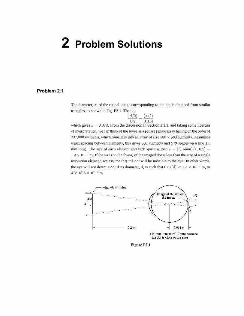
2 Problem Solutions
Problem 2.1
The diameter, x, of the retinal image corresponding to the dot is obtained from similar
triangles, as shown in Fig. P2.1. That is,(d=2)
0:2=
(x=2)
0:014which gives x = 0:07d. From the discussion in Section 2.1.1, and taking some liberties
of interpretation, we can think of the fovea as a square sensor array having on the order of
337,000 elements, which translates into an array of size 580 £ 580 elements. Assuming
equal spacing between elements, this gives 580 elements and 579 spaces on a line 1.5
mm long. The size of each element and each space is then s = [(1:5mm)=1; 159] =
1:3£10¡6 m. If the size (on the fovea) of the imaged dot is less than the size of a single
resolution element, we assume that the dot will be invisible to the eye. In other words,
the eye will not detect a dot if its diameter, d, is such that 0:07(d) < 1:3 £ 10¡6 m, or
d < 18:6 £ 10¡6 m.
Figure P2.1
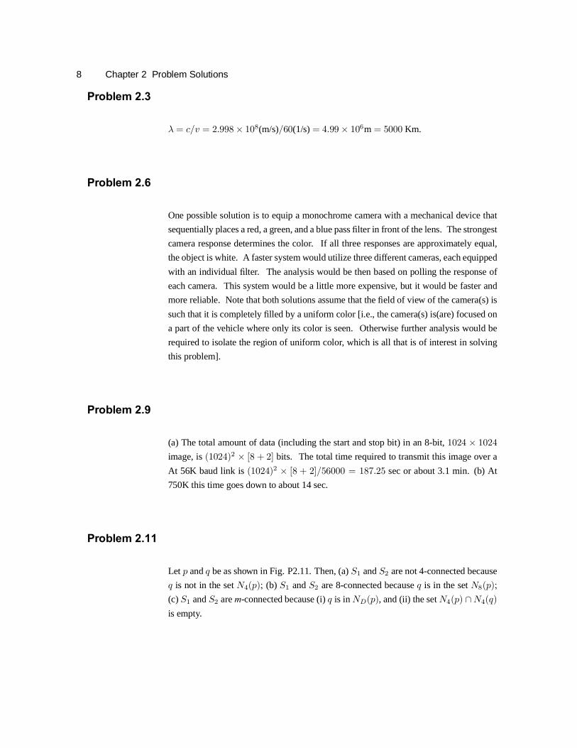
8 Chapter 2 Problem Solutions
Problem 2.3
¸ = c=v = 2:998 £ 108(m/s)=60(1/s) = 4:99 £ 106m = 5000 Km.
Problem 2.6
One possible solution is to equip a monochrome camera with a mechanical device that
sequentially places a red, a green, and a blue pass filter in front of the lens. The strongest
camera response determines the color. If all three responses are approximately equal,
the object is white. A faster system would utilize three different cameras, each equipped
with an individual filter. The analysis would be then based on polling the response of
each camera. This system would be a little more expensive, but it would be faster and
more reliable. Note that both solutions assume that the field of view of the camera(s) is
such that it is completely filled by a uniform color [i.e., the camera(s) is(are) focused on
a part of the vehicle where only its color is seen. Otherwise further analysis would be
required to isolate the region of uniform color, which is all that is of interest in solving
this problem].
Problem 2.9
(a) The total amount of data (including the start and stop bit) in an 8bit, 1024 £ 1024
image, is (1024)2 £ [8 + 2] bits. The total time required to transmit this image over a
At 56K baud link is (1024)2 £ [8 + 2]=56000 = 187:25 sec or about 3.1 min. (b) At
750K this time goes down to about 14 sec.
Problem 2.11
Let p and q be as shown in Fig. P2.11. Then, (a) S1 and S2 are not 4connected because
q is not in the set N4(p); (b) S1 and S2 are 8connected because q is in the set N8(p);
(c) S1 and S2 are mconnected because (i) q is in ND(p), and (ii) the set N4(p) \ N4(q)
is empty.
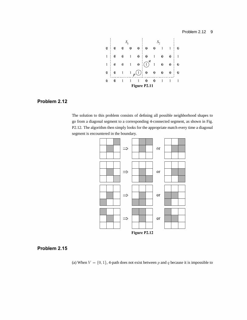
Problem 2.12 9
Figure P2.11
Problem 2.12
The solution to this problem consists of defining all possible neighborhood shapes to
go from a diagonal segment to a corresponding 4connected segment, as shown in Fig.
P2.12. The algorithm then simply looks for the appropriate match every time a diagonal
segment is encountered in the boundary.
Figure P2.12
Problem 2.15
(a) When V = f0; 1g, 4path does not exist between p and q because it is impossible to
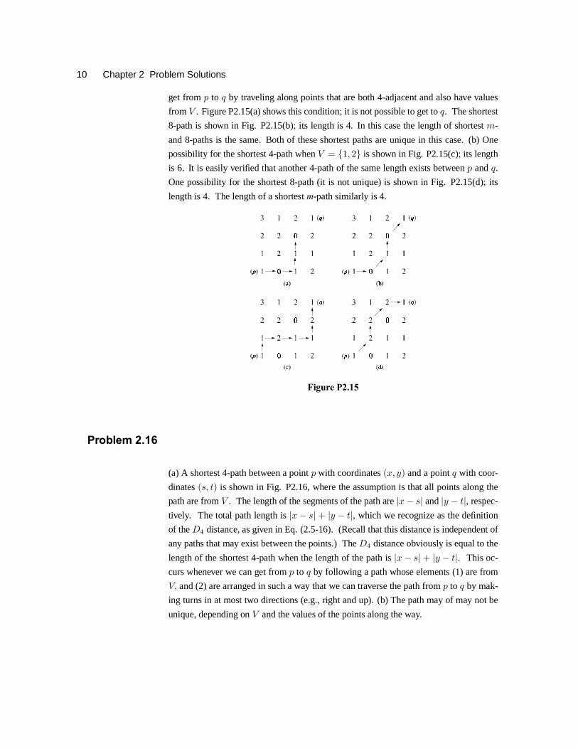
10 Chapter 2 Problem Solutions
get from p to q by traveling along points that are both 4adjacent and also have values
from V . Figure P2.15(a) shows this condition; it is not possible to get to q. The shortest
8path is shown in Fig. P2.15(b); its length is 4. In this case the length of shortest m
and 8paths is the same. Both of these shortest paths are unique in this case. (b) One
possibility for the shortest 4path when V = f1; 2g is shown in Fig. P2.15(c); its length
is 6. It is easily verified that another 4path of the same length exists between p and q.
One possibility for the shortest 8path (it is not unique) is shown in Fig. P2.15(d); its
length is 4. The length of a shortest mpath similarly is 4.
Figure P2.15
Problem 2.16
(a) A shortest 4path between a point p with coordinates (x; y) and a point q with coor
dinates (s; t) is shown in Fig. P2.16, where the assumption is that all points along the
path are from V . The length of the segments of the path are jx ¡ sj and jy ¡ tj, respec
tively. The total path length is jx ¡ sj + jy ¡ tj, which we recognize as the definition
of the D4 distance, as given in Eq. (2.516). (Recall that this distance is independent of
any paths that may exist between the points.) The D4 distance obviously is equal to the
length of the shortest 4path when the length of the path is jx ¡ sj + jy ¡ tj. This oc
curs whenever we can get from p to q by following a path whose elements (1) are from
V; and (2) are arranged in such a way that we can traverse the path from p to q by mak
ing turns in at most two directions (e.g., right and up). (b) The path may of may not be
unique, depending on V and the values of the points along the way.
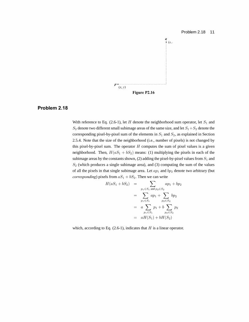
Problem 2.18 11
Figure P2.16
Problem 2.18
With reference to Eq. (2.61), let H denote the neighborhood sum operator, let S1 and
S2 denote two different small subimage areas of the same size, and let S1+S2 denote the
corresponding pixelbypixel sum of the elements in S1 and S2, as explained in Section
2.5.4. Note that the size of the neighborhood (i.e., number of pixels) is not changed by
this pixelbypixel sum. The operator H computes the sum of pixel values is a given
neighborhood. Then, H(aS1 + bS2) means: (1) multiplying the pixels in each of the
subimage areas by the constants shown, (2) adding the pixelbypixel values from S1 and
S2 (which produces a single subimage area), and (3) computing the sum of the values
of all the pixels in that single subimage area. Let ap1 and bp2 denote two arbitrary (but
corresponding) pixels from aS1 + bS2. Then we can write
H(aS1 + bS2) =X
p12S1 and p22S2
ap1 + bp2
=X
p12S1
ap1 +X
p22S2
bp2
= aX
p12S1
p1 + bX
p22S2
p2
= aH(S1) + bH(S2)
which, according to Eq. (2.61), indicates that H is a linear operator.

3 Problem Solutions
Problem 3.2
(a)
s = T (r) =1
1 + (m=r)E:
Problem 3.4
(a) The number of pixels having different gray level values would decrease, thus causing
the number of components in the histogram to decrease. Since the number of pixels
would not change, this would cause the height some of the remaining histogram peaks
to increase in general. Typically, less variability in gray level values will reduce contrast.
Problem 3.5
All that histogram equalization does is remap histogram components on the intensity
scale. To obtain a uniform (flat) histogram would require in general that pixel intensities
be actually redistributed so that there are L groups of n=L pixels with the same intensity,
where L is the number of allowed discrete intensity levels and n is the total number of
pixels in the input image. The histogram equalization method has no provisions for this
type of (artificial) redistribution process.
Problem 3.8
We are interested in just one example in order to satisfy the statement of the problem.
Consider the probability density function shown in Fig. P3.8(a). A plot of the trans
formation T (r) in Eq. (3.34) using this particular density function is shown in Fig.
P3.8(b). Because pr(r) is a probability density function we know from the discussion
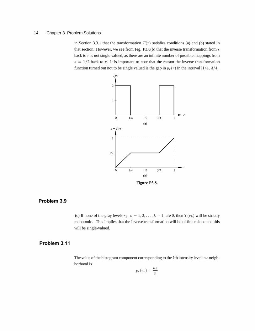
14 Chapter 3 Problem Solutions
in Section 3.3.1 that the transformation T (r) satisfies conditions (a) and (b) stated in
that section. However, we see from Fig. P3.8(b) that the inverse transformation from s
back to r is not single valued, as there are an infinite number of possible mappings from
s = 1=2 back to r. It is important to note that the reason the inverse transformation
function turned out not to be single valued is the gap in pr(r) in the interval [1=4; 3=4].
Figure P3.8.
Problem 3.9
(c) If none of the gray levels rk; k = 1; 2; : : : ; L ¡ 1; are 0, then T (rk) will be strictly
monotonic. This implies that the inverse transformation will be of finite slope and this
will be singlevalued.
Problem 3.11
The value of the histogram component corresponding to the kth intensity level in a neigh
borhood is
pr(rk) =nk
n
Problem 3.14 15
for k = 1; 2; : : : ;K ¡ 1;where nk is the number of pixels having gray level value rk, n
is the total number of pixels in the neighborhood, and K is the total number of possible
gray levels. Suppose that the neighborhood is moved one pixel to the right. This deletes
the leftmost column and introduces a new column on the right. The updated histogram
then becomes
p0r(rk) =
1
n[nk ¡ nLk
+ nRk]
for k = 0; 1; : : : ;K ¡ 1, where nLk is the number of occurrences of level rk on the left
column and nRkis the similar quantity on the right column. The preceding equation can
be written also as
p0r(rk) = pr(rk) +
1
n[nRk
¡ nLk]
for k = 0; 1; : : : ; K ¡ 1: The same concept applies to other modes of neighborhood
motion:
p0r(rk) = pr(rk) +
1
n[bk ¡ ak]
for k = 0; 1; : : : ;K ¡1, where ak is the number of pixels with value rk in the neighbor
hood area deleted by the move, and bk is the corresponding number introduced by the
move.
¾2g = ¾2
f +1
K2[¾2
´1+ ¾2
´2+ ¢ ¢ ¢ + ¾2
´K
]
The first term on the right side is 0 because the elements of f are constants. The various
¾2´i
are simply samples of the noise, which is has variance ¾2´. Thus, ¾2
´i= ¾2
´ and we
have
¾2g =
K
K2¾2
´ =1
K¾2
´
which proves the validity of Eq. (3.45).
Problem 3.14
Let g(x; y) denote the golden image, and let f(x; y) denote any input image acquired
during routine operation of the system. Change detection via subtraction is based on
computing the simple difference d(x; y) = g(x; y) ¡ f(x; y). The resulting image
d(x; y) can be used in two fundamental ways for change detection. One way is use a
pixelbypixel analysis. In this case we say that f(x; y) is ”close enough” to the golden
image if all the pixels in d(x; y) fall within a specified threshold band [Tmin; Tmax]
where Tmin is negative and Tmax is positive. Usually, the same value of threshold is
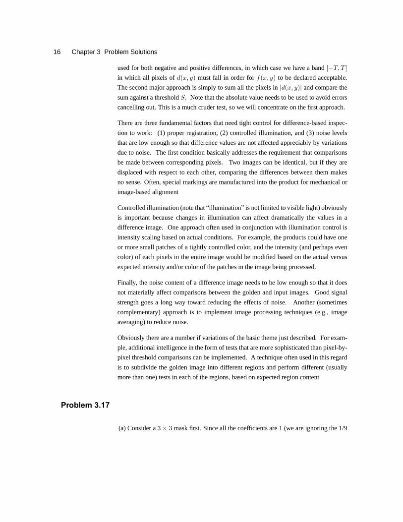
16 Chapter 3 Problem Solutions
used for both negative and positive differences, in which case we have a band [¡T; T ]
in which all pixels of d(x; y) must fall in order for f(x; y) to be declared acceptable.
The second major approach is simply to sum all the pixels in jd(x; y)j and compare the
sum against a threshold S. Note that the absolute value needs to be used to avoid errors
cancelling out. This is a much cruder test, so we will concentrate on the first approach.
There are three fundamental factors that need tight control for differencebased inspec
tion to work: (1) proper registration, (2) controlled illumination, and (3) noise levels
that are low enough so that difference values are not affected appreciably by variations
due to noise. The first condition basically addresses the requirement that comparisons
be made between corresponding pixels. Two images can be identical, but if they are
displaced with respect to each other, comparing the differences between them makes
no sense. Often, special markings are manufactured into the product for mechanical or
imagebased alignment
Controlled illumination (note that “illumination” is not limited to visible light) obviously
is important because changes in illumination can affect dramatically the values in a
difference image. One approach often used in conjunction with illumination control is
intensity scaling based on actual conditions. For example, the products could have one
or more small patches of a tightly controlled color, and the intensity (and perhaps even
color) of each pixels in the entire image would be modified based on the actual versus
expected intensity and/or color of the patches in the image being processed.
Finally, the noise content of a difference image needs to be low enough so that it does
not materially affect comparisons between the golden and input images. Good signal
strength goes a long way toward reducing the effects of noise. Another (sometimes
complementary) approach is to implement image processing techniques (e.g., image
averaging) to reduce noise.
Obviously there are a number if variations of the basic theme just described. For exam
ple, additional intelligence in the form of tests that are more sophisticated than pixelby
pixel threshold comparisons can be implemented. A technique often used in this regard
is to subdivide the golden image into different regions and perform different (usually
more than one) tests in each of the regions, based on expected region content.
Problem 3.17
(a) Consider a 3 £ 3 mask first. Since all the coefficients are 1 (we are ignoring the 1/9
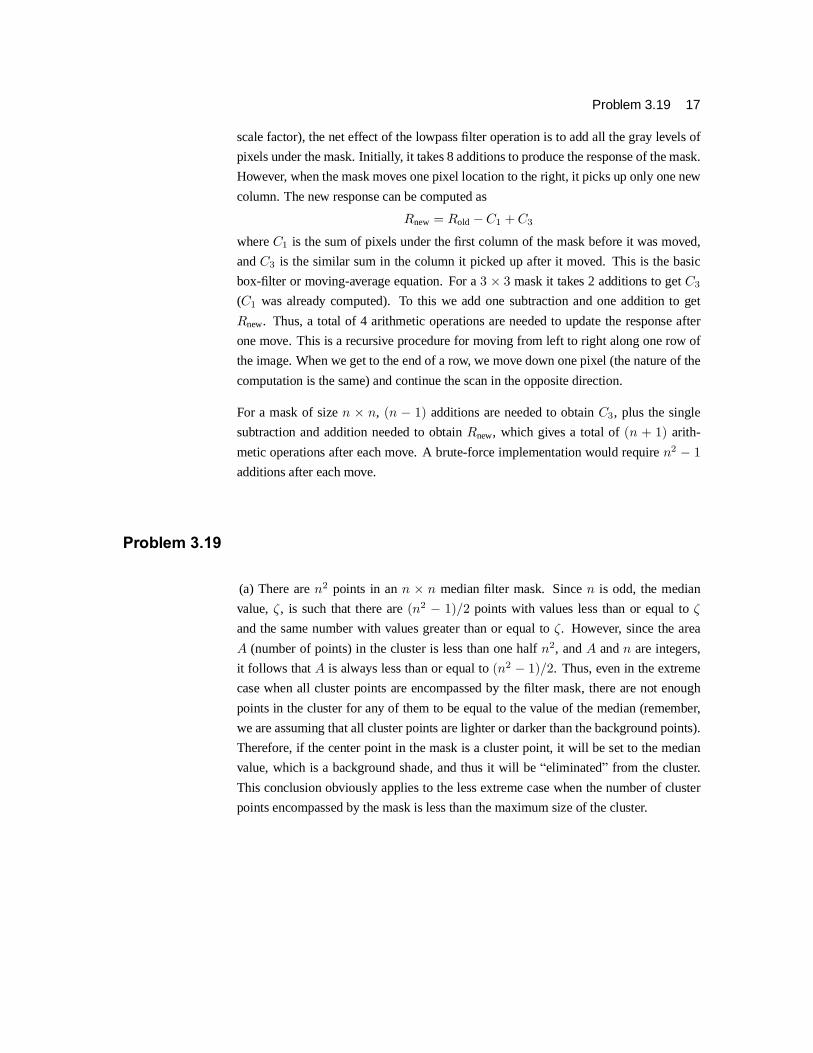
Problem 3.19 17
scale factor), the net effect of the lowpass filter operation is to add all the gray levels of
pixels under the mask. Initially, it takes 8 additions to produce the response of the mask.
However, when the mask moves one pixel location to the right, it picks up only one new
column. The new response can be computed as
Rnew = Rold ¡ C1 + C3
where C1 is the sum of pixels under the first column of the mask before it was moved,
and C3 is the similar sum in the column it picked up after it moved. This is the basic
boxfilter or movingaverage equation. For a 3 £ 3 mask it takes 2 additions to get C3
(C1 was already computed). To this we add one subtraction and one addition to get
Rnew. Thus, a total of 4 arithmetic operations are needed to update the response after
one move. This is a recursive procedure for moving from left to right along one row of
the image. When we get to the end of a row, we move down one pixel (the nature of the
computation is the same) and continue the scan in the opposite direction.
For a mask of size n £ n, (n ¡ 1) additions are needed to obtain C3, plus the single
subtraction and addition needed to obtain Rnew, which gives a total of (n + 1) arith
metic operations after each move. A bruteforce implementation would require n2 ¡ 1
additions after each move.
Problem 3.19
(a) There are n2 points in an n £ n median filter mask. Since n is odd, the median
value, ³ , is such that there are (n2 ¡ 1)=2 points with values less than or equal to ³
and the same number with values greater than or equal to ³. However, since the area
A (number of points) in the cluster is less than one half n2, and A and n are integers,
it follows that A is always less than or equal to (n2 ¡ 1)=2. Thus, even in the extreme
case when all cluster points are encompassed by the filter mask, there are not enough
points in the cluster for any of them to be equal to the value of the median (remember,
we are assuming that all cluster points are lighter or darker than the background points).
Therefore, if the center point in the mask is a cluster point, it will be set to the median
value, which is a background shade, and thus it will be “eliminated” from the cluster.
This conclusion obviously applies to the less extreme case when the number of cluster
points encompassed by the mask is less than the maximum size of the cluster.
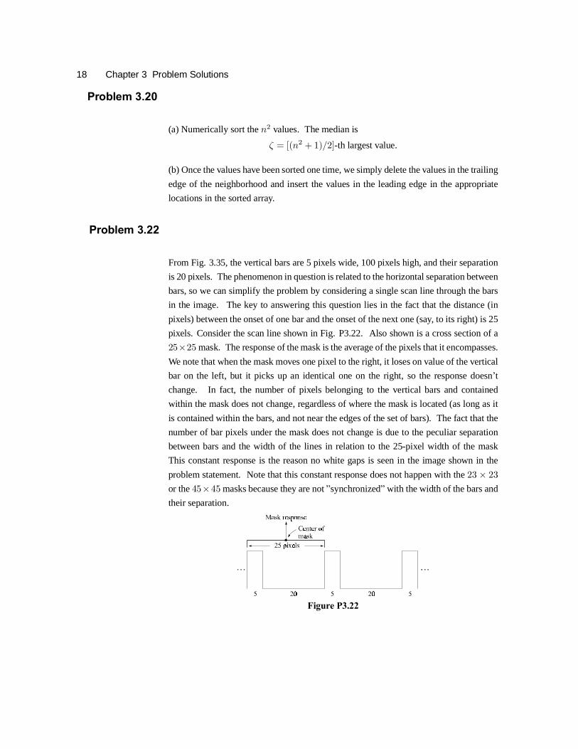
18 Chapter 3 Problem Solutions
Problem 3.20
(a) Numerically sort the n2 values. The median is
³ = [(n2 + 1)=2]th largest value.
(b) Once the values have been sorted one time, we simply delete the values in the trailing
edge of the neighborhood and insert the values in the leading edge in the appropriate
locations in the sorted array.
Problem 3.22
From Fig. 3.35, the vertical bars are 5 pixels wide, 100 pixels high, and their separation
is 20 pixels. The phenomenon in question is related to the horizontal separation between
bars, so we can simplify the problem by considering a single scan line through the bars
in the image. The key to answering this question lies in the fact that the distance (in
pixels) between the onset of one bar and the onset of the next one (say, to its right) is 25
pixels. Consider the scan line shown in Fig. P3.22. Also shown is a cross section of a
25£25 mask. The response of the mask is the average of the pixels that it encompasses.
We note that when the mask moves one pixel to the right, it loses on value of the vertical
bar on the left, but it picks up an identical one on the right, so the response doesn’t
change. In fact, the number of pixels belonging to the vertical bars and contained
within the mask does not change, regardless of where the mask is located (as long as it
is contained within the bars, and not near the edges of the set of bars). The fact that the
number of bar pixels under the mask does not change is due to the peculiar separation
between bars and the width of the lines in relation to the 25pixel width of the mask
This constant response is the reason no white gaps is seen in the image shown in the
problem statement. Note that this constant response does not happen with the 23 £ 23
or the 45£45 masks because they are not ”synchronized” with the width of the bars and
their separation.
Figure P3.22
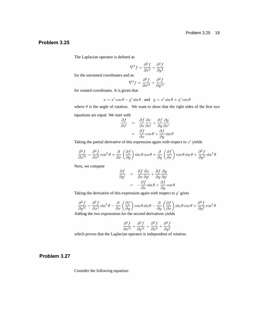
Problem 3.25 19
Problem 3.25
The Laplacian operator is defined as
r2f =@2f
@x2+
@2f
@y2
for the unrotated coordinates and as
r2f =@2f
@x02 +@2f
@y02 :
for rotated coordinates. It is given that
x = x0 cos µ ¡ y0 sin µ and y = x0 sin µ + y0 cos µ
where µ is the angle of rotation. We want to show that the right sides of the first two
equations are equal. We start with@f
@x0 =@f
@x
@x
@x0 +@f
@y
@y
@x0
=@f
@xcos µ +
@f
@ysin µ
Taking the partial derivative of this expression again with respect to x0 yields
@2f
@x02 =@2f
@x2cos2 µ +
@
@x
µ@f
@y
¶sin µ cos µ +
@
@y
µ@f
@x
¶cos µ sin µ +
@2f
@y2sin2 µ
Next, we compute@f
@y0 =@f
@x
@x
@y0 +@f
@y
@y
@y0
= ¡@f
@xsin µ +
@f
@ycos µ
Taking the derivative of this expression again with respect to y0 gives
@2f
@y02 =@2f
@x2sin2 µ ¡ @
@x
µ@f
@y
¶cos µ sinµ ¡ @
@y
µ@f
@x
¶sin µ cos µ +
@2f
@y2cos2 µ
Adding the two expressions for the second derivatives yields
@2f
@x02 +@2f
@y02 =@2f
@x2+
@2f
@y2
which proves that the Laplacian operator is independent of rotation.
Problem 3.27
Consider the following equation:
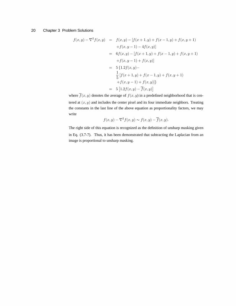
20 Chapter 3 Problem Solutions
f(x; y) ¡ r2f(x; y) = f(x; y) ¡ [f(x + 1; y) + f(x ¡ 1; y) + f(x; y + 1)
+f(x; y ¡ 1) ¡ 4f(x; y)]
= 6f(x; y) ¡ [f(x + 1; y) + f(x ¡ 1; y) + f(x; y + 1)
+f(x; y ¡ 1) + f(x; y)]
= 5 f1:2f(x; y)¡1
5[f(x + 1; y) + f(x ¡ 1; y) + f(x; y + 1)
+f(x; y ¡ 1) + f(x; y)]g= 5
£1:2f(x; y) ¡ f(x; y)
¤
where f(x; y) denotes the average of f(x; y) in a predefined neighborhood that is cen
tered at (x; y) and includes the center pixel and its four immediate neighbors. Treating
the constants in the last line of the above equation as proportionality factors, we may
write
f(x; y) ¡ r2f(x; y) s f(x; y) ¡ f(x; y):
The right side of this equation is recognized as the definition of unsharp masking given
in Eq. (3.77). Thus, it has been demonstrated that subtracting the Laplacian from an
image is proportional to unsharp masking.