Digital Image Processing Programming Exercise 2011 – Part 3

The third part of the Digital Image Programming Exercise is actually a small image processing project in which you will implement a Matlab code for detecting visual code markers from webcam-quality images.

Check the web page http://www.ee.oulu.fi/research/imag/courses/dkk/pexercise/occasionally since updates and errata of these instructions will be published on that page. If you experience problems that cannot be solved using the course material and Matlab help files, contact the programming exercise assistant at email address dkk-staff@ee.oulu.fi or by visiting the office TS315.

No actual written report is requested this time. Therefore, the report must include only aftermath, list of references and all Matlab code. Return the “report”, stapled together with the filled cover page (download the cover page from the web address mentioned above).

You are encouraged to seek information in other places than the course book, lecture material and the article mentioned below but list all the sources you used in the report.

When you have completed the exercise,1. Return your “report” (consisting of cover page, references, feeback and Matlab

codes) on paper to the mail box with sign “Digital image processing” on the 3 rd floor of Tietotalo

2. Send all the requested Matlab scripts and functions by e-mail to dkk-staff@ee.oulu.fi. Put your student id number and your name to the subject of the email.

The deadline for returning the report and sending the e-mail is 22.12.2011 15:45.

Visual code marker detection

Recognition and tracking of objects or environments using computer vision is still a very challenging problem because the natural features are difficult to detect and match due to variations caused by e.g. illumination and viewpoints changes. However, there exist methods which can be used for registration and tracking of well-textured objects but these techniques cannot be used for instance if the target object or environment does not contain unique points of interest (e.g. untextured surfaces).

One can simplify the problem by modifying the target objects or environments by adding fiducials, e.g. LEDs or planar visual markers, on the objects or in the scene. These fiducials can be easily to detected in real time using simple image processing algorithms. Figure 1 shows some examples of planar visual markers used in this exercise. The visual markers contain some kind of extra information, such as their identifier, which is usually be encoded in 2D barcodes (which can also be seen in Figure 1). Also the camera orientation and location (camera pose) relative to the visual marker can be computed based on the marker's location in an image. Thus, if the marker's pose is known in world coordinate system (WCS), also the camera pose can be retrieved in WCS.

Figure 1. Example images of visual code markers and their description.

Since 3D computer vision and computer graphics are out of our scope, we consider only simple marker detection and normalization using image processing techniques. Therefore, your task is to write Matlab code which is able to detect 2D visual code markers from the given webcam-quality test images. Decoding the 2D barcode is an extra task. This document and the function templates should provide all the necessary information for implementing the different stages of this image processing task. However, you can also try out your own methods if you want to.

Visual code marker details

The visual code markers that we consider are 2-dimensional arrays. The array consists of 11x11 elements. Each element is either black or white. As shown in the Figure 2 below, we fix the elements in three of the corners to be black. One vertical guide bar (7 elements long) and one horizontal guide bar (5 elements long) are also included. The immediate neighbors of the corner elements and the guide bar elements are fixed to be white. This leaves us with 83 data elements (bits) which can be either black or white.

Figure 2. Example of the used visual code marker where the fixed guide bars and corner elements can be seen. The actual data region is the area marked with red color.

Image processing pipeline

In order to detect the visual code markers, several image processing tasks must be performed. The image processing pipeline that should be implemented can be seen below in Figure 3.

Figure 3. Image processing pipeline needed for visual code marker detection (minimum requirements for passing this exercise are marked with red).

1. PreprocessingThe purpose of the preprocessing step is to enhance the original image and to produce an output image from which the visual markers are easier to locate. In our case, we first apply the Canny edge detector on the image which results to a quite noisy edge (binary) image as seen in Figure 4. In order to remove most of the unwanted edges, we find all connected components in the image and filter out the components that do not have exactly one hole based on their Euler number. By performing these operations we get a preprocessed binary image from which we are able to locate all visual markers.

Hint: You can use function edge for edge filtering (SIGMA = 1 for Canny filtering and you leave the threshold field empty, [],, and use 'canny_old' argument if using R2011a or newer version of Matlab) and for binary image processing functions bwconncomp and regionprops are really handy.

Figure 4. Image preprocessing, original image (left), Canny edge filtered image (middle) and filtered edge image (right) which consists only of connected components that have exactly one hole.

2. Finding fixed guide barsThe fixed guide bar candidates are filtered from the preprocessed image based on some shape properties of the connected components. The guide bars are long rectangles so their bar-like shape can be presented using shape five descriptors, eccentricity, major and minor axis lengths and area. We also use a descriptor called 'solidity' which is the area divided by the convex hull area to remove some spurious matches. The proper threshold value limits of the different shape descriptors used in this “object recognition task” can be found in Table 1. An example image of the found bar candidates can be seen in Figure 5.

The filtered image of bar candidates still has some false detections. In order to get rid of them and to find all pairs of fixed guide bars, we should iterate through all candidates and

PreprocessingRGB image

Find fixed guide bars

Binary image

Geometric normalization

Find corner points

Decode 2D barcode

Guide bars Detected markers

Marker images

Bit sequences

form pairs which meet the following two requirements: the distance between their centroids must be close enough to each other and the orientation of the bars must be nearly perpendicular (nearly because the perspective projection causes distortion). The distance and angle value limits needed for finding true fixed guide bar pairs can also be found in Table 1. An example end result of fixed bar finding process can be seen in Figure 5.

Hint: Again, binary image processing functions bwconncomp and regionprops are really handy.

Figure 5. Finding fixed guide bars, preprocessed image (left), possible bar candidates (middle) and true fixed guide bar pair.

3. Finding fixed corner pointsThe fixed corner elements can be located when the guide bar locations have been determined. First the corner point candidates candidates are filtered from the preprocessed image based on shape properties of the connected components (like in previous guide bar finding phase). This time we are looking for circular objects with predefined size requirements, so now we consider only following shape descriptors, eccentricity, major axis length and area. The threshold value limits for these parameters can be found in Table 2. In Figure 6 you can see the results of corner point filtering combined with the detected guide bar pairs.

Figure 6. Combined binary image of corner point candidates and detected fixed guide bar pairs.

When we have obtained a binary image which contains all corner point candidates, we can once again label all remaining connected components and store their centroids in a list. In

order to find the three corresponding corner points for each guide par pair, we have to iterate through all pairs and:

1. Compute the estimated location of the corner points based on the guide bar orientations and centroids.

2. Locate the correct corner points by looking for the corner point candidate which is closest to the estimated corner point location.

For the first phase, guide bar orientation must be normalized to be parallel with the actual search direction because the orientation of the guide bar is unambiguous. This ambiguity can be done by searching the nearest extrema points between the two guide bars, see Figure 7. When these extrema points are known, we can form a reference vector from the extrema point to the centroid of the guide bar. The dot product of the reference vector and the bar orientation tells us if the bar orientation is defined in “right” or “wrong” direction. If the dot product is positive, the directions of these vectors correlate, when the original bar orientation can be used as search direction. Otherwise, we must change the bar orientation vector to the opposite direction.

Figure 7. Normalization of the fixed guide bar orientation based on the closest extrema points.

The following formulas can be then used for computing the estimated locations of the corner points when the search direction is known:

v x=[ cosθ−sinθ]

cur=c l+57

maj l v l c l l=cs+85

maj s vs

cul1=c l l+107

majl vl cul2=cur+105

maj s vs

cul=cul1+cul2

2

where vx = normalized orientation of the guide bar, cxx (x,y) = the estimated centroid of the corner point xx, cx (x,y) = the centroid of the fixed guide bar x, majorx = major axis length of the guide bar x, and the subscripts stand for: ur = upper right, ll = lower left, ul = upper left, l = longer and s = shorter.

When the all corner points are successfully retrieved, the visualization script should be able to produce the following image (see Figure 8).

Figure 8. Visualization of a successful marker detection.

4. Geometric normalization of detected marker imagesBefore we can read the actual 2D barcode, the marker image must be normalized geometrically. The resulting image should be size of 110x110 pixels (ten pixels per marker element). An example image of geometrically normalized marker image can be seen in Figure 9. The fixed locations of the five detected reference points in the normalized image are listed in Table 2. The projective geometrical correction to the marker image can be performed using two Matlab functions, cp2tform and imtransform.

Figure 9. Example image of a geometrically normalized visual code marker.

5. Decoding the 2D barcode into bit sequenceFor reading the data field, the normalized visual code marker image must be first thresholded to get a binary image. An example of thresholded marker image is presented in Figure 10. With the algorithms presented here and our test images, it is enough to use only the "middle" pixel value of each data element (instead of considering statistics of all pixel values on the grid) for predicting the true bit values. When all 11x11 elements of the 2D barcode have been retrieved, the 2D binary code can be read column-wise into one bit sequence.

Figure 10. Binary image of the normalized visual code marker with overlaid element grid.

Minimum requirements and extra features

The minimum task needed to pass this part is that:• You implement Matlab functions needed for preprocessing and finding fixed guide

bars. • Your code must work and also be easy to follow, e.g. well commented, etc.

◦ The guide bars must be found in every test image which should not be that hard if the used parameters are taken from this document. The algorithms can be tested on the provided test images which show you how well your implementation works.

• You do not have to write an actual report this time and therefore only references and feedback is required + all Matlab code.

In order to get the maximum number of points you will have to implement also some extra features:

1. Finding fixed corner points2. Geometrical normalization of the visual code marker images3. 2D barcode decoding

Extra features must be implemented in this order since they are dependent on each other in inverse order.

Function specifications

In addition to the test images, the given zip file includes scripts, functions and function templates which should be used or implemented. The detect_code function is the main function which contains the image processing pipeline that should be implemented. The detect_code function and the function templates have already some documentation, e.g. definition of input and output arguments and some instructions .

You are also encouraged to use you own functions inside the function templates to make the code more readable and avoid overlapping procedures, but please make sure that the data structures for the input and output arguments of the image processing pipeline follow the definitions.

Testing your algorithm

The zip file includes also scripts for testing your the performance of your implementation e.g. detect_code_all_images which executes the detect_code function on all available test images. An evaluation script will be available later and it computes e.g. the accuracy of correctly recognized bits compared to ground truth data.

Grading

● Minimum requirements (25 points)

● Implemented extra features (MAX. 25 points)1. Finding corner points (15p)2. Geometrical normalization (5p)3. Decoding 2D barcode (5p)

Total maximum 50 points

Aftermath

1. How much time did you need to complete this exercise?2. Did you experience any problems with the exercise? Was there enough help

available? Where did you look for help?3. What did you learn?

Tables

Note that the following threshold values are not optimal ones but they should work for all the test images.

Table 1.

Property Threshold value limits

Eccentricity (E) E > 0.93

Area (A) A > 45

Minor axis length (Mi) 6 < Mi < 20

Major axis length (Ma) 30 < Ma < 90

Solidity (S) S > 0.19

Orienation difference (θ) 65 < |θ| < 120

Distance between centroids (D) 22 < D < 55

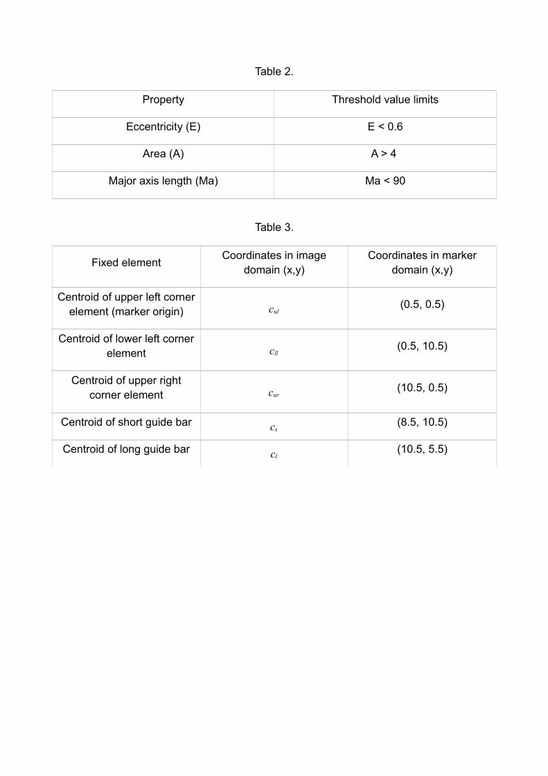
Table 2.

Property Threshold value limits

Eccentricity (E) E < 0.6

Area (A) A > 4

Major axis length (Ma) Ma < 90

Table 3.

Fixed element Coordinates in image domain (x,y)

Coordinates in marker domain (x,y)

Centroid of upper left corner element (marker origin) cul

(0.5, 0.5)

Centroid of lower left corner element cll

(0.5, 10.5)

Centroid of upper right corner element cur

(10.5, 0.5)

Centroid of short guide bar cs(8.5, 10.5)

Centroid of long guide bar cl(10.5, 5.5)