
Digital Image Processing Ming Jiang - PKU · 2016-04-22 · 1.2.1 Low-level image processing...
559
Digital Image Processing Ming Jiang Revision : 1.1. June 5, 2009 School of Mathematical Sciences, Peking University
Transcript of Digital Image Processing Ming Jiang - PKU · 2016-04-22 · 1.2.1 Low-level image processing...

Digital Image Processing
Ming JiangRevision : 1.1. June 5, 2009
School of Mathematical Sciences, Peking University

Contents
1 Introduction and Course Overview 11.1 Digital image processing: What, Why and How . . . . . . . . . . . 2
1.1.1 What is and why we need digital image processing . . . . . 31.1.2 Example: Detection of Ozone Layer Hole . . . . . . . . . . 4
1.2 General Procedures . . . . . . . . . . . . . . . . . . . . . . . . . 81.2.1 Low-level image processing . . . . . . . . . . . . . . . . . 101.2.2 High-level image processing . . . . . . . . . . . . . . . . . 12
1.3 Digital Image Processing and Other Disciplines . . . . . . . . . . . 131.4 What Are the Difficulties . . . . . . . . . . . . . . . . . . . . . . 14
1.4.1 Poor understanding of the human vision system . . . . . . 141.4.2 Internal representation is not directly understandable . . . . 20
2

CONTENTS 3
1.5 Course Overview . . . . . . . . . . . . . . . . . . . . . . . . . . . 22
1.5.1 Course syllabus . . . . . . . . . . . . . . . . . . . . . . . . 22
1.5.2 Textbooks and references . . . . . . . . . . . . . . . . . . 22
2 The Digitized Image and its Properties 232.1 Basic concepts . . . . . . . . . . . . . . . . . . . . . . . . . . . . 24
2.1.1 Image functions . . . . . . . . . . . . . . . . . . . . . . . 25
2.2 Image digitization . . . . . . . . . . . . . . . . . . . . . . . . . . 35
2.2.1 Sampling . . . . . . . . . . . . . . . . . . . . . . . . . . . 36
2.2.2 Quantization . . . . . . . . . . . . . . . . . . . . . . . . . 45
2.2.3 Color Images . . . . . . . . . . . . . . . . . . . . . . . . . 47
2.3 Digital image properties . . . . . . . . . . . . . . . . . . . . . . . 50
2.3.1 Metric and topological properties of digital images . . . . . 50
2.3.2 Histogram . . . . . . . . . . . . . . . . . . . . . . . . . . 66
2.3.3 Visual perception of the image . . . . . . . . . . . . . . . 68
2.3.4 Image quality . . . . . . . . . . . . . . . . . . . . . . . . . 73
2.3.5 Noise in images . . . . . . . . . . . . . . . . . . . . . . . 76
3 Data structures for image analysis 973.1 Levels of representation . . . . . . . . . . . . . . . . . . . . . . . 98
3.2 Traditional image data structures . . . . . . . . . . . . . . . . . . 104

4 CONTENTS
3.2.1 Matrices . . . . . . . . . . . . . . . . . . . . . . . . . . . 1053.2.2 Chains . . . . . . . . . . . . . . . . . . . . . . . . . . . . 1103.2.3 Topological data structures . . . . . . . . . . . . . . . . . 1143.2.4 Relational structures . . . . . . . . . . . . . . . . . . . . . 118
3.3 Hierarchical data structures . . . . . . . . . . . . . . . . . . . . . 1203.3.1 Pyramids . . . . . . . . . . . . . . . . . . . . . . . . . . . 1223.3.2 Quadtrees . . . . . . . . . . . . . . . . . . . . . . . . . . 125
4 Image Pre-processing 1304.1 Pixel brightness transformations . . . . . . . . . . . . . . . . . . . 134
4.1.1 Position dependent brightness correction . . . . . . . . . . 1354.1.2 Grey scale transformation . . . . . . . . . . . . . . . . . . 138
4.2 Geometric transformations . . . . . . . . . . . . . . . . . . . . . . 1614.2.1 Pixel co-ordinate transformations . . . . . . . . . . . . . . 1674.2.2 Brightness interpolation . . . . . . . . . . . . . . . . . . . 173
4.3 Local pre-processing . . . . . . . . . . . . . . . . . . . . . . . . . 1834.3.1 Image smoothing . . . . . . . . . . . . . . . . . . . . . . . 1874.3.2 Edge detectors . . . . . . . . . . . . . . . . . . . . . . . . 2104.3.3 Zero-crossings of the second derivative . . . . . . . . . . . 2374.3.4 Scale in image processing . . . . . . . . . . . . . . . . . . 2484.3.5 Canny edge detection . . . . . . . . . . . . . . . . . . . . 255

CONTENTS 5
4.3.6 Parametric edge models . . . . . . . . . . . . . . . . . . . 2644.3.7 Edges in multi-spectral images . . . . . . . . . . . . . . . 2674.3.8 Line detection by local pre-processing operators . . . . . . . 2694.3.9 Corners and interesting points . . . . . . . . . . . . . . . . 2794.3.10 Adaptive neighborhood pre-processing . . . . . . . . . . . . 289
4.4 Image restoration . . . . . . . . . . . . . . . . . . . . . . . . . . 3004.4.1 Degradation that are easy to restore . . . . . . . . . . . . 3084.4.2 Inverse filtration . . . . . . . . . . . . . . . . . . . . . . . 3104.4.3 Wiener filtration . . . . . . . . . . . . . . . . . . . . . . . 313
5 Segmentation 3335.1 Thresholding . . . . . . . . . . . . . . . . . . . . . . . . . . . . . 340
5.1.1 Threshold detection methods . . . . . . . . . . . . . . . . 3495.1.2 Optimal thresholding . . . . . . . . . . . . . . . . . . . . . 354
5.2 Edge-based segmentation . . . . . . . . . . . . . . . . . . . . . . 3635.2.1 Edge image thresholding . . . . . . . . . . . . . . . . . . . 3655.2.2 Edge relaxation . . . . . . . . . . . . . . . . . . . . . . . 3665.2.3 Border tracing . . . . . . . . . . . . . . . . . . . . . . . . 3795.2.4 Border detection as graph searching . . . . . . . . . . . . . 3985.2.5 Border detection as dynamic programming . . . . . . . . . 4215.2.6 Hough transform . . . . . . . . . . . . . . . . . . . . . . . 431

6 CONTENTS
5.3 Region-based segmentation . . . . . . . . . . . . . . . . . . . . . 4515.3.1 Region merging . . . . . . . . . . . . . . . . . . . . . . . 4555.3.2 Region splitting . . . . . . . . . . . . . . . . . . . . . . . 4655.3.3 Splitting and merging . . . . . . . . . . . . . . . . . . . . 4675.3.4 Watershed segmentation . . . . . . . . . . . . . . . . . . . 4715.3.5 Region growing post-processing . . . . . . . . . . . . . . . 481
5.4 Active contour models — snakes . . . . . . . . . . . . . . . . . . 4835.4.1 Traditional snakes and balloons . . . . . . . . . . . . . . . 4865.4.2 Gradient vector flow snakes . . . . . . . . . . . . . . . . . 495
5.5 Geometric deformable models — level sets and geodesic active contours500
6 Scale-space Theory with PDE 5156.1 Introduction . . . . . . . . . . . . . . . . . . . . . . . . . . . . . 518
6.1.1 Transformation invariance . . . . . . . . . . . . . . . . . . 5196.1.2 Causality . . . . . . . . . . . . . . . . . . . . . . . . . . . 5206.1.3 Morphological invariance . . . . . . . . . . . . . . . . . . . 521
6.2 Some classical approaches . . . . . . . . . . . . . . . . . . . . . . 5226.2.1 Linear scale-space . . . . . . . . . . . . . . . . . . . . . . 5236.2.2 Quadtrees . . . . . . . . . . . . . . . . . . . . . . . . . . 5256.2.3 Pyramids . . . . . . . . . . . . . . . . . . . . . . . . . . . 525
6.3 Axioms and basic principles . . . . . . . . . . . . . . . . . . . . . 526

CONTENTS 7
6.3.1 Causality . . . . . . . . . . . . . . . . . . . . . . . . . . . 5276.3.2 Morphological invariance . . . . . . . . . . . . . . . . . . . 5326.3.3 Transformation invariance . . . . . . . . . . . . . . . . . . 533
6.4 PDEs for the scale-space theory . . . . . . . . . . . . . . . . . . . 5346.4.1 The Marr-Hildreth-Koenderink-Witkin theory . . . . . . . . 5396.4.2 The general morphological multiscale analysis . . . . . . . . 545

Chapter 1
Introduction and Course Overview
1

2 CHAPTER 1. INTRODUCTION AND COURSE OVERVIEW
1.1 Digital image processing: What, Why and How

1.1. DIGITAL IMAGE PROCESSING: WHAT, WHY AND HOW 3
1.1.1 What is and why we need digital image processing
• Image is better than any other information form for our human being to per-ceive. Vision allows humans to perceive and understand the world surroundingus.
• Human are primarily visual creatures. Not all animals depend on their eyes, aswe do, for 99% ([Russ, 1995]) (some says it is 90% [hua Zhao and hua Zhong, 1982])or more of the information received about the world.
• Giving computers the ability to see is not an easy task — we live in a threedimensional (3D) world, and when computers try to analyze objects in 3Dspace, available visual sensors (e.g., TV cameras) usually give two dimensional(2D) images, and this projection to a lower number of dimensions incurs anenormous loss of information. Dynamic scenes such as those to which we areaccustomed, with moving objects or a moving camera, make this task evenmore complicated.
• Image understanding, image analysis, and computer vision aim to duplicatethe effect of human vision by electronically ( = digitally, in the present context)perceiving and understanding image(s).
Let’s first look at an example in § 1.1.2, which illustrate a few common issues.

4 CHAPTER 1. INTRODUCTION AND COURSE OVERVIEW
1.1.2 Example: Detection of Ozone Layer Hole
(a) An ozone layer hole over Antarctica. (b) An ozone layer image in 1990.
The image in Fig. 1.1(a) shows the ozone () layer hole over Antarctica, ascaptured by apparatus on board NASA’s Nimbus 7 satellite over a period of years:‘TOMS’ here stands for Total Ozone Mapping Spectrometer, and Dobson unitsare standard units (multiple of molecules per cubic centimeter) used used in ozone

1.1. DIGITAL IMAGE PROCESSING: WHAT, WHY AND HOW 5
mapping — the normal value is about 300 Dobson units and so depletion () isobvious in these pictures.
It is natural to develop methods by which pictures like this may be analyzedautomatically — the qualitative conclusion that there is a trend toward ozonedepletion should be available from the changes in colors between the successivepictures, and we might also hope for some quantitative conclusions saying exactly(can we?) how much change is occurring. In fact, though, these pictures containformidable quantities of information that make them far from trivial to analyze.
In the picture presented, a great deal of computer processing has already beenapplied: intensity normalization (normalization of the differences due to differentscene environment conditions), geometric transformation, and a number of otherfilters which will be described in the course.

6 CHAPTER 1. INTRODUCTION AND COURSE OVERVIEW
Example 1.1.1. Delimit accurately (can we?) the ozone regions of different Dobsonunits in the picture and then draw conclusions about overall concentrations andtrends.
Let us look at the most latest picture at 1990 in Fig. 1.1(b).The Khoros workspace for this example is here ozone example.The result by thresholding is in Fig. 1.1(c). The result by using “Optimal Dif-
ference Recursive Filter for Edge Detection” is in Fig. 1.1(d).
(c) Image obtained by thresh-olding.
(d) Image obtained by usingthe “Optimal Difference Re-cursive Filter for Edge Detec-tion”.

1.1. DIGITAL IMAGE PROCESSING: WHAT, WHY AND HOW 7
We see that
• While some of the clear evidence in the original is still visible, not all of it.There are a significant amount of further work to do on the early processingbefore being able to proceed.
• Several of the region boundaries are incomplete, while some significant infor-mation has disappeared altogether.
These are problems that will be discussed and solutions presented in this course.
Following this stage would come higher-level analysis in which values derivedfrom the scale on the right of Fig. 1.1(a) would be attached to the region ofFig. 1.1(d). We would make reference to the color detected with the region lo-cated (the spectrometer information about its spectrum), and would probably de-ploy high-level (“domain”) knowledge, such as expecting ozone concentration tovary continuously across the globe.
This sequence of operations — image capture, early processing, region extrac-tion, region labeling, high-level identification, qualitative/quantitative conclusion —is characteristics of image understanding and computer vision problems.

8 CHAPTER 1. INTRODUCTION AND COURSE OVERVIEW
1.2 General Procedures
• There are philosophically two approaches: bionics () and engineering (that isproject attempt coordinated), approaches. The bionics approach has not beenso successful, since we do have a through understanding about the biologicalvision system.
• In order to simplify the tasks, two levels are generally, usually and universallyrecognized and distinguished: low-level image processing and high-level imageunderstanding or computer vision. The goal is to obtain similar results to thoseprovided by biological systems.
• Low-level methods usually use very little knowledge about the content orsemantics of images.
• High-level processing is based on knowledge, goals, and plans of how toachieve those goals. High-level computer vision tries to imitate human cogni-tion and the ability to make decisions according to the information containedin the image.
• Low-level image processing and high-level computer vision differ in the dataused, Low-level data are comprised of original images represented by matricescomposed of brightness values, while high-level data originates in images as

1.2. GENERAL PROCEDURES 9
well, but only those data which are relevant to high-level goal are extracted,reducing the data quantity considerably. High-level data represent knowledgeabout the image content — for example, object size, shape and mutual rela-tions among objects in the images. High-level data are usually represented insymbolic form.
• This course deals almost exclusively with low-level image processing.

10 CHAPTER 1. INTRODUCTION AND COURSE OVERVIEW
1.2.1 Low-level image processing
Low-level image processing techniques overlap almost completely with digital imageprocessing, which has been practiced for decades. Most current low-level imageprocessing methods were proposed in the 1970s or earlier. Recent research is tryingto find more efficient and more general algorithms and implement them on moretechnologically sophisticated equipment — in particular, parallel machines are beingused to ease the enormous computational load of operations conducted on imagedate sets.
A complicated and so far unsolved problem is how to order low-level steps tosolve a specific task, and the aim of automating this problem has not yet beenachieved. It is not surprising that in 1980s many projects focused on this problemusing expert systems, but expert systems do not solve the problem by themselves.

1.2. GENERAL PROCEDURES 11
The following sequence of processing steps is commonly recognized:
• Image Acquisition: An image is captured by a sensor (such as a TV camera)and digitized. Image may come in many formats and ways.
• Preprocessing: Image reconstruction or restoration, denoising and enhance-ment. E.g., computer tomography.
• Image coding and compression: this is important for transferring images.
• Image segmentation: computer tries to separate objects from the image back-ground.
• Object description and classification in a totally segmented image is also un-derstood as part of low-level image processing.

12 CHAPTER 1. INTRODUCTION AND COURSE OVERVIEW
1.2.2 High-level image processing
High-level Processing is based on knowledge, goals and plans of how to achieve thosegoals and artificial intelligence methods are widely applicable. High-level computervision tries to imitate human cognition and the ability to make decisions accordingto the information contained in the image.
In the ozone example above, high-level knowledge would be the continuity ofthe concentration figures and the fact that the area of similar concentration appearas (distorted) annuli centered at the polar area.
High-level vision begins with some form of formal model of the world, and thenthe reality perceived in the form of digitized images is compared to the model. Amatch is attempted, and when difference emerge, partial matches (or sub-goals)are sought that overcome the mismatch; the computer switches to low-level imageprocessing to find information needed to update the model. This process is therepeated iteratively, and understanding an image thereby becomes a co-operationbetween top-down and bottom-up processes. A feedback loop is introduced inwhich high-level partial results and knowledge create task for low-level image pro-cessing, and the iterative image understanding process should eventually convergeto the global goal.
Unsurprising this process is very complicated and computation intensive.

1.3. DIGITAL IMAGE PROCESSING AND OTHER DISCIPLINES 13
1.3 Digital Image Processing and Other Disciplines
Many techniques of image processing, image understanding and analysis, and com-puter vision use the results and methods of mathematics, pattern recognition, arti-ficial intelligence, psychophysiology (), physiopsychology (), cognitive science, com-puter science, electronics and other scientific disciplines.

14 CHAPTER 1. INTRODUCTION AND COURSE OVERVIEW
1.4 What Are the Difficulties
1.4.1 Poor understanding of the human vision system
Example 1.4.1. How the human perceive process and store the visual information?
Explanation and information from Home of Vision Illusion.

1.4. WHAT ARE THE DIFFICULTIES 15
We do not have a clear understanding how the human perceive, process and storethe visual information. We do not even know how the human measures internallythe image visual quality and discrimination.
Do you see an old woman or a young woman in this illustration? They are bothpresent, but you will not be able to see both of them simultaneously. Once youperceive both figures, see if you can get them to fluctuate back and forth betweenthe two interpretations.
This type of reversible figure concerns the meaningful content of what is inter-preted by your brain from the same static image. Your perception of each figuretends to remain stable until you attend to different regions or contours. Certainregions and contours tend to favor one perception, others the alternative.
Your visual system tends to group like or related regions together. It does notpresent you with some odd mixture of the two alternatives.
Attending to different regions or contours does tend to initiate a change ofperception.
If this image is looked at with a steady eye, it will still change, though lessoften. Researchers have stabilized the image directly onto the retina to eliminateany effects that may arise from eye movements. Even under these conditions, aperceptual reversal may occur. This indicates that higher cortical processing occursthat strives to make meaning out of a stable image presented to the retina. Thisillustrates once more that vision is an active process that attempts to make sense of

16 CHAPTER 1. INTRODUCTION AND COURSE OVERVIEW
incoming information. As the late David Marr said, “Perception is the constructionof a description.”

1.4. WHAT ARE THE DIFFICULTIES 17
History of this illustrationFor many years the creator of this famous figure was thought to be British
cartoonist W. E. Hill, who published it in 1915. Hill almost certainly adapted thefigure from an original concept that was popular throughout the world on tradingand puzzle cards.
This anonymous dated German postcard (shown at the top of the page) from1888 depicts the image in its earliest known form.
The 1890 example on the left shows quite clearly its association as “My Wifeand Mother-in-Law.” Both of these examples predate the Punch cartoon that waspreviously thought to serve as the figure’s inspiration.
The figure was later altered and adapted by others, including the two psycholo-gists, R. W. Leeper and E. G. Boring who described the figure and made it famouswithin psychological circles in 1930. It has often been referred to as the “Boringfigure.”
Versions of the figure proved to be popular and the image was frequentlyreprinted; however, perceptual biases started to occur in the image, unbeknownstto the plagiarizing artists and psychologists who were reprinting the images. Vari-ations have appeared in the literature that unintentionally are biased to favor oneinterpretation or another, which defeats its original purpose as a truly ambiguousfigure.

18 CHAPTER 1. INTRODUCTION AND COURSE OVERVIEW
In the three versions shown above, can you tell which one is biased toward theyoung girl, the old woman?

1.4. WHAT ARE THE DIFFICULTIES 19
In 1961, J, Botwinick redesigned this figure once again, and entitled it, ”Husbandand Father-in-Law.”

20 CHAPTER 1. INTRODUCTION AND COURSE OVERVIEW
1.4.2 Internal representation is not directly understandable
Images are usually represented as a two dimensional function. Digitized images areusually represented by two dimensional array. However, those representations arenot suitable for machine understanding, while the computer is able to process thoserepresentations. General knowledge, domain-specific knowledge, and informationextracted from the image will be essential in attempting to understanding thosearrays of numbers.

1.4. WHAT ARE THE DIFFICULTIES 21
Example 1.4.2. Internal image representations for computer are not directly un-derstandable.
Given an matrix, what is the perceived information by human?Do the following exercise:
• Read and display a image file as a two dimensional function. The examplematlab script file is here matlab display example.
Both presentation contain exactly the same information, but for a human ob-server it is very difficult to find a correspondence between, and without the second,it is unlikely that one would recognize the child. The point is that a lot of a prioriknowledge is used by humans to interpret the images; the machine only begins withan array of numbers and so will be attempting to us are more like the first displaythen the second display.

22 CHAPTER 1. INTRODUCTION AND COURSE OVERVIEW
1.5 Course Overview
1.5.1 Course syllabus
Digital image processing, image analysis, image understanding are related branchesof computer vision. This course is about digital image processing.
1.5.2 Textbooks and references
The main textbook is
• Milan Sonka, V. Hlavac, R. Boyle: Image Processing, Analysis and MachineVision. Brooks/Cole Publishing Company, 1999.
Two main reference books are:
A. Kenneth R. Castleman: Digital Image Processing. Prentice-Hall International,Inc. 1996. Or Tsinghua University Press, 1998.
B. Rongchun Zhao: Digital Image Processing (in Chinese). Northwestern Poly-technical University Press, 1996.

Chapter 2
The Digitized Image and itsProperties
23

24 CHAPTER 2. THE DIGITIZED IMAGE AND ITS PROPERTIES
2.1 Basic concepts
• Fundamental concepts and mathematical tools are introduced in this chapterwhich will be used throughout the course.
• Mathematical models are often used to describe images and other signals.
• A signal is a function depending on some variable with physical meaning.Signals can be
– one-dimensional (e.g., audio signal dependent on time);
– two-dimensional (e.g., images dependent on two co-ordinates in a plane);
– three-dimensional (e.g., describing an object in space or video signal);
– or higher-dimensional.
• A scalar function may be sufficient to describe a monochromatic image, whilevector functions are to represent, for example, color images consisting of threecomponent colors.
• Functions we shall work with may be categorized as continuous, discrete anddigital. A continuous function has continuous domain and range; if the domainset is discrete, then we get a discrete function; if the range set is also discrete,then we have a digital function.

2.1. BASIC CONCEPTS 25
2.1.1 Image functions
• The image can be modeled by a continuous function of two or three variables;arguments are co-ordinates x and y in a plane, while if images change in timea third variable t might be added.
• The image function values correspond to the brightness at image points.
• The function value can express other physical quantities as well (temperature,pressure distribution, distance from the observer, etc.).
• The brightness integrates different optical quantities — using brightness asa basic quantity allows us to avoid the description of the very complicatedprocess of image formation.

26 CHAPTER 2. THE DIGITIZED IMAGE AND ITS PROPERTIES
• The image on the human eye retina or on a TV camera sensor is intrinsically2D. We shall call such a 2D image bearing information about brightness pointsan intensity image.
• The real world which surrounds us is intrinsically 3D.
• The 2D intensity image is the result of a perspective projection of the 3Dscene.
• When 3D objects are mapped into the camera plane by perspective projectiona lot of information disappears as such a transformation is not one-to-one.
• Recognizing or reconstructing objects in a 3D scene from one image is anill-posed problem.
• Recovering information lost by perspective projection is only one, mainly ge-ometric, problem of computer vision. The aim is to recover a full 3D repre-sentation such as may be used in computer graphics.
• The second problem is how to understand image brightness. The only infor-mation available in an intensity image is brightness of the appropriate pixel,which is dependent on a number of independent factors such as object sur-face reflectance properties (given by the surface material, micro-structure and

2.1. BASIC CONCEPTS 27
marking), illumination properties, and object surface orientation with respectto a viewer and light source. This is a non-trivial and again ill-posed problem.

28 CHAPTER 2. THE DIGITIZED IMAGE AND ITS PROPERTIES
• Some scientific and technical disciplines work with 2D images directly; forexample,
– an image of the flat specimen viewed by a microscope with transparentillumination;
– a character drawn on a sheet of paper;
– the image of a fingerprint, etc.
• Many basic and useful methods used in digital image analysis do not dependon whether the object was originally 2D or 3D (e.g, FFT).

2.1. BASIC CONCEPTS 29
• The image formation process is described in [Horn, 1986, Wang and Wu, 1991].
• Related disciplines are photometry which is concerned with brightness mea-surement, and colorimetry which studies light reflectance or emission depend-ing on wavelength.
• A light source energy distribution C (x , y , t,λ) depends in general on imageco-ordinates (x , y), time t, and wavelength λ.
• For the human eye and most technical image sensors (e.g., TV cameras),the “brightness” f depends on the light source energy distribution C and thespectral sensitivity of the sensor, S(λ) (dependent on the wavelength)
f (x , y , t) =
∫ ∞0
C (x , y , t,λ)S(λ) dλ (2.1)
An intensity image f (x , y , t) provides the brightness distribution.
• In a color or multi-spectral image, the image is represented by a real vectorfunction f
f (x , y , t) = (f1(x , y , t), f2(x , y , t), · · · , fn(x , y , t)) (2.2)
where, for example, there may be red, green and blue, three components.

30 CHAPTER 2. THE DIGITIZED IMAGE AND ITS PROPERTIES
• Image processing often deals with static images, in which time t is constant.
• A monochromatic static image is represented by a continuous image functionf(x,y) whose arguments are two co-ordinates in the plane.
• Most methods introduced in this course is primarily for intensity static image.It is often the case that the extension of the techniques to the multi-spectralcase is obvious.

2.1. BASIC CONCEPTS 31
• Computerized image processing uses digital image functions which are usuallyrepresented by matrices, so co-ordinates are integer numbers. The domain ofthe image function is a region R in the plane
R = {(x , y) : 1 ≤ x ≤ xm, 1 ≤ y ≤ yn} (2.3)
where xm and yn represent maximal image co-ordinates.
• The image function has a limited domain — infinite summation or integrationlimits can be used, as it is assumed that the image function is zero outsidethe domain.
• The customary orientation of co-ordinates in an image is in the normal Carte-sian fashion (horizontal x axis, vertical y axis), although the (row, column)orientation used in matrices is also quite often used in digital image processing.
• The range of image function values is also limited; by convention, in intensityimages the lowest value corresponds to black and the highest to white.
• Brightness values bounded by these limits are gray levels.
• The gray level range is 0, 1, · · · , 255, represented by 8 bits, the data typeused is unsigned char. In some applications, 14 bits or more is used, e.g, formedical images.

32 CHAPTER 2. THE DIGITIZED IMAGE AND ITS PROPERTIES
• The usual computer display supports 8 bit gray level.

2.1. BASIC CONCEPTS 33
Homework 2.1.1. How to display a 16 bit gray level image? Generate an imageof 16 bit and try to display it with your computer.
Homework 2.1.2. If a discrete image is of continuous range, the image matrix isof type float or double. How to display it? Generate an image of float or doubletype and try to display it with your computer.

34 CHAPTER 2. THE DIGITIZED IMAGE AND ITS PROPERTIES
• The quality of a digital image grows in proportion to the spatial, spectral,radiometric, and time resolution.
• The spatial resolution is given by the proximity of image samples in the imageplane.
• The spectral resolution is given by the bandwidth of the light frequenciescaptured by the sensor.
• The radiometric (contrast, or density) resolution corresponds to the numberof distinguishable gray levels.
• The time resolution is given by the interval between time samples at whichimages are captured.

2.2. IMAGE DIGITIZATION 35
2.2 Image digitization
• An image captured by a sensor is expressed as a continuous function f (x , y)of two co-ordinates in the plane.
• Image digitization means that the function f (x , y) is sampled into a matrixwith M rows and N columns.
• The image quantization assigns to each continuous sample an integer value.The continuous range of the image function f (x , y) is split into K intervals.
• The finer the sampling (i.e., the larger M and N) and quantization (the largerK ) the better the approximation of the continuous image function f (x , y).
• Two questions should be answered in connection with image function sam-pling:
– First, the sampling period should be determined – the distance betweentwo neighboring sampling points in the image;
– Second, the geometric arrangement of sampling points (sampling grid)should be set.

36 CHAPTER 2. THE DIGITIZED IMAGE AND ITS PROPERTIES
2.2.1 Sampling
• A continuous image function f (x , y) can be sampled using a discrete grid ofsampling points in the plane.
• The image is sampled at points x = j∆x , y = k∆y
• Two neighboring sampling points are separated by distances ∆x along the xaxis and ∆y along the y axis. Distances ∆x and ∆y are called the samplinginterval and the matrix of samples constitutes the discrete image.
• The ideal sampling s(x , y) in the regular grid can be represented using acollection of Dirac distributions
s(x , y) =∞∑
j=−∞
∞∑
k=−∞δ(x − j∆x , y − k∆y) (2.4)
• The sampled image is the product of the continuous image f (x , y) and thesampling function s(x , y)
fs(x , y) = s(x , y)f (x , y) (2.5)

2.2. IMAGE DIGITIZATION 37
• The collection of Dirac distributions in equation (2.4) can be regarded asperiodic with period ∆x , ∆y and expanded into a Fourier series (assumingfor a moment that the sampling grid covers the whole plane (infinite limits))
s =∞∑
m=−∞
∞∑n=−∞
amne2πi( mx∆x
+ ny∆y ) (2.6)
where the coefficients of the Fourier expansion can be calculated as
amn =1
∆x∆y
∫ ∆x2
−∆x2
∫ ∆y2
−∆y2
∞∑j=−∞
∞∑
k=−∞δ(x − j∆x , y − k∆y)e2πi( mx
∆x+ ny
∆y ) dxdy
(2.7)
• Noting that only the term for j = 0 and k = 0 in the sum is nonzero in therange of integration (for other j and k , the center of the Delta function isoutside the integral interval), the coefficients are
amn =1
∆x∆y
∫ ∆x2
−∆x2
∫ ∆y2
−∆y2
δ(x , y)e2πi( mx∆x
+ ny∆y ) dxdy =
1
∆x∆y(2.8)
• Then, (2.5) can be rewritten as
fs(x , y) = f (x , y)1
∆x∆y
∞∑m=−∞
∞∑n=−∞
e2πi( mx∆x
+ ny∆y ) (2.9)

38 CHAPTER 2. THE DIGITIZED IMAGE AND ITS PROPERTIES
• In frequency domain then
Fs(u, v) =1
∆x∆y
∞∑m=−∞
∞∑n=−∞
F (u − m
∆x, v − n
∆y) (2.10)
where F and Fs are the Fourier transform of f and fs respectively.
• Recall the Fourier transform is
F (u, v) =
∫ ∞−∞
∫ ∞−∞
f (x , y)e−2πi(ux+vy) dxdy (2.11)
• Thus the Fourier transform of the sampled image is the sum of periodicallyrepeated Fourier transforms F (u, v) of the origin image.

2.2. IMAGE DIGITIZATION 39
• Periodic repetition of the Fourier transform result F (u, v) may under certainconditions cause distortion of the image which is called aliasing; this happenswhen individual digitized components F (u, v) overlap.

40 CHAPTER 2. THE DIGITIZED IMAGE AND ITS PROPERTIES
• There is no aliasing if the image function f (x , y) has a band limited spectrum,its Fourier transform F (u, v) = 0 outside a certain interval of frequencies|u| > U and |v | > V .
T-U-U U T
Figure 2.1: Where T = 1∆x
.

2.2. IMAGE DIGITIZATION 41
• As you know from general sampling theory [Oppenheim et al., 1997], overlap-ping of the periodically repeated results of the Fourier transform F (u, v) of animage with band limited spectrum can be prevented if the sampling intervalis chosen according to
∆x ≤ 1
2U, ∆x ≤ 1
2V. (2.12)
• This is the Shannon sampling theorem that has a simple physical interpretationin image analysis: The sampling interval should be chosen in size such that itis less than or equal to half of the smallest interesting detail in the image.

42 CHAPTER 2. THE DIGITIZED IMAGE AND ITS PROPERTIES
• The sampling function is not the Dirac distribution in real digitizers – narrowimpulses with limited amplitude are used instead.
• Assume a rectangular sampling grid which consists of M ×N such equal andnon-overlapping impulses hs(x , y) with sampling period ∆x and ∆y . Ideally,hs(x , y) = δ(x , y). The function hs(x , y) simulates realistically the real im-age sensors. Outside the sensitive area of the sensor, the sampling elemenths(x , y) = 0. The sampled image is then given by the convolution computedin direct co-ordinates x = j∆x , y = k∆y ,
fs(x , y) = f (x , y)∞∑
j=−∞
∞∑
k=−∞hs(x − j∆x , y − k∆y) (2.13)
• The sampled image fs is distorted by the convolution of the original image fand the limited impulse hs . The distortion of the frequency spectrum of thefunction Fs can be expressed using the Fourier transform
Fs(u, v) =1
∆x∆y
∞∑m=−∞
∞∑n=−∞
F (u − m
∆x, v − n
∆y)Hs(
m
∆x,
n
∆y). (2.14)
Homework 2.2.1. Prove (2.14) from (2.13).

2.2. IMAGE DIGITIZATION 43
• There are other sampling schemes.
• These sampling points are ordered in the plane and their geometric relationis called the grid. Grids used in practice are mainly square or hexagonal
• One infinitely small sampling point in the grid corresponds to one pictureelement (pixel) in the digital image. The set of pixels together covers theentire image.

44 CHAPTER 2. THE DIGITIZED IMAGE AND ITS PROPERTIES
• Pixels captured by a real digitization device have finite sizes.
• The pixel is a unit which is not further divisible, sometimes pixels are alsocalled points.

2.2. IMAGE DIGITIZATION 45
2.2.2 Quantization
• A magnitude of the sampled image is expressed as a digital value in imageprocessing.
• The transition between continuous values of the image function (brightness)and its digital equivalent is called quantization.
• The number of quantization levels should be high enough for human percep-tion of fine shading details in the image.
• The occurrence of false contours is the main problem in image which havebeen quantized with insufficient brightness levels. This effect arises whenthe number of brightness levels is lower than that which humans can easilydistinguish.
• This number is dependent on many factors — for example, the average localbrightness — but displays which avoids this effect will normally provide arange of at least 100 intensity levels.
• This problem can be reduced when quantization into intervals of unequallength is used; the size of intervals corresponding to less probable brightnessesin the image is enlarged. These gray-scale transformation techniques areconsidered in later sections.

46 CHAPTER 2. THE DIGITIZED IMAGE AND ITS PROPERTIES
• Most digital image processing devices use quantization into k equal intervals.
• If b bits are used ... the number of brightness levels is k = 2b.
• Eight bits per pixel are commonly used, specialized measuring devices use 12and more bits per pixel.
Example 2.2.2. Do quantization experiment. The Khoros workspace for thisexample is here quantization example.
Do you observe the false contours when the quantization levels is decreasing?

2.2. IMAGE DIGITIZATION 47
2.2.3 Color Images
• Color is a property of enormous importance to human visual perception.
• This is due to the biological structure of the human retina.
• But historically it has not been particularly used in digital image processing.The reason for this has been the cost of suitable hardware.
• Since 1980’s, this has changed significantly. Color images are now routinelyaccessible via TV cameras or scanners. Color display is the default in mostcomputer systems.
• Color is connected with the ability of objects to reflect electromagnetic wavesof different wavelengths.
• The visible chromatic spectrum spans the electromagnetic spectrum from400 nm to 700 nm.
• Human detect colors as combination of the primary colors red, green andblue, whose wavelength for the purpose of standardization have been definedas 700 nm, 546.1 nm and 435.8 nm, respectively, [Pratt, 1978].
• Hardware will generally deliver or display color via an RGB model.

48 CHAPTER 2. THE DIGITIZED IMAGE AND ITS PROPERTIES
• A particular pixel may have associate with it a three dimensional vector(r , g , b) which provides the respective color intensities.
• (0, 0, 0) is black, (k , k , k) is white, (k , 0, 0) is pure red, where k is the quan-tization level. Usually k = 256 = 28.
• Most image sensors will provide data according this model. The image canbe captured by several sensors, each of which is sensitive to a rather narrowband of wavelengths, (2.1).
• Each spectral band is digitized independently and is represented by an indi-vidual digital image function as if it were a monochromatic image.
• Some images are delivered using a similar approach, but with a differentcomplements — e.g., the LANDSAT 4 satellite transmits digital images infive spectral bands from near-ultraviolet to infrared.
• For our purpose this is useful, since a monochromatic image may not con-tain enough information for many applications, while color or multi-spectralimages can often help.
Example 2.2.3. Multi-spectral image captured by Land-sat TM-5. The exampleuses the images from its 3rd, 4th and 5th spectral bands. The Khoros workspacefor this example is here Multi-spectral image example.

2.2. IMAGE DIGITIZATION 49
• Other color models turn out to be equally important, if less intuitive.
• There are many of them: CMY, CMYK, YIQ, HSI, ....
Remark 2.2.4. Be careful for formulas in various books.

50 CHAPTER 2. THE DIGITIZED IMAGE AND ITS PROPERTIES
2.3 Digital image properties
A digital image has several properties, both metric and topological, which are some-what different from those of continuous two-dimensional functions we are familiarwith.
2.3.1 Metric and topological properties of digital images
• A digital image consists of picture elements of finite size.
• Usually pixels are arranged in a rectangular grid.
• A digital image is represented by a two-dimensional matrix whose elementsare integer numbers corresponding to the quantization levels in the brightnessscale.
• Some intuitively clear properties of continuous images have no straightforwardanalogy in the domain of digital images.

2.3. DIGITAL IMAGE PROPERTIES 51
Metric properties of digital images
• Distance is an important example.
• The distance between two pixels in a digital image is a significant quantitativemeasure.
• The distance between points with co-ordinates (i , j) and (h, k) may be definedin several different ways:
• The Euclidean distance DE is defined by
DE [(i , j), h, k] =√
(i − h)2 + (j − k)2 (2.15)
The advantage of the Euclidean distance is the fact that it is intuitively obvi-ous. The disadvantages are costly calculation due to the square root, and itsnot-integer value.
• The distance between two points can also expressed as the minimum numberof elementary steps in the digital grid which are needed to move from thestarting point to the end point.
• If only horizontal and vertical moves are allowed, the distance D4 or city blockdistance is obtained:
D4[(i , j), h, k] = |i − h|+ |j − k | (2.16)

52 CHAPTER 2. THE DIGITIZED IMAGE AND ITS PROPERTIES
which is the analogy with the distance between two locations in a city with arectangular grid of streets and closed blocks of buildings.
• If moves in diagonal directions are allowed in addition, the distance D8 or thechess-board distance is obtained:
D8[(i , j), h, k] = max{|i − h|, |j − k |} (2.17)

2.3. DIGITAL IMAGE PROPERTIES 53
Topological properties of digital images
• Pixel adjacency is another important concept in digital images.
• Any two pixels are called 4-neighbors if they have distance D4 = 1 from eachother. Analogously, 8-neighbors are two pixels with D8 = 1.
• 4-neighbors and 8-neighbors are illustrated in Figure 2.3.1.
Figure 2.2: Pixel neighborhoods.
• It will become necessary to consider important sets consisting of several ad-jacent pixels — regions.
• Region is a contiguous (touching, neighboring, near to) set.

54 CHAPTER 2. THE DIGITIZED IMAGE AND ITS PROPERTIES
• A path from pixel P to pixel Q as a sequence of points A1, A2, · · · , An, whereA1 = P and An = Q, and Ai+1 is a neighbor of Ai , i = 1, · · · , n − 1.
• A region is a set of pixels in which there is a path between any pair of itspixels, all of whose pixels also belong to the set.
• If there is a path between two pixels in the image, these pixels are calledcontiguous.
• The relation to be contiguous is reflexive, symmetric and transitive and there-fore defines a decomposition of the set (in our case image) into equivalenceclasses (regions).
• Assume that Ri are disjoint regions in the image and that these regions donot touch the image boundary (to avoid special cases). Let R be the unionof all regions Ri . Let RC be the complement of R with respect to the image.
• The subset of RC , which is contiguous with the image boundary, is calledbackground, and the rest of the complement RC is called holes.
• If there are no holes in a region we call it a simply contiguous region.
• A region with holes is called multiply contiguous.
2.3. DIGITAL IMAGE PROPERTIES 55
• Note that the concept of region uses only the property to be contiguous.Secondary properties can be attached to regions which originate in imagedata interpretation. It is common to call some regions in the image objects.
• A process which determines which regions in an image correspond to objectsin the world is part of image segmentation().
• E.g., the brightness of a pixel is a very simple property which can be used tofind objects in some images.
If a pixel is darker than some other predefined values (threshold), then itbelongs to some object. All such points which are also contiguous constituteone object. A hole consists of points which do not belong to the object andsurrounded by the object, and all other points constitute the background.
• An example is the black printed text on the white paper, in which individualletters are objects. White areas surrounded by the letter are holes, e.g., thearea inside a letter ’O’. Other which parts of the paper are background.

56 CHAPTER 2. THE DIGITIZED IMAGE AND ITS PROPERTIES
Contiguity paradoxes
These neighborhood and contiguity definitions on the square grid create some para-doxes.

2.3. DIGITAL IMAGE PROPERTIES 57
Example 2.3.1. The following figure shows three digital lines with 45o and −45o
slope.
• If 4-connectivity is used, the lines are not contiguous at each of their points.
• An even worse conflict with intuitive understanding of line properties is: twoperpendicular lines do intersect in one case (upper right intersection) and donot intersect in another case (lower left), as they do not have any commonpoint.

58 CHAPTER 2. THE DIGITIZED IMAGE AND ITS PROPERTIES
Example 2.3.2. The following figure shows another paradox. It is known from
Euclidean geometry that each closed curve divides the plane into two non-contiguousregions. If image are digitized in a square grid using 8-connectivity, we can draw aline from the inner part of a closed curve into the outer part which does not intersectthe curve. This implies that the inner and outer parts of the curve constitute onlyone contiguous region.

2.3. DIGITAL IMAGE PROPERTIES 59
Example 2.3.3. (Connectivity paradox).
A D
C B
Figure 2.3: Connectivity paradox on a discrete grid.
• If we assume 4-connectivity, the figure contains four separate contiguous re-gions A, B , C and D. A∪B are disconnected, as well as C ∪D. A topologicalcontradiction. Intuitively, C∪D should be connected if A∪B are disconnected.
• If we assume 8-connectivity, there are two regions, A ∪ B and C ∪ D. Bothsets contain paths AB and CD entirely within themselves, but which alsointersect!

60 CHAPTER 2. THE DIGITIZED IMAGE AND ITS PROPERTIES
• One possible solution to contiguity paradox is to treat objects using 4-neighborhoodsand background using 8-neighborhoods (or vice versa).
• More exact treatment of digital contiguity paradox and their solution for binaryimages and images with more brightness levels can be found in [Pavlidis, 1977].
• These problems are typical on square grids — a hexagonal grid (2.2.1) solvesmany of them. However, a grid of this type has also a number of disadvan-tages, [Pavlidis, 1977], p. 60.
• For reasons of simplicity and ease of processing, most digitizing devices use asquare grid despite the stated drawbacks.
• And for the same reason, we do not pursue further into this topic in thiscourse, but use the simple approach, although there are some paradoxes.

2.3. DIGITAL IMAGE PROPERTIES 61
• An alternative approach to the connectivity problems is to use discrete topol-ogy based on CW complex theory in topology, which is called cell complex in[Kovalevski, 1989].
• This approach develops a complete strand of image encoding and segmenta-tion.
• The idea, first proposed by Riemann in the nineteenth century, considersfamilies of sets of different dimensions:
– points, which are 0-dimensional, may then be assigned to sets containinghigher dimensional structures (such as pixel array), which permits theremoval of the paradoxes we have seen.
– line segments, which are 1-dimensional, gives precise definition of edgeand border.

62 CHAPTER 2. THE DIGITIZED IMAGE AND ITS PROPERTIES
Other topological and geometrical properties
• Border of a region is another important concept in image analysis.
• The border of a region R is the set of pixels within the region that have oneor more neighbors outside R .
• This definition of border is sometimes referred to as inner border, to distin-guish it from the outer border, which is the border of the background (i.e.,the complement of) of the region.
• Edge is a local property of a pixel and its immediate neighborhood — it is avector given by a magnitude and direction.
• The edge direction is perpendicular to the gradient direction which points inthe direction of image function growth.
Remark 2.3.4. Note the difference between border and edge.
• The border is a global concept related to a region, while edge expresses localproperties of an image function.
• The border and edge are related as well.

2.3. DIGITAL IMAGE PROPERTIES 63
• One possibility for finding boundaries is chaining the significant edges (pointswith high gradient of the image function).

64 CHAPTER 2. THE DIGITIZED IMAGE AND ITS PROPERTIES
• The edge property is attached to one pixel and its neighborhood — sometimesit is of advantage to assess properties between pairs of neighboring pixels.
• The concept of the crack edge comes from this idea.
• Four crack edges are attached to each pixel, which are defined by its relationto its 4-neighbors.
The direction of the crack edge is that of increasing brightness, and is amultiple of 90 degrees, while its magnitude is the absolute difference betweenthe brightness of the relevant pair of pixels.

2.3. DIGITAL IMAGE PROPERTIES 65
• Convex hull is used to describe geometrical properties of objects.
• The convex hull is the smallest region which contains the object, such thatany two points of the region can be connected by a straight line, all points ofwhich belong to the region.
• An object can be represented by a collection of its topological components.The sets inside the convex hull which does not belong to an object is calledthe deficit of convexity.
• This can be split into two subsets. First, lakes are fully surrounded by theobjects; and second, bays are contiguous with the border of the convex hullof the object.
• The convex hull, lakes and bays are sometimes used for object description.

66 CHAPTER 2. THE DIGITIZED IMAGE AND ITS PROPERTIES
2.3.2 Histogram
• Brightness histogram provides the frequency of the brightness value in theimage.
• The brightness histogram hf (z) is a function showing, for each brightnessvalue z , the number of pixels in the image f that have that brightness valuez .
• The histogram of an image with L gray levels is represented by a one-dimensionalarray with L elements.

2.3. DIGITAL IMAGE PROPERTIES 67
• For a digital image of brightness value ranging in [0, L − 1], the followingalgorithm produces the brightness histogram:
Algorithm 2.3.5. Computing brightness histogram
1. Assign zero values to all element of the array hf ;
2. For all pixels (x , y) of the image f , increment hf [f (x , y)] by 1.
• The histogram is often displayed as a bar graph.
• Readers familiar with statistics will recognize that Computing brightness his-togram is similar to generating the histogram of a random variable from agiven group of samples of the random variable.
• In the above algorithm, we take the starting value as 0, bin-width as 1, andbin number as L, to generate the histogram.
• This algorithm can be modified to generate brightness histogram of arbitrarybin-width and bin number.
• For multi-spectral band images, histogram of each individual band can begenerated in a similar way.
Example 2.3.6. Histogram example. The Khoros workspace for this example ishere Histogram Example.

68 CHAPTER 2. THE DIGITIZED IMAGE AND ITS PROPERTIES
2.3.3 Visual perception of the image
• Anyone who creates or uses algorithms or devices for digital image processingshould take into account the principle of human visual perception.
• There are psycho-physical parameters such as contrast, border, shape, texture,color, etc.
• Human perception of image provokes many illusions, the understanding ofwhich provides valuable clues about visual mechanisms.
• The topic is covered exhaustively from the point of view of computer visionin [Frisby, 1979].
• This is a difficult and complicated field. We will only touch briefly on it inthis course.

2.3. DIGITAL IMAGE PROPERTIES 69
Contrast
• Contrast is the local change in brightness and is defined as the ratio betweenaverage brightness of an object and the background brightness.
• The human eye is logarithmically sensitive to brightness. That is why thegamma correction in most computer monitors is needed.
• Apparent brightness depends very much on the brightness of the local back-ground; this effect is called conditional contrast.
• The following figure illustrates this effect with two small squares of the samebrightness on a dark and a light background.
• Human perceive the brightness of the small squares as different.

70 CHAPTER 2. THE DIGITIZED IMAGE AND ITS PROPERTIES
Acuity
• Acuity is the ability to detect details in image.
• The human eye is less sensitive to slow and fast changes in brightness in theimage plane but is more sensitive to intermediate changes.
• Acuity also decreases with increasing distance from the optical axis.
• Resolution in an image is firmly bounded by the resolution ability of the humaneye; there is no sense in representing visual information with higher resolutionthan that of the viewer.
• Resolution in optics is defined as the inverse value of a maximum viewing anglebetween the viewer and two proximate points which human cannot distinguish,and so fuse together.

2.3. DIGITAL IMAGE PROPERTIES 71
• Human vision has the best resolution for objects which are at a distance ofabout 25cm from an eye under illumination of about 500lux.
• This illumination is provided by a 60W from a distance 40cm. Under thisconditions the distance between two distinguishable points is approximately0.16mm.
• Another report says that the minimal distinguishable distance is 0.47mm,[Kutter, 1999].
Quiz 2.3.7. Given the above two minimal distinguishable distance, what is theresolution in DPI needed for a printer to produce perfect output?
DPI means “Dots Per Inch” (1in = 2.54cm).

72 CHAPTER 2. THE DIGITIZED IMAGE AND ITS PROPERTIES
Object border
• Object borders carry a lot of information, [Marr, 1982].
• Boundaries of objects and simple patterns such as blobs or lines enable adap-tion effects similar to conditional contrast.
• The Ebbinghaus illusion is a well known example — two circles of the samediameter in the center of images appear to have different size.

2.3. DIGITAL IMAGE PROPERTIES 73
2.3.4 Image quality
• An image might be degraded during capture, transmission, or processing, andmeasures of image quality can be used to assess the degree of degradation.
• The quality required naturally depends on the purpose for which an image isused.
• Methods for assessing image quality can be divided into two categories: sub-jective and objective.

74 CHAPTER 2. THE DIGITIZED IMAGE AND ITS PROPERTIES
• The quality of the image f (x , y) is usually estimated by comparison with aknown reference image g(x , y).
• A synthesized image g(x , y) is often used for this purpose.
• One class of methods uses simple measures such as the mean quadratic dif-ference (or mean squared error, MSE)
∑x ,y
(g(x , y)− f (x , y))2 (2.18)
• The problem here is that it is not possible to distinguish a few big differencesfrom a lot of small differences.
• Instead of the mean quadratic difference, the mean absolute difference orsimply maximal absolute difference may be used.
• Correlation between images f and g is another alternative.

2.3. DIGITAL IMAGE PROPERTIES 75
• Signal to noise ratio SNR is also used as a image degradation measure. Letf (x , y) be the original image and f ′(x , y) be the degraded image, the degreeof degradation is measured by
SNR(f ′, f ) = 10 log10
∑x ,y f (x , y)2
∑x ,y (f (x , y)− f ′(x , y))2
(db) (2.19)
• Peak signal to noise ratio PSNR is another measure in this class. It is definedas
PSNR(f ′, f ) = 10 log10
N maxx ,y f (x , y)2
∑x ,y (f (x , y)− f ′(x , y))2
(db) (2.20)
where N is number of pixels.
Experimentally, a PSNR larger than 32db means invisible visual degradation.
• Measures of image similarity are becoming more important since they may beused in image retrieval from multimedia databases.
• There are many other measures of image similarity based on distance func-tions, [D. R. Wilson and T. R. Martinez, 1997].
Example 2.3.8. Image quality/similarity example. The Khoros workspace for thisexample is here Quality/SimilarityExample.

76 CHAPTER 2. THE DIGITIZED IMAGE AND ITS PROPERTIES
2.3.5 Noise in images
Image Noise
• Images are often degraded by random noise.
• Noise can occur during image capture, transmission or processing, and maybe dependent on or independent of image content.
• Noise is usually described by its probabilistic characteristics.
• White noise — constant power spectrum (its intensity does not decrease withincreasing frequency); it is frequently applied as a crude approximation ofimage noise in most cases. Its auto-correlation is the delta function. So it isun-correlated at two different instances.
• The advantage is that it simplifies the calculations.
• A special case of noise is Gaussian noise.
– Gaussian noise is a very good approximation of noise that occurs in manypractical cases.
– Probability density of the random variable is given by the Gaussian func-tion.

2.3. DIGITAL IMAGE PROPERTIES 77
– 1D Gaussian noise — µ is the mean and σ is the standard deviation ofthe random variable.
p(x) =1√
2πσ2e−
(x−µ)2
2σ2 . (2.21)
Noise Type
Noise may be
• additive noise ν and image signal g are independent
f (x , y) = g(x , y) + ν(x , y). (2.22)
During image transmission, noise is usually independent of the image signaloccurs. The degradation can be modeled as additive noise.
• multiplicative noise is a function of signal magnitude
f (x , y) = g(x , y) + ν(x , y)g(x , y) = g(x , y)(1 + ν(x , y)) = g(x , y)n(x , y).(2.23)
• impulse noise means that an image is corrupted with individual noisy pixelswhose brightness differs significantly from that of the neighborhood.

78 CHAPTER 2. THE DIGITIZED IMAGE AND ITS PROPERTIES
• The term “salt and pepper noise” is used to describe saturated impulsive noise— an image corrupted with white and/or black pixel is an example.

2.3. DIGITAL IMAGE PROPERTIES 79
The problem of suppressing noise in images is addressed in subsequent lecturesof this course.
Simulation of noise
We first consider the simulation of Gaussian noise.

80 CHAPTER 2. THE DIGITIZED IMAGE AND ITS PROPERTIES
Theorem 2.3.9. (Box-Muller Method) Let U1 and U2 be i.i.d (independent identicaldistributed) uniformly distributed random variables on (0, 1). Then the randomvariables
N1 =√−2 log U1 cos(2πU2) (2.24)
N2 =√−2 log U1 sin(2πU2) (2.25)
are independent standard Gaussian.

2.3. DIGITAL IMAGE PROPERTIES 81
To prove it we need the following
Theorem 2.3.10. (Transformation Theorem for Densities) Let Z1, Z2 and U1, U2
be random variables. Assume
• (U1, U2) takes values in the open set G ′ of R2 and has density f on G ′;
• (Z1, Z2) takes values in the open set G of R2;
• ϕ : G 7−→ G ′ is a continuously differentiable bijection with continuouslydifferentiable inverse ϕ−1 : G ′ = ϕ(G ) 7−→ G .
Given (U1
U2
)= ϕ
(Z1
Z2
). (2.26)
the random vector (Z1, Z2) on G has the density
g(z) = f ◦ ϕ(z)|Jϕ(z)| (2.27)
where Jϕ(z) = ∂(ϕ1,ϕ2)∂(z1,z2)
is the Jacobian of ϕ.

82 CHAPTER 2. THE DIGITIZED IMAGE AND ITS PROPERTIES
Proof of Theorem 2.3.9: Let us first determine the map ϕ from the last theorem.We have
N21 = −2 log U1 cos2(2πU2) (2.28)
N22 = −2 log U1 sin2(2πU2). (2.29)
Hence
N21 + N2
2 = −2 log U1 (2.30)
and
U1 = e−N2
1 +N22
2 . (2.31)
Moreover, by (2.24),N2
N1= tan(2πU2), (2.32)
i.e.,
U2 =1
2πarctan
(N2
N1
). (2.33)
Hence
ϕ(z1, z2) =
(e−
z21 +z2
22
12π
arctan( z2
z1)
)(2.34)

2.3. DIGITAL IMAGE PROPERTIES 83
The transform domains are
G = R2 \ [{z1 = 0} ∪ {z2 = 0 and z1 > 0}] (2.35)
and
G ′ = (0, 1)× (0, 1) \ {u2 =1
4or u2 =
3
4} (2.36)
The partial derivatives of ϕ are
∂ϕ1
∂z1(z) = −z1e−
z21 +z2
22 ,
∂ϕ1
∂z2(z) = −z2e−
z21 +z2
22 (2.37)

84 CHAPTER 2. THE DIGITIZED IMAGE AND ITS PROPERTIES
∂ϕ1
∂z1(z) =
1
2π
−z2
z21 + z2
2
,∂ϕ1
∂z2(z) =
1
2π
z1
z21 + z2
2
. (2.38)
which implies
Jϕ(z) =1
2πe−
z21 +z2
22 =
1√2π
e−z212 · 1√
2πe−
z222 (2.39)
Since (U1, U2) has density χ(0,1)×(0,1), which is identically 1 on χ(0,1)×(0,1), (N1, N2)has density
1√2π
e−z212 · 1√
2πe−
z222 (2.40)
on G . Therefore they are independent Gaussian variables. ¤
The rejection method
• This method uses an auxiliary density for generation of random quantitiesfrom distributions not amenable to analytic treatment.
• Consider the generation of samples from a density π.
• Consider also an auxiliary density q for which we know how to generate sam-ples.

2.3. DIGITAL IMAGE PROPERTIES 85
• The method is general enough to generate samples from π without knowingthe complete expression for π.
• It is extremely common in statistics to encounter such situations where thekernel of π is known but the constant ensuring it integrals to 1 cannot beobtained analytically.
• The idea is to use q to make samples from π.
• The only mathematical restriction over q is that there must exist a constantA such that
π(x) ≤ Aq(x) (2.41)
for every possible value of x .
• The method consists of independently drawing X from q and U ∼ U[0, 1]and accepting X as a sample generated from π if
AUq(X ) ≤ π(X ). (2.42)
Otherwise X is not accepted as a sample from π and the process must bereinitialized until a value X is accepted.
• Hence the name of the method, which is also known as the acceptance/rejectionmethod.

86 CHAPTER 2. THE DIGITIZED IMAGE AND ITS PROPERTIES
• The samples to be generated can have any form: scalar, vector or matrix.
• In each case, the rejection step is based on a comparison of densities with aidof a scalar uniform random variable.

2.3. DIGITAL IMAGE PROPERTIES 87
Proof of rejection method: To prove the rejection procedure effectively gener-ates samples from π, we need to show that the density function of X is a constantmultiple of π, when conditioned by the acceptance condition, (2.42).
The joint density of (X , U) is f (x , u) = q(x)χ[0,1](u), by the independencebetween X and U and the uniformity of U .
Then the conditional probability, by Bayes’ theorem,
Pr(X ≤ t|AUq(X ) ≤ π(X )) = Pr(X ≤ t|U ≤ π(X )
Aq(X )) (2.43)
=Pr(X ≤ t, U ≤ π(X )
Aq(X ))
Pr(U ≤ π(X )Aq(X )
)(2.44)
=
∫∞−∞∫∞−∞ q(x)χ[0,1](u)χ{x≤t,u≤ π(x)
Aq(x)}(x , u) dxdu∫∞−∞∫∞−∞ q(x)χ[0,1](u)χ{u≤ π(x)
Aq(x)}(x , u) dxdu
(2.45)
=
∫ t
−∞ dx∫ π(x)
Aq(x)
0 q(x)χ[0,1](u) du
∫∞−∞ dx
∫ π(x)Aq(x)
0 q(x)χ[0,1](u) du
(2.46)

88 CHAPTER 2. THE DIGITIZED IMAGE AND ITS PROPERTIES
=
∫ t
−∞π(x)
Aq(x)q(x) dx
∫∞−∞
π(x)Aq(x)
q(x) dx(2.47)
=
∫ t
−∞ π(x) dx∫∞−∞ π(x) dx
(2.48)
as required. ¤

2.3. DIGITAL IMAGE PROPERTIES 89
• The required density is given by the normalized version of π.
• When π is already the complete expression of a density, the normalization isnot needed, as
∫∞−∞ π(x) dx = 1.
• q should be a density that is easy to draw samples from.
• The overall acceptance probability is
Pr(U ≤ π(X )
Aq(X )) =
1
A
∫ ∞−∞
π(x) dx (2.49)
Hence, A must be chosen as close as possible to∫∞−∞ π(x) dx .
• An extreme case is that π = q. Then∫ ∞−∞
π(x) dx =
∫ ∞−∞
q(x) dx = 1 (2.50)
as q is a normalized density. We can choose A = 1 to satisfy the mathemat-ical requirement (2.41) and get the maximal acceptance probability — theacceptance condition (2.42) is satisfied for all x and u. This is obvious, sinceeach sample from q is also a sample from π.

90 CHAPTER 2. THE DIGITIZED IMAGE AND ITS PROPERTIES
• A special case of rejection sampling is given for truncated distributions.
• Let q be any density and π be its truncation to the region C , i.e., π = qχC ≤q.
• Taking A = 1, the acceptance condition is
Uq(X ) ≤ π(X ) = qχC (2.51)
which is satisfied, almost surely, if and only if X ∈ C .
• Hence, to generate sample from q restricted to C , one simply has to drawsample from q and accept it if and only if it is in C .
The Polar method
• This a variant of the Box-Muller method to generate standard normal deviates.It is due to G. Marsaglia.
• It is substantially faster than the Box-Muller method since it avoids the cal-culation of the trigonometric functions (but still slower than other methods,[Knuth, 1981]) and it has essential perfect accuracy.

2.3. DIGITAL IMAGE PROPERTIES 91
• The Box-Muller method may be rephrased as follows:
– given (W , Θ) uniformly distributed on [0, 1]× [0, 2π];
– the variables
N1 =√−2 log W cos(Θ) (2.52)
N2 =√−2 log W sin(Θ) (2.53)
are independent standard Gaussian.

92 CHAPTER 2. THE DIGITIZED IMAGE AND ITS PROPERTIES
• The rejection method allows us to sample directly from√
W cos Θ and√
W sin Θ,thus avoiding to calculate the sines and cosines:
– Given (Z1, Z2) uniformly distributed on the unit disk;
– Z1 = R cos Θ and Z2 = R sin Θ in polar coordinates R , Θ;
– Then W = R2 and Θ have joint density
1
πχ{|r |≤1}(
√W cos Θ,
√W sin Θ)|∂Z1, Z2
∂W , Θ| (2.54)
=1
πχ(0,1]×[0,2π)
∣∣∣∣( cos Θ
2√
Wsin Θ2√
W
−√
W sin Θ√
W cos Θ
)∣∣∣∣ (2.55)
=1
2πχ[0,1]×[0,2π) (2.56)
on (0, 1]× [0, 2π);
– Hence (W , Θ) constructed above is uniform and independent on (0, 1]×[0, 2π);
– Clearly W = Z 21 + Z 2
2 and cos Θ = Z1√W
, and sin Θ = Z2√W
;
– Then the Box-Muller transform can be written as
N1 =
√−2 log W
WZ1 (2.57)

2.3. DIGITAL IMAGE PROPERTIES 93
N2 =
√−2 log W
WZ2 (2.58)
W = Z 21 + Z 2
2 (2.59)
• To sample from the unit disk, we adopt the truncated rejection method:
– sample (V1, V2) uniformly from [−1, 1]× [−1, 1];
– until 0 < V 21 + V 2
2 ≤ 1, set (Z1, Z2) = (V1, V2).
Algorithm 2.3.11. C code for generating Gaussian deviates by the polar method:
#include <math.h>
/*
* your_rand (): the function that generate sample
* from uniform distribution on [-1,1]
*/
float your_rand (void);
float gasdev(void)
{

94 CHAPTER 2. THE DIGITIZED IMAGE AND ITS PROPERTIES
static int iset = 0;
static float gset;
float fac, rsq, v1, v2;
if (iset == 0)
{
do
{
v1 = 2.0 * your_rand () - 1.0;
v2 = 2.0 * your_rand () - 1.0;
rsq = v1 * v1 + v2 * v2;
} while (rsq >= 1.0 || rsq == 0.0);
fac = sqrt (-2.0 * log (rsq) / rsq);
gset = v1 * fac;
iset = 1;
return v2 * fac;
}
else
{
iset = 0;
return gset;

2.3. DIGITAL IMAGE PROPERTIES 95
}
}
/* modified from Numerical Recipes */
/* (C) Copr. 1986-92 Numerical Recipes Software )#40. */

96 CHAPTER 2. THE DIGITIZED IMAGE AND ITS PROPERTIES
Reference for this section is [Press et al., 1992, Wrinkler, 1995, Gamerman, 1997].
Example 2.3.12. Noise example. The Khoros workspace for this example is hereNoise Example.

Chapter 3
Data structures for image analysis
• Data and an algorithm are the two basic parts of any program.
• Computer program = data + algorithm.
• Data organization can considerably affect the simplicity of the selection andthe implementation of an algorithm. The choice of data structures is funda-mental when writing a program.
• The difficulties in image processing, image analysis and computer vision comefrom the bad representation or organization of the data involved. In fact, the
97

98 CHAPTER 3. DATA STRUCTURES FOR IMAGE ANALYSIS
visual information representation and organization inside human brain is notwell understood at present.
• Although we are to discuss some representations used so far, none of themare appropriate for a general purpose processing target.
3.1 Levels of representation
• The aim of computer visual perception is to find a relation between an inputimage and the models of the real world.
• During the transition from the raw image to the model, semantic knowledgeabout the interpretation of image data is used more and more.
• Several levels of visual information representation are defined on the waybetween the input image the model.
• Computer vision then comprises a design of the
– Intermediate representations (data structures).
– Algorithms used for the creation of representation and introduction ofrelations between them.

3.1. LEVELS OF REPRESENTATION 99
• The representation can be stratified in four levels.
• However, there are no strict borders between them and a more detailed clas-sification of the representational levels may be used in some applications. Forsome specific uses, some representations can be omitted.
• These four representational levels are ordered from signals at low level ofabstraction to the description that a human can understand.
• The information flow between the levels may be bi-directional.
• The four levels are
– Iconic images
– Segmented images
– Geometric representations
– Relational models

100 CHAPTER 3. DATA STRUCTURES FOR IMAGE ANALYSIS
• Iconic images — consists of images containing original data; integer matriceswith data about pixel brightness.
• E.g., outputs of pre-processing operations (e.g., filtration or edge sharpen-ing) used for highlighting some aspects of the image important for furthertreatment.

3.1. LEVELS OF REPRESENTATION 101
• Segmented images — parts of the image are joined into groups that probablybelong to the same objects.
• E.g., the output of the segmentation of a scene with polyhedrons is either linesegments coinciding with borders or two-dimensional regions correspondingwith faces of bodies.
• It is useful to know something about the application domain while doingimage segmentation; it is then easier to deal with noise and other problemsassociated with erroneous image data.

102 CHAPTER 3. DATA STRUCTURES FOR IMAGE ANALYSIS
• Geometric representations — hold knowledge about 2D and 3D shapes.
• The quantification of a shape is very difficult but very important.
• It is the inverse problem of computer graphics.

3.1. LEVELS OF REPRESENTATION 103
• Relational models - give the ability to treat data more efficiently and at ahigher level of abstraction.
• A priori knowledge about the case being solved is usually used in processingof this kind.
• Example - counting planes standing at an airport using satellite images
– position of the airport (e.g., from a map).
– relations to other objects in the image ( e.g., to roads, lakes, urbanareas).
– geometric models of planes for which we are searching.
– etc.
• AI techniques are often explored.
• Information gained from the image may be represented by semantic nets orframes.

104 CHAPTER 3. DATA STRUCTURES FOR IMAGE ANALYSIS
3.2 Traditional image data structures
• Traditional image data structures, such as
– matrices
– chains
– graphs
– lists of object properties
– relational databases
– etc.
are important not only for the direct representation of image information, butalso a basis of more complex hierarchical methods of image representation.

3.2. TRADITIONAL IMAGE DATA STRUCTURES 105
3.2.1 Matrices
• Most common data structure for low level image representation
• Elements of the matrix are integer, real or complex numbers, corresponding tobrightness, or to another property of the corresponding pixel of the samplinggrid.
• Image data of this kind are usually the direct output of the image capturingdevice, e.g., a scanner.
• Pixels of both rectangular and hexagonal sampling grids((2.2.1)) can be rep-resented by a matrix.
• The correspondence between data and matrix elements is obvious for a rect-angular grid; with a hexagonal grid every row in the image is shifted half apixel to the right or left.
!
• Image information is the matrix is accessible through the co-ordinates of apixel that correspond with row and column indexes.

106 CHAPTER 3. DATA STRUCTURES FOR IMAGE ANALYSIS
• The matrix is a full representation of the image, independent of the contentsof the image data.
• A representation of a segmented image by a matrix usually saves memory thanan explicit list of all spatial relations between all objects, although sometimeswe need to record other relations among objects.
!
• Some special images that are represented by matrices are:
– Binary images (an image with two brightness levels only) is representedby a matrix containing zeros and ones.
– Several matrices can contain information about one multi-spectral image.Each of these matrices contains one image corresponding to one spectralband.
– Matrices of different resolution are used to obtain hierarchical imagedata structures. This hierarchical representation of the image can be veryconvenient for parallel computers with the “processor array” architecture.

3.2. TRADITIONAL IMAGE DATA STRUCTURES 107
• Most programming language use a standard array data structure to representa matrix.
• In C, an image of 256 gray-levels with dimension M × N can be stored in atwo dimensional array
unsigned char image [M][N]
• The above stored array may be dis-continuous in memory. Then another wayto represent the image is by a one-dimensional array, which is continuous inthe memory
unsigned char image [M * N]
• We need to know the image dimension M and N usually.

108 CHAPTER 3. DATA STRUCTURES FOR IMAGE ANALYSIS
• Another method is to represent an image by a structure type,
typedef struct _image
{
int rows;
int columns;
char *values;
<other useful information>;
} Image;
or use a pointer to the above structure
typedef Image * ImageX;
or declared as
typedef struct _image * ImageX;
When initialized,

3.2. TRADITIONAL IMAGE DATA STRUCTURES 109
value = (char *) malloc (sizeof(char) * rows * columns);
• To access one element of the matrix at pixel (m, n), use the following macro
#define Pixel(IX, m, n) \
(IX->values[m*(IX->columns)+n])
where 0 ≤ m ≤ M − 1 and 0 ≤ n ≤ N − 1.
• You may use other type such as
float *values;
or
double *values;
to gain much precise computation.

110 CHAPTER 3. DATA STRUCTURES FOR IMAGE ANALYSIS
3.2.2 Chains
• Chains are used for the representation of object borders in computer vision.
• One element of the chain is a basic symbol, which corresponds to some kindof primitives in the image.
• Chains are appropriate for data that can be arranged as a sequence of symbols.
• The neighboring symbols in a chain usually correspond to the neighboring ofprimitives in the image.

3.2. TRADITIONAL IMAGE DATA STRUCTURES 111
• Chain codes or Freeman codes [Freeman, 1961] are often used for thedescription of object borders, or other one-pixel-wide primitives in images.
• The border is defined by the co-ordinates of its reference pixel and the se-quence of symbols corresponding to the line of the unit length in severalpredefined orientations.
• Notice that a chain code is of a relative nature; data are expressed with respectto some reference point.
• Chain codes describe an object by a sequence of unit-size length line segmentswith a given orientation.
• The first element of such a sequence must bear information about its positionto permit the region to be reconstructed.
• The result is a sequence of numbers, indicating the orientation.

112 CHAPTER 3. DATA STRUCTURES FOR IMAGE ANALYSIS
• An example of a chain code is shown in the following figure, where 8-neighborhoodsare used — it is possible to define chain code using 4-neighborhoods as well.The reference pixel is marked by an arrow. The chain code is
00077665555556600000006444444442221111112234445652211

3.2. TRADITIONAL IMAGE DATA STRUCTURES 113
• To exploit the position invariance of chain codes, e.g., when used for matching,the first element, which contains the position information, should be omitted.One need a method to normalize the chain codes.
• A chain code is very sensitive to noise and arbitrary changes in scale androtation may cause problems if used fro recognition.
• The description of an image by chains is appropriate for syntactic patternrecognition that is based on formal language theory approaches.
• Chains can be represented using static data structures (e.g., 1D arrays); theirsize is the longest length of the chain expected.
• Dynamic data structures are more advantageous to save memory.

114 CHAPTER 3. DATA STRUCTURES FOR IMAGE ANALYSIS
3.2.3 Topological data structures
• Topological data structures describe the image as a set of elements and theirrelations.
• These relations are often represented using graphs.
• A graph G = (V , E ) is an algebraic structure which consists of a set of nodes
V = {v1, v2, · · · , vn}and a set of arcs
E = {e1, e2, · · · , em}• Each arc ek is naturally connected with an unordered pair of nodes {vi , vj}
which are not necessarily distinct.
• The degree of the node is equal to the number of incident arcs of the node.
!
• An evaluated graph is a graph in which values are assigned to arcs, to nodesor to both — these values may, e.g., represent weights, or costs.

3.2. TRADITIONAL IMAGE DATA STRUCTURES 115
• The region adjacency graph is typical of this class of data structures.
• Nodes correspond to regions and neighboring regions are connected by an arc.
• The segmented image consists of regions of pixels with similar properties(brightness, texture, color, ...) that correspond to some entities in the scene,and the neighborhood relation is fulfilled when the regions have some commonborder.

116 CHAPTER 3. DATA STRUCTURES FOR IMAGE ANALYSIS
Example 3.2.1. An example of an image with regions labeled by numbers andcorresponding region adjacency graph is shown in the following figure The label 0
is denotes pixels out of the image. This value is used to indicate regions that touchborders of the image in the region adjacency graph.

3.2. TRADITIONAL IMAGE DATA STRUCTURES 117
• The region adjacency graph has several attractive features.
• If a region enclose other regions, then the part of the graph correspondingwith the areas inside can be separated by a cut in the graph.
• Nodes of degree 1 represent simple holes.
• The region adjacency graph can be used for matching with a stored patternfor recognition purpose.
!
• The region adjacency graph is usually created from the region map, which isa matrix of the same dimension as the original image matrix whose elementsare identification labels of the regions.
• To created the region adjacency graph, borders of all regions in the image aretraced, and labels of all neighboring regions are stored.
• The region adjacency graph can easily be created from an image representedby a quadtree (3.3.2) as well.

118 CHAPTER 3. DATA STRUCTURES FOR IMAGE ANALYSIS
3.2.4 Relational structures
• Relational databases can also be used for representation of information froman image.
• All the information is then concentrated in relations between semanticallyimportant parts of the image — objects — that are the result of segmentation.
• Relations are recorded in the form of tables.
• Individual objects are associated with their names and other features, e.g.,the top-left pixel of the corresponding region in the image.
• Relations between objects are expressed in the relational table as well.
• Description by means of relational structures is appropriate for higher levelimage understanding.
• Search using keys, similar to database searches, can be used to speed up thewhole process.
Example 3.2.2. An example of such a representation is shown in the followingfigure and table.

3.2. TRADITIONAL IMAGE DATA STRUCTURES 119
(a) Image
(b) Database

120 CHAPTER 3. DATA STRUCTURES FOR IMAGE ANALYSIS
3.3 Hierarchical data structures
• Computer vision is by its nature very computationally expensive, if for no otherreason than the large amount of data to be processed.
• Systems which we might call sophisticated must process considerable quanti-ties of image data — hundreds of kilobytes to tens of megabytes.
• The visual information perceived by the two human eyes is about 3000MB/s(add reference here!!!).
• One of the solutions is using parallel computers (in other words brute force).
• Unfortunately many computer vision problems are difficult to divide amongprocessors, or decompose in any way.

3.3. HIERARCHICAL DATA STRUCTURES 121
• Hierarchical data structures make it possible to use algorithms which decidea strategy for processing on the basis of relatively small quantities of data.
• They work at the finest resolution only with those parts of the image for whichit is necessary, using knowledge instead of brute force to ease and speed upthe processing.
• We are going to introduce two typical hierarchical structures, pyramids andquadtrees.

122 CHAPTER 3. DATA STRUCTURES FOR IMAGE ANALYSIS
3.3.1 Pyramids
• Pyramids are among the simplest hierarchical data structures.
• We distinguish between M-pyramids (matrix pyramids) and T-pyramids(tree pyramids).
!
• A M-pyramid is a sequence {ML, ML−1, · · · , M0} of images.
• ML has the same dimensions and elements as the original image.
• Mi−1 is derived from the Mi by reducing the resolution by one half.
• When creating pyramids, it is customary to work with square matrices withdimensions equal to powers of 2.
• For images with arbitrary dimensions, a resampling procedure is needed increating the pyramids.
• M0 corresponds to one pixel only.

3.3. HIERARCHICAL DATA STRUCTURES 123
• The number of image pixels used by an M-pyramid for storing all matrices is
N2
(1 +
1
4+
1
16+ · · ·
)= 1.33N2
!
• M-pyramids are used when it is necessary to work with an image at differentresolutions simultaneously.
• An image having one degree smaller resolution in a pyramid contains fourtimes less data, so that it is processed approximately four times as quickly.
!
Example 3.3.1. M-pyramid created by shrinking the image dimensions. The Khorosworkspace for this example is here M-pyramid example.

124 CHAPTER 3. DATA STRUCTURES FOR IMAGE ANALYSIS
• Often it is advantageous to use several images of the same resolution simulta-neously rather than to create just one image at a resolution in the M-pyramid.
• E.g., we use images at a resolution, containing additional information at thisresolution, texture, orientation and segmentation properties, etc.
• Such images can be represented using tree pyramids — T-pyramids.
• The following figure is a example T-pyramid tree. Every node of the T-pyramidhas 4 child nodes.

3.3. HIERARCHICAL DATA STRUCTURES 125
3.3.2 Quadtrees
• Quadtrees are modifications of T-pyramids.
• Every node of the tree except the leaves has four children (NW: north-western,NE: north-eastern, SW: south-western, SE: south-eastern).
• the image is divided into four quadrants at each hierarchical level, however itis not necessary to keep nodes at all levels.
• If a parent node has four children of the same (e.g., brightness) value, (whichis often characterized by the differences among the pixel brightness and theaverage with a given threshold value), it is not necessary to record them.

126 CHAPTER 3. DATA STRUCTURES FOR IMAGE ANALYSIS

3.3. HIERARCHICAL DATA STRUCTURES 127
• Quadtrees are usually represented by recording the whole tree as a list of itsindividual nodes, every node being a record with several items characterizingit.
• An example is given as following
node = {
node_type,
pointer_to_NW_son,
pointer_to_NE_son,
pointer_to_SW_son,
pointer_to_SE_son,
pointer_to_Father,
other_data
}
– In the item “node type”, there is information about whether the node isa leaf or inside the tree.
– “other data” can be the level of the node in the tree, position in thepicture, brightness for this node, etc.

128 CHAPTER 3. DATA STRUCTURES FOR IMAGE ANALYSIS
• This kind of representation is redundant and expansive in memory. Its advan-tage is easy access to any node.
!
Example 3.3.2. Example from matlab. Launch matlab, run the demo “qtdemo”.matlab uses sparse matrix to store the quadtree decomposition, without the bright-ness value information for each node or block.
Use the demo data from “help qtdecomp” to see the result numerically.

3.3. HIERARCHICAL DATA STRUCTURES 129
• Problems associated with hierarchical image representation:
– Dependence on the position, orientation and relative size of objects.
– Two similar images with just very small differences can have very differentpyramid or quadtree representations.
– Even two images depicting the same, slightly shifted scene, can haveentirely different representations.

Chapter 4
Image Pre-processing
• Pre-processing is a common name for operations with images at the lowestlevel of abstraction — both input and output are intensity images.
• These iconic images are of the same kind as the original data captured bythe sensor, with an intensity image usually represented by a matrix of imagefunction values (brightness).
• The aim of pre-processing is an improvement of the image data that suppressesunwanted distortions or enhances some image features important for further
130

131
processing.
• Four categories of image pre-processing methods according to the size of thepixel neighborhood that is used for the calculation of a new pixel brightness:
– pixel brightness transformations.
– geometric transformations.
– pre-processing methods that use a local neighborhood of the processedpixel.
– image restoration that requires knowledge about the entire image.
• Other classifications of image pre-processing methods exist.
!
• Image pre-processing methods use the considerable redundancy in images.
• Neighboring pixels corresponding to one object in real images have essentiallythe same or similar brightness value.
• Thus, distorted pixel can often be restored as an average value of neighboringpixels.

132 CHAPTER 4. IMAGE PRE-PROCESSING
Quiz 4.0.1. Do you remember the example of filtering impulse noise? (2.3.12)
!
• If pre-processing aims to correct some degradation in the image, the natureof a priori information is important and is used to different extent:
– no knowledge about the nature of the degradation is used; only verygeneral properties of the degradation are assumed.
– using knowledge about the properties of the image acquisition device,and conditions under which the image was obtained. The nature of noise(usually its spectral characteristics) is sometimes known.
– using knowledge about objects that are searched for in the image, whichmay simplify the pre-processing quite considerably.

133
• If knowledge about objects is not available in advance it can be estimatedduring the processing.
• The following strategy is possible.
– First the image is coarsely processed to reduce data quantity and to findimage objects.
– The image information derived is used to create a hypothesis aboutimage object properties and this hypothesis is then verified in the imageat finer resolution.
– Such an iterative process cab be repeated until the presence of knowledgeis verified or rejected.
– This feedback may span more than pre-processing, since segmentationalso yields semantic knowledge about objects — thus feedback can beinitiated after the object segmentation.

134 CHAPTER 4. IMAGE PRE-PROCESSING
4.1 Pixel brightness transformations
• Brightness transformations modify pixel brightness — the transformation de-pends on the properties of a pixel itself.
• There are two brightness transformations:
• Brightness corrections
– consider the original brightness
– and pixel position in the image.
• Gray scale transformation
– change brightness without regard to position in the image.

4.1. PIXEL BRIGHTNESS TRANSFORMATIONS 135
4.1.1 Position dependent brightness correction
• Ideally, the sensitivity of image acquisition and digitization devices should notdepend on position in the image, but this assumption is not valid in practice.
• Sources of degradation:
– non-homogeneous property of optical system;
The lens attenuates light more if it passes farther from the optical axis.
– non-homogeneous sensitivity of light sensors;
The photo sensitive part of the sensor (vacuum-tube camera, CCD cam-era elements) is not of identical sensitivity.
– non-homogeneous object illumination.
• Systematic degradation can be suppressed by brightness correction.
• Let a multiplicative error coefficient e(i , j) describe the change from the idealidentity transfer function
– g(i , j) is the original undegraded image (or desired image);
– f (i , j) is the image containing degradation.
f (i , j) = e(i , j)g(i , j) (4.1)
136 CHAPTER 4. IMAGE PRE-PROCESSING
• If a reference image gc(i , j) is known (e.g., constant brightness c)
– the degraded result is fc(i , j)
– systematic brightness errors can be suppressed:
g(i , j) =f (i , j)
e(i , j)=
gc(i , j)f (i , j)
fc(i , j)=
c
fc(i , j)f (i , j) (4.2)
• This method can be used only if the image degradation process is stable.
If we wish to suppress this kind of degradation in the image capture process,we should calibrate the device from time to time (find error coefficients e(i , j))
• This method implicitly assumes linearity of the transformation, which is nottrue in reality as the brightness scale is limited into some interval.
– overflow is possible in (4.2). Then the limits of the brightness scale areused instead in (4.2).
– the best reference image should have brightness that is far enough fromboth limits.
• If the gray scale has 256 brightnesses the ideal image has constant brightnessvalue 128.

4.1. PIXEL BRIGHTNESS TRANSFORMATIONS 137
– Most TV cameras have automatic control of the gain which allows themto operate under changing illumination conditions. If systematic errorsare suppressed using error coefficients, this automatic gain control shouldbe switched off first.
!
Example 4.1.1. Brightness correction example. The Khoros workspace for thisexample is here Brightness correction Example.

138 CHAPTER 4. IMAGE PRE-PROCESSING
4.1.2 Grey scale transformation
• Grey scale transformations do not depend on the position of the pixel in theimage.

4.1. PIXEL BRIGHTNESS TRANSFORMATIONS 139
• Brightness transform is a monotonic function:
q = T (p) (4.3)
– a - Negative transformation
– b - contrast enhancement (between p1 and p2)
– c - Brightness thresholding

140 CHAPTER 4. IMAGE PRE-PROCESSING
• Some other examples:
!
• Grey scale transformations can be performed using look-up tables.
• Grey scale transformations are mostly used if the result is viewed by a human.

4.1. PIXEL BRIGHTNESS TRANSFORMATIONS 141

142 CHAPTER 4. IMAGE PRE-PROCESSING

4.1. PIXEL BRIGHTNESS TRANSFORMATIONS 143

144 CHAPTER 4. IMAGE PRE-PROCESSING

4.1. PIXEL BRIGHTNESS TRANSFORMATIONS 145

146 CHAPTER 4. IMAGE PRE-PROCESSING
Windows and level
• An interactive contrast enhancement tool normally available in image process-ing software is called Window and Level.
• It is an expansion of the contrast of the pixels within a given window range.
• Two parameters define the range: the middle point Level, and the width ofthe range Window.
• Another name for this operation is Intensity of Interest (IOI).
• A graphic visualization of this process is shown below.

4.1. PIXEL BRIGHTNESS TRANSFORMATIONS 147
Figure 4.1: A graphic visualization of this process.

148 CHAPTER 4. IMAGE PRE-PROCESSING
Example 4.1.2. Window and Level example. The Khoros workspace for this ex-ample is here Window Level Example.
First find the minimum and maximum value, decide the start value, bin-widthand number of bins for computing the histogram. From the histogram, chose thelower and upper cutoff value.

4.1. PIXEL BRIGHTNESS TRANSFORMATIONS 149
Histogram stretching
• Histogram stretching can be seen as a Window and Level contrast enhance-ment technique where the window ranges from the minimum to the maximumpixel values of the image.
• This normalization or histogram stretching operation is automatically per-formed in many display operators.
• To fully illustrate the difference between the two images above (original andstretched) a gray level scale was superimposed in both images to guaranteethat the display operator will use the same gray-level scale.
!
Example 4.1.3. Another Window and Level example. The Khoros workspace forthis example is here Window Level Example.

150 CHAPTER 4. IMAGE PRE-PROCESSING
Histogram equalization
• Histogram equalization is another typical gray level transform.
• The aim is to produce an image with equally distributed brightness levels overthe whole brightness scale.
• Let H(p) be the input histogram and that the input gray-scale is [p0, pk ].

4.1. PIXEL BRIGHTNESS TRANSFORMATIONS 151
• The intention is to find a monotonic pixel brightness q = T (p) such thatthe output histogram G (q) is uniform over the whole output brightness scale[q0, qk ].
• The histogram is a discrete probability density function.
• The monotonic property of the transform T implies
j∑i=0
G (qi ) =
j∑i=0
H(pi ) (4.4)
where qi = T (pi ).
• The sum in the above equation can be interpreted as discrete distributionfunction.

152 CHAPTER 4. IMAGE PRE-PROCESSING
• The equalized histogram can be obtained precisely only for the “idealized”continuous probability density.

4.1. PIXEL BRIGHTNESS TRANSFORMATIONS 153
• Assume that the image has M rows and N columns. The total number ofpixels is MN .
• The equalized histogram corresponding to the uniform probability densityfunction f whose function value satisfies
f (q)(qk − q0) = MN . (4.5)
• The continuous version of (4.4) is
∫ q
q0
f (r) dr =
∫ p
p0
H(s) ds, q = T (p). (4.6)
• Therefore, we obtain,
MN
∫ q
q0
1
qk − q0dr =
MN(q − q0)
qk − q0=
∫ p
p0
H(s) ds. (4.7)
• The desired pixel brightness transformation T can then be derived as
q = T (p) =qk − q0
MN
∫ p
p0
H(s) ds + q0. (4.8)

154 CHAPTER 4. IMAGE PRE-PROCESSING
• The integral in the above equation is called the cumulative histogram, whichis approximated by a sum for digital images, for example, as follows,
F [p] =
∫ p
p0
H(s) ds =
j∑i=0
H(pi ), p = round(pj ) (4.9)
• So the resulting histogram is not equalized ideally.
• The discrete approximation of the continuous pixel brightness transformationform the above equation is
qj = T (pj ) =qk − q0
MN
j∑i=0
H(pi ) + q0 (4.10)
• The algorithm to perform equalization is as follows
Algorithm 4.1.4. Histogram equalization
1. For an N ×M image of G gray-levels (often 256), create two arrays H andT of length G initialized with 0 values.

4.1. PIXEL BRIGHTNESS TRANSFORMATIONS 155
2. Form the image histogram: scan every pixel and increment the relevant mem-ber of H — if pixel X has intensity p, perform
H[p] = H[p] + 1 (4.11)
3. Form the cumulative image histogram Hc . We may use the same array H tostored the result.
H [0] = H[0]
H[p] = H [p − 1] + H[p]
for p = 1, · · · , G − 1.
4. Set
T [p] = round
[G − 1
MNH[p]
]. (4.12)
Note the new gray-scale is assumed the same as the input image, i.e., qk =G − 1 and q0 = 0.
5. Rescan the image and write an output image with gray-levels q, setting
q = T [p]. (4.13)

156 CHAPTER 4. IMAGE PRE-PROCESSING
Example 4.1.5. Histogram equalization example. The Khoros workspace for thisexample is here Histogram equalization Example.
Example 4.1.6. Histogram equalization example. The matlab script from vision-book is is here Histogram equalization Example.
!
Remark 4.1.7. ([Klette and Zamperoni, 1996], p. 148)
• The gray value range equalization may be used for improving the image qualityif the original image covers only a part of the full gray scale.
• An insufficient exploitation of the full gray scale is mostly due to image acqui-sition circumstances, as e.g., low scene illumination or automatic gain controlof the camera.
• In case of good gray value dynamics of the input image, an equalization canlead even to quality losses in form of unsharp edges.
!

4.1. PIXEL BRIGHTNESS TRANSFORMATIONS 157
Example 4.1.8. Another histogram equalization example. The Khoros workspacefor this example is here Histogram equalization Example.
Some regions/edges disappear after equalization.

158 CHAPTER 4. IMAGE PRE-PROCESSING
Histogram matching
• The generalization of histogram equalization is called histogram matching.
• The aim is to produce an image with desired distributed brightness levels overthe whole brightness scale.
• Assume the desired probability density function is G (q).
• Let the desired pixel brightness transform be T .
• Similarly we have
F [p] =
∫ q=T [p]
q0
G [s] ds (4.14)
where F [p] is the cumulative histogram of the input image. Assumed thatthe cumulative histogram is normalized in [0, 1].
• From the above equation, it is possible to find the transformation T .
• E.g., if G is the exponential distribution,
G [q] = αe−α(q−q0) (4.15)
for q ≥ q0.

4.1. PIXEL BRIGHTNESS TRANSFORMATIONS 159
• We haveF [p] = 1− e−α(T [p]−q0) (4.16)
• Then we find the transformation
T [p] = q0 − 1
αlog(1− F [p]) (4.17)
• In the discrete case, the transformation can be implemented by building look-up tables.

160 CHAPTER 4. IMAGE PRE-PROCESSING
Homework 4.1.9. Find in the reference book B, (1.5.2), p. 81, some other prob-ability density functions and the related transforms. Implementation of those trans-forms are left as homework. The homework includes:
1. Simulation of the brightness correction;
2. Grey scale transformations with given functions such as exponent, logarithm,user defined (by some control points for a piece wise linear function), etc.;
3. Histogram stretching to a given range;
4. Histogram equalization;
5. Histogram matching to given density functions;
6. F Histogram matching to the histogram of a given image.
7. Histogram should be plotted when histogram is involved.
8. Your final score will also depend on the interface of your program. Be sure togive us a friendly interface.
9. Be sure to choose illustrative images.

4.2. GEOMETRIC TRANSFORMATIONS 161
4.2 Geometric transformations
• Geometric transformations are common in computer graphics, and are oftenused in image analysis.
• Geometric transforms permit the elimination of geometric distortion that oc-curs when an image is captured.
• If one attempts to match two different images of the same object, a geometrictransformation may be needed.

162 CHAPTER 4. IMAGE PRE-PROCESSING
• An example is an attempt to match remotely sensed images of the same areataken after one year, when the more recent image was probably not takenfrom precisely the same position.
• To inspect changes over the year, it is necessary first to execute a geometrictransformation, and then subtract one image from the other, to determine ifmore geometric calibration is needed.
!
• Another example, commonly encountered in document image processing ap-plications, is correcting for document skew, which occurs when an image withan obvious orientation (e.g., a printed page) is scanned, or otherwise captured,at a different orientation.
• This orientation difference may be very small, but can be critical if the ori-entation is exploited in subsequent processing — this is usually the case inoptical character recognition (OCR).

4.2. GEOMETRIC TRANSFORMATIONS 163
• A geometric transform is a vector function T that maps the pixel (x , y) to anew position (x ′, y ′),
x ′ = Tx (x , y) y ′ = Ty (x , y) (4.18)

164 CHAPTER 4. IMAGE PRE-PROCESSING
• The transformation equations are
– either known in advance,
– or can be determined from known original and transformed images,
– or can be estimated from known obvious orientations (e.g., OCR appli-cations).
– Several pixels in both images with known correspondence are used toderive the unknown transformation.

4.2. GEOMETRIC TRANSFORMATIONS 165
• A geometric transform consists of two basic steps:
1. determining the pixel co-ordinate transformation
– mapping of the co-ordinates of the input image pixel to the pointin the output image.
– the output point co-ordinates should be computed as continuousvalues (real numbers) as the position does not necessarily matchthe digital grid after the transform.
2. determining the brightness of the points in the digital grid.

166 CHAPTER 4. IMAGE PRE-PROCESSING
• The brightness values are usually computed as an interpolation of the bright-nesses of several points in the neighborhood.
• This idea enables the classification of geometric transformation among otherpre-processing techniques, the criterion being that only the neighborhood ofa processed pixel is needed for the calculation.
• Geometric transformations are on the boundary between point and local op-erations.

4.2. GEOMETRIC TRANSFORMATIONS 167
4.2.1 Pixel co-ordinate transformations
Polynomial approximation
• General case of finding the co-ordinates of a point in the output image aftera geometric transform.
– usually approximated by a polynomial equation (of degree m)
x ′ =m∑
r=0
m−r∑
k=0
arkx r y k (4.19)
y ′ =m∑
r=0
m−r∑
k=0
brkx r y k . (4.20)
• This transform is linear with respect to the coefficients ark and brk .
• If pairs of corresponding points (x , y), (x ′, y ′) in both images are known, it ispossible to determine ark and brk by solving a set of linear equations.
• More points than coefficients are usually used to get robustness. The meansquare method (least squares fitting) is often used.

168 CHAPTER 4. IMAGE PRE-PROCESSING
• If the geometric transform does not change rapidly depending on position inthe image, low order approximating polynomials, m = 2 or m = 3, are used,needing at least 6 or 10 pairs of corresponding points.
• The corresponding points should be distributed in the image in a way that canexpress the geometric transformation — usually they are spread uniformly.
• The higher the degree of the approximating polynomial, the more sensitive tothe distribution of the pairs of corresponding points the geometric transform.
!
• A geometric transform applied to the whole image may change the co-ordinatesystem, and a Jacobean J provides information about how the co-ordinatesystem changes
J(x , y) =∂(x ′, y ′)∂(x , y)
(4.21)
• The area of the image is invariant if and only if |J | = 1.

4.2. GEOMETRIC TRANSFORMATIONS 169
Bilinear transform
• In practice, the geometric transform is often approximated by the bilineartransformation:
x ′ = a0 + a1x + a2y + a3xy , (4.22)
y ′ = b0 + b1x + b2y + b3xy . (4.23)
• 4 pairs of corresponding points are sufficient to find transformation coeffi-cients.
!
• Even simpler is the affine transformation for which three pairs of correspondingpoints are sufficient to find the coefficients:
x ′ = a0 + a1x + a2y (4.24)
y ′ = b0 + b1x + b2y (4.25)
• The affine transformation includes typical geometric transformations such asrotation, translation, scaling and skewing (shear).

170 CHAPTER 4. IMAGE PRE-PROCESSING
Important transformations
• Rotation by the angle φ
x ′ = x cosφ + y sinφ (4.26)
y ′ = −x sinφ + y cosφ (4.27)
J = 1 (4.28)
• Change of scale a in the x-axis and b in the y -axis
x ′ = ax (4.29)
y ′ = by (4.30)
J = ab (4.31)

4.2. GEOMETRIC TRANSFORMATIONS 171
• Skew by the angel φ
x ′ = x + y tanφ (4.32)
y ′ = y (4.33)
J = 1 (4.34)

172 CHAPTER 4. IMAGE PRE-PROCESSING
• It is possible to approximate complex geometric transformations (distortion)by partitioning an image into smaller rectangular sub-images.
• For each sub-image, a simple geometric transformation, such as the affine, isestimated using pairs of corresponding pixels.
• The geometric transformation (distortion) is then performed separately in eachsub-image.

4.2. GEOMETRIC TRANSFORMATIONS 173
4.2.2 Brightness interpolation
• Assume that the planar transformation has been accomplished, and new pointco-ordinates (x ′, y ′) were obtained.
• The position of the pixel transformed does not in general fit the discrete gridof the output image.
• Values on the integer grid are needed.
• Each pixel value in the output image can be obtained by brightness interpo-lation of some neighboring non-integer samples, transformed from the inputimage.
• The brightness interpolation problem is usually expressed in a dual way (bydetermining the brightness of the original point in the input image that cor-responds to the point in the output image lying on the discrete raster).
• Assume that we wish to compute the brightness value of the pixel (x ′, y ′) inthe output image where x ′ and y ′ lie on the discrete grid.
• The co-ordinates of the point (x , y) in the original image can be obtained byinverting the transformation
(x , y) = T−1(x ′, y ′). (4.35)

174 CHAPTER 4. IMAGE PRE-PROCESSING
• In general the real co-ordinates (x , y) after inverse transformation do not fitthe input image discrete grid, and so brightness is not known.
• To get the brightness value of the point (x , y) the input image is re-sampledor interpolated:
fn(x , y) =∞∑
l=−∞
∞∑
k=−∞gs(l∆x , k∆y)hn(x − l∆x , y − k∆y) (4.36)
where fn(x , y) is the result of interpolation and hn is the interpolation kernel.n distinguishes different interpolation methods.
• Usually, a small neighborhood is used, outside which hn is zero.

4.2. GEOMETRIC TRANSFORMATIONS 175
Nearest neighbor interpolation
• Assign to the point (x , y) the brightness value of the nearest point g in thediscrete raster. The right side of the above figure shows how the new bright-
ness is assigned. Dashed lines show how the inverse planar transformationmaps the grids of the output image into the input image — solid lines showthe grids of the input image.
• Nearest neighbor interpolation is given by
f1(x , y) = gs(round(x), round(y)). (4.37)

176 CHAPTER 4. IMAGE PRE-PROCESSING
Remark 4.2.1. The interpolation kernel h1 as in (4.36) is
h1(x , y) = h11(x)h1
1(y), (4.38)
where,
h11(t) =
{1, if t ∈ [−0.5, 0.5],
0, otherwise.(4.39)
!
• The position error of the nearest neighborhood interpolation is at most halfa pixel.
• This error is perceptible on objects with straight line boundaries that mayappear step-like after the transformation.

4.2. GEOMETRIC TRANSFORMATIONS 177
Bilinear interpolation
• Bilinear interpolation explores four points neighboring the point (x , y), andassumes that the brightness function is bilinear in this neighborhood.

178 CHAPTER 4. IMAGE PRE-PROCESSING
• Bilinear interpolation is given by
f2(x , y) =(1− a)(1− b)gs(l , k) + a(1− b)gs(l + 1, k)
(1− a)bgs(l , k + 1) + abgs(l + 1, k + 1)
=gs(l , k)
+ (gs(l + 1, k)− gs(l , k))a
+ (gs(l , k + 1)− gs(l , k))b
+ (gs(l , k) + gs(l + 1, k + 1)− gs(l + 1, k)− gs(l , k + 1))ab,
where
l = floor(x), a = x − l , (4.40)
k = floor(y), b = y − k . (4.41)

4.2. GEOMETRIC TRANSFORMATIONS 179
Proof. Note by construction
x = a · (l + 1) + (1− a) · l (4.42)
y = b · (k + 1) + (1− b) · k (4.43)
Since f2 is bilinear,
f2(x , k) = (1− a)gs(l , k) + ags(l + 1, k) (4.44)
f2(x , k + 1) = (1− a)gs(l , k + 1) + ags(l + 1, k + 1). (4.45)
Then
f2(x , y) =bf2(x , k + 1) + (1− b)f2(x , k)
=b(1− a)gs(l , k + 1) + bags(l + 1, k + 1)
+ (1− b)(1− a)gs(l , k) + (1− b)ags(l + 1, k)
¤

180 CHAPTER 4. IMAGE PRE-PROCESSING
Remark 4.2.2. The interpolation kernel h2 is
h2(x , y) = h12(x)h1
2(y), (4.46)
where
h12(t) = h1
1 ∗ h11(t) =
1− t, if t ∈ [0, 1],
t + 1, if t ∈ [−1, 0],
0, otherwise.
(4.47)
!
• Linear interpolation can cause a small decrease in resolution and blurring dueto its averaging nature.
• The problem of step like straight boundaries with the nearest neighborhoodinterpolation is reduced.

4.2. GEOMETRIC TRANSFORMATIONS 181
Bi-cubic interpolation
• Bi-cubic interpolation improves the model of the brightness function by ap-proximating it locally by a bicubic polynomial surface; 16 neighboring pointsare used for interpolation.
• interpolation kernel (‘Mexican hat’) is defined via
h13(t) =
1− 2|t|2 + |t|3, if |t| < 1
4− 8|t|+ 5|t|2 − |t|3, if 1 ≤ |t| < 2
0, otherwise
(4.48)
byh3(x , y) = h1
3(x)h13(y). (4.49)
• Bicubic interpolation does not suffer from the step-like boundary problemof nearest neighborhood interpolation, and copes with linear interpolationblurring as well.
• Bicubic interpolation is often used in raster displays that enable zooming toan an arbitrary scale.
• Bicubic interpolation preserves fine details in the image very well.

182 CHAPTER 4. IMAGE PRE-PROCESSING
Example 4.2.3. Geometric transform example. The Khoros workspace for thisexample is here Geometric transform Example
Example 4.2.4. Geometric transform example. The matlab script from visionbookis is here Geometric transform Example.

4.3. LOCAL PRE-PROCESSING 183
4.3 Local pre-processing
• Pre-processing methods use a small neighborhood of a pixel in an input imageto get a new brightness value in the output image.
• Such pre-processing operations are called also filtration (or filtering) if signalprocessing terminology is used.
• Local pre-processing methods can be divided into the two groups accordingto the goal of the processing:
– First, smoothing aims to suppress noise or other small fluctuations inthe image.
– Smoothing is equivalent to the suppression of high frequencies in thefrequency domain.
– Unfortunately, smoothing also blurs all sharp edges that bear importantinformation about the image.
– If objects are rather large, an image can be enhanced by smoothing ofsmall degradations.
– Smoothing operators will benefit if some general knowledge about imagedegradation is available; this might, e.g., be statistical parameters of thenoise.

184 CHAPTER 4. IMAGE PRE-PROCESSING
!
– Second, gradient operators are based on local derivatives of the im-age function.
– Derivatives are bigger at locations of the image where the image functionundergoes rapid changes.
– The aim of gradient operators is to indicate such locations in the image.
– Gradient operators have a similar effect as suppressing low frequenciesin the frequency domain.
– Noise is often high frequency in nature; unfortunately, if a gradient op-erator is applied to an image, the noise level increases simultaneously.
!
• Clearly, smoothing and gradient operators have conflicting aims.
• Some pre-processing algorithms solve this problem and permit smoothing andedge enhancement simultaneously.

4.3. LOCAL PRE-PROCESSING 185
• Another classification of local pre-processing methods is according to thetransformation properties.
• Linear and nonlinear transformations can be distinguished.
• Linear operations calculate the resulting value in the output image pixel g(i , j)as a linear combination of brightnesses in a local neighborhood of the pixelf (i , j) in the input image.
• The contribution of the pixels in the neighborhood is weighted by coefficientsh
f (i , j) =∑∑
(m,n)∈Oh(i −m, j − n)g(m, n) (4.50)
• The above equation is equivalent to discrete convolution with the kernel h,that is called a convolution mask.
• Rectangular neighborhoods O are often used with an odd number of pixelsin rows and columns, enabling the specification of the central pixel of theneighborhood.
• The choice of the local transformation, size, and shape of the neighborhoodO depends strongly on the size of objects in the processed image.

186 CHAPTER 4. IMAGE PRE-PROCESSING
• Convolution-based operators (filters) can be used for smoothing, gradientoperators, and line detectors.
• There are methods that enable the speed-up of calculations to ease imple-mentation in hardware — examples are recursive filters or separable filters.
!
• Local pre-processing methods typically use very little a priori knowledge aboutthe image contents.
• It is very difficult to infer this knowledge while an image is being processed,as the known neighborhood O of the processed pixel is small.

4.3. LOCAL PRE-PROCESSING 187
4.3.1 Image smoothing
• Image smoothing is the set of local pre-processing methods whose predomi-nant use is the suppression image noise — it uses redundancy in the imagedata.
• Calculation of the new value is based on averaging of brightness values insome neighborhood O.
• Smoothing poses the problem of blurring sharp edges in the image, and so weshall study smoothing methods which are edge preserving.
• They are based on the general idea that the average is computed only fromthose points in the neighborhood which have similar properties to the pro-cessed point.
• Local image smoothing can effectively eliminate impulsive noise or degrada-tions appearing as thin stripes, but does not work if degradations are largeblobs or thick stripes.
• The solution for complicated degradations may be to use image restorationtechniques, described in section § 4.4.

188 CHAPTER 4. IMAGE PRE-PROCESSING
Averaging
• Assume that the noise value ν at each pixel is an independent random variablewith zero mean and standard deviation σ.
• We can obtain such an image by capturing the same static scene several times.
• The result of smoothing is an average of the same n points in these imagesg1, · · · , gn with noise values 1, · · · , n.
g1 + · · ·+ gn
n+ν1 + · · ·+ νn
n(4.51)
• The second term here describes the effect of the noise, which is again a randomvalue with zero mean and standard deviation σ√
n. The standard deviation is
decreased by a factor√
n.
• Thus if n images of the same scene are available, the smoothing can beaccomplished without blurring the image by
f (i , j) =1
n
n∑
k=1
gk(i , j) (4.52)
!

4.3. LOCAL PRE-PROCESSING 189
• In many cases only one image with noise is available, and averaging is thenrealized in a local neighborhood.
• Results are acceptable if the noise is smaller in size than the smallest objectsof interest in the image, but blurring of edges is a serious disadvantage.
• In the case of smoothing within a single image, one has to assume that thereare no changes in the gray levels of the underlying image data.
• This assumption is clearly violated at locations of image edges, and edgeblurring is a direct consequence of violating the assumption.
• Averaging is a special case of discrete convolution. For a 3× 3 neighborhoodthe convolution mask h is
h =1
9
1 1 11 1 11 1 1
(4.53)
• The significance of the central pixel may be increased, as it approximates theproperties of noise with a Gaussian probability distribution.
h =1
10
1 1 11 2 11 1 1
h =
1
16
1 2 12 4 21 2 1
(4.54)

190 CHAPTER 4. IMAGE PRE-PROCESSING
• Larger convolution masks for averaging are created analogously.
!
Example 4.3.1. Noise suppression. An image corrupted with different additivenoise is used to demonstrate the effect of averaging. The Khoros workspace for thisexample is here Average Example.

4.3. LOCAL PRE-PROCESSING 191
Averaging with data validity
• Methods that average with limited data validity try to avoid blurring by aver-aging only those pixels which satisfy some criterion, the aim being to preventinvolving pixels that are part of a separate feature.
• A very simple criterion is to use only pixels in the original image with brightnessin a predefined interval [min, max].
• Considering the point (m, n) in the image, the convolution mask is calculatedin the neighborhood O from the nonlinear formula
h(i , j) =
{1, for g(m + i , n + j) ∈ [min, max]
0, otherwise.(4.55)
Note that in the equation above, the interval [min, max] represents valid data.
!
• The second method performs the averaging only if the computed brightnesschange of a pixel is in some predefined interval.

192 CHAPTER 4. IMAGE PRE-PROCESSING
• This method permits repair to large-area errors resulting from slowly changingbrightness of the background without affecting the rest of the image.
!
• The third method uses edge strength (i.e., magnitude of a gradient) as acriterion.
• The magnitude of some gradient operator is first computed for the entireimage, and only pixels in the input image with a gradient magnitude smallerthan a predefined threshold are used in averaging.

4.3. LOCAL PRE-PROCESSING 193
Averaging according to inverse gradient
• The convolution mask is calculated at each pixel according to the inversegradient.
• The idea is that brightness change within a region is usually smaller thanbetween neighboring regions.
• Let (i , j) be the central pixel of a convolution mask with odd size; the inversegradient at the point (m, n) with respect to (i , j) is then
δ(i , j , m, n) =
{1
|g(m,n)−g(i ,j)| , if g(m, n) 6= g(i , j);
2 if g(m, n) = g(i , j).(4.56)
• The inverse gradient is then in the interval (0, 2], and is smaller on the edgethan in the interior of a homogeneous region.
• Weight coefficients in the convolution mask h are normalized by the inversegradient,
h(i , j , m, n) =δ(i , j , m, n)∑
(m′,n′)∈Oδ(i , j , m′, n′)
, if (m, n) ∈ O. (4.57)

194 CHAPTER 4. IMAGE PRE-PROCESSING
!
• The above method assumes sharp edges.
• Isolated noise points within homogeneous regions have small values of theinverse gradient; points from the neighborhood take part in averaging and thenoise is removed.
• When the convolution mask is close to an edge, pixels from the region havelarger coefficients than pixels near the edge, and it is not blurred.

4.3. LOCAL PRE-PROCESSING 195
Averaging using a rotating mask
• This method avoids edge blurring by searching for the homogeneous part ofthe current pixel neighborhood.
• The resulting image is in fact sharpened.
• Brightness average is calculated only within the homogeneous region.
• A brightness dispersion σ2 is used as the region homogeneity measure.
• Let n be the number of pixels in a region R and g(i , j) be the input image.Dispersion σ2 is calculated as
σ2 =1
n
∑
(i ,j)∈R
g(i , j)− 1
n
∑
(i ′,j ′)∈R
g(i ′, j ′)
2
(4.58)
• The computational complexity (number of multiplications) of the dispersioncalculation can be reduced if expressed as follows
σ2 =1
n
∑
(i ,j)∈R
g(i , j)2 − 2g(i , j)
∑(i ′,j ′)∈R g(i ′, j ′)
n+
[∑(i ′,j ′)∈R g(i ′, j ′)
n
]2

196 CHAPTER 4. IMAGE PRE-PROCESSING
=1
n
∑
(i ,j)∈R
g(i , j)2 − 2
[∑(i ′,j ′)∈R g(i ′, j ′)
]2
n+ n
[∑(i ′,j ′)∈R g(i ′, j ′)
n
]2
=1
n
∑
(i ,j)∈R
g(i , j)2 −
[∑(i ,j)∈R g(i , j)
]2
n

4.3. LOCAL PRE-PROCESSING 197
• Having computed region homogeneity, we consider its shape and size.
• The eight possible 3× 3 masks that cover a 5× 5 neighborhood of a currentpixel (marked by small cross in the following figure) are shown in the followingfigure The ninth mask is the 3× 3 neighborhood of the current pixel itself.

198 CHAPTER 4. IMAGE PRE-PROCESSING
• Image smoothing using the rotating mask technique uses the following algo-rithm.
Algorithm 4.3.2. Smoothing using a rotating mask
1. Consider each image pixel (i , j). Calculate dispersion in the mask for allpossible mask rotations about pixel (i , j).
2. Choose the mask with minimum dispersion.
3. Assign to the pixel (i , j) in the output image the average brightness in thechosen mask.

4.3. LOCAL PRE-PROCESSING 199
• Other mask shapes can also be used.
• The following figure shows another set of eight masks covering a 5× 5 neigh-borhood of the current pixel Again the ninth mask is the 3× 3 neighborhood
of the current pixel itself.
• Another possibility is to rotate a small 2× 1 mask to cover the 3× 3 neigh-borhood of the current pixel.
• This algorithm can be used iteratively. (What about other algorithms?)
• The iterative process converges quite quickly to stable state (that is, the imagedoes not change any more).

200 CHAPTER 4. IMAGE PRE-PROCESSING
Example 4.3.3. Rotating mask example. The matlab script from visionbook is ishere Rotating mask Example.

4.3. LOCAL PRE-PROCESSING 201
Median filtering
• In a set of ordered values, the median is the central value.
• Median filtering assigns the output pixel brightness value to be the medianvalue of the brightness values in a neighborhood of the pixel.
• Median filtering reduces blurring of edges.
• The idea is to replace the current point in the image by the median of thebrightness in its neighborhood.
• The median of the brightness in the neighborhood is not affected by individualnoise spikes and so median smoothing eliminates impulsive noise quite well.
• As median filtering does not blur edges much, it can be applied iteratively.

202 CHAPTER 4. IMAGE PRE-PROCESSING
• The main disadvantage of median filtering in a rectangular neighborhood is itsdamaging of thin lines and sharp corners in the image — this can be avoidedif another shape of neighborhood is used.
• Variants of median filtering is to choose the maximum and minimum valuesin the neighborhood. This leads to the dilation and erosion operators inmathematical morphology.

4.3. LOCAL PRE-PROCESSING 203
Example 4.3.4. The original image Birds.gif that was corrupted with black andwhite lines can be found in the data directory. This example is to remove the lines
from the image using median filtering. The Khoros workspace for this example ishere Median Example.
Example 4.3.5. Median Filter example. The matlab script from visionbook is ishere Median Filter Example.

204 CHAPTER 4. IMAGE PRE-PROCESSING
Non-linear mean filtering
• The non-linear mean filter is another generalization of averaging techniques.
• It is defined by
f (i , j) = u−1
∑(m,n)∈O
a(m, n)u[g(m, n)]
∑(m,n)∈O
a(m, n)
(4.59)
where f (i , j) is the result of the filtering, g(m, n) is the pixel in the inputimage, and O us a local neighborhood of the current pixel (i , j).
• The function u of one variable has an inverse function u−1. The a(m, n) areweight coefficients.
• If the coefficients a(i , j) are constants, the filter is called homomorphic.
• Some homomorphic filters used in image processing are
– Arithmetic mean, u(g) = g .
– Harmonic mean, u(g) = 1g
.
– Geometric mean, u(g) = log g .

4.3. LOCAL PRE-PROCESSING 205
Example 4.3.6. Non-linear mean filtering. The matlab script to run this exampleis here Non-linear mean filtering Example.
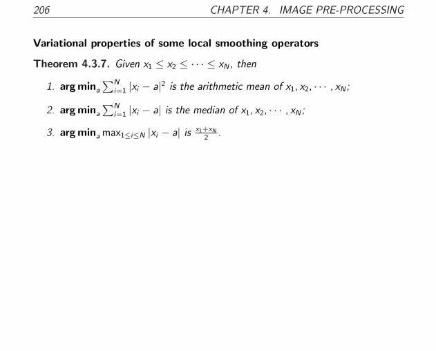
206 CHAPTER 4. IMAGE PRE-PROCESSING
Variational properties of some local smoothing operators
Theorem 4.3.7. Given x1 ≤ x2 ≤ · · · ≤ xN , then
1. arg mina
∑Ni=1 |xi − a|2 is the arithmetic mean of x1, x2, · · · , xN ;
2. arg mina
∑Ni=1 |xi − a| is the median of x1, x2, · · · , xN ;
3. arg mina max1≤i≤N |xi − a| is x1+xN
2.

4.3. LOCAL PRE-PROCESSING 207
Proof. (1) Let
g(a) =N∑
i=1
|xi − a|2. (4.60)
The result follows immediately by calculus.(2) Let
g(a) =N∑
i=1
|xi − a|. (4.61)
Let a0 and a1 be arbitrary number such that
a0 < x1 ≤ xN < a1 (4.62)
Then
g(a0) =N∑
i=1
xi − Na0 (4.63)
and
g(a1) = Na1 −N∑
i=1
xi . (4.64)
If a ∈ [x1, xN ], assume that
xk ≤ a < xk+1. (4.65)

208 CHAPTER 4. IMAGE PRE-PROCESSING
Then
g(a) =k∑
i=1
(a − xi ) +N∑
i=k+1
(xi − a) =N∑
i=k+1
xi −k∑
i=1
xi + (2k − N)a. (4.66)
If 2k ≤ N ,
g(a0)− g(a) = 2k∑
i=1
xi − Na0 + (N − 2k)a
= 2k∑
i=1
(xi − a0) + (N − 2k)(a − a0) ≥ 0.
If 2k ≥ N ,
g(a1)− g(a) = Na1 − 2N∑
i=k+1
xi + (N − 2k)a
= 2N∑
i=k+1
(a1 − xi ) + (N − 2(N − k))a1 + (N − 2k)a
= 2N∑
i=k+1
(a1 − xi ) + (2k − N)(a1 − a) ≥ 0.

4.3. LOCAL PRE-PROCESSING 209
Therefore, the minimum of g(a) is attained in [x1, xN ]. Note that g(a) is con-tinuous, piece wise linear function on [x1, xN ]. g(a) is decreasing if 2k ≤ N andincreasing if 2k ≥ N .
If N = 2m is even, the minimum of g(a) is attained in the central sub-interval[xm, xm+1]. Since g(a) is constant on this sub-interval, any value of [xm, xm+1] is aminimizer of g(a). We choose a = xm+xm+1
2the median as the minimizer.
If N = 2m+1, g(a) is decreasing in one of the central sub-interval [xm, xm+1] andincreasing in another central sub-interval [xm+1, xm+2]. Then xm+1 is the minimizer,which is the median in this case.
(3) Letg(a) = max
1≤i≤N|xi − a|. (4.67)
Then it is easy to verify that
g(a) =
xN − a, if a < x1;
xN − a, if x1 ≤ a < x1+xN
2;
a − x1, if x1+xN
2≤ a ≤ xN ;
a − x1, if xN < a.
(4.68)
The conclusion follows immediately. ¤

210 CHAPTER 4. IMAGE PRE-PROCESSING
4.3.2 Edge detectors
Edge: what is it?
• Edge detectors are a collection of very important local image pre-processingmethods used to locate (sharp) changes in the intensity function.
• Edges are pixels where the brightness function changes abruptly.
!
• Neurological and psychophysical research suggests that locations in the im-age in which the function value changes abruptly are important for imageperception.
• Edges are to a certain degree invariant to changes of illumination and view-point.
• If only edge elements with strong magnitude (edgels) are considered, suchinformation often suffices for image understanding.
• The positive effect of such a process is that it leads to significant reductionof image data.

4.3. LOCAL PRE-PROCESSING 211
• Nevertheless such a data reduction does not undermine understanding thecontent of the image (interpretation) in many cases.
• Edge detection provides appropriate generalization of the image data.

212 CHAPTER 4. IMAGE PRE-PROCESSING
• For instance, painters of line drawings perform such a generalization.
Figure 4.2: Siesta by Pablo Picasso, 1919.

4.3. LOCAL PRE-PROCESSING 213
• We shall consider which physical phenomena in the image formation processlead to abrupt changes in image values.
• Calculus describes changes of continuous functions using derivatives.
• An image function depends on two variables — co-ordinates in the imageplane — so operators describing edges are expressed using partial derivatives.

214 CHAPTER 4. IMAGE PRE-PROCESSING
• A change of the image function can be described by a gradient that points inthe direction of the largest growth of the image function.

4.3. LOCAL PRE-PROCESSING 215
• An edge is a (local) property attached to an individual pixel and is calculatedfrom the image function in a neighborhood of the pixel.
• It is a vector variable with two components
– magnitude of the gradient;
– and direction φ is rotated with respect to the gradient direction ψ by−90o .
• The gradient direction gives the direction of maximal growth of the function,e.g., from black (g(i , j) = 0) to white (f (i , j) = 255).
• This is illustrated below; closed contour lines are lines of the same brightness;the orientation 0o points East.

216 CHAPTER 4. IMAGE PRE-PROCESSING
• Edges are often used in image analysis for finding region boundaries.
• Boundary is at the pixels where the image function varies and consists of pixelswith high(?) edge magnitude.
• Boundary and its parts (edges) are perpendicular to the direction of the gra-dient.

4.3. LOCAL PRE-PROCESSING 217
• The following figure shows several typical standard edge profiles.

218 CHAPTER 4. IMAGE PRE-PROCESSING
• Roof edges are typical for objects corresponding to thin lines in the image.
• Edge detectors are usually tuned for some type of edge profile.
!
• Sometimes we are interested only in changing magnitude without regard tothe changing orientation.
• A linear differential operator called the Laplacian may be used.
• The Laplacian has the same properties in all directions and is therefore invari-ant to rotation in the image.
∆g(x , y) =∂2g(x , y)
∂x2+∂2g(x , y)
∂y 2(4.69)

4.3. LOCAL PRE-PROCESSING 219
Finite Gradient
• The gradient magnitude and gradient direction are image functions,
|gradg(x , y)| =
√(∂g
∂x
)2
+
(∂g
∂y
)2
(4.70)
ψ = arg(∂g
∂x,∂g
∂y) (4.71)
where arg(u, v) = arctan( vu
) is the angle (in radians) from the x-axis to thepoint (u, v).
• In practice, for fast computation, the magnitude is approximated by
|gradg(x , y)| = |∂g
∂x|+ |∂g
∂y| (4.72)
or
|gradg(x , y)| = max{|∂g
∂x|, |∂g
∂y|} (4.73)
• A digital image is discrete in nature. So derivatives must be approximated byfinite differences.

220 CHAPTER 4. IMAGE PRE-PROCESSING
• The first order differences of the image g in the vertical direction (for fixed i)and in the horizontal direction (for fixed j) are given by backward difference
∆i g(i , j) =g(i , j)− g(i − n, j)
n(4.74)
∆j g(i , j) =g(i , j)− g(i , j − n)
n(4.75)
or by forward difference
∆i g(i , j) =g(i + n, j)− g(i , j)
n(4.76)
∆j g(i , j) =g(i , j + n)− g(i , j)
n(4.77)
• n is a small integer, usually 1.
• The value n should be chosen small enough to provide a good approximationto the derivative, but large enough to neglect unimportant changes in theimage function.
• Symmetric expressions for the difference, i.e., central differences, are not usu-ally used because they neglect the impact of the pixel (i , j) itself.
∆i g(i , j) =g(i + n, j)− g(i − n, j)
2n(4.78)

4.3. LOCAL PRE-PROCESSING 221
∆j g(i , j) =g(i , j + n)− g(i , j − n)
2n(4.79)
• Individual gradient operators that examine small local neighborhoods are infact linear space-invariant operators, hence are equivalent to convolutions, cf.(4.50), and can be expressed by convolution masks.
• Each convolution mask corresponds to a derivative in one certain direction, ifthe masks induces edge orientation information.
!
Example 4.3.8. Example: computing the gradient and edge magnitude and di-rection by finite difference. The Khoros workspace for this example is here FiniteDifference Example.

222 CHAPTER 4. IMAGE PRE-PROCESSING
More on gradient operators
• Gradient operators as a measure of edge sheerness can be divided into threecategories
1. Operators approximating derivatives of the image function using finitedifferences (introduced above):
– Some of them are rotationally invariant (e.g., the Laplacian) anddirection independent and thus need one convolution mask only.
– Others approximate first derivatives using several masks. The direc-tion of the gradient is given by the mask giving maximal response.The absolute value of the response on that mask is the magnitude?
2. Operators based on the zero crossings of the second derivatives of theimage function (e.g., Marr-Hildreth or Canny edge detector).
3. Operators which attempt to match an image function to a parametricmodel of edges.

4.3. LOCAL PRE-PROCESSING 223
• The remainder of this section will consider some of the many operators whichfall into the first category, and the next section will consider the second cat-egory.
• The last category is briefly outlined in (4.3.6). Parametric models describeedges more precisely than simple edge magnitude and direction and are muchmore computationally intensive.
• This is an area of active research.
• It may be difficult to select the optimal edge detection strategy.

224 CHAPTER 4. IMAGE PRE-PROCESSING
Roberts operator
• The Roberts operator is one of the oldest operators.
• It is very easy to compute as it uses only a 2× 2 neighborhood of the currentpixel.
• Its convolution masks are
h1 =
[h1(0, 0) h1(1, 0)h1(0, 1) h1(1, 1)
]=
[1 00 −1
]h2 =
[0 1−1 0
](4.80)
• The magnitude of the edge is computed as
|g(i , j)− g(i + 1, j + 1)|+ |g(i , j + 1)− g(i + 1, j)| (4.81)
• The primary disadvantage of the Roberts operator is its high sensitivity tonoise, because very few pixels are used to approximate the gradient.

4.3. LOCAL PRE-PROCESSING 225
Discrete Laplacian
• The Laplace operator is a very popular operator approximating the secondderivative which gives the gradient magnitude only.
• The Laplacian (4.69) is approximated in digital images by a convolution sum.
• A 3× 3 mask h4 is often used, for 4-neighborhoods and it is defined as
h4,1 =
0 1 01 −4 10 1 0
or h4,2 =
1
2
1 0 10 −4 01 0 1
(4.82)
and for 8-neighborhoods it is defined as
h8,1 =h4,1 + 2h4,2
3=
1
3
1 1 11 −8 11 1 1
(4.83)
or
h8,2 =4h4,2 − h4,1
3=
1
3
2 −1 2−1 −4 −12 −1 2
(4.84)

226 CHAPTER 4. IMAGE PRE-PROCESSING
or
h8,3 = 3h4,1 − 2h4,2 =
−1 3 −13 −8 3−1 3 −1
(4.85)
• A Laplacian operator with stressed significance of the the central pixel or itsneighborhood is sometimes used.

4.3. LOCAL PRE-PROCESSING 227
Prewitt operator
• The Prewitt operator, similarly to the Sobel, Kirsch, Robinson (as discussedlater) and some other operators, approximates the first derivative.
• The gradient is estimated in eight (for a 3 × 3 convolution mask) possibledirections.
• The convolution result of the greatest magnitude indicates the gradient mag-nitude.
• The convolution mask of greatest magnitude indicates the gradient direction.
• Larger masks are possible.
• Operators approximating first derivative of an image function are sometimescalled compass operators because of the ability to determine gradient di-rection.
• We present only the first three 3× 3 masks for each operator; the others canbe created by simple repeated clockwise 45o rotation.

228 CHAPTER 4. IMAGE PRE-PROCESSING
• Prewitt operator
h1 =
1 1 10 0 0−1 −1 −1
h2 =
0 1 1−1 0 1−1 −1 0
h3 =
−1 0 1−1 0 1−1 0 1
(4.86)

4.3. LOCAL PRE-PROCESSING 229
Sobel operator
•
h1 =
1 2 10 0 0−1 −2 −1
h2 =
0 1 2−1 0 1−2 −1 0
h3 =
−1 0 1−2 0 2−1 0 1
(4.87)
• The Sobel operator is often used as a simple detector of horizontality andverticality of edges. In this case only masks h1 and h3 are used.
• If the h1 response is y and the h3 response x , we might then derive edgestrength (magnitude) as
√x2 + y 2 or|x |+ |y | (4.88)
and direction asarctan(
y
x) (4.89)

230 CHAPTER 4. IMAGE PRE-PROCESSING
Robinson operator
•
h1 =
1 1 11 −2 1−1 −1 −1
h2 =
1 1 1−1 −2 1−1 −1 1
h3 =
−1 1 1−1 −2 1−1 1 1
(4.90)

4.3. LOCAL PRE-PROCESSING 231
Kirsch operator
•
h1 =
3 3 33 0 3−5 −5 −5
h2 =
3 3 3−5 0 3−5 −5 3
h3 =
−5 3 3−5 0 3−5 3 3
(4.91)

232 CHAPTER 4. IMAGE PRE-PROCESSING
Examples
Example 4.3.9. Example: Roberts operator. The Khoros workspace for this ex-ample is here Roberts operator Example.
Example 4.3.10. Example: Laplacian operator. The Khoros workspace for thisexample is here Laplacian operator Example.
Example 4.3.11. Example: Prewitt operator. The Khoros workspace for this ex-ample is here Prewitt operator Example.
Example 4.3.12. Example: Sobel operator. The Khoros workspace for this exampleis here Sobel operator Example.
Example 4.3.13. Example: Robinson operator. The Khoros workspace for thisexample is here Robinson operator Example.
Example 4.3.14. Example: Kirsch operator. The Khoros workspace for this exam-ple is here Kirsch operator Example.

4.3. LOCAL PRE-PROCESSING 233
Remark 4.3.15. 1. Visually, the edge images produced by the foregoing edgeoperators (Roberts, Prewitt, Sobel, Kirsch, Robinson operators) appears rathersimilar.
2. The Roberts operator, being two by two, responds best on sharp transitionsin low-noise images.
3. The other operators, being three by three, handle more gradual transition andnoisier images better.

234 CHAPTER 4. IMAGE PRE-PROCESSING
Image sharpening
• Image sharpening makes edges steeper — the sharpened image is intended tobe observed by a human.
• The sharpened output image f is obtained from the input image g as
f (i , j) = g(i , j)− CS(i , j) (4.92)
• C is a positive coefficient which gives the strength of sharpening and S(i , j) isa measure of the image function sheerness that is calculated using a gradientoperator.
• The Laplacian is very often used to estimate S(i , j).

4.3. LOCAL PRE-PROCESSING 235
• Image sharpening/edge detection can be interpreted in the frequency domainas well.
• The result of the Fourier transform is a combination of harmonic functions.
• The derivative of the harmonic function sin(nx) is n cos(nx); thus the higherthe frequency, the higher the magnitude of its derivative. This is anotherexplanation of why gradient operators enhance edges.
Example 4.3.16. Example: Image sharpen by Laplacian. The Khoros workspacefor this example is here Image sharpen Example.
Example 4.3.17. Image sharpen by Laplacian. The matlab script from visionbookis is here Image sharpen Example.

236 CHAPTER 4. IMAGE PRE-PROCESSING
Unsharp masking
• Unsharp masking is often used in printing industry applications — anotherimage sharpening approach. (Note the conflicting name.)
• A signal proportional to an unsharp image (e.g., blurred by some smoothingoperator) is subtracted from the original image, again a parameter C may beused to control the weight of the subtraction.
Example 4.3.18. Example: Unsharp masking. The Khoros workspace for thisexample is here Unsharpen masking.

4.3. LOCAL PRE-PROCESSING 237
4.3.3 Zero-crossings of the second derivative
• In the 1970’s, Marr’s theory conclude from neurophysiological experimentsthat object boundaries are the most important cues that link an intensityimage with its interpretation.
• Edge detection techniques at that time like the Kirsch, Sobel, Prewitt opera-tors are based on convolution in very small neighborhoods and work well forspecific images only.
• The main disadvantage of these edge detectors is their dependence on thesize of objects and sensitivity to noise.
!
• An edge detection technique, based on the zero crossings of the secondderivative (in its original form, the Marr-Hildreth edge detector) explores thefact that a step edge corresponds to an abrupt change in the image function.

238 CHAPTER 4. IMAGE PRE-PROCESSING
• The first derivative of the image function should have an extreme at theposition corresponding to the edge in the image, and so the second derivativeshould be zero at the same position.
• It is much easier and more precise to find a zero crossing position than anextreme - see the follwoing figure.

4.3. LOCAL PRE-PROCESSING 239
• The crucial question is how to compute the the 2nd derivative robustly.
• One possibility is to smooth an image first (to reduce noise) and then computesecond derivatives.
!
• When choosing a smoothing filter, there are two criteria that should be ful-filled, [Marr and Hildreth, 1980].
1. The filter should be smooth and roughly band limited in the frequencydomain to reduce the possible number of frequencies at which functionchanges can take place.
2. The constraint of spatial localization requires the response of a filter tobe from nearby points in the image.
• These two criteria are conflicting — Heisenberg uncertainty principle.

240 CHAPTER 4. IMAGE PRE-PROCESSING
• A nonzero function and its Fourier transform cannot both be sharply localized.[Folland and Sitaram, 1997, p. 207]
• ([Folland and Sitaram, 1997, Theorem 1.1]) For any f ∈ L2(R) and any a ∈ Rand b ∈ R,
∫(x − a)2|f (x)|2 dx
∫(ξ − b)2|f (ξ)|2 dξ ≥ ‖f ‖
42
16π2(4.93)
Equality holds if and only if f = Ce2πibx−γ(x−a)2for some C ∈ C and γ > 0.
• [Folland and Sitaram, 1997, Theorem 7.6] For a, b > 0, let E (a, b) be thespace of all measurable functions f on R such that
|f (x)| ≤ ce−aπx2
, |f (ξ)| ≤ ce−bπξ2
, (4.94)
for some c > 0. Then
(1) If ab < 1, dim E (a, b) =∞;
(2) If ab = 1, dim E (a, b) = Ce−aπx2;
(3) If ab > 1, dim E (a, b) = {0};

4.3. LOCAL PRE-PROCESSING 241
• There is a well known joke: “Heisenberg is pulled over by a policeman whilstdriving down a motorway, the policeman gets out of his car, walks towardsHeisenberg’s window and motions with his hand for Heisenberg to wind thewindow down, which he does. The policeman then says ‘Do you know whatspeed you were driving at sir?’, to which Heisenberg responds ‘No, but I knewexactly where I was.”’1
1 This is copy-edited from http:en.wikipedia.orgwikiUncertainty principle.

242 CHAPTER 4. IMAGE PRE-PROCESSING
• But they can be optimized simultaneously using a Gaussian distribution.
• The 2D Gaussian smoothing operator G (x , y)
G (x , y) =1
2πσ2e−
x2+y2
2σ2 (4.95)
where x and y are the image co-ordinates and σ is the standard deviation ofthe associated probability distribution.
• The standard deviation σ is the only parameter of the Gaussian filter — it isproportional to the size of neighborhood on which the filter operates.
• Pixels more distant from the center of the operator have smaller influence,and pixels further than 3σ from the center have negligible influence.
!
• Our goal is to get a second derivative of a smoothed 2D function f (x , y).
• We have seen that the Laplacian operator gives the second derivative, and isnon-directional (isotropic).

4.3. LOCAL PRE-PROCESSING 243
• Consider then the Laplacian of an image f (x , y) smoothed by a Gaussian.
• This operator is abbreviated by some authors as LoG, from Laplacian ofGaussian:
∆[G (x , y) ∗ f (x , y)] (4.96)
• The order of differentiation and convolution can be interchanged due to lin-earity of the operations:
[∆G (x , y)] ∗ f (x , y) (4.97)
• The derivative of the Gaussian filter is independent of the image under con-sideration and can be precomputed analytically reducing the complexity of thecomposite operation.
∆G (x , y) =x2 + y 2 − 2σ2
2πσ6e−
r2
2σ2 (4.98)
• Because its shape, the LoG operator is commonly called a Mexican hat.

244 CHAPTER 4. IMAGE PRE-PROCESSING
Figure 4.3: LoG filter.

4.3. LOCAL PRE-PROCESSING 245
• Finding second derivatives in this way is very robust(?).
• Gaussian smoothing effectively suppresses the influence of the pixels that areup to a distance 3σ from the current pixel; then the Laplace operator is anefficient and stable measure of changes in the image.
!
• The location in the LoG image where the zero level is crossed corresponds tothe position of the edges.
• The advantage of this approach compared to classical edge operators of smallsize is that a larger area surrounding the current pixel is taken into account;the influence of more distant points decreases according to the variance σ ofthe Gaussian.
!
• Convolution masks become large for larger.
• Fortunately, there is a separable decomposition of the ∆G operator that can

246 CHAPTER 4. IMAGE PRE-PROCESSING
speed up computation considerable.
!
• The practical implication of Gaussian smoothing is that edges are found reli-ably.
• If only globally significant edges are required, the standard deviation of theGaussian smoothing filter may be increased, having the effect of suppressingless significant evidence.
!
• The LoG operator can be very effectively approximated by convolution with amask that is the difference of two Gaussian averaging masks with substantiallydifferent — this method is called the Difference of Gaussians — DoG.
• Even coarser approximations to LoG are sometimes used — the image isfiltered twice by an averaging operator with smoothing masks of different sizeand the difference image is produced.
!

4.3. LOCAL PRE-PROCESSING 247
• When implementing a zero-crossing edge detector, trying to detect zeros in theLoG or DoG image will inevitably fail, while naive approaches of thresholdingthe LoG/DoG image and defining the zero-crossings in some interval of valuesclose to zero give piecewise disconnected edges at best.
• Many other approaches improving zero-crossing performance can be found inthe literature.
!
• The traditional second-derivative zero-crossing has disadvantages as well:
– it smooths the shape too much; for example, sharp corners are lost.
– it tends to create closed loops of edges (nicknamed the ‘plate of spaghetti’effect).
• Neurophysiological experiments provide evidence that the human retina oper-ation on image can be described analytically as the convolution of the imagewith the ∆G operator.
Example 4.3.19. Marr-Hildreth edge detector. The Khoros workspace for thisexample is here Marr-Hildreth edge detector.

248 CHAPTER 4. IMAGE PRE-PROCESSING
4.3.4 Scale in image processing
• Many image processing techniques work locally, theoretically at the level ofindividual pixels — edge detection methods are examples.
• The essential problem in such computation is scale.
• Edges correspond to the gradient of the image function that is computed asa difference among pixels in some neighborhood.
!
• There is seldom a sound reason for choosing a particular size of neighborhood:
– The ‘right’ size depends on the size of the objects under investigation.
– To know what the objects are assumes that it is clear how to interpretan image and this is not in general known at the pre-processing stage.

4.3. LOCAL PRE-PROCESSING 249
• The phenomenon under investigation is expressed at different resolutions ofthe description, and a formal model is created at each resolution.
• Then the qualitative behavior of the model is studied under changing resolu-tion of the description.
• Such a methodology enables the deduction of meta-knowledge about the phe-nomenon that is not seen at the individual description.
!
• Different description levels are easily interpreted as different scales in thedomain of digital images.
• The idea of scale is fundamental to Marr’s edge detection technique, intro-duced in the last sub-section, where different scales are provided by differentsizes of Gaussian filter masks.
• The aim was not only to eliminate fine scale noise but also to separate eventsat different scales arising from distinct physical processes, [Marr, 1982].

250 CHAPTER 4. IMAGE PRE-PROCESSING
• Assume that a signal has been smoothed with several masks of variable sizes.
• Every setting of the scale parameters implies a different description, but it isnot known which one is correct.
• For many tasks, no one scale is categorically correct.
• If the ambiguity introduced by the scale is inescapable, the goal of scale-independent description is to reduce this ambiguity as much as possible.
!
• Many publications tackle scale-space problems. Here we shall consider justthree examples of the application of multiple scale description to image anal-ysis.
• There are other approaches involving non-linear partial differential equationsto generate non-linear scale-space descriptions.
!
• The first approach aimed to process planar noisy curves at a range of scales— the segment of curve that represents the underlying structure of the sceneneeds to be found.

4.3. LOCAL PRE-PROCESSING 251
• The problem is illustrated in by an example of two noisy curves in the followingfigure.
• One of these may be interpreted as a closed (perhaps circular) curve, whilethe other could be described as two intersecting straight lines.
• Local tangent direction and curvature of the curve are significant only withsome scales after the curve is smoothed by Gaussian filter with varying stan-dard deviations.

252 CHAPTER 4. IMAGE PRE-PROCESSING
• After smoothing using the Gaussian filter with varying standard deviations,the significant segments of the original curve can be found.
!
• The second approach, called scale space filtering, tried to describe signalsqualitatively with respect to scale.
• The problem was formulated for 1D signals f (x), but it could easily be gen-eralized to 2D functions as images.
• The original 1D signal f(x) is smoothed by convolution with a 1D Gaussian
f (x ,σ) = G (x ,σ) ∗ f (x) (4.99)
• If the standard deviation σ is slowly changed the function f (x , σ) representsa surface on the (x ,σ) plane that is called the scale-space image.
• Inflection points of the curve f (x ,σ0) for a distinct value σ0
∂2f (x ,σ0)
∂x2= 0,
∂3f (x ,σ0)
∂x36= 0. (4.100)
describe the curve f (x) qualitatively.

4.3. LOCAL PRE-PROCESSING 253
• The positions of inflection points can be drawn as a set of curves
Σ(x ,σ0) (4.101)
in (x ,σ) co-ordinates

254 CHAPTER 4. IMAGE PRE-PROCESSING
• Coarse to fine analysis of the curves corresponding to inflection points, i.e.,in the direction of the decreasing value of the σ, localizes events at differentscales.
• The qualitative information contained in the scale-space image can be trans-formed into a simple interval tree that expresses the structure of the signalf (x) over all (observed) scales.
• The interval tree is built from the root that corresponds to the largest scale.
• Then the scale-space image is searched in the direction of decreasing σ.
• The interval tree branches at those points where new curves correspondinginflection points appears.
!
• The third example of the application of scale — Canny edge detector, dis-cussed in the next sub-section.

4.3. LOCAL PRE-PROCESSING 255
4.3.5 Canny edge detection
• Canny edge detector is optimal for step edges corrupted by white noise.
• The optimality of it is related to three criteria:
– The detection criterion expresses that fact that important edges shouldnot be missed, and that there should be no spurious responses.
– The localization criterion says that the distance between the actual andlocated position of the edge should be minimal.
– The one response criterion minimizes multiple responses to a singleedge (also partly covered by the first criterion, since when there are tworesponses to a single edge one of them should be considered as false).

256 CHAPTER 4. IMAGE PRE-PROCESSING
• Canny’s edge detector is based on several ideas:
1. The edge detector was expressed for a 1D signal and the first two opti-mality criteria. A closed form solution was found using the calculus ofvariations.
2. If the third criterion (multiple responses) is added, the best solutionmay be found by numerical optimization. The resulting filter can beapproximated effectively by the first derivative of a Gaussian smoothingfilter with standard deviation σ; the reason for doing this is the existenceof an effective implementation.
– There is a strong similarity here to the Marr-Hildreth edge detector(Laplacian of a Gaussian)
3. The detector is then generalized to two dimension. A step edge is givenby its position, orientation, and possibly magnitude (strength).
– It can be shown that convolving an image with a symmetric 2DGaussian and then differentiating in the direction of the gradient(perpendicular to the edge direction) forms a simple and effectivedirectional operator.
– Recall that the Marr-Hildreth zero crossing operator does not giveinformation about edge direction as it uses Laplacian filter.

4.3. LOCAL PRE-PROCESSING 257
– Suppose G is a 2D Gaussian (4.95) and assume we wish to convolutethe image with an operator Gn which is a first derivative of G in thedirection n.
Gn =∂G
∂n= n · ∇G (4.102)
– The direction n should be oriented perpendicular to the edge
∗ this direction is not known in advance
∗ however, a robust estimate of it based on the smoothed gradientdirection is available
∗ if g is the image, the normal to the edge is estimated as
n =∇(G ∗ g)
|∇(G ∗ g)| (4.103)
– The edge location is then at the local maximum in the direction nof the operator Gn convoluted with the image g
∂
∂nGn ∗ g = 0. (4.104)
– Substituting in equation (4.104) for Gn from equation (4.102), weget
∂2
∂n2G ∗ g = 0. (4.105)

258 CHAPTER 4. IMAGE PRE-PROCESSING
– This equation (4.105) shows how to find local maxima in the direc-tion perpendicular to the edge; this operation is often referred to asnon-maximal suppression.
– As the convolution and derivative are associative operations in equa-tion (4.105)
∗ first convolute an image g with a symmetric Gaussian G ;
∗ then compute the directional second derivative using an esti-mate of the direction n computed according to equation (4.103);
∗ strength of the edge (magnitude of the gradient of the imageintensity function g) is measured as
|Gn ∗ g | = |∇(G ∗ g)|. (4.106)
4. Spurious responses to the single edge caused by noise usually create aso called ’streaking’ problem that is very common in edge detection ingeneral.
– Output of an edge detector is usually thresholded to decide whichedges are significant.
– Streaking means breaking up of the edge contour caused by theoperator fluctuating above and below the threshold.

4.3. LOCAL PRE-PROCESSING 259
– Streaking can be eliminated by thresholding with hysteresis.
∗ If any edge response is above a high threshold, those pixelsconstitute definite output of the edge detector for a particularscale.
∗ Individual weak responses usually correspond to noise, but ifthese points are connected to any of the pixels with strongresponses they are more likely to be actual edges in the image.
∗ Such connected pixels are treated as edge pixels if their responseis above a low threshold.
∗ The low and high thresholds are set according to an estimatedsignal to noise ratio. Please refer to Canny’s original paper fordetailed discussions. Canny discussed the one dimensional casein §VI in his paper.
5. The correct scale for the operator depends on the objects contained inthe image.
– The solution to this unknown is to use multiple scales and aggregateinformation from them.
– Different scale for the Canny detector is represented by differentstandard deviations σ of the Gaussians.
– There may be several scales of operators that give significant re-

260 CHAPTER 4. IMAGE PRE-PROCESSING
sponses to edges (i.e., signal to noise ratio above the threshold); inthis case the operator with the smallest scale is chosen as it givesthe best localization of the edge.
– Canny proposed a Feature synthesis approach.
– All significant edges from the operator with the smallest scale aremarked first.
– Edges of a hypothetical operator with larger σ are synthesized fromthem (i.e., a prediction is made of how the larger σ should performon the evidence gleaned from the smaller σ).
– Then the synthesized edge response is compared with the actualedge response for larger σ.
– Additional edges are marked only if they have significantly strongerresponse than that predicted from synthetic output.
– This procedure may be repeated for a sequence of scales, a cumula-tive edge map is built by adding those edges that were not identifiedat smaller scales.

4.3. LOCAL PRE-PROCESSING 261
Algorithm 4.3.20. Canny edge detector
1. Repeat steps (2) till (6) for ascending values of the standard deviation.
2. Convolve an image g with a Gaussian of scale σ.
3. Estimate local edge normal directions n using equation (4.103) for each pixelin the image.
4. Find the location of the edges using equation (4.105) (non-maximal suppres-sion).
5. Compute the magnitude of the edge using equation (4.106).
6. Threshold edges in the image with hysteresis to eliminate spurious responses.
7. Aggregate the final information about edges at multiple scale using the “fea-ture synthesis” approach.

262 CHAPTER 4. IMAGE PRE-PROCESSING
• Canny’s detector represents a complicated but major contribution to edgedetection.
• Its full implementation is unusual, it being common to find implementationsthat omit feature synthesis — that is, just steps 2 — 6 of algorithm.
• Reference for this section is Canny’s paper [Canny, 1986].

4.3. LOCAL PRE-PROCESSING 263
Example 4.3.21. Canny edge detector. The example matlab script file is hereCanny edge detector example.
(You need to start matlab.)Compare the result with the edge detector with other filters. Note the improve-
ment at the top part of the hat.Study the matlab code. Note the “thin” code.
Homework 4.3.22. This is an important homework. The total score is 20. Thehomework includes:
1. (4) Implement median filter with variable window size and shape;
2. (4) Implement another local smoothing filter you know with possible variableparameters;
3. (8) Implement Canny edge detector; what is your extension to step 7? (With-out step 7, you can only get at most 4 scores).
4. (4) Implement another edge detector you know; compare it with Canny de-tector.

264 CHAPTER 4. IMAGE PRE-PROCESSING
4.3.6 Parametric edge models
• Parametric models are based on the idea that the discrete image intensityfunction can be considered a sampled and noisy approximation of the under-lying continuous or piecewise continuous image intensity function.
• While the continuous image function is not known, it can be estimated fromthe available discrete image intensity function and image properties can bedetermined from this estimate, possibly with sub-pixel precision.
• Piecewise continuous function estimate called facets are used to represent(a neighborhood) image pixel.
• Such image representation is called facet model.

4.3. LOCAL PRE-PROCESSING 265
• The intensity function in a pixel neighborhood can be estimated using modelsof different complexity.
• The simplest one is the flat facet model that uses piecewise constants andeach pixel neighborhood is represented by a flat function of constant intensity.
• The sloped model uses piecewise linear functions forming a sloped plane fittedto the image intensities in the pixel neighborhood.
• Quadratic and bi-cubic facet models employ correspondingly more complexfunctions.
• A thorough treatment of facet models and their modifications for peak noiseremoval, segmentation into constant-gray-level regions, determination of sta-tistically significant edges, gradient edge detection, directional second-derivativezero-crossing detection, and line and corner detection is given in [Haralic and Shapiro, 1992].

266 CHAPTER 4. IMAGE PRE-PROCESSING
• An edge detection example is given in the following.
• Consider a bi-cubic facet model
g(x , y) = c1 + c2x + c3y + c4x2 + c5xy + c6y 2 + c7x3 + c8x2y + c9xy 2 + c10y 3
(4.107)The parameter of which are estimated from a pixel neighborhood(the co-ordinate of the central pixel is (0, 0)).
• To determine the model parameters, a least-squares method with singular-value decomposition may be used.
• Once the facet model parameters are available for each image pixel, edges canbe detected as extrema of the first directional derivative and/or zero-crossingsof the the second directional derivative of the local continuous facet modelfunctions.
• Edge detectors based on parametric models describe edges more precisely thanconvolution based edge detectors.
• Additionally, they carry the potential for sub-pixel edge localization (?).
• However, their computational requirements are much higher.

4.3. LOCAL PRE-PROCESSING 267
4.3.7 Edges in multi-spectral images
• There are several possibilities for the detection of edges in multi-spectral im-ages.
• The first is to detect edges separately in individual image spectral componentsusing the ordinary local gradient operators mentioned in Section (4.3.2).
– Individual images of edges can be combined to get the resulting edgeimage, with the value corresponding to edge magnitude and directionbeing the maximal edge value from all spectral components.
– A linear combination of edge spectral components can also be used, andother combination techniques are possible.
• A second possibility is to use the brightness difference of the same pixel intwo different spectral components.
– The ratio instead of the difference can also be used as well, although itis necessary to assume that pixel values are not zero in this case.
• A third possibility is to create a multi-spectral edge detector which uses bright-ness information from all n spectral bands.

268 CHAPTER 4. IMAGE PRE-PROCESSING
– An edge detector of this kind was proposed in [Cervenka and Charvat, 1987].
– The neighborhood used has size 2 × 2 × n pixels, where the 2 × 2neighborhood is similar to that of the Roberts gradient, (4.80).
– The coefficients weighting the influence of the component pixels aresimilar to the correlation correlation coefficients.
– Let f (i , j) denote the arithmetic mean of the brightness correspondingto the pixel with the same co-ordinates (i , j) in all n spectral componentimages and fr be the brightness of the r th spectral component.
– The edge detector result in pixel (i , j) is given as the minimum of thefollowing expressions:
∑nr=1
[fr (i , j)− f (i , j)
] [fr (i + 1, j + 1)− f (i + 1, j + 1)
]√∑n
r=1
[fr (i , j)− f (i , j)
]2∑nr=1
[fr (i + 1, j + 1)− f (i + 1, j + 1)
]2
·∑n
r=1
[fr (i + 1, j)− f (i + 1, j)
] [fr (i , j + 1)− f (i , j + 1)
]√∑n
r=1
[fr (i + 1, j)− f (i + 1, j)
]2∑nr=1
[fr (i , j + 1)− f (i , j + 1)
]2
– This multi-spectral edge detector gives very good (?) results on remotelysensed images.

4.3. LOCAL PRE-PROCESSING 269
4.3.8 Line detection by local pre-processing operators
• Several other local operations exists which do not belong to the taxonomy inthis Section (4.3), as they are used for different purposes.
• Line finding, line thinning, and line filling operators are amongthem.
• The second group of operators finds interest points or locations of
interest in the image.
• There is yet another class of local nonlinear operators, mathematical morphology
techniques.

270 CHAPTER 4. IMAGE PRE-PROCESSING
• Recall that one of the reasons why edges are being detected is that they beara lot of information about underlying objects in the scene.
• Taking just edge elements instead of all pixels reduces the amount of datawhich has to be processed.
• The edge detector is a general tool which does not depend on the content ofthe particular image.
• The detected edges are to some degree robust as they do not depend muchon small changes in illumination, viewpoint change, etc.
!
• It is interesting to seek yet richer features which can be reliably detected inthe image and which can outperform simple edge detectors in some classes ofapplications.
• Line detectors and corner detectors are some such.

4.3. LOCAL PRE-PROCESSING 271
Line detection
• Line finding operators aim to find very thin curves in the image, e.g.,roads in satellite images.
• It is assumed that curves do not bend sharply. Such curves and straight linesare called lines for the purpose of describing this technique.
• Lines are modeled by a roof profile among edges, Fig. 4.3.2.
• We assume that the width of the lines is approximately one or two pixels.
• Lines in the image can be detected by a number of local convolution operatorshk , which serve as line patterns [Cervenka and Charvat, 1987].
• The output value of the line finding detector in pixel (i , j) is given by
f (i , j) = max{
0, maxk
(f ∗ hk)}
(4.108)
where f ∗hk denotes the convolution of the k-th mask with the neighborhoodof a pixel (i , j) in the input image.

272 CHAPTER 4. IMAGE PRE-PROCESSING
• The simplest collection of four such patterns of size 3 x 3 is able to detectlines rotated modulo the angle 45o :

4.3. LOCAL PRE-PROCESSING 273
• A similar principle can be applied to bigger masks.
• The following is a set of convolution masks of size 5×5. There are 14 possibleorientation of the line finding convolution mask of this size; only the first eightare shown, as the others are obvious by rotation.
• Such line detectors sometimes produce more lines than needed, and othernon-linear constraints may be added to reduce this number.

274 CHAPTER 4. IMAGE PRE-PROCESSING

4.3. LOCAL PRE-PROCESSING 275
Line thinning
• In the edge detection methods introduced so far, edges are usually found bysimple thresholding of the edge magnitude.
• Such edge thresholding does not provide ideal contiguous boundaries that areone pixel wide.
• Sophisticated segmentation techniques are discussed in the next chapter.
• Here, much simpler edge thinning and filling methods are described.
• These techniques are based on knowledge of small local neighborhoods andare very similar to other local pre-processing techniques.

276 CHAPTER 4. IMAGE PRE-PROCESSING
• One line thinning method uses knowledge about orientation and in this caseedges are thinned before thresholding.
• Edge magnitude and directions provided by some gradient operator are usedas input, and the edge magnitude of two neighboring pixels perpendicular tothe edge direction are examined for each pixel in the image.
• If at least one of these pixels has edge magnitude higher than the edge mag-nitude of the examined pixel, then the edge magnitude of the examined pixelis assigned a zero value.
• The technique is called non-maximal suppression and is similar to the ideamentioned in conjunction with the Canny edge detector.
!
• There are many line thinning methods which we do not present here.
• In most cases the best line thinning is achieved using mathematical morphol-ogy methods (?).

4.3. LOCAL PRE-PROCESSING 277
Edge filling
• Edge points after thresholding do not create contiguous boundaries and theedge filling method tries to recover edge pixels on the potential object bound-ary which are missing.
• We present here a very simple local edge filling technique; more complicatedmethods based on edge relaxation are discussed in the next chapter.
• The local edge filling procedure checks the 3× 3 neighborhood of the currentpixel matches one of the following masks If so, the central pixel of the mask
is changed from zero to one.

278 CHAPTER 4. IMAGE PRE-PROCESSING
!
• These simple methods for edge thinning and filling do not guarantee that thewidth of the lines will be equal to one and the contiguity of the edges are isnot certain either.
• Note that local thinning and filling operators can be treated as special casesof mathematical morphology operators.

4.3. LOCAL PRE-PROCESSING 279
4.3.9 Corners and interesting points
• In many cases it is of advantage to find pairs of corresponding points intwo similar images.
• E.g., when finding geometric transforms, knowing the position of correspond-ing points enables the estimation of geometric transforms from live data.
• Finding corresponding points is also a core problem in the analysis of movingimages and fir recovering depth information form pairs of stereo images.
• In general, all possible pairs of points should be examined to solve thiscorrespondence problem, and this is very computation expensive.
• If two images have n pixels each, the complexity is O(n2).
• This process might be simplified if the correspondence is examined among amuch smaller number of points, called interest points.
• An interest point should have some typical local property.
• E.g., if square objects are present in the image, then corners are very goodinterest points.

280 CHAPTER 4. IMAGE PRE-PROCESSING
• Corners serve better than lines when the correspondence problem is to besolved.
• This is due to the aperture problem.
• Assume a moving line is seen through a small aperture. In such a case, onlythe motion vector perpendicular to the line can be observed.
• The component collinear with the line remains invisible.
• The situation is better with corners. They provide ground for unique matching,cf. the following figure for illustration.

4.3. LOCAL PRE-PROCESSING 281
• Edge detectors themselves are not stable at corners.
• This is natural as the gradient at the tip of the corner is ambiguous.
• Near the corner there is a discontinuity in the gradient direction.
• This observation is used in corner detectors.
!
• Corners in image can be located using local detectors.
• Input to the corner detector is the gray-level image and output is the imagef (i , j) in which values are proportional to the likelihood that the pixel is acorner.
• Interest points are obtained by thresholding the result of the corner detector.
!
• The corner in the image can be defined as a pixel in whose small neighborhoodthere are two dominant and different edge directions.

282 CHAPTER 4. IMAGE PRE-PROCESSING
• This definition is not precise as an isolated point of local intensity maximumor minimum, line endings, or an abrupt change in the curvature of a curvewith a response similar to a corner.
• Nevertheless, such detectors are named corner detectors in the literature andare widely used.
• If corners have to be detected then some additional constraints have to beapplied.
!
• Corner detectors are not usually very robust.
• This deficiency is overcome either by manual expert supervision or large redun-dancies introduced to prevent the effect of individual errors from dominatingthe task.
• The latter means that many more corners are detected in two or more imagesthan necessary for estimating a transformation sought between these images.
!

4.3. LOCAL PRE-PROCESSING 283
• The simplest corner detector is the Moravec detector which is maximal inpixels with high contrast.
• These points are on corners and sharp edges.
• The Moravec operator MO is given by
MO(i , j) =1
8
i+1∑
k=i−1
j+1∑
l=j−1
|g(k , l)− g(i , j)|. (4.109)
!
• Better results are produced by computationally more expensive corner opera-tors based on the facet model, (4.107).
• The image function g is approximated in the neighborhood of the pixel (i , j)by a bi-cubic polynomial with coefficients ck as in (4.107).
g(x , y) = c1 + c2x + c3y + c4x2 + c5xy + c6y 2 + c7x3 + c8x2y + c9xy 2 + c10y 3
(4.110)

284 CHAPTER 4. IMAGE PRE-PROCESSING
• The Zuniga-Haralick operator ZH is given by
ZH(i , j) =− (c2
2 c6 − 2c2c3c5 + c23 c4)
(c22 + c2
3 )32
(4.111)
which is the curvature of the plane curve g(x , y) = const.
• The Kitchen-Rosenfeld KR is given by
KR(i , j) =− (c2
2 c6 − 2c2c3c5 + c23 c4)
c22 + c2
3
(4.112)
which is the second order derivative along the direction of edge.
• The ZH operator has been shown to outperform the KR detector in testimages.
!
• The Harris corner detector improved upon Moravec’s by considering the dif-ferential of the corner score (sum of square differences).
• Consider a 2D gray-scale image f .

4.3. LOCAL PRE-PROCESSING 285
• An image patch W in f is taken and is shifted by ∆x and ∆y .
• The sum of square differences S between values of the image f given by thepatch W and its shifted variant by ∆x and ∆y is given by:
SW (∆x , ∆y) =∑
(xi ,yi )∈W
(f (xi , yi )− f (xi −∆x , yi −∆y))2 . (4.113)
• A corner point not suffering from the aperture problem must have a highresponse of SW (∆x , ∆y) for all ∆x and ∆y .
!
• If the shifted image patch is approximated by the first-order Taylor expansion
f (xi −∆x , yi −∆y) = f (xi , yi )− ∂f
∂x(xi , yi )∆x − ∂f
∂y(xi , yi )∆y , (4.114)
then the minimum of SW (∆x , ∆y) can be obtained analytically.
• Substituting (4.114) into (4.113),
SW (∆x , ∆y) =∑
(xi ,yi )∈W
(∂f
∂x(xi , yi )∆x +
∂f
∂y(xi , yi )∆y ,
)2

286 CHAPTER 4. IMAGE PRE-PROCESSING
=(∆x ∆y
)AW (x , y)
(∆x∆y
)
where the Harris matrix
AW (x , y) =∑
(xi ,yi )∈W
(∂f∂x
(xi , yi ))2 ∂f
∂x(xi , yi )
∂f∂y
(xi , yi )
∂f∂x
(xi , yi )∂f∂y
(xi , yi )(∂f∂y
(xi , yi ))2
. (4.115)
• Usually an isotropic window W is used, such as a Gaussian.
• The response will be isotropic too.
!
• The local structure matrix AW represents the neighborhood — the Harrismatrix AW is symmetric and positive semi-definite.
• Its main modes of variation correspond to partial derivatives in orthogonaldirections and are reflected in eigenvalues λ1 and λ2 of the matrix AW .
!
• Three distinct cases can appear:

4.3. LOCAL PRE-PROCESSING 287
1. Both eigenvalues are small. This means that image f is flat in theexamined pixel. There are no edges or corners in this location.
2. One eigenvalue is small and the second one large. The local neighbor-hood is ridge-shaped. Significant change of image f occurs if a smallmovement is made perpendicularly to the ridge.
3. Both eigenvalues are rather large. A small shift in any direction causessignificant change of the image f . A corner is found.
!
• Harris suggested that exact eigenvalue computation can be avoided by cal-culating the response function R(A) = det(A) − κtrace2(A), where κ is atunable parameter where values from 0.04 to 0.15 were reported in literatureas appropriate.
Algorithm 4.3.23. Harris corner detector
1. Filter the image with a Gaussian.
2. Estimate intensity gradient in two perpendicular directions for each pixel.This is performed by twice using a ID convolution with the kernel ap-proximating the derivative.

288 CHAPTER 4. IMAGE PRE-PROCESSING
3. For each pixel and a given neighborhood window:
– Calculate the local structure matrix A;
– Evaluate the response function R(A).
4. Choose the best candidates for corners by selecting a threshold on theresponse function R(A) and perform non-maximal suppression.
!
• The Harris corner detector has been very popular.
• Its advantages are insensitivity to 2D shift and rotation, to small illuminationvariations, to small viewpoint change, and its low computational requirements.
• On the other hand, it is not invariant to larger scale change, viewpoint changesand significant changes in contrast.
• Many more corner-like detectors exist, and the reader is referred to the overviewpapers.
Example 4.3.24. Corner detection example with Harris corner detector. The mat-lab script from visionbook is is here Corner Detection Example.

4.3. LOCAL PRE-PROCESSING 289
4.3.10 Adaptive neighborhood pre-processing
• The majority of pre-processing operators work in neighborhoods of fixed sizesin the whole image, of which square windows (3×3, 5×5, or 7×7) are mostcommon.
• Pre-processing operators of variable sizes and shapes exist and bring improvedpre-processing results.
• They are based on detection of the most homogeneous neighborhood of eachpixel.
• However they are not widely used, mostly because of computational demandsand the non-existence of a unifying approach.

290 CHAPTER 4. IMAGE PRE-PROCESSING
• A recent approach to image pre-processing introduces the concept of an adap-tive neighborhood which is determined for each image pixel.
• The neighborhood size and shape are dependent on characteristics of imagedata and on parameters which define measures of homogeneity of a pixelneighborhood.
• A significant property of the neighborhood for each pixel is the ability to selftune to contextual details in the image.
Neighborhood
• An adaptive neighborhood is constructed for each pixel, this pixel being calleda seed pixel of the neighborhood.
• The adaptive neighborhood consists of all the 8-connected ((2.3.1)) pixelswhich satisfy a property of similarity with the seed pixel.
• The pixel property may represent a gray-level, or some more complex imageproperties such as texture, local motion parameters, etc.
• Let’s consider gray-level as a basic pixel property — the adaptive neighborhoodfor gray-level image pre-processing is based on as additive or multiplicativetolerance interval.

4.3. LOCAL PRE-PROCESSING 291
• All the pixels which are 8-connected with the seed pixel and which have theirgray-levels in a tolerance interval become members of the adaptive neighbor-hood.
• Let (i , j) represent the seed pixel, and (k , l) represent pixels 8-connected tothe seed pixel.
• The adaptive neighborhood of the pixel (i , j) is defined as a set of pixels(k , l) 8-connected to the seed pixel and tither satisfying the additive toleranceproperty
|f (k , l)− f (i , j)| ≤ T1 (4.116)
or satisfying a multiplicative property
|f (k , l)− f (i , j)|f (i , j)
≤ T2 (4.117)
where T1 and T2 are parameters of the adaptive neighborhood and representthe maximum allowed dissimilarity of a neighborhood pixel from the seed pixel.
• The above procedure defines the first layer of the adaptive neighborhood(called th foreground layer) which is used in all adaptive neighborhood pre-processing

292 CHAPTER 4. IMAGE PRE-PROCESSING
• Sometimes not only the foreground layer but also a background layer mustbe used to represent more diverse contextual information. The second (back-ground) layer is molded to the outline of the first layer and has a thickness ofs pixels, s being a parameter for the adaptive neighborhood.
• Although a neighborhood is constructed for each pixel, all pixels in the givenforeground layer that have the same gray-level as the seed pixel produce thesame adaptive neighborhood. These pixels are called redundant seed pixels.
• Many fixed-neighborhood pre-processing may be implemented by applying theadaptive neighborhood concept.
Noise suppression
• An adaptive neighborhood is not formed across region boundaries.
• Therefore, noise suppression will not blur image edges as often happens withother techniques.
• If noise suppression is the goal, only the foreground neighborhood layer isused.

4.3. LOCAL PRE-PROCESSING 293

294 CHAPTER 4. IMAGE PRE-PROCESSING
• Having constructed the adaptive neighborhood for each pixel, the rest isstraightforward: Each seed pixel is assigned a new value computed as a mean,median, etc., of all the pixels in the adaptive neighborhood.
• If the noise is additive, the additive criterion for neighborhood constructionshould be applied; if the noise is multiplicative, the multiplicative tolerancecriterion is appropriate.
• Adaptive neighborhood noise suppression may be applied several times in asequence with good results and the edges will not be blurred.
• Adaptive neighborhood smoothing does not work well for impulse noise be-cause large gray-level difference between the noise pixel and other pixels in theneighborhood cause the adaptive neighborhood to consist of only the noisepixel.
• A solution may be to apply a fixed-size averaging or median filtering pre-processing step prior to the adaptive neighborhood operations.
• Show Fig. 4.25.

4.3. LOCAL PRE-PROCESSING 295
Histogram modification
• The main disadvantage of full-frame histogram equalization is that the globalimage properties may not be appropriate under a local context.
• Local area histogram equalization computes a new gray-level for each pixelbased on the equalization of a histogram acquired in a local fixed-size neigh-borhood.
• Adaptive neighborhood histogram modification is based on the same principle— the local histogram is computed from a neighborhood which reflects localcontextual image properties.
• Show Fig. 4.26.
Contrast enhancement
• Contrast is a property based on human abilities.
• An approximate definition of contrast is
c =F − B
F + B(4.118)

296 CHAPTER 4. IMAGE PRE-PROCESSING
where F and B are the mean gray-levels of two regions whose contrast isevaluated.
• Standard contrast enhancement techniques such as sharpening (4.3.2) do notenhance the contrast of regions, only local edge perception.
• The larger the contrast between image parts, the larger is the enhancement.
• In other words, the most serious enhancement is achieved where the contrastis sufficient anyway.
• The adaptive neighborhood is associated with objects and therefore it is fea-sible to enhance contrast in regions by modifying gray-levels in regions andnot only along their borders.
• Further, the contrast enhancement may be non-linear:
– No enhancement for very small gray-level difference between neighbor-hoods (caused probably by quantization noise or very small gray-levelvariance);
– Moderate to strong enhancement applied if the contrast between regionsis small but outside the range of quantization contrast;

4.3. LOCAL PRE-PROCESSING 297
– No contrast enhancement is applied if the contrast is already sufficient.
• For contrast enhancement, both foreground and background adaptive neigh-borhood layers are used, the background size being comparable in size to theforeground size.
• For each seed pixel and corresponding adaptive neighborhood, the original

298 CHAPTER 4. IMAGE PRE-PROCESSING
contrast c is computed using (4.118).
• The new desired contrast c ′ is obtained from the applied contrast curve(4.3.10).
• The new gray value f ′(i , j) to be assigned to the seed pixel (i , j) is computedas
f ′(i , j) = B1 + c ′
1− c ′(4.119)
where B is the original mean gray-level of the background adaptive neighbor-hood layer.
• The contrast between the seed pixel and the background layer is c ′.
• Show Fig. 4.28.

4.3. LOCAL PRE-PROCESSING 299
Remark 4.3.25. • The principle of adaptive neighborhood pre-processing givessignificantly better results, but larger computational load is the price to payfor this improvement.
• Nevertheless, taking advantage of redundant seed pixels decreases the compu-tational demands, also, feasibility of implementing these methods in parallelmay soon make these methods as standard as fixed neighborhood methodsare today.

300 CHAPTER 4. IMAGE PRE-PROCESSING
4.4 Image restoration
• Pre-processing methods that aim to suppressing image degradation usingknowledge about its nature are called image restoration.
• Most image restoration methods are based on convolution applied globally tothe whole image.

4.4. IMAGE RESTORATION 301
• Degradation of images can have many causes
– defects of optical lenses;
– nonlinearity of the electro-optical sensor;
– graininess of the film material;
– relative motion between an object and camera
– wrong focus,
– atmospheric turbulence in remote sensing or astronomy,
– etc.
• The objective of image restoration is to reconstruct the original image fromits degraded version.

302 CHAPTER 4. IMAGE PRE-PROCESSING
• Image restoration techniques can be classified into two groups:
– Deterministic methods are applicable to images with little noise anda known degradation function.
– The original image is obtained from the degraded one by a transformationinverse to the degradation.
– Stochastic techniques try to find the best restoration according toparticular stochastic criterion, e.g., a least squares method.
– In some cases the degradation transformation must be estimated first.

4.4. IMAGE RESTORATION 303
• It is advantageous to know the degradation function explicitly.
• The better this knowledge is, the better are the results of the restoration.
• There are three typical degradations with a simple function:
– Relative constant speed movement of the object with respect to thecamera,
– wrong lens focus,
– and atmospheric turbulence.

304 CHAPTER 4. IMAGE PRE-PROCESSING
• In most practical cases, there is insufficient knowledge about the degradation,and it must be estimated and modeled.
• The estimation can be classified into two groups according to the informationavailable a priori and a posteriori.
• If degradation type and/or parameters need to be estimated, this step is themost crucial one, being responsible for image restoration success or failure.
• It is also the most difficult part of image restoration.

4.4. IMAGE RESTORATION 305
• A priori knowledge
– A priori knowledge about degradation is either known in advance or canbe obtained before restoration.
– E.g., if it is clear in advance that the image was degraded by relativemotion of an object with respect to the sensor then the modeling onlyinvolves the speed and direction of the motion.
– E.g., parameters of a capturing device such as a TV camera or digitizer,whose degradation remains unchanged over a period of time and can bemodeled by studying a known sample image and its degraded version.
• A posteriori knowledge is obtained by analyzing the degraded image.
– A posteriori knowledge is obtained by analyzing the degraded image.
– A typical example is to find some interest points in the image (e.g.corners, straight lines) and guess how they looked before degradation.
– Another possibility is to use spectral characteristics of the regions in theimage that are relatively homogeneous.

306 CHAPTER 4. IMAGE PRE-PROCESSING
• Only the basics of the restoration and three typical degradations are consideredhere.

4.4. IMAGE RESTORATION 307
• A degraded image g can arise from the original image f by a process whichcan be expressed as
g(i , j) = s
(∫
(a,b)∈Of (a, b)h(a, b, i , j) dadb
)+ ν(i , j) (4.120)
where s is some nonlinear function and ν describes the noise.
• The degradation is very often simplified by
– neglecting the nonlinearity;
– assuming that the function h is invariant with respect to position in theimage.
• Degradation can be then expressed as convolution
g(i , j) = (f ∗ h)(i , j) + ν(i , j) (4.121)
• If the degradation is given by equation (4.121) and the noise is not significantthen image restoration equates to inverse convolution (also called deconvolu-tion).
• If noise is not negligible then the inverse convolution is solved as an undeter-mined system of linear equations.

308 CHAPTER 4. IMAGE PRE-PROCESSING
• Methods based on minimization of the least square error such as Wienerfiltering or Kalman filtering are examples.
4.4.1 Degradation that are easy to restore
• Some degradations can be easily expressed mathematically (convolution) andalso restored simply in images.
• These degradation can be expressed by convolution, equation (4.121).
• Let F , G and H be the Fourier transform of the undegraded image f , thedegraded image g and the convolution kernel h, respectively.
• In the absence of noise, the relationship is
G = HF (4.122)
• Therefore, not considering image noise ν, knowledge of the degradation func-tion fully determines image restoration by inverse filtration, (4.4.2), discussedin the next section.
• We first discuss several degradation functions.

4.4. IMAGE RESTORATION 309
Relative motion of the camera and the object
• Assume an image is acquired with a camera with a mechanical shutter.
• Relative motion of the camera and the photographed object during the shutteropen time T causes smoothing of the object in the image.
• Suppose V is the constant speed in the direction of the x axis; the Fouriertransform H(u, v) of the degradation caused in time T is given by
H(u, v) =sin(πVTu)
πVu(4.123)
Wrong lens focus
• Image smoothing caused by imperfect focus of a thin lens can be describedby the following function
H(u, v) =J1(ar)
ar(4.124)
where J1 is the Bessel function of the first order, r 2 = u2 + v 2, and a is thedisplacement.

310 CHAPTER 4. IMAGE PRE-PROCESSING
Atmospheric turbulence
• Atmospheric turbulence is degradation that needs to be restored in remotesensing and astronomy.
• It is caused by temperature non-homogeneity in the atmosphere that deviatespassing light rays.
• The mathematical model
H(u, v) = e−c(u2+v2)56
(4.125)
where c is a constant that depends on the type of turbulence which is usuallyfound experimentally.
• The power 5/6 is sometimes replaced by 1.
4.4.2 Inverse filtration
• An obvious approach to image restoration is based on the properties of theFourier transform.
• Inverse filtration uses the assumption that degradation was caused by a linearconvolution kernel h(i , j).

4.4. IMAGE RESTORATION 311
• the additive noise ν is another source of degradation.
• It is further assumed that ν is independent of the signal.
• Applying the Fourier transform to equation (4.121)
G (u, v) = H(u, v)F (u, v) + N(u, v) (4.126)
• The degradation can be eliminated if the restoration filter has a transfer func-tion that is inverse to the degradation h.
• The Fourier transform of the inverse filter is then expressed as H−1(u, v).
• The undegraded image F is derived from its degraded version G .
F (u, v) = G (u, v)H−1(u, v)− N(u, v)H−1(u, v) (4.127)

312 CHAPTER 4. IMAGE PRE-PROCESSING
• This equation shows that inverse filtration works well for images that arenot corrupted by noise, not considering possible computational problems ifH(u, v) gets close to zero at some location of the u, v space — fortunately,such locations can be neglected without perceivable effect on the restorationresult.
• If noise is present, some problems arise:
– its influence is significant for frequencies where H(u, v) has small mag-nitude.
– These usually correspond to high frequencies u, v and thus fine detailsare blurred in the image.
– In reality, H(u, v) usually decreases in magnitude much more rapidly thanN(u, v) and thus the noise effect may dominate the entire restorationresult.
– Limiting the restoration to a small neighborhood of the u, v origin inwhich H(u, v) is sufficiently large overcomes this problem and the resultsusually quite acceptable.
– The second problem deals with the spectrum of the noise itself — weusually do not have enough information about the noise to determineN(u, v) sufficiently well.

4.4. IMAGE RESTORATION 313
4.4.3 Wiener filtration
Discrete Fourier transform, convolution and correlation
• Let f (m, n) be a M×N two dimensional periodic discrete signals, the discreteFourier transform of it is defined as
F (u, v) =M−1∑m=0
N−1∑n=0
f (m, n)e−j2π( umM
+ vnN ) (4.128)
for u = 0, · · · , M − 1 and v = 0, · · · , N − 1.
• The Fourier transform is still a periodic signal of the same periodicity.
• The inverse transform is defined as
f (m, n) =1
MN
M−1∑u=0
N−1∑v=0
F (u, v)ej2π( umM
+ vnN ) (4.129)
• If f and g are periodic signals of the same periodicity, the circulant convolutionof f and g is defined as
f ¯ g(r , s) =M−1∑m=0
N−1∑n=0
f (m, n)g(r −m, s − n) (4.130)

314 CHAPTER 4. IMAGE PRE-PROCESSING
which is still a periodic signal of the same periodicity.
• Note that the circulant convolution is different from the ordinary convolutionwhen f and g are treated as two discrete non-periodic signals.
• Recall the (ordinary) convolution is defined for two discrete signals f and gof M × N and and A× B samples, respectively, as
f ∗ g(r , s) =r∑
m=0
s∑n=0
f (m, n)g(r −m, s − n). (4.131)
The size of f ∗ g is (M + A− 1)× (N + B − 1).
• Let
F (z1, z2) =M−1∑m=0
N−1∑n=0
f (m, n)z−m1 z−n
2
G (z1, z2) =A−1∑m=0
B−1∑n=0
g(m, n)z−m1 z−n
2
be the z-transform of f and g respectively. Then f ∗g(r , s) is the coefficientsof the mono term z−r
1 z−s2 in the product F (z1, z2)G (z1, z2).

4.4. IMAGE RESTORATION 315
• We use F to denote the Fourier transform.
• With circulant convolution, we have the convolution theorem for Fourier trans-form
F [f ¯ g ] = F [f ] · F [g ] (4.132)
• This property does not hold for the (ordinary) convolution.

316 CHAPTER 4. IMAGE PRE-PROCESSING
• To calculate the (ordinary) convolution by Fourier transform, we procedure asfollowing.
1. Extending f and g by zero-padding to size K ×L, where K ≥ M + A−1and L ≥ N + B − 1,
fe(m, n) =
{f (m, n), 0 ≤ m < M and 0 ≤ n < N ;
0, otherwise.
ge(m, n) =
{g(m, n), 0 ≤ m < A and 0 ≤ n < B ;
0, otherwise.
2. CalculatingF−1[F [f ] · F [g ]] (4.133)
and convolution result result is obtained by taking those part of size(M + A− 1)× (N + B − 1) from the beginning.
• If f and g are periodic signals of the same periodicity, the correlation of fand g is defined as
Rfg (r , s) =M−1∑m=0
N−1∑n=0
f (m + r , n + s)g(m, n) (4.134)

4.4. IMAGE RESTORATION 317
which is still a periodic signal of the same periodicity.
• Similarly to the circulant convolution, we have the discrete correlation property
F [Rfg ] = F [f ] · F [g ]∗ (4.135)
where a∗ denotes the complex conjugate of a.
• Rff is called the auto-correlation of f and its Fourier transform is called thepower spectrum of f , denoted by Sf .
• Recall that white noise is defined with constant power spectrum.
Discrete representation of the image degradation model
• The discrete image degradation (4.121), after zero-padding, could be writtenas circulant convolution
g(i , j) = (f ¯ h)(i , j) + ν(i , j) (4.136)
• If the original image f is of size M × N , one may be only interested in thosepart of size M×N from the beginning of (4.133) or only those part is availablein a practical image acquiring device, i.e., we assume that the original and theobserved images are of the same resolution.

318 CHAPTER 4. IMAGE PRE-PROCESSING
• To simplify notations, we denote f , g and ν by a specified one dimensionalindex i or j (e.g., by the dictionary order) and write (4.136) in the followingmatrix form
g = hf + ν (4.137)
where f and g are vector in RN and h is a N × N matrix.
• Note that the resolutions of f and g may not be the same. Then the matrixh may not be a square matrix.
• However, one should keep in mind that the matrix multiplication hf is circulantconvolution in the following.
Ill-posed Problem
• Given the basic formulation of image restoration problem above in (4.137).
• One of the most essential problems is the fact that image restoration is anill-conditioned problem at best and a singular problem at worst.
• These terms will be left undefined for the moment, their specific meaning isto be calrified.

4.4. IMAGE RESTORATION 319
• In the mathematical sense, the problem of image restoration corresponds tothe existence and uniqueness of an inverse transformation.

320 CHAPTER 4. IMAGE PRE-PROCESSING
• In the best case, the noise is zero.
• If the inverse transform h−1 does not exist, then there is no mathematicalbasis for asserting that g can be exactly recovered from f .
• This is called singular.
• Singularity is common in image restoration.

4.4. IMAGE RESTORATION 321
• In the worst case, the noise is not zero.
• Every possible function in the ensemble of the random process ν is potentiallythe function added to g .
• There is an infinite family of object distribution.
• Even if h−1 exists, it may be ill-conditioned.
• I.e., a trivial(small) perturbation in g can produce non-trivial perturbations inthe restored image.
• Examples can be constructed by Riemann-Lebesgue lemma, [Andrews and Hunt, 1977].

322 CHAPTER 4. IMAGE PRE-PROCESSING
• Another ill-conditioned source is when the smallest eigenvalue approacheszero.
• In the presence of noise(whether sensor noise or computational noise in thesolution process), neat singularity is associated with very small eigenvaluesand the solution of the resulting linear equations become difficult.
• Thus, solution of the digital restoration problem is thus tied to the solution ofill-conditioned (near-singular) systems of linear equations and computationalmethods become important.

4.4. IMAGE RESTORATION 323
• There is no unique solution in view of noise and ill-conditioning, and somemeaningful rationale must be employed to pick a better solution.
• The selection of a specific solution from the family must be guided by somecriterion or a set of criteria.
• Virtually, all image restoration schemes can be posed as the solution of someparticular optimization problem.
• The restoration schemes will differ in the choice of criteria functions and/orthe specific side conditions included as problem constraints.
Unconstrained least square restoration
• In the total absence of any knowledge about the noise term ν, the philosophymight be adopted that a criterion for solution would be based on an estimateof the restored object distribution, f , that would satisfy (4.137) with the noiseterm ν being minimal in some sense.
• Picking the measure of ν as the norm of the vector, then the criterion statedin the previous sentence is equivalent to finding a solution f such that
< g − hf , g − hf >=< n, n >= ntrn (4.138)

324 CHAPTER 4. IMAGE PRE-PROCESSING
is minimum.
• This is the so called least squares solution philosophy.
• Let
L(f ) =< g − hf , g − hf >=∑
i
(gi −
∑j
hij fj
)2
. (4.139)
• Differentiating with respect to each fj (using the one-dimensional index intro-duced above),
∂L(f )
∂fj= −2
∑i
hij
(gi −
∑
j ′hij ′fj ′
)
i.e.,∂L(f )
∂f= −2htr(g − hf ).
• By the minimum criterion,
∂L(f )
∂f= −2htr(g − hf ) = 0.

4.4. IMAGE RESTORATION 325
• Thereforehtrhf = htrg .
• Thenf = (htrh)
−1htrg
• f is equivalent to the inverse filtration if h is square and invertible,
f = h−1g
• If H(u, v) has zeros, h is singular and neither h−1 nor (htrh)−1 exists.
Wiener Filtration
• Rather than seeking a solution consistent with minimum contamination bynoise, we wish to attack the restoration problem directly and propose a cri-terion that explicitly evaluates how close the restoration is to the originalimage.
• Assume an estimate of the original image f . Call this estimate f .
• A number of criteria measuring the estimation error can be posed. We usethe minimum mean-square error (MMSE) here.

326 CHAPTER 4. IMAGE PRE-PROCESSING
• The error is defined as
ε = f − f . (4.140)
• The MMSE criterion requires the total error of estimation to be a minimumover entire ensemble of all possible images.
• The error as defined above can fluctuate both positive and negative.
• Hence, we consider the positive quantity
|ε|2 =< ε, ε > (4.141)
• Since the transform h is linear, pragmatism indicates a linear estimate.
• I.e., an estimate of f derived by a linear operation on the observed image,
f = lg (4.142)
We also assume that the above multiplication by l is also a two dimensionalcirculant convolution. Let the Fourier transform of l be L.
• L is to be derived such that (4.141) is minimized.

4.4. IMAGE RESTORATION 327
• Note
|ε|2 = ||F − F ||2 = ||F − LG ||2
=M−1∑m=0
N−1∑n=0
(L(u, v)G (u, v)− F (u, v)) (L(u, v)∗G (u, v)∗ − F (u, v)∗)
• Differentiating with respect to L(u, v)∗ we have
G (u, v)∗ (L(u, v)G (u, v)− F (u, v)) = 0
for u = 0, · · · , M − 1 and v = 0, · · · , N − 1.
• Then
L(u, v) =G (u, v)∗F (u, v)
|G (u, v)2(4.143)
=(H(u, v)∗F (u, v)∗ + N(u, v)∗)F (u, v)
|H(u, v)|2|F (u, v)|2 + 2Re [H(u, v)F (u, v)N(u, v)∗] + |N(u, v)|2(4.144)
• By the discrete correlation property (4.135),
|F |2 = Sf and |N |2 = Sn
being the power spectra of f and n respectively.

328 CHAPTER 4. IMAGE PRE-PROCESSING
• We assume the the signal f and the noise n are uncorrelated, i.e.,
Rfn = 0.
• By the discrete correlation property (4.135) again,
F [Rfn] = FN∗ = 0
• Then, by (4.143)
L(u, v) =H(u, v)∗Sf (u, v)
|H(u, v)|2Sf (u, v) + Sn(u, v)
=H(u, v)∗
|H(u, v)|2 + Sn(u,v)Sf (u,v)

4.4. IMAGE RESTORATION 329
• If the noise is not present, Sn = 0, Wiener filtration reduces to inverse filtra-tion.

330 CHAPTER 4. IMAGE PRE-PROCESSING
• Usually the power spectra of the original image and the noise is not known apriori, a simplification to Wiener filtration is use a constant K to denote theration of both of the spectra, assuming both are of constant power spectra.
• Then we have the following simplified Wiener filtration
L(u, v) =H(u, v)∗
|H(u, v)|2 + K
• Note that1
K=
Sf (u, v)
Sn(u, v)
is the signal-to-noise ratio.

4.4. IMAGE RESTORATION 331
Remark 4.4.1. 1. The estimate by Wiener filtration is equal to the theoreticaloptimum only if the stochastic processes describing images f , g and the noiseν are stationary Gaussian. These conditions are not usually fulfilled for reallife images.
2. The criterion of optimality is based on minimum mean square error and weightsall errors equally, a mathematically fully acceptable criterion that unfortunatelydoes not perform well if an image is restored for human viewing. The reasonis that humans perceive the restoration errors more seriously in constant-gray-level area and in brightness regions and are much less sensitive to errorslocated in dark regions and in high gradient areas.
3. Spatially variant degradations cannot be restored using the standard Wienerfiltration approach.
4. There are many other restoration techniques. This is an old but active researchfield.

332 CHAPTER 4. IMAGE PRE-PROCESSING
Example 4.4.2. Restoration example by Wiener filtration. The Khoros workspacefor this example is here Wiener filtration.

Chapter 5
Segmentation
• Image segmentation is one of the most important steps leading to the analysisof processed image data.
• Its main goal is to divide an image into parts that have a strong correlationwith objects or areas of the real world contained in the image.
333

334 CHAPTER 5. SEGMENTATION
• Two kinds of segmentation
• Complete segmentation:
– which results in set of disjoint regions uniquely corresponding with ob-jects in the input image.
– Cooperation with higher processing levels which use specific knowledgeof the problem domain is necessary.
!
• Partial segmentation:
– in which regions do not correspond directly with image objects.
– Image is divided into separate regions that are homogeneous with respectto a chosen property such as brightness, color, reflectivity, texture, etc.
– In a complex scene, a set of possibly overlapping homogeneous regionsmay result. The partially segmented image must then be subjected tofurther processing, and the final image segmentation may be found withthe help of higher level information.

335
• However, there is a whole class of segmentation problems that can be solvedsuccessfully using low-level processing only.
• In this case, the image commonly consists of contrasted objects on a uniformbackground — simple assembly tasks, blood cells, printed characters, etc.
• Here, a simple global approach can be used and the complete segmentationof an image into objects and background can be obtained.
• Such processing is context independent — no object-related model is usedand no knowledge about expected segmentation results contributes to thefinal segmentation.
• Example: thresholding....

336 CHAPTER 5. SEGMENTATION
• Image data ambiguity is one of the main segmentation problems, often ac-companied by information noise.
!
• Totally correct and complete segmentation of complex scenes usually cannotbe achieved in this (low-level) processing phase.
• A reasonable aim is to use partial segmentation as an input to higher levelprocessing.

337
• Segmentation methods can be divided into three groups according to thedominant features they employ
– First is the global knowledge segmentation about an image or itspart; the knowledge is usually represented by a histogram of image fea-tures.
– The Edge-based segmentation form the second group;
– The region-based segmentation is the third.

338 CHAPTER 5. SEGMENTATION
• Many different characteristics used in edge detection or region growing
– brightness
– texture
– velocity field
– etc.
!
• Edge-based and region-bases segmentation approaches solve a dual problem... border × region.
• Each region can be represented by its closed boundary and each closed bound-ary describes a region.

339
• Because of the different natures of the various edge- and region-based algo-rithms, they may be expected to give somewhat different results and conse-quently different information.
• The segmentation results of these two approaches can therefore be combinedin a single description structure.
• A common example of this is a region adjacent graph, in which regions arerepresented by nodes and graph arcs represent adjacent relations based ondetected region borders, (3.2.3).

340 CHAPTER 5. SEGMENTATION
5.1 Thresholding
• Gray-level thresholding is the simplest segmentation process.
• Many objects or image regions are characterized by constant reflectivity orlight absorption of their surface; a brightness constant or threshold can bedetermined to segment objects and background.
• Thresholding is computationally inexpensive and fast — it is the oldest seg-mentation method and is still widely used in simple applications.
• Thresholding can easily be done in real time using specialized hardware.
!
• A complete segmentation of an image R is a finite set of regions R1, · · · , RS ,
R =S⋃
i=1
Ri , Ri
⋂Rj = ∅ if i 6= j . (5.1)
• Complete segmentation can result from thresholding in simple scenes.

5.1. THRESHOLDING 341
• Thresholding is the transformation of an input image f to an output (seg-mented) binary image g as follows
g(i , j) =
{1, for f (i , j) ≥ T ;
0, for f (i , j) < T(5.2)
where T is the threshold, g(i , j) = 1 for image elements of objects andg(i , j) = 0 for image elements of the background (or vice versa).
!
Algorithm 5.1.1. Basic thresholding
Search all the pixels (i , j) of the image f . A pixel (i , j) is an object pixel iff (i , j) ≥ T , and is a background pixel otherwise.

342 CHAPTER 5. SEGMENTATION
• If objects do not touch each other, and if their gray-levels are clearly distinctfrom background gray-levels, thresholding is a suitable segmentation method.
• Correct threshold selection is crucial for successful threshold segmentation.
• Threshold selection can be interactive or it can be the result of some thresholddetection method that will be discussed in the next sub-section.
Example 5.1.2. Basic thresholding example. The Khoros workspace for thisexample is here Basic Thresholding.
– Show students the results with different thresholding values.
– Change the input image to airplane.kdf. Can we find a suitablethreshold?

5.1. THRESHOLDING 343
• Only under very unusual circumstances can thresholding be successful using asingle threshold for the whole image (global thresholding), since in very simpleimages there are likely gray-level variations in objects and background;
• This variation may be due to non-uniform lighting, non-uniform input deviceparameters or a number of other factors.
!
• Segmentation using variable thresholding (also called adaptive threshold-ing), in which the threshold value varies over the image as a function of localimage characteristics, can produce the solution in these cases.
– A global threshold is determined from the whole image f
T = T (f ). (5.3)
– On the other hand, local thresholds are position dependent
T = T (f , fc) (5.4)
where fc is the image part in which the threshold is determined.

344 CHAPTER 5. SEGMENTATION
– One option is
∗ dividing the image f into sub-images fc and determining a thresholdindependently in each sub-image;
∗ if a threshold cannot be determined in some sub-image, it can beinterpolated from thresholds determined in neighboring sub-images;
∗ each sub-image is then processed with respect to its local threshold.

5.1. THRESHOLDING 345
• Basic thresholding as defined by equation (5.2) has many modifications.
– Band-thresholding
∗ Segment an image into regions of pixels with gray levels from a setD and into background otherwise
g(i , j) =
{1, for f (i , j) ∈ D;
0, otherwise(5.5)
∗ Thid thresholding can be useful, e.g., in micrroscopic blood cellsegmentations.
∗ This thresholding definition can serve as a border detector as well.
∗ If the gray-level set D is chosen to contain just these object-bordergray-levels, and if thresholding according to (5.5) is used, objectborders can be found.
∗ Isolines of gray can be found using this appropriate gray-level set D.

346 CHAPTER 5. SEGMENTATION
– There are many modification that use multi-thresholding, after whichthe resulting image is no longer binary, but rather an image consistingof a very limited set of gray-levels
g(i , j) =
1, for f (i , j) ∈ D1;
2, for f (i , j) ∈ D2;
· · ·n, for f (i , j) ∈ Dn;
0, otherwise
(5.6)
where each Di is a specified subset of gray-levels.

5.1. THRESHOLDING 347
– Another special method of thresholding defines semi-thresholding
∗ which is sometimes used to make human-assisted analysis easier
g(i , j) =
{f (i , j), for f (i , j) ≥ T ;
0, for f (i , j) < T(5.7)
∗ This process aims to mask out the image background, leaving graylevel information present in the objects

348 CHAPTER 5. SEGMENTATION
• Thresholding has been presented relying only on gray-level image properties.Note that this is just one of many possibilities;
• Thresholding can also be applied if the values f (i , j) do not represent gray-levels, but instead represent gradient, a local texture property or the value ofany other image decomposition criterion.

5.1. THRESHOLDING 349
5.1.1 Threshold detection methods
• If some property of an image after segmentation is known a priori, the task ofthreshold selection is simplified, since the threshold is chosen to ensure thisproperty is satisfied.
• A printed text sheet may be an example if we know that characters of thetext cover 1/p of the sheet area.
• Using this prior information about the ratio between the sheet area and char-acter area, it is very easy to choose a threshold T (based on the imagehistogram), such that 1/p of the image area has gray values less than T andthe rest has gray values larger than T.
• This method is called p-tile-thresholding.

350 CHAPTER 5. SEGMENTATION
• Most complex methods of threshold detection are based on histogram shapeanalysis.
• If an image consists of objects of approximately the same gray level that differsfrom the gray level of the background, the resulting histogram is bi-modal.

5.1. THRESHOLDING 351
• Pixels of objects form one of its peaks, while pixels of the background formthe second peak.
• The histogram shape illustrates the fact that the gray values between the twopeaks are not common in the image, and probably result from border pixelsbetween objects and background.
• The chosen threshold must meet minimum segmentation error requirements.
• It makes intuitive sense to determine the threshold as the gray-level that hasa minimum histogram value between the two mentioned maxima.
• If the histogram is multi-modal, more thresholds may be determined at minimabetween any two peaks.
• Each threshold gives different segmentation results, of course.
• Multi-thresholding is another option.

352 CHAPTER 5. SEGMENTATION
• To decide if a histogram is bimodal or multi-modal may not be so simple inreality.
• It is often impossible to interpret the significance of local histogram maxima.
!
• Bi-modal histogram threshold detection algorithms usually find the highestlocal maxima first and detect the threshold as a minimum between them.
• This technique is called the mode method.
!
• To avoid detection of two local maxima belonging to the same global max-imum, a minimum distance in gray levels between these maxima is usuallyrequired or techniques to smooth histograms are applied.
• Note that histogram bi-modality itself does not guarantee correct thresholdsegmentation — even if the histogram is bi-modal, correct segmentation maynot occur with objects located on a background of different gray-levels.
!

5.1. THRESHOLDING 353
• A two-part image with one half white and the second half black actually hasthe same histogram as an image with randomly spread white and black pixels.
• This is one example showing the need to check threshold segmentaion resultswhenever the threshold has been determined from a histogram only, using noother image characteristics.
!
• Thresholding is a very popular tool in image segmentation, and a large varietyof thresholding detection techniques exist in addition to the main techniquesdiscussed above.
• Real-time threshold detection is a current research effort.

354 CHAPTER 5. SEGMENTATION
5.1.2 Optimal thresholding
• This method is based on approximation of the histogram of an image using aweighted sum of two or more probability densities with normal distributions.
• The threshold is set as the closest gray level corresponding to the probabilitybetween the maxima of two or more normal distributions, which results inminimum error segmentation, i.e., the number of mis-segmented pixels issmallest,

5.1. THRESHOLDING 355

356 CHAPTER 5. SEGMENTATION
• Let’s consider a simple case in the following to illustrate the idea of thismethod.
• Assume the image consists of the objects and background, where the objectsoccupies θ percent of the pixels.
• Assume the objects are subject to a normal distribution N (mo ,σo) and thatthe background is subject to a normal distribution N (mb,σb), as shown inthe above figure.

5.1. THRESHOLDING 357
• By the total probability rule, the image is with the following density function
d(z) = θN (mo , σo) + (1− θ)N (mb,σb) (5.8)
Proof. Let f be the random variable representing the image. Let o and bbe the random variables representing the object and background, respectively.By the total probability rule,
Pr(A) =∑
i
Pr(Hi )Pr(A|Hi ) (5.9)
where Hi are events such that⋃
i Hi is the total space and Hi
⋂Hj = ∅ if
i 6= j .
Then
Pr(f ≤ z) = Pr(f = o)Pr(f ≤ z |f = o) + Pr(f = b)Pr(f ≤ z |f = b)
= θPr(o ≤ z) + (1− θ)Pr(b ≤ z)
¤

358 CHAPTER 5. SEGMENTATION
• Now let t be the threshold. Then the mis-segmentation takes place in thefollowing two cases.
• Background pixels are mis-classified into object pixels: the error prob-ability (or the number of errors) is
∫ ∞t
N (mb,σb)(z)dz = 1−∫ t
−∞N (mb,σb)(z)dz . (5.10)
• Object pixels are mis-classified into background pixels: the error prob-ability (or the number of errors) is
∫ t
−∞N (mo , σo)(z)dz . (5.11)
• So the total error of mis-segmentation is, again by the total probability rule
E (t) = θ
∫ t
−∞N (mo , σo)(z)dz +(1−θ)
[1−
∫ t
−∞N (mb,σb)(z)dz
](5.12)
• The optimal threshold is
t = arg mint
E (t) (5.13)

5.1. THRESHOLDING 359
• Differentiating E (t), we find t should satisfy
∂E (t)
∂t= θN (mo ,σo)(t)− (1− θ)N (mb,σb)(t) = 0 (5.14)
• I.e.,θN (mo ,σo)(t) = (1− θ)N (mb, σb)(t) (5.15)
• Substituting the formulas for the Gaussians into the above equation, we obtain
θ√2πσ2
o
e− (t−µo )2
2σ2o =
1− θ√2πσ2
b
e− (t−µb)2
2σ2b (5.16)
• Or(t − µo)2
2σ2o
− (t − µb)2
2σ2b
= logθσb
(1− θ)σo(5.17)
• Two specific examples are as following.
• If θ = 12
and σo = σb, the optimal threshold is
t =mo + mb
2. (5.18)

360 CHAPTER 5. SEGMENTATION
• If σo = σb, the optimal threshold is
t =mo + mb
2+
σo
mb −molog
θ
1− θ . (5.19)
!
• The above approach can be easily extended to the case using the combinationof several Gaussians to approximate the the histogram of the image and tomulti-thresholding.
• The difficulty with this method is in estimating normal distribution parameterstogether with the uncertainty that the distribution may be considered normal.
• Alternatively, other minimization approaches may be used.
!
• The following algorithm represents a simpler version that shows a rational forthis approach and works well even if the image histogram is not bi-modal.
• It assumes that regions of two main gray-levels are present in image, thresh-olding of printed text being an example.

5.1. THRESHOLDING 361
• The algorithm is iterative, four to ten iterations usually being sufficient.
Algorithm 5.1.3. Iterative optimal threshold selective algorithm
1. Assuming no knowledge about the exact location of objects, consider asa first approximation that the four corners of the image contain back-ground pixels only and the remainder contains object pixels;
2. At step n, compute µnB and µn
O as the mean background and object gray-level, respectively, where segmentation into background and objects atstep n is defined by the threshold T n determined in the previous step;
3. Set
T (n+1) =µn
B + µnO
2. (5.20)
T (n+1) now provides an updated background-object distinction.
4. If T (n+1) = T n, halt; otherwise return to step 2.

362 CHAPTER 5. SEGMENTATION
Example 5.1.4. Threshold a grayscale image using the terative optimal thresholdselective algorithm. The matlab script from visionbook is here Histogram equal-ization Example.

5.2. EDGE-BASED SEGMENTATION 363
5.2 Edge-based segmentation
• Edge-based segmentation represents a large group of methods based on in-formation about edges in the image; it is one of the earliest segmentationapproaches and still remains very important.
• Edge-based segmentations rely on edges found in an image by edge detectingoperators — these edges mark image locations of discontinuities in gray level,color, texture, etc.
• But the image resulting from edge detection cannot be used as a segmentationresult.
• Supplementary processing steps must follow to combine edges into edge chainsthat correspond better with borders in the image.
• The final aim is to reach at least a partial segmentation — that is, to grouplocal edges into an image where only edge chains with a correspondence toexisting objects or image parts are present.

364 CHAPTER 5. SEGMENTATION
• We will discuss several edge-based segmentation methods which differ instrategies leading to final border construction, and also differ in the amountof prior information that can be incorporated into the method.
• The more prior information that is available to the segmentation process, thebetter the segmentation results that can be obtained.
!
• The most common problems of edge-based segmentation, caused by imagenoise or unsuitable information in an image, are an edge presence in locationswhere there is no border, and no edge presence where a real border exists.
• First we will discuss simple edge-based methods requiring minimum prior infor-mation and the necessity for prior knowledge will increase during the section.Construction of regions from edge-based partial segmentations is discussed atthe end of the section.

5.2. EDGE-BASED SEGMENTATION 365
5.2.1 Edge image thresholding
• Almost no zero-value pixels are present in an edge image, but small edgevalues correspond to non-significant gray level changes resulting from, e.g.,quantization noise, small lighting irregularities, etc.
• Simple thresholding of an edge image can be applied to remove these smallvalues.
• The approach is based on an image of edge magnitude processed by an ap-propriate threshold.
• Selection of an appropriate global threshold is often difficult and sometimesimpossible; p-tile thresholding can be applied to define a threshold.
• Alternatively, non-maximal suppression (4.3.8) and hysteresis thresholding(4.3.5) can be used as was introduced in the Canny edge detector.

366 CHAPTER 5. SEGMENTATION
5.2.2 Edge relaxation
• Borders resulting from the previous method are strongly affected by imagenoise, often with important parts missing.
• Considering edge properties in the context of their mutual neighbors can in-crease the quality of the resulting image.
• All the image properties, including those of further edge existence, are itera-tively evaluated with more precision until the edge context is totally clear —based on the strength of edges in a specified local neighborhood, the confi-dence of each edge is either increased or decreased.
• A weak edge positioned between two strong edges provides an example ofcontext; it is highly probable that this inter-positioned weak edge should bea part of a resulting boundary.
• If, on the other hand, an edge (even a strong one) is positioned by itself withno supporting context, it is probably not a part of any border.

5.2. EDGE-BASED SEGMENTATION 367
• A method we are going to discuss here is a classical example of edge contextevaluation.
• This method uses crack edges (edges located between pixels), (2.3.1).
• Edge context is considered at both ends of an edge, giving the minimal edgeneighborhood.
• The central edge e has a vertex at each of its ends and three possible bordercontinuations can be found from both of these vertexes.

368 CHAPTER 5. SEGMENTATION
• All three possible edge positions at the end of the edge e must be includedto cover all the possible ways the border can continue from both ends of e.
• Edge relaxation aims for continuous border construction, so we discuss theedge patterns that can be found in the local neighborhood.
• Let each vertex be evaluated according to the number of edges emanatingfrom the vertex, not counting the edge e. Call this number the vertex type.
• The type of edge e can then be represented using a number pair i−j describingedge patterns at each vertex, where i and j are the vertex types of the edgee.

5.2. EDGE-BASED SEGMENTATION 369
• By symmetry, we only list the cases where i ≤ j . The following contextsituations are possible:
– 0− 0: isolated edge — negative influence on the edge confidence;
– 0− 2, 0− 3: dead end — negative influence on edge confidence;
– 0− 1: uncertain — weak positive, or no influence on edge confidence;
– 1− 1: continuation — strong positive influence on edge confidence;
– 1 − 2, 1 − 3: continuation to border intersection — medium positiveinfluence on edge confidence;
– 2 − 2, 2 − 3, 3 − 3: bridge between borders — not necessary for seg-mentation, no influence on edge confidence.

370 CHAPTER 5. SEGMENTATION
• Edge relaxation is an iterative method, with edge confidences converging ei-ther to zero (edge termination) or one (the edge forms a border).
• The confidence of each edge e in the first iteration can be defined as anormalized magnitude of the crack edge, with normalization based on
– either the global maximum of crack edges in the whole image;
– or on a local maximum in some large neighborhood of the edge, therebydecreasing the influence of a few very high values of edge magnitude inthe image.

5.2. EDGE-BASED SEGMENTATION 371
Algorithm 5.2.1. Edge Relaxation
1. Evaluate a confidence c (1)(e) for all crack edges e in the image;
2. Find the edge type of each edge based on edge confidences in its neighborhood;
3. Update the confidence c (k+1)(e) according to its type and its previous confi-dence c (k)(e);
4. Stop if all edge confidence have converged either to 0 or 1. Repeat steps (2)and (3) otherwise.
• The main steps of the above algorithm are evaluation of vertex types followedby evaluation of edge types, and the manner in which the edge confidencesare modified.

372 CHAPTER 5. SEGMENTATION
• A vertex is considered to be of type i if
type(i) = arg maxk=0,1,2,3
type(k) (5.21)
where
type(0) = (m − a)(m − b)(m − c) (5.22)
type(1) = a(m − b)(m − c) (5.23)
type(2) = ab(m − c) (5.24)
type(3) = abc (5.25)
where a, b, c are the normalized values of the other incident crack edges,a ≥ b ≥ c ,
m = max{a, b, c , q}. (5.26)
The introduction of the quantity q ensures that type(0), is non-zero for smallvalues of a and is comprable with respect to type(1), type(2), and type(3).
• For example, consider the case q = 0.5, and a, b, c take the values 0 or 1.Equation gives the correct vertex type as we discussed above.
• Another non-trivial example, choosing q = 0.1, a vertex (a, b, c) = (0.5, 0.05, 0.05)is a type 1 vertex, while a vertex (0.3, 0.2, 0.2) is a type 3 vertex.

5.2. EDGE-BASED SEGMENTATION 373
• Similar results can be obtained by simply counting the number of edges ema-nating from the vertex above a threshold value. This coincides with the aboveexample where a, b, c only take the 0 and 1 values., (5.2.2).

374 CHAPTER 5. SEGMENTATION
• Edge confidences are modified as follows, increased or decrease according tothe influence on the edge confidence, (5.21):
confidence increase: c (k+1)(e) = min{1, c (k)(e) + δ} (5.27)
confidence decrease: c (k+1)(e) = max{0, c (k)(e)− δ} (5.28)
(5.29)
!
• Edge relaxation, as described above, rapidly improves the initial edge labelingin the first few iterations.

5.2. EDGE-BASED SEGMENTATION 375
• Unfortunately, it often slowly drifts, giving worse results than expected afterlarger numbers of iterations.
• The reason for this strange behavior is in searching for the global maximum ofthe edge consistency criterion over all the image, which may not give locallyoptimal results.
• A theoretical explanation, convergence proof, and practical solutions are givenin the reference in the text book.
• A solution is found in setting edge confidences to zero under a certain thresh-old, and to one over another threshold which increases the influence of originalimage data.
• Therefore, one additional step must be added to the edge confidence compu-tation (5.27) and (5.28)
if c (k+1)(e) > T1 then assign c (k+1)(e) = 1 (5.30)
if c (k+1)(e) < T2 then assign c (k+1)(e) = 0 (5.31)
(5.32)
where T1 and T2 are parameters controlling the edge relaxation convergencespeed and resulting border accuracy.

376 CHAPTER 5. SEGMENTATION
Example 5.2.2. Edge detection by edge relaxation.
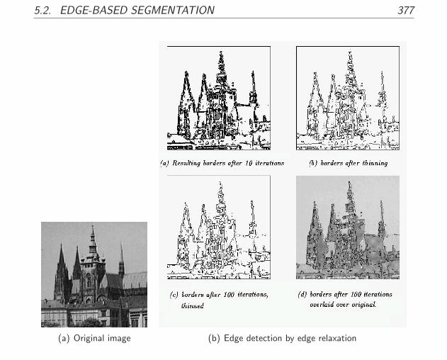
5.2. EDGE-BASED SEGMENTATION 377
(a) Original image (b) Edge detection by edge relaxation

378 CHAPTER 5. SEGMENTATION
• More recent approaches to edge relaxation use edge and border informationderived from image data.
• A method to determine probabilistic distribution of possible edge neighbor-hood is given in recent literature.

5.2. EDGE-BASED SEGMENTATION 379
5.2.3 Border tracing
Simple border tracing
• If a region border is not known but regions have been defined in the image,borders can be uniquely detected.
• First, let us assume that the image with regions is either binary or that regionshave been labeled.
• An inner region border is a subset of the region while an outer border is nota subset of the region, § 2.3.1.
• The first goal is to determine inner region borders.

380 CHAPTER 5. SEGMENTATION
• The following algorithm covers inner boundary tracing in both 4-connectivityand 8-connectivity.
Algorithm 5.2.3. Inner boundary tracing
1. Search the image from top left until a pixel of a new region is found;This pixel P0 then has the minimum column value of all pixels of thatregion having the minimum row value. Pixel P0 is a starting pixel of theregion border.
Define a variable dir which stores the direction of the previous movealong the border from the previous border element to the current borderelement. Assign
(a) dir = 3 if the border is detected in 4-connectivity;
(b) dir = 7 if the border is detected in 8-connectivity.
2. Search the 3× 3 neighborhood of the current pixel in an anti-clockwisedirection, beginning the neighborhood search in the pixel positioned inthe direction
(a) (dir + 3) mod 4 if the border is detected in 4-connectivity;
(b) (dir + 7) mod 8 if dir is even;(dir + 6) mod 8 if dir is odd.

5.2. EDGE-BASED SEGMENTATION 381
The first pixel found with the same value as the current pixel is a newboundary element Pn.
Update the dir value.
3. If the current boundary element Pn is equal to the second border ele-ment P1, and if the previous border element Pn−1 is equal to P0, stop.Otherwise repeat step 2.
4. The detected inner border is represented by pixels P0 · · ·Pn−2.

382 CHAPTER 5. SEGMENTATION

5.2. EDGE-BASED SEGMENTATION 383
• The above algorithm works for all regions larger than one pixel.
• This algorithm is able to find region borders but does not find borders ofregion holes.
• To search for hole borders as well, the border must be traced starting in eachregion or hole border element if this element has never been a member of anyborder previously traced.
• The search for border elements always starts after a currently traced border isclosed, and the search for ‘unused’ border elements can continue in the sameway as the search for the first border element was done.
• Note that if objects are of unit width, more conditions must be added.

384 CHAPTER 5. SEGMENTATION
• If the goal is to detect an outer region border, the given algorithm may stillbe used based on 4-connectivity.
Algorithm 5.2.4. Outer boundary tracing
1. Trace the inner region boundary in 4-connectivity until done;
2. The outer boundary consists of all non-region pixels that were tested duringthe search process; if some pixels were tested more than once, they are listedmore than once in the outer boundary list.

5.2. EDGE-BASED SEGMENTATION 385
• Note that some border elements may be repeated in the outer border up tothree times. See the following figure.
• The outer region border is useful for deriving properties such as perimeter,compactness, etc.

386 CHAPTER 5. SEGMENTATION
Extended border tracing
• The inner border is always part of a region but the outer border never is.
• Therefore, if two regions are adjacent, they never have a common border,which causes difficulties in higher processing levels with region description,region merging, etc.
• The inter-pixel boundary extracted, for instance, from crack edges is commonto adjacent borders; nevertheless, its position cannot be specified in pixelco-ordinates.
• Boundary properties better than those of outer borders may be found inextended borders, [Pavlidis, 1977].

5.2. EDGE-BASED SEGMENTATION 387
• The advantages of the extended boundary definition are:
– it defines a single common border between adjacent regions;
– it may be specified using standard pixel co-ordinates;
– all the useful properties of the outer border still remain, for derivingproperties such as perimeter, compactness, etc.;
– the boundary shape is exactly equal to the inter-pixel shape but is shiftedone half-pixel down and one half-pixel right

388 CHAPTER 5. SEGMENTATION
• The existence of a common border between regions makes it possible to in-corporate into the boundary tracing a boundary description process.
• An evaluated graph consisting of border segments and vertexes may resultdirectly from the boundary tracing process; also the border between adjacentregions may be traced only once and not twice as in conventional approaches.

5.2. EDGE-BASED SEGMENTATION 389
• The extended boundary is defined using 8-neighborhoods and the pixels arecoded according to the following figure:
• E.g., P4(P) denotes the pixel immediately to the left of pixel P .

390 CHAPTER 5. SEGMENTATION
• Four kinds of inner boundary pixels of a region R are defined; if Q denotesthe pixels outside the region R , then a pixel P ∈ R is
a LEFT pixel of R if P4(P) ∈ Q
a RIGHT pixel of R if P0(P) ∈ Q
an UPPER pixel of R if P2(P) ∈ Q
a LOWER pixel of R if P6(P) ∈ Q.
• Let LEFT(R), RIGHT(R), UPPER(R), LOWER(R) represent the correspond-ing subsets of R .

5.2. EDGE-BASED SEGMENTATION 391
• The extended boundary EB is defined as the following:
EB ={P : P ∈ LEFT(R)} ∪ {P : P ∈ UPPER(R)}∪ {P6(P) : P ∈ LOWER(R)} ∪ {P0(P) : P ∈ RIGHT(R)}∪ {P7(P) : P ∈ RIGHT(R)}.

392 CHAPTER 5. SEGMENTATION
• The extended boundary can easily be constructed from the outer boundary.
• Using an intuitive definition of RIGHT, LEFT, UPPER, and LOWER outerboundary points, the extended boundary may be obtained by shifting all theUPPER outer boundary points one pixel down and right, shifting all the LEFTouter boundary points one pixel to the right, and shifting all the RIGHT outerboundary points one pixel down. The LOWER outer boundary point positionsremain unchanged.
• The following figure illustrates the construction.

5.2. EDGE-BASED SEGMENTATION 393
• A more sophisticated approach for extended boundary tracing is based ondetecting common boundary segments between adjacent regions and vertexpoints in boundary segment connections.
• The detection process is based on a look-up table, which defines all 12 possiblesituations of the local configuration of 2× 2 pixel windows, depending on theprevious detected direction of boundary, and on the status of window pixelswhich can be inside or outside a region.

394 CHAPTER 5. SEGMENTATION
Figure 5.1:

5.2. EDGE-BASED SEGMENTATION 395
Algorithm 5.2.5. Extended boundary tracing via look-up table.
1. Define a starting pixel of an extended boundary in a standard way (the first re-gion pixel found in a left-to-right and top-to-bottom line-by-line image search).
2. The first move along the traced boundary from the starting pixel is in directiondir = 6 (down), corresponding to the situation (i) in Fig. 5.1.
3. Trace the extended boundary using the look-up table in the above figure untila closed extended border results.
• Note that there is no hole-border tracing included in the algorithm.
• The holes are considered separate regions and therefore the borders betweenthe region and its hole are traced as a border of the hole.

396 CHAPTER 5. SEGMENTATION
• The look-up table approach makes the tracing more efficient than conventionalmethods and makes parallel implementation possible.
• A pseudo-code description of algorithmic details is given in [Liow, 1991], wherea solution to the problem of tracing all the borders in an image in an efficientway is given.
• In addition to extended boundary tracing, it provides a description of eachboundary segment in chain code form together with information about ver-tices’s.
• This method is very suitable for representing borders in higher level segmenta-tion approaches including methods that integrate edge-based and region-basedsegmentation results.
• Moreover, in the conventional approaches, each border between two regionsmust be traced twice. The algorithm can trace each boundary segment onlyonce storing the information about what has already been done in double-linked lists.

5.2. EDGE-BASED SEGMENTATION 397
Border tracing in gray-level images
• A more difficult situation is encountered if the borders are traced in gray levelimages where regions have not yet been defined.
• The border is represented by a simple path of high-gradient pixels in the image.
• Border tracing should be started in a pixel with a high probability of being aborder element, and then border construction is based on the idea of addingthe next elements which are in the most probable direction.
• To find the following border elements, edge gradient magnitudes and directionsare usually computed in pixels of probable border continuation.

398 CHAPTER 5. SEGMENTATION
5.2.4 Border detection as graph searching
• Whenever additional knowledge is available for boundary detection, it shouldbe used.
• One example of prior knowledge is a known starting point and a ending pointof the border, even if the precise border location is not known.
• Even some relatively weak additional requirements such as smoothness, lowcurvature, etc., may be included as prior knowledge.
• If this kind of supporting information is available in the border detection task,general problem solving methods used in AI can be applied.

5.2. EDGE-BASED SEGMENTATION 399
• A graph is a general structure consisting of a set of nodes ni and arcs betweenthe nodes (ni , nj ), § 3.2.3. We consider oriented and numerically weightedarcs, these weights being called costs.
• The border detection process is transformed into a search for the optimal pathin the weighted graph, the aim being to find the best path that connects twospecified nodes, the starting and ending nodes.
• While cost minimization is considered throughout this section, the approachworks equally well if a maximum cost path is sought.
!
• Assume that both edge magnitude s(x) and edge direction φ(x) informationis available in an edge image.
• Each image pixel corresponds to a graph node weighted by a values s(x).
• Two nodes ni and nj corresponding to two 8-connected adjacent pixels xi andxj are connected by an arc if the edge directions φ(xi ) and φ(xj ) match thelocal border direction in a sense to be defined below.

400 CHAPTER 5. SEGMENTATION
• We can apply the following rules to construct the graph: To connect a nodeni representing the pixel xi with a node nj representing the pixel xj ,
1. pixel xj must be one of three existing neighbors of xi in the directiond ∈ [φ(xi )− π/4,φ(xi ) + π/4];
2. s(xi ) and s(xj ) must be greater than T , where T is some preset thresholdof edge significance.
!
• Another common requirement is to connect two nodes only if the differenceof their edge direction is less than π/2.
!
• These conditions can be modified in specific edge detection problems.

5.2. EDGE-BASED SEGMENTATION 401
• The following figure shows an image of edge directions, with only significantedges according their magnitudes listed, and the oriented graph constructedin accordance with the edge image.
!
• The application of graph search to edge detection was first published in[Martelli, 1972].
• Let xA be the starting border element, and xB be the end border element.

402 CHAPTER 5. SEGMENTATION
• To use graph search for region border detection, a method of oriented weighted-graph expansion must first be defined (one method is just described.)
• A cost function f (xi ) must also be defined that is a cost estimate of thepath between nodes nA and nB (pixels xA and xB) which goes through anintermediate node ni (pixel xi ).
• The cost function f (xi ) typically consists of two components: an estimateg(xi ) of the minimum path cost between the starting element xA and xi , andan estimate h(xi ) of the minimum path cost between xi and the end borderelement xB .
• The cost g(xi ) of the path from the starting element xA to the node xi isusually a sum of costs associated with the arcs or nodes that are in the path.
• The cost function must be separable and monotonic with respect to the pathlength, and therefore the local costs associated with arcs are required to benon-negative.
• A simple example of g(xi ) satisfying the given conditions is to consider thepath length from xA to xi .
• An estimate h(xi ) may be the length of the border from xi to xB , it makingsense to prefer shorter borders between xA and xB as the path with lower cost.

5.2. EDGE-BASED SEGMENTATION 403
• The following graph search algorithm (Nilsson’s A-algorithm from AI) can beapplied to the border detection.
!
Algorithm 5.2.6. A-algorithm graph search
1. Expand the starting node nA and put all its successors into an OPEN listwith pointers back to the starting node nA. Evaluate the cost function forexpanded node;
2. If the OPEN list is empty, fail; Determine the node ni from the OPEN listwith the lowest associated cost f (ni ) and remove it. If ni = nB , then trackback through the pointers to find the optimum path and stop;
3. If the option to stop was not taken in step 2, expand the specified node ni ,and put its successors on the OPEN list with pointers back to ni . Computetheir costs f . Go to step 2.

404 CHAPTER 5. SEGMENTATION
Example 5.2.7. Example of a graph searching using the A-algorithm, based on(weighted) path length.

5.2. EDGE-BASED SEGMENTATION 405

406 CHAPTER 5. SEGMENTATION

5.2. EDGE-BASED SEGMENTATION 407

408 CHAPTER 5. SEGMENTATION

5.2. EDGE-BASED SEGMENTATION 409

410 CHAPTER 5. SEGMENTATION

5.2. EDGE-BASED SEGMENTATION 411

412 CHAPTER 5. SEGMENTATION

5.2. EDGE-BASED SEGMENTATION 413
• If no additional requirements are set on the graph construction and search,this process can easily result in an infinite loop.

414 CHAPTER 5. SEGMENTATION
• To prevent this behavior, no node expansion is allowed that puts a node onthe OPEN list if this node has already been visited, and put on the OPEN listin the past.
• On the other hand, prohibiting the backward search may limit the shapes ofborders that can be successfully identified.
• A simple solution is not to allow searching in a backward direction.
• It may be possible to straighten the processed image (and the graph).

5.2. EDGE-BASED SEGMENTATION 415

416 CHAPTER 5. SEGMENTATION
• The estimate of the cost of the path from the current node ni to the endnode nB has a substantial influence on the search behavior.
• If this estimate h(ni ) of the true cost h(ni ) is not considered, so h(ni ) = 0,no heuristic is included in the algorithm and a breadth-first search is done.
• Hence, the detected path will always be optimal according to the criterionused, the minimum cost path will always be found.
• However, applying heuristics, the detected cost does not always have to beoptimal but the search can often be much faster.
Z
• The closer the estimate h(ni ) is to h(ni ), the lower the number of nodesexpanded in the search.
• The problem is that the exact cost of the path from the node ni to the endnode nB is not known beforehand.
• In some applications, it may be more important to get a quick rather than anoptimal solution.
• Optimality is not guaranteed but the number of expanded nodes will typicallybe smaller because the search can be stopped before the optimum is found.

5.2. EDGE-BASED SEGMENTATION 417
• A crucial question is how to choose the evaluation cost functions for graph-search border detection.
• A good cost function should have elements common to most edge detectionproblems and also specific terms related to the particular application.
• Some generally applicable cost functions are:
1. Strength of edges forming a border:
The heuristic “the stronger the edges that form the border, the higherthe probability of the border” is very natural and almost always givesgood results.
If a border consists of strong edges, the cost of that border is small.
The cost of adding another node to the border will be
(max
xk∈images(xk)
)− s(xi ). (5.33)

418 CHAPTER 5. SEGMENTATION
2. Border curvature:
Sometimes, borders with a small curvature are preferred.
If this is the case, the total border curvature can be evaluated as mono-tonic function of local curvature increments:
diff [φ(xi )− φ(xj )] , (5.34)
where diff is some suitable function evaluating the difference in edgedirections in two consecutive border elements.
3. Estimates of the distance to the goal (end point):
If a border is reasonably straight, it is natural to support expansion ofthose nodes that are located closer to the goal node than other nodes:
h(xi ) = dist(xi , xB). (5.35)
• Since the range of border detection applications is quite wide, the cost func-tions described may need some modification to be relevant to a particulartask.

5.2. EDGE-BASED SEGMENTATION 419
Example 5.2.8. Border detection by graph searching.

420 CHAPTER 5. SEGMENTATION
• Graph searching techniques offer a convenient way to ensure global optimalityof the detected contour.
• Searching for all the borders in the image without knowledge of the start andend-points is more complex.
• A good overview of recent detection and edge linking methods can be foundin [van der Heijden, 1995].

5.2. EDGE-BASED SEGMENTATION 421
5.2.5 Border detection as dynamic programming
• Dynamic Programming is an optimization method, which searches for optimaof functions in which not all variables are simultaneously interrelated.
• Consider the following simple boundary-tracing problem,
• The aim is to find the best path (minimum cost) between one of the possi-ble start points A, B , C and one of the possible ending points G , H , I . Theboundary must be contiguous in 8-connectivity. The graph representing theproblem, together with assigned partial cost is shown.

422 CHAPTER 5. SEGMENTATION
• The main idea of the principle of optimality is: Whatever the path to the nodeE was, there exists an optimal path between E and the end point. In otherwords, if the optimal path [start point-endpoint] goes through E , then bothits parts [start point-E ] and [E -end point] are also optimal, respectively.
• Therefore, the optimal path can be found by following only the partial optimalpath, sucessively layer-by-layer.

5.2. EDGE-BASED SEGMENTATION 423
• The end point with the minimum path cost represents the optimum path; nodeH is therefore the optimal boundary end point, and the optimal boundary isB − F − H (Fig. (f)).

424 CHAPTER 5. SEGMENTATION
• The following is an example in which node costs are used (not arc cost asin the above example). Note that the graph, the cost function and resultingpath are identical to those used in the previous section.

5.2. EDGE-BASED SEGMENTATION 425
• If the graph has more layers, the process is repeated until one of the endpoints is reached. Each repetition consists of a simpler optimization as shownin the following figure:
C (xm+1k ) = min
i[C (xm
i ) + g m(i , k)] , (5.36)
where C (xm+1k ) is the new cost assigned to the node xm+1
k , and g m(i , k) isthe partial path cost between nodes xm
i and xm+1k .

426 CHAPTER 5. SEGMENTATION
• For the complete optimization problem,
min[C (x1, x2, · · · , xM)
]= min
k
[C (xM
k )]
, (5.37)
where
– xMk are the end point nodes,
– M is the number of graph layers between start points and end points,
– C (x1, x2, · · · , xM) denotes the cost of a path between the first and thelast (M th) graph layer.
• The final optimal path results from back-tacking through the searched graph.

5.2. EDGE-BASED SEGMENTATION 427
• Requiring an 8-connected border and assuming n nodes in each graph layerm,
– 3n cost combinations must be computed for each layer,
– 3n(M − 1) + n is the total number of cost combination computations.
• Compared to the brute-force enumerative search, where n3M−1 combinationsmust be computed, the improvement is obvious.
!
• Note that the number of neighbors depends on the definition of contiguityand definition of the searched graph and is not limited to three.

428 CHAPTER 5. SEGMENTATION
Algorithm 5.2.9. Boundary tracing as dynamic programming
1. Specify initial costs C (x1i ) in the first graph layer, i = 1, · · · , n and partial
path costs g m(i , k), m = 1, · · · , M − 1.
2. Repeat step 3 for all m = 1, · · · , M − 1.
3. Repeat step 4 for all nodes k = 1, · · · , n in the graph layer m.
4. LetC (xm+1
k ) = mini=−1,0,1
[C (xm
k+i ) + g m(i , k)]
. (5.38)
Set pointer from node xm+1k back to node xm∗
i where ∗ denotes the optimalpredecessor.
5. Find an optimal node xM∗i in the last graph layer M and obtain and optimal
path by back-tracking through the pointers from xM∗i to x1∗
i .

5.2. EDGE-BASED SEGMENTATION 429
• It has been shown that heuristic search may be more efficient than dynamicprogramming for finding a path between two nodes in a graph.
• Further, an A-algorithm-based graph search does not require explicit definitionof the graph (only the rule for node expansion).
• However, dynamic programming presents an efficient way of simultaneouslysearching for optimal paths from multiple starting and ending points.
• If these points are not known, dynamic programming is probably a betterchoice, especially if computation of the partial costs g m(i , k) is simple.
• Nevertheless, which approach is more efficient for a particular problem dependson evaluation functions and on the quality of heuristics for an A-algorithm.
• Please refer to the text book for further discussions.

430 CHAPTER 5. SEGMENTATION
• Tracing borders of elongated objects such as roads and rivers in aerial pho-tographs and vessels in medical images, represents typical applications of dy-namic programming in image segmentation.
Example 5.2.10. “Find a minimum-cost connected path between the first and lastrow of an image matrix. A connected path is only allowed to move by at most onepixel horizontally for each vertical step. The advantage of dynamic programmingis that the algorithm is fast and exact (not heuristic). While the formulation mayseem restrictive, a surprisingly large number of segmentation and boundary findingproblems may be coerced into it.” (from dpboundary.m)
“We demonstrate dpboundary on the task of tracing a blood vessel on part ofan MRI image of a lower limb (leg). Since the vessel is bright, we take a negativevalue of the brightness as the cost function.” (from dpboundary demo.m)
The matlab script from visionbook is here Border detection by dynamic pro-gramming.

5.2. EDGE-BASED SEGMENTATION 431
5.2.6 Hough transform
• If an image consists of objects with known shape and size. segmentation canbe viewed as a problem of finding this object within an image.
• Typical tasks are to locate circular pads in printed circuit boards. or to findobjects of specific shapes in aerial or satellite data, etc.
• One of many possible ways to solve these problems is to move a mask with anappropriate shape and size along the image and look for correlation betweenthe image and the mask.
• Unfortunately, the specified mask often differs too much from the object’srepresentation in the processed data, because of shape distortions, rotation,zoom, etc.
• One very effective method that can solve this problem is the Hough transform,which can even be used successfully in segmentation of overlapping or semi-occluded objects.

432 CHAPTER 5. SEGMENTATION
• To introduce the main concepts of the Hough transform, consider an exampleof circle detection.

5.2. EDGE-BASED SEGMENTATION 433
• Let the task be to detect a dark circle of a known radius r in an image witha uniform bright background.
• The method starts with a search for dark image pixels; after such a pixel isfound, a locus of potential center points of the circle associated with it canbe determined.
• Such a locus of potential center points forms a circle with the radius r asdemonstrated in the figure (b).
• If the loci of potential circle centers are constructed for all dark pixels identifiedin the original image, the frequency can be determined with which each pixelof the image occurs as an element of the circle-center loci.
• As seen from the figure (c), the true center of the circle being sought isrepresented by the pixel with the highest frequency of occurrence in the circle-center loci.
• Thus, the center of the searched circle is determined.
• With the known circle radius, the image segmentation is completed.

434 CHAPTER 5. SEGMENTATION
• The original Hough transform was designed to detect straight lines and curvesand this original method can be used if analytic equations of object borderlinesare known — no prior knowledge of region position is necessary.
• An advantage of this approach is its robustness of segmentation results; thatis, segmentation is not too sensitive to imperfect data or noise.
• It is often impossible to get analytic expressions describing border.
• There is a generalized Hough transform designed to find objects even if ananalytic expression of the border is not known.

5.2. EDGE-BASED SEGMENTATION 435
• The basic idea of the method can be seen from the simple problem of detectinga straight line in an image.
• A straight line is defined by two points A = (x1, y1) and B = (x2, y2), shownin the following figure.
Figure 5.2: Hough transform principle: (a) image space; (b) k , q parameter space.

436 CHAPTER 5. SEGMENTATION
• All straight lines going through the point A are given by the expression y1 =kx1 + q for some values of k and q.
• This means that the same equation can be interpreted as an equation in theparameter space k , q.
• All the straight lines going through the point A are then represented by theequation
q = −kx1 + y1 (5.39)
in the parameter space k , q.
• Straight lines going through the point B can likewise be represented as q =−kx2 + y2.
• The only common point of both straight lines in the k , q parameter spaceis the point which in the original image space represents the only existingstraight line connecting points A and B .

5.2. EDGE-BASED SEGMENTATION 437
• This means that any straight line in the image is represented by a single pointin the k , q parameter space and any part of this straight line is transformedinto the same point.
• The main idea of this method is to determine all the possible line pixelsin the image, by transforming all lines that can go through the pixels intocorresponding points in the parameter space and detecting the points k , q inthe parameter space that frequently resulted from the Hough transform oflines, q = −kx2 + y2, in the image.
• The main steps will be descrined in details in the following.
!
• Detection of all possible line pixels in the image may be achieved by applyingan edge detector to the image; then, all pixels with edge magnitude exceedingsome threshold can be considered possible line pixels (referred to as edgepixels below).
!
• In the general case, nothing is known about lines in the image and thereforelines of any direction may go through any of the edge pixels.

438 CHAPTER 5. SEGMENTATION
• In reality, the number of these lines is infinite; however, for practical purposes,only a limited number of line directions may be considered.
• The possible directions of lines define a discretization of the parameter k .
• Similarly, the parameter q is sampled into a limited number of values.
• The parameter space is not continuous any more, but rather is represented bya rectangular structure of cells.
• This array of cells is called the accumulator array A, whose elements areaccumulator cells A(k , q).
!
• For each edge pixel, parameters k , q are determined which represent lines ofallowed direction going through this pixel.
• For each such line, the values of line parameters k , q are used to increase thevalue of the accumulator cell A(k , q).
• If a line represented by an equation y = kx + q is present in the image, thevalue of the accumulator cell A(k , q) will be increased many times — as many

5.2. EDGE-BASED SEGMENTATION 439
times as the line y = kx + q us detected as a line possibly going through anyof the edge pixels.
!
• For any pixel P , lines going through it may have any direction k (from theset of allowed directions), but the second parameter q is constrained by theimage co-ordinates of the pixel P and the direction k .
• Therefore, lines existing in the image will cause large values of the appropriateaccumulator cells in the image, while other possibly going through edge pixels,which do not correspond to lines existing in the image, have different k , qparameters for each edge pixel, and therefore the corresponding accumulatorcells are increased rarely.
• In other words, lines existing in the image may be detected as high-valuedaccumulator cells in the accumulator array, and the parameters of the detectedline are specified by the accumulator array co-ordinates.
• As a result, line detection in the image is transformed to detection of localmaxima in the accumulator space.

440 CHAPTER 5. SEGMENTATION
• It has been noted that an important property of the Hough transform is itsinsensitivity to mission part of lines, to image noise, and to other non-linestructures co-existing in the image.
• This is caused by the robustness of transformation from the image space tothe accumulator space — a missing part of the line will cause only a lowerlocal maximum because a smaller number of edge pixels contributes to thecorresponding accumulator cell.

5.2. EDGE-BASED SEGMENTATION 441
• Insensitivity to data imprecision and noise can be seen in the following figure.

442 CHAPTER 5. SEGMENTATION
• Note that the parametric equation of the line y = kx + q is appropriateonly for explanation of the Hough transform principles — it causes difficultiesin vertical line detection (k → ∞) and in nonlinear discretization of theparameter k .
• If a line is represented as
x cos θ + y sin θ = s, (5.40)
the Hough transform does not suffer from those limitations. All the propertiesof the Hough transform still hold for this parametrization.
Figure 5.3: Hough transform in s, θ space. (a) Straightline in image space. (b) s, θparameter space.

5.2. EDGE-BASED SEGMENTATION 443
• A practical example showing the segmentation of an MR image of the braininto the left and right hemispheres is given in the following figure.

444 CHAPTER 5. SEGMENTATION
• Discretization of the parameter space is an important part of this approach;also detecting the local maxima in the accumulator array is a non-trivial prob-lem.
• In reality, the resulting discrete parameter space usually has more than onelocal maximum per line existing in the image, and smoothing the discreteparameter space may be a solution.
• The above remarks remain valid if more complex curves are sought in theimage using the Hough transform, the only difference being the dimensionalityof the accumulator array.

5.2. EDGE-BASED SEGMENTATION 445
• Generalization to more complex curves that can be described by an analyticequation is straightforward.
• Consider an arbitrary curve represented by an equation
f (x , a) = 0, (5.41)
where a is the vector of curve parameters.

446 CHAPTER 5. SEGMENTATION
Algorithm 5.2.11. Curve detection using the Hough transform
1. Quantize parameter space within the limits of parameters a. The dimension-ality n of the parameter space is given by the number of parameters of thevector a.
2. Form an n-dimensional accumulator array A(a) with structure matching thequantization of the parameter space; set all elements to zero.
3. For each image point (x1, x2) with non-zero pixel value in the appropriatelythresholded gradient image, increase all accumulator cells A(a) if f (x , a) = 0,
A(a) = A(a) + ∆A (5.42)
for all a inside the limits used in step 1.
4. Local maxima in the accumulator array A(a) correspond to realizations ofcurves f (x , a) that are present in the original image.

5.2. EDGE-BASED SEGMENTATION 447
• If we are looking for circles, the analytic expression f (x , a) of the desired curveis
(x1 − a)2 + (x2 − b)2 = r 2 (5.43)
where the circle has center (a, b) and radius r .
• Therefore, the accumulator data structure must be 3-dimensional.
• For each pixel x whose edge magnitude exceeds a given threshold, all accu-mulator cells corresponding to potential circle centers (a, b) are incrementedin step 3 of the given algorithm.
• The accumulator cell A(a, b, r) is incremented if the point (a, b) is at distancer from point x .
• If some potential center (a, b) of a circle of radius r is frequently found inthe parameter space, it is highly probable that a circle with center (a, b) andradius r really exist in the processed data.

448 CHAPTER 5. SEGMENTATION
Figure 5.4: Hough transform — circle detection: (a) original image; (b) edge image(note that the edge informaiton is far from perfect; (c) parameter space; (d) detectedcircles.

5.2. EDGE-BASED SEGMENTATION 449
• The processing results in a set of parameters of desired curves f (x , a) = 0that correspond to local maxima of accumulator cells in the parameter space;these maxima best match the desired curves and processed data.
• Parameters may represent unbounded analytic curves (e.g., line, parabola,etc.), but to look for finite parts of these curves, the end points must be ex-plicitly defined and other conditions must be incorporated into the algorithm.
• Even though the Hough transform is a very powerful technique for curvedetection, exponential growth of the accumulator data structure with theincrease of the number of curve parameters restricts its practical usability tocurves with few parameters.

450 CHAPTER 5. SEGMENTATION
• If prior information about edge directions is used, computational demands canbe decreased significantly.
• Please refer to the textbook for discussions.
!
• The randomized Hough transform offers a different approach to achieve in-creased efficiency.
• It randomly selects n pixels from the edge image and determines n parametersof the detected curve followed by incrementing a single accumulator cell only.
• Please refer to the textbook for discussions.
Example 5.2.12. Line detection in chessboard.The matlab script from visionbookis here Line detection example.

5.3. REGION-BASED SEGMENTATION 451
5.3 Region-based segmentation
• The aim of segmentation methods described in the previous section was tofind borders between regions; the following methods construct regions directly.
• It is easy to construct regions from their borders, and it is easy to detectborders of existing regions.
• However, segmentations resulting from edge-based methods and region-growingmethods are not usually exactly the same, and a combination of results mayoften be a good idea.
• Region growing techniques are generally better in noisy images, where bordersare extremely difficult to detect.
• Homogeneity is an important property of regions and is used as the mainsegmentation criterion in region growing, whose basic idea is to divide animage into zones of maximum homogeneity.

452 CHAPTER 5. SEGMENTATION
• The homogeneity criteria affect the region-based methods.
• General and specific heuristics for homogeneity may also be incorporated.
• The criteria for homogeneity can be based on gray-level, color, texture, shape,model (using semantic information), etc.
• The simplest homogeneity criterion uses an average gray-level of the region,its color properties, simple texture properties, or an m-dimensional vector ofaverage gray values for multi-spectral images.
• Properties chosen to describe regions influence the form, complexity, andamount of prior information in the specific region-growing segmentation method.
• Methods that specifically address region-growing segmentation of color imagesare reported in the literature.

5.3. REGION-BASED SEGMENTATION 453
• Regions have already been defined before.
• A complete segmentation of an image R is a finite set of regions R1, · · · , RS ,
R =S⋃
i=1
Ri , Ri
⋂Rj = ∅ if i 6= j (5.44)
where S is the total number of regions in the image.
• Further assumptions needed in this section are that regions must satisfy thefollowing conditions:
H(Ri ) = TRUE, for i = 1, · · · , S (5.45)
and
H(Ri
⋃Rj ) = FALSE, for i 6= j and Ri is adjacent to Rj . (5.46)
where H(Ri ) is a binary homogeneity evaluation of the region Ri .
• Resulting regions of the segmented image must be both homogeneous andmaximal, where by ’maximal’ we mean that the homogeneity criterion wouldnot be true after merging a region with any adjacent region.
!

454 CHAPTER 5. SEGMENTATION
• While the region growing methods discussed below deal with two-dimensionalimages, three-dimensional implementations are often possible.
• Considering three-dimensional connectivity constraints, homogeneous regions(volumes) of a three-dimensional image can be determined using three-dimensionalregion growing.

5.3. REGION-BASED SEGMENTATION 455
5.3.1 Region merging
• The most natural method of region growing is to begin the growth in the rawimage data, each pixel representing a single region.
• These regions almost certainly do not satisfy the condition of equation (5.46),and so regions will be merged as long as equation (5.45) remains satisfied.
Algorithm 5.3.1. Region merging (outline)
1. Define some starting method to segment the image into many small regionssatisfying condition (5.45).
2. Define a criterion for merging two adjacent regions.
3. Merge all adjacent regions satisfying the merging criterion. If no two regionscan be merged maintaining condition (5.45), stop.
456 CHAPTER 5. SEGMENTATION
• This algorithm represents a general approach to region merging segmentation.
• Specific methods differ in the definition of the starting segmentation and inthe criterion for merging.
• In the descriptions that follow, regions are those parts of the image that can besequentially merged into larger regions satisfying equation (5.45) and (5.46).
!
• The result of region merging usually depends on the order in which regions aremerged, meaning that segmentation results will probably differ if segmentationbegins, for instance, in the upper left or lower right corner.
• This is because the merging order can cause two similar adjacent regionsR1 and R2 not to be merged, since an earlier merge used R1 and its newcharacteristics no longer allow it to merged with region R2. If the mergingprocess used a different order, this merge may have been realized.

5.3. REGION-BASED SEGMENTATION 457
• The simplest methods begin merging by starting the segmentation using re-gions of 2 × 2, 4 × 4 or 8 × 8. Region descriptions are then based on theirstatistical gray-level properties — a region gray-level histogram is a goodexample.
• A region description is compared with the description of an adjacentregion; if they match, they are merged into a larger region and a new regiondescription is computed.
• Otherwise, regions are marked as non-matching.
• Merging of adjacent regions continues between all neighbors, including newlyformed ones.
• If a region cannot be merged with any of its neighbors, it is marked ‘final’.
• The merging process stops when all image regions are so marked.

458 CHAPTER 5. SEGMENTATION
• Another approach uses the supergrid.
• The super-grid carries all the necessary information for easy region mergingin 4-adjacency, see the following figure:
Figure 5.5: Super-grid data structure: × – image data, ◦ – crack edges; • – unused.
• Starting regions are formed by pixels of the same gray-level.
• Region merging is based on the crack edge computation, where local bound-aries between regions are evaluated by the strength of crack edges along theircommon border.

5.3. REGION-BASED SEGMENTATION 459
• This region merging uses the following two heuristics:
1. Two adjacent regions are merged if a significant part of their commonboundary consists of weak edges (significance can be based on the regionwith the shorter perimeter; the ratio of the number of weak commonedges to the total length of the region perimeter).
2. Two adjacent region are also merged if a significant part of their commonboundary consists of weak edges, but in this case not considering thetotal length of the region borders.
• Of the two heuristics, the first is more general and the second cannot be usedalone because it does not consider the influence of different region sizes.
• Edge significance can be evaluated according to the formula
vij =
{0, if sij < T1;
1, otherwise(5.47)
where vij = 1 indicates a significant edge, and vij = 0 a weak edge, T1 is apreset threshold, and sij is the crack edge value (e.g., sij = |f (xi )− f (xj )|).
• The algorithm is as follows.

460 CHAPTER 5. SEGMENTATION
Algorithm 5.3.2. Region merging via boundary melting
1. Define a starting image segmentation into regions of constant gray-level. Con-struct a super-grid edge data structure in which to store the crack edge infor-mation.
2. Remove all weak crack edge data structure (using (5.47) and threshold T1).
3. Recursively remove common boundaries of adjacent regions Ri and Rj , if
W
min(Li , Lj )≥ T2 (5.48)
where W is the number of weak edges on the common boundary, Li and Lj arethe perimeter lengths of regions Ri and Rj , and T2 is another preset threshold.
4. Recursively remove common boundaries of adjacent regions Ri and Rj , if
W
min(L)≥ T3 (5.49)
or, using a weaker criterionW ≥ T3 (5.50)
where L is the length of the common boundary and T3 is a third threshold.

5.3. REGION-BASED SEGMENTATION 461
• Note that even if we have described a region growing method, the mergingcriterion is based on border properties and so the merging does not necessarilykeep condition (5.45).
• Please refer to the textbook for discussions on using a more advanced datastructure than the supergrid.

462 CHAPTER 5. SEGMENTATION
• The following figure gives a comparison of region merging methods.
• The original image is displayed in its pseudo-color representation
• The original image cannot be segmented by thresholding because of the sig-nificant and continuous gray-level in all regions.

5.3. REGION-BASED SEGMENTATION 463
• Results of a recursive region merging method — pixels are merged in therow-first fashion as long as they do not differ by more than a pre-specifiedparameter from the seed pixel, are shown as follows:
• Note the resulting horizontally elongated regions corresponding to verticalchanges of image gray-levels.

464 CHAPTER 5. SEGMENTATION
• If region merging via boundary melting is applied, the result is improved dra-matically.
Example 5.3.3. Region merging with boundary melting. The matlab script fromvisionbook is here Region merging example.

5.3. REGION-BASED SEGMENTATION 465
5.3.2 Region splitting
• Region splitting is the opposite of region merging, and begins with the wholeimage represented as a single region which does not usually satisfy the condi-tion (5.45).
• Therefore, the existing image region are sequentially split to satisfy (5.44),(5.45) and (5.46).
• It generally uses similar criteria of homogeneity as region merging method anddiffers only in the direction of their application.
• Even if this approach seems to be dual to region merging, region splitting doesnot result in the same segmentation even if the same homogeneity criteria areused.
– Some regions may be homogeneous during the splitting process andtherefore are not split any more.
– Considering the homogeneous regions created by region merging pro-cedures, some may not be constructed because of the impossibility ofmerging smaller sub-regions earlier in the process.

466 CHAPTER 5. SEGMENTATION
• A fine black-and-white chessboard is an example: let the homogeneity criterionbe based on variance of average gray-levels in the quadrants of the evaluatedregion in the next lower pyramid level.
Figure 5.6: Different segmentations may result from region splitting and regionmerging approaches. (a) Chessboard imaging, corresponding pyramid. (b) Regionsplitting segmentation (upper pyramid level is homogeneous, no splitting possible).(c) Region merging segmentation (lowest pyramid level consists of regions thatcannot be merged).

5.3. REGION-BASED SEGMENTATION 467
5.3.3 Splitting and merging
• A combination of splitting and merging may result in a method with theadvantage of both approaches.
• Split-and-merge approaches work using pyramid image representations. Re-gions are square shaped and corresponding to elements of the appropriatepyramid level.

468 CHAPTER 5. SEGMENTATION
• If any region in any pyramid level is not homogeneous (excluding the lowestlevel), it is split into four sub-regions — these are elements of higher resolutionat the level below.
• If four regions with the same parent node exists at any pyramid level withapproximately the same value of homogeneity measure, they are merged intoa single region in an upper pyramid level.
• The segmentation process can be understood as the construction of a seg-mentation quadtree where each leaf node represents a homogeneous region— that is, an element of some pyramid level.
• Splitting and merging corresponds to removing or building parts of the seg-mentation quadtree — the number of leaf nodes of the tree corresponds tothe number of segmented regions after the segmentation process is over.
• These approaches are sometimes called split-and-link methods if they usesegmentation tress for storing information about adjacent regions. Split-and-merge methods usually store the adjacency information in region adjacencygraphs (or similar data structures).

5.3. REGION-BASED SEGMENTATION 469
• An unpleasant drawback of segmentation quadtree is the square-region shapeassumption, see the following figure:

470 CHAPTER 5. SEGMENTATION
• The homogeneity criterion plays a major role in split-and-merge algorithms,as it does in all other region growing methods.
• If the image being processed is reasonably simple, a split-and-merge approachcan be based on local image properties.
• If the image is very complex, even elaborate criteria including semantic infor-mation may not give acceptable results.

5.3. REGION-BASED SEGMENTATION 471
5.3.4 Watershed segmentation
• The concepts of watersheds and catchment basins are well known in topog-raphy.
• Watershed lines divide individual catchment basins.
• The North American Continental Divide is a textbook example of a watershedline with catchment basins formed by the Atlantic and Pacific Oceans.
• Working the 2D function presentations, image data may be interpreted as atopographic surface where the (gradient) image gray-levels represent altitudes.
• Thus, region edges correspond to high watersheds and low-gradient regioninteriors correspond to catchment basins.
• According to equations (5.44), (5.45) and (5.46), the goal of region growingsegmentation is to create homogeneous regions.
• In watershed segmentation, catchment basins of the topographic surface arehomogeneous in the sense that all pixels belonging to the same catchmentbasin are connected with the basin’s region of minimum altitude (gray-level)by a simple path of pixels that have monotonically decreasing altitude (gray-level) along the path.

472 CHAPTER 5. SEGMENTATION
• Such catchment basins then represent the regions of the segmented image.
Figure 5.7: One dimensional example of watershed segmentation. (a) Gray-levelprofile of image data. (b) Watershed segementation — local minima of gray-level(altitude) yield catchment basins, local maxima define the watershed lines.
• While the concept of watersheds and catchment basins is quite straightfor-ward, development of algorithms for watershed segmentation is a complextask, with many of the early methods resulting in either slow or inaccurateexecution.

5.3. REGION-BASED SEGMENTATION 473
• There are two basic approaches to watershed image segmentation.
• The first one starts with finding a downstream path from each pixel of theimage to a local minimum of image surface altitude.
• A catchment basin is then defined as the set of pixels for which their respectivedownstream paths all end up in the same altitude minimum.
• While the downstream paths are easy to determine for continuous altitudesurfaces by calculating the local gradients, no rules exist to define the down-stream paths uniquely for digital surfaces.

474 CHAPTER 5. SEGMENTATION
• The second watershed segmentation approach represented by a seminal paper[Vincent and Soille, 1992] makes the idea practical.
• This approach is essentially dual to the first one.
• Instead of identifying the downstream paths, the catchment basins fill fromthe bottom.
• As was explained earlier, each minimum represents one catchment basin, andthe strategy is to start at the altitude minima.
• Imagine that there is a hole in each local minimum, and that the topographicsurface is immersed on water.
• As a result, the water starts filling all catchment basins, minima of which areunder the water level.
• If two catchment basins would merge as a result of further immersion, a damis built all the way to the highest surface altitude and the dam represents thewatershed line.
• An efficient algorithm for such watershed segmentation was presented in[Vincent and Soille, 1992].

5.3. REGION-BASED SEGMENTATION 475
• The algorithm is based on sorting the pixels in an increasing order of their grayvalues, followed by a flooding step consisting of a fast breadth-first scanningof all pixels in the order of their gray-levels.
!
• During the sorting step, a brightness histogram is computed.
• Simultaneously, a list of pointers to pixels of gray-level h is created and asso-ciated with each histogram gray-level to enable direct access to all pixels ofany gray-level.
• Information about the image pixel sorting is used extensively in the floodingstep.
!
• Suppose the flooding has been completed up to a level (gray-level, altitude)k .
Then every pixel having gray-level less than or equal to k has already beenassigned a unique catchment basin label.

476 CHAPTER 5. SEGMENTATION
• Next, pixels having gray-level k + 1 will be processed; all such pixels can befound in the list prepared in the sorting step — all these pixels can be accesseddirectly.
• A pixel having gary-level k + 1 may belong to a catchment basin labeled L ifat least one of its neighbors already carries this label.
• Pixels that represent potential catchment basin members are put in a first-infirst-out queue and await further processing.

5.3. REGION-BASED SEGMENTATION 477
• Geodesic influence zones are computed for all hitherto determined catchmentbasins.
A geodesic influence zone of a catchment basin Li is the locus of non-labeledimage pixels of gray-level k + 1 that are contiguous with the catchment basinLi (contiguous within the region of pixels of gray-level k + 1) for which theirdistance to Li is smaller than their distance to any other catchment basin Lj .

478 CHAPTER 5. SEGMENTATION
• All pixels with gray-level k +1 that belong to the influence zone of a catchmentbasin labeled L are also labeled with the label L, thus causing the catchmentbasin to grow.
• The pixels from the queue are processed sequentially, and all pixels from thequeue that cannot be assigned an existing label represent newly discoveredcatchment basins and are marked with new and unique labels.

5.3. REGION-BASED SEGMENTATION 479
• The following is an example of watershed segmentation.

480 CHAPTER 5. SEGMENTATION
• Note that the raw watershed segmentation produces a severely over-segmentedimage with hundreds or thousands of catchment basins (c).
• To overcome this problem, region markers and other approaches have beensuggested to generate good segmentation (d).
!
• Please refer to the textbook for further discussions.

5.3. REGION-BASED SEGMENTATION 481
5.3.5 Region growing post-processing
• Images segmented by region growing methods often contain either too manyregions (under-growing)or too few regions (over-growing) as a result of non-optimal parameter setting.
• To improve classification results, a variety of post-processors has been devel-oped. Some of them combine segmentation information obtained from regiongrowing and edge-based segmentation. See the references in the text book.
!
• Simpler post-processors are based on general heuristics and decrease the num-ber of small regions in the segmented image that cannot be merged with anyadjacent region according to the originally applied homogeneity criteria.
• These small regions are usually not significant in further processing and canbe considered as segmentation noise. It is possible to remove them from theimage as follows.

482 CHAPTER 5. SEGMENTATION
Algorithm 5.3.4. 1. Search for the smallest image region Rmin.
2. Find the adjacent region R most similar to Rmin, according to the homogeneitycriteria used. Merge R and Rmin.
3. Repeat steps 1 and 2 until all regions smaller than a pre-selected size areremoved from the image.
• This algorithm will execute much faster if all regions smaller than a pre-selected size are merged with their neighbors without having to order themby size.
Example 5.3.5. Small region removal remsmall algorithm. The matlab script fromvisionbook is here Small region removal example.

5.4. ACTIVE CONTOUR MODELS — SNAKES 483
5.4 Active contour models — snakes
• The development of active contour models results from the work [Kass et al., 1988].
• It is a energy-minimization approach to a variety of tasks in image analysissuch as image segmentation, and is suitable for analysis of dynamic imagedata or 3D image data.
• The active contour model, or snake, is defined as an energy-minimizing spline— the snake’s energy depends on its shape and location within the image.
• Local minima of this energy then correspond to desired image properties.

484 CHAPTER 5. SEGMENTATION
• The following figure illustrates how a snake is defomed from its initial positionto the target.
Figure 5.8: Active contour model — snake. (a) Initial snake position (dotted)defined interactively near the true contour. (b), (c) Iteration steps of snake energyminimization: the snake is pulled toward the true contour.

5.4. ACTIVE CONTOUR MODELS — SNAKES 485
• Snakes may be understood as a special case of a more general technique ofmatching a deformable model to an image by means of energy minimization.
• Snakes do not solve the entire problem of finding contours in images; rather,they depend on other mechanisms such as interaction with a user, interac-tion with some higher-level image understanding process, or information fromimage data adjacent in time or space.
• This interaction must specify an approximate shape and starting position forthe snake somewhere near the desired contour.
• A priori as well as image-based information are then used to push the snaketoward an appropriate solution.
• Unlike most other image models, the snake is active, always minimizing itsenergy functional, therefore exhibiting dynamic behavior.

486 CHAPTER 5. SEGMENTATION
5.4.1 Traditional snakes and balloons
• The energy functional which is minimized is a weighted combination of internaland external forces.
• The internal forces emanate from the shape of the snake, while the externalforces come from the image andor from higher-level image understandingprocesses.
• The snake is defined parametrically as v(s) = [x(s), y(s)], where x(s) andy(s) are (x , y) co-ordinates along the contour and s ∈ [0, 1].
Figure 5.9: Active contour model — a parametric representation of the boundary.

5.4. ACTIVE CONTOUR MODELS — SNAKES 487
• The energy functional to be minimized may be written as
E ∗snake =
∫ 1
0
Esnake(v(s)) ds (5.51)
=
∫ 1
0
{Eint(v(s)) + Eimage(v(s)) + Econ(v(s))
}ds. (5.52)
where
– Eint represents the internal energy of the spline due to bending,
– Eimage denotes image forces,
– Econ external constraint forces.
• Usually, v(s) is approximated as a spline to ensure desirable properties ofcontinuity.

488 CHAPTER 5. SEGMENTATION
• The internal spline energy can be written as
Eint(v(s)) = α(s)
∣∣∣∣dv
ds
∣∣∣∣2
+ β(s)
∣∣∣∣d2v
ds2
∣∣∣∣2
(5.53)
where α(s) and β(s) specify the elasticity and stiffness of the snake.
• α(s) and β(s) control how the snake shrinks.
• Note that setting β(sk) = 0 at a point sk allows the snake to become second-order discontinuous at that point, and develop a corner.

5.4. ACTIVE CONTOUR MODELS — SNAKES 489
• The image force term Eimage is derived from the image data over which the
snake lies.
• As an example, a weighted combination of three different functionals is pre-sented which attracts the snake to lines, edges, and terminations
Eimage = wlineEline + wedgeEedge + wtermEterm. (5.54)
• The line-based functional may be very simple
Eline = f (x , y), (5.55)
or
Eline = Gσ ∗ f (x , y), (5.56)
where f (x , y) denotes image gray-levels at image location (x , y).
Then depending on the sign of wline, the snake will be attracted to light ordark lines.

490 CHAPTER 5. SEGMENTATION
• The edge-based functional
Eedge = − |∇f (x , y)|2 , (5.57)
or
Eedge = − |∇ [Gσ ∗ f (x , y)]|2 , (5.58)
attracts the snake to contours with large image gradients — that is, to loca-tions of strong edges, and is minimal at edges if defined as
• In order to find teminations and corners, we use the curvature of level lines ina slightly smoothed image.
• Let C (x , y) = Gσ(x , y) ∗ f (x , y) be a slightly smoothed version of the image.
• Then the curvature of the level contours in C (x , y) can be written as
Eterm =Cyy C 2
x − 2Cxy Cx Cy + Cxx C 2y√
C 2x + C 2
y3 . (5.59)

5.4. ACTIVE CONTOUR MODELS — SNAKES 491
• The snake behavior may be controlled by adjusting the weights wline, wedgeand wterm.
• A snake attracted to edges and terminations is shown in the follwing figure.
Figure 5.10: A snake attracted to edges arid terminations, (a) Contour illusion, (b)A snake attracted to the subjective contour. Adapted from [Kass et al., 1987].

492 CHAPTER 5. SEGMENTATION
• The third term of the integral (5.52) comes from external constraints imposedeither by a user or some other higher-level process which may force the snaketoward or away from particular features.
• If the snake is near to some desirable feature, the energy minimization willpull the snake the rest of the way.
• However, if the snake settles in a local energy minimum that a higher-levelprocess determines as incorrect, an area of energy peak may be made at thislocation to force the snake away to a different local minimum.

5.4. ACTIVE CONTOUR MODELS — SNAKES 493
• A contour is defined to lie in the position in which the snake reaches a localenergy minimum.
• From (5.52) and the calculus of variations, the Euler-Lagrange condition statesthat the spline v(s) which minimizes E ∗snake must satisfy
δE ∗snakeδv
= − d
ds
(α(s)
dv
ds
)+
d2
ds2
(β(s)
d2v
ds2
)+∇Eext(v(s)) = 0,
(5.60)
where Eext = Eimage + Econ.
• To solve the Euler-Lagrange equation, suppose an initial estimate of the so-lution is available. An evolution equation is formed:
∂v(s, t)
∂t= −
δE ∗snakeδv
=d
ds
(α(s)
dv
ds
)− d2
ds2
(β(s)
d2v
ds2
)−∇Eext(v(s)).
(5.61)
• The solution is found if ∂v(s,t)∂t
= 0.

494 CHAPTER 5. SEGMENTATION
• Numerous parameters must be designed (weighting factors, iteration steps,etc.), a reasonable initialization must be available, and, moreover, the solutionof the Euler-Lagrange equation suffers from numerical instability.
• Please refer to the textbook and recent literature for the development of thesnake model and its numerical methods.

5.4. ACTIVE CONTOUR MODELS — SNAKES 495
5.4.2 Gradient vector flow snakes
• Two main limitations common to these approaches are
– the requirement of snake initialization being close to the desired solution,
– difficulties in segmenting concave portions of the boundary.
• To overcome these problems, gradient vector flow (GVF) fields and their usein snake image segmentation were reported in [Xu and Prince, 1998].
• GVF field is an external force field that points toward the boundaries when intheir proximity and varies smoothly over homogeneous image regions all theway to image borders.
• Consequently, it can drive a snake toward a border from a large distance andcan segment object concavities.
• The GVF field is derived from an image by minimization of an energy func-tional by solving decoupled linear partial differential equations via diffusingthe gradient vectors of the edge image.
• The GVF is then used as an external force in the snake equations (5.60) and(5.61) forming a GVF snake.

496 CHAPTER 5. SEGMENTATION
(a) Snake force
(b) GVF force
Figure 5.11: When adding distance-based forces, the snake segmentation fails in asimilar fashion. Adapted from [Xu and Prince, 1998].

5.4. ACTIVE CONTOUR MODELS — SNAKES 497
• The GVF field g(x , y) = (u(x , y), v(x , y)) minimizes the energy functional
E =
∫∫µ[u2
x + u2y + v 2
x + v 2y
]+ |∇f |2 |g −∇f |2 dxdy . (5.62)
where µ is a regularization parameter balancing the weight of the first andsecond terms (increasing µ with increased noise).
• The GVF can be obtained by solving the Euler equations
µ∆u − (u − fx )(f 2x + f 2
y ) = 0, (5.63)
µ∆v − (v − fy )(f 2x + f 2
y ) = 0. (5.64)
• The second term in (5.63) and (5.63) is zero in homogeneous regions sincethe derivatives fx , fy are zero.
• Consequently, the GVF behavior in the homogeneous regions is fully defined bythe Laplace equation effectively diffusing the information from the boundariesto the homogeneous parts of the image.

498 CHAPTER 5. SEGMENTATION
• Solutions to (5.63) and (5.63) can be found by solving the following twodecoupled equations for t →∞,
∂u
∂t= µ∆u − (u − fx )(f 2
x + f 2y ) = 0, (5.65)
∂v
∂t= µ∆v − (v − fy )(f 2
x + f 2y ) = 0. (5.66)
• These generalized diffusion equations can be solved as separate scalar partialdifferential equations in u and v .
• Once g(x , y) is computed, (5.61) is modified using the GVF external forceg(x , y) yielding the GVF snake equation
∂v(s, t)
∂t=
d
ds
(α(s)
dv
ds
)− d2
ds2
(β(s)
d2v
ds2
)+ g(v(s)). (5.67)
• GVF can be generalized to higher dimensions defining the d-dimensional GVFfield.

5.4. ACTIVE CONTOUR MODELS — SNAKES 499
• Active contour models represent a recent approach to contour detection andimage interpretation.
• They differ substantially from classical approaches, where features are ex-tracted from an image and higher-level processes try to interpolate sparsedata to find a representation that matches the original data.
• Active contour models start from an initial estimate based on higher-levelknowledge, and an optimization method is used to refine the initial estimate.
• During the optimization, image data, an initial estimate, desired contour prop-erties, and knowledge-based constraints are considered.
• Feature extraction and knowledge-based constrained grouping of these fea-tures are integrated into a single process, which seems to be the biggestadvantage.
• Active contour models, however, search for local energy minima not attempt-ing to achieve globally optimal solutions.
• Applications can be found in many areas of machine vision and medical imageanalysis.
• Please refer to the GVF page.

500 CHAPTER 5. SEGMENTATION
5.5 Geometric deformable models — level sets andgeodesic active contours
• There are two main groups of deformable contour/surface models: the snakesbelong to the parametric model family as borders are represented in a para-metric form.
• While appropriate for many segmentation tasks, they may yield cusps or in-tersecting boundaries in some situations.
• They are not capable of handling topology changes of the evolving contours,with direct implementation [Sapiro, 2001, p. 143–144].
• The topology of the final curve will be as the initial one, unless special pro-ceedures are implemented for possible splitting and merging [Sapiro, 2001,p. 143–144].
• This is a problem when an unknown number of objects must be simultaneouslydetected [Sapiro, 2001, p. 143–144].
• This approach is also non-intrinsic, as the energy depends on the parametriza-tion of the curve and is not directly related to the object geometry [Sapiro, 2001,p. 143–144].

5.5. GEOMETRIC DEFORMABLE MODELS — LEVEL SETS AND GEODESICACTIVE CONTOURS 501
• The second family of deformable surfaces — geometric deformable models
— overcome this problem by representing developing surfaces by partial dif-ferential equations.
• The geometric deformable model literature has grown extensively in the pastyears, in many cases reporting a variety of applications in which deformablemodel based segmentation can be used.
• Geometric deformable models were named level set front propagation
and geodesic active contour segmentation approaches, respectively, inthe literature.
• The main feature separating geometric deformable models from parametricones is that curves are evolved using only geometric computations, indepen-dent of any parameterization: the process is implicit.
• Consequently, the curves and/or surfaces can be represented as level setsof higher dimensional functions yielding seamless treatment of topologicalchanges.
• Hence, without resorting to dedicated contour tracking, unknown numbers ofmultiple objects can be detected simultaneously.

502 CHAPTER 5. SEGMENTATION
• Let a curve moving in time t be denoted by X(s.t) = [X (s, t), Y (s, t)] wheres is the curve parameterization.
• Let N be the moving curve’s inward normal, and c its curvature, and let thecurve develop along its normal direction according to the partial differentialequation
∂X
∂t= V (c)N, (5.68)
where V (c) is the speed function.

5.5. GEOMETRIC DEFORMABLE MODELS — LEVEL SETS AND GEODESICACTIVE CONTOURS 503
• The following figure demonstrates the concept of front evolution.
Figure 5.12: Concept of front evolution, (a) Initial curve at t = 0. (b) Curve att = 1. Note that each curve point moved in direction of N by distance given byvelocity V . (c) Curve at t = 1 assuming the velocity V (c) is a function of curvature.
• As the curve is moving, it may need to be reparameterized to satisfy equation(5.68).

504 CHAPTER 5. SEGMENTATION
• If the curve evolution is driven by a curvature deformation equation, the par-tial differential equation describes a curve smoothing process which removespotential singularities and eventually shrinks the curve to a point
∂X
∂t= αcN, (5.69)
where α is a constant — similar to elastic internal forces used in snakes (5.53).
• The following figure shows deformation behavior using positive (α > 0) andnegative (α < 0) curvature.

5.5. GEOMETRIC DEFORMABLE MODELS — LEVEL SETS AND GEODESICACTIVE CONTOURS 505
Figure 5.13: Evolution of a closed 2D curve using curvature deformation, (a-d)Using positive curvature, iterations 100, 2,000, 4,000, 17,000. (e-h) Using negativecurvature, iterations 100, 2,000, 4,000, 17,000.

506 CHAPTER 5. SEGMENTATION
• Curve deformation driven by the constant deformation equation
∂X
∂t= V0N, (5.70)
is complementary, and is similar to the inflation balloon force discussedearlier and may introduce singularities like sharp corners.

5.5. GEOMETRIC DEFORMABLE MODELS — LEVEL SETS AND GEODESICACTIVE CONTOURS 507
• Geometric deformable models perform image segmentation by starting withan initial curve and evolving its shape using the speed equation (5.68).
• During the evolution process, curvature deformation and/or constant defor-mation are used and the speed of curve evolution is locally dependent on theimage data — this represents the motivation for the approach.
• The ultimate goal of curve evolution is to yield desirable image segmentationfor t →∞: in other words, curve evolution should stop at object boundaries.
• This evolution can be implemented using level sets and — similar to manygeneral techniques — the exact behavior of the segmentation technique de-pends on the segmentation parameters.
• In this case, the segmentation behavior depends on the design of the speedfunction V (c).

508 CHAPTER 5. SEGMENTATION
• An important question however remains — how to efficiently execute the curveevolution process.
• The idea that made geometric deformable models feasible is to represent thesegmentation boundary/surface implicitly as a level set of a higher-dimensionalfunction — the level set function φ — defined on the same image domain.
Figure 5.14: An example of embedding a curve as a level set. (a) A single curve, (b)The level set function where the curve is embedded as the zero level set φ(X(s, t)) =0 (in black), (c) The height map of the level set function with its zero level setdepicted in black.

5.5. GEOMETRIC DEFORMABLE MODELS — LEVEL SETS AND GEODESICACTIVE CONTOURS 509
• Using the level set representation of the curve allows its evolution by updatingthe level set function φ(t).
• Instances of curve evolution are obtained by determination of the zero-levelset for individual time points φ(t) = 0.
• The final solution is given by the zero-level set φ(t →∞) = 0.

510 CHAPTER 5. SEGMENTATION
• Importantly, the level set approach allows topology changes, singularity devel-opment, etc.
Figure 5.15: Topology change using level sets. As the level set function is updatedfor t = 1, 2, 3, the zero-level set changes topology, eventually providing a 2-objectboundary.

5.5. GEOMETRIC DEFORMABLE MODELS — LEVEL SETS AND GEODESICACTIVE CONTOURS 511
• A more formal treatment to define a level set embedding of the curve evolutionequation (5.68) is now appropriate.
• Having a level set function φ(x , y .t) with the contour X(s, t) as its zero-levelset, it follows that
φ(X(s, t)) = 0. (5.71)
• If this equation is differentiated with respect to t and the chain rule is used,
∂φ
∂t+
⟨∇φ,
∂X
∂t
⟩= 0. (5.72)
• Now assuming that φ is negative inside the zero-level set and positive outside,the inward unit normal to the level set curve is
N = − ∇φ|∇φ| , (5.73)
and from the speed equation (5.68)
∂X
∂t= −V (c)
∇φ|∇φ| . (5.74)

512 CHAPTER 5. SEGMENTATION
• Hence,
∂φ
∂t− V (c)
⟨∇φ,
∇φ|∇φ|
⟩= 0. (5.75)
• Therefore,
∂φ
∂t= V (c)|∇φ|. (5.76)
• The curvature c at the zero-level set is
c = ∇ ∇φ|∇φ| =φyyφ
2x − 2φxyφxφy + φxxφ
2y√
φ2x + φ2
y3 . (5.77)
• Equation (5.76) shows how to perform curve evolution specified by equation(5.68) using the level set method.

5.5. GEOMETRIC DEFORMABLE MODELS — LEVEL SETS AND GEODESICACTIVE CONTOURS 513
• To implement geometric deformable contours, an initial level set functionφ(x , y , t = 0) must be defined, the speed function must be derived for theentire image domain, and evolution must be defined for locations in whichnormals do not exist due to the development of singularities.
• The initial level set function is frequently based on the signed distance D(x .y)from each grid point to the zero-level set, φ(x , y , 0) = D(x , y).
• An efficient algorithm for construction of the signed distance function is calleda fast marching method [Sethian, 1999].
!
• Note that the evolution equation (5.76) is only derived for the zero-level set.
• Consequently, the speed function V (c) is undefined on other level sets andneeds to be extended to all level sets.
• A number of extension approaches, including the frequently used narrow
band extension, can be found in [Sethian, 1999].
• The level set equation can be solved iteratively using time step At. However,inherent time step requirements exist to ensure stability of the numericalscheme via the Courant- Friedrichs-Lewy (CFL) condition.

514 CHAPTER 5. SEGMENTATION
• Further numerical issues are discussed in [Sethian, 1999].
!
• A large variety of applications exist in which geometric deformable modelswere used for image segmentation.
!
• The frequently highlighted feature of geometric deformable model segmen-tations allowing topology changes is an important contribution to the imagesegmentation tool set.
• However, this behavior may be as detrimental as it may be useful.
• When applied to noisy data with boundary gaps, shapes may be generatedwhich have topology inconsistent with that of the underlying objects.
• In such situations, segmentation topology constraints may be required and achoice of parametric deformable models or graph-based approaches may bemore suitable.

Chapter 6
Scale-space Theory with PDE
• The main references for this lecture is [Perona and Malik, 1990, Alvarez et al., 1993,ter Haar Romeny, 1994, Ames, 1992]
• This lecture deals with a fundamental aspect of early image representation —the notion of scale.
515

516 CHAPTER 6. SCALE-SPACE THEORY WITH PDE
• The problem of scale must be faced in any imaging situation.
• An inherent property of objects in the world and details in image is that theyonly exists as meaningful entities over certain range of scale.
– A simple example of this is the concept of a branch of a tree, whichmakes sense only at a scale from, say, a few centimeters to at most afew meters.
– It is meaningless to discuss the tree concept at the nanometer or thekilometer level. At those scales it is more relevant to talk about themolecules that form the leaves, or the forest in which the tree grows.
• Consequently, a multi-scale representation is of crucial importance ifone aims at describing the structure of the world, or more specially the struc-ture of projections of the three dimensional world onto two dimensional im-ages.

517
• A vision system for handling objects of different sizes and at different distancesneeds a way to control the scale(s) at which the world is observed.
• Why should one represent a signal at multiple scales when all information ispresent in the original data anyway?
• The major reason for this is to explicitly represent the multi-scale aspect ofreal world images.
• Another aim is to simplify further processing by removing unnecessary anddisturbing details.

518 CHAPTER 6. SCALE-SPACE THEORY WITH PDE
6.1 Introduction
• We define a multi-scale analysis to be a family of transforms (Tt)t≥0
which, when applied to the original picture I0(x), yield a sequence of picturesI (t, x) = (Tt I0)(x).
• We do not now define the scale t, its meaning will be clear from the mathe-matical formulation below.
• The image I (t, x) is called the analysis of the image I0 at scale t.
• The goal of this lecture is to review some fundamental results concerning aframework known as scale-space that has been developed by the computervision community for controlling the scale of observation and representing themulti-scale nature of image data.
• We shall see that a few formal principles (or axioms) are enough to characterizeand unify the theories and algorithms.

6.1. INTRODUCTION 519
6.1.1 Transformation invariance
• The Euclidean nature of the world around us and the perspective mappingonto images impose natural constraints on the possible operations.
• Objects move rigidly, the illumination varies, the size of objects at the retinachanges with the depth from the eye, and view directions may change etc.
• Hence, it is natural to require early visual operations to be unaffected bycertain primitive transformations (e.g., translations, rotations, and gray-scaletransformations).
• In other words, the visual system should extract properties that are invariantwith respect to these transformations.

520 CHAPTER 6. SCALE-SPACE THEORY WITH PDE
6.1.2 Causality
• A crucial requirement is that structures at coarse scales in the multi-scalerepresentation should constitute simplifications of corresponding structures atfiner scales — there should not be any accidental phenomena created by thesmoothing method.
• Structures at coarse scales should be related to structures at finer scales in awell-behaved manner.
• Hummel [Hummel, 1986] made the important observation that the maximumprinciple from the theory of parabolic differential equations is equivalent tocausality.
• Therefore, one would expect that a number of (possible nonlinear) differentialequations would satisfy causality and possibly have useful applications in visionand image processing.

6.1. INTRODUCTION 521
6.1.3 Morphological invariance
• Another requirement essential to the understanding of images is to take intoaccount how arbitrary the gray scale of perceptual or digital image is.
• In the case of digital pictures, many electronic devices are applied successivelyto an image before its arrival at the human eye or at some automatic imageanalysis device.
• Since the gray scale of the resulting image has been changed by each device,the only sound assumption about the information preserving properties of thewhole chain of captors or transmitters is that they might preserve the orderof gray levels.
• In other terms, if some point or some region was brighter than an another inthe original picture, this order should be preserved in the final picture.
• This means a “multi-scale” image analysis should not depend upon the im-age contrast, as the human vision system does not depend upon the imagecontrast, eps. the local image contrast.

522 CHAPTER 6. SCALE-SPACE THEORY WITH PDE
6.2 Some classical approaches
• There exists a large number of possible ways to construct a one-parameterfamily of derived signals from a given signal.
• The terminology that will be adopted here is to refer a multi-scale representation
as any one-parameter family for which the parameter has a clear interpretationin terms of spatial scale.

6.2. SOME CLASSICAL APPROACHES 523
6.2.1 Linear scale-space
• An earlier formalism for this problem is the idea of scale-space filtering.
• The essential idea of this approach is quite simple: embed the original imagein a family of derived images I (t, x , y) obtained by convolving the originalimage I0(x , y) with a Gaussian kernel G (x , y , t) of variance t:
I (t, x , y) = I0(x , y) ∗ G (x , y , t). (6.1)
• Larger values of t, the scale-space parameter, correspond to images at coarserresolutions.
• This one parameter family of derived images may equivalently be viewed asthe solution of the heat conduct or diffusion equation (with heat conductcoefficient or diffusion coefficient c = 1)
∂I
∂t(t, x , y) = ∆I
I (0, x , y) = I0(x , y).(6.2)

524 CHAPTER 6. SCALE-SPACE THEORY WITH PDE
• Koenderink [Koederink, 1984] motivates the diffusion equation formation bystating two criteria:
1. Causality: Any feature at a coarse level is required to possess a (notnecessarily unique) “cause” at a finer level of resolution although thereverse need not be true.
In other words, no spurious details should be generated when the reso-lution is diminished;
2. Homogeneity and Isotropy: the blurring is required to be space invariant.

6.2. SOME CLASSICAL APPROACHES 525
6.2.2 Quadtrees
• One of the earliest types of multi-scale representations of image data is thequadtrees in § 3.3.2 introduced by Klinger [Klinger, 1971].
6.2.3 Pyramids
• Pyramids are another multi-scale representations, § 3.3.1.
• The main advantage of the pyramid representation are that they lead to arapidly decreasing image size, which reduces the computational work both inthe actual computation of the representation and in the subsequent processing.
• The main disadvantage concerning pyramid is that they correspond to quite acoarse quantization along the scale direction, which makes it algorithmicallycomplicated to relate (match) structures across scales,
• Further, pyramids are not translationally invariant.

526 CHAPTER 6. SCALE-SPACE THEORY WITH PDE
6.3 Axioms and basic principles
What basic principles must the scale space of image obey?

6.3. AXIOMS AND BASIC PRINCIPLES 527
6.3.1 Causality
• Since the scale space is assumed to yield more and more global informationabout the image and its features, it is clear that when the scale increases, nonew feature should be created by the multi-scale analysis.
• The image and edges at scale t ′ > t must be simpler than the edges at scalet.
• The formalization has been discussed by many authors.
• The result of the discussion in the case of image processing is that causalitymust be formalized as pyramidality plus a local comparison principle.

528 CHAPTER 6. SCALE-SPACE THEORY WITH PDE
• First we present the pyramidality assumption.
• We assume that the output at scale t + h can be computed from the outputat a scale t for very small h.
• This relationship is obtained by composition of transition filters whichwe call Tt+h,t .
• We have the following formal formulation
Pyramidal Structure (Causality 1) Tt+h = Tt+h,t ◦ Tt , Tt,t = T0 = Id .
• A special case of the above axiom is when the transition filters Tt+h,t = Th.
• We have the following semi-group property requirement for Tt ,
Semi-group Tt+h = Th ◦ Tt , T0 = Id .

6.3. AXIOMS AND BASIC PRINCIPLES 529
• Furthermore, the operator Tt+h,t will always be assumed to act “locally”, i.e.,to look at a small part of the processed image.
• In other terms, Tt+h,t(I )(x) must essentially depend upon the values of I (y)where y lies in a small neighborhood of x .
• Its physical interpretation is as follows: if the basic elements of the pyramidare assumed to be “neurons”, this only means that a neuron is primarilyinfluenced by its neighbors.
• A clear argument for that is based on time: only neurons which are close caninfluence without transmission delay.
• The local comparison principle is: if an image I is locally brighter than anotherJ , then this order must be conserved sometime by the analysis:
Local Comparison Principle (Causality 2) If I (y) > J(y) for y in a neigh-borhood of x , then for h small enough,
Tt+h,t(I )(x) ≥ Tt+h,t(J)(x). (6.3)

530 CHAPTER 6. SCALE-SPACE THEORY WITH PDE
• We finally need some assumption stating that a very smooth image mustevolve in a smooth way with the multi scale analysis.
• Somehow, this belongs to the “causality” galaxy — structures at coarse scalesshould be related to structures at finer scales in a well-behaved manner.
• But we prefer to call it regularity and it clearly corresponds to the assumptionof the existence of an infinitesimal generator for the multi-scale analysis.
• Readers familiar with the semi-group theory of functional analysis will recog-nize that the following axiom is similar to the definition of the infinitesimalgenerator of a linear semi-group.
• However, we only need the axiom holds for quadratic forms.
Regularity Let I (y) = 12< A · (x − y), x − y > + < p, x − y > +c be
a quadratic form of RN . There exists a function F (A, p, x , c , t), continuouswith respect to A, such that
(Tt+h,t(I )− I )(x)
h→ F (A, p, x , c , t), when h→ 0+. (6.4)

6.3. AXIOMS AND BASIC PRINCIPLES 531
• In [Alvarez et al., 1993], the regularity formalization is more general than theformalization (6.4).
• The regularity assumptions in [Alvarez et al., 1993] are: the regularity of theoperator Tt+h,t on some specific function space when t and h are fixed; tem-poral regularity of the operator Tt+h,t with respect to t and s; and some otherinvariance assumptions.
• However, with those invariance assumptions ([Translation invariance], [Grey-scale-shift invariance]), the regularity assumptions in [Alvarez et al., 1993] isequivalent to (6.4), under causality and conditions.

532 CHAPTER 6. SCALE-SPACE THEORY WITH PDE
6.3.2 Morphological invariance
• The morphological invariance that image analysis should not depend upon thecontrast change implies that if g is a nondecreasing continuous function:
Morphological Invariance g ◦Tt+h,t = Tt+h,t ◦g , which means that changeof contrast and multi-scale analysis can be applied in any order.

6.3. AXIOMS AND BASIC PRINCIPLES 533
6.3.3 Transformation invariance
• For z ∈ R2, defineτz(I )(x) = I (x + z) (6.5)
to be the translation operator. The translation invariance is
Translation Invariance τz Tt+h,t = Tt+h,tτz .
• If A is an isometry, denote by Au the function Au(x) = u(Ax). The Euclideaninvariance is
Euclidean Invariance ATt+h,t = Tt+h,tA.

534 CHAPTER 6. SCALE-SPACE THEORY WITH PDE
6.4 PDEs for the scale-space theory
• There are therefore six main axioms and we shall see that they allow to com-pletely classify and characterize the theories of multi-scale image analysis, tounify and to improve several of them.
• First we present the fundamental theorem in this framework.
Theorem 6.4.1. If an image multi-scale analysis Tt is causal1 and regularthen I (t, x) = Tt(I )(x) is a viscosity solution of
∂I
∂t= F (∇2I ,∇I , I , x , t) (6.6)
where the function F , defined in the regularity axiom (6.4), is nondecreasingwith respect to its first argument ∇2I .
Conversely, if I0 is a bounded uniformly continuous image, then the equation(6.6) has a unique viscosity solution.
1It means that Tt satisfies both causalities 1 and 2.

6.4. PDES FOR THE SCALE-SPACE THEORY 535
• One particular case of this equation is that F (A, p, c , x , t) = tr(A). We getthe classical heat equation
∂I
∂t= ∆I (6.7)
• As a consequence of this theorem, all multi-scale models can be classified andnew, more invariant models can be proposed.

536 CHAPTER 6. SCALE-SPACE THEORY WITH PDE
Proof We give a simplified proof by assuming that I (t, x) is C 2. A completedand rigorous proof could be found in [Alvarez et al., 1993]. In a neighborhoodof (t, x), we have
I (t, y) = I (t, x)+ < ∇I (x), y−x > +1
2< ∇2I (x)(y−x), y−x > +o(|y−x |2).
Let ε > 0 and Qε the quadratic form given by
Qε(y) = I (t, x)+ < ∇I (x), y−x > +1
2< ∇2I (x)·(y−x), y−x > +ε|y−x |2.
Then, in a neighborhood of (t, x)
Q−ε < I (t, y) < Qε(y) for y 6= x .
By using the causality principle “Local Comparison Principle”, we obtain
Tt+h,t(Q−ε)(x) ≤ Tt+h,t(I (t))(x) ≤ Tt+h,t(Qε)(x).
On the other hand, we also have
Q−ε(x) = I (t, x) = Qε(x)

6.4. PDES FOR THE SCALE-SPACE THEORY 537
Therefore we deduce from the above relations, when h→ 0+,
F (∇2I − 2εId ,∇I , I , x , t) = limTt+h,t(Q−ε)(x) − Q−ε(x)
h
≤ lim infTt+h,t(I (t))(x) − I (t, x)
h= lim inf
I (t + h, x)− I (t, x)
h
≤ lim supI (t + h, x)− I (t, x)
h= lim sup
Tt+h,t(I (t))(x) − I (t, x)
h
≤ limTt+h,t(Qε)(x) − Qε(x)
h= F (∇2I + 2εId ,∇I , I , x , t)
By using the regularity principle and the continuity of the function F withrespect to A, and taking ε → 0+, we obtain that I (t, x) satisfies equation(6.6).
Finally, in order to obtain that F (A, p, c , x , t) is nondecreasing with respectto A, we notice that if A ≤ B then the quadratic forms
QA(y) =1
2< A · (x − y), x − y > + < p, x − y > +c
QB(y) =1
2< B · (x − y), x − y > + < p, x − y > +c

538 CHAPTER 6. SCALE-SPACE THEORY WITH PDE
satisfy QA(y) ≤ QB(y) and QA(x) ≤ QB(x). By using an obvious adaptationof the above proof, we obtain
F (A, p, c , x , t) ≤ F (B , p, c , x , t)
¤
• To simplify the exposition, we have showed that equation (6.6) is true in thecase where I is a C 2 function.
• By using the viscosity solutions (see [Bardi et al., 1997]), it can be shownsthat equation (6.6) is true in the sense of viscosity solution for any I (t, x)uniformly continuous satisfying the causality and regularity principles.
• For a proof that if I0(x) is a bounded uniformly continuous function, the equa-tion (6.6) has a unique solution, see the introduction in [Bardi et al., 1997])and the references therein.

6.4. PDES FOR THE SCALE-SPACE THEORY 539
6.4.1 The Marr-Hildreth-Koenderink-Witkin theory
• We now deduce from Theorem 6.4.1 a characterization of the heat equation∂I∂t
= ∆I as the unique linear and isometrically invariant multiscale model.
• Thus we get a formal justification of a theory based on many formal andheuristic arguments which has always pointed to the heat equation as theonly possible multiscale analysis.
• We give here a proof of this intuition: the heat equation is the only linearisometrically invariant multiscale analysis.
• Thus for image models, linearity and morphological invariance are incompati-ble.
• We also obtain an explanation for the coexistence of (at least) two differ-ent schools in image processing: mathematical morphology on one side andclassical multiscale analysis on the other.

540 CHAPTER 6. SCALE-SPACE THEORY WITH PDE
• The classical model comes from Marr and Hildreth [Marr and Hildreth, 1980]and has been formalized by Witkin [Witkin, 1983] and Koenderink [Koederink, 1984].Canny [Canny, 1986] proposed an efficient variant. The basic step of the mul-tiscale analysis is the convolution of the original image with Gaussian of in-creasing variance. Koenderink [Koederink, 1984] noticed that the convolutionof the signal with Gaussian at each scale is equivalent to the solution of theheat equation with the signal as initial datum.

6.4. PDES FOR THE SCALE-SPACE THEORY 541
• To state the result in our axiomatic approach, we need the following invarianceaxiom, instead of the morphological invariance,
Grey-scale-shift Invariance Tt(0) = 0, Tt(I + C ) = Tt(I ) + C .
Theorem 6.4.2. If a multiscale analysis is causal, regular, translation invari-ant, Euclidean invariant, gray-scale-shift invariant, and linear, then up to arescaling t ′ = h(t), I (t, x) = Tt(I0)(x) is the solution of the heat equation
{∂I∂t
= ∆I ,
I |t=0 = I0.(6.8)
Proof For z ∈ R2, by translation invariant,
Iz(t, x) = I (t, x + z) = τz(I (t))(x) = τz(Tt(I0))(x) = Tt(τz(I0))(x)
is the solution of ∂Iz∂t
= F (∇2Iz ,∇Iz , Iz , x , t). We have
∂I
∂t(t, x + z) = F (∇2I (t, x + z),∇I (t, x + z), I (t, x + z), x , t).
On the other hand Iz(t, x) satisfies, by the equation of I ,
∂I
∂t(t, x + z) = F (∇2I (t, x + z),∇I (t, x + z), I (t, x + z), x + z , t).

542 CHAPTER 6. SCALE-SPACE THEORY WITH PDE
Therefore, by comparing the above two equation, we have
F (A, p, c , x , t) = F (A, p, c , x + z , t).
Then we conclude that F (A, p, c , x , t) does not depend on x . We get
F (A, p, c , x , t) = F (A, p, c , t).
Similarly, by Grey-scale-shift invariance, we get
F (A, p, c , x , t) = F (A, p, t).
By linearity, F (A, p, t) is a linear function of A and p for each fixed t. Wemay write
F (A, p, t) = F2(A, t) + F1(p, t).
Now consider the Euclidean invariance. Given an isometry R ,
IR(t, x) = I (t, R · x) = R(I (t))(x) = R(Tt(I0))(x) = Tt(R(I0))(x)
is the solution of ∂IR∂t
= F (∇2IR ,∇IR , t). We have
∂I
∂t(t, R · x) = F (∇2I (t, R · x),∇I (t, R · x), t).

6.4. PDES FOR THE SCALE-SPACE THEORY 543
On the other hand IR(t, x) satisfies, by the equation of I ,
∂I
∂t(t, R · x) = F (R tr · ∇2I (R · x) · R , R tr∇I (R · x), t).
Therefore, by comparing the above two equation, we have
F2(R trAR , t) = F2(A, t)
F1(R trp, t) = F1(p, t)
where A is any symmetric matrix.
Consider first F1. For any p 6= 0, we can find an R such that
R trp = (1, 0).
Therefore F1 takes at most two possible values F1(0) and F1(1, 0). Since F1
is linear, F1 = 0.
Now consider F2. Since for any symmetric matrix A, there exists orthogonalmatrix R such that R trAR is a diagonal matrix, the elements on the diagonalline being the eigenvalues of A, λ1, λ2. We may write
F2(A, t) = F2(λ1,λ2, t)

544 CHAPTER 6. SCALE-SPACE THEORY WITH PDE
Since F2 does not depend on the order of the eigenvalues, it is a symmetricfunction of the eigenvalues. Now the only linear symmetric function is thesum. We conclude
F2(A, t) = c(t)trace(A).
In summary, the equation (6.6) becomes
∂I
∂t= c(t)∆I
Thus with the rescaling ∂t′∂t
= c(t), we obtain the heat equation. ¤

6.4. PDES FOR THE SCALE-SPACE THEORY 545
6.4.2 The general morphological multiscale analysis
Theorem 6.4.3. Let N = 2. If a multiscale analysis is causal, regular,translation invariant, Euclidean invariant, morphological invariant, I (t, x) =Tt(I0)(x) is the solution of the heat equation
{∂I∂t
= |∇I |G (div( ∇I|∇I |)),
I |t=0 = I0.(6.9)
where G is a continuous function on R× (R2 \ {0}).
• This is equivalent to a curve evolution by
∂X
∂t= −G (κ)−→n , (6.10)
by the level-set method (5.76).

Bibliography
[Alvarez et al., 1993] Alvarez, L., Guichard, F., Lions, P. L., and Morel, J. M.(1993). Axioms and fundamental equations of image processing. Archive forRational Mechanics and Analysis, 123(3):199 – 257.
[Ames, 1992] Ames, W. F. (1992). Numerical Methods for Partial Differential Equa-tions. Academic Press, San Diego.
[Andrews and Hunt, 1977] Andrews, H. C. and Hunt, B. R. (1977). Digital ImageRestoration. Prentice–Hall, Englewood Cliffs, NJ.
[Bardi et al., 1997] Bardi, M. et al. (1997). Viscosity Solutions and Applica-tions, volume 1660 of Lecture Notes in Mathematics. Springer–Verlag, Berlin–Heideberg–New York.
546

BIBLIOGRAPHY 547
[Canny, 1986] Canny, A. (1986). A computational approach to edge detection.IEEE Transactions on Pattern Analysis and Machine Intelligence, 8:769 – 698.
[Cervenka and Charvat, 1987] Cervenka, V. and Charvat, K. (1987). Survey of theimage processing research applicable to the thematic mapping based on aero-cosmic data. Technical report, Geodetic and Carthographic Institute, Prague,Czechoslovakia. Technical Report A 12-346-811.
[D. R. Wilson and T. R. Martinez, 1997] D. R. Wilson and T. R. Martinez (1997).Improved heterogeneous distance functions. Journal of Artificial Intelligence Re-search.
[Folland and Sitaram, 1997] Folland, G. B. and Sitaram, A. (1997). The uncertaintyprinciple: A mathematical survey. Journal of Fourier Analysis and Applications,3:207 – 238.
[Freeman, 1961] Freeman, H. (1961). On the envoding of arbitrary geometric con-fgiuration. IRE Transactions on Electronic Computers, EC-10(2):260 – 268.
[Frisby, 1979] Frisby, J. P. (1979). Seeing — Illusion, Brain and Mind. OxfordUniversity Press, Oxford.
[Gamerman, 1997] Gamerman, D. (1997). Markov Chain Monte Carlo: stochasticsimulation for Bayesian inference. Chapman & Hall.

548 BIBLIOGRAPHY
[Haralic and Shapiro, 1992] Haralic, R. M. and Shapiro, L. G. (1992). Computerand Robot Vision. Reading: Addision Wesley.
[Horn, 1986] Horn, B. R. (1986). Robot Vision. M.I.T. Press, Cambridge.
[hua Zhao and hua Zhong, 1982] hua Zhao, K. and hua Zhong, X. (1982). Optics.Peking University Press, Beijing. 2 volumes, in Chinese.
[Hummel, 1986] Hummel, R. A. (1986). Representations based on zero crossings inscale space. In Proceedings of the IEEE computer Vision and Pattern RecognitionConference, pages 204 – 209.
[Kass et al., 1987] Kass, M., Witkin, A., and Terzopoulos, D. (1987). Snakes:active contour models. In 1st International Conference on Computer Vision,pages 259 – 268, London, England.
[Kass et al., 1988] Kass, M., Witkin, A., and Terzopoulos, D. (1988). Snakes:Active contour models. International Journal of Computer Vision, 1:321–331.
[Klette and Zamperoni, 1996] Klette, R. and Zamperoni, P. (1996). Handbook ofImage Processing Operators. John Wiley & Sons, Inc, New York.
[Klinger, 1971] Klinger, A. (1971). Pattern and search statistics. In Rustagi, J. S.,editor, Optimizing Methods in Statistics. Academic Press.

BIBLIOGRAPHY 549
[Knuth, 1981] Knuth, D. E. (1981). Seminumerical Algorithms. Addison-Wesley,Reading, Massachusetts, 2nd edition. volume 2 of The art of Computer Program-ming.
[Koederink, 1984] Koederink, J. J. (1984). The structure of images. BiologicalCybernetics, 50:363 – 370.
[Kovalevski, 1989] Kovalevski, V. A. (1989). Finite topology as applied to imageanalysis. Computer Vision, Graphics and Image Processing, 46:141 – 161.
[Kutter, 1999] Kutter, M. (1999). Digital Image Watermarking: hiding informa-tion in images. ph.d dissertation, Department d’Electricite, Ecole PolytechniqueFederale de Lausanne.
[Liow, 1991] Liow, Y. T. (1991). A contour tracing algorithm that preserves com-mon boundaries between regions. CVGIP – image understanding, 53:313 – 321.
[Marr, 1982] Marr, D. (1982). Vision. Freeman.
[Marr and Hildreth, 1980] Marr, D. and Hildreth, E. (1980). Theory of edge detec-tion. Proceedings of the Royal Society of London. Series B, 207:187 – 217.
[Martelli, 1972] Martelli, A. (1972). Edge detection using heuristic search methods.Computer Vision, Graphics and Image Processing, 1:169 – 182.

550 BIBLIOGRAPHY
[Oppenheim et al., 1997] Oppenheim, A. V., Willsky, A. S., and Nawwab, S. H.(1997). Signals and Systems. Prentice Hall, Inc.
[Pavlidis, 1977] Pavlidis, T. (1977). Structural Pattern Recognition. Springer Ver-lag, Berlin, Heidelberg, New York.
[Perona and Malik, 1990] Perona, P. and Malik, J. (1990). Scale-space and edgedetection using anisotropic diffusion. IEEE Transactions on Pattern Analysis andMachine Intelligence, 12(7):629 – 639.
[Pratt, 1978] Pratt, W. K. (1978). Digital Image Processing. John Wiley & Sons,Inc, New York.
[Press et al., 1992] Press, W. H., Teukolsky, S. A., Vetterling, W. T., and Flannery,B. P. (1992). Numerical Recipes in C: The Art of Scientifc Computing. CambridgeUniversity Press, 2nd edition.
[Russ, 1995] Russ, J. C. (1995). The Image Processing Handbook, 2nd ed. CRCPress.
[Sapiro, 2001] Sapiro, G. (2001). Geometric partial differential equations in imageanalysis. Cambridge University Press, New York, NY, USA.

BIBLIOGRAPHY 551
[Sethian, 1999] Sethian, J. A. (1999). Level Set Methods and Fast Marching Meth-ods: Evolving Interfaces in Computational Geometry, Fluid Mechanics, ComputerVision, and Materials Science. Cambridge University Press. Cambridge Mono-graph on Applied and Computational Mathematics.
[ter Haar Romeny, 1994] ter Haar Romeny, B. M., editor (1994). Geometric-DrivenDiffusion in Computer Vision. Kluwer Academic Publishers, Dordrecht.
[van der Heijden, 1995] van der Heijden, F. (1995). Edge and kine feature extrac-tion based on covariance models. IEEE Transactions on Pattern Analysis andMachine Intelligence, 17:69 – 77.
[Vincent and Soille, 1992] Vincent, L. and Soille, O. (1992). Watersheds in digitalspaces: an efficient algorithm based on immersion simulations. IEEE Transactionson Pattern Analysis and Machine Intelligence, 13(6):583 – 598.
[Wang and Wu, 1991] Wang, Z. J. and Wu, S. D. (1991). Imaging Optics. SciencePress, Beijing. in Chinese.
[Witkin, 1983] Witkin, A. P. (1983). Space-scale filtering. In Proc. of IJCAI, pages1019 – 1021.
[Wrinkler, 1995] Wrinkler, G. (1995). Image Analysis, Random Fields and DynamicMonte Carlo Methods. Springer, Berlin–Heideberg.

552 BIBLIOGRAPHY
[Xu and Prince, 1998] Xu, C. and Prince, J. L. (1998). Snakes, shapes, and gradientvector flow. IEEE Transactions on Image Processing, 7(3):359 – 369.