Digital FM-Tutorial

Item Type text; Proceedings

Authors Salz, J.

Publisher International Foundation for Telemetering

Journal International Telemetering Conference Proceedings

Rights Copyright © International Foundation for Telemetering

Download date 05/05/2018 05:34:40

Link to Item http://hdl.handle.net/10150/606515

1 This work was supported by the National Aeronautics and Space Administration under ContractNo. NsG-542 Supplement No. 4

DIGITAL FM - TUTORIAL1

J. SALZElectrical Engineering Department

University of Florida.

Summary A review of the state of knowledge of digital FM techniques is undertaken.The digital FM signal and its spectral properties are first discussed. We then turn to theanalysis of discrimination detection and review a recently proposed phenomenologicalmodel from which the error causing mechanism can be understood. We use this model toderive estimates of error-rate as a function of pertinent system parameters. The resultsobtained for practically instrumented systems are then compared with the ideal. Thepaper concludes with a discussion of some computer-aided analysis capable of predictingthe performance of digital FM systems operating over the dispersive gaussian channel.

Introduction Frequency modulation (FM) techniques are widely used in telemeteringsystems and other data communications systems. Noncoherent digital FM techniqueshave particularly great appeal because of instrumentation advantages over other systems.The instrumentation advantages derive principally due to the noncoherent nature of themodulation process and the relative ease of signal generation. The various demodulatorsoperate directly on the received signal-plus-noise and detection is achieved without theneed to recover carrier phase as is usually done in linear modulation systems such assingle or vestigial-sideband AM. However if optimum efficiency in data rate per unitbandwidth is desired, FM clearly is not the best technique. This is because FM isbasically a double-sideband process requiring both upper and lower sidebands forefficient detection. We remark however that single-sideband FM has beeninvestigated(1),(2) in the literature but the 3 dB saving in bandwidth promised theoreticallycannot generally be realized in practice.

When bandwidth utilization is not the major consideration, FM does provide excellentperformance with minimum equipment complexity. FM techniques are also immune, tosome degree, to certain transmission medium impairments such as frequency and phaseshifts and some types of nonlinearities. Moreover, since only the frequency of a sinusoidis modulated, the amplitude and consequently the power level of the modulated signal isconstant. These attributes make FM well suited in applications where the peak powermust be limited and independent of-the modulating signal.

In this paper we undertake to review the state of knowledge concerning performance ofFM systems. We begin by discussing the digital FM signal and its spectral properties.We then turn to the analysis of discrimination detection and review a recently proposedphenomenological model from which the error causing mechanism can readily beunderstood. We use this model to derive error-rate vs signal-to-noise ratio formulaswhen signaling takes place over the additive gaussian channel. We then compare theattainable performance of practically instrumented systems with the best possibletheoretical performance. We conclude the paper by reviewing some computer-aidedanalysis capable of predicting the performance of digital FM systems operating over thedispersive gaussian channel.

The Digital FM Signal and Spectral Properties A continuous-phase constant-envelope FM signal is customarily generated by varying the quiescent frequency of anoscillator in accordance with an information-carrying signal. These oscillators arecommonly referred to as voltage-controlled oscillators (VCO). If we let x(t) represent thebaseband information-carrying signal and To the quiescent radian frequency of theoscillator, the output signal from the VCO may ideally be represented by

(1)

where A is the amplitude of the oscillator and N is an initial phase angle. The constant Td is a conversion factor relating radians to units of x(t).

In this paper we shall be primarily concerned with digital FM waves and therefore weassume for the purposes of this discussion that x(t) can be represented by

(2)

where (an) is a sequence of integers picked at random. The pulse g(t) satisfies

(3)

where 1/T is the baud (signaling rate). When the representation of the baseband signal asindicated in Eq. 2 is used in Eq. 1 we see that the wave y(t) is a frequency-shift-keyed(FSK) signal. The frequency in each T-interval is Td an + Tc . For example if an = ± 1, forall n, we have a binary FSK wave having two possible frequencies Tc ± Td in eachT-interval.

2 See references (3), and (4) for bibliography.

Of course it is possible to generate an FSK wave without regard to phase continuity as isimplied in Eq. 1. This may be accomplished by having many oscillators tuned to thevarious desired frequencies and then switching their outputs in accordance with theinformation source. This method gives rise to undesirable switching transients inaddition to complicating the transmitter and therefore is rarely used in practiceparticularly when the number of frequencies is large.

Spectral properties of digital FM signals have been extensively studied in the literature2.The general problem of understanding the relationship between baseband spectra andangle-modulated spectra is an old one and is hampered by the nonlinear relationshipsinvolved. However when the modulation is digital exact formulas for the spectral densityof an FM wave are available. As would be expected because of the nonlinear nature ofthe modulation, FM techniques generally alter the baseband spectral shaping and canspread the bandwidth for some choice of modulation parameters. This provides thedesigner with the flexibility of generating large time-bandwidth product signals on onehand and on the other hand, bandwidths of the same order as double-sideband (DSB)AM can also be achieved. Since constant-envelope FM waves are generally not strictlyband limited, we must adopt a practical definition of bandwidth. For instance we mayregard the frequency band outside of which the intensity of the spectrum is below somearbitrarily small fraction of its peak as a practical measure of bandwidth.

For a baseband signal having L possible levels, the data symbols can be expressed as

(4)

for all n (L is assumed to be even).

It can be shown that the normalized spectral density of the wave 1 is given by

is the characteristic function of the random variable a evaluated at TdT.

By analyzing formula (5) it can be seen that the shape of the spectrum critically dependson the single parameter Td T. When the magnitude of the characteristic function Ca(x)evaluated at x = TdT is unity the spectrum contains discrete lines (delta functions)occurring at for all n with minimum spacing equal to the baud. Reference(4) shows various, plots of the spectral density versus normalized frequency for different values of TdT and L - the number of levels. For instance inthe binary case when TdT = B/2 the spectrum exhibits a very smooth roll-off with acenter peak occurring at the carrier frequency. For this case the intensity is sufficientlylow at 3/4 the data rate on either side of the carrier. Thus it is possible to conclude thatfor this choice of the parameter TdT, a bandwidth of approximately 1.5 times the datarate is necessary to achieve reasonable performances. This in fact is born outexperimentally(5). From the curves given in Reference (4) it can also be seen that as TdT isincreased to approximately 0.65B, the spectrum becomes approximately rectangular.Also as TdT approaches B the curve is smooth again but of greater spread and containsdelta functions in addition to the continuous pectrum. As we shall see the performance ofdigital FM systems is critically dependent on the choice of the parameter TdT.

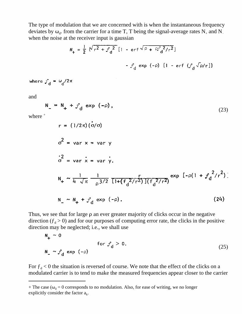
Discrimination Detection of Digital FM A block diagram of a digital FM system isshown in Figure 1. The data source emits a sequence of multilevel symbols {an} whichwe shall assume are independent of each other and assume the different integers withequal probability. As was discussed in the previous section, the VCO generates a signalspecified by Eq. 1. In practical situations, a transmitting filter is provided whose function

+The symbol <·> denotes the ensemble average

it is to restrict the energy in the frequency-modulated wave to a range of frequenciespassed by the medium, (we shall assume throughout this discussion that the transmissionmedium is a time invariant linear filter). It is therefore convenient to combine themedium characteristics with those of the transmitting filter into a single compositenetwork function determining the signal presented to the receiving bandpass filter in theabsence of noise.

The receiving bandpass filter is included and its function is to exclude out-of-band noise.It can also serve to shape the signal waveform and may include compensation for linearin-band distortion suffered in transmission. Usually two contradictory attributes aresought in the filter - a narrow band to reject noise and a wide band to supply a goodsignal wave to the detector. An opportunity for an optimum design thus exists.(6)

The frequency detector is assumed to differentiate the phase with respect to time. Thepost-detection filter can perform further noise rejection and shaping in the basebandrange. We shall assume that the post-detection filter is matched to the baseband pulseg(t). In order to obtain estimates of the symbol sequence {an}, the output of the filter isperiodically sampled. We thus must postulate that the receiver has independent timinginformation.

The noise-free input to the detector will be written in the form

(6)

where P(t) and Q(t) represent in-phase and quadrature signal modulation componentsrespectively. Such a resolution can always be made, even though the details in actualexamples may be burdensome. The added noise at the detector input is assumed to begaussian distributed with zero mean and can likewise be represented as

(7)

where x(t) and y(t) are independent baseband gaussian noise waves.

Let the input signal-plus noise to the limiter be

(8)

where

and

(We have set the constant angle 2 to zero without loss of generality). With theserepresentations the output of the discriminator is taken to be

(9)

where the dots over x' and y' denote differentiation with respect to time. The post-detection matched filter acts on the quantity 9 and the sampled output of the matchedfilter is

(10)

The observable q' contains the desired information and its statistical behaviour isanalyzed in the next section.

The Click Theory Recently S. O. Rice (7) and previously J. Cohn (8) attacked the oldthreshold problem fn FM receivers by using the notion of “clicks”. It has been observedthat when the noise at the input of an FM receiver is increased beyond some value, thereceiver “breaks”, that is, for a given (S/N) at the input, a much poorer (S/N) at theoutput is measured than would be predicted from a linearized analysis of the receiver.Before the breaking point, clicks are heard in the output of an audio receiver. As theinput noise is further increased, the clicks merge into a sputtering sound. Rice’s approachis to relate this breaking point to the expected number of clicks per second at the outputdue to the added noise at the input.

While in analog applications the criterion of (S/N) transfer is satisfactory, in digital datatransmission it does not by itself furnish an adequate performance criterion. Usuallyperformance is judged in terms of error rates which cannot be predicted from the (S/N)for nonlinear receivers. The error rate clearly depends on the statistical distribution of theoutput noise. In good systems, the errors are very infrequent and are associated with rarepeak noise conditions. The statistical structure of the occurrence of infrequent noisepeaks and the manner in which they cause errors in FM receivers will be our mainconcern here.

In the past several years a theory, based on the notion of “clicks” has beenadvanced(9),(10),(11) from which the performance of digital FM detectors with arbitraryprocessing gain can be predicted. In order to facilitate analysis and to gain physical

insight we assume that the medium has perfect transmission at all frequencies and thetransmitting and receiving filters are inverses to one another. Because of theseassumptions it is possible by use of rotating coordinates to write Eq. 10 as

(11)

where y(t) is now a zero mean quadrature gaussian noise process, while x(t) is an in-phase noise process with mean equal to the FM carrier amplitude A.

To exhibit the notion of “clicks” in digital FM reception we proceed formally withEq. 11 and define a quantity

(12)and express q as a line integral

(13)

In (13) we have written dN = d(tan-1 y/x), but of course we do not mean that N isevaluated using some fixed branch of tan-1 y/x since this would give N as a single valuedfunction of y and x and would not allow for the fact that as we circle once about theorigin in the xy-plane N is increased by 2B. The noise processes y(t) and x(t) wanderabout the xy-plane (see Figure 2), usually staying close to their mean values butoccasionally taking large excursions and encircling the origin. Each infinitesimal portionof the path contributes an amount d N to the output and all these small amounts from allthe small portions of the path must be added together to form the total contribution q. Itis easy to see that q depends on the path taken, not just on its endpoints. A simplemathematical reason for this is that the transformation (12) is undefined possibility existsof stopping the process immediately after we have crossed over to the left-half plane. Wewill show later that for large signal-to-noise ratios, these end-effects may be neglectedbecause they occur with a probability that is asymptotically negligible compared with theprobability of a click.

An important fact to observe before proceeding with the analysis is that q can bedecomposed into the sum of three random variables. The first two random variablesappearing in (15) are continuous and bounded. Their probability densities are related tothe elementary statistics of x(t) and y(t). The third random variable is a discrete one,whose probabilities are determined from the probabilities of zero-crossings of x(t) andy(t).

The remarks made thus far about the effect of noise on FM reception have been general;no assumptions have been made about the statistical nature of the additive disturbance.In order to obtain quantitative results some definite assumptions are necessary. We thusset ourselves the task of studying the structure of the probability distribution of q whenthe input noise statistics are those of a gaussian process having a symmetric Spectraldensity about the carrier. From these distributions we determine the error rates as afunction of the pertinent system parameters. We shall make no attempt to derive an exactprobability density for the random variable q. This is not a mathematically tractableproblem since it requires knowledge of the probability distribution of zero-crossings ofrandom processes. This by itself has been an area of investigation for many years withouttoo much success. The probability distribution of the zero-crossings of most elementaryrandom processes is not currently known.

In order to permit an analysis of the model two assumptions are made, both of which arequite reasonable. These two assumptions taken together state that the three randomvariables that determine q via (15) are all independent. This statement is separated intotwo assumptions because their individual justification stems from two different physicalarguments, one having to do with bandwidth and the other with signal-to-noise ratio. Thefirst assumption states that tan-1 r(T) and tan-1 r(0) are independent. For flat gaussiannoise input this will be a good approximation if T >= 1/W, where W is the input noisebandwidth. Since T is also the signaling interval, and the correlation function of theinput noise has its first zero at J ~ 1/W, the motivation for this assumption is clear. Thesecond assumption, somewhat harder to justify, states that n(T) is independent of theprevious two random variables and the clicks, which comprise n(T), are independent,from one another. This is clearly an assumption expressing an intuitive feeling that theclicks occur rarely and of sufficiently short duration. In general, they will be rare if theSignal-to-noise ratio is large, and short if the bandwidth satisfies W >

= 1/T as requiredabove.

These two assumptions plus the identification of crossings of the negative x-axis by themoving point in the xy-plane (as calculated by Rice) with the occurrence of a click shallconstitute the model for the error mechanism.

The Basic Probability Distributions In order to enable the calculation of error rateswe collect and summarize several basic formulas which may be deduced from the clicktheory.

We begin by observing that if y is a zero mean gaussian variable with whenever x(t) = 0.Further, the paths taken in the xy-plane are random, and q is therefore, a random variablewith some probability density related to the statistics of r(t). Unfortunately, thisprobability density is not determined solely by the elementary statistics of r(t). As will be

seen, in addition to the elementary statistics of r(t) the distribution of its singularities onthe time axis enters the picture. The singularities of r(t) are determined by the zero-crossings of x(t). Thus, the behaviour of FM receivers is intimately related to thestructure of the zero crossings of the added noise.

To see how to handle the situation, visualize the following hypothetical state of affairs.Suppose for 0 # t # T we have that y(t) > 0, and the x(t) is positive for awhile, decreasesonce through zero at t = to, and then remains negative. A possible plot of r(t) versus tover this time interval is then shown in Figure 3. For this particular path one has

(14)

In (14) the straightforward interpretation of the integrals is meant. Evaluating the infiniteone obtains for this path

where tan-1 x means the principal value inverse tangent function, *tan-1 x*#B/2. Ingeneral, one has the result that

(15)

where tan-1 x again has the principal value interpretation and n(T) is an integer (whichmay be positive, negative, or zero) and is related to the number of times x(t) vanishes inthe interval T and to the sign of y(t) when x(t) vanishes. For large signal-to-noise ratios itis clear that if x(t) vanishes by going to zero from the positive side that it will almostimmediately be followed by another vanishing of x(t) in the other direction. If y(t) hasnot changed, the contribution of the “return trip” to n(T) will cancel the contributionfrom the previous crossing of the y-axis. On the other hand, if y(t) does change sign so asto cause an encircling of the origin then the contribution to n(t) will be the same as theprevious crossing. The net contribution to n(T) of a number of paths is shown inFigure 4. The paths which have )n = ± 2 are immediately recognized as the “clicks”discussed by Rice. The “clicks” are not the only contribution to n(T) however. There isalso a contribution because of the fact that at t = 0, when our process begins, we may bein the middle of a large noise fluctuation and be over in the left-half plane. Immediatelyafterwards, at t = 0 +, we will experience a contribution of ± 1 to n(T); a similar situation

may prevail at time t = T, when a

where D = A2/2F2.

The probability PL of finding the signal point in the left half of the xy-plane is

(16b)

(17)

for *N * # B/2.

Suppose N1 and N2 are two independent anqles which have the density (17), and definean angle M = N1 -N2 *M*<

= B. It will be of interest for us to determine the probability PN

that M exceeds some angle N > 0, i.e., we would like to determine

(18)

The asymptotic evaluation of (18) is carried out in detail in reference (11); wedistinguish three cases:‡

Case I;0 < N < B/2

(19a)

+ Recall that even though our x(t) and y(t) are not independent processes because the noise spectrum will not be

symmetrical about (To + an Td ), they are independent variables.

‡ In (19) the symbol “~” is used to denote asymptotic equality; this has also been used in (16). Also (19a) and(19c) do not hold if N gets too close to the end points of the appropriate interval. As a rough rule N should not becloset than 1/%D radians to the end points.

Case II; < = B/2:

(19b)

Case III; N > B/2:

(19c)

The most important characteristic of the result (19) is the dependence of the exponent onangle, since for large p the nonexponential factors are relatively slowly varying.

The final item that we discuss in this section is the density of n(T), or rather we discussthe density of that part of n(T) that arises from the clicks ()n = ± 2), ignoring )n = ± 1contributions. For this we need only take over some ideas and formulas from Rice. Wehave that (ignoring )n = ± 1)

(20)

where N(T) is the number of clicks that occur in time T. Following Rice, we assume thatall clicks are independent and that those tending to increase (decrease ) N by 2B form aPoisson process with rate of occurrence N + (N-). In general, in the presence ofmodulated signal, N+ and N! are not equal. The probability density D(z) of z = N(T) isthen given by

as may be shown by forming the discrete convolution of the densities of the positive andnegative clicks. In (21) *(·) is the Dirac delta function and Ik(F) is the modified Besselfunction of integer order k, behaving for small F as

(22)

also

+ The case (Td = 0 corresponds to no modulation. Also, for ease of writing, we no longerexplicitly consider the factor ak.

The type of modulation that we are concerned with is when the instantaneous frequencydeviates by Td. from the carrier for a time T, T being the signal-average rates N+ and N!

when the noise at the receiver input is gaussian

and

(23)where +

Thus, we see that for large D an ever greater majority of clicks occur in the negativedirection (ƒd > 0) and for our purposes of computing error rate, the clicks in the positivedirection may be neglected; i.e., we shall use

(25)

For ƒd < 0 the situation is reversed of course. We note that the effect of the clicks on amodulated carrier is to tend to make the measured frequencies appear closer to the carrier

+ We confine ourselves to ƒd > 0. Exactly analogous consideration apply to ƒd < 0. The case ƒd =0 occurs if an odd number of frequencies are allowed.

frequency than the transmitted frequencies. That is, confining oneself for the moment toonly errors caused by clicks, frequencies transmitted higher (lower) than the carrier willbe measured to be at that frequency or a lower (higher) one, when the noise is small.

Since we shall use approximation (25), the distribution (21) for z = N(T) may bereplaced by the simpler Poisson one, where the probability of getting exactly N(negative) clicks in time T is given by+

(26)

Also the probability of getting M or more clicks is, for large signal-to-noise ratios,approximately the probability of getting exactly M clicks.

Distribution of Output and Probability of Error Eq. 16, 19, 25, and 26 provide theinformation required to calculate the distribution of q, (Eq. 15). In principle we simplyconvolve the continuous density of [tan-1 r(T) -tan-1 r(0)] with the discrete density ofn(T)B. In Figure 5, we give a qualitative sketch of the result, neglecting end effects. Thispicture is intended to show that the density consists of a central lobe about thetransmitted frequency extending to ± B on each side, which is the density of [tan-1 r(T)-tan-1 r(0)], plus identically shaped lobes displaced by intergral multiples of 2B towardlower frequencies (ƒd > 0). These displaced lobes are weighted by the probability ofgetting tge appropriate number of clicks to effect the displacement. Thus, the lobeoccupying the space -2nB±B is weighted by the probability of getting exactly n clicks intime T. For n = 0 the weighting is essentially one, for large S/N. There are, strictlyspeaking, similar lobes and weightings on the opposite side as well, but these weightsare, for large S/N, negligible compared to the corresponding lobe we have drawn. That isto say, the first lobe on the right (not shown in Figure 5) has small probability comparedto the first lobe on the left, but has a large probability compared to the second lobe on theleft. Nevertheless, we have neglected to include it because we will generally beconcerned with probabilities like Pr [*q - ƒdT* > N], and thus corresponding weights areimportant. We dwell on this point because it is conceivable that for some practical orconceptual application the neglect would not be justified.

The discussion given above is still not quite complete it is modified when weinclude end effects. The principal correction that inclusion of end effects will cause is toadd two more side lobes, one over the interval L-27r,01 and the other over the interval[0,2Tr]. The weightings of these lobes certainly should not exceed the estimate given in(16), and this will be enough to exclude them for our purposes.

+ Note the special sense in which the term is used here.

++ The Pe for a frequency at the end is one-half the expression (27).

We now apply our results to some typical calculations. Consider the case of narrowband+ FM (defined by )ƒdT < B), where one has J equally spaced frequencies ofseparation ƒ)d crowded into a bandwidth W. The probability of error for any one of thefrequencies++ (not situated at the ends) is the area outside of the interval bounded bylines L2 and L3 in Figure 5. If L2 and L3 are defined by *q* then the probability of errorfor such a frequency is from (19a).

(27)

where, if one assumes that the bandwidth W = J )ƒd one would take

(28)

(29)But expression (29) is, asymptotically, exponentially small compared to (27). Likewise,the area due to the side lobes caused by end effects is exponentially small, and theprobability of error for narrow-band FM is given by (27).

Next, consider the asymptotic evaluation ofe P for the case of orthogonal signals; thiscase corresponds to ()Td)T = B, we assume that the thresholds are spaced midwaybetween the frequencies. Thus, (for a frequency not on the edges) we have that the errorprobability is given by the area outside of that bounded between the lines L1 and L4. Thecontribution from the major lobe is, from (19b),

In addition, the area of the first side lobe is asymptotically comparable to this and is

being weakly dependent on the frequency sent. In fact, for the nth signal (j = 2n) we havefor orthogonal signals that

The average error rate is then, for orthogonal signals (J of them, J even, and equallyspaced signals and thresholds),

(30)

Eq. 30 is indeed a surprising result. The first term of (30) is the probability of confusingthe transmitted frequency with one of its nearest neighbors. The second term is the(average) probability of confusing it with its second nearest neighbor closest to thecarrier. This is because the area from (-B) to (-3 B/2) is, by application of (19b),negligible compared to the area from (-3 B/2) to (-5 B/2). Thus, it states that for themultilevel situations considered here (a not unreasonable one) it is to confuse it with aparticular one of its second nearest neighbors. We see from (30) that the error rate fromthe continuous part of the output is comparable to the error rate caused by clicks.

For a final example, consider the wide-band situation where the signals are looselypacked in the band; i.e., ()Td) T > B. Now no errors will be caused by the continuouspart of the output; only clicks will cause errors. If the frequencies are widely spaced asingle click may not cause an error; several clicks during the time interval T may berequired. Thus, suppose that the frequencies are spaced so that the phase differences ofnearest neighbors is ()Td) T = 2n B, n being any positive integer. The probability oferror will then be the probability of getting n (or more) clicks in time T, which from (25)and (26) behaves as

(31)

The coefficient in (31) is at least as bad as for the orthogonal case, but the important itemis the exponent. Superficially at least it appears that we have gained in performance byspacing the frequencies widely, since the exponential has changed from e-D from theminimum orthogonal case ()Td-T = B. to e-nD. It must be realized, however, that here weare talking about different D’s. The bandwidth for the case under consideration isessentially 2n times the minimum orthogonal one and therefore, for the same signalpower, the nominal value of D has decreased by 2n, and one has in fact not gained afactor of n in the exponent. In addition to the bandwidth penalty, error performance hasactually suffered too.

Comparison with Optimum It is possible to demonstrate how the FM discriminatorcompares with the ideal detector when used to detect orthogonal signals; i.e. when)TdT = B. It is known that when optimum detection is used for any orthogonal set ofsignals, the (exponential part of the) error rate behaves as exp [-E/No], where E is thesignal energy (assumed common to all J levels) and No/2 is the (two-sided) spectraldensity of the noise. If we let S denote the average signal power, such that E = ST, andestimate the total bandwidth W for large J by W ~ J/(2T), we see that the ideal exponentbecomes exp [-JD/2]. However, we had seen that, regardless of the number of levels, thediscriminator error rate )TdT = B. behaves as exp [-D]. Thus, we have lost a factor of J inthe error exponent by substituting discrimination detection for matched filter detection.

An important conclusion may immediately be drawn concerning the performance ofconventional FM receivers as detectors of orthogonal signals. Our results show that thereceiver is indeed inferior in performance when compared with the optimum. This facthas been stated by Wozencraft and Jacobs (13) and the reasons are clear from this analysis.The FM receiver admits too much noise at its front-end which cannot be cleaned by thepost-detection filter because of the nonlinear anomalies, namely the clicks. As a matterof fact, the amount of noise grows in direct proportion to the number of orthogonalsignals, hence the inferior exponent. On the other hand, the optimum detector iscomposed of a bank of matched filters. The noise power at the output of each filter doesnot grow with the number of signals; it is a fixed constant determined by the bandwidthof the filter, which roughly needs be no broader than the symbol rate, 1/T.

This poor performance of conventional FM receivers when used to detect data might beremedie by employing an FM with feedback such as described in references (14) and (15).The physical argument to support this contention is often stated as follows. In theabsence of the feedback loop, the IF filter must be wide enough to pass the total swing ofthe incoming signal. However, since the feedback loop tracks the incoming frequency,this IF filter, whose width determines the noise variance, could be narrowed and lessnoise would be admitted.

This possibility of making use of FM with feedback to im rove the error rate in digitalsystems has been suggested in reference (13). Unfortunately a mathematical treatment ofthis difficult problem does not exist at present.

Signaling over the Gaussian Dispersive Medium When a dispersive medium ispresent between transmitter and receiver, error rate calculations become extremelycomplicated and can only be carried out in certain special cases. Although themechanism of error production can still be explained in terms of the clicks, very fewquantitative results are available.(16) The difficulty arises because the signal-plus-noise issubjected to a mixture of linear and nonlinear operations. The dispersive medium

introduces intersymbol interference in a very complicated manner affecting the rate atwhich clicks are produced.

A major source of difficulty in the analysis of digital FM detection is the presence of thepost-detection filter. If one assumes that this filter is ideal, in the sense that it does notperform significant baseband processing, the mathematical problems become tractable.In many applications this assumption is valid. In particular it is a good one when themodulated signal bandwidth is of the same order as that of the baseband signal. In theseapplications exact formulas for the probability distribution of the instantaneousfrequency of signal-plus-noise are available in references (17) and (18). Even here theuse of these formulas becomes very tedious since it is necessary to make separatecalculations for every input symbol sequence. This often can only be accomplished withthe aid of a high speed digital computer. Only the binary case has been adequately treatedin the literature(19), (20), (21). Experimental results with multilevel FM operating over amoderately dispersive medium have been reported on in the literature.(5) No adequatetheory however is at present available capable of handling situations where the post-detection filter cannot be neglected.

References

1) Powers, K. H., Bedrosian, E., “The Analytic Signal representation of ModulatedWaveforms” Proc. IRE, Vol. 50, October 1962.

2) Mazo, J. E., SaIz, J., “Spectral properties of Signal-Side-band Angle Modulation”IEEE Trans. Comm. Tech., February 1968.

3) Bennett, R. W., Davey, J. R., “Data Transmission” McGraw-Hill Book Co., 1965.

4) Lucky, R. W., SaIz, J., Weldon, E. J., Jr., “Principles of Data Communication”McGraw-Hill Book Co., 1968.

5) Salz, J., Koll, V. G., “An Experimental Digital Multilevel FM Modem,” IEEETrans., COM-14, 1966, pp. 259-265.

6) Salz, J., “Performance of Multilevel Narrow-Band FM Digital CommunicationSystems,” IEEE Trans., COM-13, 1965, pp. 420-424.

7) Rice, S. O., “Noise in FM Receivers,” Chapter 25 of Times Series Analysis,Rosenblatt, M., (ed.), John Wiley & Sons, Inc., New York, 1963.

8) Cohn, John, Proc N.E.C., (Chicago) 12, 1956, pp. 221-236.

9) Schilling, D. C., Hoffman, E., and Nelson, E. A., “Error Rates for Digital SignalsDemodulated by an FM Discriminator,” IEEE Trans. Communication Technology,COM-15 (August 1967), PP. 507-517.

10) Klapper, J., “Demodulator Threshold Performance and Error Rates in AngleModulated Digital Signals,” RCA Review 27 (June 1966), pp. 226-244.

11) Mazo, J. E. and Salz, J., “Theory of Error Rates for Digital FM, BSTJ,45(November 1966), pp. 1511-1535.

12) Bennett, W. R., “Methods of Solving Noise Problems,” Proc. IRE, 44, 1956, pp.609-638, See (253).

13) Wozencraft, J. M. and Jacobs, I. M., “Principles of Communication Engineering,”John Wiley & Sons, Inc., New York, 1965.

14) Chaffe, J. G., “The Application of Negative Feedback to Frequency ModulationSystems, B.S.T.J., 18, July, 1939, pp. 403-437.

15) Enloe, L. H., “Decreasing the Threshold in FM by Frequency Feedback,” Proc.IRE, 50, 1962, pp. 18-30.

16) Schneider, H. L., “Click Comparison of Digital and Matched Filter Reception,”B.S.T.J., March 1968.

17) Salz, J. and Stein, S., “Distribution of Instantaneous Frequency for Signal PlusNoise,” IEEE Trans., IT-10, 1964, pp. 272-274.

18) Mazo, J. E. and Salz, J., “Probability of Error for Quadratic Detectors,” B.S.T.J.,44, November, 1965, pp. 2165-2186.

19) Bennett, W. R. and Salz, J., “Binary Data Transmission by FM Over a RealChannel,” B.S.T.J., 42, 1963, pp. 2387-2426.

20) Meyerhoff, A. A. and Mazer, W. M., “Optimum Binary FM Reception UsingDiscriminator Detection and I-F Shaping,” RCA Review, 22, Dec. 1961, pp. 698-728.

21) Smith, E. F., “Attainable Error Probabilities in Demodulation of Rand om BinaryPCM/FM Waveforms,” IRE Trans. on Space Elec. and Telemetry, SET-8, Dec.1962, pp. 290-297.

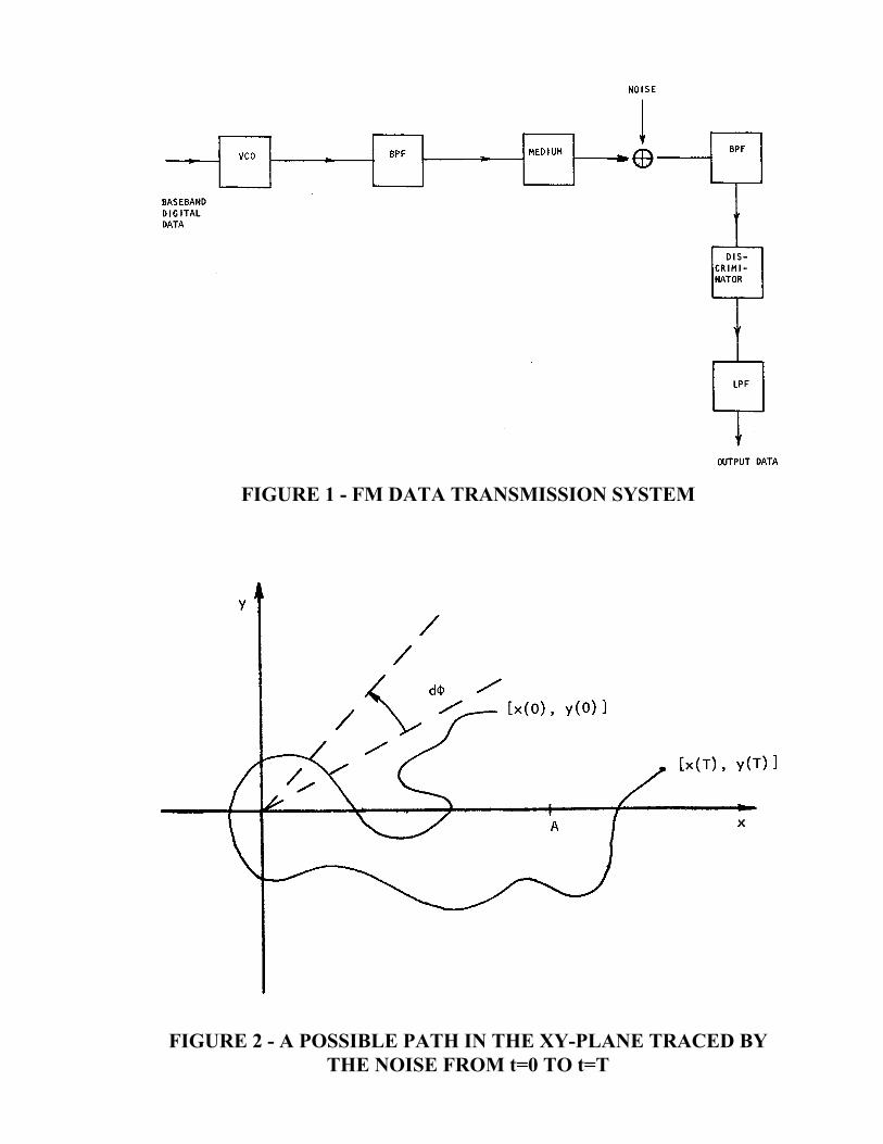
FIGURE 1 - FM DATA TRANSMISSION SYSTEM

FIGURE 2 - A POSSIBLE PATH IN THE XY-PLANE TRACED BYTHE NOISE FROM t=0 TO t=T

FIGURE 3 - A POSSIBLE SAMPLE FUNCTION OF r(t)

FIGURE 4 - NET CHANGES )n IN n(T) CAUSED BY SOME TYPICALPATHS IN THE XY-PLANE

FIGURE 5 - QUALITATIVE SKETCH OF THE PROBABILITYDENSITY OF q