AMERICAN UNIVERSITY OF BEIRUT FACULTY OF ENGINEERING AND ARCHITECTURE

DEPARTMENT OF ELECTRICAL AND COMPUTER ENGINEERING

EECE691C – Digital Signal Processing – Laboratory Week 3

Digitization of Signals – Pre-lab 1 Overview and Goals As you should have discovered by now, digital signal processing is the analysis of signals using a digital computer. In order for that to be possible, signals should be in digital form, i.e. a sequence of numbers. Sometimes, signals are digital in nature, such as when temperature measurements are taken periodically. However, most often signals are continuous (analog) and have to be digitized before processing.

This digitization usually involves 2 stages: sampling, i.e. the measurement at discretely spaced time intervals, and quantization, i.e. the transformation of the measurements into finite-precision numbers, such that they can be represented in computer memory. This week, we will investigate these processes. The major highlights are as follows:

Synthesis of sinusoidal signals, and aliasing of sinusoids.

Generation of digital music, and study of aliasing in audio.

Digital images and anti-aliasing of computer graphics.

Quantization effects in audio signals.

Quantization effects in digital images.

2 Sinusoidal Signals You have previously seen how to generate sinusoids in MATLAB. In this section, you will take a closer look at the behavior of digital sinusoids, from a sampling and aliasing viewpoint. A sinusoidal signal, in the continuous realm, is usually expressed in the following form:

( ) ( )tFtxa π2cos=

Where the subscript ‘a’ denotes the analog nature, F is the frequency and t is continuous time. In this section, we will create, or synthesize, digital sinusoidal signals. First, it is important to understand that what we will generate is a sequence of numbers not a continuous curve. Between these numbers nothing exists. It is wrong to connect these points by lines, or even consider that this value remains a constant from one point to the other.

We will measure the analog signal, i.e. in our case “evaluate the sinusoid”, at constant intervals of time. This is called uniform sampling, and the interval length T, is called the sampling period.The sampling frequency is therefore Fs = 1 / T.

1

We will denote by “n” the sample number, starting from 0 at time t = 0. This means that the 10th sample will be numbered n = 9, and it will correspond to time t = 9T. In general, we may write t = nT= n / Fs, and the digital sinusoid can be written as such:

= n

FsFnx π2cos)(

(a) Keeping a fixed sampling frequency of Fs = 8 kHz, generate sinusoids with F = 1, 2, 3.5, 6 and 7 kHz. Plot the sinuoids on sperate figures. Why are some of these plots similar? Do they reflect the true frequency content, i.e. the frequency of the analog sinusoids?

(b) Analog sinusoids are pure frequency signals, i.e. their continuous Fourier transform contains an impulse at their precise frequency, and nothing elsewhere. Having that in mind, and from the results in part (a), what can you suggest has happened in the frequency domain of the sampled signals at frequencies higher than half the sampling frequency? Are the results justified from what you know of the sampling theorem?

(c) Create a new digital signal, y(n), at the same frequencies mentioned in part (a), but sampled at a ten-fold frequency, say Fs = 80 kHz, and extending over the same interval of time as x, i.e. if x had N samples, y should have 10×N samples. Plot the x and y sequences corresponding to the same frequency on the same figure, in a superposed fashion, using different colors. Can you now give a time-domain explanation of the aliasing phenomenon? [ Hints: (1) Use plot(nx/Fsx,x) for x and plot(ny/Fsy,y) for y, to plot in time units, not sample units. Note that nx and ny are the sample number sequences while Fsx and Fsy are the sampling frequencies of x and y respectively. (2) Use markers when plotting, to clarify sample locations. This can be done by adding an extra parameter to the plot command, or from the figure GUI. Try help plot for more info. ]

3 Aliasing Phenomena and Anti-aliasing Techniques As you saw in the previous section, aliasing occurs when the sampling frequency is not above the Nyquist rate, i.e. twice the highest frequency content of the signal. In the frequency domain, aliasing is expressed as high-frequency components being present in the low-frequency range. In the time domain, aliasing is the loss of detail in the signal, and the false perception of reading a low frequency signal. As such, aliasing is an unwanted phenomenon, and is to be avoided.

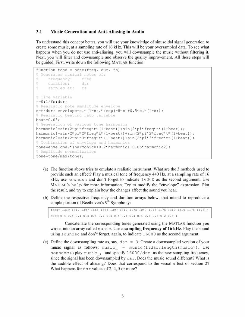
Unfortunately, most real-world signals extend in an infinite frequency range. Therefore, increasing the sampling frequency will not help, and the only way to avoid aliasing is to throw away all the high-frequency components of a signal that will not affect its correct perception. This is done through an analog pre-filter, just before sampling occurs, as shown below:

Digital

Processing Sampling & Quantization

Analog Pre-Filter

Most often, the requirements on this analog filter are very strict, i.e. it should have a very sharp transitional band. To reduce that, an alternative is to (1) oversample the signal, i.e. use an N-fold sampling rate (2) apply a digital anti-aliasing filter to the (now digital) signal (3) downsample the signal to the required rate, i.e. keep 1 of every N sample. How does this help? The analog filter becomes simple to build, since it is allowed to have a wider tansitional- band. Why do we downsample? To keep just what is needed to do the required processing. More samples means more processing effort, and that’s to be minimized.

2

3.1 Music Generation and Anti-Aliasing in Audio To understand this concept better, you will use your knowledge of sinusoidal signal generation to create some music, at a sampling rate of 16 kHz. This will be your oversampled data. To see what happens when you do not use anti-aliasing, you will downsample the music without filtering it. Next, you will filter and downsample and observe the quality improvement. All these steps will be guided. First, write down the following MATLAB function:

function tone = note(freq, dur, fs) % Generates musical notes of: % frequency: freq % duration: dur % sampled at: fs % Time variable t=0:1/fs:dur; % Realistic note amplitude envelope x=t/dur; envelope=x.*(1-x).*(exp(-8*x)+0.5*x.*(1-x)); % Realistic beating rato variable beat=0.08; % Generation of various tone harmonics harmonic0=sin(2*pi*freq*t*(1-beat))+sin(2*pi*freq*t*(1+beat)); harmonic1=sin(2*pi*2*freq*t*(1-beat))+sin(2*pi*2*freq*t*(1+beat)); harmonic2=sin(2*pi*3*freq*t*(1-beat))+sin(2*pi*3*freq*t*(1+beat)); % Combination of envelope and harmonics tone=envelope.*(harmonic0+0.2*harmonic1+0.05*harmonic2); % Amplitude normalization tone=tone/max(tone);

(a) The function above tries to emulate a realistic instrument. What are the 3 methods used to provide such an effect? Play a musical tone of frequency 440 Hz, at a sampling rate of 16 kHz, use soundsc and don’t forget to indicate 16000 as the second argument. Use MATLAB’s help for more information. Try to modify the “envelope” expression. Plot the result, and try to explain how the changes affect the sound you hear.

(b) Define the respective frequency and duration arrays below, that intend to reproduce a simple portion of Beethoven’s 9th Symphony: freq=[1319 1319 1397 1568 1568 1397 1319 1175 1047 1047 1175 1319 1319 1175 1175];

dur=[0.4 0.4 0.4 0.4 0.4 0.4 0.4 0.4 0.4 0.4 0.4 0.4 0.6 0.2 0.5];

Concatenate the corresponding tones generated using the MATLAB function you wrote, into an array called music. Use a sampling frequency of 16 kHz. Play the sound using soundsc and don’t forget, again, to indicate 16000 as the second argument.

(c) Define the downsampling rate as, say, dsr = 3. Create a downsampled version of your music signal as follows: music_ = music(1:dsr:length(music)). Use soundsc to play music_, and specify 16000/dsr as the new sampling frequency, since the signal has been downsampled by dsr. Does the music sound different? What is the audible effect of aliasing? Does that correspond to the visual effect of section 2? What happens for dsr values of 2, 4, 5 or more?

3

(d) Unlike in part (c), where you downsampled without prior filtering, you will now use functions from the Signal Processing Toolbox of MATLAB, to implement an anti-aliasing filter. Add the following lines before your downsampling code:

filter_coeff = fir1(64, 1/dsr); music = filter( filter_coeff, 1, music );

As you will learn in the course, and experiment with in subsequent lab sessions, the above lines are performing an FIR low pass filtering operation. The fir1 call will design automatically a 64-point low pass filter. Using help fir1, can you tell what is the cut-off frequency of the specified filter? How can you justify that value, knowing that the new sampling frequency, i.e. after downsampling, will become 16 kHz divided by dsr?

The filter call will apply the designed filter to the music. Play the resulting signal and compare it to the result you obtained in part (c). Perform the comparison for the various dsr values you tried in part (c). Is anti-aliasing effective? What happens when you downsample too much (dsr > 5)? Does anti-aliasing help in that situation? Why?

(e) Use MATLAB’s wavread function to read wave-files, which are standard Microsoft Windows audio-files. Wave-files come in various formats, and might have one of many sampling frequencies. Find wave-files of recorded music at 16 kHz, or convert them to that rate, using the Sound Recorder application in Windows. Apply the downsampling (with and without anti-aliasing) procedure that you used above on the wave-file. Are the same phenomena and results obtained? In what cases is aliasing most noteworthy?

3.2 Digital Images and Anti-aliasing of Computer Graphics One of the interesting aspects of signal processing is its application to various areas that seem otherwise non-related. Digital image processing is such an example. In this section, we will see how the concepts of aliasing, and anti-aliasing, apply equally well to images. What is an analog image? Although this term is never used, but most images have actually infinite resolution: photographs, MRI (magnetic resonance imaging) medical images, pressure/temperature maps are all good examples. A particular case that we will address in this section is that of computer-generated images, such as 3D-graphics, font and vector-graphics rendering.

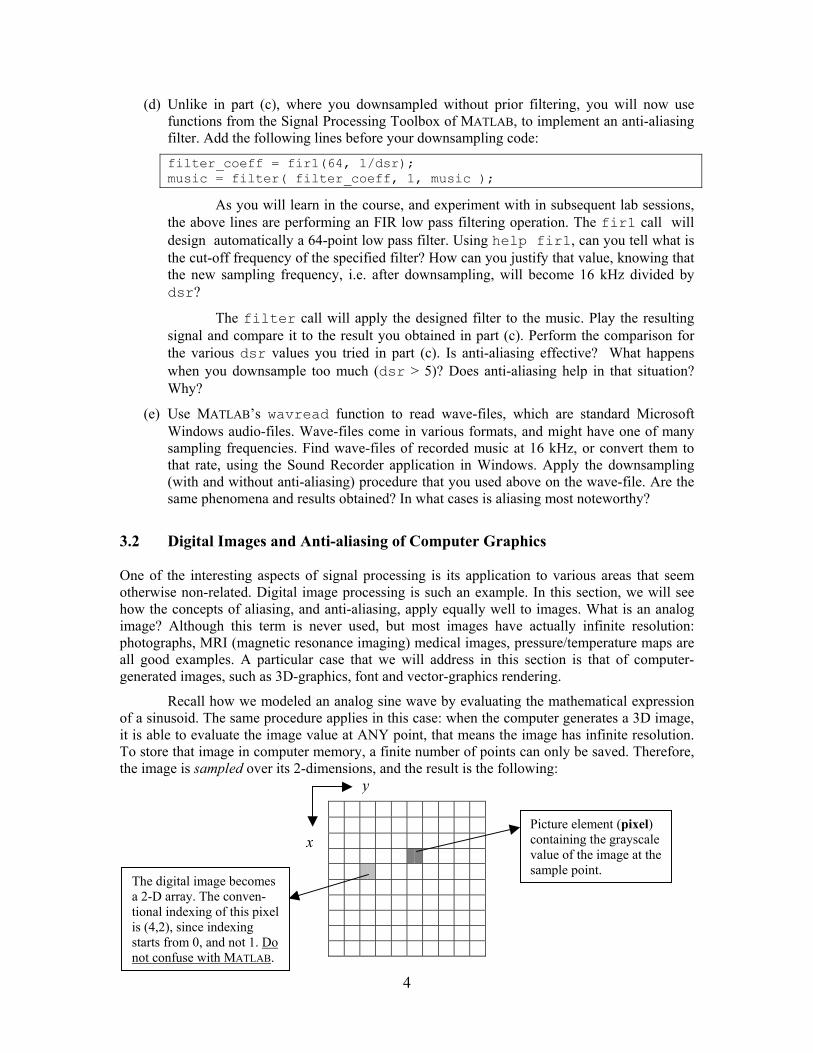
Recall how we modeled an analog sine wave by evaluating the mathematical expression of a sinusoid. The same procedure applies in this case: when the computer generates a 3D image, it is able to evaluate the image value at ANY point, that means the image has infinite resolution. To store that image in computer memory, a finite number of points can only be saved. Therefore, the image is sampled over its 2-dimensions, and the result is the following:

The digital image becomes a 2-D array. The conven- tional indexing of this pixel is (4,2), since indexing starts from 0, and not 1. Do not confuse with MATLAB.

Picture element (pixel) containing the grayscale value of the image at the sample point.

x

y

4

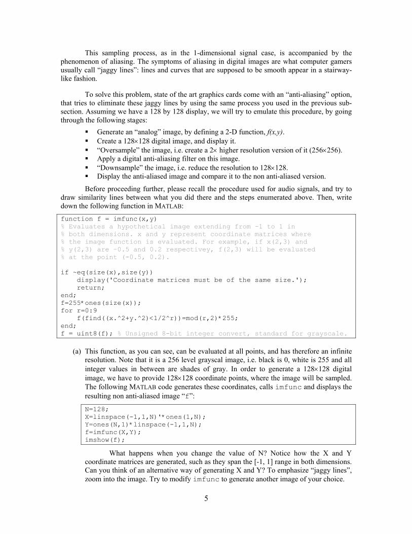
This sampling process, as in the 1-dimensional signal case, is accompanied by the phenomenon of aliasing. The symptoms of aliasing in digital images are what computer gamers usually call “jaggy lines”: lines and curves that are supposed to be smooth appear in a stairway-like fashion.

To solve this problem, state of the art graphics cards come with an “anti-aliasing” option, that tries to eliminate these jaggy lines by using the same process you used in the previous sub-section. Assuming we have a 128 by 128 display, we will try to emulate this procedure, by going through the following stages:

Generate an “analog” image, by defining a 2-D function, f(x,y). Create a 128×128 digital image, and display it. “Oversample” the image, i.e. create a 2× higher resolution version of it (256×256). Apply a digital anti-aliasing filter on this image. “Downsample” the image, i.e. reduce the resolution to 128×128. Display the anti-aliased image and compare it to the non anti-aliased version.

Before proceeding further, please recall the procedure used for audio signals, and try to draw similarity lines between what you did there and the steps enumerated above. Then, write down the following function in MATLAB:

function f = imfunc(x,y) % Evaluates a hypothetical image extending from –1 to 1 in % both dimensions. x and y represent coordinate matrices where % the image function is evaluated. For example, if x(2,3) and % y(2,3) are –0.5 and 0.2 respectivey, f(2,3) will be evaluated % at the point (-0.5, 0.2). if ~eq(size(x),size(y)) display('Coordinate matrices must be of the same size.'); return; end; f=255*ones(size(x)); for r=0:9 f(find((x.^2+y.^2)<1/2^r))=mod(r,2)*255; end; f = uint8(f); % Unsigned 8-bit integer convert, standard for grayscale.

(a) This function, as you can see, can be evaluated at all points, and has therefore an infinite

resolution. Note that it is a 256 level grayscal image, i.e. black is 0, white is 255 and all integer values in between are shades of gray. In order to generate a 128×128 digital image, we have to provide 128×128 coordinate points, where the image will be sampled. The following MATLAB code generates these coordinates, calls imfunc and displays the resulting non anti-aliased image “f”:

N=128; X=linspace(-1,1,N)'*ones(1,N); Y=ones(N,1)*linspace(-1,1,N); f=imfunc(X,Y); imshow(f);

What happens when you change the value of N? Notice how the X and Y coordinate matrices are generated, such as they span the [-1, 1] range in both dimensions. Can you think of an alternative way of generating X and Y? To emphasize “jaggy lines”, zoom into the image. Try to modify imfunc to generate another image of your choice.

5

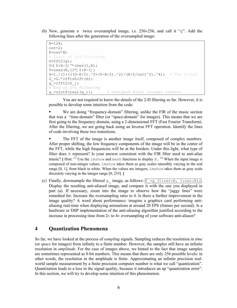
(b) Now, generate a twice oversampled image, i.e. 256×256, and call it “g”. Add the following lines after the generation of the oversampled image:

N=128; osr=2; R=osr*N; % Start of 2-D Filtering G=fft2(g); U=[0:R-1]'*ones(1,R); V=ones(R,1)*[0:R-1]; H=1./(1+(((U-R/2).^2+(V-R/2).^2)/(R/2/osr)^2).^4); % The filter G_=G.*ifftshift(H); g_=ifft2(G_); % End of 2-D Filtering g_=uint8(real(g_)); % Unsigned 8-bit integer convert

You are not required to know the details of the 2-D filtering so far. However, it is possible to develop some intuition from the code:

We are doing “frequency-domain” filtering, unlike the FIR of the music section that was a “time-domain” filter (or “space-domain” for images). This means that we are first going to the frequency domain, using a 2-dimensional FFT (Fast Fourier Transform). After the filtering, we are going back using an Inverse FFT operation. Identify the lines of code involving these two transitions.

The FFT of the image is another image itself, composed of complex numbers. After proper shifting, the low frequency components of the image will be in the center of the FFT, while the high frequencies will be at the borders. Under this light, what type of filter does H represent? Is your answer consistent with the FIR filter used to anti-alias music? [ Hint: (1) Use the imshow and mesh functions to display H. (2) When the input image is composed of non-integer values, imshow takes them as gray scales smoothly varying in the real range [0, 1], from black to white. When the values are integers, imshow takes them as gray scale discretely varying in the integer range [0, 255]. ]

(c) Finally, downsample the filtered g_ image, as follows: f_=g_(1:osr:R, 1:osr:R);. Display the resulting anti-aliased image, and compare it with the one you displayed in part (a). If necessary, zoom into the image to observe how the “jaggy lines” were remedied for. Increase the oversampling ratio to 4. Is there a further improvement in the image quality? A word about performance: imagine a graphics card performing anti-aliasing real-time when displaying animations at around 20 FPS (frames per second). Is a hardware or DSP implementation of the anti-aliasing algorithm justified according to the increase in processing time from 2× to 4× oversampling of your software anti-aliaser?

4 Quantization Phenomena So far, we have looked at the process of sampling signals. Sampling reduces the resolution in time (or space for images) from infinity to a finite number. However, the samples still have an infinite resolution in amplitude. For the case of images above, we hinted to the fact that image samples are sometimes represented as 8-bit numbers. This means that there are only 256 possible levels: in other words, the resolution in the amplitude is finite. Approximating an infinite precision real-world sample measurement by a finite precision computer number is what we call “quantization”. Quantization leads to a loss in the signal quality, because it introduces an ap “quantization error”. In this section, we will try to develop some intuition of this phenomenon.

6

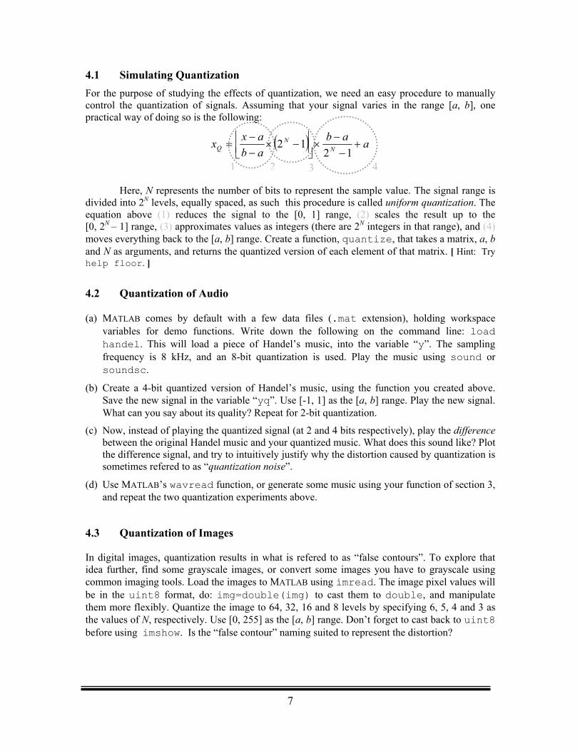
4.1 Simulating Quantization For the purpose of studying the effects of quantization, we need an easy procedure to manually control the quantization of signals. Assuming that your signal varies in the range [a, b], one practical way of doing so is the following:

( ) aababaxx N

NQ +

−−

×

−×

−−

=12

12

1 2 4

Here, N represents the ndivided into 2N levels, equally spequation above (1) reduces the[0, 2N – 1] range, (3) approximatemoves everything back to the [a, and N as arguments, and returns help floor. ]

4.2 Quantization of Audio (a) MATLAB comes by default

variables for demo functionhandel. This will load a pfrequency is 8 kHz, and ansoundsc.

(b) Create a 4-bit quantized verSave the new signal in the vaWhat can you say about its q

(c) Now, instead of playing the qbetween the original Handel the difference signal, and try sometimes refered to as “qua

(d) Use MATLAB’s wavread fuand repeat the two quantizati

4.3 Quantization of Imag In digital images, quantization reidea further, find some grayscalecommon imaging tools. Load thebe in the uint8 format, do: ithem more flexibly. Quantize thethe values of N, respectively. Usebefore using imshow. Is the “fa

umber of aced, as s signal ts values b] range. the quant

with a fs. Writeiece of H 8-bit qu

sion of Hriable “y

uality? Re

uantized music andto intuitivntization

nction, oron experim

es

sults in w images,

images tomg=doub image to [0, 255] lse conto

bits to reuch this o the [0as integerCreate a fized versi

ew data down th

andel’s antization

andel’s mq”. Use [-peat for 2

signal (at your quaely justif

noise”.

generateents abo

hat is re or conve MATLABle(img 64, 32, 1as the [a,ur” namin

7

3

present the samprocedure is ca, 1] range, (2s (there are 2N unction, quanon of each elem

files (.mat ee following omusic, into th is used. Play

usic, using th1, 1] as the [a,-bit quantizatio

2 and 4 bits rentized music. Wy why the disto

some music usve.

fered to as “fart some image using imrea) to cast them6 and 8 levels

b] range. Don’g suited to repr

ple value. The signal range is lled uniform quantization. The ) scales the result up to the integers in that range), and (4) tize, that takes a matrix, a, b ent of that matrix. [ Hint: Try

xtension), holding workspace n the command line: load

e variable “y”. The sampling the music using sound or

e function you created above. b] range. Play the new signal. n.

spectively), play the difference hat does this sound like? Plot

rtion caused by quantization is

ing your function of section 3,

lse contours”. To explore that s you have to grayscale using d. The image pixel values will to double, and manipulate by specifying 6, 5, 4 and 3 as t forget to cast back to uint8 esent the distortion?

Standard Musical Note Frequencies

STANDARD FREQUENCIES (Hz) OF MUSICAL NOTES FOR INSTRUMENTS EXCEPT PIANO

OCT # C C# D D# E F F# G G# A A# B

1 32.703 34.648 36.708 38.891 41.203 43.654 46.249 48.999 51.913 55.000 58.270 61.7352 65.406 69.296 73.416 77.782 82.407 87.307 92.499 97.999 103.83 110.00 116.54 123.473 130.81 138.59 146.83 155.56 164.81 174.61 185.00 196.00 207.65 220.00 233.08 246.944 261.63 277.18 293.66 311.13 329.63 349.23 369.99 392.00 415.30 440.00 466.16 493.885 523.25 554.37 587.33 622.25 659.26 698.46 739.99 783.99 830.61 880.00 932.33 987.776 1046.5 1108.7 1174.7 1244.5 1318.5 1396.9 1480.0 1568.0 1661.2 1760.0 1864.7 1975.57 2093.0 2217.5 2349.3 2489.0 2637.0 2793.8 2960.0 3136.0 3322.4 3520.0 3729.3 3951.18 4186.0 4434.9 4698.6 4978.0 5274.0 5587.7 5919.9 6271.9 6644.9 7040.0 7458.6 7902.1

MIDDLE C is C4 at 261.63Hz. STANDARD PITCH is A4 at 440Hz

http://www.geocities.com/cjhope_2000/pitches.html [10/10/2002 7:16:52 PM]