DIFFUSION-CONTROLLED COMBUSTION

Amable Lifian

Abstract We devote this brief review to some relevant aspects of diffusion-controlled combustion. After a survey of the conservation equations involved, we shall describe the Burke-Schumann limit, which is appli­cable when the reaction time at the flame is very short compared with the mixing time. Using as a protopypical example the How downstream from a fuel injector in a combustor chamber, we next introduce some phenomena related to finite-rate kinetics. We shall see how the high temperature sensitivity typical of combustion reactions is responsible for the presence near the injector of chemically frozen regions of low temperature where the reactants mix without chemical reaction, these regions being separated by thin premixed flames, with rich and lean branches, from regions of near equilibrium flow, where the reactants coexist only in a thin trailing diffusion flame. The role of these triple flames in the ignition, anchoring, and lift-off processes of diffusion flames will be briefly discussed.

1. INTRODUCTION AND CONSERVATION EQUATIONS

Most of the combustion reactions between fuels and the oxygen of the air occur only after vaporization or gasification of the fuel and mixing with the air. In many systems the reactants are unmixed when they enter the combustion chamber, and the reaction time is so short in regions of high temperature that the reactants coexist only in thin reaction layers, or diffusion flames. There, the reaction takes place at a rate determined by the rate of generation of fuel vapors, when we deal with liquid or solid fuels, and the rate of mixing with the oxygen of the air.

The burning process of a typical hydrocarbon in air involves dozens of chemical species and hundreds of elementary chemical reactions. Although a detailed account of the chemistry is necessary, for instance, in the description of the production of such combustion pollutants as

carbon monoxide and oxides of nitrogen, many aspects of the combus­tion process can be understood by assuming that the chemical reaction between the fuel and the oxygen of the air takes place in a single overall step, an approach to be adopted in the following development. Thus, we consider that the fuel, F, reacts with the oxygen of the air, O2, to pro­duce combustion products according to the irreversible global reaction

F + s 0 2 -> (l + a) Products + (q), (1)

where .v and q represent, respectively, the mass of oxygen burnt and the amount of heat released per unit mass of fuel consumed.

In diffusion-controlled combustion systems, different streams provide the fuel and the air. We let YQ2A and *FO £• 1 denote, respectively, the mass fractions of oxygen and fuel in their corresponding feed streams. Dilution is permitted in the fuel stream for generality, while Yo2A — 0.23 in air. Correspondingly, S = SYFQ/YO2A is the mass of air that one needs to mix with the unit mass of gas of the fuel stream to gener­ate a stoichiometric mixture. The adiabatic combustion of the resulting mixture at constant pressure produces a temperature increment given by TS — TQ — qYpo/[cp(l+S)], with the initial temperature of the air stream, TA, being assumed to be equal to the fuel stream temperature, To. Here, cp denotes the specific heat at constant pressure, assumed to be constant for simplicity. We shall see that Ts becomes the maximum temperature achieved in adiabatic diffusion flames when the chemistry is infinitely fast and the diffusivities of both reactants are equal to the thermal dif-fusivity. Two fundamental thermochemical parameters emerge therefore in nonpremixed combustion, namely,

sYF0 Ts -T0

S = and 7 = —— , (2) JO2A J-o

the second being an appropriate dimensionless measure of the exother-micity of the reaction. Typical values for S and 7 in a hydrocarbon-air flame are S ~ 15 and 7 ^ 6.

It is assumed that the local rate at which the overall combustion process given in Eqn. (1) takes place depends on the fuel and oxygen mass fractions Yp and Yo2, and on the temperature T, with a dependence that can be represented by an Arrhenius law of the form

WF = ^!2l = _ products = -pBe-WKfYpYg? , (3)

where w\ represents the mass of species / produced per unit volume per unit time, p is the density, and R is the universal gas constant. Since (1) is not an elementary reaction, its corresponding rate (3) does not

follow the law of mass action; it is a heuristic law that, with appropriate selections for the reaction-rate parameters, reproduces approximately the global combustion rate in a limited range of operational conditions.

Four different reaction-rate parameters appear in Eqn. (3), namely, the dimensionless reaction orders np and no, the activation energy E, and the pre-exponential frequency factor B. In combustion applications, the activation energy is so large that the exponent E/{RT) is much larger than unity everywhere. For instance, E/(RTs) may be of order 10 whereas E/(RTQ) is much larger, of the order of 100. Consequently, the resulting combustion rate given in Eqn. (3) becomes very sensitive to relatively small temperature variations of order [E/(RT)]~l, and it changes by many orders of magnitude as the temperature increases from the initial value typically found in the reactant feed streams to the peak values found at the flame.

The conservation equations for combustion are the Navier-Stokes equations of mass, momentum, and energy, supplemented with conser­vation equations for the different chemical species (Williams 1985). It is always convenient to write these equations in dimensionless form. The

Figure 1 Fuel injector with coaxial air flow tor Re ~ 1 and Da » 1.

selection of the characteristic scales of length, time, and velocity must be based on the geometry and boundary conditions of the particular prob­lem under study. For illustrative purposes, let us consider for instance the prototypical configuration sketched in Fig. 1, corresponding to a fuel injector of radius a with coaxial air flow. If the characteristic velocity

of the fuel jet is UQ, then a, UQ, and a/Ua emerge as the natural scales for defining the dimensionless distance, dimensionless velocity v, and dimensionless time t, respectively. Furthermore, we shall use the values of the density and thermal diffusivity in the fuel stream, po and £>roi to define the dimensionless variables p and DT- For the chemistry pre­viously described, use of these variables enables the associated species and energy conservation equations to be written in the form

f (PVM + V • <**) - jLv • ( £ £ v f F ) = „ r , (4)

!<,?„> + V • (pvYo) - i v • ( £ £ v f o ) = A*, (5)

1(4)+v • (""!)- i v • (*&B - -*+s>* • <6» In the conservation equations for reactants, the normalized variables Yp = Yp/Ypo and YQ — Yo2/Yo7/\. are employed, and a Fickian descrip­tion is adopted for the molecular transport, with Lp and LQ represent­ing, respectively, the Lewis numbers of fuel and oxygen (the ratio of the thermal diffusivity to the molecular diffusivity of the species) and Pr being the Prandtl number of the gas mixture (the ratio of the kinematic viscosity v to the thermal diffusivity). The dimensionless reaction rate I5F = WF/(POYFQU0/(I) appearing on the left-hand side of Eqns. (4)-(6) can be written from Eqn. (3) as

tDF = - pg yF"Fy0"o = -pD&Y^Y£° , (7)

uo/ci

where B = BYplQ~ YO°A 'S a n appropriately modified frequency factor. With the scales employed, two different dimensionless numbers appear above characterizing the relative importance of the different terms—the variable Damkohler number Da = {a/UQ)Be~BlRr and the Reynolds number Re = Uoa/vo, in which ^denotes the value of v in the fuel feed stream. As discussed below, distinguishable regimes can be identified when these nondimensional numbers take extreme values.

A number of simplifications have been made in deriving Eqn. (6). For instance, changes in cp from the mean value have been neglected, along with radiative heat transfer. Since the Mach number is small in most practical applications of diffusion flames (except those concerning super­sonic combustion), the effect of changes in kinetic energy on the energy balance is negligible, and has been therefore ignored in writing Eqn. (6). In this low-Mach-number approximation, the spatial pressure variations are much smaller than the existing pressure, although temporal changes,

which tire omitted in Eqn. (6), may be relevant in some cases (e.g. diesel combustion). Note that in this quasi-isobaric limit one must retain the small spatial pressure differences in the momentum conservation equa­tion, since they are fundamental in establishing the fluid motion, but may neglect pressure variations in writing the ideal gas law PT/TQ = M, in which M denotes the mean molecular mass of the gas mixture scaled with its value in the fuel feed stream.

Equations (4)-(6), supplemented with the continuity and momentum equations, must be integrated with appropriate initial and boundary conditions. For instance, in the fuel stream Y? — 1, YQ = 0, and T — To, and in the air stream Yp = 0, YQ = 1, and T = T&- At the walls, the condition of vanishing diffusion fluxes n • VYp = n • VYo = 0 must be imposed, with fi denoting the unit normal vector. Writing the boundary conditions for the temperature at the wall surface requires in general consideration of heat conduction in the wall, with two limiting cases of practical interest being that of isothermal walls, for which T = Tw = const, and that of isobaric walls, for which fi • VT = 0.

The strong dependence of the chemical rate on the temperature causes its value to change by many orders of magnitude across the combustor. This disparity, which is a consequence of the large activation energy E/(R'I~) present in Eqn. (3), holds also for more realistic kinetics. Near the injector one may find regions where the temperature is close to the initial temperature Tq ~ TU, and where the resulting Damkohler num­ber is Dao = (a/Uo)Bexp[-E/(RTo)} < 1. According to the scalings identified here, in these regions of cold flow the two streams mix without significant chemical reaction.

The shortest chemical time, on the other hand, is found at the flame, where the temperature will approach Ts- It often happens in appli­cations that the Damkohler number constructed with this minimum chemical time, Das = (a>/Uo)Bexp[-E/(RTs)], is much larger than unity. With the Reynolds number being always of order unity or larger this condition of large Damkohler number guarantees that the chemical term dominates over the transport and accumulation terms, so that in the limit Da -+ oo, Eqn. (4)-(6) yield

YpYo = 0. (8)

Correspondingly, two different regions can be identified in the equilib­rium solution that appears—the fuel region ftp, where YQ — 0, and the oxidizer region fio, where Y$ — 0. The reactants can coexist only in infinitesimally small concentrations within the flame sheet E/ that sep­arates the fuel domain from the oxidizer domain, where the chemical reaction takes place at an infinitely fast rate. This singular character of

the chemical reaction causes the normal gradients of composition and temperature to be discontinuous at £/. A schematic example of the equilibrium flow emerging for Da » 1, including transverse profiles of reactants and temperature, is given in Fig. 1.

The configuration depicted in Fig. 1 corresponds to values of the Reynolds number of order unity, for which convection and diffusion are equally important in a region of characteristic length a around the fuel injector. For increasing values of Re, the effect of molecular diffusion becomes less significant, so that for Re » 1, the fuel and air streams do not mix appreciably in this region of characteristic length a. Mixing is restricted to thin mixing layers of thickness Sm separating the two streams, within which the diffusion time S^/DTO is comparable with the residence time. Since the reactants have to be mixed at the molec­ular level for the chemical reaction to occur, if the flame exists, then it necessarily lies within these thin mixing layers. As the flow devel­ops downstream, the thickness of the mixing layers increases, becoming comparable with the radius a as the flame ends at downstream distances of order Re a » a. The computation of the resulting slender flows can make use of the boundary-layer approximation, in which both upstream molecular diffusion and transverse pressure variations are neglected.

The description of diffusion flames at large Reynolds numbers is fur­ther complicated by the appearance of flow instabilities and the onset of turbulence. The mixing layers at high Reynolds numbers become thin vorticity layers, which are known to be unstable to small disturbances. The flow in the mixing layer then becomes turbulent, with vorticity initially concentrated in discrete vortices that grow in size by pairing. Three-dimensional instabilities also enter to produce vortices of decreas­ing size. The resulting mixing layers are strongly corrugated by the surrounding turbulent flow, thereby enhancing the mixing process. A detailed account of turbulent combustion can be found in the book of Libby and Williams (1994) and the more recent book of Peters (2000).

We shall see below that in the limits Da «; 1 (frozen flow) and Da » 1 (equilibrium flow) the problem reduces to one of mixing, which is described in terms of conserved scalars not affected by the chemical reaction. This mixing process is turbulent when Re » 1, with an impor­tant role played by coherent structures, which are influenced by the heat release (see the review article of Dimotakis in these Proceedings).

2. THE BURKE-SCHUMANN ANALYSIS OF DIFFUSION FLAMES FOR LF ^ L0 # 1

As seen in Eqn. (8), when the chemical time is much shorter than the residence time, that is, for large values of the Damkohler number, the reactants cannot coexist. The oxygen and fueJ domains are separated by an infinitesimaily thin flame sheet where the chemical reaction takes place at an infinitely fast rate. The reaction rate then becomes a Dirac-delta distribution whose location £ / and strength must be determined as part of the solution to a complex free-boundary problem. Burke and Schumann (1928) indicated the procedure to integrate this problem by introducing coupling functions not affected by the chemical reaction. Although the analysis of Burke and Schumann was restricted to unity values of the reactant Lewis numbers, it is possible to extend their pro­cedure to cover also systems with nonunity Lewis numbers (Lilian 1991, Lilian and Williams 1993), a development presented below.

Following the methodology of Burke and Schumann (1928). we pro­ceed by eliminating the reaction terms by linear combinations of the conservation equations. For instance, multiplying Eqn. (4) by S and sub­tracting Eqn. (5) yields a chemistry-free conservation equation, in which the coupling function emerging in the diffusion term, (SYp/Lp —Yo/Lo), differs from that appearing in the accumulation and convection terms, SYp/Yo. It is convenient to normalize these functions to be unity in the fuel stream and zero in the oxidizer stream, thereby giving the two mixture-fraction variables

_ SYF -YQ + 1 . f SYF -Yo + l Z = — and Z = = , (9)

5 + 1 5 + 1 where S = SLo/Lp is an appropriately modified stoichiometric ratio. The corresponding chemistry-free conservation equation reduces to

! ( r f ) + V . ( ^ ) - £ v . ( g > L v * ) - 0 . (10)

where Lm — LQ{S + l ) / ( 5 + 1) is an average Lewis number. A similar treatment of the energy equation leads to the conservation equation

| ( p t f ) + V • (pvH) - i - V • (P&H) = 0 , (11) dtvr ' ' ' Re V Pr

for the excess-enthalpy variables

H=L^ + YF + Yo-l and H = f ^ + f °+ **fl. (12)

Equations (10) and (11), together with Eqn. (8), replace Eqns. (4) -(6) in the integration of the problem, thereby removing the singularity associated with the reaction term. It can be shown that the conserved scalars Z and H and their derivatives are continuous everywhere, while the gradients of the continuous functions Z and H have jumps across the flame sheet. Since Yp = 0 on the oxidizer side and Yo = 0 on the fuel side, both reactant concentrations vanish at the flame surface, which is therefore Jocated where breaches the stoichiometric value Zs = 1/(5 + 1). Since Z < Zs in the oxidizer domain and Z > Zs in the fuej domain, the composition can be readily related to the mixture fraction Z through the piece wise linear expressions represented in Fig. 2, which also shows the supplementary expressions needed to compute Z and H — H in terms of Z, to be used in integrating Eqns. (10) and (11). Note that,

Figure 2 The reactant mass fractions and the functions Z and H — H as functions of the modified mixture fraction Z.

from the definitions given in Eqns. (9) and (12). it is straightforward to compute the temperature field from the coupling functions Z and H.

Boundary conditions for Z and H are Z — 1 = H = 0 in the fuel stream and Z = H - {TA - T0)/{TS - T0) - 1/LQ + l/LF = 0 in the air stream. At the combustor walls, the condition of nonpermeability yields fiVZ = 0, while the boundary condition for His in general more complicated. Two limiting cases of interest are that of an adiabatic wall, for which n • VH = 0, and that of an isothermal] wall at T = Tu,,for which H = {TW- TQ)/(TS - To) + Z # ( l - Z/Zs) - L?1 if Z < Zs and H = (TW~ To)/(Ts - To) - £px( l - Z) / ( l - Zs) if Z > Zs.

The present formulation simplifies to the classical Burke-Schumann analysis when when Lp = Lo — 1. In this equidiffusional case, Z = Z and H = H. Furthermore, if the combustion walls are adiabatic and TA = To, then H = H = 0 everywhere, and the flame temperature reduces to Tj = Ts, as can be obtained from Eqn. (12). In the more general case, the flame temperature depends on the value of H — Hj at

Sy according to (T/—To)/(Ts - T0) = H/ + 1/Lp, yielding in general a value that differs from the adiabatic flame value Ts-, a noticeable result of the differential diffusion effects.

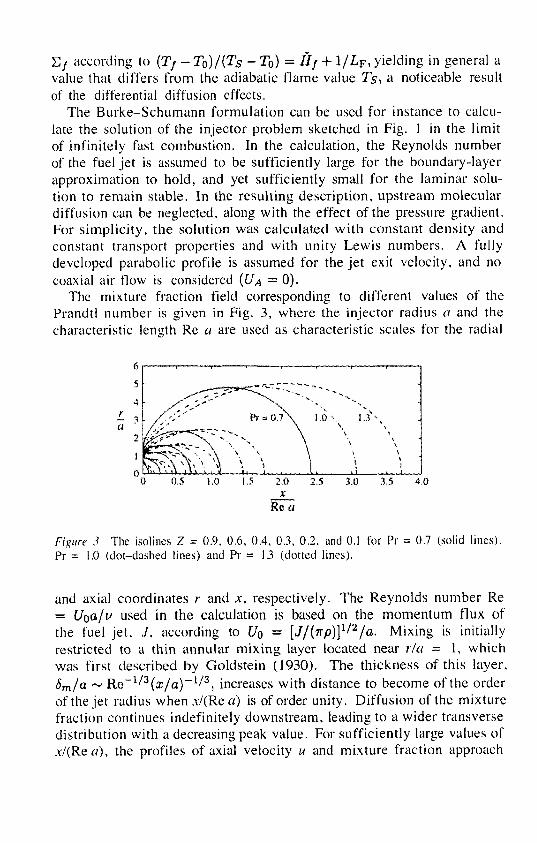
The Burke-Schumann formulation can be used for instance to calcu­late the solution of the injector problem sketched in Fig. 1 in the limit of infinitely fast combustion. In the calculation, the Reynolds number of the fuel jet is assumed to be sufficiently large for the boundary-layer approximation to hold, and yet sufficiently small for the laminar solu­tion to remain stable. In the resulting description, upstream molecular diffusion can be neglected, along with the effect of the pressure gradient. For simplicity, the solution was calculated with constant density and constant transport properties and with unity Lewis numbers. A fully developed parabolic profile is assumed for the jet exit velocity, and no coaxial air flow is considered (UA = 0).

The mixture fraction field corresponding to different values of the Prandtl number is given in Fig. 3, where the injector radius a and the characteristic length Re a are used as characteristic scales for the radial

6

5

4 T- 3

a *" ££*--<; ~-r~ \ '• \ ' s

0 I v.\ \ t IV •),>„) iVi-t,.i u 1 i 1 1 11 i i I

0 0.5 1.0 1.5 2.0 2.5 3.0 3.5 4.0

Re a

Figure .? The isolines Z = 0.9. 0.6, 0.4, 0.3, 0.2, and 0.1 for Pr = 0.7 (solid lines). Pr = 1.0 (dot-dashed lines) and Pr = 13 (dotted lines).

and axial coordinates r and x, respectively. The Reynolds number Re = U^a/v used in the calculation is based on the momentum flux of the fuel jet. ,/. according to UQ = [J/{np)]l/2/a. Mixing is initially restricted to a thin annular mixing layer located near rla = 1, which was first described by Goldstein (1930). The thickness of this layer, 6m/a ~ Re~1/3(a:/a)'~"1/3, increases with distance to become of the order of the jet radius when.v/(Re«) is of order unity. Diffusion of the mixture fraction continues indefinitely downstream, leading to a wider transverse distribution with a decreasing peak value. For sufficiently large values of .v/(Re«), the profiles of axial velocity u and mixture fraction approach

the Schlichting self-similar solution (Schlichting 1933, Squirre 1951)

/i— \ i / P r

8 x u I / l x 16Z \ 1 3 R e a t / 0 \ V 3 Rea 2Pr + l 1 / .. ^ 2

1 + J / " 64 \x/Re

in which peak values at the axis decrease monotonically with the recip­rocal of the downstream distance.

As previously mentioned, the flame lies where Z equals the stoichio­metric value Zs = 1/(5"+ 1). Therefore, the isolines of Fig. 3 give the flame shape for different values of Zs- In systems where undilute fuel feed is employed, the stoichiometric mass fraction S = Su = S/YQ2A

is very large, and the corresponding value of Zs = Z$u = l/(Su + 1) is very small. For instance, in methane-air combustion, s = 4, Su = 4/0.23 ~ 17, and Zsu — 0.05. In these undilute systems, the flame lies in the self-similar region described by Eqn. (13), which can be used to compute approximately the flame length xj according to x//a = (2Pr + l)(v/3/16)(Re/Zs). This result suggests that one may reduce the flame length by diluting the fuel stream to increase the value of Zs-Since l/Zs — SuYpo for SuYpo » 1, moderate dilution may be expected to lead to a linear decrease in (lame length from the undilute value Xfu

according to xj ~ X/UY"FO-

It is interesting to note that, unlike the flame length, the flame temper­ature Ts is rather insensitive to fuel dilution, as can be seen by expressing T$ in terms of the undilute peak temperature Tsu = TQ + ?/[cp(l + Su)} to yield (Ts - T0)/{TSu - T0) =s [1 + l/(S„yFo)]_1. Clearly, to pro­duce significant differences in flame temperature, one needs to dilute the fuel stream with Su parts of inert gas to give YFO ~ l/Su, whereas moderate dilution does not change significantly the value of Ts- For instance, to reduce the temperature in atmospheric methane-air com­bustion {Tsu - 2400 K) to values near extinction {Ts ^ 1600 K), one needs to decrease the fuel content of the fuel feed stream to yp0 — 0.08.

3. FINITE RATE EFFECTS We have seen how small values of the Damkohler number correspond

to chemically frozen solutions in which the reactant streams mix with­out significant chemical reaction, while large values of Da yield chemical equilibrium solutions, in which the reactants can coexist only in a thin flame sheet separating the fuel and oxidizer domains. Because of the high sensitivity of the chemical rate to temperature variations, the Damkohler number evaluated at the feed temperature Dao and that corresponding

to the adiabatic flame temperature Das typically differ by many orders of magnitude. Since the Damkohler number in the combustor necessarily lies in the intermediate range Dao < Da < Das, the condition Dao S> 1 guarantees the existence of equilibrium flow, whereas frozen mixing is the solution that appears necessarily if Das < 1- As previously antici­pated, in both limits the problem reduces to one of mixing. To illustrate the analogy further, one may note that the distribution of Z given in Fig. 3 for the equilibrium flow corresponds also to the distribution of reactants Yp = 1 — l b = Z resulting from frozen mixing of the fuel jet with the surrounding air in the limit Da <S 1, with the Prandtl number representing in this equidiflusional case the Schmidt number Sc = PrLp = PrLo of the reactants.

Multiple solutions may exist when Dao «C 1 < Das, a condition often satisfied in practical systems (Linan 1994). In the absence of an exter­nal ignition source, the weak reaction rate at T = TQ is not sufficient to produce a flame. The mixing of the fuel jet with the surrounding air proceeds then without significant chemical reaction, giving the frozen reactant distribution calculated in Fig. 3. Ignition can be forced exter­nally, however. An ignition source (a spark or a hot body) applied somewhere in the reactant mixture downstream from the injector may increase locally the reaction rate sufficiently to trigger the combustion process. For the large values of the Reynolds number typical of most practical applications, the flame front resulting after ignition is thin compared with the jet radius, and its local structure is that of a planar premixed flame, whose propagation velocity is known to reach a maxi­mum value SL where the mixture is stoichiometric (or slightly rich), and to decay rapidly as the mixture becomes either leaner or richer. Cor­respondingly, the premixed flame that forms moves both upstream and downstream along the stoichiometric surface Z = Zs and exhibits a char­acteristic structure with a lean branch and a rich branch (Linan 1988, Dold et al. 1991). On the lean side the premixed flame consumes all the available fuel, leaving behind oxygen that reacts in a trailing diffusion flame with the fuel left behind by the rich branch. Due to their reduced propagation velocity, the lean and rich branches of the flame front curve backwards from the leading stoichiometric point with a radius of curva­ture that is of the order of Sm = Zs/\VZ\s, a characteristic measure of the local mixing-layer thickness.

The triple flame moves relative to the flow with a propagation velocity Uj of the order of SL, that depends on the exothermicity of the reac­tion through the parameter 7. The flow in the nose region downstream from the flame is rotational, with overpressures that deflect the incoming streamlines outwards, and slow the flow velocity along Z = Zs- Cor-

respondingly, the front propagation velocity £//, relative to the unper­turbed flow, is somewhat larger than Sx (Ruetsch et al. 1995). As seen by Dold and coworkers (1991), when 8m is of the order of the character­istic thickness of the flame front, i.e. Si = DTO/SI, the front velocity Uj is also a function of Si/Sm, becoming independent of &i,/$m when &Ll$m ^ 1- For instance, for the laminar jet of Fig. 3, for which the thickness of the Goldstein mixing layer increases with distance from the injector rim according to 5m/o ~ Re_ 1/3(x/a)1 ' / 3 , Uj is no longer dependent on Si/6m at distances x such that x/a » Re_2{£/o/<Sx)3. The previous estimate of 6m yields Sm/a <C 1 for x <S Re a, indicating that triple flames propagating at such distances are locally two-dimensional. For x > Re a, on the other hand, the value of Z at the axis is compara­ble with the value of Zs- The associated flame fronts, which satisfy the condition 8i/8m <C 1, exhibit a radius of curvature of the order of the local jet radius, and possess therefore an inherendy three-dimensional structure that can be expected to influence the value of Uf when thermal-expansion effects are nonnegligible.

For the triple flame to move upstream, its propagation velocity Uf ~ SL must be larger than the flow velocity us along the stoichiometric surface Z = Zs, whose distribution is exhibited in Fig. 4 for the lam­inar jet flow of Fig. 3. The curves in Fig. 4 correspond in particu­lar to Zs = 0.1, a realistic small value for which the velocities found

02

0 0 1 2 3 4

X

Re a

Figure 4 The velocity distribution along the surface Z = Zs = 0.1 for Sc = 0.7, 1.0, and 13.

1/Sc are small, of order Zs' . In the vicinity of the injector, the stoichio­metric surface is embedded in the Goldstein mixing layer, and thereby exhibits a velocity that increases with the cube root of the distance to the injector rim. The behavior of us as the jet develops for values of x > Re a is given by the first equation in (13), which yields the depen­dence US/UQ ~ Zg^lx/iRea)}1/^-1, revealing that departures of the

Schmidt number from unity affect in a fundamental way the velocity dis­tribution (Lee and Chung 1997). Thus, a value of the Schmidt number above unity results in values of Us decreasing with x for x » Re a, which in turn causes the associated velocity distribution along the stoichio­metric surface to possess a maximum value at an intermediate location x ~ Re a. On the other hand, the velocity distributions corresponding to Sc < 1 increase monotonically with distance, a characteristic that precludes the existence of lift-off flames as explained below.

Using the plot, one may easily determine the downstream location where us equals Uj. If the flow velocity is decaying with distance at the given location, as may occur sufficiently downstream when the Schmidt number is above unity, then the solution found is stable, and corresponds to a lift-off triple flame (Lee and Chung 1997, Chen and Bilger 2000). On the other hand, if us is an increasing function of x where us = Uf, as occurs for Sc < 1 and also close to the injector for Sc > 1, then the resulting solution is unstable. The value of x determined in this manner corresponds to the farthermost location where, by applying an ignition source, one may generate a premixed front that propagates upstream to the injector rim. The dependence of the velocity distribution on the Schmidt number explains why lifted-off solutions are typical of heavy hydrocarbons, but do not appear for instance in laminar methane or ethane combustion (Lee and Chung 1997).

The structure of the diffusion flame edge (Buckmaster 1996) in its anchoring region, in the near wake of the injector, is obviously strongly dependent on the Reynolds number Uaa/va, typically much larger than unity in applications, and also on the thickness dp <g. a of the injector wall. The wall value of the velocity gradients near the injector rim is going to enter in the scales of the anchoring region. This value is equal to A = 4Uo/a in the fuel stream when the fuel jet flow corresponds to a Poiseuille solution, as occurs with long injectors of length Re a or larger. Otherwise, the value of the velocity gradient is determined by the thickness of the boundary layer that forms adjacent to the injector wall in the fuel stream. In systems with co-flowing air, a boundary layer also develops at the wall in the air stream. These boundary layers merge to form a mixing layer when they separate from the injector wall. If the fuel boundary layer has developed in a length of order a, and if it is laminar, the resulting thickness 6B will be of order oRe - 1 ' 2 , leading to a wall value of the velocity gradient A of order (UO/O,)RQ~1/2. A similar wall velocity gradient aA will be encountered in the air stream, where the factor a is zero if the jet mixes with stagnant air.

When the mixing layers begin to merge, the mixing layer is thin com­pared with 6B and its structure is that of a Goldstein mixing layer,

which is determined exclusively by the wall velocity gradients (in the limit dpj'6B < 1). Because Re » 1, the effects of upstream heat con­duction and diffusion will be negligible in the annular mixing layer out­side a small Navier-Stokes (N-S) region, at the rear end of the injec­tor. The characteristic size 6^ = S/VQ/A and characteristic velocity ttjv = \/VQA of this region are determined by the fuel boundary-layer wall velocity gradient A and the condition ttjv^/v/^o = li required to allow for upstream heat conduction and diffusion there. For the diffu­sion flame to remain attached to this N-S region, one can anticipate that UN should not exceed Si significantly, or equivalently, the local Damkohler number D^ = S\/{VQA) should not be lower than a critical value (DN)C of order unity.

In order to calculate (JDJV)CJ and the diffusion-flame edge structure for DJV > {DN)CI one should solve the locally two-dimensional and steady form of the reacting N-S equations nondimensionalized with the scales SN and ujv, as done recently by Fernandez et al. (2000). The main parameters determining the solution are D^, S, 7, and the air/fuel ratio a of wall velocity gradients, together with the nondimensional thickness dp/Sff of the injector wall and the nondimensional activation energy E/(RTs) (if an Arrhenius law like that of Eqn. (3) is adopted for the chemistry description). With the scales of this N-S region, the incoming air and fuel flows are seen as uniform shear flows at the temperature of the wall, intermediate between those of the two streams To and TA- It is worth noting that the structure of the edge flames that form in the near-wake of the injector is similar to that of the edge flames emerging in flame spread over solid fuel.

When the Reynolds number based on the boundary-layer thickness UQ5B/VO exceeds a critical value, the boundary layer can be expected to become turbulent. In this case, the average values for the scales of the flame attachment region are the friction velocity and the thickness of the viscous sublayer, where the local Reynolds number is of order unity and the Reynolds stresses are no longer dominant. The analysis of the attachment region can be anticipated to be similar to that of the laminar case, with the effect of turbulence introducing in this case time variations in the wall velocity gradients.

As a final remark, one should mention that finite-rate kinetics is also responsible for the phenomenon of strain-induced extinction. In most combustion applications, the Reynolds number is so large that the flow becomes turbulent. Then diffusion flames appear embedded in thin mixing layers that are locally strained by the turbulent motion. The maximum strain rate, of order R e ^ t / b / a is associated with the small­est eddies, whose characteristic size and velocity are given according

to Kolmogorov by /& ~ Re - 3 / 4 a and n* ~ R e - 1 / 4 ^ - As seen by Linan (1974), local flame extinction may occur for sufficiently large strain rates, when the rate of mixing (or, equivalently, the rate of fuel burning per unit flame surface), measured by l/8m = ZgX\VZ\s, is increased above a critical value, defined in order of magnitude by l/8m ~ I/SL ~ SLI^Q.

Note that, with the wall value of the velocity gradient A ~ (Uo/a)Ke~ ' corresponding to injectors of characteristic length a, the scales emerging in the N-S region <5jv = y/vofA ~ Re~3/4a and ujq — \/VQA ~ Re~l^Uo are the Kolmogorov scales 5k and Uk of the associated turbulent flow. For these systems, the criteria for lift-off 8^ ~ 8i and that of local extinction Sm ~ 8i coincide, so that both phenomena may be expected to happen simultaneously.