DIFFERENTIAL OPERATORS AND BOUNDARYVALUE PROBLEMS ON HYPERSURFACES

ROLAND DUDUCHAVA, DORINA MITREA & MARIUS MITREA

dedicated to Victor Kupradze’s 100th birthday anniversary

Abstract. We explore the extent to which basic differential operators (such asLaplace-Beltrami, Lame, Navier-Stokes, etc.) and boundary value problems on ahypersurface S in Rn can be expressed globally, in terms of the standard spatialcoordinates in Rn. The approach we develop also provides, in some importantcases, useful simplifications as well as new interpretations of classical operatorsand equations.

1 INTRODUCTION

Boundary value problems (BVP’s) for partial differential equations (PDE’s) on surfacesarise in a variety of situations and have many practical applications. See, for example,

72[Ha,

§72] for the heat conduction by surfaces,10[Ar, §10] for the equations of surface flow,

Ci[Ci],Ci2

[Ci2],Go[Go] for shell problems in elasticity,

AC[AC] for the vacuum Einstein equations describ-

ing gravitational fields,TZ[TZ] for the Navier-Stokes equations on spherical domains, as well

as the references therein. Furthermore, while studying the asymptotic behavior of solutionsto elliptic boundary value problems in the neighborhood of a conical point one is led to con-sidering a one-parameter family of boundary value problems in a subdomain S of Sn−1, theunit sphere in Rn, naturally associated (via the Mellin transform) with the original ellipticproblem. A classical reference in this regard is

Ko[Ko]. Finally, PDE’s on surfaces also turn

up naturally in the limit case, as the thickness goes to zero, of equations in thin layers orshells. Cf.

3[Ci, §3] for the case of elasticity, and

TW[TW],

TZ[TZ] for the case of Navier-Stokes

equations.A hypersurface S in Rn has the natural structure of a (n− 1)-dimensional Riemannian

manifold and the aforementioned PDE’s are not the immediate analogues of the ones cor-responding to the flat, Euclidean case, since they have to take into consideration geometriccharacteristics of S such as curvature. Inherently, these PDE’s are originally written in localcoordinates, intrinsic to the manifold structure of S .

The main aim of this paper is to explore the extent to which the most basic partial dif-ferential operators (PDO’s), as well as their associated boundary value problems, on a hy-persurface S in Rn, can be expressed globally, in terms of the standard spatial coordinatesin Rn. It turns out that a convenient way to carry out this program is by employing the theso-called Gunter derivatives (cf.

Gu[Gu],

KGBB[KGBB],

Du[Du]):

D := (D1,D2, ..., Dn). (1.1) eq1.1

Here, for each 1 ≤ j ≤ n, the first-order differential operator Dj is the directional derivativealong π ej , where π : Rn → TS is the orthogonal projection onto the tangent plane to Sand, as usual, ej = (δjk)1≤k≤n ∈ Rn, with δjk denoting the Kronecker symbol. The operatorD is globally defined on (as well as tangential to) S , and has a relatively simple structure.In terms of (

eq1.11.1), the Laplace-Beltrami operator on S simply becomes

2

∆S = D •D on S . (1.2) eq1.2

(Cf.MaMi[MaMi, pp. 2 ff and p. 8].) Alternatively, this is the natural operator associated with the

Euler-Lagrange equations for the variational integral

E [u] = −1

2

∫

S

‖Du‖2 dS. (1.3) eq1.3

A similar approach, based on the principle that, at equilibrium, the displacement min-imizes the potential energy, leads to the following expression for the Lame operator L onS :

L u = µπ (D •D)u + (λ + µ) D(D •u)− µ (n− 1)H W u, (1.4) eq1.4

for arbitrary vector fields u on S , which are tangent to S . Above, λ, µ ∈ R are the Lamemoduli, whereas H , W stand, respectively, for the the mean curvature and the Weingartenmap of S . In particular, when combined with the recent work from

MMT[MMT] (dealing with

general elliptic BVP’s on Lipschitz subdomains of Riemannian manifolds), this identificationensures the well-posedness of the boundary-value problem

u = (u1, ..., un) ∈ Hs+1/2,2(S ,Rn),

〈u, N〉 = 0 in S ,

µ π (D •D)u + (λ + µ) D(D •u)− µ (n− 1)H W u = 0 in S ,

u∣∣∣∂S

= ~f ∈ Hs,2(∂S ,Rn), 〈~f, N〉 = 0 on ∂S ,

(1.5) eq1.5

whenever µ > 0, 2µ + λ > 0, and 0 ≤ s ≤ 1. Here Hs,2 stands for the usual L2-basedSobolev scale. Other operators discussed in this paper are the Hodge-Laplacian

∆HL := −dS d∗S − d∗S dS , (1.6) eq1.6

where dS is the exterior derivative operator on S , and d∗S its formal adjoint, and the Navier-Stokes system on S × (0,∞); see §7 for details.

These results are useful in numerical and engineering applications (cf.AN[AN],

Be[Be],

Ce[Ce],Co

[Co],DL[DL],

BGS[BGS],

Sm[Sm]) and we plan to treat a number of special hypersurfaces in greater

detail in a subsequent publication.The layout of the paper is as follows. In §2 we review some basic differential-geometric

concepts which are relevant for the work at hand. In §3, starting from first principles, weidentify the natural Lame operator on a general (elastic, linear, isotropic) manifold M . Ourapproach is based on variational methods. Starting with §4, we specialize our discussion tothe case of a hypersurface S , viewed as a Riemannian manifold with the metric inheritedfrom the ambient Euclidean space. In particular, here we discuss the possibility of extendingthe unit normal to S , i.e. N : S → Sn−1 in a neighborhood of S under additionalassumptions. In §5 we derive some very useful ‘integration by parts’ formulas for first orderoperators which are tangent to a hypersurface S .

The proof of the identification (eq1.21.2) is given in §6, via a method which is interesting in

its own right. In fact, this is flexible enough to apply to the case of systems of equations,

2. BRIEF REVIEW OF CLASSICAL DIFFERENTIAL GEOMETRY OF MANIFOLDS 3

such as the Lame operators. This yields (eq1.41.4), in §7. Finally, applications to elliptic BVP’s

on smooth hypersurfaces with Lipschitz boundaries (such as (eq1.51.5)), are presented in §8.

Acknowledgments. This work has had a long period of gestation: it has been initiated whilethe first named author was visiting the University of Missouri-Columbia in 2002. The hos-pitality of this institution as well as the financial support which made this visit possible aregratefully acknowledged. The last named author has been supported in part by NSF andthe UMC Research Office. After this manuscript was circulated in preprint format, we havelearned that several of our operator identities have been obtained in

MaMi[MaMi], though the aims

and methods in this book are substantially different from ours.

2 BRIEF REVIEW OF CLASSICAL DIFFERENTIAL GEOMETRY OF MANIFOLDS

Let M be a smooth manifold, possibly with boundary, of (real) dimension n. As usual,by TM and T ∗M we denote, respectively, the tangent and cotangent bundle on M . Through-out, we shall also denote by TM global (C∞) sections in TM (i.e., TM ≡ C∞(M, TM));similarly, T ∗M ≡ C∞(M,T ∗M). More generally, if Λ`TM stands for the correspondingexterior power bundle (differential forms of degree `), then we shall use the abbreviationΛ`TM ≡ C∞(M, Λ`TM).

We shall assume that M is equipped with a smooth Riemannian metric tensor g =∑j,k gjkdxj ⊗ dxk, denote by (gjk)jk the inverse matrix to (gjk) and set g := det (gjk)jk. In

particular, dVol, the volume element in M is locally given by dVol =√

g dx1...dxn. Recallnext that

div X :=∑

j

√g−1∂j(

√gXj) if X =

∑j

Xj∂/∂xj ∈ TM, (2.1) eq2.1

and

grad f =∑

j,k

(gjk∂jf) ∂/∂xk (2.2) eq2.2

are, respectively, the usual divergence and gradient operators. Accordingly, the Laplace-Beltrami operator ∆ becomes

∆ := div grad =√

g−1n∑

j,k=1

∂j(gj,k√g∂k · ) . (2.3) eq2.3

The pairing 〈dxj, dxk〉 := gjk defines an inner product in Λ1TM . With respect to this,grad and −div are adjoint to each other. We shall also abbreviate dxi1 ∧ dxi2 ∧ ... ∧ dxi` bydxI , where I = (i1, i2, ..., i`) and let wedge stand for the ordinary exterior product of forms.Then, 〈dxI , dxJ〉 := det

((gij) i∈I

j∈J

), |I| = |J | = `, defines an inner product in Λ`TM for

each 1 ≤ ` ≤ n.If, as usual, we let d =

∑j ∂/∂xj dxj∧ stand for the exterior derivative operator on

M , and denote by δ its formal adjoint (with respect to the above metric), then the Hodge-Laplacian on M becomes

4

∆ := −dδ − δd. (2.4) eq2.4

As is customary, we may identify vector fields with one-forms, i.e., TM ∼= T ∗M =Λ1TM , via ∂/∂xj 7→ gjkdxk (lowering indices). This mapping is an isometry whose in-verse is given by dxj 7→ gjk∂/∂xk (raising indices). In the sequel, we shall not make anynotational distinction between a vector field and its associated 1-form (i.e., we shall tac-itly identify TM ≡ T ∗M ). Under this identification, grad : C∞(M) → C∞(M, TM)becomes d : C∞(M) → C∞(M, Λ1TM) and div : C∞(M,TM) → C∞(M) becomes−δ : C∞(M, Λ1TM) → C∞(M).

A tensor of type (k, j) is a map

F : (TM × ...× TM)× (Λ1TM × ...× Λ1TM) → C∞(M) (2.5) eq2.5

(with j factors of TM and k factors of Λ1TM ) which is linear in each factor over the ringC∞(M). There is a natural inner product at the level of (k, j) tensors defined by

〈F, G〉 :=∑

F (Xα1 , Xα2 , ..., Xαj, ωβ1 , ωβ2 , ..., ωβk

)

·G(Xα1 , Xα2 , ..., Xαj, ωβ1 , ωβ2 , ..., ωβk

), (2.6) eq2.6

where Xα’s are an orthonormal frame for TM and ωβ’s are the dual basis in Λ1TM (sum-mation over all possible choices of indices).

Next, let ∇ be the associated Levi-Civita connection. Among other things, the metricproperty

Z〈X, Y 〉 = ∇Z 〈X, Y 〉 = 〈∇ZX, Y 〉+ 〈X,∇ZY 〉, ∀X,Y, Z ∈ TM, (2.7) eq2.7

holds. This, in concert with

X∗ = −X − div X, ∀X ∈ TM. (2.8) eq2.8

further entails that

(∇X)∗ = −∇X − div X, ∀X ∈ TM. (2.9) eq2.9

For each X ∈ TM , ∇X is the tensor of type (0, 2) defined by

(∇X)(Y, Z) := 〈∇ZX, Y 〉, ∀Y, Z ∈ TM. (2.10) eq2.10

with trace

Tr(∇X) =n∑

j=1

〈∇TjX,Tj〉 = div X (2.11) eq2.11

2. BRIEF REVIEW OF CLASSICAL DIFFERENTIAL GEOMETRY OF MANIFOLDS 5

for any orthonormal frame Tjj in TM . For any X ∈ TM , the antisymmetric part of ∇Xis simply dX , i.e.

dX(Y, Z) = 〈dX, Y ∧ Z〉 = 12

〈∇Y X, Z〉 − 〈∇ZX,Y 〉

, ∀Y, Z ∈ TM, (2.12) eq2.12

whereas the symmetric part of ∇X is Def X , the deformation of X , i.e.

(Def X)(Y, Z) = 12

〈∇Y X, Z〉+ 〈∇ZX,Y 〉

, ∀Y, Z ∈ TM. (2.13) eq2.13

Thus, Def X is a symmetric tensor field of type (0, 2). In coordinate notation,

(Def X)jk = 12(Xj;k + Xk;j), ∀ j, k. (2.14) eq2.14

Here, as usual, for a vector field X =∑

j Xj∂j , we set Xk;j := ∂jXk −∑

l ΓlkjXl,

where Xk =∑

l gklXl and Γl

kj are the Christoffel symbols associated with the metric.Deformation-free vectors fields X are usually referred to as Killing fields. They satisfy

∑

`

[gk`X

`;j + gj`X

`;k

]= Xk;j + Xj;k = 0, ∀ j, k. (2.15) eq2.15

The adjoint of Def is Def∗ defined in local coordinates by (Def∗w)j = −wjk;k for each

symmetric tensor field w of type (0, 2). In particular, if ν ∈ TM is the outward unit normalto ∂M → M , then the integration by parts formula

∫

M

〈Def u,w〉 dVol =

∫

M

〈u, Def∗w〉 dVol +

∫

∂M

w(ν, u) dvol, (2.16) eq2.16

holds for any u ∈ TM , and any symmetric tensor field w of type (0, 2). Here and elsewhere,dvol will denote the volume element on ∂M .

Formula (eq2.162.16) is a particular case of a more general integration by parts identity, to the

effect that∫

M

〈Pu, w〉 dVol =

∫

M

〈u, P ∗w〉 dVol +

∫

∂M

〈σ(P ; ν)u,w〉 dvol, (2.17) eq2.17

valid for a general first-order differential operator P =∑

j Aj∂j + zero order terms (actingbetween two hermitian vector bundles on M ), with principal symbol σ(P ; ξ) =

∑j Ajξj ,

for ξ ∈ T ∗M .For further reference, let us note here that σ(∇X ; ξ) = 〈X, ξ〉, and that σ(d; ξ) = ξ ∧ ·,

σ(δ; ξ) = ξ ∨ ·, where we have denote by ∨ the adjoint of the exterior product, in the sensethat

〈ξ ∨ u,w〉 = 〈u, ξ ∧ w〉, ξ ∈ Λ1TM, u ∈ Λ`TM, w ∈ Λ`−1TM. (2.18) eq2.18

6

The Riemann curvature tensor R of M is given by

R(X,Y )Z = [∇X ,∇Y ]Z −∇[X,Y ]Z, X, Y, Z ∈ TM, (2.19) eq2.19

where [X, Y ] := XY − Y X is the usual commutator bracket. It is convenient to change thisinto a (0, 4)-tensor by setting

R(X, Y, Z, W ) := 〈R(X, Y )Z, W 〉, X, Y, Z, W ∈ TM. (2.20) eq2.20

The Ricci curvature Ric on M is a (0, 2)-tensor defined as a contraction of R:

Ric (X, Y ) :=n∑

j=1

〈R(Tj, Y )X, Tj〉 =n∑

j=1

〈R(Y, Tj)Tj, X〉, ∀X, Y ∈ TM, (2.21) eq2.21

where T1, . . . , Tn is an orthonormal frame in TM . Thus, Ric is a symmetric bilinear form.Under the identification TM ≡ Λ1TM , the Bochner Laplacian and the Hodge Laplacian

are related by

∇∗∇ ≡ −∆− Ric, (2.22) eq2.22

a special case of the Weitzenbock identity.Consider now S → M , a smooth, orientable submanifold of codimension one in M ,

and fix some ν ∈ TM such that ν|S becomes the outward unit normal to S . If ∇S is theinduced Levi-Civita connection on S (from the metric inherited from M ) it is then well-known that

∇SX Y = π(∇XY ), ∀X,Y ∈ TS , (2.23) eq2.23

where

π : TM −→ TS , π = I − 〈·, ν〉ν = ν ∨ (ν ∧ · ), (2.24) eq2.24

is the canonical orthogonal projection onto TS . In particular, the second fundamental formof S becomes

II(X,Y ) := ∇XY −∇SX Y = π(∇XY ), ∀X, Y ∈ TS . (2.25) eq2.25

In this setting, the Weingarten map

W : TS −→ TS , (2.26) eq2.26

originally defined uniquely by the requirement that

〈W X,Y 〉 = 〈ν, II(X, Y )〉, ∀X, Y ∈ TS , (2.27) eq2.27

reduces to

3. THE DERIVATION OF THE LAME OPERATOR ON MANIFOLDS 7

W X = −∇Xν on S , ∀X ∈ TS , (2.28) eq2.28

known as Weingarten formula.An excellent reference for the material in this section is

Ta2[Ta2]. Here we only want to

point out that, whenever necessary in order to avoid confusion, we shall write dM , gradM ,divM , ∆M , etc., in place of d, grad, div, ∆, etc.

3 THE DERIVATION OF THE LAME OPERATOR ON MANIFOLDS

One way of understanding the genesis of the Laplace-Beltrami operator (eq2.32.3) is to con-

sider the energy functional

E [u] :=

∫

M

‖grad u‖2 dVol, u ∈ C∞(M). (3.1) eq3.1

Then any minimizer u of (eq3.13.1) should satisfy

d

dtE [u + tv]

∣∣∣t=0

= 0, ∀ v ∈ C∞o (M), (3.2) eq3.2

thus, after an integration by parts,

∆u = 0 on M. (3.3) eq3.3

In other words, (eq3.33.3) is the Euler-Lagrange equation associated with the integral func-

tional (eq3.13.1).

Similarly, minimizers of the energy functional

E [u] := −1

2

∫

M

[‖du‖2 + ‖δu‖2

]dVol, u ∈ Λ`TM, (3.4) eq3.4

are null-solutions of the Hodge-Laplacian (eq2.42.4), while minimizers of the energy functional

E [u] := −1

2

∫

M

‖∇u‖2 dVol, u ∈ TM, (3.5) eq3.5

are null-solutions of the Bochner-Laplacian (eq2.222.22).

Our aim is to adopt a similar point of view in the case of the (possibly anisotropic) Lamesystem of elasticity on M . The departure point is to consider the total free elastic energy

E [u] := −1

2

∫

M

E(x,∇u(x)) dVolx, u ∈ TM, (3.6) eq3.6

ignoring at the moment the displacement boundary conditions. As before, equilibria statescorrespond to minimizers of the above variational integral. The first order of business isto identify the correct form of the stored energy density E(x,∇u(x)). We shall restrictattention to the case of linear elasticity. In this scenario, E depends bilinearly on the stresstensor σ = (σjk)jk and the deformation (strain) tensor ε = (εjk)jk which, according to

8

Hooke’s law, satisfy σ = T ε, for some linear, fourth-order tensor T . If the medium is alsohomogeneous (i.e. the density and elastic parameters are position-independent), it followsthat E depends quadratically on ∇u, i.e.

E(x,∇u(x)) = 〈T ∇u(x),∇u(x)〉 (3.7) eq3.7

for some linear operator

T : Mn,n(R) −→ Mn,n(R), (3.8) eq3.8

where Mn,n(R) stands for the vector space of all n× n matrices with real entries. Hereafter,we organize Mn,n(R) as a real Hilbert space with respect to the inner product

〈A,B〉 := Tr(AB>), ∀A,B ∈ Mn,n(R), (3.9) eq3.9

where the superscript > denotes transposition, and Tr is the usual trace operator for squarematrices. It is customary to assume that the linear operator (

eq3.83.8) is self-adjoint, that is

〈T A,B〉 = 〈A, T B〉 , A,B ∈ Mn,n(R) . (3.10) eq3.91

The operator T = (cijk`)ijk`, i.e.,

T A =(∑

k,`

cijk`ak`

)ij, for A = (ak`)k` ∈ Mn,n(R), (3.11) eq3.13

will be referred to in the sequel as the elasticity tensor. The condition (eq3.913.10), written in

coordinate notation, is equivalent to the following equality

cijk` = ck`ij, ∀ i, j, k, ` . (3.12) eq3.20

It is also customary to impose a symmetry condition and one is presented with two naturaloptions, namely

T (A>) = T A, ∀A ∈ Mn,n(R), (3.13) eq3.11

and

(T A)> = T A, ∀A ∈ Mn,n(R). (3.14) eq3.12

Then (eq3.113.13) amounts to symmetry in the second pair of indices, i.e.

cijk` = cij`k, ∀ i, j, k, `, (3.15) eq3.14

whereas (eq3.123.14) is equivalent to symmetry in the first pair of indices, i.e.

cijk` = cjik`, ∀ i, j, k, `. (3.16) eq3.15

To sum up our discussion so far, we note that a linear operator T (as in (eq3.83.8)), which

corresponds to the energy functional of anisotropic elasticity (cf. (eq3.73.7)), satisfies the symme-

try conditions (eq3.913.10), (

eq3.113.13), (

eq3.123.14). Thus, for the corresponding matrix T = (cijk`)

nijk`=1,

3. THE DERIVATION OF THE LAME OPERATOR ON MANIFOLDS 9

the symmetry conditions (eq3.203.12), (

eq3.143.15) and (

eq3.153.16) hold, so this matrix may have at most

n + n2(n− 1)2/2 different entries.The isotropic media is further assumed to satisfy

T (UAU−1) = U(T A)U−1, ∀A,U ∈ Mn,n(R), U unitary. (3.17) eq3.10

As we shall see a posteriori, the conditions (eq3.113.13), (

eq3.123.14) and (

eq3.103.17) imply the linear operator

(eq3.83.8) is self adjoint, i.e., imply the condition (

eq3.913.10). Indeed, we have:

p3.1 Proposition 3.1 Consider a linear operator T , as in (eq3.83.8), such that the isotropy condition

(eq3.103.17) holds. Then T satisfies (

eq3.113.13) if and only if it satisfies (

eq3.123.14). Furthermore, any linear

operator T which satisfies (eq3.103.17) along with either (

eq3.113.13) or (

eq3.123.14) has the form

T A = λ (Tr A)I + µ (A + A>), A ∈ Mn,n(R), (3.18) eq3.17

for some constants λ, µ ∈ R.

Proof. Let us first show that any linear operator (eq3.83.8) satisfying (

eq3.103.17)-(

eq3.113.13) can be repre-

sented in the form (eq3.173.18). By the previous discussion, it suffices to prove that the space of

linear operators (eq3.83.8) satisfying (

eq3.103.17)-(

eq3.113.13) has dimension two.

Since for any A ∈ Mn,n(R) we have T A = 12T (A + A>), thanks to (

eq3.113.13), and since

A+A> can be diagonalized (via a suitable conjugation with an unitary matrix U ), it sufficesto show that

T D =

a 0 0 ... 00 b 0 ... 00 0 b ... 0

...0 0 0 ... b

, where D :=

1 0 ... 00 0 ... 0

...0 0 ... 0

for two numbers a, b ∈ R. To this end, consider the following types of unitary matrices:

Uio,jo :=

1 0 ... ... ... ... 00 1 0 ... ... ... 00 ... 0 ... 1 ... 0

... ... ...0 ... 1 ... 0 ... 0

... ... ...0 0 0 ... ... 1 00 0 0 ... ... ... 1

, Wio,jo :=

1 0 ... ... ... ... 00 1 0 ... ... ... 00 ... 0 ... 1 ... 0

... ... ...0 ... −1 ... 0 ... 0

... ... ...0 0 0 ... ... 1 00 0 0 ... ... ... 1

where the only non-zero, off the diagonal entries are at (io, jo) and (jo, io). Next, set

A := T D, A =(aij

)1≤i,j≤n

and observe that D is invariant under conjugation by Wio,jo , i.e. Wio,joDW>io,jo

= D, aslong as io 6= 1 and jo 6= 1. Thus, by (

eq3.103.17), the same is true for A = T D which, in turn,

eventually implies that

10

aioio = ajojo , ∀ io, jo 6= 1. (3.19) eq3.18

The next observation is that D is invariant under conjugation by the product UiojoWio,jo , i.e.UiojoWio,joDU>

iojoW>

io,jo= D, this time for every 1 ≤ io 6= jo ≤ n. Hence, by (

eq3.103.17), the

same holds for A = T D, which ultimately implies that aiojo = −ajoio for every pair ofindices 1 ≤ io 6= jo ≤ n. Consequently,

aiojo = 0, for every 1 ≤ io 6= jo ≤ n. (3.20) eq3.19

Under the current assumptions, i.e. (eq3.103.17)-(

eq3.113.13), the desired conclusion, i.e. that T D

has the two-parameter diagonal form indicated above, now follows readily from (eq3.183.19) and

(eq3.193.20).

There remains to analyze the case when the linear operator T satisfies (eq3.103.17) along

with (eq3.123.14). In this situation, it can be readily checked that T ∗, the adjoint of T with

respect to the inner product (eq3.93.9), satisfies (

eq3.103.17)-(

eq3.113.13), so the previous reasoning applies.

Consequently, T ∗ can be represented in the form (eq3.173.18), which is invariant under adjunction.

Hence T can be written in the form (eq3.173.18) also. In particular, (

eq3.173.18) holds in this case as

well, and this finishes the proof of the proposition.

Remark. The above proof can be modified to hold in the case when (eq3.103.17) is (seemingly)

weakened to allow only orientation preserving unitary matrices U . All one has to do inthis later case is to employ the invariance of D under conjugation by Uko`oUiojoWio,jo (withko, `o 6= 1), in place of conjugation by (the inversion) UiojoWio,jo as in the original proof.

We are now ready to derive the Lame equations of elasticity on M .

t3.2 Theorem 3.2 On a Riemannian manifold M , modeling a homogeneous, linear, isotropic,elastic medium, the Lame operator L is given by

L = −2µ Def∗Def + λ grad div. (3.21) eq3.21

In particular, L is strongly elliptic, formally self-adjoint.If u ∈ TM denotes the displacement, natural boundary conditions for L include pre-

scribing u|∂M , Dirichlet type, and

Traction u := 2µ (Def u)ν + λ (div u)ν on ∂M, (3.22) eq3.22

Neumann type.

Here ν ∈ TM is the outward unit normal to ∂M and we identify (Def u)ν with thevector field uniquely determined by the requirement that 〈(Def u)ν, X〉 = (Def u)(ν,X) foreach X ∈ TM .Proof. For elastic materials, it is known that the elasticity tensor (

eq3.83.8) is symmetric matrix-

valued, i.e. it satisfies (eq3.113.13). Thus, according to the discussion in the first part of this section,

the elasticity tensor in the case of linear, isotropic, elastic media is given by (eq3.173.18), where

λ, µ are the Lame moduli. Consequently, the stored energy density we need to consider is

E(A) = 〈T A, A〉 = λ (Tr A)2 +µ

2Tr ((A + A>)2). (3.23) eq3.23

4. DISTINGUISHED EXTENSIONS OF THE UNIT NORMAL TO A HYPERSURFACE 11

Further substituting A := ∇u in (eq3.233.23) yields

E(x,∇u(x)) = λ (div u)2(x) + 2µ 〈(Def u)(x), (Def u)(x)〉, (3.24) eq3.24

by (eq2.112.11) and (

eq2.132.13). Thus, we are led to considering the variational integral

E [u] = −1

2

∫

M

[λ (div u)2 + 2µ 〈Def u, Def u〉

]dVol, u ∈ TM. (3.25) eq3.25

To determine the associated Euler-Lagrange equation, for an arbitrary v ∈ TM , smooth andcompactly supported, we compute

d

dtE [u + tv]

∣∣∣t=0

= −∫

M

[λ (div u)(div v) + 2µ 〈Def u, Def v〉

]dVol

=

∫

M

〈(λ grad div − 2µ Def∗Def )u, v〉 dVol

−∫

∂M

〈2µ (Def u)ν + λ (div u)ν , v〉 dvol (3.26) eq3.26

after integrating by parts, based on (eq2.162.16) and the Divergence Theorem (i.e. (

eq2.172.17) with

P = div). ¿From (eq3.263.26), the desired conclusions follow without difficulty.

Remark. In the (linear) anisotropic case, the Lame operator takes the less explicit form

L u = −∇∗T ∇u, u ∈ TM, (3.27) eq3.27

where, as before, T is the elasticity tensor; cf. (eq3.133.11).

4 DISTINGUISHED EXTENSIONS OF THE UNIT NORMAL TO A HYPERSURFACE

We retain the notation adopted in §2, albeit specialized to the case M = Rn. In particular,∇ and div are the usual gradient and divergence operators,∇ := (∂1, . . . , ∂n) and div = ∇ • ,respectively, in Rn. Also, if X is a vector field in Rn, we denote by ∂X the directionalderivative X •∇. Hereafter, X •Y = 〈X, Y 〉 stands for the standard inner product in Rn.Thus,

∇XY = (X •∇)Y = (Xk(∂kYj))j, if Y = (Yj)j, X = (Xk)k.

Also, ∇X is naturally identified with the matrix (∂kXj)j,k.

Next, let S be a Ck-hypersurface, i.e. an orientable, submanifold of class Ck, k ≥ 1, ofcodimension one in Rn, with unit normal N(x) = (N1(x), . . . , N(x)), x ∈ S .

12

s

s

pppppppppppppppppppppppppppppppppppp

pppppppppppppppppppppppppppppppppppppp

pppppppppppppppppppppppppppppppppppppppppppppppppppppppppppppppppppppppppppppppppppppppppppppppppppppppppppppppppppppppppppppppppppppppppppppppppppppppppppppppppppppppppppppppppppppppppppppppppppppppppppppppppppppppppppppppppppppp pppppppppppppppppppppppppppppppppppppp

..................................................

..............................................................................

.....................................................................

....................................................................................................................................................................................

................................................................................

........................................

..................................................

.........................................................................................................................................................................................................................................................................................................................................................................................................................

...........................................................................................................................................................................................................................................................................................................................................................................................................................................................................................................................................

...................................................

........

.. .......... ..........

.......... .......... .......... .......... .......... .......... .......... .......... .......... .......... .......... .......... .......... .......... .......... .......... .......... .......... .......... .......... .......... .......... .......... .......... .......... .................................

s0

Rnxn

x1

x2

S

∂S

γ

N

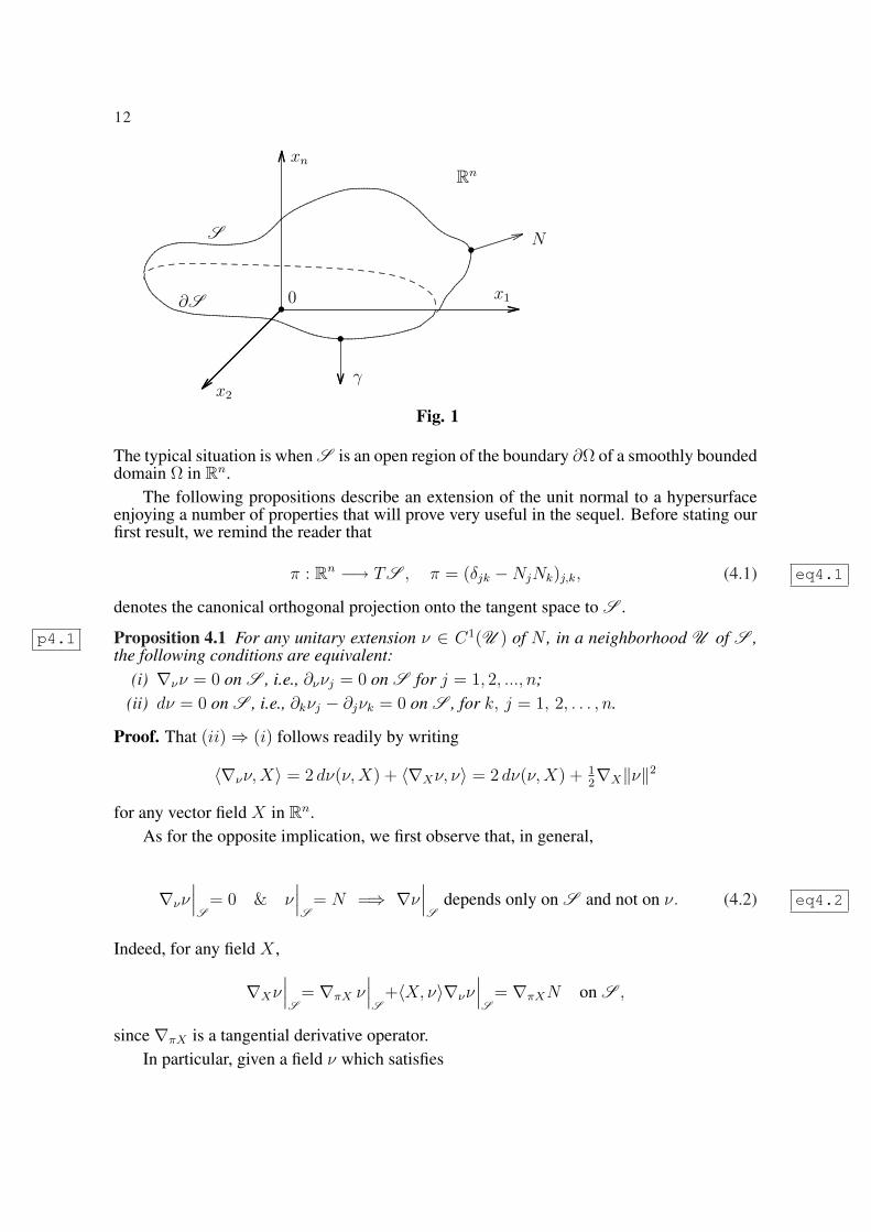
Fig. 1

The typical situation is when S is an open region of the boundary ∂Ω of a smoothly boundeddomain Ω in Rn.

The following propositions describe an extension of the unit normal to a hypersurfaceenjoying a number of properties that will prove very useful in the sequel. Before stating ourfirst result, we remind the reader that

π : Rn −→ TS , π = (δjk −NjNk)j,k, (4.1) eq4.1

denotes the canonical orthogonal projection onto the tangent space to S .

p4.1 Proposition 4.1 For any unitary extension ν ∈ C1(U ) of N , in a neighborhood U of S ,the following conditions are equivalent:

(i) ∇νν = 0 on S , i.e., ∂ννj = 0 on S for j = 1, 2, ..., n;(ii) dν = 0 on S , i.e., ∂kνj − ∂jνk = 0 on S , for k, j = 1, 2, . . . , n.

Proof. That (ii) ⇒ (i) follows readily by writing

〈∇νν, X〉 = 2 dν(ν, X) + 〈∇Xν, ν〉 = 2 dν(ν, X) + 12∇X‖ν‖2

for any vector field X in Rn.As for the opposite implication, we first observe that, in general,

∇νν∣∣∣S

= 0 & ν∣∣∣S

= N =⇒ ∇ν∣∣∣S

depends only on S and not on ν. (4.2) eq4.2

Indeed, for any field X ,

∇Xν∣∣∣S

= ∇πX ν∣∣∣S

+〈X, ν〉∇νν∣∣∣S

= ∇πXN on S ,

since ∇πX is a tangential derivative operator.In particular, given a field ν which satisfies

4. DISTINGUISHED EXTENSIONS OF THE UNIT NORMAL TO A HYPERSURFACE 13

‖ν‖ = 1 near S , ν = N on S , and ∇νν = 0 on S , (4.3) eq4.3

it follows that dν∣∣∣S

depends intrinsically on the hypersurface S .

Let us now consider a particular extension. To set the stage, let r : Rn → R be a functionof class Ck with the property that r = 0 on S and dr 6= 0 in some neighborhood U of S .For example, r can be taken to be the “signed” distance to S , defined as dist (x, S ) for xabove S and −dist (x, S ) for x below S , first in some neighborhood of S then extendedto the whole Rn.

In particular, dr/‖dr‖ is a unitary extension of N , the normal to S . Upon noting thatdr/‖dr‖ = d(r/‖dr‖) on S , we finally, take

ν := d(

r‖dr‖

)/∥∥∥d(

r‖dr‖

)∥∥∥

in some neighborhood U of S . Clearly, ‖ν‖ = 1 in U and

dν = d2(

r‖dr‖

)/∥∥∥d(

r‖dr‖

)∥∥∥− d(

r‖dr‖

)∧ d

∥∥∥d(

r‖dr‖

)∥∥∥−1

.

Recall now that d2 = 0 in Rn so that the first term in the right-side above is zero. Next,

d(r/‖dr‖) = N on S , so that∥∥∥d

(r

‖dr‖

)∥∥∥−1

= 1 on S . Since the differential operatorN ∧ d =

∑j<k(Nj∂k −Nk∂j)dxj ∧ dxk contains only tangential derivatives (cf. (

eq5.105.10) and

the discussion in §5), it follows that the second term in the right-side above is also zero. Allin all, dν = 0 on S .

In particular, by the implication already proved (i.e. (ii) ⇒ (i)) it follows that ν satisfies(i). Hence, since this particular field satisfies dν = 0 on S , the above discussion impliesthat any other extension of N as in (

eq4.34.3) has this property.

The proof of the proposition is therefore finished.

In the sequel, given a hypersurface S and an extended unit vector ν in a neighborhoodU of S , we shall tacitly assume that the projection π has been extended to U by settingπ = I − 〈·, ν〉ν = ν ∨ (ν ∧ · ).

p4.2 Proposition 4.2 For any unitary extension ν ∈ C1(U ) of N , in a neighborhood U of thehypersurface S , the quantity div ν|S depends only on S and not on the particular ν itself.In fact,

G := div ν satisfies G∣∣∣S

= (n− 1)H , (4.4) eq4.4

where H stands for the mean curvature of S .

Proof. Fix a local ortho-normal frame T1, . . . , Tn−1 in some open subset O of S . In partic-ular,

T1, . . . , Tn−1, ν is a local orthonormal basis for Rn (4.5) eq4.5

14

at each point on O . Next, recall that

div ν∣∣∣O= Tr (∇ν)

∣∣∣O=

n∑j=1

〈∇Tjν, Tj〉|O =

n−1∑j=1

〈∇TjN, Tj〉 on O,

since 〈∇νν, ν〉 = 12∇ν‖ν‖2 = 0 in U . Now, the last expression above is clearly independent

of ν. Since O is arbitrary, this justifies the first claim of the proposition.To prove the second part, i.e. the identity (

eq4.44.4), it suffices to perform calculations for a

particular choice of the unitary extension ν of N . If, locally, S is given as the graph of afunction ϕ : Rn−1 → R, pick

ν(x) :=(∇ϕ(x′),−1)√1 + ‖∇ϕ(x′)‖2

, ∀x = (x′, xn) ∈ Rn ≡ Rn−1 × R.

Then (div ν

)(x′, ϕ(x′)) =

n−1∑j=1

∂

∂xj

[ ∂jϕ(x′)√1 + ‖∇ϕ(x′)‖2

], ∀x′ ∈ Rn−1.

As is well-known, the right hand-side above is n − 1 times the mean-curvature at the point(x′, ϕ(x′)) on the graph of ϕ.

d4.3 Definition 4.3 Let S be a hypersurface in Rn with unit normal N . A vector filed ν ∈C1(U ), where U is a neighborhood of S , will be called an extended unit field for S ifν∣∣∣S

= N , ‖ν‖ = 1 in U , and if ν satisfies either one of the (equivalent) conditions listed inProposition

p4.14.1.

It is implicit in the course of the proof of Propositionp4.14.1 that each Ck, k ≥ 2, hypersur-

face S has a Ck−1 extended unit field (which, nonetheless, is not unique).

p4.4 Proposition 4.4 Let S be a hypersurface in Rn and fix an extended unit field ν in a neigh-borhood U of S . Then, for the n× n matrix valued function

R(x) := ∇ν(x) = (∂kνj(x))j,k, x ∈ U , (4.6) eq4.6

the following are true:(i) Rν = 0 in U ;(ii) Tr (R) = G in U .

Moreover, when restricted to the hypersurface S , R has the following additional properties:(iii) R depends only on S and not on the choice of the extended unit ν.(iv) R> = R on S ;(v) (Ru)|S is tangential to S for any vector field u : S → Rn. In fact,

R∣∣∣TS

= −W (4.7) eq4.7

the opposite of the Weingarten map of S . In particular, the eigenvalues κj1≤j≤n−1 of−R (at points on S ) as an operator on TS are the principal curvatures of S , whereas itsdeterminant is Gauss’s total curvature of S ;

5. CALCULUS OF TANGENTIAL DIFFERENTIAL OPERATORS 15

Proof. First, Rν = ∇‖ν‖2 = 0 in U , justifying (i). Next, (ii) follows from (eq4.44.4) and (

eq4.64.6),

whereas (iii) − (iv) are direct consequences of (eq4.24.2) and (i) in Proposition

p4.14.1. Next, the

first part of(v) is a consequence (i) and (iii). As for (eq4.74.7), for each X ∈ TS we write

W X = −∇SX ν = −π(∇Xν) = −∇Xν = −RX

since, as we have just seen, ∇Xν = RX is tangential to S .

Remark. If vj ∈ TS , 1 ≤ j ≤ n − 1, form an orthonormal system of TS and areeigenvectors for the matrix −R, i.e. −Rvj = κjvj , 1 ≤ j ≤ n− 1, it follows that

∂vjν = −κj vj, 1 ≤ j ≤ n− 1.

5 CALCULUS OF TANGENTIAL DIFFERENTIAL OPERATORS

Let

Pu =(∑

j,β

aαβj ∂juβ +

∑

β

bαβuβ

)α

(5.1) eq5.1

be a first-order differential operator acting on vector-valued functions u = (uβ)β in Rn. Itsadjoint (in Rn) is then defined by

P ∗v =(−

∑j,α

∂j(aαβj vα) +

∑α

bαβvα

)β

(5.2) eq5.2

and its symbol is given by the matrix-valued function

σ(P ; ξ) :=(∑

j

aαβj ξj

)αβ

, ξ = (ξj)1≤j≤n. (5.3) eq5.3

We say that P is a weakly tangential operator to the hypersurface S , with unit normal N ,provided

σ(P ; N) = 0 on the hypersurface S . (5.4) eq5.4

If Ω ⊂ Rn is a smooth, bounded domain, and if P is a first-order operator, weakly tangentialto ∂Ω, then P can be integrated by parts over Ω without boundary terms, i.e.

∫

Ω

〈Pu, v〉 dx =

∫

Ω

〈u, P ∗v〉 dx, (5.5) eq5.5

for any C1, vector-valued functions u, v in Ω.Next, call P a strongly tangential operator to S provided there exists an extended unit

field ν such that

σ(P ; ν) = 0 in an open neighborhood of S in Rn. (5.6) eq5.6

16

Since σ(P ∗; ξ) = −σ(P ; ξ)>, for each ξ ∈ Rn, it follows that P is weakly/strongly tangentialif and only if P ∗ is so.

Recall that dS, ds stand for the volume elements on S , ∂S , and that N , γ denote theoutward unit vectors to S and ∂S , respectively.

t5.1 Theorem 5.1 Let P be a first-order differential operator as in (eq5.15.1) with coefficients of class

C1 in Rn. If P is weakly tangential to S then P extends uniquely to an operator (stilldenoted by P ) which acts on C1 vector-valued functions defined on S . In fact, this extensionsatisfies

(Pu)∣∣∣S

= P(u|S

)(5.7) eq5.7

for every C1 function u defined in a neighborhood of S . Furthermore, similar considera-tions apply to P ∗, and

∫

S

〈Pu, v〉 dS =

∫

S

〈u, P ∗v〉 dS +∑

j,α,β

∫

S

(∂Naαβj )Njuβvα dS

+

∮

∂S

〈σ(P ; γ)u, v〉 ds, (5.8) eq5.8

for any C1, vector-valued functions u, v defined on S .If in fact P is strongly tangential to S then the following integration by parts formula

holds:∫

S

〈Pu, v〉 dS =

∫

S

〈u, P ∗v〉 dS +

∮

∂S

〈σ(P ; γ)u, v〉 ds, (5.9) eq5.9

for any C1, vector-valued functions u, v defined on S .

As a corollary, for a first-order differential operator P which is weakly tangential to ahypersurface S , its transposed inRn differs from its transposed in the sense of integration byparts along S by a zero-order term. In fact, this term disappears if P is strongly tangentialto S .

Let S be a fixed, C2-hypersurface in Rn, with unit normal N and consider the first-order, tangential differential operators (Stokes’s derivatives)

Mjk := Nj∂k −Nk∂j, 1 ≤ j, k ≤ n. (5.10) eq5.10

If ν is an extended unit field for S , then each surface operator Mjk extends accordinglyby setting Mjk = νj∂k − νk∂j . In the sequel, we shall make no distinction between thisoperator in Rn and (

eq5.105.10).

l5.2 Lemma 5.2 The following formulas hold:(i) Mjk = −Mkj , for each 1 ≤ j, k ≤ n;(ii) ∂k =

∑nj=1 νjMjk + νk∂ν , for each 1 ≤ k ≤ n;

(iii)∑n

k=1 Mjkνk = νjG , for each 1 ≤ j ≤ n.

5. CALCULUS OF TANGENTIAL DIFFERENTIAL OPERATORS 17

Proof. The first two identities are immediate from definitions. To see the last one, we write

n∑

k=1

Mjkνk =n∑

k=1

(νj∂k − νk∂j)νk = νj div ν − 12∂j(‖ν‖2) = νjG ,

as desired.

Hereafter, we let dS and ds denote the ‘volume’ element on S and ∂S , respectively.Also, let γ = (γ1, ..., γn) stand for the outward unit vector to ∂S , relative to S .

l5.3 Lemma 5.3 For any C1, real-valued functions f, g on S and any 1 ≤ j < k ≤ n, thereholds

∫

S

[(Mjkf)g + f(Mjkg)

]dS =

∮

∂S

(Njγk −Nkγj)fg ds. (5.11) eq5.11

Proof. Let ι : S → Rn, : ∂S → S , and i : ∂S → Rn be the natural inclusionoperators. In particular, i = ι . It is then essentially well-known that, with the superscript‘star’ denoting pull-back,

ι∗(dx1 ∧ ... ∧ dxj ∧ ... ∧ dxn) = (−1)j+1Nj dS, j = 1, 2, ..., n, (5.12) eq5.12

and, for 1 ≤ j < k ≤ n,

i∗(dx1 ∧ ... ∧ dxj ∧ ... ∧ dxk ∧ ... ∧ dxn) = (−1)j+k+1(Njγk −Nkγj) ds. (5.13) eq5.13

Here, as usual, the ‘hat’ symbol indicates omission. Now, if we set

ω := (−1)j+k+1fg dx1 ∧ ... ∧ dxj ∧ ... ∧ dxk ∧ ... ∧ dxn,

then

dω = (−1)k∂j(fg) dx1 ∧ ... ∧ dxk ∧ ... ∧ dxn

−(−1)j∂k(fg) dx1 ∧ ... ∧ dxk ∧ ... ∧ dxn. (5.14) eq5.14

Consequently,

dS ι∗(ω) = ι∗(dRnω) = [Nj∂k(fg)−Nk∂j(fg)] dS (5.15) eq5.15

whereas

∗(ι∗ω) = (ι )∗ω = i∗ω = (Njγk −Nkγj)fg ds. (5.16) eq5.16

The desired conclusion then follows from Stokes’s classical formula

18

∫

S

dS (ι∗ω) =

∮

∂S

∗(ι∗ω) (5.17) eq5.17

with the help of (eq5.155.15), (

eq5.165.16).

After this preamble, we are ready to present the

Proof of Theoremt5.15.1. Fix two arbitrary C1, vector-valued functions defined in a neighbor-

hood of S . For starters we note that, on S ,

(Pu)α =∑

j,β

aαβj ∂juβ +

∑

β

bαβ∂juβ

= −∑

j,k,β

aαβj NkMjkuβ +

∑

j,β

aαβj Nj∂Nuβ +

∑

β

bαβ∂juβ

= −∑

j,k,β

aαβj NkMjkuβ +

∑

β

bαβ∂juβ + (σ(P ; N)∇Nu)α

= −∑

j,k,β

aαβj NkMjkuβ, +

∑

β

bαβ∂juβ (5.18) eq5.18

on account of the weak tangentiality of P . If we now take the last expression above as adefinition of P on functions which are defined only on S , then (

eq5.75.7) holds.

Next, fix an extended unit field ν for S . Using (eq5.115.11) and integrating by parts we get

∫

S

〈Pu, v〉 dS = −∑

j,k

∑

α,β

∫

S

aαβj νk(Mjkuβ)vα dS +

∑

α,β

∫

S

bαβ∂juβvα dS

=∑

j,k

∑

α,β

∫

S

uβ[Mjk(aαβj νkvα)] dS +

∑

α,β

∫

S

bαβ∂juβvα dS

−∮

∂S

∑

j,k

∑

α,β

(νjγk − νkγj)aαβj νkuβvα ds. (5.19) eq5.19

In the boundary integral, we write

−∑

j,k

∑

α,β

[νjγkaαβj νkuβvα − νkγja

αβj νkuβvα]

= −〈γ, ν〉〈σ(P ; ν)u, v〉+ ‖ν‖2〈σ(P ; γ)u, v〉= 〈σ(P ; γ)u, v〉, (5.20) eq5.20

since 〈γ, ν〉 = 0 on S ; this term is in agreement with (eq5.85.8).

5. CALCULUS OF TANGENTIAL DIFFERENTIAL OPERATORS 19

As for the first surface integral in the rightmost expression in (eq5.195.19), use Leibnitz’s rule

to expand

∑

j,k

∑

α,β

uβ[Mjk(aαβj νkvα)] =

∑

j,k

∑

α,β

uβaαβj vαMjkνk +

∑

j,k

∑

α,β

uβνkMjk(aαβj vα)

= : I + II. (5.21) eq5.21

With regard to I above, we invoke (iii) in Lemmal5.25.2 to write

I =∑

j,α,β

uβaαβj vανjG = 〈σ(P ; ν)u, v〉G = 0, (5.22) eq5.22

once again due to (eq5.65.6). Turning our attention to II , recall from (ii) in Lemma

l5.25.2 that∑n

k=1 νkMjk = νj∂ν − ∂j . Thus,

II +∑

α,β

bαβuβvα = −∑

j,α,β

uβ∂j(aαβj vα) +

∑

j,α,β

uβνj∂ν(aαβj vα) +

∑

α,β

bαβuβvα

= 〈u, P ∗v〉+∑

j,α,β

[uβνj(∂νa

αβj )vα + uβνja

αβj ∂νvα

]

= 〈u, P ∗v〉+∑

j,α,β

[uβ∂ν(νja

αβj )vα − uβ(∂ννj)a

αβj vα

]

+〈σ(P ; ν)u,∇νv〉= 〈u, P ∗v〉+ 〈[∂νσ(P ; ν)]u, v〉 − 〈σ(P ;∇νν)u, v〉

+〈σ(P ; ν)u,∇νv〉. (5.23) eq5.23

Thanks to the weak tangentiality of P , the last term in the last line above vanishes on S ;in fact, since ∇νν = 0 on S so does the next-to-the-last term. Finally, 〈[∂νσ(P ; ν)]u, v〉 =∑

j,α,β(∂Naαβj )Njuβvα on S , after some simple algebra. Thus, ultimately,

II +∑

α,β

bαβ∂juβvα = 〈u, P ∗v〉+∑

j,α,β

(∂Naαβj )Njuβvα on S .

This, in concert with (eq5.195.19)-(

eq5.205.20) and (

eq5.225.22), finishes the proof of (

eq5.85.8).

In the case when P is strongly tangent the identity also follows from what we haveproved so far since, in this scenario, ∂νσ(P ; ν) = 0 by definition.

Remark. By iteration, an identity similar in spirit to (eq5.95.9) holds for higher order differential

operators which are successive compositions of first-order differential operators, stronglytangential to S .

The Stokes derivative operators Mjk = νj∂k−νk∂j , introduced in connection with a hy-persurface S (with ν denoting an extended unit field for S ), are clearly strongly tangential

20

to S , since σ(Mjk; ξ) = νjξk − νkξj . As M ∗jk = ∂k(νj · )− ∂j(νk · ) which becomes −Mjk

on S , it follows that, a posteriori, Lemmal5.35.3 is a special case of Theorem

t5.15.1.

In this connection, let us also point out that ν∧d, acting on scalar functions on S , is nat-urally identified with the skew-symmetric matrix whose entries are the Stokesian derivatives,in the sense that

ν ∧ d = 12

n∑

j,k=1

Mjk dxj ∧ dxk =∑

1≤j<k≤n

Mjk dxj ∧ dxk. (5.24) eq5.24

Of special interest for us in this paper are the so-called Gunter derivatives

Dj := ∂j − νj∂ν = ∂j −n∑

k=1

νjνk∂k , j = 1, 2, ..., n. (5.25) eq5.25

We set

Df :=(D1f, D2f, ..., Dnf

), for scalar-valued functions, (5.26) eq5.26

D •u :=n∑

j=1

Djuj, if u = (u1, ..., un). (5.27) eq5.27

For further reference, below we collect some of the most basic properties of this systemof differential operators.

p5.4 Proposition 5.4 The following relations are valid:

(i) Dj =n∑

k=1

νkMkj , for each 1 ≤ j ≤ n;

(ii) Mjk = νjDk − νkDj for each 1 ≤ j, k ≤ n;

(iii)n∑

j=1

νjDj = 0 andn∑

j=1

Djνj = G .

(iv) [Dj,Dk] = νj(∇νk •∇)− νk(∇νj •∇) on S , for each 1 ≤ j, k ≤ n;(v) for every C1 functions f, g on S , and every 1 ≤ j ≤ n,

∫

S

(Djf)g dS =

∫

S

[−f(Djg) + NjG fg

]dS +

∮

∂S

γjfg ds. (5.28) eq5.28

Proof. The first three identities are simple consequences of definitions. To prove (iv) wefirst note that

DjDk = (∂j − νj∂ν)(∂k − νk∂ν) (5.29) eq5.29

= ∂j∂k − (∂jνk)∂ν −n∑

l=1

[νk(∂jνl)∂l + νkνl∂j∂l + νjνl∂l∂k

]+ νjνk∂

2ν

5. CALCULUS OF TANGENTIAL DIFFERENTIAL OPERATORS 21

where the second equality utilizes the fact that ∂ννk = 0 on S (cf. (i) in Propositionp4.14.1). If

we now observe, with the aid of (ii) in Propositionp4.14.1, that the expression

∂j∂k − (∂jνk)∂ν −n∑

l=1

[νkνl∂j∂l + νjνl∂l∂k

]+ νjνk∂

2ν

is symmetric in j and k, then the desired commutator identity follows from (eq5.295.29).

Turning to (v), note that Dj is a first-order differential operator defined in a neighbor-hood of S in Rn, and whose principal symbol is σ(Dj; ξ) = ξj − νj〈ξ, ν〉, for ξ ∈ Rn. Inparticular, Dj is strongly tangential to S , and σ(Dj; γ) = γj . Thus, (

eq5.285.28) will follow from

Theoremt5.15.1 as soon as the transposed of Dj in Rn is properly identified. To this end, we

compute

(Dj)∗ =

(∂j − νj

n∑

k=1

νk∂k

)∗= −∂j +

n∑

k=1

∂k(νkνj) = −Dj + νjG + ∂ννj (5.30) eq5.30

and observe that, when further restricted to S , the last term vanishes, as desired.

Other important examples of strongly tangential, first-order differential operators areoffered by

P1 := div − ∂ν〈·, ν〉, with P ∗1 = −∇+ (∂ν · )ν + G ν,

P2 := ∇νπ − ν ∨ d, with P ∗2 = −π∇ν + G π − δ(ν ∧ · ), (5.31) eq5.31

P3 := div π(·), with P ∗3 = −π∇.

Indeed,

σ(P1; ξ) = 〈ξ, ·〉−〈ν, ξ〉〈ν, ·〉, σ(P2; ξ) = 〈ξ, ν〉 π−ν∨(ξ∧·) and σ(P3; ξ) = 〈ξ, π(·)〉,so that (

eq5.65.6) is easily verified in each case.

We are interested to express these operators in terms of the Gunter derivatives (eq5.255.25)

rather than the ordinary ∂j’s. A general result to this effect is as follows.

p5.5 Proposition 5.5 Let

Pu =(∑

j,β

aαβj ∂juβ +

∑

β

bαβuβ

)α

(5.32) eq5.32

be a first-order differential operator which is strongly tangential to a hypersurface S . ThenP remains unchanged (in a neighborhood of S ) if one formally replaces ∂j by Dj , i.e.

Pu =(∑

j,β

aαβj Djuβ +

∑

β

bαβuβ

)α. (5.33) eq5.33

22

Proof. The two right sides in (eq5.325.32) and (

eq5.335.33) differ by σ(P ; ν)(∇νu).

When used in conjunction with the operators (eq5.315.31), the above proposition gives

p5.6 Proposition 5.6 For an arbitrary vector field u we have

P1u = D • (π u) + G 〈ν, u〉 − 〈Ru, ν〉,P2u = D(〈ν, u〉) + 〈ν, u〉∇νν −R>u, (5.34) eq5.34

P3u = D • (π u)− 〈Ru, ν〉,

where R :=(∂kνj

)j,k

has been introduced in Propositionp4.44.4.

Proof. These follow by invoking Propositionp5.55.5 plus a straightforward calculation. In the

case of P2, it helps to first notice that, if u = (u1, ..., un) ≡ u1dx1 + ... + undxn, then

ν ∨ du =n∑

j=1

( n∑

k=1

νk∂kuj

)dxj −

n∑j=1

( n∑

k=1

νk∂juk

)dxj

= ∇νu−∇〈ν, u〉+ R>u. (5.35) eq5.35

We leave the details to the interested reader.

6 EXPRESSING SURFACE DIFFERENTIAL OPERATORS IN SPATIAL COORDINATES

Throughout this section we shall regard the hypersurface S as a Riemannian manifoldwith the natural metric inherited from Rn. The goal is to describe the action of divS on TS ,as well as that of gradS and ∆S on scalar functions on S , it terms of the Gunter derivatives(eq5.255.25). Our main result in this regard is as follows.

t6.1 Theorem 6.1 For any smooth, tangential field u = (u1, ..., un) on S we have

divS u = D •u =n∑

j=1

Djuj. (6.1) eq6.1

Also, for any smooth, real-valued function f on S ,

gradS f = Df =(D1f, D2f, ..., Dnf

). (6.2) eq6.2

In particular, the Laplace-Beltrami operator ∆S on S takes the form

∆S f = divS gradS f = D •

(Df

)=

n∑j=1

D2j f. (6.3) eq6.3

6. EXPRESSING SURFACE DIFFERENTIAL OPERATORS IN SPATIAL COORDINATES 23

Proof. The operators in question have local character, so it suffices to carry out calculationsin some fixed, small open subset O of S . With π denoting the orthogonal projection ontoTS , we consider the n× n matrix A(u) uniquely defined by the requirement that

〈A(u)X, Y 〉 = 〈∇πX u, πY 〉, ∀X, Y ∈ Rn. (6.4) eq6.4

Also, fix an ortho-normal frame T1, . . . , Tn−1 to TS in O , so that

T1, . . . , Tn−1, ν is an orthonormal basis for Rn (6.5) eq6.5

at each point in O . Thus, if we set Tn := ν then the vectors T1, . . . , Tn form an ortho-normalbasis in Rn, when evaluated at points in O .

Going further, if ∇S stands for the Levi-Civita connection on S then, according to(eq2.232.23), ∇S

X Y = π(∇XY ) for any X, Y ∈ TS . For any u ∈ TS supported in O , we maytherefore write

divS u =n−1∑j=1

〈∇STj

u, Tj〉 =n∑

j=1

〈∇Tju, Tj〉 =

n∑j=1

〈A(u)Tj, Tj〉. (6.6) eq6.6

At this point we claim that the last term in (eq6.66.6) does not depend on the particular basis of

Rn. Indeed, this is folklore and, for the reader’s convenience, a couple of such statementsare collected below.

l6.2 Lemma 6.2 If A is a n× n matrix with real entries then

Tr A =n∑

j=1

〈ATj, Tj〉 (6.7) eq6.7

for any orthonormal basis Tjj in Rn. In particular, the sum in the right side above isindependent of the particular orthonormal basis Tjj .

Also, if B is another n× n matrix with real entries, then

Tr (AB>) =n∑

j,k=1

〈ATj, Tk〉〈BTj, Tk〉 (6.8) eq6.8

is independent of the particular orthonormal basis Tjj .

Returning to the task of carrying on the calculation initiated in (eq6.66.6) we denote by ej :=

(0, . . . , 1, . . . , 0), for j = 1, . . . , n, the usual canonical basis in Rn, and by

ej := πej = ej − νjν =n∑

k=1

(δjk − νjνk)ek, j = 1, . . . , n. (6.9) eq6.9

the projection of ej onto TS . One simple yet important observation is the fact that theGunter operators are directional derivatives corresponding to the ej’s, i.e.

Dj = ∇ej, j = 1, 2, ..., n.

24

Relying on these observations, we may now continue –invoking Lemmal6.26.2– with

divS u =n∑

j=1

〈A(u)ej, ej〉 =n∑

j=1

〈∇eju, ej〉 =

n∑

j,k=1

(Djuk)〈ek, ej〉

=n∑

j=1

Djuj −n∑

j,k=1

νj(Djuk)νk =n∑

j=1

Djuj, (6.10) eq6.10

justifying (eq6.16.1).

Turning attention to the operator gradS , we note that if f is scalar and u ∈ TS , bothsmooth and supported away from ∂S , then

∫

S

〈gradS f, u〉 dS = −∫

S

fdivS u dS = −∫

S

f

n∑j=1

Djuj

= −∫

S

n∑j=1

(D∗j f)uj dS =

∫

S

n∑j=1

ujDjf dS.

=

∫

S

〈Df, u〉 dS. (6.11) eq6.11

Here we have used (eq5.285.28) and the tangentiality of u. Since both gradS f and Df are tan-

gential, it follows that (eq6.116.11) holds for arbitrary smooth vector fields u : S → Rn (not just

tangential). We may therefore conclude that gradS f = Df , as desired.Finally, (

eq6.36.3) follows from (

eq2.32.3) and what we have proved so far. This finishes the proof

of the theorem.

Define

(∂2Nf)|S :=

∑

j,k

NjNk(∂j∂kf)|S = (∂2νf)|S . (6.12) eq6.12

c6.3new Corollary 6.3 For any smooth scalar function f , defined in a neighborhood of S , thereholds

(∆Rnf

)∣∣∣S

= ∆S (f |S ) + G (∂Nf)|S + (∂2Nf)|S . (6.13) eq6.13

To keep matters in perspective, it is illuminating to work out in detail the case when S =Sn−1, the unit sphere in Rn. In this scenario, one can choose ν(x) := x/‖x‖, x ∈ Rn \ 0, sothat G := div ν = (n − 1)/‖x‖, and ∂ν =

∑(xj/‖x‖)∂j = ∂r, the radial derivative in Rn.

Then (eq6.136.13) becomes, after a rescaling, the classical formula

∆Rn =∂2

∂r2+

n− 1

r

∂

∂r+

1

r2∆Sn−1 .

6. EXPRESSING SURFACE DIFFERENTIAL OPERATORS IN SPATIAL COORDINATES 25

Proof. The identity (eq6.136.13) follows by expanding

∆S =n∑

j=1

D2j =

n∑j=1

(∂j − νj∂ν)(∂j − νj∂ν)

and performing straightforward algebraic manipulations based on Propositionp4.14.1. We omit

the straightforward details.

c6.3 Corollary 6.4 For any smooth scalar function f , and any smooth vector field u defined in aneighborhood of S , the following identities hold:

gradS (〈N, u|S 〉) = [∇ν(π u)]|S −N ∨ (du)|S + R(u|S ), (6.14) eq6.14

(div u)∣∣S

= divS (π u|S ) + G 〈u|S , N〉+ 〈(∇Nu)|S , N〉, (6.15) eq6.15

divS (π u|S ) = div(π u)|S , (6.16) eq6.16

gradS (f |S ) = [π∇f ]|S , (6.17) eq6.17

where R is as in (eq4.64.6).

Proof. To justify (eq6.146.14)-(

eq6.166.16), in the light of (

eq5.75.7), we simply point to the alternative repre-

sentations of the operators P1, P2, P3 in (eq5.315.31) and (

eq5.345.34), keeping in mind that ∇νν = 0 on

S . Finally, (eq6.176.17) is the adjoint of (

eq6.166.16).

c6.4 Corollary 6.5 For the Stokes derivatives from (eq5.105.10), here holds

12

n∑

j,k=1

M 2jk =

∑

1≤j<k≤n

M 2jk = ∆S on S . (6.18) eq6.18

Proof. Denote by Q the second-order differential operator in the left side of (eq6.186.18), and fix

two scalar functions f, g on S , supported away from the boundary. We may then write

∫

S

(Qf)g dS = −∑

1≤j<k≤n

∫

S

(Mjkf)(Mjkg) dS = −∫

S

〈ν ∧ df, ν ∧ dg〉 dS

=

∫

S

[div (π∇f)]g dS (6.19) eq6.19

thanks to (eq5.115.11), (

eq5.245.24), and the fact that P := ν ∧d is strongly tangential to S , with adjoint

P ∗ = δ(ν ∨ · ). Since f and g are arbitrary, it follows that

Q|S = div (π∇·)|S = divS (π∇ · |S ) = divS (gradS · |S ) = ∆S on S ,

by (eq6.166.16)-(

eq6.176.17) and (

eq6.36.3).

A number of related identities, at least for n = 3 and special extensions of the unitnormal, can be found in

DL[DL],

Ce[Ce],

Co[Co],

KGBB[KGBB],

NDS[NDS],

Ne[Ne] and the references therein.

26

7 THE IDENTIFICATION OF THE SURFACE LAME OPERATOR AND RELATED PDO’S

Recall from §3 that the geometric-differential definition of the deformation tensor DefSand the Lame operator L on S are, respectively,

DefS (X)(Y, Z) := 12〈∇S

Y X, Z〉+ 〈∇SZ X, Y 〉, ∀X, Y, Z,∈ TS , (7.1) eq7.1

and

L := −2µ Def∗S DefS + λ gradS divS . (7.2) eq7.2

The main result in this section, dealing with the identification of Lame operator (eq7.27.2), is as

follows.

t7.1 Theorem 7.1 The following identities hold on S :

L = µ π∆S + (λ + µ) gradS divS + µ G R

= µ π (D •D) + (λ + µ) D(D • ) + µ G R. (7.3) eq7.3

In particular, L : TS −→ TS is a second-order, strongly-elliptic, formally self-adjoint,differential operator on S .

Proof. Given the local nature of the identities we seek to prove, it suffices to work locally,in a small open subset O of S , where an ortho-normal frame T1, . . . , Tn−1 to TS has beenfixed. As before, we set Tn := ν so that Tj1≤j≤n is an ortho-normal basis for Rn, at pointsin O .

Next, fix u a tangent field to S supported in O , and let A(u) = (ajk(u))j,k be the n× nmatrix uniquely defined by the requirement that

〈A(u)X, Y 〉 := DefS (u)(πX, πY ), ∀X, Y ∈ Rn. (7.4) eq7.4

It is then clear that

[A(u)]> = A(u) and A(u)ν = 0. (7.5) eq7.5

For each j, k we can write

ajk(u) = 〈A(u)ek, ej〉 = DefS (u)(ek, ej)

= 12

(〈∇S

eku, ej〉+ 〈∇S

eju, ek〉

)= 1

2

(〈∇eku, ej〉+ 〈∇ej

u, ek〉)

= 12

n∑r=1

[(Dkur)(δjr − νjνr) + (Djur)(δkr − νkνr)

]. (7.6) eq7.6

To further simplify (eq7.67.6) we note that, on S ,

7. THE IDENTIFICATION OF THE SURFACE LAME OPERATOR AND RELATED PDO’S 27

n∑r=1

(Dkur)νjνr = Dk

( n∑r=1

urνr

)−

n∑r=1

ur(Dkνr)νj = −n∑

r=1

ur(∂rνk)νj, (7.7) eq7.7

for every j, k. In the last step above we have used the fact that 〈u, ν〉 = 0 on S , and (i) inProposition

p4.14.1. Combining (

eq7.67.6) and (

eq7.77.7) we eventually arrive at

ajk(u) = 12

[Dkuj + Djuk +∇u(νjνk)

]. (7.8) eq7.8

Now if v is also a smooth vector field, tangent to S , we get –keeping in mind thatDefS (u) is symmetric– that

〈DefS (u), DefS (v)〉 = Tr(DefS (u)DefS (v)

)

=n−1∑

j,k=1

DefS (u)(Tj, Tk)DefS (v)(Tj, Tk)

=n−1∑

j,k=1

〈A(u)Tj, Tk〉〈A(v)Tj, Tk〉 =n∑

j,k=1

〈A(u)Tj, Tk〉〈A(v)Tj, Tk〉

=n∑

j,k=1

〈A(u)ej, ek〉〈A(v)ej, ek〉 =n∑

j,k=1

ajk(u)ajk(v). (7.9) eq7.9

The second to the last equality in (eq7.97.9) relies on the second part of Lemma

l6.26.2. Integrating,

this leads to

4n∑

j,k=1

∫

S

ajk(u)ajk(v) dS

=

∫

S

[Dkuj + Djuk +∇u(νjνk)

][Dkvj + Djvk +∇v(νjνk)

]dS. (7.10) eq7.10

To proceed, we first consider

∫

S

n∑

j,k=1

(Djuk + Dkuj)(Djvk + Dkvj) dS = 2

∫

S

n∑

j,k=1

D∗j (Djuk + Dkuj)vk dS

= 2

∫

S

n∑

j,k=1

[−vkD

2j uk − vkDjDkuj + G νj(Djuk)vk + G νj(Dkuj)vk

]dS

=: 2(I + II + III + IV ). (7.11) eq7.11

28

It is immediate that I = − ∫S〈∆S u, v〉 dS, while

n∑j=1

νjDj = 0 on S forces III = 0. Next

we concentrate on IV . By using Propositionp4.14.1 and the tangentiality of u we get

IV =

∫

S

Gn∑

k=1

vk

(Dk

( n∑j=1

νjuj

)−

n∑j=1

uj(∂kνj − νk∂ννj)

)dS

= −∫

S

G 〈Ru, v〉 dS. (7.12) eq7.12

As for II , we employ the commutator identity from (iv) in Propositionp5.45.4 plus the fact that

u and v are tangential to write

n∑

j,k=1

vkDjDkuj =n∑

j,k=1

vkDkDjuj +n∑

j,k=1

vk[Dj,Dk]uj

=n∑

j,k=1

vkDkDjuj +n∑

j,k=1

(∂kνl)(∂lνj)ujvk (7.13) eq7.13

on S . Thus,

−II =

∫

S

( n∑

j,k=1

vkDkDjuj −n∑

l,j,k=1

(∂kνl)(∂lνj)ujvk

)dS

=

∫

S

〈gradS divS u, v〉 dS −∫

S

〈R2u, v〉 dS. (7.14) eq7.14

At this point, we may therefore conclude that

∫

S

n∑

j,k=1

(Djuk + Dkuj)(Djvk + Dkvj) dS

= 2

∫

S

〈−∆S u− gradS divS u + R2u− G Ru, v〉 dS. (7.15) eq7.15

We now proceed to analyze the remaining terms in (eq7.107.10). More precisely, we still have

to take into account the terms containing either ∇u(νjνk) or ∇v(νjνk). We start with theidentity

7. THE IDENTIFICATION OF THE SURFACE LAME OPERATOR AND RELATED PDO’S 29

n∑

j,k=1

(Dkuj)∇v(νjνk)

=n∑

j,k=1

νk(Dkuj)∇vνj +n∑

k=1

(∇vνk)(Dk

( n∑j=1

ujνj

)−n∑

j=1

uj∂kνj

)

= −n∑

k,j=1

(∇vνk)(∇uνk) = −〈R2u, v〉, (7.16) eq7.16

valid at points on S . There are four such terms in (eq7.107.10), i.e. containing either ∇u(νjνk) or

∇v(νjνk), but not both. An inspection of the above calculation shows that, on S , they areall equal to −〈R2u, v〉.

We are still left with computing

n∑

j,k=1

∇u(νjνk)∇v(νjνk) =n∑

j,k,r,l=1

[ur(∂rνj)νk + ur(∂rνk)νj

][vl(∂lνj)νk + vl(∂lνk)νj

]

= 2〈R2u, v〉+ 2n∑

k,r,l=1

ur(∂rνk)vlνk12∂l

( n∑j=1

ν2j

)= 2〈R2u, v〉, (7.17) eq7.17

on S . At this point we combine all the above to get

4n∑

j,k=1

∫

S

ajk(u)ajk(v) dS = 2

∫

S

〈−∆S u− gradS divS u− G Ru, v〉 dS. (7.18) eq7.18

Having deduced (eq7.187.18), we may now compute

4

∫

S

〈Def∗S DefS (u), v〉 dS =

∫

S

〈DefS (u), DefS (v)〉 dS

= 4n∑

j,k=1

∫

S

ajk(u)ajk(v) dS (7.19) eq7.19

= 2

∫

S

〈−∆S u− gradS divS u− G Ru , v〉 dS.

Thus,

4 Def∗S DefS = −2 π∆S − 2 gradS divS − 2 G R, (7.20) eq7.20

30

since the tangential vectors fields u, v are arbitrary (note that here we use the fact that theimage of R is a subspace of TS ).

The first identity in (eq7.37.3) now follows easily from (

eq7.207.20) and (

eq7.27.2). The remaining iden-

tity in (eq7.37.3) then follows from what we have just proved and Theorem

eq6.16.1.

Next recall the definition of the Hodge-Laplacian acting on 1-forms, i.e.

∆HL := −dS d∗S − d∗S dS : Λ1TS −→ Λ1TS (7.21) eq7.21

where dS is the exterior derivative operator on S , and d∗S its formal adjoint. As explainedin §2, 1-forms on S are naturally identified with tangent fields to S so, from now on, weshall think of ∆HL as mapping TS into itself.

As pointed out in §2, the Hodge-Laplacian (eq7.217.21) is related to

∆BL := −(∇S )∗∇S , (7.22) eq7.22

the Bochner-Laplacian on S , via the Weitzenbock identity

∆BL = ∆HL + RicS . (7.23) eq7.23

Our aim is to find alternative expressions for all these objects, starting with the Ricci tensor.

t7.2 Theorem 7.2 On S , there holds

RicS = −R2 + G R. (7.24) eq7.24

In particular, when n = 3 –i.e. for a two-dimensional surface S in R3– the above identityreduces to

RicS = −det W = −K , (7.25) eq7.25

where K is the Gaussian curvature of the surface S . Consequently,

Proof. Let us denote by RS the Riemann curvature tensor of S . Since Rn has zero cur-vature, it follows from Gauss’s Theorema Egregium that, if X , Y , Z, W are tangent vectorfields to S , then

〈RS (X,Y )Z,W 〉 = 〈IIS (X, W ), IIS (Y, Z)〉 − 〈IIS (Y, W ), IIS (X, Z)〉. (7.26) eq7.26

See, e.g.,Ta2[Ta2], Vol. II, p. 481. In this context, the second fundamental form of S becomes

IIS (X, Y ) = ∇XY −∇SX Y = 〈∇XY, ν〉ν, by (

eq2.232.23). Thus, on S ,

〈RS (X, Y )Z,W 〉 = 〈∇XW, ν〉〈∇Y Z, ν〉 − 〈∇Y W, ν〉〈∇XZ, ν〉= 〈W,∇Xν〉〈Z,∇Y ν〉 − 〈W,∇Y ν〉〈Z,∇Xν〉= 〈RW,X〉〈RZ, Y 〉 − 〈RW,Y 〉〈RZ, X〉. (7.27) eq7.27

7. THE IDENTIFICATION OF THE SURFACE LAME OPERATOR AND RELATED PDO’S 31

For the second equality in (eq7.277.27) we have used the fact that X , Y , Z, and W are tangential,

so in particular, ∇X〈W, ν〉 = 0, ∇Y 〈Z, ν〉 = 0, ∇Y 〈W, ν〉 = 0, and ∇X〈Z, ν〉 = 0 on S .Next, recall from (

eq2.212.21) the definition of the Ricci tensor, i.e.

Ric (X,Y )S :=n−1∑j=1

〈RS (Tj, Y )X, Tj〉, (7.28) eq7.28

where T1, . . . , Tn−1 is, locally, an orthonormal basis in TS , and X , Y are arbitrary tangen-tial vector fields to S . If we set Tn := ν, and employ (

eq7.277.27) together with Rν = 0, we

obtain

n−1∑j=1

〈RS (Tj, Y )X,Tj〉 =n∑

j=1

[〈RTj, Tj〉〈RX, Y 〉 − 〈RTj, Y 〉〈RX, Tj〉]

= G 〈RX, Y 〉 − 〈RY,

n∑j=1

〈Tj, RX〉Tj〉 = −〈(R2 − G R)X,Y 〉, (7.29) eq7.29

which takes care of (eq7.247.24).

Finally, (eq7.257.25) is a consequence of what we have proved so far, (

eq4.74.7), and the elementary

identity A2 − (Tr A)2A = −(det A)I , valid for any 2× 2 matrix A.

t7.3 Theorem 7.3 The following identities are valid:

∆BL = π∆S + R2, (7.30) eq7.30

∆HL = π∆S + 2R2 − G R. (7.31) eq7.31

Proof. In order to identify the Bochner-Laplacian operator ∆BL on S we observe that, withu tangential field fixed, if the matrix A(u) satisfies 〈A(u)X, Y 〉 = 〈∇S

πX u, πY 〉, for eachX,Y ∈ Rn then, much as in the proof of Theorem

t6.16.1,

ajk(u) := 〈A(u)ek, ej〉 = 〈∇eku, ej〉 = Dkuj −

n∑r=1

νjνrDk(ur). (7.32) eq7.32

On account of this and Lemmal6.26.2 we can now write

∫

S

〈(∇S )∗∇S u, v〉 dS =

∫

S

〈∇S u,∇S v〉 dS =n−1∑

j,k=1

∫

S

〈∇STj

u, Tk〉〈∇STj

v, Tk〉 dS

=n∑

j,k=1

∫

S

〈A(u)Tj, Tk〉〈A(v)Tj, Tk〉 dS =n∑

j,k=1

∫

S

ajk(u)ajk(v) dS

32

=n∑

j,k=1

∫

S

[DkujDkvj

−n∑

r=1

νjνrDjurDkvj −n∑

l=1

νjνlDkujDkvl +n∑

r,l=1

νrνlDkurDkvl

]dS

=n∑

j,k=1

∫

S

[(D∗

kDkuj)vj −n∑

r=1

urvj(∂kνr)(∂kνj)]dS

=

∫

S

〈−∆S u−R2u, v〉 dS. (7.33) eq7.33

In the next-to-the-last equality, we have applied the following identity to the terms under theintegral sign in the fourth line above:

n∑r=1

νrDswr = Ds

( n∑r=1

νrwr

)−

n∑r=1

wrDsνr = −n∑

r=1

wr∂sνr, on S , (7.34) eq7.34

valid for any tangential vector field w, and any index s ∈ 1, . . . , n. In turn, the identity(eq7.347.34) can be seen from a direct computation (recall that ∂ννr = 0 on S ). Finally, to justify

the last equality in (eq7.337.33), it suffices to recall (

eq5.305.30), (

eq6.36.3) and the fact that

n∑k=1

νkDk = 0.

The conclusion is that (eq7.307.30) holds. Finally, the identity (

eq7.307.30) in concert with (

eq7.237.23) and

(eq7.247.24) implies (

eq7.317.31).

Recall now from\protect \it Note Added in Proof[EM, Note Added in Proof, pp.161-162],

Ta[Ta] (cf. also the remark at

the end of this paper), andTa2[Ta2, Vol. III], that the Navier-Stokes system for a velocity field

u, tangent to S , and a (scalar-valued) pressure function p on S reads

∂u

∂t− 2 Def∗S DefS (u) +∇S

u u− gradS p = ~f in S × (0,∞),

divS u = 0, in S . (7.35) eq7.35

t7.4 Theorem 7.4 The Navier-Stokes system (eq7.357.35) is equivalent to

∂u

∂t− π∇uu + π∆S u + G Ru− gradS p = ~f in S × (0,∞),

divS u = 0 in S . (7.36) eq7.36

Proof. This is a direct consequence of (eq7.207.20) and (

eq2.232.23).

8. FURTHER APPLICATIONS 33

8 FURTHER APPLICATIONS

We debut by briefly discussing a number of boundary value problems for tangentialoperators to a smooth hypersurface S in Rn, for which ∂S is a Lipschitz submanifold ofcodimension one in S .

For starters, the treatment of the classical Dirichlet and Neumann boundary problemsfor the Laplace-Beltrami operator in Lipschitz subdomains of Riemannian manifolds fromMT[MT] translate into the well-posedness results about

(D •D)u = f in S ,

u∣∣∣∂S

or ∇γu prescribed on ∂S .

In order to be more specific, consider the case of the Lame system on S and, to set thestage, let Hs,p stand for the scale of Lp-based Sobolev spaces, 1 < p < ∞, s ∈ R.

t8.1 Theorem 8.1 Assume that S is a C∞ hypersurface in Rn with unit normal N and a Lips-chitz boundary ∂S . If the Lame moduli λ, µ ∈ R satisfy

µ > 0, 2µ + λ > 0, (8.1) eq8.1

then the boundary value problem

u = (u1, ..., un) ∈ Hs+1/2,2(S ,Rn),

〈u,N〉 = 0 in S ,

µ π (D •D)u + (λ + µ) D(D •u) + µ G Ru = 0 in S ,

u∣∣∣∂S

= ~f ∈ Hs,2(∂S ,Rn), 〈~f, N〉 = 0 on ∂S ,

(8.2) eq8.2

is well-posed for each 0 ≤ s ≤ 1.Furthermore, if the traction operator is defined by

Traction u = 2µ Def (u)γ + µ 〈Ru, γ〉ν + λ (D • u)γ (8.3) eq8.3

whereDef (u) :=

(Dkuj + Djuk

)1≤j ,k≤n

(recall that γ ∈ TS is the outward unit normal to ∂S ), then

u = (u1, ..., un) ∈ H3/2−s,2(S ,Rn),

〈u,N〉 = 0 in S ,

µ π (D •D)u + (λ + µ) D(D •u) + µ G Ru = 0 in S ,

Traction u∣∣∣∂S

= ~f ∈ H−s,2(∂S ,Rn),

(8.4) eq8.4

is Fredholm solvable, of index zero, for each 0 ≤ s ≤ 1.

34

For a discussion pertaining to the physical significance of (eq8.18.1) see

LL[LL], p. 11. The proof

relies on the corresponding statement for the boundary problem for the intrinsic Lame oper-ator for S (viewed as an abstract Riemannian manifold) from

Mi[Mi], and the identifications

(eq7.37.3).

t8.2 Theorem 8.2 Let S be a C∞ hypersurface in Rn with unit normal N and Lipschitz bound-ary ∂S . Then the boundary value problem

u = (u1, ..., un) ∈ Hs+1/2,2(S ,Rn), p ∈ Hs−1/2,2(S ),

〈u,N〉 = 0 in S ,∫

Sp dS = 0,

π (D •D)u + G Ru−Dp = 0 in S ,

D •u = 0 in S ,

u∣∣∣∂S

= ~f ∈ Hs,2(∂S ,Rn), 〈~f,N〉 = 0 on ∂S ,∮

∂S〈~f, γ〉 ds = 0,

(8.5) eq8.5

is well-posed for each 0 ≤ s ≤ 1.

Once again, this follows by translating the main result inMT2[MT2] by means of the identi-

fications (eq7.37.3).

Finally, natural boundary value problems for the Hodge-Laplacian on Lipschitz sub-domains of (general) Riemannian manifolds have been recently treated in

MMT[MMT]. When

phrased in terms of the operators studied in this paper, these yield the following sampleresult:

t8.3 Theorem 8.3 Let S be a C∞ hypersurface in Rn with unit normal N and Lipschitz bound-ary ∂S . Then the boundary value problem

u = (u1, ..., un) ∈ H1/2,2(S ,Rn), 〈u, N〉 = 0 in S ,

π (D •D)u + (2R2 − G R)u = 0 in S ,

(N ∧ d)u = 0 in S ,

〈γ, u|∂S 〉 = ~f ∈ L2(∂S ,Rn), 〈~f, N〉 = 0, 〈~f, γ〉 = 0 on ∂S ,

(8.6) eq8.6

is Fredholm solvable, of index zero.

We conclude with a regularity result, very useful in electromagnetic theory (see, e.g.,Ne[Ne] for a discussion in a lower dimensional case).

t8.4 Theorem 8.4 Let Ω be a smooth, bounded subdomain of Rn and set S := ∂Ω. As usual,we let N stand for the outward unit normal to ∂Ω and denote by π the orthogonal projectiononto TS . Then for each field u = (u1, ..., un) ∈ L2(Ω,Rn) such that

n∑j=1

∂juj ∈ L2(Ω) and ∂juk − ∂kuj ∈ L2(Ω) for each 1 ≤ j, k ≤ n, (8.7) eq8.7

8. FURTHER APPLICATIONS 35

the following statements are equivalent:(i) u ∈ H1,2(Ω,Rn);

(ii) πu|S ∈ H−1/2,2(S ,Rn) and divS (πu|S ) ∈ H−1/2,2(S );

(iii) 〈N, (u|S )〉 ∈ H1/2,2(S ).

Proof. The departure point is to write, via (eq2.222.22) and repeated integrations by parts (cf.

(eq2.172.17)), that

∫

Ω

‖∇u‖2 dx =

∫

Ω

〈∇∗∇u, u〉 dx +

∫

S

〈∇Nu, u〉 dS

=

∫

Ω

〈(dδ + δd)u, u〉 dx +

∫

S

〈∇Nu, u〉 dS

=

∫

Ω

[‖du‖2 + ‖δu‖2

]dx +

∫

S

〈Pu, u〉 dS (8.8) eq8.8

where

Pu := ∇νu− ν ∨ du− (div u)ν. (8.9) eq8.9

Next, we decompose∇νu = ∇ν(πu)+∇ν(〈u, ν〉ν), and use (eq6.146.14)-(

eq6.156.15) to replace the last

two terms in (eq8.98.9). This procedure yields

〈Pu, u〉 = 〈gradS (〈ν, u〉), πu〉 − divS (πu)〈ν, u〉 − G 〈ν, u〉2 − 〈Rπu, πu〉, (8.10) eq8.10

so that, all in all,

∫

Ω

‖∇u‖2 dx =

∫

Ω

[‖du‖2 + ‖δu‖2

]dx

−∫

S

[2〈ν, u〉divS (πu) + G 〈ν, u〉2 + 〈Rπu, πu〉

]dS. (8.11) eq8.11

The boundary integral in (eq8.118.11) can be estimated by a (fixed) multiple of

‖〈ν, u〉‖H1/2,2(S ) · ‖divS (πu)‖H−1/2,2(S )

+‖〈ν, u〉‖H1/2,2(S ) · ‖〈ν, u〉‖H−1/2,2(S )

+‖πu‖H1/2,2(S ) · ‖πu‖H−1/2,2(S ) (8.12) eq8.12

In concert with standard trace theorems, to the effect that

36

‖u‖H1/2,2(S ,Rn) ≤ C[‖∇u‖L2(Ω,Rn2

) + ‖u‖L2(Ω,Rn)

],

‖〈N, u〉‖H−1/2,2(S ,Rn) ≤ C[‖div u‖L2(Ω) + ‖u‖L2(Ω,Rn)

], (8.13) eq8.13

‖πu‖H−1/2,2(S ,Rn) ≤ C[∑

j,k

‖∂juk − ∂kuj‖L2(Ω) + ‖u‖L2(Ω,Rn)

],

this implies equivalence of norms

‖u‖H1,2(Ω,Rn) ≈∑

j,k

‖∂juk − ∂kuj‖L2(Ω) +∑

j

‖∂juj‖L2(Ω)

+‖πu‖H−1/2,2(S ) + ‖divS (πu)‖H−1/2,2(S ) (8.14) eq8.14

≈∑

j,k

‖∂juk − ∂kuj‖L2(Ω) +∑

j

‖∂juj‖L2(Ω) + ‖〈N, u〉‖H1/2,2(S ).

With this a priori estimate at hand, the desired conclusion follows from a standard densityargument.

BIBLIOGRAPHY 37

BIBLIOGRAPHY

AN [AN] H. Ammari and J.-C. Nedelec, Generalized impedance boundary conditions for the Maxwellequations as singular perturbations problems, Commun. PDE, Vol. 24 (1999), 821–849.

AC [AC] L. Andersson, P.T. Chrusciel, Cauchy data for vacuum Einstein equations and obstructions tosmoothness of null infinity. Phys. Rev. Lett. 70, 1993, 2829–2832.

Ar [Ar] R. Aris, Vectors, Tensors, and the Basic Equations of Fluid Mechanics, Prentice-Hall, Engle-wood Cliffs, N.J., 1962.

Be [Be] A. Bendali, Numerical analysis of the exterior boundary value problem for the time-harmonicMaxwell equations by a boundary finite element method. Part I: The continuous problem, Math-ematics of Computation, Vol. 43 (1984), 29–46.

BGS [BGS] B.D. Bonner, I.G. Graham and V.P. Smyshlyaev, The computation of conical diffraction coef-ficients in high-frequency acoustic wave scattering, Preprint N103047, Isaac Newton Institute,Cambridge, July 2003.

Ce [Ce] M. Cessenat, Mathematical methods in electromagnetism. Linear theory and applications, Se-ries on Advances in Mathematics for Applied Sciences, Vol. 41, World Scientific Publishing Co.,Inc., River Edge, NJ, 1996.

Ci [Ci] P.G. Ciarlet, Introduction to Linear Shell Theory, Series in Applied Mathematics, Vol. 1,Gauthier-Villars, Editions Scientifiques et Medicales Elsevier, Paris, North-Holland, Amsterdam,1998.

Ci2 [Ci2] P.G. Ciarlet, Mathematical Elasticity, Vol. III: Theory of Shells, Studies in Mathematics andApplications, 29, Elsevier, North-Holland, Amsterdam, 2000.

Co [Co] M. Costabel, A coercive bilinear form for Maxwell’s equations, J. Math. Anal. Appl., Vol. 157(1991), 527–541.

DL [DL] R. Dautray and J.-L. Lions, Mathematical Analysis and Numerical Methods for Science andTechnology, Springer-Verlag, Berlin, 1990.

Du [Du] R. Duduchava, The Green formula and layer potentials, Integral Equations and Operator The-ory, Vol. 41 (2001), 127–178.

EM [EM] D.G. Ebin and J. Marsden, Groups of diffeomorphisms and the notion of an incompressiblefluid, Ann. of Math., Vol. 92 (1970), 102–163.

Go [Go] A.L. Gol’denveızer, Theory of elastic thin shells, Translation from the Russian edited byG. Herrmann. International Series of Monographs on Aeronautics and Astronautics, publishedfor the American Society of Mechanical Engineers by Pergamon Press, Oxford-London-NewYork-Paris, 1961.

Gu [Gu] N. Gunter, Potential Theory and its Application to the Basic Problems of Mathematical Physics,Fizmatgiz, Moscow 1953 (Russian. Translation in French: Gauthier–Villars, Paris 1994).

38 BIBLIOGRAPHY

Ha [Ha] W. Haack, Elementare Differentialgeometrie (German), Lehrbucher und Monographien ausdem Gebiete der exakten Wissenschaften, 20, Basel-Stuttgart: Birkhauser Verlag, VIII, 1955.

Ko [Ko] V.A. Kondratev, Boundary value problems for elliptic equations in domains with conical orangular points, (Russian), Trudy Moskov. Mat. Obsc, Vol. 16 (1967), 209–292.

KGBB [KGBB] V. Kupradze, T. Gegelia, M. Basheleishvili and T. Burchuladze, Three-Dimensional Prob-lems of the Mathematical Theory of Elasticity and Thermoelasticity, North-Holland, Amsterdam1979 (Russian edition: Nauka, Moscow 1976).

LL [LL] L.D. Landau and E.M. Lifshitz, Theory of Elasticity, Pergamon, 1970.

MaMi [MaMi] U. Massari and M. Miranda, Minimal Surfaces of Codimension One, North-Holland Mathe-matics Studies, 91. Mathematical Notes (95). North-Holland Publishing Co., Amsterdam, 1984.

MMT [MMT] D. Mitrea, M. Mitrea and M. Taylor, Layer potentials, the Hodge Laplacian, and globalboundary problems in nonsmooth Riemannian manifolds, Memoirs Am. Math. Soc., Vol. 713,2001.

Mi [Mi] M. Mitrea, The Neumann problem for the Lame and Stokes systems on Lipschitz subdomains ofRiemannian manifolds, preprint, (2003).

MT [MT] M. Mitrea and M. Taylor, Potential theory on Lipschitz domains in Riemannian manifolds:Sobolev-Besov space results and the Poisson problem, Journal of Functional Analysis, Vol. 176(2000), 1–79.

MT2 [MT2] M. Mitrea and M. Taylor, Navier-Stokes equations on Lipschitz domains in Riemannian man-ifolds, Math. Ann., Vol. 321 (2001), 955–987.

NDS [NDS] D. Natroshvili, A. Djagmaidze, M. Svanadze, Problems of the linear theory of elastic mix-tures, Tbilisi University Press, Tbilisi, 1986 (Russian).

Ne [Ne] J.-C. Nedelec, Acoustic and Electromagnetic Equations, Applied Math. Sci., Vol. 144, Springer-Verlag, New York, 2001.

Sm [Sm] V. P. Smyshlyaev, Diffraction by conical surfaces at high frequencies, Wave Motion Vol. 12,No.4, 329-339 (1990).

Ta [Ta] M. Taylor, Analysis on Morrey spaces and applications to Navier-Stokes and other evolutionequations, Comm. Partial Differential Equations, Vol. 17 (1992), 1407–1456.

Ta2 [Ta2] M. Taylor, Partial Differential Equations, Vol. I-III, Springer-Verlag, 1996.

TZ [TZ] R. Temam and M. Ziane, Navier-Stokes equations in thin spherical domains, OptimizationMethods in Partial Differential Equations, Contemporaty Math., AMS, Vol. 209, pp. 281–314.

TW [TW] R. Temam and S.H. Wang, Inertial forms of Navier-Stokes equations on the sphere, J. Funct.Anal., Vol. 117 (1993), 215–242.

BIBLIOGRAPHY 39

——————————————–

R. DuduchavaA.Razmadze Mathematical InstituteAcademy of Sciences of Georgia1, M.Alexidze str.Tbilisi 93, Georgia

E-mail: duduch@rmi.acnet.ge

D. MitreaDepartment of MathematicsUniversity of Missouri-ColumbiaMO 65211, USA

E-mail: dorina@math.missouri.edu

M. MitreaDepartment of MathematicsUniversity of Missouri-ColumbiaMO 65211, USA

E-mail: marius@math.missouri.edu

2000 AMS Classification Numbers: 58G03, 58G20, 74B05, 35J25, 35J55, 35Q30

Key words and phrases: tangential differential operators, integration by parts on sur-faces, the Laplace-Beltrami operator on surfaces, the Lame system on surfaces, boundaryproblems on surfaces