Differential ode
306
ORDINARY DIFFERENTIAL EQUATIONS GABRIEL NAGY Mathematics Department, Michigan State University, East Lansing, MI, 48824. MARCH 18, 2014 Summary. This is an introduction to ordinary differential equations. We describe the main ideas to solve certain differential equations, like first order scalar equations, second order linear equations, and systems of linear equations. We use power series methods to solve variable coefficients second order linear equations. We introduce Laplace trans- form methods to find solutions to constant coefficients equations with generalized source functions. We provide a brief introduction to boundary value problems, Sturm-Liouville problems, and Fourier Series expansions. We end these notes solving our first partial differential equation, the Heat Equation. We use the method of separation of variables, hence solutions to the partial differential equation are obtained solving infinitely many ordinary differential equations. x 2 x 1 x 1 x 2 a b 0 1
-
Upload
30gm-unilorin -
Category
Documents
-
view
266 -
download
0
description
Transcript of Differential ode

ORDINARY DIFFERENTIAL EQUATIONS
GABRIEL NAGY
Mathematics Department,
Michigan State University,East Lansing, MI, 48824.
MARCH 18, 2014
Summary. This is an introduction to ordinary differential equations. We describe themain ideas to solve certain differential equations, like first order scalar equations, second
order linear equations, and systems of linear equations. We use power series methodsto solve variable coefficients second order linear equations. We introduce Laplace trans-form methods to find solutions to constant coefficients equations with generalized source
functions. We provide a brief introduction to boundary value problems, Sturm-Liouvilleproblems, and Fourier Series expansions. We end these notes solving our first partialdifferential equation, the Heat Equation. We use the method of separation of variables,hence solutions to the partial differential equation are obtained solving infinitely many
ordinary differential equations.
x2
x1
x1
x2
ab
0
1

G. NAGY – ODE March 18, 2014 I
Contents
Chapter 1. First Order Equations 11.1. Linear Constant Coefficients Equations 21.1.1. Overview of Differential Equations 21.1.2. Linear Equations 31.1.3. Linear Equations with Constant Coefficients 41.1.4. The Initial Value Problem 71.1.5. Exercises 91.2. Linear Variable Coefficients Equations 101.2.1. Linear Equations with Variable Coefficients 101.2.2. The Initial Value Problem 121.2.3. The Bernoulli Equation 151.2.4. Exercises 181.3. Separable Equations 191.3.1. Separable Equations 191.3.2. Euler Homogeneous Equations 241.3.3. Exercises 281.4. Exact Equations 291.4.1. Exact Differential Equations 291.4.2. The Poincare Lemma 301.4.3. Solutions and a Geometric Interpretation 311.4.4. The Integrating Factor Method 341.4.5. The Integrating Factor for the Inverse Function 371.4.6. Exercises 391.5. Applications 401.5.1. Radioactive Decay 401.5.2. Newton’s Cooling Law 411.5.3. Salt in a Water Tank 421.5.4. Exercises 471.6. Nonlinear Equations 481.6.1. The Picard-Lindelof Theorem 481.6.2. Comparison Linear Nonlinear Equations 531.6.3. Direction Fields 561.6.4. Exercises 58
Chapter 2. Second Order Linear Equations 592.1. Variable Coefficients 602.1.1. The Initial Value Problem 602.1.2. Homogeneous Equations 622.1.3. The Wronskian Function 662.1.4. Abel’s Theorem 682.1.5. Exercises 702.2. Reduction of Order Methods 712.2.1. Special Second Order Equations 712.2.2. Reduction of Order Method 742.2.3. Exercises 772.3. Homogeneous Constant Coefficients Equations 782.3.1. The Roots of the Characteristic Polynomial 782.3.2. Real Solutions for Complex Roots 82

II G. NAGY – ODE march 18, 2014
2.3.3. Constructive proof of Theorem 2.3.2 842.3.4. Exercises 872.4. Repeated Roots 882.5. Applications 892.5.1. Review of Constant Coefficient Equations 892.5.2. Undamped Mechanical Oscillations 892.5.3. Damped Mechanical Oscillations 922.5.4. Electrical Oscillations 942.5.5. Exercises 962.6. Nonhomogeneous Equations 972.6.1. The General Solution Formula 972.6.2. The Undetermined Coefficients Method 982.6.3. The Variation of Parameters Method 1022.6.4. Exercises 1072.7. Variation of Parameters 108
Chapter 3. Power Series Solutions 1093.1. Solutions Near Regular Points 1103.1.1. Review of Power Series 1103.1.2. Solutions Near Regular Points 1133.1.3. The Legendre Equation 1203.1.4. Exercises 1233.2. The Euler Equidimensional Equation 1243.2.1. The Roots of the Indicial Polynomial 1243.2.2. Real Solutions for Complex Roots 1283.2.3. Exercises 1303.3. Solutions Near Regular Singular Points 1313.3.1. Regular Singular Points 1313.3.2. The Frobenius Method 1343.3.3. Exercises 139
Chapter 4. The Laplace Transform 1404.1. Definition and Properties 1404.1.1. Review of improper integrals 1404.1.2. Definition of the Laplace Transform 1414.1.3. Properties of the Laplace Transform 1444.1.4. Exercises 1464.2. The Initial Value Problem 1474.2.1. Summary of the Laplace Transform method 1474.2.2. Exercises 1524.3. Discontinuous Sources 1534.3.1. The Step function 1534.3.2. The Laplace Transform of Step functions 1544.3.3. The Laplace Transform of translations 1554.3.4. Differential equations with discontinuous sources 1584.3.5. Exercises 1634.4. Generalized Sources 1644.4.1. The Dirac delta generalized function 1644.4.2. The Laplace Transform of the Dirac delta 1664.4.3. The fundamental solution 168

G. NAGY – ODE March 18, 2014 III
4.4.4. Exercises 1724.5. Convolution Solutions 1734.5.1. The convolution of two functions 1734.5.2. The Laplace Transform of a convolution 1744.5.3. The solution decomposition Theorem 1764.5.4. Exercises 178
Chapter 5. Systems of Differential Equations 1795.1. Linear Differential Systems 1795.1.1. First order linear systems 1795.1.2. Order transformation 1815.1.3. The initial value problem 1835.1.4. Homogeneous systems 1845.1.5. The Wronskian and Abel’s Theorem 1875.1.6. Exercises 1915.2. Constant Coefficients Diagonalizable Systems 1925.2.1. Decoupling the systems 1925.2.2. Eigenvector solution formulas 1955.2.3. Alternative solution formulas 1975.2.4. Non-homogeneous systems 2025.2.5. Exercises 2055.3. Two-by-Two Constant Coefficients Systems 2065.3.1. The diagonalizable case 2065.3.2. Non-diagonalizable systems 2095.3.3. Exercises 2125.4. Two-by-Two Phase Portraits 2135.4.1. Real distinct eigenvalues 2145.4.2. Complex eigenvalues 2175.4.3. Repeated eigenvalues 2195.4.4. Exercises 2215.5. Non-Diagonalizable Systems 222
Chapter 6. Autonomous Systems and Stability 2236.1. Flows on the Line 2246.1.1. Autonomous Equations 2246.1.2. A Geometric Analysis 2266.1.3. Population Growth Models 2296.1.4. Linear Stability Analysis 2326.1.5. Exercises 2356.2. Flows on the Plane 2366.3. Linear Stability 236
Chapter 7. Boundary Value Problems 2377.1. Eigenvalue-Eigenfunction Problems 2377.1.1. Comparison: IVP and BVP 2377.1.2. Eigenvalue-eigenfunction problems 2417.1.3. Exercises 2467.2. Overview of Fourier Series 2477.2.1. Origins of Fourier series 2477.2.2. Fourier series 249

IV G. NAGY – ODE march 18, 2014
7.2.3. Even and odd functions 2537.2.4. Exercises 2557.3. Application: The heat Equation 256
Chapter 8. Review of Linear Algebra 2578.1. Systems of Algebraic Equations 2578.1.1. Linear algebraic systems 2578.1.2. Gauss elimination operations 2618.1.3. Linearly dependence 2648.1.4. Exercises 2658.2. Matrix Algebra 2668.2.1. A matrix is a function 2668.2.2. Matrix operations 2678.2.3. The inverse matrix 2718.2.4. Determinants 2738.2.5. Exercises 2768.3. Diagonalizable Matrices 2778.3.1. Eigenvalues and eigenvectors 2778.3.2. Diagonalizable matrices 2838.3.3. The exponential of a matrix 2878.3.4. Exercises 290
Chapter 9. Appendices 291Appendix A. Review Complex Numbers 291Appendix B. Review Exercises 291Appendix C. Practice Exams 291Appendix D. Answers to Exercises 291References 301

G. NAGY – ODE March 18, 2014 1
Chapter 1. First Order Equations
We start our study of differential equations in the same way the pioneers in this field did. Weshow particular techniques to solve particular types of first order differential equations. Thetechniques were developed in the eighteen and nineteen centuries and the equations includelinear equations, separable equations, Euler homogeneous equations, and exact equations.Soon this way of studying differential equations reached a dead end. Most of the differentialequations cannot be solved by any of the techniques presented in the first sections of thischapter. People then tried something different. Instead of solving the equations they tried toshow whether an equation has solutions or not, and what properties such solution may have.This is less information than obtaining the solution, but it is still valuable information. Theresults of these efforts are shown in the last sections of this chapter. We present Theoremsdescribing the existence and uniqueness of solutions to a wide class of differential equations.
t
y
π
2
0
−π2
y′ = 2 cos(t) cos(y)

2 G. NAGY – ODE march 18, 2014
1.1. Linear Constant Coefficients Equations
1.1.1. Overview of Differential Equations. A differential equation is an equation, theunknown is a function, and both the function and its derivatives may appear in the equation.Differential equations are essential for a mathematical description of nature. They are at thecore of many physical theories: Newton’s and Lagrange equations for classical mechanics,Maxwell’s equations for classical electromagnetism, Schrodinger’s equation for quantummechanics, and Einstein’s equation for the general theory of gravitation, to mention a fewof them. The following examples show how differential equations look like.
(a) Newton’s second law of motion for a single particle. The unknown is the position inspace of the particle, x(t), at the time t. From a mathematical point of view the unknownis a single variable vector-valued function in space. This function is usually written asx or x : R → R3, where the function domain is every t ∈ R, and the function range isany point in space x(t) ∈ R3. The differential equation is
md2x
dt2(t) = f (t,x(t)),
where the positive constant m is the mass of the particle and f : R × R3 → R3 is theforce acting on the particle, which depends on the time t and the position in space x.This is the well-known law of motion mass times acceleration equals force.
(b) The time decay of a radioactive substance. The unknown is a scalar-valued functionu : R → R, where u(t) is the concentration of the radioactive substance at the time t.The differential equation is
du
dt(t) = −k u(t),
where k is a positive constant. The equation says the higher the material concentrationthe faster it decays.
(c) The wave equation, which describes waves propagating in a media. An example is sound,where pressure waves propagate in the air. The unknown is a scalar-valued function oftwo variables u : R × R3 → R, where u(t,x) is a perturbation in the air density at thetime t and point x = (x, y, z) in space. (We used the same notation for vectors andpoints, although they are different type of objects.) The equation is
∂ttu(t,x) = v2[∂xxu(t,x) + ∂yyu(t,x) + ∂zzu(t,x)
],
where v is a positive constant describing the wave speed, and we have used the notation∂ to mean partial derivative.
(d) The heat conduction equation, which describes the variation of temperature in a solidmaterial. The unknown is a scalar-valued function u : R×R3 → R, where u(t,x) is thetemperature at time t and the point x = (x, y, z) in the solid. The equation is
∂tu(t,x) = k[∂xxu(t,x) + ∂yyu(t,x) + ∂zzu(t,x)
],
where k is a positive constant representing thermal properties of the material.
The equations in examples (a) and (b) are called ordinary differential equations (ODE),since the unknown function depends on a single independent variable, t in these examples.The equations in examples (c) and (d) are called partial differential equations (PDE),since the unknown function depends on two or more independent variables, t, x, y, and z inthese examples, and their partial derivatives appear in the equations.
The order of a differential equation is the highest derivative order that appears in theequation. Newton’s equation in Example (a) is second order, the time decay equation inExample (b) is first order, the wave equation in Example (c) is second order is time and

G. NAGY – ODE March 18, 2014 3
space variables, and the heat equation in Example (d) is first order in time and second orderin space variables.
1.1.2. Linear Equations. A good start is a precise definition of the differential equationswe are about to study in this Chapter. We use primes to denote derivatives,
dy
dt(t) = y′(t).
This is a compact notation and we use it when there is no risk of confusion.
Definition 1.1.1. A first order ordinary differential equation in the unknown y is
y′(t) = f(t, y(t)), (1.1.1)
where y : R → R is the unknown function and f : R2 → R is a given function. The equationin (1.1.1) is called linear iff the function with values f(t, y) is linear on its second argument;that is, there exist functions a, b : R → R such that
y′(t) = a(t) y(t) + b(t), f(t, y) = a(t) y + b(t). (1.1.2)
A different sign convention for Eq. (1.1.2) may be found in the literature. For example,Boyce-DiPrima [3] writes it as y′ = −a y + b. The sign choice in front of function a is justa convention. Some people like the negative sign, because later on, when they write theequation as y′ + a y = b, they get a plus sign on the left-hand side. In any case, we stickhere to the convention y′ = ay + b.
A linear first order equation has constant coefficients iff both functions a and b inEq. (1.1.2) are constants. Otherwise, the equation has variable coefficients.
Example 1.1.1:
(a) An example of a first order linear ODE is the equation
y′(t) = 2 y(t) + 3.
In this case, the right-hand side is given by the function f(t, y) = 2y + 3, where we cansee that a(t) = 2 and b(t) = 3. Since these coefficients do not depend on t, this is aconstant coefficients equation.
(b) Another example of a first order linear ODE is the equation
y′(t) = −2
ty(t) + 4t.
In this case, the right-hand side is given by the function f(t, y) = −2y/t + 4t, wherea(t) = −2/t and b(t) = 4t. Since the coefficients are non-constant functions of t, this isa variable coefficients equation. C
A function y : D ⊂ R → R is solution of the differential equation in (1.1.1) iff theequation is satisfied for all values of the independent variable t in the domain D of thefunction y.
Example 1.1.2: Show that y(t) = e2t − 3
2is solution of the equation y′(t) = 2 y(t) + 3.
Solution: We need to compute the left and right-hand sides of the equation and verifythey agree. On the one hand we compute y′(t) = 2e2t. On the other hand we compute
2 y(t) + 3 = 2(e2t − 3
2
)+ 3 = 2e2t.
We conclude that y′(t) = 2 y(t) + 3 for all t ∈ R. C
4 G. NAGY – ODE march 18, 2014
1.1.3. Linear Equations with Constant Coefficients. Constant coefficient equationsare simpler to solve than variable coefficient ones. There are many ways to solve them. In-tegrating each side of the equation, however, does not work. For example, take the equation
y′ = 2 y + 3,
and integrate on both sides,∫y′(t) dt = 2
∫y(t) dt+ 3t+ c, c ∈ R.
The fundamental Theorem of Calculus implies y(t) =∫y′(t) dt. Using this equality in the
equation above we get
y(t) = 2
∫y(t) dt+ 3t+ c.
We conclude that integrating both sides of the differential equation is not enough to findthe solution y. We still need to find a primitive of y. Since we do not know y, we cannotfind its primitive. The only thing we have done here is to rewrite the original differentialequation as an integral equation. That is why integrating both side of a linear equationdoes not work.
One needs a better idea to solve a linear differential equation. We describe here onepossibility, the integrating factor method. Multiply the differential equation by a particularlychosen non-zero function, called the integrating factor. Choose the integrating factor havingone important property. The whole equation is transformed into a total derivative of afunction, called potential function. Integrating the differential equation is now trivial, theresult is the potential function equal any constant. Any solution of the differential equationis obtained inverting the potential function. This whole idea is called the integrating factormethod.
In the next Section we generalize this idea to find solutions to variable coefficients linearODE, and in Section 1.4 we generalize this idea to certain non-linear differential equations.We now state in a theorem a precise formula for the solutions of constant coefficient linearequations.
Theorem 1.1.2 (Constant coefficients). The linear differential equation
y′(t) = a y(t) + b (1.1.3)
where a 6= 0, b are constants, has infinitely many solutions labeled by c ∈ R as follows,
y(t) = c eat − b
a. (1.1.4)
Remark: Theorem 1.1.2 says that Eq. (1.1.3) has infinitely many solutions, one solution foreach value of the constant c, which is not determined by the equation. This is reasonable.Since the differential equation contains one derivative of the unknown function y, findinga solution of the differential equation requires to compute an integral. Every indefiniteintegration introduces an integration constant. This is the origin of the constant c above.
Proof of Theorem 1.1.2: The integrating factor method is the key idea in the proof ofTheorem 1.1.2. Write the differential equation with the unknown function on one side only,
y′(t)− a y(t) = b,
and then multiply the differential equation by the exponential e−at, where the exponentis negative the constant coefficient a in the differential equation multiplied by t. This

G. NAGY – ODE March 18, 2014 5
exponential function is an integrating factor for the differential equation. The reason tochoose this particular function, e−at, is explained in Lemma 1.1.3, below. The result is[
y′(t)− a y(t)]e−at = b e−at ⇔ e−at y′(t)− a e−at y(t) = b e−at.
This exponential is chosen because of the following property,
−a e−at =(e−ay
)′.
Introducing this property into the differential equation we get
e−at y′(t) +(e−at
)′y(t) = b e−at.
Now the product rule for derivatives implies that the left-hand side above is a total derivative,[e−at y(t)
]′= b e−at.
At this point we can go one step further, writing the right-hand side in the differential
equation as b e−at =[− b
ae−at
]′. We obtain[
e−at y(t) +b
ae−at
]′= 0 ⇔
[(y(t) +
b
a
)e−at
]′= 0.
Hence, the whole differential equation is a total derivative. The whole differential equationis the total derivative of the function,
ψ(t, y(t)) =(y(t) +
b
a
)e−at,
called potential function. The equation now has the form
dψ
dt(t, y(t)) = 0.
It is simple to integrate the differential equation when written using a potential function,
ψ(t, y(t)) = c ⇔(y(t) +
b
a
)e−at = c.
Simple algebraic manipulations imply that
y(t) = c eat − b
a.
This establishes the Theorem. �Remarks:
(a) Why do we start the Proof of Theorem 1.1.2 multiplying the equation by the functione−at? At first sight it is not clear where this idea comes from. In Lemma 1.1.3 we showthat only functions proportional to the exponential e−at have the property needed tobe an integrating factor for the differential equation. In Lemma 1.1.3 we multiply thedifferential equation by a function µ, and only then one finds that this function mustbe µ(t) = c e−at.
(b) Since the function µ is used to multiply the original differential equation, we can freelychoose the function µ with c = 1, as we did in the proof of Theorem 1.1.2.
(c) It is important we understand the origin of the integrating factor e−at in order to extendresults from constant coefficients equations to variable coefficients equations.
The following Lemma states that those functions proportional to e−at are integrating factorsfor the differential equation in (1.1.3).

6 G. NAGY – ODE march 18, 2014
Lemma 1.1.3 (Integrating Factor). Given any differentiable function y and constant a,every function µ satisfying
(y′ − ay)µ = (yµ)′,
must be given by the expression below, for any c ∈ R,µ(t) = c e−at.
Proof of Lemma 1.1.3: Multiply Eq. (1.1.3) by a non-vanishing but otherwise arbitraryfunction with values µ(t), and order the terms in the equation as follows
µ(y′ − a y) = b µ. (1.1.5)
The key idea of the proof is to choose the function µ such that the following equation holds
µ(y′ − a y) =(µy
)′. (1.1.6)
This Eq. (1.1.6) is an equation for µ. To see that this is the case, rewrite it as follows,
µ y′ − aµy = µ′ y + µ y′ ⇔ −aµy = µ′ y ⇔ −aµ = µ′.
The function y does not appear on the equation on the far right above, making it an equationfor µ. So the same is true for Eq. (1.1.6). The equation above can be solved for µ as follows:
µ′
µ= −a ⇔
[ln(µ)
]′= −a.
Integrate the equation above,
ln(µ) = −at+ c0 ⇔ eln(µ) = e−at+c0 = e−atec0 ,
where c0 is an arbitrary constant. Denoting c = ec0 , the integrating factor is the non-vanishing function
µ(t) = c e−at.
This establishes the Lemma. �We first solve the problem in Example 1.1.3 below using the formula in Theorem 1.1.2.
Example 1.1.3: Find all solutions to the constant coefficient equation
y′ = 2y + 3 (1.1.7)
Solution: The equation above is the particular case of Eq. (1.1.3) given by a = 2 andb = 3. Therefore, using these values in the expression for the solution given in Eq. (1.1.4)we obtain
y(t) = ce2t − 3
2.
C
We now solve the same problem above following the steps given in the proof of Theo-rem 1.1.2. In this way we see how the ideas in the proof of the Theorem work in a particularexample.
Example 1.1.4: Find all solutions to the constant coefficient equation
y′ = 2y + 3 (1.1.8)
Solution: Write down the equation in (1.1.8) as follows,
y′ − 2y = 3.
Multiply this equation by the exponential e−2t, that is,
e−2ty′ − 2 e−2t y = 3 e−2t ⇔ e−2ty′ +(e−2t
)′y = 3 e−2t.

G. NAGY – ODE March 18, 2014 7
The equation on the far right above is
(e−2t y)′ = 3 e−2t.
Integrating on both sides get∫(e−2t y)′ dt =
∫3 e−2t dt+ c,
e−2t y = −3
2e−2t + c.
Multiplying the whole equation by e2t,
y(t) = c e2t − 3
2, c ∈ R.
C
y
t− 32
c > 0
c = 0
c < 0
Figure 1. A few solutionsto Eq. (1.1.8) for different c.
1.1.4. The Initial Value Problem. Sometimes in physics one is not interested in allsolutions to a differential equation, but only in those solutions satisfying an extra condition.For example, in the case of Newton’s second law of motion for a point particle, one couldbe interested only in those solutions satisfying an extra condition: At an initial time theparticle must be at a specified initial position. Such condition is called an initial condition,and it selects a subset of solutions of the differential equation. An initial value problemmeans to find a solution to both a differential equation and an initial condition.
Definition 1.1.4. The initial value problem (IVP) for a constant coefficients first orderlinear ODE is the following: Given a, b, t0, y0 ∈ R, find a solution y : R → R of the problem
y′ = a y + b, y(t0) = y0. (1.1.9)
The second equation in (1.1.9) is called the initial condition of the problem. Althoughthe differential equation in (1.1.9) has infinitely many solutions, the associated initial valueproblem has a unique solution.
Theorem 1.1.5 (Constant coefficients IVP). The initial value problem in (1.1.9), forgiven constants a, b, t0, y0 ∈ R, and a 6= 0, has the unique solution
y(t) =(y0 +
b
a
)ea(t−t0) − b
a. (1.1.10)
The particular case is t0 = 0 is very common. The initial condition is y(0) = y0 and thesolution y is
y(t) =(y0 +
b
a
)eat − b
a.
To prove Theorem 1.1.5 we use Theorem 1.1.2 to write down the general solution of thedifferential equation. Then the initial condition fixes the integration constant c.Proof of Theorem 1.1.5: The general solution of the differential equation in (1.1.9) isgiven in Eq. (1.1.4),
y(t) = c eat − b
a.
where c is so far an arbitrary constant. The initial condition determines the value of theconstant c, as follows
y0 = y(t0) = c eat0 − b
a⇔ c =
(y0 +
b
a
)e−at0 .

8 G. NAGY – ODE march 18, 2014
Introduce this expression for the constant c into the differential equation in Eq. (1.1.9),
y(t) =(y0 +
b
a
)ea(t−t0) − b
a.
This establishes the Theorem. �
Example 1.1.5: Find the unique solution of the initial value problem
y′ = 2y + 3, y(0) = 1. (1.1.11)
Solution: Every solution of the differential equation is given by y(t) = ce2t − (3/2), wherec is an arbitrary constant. The initial condition in Eq. (1.1.11) determines the value of c,
1 = y(0) = c− 3
2⇔ c =
5
2.
Then, the unique solution to the IVP above is
y(t) =5
2e2t − 3
2.
C
Example 1.1.6: Find the solution y to the initial value problem
y′ = −3y + 1, y(0) = 1.
Solution: Write the differential equation as y′ + 3 y = 1. Multiplying the equation by theexponential e3t converts the left-hand side above into a total derivative,
e3ty′ + 3 e3t y = e3t ⇔ e3ty′ +(e3t
)′y = e3t.
This is the key idea, because the derivative of a product implies[e3t y
]′= e3t.
The exponential e3t is called an integrating factor. Integrating on both sides of the equationwe get
e3t y =1
3e3t + c,
so every solution of the ODE above is given by
y(t) = c e−3t +1
3, c ∈ R.
The initial condition y(0) = 2 selects only one solution:
1 = y(0) = c+1
3⇒ c =
2
3.
We conclude that y(t) =2
3e−3t +
1
3. C
Notes.This section corresponds to Boyce-DiPrima [3] Section 2.1, where both constant and
variable coefficient equations are studied. Zill and Wright give a more concise expositionin [14] Section 2.3, and a one page description is given by Simmons in [8] in Section 2.10.

G. NAGY – ODE March 18, 2014 9
1.1.5. Exercises.
1.1.1.- Verify that y(t) = (t+2) e2t is solu-tion of the IVP
y′ = 2y + e2t, y(0) = 2.
1.1.2.- Find the general solution of
y′ = −4y + 2
1.1.3.- Find the solution of the IVP
y′ = −4y + 2, y(0) = 5.
1.1.4.- Find the solution of the IVPdy
dt(t) = 3 y(t)− 2, y(1) = 1.
1.1.5.- Express the differential equation
y′(t) = 6 y(t) + 1 (1.1.12)
as a total derivative of a potential func-tion ψ(t, y(t)), that is, find ψ satisfying
dψ
dt= 0
for every y solution of Eq. (1.1.12).Then, find the general solution y of theequation above.
1.1.6.- Find the solution of the IVP
y′ = 6 y + 1, y(0) = 1.

10 G. NAGY – ODE march 18, 2014
1.2. Linear Variable Coefficients Equations
We presented first order, linear, differential equations in Section 1.1. When the equationhas constant coefficients we found an explicit formula for all solutions, Eq. (1.1.3) in The-orem 1.1.2. We learned that an initial value problem for these equations has a uniquesolution, Theorem 1.1.5. Here we generalize these results to variable coefficients equations,
y′(t) = a(t) y(t) + b(t),
where a, b : (t1, t2) → R are continuous functions. We do it generalizing the integratingfactor method from constant coefficients to variable coefficients equations. We will end thisSection introducing the Bernoulli equation, which is a nonlinear differential equation. Thisnonlinear equation has a particular property: It can be transformed into a linear equationby and appropriate change in the unknown function. One then solves the linear equationfor the changed function using the integrating factor method. Finally one transforms backthe changed function into the original function.
1.2.1. Linear Equations with Variable Coefficients. We start this section generalizingTheorem 1.1.2 from constant coefficients equations to variable coefficients equations.
Theorem 1.2.1 (Variable coefficients). If the functions a, b are continuous, then
y′ = a(t) y + b(t), (1.2.1)
has infinitely many solutions and every solution, y, can be labeled by c ∈ R as follows
y(t) = c eA(t) + eA(t)
∫e−A(t) b(t) dt, (1.2.2)
where we introduced the function A(t) =
∫a(t) dt, any primitive of the function a.
Remark: In the particular case of constant coefficients we see that a primitive for theconstant function a ∈ R is A(t) = at, while
eA(t)
∫e−A(t) b(t) dt = eat
∫b e−at dt = eat
(− b
ae−at
)= − b
a,
hence we recover the expression y(t) = c eat − b
agiven in Eq. (1.1.3).
Proof of Theorem 1.2.1: We generalize the integrating factor method from constantcoefficients to variable coefficients equations. Write down the differential equation as
y′ − a(t) y = b(t).
Let A(t) =
∫a(t) dt be any primitive (also called antiderivative) of function a. Multiply
the equation above by the function e−A(t), called the integrating factor,[y′ − a(t) y
]eA(t) = b(t) e−A(t) ⇔ e−A(t)y′ − a(t) e−A(t) y = b(t) e−A(t).
This exponential was chosen because of the property
−a(t) e−A(t) =[e−A(t)
]′,
since A′(t) = a(t). Introducing this property into the differential equation,
e−A(t)y′ +[e−A(t)
]′y = b(t) e−A(t).
The product rule for derivatives says that the left-hand side above is a total derivative,[e−A(t)y
]′= b(t) e−A(t).

G. NAGY – ODE March 18, 2014 11
One way to proceed at this point is to rewrite the right-hand side above in terms of its
primitive function, B(t) =
∫e−A(t) b(t) dt, that is,[
e−A(t)y]′= B′(t) ⇔
[e−A(t)y −B(t)
]′= 0.
As in the constant coefficient case, the whole differential equation has been rewritten as thetotal derivative of a function, in this case,
ψ(t, y(t)) = e−A(t) y(t)−∫e−A(t) b(t) dt,
called potential function. The differential equation now has the form
dψ
dt(t, y(t)) = 0.
It is simple to integrate the differential equation when written using a potential function,
ψ(t, y(t)) = c ⇔ e−A(t) y(t)−∫e−A(t) b(t) dt = c.
For each value of the constant c ∈ R we have the solution
y(t) = c eA(t) + eA(t)
∫e−A(t) b(t) dt.
This establishes the Theorem. �Lemma 1.1.3 can be generalized to the variable coefficient case, henceforth stating that
the integrating factor µ(t) = e−A(t) describes all possible integrating factors for Eq. (1.2.1).
Lemma 1.2.2 (Integrating Factor). Given any differentiable function y and integrablefunction a, every function µ satisfying
(y′ − ay)µ = (yµ)′,
must be given in terms of any primitive of function a, A(t) =
∫a(t) dt, as follows,
µ(t) = e−A(t).
Proof of Lemma 1.2.2: Multiply Eq. (1.2.1) by a non-vanishing, but otherwise arbitrary,function with values µ(t),
µ(y′ − a(t) y) = b(t)µ. (1.2.3)
The key idea of the proof is to choose the function µ such that the following equation holds
µ(y′ − a(t) y) =(µy
)′. (1.2.4)
Eq. (1.2.4) is an equation for µ, since it can be rewritten as follows,
µ y′ − a(t)µy = µ′ y + µ y′ ⇔ −a(t)µy = µ′ y ⇔ −a(t)µ = µ′.
The function y does not appear the last equation above, so it does not appear in Eq. (1.2.4)either. The equation on the far right above can be solved for µ as follows,
µ′
µ= −a(t) ⇔
[ln(µ)
]′= −a(t).
Integrate the equation above and denote A(t) =
∫a(t) dt, so A is any primitive of a,
ln(µ) = −A(t) ⇔ eln(µ) = e−A(t) ⇔ µ(t) = e−A(t).
This establishes the Lemma. �

12 G. NAGY – ODE march 18, 2014
Example 1.2.1: Find all solutions y to the differential equation
y′ =3
ty + t5.
Solution: Rewrite the equation as
y′ − 3
ty = t5.
Introduce a primitive of the coefficient function a(t) = 3/t,
A(t) =
∫3
tdt = 3 ln(t) = ln(t3),
so we have A(t) = ln(t3). The integrating factor µ is then
µ(t) = e−A(t) = e− ln(t3) = eln(t−3) = t−3,
hence µ(t) = t−3. We multiply the differential equation by the integrating factor
t−3(y′ − 3
ty − t5
)= 0 ⇔ t−3 y′ − 3 t−4 y − t2 = 0.
Since −3 t−4 = (t−3)′, we get
t−3 y′ + (t−3)′ y − t2 = 0 ⇔(t−3 y − t3
3
)′= 0.
The potential function in this case is ψ(t, y) = t−3 y − t3
3. Integrating the total derivative
we obtain
t−3 y − t3
3= c ⇒ t−3 y = c+
t3
3,
so all solutions to the differential equation are y(t) = c t3 +t6
3, with c ∈ R. C
1.2.2. The Initial Value Problem. We now generalize Theorems 1.1.5 from constantcoefficients to variable coefficients equations. We first introduce the initial value problemfor a variable coefficients equation, a simple generalization of Def. 1.1.4.
Definition 1.2.3. The initial value problem (IVP) for a first order linear ODE is thefollowing: Given functions a, b : R → R and constants t0, y0 ∈ R, find y : R → R solution of
y′ = a(t) y + b(t), y(t0) = y0. (1.2.5)
As we did with the constant coefficients IVP, the second equation in (1.2.5) is called theinitial condition of the problem. We saw in Theorem 1.2.1 that the differential equationin (1.2.5) has infinitely many solutions, parametrized by a real constant c. The associatedinitial value problem has a unique solution though, because the initial condition fixes theconstant c.
Theorem 1.2.4 (Variable coefficients IVP). Given continuous functions a, b, with do-main (t1, t2), and constants t0 ∈ (t1, t2) and y0 ∈ R, the initial value problem
y′ = a(t) y + b(t), y(t0) = y0, (1.2.6)
has the unique solution y : (t1, t2) → R given by
y(t) = eA(t)(y0 +
∫ t
t0
e−A(s) b(s) ds), (1.2.7)
where the function A(t) =
∫ t
t0
a(s) ds is a particular primitive of function a.
G. NAGY – ODE March 18, 2014 13
Remark: In the particular case of a constant coefficients equation, that is, a, b ∈ R, thesolution given in Eq. (1.2.7) reduces to the one given in Eq. (1.1.10). Indeed,
A(t) = −∫ t
t0
a ds = −a(t− t0),
∫ t
t0
e−a(s−t0) b ds = − b
ae−a(t−t0) +
b
a.
Therefore, the solution y can be written as
y(t) = y0 ea(t−t0) +
(− b
ae−a(t−t0) +
b
a
)ea(t−t0) =
(y0 +
b
a
)ea(t−t0) − b
a.
Proof Theorem 1.2.4: We follow closely the proof of Theorem 1.1.2. From Theorem 1.2.1we know that all solutions to the differential equation in (1.2.6) are given by
y(t) = c eA(t) + eA(t)
∫e−A(t) b(t) dt,
for every c ∈ R. Let us use again the notation B(t) =
∫e−A(t) b(t) dt, and then introduce
the initial condition in (1.2.6), which fixes the constant c,
y0 = y(t0) = c eA(t0) + eA(t0)B(t0).
So we get the constant c,
c = y0 e−A(t0) −B(t0).
Using this expression in the general solution above,
y(t) =(y0 e
−A(t0) −B(t0))eA(t) + eA(t)B(t) = y0 e
A(t)−A(t0) + eA(t)(B(t)−B(t0)
).
Let us introduce the particular primitives A(t) = A(t) − A(t0) and B(t) = B(t) − B(t0),which vanish at t0, that is,
A(t) =
∫ t
t0
a(s) ds, B(t) =
∫ t
t0
e−A(s) b(s) ds.
Then the solution y of the IVP has the form
y(t) = y0 eA(t) + eA(t)
∫ t
t0
e−A(s) b(s) ds
which is equivalent to
y(t) = y0 eA(t) + eA(t)−A(t0)
∫ t
t0
e−[A(s)−A(t0)] b(s) ds,
so we conclude that
y(t) = eA(t)(y0 +
∫ t
t0
e−A(s) b(s) ds).
Renaming the particular primitive A simply by A, we then establish the Theorem. �We solve the next Example following the main steps in the proof of Theorem 1.2.4 above.
Example 1.2.2: Find the function y solution of the initial value problem
ty′ + 2y = 4t2, y(1) = 2.
Solution: We first write the equation above in a way it is simple to see the functions aand b in Theorem 1.2.4. In this case we obtain
y′ = −2
ty + 4t ⇔ a(t) = −2
t, b(t) = 4t. (1.2.8)

14 G. NAGY – ODE march 18, 2014
Now rewrite the equation as
y′ +2
ty = 4t,
and multiply it by the function µ = eA(t),
eA(t) y′ +2
teA(t) y = 4t eA(t).
The function A in the integrating factor eA(t) must be the one satisfying
A′(t) =2
t⇔ A(t) =
∫2
tdt.
In this case the differential equation can be written as
eA(t) y′ +A′(t) eA(t) y = 4t eA(t) ⇔[eA(t) y
]′= 4t eA(t).
We now compute the function A,
A(t) = 2
∫dt
t= 2 ln(|t|) ⇒ A(t) = ln(t2).
This implies that
eA(t) = t2.
The differential equation, therefore, can be written as(t2 y
)′= 4t3.
Integrating on both sides we obtain that
t2 y = t4 + c ⇒ y(t) = t2 +c
t2.
The initial condition implies that
2 = y(1) = c+ 1 ⇒ c = 1 ⇒ y(t) =1
t2+ t2.
C
Remark: It is not needed to compute the potential function to find the solution in theExample above. However, it could be useful to see this function for the differential equationin the Example. When the equation is written as(
t2 y)′
= 4t3 ⇔ (t2y)′ = (t4)′ ⇔ (t2y − t4)′ = 0,
it is simple to see that the potential function is
ψ(t, y(t)) = t2 y(t)− t4.
The differential equation is then trivial to integrate,
t2y − t4 = c ⇔ t2y = c+ t4 ⇔ y(t) =c
t2+ t2.
Example 1.2.3: Find the solution of the problem given in Example 1.2.2 using the resultsof Theorem 1.2.4.
Solution: We find the solution simply by using Eq. (1.2.7). First, find the integratingfactor function µ as follows:
A(t) = −∫ t
1
2
sds = −2
[ln(t)− ln(1)
]= −2 ln(t) ⇒ A(t) = ln(t−2).
The integrating factor is µ(t) = e−A(t), that is,
µ(t) = e− ln(t−2) = eln(t2) ⇒ µ(t) = t2.

G. NAGY – ODE March 18, 2014 15
Then, we compute the solution as follows:
y(t) =1
t2
[2 +
∫ 2
1
s2 4s ds]
=2
t2+
1
t2
∫ t
1
4s3ds
=2
t2+
1
t2(t4 − 1)
=2
t2+ t2 − 1
t2⇒ y(t) =
1
t2+ t2.
C
1.2.3. The Bernoulli Equation. In 1696 Jacob Bernoulli struggled for months trying tosolve a particular differential equation, now known as Bernoulli’s differential equation. Hecould not solve it, so he organized a contest among his peers to solve the equation. Inshort time his brother Johann Bernoulli solved it. This was bad news for Jacob becausethe relation between the brothers was not the best at that time. Later on the equation wassolved by Leibniz using a different method than Johann. Leibniz transformed the originalnonlinear equation into a linear equation. We now explain Leibniz’s idea in more detail.
Definition 1.2.5. A Bernoulli equation in the unknown function y, determined by thefunctions p, q : (t1, t2) → R and a number n ∈ R, is the differential equation
y′ = p(t) y + q(t) yn. (1.2.9)
In the case that n = 0 or n = 1 the Bernoulli equation reduces to a linear equation. Theinteresting cases are when the Bernoulli equation is nonlinear. We now show in an Examplethe main idea to solve a Bernoulli equation: To transform the original nonlinear equationinto a linear equation.
Example 1.2.4: Find every solution of the differential equation
y′ = y + 2y5.
Solution: This is a Bernoulli equation for n = 5. Divide the equation by the nonlinearfactor y5,
y′
y5=
1
y4+ 2.
Introduce the function v = 1/y4 and its derivative v′ = −4(y′/y5), into the differentialequation above,
−v′
4= v + 2 ⇒ v′ = −4 v − 8 ⇒ v′ + 4 v = −8.
The last equation is a linear differential equation for the function v. This equation can besolved using the integrating factor method. Multiply the equation by µ(t) = e4t, then(
e4tv)′
= −8 e4t ⇒ e4tv = −8
4e4t + c.
We obtain that v = c e−4t − 2. Since v = 1/y4,
1
y4= c e−4t − 2 ⇒ y(t) = ± 1(
c e−4t − 2)1/4 .
C

16 G. NAGY – ODE march 18, 2014
The following result summarizes the first part of the calculation in the Example above.The nonlinear Bernoulli equation for y can be transformed into a linear equation for thefunction v.
Theorem 1.2.6 (Bernoulli). The function y is a solution of the Bernoulli equation
y′ = p(t) y + q(t) yn, n 6= 1,
iff the function v = 1/y(n−1) is solution of the linear differential equation
v′ = −(n− 1)p(t) v − (n− 1)q(t).
This result says how to transform the Bernoulli equation for y, which is nonlinear, intoa linear equation for v = 1/y(n−1). One then solves the linear equation for v using theintegrating factor method. The last step is to transform back to y = (1/v)1/(n−1).Proof of Theorem 1.2.6: Divide the Bernoulli equation by yn,
y′
yn=
p(t)
yn−1+ q(t).
Introduce the new unknown v = y−(n−1) and compute its derivative,
v′ =[y−(n−1)
]′= −(n− 1)y−n y′ ⇒ − v′(t)
(n− 1)=
y′(t)
yn(t).
If we substitute v and this last equation into the Bernoulli equation we get
− v′
(n− 1)= p(t) v + q(t) ⇒ v′ = −(n− 1)p(t) v − (n− 1)q(t).
This establishes the Theorem. �
Example 1.2.5: Given any constants a0, b0, find every solution of the differential equation
y′ = a0y + b0y3.
Solution: This is a Bernoulli equation. Divide the equation by y3,
y′
y3=a0y2
+ b0.
Introduce the function v = 1/y2 and its derivative v′ = −2(y′/y3), into the differentialequation above,
−v′
2= a0v + b0 ⇒ v′ = −2a0v − 2b0 ⇒ v′ + 2a0v = −2b0.
The last equation is a linear differential equation for v. This equation can be solved usingthe integrating factor method. Multiply the equation by µ(t) = e2a0t,(
e2a0tv)′
= −2b0 e2a0t ⇒ e2a0tv = − b0
a0e2a0t + c
We obtain that v = c e−2a0t − b0a0
. Since v = 1/y2,
1
y2= c e−2a0t − b0
a0⇒ y(t) = ± 1(
c e−2a0t − b0a0
)1/2 .C

G. NAGY – ODE March 18, 2014 17
Example 1.2.6: Find every solution of the equation t y′ = 3y + t5 y1/3.
Solution: Rewrite the differential equation as
y′ =3
ty + t4 y1/3.
This is a Bernoulli equation for n = 1/3. Divide the equation by y1/3,
y′
y1/3=
3
ty2/3 + t4.
Define the new unknown function v = 1/y(n−1), that is, v = y2/3, compute is derivative,
v′ =2
3
y′
y1/3, and introduce them in the differential equation,
3
2v′ =
3
tv + t4 ⇒ v′ − 2
tv =
2
3t4.
This is a linear equation for v. Integrate this equation using the integrating factor method.To compute the integrating factor we need to find
A(t) =
∫2
tdt = 2 ln(t) = ln(t2).
Then, the integrating factor is µ(t) = e−A(t). In this case we get
µ(t) = e− ln(t2) = eln(t−2) ⇒ µ(t) =
1
t2.
Therefore, the equation for v can be written as a total derivative,
1
t2(v′ − 2
tv)=
2
3t2 ⇒
( vt2
− 2
9t3)′
= 0.
The potential function is ψ(t, v) = v/t2−(2/9)t3 and the solution of the differential equationis ψ(t, v(t)) = c, that is,
v
t2− 2
9t3 = c ⇒ v(t) = t2
(c+
2
9t3)
⇒ v(t) = c t2 +2
9t5.
Once v is known we compute the original unknown y = ±v3/2, where the double sign isrelated to taking the square root. We finally obtain
y(t) = ±(c t2 +
2
9t5)3/2
.
C
18 G. NAGY – ODE march 18, 2014
1.2.4. Exercises.
1.2.1.- Find the solution y to the IVP
y′ = −y + e−2t, y(0) = 3.
1.2.2.- Find the solution y to the IVP
y′ = y + 2te2t, y(0) = 0.
1.2.3.- Find the solution y to the IVP
t y′ + 2 y =sin(t)
t, y
(π2
)=
2
π,
for t > 0.
1.2.4.- Find all solutions y to the ODE
y′
(t2 + 1)y= 4t.
1.2.5.- Find all solutions y to the ODE
ty′ + n y = t2,
with n a positive integer.
1.2.6.- Find all solutions to the ODE
2ty − y′ = 0.
Show that given two solutions y1 andy2 of the equation above, the additiony1 + y2 is also a solution.
1.2.7.- Find every solution of the equation
y′ + t y = t y2.
1.2.8.- Find every solution of the equation
y′ = −x y = 6x√y.

G. NAGY – ODE March 18, 2014 19
1.3. Separable Equations
1.3.1. Separable Equations. Often non-linear differential equations are more complicatedto solve than the linear ones. One type of non-linear differential equations, however, issimpler to solve than linear equations. We are talking about separable equations, which aresolved just by integrating on both sides of the differential equation. Precisely the first ideawe had to solve a linear equation, idea that did not work in that case.
Definition 1.3.1. A separable differential equation for the unknown y has the form
h(y) y′(t) = g(t),
where h, g are given scalar functions.
It is not difficult to see that a differential equation y′(t) = f(t, y(t)) is separable iff
y′ =g(t)
h(y)⇔ f(t, y) =
g(t)
h(y).
Example 1.3.1:
(a) The differential equation
y′(t) =t2
1− y2(t)
is separable, since it is equivalent to(1− y2
)y′(t) = t2 ⇒
{g(t) = t2,
h(y) = 1− y2.
(b) The differential equation
y′(t) + y2(t) cos(2t) = 0
is separable, since it is equivalent to
1
y2y′(t) = − cos(2t) ⇒
g(t) = − cos(2t),
h(y) =1
y2.
The functions g and h are not uniquely defined; another choice in this example is:
g(t) = cos(2t), h(y) = − 1
y2.
(c) The linear differential equation y′(t) = −a(t) y(t) is separable, since it is equivalent to
1
yy′(t) = −a(t) ⇒
g(t) = −a(t),
h(y) =1
y.
(d) The constant coefficients linear differential equation y′(t) = −a0 y(t) + b0 is separable,since it is equivalent to
1
(−a0 y + b0)y′(t) = 1 ⇒
g(t) = 1,
h(y) =1
(−a0 y + b0).
(e) The differential equation y′(t) = ey(t) + cos(t) is not separable.(f) The linear differential equation y′(t) = −a(t) y(t) + b(t), with b(t) non-constant, is not
separable.
20 G. NAGY – ODE march 18, 2014
C
The last example above shows that a linear differential equation is separable in the casethat the function b is constant. So, solutions to constant coefficient linear equations can becomputed using either the integrating factor method studied in Sect. 1.2 or the result weshow below. Here is how we solve any separable differential equation.
Theorem 1.3.2 (Separable equations). If the functions h, g are continuous, with h 6= 0,then, the separable differential equation
h(y) y′ = g(t) (1.3.1)
has infinitely many solutions y satisfying the algebraic equation
H(y(t)) = G(t) + c, (1.3.2)
where c ∈ R is arbitrary, H is a primitives (antiderivatives) of h, and G is a primitive of g.
Remark: That function H is a primitive of function h means H ′ = h. The prime heremeans H ′ = dH/dy. A similar relation holds for G and g, that is G′ = g. The prime heremeans G′ = dG/dt.
Before we prove this Theorem we solve a particular example. The example will help usidentify the functions h, g, H and G, and it will also show how to prove the theorem.
Example 1.3.2: Find all solutions y to the differential equation
y′(t) =t2
1− y2(t). (1.3.3)
Solution: We write the differential equation in (1.3.3) in the form h(y) y′ = g(t),[1− y2(t)
]y′(t) = t2.
In this example the functions h and g defined in Theorem 1.3.2 are given by
h(y) = (1− y2), g(t) = t2.
We now integrate with respect to t on both sides of the differential equation,∫ [1− y2(t)
]y′(t) dt =
∫t2 dt+ c,
where c is any constant. The integral on the right-hand side can be computed explicitly.The integral on the left-hand side can be done by substitution. The substitution is
u = y(t), du = y′(t) dt.
This substitution on the left-hand side integral above gives,∫(1− u2) du =
∫t2 dt+ c ⇔ u− u3
3=t3
3+ c.
Substitute back the original unknown y into the last expression above and we obtain
y(t)− y3(t)
3=t3
3+ c.
We have solved the differential equation, since there are no derivatives in this last equation.When the solution is given in terms of an algebraic equation, we say that the solution y isgiven in implicit form. C

G. NAGY – ODE March 18, 2014 21
Remark: A primitive of function h(y) = 1 − y2 is function H(y) = y − y3/3. A primitiveof function g(t) = t2 is function G(t) = t3/3. The implicit form of the solution found inExample 1.3.2 can be written in terms of H and G as follows,
y(t)− y3(t)
3=t3
3+ c. ⇔ H(y) = G(t) + c.
The expression above using H and G is the one we use in Theorem 1.3.2.
Definition 1.3.3. A solution y of a separable equation h(y) y′ = g(t) is given in implicitform iff the function y is solution of the algebraic equation
H(y(t)
)= G(t) + c,
where H and G are any primitives of h and g. In the case that function H is invertible, thesolution y above is given in explicit form iff is written as
y(t) = H−1(G(t) + c
).
Sometimes is difficult to find the inverse of function H. This is the case in Example 1.3.2.In such cases we leave the solution y written in implicit form. If H−1 is simple to compute,we write the solution y in explicit form. We now show a proof of Theorem 1.3.2 that isbased in an integration by substitution, just like we did in the Example 1.3.2.Proof of Theorem 1.3.2: Integrate with respect to t on both sides in Eq. (1.3.1),
h(y(t)) y′(t) = g(t) ⇒∫h(y(t)) y′(t) dt =
∫g(t) dt+ c,
where c is an arbitrary constant. Introduce on the left-hand side of the second equationabove the substitution
u = y(t), du = y′(t) dt.
The result of the substitution is∫h(y(t)) y′(t) dt =
∫h(u)du ⇒
∫h(u) du =
∫g(t) dt+ c.
To integrate on each side of this equation means to find a function H, primitive of h, anda function G, primitive of g. Using this notation we write
H(u) =
∫h(u) du, G(t) =
∫g(t) dt.
Then the equation above can be written as follows,
H(u) = G(t) + c.
Substitute u back by y(t). We arrive to the algebraic equation for the function y,
H(y(t)
)= G(t) + c.
This establishes the Theorem. �In the Example below we solve the same problem than in Example 1.3.2 but now we just
use the result of Theorem 1.3.2.
Example 1.3.3: Use the formula in Theorem 1.3.2 to find all solutions y to the equation
y′(t) =t2
1− y2(t). (1.3.4)
Solution: Theorem 1.3.2 tell us how to obtain the solution y. Writing Eq. (1.3.3) as(1− y2
)y′(t) = t2,

22 G. NAGY – ODE march 18, 2014
we see that the functions h, g are given by
h(u) = 1− u2, g(t) = t2.
Their primitive functions, H and G, respectively, are simple to compute,
h(u) = 1− u2 ⇒ H(u) = u− u3
3,
g(t) = t2 ⇒ G(t) =t3
3.
Then, Theorem 1.3.2 implies that the solution y satisfies the algebraic equation
y(t)− y3(t)
3=t3
3+ c, (1.3.5)
where c ∈ R is arbitrary. C
Remark: For me it is easier to remember ideas than formulas. So for me it is easier tosolve a separable equation as we did in Example 1.3.2 than in Example 1.3.3. (Although inthe case of separable equations both methods are very close.)
In the next Example we show that an initial value problem can be solved even when thesolutions of the differential equation are given in implicit form.
Example 1.3.4: Find the solution of the initial value problem
y′(t) =t2
1− y2(t), y(0) = 1. (1.3.6)
Solution: From Example 1.3.2 we know that all solutions to the differential equationin (1.3.6) are given by
y(t)− y3(t)
3=t3
3+ c,
where c ∈ R is arbitrary. This constant c is now fixed with the initial condition in Eq. (1.3.6)
y(0)− y3(0)
3=
0
3+ c ⇒ 1− 1
3= c ⇔ c =
2
3⇒ y(t)− y3(t)
3=t3
3+
2
3.
So we can rewrite the algebraic equation defining the solution functions y as the roots of acubic polynomial,
y3(t)− 3y(t) + t3 + 2 = 0.
C
We present now a few more Examples.
Example 1.3.5: Find the solution of the initial value problem
y′(t) + y2(t) cos(2t) = 0, y(0) = 1. (1.3.7)
Solution: The differential equation above is separable, with
g(t) = − cos(2t), h(y) =1
y2,
therefore, it can be integrated as follows:
y′(t)
y2(t)= − cos(2t) ⇔
∫y′(t)
y2(t)dt = −
∫cos(2t) dt+ c.
Again the substitutionu = y(t), du = y′(t) dt

G. NAGY – ODE March 18, 2014 23
implies that ∫du
u2= −
∫cos(2t) dt+ c ⇔ − 1
u= −1
2sin(2t) + c.
Substitute the unknown function y back in the equation above,
− 1
y(t)= −1
2sin(2t) + c.
The solution is given in implicit form. However, in this case is simple to solve this algebraicequation for y and we obtain the following explicit form for the solutions,
y(t) =2
sin(2t)− 2c.
The initial condition implies that
1 = y(0) =2
0− 2c⇔ c = −1.
So, the solution to the IVP is given in explicit form by
y(t) =2
sin(2t) + 2.
C
Example 1.3.6: Follow the proof in Theorem 1.3.2 to find all solutions y of the ODE
y′(t) =4t− t3
4 + y3(t).
Solution: The differential equation above is separable, with
g(t) = 4t− t3, h(y) = 4 + y3,
therefore, it can be integrated as follows:[4 + y3(t)
]y′(t) = 4t− t3 ⇔
∫ [4 + y3(t)
]y′(t) dt =
∫(4t− t3) dt+ c.
Again the substitution
u = y(t), du = y′(t) dt
implies that∫(4 + u3) du =
∫(4t− t3) dt+ c0. ⇔ 4u+
u4
4= 2t2 − t4
4+ c0.
Substitute the unknown function y back in the equation above and calling c1 = 4c0 we obtainthe following implicit form for the solution,
y4(t) + 16y(t)− 8t2 + t4 = c1.
C
Example 1.3.7: Find the explicit form of the solution to the initial value problem
y′(t) =2− t
1 + y(t)y(0) = 1. (1.3.8)
Solution: The differential equation above is separable with
g(t) = 2− t, h(u) = 1 + u.

24 G. NAGY – ODE march 18, 2014
Their primitives are respectively given by,
g(t) = 2− t ⇒ G(t) = 2t− t2
2, h(u) = 1 + u ⇒ H(u) = u+
u2
2.
Therefore, the implicit form of all solutions y to the ODE above are given by
y(t) +y2(t)
2= 2t− t2
2+ c,
with c ∈ R. The initial condition in Eq. (1.3.8) fixes the value of constant c, as follows,
y(0) +y2(0)
2= 0 + c ⇒ 1 +
1
2= c ⇒ c =
3
2.
We conclude that the implicit form of the solution y is given by
y(t) +y2(t)
2= 2t− t2
2+
3
2, ⇔ y2(t) + 2y(t) + (t2 − 4t− 3) = 0.
The explicit form of the solution can be obtained realizing that y(t) is a root in the quadraticpolynomial above. The two roots of that polynomial are given by
y±(t) =1
2
[−2±
√4− 4(t2 − 4t− 3)
]⇔ y±(t) = −1±
√−t2 + 4t+ 4.
We have obtained two functions y+ and Y−. However, we know that there is only onesolution to the IVP. We can decide which one is the solution by evaluating them at thevalue t = 0 given in the initial condition. We obtain
y+(0) = −1 +√4 = 1,
y−(0) = −1−√4 = −3.
Therefore, the solution is y+, that is, the explicit form of the solution is
y(t) = −1 +√−t2 + 4t+ 4.
C
1.3.2. Euler Homogeneous Equations. Sometimes a differential equation is not separa-ble but it can be transformed into a separable equation by a change in the unknown function.This is the case for a type of differential equations called Euler homogeneous equations.
Definition 1.3.4. A first order differential equation of the form y′(t) = f(t, y(t)
)is called
Euler homogeneous iff for every real numbers t, u and every c 6= 0 the function f satisfies
f(ct, cu) = f(t, u).
Remark: The condition f(ct, cu) = f(t, u) means that the function f is scale invariant.
Remark: A function of two variables, f , with values f(t, u), is scale invariant iff thefunction depends on (t, u) only through their quotient, u/t. In other words, there exists asingle variable function F such that
f(t, u) = F(ut
).
Proof of the Remark:
(a) (⇒) If f(t, u) = F (u/t), then f(ct, cu) = F ((cu)/(ct)) = F (u/t) = f(u, t).(b) (⇐) If f(t, u) = f(ct, cu) then pick c = 1/t, which gives f(t, u) = f(t/t, u/t) = f(1, u/t);
denoting F (u/t) = f(1, u/t) we conclude that f(t, u) = F (u/t).
This establishes the Remark. �

G. NAGY – ODE March 18, 2014 25
From the previous two remarks we conclude that a first order differential equation isEuler homogeneous iff it has the form
y′(t) = F(y(t)
t
). (1.3.9)
Equation 1.3.9 is often in the literature the definition of an Euler homogeneous equation.
Example 1.3.8: Show that the equation below is Euler homogeneous,
(t− y) y′ − 2y + 3t+y2
t= 0.
Solution: Rewrite the equation in the standard form
(t− y) y′ = 2y − 3t− y2
t⇒ y′ =
(2y − 3t− y2
t
)(t− y)
.
So the function f in this case is given by
f(t, y) =
(2y − 3t− y2
t
)(t− y)
.
We now check whether f is scale invariant or not. We compute f(ct, cy) and we checkwhether the c cancels out or not.
f(ct, cy) =
(2cy − 3ct− c2y2
ct
)(ct− cy)
=c(2y − 3t− y2
t
)c(t− y)
= f(t, y).
We conclude that f is scale invariant, so the differential equation is Euler homogeneous.C
Remark: We verified that the differential equation in Example 1.3.8 is Euler homogeneous.We can now rewrite it in terms of the single variable function F given in the a remark above.There are at least two ways to find that function F :
(a) Use the definition given in a remark above, F (y/t) = f(1, y/t). Recall that
f(t, y) =
(2y − 3t− y2
t
)(t− y)
⇒ f(1, y) =
(2y − 3− y2
)(1− y)
.
Since F (y/t) = f(1, y/t), we obtain F (y/t) =2(yt
)− 3−
(yt
)2
[1−
(yt
)] .
(b) Multiply f by one, in the form (1/t)/(1/t), that is,
f(t, y) =
(2y − 3t− y2
t
)(t− y)
(1t
)(1t
) ⇒ f(t, y) =2(yt
)− 3−
(yt
)2
[1−
(yt
)] .
The right-hand side on the last equation above depends only on y/t. So we have shownthat f(t, y) = F (y/t), where
F (y/t) =2(yt
)− 3−
(yt
)2
[1−
(yt
)] .
Recall that f is scale invariant, so f(t, y) = f(1, y/t).

26 G. NAGY – ODE march 18, 2014
Example 1.3.9: Determine whether the equation below is Euler homogeneous,
y′ =t2
1− y3.
Solution: The differential equation is written in the standard for y′ = f(t, y), where
f(t, y) =t2
1− y3.
We now check whether the function f is scale invariant.
f(ct, cy) =c2t2
1− c3y3=
c2t2
c3((1/c3)− y3)=
t2
c((1/c3)− y3).
Since f(ct, cy) 6= f(t, y), we conclude that the equation is not Euler homogeneous. C
Up to this point we know how to identify an Euler homogeneous differential equation.Now we say how to solve an Euler homogeneous equation.
Theorem 1.3.5 (Euler Homogeneous). If the differential equation for a function y
y′(t) = f(t, y(t)
)is Euler homogeneous, then the function v(t) =
y(t)
tsatisfies the separable equation
v′
(F (v)− v)=
1
t,
where we have denoted F (v) = f(1, v).
Remark: Theorem 1.3.5 says that Euler homogeneous equations can be transformed intoseparable equations. We used a similar idea to solve a Bernoulli equation, where we trans-formed a non-linear equation into a linear one. In the case of an Euler homogeneous equa-tion for the function y, we transform it into a separable equation for the unknown functionv = y/t. We solve for v in implicit or explicit form. Then, we transform back to y = t v.
Proof of Theorem 1.3.5: If y′ = f(t, y) is homogeneous, then we saw in one of theremarks above that the equation can be written as y′ = F (y/t), where F (y/t) = f(1, y/t).Introduce the function v = y/t into the differential equation,
y′ = F (v).
We still need to replace y′ in terms of v. This is done as follows,
y(t) = t v(t) ⇒ y′(t) = v(t) + t v′(t).
Introducing these expressions into the differential equation for y we get
v + t v′ = F (v) ⇒ v′ =
(F (v)− v
)t
⇒ v′(F (v)− v
) =1
t.
The equation on the far right is separable. This establishes the Theorem. �
Example 1.3.10: Find all solutions y of the differential equation y′ =t2 + 3y2
2ty.
Solution: The equation is Euler homogeneous, since
f(ct, cy) =c2t2 + 3c2y2
2ctcy=c2(t2 + 3y2)
2c2ty=t2 + 3y2
2ty= f(t, y).

G. NAGY – ODE March 18, 2014 27
The next step is to compute the function F . Since we got a c2 in numerator and denominator,we choose to multiply the right-hand side of the differential equation by one in the form(1/t2)/(1/t2),
y′ =(t2 + 3y2)
2ty
( 1
t2
)( 1
t2
) ⇒ y′ =1 + 3
(yt
)2
2(yt
) .
Now we introduce the change of unknown v = y/t, so y = t v and y′ = v + t v′. Hence
v + t v′ =1 + 3v2
2v⇒ t v′ =
1 + 3v2
2v− v =
1 + 3v2 − 2v2
2v
We obtain the separable equation v′ =1
t
(1 + v2
2v
). We rewrite and integrate it,
2v
1 + v2v′ =
1
t⇒
∫2v
1 + v2v′ dt =
∫1
tdt+ c0.
The substitution u = 1 + v2(t) implies du = 2v(t) v′(t) dt, so∫du
u=
∫dt
t+ c0 ⇒ ln(u) = ln(t) + c0 ⇒ u = eln(t)+c0 .
But u = eln(t)ec0 , so denoting c1 = ec0 , then u = c1t. Hence, the explicit form of the solutioncan be computed as follows,
1 + v2 = c1t ⇒ 1 +(yt
)2
= c1t ⇒ y(t) = ±t√c1t− 1.
C
Example 1.3.11: Find all solutions y of the differential equation y′ =t(y + 1) + (y + 1)2
t2.
Solution: This equation is not homogeneous in the unknown y and variable t, however,it becomes homogeneous in the unknown u(t) = y(t) + 1 and the same variable t. Indeed,u′ = y′, thus we obtain
y′ =t(y + 1) + (y + 1)2
t2⇔ u′ =
tu+ u2
t2⇔ u′ =
u
t+
(ut
)2
.
Therefore, we introduce the new variable v = u/t, which satisfies u = t v and u′ = v + t v′.The differential equation for v is
v + t v′ = v + v2 ⇔ t v′ = v2 ⇔∫
v′
v2dt =
∫1
tdt+ c,
with c ∈ R. The substitution w = v(t) implies dw = v′ dt, so∫w−2 dw =
∫1
tdt+ c ⇔ −w−1 = ln(|t|) + c ⇔ w = − 1
ln(|t|) + c.
Substituting back v, u and y, we obtain w = v(t) = u(t)/t = [y(t) + 1]/t, so
y + 1
t= − 1
ln(|t|) + c⇔ y(t) = − t
ln(|t|) + c− 1.
C

28 G. NAGY – ODE march 18, 2014
1.3.3. Exercises.
1.3.1.- Find all solutions y to the ODE
y′ =t2
y.
Express the solutions in explicit form.
1.3.2.- Find every solution y of the ODE
3t2 + 4y3y′ − 1 + y′ = 0.
Leave the solution in implicit form.
1.3.3.- Find the solution y to the IVP
y′ = t2y2, y(0) = 1.
1.3.4.- Find every solution y of the ODE
ty +√
1 + t2 y′ = 0.
1.3.5.- Find every solution y of the Eulerhomogeneous equation
y′ =y + t
t.
1.3.6.- Find all solutions y to the ODE
y′ =t2 + y2
ty.
1.3.7.- Find the explicit solution to the IVP
(t2 + 2ty) y′ = y2, y(1) = 1.
1.3.8.- Prove that if y′ = f(t, y) is an Eulerhomogeneous equation and y1(t) is a so-lution, then y(t) = (1/k) y1(kt) is also asolution for every non-zero k ∈ R.
G. NAGY – ODE March 18, 2014 29
1.4. Exact Equations
A differential equation is called exact when it can be written as a total derivative of anappropriate function, called potential function. When the equation is written in that way itis simple to find implicit solutions. Given an exact equation, we just need to find a potentialfunction, and a solution of the differential equation will be determined by any level surfaceof that potential function.
There are differential equations that are not exact but they can be converted into exactequations when they are multiplied by an appropriate function, called an integrating factor.An integrating factor converts a non-exact equation into an exact equation. Linear differ-ential equations are a particular case of this type of equations, and we have studied them inSections 1.1 and 1.2. For linear equations we computed integrating factors that transformedthe equation into a derivative of a potential function. We now generalize this idea to a classof non-linear equations.
1.4.1. Exact Differential Equations. We start with a definition of an exact equationthat is simple to verify in particular examples. Partial derivatives of certain functions mustagree. Later on we show that this condition is equivalent to the existence of a potentialfunction.
Definition 1.4.1. The differential equation in the unknown function y given by
N(t, y(t)) y′(t) +M(t, y(t)) = 0
is called exact on an open rectangle R = (t1, t2)×(u1, u2) ⊂ R2 iff for every point (t, u) ∈ Rthe functions M,N : R→ R are continuously differentiable and satisfy the equation
∂tN(t, u) = ∂uM(t, u)
We use the notation for partial derivatives ∂tN =∂N
∂tand ∂uM =
∂M
∂u. Let us see
whether the following equations are exact or not.
Example 1.4.1: Show whether the differential equation below is exact or not,
2ty(t) y′(t) + 2t+ y2(t) = 0.
Solution: We first identify the functions N and M . This is simple in this case, since[2ty(t)
]y′(t) +
[2t+ y2(t)
]= 0 ⇒ N(t, u) = 2tu, M(t, u) = 2t+ u2.
The equation is indeed exact, since
N(t, u) = 2tu ⇒ ∂tN(t, u) = 2u,
M(t, u) = 2t+ u2 ⇒ ∂uM(t, u) = 2u,
}⇒ ∂tN(t, u) = ∂uM(t, u).
Therefore, the differential equation is exact. C
Example 1.4.2: Show whether the differential equation below is exact or not,
sin(t)y′(t) + t2ey(t)y′(t)− y′(t) = −y(t) cos(t)− 2tey(t).
Solution: We first identify the functions N and M by rewriting the equation as follows,[sin(t) + t2ey(t) − 1
]y′(t) +
[y(t) cos(t) + 2tey(t)
]= 0
we can see that
N(t, u) = sin(t) + t2eu − 1 ⇒ ∂tN(t, u) = cos(t) + 2teu,
M(t, u) = u cos(t) + 2teu ⇒ ∂uM(t, u) = cos(t) + 2teu.

30 G. NAGY – ODE march 18, 2014
Therefore, the equation is exact, since
∂tN(t, u) = ∂uM(t, u).
C
The last example shows whether the linear differential equations we studied in Section 1.2are exact or not.
Example 1.4.3: Show whether the linear differential equation below is exact or not,
y′(t) = a(t) y(t) + b(t), a(t) 6= 0.
Solution: We first find the functions N and M rewriting the equation as follows,
y′ + a(t)y − b(t) = 0 ⇒ N(t, u) = 1, M(t, u) = −a(t)u− b(t).
Now is simple to see what the outcome will be, since
N(t, u) = 1 ⇒ ∂tN(t, u) = 0,
M(t, u) = −a(t)u− b(t) ⇒ ∂uM(t, u) = −a(t),
}⇒ ∂tN(t, u) 6= ∂uM(t, u).
The differential equation is not exact. C
1.4.2. The Poincare Lemma. It is simple to check if a differential equation is exact. It isnot so simple, however, to write the exact equation as a total derivative. The main difficultiesare to show that a potential function exists and how to relate the potential function to thedifferential equation. Both results were proven by Henri Poincare around 1880. The proofis rather involved, so we show this result without the complicated part of the proof.
Lemma 1.4.2 (Poincare). Continuously differentiable functions M,N : R → R, on anopen rectangle R = (t1, t2)× (u1, u2), satisfy the equation
∂tN(t, u) = ∂uM(t, u) (1.4.1)
iff there exists a twice continuously differentiable function ψ : R → R, called potentialfunction, such that for all (t, u) ∈ R holds
∂uψ(t, u) = N(t, u), ∂tψ(t, u) =M(t, u). (1.4.2)
Remark: A differential equation provides the definition of functions N and M . The exactcondition in (1.4.1) is equivalent to the existence of the potential function ψ, which relatesto N and M through Eq. (1.4.2).
Proof of Lemma 1.4.2:(⇐) We assume that the potential function ψ is given and satisfies Eq. (1.4.2). Since ψ istwice continuously differentiable, its cross derivatives are the same, that is, ∂t∂uψ = ∂u∂tψ.We then conclude that
∂tN = ∂t∂uψ = ∂u∂tψ = ∂uM.
(⇒) It is not given. See [7]. �
Remark: If a differential equation is exact, then the Poincare Lemma says that the potentialfunction exists for that equation. Not only that, but it gives us a way to compute thepotential function by integrating the equations in (1.4.2).
Now we verify that a given function ψ is the potential function for an exact differentialequation. Later on we show how to compute such potential function from the differentialequation, by integrating the equations in (1.4.2).

G. NAGY – ODE March 18, 2014 31
Example 1.4.4: Show that the function ψ(t, u) = t2 + tu2 is the potential function for theexact differential equation
2ty(t) y′(t) + 2t+ y2(t) = 0.
Solution: In Example 1.4.1 we showed that the differential equation above is exact, since
N(t, u) = 2tu, M(t, u) = 2t+ u2 ⇒ ∂tN = 2u = ∂uM.
Let us check that the function ψ(t, u) = t2 + tu2, is the potential function of the differentialequation. First compute the partial derivatives,
∂tψ = 2t+ u2 =M, ∂uψ = 2tu = N.
Now use the chain rule to compute the t derivative of the following function,
d
dtψ(t, y(t)) = ∂yψ
dy
dt+ ∂tψ.
But we have just computed these partial derivatives,
d
dtψ(t, y(t)) =
(2t y(t)
)y′ +
(2t+ y2(t)
)= 0.
So we have shown that the differential equation can be written asdψ
dt
(t, y(t)
)= 0. C
1.4.3. Solutions and a Geometric Interpretation. A potential function ψ of an exactdifferential equation is crucial to find implicit solutions of that equation. Solutions aredefined by level curves of a potential function.
Theorem 1.4.3 (Exact equation). If the differential equation
N(t, y(t)) y′(t) +M(t, y(t)) = 0 (1.4.3)
is exact on R = (t1, t2)× (u1, u2), then every solution y must satisfy the algebraic equation
ψ(t, y(t)) = c, (1.4.4)
where c ∈ R and ψ : R→ R is a potential function for Eq. (1.4.3).
Proof of Theorem 1.4.3: The differential equation in (1.4.3) is exact, then Lemma 1.4.2implies that there exists a potential function ψ satisfying Eqs. (1.4.2). Write functions Nand M in the differential equation in terms of ∂yψ and ∂tψ. The differential equation isthen given by
0 = N(t, y(t)) y′(t) +M(t, y(t))
= ∂yψ(t, y(t))d
dty(t) + ∂tψ(t, y(t)).
The chain rule, which is the derivative of a composition of functions, implies that
0 = ∂yψ(t, y(t))d
dty(t) + ∂tψ(t, y(t)) =
d
dtψ(t, y(t)).
The differential equation has been rewritten as a total t-derivative of the potential function,
d
dtψ(t, y(t)) = 0.
This equation is simple to integrate,
ψ(t, y(t)) = c,
where c is an arbitrary constant. This establishes the Theorem. �

32 G. NAGY – ODE march 18, 2014
Remark: There is a nice geometrical interpretation of both an exact differential equationand its solutions. We can start with Eq. (1.4.4), which says that a solution y is defined bya level curve of the potential function,
ψ = c.
On the one hand, a solution function y de-fines on the ty-plane a vector-valued functionr(t) = 〈t, y(t)〉. The t-derivative of this func-tion is,
dr
dt= 〈1, y′〉,
which must be tangent to the curve defined byr. On the other hand, the vector gradient ofthe potential function,
∇ψ = 〈∂tψ, ∂yψ〉 = 〈M,N〉.must be perpendicular to the curve definedby r. This is precisely what the differentialequation for y is telling us, since
0 = Ny′ +M = 〈M,N〉 · 〈1, y′〉,we see that the differential equation for y isequivalent to
∇ψ · drdt
= 0.
In Fig. 2 we picture the case where the poten-tial function is a paraboloid, ψ(t, y) = t2+ y2.
c
y
t
z = ψ(y, t)z
Figure 2. Potential ψ withlevel curve ψ = c defines asolution y on the ty-plane.
Example 1.4.5: Find all solutions y to the differential equation
2ty(t) y′(t) + 2t+ y2(t) = 0.
Solution: The first step is to verify whether the differential equation is exact. We knowthe answer, the equation is exact, we did this calculation before in Example 1.4.1, but wereproduce it here anyway.
N(t, u) = 2tu ⇒ ∂tN(t, u) = 2u,
M(t, u) = 2t+ u2 ⇒ ∂uM(t, u) = 2u.
}⇒ ∂tN(t, u) = ∂uM(t, u).
Since the equation is exact, Lemma 1.4.2 implies that there exists a potential function ψsatisfying the equations
∂uψ(t, u) = N(t, u), (1.4.5)
∂tψ(t, u) =M(t, u). (1.4.6)
We now proceed to compute the function ψ. Integrate Eq. (1.4.5) in the variable u keepingthe variable t constant,
∂uψ(t, u) = 2tu ⇒ ψ(t, u) =
∫2tu du+ g(t),
where g is a constant of integration on the variable u, so g can only depend on t. We obtain
ψ(t, u) = tu2 + g(t). (1.4.7)

G. NAGY – ODE March 18, 2014 33
Introduce into Eq. (1.4.6) the expression for the function ψ in Eq. (1.4.7) above, that is,
u2 + g′(t) = ∂tψ(t, u) =M(t, u) = 2t+ u2 ⇒ g′(t) = 2t
Integrate in t the last equation above, and choose the integration constant to be zero,
g(t) = t2.
We have found that a potential function is given by
ψ(t, u) = tu2 + t2.
Therefore, Theorem 1.4.3 implies that all solutions y satisfy the implicit equation
ty2(t) + t2 = c,
where c ∈ R is an arbitrary constant.
Remark: The choice g(t) = t2 + c0 only modifies the constant c above. C
Example 1.4.6: Find all solutions y to the equation[sin(t) + t2ey(t) − 1
]y′(t) + y(t) cos(t) + 2tey(t) = 0.
Solution: The first step is to verify whether the differential equation is exact. We knowthe answer, the equation is exact, we did this calculation before in Example 1.4.2, but wereproduce it here anyway.
N(t, u) = sin(t) + t2eu − 1 ⇒ ∂tN(t, u) = cos(t) + 2teu,
M(t, u) = u cos(t) + 2teu ⇒ ∂uM(t, u) = cos(t) + 2teu.
Therefore, the differential equation is exact. Then, Lemma 1.4.2 implies that there exists apotential function ψ satisfying the equations
∂uψ(t, u) = N(t, u), (1.4.8)
∂tψ(t, u) =M(t, u). (1.4.9)
We know proceed to compute the function ψ. We first integrate in the variable u theequation ∂uψ = N keeping the variable t constant,
∂uψ(t, u) = sin(t) + t2eu − 1 ⇒ ψ(t, u) =
∫ [sin(t) + t2eu − 1
]du+ g(t)
where g is a constant of integration on the variable u, so g can only depend on t. We obtain
ψ(t, u) = u sin(t) + t2eu − u+ g(t).
Now introduce the expression above for the potential function ψ in Eq. (1.4.9), that is,
u cos(t) + 2teu + g′(t) = ∂tψ(t, u) =M(t, u) = u cos(t) + 2teu ⇒ g′(t) = 0.
The solution is g(t) = c0, with c0 a constant, but we can always choose that constant to bezero. (Se the Remark at the end of the previous example.) We conclude that
g(t) = 0.
We found g, so we have the complete potential function,
ψ(t, u) = u sin(t) + t2eu − u.
Theorem 1.4.3 implies that any solution y satisfies the implicit equation
y(t) sin(t) + t2ey(t) − y(t) = c.
The solution y above cannot be written in explicit form.
Remark: The choice g(t) = c0 only modifies the constant c above. C

34 G. NAGY – ODE march 18, 2014
1.4.4. The Integrating Factor Method. Sometimes a non-exact differential equation canbe rewritten as an exact differential equation. One way this could happen is multiplyingthe differential equation by an appropriate function. If the new equation is exact, themultiplicative function is called an integrating factor.
This is precisely the case with linear differential equations. We have seen in Example 1.4.3that linear equations with coefficient a 6= 0 are not exact. But in Section 1.2 we have ob-tained solutions to linear equations multiplying the equation by an appropriate function.We called that function an integrating factor. That function converted the original differen-tial equation into a total derivative of a function, which we called potential function. Usingthe terminology of this Section, the integrating factor transformed a linear equation into anexact equation.
Now we generalize this idea to non-linear differential equations.
Theorem 1.4.4 (Integrating factor I). Assume that the differential equation
N(t, y) y′ +M(t, y) = 0 (1.4.10)
is not exact because ∂tN(t, u) 6= ∂uM(t, u) holds for the continuously differentiable functionsM,N on their domain R = (t1, t2)× (u1, u2). If N 6= 0 on R and the function
1
N(t, u)
[∂uM(t, u)− ∂tN(t, u)
](1.4.11)
does not depend on the variable u, then the equation below is exact,
(µN) y′ + (µM) = 0 (1.4.12)
where the function µ, which depends only on t ∈ (t1, t2), is a solution of the equation
µ′(t)
µ(t)=
1
N(t, u)
[∂uM(t, u)− ∂tN(t, u)
].
Proof of Theorem 1.4.4: We know that the original differential equation in (1.4.10) is notexact because ∂tN 6= ∂uM . Now multiply the differential equation by a non-zero functionµ that depends only on t,
(µN) y′ + (µM) = 0. (1.4.13)
We look for a function µ such that this new equation is exact. This means that µ mustsatisfy the equation
∂t(µN) = ∂u(µM).
Recalling that µ depends only on t and denoting ∂tµ = µ′, we get
µ′N + µ∂tN = µ∂uM ⇒ µ′N = µ (∂uM − ∂tN).
So the differential equation in (1.4.13) is exact iff holds
µ′
µ=
(∂uM − ∂tN)
N,
and a necessary condition for such an equation to have solutions is that the right-hand sidebe independent of the variable u. This establishes the Theorem. �
Example 1.4.7: Find all solutions y to the differential equation[t2 + t y(t)
]y′(t) +
[3t y(t) + y2(t)
]= 0. (1.4.14)
Solution: We first verify whether this equation is exact:
N(t, u) = t2 + tu ⇒ ∂tN(t, u) = 2t+ u,
M(t, u) = 3tu+ u2 ⇒ ∂uM(t, u) = 3t+ 2u,

G. NAGY – ODE March 18, 2014 35
therefore, the differential equation is not exact. We now verify whether the extra conditionin Theorem 1.4.4 holds, that is, whether the function in (1.4.11) is u-independent;
1
N(t, u)
[∂uM(t, u)− ∂tN(t, u)
]=
1
(t2 + tu)
[(3t+ 2u)− (2t+ u)
]=
1
t(t+ u)(t+ u)
=1
t.
The function (∂uM − ∂tN)/N is u independent. Therefore, Theorem 1.4.4 implies that thedifferential equation in (1.4.14) can be transformed into an exact equation. We need tomultiply the differential equation by a function µ solution of the equation
µ′(t)
µ(t)=
1
N
[∂uM − ∂tN
]=
1
t⇒ ln(µ(t)) = ln(t) ⇒ µ(t) = t,
where we have chosen in second equation the integration constant to be zero. Then, multi-plying the original differential equation in (1.4.14) by the integrating factor µ we obtain[
3t2 y(t) + t y2(t)]+[t3 + t2 y(t)
]y′(t) = 0. (1.4.15)
This latter equation is exact, since
N(t, u) = t3 + t2u ⇒ ∂tN(t, u) = 3t2 + 2tu,
M(t, u) = 3t2u+ tu2 ⇒ ∂uM(t, u) = 3t2 + 2tu,
so we get the exactness condition ∂tN = ∂uM . The solution y can be found as we did in theprevious examples in this Section. That is, we find the potential function ψ by integratingthe equations
∂uψ(t, u) = N(t, u), (1.4.16)
∂tψ(t, u) = M(t, u). (1.4.17)
From the first equation above we obtain
∂uψ = t3 + t2u ⇒ ψ(t, u) =
∫ (t3 + t2u
)du+ g(t).
Integrating on the right hand side above we arrive to
ψ(t, u) = t3u+1
2t2u2 + g(t).
Introduce the expression above for ψ in Eq. (1.4.17),
3t2u+ tu2 + g′(t) = ∂tψ(t, u) = M(t, u) = 3t2u+ tu2,
g′(t) = 0.
A solution to this last equation is g(t) = 0. So we get a potential function
ψ(t, u) = t3u+1
2t2u2.
All solutions y to the differential equation in (1.4.14) satisfy the equation
t3 y(t) +1
2t2[y(t)
]2= c0,
where c0 ∈ R is arbitrary. C

36 G. NAGY – ODE march 18, 2014
We have seen in Example 1.4.3 that linear differential equations with a 6= 0 are not exact.In Section 1.2 we found solutions to linear equations using the integrating factor method.We multiplied the linear equation by a function that transformed the equation into a totalderivative. Those calculations are now a particular case of Theorem 1.4.4, as we can see itin the following Example.
Example 1.4.8: Use Theorem 1.4.4 to find all solutions to the linear differential equation
y′(t) = a(t) y(t) + b(t), a(t) 6= 0. (1.4.18)
Solution: We first write the linear equation in a way we can identify functions N and M ,
y′ +[−a(t) y − b(t)
]= 0.
We now verify whether the linear equation is exact or not. Actually, we have seen inExample 1.4.3 that this equation is not exact, since
N(t, u) = 1 ⇒ ∂tN(t, u) = 0,
M(t, u) = −a(t)u− b(t) ⇒ ∂uM(t, u) = −a(t).But now we can go further, we can check wheteher the condtion in Theorem 1.4.4 holds ornot. We compute the function
1
N(t, u)
[∂uM(t, u)− ∂tN(t, u)
]= −a(t)
and we see that it is independent of the variable u. Theorem 1.4.4 says that we can transformthe linear equation into an exact equation. We only need to multiply the linear equation bya function µ, solution of the equation
µ′(t)
µ(t)= −a(t) ⇒ µ(t) = e−A(t), A(t) =
∫a(t)dt.
This is the same integrating factor we discovered in Section 1.2. Therefore, the equationbelow is exact,
e−A(t)y′ −[a(t) e−A(t)y − b(t) e−A(t)
]= 0. (1.4.19)
This new version of the linear equation is exact, since
N(t, u) = e−A(t) ⇒ ∂tN(t, u) = −a(t) e−A(t),
M(t, u) = −a(t) e−A(t)u− b(t) e−A(t) ⇒ ∂uM(t, u) = −a(t) e−A(t).
Since the linear equation is now exact, the solutions y can be found as we did in the previousexamples in this Section. We find the potential function ψ integrating the equations
∂uψ(t, u) = N(t, u), (1.4.20)
∂tψ(t, u) = M(t, u). (1.4.21)
From the first equation above we obtain
∂uψ = e−A(t) ⇒ ψ(t, u) =
∫e−A(t) du+ g(t).
The integral is simple, since e−A(t) is u-independent. We then get
ψ(t, u) = e−A(t)u+ g(t).
We introduce the expression above for ψ in Eq. (1.4.17),
−a(t) e−A(t)u+ g′(t) = ∂tψ(t, u) = M(t, u) = −a(t) e−A(t)u− b(t) e−A(t),
g′(t) = −b(t) e−A(t).

G. NAGY – ODE March 18, 2014 37
A solution for function g is then given by
g(t) = −∫b(t) e−A(t) dt.
Having that function g, we get a potential function
ψ(t, u) = e−A(t)u−∫b(t) e−A(t) dt.
All solutions y to the linear differential equation in (1.4.18) satisfy the equation
e−A(t)y(t)−∫b(t) e−A(t) dt = c0,
where c0 ∈ R is arbitrary. This is the implicit form of the solution. In this case it is simpleto find the explicit formof the solution, which is given by
y(t) = eA(t)[c0 +
∫b(t) e−A(t) dt
].
This expression agrees with the one in Theorem 1.2.4, when we studied linear equations. C
1.4.5. The Integrating Factor for the Inverse Function. If a differential equation fora function y is exact, then the equation for the inverse function y−1 is also exact. Whenthe equation for y is not exact, Theorem 1.4.4 says when there is an integrating factor andhow to find it. Sometimes the integrating factor for the differential equation for y does notexist, but the integrating factor for the differential equation for y−1 does, infact, exist. Westudy this situation in a bit more detail now.
Let us use the notation y(x) for the function values, and x(y) for the inverse functionvalues. This is common in the literature. So in this last part of the section we replace thevariable t by x.
Theorem 1.4.5. If a differential equation is exact, as defined in this section, and a solutionis invertible, then the differential equation for the inverse function is also exact.
Proof of Theorem 1.4.5: Write the differential equation of a function y with values y(x),
N(x, y) y′ +M(x, y) = 0.
We have assumed that the equation is exact, so in this notation ∂xN = ∂yM . If a solutiony is invertible and we use the notation y−1(y) = x(y), we have the well-known relation
x′(y) =1
y′(x(y)).
Divide the differential equation above by y′ and use the relation above, then we get
N(x, y) +M(x, y)x′ = 0,
where now y is the independent variable and the unknwon function is x, with values x(y),and the prime means x′ = dx/dy. The condition for this last equation to be exact is
∂yM = ∂xN,
which we know holds because the equation for y is exact. This establishes the Theorem. �Suppose now that a differential equation N(x, y) y′ + M(x, y) = 0 is not exact. In
Theorem 1.4.4 we have seen that a non-exact differential equation can be transformed intoan exact equation in the case that the function (∂yM − ∂xN)/N does not depend on y. Inthat case the differential equation
(µN) y′ + (µM) = 0

38 G. NAGY – ODE march 18, 2014
is exact when the integrating factor function µ is a solution of the equation
µ′(x)
µ(x)=
(∂yM − ∂xN)
N.
If the function (∂yM−∂xN)/N does depend on y, the integrating factor µ for the equationfor y does not exist. But the integrating factor for the equation for the inverse function xmight exist. The following result says when this is the case.
Theorem 1.4.6 (Integrating factor II). Assume that the differential equation
M(x, y)x′ +N(x, y) = 0 (1.4.22)
is not exact because ∂yM(x, y) 6= ∂xN(x, y) holds for the continuously differentiable func-tions M,N on their domain R = (x1, x2)× (y1, y2). If M 6= 0 on R and the function
− 1
M(x, y)
[∂yM(x, y)− ∂xN(x, y)
](1.4.23)
does not depend on the variable y, then the equation below is exact,
(µM)x′ + (µN) = 0 (1.4.24)
where the function µ, which depends only on y ∈ (y1, y2), is a solution of the equation
µ′(y)
µ(y)= − 1
M(x, y)
[∂yM(x, y)− ∂xN(x, y)
].
Proof of Theorem 1.4.6: We know that the original differential equation in (1.4.22) is notexact because ∂yM 6= ∂xN . Now multiply the differential equation by a non-zero functionµ that depends only on y,
(µM)x′ + (µN) = 0. (1.4.25)
We look for a function µ such that this new equation is exact. This means that µ mustsatisfy the equation
∂y(µM) = ∂x(µN).
Recalling that µ depends only on y and denoting ∂yµ = µ′, we get
µ′M + µ∂yM = µ∂xN ⇒ µ′M = µ (∂xN − ∂yM).
So the differential equation in (1.4.13) is exact iff holds
µ′
µ= − (∂yM − ∂xN)
M,
and a necessary condition for such an equation to have solutions is that the right-hand sidebe independent of the variable x. This establishes the Theorem. �

G. NAGY – ODE March 18, 2014 39
1.4.6. Exercises.
1.4.1.- Consider the equation
(1 + t2) y′ = −2t y.
(a) Determine whether the differentialequation is exact.
(b) Find every solution of the equationabove.
1.4.2.- Consider the equation
t cos(y) y′ − 2y y′ = −t− sin(y).
(a) Determine whether the differentialequation is exact.
(b) Find every solution of the equationabove.
1.4.3.- Consider the equation
y′ =−2− y ety
−2y + t ety.
(a) Determine whether the differentialequation is exact.
(b) Find every solution of the equationabove.
1.4.4.- Consider the equation
(6x5 − xy) + (−x2 + xy2)y′ = 0,
with initial condition y(0) = 1.
(a) Find the integrating factor µ thatconverts the equation above into anexact equation.
(b) Find an implicit expression for thesolution y of the IVP.
1.4.5.- Consider the equation(2x2y +
y
x2
)y′ + 4xy2 = 0,
with initial condition y(0) = −2.
(a) Find the integrating factor µ thatconverts the equation above into anexact equation.
(b) Find an implicit expression for thesolution y of the IVP.

40 G. NAGY – ODE march 18, 2014
1.5. Applications
Different physical systems may be described by the same mathematical structure. Theradioactive decay of a substance, the cooling of a solid material, or the salt concentrationon a water tank can be described with linear differential equations. A radioactive substancedecays at a rate proprotional to the substance amount at the time. Something similarhappens to the temperature of a cooling body. Linear, constant coefficients, differentialequations describe these two situations. The salt concentration inside a water tank changesin the case that salty water is allowed in and out of the tank. This situation is describedwith a linear variable coefficients differential equation.
1.5.1. Radioactive Decay. Radioactive decay occurs in the nuclei of certain substances,for example Uranium-235, Radium-226, Radon-222, Polonium-218, Lead-214, Cobalt-60,Carbon-14, etc. The nuclei emit different types of particles and end up in states of lowerenergy. There are many types of radioactive decays. Certain nuclei emit alpha particles(Helium nuclei), other nuclei emit protons (Hydrogen nuclei), even other nuclei emit anelectrons, gamma-rays, neutrinos, etc. The radioactive decay of a single nucleus cannot bepredicted but the decay of a large number can. The rate of change in the amount of aradioactive substance in a sample is proportional to the negative of that amount.
Definition 1.5.1. The amount N of a radioactive substance in a sample as function oftime satifies the radioactive decay equation iff the function N is solution of
N ′(t) = −kN(t),
where k > 0 is called the decay constant and characterizes the radioactive material.
The differential equation above is both linear and separable. We choose to solve it usingthe integrating factor method. The integrating factor is ekt, then[
N ′(t) + kN(t)]ekt = 0 ⇔
[ektN(t)
]′= 0.
We get that all solutions of the radioactive decay equations are given by
N(t) = N0 e−kt,
where N0 = N(0) is the initial amount of the substance. The amount of a radioactivematerial in a sample decays exponentially in time.
Remark: Radioactive materials are often characterized not by their decay constant k butby their half-life τ . This is a time such that half of the original amout of the radioactivesubstance has decayed.
Definition 1.5.2. The half-life of a radioactive substance is the time τ such that
N(τ) =N0
2,
where N0 is the initial amount of the radioactive substance.
There is a simple relation between the material constant and the material half-life.
Theorem 1.5.3. A radioactive material constant k and half-life τ are related by the equation
kτ = ln(2).

G. NAGY – ODE March 18, 2014 41
Proof of Theorem 1.5.3: We know that the amount of a radioactive material as functionof time is given by
N(t) = N0 e−kt.
Then, the definition of half-life implies,
N0
2= N0 e
−kτ ⇒ −kτ = ln(12
)⇒ kτ = ln(2).
This establishes the Theorem. �The amount of a radioactive material, N , can be expressed in terms of the half-life,
N(t) = N0 e(−t/τ) ln(2) ⇒ N(t) = N0 e
ln[2(−t/τ)] ⇒ N(t) = N0 2−t/τ .
From this last expression is clear that for t = τ we get N(τ) = N0/2.Our first example is about dating remains with Carbon-14. The Carbon-14 is a radioac-
tive isotope of Carbon-12 with a half-life of τ = 5730 years. Carbon-14 is being constantlycreated in the atmosphere and is accumulated by living organisms. While the organismlives, the amount of Carbon-14 in the organism is held constant. The decay of Carbon-14is compensated with new amounts when the organism breaths or eats. When the organismdies, the amount of Carbon-14 in its remains decays. So the balance between normal andradioactive carbon in the remains changes in time.
Example 1.5.1: If certain remains are found containing an amount of 14 % of the originalamount of Carbon-14, find the date of the remains.
Solution: Suppose that t = 0 is set at the time when the organism dies. If at the presenttime t the remains contain 14% of the original amount, that means
N(t) =14
100N0.
Since Carbon-14 is a radioactive substant with half-life τ , the amount of Carbon-14 decaysin time as follows,
N(t) = N0 2−t/τ ,
where τ = 5730 years is the Carbon-14 half-life. Therefore,
2−t/τ =14
100⇒ − t
τ= log2(14/100) ⇒ t = τ log2(100/14).
We obtain that t = 16, 253 years. The organism died more that 16, 000 years ago. C
1.5.2. Newton’s Cooling Law. The Newton cooling law describes how objects cool downwhen they are placed in a medium held at a constant temperature.
Definition 1.5.4. The Newton cooling law says that the temperature T at a time t of amaterial placed in a surrounding medium held at a constant temperature Ts satisfies
(∆T )′ = −k (∆T ),
with ∆T (t) = T (t)−Ts, and k > 0, constant, characterizing the material thermal properties.
Remark: The Newton cooling law equation for the temperature difference ∆T is the sameas the radioactive decay equation.
We know that the solution is for the temperatre difference is (∆T )(t) = (∆T )0 e−kt,
where (∆T )0 = T (0)− Ts. So we get,
(T − Ts)(t) = (T0 − Ts) e−kt ⇒ T (t) = (T0 − Ts) e
−kt + Ts.
where the constant k > 0 depends on the material and the surrounding medium.

42 G. NAGY – ODE march 18, 2014
Example 1.5.2: A cup with water at 45 C is placed in the cooler held at 5 C. If after 2minutes the water temperature is 25 C, when will the water temperature be 15 C?
Solution: We know that the solution of the Newton cooling law equation is
T (t) = (T0 − Ts) e−kt + Ts,
and we also know that in this case we have
T0 = 45, Ts = 5, T (2) = 25.
In this example we need to find t1 such that T (t1) = 15. In order to find that t1 we firstneed to find the constant k,
T (t) = (45− 5) e−kt + 5 ⇒ T (t) = 40 e−kt + 5.
Now use the fact that T (2) = 25 C, that is,
20 = T (2) = 40 e−2k ⇒ ln(1/2) = −2k ⇒ k =1
2ln(2).
Having the constant k we can now go on and find the time t1 such that T (t1) = 15 C.
T (t) = 40 e−t ln(√2) + 5 ⇒ 10 = 40 e−t1 ln(
√2) ⇒ t1 = 4. C
1.5.3. Salt in a Water Tank. We study the system pictured in Fig. 3. A tank has a saltmass Q(t) dissolved in a volume V (t) of water at a time t. Water is pouring into the tankat a rate ri(t) with a salt concentration qi(t). Water is also leaving the tank at a rate ro(t)with a salt concentration qo(t). Recall that a water rate r means water volume per unittime, and a salt concentration q means salt mass per unit volume.
We assume that the salt entering in the tankgets instantaneously mixed. As a consequencethe salt concentration in the tank is homoge-neous at every time. This property simplifiesthe mathematical model describing the salt inthe tank.Before stating the problem we want to solve,we review the physical units of the main fieldsinvolved in it. Denote by [ri] the units of thequantity ri. Then we have
[ri] = [ro] =Volume
Time, [qi] = [qo] =
Mass
Volume,
[V ] = Volume, [Q] = Mass.
Instantaneously mixed
Tank
ro, qo(t)V (t) Q(t)
ri, qi(t)
Figure 3. Description ofthe water tank problem.
Definition 1.5.5. The Water Tank Problem refers to water coming into a tank at a rateri with salt concentration qi, and going out the tank at a rate ro and salt concentration qo,so that the water volume V and the total amount of salt Q, which is instantaneously mixed,in the tank satisfy the following equations,
V ′(t) = ri(t)− ro(t), (1.5.1)
Q′(t) = ri(t) qi(t)− ro(t), qo(t), (1.5.2)
qo(t) =Q(t)
V (t), (1.5.3)
r′i(t) = r′o(t) = 0. (1.5.4)

G. NAGY – ODE March 18, 2014 43
The first and second equations above are just the mass conservation of water and salt,respectively. Water volume and mass are proportional, so both are conserved, and wechose the volume to write down this conservation in Eq. (1.5.1). This equation is indeeda conservation because it says that the water volume variation in time is equal to thedifference of volume time rates coming in and going out of the tank. Eq. (1.5.2) is the saltmass conservation, since the salt mass variation in time is equal to the difference of thesalt mass time rates coming in and going out of the tank. The product of a rate r timesa concentration q has units of mass per time and represents the amount of salt entering orleaving the tank per unit time. Eq.(1.5.3) is implied by the instantaneous mixing mechanismin the tank. Since the salt is mixed instantaneously in the tank, the salt concentration inthe tank is homogeneous with value Q(t)/V (t). Finally the equations in (1.5.4) say thatboth rates in and out are time independent, that is, constants.
Theorem 1.5.6. The amount of salt Q in a water tank problem defined in Def. 1.5.5satisfies the differential equation
Q′(t) = a(t)Q(t) + b(t), (1.5.5)
where the coefficients in the equation are given by
a(t) = − ro(ri − ro) t+ V0
, b(t) = ri qi(t). (1.5.6)
Proof of Theorem 1.5.6: The equation for the salt in the tank given in (1.5.5) comesfrom Eqs. (1.5.1)-(1.5.4). We start noting that Eq. (1.5.4) says that the water rates areconstant. We denote them as ri and ro. This information in Eq. (1.5.1) implies that V ′ isconstant. Then we can easily integrate this equation to obtain
V (t) = (ri − ro) t+ V0, (1.5.7)
where V0 = V (0) is the water volume in the tank at the initial time t = 0. On the otherhand, Eqs.(1.5.2) and (1.5.3) imply that
Q′(t) = ri qi(t)−roV (t)
Q(t).
Since V (t) is known from Eq. (1.5.7), we get that the function Q must be solution of thedifferential equation
Q′(t) = ri qi(t)−ro
(ri − ro) t+ V0
Q(t).
This is a linear ODE for the function Q. Indeed, introducing the functions
a(t) = − ro(ri − ro) t+ V0
, b(t) = ri qi(t),
the differential equation for Q has the form
Q′(t) = a(t)Q(t) + b(t).
This establishes the Theorem. �We could use the formula for the general solution of a linear equation given in Section 1.2
to write the solution of Eq. (1.5.5) for Q. Such formula covers all cases we are going tostudy in this section. Since we already know that formula, we choose to find solutions inparticular cases. These cases are given by specific choices of the rate constants ri, ro, theconcentration function qi, and the initial data constants V0 and Q0 = Q(0). The study ofsolutions to Eq. (1.5.5) in several particular cases might provide a deeper understanding ofthe physical situation under study than the expression of the solution Q in the general case.

44 G. NAGY – ODE march 18, 2014
Example 1.5.3: Consider a water tank problem with equal constant water rates ri = ro = r,with constant incoming concentration qi, and with a given initial water volume in the tankV0. Then, find the solution to the initial value problem
Q′(t) = a(t)Q(t) + b(t), Q(0) = Q0,
where function a and b are given in Eq. (1.5.6). Graph the solution function Q for differentvalues of the initial condition Q0.
Solution: The assumption ri = ro = r implies that the function a is constant, while theassumption that qi is constant implies that the function b is also constant too,
a(t) = − ro(ri − ro) t+ V0
⇒ a(t) = − r
V0
= a0,
b(t) = ri qi(t) ⇒ b(t) = ri qi = b0.
Then, we must solve the initial value problem for a constant coefficients linear equation,
Q′(t) = a0Q(t) + b0, Q(0) = Q0,
The integrating factor method can be used to find the solution of the initial value problemabove. The formula for the solution is given in Theorem 1.1.5,
Q(t) =(Q0 +
b0a0
)ea0t − b0
a0.
In our case the we can evaluate the constant b0/a0, and the result is
b0a0
= (rqi)(−V0
r
)⇒ − b0
a0= qiV0.
Then, the solution Q has the form,
Q(t) =(Q0 − qiV0
)e−rt/V0 + qiV0. (1.5.8)
The initial amount of salt Q0 in the tank can be any non-negative real number. The solutionbehaves differently for different values of Q0. We classify these values in three classes:
(a) The initial amount of salt in the tank isthe critical value Q0 = qiV0. In this casethe solution Q remains constant equal tothis critical value, that is, Q(t) = qiV0.
(b) The initial amount of salt in the tank isbigger than the critical value, Q0 > qiV0.In this case the salt in the tank Q de-creases exponentially towards the criticalvalue.
(c) The initial amount of salt in the tank issmaller than the critical value, Q0 < qiV0.In this case the salt in the tank Q in-creases exponentially towards the criticalvalue.
The graphs of a few solutions in these threeclasses are plotted in Fig. 4.
y
t
qiV0
Figure 4. The function Qin (1.5.8) for a few values ofthe initial condition Q0.
C

G. NAGY – ODE March 18, 2014 45
Example 1.5.4: Consider a water tank problem with equal constant water rates ri = ro = rand fresh water is coming into the tank, hence qi = 0. Then, find the time t1 such that thesalt concentration in the tank Q(t)/V (t) is 1% the initial value. Write that time t1 in termsof the rate r and initial water volume V0.
Solution: The first step to solve this problem is to find the solution Q of the initial valueproblem
Q′(t) = a(t)Q(t) + b(t), Q(0) = Q0,
where function a and b are given in Eq. (1.5.6). In this case they are
a(t) = − ro(ri − ro) t+ V0
⇒ a(t) = − r
V0
,
b(t) = ri qi(t) ⇒ b(t) = 0.
The initial value problem we need to solve is
Q′(t) = − r
V0
Q(t), Q(0) = Q0.
From Section 1.1 we know that the solution is given by
Q(t) = Q0 e−rt/V0 .
We can now proceed to find the time t1. We first need to find the concentration Q(t)/V (t).We already have Q(t) and we now that V (t) = V0, since ri = ro. Therefore,
Q(t)
V (t)=Q(t)
V0
=Q0
V0
e−rt/V0 .
The condition that defines t1 isQ(t1)
V (t1)=
1
100
Q0
V0
.
From these two equations above we conclude that
1
100
Q0
V0
=Q(t1)
V (t1)=Q0
V0
e−rt1/V0 .
The time t1 comes from the equation
1
100= e−rt1/V0 ⇔ ln
( 1
100
)= −rt1
V0
⇔ ln(100) =rt1V0
.
The final result is given by
t1 =V0
rln(100).
C
Example 1.5.5: Consider a water tank problem with equal constant water rates ri = ro = r,with only fresh water in the tank at the initial time, hence Q0 = 0 and with a given initialvolume of water in the tank V0. Then find the function salt in the tank Q if the incomingsalt concentration is given by the function
qi(t) = 2 + sin(2t).
Solution: We need to find the solution Q to the initial value problem
Q′(t) = a(t)Q(t) + b(t), Q(0) = 0,

46 G. NAGY – ODE march 18, 2014
where function a and b are given in Eq. (1.5.6). In this case we have
a(t) = − ro(ri − ro) t+ V0
⇒ a(t) = − r
V0
= −a0,
b(t) = ri qi(t) ⇒ b(t) = r[2 + sin(2t)
].
We are changing the sign convention for a0 so that a0 > 0. The initial value problem weneed to solve is
Q′(t) = −a0Q(t) + b(t), Q(0) = 0.
The solution is computed using the integrating factor method and the result is
Q(t) = e−a0t
∫ t
0
ea0sb(s) ds,
where we used that the initial condition is Q0 = 0. Recalling the definition of the functionb we obtain
Q(t) = e−a0t
∫ t
0
ea0s[2 + sin(2s)
]ds.
This is the formula for the solution of the problem, we only need to compute the integralgiven in the equation above. This is not straightforward though. We start with the followingintegral found in an integration table,∫
eks sin(ls) ds =eks
k2 + l2[k sin(ls)− l cos(ls)
],
where k and l are constants. Therefore,∫ t
0
ea0s[2 + sin(2s)
]ds =
[ 2
a0ea0s
]∣∣∣t0+[ ea0s
a20 + 22[a0 sin(2s)− 2 cos(2s)
]]∣∣∣t0,
=2
a0q(ea0t − 1
)+
ea0t
a20 + 22[a0 sin(2t)− 2 cos(2t)
]+
2
a20 + 22.
With the integral above we can compute the solution Q as follows,
Q(t) = e−a0t[ 2
a0
(ea0t − 1
)+
ea0t
a20 + 22[a0 sin(2t)− 2 cos(2t)
]+
2
a20 + 22
],
recalling that a0 = r/V0. We rewrite expression above as follows,
Q(t) =2
a0+
[ 2
a20 + 22− 2
a0
]e−a0t +
1
a20 + 22[a0 sin(2t)− 2 cos(2t)
]. (1.5.9)
C
t
y
2
f(x) = 2− 8
5e−x
Q(t)
Figure 5. The graph of the function Q given in Eq. (1.5.9) for a0 = 1.
G. NAGY – ODE March 18, 2014 47
1.5.4. Exercises.
1.5.1.- A radioactive material decays ata rate proportional to the amountpresent. Initially there are 50 mil-ligrams of the material present and afterone hour the material has lost 80% of itsoriginal mass.
(a) Find the mass of the material asfunction of time.
(b) Find the mass of the material afterfour hours.
(c) Find the half-life of the material.
1.5.2.- A tank initially contains V0 = 100liters of water with Q0 = 25 grams ofsalt. The tank is rinsed with fresh wa-ter flowing in at a rate of ri = 5 litersper minute and leaving the tank at thesame rate. The water in the tank is well-stirred. Find the time such that theamount the salt in the tank is Q1 = 5grams.
1.5.3.- A tank initially contains V0 = 100liters of pure water. Water enters thetank at a rate of ri = 2 liters per minutewith a salt concentration of q1 = 3grams per liter. The instantaneouslymixed mixture leaves the tank at thesame rate it enters the tank. Find thesalt concentration in the tank at anytime t > 0. Also find the limitingamount of salt in the tank in the limitt→ ∞.
1.5.4.- A tank with a capacity of Vm = 500liters originally contains V0 = 200 litersof water with Q0 = 100 grams of saltin solution. Water containing salt withconcentration of qi = 1 gram per literis poured in at a rate of ri = 3 litersper minute. The well-stirred water isallowed to pour out the tank at a rateof ro = 2 liters per minute. Find thesalt concentration in the tank at thetime when the tank is about to overflow.Compare this concentration with thelimiting concentration at infinity timeif the tank had infinity capacity.

48 G. NAGY – ODE march 18, 2014
1.6. Nonlinear Equations
Linear differential equations are simpler to solve than nonlinear differential equations. Wehave found an explicit formula for the solutions to all linear equations, given in Theo-rem 1.2.4, while no general formula exists for all nonlinear equations. In §§ 1.2-1.4 wesolved different types of nonlinear equations using different methods and arrived at differentformulas for their solutions. And the nonlinear equations we solved are just a tiny part ofall possible nonlinear equations.
We start this section with the Picard-Lindelof Theorem. This statement says that a largeclass of nonlinear differential equations have solutions. But it does not provide a formula forthe solutions. The proof of the Picard-Lindelof Theorem is important. This proof providesan iteration to construct approximations to the solutions of differential equations. Weend this section highlighting the main differences between solutions to linear and nonlineardifferential equations.
1.6.1. The Picard-Lindelof Theorem. There exists no formula for the solutions of allnonlinear differential equations. We will prove this statement in the second part of thissection. So there is no point in looking for such formula. What we can do, however, isto show whether a nonlinear differential equations have solutions or not. And whether thesolution of an initial value problem is unique or not. This information is certainly less thanhaving a formula for the solutions. But it is nonetheless valuable information. Resultslike this one are called existence and uniqueness statements about solutions to nonlineardifferential equations.
We start with a precise definition of the nonlinear differential we are going to study.
Definition 1.6.1. An ordinary differential equation y′(t) = f(t, y(t)) is called nonlineariff the function f is nonlinear in the second argument.
Example 1.6.1:(a) The differential equation
y′(t) =t2
y3(t)
is nonlinear, since the function f(t, u) = t2/u3 is nonlinear in the second argument.(b) The differential equation
y′(t) = 2ty(t) + ln(y(t)
)is nonlinear, since the function f(t, u) = 2tu+ln(u) is nonlinear in the second argument,due to the term ln(u).
(c) The differential equation
y′(t)
y(t)= 2t2
is linear, since the function f(t, u) = 2t2u is linear in the second argument.C
The main result for this section is the Picard-Lindelof Theorem. This is an existence anduniqueness result. It states what type of nonlinear differential equations have solutions. Italso states when the solution of an initial value problem is unique or not. This statement doesnot provide a formula for the solutions. The proof is to construct a sequence of approximatesolution of the differential equation and to show that this sequence coverges to a uniquelimit. That limit is the solution of the initial value problem for the nonlinear differentialequation.

G. NAGY – ODE March 18, 2014 49
Theorem 1.6.2 (Picard-Lindelof). Consider the initial value problem
y′(t) = f(t, y(t)), y(t0) = y0. (1.6.1)
If f : S → R is continuous on the square S = [t0 − a, t0 + a]× [y0 − a, y0 + a] ⊂ R2, for somea > 0, and satisfies the Lipschitz condition that there exists k > 0 such that
|f(t, y2)− f(t, y1)| < k |y2 − y1|,for all (t, y2), (t, y1) ∈ S, then there exists a positive b < a such that there exists a uniquesolution y : [t0 − b, t0 + b] → R to the initial value problem in (1.6.1).
Remark: For the proof we start rewriting the differential equation as an integral equationfor the unknown function y. We use this integral equation to construct a sequence ofapproximate solutions {yn} to the original initial value problem. We show that this sequenceof approximate solutions has a unique limit as n→ ∞. We end the proof showing that thislimit is the solution of the original initial value problem.
Remark: The proof below follows [12] § 1.6 and Zeidler’s [13] § 1.8. It is important toread the review on complete normed vector spaces, called Banach spaces, given in thesereferences.
Proof of Theorem 1.6.2: We must write the differential equation in 1.6.1 as an integralequation. So, integrate on both sides of that equation with respect to t,∫ t
t0
y′(s) ds =
∫ t
t0
f(s, y(s)) ds ⇒ y(t) = y0 +
∫ t
t0
f(s, y(s)) ds. (1.6.2)
We have used the Fundamental Theorem of Calculus on the left-hand side of the firstequation to get the second equation. And we have introduced the initial condition y(t0) = y0.We use this integral form of the original differential equation to construct a sequence offunctions {yn}∞n=0. The domain of every function in this sequence is Da = [t0 − a, t0 + a].The sequence is defined as follows,
yn+1(t) = y0 +
∫ t
t0
f(s, yn(s)) ds, n > 0, y0(t) = y0. (1.6.3)
We see that the first element in the sequence is the constant function determined by theinitial conditions in (1.6.1). The iteration in (1.6.3) is called the Picard iteration. Thecentral idea of the proof is to show that the sequence {yn} is a Cauchy sequence in thespace C(Db) of uniformly continuous functions in the domain Db = [t0− b, t0+ b] for a smallenough b > 0. This function space is a Banach space under the norm
‖u‖ = maxt∈Db
|u(t)|.
See [12] and references therein for the definition of Banach spaces and the proof that C(Db)with that norm is a Banach space. We now show that the sequence {yn} is a Cauchysequence in that space. Any two consecutive elements in the sequence satisfy
‖yn+1 − yn‖ = maxt∈Db
∣∣∣∫ t
t0
f(s, yn(s)) ds−∫ t
t0
f(s, yn−1(s)) ds∣∣∣
6 maxt∈Db
∫ t
t0
∣∣f(s, yn(s))− f(s, yn−1(s))∣∣ ds
6 k maxt∈Db
∫ t
t0
|yn(s)− yn−1(s)| ds
6 kb ‖yn − yn−1‖.

50 G. NAGY – ODE march 18, 2014
Denoting r = kb, we have obtained the inequality
‖yn+1 − yn‖ 6 r ‖yn − yn−1‖ ⇒ ‖yn+1 − yn‖ 6 rn ‖y1 − y0‖.Using the triangle inequality for norms and and the sum of a geometric series one computethe following,
‖yn − yn+m‖ = ‖yn − yn+1 + yn+1 − yn+2 + · · ·+ yn+(m−1) − yn+m‖6 ‖yn − yn+1‖+ ‖yn+1 − yn+2‖+ · · ·+ ‖yn+(m−1) − yn+m‖6 (rn + rn+1 + · · ·+ rn+m) ‖y1 − y0‖6 rn(1 + r + r2 + · · ·+ rm) ‖y1 − y0‖
6 rn(1− rm
1− r
)‖y1 − y0‖.
Now choose the positive constant b such that b < min{a, 1/k}, hence 0 < r < 1. In this casethe sequence {yn} is a Cauchy sequence in the Banach space C(Db), with norm ‖ ‖, henceconverges. Denote the limit by y = limn→∞ yn. This function satisfies the equation
y(t) = y0 +
∫ t
t0
f(s, y(s)) ds,
which says that y is not only continuous but also differentiable in the interior of Db, hencey is solution of the initial value problem in (1.6.1). The proof of uniqueness is left as anexercise. This establishes the Theorem. �
Example 1.6.2: Use the proof of Picard-Lindelof’s Theorem to find the solution to
y′ = t y, y(0) = 1.
Solution: We first transform the differential equation into an integral equation.∫ t
0
y′(s) ds =
∫ t
0
s y(s) ds ⇒ y(t)− y(0) =
∫ t
0
s y(s) ds.
Using the initial condition, y(0) = 1, we get the integral equation
y(t) = 1 +
∫ t
0
s y(s) ds.
We now define the sequence of approximate solutions, {yn}∞n=0, as follows,
y0 = y(0) = 1, yn+1(t) = 1 +
∫ t
0
s yn(s) ds, n > 0.
We now compute the first elements in the sequence. We start computing y1,
n = 0, y1(t) = 1 +
∫ t
0
s y0(s) ds = 1 +
∫ t
0
s ds = 1 +t2
2.
So y0 = 1, and y1 = 1 +t2
2. Let’s compute y2,
y2 = 1 +
∫ t
0
s y1(s) ds = 1 +
∫ t
0
(s+
s3
2
)ds = 1 +
t2
2+t4
8.
So we’ve got y2(t) = 1 +( t22
)+
1
2
( t22
)2
. In the same way it can be computed y3, which is
left as an exercise. The result is
y3(t) = 1 +( t22
)+
1
2!
( t22
)2
+1
3!
( t22
)3
.

G. NAGY – ODE March 18, 2014 51
By computing few more terms one finds
yn(t) =
n∑k=0
1
k!
( t22
)k
.
Hence the limit n→ ∞ is given by
y(t) = limn→∞
yn(t) =
∞∑k=0
1
k!
( t22
)k
= et2/2.
The last equality above follows from the expansion ex = 1 + x +x2
2!+x3
3!+ · · · =
∞∑k=0
xk
k!,
with x = t2/2. So we conclude, y(t) = et2/2. C
Remark: The differential equation y′ = t y is of course separable, so the solution to theinitial value problem in Example 1.6.2 can be obtained using the methods in Section 1.3,
y′
y= t ⇒ ln(y) =
t2
2+ c ⇒ y(t) = c et
2/2; 1 = y(0) = c ⇒ y(t) = et2/2.
Example 1.6.3: Use the proof of Picard-Lindelof’s Theorem to find the solution to
y′ = 2 y + 3 y(0) = 1.
Solution: We first transform the differential equation into an integral equation.∫ t
0
y′(s) ds =
∫ t
0
(2 y(s) + 3) ds ⇒ y(t)− y(0) =
∫ t
0
(2 y(s) + 3) ds.
Using the initial condition, y(0) = 1,
y(t) = 1 +
∫ t
0
(2 y(s) + 3) ds.
We now define the sequence of approximate solutions:
y0 = y(0) = 1, yn+1(t) = 1 +
∫ t
0
(2 yn(s) + 3) ds, n > 0.
We now compute the first elements in the sequence. We said y0 = 1, now y1 is given by
n = 0, y1(t) = 1 +
∫ t
0
(2 y0(s) + 3) ds = 1 +
∫ t
0
5 ds = 1 + 5t.
So y1 = 1 + 5t. Now we compute y2,
y2 = 1+
∫ t
0
(2 y1(s)+3) ds = 1+
∫ t
0
(2(1+5s)+3
)ds ⇒ y2 = 1+
∫ t
0
(5+10s
)ds = 1+5t+5t2.
So we’ve got y2(t) = 1 + 5t+ 5t2. Now y3,
y3 = 1 +
∫ t
0
(2 y2(s) + 3) ds = 1 +
∫ t
0
(2(1 + 5s+ 5s2) + 3
)ds
so we have,
y3 = 1 +
∫ t
0
(5 + 10s+ 10s2
)ds = 1 + 5t+ 5t2 +
10
3t3.

52 G. NAGY – ODE march 18, 2014
So we’ve got y3(t) = 1 + 5t + 5t2 +10
3t3. Recall now that the power series expansion for
the exponential
eat =
∞∑k=0
(at)k
k!.
The expression we got for y3 has the t powers of an exponential series expansion, but notthe factorials in the denominators. A bit of rewriting gives,
y3(t) = 1 + 5t+ 52
2t2 +
2
2
10
3t3 = 1 + 5
(t+
2t2
2!+
22t3
3!
).
Now the factorials in the denominators match the powers of t in their numerators. But thepowers of 2 in the numerators do not match the powers of t. So we do a bit more rewriting,
y3(t) = 1 +5
2
(2t+
22t2
2!+
23t3
3!
).
The expression between parenthesis can be written as follows,
y3(t) = 1 +5
2
3∑k=1
(2t)k
k!.
By computing more terms one gets
yn(t) = 1 +5
2
n∑k=1
(2t)k
k!
Notice that the sum starts at k = 1. Then, the limit n→ ∞ is given by
y(t) = limn→∞
yn(t) = 1 +5
2
∞∑k=1
(2t)k
k!= 1 +
5
2
(e2t − 1
),
We have been able to add the power series and we have the solution written in closed form.We have used the expansion for the exponential function
eat − 1 = (at) +(at)2
2!+
(at)3
3!+ · · · =
∞∑k=1
(at)k
k!
with a = 2. One last rewriting of the solution and we obtain
y(t) =5
2e2t − 3
2.
C
Remark: The differential equation y′ = 2 y + 3 is of course linear, so the solution to theinitial value problem in Example 1.6.3 can be obtained using the methods in Section 1.1,
e−2t (y′ − 2 y) = e−2t 3 ⇒ e−2t y = −3
2e−2t + c ⇒ y(t) = c e2t − 3
2;
and the initial condition implies
1 = y(0) = c− 3
2⇒ c =
5
2⇒ y(t) =
5
2e2t − 3
2.

G. NAGY – ODE March 18, 2014 53
1.6.2. Comparison Linear Nonlinear Equations. Let us recall the initial value problemfor a linear differential equation. Given functions a, b and constants t0, y0, find a function ysolution of the equations
y′ = a(t) y + b(t), y(t0) = y0. (1.6.4)
The main result regarding solutions to this problem is summarized in Theorem 1.2.4, whichwe reproduce it below.
Theorem 1.2.4 (Variable coefficients). Given continuous functions a, b : (t1, t2) → Rand constants t0 ∈ (t1, t2) and y0 ∈ R, the initial value problem
y′ = a(t) y + b(t), y(t0) = y0, (1.2.6)
has the unique solution y : (t1, t2) → R given by
y(t) = eA(t)[y0 +
∫ t
t0
e−A(s) b(s) ds], (1.2.7)
where we introduced the function A(t) =
∫ t
t0
a(s) ds.
From the Theorem above we can see that solutions to linear differential equations satisfiythe following properties:
(a) There is an explicit expression for the solutions of a differential equations.(b) For every initial condition y0 ∈ R there exists a unique solution.(c) For every initial condition y0 ∈ R the solution y(t) is defined for all (t1, t2).
Remark: None of these properties hold for solutions of nonlinear differential equations.
From the Picard-Lindelof Theorem one can see that solutions to nonlinear differentialequations satisfy the following properties:
(i) There is no explicit formula for the solution to every nonlinear differential equation.(ii) Solutions to initial value problems for nonlinear equations may be non-unique when
the function f does not satisfy the Lipschitz condition.(iii) The domain of a solution y to a nonlinear initial value problem may change when we
change the initial data y0.
The next three examples (1.6.4)-(1.6.6) are particular cases of the statements in (i)-(iii).We start with an equation whose solutions cannot be written in explicit form. The reasonis not lack of ingenuity, it has been proven that such explicit expression does not exist.
Example 1.6.4: For every constant a1, a2, a3, a4, find all solutions y to the equation
y′(t) =t2(
y4(t) + a4 y3(t) + a3 y2(t) + a2 y(t) + a1) . (1.6.5)
Solution: The nonlinear differential equation above is separable, so we follow § 1.3 to findits solutions. First we rewrite the equation as(
y4(t) + a4 y3(t) + a3 y
2(t) + a2 y(t) + a1)y′(t) = t2.
Then we integrate on both sides of the equation,∫ (y4(t) + a4 y
3(t) + a3 y2(t) + a2 y(t) + a1
)y′(t) dt =
∫t2 dt+ c.
Introduce the substitution u = y(t), so du = y′(t) dt,∫(u4 + a4 u
3 + a3 u2 + a2 u+ a1
)du =
∫t2 dt+ c.

54 G. NAGY – ODE march 18, 2014
Integrate the left-hand side with respect to u and the right-hand side with respect to t.Substitute u back by the function y, hence we obtain
1
5y5(t) +
a44y4(t) +
a33y3(t) +
a22y(t) + a1 y(t) =
t3
3+ c.
This is an implicit form for the solution y of the problem. The solution is the root of apolynomial degree five for all possible values of the polynomial coefficients. But it has beenproven that there is no formula for the roots of a general polynomial degree bigger or equalfive. We conclude that that there is no explicit expression for solutions y of Eq. (1.6.5). C
We now give an example of the statement in (ii). We consider a differential equationdefined by a function f that does not satisfy one of the hypothesis in Theorem 1.6.2. Thefunction values f(t, u) have a discontinuity at a line in the (t, u) plane where the initialcondition for the initial value problem is given. We then show that such initial value problemhas two solutions instead of a unique solution.
Example 1.6.5: Find every solution y of the initial value problem
y′(t) = y1/3(t), y(0) = 0. (1.6.6)
Remark: The equation above is nonlinear, separable, and f(t, u) = u1/3 has derivative
∂uf =1
3
1
u2/3.
Since the function ∂uf is not continuous at u = 0, it does not satisfies the Lipschitz conditionin Theorem 1.6.2 on any domain of the form S = [−a, a]× [−a, a] with a > 0.
Solution: The solution to the initial value problem in Eq. (1.6.6) exists but it is not unique,since we now show that it has two solutions. The first solution is
y1(t) = 0.
The second solution can be computed as using the ideas from separable equations, that is,∫ [y(t)
]−1/3y′(t) dt =
∫dt+ c0.
Then, the substitution u = y(t), with du = y′(t) dt, implies that∫u−1/3 du =
∫dt+ c0.
Integrate and substitute back the function y. The result is
3
2
[y(t)
]2/3= t+ c0 ⇒ y(t) =
[23(t+ c0)
]3/2.
The initial condition above implies
0 = y(0) =(23c0
)3/2
⇒ c0 = 0,
so the second solution is:
y2(t) =(23t)3/2
.
C
Finally, an example of the statement in (iii). In this example we have an equation withsolutions defined in a domain that depends on the initial data.

G. NAGY – ODE March 18, 2014 55
Example 1.6.6: Find the solution y to the initial value problem
y′(t) = y2(t), y(0) = y0.
Solution: This is a nonlinear separable equation, so we can again apply the ideas inSect. 1.3. We first find all solutions of the differential equation,∫
y′(t) dt
y2(t)=
∫dt+ c0 ⇒ − 1
y(t)= t+ c0 ⇒ y(t) = − 1
c0 + t.
We now use the initial condition in the last expression above,
y0 = y(0) = − 1
c0⇒ c0 = − 1
y0.
So, the solution of the initial value problem above is:
y(t) =1( 1
y0− t
) .This solution diverges at t = 1/y0, so the domain of the solution y is not the whole real lineR. Instead, the domain is R− {y0}, so it depends on the values of the initial data y0. C
In the next example we consider an equation of the form y′(t) = f(t, y(t)) for a particualrfunction f . We study the function values f(t, u) and show the regions on the tu-plane wherethe hypotheses in Theorem 1.6.2 are not satisfied.
Example 1.6.7: Consider the nonlinear initialvalue problem
y′(t) =1
(t− 1)(t+ 1)(y(t)− 2)(y(t) + 3),
y(t0) = y0. (1.6.7)
Find the regions on the plane where the hypothesesin Theorem 1.6.2 are not satisfied.
Solution: In this case the function f is given by:
f(t, u) =1
(t− 1)(t+ 1)(u− 2)(u+ 3), (1.6.8)
so f is not defined on the lines
t = 1, t = −1, u = 2, u = −3.
See Fig. 6. For example, in the case that the initialdata is t0 = 0, y0 = 1, then Theorem 1.6.2 impliesthat there exists a unique solution on any region Rcontained in the rectangle R = (−1, 1) × (−3, 2).If the initial data for the initial value problem inEq. (1.6.7) is t = 0, y0 = 2, then the hypotheses ofTheorem 1.6.2 are not satisfied. C
u
t0
R
u = 2
u = −3
t = −1 t = 1
Figure 6. Red regionswhere f in Eq. (1.6.8) isnot defined.
Summary: Both Theorems 1.2.4 and 1.6.2 state that there exist solutions to linear andnonlinear differential equations, respectively. However, Theorem 1.2.4 provides more infor-mation about the solutions to a reduced type of equations, linear problems; while Theo-rem 1.6.2 provides less information about solutions to wider type of equations, linear andnonlinear.

56 G. NAGY – ODE march 18, 2014
• Initial Value Problem for Linear Differential Equations(a) There is an explicit expression for all the solutions.(b) For every initial condition y0 ∈ R there exists a unique solution.(c) The domain of all solutionis independent of the initial condition y0 ∈ R.
• Initial Value Problem for Nonlinear Differential Equations(i) There is no general explicit expression for all solutions y(t).(ii) Solutions may be nonunique at points (t, u) ∈ R2 where ∂uf is not continuous.(iii) The domain of the solution may depend on the initial data y0.
1.6.3. Direction Fields. Nonlinear differential equations are more difficult to solve thatthe linear ones. Then it is important to develop methods to obtain any type of informationfrom the solution of a differential equation without having to actually solve the equation.One of such methods is based on direction fields. Consider a differential equation
y′(t) = f(t, y(t)).
One does not need to solve the differential equation above to have a qualitative idea of thesolution. We only need to recall that y′(t) represents the slope of the tangent line to thegraph of function y at the point (t, y(t)) in the ty-plane. Therefore, the differential equationabove provides all these slopes, f(t, y(t)), for every point (t, y(t)) in the ty-plane. So herecoems the key idea to construct a direction field. Graph the function values f(t, y) on thety-plane, not as points, but as slopes of small segments.
Definition 1.6.3. A direction field for the differential equation y′(t) = f(t, y(t)) is thegraph on the ty-plane of the values f(t, y) as slopes of a small segments.
Example 1.6.8: We know that the solutions of y′ = y are the exponentials y(t) = y0 et, for
any constant y0 ∈ R. The graph of these solution is simple. So is the direction field shownin Fig. 7. C
t
y
1
0
−1
y′ = y
Figure 7. Direction field for the equation y′ = y.

G. NAGY – ODE March 18, 2014 57
Example 1.6.9: The equation y′ = sin(y) is separable so the solutions can be computed
using the ideas from § 1.3. The implicit solutions are ln∣∣∣csc(y0) + cot(y0)
csc(y) + cot(y)
∣∣∣ = t, for any
y0 ∈ R. The graphs of these solutions are not simple to do. But the direction field is simplerto plot and can be seen in Fig. 8. C
t
y
π
0
−π
y′ = sin(y)
Figure 8. Direction field for the equation y′ = sin(y).
Example 1.6.10: We do not need to compute the explicit solution of y′ = 2 cos(t) cos(y) tohave a qualitative idea of its solutions. The direction field can be seen in Fig. 9. C
t
y
π
2
0
−π2
y′ = 2 cos(t) cos(y)
Figure 9. Direction field for the equation y′ = 2 cos(t) cos(y).

58 G. NAGY – ODE march 18, 2014
1.6.4. Exercises.
1.6.1.- By looking at the equation coeffi-cients, find a domain where the solutionof the initial value problem below exists,
(a) (t2−4) y′+2 ln(t) y = 3t, and initial
condition y(1) = −2.
(b) y′ =y
t(t− 3), and initial condition
y(−1) = 2.
1.6.2.- State where in the plane with points(t, y) the hypothesis of Theorem 1.6.2are not satisfied.
(a) y′ =y2
2t− 3y.
(b) y′ =√
1− t2 − y2.
1.6.3.- Find the domain where the solutionof the initial value problems below iswell-defined.
(a)
y′ =−4t
y, y(0) = y0 > 0.
(b)
y′ = 2ty2, y(0) = y0 > 0.

G. NAGY – ODE March 18, 2014 59
Chapter 2. Second Order Linear Equations
Newton’s second law of motion, ma = f , is maybe one of the first differential equationswritten. This is a second order equation, since the acceleration is the second time derivativeof the particle position function. Second order differential equations are more difficult tosolve than first order equations. In § 2.1 we compare results on linear first and second orderequations. While there is an explicit formula for all solutions to first order linear equations,not such formula exists for all solutions to second order linear equations. The most onecan get is the result in Theorem 2.1.7. In § 2.2 we introduce the Reduction Order Methodto find a new solution of a second order equation if we already know one solution of theequation. In § 2.3 we find explicit formulas for all solutions to linear second order equationsthat are both homogeneous and with constant coefficients. These formulas are generalizedto nonhomogeneous equations in § ??, 2.7. In § 2.5 we describe a few physical systemsdescribed by second order linear differential equations.
t
y1 y2
e−ωdt
−e−ωdt

60 G. NAGY – ODE march 18, 2014
2.1. Variable Coefficients
We studied first order linear equations in § 1.1-1.2. We obtained a formula for all solutionsto these equations. We could say that we know all that can be known about the solutionsto first order linear equations. This is not the case for solutions to second order linearequations. We do not have a general formula for all solutions to these equations. In thissection we present two main results, which are the closer we can get to a formula for solutionsto second order linear equations. Theorem 2.1.2 states that there exist solutions to secondorder linear equations when the equation coefficients are continuous functions, and thesesolutions have two free parameters that can be fixed by appropriate initial conditions. Thisis pretty far from having a formula for all solutions. Theorem 2.1.7 applies to homogeneousequations only. We have given up the case with nonzero source. This result says thatto know all solutions to a second order linear homogeneous differential equation we needto know only two solutions that are not proportional to each other. Knowing two suchsolutions is equivalent to knowing them all. This is the closer we can get to a formula for allsolutions. We need to find two solutions that are not proportional to each other. And thisis for homogeneous equations only. The proof of the first result can be done with a Picarditeration, and it is left for a later section. The proof of the second theorem is also involved,but we do it in this section. We need to introduce a Wronskian function and prove otherresults, including Abel’s Theorem.
2.1.1. The Initial Value Problem. We start with a definition of second order linear differ-ential equations. After a few examples we state the first of the main results, Theorem 2.1.2,about existence and uniqueness of solutions to an initial value problem in the case that theequation coefficients are continuous functions.
Definition 2.1.1. A second order linear differential equation in the unknown y is
y′′ + a1(t) y′ + a0(t) y = b(t), (2.1.1)
where a1, a0, b : I → R are given functions on the interval I ⊂ R. Equation (2.1.1)is called homogeneous iff the source b(t) = 0 for all t ∈ R. Equation (2.1.1) is calledof constant coefficients iff a1 and a0 are constants; otherwise the equation is called ofvariable coefficients.
Remark: The notion of an homogeneous equation presented here is different from the Eulerhomogeneous equations we studied in Section 1.3.
Example 2.1.1:
(a) A second order, linear, homogeneous, constant coefficients equation is
y′′ + 5y′ + 6 = 0.
(b) A second order, linear, nonhomogeneous, constant coefficients, equation is
y′′ − 3y′ + y = cos(3t).
(c) A second order, linear, nonhomogeneous, variable coefficients equation is
y′′ + 2t y′ − ln(t) y = e3t.
(d) Newton’s second law of motion for point particles of mass m moving in one spacedimension under a force f is given by
my′′(t) = f(t).
This equation that says that “mass times acceleration equal force.” The acceleration isthe second time derivative of the position function y. C

G. NAGY – ODE March 18, 2014 61
Example 2.1.2: Find the differential equation satisfied by the family of functions
y(t) = c1 e4t + c2 e
−4t.
where c1, c2 are arbitrary constants.
Solution: From the definition of y compute c1,
c1 = y e−4t − c2 e−8t.
Now compute the derivative of function y
y′ = 4c1e4t − 4c2 e
−4t,
Replace c1 from the first equation above into the expression for y′,
y′ = 4(y e−4t − c2 e−8t)e4t − 4c2e
−4t ⇒ y′ = 4y + (−4− 4)c2e−4t,
so we get an expression for c2 in terms of y and y′,
c2 =1
8(4y − y′) e4t
We can now compute c1 in terms of y and y′,
c1 = y e−4t − 1
8(4y − y′)e4te−8t ⇒ c1 =
1
8(4y + y′) e−4t.
We can now take the expression of either c1 or c2 and compute one more derivative. Wechoose c2,
0 = c′2 =1
2(4y − y′)e4t +
1
8(4y′ − y′′) e4t ⇒ 4(4y − y′) + (4y′ − y′′) = 0
which gives us the following second order linear differential equation for y,
y′′ − 16 y = 0.
C
Example 2.1.3: Find the differential equation satisfied by the family of functions
y(x) = c1 x+ c2 x2.
where c1, c2 are arbitrary constants.
Solution: Compute the derivative of function y
y′(x) = c1 + 2c2 x,
From here it is simple to get c1,
c1 = y′ − 2c2 x.
Use this expression for c1 in the expression for y,
y = (y′ − 2c2 x)x+ c2 x2 = x y′ − c2 x
2 ⇒ c2 =y′
x− y
x2.
Therefore we get for c1 the expression
c1 = y′ − 2(y′
x− y
x2)x = y′ − 2 y′ +
2y
x⇒ c1 = −y′ + 2y
x.
To obtain an equation for y we compute its second derivative, and replace in that derivativethe formulas for the constants c1 and c2. In this particular example we only need c2,
y′′ = 2c2 = 2(y′x
− y
x2
)⇒ y′′ − 2
xy′ +
2
x2y = 0.
C
62 G. NAGY – ODE march 18, 2014
Here is the first of the two main results in this section. Second order linear differentialequations have solutions in the case that the equation coefficients are continuous functions.Since the solution is unique when we specify two extra conditions, called initial conditions,we infer that a general solution must have two arbitrary integration constants.
Theorem 2.1.2 (Variable Coefficients). If the functions a1, a0, b : I → R are continuouson a closed interval I ⊂ R, t0 ∈ I, and y0, y1 ∈ R are any constants, then there exists aunique solution y : I → R to the initial value problem
y′′ + a1(t) y′ + a0(t) y = b(t), y(t0) = y0, y′(t0) = y1. (2.1.2)
Remark: The fixed point argument used in the proof of Picard-Lindelof’s Theorem 1.6.2can be extended to prove Theorem 2.1.2. This proof will be presented later on.
Example 2.1.4: Find the longest interval I ∈ R such that there exists a unique solution tothe initial value problem
(t− 1)y′′ − 3ty′ + 4y = t(t− 1), y(−2) = 2, y′(−2) = 1.
Solution: We first write the equation above in the form given in Theorem 2.1.2,
y′′ − 3t
t− 1y′ +
4
t− 1y = t.
The intervals where the hypotheses in the Theorem above are satisfied, that is, where theequation coefficients are continuous, are I1 = (−∞, 1) and I2 = (1,∞). Since the initialcondition belongs to I1, the solution domain is
I1 = (−∞, 1).C
2.1.2. Homogeneous Equations. We need to simplify the problem to get further in itssolution. From now on in this section we study homogeneous equations only. Once we learnproperties of solutions to homogeneous equations we can get back at the nonhomogeneouscase. But before getting into homogeneous equations, we introduce a new notation to writedifferential equations. This is a shorter, more economical, notation. Given two functionsa1, a0, introduce the function L acting on a function y, as follows,
L(y) = y′′ + a1(t) y′ + a0(t) y. (2.1.3)
The function L acts on the function y and the result is another function, given by Eq. (2.1.3).
Example 2.1.5: Compute the operator L(y) = t y′′ + 2y′ − 8
ty acting on y(t) = t3.
Solution: Since y(t) = t3, then y′(t) = 3t2 and y′′(t) = 6t, hence
L(t3) = t (6t) + 2(3t2)− 8
tt3 ⇒ L(t3) = 4t2.
The function L acts on the function y(t) = t3 and the result is the function L(t3) = 4t2. C
To emphasize that L is a function that acts on other functions, instead of acting onnumbers, like usual functions, is that L is also called a functional, or an operator. As shownin the Example above, operators may involve computing derivatives of the function they actupon. So, operators are useful to write differential equations in a compact notation, since
y′′ + a1(t) y′ + a0(t) y = f(t)

G. NAGY – ODE March 18, 2014 63
can be written using the operator L(y) = y′′ + a1(t) y′ + a0(t) y as
L(y) = f.
An important type of operators is called linear operators.
Definition 2.1.3. An operator L is called a linear operator iff for every pair of functionsy1, y2 and constants c1, c2 holds true that
L(c1y1 + c2y2) = c1L(y1) + c2L(y2). (2.1.4)
In this Section we work with linear operators, as the following result shows.
Theorem 2.1.4 (Linear Operator). The operator L(y) = y′′ + a1 y′ + a0 y, where a1, a0
are continuous functions and y is a twice differentiable function, is a linear operator.
Proof of Theorem 2.1.4: This is a straightforward calculation:
L(c1y1 + c2y2) = (c1y1 + c2y2)′′ + a1 (c1y1 + c2y2)
′ + a0 (c1y1 + c2y2).
Recall that derivations is a linear operation and then reoorder terms in the following way,
L(c1y1 + c2y2) =(c1y
′′1 + a1 c1y
′1 + a0 c1y1
)+(c2y
′′2 + a1 c2y
′2 + a0 c2y2
).
Introduce the definition of L back on the right-hand side. We then conclude that
L(c1y1 + c2y2) = c1L(y1) + c2L(y2).
This establishes the Theorem. �The linearity of an operator L translates into the superposition property of the solutions
to the homogeneous equation L(y) = 0.
Theorem 2.1.5 (Superposition). If L is a linear operator and y1, y2 are solutions of thehomogeneous equations L(y1) = 0, L(y2) = 0, then for every constants c1, c2 holds true thatL(c1 y1 + c2 y2) = 0.
Remark: This result is not true for nonhomogeneous equations.
Proof of Theorem 2.1.5: Verify that the function y = c1y1 + c2y2 satisfies L(y) = 0 forevery constants c1, c2, that is,
L(y) = L(c1y1 + c2y2) = c1 L(y1) + c2 L(y2) = c1 0 + c2 0 = 0.
This establishes the Theorem. �We now introduce the notion of linearly dependent and linearly independent functions.
Definition 2.1.6. Two continuous functions y1, y2 : I → R are called linearly dependenton the interval I iff there exists a constant c such that for all t ∈ I holds
y1(t) = c y2(t).
Two functions are called linearly independent on I iff they are not linearly dependent.
In words only, two functions are linearly dependent on an interval iff the functions areproportional to each other on that interval, otherwise they are linearly independent.
Remark: The function y1 = 0 is proportional to every other function y2, since holdsy1 = 0 = 0 y2. Hence, any set containing the zero function is linearly dependent.
The definitions of linearly dependent or independent functions found in the literatureare equivalent to the definition given here, but they are worded in a slight different way.One usually finds in the literature that two functions are called linearly dependent on theinterval I iff there exist constants c1, c2, not both zero, such that for all t ∈ I holds
c1y1(t) + c2y2(t) = 0.

64 G. NAGY – ODE march 18, 2014
Two functions are called linearly independent on the interval I iff they are not linearlydependent, that is, the only constants c1 and c2 that for all t ∈ I satisfy the equation
c1y1(t) + c2y2(t) = 0
are the constants c1 = c2 = 0. This latter wording makes it simple to generalize thesedefinitions to an arbitrary number of functions.Example 2.1.6:
(a) Show that y1(t) = sin(t), y2(t) = 2 sin(t) are linearly dependent.(b) Show that y1(t) = sin(t), y2(t) = t sin(t) are linearly independent.
Solution:Part (a): This is trivial, since 2y1(t)− y2(t) = 0.
Part (b): Find constants c1, c2 such that for all t ∈ R holds
c1 sin(t) + c2t sin(t) = 0.
Evaluating at t = π/2 and t = 3π/2 we obtain
c1 +π
2c2 = 0, c1 +
3π
2c2 = 0 ⇒ c1 = 0, c2 = 0.
We conclude: The functions y1 and y2 are linearly independent. C
We now introduce the second main result in this section. If you know two linearly in-dependent solutions to a second order linear homogeneous differential equation, then youactually know all possible solutions to that equation. Any other solution is just a linearcombination of the previous two solutions. We repeat that the equation must be homoge-neous. This is the closer we can get to a general formula for solutions to second order linearhomogeneous differential equations.
Theorem 2.1.7 (General Solution). If y1 and y2 are linearly independent solutions ofthe equation L(y) = 0 on an interval I ⊂ R, where L(y) = y′′ + a1 y
′ + a0 y, and a1, a2 arecontinuous functions on I, then there exist unique constants c1, c2 such that every solutiony of the differential equation L(y) = 0 on I can be written as a linear combination
y(t) = c1 y1(t) + c2 y2(t).
Before we prove Theorem 2.1.7, it is convenient to state the following the definitions,which come out naturally from this Theorem.Definition 2.1.8.
(a) The functions y1 and y2 are fundamental solutions of the equation L(y) = 0 iff holdsthat L(y1) = 0, L(y2) = 0 and y1, y2 are linearly independent.
(b) The general solution of the homogeneous equation L(y) = 0 is a two-parameter familyof functions ygen given by
ygen(t) = c1 y1(t) + c2 y2(t),
where the arbitrary constants c1, c2 are the parameters of the family, and y1, y2 arefundamental solutions of L(y) = 0.
Example 2.1.7: Show that y1 = et and y2 = e−2t are fundamental solutions to the equation
y′′ + y′ − 2y = 0.
Solution: We first show that y1 and y2 are solutions to the differential equation, since
L(y1) = y′′1 + y′1 − 2y1 = et + et − 2et = (1 + 1− 2)et = 0,

G. NAGY – ODE March 18, 2014 65
L(y2) = y′′2 + y′2 − 2y2 = 4 e−2t − 2 e−2t − 2e−2t = (4− 2− 2)e−2t = 0.
It is not difficult to see that y1 and y2 are linearly independent. It is clear that they are notproportional to each other. A proof of that statement is the following: Find the constantsc1 and c2 such that
0 = c1 y1 + c2 y2 = c1 et + c2 e
−2t t ∈ R ⇒ 0 = c1 et − 2c2 e
−2t
The second equation is the derivative of the first one. Take t = 0 in both equations,
0 = c1 + c2, 0 = c1 − 2c2 ⇒ c1 = c2 = 0.
We conclude that y1 and y2 are fundamental solutions to the differential equation above.C
Remark: The fundamental solutions to the equation above are not unique. For example,show that another set of fundamental solutions to the equation above is given by,
y1(t) =2
3et +
1
3e−2t, y2(t) =
1
3
(et − e−2t
).
To prove Theorem 2.1.7 we need to introduce the Wronskian function and to verify someof its properties. The Wronskian function is studied in the following Subsection and Abel’sTheorem is proved. Once that is done we can say that the proof of Theorem 2.1.7 iscomplete.Proof of Theorem 2.1.7: We need to show that, given any fundamental solution pair,y1, y2, any other solution y to the homogeneous equation L(y) = 0 must be a unique linearcombination of the fundamental solutions,
y(t) = c1 y1(t) + c2 y2(t), (2.1.5)
for appropriately chosen constants c1, c2.First, the superposition property implies that the function y above is solution of the
homogeneous equation L(y) = 0 for every pair of constants c1, c2.Second, given a function y, if there exist constants c1, c2 such that Eq. (2.1.5) holds, then
these constants are unique. The reason is that functions y1, y2 are linearly independent.This can be seen from the following argument. If there are another constants c1, c2 so that
y(t) = c1 y1(t) + c2 y2(t),
then subtract the expression above from Eq. (2.1.5),
0 = (c1 − c1) y1 + (c2 − c2) y2 ⇒ c1 − c1 = 0, c2 − c2 = 0,
where we used that y1, y2 are linearly independent. This second part of the proof can beobtained from the part three below, but I think it is better to highlight it here.
So we only need to show that the expression in Eq. (2.1.5) contains all solutions. Weneed to show that we are not missing any other solution. In this third part of the argumententers Theorem 2.1.2. This Theorem says that, in the case of homogeneous equations, theinitial value problem
L(y) = 0, y(t0) = y0, y′(t0) = y1,
always has a unique solution. That means, a good parametrization of all solutions to thedifferential equation L(y) = 0 is given by the two constants, y0, y1 in the initial condition.To finish the proof of Theorem 2.1.7 we need to show that the constants c1 and c2 are alsogood to parametrize all solutions to the equation L(y) = 0. One way to show this, is to
66 G. NAGY – ODE march 18, 2014
find an invertible map from the constants y0, y1, which we know parametrize all solutions,to the constants c1, c2. The map itself is simple to find,
y0 = c1 y1(t0) + c2 y2(t0)
y1 = c1 y′1(t0) + c2 y
′2(t0).
We now need to show that this map is invertible. From linear algebra we know that thismap acting on c1, c2 is invertible iff the determinant of the coefficient matrix is nonzero,∣∣∣∣y1(t0) y2(t0)
y′1(t0) y′2(t0)
∣∣∣∣ = y1(t0) y′2(t0)− y′1(t0)y2(t0) 6= 0.
This leads us to investigate the function
Wy1,y2(t) = y1(t) y′2(t)− y′1(t)y2(t)
This function is called the Wronskian of the two functions y1, y2. So, now the proof of theTheorem rests in the answer to the question: Given any two linearly independent solutionsy1, y2 of the homogeneous equation L(y) = 0 in the interval I, is it true that their Wronskianat every point t ∈ I is nonzero? We prove in the next Subsection 2.1.3, Corollary 2.1.13,that the answer is “yes”. This establishes the Theorem. �
2.1.3. The Wronskian Function. We now introduce a function that provides importantinformation about the linear dependency of two functions y1, y2. This function, W , is calledthe Wronskian to honor the polish scientist Josef Wronski, who first introduced this functionin 1821 while studying a different problem.
Definition 2.1.9. The Wronskian of the differentiable functions y1, y2 is the function
Wy1y2(t) = y1(t)y′2(t)− y′1(t)y2(t).
Remark: Introducing the matrix-valued function A(t) =
[y1(t) y2(t)y′1(t) y′2(t)
]the Wronskian can
be written using the determinant of that 2×2 matrix, Wy1y2(t) = det(A(t)
). An alternative
notation is: Wy1y2 =
∣∣∣∣y1 y2y′1 y′2
∣∣∣∣.Example 2.1.8: Find the Wronskian of the functions:
(a) y1(t) = sin(t) and y2(t) = 2 sin(t). (ld)(b) y1(t) = sin(t) and y2(t) = t sin(t). (li)
Solution:Part (a): By the definition of the Wronskian:
Wy1y2(t) =
∣∣∣∣y1(t) y2(t)y′1(t) y′2(t)
∣∣∣∣ = ∣∣∣∣sin(t) 2 sin(t)cos(t) 2 cos(t)
∣∣∣∣ = sin(t)2 cos(t)− cos(t)2 sin(t)
We conclude that Wy1y2(t) = 0. Notice that y1 and y2 are linearly dependent.
Part (b): Again, by the definition of the Wronskian:
Wy1y2(t) =
∣∣∣∣sin(t) t sin(t)cos(t) sin(t) + t cos(t)
∣∣∣∣ = sin(t)[sin(t) + t cos(t)
]− cos(t)t sin(t).
We conclude that Wy1y2(t) = sin2(t). Notice that y1 and y2 are linearly independent. C
It is simple to prove the following relation between the Wronskian of two functions andthe linear dependency of these two functions.

G. NAGY – ODE March 18, 2014 67
Theorem 2.1.10 (Wronskian I). If the functions y1, y2 : I → R are linearly dependent,then their Wronskian function vanishes identically on the interval I.
Proof of Theorem 2.1.10: Since the functions y1, y2 are linearly dependent, there existsa nonzero constant c such that y1 = c y2; hence holds,
Wy1y2 = y1 y′2 − y′1 y2 = (c y2) y
′2 − (c y2)
′ y2 = 0.
This establishes the Theorem. �
Remark: The converse statement to Theorem 2.1.10 is false. If Wy1y2(t) = 0 for all t ∈ I,that does not imply that y1 and y2 are linearly dependent. Just consider the example
y1(t) = t2, and y2(t) = |t| t,
for t ∈ R. Both functions are differentiable in R, so their Wronskian can be computed. Itis not hard to see that these functions have Wy1y2(t) = 0 for t ∈ R. However, they are notlinearly dependent, since y1(t) = −y2(t) for t < 0, but y1(t) = y2(t) for t > 0.
Often in the literature one finds the negative of Theorem 2.1.10. This is not new for usnow, since it is equivalent to Theorem 2.1.10. We show it as a Corollary of that Theorem.
Corollary 2.1.11 (Wronskian I). If the Wronskian Wy1y2(t0) 6= 0 at a single point t0 ∈ I,then the functions y1, y2 : I → R are linearly independent.
By looking at the Corollary is clear that we need some sort of converse statement to thisCorollary to finish the proof of Theorem 2.1.7. However, as we stated in the Remark, theconverse statement for Theorem 2.1.10 is not true, hence the same holds for the Corollaryabove. One needs to know something else about the functions y1, y2, besides their zeroWronskian, to conclude that these functions are linearly dependent. In our case, this ex-tra hypothesis is that functions y1, y2 are solutions to the same homogeneous differentialequation. One then obtains a result much stronger than the converse of Theorem 2.1.10.
Theorem 2.1.12 (Wronskian II). Let y1, y2 : I → R be both solutions of L(y) = 0 on I.If there exists one point t0 ∈ I such that Wy1y2(t0) = 0, then y1 y2 are linearly dependent.
Remark: Since in the Theorem above we conclude that the functions y1, y2 are linearlydependent, then Theorem 2.1.10 says that their Wronskian vanishes identically in I.
We present the negative of this statement as the following Corollary, since it is preciselythis Corollary what we need to finish the proof of Theorem 2.1.7.
Corollary 2.1.13 (Wronskian II). Let y1, y2 : I → R be both solutions of L(y) = 0 on I.If y1 y2 are linearly independent on I, then their Wronskian Wy1y2(t) 6= 0 for all t ∈ I.
Since to prove Theorem 2.1.12 is to prove the Corollary 2.1.13, we focus on the Theorem.Proof of Theorem 2.1.12: The first step is to use Abel’s Theorem, which is stated anproven below. Abel’s Theorem says that, if the Wronskian Wy1y2(t0) = 0, then Wy1y2(t) = 0for all t ∈ I. Knowing that the Wronskian vanishes identically on I, we can write down,
y1 y′2 − y′1 y2 = 0,
on I. If either y1 or y2 is the function zero, then the set is linearly dependent. So wecan assume that both are not identically zero. Let’s assume there exists t1 ∈ I such thaty1(t1) 6= 0. By continuity, y1 is nonzero in an open neighborhood I1 ⊂ I of t1. So in thatneighborhood we can divide the equation above by y21 ,
y1 y′2 − y′1 y2y21
= 0 ⇒(y2y1
)′= 0 ⇒ y2
y1= c, on I1,
68 G. NAGY – ODE march 18, 2014
where c ∈ R is an arbitrary constant. So we conclude that y1 is proportional to y2 on theopen set I1. That means that the function y(t) = y2(t)− c y1(t), satisfies
L(y) = 0, y(t1) = 0, y′(t1) = 0.
Therefore, the existence and uniqueness Theorem 2.1.2 says that y(t) = 0 for all t ∈ I. Thisfinally shows that y1 and y2 are linearly dependent. This establishes the Theorem. �
2.1.4. Abel’s Theorem. So we only need to put the final piece of this puzzle. We nowstate and prove Abel’s Theorem on the Wronskian of two solutions to an homogeneousdifferential equation.
Theorem 2.1.14 (Abel). If y1, y2 are twice continuously differentiable solutions of
y′′ + a1(t) y′ + a0(t) y = 0, (2.1.6)
where a1, a0 are continuous on I ⊂ R, then the Wronskian Wy1y2 satisfies
W ′y1y2
+ a1(t)Wy1y2 = 0.
Therefore, for any t0 ∈ I, the Wronskian Wy1y2 is given by the expression
Wy1y2(t) =W0 e−A1(t),
where W0 =Wy1y2(t0) and A1(t) =
∫ t
t0
a1(s) ds.
Before the proof of Abel’s Theorem, we show an application.
Example 2.1.9: Find the Wronskian of two solutions of the equation
t2 y′′ − t(t+ 2) y′ + (t+ 2) y = 0, t > 0.
Solution: Notice that we do not known the explicit expression for the solutions. Neverthe-less, Theorem 2.1.14 says that we can compute their Wronskian. First, we have to rewritethe differential equation in the form given in that Theorem, namely,
y′′ −(2t+ 1
)y′ +
( 2
t2+
1
t
)y = 0.
Then, Theorem 2.1.14 says that the Wronskian satisfies the differential equation
W ′y1y2
(t)−(2t+ 1
)Wy1y2(t) = 0.
This is a first order, linear equation for Wy1y2 , so its solution can be computed using themethod of integrating factors. That is, first compute the integral
−∫ t
t0
(2s+ 1
)ds = −2 ln
( tt0
)− (t− t0)
= ln( t20t2
)− (t− t0).
Then, the integrating factor µ is given by
µ(t) =t20t2e−(t−t0),
which satisfies the condition µ(t0) = 1. So the solution, Wy1y2 is given by[µ(t)Wy1y2(t)
]′= 0 ⇒ µ(t)Wy1y2(t)− µ(t0)Wy1y2(t0) = 0
so, the solution is
Wy1y2(t) =Wy1y2(t0)t2
t20e(t−t0).

G. NAGY – ODE March 18, 2014 69
If we call the constant c =Wy1y2(t0)/[t20e
t0 ], then the Wronskian has the simpler form
Wy1y2(t) = c t2et.
C
Proof of Theorem 2.1.14: We start computing the derivative of the Wronskian function,
W ′y1y2
=(y1 y
′2 − y′1 y2
)′= y1 y
′′2 − y′′1 y2.
Recall that both y1 and y2 are solutions to Eq. (2.1.6), meaning,
y′′1 = −a1 y′1 − a0 y1, y′′2 = −a1 y′2 − a0 y2.
Replace these expressions in the formula for W ′y1y2
above,
W ′y1y2
= y1(−a1 y′2 − a0 y2
)−(−a1 y′1 − a0 y1
)y2 ⇒ W ′
y1y2= −a1
(y1 y
′2 − y′1 y2
)So we obtain the equation
W ′y1y2
+ a1(t) Wy1y2 = 0.
This equation for Wy1y2 is a first order linear equation; its solution can be found using themethod of integrating factors, given in Section 1.1, which results is the expression in theTheorem 2.1.14. This establishes the Theorem. �

70 G. NAGY – ODE march 18, 2014
2.1.5. Exercises.
2.1.1.- Compute the Wronskian of the fol-lowing functions:
(a) f(t) = sin(t), g(t) = cos(t).(b) f(x) = x, g(x) = x ex.
(c) f(θ) = cos2(θ), g(θ) = 1 + cos(2θ).
2.1.2.- Find the longest interval where thesolution y of the initial value problemsbelow is defined. (Do not try to solvethe differential equations.)
(a) t2y′′ + 6y = 2t, y(1) = 2, y′(1) = 3.(b) (t − 6)y′ + 3ty′ − y = 1, y(3) =
−1, y′(3) = 2.
2.1.3.- (a) Verify that y1(t) = t2 andy2(t) = 1/t are solutions to the dif-ferential equation
t2y′′ − 2y = 0, t > 0.
(b) Show that y(t) = a t2 +b
tis so-
lution of the same equation for allconstants a, b ∈ R.
2.1.4.- If the graph of y, solution to a sec-ond order linear differential equationL(y(t)) = 0 on the interval [a, b], is tan-gent to the t-axis at any point t0 ∈ [a, b],then find the solution y explicitly.
2.1.5.- Can the function y(t) = sin(t2) besolution on an open interval containingt = 0 of a differential equation
y′′ + a(t) y′ + b(t)y = 0,
with continuous coefficients a and b?Explain your answer.
2.1.6.- Verify whether the functions y1, y2below are a fundamental set for the dif-ferential equations given below:
(a) y1(t) = cos(2t), y2(t) = sin(2t),
y′′ + 4y = 0.
(b) y1(t) = et, y2(t) = t et,
y′′ − 2y′ + y = 0.
(c) y1(x) = x, y2(t) = x ex,
x2 y′′ − 2x(x+ 2) y′ + (x+ 2) y = 0.
2.1.7.- If the Wronskian of any two solu-tions of the differential equation
y′′ + p(t) y′ + q(t) y = 0
is constant, what does this imply aboutthe coefficients p and q?
2.1.8.- Let y(t) = c1 t+ c2 t2 be the general
solution of a second order linear differ-ential equation L(y) = 0. By eliminat-ing the constants c1 and c2, find the dif-ferential equation satisfied by y.

G. NAGY – ODE March 18, 2014 71
2.2. Reduction of Order Methods
Sometimes a solution to a second order differential equation can be obtained solving two firstorder equations, one after the other. When that happens we say we have reduced the orderof the equation. Although the equation is still second order, the two equations we solve areeach one first order. We then use methods from Chapter 1 to solve the first order equations.In this section we focus on three types of differential equations where such reduction of orderhappens. The first two cases are usually called special second order equations and only thethird case is called a reduction of order method. We follow this convention here, althoughtall three methods reduce the order of the original equation.
2.2.1. Special Second Order Equations. A second order differential equation is calledspecial when either the unknown function or the independent variable does not appearexplicitly in the equation. In either case, such second order equation can be transformedin a first order equation for a new unknown function. The transformation to get the newunknown function is different on each case. One then solves the first order equation andtransforms back solving another first order equation to get the original unknown function.We now start with a few definitions.
Definition 2.2.1. A second order equation in the unknown function y is an equation
y′′ = f(t, y, y′).
where the function f : R3 → R is given. The equation is linear iff function f is linear inboth arguments y and y′. The second order differential equation above is special iff one ofthe following conditions hold:
(a) y′′ = f(t, y′), so the function y does not appear explicitly in the equation;(b) y′′ = f(y, y′), so the independent variable t does not appear explicitly in the equation.
It is simpler to solve special second order equations when the function y missing, case (a),than when the variable t is missing, case (b). This can be seen comparing Theorems 2.2.2and 2.2.3.
Theorem 2.2.2 (Function y Missing). If a second order differential equation has theform y′′ = f(t, y′), then v = y′ satisfies the first order equation v′ = f(t, v).
The proof is trivial, so we go directly to an example.
Example 2.2.1: Find the y solution of the second order nonlinear equation y′′ = −2t (y′)2
with initial conditions y(0) = 2, y′(0) = −1.
Solution: Introduce v = y′. Then v′ = y′′, and
v′ = −2t v2 ⇒ v′
v2= −2t ⇒ −1
v= −t2 + c.
So,1
y′= t2 − c, that is, y′ =
1
t2 − c. The initial condition implies
−1 = y′(0) = −1
c⇒ c = 1 ⇒ y′ =
1
t2 − 1.
Then, y =
∫dt
t2 − 1+ c. We integrate using the method of partial fractions,
1
t2 − 1=
1
(t− 1)(t+ 1)=
a
(t− 1)+
b
(t+ 1).

72 G. NAGY – ODE march 18, 2014
Hence, 1 = a(t+ 1) + b(t− 1). Evaluating at t = 1 and t = −1 we get a =1
2, b = −1
2. So
1
t2 − 1=
1
2
[ 1
(t− 1)− 1
(t+ 1)
].
Therefore, the integral is simple to do,
y =1
2
(ln |t− 1| − ln |t+ 1|
)+ c. 2 = y(0) =
1
2(0− 0) + c.
We conclude y =1
2
(ln |t− 1| − ln |t+ 1|
)+ 2. C
Special second order equations where the variable t is missing, case (b), are more com-plicated to solve.
Theorem 2.2.3 (Variable t Missing). If a second order differential equation has the form
y′′ = f(y, y′),
and a solution y is invertible, with values y(t) and inverse function values t(y), then thefunction w(y) = v(t(y)), where v(t) = y′(t), satisfies the first order equation
w =f(y, w)
w,
where we denoted w = dw/dy.
Remark: The chain rule for the derivative of a composition of functions allows us to trans-form original differential equation in the independent variable t to a differential equation inthe independent variable y.
Proof of Theorem 2.2.3: Introduce the notation
w(y) =dw
dy, v′(t) =
dv
dt.
The differential equation in terms of v has the form v′(t) = f(y(t), v(t)). It is not clearhow to solve it, since the function y still appears in that equation. For that reason we nowintroduce the function w(y) = v(t(y)), and we use the chain rule to find out the equationsatisfied by that function w. The chain rule says,
w(y) =dw
dy
∣∣∣y=dv
dt
∣∣∣t(y)
dt
dy
∣∣∣t(y)
=v′(t)
y′(t)
∣∣∣t(y)
=v′(t)
v(t)
∣∣∣t(y)
=f(y(t), v(t))
v(t)
∣∣∣t(y)
=f(y, w(y))
w(y).
Therefore, we have obtained the equation for w, namely
w =f(y, w)
wThis establishes the Theorem. �
Example 2.2.2: Find a solution y to the second order equation y′′ = 2y y′.
Solution: The variable t does not appear in the equation. So we start introduciong thefunction v(t) = y′(t). The equation is now given by v′(t) = 2y(t) v(t). We look for invertiblesolutions y, then introduce the function w(y) = v(t(y)). This function satisfies
w(y) =dw
dy=
(dvdt
dt
dy
)∣∣∣t(y)
=v′
y′
∣∣∣t(y)
=v′
v
∣∣∣t(y)
.
Using the differential equation,
w(y) =2yv
v
∣∣∣t(y)
⇒ dw
dy= 2y ⇒ w(y) = y2 + c.

G. NAGY – ODE March 18, 2014 73
Since v(t) = w(y(t)), we get v(t) = y2(t) + c. This is a separable equation,
y′(t)
y2(t) + c= 1.
Since we only need to find a solution of the equation, and the integral depends on whetherc > 0, c = 0, c < 0, we choose (for no special reason) only one case, c = 1.∫
dy
1 + y2=
∫dt+ c0 ⇒ arctan(y) = t+ c0y(t) = tan(t+ c0).
Again, for no reason, we choose c0 = 0, and we conclude that one possible solution to ourproblem is y(t) = tan(t). C
Example 2.2.3: Find the solution y to the initial value problem
y y′′ + 3(y′)2 = 0, y(0) = 1, y′(0) = 6.
Solution: We start rewriting the equation in the standard form
y′′ = −3(y′)2
y.
The variable t does not appear explicitly in the equation, so we introduce the functionv(t) = y′(t). The differential equation now has the form v′(t) = −3v2(t)/y(t). We look forinvertible solutions y, and then we introduce the function w(y) = v(t(y)). Because of thechain rule for derivatives, this function satisfies
w(y) =dw
dy(y) =
(dvdt
dt
dy
)∣∣∣t(y)
=v′
y′
∣∣∣t(y)
=v′
v
∣∣∣t(y)
⇒ w(y) =v′(t(y))
w(y).
Using the differential equation on the factor v′, we get
w(y) =−3v2(t(y))
y
1
w=
−3w2
yw⇒ w =
−3w
y.
This is a separable equation for function w. The problem for w also has initial conditions,which can be obtained from the initial conditions from y. Recalling the definition of inversefunction,
y(t = 0) = 1 ⇔ t(y = 1) = 0.
Therefore,w(y = 1) = v(t(y = 1)) = v(0) = y′(0) = 6,
where in the last step above we use the initial condition y′(0) = 6. Summarizing, the initialvalue problem for w is
w =−3w
y, w(1) = 6.
The equation for w is separable, so the method from § 1.3 implies that
ln(w) = −3 ln(y) + c0 = ln(y−3) + c0 ⇒ w(y) = c1 y−3, c1 = ec0 .
The initial condition fixes the constant c1, since
6 = w(1) = c1 ⇒ w(y) = 6 y−3.
We now transform from w back to v as follows,
v(t) = w(y(t)) = 6 y−3(t) ⇒ y′(t) = 6y−3(t).
This is now a first order separable equation for y. Again the method from § 1.3 imply that
y3 y′ = 6 ⇒ y4
4= 6t+ c2

74 G. NAGY – ODE march 18, 2014
The initial condition for y fixes the constant c2, since
1 = y(0) ⇒ 1
4= 0 + c2 ⇒ y4
4= 6t+
1
4.
So we conclude that the solution y to the initial value problem is
y(t) = (24t+ 1)4.
C
2.2.2. Reduction of Order Method. This method provides a way to obtain a secondsolution to a differential equation if we happen to know one solution.
Theorem 2.2.4 (Reduction of Order). If a nonzero function y1 is solution to
y′′ + p(t) y′ + q(t) y = 0. (2.2.1)
where p, q are given functions, then a second solution to this same equation is given by
y2(t) = y1(t)
∫e−P (t)
y21 (t)dt, (2.2.2)
where P (t) =∫p(t) dt. Furthermore, y1 and y2 are fundamental solutions to Eq. (2.2.1).
Remark: In the first pat of the proof we write y2(t) = v(t) y1(t) and show that y2 is solutionof Eq. (2.2.1) iff the function v is solution of
v′′ +(2y′1(t)
y1(t)+ p(t)
)v′ = 0. (2.2.3)
In the second part we solve the equation for v. This is a first order equation for for w = v′,since v itself does not appear in the equation, hence the name reduction of order method.The equation for w is linear and first order, so we can solve it using the integrating factormethod. Then one more integration gives the function v, which is the factor multiplying y1in Eq. (2.2.2).
Remark: The functions v and w in this subsection have no relation with the functions vand w from the previous subsection.
Proof of Theorem 2.2.4: We write y2 = vy1 and we put this function into the differentialequation in 2.2.1, which give us an equation for v. To start, compute y′2 and y
′′2 ,
y′2 = v′ y1 + v y′1, y′′2 = v′′ y1 + 2v′ y′1 + v y′′1 .
Introduce these equations into the differential equation,
0 = (v′′ y1 + 2v′ y′1 + v y′′1 ) + p (v′ y1 + v y′1) + qv y1
= y1 v′′ + (2y′1 + p y1) v
′ + (y′′1 + p y′1 + q y1) v.
The function y1 is solution to the differential original differential equation,
y′′1 + p y′1 + q y1 = 0,
then, the equation for v is given by
y1 v′′ + (2y′1 + p y1) v
′ = 0. ⇒ v′′ +(2y′1y1
+ p)v′ = 0.
This is Eq. (2.2.3). The function v does not appear explicitly in this equation, so denotingw = v′ we obtain
w′ +(2y′1y1
+ p)w = 0.

G. NAGY – ODE March 18, 2014 75
This is is a first order linear equation for w, so we solve it using the integrating factormethod, with integrating factor
µ(t) = y21 (t) eP (t), where P (t) =
∫p(t) dt.
Therefore, the differential equation for w can be rewritten as a total t-derivative as(y21 e
P w)′
= 0 ⇒ y21 eP w = w0 ⇒ w(t) = w0
e−P (t)
y21 (t).
Since v′ = w, we integrate one more time with respect to t to obtain
v(t) = w0
∫e−P (t)
y21 (t)dt+ v0.
We are looking for just one function v, so we choose the integration constants w0 = 1 andv0 = 0. We then obtain
v(t) =
∫e−P (t)
y21 (t)dt ⇒ y2(t) = y1(t)
∫e−P (t)
y21 (t)dt.
For the furthermore part, we now need to show that the functions y1 and y2 = vy1 arelinearly independent. We start computing their Wronskian,
Wy1y2 =
∣∣∣∣y1 vy1y′1 (v′y1 + vy′1)
∣∣∣∣ = y1(v′y1 + vy′1)− vy1y
′1 ⇒ Wy1y2 = v′y21 .
Recall that above in this proof we have computed v′ = w, and the result was w = e−P /y21 .So we get v′y21 = e−P , and then the Wronskian is given by
Wy1y2 = e−P .
This is a nonzero function, therefore the functions y1 and y2 = vy1 are linearly independent.This establishes the Theorem. �
Example 2.2.4: Find a second solution y2 linearly independent to the solution y1(t) = t ofthe differential equation
t2y′′ + 2ty′ − 2y = 0.
Solution: We look for a solution of the form y2(t) = t v(t). This implies that
y′2 = t v′ + v, y′′2 = t v′′ + 2v′.
So, the equation for v is given by
0 = t2(t v′′ + 2v′
)+ 2t
(t v′ + v
)− 2t v
= t3 v′′ + (2t2 + 2t2) v′ + (2t− 2t) v
= t3 v′′ + (4t2) v′ ⇒ v′′ +4
tv′ = 0.
Notice that this last equation is precisely Eq. (??), since in our case we have
y1 = t, p(t) =2
t⇒ t v′′ +
[2 +
2
tt]v′ = 0.
The equation for v is a first order equation for w = v′, given by
w′
w= −4
t⇒ w(t) = c1t
−4, c1 ∈ R.
Therefore, integrating once again we obtain that
v = c2t−3 + c3, c2, c3 ∈ R,

76 G. NAGY – ODE march 18, 2014
and recalling that y2 = t v we then conclude that
y2 = c2t−2 + c3t.
Choosing c2 = 1 and c3 = 0 we obtain that y2(t) = t−2. Therefore, a fundamental solutionset to the original differential equation is given by
y1(t) = t, y2(t) =1
t2.
C
G. NAGY – ODE March 18, 2014 77
2.2.3. Exercises.
2.2.1.- Find the solution y to the second or-der, nonlinear equation
t2 y′′ + 6t y′ = 1, t > 0.
2.2.2.- .

78 G. NAGY – ODE march 18, 2014
2.3. Homogeneous Constant Coefficients Equations
All solutions to a second order linear homogeneous equation can be obtained from any pairof nonproportional solutions. This is the main notion in § 2.1, Theorem 2.1.7. In thissection we obtain these two linearly independent solutions in the particular case that theequation has constant coefficients. Such problem reduces to solve for the roots of a degreetwo polynomial, the characteristic polynomial.
2.3.1. The Roots of the Characteristic Polynomial. Thanks to the work done in § 2.1we only need to find two linearly independent solutions to the second order linear homoge-neous equation. Then Theorem 2.1.7 says that every other solution is a linear combinationof the former two. How do we find any pair of linearly independent solutions? Since theequation is so simple, having constant coefficients, we find such solutions by trual amd error.Here is an example of this idea.
Example 2.3.1: Find solutions to the equation
y′′ + 5y′ + 6y = 0. (2.3.1)
Solution: We try to find solutions to this equation using simple test functions. For exam-ple, it is clear that power functions y = tn won’t work, since the equation
n(n− 1) t(n−2) + 5n t(n−1) + 6 tn = 0
cannot be satisfied for all t ∈ R. We obtained, instead, a condition on t. This rules outpower functions. A key insight is to try with a test function having a derivative proportionalto the original function, y′(t) = r y(t). Such function would be simplified from the equation.For example, we try now with the test function y(t) = ert. If we introduce this function inthe differential equation we get
(r2 + 5r + 6) ert = 0 ⇔ r2 + 5r + 6 = 0. (2.3.2)
We have eliminated the exponential from the differential equation, and now the equation isa condition on the constant r. We now look for the appropriate values of r, which are theroots of a polynomial degree two,
r± =1
2
(−5±
√25− 24
)=
1
2(−5± 1) ⇒
{r+ = −2,
r− = −3.
We have obtained two different roots, which implies we have two different solutions,
y1(t) = e−2t, y2(t) = e−3t.
These solutions are not proportional to each other, so the are fundamental solutions to thedifferential equation in (2.3.1). Therefore, Theorem 2.1.7 in § 2.1 implies that we have foundall possible solutions to the differential equation, and they are given by
y(t) = c1e−2t + c2e
−3t, c1, c2 ∈ R. (2.3.3)
C
From the example above we see that this idea will produce fundamental solutions toall constant coefficients homogeneous equations having associated polynomials with twodifferent roots. Such polynomial play an important role to find solutions to differentialequations as the one above, so we give such polynomial a name.

G. NAGY – ODE March 18, 2014 79
Definition 2.3.1. The characteristic polynomial and characteristic equation of thesecond order linear homogeneous equation with constant coefficients
y′′ + a1y′ + a0 = 0,
are given by
p(r) = r2 + a1r + a0, p(r) = 0.
As we saw in Example 2.3.1, the roots of the characteristic polynomial are crucial toexpress the solutions of the differential equation above. The characteristic polynomial is asecond degree polynomial with real coefficients, and the general expression for its roots is
r± =1
2
(−a1 ±
√a21 − 4a0
).
If the discriminant (a21 − 4a0) is positive, zero, or negative, then the roots of p are differentreal numbers, only one real number, or a complex-conjugate pair of complex numbers. Foreach case the solution of the differential equation can be expressed in different forms.
Theorem 2.3.2 (Constant Coefficients). If r± are the roots of the characteristic poly-nomial to the second order linear homogeneous equation with constant coefficients
y′′ + a1y′ + a0y = 0, (2.3.4)
and if c+, c- are arbitrary constants, then the following statements hold true.
(a) If r+ 6= r-, real or complex, then the general solution of Eq. (2.3.4) is given by
ygen(t) = c+ er+t + c- e
r-t.
(b) If r+ = r- = r0 ∈ R, then the general solution of Eq. (2.3.4) is given by
ygen(t) = c+ er0t + c- te
r0t.
Furthermore, given real constants t0, y0 and y1, there is a unique solution to the initial valueproblem given by Eq. (2.3.4) and the initial conditions y(t0) = y0 and y′(t0) = y1.
Remarks:
(a) The proof is to guess that functions y(t) = ert must be solutions for appropriate values ofthe exponent constant r, the latter being roots of the characteristic polynomial. Whenthe characteristic polynomial has two different roots, Theorem 2.1.7 says we have allsolutions. When the root is repeated we use the reduction of order method to find asecond solution not proportional to the first one.
(b) At the end of the section we show a proof where we construct the fundamental solutionsy1, y2 without guessing them. We do not need to use Theorem 2.1.7 in this second proof,which is based completely in a generalization of the reduction of order method.
Proof of Theorem 2.3.2: We guess that particular solutions to Eq. 2.3.4 must be expo-nential functions of the form y(t) = ert, because the exponential will cancel out from theequation and only a condition for r will remain. This is what happens,
r2ert + a1ert + a0e
rt = 0 ⇒ r2 + a1r + a0 = 0.
The second equation says that the appropriate values of the exponent are the root of thecharacteristic polynomial. We now have two cases. If r+ 6= r- then the solutions
y+(t) = er+t, y-(t) = er-t,
are linearly independent, so the general solution to the differential equation is
ygen(t) = c+ er+t + c- e
r-t.

80 G. NAGY – ODE march 18, 2014
If r+ = r- = r0, then we have found only one solution y+(t) = er0t, and we need to find asecond solution not proportional to y+. This is what the reduction of order method is perfectfor. We write the second solution as
y-(t) = v(t) y+(t) ⇒ y-(t) = v(t) er0t,
and we put this expression in the differential equation (2.3.4),(v′′ + 2r0v
′ + vr20)er0t +
(v′ + r0v
)a1e
r0t + a0v er0t = 0.
We cancel the exponential out of the equation and we reorder terms,
v′′ + (2r0 + a1) v′ + (r20 + a1r0 + a0) v = 0.
We now need to use that r0 is a root of the characteristic polynomial, r20 + a1r0 + a0 = 0,so the last term in the equation above vanishes. But we also need to use that the root r0 isrepeated,
r0 = −a12
± 1
2
√a21 − 4a0 = −a1
2⇒ 2r0 + a1 = 0.
The equation on the right side above implies that the second term in the differential equationfor v vanishes. So we get that
v′′ = 0 ⇒ v(t) = c1 + c2t
and the second solution is y-(t) = (c1 + c2t) y+(t). If we choose the constant c2 = 0, thefunction y- is proportional to y+. So we definitely want c2 6= 0. The other constant, c1, onlyadds a term proportional to y+, we can choose it zero. So the simplest choice is c1 = 0,c2 = 1, and we get the fundamental solutions
y+(t) = er0t, y-(t) = t er0t.
So the general solution for the repeated root case is
ygen(t) = c+ er0t + c-t e
r0t.
The furthermore part follows from solving a 2× 2 linear system for the unknowns c+ and c-.The initial conditions for the case r+ 6= r- are the following,
y0 = c+ er+t0 + c- e
r-t0 , y1 = r+c+ er+t0 + r-c- e
r-t0 .
It is not difficult to verify that this system is always solvable and the solutions are
c+ = − (r-y0 − y1)
(r+ − r-) er+t0, c- =
(r+y0 − y1)
(r+ − r-) er-t0.
The initial conditions for the case r- = r- = r0 are the following,
y0 = (c+ + c-t0) er0t0 , y1 = c- e
r0t0 + r0(c+ + c-t0) er0t0 .
It is also not difficult to verify that this system is always solvable and the solutions are
c+ =y0 + t0(r0y0 − y1)
er0t0, c- = − (r0y0 − y0)
er0t0.
This establishes the Theorem. �
Example 2.3.2: Find the solution y of the initial value problem
y′′ + 5y′ + 6 = 0, y(0) = 1, y′(0) = −1.
Solution: We know that the general solution of the differential equation above is
ygen(t) = c+e−2t + c-e
−3t.

G. NAGY – ODE March 18, 2014 81
We now find the constants c+ and c- that satisfy the initial conditions above,
1 = y(0) = c+ + c-
−1 = y′(0) = −2c+ − 3c-
}⇒
{c+ = 2,
c- = −1.
Therefore, the unique solution to the initial value problem is
y(t) = 2e−2t − e−3t.
C
Example 2.3.3: Find the general solution ygen of the differential equation
2y′′ − 3y′ + y = 0.
Solution: We look for every solutions of the form y(t) = ert, where r is solution of thecharacteristic equation
2r2 − 3r + 1 = 0 ⇒ r =1
4
(3±
√9− 8
)⇒
r+ = 1,
r- =1
2.
Therefore, the general solution of the equation above is
ygen(t) = c+et + c-e
t/2.
C
Example 2.3.4: Find the general solution ygen of the equation
y′′ − 2y′ + 6y = 0.
Solution: We first find the roots of the characteristic polynomial,
r2 − 2r + 6 = 0 ⇒ r± =1
2
(2±
√4− 24
)⇒ r± = 1± i
√5.
Since the roots of the characteristic polnomial are different, Theorem 2.3.2 says that thegeneral solution of the differential equation above, which includes complex-valued solutions,can be written as follows,
ygen(t) = c+ e(1+i
√5)t + c- e
(1−i√5)t, c+, c- ∈ C.
C
Example 2.3.5: Find the solution to the initial value problem
9y′′ + 6y′ + y = 0, y(0) = 1, y′(0) =5
3.
Solution: The characteristic polynomial is p(r) = 9r2 + 6r + 1, with roots given by
r± =1
18
(−6±
√36− 36
)⇒ r+ = r- = −1
3.
Theorem 2.3.2 says that the general solution has the form
ygen(t) = c+ e−t/3 + c-t e
−t/3.
We need to compute the derivative of the expression above to impose the initial conditions,
y′gen(t) = −c+3e−t/3 + c-
(1− t
3
)e−t/3,

82 G. NAGY – ODE march 18, 2014
then, the initial conditions imply that
1 = y(0) = c+,
5
3= y′(0) = −c+
3+ c-
⇒ c+ = 1, c- = 2.
So, the solution to the initial value problem above is: y(t) = (1 + 2t) e−t/3. C
2.3.2. Real Solutions for Complex Roots. We study in more detail the solutions tothe differential equation (2.3.4) in the case that the characteristic polynomial has complexroots. Since these roots have the form
r± = −a12
± 1
2
√a21 − 4a0,
the roots are complex-valued in the case a21 − 4a0 < 0. We use the notation
r± = α± iβ, with α = −a12, β =
√a0 −
a214.
The fundamental solutions in Theorem 2.3.2 are the complex-valued functions
y+ = e(α+iβ)t, y- = e(α−iβ)t.
The general solution constructed from these solutions is
ygen(t) = c+ e(α+iβ)t + c- e
(α−iβ)t, c+, c- ∈ C.
This formula for the general solution includes real valued and complex valued solutions.But it is not so simple to single out the real valued solutions. Knowing the real valuedsolutions could be important in physical applications. If a physical system is described by adifferential equation with real coefficients, more often than not one is interested in findingreal valued solutions. For that reason we now provide a new set of fundamental solutionsthat are real valued. Using real valued fundamental solution is simple to separate all realvalued solutions from the complex valued ones.
Theorem 2.3.3 (Real Valued Fundamental Solutions). If the differential equation
y′′ + a1 y′ + a0 y = 0, (2.3.5)
where a1, a0 are real constants, has characteristic polynomial with complex roots r± = α±iβand complex valued fundamental solutions
y+(t) = e(α+iβ)t, y-(t) = e(α−iβ)t,
then the equation also has real valued fundamental solutions given by
y+(t) = eαt cos(βt), y-(t) = eαt sin(βt).
Proof of Theorem 2.3.3: We start with the complex valued fundamental solutions
y+(t) = e(α+iβ)t, y-(t) = e(α−iβ)t.
We take the function y+ and we use a property of complex exponentials,
y+(t) = e(α+iβ)t = eαt eiβt = eαt(cos(βt) + i sin(βt)
),
where on the last step we used Euler’s formula eiθ = cos(θ)+i sin(θ). Repeat this calculationfor y- we get,
y+(t) = eαt(cos(βt) + i sin(βt)
), y-(t) = eαt
(cos(βt)− i sin(βt)
).
G. NAGY – ODE March 18, 2014 83
If we recall the superposition property of linear homogeneous equations, Theorem 2.1.5,we know that any linear combination of the two solutions above is also a solution of thedifferential equation (2.3.6), in particular the combinations
y+(t) =1
2
(y+(t) + y-(t)
), y-(t) =
1
2i
(y+(t)− y-(t)
).
A straightforward computation gives
y+(t) = eαt cos(βt), y-(t) = eαt sin(βt).
This establishes the Theorem. �
Example 2.3.6: Find the real valued general solution of the equation
y′′ − 2y′ + 6y = 0.
Solution: We already found the roots of the characteristic polynomial, but we do it again,
r2 − 2r + 6 = 0 ⇒ r± =1
2
(2±
√4− 24
)⇒ r± = 1± i
√5.
So the complex valued fundamental solutions are
y+(t) = e(1+i√5) t, y-(t) = e(1−i
√5) t.
Theorem ?? says that real valued fundamental solutions are given by
y+(t) = et cos(√5t), y-(t) = et sin(
√5t).
So the real valued general solution is given by
ygen(t) =(c+ cos(
√5 t) + c- sin(
√5 t)
)et, c+, c- ∈ R.
C
Remark: Sometimes it is difficult to remember the formula for real valued solutions. Oneway to obtain those solutions without remembering the formula is to start repeat the proofof Theorem 2.3.3. Start with the complex valued solution y+ and use the properties of thecomplex exponential,
y+(t) = e(1+i√5)t = et ei
√5t = et
(cos(
√5t) + i sin(
√5t)
).
The real valued fundamental solutions are the real and imaginary parts in that expression.
Example 2.3.7: Find real valued fundamental solutions to the equation
y′′ + 2 y′ + 6 y = 0.
Solution: The roots of the characteristic polynomial p(r) = r2 + 2r + 6 are
r± =1
2
[−2±
√4− 24
]=
1
2
[−2±
√−20
]⇒ r± = −1± i
√5.
These are complex-valued roots, with
α = −1, β =√5.
Real-valued fundamental solutions are
y1(t) = e−t cos(√5 t), y2(t) = e−t sin(
√5 t).

84 G. NAGY – ODE march 18, 2014
t
y1 y2
e−t
−e−t
Figure 10. Solutions from Ex. 2.3.7.
Second order differential equations withcharacteristic polynomials having com-plex roots, like the one in this exam-ple, describe physical processes relatedto damped oscillations. An examplefrom physics is a pendulums with fric-tion. C
Example 2.3.8: Find the real valued general solution of y′′ + 5 y = 0.
Solution: The characteristic polynomial is p(r) = r2 + 5, with roots r± = ±√5 i. In this
case α = 0, and β =√5. Real valued fundamental solutions are
y+(t) = cos(√5 t), y-(t) = sin(
√5 t).
The real valued general solution is
ygen(t) = c+ cos(√5 t) + c- sin(
√5 t), c+, c- ∈ R.
C
Remark: Physical processes that oscillate in time without dissipation could be describedby differential equations like the one in this example.
2.3.3. Constructive proof of Theorem 2.3.2. We now present an alternative proof forTheorem 2.3.2 that does not involve guessing the fundamental solutions of the equation.Instead, we construct these solutions using a generaization of the reduction of order method.
Proof of Theorem 2.3.2: The proof has two main parts: First, we transform the originalequation into an equation simpler to solve for a new unknown; second, we solve this simplerproblem.
In order to transform the problem into a simpler one, we express the solution y as aproduct of two functions, that is, y(t) = u(t)v(t). Choosing v in an appropriate way theequation for u will be simpler to solve than the equation for y. Hence,
y = uv ⇒ y′ = u′v + v′u ⇒ y′′ = u′′v + 2u′v′ + v′′u.
Therefore, Eq. (2.3.4) implies that
(u′′v + 2u′v′ + v′′u) + a1 (u′v + v′u) + a0 uv = 0,
that is, [u′′ +
(a1 + 2
v′
v
)u′ + a0 u
]v + (v′′ + a1 v
′)u = 0. (2.3.6)
We now choose the function v such that
a1 + 2v′
v= 0 ⇔ v′
v= −a1
2. (2.3.7)
We choose a simple solution of this equation, given by
v(t) = e−a1t/2.
Having this expression for v one can compute v′ and v′′, and it is simple to check that
v′′ + a1v′ = −a
21
4v. (2.3.8)

G. NAGY – ODE March 18, 2014 85
Introducing the first equation in (2.3.7) and Eq. (2.3.8) into Eq. (2.3.6), and recalling thatv is non-zero, we obtain the simplified equation for the function u, given by
u′′ − k u = 0, k =a214
− a0. (2.3.9)
Eq. (2.3.9) for u is simpler than the original equation (2.3.4) for y since in the former thereis no term with the first derivative of the unknown function.
In order to solve Eq. (2.3.9) we repeat the idea followed to obtain this equation, thatis, express function u as a product of two functions, and solve a simple problem of one ofthe functions. We first consider the harder case, which is when k 6= 0. In this case, let us
express u(t) = e√kt w(t). Hence,
u′ =√ke
√kt w + e
√kt w′ ⇒ u′′ = ke
√kt w + 2
√ke
√kt w′ + e
√kt w′′.
Therefore, Eq. (2.3.9) for function u implies the following equation for function w
0 = u′′ − ku = e√kt (2
√k w′ + w′′) ⇒ w′′ + 2
√kw′ = 0.
Only derivatives of w appear in the latter equation, so denoting x(t) = w′(t) we have tosolve a simple equation
x′ = −2√k x ⇒ x(t) = x0e
−2√kt, x0 ∈ R.
Integrating we obtain w as follows,
w′ = x0e−2
√kt ⇒ w(t) = − x0
2√ke−2
√kt + c0.
renaming c1 = −x0/(2√k), we obtain
w(t) = c1e−2
√kt + c0 ⇒ u(t) = c0e
√kt + c1e
−√kt.
We then obtain the expression for the solution y = uv, given by
y(t) = c0e(− a1
2 +√k)t + c1e
(− a12 −
√k)t.
Since k = (a21/4− a0), the numbers
r± = −a12
±√k ⇔ r± =
1
2
(−a1 ±
√a21 − 4a0
)are the roots of the characteristic polynomial
r2 + a1 r + a0 = 0,
we can express all solutions of the Eq. (2.3.4) as follows
y(t) = c0er+t + c1e
r-t, k 6= 0.
Finally, consider the case k = 0. Then, Eq. (2.3.9) is simply given by
u′′ = 0 ⇒ u(t) = (c0 + c1t) c0, c1 ∈ R.
Then, the solution y to Eq. (2.3.4) in this case is given by
y(t) = (c0 + c1t) e−a1t/2.
Since k = 0, the characteristic equation r2+a1 r+a0 = 0 has only one root r+ = r− = −a1/2,so the solution y above can be expressed as
y(t) = (c0 + c1t) er+t, k = 0.
The Furthermore part is the same as in Theorem 2.3.2. This establishes the Theorem. �

86 G. NAGY – ODE march 18, 2014
Notes.In the case that the characteristic polynomial of a differential equation has repeated roots
there is an interesting argument to guess the solution y-. The idea is to take a particulartype of limit in solutions of differential equations with complex valued roots.
Consider the equation in (2.3.4) with a characteristic polynomial having complex valuedroots given by r± = α± iβ, with
α = −a12, β =
√a0 −
a214.
Real valued fundamental solutions in this case are given by
y+ = eα t cos(βt), y- = eα t sin(βt).
We now study what happen to these solutions y+ and y- in the following limit: The variablet is held constant, α is held constant, and β → 0. The last two conditions are conditions onthe equation coefficients, a1, a0. For example, we fix a1 and we vary a0 → a21/4 from above.
Since cos(βt) → 1 as β → 0 with t fixed, then keeping α fixed too, we obtain
y+(t) = eα t cos(βt) −→ eα t = y+(t).
Sincesin(βt)
βt→ 1 as β → 0 with t constant, that is, sin(βt) → βt, we conclude that
y-(t)
β=
sin(βt)
βeα t =
sin(βt)
βtt eα t −→ t eα t = y-(t).
The calculation above says that the function y-/β is close to the function y-(t) = t eα t inthe limit β → 0, t held constant. This calculation provides a candidate, y-(t) = t y+(t),of a solution to Eq. (2.3.4). It is simple to verify that this candidate is in fact solutionof Eq. (2.3.4). Since y- is not proportional to y+, one then concludes the functions y+, y-are a fundamental set for the differential equation in (2.3.4) in the case the characteristicpolynomial has repeated roots.

G. NAGY – ODE March 18, 2014 87
2.3.4. Exercises.
2.3.1.- . 2.3.2.- .

88 G. NAGY – ODE march 18, 2014
2.4. Repeated Roots
The contents of this section have been included in § 2.3.

G. NAGY – ODE March 18, 2014 89
2.5. Applications
Different physical systems are mathematically identical. In this Section we show that aweight attached to a spring, oscillating trough air of under water, is mathematically identicalto the behavior of an electric current in a circuit containing a resistor, a capacitor, and aninductor. Mathematical identical means in this case that both systems are described by thesame differential equation.
2.5.1. Review of Constant Coefficient Equations. In § 2.3 we have found solutions tosecond order, linear, homogeneous, differential equations with constant coefficients,
y′′ + a1 y′ + a0 y = 0, a1, a0 ∈ R. (2.5.1)
Theorem 2.3.2 contains formulas for the general solution of this equation. We review theseformulas here and at the same time we introduce new names that are common in the physicsliterature to describe these solutions. The first step to obtain solutions to Eq. (2.5.1) is tofind the roots or the characteristic polynomial p(r) = r2 + a1r + a0, which are given by
r± = −a12
± 1
2
√a21 − 4a0.
We then have three different cases to consider.
(a) A system is called overdamped in the case that a21−4a0 > 0. In this case the characteristicpolynomial has real and distinct roots, r+, r-, and the corresponding solutions to thedifferential equation are
y+(t) = er+t, y-(t) = er-t.
So the solutions are exponentials, increasing or decreasing, according whether the rootsare positive or negative, respectively. The decreasing exponential solutions originate thename overdamped solutions.
(b) A system is called critically damped in the case that a21−4a0 = 0. In this case the charac-teristic polynomial has only one real, repeated, root, r0 = −a1/2, and the correspondingsolutions to the differential equation are then,
y+(t) = e−a1t/2, y-(t) = t e−a1t/2.
(c) A system is called underdamped in the case that a21 −4a0 < 0. In this case the character-istic polynomial has two complex roots, r± = α± βi, one being the complex conjugateof the other, since the polynomial has real coefficients. The corresponding solutions tothe differential equation are
y+(t) = eαt cos(βt), y-(t) = eαt sin(βt).
where α = −a12
and β =1
2
√4a0 − a21 . In the particular case that the real part of
the solutions vanishes, a1 = 0, the system is called undamped, since it has oscillatorysolutions without any exponential decay or increase.
2.5.2. Undamped Mechanical Oscillations. Springs are curious objects, when you slightlydeform them they create a force proportional and in opposite direction to the deformation.When you release the spring, it goes back to its original shape. This is true for small enoughdeformations. If you stretch the spring long enough, the deformations are permanent.
Consider a spring-plus-body system as shown in Fig. 2.5.2. A spring is fixed to a ceilingand hangs vertically with a natural length l. It stretches by ∆l when a body with mass mis attached to the spring lower end, just like the middle spring in Fig. 2.5.2. We assumethat the weight m is small enough so that the spring is not damaged. This means that thespring acts like a normal spring, whenever it is deformed by an amount ∆l it makes a force

90 G. NAGY – ODE march 18, 2014
proportional and opposite to the deformation, Fs0 = −k∆l. Here k > 0 is a constant thatdepends on the type of spring. Newton’s law of motion implies the following result.
Theorem 2.5.1. A spring-plus-body system with spring constant k, body mass m, at restwith a spring deformation ∆l, within the range where the spring acts like a spring, satisfies
mg = k∆l.
Proof of Theorem 2.5.1: Since the spring-plus-body system is at rest, Newton’s law ofmotion implies that all forces acting on the body must add up to zero. The only two forcesacting on the body are its weight, Fg = mg, and the force done by the spring, Fs0 = −k∆l.
We have used the hypothesis that ∆l is smallenough so the spring is not damaged. Weare using the sign convention displayed inFig. 2.5.2, where forces downwards are posi-tive. As we said above, since the body is atrest, the addition of all forces acting on thebody must vanish,
Fg + Fs0 = 0 ⇒ mg = k∆l.
This establishes the Theorem. �Rewriting the equation above as
k =mg
∆l.
it is possible to compute the spring constant kby measuring the displacement ∆l and know-ing the body mass m.
y
∆l0
m
y(t)m
Figure 11. Springs with weights.
We now find out how the body will move when we take it away from the rest position.To describe that movement we introduce a vertical coordinate for the displacements, y, asshown in Fig. 2.5.2, with y positive downwards, and y = 0 at the rest position of the springand the body. The physical system we want to describe is simple; we further stretch thespring with the body by y0 and then we release it with an initial velocity y0. Newton’s lawof motion determine the subsequent motion.
Theorem 2.5.2. The vertical movement of a spring-plus-body system in air with springconstant k > 0 and body mass m > 0 is described by the solutions of the differential equation
my′′(t) + k y(t) = 0, (2.5.2)
where y is the vertical displacement function as shown in Fig. 2.5.2. Furthermore, there isa unique solution to Eq. (2.5.2) satisfying the initial conditions y(0) = y0 and y′(0) = y1,
y(t) = A cos(ω0t− φ),
with natural frequency ω0 =
√k
m, where the amplitude A > 0 and phase-shift φ ∈ (−π, π],
A =
√y20 +
y21ω20
, φ = arctan( y1ω0y0
).
Remark: The natural frequency of the system ω0 =√k/m is an angular, or circular,
frequency. So when ω0 6= 0 the motion of the system is periodic with period T = 2π/ω0 andfrequency ν0 = ω0/(2π).

G. NAGY – ODE March 18, 2014 91
Proof of Theorem 2.5.2: Newton’s second law of motion says that mass times accelerationof the body my′′(t) must be equal to the sum of all forces acting on the body, hence
my′′(t) = Fg + Fs0 + Fs(t),
where Fs(t) = −k y(t) is the force done by the spring due to the extra displacement y.Since the first two terms on the right hand side above cancel out, Fg + Fs0 = 0, the bodydisplacement from the equilibrium position, y(t), must be solution of the differential equation
my′′(t) + k y(t) = 0.
which is Eq. (2.5.2). In § 2.3 we have seen how to solve this type of differential equations.The characteristic polynomial is p(r) = mr2 + k, which has complex roots r± = ±ω2
0 i,where we introduced the natural frequency of the system,
ω0 =
√k
m.
The reason for this name is the calculations done in § 2.3, where we found that a real-valuedexpression for the general solution to Eq. (2.5.2) is given by
ygen(t) = c+ cos(ω0t) + c- sin(ω0t).
This means that the body attached to the spring oscillates around the equilibrium positiony = 0 with period T = 2π/ω0, hence frequency ν0 = ω0/(2π). There is an equivalent way toexpress the general solution above given by
ygen(t) = A cos(ω0t− φ).
These two expressions for ygen are equivalent because of the trigonometric identity
A cos(ω0t− φ) = A cos(ω0t) cos(φ) +A sin(ω0t) sin(φ),
which holds for all A and φ, and ω0t. Then, it is not difficult to see that
c+ = A cos(φ),
c- = A sin(φ).
}⇔
A =√c2+ + c2- ,
φ = arctan(c-c+
).
Since both expressions for the general solution are equivalent, we use the second one, interms of the amplitude and phase-shift. The initial conditions y(0) = y0 and y′(0) = y1determine the constants A and φ. Indeed,
y0 = y(0) = A cos(φ),
y1 = y′(0) = Aω0 sin(φ).
}⇒
A =
√y20 +
y21ω20
,
φ = arctan( y1ω0y0
).
This establishes the Theorem. �
Example 2.5.1: Find the movement of a 50 gr mass attached to a spring moving in airwith initial conditions y(0) = 4 cm and y′(0) = 40 cm/s. The spring is such that a 30 grmass stretches it 6 cm. Approximate the acceleration of gravity by 1000 cm/s2.
Solution: Theorem 2.5.2 says that the equation satisfied by the displacement y is given by
my′′ + ky = 0.

92 G. NAGY – ODE march 18, 2014
In order to solve this equation we need to find the spring constant, k, which by Theorem 2.5.1is given by k = mg/∆l. In our case when a mass of m = 30 gr is attached to the sprint, itstretches ∆l = 6 cm, so we get,
k =(30) (1000)
6⇒ k = 5000
gr
s2.
Knowing the spring constant k we can now describe the movement of the body with massm = 50 gr. The solution of the differential equation above is obtained as usual, first find theroots of the characteristic polynomial
mr2 + k = 0 ⇒ r± = ±ω0i, ω0 =
√k
m=
√5000
50⇒ ω0 = 10
1
s.
We write down the general solution in terms of the amplitude A and phase-shift φ,
y(t) = A cos(ω0t− φ) ⇒ y(t) = A cos(10 t− φ).
To accommodate the initial conditions we need the function y′(t) = −Aω0 sin(ω0t−φ). Theinitial conditions determine the amplitude and phase-shift, as follows,
4 = y(0) = A cos(φ),
40 = y′(0) = −10A sin(−φ)
}⇒
A =
√16 + 16,
φ = arctan( 40
(10)(4)
).
We obtain that A = 4√2 and tan(φ) = 1. The later equation implies that either φ = π/4 or
φ = −3π/4, for φ ∈ (−π, π]. If we pick the second value, φ = −3π/4, this would imply thaty(0) < 0 and y′(0) < 0, which is not true in our case. So we must pick the value φ = π/4.We then conclude:
y(t) = 4√2 cos
(10 t− π
4
).
C
2.5.3. Damped Mechanical Oscillations. Suppose now that the body in the spring-plus-body system is a thin square sheet of metal. If the main surface of the sheet is perpendicularto the direction of motion, then the air dragged by the sheet during the spring oscillationswill be significant enough to slow down the spring oscillations in an appreciable time. Onecan find out that the friction force done by the air opposes the movement and it is pro-portional to the velocity of the body, that is, Fd = −d y′(t). We call such force a dampingforce, where d > 0 is the damping constant, and systems having such force damped systems.We now describe the spring-plus-body system in the case that there is a non-zero dampingforce.
Theorem 2.5.3.
(a) The vertical displacement y, function as shown in Fig. 2.5.2, of a spring-plus-body sys-tem with spring constant k > 0, body mass m > 0, and damping constant d > 0, isdescribed by the solutions of
my′′(t) + d y′(t) + k y(t) = 0, (2.5.3)
(b) The roots of the characteristic polynomial of Eq. (2.5.3) are r± = −ωd ±√ω2d − ω2
0,
with damping frequency ωd =d
2mand natural frequency ω0 =
√k
m.

G. NAGY – ODE March 18, 2014 93
(c) The solutions to Eq. (2.5.3) fall into one of the following cases:(i) A system with ωd > ω0 is called overdamped, with general solution to Eq. (2.5.3)
ygen(t) = c+ er+t + c- e
r-t.
(ii) A system with ωd = ω0 is called critically damped, with general solution to Eq. (2.5.3)
ygen(t) = c+ e−ωdt + c- t e
−ωdt.
(iii) A system with ωd < ω0 is called underdamped, with general solution to Eq. (2.5.3)
ygen(t) = Ae−ωdt cos(βt− φ),
where β =√ω20 − ω2
d is the system frequency. The case ωd = 0 is called undamped.(d) There is a unique solution to Eq. (2.5.2) with initial conditions y(0) = y0 and y
′(0) = y1.
Remark: In the case the damping constant vanishes we recover Theorem 2.5.2.
Proof of Therorem 2.5.2: Newton’s second law of motion says that mass times acceler-ation of the body my′′(t) must be equal to the sum of all forces acting on the body. In thecase that we take into account the air dragging force we have
my′′(t) = Fg + Fs0 + Fs(t) + Fd(t),
where Fs(t) = −k y(t) as in Theorem 2.5.2, and Fd(t) = −d y′(t) is the air-body draggingforce. Since the first two terms on the right hand side above cancel out, Fg + Fs0 = 0,as mentioned in Theorem 2.5.1, the body displacement from the equilibrium position, y(t),must be solution of the differential equation
my′′(t) + +d y′(t) + k y(t) = 0.
which is Eq. (2.5.3). In § 2.3 we have seen how to solve this type of differential equations.The characteristic polynomial is p(r) = mr2 + dr + k, which has complex roots
r± =1
2m
[−d±
√d2 − 4mk
]= − d
2m±
√( d
2m
)2
− k
m⇒ r± = −ωd ±
√ω2d − ω2
0 .
where ωd =d
2mand ω0 =
√k
m. In § 2.3 we found that the general solution of a differential
equation with a characteristic polynomial having roots as above can be divided into threegroups. For the case r+ 6= r- real valued, we obtain case (ci), for the case r+ = r- weobtain case (cii). Finally, we said that the general solution for the case of two complex rootsr± = α+ βi was given by
ygen(t) = eαt(c+ cos(βt) + c- sin(βt)
).
In our case α = −ωd and β =√ω20 − ω2
d. We now rewrite the second factor on the right-handside above in terms of an amplitude and a phase shift,
ygen(t) = Ae−ωdt cos(βt− φ).
The main result from § 2.3 says that the initial value problem in Theorem 2.5.3 has a uniquesolution for each of the three cases above. This establishes the Theorem. �
Example 2.5.2: Find the movement of a 5Kg mass attached to a spring with constantk = 5Kg/Secs
2moving in a medium with damping constant d = 5Kg/Secs, with initial
conditions y(0) =√3 and y′(0) = 0.
Solution: By Theorem 2.5.3 the differential equation for this system is my′′+dy′+ky = 0,with m = 5, k = 5, d = 5. The roots of the characteristic polynomial are
r± = −ωd ±√ω2d − ω2
0 , ωd =d
2m=
1
2, ω0 =
√k
m= 1,

94 G. NAGY – ODE march 18, 2014
that is,
r± = −1
2±√
1
4− 1 = −1
2± i
√3
2.
This means our system has underdamped oscillations. Following Theorem 2.5.3 part (ciii),our solution must be given by
y(t) = Ae−t/2 cos(√3
2t− φ
).
We only need to introduce the initial conditions into the expression for y to find out theamplitude A and phase-shift φ. In order to do that we first compute the derivative,
y′(t) = −1
2Ae−t/2 cos
(√3
2t− φ
)−
√3
2Ae−t/2 sin
(√3
2t− φ
).
The initial conditions in the example imply,
√3 = y(0) = A cos(φ), 0 = y′(0) = −1
2A cos(φ) +
√3
2A sin(φ).
The second equation above allows us to compute the phase-shift, since
tan(φ) =1√3
⇒ φ =π
6, or φ =
π
6− π = −5π
6.
If φ = −5π/6, then y(0) < 0, which is not out case. Hence we must choose φ = π/6. Withthat phase-shift, the amplitude is given by
√3 = A cos
(π6
)= A
√3
2⇒ A = 2.
We conclude: y(t) = 2 e−t/2 cos(√3
2t− π
6
). C
2.5.4. Electrical Oscillations. We describe the electric current flowing through an electriccircuit consisting of a resistor, a capacitor, and an inductor connected in series as shown inFig. 12. A current can start when a magnet is moved near the inductor. If the circuit has lowresistance, the current will keep flowing through the inductor between the capacitor plates,endlessly. There is no need of a power source to keep the current flowing. The presence ofa resistance transforms the current energy into heat, damping the current oscillation.
This system, called RLC circuit, is describedby an integro-differential equation found byKirchhoff, now called Kirchhoff’s voltage law,relating the resistor R, capacitor C, inductorL, and the current I in a circuit as follows,
LI ′(t) +RI(t) +1
C
∫ t
t0
I(s) ds = 0. (2.5.4)
RC
L
I(t) = electric current
Figure 12. An RLC circuit.
Kirchhoff’s voltage law is all we need to present the following result.
Theorem 2.5.4. The electric current function I in an RLC circuit with resistance R > 0,capacitance C > 0, and inductance L > 0, satisfies the differential equation
LI ′′ +RI ′ +1
CI = 0.

G. NAGY – ODE March 18, 2014 95
Furthermore, the results in Theorem 2.5.3 parts (c), (d), hold with the roots of the charac-
teristic polynomial r± = −ωd ±√ω2d − ω2
0 , and with the damping frequency ωd =R
2Land
natural frequency ω0 =
√1
LC.
Proof of Theorem 2.5.4: Compute the derivate on both sides in Eq. (2.5.4),
LI ′′ +RI ′ +1
CI = 0,
and divide by L,
I ′′(t) + 2( R2L
)I ′(t) +
1
LCI(t) = 0.
Introduce ωd =R
2Land ω0 =
1√LC
, then Kirchhoff’s law can be expressed as the second
order, homogeneous, constant coefficients, differential equation
I ′′ + 2ωd I′ + ω2
0 I = 0.
The rest of the proof follows the one of Theorem 2.5.3. This establishes the Theorem. �
Example 2.5.3: Find real-valued fundamental solutions to I ′′ + 2ωd I′ + ω2
0 I = 0, whereωd = R/(2L), ω2
0 = 1/(LC), in the cases (a), (b) below.
Solution: The roots of the characteristic polynomial, p(r) = r2 + 2ωdr + ω20 , are given by
r± =1
2
[−2ωd ±
√4ω2
d − 4ω20
]⇒ r± = −ωd ±
√ω2d − ω2
0 .
Case (a): R = 0. This implies ωd = 0, so r± = ±iω0. Therefore,
I1(t) = cos(ω0t), I2(t) = sin(ω0t).
Remark: When the circuit has no resistance, the current oscillates without dissipation.
Case (b): R <√4L/C. This implies
R2 <4L
C⇔ R2
4L2<
1
LC⇔ ω2
d < ω20 .
Therefore, the characteristic polynomial hascomplex roots r± = −ωd± i
√ω20 − ω2
d, hencethe fundamental solutions are
I1(t) = e−ωdt cos(β t),
I2(t) = e−ωdt sin(β t),
with β =√ω20 − ω2
d. Therefore, the resis-tance R damps the current oscillations pro-duced by the capacitor and the inductance.C
t
I1 I2
e−ωdt
−e−ωdt
Figure 13. Typical currentsI1, I2 for case (b).

96 G. NAGY – ODE march 18, 2014
2.5.5. Exercises.
2.5.1.- . 2.5.2.- .

G. NAGY – ODE March 18, 2014 97
2.6. Nonhomogeneous Equations
All solutions of a linear homogeneous equation can be obtained from only two solutionsthat are linearly independent, called fundamental solutions. Every other solution is a linearcombination of these two. This is the general solution formula for homogeneous equations,and it is the main result in § 2.1, Theorem 2.1.7. This result is not longer true for nonhomo-geneous equations. The superposition property, Theorem 2.1.5, which played an importantpart to get the general solution formula for homogeneous equations, is not true for non-homogeneous equations. In this section we prove a new general solution formula that istrue for nonhomogeneous equations. We show that all solutions of a linear nonhomogeneousequation can be obtained from only three functions. The first two functions are fundamen-tal solutions of the homogeneous equation. The third function is one single solution of thenonhomogeneous equation. It does not matter which one. It is called a particular solution ofthe nonhomogeneous equation. Then every other solution of the nonhomogeneous equationis obtained from these three functions.
In this section we show two different ways to compute the particular solution of a nonho-mogeneous equation, the undetermined coefficients method and the variation of parametersmethod. In the former method we guess a particular solution from the expression of thesource in the equation. The guess contains a few unknown constants, the undeterminedcoefficients, that must be determined by the equation. The undetermined method worksfor constant coefficients linear operators and simple source functions. The source functionsand the associated guessed solutions are collected in a small table. This table is constructedby trial and error, and the calculation to find the coefficients in the solutions are simple.In the latter method we have a formula to compute a particular solution in terms of theequation source, and the fundamental solutions of the homogeneous equation. The variationof parameters method works with variable coefficients linear operators and general sourcefunctions. But the calculations to find the solution are usually not so simple as in theundetermined coefficients method.
2.6.1. The General Solution Formula. The general solution formula for homogeneousequations, Theorem 2.1.7, is no longer true for nonhomogeneous equations. But there isa general solution formula for nonhomogeneous equations. Such formula involves threefunctions, two of them are fundamental solutions of the homogeneous equation, and thethird function is any solution of the nonhomogeneous equation. Every other solution of thenonhomogeneous equation can be obtained from these three functions.
Theorem 2.6.1 (General Solution). Every solution y of the nonhomogeneous equation
L(y) = f, (2.6.1)
with L(y) = y′′ + p y′ + q y, where p, q, and f are continuous functions, is given by
y = c1 y1 + c2 y2 + yp,
where the functions y1 and y2 are fundamental solutions of the homogeneous equation,L(y1) = 0, L(y2) = 0, and yp is any solution of the nonhomogeneous equation L(yp) = f .
Before we proof Theorem 2.6.1 we state the following definition, which comes naturallyfrom this Theorem.
Definition 2.6.2. The general solution of the nonhomogeneous equation L(y) = f is atwo-parameter family of functions
ygen(t) = c1 y1(t) + c2 y2(t) + yp(t), (2.6.2)
where the functions y1 and y2 are fundamental solutions of the homogeneous equation,L(y1) = 0, L(y2) = 0, and yp is any solution of the nonhomogeneous equation L(yp) = f .
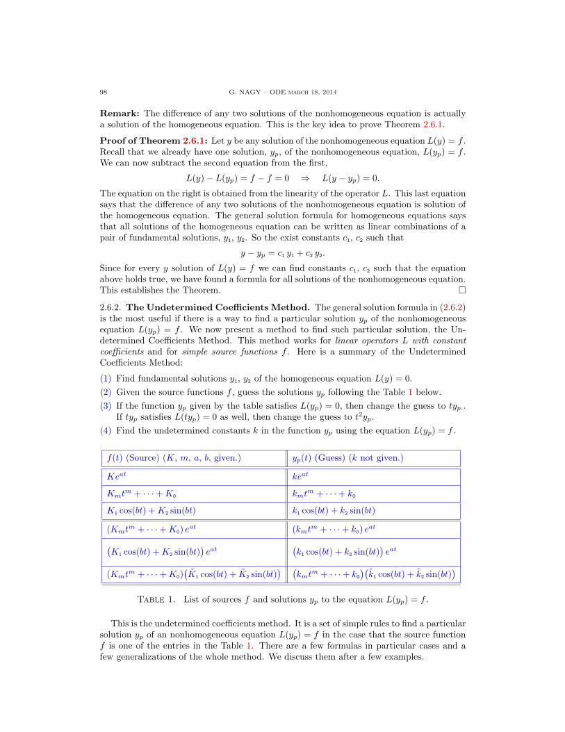
98 G. NAGY – ODE march 18, 2014
Remark: The difference of any two solutions of the nonhomogeneous equation is actuallya solution of the homogeneous equation. This is the key idea to prove Theorem 2.6.1.
Proof of Theorem 2.6.1: Let y be any solution of the nonhomogeneous equation L(y) = f .Recall that we already have one solution, yp, of the nonhomogeneous equation, L(yp) = f .We can now subtract the second equation from the first,
L(y)− L(yp) = f − f = 0 ⇒ L(y − yp) = 0.
The equation on the right is obtained from the linearity of the operator L. This last equationsays that the difference of any two solutions of the nonhomogeneous equation is solution ofthe homogeneous equation. The general solution formula for homogeneous equations saysthat all solutions of the homogeneous equation can be written as linear combinations of apair of fundamental solutions, y1, y2. So the exist constants c1, c2 such that
y − yp = c1 y1 + c2 y2.
Since for every y solution of L(y) = f we can find constants c1, c2 such that the equationabove holds true, we have found a formula for all solutions of the nonhomogeneous equation.This establishes the Theorem. �
2.6.2. The Undetermined Coefficients Method. The general solution formula in (2.6.2)is the most useful if there is a way to find a particular solution yp of the nonhomogeneousequation L(yp) = f . We now present a method to find such particular solution, the Un-determined Coefficients Method. This method works for linear operators L with constantcoefficients and for simple source functions f . Here is a summary of the UndeterminedCoefficients Method:
(1) Find fundamental solutions y1, y2 of the homogeneous equation L(y) = 0.
(2) Given the source functions f , guess the solutions yp following the Table 1 below.
(3) If the function yp given by the table satisfies L(yp) = 0, then change the guess to typ..If typ satisfies L(typ) = 0 as well, then change the guess to t2yp.
(4) Find the undetermined constants k in the function yp using the equation L(yp) = f .
f(t) (Source) (K, m, a, b, given.) yp(t) (Guess) (k not given.)
Keat keat
Kmtm + · · ·+K0 kmt
m + · · ·+ k0
K1 cos(bt) +K2 sin(bt) k1 cos(bt) + k2 sin(bt)
(Kmtm + · · ·+K0) e
at (kmtm + · · ·+ k0) e
at
(K1 cos(bt) +K2 sin(bt)
)eat
(k1 cos(bt) + k2 sin(bt)
)eat
(Kmtm + · · ·+K0)
(K1 cos(bt) + K2 sin(bt)
) (kmt
m + · · ·+ k0)(k1 cos(bt) + k2 sin(bt)
)Table 1. List of sources f and solutions yp to the equation L(yp) = f .
This is the undetermined coefficients method. It is a set of simple rules to find a particularsolution yp of an nonhomogeneous equation L(yp) = f in the case that the source functionf is one of the entries in the Table 1. There are a few formulas in particular cases and afew generalizations of the whole method. We discuss them after a few examples.

G. NAGY – ODE March 18, 2014 99
Example 2.6.1: Find all solutions to the nonhomogeneous equation
y′′ − 3y′ − 4y = 3e2t.
Solution: From the problem we get L(y) = y′′ − 3y′ − 4y and f(t) = 3e2t.
(1): Find fundamental solutions y+, y- to the homogeneous equation L(y) = 0. Since thehomogeneous equation has constant coefficients we find the characteristic equation
r2 − 3r − 4 = 0 ⇒ r+ = 4, r- = −1, ⇒ ytipl(t) = e4t, y- = (t) = e−t.
(2): The table says: For f(t) = 3e2t guess yp(t) = k e2t. The constant k is the undeterminedcoefficient we must find.
(3): Since yp(t) = k e2t is not solution of the homogeneous equation, we do not need tomodify our guess. (Recall: L(y) = 0 iff exist constants c+, c- such that y(t) = c+ e
4t+c- e−t.)
(4): Introduce yp into L(yp) = f and find k. So we do that,
(22 − 6− 4)ke2t = 3e2t ⇒ −6k = 3 ⇒ k = −1
2.
We guessed that yp must be proportional to the exponential e2t in order to cancel out theexponentials in the equation above. We have obtained that
yp(t) = −1
2e2t.
The undetermined coefficients method gives us a way to compute a particular solution yp ofthe nonhomogeneous equation. We now use the general solution theorem, Theorem 2.6.1,to write the general solution of the nonhomogeneous equation,
ygen(t) = c+ e4t + c- e
−t − 1
2e2t.
C
Remark: The step (4) in Example 2.6.1 is a particular case of the following statement.
Lemma 2.6.3. Consider a nonhomogeneous equation L(y) = f with a constant coefficientoperator L and characteristic polynomial p. If the source function is f(t) = K eat, withp(a) 6= 0, then a particular solution of the nonhomogeneous equation is
yp(t) =K
p(a)eat.
Proof of Lemma 2.6.3: Since the linear operator L has constant coefficients, let us writeL and its associated characteristic polynomial p as follows,
L(y) = y′′ + a1y′ + a0y, p(r) = r2 + a1r + a0.
Since the source function is f(t) = K eat, the Table 1 says that a good guess for a particularsoution of the nonhomogneous equation is yp(t) = k eat. Our hypothesis is that this guessis not solution of the homogenoeus equation, since
L(yp) = (a2 + a1a+ a0) k eat = p(a) k eat, and p(a) 6= 0.
We then compute the constant k using the equation L(yp) = f ,
(a2 + a1a+ a0) k eat = K eat ⇒ p(a) k eat = K eat ⇒ k =
K
p(a).
We get the particular solution yp(t) =K
p(a)eat. This establishes the Lemma. �

100 G. NAGY – ODE march 18, 2014
Remark: As we said, the step (4) in Example 2.6.1 is a particular case of Lemma 2.6.3,
yp(t) =3
p(2)e2t =
3
(22 − 6− 4)e2t =
3
−6e2t ⇒ yp(t) = −1
2e2t.
In the following example our first guess for a particular solution yp happens to be asolution of the homogenous equation.
Example 2.6.2: Find all solutions to the nonhomogeneous equation
y′′ − 3y′ − 4y = 3 e4t.
Solution: If we write the equation as L(y) = f , with f(t) = 3 e4t, then the operator L isthe same as in Example 2.6.1. So the solutions of the homogeneous equation L(y) = 0, arethe same as in that example,
y+(t) = e4t, y-(t) = e−t.
The source function is f(t) = 3 e4t, so the Table 1 says that we need to guess yp(t) = k e4t.However, this function yp is solution of the homogeneous equation, because
yp = k y+.
We have to change our guess, as indicated in the undetermined coefficients method, step (3)
yp(t) = kt e4t.
This new guess is not solution of the homogeneous equation. So we proceed to compute theconstant k. We introduce the guess into L(yp) = f ,
y′p = (1 + 4t) k e4t, y′′p = (8 + 16t) k e4t ⇒[8− 3 + (16− 12− 4)t
]k e4t = 3 e4t,
therefore, we get that
5k = 3 ⇒ k =3
5⇒ yp(t) =
3
5t e4t.
The general solution theorem for nonhomogneneous equations says that
ygen(t) = c+ e4t + c- e
−t +3
5t e4t.
C
In the following example the equation source is a trigonometric function.
Example 2.6.3: Find all the solutions to the nonhomogeneous equation
y′′ − 3y′ − 4y = 2 sin(t).
Solution: If we write the equation as L(y) = f , with f(t) = 2 sin(t), then the operator Lis the same as in Example 2.6.1. So the solutions of the homogeneous equation L(y) = 0,are the same as in that example,
y+(t) = e4t, y-(t) = e−t.
Since the source function is f(t) = 2 sin(t), the Table 1 says that we need to choose thefunction yp(t) = k1 cos(t) + k2 sin(t). This function yp is not solution to the homogeneousequation. So we look for the constants k1, k2 using the differential equation,
y′p = −k1 sin(t) + k2 cos(t), y′′p = −k1 cos(t)− k2 sin(t),
and then we obtain
[−k1 cos(t)− k2 sin(t)]− 3[−k1 sin(t) + k2 cos(t)]− 4[k1 cos(t) + k2 sin(t)] = 2 sin(t).

G. NAGY – ODE March 18, 2014 101
Reordering terms in the expression above we get
(−5k1 − 3k2) cos(t) + (3k1 − 5k2) sin(t) = 2 sin(t).
The last equation must hold for all t ∈ R. In particular, it must hold for t = π/2 and fort = 0. At these two points we obtain, respectively,
3k1 − 5k2 = 2,
−5k1 − 3k2 = 0,
}⇒
k1 =
3
17,
k2 = − 5
17.
So the particular solution to the nonhomogeneous equation is given by
yp(t) =1
17
[3 cos(t)− 5 sin(t)
].
The general solution theorem for nonhomogeneous equations implies
ygen(t) = c+ e4t + c- e
−t +1
17
[3 cos(t)− 5 sin(t)
].
C
The next example collects a few nonhomogeneous equations and the guessed function yp.
Example 2.6.4: We provide few more examples of nonhomogeneous equations and theappropriate guesses for the particular solutions.
(a) For y′′ − 3y′ − 4y = 3e2t sin(t), guess, yp(t) =[k1 cos(t) + k2 sin(t)
]e2t.
(b) For y′′ − 3y′ − 4y = 2t2 e3t, guess, yp(t) =(k2t
2 + k1t+ k0)e3t.
(c) For y′′ − 3y′ − 4y = 2t2 e4t, guess, yp(t) =(k2t
2 + k1t+ k0)t e4t.
(d) For y′′ − 3y′ − 4y = 3t sin(t), guess, yp(t) = (k1t+ k0)[k1 cos(t) + k2 sin(t)
].
C
Remark: Suppose that the source function f does not appear in Table 1, but f can bewritten as f = f1+f2, with f1 and f2 in the table. In such case look for a particular solutionyp = yp1 + yp2 , where L(yp1) = f1 and L(yp2) = f2. Since the operator L is linear,
L(yp) = L(yp1 + yp2) = L(yp1) + L(yp2) = f1 + f2 = f ⇒ L(yp) = f.
Example 2.6.5: Find all solutions to the nonhomogeneous equation
y′′ − 3y′ − 4y = 3 e2t + 2 sin(t).
Solution: If we write the equation as L(y) = f , with f(t) = 2 sin(t), then the operator Lis the same as in Example 2.6.1 and 2.6.3. So the solutions of the homogeneous equationL(y) = 0, are the same as in these examples,
y+(t) = e4t, y-(t) = e−t.
The source function f(t) = 3 e2t + 2 sin(t) does not appear in Table 1, but each term does,f1(t) = 3 e2t and f2(t) = 2 sin(t). So we look for a particular solution of the form
yp = yp1 + yp2 , where L(yp1) = 3 e2t, L(yp2) = 2 sin(t).
We have chosen this example because we have solved each one of these equations before, inExample 2.6.1 and 2.6.3. We found the solutions
yp1(t) = −1
2e2t, yp2(t) =
1
17
(3 cos(t)− 5 sin(t)
).

102 G. NAGY – ODE march 18, 2014
Therefore, the particular solution for the equation in this example is
yp(t) = −1
2e2t +
1
17
(3 cos(t)− 5 sin(t)
).
Using the general solution theorem for nonhomogeneous equations we obtain
ygen(t) = c+ e4t + c- e
−t − 1
2e2t +
1
17
(3 cos(t)− 5 sin(t)
).
C
2.6.3. The Variation of Parameters Method. This method provides a second way tofind a particular solution yp to a nonhomogeneous equation L(y) = f . We summarize thismethod in formula to compute yp in terms of any pair of fundamental solutions to thehomogeneous equation L(y) = 0. The variation of parameters method works with secondorder linear equations having variable coefficients and contiuous but otherwise arbitrarysources. When the source function of a nonhomogeneous equation is simple enough toappear in Table 1 the undetermined coefficients method is a quick way to find a particularsolution to the equation. When the source is more complicated, one usually turns to thevariation of parameters method, with its more involved formula for a particular solution.
Theorem 2.6.4 (Variation of Parameters). A particular solution to the equation
L(y) = f,
with L(y) = y′′ + p(t) y′ + q(t) y and p, q, f continuous functions, is given by
yp = u1y1 + u2y2,
where y1, y2 are fundamental solutions of the homogeneous equatio L(y) = 0 and the func-tions u1, u2 are defined by
u1(t) =
∫−y2(t)f(t)Wy1y2(t)
dt, u2(t) =
∫y1(t)f(t)
Wy1y2(t)dt, (2.6.3)
where Wy1y2 is the Wronskian of y1 and y2.
The proof rests in a generalization of the reduction order method. Recall that the re-duction order method is a way to find a second solution y2 of an homogeneous equation ifwe already know one solution y1. One writes y2 = u y1 and the original equation L(y2) = 0provides an equation for u. This equation for u is simpler than the original equation for y2because the function y1 satisfies L(y1) = 0.
The formula for yp is obtained generalizing the reduction order method. We write yp interms of both fundamental solutions y1, y2 of the homogeneous equation,
yp(t) = u1(t) y1(t) + u2(t) y2(t).
We put this yp in the equation L(yp) = f and we find an equation relating u1 and u2. Itis important to realize that we have added one new function to the original problem. Theoriginal problem is to find yp. Now we need to find u1 and u2, but we still have only oneequation to solve, L(yp) = f . The problem for u1, u2 cannot have a unique solution. So weare completely free to add a second equation to the original equation L(yp) = f . We choosethe second equation so that we can solve for u1 and u2. We unveil this second equationwhen we are in the middle of the proof of Theorem 2.6.4.
Proof of Theorem 2.6.4: We must find a function yp solution of L(yp) = f . We know apair of fundamental solutions, y1, y2, of the homogeneous equation L(y) = 0. Here is wherewe generalize the reduction order method by looking for a function yp of the form
yp = u1 y1 + u2 y2,

G. NAGY – ODE March 18, 2014 103
where the functions u1, u2 must be determined from the equation L(yp) = f . We startedlooking for one function, yp, and now we are looking for two functions u1, u2. The originalequation L(yp) = f will give us a relation between u1 and u2. Because we have added anew function to the problem, we need to add one more equation to the problem so we geta unique solution u1, u2. We are completely free to choose this extra equation. However, atthis point we have no idea what to choose.
Before adding a new equation to the system, we work with the original equation. Weintroduce yp into the equation L(yp) = f . We must first compute the derivatives
y′p = u′1 y1 + u1 y′1 + u′2 y2 + u2 y
′2, y′′p = u′′1 y1 + 2u′1 y
′1 + u1 y
′′1 + u′′2 y2 + 2u′2 y
′2 + u2 y
′′2 .
We reorder a few terms and we see that L(yp) = f has the form
u′′1 y1 + u′′2 y2 + 2(u′1 y′1 + u2 y
′2) + p (u′1 y1 + u′2 y2)
+u1 (y′′1 + p y′1 + q y1) + u2 (y
′′2 + p y′2 + q y2) = f.
The functions y1 and y2 are solutions to the homogeneous equation,
y′′1 + p y′1 + q y1 = 0, y′′2 + p y′2 + q y2 = 0,
so u1 and u2 must be solution of a simpler equation that the one above, given by
u′′1 y1 + u′′2 y2 + 2(u′1 y′1 + u′2 y
′2) + p (u′1 y1 + u′2 y2) = f. (2.6.4)
As we said above, this equation does not have a unique solution u1, u2. This is just a relationbetween these two functions. Here is where we need to add a new equation so that we canget a unique solution for u1, u2. What is an appropriate equation to add? Any equationthat simplifies the Eq. (2.6.4) is a good candidate. For two reasons, we take the equation
u′1 y1 + u′2 y2 = 0. (2.6.5)
The first reason is that this equation makes the last term on the righ-hand side of Eq. (2.6.4)vanish. So the system we need to solve is
u′′1 y1 + u′′2 y2 + 2(u′1 y′1 + u′2 y
′2) = f (2.6.6)
u′1 y1 + u′2 y2 = 0. (2.6.7)
The second reason is that this second equation simplifies the first equation even further.Just take the derivative of the second equation,(
u′1 y1 + u′2 y2)′
= 0 ⇒ u′′1 y1 + u′′2 y2 + (u′1 y′1 + u′2 y
′2) = 0.
This last equation implies that the first three terms in Eq. (2.6.6) vanish identically, becauseof Eq.(2.6.7). So we end with the equations
u′1 y′1 + u′2 y
′2 = f
u′1 y1 + u′2 y2 = 0.
And this is a 2× 2 algebraic linear system for the unknowns u′1, u′2. It is hard to overstate
the importance of the word “algebraic” in the previous sentence. From the second equationabove we compute u′2 and we introduce it in the first equation,
u′2 = −y1y2u′1 ⇒ u′1y
′1 −
y1y′2
y2u′1 = f ⇒ u′1
(y′1y2 − y1y′2
y2
)= f.
Recall that the Wronskian of two functions is Wy1y2 = y1y′2 − y′1y2, we get
u′1 = − y2f
Wy1y2
⇒ u′2 =y1f
Wy1y2
.
These equations are the derivative of Eq. (2.6.3). Integrate them in the variable t and choosethe integration constants to be zero. We get Eq. (2.6.3). This establishes the Theorem. �

104 G. NAGY – ODE march 18, 2014
Remark: The integration constants in the expressions for u1, u2 can always be chosen tobe zero. To understand the effect of the integration constants in the function yp, let us dothe following. Denote by u1 and u2 the functions in Eq. (2.6.3), and given any real numbersc1 and c2 define
u1 = u1 + c1, u2 = u2 + c2.
Then the corresponding solution yp is given by
yp = u1 y1 + u2 y2 = u1 y1 + u2 y2 + c1 y1 + c2 y2 ⇒ yp = yp + c1 y1 + c2 y2.
The two solutions yp and yp differ by a solution to the homogeneous differential equation.So both functions are also solution to the nonhomogeneous equation. One is then free tochoose the constants c1 and c2 in any way. We chose them in the proof above to be zero.
Example 2.6.6: Find the general solution of the nonhomogeneous equation
y′′ − 5y′ + 6y = 2et.
Solution: The formula for yp in Theorem 2.6.4 requires we know fundamental solutions tothe homogeneous problem. So we start finding these solutions first. Since the equation hasconstant coefficients, we compute the characteristic equation,
r2 − 5r + 6 = 0 ⇒ r± =1
2
(5±
√25− 24
)⇒
{r+ = 3,
r- = 2.
So, the functions y1 and y2 in Theorem 2.6.4 are in our case given by
y1(t) = e3t, y2(t) = e2t.
The Wronskian of these two functions is given by
Wy1y2(t) = (e3t)(2e2t)− (3e3t)(e2t) ⇒ Wy1y2(t) = −e5t.
We are now ready to compute the functions u1 and u2. Notice that Eq. (2.6.3) the followingdifferential equations
u′1 = − y2f
Wy1y2
, u′2 =y1f
Wy1y2
.
So, the equation for u1 is the following,
u′1 = −e2t(2et)(−e−5t) ⇒ u′1 = 2e−2t ⇒ u1 = −e−2t,
u′2 = e3t(2et)(−e−5t) ⇒ u′2 = −2e−t ⇒ u2 = 2e−t,
where we have chosen the constant of integration to be zero. The particular solution we arelooking for is given by
yp = (−e−2t)(e3t) + (2e−t)(e2t) ⇒ yp = et.
Then, the general solution theorem for nonhomogeneous equation implies
ygen(t) = c+ e3t + c- e
2t + et c+, c- ∈ R.
C
Example 2.6.7: Find a particular solution to the differential equation
t2y′′ − 2y = 3t2 − 1,
knowing that y1 = t2 and y2 = 1/t are solutions to the homogeneous equation t2y′′−2y = 0.
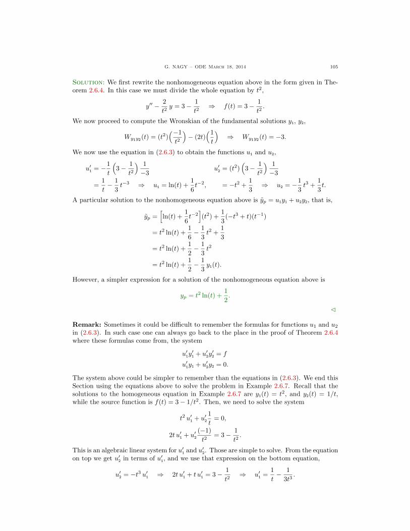
G. NAGY – ODE March 18, 2014 105
Solution: We first rewrite the nonhomogeneous equation above in the form given in The-orem 2.6.4. In this case we must divide the whole equation by t2,
y′′ − 2
t2y = 3− 1
t2⇒ f(t) = 3− 1
t2.
We now proceed to compute the Wronskian of the fundamental solutions y1, y2,
Wy1y2(t) = (t2)(−1
t2
)− (2t)
(1t
)⇒ Wy1y2(t) = −3.
We now use the equation in (2.6.3) to obtain the functions u1 and u2,
u′1 = −1
t
(3− 1
t2
) 1
−3
=1
t− 1
3t−3 ⇒ u1 = ln(t) +
1
6t−2,
u′2 = (t2)(3− 1
t2
) 1
−3
= −t2 + 1
3⇒ u2 = −1
3t3 +
1
3t.
A particular solution to the nonhomogeneous equation above is yp = u1y1 + u2y2, that is,
yp =[ln(t) +
1
6t−2
](t2) +
1
3(−t3 + t)(t−1)
= t2 ln(t) +1
6− 1
3t2 +
1
3
= t2 ln(t) +1
2− 1
3t2
= t2 ln(t) +1
2− 1
3y1(t).
However, a simpler expression for a solution of the nonhomogeneous equation above is
yp = t2 ln(t) +1
2.
C
Remark: Sometimes it could be difficult to remember the formulas for functions u1 and u2in (2.6.3). In such case one can always go back to the place in the proof of Theorem 2.6.4where these formulas come from, the system
u′1y′1 + u′2y
′2 = f
u′1y1 + u′2y2 = 0.
The system above could be simpler to remember than the equations in (2.6.3). We end thisSection using the equations above to solve the problem in Example 2.6.7. Recall that thesolutions to the homogeneous equation in Example 2.6.7 are y1(t) = t2, and y2(t) = 1/t,while the source function is f(t) = 3− 1/t2. Then, we need to solve the system
t2 u′1 + u′21
t= 0,
2t u′1 + u′2(−1)
t2= 3− 1
t2.
This is an algebraic linear system for u′1 and u′2. Those are simple to solve. From the equation
on top we get u′2 in terms of u′1, and we use that expression on the bottom equation,
u′2 = −t3 u′1 ⇒ 2t u′1 + t u′1 = 3− 1
t2⇒ u′1 =
1
t− 1
3t3.

106 G. NAGY – ODE march 18, 2014
Substitue back the expression for u′1 in the first equation above and we get u′2. We get,
u′1 =1
t− 1
3t3
u′2 = −t2 + 1
3.
We should now integrate these functions to get u1 and u2 and then get the particular solutionyp = u1y1 + u2y2. We do not repeat these calculations, since they are done Example 2.6.7.

G. NAGY – ODE March 18, 2014 107
2.6.4. Exercises.
2.6.1.- . 2.6.2.- .

108 G. NAGY – ODE march 18, 2014
2.7. Variation of Parameters
The contents of this section have been included in § 2.6.

G. NAGY – ODE March 18, 2014 109
Chapter 3. Power Series Solutions
The first differential equations were solved around the end of the seventeen century andbeginning of the eighteen century. We studied a few of these equations in § 1.1-1.4 and theconstant coefficients equations in Chapter 2. By the middle of the eighteen century peoplerealized that the methods we learnt in these first sections had reached a dead end. Amongthe reasons was the lack of functions to write the solutions to differential equations. Theelementary functions we use in calculus were simply not enough. These functions includepolynomials, quotient of polynomials, trigonometric functions, exponentials, and logarithms.People even started to think of differential equations as sources to find new functions. Itwas matter of little time before mathematicians started to use power series expansions tofind solutions of differential equations. Power series define functions more general than theelementary functions from calculus.
In § 3.1 we study the simplest case, when the power series is centered at a regular pointof the equation. Regular points are points where all the equation coefficients functions arecontinuous. In § 3.2 we study the Euler differential equation. The coefficients in an Eulerdifferential equation diverge at a particular point in a very specific way. No power seriesare needed to find solutions in this case. In § 3.3 we solve equations with regular-singularpoints. Regular-singular points are points where the equation coefficients diverge in a waysimilar to an Euler differential equation. We will find solutions to these equations usingpower series centered precisely at a regular-singular point of the equation.
−1 1 t
y
y(x) =
∞∑n=0
xn
y(x) =1
1− x

110 G. NAGY – ODE march 18, 2014
3.1. Solutions Near Regular Points
We study second order linear differential equations with variable coefficients. We look forsolutions on a domain where the equation coefficients have power series expansions and thecoefficient multiplying the second derivative of the unknown function is nonzero. Any pointon such domain will be called a regular point of the equation. We look for solutions thatcan be written as power series centered at a regular point. For simplicity we solve onlyhomogeneous equations, but the power series method can be used with nonhomogeneousequations without introducing substantial modifications.
3.1.1. Review of Power Series. We summarize a few results on power series that we willneed to find solutions to differential equations. A more detailed presentation of these ideascan be found in standard calculus textbooks, [1, 2, 9, 11]. We start with the definition ofanalytic functions, which are functions that can be written as a power series expansion onan appropriate domain.
Definition 3.1.1. A function y is analytic on an interval (x0 − ρ, x0 + ρ) iff it can bewritten as the power series expansion below, convergent for |x− x0| < ρ,
y(x) =
∞∑n=0
an (x− x0)n.
Example 3.1.1: We show a few examples of analytic functions on appropriate domains.
(a) The function y(x) =1
1− xis analytic on the interval (−1, 1), because it has the power
series expansion centered at x0 = 0, convergent for |x| < 1,
1
1− x=
∞∑n=0
xn = 1 + x+ x2 + x3 + · · · .
It is clear that this series diverges for x > 1, but it is not obvious that this seriesconverges if and only if |x| < 1.
(b) The function y(x) = ex is analytic on R, and can be written as the power series
ex =
∞∑n=0
xn
n!= 1 + x+
x2
2!+x3
3!+ · · · .
(c) A function y having at x0 both infinitely many continuous derivatives and a convergentpower series is analytic where the series converges. The Taylor expansion centered atx0 of such a function is
y(x) =
∞∑n=0
y(n)(x0)
n!(x− x0)
n,
and this means
y(x) = y(x0) + y′(x0) (x− x0) +y′′(x0)
2!(x− x0)
2 +y′′′(x0)
3!(x− x0)
3 + · · · .
C
The Taylor series can be very useful to find the power series expansions of function havinginfinitely many continuous derivatives.

G. NAGY – ODE March 18, 2014 111
Example 3.1.2: Find the Taylor series of y(x) = sin(x) centered at x0 = 0.
Solution: We need to compute the derivatives of the function y and evaluate these deriva-tives at the point we center the expansion, in this case x0 = 0.
y(x) = sin(x) ⇒ y(0) = 0, y′(x) = cos(x) ⇒ y′(0) = 1,
y′′(x) = − sin(x) ⇒ y′′(0) = 0, y′′′(x) = − cos(x) ⇒ y′′′(0) = −1.
One more derivative gives y(4)(t) = sin(t), so y(4) = y, the cycle repeats itself. It is notdifficult to see that the Taylor’s formula implies,
sin(x) = x− x3
3!+x5
5!− · · · ⇒ sin(x) =
∞∑n=0
(−1)n
(2n+ 1)!x(2n+1).
C
Remark: The Taylor series at x0 = 0 for y(x) = cos(x) is computed in a similar way,
cos(x) =
∞∑n=0
(−1)n
(2n)!x(2n).
Elementary functions like quotient of polynomials, trigonometric functions, exponentialand logarithms can be written as power series. But the power series of any of these functionsmay not be defined on the whole domain of the function. The following example shows afunction with this property.
Example 3.1.3: Find the Taylor series for y(x) =1
1− xcentered at x0 = 0.
Solution: Notice that this function is welldefined for every x ∈ R − {1}. The func-tion graph can be seen in Fig. 14. To findthe Taylor series we need to compute the n-derivative, y(n)(0). It simple to check that,
y(n)(x) =n!
(1− x)n+1, so y(n)(0) = n!.
We conclude that: y(x) =1
1− x=
∞∑n=0
xn.
One can prove that this power series con-verges if and only if |x| < 1. C
−1 1 t
y
y(x) =∞∑
n=0
xn
Figure 14. The graph of
y =1
(1− x).
Remark: The power series y(x) =
∞∑n=0
xn does not converge on (−∞,−1]∪[1,∞). But there
are different power series that converge to y(x) =1
1− xon intervals inside that domain.
For example the Taylor series about x0 = 2 converges for |x− 2| < 1, that is 1 < x < 3.
y(n)(x) =n!
(1− x)n+1⇒ y(n)(2) =
n!
(−1)n+1⇒ y(x) =
∞∑n=0
(−1)n+1(x− 2)n.

112 G. NAGY – ODE march 18, 2014
Later on we might need the notion of convergence of an infinite series in absolute value.
Definition 3.1.2. The power series y(x) =
∞∑n=0
an (x−x0)n converges in absolute value
iff the series
∞∑n=0
|an| |x− x0|n converges.
Remark: If a series converges in absolute value, it converges. The converse is not true.
Example 3.1.4: One can show that the series s =
∞∑n=1
(−1)n
nconverges, but this series does
not converge absolutely, since
∞∑n=1
1
ndiverges. See [9, 11]. C
Since power series expansions of functions might not converge on the same domain wherethe function is defined, it is useful to introduce the region where the power series converges.
Definition 3.1.3. The radius of convergence of a power series y(x) =
∞∑n=0
an (x− x0)n
is the number ρ > 0 satisfying both the series converges absolutely for |x− x0| < ρ and theseries diverges for |x− x0| > ρ.
Remark: The radius of convergence defines the size of the biggest open interval where thepower series converges. This interval is symmetric around the series center point x0.
x
diverges converges diverges
x0 − ρ x0 x0 + ρ( )
Figure 15. Example of the radius of convergence.
Example 3.1.5: We state the radius of convergence of few power series. See [9, 11].
(1) The series1
1− x=
∞∑n=0
xn has radius of convergence ρ = 1.
(2) The series ex =∞∑
n=0
xn
n!has radius of convergence ρ = ∞.
(3) The series sin(x) =
∞∑n=0
(−1)n
(2n+ 1)!x(2n+1) has radius of convergence ρ = ∞.
(4) The series cos(x) =
∞∑n=0
(−1)n
(2n)!x(2n) has radius of convergence ρ = ∞.
(5) The series sinh(x) =
∞∑n=0
1
(2n+ 1)!x(2n+1) has radius of convergence ρ = ∞.
(6) The series cosh(x) =
∞∑n=0
1
(2n)!x(2n) has radius of convergence ρ = ∞.
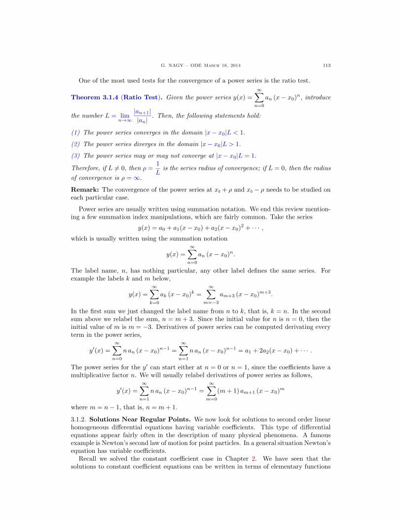
G. NAGY – ODE March 18, 2014 113
One of the most used tests for the convergence of a power series is the ratio test.
Theorem 3.1.4 (Ratio Test). Given the power series y(x) =
∞∑n=0
an (x− x0)n, introduce
the number L = limn→∞
|an+1||an|
. Then, the following statements hold:
(1) The power series converges in the domain |x− x0|L < 1.
(2) The power series diverges in the domain |x− x0|L > 1.
(3) The power series may or may not converge at |x− x0|L = 1.
Therefore, if L 6= 0, then ρ =1
Lis the series radius of convergence; if L = 0, then the radius
of convergence is ρ = ∞.
Remark: The convergence of the power series at x0 + ρ and x0 − ρ needs to be studied oneach particular case.
Power series are usually written using summation notation. We end this review mention-ing a few summation index manipulations, which are fairly common. Take the series
y(x) = a0 + a1(x− x0) + a2(x− x0)2 + · · · ,
which is usually written using the summation notation
y(x) =
∞∑n=0
an (x− x0)n.
The label name, n, has nothing particular, any other label defines the same series. Forexample the labels k and m below,
y(x) =
∞∑k=0
ak (x− x0)k =
∞∑m=−3
am+3 (x− x0)m+3.
In the first sum we just changed the label name from n to k, that is, k = n. In the secondsum above we relabel the sum, n = m + 3. Since the initial value for n is n = 0, then theinitial value of m is m = −3. Derivatives of power series can be computed derivating everyterm in the power series,
y′(x) =
∞∑n=0
nan (x− x0)n−1 =
∞∑n=1
nan (x− x0)n−1 = a1 + 2a2(x− x0) + · · · .
The power series for the y′ can start either at n = 0 or n = 1, since the coefficients have amultiplicative factor n. We will usually relabel derivatives of power series as follows,
y′(x) =
∞∑n=1
nan (x− x0)n−1 =
∞∑m=0
(m+ 1) am+1 (x− x0)m
where m = n− 1, that is, n = m+ 1.
3.1.2. Solutions Near Regular Points. We now look for solutions to second order linearhomogeneous differential equations having variable coefficients. This type of differentialequations appear fairly often in the description of many physical phenomena. A famousexample is Newton’s second law of motion for point particles. In a general situation Newton’sequation has variable coefficients.
Recall we solved the constant coefficient case in Chapter 2. We have seen that thesolutions to constant coefficient equations can be written in terms of elementary functions

114 G. NAGY – ODE march 18, 2014
such as quotient of polynomials, trigonometric functions, exponentials, and logarithms. Forexample, the equation
y′′ + y = 0
has the fundamental solutions y1(x) = cos(x) and y2(x) = sin(x). But the equation
x y′′ + y′ + x y = 0
cannot be solved in terms of elementary functions. Except for constant coefficient equationsand variable coefficient equations that can be transformed into constant coefficient equationsby a change of variable, there is not known second order linear equations that can be solved interms of elementary functions. Nevertheless, we are interested in finding explicit expressionsfor the solutions to variable coefficient equations. Mainly because these equations appearin the description of so many physical systems.
We have said that power series define more general functions than the elementary func-tions mentioned above. So we look for solutions using power series. In this section we centerthe power series at a regular point of the equation.
Definition 3.1.5. A point x0 ∈ R is called a regular point of the equation
y′′ + p(x) y′ + q(x) y = 0, (3.1.1)
iff p, q are analytic functions at x0. Otherwise x0 is called a singular point of the equation.
Remark: Near a regular point x0 the coefficients p and q in the differential equation abovecan be written as
p(x) = p0 + p1 (x− x0) + p2 (x− x0)2 + · · · =
∞∑n=0
pn (x− x0)n,
q(x) = q0 + q1 (x− x0) + q2 (x− x0)2 + · · · =
∞∑n=0
qn (x− x0)n,
and these power series converge in a neighborhood of x0.
Example 3.1.6: Find all the regular points of the equation
x y′′ + y′ + x y = 0.
Solution: We write the equation in the form of Eq. (3.1.1),
y′′ +1
xy′ + y = .
In this case the coefficient functions are p(x) = 1/x, and q(x) = 1. The function q is analyticin R. The function p is analytic for all points in R− {0}. So the point x0 = 0 is a singularpoint of the equation. Every other point is a regular point of the equation. C
Theorem 3.1.6. If the functions p, q are analytic on an open interval (x0−ρ, x0+ρ) ⊂ R,then the differential equation
y′′ + p(x) y′ + q(x) y = 0,
has two independent solutions, y1, y2, which are analytic on the same interval.
Remark: The proof of this theorem can be found in [2], Page 169. See also [8], § 29.
Theorem 3.1.6 says that for every regular point x0 of a differential equation there exist twoindependent solutions y1, y2, defined in a neighborhood of x0. These solutions are analyticat x0, so they can be written as power series centered at x0. We now summarize a simplemethod to find these solutions y1, y2.

G. NAGY – ODE March 18, 2014 115
(a) Write a power series expansion of the solution centered at a regular point x0,
y(x) =
∞∑n=0
an (x− x0)n.
(b) Introduce the power series expansion above into the differential equation and find arecurrence relation among the coefficients an.
(c) Solve the recurrence relation in terms of free coefficients.
(d) If possible, add up the resulting power series for the solutions y1, y2.
We follow these steps in the examples below to find solutions to several differential equa-tions. We start with a first order constant coefficient equation, and then we continue witha second order constant coefficient equation. The last two examples consider variable coef-ficient equations.
Example 3.1.7: Find a power series solution y around the point x0 = 0 of the equation
y′ + c y = 0, c ∈ R.
Solution: We already know every solution to this equation. This is a first order, linear,differential equation, so using the method of integrating factor we find that the solution is
y(x) = a0 e−c x, a0 ∈ R.
We are now interested in obtaining such solution with the power series method. Althoughthis is not a second order equation, the power series method still works in this example.Propose a solution of the form
y =
∞∑n=0
an xn ⇒ y′ =
∞∑n=1
nan x(n−1).
We can start the sum in y′ at n = 0 or n = 1. We choose n = 1, since it is more convenientlater on. Introduce the expressions above into the differential equation,
∞∑n=1
nan xn−1 + c
∞∑n=0
an xn = 0.
Relabel the first sum above so that the functions xn−1 and xn in the first and second sumhave the same label. One way is the following,
∞∑n=0
(n+ 1)a(n+1) xn +
∞∑n=0
c an xn = 0
We can now write down both sums into one single sum,
∞∑n=0
[(n+ 1)a(n+1) + c an
]xn = 0.
Since the function on the left-hand side must be zero for every x ∈ R, we conclude thatevery coefficient that multiplies xn must vanish, that is,
(n+ 1)a(n+1) + c an = 0, n > 0.
The last equation is called a recurrence relation among the coefficients an. The solution ofthis relation can be found by writing down the first few cases and then guessing the general

116 G. NAGY – ODE march 18, 2014
expression for the solution, that is,
n = 0, a1 = −c a0 ⇒ a1 = −c a0,
n = 1, 2a2 = −c a1 ⇒ a2 =c2
2!a0,
n = 2, 3a3 = −c a2 ⇒ a3 = −c3
3!a0,
n = 3, 4a4 = −c a3 ⇒ a4 =c4
4!a0.
One can check that the coefficient an can be written as
an = (−1)ncn
n!a0,
which implies that the solution of the differential equation is given by
y(x) = a0
∞∑n=0
(−1)ncn
n!xn ⇒ y(x) = a0
∞∑n=0
(−c x)n
n!⇒ y(x) = a0 e
−c x.
C
Example 3.1.8: Find a power series solution y(x) around the point x0 = 0 of the equation
y′′ + y = 0.
Solution: We know that the solution can be found computing the roots of the characteristicpolynomial r2 + 1 = 0, which gives us the solutions
y(x) = a0 cos(x) + a1 sin(x).
We now recover this solution using the power series,
y =
∞∑n=0
an xn ⇒ y′ =
∞∑n=1
nan x(n−1), ⇒ y′′ =
∞∑n=2
n(n− 1)an x(n−2).
Introduce the expressions above into the differential equation, which involves only the func-tion and its second derivative,
∞∑n=2
n(n− 1)an xn−2 +
∞∑n=0
an xn = 0.
Relabel the first sum above, so that both sums have the same factor xn. One way is,∞∑
n=0
(n+ 2)(n+ 1)a(n+2) xn +
∞∑n=0
an xn = 0.
Now we can write both sums using one single sum as follows,∞∑
n=0
[(n+ 2)(n+ 1)a(n+2) + an
]xn = 0 ⇒ (n+ 2)(n+ 1)a(n+2) + an = 0. n > 0.
The last equation is the recurrence relation. The solution of this relation can again be foundby writing down the first few cases, and we start with even values of n, that is,
n = 0, (2)(1)a2 = −a0 ⇒ a2 = − 1
2!a0,
n = 2, (4)(3)a4 = −a2 ⇒ a4 =1
4!a0,
n = 4, (6)(5)a6 = −a4 ⇒ a6 = − 1
6!a0.
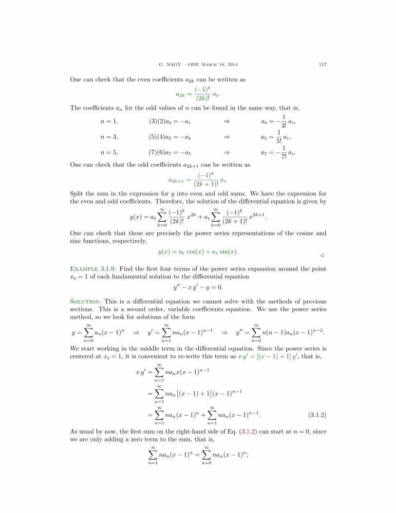
G. NAGY – ODE March 18, 2014 117
One can check that the even coefficients a2k can be written as
a2k =(−1)k
(2k)!a0.
The coefficients an for the odd values of n can be found in the same way, that is,
n = 1, (3)(2)a3 = −a1 ⇒ a3 = − 1
3!a1,
n = 3, (5)(4)a5 = −a3 ⇒ a5 =1
5!a1,
n = 5, (7)(6)a7 = −a5 ⇒ a7 = − 1
7!a1.
One can check that the odd coefficients a2k+1 can be written as
a2k+1 =(−1)k
(2k + 1)!a1.
Split the sum in the expression for y into even and odd sums. We have the expression forthe even and odd coefficients. Therefore, the solution of the differential equation is given by
y(x) = a0
∞∑k=0
(−1)k
(2k)!x2k + a1
∞∑k=0
(−1)k
(2k + 1)!x2k+1.
One can check that these are precisely the power series representations of the cosine andsine functions, respectively,
y(x) = a0 cos(x) + a1 sin(x). C
Example 3.1.9: Find the first four terms of the power series expansion around the pointx0 = 1 of each fundamental solution to the differential equation
y′′ − x y′ − y = 0.
Solution: This is a differential equation we cannot solve with the methods of previoussections. This is a second order, variable coefficients equation. We use the power seriesmethod, so we look for solutions of the form
y =
∞∑n=0
an(x− 1)n ⇒ y′ =
∞∑n=1
nan(x− 1)n−1 ⇒ y′′ =
∞∑n=2
n(n− 1)an(x− 1)n−2.
We start working in the middle term in the differential equation. Since the power series iscentered at x0 = 1, it is convenient to re-write this term as x y′ = [(x− 1) + 1] y′, that is,
x y′ =
∞∑n=1
nanx(x− 1)n−1
=
∞∑n=1
nan[(x− 1) + 1
](x− 1)n−1
=
∞∑n=1
nan(x− 1)n +
∞∑n=1
nan(x− 1)n−1. (3.1.2)
As usual by now, the first sum on the right-hand side of Eq. (3.1.2) can start at n = 0, sincewe are only adding a zero term to the sum, that is,
∞∑n=1
nan(x− 1)n =
∞∑n=0
nan(x− 1)n;

118 G. NAGY – ODE march 18, 2014
while it is convenient to relabel the second sum in Eq. (3.1.2) follows,
∞∑n=1
nan(x− 1)n−1 =
∞∑n=0
(n+ 1)a(n+1)(x− 1)n;
so both sums in Eq. (3.1.2) have the same factors (x− 1)n. We obtain the expression
x y′ =
∞∑n=0
nan(x− 1)n +
∞∑n=0
(n+ 1)a(n+1)(x− 1)n
=
∞∑n=0
[nan + (n+ 1)a(n+1)
](x− 1)n. (3.1.3)
In a similar way relabel the index in the expression for y′′, so we obtain
y′′ =∞∑
n=0
(n+ 2)(n+ 1)a(n+2)(x− 1)n. (3.1.4)
If we use Eqs. (3.1.3)-(3.1.4) in the differential equation, together with the expression for y,the differential equation can be written as follows
∞∑n=0
(n+ 2)(n+ 1)a(n+2)(x− 1)n −∞∑
n=0
[nan + (n+ 1)a(n+1)
](x− 1)n −
∞∑n=0
an(x− 1)n = 0.
We can now put all the terms above into a single sum,
∞∑n=0
[(n+ 2)(n+ 1)a(n+2) − (n+ 1)a(n+1) − nan − an
](x− 1)n = 0.
This expression provides the recurrence relation for the coefficients an with n > 0, that is,
(n+ 2)(n+ 1)a(n+2) − (n+ 1)a(n+1) − (n+ 1)an = 0
(n+ 1)[(n+ 2)a(n+2) − a(n+1) − an
]= 0,
which can be rewritten as follows,
(n+ 2)a(n+2) − a(n+1) − an = 0. (3.1.5)
We can solve this recurrence relation for the first four coefficients,
n = 0 2a2 − a1 − a0 = 0 ⇒ a2 =a12
+a02,
n = 1 3a3 − a2 − a1 = 0 ⇒ a3 =a12
+a06,
n = 2 4a4 − a3 − a2 = 0 ⇒ a4 =a14
+a06.
Therefore, the first terms in the power series expression for the solution y of the differentialequation are given by
y = a0 + a1(x− 1) +(a02
+a12
)(x− 1)2 +
(a06
+a12
)(x− 1)3 +
(a06
+a14
)(x− 1)4 + · · ·
which can be rewritten as
y = a0
[1 +
1
2(x− 1)2 +
1
6(x− 1)3 +
1
6(x− 1)4 + · · ·
]+ a1
[(x− 1) +
1
2(x− 1)2 +
1
2(x− 1)3 +
1
4(x− 1)4 + · · ·
]

G. NAGY – ODE March 18, 2014 119
So the first four terms on each fundamental solution are given by
y1 = 1 +1
2(x− 1)2 +
1
6(x− 1)3 +
1
6(x− 1)4,
y2 = (x− 1) +1
2(x− 1)2 +
1
2(x− 1)3 +
1
4(x− 1)4.
C
Example 3.1.10: Find the first three terms of the power series expansion around the pointx0 = 2 of each fundamental solution to the differential equation
y′′ − x y = 0.
Solution: We then look for solutions of the form
y =
∞∑n=0
an(x− 2)n.
It is convenient to rewrite the function x y = [(x− 2) + 2] y, that is,
xy =
∞∑n=0
anx(x− 2)n
=
∞∑n=0
an[(x− 2) + 2
](x− 2)n
=
∞∑n=0
an(x− 2)n+1 +
∞∑n=0
2an(x− 2)n. (3.1.6)
We now relabel the first sum on the right-hand side of Eq. (3.1.6) in the following way,
∞∑n=0
an(x− 2)n+1 =
∞∑n=1
a(n−1)(x− 2)n. (3.1.7)
We do the same type of relabeling on the expression for y′′,
y′′ =
∞∑n=2
n(n− 1)an(x− 2)n−2
=
∞∑n=0
(n+ 2)(n+ 1)a(n+2)(x− 2)n.
Then, the differential equation above can be written as follows
∞∑n=0
(n+ 2)(n+ 1)a(n+2)(x− 2)n −∞∑
n=0
2an(x− 2)n −∞∑
n=1
a(n−1)(x− 2)n = 0
(2)(1)a2 − 2a0 +
∞∑n=1
[(n+ 2)(n+ 1)a(n+2) − 2an − a(n−1)
](x− 2)n = 0.
So the recurrence relation for the coefficients an is given by
a2 − a0 = 0, (n+ 2)(n+ 1)a(n+2) − 2an − a(n−1) = 0, n > 1.

120 G. NAGY – ODE march 18, 2014
We can solve this recurrence relation for the first four coefficients,
n = 0 a2 − a0 = 0 ⇒ a2 = a0,
n = 1 (3)(2)a3 − 2a1 − a0 = 0 ⇒ a3 =a06
+a13,
n = 2 (4)(3)a4 − 2a2 − a1 = 0 ⇒ a4 =a06
+a112.
Therefore, the first terms in the power series expression for the solution y of the differentialequation are given by
y = a0 + a1(x− 2) + a0(x− 2)2 +(a06
+a13
)(x− 2)3 +
(a06
+a112
)(x− 2)4 + · · ·
which can be rewritten as
y = a0
[1 + (x− 2)2 +
1
6(x− 2)3 +
1
6(x− 2)4 + · · ·
]+ a1
[(x− 2) +
1
3(x− 2)3 +
1
12(x− 2)4 + · · ·
]So the first three terms on each fundamental solution are given by
y1 = 1 + (x− 2)2 +1
6(x− 2)3,
y2 = (x− 2) +1
3(x− 2)3 +
1
12(x− 2)4.
C
3.1.3. The Legendre Equation. The Legendre equation appears when one solves theLaplace equation in spherical coordinates. The Laplace equation describes several phenom-ena, such as the static electric potential near a charged body, or the gravitational potentialof a planet or star. When the Laplace equation describes a situation having spherical sym-metry it makes sense to use spherical coordinates to solve the equation. It is in that casethat the Legendre equation appears for a variable related to the polar angle in the sphericalcoordinate system. See Jackson’s classic book on electrodynamics [6], § 3.1, for a derivationof the Legendre equation from the Laplace equation.
Example 3.1.11: Find all solutions to the Legendre equation
(1− x2) y′′ − 2x y′ + l(l + 1) y = 0,
where l is any real constant, using power series centered at x0 = 0.
Solution: We start writing the equation in the form of Theorem 3.1.6,
y′′ − 2
(1− x2)y′ +
l(l + 1)
(1− x2)y = 0.
It is clear that the coefficient functions
p(x) = − 2
(1− x2), q(x) =
l(l + 1)
(1− x2),
are analytic at x0 = 0 in the interval given by |x| < 1. Theorem 3.1.6 says that there aretwo solutions linearly independent which are analytic at x0 = 0. So we write the solution as
y(x) =
∞∑n=0
an xn.

G. NAGY – ODE March 18, 2014 121
Then we get,
y′′ =
∞∑n=0
(n+ 2)(n+ 1)a(n+2) xn,
−x2 y′′ =∞∑
n=0
−(n− 1)nan xn,
−2x y′ =
∞∑n=0
−2nan xn,
l(l + 1) y =
∞∑n=0
l(l + 1)an xn.
The Legendre equation says that the addition of the four equations above must be zero,∞∑
n=0
((n+ 2)(n+ 1)a(n+2) − (n− 1)nan − 2nan + l(l + 1)an
)xn = 0.
Therefore,every term in that sum must vanish,
(n+ 2)(n+ 1)a(n+2) − (n− 1)nan − 2nan + l(l + 1)an = 0, n > n.
This is the recurrence relation for the coefficients an. After a few manipulations the recur-rence relation becomes
a(n+2) = − (l − n)(l + n+ 1)
(n+ 2)(n+ 1)an, n > 0.
By giving values to n we obtain,
a2 = − l(l + 1)
2!a0, a3 = − (l − 1)(l + 2)
3!a1.
Since a4 is related to a2 and a5 is related to a3, we get,
a4 = − (l − 2)(l + 3)
(3)(4)a2 ⇒ a4 =
(l − 2)l(l + 1)(l + 3)
4!a0,
a5 = − (l − 3)(l + 4)
(4)(5)a3 ⇒ a5 =
(l − 3)(l − 1)(l + 2)(l + 4)
5!a1.
If one keeps solving the coefficients an in terms of either a0 or a1, one gets the expression,
y(x) = a0
[1− l(l + 1)
2!x2 +
(l − 2)l(l + 1)(l + 3)
4!x4 + · · ·
]+ a1
[x− (l − 1)(l + 2)
3!x3 +
(l − 3)(l − 1)(l + 2)(l + 4)
5!x5 + · · ·
].
Hence, the fundamental solutions are
y1(x) = 1− l(l + 1)
2!x2 +
(l − 2)l(l + 1)(l + 3)
4!x4 + · · ·
y2(x) = x− (l − 1)(l + 2)
3!x3 +
(l − 3)(l − 1)(l + 2)(l + 4)
5!x5 + · · · .
The ration test provides the interval where the seires above converge. For function y1 weget, replacing n by 2n,∣∣∣a2n+2 x
2n+2
a2n x2n
∣∣∣ = ∣∣∣= (l − 2n)(l + 2n+ 1)
(2n+ 1)(2n+ 2)
∣∣∣ |x2| → |x|2 as n→ ∞.
A similar result holds for y2. So both series converge on the interval defined by |x| < 1. C

122 G. NAGY – ODE march 18, 2014
Remark: The functions y1, y2 are called Legendre functions. For a noninteger value ofthe constant l these functions cannot be written in terms of elementary functions. Butwhen l is an integer, one of these series terminate and bacomes a polynomial. The casel being a nonnegative integer is specially relevant in physics. For l even the function y1becomes a polynomial while y2 remains an infinite series. For l odd the function y2 becomesa polynomial while the y1 remains an infinite series. These polynomials are called Legendrepolynomials.

G. NAGY – ODE March 18, 2014 123
3.1.4. Exercises.
3.1.1.- . 3.1.2.- .

124 G. NAGY – ODE march 18, 2014
3.2. The Euler Equidimensional Equation
When the coefficients p and q are analytic functions on a given domain, the equation
y′′ + p(x) y′ + q(x) y = 0
has analytic fundamental solutions on that domain. This is the main result in § 3.1, The-orem 3.1.6. Recall that a function is analytic on an open domain iff the function admitsa convergent power series on that domain. In this section we start the study of equationswhere the coefficients p and q are not analytic functions. We want to study equations withcoefficients p and q having singularities. We want to find solutions defined arbitrarily closeto these singularities. On the one hand, this is an important problem because many differ-ential equations in physics have coefficients with singularities. And finding solutions withphysical meaning often involves studying all solutions near these singularities. On the otherhand, this is a difficult problem, and when p and q are completely arbitrary functions thereis not much that can be learned from the solutions of the equation. For this reason we startour study with one of the simplest cases, Euler’s equidimensional equation.
3.2.1. The Roots of the Indicial Polynomial. We study the differential equation
y′′ + p(x) y′ + q(x) y = 0,
where the coefficients p and q are given by
p(x) =p0
(x− x0), q(x) =
q0(x− x0)2
,
with p0 and q0 constants. The point x0 is a singular point of the equation; the functions pand q are not analytic on an open set including x0. But the singularity is of a good type,the type we know how find solutions. We start with a small rewriting of the differentialequation we are going to study.
Definition 3.2.1. The Euler equidimensional equation for the unknown y with singularpoint at x0 ∈ R is given by
(x− x0)2 y′′ + p0 (x− x0) y
′ + q0 y = 0,
where p0, q0, are constants.
Remarks:
(a) This equation is also called Cauchy equidimensional equation, Cauchy equation, Cauchy-Euler equation, or simply Euler equation. As George Simmons says in [8], “Euler studieswere so extensive that many mathematicians tried to avoid confusion by naming subjectsafter the person who first studied them after Euler.”
(b) The equation is called equidimensional because if the variable x has any physical di-
mensions, then the terms with (x−x0)n dn
dxn, for any nonnegative integer n, are actually
dimensionless.
(c) The exponential functions y(x) = erx are not solutions of the Euler equation. Justintroduce such a function into the equation, and it is simple to show that there is noconstant r such that the exponential is solution.
(d) As we mentioneed above, the point x0 ∈ R is a singular point of the equation.
(e) The particular case x0 = 0 is
x2 y′′ + p0 x y′ + q0 y = 0.
We now summarize what is known about solutions of the Euler equation.

G. NAGY – ODE March 18, 2014 125
Theorem 3.2.2 (Euler Equation). Consider the Euler equidimensional equation
(x− x0)2 y′′ + p0 (x− x0) y
′ + q0 y = 0, x > x0, (3.2.1)
where p0, q0, and x0 are real constants, and let r± be the roots of the indicial polynomialp(r) = r(r − 1) + p0r + q0.
(a) If r+ 6= r-, then the general solution of Eq. (3.2.1) is given by
ygen(t) = c+(x− x0)r+ + c-(x− x0)
r- , x 6= x0, c+, c- ∈ R.
(b) If r+ = r- = r0 ∈ R, then the general solution of Eq. (3.2.1) is given by
ygen(t) = c+ (x− x0)r0 + c- (x− x0)
r0 ln(x− x0), x 6= x0, c+, c- ∈ R.
Furthermore, given real constants x1 6= x0, y0 and y1, there is a unique solution to the initialvalue problem given by Eq. (3.2.1) and the initial conditions
y(x1) = y0, y′(x1) = y1.
Remark: We have restricted to a domain with x > x0. Similar results hold for x < x0. Infact one can prove the following: If a solution y has the value y(x− x0) at x− x0 > 0, thenthe function y defined as y(x− x0) = y(−(x− x0)), for x− x0 < 0 is solution of Eq. (3.2.1)for x−x0 < 0. For this reason the solution for x 6= x0 is sometimes written in the literature,see [3] § 5.4, as follows,
ygen(t) = c+|x− x0|r+ + c-|x− x0|r- , r+ 6= r-,
ygen(t) = c+ |x− x0|r0 + c- |x− x0|r0 ln |x− x0|, r+ = r- = r0.
However, when solving an initial value problem, we need to pick the domain that containsthe initial data point x1. This domain will be a subinterval in either (−∞, x0) or (x0,∞).
The proof of this theorem closely follows the ideas to find all solutions of second order lin-ear equations with constant coefficients, Theorem 2.3.2, in § 2.3. We first found fundamentalsolutions to the differential equation
y′′ + a1 y′ + a0 y = 0,
and then we recalled that Theorem 2.1.7 says that any other solution is a linear combinantionof any fundamental solutions pair. To get fundamental solutions we looked for exponentialfunctions y(x) = erx, where the constant r was a root of the characteristic polynomial
r2 + a1r + a0 = 0.
When this polynomial had two different roots, r+ 6= r-, we got the fundamental solutions
y+(x) = er+x, y-(x) = er-x.
When the root was repeated, r+ = r- = r0, we used the reduction order method to get thefundamental solutions
y+(x) = er0x, y-(x) = x er0x.
Well, the proof of Theorem 3.2.2 closely follows this proof, replacing the exponential functionby power functions.
Proof of Theorem 3.2.2: For simplicity we consider the case x0 = 0. The general casex0 6= 0 follows from the case x0 = 0 replacing x by (x− x0). So, consider the equation
x2 y′′ + p0 x y′ + q0 y = 0, x > 0.
We look for solutions of the form y(x) = xr, because power functions have the property that
y′ = r xr−1 ⇒ x y′ = r xr.

126 G. NAGY – ODE march 18, 2014
A similar property holds for the second derivative,
y′′ = r(r − 1)xr−2 ⇒ x2 y′′ = r(r − 1)xr.
When we introduce this function into the Euler equation we get an algebraic equation for r,[r(r − 1) + p0r + q0
]xr = 0 ⇔ r(r − 1) + p0r + q0 = 0.
The constant r must be a root of the indicial polynomial
p(r) = r(r − 1) + p0r + q0.
This polynomial is sometimes called the Euler characteristic polynomial. So we have twopossibilities. If the roots are different, r+ 6= r-, we get the fundamental solutions
y+(x) = xr+ , y-(x) = xr- .
If we have a repeated root r+ = r- = r0, thhen one solution is y+(x) = xr0 . To obtainthe second solution we use the reduction order method. Since we have one solution to theequation, y+, the second solution is
y-(x) = v(x) y+(x) ⇒ y-(x) = v(x)xr0 .
We need to compute the first two derivatives of y-,
y′- = r0v xr0−1 + v′ xr0 , y′′- = r0(r0 − 1)v xr0−2 + 2r0v
′ xr0−1 + v′′ xr0 .
We now put these expressions for y-, y′- and y
′′- into the Euler equation,
x2(r0(r0 − 1)v xr0−2 + 2r0v
′ xr0−1 + v′′ xr0)+ p0x
(r0v x
r0−1 + v′ xr0)+ q0 v x
r0 = 0.
Let us reorder terms in the following way,
v′′ xr0+2 + (2r0 + p0) v′ xr0+1 +
[r0(r0 − 1) + p0r0 + q0
]v xr0 = 0.
We now need to recall both that r0 is a root of the indicial polynomial,
r0(r0 − 1) + p0r0 + q0 = 0,
and that r0 is a repeated root, that is (p0 − 1)2 = 4q0, hence
r0 = − (p0 − 1)
2⇒ 2r0 + p0 = 1.
Using these two properties of r0 in the Euler equation above, we get the equation for v,
v′′ xr0+2 + v′ xr0+1 = 0 ⇒ v′′ x+ v′ = 0.
This is a first order equation for w = v′,
w′ x+ w = 0 ⇒ (xw)′ = 0 ⇒ w(x) =w0
x.
We now integrate one last time to get function v,
v′ =w0
x⇒ v(x) = w0 ln(x) + v0.
So the second solution to the Euler equation in the case of repeated roots is
y-(x) =(w0 ln(x) + v0
)xr0 ⇒ y-(x) = w0x
r0 ln(x) + v0 y+(x).
It is clear we can choose v0 = 0 and w0 = 1 to get
y-(x) = xr0 ln(x).
We have found fundamental solutions for all possible roots of the indicial polynomial. Theformulas for the general solutions follow from Theorem 2.1.7 in § 2.1. This establishes theTheorem. �

G. NAGY – ODE March 18, 2014 127
Example 3.2.1: Find the general solution of the Euler equation below for x > 0,
x2 y′′ + 4x y′ + 2 y = 0.
Solution: We look for solutions of the form y(x) = xr, which implies that
x y′(x) = rxr, x2 y′′(x) = r(r − 1)xr,
therefore, introducing this function y into the differential equation we obtain[r(r − 1) + 4r + 2
]xr = 0 ⇔ r(r − 1) + 4r + 2 = 0.
The solutions are computed in the usual way,
r2 + 3r + 2 = 0 ⇒ r± =1
2
[−3±
√9− 8
]⇒
{r+ = −1
r- = −2.
So the general solution of the differential equation above is given by
ygen(x) = c+ x−1 + c- x
−2.C
Remark: Both fundamental solutions in the example above are not analytic on any intervalincluding x = 0. Both solutions diverge at x = 0.
Example 3.2.2: Find the general solution of the Euler equation below for x > 0,
x2 y′′ − 3x y′ + 4 y = 0.
Solution: We look for solutions of the form y(x) = xr, then the constant r must be solutionof the Euler characteristic polynomial
r(r − 1)− 3r + 4 = 0 ⇔ r2 − 4r + 4 = 0 ⇒ r+ = r- = 2.
Therefore, the general solution of the Euler equation in this case is given by
ygen(x) = c+x2 + c-x
2 ln(x).C
Remark: The fundamental solution y+(x) = x2 is analytic at x = 0, but the solutiony-(x) = x2 ln(x) is not.
Example 3.2.3: Find the general solution of the Euler equation below for x > 0,
x2 y′′ − 3x y′ + 13 y = 0.
Solution: We look for solutions of the form y(x) = xr, which implies that
x y′(x) = rxr, x2 y′′(x) = r(r − 1)xr,
therefore, introducing this function y into the differential equation we obtain[r(r − 1)− 3r + 13
]xr = 0 ⇔ r(r − 1)− 3r + 13 = 0.
The solutions are computed in the usual way,
r2 − 4r + 13 = 0 ⇒ r± =1
2
[4±
√−36
]⇒
{r+ = 2 + 3i
r- = 2− 3i.
So the general solution of the differential equation above is given by
ygen(x) = c+ x(2+3i) + c- x
(2−3i). (3.2.2)C

128 G. NAGY – ODE march 18, 2014
3.2.2. Real Solutions for Complex Roots. We study in more detail the solutions to theEuler equation in the case that the indicial polynomial has complex roots. Since these rootshave the form
r± = − (p0 − 1)
2± 1
2
√(p0 − 1)2 − 4q0,
the roots are complex-valued in the case (p0 − 1)2 − 4q0 < 0. We use the notation
r± = α± iβ, with α = − (p0 − 1)
2, β =
√q0 −
(p0 − 1)2
4.
The fundamental solutions in Theorem 3.2.2 are the complex-valued functions
y+(x) = x(α+iβ), y-(x) = x(α−iβ).
The general solution constructed from these solutions is
ygen(x) = c+ x(α+iβ) + c- x
(α−iβ), c+, c- ∈ C.This formula for the general solution includes real valued and complex valued solutions.But it is not so simple to single out the real valued solutions. Knowing the real valuedsolutions could be important in physical applications. If a physical system is described by adifferential equation with real coefficients, more often than not one is interested in findingreal valued solutions. For that reason we now provide a new set of fundamental solutionsthat are real valued. Using real valued fundamental solution is simple to separate all realvalued solutions from the complex valued ones.
Theorem 3.2.3 (Real Valued Fundamental Solutions). If the differential equation
(x− x0)2 y′′ + p0(x− x0) y
′ + q0 y = 0, x > x0, (3.2.3)
where p0, q0, x0 are real constants, has indicial polynomial with complex roots r± = α ± iβand complex valued fundamental solutions
y+(x) = (x− x0)(α+iβ), y-(x) = (x− x0)
(α−iβ),
then the equation also has real valued fundamental solutions given by
y+(x) = (x− x0)α cos
(β ln(x− x0)
), y-(x) = (x− x0)
α sin(β ln(x− x0)
).
Proof of Theorem 3.2.3: For simplicity consider the case x0 = 0. Take the solutions
y+(x) = x(α+iβ), y-(x) = x(α−iβ).
Rewrite the power function as follows,
y+(x) = x(α+iβ) = xα xiβ = xα eln(xiβ) = xα eiβ ln(x) ⇒ y+(x) = xα eiβ ln(x).
A similar calculation yields
y-(x) = xα e−iβ ln(x).
Recall now Euler formula for complex exponentials, eiθ = cos(θ) + i sin(θ), then we get
y+(x) = xα[cos
(β ln(x)
)+ i sin
(β ln(x)
)], y-(x) = xα
[cos
(β ln(x)
)− i sin
(β ln(x)
)].
Since y+ and y- are ssolutions to Eq. (3.2.3), so are the functions
y1(x) =1
2
[y1(x) + y2(x)
], y2(x) =
1
2i
[y1(x)− y2(x)
].
It is not difficult to see that these functions are
y+(x) = xα cos(β ln(x)
), y-(x) = xα sin
(β ln(x)
).
To prove the case having x0 6= 0, just replace x by (x−x0) on all steps above. This establishesthe Theorem. �

G. NAGY – ODE March 18, 2014 129
Example 3.2.4: Find a real-valued general solution of the Euler equation below for x > 0,
x2 y′′ − 3x y′ + 13 y = 0.
Solution: The indicial equation is r(r − 1)− 3r + 13 = 0, with solutions
r2 − 4r + 13 = 0 ⇒ r+ = 2 + 3i, r- = 2− 3i.
A complex-valued general solution is,
ygen(x) = c+ x(2+3i) + c- x
(2−3i) c+, c- ∈ C.A real-valued general solution is
ygen(x) = c+ x2 cos
(3 ln(x)
)+ c- x
2 sin(3 ln(x)
), c+, c- ∈ R.
C
Remark: Teorem 3.2.2 shows that power functions y(x) = xr, with r any root of theindicial polynomial, are solutions to the Euler equidimensional equation
x2 y′′ + p0x y′ + q0 y = 0, x > 0.
The proof of that theorem starts when we put these power functions into the differentialequation and we get the indicial polynomial. How did we know we needed to try with powerfunctions y(x) = xr? One answer could be, this is a guess, a lucky one. Another answercould be the following. The Euler equation can be transformed into a constant coefficientequation by the change of variable
x = ez, x > 0.
To see that this is the case, given a function y, introduce the function
u(z) = y(x(z)) ⇒ u(z) = y(ez).
Then, the derivatives of u and y are related by the chain rule,
u(z) =du
dz(z) =
dy
dx(x(z))
dx
dz(z) = y′(x(z))
d(ez)
dz= y′(x(z)) ez
so we obtainu(z) = x y′(x),
where we have denoted u = du/dz. The relation for the second derivatives is
u(z) =d
dx
(x y′(x)
) dxdz
(z) =(x y′′(x) + y′(x)
) d(ez)dz
=(x y′′(x) + y′(x)
)x
so we obtainu(z) = x2 y′′(x) + x y′(x).
Combining the equations for u and u we get
x2 y′′ = u− u, x y′ = u.
The function y is solution of the Euler equation x2 y′′ + p0x y′ + q0 y = 0 iff holds
u− u+ p0 u+ q0 u = 0 ⇒ u+ (p0 − 1) u+ q0 u = 0.
This is a second order linear equation with constant coefficients. The solutions are
u(z) = erz, r2 + (p0 − 1)r + q0 = 0.
So r must be a root of the indicial polynomial. Recalling that y(x) = u(z(x)), we get
y(x) = er z(x) = er ln(x) = eln(xr) ⇒ y(x) = xr.
So, this is another way to find the solutions to an Euler equation: Transform the Eulerequation into a constant coefficient equation by an appropriate change of variables.

130 G. NAGY – ODE march 18, 2014
3.2.3. Exercises.
3.2.1.- . 3.2.2.- .

G. NAGY – ODE March 18, 2014 131
3.3. Solutions Near Regular Singular Points
We continue with our study of the solutions to the differential equation
y′′ + p(x) y′ + q(x) y = 0.
In § 3.1 we studied the case where the coefficient functions p and q were analytic functions.We saw that the solutions were also analytic and we used power series to find them. In§ 3.2 we studied the case where the coefficients p and q were singular at a point x0. Thesingularity was of a very particular form,
p(x) =p0
(x− x0), q(x) =
q0(x− x0)2
,
where p0, q0 are constants. The equation was called the Euler equidimensional equation.We found solutions near the singular point x0. We found out that some solutions wereanalytic at x0 and some solutions were singular at x0. In this section we study equationswith coefficients p and q being again singular at a point x0. The singularity in this case issuch that both functions below
(x− x0)p(x), (x− x0)2q(x)
are analytic in a neighborhood of x0. The Euler equation is the particular case where thesefunctions above are constants. Now we say they admit power series expansions centered atx0. So we study equations that are close to Euler equations when the variable x is close tothe singular point x0. We will call the point x0 a regular singular point. That is, a singularpoint that is not so singular. We will find out that some solutions may be well defined atthe regular singular point and some other solutions may be singular at that point.
3.3.1. Regular Singular Points. In § 3.1 we studied second order equations
y′′ + p(x) y′ + q(x) y = 0.
and we looked for solutions near regular points of the equation. A point x0 is a regular pointof the equation iff the functions p and q are analytic in a neighborhood of x0. In particularthe definition means that these functions have power series centered at x0,
p(x) =
∞∑n=0
pn(x− x0)n, q(x) =
∞∑n=0
qn(x− x0)n,
which converge in a neighborhood of x0. A point x0 is called a singular point of the equationif the coefficients p and q are not analytic on any set containing x0. In this section we studya particular type of singular points. We study singular points that are not so singular.
Definition 3.3.1. A point x0 ∈ R is a regular singular point of the equation
y′′ + p(x) y′ + q(x) y = 0.
iff both functions px0and qx0
are analytic on a neighborhood containing x0, where
px0(x) = (x− x0)p(x), qx0
(x) = (x− x0)2q(x).
Remark: The singular point x0 in an Euler equidimensional equation is regular singular.In fact, the functions px0
and qx0are not only analytic, they are actually constant. The
proof is simple, take the Euler equidimensional equation
y′′ +p0
(x− x0)y′ +
q0(x− x0)2
y = 0,
and compute the functions px0and qx0
for the point x0,
px0(x) = (x− x0)
( p0(x− x0)
)= p0, qx0
(x) = (x− x0)2( q0(x− x0)2
)= q0.

132 G. NAGY – ODE march 18, 2014
Example 3.3.1: Show that the singular point of Euler equation below is regular singular,
(x− 3)2 y′′ + 2(x− 3) y′ + 4 y = 0.
Solution: Divide the equation by (x− 3)2, so we get the equation in the standard form
y′′ +2
(x− 3)y′ +
4
(x− 3)2y = 0.
The functions p and q are given by
p(x) =2
(x− 3), q(x) =
4
(x− 3)2.
The functions p3 and q3 for the point x0 = 3 are constants,
p3(x) = (x− 3)( 2
(x− 3)
)= 2, q3(x) = (x− 3)2
( 4
(x− 3)2
)= 4.
Therefore they are analytic. This shows that x0 = 3 is regular singular. C
Example 3.3.2: Find the regular-singular points of the Legendre equation
(1− x2) y′′ − 2x y′ + l(l + 1) y = 0,
where l is a real constant.
Solution: We start writing the Legendre equation in the standard form
y′′ − 2x
(1− x2)y′ +
l(l + 1)
(1− x2)y = 0,
The functions p and q are given by
p(x) = − 2x
(1− x2), q(x) =
l(l + 1)
(1− x2).
These functions are analytic except where the denominators vanish.
(1− x2) = (1− x)(1 + x) = 0 ⇒{x0 = 1,
x1 = −1.
Let us start with the singular point x0 = 1. The functions px0and qx0
for this point are,
px0(x) = (x− 1)p(x) = (x− 1)
(− 2x
(1− x)(1 + x)
)⇒ px0
(x) =2x
(1 + x),
qx0(x) = (x− 1)2q(x) = (x− 1)2
( l(l + 1)
(1− x)(1 + x)
)⇒ qx0
(x) = − l(l + 1)(x− 1)
(1 + x).
These two functions are analytic in a neighborhood of x0 = 1. (Both px0and qx0
have novertical asymptote at x0 = 1.) Therefore, the point x0 = 1 is a regular singular point. Wenow need to do a similar calculation with the point x1 = −1. The functions px1 and qx1 forthis point are,
px1(x) = (x+ 1)p(x) = (x+ 1)(− 2x
(1− x)(1 + x)
)⇒ px1(x) = − 2x
(1− x),
qx1(x) = (x+ 1)2q(x) = (x+ 1)2( l(l + 1)
(1− x)(1 + x)
)⇒ qx1(x) =
l(l + 1)(x+ 1)
(1− x).
These two functions are analytic in a neighborhood of x1 = −1. (Both px1 and qx1 have novertical asymptote at x1 = −1.) Therefore, the point x1 = −1 is a regular singular point.C
G. NAGY – ODE March 18, 2014 133
Example 3.3.3: Find the regular singular points of the differential equation
(x+ 2)2(x− 1) y′′ + 3(x− 1) y′ + 2 y = 0.
Solution: We start writing the equation in the standard form
y′′ +3
(x+ 2)2y′ +
2
(x+ 2)2(x− 1)y = 0.
The functions p and q are given by
p(x) =3
(x+ 2)2, q(x) =
2
(x+ 2)2(x− 1).
The denominators of the functions above vanish at x0 = −2 and x1 = 1. These are singularpoints of the equation. Let us find out whether these singular points are regular singular ornot. Let us start with x0 = −2. The functions px0
and qx0for this point are,
px0(x) = (x+ 2)p(x) = (x+ 2)
( 3
(x+ 2)2
)⇒ px0
(x) =3
(x+ 2),
qx0(x) = (x+ 2)2q(x) = (x+ 2)2
( 2
(x+ 2)2(x− 1)
)⇒ qx0
(x) = − 2
(x− 1).
We see that qx0is analytic on a neighborhood of x0 = −2, but px0
is not analytic on anyneighborhood containing x0 = −2, because the function px0
has a vertical asymptote atx0 = −2. So the point x0 = −2 is not a regular singular point. We need to do a similarcalculation for the singular point x1 = 1. The functions px1 and qx1 for this point are,
px1(x) = (x− 1)p(x) = (x− 1)( 3
(x+ 2)2
)⇒ px1(x) =
3(x− 1)
(x+ 2),
qx1(x) = (x− 1)2q(x) = (x− 1)2( 2
(x+ 2)2(x− 1)
)⇒ qx1(x) = −2(x− 1)
(x+ 2).
We see that both functions px1 and qx1 are analytic on a neighborhood containing x1 = 1.(Both px1 and qx1 have no vertical asymptote at x1 = 1.) Therefore, the point x1 = 1 is aregular singular point. C
Remark: It is fairly simple to find the regular singular points of an equation. Take theequation in out last example, written in standard form,
y′′ +3
(x+ 2)2y′ +
2
(x+ 2)2(x− 1)y = 0.
The functions p and q are given by
p(x) =3
(x+ 2)2, q(x) =
2
(x+ 2)2(x− 1).
The singular points are given by the zeros in the denominators, that is x0 = −2 and x1 = 1.The point x0 is not regular singular because function p diverges at x0 = −2 faster than
1
(x+ 2). The point x1 = 1 is regular singular because function p is regular at x1 = 1 and
function q diverges at x1 = 1 slower than1
(x− 1)2.

134 G. NAGY – ODE march 18, 2014
3.3.2. The Frobenius Method. We now assume that the differential equation
y′′ + p(x) y′ + q(x) y = 0, (3.3.1)
has a regular singular point. We want to find solutions to this equation that are definedarbitrary close to that regular singular point. Recall that a point x0 is a regular singularpoint of the equation above iff the functions (x− x0) p and (x− x0)
2 q are analytic at x0. Afunction is analytic at a point iff it has a convergent power series expansion in a neighborhoodof that point. In our case this means that near a regular singular point holds
(x− x0) p(x) =
∞∑n=0
pn (x− x0)n = p0 + p1(x− x0) + p2(x− x0)
2 + · · ·
(x− x0)2 q(x) =
∞∑n=0
qn (x− x0)n = q0 + q1(x− x0) + q2(x− x0)
2 + · · ·
This means that near x0 the function p diverges at most like (x − x0)−1 and function q
diverges at most like (x− x0)−2, as it can be seen from the equations
p(x) =p0
(x− x0)+ p1 + p2(x− x0) + · · ·
q(x) =q0
(x− x0)2+
q1(x− x0)
+ q2 + · · ·
Therefore, for p0 and q0 nonzero and x close to x0 we have the relations
p(x) ' p0(x− x0)
, q(x) ' q0(x− x0)2
, x ' x0,
where the symbol a ' b, with a, b ∈ R means that |a − b| is close to zero. In other words,the for x close to a regular singular point x0 the coefficients of Eq. (3.3.1) are close to thecoefficients of the Euler equidimensional equation
(x− x0)2 y′′e + p0(x− x0) y
′′e + q0 ye = 0,
where p0 and q0 are the zero order terms in the power series expansions of (x − x0) p and(x−x0)
2 q given above. One could expect that solutions y to Eq. (3.3.1) are close to solutionsye to this Euler equation. One way to put this relation in a more precise way is
y(x) = ye(x)
∞∑n=0
an(x− x0)n ⇒ y(x) = ye(x)
(a0 + a1(x− x0) + · · ·
).
Recalling that at least one solution to the Euler equation has the form ye(x) = (x − x0)r,
where r is a root of the indicial polynomial
r(r − 1) + p0r + q0 = 0,
we then expect that for x close to x0 the solution to Eq. (3.3.1) be close to
y(x) = (x− x0)r
∞∑n=0
an(x− x0)n.
This expression for the solution is usually written in a more compact way as follows,
y(x) =
∞∑n=0
an(x− x0)(r+n).
This is the main idea of the Frobenius method to find solutions to equations with regularsingular points. To look for solutions that are close to solutions to an appopriate Eulerequation. We now state two theorems summarize a few formulas for solutions to differentialequations with regular singular points.

G. NAGY – ODE March 18, 2014 135
Theorem 3.3.2 (Frobenius). Assume that the differential equation
y′′ + p(x) y′ + q(x) y = 0, (3.3.2)
has a regular singular point x0 ∈ R and denote by p0, q0 the zero order terms in
(x− x0) p(x) =
∞∑n=0
pn (x− x0)n, (x− x0)
2 q(x) =
∞∑n=0
qn (x− x0)n.
Let r+, r- be the solutions of the indicial equation
r(r − 1) + p0 r + q0 = 0.
(a) If (r+−r-) is not an integer, then the differential equation in (3.3.2) has two independentsolutions y+, y- of the form
y+(x) = |x− x0|r+∞∑
n=0
an (x− x0)n, with a0 = 1,
y-(x) = |x− x0|r-∞∑
n=0
bn (x− x0)n, with b0 = 1.
(b) If (r+ − r-) = N , a nonnegative integer, then the differential equation in (3.3.2) has twoindependent solutions y+, y- of the form
y+(x) = |x− x0|r+∞∑
n=0
an (x− x0)n, with a0 = 1,
y-(x) = |x− x0|r-∞∑
n=0
bn (x− x0)n + c y+(x) ln |x− x0|, with b0 = 1.
The constant c is nonzero if N = 0. If N > 0, the constant c may or may not be zero.
In both cases above the series converge in the interval defined by |x − x0| < ρ and thedifferential equation is satisfied for 0 < |x− x0| < ρ.
Remark: The statements above are taken from Apostol’s second volume [2], Theorems6.14, 6.15. For a sketch of the proof see Simmons [8]. A proof can be found in [4, 5].
We now give a summary of the Frobenius method to find the solution y+ in Theorem 3.3.2to a differential equation having a regular singular point.
(1) Look for a solution y of the form y(x) =
∞∑n=0
an (x− x0)(n+r).
(2) Introduce this power series expansion into the differential equation and find the indicialequation for the exponent r. Find the larger solution of the indicial equation.
(3) Find a recurrence relation for the coefficients an.
(4) Introduce the larger root r into the recurrence relation for the coefficients an. Onlythen, solve this latter recurrence relation for the coefficients an.
(5) Using this procedure we will find the solution y+ in Theorem 3.3.2.
We now show how to use these steps to find one solution of a differential equation near aregular singular point. We show the case where the roots of the indicial polynomial differ byan integer. We show that in this case we obtain only solution y+. The solution y- does not
have the form y(x) =
∞∑n=0
an (x − x0)(n+r). Theorem 3.3.2 says that there is a logarithmic
term in the solution. We do not compute that solution here.

136 G. NAGY – ODE march 18, 2014
Example 3.3.4: Find the solution y near the regular singular point x0 = 0 of the equation
x2 y′′ − x(x+ 3) y′ + (x+ 3) y = 0.
Solution: We look for a solution of the form
y(x) =
∞∑n=0
an x(n+r).
The first and second derivatives are given by
y′(x) =
∞∑n=0
(n+ r)an x(n+r−1), y′′(x) =
∞∑n=0
(n+ r)(n+ r − 1)an x(n+r−2).
In the case r = 0 we had the relation∑∞
n=0 nan x(n−1) =
∑∞n=1 nan x
(n−1). But in ourcase r 6= 0, so we do not have the freedom to change in this way the starting value of thesummation index n. If we want to change the initial value for n, we have to re-label thesummation index. We now introduce these expressions into the differential equation. It isconvenient to do this step by step. We start with the term (x+ 3)y, which has the form,
(x+ 3) y = (x+ 3)∞∑
n=0
an x(n+r)
=
∞∑n=0
an x(n+r+1) +
∞∑n=0
3an x(n+r)
=
∞∑n=1
a(n−1) x(n+r) +
∞∑n=0
3an x(n+r). (3.3.3)
We continue with the term containing y′,
−x(x+ 3) y′ = −(x2 + 3x)
∞∑n=0
(n+ r)an x(n+r−1)
= −∞∑
n=0
(n+ r)an x(n+r+1) −
∞∑n=0
3(n+ r)an x(n+r)
= −∞∑
n=1
(n+ r − 1)a(n−1) x(n+r) −
∞∑n=0
3(n+ r)an x(n+r). (3.3.4)
Then, we compute the term containing y′′ as follows,
x2 y′′ = x2∞∑
n=0
(n+ r)(n+ r − 1)an x(n+r−2)
=
∞∑n=0
(n+ r)(n+ r − 1)an x(n+r). (3.3.5)
As one can see from Eqs.(3.3.3)-(3.3.5), the guiding principle to rewrite each term is tohave the power function x(n+r) labeled in the same way on every term. For example, inEqs.(3.3.3)-(3.3.5) we do not have a sum involving terms with factors x(n+r−1) or factors
G. NAGY – ODE March 18, 2014 137
x(n+r+1). Then, the differential equation can be written as follows,∞∑
n=0
(n+ r)(n+ r − 1)an x(n+r) −
∞∑n=1
(n+ r − 1)a(n−1) x(n+r)
−∞∑
n=0
3(n+ r)an x(n+r) +
∞∑n=1
a(n−1) x(n+r) +
∞∑n=0
3an x(n+r) = 0.
In the equation above we need to split the sums containing terms with n > 0 into the termn = 0 and a sum containing the terms with n > 1, that is,[
r(r − 1)− 3r + 3]a0x
r+∞∑
n=1
[(n+ r)(n+ r − 1)an − (n+ r − 1)a(n−1) − 3(n+ r)an + a(n−1) + 3an
]x(n+r) = 0,
and this expression can be rewritten as follows,[r(r − 1)− 3r + 3
]a0x
r+∞∑
n=1
[[(n+ r)(n+ r − 1)− 3(n+ r) + 3
]an − (n+ r − 1− 1)a(n−1)
]x(n+r) = 0
and then, [r(r − 1)− 3r + 3
]a0x
r+∞∑
n=1
[[(n+ r)(n+ r − 1)− 3(n+ r − 1)
]an − (n+ r − 2)a(n−1)
]x(n+r) = 0
hence,[r(r − 1)− 3r + 3
]a0x
r +∞∑
n=1
[(n+ r − 1)(n+ r − 3)an − (n+ r − 2)a(n−1)
]x(n+r) = 0.
The indicial equation and the recurrence relation are given by the equations
r(r − 1)− 3r + 3 = 0, (3.3.6)
(n+ r − 1)(n+ r − 3)an − (n+ r − 2)a(n−1) = 0. (3.3.7)
The way to solve these equations in (3.3.6)-(3.3.7) is the following: First, solve Eq. (3.3.6) forthe exponent r, which in this case has two solutions r±; second, introduce the first solutionr+ into the recurrence relation in Eq. (3.3.7) and solve for the coefficients an; the result isa solution y+ of the original differential equation; then introduce the second solution r- intoEq. (3.3.7) and solve again for the coefficients an; the new result is a second solution y-. Letus follow this procedure in the case of the equations above:
r2 − 4r + 3 = 0 ⇒ r± =1
2
[4±
√16− 12
]⇒
{r+ = 3,
r- = 1.
Introducing the value r+ = 3 into Eq. (3.3.7) we obtain
(n+ 2)nan − (n+ 1)an−1 = 0.
One can check that the solution y+ obtained form this recurrence relation is given by
y+(x) = a0 x3[1 +
2
3x+
1
4x2 +
1
15x3 + · · ·
].
Notice that r+ − r- = 3 − 1 = 2, this is a nonpositive integer. Theorem 3.3.2 says thatthe solution y- contains a logarithmic term. Therefore, the solution y- is not of the form

138 G. NAGY – ODE march 18, 2014
∞∑n=0
anx(r+n), as we have assumed in the calculations done in this example. But, what does
happen if we continue this calculation for r- = 1? What solution do we get? Let us findout. We introduce the value r- = 1 into Eq. (3.3.7), then we get
n(n− 2)an − (n− 1)an−1 = 0.
One can also check that the solution y- obtained form this recurrence relation is given by
y-(x) = a2 x[x2 +
2
3x3 +
1
4x4 +
1
15x5 + · · ·
],
= a2 x3[1 +
2
3x+
1
4x2 +
1
15x3 + · · ·
]⇒ y- =
a2a1y+.
So get a solution, but this solution is proportional to y+. To get a solution not proportionalto y+ we need to add the logarithmic term, as in Theorem 3.3.2. C

G. NAGY – ODE March 18, 2014 139
3.3.3. Exercises.
3.3.1.- . 3.3.2.- .

140 G. NAGY – ODE march 18, 2014
Chapter 4. The Laplace Transform
In this Chapter we introduce and develop an idea to find solutions to differential equationsthat is radically different from all we have studied so far. The idea is centered around theLaplace Transform of a function. The Laplace Transform is a functional, that is, is a mapthat transforms a function into a new function. The Laplace Transform converts deriva-tives into multiplications, hence it converts differential equations into algebraic equations.For certain types of functions the Laplace Transform is invertible. So, Laplace transformscan be used to solve differential equations: First transform the whole differential equationinto an algebraic equation; second solve the algebraic equation; third transform back theresult, which is the solution to the differential equation. Laplace Transforms can be usedto find solutions to differential equations with arbitrary source functions but with constantcoefficients.
4.1. Definition and Properties
The Laplace Transform is defined by a particular improper integral, so we start thisSection with a brief review on improper integral and few examples. Then we introduce thedefinition of the Laplace Transform and then present several examples. In the followingSections we explain how to use such transform to find solutions to differential equations.The Laplace transform method is useful to solve non-homogeneous differential equations,but only with constant coefficients.
4.1.1. Review of improper integrals. Improper integrals are integrals on unboundeddomains. They are defined as a limit of definite integrals. More precisely,∫ ∞
t0
g(t) dt = limN→∞
∫ N
t0
g(t) dt.
We say that the integral above converges iff the limit exists, and diverges iff the limit doesnot exist. In the following Example we compute an improper integral that is very useful tocompute Laplace Transforms.
Example 4.1.1: Compute the improper integral
∫ ∞
0
e−at dt, with a ∈ R.
Solution: Following the definition above we need to first compute a definite integral andthen take a limit. So, from the definition,∫ ∞
0
e−at dt = limN→∞
∫ N
0
e−at dt.
We first compute the definite integral,∫ ∞
0
e−at dt = limN→∞
−1
a
(e−aN − 1
).
Since limN→∞
e−aN = 0, for a > 0, we conclude∫ ∞
0
e−at dt =1
a, a > 0. (4.1.1)
In the case that a = 0, the improper integral diverges, since we are computing the area ofa rectangle with sides equal to one and infinity. In the case a < 0 holds lim
N→∞e−aN = ∞.
Therefore, the improper integral converges only for a > 0 and it is given by the expressionin Eq. (4.1.1). C

G. NAGY – ODE March 18, 2014 141
4.1.2. Definition of the Laplace Transform. The Laplace Transform of a function isdefined as an improper integral of the function times an exponential.
Definition 4.1.1. The function f : Df → R is the Laplace Transform of the function
f : (0,∞) → R iff holds
f(s) =
∫ ∞
0
e−stf(t) dt (4.1.2)
where Df ⊂ R is the open set where the integral above converges.
We will often use an alternative notation for f , the Laplace transform of f , namely,
f = L[f ].
This notation emphasizes that the Laplace transform defines a map from the set of piecewisecontinuous functions into the same set. Maps between function spaces are often calledfunctionals. Recalling that a scalar-valued function of a single variable is a map denotedby t 7→ f(t), the same notation can be used with the Laplace transform, that is, f 7→ L[f ].In this Section we are interested to study the properties of this map L. In particular wewill show in Theorem 4.1.3 that this map is linear, and in Theorem 4.1.5 that this map isone-to-one and so invertible on the appropriate sets.
It can be seen from this definition that the Laplace transform of a function f is an im-proper integral. We will see in the Examples below that this improper integral in Eq. (4.1.2)does not converge for every s ∈ (0,∞). The interval where the Laplace transform of a func-tion f is well-defined depends on the particular function f . So, we will see below that L[eat]with a > 0 is well-defined for s > a, while L[sin(at)] is well-defined for s > 0. We nowcompute the Laplace transforms of simple functions.
Example 4.1.2: Compute L[1].
Solution: The function f(t) = 1 is the simplest function we can use to find its Laplacetransform. Following the definition,
L[1] =∫ ∞
0
e−st dt
We have computed this improper integral in Example 4.1.1. Just replace a = s in thatexample. The result is,
L[1] = 1
sfor s > 0,
and the Laplace Transform is not defined for s 6 0. C
Example 4.1.3: Compute L[eat], where a ∈ R.
Solution: Following the definition of a Laplace Transform we obtain,
L[eat] =∫ ∞
0
e−steat dt =
∫ ∞
0
e−(s−a)t dt.
Here we can again use the result in Example 4.1.1, just replace a in that Example by (s−a).We obtain,
L[eat] = 1
(s− a)for s > a,
and the Laplace Transform is not defined for s 6 a. C

142 G. NAGY – ODE march 18, 2014
Example 4.1.4: Compute L[teat], where a ∈ R.
Solution: In this case the calculation is more complicated than above, since we need tointegrate by parts. We start with the definition of the Laplace Transform,
L[teat] =∫ ∞
0
e−stteat dt = limn→∞
∫ n
0
te−(s−a)t dt.
We now integrate by parts,
L[teat] = limn→∞
[− 1
(s− a)te−(s−a)t
∣∣∣n0
+1
s− a
∫ n
0
e−(s−a)t dt],
that is,
L[teat] = limn→∞
[− 1
(s− a)te−(s−a)t
∣∣∣n0
− 1
(s− a)2e−(s−a)t
∣∣∣n0
]Notice that the first term on the right-hand side of the last line above vanishes, since
limn→∞
− 1
(s− a)ne−(s−a)n = 0,
1
(s− a)te−(s−a)t
∣∣t=0
= 0.
Regarding the other term,
limn→∞
− 1
(s− a)2e−(s−a)n = 0,
1
(s− a)2e−(s−a)t
∣∣t=0
=1
(s− a)2.
Therefore, we conclude that
L[teat] = 1
(s− a)2, s > a.
C
Example 4.1.5: Compute L[sin(at)], where a ∈ R.
Solution: In this case we need to compute
L[sin(at)] = limn→∞
∫ n
0
e−st sin(at) dt.
The definite integral in the last line above can be computed as follows: Integrating by partstwice it is not difficult to check that the following formula holds,∫ n
0
e−st sin(at) dt = −1
s
[e−st sin(at)
]∣∣∣n0
− a
s2[e−st cos(at)
]∣∣∣n0
− a
s2
∫ n
0
e−st sin(at) dt,
which implies that(1 +
a
s2
)∫ n
0
e−st sin(at) dt = −1
s
[e−st sin(at)
]∣∣∣n0
− a
s2[e−st cos(at)
]∣∣∣n0
.
Hence, it is not difficult to see that(s2 + a2
s2
)∫ ∞
0
e−st sin(at) dt =a
s2, s > 0,
which is equivalent to
L[sin(at)] = a
s2 + a2, s > 0.
C
We here present a short list of Laplace transforms. They can be computed in the sameway we computed the examples above.

G. NAGY – ODE March 18, 2014 143
f(t) f(s) = L[f(t)]
f(t) = 1 f(s) =1
ss > 0
f(t) = eat f(s) =1
(s− a)s > max{a, 0}
f(t) = tn f(s) =n!
s(n+1)s > 0
f(t) = sin(at) f(s) =a
s2 + a2s > 0
f(t) = cos(at) f(s) =s
s2 + a2s > 0
f(t) = sinh(at) f(s) =a
s2 − a2s > |a|
f(t) = cosh(at) f(s) =s
s2 − a2s > |a|
f(t) = tneat f(s) =n!
(s− a)(n+1)s > max{a, 0}
f(t) = eat sin(bt) f(s) =b
(s− a)2 + b2s > max{a, 0}
f(t) = eat cos(bt) f(s) =(s− a)
(s− a)2 + b2s > max{a, 0}
f(t) = eat sinh(bt) f(s) =b
(s− a)2 − b2s > max{a, |b|}
f(t) = eat cosh(bt) f(s) =(s− a)
(s− a)2 − b2s > max{a, |b|}
Table 2. List of a few Laplace Transforms.
We have seen how to compute the Laplace transform of several functions. We now answerthe following question: How big is the set of functions that have a well-defined Laplacetransform? It turns out that this is a big set of functions, containing all functions that canbe bounded by an exponential. This is the main concept is the following result.
Theorem 4.1.2 (Sufficient conditions). If the function f : R+ → R is piecewise contin-uous and there exist positive constants k and a such that
|f(t)| 6 k eat,
then the Laplace transform of f exists for all s > a.
Proof of Theorem 4.1.2: We show that f is well-defined, that is, finite, by bounding itsabsolute value by a finite number. One can check that the following inequalities hold,
|f(s)| =∣∣∣∫ ∞
0
e−stf(t) dt∣∣∣ 6 ∫ ∞
0
e−st|f(t)| dt 6∫ ∞
0
e−stkeat dt = kL[eat].
144 G. NAGY – ODE march 18, 2014
Therefore, we can bound |f(s)| by the function
|f(s)| 6 kL[eat] = k
s− as > a.
Since |f(s)| is bounded by a finite number for s > a, then f(s) is well-defined. This boundestablishes the Theorem. �
4.1.3. Properties of the Laplace Transform. We conclude this Section presenting threeimportant properties of the Laplace transform, which are summarized in the following threeTheorems. The first one says that the Laplace transform of a linear combination of functionsis the linear combination of their Laplace transforms.
Theorem 4.1.3 (Linear combination). If the Laplace transforms L[f ] and L[g] of thefunctions f and g are well-defined and a, b are constants, then the following equation holds
L[af + bg] = aL[f ] + bL[g].
Proof of Theorem 4.1.3: Since integration is a linear operation, so is the Laplace trans-form, as this calculation shows,
L[af + bg] =
∫ ∞
0
e−st[af(t) + bg(t)
]dt
= a
∫ ∞
0
e−stf(t) dt+ b
∫ ∞
0
e−stg(t) dt
= aL[f ] + b cL[g].
This establishes the Theorem. �
Example 4.1.6: Compute L[3t2 + 5 cos(4t)].
Solution: From the Theorem above we know that
L[3t2 + 5 cos(4t)] = 3L[t2] + 5L[cos(4t)]
= 3( 2
s3
)+ 5
( s
s2 + 42
)=
6
s3+
5s
s2 + 42.
Therefore,
L[3t2 + 5 cos(4t)] =5s4 + 6s2 + 96
s3(s2 + 16).
C
The second Theorem relates L[f ′] with L[f ]. This result is crucial to use the Laplacetransform to solve differential equations.
Theorem 4.1.4 (Derivatives). If the L[f ] and L[f ′] are well-defined, then holds
L[f ′] = sL[f ]− f(0).
Furthermore, if L[f ′′] is well-defined, then it also holds
L[f ′′] = s2 L[f ]− s f(0)− f ′(0).

G. NAGY – ODE March 18, 2014 145
Proof of Theorem 4.1.4: The first formula in the Theorem is proved by an integrationby parts, namely,
L[f ′] = limn→∞
∫ n
0
e−stf ′(t) dt
= limn→∞
[(e−stf(t)
)∣∣∣n0
−∫ n
0
(−s)e−stf(t) dt]
= limn→∞
[e−snf(n)− f(0)
]+ s
∫ ∞
0
e−stf(t) dt
= −f(0) + sL[f ].Since L[f ] is well-defined, we have used the equation
limn→∞
e−snf(n) = 0.
we then conclude thatL[f ′] = sL[f ]− f(0).
This proves the first part of the Theorem. The furthermore part is obtained using therelation we have just proved, namely
L[f ′′] = sL[f ′]− f ′(0)
= s(sL[f ]− f(0)
)− f ′(0)
= s2 L[f ]− s f(0)− f ′(0).
This establishes the Theorem. �The third and last Theorem of this Section is also crucial to use this transform to solve
differential equations. It says that the map L acting on the set of piecewise continuousfunctions is one-to-one. This property is essential to define the inverse of the Laplacetransform, L−1. We present this result without the proof.
Theorem 4.1.5 (One-to-one). Given any piecewise continuous functions f and g, it holds
L[f ] = L[g] ⇒ f = g.
As we mentioned before, this last result allows to define the inverse Laplace transform:
Given a continuous function with values f(s), we define L−1 as follows,
L−1[f(s)] = f(t) ⇔ L[f(t)] = f(s).

146 G. NAGY – ODE march 18, 2014
4.1.4. Exercises.
4.1.1.- . 4.1.2.- .

G. NAGY – ODE March 18, 2014 147
4.2. The Initial Value Problem
4.2.1. Summary of the Laplace Transform method. We use the Laplace Transformto find solutions to second order differential equations. On the one hand this method worksonly with constant coefficients equations, which is a restriction. On the other hand, thismethod works with very general source functions, including discontinuous step functionsand Dirac’s delta generalized functions. The main idea of the method can be summarizedin the following scheme:
L
[differential eq.
for y(t).
](1)−→
Algebraic eq.
for L[y(t)].(2)−→
Solve the
algebraic eq.
for L[y(t)].
(3)−→Transform back
to obtain y(t).
(Use the table.)
(a) Compute the Laplace transform of the whole differential equation;
(b) Use Theorems 4.1.3 and 4.1.4, that is,
L[a f(t) + b g(t)] = aL[f(t)] + bL[g(t)],
L[y(n)
]= sn L[y]− s(n−1) y(0)− s(n−2) y′(0)− · · · − y(n−1)(0),
to transform the original differential equation for the unknown function y into an alge-braic equation for the unknown function L[y];
(c) Solve the algebraic equation for L[y];(d) Transform back to obtain the solution function y.
We provides several examples to help understand how this method works.
Example 4.2.1: Use the Laplace transform to find the solution y to the initial value problem
y′ + 2y = 0, y(0) = 3.
Solution: We have seen in Section 1.1 that the solution to this problem is y(t) = 3e−2t.We now recover this result using Laplace Transforms. First, compute the Laplace Transformof the differential equation,
L[y′ + 2y] = L[0] = 0.
Theorem 4.1.3 says the Laplace Transform is a linear operation, that is,
L[y′] + 2L[y] = 0.
Theorem 4.1.4 relates derivatives and multiplications, as follows,[sL[y]− y(0)
]+ 2L[y] = 0 ⇒ (s+ 2)L[y] = y(0).
In the last equation we have been able to transform the original differential equation for yinto an algebraic equation for L[y]. We can solve for the unknown L[y] as follows,
L[y] = y(0)
s+ 2⇒ L[y] = 3
s+ 2,
where in the last step we introduced the initial condition y(0) = 3. From the list of Laplacetransforms given in Sect. 4.1 we know that
L[eat] = 1
s− a⇒ 3
s+ 2= 3L[e−2t] ⇒ 3
s+ 2= L[3e−2t].
So we arrive at L[y] = L[3e−2t]. The Laplace Transform is invertible in the set of piecewisecontinuous functions, then
y(t) = 3e−2t.
C

148 G. NAGY – ODE march 18, 2014
Example 4.2.2: Use the Laplace transform to find the solution y to the initial value problem
y′′ − y′ − 2y = 0, y(0) = 1, y′(0) = 0.
Solution: First, compute the Laplace transform of the differential equation,
L[y′′ − y′ − 2y] = L[0] = 0.
Theorem 4.1.3 says that the Laplace Transform is a linear operation,
L[y′′]− L[y′]− 2L[y] = 0.
Then, Theorem 4.1.4 relates derivatives and multiplications,[s2 L[y]− s y(0)− y′(0)
]−
[sL[y]− y(0)
]− 2L[y] = 0,
which is equivalent to the equation
(s2 − s− 2)L[y] = (s− 1) y(0) + y′(0).
Once again we have transformed the original differential equation for y into an algebraicequation for L[y]. Introduce the initial condition into the last equation above, that is,
(s2 − s− 2)L[y] = (s− 1).
Solve for the unknown L[y] as follows,
L[y] = (s− 1)
(s2 − s− 2).
We now use partial fraction methods to find a function whose Laplace transform is the right-hand side of the equation above. First find the roots of the polynomial in the denominator,
s2 − s− 2 = 0 ⇒ s± =1
2
[1±
√1 + 8
]⇒
{s+ = 2,
s− = −1,
that is, the polynomial has two real roots. In this case we factorize the denominator,
L[y] = (s− 1)
(s− 2)(s+ 1).
The partial fraction decomposition of the right-hand side in the equation above is the fol-lowing: Find constants a and b such that
(s− 1)
(s− 2)(s+ 1)=
a
s− 2+
b
s+ 1.
A simple calculation shows
(s− 1)
(s− 2)(s+ 1)=
a
s− 2+
b
s+ 1=a(s+ 1) + b(s− 2)
(s− 2)(s+ 1)=s(a+ b) + (a− 2b)
(s− 2)(s+ 1).
Hence constants a and b must be solutions of the equations
(s− 1) = s(a+ b) + (a− 2b) ⇒{
a+ b = 1,
a− 2b = −1.
The solution is a =1
3and b =
2
3. Hence,
L[y] = 1
3
1
(s− 2)+
2
3
1
(s+ 1).
From the list of Laplace transforms given in Sect. 4.1 we know that
L[eat] = 1
s− a⇒ 1
s− 2= L[e2t], 1
s+ 1= L[e−t].
G. NAGY – ODE March 18, 2014 149
So we arrive at the equation
L[y] = 1
3L[e2t] + 2
3L[e−t] = L
[13
(e2t + 2e−t
)]We conclude that
y(t) =1
3
(e2t + 2e−t
).
C
Example 4.2.3: Use the Laplace transform to find the solution y to the initial value problem
y′′ − 4y′ + 4y = 0, y(0) = 1, y′(0) = 1.
Solution: First, compute the Laplace transform of the differential equation,
L[y′′ − 4y′ + 4y] = L[0] = 0.
Theorem 4.1.3 says that the Laplace Transform is a linear operation,
L[y′′]− 4L[y′] + 4L[y] = 0.
Theorem 4.1.4 relates derivatives with multiplication,[s2 L[y]− s y(0)− y′(0)
]− 4
[sL[y]− y(0)
]+ 4L[y] = 0,
which is equivalent to the equation
(s2 − 4s+ 4)L[y] = (s− 4) y(0) + y′(0).
Introduce the initial conditions y(0) = 1 and y′(0) = 1 into the equation above,
(s2 − 4s+ 4)L[y] = s− 3.
Solve the algebraic equation for L[y],
L[y] = (s− 3)
(s2 − 4s+ 4).
We now want to find a function y whose Laplace transform is the right-hand side in theequation above. In order to see if partial fraction methods will be needed, we now find theroots of the polynomial in the denominator,
s2 − 4s+ 4 = 0 ⇒ s± =1
2
[4±
√16− 16
]⇒ s+ = s− = 2.
that is, the polynomial has a single real root, so L[y] can be written as
L[y] = (s− 3)
(s− 2)2.
This expression is already in the partial fraction decomposition. We now rewrite the right-hand side of the equation above in a way it is simple to use the Laplace Transform table inSection 4.1,
L[y] = (s− 2) + 2− 3
(s− 2)2=
(s− 2)
(s− 2)2− 1
(s− 2)2⇒ L[y] = 1
s− 2− 1
(s− 2)2.
From the list of Laplace Transforms given in Sect. 4.1 we know that
L[eat] = 1
s− a⇒ 1
s− 2= L[e2t],
L[teat] = 1
(s− a)2⇒ 1
(s− 2)2= L[te2t].

150 G. NAGY – ODE march 18, 2014
So we arrive at the equation
L[y] = L[e2t]− L[te2t] = L[e2t − te2t
]⇒ y(t) = e2t − te2t.
C
Example 4.2.4: Use the Laplace transform to find the solution y to the initial value problem
y′′ − 4y′ + 4y = 3 sin(2t), y(0) = 1, y′(0) = 1.
Solution: First, compute the Laplace transform of the differential equation,
L[y′′ − 4y′ + 4y] = L[3 sin(2t)].The right-hand side above can be expressed as follows,
L[3 sin(2t)] = 3L[sin(2t)] = 32
s2 + 22=
6
s2 + 4.
Theorem 4.1.3 says that the Laplace Transform is a linear operation,
L[y′′]− 4L[y′] + 4L[y] = 6
s2 + 4,
and Theorem 4.1.4 relates derivatives with multiplications,[s2 L[y]− s y(0)− y′(0)
]− 4
[sL[y]− y(0)
]+ 4L[y] = 6
s2 + 4.
Re-order terms,
(s2 − 4s+ 4)L[y] = (s− 4) y(0) + y′(0) +6
s2 + 4.
Introduce the initial conditions y(0) = 1 and y′(0) = 1,
(s2 − 4s+ 4)L[y] = s− 3 +6
s2 + 4.
Solve this algebraic equation for L[y], that is,
L[y] = (s− 3)
(s2 − 4s+ 4)+
6
(s2 − 4 + 4)(s2 + 4).
From the Example above we know that s2 − 4s+ 4 = (s− 2)2, so we obtain
L[y] = 1
s− 2− 1
(s− 2)2+
6
(s− 2)2(s2 + 4). (4.2.1)
From the previous example we know that
L[e2t − te2t] =1
s− 2− 1
(s− 2)2. (4.2.2)
We know use partial fractions to simplify the third term on the right-hand side of Eq. (4.2.1).The appropriate partial fraction decomposition for this term is the following: Find constantsa, b, c, d, such that
6
(s− 2)2 (s2 + 4)=as+ b
s2 + 4+
c
(s− 2)+
d
(s− 2)2
Take common denominator on the right-hand side above, and one obtains the system
a+ c = 0,
−4a+ b− 2c+ d = 0,
4a− 4b+ 4c = 0,
4b− 8c+ 4d = 6.

G. NAGY – ODE March 18, 2014 151
The solution for this linear system of equations is the following:
a =3
8, b = 0, c = −3
8, d =
3
4.
Therefore,6
(s− 2)2 (s2 + 4)=
3
8
s
s2 + 4− 3
8
1
(s− 2)+
3
4
1
(s− 2)2
We can rewrite this expression above in terms of the Laplace transforms given on the list inSect. 4.1, as follows,
6
(s− 2)2 (s2 + 4)=
3
8L[cos(2t)]− 3
8L[e2t] + 3
4L[te2t],
and using the linearity of the Laplace Transform,
6
(s− 2)2 (s2 + 4)= L
[38cos(2t)− 3
8e2t +
3
4te2t
]. (4.2.3)
Finally, introducing Eqs. (4.2.2) and (4.2.3) into Eq. (4.2.1) we obtain
L[y(t)] = L[(1− t) e2t +
3
8(−1 + 2t) e2t +
3
8cos(2t)
].
Since the Laplace Transform is an invertible transformation, we conclude that
y(t) = (1− t) e2t +3
8(2t− 1) e2t +
3
8cos(2t).
C

152 G. NAGY – ODE march 18, 2014
4.2.2. Exercises.
4.2.1.- . 4.2.2.- .

G. NAGY – ODE March 18, 2014 153
4.3. Discontinuous Sources
We have mentioned that the Laplace Transform method is useful to solve differential equa-tions with discontinuous source functions. In this Section review the simplest discontinuousfunction, the step function, and we use it to construct more general piecewise continuousfunctions. We then compute the Laplace Transform of these discontinuous functions. Wealso establish useful formulas for the Laplace Transform of certain function translations.These formulas and the Laplace Transform table in Section 4.1 are the key to solve a largeset of differential equations with discontinuous sources.
4.3.1. The Step function. We start with a definition of a step function.
Definition 4.3.1. A function u is called a step function at t = 0 iff holds
u(t) =
{0 t < 0,
1 t > 0.(4.3.1)
The step function u at t = 0 and its right and left translations are plotted in Fig. 16.
t
u
0
1u(t)
t
u
0 c
u(t− c)
t
u
0−c
u(t+ c)
Figure 16. The graph of the step function given in Eq. (4.3.1), a right ana left translation by a constant c > 0, respectively, of this step function.
Recall that given a function with values f(t) and a positive constant c, then f(t− c) andf(t+ c) are the function values of the right translation and the left translation, respectively,of the original function f . In Fig. 17 we plot the graph of functions f(t) = eat, g(t) = u(t) eat
and their respective right translations by c ∈ R.
t
f
0
1
f(t) = et
t
f
0
1
f(t) = et−c
c t
f
0
1
f(t) = u(t) et
t
f
0
1
f(t) = u(t− c) et−c
c
Figure 17. The function f(t) = et, its right translation, the functionf(t) = u(t) eat and its right translation.
Right and left translations of step functions are useful to construct bump functions. Abump function is a function with nonzero values only on a finite interval [a, b].
b(t) = u(t− a)− u(t− b) ⇔ b(t) =
0 t < a,
1 a 6 t < b
0 t > b.
(4.3.2)
The graph of a bump function is given in Fig. 18, constructed from two step functions.Step and bump functions are useful to construct more general piecewise continuous functions.

154 G. NAGY – ODE march 18, 2014
t
u
0
1
a b
u(t− a)
t
u
0
1
a b
u(t− b)
t
u
0
1
a b
b(t)
Figure 18. A bump function b constructed with translated step functions.C
Example 4.3.1: Graph the function
f(t) =[u(t− 1)− u(t− 2)
]eat.
Solution: The graph of the function is displayed inthe Figure on the right.
t
y
0
1
1 2
f(t)
C
4.3.2. The Laplace Transform of Step functions. We are interested to find the Laplacetransform of the step functions. The following statement says they are not difficult tocompute.
Theorem 4.3.2. For every number c ∈ R and and every s > 0 holds
L[u(t− c)] =
e−cs
sfor c > 0,
1
sfor c < 0.
Proof of Lemma 4.3.2: Consider the case c > 0. The Laplace Transform is
L[u(t− c)] =
∫ ∞
0
e−stu(t− c) dt =
∫ ∞
c
e−st dt,
where we used that the step function vanishes for t < c. Now compute the improper integral,
L[u(t− c)] = limN→∞
−1
s
(e−Ns − e−cs
)=e−cs
s⇒ L[u(t− c)] =
e−cs
s.
Consider now the case of c < 0. The step function is identically equal to one in the domainof integration of the Laplace Transform, which is [0,∞), hence
L[u(t− c)] =
∫ ∞
0
e−stu(t− c) dt =
∫ ∞
0
e−st dt = L[1] = 1
s.
This establishes the Theorem. �
Example 4.3.2: Compute L[3u(t− 2)].
Solution: The Laplace Transform is a linear operation, so
L[3u(t− 2)] = 3L[u(t− 2)],
and the Theorem 4.3.2 above implies that L[3u(t− 2)] =3e−2s
s. C

G. NAGY – ODE March 18, 2014 155
Example 4.3.3: Compute L−1[e−3s
s
].
Solution: Theorem 4.3.2 says thate−3s
s= L[u(t− 3)], so L−1
[e−3s
s
]= u(t− 3). C
4.3.3. The Laplace Transform of translations. We now introduce two important prop-erties of the Laplace transform.
Theorem 4.3.3 (Translations). If L[f(t)](s) exists for s > a, then hold
L[u(t− c)f(t− c)] = e−cs L[f(t)], s > a, c > 0 (4.3.3)
L[ectf(t)] = L[f(t)](s− c), s > a+ c, c ∈ R. (4.3.4)
Remark: Eq. (4.3.4) holds for all c ∈ R, while Eq. (4.3.3) holds only for c > 0.
Exercise: Show that in the case that c < 0 the following equation holds,
L[u(t+ |c|)f(t+ |c|)] = e|c|s(L[f(t)]−
∫ |c|
0
e−st f(t) dt).
Remark: A cartoon version of the Theorem above could be
L[right-translation (uf)
]= (exp)
(L[f ]
),
L[(exp) (f)
]= translation
(L[f ]
).
Denoting f(s) = L[f(t)] we have the following equivalent expression for Eqs. (4.3.3)-(4.3.4),
L[u(t− c)f(t− c)] = e−cs f(s),
L[ectf(t)] = f(s− c).
The inverse form of Eqs. (4.3.3)-(4.3.4) is given by,
L−1[e−cs f(s)] = u(t− c)f(t− c), (4.3.5)
L−1[f(s− c)] = ectf(t). (4.3.6)
Proof of Theorem 4.3.3: The proof is again based in a change of the integration variable.We start with Eq. (4.3.3), as follows,
L[u(t− c)f(t− c)] =
∫ ∞
0
e−stu(t− c)f(t− c) dt
=
∫ ∞
c
e−stf(t− c) dt, τ = t− c, dτ = dt, c > 0,
=
∫ ∞
0
e−s(τ+c)f(τ) dτ
= e−cs
∫ ∞
0
e−sτf(τ) dτ
= e−cs L[f(t)], s > a.
The proof of Eq. (4.3.4) is even simpler, since
L[ectf(t)
]=
∫ ∞
0
e−stectf(t) dt =
∫ ∞
0
e−(s−c)tf(t) dt = L[f(t)](s− c),
which holds for s− c > a. This establishes the Theorem. �
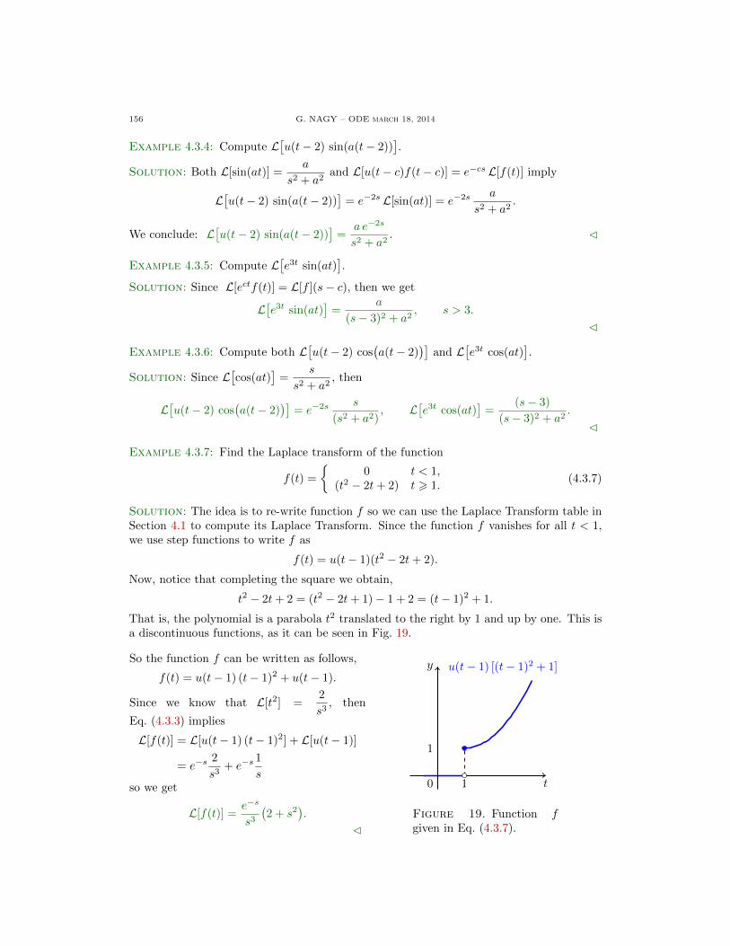
156 G. NAGY – ODE march 18, 2014
Example 4.3.4: Compute L[u(t− 2) sin(a(t− 2))
].
Solution: Both L[sin(at)] = a
s2 + a2and L[u(t− c)f(t− c)] = e−cs L[f(t)] imply
L[u(t− 2) sin(a(t− 2))
]= e−2s L[sin(at)] = e−2s a
s2 + a2.
We conclude: L[u(t− 2) sin(a(t− 2))
]=
a e−2s
s2 + a2. C
Example 4.3.5: Compute L[e3t sin(at)
].
Solution: Since L[ectf(t)] = L[f ](s− c), then we get
L[e3t sin(at)
]=
a
(s− 3)2 + a2, s > 3.
C
Example 4.3.6: Compute both L[u(t− 2) cos
(a(t− 2)
)]and L
[e3t cos(at)
].
Solution: Since L[cos(at)
]=
s
s2 + a2, then
L[u(t− 2) cos
(a(t− 2)
)]= e−2s s
(s2 + a2), L
[e3t cos(at)
]=
(s− 3)
(s− 3)2 + a2.
C
Example 4.3.7: Find the Laplace transform of the function
f(t) =
{0 t < 1,
(t2 − 2t+ 2) t > 1.(4.3.7)
Solution: The idea is to re-write function f so we can use the Laplace Transform table inSection 4.1 to compute its Laplace Transform. Since the function f vanishes for all t < 1,we use step functions to write f as
f(t) = u(t− 1)(t2 − 2t+ 2).
Now, notice that completing the square we obtain,
t2 − 2t+ 2 = (t2 − 2t+ 1)− 1 + 2 = (t− 1)2 + 1.
That is, the polynomial is a parabola t2 translated to the right by 1 and up by one. This isa discontinuous functions, as it can be seen in Fig. 19.
So the function f can be written as follows,
f(t) = u(t− 1) (t− 1)2 + u(t− 1).
Since we know that L[t2] =2
s3, then
Eq. (4.3.3) implies
L[f(t)] = L[u(t− 1) (t− 1)2] + L[u(t− 1)]
= e−s 2
s3+ e−s 1
sso we get
L[f(t)] = e−s
s3(2 + s2
).
C
t
y
0
1
u(t− 1) [(t− 1)2 + 1]
1
Figure 19. Function fgiven in Eq. (4.3.7).

G. NAGY – ODE March 18, 2014 157
Example 4.3.8: Find the function f such that L[f(t)] = e−4s
s2 + 5.
Solution: Notice that
L[f(t)] = e−4s 1
s2 + 5⇒ L[f(t)] = 1√
5e−4s
√5
s2 +(√
5)2 .
Recall that L[sin(at)] = a
(s2 + a2), then Eq. (4.3.3), or its inverse form Eq. (4.3.5) imply
L[f(t)] = 1√5L[u(t− 4) sin
(√5 (t− 4)
)]⇒ f(t) =
1√5u(t− 4) sin
(√5 (t− 4)
).
C
Example 4.3.9: Find the function f(t) such that L[f(t)] = (s− 1)
(s− 2)2 + 3.
Solution: We first rewrite the right-hand side above as follows,
L[f(t)] = (s− 1− 1 + 1)
(s− 2)2 + 3
=(s− 2)
(s− 2)2 + 3+
1
(s− 2)2 + 3
=(s− 2)
(s− 2)2 +(√
3)2 +
1√3
√3
(s− 2)2 +(√
3)2 .
We now recall Eq. (4.3.4) or its inverse form Eq. (4.3.6), which imply
L[f(t)] = L[e2t cos
(√3 t
)]+
1√3L[e2t sin
(√3 t
)].
So, we conclude that
f(t) =e2t√3
[√3 cos
(√3 t
)+ sin
(√3 t
)].
C
Example 4.3.10: Find L−1[ 2e−3s
s2 − 4
].
Solution: Since L−1[ a
s2 − a2
]= sinh(at) and L−1
[e−cs f(s)
]= u(t− c) f(t− c), then
L−1[ 2e−3s
s2 − 4
]= L−1
[e−3s 2
s2 − 4
]⇒ L−1
[ 2e−3s
s2 − 4
]= u(t− 3) sinh
(2(t− 3)
).
C
Example 4.3.11: Find a function f such that L[f(t)] = e−2s
s2 + s− 2.
Solution: Since the right-hand side above does not appear in the Laplace Transform tablein Section 4.1, we need to simplify it in the appropriate way. The plan is to rewrite thedenominator of the rational function 1/(s2+s−2), so we can use the partial fraction methodto simplify this rational function. We first find out whether this denominator has real orcomplex roots:
s± =1
2
[−1±
√1 + 8
]⇒
{s+ = 1,
s− = −2.

158 G. NAGY – ODE march 18, 2014
We are in the case of real roots, so we can rewrite
s2 + s− 2 = (s− 1) (s+ 2).
The partial fraction decomposition in this case is given by
1
(s− 1) (s+ 2)=
a
(s− 1)+
b
(s+ 2)=
(a+ b) s+ (2a− b)
(s− 1) (s+ 2)⇒
{a+ b = 0,
2a− b = 1.
The solution is a = 1/3 and b = −1/3, so we arrive to the expression
L[f(t)] = 1
3e−2s 1
s− 1− 1
3e−2s 1
s+ 2.
Recalling that
L[eat] = 1
s− a,
and Eq. (4.3.3) we obtain the equation
L[f(t)] = 1
3L[u(t− 2) e(t−2)
]− 1
3L[u(t− 2) e−2(t−2)
]which leads to the conclusion:
f(t) =1
3u(t− 2)
[e(t−2) − e−2(t−2)
].
C
4.3.4. Differential equations with discontinuous sources. The last three examples inthis Section show how to use the methods presented above to solve differential equationswith discontinuous source functions.
Example 4.3.12: Use the Laplace Transform to find the solution of the initial value problem
y′ + 2y = u(t− 4), y(0) = 3.
Solution: We compute the Laplace transform of the whole equation,
L[y′] + 2L[y] = L[u(t− 4)] =e−4s
s.
From the previous Section we know that[sL[y]− y(0)
]+ 2L[y] = e−4s
s⇒ (s+ 2)L[y] = y(0) +
e−4s
s.
We introduce the initial condition y(0) = 3 into equation above,
L[y] = 3
(s+ 2)+ e−4s 1
s(s+ 2)⇒ L[y] = 3L
[e−2t
]+ e−4s 1
s(s+ 2).
We need to invert the Laplace transform on the last term on the right-hand side in equationabove. We use the partial fraction decomposition on the rational function above, as follows
1
s(s+ 2)=a
s+
b
(s+ 2)=a(s+ 2) + bs
s(s+ 2)=
(a+ b) s+ (2a)
s(s+ 2)⇒
{a+ b = 0,
2a = 1.
We conclude that a = 1/2 and b = −1/2, so
1
s(s+ 2)=
1
2
[1s− 1
(s+ 2)
].

G. NAGY – ODE March 18, 2014 159
We then obtain
L[y] = 3L[e−2t
]+
1
2
[e−4s 1
s− e−4s 1
(s+ 2)
]= 3L
[e−2t
]+
1
2
(L[u(t− 4)]− L
[u(t− 4) e−2(t−4)
]).
Hence, we conclude that
y(t) = 3e−2t +1
2u(t− 4)
[1− e−2(t−4)
].
C
Example 4.3.13: Use the Laplace transform to find the solution to the initial value problem
y′′ + y′ +5
4y = b(t), y(0) = 0, y′(0) = 0, b(t) =
{1 0 6 t < π0 t > π.
(4.3.8)
Solution: From Fig. 20, the source function b can be written as
b(t) = u(t)− u(t− π).
t
u
0
1
π
u(t)
t
u
0
1
π
u(t− π)
t
b
0
1
π
u(t)− u(t− π)
Figure 20. The graph of the u, its translation and b as given in Eq. (4.3.8).
The last expression for b is particularly useful to find its Laplace transform,
L[b(t)] = L[u(t)]− L[u(t− π)] =1
s+ e−πs 1
s⇒ L[b(t)] = (1− e−πs)
1
s.
Now Laplace transform the whole equation,
L[y′′] + L[y′] + 5
4L[y] = L[b].
Since the initial condition are y(0) = 0 and y′(0) = 0, we obtain(s2 + s+
5
4
)L[y] =
(1− e−πs
) 1s
⇒ L[y] =(1− e−πs
) 1
s(s2 + s+ 5
4
) .Introduce the function
H(s) =1
s(s2 + s+ 5
4
) ⇒ y(t) = L−1[H(s)]− L−1[e−πsH(s)].
That is, we only need to find the inverse Laplace Transform of H. We use the partial fractionmethod to simplify the expression of H. We first find out whether the denominator has realor complex roots:
s2 + s+5
4= 0 ⇒ s± =
1
2
[−1±
√1− 5
],
so the roots are complex-valued. The appropriate partial fraction decomposition is
H(s) =1
s(s2 + s+ 5
4
) =a
s+
(bs+ c)(s2 + s+ 5
4
)
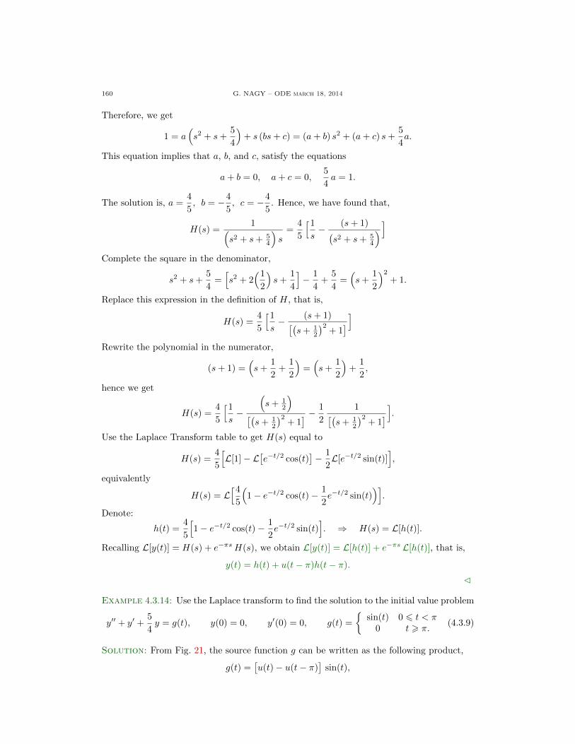
160 G. NAGY – ODE march 18, 2014
Therefore, we get
1 = a(s2 + s+
5
4
)+ s (bs+ c) = (a+ b) s2 + (a+ c) s+
5
4a.
This equation implies that a, b, and c, satisfy the equations
a+ b = 0, a+ c = 0,5
4a = 1.
The solution is, a =4
5, b = −4
5, c = −4
5. Hence, we have found that,
H(s) =1(
s2 + s+ 54
)s=
4
5
[1s− (s+ 1)(
s2 + s+ 54
)]Complete the square in the denominator,
s2 + s+5
4=
[s2 + 2
(12
)s+
1
4
]− 1
4+
5
4=
(s+
1
2
)2
+ 1.
Replace this expression in the definition of H, that is,
H(s) =4
5
[1s− (s+ 1)[(
s+ 12
)2+ 1
]]Rewrite the polynomial in the numerator,
(s+ 1) =(s+
1
2+
1
2
)=
(s+
1
2
)+
1
2,
hence we get
H(s) =4
5
[1s−
(s+ 1
2
)[(s+ 1
2
)2+ 1
] − 1
2
1[(s+ 1
2
)2+ 1
]].Use the Laplace Transform table to get H(s) equal to
H(s) =4
5
[L[1]− L
[e−t/2 cos(t)
]− 1
2L[e−t/2 sin(t)]
],
equivalently
H(s) = L[45
(1− e−t/2 cos(t)− 1
2e−t/2 sin(t)
)].
Denote:
h(t) =4
5
[1− e−t/2 cos(t)− 1
2e−t/2 sin(t)
]. ⇒ H(s) = L[h(t)].
Recalling L[y(t)] = H(s) + e−πsH(s), we obtain L[y(t)] = L[h(t)] + e−πs L[h(t)], that is,
y(t) = h(t) + u(t− π)h(t− π).
C
Example 4.3.14: Use the Laplace transform to find the solution to the initial value problem
y′′ + y′ +5
4y = g(t), y(0) = 0, y′(0) = 0, g(t) =
{sin(t) 0 6 t < π0 t > π.
(4.3.9)
Solution: From Fig. 21, the source function g can be written as the following product,
g(t) =[u(t)− u(t− π)
]sin(t),
G. NAGY – ODE March 18, 2014 161
since u(t) − u(t − π) is a box function, taking value one in the interval [0, π] and zero onthe complement. Finally, notice that the equation sin(t) = − sin(t − π) implies that thefunction g can be expressed as follows,
g(t) = u(t) sin(t)− u(t− π) sin(t) ⇒ g(t) = u(t) sin(t) + u(t− π) sin(t− π).
The last expression for g is particularly useful to find its Laplace transform,
t
v
0
1
π
v(t) = sin(t)
t
b
0
1
π
u(t)− u(t− π)
t
g
0
1
π
g(t)
Figure 21. The graph of the sine function, a square function u(t)−u(t−π)and the source function g given in Eq. (4.3.9).
L[g(t)] = 1
(s2 + 1)+ e−πs 1
(s2 + 1).
Having this last transform is then not difficult to solve the differential equation. As usual,Laplace transform the whole equation,
L[y′′] + L[y′] + 5
4L[y] = L[g].
Since the initial condition are y(0) = 0 and y′(0) = 0, we obtain(s2 + s+
5
4
)L[y] =
(1 + e−πs
) 1
(s2 + 1)⇒ L[y] =
(1 + e−πs
) 1(s2 + s+ 5
4
)(s2 + 1)
.
Introduce the function
H(s) =1(
s2 + s+ 54
)(s2 + 1)
⇒ y(t) = L−1[H(s)] + L−1[e−πsH(s)].
That is, we only need to find the inverse Laplace Transform of H. We use the partial fractionmethod to simplify the expression of H. We first find out whether the denominator has realor complex roots:
s2 + s+5
4= 0 ⇒ s± =
1
2
[−1±
√1− 5
],
so the roots are complex-valued. The appropriate partial fraction decomposition is
H(s) =1(
s2 + s+ 54
)(s2 + 1)
=(as+ b)(s2 + s+ 5
4
) +(cs+ d)
(s2 + 1).
Therefore, we get
1 = (as+ b)(s2 + 1) + (cs+ d)(s2 + s+
5
4
),
equivalently,
1 = (a+ c) s3 + (b+ c+ d) s2 +(a+
5
4c+ d
)s+
(b+
5
4d).
This equation implies that a, b, c, and d, are solutions of
a+ c = 0, b+ c+ d = 0, a+5
4c+ d = 0, b+
5
4d = 1.

162 G. NAGY – ODE march 18, 2014
Here is the solution to this system:
a =16
17, b =
12
17, c = −16
17, d =
4
17.
We have found that,
H(s) =4
17
[ (4s+ 3)(s2 + s+ 5
4
) +(−4s+ 1)
(s2 + 1)
].
Complete the square in the denominator,
s2 + s+5
4=
[s2 + 2
(12
)s+
1
4
]− 1
4+
5
4=
(s+
1
2
)2
+ 1.
H(s) =4
17
[ (4s+ 3)[(s+ 1
2
)2+ 1
] +(−4s+ 1)
(s2 + 1)
].
Rewrite the polynomial in the numerator,
(4s+ 3) = 4(s+
1
2− 1
2
)+ 3 = 4
(s+
1
2
)+ 1,
hence we get
H(s) =4
17
[4
(s+ 1
2
)[(s+ 1
2
)2+ 1
] +1[(
s+ 12
)2+ 1
] − 4s
(s2 + 1)+
1
(s2 + 1)
].
Use the Laplace Transform table to get H(s) equal to
H(s) =4
17
[4L
[e−t/2 cos(t)
]+ L
[e−t/2 sin(t)
]− 4L[cos(t)] + L[sin(t)]
],
equivalently
H(s) = L[ 4
17
(4e−t/2 cos(t) + e−t/2 sin(t)− 4 cos(t) + sin(t)
)].
Denote:
h(t) =4
17
[4e−t/2 cos(t) + e−t/2 sin(t)− 4 cos(t) + sin(t)
]⇒ H(s) = L[h(t)].
Recalling L[y(t)] = H(s) + e−πsH(s), we obtain L[y(t)] = L[h(t)] + e−πs L[h(t)], that is,y(t) = h(t) + u(t− π)h(t− π).
C

G. NAGY – ODE March 18, 2014 163
4.3.5. Exercises.
4.3.1.- . 4.3.2.- .
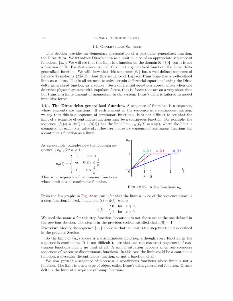
164 G. NAGY – ODE march 18, 2014
4.4. Generalized Sources
This Section provides an elementary presentation of a particular generalized function,the Dirac delta. We introduce Dirac’s delta as a limit n→ ∞ of an appropriate sequence offunctions, {δn}. We will see that this limit is a function on the domain R−{0}, but it is nota function on R. For that reason we call this limit a generalized function, the Dirac deltageneralized function. We will show that this sequence {δn} has a well-defined sequence ofLaplace Transforms {L[δn]}. And this sequence of Laplace Transforms has a well-definedlimit as n→ ∞. This is all we need to solve certain differential equations having the Diracdelta generalized function as a source. Such differential equations appear often when onedescribes physical systems with impulsive forces, that is, forces that act on a very short timebut transfer a finite amount of momentum to the system. Dirac’s delta is tailored to modelimpulsive forces.
4.4.1. The Dirac delta generalized function. A sequence of functions is a sequence,whose elements are functions. If each element in the sequence is a continuous function,we say that this is a sequence of continuous functions. It is not difficult to see that thelimit of a sequence of continuous functions may be a continuous function. For example, thesequence {fn(t) = sin((1 + 1/n)t)} has the limit limn→∞ fn(t) = sin(t), where the limit iscomputed for each fixed value of t. However, not every sequence of continuous functions hasa continuous function as a limit.
As an example, consider now the following se-quence, {un}, for n > 1,
un(t) =
0, t < 0
nt, 0 6 t 61
n
1, t >1
n.
This is a sequence of continuous functionswhose limit is a discontinuous function.
t
un
0
1u1(t)u2(t)u3(t)
11
2
1
3
Figure 22. A few functions un.
From the few graphs in Fig. 22 we can infer that the limit n→ ∞ of the sequence above isa step function, indeed, limn→∞ un(t) = u(t), where
u(t) =
{0 for t 6 0,
1 for t > 0.
We used the name u for this step function, because it is not the same as the one defined inthe previous Section. The step u in the previous section satisfied that u(0) = 1.
Exercise: Modify the sequence {un} above so that its limit is the step function u as definedin the previous Section.
So the limit of {un} above is a discontinuous function, although every function in thesequence is continuous. It is not difficult to see that one can construct sequences of con-tinuous functions having no limit at all. A similar situation happens when one considerssequences of piecewise discontinuous functions. In this case the limit could be a continuousfunction, a piecewise discontinuous function, or not a function at all.
We now present a sequence of piecewise discontinuous functions whose limit is not afunction. The limit is a new type of object called Dirac’s delta generalized function. Dirac’sdelta is the limit of a sequence of bump functions.

G. NAGY – ODE March 18, 2014 165
Definition 4.4.1. Given the sequence for n > 1 of bump functions
δn(t) = n[u(t)− u
(t− 1
n
)], (4.4.1)
we call the Dirac delta generalized function to the pointwise limit, for every t ∈ R,
limn→∞
δn(t) = δ(t).
It is simple to see that the sequence of bumpfunctions introduced above can be re-writtenas follows,
δn(t) =
0, t < 0
n, 0 6 t <1
n
0, t >1
n.
We then obtain,
δ(t) =
{0 for t 6= 0,
∞ for t = 0.
δn
t0
1
2
3
11
2
1
3
u1(t)
u2(t)
u3(t)
Figure 23. A few functions δn.
Remark: It can be shown that there exist infinitely many sequences {δn} such that theirlimit as n→ ∞ is Dirac’s delta. For example, another sequence is
δn(t) = n[u(t+
1
2n
)− u
(t− 1
2n
)]=
0, t < − 1
2n
n, − 1
2n6 t 6
1
2n
0, t >1
2n.
We see that the Dirac delta generalized function is a function on the domain R − {0},indeed it is the zero function, and it is not defined at t = 0, since the limit diverges at
that point. From the graphs given in Fig. 23 is simple to see that
∫ 1
0
δn(t) dt = 1 for every
n > 1. Therefore, the sequence of integrals is the constant sequence, {1, 1, · · · }, which has atrivial limit equal to one as n→ ∞. This says that the divergence at t = 0 of the sequence{δn} is of a very particular type. Using this limit procedure, one can generalize severaloperations from functions to limits of function sequences. For example, translations, linearcombinations, and multiplications of a function by a generalized function, integration andLaplace Transforms, as follows:
Definition 4.4.2. We introduce the following operations on the Dirac delta:
f(t) δ(t− c) + g(t) δ(t− c) = limn→∞
[f(t) δn(t− c) + g(t) δn(t− c)
],∫ b
a
δ(t− c) dt = limn→∞
∫ b
a
δn(t− c) dt, L[δ(t− c)] = limn→∞
L[δn(t− c)].
Remark: The notation in the definitions above could be misleading. In the left handsides above we use the same notation as we use on functions, although Dirac’s delta is not

166 G. NAGY – ODE march 18, 2014
a function on R. Take the integral, for example. When we integrate a function f , theintegration symbol means “take a limit of Riemann sums”, that is,∫ b
a
f(t) dt = limn→∞
n∑i=0
f(xi)∆x, xi = a+i
n, ∆x =
b− a
n.
However, when f is a generalized function in the sense of a limit of a sequence of functions{fn}, then by the integration symbol we mean to compute a different limit,∫ b
a
f(t) dt = limn→∞
∫ b
a
fn(t) dt.
We use the same symbol, the integration, to mean two different things, depending whetherwe integrate a function or a generalized function. This remark also holds for all the oper-ations we introduce on generalized functions, specially the Laplace Transform, that will beoften used in the rest of the Section.
4.4.2. The Laplace Transform of the Dirac delta. Once we have the definitions ofoperations involving the Dirac delta, we can actually compute these limits. The followingstatement summarizes few interesting results. The first formula below says that the infinitywe found in the definition of Dirac’s delta is of a very particular type; that infinity is suchthat Dirac’s delta is integrable, in the sense defined above, with integral equal one.
Theorem 4.4.3. For every c ∈ R and ε > 0 holds,
∫ c+ε
c−ε
δ(t− c) dt = 1.
Proof of Theorem 4.4.3: The integral of a Dirac’s delta generalized function is computedas a limit of integrals, ∫ c+ε
c−ε
δ(t− c) dt = limn→∞
∫ c+ε
c−ε
δn(t− c) dt
= limn→∞
∫ c+ 1n
c
ndt,1
n< ε,
= limn→∞
n(c+
1
n− c
)= lim
n→∞1
= 1.
This establishes the Theorem. �
Theorem 4.4.4. If f is continuous on (a, b) and c ∈ (a, b), then
∫ b
a
f(t) δ(t− c) dt = f(c).
Proof of Theorem 4.4.4: We again compute the integral of a Dirac’s delta as a limit ofa sequence of integrals,∫ b
a
δ(t− c) f(t) dt = limn→∞
∫ b
a
δn(t− c) f(t) dt
= limn→∞
∫ b
a
n[u(t− c)− u
(t− c− 1
n
)]f(t) dt
= limn→∞
∫ c+ 1n
c
n f(t) dt,1
n< (b− c),

G. NAGY – ODE March 18, 2014 167
where in the last line we used that c ∈ [a, b]. If we denote by F any primitive of f , that is,F ′ = f , then we can write,∫ b
a
δ(t− c) f(t) dt = limn→∞
n[F(c+
1
n
)− F (c)
]= lim
n→∞
1(1n
)[F (c+ 1
n
)− F (c)
]= F ′(c)
= f(c).
This establishes the Theorem. �
Theorem 4.4.5. For all s ∈ R holds L[δ(t− c)] =
{e−cs for c > 0,
0 for c < 0.
Proof of Theorem 4.4.5: The Laplace Transform of a Dirac’s delta is computed as a limitof Laplace Transforms,
L[δ(t− c)] = limn→∞
L[δn(t− c)]
= limn→∞
L[n[u(t− c)− u
(t− c− 1
n
)]]= lim
n→∞
∫ ∞
0
n[u(t− c)− u
(t− c− 1
n
)]e−st dt.
The case c < 0 is simple. For1
n< |c| holds
L[δ(t− c)] = limn→∞
∫ ∞
0
0 dt ⇒ L[δ(t− c)] = 0, for s ∈ R, c < 0.
Consider now the case c > 0. We then have,
L[δ(t− c)] = limn→∞
∫ c+ 1n
c
n e−st dt.
For s = 0 we get
L[δ(t− c)] = limn→∞
∫ c+ 1n
c
ndt = 1 ⇒ L[δ(t− c)] = 1 for s = 0, c > 0.
In the case that s 6= 0 we get,
L[δ(t− c)] = limn→∞
∫ c+ 1n
c
n e−st dt = limn→∞
−ns
(e−cs − e−(c+ 1
n )s)= e−cs lim
n→∞
(1− e−sn )( s
n
) .
The limit on the last line above is a singular limit of the form 00 , so we can use the l’Hopital
rule to compute it, that is,
limn→∞
(1− e−sn )( s
n
) = limn→∞
(− s
n2e−
sn
)(− s
n2
) = limn→∞
e−sn = 1.
We then obtain,
L[δ(t− c)] = e−cs for s 6= 0, c > 0.
This establishes the Theorem. �

168 G. NAGY – ODE march 18, 2014
4.4.3. The fundamental solution. In this Subsection we solve differential equations withthe Dirac delta as a source. Since Dirac’s delta is not a function, we need to clarify a bitwhat do we mean by a solution to a differential equation with such a source.
Definition 4.4.6. Given constants a1, a0, y0, y1, c ∈ R, consider the sequence of functions{yn}, with n > 1, solutions of the initial value problems
y′′n + a1 y′n + a0 yn = δn(t− c), yn(0) = y0, y′n(0) = y1. (4.4.2)
We define y(t) = L−1[limn→∞
L[yn(t)]]to be the solution of the IVP with Dirac’s delta source
y′′ + a1 y′ + a0 y = δ(t− c), y(0) = y0, y′(0) = y1, (4.4.3)
The solution of a differential equation having a Dirac’s delta as a source is obtained througha limit. We solve a sequence of IVPs, each one having as source the functions δn, obtaininga sequence of solutions, yn. The limit limn→∞ yn defines a function yδ. We define thisfunction yδ as the solution of the IVP having Dirac’s delta as a source. This type of limitprocedure is similar to the ones we used to introduce algebraic operations on Dirac’s deltas.
The definition above seems difficult to work with. However, the following result says thatit is fairly simple to find the function yδ solution of differential equations with Dirac’s deltasas sources.
Theorem 4.4.7. The function y is solution of the IVP with Dirac’s delta source
y′′ + a1 y′ + a0 y = δ(t− c), y(0) = y0, y′(0) = y1, c > 0,
iff its Laplace Transform satisfies the equation(s2 L[y]− sy0 − y1
)+ a1
(sL[y]− y0
)− a0 L[y] = e−cs.
This Theorem tells us that to find the solution y to an IVP when the source is a Dirac’s deltawe have to apply the Laplace Transform to the equation and perform the same calculationsas if the Dirac’s delta were a function. So, the final calculation is remarkably simple.Proof of Theorem 4.4.7: Compute the Laplace Transform on Eq. (4.4.2),
L[y′′n] + a1 L[y′n] + a0 L[yn] = L[δn(t− c)].
Recall the relations between the Laplace Transform and derivatives and use the initialconditions,
L[y′′n] = s2 L[yn]− sy0 − y1, L[y′] = sL[yn]− y0,
and use these relation in the differential equation,
(s2 + a1s+ a0)L[yn]− sy0 − y1 − a1y0 = L[δn(t− c)],
Since we have shown that limn→∞
L[δn(t− c)] = e−cs for c > 0, then
(s2 + a1s+ a0) limn→∞
L[yn]− sy0 − y1 − a1y0 = e−cs.
From the definition of y we see that we can re-write the equation above as
(s2 + a1s+ a0)L[y]− sy0 − y1 − a1y0 = e−cs,
which is equivalent to(s2 L[y]− sy0 − y1
)+ a1
(sL[y]− y0
)− a0 L[y] = e−cs.
This establishes the Theorem. �We now introduce a name for the solution of a differential equation with a Dirac’s delta
generalized function as a source and zero initial conditions. Such solution will play animportant role later on, that is why we give that function a particular name.

G. NAGY – ODE March 18, 2014 169
Definition 4.4.8. The function yδ is a fundamental solution of the linear operatorL(y) = y′′ + p y′ + q y, where p, q are continuous functions, iff the function yδ is solution ofthe initial value problem
L(yδ) = δ(t− c), yδ(0) = 0, y′δ(0) = 0, c > 0.
Remark: Fundamental solutions are also called impulse response solutions.
Example 4.4.1: Find the function yδ, the fundamental solution of the initial value problem
y′′ + 2y′ + 2y = δ(t), y(0) = 0, y′(0) = 0.
Solution: We compute the Laplace transform on both sides of the equation above,
L[y′′] + 2L[y′] + 2L[y] = L[δ(t)] = 1 ⇒ (s2 + 2s+ 2)L[y] = 1,
where we have introduced the initial conditions on the last equation above. So we obtain
L[y] = 1
(s2 + 2s+ 2).
The denomination in the equation above has complex valued roots, since
s± =1
2
[−2±
√4− 8
],
therefore, we complete squares s2 + 2s+ 2 = (s+ 1)2 + 1. We need to solve the equation
L[y] = 1[(s+ 1)2 + 1
] = L[e−t sin(t)] ⇒ yδ(t) = e−t sin(t).
C
Example 4.4.2: Find the impulse response solution at t = c > 0 of the initial value problem
y′′δ + 2 y′δ + 2 yδ = δ(t− c), yδ(0) = 0, y′δ(0) = 0, .
Solution: We have to use the Laplace Transform to solve this problem because the sourceis a Dirac’s delta generalized function. So, compute the Laplace Transform of the differentialequation,
L[y′′δ ] + 2L[y′δ] + 2L[yδ] = L[δ(t− c)].
Since the initial conditions are all zero and c > 0, we get
(s2 + 2s+ 2)L[yδ] = e−cs ⇒ L[yδ] =e−cs
(s2 + 2s+ 2).
Find the roots of the denominator,
s2 + 2s+ 2 = 0 ⇒ s± =1
2
[−2±
√4− 8
]The denominator has complex roots. Then, it is convenient to complete the square in thedenominator,
s2 + 2s+ 2 =[s2 + 2
(22
)s+ 1
]− 1 + 2 = (s+ 1)2 + 1.
Therefore, we obtain the expression,
L[yδ] =e−cs
(s+ 1)2 + 1.
170 G. NAGY – ODE march 18, 2014
Recall that L[sin(t)] = 1
s2 + 1, and L[f ](s− c) = L[ect f(t)]. Then,
1
(s+ 1)2 + 1= L[e−t sin(t)] ⇒ L[yδ] = e−cs L[e−t sin(t)].
Since for c > 0 holds e−cs L[f ](s) = L[u(t− c) f(t− c)], we conclude that
yδ(t) = u(t− c) e−(t−c) sin(t− c).
C
Example 4.4.3: Find the solution y to the initial value problem
y′′ − y = −20 δ(t− 3), y(0) = 1, y′(0) = 0.
Solution: The Laplace transform of the differential equation is given by
L[y′′]− L[y] = −20L[δ(t− 3)] ⇒ (s2 − 1)L[y]− s = −20 e−3s,
where in the second equation we have already introduced the initial conditions. We arriveto the equation
L[y] = s
(s2 − 1)− 20 e−3s 1
(s2 − 1)= L[cosh(t)]− 20L[u(t− 3) sinh(t− 3)],
which leads to the solution
y(t) = cosh(t)− 20u(t− 3) sinh(t− 3).
C
Example 4.4.4: Find the solution to the initial value problem
y′′ + 4y = δ(t− π)− δ(t− 2π), y(0) = 0, y′(0) = 0.
Solution: We again Laplace transform both sides of the differential equation,
L[y′′] + 4L[y] = L[δ(t− π)]− L[δ(t− 2π)] ⇒ (s2 + 4)L[y] = e−πs − e−2πs,
where in the second equation above we have introduced the initial conditions. Then,
L[y] = e−πs
(s2 + 4)− e−2πs
(s2 + 4)
=e−πs
2
2
(s2 + 4)− e−2πs
2
2
(s2 + 4)
=1
2L[u(t− π) sin
[2(t− π)
]]− 1
2L[u(t− 2π) sin
[2(t− 2π)
]].
The last equation can be rewritten as follows,
y(t) =1
2u(t− π) sin
[2(t− π)
]− 1
2u(t− 2π) sin
[2(t− 2π)
],
which leads to the conclusion that
y(t) =1
2
[u(t− π)− u(t− 2π)
]sin(2t).
C
G. NAGY – ODE March 18, 2014 171
Remark: Dirac’s delta generalized function is useful to describe impulsive forces in mechan-ical systems. An impulsive force on a particle is a force that transmits a finite momentumto the particle in an infinitely short time. For example, the momentum transmitted to apendulum when hit by a hammer. The force acting on the pendulum due to the hammercan be described with a Dirac’s delta. Recall Newton’s law of motion,
mv′(t) = F (t), with F (t) = F0 δ(t− t0).
Then, the linear momentum transfer from the hammer to the pendulum is,
∆I = lim∆t→0
mv(t)∣∣∣t0+∆t
t0−∆t= lim
∆t→0
∫ t0+∆t
t0−∆t
F (t) dt = F0.
That is, ∆I = F0; we have transferred a finite amount of momentum to the pendulumthrough an interaction at a single time t0.

172 G. NAGY – ODE march 18, 2014
4.4.4. Exercises.
4.4.1.- . 4.4.2.- .

G. NAGY – ODE March 18, 2014 173
4.5. Convolution Solutions
This Section describes a way to express a solution to an inhomogeneous linear differen-tial equation in terms of a convolution between the fundamental solution and the sourcefunction of the differential equation. This particular form to express the solution is usefulin mathematical physics to study different properties of solution. It is also a widely usedin physics and engineering. The plan for this Section is to first present the definition of aconvolution of two functions, and then discuss the main properties of this operation, withTheorems 4.5.3 and 4.5.4 containing perhaps the most important results of this Section. Thelatter result uses convolutions to write solutions to inhomogeneous differential equations.
4.5.1. The convolution of two functions. We start with a definition of the convolutionof two functions. One can say that the convolution is a generalization of the product of twofunctions. In a convolution one multiplies the two functions evaluated at different points,and then integrates the result. Here is a precise definition.
Definition 4.5.1. Assume that f and g are piecewise continuous functions, or one of themis a Dirac’s delta generalized function. The convolution of f and g is a function denotedby f ∗ g and given by the following expression,
(f ∗ g)(t) =∫ t
0
f(τ)g(t− τ) dτ.
In the Example we explicitly compute the integral defining the convolution of two functions.
Example 4.5.1: Find the convolution of the functions f(t) = e−t and g(t) = sin(t).
Solution: The definition of convolution is,
(f ∗ g)(t) =∫ t
0
e−τ sin(t− τ) dτ.
This integral is not difficult to compute. Integrate by parts twice,∫ t
0
e−τ sin(t− τ) dτ =[e−τ cos(t− τ)
]∣∣∣t0
−[e−τ sin(t− τ)
]∣∣∣t0
−∫ t
0
e−τ sin(t− τ) dτ,
that is,
2
∫ t
0
e−τ sin(t− τ) dτ =[e−τ cos(t− τ)
]∣∣∣t0
−[e−τ sin(t− τ)
]∣∣∣t0
= e−t − cos(t)− 0 + sin(t).
We then conclude that
(f ∗ g)(t) = 1
2
[e−t + sin(t)− cos(t)
]. (4.5.1)
C
The main properties of the convolution are summarized in the following result:
Lemma 4.5.2 (Properties). For every piecewise continuous functions f , g, and h, hold:
(i) Commutativity: f ∗ g = g ∗ f ;(ii) Associativity: f ∗ (g ∗ h) = (f ∗ g) ∗ h;(iii) Distributivity: f ∗ (g + h) = f ∗ g + f ∗ h;(iv) Neutral element: f ∗ 0 = 0;
(v) Identity element: f ∗ δ = f .

174 G. NAGY – ODE march 18, 2014
Proof of Lemma 4.5.2: We only prove properties (i) and (v), the rest are simple to obtainfrom the definition of convolution. The first property can be obtained by a change of theintegration variable as follows,
(f ∗ g)(t) =∫ t
0
f(τ) g(t− τ) dτ, τ = t− τ, dτ = −dτ,
=
∫ 0
t
f(t− τ) g(τ)(−1) dτ
=
∫ t
0
g(τ) f(t− τ) dτ ⇒ (f ∗ g)(t) = (g ∗ f)(t).
Finally, property (v) is straightforward form the definition of the delta generalized function,
(f ∗ δ)(t) =∫ t
0
f(τ) δ(t− τ) dτ = f(t).
This establishes the Lemma. �
4.5.2. The Laplace Transform of a convolution. We now show the relation betweenthe Laplace transform and the convolution operations. This is one of the most importantresults we need to solve differential equations. The Laplace transform of a convolution isthe usual product of the individual Laplace transforms.
Theorem 4.5.3 (Laplace Transform). If the functions f and g have well-defined LaplaceTransforms L[f ] and L[g], including the case that one of them is a Dirac’s delta, then
L[f ∗ g] = L[f ]L[g].
Example 4.5.2: Compute the Laplace transform of the function u(t) =
∫ t
0
e−τ sin(t−τ) dτ .
Solution: The function u above is the convolution of the functions
f(t) = e−t, g(t) = sin(t),
that is, u = f ∗ g. Therefore, Theorem 4.5.3 says that
L[u] = L[f ∗ g] = L[f ]L[g].Since,
L[f ] = L[e−t] =1
s+ 1, L[g] = L[sin(t)] = 1
s2 + 1,
we then conclude that L[u] = L[f ∗ g] is given by
L[f ∗ g] = 1
(s+ 1)(s2 + 1).
C
Proof of Theorem 4.5.3: The key step is to interchange two integrals. We start we theproduct of the Laplace Transforms,
L[f ]L[g] =[∫ ∞
0
e−stf(t) dt] [∫ ∞
0
e−stg(t) dt]
=
∫ ∞
0
e−stg(t)(∫ ∞
0
e−stf(t) dt)dt
=
∫ ∞
0
g(t)(∫ ∞
0
e−s(t+t)f(t) dt)dt,

G. NAGY – ODE March 18, 2014 175
where we only introduced the integral in t as a constant inside the integral in t. Introducethe Change of variables in the inside integral τ = t+ t, hence dτ = dt. Then, we get
L[f ]L[g] =∫ ∞
0
g(t)(∫ ∞
t
e−sτf(τ − t) dτ)dt (4.5.2)
=
∫ ∞
0
∫ ∞
t
e−sτ g(t) f(τ − t) dτ dt. (4.5.3)
Here is the key step, we must switch the order ofintegration. From Fig. 24 we see that changing theorder of integration gives the following expression,
L[f ]L[g] =∫ ∞
0
∫ τ
0
e−sτ g(t) f(τ − t) dt dτ.
Then, is straightforward to check that
L[f ]L[g] =∫ ∞
0
e−sτ(∫ τ
0
g(t) f(τ − t) dt)dτ
=
∫ ∞
0
e−sτ (g ∗ f)(τ) dt
= L[g ∗ f ] ⇒ L[f ]L[g] = L[f ∗ g].This establishes the Theorem. �
τ
t
0
t = τ
Figure 24. Domain ofintegration in (4.5.3).
Example 4.5.3: Use Laplace transforms to compute u(t) =
∫ t
0
e−τ sin(t− τ) dτ .
Solution: We know that u = f ∗ g, with f(t) = e−t and g(t) = sin(t), and we have seen inExample 4.5.2 that
L[u] = L[f ∗ g] = 1
(s+ 1)(s2 + 1).
A partial fraction decomposition of the right-hand side above implies that
L[u] = 1
2
[ 1
(s+ 1)+
(1− s)
(s2 + 1)
]=
1
2
[ 1
(s+ 1)+
1
(s2 + 1)− s
(s2 + 1)
]=
1
2
(L[e−t] + L[sin(t)]− L[cos(t)]
).
This says that
u(t) =1
2
[e−t + sin(t)− cos(t)
].
We then conclude that
(f ∗ g)(t) = 1
2
[e−t + sin(t)− cos(t)
],
which agrees with Eq. (4.5.1) in the first example above. C

176 G. NAGY – ODE march 18, 2014
4.5.3. The solution decomposition Theorem. One could say Theorem 4.5.4 is the mainresult of this Section. It presents a decomposition of the solution to a general second order,linear, constant coefficients initial value problem. The statement says that the solution tosuch problem can always be split in two terms, the first containing information only aboutthe initial data, while the second contains information only about the source function.
Theorem 4.5.4 (Solution decomposition). Given constants a0, a1, y0, y1 and a piecewisecontinuous function g, the solution y to the initial value problem
y′′ + a1 y′ + a0 y = g(t), y(0) = y0, y′(0) = y1, (4.5.4)
can be decomposed asy(t) = yh(t) + (yδ ∗ g)(t), (4.5.5)
where yh is the solution of the homogeneous initial value problem
y′′h + a1 y′h + a0 yh = 0, yh(0) = y0, y′h(0) = y1, (4.5.6)
and yδ is the impulse response solution, that is,
y′′δ + a1 y′δ + a0 yδ = δ(t), yδ(0) = 0, y′δ(0) = 0.
The solution decomposition in Eq. (4.5.5) can be expressed in the equivalent way
y(t) = yh(t) +
∫ t
0
yδ(τ)g(t− τ) dτ.
Proof of Theorem4.5.4: Compute the Laplace Transform of the differential equation,
L[y′′] + a1 L[y′] + a0 L[y] = L[g(t)].Recalling the relations between Laplace Transforms and derivatives,
L[y′′] = s2 L[y]− sy0 − y1, L[y′] = sL[y]− y0.
we re-write the differential equation for y as an algebraic equation for cL[y],
(s2 + a1s+ a0)L[y]− sy0 − y1 − a1y0 = L[g(t)].As usual, it is simple to solve the algebraic equation for cL[y],
L[y] = (s+ a1)y0 + y1(s2 + a1s+ a0)
+1
(s2 + a1s+ a0)L[g(t)].
Now, the function yh is the solution of Eq. (4.5.6), that is,
L[yh] =(s+ a1)y0 + y1(s2 + a1s+ a0)
.
And by the definition of the impulse response solution yδ we have that
L[yδ] =1
(s2 + a1s+ a0).
These last three equation imply,
L[y] = L[yh] + L[yδ]L[g(t)].This is the Laplace Transform version of Eq. (4.5.5). Inverting the Laplace Transform above,
y(t) = yh(t) + L−1[L[yδ]L[g(t)]
].
Using the result in Theorem 4.5.3 in the last term above we conclude that
y(t) = yh(t) + (yδ ∗ g)(t).�

G. NAGY – ODE March 18, 2014 177
Example 4.5.4: Use the Solution Decomposition Theorem to express the solution of
y′′ + 2 y′ + 2 y = sin(at), y(0) = 1, y′(0) = −1.
Solution: Compute the Laplace Transform of the differential equation above,
L[y′′] + 2L[y′] + 2L[y] = L[sin(at)],and recall the relations between the Laplace Transform and derivatives,
L[y′′] = s2 L[y]− sy(0)− y′(0), L[y′] = sL[y]− y(0).
Introduce the initial conditions in the equation above,
L[y′′] = s2 L[y]− s (1)− (−1), L[y′] = sL[y]− 1,
and these two equation into the differential equation,
(s2 + 2s+ 2)L[y]− s+ 1− 2 = L[sin(at)].Re-order terms to get
L[y] = (s+ 1)
(s2 + 2s+ 2)+
1
(s2 + 2s+ 2)L[sin(at)].
Now, the function yh is the solution of the homogeneous initial value problem with the sameinitial conditions as y, that is,
L[yh] =(s+ 1)
(s2 + 2s+ 2)=
(s+ 1)
(s+ 1)2 + 1= L[e−t cos(t)].
Now, the function yδ is the impulse response solution for the differential equation in thisExample, that is,
cL[yδ] =1
(s2 + 2s+ 2)=
1
(s+ 1)2 + 1= L[e−t sin(t)].
Put all this information together and denote g(t) = sin(at) to get
L[y] = L[yh] + L[yδ]L[g(t)] ⇒ y(t) = yh(t) + (yδ ∗ g)(t),More explicitly, we get
y(t) = e−t cos(t) +
∫ t
0
e−τ sin(τ) sin[a(t− τ)] dτ.
C

178 G. NAGY – ODE march 18, 2014
4.5.4. Exercises.
4.5.1.- . 4.5.2.- .

G. NAGY – ODE March 18, 2014 179
Chapter 5. Systems of Differential Equations
Newton’s second law of motion for point particles is one of the first differential equations toever be written. Even this early example of a differential equation consists not of a singleequation but of a system of three equation on three unknowns. The unknown functions arethe particle three coordinates in space as function of time. One important difficulty to solvea differential system is that the equations in a system are usually coupled. One cannot solvefor one unknown function without knowing the other unknowns. In this Chapter we studyhow to solve the system in the particular case that the equations can be uncoupled. We callsuch systems diagonalizable. Explicit formulas for the solutions can be written in this case.Later we generalize this idea to systems that cannot be uncoupled.
5.1. Linear Differential Systems
We introduce a linear differential system with variable coefficients. We present an initialvalue problem for such systems and we state that initial value problems always have aunique solution. The proof is based on a generalization of the Picard-Lindelof iteration usedin Section 1.6. We then introduce the concepts of fundamental solution, general solution,fundamental matrix, and Wronskian of solutions to a linear system.
5.1.1. First order linear systems. A single differential equation on one unknown functionis often not enough to describe certain physical problems. The description of a point particlemoving in space under Newton’s law of motion requires three functions of time, the spacecoordinates of the particle, to describe the motion together with three differential equations.To describe several proteins activating and deactivating each other inside a cell also requiresas many unknown functions and equations as proteins in the system. In this Section wepresent a first step aimed to describe such physical systems. We start introducing a firstorder linear differential system.
Definition 5.1.1. An n× n first order linear differential system is the equation
x′(t) = A(t)x(t) + g(t), (5.1.1)
where the n×n coefficient matrix A, the source n-vector g, and the unknown n-vector x aregiven in components by
A(t) =
a11(t) · · · a1n(t)...
...an1(t) · · · ann(t)
, g(t) =
g1(t)...gn(t)
, x(t) =
x1(t)...
xn(t)
.The system is called homogeneous iff the source vector g = 0. The system is called ofconstant coefficients iff the coefficient matrix A is constant.
Remarks:
(a) The derivative of a a vector-valued function is defined as x′(t) =
x′1(t)...
x′n(t)
.(b) By the definition of the matrix-vector product, Eq. (5.1.1) can be written as
x′1(t) = a11(t)x1(t) + · · ·+ a1n(t)xn(t) + g1(t),
...
x′n(t) = an1(t)x1(t) + · · ·+ ann(t)xn(t) + gn(t).

180 G. NAGY – ODE march 18, 2014
A solution of an n × n linear differential system is an n-vector-valued function x, thatis, a set of n functions {x1, · · · , xn}, that satisfy every differential equation in the system.When we write down the equations we will usually write x instead of x(t).
Example 5.1.1: The case n = 1 is a single differential equation: Find a solution x1 of
x′1 = a11(t)x1 + g1(t).
This is a linear first order equation, and solutions can be found with the integrating factormethod described in Section 1.2. C
Example 5.1.2: The case n = 2 is a 2× 2 linear system: Find functions x1, x2 solutions of
x′1 = a11(t)x1 + a12(t)x2 + g1(t),
x′2 = a21(t)x1 + a22(t)x2 + g2(t).
In this case the coefficient matrix A, the source vector g, and the unknown vector x are,
A(t) =
[a11(t) a12(t)a21(t) a22(t)
], g(t) =
[g1(t)g2(t)
], x(t) =
[x1(t)x2(t)
].
C
Example 5.1.3: Use matrix notation to write down the 2× 2 system given by
x′1 = x1 − x2,
x′2 = −x1 + x2.
Solution: In this case, the matrix of coefficients and the unknown vector have the form
A =
[1 −1
−1 1
], x(t) =
[x1(t)x2(t)
].
This is an homogeneous system, so the source vector g = 0. The differential equation canbe written as follows,
x′1 = x1 − x2
x′2 = −x1 + x2
⇔[x′1x′2
]=
[1 −1
−1 1
] [x1
x2
]⇔ x′ = Ax.
C
Example 5.1.4: Find the explicit expression for the linear system x′ = Ax+ b, where
A =
[1 33 1
], g(t) =
[et
2e3t
], x =
[x1
x2
].
Solution: The 2× 2 linear system is given by[x′1x′2
]=
[1 33 1
] [x1
x2
]+
[et
2e3t
], ⇔
x′1 = x1 + 3x2 + et,
x′2 = 3x1 + x2 + 2e3t.
C
Example 5.1.5: Show that the vector-valued functions x(1) =
[21
]e2t and x(2) =
[12
]e−t
are solutions to the 2× 2 linear system x′ = Ax, where A =
[3 −22 −2
].

G. NAGY – ODE March 18, 2014 181
Solution: We compute the left-hand side and the right-hand side of the differential equationabove for the function x(1) and we see that both side match, that is,
Ax(1) =
[3 −22 −2
] [21
]e2t =
[42
]e2t = 2
[21
]e2t; x(1)′ =
[21
] (e2t
)′=
[21
]2 e2t,
so we conclude that x(1) ′ = Ax(1). Analogously,
Ax(2) =
[3 −22 −2
] [12
]e−t =
[−1−2
]e−t = −
[12
]e−t; x(2) ′ =
[12
] (e−t
)′= −
[12
]e−t,
so we conclude that x(2) ′ = Ax(2). C
Example 5.1.6: Find the explicit expression of the most general 3× 3 homogeneous lineardifferential system.
Solution: This is a system of the form x′ = A(t)x, with A beaing a 3×3 matrix. Therefore,we need to find functions x1, x2, and x3 solutions of
x′1 = a11(t)x1 + a12(t)x2 + a13(t)x3
x′2 = a21(t)x1 + a22(t)x2 + a13(t)x3
x′3 = a31(t)x1 + a32(t)x2 + a33(t)x3.
C
5.1.2. Order transformation. We present two results that make use of 2×2 linear systems.The first result transforms any second order linear equation into a 2 × 2 first order linearsystem. The second result is kind of a converse. It transforms any 2× 2 first order, linear,constant coefficients system into a second order linear differential equation. We start withour first result.
Theorem 5.1.2 (First order reduction). A function y solves the second order equation
y′′ + p(t) y′ + q(t) y = g(t), (5.1.2)
iff the functions x1 = y and x2 = y′ are solutions to the 2× 2 first order differential system
x′1 = x2, (5.1.3)
x′2 = −q(t)x1 − p(t)x2 + g(t). (5.1.4)
Proof of Theorem 5.1.2:(⇒) Given a solution y of Eq. (5.1.2), introduce the functions x1 = y and x2 = y′. ThereforeEq. (5.1.3) holds, due to the relation
x′1 = y′ = x2,
Also Eq. (5.1.4) holds, because of the equation
x′2 = y′′ = −q(t) y − p(t) y′ + g(t) ⇒ x′′2 = −q(t)x1 − p(t)x2 + g(t).
(⇐) Differentiate Eq. (5.1.3) and introduce the result into Eq. (5.1.4), that is,
x′′1 = x′2 ⇒ x′′1 = −q(t)x1 − p(t)x′1 + g(t).
Denoting y = x1, we obtain,
y′′ + p(t) y′ + q(t) y = g(t).
This establishes the Theorem. �

182 G. NAGY – ODE march 18, 2014
Example 5.1.7: Express as a first order system the second order equation
y′′ + 2y′ + 2y = sin(at).
Solution: Introduce the new unknowns
x1 = y, x2 = y′ ⇒ x′1 = x2.
Then, the differential equation can be written as
x′2 + 2x2 + 2x1 = sin(at).
We conclude thatx′1 = x2, x′2 = −2x1 − 2x2 + sin(at).
C
The transformation of a 2 × 2 first order system into a second order equation given inTheorem 5.1.2 can be generalized to any 2×2 constant coefficient linear differential system.
Theorem 5.1.3 (Second order increase). Any 2× 2 constant coefficients linear system
x′ = Ax, with x =
[x1
x2
], can be written as the second order equation for x1 given by
x′′1 − tr (A)x1 + det(A)x1 = 0. (5.1.5)
Proof of Theorem 5.1.3: Denoting A =
[a11 a12a21 a22
], the system has the form
x′1 = a11 x1 + a12 x2 (5.1.6)
x′2 = a21 x1 + a22 x2. (5.1.7)
Compute the derivative of the first equation,
x′′1 = a11 x′1 + a12 x
′2.
Use Eq. (5.1.7) to replace x′2 on the right-hand side above,
x′′1 = a11 x′1 + a12
(a21 x1 + a22 x2
).
Finally, replace the term with x2 above using Eq. (5.1.6), that is,
x′′1 = a11 x′1 + a12a21 x1 + a12a22
(x′1 − a11 x1
)a12
.
A simple cancellation and reorganization of terms gives the equation,
x′′1 = (a11 + a22)x1 + (a12a21 − a11a22)x1.
Recalling that tr (A) = a11 + a22, and det(A) = a11a22 − a12a21, we get Eq. (5.1.5). Thisestablishes the Theorem. �
Example 5.1.8: Express as a single second order equation the 2× 2 system and solve it,
x′1 = −x1 + 3x2,
x′2 = x1 − x2.
Solution: Compute x1 from the second equation: x1 = x′2 + x2. Introduce this expressioninto the first equation,
(x′2 + x2)′ = −(x′2 + x2) + 3x2 ⇒ x′′2 + x′2 = −x′2 − x2 + 3x2,
so we obtain the second order equation
x′′2 + 2x′2 − 2x2 = 0.

G. NAGY – ODE March 18, 2014 183
We solve this equation with the methods studied in Chapter 2, that is, we look for solutionsof the form x2(t) = ert, with r solution of the characteristic equation
r2 + 2r − 2 = 0 ⇒ r± =1
2
[−2±
√4 + 8
]⇒ r± = −1±
√3.
Therefore, the general solution to the second order equation above is x2 = c1 er+t + c2 e
r-t,with c1, c2 ∈ R. Since x1 = x′2 + x2, we obtain
x1 =(c1r+ e
r+t + c2r- er-t
)+
(c1 e
r+t + c2 er-t
),
Re-ordering terms we get the expression for the function x1, that is,
x1 = c1(1 + r+) er+t + c2(1 + r-) e
r-t.
C
5.1.3. The initial value problem. This notion for linear systems is similar to initial valueproblems for single differential equations. In the case of an n×n first order system we needn initial conditions, one for each unknown function, which are collected in an n-vector.
Definition 5.1.4. An Initial Value Problem for an n × n linear differential system isthe following: Given an n×n matrix-valued function A, and an n-vector-valued function b,a real constant t0, and an n-vector x0, find an n-vector-valued function x solution of
x′ = A(t)x+ b(t), x(t0) = x0.
Remark: The initial condition vector x0 represents n conditions, one for each componentof the unknown vector x.
Example 5.1.9: Write down explicitly the initial value problem for x =
[x1
x2
]given by
x′ = Ax, x(0) =
[23
], A =
[1 33 1
].
Solution: This is a 2× 2 system in the unknowns x1, x2, with two linear equations
x′1 = x1 + 3x2
x′2 = 3x1 + x2,
and the initial conditions x1(0) = 2 and x2(0) = 3. C
The main result about existence and uniqueness of solutions to an initial value problemfor a linear system is also analogous to Theorem 2.1.2
Theorem 5.1.5 (Variable Coefficients). If the functions A and b are continuous on aclosed interval I ⊂ R, t0 ∈ I, and x0 are any constants, then there exists a unique solutionx to the initial value problem
x′ = A(t)x+ b(t), x(t0) = x0. (5.1.8)
Remark: The fixed point argument used in the proof of Picard-Lindelof’s Theorem 1.6.2can be extended to prove Theorem 5.1.5. This proof will be presented later on.

184 G. NAGY – ODE march 18, 2014
5.1.4. Homogeneous systems. Solutions to a linear homogeneous differential system sat-isfy the superposition property: Given two solutions of the homogeneous system, their linearcombination is also a solution to that system.
Theorem 5.1.6 (Superposition). If the n-vector-valued functions x(1),x(2) are solutionsof x(1)′ = A(t)x(1) and x(2)′ = A(t)x(2), then any the linear combination x = ax(1) + bx(2), forall a, b ∈ R, is also solution of x′ = Ax.
Remark: This Theorem contains two particular cases:
(a) a = b = 1: If x(1) and x(2) are solutions of an homogeneous linear system, so is x(1)+x(2).(b) b = 0 and a arbitrary: If x(1) is a solution of an homogeneous linear system, so is ax(1).
Proof of Theorem 5.1.6: We check that the function x = ax(1) + bx(2) is a solution ofthe differential equation in the Theorem. Indeed, since the derivative of a vector-valuedfunction is a linear operation, we get
x′ =(ax(1) + bx(2)
)′= ax(1) ′ + bx(2) ′.
Replacing the differential equation on the right-hand side above,
x′ = aAx(1) + bAx(2).
The matrix-vector product is a linear operation, A(ax(1) + bx(2)
)= aAx(1) + bAx(2), hence,
x′ = A(ax(1) + bx(2)
)⇒ x′ = Ax.
This establishes the Theorem. �
Example 5.1.10: Verify that x(1) =
[11
]e−2t and x(2) =
[−11
]e4t and x(1) + x(2) are
solutions to the homogeneous linear system
x′ = Ax, A =
[1 −3
−3 1
].
Solution: The function x(1) is solution to the differential equation, since
x(1) ′ = −2
[11
]e−2t, Ax(1) =
[1 −3
−3 1
] [11
]e−2t =
[−2−2
]e−2t = −2
[11
]e−2t.
We then conclude that x(1) ′ = Ax(1). Analogously, the function x(2) is solution to thedifferential equation, since
x(2) ′ = 4
[−11
]e4t, Ax(2) =
[1 −3
−3 1
] [−11
]e4t =
[−44
]e4t = 4
[−11
]e4t.
We then conclude that x(2) ′ = Ax(2). To show that x(1) + x(2) is also a solution we coulduse the linearity of the matrix-vector product, as we did in the proof of the Theorem 5.1.6.Here we choose the straightforward, although more obscure, calculation: On the one hand,
x(1) + x(2) =
[e−2t − e4t
e−2t + e4t
]⇒
(x(1) + x(2)
)′=
[−2e−2t − 4e4t
−2e−2t + 4e4t
].
On the other hand,
A(x(1) + x(2)
)=
[1 −3
−3 1
] [e−2t − e4t
e−2t + e4t
]=
[e−2t − e4t − 3e−2t − 3e4t
−3e−2t + 3e4t + e−2t + e4t
],
that is,
A(x(1) + x(2)
)=
[−2e−2t − 4e4t
−2e−2t + 4e4t
].

G. NAGY – ODE March 18, 2014 185
We conclude that(x(1) + x(2)
)′= A
(x(1) + x(2)
). C
We now introduce the notion of a linearly dependent and independent set of functions.
Definition 5.1.7. A set of n vector-valued functions {x(1), · · · ,x(n)} is called linearlydependent on an interval I ∈ R iff for all t ∈ I there exist constants c1, · · · , cn, not all ofthem zero, such that it holds
c1 x(1)(t) + · · ·+ cn x
(n)(t) = 0.
A set of n vector-valued functions is called linearly independent on I iff the set is notlinearly dependent.
Remark: This notion is a generalization of Def. 2.1.6 from two functions to n vector-valuedfunctions. For every value of t ∈ R this definition agrees with the definition of a set of linearlydependent vectors given in Linear Algebra and reviewed in the Appendices.
We now generalize Theorem 2.1.7 to linear systems. If you know a linearly independentset of n solutions to an n×n first order, linear, homogeneous system, then you actually knowall possible solutions to that system, since any other solution is just a linear combination ofthe previous n solutions.
Theorem 5.1.8 (General solution). If {x(1), · · · ,x(n)} is a linearly independent set ofsolutions of the n×n system x′ = Ax, where A is a continuous matrix-valued function, thenthere exist unique constants c1, · · · , cn such that every solution x of the differential equationx′ = Ax can be written as the linear combination
x(t) = c1 x(1)(t) + · · ·+ cn x
(n)(t). (5.1.9)
Before we present a sketch of the proof for Theorem 5.1.8, it is convenient to state thefollowing the definitions, which come out naturally from Theorem 5.1.8.Definition 5.1.9.
(a) The set of functions {x(1), · · · ,x(n)} is a fundamental set of solutions of the equationx′ = Ax iff it holds that x(i)′ = Ax(i), for i = 1, · · · , n, and the set {x(1), · · · ,x(n)} islinearly independent.
(b) The general solution of the homogeneous equation x′ = Ax denotes any vector-valuedfunction xgen that can be written as a linear combination
xgen(t) = c1 x(1)(t) + · · ·+ cn x
(n)(t),
where x(1), · · · ,x(n) are the functions in any fundamental set of solutions of x′ = Ax,while c1, · · · , cn are arbitrary constants.
Remark: The names above are appropriate, since Theorem 5.1.8 says that knowing then functions of a fundamental set of solutions is equivalent to knowing all solutions to thehomogeneous linear differential system.
Example 5.1.11: Show that the set of functions{x(1) =
[11
]e−2t, x(2) =
[−11
]e4t
}is a
fundamental set of solutions to the system x′ = Ax, where A =
[1 −3
−3 1
].
Solution: In Example 5.1.10 we have shown that x(1) and x(2) are solutions to the dif-ferential equation above. We only need to show that these two functions form a linearly

186 G. NAGY – ODE march 18, 2014
independent set. That is, we need to show that the only constants c1, c2 solutions of theequation below, for all t ∈ R, are c1 = c2 = 0, where
0 = c1 x(1) + c2 x
(2) = c1
[11
]e−2t + c2
[−11
]e4t =
[e−2t −e4te−2t e4t
] [c1c2
]= X(t) c,
where X(t) =[x(1)(t), x(2)(t)
]and c =
[c1c2
]. Using this matrix notation, the linear system
for c1, c2 has the formX(t) c = 0.
We now show that matrix X(t) is invertible for all t ∈ R. This is the case, since itsdeterminant is
det(X(t)
)=
∣∣∣∣e−2t −e4te−2t e4t
∣∣∣∣ = e2t + e2t = 2 e2t 6= 0 for all t ∈ R.
Since X(t) is invertible for t ∈ R, the only solution for the linear system above is c = 0,that is, c1 = c2 = 0. We conclude that the set
{x(1), x(2)
}is linearly independent, so it is a
fundamental set of solution to the differential equation above. C
Proof of Theorem 5.1.8: The superposition property in Theorem 5.1.6 says that given anyset of solutions {x(1), · · · ,x(n)} of the differential equation x′ = Ax, the linear combinationx(t) = c1 x
(1)(t) + · · · + cn x(n)(t) is also a solution. We now must prove that, in the case
that {x(1), · · · ,x(n)} is linearly independent, every solution of the differential equation isincluded in this linear combination.
Let now x be any solution of the differential equation x′ = Ax. The uniqueness statementin Theorem 5.1.5 implies that this is the only solution that at t0 takes the value x(t0). Thismeans that the initial data x(t0) parametrizes all solutions to the differential equation. Wenow try to find the constants {c1, · · · , cn} solutions of the algebraic linear system
x(t0) = c1 x(1)(t0) + · · ·+ cn x
(n)(t0).
Introducing the notation
X(t) =[x(1)(t), · · · ,x(n)(t)
], c =
c1...cn
,the algebraic linear system has the form
x(t0) = X(t0) c.
This algebraic system has a unique solution c for every source x(t0) iff the matrix X(t0)is invertible. This matrix is invertible iff det
(X(t0)
)6= 0. The generalization of Abel’s
Theorem to systems, Theorem 5.1.11, says that det(X(t0)
)6= 0 iff the set {x(1), · · · ,x(n)} is
a fundamental set of solutions to the differential equation. This establishes the Theorem. �
Example 5.1.12: Find the general solution to differential equation in Example 5.1.5 andthen use this general solution to find the solution of the initial value problem
x′ = Ax, x(0) =
[15
], A =
[3 −22 −2
].
Solution: From Example 5.1.5 we know that the general solution of the differential equa-tion above can be written as
x(t) = c1
[21
]e2t + c2
[12
]e−t.

G. NAGY – ODE March 18, 2014 187
Before imposing the initial condition on this general solution, it is convenient to write thisgeneral solution using a matrix-valued function, X, as follows
x(t) =
[2e2t e−t
e2t 2e−t
] [c1c2
]⇔ x(t) = X(t)c,
where we introduced the solution matrix and the constant vector, respectively,
X(t) =
[2e2t e−t
e2t 2e−t
], c =
[c1c2
].
The initial condition fixes the vector c, that is, its components c1, c2, as follows,
x(0) = X(0) c ⇒ c =[X(0)
]−1x(0).
Since the solution matrix X at t = 0 has the form,
X(0) =
[2 11 2
]⇒
[X(0)
]−1=
1
3
[2 −1
−1 2
],
introducing[X(0)
]−1in the equation for c above we get
c =1
3
[2 −1
−1 2
] [15
]=
[−13
]⇒
{c1 = −1,
c2 = 3.
We conclude that the solution to the initial value problem above is given by
x(t) = −[21
]e2t + 3
[12
]e−t.
C
5.1.5. The Wronskian and Abel’s Theorem. From the proof of Theorem 5.1.8 abovewe see that it is convenient to introduce the notion of solution matrix and Wronskian of aset of n solutions to an n× n linear differential system,Definition 5.1.10.
(a) The solution matrix of any set {x(1), · · · ,x(n)} of solutions to a differential equationx′ = Ax is the n× n matrix-valued function
X(t) =[x1(t), · · · ,xn(t)
]. (5.1.10)
Xis called a fundamental matrix iff the set {x1, · · · ,xn} is a fundamental set.(b) The Wronskian of the set {x1, · · · ,xn} is the function W (t) = det
(X(t)
).
Remark: A fundamental matrix provides a more compact way to write down the generalsolution of a differential equation. The general solution in Eq. (5.1.9) can be rewritten as
xgen(t) = c1x1(t) + · · ·+ cnx
n(t) =[x1(t), · · · ,xn(t)
] c1...cn
= X(t) c, c =
c1...cn
.This is a more compact notation for the general solution,
xgen(t) = X(t) c. (5.1.11)
Remark: Consider the case that a linear system is a first order reduction of a second orderlinear homogeneous equation, y′′ + a1y
′ + a0y = 0, that is,
x′1 = x2, x′2 = −a0x1 − a1x2.

188 G. NAGY – ODE march 18, 2014
In this case, the Wronskian defined here coincides with the definition given in Sect. 2.1. Theproof is simple. Suppose that y1, y2 are fundamental solutions of the second order equation,then the vector-valued functions
x(1) =
[y1y′1
], x(2) =
[y2y′2
],
are solutions of the first order reduction system. Then holds,
W = det([x(1),x(2)
])=
∣∣∣∣y1 y2y′1 y′2
∣∣∣∣ =Wy1y2 .
Example 5.1.13: Find two fundamental matrices for the linear homogeneous system inExample 5.1.10.
Solution: One fundamental matrix is simple to find, is it constructed with the solutionsgiven in Example 5.1.10, that is,
X =[x(1),x(2)
]⇒ X(t) =
[e−2t −e4te−2t e4t
].
A second fundamental matrix can be obtained multiplying by any non-zero constant eachsolution above. For example, another fundamental matrix is
X =[2x(1), 3x(2)
]⇒ X(t) =
[2e−2t −3e4t
2e−2t 3e4t
].
C
Example 5.1.14: Compute the Wronskian of the vector-valued functions given in Exam-
ple 5.1.10, that is, x(1) =
[11
]e−2t and x(2) =
[−11
]e4t.
Solution: The Wronskian is the determinant of the solution matrix, with the vectorsplaced in any order. For example, we can choose the order
[x(1),x(2)
]. If we choose the
order[x(2),x(1)
], this second Wronskian is the negative of the first one. Choosing the first
order we get,
W (t) = det([x(1),x(2)
])=
∣∣∣∣e−2t −e4te−2t e4t
∣∣∣∣ = e−2t e4t + e−2t e4t.
We conclude that W (t) = 2e2t. C
Example 5.1.15: Show that the set of functions{x(1) =
[e3t
2e3t
], x(2) =
[e−t
−2e−t
]}is
linearly independent for all t ∈ R.
Solution: We compute the determinant of the matrix X(t) =
[e3t e−t
2e3t −2e−t
], that is,
w(t) =
∣∣∣∣ e3t e−t
2e3t −2e−t
∣∣∣∣ = −2e2t − 2e2t ⇒ w(t) = −4e2t 6= 0 t ∈ R.C
We now generalize Abel’s Theorem 2.1.14 from a single equation to an n×n linear system.
Theorem 5.1.11 (Abel). The Wronskian function W = det(X(t)
)of a solution matrix
X(t) =[x(1), · · · ,x(n)
]of the linear system x′ = A(t)x, where A is an n × n continuous
matrix-valued function on a domain I ⊂ R, is given by
W (t) =W (t0) eα(t), α(t) =
∫ t
t0
tr(A(τ)
)dτ.

G. NAGY – ODE March 18, 2014 189
where tr (A) is the trace of A and t0 is any point in I.
Remarks:
(a) In the case of a constant matrix A, the equation above for the Wronskian reduces to
W (t) =W (t0) etr (A) (t−t0),
(b) The Wronskian function vanishes at a single point iff it vanishes identically for all t ∈ I.(c) A consequence of (b): n solutions to the system x′ = A(t)x are linearly independent at
the initial time t0 iff they are linearly independent for every time t ∈ I.
Proof of Theorem 5.1.11: The proof is based in an identity satisfied by the determinantof certain matrix-valued functions. The proof of this identity is quite involved, so we donot provide it here. The identity is the following: Every n × n, differentiable, invertible,matrix-valued function Z, with values Z(t) for t ∈ R, satisfies the identity:
d
dtdet(Z) = det(Z) tr
(Z−1 d
dtZ).
We use this identity with any fundamental matrix X =[x(1), · · · ,x(n)
]of the linear homo-
geneous differential system x′ = Ax. Recalling that the Wronskian w(t) = det(X(t)
), the
identity above says,
W ′(t) =W (t) tr[X−1(t)X ′(t)
].
We now compute the derivative of the fundamental matrix,
X ′ =[x(1) ′, · · · ,x(n) ′
]=
[Ax(1), · · · , Ax(n)
]= AX,
where the equation on the far right comes from the definition of matrix multiplication.Replacing this equation in the Wronskian equation we get
W ′(t) =W (t) tr(X−1AX
)=W (t) tr
(XX−1A
)=W (t) tr (A),
where in the second equation above we used a property of the trace of three matrices:tr (ABC) = tr (CAB) = tr (BCA). Therefore, we have seen that the Wronskian satisfiesthe equation
W ′(t) = tr[A(t)
]W (t). (5.1.12)
This is a linear differential equation of a single function W : R → R. We integrate it usingthe integrating factor method from Section 1.2. The result is
W (t) =W (t0) eα(t), α(t) =
∫ t
t0
tr[A(τ)
]dτ.
This establishes the Theorem. �
Example 5.1.16: Show that the Wronskian of the fundamental matrix constructed withthe solutions given in Example 5.1.3 satisfies Eq. (5.1.12) above.
Solution: In Example 5.1.5 we have shown that the vector-valued functions x(1) =
[21
]e2t
and x(2) =
[12
]e−t are solutions to the system x′ = Ax, where A =
[3 −22 −2
]. The matrix
X(t) =
[2e2t e−t
e2t 2e−t
]is a fundamental matrix of the system, since its Wronskian is non-zero,
W (t) =
∣∣∣∣2e2t e−t
e2t 2e−t
∣∣∣∣ = 4et − et ⇒ W (t) = 3et.
190 G. NAGY – ODE march 18, 2014
We need to compute the right-hand side and the left-hand side of Eq. (5.1.12) and verifythat they coincide. We start with the left-hand side,
W ′(t) = 3et =W (t).
The right-hand side istr (A)W (t) = (3− 2)W (t) =W (t).
Therefore, we have shown that W (t) = tr (A)W (t). C

G. NAGY – ODE March 18, 2014 191
5.1.6. Exercises.
5.1.1.- . 5.1.2.- .

192 G. NAGY – ODE march 18, 2014
5.2. Constant Coefficients Diagonalizable Systems
Explicit formulas for the solutions of linear differential systems can be found for constantcoefficient systems. We find such solution formulas for diagonalizable systems. In this casewe transform the originally coupled system into a decoupled system. We then solve thedecoupled system and transform back to the original variables. We then arrive at a solutionof the original system written in terms of the eigenvalues and eigenvectors of the systemcoefficient matrix.
5.2.1. Decoupling the systems. The equations in a system of differential equations areusually coupled. In the 2×2 system in Example 5.2.1 below, one must know the function x2in order to integrate the first equation to obtain the function x1. Similarly, one has to knowfunction x1 to integrate the second equation to get function x2. The system is coupled; onecannot integrate one equation at a time. One must integrate the whole system together.However, certain coupled differential systems can be decoupled. Such systems are calleddiagonalizable, and the example below is one of these.
Example 5.2.1: Find functions x1, x2 solutions of the first order, 2×2, constant coefficients,homogeneous differential system
x′1 = x1 − x2,
x′2 = −x1 + x2.
Solution: The main idea to solve this system comes from the following observation. If weadd up the two equations equations, and if we subtract the second equation from the first,we obtain, respectively,
(x1 + x2)′ = 0, (x1 − x2)
′ = 2(x1 − x2).
To understand the consequences of what we have done, let us introduce the new unknownsv = x1 + x2, and w = x1 − x2, and re-write the equations above with these new unknowns,
v′ = 0, w′ = 2w.
We have decoupled the original system. The equations for x1 and x2 are coupled, but wehave found a linear combination of the equations such that the equations for v and w arenot coupled. We now solve each equation independently of the other.
v′ = 0 ⇒ v = c1,
w′ = 2w ⇒ w = c2e2t,
with c1, c2 ∈ R. Having obtained the solutions for the decoupled system, we now transformback the solutions to the original unknown functions. From the definitions of v and w wesee that
x1 =1
2(v + w), x2 =
1
2(v − w).
We conclude that for all c1, c2 ∈ R the functions x1, x2 below are solutions of the 2 × 2differential system in the example, namely,
x1(t) =1
2(c1 + c2e
2t), x2(t) =1
2(c1 − c2e
2t).C
Let us review what we did in the example above. The equations for x1 and x2 are coupled,so we found an appropriate linear combination of the equations and the unknowns suchthat the equations for the new unknown functions, u and v, are decoupled. We integratedeach equation independently of the other, and we finally transformed back to the originalunknowns x1 and x2. The key step is to find the transformation from the x1, x2 into the u, v.

G. NAGY – ODE March 18, 2014 193
For general systems this transformation may not exists. It exists, however, for a particulartype of systems, called diagonalizable. We start reviewing the concept of a diagonalizablematrix.
Definition 5.2.1. An n×n matrix A is called diagonalizable iff there exists an invertiblematrix P and a diagonal matrix D such that
A = PDP−1.
Remark: This and other concepts of linear algebra can be reviewed in Chapter 8.
Example 5.2.2: Show that matrix A =
[1 33 1
]is diagonalizable, where
P =
[1 −11 1
]and D =
[4 00 −2
].
Solution: That matrix P is invertible can be verified by computing its determinant,det(P ) = 1 − (−1) = 2. Since the determinant is non-zero, P is invertible. Using lin-
ear algebra methods one can find out that the inverse matrix is P−1 = 12
[1 1
−1 1
]. Now we
only need to verify that PDP−1 is indeed A. A straightforward calculation shows
PDP−1 =
[1 −11 1
] [4 00 −2
]1
2
[1 1
−1 1
]=
[4 24 −2
]1
2
[1 1
−1 1
]=
[2 12 −1
] [1 1
−1 1
]=
[1 33 1
]⇒ PDP−1 = A.
C
Remark: Not every matrix is diagonalizable. For example the matrix B =1
2
[3 1
−1 5
]is not diagonalizable. The following result tells us how to find out whether a matrix isdiagonalizable or not, and in the former case, how to compute matrices P and D. SeeChapter 8 for a proof.
Theorem 5.2.2 (Diagonalizable matrices). An n×n matrix A is diagonalizable iff thismatrix A has a linearly independent set of n eigenvectors. Furthermore, the decompositionA = PDP−1 holds for matrices P and D given by
P = [v1, · · · , vn], D = diag[λ1, · · · , λn
],
where λi, vi, for i = 1, · · · , n, are eigenvalue-eigenvector pairs of matrix A.
Example 5.2.3: Show that matrix A =
[1 33 1
]is diagonalizable.
Solution: We need to find the eigenvalues of matrix A. They are the roots of the charac-teristic polynomial p(λ) = det(A− λI). So we first compute
A− λI =
[1 33 1
]− λ
[1 00 1
]=
[1 33 1
]−
[λ 00 λ
]=
[(1− λ) 3
3 (1− λ)
].

194 G. NAGY – ODE march 18, 2014
Then we compute its determinant,
p(λ) = det(A− λI) =
∣∣∣∣(1− λ) 33 (1− λ)
∣∣∣∣ = (λ− 1)2 − 9
The roots of the characteristic polynomial are the eigenvalues of matrix A,
p(λ) = (λ− 1)2 − 9 = 0 ⇒{λ+ = 4,
λ- = −2.
We have obtained two eigenvalues, so now we compute their associated eigenvectors. Theeigenvector v+ associated with the eigenvalue λ+ is a solution of the equation
Av+ = λ+v+ ⇔ (A− λ+I)v
+ = 0.
So we first compute matrix A− λ+I for λ+ = 4, that is,
A− 4I =
[1− 4 33 1− 4
]=
[−3 33 −3
].
Then we solve for v+ the equation
(A− 4I)v+ = 0 ⇔[−3 33 −3
] [v+1v+2
]=
[00
].
The solution can be found using Gauss elimination operations, as follows,[−3 33 −3
]→
[1 −13 −3
]→
[1 −10 0
]⇒
{v+1 = v+2 ,
v+2 free.
Al solutions to the equation above are then given by
v+ =
[v+2v+2
]=
[11
]v+2 ⇒ v+ =
[11
],
where we have chosen v+2 = 1. A similar calculation provides the eigenvector v- associatedwith the eigenvalue λ- = −2, that is, first compute the matrix
A+ 2I =
[3 33 3
]then we solve for v- the equation
(A+ 2I)v- = 0 ⇔[3 33 3
] [v-1v-2
]=
[00
].
The solution can be found using Gauss elimination operations, as follows,[3 33 3
]→
[1 13 3
]→
[1 10 0
]⇒
{v-1 = −v-2 ,v-2 free.
Al solutions to the equation above are then given by
v- =
[−v-2v-2
]=
[−11
]v-2 ⇒ v- =
[−11
],
where we have chosen v-2 = 1. We therefore conclude that the eigenvalues and eigenvectorsof the matrix A above are given by
λ+ = 4, v+ =
[11
], λ- = −2, v- =
[−11
].
With these eigenvalues and eigenvectors we construct matrices P and D as in Theorem 5.2.2,
P =[v+, v-
]⇒ P =
[1 −11 1
];

G. NAGY – ODE March 18, 2014 195
D = diag[λ+, λ-
]⇒ D =
[4 00 −2
].
We have already shown in Example 5.1.7 that P is invertible and that A = PDP−1. C
5.2.2. Eigenvector solution formulas. Explicit formulas for the solution of linear differ-ential system can be obtained in the case that the system coefficient matrix is diagonalizable.
Definition 5.2.3. A diagonalizable differential system is a differential equation of theform x′ = Ax+ g, where the coefficient matrix A is diagonalizable.
For diagonalizable differential systems there is an explicit formula for the solution of thedifferential equation. The formula includes the eigenvalues and eigenvectors of the coefficientmatrix.
Theorem 5.2.4 (Eigenpairs expression). If the n×n constant matrix A is diagonalizable,with a set of linearly independent eigenvectors
{v1, · · · , vn
}and corresponding eigenvalues
{λ1, · · · , λn}, then, the system x′ = Ax has a set of fundamental solutions given by{x1(t) = v1eλ1t, · · · ,xn(t) = vneλnt
}. (5.2.1)
Furthermore, every initial value problem x′(t) = Ax(t), with x(t0) = x0, has a unique forevery initial condition x0 ∈ Rn,
x(t) = c1v1eλ1t + · · ·+ cnv
neλnt, (5.2.2)
where the constants c1, · · · , cn are solution of the algebraic linear system
x0 = c1v1eλ1t0 + · · ·+ cnv
neλ1t0 . (5.2.3)
Remarks:
(a) We show two proofs of this Theorem. The first one is short but uses Theorem 5.1.8.The second proof is constructive, longer than the first proof, and it makes no use ofTheorem 5.1.8.
(b) The second proof follows the same idea presented to solve Example 5.2.1. We decouplethe system, we solve the uncoupled system, and we transform back to the originalunknowns. The differential system is decoupled when written in the basis of eigenvectorsof the coefficient matrix.
First proof of Theorem 5.2.4: Each function xi = vieλit, for i = 1, · · · , n, is solution ofthe system x′ = Ax, because
xi′ = λivieλ1t, Axi = Avi eλit = λiv
ieλit,
hence xi′ = Axi. Since A is diagonalizable, the set{x1(t) = v1eλ1t, · · · ,xn(t) = vneλnt
}is
a fundamental set of the system. Therefore, Theorem 5.1.8 says that teh general solutionto the system is
x(t) = c1v1eλ1t + · · ·+ cnv
neλnt.
The constants c1, · · · , cn are computed by evaluating the equation above at t0 and recallingthe initial condition x(t0) = x0. The result is Eq. (5.2.3). This establishes the Theorem. �
Remark: The proof above does not say how one can find out that a function of the formxi = vieλit is a solution in the first place. The second proof below constructs the solutionsand shows that the solutions are indeed the ones in the first proof.

196 G. NAGY – ODE march 18, 2014
Second proof of Theorem 5.2.4: Since the coefficient matrix A is diagonalizable, thereexist an n× n invertible matrix P and an n× n diagonal matrix D such that A = PDP−1.Introduce that into the differential equation and multiplying the whole equation by P−1,
P−1x′(t) = P−1(PDP−1
)x(t).
Since matrix A is constant, so is P and D. In particular P−1x′ =(P−1x
)′, hence
(P−1x)′ = D(P−1 x
).
Define the unknown function y =(P−1x
). The differential equation is now given by
y′(t) = D y(t).
Since matrix D is diagonal, the system above is a decoupled for the unknown y. Transformthe initial condition too, that is, P−1x(t0) = P−1x0. Introduce the notation y0 = P−1x0, sothe initial condition is
y(t0) = y0.
Solve the decoupled initial value problem y′(t) = D y(t),
y′1(t) = λ1 y1(t),
...
y′n(t) = λn yn(t),
⇒
y1(t) = c1 e
λ1t,
...
yn(t) = cn eλnt,
⇒ y(t) =
c1 eλ1t
...cn e
λnt
.Once y is found, we transform back to x,
x(t) = P y(t) =[v1, · · · , vn
] c1 eλ1t
...cn e
λnt
= c1 v1eλ1t + · · ·+ cn v
neλnt.
This is Eq. (5.2.2). Evaluating it at t0 we obtain Eq. (5.2.3). This establishes the Theorem.�
Example 5.2.4: Find the vector-valued function x solution to the differential system
x′ = Ax, x(0) =
[32
], A =
[1 22 1
].
Solution: First we need to find out whether the coefficient matrix A is diagonalizable ornot. Theorem 5.2.2 says that a 2 × 2 matrix is diagonalizable iff there exists a linearlyindependent set of two eigenvectors. So we start computing the matrix eigenvalues, whichare the roots of the characteristic polynomial
p(λ) = det(A− λI2) =
∣∣∣∣(1− λ) 22 (1− λ)
∣∣∣∣ = (1− λ)2 − 4.
The roots of the characteristic polynomial are
(λ− 1)2 = 4 ⇔ λ± = 1± 2 ⇔ λ+ = 3, λ- = −1.
The eigenvectors corresponding to the eigenvalue λ+ = 3 are the solutions v+ of the linearsystem (A− 3I2)v
+ = 0. To find them, we perform Gauss operations on the matrix
A− 3I2 =
[−2 22 −2
]→
[1 −10 0
]⇒ v+1 = v+2 ⇒ v+ =
[11
].
G. NAGY – ODE March 18, 2014 197
The eigenvectors corresponding to the eigenvalue λ- = −1 are the solutions v- of the linearsystem (A+ I2)v
- = 0. To find them, we perform Gauss operations on the matrix
A+ I2 =
[2 22 2
]→
[1 10 0
]⇒ v-1 = −v-2 ⇒ v- =
[−11
].
Summarizing, the eigenvalues and eigenvectors of matrix A are following,
λ+ = 3, v+ =
[11
], and λ- = −1, v- =
[−11
].
Once we have the eigenvalues and eigenvectors of the coefficient matrix, Eq. (5.2.2) gives usthe general solution
x(t) = c+
[11
]e3t + c-
[−11
]e−t,
where the coefficients c+ and c- are solutions of the initial condition equation
c+
[11
]+ c-
[−11
]=
[32
]⇒
[1 −11 1
] [c+c-
]=
[32
]⇒
[c+c-
]=
1
2
[1 1
−1 1
] [32
].
We conclude that c+ = 5/2 and c- = −1/2, hence
x(t) =5
2
[11
]e3t − 1
2
[−11
]e−t ⇔ x(t) =
1
2
[5e3t + e−t
5e3t − e−t
].
C
Example 5.2.5: Find the general solution to the 2× 2 differential system
x′ = Ax, A =
[1 33 1
].
Solution: We start finding the eigenvalues and eigenvectors of the coefficient matrix A.This part of the work was already done in Example 5.2.3. We have found that A has twolinearly independent eigenvectors, more precisely,
λ+ = 4, v+ =
[11
]⇒ x+(t) =
[11
]e4t,
λ- = −2, v- =
[−11
]⇒ x-(t) =
[−11
]e−2t.
Therefore, the general solution of the differential equation is
x(t) = c+
[11
]e4t + c-
[−11
]e−2t, c+, c- ∈ R.
C
5.2.3. Alternative solution formulas. There are several ways to write down the solutionfound in Theorem 5.2.4. The formula in Eq. (5.2.2) is useful to write down the generalsolution to the equation x′ = Ax when A diagonalizable. It is a formula easy to remember,you just add all terms of the form vieλit, where λi, v
i is any eigenpair of A. But thisformula is not the best one to write down solutions to initial value problems. As you cansee in Theorem 5.2.4, I did not provide a formula for that. I only said that the constantsc1, · · · , cn are the solutions of the algebraic linear system in (5.2.3). But I did not writedown the solution for the c’s. It is too complicated in this notation, though it is not difficultto do on a particular example, as near the end of Example 5.2.2.

198 G. NAGY – ODE march 18, 2014
A fundamental matrix, introduced in Eq. (5.1.10), provides a more compact form for thesolution of an initial value problem. We have seen this compact notation in Eq. (5.1.11),
x(t) = X(t) c,
where we used the fundamental matrix constructed with the fundamental solutions in (5.2.1),and we collected all the c’s in a vector,
X(t) =[v1eλ1t, · · · , vneλnt
], c =
c1...cn
.The equation from the initial condition is now
x0 = x(t0) = X(t0) c ⇒ c = X(t0)−1x0,
which makes sense, since X(t) is an invertible matrix for all t where it is defined. Using thisformula for the constant vector c we get,
x(t) = X(t)X(t0)−1 x0.
We summarize this result in a statement.
Theorem 5.2.5 (Fundamental matrix expression). If the n× n constant matrix A isdiagonalizable, with a set of linearly independent eigenvectors
{v1, · · · , vn
}and correspond-
ing eigenvalues {λ1, · · · , λn}, then, the initial value problem x′ = Ax with x(t0) = x0 has aunique solution given by
x(t) = X(t)X(t0)−1 x0 (5.2.4)
where X(t) =[v1eλ1t, · · · , vneλnt
]is a fundamental matrix of the system.
Remark: Eq. (5.2.4) also holds in the case that the coefficient matrix A is not diagonaliz-able. In such case the fundamental matrix X is not given by the expression provided in theTheorem. But with an appropriate fundamental matrix, Eq. (5.2.4) still holds.
Example 5.2.6: Find a fundamental matrix for the system below and use it to write downthe general solution to the system, where
x′ = Ax, A =
[1 22 1
].
Solution: One way to find a fundamental matrix of a system is to start computing theeigenvalues and eigenvectors of the coefficient matrix. The differential equation in thisExample is the same as the one given in Example 5.2.2. In that Example we found out thatthe eigenvalues and eigenvectors of the coefficient matrix were,
λ+ = 3, v+ =
[11
], and λ- = −1, v- =
[−11
].
We see that the coefficient matrix is diagonalizable, so with the information above we canconstruct a fundamental set of solutions,{
x+(t) =
[11
]e3t, x-(t) =
[−11
]e−t
}.
From here we construct a fundamental matrix
X(t) =
[e3t −e−t
e3t e−t
].

G. NAGY – ODE March 18, 2014 199
Then we have the general solution
xgen(t) = X(t)c ⇒ xgen(t) =
[e3t −e−t
e3t e−t
] [c+c-
], c =
[c+c-
].
C
Example 5.2.7: Use the fundamental matrix found in Example 5.2.6 to write down thesolution to the initial value problem
x′ = Ax, x(0) =
[x1(0)x2(0)
], A =
[1 22 1
].
Solution: In Example 5.2.6 we found the general solution to the differential equation,
xgen(t) =
[e3t −e−t
e3t e−t
] [c+c-
]The initial condition has the form[
x1(0)x2(0)
]= x(0) = X(0) c =
[1 −11 1
] [c+c-
]We need to compute the inverse of matrix X(0),
X(0)−1 =1
2
[1 1
−1 1
],
so we compute the constant vector c,[c+c-
]=
1
2
[1 1
−1 1
] [x1(0)x2(0)
].
So the solution to the initial value problem is,
x(t) = X(t)X(0)−1x(0) ⇔ x(t) =
[e3t −e−t
e3t e−t
]1
2
[1 1
−1 1
] [x1(0)x2(0)
].
If we compute the matrix on the last equation, explicitly, we get,
x(t) =1
2
[(e3t + e−t) (e3t − e−t)(e3t − e−t) (e3t + e−t)
] [x1(0)x2(0)
].
C
Example 5.2.8: Use a fundamental matrix to write the solution to the initial value problem
x′ = Ax, x(0) =
[24
], A =
[1 33 1
].
Solution: We known from Example ?? that the general solution to the differential equationabove is given by
x(t) = c+
[11
]e4t + c-
[−11
]e−2t, c+, c- ∈ R.
Equivalently, introducing the fundamental matrix X and the vector c as in Example ??,
X(t) =
[e4t −e−2t
e4t e−2t
], c =
[c1c2
],
so the general solution can be written as
x(t) = X(t)c ⇒ x(t) =
[e4t −e−2t
e4t e−2t
] [c1c2
].

200 G. NAGY – ODE march 18, 2014
The initial condition is an equation for the constant vector c,
X(0)c = x(0) ⇔[1 −11 1
] [c1c2
]=
[24
].
The solution of the linear system above can be expressed in terms of the inverse matrix[X(0)
]−1=
1
2
[1 1
−1 1
],
as follows,
c =[X(0)
]−1x(0) ⇔
[c1c2
]=
1
2
[1 1
−1 1
] [24
]⇒
[c1c2
]=
[31
].
So, the solution to the initial value problem in vector form is given by
x(t) = 3
[11
]e4t +
[−11
]e−2t,
and using the fundamental matrix above we get
x(t) =
[e4t −e−2t
e4t e−2t
] [31
]⇒ x(t) =
[3e4t − e−2t
3e4t + e−2t
].
C
We saw that the solution to the initial value problem x′ = Ax with x(t0) = x0 can bewritten using a fundamental matrix X,
x(t) = X(t)X(t0)−1 x0.
There is an alternative expression to write the solution of the initial value problem above.It makes use of the exponential of a the coefficient matrix.
Theorem 5.2.6 (Exponential expression). The initial value problem for an n × n ho-mogeneous, constant coefficients, linear differential system
x′ = Ax, x(t0) = x0
has a unique solution x for every t0 ∈ R and every n-vector x0, given by
x(t) = eA(t−t0)x0. (5.2.5)
Remarks:
(a) The Theorem holds as it is written, for any constant n × n matrix A, whether it isdiagonalizable or not. But in this Section we provide a proof of the Theorem only inthe case that A is diagonalizable.
(b) Eq. 5.2.5 is a nice generalization of the solutions for a single linear homogeneous equa-tions we found in Section 1.1.
Proof of Theorem 5.2.6 for a diagonalizable matrix A: We start with the formulafor the fundamental matrix given in Theorem 5.2.5,
X(t) =[v1eλ1t, · · · , vneλnt
]=
[v1, · · · , vn
] eλ1t · · · 0...
. . ....
0 · · · eλnt
,The diagonal matrix on the last equation above is the exponential of the diagonal matrix
Dt = diag[λ1t, · · · , λnt
].

G. NAGY – ODE March 18, 2014 201
This is the case, since by the definitions in Chapter 8 we have,
eDt =
∞∑n=0
(Dt)n
n!= diag
[ ∞∑n=0
(λ1t)n
n!, · · · ,
∞∑n=0
(λnt)n
n!
]which gives us the expression for the exponential of a diagonal matrix,
eDt = diag[eλ1t, · · · , eλnt
].
One more thing, let us denote P =[v1, · · · , vn
], as we did in Chapter 8. If we use these
two expressions into the formula for X above, we get
X(t) = P eDt.
Using properties of invertible matrices, given in Chapter 8 we get the following,
X(t0)−1 =
(PeDt0
)−1= e−Dt0P−1,
where we used that(eDt0
)−1= e−Dt0 . These manipulations lead us to the formula
X(t)X(t0)−1 = PeDte−Dt0P−1 ⇒ X(t)X(t0)
−1 = PeD(t−t0)P−1.
The last step of the argument is to relate the equation above with eA(t−t0). Since A isdiagonalizable, A = PDP−1, for the matrices P and D defined above. Then,
eA(t−t0) =
∞∑n=0
An(t− t0)n
n!=
∞∑n=0
(PDP−1)n(t− t0)n
n!= P
( ∞∑n=0
Dn(t− t0)n
n!
)P−1,
and by the calculation we did in the first part of this proof we get,
eA(t−t0) = PeD(t−t0)P−1
We conclude that X(t)X(t0)−1 = eA(t−t0), which gives us to the formula
x(t) = eA(t−t0)x0.
This establishes the Theorem. �Let us take another look at the problem in the Example 5.2.4.
Example 5.2.9: Compute the exponential function eAt and use it to express the vector-valued function x solution to the initial value problem
x′ = Ax, x(0) =
[x1(0)x2(0)
]A =
[1 22 1
].
Solution: In Example 5.2.6 we found that a fundamental matrix for this system was
X(t) =
[e3t −e−t
e3t e−t
].
From the proof of the Theorem above we see that
X(t)X(t0)−1 = PeD(t−t0)P−1 = eA(t−t0).
In this Example t0 = 0 and
P =
[1 −11 1
], D =
[3 00 −1
],
so we get X(t)X(0)−1 = PeDtP−1 = eAt, that is,
eAt = PeDtP−1 =
[1 −11 1
] [e3t 00 e−t
]1
2
[1 1
−1 1
],

202 G. NAGY – ODE march 18, 2014
so we conclude that
eAt =1
2
[(e3t + e−t) (e3t − e−t)(e3t − e−t) (e3t + e−t)
].
The solution to the initial value problem above is,
x(t) = eAtx0 =1
2
[(e3t + e−t) (e3t − e−t)(e3t − e−t) (e3t + e−t)
] [x1
x2
].
C
5.2.4. Non-homogeneous systems. We continue our study of diagonalizable linear dif-ferential systems with the case of non-homogeneous, continuous sources. The solution ofan initial value problem in this case involves again the exponential of the coefficient ma-trix. The solution for these systems is a generalization of the solution formula for singlescalar equations, which is given by Eq. (1.2.7), in the case that the coefficient function a isconstant.
Theorem 5.2.7 (Exponential expression). If the n× n constant matrix A is diagonal-izable and the n-vector-valued function g is constant, then the initial value problem
x′(t) = Ax(t) + g, x(t0) = x0.
has a unique solution for every initial condition x0 ∈ Rn given by
x(t) = eA(t−t0)[x0 +
∫ t
t0
e−A(τ−t0)g(τ) dτ]. (5.2.6)
Remark: In the case of an homogeneous system, g = 0, and we reobtain Eq. (5.2.5). Inthe case that the coefficient matrix A is invertible and the source function g is constant, theintegral in Eq. (5.2.6) can be computed explicitly and the result is
x(t) = eA(t−t0)(x0 −A−1g
)−A−1g.
The expression above is the generalizations for systems of Eq. (1.1.10) for scalar equations.
Proof of Theorem 5.2.7: Since the coefficient matrix A is diagonalizable, there exist ann×n invertible matrix P and an n×n diagonal matrixD such that A = PDP−1. Introducingthis information into the differential equation in Eq. (1.1.10), and then multiplying the wholeequation by P−1, we obtain,
P−1x′(t) = P−1(PDP−1
)x(t) + P−1g(t).
Since matrix A is constant, so is P and D. In particular P−1x′ =(P−1x
)′. Therefore,
(P−1x)′ = D(P−1 x
)+(P−1g
).
Introduce the new unknown function y =(P−1x
)and the new source function h =
(P−1g
),
then the equation above has the form
y′(t) = D y(t) + h(t).
Now transform the initial condition too, that is, P−1x(t0) = P−1x0. Introducing the nota-tion y0 = P−1x0, we get the initial condition
y(t0) = y0.
Since the coefficient matrix D is diagonal, the initial value problem above for the unknowny is decoupled. That is, expressing D = diag[λ1, · · · , λn], h = [hi], y0 = [y0i], and y = [yi],then for i = 1, · · · , n holds that the initial value problem above has the form
y′i(t) = λi yi(t) + hi(t), yi(t0) = y0i.
G. NAGY – ODE March 18, 2014 203
The solution of each initial value problem above can be found using Eq. (1.2.7), that is,
yi(t) = eλi(t−t0)[y0i +
∫ t
t0
e−λi(τ−t0)hi(τ) dτ].
We rewrite the equations above in vector notation as follows,
y(t) = eD(t−t0)[y0 +
∫ t
t0
e−D(τ−t0)h(τ) dτ],
where we recall that eD(t−t0) = diag[eλ1(t−t0), · · · , eλn(t−t0)
]. We now multiply the whole
equation by the constant matrix P and we recall that P−1P = In, then
Py(t) = PeD(t−t0)[(P−1P )y0 + (P−1P )
∫ t
t0
e−D(τ−t0)(P−1P )h(τ) dτ].
Recalling that Py = x, Py0 = x0, Ph = g, and eAt = PeDtP−1, we obtain
x(t) = eA(t−t0)[x0 +
∫ t
t0
e−A(τ−t0)g(τ) dτ].
This establishes the Theorem. �We said it in the homogenoeus equation and we now say it again. Although the expression
for the solution given in Eq. (??) looks simple, the exponentials of the coefficient matrix areactually not that simple to compute. We show this in the following example.
Example 5.2.10: Find the vector-valued solution x to the differential system
x′ = Ax+ g, x(0) =
[32
], A =
[1 22 1
], g =
[12
].
Solution: In Example 5.2.4 we have found the eigenvalues and eigenvectors of the coeffi-cient matrix, and the result is
λ1 = 3, v(1) =
[11
], and λ2 = −1, v(2) =
[−11
].
With this information and Theorem 5.2.2 we obtain that
A = PDP−1, P =
[1 −11 1
], D =
[3 00 −1
],
and also that
eAt = PeDtP−1 =
[1 −11 1
] [e3t 00 e−t
]1
2
[1 1
−1 1
],
so we conclude that
eAt =1
2
[(e3t + e−t) (e3t − e−t)(e3t − e−t) (e3t + e−t)
]⇒ e−At =
1
2
[(e−3t + et) (e−3t − et)(e−3t − et) (e−3t + et)
].
The solution to the initial value problem above is,
x(t) = eAtx0 + eAt
∫ t
0
e−Aτg dτ.
Since
eAtx0 =1
2
[(e3t + e−t) (e3t − e−t)(e3t − e−t) (e3t + e−t)
] [32
]=
1
2
[5e3t + e−t
5e3t − e−t
],
in a similar way
e−Aτg =1
2
[(e−3τ + eτ ) (e−3τ − eτ )(e−3τ − eτ ) (e−3τ + eτ )
] [12
]=
1
2
[3e−3τ − eτ
3e−3τ + eτ
].
204 G. NAGY – ODE march 18, 2014
Integrating the last expresion above, we get∫ t
0
e−Aτg dτ =1
2
[−e−3t − et
−e−3t + et
]+
[10
].
Therefore, we get
x(t) =1
2
[5e3t + e−t
5e3t − e−t
]+
1
2
[(e3t + e−t) (e3t − e−t)(e3t − e−t) (e3t + e−t)
] [12
[−e−3t − et
−e−3t + et
]+
[10
]].
Multiplying the matrix-vector product on the second term of the left-hand side above,
x(t) =1
2
[5e3t + e−t
5e3t − e−t
]−[10
]+
1
2
[(e3t + e−t)(e3t − e−t)
].
We conclude that the solution to the initial value problem above is
x(t) =
[3e3t + e−t − 13e3t − e−t
].
C
G. NAGY – ODE March 18, 2014 205
5.2.5. Exercises.
5.2.1.- . 5.2.2.- .

206 G. NAGY – ODE march 18, 2014
5.3. Two-by-Two Constant Coefficients Systems
2 × 2 linear systems are important not only by themselves but as approximations ofmore complicated nonlinear systems. They are important by themselves because 2 × 2systems are simple enough so their solutions can be computed and classified. But theyare non-trivial enough so their solutions describe several situations including exponentialdecays and oscillations. In this Section we study 2×2 systems in detail and we classify themaccording the eigenvalues of the coefficient matrix. In a later Chapter we will use them asapproximations of more complicated systems.
5.3.1. The diagonalizable case. Consider a 2×2 constant coefficient, homogeneous lineardifferential system,
x′ = Ax, A =
[a11 a12a21 a22
],
where we assume that all matrix coefficents are real constants. The characteristic polynomialof the coefficient matrix is p(λ) = det(A − λI). This is a polynomial degree two with realcoefficients. Hence it may have two distinct roots–real or complex–or one repeated realroot. In the case that the roots are distinct the coefficient matrix is diagonalizable, seeChapter 8. In the case that the root is repeated, the coefficient matrix may or may not bediagonalizable. Theorem 5.2.4 holds for a diagonalizable 2 × 2 coefficient matrix and it isreproduce below in the notation we use for 2 × 2 systems. One last statement is added tothe Theorem, to address the non-diagonalizable case.
Theorem 5.3.1. If the 2× 2 constant matrix A is diagonalizable with eigenvalues λ± andcorresponding eigenvectors v±, then the general solution to the linear system x′ = Ax is
xgen(t) = c+v+eλ+t + c-v
-eλ-t. (5.3.1)
We classify the 2× 2 linear systems by the eigenvalues of their coefficient matrix:
(A) The eigenvalues λ+, λ- are real and distinct;(B) The eigenvalues λ± = α± βi are distinct and complex, with λ+ = λ-;(C) The eigenvalues λ+ = λ- = λ0 is repeated and real.
We now provide a few examples of systems on each of the cases above, starting with anexample of case (A).
Example 5.3.1: Find the general solution of the 2× 2 linear system
x′ = Ax, A =
[1 33 1
].
Solution: We have computed in Example 5.2.3 the eigenvalues and eigenvectors of thecoefficient matrix,
λ+ = 4, v+ =
[11
], and λ- = −2, v- =
[−11
].
This coefficient matrix has distinct real eigenvalues, so the general solution to the differentialequation is
xgen(t) = c+
[11
]e4t + c-
[−11
]e−2t.
C
We now focus on case (B). The coefficient matrix is real-valued with the complex-valuedeigenvalues. In this case each eigenvalue is the complex conjugate of the other. A similarresult is true for n×n real-valued matrices. When such n×nmatrix has a complex eigenvalueλ, there is another eigenvalue λ. A similar result holds for the respective eigenvectors.

G. NAGY – ODE March 18, 2014 207
Theorem 5.3.2 (Conjugate pairs). If an n × n real-valued matrix A has a complexeigenvalue eigenvector pair λ, v, then the complex conjugate pair λ, v is an eigenvalueeigenvector pair of matrix A.
Proof of Theorem 5.3.2: Complex conjugate the eigenvalue eigenvector equation for λand v, and recall that matrix A is real-valued, hence A = A. We obtain,
Av = λv ⇔ Av = λ v,
This establishes the Theorem. �Complex eigenvalues of a matrix with real coefficients are always complex conjugate pairs.
Same it’s true for their respective eigenvectors. So they can be written in terms of their realand imaginary parts as follows,
λ± = α± iβ, v(±) = a± ib, (5.3.2)
where α, β ∈ R and a, b ∈ Rn.The general solution formula in Eq. (5.3.1) still holds in the case that A has complex
eigenvalues and eigenvectors. The main drawback of this formula is similar to what wefound in Chapter 2. It is difficult to separate real-valued from complex-valued solutions.The fix to that problem is also similar to the one found in Chapter 2: Find a real-valuedfundamental set of solutions. The following result holds for n× n systems.
Theorem 5.3.3 (Complex and real solutions). If λ± = α ± iβ are eigenvalues of ann × n constant matrix A with eigenvectors v(±) = a ± ib, where α, β ∈ R and a, b ∈ Rn,and n > 2, then a linearly independent set of two complex-valued solutions to x′ = Ax is{
x+(t) = v+ eλ+t, x-(t) = v- eλ-t,}. (5.3.3)
Furthermore, a linearly independent set of two real-valued solutions to x′ = Ax is given by{x1(t) =
(a cos(βt)− b sin(βt)
)eαt, x2(t) =
(a sin(βt) + b cos(βt)
)eαt
}. (5.3.4)
Proof of Theorem 5.3.3: Theorem 5.2.4 implies the the set in (5.3.3) is a linearly inde-pendent set. The new information in Theorem 5.3.3 above is the real-valued solutions inEq. (5.3.4). They are obtained from Eq. (5.3.3) as follows:
x± = (a± ib) e(α±iβ)t
= eαt(a± ib) e±iβt
= eαt(a± ib)(cos(βt)± i sin(βt)
)= eαt
(a cos(βt)− b sin(βt)
)± ieαt
(a sin(βt) + b cos(βt)
).
Since the differential equation x′ = Ax is linear, the functions below are also solutions,
x1 =1
2
(x+ + x-
)=
(a cos(βt)− b sin(βt)
)eαt,
x2 =1
2i
(x+ − x-
)=
(a sin(βt) + b cos(βt)
)eαt.
This establishes the Theorem. �
Example 5.3.2: Find a real-valued set of fundamental solutions to the differential equation
x′ = Ax, A =
[2 3
−3 2
]. (5.3.5)
Solution: Fist find the eigenvalues of matrix A above,
0 =
∣∣∣∣ (2− λ) 3−3 (2− λ)
∣∣∣∣ = (λ− 2)2 + 9 ⇒ λ± = 2± 3i.
208 G. NAGY – ODE march 18, 2014
Then find the respective eigenvectors. The one corresponding to λ+ is the solution of thehomogeneous linear system with coefficients given by[
2− (2 + 3i) 3−3 2− (2 + 3i)
]=
[−3i 3−3 −3i
]→
[−i 1−1 −i
]→
[1 i−1 −i
]→
[1 i0 0
].
Therefore the eigenvector v+ =
[v+1v+2
]is given by
v+1 = −iv+2 ⇒ v+2 = 1, v+1 = −i, ⇒ v+ =
[−i1
], λ+ = 2 + 3i.
The second eigenvector is the complex conjugate of the eigenvector found above, that is,
v- =
[i1
], λ- = 2− 3i.
Notice that
v(±) =
[01
]±[−10
]i.
Then, the real and imaginary parts of the eigenvalues and of the eigenvectors are given by
α = 2, β = 3, a =
[01
], b =
[−10
].
So a real-valued expression for a fundamental set of solutions is given by
x1 =([0
1
]cos(3t)−
[−10
]sin(3t)
)e2t ⇒ x1 =
[sin(3t)cos(3t)
]e2t,
x2 =([
01
]sin(3t) +
[−10
]cos(3t)
)e2t ⇒ x2 =
[− cos(3t)sin(3t)
]e2t.
C
We end with case (C). There are no many possibilities left for a 2 × 2 real matrix thatboth is diagonalizable and has a repeated eigenvalue. Such matrix must be proportional tothe identity matrix.
Theorem 5.3.4. Every 2×2 diagonalizable matrix with repeated eigenvalue λ0 has the form
A = λ0I.
Proof of Theorem 5.3.4: Since matrix A diagonalizable, there exists a matrix P invertiblesuch that A = PDP−1. Since A is 2× 2 with a repeated eigenvalue λ|tizero, then
D =
[λ 00 λ
]= λ0 I2.
Put these two fatcs together,
A = Pλ0IP−1 = λ0P P
−1 = λ0I.
�Remark: The general solution xgen for x′ = λI x is simple to write. Since any non-zero2-vector is an eigenvector of λ0I2, we choos the linearly independent set{
v1 =
[10
], v2 =
[01
]}.
Using these eigenvectors we can write the general solution,
xgen(t) = c1v1eλ0t + c2v
2eλ0t = c1
[10
]eλ0t + c2
[01
]eλ0t ⇒ xgen(t) =
[c1c2
]eλt.

G. NAGY – ODE March 18, 2014 209
5.3.2. Non-diagonalizable systems. A 2× 2 linear systems might not be diagonalizable.This can happen only when the coefficient matrix has a repeated eigenvalue and all eigen-vectors are proportional to each other. If we denote by λ the repeated eigenvalue of a 2× 2matrix A, and by v an associated eigenvector, then one solution to the differential systemx′ = Ax is
x1(t) = v eλt.
Every other eigenvector v associated with λ is proportional to v. So any solution of the formv eλt is proportional to the solution above. The next result provides a linearly independentset of two solutions to the system x′ = Ax associated with the repeated eigenvalue λ.
Theorem 5.3.5 (Repeated eigenvalue). If an 2× 2 matrix A has a repeated eigenvalueλ with only one associated eigen-direction, given by the eigenvector v, then the differentialsystem x′(t) = Ax(t) has a linearly independent set of solutions{
x1(t) = v eλt, x2(t) =(v t+w
)eλt
},
where the vector w is one of infinitely many solutions of the algebraic linear system
(A− λI)w = v. (5.3.6)
Remark: The eigenvalue λ is the precise number that makes matrix (A−λI) not invertible,that is, det(A − λI) = 0. This implies that an algebraic linear system with coefficientmatrix (A − λI) is not consistent for every source. Nevertheless, the Theorem above saysthat Eq. (5.3.6) has solutions. The fact that the source vector in that equation is v, aneigenvector of A, is crucial to show that this system is consistent.
Proof of Theorem 5.3.5: One solution to the differential system is x1(t) = v eλt. Inspiredby the reduction order method we look for a second solution of the form
x2(t) = u(t) eλt.
Inserting this function into the differential equation x′ = Ax we get
u′ + λu = Au ⇒ (A− λI)u = u′.
We now introduce a power series expansion of the vector-valued function u,
u(t) = u0 + u1t+ u2t2 + · · · ,
into the differential equation above,
(A− λI)(u0 + u1t+ u2t2 + · · · ) = (u1 + 2u2t+ · · · ).
If we evaluate the equation above at t = 0, and then its derivative at t = 0, and so on, weget the following infinite set of linear algebraic equations
(A− λI)u0 = u1,
(A− λI)u1 = 2u2,
(A− λI)u2 = 3u3
...
Here is where we use Cayley-Hamilton’s Theorem. Recall that the characteristic polynomialp(λ) = det(A− λI) has the form
p(λ) = λ2 − tr (A) λ+ det(A).
Cayley-Hamilton Theorem says that the matrix-valued polynomial p(A) = 0, that is,
A2 − tr (A)A+ det(A) I = 0.

210 G. NAGY – ODE march 18, 2014
Since in the case we are interested in matrix A has a repeated root λ, then
p(λ) = (λ− λ)2 = λ2 − 2λ λ+ λ2.
Therefore, Cayley-Hamilton Theorem for the matrix in this Theorem has the form
0 = A2 − 2λA+ λ2 I ⇒ (A− λI)2 = 0.
This last equation is the one we need to solve the system for the vector-valued u. Multiplythe first equation in the system by (A− λI) and use that (A− λI)2 = 0, then we get
0 = (A− λI)2u0 = (A− λI)u1 ⇒ (A− λI)u1 = 0.
This implies that u1 is an eigenvector of A with eigenvalue λ. We can denote it as u1 = v.Using this information in the rest of the system we get
(A− λI)u0 = v,
(A− λI)v = 2u2 ⇒ u2 = 0,
(A− λI)u2 = 3u3 ⇒ u3 = 0,
...
We conclude that all terms u2 = u3 = · · · = 0. Denoting u0 = w we obtain the followingsystem of algebraic equations,
(A− λI)w = v,
(A− λI)v = 0.
For vectors v and w solution of the system above we get u(t) = w + tv. This means thatthe second solution to the differential equation is
x2(t) = (tv+w) eλt.
This establishes the Theorem. �
Example 5.3.3: Find the fundamental solutions of the differential equation
x′ = Ax, A =1
4
[−6 4−1 −2
].
Solution: As usual, we start finding the eigenvalues and eigenvectors of matrix A. Theformer are the solutions of the characteristic equation
0 =
∣∣∣∣(− 32 − λ
)1
− 14
(− 1
2 − λ)∣∣∣∣ = (
λ+3
2
)(λ+
1
2
)+
1
4= λ2 + 2λ+ 1 = (λ+ 1)2.
Therefore, there solution is the repeated eigenvalue λ = −1. The associated eigenvectorsare the vectors v solution to the linear system (A+ I)v = 0,[(
− 32 + 1
)1
− 14
(− 1
2 + 1)] =
[− 1
2 1− 1
412
]→
[1 −21 −2
]→
[1 −20 0
]⇒ v1 = 2v2.
Choosing v2 = 1, then v1 = 2, and we obtain
λ = −1, v =
[21
].
Any other eigenvector associated to λ = −1 is proportional to the eigenvector above. Thematrix A above is not diagonalizable. So. we follow Theorem 5.3.5 and we solve for a vectorw the linear system (A+ I)w = v. The augmented matrix for this system is given by,[
− 12 1
∣∣ 2− 1
412
∣∣ 1
]→
[1 −2
∣∣ −41 −2
∣∣ −4
]→
[1 −2
∣∣ −40 0
∣∣ 0
]⇒ w1 = 2w2 − 4.

G. NAGY – ODE March 18, 2014 211
We have obtained infinitely many solutions given by
w =
[21
]w2 +
[−40
].
As one could have imagined, given any solution w, the cv + w is also a solution for anyc ∈ R. We choose the simplest solution given by
w =
[−40
].
Therefore, a fundamental set of solutions to the differential equation above is formed by
x1(t) =
[21
]e−t, x2(t) =
([21
]t+
[−40
])e−t. (5.3.7)
C

212 G. NAGY – ODE march 18, 2014
5.3.3. Exercises.
5.3.1.- . 5.3.2.- .
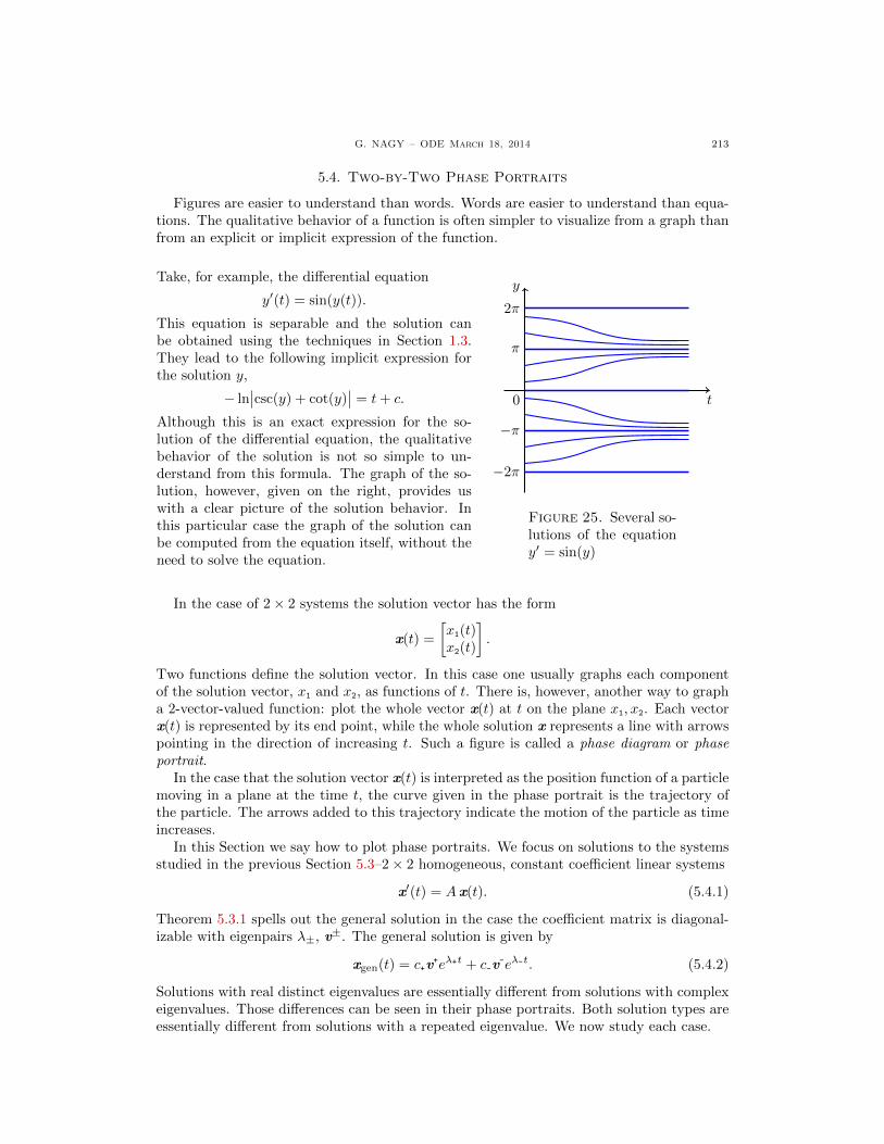
G. NAGY – ODE March 18, 2014 213
5.4. Two-by-Two Phase Portraits
Figures are easier to understand than words. Words are easier to understand than equa-tions. The qualitative behavior of a function is often simpler to visualize from a graph thanfrom an explicit or implicit expression of the function.
Take, for example, the differential equation
y′(t) = sin(y(t)).
This equation is separable and the solution canbe obtained using the techniques in Section 1.3.They lead to the following implicit expression forthe solution y,
− ln∣∣csc(y) + cot(y)
∣∣ = t+ c.
Although this is an exact expression for the so-lution of the differential equation, the qualitativebehavior of the solution is not so simple to un-derstand from this formula. The graph of the so-lution, however, given on the right, provides uswith a clear picture of the solution behavior. Inthis particular case the graph of the solution canbe computed from the equation itself, without theneed to solve the equation.
t
y
0
π
2π
−π
−2π
Figure 25. Several so-lutions of the equationy′ = sin(y)
In the case of 2× 2 systems the solution vector has the form
x(t) =
[x1(t)x2(t)
].
Two functions define the solution vector. In this case one usually graphs each componentof the solution vector, x1 and x2, as functions of t. There is, however, another way to grapha 2-vector-valued function: plot the whole vector x(t) at t on the plane x1, x2. Each vectorx(t) is represented by its end point, while the whole solution x represents a line with arrowspointing in the direction of increasing t. Such a figure is called a phase diagram or phaseportrait.
In the case that the solution vector x(t) is interpreted as the position function of a particlemoving in a plane at the time t, the curve given in the phase portrait is the trajectory ofthe particle. The arrows added to this trajectory indicate the motion of the particle as timeincreases.
In this Section we say how to plot phase portraits. We focus on solutions to the systemsstudied in the previous Section 5.3–2× 2 homogeneous, constant coefficient linear systems
x′(t) = Ax(t). (5.4.1)
Theorem 5.3.1 spells out the general solution in the case the coefficient matrix is diagonal-izable with eigenpairs λ±, v
±. The general solution is given by
xgen(t) = c+v+eλ+t + c-v
-eλ-t. (5.4.2)
Solutions with real distinct eigenvalues are essentially different from solutions with complexeigenvalues. Those differences can be seen in their phase portraits. Both solution types areessentially different from solutions with a repeated eigenvalue. We now study each case.

214 G. NAGY – ODE march 18, 2014
5.4.1. Real distinct eigenvalues. We study the system in (5.4.1) in the case that matrixA has two real eigenvalues λ+ 6= λ-. The case where one eigenvalues vanishes is left oneof the exercises at the end of the Section. We study the case where both eigenvalues arenon-zero. Two non-zero eigenvalues belong to one of hte following cases:
(i) λ+ > λ- > 0, both eigenvalues positive;(ii) λ+ > 0 > λ-, one eigenvalue negative and the other positive;(iii) 0 > λ+ > λ-, both eigenvalues negative.
In a phase portrait the solution vector x(t) at t is displayed on the plane x1, x2. Thewhole vector is shown, only the end point of the vector is shown for t ∈ (−∞,∞). Theresult is a curve in the x1, x2 plane. One usually adds arrows to determine the direction ofincreasing t. A phase portrait contains several curves, each one corresponding to a solutiongiven in Eq. (5.4.2) for particular choice of constants c+ and c-. A phase diagram can besketched by following these few steps:
(a) Plot the eigenvectors v+ and v- corresponding to the eigenvalues λ+ and λ-.(b) Draw the whole lines parallel to these vectors and passing through the origin. These
straight lines correspond to solutions with either c+ or c- zero.(c) Draw arrows on these lines to indicate how the solution changes as the variable t in-
creases. If t is interpreted as time, the arrows indicate how the solution changes intothe future. The arrows point towards the origin if the corresponding eigenvalue λ isnegative, and they point away form the origin if the eigenvalue is positive.
(d) Find the non-straight curves correspond to solutions with both coefficient c+ and c-non-zero. Again, arrows on these curves indicate the how the solution moves into thefuture.
Case λ+ > λ- > 0.
Example 5.4.1: Sketch the phase diagram of the solutions to the differential equation
x′ = Ax, A =1
4
[11 31 9
]. (5.4.3)
Solution: The characteristic equation for this matrix A is given by
det(A− λI) = λ2 − 5λ+ 6 = 0 ⇒{λ+ = 3,
λ- = 2.
One can show that the corresponding eigenvectors are given by
v+ =
[31
], v- =
[−22
].
So the general solution to the differential equation above is given by
x(t) = c+ v+eλ+t + c- v
-eλ-t ⇔ x(t) = c+
[31
]e3t + c-
[−22
]e2t.
In Fig. 26 we have sketched four curves, each representing a solution x corresponding to aparticular choice of the constants c+ and c-. These curves actually represent eight differentsolutions, for eight different choices of the constants c+ and c-, as is described below. Thearrows on these curves represent the change in the solution as the variable t grows. Sinceboth eigenvalues are positive, the length of the solution vector always increases as t increases.The straight lines correspond to the following four solutions:
c+ = 1, c- = 0; c+ = 0, c- = 1; c+ = −1, c- = 0; c+ = 0, c- = −1.
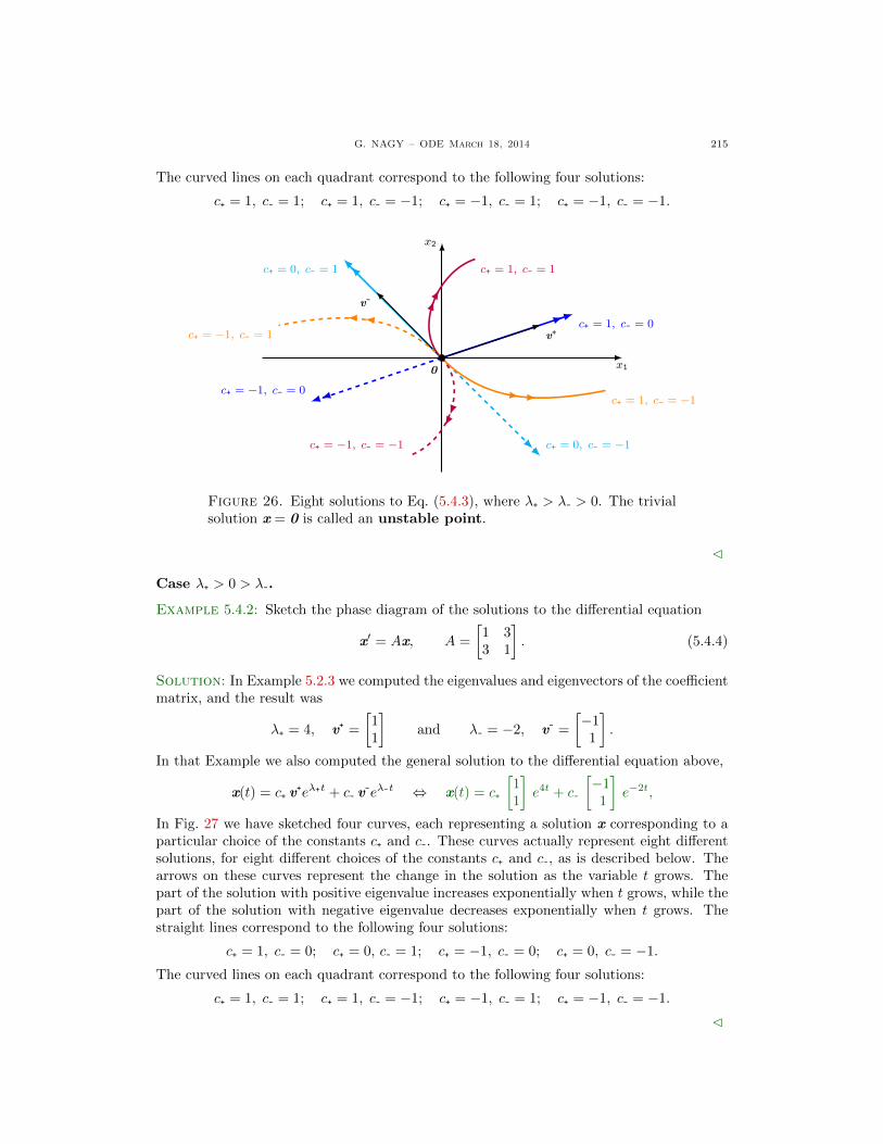
G. NAGY – ODE March 18, 2014 215
The curved lines on each quadrant correspond to the following four solutions:
c+ = 1, c- = 1; c+ = 1, c- = −1; c+ = −1, c- = 1; c+ = −1, c- = −1.
x2
x1
c+ = 1, c- = 0
c+ = 0, c- = 1
v+
v-
c+ = −1, c- = 0
c+ = 0, c- = −1
c+ = 1, c- = 1
c+ = 1, c- = −1
c+ = −1, c- = −1
c+ = −1, c- = 1
0
Figure 26. Eight solutions to Eq. (5.4.3), where λ+ > λ- > 0. The trivialsolution x = 0 is called an unstable point.
C
Case λ+ > 0 > λ-.
Example 5.4.2: Sketch the phase diagram of the solutions to the differential equation
x′ = Ax, A =
[1 33 1
]. (5.4.4)
Solution: In Example 5.2.3 we computed the eigenvalues and eigenvectors of the coefficientmatrix, and the result was
λ+ = 4, v+ =
[11
]and λ- = −2, v- =
[−11
].
In that Example we also computed the general solution to the differential equation above,
x(t) = c+ v+eλ+t + c- v
-eλ-t ⇔ x(t) = c+
[11
]e4t + c-
[−11
]e−2t,
In Fig. 27 we have sketched four curves, each representing a solution x corresponding to aparticular choice of the constants c+ and c-. These curves actually represent eight differentsolutions, for eight different choices of the constants c+ and c-, as is described below. Thearrows on these curves represent the change in the solution as the variable t grows. Thepart of the solution with positive eigenvalue increases exponentially when t grows, while thepart of the solution with negative eigenvalue decreases exponentially when t grows. Thestraight lines correspond to the following four solutions:
c+ = 1, c- = 0; c+ = 0, c- = 1; c+ = −1, c- = 0; c+ = 0, c- = −1.
The curved lines on each quadrant correspond to the following four solutions:
c+ = 1, c- = 1; c+ = 1, c- = −1; c+ = −1, c- = 1; c+ = −1, c- = −1.
C

216 G. NAGY – ODE march 18, 2014
x2
x1
c+ = 1, c- = 0
c+ = −1, c- = 0
c+ = 0, c- = 1
c+ = 0, c- = −1
v+v-
c+ = 1, c- = 1
c+ = 1, c- = −1
c+ = −1, c- = −1
c+ = −1, c- = 1
0
Figure 27. Several solutions to Eq. (5.4.4), λ+ > 0 > λ-. The trivialsolution x = 0 is called a saddle point.
Case 0 > λ+ > λ-.
Example 5.4.3: Sketch the phase diagram of the solutions to the differential equation
x′ = Ax, A =1
4
[−9 31 −11
]. (5.4.5)
Solution: The characteristic equation for this matrix A is given by
det(A− λI) = λ2 + 5λ+ 6 = 0 ⇒{λ+ = −2,
λ- = −3.
One can show that the corresponding eigenvectors are given by
v+ =
[31
], v- =
[−22
].
So the general solution to the differential equation above is given by
x(t) = c+ v+eλ+t + c- v
-eλ-t ⇔ x(t) = c+
[31
]e−2t + c-
[−22
]e−3t.
In Fig. 28 we have sketched four curves, each representing a solution x corresponding to aparticular choice of the constants c+ and c-. These curves actually represent eight differ-ent solutions, for eight different choices of the constants c+ and c-, as is described below.The arrows on these curves represent the change in the solution as the variable t grows.Since both eigenvalues are negative, the length of the solution vector always decreases as tgrows and the solution vector always approaches zero. The straight lines correspond to thefollowing four solutions:
c+ = 1, c- = 0; c+ = 0, c- = 1; c+ = −1, c- = 0; c+ = 0, c- = −1.
The curved lines on each quadrant correspond to the following four solutions:
c+ = 1, c- = 1; c+ = 1, c- = −1; c+ = −1, c- = 1; c+ = −1, c- = −1.
C

G. NAGY – ODE March 18, 2014 217
x2
x1
c+ = 1, c- = 0
c+ = 0, c- = 1
v+
v-
c+ = −1, c- = 0
c+ = 0, c- = −1
c+ = 1, c- = 1
c+ = −1, c- = 1
c+ = 1, c- = −1
c+ = −1, c- = −1
0
Figure 28. Several solutions to Eq. (5.4.5), where 0 > λ+ > λ-. The trivialsolution x = 0 is called a stable point.
5.4.2. Complex eigenvalues. A real-valued matrix may have complex-valued eigenvalues.These complex eigenvalues come in pairs, because the matrix is real-valued. If λ is one ofthese complex eigenvalues, then λ is also an eigenvalue. A usual notation is λ± = α ± iβ,with α, β ∈ R. The same happens with their eigenvectors, which are written as v± = a± ib,with a, b ∈ Rn, in the case of an n × n matrix. When the matrix is the coefficient matrixof a differential equation,
x′ = Ax,
the solutions x+(t) = v+eλ+t and x-(t) = v-eλ-t are complex-valued. In the previous Sec-tion we presented Theorem 5.3.3, which provided real-valued solutions for the differentialequation. They are the real part and the imaginary part of the solution x+, given by
x1(t) =(a cos(βt)− b sin(βt)
)eαt, x2(t) =
(a sin(βt) + b cos(βt)
)eαt. (5.4.6)
These real-valued solutions are used to draw phase portraits. We start with an example.
Example 5.4.4: Find a real-valued set of fundamental solutions to the differential equationbelow and sketch a phase portrait, where
x′ = Ax, A =
[2 3
−3 2
].
Solution: We have found in Example 5.3.2 that the eigenvalues and eigenvectors of thecoefficient matrix are
λ± = 2± 3i, v± =
[∓i1
].
Writing them in real and imaginary parts, λ± = α± iβ and v± = a± ib, we get
α = 2, β = 3, a =
[01
], b =
[−10
].
These eigenvalues and eigenvectors imply the following real-valued fundamental solutions,{x1(t) =
[sin(3t)cos(3t)
]e2t, x2(t) =
[− cos(3t)sin(3t)
]e2t
}. (5.4.7)

218 G. NAGY – ODE march 18, 2014
The phase diagram of these two fundamental solutions is given in Fig. 29 below. There isalso a circle given in that diagram, corresponding to the trajectory of the vectors
x1(t) =
[sin(3t)cos(3t)
]x2(t) =
[− cos(3t)sin(3t)
].
The phase portrait of these functions is a circle, since they are unit vector-valued functions–they have length one. C
x2
x1
x1
x2
a
b 0
Figure 29. The graph of the fundamental solutions x(1) and x(2) in Eq. (5.4.7).
Suppose that the coefficient matris of a 2× 2 differential equation x′ = Ax has complexeigenvalues and eigenvectors
λ± = α± iβ, v± = a± ib.
We have said that real-valued fundamental solutions are given by
x1(t) =(a cos(βt)− b sin(βt)
)eαt, x2(t) =
(a sin(βt) + b cos(βt)
)eαt.
We now sketch phase portraits of these solutions for a few choices of α, a and b. We startfixing the vectors a, b and plotting phase diagrams for solutions having α > 0, α = 0,and α < 0. The result can be seen in Fig. 30. For α > 0 the solutions spiral outward as tincreases, and for α < 0 the solutions spiral inwards to the origin as t increases. The rotationdirection is from vector b towards vector a. The solution vector 0, is called unstable forα > 0 and stable for α < 0.
We now change the direction of vector b, and we repeat the three phase portraits givenabove; for α > 0, α = 0, and α < 0. The result is given in Fig. 31. Comparing Figs. 30and 31 shows that the relative directions of the vectors a and b determines the rotationdirection of the solutions as t increases.

G. NAGY – ODE March 18, 2014 219
x2 α > 0
x1
x1
x2
ab
0
x2 α = 0
x1
x1
x2
ab
0
x2 α < 0
x1
x1
x2
ab
0
Figure 30. Fundamental solutions x1 and x2 in Eq. (5.4.6) for α > 0,α = 0, and α < 0. The relative positions of a and b determines therotation direction. Compare with Fig. 31.
x2 α > 0
x1
x1
x2
a
b
0
x2 α = 0
x1
x1
x2
a
b
0
x2 α < 0
x1
x1
x2
a
b
0
Figure 31. Fundamental solutions x1 and x2 in Eq. (5.4.6) for α > 0,α = 0, and α < 0. The relative positions of a and b determines therotation direction. Compare with Fig. 30.
5.4.3. Repeated eigenvalues. A matrix with repeated eigenvalues may or may not bediagonalizable. If a 2 × 2 matrix A is diagonalizable with repeated eigenvalues, then byTheorem 5.3.4 this matrix is proportional to the identity matrix, A = λ0I, with λ0 therepeated eigenvalue. We saw in Section 5.3 that the general solution of a differential systemwith such coefficient matrix is
xgen(t) =
[c1c2
]eλ0t.
Phase portraits of these solutions are just straight lines, starting from the origin for λ0 > 0,or ending at the origin for λ0 < 0.
Non-diagonalizable 2 × 2 differential systems are more interesting. If x′ = Ax is such asystem, it has fundamental solutions
x1(t) = v eλ0t, x2(t) = (v t+w) eλ0t, (5.4.8)
where λ0 is the repeated eigenvalue of A with eigenvector v, and vector w is any solution ofthe linear algebraic system
(A− λ0I)w = v.
The phase portrait of these fundamental solutions is given in Fig 32. To construct thisfigure start drawing the vectors v and w. The solution x1 is simpler to draw than x2, sincethe former is a straight semi-line starting at the origin and parallel to v.
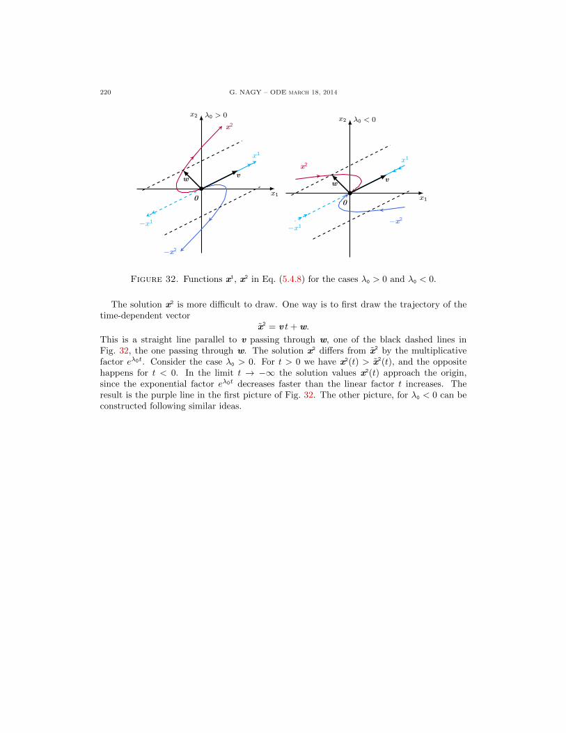
220 G. NAGY – ODE march 18, 2014
x2 λ0 > 0
x1
x2
−x2
x1
−x1
vw
0
x2 λ0 < 0
x1
x2
−x2
x1
−x1
vw
0
Figure 32. Functions x1, x2 in Eq. (5.4.8) for the cases λ0 > 0 and λ0 < 0.
The solution x2 is more difficult to draw. One way is to first draw the trajectory of thetime-dependent vector
x2 = v t+w.
This is a straight line parallel to v passing through w, one of the black dashed lines inFig. 32, the one passing through w. The solution x2 differs from x2 by the multiplicativefactor eλ0t. Consider the case λ0 > 0. For t > 0 we have x2(t) > x2(t), and the oppositehappens for t < 0. In the limit t → −∞ the solution values x2(t) approach the origin,since the exponential factor eλ0t decreases faster than the linear factor t increases. Theresult is the purple line in the first picture of Fig. 32. The other picture, for λ0 < 0 can beconstructed following similar ideas.

G. NAGY – ODE March 18, 2014 221
5.4.4. Exercises.
5.4.1.- . 5.4.2.- .

222 G. NAGY – ODE march 18, 2014
5.5. Non-Diagonalizable Systems
Coming up.

G. NAGY – ODE March 18, 2014 223
Chapter 6. Autonomous Systems and Stability
By the end of the seventeenth century Newton had invented differential equations, discov-ered his laws of motion and the law of universal gravitation. He combined all of them toexplain Kepler laws of planetary motion. Newton solved what now is called the two-bodyproblem. Kepler laws correspond to the case of one planet orbiting the Sun. People thenstarted to study the three-body problem. For example the movement of Earth, Moon, andSun. This problem turned out to be far more difficult than the two-body problem and nosolution was ever found. Around the end of the nineteenth century Henri Poincare proveda breakthrough result. The solutions of the three body problem could not be found explic-itly in terms of elementary functions, such as combinations of polynomials, trigonometricfunctions, exponential, and logarithms. This led him to invent the so-called QualitativeTheory of Differential Equations. In this theory one studies the geometric properties ofsolutions–whether they show periodic behavior, tend to fixed points, tend to infinity, etc.This approach evolved into the modern field of dynamics. In this chapter we introduce afew basic concepts and we use them to find qualitative information of a particular type ofdifferential equations, called autonomous equations.
y
t
2π
CD
π
CU
CD
CU
0
CD
CU
CD
−π
CU
−2π
Unstable
Stable
Unstable
Stable
Unstable
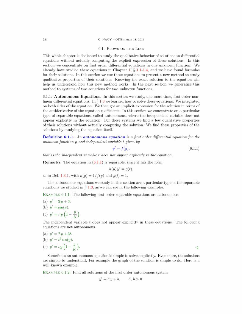
224 G. NAGY – ODE march 18, 2014
6.1. Flows on the Line
This whole chapter is dedicated to study the qualitative behavior of solutions to differentialequations without actually computing the explicit expression of these solutions. In thissection we concentrate on first order differential equations in one unknown function. Wealready have studied these equations in Chapter 1, § 1.1-1.4, and we have found formulasfor their solutions. In this section we use these equations to present a new method to studyqualitative properties of their solutions. Knowing the exact solution to the equation willhelp us understand how this new method works. In the next section we generalize thismethod to systems of two equations for two unknown functions.
6.1.1. Autonomous Equations. In this section we study, one more time, first order non-linear differential equations. In § 1.3 we learned how to solve these equations. We integratedon both sides of the equation. We then got an implicit expression for the solution in terms ofthe antiderivative of the equation coefficients. In this section we concentrate on a particulartype of separable equations, called autonomous, where the independent variable does notappear explicitly in the equation. For these systems we find a few qualitative propertiesof their solutions without actually computing the solution. We find these properties of thesolutions by studying the equation itself.
Definition 6.1.1. An autonomous equation is a first order differential equation for theunknown function y and independent variable t given by
y′ = f(y), (6.1.1)
that is the independent variable t does not appear explicitly in the equation.
Remarks: The equation in (6.1.1) is separable, since it has the form
h(y) y′ = g(t),
as in Def. 1.3.1, with h(y) = 1/f(y) and g(t) = 1.
The autonomous equations we study in this section are a particular type of the separableequations we studied in § 1.3, as we can see in the following examples.
Example 6.1.1: The following first order separable equations are autonomous:
(a) y′ = 2 y + 3.
(b) y′ = sin(y).
(c) y′ = r y(1− y
K
).
The independent variable t does not appear explicitly in these equations. The followingequations are not autonomous.
(a) y′ = 2 y + 3t.
(b) y′ = t2 sin(y).
(c) y′ = t y(1− y
K
). C
Sometimes an autonomous equation is simple to solve, explicitly. Even more, the solutionsare simple to understand. For example the graph of the solution is simple to do. Here is awell known example.
Example 6.1.2: Find all solutions of the first order autonomous system
y′ = a y + b, a, b > 0.

G. NAGY – ODE March 18, 2014 225
Solution:
This is a linear, constant coefficients equation,so it could be solved using the integrating fac-tor method. But this is also a separable equa-tion, so we solve it as follows,∫
dy
a y + b=
∫dt ⇒ 1
aln(a y + b) = t+ c0
so we get,a y + b = eateac0
and denoting c = eac0/a, we get the expression
y(t) = c eat − b
a. (6.1.2)
This is the expression for the solution we gotin Theorem 1.1.2. C
y
t− ba
c > 0
c = 0
c < 0
Figure 33. A few solutionsto Eq. (6.1.2) for different c.
However, the solutions of an autonomous equation are sometimes not so simple to un-derstand. Even in the case that we can solve the differential equation.
Example 6.1.3: Sketch a qualitative graph of solutions to y′ = sin(y), for different initialdata conditions y(0) = y0.
Solution: We first find the exact solutions and then we see if we can graph them. Theequation is separable, then
y′(t)
sin(y(t)
) = 1 ⇒∫ t
0
y′(t)
sin(y(t)
) dt = t.
Use the usual substitution u = y(t), so du = y′(t) dt, so we get∫ y(t)
y0
du
sin(u)= t.
In an integration table we can find that
ln[ sin(u)
1 + cos(u)
]∣∣∣y(t)y0
= t ⇒ ln[ sin(y)
1 + cos(y)
]− ln
[ sin(y0)
1 + cos(y0)
]= t.
We can rewrite the expression above in terms of one single logarithm,
ln[ sin(y)(
1 + cos(y)) (
1 + cos(y0))
sin(y0)
]= t.
If we compute the exponential on both sides of the equation above we get an implicitexpression of the solution,
sin(y)(1 + cos(y)
) =sin(y0)(
1 + cos(y0)) et. (6.1.3)
Although we have the solution, in this case in implicit form, it is not simple to graph thatsolution without the help of a computer. So, we do not sketch the graph right now. C
Sometimes the exact expression for the solution of a differential equation is difficult tointerpret. For example, take the solution in (6.1.3), in Example 6.1.3. It is not so easy tosee, for an arbitrary initial condition y0, what is the behavior of the solution values y(t) ast → ∞. To be able to answer questions like this one is that we introduce a new approach,a geometric approach.

226 G. NAGY – ODE march 18, 2014
6.1.2. A Geometric Analysis. The idea is to obtain qualitative information about solu-tions to an autonomous equation using the equation itself, without solving it. We now usethe equation of Example 6.1.3 to show how this can be done.
Example 6.1.4: Sketch a qualitative graph of solutions to y′ = sin(y), for different initialdata conditions y(0).
Solution: The differential equation has the form y′ = f(y), where f(y) = sin(y). The firststep in the graphical approach is to graph the function f .
f
y0 2ππ−π−2π
f(y) = sin(y)
Figure 34. Graph of the function f(y) = sin(y).
The second step is to identify all the zeros of the function f . In this case,
f(y) = sin(y) = 0 ⇒ yn = nπ, where n = · · · ,−2,−1, 0, 1, 2, · · · .
It is important to realize that these constants yn are solutions of the differential equation.On the one hand, they are constants, t-independent, so y′n = 0. On the other hand, theseconstants yn are zeros of f , hence f(yn) = 0. So yn are solutions of the differential equation
0 = y′n = f(yn) = 0.
These t-independent solutions, yn, are called stationary solutions. They are also calledequilibrium solutions, or fixed points, or critical points.
The third step is to identify the regions on the line where f is positive, and where f isnegative. These regions are bounded by the critical points. Now, in an interval where f > 0write a right arrow, and in the intervals where f < 0 write a left arrow, as shown below.
f
y0 2ππ−π−2π
f(y) = sin(y)
Figure 35. Critical points and increase/decrease information added to Fig. 34.
It is important to notice that in the regions where f > 0 a solution y is increasing. And inthe regions where f < 0 a solution y is decreasing. The reason for this claim is, of course,the differential equation, f(y) = y′.
The fourth step is to find the regions where the curvature of a solution is concave up orconcave down. That information is given by y′′. But the differential equation relates y′′ to
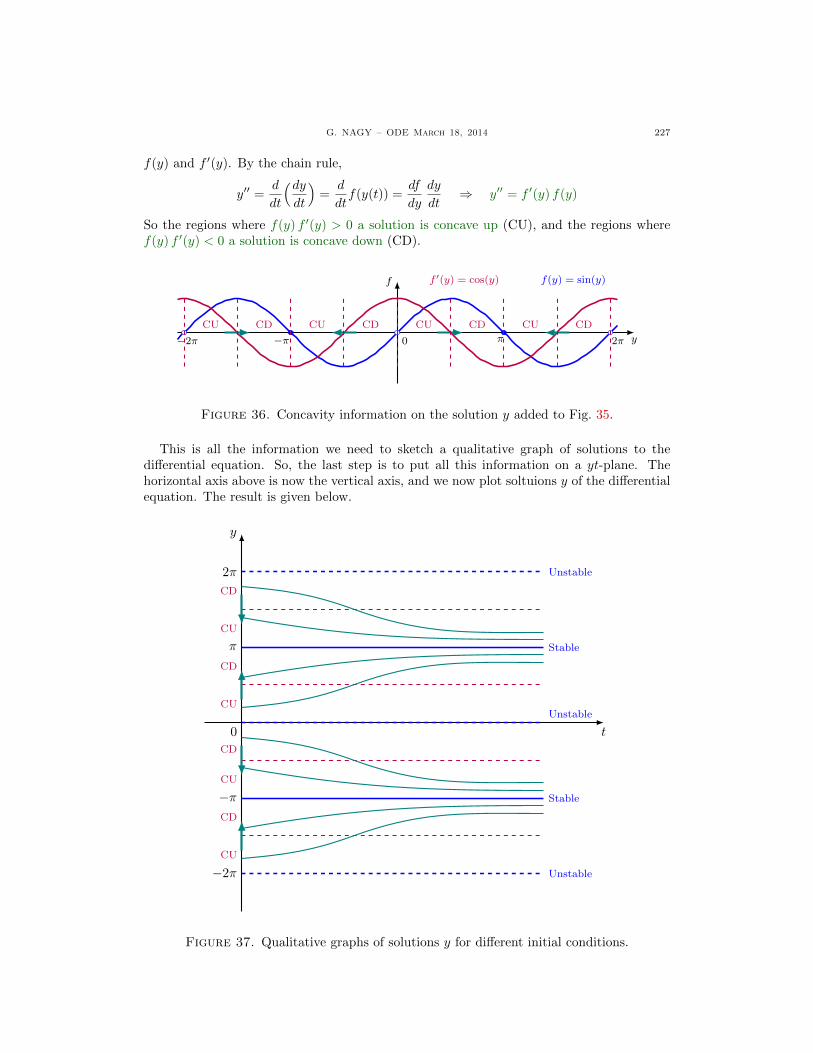
G. NAGY – ODE March 18, 2014 227
f(y) and f ′(y). By the chain rule,
y′′ =d
dt
(dydt
)=
d
dtf(y(t)) =
df
dy
dy
dt⇒ y′′ = f ′(y) f(y)
So the regions where f(y) f ′(y) > 0 a solution is concave up (CU), and the regions wheref(y) f ′(y) < 0 a solution is concave down (CD).
f
y0 2ππ−π−2π
CU CD CU CDCDCUCDCU
f(y) = sin(y)f ′(y) = cos(y)
Figure 36. Concavity information on the solution y added to Fig. 35.
This is all the information we need to sketch a qualitative graph of solutions to thedifferential equation. So, the last step is to put all this information on a yt-plane. Thehorizontal axis above is now the vertical axis, and we now plot soltuions y of the differentialequation. The result is given below.
y
t
2π
CD
π
CU
CD
CU
0
CD
CU
CD
−π
CU
−2π
Unstable
Stable
Unstable
Stable
Unstable
Figure 37. Qualitative graphs of solutions y for different initial conditions.

228 G. NAGY – ODE march 18, 2014
The picture above contains the graph of several solutions y for different choices of initialdata y(0). Stationary solutions are in blue, t-dependent solutions in green. The stationarysolutions are separated in two types. The stable solutions y-1 = −π, y1 = π, are picturedwith solid blue lines. The unstable solutions y-2 = −2π, y0 = 0, y2 = 2π, are pictured withdashed blue lines. C
Remark: A qualitative graph of the solutions does not provide all the possible informationabout the solution. For example, we know from the graph above that for some initialconditions the corresponding solutions have inflection points at some t > 0. But we cannotknow the exact value of t where the inflection point occurs. Such information could beuseful to have, since |y′| has its maximum value at those points.
The geometric approach used in Example 6.1.3 suggests the following definitions.
Definition 6.1.2.
(i) A constant yc is a critical point of the equation y′ = f(y) iff holds f(yc) = 0.(ii) A critical point yc is stable iff f(y) > 0 for every y 6= yc in a neighborhood of yc.(iii) A critical point yc is unstable iff f(y) < 0 for every y 6= yc in a neighborhood of yc.(iv) A critical point yc is semistable iff the point is stable on one side of the critical point
and unstable on the other side.
Remarks:
(a) Critical points are also called fixed points, stationary solutions, equilibrium solutions,critical solutions. We may use all these names in this notes. Stable points are also calledattractors or sinks. Unstable points are also called repellers or sources. Semistablepoints are also called neutral points.
(b) That a critical point is stable means that for initial data close enough to the criticalpoint all solutions approach the critical point as t→ ∞.
In Example 6.1.3 the critical points are yn = nπ. In the second graph of that examplewee only marked −2π, −π, 0, π, and 2π. Filled dots represent stable critical points, andwhite dots represent unstable or semistable critical points. In this example all white pointsare unstable points.
In that second graph one can see that stable critical points have green arrows directedto them on both sides, and unstable points have arrows directed away from them on bothsides. This is always the case for stable and unstable critical points. A semistable pointwould have one arrow pointing to the point on one side, and the other arrow pointing awayfrom the point on the other side.
In terms of the differential equation critical points represent stationary solutions, alsocalled t-independent solutions, or equilibrium solutions, or steady solutions. We will usuallymention critical points as stationary solutions when we describe them in a yt-plane, and wereserve the name critical point when we describe them in a y-line.
On the last graph in Example 6.1.3 we have pictured the stationary solutions that arestable with a solid line, and those that are unstable with a dashed line. Semistable stationarysolutions are also pictured with dashed lines. An equilibrium solutions is defined to be stableif all sufficiently small disturbances away from it damp out in time. An equilibrium solutionis defined to be unstable if all sufficiently disturbances away from it grow in time.
Example 6.1.5: Find all the critical points of the first order linear system
y′ = a y.
Study the stability of the critical points both for a > 0 and for a < 0. Sketch qualitativegraphs of solutions close to the critical points.

G. NAGY – ODE March 18, 2014 229
Solution: This is an equation of the form y′ = f(y) for f(y) = ay. The critical pointsare the constants yc such that 0 = f(yc) = ayc, so yc = 0. We could now use the graphicalmethod to study the stability of the critical point yc = 0, but we do not need to do it.This equation is the particular case b = 0 of the equation solved in Example 6.1.2. So thesolution for arbitrary initial data y(0) = y0 is
y(t) = y0 eat.
We use this expression to graph the solutions near a critical point. The result is shownbelow.
y
t0
y0 > 0
a > 0
Unstable
y0 < 0
y
t0
y0 > 0
a < 0
Stable
y0 < 0
Figure 38. The graph of the functions y(t) = y(0) eat for a > 0 and a < 0.
We conclude that the critical point yc = 0 is stable for a < 0 and is unstable for a > 0. C
Remark: The stability of the critical point yc = 0 of the linear system y′ = ay will beimportant when we study the linearization of a nonlinear autonomous system. For thatreason we highlighted these stability results in Example 6.1.5.
6.1.3. Population Growth Models. The simplest model for the population growth of anorganism is N ′ = rN where N(t) is the population at time t and r > 0 is the growth rate.This model predicts exponential population growth N(t) = N0 e
rt, where N0 = N(0). Westudied this model in § 1.5. Among other things, this model assumes that the organismshave unlimited food supply. This assumption implies that the per capita growth N ′/N = ris constant.
A more realistic model assumes that the per capita growth decreases linearly with N ,starting with a positive value, r, and going down to zero for a critical population N = K > 0.So when we consider the per capita growth N ′/N as a function of N , it must be given bythe formula N ′/N = −(r/K)N + r. This equation, when thought as a differential equationfor N is called the logistic equation model for population growth.
Definition 6.1.3. The logistic equation describes the organisms population function Nin time as the solution of the autonomous differential equation
N ′ = rN(1− N
K
),
where the initial growth rate constant r and the carrying capacity constant K are positive.
We now use the graphical method to carry out a stability analysis of the logistic popu-lation growth model. Later on we find the explicit solution of the differential equation. Wecan then compare the two approaches to study the solutions of the model.
Example 6.1.6: Sketch a qualitative graph of solutions for different initial data conditionsy(0) = y0 to the logistic equation below, where r and K are given positive constants,
y′ = ry(1− y
K
).

230 G. NAGY – ODE march 18, 2014
Solution:
The logistic differential equation forpopulation growth can be writteny′ = f(y), where function f is thepolynomial
f(y) = ry(1− y
K
).
The first step in the graphical ap-proach is to graph the function f .The result is in Fig. 39.The second step is to identify all crit-ical points of the equation. The crit-ical points are the zeros of the func-tion f . In this case, f(y) = 0 implies
y0 = 0, y1 = K.
The third step is to find out whetherthe critical points are stable or un-stable. Where function f is posi-tive, a solution will be increasing,and where function f is negative asolution will be decreasing. Theseregions are bounded by the criticalpoints. Now, in an interval wheref > 0 write a right arrow, and inthe intervals where f < 0 write a leftarrow, as shown in Fig. 40.The fourth step is to find the re-gions where the curvature of a solu-tion is concave up or concave down.That information is given by y′′. Butthe differential equation relates y′′
to f(y) and f ′(y). We have shownin Example 6.1.4 that the chain ruleand the differential equation imply,
y′′ = f ′(y) f(y)
So the regions where f(y) f ′(y) > 0a solution is concave up (CU), andthe regions where f(y) f ′(y) < 0 asolution is concave down (CD). Theresult is in Fig. 41.
f
y0 KK
2
rK
4
f(y) = ry(1−
y
K
)
Figure 39. The graph of f .
f
y0 KK
2
rK
4
f(y) = ry(1−
y
K
)
Figure 40. Critical points added.
f
y0 KK
2
rK
4
CD CU CD CU
f(y) = ry(1−
y
K
)
Figure 41. Concavity information added.
This is all the information we need to sketch a qualitative graph of solutions to thedifferential equation. So, the last step is to put all this information on a yt-plane. Thehorizontal axis above is now the vertical axis, and we now plot solutions y of the differentialequation. The result is given in Fig. 42.

G. NAGY – ODE March 18, 2014 231
y
t
K
K
2
0
CD
CU
CD
CU
Stable
Unstable
Figure 42. Qualitative graphs of solutions y for different initial conditions.
The picture above contains the graph of several solutions y for different choices of initialdata y(0). Stationary solutions are in blue, t-dependent solutions in green. The stationarysolution y0 = 0 is unstable and pictured with a dashed blue line. The stationary solutiony1 = K is stable and pictured with a solid blue line. C
In Examples 6.1.4 and 6.1.6 we have used that the second derivative of the solutionfunction is related to f and f ′. This is a result that we remark here in its own statement.
Theorem 6.1.4. If y is a solution of the autonomous system y′ = f(y), then
y′′ = f ′(y) f(y).
Remark: This result has been used to find out the curvature of the solution y of anautonomous system y′ = f(y). The graph of y has positive curvature iff f ′(y) f(y) > 0 andnegative curvature iff f ′(y) f(y) < 0.
Proof:
y′′ =d
dt
(dydt
)=
d
dtf(y(t)) =
df
dy
dy
dt⇒ y′′ = f ′(y) f(y).
�Remark: The logistic equation is, of course, a separable equation, so it can be solved usingthe method from § 1.3. We solve it below, so you can compare the qualitative graphs fromExample 6.1.6 with the exact solution below.
Example 6.1.7: Find the exact expression for the solution to the logistic equation forpopulation growth
y′ = ry(1− y
K
), y(0) = y0, 0 < y0 < K.
Solution: This is a separable equation,
K
r
∫y′ dt
(K − y)y= t+ c0.
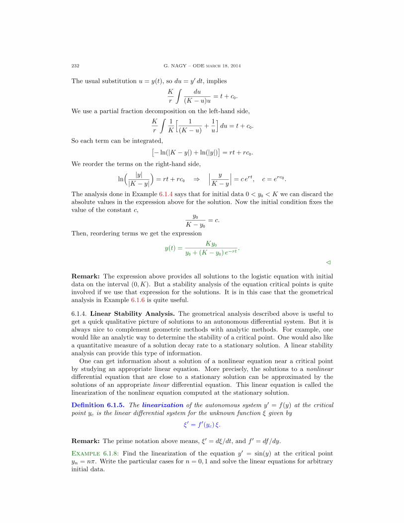
232 G. NAGY – ODE march 18, 2014
The usual substitution u = y(t), so du = y′ dt, implies
K
r
∫du
(K − u)u= t+ c0.
We use a partial fraction decomposition on the left-hand side,
K
r
∫1
K
[ 1
(K − u)+
1
u
]du = t+ c0.
So each term can be integrated,[− ln(|K − y|) + ln(|y|)
]= rt+ rc0.
We reorder the terms on the right-hand side,
ln( |y||K − y|
)= rt+ rc0 ⇒
∣∣∣ y
K − y
∣∣∣ = c ert, c = erc0 .
The analysis done in Example 6.1.4 says that for initial data 0 < y0 < K we can discard theabsolute values in the expression above for the solution. Now the initial condition fixes thevalue of the constant c,
y0K − y0
= c.
Then, reordering terms we get the expression
y(t) =Ky0
y0 + (K − y0) e−rt.
C
Remark: The expression above provides all solutions to the logistic equation with initialdata on the interval (0,K). But a stability analysis of the equation critical points is quiteinvolved if we use that expression for the solutions. It is in this case that the geometricalanalysis in Example 6.1.6 is quite useful.
6.1.4. Linear Stability Analysis. The geometrical analysis described above is useful toget a quick qualitative picture of solutions to an autonomous differential system. But it isalways nice to complement geometric methods with analytic methods. For example, onewould like an analytic way to determine the stability of a critical point. One would also likea quantitative measure of a solution decay rate to a stationary solution. A linear stabilityanalysis can provide this type of information.
One can get information about a solution of a nonlinear equation near a critical pointby studying an appropriate linear equation. More precisely, the solutions to a nonlineardifferential equation that are close to a stationary solution can be approximated by thesolutions of an appropriate linear differential equation. This linear equation is called thelinearization of the nonlinear equation computed at the stationary solution.
Definition 6.1.5. The linearization of the autonomous system y′ = f(y) at the criticalpoint yc is the linear differential system for the unknown function ξ given by
ξ′ = f ′(yc) ξ.
Remark: The prime notation above means, ξ′ = dξ/dt, and f ′ = df/dy.
Example 6.1.8: Find the linearization of the equation y′ = sin(y) at the critical pointyn = nπ. Write the particular cases for n = 0, 1 and solve the linear equations for arbitraryinitial data.

G. NAGY – ODE March 18, 2014 233
Solution: If we write the nonlinear system as y′ = f(y), then f(y) = sin(y). We thencompute its y derivative, f ′(y) = cos(y). We evaluate this expression at the critical points,f ′(yn) = cos(nπ) = (−1)n. The linearization at yn of the nonlinear equation above is thelinear equation for the unknown function ξn given by
ξ′n = (−1)n ξn.
The particular cases n = 0 and n = 1 are given by
ξ′0 = ξ0, ξ′1 = −ξ1.It is simple to find solutions to first order linear homogeneous equations with constantcoefficients. The result, for each equation above, is
ξ0(t) = ξ0(0) et, ξ1(t) = ξ1(0) e
−t,
From this last expression we can see that for n = 0 the critical solution ξ0 = 0 is unstable,while for n = 1 the critical solution ξ1 = 0 is stable. The stability of the trivial solutionξ0 = x1 = 0 of the linearized systems coincides with the stability of the critical points y0 = 0,y1 = π for the nonlinear equation. C
In the example above we have used a result that we highlight in the following statement.
Theorem 6.1.6. The trivial solution ξ = 0 of the constant coefficients equation
ξ′ = a ξ
is stable iff a < 0, and it is unstable iff a > 0.
Proof of Theorem 6.1.6: The stability analysis follows from the explicit solutions to thedifferential equation, ξ(t) = ξ(0) eat. For a > 0 the solutions diverge to ±∞ as t→ ∞, andfor a < 0 the solutions approach to zero as t→ ∞. �
Example 6.1.9: Find the linearization of the logistic equation y′ = ry(1 − y
K
)at the
critical points y0 = 0 and y1 = K. Solve the linear equations for arbitrary initial data.
Solution: If we write the nonlinear system as y′ = f(y), then f(y) = ry − r
Ky2. Then,
f ′(y) = r − 2r
Ky. For the critical point y0 = 0 we get the linearized system
ξ′0(t) = r ξ0 ⇒ ξ0(t) = ξ0(0) ert.
For the critical point y1 = K we get the linearized system
ξ′1(t) = −r ξ1 ⇒ ξ1(t) = ξ1(0) e−rt.
From this last expression we can see that for y0 = 0 the critical solution ξ0 = 0 is unstable,while for y1 = K the critical solution ξ1 = 0 is stable. The stability of the trivial solutionξ0 = ξ1 = 0 of the linearized system coincides with the stability of the critical points y0 = 0,y1 = K for the nonlinear equation. C
Remark: In the Examples 6.1.8 and 6.1.9 we have seen that the stability of a critical pointyc to a nonlinear differential equation y′ = f(y) is the same as the stability of the trivialsolution ξ = 0 of the linearized equation ξ′ = f ′(yc) ξ. This is a general result, which westate below.
Theorem 6.1.7. Let yc be a critical point of the autonomous system y′ = f(y).
(a) The critical point yc is stable iff f ′(yc) < 0.(b) The critical point yc is unstable iff f ′(yc) > 0.

234 G. NAGY – ODE march 18, 2014
Furthermore, If the initial data y(0) ' yc, is close enough to the critial point yc, then thesolution with that initial data of the equation y′ = f(y) are close enough to yc in the sense
y(t) ' yc + ξ(t),
where ξ is the solution to the linearized equation at the critical point yc,
ξ′ = f ′(yc) ξ, ξ(0) = y(0)− yc.
Remark: The proof of this result can be found in § 43 in Simmons’ textbook [8].
Remark: The first part of Theorem 6.1.7 highlights the importance of the sign fo thecoefficient f ′(yc), which determines the stability of the critical point yc. The furthermorepart of the Theorem highlights how stable is a critical point. The value |f ′(yc)| playsa role of an exponential growth or a exponential decay rate. Its reciprocal, 1/|f ′(yc)| isa characteristic scale. It determines the value of t required for the solution y to varysignificantly in a neighborhood of the critical point yc.
NotesThis section follows a few parts of Chapter 2 in Steven Strogatz’s book on Nonlinear
Dynamics and Chaos, [10], and also § 2.5 in Boyce DiPrima classic textbook [3].

G. NAGY – ODE March 18, 2014 235
6.1.5. Exercises.
6.1.1.- . 6.1.2.- .
236 G. NAGY – ODE march 18, 2014
6.2. Flows on the Plane
Coming up.
6.3. Linear Stability
Coming up.

G. NAGY – ODE March 18, 2014 237
Chapter 7. Boundary Value Problems
7.1. Eigenvalue-Eigenfunction Problems
In this Section we consider second order, linear, ordinary differential equations. In thefirst half of the Section we study boundary value problems for these equations and in thesecond half we focus on a particular type of boundary value problems, called the eigenvalue-eigenfunction problem for these equations.
7.1.1. Comparison: IVP and BVP. Given real constants a1 and a0, consider the secondorder, linear, homogeneous, constant coefficients, ordinary differential equation
y′′ + a1 y′ + a0 y = 0. (7.1.1)
We now review the initial boundary value problem for the equation above, which was dis-cussed in Sect. ??, where we showed in Theorem ?? that this initial value problem alwayshas a unique solution.
Definition 7.1.1 (IVP). Given the constants t0, y0 and y1, find a solution y of Eq. (7.1.1)satisfying the initial conditions
y(t0) = y0, y′(t0) = y1. (7.1.2)
There are other problems associated to the differential equation above. The followingone is called a boundary value problem.
Definition 7.1.2 (BVP). Given the constants t0 6= t1, y0 and y1, find a solution y ofEq. (7.1.1) satisfying the boundary conditions
y(t0) = y0, y(t1) = y1. (7.1.3)
One could say that the origins of the names “initial value problem” and “boundary valueproblem” originates in physics. Newton’s second law of motion for a point particle wasthe differential equation to solve in an initial value problem; the unknown function y wasinterpreted as the position of the point particle; the independent variable t was interpretedas time; and the additional conditions in Eq. (7.1.2) were interpreted as specifying theposition and velocity of the particle at an initial time. In a boundary value problem, thedifferential equation was any equation describing a physical property of the system understudy, for example the temperature of a solid bar; the unknown function y represented anyphysical property of the system, for example the temperature; the independent variable trepresented position in space, and it is usually denoted by x; and the additional conditionsgiven in Eq. (7.1.3) represent conditions on the physical quantity y at two different positionsin space given by t0 and t1, which are usually the boundaries of the system under study, forexample the temperature at the boundaries of the bar. This originates the name “boundaryvalue problem”.
We mentioned above that the initial value problem for Eq. (7.1.1) always has a uniquesolution for every constants y0 and y1, result presented in Theorem ??. The case of theboundary value problem for Eq. (7.1.1) is more complicated. A boundary value problemmay have a unique solution, or may have infinitely many solutions, or may have no solution,depending on the boundary conditions. This result is stated in a precise way below.
Theorem 7.1.3 (BVP). Fix real constants a1, a0, and let r± be the roots of the charac-teristic polynomial p(r) = r2 + a1r + a0.
(i) If the roots r± ∈ R, then the boundary value problem given by Eqs. (7.1.1) and (7.1.3)has a unique solution for all y0, y1 ∈ R.

238 G. NAGY – ODE march 18, 2014
(ii) If the roots r± form a complex conjugate pair, that is, r± = α±βi, with α, β ∈ R, thenthe solution of the boundary value problem given by Eqs. (7.1.1) and (7.1.3) belongsto only one of the following three possibilities:(a) There exists a unique solution;(b) There exists infinitely many solutions;(c) There exists no solution.
Before presenting the proof of Theorem 7.1.3 concerning boundary value problem, letus review part of the proof of Theorem ?? concerning initial value problems using matrixnotation to highlight the crucial part of the calculations. For the simplicity of this review,we only consider the case r+ 6= r-. In this case the general solution of Eq. (7.1.1) can beexpressed as follows,
y(t) = c1 er- t + c2 e
r+ t, c1, c2 ∈ R.The initial conditions in Eq. (7.1.2) determine the values of the constants c1 and c2 as follows:
y0 = y(t0) = c1 er- t0 + c2 e
r+ t0
y1 = y′(t0) = c1r- er- t0 + c2r+ e
r+ t0
}⇒
[er- t0 er+ t0
r- er-t0 r+ e
r+ t0
] [c1c2
]=
[y0y1
].
The linear system above has a unique solution c1 and c2 for every constants y0 and y1 iff thedeterminant of the coefficient matrix Z is non-zero, where
Z =
[er- t0 er+ t0
r- er- t0 r+ e
r+ t0
].
A simple calculation shows
det(Z) =(r+ − r-
)e(r++r-) t0 6= 0 ⇔ r+ 6= r-.
Since r+ 6= r-, the matrix Z is invertible and so the initial value problem above a uniquesolution for every choice of the constants y0 and y1. The proof of Theorem 7.1.3 for theboundary value problem follows the same steps we described above: First find the generalsolution to the differential equation, second find whether the matrix Z above is invertibleor not.Proof of Theorem 7.1.3:
Part (i): Assume that r± are real numbers. We have two cases, r+ 6= r- and r+ = r-. Inthe former case the general solution to Eq. (7.1.1) is given by
y(t) = c1 er- t + c2 e
r+ t, c1, c2 ∈ R. (7.1.4)
The boundary conditions in Eq. (7.1.3) determine the values of the constants c1, c2, since
y0 = y(t0) = c1er- t0 + c2e
r+ t0
y1 = y(t1) = c1er- t1 + c2e
r+ t1
}⇒
[er- t0 er+ t0
er- t1 er+ t1
] [c1c2
]=
[y0y1
]. (7.1.5)
The linear system above has a unique solution c1 and c2 for every constants y0 and y1 iff thedeterminant of the coefficient matrix Z is non-zero, where
Z =
[er- t0 er+ t0
er- t1 er+ t1
]. (7.1.6)
A straightforward calculation shows
det(Z) = er+ t1er- t0 − er+ t0er- t1 = er+ t0er- t0[er+ (t1−t0) − er- (t1−t0)
]. (7.1.7)
So it is simple to verify that
det(Z) 6= 0 ⇔ er+ (t1−t0) 6= er- (t1−t0) ⇔ r+ 6= r-. (7.1.8)
Therefore, in the case r+ 6= r- the matrix Z is invertible and so the boundary value problemabove has a unique solution for every choice of the constants y0 and y1. In the case that

G. NAGY – ODE March 18, 2014 239
r+ = r- = r0, then we have to start over, since the general solution of Eq. (7.1.1) is not givenby Eq. (7.1.4) but by the following expression
y(t) = (c1 + c2 t) er0t, c1, c2 ∈ R.
Again, the boundary conditions in Eq. (7.1.3) determine the values of the constants c1 andc2 as follows:
y0 = y(t0) = c1er0t0 + c2t0e
r0t0
y1 = y(t1) = c1er0t1 + c2t1e
r0t1
}⇒
[er0t0 t0e
r0t0
er0t1 t1er0t1
] [c1c2
]=
[y0y1
].
The linear system above has a unique solution c1 and c2 for every constants y0 and y1 iff thedeterminant of the coefficient matrix Z is non-zero, where
Z =
[er0t0 t0e
r0t0
er0t1 t1er0t1
]A simple calculation shows
det(Z) = t1er0(t1+t0) − t0e
r0(t1+t0) = (t1 − t0)er0(t1+t0) 6= 0 ⇔ t1 6= t0.
Therefore, in the case r+ = r- = r0 the matrix Z is again invertible and so the boundaryvalue problem above has a unique solution for every choice of the constants y0 and y1. Thisestablishes part (i) of the Theorem.
Part (ii): Assume that the roots of the characteristic polynomial have the form r± = α±βiwith β 6= 0. In this case the general solution to Eq. (7.1.1) is still given by Eq. (7.1.4), andthe boundary condition of the problem are still given by Eq. (7.1.5). The determinant ofmatrix Z introduced in Eq. (7.1.6) is still given by Eq. (7.1.7). However, the claim givenin Eq. (7.1.8) is true only in the case that r± are real numbers, and it does not hold in thecase that r± are complex numbers. The reason is the following calculation: Let us startwith Eq. (7.1.7) and then introduce that r± = α± βi;
det(Z) = e(r++r-) t0[er+ (t1−t0) − er- (t1−t0)
]= e2αt0 eα(t1−t0)
[eiβ(t1−t0) − e−iβ(t1−t0)
]= 2i eα(t1+t0) sin
[β(t1 − t0)
].
We then conclude that
det(Z) = 0 ⇔ sin[β(t1 − t0)
]= 0 ⇔ β =
nπ
(t1 − t0), (7.1.9)
where n = 1, 2, · · · and we are using that t1 6= t0. This last equation in (7.1.9) is the keyto obtain all three cases in part (ii) of this Theorem, as can be seen from the followingargument:
Part (iia): If the coefficients a1, a0 in Eq. (7.1.1) and the numbers t1, t0 in the boundaryconditions in (7.1.3) are such that Eq. (7.1.9) does not hold, that is,
β 6= nπ
(t1 − t0),
then det(Z) 6= 0 and so the boundary value problem for Eq. (7.1.1) has a unique solutionfor all constants y0 and y1. This establishes part (iia).
Part (iib) and Part (iic): If the coefficients a1, a0 in Eq. (7.1.1) and the numbers t1, t0in the boundary conditions in (7.1.3) are such that Eq. (7.1.9) holds, then det(Z) = 0, andso the system of linear equation given in (7.1.5) may or may not have solutions, dependingon the values of the constants y0 and y1. In the case that there exists a solution, then thereare infinitely many solutions, since det(Z) = 0. This establishes part (iib). The remaining

240 G. NAGY – ODE march 18, 2014
case, when y0 and y1 are such that Eq. (7.1.5) has no solution is the case in part (iic). Thisestablishes the Theorem. �
Our first example is a boundary value problem with a unique solution. This correspondsto case (iia) in Theorem 7.1.3. The matrix Z defined in the proof of that Theorem isinvertible and the boundary value problem has a unique solution for every y0 and y1.
Example 7.1.1: Find the solution y(x) to the boundary value problem
y′′ + 4y = 0, y(0) = 1, y(π/4) = −1.
Solution: We first find the general solution to the differential equation above. We knowthat we have to look for solutions of the form y(x) = erx, with the constant r being solutionsof the characteristic equation
r2 + 4 = 0 ⇔ r± = ±2i.
We know that in this case we can express the general solution to the differential equationabove as follows,
y(x) = c1 cos(2x) + c2 sin(2x).
The boundary conditions imply the following system of linear equation for c1 and c2,
1 = y(0) = c1
−1 = y(π/4) = c2
}⇒
[1 00 1
] [c1c2
]=
[1
−1
].
The linear system above has the unique solution c1 = 1 and c2 = −1. Hence, the boundaryvalue problem above has the unique solution
y(x) = cos(2x)− sin(2x).C
The following example is a small variation of the previous one, we change the valueof the constant t1, which is the place where we impose the second boundary condition,from π/4 to π/2. This is enough to have a boundary value problem with infinitely manysolutions, corresponding to case (iib) in Theorem 7.1.3. The matrix Z in the proof of thisTheorem 7.1.3 is not invertible in this case, and the values of the constants t0, t1, y0, y1, a1and a0 are such that there are infinitely many solutions.
Example 7.1.2: Find the solution y(x) to the boundary value problem
y′′ + 4y = 0, y(0) = 1, y(π/2) = −1.
Solution: The general solution is the same as in Example 7.1.1 above, that is,
y(x) = c1 cos(2x) + c2 sin(2x).
The boundary conditions imply the following system of linear equation for c1 and c2,
1 = y(0) = c1
−1 = y(π/2) = −c1
}⇒
[1 0
−1 0
] [c1c2
]=
[1
−1
].
The linear system above has infinitely many solution, as can be seen from the following:[1 0 | 1
−1 0 | −1
]→
[1 0 | 10 0 | 0
]⇒
{c1 = 1,
c2 free.
Hence, the boundary value problem above has infinitely many solutions given by
y(x) = cos(2x) + c2 sin(2x), c2 ∈ R.C
G. NAGY – ODE March 18, 2014 241
The following example again is a small variation of the previous one, this time we changethe value of the constant y1 from −1 to 1. This is enough to have a boundary value problemwith no solutions, corresponding to case (iic) in Theorem 7.1.3. The matrix Z in the proofof this Theorem 7.1.3 is still not invertible, and the values of the constants t0, t1, y0, y1, a1and a0 are such that there is not solution.
Example 7.1.3: Find the solution y to the boundary value problem
y′′(x) + 4y(x) = 0, y(0) = 1, y(π/2) = 1.
Solution: The general solution is the same as in Examples 7.1.1 and 7.1.2 above, that is,
y(x) = c1 cos(2x) + c2 sin(2x).
The boundary conditions imply the following system of linear equation for c1 and c2,
1 = y(0) = c1
1 = y(π/2) = −c1From the equations above we see that there is no solution for c1, hence there is no solutionfor the boundary value problem above.Remark: We now use matrix notation, in order to follow the same steps we did in theproof of Theorem 7.1.3: [
1 0−1 0
] [c1c2
]=
[11
].
The linear system above has infinitely many solutions, as can be seen from the followingGauss elimination operations[
1 0∣∣ 1
−1 0∣∣ 1
]→
[1 0
∣∣ 10 0
∣∣ 2
]→
[1 0
∣∣ 10 0
∣∣ 1
]Hence, there are no solutions to the linear system above. C
7.1.2. Eigenvalue-eigenfunction problems. A particular type of boundary value prob-lems are called eigenvalue-eigenfunction problems. The main example we study in thisSection is the following: Find all the numbers λ and the non-zero functions with values y(x)solutions of the homogeneous boundary value problem
y′′ = λy, y(0) = 0, y(`) = 0, ` > 0. (7.1.10)
This problem is analogous to the eigenvalue-eigenvector problem studied in Sect. 8.3, that is,given an n×n matrix A find all numbers λ and non-zero vectors v solution of the algebraiclinear system Av = λv. The role of matrix A is played by d2/dx2, the role of the vectorspace Rn is played by the vector space of all infinitely differentiable functions f with domain[0, `] ⊂ R satisfying f(0) = f(`) = 0. We mentioned in Sect. 8.3 that given any n×n matrixA there exist at most n eigenvalues and eigenvectors. In the case of the boundary valueproblem in Eq. (7.1.10) there exist infinitely many solutions λ and y(x), as can be seen inthe following result.
Theorem 7.1.4 (Eigenvalues-eigenfunctions). The homogeneous boundary value prob-lem in Eq. (7.1.10) has the infinitely many solutions, labeled by a subindex n ∈ N,
λn = −n2π2
`2, yn(x) = sin
(nπx`
).

242 G. NAGY – ODE march 18, 2014
Proof of Theorem 7.1.4: We first look for solutions having eigenvalue λ = 0. In such acase the general solution to the differential equation in (7.1.10) is given by
y(x) = c1 + c2x, c1, c2 ∈ R.
The boundary conditions imply the following conditions on c1 and c2,
0 = y(0) = c1,
0 = y(`) = c1 + c2`
}⇒ c1 = c2 = 0.
Since the only solution in this case is y = 0, there are no non-zero solutions.We now look for solutions having eigenvalue λ > 0. In this case we redefine the eigenvalue
as λ = µ2, with µ > 0. The general solution to the differential equation in (7.1.10) is givenby
y(x) = c1e−µx + c2e
µx,
where we used that the roots of the characteristic polynomial r2 − µ2 = 0 are given byr± = ±µ. The boundary conditions imply the following conditions on c1 and c2,
0 = y(0) = c1 + c2,
0 = y(`) = c1e−µ` + c2e
µ`
}⇒
[1 1
e−µ` eµ`
] [c1c2
]=
[00
].
Denoting by
Z =
[1 1
e−µ` eµ`
]we see that
det(Z) = eµ` − e−µ` 6= 0 ⇔ µ 6= 0.
Hence the matrix Z is invertible, and then we conclude that the linear system above for c1,c2 has a unique solution given by c1 = c2 = 0, and so y = 0. Therefore there are no non-zerosolutions y in the case that λ > 0.
We now study the last case, when the eigenvalue λ < 0. In this case we redefine theeigenvalue as λ = −µ2, with µ > 0, and the general solution to the differential equationin (7.1.10) is given by
y(x) = c1e−iµx + c2e
iµx,
where we used that the roots of the characteristic polynomial r2 + µ2 = 0 are given byr± = ±iµ. In a case like this one, when the roots of the characteristic polynomial arecomplex, it is convenient to express the general solution above as a linear combination ofreal-valued functions,
y(x) = c1 cos(µx) + c2 sin(µx).
The boundary conditions imply the following conditions on c1 and c2,
0 = y(0) = c1,
0 = y(`) = c1 cos(µ`) + c2 sin(µ`)
}⇒ c2 sin(µ`) = 0.
Since we are interested in non-zero solutions y, we look for solutions with c2 6= 0. Thisimplies that µ cannot be arbitrary but must satisfy the equation
sin(µ`) = 0 ⇔ µn` = nπ, n ∈ N.
We therefore conclude that the eigenvalues and eigenfunctions are given by
λn = −n2π2
`2, yn(x) = cn sin
(nπx`
).
Choosing the free constants cn = 1 we establish the Theorem. �

G. NAGY – ODE March 18, 2014 243
Example 7.1.4: Find the numbers λ and the non-zero functions with values y(x) solutionsof the following homogeneous boundary value problem
y′′ = λy, y(0) = 0, y′(π) = 0.
Solution: This is also an eigenvalue-eigenfunction problem, the only difference with thecase studied in Theorem 7.1.4 is that the second boundary condition here involves thederivative of the unknown function y. The solution is obtained following exactly the samesteps performed in the proof of Theorem 7.1.4.
We first look for solutions having eigenvalue λ = 0. In such a case the general solutionto the differential equation is given by
y(x) = c1 + c2x, c1, c2 ∈ R.The boundary conditions imply the following conditions on c1 and c2,
0 = y(0) = c1, 0 = y′(π) = c2.
Since the only solution in this case is y = 0, there are no non-zero solutions with λ = 0.We now look for solutions having eigenvalue λ > 0. In this case we redefine the eigenvalue
as λ = µ2, with µ > 0. The general solution to the differential equation is given by
y(x) = c1e−µx + c2e
µx,
where we used that the roots of the characteristic polynomial r2 − µ2 = 0 are given byr± = ±µ. The boundary conditions imply the following conditions on c1 and c2,
0 = y(0) = c1 + c2,
0 = y′(π) = −µc1e−µπ + µc2eµπ
}⇒
[1 1
−µe−µπ µeµπ
] [c1c2
]=
[00
].
Denoting by
Z =
[1 1
−µe−µπ µeµπ
]we see that
det(Z) = µ(eµπ + e−µπ
)6= 0.
Hence the matrix Z is invertible, and then we conclude that the linear system above for c1,c2 has a unique solution given by c1 = c2 = 0, and so y = 0. Therefore there are no non-zerosolutions y in the case that λ > 0.
We now study the last case, when the eigenvalue λ < 0. In this case we redefine theeigenvalue as λ = −µ2, with µ > 0, and the general solution to the differential equationin (7.1.10) is given by
y(x) = c1e−iµx + c2e
iµx,
where we used that the roots of the characteristic polynomial r2 + µ2 = 0 are given byr± = ±iµ. As we did in the proof of Theorem 7.1.4, it is convenient to express the generalsolution above as a linear combination of real-valued functions,
y(x) = c1 cos(µx) + c2 sin(µx).
The boundary conditions imply the following conditions on c1 and c2,
0 = y(0) = c1,
0 = y′(π) = −µc1 sin(µπ) + µc2 cos(µπ)
}⇒ c2 cos(µπ) = 0.
Since we are interested in non-zero solutions y, we look for solutions with c2 6= 0. Thisimplies that µ cannot be arbitrary but must satisfy the equation
cos(µπ) = 0 ⇔ µnπ = (2n+ 1)π
2, n ∈ N.

244 G. NAGY – ODE march 18, 2014
We therefore conclude that the eigenvalues and eigenfunctions are given by
λn = − (2n+ 1)2
4, yn(x) = cn sin
[ (2n+ 1)x
2
], n ∈ N.
C
Example 7.1.5: Find the numbers λ and the non-zero functions with values y(x) solutionsof the homogeneous boundary value problem
x2 y′′ − x y′ = λ y, y(1) = 0, y(`) = 0, ` > 1.
Solution: This is also an eigenvalue-eigenfunction problem, the only difference with thecase studied in Theorem 7.1.4 is that the differential equation is now the Euler equation,studied in Sect. 3.2, instead of a constant coefficient equation. Nevertheless, the solution isobtained following exactly the same steps performed in the proof of Theorem 7.1.4.
Writing the differential equation above in the standard form of an Euler equation,
x2 y′′ − x y′ − λy = 0,
we know that the general solution to the Euler equation is given by
y(x) =[c1 + c2 ln(x)
]xr0
in the case that the constants r+ = r- = r0, where r± are the solutions of the Euler charac-teristic equation
r(r − 1)− r − λ = 0 ⇒ r± = 1±√1 + λ.
In the case that r+ 6= r-, then the general solution to the Euler equation has the form
y(x) = c1xr- + c2x
r+ .
Let us start with the first case, when the roots of the Euler characteristic polynomial arerepeated r+ = r- = r0. In our case this happens if 1 + λ = 0. In such a case r0 = 1, and thegeneral solution to the Euler equation is
y(x) =[c1 + c2 ln(x)
]x.
The boundary conditions imply the following conditions on c1 and c2,
0 = y(1) = c1,
0 = y(`) =[c1 + c2 ln(`)
]`
}⇒ c2` ln(`) = 0,
hence c2 = 0. We conclude that the linear system above for c1, c2 has a unique solutiongiven by c1 = c2 = 0, and so y = 0. Therefore there are no non-zero solutions y in the casethat 1 + λ = 0.
We now look for solutions having eigenvalue λ satisfying the condition 1+ λ > 0. In thiscase we redefine the eigenvalue as 1 + λ = µ2, with µ > 0. Then, r± = 1 ± µ, and so thegeneral solution to the differential equation is given by
y(x) = c1x(1−µ) + c2x
(1+µ),
The boundary conditions imply the following conditions on c1 and c2,
0 = y(1) = c1 + c2,
0 = y(`) = c1`(1−µ) + c2`
(1+µ)
}⇒
[1 1
`(1−µ) `(1+µ)
] [c1c2
]=
[00
].
Denoting by
Z =
[1 1
`(1−µ) `(1+µ)
]

G. NAGY – ODE March 18, 2014 245
we see thatdet(Z) = `
(`µ − `−µ
)6= 0 ⇔ ` 6= ±1.
Hence the matrix Z is invertible, and then we conclude that the linear system above for c1,c2 has a unique solution given by c1 = c2 = 0, and so y = 0. Therefore there are no non-zerosolutions y in the case that 1 + λ > 0.
We now study the second case, when the eigenvalue satisfies that 1 + λ < 0. In this casewe redefine the eigenvalue as 1 + λ = −µ2, with µ > 0. Then r± = 1± iµ, and the generalsolution to the differential equation is given by
y(x) = c1x(1−iµ) + c2x
(1+iµ),
As we did in the proof of Theorem 7.1.4, it is convenient to express the general solutionabove as a linear combination of real-valued functions,
y(x) = x[c1 cos
(µ ln(x)
)+ c2 sin
(µ ln(x)
)].
The boundary conditions imply the following conditions on c1 and c2,
0 = y(1) = c1,
0 = y(`) = c1` cos[µ ln(`)
]+ c2` sin
[(µ ln(`)
]} ⇒ c2` sin[µ ln(`)
]= 0.
Since we are interested in non-zero solutions y, we look for solutions with c2 6= 0. Thisimplies that µ cannot be arbitrary but must satisfy the equation
sin[µ ln(`)
]= 0 ⇔ µn ln(`) = nπ, n ∈ N.
We therefore conclude that the eigenvalues and eigenfunctions are given by
λn = −1− n2π2
ln2(`), yn(x) = cnx sin
[nπ ln(x)ln(`)
], n ∈ N.
C

246 G. NAGY – ODE march 18, 2014
7.1.3. Exercises.
7.1.1.- . 7.1.2.- .

G. NAGY – ODE March 18, 2014 247
7.2. Overview of Fourier Series
This Section is a brief introduction to the Fourier series expansions of periodic functions.We first recall the origins of this type of series expansions. We then review basic few notionsof linear algebra that are satisfied by the set of infinitely differentiable functions. One crucialconcept is the orthogonality of the sine and cosine functions. We then introduce the Fourierseries of periodic functions, and we end this Section with the study two particular cases:The Fourier series of odd and of even functions, which are called sine and cosine series,respectively.
7.2.1. Origins of Fourier series. Thestudy of solutions to the wave equation inone space dimension by Daniel Bernoulli inthe 1750s is a possible starting point to de-scribe the origins of the Fourier series. Thephysical system is a vibrating elastic stringwith fixed ends, the unknown function withvalues u(t, x) represents the vertical displace-ment of a point in the string at the time t andposition x, as can be seen in the sketch givenin Fig. 43. A constant c > 0 characterizesthe material that form the string.
x
y
0 L
u(t, x)
Figure 43. Vibrating stringmoving on the vertical direc-tion with fixed ends.
The mathematical problem to solve is the following initial-boundary value problem: Givena function with values f(x) defined in the interval [0, `] ⊂ R satisfying f(0) = f(`) = 0, finda function with values u(t, x) solution of the wave equation
∂2t u(t, x) = c2 ∂2xu(t, x),
u(t, 0) = 0, u(t, `) = 0,
u(0, x) = f(x), ∂tu(0, x) = 0.
The equations on the second line are called boundary conditions, since they are conditionsat the boundary of the vibrating string for all times. The equations on the third line arecalled initial conditions, since they are equation that hold at the initial time only. The firstequation says that the initial position of the string is given by the function f , while thesecond equation says that the initial velocity of the string vanishes. Bernoulli found thatthe functions
un(t, x) = cos(cnπt
`
)sin
(nπx`
)are particular solutions to the problem above in the case that the initial position functionis given by
fn(x) = sin(nπx
`
).
He also found that the function
u(t, x) =
∞∑n=1
cn cos(cnπt
`
)sin
(nπx`
)is also a solution to the problem above with initial condition
f(x) =
∞∑n=1
cn sin(nπx
`
). (7.2.1)

248 G. NAGY – ODE march 18, 2014
Is the set of initial functions f given in Eq. (7.2.1) big enough to include all continuousfunctions satisfying the compatibility conditions f(0) = f(`) = 0? Bernoulli said the answerwas yes, and his argument was that with infinitely many coefficients cn one can computeevery function f satisfying the compatibility conditions. Unfortunately this argument doesnot prove Bernoulli’s claim. A proof would be a formula to compute the coefficients cn interms of the function f . However, Bernoulli could not find such a formula.
A formula was obtained by Joseph Fourier in the 1800s while studying a different prob-lem. He was looking for solutions to the following initial-boundary value problem: Given afunction with values f(x) defined in the interval [0, `] ⊂ R satisfying f(0) = f(`) = 0, andgiven a positive constant k, find a function with values u(t, x) solution of the differentialequation
∂tu(t, x) = k ∂2xu(t, x),
u(t, 0) = 0, u(t, `) = 0,
u(0, x) = f(x).
The values of the unknown function u(t, x) are interpreted as the temperature of a solidbody at the time t and position x. The temperature in this problem does not depend on they and z coordinates. The partial differential equation on the first line above is called theheat equation, and describes the variation of the body temperature. The thermal propertiesof the body material are specified by the positive constant k, called the thermal diffusivity.The main difference with the wave equation above is that only first time derivatives appearin the equation. The boundary conditions on the second line say that both borders of thebody are held at constant temperature. The initial condition on the third line provides theinitial temperature of the body. Fourier found that the functions
un(t, x) = e−(nπ` )2kt sin
(nπx`
)are particular solutions to the problem above in the case that the initial position functionis given by
fn(x) = sin(nπx
`
).
Fourier also found that the function
u(t, x) =
∞∑n=1
cn e−(nπ
` )2kt sin(nπx
`
)is also a solution to the problem above with initial condition
f(x) =
∞∑n=1
cn sin(nπx
`
). (7.2.2)
Fourier was able to show that any continuous function f defined on the domain [0, `] ⊂ Rsatisfying the conditions f(0) = f(`) = 0 can be written as the series given in Eq. (7.2.2),where the coefficients cn can be computed with the formula
cn =2
`
∫ `
0
f(x) sin(nπx
`
)dx.
This formula for the coefficients cn, together with few other formulas that we will studylater on in this Section, was an important reason to name after Fourier instead of Bernoullithe series containing those given in Eq. (7.2.2).

G. NAGY – ODE March 18, 2014 249
7.2.2. Fourier series. Every continuous τ -periodic function f can be expressed as an infi-nite linear combination of sine and cosine functions. Before we present this result in a preciseform we need to introduce few definitions and to recall few concepts from linear algebra.We start defining a peridic function saying that it is invariant under certain translations.
Definition 7.2.1. A function f : R → R is called τ-periodic iff for all x ∈ R holds
f(x− τ) = f(x), τ > 0.
The number τ is called the period of f , and the definition says that a function τ -periodic iffit is invariant under translations by τ and so, under translations by any multiple of τ .
Example 7.2.1: The following functions are periodic, with period τ ,
f(x) = sin(x), τ = 2π,
f(x) = cos(x), τ = 2π,
f(x) = tan(x), τ = π,
f(x) = sin(ax), τ =2π
a.
The following function is also periodic and its graph is given in Fig. 44,
f(x) = ex, x ∈ [0, 2), f(x− 2) = f(x). (7.2.3)
t
f
0−2 2 4
1
f(t)
Figure 44. The graph of the function given in Eq. (7.2.3).
C
Example 7.2.2: Show that the following functions are τ -periodic for all n ∈ N,
fn(x) = cos(2πnx
τ
), gn(x) = sin
(2πnxτ
).
Solution: The following calculation shows that fn is τ -periodic,
fn(x+ τ) = cos(2πn(x+ τ)
τ
),
= cos(2πnx
τ+ 2πn
),
= cos(2πnx
τ
),
= fn(x) ⇒ fn(xτ ) = fn(x).
A similar calculation shows that gn is τ -periodic. C
250 G. NAGY – ODE march 18, 2014
It is simple to see that a linear combination of τ -periodic functions is also τ -periodic.Indeed, let f and g be τ -periodic function, that is, f(x − τ) = f(x) and g(x − τ) = g(x).Then, given any constants a, b holds
a f(x− τ) + b g(x− τ) = a f(x) + b g(x).
A simple application of this result is given in the following example.
Example 7.2.3: Show that the following function is τ -periodic,
f(x) =a02
+
∞∑n=1
[an cos
(2πnxτ
),+bn sin
(2πnxτ
)].
Solution: f is τ -periodic, since it is a linear combination of τ -periodic functions. C
The set of infinitely many differentiable functions f : [−`, `] ⊂ R → R, with ` > 0,together with the operation of linear combination of functions define a vector space. Themain difference between this vector space and Rn, for any n > 1, is that the space offunctions is infinite dimensional. An inner product in a vector space is an operation thatassociates to every pair of vectors a real number, and this operation is positive definite,symmetric and bilinear. An inner product in the vector space of functions is defined asfollows: Given any two functions f and g, define its inner product, denoted by (f, g), as thefollowing number,
(f, g) =
∫ `
−`
f(x) g(x) dx.
This is an inner product since it is positive definite,
(f, f) =
∫ `
−`
f2(x) dx > 0, with{(f, f) = 0 ⇔ f = 0
};
it is symmetric,
(f, g) =
∫ `
−`
f(x) g(x) dx =
∫ `
−`
g(x) f(x) dx = (g, f);
and bilinear since it is symmetric and linear,
(f, [ag + bh]
)=
∫ `
−`
f(x)[a g(x) + b h(x)
]dx
= a
∫ `
−`
f(x) g(x) dx+ b ∈`−` f(x)h(x) dx
= a(f, g) + b(f, h).
An inner product provides the notion of angle in a vector space, and so the notion oforthogonality of vectors. The idea of perpendicular vectors in the three dimensional spaceis indeed a notion that belongs to a vector space with an inner product, hence it can begeneralized to the space of functions. The following result states that certain sine and cosinefunctions can be perpendicular to each oder.

G. NAGY – ODE March 18, 2014 251
Theorem 7.2.2 (Orthogonality). The following relations hold for all n, m ∈ N,
∫ `
−`
cos(nπx
`
)cos
(mπx`
)dx =
0 n 6= m,
` n = m 6= 0,
2` n = m = 0,∫ `
−`
sin(nπx
`
)sin
(mπx`
)dx =
{0 n 6= m,
` n = m,∫ `
−`
cos(nπx
`
)sin
(mπx`
)dx = 0.
Remark: The proof of this result is based in the following trigonometric identities:
cos(θ) cos(φ) =1
2
[cos(θ + φ) + cos(θ − φ)
],
sin(θ) sin(φ) =1
2
[cos(θ − φ)− cos(θ + φ)
],
sin(θ) cos(φ) =1
2
[sin(θ + φ) + sin(θ − φ)
].
Proof of Theorem 7.2.2: We show the proof of the first equation in Theorem 7.2.2, theproof of the other two equations is similar. So, From the trigonometric identities above weobtain∫ `
−`
cos(nπx
`
)cos
(mπx`
)dx =
1
2
∫ `
−`
cos[ (n+m)πx
`
]dx+
1
2
∫ `
−`
cos[ (n−m)πx
`
]dx.
Now, consider the case that at least one of n or m is strictly greater than zero. In this caseit holds the first term always vanishes, since
1
2
∫ `
−`
cos[ (n+m)πx
`
]dx =
`
2(n+m)πsin
[ (n+m)πx
`
]∣∣∣`−`
= 0;
while the remaining term is zero in the sub-case n 6= m, due to the same argument as above,
1
2
∫ `
−`
cos[ (n−m)πx
`
]dx =
`
2(n−m)πsin
[ (n−m)πx
`
]∣∣∣`−`
= 0;
while in the sub-case that n = m 6= 0 we have that
1
2
∫ `
−`
cos[ (n−m)πx
`
]dx =
1
2
∫ `
−`
dx = `.
Finally, in the case that both n = m = 0 is simple to see that∫ `
−`
cos(nπx
`
)cos
(mπx`
)dx =
∫ `
−`
dx = 2`.
This establishes the first equation in Theorem 7.2.2. The remaining equations are provenin a similar way. �
The main result of this Section is that any twice continuously differentiable functiondefined on an interval [−`, `] ⊂ R, with ` > 0, admits a Fourier series expansion.
Theorem 7.2.3 (Fourier Series). Given ` > 0, assume that the functions f , f ′ andf ′′ : [−`, `] ⊂ R → R are continuous. Then, f can be expressed as an infinite series
f(x) =a02
+
∞∑n=1
[an cos
(nπx`
)+ bn sin
(nπx`
)](7.2.4)

252 G. NAGY – ODE march 18, 2014
with the constants an and bn given by
an =1
`
∫ `
−`
f(x) cos(nπx
`
)dx, n > 0, (7.2.5)
bn =1
`
∫ `
−`
f(x) sin(nπx
`
)dx, n > 1. (7.2.6)
Furthermore, the Fourier series in Eq. (7.2.4) provides a 2`-periodic extension of f fromthe domain [−`, `] ⊂ R to R.
Remark: The Fourier series given in Eq. (7.2.4) also exists for functions f which are onlypiecewise continuous, although the proof of the Theorem for such functions is more involvedthan in the case where f and its first two derivatives are continuous. In this notes we presentthe simpler proof.Proof of Theorem 7.2.3: We split the proof in two parts: First, we show that if f admitsan infinite series of the form given in Eq. (7.2.4), then the coefficients an and bn mustbe given by Eqs. (7.2.5)-(7.2.6); second, we show that the functions fN approaches f asN → ∞, where
fN (x) =a02
+
N∑n=1
[an cos
(nπx`
)+ bn sin
(nπx`
)].
Regarding the first part, assume that f can be expressed by a series as given in Eq. (7.2.4).Then, multiply both sides of this equation by a cosine function and integrate as follows,∫ `
−`
f(x) cos(mπx
`
)dx =
a02
∫ `
−`
cos(mπx
`
)dx
+
∞∑n=1
[an
∫ `
−`
cos(mπx
`
)cos
(nπx`
)dx
+ bn
∫ `
−`
cos(mπx
`
)sin
(nπx`
)dx
].
In the case that m = 0 only the first term on the right-hand side above is nonzero, andTheorem 7.2.2 implies that∫ `
−`
f(x) dx =a02
2` ⇒ a0 =1
`
∫ `
−`
f(x) dx,
which agrees with Eq. (7.2.5) for n = 0. In the case m > 1 Theorem 7.2.2 implies that∫ `
−`
f(x) cos(mπx
`
)dx = an`,
which again agrees with Eq. (7.2.5). Instead of multiplying by a cosine one multiplies theequation above by sin
(nπx`
), then one obtains Eq. (7.2.6). The second part of the proof is
similar and it is left as an exercise. This establishes the Theorem. �
Example 7.2.4: Find the Fourier series expansion of the function
f(x) =
{1 + x x ∈ [−1, 0),
1− x x ∈ [0, 1].
Solution: The Fourier series expansion is given by
f(x) =a02
+
∞∑n=1
[an cos(nπx) + bn sin(nπx)
],

G. NAGY – ODE March 18, 2014 253
where the coefficients an, bn are given in Theorem 7.2.3. We start computing a0, that is,
a0 =
∫ 1
−1
f(x) dx
=
∫ 0
−1
(1 + x) dx+
∫ 1
0
(1− x) dx
=(x+
x2
2
)∣∣∣0−1
+(x− x2
2
)∣∣∣10
=(1− 1
2
)+(1− 1
2
)⇒ a0 = 1.
Similarly,
an =
∫ 1
−1
f(x) cos(nπx) dx
=
∫ 0
−1
(1 + x) cos(nπx) dx+
∫ 1
0
(1− x) cos(nπx) dx.
Recalling the integrals∫cos(nπx) dx =
1
nπsin(nπx),∫
x cos(nπx) dx =x
nπsin(nπx) +
1
n2π2cos(nπx),
it is not difficult to see that
an =1
nπsin(nπx)
∣∣∣0−1
+[ xnπ
sin(nπx) +1
n2π2cos(nπx)
]∣∣∣0−1
+1
nπsin(nπx)
∣∣∣10−[ xnπ
sin(nπx) +1
n2π2cos(nπx)
]∣∣∣10
=[ 1
n2π2− 1
n2π2cos(−nπ)
]−[ 1
n2π2cos(−nπ)− 1
n2π2
],
we then conclude that
an =2
n2π2
[1− cos(−nπ)
].
Finally, we must find the coefficients bn. The calculation is similar to the one done abovefor an, and it is left as an exercise: Show that bn = 0. Then, the Fourier series of f is
f(x) =1
2+
∞∑n=1
2
n2π2
[1− cos(−nπ)
]cos(nπx).
C
7.2.3. Even and odd functions. There exist particular classes of functions with simpleFourier series expansions. Simple means that either the bn or the an coefficients vanish.These functions are called even or odd, respectively.
Definition 7.2.4. Given any ` > 0, a function f : [−`, ` ] → R is called even iff holds
f(−x) = f(x), for all x ∈ [−`, ` ].
A function f : [−`, ` ] → R is called odd iff holds
f(−x) = −f(x), for all x ∈ [−`, ` ].

254 G. NAGY – ODE march 18, 2014
Example 7.2.5: Even functions are the following:
f(x) = cos(x), f(x) = x2, f(x) = 3x4 − 7x2 + cos(3x).
Odd functions are the following:
f(x) = sin(x), f(x) = x3, f(x) = 3x3 − 7x+ sin(3x).
There exist functions that are neither even nor odd:
f(x) = ex, f(x) = x2 + 2x− 1.
Notice that the product of two odd functions is even: For example f(x) = x sin(x) is even,while both x and sin(x) are odd functions. Also notice that the product of an odd functionwith an even function is again an odd function. C
The Fourier series of a function which is either even or odd is simple to find.
Theorem 7.2.5 (Cosine and sine series). Consider the Fourier series of the functionf : [−`, `] → R, that is,
f(x) =a02
+
∞∑n=1
[an cos
(nπx`
)+ bn sin
(nπx`
)].
(a) The function f is even iff the coefficients bn = 0 for all n > 1. In this case the Fourierseries is called a cosine series.
(b) The function f is odd iff the coefficients an = 0 for all n > 0. In this case the Fourierseries is called a sine series.
Proof of Theorem 7.2.5:Part (a): Suppose that f is even, that is, f(−x) = f(x), and compute the coefficients bn,
bn =
∫ `
−`
f(x) sin(nπx
`
)dx
=
∫ −`
`
f(−y) sin(nπ(−y)
`
)(−dy), y = −x, dy = −dx,
=
∫ `
−`
f(−y) sin(nπ(−y)
`
)dy,
= −∫ `
−`
f(y) sin(nπy
`
)dy,
= −bn ⇒ bn = 0.
Part (b): The proof is similar. This establishes the Theorem. �

G. NAGY – ODE March 18, 2014 255
7.2.4. Exercises.
7.2.1.- . 7.2.2.- .

256 G. NAGY – ODE march 18, 2014
7.3. Application: The heat Equation
Coming up.

G. NAGY – ODE March 18, 2014 257
Chapter 8. Review of Linear Algebra
8.1. Systems of Algebraic Equations
We said in the previous Section that one way to solve a linear differential system is totransform the original system and unknowns into a decoupled system, solve the decoupledsystem for the new unknowns, and then transform back the solution to the original un-knowns. These transformations, to and from, the decoupled system are the key steps tosolve a linear differential system. One way to understand these transformations is using theideas and notation from Linear Algebra. This Section is a review of concepts from LinearAlgebra needed to introduce the transformations mentioned above. We start introducingan algebraic linear system, we then introduce matrices and matrix operations, column vec-tors and matrix vector products. The transformations on a system of differential equationsmentioned above will be introduced in a later Section, when we study the eigenvalues andeigenvectors of a square matrix.
8.1.1. Linear algebraic systems. One could say that the set of results we call LinearAlgebra originated with the study of linear systems of algebraic equations. Our review ofelementary concepts from Linear Algebra starts with a study of these type of equations.
Definition 8.1.1. An n × n system of linear algebraic equations is the following:Given constants aij and bi, where i, j = 1 · · · , n > 1, find the constants xj solutions of
a11x1 + · · ·+ a1nxn = b1, (8.1.1)
...
an1x1 + · · ·+ annxn = bn. (8.1.2)
The system is called homogeneous iff all sources vanish, that is, b1 = · · · = bn = 0.
Example 8.1.1:
(a) A 2× 2 linear system on the unknowns x1 and x2 is the following:
2x1 − x2 = 0,
−x1 + 2x2 = 3.
(b) A 3× 3 linear system on the unknowns x1, x2 and x3 is the following:
x1 + 2x2 + x3 = 1,
−3x1 + x2 + 3x3 = 24,
x2 − 4x3 = −1.C
One way to find a solution to an n × n linear system is by substitution. Compute x1
from the first equation and introduce it into all the other equations. Then compute x2 fromthis new second equation and introduce it into all the remaining equations. Repeat thisprocedure till the last equation, where one finally obtains xn. Then substitute back andfind all the xi, for i = 1, · · · , n − 1. A computational more efficient way to find a solutionis to perform Gauss elimination operations on the augmented matrix of the system. Sincematrix notation will simplify calculations, it is convenient we spend some time on this. Westart with the basic definitions.

258 G. NAGY – ODE march 18, 2014
Definition 8.1.2. An m× n matrix, A, is an array of numbers
A =
a11 · · · a1n...
...am1 · · · amn
, m rows,
n columns,aij ∈ C,
where i = 1, · · · ,m, and j = 1, · · · , n. An n× n matrix is called a square matrix.
Example 8.1.2:
(a) Examples of 2× 2, 2× 3, 3× 2 real-valued matrices, and a 2× 2 complex-valued matrix:
A =
[1 23 4
], B =
[1 2 34 5 6
], C =
1 23 45 6
, D =
[1 + i 2− i3 4i
].
(b) The coefficients of the algebraic linear systems in Example 8.1.1 can be grouped inmatrices, as follows,
2x1 − x2 = 0,
−x1 + 2x2 = 3,
}⇒ A =
[2 −1
−1 2
].
x1 + 2x2 + x3 = 1,
−3x1 + x2 + 3x3 = 24,
x2 − 4x3 = −1.
⇒ A =
1 2 1−3 1 30 1 −4
.C
The particular case of an m× 1 matrix is called an m-vector.
Definition 8.1.3. An m-vector, v, is the array of numbers v =
v1...vm
, where the vector
components vi ∈ C, with i = 1, · · · ,m.
Example 8.1.3: The unknowns of the algebraic linear systems in Example 8.1.1 can begrouped in vectors, as follows,
2x1 − x2 = 0,
−x1 + 2x2 = 3,
}⇒ x =
[x1x2
].
x1 + 2x2 + x3 = 1,
−3x1 + x2 + 3x3 = 24,
x2 − 4x3 = −1.
⇒ x =
x1x2x3
.C
Definition 8.1.4. The matrix-vector product of an n × n matrix A and an n-vector xis an n-vector given by
Ax =
a11 · · · a1n...
...an1 · · · ann
x1
...xn
=
a11x1 + · · ·+ a1nxn...
an1x1 + · · ·+ a1nxn
The matrix-vector product of an n × n matrix with an n-vector is another n-vector. Thisproduct is useful to express linear systems of algebraic equations in terms of matrices andvectors.
Example 8.1.4: Find the matrix-vector products for the matrices A and vectors x in Ex-amples 8.1.2(b) and Example 8.1.3, respectively.
Solution: In the 2× 2 case we get
Ax =
[2 −1
−1 2
] [x1
x2
]=
[2x1 − x2
−x1 + 2x2
].

G. NAGY – ODE March 18, 2014 259
In the 3× 3 case we get,
Ax =
1 2 1−3 1 30 1 −4
x1
x2
x3
=
x1 + 2x2 + x3
−3x1 + x2 + 3x3
x2 − 4x3
.C
Example 8.1.5: Use the matrix-vector product to express the algebraic linear system below,
2x1 − x2 = 0,
−x1 + 2x2 = 3.
Solution: Introduce the coefficient matrix A, the unknown vector x, and the source vectorb as follows,
A =
[2 −1
−1 2
], x =
[x1x2
], b =
[03
].
Since the matrix-vector product Ax is given by
Ax =
[2 −1
−1 2
] [x1x2
]=
[2x1 − x2−x1 + 2x2
],
then we conclude that
2x1 − x2 = 0,
−x1 + 2x2 = 3,
}⇔
[2x1 − x2−x1 + 2x2
]=
[03
]⇔ Ax = b.
C
It is simple to see that the result found in the Example above can be generalized to everyn× n algebraic linear system.
Theorem 8.1.5. Given the algebraic linear system in Eqs. (8.1.1)-(8.1.2), introduce thecoefficient matrix A, the unknown vector x, and the source vector b, as follows,
A =
a11 · · · a1n...
...an1 · · · ann
, x =
x1
...xn
, b =
b1...bn
.Then, the algebraic linear system can be written as
Ax = b.
Proof of Theorem 8.1.5: From the definition of the matrix-vector product we have that
Ax =
a11 · · · a1n...
...an1 · · · ann
x1
...xn
=
a11x1 + · · ·+ a1nxn...
an1x1 + · · ·+ a1nxn
.Then, we conclude that
a11x1 + · · ·+ a1nxn = b1,
...
an1x1 + · · ·+ annxn = bn,
⇔
a11x1 + · · ·+ a1nxn...
an1x1 + · · ·+ a1nxn
=
b1...bn
⇔ Ax = b.
�We introduce one last definition, which will be helpful in the next subsection.
Definition 8.1.6. The augmented matrix of Ax = b is the n× (n+ 1) matrix [A|b].

260 G. NAGY – ODE march 18, 2014
The augmented matrix of an algebraic linear system contains the equation coefficients andthe sources. Therefore, the augmented matrix of a linear system contains the completeinformation about the system.
Example 8.1.6: Find the augmented matrix of both the linear systems in Example 8.1.1.
Solution: The coefficient matrix and source vector of the first system imply that
A =
[2 −1
−1 2
], b =
[03
]⇒ [A|b] =
[2 −1
∣∣ 0−1 2
∣∣ 3
].
The coefficient matrix and source vector of the second system imply that
A =
1 2 1−3 1 30 1 −4
, b =
124−1
⇒ [A|b] =
1 2 1∣∣ 1
−3 1 3∣∣ 24
0 1 −4∣∣ −1
.C
Recall that the linear combination of two vectors is defined component-wise, that is, givenany numbers a, b ∈ R and any vectors x, y, their linear combination is the vector given by
ax+ by =
ax1 + by1...
axn + byn
, where x =
x1
...xn
, y =
y1...yn
.With this definition of linear combination of vectors it is simple to see that the matrix-vectorproduct is a linear operation.
Theorem 8.1.7. The matrix-vector product is a linear operation, that is, given an n × nmatrix A, then for all n-vectors x, y and all numbers a, b ∈ R holds
A(ax+ by) = aAx+ bAy. (8.1.3)
Proof of Theorem 8.1.7: Just write down the matrix-vector product in components,
A(ax+ by) =
a11 · · · a1n...
...am1 · · · amn
ax1 + by1
...axn + byn
=
a11(ax1 + by1) + · · ·+ a1n(axn + byn)...
an1(ax1 + by1) + · · ·+ ann(axn + byn)
.Expand the linear combinations on each component on the far right-hand side above andre-order terms as follows,
A(ax+ by) =
a (a11x1 + · · ·+ a1nxn) + b (a11y1 + · · ·+ a1nyn)...
a (an1x1 + · · ·+ annxn) + b (an1y1 + · · ·+ annyn)
.Separate the right-hand side above,
A(ax+ by) = a
(a11x1 + · · ·+ a1nxn)...
(an1x1 + · · ·+ annxn)
+ b
(a11y1 + · · ·+ a1nyn)...
(an1y1 + · · ·+ annyn)
.We then conclude that
A(ax+ by) = aAx+ bAy.
This establishes the Theorem. �

G. NAGY – ODE March 18, 2014 261
8.1.2. Gauss elimination operations. We now review three operations that can be per-formed on an augmented matrix of a linear system. These operations change the augmentedmatrix of the system but they do not change the solutions of the system. The Gauss elim-ination operations were already known in China around 200 BC. We call them after CarlFriedrich Gauss, since he made them very popular around 1810, when he used them to studythe orbit of the asteroid Pallas, giving a systematic method to solve a 6× 6 algebraic linearsystem.
Definition 8.1.8. The Gauss elimination operations are three operations on a matrix:
(i) Adding to one row a multiple of the another;(ii) Interchanging two rows;(iii) Multiplying a row by a non-zero number.
These operations are respectively represented by the symbols given in Fig. 45.
(i) a (ii) (iii) a 6= 0
Figure 45. A sketch of the Gauss elimination operations.
As we said above, the Gauss elimination operations change the coefficients of the augmentedmatrix of a system but do not change its solution. Two systems of linear equations havingthe same solutions are called equivalent. It can be shown that there is an algorithm usingthese operations that transforms any n × n linear system into an equivalent system wherethe solutions are explicitly given.
Example 8.1.7: Find the solution to the 2× 2 linear system given in Example 8.1.1 usingthe Gauss elimination operations.
Solution: Consider the augmented matrix of the 2 × 2 linear system in Example (8.1.1),and perform the following Gauss elimination operations,[
2 −1∣∣ 0
−1 2∣∣ 3
]→
[2 −1
∣∣ 0−2 4
∣∣ 6
]→
[2 −1
∣∣ 00 3
∣∣ 6
]→
[2 −1
∣∣ 00 1
∣∣ 2
]→
[2 0
∣∣ 20 1
∣∣ 2
]→
[1 0
∣∣ 10 1
∣∣ 2
]⇔
{x1 + 0 = 1
0 + x2 = 2
}⇔
{x1 = 1
x2 = 2
C
Example 8.1.8: Find the solution to the 3× 3 linear system given in Example 8.1.1 usingthe Gauss elimination operations
Solution: Consider the augmented matrix of the 3× 3 linear system in Example 8.1.1 andperform the following Gauss elimination operations, 1 2 1
∣∣ 1−3 1 3
∣∣ 240 1 −4
∣∣ −1
→
1 2 1∣∣ 1
0 7 6∣∣ 27
0 1 −4∣∣ −1
→
1 2 1∣∣ 1
0 1 −4∣∣ −1
0 7 6∣∣ 27
,1 0 9
∣∣ 30 1 −4
∣∣ −10 0 34
∣∣ 34
→
1 0 9∣∣ 3
0 1 −4∣∣ −1
0 0 1∣∣ 1
→
1 0 0∣∣ −6
0 1 0∣∣ 3
0 0 1∣∣ 1
⇒
x1 = −6,
x2 = 3,
x3 = 1.C

262 G. NAGY – ODE march 18, 2014
In the last augmented matrix on both Examples 8.1.7 and 8.1.8 the solution is given ex-plicitly. This is not always the case with every augmented matrix. A precise way to definethe final augmented matrix in the Gauss elimination method is captured in the notion ofechelon form and reduced echelon form of a matrix.
Definition 8.1.9. An m× n matrix is in echelon form iff the following conditions hold:
(i) The zero rows are located at the bottom rows of the matrix;(ii) The first non-zero coefficient on a row is always to the right of the first non-zero
coefficient of the row above it.
The pivot coefficient is the first non-zero coefficient on every non-zero row in a matrix inechelon form.
Example 8.1.9: The 6× 8, 3× 5 and 3× 3 matrices given below are in echelon form, wherethe ∗ means any non-zero number and pivots are highlighted.
∗ ∗ ∗ ∗ ∗ ∗ ∗ ∗0 0 ∗ ∗ ∗ ∗ ∗ ∗0 0 0 ∗ ∗ ∗ ∗ ∗0 0 0 0 0 0 ∗ ∗0 0 0 0 0 0 0 00 0 0 0 0 0 0 0
,∗ ∗ ∗ ∗ ∗0 0 ∗ ∗ ∗0 0 0 0 0
,∗ ∗ ∗0 ∗ ∗0 0 ∗
.C
Example 8.1.10: The following matrices are in echelon form, with pivot highlighted.[1 30 1
],
[2 3 20 4 −2
],
2 1 10 3 40 0 0
.C
Definition 8.1.10. An m × n matrix is in reduced echelon form iff the matrix is inechelon form and the following two conditions hold:
(i) The pivot coefficient is equal to 1;(ii) The pivot coefficient is the only non-zero coefficient in that column.
We denote by EA a reduced echelon form of a matrix A.
Example 8.1.11: The 6×8, 3×5 and 3×3 matrices given below are in echelon form, wherethe ∗ means any non-zero number and pivots are highlighted.
1 ∗ 0 0 ∗ ∗ 0 ∗0 0 1 0 ∗ ∗ 0 ∗0 0 0 1 ∗ ∗ 0 ∗0 0 0 0 0 0 1 ∗0 0 0 0 0 0 0 00 0 0 0 0 0 0 0
,1 ∗ 0 ∗ ∗0 0 1 ∗ ∗0 0 0 0 0
,1 0 00 1 00 0 1
.C
Example 8.1.12: And the following matrices are not only in echelon form but also inreduced echelon form; again, pivot coefficients are highlighted.[
1 00 1
],
[1 0 40 1 5
],
1 0 00 1 00 0 0
.C
Summarizing, the Gauss elimination operations can transform any matrix into reducedechelon form. Once the augmented matrix of a linear system is written in reduced echelonform, it is not difficult to decide whether the system has solutions or not.

G. NAGY – ODE March 18, 2014 263
Example 8.1.13: Use Gauss operations to find the solution of the linear system
2x1 − x2 = 0,
−1
2x1 +
1
4x2 = −1
4.
Solution: We find the system augmented matrix and perform appropriate Gauss elimina-tion operations,[
2 −1∣∣ 0
− 12
14
∣∣ − 14
]→
[2 −1
∣∣ 0−2 1
∣∣ −1
]→
[2 −1
∣∣ 00 0
∣∣ 1
]From the last augmented matrix above we see that the original linear system has the samesolutions as the linear system given by
2x1 − x2 = 0,
0 = 1.
Since the latter system has no solutions, the original system has no solutions. C
The situation shown in Example 8.1.13 is true in general. If the augmented matrix [A|b] ofan algebraic linear system is transformed by Gauss operations into the augmented matrix[A|b] having a row of the form [0, · · · , 0|1], then the original algebraic linear system Ax = bhas no solution.
Example 8.1.14: Find all vectors b such that the system Ax = b has solutions, where
A =
1 −2 3−1 1 −22 −1 3
, b =
b1b2b3
.Solution: We do not need to write down the algebraic linear system, we only need itsaugmented matrix,
[A|b] =
1 −2 3∣∣ b1
−1 1 −2∣∣ b2
2 −1 3∣∣ b3
→
1 −2 3∣∣ b1
0 −1 1∣∣ b1 + b2
2 −1 3∣∣ b3
→
1 −2 3∣∣ b1
0 1 −1∣∣ −b1 − b2
0 3 −3∣∣ b3 − 2b1
→
1 −2 3∣∣ b1
0 1 −1∣∣ −b1 − b2
0 0 0∣∣ b3 + b1 + 3b2
.Therefore, the linear system Ax = b has solu-tions ⇔ the source vector satisfies the equa-tion holds b1 + 3b2 + b3 = 0.That is, every source vector b that lie on theplane normal to the vector n is a source vec-tor such that the linear system Ax = b hassolution, where
n =
131
.C
b1
b2
b3n
b
264 G. NAGY – ODE march 18, 2014
8.1.3. Linearly dependence. We generalize the idea of two vectors lying on the same line,and three vectors lying on the same plane, to an arbitrary number of vectors.
Definition 8.1.11. A set of vectors {v1, · · · , vk}, with k > 1 is called linearly dependentiff there exists constants c1, · · · , ck, with at least one of them non-zero, such that
c1 v1 + · · ·+ ck vk = 0. (8.1.4)
The set of vectors is called linearly independent iff it is not linearly dependent, that is,the only constants c1, · · · , ck that satisfy Eq. (8.1.4) are given by c1 = · · · = ck = 0.
In other words, a set of vectors is linearly dependent iff one of the vectors is a linear combi-nation of the other vectors. When this is not possible, the set is called linearly independent.
Example 8.1.15: Show that the following set of vectors is linearly dependent,{123
,321
,−1
25
},and express one of the vectors as a linear combination of the other two.
Solution: We need to find constants c1, c2, and c3 solutions of the equation123
c1 +
321
c2 +
−125
c3 =
000
⇔
1 3 −12 2 23 1 5
c1c2c3
+
000
.The solution to this linear system can be obtained with Gauss elimination operations,1 3 −1
2 2 23 1 5
→
1 3 −10 −4 40 −8 8
→
1 3 −10 1 −10 1 −1
→
1 0 20 1 −10 0 0
⇒
c1 = −2c3,
c2 = c3,
c3 = free.
Since there are non-zero constants c1, c2, c3 solutions to the linear system above, the vectorsare linearly dependent. Choosing c3 = −1 we obtain the third vector as a linear combinationof the other two vectors,
2
123
−
321
−
−125
=
000
⇔
−125
= 2
123
−
321
.C

G. NAGY – ODE March 18, 2014 265
8.1.4. Exercises.
8.1.1.- . 8.1.2.- .

266 G. NAGY – ODE march 18, 2014
8.2. Matrix Algebra
The matrix-vector product introduced in Section 8.1 implies that an n× n matrix A is afunction A : Rn → Rn. This idea leads to introduce matrix operations, like the operationsintroduced for functions f : R → R. These operations include linear combinations ofmatrices; the composition of matrices, also called matrix multiplication; the inverse of asquare matrix; and the determinant of a square matrix. These operations will be needed inlater Sections when we study systems of differential equations.
8.2.1. A matrix is a function. The matrix-vector product leads to the interpretationthat an n× n matrix A is a function. If we denote by Rn the space of all n-vectors, we seethat the matrix-vector product associates to the n-vector x the unique n-vector y = Ax.Therefore the matrix A determines a function A : Rn → Rn.
Example 8.2.1: Describe the action on R2 of the function given by the 2× 2 matrix
A =
[0 11 0
]. (8.2.1)
Solution: The action of this matrix on an arbitrary element x ∈ R2 is given below,
Ax =
[0 11 0
] [x1
x2
]=
[x2
x1
].
Therefore, this matrix interchanges the components x1 and x2 of the vector x. It can beseen in the first picture in Fig. 46 that this action can be interpreted as a reflection on theplane along the line x1 = x2. C
x1
x2
x2 = x1
x
Ax
x1
x2
x
Ax
yAy
z
Az
Figure 46. Geometrical meaning of the function determined by the matrixin Eq. (8.2.1) and the matrix in Eq. (8.2.2), respectively.
Example 8.2.2: Describe the action on R2 of the function given by the 2× 2 matrix
A =
[0 −11 0
]. (8.2.2)
Solution: The action of this matrix on an arbitrary element x ∈ R2 is given below,
Ax =
[0 −11 0
] [x1
x2
]=
[−x2
x1
].
In order to understand the action of this matrix, we give the following particular cases:[0 −11 0
] [10
]=
[01
],
[0 −11 0
] [11
]=
[−11
],
[0 −11 0
] [−10
]=
[0
−1
].
G. NAGY – ODE March 18, 2014 267
These cases are plotted in the second figure on Fig. 46, and the vectors are called x, y andz, respectively. We therefore conclude that this matrix produces a ninety degree counter-clockwise rotation of the plane. C
An example of a scalar-valued function is f : R → R. We have seen here that an n×n matrixA is a function A : Rn → Rn. Therefore, one can think an n× n matrix as a generalizationof the concept of function from R to Rn, for any positive integer n. It is well-known how todefine several operations on scalar-valued functions, like linear combinations, compositions,and the inverse function. Therefore, it is reasonable to ask if these operation on scalar-valuedfunctions can be generalized as well to matrices. The answer is yes, and the study of theseand other operations is the subject of the rest of this Section.
8.2.2. Matrix operations. The linear combination of matrices refers to the addition of twomatrices and the multiplication of a matrix by scalar. Linear combinations of matrices aredefined component by component. For this reason we introduce the component notationfor matrices and vectors. We denote an m × n matrix by A = [Aij ], where Aij are thecomponents of matrix A, with i = 1, · · · ,m and j = 1, · · · , n. Analogously, an n-vector isdenoted by v = [vj ], where vj are the components of the vector v. We also introduce thenotation F = {R,C}, that is, the set F can be the real numbers or the complex numbers.
Definition 8.2.1. Let A = [Aij ] and B = [Bij ] be m × n matrices in Fm,n and a, b benumbers in F. The linear combination of A and B is also and m × n matrix in Fm,n,denoted as aA+ bB, and given by
aA+ bB = [aAij + bBij ].
The particular case where a = b = 1 corresponds to the addition of two matrices, and theparticular case of b = 0 corresponds to the multiplication of a matrix by a number, that is,
A+B = [Aij +Bij ], aA = [aAij ].
Example 8.2.3: Find the A+B, where A =
[1 23 4
], B =
[2 35 1
].
Solution: The addition of two equal size matrices is performed component-wise:
A+B =
[1 23 4
]+
[2 35 1
]=
[(1 + 2) (2 + 3)(3 + 5) (4 + 1)
]=
[3 58 5
].
C
Example 8.2.4: Find the A+B, where A =
[1 23 4
], B =
[1 2 34 5 6
].
Solution: The matrices have different sizes, so their addition is not defined. C
Example 8.2.5: Find 2A and A/3, where A =
[1 3 52 4 6
].
Solution: The multiplication of a matrix by a number is done component-wise, therefore
2A = 2
[1 3 52 4 6
]=
[2 6 104 8 12
],
A
3=
1
3
[1 3 52 4 6
]=
1
31
5
3
2
3
4
32
.C
Since matrices are generalizations of scalar-valued functions, one can define operationson matrices that, unlike linear combinations, have no analogs on scalar-valued functions.One of such operations is the transpose of a matrix, which is a new matrix with the rowsand columns interchanged.

268 G. NAGY – ODE march 18, 2014
Definition 8.2.2. The transpose of a matrix A = [Aij ] ∈ Fm,n is the matrix denoted asAT =
[(AT )kl
]∈ Fn,m, with its components given by
(AT
)kl
= Alk.
Example 8.2.6: Find the transpose of the 2× 3 matrix A =
[1 3 52 4 6
].
Solution: Matrix A has components Aij with i = 1, 2 and j = 1, 2, 3. Therefore, itstranspose has components (AT )ji = Aij , that is, A
T has three rows and two columns,
AT =
1 23 45 6
.C
If a matrix has complex-valued coefficients, then the conjugate of a matrix can be definedas the conjugate of each component.
Definition 8.2.3. The complex conjugate of a matrix A = [Aij ] ∈ Fm,n is the matrix
A =[Aij
]∈ Fm,n.
Example 8.2.7: A matrix A and its conjugate is given below,
A =
[1 2 + i−i 3− 4i
], ⇔ A =
[1 2− ii 3 + 4i
].
C
Example 8.2.8: A matrix A has real coefficients iff A = A; It has purely imaginary coeffi-cients iff A = −A. Here are examples of these two situations:
A =
[1 23 4
]⇒ A =
[1 23 4
]= A;
A =
[i 2i3i 4i
]⇒ A =
[−i −2i−3i −4i
]= −A.
C
Definition 8.2.4. The adjoint of a matrix A ∈ Fm,n is the matrix A∗ = AT ∈ Fn,m.
Since(A)T
= (AT ), the order of the operations does not change the result, that is why thereis no parenthesis in the definition of A∗.
Example 8.2.9: A matrix A and its adjoint is given below,
A =
[1 2 + i−i 3− 4i
], ⇔ A∗ =
[1 i
2− i 3 + 4i
].
C
The transpose, conjugate and adjoint operations are useful to specify certain classes ofmatrices with particular symmetries. Here we introduce few of these classes.
Definition 8.2.5. An n× n matrix A is called:
(a) symmetric iff holds A = AT ;(b) skew-symmetric iff holds A = −AT ;(c) Hermitian iff holds A = A∗;(d) skew-Hermitian iff holds A = −A∗.

G. NAGY – ODE March 18, 2014 269
Example 8.2.10: We present examples of each of the classes introduced in Def. 8.2.5.Part (a): Matrices A and B are symmetric. Notice that A is also Hermitian, while B is
not Hermitian,
A =
1 2 32 7 43 4 8
= AT , B =
1 2 + 3i 32 + 3i 7 4i
3 4i 8
= BT .
Part (b): Matrix C is skew-symmetric,
C =
0 −2 32 0 −4
−3 4 0
⇒ CT =
0 2 −3−2 0 43 −4 0
= −C.
Notice that the diagonal elements in a skew-symmetric matrix must vanish, since Cij = −Cji
in the case i = j means Cii = −Cii, that is, Cii = 0.Part (c): Matrix D is Hermitian but is not symmetric:
D =
1 2 + i 32− i 7 4 + i3 4− i 8
⇒ DT =
1 2− i 32 + i 7 4− i3 4 + i 8
6= D,
however,
D∗ = DT=
1 2 + i 32− i 7 4 + i3 4− i 8
= D.
Notice that the diagonal elements in a Hermitian matrix must be real numbers, since thecondition Aij = Aji in the case i = j implies Aii = Aii, that is, 2iIm(Aii) = Aii − Aii = 0.
We can also verify what we said in part (a), matrix A is Hermitian since A∗ = AT= AT = A.
Part (d): The following matrix E is skew-Hermitian:
E =
i 2 + i −3−2 + i 7i 4 + i
3 −4 + i 8i
⇒ ET =
i −2 + i 32 + i 7i −4 + i−3 4 + i 8i
therefore,
E∗ = ET
−i −2− i 32− i −7i −4− i−3 4− i −8i
= −E.
A skew-Hermitian matrix has purely imaginary elements in its diagonal, and the off diagonalelements have skew-symmetric real parts with symmetric imaginary parts. C
The trace of a square matrix is a number, the sum of all the diagonal elements of the matrix.
Definition 8.2.6. The trace of a square matrix A =[Aij
]∈ Fn,n, denoted as tr (A) ∈ F,
is the sum of its diagonal elements, that is, the scalar given by tr (A) = A11 + · · ·+Ann.
Example 8.2.11: Find the trace of the matrix A =
1 2 34 5 67 8 9
.Solution: We only have to add up the diagonal elements:
tr (A) = 1 + 5 + 9 ⇒ tr (A) = 15.
C

270 G. NAGY – ODE march 18, 2014
The operation of matrix multiplication originates in the composition of functions. Wecall it matrix multiplication instead of matrix composition because it reduces to the mul-tiplication of real numbers in the case of 1 × 1 real matrices. Unlike the multiplication ofreal numbers, the product of general matrices is not commutative, that is, AB 6= BA inthe general case. This property reflects the fact that the composition of two functions is anon-commutative operation.
Definition 8.2.7. The matrix multiplication of the m × n matrix A = [Aij ] and then × ` matrix B = [Bjk], where i = 1, · · · ,m, j = 1, · · · , n and k = 1, · · · , `, is the m × `matrix AB given by
(AB)ik =
n∑j=1
AijBjk. (8.2.3)
The product is not defined for two arbitrary matrices, since the size of the matrices isimportant: The numbers of columns in the first matrix must match the numbers of rows inthe second matrix.
Am× n
times Bn× `
defines ABm× `
Example 8.2.12: Compute AB, where A =
[2 −1
−1 2
]and B =
[3 02 −1
].
Solution: The component (AB)11 = 4 is obtained from the first row in matrix A and thefirst column in matrix B as follows:[
2 −1−1 2
] [3 02 −1
]=
[4 11 −2
], (2)(3) + (−1)(2) = 4;
The component (AB)12 = −1 is obtained as follows:[2 −1
−1 2
] [3 02 −1
]=
[4 11 −2
], (2)(0) + (−1)(1) = −1;
The component (AB)21 = 1 is obtained as follows:[2 −1
−1 2
] [3 02 −1
]=
[4 11 −2
], (−1)(3) + (2)(2) = 1;
And finally the component (AB)22 = −2 is obtained as follows:[2 −1
−1 2
] [3 02 −1
]=
[4 11 −2
], (−1)(0) + (2)(−1) = −2.
C
Example 8.2.13: Compute BA, where A =
[2 −1
−1 2
]and B =
[3 02 −1
].
Solution: We find that BA =
[6 −35 −4
]. Notice that in this case AB 6= BA. C
Example 8.2.14: Compute AB and BA, where A =
[4 32 1
]and B =
[1 2 34 5 6
].
Solution: The product AB is
AB =
[4 32 1
] [1 2 34 5 6
]⇒ AB =
[16 23 306 9 12
].
The product BA is not possible. C

G. NAGY – ODE March 18, 2014 271
8.2.3. The inverse matrix. We now introduce the concept of the inverse of a squarematrix. Not every square matrix is invertible. The inverse of a matrix is useful to computesolutions to linear systems of algebraic equations.
Definition 8.2.8. The matrix In ∈ Fn,n is the identity matrix iff Inx = x for all x ∈ Fn.
It is simple to see that the components of the identity matrix are given by
In = [Iij ] with
{Iii = 1
Iij = 0 i 6= j.
The cases n = 2, 3 are given by
I2 =
[1 00 1
], I3 =
1 0 00 1 00 0 1
.Definition 8.2.9. A matrix A ∈ Fn,n is called invertible iff there exists a matrix, denotedas A−1, such that
(A−1
)A = In, and A
(A−1
)= In.
Example 8.2.15: Verify that the matrix and its inverse are given by
A =
[2 21 3
], A−1 =
1
4
[3 −2
−1 2
].
Solution: We have to compute the products,
A(A−1
)=
[2 21 3
]1
4
[3 −2
−1 2
]=
1
4
[4 00 4
]⇒ A
(A−1
)= I2.
It is simple to check that the equation(A−1
)A = I2 also holds. C
Theorem 8.2.10. Given a 2× 2 matrix A introduce the number ∆ as follows,
A =
[a bc d
], ∆ = ad− bc.
The matrix A is invertible iff ∆ 6= 0. Furthermore, if A is invertible, its inverse is given by
A−1 =1
∆
[d −b
−c a
]. (8.2.4)
The number ∆ is called the determinant of A, since it is the number that determines whetherA is invertible or not.
Example 8.2.16: Compute the inverse of matrix A =
[2 21 3
], given in Example 8.2.15.
Solution: Following Theorem 8.2.10 we first compute ∆ = 6 − 4 = 4. Since ∆ 6= 0, thenA−1 exists and it is given by
A−1 =1
4
[3 −2
−1 2
].
C
Example 8.2.17: Compute the inverse of matrix A =
[1 23 6
].
Solution: Following Theorem 8.2.10 we first compute ∆ = 6 − 6 = 0. Since ∆ = 0, thenmatrix A is not invertible. C

272 G. NAGY – ODE march 18, 2014
Gauss operations can be used to compute the inverse of a matrix. The reason for this issimple to understand in the case of 2× 2 matrices, as can be seen in the following Example.
Example 8.2.18: Given any 2× 2 matrix A, find its inverse matrix, A−1, or show that theinverse does not exist.
Solution: If the inverse matrix, A−1 exists, then denote it as A−1 = [x1, x2]. The equation
A(A−1) = I2 is then equivalent to A [x1, x2] =
[1 00 1
]. This equation is equivalent to solving
two algebraic linear systems,
Ax1 =
[10
], Ax2 =
[01
].
Here is where we can use Gauss elimination operations. We use them on both systems[A
∣∣∣∣∣ 1
0
],
[A
∣∣∣∣∣ 0
1
].
However, we can solve both systems at the same time if we do Gauss operations on thebigger augmented matrix [
A
∣∣∣∣∣ 1
0
0
1
].
Now, perform Gauss operations until we obtain the reduced echelon form for [A|I2]. Thenwe can have two different types of results:
• If there is no line of the form [0, 0|∗, ∗] with any of the star coefficients non-zero,then matrix A is invertible and the solution vectors x1, x2 form the columns of theinverse matrix, that is, A−1 = [x1,x2].
• If there is a line of the form [0, 0|∗, ∗] with any of the star coefficients non-zero, thenmatrix A is not invertible. C
Example 8.2.19: Use Gauss operations to find the inverse of A =
[2 21 3
].
Solution: As we said in the Example above, perform Gauss operation on the augmentedmatrix [A|I2] until the reduced echelon form is obtained, that is,[
2 2∣∣ 1 0
1 3∣∣ 0 1
]→
[1 3
∣∣ 0 12 2
∣∣ 1 0
]→
[1 3
∣∣ 0 10 −4
∣∣ 1 −2
]→
[1 3
∣∣ 0 10 1
∣∣ − 14
12
]→
[1 0
∣∣ 34 − 1
20 1
∣∣ − 14
12
]That is, matrix A is invertible and the inverse is
A−1 =
[34 − 1
2− 1
412
]⇔ A−1 =
1
4
[3 −2
−1 2
].
C
Example 8.2.20: Use Gauss operations to find the inverse of A =
1 2 32 5 73 7 9
.

G. NAGY – ODE March 18, 2014 273
Solution: We perform Gauss operations on the augmented matrix [A|I3] until we obtainits reduced echelon form, that is,1 2 3
∣∣ 1 0 02 5 7
∣∣ 0 1 03 7 9
∣∣ 0 0 1
→
1 2 3∣∣ 1 0 0
0 1 1∣∣ −2 1 0
0 1 0∣∣ −3 0 1
→
1 0 1∣∣ 5 −2 0
0 1 1∣∣ −2 1 0
0 0 −1∣∣ −1 −1 1
→
1 0 1∣∣ 5 −2 0
0 1 1∣∣ −2 1 0
0 0 1∣∣ 1 1 −1
1 0 1
∣∣ 5 −2 00 1 1
∣∣ −2 1 00 0 1
∣∣ 1 1 −1
→
1 0 0∣∣ 4 −3 1
0 1 0∣∣ −3 0 1
0 0 1∣∣ 1 1 −1
We conclude that matrix A is invertible and
A−1 =
4 −3 1−3 0 11 1 −1
.C
8.2.4. Determinants. A determinant is a scalar computed form a square matrix that givesimportant information about the matrix, for example if the matrix is invertible or not. Wenow review the definition and properties of the determinant of 2× 2 and 3× 3 matrices.
Definition 8.2.11. The determinant of a 2× 2 matrix A =
[a11 a12a21 a22
]is given by
det(A) =
∣∣∣∣a11 a12a21 a22
∣∣∣∣ = a11a22 − a12a21.
The determinant of a 3× 3 matrix A =
a11 a12 a13a21 a22 a23a31 a32 a33
is given by
det(A) =
∣∣∣∣∣∣a11 a12 a13a21 a22 a23a31 a32 a33
∣∣∣∣∣∣ = a11
∣∣∣∣a22 a23a32 a33
∣∣∣∣− a12
∣∣∣∣a21 a23a31 a33
∣∣∣∣+ a13
∣∣∣∣a21 a22a31 a32
∣∣∣∣ .Example 8.2.21: The following three examples show that the determinant can be a negative,zero or positive number.∣∣∣∣1 2
3 4
∣∣∣∣ = 4− 6 = −2,
∣∣∣∣2 13 4
∣∣∣∣ = 8− 3 = 5,
∣∣∣∣1 22 4
∣∣∣∣ = 4− 4 = 0.
The following is an example shows how to compute the determinant of a 3× 3 matrix,∣∣∣∣∣∣1 3 −12 1 13 2 1
∣∣∣∣∣∣ = (1)
∣∣∣∣1 12 1
∣∣∣∣− 3
∣∣∣∣2 13 1
∣∣∣∣+ (−1)
∣∣∣∣2 13 2
∣∣∣∣= (1− 2)− 3 (2− 3)− (4− 3)
= −1 + 3− 1
= 1. C

274 G. NAGY – ODE march 18, 2014
The absolute value of the determinant of a 2 × 2 matrix A = [a1,a2] has a geometricalmeaning: It is the area of the parallelogram whose sides are given by a1 and bia2, that is, bythe columns of the matrix A; see Fig. 47. Analogously, the absolute value of the determinantof a 3 × 3 matrix A = [a1,a2,a3] also has a geometrical meaning: It is the volume of theparallelepiped whose sides are given by a1, a2 and a3, that is, by the columns of the matrixA; see Fig. 47.
x1
x2 R2
a1
a2
x3
x2
x1
R3
a1
a2
a3
Figure 47. Geometrical meaning of the determinant.
The determinant of an n × n matrix A can be defined generalizing the properties thatareas of parallelogram have in two dimensions and volumes of parallelepipeds have in threedimensions. One of these properties is the following: if one of the column vectors of thematrix A is a linear combination of the others, then the figure determined by these columnvectors is not n-dimensional but (n−1)-dimensional, so its volume must vanish. We highlightthis property of the determinant of n× n matrices in the following result.
Theorem 8.2.12. The set of n-vectors {v1, · · · , vn}, with n > 1, is linearly dependent iff
det[v1, · · · , vn] = 0.
Example 8.2.22: Show whether the set of vectors below linearly independent,{123
,321
,−3
27
}.The determinant of the matrix whose column vectors are the vectors above is given by∣∣∣∣∣∣
1 3 −32 2 23 1 7
∣∣∣∣∣∣ = (1) (14− 2)− 3 (14− 6) + (−3) (2− 6) = 12− 24 + 12 = 0.
Therefore, the set of vectors above is linearly dependent. C
The determinant of a square matrix also determines whether the matrix is invertible or not.
Theorem 8.2.13. An n× n matrix A is invertible iff holds det(A) 6= 0.
Example 8.2.23: Is matrix A =
1 2 32 5 73 7 9
invertible?
Solution: We only need to compute the determinant of A.
det(A) =
∣∣∣∣∣∣1 2 32 5 73 7 9
∣∣∣∣∣∣ = (1)
∣∣∣∣5 77 9
∣∣∣∣− (2)
∣∣∣∣2 73 9
∣∣∣∣+ (3)
∣∣∣∣2 53 7
∣∣∣∣ .

G. NAGY – ODE March 18, 2014 275
Using the definition of determinant for 2× 2 matrices we obtain
det(A) = (45− 49)− 2(18− 21) + 3(14− 15) = −4 + 6− 3.
Since det(A) = −1, that is, non-zero, matrix A is invertible. C

276 G. NAGY – ODE march 18, 2014
8.2.5. Exercises.
8.2.1.- . 8.2.2.- .

G. NAGY – ODE March 18, 2014 277
8.3. Diagonalizable Matrices
We continue with the review on Linear Algebra we started in Sections 8.1 and 8.2. Wehave seen that a square matrix is a function on the space of vectors. The matrix acts on avector and the result is another vector. In this section we see that, given an n× n matrix,there may exist lines in Rn that are left invariant under the action of the matrix. Thematrix acting on a non-zero vectors in such line is proportional to that vector. The vectoris called an eigenvector of the matrix, and the proportionality factor is called an eigenvalue.If an n × n matrix has a linearly independent set containing n eigenvectors, then we callthat matrix diagonalizable. In the next Section we will study linear differential systemswith constant coefficients having a diagonalizable coefficients matrix. We will see that it isfairly simple to find solutions to such differential systems. The solutions can be expressed interms of the exponential of the coefficient matrix. For that reason we study in this Sectionhow to compute exponentials of square diagonalizable matrices.
8.3.1. Eigenvalues and eigenvectors. When a square matrix acts on a vector the resultis another vector that, more often than not, points in a different direction from the originalvector. However, there may exist vectors whose direction is not changed by the matrix. Wegive these vectors a name.
Definition 8.3.1. A non-zero n-vector v and a number λ are respectively called an eigenvectorand eigenvalue of an n× n matrix A iff the following equation holds,
Av = λv.
We see that an eigenvector v determines a particular direction in the space Rn, given by(av) for a ∈ R, that remains invariant under the action of the function given by matrix A.That is, the result of matrix A acting on any vector (av) on the line determined by v isagain a vector on the same line, as the following calculation shows it,
A(av) = aAv = aλv = λ(av).
Example 8.3.1: Verify that the pair λ1, v1 and the pair λ2, v2 are eigenvalue and eigenvectorpairs of matrix A given below,
A =
[1 33 1
],
λ1 = 4 v1 =
[11
],
λ2 = −2 v2 =
[−11
].
Solution: We just must verify the definition of eigenvalue and eigenvector given above.We start with the first pair,
Av1 =
[1 33 1
] [11
]=
[44
]= 4
[11
]= λ1v1 ⇒ Av1 = λ1v1.
A similar calculation for the second pair implies,
Av2 =
[1 33 1
] [−11
]=
[2
−2
]= −2
[−11
]= λ2v2 ⇒ Av2 = λ2v2.
C
Example 8.3.2: Find the eigenvalues and eigenvectors of the matrix A =
[0 11 0
].
Solution: This is the matrix given in Example 8.2.1. The action of this matrix on theplane is a reflection along the line x1 = x2, as it was shown in Fig. 46. Therefore, this line

278 G. NAGY – ODE march 18, 2014
x1 = x2 is left invariant under the action of this matrix. This property suggests that aneigenvector is any vector on that line, for example
v1 =
[11
]⇒
[0 11 0
] [11
]=
[11
]⇒ λ1 = 1.
So, we have found one eigenvalue-eigenvector pair: λ1 = 1, with v1 =
[11
]. We remark that
any non-zero vector proportional to v1 is also an eigenvector. Another choice fo eigenvalue-
eigenvector pair is λ1 = 1, with v1 =
[33
]. It is not so easy to find a second eigenvector
which does not belong to the line determined by v1. One way to find such eigenvector isnoticing that the line perpendicular to the line x1 = x2 is also left invariant by matrix A.Therefore, any non-zero vector on that line must be an eigenvector. For example the vectorv2 below, since
v2 =
[−11
]⇒
[0 11 0
] [−11
]=
[1
−1
]= (−1)
[−11
]⇒ λ2 = −1.
So, we have found a second eigenvalue-eigenvector pair: λ2 = −1, with v2 =
[−11
]. These
two eigenvectors are displayed on Fig. 48. C
x1
x2
x2 = x1
x
Ax
Av1 = v1
v2
Av2 = −v2
x1
x2
x
Ax
θ =π
2
Figure 48. The first picture shows the eigenvalues and eigenvectors ofthe matrix in Example 8.3.2. The second picture shows that the matrixin Example 8.3.3 makes a counterclockwise rotation by an angle θ, whichproves that this matrix does not have eigenvalues or eigenvectors.
There exist matrices that do not have eigenvalues and eigenvectors, as it is show in theexample below.
Example 8.3.3: Fix any number θ ∈ (0, 2π) and define the matrix A =
[cos(θ) − sin(θ)sin(θ) cos(θ)
].
Show that A has no real eigenvalues.
Solution: One can compute the action of matrix A on several vectors and verify that theaction of this matrix on the plane is a rotation counterclockwise by and angle θ, as shownin Fig. 48. A particular case of this matrix was shown in Example 8.2.2, where θ = π/2.Since eigenvectors of a matrix determine directions which are left invariant by the action ofthe matrix, and a rotation does not have such directions, we conclude that the matrix Aabove does not have eigenvectors and so it does not have eigenvalues either. C

G. NAGY – ODE March 18, 2014 279
Remark: We will show that matrix A in Example 8.3.3 has complex-valued eigenvalues.
We now describe a method to find eigenvalue-eigenvector pairs of a matrix, if they exit.In other words, we are going to solve the eigenvalue-eigenvector problem: Given an n × nmatrix A find, if possible, all its eigenvalues and eigenvectors, that is, all pairs λ and v 6= 0solutions of the equation
Av = λv.
This problem is more complicated than finding the solution x to a linear system Ax = b,where A and b are known. In the eigenvalue-eigenvector problem above neither λ nor v areknown. To solve the eigenvalue-eigenvector problem for a matrix A we proceed as follows:
(a) First, find the eigenvalues λ;(b) Second, for each eigenvalue λ find the corresponding eigenvectors v.
The following result summarizes a way to solve the steps above.
Theorem 8.3.2 (Eigenvalues-eigenvectors).
(a) The number λ is an eigenvalue of an n× n matrix A iff holds,
det(A− λI) = 0. (8.3.1)
(b) Given an eigenvalue λ of an n × n matrix A, the corresponding eigenvectors v are thenon-zero solutions to the homogeneous linear system
(A− λI)v = 0. (8.3.2)
Proof of Theorem 8.3.2: The number λ and the non-zero vector v are an eigenvalue-eigenvector pair of matrix A iff holds
Av = λv ⇔ (A− λI)v = 0,
where I is the n × n identity matrix. Since v 6= 0, the last equation above says that thecolumns of the matrix (A− λI) are linearly dependent. This last property is equivalent, byTheorem 8.2.12, to the equation
det(A− λI) = 0,
which is the equation that determines the eigenvalues λ. Once this equation is solved,substitute each solution λ back into the original eigenvalue-eigenvector equation
(A− λI)v = 0.
Since λ is known, this is a linear homogeneous system for the eigenvector components. Italways has non-zero solutions, since λ is precisely the number that makes the coefficientmatrix (A− λI) not invertible. This establishes the Theorem. �
Example 8.3.4: Find the eigenvalues λ and eigenvectors v of the matrix A =
[1 33 1
].
Solution: We first find the eigenvalues as the solutions of the Eq. (8.3.1). Compute
A− λI =
[1 33 1
]− λ
[1 00 1
]=
[1 33 1
]−
[λ 00 λ
]=
[(1− λ) 3
3 (1− λ)
].
Then we compute its determinant,
0 = det(A− λI) =
∣∣∣∣(1− λ) 33 (1− λ)
∣∣∣∣ = (λ− 1)2 − 9 ⇒{λ+ = 4,
λ- = −2.
We have obtained two eigenvalues, so now we introduce λ+ = 4 into Eq. (8.3.2), that is,
A− 4I =
[1− 4 33 1− 4
]=
[−3 33 −3
].

280 G. NAGY – ODE march 18, 2014
Then we solve for v+ the equation
(A− 4I)v+ = 0 ⇔[−3 33 −3
] [v+1v+2
]=
[00
].
The solution can be found using Gauss elimination operations, as follows,[−3 33 −3
]→
[1 −13 −3
]→
[1 −10 0
]⇒
{v+1 = v+2 ,
v+2 free.
Al solutions to the equation above are then given by
v+ =
[v+2v+2
]=
[11
]v+2 ⇒ v+ =
[11
],
where we have chosen v+2 = 1. A similar calculation provides the eigenvector v- associatedwith the eigenvalue λ- = −2, that is, first compute the matrix
A+ 2I =
[3 33 3
]then we solve for v- the equation
(A+ 2I)v- = 0 ⇔[3 33 3
] [v-1v-2
]=
[00
].
The solution can be found using Gauss elimination operations, as follows,[3 33 3
]→
[1 13 3
]→
[1 10 0
]⇒
{v-1 = −v-2 ,v-2 free.
All solutions to the equation above are then given by
v- =
[−v-2v-2
]=
[−11
]v-2 ⇒ v- =
[−11
],
where we have chosen v-2 = 1. We therefore conclude that the eigenvalues and eigenvectorsof the matrix A above are given by
λ+ = 4, v+ =
[11
], λ- = −2, v- =
[−11
].
C
It is useful to introduce few more concepts, that are common in the literature.
Definition 8.3.3. The characteristic polynomial of an n× n matrix A is the function
p(λ) = det(A− λI).
Example 8.3.5: Find the characteristic polynomial of matrix A =
[1 33 1
].
Solution: We need to compute the determinant
p(λ) = det(A− λI) =
∣∣∣∣(1− λ) 33 (1− λ)
∣∣∣∣ = (1− λ)2 − 9 = λ2 − 2λ+ 1− 9.
We conclude that the characteristic polynomial is p(λ) = λ2 − 2λ− 8. C
Since the matrix A in this example is 2× 2, its characteristic polynomial has degree two.One can show that the characteristic polynomial of an n × n matrix has degree n. Theeigenvalues of the matrix are the roots of the characteristic polynomial. Different matricesmay have different types of roots, so we try to classify these roots in the following definition.

G. NAGY – ODE March 18, 2014 281
Definition 8.3.4. Given an n× n matrix A with eigenvalues λi, with i = 1, · · · , k 6 n, itis always possible to express the matrix characteristic polynomial as
p(λ) = (λ− λ1)r1 · · · (λ− λk)
rk .
The number ri is called the algebraic multiplicity of the eigenvalue λi. Furthermore, thegeometric multiplicity of the eigenvalue λi, denoted as si, is the maximum number ofeigenvectors vectors corresponding to that eigenvalue λi forming a linearly independent set.
Example 8.3.6: Find the eigenvalues algebraic and geometric multiplicities of the matrix
A =
[1 33 1
]Solution: In order to find the algebraic multiplicity of the eigenvalues we need first to findthe eigenvalues. We now that the characteristic polynomial of this matrix is given by
p(λ) =
∣∣∣∣(1− λ) 33 (1− λ)
∣∣∣∣ = (λ− 1)2 − 9.
The roots of this polynomial are λ1 = 4 and λ2 = −2, so we know that p(λ) can be rewrittenin the following way,
p(λ) = (λ− 4)(λ+ 2).
We conclude that the algebraic multiplicity of the eigenvalues are both one, that is,
λ1 = 4, r1 = 1, and λ2 = −2, r2 = 1.
In order to find the geometric multiplicities of matrix eigenvalues we need first to find thematrix eigenvectors. This part of the work was already done in the Example 8.3.4 aboveand the result is
λ1 = 4, v(1) =
[11
], λ2 = −2, v(2) =
[−11
].
From this expression we conclude that the geometric multiplicities for each eigenvalue arejust one, that is,
λ1 = 4, s1 = 1, and λ2 = −2, s2 = 1.
C
The following example shows that two matrices can have the same eigenvalues, and so thesame algebraic multiplicities, but different eigenvectors with different geometric multiplici-ties.
Example 8.3.7: Find the eigenvalues and eigenvectors of the matrix A =
3 0 10 3 20 0 1
.Solution: We start finding the eigenvalues, the roots of the characteristic polynomial
p(λ) =
∣∣∣∣∣∣(3− λ) 0 1
0 (3− λ) 20 0 (1− λ)
∣∣∣∣∣∣ = −(λ− 1)(λ− 3)2 ⇒{λ1 = 1, r1 = 1,
λ2 = 3, r2 = 2.
We now compute the eigenvector associated with the eigenvalue λ1 = 1, which is the solutionof the linear system
(A− I)v(1) = 0 ⇔
2 0 10 2 20 0 0
v
(1)1
v(1)2
v(1)3
=
000
.

282 G. NAGY – ODE march 18, 2014
After the few Gauss elimination operation we obtain the following,
2 0 10 2 20 0 0
→
1 0 12
0 1 10 0 0
⇒
v(1)1 = −v
(1)3
2,
v(1)2 = −v(1)3 ,
v(1)3 free.
Therefore, choosing v(1)3 = 2 we obtain that
v(1) =
−1−22
, λ1 = 1, r1 = 1, s1 = 1.
In a similar way we now compute the eigenvectors for the eigenvalue λ2 = 3, which are allsolutions of the linear system
(A− 3I)v(2) = 0 ⇔
0 0 10 0 20 0 −2
v
(2)1
v(2)2
v(2)3
=
000
.After the few Gauss elimination operation we obtain the following,0 0 1
0 0 20 0 −2
→
0 0 10 0 00 0 0
⇒
v(2)1 free,
v(2)2 free,
v(2)3 = 0.
Therefore, we obtain two linearly independent solutions, the first one v(2) with the choice
v(2)1 = 1, v
(2)2 = 0, and the second one w(2) with the choice v
(2)1 = 0, v
(2)2 = 1, that is
v(2) =
100
, w(2) =
010
, λ2 = 3, r2 = 2, s2 = 2.
Summarizing, the matrix in this example has three linearly independent eigenvectors. C
Example 8.3.8: Find the eigenvalues and eigenvectors of the matrix A =
3 1 10 3 20 0 1
.Solution: Notice that this matrix has only the coefficient a12 different from the previousexample. Again, we start finding the eigenvalues, which are the roots of the characteristicpolynomial
p(λ) =
∣∣∣∣∣∣(3− λ) 1 1
0 (3− λ) 20 0 (1− λ)
∣∣∣∣∣∣ = −(λ− 1)(λ− 3)2 ⇒{λ1 = 1, r1 = 1,
λ2 = 3, r2 = 2.
So this matrix has the same eigenvalues and algebraic multiplicities as the matrix in theprevious example. We now compute the eigenvector associated with the eigenvalue λ1 = 1,which is the solution of the linear system
(A− I)v(1) = 0 ⇔
2 1 10 2 20 0 0
v
(1)1
v(1)2
v(1)3
=
000
.

G. NAGY – ODE March 18, 2014 283
After the few Gauss elimination operation we obtain the following,2 1 10 2 20 0 0
→
1 1 10 1 10 0 0
→
1 0 00 1 10 0 0
⇒
v(1)1 = 0,
v(1)2 = −v(1)3 ,
v(1)3 free.
Therefore, choosing v(1)3 = 1 we obtain that
v(1) =
0−11
, λ1 = 1, r1 = 1, s1 = 1.
In a similar way we now compute the eigenvectors for the eigenvalue λ2 = 3. However, inthis case we obtain only one solution, as this calculation shows,
(A− 3I)v(2) = 0 ⇔
0 1 10 0 20 0 −2
v
(2)1
v(2)2
v(2)3
=
000
.After the few Gauss elimination operation we obtain the following,0 1 1
0 0 20 0 −2
→
0 1 00 0 10 0 0
⇒
v(2)1 free,
v(2)2 = 0,
v(2)3 = 0.
Therefore, we obtain only one linearly independent solution, which corresponds to the choice
v(2)1 = 1, that is,
v(2) =
100
, λ2 = 3, r2 = 2, s2 = 1.
Summarizing, the matrix in this example has only two linearly independent eigenvectors,and in the case of the eigenvalue λ2 = 3 we have the strict inequality
1 = s2 < r2 = 2.
C
8.3.2. Diagonalizable matrices. We first introduce the notion of a diagonal matrix. Lateron we define the idea of a diagonalizable matrix as a matrix that can be transformed into adiagonal matrix by a simple transformation.
Definition 8.3.5. An n× n matrix A is called diagonal iff holds A =
a11 · · · 0...
. . ....
0 · · · ann
.That is, a matrix is diagonal iff every non-diagonal coefficient vanishes. From now on weuse the following notation for a diagonal matrix A:
A = diag[a11, · · · , ann
]=
a11 · · · 0...
. . ....
0 · · · ann
.This notation says that the matrix is diagonal and shows only the diagonal coefficients,since any other coefficient vanishes. Diagonal matrices are simple to manipulate since theyshare many properties with numbers. For example the product of two diagonal matrices is

284 G. NAGY – ODE march 18, 2014
commutative. It is simple to compute power functions of a diagonal matrix. It is also simpleto compute more involved functions of a diagonal matrix, like the exponential function.
Example 8.3.9: For every positive integer n find An, where A =
[2 00 3
].
Solution: We start computing A2 as follows,
A2 = AA =
[2 00 3
] [2 00 3
]=
[22 00 32
].
We now compute A3,
A3 = A2A =
[22 00 32
] [2 00 3
]=
[23 00 33
].
Using induction, it is simple to see that An =
[2n 00 3n
]. C
Many properties of diagonal matrices are shared by diagonalizable matrices. These arematrices that can be transformed into a diagonal matrix by a simple transformation.
Definition 8.3.6. An n×n matrix A is called diagonalizable iff there exists an invertiblematrix P and a diagonal matrix D such that
A = PDP−1.
Systems of linear differential equations are simple to solve in the case that the coefficientmatrix is diagonalizable. In such case, it is simple to decouple the differential equations.One solves the decoupled equations, and then transforms back to the original unknowns.
Example 8.3.10: We will see later on that matrix A is diagonalizable while B is not, where
A =
[1 33 1
], B =
1
2
[3 1
−1 5
].
C
There is a deep relation between the eigenvalues and eigenvectors of a matrix and theproperty of diagonalizability.
Theorem 8.3.7 (Diagonalizable matrices). An n × n matrix A is diagonalizable iffmatrix A has a linearly independent set of n eigenvectors. Furthermore,
A = PDP−1, P = [v1, · · · , vn], D = diag[λ1, · · · , λn
],
where λi, vi, for i = 1, · · · , n, are eigenvalue-eigenvector pairs of matrix A.
Proof of Theorem 8.3.7:(⇒) Since matrix A is diagonalizable, there exist an invertible matrix P and a diagonal
matrix D such that A = PDP−1. Multiply this equation by P−1 on the left and by P onthe right, we get
D = P−1AP. (8.3.3)
Since n× n matrix D is diagonal, it has a linearly independent set of n eigenvectors, givenby the column vectors of the identity matrix, that is,
De(i) = diie(i), D = diag
[d11, · · · , dnn
], I =
[e(1), · · · , e(n)
].
So, the pair dii, e(i) is an eigenvalue-eigenvector pair of D, for i = 1 · · · , n. Using this
information in Eq. (8.3.3) we get
diie(i) = De(i) = P−1APe(i) ⇒ A
(Pe(i)
)= dii
(Pe(i)
),

G. NAGY – ODE March 18, 2014 285
where the last equation comes from multiplying the former equation by P on the left. Thislast equation says that the vectors v(i) = Pe(i) are eigenvectors of A with eigenvalue dii.By definition, v(i) is the i-th column of matrix P , that is,
P =[v(1), · · · , v(n)
].
Since matrix P is invertible, the eigenvectors set {v(1), · · · , v(n)} is linearly independent.This establishes this part of the Theorem.
(⇐) Let λi, v(i) be eigenvalue-eigenvector pairs of matrix A, for i = 1, · · · , n. Now use the
eigenvectors to construct matrix P =[v(1), · · · , v(n)
]. This matrix is invertible, since the
eigenvector set {v(1), · · · , v(n)} is linearly independent. We now show that matrix P−1APis diagonal. We start computing the product
AP = A[v(1), · · · , v(n)
]=
[Av(1), · · · , Av(n)
],=
[λ1v
(1) · · · , λnv(n)].
that is,
P−1AP = P−1[λ1v
(1), · · · , λnv(n)]=
[λ1P
−1v(1), · · · , λnP−1v(n)].
At this point it is useful to recall that P−1 is the inverse of P ,
I = P−1P ⇔[e(1), · · · , e(n)
]= P−1
[v(1), · · · , v(n)
]=
[P−1v(1), · · · , P−1v(n)
].
We conclude that e(i) = P−1v(i), for i = 1 · · · , n. Using these equations in the equation forP−1AP we get
P−1AP =[λ1e
(1), · · · , λne(n)]= diag
[λ1, · · · , λn
].
Denoting D = diag[λ1, · · · , λn
]we conlude that P−1AP = D, or equivalently
A = PDP−1, P =[v(1), · · · , v(n)
], D = diag
[λ1, · · · , λn
].
This means that A is diagonalizable. This establishes the Theorem. �
Example 8.3.11: Show that matrix A =
[1 33 1
]is diagonalizable.
Solution: We know that the eigenvalue eigenvector pairs are
λ1 = 4, v1 =
[11
]and λ2 = −2, v2 =
[−11
].
Introduce P and D as follows,
P =
[1 −11 1
]⇒ P−1 =
1
2
[1 1
−1 1
], D =
[4 00 −2
].
We must show that A = PDP−1. This is indeed the case, since
PDP−1 =
[1 −11 1
] [4 00 −2
]1
2
[1 1
−1 1
].
PDP−1 =
[4 24 −2
]1
2
[1 1
−1 1
]=
[2 12 −1
] [1 1
−1 1
]We conclude, PDP−1 =
[1 33 1
]⇒ PDP−1 = A, that is, A is diagonalizable. C
286 G. NAGY – ODE march 18, 2014
Example 8.3.12: Show that matrix B =1
2
[3 1
−1 5
]is not diagonalizable.
Solution: We first compute the matrix eigenvalues. The characteristic polynomial is
p(λ) =
∣∣∣∣∣∣∣(32− λ
) 1
2
−1
2
(52− λ
)∣∣∣∣∣∣∣ =
(32− λ
)(52− λ
)+
1
4= λ2 − 4λ+ 4.
The roots of the characteristic polynomial are computed in the usual way,
λ =1
2
[4±
√16− 16
]⇒ λ = 2, r = 2.
We have obtained a single eigenvalue with algebraic multiplicity r = 2. The associatedeigenvectors are computed as the solutions to the equation (A− 2I)v = 0. Then,
(A− 2I) =
(32− 2
) 1
2
−1
2
(52− 2
) =
−1
2
1
2
−1
2
1
2
→[1 −10 0
]⇒ v =
[11
], s = 1.
We conclude that the biggest linearly independent set of eigenvalues for the 2× 2 matrix Bcontains only one vector, insted of two. Therefore, matrix B is not diagonalizable. C
Because of Theorem 8.3.7 it is important in applications to know whether an n×n matrixhas a linearly independent set of n eigenvectors. More often than not there is no simple wayto check this property other than to compute all the matrix eigenvectors. However, there isa simple particular case: When the n × n matrix has n different eigenvalues. In such casewe do not need to compute the eigenvectors. The following result says that such matrixalways have a linearly independent set of n eigenvectors, and so, by Theorem 8.3.7, will bediagonalizable.
Theorem 8.3.8 (Different eigenvalues). If an n× n matrix has n different eigenvalues,then this matrix has a linearly independent set of n eigenvectors.
Proof of Theorem 8.3.8: Let λ1, · · · , λn be the eigenvalues of an n × n matrix A,all different from each other. Let v(1), · · · , v(n) the corresponding eigenvectors, that is,Av(i) = λiv
(i), with i = 1, · · · , n. We have to show that the set {v(1), · · · , v(n)} is linearlyindependent. We assume that the opposite is true and we obtain a contradiction. Let usassume that the set above is linearly dependent, that is, there exists constants c1, · · · , cn,not all zero, such that,
c1v(1) + · · ·+ cnv
(n) = 0. (8.3.4)
Let us name the eigenvalues and eigenvectors such that c1 6= 0. Now, multiply the equationabove by the matrix A, the result is,
c1λ1v(1) + · · ·+ cnλnv
(n) = 0.
Multiply Eq. (8.3.4) by the eigenvalue λn, the result is,
c1λnv(1) + · · ·+ cnλnv
(n) = 0.
Subtract the second from the first of the equations above, then the last term on the right-hand sides cancels out, and we obtain,
c1(λ1 − λn)v(1) + · · ·+ cn−1(λn−1 − λn)v
(n−1) = 0. (8.3.5)

G. NAGY – ODE March 18, 2014 287
Repeat the whole procedure starting with Eq. (8.3.5), that is, multiply this later equationby matrix A and also by λn−1, then subtract the second from the first, the result is,
c1(λ1 − λn)(λ1 − λn−1)v(1) + · · ·+ cn−2(λn−2 − λn)(λn−2 − λn−1)v
(n−2) = 0.
Repeat the whole procedure a total of n− 1 times, in the last step we obtain the equation
c1(λ1 − λn)(λ1 − λn−1) · · · (λ1 − λ2)v(1) = 0.
Since all the eigenvalues are different, we conclude that c1 = 0, however this contradicts ourassumption that c1 6= 0. Therefore, the set of n eigenvectors must be linearly independent.
�
Example 8.3.13: Is matrix A =
[1 11 1
]diagonalizable?
Solution: We compute the matrix eigenvalues, starting with the characteristic polynomial,
p(λ) =
∣∣∣∣(1− λ) 11 (1− λ)
∣∣∣∣ = (1− λ)2 − 1 = λ2 − 2λ ⇒ p(λ) = λ(λ− 2).
The roots of the characteristic polynomial are the matrix eigenvalues,
λ1 = 0, λ2 = 2.
The eigenvalues are different, so by Theorem 8.3.8, matrix A is diagonalizable. C
8.3.3. The exponential of a matrix. Functions of a diagonalizable matrix are simpleto compute in the case that the function admits a Taylor series expansion. One of suchfunctions is the exponential function. In this Section we compute the exponential of adiagonalizable matrix. However, we emphasize that this method can be trivially extendedto any function admitting a Taylor series expansion. A key result needed to compute theTaylor series expansion of a matrix is the n-power of the matrix.
Theorem 8.3.9. If the n × n matrix A is diagonalizable, with invertible matrix P anddiagonal matrix D satisfying A = PDP−1, then for every integer n > 1 holds
An = PDnP−1. (8.3.6)
Proof of Theorem 8.3.9: It is not difficult to generalize the calculation done in Exam-ple 8.3.9 to obtain the n-th power of a diagonal matrix D = diag
[d1, · · · , dn
], and the result
is another diagonal matrix given by
Dn = diag[dn1 , · · · , dnn
].
We use this result and induction in n to prove Eq.(8.3.6). Since the case n = 1 is triviallytrue, we start computing the case n = 2. We get
A2 =(PDP−1
)2=
(PDP−1
)(PDP−1
)= PDDP−1 ⇒ A2 = PD2P−1,
that is, Eq. (8.3.6) holds for n = 2. Now, assuming that this Equation holds for n, we showthat it also holds for n+ 1. Indeed,
A(n+1) = AnA =(PDnP−1
)(PDP−1
)= PDnP−1PDP−1 = PDnDP−1.
We conclude that A(n+1) = PD(n+1)P−1. This establishes the Theorem. �The exponential function f(x) = ex is usually defined as the inverse of the natural
logarithm function g(x) = ln(x), which in turns is defined as the area under the graph ofthe function h(x) = 1/x from 1 to x, that is,
ln(x) =
∫ x
1
1
ydy, x ∈ (0,∞).

288 G. NAGY – ODE march 18, 2014
It is not clear how to extend to matrices this way of defining the exponential function onreal numbers. However, the exponential function on real numbers satisfies several identitiesthat can be used as definition for the exponential on matrices. One of these identities is theTaylor series expansion
ex =
∞∑k=0
xk
k!= 1 + x+
x2
2!+x3
3!+ · · · .
This identity is the key to generalize the exponential function to diagonalizable matrices.
Definition 8.3.10. The exponential of a square matrix A is defined as the infinite sum
eA =
∞∑n=0
An
n!. (8.3.7)
One must show that the definition makes sense, that is, that the infinite sum in Eq. (8.3.7)converges. We show in these notes that this is the case when matrix A is diagonal and whenmatrix A is diagonalizable. The case of non-diagonalizable matrix is more difficult to prove,and we do not do it in these notes.
Theorem 8.3.11. If D = diag[d1, · · · , dn
], then holds eD = diag
[ed1 , · · · , edn
].
Proof of Theorem 8.3.11: It is simple to see that the infinite sum in Eq (8.3.7) convergesfor diagonal matrices. Start computing
eD =
∞∑k=0
1
k!
(diag
[d1, · · · , dn
])k=
∞∑k=0
1
k!diag
[(d1)
k, · · · , (dn)k].
Since each matrix in the sum on the far right above is diagonal, then holds
eD = diag[ ∞∑k=0
(d1)k
k!, · · · ,
∞∑k=0
(dn)k
k!
].
Now, each sum in the diagonal of matrix above satisfies
∞∑k=0
(di)k
k!= edi . Therefore, we
arrive to the equation eD = diag[ed1 , · · · , edn
]. This establishes the Theorem. �
Example 8.3.14: Compute eA, where A =
[2 00 7
].
Solution: Theorem 8.3.11 implies that eA =
[e2 00 e7
]. C
The case of diagonalizable matrices is more involved and is summarized below.
Theorem 8.3.12. If the n × n matrix A is diagonalizable, with invertible matrix P anddiagonal matrix D satisfying A = PDP−1, then the exponential of matrix A is given by
eA = PeDP−1. (8.3.8)
The formula above says that to find the exponential of a diagonalizable matrix there is noneed to compute the infinite sum in Definition 8.3.10. To compute the exponential of adiagonalizable matrix it is only needed to compute the product of three matrices. It alsosays that to compute the exponential of a diagonalizable matrix we need to compute theeigenvalues and eigenvectors of the matrix.

G. NAGY – ODE March 18, 2014 289
Proof of Theorem 8.3.12: We again start with Eq. (8.3.7),
eA =
∞∑k=0
1
k!An =
∞∑k=0
1
k!(PDP−1)n =
∞∑k=0
1
k!(PDnP−1),
where the last step comes from Theorem 8.3.9. Now, in the expression on the far right wecan take common factor P on the left and P−1 on the right, that is,
eA = P( ∞∑k=0
1
k!Dn
)P−1.
The terms between brackets sum up to the exponential of the diagonal matrix D, that is,
eA = PeDP−1.
Since the exponential of a diagonal matrix is computed in Theorem 8.3.11, this establishesthe Theorem. �
Example 8.3.15: Compute eA, where A =
[1 33 1
].
Solution: To compute the exponential of matrix A above we need the decompositionA = PDP−1. Matrices P and D are constructed with the eigenvectors and eigenvalues ofmatrix A, respectively. From Example 8.3.4 we know that
λ1 = 4, v1 =
[11
]and λ2 = −2, v2 =
[−11
].
Introduce P and D as follows,
P =
[1 −11 1
]⇒ P−1 =
1
2
[1 1
−1 1
], D =
[4 00 −2
].
Then, the exponential function is given by
eAt = PeDtP−1 =
[1 −11 1
] [e4t 00 e−2t
]1
2
[1 1
−1 1
].
Usually one leaves the function in this form. If we multiply the three matrices out we get
eAt =1
2
[(e4t + e−2t) (e4t − e−2t)(e4t − e−2t) (e4t + e−2t)
].
C
The exponential of an n× n matrix A can be used to define the matrix-valued functionwith values eAt. In the case that the matrix A is diagonalizable we obtain
eAt = PeDtP−1,
where eDt = diag[ed1t, · · · , ednt
]and D = diag
[d1, · · · , dn
]. It is not difficult to show that
deAt
dt= AeAt = eAtA.
This exponential function will be useful to express solutions of a linear homogeneous differ-ential system x′ = Ax. This is the subject of the next Section.

290 G. NAGY – ODE march 18, 2014
8.3.4. Exercises.
8.3.1.- . 8.3.2.- .

G. NAGY – ODE March 18, 2014 291
Chapter 9. Appendices
Appendix A. Review Complex Numbers
Coming up.
Appendix B. Review Exercises
Coming up.
Appendix C. Practice Exams
Coming up.
Appendix D. Answers to Exercises
Chapter 1: First order equations
Section 1.1: Linear constant coefficients equations
1.1.1.- It is simple to see that:
y′ = 2(t+ 2) e2t + e2t,
and that
2y + e2t = 2(t+ 2) e2t + e2t.
Hence y′ = 2y + e2t. Also holds thaty(0) = (0 + 2) e0 = 2.
1.1.2.- y(t) = c e−4t +1
2, with c ∈ R.
1.1.3.- y(t) =9
2e−4t +
1
2.
1.1.4.- y(x) = c e6t − 1
6, with c ∈ R.
1.1.5.- y(x) =7
6e6t − 1
6.
1.1.6.- y(t) =1
3e3(t−1) +
2
3.
Section 1.2: Linear variable coefficients equations
1.2.1.- y(t) = 4e−t − e−2t.
1.2.2.- y(t) = 2et + 2(t− 1) e2t.
1.2.3.- y(t) =π
2t2− cos(t)
t2.
1.2.4.- y(t) = c e(1+t2)2 , with c ∈ R.
1.2.5.- y(t) =t2
n+ 2+
c
tn, with c ∈ R.
1.2.6.- y(t) = c et2
, with c ∈ R.Let y1 and y2 be solutions, that is,2ty1 − y′1 = 0 and 2ty2 − y′2 = 0. Then
2t(y1 + y2)− (y1 + y2)′ =
(2ty1 − y′1) + (2ty2 − y′2) = 0.
1.2.7.- Define v(t) = 1/y(t). The equa-tion for v is v′ = t v − t. Its solution is
v(t) = c et2/2 + 1. Therefore,
y(t) =1
t et2/2 + 1.
1.2.8.- y(x) =(6 + c e−x2/4
)2Section 1.3: Separable equations

292 G. NAGY – ODE march 18, 2014
1.3.1.- Implicit form:y2
2=t3
3+ c.
Explicit form: y = ±√
2t3
3+ 2c.
1.3.2.- y4 + y = t− t3 + c, with c ∈ R.
1.3.3.- y(t) =3
3− t3.
1.3.4.- y(t) = c e√
1+t2 .
1.3.5.- y(t) = t(ln(|t|) + c
).
1.3.6.- y2(t) = 2t2(ln(|t|) + c
).
1.3.7.- Implicit: y2 + ty − 2t = 0.
Explicit: y(t) =1
2
(−t+
√t2 + 8t
).
1.3.8.- Hint: Recall the Defini-tion 1.3.4 and use that
y′1(x) = f(x, y1(x)
),
for any independent variable x, for ex-ample for x = kt.

G. NAGY – ODE March 18, 2014 293
Section 1.4: Exact equations
1.4.1.-
(a) The equation is exact. N = (1+t2),M = 2t y, so ∂tN = 2t = ∂yM .
(b) Since a potential function is givenby ψ(t, y) = t2 y+ y, the solution is
y(t) =c
t2 + 1, c ∈ R.
1.4.2.-
(a) The equation is exact. We haveN = t cos(y)− 2y, M = t+ sin(y),
∂tN = cos(y) = ∂yM.
(b) Since a potential function is given
by ψ(t, y) =t2
2+ t sin(y) − y2, the
solution is
t2
2+ t sin(y(t))− y2(t) = c,
for c ∈ R.
1.4.3.-
(a) The equation is exact. We haveN = −2y + t ety, M = 2 + y ety,
∂tN = (1 + t y) ety = ∂yM.
(b) Since the potential function is given
by ψ(t, y) = 2t+ ety − y2, the solu-tion is
2t+ et y(t) − y2(t) = c,
for c ∈ R.
1.4.4.-
(a) µ(x) = 1/x.
(b) y3 − 3xy +18
5x5 = 1.
1.4.5.-
(a) µ(x) = x2.
(b) y = − 2√1 + 2x4
. The negative
square root is selected because thethe initial condition is y(0) < 0.

294 G. NAGY – ODE march 18, 2014
Section 1.5: Applications
1.5.1.-
(a) Denote m(t) the material mass asfunction of time. Use m in mgr andt in hours. Then
m(t) = m0 e−kt,
where m0 = 50 mgr and k = ln(5)hours.
(b) m(4) =2
25mgr.
(c) τ =ln(2)
ln(5)hours, so τ ' 0.43 hours.
1.5.2.- Since
Q(t) = Q0e−(ro/V0)t,
the condition
Q1 = Q0e−(ro/V0)t1
implies that
t1 =V0
roln(Q0
Q1
).
Therefore, t = 20 ln(5) minutes.
1.5.3.- Since
Q(t) = V0qi(1− e−(ro/V0)t
)and
limt→∞
Q(t) = V0qi,
the result in this problem is
Q(t) = 300(1− e−t/50)
and
limt→∞
Q(t) = 300 grams.
1.5.4.- Denoting ∆r = ri − ro andV (t) = ∆r t+ V0, we obtain
Q(t) =[ V0
V (t)
] ro∆rQ0
+ qi[V (t)− V0
[ V0
V (t)
] ro∆r
].
A reordering of terms gives
Q(t) = qiV (t)−[ V0
V (t)
] ro∆r
(qiV0 −Q0)
and replacing the problem values yields
Q(t) = t+ 200− 100(200)2
(t+ 200)2.
The concentration q(t) = Q(t)/V (t) is
q(t) = qi −[ V0
V (t)
] ro∆r
+1(qi −
Q0
V0
).
The concentration at V (t) = Vm is
qm = qi −[ V0
Vm
] ro∆r
+1(qi −
Q0
V0
),
which gives the value
qm =121
125grams/liter.
In the case of an unlimited capacity,limt→∞ V (t) = ∞, thus the equation forq(t) above says
limt→∞
q(t) = qi.

G. NAGY – ODE March 18, 2014 295
Section 1.6: Non-linear equations
1.6.1.-
(a) Write the equation as
y′ = − 2 ln(t)
(t2 − 4)y.
The equation is not defined for
t = 0 t = ±2.
This provides the intervals
(−∞,−2), (−2, 2), (2,∞).
Since the initial condition is at t =1, the interval where the solution isdefined is
D = (0, 2).
(b) The equation is not defined for
t = 0, t = 3.
This provides the intervals
(−∞, 0), (0, 3), (3,∞).
Since the initial condition is at t =−1, the interval where the solutionis defined is
D = (−∞, 0).
1.6.2.-
(a) y =2
3t.
(b) Outside the disk t2 + y2 6 1.
1.6.3.-
(a) Since y =√y20 − 4t2, and the ini-
tial condition is at t = 0, the solu-tion domain is
D =[−y0
2,y02
].
(b) Since y =y0
1− t2y0and the initial
condition is at t = 0, the solutiondomain is
D =[− 1√y0,
1√y0
].
296 G. NAGY – ODE march 18, 2014
Chapter 2: Second order linear equations
Section 2.1: Variable coefficients
2.1.1.- . 2.1.2.- .
Section ??: Constant coefficients
??.1.- . ??.2.- .
Section ??: Complex roots
??.1.- . ??.2.- .
Section 2.4: Repeated roots
2.4.??.- . 2.4.??.- .
Section ??: Undetermined coefficients
??.??.- . ??.??.- .
Section 2.7: Variation of parameters
2.7.??.- . 2.7.??.- .

G. NAGY – ODE March 18, 2014 297
Chapter 3: Power series solutions
Section 3.1: Regular points
3.1.1.- . 3.1.2.- .
Section 3.2: The Euler equation
3.2.1.- . 3.2.2.- .
Section 3.3: Regular-singular points
3.3.1.- . 3.3.2.- .

298 G. NAGY – ODE march 18, 2014
Chapter 4: The Laplace Transform
Section 4.1: Regular points
4.1.1.- . 4.1.2.- .
Section 4.2: The initial value problem
4.2.1.- . 4.2.2.- .
Section 4.3: Discontinuous sources
4.3.1.- . 4.3.2.- .
Section 4.4: Generalized sources
4.4.1.- . 4.4.2.- .
Section 4.5: Convolution solutions
4.5.1.- . 4.5.2.- .

G. NAGY – ODE March 18, 2014 299
Chapter 5: Systems of differential equations
Section ??: Introduction
??.1.- . ??.2.- .
Section 8.1: Systems of algebraic equations
8.1.1.- . 8.1.2.- .
Section 8.2: Matrix algebra
8.2.1.- . 8.2.2.- .
Section ??: Linear differential systems
??.??.- . ??.??.- .
Section 8.3: Diagonalizable matrices
8.3.1.- . 8.3.2.- .
Section ??: Constant coefficients systems
??.??.- . ??.??.- .

300 G. NAGY – ODE march 18, 2014
Chapter 7: Boundary value problems
Section 7.1: Eigenvalue-eigenfunction problems
7.1.1.- . 7.1.2.- .
Section 7.2: Overview of Fourier series
7.2.1.- . 7.2.2.- .
Section 7.3: Applications: The heat equation
7.3.??.- . 7.3.??.- .

G. NAGY – ODE March 18, 2014 301
References
[1] T. Apostol. Calculus. John Wiley & Sons, New York, 1967. Volume I, Second edition.[2] T. Apostol. Calculus. John Wiley & Sons, New York, 1969. Volume II, Second edition.
[3] W. Boyce and R. DiPrima. Elementary differential equations and boundary value problems. Wiley, New
Jersey, 2012. 10th edition.[4] E. Coddington. An Introduction to Ordinary Differential Equations. Prentice Hall, 1961.
[5] E. Hille. Analysis. Vol. II.
[6] J.D. Jackson. Classical Electrodynamics. Wiley, New Jersey, 1999. 3rd edition.[7] W. Rudin. Principles of Mathematical Analysis. McGraw-Hill, New York, NY, 1953.
[8] G. Simmons. Differential equations with applications and historical notes. McGraw-Hill, New York,1991. 2nd edition.
[9] J. Stewart. Multivariable Calculus. Cenage Learning. 7th edition.
[10] S. Strogatz. Nonlinear Dynamics and Chaos. Perseus Books Publishing, Cambridge, USA, 1994. Pa-perback printing, 2000.
[11] G. Thomas, M. Weir, and J. Hass. Thomas’ Calculus. Pearson. 12th edition.
[12] E. Zeidler. Nonlinear Functional Analysis and its Applications I, Fixed-Point Theorems. Springer, NewYork, 1986.
[13] E. Zeidler. Applied functional analysis: applications to mathematical physics. Springer, New York,1995.
[14] D. Zill and W. Wright. Differential equations and boundary value problems. Brooks/Cole, Boston, 2013.
8th edition.