Different statistical tests

There are several different statistical tests you can use, and the best one to pick will depend on the type of data you are dealing with. Read about some common tests below, and follow the links to more information and videos on each.

Chi-squared testThe chi-squared test is used with categorical data to see whether any difference in frequencies between your sets of results is due to chance. For example, a ladybird lays a clutch of eggs. You expect that all of the clutch will hatch, but only three-quarters of them do. Is the failure of some of the clutch to hatch statistically significant, and if it is, what could be the reason for it?

In a chi-squared test, you draw a table of your observed frequencies and your predicted frequencies and calculate the chi-squared value. You compare this to the critical value to see whether the difference between them is likely to have occurred by chance. If your calculated value is bigger than the critical value, you reject your null hypothesis.

This worked example from the Big Picture team is about vitamin C and getting colds. This worked example from the Field Studies Council is on ecology. This video on chi-squared from the Big Picture team investigates fingerprint types. This video on chi-squared is from Paul Andersen.

T-testThe t-test enables you to see whether two samples are different when you have data that are continuous and normally distributed.

The test allows you to compare the means and standard deviations of the two groups to see whether there is a statistically significant difference between them. For example, you could test the heights of the members of two different biology classes.

This video from StatsCast explains the purpose of t-tests, how they work, and how to interpret the results.

Mann-Whitney U-testThe Mann-Whitney U-test is similar to the t-test. It is used when comparing ordinal data (i.e. data that can be ranked or has some sort of rating scale) that are not normally distributed. Measurements must be categorical - for instance, yes or no - and independent of each other (e.g. a single person cannot be represented twice). 

For example, the Mann-Whitney U-test could be used to test the effectiveness of an antihistamine tablet compared to a spray in a group of people with hay fever. To do this, you would split the group in half, then give each half a different treatment and ask each person how effective they thought it was. The test could be used to see whether there is a difference in the perceived efficacy of the two treatments.

This PDF from Salters Nuffield Advanced Biology includes a worked example of the test.

Standard error and 95 per cent confidence limitsThe standard error and 95 per cent confidence limits allow us to gauge how representative of the real world population the data are.

A video tutorial explaining what the standard error is and how to work it out, with Paul Andersen.

This site from the University of Glasgow outlines why we use confidence intervals and has questions to test your understanding.

Spearman’s rank correlation coefficientThe Spearman's rank correlation coefficient tests the relationship between two variables in a dataset; for example, is a person's weight related to their height? If there is a statistically significant relationship, you can reject the null hypothesis, which may be that there is no link between the two variables.

This site from the Barcelona Field Studies Centre explains the theories behind the test, outlines the potential pitfalls and includes a worked example.

Wilcoxon matched pairs testLike the Mann-Whitney U-test, this test is used for discontinuous data that are not normally distributed but do have a link between the two datasets. For example, when asking people to rank how hungry they feel before a meal and doing so again after they have eaten - because the same person is providing both answers, the datasets are not independent.

This site from the University of Central Missouri includes a worked example on a biological topic.

This is part of the online content for ‘Big Picture: Number Crunching’.

What statistical analysis should I use?Statistical analyses using StataVersion info: Code for this page was tested in Stata 12.

IntroductionThis page shows how to perform a number of statistical tests using Stata.  Each section gives a brief description of the aim of the statistical test, when it is used, an example showing the Stata commands and Stata output with a brief interpretation of the output. You can see the page Choosing the Correct Statistical Test for a table that shows an overview of when each test is appropriate to use.  In deciding which test is appropriate to use, it is important to consider the type of variables that you have (i.e., whether your variables are categorical, ordinal or interval and whether they are normally distributed), see What is the difference between categorical, ordinal and interval variables? for more information on this.

About the hsb data fileMost of the examples in this page will use a data file called hsb2, high school and beyond.  This data file contains 200 observations from a sample of high school students with demographic information about the students, such as their gender (female), socio-economic status (ses) and ethnic background (race). It also contains a number of scores on standardized tests, including tests of reading (read), writing (write), mathematics (math) and social studies (socst).  You can get the hsb2data file from within Stata by typing:

use http://www.ats.ucla.edu/stat/stata/notes/hsb2

One sample t-testA one sample t-test allows us to test whether a sample mean (of a normally distributed interval variable) significantly differs from a hypothesized value.  For example, using the hsb2 data file, say we wish to test whether the average writing score (write) differs significantly from 50.  We can do this as shown below.

ttest write=50One-sample t test

------------------------------------------------------------------------------Variable | Obs Mean Std. Err. Std. Dev. [95% Conf. Interval]

---------+-------------------------------------------------------------------- write | 200 52.775 .6702372 9.478586 51.45332 54.09668------------------------------------------------------------------------------Degrees of freedom: 199 Ho: mean(write) = 50

Ha: mean < 50 Ha: mean ~= 50 Ha: mean > 50 t = 4.1403 t = 4.1403 t = 4.1403 P < t = 1.0000 P > |t| = 0.0001 P > t = 0.0000The mean of the variable write for this particular sample of students is 52.775, which is statistically significantly different from the test value of 50.  We would conclude that this group of students has a significantly higher mean on the writing test than 50.

See also

Stata Textbook Examples. Introduction to the Practice of Statistics, Chapter 7

Stata Code Fragment: Descriptives, ttests, Anova and Regression

Stata Class Notes: Analyzing Data

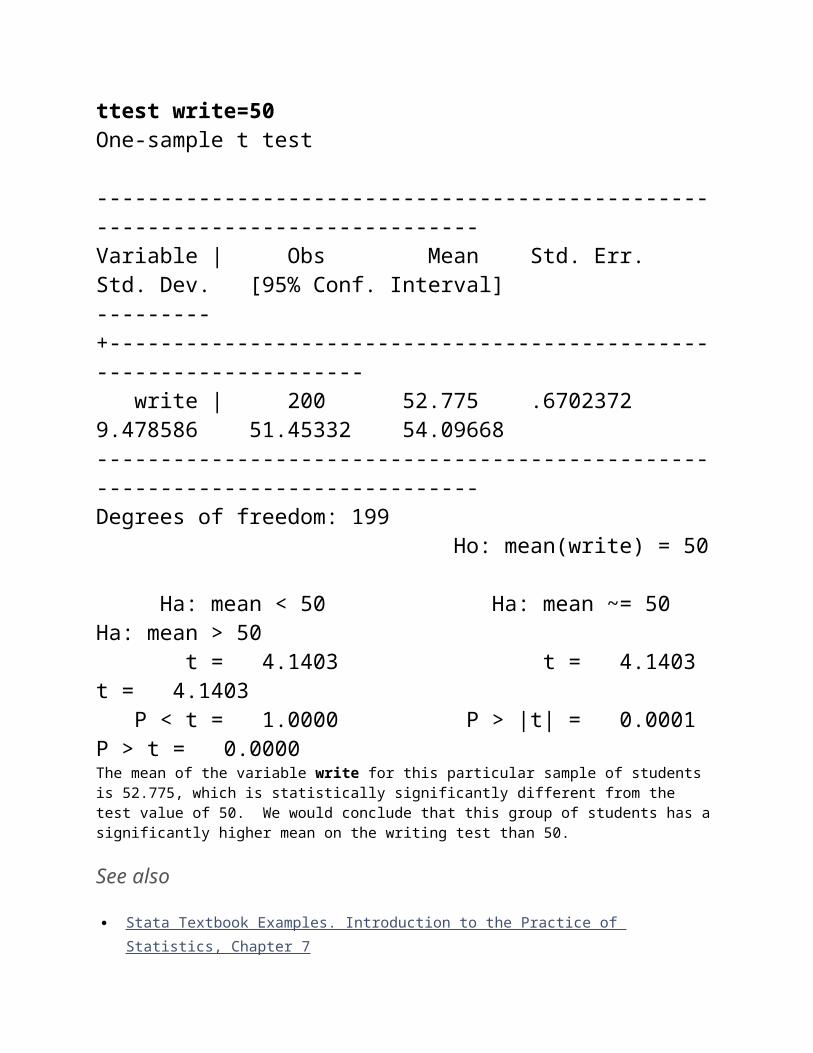
One sample median testA one sample median test allows us to test whether a sample median differs significantly from a hypothesized value.  We will use the same variable, write, as we did in the one sample t-test example above, but we do not need to assume that it is interval and normally distributed (we only need to assume that write is an ordinal variable and that its distribution is symmetric).  We will test whether the median writing score (write) differs significantly from 50.  

signrank write=50Wilcoxon signed-rank test

sign | obs sum ranks expected-------------+---------------------------------

positive | 126 13429 10048.5 negative | 72 6668 10048.5 zero | 2 3 3-------------+--------------------------------- all | 200 20100 20100

unadjusted variance 671675.00adjustment for ties -1760.25adjustment for zeros -1.25 ---------adjusted variance 669913.50

Ho: write = 50 z = 4.130 Prob > |z| = 0.0000The results indicate that the median of the variable write for this group is statistically significantly different from 50.  

See also

Stata Code Fragment: Descriptives, ttests, Anova and Regression

Binomial testA one sample binomial test allows us to test whether the proportion of successes on a two-level categorical dependent variable significantly differs from a hypothesized value.  For example, using the hsb2 data file, say we wish to test whether the proportion of females (female) differs significantly from 50%, i.e., from .5.  We can do this as shown below.

bitest female=.5Variable | N Observed k Expected k Assumed p Observed p-------------+------------------------------------------------------------ female | 200 109 100 0.50000 0.54500

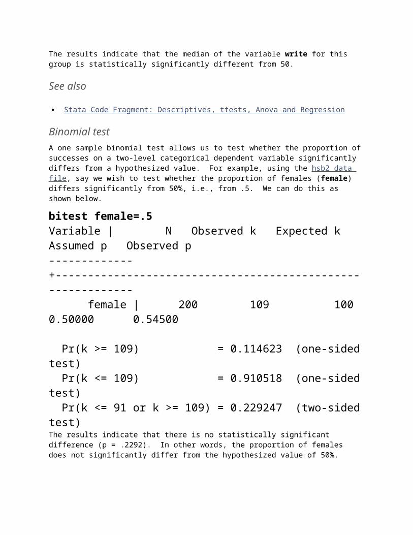
Pr(k >= 109) = 0.114623 (one-sided test) Pr(k <= 109) = 0.910518 (one-sided test) Pr(k <= 91 or k >= 109) = 0.229247 (two-sided test)The results indicate that there is no statistically significant difference (p = .2292).  In other words, the proportion of females does not significantly differ from the hypothesized value of 50%.

See also

Stata Textbook Examples: Introduction to the Practice of Statistics, Chapter 5

Chi-square goodness of fitA chi-square goodness of fit test allows us to test whether the observed proportions for a categorical variable differ from hypothesized proportions.  For example, let's suppose that we believe that the general population consists of 10% Hispanic, 10% Asian, 10% African American and 70% White folks.  We want to test whether the observed proportions from our sample differ significantly from these hypothesized proportions. To conduct the chi-square goodness of fit test, you need to first download the csgof program that performs this test.  You can download csgof from within Stata by typing findit csgof (seeHow can I used the findit command to search for programs and get additional help? for more information about using findit).

Now that the csgof program is installed, we can use it by typing:

csgof race, expperc(10 10 10 70)

race expperc expfreq obsfreq hispanic 10 20 24 asian 10 20 11african-amer 10 20 20 white 70 140 145

chisq(3) is 5.03, p = .1697These results show that racial composition in our sample does not differ significantly from the hypothesized values that we supplied (chi-square with three degrees of freedom = 5.03, p = .1697).

See also

Useful Stata Programs

Stata Textbook Examples: Introduction to the Practice of Statistics, Chapter 8

Two independent samples t-testAn independent samples t-test is used when you want to compare the means of a normally distributed interval dependent variable for two independent groups.  For example, using the hsb2 data file, say we wish to test whether the mean for write is the same for males and females.  

ttest write, by(female)

Two-sample t test with equal variances

------------------------------------------------------------------------------ Group | Obs Mean Std. Err. Std. Dev. [95% Conf. Interval]---------+-------------------------------------------------------------------- male | 91 50.12088 1.080274 10.30516 47.97473 52.26703 female | 109 54.99083 .7790686 8.133715 53.44658 56.53507---------+--------------------------------------------------------------------combined | 200 52.775 .6702372 9.478586 51.45332 54.09668---------+-------------------------------------------------------------------- diff | -4.869947 1.304191 -7.441835 -2.298059

------------------------------------------------------------------------------Degrees of freedom: 198

Ho: mean(male) - mean(female) = diff = 0

Ha: diff < 0 Ha: diff ~= 0 Ha: diff > 0 t = -3.7341 t = -3.7341 t = -3.7341 P < t = 0.0001 P > |t| = 0.0002 P > t = 0.9999The results indicate that there is a statistically significant difference between the mean writing score for males and females (t = -3.7341, p = .0002).  In other words, females have a statistically significantly higher mean score on writing (54.99) than males (50.12).

See also

Stata Learning Module: A Statistical Sampler in Stata

Stata Textbook Examples. Introduction to the Practice of Statistics, Chapter 7

Stata Class Notes: Analyzing Data

Wilcoxon-Mann-Whitney testThe Wilcoxon-Mann-Whitney test is a non-parametric analog to the independent samples t-test and can be used when you do not assume that the dependent variable is a normally distributed interval variable (you only assume that the variable is at least ordinal).  You will notice that the Stata syntax for the Wilcoxon-Mann-Whitney test is almost identical to that of the independent samples t-test.  We will use the same data file (the hsb2 data file) and the same variables in this example as we did in the independent t-test example above and will not assume that write, our dependent variable, is normally distributed.

ranksum write, by(female)Two-sample Wilcoxon rank-sum (Mann-Whitney) test

female | obs rank sum expected-------------+--------------------------------- male | 91 7792 9145.5 female | 109 12308 10954.5

-------------+--------------------------------- combined | 200 20100 20100

unadjusted variance 166143.25adjustment for ties -852.96 ----------adjusted variance 165290.29

Ho: write(female==male) = write(female==female) z = -3.329 Prob > |z| = 0.0009The results suggest that there is a statistically significant difference between the underlying distributions of the write scores of males and the write scores of females (z = -3.329, p = 0.0009).  You can determine which group has the higher rank by looking at the how the actual rank sums compare to the expected rank sums under the null hypothesis.  The sum of the female ranks was higher while the sum of the male ranks was lower.  Thus the female group had higher rank.

See also

FAQ: Why is the Mann-Whitney significant when the medians are equal?

Stata Class Notes: Analyzing Data

Chi-square testA chi-square test is used when you want to see if there is a relationship between two categorical variables.  In Stata, the chi2option is used with the tabulate command to obtain the test statistic and its associated p-value.  Using the hsb2 data file, let's see if there is a relationship between the type of school attended (schtyp) and students' gender (female).  Remember that the chi-square test assumes the expected value of each cell is five or higher.  This assumption is easily met in the examples below.  However, if this assumption is not met in your data, please see the section on Fisher's exact test below.

tabulate schtyp female, chi2

type of | female school | male female | Total-----------+----------------------+---------- public | 77 91 | 168 private | 14 18 | 32

-----------+----------------------+---------- Total | 91 109 | 200

Pearson chi2(1) = 0.0470 Pr = 0.828These results indicate that there is no statistically significant relationship between the type of school attended and gender (chi-square with one degree of freedom = 0.0470, p = 0.828).  

Let's look at another example, this time looking at the relationship between gender (female) and socio-economic status (ses).  The point of this example is that one (or both) variables may have more than two levels, and that the variables do not have to have the same number of levels.  In this example, female has two levels (male and female) and ses has three levels (low, medium and high).

tabulate female ses, chi2

| ses female | low middle high | Total-----------+---------------------------------+---------- male | 15 47 29 | 91 female | 32 48 29 | 109 -----------+---------------------------------+---------- Total | 47 95 58 | 200

Pearson chi2(2) = 4.5765 Pr = 0.101Again we find that there is no statistically significant relationship between the variables (chi-square with two degrees of freedom = 4.5765, p = 0.101).

See also

Stata Learning Module: A Statistical Sampler in Stata

Stata Teaching Tools: Probability Tables

Stata Teaching Tools: Chi-squared distribution

Stata Textbook Examples: An Introduction to Categorical Analysis, Chapter 2

Fisher's exact testThe Fisher's exact test is used when you want to conduct a chi-square test, but one or more of your cells has an expected frequency of five or less.  Remember that the chi-square test assumes that each cell has an expected frequency of five or more, but the Fisher's exact test has no such assumption and can be used regardless of how small the expected frequency is. In the example below, we have cells with observed frequencies of two and one, which may indicate expected frequencies that could be below five, so we will use Fisher's exact test with the exact option on the tabulate command.

tabulate schtyp race, exact

type of | race school | hispanic asian african-a white | Total-----------+--------------------------------------------+---------- public | 22 10 18 118 | 168 private | 2 1 2 27 | 32 -----------+--------------------------------------------+---------- Total | 24 11 20 145 | 200

Fisher's exact = 0.597These results suggest that there is not a statistically significant relationship between race and type of school (p = 0.597). Note that the Fisher's exact test does not have a "test statistic", but computes the p-value directly.

See also

Stata Learning Module: A Statistical Sampler in Stata

Stata Textbook Examples: Statistical Methods for the Social Sciences, Chapter 7

One-way ANOVAA one-way analysis of variance (ANOVA) is used when you have a categorical independent variable (with two or more categories) and a normally distributed interval dependent variable and you wish to test for differences in the means of the dependent variable broken down by the levels of the independent variable.  For example, using the hsb2 data file, say we wish to test whether the mean of write differs between the three program types (prog).  The command for this test would be:

anova write prog

Number of obs = 200 R-squared = 0.1776 Root MSE = 8.63918 Adj R-squared = 0.1693

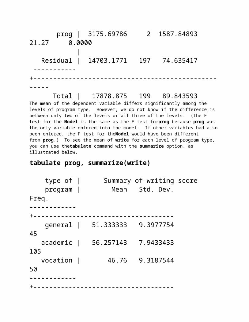
Source | Partial SS df MS F Prob > F -----------+---------------------------------------------------- Model | 3175.69786 2 1587.84893 21.27 0.0000 | prog | 3175.69786 2 1587.84893 21.27 0.0000 | Residual | 14703.1771 197 74.635417 -----------+---------------------------------------------------- Total | 17878.875 199 89.843593 The mean of the dependent variable differs significantly among the levels of program type.  However, we do not know if the difference is between only two of the levels or all three of the

levels.  (The F test for the Model is the same as the F test forprog because prog was the only variable entered into the model.  If other variables had also been entered, the F test for theModel would have been different from prog.)  To see the mean of write for each level of program type, you can use thetabulate command with the summarize option, as illustrated below.

tabulate prog, summarize(write)

type of | Summary of writing score program | Mean Std. Dev. Freq.------------+------------------------------------ general | 51.333333 9.3977754 45 academic | 56.257143 7.9433433 105 vocation | 46.76 9.3187544 50------------+------------------------------------ Total | 52.775 9.478586 200From this we can see that the students in the academic program have the highest mean writing score, while students in the vocational program have the lowest.

See also

Design and Analysis: A Researchers Handbook Third Edition by Geoffrey Keppel

Stata Topics: ANOVA

Stata Frequently Asked Questions

Stata Programs for Data Analysis

Kruskal Wallis testThe Kruskal Wallis test is used when you have one independent variable with two or more levels and an ordinal dependent variable. In other words, it is the non-parametric version of ANOVA and a generalized form of the Mann-Whitney test method since it permits 2 or more groups.  We will use the same data file as the one way ANOVA example above (the hsb2 data

file) and the same variables as in the example above, but we will not assume that write is a normally distributed interval variable.

kwallis write, by(prog)Test: Equality of populations (Kruskal-Wallis test)

prog _Obs _RankSum general < 45 4079.00 academic 105 12764.00 vocation 50 3257.00

chi-squared = 33.870 with 2 d.f.probability = 0.0001

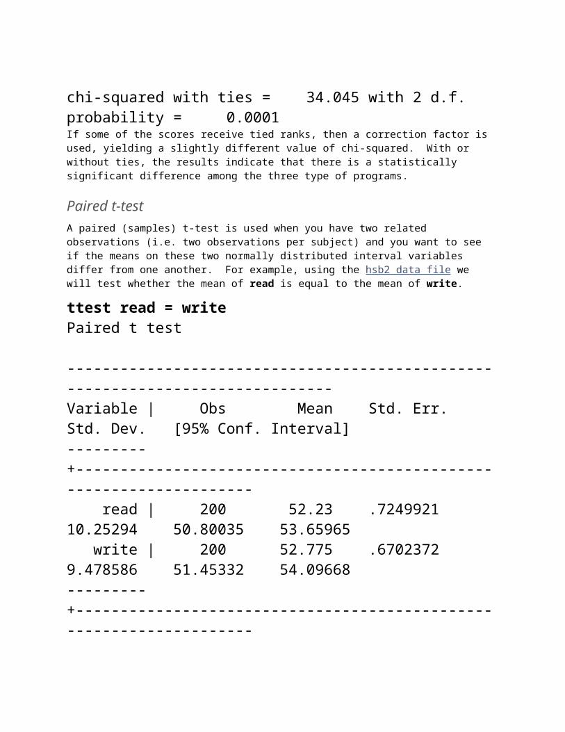
chi-squared with ties = 34.045 with 2 d.f.probability = 0.0001If some of the scores receive tied ranks, then a correction factor is used, yielding a slightly different value of chi-squared.  With or without ties, the results indicate that there is a statistically significant difference among the three type of programs.

Paired t-testA paired (samples) t-test is used when you have two related observations (i.e. two observations per subject) and you want to see if the means on these two normally distributed interval variables differ from one another.  For example, using the hsb2 data file we will test whether the mean of read is equal to the mean of write.

ttest read = writePaired t test

------------------------------------------------------------------------------Variable | Obs Mean Std. Err. Std. Dev. [95% Conf. Interval]---------+--------------------------------------------------------------------

read | 200 52.23 .7249921 10.25294 50.80035 53.65965 write | 200 52.775 .6702372 9.478586 51.45332 54.09668---------+-------------------------------------------------------------------- diff | 200 -.545 .6283822 8.886666 -1.784142 .6941424------------------------------------------------------------------------------

Ho: mean(read - write) = mean(diff) = 0

Ha: mean(diff) < 0 Ha: mean(diff) ~= 0 Ha: mean(diff) > 0 t = -0.8673 t = -0.8673 t = -0.8673 P < t = 0.1934 P > |t| = 0.3868 P > t = 0.8066These results indicate that the mean of read is not statistically significantly different from the mean of write (t = -0.8673, p = 0.3868).

See also

Stata Learning Module: Comparing Stata and SAS Side by Side

Stata Textbook Examples. Introduction to the Practice of Statistics, Chapter 7

Wilcoxon signed rank sum testThe Wilcoxon signed rank sum test is the non-parametric version of a paired samples t-test.  You use the Wilcoxon signed rank sum test when you do not wish to assume that the difference between the two variables is interval and normally distributed (but you do assume the difference is ordinal). We will use the same example as above, but we will not assume that the difference between read and write is interval and normally distributed.

signrank read = writeWilcoxon signed-rank test

sign | obs sum ranks expected-------------+--------------------------------- positive | 88 9264 9990 negative | 97 10716 9990 zero | 15 120 120-------------+--------------------------------- all | 200 20100 20100

unadjusted variance 671675.00adjustment for ties -715.25adjustment for zeros -310.00 ----------adjusted variance 670649.75

Ho: read = write z = -0.887 Prob > |z| = 0.3753The results suggest that there is not a statistically significant difference between read and write.

If you believe the differences between read and write were not ordinal but could merely be classified as positive and negative, then you may want to consider a sign test in lieu of sign rank test.  Again, we will use the same variables in this example and assume that this difference is not ordinal.

signtest read = writeSign test

sign | observed expected-------------+------------------------ positive | 88 92.5 negative | 97 92.5 zero | 15 15-------------+------------------------ all | 200 200

One-sided tests:

Ho: median of read - write = 0 vs. Ha: median of read - write > 0 Pr(#positive >= 88) = Binomial(n = 185, x >= 88, p = 0.5) = 0.7688

Ho: median of read - write = 0 vs. Ha: median of read - write < 0 Pr(#negative >= 97) = Binomial(n = 185, x >= 97, p = 0.5) = 0.2783

Two-sided test: Ho: median of read - write = 0 vs. Ha: median of read - write ~= 0 Pr(#positive >= 97 or #negative >= 97) = min(1, 2*Binomial(n = 185, x >= 97, p = 0.5)) = 0.5565This output gives both of the one-sided tests as well as the two-sided test.  Assuming that we were looking for any difference, we would use the two-sided test and conclude that no statistically significant difference was found (p=.5565).

See also

Stata Code Fragment: Descriptives, ttests, Anova and Regression

Stata Class Notes: Analyzing Data

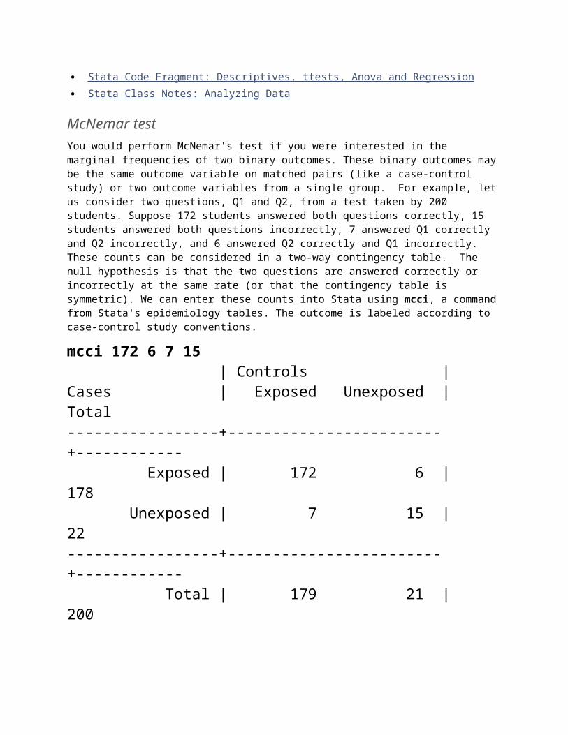
McNemar testYou would perform McNemar's test if you were interested in the marginal frequencies of two binary outcomes. These binary outcomes may be the same outcome variable on matched pairs (like a case-control study) or two outcome variables from a single group.  For example, let us consider two questions, Q1 and Q2, from a test taken by 200 students. Suppose 172 students answered both questions correctly, 15 students answered both questions incorrectly, 7 answered Q1 correctly and Q2 incorrectly, and 6 answered Q2 correctly and Q1 incorrectly. These counts can be considered in a two-way contingency table.  The null hypothesis is that the two questions are answered correctly or incorrectly at the same rate (or that the contingency table is symmetric). We can enter these counts into Stata using mcci, a command from Stata's epidemiology tables. The outcome is labeled according to case-control study conventions.

mcci 172 6 7 15 | Controls |Cases | Exposed Unexposed | Total-----------------+------------------------+------------ Exposed | 172 6 | 178 Unexposed | 7 15 | 22-----------------+------------------------+------------ Total | 179 21 | 200

McNemar's chi2(1) = 0.08 Prob > chi2 = 0.7815Exact McNemar significance probability = 1.0000

Proportion with factor Cases .89 Controls .895 [95% Conf. Interval] --------- -------------------- difference -.005 -.045327 .035327 ratio .9944134 .9558139 1.034572 rel. diff. -.047619 -.39205 .2968119

odds ratio .8571429 .2379799 2.978588 (exact)

McNemar's chi-square statistic suggests that there is not a statistically significant difference in the proportions of correct/incorrect answers to these two questions.

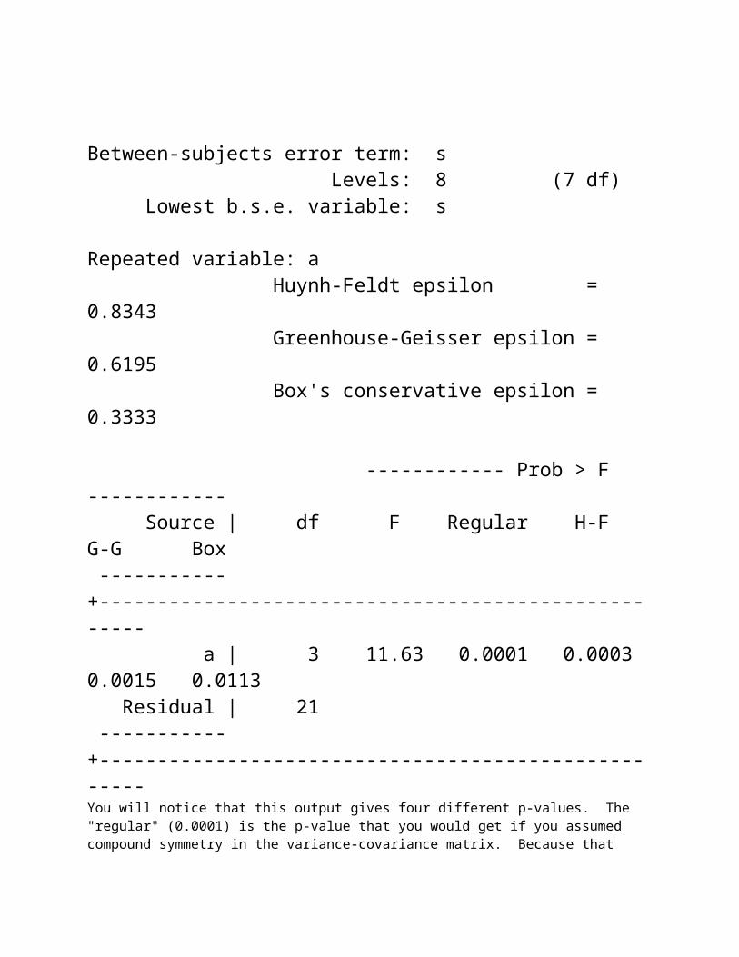
One-way repeated measures ANOVAYou would perform a one-way repeated measures analysis of variance if you had one categorical independent variable and a normally distributed interval dependent variable that was repeated at least twice for each subject.  This is the equivalent of the paired samples t-test, but allows for two or more levels of the categorical variable. This tests whether the mean of the dependent variable differs by the categorical variable.  We have an example data set called rb4, which is used in Kirk's book Experimental Design.  In this data set, y is the dependent variable, a is the repeated measure and s is the variable that indicates the subject number.

use http://www.ats.ucla.edu/stat/stata/examples/kirk/rb4anova y a s, repeated(a) Number of obs = 32 R-squared = 0.7318 Root MSE = 1.18523 Adj R-squared = 0.6041

Source | Partial SS df MS F Prob > F -----------+---------------------------------------------------- Model | 80.50 10 8.05 5.73 0.0004 | a | 49.00 3 16.3333333 11.63 0.0001 s | 31.50 7 4.50 3.20 0.0180 | Residual | 29.50 21 1.4047619

-----------+---------------------------------------------------- Total | 110.00 31 3.5483871

Between-subjects error term: s Levels: 8 (7 df) Lowest b.s.e. variable: s

Repeated variable: a Huynh-Feldt epsilon = 0.8343 Greenhouse-Geisser epsilon = 0.6195 Box's conservative epsilon = 0.3333

------------ Prob > F ------------ Source | df F Regular H-F G-G Box -----------+---------------------------------------------------- a | 3 11.63 0.0001 0.0003 0.0015 0.0113 Residual | 21 -----------+----------------------------------------------------You will notice that this output gives four different p-values.  The "regular" (0.0001) is the p-value that you would get if you assumed compound symmetry in the variance-covariance matrix.  Because that assumption is often not valid, the three other p-values offer various corrections (the Huynh-Feldt, H-F, Greenhouse-Geisser, G-G and Box's conservative, Box).  No

matter which p-value you use, our results indicate that we have a statistically significant effect of a at the .05 level.

See also

Stata FAQ: How can I test for nonadditivity in a randomized block ANOVA in Stata?

Stata Textbook Examples, Experimental Design, Chapter 7

Stata Textbook Examples, Design and Analysis, Chapter 16

Stata Code Fragment: ANOVA

Repeated measures logistic regressionIf you have a binary outcome measured repeatedly for each subject and you wish to run a logistic regression that accounts for the effect of these multiple measures from each subjects, you can perform a repeated measures logistic regression.  In Stata, this can be done using the xtgee command and indicating binomial as the probability distribution and logit as the link function to be used in the model. The exercise data file contains 3 pulse measurements of 30 people assigned to 2 different diet regiments and 3 different exercise regiments. If we define a "high" pulse as being over 100, we can then predict the probability of a high pulse using diet regiment.

First, we use xtset to define which variable defines the repetitions.  In this dataset, there are three measurements taken for each id, so we will use id as our panel variable. Then we can use i: before diet so that we can create indicator variables as needed.

use http://www.ats.ucla.edu/stat/stata/whatstat/exercise, clearxtset idxtgee highpulse i.diet, family(binomial) link(logit)Iteration 1: tolerance = 1.753e-08

GEE population-averaged model Number of obs = 90Group variable: id Number of groups = 30Link: logit Obs per group: min = 3

Family: binomial avg = 3.0Correlation: exchangeable max = 3 Wald chi2(1) = 1.53Scale parameter: 1 Prob > chi2 = 0.2157

------------------------------------------------------------------------------ highpulse | Coef. Std. Err. z P>|z| [95% Conf. Interval]-------------+---------------------------------------------------------------- 2.diet | .7537718 .6088196 1.24 0.216 -.4394927 1.947036 _cons | -1.252763 .4621704 -2.71 0.007 -2.1586 -.3469257------------------------------------------------------------------------------These results indicate that diet is not statistically significant (Z = 1.24, p = 0.216). 

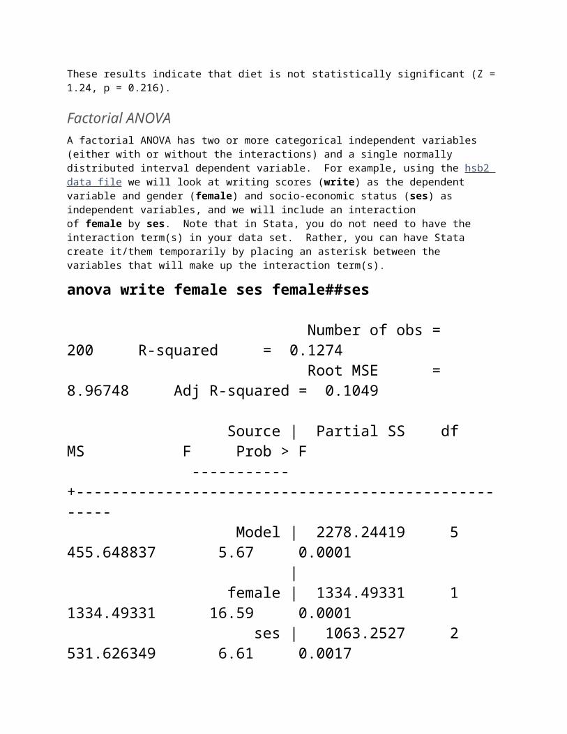
Factorial ANOVAA factorial ANOVA has two or more categorical independent variables (either with or without the interactions) and a single normally distributed interval dependent variable.  For example, using the hsb2 data file we will look at writing scores (write) as the dependent variable and gender (female) and socio-economic status (ses) as independent variables, and we will include an interaction of female by ses.  Note that in Stata, you do not need to have the interaction term(s) in your data set.  Rather, you can have Stata create it/them temporarily by placing an asterisk between the variables that will make up the interaction term(s). 

anova write female ses female##ses

Number of obs = 200 R-squared = 0.1274

Root MSE = 8.96748 Adj R-squared = 0.1049

Source | Partial SS df MS F Prob > F -----------+---------------------------------------------------- Model | 2278.24419 5 455.648837 5.67 0.0001 | female | 1334.49331 1 1334.49331 16.59 0.0001 ses | 1063.2527 2 531.626349 6.61 0.0017 female#ses | 21.4309044 2 10.7154522 0.13 0.8753 | Residual | 15600.6308 194 80.4156228 -----------+---------------------------------------------------- Total | 17878.875 199 89.843593 These results indicate that the overall model is statistically significant (F = 5.67, p = 0.001).  The variables female and ses are also statistically significant (F = 16.59, p = 0.0001 and F = 6.61, p = 0.0017, respectively).  However, that interaction betweenfemale and ses is not statistically significant (F = 0.13, p = 0.8753). 

See also

Stata Frequently Asked Questions

Stata Textbook Examples, Design and Analysis, Chapter 11

Stata Textbook Examples, Experimental Design, Chapter 9

Stata Code Fragment: ANOVA

Friedman testYou perform a Friedman test when you have one within-subjects independent variable with two or more levels and a dependent variable that is not interval and normally distributed (but at least ordinal).  We will use this test to determine if there is a difference in the reading, writing and math scores.  The null hypothesis in this test is that the distribution of the ranks of each type of score (i.e., reading, writing and math) are the same.  To conduct the Friedman test in Stata, you need to first download the friedman program that performs this test.  You can download friedman from within Stata by typing findit friedman (seeHow can I used the findit command to search for programs and get additional help? for more information about using findit).  Also, your data will need to be transposed such that subjects are the columns and the variables are the rows.  We will use thexpose command to arrange our data this way.

use http://www.ats.ucla.edu/stat/stata/notes/hsb2keep read write mathxpose, clearfriedman v1-v200Friedman = 0.6175Kendall = 0.0015P-value = 0.7344Friedman's chi-square has a value of 0.6175 and a p-value of 0.7344 and is not statistically significant.  Hence, there is no evidence that the distributions of the three types of scores are different.

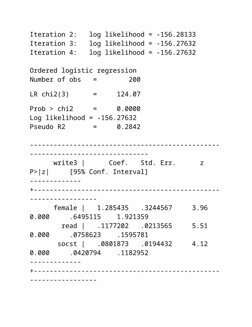
Ordered logistic regressionOrdered logistic regression is used when the dependent variable is ordered, but not continuous.  For example, using the hsb2 data file we will create an ordered variable called write3.  This variable will have the values 1, 2 and 3, indicating a low, medium or high writing score.  We do not generally recommend categorizing a continuous variable in this way; we are simply creating a variable to use for this example.  We will use gender (female), reading score (read) and social studies score (socst) as predictor variables in this model. 

use http://www.ats.ucla.edu/stat/stata/notes/hsb2generate write3 = 1replace write3 = 2 if write >= 49 & write <= 57replace write3 = 3 if write >= 58 & write <= 70ologit write3 female read socst

Iteration 0: log likelihood = -218.31357

Iteration 1: log likelihood = -157.692 Iteration 2: log likelihood = -156.28133 Iteration 3: log likelihood = -156.27632 Iteration 4: log likelihood = -156.27632

Ordered logistic regression Number of obs = 200 LR chi2(3) = 124.07 Prob > chi2 = 0.0000Log likelihood = -156.27632 Pseudo R2 = 0.2842

------------------------------------------------------------------------------ write3 | Coef. Std. Err. z P>|z| [95% Conf. Interval]-------------+---------------------------------------------------------------- female | 1.285435 .3244567 3.96 0.000 .6495115 1.921359 read | .1177202 .0213565 5.51 0.000 .0758623 .1595781 socst | .0801873 .0194432 4.12 0.000 .0420794 .1182952-------------+---------------------------------------------------------------- /cut1 | 9.703706 1.197002 7.357626 12.04979 /cut2 | 11.8001 1.304306 9.243705 14.35649------------------------------------------------------------------------------

The results indicate that the overall model is statistically significant (p < .0000), as are each of the predictor variables (p < .000).  There are two cutpoints for this model because there are three levels of the outcome variable.

One of the assumptions underlying ordinal logistic (and ordinal probit) regression is that the relationship between each pair of outcome groups is the same.  In other words, ordinal logistic regression assumes that the coefficients that describe the relationship between, say, the lowest versus all higher categories of the response variable are the same as those that describe the relationship between the next lowest category and all higher categories, etc.  This is called the proportional odds assumption or the parallel regression assumption.  Because the relationship between all pairs of groups is the same, there is only one set of coefficients (only one model).  If this was not the case, we would need different models (such as a generalized ordered logit model) to describe the relationship between each pair of outcome groups.  To test this assumption, we can use either the omodel command (findit omodel, see  How can I used the findit command to search for programs and get additional help? for more information about using findit) or the brant command.  We will show both below.

omodel logit write3 female read socst

Iteration 0: log likelihood = -218.31357Iteration 1: log likelihood = -158.87444Iteration 2: log likelihood = -156.35529Iteration 3: log likelihood = -156.27644Iteration 4: log likelihood = -156.27632

Ordered logit estimates Number of obs = 200 LR chi2(3) = 124.07 Prob > chi2 = 0.0000Log likelihood = -156.27632 Pseudo R2 = 0.2842

------------------------------------------------------------------------------ write3 | Coef. Std. Err. z P>|z| [95% Conf. Interval]

-------------+---------------------------------------------------------------- female | 1.285435 .3244565 3.96 0.000 .649512 1.921358 read | .1177202 .0213564 5.51 0.000 .0758623 .159578 socst | .0801873 .0194432 4.12 0.000 .0420794 .1182952-------------+---------------------------------------------------------------- _cut1 | 9.703706 1.197 (Ancillary parameters) _cut2 | 11.8001 1.304304 ------------------------------------------------------------------------------

Approximate likelihood-ratio test of proportionality of oddsacross response categories: chi2(3) = 2.03 Prob > chi2 = 0.5658

brant, detail

Estimated coefficients from j-1 binary regressions

y>1 y>2female 1.5673604 1.0629714 read .11712422 .13401723 socst .0842684 .06429241 _cons -10.001584 -11.671854

Brant Test of Parallel Regression Assumption

Variable | chi2 p>chi2 df-------------+-------------------------- All | 2.07 0.558 3-------------+-------------------------- female | 1.08 0.300 1 read | 0.26 0.608 1 socst | 0.52 0.470 1----------------------------------------

A significant test statistic provides evidence that the parallelregression assumption has been violated.Both of these tests indicate that the proportional odds assumption has not been violated.

See also

Stata FAQ:   In ordered probit and logit, what are the cut points?

Stata Annotated Output:   Ordered logistic regression

Factorial logistic regressionA factorial logistic regression is used when you have two or more categorical independent variables but a dichotomous dependent variable.  For example, using the hsb2 data file we will use female as our dependent variable, because it is the only dichotomous (0/1) variable in our data set; certainly not because it common practice to use gender as an outcome variable.  We will use type of program (prog) and school type (schtyp) as our predictor variables.  Because prog is a categorical variable (it has three levels), we need to create dummy codes for it.  The use of i.prog does this.  You can use thelogit command if you want to see the regression coefficients or the logistic command if you want to see the odds ratios.

logit female i.prog##schtyp

Iteration 0: log likelihood = -137.81834 Iteration 1: log likelihood = -136.25886 Iteration 2: log likelihood = -136.24502 Iteration 3: log likelihood = -136.24501

Logistic regression Number of obs = 200 LR chi2(5) = 3.15 Prob > chi2 = 0.6774Log likelihood = -136.24501 Pseudo R2 = 0.0114

------------------------------------------------------------------------------ female | Coef. Std. Err. z P>|z| [95% Conf. Interval]-------------+---------------------------------------------------------------- prog | 2 | .3245866 .3910782 0.83 0.407 -.4419125 1.091086 3 | .2183474 .4319116 0.51 0.613 -.6281839 1.064879 | 2.schtyp | 1.660724 1.141326 1.46 0.146 -.5762344 3.897683 | prog#schtyp | 2 2 | -1.934018 1.232722 -1.57 0.117 -4.350108 .4820729 3 2 | -1.827778 1.840256 -0.99 0.321 -5.434614 1.779057 | _cons | -.0512933 .3203616 -0.16 0.873 -.6791906 .576604------------------------------------------------------------------------------

The results indicate that the overall model is not statistically significant (LR chi2 = 3.15, p = 0.6774).  Furthermore, none of the coefficients are statistically significant either.  We can use the test command to get the test of the overall effect of prog as shown below.  This shows that the overall effect of prog is not statistically significant.

test 2.prog 3.prog

( 1) [female]2.prog = 0 ( 2) [female]3.prog = 0

chi2( 2) = 0.69 Prob > chi2 = 0.7086Likewise, we can use the testparm command to get the test of the overall effect of the prog by schtyp interaction, as shown below.  This shows that the overall effect of this interaction is not statistically significant.

testparm prog#schtyp

( 1) [female]2.prog#2.schtyp = 0 ( 2) [female]3.prog#2.schtyp = 0

chi2( 2) = 2.47 Prob > chi2 = 0.2902If you prefer, you could use the logistic command to see the results as odds ratios, as shown below.

logistic female i.prog##schtyp

Logistic regression Number of obs = 200 LR chi2(5) = 3.15 Prob > chi2 = 0.6774Log likelihood = -136.24501 Pseudo R2 = 0.0114

------------------------------------------------------------------------------

female | Odds Ratio Std. Err. z P>|z| [95% Conf. Interval]-------------+---------------------------------------------------------------- prog | 2 | 1.383459 .5410405 0.83 0.407 .6428059 2.977505 3 | 1.244019 .5373063 0.51 0.613 .5335599 2.900487 | 2.schtyp | 5.263121 6.006939 1.46 0.146 .5620107 49.28811 | prog#schtyp | 2 2 | .1445662 .1782099 -1.57 0.117 .0129054 1.619428 3 2 | .1607704 .2958586 -0.99 0.321 .0043629 5.924268------------------------------------------------------------------------------

CorrelationA correlation is useful when you want to see the linear relationship between two (or more) normally distributed interval variables.  For example, using the hsb2 data file we can run a correlation between two continuous variables, read and write. 

corr read write(obs=200)

| read write-------------+------------------ read | 1.0000 write | 0.5968 1.0000In the second example, we will run a correlation between a dichotomous variable, female, and a continuous variable, write. Although it is assumed that the variables are interval and normally distributed, we can include dummy variables when performing correlations.

corr female write(obs=200)

| female write-------------+------------------ female | 1.0000 write | 0.2565 1.0000In the first example above, we see that the correlation between read and write is 0.5968.  By squaring the correlation and then multiplying by 100, you can determine what percentage of the variability is shared.  Let's round 0.5968 to be 0.6, which when squared would be .36, multiplied by 100 would be 36%.  Hence read shares about 36% of its variability with write.  In the output for the second example, we can see the correlation between write and female is 0.2565.  Squaring this number yields .06579225, meaning that female shares approximately 6.5% of its variability with write.

See also

Annotated Stata Output: Correlation

Stata Teaching Tools

Stata Learning Module: A Statistical Sampler in Stata   

Stata Programs for Data Analysis

Stata Class Notes: Exploring Data

Stata Class Notes: Analyzing Data

Simple linear regressionSimple linear regression allows us to look at the linear relationship between one normally distributed interval predictor and one normally distributed interval outcome variable.  For example, using the hsb2 data file, say we wish to look at the relationship between writing scores (write) and reading scores (read); in other words, predicting write from read.  

regress write read

------------------------------------------------------------------------------ write | Coef. Std. Err. t P>|t| [95% Conf. Interval]

-------------+---------------------------------------------------------------- read | .5517051 .0527178 10.47 0.000 .4477446 .6556656 _cons | 23.95944 2.805744 8.54 0.000 18.42647 29.49242------------------------------------------------------------------------------We see that the relationship between write and read is positive (.5517051) and based on the t-value (10.47) and p-value (0.000), we would conclude this relationship is statistically significant.  Hence, we would say there is a statistically significant positive linear relationship between reading and writing.

See also

Regression With Stata: Chapter 1 - Simple and Multiple Regression

Stata Annotated Output: Regression

Stata Frequently Asked Questions

Stata Topics: Regression

Stata Textbook Example: Introduction to the Practice of Statistics, Chapter 10

Stata Textbook Examples: Regression with Graphics, Chapter 2

Stata Textbook Examples: Applied Regression Analysis, Chapter 5

Non-parametric correlationA Spearman correlation is used when one or both of the variables are not assumed to be normally distributed and interval (but are assumed to be ordinal). The values of the variables are converted in ranks and then correlated.  In our example, we will look for a relationship between read and write.  We will not assume that both of these variables are normal and interval .  

spearman read writeNumber of obs = 200Spearman's rho = 0.6167

Test of Ho: read and write are independent Prob > |t| = 0.0000

The results suggest that the relationship between read and write (rho = 0.6167, p = 0.000) is statistically significant. 

Simple logistic regressionLogistic regression assumes that the outcome variable is binary (i.e., coded as 0 and 1).  We have only one variable in thehsb2 data file that is coded 0 and 1, and that is female.  We understand that female is a silly outcome variable (it would make more sense to use it as a predictor variable), but we can use female as the outcome variable to illustrate how the code for this command is structured and how to interpret the output.  The first variable listed after the logistic (or logit) command is the outcome (or dependent) variable, and all of the rest of the variables are predictor (or independent) variables.  You can use the logit command if you want to see the regression coefficients or the logistic command if you want to see the odds ratios.  In our example, female will be the outcome variable, and read will be the predictor variable.  As with OLS regression, the predictor variables must be either dichotomous or continuous; they cannot be categorical.

logistic female read

Logit estimates Number of obs = 200 LR chi2(1) = 0.56 Prob > chi2 = 0.4527Log likelihood = -137.53641 Pseudo R2 = 0.0020

------------------------------------------------------------------------------ female | Odds Ratio Std. Err. z P>|z| [95% Conf. Interval]-------------+---------------------------------------------------------------- read | .9896176 .0137732 -0.75 0.453 .9629875 1.016984------------------------------------------------------------------------------

logit female readIteration 0: log likelihood = -137.81834Iteration 1: log likelihood = -137.53642Iteration 2: log likelihood = -137.53641

Logit estimates Number of obs = 200 LR chi2(1) = 0.56 Prob > chi2 = 0.4527Log likelihood = -137.53641 Pseudo R2 = 0.0020

------------------------------------------------------------------------------ female | Coef. Std. Err. z P>|z| [95% Conf. Interval]-------------+---------------------------------------------------------------- read | -.0104367 .0139177 -0.75 0.453 -.0377148 .0168415 _cons | .7260875 .7419612 0.98 0.328 -.7281297 2.180305------------------------------------------------------------------------------The results indicate that reading score (read) is not a statistically significant predictor of gender (i.e., being female), z = -0.75, p = 0.453.  Likewise, the test of the overall model is not statistically significant, LR chi-squared 0.56, p = 0.4527.  

See also

Stata Textbook Examples: Applied Logistic Regression (2nd Ed) Chapter 1

Stata Web Books: Logistic Regression in Stata

Stata Topics: Logistic Regression

Stata Data Analysis Example: Logistic Regression

Annotated Stata Output: Logistic Regression Analysis

Stata FAQ: How do I interpret odds ratios in logistic regression?

Stata Library

Teaching Tools: Graph Logistic Regression Curve

Multiple regressionMultiple regression is very similar to simple regression, except that in multiple regression you have more than one predictor variable in the equation.  For example, using the hsb2 data file we will predict writing score from gender (female), reading, math, science and social studies (socst) scores.

regress write female read math science socstSource | SS df MS Number of obs = 200-------------+------------------------------ F( 5, 194) = 58.60 Model | 10756.9244 5 2151.38488 Prob > F = 0.0000 Residual | 7121.9506 194 36.7110855 R-squared = 0.6017-------------+------------------------------ Adj R-squared = 0.5914 Total | 17878.875 199 89.843593 Root MSE = 6.059

------------------------------------------------------------------------------ write | Coef. Std. Err. t P>|t| [95% Conf. Interval]-------------+---------------------------------------------------------------- female | 5.492502 .8754227 6.27 0.000 3.765935 7.21907 read | .1254123 .0649598 1.93 0.055 -.0027059 .2535304

math | .2380748 .0671266 3.55 0.000 .1056832 .3704665 science | .2419382 .0606997 3.99 0.000 .1222221 .3616542 socst | .2292644 .0528361 4.34 0.000 .1250575 .3334713 _cons | 6.138759 2.808423 2.19 0.030 .599798 11.67772------------------------------------------------------------------------------The results indicate that the overall model is statistically significant (F = 58.60, p = 0.0000).  Furthermore, all of the predictor variables are statistically significant except for read.  

See also

Regression with Stata: Lesson 1 - Simple and Multiple Regression

Annotated Output: Multiple Linear Regression

Stata Annotated Output: Regression

Stata Teaching Tools

Stata Textbook Examples: Applied Linear Statistical Models

Stata Textbook Examples: Introduction to the Practice of Statistics, Chapter 11

Stata Textbook Examples: Regression Analysis by Example, Chapter 3

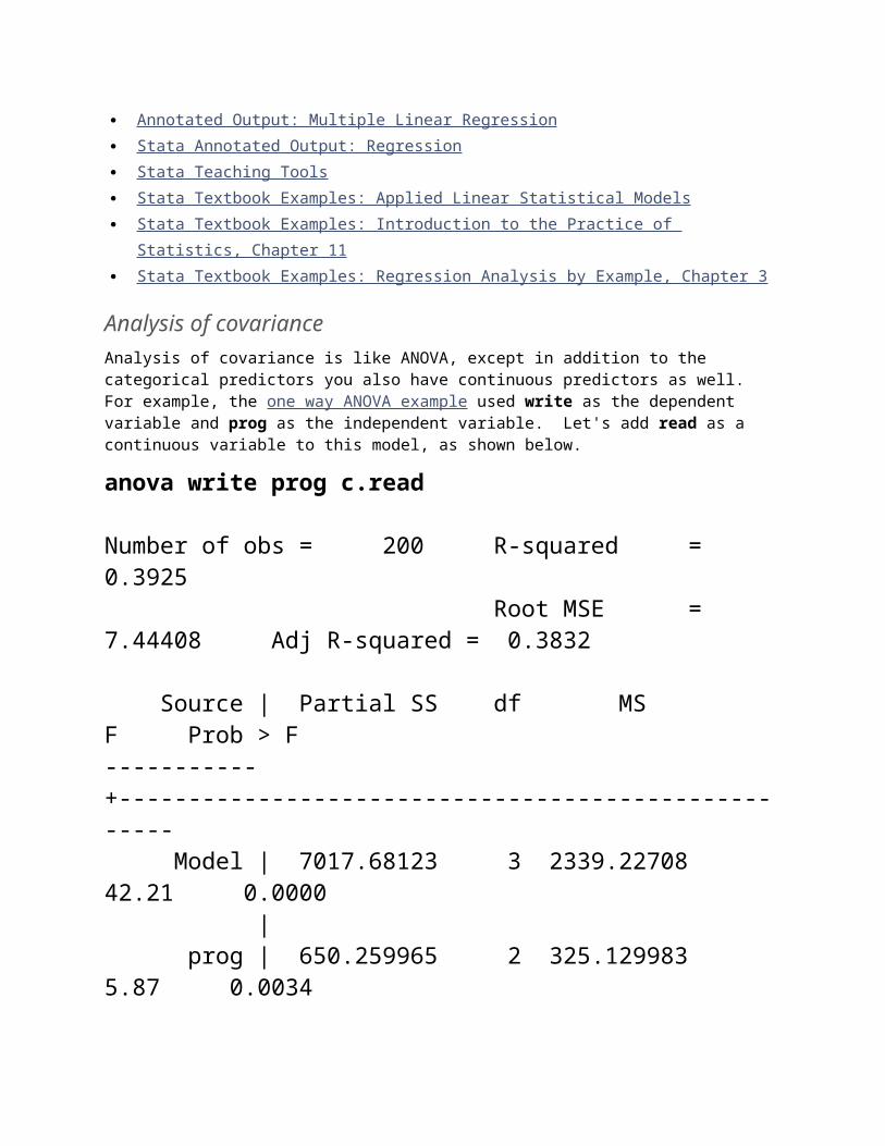
Analysis of covarianceAnalysis of covariance is like ANOVA, except in addition to the categorical predictors you also have continuous predictors as well.  For example, the one way ANOVA example used write as the dependent variable and prog as the independent variable.  Let's add read as a continuous variable to this model, as shown below.

anova write prog c.read

Number of obs = 200 R-squared = 0.3925 Root MSE = 7.44408 Adj R-squared = 0.3832

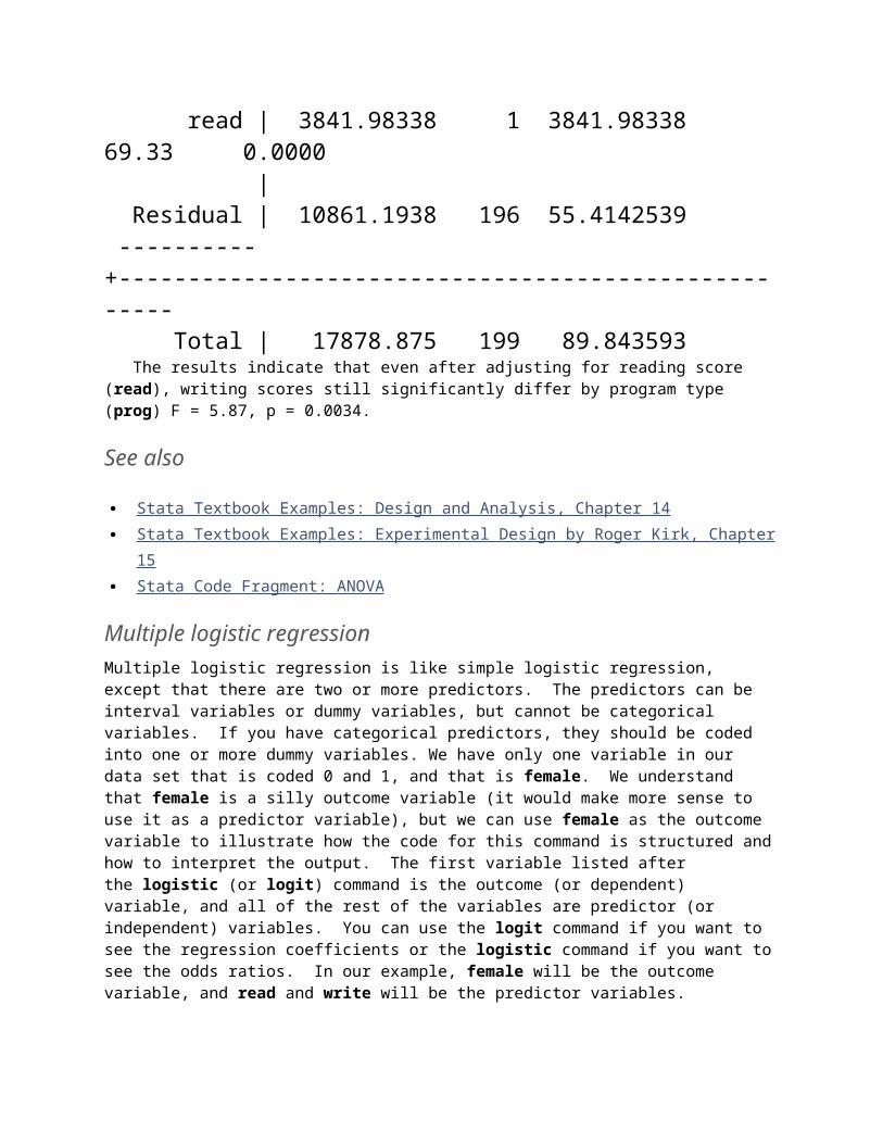
Source | Partial SS df MS F Prob > F-----------+---------------------------------------------------- Model | 7017.68123 3 2339.22708 42.21 0.0000 | prog | 650.259965 2 325.129983 5.87 0.0034 read | 3841.98338 1 3841.98338 69.33 0.0000 | Residual | 10861.1938 196 55.4142539 ----------+---------------------------------------------------- Total | 17878.875 199 89.843593    The results indicate that even after adjusting for reading score (read), writing scores still significantly differ by program type (prog) F = 5.87, p = 0.0034.

See also

Stata Textbook Examples: Design and Analysis, Chapter 14

Stata Textbook Examples: Experimental Design by Roger Kirk, Chapter 15

Stata Code Fragment: ANOVA

Multiple logistic regressionMultiple logistic regression is like simple logistic regression, except that there are two or more predictors.  The predictors can be interval variables or dummy variables, but cannot be categorical variables.  If you have categorical predictors, they should be coded into one or more dummy variables. We have only one variable in our data set that is coded 0 and 1, and that is female.  We understand that female is a silly outcome variable (it would make more sense to use it as a predictor variable), but we can use female as the outcome variable to illustrate how the code for this command is structured and how to interpret the output.  The first variable listed after the logistic (or logit) command is the outcome (or dependent) variable, and all of the rest of the variables are predictor (or independent) variables.  You can use the logit command if you want to see the regression coefficients or the logistic command if you want to see the odds

ratios.  In our example, female will be the outcome variable, and read and write will be the predictor variables. 

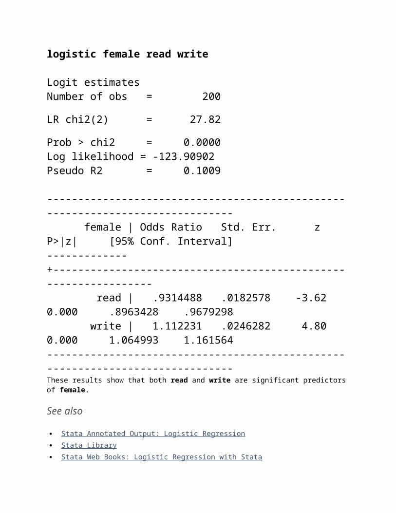
logistic female read write

Logit estimates Number of obs = 200 LR chi2(2) = 27.82 Prob > chi2 = 0.0000Log likelihood = -123.90902 Pseudo R2 = 0.1009

------------------------------------------------------------------------------ female | Odds Ratio Std. Err. z P>|z| [95% Conf. Interval]-------------+---------------------------------------------------------------- read | .9314488 .0182578 -3.62 0.000 .8963428 .9679298 write | 1.112231 .0246282 4.80 0.000 1.064993 1.161564------------------------------------------------------------------------------These results show that both read and write are significant predictors of female.

See also

Stata Annotated Output: Logistic Regression

Stata Library

Stata Web Books: Logistic Regression with Stata

Stata Topics: Logistic Regression

Stata Textbook Examples: Applied Logistic Regression, Chapter 2

Stata Textbook Examples: Applied Regression Analysis, Chapter 8

Stata Textbook Examples: Introduction to Categorical Analysis, Chapter 5

Stata Textbook Examples: Regression Analysis by Example, Chapter 12

Discriminant analysisDiscriminant analysis is used when you have one or more normally distributed interval independent variables and a categorical dependent variable.  It is a multivariate technique that considers the latent dimensions in the independent variables for predicting group membership in the categorical dependent variable.  For example, using the hsb2 data file, say we wish to useread, write and math scores to predict the type of program a student belongs to (prog).  For this analysis, you need to first download the daoneway program that performs this test. You can download daoneway from within Stata by typing findit daoneway (see  How can I used the findit command to search for programs and get additional help? for more information about using findit).

You can then perform the discriminant function analysis like this.

daoneway read write math, by(prog)One-way Disciminant Function Analysis

Observations = 200Variables = 3Groups = 3

Pct of Cum Canonical After Wilks' Fcn Eigenvalue Variance Pct Corr Fcn Lambda Chi-square df P-value | 0 0.73398 60.619 6 0.0000 1 0.3563 98.74 98.74 0.5125 | 1 0.99548 0.888 2 0.6414 2 0.0045 1.26 100.00 0.0672 |

Unstandardized canonical discriminant function coefficients

func1 func2 read 0.0292 -0.0439write 0.0383 0.1370

math 0.0703 -0.0793_cons -7.2509 -0.7635

Standardized canonical discriminant function coefficients

func1 func2 read 0.2729 -0.4098write 0.3311 1.1834 math 0.5816 -0.6557

Canonical discriminant structure matrix

func1 func2 read 0.7785 -0.1841write 0.7753 0.6303 math 0.9129 -0.2725

Group means on canonical discriminant functions

func1 func2prog-1 -0.3120 0.1190prog-2 0.5359 -0.0197prog-3 -0.8445 -0.0658Clearly, the Stata output for this procedure is lengthy, and it is beyond the scope of this page to explain all of it.  However, the main point is that two canonical variables are identified by the analysis, the first of which seems to be more related to program type than the second.  For more information, see this page on discriminant function analysis.

See also

Stata Data Analysis Examples: Discriminant Function Analysis

One-way MANOVAMANOVA (multivariate analysis of variance) is like ANOVA, except that there are two or more dependent variables. In a one-way MANOVA, there is one categorical independent variable and two or more dependent variables. For example, using thehsb2 data file, say we wish to examine

the differences in read, write and math broken down by program type (prog). For this analysis, you can use the manova command and then perform the analysis like this.

manova read write math = prog, category(prog)Number of obs = 200 W = Wilks' lambda L = Lawley-Hotelling trace P = Pillai's trace R = Roy's largest root

Source | Statistic df F(df1, df2) = F Prob>F-----------+-------------------------------------------------- prog | W 0.7340 2 6.0 390.0 10.87 0.0000 e | P 0.2672 6.0 392.0 10.08 0.0000 a | L 0.3608 6.0 388.0 11.67 0.0000 a | R 0.3563 3.0 196.0 23.28 0.0000 u |-------------------------------------------------- Residual | 197-----------+-------------------------------------------------- Total | 199-------------------------------------------------------------- e = exact, a = approximate, u = upper bound on FThis command produces three different test statistics that are used to evaluate the statistical significance of the relationship between the independent variable and the outcome variables. 

According to all three criteria, the students in the different programs differ in their joint distribution of read, write and math.

See also

Stata Data Analysis Examples: One-way MANOVA

Stata Annotated Output: One-way MANOVA

Stata FAQ: How can I do multivariate repeated measures in Stata?

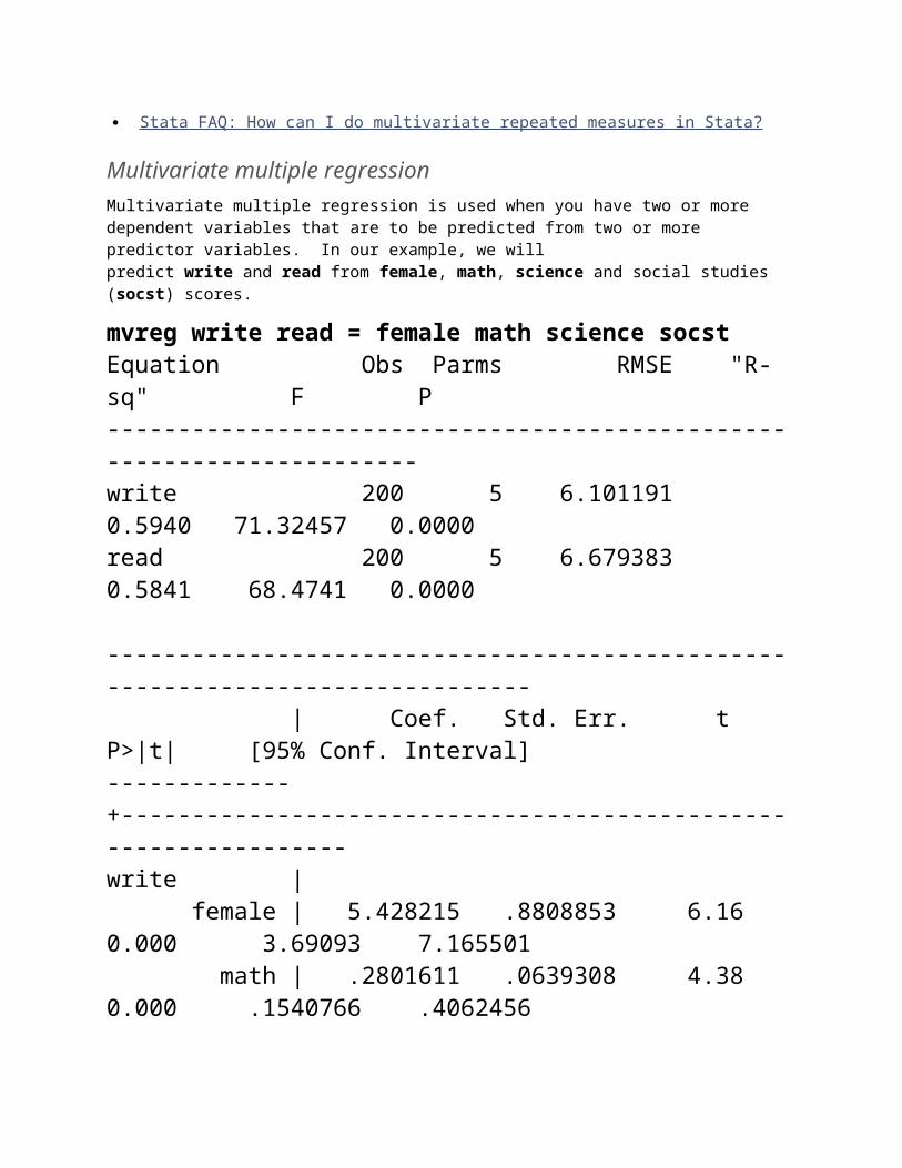
Multivariate multiple regressionMultivariate multiple regression is used when you have two or more dependent variables that are to be predicted from two or more predictor variables.  In our example, we will predict write and read from female, math, science and social studies (socst) scores.  

mvreg write read = female math science socstEquation Obs Parms RMSE "R-sq" F P----------------------------------------------------------------------write 200 5 6.101191 0.5940 71.32457 0.0000read 200 5 6.679383 0.5841 68.4741 0.0000

------------------------------------------------------------------------------ | Coef. Std. Err. t P>|t| [95% Conf. Interval]-------------+----------------------------------------------------------------write | female | 5.428215 .8808853 6.16 0.000 3.69093 7.165501 math | .2801611 .0639308 4.38 0.000 .1540766 .4062456 science | .2786543 .0580452 4.80 0.000 .1641773 .3931313

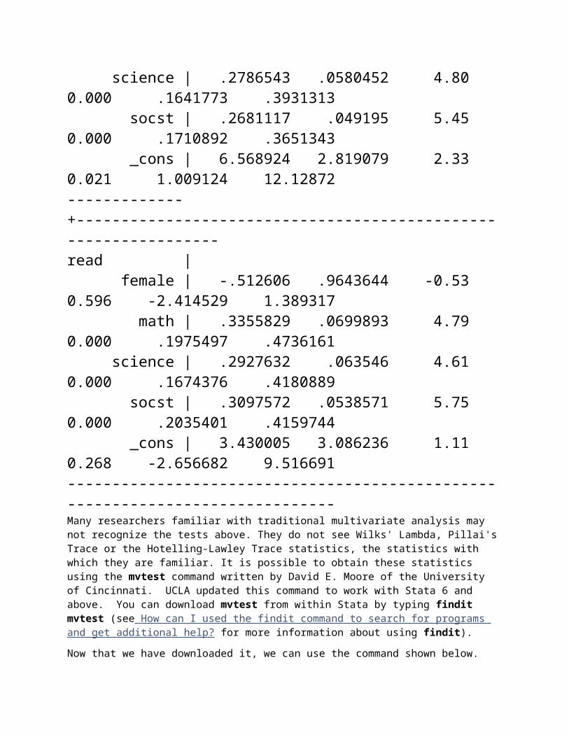
socst | .2681117 .049195 5.45 0.000 .1710892 .3651343 _cons | 6.568924 2.819079 2.33 0.021 1.009124 12.12872-------------+----------------------------------------------------------------read | female | -.512606 .9643644 -0.53 0.596 -2.414529 1.389317 math | .3355829 .0699893 4.79 0.000 .1975497 .4736161 science | .2927632 .063546 4.61 0.000 .1674376 .4180889 socst | .3097572 .0538571 5.75 0.000 .2035401 .4159744 _cons | 3.430005 3.086236 1.11 0.268 -2.656682 9.516691------------------------------------------------------------------------------Many researchers familiar with traditional multivariate analysis may not recognize the tests above. They do not see Wilks' Lambda, Pillai's Trace or the Hotelling-Lawley Trace statistics, the statistics with which they are familiar. It is possible to obtain these statistics using the mvtest command written by David E. Moore of the University of Cincinnati.  UCLA updated this command to work with Stata 6 and above.  You can download mvtest from within Stata by typing findit mvtest (see  How can I used the findit command to search for programs and get additional help? for more information about using findit).

Now that we have downloaded it, we can use the command shown below.  

mvtest female MULTIVARIATE TESTS OF SIGNIFICANCE

Multivariate Test Criteria and Exact F Statistics forthe Hypothesis of no Overall "female" Effect(s)

S=1 M=0 N=96

Test Value F Num DF Den DF Pr > FWilks' Lambda 0.83011470 19.8513 2 194.0000 0.0000Pillai's Trace 0.16988530 19.8513 2 194.0000 0.0000Hotelling-Lawley Trace 0.20465280 19.8513 2 194.0000 0.0000These results show that female has a significant relationship with the joint distribution of write and read.  The mvtestcommand could then be repeated for each of the other predictor variables.

See also

Regression with Stata: Chapter 4, Beyond OLS

Stata Data Analysis Examples: Multivariate Multiple Regression

Stata Textbook Examples, Econometric Analysis, Chapter 16

Canonical correlationCanonical correlation is a multivariate technique used to examine the relationship between two groups of variables.  For each set of variables, it creates latent variables and looks at the relationships among the latent variables. It assumes that all variables in the model are interval and normally distributed.  Stata requires that each of the two groups of variables be enclosed in parentheses.  There need not be an equal number of variables in the two groups.

canon (read write) (math science)

Linear combinations for canonical correlation 1 Number of obs = 200------------------------------------------------------------------------------ | Coef. Std. Err. t P>|t| [95% Conf. Interval]

-------------+----------------------------------------------------------------u | read | .0632613 .007111 8.90 0.000 .0492386 .077284 write | .0492492 .007692 6.40 0.000 .0340809 .0644174-------------+----------------------------------------------------------------v | math | .0669827 .0080473 8.32 0.000 .0511138 .0828515 science | .0482406 .0076145 6.34 0.000 .0332252 .0632561------------------------------------------------------------------------------ (Std. Errors estimated conditionally)Canonical correlations: 0.7728 0.0235The output above shows the linear combinations corresponding to the first canonical correlation.  At the bottom of the output are the two canonical correlations.  These results indicate that the first canonical correlation is .7728.  You will note that Stata is brief and may not provide you with all of the information that you may want.  Several programs have been developed to provide more information regarding the analysis.  You can download this family of programs by typing findit cancor (see  How can I used the findit command to search for programs and get additional help? for more information about using findit).

Because the output from the cancor command is lengthy, we will use the cantest command to obtain the eigenvalues, F-tests and associated p-values that we want.  Note that you do not have to specify a model with either the cancor or thecantest commands if they are issued after the canon command.

cantestCanon Can Corr Likelihood Approx Corr Squared Ratio F df1 df2 Pr > F

7728 .59728 0.4025 56.4706 4 392.000 0.00000235 .00055 0.9994 0.1087 1 197.000 0.7420

Eigenvalue Proportion Cumulative 1.4831 0.9996 0.9996 0.0006 0.0004 1.0000The F-test in this output tests the hypothesis that the first canonical correlation is equal to zero.  Clearly, F = 56.4706 is statistically significant.  However, the second canonical correlation of .0235 is not statistically significantly different from zero (F = 0.1087, p = 0.7420).

See also

Stata Data Analysis Examples: Canonical Correlation Analysis

Stata Annotated Output: Canonical Correlation Analysis

Stata Textbook Examples: Computer-Aided Multivariate Analysis, Chapter 10

Factor analysisFactor analysis is a form of exploratory multivariate analysis that is used to either reduce the number of variables in a model or to detect relationships among variables.  All variables involved in the factor analysis need to be continuous and are assumed to be normally distributed.  The goal of the analysis is to try to identify factors which underlie the variables.  There may be fewer factors than variables, but there may not be more factors than variables.  For our example, let's suppose that we think that there are some common factors underlying the various test scores.  We will first use the principal components method of extraction (by using the pc option) and then the principal components factor method of extraction (by using the pcf option).  This parallels the output produced by SAS and SPSS. 

factor read write math science socst, pc(obs=200)

(principal components; 5 components retained)Component Eigenvalue Difference Proportion Cumulative------------------------------------------------------------------

1 3.38082 2.82344 0.6762 0.6762 2 0.55738 0.15059 0.1115 0.7876 3 0.40679 0.05062 0.0814 0.8690 4 0.35617 0.05733 0.0712 0.9402 5 0.29884 . 0.0598 1.0000

Eigenvectors Variable | 1 2 3 4 5-------------+------------------------------------------------------ read | 0.46642 -0.02728 -0.53127 -0.02058 -0.70642 write | 0.44839 0.20755 0.80642 0.05575 -0.32007 math | 0.45878 -0.26090 -0.00060 -0.78004 0.33615 science | 0.43558 -0.61089 -0.00695 0.58948 0.29924 socst | 0.42567 0.71758 -0.25958 0.20132 0.44269Now let's rerun the factor analysis with a principal component factors extraction method and retain factors with eigenvalues of .5 or greater.  Then we will use a varimax rotation on the solution.

factor read write math science socst, pcf mineigen(.5)(obs=200)

(principal component factors; 2 factors retained) Factor Eigenvalue Difference Proportion Cumulative------------------------------------------------------------------ 1 3.38082 2.82344 0.6762 0.6762 2 0.55738 0.15059 0.1115 0.7876 3 0.40679 0.05062 0.0814 0.8690 4 0.35617 0.05733 0.0712 0.9402 5 0.29884 . 0.0598 1.0000

Factor Loadings Variable | 1 2 Uniqueness-------------+-------------------------------- read | 0.85760 -0.02037 0.26410 write | 0.82445 0.15495 0.29627 math | 0.84355 -0.19478 0.25048 science | 0.80091 -0.45608 0.15054 socst | 0.78268 0.53573 0.10041rotate, varimax

(varimax rotation) Rotated Factor Loadings Variable | 1 2 Uniqueness-------------+-------------------------------- read | 0.64808 0.56204 0.26410 write | 0.50558 0.66942 0.29627 math | 0.75506 0.42357 0.25048 science | 0.89934 0.20159 0.15054

socst | 0.21844 0.92297 0.10041Note that by default, Stata will retain all factors with positive eigenvalues; hence the use of the mineigen option or thefactors(#) option.  The factors(#) option does not specify the number of solutions to retain, but rather the largest number of solutions to retain.  From the table of factor loadings, we can see that all five of the test scores load onto the first factor, while all five tend to load not so heavily on the second factor.  Uniqueness (which is the opposite of commonality) is the proportion of variance of the variable (i.e., read) that is not accounted for by all of the factors taken together, and a very high uniqueness can indicate that a variable may not belong with any of the factors.  Factor loadings are often rotated in an attempt to make them more interpretable.  Stata performs both varimax and promax rotations.

rotate, varimax(varimax rotation) Rotated Factor Loadings Variable | 1 2 Uniqueness-------------+-------------------------------- read | 0.62238 0.51992 0.34233 write | 0.53933 0.54228 0.41505 math | 0.65110 0.45408 0.36988 science | 0.64835 0.37324 0.44033 socst | 0.44265 0.58091 0.46660

The purpose of rotating the factors is to get the variables to load either very high or very low on each factor.  In this example, because all of the variables loaded onto factor 1 and not on factor 2, the rotation did not aid in the interpretation.  Instead, it made the results even more difficult to interpret.

To obtain a scree plot of the eigenvalues, you can use the greigen command.  We have included a reference line on the y-axis at one to aid in determining how many factors should be retained.

greigen, yline(1)

See also

Stata Annotated Output: Factor Analysis

Stata Textbook Examples, Regression with Graphics, Chapter 8

How to cite this page

Report an error on this page or leave a comment

The content of this web site should not be construed as an endorsement of any particular web site, book, or software product by the University of California.

6 BASIC STATISTICAL TOOLS

There are lies, damn lies, and statistics......(Anon.)

6.1 Introduction6.2 Definitions6.3 Basic Statistics6.4 Statistical tests

6.1 Introduction

In the preceding chapters basic elements for the proper execution of analytical work such as personnel, laboratory facilities, equipment, and reagents were discussed. Before embarking upon the actual analytical work, however, one more tool for the quality assurance of the work must be dealt with: the statistical operations necessary to control and verify the analytical procedures (Chapter 7) as well as the resulting data (Chapter 8).

It was stated before that making mistakes in analytical work is unavoidable. This is the reason why a complex system of precautions to prevent errors and traps to detect them has to be set up. An important aspect of the quality control is the detection of both random and systematic errors. This can be done by critically looking at the performance of the analysis as a whole and also of the instruments and operators involved in the job. For the detection itself as well as for the quantification of the errors, statistical treatment of data is indispensable.

A multitude of different statistical tools is available, some of them simple, some complicated, and often very specific for certain purposes. In analytical work, the most important common operation is the comparison of data, or sets of data, to quantify accuracy (bias) and precision. Fortunately, with a few simple convenient statistical tools most of the information needed in regular laboratory work can be obtained: the "t-test, the "F-test", and regression analysis. Therefore, examples of these will be given in the ensuing pages.

Clearly, statistics are a tool, not an aim. Simple inspection of data, without statistical treatment, by an experienced and dedicated analyst may be just as useful as statistical figures on the desk of the disinterested. The value of statistics lies with organizing and simplifying data, to permit some objective estimate showing that an analysis is under control or that a change has occurred. Equally important is that the results of these statistical procedures are recorded and can be retrieved.

6.2 Definitions

6.2.1 Error6.2.2 Accuracy6.2.3 Precision6.2.4 Bias

Discussing Quality Control implies the use of several terms and concepts with a specific (and sometimes confusing) meaning. Therefore, some of the most important concepts will be defined first.

6.2.1 Error

Error is the collective noun for any departure of the result from the "true" value*. Analytical errors can be:

1. Random or unpredictable deviations between replicates, quantified with the "standard deviation".

2. Systematic or predictable regular deviation from the "true" value, quantified as "mean difference" (i.e. the difference between the true value and the mean of replicate determinations).

3. Constant, unrelated to the concentration of the substance analyzed (the analyte).

4. Proportional, i.e. related to the concentration of the analyte.

* The "true" value of an attribute is by nature indeterminate and often has only a very relative meaning. Particularly in soil science for several attributes there is no such thing as the true value as any value obtained is method-dependent (e.g. cation exchange capacity). Obviously, this does not mean that no adequate analysis serving a purpose is possible. It does, however, emphasize the need for the establishment of standard reference methods and the importance of external QC (see Chapter 9).

6.2.2 Accuracy

The "trueness" or the closeness of the analytical result to the "true" value. It is constituted by a combination of random and systematic errors (precision and bias) and cannot be quantified directly. The test result may be a mean of several values. An accurate determination produces a "true" quantitative value, i.e. it is precise and free of bias.

6.2.3 Precision

The closeness with which results of replicate analyses of a sample agree. It is a measure of dispersion or scattering around the mean value and usually expressed in terms of standard deviation, standard error or a range (difference between the highest and the lowest result).

6.2.4 Bias

The consistent deviation of analytical results from the "true" value caused by systematic errors in a procedure. Bias is the opposite but most used measure for "trueness" which is the agreement of the mean of analytical results with the true value, i.e. excluding the

contribution of randomness represented in precision. There are several components contributing to bias:

1. Method bias

The difference between the (mean) test result obtained from a number of laboratories using the same method and an accepted reference value. The method bias may depend on the analyte level.

2. Laboratory bias

The difference between the (mean) test result from a particular laboratory and the accepted reference value.

3. Sample bias

The difference between the mean of replicate test results of a sample and the ("true") value of the target population from which the sample was taken. In practice, for a laboratory this refers mainly to sample preparation, subsampling and weighing techniques. Whether a sample is representative for the population in the field is an extremely important aspect but usually falls outside the responsibility of the laboratory (in some cases laboratories have their own field sampling personnel).

The relationship between these concepts can be expressed in the following equation:

Figure

The types of errors are illustrated in Fig. 6-1.

Fig. 6-1. Accuracy and precision in laboratory measurements. (Note that the qualifications apply to the mean of results: in c the mean is accurate but some

individual results are inaccurate)

6.3 Basic Statistics

6.3.1 Mean6.3.2 Standard deviation6.3.3 Relative standard deviation. Coefficient of variation6.3.4 Confidence limits of a measurement6.3.5 Propagation of errors

In the discussions of Chapters 7 and 8 basic statistical treatment of data will be considered. Therefore, some understanding of these statistics is essential and they will briefly be discussed here.

The basic assumption to be made is that a set of data, obtained by repeated analysis of the same analyte in the same sample under the same conditions, has

a normalor Gaussian distribution. (When the distribution is skewed statistical treatment is more complicated). The primary parameters used are the mean (or average) and thestandard deviation (see Fig. 6-2) and the main tools the F-test, the t-test, and regression and correlation analysis.

Fig. 6-2.   A Gaussian or normal distribution. The figure shows that (approx.) 68% of the data fall in the range   ¯ x± s,   95% in the range ¯x   ±   2 s,   and 99.7% in the range ¯x ± 3 s.

6.3.1 Mean

The average of a set of n data xi:

¯

(6.1)

6.3.2 Standard deviation

This is the most commonly used measure of the spread or dispersion of data around the mean. The standard deviation is defined as the square root of the variance (V). The variance is defined as the sum of the squared deviations from the mean, divided by n-1. Operationally, there are several ways of calculation:

(6.1)

or

(6.3)

or

(6.4)

The calculation of the mean and the standard deviation can easily be done on a calculator but most conveniently on a PC with computer programs such as dBASE, Lotus 123, Quattro-Pro, Excel, and others, which have simple ready-to-use functions. (Warning: some programs use n rather than n- 1!).

6.3.3 Relative standard deviation. Coefficient of variation

Although the standard deviation of analytical data may not vary much over limited ranges of such data, it usually depends on the magnitude of such data: the larger the figures, the larger s. Therefore, for comparison of variations (e.g. precision) it is often more convenient to use the relative standard deviation (RSD) than the standard deviation itself. The RSD is expressed as a fraction, but more usually as a percentage and is then called coefficient of variation (CV). Often, however, these terms are confused.

(6.5; 6.6)

Note. When needed (e.g. for the F-test, see Eq. 6.11) the variance can, of course, be calculated by squaring the standard deviation:

V = s2 (6.7)

6.3.4 Confidence limits of a measurement

The more an analysis or measurement is replicated, the closer the mean x of the results will approach the "true" value , of the analyte content (assuming absence of bias).

A single analysis of a test sample can be regarded as literally sampling the imaginary set of a multitude of results obtained for that test sample. The uncertainty of such subsampling is expressed by

(6.8)

where

 = "true" value (mean of large set of replicates)¯x = mean of subsamplest = a statistical value which depends on the number of data and the required confidence (usually 95%).s = standard deviation of mean of subsamplesn = number of subsamples

(The term   is also known as the standard error of the mean.)

The critical values for t are tabulated in Appendix 1 (they are, therefore, here referred to as ttab ). To find the applicable value, the number of degrees of freedom has to be established by: df = n -1 (see also Section 6.4.2).

Example

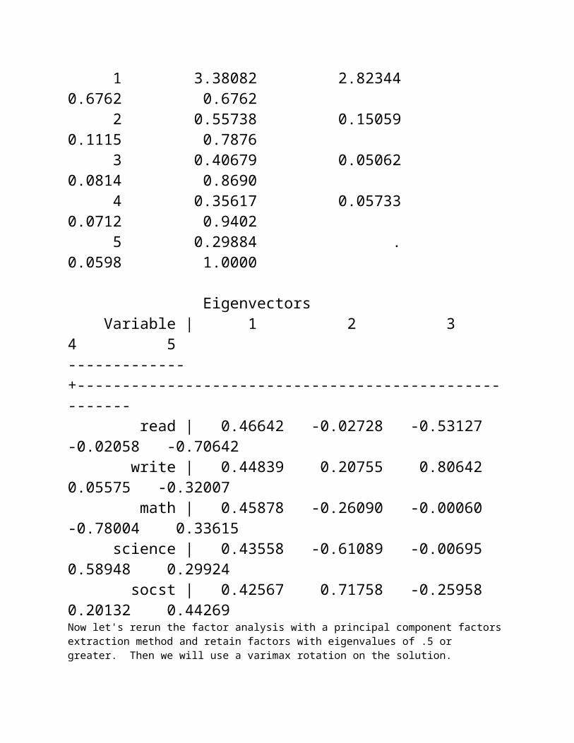
For the determination of the clay content in the particle-size analysis, a semi-automatic pipette installation is used with a 20 mL pipette. This volume is approximate and the operation involves the opening and closing of taps. Therefore, the pipette has to be calibrated, i.e. both the accuracy (trueness) and precision have to be established.

A tenfold measurement of the volume yielded the following set of data (in mL):

19.941 19.812 19.829 19.828 19.74219.797 19.937 19.847 19.885 19.804

The mean is 19.842 mL and the standard deviation 0.0627 mL. According to Appendix 1 for n = 10 is ttab = 2.26 (df = 9) and using Eq. (6.8) this calibration yields:

pipette volume = 19.842 ± 2.26 (0.0627/ ) = 19.84 ± 0.04 mL

(Note that the pipette has a systematic deviation from 20 mL as this is outside the found confidence interval. See also bias).

In routine analytical work, results are usually single values obtained in batches of several test samples. No laboratory will analyze a test sample 50 times to be confident that the result is reliable. Therefore, the statistical parameters have to be obtained in another way. Most usually this is done by method validation (see Chapter 7) and/or by keeping control charts, which is basically the collection of analytical results from one or more control samples in each batch (see Chapter 8). Equation (6.8) is then reduced to

(6.9)

where

 = "true" valuex = single measurementt = applicable ttab (Appendix 1)s = standard deviation of set of previous measurements.

In Appendix 1 can be seen that if the set of replicated measurements is large (say > 30), t is close to 2. Therefore, the (95%) confidence of the result x of a single test sample (n = 1 in Eq. 6.8) is approximated by the commonly used and well known expression

(6.10)

where S is the previously determined standard deviation of the large set of replicates (see also Fig. 6-2).

Note: This "method-s" or s of a control sample is not a constant and may vary for different test materials, analyte levels, and with analytical conditions.

Running duplicates will, according to Equation (6.8), increase the confidence of the (mean)

result by a factor  :

where

¯x = mean of duplicatess = known standard deviation of large set

Similarly, triplicate analysis will increase the confidence by a factor  , etc. Duplicates are further discussed in Section 8.3.3.

Thus, in summary, Equation (6.8) can be applied in various ways to determine the size of errors (confidence) in analytical work or measurements: single determinations in routine work, determinations for which no previous data exist, certain calibrations, etc.

6.3.5 Propagation of errors

6.3.5.1. Propagation of random errors6.3.5.2 Propagation of systematic errors

The final result of an analysis is often calculated from several measurements performed during the procedure (weighing, calibration, dilution, titration, instrument readings, moisture correction, etc.). As was indicated in Section 6.2, the total error in an analytical result is an adding-up of the sub-errors made in the various steps. For daily practice, the bias and precision of the whole method are usually the most relevant parameters (obtained from validation, Chapter 7; or from control charts, Chapter 8). However, sometimes it is useful to get an insight in the contributions of the subprocedures (and then these have to be determined separately). For instance if one wants to change (part of) the method.

Because the "adding-up" of errors is usually not a simple summation, this will be discussed. The main distinction to be made is between random errors (precision) and systematic errors (bias).

6.3.5.1. Propagation of random errors

In estimating the total random error from factors in a final calculation, the treatment of summation or subtraction of factors is different from that of multiplication or division.

I. Summation calculations

If the final result x is obtained from the sum (or difference) of (sub)measurements a, b, c, etc.:

x = a + b + c +...

then the total precision is expressed by the standard deviation obtained by taking the square root of the sum of individual variances (squares of standard deviation):

If a (sub)measurement has a constant multiplication factor or coefficient (such as an extra dilution), then this is included to calculate the effect of the variance concerned, e.g. (2b)2

Example

The Effective Cation Exchange Capacity of soils (ECEC) is obtained by summation of the exchangeable cations:

ECEC = Exch. (Ca + Mg + Na + K + H + Al)

Standard deviations experimentally obtained for exchangeable Ca, Mg, Na, K and (H + Al) on a certain sample, e.g. a control sample, are: 0.30, 0.25, 0.15, 0.15, and 0.60 cmolc/kg respectively. The total precision is:

It can be seen that the total standard deviation is larger than the highest individual standard deviation, but (much) less than their sum. It is also clear that if one wants to reduce the total standard deviation, qualitatively the best result can be expected from reducing the largest individual contribution, in this case the exchangeable acidity.

2. Multiplication calculations

If the final result x is obtained from multiplication (or subtraction) of (sub)measurements according to

then the total error is expressed by the standard deviation obtained by taking the square root of the sum of the individual relative standard deviations (RSD or CV, as a fraction or as percentage, see Eqs. 6.6 and 6.7):

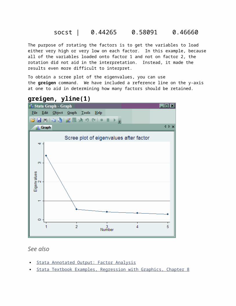
If a (sub)measurement has a constant multiplication factor or coefficient, then this is included to calculate the effect of the RSD concerned, e.g. (2RSDb)2.

Example

The calculation of Kjeldahl-nitrogen may be as follows:

where

a = ml HCl required for titration sampleb = ml HCl required for titration blanks = air-dry sample weight in gramM = molarity of HCl1.4 = 14×10-3×100% (14 = atomic weight of N)mcf = moisture correction factor

Note that in addition to multiplications, this calculation contains a subtraction also (often, calculations contain both summations and multiplications.)

Firstly, the standard deviation of the titration (a -b) is determined as indicated in Section 7 above. This is then transformed to RSD using Equations (6.5) or (6.6). Then the RSD of the other individual parameters have to be determined experimentally. The found RSDs are, for instance:

distillation: 0.8%,titration: 0.5%,molarity: 0.2%,sample weight: 0.2%,mcf: 0.2%.

The total calculated precision is:

Here again, the highest RSD (of distillation) dominates the total precision. In practice, the precision of the Kjeldahl method is usually considerably worse ( 2.5%) probably mainly as a result of the heterogeneity of the sample. The present example does not take that into account. It would imply that 2.5% - 1.0% = 1.5% or 3/5 of the total random error is due to sample heterogeneity (or other overlooked cause). This implies that painstaking efforts to improve subprocedures such as the titration or the preparation of standard solutions may not be very rewarding. It would, however, pay to improve the homogeneity of the sample, e.g. by careful grinding and mixing in the preparatory stage.

Note. Sample heterogeneity is also represented in the moisture correction factor. However, the influence of this factor on the final result is usually very small.

6.3.5.2 Propagation of systematic errors

Systematic errors of (sub)measurements contribute directly to the total bias of the result since the individual parameters in the calculation of the final result each carry their own bias. For instance, the systematic error in a balance will cause a systematic error in the sample weight (as well as in the moisture determination). Note that some systematic errors may cancel out, e.g. weighings by difference may not be affected by a biased balance.

The only way to detect or avoid systematic errors is by comparison (calibration) with independent standards and outside reference or control samples.

6.4 Statistical tests

6.4.1 Two-sided vs. one-sided test6.4.2 F-test for precision6.4.3 t-Tests for bias 6.4.4 Linear correlation and regression 6.4.5 Analysis of variance (ANOVA)

In analytical work a frequently recurring operation is the verification of performance by comparison of data. Some examples of comparisons in practice are:

- performance of two instruments,

- performance of two methods,

- performance of a procedure in different periods,

- performance of two analysts or laboratories,

- results obtained for a reference or control sample with the "true", "target" or "assigned" value of this sample.

Some of the most common and convenient statistical tools to quantify such comparisons are the F-test, the t-tests, and regression analysis.

Because the F-test and the t-tests are the most basic tests they will be discussed first. These tests examine if two sets of normally distributed data are similar or dissimilar (belong or not belong to the same "population") by comparing their standard deviations and means respectively. This is illustrated in Fig. 6-3.

Fig. 6-3. Three possible cases when comparing two sets of data (n1 = n2). A. Different mean (bias), same precision; B. Same mean (no bias), different precision; C. Both

mean and precision are different. (The fourth case, identical sets, has not been drawn).

6.4.1 Two-sided vs. one-sided test

These tests for comparison, for instance between methods A and B, are based on the assumption that there is no significant difference (the "null hypothesis"). In other words, when the difference is so small that a tabulated critical value of F or t is not exceeded, we can be confident (usually at 95% level) that A and B are not different. Two fundamentally different questions can be asked concerning both the comparison of the standard deviations s1 and s2 with the F-test, and of the means¯x1, and ¯x2, with the t-test:

1. are A and B different? (two-sided test)2. is A higher (or lower) than B? (one-sided test).

This distinction has an important practical implication as statistically the probabilities for the two situations are different: the chance that A and B are only different ("it can go two ways") is twice as large as the chance that A is higher (or lower) than B ("it can go only one way"). The most common case is the two-sided (also calledtwo-tailed) test: there are no particular reasons to expect that the means or the standard deviations of two data sets are different. An example is the routine comparison of a control chart with the previous one (see 8.3). However, when it is expected or suspected that the mean and/or the standard deviation will go only one way, e.g. after a change in an analytical procedure, the one-sided (or one-tailed) test is appropriate. In this case the probability that it goes the other way than expected is assumed to be zero and, therefore, the probability that it goes the expected way is doubled. Or, more correctly, the uncertainty in the two-way test of 5% (or the probability of 5% that the critical value is exceeded) is divided over the two tails of the Gaussian curve (see Fig. 6-2), i.e. 2.5% at the end of each tail beyond 2s. If we perform the one-sided test with 5% uncertainty, we actually increase this 2.5% to 5% at the end of one tail. (Note that for the whole gaussian curve, which is symmetrical, this is then equivalent to an uncertainty of 10% in two ways!)

This difference in probability in the tests is expressed in the use of two tables of critical values for both F and t. In fact, the one-sided table at 95% confidence level is equivalent to the two-sided table at 90% confidence level.

It is emphasized that the one-sided test is only appropriate when a difference in one direction is expected or aimed at. Of course it is tempting to perform this test after the results show a clear (unexpected) effect. In fact, however, then a two times higher probability level was used in retrospect. This is underscored by the observation that in this way even contradictory conclusions may arise: if in an experiment calculated values of F and t are found within the range between the two-sided and one-sided values of Ftab, and ttab, the two-sided test indicates no significant difference, whereas the one-sided test says that the result of A is significantly higher (or lower) than that of B. What actually happens is that in the first case the 2.5% boundary in the tail was just not exceeded, and then, subsequently, this 2.5% boundary is relaxed to 5% which is then obviously more easily exceeded. This illustrates that statistical tests differ in strictness and that for proper interpretation of results in reports, the statistical techniques used, including the confidence limits or probability, should always be specified.

6.4.2 F-test for precision

Because the result of the F-test may be needed to choose between the Student's t-test and the Cochran variant (see next section), the F-test is discussed first.

The F-test (or Fisher's test) is a comparison of the spread of two sets of data to test if the sets belong to the same population, in other words if the precisions are similar or dissimilar.

The test makes use of the ratio of the two variances:

(6.11)

where the larger s2 must be the numerator by convention. If the performances are not very different, then the estimates s1, and s2, do not differ much and their ratio (and that of their squares) should not deviate much from unity. In practice, the calculated F is compared with the applicable F value in the F-table (also called the criticalvalue, see Appendix 2). To read the table it is necessary to know the applicable number of degrees of freedom for s1, and s2. These are calculated by:

df1 = n1-1df2 = n2-1

If Fcal  Ftab one can conclude with 95% confidence that there is no significant difference in precision (the "null hypothesis" that s1, = s, is accepted). Thus, there is still a 5% chance that we draw the wrong conclusion. In certain cases more confidence may be needed, then a 99% confidence table can be used, which can be found in statistical textbooks.

Example I (two-sided test)

Table 6-1 gives the data sets obtained by two analysts for the cation exchange capacity (CEC) of a control sample. Using Equation (6.11) the calculated F value is 1.62. As we had no particular reason to expect that the analysts would perform differently, we use the F-table for the two-sided test and find Ftab = 4.03 (Appendix 2,df1, = df2 = 9). This exceeds the calculated value and the null hypothesis (no difference) is accepted. It can be concluded with 95% confidence that there is no significant difference in precision between the work of Analyst 1 and 2.

Table 6-1. CEC values (in cmolc/kg) of a control sample determined by two analysts.

1 210.2 9.710.7 9.010.5 10.29.9 10.39.0 10.8

11.2 11.1

11.5 9.410.9 9.28.9 9.8

10.6 10.2¯x: 10.34 9.97s: 0.819 0.644n: 10 10Fcal = 1.62 tcal = 1.12Ftab = 4.03 ttab = 2.10

Example 2 (one-sided test)

The determination of the calcium carbonate content with the Scheibler standard method is compared with the simple and more rapid "acid-neutralization" method using one and the same sample. The results are given in Table 6-2. Because of the nature of the rapid method we suspect it to produce a lower precision then obtained with the Scheibler method and we can, therefore, perform the one sided F-test. The applicable Ftab = 3.07 (App. 2, df1, = 12, df2 = 9) which is lower than Fcal (=18.3) and the null hypothesis (no difference) is rejected. It can be concluded (with 95% confidence) that for this one sample the precision of the rapid titration method is significantly worse than that of the Scheibler method.

Table 6-2. Contents of CaCO3 (in mass/mass %) in a soil sample determined with the Scheibler method (A) and the rapid titration method (B).

A B2.5 1.72.4 1.92.5 2.32.6 2.32.5 2.82.5 2.52.4 1.62.6 1.92.7 2.62.4 1.7- 2.4- 2.2

2.6x: 2.51 2.13s: 0.099 0.424n: 10 13Fcal = 18.3 tcal = 3.12Ftab = 3.07 ttab* = 2.18

(ttab* = Cochran's "alternative" ttab)

6.4.3 t-Tests for bias

6.4.3.1. Student's t-test6.4.3.2 Cochran's t-test6.4.3.3 t-Test for large data sets (n ³   30) 6.4.3.4 Paired t-test

Depending on the nature of two sets of data (n, s, sampling nature), the means of the sets can be compared for bias by several variants of the t-test. The following most common types will be discussed:

1. Student's t-test for comparison of two independent sets of data with very similar standard deviations;

2. the Cochran variant of the t-test when the standard deviations of the independent sets differ significantly;

3. the paired t-test for comparison of strongly dependent sets of data.

Basically, for the t-tests Equation (6.8) is used but written in a different way:

(6.12)

where

¯x = mean of test results of a sample = "true" or reference values = standard deviation of test resultsn = number of test results of the sample.

To compare the mean of a data set with a reference value normally the "two-sided t-table of critical values" is used (Appendix 1). The applicable number of degrees of freedom here is:

df = n-1

If a value for t calculated with Equation (6.12) does not exceed the critical value in the table, the data are taken to belong to the same population: there is no difference and the "null hypothesis" is accepted (with the applicable probability, usually 95%).

As with the F-test, when it is expected or suspected that the obtained results are higher or lower than that of the reference value, the one-sided t-test can be performed: if tcal > ttab, then the results are significantly higher (or lower) than the reference value.

More commonly, however, the "true" value of proper reference samples is accompanied by the associated standard deviation and number of replicates used to determine these

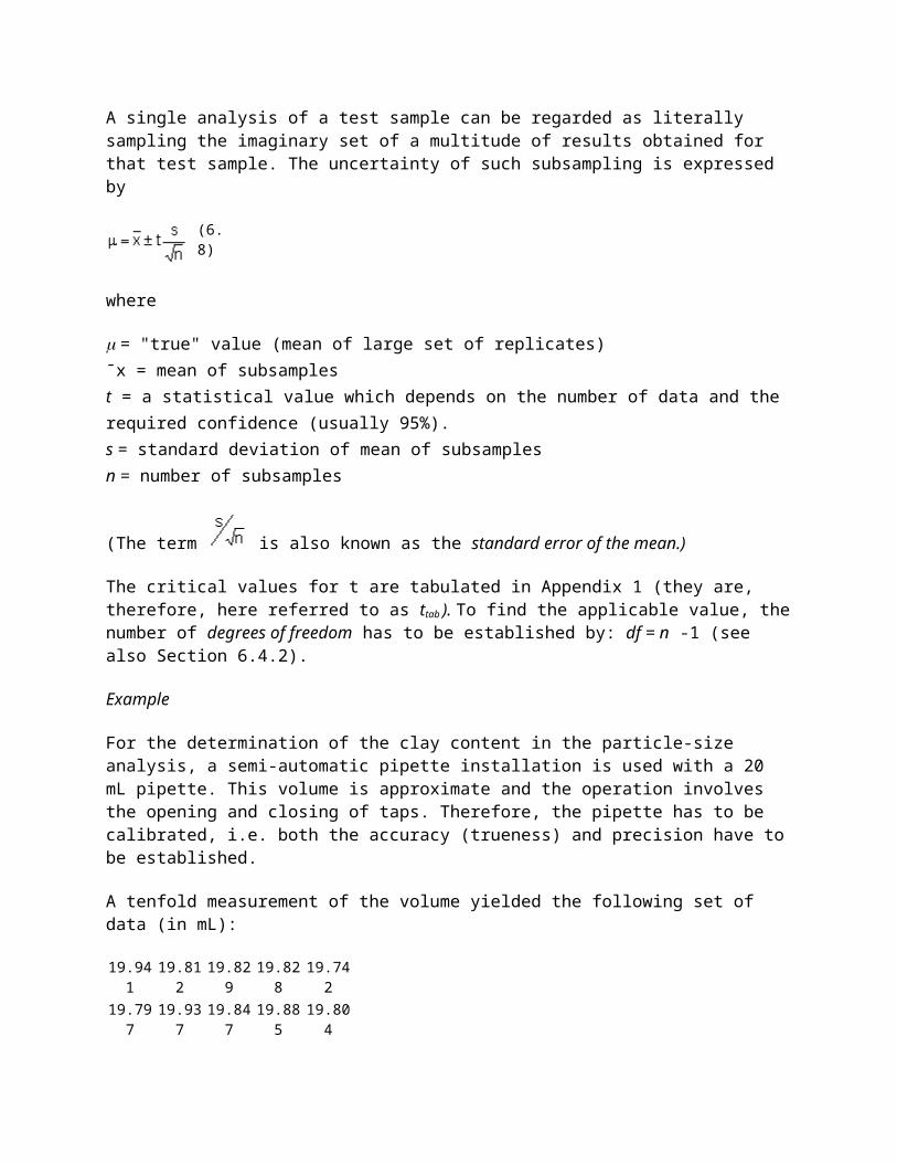
parameters. We can then apply the more general case of comparing the means of two data sets: the "true" value in Equation (6.12) is then replaced by the mean of a second data set. As is shown in Fig. 6-3, to test if two data sets belong to the same population it is tested if the two Gauss curves do sufficiently overlap. In other words, if the difference between the means ¯x1-¯x2 is small. This is discussed next.

Similarity or non-similarity of standard deviations

When using the t-test for two small sets of data (n1 and/or n2<30), a choice of the type of test must be made depending on the similarity (or non-similarity) of the standard deviations of the two sets. If the standard deviations are sufficiently similar they can be "pooled" and the Student t-test can be used. When the standard deviations are not sufficiently similar an alternative procedure for the t-test must be followed in which the standard deviations are not pooled. A convenient alternative is the Cochran variant of the t-test. The criterion for the choice is the passing or non-passing of the F-test (see 6.4.2), that is, if the variances do or do not significantly differ. Therefore, for small data sets, the F-test should precede the t-test.

For dealing with large data sets (n1, n2, 30) the "normal" t-test is used (see Section 6.4.3.3 and App. 3).

6.4.3.1. Student's t-test

(To be applied to small data sets (n1, n2 < 30) where s1, and s2 are similar according to F-test.

When comparing two sets of data, Equation (6.12) is rewritten as:

(6.13)

where

¯x1 = mean of data set 1¯x2 = mean of data set 2sp = "pooled" standard deviation of the setsn1 = number of data in set 1n2 = number of data in set 2.

The pooled standard deviation sp is calculated by:

6.14

where

s1 = standard deviation of data set 1s2 = standard deviation of data set 2n1 = number of data in set 1n2 = number of data in set 2.

To perform the t-test, the critical ttab has to be found in the table (Appendix 1); the applicable number of degrees of freedom df is here calculated by:

df = n1 + n2 -2

Example

The two data sets of Table 6-1 can be used: With Equations (6.13) and (6.14) tcal, is calculated as 1.12 which is lower than the critical value ttab of 2.10 (App. 1, df =18, two-sided), hence the null hypothesis (no difference) is accepted and the two data sets are assumed to belong to the same population: there is no significant difference between the mean results of the two analysts (with 95% confidence).

Note. Another illustrative way to perform this test for bias is to calculate if the difference between the means falls within or outside the range where this difference is still not significantly large. In other words, if this difference is less than the least significant difference (lsd). This can be derived from Equation (6.13):

6.15

In the present example of Table 6-1, the calculation yields lsd = 0.69. The measured difference between the means is 10.34 -9.97 = 0.37 which is smaller than the lsdindicating that there is no significant difference between the performance of the analysts.

In addition, in this approach the 95% confidence limits of the difference between the means can be calculated (cf. Equation 6.8):

confidence limits = 0.37 ± 0.69 = -0.32 and 1.06

Note that the value 0 for the difference is situated within this confidence interval which agrees with the null hypothesis of x1 = x2 (no difference) having been accepted.

6.4.3.2 Cochran's t-test

To be applied to small data sets (n1, n2, < 30) where s1 and s2, are dissimilar according to F-test.

Calculate t with:

6.16

Then determine an "alternative" critical t-value:

6.17

where

t1 = ttab at n1-1 degrees of freedomt2 = ttab at n2-1 degrees of freedom

Now the t-test can be performed as usual: if tcal< ttab* then the null hypothesis that the means

do not significantly differ is accepted.

Example

The two data sets of Table 6-2 can be used.

According to the F-test, the standard deviations differ significantly so that the Cochran variant must be used. Furthermore, in contrast to our expectation that the precision of the rapid test would be inferior, we have no idea about the bias and therefore the two-sided test is appropriate. The calculations yield tcal = 3.12 and ttab

*= 2.18 meaning that tcal exceeds ttab

* which implies that the null hypothesis (no difference) is rejected and that the mean of the rapid analysis deviates significantly from that of the standard analysis (with 95% confidence, and for this sample only). Further investigation of the rapid method would have to include the use of more different samples and then comparison with the one-sided t-test would be justified (see 6.4.3.4, Example 1).

6.4.3.3 t-Test for large data sets (n 30)

In the example above (6.4.3.2) the conclusion happens to have been the same if the Student's t-test with pooled standard deviations had been used. This is caused by the fact that the difference in result of the Student and Cochran variants of the t-test is largest when small sets of data are compared, and decreases with increasing number of data. Namely, with increasing number of data a better estimate of the real distribution of the population is obtained (the flatter t-distribution converges then to the standardized normal distribution). When n 30 for both sets, e.g. when comparing Control Charts (see 8.3), for all practical purposes the difference between the Student and Cochran variant is negligible. The procedure is then reduced to the "normal" t-test by simply calculating tcal with Eq. (6.16) and

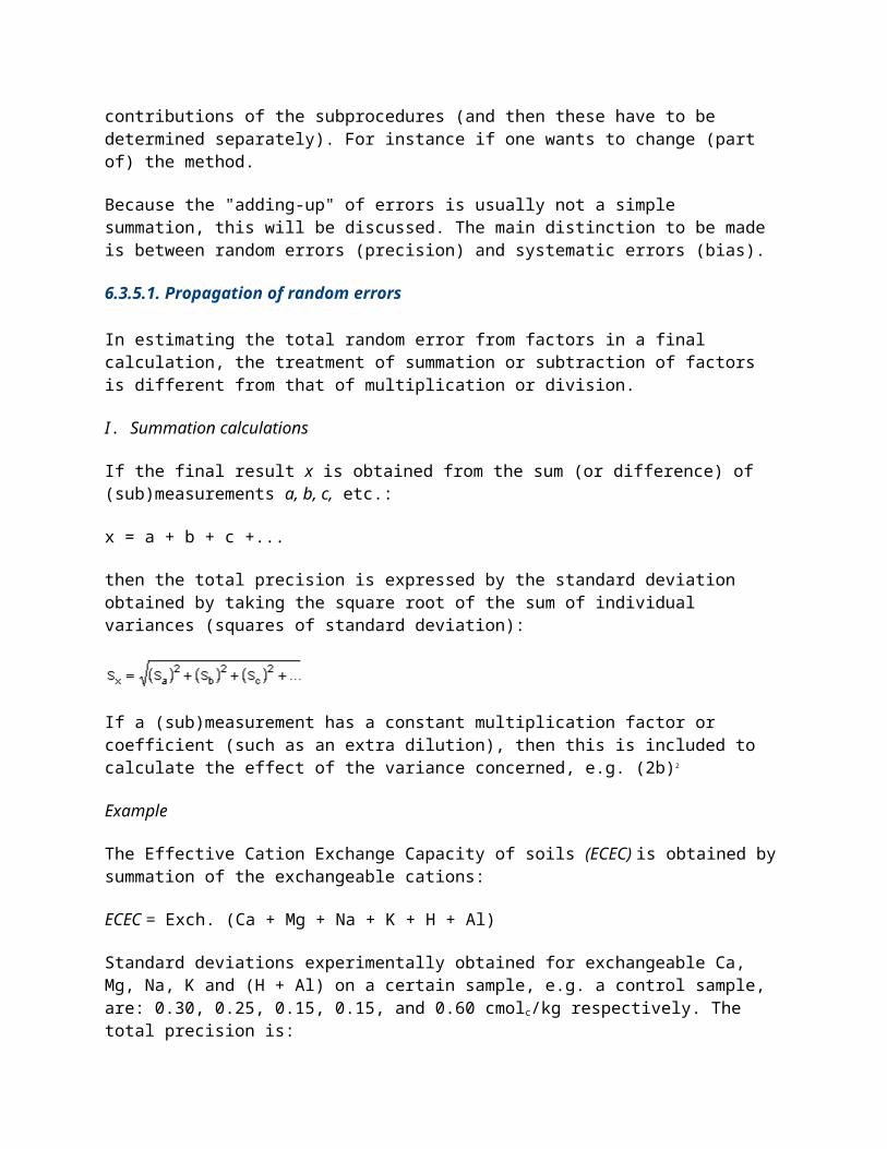
comparing this with ttab atdf = n1 + n2-2. (Note in App. 1 that the two-sided ttab is now close to 2).

The proper choice of the t-test as discussed above is summarized in a flow diagram in Appendix 3.

6.4.3.4 Paired t-test

When two data sets are not independent, the paired t-test can be a better tool for comparison than the "normal" t-test described in the previous sections. This is for instance the case when two methods are compared by the same analyst using the same sample(s). It could, in fact, also be applied to the example of Table 6-1 if the two analysts used the same analytical method at (about) the same time.

As stated previously, comparison of two methods using different levels of analyte gives more validation information about the methods than using only one level. Comparison of results at each level could be done by the F and t-tests as described above. The paired t-test, however, allows for different levels provided the concentration range is not too wide. As a rule of fist, the range of results should be within the same magnitude. If the analysis covers a longer range, i.e. several powers of ten, regression analysis must be considered (see Section 6.4.4). In intermediate cases, either technique may be chosen.

The null hypothesis is that there is no difference between the data sets, so the test is to see if the mean of the differences between the data deviates significantly from zero or not (two-sided test). If it is expected that one set is systematically higher (or lower) than the other set, then the one-sided test is appropriate.

Example 1

The "promising" rapid single-extraction method for the determination of the cation exchange capacity of soils using the silver thiourea complex (AgTU, buffered at pH 7) was compared with the traditional ammonium acetate method (NH4OAc, pH 7). Although for certain soil types the difference in results appeared insignificant, for other types differences seemed larger. Such a suspect group were soils with ferralic (oxic) properties (i.e. highly weathered sesquioxide-rich soils). In Table 6-3 the results often soils with these properties are grouped to test if the CEC methods give different results. The difference d within each pair and the parameters needed for the paired t-test are given also.

Table 6-3. CEC values (in cmolc/kg) obtained by the NH4OAc and AgTU methods (both at pH 7) for ten soils with ferralic properties.

Sample NH4OAc AgTU d1 7.1 6.5 -0.62 4.6 5.6 +1.03 10.6 14.5 +3.94 2.3 5.6 +3.35 25.2 23.8 -1.46 4.4 10.4 +6.0

7 7.8 8.4 +0.68 2.7 5.5 +2.89 14.3 19.2 +4.9

10 13.6 15.0 +1.4¯d = +2.19 tcal = 2.89sd = 2.395 ttab = 2.26

Using Equation (6.12) and noting that  d = 0 (hypothesis value of the differences, i.e. no difference), the t-value can be calculated as:

where

 = mean of differences within each pair of datasd = standard deviation of the mean of differencesn = number of pairs of data

The calculated t value (=2.89) exceeds the critical value of 1.83 (App. 1, df = n -1 = 9, one-sided), hence the null hypothesis that the methods do not differ is rejected and it is concluded that the silver thiourea method gives significantly higher results as compared with the ammonium acetate method when applied to such highly weathered soils.

Note. Since such data sets do not have a normal distribution, the "normal" t-test which compares means of sets cannot be used here (the means do not constitute a fair representation of the sets). For the same reason no information about the precision of the two methods can be obtained, nor can the F-test be applied. For information about precision, replicate determinations are needed.

Example 2

Table 6-4 shows the data of total-P in four plant tissue samples obtained by a laboratory L and the median values obtained by 123 laboratories in a proficiency (round-robin) test.

Table 6-4. Total-P contents (in mmol/kg) of plant tissue as determined by 123 laboratories (Median) and Laboratory L.

Sample Median Lab L d1 93.0 85.2 -7.82 201 224 233 78.9 84.5 5.64 175 185 10

¯d = 7.70 tcal =1.21

sd = 12.702 ttab = 3.18

To verify the performance of the laboratory a paired t-test can be performed:

Using Eq. (6.12) and noting that  d=0 (hypothesis value of the differences, i.e. no difference), the t value can be calculated as:

The calculated t-value is below the critical value of 3.18 (Appendix 1, df = n - 1 = 3, two-sided), hence the null hypothesis that the laboratory does not significantly differ from the group of laboratories is accepted, and the results of Laboratory L seem to agree with those of "the rest of the world" (this is a so-called third-line control).

6.4.4 Linear correlation and regression

6.4.4.1 Construction of calibration graph6.4.4.2 Comparing two sets of data using many samples at different analyte levels

These also belong to the most common useful statistical tools to compare effects and performances X and Y. Although the technique is in principle the same for both, there is a fundamental difference in concept: correlation analysis is applied to independent factors: if X increases, what will Y do (increase, decrease, or perhaps not change at all)? In regression analysis a unilateral response is assumed: changes in X result in changes in Y, but changes in Y do not result in changes in X.

For example, in analytical work, correlation analysis can be used for comparing methods or laboratories, whereas regression analysis can be used to construct calibration graphs. In practice, however, comparison of laboratories or methods is usually also done by regression analysis. The calculations can be performed on a (programmed) calculator or more conveniently on a PC using a home-made program. Even more convenient are the regression programs included in statistical packages such as Statistix, Mathcad, Eureka, Genstat, Statcal, SPSS, and others. Also, most spreadsheet programs such as Lotus 123, Excel, and Quattro-Pro have functions for this.

Laboratories or methods are in fact independent factors. However, for regression analysis one factor has to be the independent or "constant" factor (e.g. the reference method, or the factor with the smallest standard deviation). This factor is by convention designated X, whereas the other factor is then the dependent factor Y (thus, we speak of "regression of Y on X").

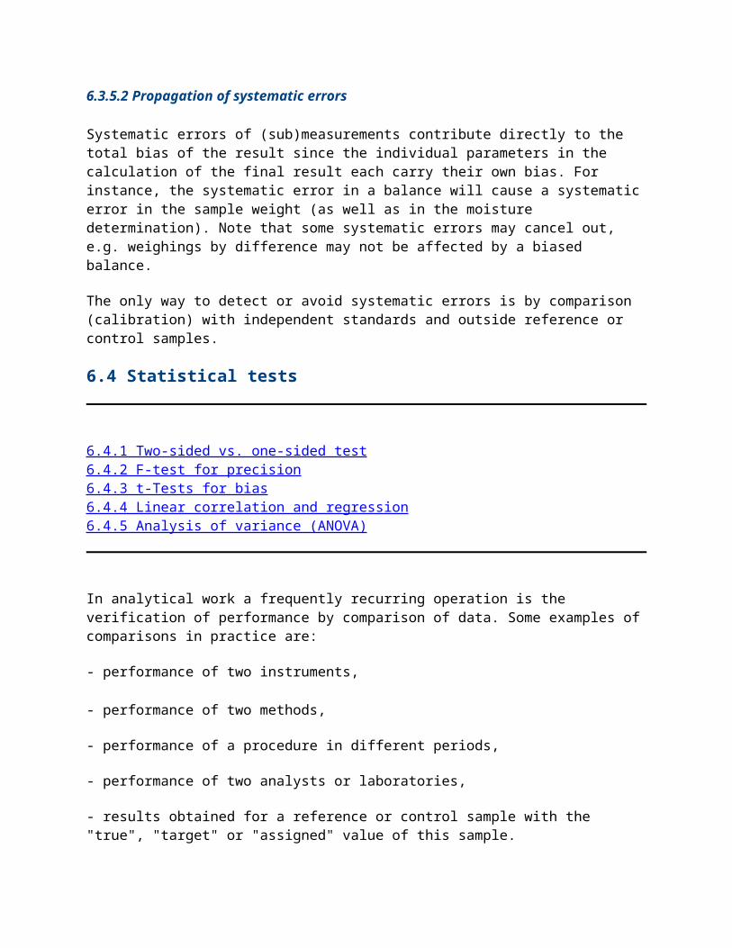
As was discussed in Section 6.4.3, such comparisons can often been done with the Student/Cochran or paired t-tests. However, correlation analysis is indicated:

1. When the concentration range is so wide that the errors, both random and systematic, are not independent (which is the assumption for the t-tests). This is often the case where concentration ranges of several magnitudes are involved.

2. When pairing is inappropriate for other reasons, notably a long time span between the two analyses (sample aging, change in laboratory conditions, etc.).

The principle is to establish a statistical linear relationship between two sets of corresponding data by fitting the data to a straight line by means of the "least squares" technique. Such data are, for example, analytical results of two methods applied to the same samples (correlation), or the response of an instrument to a series of standard solutions (regression).

Note: Naturally, non-linear higher-order relationships are also possible, but since these are less common in analytical work and more complex to handle mathematically, they will not be discussed here. Nevertheless, to avoid misinterpretation, always inspect the kind of relationship by plotting the data, either on paper or on the computer monitor.

The resulting line takes the general form:

y = bx + a (6.18)

where

a = intercept of the line with the y-axisb = slope (tangent)

In laboratory work ideally, when there is perfect positive correlation without bias, the intercept a = 0 and the slope = 1. This is the so-called "1:1 line" passing through the origin (dashed line in Fig. 6-5).

If the intercept a  0 then there is a systematic discrepancy (bias, error) between X and Y; when b  1 then there is a proportional response or difference between Xand Y.

The correlation between X and Y is expressed by the correlation coefficient r which can be calculated with the following equation:

6.19

where

xi = data X¯x = mean of data Xyi = data Y¯y = mean of data Y

It can be shown that r can vary from 1 to -1:

r = 1 perfect positive linear correlationr = 0 no linear correlation (maybe other correlation)r = -1 perfect negative linear correlation

Often, the correlation coefficient r is expressed as r2: the coefficient of determination or coefficient of variance. The advantage of r2 is that, when multiplied by 100, it indicates the percentage of variation in Y associated with variation in X. Thus, for example, when r = 0.71 about 50% (r2 = 0.504) of the variation in Y is due to the variation in X.

The line parameters b and a are calculated with the following equations:

6.20

and

a = ¯y - b¯x 6.21

It is worth to note that r is independent of the choice which factor is the independent factory and which is the dependent Y. However, the regression parameters a and do depend on this choice as the regression lines will be different (except when there is ideal 1:1 correlation).

6.4.4.1 Construction of calibration graph

As an example, we take a standard series of P (0-1.0 mg/L) for the spectrophotometric determination of phosphate in a Bray-I extract ("available P"), reading in absorbance units. The data and calculated terms needed to determine the parameters of the calibration graph are given in Table 6-5. The line itself is plotted in Fig. 6-4.

Table 6-5 is presented here to give an insight in the steps and terms involved. The calculation of the correlation coefficient r with Equation (6.19) yields a value of 0.997 (r2 = 0.995). Such high values are common for calibration graphs. When the value is not close to 1 (say, below 0.98) this must be taken as a warning and it might then be advisable to repeat or review the procedure. Errors may have been made (e.g. in pipetting) or the used range of the graph may not be linear. On the other hand, a high r may be misleading as it does not necessarily indicate linearity. Therefore, to verify this, the calibration graph should always be plotted, either on paper or on computer monitor.

Using Equations (6.20 and (6.21) we obtain:

and

a = 0.350 - 0.313 = 0.037

Thus, the equation of the calibration line is:

y = 0.626x + 0.037 (6.22)

Table 6-5. Parameters of calibration graph in Fig. 6-4.

xi yi x1-¯x (xi-¯x)2 yi-¯y (yi-¯y)2 (x1-¯x)(yi-¯y)0.0 0.05 -0.5 0.25 -0.30 0.090 0.1500.2 0.14 -0.3 0.09 -0.21 0.044 0.0630.4 0.29 -0.1 0.01 -0.06 0.004 0.0060.6 0.43 0.1 0.01 0.08 0.006 0.0080.8 0.52 0.3 0.09 0.17 0.029 0.0511.0 0.67 0.5 0.25 0.32 0.102 0.1603.0 2.10 0 0.70 0 0.2754 0.438 

¯x=0.5 ¯y = 0.35

Fig. 6-4. Calibration graph plotted from data of Table 6-5. The dashed lines delineate the 95% confidence area of the graph. Note that the confidence is highest at the

centroid of the graph.

During calculation, the maximum number of decimals is used, rounding off to the last significant figure is done at the end (see instruction for rounding off in Section 8.2).

Once the calibration graph is established, its use is simple: for each y value measured the corresponding concentration x can be determined either by direct reading or by calculation using Equation (6.22). The use of calibration graphs is further discussed in Section 7.2.2.

Note. A treatise of the error or uncertainty in the regression line is given.

6.4.4.2 Comparing two sets of data using many samples at different analyte levels

Although regression analysis assumes that one factor (on the x-axis) is constant, when certain conditions are met the technique can also successfully be applied to comparing two variables such as laboratories or methods. These conditions are:

- The most precise data set is plotted on the x-axis- At least 6, but preferably more than 10 different samples are analyzed- The samples should rather uniformly cover the analyte level range of interest.

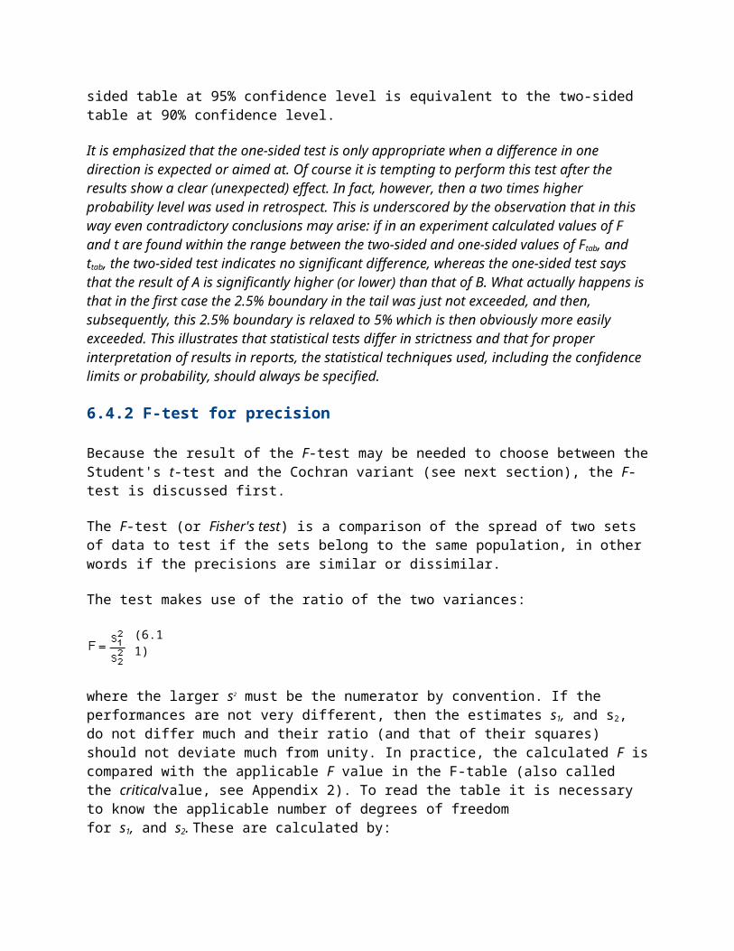
To decide which laboratory or method is the most precise, multi-replicate results have to be used to calculate standard deviations (see 6.4.2). If these are not available then the standard deviations of the present sets could be compared (note that we are now not dealing with normally distributed sets of replicate results). Another convenient way is to run the regression analysis on the computer, reverse the variables and run the analysis again. Observe which variable has the lowest standard deviation (or standard error of the intercept a, both given by the computer) and then use the results of the regression analysis where this variable was plotted on the x-axis.

If the analyte level range is incomplete, one might have to resort to spiking or standard additions, with the inherent drawback that the original analyte-sample combination may not adequately be reflected.

Example

In the framework of a performance verification programme, a large number of soil samples were analyzed by two laboratories X and Y (a form of "third-line control", see Chapter 9) and the data compared by regression. (In this particular case, the paired t-test might have been considered also). The regression line of a common attribute, the pH, is shown here as an illustration. Figure 6-5 shows the so-called "scatter plot" of 124 soil pH-H2O determinations by the two laboratories. The correlation coefficient r is 0.97 which is very satisfactory. The slope (= 1.03) indicates that the regression line is only slightly steeper than the 1:1 ideal regression line. Very disturbing, however, is the intercept a of -1.18. This implies that laboratory Y measures the pH more than a whole unit lower than laboratory X at the low end of the pH range (the intercept -1.18 is at pHx = 0) which difference decreases to about 0.8 unit at the high end.

Fig. 6-5. Scatter plot of pH data of two laboratories. Drawn line: regression line; dashed line: 1:1 ideal regression line.

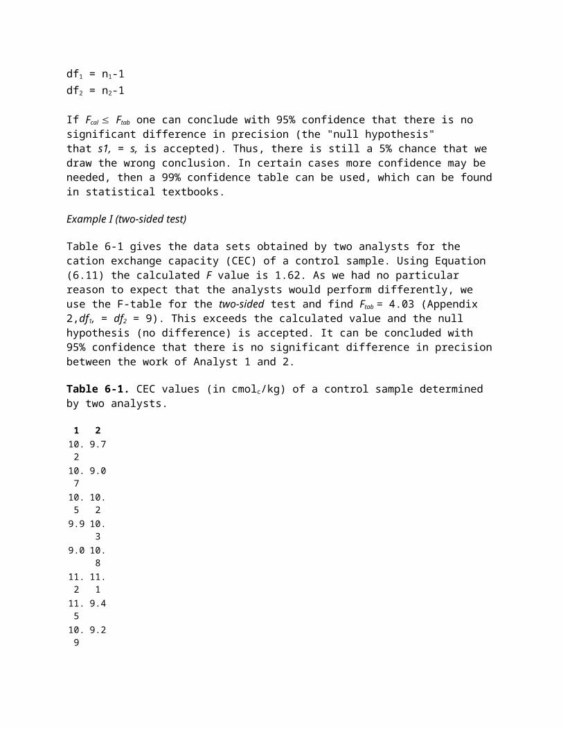
The t-test for significance is as follows:

For intercept a:  a = 0 (null hypothesis: no bias; ideal intercept is then zero), standard error =0.14 (calculated by the computer), and using Equation (6.12) we obtain:

Here, ttab = 1.98 (App. 1, two-sided, df = n - 2 = 122 (n-2 because an extra degree of freedom is lost as the data are used for both a and b) hence, the laboratories have a significant mutual bias.

For slope:  b = 1 (ideal slope: null hypothesis is no difference), standard error = 0.02 (given by computer), and again using Equation (6.12) we obtain:

Again, ttab = 1.98 (App. 1; two-sided, df = 122), hence, the difference between the laboratories is not significantly proportional (or: the laboratories do not have a significant difference in sensitivity). These results suggest that in spite of the good correlation, the two laboratories would have to look into the cause of the bias.

Note. In the present example, the scattering of the points around the regression line does not seem to change much over the whole range. This indicates that the precision of laboratory Y does not change very much over the range with respect to laboratory X. This is not always the case. In such cases,weighted regression (not discussed here) is more appropriate than the unweighted regression as used here.

Validation of a method (see Section 7.5) may reveal that precision can change significantly with the level of analyte (and with other factors such as sample matrix).

6.4.5 Analysis of variance (ANOVA)

When results of laboratories or methods are compared where more than one factor can be of influence and must be distinguished from random effects, then ANOVA is a powerful statistical tool to be used. Examples of such factors are: different analysts, samples with different pre-treatments, different analyte levels, different methods within one of the laboratories). Most statistical packages for the PC can perform this analysis.

As a treatise of ANOVA is beyond the scope of the present Guidelines, for further discussion the reader is referred to statistical textbooks, some of which are given in the list of Literature.

Error or uncertainty in the regression line

The "fitting" of the calibration graph is necessary because the response points yi, composing the line do not fall exactly on the line. Hence, random errors are implied. This is expressed by an uncertainty about the slope and intercept b and a defining the line. A quantification can be found in the standard deviation of these parameters. Most computer programmes for regression will automatically produce figures for these. To illustrate the procedure, the example of the calibration graph in Section 6.4.3.1 is elaborated here.

A practical quantification of the uncertainty is obtained by calculating the standard deviation of the points on the line; the "residual standard deviation" or "standard error of the y-estimate", which we assumed to be constant (but which is only approximately so, see Fig. 6-4):

(6.23)

where

 = "fitted" y-value for each xi, (read from graph or calculated with Eq. 6.22). Thus,   is the (vertical) deviation of the found y-values from the line.

n = number of calibration points.

Note: Only the y-deviations of the points from the line are considered. It is assumed that deviations in the x-direction are negligible. This is, of course, only the case if the standards are very accurately prepared.

Now the standard deviations for the intercept a and slope b can be calculated with:

6.24

and

6.25

To make this procedure clear, the parameters involved are listed in Table 6-6.

The uncertainty about the regression line is expressed by the confidence limits of a and b according to Eq. (6.9): a ± t.sa and b ± t.sb

Table 6-6. Parameters for calculating errors due to calibration graph (use also figures of Table 6-5).

xi yi

0 0.05 0.037 0.013 0.00020.2 0.14 0.162 -0.022 0.00050.4 0.29 0.287 0.003 0.00000.6 0.43 0.413 0.017 0.00030.8 0.52 0.538 -0.018 0.00031.0 0.67 0.663 0.007 0.0001

0.001364 

In the present example, using Eq. (6.23), we calculate

and, using Eq. (6.24) and Table 6-5:

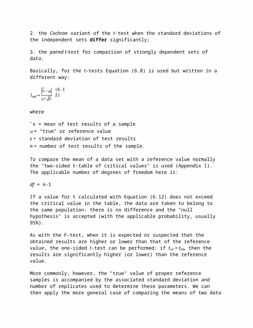
and, using Eq. (6.25) and Table 6-5:

The applicable ttab is 2.78 (App. 1, two-sided, df = n -1 = 4) hence, using Eq. (6.9):

a = 0.037 ± 2.78 × 0.0132 = 0.037 ± 0.037andb = 0.626 ± 2.78 × 0.0219 = 0.626 ± 0.061

Note that if sa is large enough, a negative value for a is possible, i.e. a negative reading for the blank or zero-standard. (For a discussion about the error in x resulting from a reading in y, which is particularly relevant for reading a calibration graph, see Section 7.2.3)

The uncertainty about the line is somewhat decreased by using more calibration points (assuming sy has not increased): one more point reduces ttab from 2.78 to 2.57 (see Appendix 1).

 Choosing A Statistical Test

 

Steps in Statistical Testing:

1) State the null hypothesis (Ho) and the alternative hypothesis (Ha).

2) Choose an acceptable and appropriate level of significance (a) and sample size (n) for your particular study design.

3) Determine the appropriate statistical technique and corresponding test statistic.

4) Collect the data and compute the value of the test statistic.

5) Calculate the number of degrees of freedom for the data set.

6) Compare the value of the test statistic with the critical values in a statistical table for the appropriate distribution and using the correct degrees of freedom.

7) Make a statistical decision and express the statistical decision in terms of the problem under study.

 

Step 1: Statement of Statistical Hypotheses

In statistical testing we always use a null hypothesis (Ho) that there is no difference between the distributions. In other words:

Ho: The survival of the animals is independent of drug treatment.

Ha: The survival of the animals is associated with drug treatment.

The alternative hypothesis (Ha) is obviously that the drug treatment does affect survival in some way. This may seem an odd way to phrase things since most biologists think of their experiment as a test of the hypothesis that drug treatment has an effect on the survival of the animals in the trial. While this may be an appropriate research hypothesis, it is actually the alternative statistical hypothesis. In statistics, we are always testing the nullhypothesis. In short, all statistical tests are simply ways to examine different types of data and to determine whether or not you have a statistically significant reason to reject the null hypothesis. The distinction between the biological or research hypothesis and the statistical hypothesis is very important.

Step 2: Levels of Significance

Further, we need to ask whether the proportion of surviving animals with the drug treatment was a specifed amount different from the proportion of untreated survivors. Researchers specify this level of significance (a) beforehand; usually at the 0.05 level or smaller. What that means is that the researcher is willing to accept a 5% chance of rejecting the null hypothesis (Ho) when it is in fact true. In other words, there is a 5% chance that the statistic will cause us to believe that the survival of the animals is associated with drug treatment when, in fact, their survival is independent of treatment. In biology we typically choose a level of significance of 0.05 or less, but a doctor using human subjects might choose a level of 0.01 (1%) or less to be safe.

The p value approach has become common in the life sciences and published results often require this format. The p value is the probability of calculating a test statisitc value equal to or greater than the result obtained from the sample data when the null

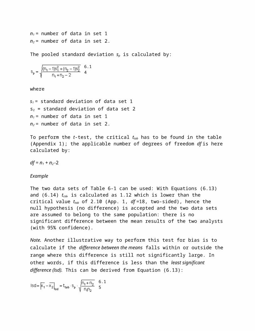
hypothesis is really ture. In other words, the p value is the smallest level of significance at which the null hypothesis can be rejected fo a given dataset.

Step 3: Choice of the Appropriate Statistical Test

Assume we have designed our experiment, stated our statistical hypothesis correctly, and determined the level of significance to be the typical 0.05 level. How do we choose the appropriate statistic from the many tests available? The choice of statistical test is in part determined by the design of the study and the type of data that is collected.

Data Types

There are basically two types of data: catagorical and numerical. Catagorical data fall into specific "catagories," such as yes and no responses to a survey. Here there are only two choices and there are no intermediates possible. Sex (male or female) would be another good example of a catagorical variable. On the other hand, data on the number of offspring a group of females produce is a type of numerical data because the answer is a number. Numerical data can be discrete or continuous. Discrete numerical variables arise from counting processes (i.e. How many cars do you own?), while continuous numerical variables arise from measuring processes (i.e. How tall are you?). The number of cars owned is discrete because there are a finite number of interger responses. You can't own half a car. Height on the other hand, in continuous because it can take on any value within a range or interval depending on the precision of the measuring device.

Measurement Scales

Technically discrete numerical data are "measured by counting" so we can also talk about levels of measurement or types of measurement scales. There are four basic types: nominal, ordinal, interval and ratio. Catagorical data are measured using either a nominal or ordinal scale. For example, data calssified into distinct catagories with no ordering of the catagories are considered nominal (i.e. yes or no, political party affiliation - democrat, republican, greens, etc). Catagorical data in which the catagories imply some sf ranking scheme are considered ordinal (i.e. freshman, sophomore, junior, senior). Interval and ratio scales of measurement are numerical but differ in one important feature. Interval scales are ordered and the differences between points on the scale have the same meaning anywhere on the scale. Temperature measurements are good examples of interval scales. If the scale has all the feature of an interval scale and there is a true zero point, then it is called a ratio scale. Measurements of length and weight are ratio scales because there is a true zero (i.e.

can't have negative heigth). Note that temperature in Celcius and Fahrenheit have a zero point on the scale, but this zero point is said to be arbitrary.

Try to classify the following numerical variables by the type of scale:

o Salaray in dollarso Age in yearso Weight in kilograms

o Calendar time

o Temperature in degrees Kelvin

o Make of automobile

o Student letter gradeso Movie ratings                                                                                                      

Ok, Back to how to choose a statistical test.

Let's keep it simple for now. On the left side of the table below are the goals of the study. Across the top of the table are types of data. The details will be discussed below.

  Type of Data Collected

Goal of the StudyFrom Normal distribution

Rank, Score, or Non-normal Distribution

Binomial (2 outcomes)

Describe one population

Mean, Std DevMedian, Interquartile range

Proportion

Compare pop. to hypothetical value

One-sample t Test Wilcoxon TestChi-square or Binomial Test

Compare 2 unpaired groups

Unpaired t Test Mann-Whitney TestFisher's Test or Chi-square*

Compare >2 unmatched groups

One-way ANOVA Kruskal-Wallis Test Chi-square Test

Compare >2 matched groups

Repeated-measures ANVOA

Friedman Test  

Association b/w 2 variables

Pearson correlation Spearman correlation  

Predict value from a Simple linear Nonparametric  

measured value regression regression

Predict value from several meaured values

Multiple linear Regression

   

* Chi-square for large samples

Notice that there is more than one method for each type of study. How do we choose? First we have to make sure our data fit the assumptions of the test (otherwise GIGO - garbage in, garbage out). The first tyoe of goal, description of a sample population, is straight forward and won't be considered further here. Suppose, however, we wish to compare our sample population with some hypothetical value for the population. The One-sample t-Test assumes that our numerical data is independently drawn from and represent a random sample of the population as a whole and that the population is normally distributed. In practice, this test should not be used for small data sets (less than 30). Less stringent assumptions are required by the non-parametric Wilconon Signed-Ranks Test. Here we do not have to have our sample drawn from a normally distributed population. (Tests that make no assumptions about the population distribution are called non-parametric tests). Wilconon test require interval or ratio data.

 

 

What statistical analysis should I use?

The following table shows general guidelines for choosing a statistical analysis. We emphasize that these are

general guidelines and should not be construed as hard and fast rules.  Usually your data could be analyzed in

multiple ways, each of which could yield legitimate answers. The table below covers a number of common

analyses and helps you choose among them based on the number of dependent variables (sometimes referred

to as outcome variables), the nature of your independent variables (sometimes referred to as predictors).  You

also want to consider the nature of your dependent variable, namely whether it is an interval variable, ordinal or

categorical variable, and whether it is normally distributed (see What is the difference between categorical,

ordinal and interval variables? for more information on this).  The table then shows one or more statistical tests

commonly used given these types of variables (but not necessarily the only type of test that could be used) and

links showing how to do such tests using SAS, Stata and SPSS.

Number of 

Dependent 

Variables

Nature of  

Independent 

Variables

Nature of

Dependent

Variable(s)

Test(s)How

to

SAS

How

to

Stat

How

to

SPSS

a

1

 0 IVs 

(1 population)

interval &

normalone-sample t-test SAS Stata SPSS

ordinal or intervalone-sample

median SAS Stata SPSS

categorical

 (2 categories)binomial test SAS Stata SPSS

categorical Chi-square

goodness-of-fit SAS Stata SPSS

 1 IV with 2 levels 

(independent groups)

interval &

normal

2 independent

sample t-test SAS Stata SPSS

 ordinal or

interval Wilcoxon-Mann

Whitney test

SAS Stata SPSS

 categorical

 Chi- square test SAS Stata SPSS

Fisher's exact

test

SAS Stata SPSS

1 IV with 2 or more levels

(independent groups)

interval &

normalone-way ANOVA SAS Stata SPSS

ordinal or interval Kruskal Wallis SAS Stata SPSS

categorical Chi- square test SAS Stata SPSS

1 IV with 2 levels

(dependent/matched

groups)

interval &

normal

paired t-test SAS Stata SPSS

 ordinal or

interval

Wilcoxon signed

ranks test  SAS Stata SPSS

 categorical McNemar SAS Stata SPSS

1 IV with 2 or more levels

(dependent/matched

groups)

interval &

normal

one-way repeated

measures ANOVA SAS Stata SPSS

ordinal or interval Friedman test SAS Stata SPSS

categoricalrepeated measures

logistic regression SAS Stata SPSS

2 or more IVs 

(independent groups)

interval &

normalfactorial ANOVA SAS Stata SPSS

ordinal or intervalordered logistic

regression SAS Stata SPSS

categoricalfactorial 

logistic regression SAS Stata SPSS

1 interval IV

interval &

normal

correlation  SAS Stata SPSS

simple linear

regression SAS Stata SPSS

ordinal or interval non-parametric

correlation SAS Stata SPSS

categoricalsimple logistic

regression SAS Stata SPSS

1 or more interval IVs

and/or

1 or more categorical

IVs

interval &

normal

multiple regression SAS Stata SPSS

analysis of

covariance

SAS Stata SPSS

categorical multiple logistic

regression

SAS Stata SPSS

discriminant

analysis

SAS Stata SPSS

2 or more1 IV with 2 or more levels

(independent groups)

interval &

normal

one-way

MANOVASAS Stata SPSS

2 or more 2 or moreinterval &

normal

multivariate

multiple linear

regressionSAS Stata SPSS

2 sets of  

2 or more0

interval &

normal

canonical

correlation SAS Stata SPSS

2 or more 0interval &

normalfactor analysis SAS Stata SPSS

Number of 

Dependent 

Variables

Nature of  

Independent 

Variables

Nature of

Dependent

Variable(s)

Test(s)

How

to

SAS

How

to

Stat

a

How

to

SPSS

This page was adapted from Choosing the Correct Statistic   developed by James D. Leeper, Ph.D.  We thank

Professor Leeper for permission to adapt and distribute this page from our site.

How to cite this page

Report an error on this page or leave a comment

The content of this web site should not be construed as an endorsement of any particular web site, book, or software product by the University of California.

Choosing the Right Test

In terms of selecting a statistical test, the most important question is "what is the main

study hypothesis?" In some cases there is no hypothesis; the investigator just wants to

"see what is there". For example, in a prevalence study there is no hypothesis to test,

and the size of the study is determined by how accurately the investigator wants to

determine the prevalence. If there is no hypothesis, then there is no statistical test. It is

important to decide a priori which hypotheses are confirmatory (that is, are testing

some presupposed relationship), and which are exploratory (are suggested by the data).

No single study can support a whole series of hypotheses.

A sensible plan is to limit severely the number of confirmatory hypotheses. Although it

is valid to use statistical tests on hypotheses suggested by the data, the P values should

be used only as guidelines, and the results treated as very tentative until confirmed by

subsequent studies. A useful guide is to use a Bonferroni correction, which states simply

that if one is testing n independent hypotheses, one should use a significance level of

0.05/n. Thus if there were two independent hypotheses a result would be declared

significant only if P<0.025. Note that, since tests are rarely independent, this is a very

conservative procedure - one unlikely to reject the null hypothesis.

The investigator should then ask "are the data independent?" This can be difficult to

decide but as a rule of thumb results on the same individual, or from matched

individuals, are not independent. Thus results from a crossover trial, or from a case

control study in which the controls were matched to the cases by age, sex and social

class, are not independent. It is generally true that the analysis should reflect the

design, and so a matched design should be followed by a matched analysis. Results

measured over time require special care. One of the most common mistakes in

statistical analysis is to treat dependent variables as independent. For example,

suppose we were looking at treatment of leg ulcers, in which some people had an ulcer

on each leg. We might have 20 subjects with 30 ulcers but the number of independent

pieces of information is 20 because the state of an ulcer on one leg may influence the

state of the ulcer on the other leg and an analysis that considered ulcers as

independent observations would be incorrect. For a correct analysis of mixed paired and

unpaired data consult a statistician.

The next question is "what types of data are being measured?" The test used should be

determined by the data. The choice of test for matched or paired data is described in

and for independent data in .

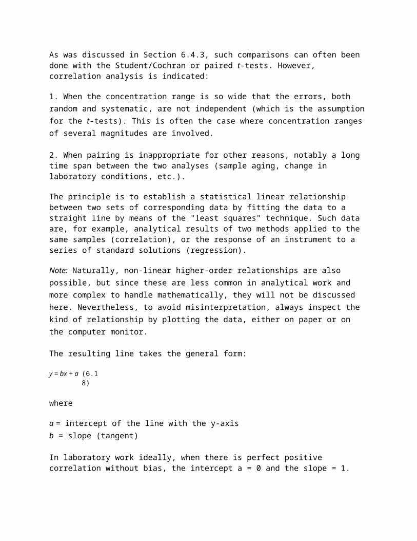
1. Choice of statistical test from paired or matched observations

Variable Test

Nominal MeNemar's Test

Ordinal (Ordered categories) Wilcoxon

Quantitative (Discrete or Non-Normal) Wilcoxon

Quantitative (Normal*) Paired T-test

* It is the difference between the paired observations that should be plausibly

Normal.

It is helpful to decide the input variables and the outcome variables. For example in

a clinical trial the input variable is type of treatment - a nominal variable - and the

outcome may be some clinical measure perhaps Normally distributed. The required test

is then the T-test. However, if the input variable is continuous, say a clinical score, and

the outcome is nominal, say cured or not cured, logistic regression is the required

analysis. A t test in this case may help but would not give us what we require, namely

the probability of a cure for a given value of the clinical score. As another example,

suppose we have a cross sectional study in which we ask a random sample of people

whether they think their general practitioner is doing a good job, on a five point scale,

and we wish to ascertain whether women have a higher opinion of general practitioners

than men have. The input variable is gender, which is nominal. The outcome variable is

the five point ordinal scale. Each person's opinion is independent of the others, so we

have independent data. From here we know we should use a   test for trend, or a

Mann-Whitney U test (with correction for ties). Note, however, if some people share a

general practitioner and others do not, then the data are not independent and a more

sophisticated analysis is called for.

Note that these tables should be considered as guides only, and each case should be

considered on its merits.

2. Choice of statistical test for independent observations

Outcome variable

Nominal Categoric

al

(>2

Categorie

s)

Ordinal Quantitativ

e Discrete

Quantitative

Non-Normal

Quantitative

Normal

Input

Variabl

e

Nominal  or

Fisher's

   trend

or Mann-

Whitney

Mann-

Whitney

Mann-

Whitney or

log-rank (a)

Student's t

test

Categorical

(>2

categories)

   Kruskal-

Wallis (b)

Kruskal-

Wallis (b)

Kruskal-

Wallis (b)

Analysis of

variance (c)

Ordinal

(Ordered

categories)

 -trend

or Mann-

Whitney

(e) Spearma

n rank

Spearman

rank

Spearman

rank

Spearman

rank or

linear

regression

(d)

Quantitativ

e Discrete

Logistic

regressio

n

(e) (e) Spearman

rank

Spearman

rank

Spearman

rank or

linear

regression

(d)

Quantitativ

e non-

Normal

Logistic

regressio

n

(e) (e) (e)

 

Plot data

and Pearson

or

Spearman

Plot data and

Pearson or

Spearman

rank and

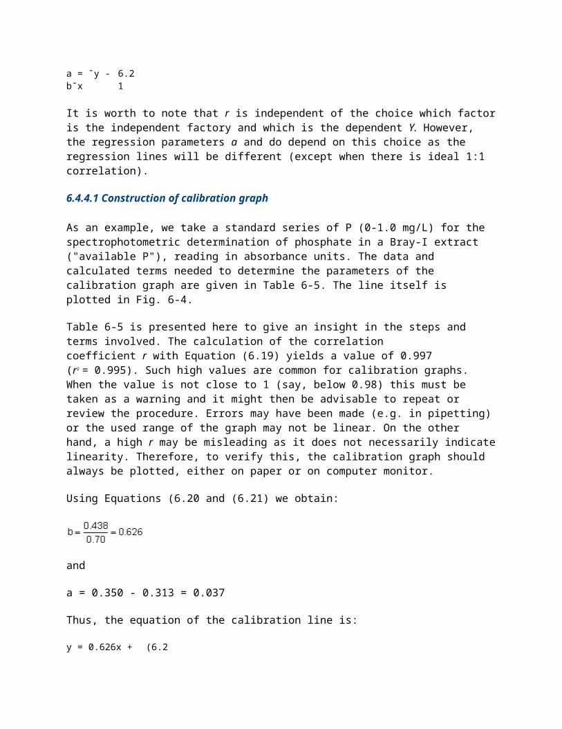
rank linear

regression

Quantitativ

e Normal

Logistic

regressio

n

(e) (e) (e) Linear

regression

(d)

Pearson and

linear

regression

( a) If data are censored.

(b) The Kruskal-Wallis test is used for comparing ordinal or non-Normal variables for

more than two groups, and is a generalisation of the Mann-Whitney U test. The

technique is beyond the scope of this book, but is described in more advanced

books and is available in common software (Epi-Info, Minitab, SPSS).

(c) Analysis of variance is a general technique, and one version (one way analysis of

variance) is used to compare Normally distributed variables for more than two groups,

and is the parametric equivalent of the Kruskal-Wallis test.

(d) If the outcome variable is the dependent variable, then provided the residuals (see )

are plausibly Normal, then the distribution of the independent variable is not important.

(e) There are a number of more advanced techniques, such as Poisson regression, for

dealing with these situations. However, they require certain assumptions and it is often

easier to either dichotomise the outcome variable or treat it as continuous.

References

1. Campbell MJ, Machin D. In: Medical Statistics: A Common-sense Approach , 2nd

edn. Chichester: Wiley, 1993:2.

2. Pocock SJ. Clinical trials: A Practical Approach . Chichester: Wiley, 1982.

3. Senn SJ. The Design and Analysis of Cross-Over Trials . Chichester: Wiley, 1992.

4. Gardner MJ, Altman DG (eds) In: Statistics with Confidence . BMJ Publishing

Group, 1989:103-5.

5. Gardner MJ, Machin D, Campbell MJ. The use of checklists in assessing the

statistical content of medical studies. BMJ 1986; 292 :810-12.

6. Macbin D, Campbell MJ, Payers P, Pinol A. Statistical Tables for the Design of

Clinical Studies . Oxford: Blackwell Scientific Publications, 1996.

7. Matthews JNS, Altman DG, Campbell MJ, Royston JP. Analysis of senal

measurements in medical research. BMJ 1990; 300 :230-5.

8. Altman DG. Practical Statistics for Medical Research . London: Chapman & Hall,

1991.

9. Armitage P, Berry G. In: Statistical Methods in Medical Research . Oxford:

Blackwell Scientific Publications, 1994.

Exercises

State the type of study described in each of the following:

13.1 To investigate the relationship between egg consumption and heart disease, a

group of patients admitted to hospital with myocardial infarction were questioned about

their egg consumption. A group of age and sex matched patients admitted to a fracture

clinic were also questioned about their egg consumption using an identical protocol.

Answer

13.2 To investigate the relationship between certain solvents and cancer, all employees

at a factory were questioned about their exposure to an industrial solvent, and the

amount and length of exposure measured. These subjects were regularly monitored,

and after 10 years a copy of the death certificate for all those who had died was

obtained.

Answer

13.3 A survey was conducted of all nurses employed at a particular hospital. Among

other questions, the questionnaire asked about the grade of the nurse and whether she

was satisfied with her career prospects.

Answer

13.4 To evaluate a new back school, patients with lower back pain were randomly

allocated to either the new school or to conventional occupational therapy. After 3

months they were questioned about their back pain, and observed lifting a weight by

independent monitors.

Answer

13.5 A new triage system has been set up at the local Accident and Emergency Unit. To

evaluate it the waiting times of patients were measured for 6 months and compared

with the waiting times at a comparable nearby hospital.

Answer

Study Design

In many ways the design of a study is more important than the analysis. A badly

designed study can never be retrieved, whereas a poorly analysed one can usually be

reanalysed. Consideration of design is also important because the design of a study will

govern how the data are to be analysed.

Most medical studies consider an input, which may be a medical intervention or

exposure to a potentially toxic compound, and an output, which is some measure of

health that the intervention is supposed to affect. The simplest way to categorise

studies is with reference to the time sequence in which the input and output are

studied.

The most powefful studies are prospective studies, and the paradigm for these is

the randomised controlled trial. In this subjects with a disease are randomised to one of

two (or more) treatments, one of which may be a control treatment. Methods of

randomisation have been described in. The importance of randomisation is that we

Imow in the long run treatment groups will be balanced in known

and unknown prognostic factors. It is important that the treatments are concurrent -

that the active and control treatments occur in the same period of time.

A parallel group design is one in which treatment and control are allocated to different

individuals. To allow for the therapeutic effect of simply being given treatment, the

control may consist of a placebo , an inert substance that is physically identical to the

active compound. If possible a study should be double blinded - neither the investigator

nor the subject being aware of what treatment the subject is undergoing. Sometimes it

is impossible to blind the subjects, for example when the treatment is some form of

health education, but often it is possible to ensure that the people evaluating the

outcome are unaware of the treatment. An example of a parallel group trial is given in,

in which different bran preparations have been tested on different individuals.

A matched design comes about when randomisation is between matched pairs, such as

in, in which randomisation was between different parts of a patient's body.

A crossover study is one in which two or more treatments are applied sequentially to

the same subject. The advantages are that each subject then acts as their own control

and so fewer subjects may be required. The main disadvantage is that there may be a

carry over effect in that the action of the second treatment is affected by the first

treatment. An example of a crossover trial is given in, in which different dosages of bran

are compared within the same individual. A number of excellent books are available on

clinical trials.

One of the major threats to validity of a clinical trial is compliance. Patients are likely to

drop out of trials if the treatment is unpleasant, and often fail to take medication as

prescribed. It is usual to adopt a pragmatic approach and analyse by intention to treat ,

that is analyse the study by the treatment that the subject was assigned to, not the one

they actually took. The alternative is to analyse per protocol or on study . Drop outs

should of course be reported by treatment group. A checklist for writing reports on

clinical trials is available.

A quasi experimental design is one in which treatment allocation is not random. An

example of this is given in in which injuries are compared in two dropping zones. This is

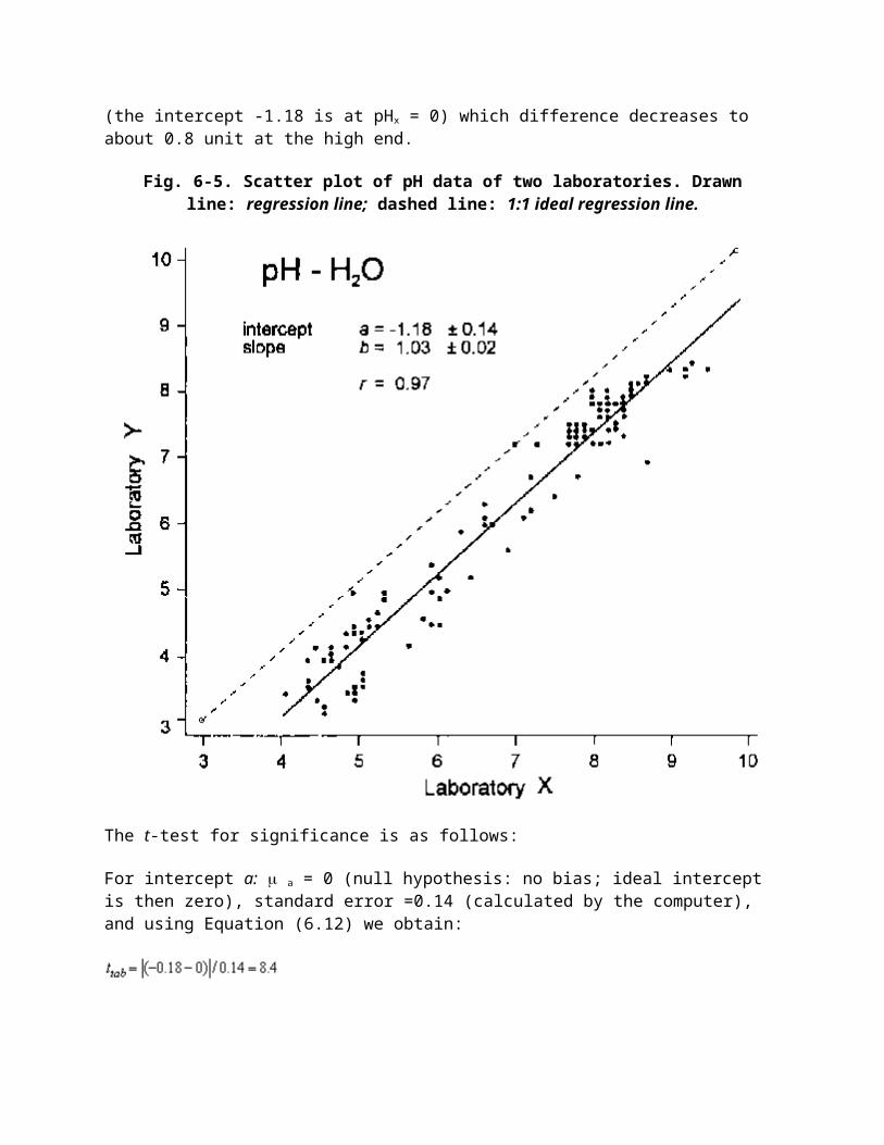
subject to potential biases in that the reason why a person is allocated to a particular

dropping zone may be related to their risk of a sprained ankle.

A cohort study is one in which subjects, initially disease free, are followed up over a

period of time. Some will be exposed to some risk factor, for example cigarette

smoking. The outcome may be death and we may be interested in relating the risk

factor to a particular cause of death. Clearly, these have to be large, long term studies

and tend to be costly to carry out. If records have been kept routinely in the past then a

historical cohort study may be carried out. Here, the cohort is all cases of appendicitis

admitted over a given period and a sample of the records could be inspected

retrospectively. A typical example would be to look at birth weight records and relate

birth weight to disease in later life.

These studies differ in essence from retrospective studies, which start with diseased

subjects and then examine possible exposure. Such case control studies are commonly

undertaken as a preliminary investigation, because they are relatively quick and

inexpensive. The comparison of the blood pressure in farmers and printers is an

example of a case control study. It is retrospective because we argued from the blood

pressure to the occupation and did not start out with subjects assigned to occupation.

There are many confounding factors in case control studies. For example, does

occupational stress cause high blood pressure, or do peop le prone to high blood

pressure choose stressful occupations? A particular problem is recall bias, in that the

cases, with the disease, are more motivated to recall apparently trivial episodes in the

past than controls, who are disease free.

Cross sectional studies are common and include surveys, laboratory experiments and

studies to examine the prevalence of a disease. Studies validating instruments and

questionnaires are also cross sectional studies. The study of urinary concentration of

lead in children and the study of the relationship between height and pulmonary

anatomical dead space were also cross sectional studies.

Data Sample size

One of the most common questions asked of a statistician about design is the number

of patients to include. It is an important question, because if a study is too small it will

not be able to answer the question posed, and would be a waste of time and money. It

could also be deemed unethical because patients may be put at risk with no apparent

benefit. However, studies should not be too large because resources would be wasted if

fewer patients would have sufficed. The sample size depends on four critical quantities:

the type I and type II error rates   and   , the variability of the data   , and the effect

size d. In a trial the effect size is the amount by which we would expect the two

treatments to differ, or is the difference that would be clinically worthwhile.

Usually   and   are fixed at 5% and 20% (or 10%) respectively. A simple formula for a

two group parallel trial with a continuous outcome is that the required sample size per

group is given by   for two sided   of 5% and   of 20%. For example, in a

trial to reduce blood pressure, if a clinically worthwhile effect for diastolic blood

pressure is 5 mmHg and the between subjects standard deviation is 10 mmHg, we

would require n = 16 x 100/25 = 64 patients per group in the study. The sample size

goes up as the square of the standard deviation of the data (the variance) and goes

down inversely as the square of the effect size. Doubling the effect size reduces the

sample size by four - it is much easier to detect large effects! In practice, the sample

size is often fixed by other criteria, such as finance or resources, and the formula is

used to determine a realistic effect size. If this is too large, then the study will have to

be abandoned or increased in size. Machin et al. give advice on a sample size

calculations for a wide variety of study designs.

Barun K Nayak and Avijit Hazra1

Author information   ►  Copyright and License information   ►

Today statistics provides the basis for inference in most medical research. Yet, for want of exposure to statistical theory and practice, it continues to be regarded as the Achilles heel by all concerned in the loop of research and publication – the researchers (authors), reviewers, editors and readers.

Most of us are familiar to some degree with descriptive statistical measures such as those of central tendency and those of dispersion. However, we falter at inferential statistics. This need not be the case, particularly with the

widespread availability of powerful and at the same time user-friendly statistical software. As we have outlined below, a few fundamental considerations will lead one to select the appropriate statistical test for hypothesis testing. However, it is important that the appropriate statistical analysis is decided before starting the study, at the stage of planning itself, and the sample size chosen is optimum. These cannot be decided arbitrarily after the study is over and data have already been collected.

The great majority of studies can be tackled through a basket of some 30 tests from over a 100 that are in use. The test to be used depends upon the type of the research question being asked. The other determining factors are the type of data being analyzed and the number of groups or data sets involved in the study. The following schemes, based on five generic research questions, should help.[1]

 Question 1: Is there a difference between groups that are unpaired? Groups or data sets are regarded as unpaired if there is no possibility of the values in one data set being related to or being influenced by the values in the other data sets. Different tests are required for quantitative or numerical data and qualitative or categorical data as shown in Fig. 1. For numerical data, it is important to decide if they follow the parameters of the normal distribution curve (Gaussian curve), in which case parametric tests are applied. If distribution of the data is not normal or if one is not sure about the distribution, it is safer to use non-parametric tests. When comparing more than two sets of numerical data, a multiple group comparison test such as one-way analysis of variance (ANOVA) or Kruskal-Wallis test should be used first. If they return a statistically significant p value (usually meaning p < 0.05) then only they should be followed by a post hoc test to determine between exactly which two data sets the difference lies. Repeatedly applying the t test or its non-parametric counterpart, the Mann-Whitney U test, to a multiple group situation increases the possibility of incorrectly rejecting the null hypothesis.

Figure 1

Tests to address the question: Is there a difference between groups – unpaired (parallel and independent groups) situation?

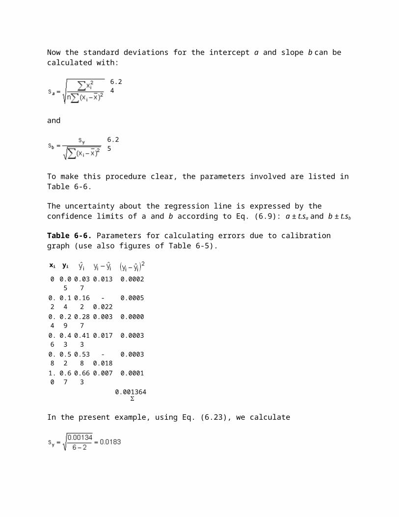
 Question 2: Is there a difference between groups which are paired? Pairing signifies that data sets are derived by repeated measurements (e.g. before-after measurements or multiple measurements across time) on the same set of subjects. Pairing will also occur if subject groups are different but values in one group are in some way linked or related to values in the other group (e.g. twin studies, sibling studies, parent-offspring studies). A crossover study design also calls for the application of paired group tests for comparing the effects of different interventions on the same subjects. Sometimes subjects are deliberately paired to match baseline characteristics such as age, sex, severity or duration of disease. A scheme similar to Fig. 1is followed in paired data set testing, as outlined in Fig. 2. Once again, multiple data set comparison should be done through appropriate multiple group tests followed by post hoc tests.

Figure 2

Tests to address the question: Is there a difference between groups – paired situation?

 Question 3: Is there any association between variables? The various tests applicable are outlined in Fig. 3. It should be noted that the tests meant for numerical data are for testing the association between two variables. These are correlation tests and they express the strength of the association as a correlation coefficient. An inverse correlation between two variables is depicted by a minus sign. All correlation coefficients vary in magnitude from 0 (no correlation at all) to 1 (perfect correlation). A perfect correlation may indicate but does not necessarily mean causality. When two numerical variables are linearly related to each other, a linear regression analysis can generate a mathematical equation, which can predict the dependent variable based on a given value of the independent variable.[2] Odds ratios and relative risks are the staple of epidemiologic studies and express the association between categorical data that can be summarized as a 2 × 2 contingency table. Logistic regression is actually a multivariate analysis method that expresses the strength of the association between a binary dependent variable and two or more independent variables as adjusted odds ratios.

Figure 3

Tests to address the question: Is there an association between variables?

 Question 4: Is there agreement between data sets? This can be a comparison between a new screening technique against the standard test, new diagnostic test against the available gold standard or agreement between the ratings or scores given by different observers. As seen from Fig. 4, agreement between numerical variables may be expressed quantitatively by the intraclass correlation coefficient or graphically by constructing a Bland-Altman plot in which the difference between two variables x and yis plotted against the mean of x and y. In case of categorical data, the Cohen’s Kappa statistic is frequently used, with kappa (which varies from 0 for no agreement at all to 1 for perfect agreement) indicating strong agreement when it is > 0.7. It is inappropriate to infer agreement by showing that there is no statistically significant difference between means or by calculating a correlation coefficient.

Figure 4

Tests to address the question: Is there an agreement between assessment (screening / rating / diagnostic) techniques?

 Question 5: Is there a difference between time-to-event trends or survival plots? This question is specific to survival analysis[3](the endpoint for such analysis could be death or any event that can occur after a period of time) which is characterized by censoring of data, meaning that a sizeable proportion of the original study subjects may not reach the endpoint in question by the time the study ends. Data sets for survival trends are always considered to be non-parametric. If there are two groups then the applicable tests are Cox-Mantel test, Gehan’s (generalized Wilcoxon) test or log-rank test. In case of more than two groups Peto and Peto’s test or log-rank test can be applied to look for significant difference between time-to-event trends.

It can be appreciated from the above outline that distinguishing between parametric and non-parametric data is important. Tests of normality (e.g. Kolmogorov-Smirnov test or Shapiro-Wilk goodness of fit test) may be applied rather than making assumptions. Some of the other prerequisites of parametric

tests are that samples have the same variance i.e. drawn from the same population, observations within a group are independent and that the samples have been drawn randomly from the population.

A one-tailed test calculates the possibility of deviation from the null hypothesis in a specific direction, whereas a two-tailed test calculates the possibility of deviation from the null hypothesis in either direction. When Intervention A is compared with Intervention B in a clinical trail, the null hypothesis assumes there is no difference between the two interventions. Deviation from this hypothesis can occur in favor of either intervention in a two-tailed test but in a one-tailed test it is presumed that only one intervention can show superiority over the other. Although for a given data set, a one-tailed test will return a smaller p value than a two-tailed test, the latter is usually preferred unless there is a watertight case for one-tailed testing.

It is obvious that we cannot refer to all statistical tests in one editorial. However, the schemes outlined will cover the hypothesis testing demands of the majority of observational as well as interventional studies. Finally one must remember that, there is no substitute to actually working hands-on with dummy or real data sets, and to seek the advice of a statistician, in order to learn the nuances of statistical hypothesis testing.

Go to:

References1. Parikh MN, Hazra A, Mukherjee J, Gogtay N, editors. Research methodology simplified: Every clinician a researcher. New Delhi: Jaypee Brothers; 2010. Hypothesis testing and choice of statistical tests; pp. 121–8.

2. Petrie A, Sabin C, editors. Medical statistics at a glance. 2 nd. London: Blackwell Publishing; 2005. The theory of linear regression and performing a linear regression analysis; pp. 70–3.

3. Wang D, Clayton T, Bakhai A. Analysis of survival data. In: Wang D, Bakhai A, editors. Clinical trials: A practical guide to design, analysis and reporting. London: Remedica; 2006. pp. 235–52.

Articles from Indian Journal of Ophthalmology are provided here courtesy of Medknow Publications

An Overview: Choosing the Correct Statistical Test 

 The correct statistical test for an experiment largely depends on the nature of the independent and dependent variables analyzed. For the purpose of choosing a statistical test, variables fall into two classes: Categorical and Continuous. Categorical variable values cannot be sequentially ordered or differentiated from each other using a mathematical method.

Examples include:

        gender

        ethnicity

        software user interfaces

 

Continuous variables are numeric values that can be ordered sequentially, and that do not naturally fall into discrete ranges.

Examples include:

        weight

        number of seconds it takes to perform a task

        number of words on a user interface

 

These concepts can be combined to make a simple model for choosing the correct statistical testi

 

  Dependent VariableCategorical Continuous

Independent

Variable

Categorical Chi Square t-test, ANOVA

Continuous LDA, QDA Regression

 The model is straightforward, illustrating how the nature of the independent and dependent variables drive the choice of a statistical test. 

With understanding of the basic model for choosing a statistical test, we can add relevant details to the model. First, we need to address two additional types of variables, ordinal and interval. First, ordinal variables are similar to continuous variables; they can be ordered sequentially. They are also similar to categorical variables because they (perhaps) cannot be differentiated from each other using a mathematical method. For example, education level is an ordinal variable. The levels of educational achievement (high school, some college, undergraduate degree, etc.) can be sequenced in the order in which they are achieved, and when defined as such, cannot be differentiated from each other mathematically. So the question is, using the simple model for choosing a statistical test, is an ordinal variable Categorical or Continuous? The answer depends on how the researcher defines the variable. When education levels are defined as high school, some college, undergraduate degree, etc., the levels are categorical, and the researcher should choose a test for categorical data. The researcher could, however, define education level in a slightly different way. If the researcher instead defined education level as years of full-time education, then the variable takes on the characteristics of a Continuous variable, and the researcher should choose a statistical test for a Continuous variable. Interval variables also exhibit characteristics of Categorical and Continuous variables. Interval variables fall into equally spaced ranges. For example, an experimenter collects salary levels using the following ranges: 

        $10,000 – 20,000        $20, 000 – 30,000        $30,0000 – 40,000, etc.

 The values can be numerically sequenced, so they are similar to Continuous variables. Because the ranges are equally spaced, though, an unnatural restriction is placed on the values, and thus they are similar to Categorical values. When it comes to choosing a statistical test, there is no hard and fast rule for defining interval data as Categorical or Continuous, and the researcher should use his/her discretion in making the choice. Granularity of ranges is a reasonable guide for deciding how to define the data. For example, when intervals are granular, the researcher may decide to define the variable as Continuous, and for coarser intervals, Categorical. Number of variablesThe number of independent and dependent variable in the experiment also affect which statistical test to choose. For example, linear regression applies when the researcher compares 1 continuous dependent variable and 1 continuous independent variable. Multiple regression applies when the researcher compares 2 or more continuous independent variables against 1 continuous dependent variable. The number of levels of a categorical variable can also drive which statistical test to use. For example, a researcher wants to compare whether gender affects the amount of time to perform a task using a given user interface. Gender serves as a 2 level categorical independent variable because it has 2 possible values: male and female. Time to complete the task would serve as the continuous dependent variable. In this example, a 2-sample t-test would be the correct statistical test. If the categorical independent variable has more than 2 values, however, one-way ANOVA

should be applied. Throughout this guide, the number of independent and dependent variables needed to run the statistical test are included right after the section heading. NormalityFor a given set of independent and dependent variables, often there are two statistical tests available: one parametric and one non-parametric. Parametric tests are appropriate when continuous variables follow a normal distribution, and non-parametric tests are appropriate when they do not. Throughout this guide, the numeric distribution requirements are included right after the section heading.