NST 1B Experimental PsychologyStatistics practical 2

Difference tests (1):parametric

Rudolf Cardinal & Mike Aitken2 / 3 December 2003; Department of Experimental Psychology

University of CambridgeHandouts:• Answers to Examples 2 (from last time)• Handout 3 (diff. tests 1)• Examples 3 (diff. tests 1)• Homophone practical datapobox.com/~rudolf/psychology

Reminder: basic principles and Z

Reminder: the logic of null hypothesis testing

Research hypothesis (H1): e.g. measure weights of 50 joggers and 50 non-joggers; research hypothesis might be ‘there is a difference between the weightsof joggers and non-joggers; the population mean of joggers is not the same asthe population mean of non-joggers’.

Usually very hard to calculate the probability of a research hypothesis(sometimes because they’re poorly specified — for example, how big adifference?).

Null hypothesis (H0): e.g. ‘there is no difference between the populationmeans of joggers and non-joggers; any observed differences are due tochance.’

Calculate probability of finding the observed data (e.g. difference) if thenull hypothesis is true. This is the p value.

If p very small, reject null hypothesis (‘chance alone is not a good enoughexplanation’). Otherwise, retain null hypothesis (Occam’s razor: chance is thesimplest explanation). Criterion level of p is called αααα.

True state of the worldDecision H0 true H0 falseReject H0 Type I error

probability = αCorrect decisionprobability = 1 – β = power

Do not reject H0 Correct decisionprobability = 1 – α

Type II errorprobability = β

Reminder: α, and errors we can make

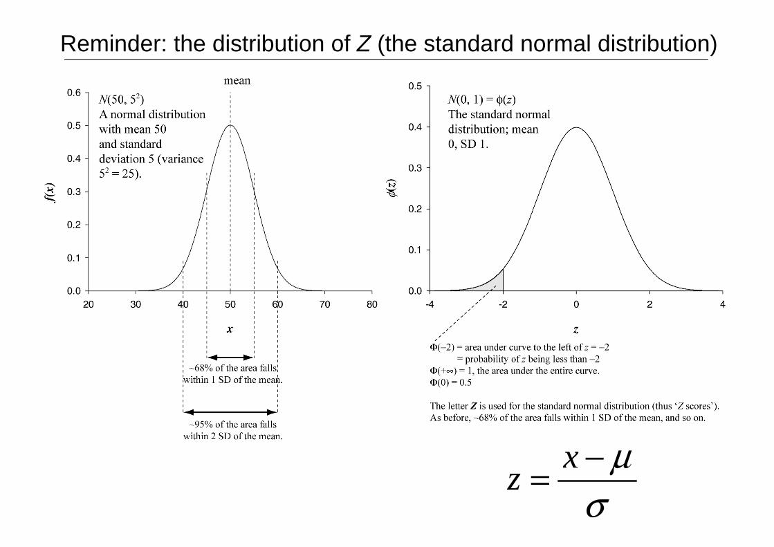
Reminder: the distribution of Z (the standard normal distribution)

σµ−= x

z

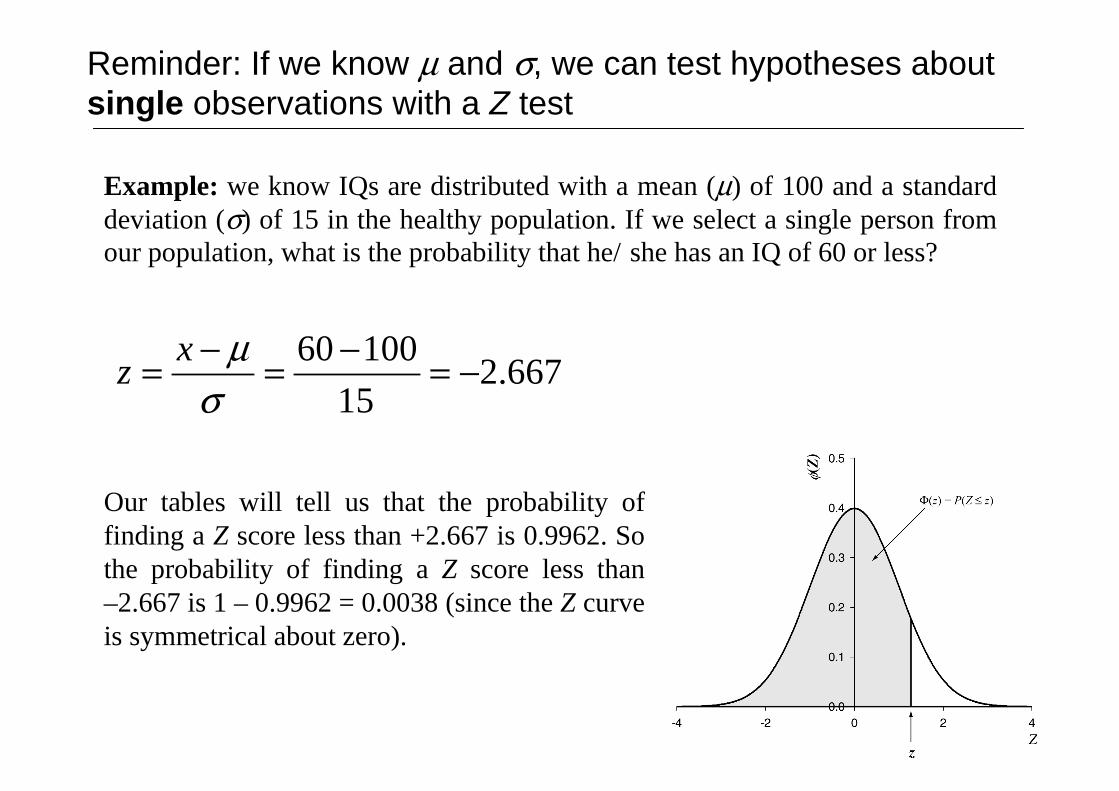
Reminder: If we know µ and σ, we can test hypotheses aboutsingle observations with a Z test

667.215

10060 −=−=−=σ

µxz

Example: we know IQs are distributed with a mean (µ) of 100 and a standarddeviation (σ) of 15 in the healthy population. If we select a single person fromour population, what is the probability that he/she has an IQ of 60 or less?

Our tables will tell us that the probability offinding a Z score less than +2.667 is 0.9962. Sothe probability of finding a Z score less than–2.667 is 1 – 0.9962 = 0.0038 (since the Z curveis symmetrical about zero).

Reminder: one- and two-tailed tests

In our example, we asked for the probability of finding an individual with an IQof 60 or less in the normal population. This is equivalent to a hypothesis testwhere the null hypothesis is ‘the individual comes from the normal populationwith mean 100 and SD 15’. We calculate p, and would reject our hypothesis ifp < α (where α is typically 0.05 by arbitrary convention).

This would be a one-tailed test. It would fail to detect deviations from themean ‘the other way’ (IQ > mean). To detect both, we use a two-tailed test,and ‘allocate’ α/2 for testing each tail to keep the overall Type I error rate at α.

The t test

The ‘sampling distribution of the mean’

This lets us test hypotheses about groups of observations (samples). For agiven n, we can find out the probability of obtaining a particular sample mean.

71.1

50.3

==

σµ 27.0

40

71.1

40

50.3

===

===

n

n

x

x

σσ

µµ

The Central Limit TheoremGiven a population with mean µ and variance σ2, from which we take samples of size n, the distribution

of sample means will have a mean µµ =x , a variance nx

22 σσ = , and a standard deviation

nx

σσ = .

As the sample size n increases, the distribution of the sample means will approach the normaldistribution.

Distribution of the population

(probability density function of rolls of a single die)

Example: we know IQs are distributed with a mean (µ) of 100 and a standarddeviation (σ) of 15 in the healthy population. Suppose we take a single sampleof 5 people and find their IQs are {140, 121, 95, 105, 91}. What is theprobability of obtaining data with this sample mean or greater from thehealthy population? Well, we can work out our sample mean: We know n: We know the mean of all sample means from this population:

… and the standard deviation of all sample means: (often called the standard error of the mean)

So we can work out a Z score:

If we know the population SD, σ, we can test hypothesesabout samples with a Z test

Our tables will tell us that P(Z < 1.55) = 0.9394. So P(Z > 1.55) =1 – 0.9394 = 0.061. We’d report p = 0.061 for our test.

55.1708.6

1004.110

708.65

15

100

5

4.110

=−=−

=

===

===

=

x

x

x

x

xz

n

n

x

σµ

σσ

µµ

But normally, we don’t. So we have to use a t test.

n

sx

s

xt

n

xxz

x

x

x

x

µµ

σµ

σµ

−=−

=

−=−

=?

If we don’t know the populationSD, σ, and very often we don’t, wecan’t use this test.

Instead, we can calculate a numberusing the sample SD (which we caneasily calculate) as an estimator ofthe population SD (which we don’tknow). But this number, which wecall t, does NOT have the samedistribution as Z.

The distribution of t: “Student’s” (Gossett’s) t distribution

As is so often the case, beer made a statistical problem go away.

Student (Gossett, W.S.) (1908). The probable error of a mean. Biometrika 6: 1–25.

The distribution of t when the null hypothesis is true dependson the sample size (⇒ d.f.)

When d.f. = ∞, the t distribution (under H0) is the same as the normal distribution.

Degrees of freedom (df). (Few understand this well!)

Two statistics are drinking in a bar. One turns to the other and asks ‘So how are youfinding married life?’ The other replies ‘It’s okay, but you lose a degree of freedom.’The first chuckles evilly. ‘You need a larger sample.’

Estimates of parameters can be based upon different amounts of information. Thenumber of independent pieces of information that go into the estimate of a parameteris called the degrees of freedom (d.f. or df).

Or, the number of observations free to vary. (Example: 3 numbers and a mean.)

Or, the df is the number of measurements exceeding the amount absolutely necessaryto measure the ‘object’ (or parameter) in question. To measure the length of a rodrequires 1 measurement. If 10 measurements are taken, then the set of 10measurements has 9 df.

In general, the df of an estimate is the number of independent scores that go into theestimate minus the number of parameters estimated from those scores as intermediatesteps. For example, if the variance σ2 is estimated (by s2) from a random sample of nindependent scores, then the number of degrees of freedom is equal to the number ofindependent scores (n) minus the number of parameters estimated as intermediatesteps (one, as µ is estimated by x) and is therefore n–1.

1

)( 22

−∑ −=

n

xxsX

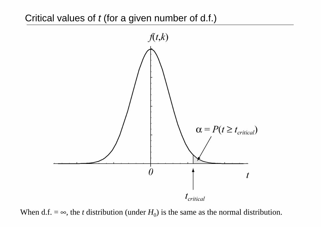
Critical values of t (for a given number of d.f.)

When d.f. = ∞, the t distribution (under H0) is the same as the normal distribution.

The one-sample t test

n

sx

s

xt

Xxn

µµ −=−=−1

We’ve just seen the logic behind this. We calculate t according to this formula:

sample mean

standard error of the mean(SEM) (standard deviation of thedistribution of sample means)

test value

sample SD

The null hypothesis is that the sample comes from a population with mean µ.

Look up the critical value of t (for a given α) using your tables of t for thecorrect number of degrees of freedom (n – 1). If your |t| is bigger, it’ssignificant.

df for this test

Degrees of freedom: we have nobservations and have calculatedone intermediate parameter (x,which estimates µ in thecalculation of sX), so t has n – 1 df.

The one-sample t test: EXAMPLE (1)

It has been suggested that 15-year-olds should sleep 8 hours per night. Wemeasure sleep duration in 8 such teenagers and find that they sleep {8.3, 5.4,7.2, 8.1, 7.6, 6.2, 9.1, 7.3} hours per night. Does their group mean differ from 8hours per night?

n

sx

tX

nµ−=−1

The one-sample t test: EXAMPLE (2)

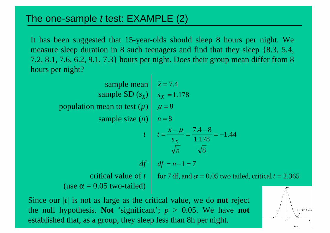
It has been suggested that 15-year-olds should sleep 8 hours per night. Wemeasure sleep duration in 8 such teenagers and find that they sleep {8.3, 5.4,7.2, 8.1, 7.6, 6.2, 9.1, 7.3} hours per night. Does their group mean differ from 8hours per night?

Since our |t| is not as large as the critical value, we do not rejectthe null hypothesis. Not ‘significant’; p > 0.05. We have notestablished that, as a group, they sleep less than 8h per night.

4.7=x

178.1=Xs

8=µ8=n

44.1

8

178.184.7 −=−=−=

n

sx

tX

µ

71 =−= ndf

365.2 critical tailed, two0.05 and df, 7for == tα

sample meansample SD (sX)

population mean to test (µ)

sample size (n)

t

df

critical value of t(use α = 0.05 two-tailed)

Paired and unpaired tests (related and unrelated data)

Now we’ll look at t tests with two samples. In general, two samples can berelated or unrelated.

• Related: e.g. measuring the same subject twice; measuring a large set oftwins; … any situation in which two measurements are more likely toresemble each other than by chance alone within the ‘domain’ of interest.• Unrelated: where no two measurements are related.

Example: measuring digit span on land and underwater. Could use either• related (within-subjects) design: measure ten people on land; measuresame ten people underwater. ‘Good’ performers on land likely to be ‘good’performers underwater; the two scores from the same subject are related.• unrelated (between-subjects) design: measure ten people on land andanother ten people underwater.

If there is ‘relatedness’ in your data, your analysis must take account of it.• This may give you more power (e.g. if the data is paired, a paired test hasmore power than an unpaired test; unpaired test may give Type II error).• beware pseudoreplication: e.g. measure one person ten times on land;measure another person ten times underwater; pretend that n = 20. In fact,n = 2, as repeated measurements of the same person do not add much moreinformation — they’re all likely to be similar. Get Type I errors.

The two-sample, paired t test

n

sx

tX

nµ−=−1

Very simple. Calculate the differences between each pair of observations. Thenperform a one-sample t test on the differences, comparing them to zero. (Nullhypothesis: the mean difference is zero.)

test value for thedifferences (zerofor the nullhypothesis ‘thereis no difference’)

The two-sample, paired t test: EXAMPLE (1)

Looking at high-frequency words only, does the rate of errors that you madewhile categorizing homophones differ from the error rate when categorizingnon-homophone (control) words — i.e. is there a non-zero homophone effect?(Each subject categorizes both homophones and control words, so we will use apaired t test.)

Relevant difference scores are labelled % errors — homophone effect — high fon your summary sheet.

n

sx

tX

nµ−=−1

The two-sample, paired t test: EXAMPLE (2)

Looking at high-frequency words only, does the rate of errors that you madewhile categorizing homophones differ from the error rate when categorizingnon-homophone (control) words — i.e. is there a non-zero homophone effect?

Since our t is larger than the critical value, we reject the null hypothesis.‘Significant’; p < 0.05. In fact, p < 0.01, since critical t for α = 0.01 and 96 df isapprox. 2.576. You made more errors for homophones (p < 0.01 two-tailed).

1.3=x

264.9=Xs

0=µ97=n

296.3

97

264.901.3 =−=−=

n

sx

tX

µ

961 =−= ndf

96.1 critical tailed, two0.05 and df, 96for ≈= tα

mean of differencessample SD (sX) of differences

mean diff. under null hypothesis (µ)

sample size (n)

t

df

critical value of t

differences },7.16,3.8,0.0,3.8{ …−=X

The two-sample, unpaired t test — (a) equal sample variances

something) theof samples ofset infinitean of SD ( something theoferror standard

something

==t

How can we test the difference between twoindependent samples? In other words, doboth samples come from underlyingpopulations with the same mean? (= Nullhypothesis.)

Basically, if the sample means are very farapart, as measured by something that depends(somehow) on the variability of the samples,then we will reject the null hypothesis.

As always,

In this case,

(SED) means ebetween th difference theoferror standard

means ebetween th difference=t

The two-sample, unpaired t test — (a) equal sample variances

2

2

1

2

212

21

222

2112

21

2

)1()1(

n

s

n

s

xxt

nn

snsns

pp

nn

p

+

−=

−+−+−=

−+

2

22

1

21

21221

n

s

n

s

xxt nn

+

−=−+

Don’t worry about how we calculate the SED (it’s inthe handout, section 3.12, if you’re bizarrely keen).

The precise format of the t test depends on whetherthe two samples have the same variance.

If the two samples have the same variance:

If the samples are the same size(n1 = n2), the formula becomes abit simpler:

If the samples are not the same size (n1 ≠ n2),we first calculate something called the ‘pooledvariance’ (sp

2) and use that to get t:

We have n1+n2 observations andestimated 2 parameters (themeans, used to calculate the twos2), so we have n1 + n2 – 2 df.

The two-sample, unpaired t test — EXAMPLE

Silly example… In low-frequency word categorization where those words arehomophones (the hardest condition, judged by mean error rate), were theredifferences between males and females?

% errors —Females: n = 61; mean = 12.7; SD = 13.4Males: n = 27; mean = 15.7; SD = 15.2Use the equal-variance unpaired t test (unequal n formula).

2

2

1

2

212

21

222

2112

21

2

)1()1(

n

s

n

s

xxt

nn

snsns

pp

nn

p

+

−=

−+−+−=

−+

86227612

93.0424.10

0.3

271.195

611.195

7.157.12

1.19586

2.15264.1360

2

)1()1(

21

2

2

1

2

21

22

21

222

2112

=−+=−+=

−=−=+

−=

+

−=

=×+×=−+

−+−=

nndf

n

s

n

s

xxt

nn

snsns

pp

p

The two-sample, unpaired t test — EXAMPLE (2)

Silly example… In low-frequency word categorization where those words arehomophones (the hardest condition, judged by mean error rate), were theredifferences between males and females? Call females ‘group 1’ and males‘group 2’. Unequal n, so...

Caveat: some people were ignored because there wasn’t enough of your nameto judge your sex by it, or because I was incapable of predicting your sex fromyour name. So these data may not be wholly accurate!

96.1 critical tailed, two0.05 and df, 86for ≈= tαNot a significant difference.

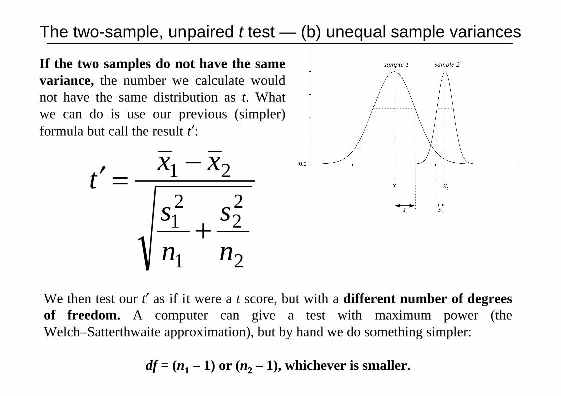
The two-sample, unpaired t test — (b) unequal sample variances

2

22

1

21

21

n

s

n

s

xxt

+

−=′

If the two samples do not have the samevariance, the number we calculate wouldnot have the same distribution as t. Whatwe can do is use our previous (simpler)formula but call the result t′:

We then test our t′ as if it were a t score, but with a different number of degreesof freedom. A computer can give a test with maximum power (theWelch–Satterthwaite approximation), but by hand we do something simpler:

df = (n1 – 1) or (n2 – 1), whichever is smaller.

So how can we tell if the variances are ‘the same’ or ‘different’ for t testing?(a) We can look at them. It may be obvious.(b) We can perform a statistical test to compare the two variances.

A popular test — not the best one, but a reasonable and easy one — is the F test.F is the ratio of two variances. Since our tables will give us critical values for F >1 (but not F < 1), we make sure F ≥ 1 by putting the bigger variance on top:

‘Are the variances equal or not?’ The F test

21

222

1

22

1,1

22

212

2

21

1,1

if

if

12

21

sss

sF

sss

sF

nn

nn

>=

>=

−−

−−

Null hypothesis is that the variances are the same (F = 1). If our F exceeds thecritical F for the relevant number of df (note that there are separate df for thenumerator and the denominator), we reject the null hypothesis. Since we haveensured that F ≥ 1, we run a one-tailed test on F — so double the stated one-tailed α to get the two-tailed α for the question ‘are the variances different?’.

Assumptions of the t test

• The mean is meaningful.

If you compare the football shirt numbers worn by England strikers who’ve scoredmore than 20 goals for their country with those worn by less successful strikers,you might find that the successful strikers have a mean shirt number that’s 1.2lower than the less successful strikers. So what?

• The underlying scores (for one-sample and unpaired t tests) or difference scores(for paired t tests) are normally distributed.

Rule of thumb: if n > 30, you’re fine to assume this. If n > 15 and the data don’tlook too weird, it’s probably OK. Otherwise, bear this in mind.

• To use the equal-variance version of the unpaired two-sample t test, the twosamples must come from populations with equal variances (whether not n1 = n2).

(There’s a helpful clue to remember that one in the name of the test.) The t test isfairly robust to violations of this assumption (gives a good estimate of the p value)if n1 = n2, but not if n1 ≠ n2.

Parametric and non-parametric tests

The t test is a parametric test: it makes assumptions about parameters of theunderlying populations (such as the distribution — e.g. assuming that the data arenormally distributed). If these assumptions are violated:

(a) we can transform the data to fit the assumptions better(NOT covered at Part 1B level)

or (b) we can use a nonparametric (‘distribution-free’) test that doesn’t make the same assumptions.

In general, if the assumptions of parametric tests are met, they are the mostpowerful. If not, we may need to use nonparametric tests. They may, for example,answer questions about medians rather than means. We’ll cover some next time.

Final thoughts and techniques

Drawing and interpreting between- and within-subject effects

SEM221

×−= xx

tIf groups have same n and SEM,

So if SEM bars overlap, means differ by <2SEM, so — never significant.4.1

2

2 =<t

t = difference/SED, so SED isalways an appropriate index ofcomparison. If difference > 2SED, t > 2… usually significantfor reasonably large n.

Reminder: multiple comparisons are potentially evil

Number of tests withα = 0.05 per test

12345

100

n

P(at least one Type I error if null hypothesis true)= 1 – P(no Type I errors if null hypothesis true)

1 – (1 – 0.05) = 0.051 – (1 – 0.05)2 = 0.09751 – (1 – 0.05)3 = 0.14261 – (1 – 0.05)4 = 0.18551 – (1 – 0.05)5 = 0.2262

1 – (1 – 0.05)100 = 0.9941

1 – (1 – 0.05)n

(But remember, you can’t make a Type I error — saying something issignificant when it isn’t — at all unless the null hypothesis is actually true. Sothese are all ‘maximum’ Type I error rates.)

Confidence intervals using t

×±=

−=

−

−

n

stx

n

sx

t

Xdfn

Xn

1for critical

1

µ

µ

06.082.110

08.082.1

262.2

±=

−=±

µ

µ

If we know the mean and SD of a sample, we could perform a t test to see if itdiffered from a given number. We could repeat that for every possible number...

Example: we measure the heights of 10UK men. Sample mean = 1.82 m, s =0.08 m. For n = 10 (df = 9), tcritical for α =0.05 two-tailed is ±2.262. Therefore

This means that there is a 95% chancethat the true mean height of UK men isbetween 1.76 and 1.88 m.

Power: the probability of FINDING a GENUINE effect

Graphs show distributions of samplemeans if H0 is true (left-hand curve ineach case) and if H1 is true (right-handcurve). Setting α determines a cut-offat which we reject H0, and is one of thethings that determines power.

Significance is not the same as effect size