Dielectrophoretic Traps for Cell Manipulation - RLE at MIT
28
8 Dielectrophoretic Traps for Cell Manipulation Joel Voldman Department of Electrical Engineering, Room 36-824, Massachusetts Institute of Technology Cambridge, MA 02139 8.1. INTRODUCTION One of the goals of biology for the next fifty years is to understand how cells work. This fundamentally requires a diverse set of approaches for performing measurements on cells in order to extract information from them. Manipulating the physical location and organization of cells or other biologically important particles is an important part in this endeavor. Apart from the fact that cell function is tied to their three-dimensional organization, one would like ways to grab onto and position cells. This lets us build up controlled multicellular aggregates, investigate the mechanical properties of cells, the binding properties of their surface proteins, and additionally provides a way to move cells around. In short, it provides physical access to cells that our fingers cannot grasp. Many techniques exist to physically manipulate cells, including optical tweezers [78], acoustic forces [94], surface modification [52], etc. Electrical forces, and in particular dielec- trophoresis (DEP), are an increasingly common modality for enacting these manipulations. Although DEP has been used successfully for many years to separate different cell types (see reviews in [20, 38]), in this chapter I focus on the use of DEP as “electrical tweezers” for manipulating individual cells. In this implementation DEP forces are used to trap or spatially confine cells, and thus the chapter will focus on creating such traps using these forces. While it is quite easy to generate forces on cells with DEP, it is another thing al- together to obtain predetermined quantitative performance. The goal for this chapter is to help others develop an approach to designing these types of systems. The focus will be on trapping cells—which at times are generalized to “particles”—and specifically mammalian
Transcript of Dielectrophoretic Traps for Cell Manipulation - RLE at MIT
8
Dielectrophoretic Traps forCell Manipulation
Joel VoldmanDepartment of Electrical Engineering, Room 36-824, Massachusetts Institute ofTechnology Cambridge, MA 02139
8.1. INTRODUCTION
One of the goals of biology for the next fifty years is to understand how cells work. Thisfundamentally requires a diverse set of approaches for performing measurements on cells inorder to extract information from them. Manipulating the physical location and organizationof cells or other biologically important particles is an important part in this endeavor. Apartfrom the fact that cell function is tied to their three-dimensional organization, one wouldlike ways to grab onto and position cells. This lets us build up controlled multicellularaggregates, investigate the mechanical properties of cells, the binding properties of theirsurface proteins, and additionally provides a way to move cells around. In short, it providesphysical access to cells that our fingers cannot grasp.
Many techniques exist to physically manipulate cells, including optical tweezers [78],acoustic forces [94], surface modification [52], etc. Electrical forces, and in particular dielec-trophoresis (DEP), are an increasingly common modality for enacting these manipulations.Although DEP has been used successfully for many years to separate different cell types(see reviews in [20, 38]), in this chapter I focus on the use of DEP as “electrical tweezers”for manipulating individual cells. In this implementation DEP forces are used to trap orspatially confine cells, and thus the chapter will focus on creating such traps using theseforces. While it is quite easy to generate forces on cells with DEP, it is another thing al-together to obtain predetermined quantitative performance. The goal for this chapter is tohelp others develop an approach to designing these types of systems. The focus will be ontrapping cells—which at times are generalized to “particles”—and specifically mammalian
160 JOEL VOLDMAN
cells, since these are more fragile than yeast or bacteria and thus are in some ways morechallenging to work with.
I will start with a short discussion on what trapping entails and then focus on the forcesrelevant in these systems. Then I will discuss the constraints when working with cells, suchas temperature rise and electric field exposure. The last two sections will describe existingtrapping structures as well as different approaches taken to measure the performance ofthose structures. The hope is that this overview will give an appreciation for the forcesin these systems, what are the relevant design issues, what existing structures exist, andhow one might go about validating a design. I will not discuss the myriad other uses ofdielectrophoresis; these are adequately covered in other texts [39, 45, 60] and reviews.
8.2. TRAPPING PHYSICS
8.2.1. Fundamentals of Trap Design
The process of positioning and physically manipulating particles—cells in this case—is a trapping process. A trap uses a set of confining forces to hold a particle against aset of destabilizing forces. In this review, the predominant confining force will be dielec-trophoresis, while the predominant destabilizing forces will be fluid drag and gravity. Thefundamental requirement for any deterministic trap is that it creates a region where the netforce on the particle is zero. Additionally, the particle must be at a stable zero, in that theparticle must do work on the force field in order to move from that zero [3]. This is allcodified in the requirement that Fnet = 0, Fnet · dr < 0 at the trapping point, where Fnet isthe net force and dr is an increment in any direction.
The design goal is in general to create a particle trap that meets specific requirements.These requirements might take the form of a desired trap strength or maximum flowratethat trapped particles can withstand, perhaps to meet an overall system throughput spec-ification. For instance, one may require a minimum flowrate to replenish the nutrientsaround trapped cells, and thus a minimum flowrate against which the cells must be trapped.When dealing with biological cells, temperature and electric-field constraints are neces-sary to prevent adverse effects on cells. Other constraints might be on minimum chamberheight or width—to prevent particle clogging—or maximum chamber dimensions—to al-low for proximate optical access. In short, predictive quantitative trap design. Under thedesired operating conditions, the trap must create a stable zero, and the design thus reducesto ensuring that stable zeros exist under the operating conditions, and additionally de-termining under what conditions those stable zeros disappear (i.e., the trap releases theparticle).
Occasionally, it is possible to analytically determine the conditions for stable trapping.When the electric fields are analytically tractable and there is enough symmetry in theproblem to make it one-dimensional, this can be the best approach. For example, one canderive an analytical expression balancing gravity against an exponentially decaying electricfield, as is done for field-flow fractionation [37]. In general, however, the fields and forcesare too complicated spatially for this approach to work. In these cases, one can numericallycalculate the fields and forces everywhere in space and find the net force (Fnet) at eachpoint, then find the zeros.
DIELECTROPHORETIC TRAPS FOR CELL MANIPULATION 161
A slightly simpler approach exists when the relevant forces are conservative. In thiscase one can define scalar potential energy functions U whose gradient gives each force(i.e., F = −∇U ). The process of determining whether a trap is successfully confining theparticle then reduces to determining whether any spatial minima exist within the trap. Thisapproach is nice because energy is a scalar function and thus easy to manipulate by handand on the computer.
In general, a potential energy approach will have limited applicability because dissi-pation is usually present. In this case, the energy in the system depends on the specifics ofthe particle motion—one cannot find a U that will uniquely define F. In systems with liquidflow, for example, an energy-based design strategy cannot be used because viscous fluidflow is dissipative. In this case, one must use the vector force-fields and find stable zeroes.
In our lab, most modeling incorporates a range of approaches spanning analytical,numerical, and finite-element modeling. In general, we find it most expedient to performfinite-element modeling only when absolutely necessary, and spend most of the designcombining those results with analytical results in a mixed-numerical framework run ona program such as Matlab c© (Mathworks, Natick, MA). Luckily, one can run one or twofinite-element simulations and then use simple scaling laws to scale the resulting dataappropriately. For instance, the linearity of Laplace’s equation means that after solving forthe electric fields at one voltage, the results can be linearly scaled to other voltages. Thus,FEA only has to be repeated when the geometry scales, if at all.
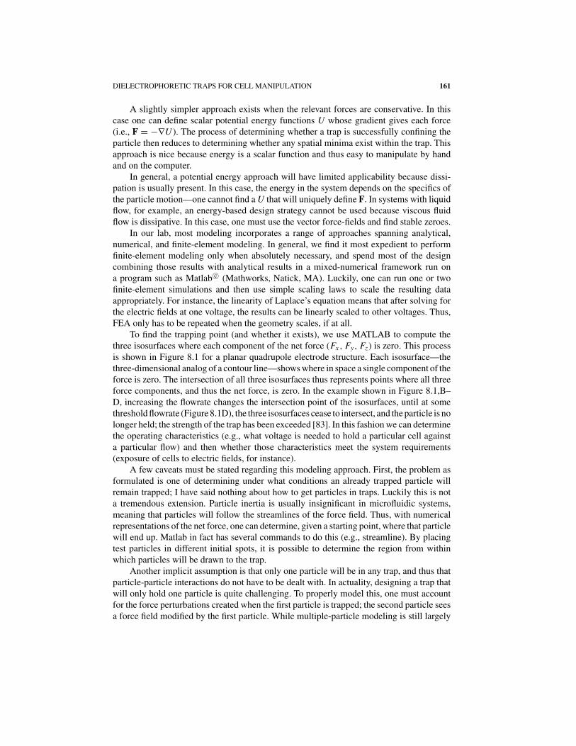
To find the trapping point (and whether it exists), we use MATLAB to compute thethree isosurfaces where each component of the net force (Fx , Fy, Fz) is zero. This processis shown in Figure 8.1 for a planar quadrupole electrode structure. Each isosurface—thethree-dimensional analog of a contour line—shows where in space a single component of theforce is zero. The intersection of all three isosurfaces thus represents points where all threeforce components, and thus the net force, is zero. In the example shown in Figure 8.1,B–D, increasing the flowrate changes the intersection point of the isosurfaces, until at somethreshold flowrate (Figure 8.1D), the three isosurfaces cease to intersect, and the particle is nolonger held; the strength of the trap has been exceeded [83]. In this fashion we can determinethe operating characteristics (e.g., what voltage is needed to hold a particular cell againsta particular flow) and then whether those characteristics meet the system requirements(exposure of cells to electric fields, for instance).
A few caveats must be stated regarding this modeling approach. First, the problem asformulated is one of determining under what conditions an already trapped particle willremain trapped; I have said nothing about how to get particles in traps. Luckily this is nota tremendous extension. Particle inertia is usually insignificant in microfluidic systems,meaning that particles will follow the streamlines of the force field. Thus, with numericalrepresentations of the net force, one can determine, given a starting point, where that particlewill end up. Matlab in fact has several commands to do this (e.g., streamline). By placingtest particles in different initial spots, it is possible to determine the region from withinwhich particles will be drawn to the trap.
Another implicit assumption is that only one particle will be in any trap, and thus thatparticle-particle interactions do not have to be dealt with. In actuality, designing a trap thatwill only hold one particle is quite challenging. To properly model this, one must accountfor the force perturbations created when the first particle is trapped; the second particle seesa force field modified by the first particle. While multiple-particle modeling is still largely
162 JOEL VOLDMAN
A B
DC
FIGURE 8.1. Surfaces of zero force describe a trap. (A) Shown are the locations of planar quadrupole electrodes
along with the three isosurfaces where one component of the force on a particle is zero. The net force on the
particle is zero where the three surfaces intersect. (B–D) As flow increases from left to right, the intersection point
moves. The third isosurface is not shown, though it is a vertical sheet perpendicular to the Fx = 0 isosurface.
(D) At some critical flow rate, the three isosurfaces no longer intersect and the particle is no longer trapped.
unresolved, the single-particle approach presented here is quite useful because one can,by manipulating experimental conditions, create conditions favorable for single-particletrapping, where the current analysis holds.
Finally, we have constrained ourselves to deterministic particle trapping. While appro-priate for biological cells, this assumption starts to break down as the particle size decreasespast ∼1μm because Brownian motion makes trapping a probabilistic event. Luckily, asnanoparticle manipulation has become more prevalent, theory and modeling approacheshave been determined. The interested reader is referred to the monographs by Morgan andGreen [60] and Hughes [39].
8.2.2. Dielectrophoresis
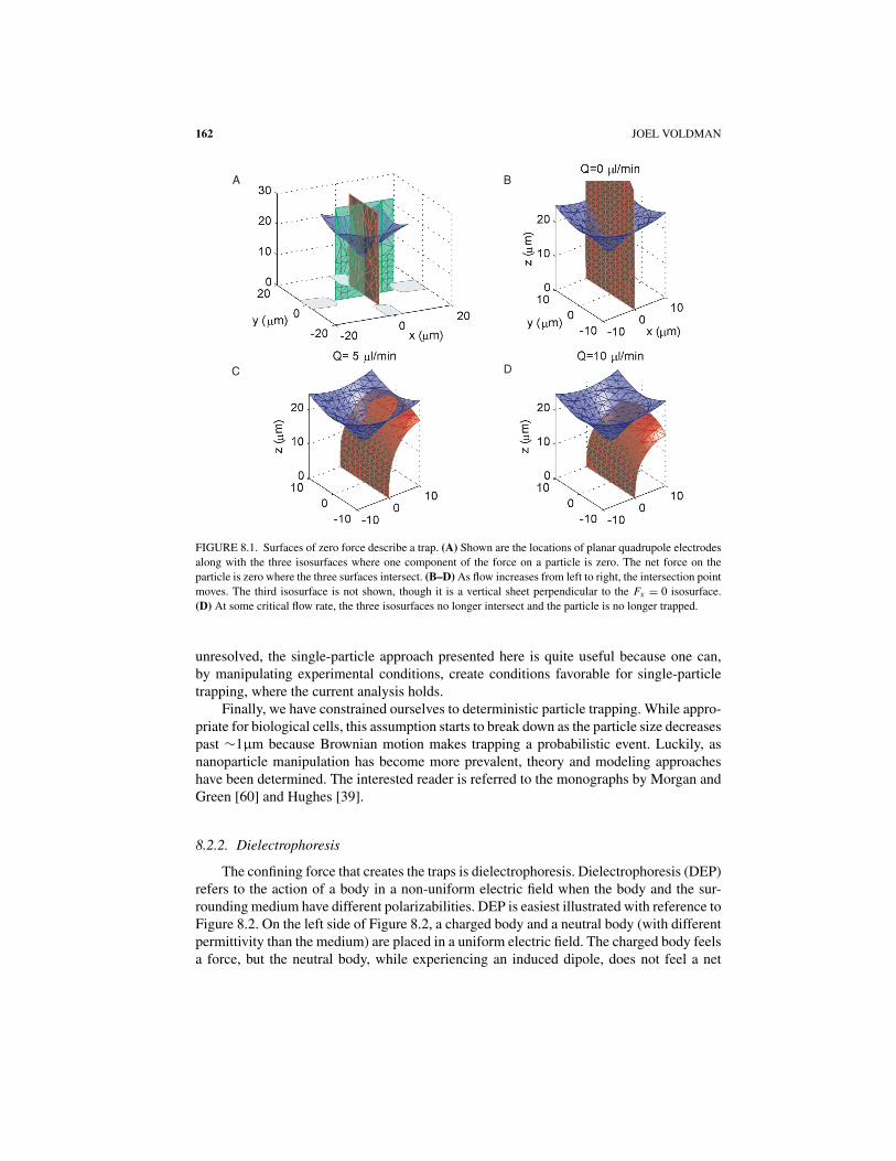
The confining force that creates the traps is dielectrophoresis. Dielectrophoresis (DEP)refers to the action of a body in a non-uniform electric field when the body and the sur-rounding medium have different polarizabilities. DEP is easiest illustrated with reference toFigure 8.2. On the left side of Figure 8.2, a charged body and a neutral body (with differentpermittivity than the medium) are placed in a uniform electric field. The charged body feelsa force, but the neutral body, while experiencing an induced dipole, does not feel a net
DIELECTROPHORETIC TRAPS FOR CELL MANIPULATION 163
-+
Cell
Electricfield
dipole
+V
-----
---
++++ +++
-VF+
B
NetForce
Uniform Field
+V
F-
Neutralbody
------- -
+++++++
F-
NoNetForce
NetForce
Chargedbody
-V
Electrodes
Induced
F-
+V
-----
---
++++ +++
+V
F-
------- -
+++++++
F-
F+A
- --
--
---
Non-uniform Field
-+
+V
-----
---
++++ +++
-VF+
B
NetForce
+V
F-
Neutralbody
------- -
+++++++
F-
NoNetForce
NetForce
Chargedbody
-V
F-
+V
-----
---
++++ +++
+V
F-
------- -
+++++++
F-
F+A
- --
--
---
-+
+V
-----
---
++++ +++
-VF+
B
NetForce
+V
F-
Neutralbody
------- -
+++++++
F-
NoNetForce
NetForce
Chargedbody
-V
F-
-----
---
++++ +++
F-
--
++
F-
F+A
- --
--
---
FIGURE 8.2. Dielectrophoresis. The left panel (A) shows the behavior of particles in uniform electric fields,
while the right panel shows the net force experienced in a non-uniform electric field (B).
force. This is because each half of the induced dipole feels opposite and equal forces, whichcancel. On the right side of Figure 8.2, this same body is placed in a non-uniform electricfield. Now the two halves of the induced dipole experience a different force magnitude andthus a net force is produced. This is the dielectrophoretic force.
The force in Figure 8.2, where an induced dipole is acted on by a non-uniform electricfield, is given by [45]
Fdep = 2πεm R3Re[C M(ω)] · ∇|E(r)|2 (8.1)
where εm is the permittivity of the medium surrounding the particle, R is the radius of theparticle, ω is the radian frequency of the applied field, r refers to the vector spatial coordinate,and E is the applied vector electric field. The Clausius-Mossotti factor (CM)—CM factor—gives the frequency (ω) dependence of the force, and its sign determines whether the particleexperiences positive or negative DEP. Importantly, the above relation is limited to instanceswhere the field is spatially invariant, in contrast to traveling-wave DEP or electrorotation(see [39, 45]).
Depending on the relative polarizabilities of the particle and the medium, the body willfeel a force that propels it toward field maxima (termed positive DEP or p-DEP) or fieldminima (negative DEP or n-DEP). In addition, the direction of the force is independent ofthe polarity of the applied voltage; switching the polarity of the voltage does not change thedirection of the force—it is still toward the field maximum in Figure 8.2. Thus DEP worksequally well with both DC and AC fields.
DEP should be contrasted with electrophoresis, where one manipulates charged par-ticles with electric fields [30], as there are several important differences. First, DEP doesnot require the particle to be charged in order to manipulate it; the particle must only differelectrically from the medium that it is in. Second, DEP works with AC fields, whereas no netelectrophoretic movement occurs in such a field. Thus, with DEP one can use AC excitationto avoid problems such as electrode polarization effects [74] and electrolysis at electrodes.Even more importantly, the use of AC fields reduces membrane charging of biologicalcells, as explained below. Third, electrophoretic systems cannot create stable non-contacttraps, as opposed to DEP—one needs electromagnetic fields to trap charges (electrophoresiscan, though, be used to trap charges at electrodes [63]). Finally, DEP forces increase withthe square of the electric field (described below), whereas electrophoretic forces increaselinearly with the electric field.
164 JOEL VOLDMAN
This is not to say that electrophoresis is without applicability. It is excellent for transport-ing charged particles across large distances, which is difficult with DEP (though traveling-wave versions exist [17]). Second, many molecules are charged and are thus movable withthis technique. Third, when coupled with electroosmosis, electrophoresis makes a powerfulseparation system, and has been used to great effect [30].
8.2.2.1. The Clausius-Mossotti Factor The properties of the particle and mediumwithin which it resides are captured in the form of the Clausius-Mossotti factor (CM)—CMfactor. The Clausius-Mossotti factor arises naturally during the course of solving Laplace’sequation and matching the boundary conditions for the electric field at the surface of theparticle (for example, see [45]). For a homogeneous spherical particle, the CM factor isgiven by
C M = ε p − εm
ε p + 2εm
(8.2)
where εm and ε p are the complex permittivities of the medium and the particle, respectively,and are each given by ε = ε + σ/( jω), where ε is the permittivity of the medium or particle,σ is the conductivity of the medium or particle, and j is
√−1.Many properties lie within this simple relation. First, one sees that competition between
the medium (εm) and particle (ε p) polarizabilities will determine the sign of CM factor,which will in turn determine the sign—and thus direction—of the DEP force. For instance,for purely dielectric particles in a non-conducting liquid (σp = σm = 0), the CM factor ispurely real and will be positive if the particle has a higher permittivity than the medium,and negative otherwise.
Second, the real part of the CM factor can only vary between +1 (ε p � εm, e.g., theparticle is much more polarizable than the medium) and −0.5 (ε p � εm, e.g., the particleis much less polarizable than the medium). Thus n-DEP can only be half as strong asp-DEP. Third, by taking the appropriate limits, one finds that at low frequency the CMfactor (Eqn. (8.2)) reduces to
C Mω→0
= σp − σm
σp + 2σm(8.3)
while at high frequency it is
C Mω→∞
= εp − εm
εp + 2εm(8.4)
Thus, similar to many electroquasistatic systems, the CM factor will be dominated byrelative permittivities at high frequency and conductivities at low frequencies; the induceddipole varies between a free charge dipole and a polarization dipole. The relaxation timeseparating the two regimes is
τMW = εp + 2εm
σp + 2σm(8.5)
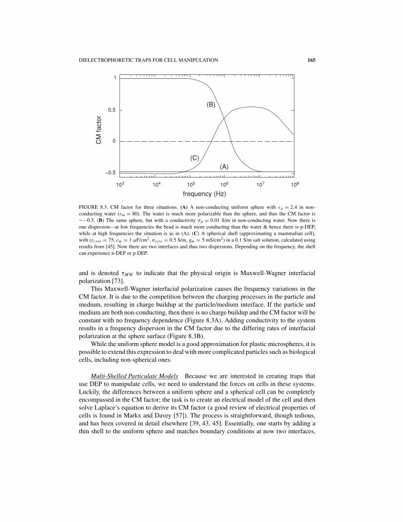
DIELECTROPHORETIC TRAPS FOR CELL MANIPULATION 165
1
0.5
0
−0.5
103 104 105 106 107 108
(B)
(C)
(A)
frequency (Hz)
CM
fact
or
FIGURE 8.3. CM factor for three situations. (A) A non-conducting uniform sphere with εp = 2.4 in non-
conducting water (εm = 80). The water is much more polarizable than the sphere, and thus the CM factor is
∼−0.5. (B) The same sphere, but with a conductivity σp = 0.01 S/m in non-conducting water. Now there is
one dispersion—at low frequencies the bead is much more conducting than the water & hence there is p-DEP,
while at high frequencies the situation is as in (A). (C) A spherical shell (approximating a mammalian cell),
with (εcyto = 75, cm = 1 μF/cm2, σcyto = 0.5 S/m, gm = 5 mS/cm2) in a 0.1 S/m salt solution, calculated using
results from [45]. Now there are two interfaces and thus two dispersions. Depending on the frequency, the shell
can experience n-DEP or p-DEP.
and is denoted τMW to indicate that the physical origin is Maxwell-Wagner interfacialpolarization [73].
This Maxwell-Wagner interfacial polarization causes the frequency variations in theCM factor. It is due to the competition between the charging processes in the particle andmedium, resulting in charge buildup at the particle/medium interface. If the particle andmedium are both non-conducting, then there is no charge buildup and the CM factor will beconstant with no frequency dependence (Figure 8.3A). Adding conductivity to the systemresults in a frequency dispersion in the CM factor due to the differing rates of interfacialpolarization at the sphere surface (Figure 8.3B).
While the uniform sphere model is a good approximation for plastic microspheres, it ispossible to extend this expression to deal with more complicated particles such as biologicalcells, including non-spherical ones.
Multi-Shelled Particulate Models Because we are interested in creating traps thatuse DEP to manipulate cells, we need to understand the forces on cells in these systems.Luckily, the differences between a uniform sphere and a spherical cell can be completelyencompassed in the CM factor; the task is to create an electrical model of the cell and thensolve Laplace’s equation to derive its CM factor (a good review of electrical properties ofcells is found in Markx and Davey [57]). The process is straightforward, though tedious,and has been covered in detail elsewhere [39, 43, 45]. Essentially, one starts by adding athin shell to the uniform sphere and matches boundary conditions at now two interfaces,
166 JOEL VOLDMAN
deriving a CM factor very similar to Eqn (8.2) but with an effective complex permittivityε′
p that subsumes the effects of the complicated interior (see §5.3 of Hughes [39]). Thisprocess can be repeated multiple times to model general multi-shelled particles.
Membrane-Covered Spheres: Mammalian Cells, Protoplasts Adding a thin shell toa uniform sphere makes a decent electrical model for mammalian cells and protoplasts.The thin membrane represents the insulating cell membrane while the sphere represents thecytoplasm. The nucleus is not modeled is this approximation. For this model the effectivecomplex permittivity can be represented by:
ε′p = cm R · εcyto
cm R + εcyto
(8.6)
where εcyto is the complex permittivity of the cytoplasmic compartment and cm refers tocomplex membrane capacitance per unit area and is given by
cm = cm + gm/( jω) (8.7)
where cm and gm are the membrane capacitance and conductance per unit area (F/m2 andS/m2) and can be related to the membrane permittivity and conductivity by cm = εm/t andgm = σm/t , where t is the membrane thickness. The membrane conductance of intact cells isoften small and can be neglected. Because cell membranes are comprised of phospholipidbilayers whose thickness and permittivity varies little across cell types, the membranecapacitance per unit area is fairly fixed at cm ∼ 0.5 − 1μF/cm2 [64].
Plotting a typical CM factor for a mammalian cell shows that it is more complicated thanfor a uniform sphere. Specifically, since it has two interfaces, there are two dispersions inits CM factor, as shown in Figure 8.3C. In low-conductivity buffers, the cell will experiencea region of p-DEP, while in saline or cell-culture media the cells will only experiencen-DEP. This last point has profound implications for trap design. If one wishes to usecells in physiological buffers, one is restricted to n-DEP excitation, irrespective of appliedfrequency. Only by moving low-conductivity solutions can one create p-DEP forces in cells.While, as we discuss below, p-DEP traps are often easier to implement, one must then dealwith possible artifacts due to the artificial media.
One challenge for the designer in applying different models for the CM factor isgetting accurate values for the different layers. In Table 8.1 we list properties culled fromthe literature for several types of particles, along with the appropriate literature references.Care must be taken in applying these, as some of the properties may be dependent on thecell type, cell physiology, and suspending medium, as well as limited by the method inwhich they were measured. Besides the values listed below, there are also values on Jurkatcells [67] and other white blood cells [21].
Sphere with Two Shells: Bacteria and Yeast Bacteria and yeast have a cell wall inaddition to a cell membrane. Iterating on the multi-shell model can be used to derive aCM factor these types of particles [35, 76, 95]. Griffith et al. also used a double-shellmodel, this time to include the nucleus of a mammalian cells, in this case the humanneutrophil [29].
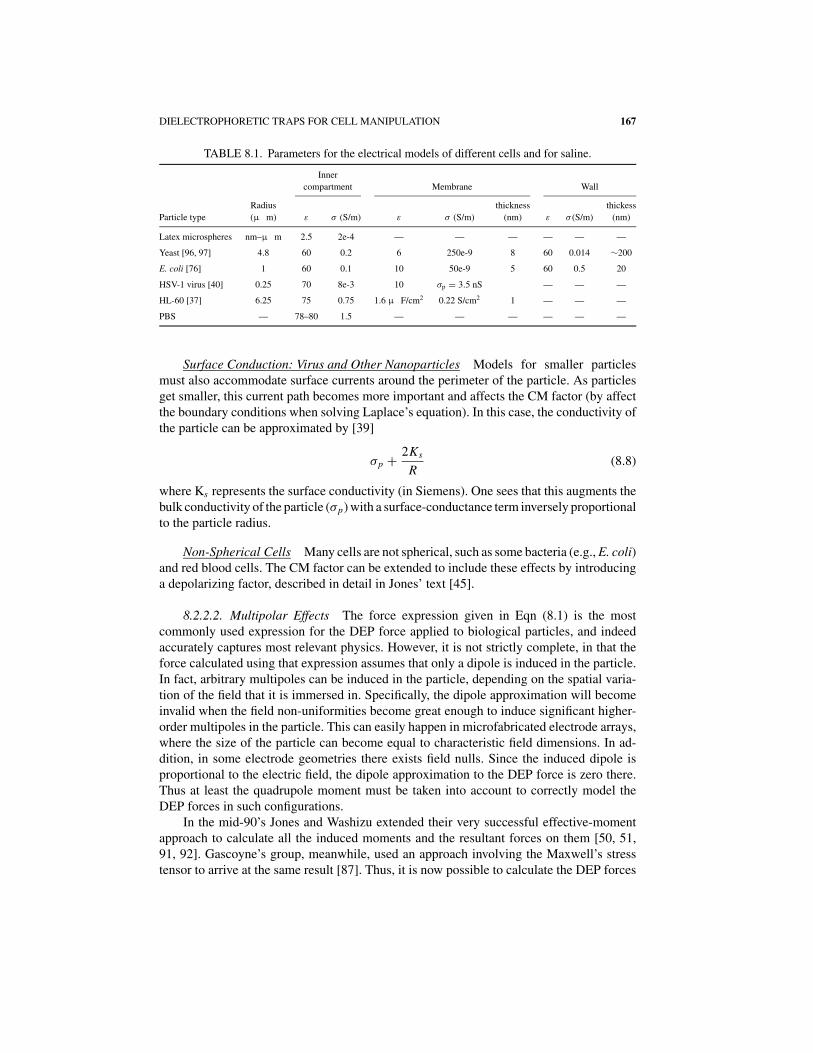
DIELECTROPHORETIC TRAPS FOR CELL MANIPULATION 167
TABLE 8.1. Parameters for the electrical models of different cells and for saline.
Inner
compartment Membrane Wall
Radius thickness thickess
Particle type (μ m) ε σ (S/m) ε σ (S/m) (nm) ε σ (S/m) (nm)
Latex microspheres nm–μ m 2.5 2e-4 — — — — — —
Yeast [96, 97] 4.8 60 0.2 6 250e-9 8 60 0.014 ∼200
E. coli [76] 1 60 0.1 10 50e-9 5 60 0.5 20
HSV-1 virus [40] 0.25 70 8e-3 10 σp = 3.5 nS — — —
HL-60 [37] 6.25 75 0.75 1.6 μ F/cm2 0.22 S/cm2 1 — — —
PBS — 78–80 1.5 — — — — — —
Surface Conduction: Virus and Other Nanoparticles Models for smaller particlesmust also accommodate surface currents around the perimeter of the particle. As particlesget smaller, this current path becomes more important and affects the CM factor (by affectthe boundary conditions when solving Laplace’s equation). In this case, the conductivity ofthe particle can be approximated by [39]
σp + 2Ks
R(8.8)
where Ks represents the surface conductivity (in Siemens). One sees that this augments thebulk conductivity of the particle (σp) with a surface-conductance term inversely proportionalto the particle radius.
Non-Spherical Cells Many cells are not spherical, such as some bacteria (e.g., E. coli)and red blood cells. The CM factor can be extended to include these effects by introducinga depolarizing factor, described in detail in Jones’ text [45].
8.2.2.2. Multipolar Effects The force expression given in Eqn (8.1) is the mostcommonly used expression for the DEP force applied to biological particles, and indeedaccurately captures most relevant physics. However, it is not strictly complete, in that theforce calculated using that expression assumes that only a dipole is induced in the particle.In fact, arbitrary multipoles can be induced in the particle, depending on the spatial varia-tion of the field that it is immersed in. Specifically, the dipole approximation will becomeinvalid when the field non-uniformities become great enough to induce significant higher-order multipoles in the particle. This can easily happen in microfabricated electrode arrays,where the size of the particle can become equal to characteristic field dimensions. In ad-dition, in some electrode geometries there exists field nulls. Since the induced dipole isproportional to the electric field, the dipole approximation to the DEP force is zero there.Thus at least the quadrupole moment must be taken into account to correctly model theDEP forces in such configurations.
In the mid-90’s Jones and Washizu extended their very successful effective-momentapproach to calculate all the induced moments and the resultant forces on them [50, 51,91, 92]. Gascoyne’s group, meanwhile, used an approach involving the Maxwell’s stresstensor to arrive at the same result [87]. Thus, it is now possible to calculate the DEP forces
168 JOEL VOLDMAN
in arbitrarily polarized non-uniform electric fields. A compact tensor representation of thefinal result in is
F(n)dep =
−...=p (n)[·]n(∇)nE
n!(8.9)
where n refers to the force order (n = 1 is the dipole, n = 2 is the quadropole, etc.),
−...=p (n)
is the multipolar induced-moment tensor, and [·]n and (∇)n represent n dot products andgradient operations. Thus one sees that the n-th force order is given by the interaction ofthe n-th-order multipolar moment with the n-th gradient of the electric field. For n = 1 theresult reverts to the force on a dipole (Eqn (8.1)).
A more explicit version of this expression for the time-averaged force in the i-th direc-tion (for sinusoidal excitation) is
⟨F (1)
i
⟩ = 2πεm R3 Re
[C M (1) Em
∂
∂xmE∗
i
]
⟨F (2)
i
⟩ = 2
3πεm R5 Re
[C M (2) ∂
∂xmEn
∂2
∂xn∂xmE∗
i
](8.10)
...
for the dipole (n = 1) and quadrupole (n = 2) force orders [51]. The Einstein summation con-vention has been applied in Eqn. (8.10). While this approach may seem much more difficultto calculate than Eqn (8.1), compact algorithms have been developed for calculating arbitrarymultiples [83]. The multipolar CM factor for a uniform lossy dielectric sphere is given by
C M (n) = ε p − εm
nε p + (n + 1)εm
(8.11)
It has the same form as the dipolar CM factor (Eqn. (2)) but has smaller limits. The quadrupo-lar CM factor (n = 2), for example, can only vary between +1/2 and −1/3.
8.2.2.3. Scaling Although the force on a dipole in a non-uniform field has beenrecognized for decades, the advent of microfabrication has really served as the launchingpoint for DEP-based systems. With the force now defined, I will now investigate whydownscaling has enabled these systems.
Most importantly, reducing the characteristic size of the system reduces the appliedvoltage needed to generate a given field gradient, and for a fixed voltage increases thatfield gradient. A recent article on scaling in DEP-based systems [46] illustrates many ofthe relevant scaling laws. Introducing the length scale L into Eqn (8.1) and appropriatelyapproximating derivatives, one gets that the DEP force (dipole term) scales as
Fdep ∼ R3 V 2
L3(8.12)
DIELECTROPHORETIC TRAPS FOR CELL MANIPULATION 169
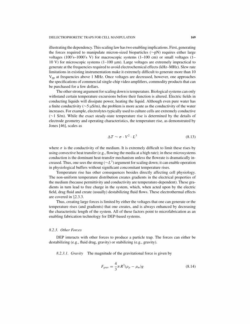
illustrating the dependency. This scaling law has two enabling implications. First, generatingthe forces required to manipulate micron-sized bioparticles (∼pN) requires either largevoltages (100’s–1000’s V) for macroscopic systems (1–100 cm) or small voltages (1–10 V) for microscopic systems (1–100 μm). Large voltages are extremely impractical togenerate at the frequencies required to avoid electrochemical effects (kHz–MHz). Slew ratelimitations in existing instrumentation make it extremely difficult to generate more than 10Vpp at frequencies above 1 MHz. Once voltages are decreased, however, one approachesthe specifications of commercial single-chip video amplifiers, commodity products that canbe purchased for a few dollars.
The other strong argument for scaling down is temperature. Biological systems can onlywithstand certain temperature excursions before their function is altered. Electric fields inconducting liquids will dissipate power, heating the liquid. Although even pure water hasa finite conductivity (∼5 μS/m), the problem is more acute as the conductivity of the waterincreases. For example, electrolytes typically used to culture cells are extremely conductive(∼1 S/m). While the exact steady-state temperature rise is determined by the details ofelectrode geometry and operating characteristics, the temperature rise, as demonstrated byJones [46], scales as
�T ∼ σ · V 2 · L3 (8.13)
where σ is the conductivity of the medium. It is extremely difficult to limit these rises byusing convective heat transfer (e.g., flowing the media at a high rate); in these microsystemsconduction is the dominant heat-transfer mechanism unless the flowrate is dramatically in-creased. Thus, one sees the strong (∼L3) argument for scaling down; it can enable operationin physiological buffers without significant concomitant temperature rises.
Temperature rise has other consequences besides directly affecting cell physiology.The non-uniform temperature distribution creates gradients in the electrical properties ofthe medium (because permittivity and conductivity are temperature-dependent). These gra-dients in turn lead to free charge in the system, which, when acted upon by the electricfield, drag fluid and create (usually) destabilizing fluid flows. These electrothermal effectsare covered in §2.3.3.
Thus, creating large forces is limited by either the voltages that one can generate or thetemperature rises (and gradients) that one creates, and is always enhanced by decreasingthe characteristic length of the system. All of these factors point to microfabrication as anenabling fabrication technology for DEP-based systems.
8.2.3. Other Forces
DEP interacts with other forces to produce a particle trap. The forces can either bedestabilizing (e.g., fluid drag, gravity) or stabilizing (e.g., gravity).
8.2.3.1. Gravity The magnitude of the gravitational force is given by
Fgrav = 4
3π R3(ρp − ρm)g (8.14)
170 JOEL VOLDMAN
where ρm and ρp refer to the densities of the medium and the particle, respectively, and g isthe gravitational acceleration constant. Cells and beads are denser than the aqueous mediaand thus have a net downward force.
8.2.3.2. Hydrodynamic Drag Forces Fluid flow past an object creates a drag force onthat object. In most systems, this drag force is the predominant destabilizing force. The fluidflow can be intentional, such as that created by pumping liquid past a trap, or unintentional,such as electrothermal flows.
The universal scaling parameter in fluid flow is the Reynolds number, which gives anindication of the relative strengths of inertial forces to viscous forces in the fluid. At thesmall length scales found in microfluidics, viscosity dominates and liquid flow is laminar.A further approximation assumes that inertia is negligible, simplifying the Navier-Stokesequations even further into a linear form. This flow regime is called creeping flow or Stokesflow and is the common approximation taken for liquid microfluidic flows.
In creeping flow, a sphere in a uniform flow field will experience a drag force—calledthe Stokes’ drag—with magnitude
Fdrag = 6πηRν (8.15)
where η is the viscosity of the liquid and ν is the far-field relative velocity of the liquid withrespect to the sphere. As an example, a 1-μm-diameter particle in a 1-mm/s water flow willexperience ∼10 pN of drag force.
Unfortunately, it is difficult to create a uniform flow field, and thus one must broadenthe drag force expression to include typically encountered flows. The most common flowpattern in microfluidics is the flow in a rectangular channel. When the channel is muchwider than it is high, this flow can be approximated as the one-dimensional flow betweento parallel plates, or plane Poiseuille flow. This flow profile is characterized by a parabolicvelocity distribution where the centerline velocity is 1.5× the average linear flow velocity
ν(z) = 1.5Q
wh
(1 −
(z − h/2
h/2
)2)
(8.16)
where Q is the volume flowrate, w and h are the width and height of the channel, respectively,and z is the height above the substrate at which the velocity is evaluated. The expression inEqn (8.15) can then be refined by using the fluid velocity at the height of the particle center.
Close to the channel wall (z � h) the quadratic term in Eqn (8.16) can be linearlyapproximated, resulting a velocity profile known as plane shear or plane Couette flow
ν(z) = 1.5Q
wh
(4
z
h
)= 6
Q
wh
z
h(8.17)
The error between the two flow profiles increases linearly with z for z � h/2; the errorwhen z = 0.1 · h is ∼10%.
Using Eqn (8.15) with the modified fluid velocities is a sufficient approximation forthe drag force in many applications, and is especially useful in non-analytical flow profiles
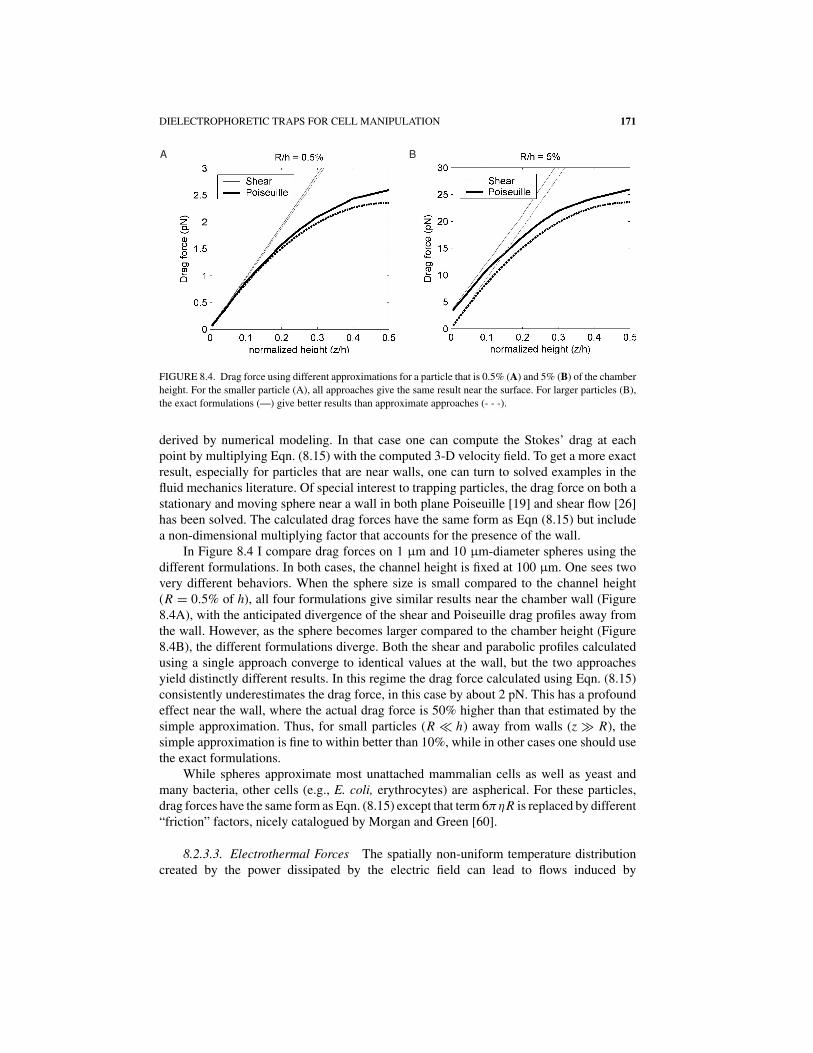
DIELECTROPHORETIC TRAPS FOR CELL MANIPULATION 171
A B
FIGURE 8.4. Drag force using different approximations for a particle that is 0.5% (A) and 5% (B) of the chamber
height. For the smaller particle (A), all approaches give the same result near the surface. For larger particles (B),
the exact formulations (—) give better results than approximate approaches (- - -).
derived by numerical modeling. In that case one can compute the Stokes’ drag at eachpoint by multiplying Eqn. (8.15) with the computed 3-D velocity field. To get a more exactresult, especially for particles that are near walls, one can turn to solved examples in thefluid mechanics literature. Of special interest to trapping particles, the drag force on both astationary and moving sphere near a wall in both plane Poiseuille [19] and shear flow [26]has been solved. The calculated drag forces have the same form as Eqn (8.15) but includea non-dimensional multiplying factor that accounts for the presence of the wall.
In Figure 8.4 I compare drag forces on 1 μm and 10 μm-diameter spheres using thedifferent formulations. In both cases, the channel height is fixed at 100 μm. One sees twovery different behaviors. When the sphere size is small compared to the channel height(R = 0.5% of h), all four formulations give similar results near the chamber wall (Figure8.4A), with the anticipated divergence of the shear and Poiseuille drag profiles away fromthe wall. However, as the sphere becomes larger compared to the chamber height (Figure8.4B), the different formulations diverge. Both the shear and parabolic profiles calculatedusing a single approach converge to identical values at the wall, but the two approachesyield distinctly different results. In this regime the drag force calculated using Eqn. (8.15)consistently underestimates the drag force, in this case by about 2 pN. This has a profoundeffect near the wall, where the actual drag force is 50% higher than that estimated by thesimple approximation. Thus, for small particles (R � h) away from walls (z � R), thesimple approximation is fine to within better than 10%, while in other cases one should usethe exact formulations.
While spheres approximate most unattached mammalian cells as well as yeast andmany bacteria, other cells (e.g., E. coli, erythrocytes) are aspherical. For these particles,drag forces have the same form as Eqn. (8.15) except that term 6πηR is replaced by different“friction” factors, nicely catalogued by Morgan and Green [60].
8.2.3.3. Electrothermal Forces The spatially non-uniform temperature distributioncreated by the power dissipated by the electric field can lead to flows induced by
172 JOEL VOLDMAN
electrothermal effects. These effects are covered in great detail by Morgan and Green[60]. Briefly, because the medium permittivity and conductivity are functions of temper-ature, temperature gradients directly lead to gradients in ε and σ . These gradients in turngenerate free charge which can be acted upon by an electric field to move and drag fluidalong with it, creating fluid flow. This fluid flow creates a drag force on an immersedbody just as it does for conventional Stokes’ drag (Eqn. (8.15)). In general, derivations ofthe electrothermal force density, the resulting liquid flow, and the drag require numericalmodeling because the details of the geometry profoundly impact the results. Castellanoset al. have derived solutions for one simple geometry, and have used it to great effect toderive some scaling laws [6].
8.3. DESIGN FOR USE WITH CELLS
Since dielectrophoretic cell manipulation exposes cells to strong electric fields, oneneeds to know how these electric fields might affect cell physiology. Ideally, one would liketo determine the conditions under which the trapping will not affect the cells and use thoseconditions to constrain the design. Of course, cells are poorly understood complex systemsand thus it is impossible to know for certain that one is not perturbing the cell. However, allbiological manipulations—cell culture, microscopy, flow cytometer, etc.—alter cell phys-iology. What’s most important is to minimize known influences on cell behavior and thenuse proper controls to account for the unknown influences. In short, good experimentaldesign.
The known influences of electric fields on cells can be split into the effects due tocurrent flow, which causes heating, and direct interactions of the fields with the cell. We’llconsider each of these in turn.
Au: Pls. checkHeadingsNumber.
8.3.1.1. Current-Induced Heating Electric fields in a conductive medium will causepower dissipation in the form of Joule heating. The induced temperature changes can havemany effects on cell physiology. As mentioned previously, microscale DEP is advantageousin that it minimizes temperature rises due to dissipated power. However, because cells canbe very sensitive to temperature changes, it is not assured that any temperature rises will beinconsequential.
Temperature is a potent affecter of cell physiology [4, 11, 55, 75]. Very high temper-atures (>4 ◦C above physiological) are known to lead to rapid mammalian cell death, andresearch has focused on determining how to use such knowledge to selectively kill cancercells [81]. Less-extreme temperature excursions also have physiological effects, possiblydue to the exponential temperature dependence of kinetic processes in the cell [93]. Onewell-studied response is the induction of the heat-shock proteins [4, 5]. These proteins aremolecular chaperones, one of their roles being to prevent other proteins from denaturingwhen under environmental stresses.
While it is still unclear as to the minimum temperature excursion needed to induceresponses in the cell, one must try to minimize any such excursions. A common rule ofthumb for mammalian cells is to keep variations to <1 ◦C, which is the approximate dailyvariation in body temperature [93]. The best way we have found to do this is to numericallysolve for the steady-state temperature rise in the system due to the local heat sources given
DIELECTROPHORETIC TRAPS FOR CELL MANIPULATION 173
by σE2. Convection and radiation can usually be ignored, and thus the problem reduces tosolving for the conduction heat flow subject to the correct boundary conditions. Then, usingthe scaling of temperature rise with electric field and fluid conductivity (Eqn. (8.13)), onecan perform a parametric design to limit temperature rises.
8.3.1.2. Direct Electric-Field Interactions Electric fields can also directly affect thecells. The simple membrane-covered sphere model for mammalian cells can be used todetermine where the fields exist in the cell as the frequency is varied. From this one candetermine likely pathways by which the fields could impact physiology [31, 73]. Performingthe analysis indicates that the imposed fields can exist across the cell membrane or thecytoplasm. A qualitative electrical model of the cell views the membrane as a parallel RCcircuit connected in-between RC pairs for the cytoplasm and the media. At low frequencies(<MHz) the circuit looks like three resistors in series and because the membrane resistance islarge the voltage is primarily dropped across it. This voltage is distinct from the endogenoustransmembrane potential that exists in the cell. Rather, it represents the voltage derived fromthe externally applied field. The total potential difference across the cell membrane wouldbe given by the sum of the imposed and endogenous potentials. At higher frequencies theimpedance of the membrane capacitor decreases sufficiently that the voltage across themembrane starts to decrease. Finally, at very high frequencies (100’s MHz) the model lookslike three capacitors in series and the membrane voltage saturates.
Quantitatively, the imposed transmembrane voltage can be derived as [73]
|Vtm | = 1.5|E|R√1 + (ωτ )2
(8.18)
where ω is the radian frequency of the applied field and τ is the time constant given by
τ = Rcm(ρcyto + 1/2ρmed )
1 + Rgm(ρcyto + 1/2ρmed )(8.19)
where ρcyto and ρmed med are the cytoplasmic and medium resistivities (�-m). At lowfrequencies |Vm | is constant at 1.5|E|R but decreases above the characteristic frequency(1/τ ). This model does not take into account the high-frequency saturation of the voltage,when the equivalent circuit is a capacitive divider.
At the frequencies used in DEP—10’s kHz to 10’s MHz—the most probably routeof interaction between the electric fields and the cell is at the membrane [79]. There areseveral reasons for this. First, electric fields already exist at the cell membrane, leading totransmembrane voltages in the 10’s of millivolts. Changes in these voltages could affectvoltage-sensitive proteins, such as voltage-gated ion channels [7]. Second, the electric fieldacross the membrane is greatly amplified over that in solution. From Eqn. (6.18) one getsthat at low frequencies
|Vtm | = 1.5|E|R√1 + (ωτ )2
≈ 1.5|E|R(8.20)
|Etm | ≈ |Vm |/t = (1.5R/t) · |E|
174 JOEL VOLDMAN
and thus at the membrane the imposed field is multiplied by a factor of 1.5 R/t (∼1000),which can lead to quite large membrane fields (Etm). This does not preclude effects dueto cytoplasmic electric fields. However, these effects have not been as intensily studied,perhaps because 1) those fields will induce current flow and thus heating, which is not adirect interaction, 2) the fields are not localized to an area (e.g., the membrane) that is likelyto have field-dependent proteins, and 3) unlike the membrane fields, the cytoplasmic fieldsare not amplified.
Several studies have investigated possible direct links between electric fields and cells.At low frequencies, much investigation has focused on 60-Hz electromagnetic fields andtheir possible effects, although the studies thus far are inconclusive [54]. DC fields have alsobeen investigated, and have been shown to affect cell growth [44] as well as reorganizationof membrane components [68]. At high frequencies, research has focused on the biologicaleffects of microwave radiation, again inconclusively [65].
In the frequency ranges involved in DEP, there has been much less research. Tsong hasprovided evidence that some membrane-bound ATPases respond to fields in the kHz–MHzrange, providing at least one avenue for interaction [79]. Electroporation and electrofu-sion are other obvious, although more violent, electric field-membrane coupling mecha-nisms [98].
Still other research has been concerned specifically with the effects of DEP on cells,and has investigated several different indicators of cell physiology to try to elucidate anyeffects. One of the first studies was by the Fuhr et al., who investigated viability, anchoragetime, motility, cell growth rates, and lag times after subjecting L929 and 3T3 fibroblast cellsin saline to short and long (up to 3 days) exposure to 30–60 kV/m fields at 10–40 MHz nearplanar quadrupoles [16]. They estimated that the transmembrane load was <20 mV. Thefields had no discernable effect.
Another study investigated changes in cell growth rate, glucose uptake, lactate andmonoclonal antibody production in CHO & HFN 7.1 cells on top of interdigitated elec-trodes excited at 10 MHz with ∼105 V/m in DMEM (for the HFN 7.1 cells) or serum-freemedium (for the CHO cells) [12]. Under these conditions they observed no differences inthe measured properties between the cells and control populations.
Glasser and Fuhr attempted to differentiate between heating and electric-field ef-fects on L929 mouse fibroblast cells in RPMI to the fields from planar quadrupoles [24].They imposed ∼40 kV/m fields of between 100 kHZ and 15 MHz for 3 days andobserved monolayers of cells near the electrodes with a video microscopy setup,similar to their previous study [16]. They indirectly determined that fields of ∼40kV/m caused an ∼2 ◦C temperature increase in the cells, but did not affect cell-division rates. They found that as they increased field frequency (from 500 kHZ to 15MHz) the maximum tolerable field strength (before cell-division rates were altered) in-creased. This is consistent with a decrease in the transmembrane load with increasingfrequency.
Wang et al. studied DS19 murine erythroleukemia cells exposed to fields (∼105 V/m)of 1 kHz–10 MHz in low-conductivity solutions for up to 40-min [90]. They foundno effects due to fields above 10 kHz. They determined that hydrogen peroxideproduced by reactions at the electrode interfaces for 1 kHz fields caused changesin cell growth lag phase, and that removal of the peroxide restored normal cellgrowth.
DIELECTROPHORETIC TRAPS FOR CELL MANIPULATION 175
On the p-DEP side, Archer et al. subjected fibroblast-like BHK 21 C13 cells top-DEP forces produced by planar electrodes arranged in a sawtooth configuration [1].They used low-conductivity (10 mS/m) isoosmotic solutions and applied fields of ∼105
V/m at 5 MHz. They monitored cell morphology, cell doubling time, oxidative respira-tion (mitochondrial stress assay), alterations in expression of the immediate-early proteinfos, and non-specific gene transcription directly after a 15 minute exposure and after a30-min time delay. They observed 20–30% upregulation of fos expression and a upregulationof a few unknown genes (determined via mRNA analysis). Measured steady-state tempera-tures near the cells were <1 ◦C above normal, and their calculated transmembrane voltageunder their conditions was <100 μV, which should be easily tolerable. The mechanism—thermal or electrical—of the increased gene expression was left unclear. It is possible thatartifacts from p-DEP attraction of the cells to the electrodes led to observed changes. Ei-ther way, this study certainly demonstrates the possibility that DEP forces could affect cellphysiology.
Finally, Gray et al. exposed bovine endothelial cells in sucrose media (with serum) todifferent voltages—and thus fields—for 30-min in order to trap them and allow them toadhere to their substrates. They measured viability and growth of the trapped cells and foundthat cell behavior was the same as controls for the small voltages but that large voltagescaused significant cell death [27]. This study thus demonstrates the p-DEP operation inartificial media under the proper conditions does not grossly affect cell physiology.
In summary, studies specifically interested in the effects of kHz–MHz electroquasistaticfields on cells thus far demonstrate that choosing conditions under which the transmem-brane loads and cell heating are small—e.g., >MHz frequencies, and fields in ∼10’s kV/mrange—can obviate any gross effects. Subtler effects, such as upregulation of certain geneticpathways or activation of membrane-bound components could still occur, and thus DEP, aswith any other assay technique, must be used with care.
8.4. TRAP GEOMETRIES
The electric field, which creates the DEP force, is in turn created by electrodes. Inthis section I will examine some of the electrode structures used in this field and theirapplicability to trapping cells and other microparticles. The reader is also encouraged toread the relevant chapters in Hughes’ [39] and Morgan and Green’s texts [60], which containdescriptions of some field geometries.
One can create traps using either p-DEP or n-DEP. Using n-DEP a zero-force pointis created away from electrodes at a field minimum and the particle is trapped by pushingat it from all sides. In p-DEP the zero-force point is at a field maximum, typically at theelectrode surface or at field constrictions. Both approaches have distinct advantages anddisadvantages, as outlined in Table 8.2. For each application, the designer must balancethese to select the best approach.
8.4.1. n-DEP Trap Geometries
Although an infinite variety of electrode geometries can be created, the majority ofresearch has focused on those that are easily modeled or easily created.
176 JOEL VOLDMAN
TABLE 8.2. Comparison of advantages and disadvantages of p-DEP and n-DEP approaches
to trapping cells.
p-DEP n-DEP
Must use low conductivity artificial media (−) Can use saline or other high-salt buffers (+)
CM factor can go to +1 (+) CM factor can go to −0.5 (−)
Less heating (+) More heating (−)
Typically easier to trap by pulling (+) Typically harder to trap by pushing (−)
Traps usually get stronger as V increases (+) Traps often do not get stronger with increasing V (−)
Cells stick to or can be damaged by electrodes (−) Cells are physically removed from electrodes (+)
Cells go to maximum electric field (−) Cells go to minimum electric field (+)
8.4.1.1. Interdigitated Electrodes Numerous approximate and exact analytical so-lutions exist for the interdigitated electrode geometry (Figure 8.5A), using techniques asvaried as conformal mapping [23, 82], Green’s function [10, 86], and Fourier series [33,61]. Recently, an elegant exact closed-form solution was derived [8]. Numerical solutionsare also plentiful [28].
While the interdigitated electrode geometry has found much use in DEP separations, itdoes not make a good trap for a few reasons. First, the long extent of the electrodes in onedirection creates an essentially 2-D field geometry and thus no trapping is possible alongthe length of the electrodes. Further, the spatial variations in the electric field—which createthe DEP force—decrease exponentially away from the electrode surface. After about oneelectrode’s worth of distance away from the susbtrate, the field is mostly uniform at a givenheight, and thus DEP trapping against fluid flows or other perpendicular forces cannot occur.Increasing the field to attempt to circumvent this only pushes the particle farther away fromthe electrodes, a self-defeating strategy; like the planar quadrupole [83], this trap is actuallystrongest at lower voltages, when the particle is on the substrate.
8.4.1.2. Quadrupole Electrodes Quadrupole electrodes are four electrodes with al-ternating voltage polarities applied to every other electrode (Figure 8.5B). The field for fourpoint charges can be easily calculated by superposition, but relating the charge to voltage(via the capacitance) is difficult in general and must be done numerically.
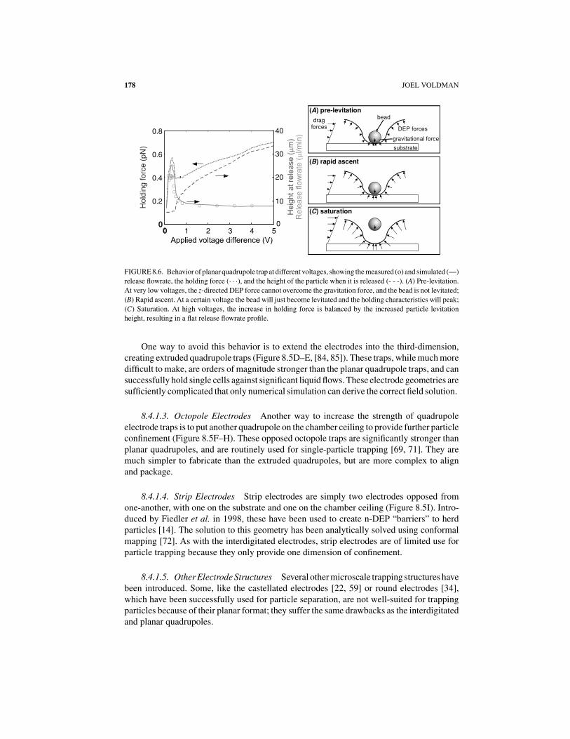
Planar quadrupoles can create rudimentary particle traps (Figure 8.5B), and can trapsingle particles down to 100’s of nm [40]. Using n-DEP, they provide in-plane particleconfinement, and can provide three-dimensional confinement if the particle is denser thanthe suspending medium. As with interdigitated electrodes, however, these traps suffer fromthe drawback that increasing the field only pushes the particle farther out of the trap anddoes not necessarily increase confinement. We showed this in 2001 with measurements ofthe strength of these traps [83]. Unexpectedly, the traps are strongest at an intermediatevoltage, just before the particle is about to be levitated (Figure 8.6).
A variant of the quadrupole electrodes is the polynomial electrode geometry (Figure8.5C), introduced by Huang and Pethig in 1991 [36]. By placing the electrode edges at theequipotentials of the applied field, it is possible to analytically specify the field between theelectrodes. One caveat of this approach is that it solves the 2-D Laplace equation, which isnot strictly correct for the actual 3-D geometry; thus, the electric field is at best only trulyspecified right at the electrode surface, and not in all of space.
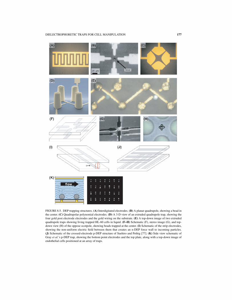
DIELECTROPHORETIC TRAPS FOR CELL MANIPULATION 177
FIGURE 8.5. DEP trapping structures. (A) Interdigitated electrodes. (B) A planar quadrupole, showing a bead in
the center. (C) Quadrupolar polynomial electrodes. (D) A 3-D view of an extruded quadrupole trap, showing the
four gold post electrode electrodes and the gold wiring on the substrate. (E) A top-down image of two extruded
quadrupole traps showing living trapped HL-60 cells in liquid. (F–H) Schematic (F), stereo image (G), and top-
down view (H) of the oppose ocotpole, showing beads trapped at the center. (I) Schematic of the strip electrodes,
showing the non-uniform electric field between them that creates an n-DEP force wall to incoming particles.
(J) Schematic of the crossed-electrode p-DEP structure of Suehiro and Pethig [77]. (K) Side view schematic of
Gray et al.’s p-DEP trap, showing the bottom point electrodes and the top plate, along with a top-down image of
endothelial cells positioned at an array of traps.
178 JOEL VOLDMAN
1 2 3 4 5
0.2 10
0
20
30
40
0.4
0.6
0.8
drag forces DEP forces
gravitational force
substrate
bead( ) pre-levitationA
( ) rapid ascentB
( ) saturationC
FIGURE 8.6. Behavior of planar quadrupole trap at different voltages, showing the measured (o) and simulated (—)
release flowrate, the holding force (· · ·), and the height of the particle when it is released (- - -). (A) Pre-levitation.
At very low voltages, the z-directed DEP force cannot overcome the gravitation force, and the bead is not levitated;
(B) Rapid ascent. At a certain voltage the bead will just become levitated and the holding characteristics will peak;
(C) Saturation. At high voltages, the increase in holding force is balanced by the increased particle levitation
height, resulting in a flat release flowrate profile.
One way to avoid this behavior is to extend the electrodes into the third-dimension,creating extruded quadrupole traps (Figure 8.5D–E, [84, 85]). These traps, while much moredifficult to make, are orders of magnitude stronger than the planar quadrupole traps, and cansuccessfully hold single cells against significant liquid flows. These electrode geometries aresufficiently complicated that only numerical simulation can derive the correct field solution.
8.4.1.3. Octopole Electrodes Another way to increase the strength of quadrupoleelectrode traps is to put another quadrupole on the chamber ceiling to provide further particleconfinement (Figure 8.5F–H). These opposed octopole traps are significantly stronger thanplanar quadrupoles, and are routinely used for single-particle trapping [69, 71]. They aremuch simpler to fabricate than the extruded quadrupoles, but are more complex to alignand package.
8.4.1.4. Strip Electrodes Strip electrodes are simply two electrodes opposed fromone-another, with one on the substrate and one on the chamber ceiling (Figure 8.5I). Intro-duced by Fiedler et al. in 1998, these have been used to create n-DEP “barriers” to herdparticles [14]. The solution to this geometry has been analytically solved using conformalmapping [72]. As with the interdigitated electrodes, strip electrodes are of limited use forparticle trapping because they only provide one dimension of confinement.
8.4.1.5. Other Electrode Structures Several other microscale trapping structures havebeen introduced. Some, like the castellated electrodes [22, 59] or round electrodes [34],which have been successfully used for particle separation, are not well-suited for trappingparticles because of their planar format; they suffer the same drawbacks as the interdigitatedand planar quadrupoles.
DIELECTROPHORETIC TRAPS FOR CELL MANIPULATION 179
Recently, a team in Europe has been developing an active n-DEP-based trappingarray [56]. Essentially, their device consists of a two-dimensional array of square elec-trodes and a conductive lid. The key is that incorporating CMOS logic (analog switchesand memory) allows each square electrode to be connected to in-phase or out-of-phase ACvoltage in a programmable fashion. By putting a center square at +V and the surroundingsquares at −V, they can create an in-plane trap. Further putting the chamber top at +Vcloses the cage, giving 3-D confinement. The incorporation of CMOS further means thatvery few leads are required to control an indefinite number of sites, creating a readily scal-able technology. Using this trap geometry, they have successfully manipulated both beadsand cells, although moving cells from one site to another is currently quite slow (∼sec).
8.4.2. p-DEP Trap Geometries
p-DEP traps, while easier to create, have seen less use, probably because the requiredlow-conductivity media can perturb cell physiology (at least for mammalian cells) and be-cause of concerns about electrode-cell interactions. As stated earlier, obtaining p-DEP withmammalian cells requires low-conductivity buffer, and this can create biological artifactsin the system. Nonetheless, several geometries do exist.
An early p-DEP-based trapping system was described by Suehiro and Pethig (Figure8.5J, [77]). This used a set of parallel individually addressable electrodes on one substrateand another set of electrodes on the bottom substrate that were rotated 90◦. By actuatingone electrode on top and bottom, they could create a localized field maximum that couldbe moved around, allowing cell manipulation.
Another example is a concentric ring levitator that uses feedback-controlled p-DEP toactually trap particles away from electrodes [66]. In an air environment, they can levitatedrops of water containing cells by pulling up against gravity with an upper electrode, feedingback the vertical position of the droplet to maintain a constant height.
Recently Gray et al. created a geometry consisting of a uniform top plate and electrodepoints on the substrate to create the field concentrations (Figure 8.5K, [27]). They were ableto pattern cells onto the stubs using p-DEP. Importantly, experiments showed that the low-conductivity buffer did not affect the gross physiology of the cells at reasonable voltages.Finally, Chou et al. used geometric constrictions in an insulator to create field maxima in aconductivity-dominated system [9]. These maxima were used to trap DNA.
8.4.3. Lessons for DEP Trap Design
The preceding discussion raises some important points for DEP trap design. First, thechoice of whether to trap via p-DEP or n-DEP is a system-level partitioning problem. Forinstance, if one absolutely requires use in saline, then n-DEP must be used. If, however,minimizing temperature rises is most important, then p-DEP may be better, as the low-conductivity media will reduce temperature rises. The decision may also be affected byfabrication facilities, etc.
In general, p-DEP traps are easier to create than n-DEP traps, because it is easier tohold onto a particle by attracting it than repelling it. The tradeoff is that p-DEP requiresartificial media for use with mammalian cells. Nonetheless, the key for effective p-DEP isthe creation of isolated field maxima. Because the particles are pulled into the field, p-DEPtraps always trap stronger at higher voltages.
180 JOEL VOLDMAN
Creating effective n-DEP traps is more difficult, and requires some sort of three-dimensional confinement. This is difficult (though not impossible) to do with planar elec-trode structures, because the +z-component of the DEP force scales with voltage just asmuch as the in-plane components. This fundamentally pushes the particle away from thetrap when one increases the voltage, drastically limiting trap strength. Any planar electrodestructure, including the planar quadrupoles and interdigitated electrodes described abovefail this test and therefore make a poor n-DEP trap. The two extant structures that exhibitstrong trapping create three-dimensional trapping by removing the net +z-directed DEPforce. Both the extruded quadrupole and opposed octopole structures do this by creating astructure that cancels out z-directed DEP forces at the trap center, enabling one to increasevoltage—and thus trap strength—without pushing the particle farther away.
8.5. QUANTITATING TRAP CHARACTERISTICS
In order to assess whether a quantitative design is successful, one needs some quanti-tative validation of the fields and forces in DEP traps. Given that the complete DEP theoryis known and that the properties of at least some particles are known, it should be possibleto quantitate trap parameters. Those that are of interest include trap strength, field strength,and the spatial extents of the trap.
Measuring traps requires a quantitative readout. This typically takes the form of a testparticle (or particles), whose location or motion can be measured and then matched againstsome prediction. Quantitative matching gives confidence in the validity of a particularmodeling technique, thus allowing predictive design of new traps.
Starting in the 1970’s, Tom Jones and colleagues explored DEP levitation in macro-scopic electrode systems [47–49, 53]. Using both stable n-DEP traps and p-DEP traps withfeedback control, they could measure levitation heights of different particles under variousconditions. Knowledge of the gravitation force on the particle could then be used to as aprobe of the equally opposing DEP forces at equilibrium.
Levitation measurements have continued to the present day, but now applied to micro-fabricated electrode structures, such as levitation height measurements of beads in planarquadrupoles [15, 25, 32], or on top of interdigitated electrodes [37, 58]. In all these mea-surements, errors arise because of the finite depth of focus of the microscope objectiveand because it is difficult to consistently focus on the center of the particle. The boundarybetween levitation and the particle sitting on the ground is a “sharp” event and is usuallyeasier to measure and correlate to predictions than absolute particle height [25].
Wonderful pioneering work in quantitating the shapes of the fields was reported by thegroup in Germany in the 1992 and 1993 when they introduced their planar quadrupole [15]and opposed octopole [69] trap geometries. In the latter paper, the authors trapped 10’s ofbeads that were much smaller than the trap size. The beads packed themselves to minimizetheir overall energy, in the process creating surfaces that reflected the force distribution inthe trap. By comparing the experimental and predicted surfaces, they could validate theirmodeling.
An early velocity-measurement approach was described X.-B. Wang et al., who usedspiral electrodes and measured radial velocity and levitation height of breast cancer cells asthey varied frequency, particle radius, and medium conductivity [89]. They then matched
DIELECTROPHORETIC TRAPS FOR CELL MANIPULATION 181
the data to DEP theory, using fitting parameters to account for unknown material prop-erties, and obtained good agreement. These researchers performed similar analyses usingerythroleukemia cells in interdigitated electrode geometries, again obtaining good fits ofthe data to the theory [88].
Another approach that compares drag force to DEP force is described by Tsukaharaet al., where they measured the velocity as a particle moved toward or away from theminimum in a planar quadrupole polynomial electrode [80]. If the electric field and particleproperties are known, it should be possible to relate the measured velocity to predictions,although, as described earlier, the use of Stokes drag introduces errors when the particle isnear the wall and the forces they calculated for their polynomial electrodes are only valid atthe electrode symmetry plane. This was reflected in the use of a fitting parameter to matchpredictions with experiment, although in principle absolute prediction should be possible.
The German team that initially introduced the idea of opposed electrodes on both thebottom and top of the chamber have continued their explorations into this geometry withgreat success. They have attempted to quantify the strength of their traps in two differentways. In the first approach, they measure the maximum flowrate against which a trap canhold a particle. Because of the symmetry of their traps, the particles are always along themidline of the flow, and by approximating the drag force on the particle with the Stokesdrag (Eqn (8.15)) they can measure the strength of the trap in piconewtons [13, 62, 72].Because they can calculate the electric fields and thus DEP forces, they have even been ableto absolutely correlate predictions to experiment [72]. With such measurements they havedetermined that their opposed electrode devices can generate ∼20pN of force on 14.9-μmdiameter beads [62].
The other approach that these researchers have taken to measuring trap strength isto combine DEP octopole traps with optical tweezers [2]. If the strength of one of thetrapping techniques is known then it can be used to calibrate the other. In one approach,this was done by using optical tweezers to displace a bead from equilibrium in a DEPtrap, then measuring the voltage needed to make that bead move back to center [18]. Theyused this approach to measure the strength of the optical tweezers by determining the DEPforce on the particle at that position at the escape voltage. In principle, one could use thisto calibrate the trap if the optical tweezer force constant was known.
In the other approach, at a given voltage and optical power, they measured the maximumthat the bead could be displaced from the DEP minimum before springing back [70]. Thisis very similar to the prior approach, although it also allows one to generate a force-displacement characteristic for the DEP trap, mapping out the potential energy well.
A clever and conceptually similar approach was tried by Hughes and Morgan with aplanar quadrupole [41], although in this case the unknown was the thrust exerted by E. colibacteria. By measuring the maximum point that the bacteria could be displaced from theDEP trap minimum, they could back out the bacterial thrust if the DEP force characteristicin the trap was known. They achieved good agreement between predictions and modeling,at least at lower voltages.
For much smaller particles, where statistics are important, Chou et al. captured DNA inelectrodeless p-DEP traps. They used the spatial distribution of the bacteria to measure thestrength of the traps [9]. They measured the width of the fluorescence intensity distributionof labeled DNA in the trap, and assuming that the fluorescence intensity was linearly relatedto concentration, could extract the force of the trap by equating the “Brownian” diffusive
182 JOEL VOLDMAN
force to the DEP force. The only unknown in this approach, besides the assumptions oflinearity, was the temperature, which could easily be measured.
In our lab we have been interested in novel trap geometries to enable novel trappingfunctionalities. One significant aim has been to create DEP traps for single cells that arestrong enough to hold against significant liquid flows, such that cells and reagents can betransported on and off the chips within reasonable time periods (∼min). Our approachto measuring trap strength is similar to the one described above, where the fluid velocitynecessary to break through a barrier is correlated to a barrier force [13, 62, 72]. This approachis also similar to those undertaken by the optical tweezer community, who calibrate theirtweezers by measuring the escape velocity of trapped particles at various laser powers.
We have chosen to generalize this approach to allow for particles that may be nearsurfaces where Stokes drag is not strictly correct, where multipolar DEP forces may beimportant, and where electrode geometries may be complex [83]. In our initial validationof this approach, we were able to make absolute prediction of trap strength, as measured bythe minimum volumetric flowrate needed for the particle to escape the trap. This volumetricflowrate can be related to a linear flowrate and then to a drag force using the analyticalsolutions for the drag on a stationary particle near a wall.
Our validation explained the non-intuitive trapping behavior of planar quadrupole traps(Figure 8.6), giving absolute agreement—to within 30%—between modeling and exper-iment with no fitting parameters [83]. We then extended this modeling to design a new,high-force trap created from extruded electrodes that could hold 13.2-μm beads with 95 pNof force at 2 V, and HL-60 cells with ∼60 pN of force at the same voltage [84, 85]. Again, wecould make absolute predictions and verify them with experiments. We continue to extendthis approach to design traps for different applications.
8.6. CONCLUSIONS
In conclusion, DEP traps, when properly confined, can be used to confine cells, actingas electrical tweezers. In this fashion cells can be positioned and manipulated in ways notachievable using other techniques, due to the dynamic nature of electric fields and the abilityto shape the electrodes that create them.
Achieving a useful DEP system for manipulating cells requires an understanding ofthe forces present in these systems and an ability to model their interactions so as to predictthe operating system conditions and whether they are compatible with cell health, etc. I havepresented one approach to achieving these goals that employs quantitative modeling of thesesystems, along with examples of others who have sought to quantitate the performance oftheir systems.
8.7. ACKNOWLEDGEMENTS
The author wishes to thank Tom Jones for useful discussions and Thomas Schnelle forthe some of the images in Figure 8.4. The author also wishes to acknowledge support fromNIH, NSF, Draper Laboratories, and MIT for this work.
DIELECTROPHORETIC TRAPS FOR CELL MANIPULATION 183
REFERENCESAu: Providearticle title.[1] S. Archer, T.T. Li, A.T. Evans, S.T. Britland, and H. Morgan. Biochem. Biophys. Res. Commun., 257:687,
1999.
[2] A. Ashkin. Proc. Natl. Acad. Sci. U.S.A., 94:4853, 1997.
[3] A. Blake. Handbook of Mechanics, Materials, and Structures. Wiley, New York, 1985.
[4] R.H. Burdon. Biochem. J., 240:313, 1986.
[5] S.W. Carper, J.J. Duffy, and E.W. Gerner. Cancer Res., 47:5249, 1987.
[6] A. Castellanos, A. Ramos, A. Gonzalez, F. Morgan, and N. Green. Proceedings of 14th International Con-ference on Dielectric Liquids 7–12 July 2002. pp. 52, 2002.
[7] W.A. Catterall. Ann. Rev. Biochem., 64:493, 1995.
[8] D.E. Chang, S. Loire, and I. Mezic. J. Phys. D: Appl. Phys., 36:3073, 2003.
[9] C.F. Chou, J.O. Tegenfeldt, O. Bakajin, S.S. Chan, E.C. Cox, N. Darnton, T. Duke, and R.H. Austin. Biophys.J., 83:2170, 2002.
[10] D.S. Clague and E.K. Wheeler. Phys. Rev. E, 64:026605, 2001.
[11] E.A. Craig. CRC Crit. Rev. Biochem., 18:239, 1985.
[12] A. Docoslis, N. Kalogerakis, and L.A. Behie. Cytotechnology, 30:133, 1999.
[13] M. Durr, J. Kentsch, T. Muller, T. Schnelle, and M. Stelzle. Electrophoresis, 24:722, 2003.
[14] S. Fiedler, S.G. Shirley, T. Schnelle, and G. Fuhr. Anal. Chem., 70:1909, 1998.
[15] G. Fuhr, W.M. Arnold, R. Hagedorn, T. Muller, W. Benecke, B. Wagner, and U. Zimmermann. Biochimi. Et.Biophys. Acta, 1108:215, 1992a.
[16] G. Fuhr, H. Glasser, T. Muller, and T. Schnelle. Biochimi. Et. Biophys. Acta-Gen. Sub., 1201:353, 1994.
[17] G. Fuhr, R. Hagedorn, T. Muller, W. Benecke, and B.Wagner. J. Microelectromech. Sys., 1:141, 1992b.
[18] G. Fuhr, T. Schnelle, T. Muller, H. Hitzler, S. Monajembashi, and K.O. Greulich. Appl. Phys. A-Mater. Sci.Process., 67:385, 1998.
[19] P. Ganatos, R. Pfeffer, and S. Weinbaum. J. Fluid Mech., 99:755, 1980.
[20] P.R.C. Gascoyne and J. Vykoukal. Electrophoresis, 23:1973, 2002.
[21] P.R.C. Gascoyne, X.-B. Wang, Y. Huang, and F.F. Becker. IEEE Trans. Ind. Appl., 33:670, 1997.
[22] P.R.C. Gascoyne, H. Ying, R. Pethig, J. Vykoukal, and F.F. Becker. Measure. Sci. Technol., 3:439, 1992.
[23] W.J. Gibbs. Conformal Transformations in Electrical Engineering. Chapman & Hall, London, 1958.
[24] H. Glasser and G. Fuhr. Bioelectrochem. Bioenerget., 47:301, 1998.
[25] H. Glasser, T. Schnelle, T. Muller, and G. Fuhr. Thermochimi. Acta, 333:183, 1999.
[26] A.J. Goldman, R.G. Cox, and H. Brenner. Chem. Eng. Sci., 22:653, 1967.
[27] D.S. Gray, J.L. Tan, J. Voldman, and C.S. Chen. Biosens. Bioelectron., 19:771, 2004.
[28] N.G. Green, A. Ramos, and H. Morgan. J. Electrostat., 56:235, 2002.
[29] A.W. Griffith and J.M. Cooper. Anal. Chem., 70:2607, 1998.
[30] A.J. Grodzinsky and M.L. Yarmush. Electrokinetic separations. In G. Stephanopoulus (ed.), Bioprocessing,
Weinheim, Germany; New York, VCH, pp. 680, 1991.
[31] C. Grosse and H.P. Schwan. Biophys. J., 63:1632, 1992.
[32] L.F. Hartley, K. Kaler, and R. Paul. J. Electrostat., 46:233, 1999.
[33] Z. He. Nuclear instruments & methods in physics research, Section A accelerators, spectrometers, detectors
and associated equipment, 365:572, 1995.
[34] Y. Huang, K.L. Ewalt, M. Tirado, T.R. Haigis, A. Forster, D. Ackley, M.J. Heller, J.P. O’Connell, and M.
Krihak. Anal. Chem., 73:1549, 2001.
[35] Y. Huang, R. Holzel, R. Pethig, and X.-B. Wang. Phys. Med. Biol., 37:1499, 1992.
[36] Y. Huang and R. Pethig. Measure. Sci. Technol., 2:1142, 1991.
[37] Y. Huang, X.-B. Wang, F.F. Becker, and P.R.C. Gascoyne. Biophys. J., 73:1118, 1997.
[38] M.P. Hughes. Electrophoresis, 23:2569, 2002.
[39] M.P. Hughes. Nanoelectromechanics in Engineering and Biology, CRC Press, Boca Raton, Fla., 2003.
[40] M.P. Hughes and H. Morgan. J. Phys. D-Appl. Phys., 31:2205, 1998.
[41] M.P. Hughes and H. Morgan. Biotechnol. Prog., 15:245, 1999.
[42] M.P. Hughes, H. Morgan, F.J. Rixon, J.P. Burt, and R. Pethig. Biochim. Biophys. Acta, 1425:119, 1998.
[43] A. Irimajiri, T. Hanai, and A. Inouye. J. Theoret. Biol., 78:251, 1979.
[44] L.F. Jaffe and M.M. Poo. J. Exp. Zool., 209:115, 1979.
184 JOEL VOLDMAN
[45] T.B. Jones. Electromechanics of Particles. Cambridge University Press, Cambridge, 1995.
[46] T.B. Jones. IEEE Proc.-Nanobiotechnnol., 150:39, 2003.
[47] T.B. Jones and G.W. Bliss. J. Appl. Phys., 48:1412, 1977.
[48] T.B. Jones, G.A. Kallio, and C.O. Collins. J. Electrostat., 6:207, 1979.
[49] T.B. Jones and J.P. Kraybill. J. Appl. Phys., 60:1247, 1986.
[50] T.B. Jones and M. Washizu. J. Electrostat., 33:199, 1994.
[51] T.B. Jones and M. Washizu. J. Electrostat., 37:121, 1996.
[52] D.R. Jung, R. Kapur, T. Adams, K.A. Giuliano, M. Mrksich, H.G. Craighead, and D.L. Taylor. Crit. Rev.Biotechnol., 21:111, 2001.
[53] K.V.I.S. Kaler and T.B. Jones. Biophys. J., 57:173, 1990.
[54] A. Lacy-Hulbert, J.C. Metcalfe, and R. Hesketh. FASEB J., 12:395, 1998.
[55] S. Lindquist. Annu. Rev. Biochem., 55:1151, 1986.
[56] N. Manaresi, A. Romani, G. Medoro, L. Altomare, A. Leonardi, M. Tartagni, and R. Guerrieri. IEEE J.Solid-State Circ., 38:2297, 2003.
[57] G.H. Markx and C.L. Davey. Enzyme Microb. Technol., 25:161, 1999.
[58] G.H. Markx, R. Pethig, and J. Rousselet. J. Phys. D (Applied Physics), 30:2470, 1997.
[59] G.H. Markx, M.S. Talary, and R. Pethig. J. Biotechnol., 32:29, 1994.
[60] H. Morgan and N.G. Green. AC Electrokinetics: Colloids and Nanoparticles. Research Studies Press,
Baldock, Hertfordshire, England, 2003.
[61] H. Morgan, A.G. Izquierdo, D. Bakewell, N.G. Green, and A. Ramos. J. Phys. D-Appl. Phys., 34:1553, 2001.
[62] T. Muller, G. Gradl, S. Howitz, S. Shirley, T. Schnelle, and G. Fuhr. Biosens. Bioelectron., 14:247, 1999.
[63] M. Ozkan, T. Pisanic, J. Scheel, C. Barlow, S. Esener, and S.N. Bhatia. Langmuir, 19:1532, 2003.
[64] R. Pethig and D.B. Kell. Phys. Med. Biol., 32:933, 1987.
[65] C. Polk and E. Postow. Handbook of Biological Effects of Electromagnetic Fields. CRC Press, Boca Raton,
FL, 1996.
[66] L. Qian, M. Scott, K.V.I.S. Kaler, and R. Paul. J. Electrostat., 55:65, 2002.
[67] C. Reichle, T. Schnelle, T. Muller, T. Leya, and G. Fuhr. Biochim. Et. Biophys. Acta-Bioenerg., 1459:218,
2000.
[68] T.A. Ryan, J. Myers, D. Holowka, B. Baird, and W.W. Webb. Science, 239:61, 1988.
[69] T. Schnelle, R. Hagedorn, G. Fuhr, S. Fiedler, and T. Muller. Biochim. Et Biophys. Acta, 1157:127, 1993.
[70] T. Schnelle, T. Muller, and G. Fuhr. J. Electrostat., 46:13, 1999a.
[71] T. Schnelle, T. Muller, and G. Fuhr. J. Electrostat., 50:17, 2000.
[72] T. Schnelle, T. Muller, G. Gradl, S.G. Shirley, and G. Fuhr. J. Electrostat., 47:121, 1999b.
[73] H.P. Schwan. Dielectrophoresis and rotation of cells. In E. Neumann, A.E. Sowers, and C.A. Jordan, (eds.)
Electroporation and Electrofusion in Cell Biology. New York, Plenum Press, pp. 3, 1989.
[74] H.P. Schwan. Ann. Biomed. Eng., 20:269, 1992.
[75] J.R. Subjeck and T.T. Shyy. Am. J. Physiol., 250:C1, 1986.
[76] J. Suehiro, R. Hamada, D. Noutomi, M. Shutou, and M. Hara. J. Electrostat., 57:157, 2003.
[77] J. Suehiro and R. Pethig. J. Phys. D-Appl. Phys., 31:3298, 1998.
[78] K. Svoboda and S.M. Block. Ann. Rev. Biophys. Biomol. Struc., 23:247, 1994.
[79] T.Y. Tsong. Biochim. et Biophys. Acta, 1113:53, 1992.
[80] S. Tsukahara, T. Sakamoto, and H. Watarai. Langmuir, 16:3866, 2000.
[81] M. Urano and E.B. Douple. Thermal effects on cells and tissues. VSP, Utrecht, The Netherlands, 1988.
[82] P. Van Gerwen, W. Laureyn, W. Laureys, G. Huyberechts, M.O. De Beeck, K. Baert, J. Suls, W. Sansen,
P. Jacobs, L. Hermans, and R. Mertens. Sens. Actu. B-Chem., 49:73, 1998.
[83] J. Voldman, R.A. Braff, M. Toner, M.L. Gray, and M.A. Schmidt. Biophys. J., 80:531, 2001.
[84] J. Voldman, M. Toner, M.L. Gray, and M.A. Schmidt. Anal. Chem., 74:3984, 2002.
[85] J. Voldman, M. Toner, M.L. Gray, and M.A. Schmidt. J. Electrostat. 57:69, 2003.
[86] X. Wang, X.-B. Wang, F.F. Becker, and P.R.C. Gascoyne. J. Phys. D (Applied Physics), 29:1649, 1996.
[87] X. Wang, X.-B. Wang, and P.R.C. Gascoyne. J. Electrostat., 39:277, 1997a.
[88] X.-B. Wang, Y. Huang, P.R.C. Gascoyne, and F.F. Becker. IEEE Trans. Ind. Appl., 33:660, 1997b.
[89] X.-B. Wang, Y. Huang, X. Wang, F.F. Becker, and P.R.C. Gascoyne. Biophys. J., 72:1887, 1997c.
[90] X. J. Wang, J. Yang, and P.R.C. Gascoyne. Biochimi. Et Biophys. Acta-Gen. Sub., 1426:53, 1999.
[91] M. Washizu and T.B. Jones. J. Electrostat., 33:187, 1994.
[92] M. Washizu. and T. B. Jones. J. Electrostat., 38:199, 1996.

DIELECTROPHORETIC TRAPS FOR CELL MANIPULATION 185
[93] J.C. Weaver, T.E. Vaughan, and G.T. Martin. Biophys. J., 76:3026, 1999.
[94] J. Wu. J. Acoust. Soc. Am., 89:2140, 1991.
[95] G. Zhou, M. Imamura, J. Suehiro, and M. Hara. Conference Record of the IEEE Industry ApplicationsConference, 2:1404, 2002.
[96] X.F. Zhou, J.P.H. Burt, and R. Pethig. Phys. Med. Biol., 43:1075, 1998.
[97] X.F. Zhou, G.H. Markx, and R. Pethig. Biochim. Et Biophys. Acta-Biomem., 1281:60, 1996.
[98] U. Zimmermann. Rev. Phys. Biochem. Pharma., 105:175, 1986.