Dielectic measurement final
25
Project Report on Measurement of Dielectric Properties of Materials at Microwave Frequencies INDIAN SCHOOL OF MINES DHANBAD-826 004 DEPARTMENT OF ELECTRONICS ENGINEERING Submitted to: - Submitted by:- Dr. R. K. Gangwar Niranjan Gupta (2013JE0734) Rajesh Meena (2013JE0803)
-
Upload
niranjan-gupta -
Category
Engineering
-
view
40 -
download
1
Transcript of Dielectic measurement final

Project Report on Measurement of Dielectric Properties of Materials at
Microwave Frequencies
INDIAN SCHOOL OF MINES DHANBAD-826 004
DEPARTMENT
OF ELECTRONICS ENGINEERING
Submitted to: - Submitted by:-
Dr. R. K. Gangwar Niranjan Gupta (2013JE0734)
Rajesh Meena (2013JE0803)

S. no.
1.
2.
3.
4.
5.
6.
7.
8.
9.
10.
11.
12.
Content
Introduction
Dielectric constant,
2.1 Permeability
2.2Permittivity
Maxwell equation
Microwave frequency
Terminology
5.1 Resonant cavity
5.2 Waveguide
5.3Quality factor
Cavity method
Cavity Perturbation Technique
Dielectric Samples in Waveguide Viewed as Two-Port
Measurement of dielectric constant involving two reactive terminations
Two point method
Measurement of dielectric constant of a high loss material by Infinite sample method.
Summary of measurement.
Page no.
2
2-3
3-5
5
5-7
9-10
11-13
14-15
16-19
19-22
23-24
24-25

Introduction -Every material has a unique set of electrical characteristics that are dependent on its dielectric properties. Accurate measurements of these properties can provide scientists and engineers with valuable information to properly incorporate the material into its intended application for more solid designs or to monitor a manufacturing process for improved quality control. A dielectric materials measurement can provide critical design parameter information for many electronics applications. For example, the loss of a cable insulator, the impedance of a substrate, or the frequency of a dielectric resonator can be related to its dielectric properties. The information is also useful for improving ferrite, absorber, and packaging designs. More recent applications in the area of industrial microwave processing of food, rubber, plastic and ceramics have also been found to benefit from knowledge of dielectric properties.
The dielectric properties that will be discussed here are permittivity and permeability. It is important to note that permittivity and permeability are not constant. They can change with frequency, temperature, orientation, mixture, pressure, and molecular structure of the material.
Dielectric constant -A material is classified as “dielectric” if it has the ability to store energy when an external electric field is applied. Dielectric (k= ε/ εo , k = er – jer'') constant of a material is the ratio of its permittivity ( ε) to the permittivity of vacuum (εo). The real part of permittivity (εr') is a measure of how much energy from an external electric field is stored in a material. The imaginary part of permittivity (εr'') is called the loss factor and is a measure of how dissipative or lossy a material is to an external electric field. The imaginary part of permittivity (er") is always greater than zero and is usually much smaller than (εr'). The loss factor includes the effects of both dielectric loss and conductivity.
Permittivity -Permittivity is a physical quantity that describes how an electric field affects and is affected by a dielectric medium and is determined by the ability of a material to polarize in response to an applied electric field, and thereby to cancel, partially, the field inside the material. Permittivity relates therefore to a material's ability to transmit (or "permit") an electric field. The permittivity of a material is usually given relative to that of vacuum, as a relative permittivity, (also called dielectric constant in some cases.
Permeability - Permeability (µ) describes the interaction of a material with a magnetic field.

Maxwell equations- Maxwell's equations represent one of the most elegant and concise ways to state the fundamentals of electricity and magnetism. From them one can develop most of the working relationships in the field. Because of their concise statement, they embody a high level of mathematical sophistication and are therefore not generally introduced in an introductory treatment of the subject, except perhaps as summary relationships. Word explanation with mathematical interpretation given below-
1. The magneto motive force (magnetic voltage) around a closed path is equal to the conduction current plus the time derivative of electric displacement through any surface bounded by the path.
(1)
2. The electromotive force (electric voltage) around a closed path is equal to
the time derivative of magnetic displacement through any surface bounded by the path.
(2)
3. Total electric displacement through the surface enclosing a volume is equal to the total charge within the volume.
(3)
4. The net magnetic flux emerging through any closed surface is zero.
(4)
We can rewrite the equation (1) and (2) as
∇ × � = ���� + � And � × � = −��∗�� (5)
∇ × � = ���∗� Where �∗ = ��(�� − ��") (6)
ε is associated with ability of dielectric material to store electric energy and
ε is associated with dielectric losses occurs in dielectric material.
tan δ= ε / ε =ratio of power loss in dielectric material vs. power store in dielectric material.
Jt
DH +
∂∂=×∇
t
BE
∂∂−=×∇
ρ=∇ D.
0. =∇ B

�� = ��(1 − � ����) (7)
It is noticed that εr is affected by temperature so that temperature should be held reasonably constant during measurement and value should be recorded with experiment. Dielectric constant of some material is also change with humidity so we have special arrangement for this.
Microwave frequency: - The microwave region is typically defined as those frequencies between 300 MHz and 300 GHz. These frequencies include free-space wavelengths between 1 m and 1 mm. Dielectric is not independent of frequency and stay constant over small portion of frequency spectrum so that we study over in only microwave frequency.
Resonant Cavity: To provide a resonant circuit at UHF and higher frequencies, an enclosure completely surrounded by conducting walls is required. Such a shielded enclosure confines electromagnetic fields inside and furnishes large areas for current flow. Thus, eliminates radiation and high-resistance effects. These enclosures have natural resonant frequencies and a very high Q (Quality factor), and are called cavity resonator. Cavity has both ends short circuited. Designation of transverse electric (TE) and transverse magnetic(TM) modes in resonator cavity is not unique because we are free to choose x or y or z as the "direction of propagation"; that is, there is no unique "longitudinal direction".

Quality Factor: - Q of a resonator, is associated with the loss factor of the cavity resonator and is defined as: The Quality factor, Q of a cavity resonator is extremely high in comparison with that obtainable from lumped L-C resonant circuits or the Q factor (quality factor) of a resonator is a measure of the strength of the damping of its oscillations, or for the relative line width.
� = 2� �� ! �"�#�$! !�!#$% &�'#!( �� � #!&'���� )#!*+!�,%��!#$% (�((�-��!( �� '�! -!#�'( ') �ℎ�& )#!*+!�,%
Waveguide:-A waveguide is a structure that guides waves, such as electro -magnetic wave or sound waves. There are different types of waveguides for each type of wave. The original and most common meaning is a hollow conductive metal pipe used to carry high frequency radio waves, particularly microwaves. Waveguide restricts the three dimensional "free space" propagation of the electromagnetic wave to a single dimension or waveguides are used to transfer electromagnetic power efficiently from one point in space to another. Some common guiding structures are shown in the figure below.

About sample:-sample must be homogeneous and isotropic material but some time we extend it to non-homogeneous and non-isotropic according to our need. Location of sample is also an important matter. The principle direction associated with the material may only oriented either parallel or perpendicular to direction of propagation or electric field. In case sample is fibrous material and distance between adjacent thread are small compare to wave length the direction of thread can be neglected and suppose fabric as homogeneous plane.
Once the proper orientation for such material has been determine And appropriate sample made up the measurement proceed precisely by any method.
Fabrication of sample for testing in waveguide and coaxial line:-The accuracy of result of experiment to determine εr depend on the large extent of smooth mess of sample. So ensure it that sample is proper square w.r.t. each other. So very carefully of smoothness, size and squared surface. It important that (εo) change with temperature so try to stable temperature during experiment.
The microwave measurement techniques for dielectric properties measurements can be divided into two groups:-
(1) Resonance techniques
(2) Transmission techniques
The resonance techniques do not have the swept frequency capability. Only one or certain frequency (only at resonance frequency) points can be measured. All three space dimensions are considered for the computation of dielectric

properties. Unlike the resonance techniques, the transmission techniques usually have the swept frequency ability for the measured frequency range. The transmission and/or reflection signals are always tested to calculate the dielectric properties of the specimen. Only one dimension (direction of signal propagation) is mainly considered. However, dielectric properties measurements by the resonance techniques have higher accuracy than measurements by the transmission techniques especially for the dielectric loss. Therefore, resonance techniques are still widely used. The resonance techniques can be further divided into two categories: The first is that the resonance is basically supported by the dielectric sample itself. The sample acts as a dielectric resonator. Metal shields with different geometries are always introduced to prevent radiation loss. This type is called dielectric resonance technique. The second type is that the resonance is supported by the metal walls of the metal cavity. The presence of samples in the cavity causes only a “perturbation” on the field distributions in the metal cavity.

CAVITY METHODS
Cavity method:-cavity measurement is technique which based on rigorous solution of electromagnetic problem. This type of solution is possible when sample contain sufficient geometric cavity. Cavity measurement method made under assumption that the cavity resonate in specific mode in the time of measurement. When the lowest mode or at least one of the lowest mode is to be used. The probability of mistaking one mode for another is slight; as higher mode are resorted. This probability increase considerably in view of associated in mode density. The experimenter should consequently be alert for such possibilities and take necessary precaution to avoid error from this source.
Measurement of ϵ and tanδ of dielectric sample is related to frequency and quality factor (discuss as above) or
Q=ωr &�'#! !�!#$% �� ,�"��%�"�#�$! -'1!# 2'&&
Where ωr is resonate frequency.
UE= 3�4 5 6 ∗ �4 78 dv (9) UH =
9�4 5 � ∗ �4 78 dv
(8) UT =total stored energy in cavity of sum of instantaneous electric and magnetic energy.
UE=maximum electric energy. UH=maximum magnetic energy.
At any point UT =UE +UH because we know that energy in electromagnetic wave transfer one state to another state continuously.
There are various quality factor in use but we use three of them. Loaded quality factor (QL), unloaded quality factor (QU) and external quality factor (QE). QL is define as loss in cavity and as well as through the cavity coupling. QU is define as loss in cavity and QE is define as the only loss in coupling loop.
:
;<= :
;= + :;> (10)
We have many formula on quality factor but basic is simply assume that energy leaking out through the coupling mechanism enters a matched

transmission line, It is ω is to provide condition closely corresponding to match is the situation where the such formula occur. Power loss in cavity itself always occur a loss in cavity walls and when lossy dielectric medium fills the cavity called dielectric lose due to cavity wall.
Pw = :4 5 ?@ ∗ A4B8 (" (11)
Where the RS define as surface resistivity, The J defined as maximum instantaneous current density.
PE = :4 5 ∗ �478 (" (12)
Where the PE is define as average power loss due to cavity wall, let’s assume that cavity completely filled with slightly loss dielectric material. Calculate unloaded quality factor for it.
�C: = �� D CEFGHF=I (13)
Where UT ,PW and PE area taken from previous equation. Let’s assume that cavity completely filled with slightly lossy material the relation we can define is
QU1== J�:∗3�∗3� 5 KLMN OPJ�:∗3�∗3QQ 5 KLMN OPHR@∗5 SLTN
(14)
Subscript 1(one) represent sample in cavity and 0(zero) represent cavity is empty.
Calculation for completely filled cavity of arbitrary shape, let’s take a dielectric material having quality factor QU2 and resonate frequency ωr1 and formula determine for ε2 by ε1 using basic relationship but configuration of field must be same in both condition, amplitude of electric field and magnetic field must be constant. Subscript 1(one) and 2(two) employed throughout distinguish the various quantity associated with the two cavity under the two different condition.
����4 = :;>U + D :
;>U − ����:I VWXUWXL (15)

Cavity Perturbation Technique: - The fundamental concept of the perturbation technique is that the presence of a small piece of the dielectric sample in the resonant cavity will cause a shift of resonant frequency and a decrease of the quality factor of the cavity. The “small” means that the volume of the sample is much smaller than the volume of the cavity. It is also assumed the presence of the specimen to the change in the overall geometrical configurations of the electromagnetics must be very small. The complex permittivity of the specimen can then be calculated from the changes of resonant frequency and quality factor of the metal cavity. The sample is always put in the position of maximum electric field for testing, where the equations for the calculations of dielectric constant and loss can be derived more easily than by putting the specimen in the non-maximum position. The main advantages of the cavity perturbation technique are:
1: Requirement for specimen size is very small. Usually, a small piece of rod, sheet, or bar shaped sample is adopted for measurements. The standard cross section of the sample is about 1 mm, therefore the sample is easily prepared. Due to the thin rod shape of fibers, perturbation technique is the most suitable method for the measurements of dielectric properties of fiber samples at microwave frequencies.
2: Unlike the dielectric resonance techniques, where computer programs are required to solved the complicated characteristic equations, the calculations for the complex permittivity of the perturbation technique is relatively simple and does not require the computer program to solve.
Therefore, this technique was widely adopted for microwave dielectric properties measurements. In the conventional cavity perturbation theory, both the formulas for the calculations of dielectric constant and loss tangent measurement and the procedure of measurement are very simple.

Cavity perturbation method can be higher accurate and party -curly advantageous in determination of small loss tangent(tan δ). Perturbation technique also permit the measurement of dielectric sample of small size and various shape. It’s also useful for some non-classical shapes still produce some useful and reasonable result.
1. Expression relating to quality factor and real frequency: -
(�� = )�4−)�:
)�:+ �
2 Y 1�Z4
− 1�Z:
[
fr1 and fr2 is define as resonate frequency. Subscript 1 and 2 define for respectively first cavity and second cavity.
2. Expression relating to magnetic and electric energy in lossless cavity: -
5 6 �4 (" = 5 � �478 ("78 (17) Above expression show that cavity containing lossless medium and completely enclose by perfectly conducting wall having maximum electric and magnetic field always equal.
3. Formula for cavity perturbation took two source cavity and assume cavity wall as lossless and use Maxwell equation: -
�4 − �:�:
= 5 \(�4 − �:) �: ∗ �4 − (�4 − �:)�: ∗ �4] ("785 �:�: ∗ �4 −78 �: �: ∗ �4
Above formula is basic cavity perturbation formula from which subsidiary result are derived. Case when the first cavity is empty (ε1= εo and μ1=μo),in which cavity contain sample is homogeneous (μo ,εo is constant) and in which when the volume of sample Vs is very less than Vic. under these condition the equation can be written as: -
�4 − �:�:
= (�4 − ��) 5 �: ∗ �4 (" − (�4 − ��) 5 �: ∗ �4 ("7@7@2�� ∗ 578 (�:)4 ("
Sample is small and consequents so assume that the change the electric and magnetic field in cavity is slight so we can say H1 =H2, E1 =E2 and H1*H 2= -H2 using this relation we can

�4 − �:�:
= −(�� − 1) 5 �: ∗ �4^& ("2 ∗ 5 , (�:)2 ("
Further we can relate the quality factor and frequency using above expression
)�4−)�:)�:
+ �2 Y 1
�Z4− 1
�Z:[ = −(�# − 1) 5 �1 ∗ �27@ ("
2 ∗ 578 (�1)4 ("
Completely filled cavity of arbitrary shape, frequency variation comparison with standard material: -
1. Measure fr1 resonate frequency of the cavity containing the reference material with known constant tanδ1 and ε1 and determine associated loaded quality factor Ql1.
2. Fill the cavity with unknown material and repeat the measurement to find fr2 and Ql2 but be sure that cavity resonate in same mode then find tanδ2 and ε2 by using above equation.
Completely filled cavity of arbitrary shape, frequency variation comparison with empty cavity: -
1. Measure the fr1, the resonate frequency of empty cavity and determine associated loaded quality factor Ql1.
2. Fill the cavity with unknown material and repeat the measurement to find fr2 and Ql2 but be sure that cavity resonate in same mode then find tanδ2 and ε2 by using above equation and set the tanδ1=0 and ε1 =1.

TRANSMISSION LINE METHODS
Dielectric Samples in Waveguide Viewed as Two-Port: - This is always possible
if the sample is located in a waveguide propagating a single mode. A
representation of the sample with terminal plane at the air-dielectric interfaces
Tε1 and Tε2 (as shown in fig.) becomes particularly fruitful since the determinant
of the admittance representation at these planes , which is here defined as Vε ,
is simply related to the dielectric constant and since many more directly
measurable quantities are likewise simply related to Vε . Fig. shows a dielectric
sample located in a waveguide , together with its impedance, admittance and
scattering representations .since the sample is symmetric, the representations
are, of course, also symmetric.
The relation between the dielectric constant and the network parameters as:

_ = ::4 + :44 = _4
�4
Where Y11 and Y12 are presumed to be normalized to Y0 .
In general,
_ = ::4 − :44 = 1a::4 − a:44 = (1 − b::4 )4 − b:44
(1 + b::4 )4 − b:44
Or as _ = �8 @8 = :cdNceN
Where Yoc (and Zoc) and Ysc (and Zsc) are the admittances (and impedances)
normalized to Yo (or Zo) looking to the right at terminal plane Tε1 when an open
and short circuit, respectively, are located at terminal plane Tε1, as shown in
below fig.
Vε is also related to Zε, Yε, and kε by:
_ = fghgdi = fcd
chi
Where Yo, Zo and k are the characteristics admittance and impedance and the
propagation wave-number of the same transmission lines when they are filled
with air instead of the dielectric.
DETERMINATION OF εr (the relative dielectric constant) FROM Vε (the
determination of the admittance representation):
Vε is in general complex, so that it may be written as,
j = kj + ��j
Eliminating λ in favor of the guide wave-length λg by the use of,
:lL = :
lNL+ :
lmL
The relationship of Vε to the dielectric constant is not unique, but depend on the
wave guide cross section. The shows as: -

εr = 73H\no/n8]L:H\no/n8]L
1. Measurement of dielectric constant involving two reactive terminations: The dielectric constant of a sample can be measured very simply when two different purely reactive terminations are available. Advantages of this method are that the solution for (εr) does not involve a transcendental equation and that only the simplest equipment is required for the measurement. Unless pain stacking care is taken in this method, the method involving the transcendental equation is generally more accurate and reliable.
Theory: - The dielectric constant is readily derivable from the admittance determinant Vε, which forms part of the well-known input-output relation
Yin =7hHgUUgdq
gLLHgdq
Where Yin and Yon are input and output admittances, respectively. In view of the symmetry of dielectric samples, Y11 = Y22, so that one can rewrite above equation in the form
Y11 = 7hrgsqgdq
gsqrgdq
Solve above equation for Vε.
Equipment: - Basic arrangement of equipment for this measurement technique is shown below. Required equipment is power source, slotted lines, detector, wave guide etc.

Procedure: - Two Point Method with Two Reactive Terminations:-
i. Connect the equipment as shown above in figure follow the general warm-up and turning procedures.
ii. Place the dielectric sample to be measured in the waveguide between the slotted line and short-circuited transmission line.
iii. Measure the distance, S1, from the back face of the sample to the short circuit.
iv. Measure the distance, D1, from the front face of the dielectric sample to the voltage minimum in the slotted line. Note r1, the VSWR (voltage standard wave ratio) in the slotted line.
v. Change the position of the short circuit by either an arbitrary amount or by an amount as indicated in the "Analysis of Data" below.
vi. Repeat steps 3 & 4 and measure S2, D2, and r2, corresponding to the new position of the short circuit.
vii. Determine the guide wavelength, λg, by measuring the distance between alternate minima in the slotted line.
Analysis of data:-
Computations for four different cases involving particular choices of S1 and S2
are indicated below. In all these cases, Yi1 and Yi2 must be computed as indicated:
1. Compute:
k = 2/λg
2. Compute:
|rin|k = (rk -1)/ (rk + 1) ; k = 1, 2
3. Compute:
Y ik = [1 + |rin|k ej2kDk] / [1 - |rin|k ej2kD
k ] ; k = 1, 2
After obtaining Vε as indicated below, εr is computed according to equation,

Case 1: S1 and S2 are both arbitrary.
4. Compute Yo1 and Yo2 from:
�t = −�bt,'�u ; k = 1, 2
5. Using the result of above equation compute Vε from:
Vε = gsUgdU(gsLrgdL)rgsLgdL(gsUrgdU)
(gsLrgdL)r(gsUrgdU)
Case 2: S1 = mλg /2; m = 0,1,2,3.... And S2 is arbitrary. Optimum sample length are nλgε /4; n = 1, 3, 5, 7....
4. Compute Yo2 from:
Yo2 = −�b4,'�u
5. using the result of above eqn, find Vε from:
Vε = Yi1 (Yi2- Yo2) + Yi2Yo1
Case 3: S2 = (2m + 1) λg /4 ; m = 0, 1, 2, 3 ...and S1 is arbitrary. Optimum
sample length are vlwj
4 ; n = 1, 2, 3,
4. Compute Yo1 from:
Yo1 = −�b4,'�u
5. using the result of above equation, find Vε from:
Vε = gsUgsLgdU
gsLHgdUrgsU
Case 4: S1 = nλg /2; m = 0, 1, 2, 3 ...and S2 = (2m' + 1) λg /4; m’ = 0, 1, 2, 3...... Optimum sample length are nλgε /8; n = 1, 3, 5, 7..... In this case.
4. Using the result of eqn (5) only, find VE from:
Vε = Yi1Y i2
The optimum sample length (for case 4 ) is ( 2C + 1 )λgε /8 ; C = 0, 1, 2, 3, ...... and λgε , the guide wavelength in the dielectric , is given by

λgε = l
xjQrD yyNILz
UL
The equivalent equation for coaxial line is
. λgε = l
\jQ]UL
in both these equation, λ is free space wavelength and ε' the real part.
2. Two point method: - it is method to measuring dielectric constant involving the solution of a transcendental equation. This type of measurement is perhaps the best known and most widely used. It may be either crude or accurate, depending on equipment and on the care taken during the experiment, and has its application to almost all dielectric constant without special equipment and techniques, however, it is best applied to either “lossless” dielectrics or dielectrics with medium loss.
Theory: - Figure below Shows an empty short-circuited waveguide with a probe located at a voltage minimum DR. Figure Shows same waveguide, now containing a sample of length l with the probe located at a new voltage minimum D. The sample is adjacent to short circuit. Looking from Te1 towards the right and the left, one can write the impedance equation.
a� tan(u2) = −a_tan (u_2_)
Likewise, in Fig.9.4, looking towards the right one has

a� tan(2R + 2_) = 0
Now, consider
���u(�R − � + 2_) = ���u\(2R + 2_) − (2 + 2_) + 2_] = ���u\(2_ + 2R) − 2] Upon expanding the tangent and making use of eqn, substitution into eqn yields
a����u(�R − � + 2_) = a_tan (u_2_)
When it is recalled that Zo/Zε = kε/k, one can rewrite eqn in the form,
���t(��r�HZh)�Zh =
��v (thZh)thZh
It is now noted that all the quantities associated with the left-hand member are measurable.
Equipment:-Basic arrangement of equipment for this measurement technique is shown below. Requirement of equipment is power source, slotted line, detector etc.
PROCEDURE: - TWO POINT METHOD WITH TRANSCENDENTAL SOLUTION: -
1. Connect the equipment as shown in above figure

2. With no sample dielectric in the short circuited line find DR ,the position of the slotted line with respect to an arbitrarily chosen reference plane(D=0).
3. Measure the guide wavelength, λg, by measuring the distance between alternate minima in the slotted line.
4. Remove the short circuit, insert the sample dielectric, and replace the short circuit in such a manner that the short circuit touches the end of the sample.
5. Measure D, the position of the minimum in the slotted line, with respect to the reference plane (D=0) as shown in above figure, the VSWR in the slotted line.
ANALYSISOF THE DATA: -
Case 1: "Lossless" Dielectric
If the dielectric material is "lossless"(r=∞), the dielectric constant ε′ may be computed as follows:
1. Compute the propagation constant k (in empty waveguide)
k = 4�lw
2. Compute k: k = ��v\�(�jH��r�)]
��j
3. Solve the transcendental equation, for X:
k = ��v�
�
Although there are infinite solution of this equation, it is sufficient to consider only small number of the lowest of these. Plot the graph between tanX/X vs X and determine graphically the approximate value of tanX equal to k from equation ,there after X can be determine more accurately by hit and trail method.If the sample has been measured in rectangular waveguide with the dominant mode propagating, the dielectric constant will be given by:
ε’r = :H\�/�]L \�Q/Z�]L
:H\4�/n8]L

a = width of rectangular waveguide. λg = guide wavelength of empty waveguide
If the sample has been measured in coaxial line. Dielectric constant will be:-
ε’r = :
�L f��Z�i4
3. Measurement of dielectric constant of a high loss material by Infinite sample method: -When a dielectric material has a very high loss tangent (tan δ), it becomes difficult to measure it satisfactorily with the methods usually applied to low and medium loss materials. This is so because if, on one hand, the sample is very short, the error in the measured sample length may be large; if on the other hand, the sample is made longer, a change in the terminal impedance does not cause a significant change in the input data.
Theory: -The theory underlying this measurement follows from the fact that the normalized input impedance, Z’, at an interface of two dielectrics in a waveguide, as shown in fig. is given by Zε2/Zε1 when the second dielectric (ε2
*) "infinitely" long and when Z' is measured in the first dielectric (ε*
1), which, in most practical cases, is air. The characteristics impedances Zε1 and Zε2 are simple function of the dielectric constants of the material filling the waveguide.
Equipment: - basic arrangement of equipment for this measurement technique is shown below. Requirement of equipment is power source, slotted line, detector etc.

Procedure: - Infinite Sample Method:-
i. Connect the equipment as shown above in figure and follow the general warm-up and tuning procedures.
ii. Terminate the slotted line with a short circuit and then read the position of the minimum DR in the slotted line (with respect to an arbitrary reference plane D = 0).
iii. Replace the short circuit with the line containing the sample, making sure that the face of the dielectric constant to the slotted line, Tε1, lies exactly at T1.
iv. Terminate the line containing the sample in various different impedance and observe whether or not the position of the minimum, D, and the VSWR, r, in the slotted line change perceptibly.
v. Determine λg, the guide wavelength in the empty waveguide, by measuring the distance between alternate minima in the slotted line.
The dielectric constant can now be computed from one of the following formulas. In waveguides with an H (TE) made propagating:
εr = :
:H\y�y�]L +
::H\y�
y�]L[ �r���v\�(�r��)]:r���v\�(�r��)] ]
2
Where u = 4�nm
λg = guide wavelength
λc = cutoff wavelength in the waveguide
r = VSWR
D = position of minimum (corresponding to r)
DR = position of minimum
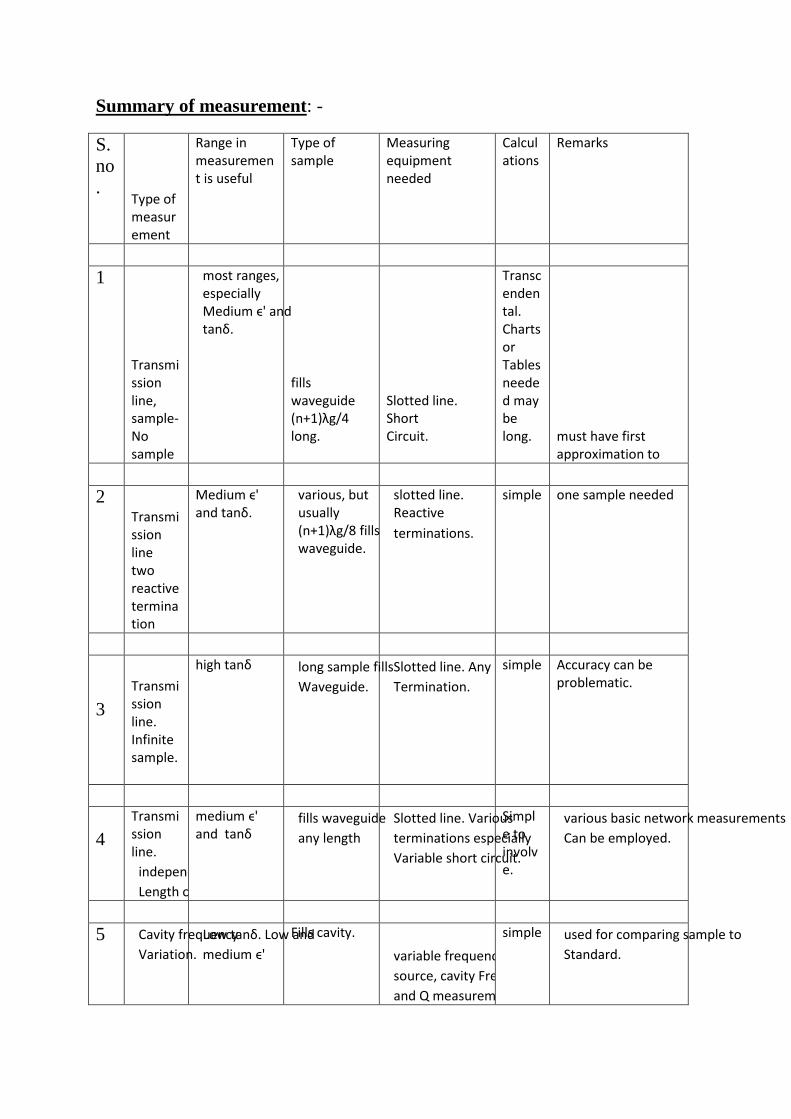
Summary of measurement: -
S. no.
Type of
measur
ement
Range in
measuremen
t is useful
Type of
sample
Measuring
equipment
needed
Calcul
ations
Remarks
1
Transmi
ssion
line,
sample-
No
sample
most ranges,
especially
Medium ϵ' and
tanδ.
fills
waveguide
(n+1)λg/4
long.
Slotted line.
Short
Circuit.
Transc
enden
tal.
Charts
or
Tables
neede
d may
be
long.
must have first
approximation to
2
Transmi
ssion
line
two
reactive
termina
tion
Medium ϵ'
and tanδ.
various, but
usually
(n+1)λg/8 fills
waveguide.
slotted line.
Reactive
terminations.
simple
one sample needed
3
Transmi
ssion
line.
Infinite
sample.
high tanδ
long sample fills
Waveguide.
Slotted line. Any
Termination.
simple
Accuracy can be
problematic.
4
Transmi
ssion
line.
independent of sample
Length or location.
medium ϵ'
and tanδ
fills waveguide
any length
Slotted line. Various
terminations especially
Variable short circuit.
Simpl
e to
involv
e.
various basic network measurements
Can be employed.
5 Cavity frequency
Variation.
Low tanδ. Low and
medium ϵ'
Fills cavity.
variable frequency power
source, cavity Frequency
and Q measurement
simple
used for comparing sample to
Standard.

6 Cavity frequency
Variation.
Low tanδ and
ϵ'.
fills cavity variable frequency power
source, cavity Frequency
and Q measurement
simple
Used for gases
7 Cavity frequency
Variation.
to measure resistivity of
Metal.
Cavity wall is
the sample.
variable frequency power
source, cavity Frequency
and Q measurement
simple
Not a dielectric
constant
measurement.
8 Cavity frequency
Variation.
relatively small ϵ' low
To medium tanδ.
Fill cross
section.
variable frequency power
source, cavity Frequency
and Q measurement
Transc
enden
tal.
Involv
ed.
Sample located in
high E field.
9 Cavity frequency
Variation.
Medium high ϵ'. Low to
Medium tan.
Fill cross
section.
variable frequency power
source, cavity Frequency
and Q measurement
Transc
enden
tal
Involv
ed.
Sample located in
high E field.
10 Cavity.
Length
variatio
n.
Medium high ϵ'. Low to
Medium tan.
Medium high ϵ'. Low to
Medium tanδ.
Transcendental
Involved.
Transc
enden
tal.
Involv
ed.
Sample located in
high E field.
11 Cavity perturbation.
Frequency variation.
various ϵ*(and also μ*)
depending on choice
Of sample shape & size.
small samples of various
shapes: spheres, rods,
slabs,etc.
variable frequency power
Source, cavity. Frequency
And Q measurement.
simple
can be used for "imperfect" geometric
Shapes.
12 Transmission line.
Short circuit.
lossless to medium loss
ϵ* and μ*
(simultaneously)
Fills
waveguide.
Slotted line. Open and
Short circuit.
simple
must have first approximation to ϵ' or
otherwise, two samples must be
Measured.