Didymium and Sodalime Glass Beads - MITRE

©2014 Society of Photo-Optical Instrumentation Engineers. All rights reserved.

An analysis of the nonlinear spectral mixing of didymium and soda-lime glass beads using hyperspectral imagery (HSI) microscopy

Ronald G. Resmini1*, Robert S. Rand2, David W. Allen3, and Christopher J. Deloye1

1The MITRE Corporation

7594 Colshire Drive, MS T630, McLean, Virginia 22102

2The National Geospatial-Intelligence Agency (NGA) 7500 GEOINT Drive, Springfield, Virginia 22150

3The National Institute of Standards and Technology (NIST)

100 Bureau Drive, Gaithersburg, Maryland 20899

ABSTRACT Nonlinear spectral mixing occurs when materials are intimately mixed. Intimate mixing is a common characteristic of granular materials such as soils. A linear spectral unmixing inversion applied to a nonlinear mixture will yield subpixel abundance estimates that do not equal the true values of the mixture's components. These aspects of spectral mixture analysis theory are well documented. Several methods to invert (and model) nonlinear spectral mixtures have been proposed. Examples include Hapke theory, the extended endmember matrix method, and kernel-based methods. There is, however, a relative paucity of real spectral image data sets that contain well characterized intimate mixtures. To address this, special materials were custom fabricated, mechanically mixed to form intimate mixtures, and measured with a hyperspectral imaging (HSI) microscope. The results of analyses of visible/near-infrared (VNIR; 400 nm to 900 nm) HSI microscopy image cubes (in reflectance) of intimate mixtures of the two materials are presented. The materials are spherical beads of didymium glass and soda-lime glass both ranging in particle size from 63 µm to 125 µm. Mixtures are generated by volume and thoroughly mixed mechanically. Three binary mixtures (and the two endmembers) are constructed and emplaced in the wells of a 96-well sample plate: 0%/100%, 25%/75%, 50%/50%, 80%/20%, and 100%/0% didymium/soda-lime. Analysis methods are linear spectral unmixing (LSU), LSU applied to reflectance converted to single-scattering albedo (SSA) using Hapke theory, and two kernel-based methods. The first kernel method uses a generalized kernel with a gamma parameter that gauges non-linearity, applying the well-known kernel trick to the least squares formulation of the constrained linear model. This method attempts to determine if each pixel in a scene is linear or non-linear, and adapts to compute a mixture model at each pixel accordingly. The second method uses 'K-hype' with a polynomial (quadratic) kernel. LSU applied to the reflectance spectra of the mixtures produced poor abundance estimates regardless of the constraints applied in the inversion. The 'K-hype' kernel-based method also produced poor fraction estimates. The best performers are LSU applied to the reflectance spectra converted to SSA using Hapke theory and the gamma parameter kernel-based method. Key words: hyperspectral remote sensing, hyperspectral imagery, HSI, microscopy, HSI microscopy, linear spectral mixing, nonlinear spectral mixing, reflectance spectroscopy, kernel method, kernel

1. INTRODUCTION

It is well known that intimately mixed materials frequently exhibit nonlinear spectral mixing. Granular materials, such as soils, are often intimate mixtures of numerous different inorganic (minerals) and organic (humic) substances. And since soils are often significant constituents of spectral remote sensing scenes, intimate mixing may safely be assumed to be a common phenomenon. Thus the impact of nonlinear spectral mixing on algorithm results must be well understood if we are to achieve a major goal of hyperspectral imaging (HSI): the areal mapping and quantification of materials that comprise remotely sensed scenes.

*Corresponding author; v: 703-470-3022, e1: [email protected] e2: [email protected]

Approved for Public Release: 14-1197.

Copyright has been transferred to another party. Reuse is restricted.

Contact Dr. Ronald G. Resmini, v: 703-470-3022, e1: [email protected], e2: [email protected].


It is also very common, as part of the data analysis process, to apply linear spectral unmixing to imaging spectrometer data. However, a linear spectral unmixing inversion applied to an intimate mixture exhibiting nonlinear spectral mixing will yield subpixel material abundance estimates that do not equal the true values of the mixture's constituents. An example of this is provided in Keshava and Mustard (2002) [1]. To address this, several methods of spectral unmixing of nonlinear spectral mixtures have been proposed. Examples include Hapke theory, the extended endmember matrix method, kernel-based methods, and Gaussian processes. Reviews of nonlinear spectral mixture analysis are given in refs. [1], [2], and [3] and references cited therein. However, there is a relative paucity of real spectral image data sets that contain well characterized intimate mixtures that may be used for algorithm development and testing and that are freely available to researchers [4]. To address these issues, two granular materials were custom fabricated and mechanically mixed to form intimate mixtures. The materials are spherical beads of didymium glass and soda-lime glass both ranging in particle size from 63 µm to 125 µm. The mixtures, which exhibit largely nonlinear spectral mixing, were then observed with a visible/near-infrared (VNIR; 400 nm to 900 nm) hyperspectral imaging (HSI) microscope. The HSI microscope utilized here acquires data cubes of fields of view ranging from centimeters to millimeters in size and 'ground' sampling distance (GSD) selectable from ~10 µm/pixel to >100 µm/pixel. This measurement capability can easily and rapidly generate large amounts of data of individual or numerous target materials to facilitate a broad range of spectral signature phenomenology and modeling studies and statistical analyses. Here, we focus on HSI microscopy data of mechanical mixtures of the two specially-designed and fabricated particulate, granular materials. Three binary mixtures (and the two endmembers) are constructed and emplaced in the wells of a 96-well sample plate: 0%/100%, 25%/75%, 50%/50%, 80%/20%, and 100%/0% of didymium/soda-lime (percentages by volume). We describe here the results of analyses of the HSI microscopy data (in reflectance) of the intimate mixtures. Analysis methods applied to the reflectance data are linear spectral unmixing (LSU); LSU applied to reflectance converted to single-scattering albedo (SSA) using Hapke theory; and two kernel-based methods (those of Broadwater and Banerjee, 2011 [5]; and Chen et al., 2013 [6]). The best performers in terms of retrieving accurate endmember abundance estimates are LSU applied to the reflectance spectra converted to SSA using Hapke theory and the kernel-based method of Broadwater and Banerjee (2011) [5]. LSU applied to the reflectance spectra of the mixtures produced poor abundance estimates as did the 'K-Hype' kernel-based method of Chen et al. (2013) [6]. This work was conducted to contribute to the general understanding of nonlinear spectral mixing and to generate data sets for use by the spectral remote sensing research community. It is also intended, along with Resmini et al. (2013) [7] and Allen et al. (2013) [8], to continue demonstrating the role and relevance of HSI microscopy as a tool for generating spectral scene and signature data for a wide range of uses by the remote sensing community.

2. METHODS 2.1 The Pika II VNIR HSI Microscope A Resonon Pika II imaging spectrometer with a Xenoplan 1.4/23-0902 objective lens [9], [10], [34], and [35], shown in Figure 1, is used to measure the glass bead mixtures. The Pika II is mounted nadir-looking at a mechanical translation table on which the sample to be imaged is placed. The Pika II is a pushbroom sensor with a slit aperture, thus the need for a translation table to move the sample to facilitate hyperspectral image cube formation. The height of the sensor above the table is user selectable; a height was chosen such that all mixtures are captured in the same scene thus the data have a ground sample distance of ~75 µm/pixel. Though capable of acquiring 240 bands from 400.0 nm to 900.0 nm, the sensor was configured to acquire 80 bands by binning spectrally by three resulting in a sampling interval of ~6.25 nm and high signal-to-noise ratio spectra. Four quartz-tungsten-halogen (QTH) lamps are used for illumination approximating a hemispherical-directional illumination/viewing geometry. Sensor and translation table operation, data acquisition, and data calibration are achieved by software that runs on a laptop computer. Calibration consists of a


Figure 1. Photograph of the VNIR HSI microscope. The Resonon Pika II is shown with

the Xenoplan 1.4/23-0902 objective lens [36].

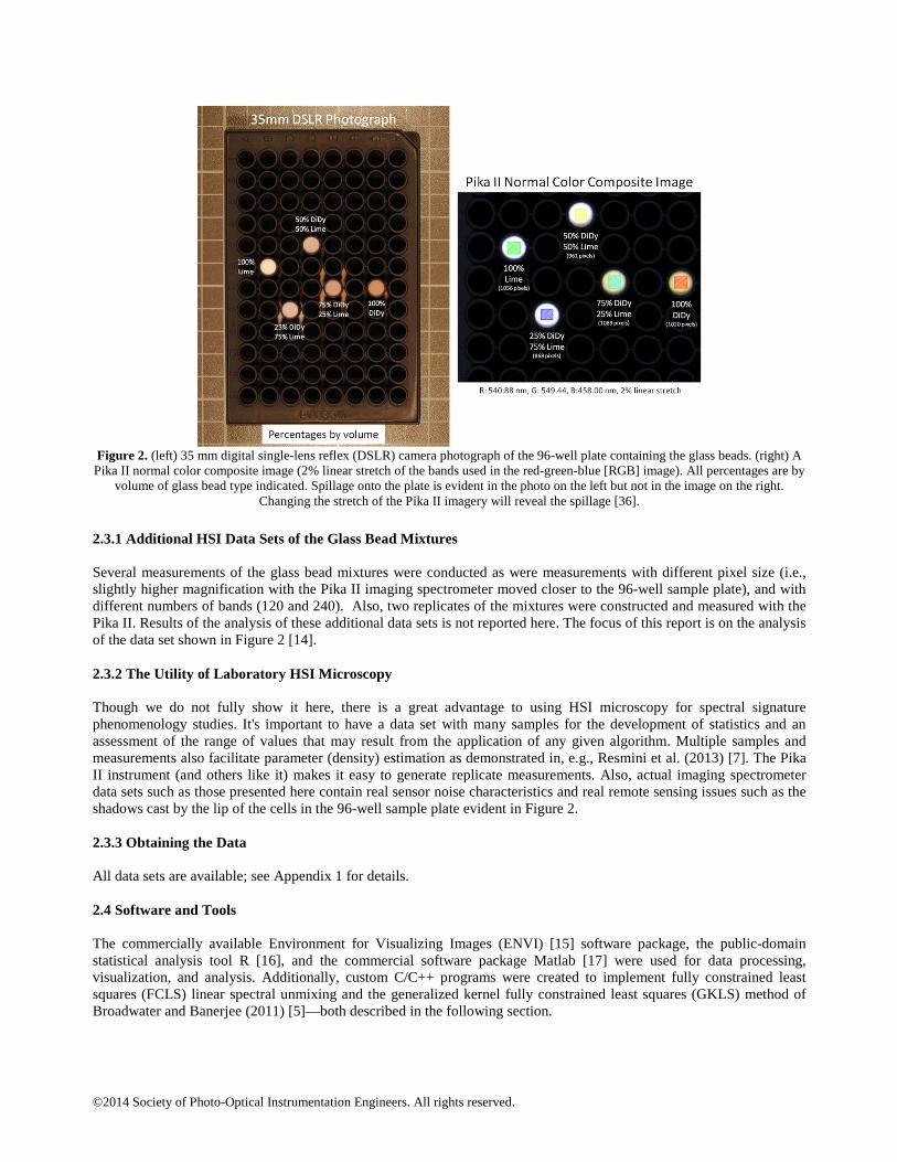
measurement of dark frame data (i.e., acquiring a cube with the lens cap on) and a measurement of a polytetrafluoroethylene (PTFE) reference plaque (large enough to entirely fill the field-of-view). Then, for each HSI cube measured, the sensor's software first subtracts the dark data and then uses the PTFE data (also dark subtracted) to ratio the spectral measurements to give relative reflectance (also known as reflectance factor; Hapke, 1993 [11]; Schott, 2007 [12]). 2.2 Data Processing and Analysis The Pika II system generates a band-interleaved-by-line (BIL) relative reflectance data cube and an associated ENVI (see Sec. 2.4) header (.hdr) file. The data are thus easily imported into ENVI for data inspection, exploratory analysis, and exploitation. Image cubes are 640 samples by a user-selectable number of lines. Using ENVI's 'Spectral Math' capability, the Pika II relative reflectance data cubes are multiplied with a PTFE truth reflectance spectrum for conversion to absolute reflectance though in practice the reflectance values pre- and post-multiplication are very close. The root mean squared (rms) value of the difference of the two scene maximum spectra (i.e., for the relative and absolute reflectance cubes) is 0.005; the rms value of the difference of the two scene mean spectra is 0.0002. Fifteen data cubes were acquired; however, we focus here on the analysis of one cube comprised of 640 samples, 500 lines, and 75 bands ranging from 434.0 nm to 885.0 nm. Of the 80 bands acquired the first 5 were discarded due to noise content. Creating the spectrally subsetted cube of 75 bands of absolute reflectance is also accomplished in ENVI. Regions of interest (ROIs) are then created (see Figure 2) from which mean spectra are calculated and used in the various spectral unmixing inversions. As is evident from Figure 2, large ROIs on each cell are easily defined and contain several hundred spectra. Shadowing around the edges of the cells is also easily avoided [13]. The spectra in the ROIs are exported to ASCII text files. These files are then imported into R and Matlab (see Sec. 2.4) for our implementation of the Chen et al. (2013) [6] 'K-Hype' kernel method. 2.3 The Glass Bead Mixtures Five cells of a 96-well sample plate, spray-painted flat black, were filled with the various glass bead mixtures; this is shown in Figure 2. The volume of each cell is 330 µL (0.33 mL). Three binary mixtures and the two 100% endmembers are constructed and emplaced in five of the wells of the 96-well sample plate: 0%/100%, 25%/75%, 50%/50%, 80%/20%, and 100%/0% didymium/soda-lime. The materials are spherical beads of didymium glass and soda-lime glass both ranging in particle size from 63 µm to 125 µm. Mixtures are by volume. This is a data set with largely non-linear spectral mixing; the glass beads, didymium and soda-lime, are translucent. Their chemical composition, densities, and particle size range are well known. Note that the glass bead particle size range is much larger than the VNIR wavelengths used in this analysis. The glass beads and their mixtures display subtle, though interesting, gonioapparent changes in color.


Figure 2. (left) 35 mm digital single-lens reflex (DSLR) camera photograph of the 96-well plate containing the glass beads. (right) A Pika II normal color composite image (2% linear stretch of the bands used in the red-green-blue [RGB] image). All percentages are by

volume of glass bead type indicated. Spillage onto the plate is evident in the photo on the left but not in the image on the right. Changing the stretch of the Pika II imagery will reveal the spillage [36].

2.3.1 Additional HSI Data Sets of the Glass Bead Mixtures Several measurements of the glass bead mixtures were conducted as were measurements with different pixel size (i.e., slightly higher magnification with the Pika II imaging spectrometer moved closer to the 96-well sample plate), and with different numbers of bands (120 and 240). Also, two replicates of the mixtures were constructed and measured with the Pika II. Results of the analysis of these additional data sets is not reported here. The focus of this report is on the analysis of the data set shown in Figure 2 [14]. 2.3.2 The Utility of Laboratory HSI Microscopy Though we do not fully show it here, there is a great advantage to using HSI microscopy for spectral signature phenomenology studies. It's important to have a data set with many samples for the development of statistics and an assessment of the range of values that may result from the application of any given algorithm. Multiple samples and measurements also facilitate parameter (density) estimation as demonstrated in, e.g., Resmini et al. (2013) [7]. The Pika II instrument (and others like it) makes it easy to generate replicate measurements. Also, actual imaging spectrometer data sets such as those presented here contain real sensor noise characteristics and real remote sensing issues such as the shadows cast by the lip of the cells in the 96-well sample plate evident in Figure 2. 2.3.3 Obtaining the Data All data sets are available; see Appendix 1 for details. 2.4 Software and Tools The commercially available Environment for Visualizing Images (ENVI) [15] software package, the public-domain statistical analysis tool R [16], and the commercial software package Matlab [17] were used for data processing, visualization, and analysis. Additionally, custom C/C++ programs were created to implement fully constrained least squares (FCLS) linear spectral unmixing and the generalized kernel fully constrained least squares (GKLS) method of Broadwater and Banerjee (2011) [5]—both described in the following section.


2.5 Algorithms 2.5.1 'Traditional' Linear Spectral Unmixing (LSU) – Different Constraints 2.5.1.1 LSU – Sum-to-One Constraint, Only Linear spectral unmixing (LSU) was applied to reflectance data using the capability in ENVI. LSU is the inversion of a linear spectral mixing signal model for a pixel given as:

x = Ea eq. (1)

where x is an Lx1 vector containing the spectral signature of the current image pixel, E is an LxN matrix containing the endmember signatures (the ith column contains the ith endmember spectrum), and a is an Nx1 vector containing the estimated abundances (the ith entry represents the abundance value ai). L is the number of bands in the HSI data and N is the number of endmembers within the image (here, L = 75 and N = 2). LSU was applied with and without a sum-to-one constraint (the only constraint available in the ENVI implementation). Endmember spectra are the two regions-of-interest (ROI) mean spectra of 100% didymium and 100% soda-lime; the ROIs are shown Figure 2 (there are 1020 spectra in the red ROI for 100% didymium and 1056 spectra in the green ROI for 100% soda-lime). The LSU inversions (solutions to eq. (1)) were applied to every pixel (spectrum) in the data set; i.e., the entire scene was passed to the ENVI LSU algorithm; there was no spatial subsetting or masking. LSU generated two fraction planes: one corresponding to the didymium endmember and one for the soda-lime. A mean of the fractions was calculated using the same ROIs shown in Figure 2. Thus, for a given trial of LSU, five fraction values of didymium and five fraction values of soda-lime were calculated—one for each well (containing glass beads) in the 96-well plate. No shade/shadow endmember was included in the solutions to eq. (1) with the sum-to-one-only, constraint. 2.5.1.2 LSU – Fully Constrained Least Squares (FCLS) LSU was also applied with additional constraints. Fully constrained least squares (FCLS) [18][19] is also a linear spectral mixing model, X = Ea (eq. 1), but with the following constraints:

ai ≥ 0 and ∑=

=N

1ii 1a eq. (2)

Thus, in addition to the sum-to-one constraint, all fractions are positive (unlike the sum-to-one constraint, only, for which fractions may be negative). The solution to eqs. (1) and (2) can be found in a number of ways, but can be posed as:

�� = argmin � �⟨�, �⟩ − ��⟨�, �⟩ + ��⟨�, �⟩��, �. �.a� ≥ 0, ∀� eq. (3)

2.5.1.3 LSU – Single-Scattering Albedo Spectra (SSA): Hapke Theory LSU in ENVI was also applied to the reflectance spectra converted to single-scattering albedo (SSA) spectra. Two different sets of SSA spectra were generated. Conversion to SSA is described in Resmini et al. (1996) [20] and Resmini (1997) [21] (both studies following Hapke, 1993 [11]; and Mustard and Pieters, 1987 [22]; see also [33]) assuming the reflectance spectra are bidirectional. SSA spectra were also generated assuming the input reflectance spectra are hemispherical-directional. The expressions to transform reflectance spectra to SSA are given by eqs. (4) and (5) for bi-directional (bd) reflectance and for hemispherical-directional (hd) reflectance, respectively. In the derivation of both expressions, phase angle is large enough that the opposition effect is assumed negligible.

( ) ( )( )[ ] ( )( )

2

0

0

5.0

022

0

0.40.1

0.10.40.10.1

Γµµ+Γµ+µ−Γ−Γµµ++Γµ+µ−=ϖ eq. (4)


2

0.20.1

0.10.1

Γµ+Γ−−=ϖ eq. (5)

In eqs. (4) and (5), ϖ is single scattering albedo; Γ is reflectance factor (see Section 2.1 and Hapke, 1993 [11]), µ0 is the cosine of the angle of incidence of the illumination, and µ is the cosine of the viewing angle. Note that one reflectance is calculated as described previously in Section 2.1 though two different equations are used to generate the two sets of SSA spectra. Given the use of four QTH lamps as illumination (see Figure 1), the reflectances (actually reflectance factors) produced are not strictly rbd or rhd but some combination of both. Because of this, it is instructive to compare fractions based on SSA assuming rbd and rhd from the imaging spectrometer. µ0 and µ are set to 1.0 in the application of eqs. (4) and (5). The conversion of reflectance spectra to SSA using eqs. (4) and (5) is applied using ENVI's 'Band Math' capability. It is a simple computation that requires only seconds of processing. 2.5.2 Kernel Methods Spectral mixing in an intimate mixture is described by nonlinear functions. The nonlinear terms capture cross-material spectral (i.e., light) interactions such as a photon stream, in a binary mixture, bouncing off material A and then material B and then off to the sensor. Given: i) the variety of the cross-material interactions that may occur in compositionally diverse particulate mixtures; ii) the range of values of the optical constants of the constituent materials; and iii) a mixture's morphology (particle size, surface roughness/microtopography, compaction), a nonlinear spectral mixing model is difficult to construct. But doing so is worthwhile because inversions with it can show up to 30% improvement in subpixel fraction estimates compared to a linear mixing model. It is difficult to model nonlinear mixtures in practice because much of the necessary information is not known a priori. Kernel methods may be used to generalize linear algorithms to nonlinear data [23], [24]. For material detection, identification, and classification in HSI data, kernel functions induce high dimensional feature spaces in which classes are made linearly separable. Linear methods can be applied in this new feature space that produce nonlinear boundaries in the original data space (generally reflectance but may also be applied to radiance spectra). An interesting variation is the kernel principal components analysis (PCA) method [25]. In this case, the kernel is not used to induce a high dimensional space, but is used to better match the data structure through nonlinear mappings. It is in this mode that kernels may be used to produce nonlinear mixing results while essentially using a linear mixture model. Particularly appealing is that such a method is ideal, in terms of the physical interactions of light and matter, if the kernel is properly constructed. The drawbacks with earlier kernel algorithms for classification and detection are that they: 1) used non-physical endmembers and/or 2) produced abundance estimates that do not meet the non-negativity and sum-to-one constraints. The first issue has recently been addressed by introducing the support vector data description (SVDD) algorithm to extract physical endmembers in the feature space [26]. The second issue has been recently addressed by the development of a kernel fully constrained least squares (KFCLS) method which computes kernel-based abundance estimates to meet the physical abundance constraints [27]. Further investigation of the KFCLS method has resulted in (1) the development of a generalized kernel for areal (linear) and intimate (non-linear) mixtures [28] and (2) an adaptive kernel-based technique for mapping areal and intimate mixtures [29]. The generalized kernel and adaptive techniques provide ways to adaptively estimate a mixture model suitable to the degree of non-linearity that may be occurring at each pixel in a scene. This is important because a scene may contain both areal and intimate mixtures and it not always known a priori which model is appropriate for a given pixel. 2.5.2.1 Kernel Fully Constrained Least Squares The kernel fully constrained least square (KFCLS) mixing model was derived previously by Broadwater et al. (2007) [27]. This method estimates the abundances of a model using the expression:

�� = argmin � � ��, x� − �� , �� + �� , ��, �. �.a� ≥ 0, ∀� eq. (6)


where E is the endmember matrix and â is the estimated abundance vector, discussed above for eq. (1). The abundance estimates are computed using a quadratic programming method to enforce the non-negativity constraint. The specific choice of kernel determines the ability of the KFCLS to respond to different types of mixing. Choosing the linear kernel K(x,y)=xTy is ideal for modeling linear mixtures; however, it is not suitable for intimate mixtures. A physics-based kernel has been proposed and has been shown to provide significantly improved behavior to model nonlinear mixtures [29]. However, it was demonstrated that although each kernel provides good results for the type of mixing intended, only one kernel or the other could be used, for either areal mixtures or intimate mixtures, but not both. 2.5.2.2 Generalized Kernel Fully Constrained Least Squares The KFCLS was further developed by Broadwater and Banerjee (2009, 2010) [28], [29] into a generalized KFCLS method for adaptive areal and intimate mixtures. The generalized KFCLS utilizes the following kernel: K#��, $� = �1 − &'()�*�1 − &'(+� eq. (7) The kernel Kγ(x,y) can be used to model either areal or intimate mixtures so long as the correct γ is used. If γ is very small then Kγ(x,y) approximates linear mixing. If γ is large then Kγ(x,y) approximates intimate mixing in cases when the reflectance occurring from intimate mixing is modeled as: , = -

.�/0/1� 2H�-, μ�H�-, μ5�6 eq. (8)

where r is reflectance (as a spectrum), H is Chandrasekhar’s function for isotropic scattering, ϖ is the average single-scattering albedo, µ0 is the cosine of the angle of incidence, and µ is the cosine of the angle of emergence [11], [30]. The computation is similar in form to eq. (6) except the minimization is done according to

7� = argmin# � 8 9��, �� − ��9� 9��, �� + ��9� ��, ��9:, �. �.a� ≥ 0, ∀� eq. (9)

where âγγγγ is the abundance estimate using KFCLS and Kγ(x,y) is the kernel evaluated with the parameter value γ. A numerical optimization based on the golden search method is used to minimize eq. (5) [31], [32]. An implementation of this generalized method, referred to here as generalized kernel least squares (GKLS), is applied to the glass bead HSI data. FCLS and GKLS were applied to different ROIs than those in Figure 2 (and not shown here); however, the ROIs each contained several hundred pixels. 2.5.2.3 The 'K-Hype' Kernel Method of Chen et al. (2013) The 'K-Hype' method of Chen et al. (2013) [6] with a second-degree polynomial (quadratic) kernel was also applied. The kernel is given in eq. (10) (which is eq. (27) of ref. [6]). K-Hype is the solution to a quadratic programming problem given by eq. (11) followed by the retrieval of fractions using eq. (12) (which are eqs. (19) and (21) in ref. [6], respectively; see Appendix 2 for a description of the symbols). The fractions meet the constraints of eq. (2); i.e., are ≥ 0 and sum to one. Seven trials with µ (a regularization constant) varying from zero to one were conducted. One 'K-Hype' trial with a Gaussian kernel with µ = 0.25 was also conducted.

κ<=�< >?@A ,?@BC = D1 + EFG 8?@A − 1 2I :J >?@B − 1 2I CK

L eq. (10)

eq. (11)


M∗ = OJβ∗ + γ∗ − λ∗ eq. (12)

A complete analysis of the data with 'SK-Hype' of Chen et al. (2013) [6] was not implemented for this study though a single trial, not shown here, (with the quadratic kernel and µ = 0.25) yielded fractions essentially the same as those of 'K-Hype' (also with the quadratic kernel and µ = 0.25). K-Hype is straightforward to implement and requires very little computation time; results are generated in seconds—even for running multiple trials varying µ. There are, however, parameters and kernel-type choices in this (and other) kernel methods. It is difficult to predict a priori which kernel and which value(s) of the various parameters will generate accurate abundances. Thus, compared to LSU applied to reflectance or SSA spectra—straightforward and rapid processing with no need for free parameters—kernel methods require more effort on the part of the analyst (and are perhaps less well-understood) with respect to implementation and interpretation of results. Efforts to select and design kernels that are based on models of the physical interactions of photons of light and matter (such as Hapke theory) are to be encouraged.

3. RESULTS AND DISCUSSION 3.1 The Didymium and Soda-Lime Spectra The five regions of interest (ROI) mean spectra of the didymium and soda-lime glass beads (endmembers and mixtures) are shown in Figure 3. The ROIs from which these mean spectra are derived are those in Figure 2. Note that the didymium spectrum has many features in the VNIR region of the spectrum in stark contrast to that of the soda-lime.

Figure 3. Mean spectra from the regions of interest (ROI) shown in Figure 2. Plot color corresponds to ROI color in Figure 2.

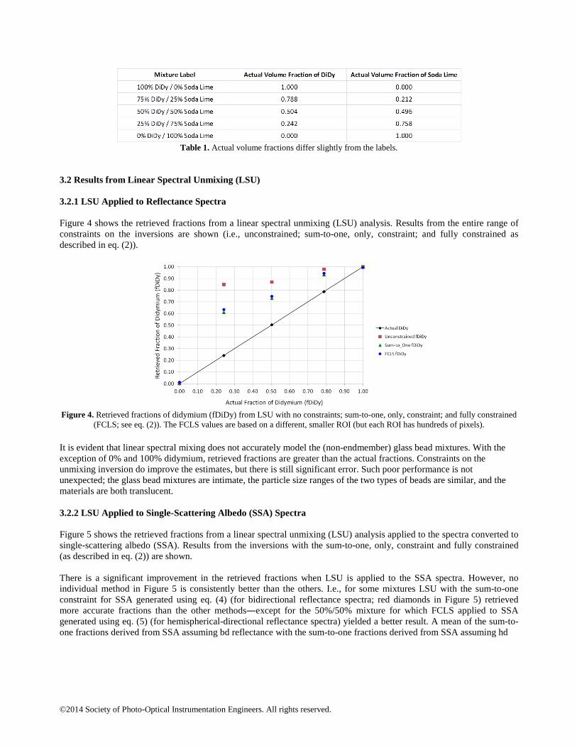
Fractions are by volume; 'DiDy' = didymium; 'Lime' = soda-lime. The actual volume fractions of didymium (DiDy) and soda-lime in the mixtures varies slightly from the ideal, round whole numbers indicated up to this point in this report. The actual values are given in Table 1. The labels will remain as the round, whole numbers but be aware that the actual fractions differ. The actual fraction values are used in all subsequent plots when displaying results of the various unmixing algorithms.


Table 1. Actual volume fractions differ slightly from the labels.

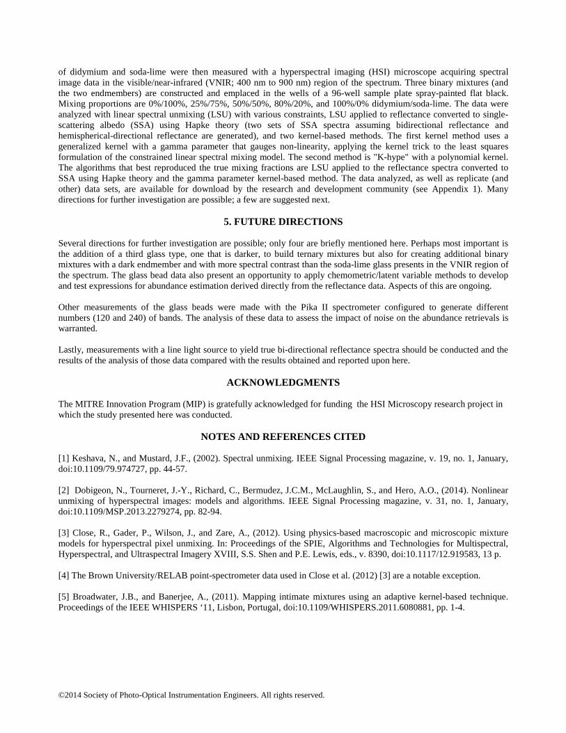
3.2 Results from Linear Spectral Unmixing (LSU) 3.2.1 LSU Applied to Reflectance Spectra Figure 4 shows the retrieved fractions from a linear spectral unmixing (LSU) analysis. Results from the entire range of constraints on the inversions are shown (i.e., unconstrained; sum-to-one, only, constraint; and fully constrained as described in eq. (2)).

Figure 4. Retrieved fractions of didymium (fDiDy) from LSU with no constraints; sum-to-one, only, constraint; and fully constrained

(FCLS; see eq. (2)). The FCLS values are based on a different, smaller ROI (but each ROI has hundreds of pixels).

It is evident that linear spectral mixing does not accurately model the (non-endmember) glass bead mixtures. With the exception of 0% and 100% didymium, retrieved fractions are greater than the actual fractions. Constraints on the unmixing inversion do improve the estimates, but there is still significant error. Such poor performance is not unexpected; the glass bead mixtures are intimate, the particle size ranges of the two types of beads are similar, and the materials are both translucent. 3.2.2 LSU Applied to Single-Scattering Albedo (SSA) Spectra Figure 5 shows the retrieved fractions from a linear spectral unmixing (LSU) analysis applied to the spectra converted to single-scattering albedo (SSA). Results from the inversions with the sum-to-one, only, constraint and fully constrained (as described in eq. (2)) are shown. There is a significant improvement in the retrieved fractions when LSU is applied to the SSA spectra. However, no individual method in Figure 5 is consistently better than the others. I.e., for some mixtures LSU with the sum-to-one constraint for SSA generated using eq. (4) (for bidirectional reflectance spectra; red diamonds in Figure 5) retrieved more accurate fractions than the other methods―except for the 50%/50% mixture for which FCLS applied to SSA generated using eq. (5) (for hemispherical-directional reflectance spectra) yielded a better result. A mean of the sum-to-one fractions derived from SSA assuming bd reflectance with the sum-to-one fractions derived from SSA assuming hd


Figure 5. Retrieved fractions from LSU applied to single-scattering albedo spectra (SSA) with Hapke theory; bd = bidirectional; hd = hemispherical-directional (see text and eqs. 4 and 5). LSU applied with the sum-to-one, only, constraint and fully constrained (FCLS). The FCLS values are based on a different, smaller ROI (but each ROI has hundreds of pixels). reflectance was calculated and is plotted in Figure 5 (green diamonds). This combination of the abundances was generated because there is perhaps some ambiguity as to the type of reflectance spectra measured due to the four lamp illumination arrangement of the Pika II sensor. It is not, however, an improvement in the accuracy of the retrieved abundances. Overall, the conversion of the reflectance data to SSA and then the application of LSU generated abundance estimates that are better than those derived from reflectance spectra. This, too, is not unexpected because the glass bead mixture generates nonlinear spectral mixing interactions and, perhaps more to the point, the validity and bounds of applicability of Hapke theory are well-known and widely discussed in the literature. 3.3 Results from the Kernel Methods 3.3.1 GKLS Figure 6 shows the retrieved fractions using GKLS. The retrieved abundance estimates are very good with the exception of the 80%/20% mixture. The abundances are approximately the same as those derived from LSU with the sum-to-one constraint applied to SSA for bd spectra. However, in contrast to applying LSU to SSA spectra, a process that requires only seconds of processing time, the GKLS method takes much longer to compute (about 15 times longer). For this experiment, the FCLS method, including SSA conversion, took 12 seconds whereas GKLS needed 177 seconds to finish (on a laptop personal computer with an i5 processor running at 2.4 GHz).

Figure 6. Didymium fractions (fDiDy) retrieved with generalized kernel fully constrained least squares (GKLS).


The significantly longer run time of GKLS is caused by the method iterating through many values of gamma attempting to characterize the amount of non-linearity in each sample. If samples are already known to be non-linear, then a fixed gamma can be chosen, reducing run time considerably. For the scene in this experiment, GKLS with fixed gamma takes only 14 seconds. The performance of GKLS, similar to that achieved with LSU applied to SSA spectra, is expected due to its incorporation of Hapke theory as shown by eq. (8). 3.3.2 K-Hype of Chen et al. (2013) Figure 7 shows the retrieved fractions using K-Hype with a quadratic kernel and with various values of the regularization parameter, µ. With only one exception, 80% DiDy with µ = 0.0, the retrieved abundances do not agree well with the actual values. Smaller values of µ, however, move the retrieved fractions closer the actual values. The GKLS and LSU with SSA spectra are plotted for comparison. Overall, LSU with SSA spectra (and the sum-to-one constraint) and GKLS perform better than the K-Hype method with a quadratic kernel. Figure 8 shows the results of one trial of 'K-Hype' with a Gaussian kernel. Here, too, retrieved fractions do not match the actual values.

Figure 7. K-Hype with quadratic kernel; µ ranges from 0.000 to 1.000. Results from LSU with sum-to-one constraint applied to SSA

spectra and GKLS are shown for comparison.

Figure 8. K-Hype with Gaussian kernel (brown square) and quadratic kernel (green triangle); both with µ = 0.25. LSU applied to

reflectance spectra (with a sum-to-one constraint) shown for comparison.

4. SUMMARY AND CONCLUSIONS Two compositionally distinct particulate materials were custom fabricated and mechanically mixed in different proportions to form intimate mixtures to investigate nonlinear spectral mixing. The mixtures, by volume, of glass beads


of didymium and soda-lime were then measured with a hyperspectral imaging (HSI) microscope acquiring spectral image data in the visible/near-infrared (VNIR; 400 nm to 900 nm) region of the spectrum. Three binary mixtures (and the two endmembers) are constructed and emplaced in the wells of a 96-well sample plate spray-painted flat black. Mixing proportions are 0%/100%, 25%/75%, 50%/50%, 80%/20%, and 100%/0% didymium/soda-lime. The data were analyzed with linear spectral unmixing (LSU) with various constraints, LSU applied to reflectance converted to single-scattering albedo (SSA) using Hapke theory (two sets of SSA spectra assuming bidirectional reflectance and hemispherical-directional reflectance are generated), and two kernel-based methods. The first kernel method uses a generalized kernel with a gamma parameter that gauges non-linearity, applying the kernel trick to the least squares formulation of the constrained linear spectral mixing model. The second method is "K-hype" with a polynomial kernel. The algorithms that best reproduced the true mixing fractions are LSU applied to the reflectance spectra converted to SSA using Hapke theory and the gamma parameter kernel-based method. The data analyzed, as well as replicate (and other) data sets, are available for download by the research and development community (see Appendix 1). Many directions for further investigation are possible; a few are suggested next.

5. FUTURE DIRECTIONS Several directions for further investigation are possible; only four are briefly mentioned here. Perhaps most important is the addition of a third glass type, one that is darker, to build ternary mixtures but also for creating additional binary mixtures with a dark endmember and with more spectral contrast than the soda-lime glass presents in the VNIR region of the spectrum. The glass bead data also present an opportunity to apply chemometric/latent variable methods to develop and test expressions for abundance estimation derived directly from the reflectance data. Aspects of this are ongoing. Other measurements of the glass beads were made with the Pika II spectrometer configured to generate different numbers (120 and 240) of bands. The analysis of these data to assess the impact of noise on the abundance retrievals is warranted. Lastly, measurements with a line light source to yield true bi-directional reflectance spectra should be conducted and the results of the analysis of those data compared with the results obtained and reported upon here.

ACKNOWLEDGMENTS The MITRE Innovation Program (MIP) is gratefully acknowledged for funding the HSI Microscopy research project in which the study presented here was conducted.

NOTES AND REFERENCES CITED [1] Keshava, N., and Mustard, J.F., (2002). Spectral unmixing. IEEE Signal Processing magazine, v. 19, no. 1, January, doi:10.1109/79.974727, pp. 44-57. [2] Dobigeon, N., Tourneret, J.-Y., Richard, C., Bermudez, J.C.M., McLaughlin, S., and Hero, A.O., (2014). Nonlinear unmixing of hyperspectral images: models and algorithms. IEEE Signal Processing magazine, v. 31, no. 1, January, doi:10.1109/MSP.2013.2279274, pp. 82-94. [3] Close, R., Gader, P., Wilson, J., and Zare, A., (2012). Using physics-based macroscopic and microscopic mixture models for hyperspectral pixel unmixing. In: Proceedings of the SPIE, Algorithms and Technologies for Multispectral, Hyperspectral, and Ultraspectral Imagery XVIII, S.S. Shen and P.E. Lewis, eds., v. 8390, doi:10.1117/12.919583, 13 p. [4] The Brown University/RELAB point-spectrometer data used in Close et al. (2012) [3] are a notable exception. [5] Broadwater, J.B., and Banerjee, A., (2011). Mapping intimate mixtures using an adaptive kernel-based technique. Proceedings of the IEEE WHISPERS ‘11, Lisbon, Portugal, doi:10.1109/WHISPERS.2011.6080881, pp. 1-4.


[6] Chen, J., Richard, C., Honeine, P., (2013). Nonlinear unmixing of hyperspectral data based on a linear-mixture/nonlinear-fluctuation model. IEEE Transactions on Signal Processing, v. 61, no. 2, doi:10.1109/TSP.2012.2222390, Jan. 15, 2013, pp. 480-492. [7] Resmini, R.G., Deloye, C.J., and Allen, D.W., (2013). An analysis of the probability distribution of spectral angle and Euclidean distance in hyperspectral remote sensing using microspectroscopy. In Proceedings of the SPIE, Algorithms and Technologies for Multispectral, Hyperspectral, and Ultraspectral Imagery XIX, S.S. Shen and P.E. Lewis, eds., v. 8743, doi:http://dx.doi.org/10.1117/12.2015701, Baltimore, MD, 29 April-3 May, 2013, 13 p. [8] Allen, D.W., Resmini, R.G., Deloye, C.J., and Stevens, J.R., (2013). A microscene approach to the evaluation of hyperspectral system level performance. In Proceedings of the SPIE, Algorithms and Technologies for Multispectral, Hyperspectral, and Ultraspectral Imagery XIX, S.S. Shen and P.E. Lewis, eds., v. 8743, doi:http://dx.doi.org/10.1117/12.2015834, Baltimore, MD, 29 April-3 May, 2013, 13 p. [9] http://www.resonon.com/imagers_pika_iii.html (last accessed on Dec. 3, 2013). [10] We have also used an Edmund Optics Gold Series 1.0X telecentric lens that gives ~8 µm/pixel. However, data at such a high spatial resolution were not required for the analyses reported upon here. [11] Hapke, B., (1993). Theory of Reflectance and Emittance Spectroscopy. Cambridge University Press, 455 p. [12] Schott, J.R., (2007). Remote Sensing: The Image Chain Approach, 2nd ed. Oxford University Press, New York, 688 p. [13] Circular regions of interest drawn to encompass all of the glass bead area in a cell of the 96-well plate each contain over 3000 pixels. The rectangular ROIs in Figure 2 are drawn to exclude the shaded regions occurring in each cell. [14] File: 20130521_sphere_array_2.bil; see Appendix 1 and Table A.1. [15] http://www.exelisvis.com/ProductsServices/ENVI.aspx (last accessed 1 Mar., 2013). [16] R Development Core Team, (2011). R: A language and environment for statistical computing. R Foundation for Statistical Computing, Vienna, Austria. ISBN 3-900051-07-0, URL http://www.R-project.org/ (last accessed 1 Mar., 2013). [17] http://www.mathworks.com/products/matlab/ (last accessed 9 Dec., 2013). [18] Montgomery D. and Peck E., (1992). Introduction to Linear Regression Analysis, 2nd ed. Wiley Series in Probability and Mathematical Statistics, John Wiley and Sons, 544 p. [19] Heinz D.C. and Chang C.-I., (2001). Fully constrained least squares linear spectral mixture analysis method for material quantification in hyperspectral imagery. IEEE Transactions on Geoscience and Remote Sensing, v. 39, no. 3, pp. 529-545. [20] Resmini, R.G., Graver, W.R., Kappus, M.E., and Anderson, M.E., (1996). Constrained energy minimization applied to apparent reflectance and single-scattering albedo spectra: a comparison. Proceedings of the SPIE: Hyperspectral Remote Sensing and Applications, Sylvia S. Shen, ed., Denver, Colo., August 5-6, v. 2821, pp. 3-13, doi:10.1117/12.257168. [21] Resmini, R.G., (1997). Enhanced detection of objects in shade using a single-scattering albedo transformation applied to airborne imaging spectrometer data. The International Symposium on Spectral Sensing Research, San Diego, California, CD-ROM, 7 p.


[22] Mustard, J.F., and Pieters, C.M., (1987). Abundance and distribution of ultramafic microbreccia in Moses Rock Dike: Quantitative application of mapping spectroscopy. Journal of Geophysical Research, v. 92 (10 September), no. B10, pp. 10,376-10,390. [23] Kwon, H., and Nasrabadi, N.M., (2006). Kernel matched subspace detectors for hyperspectral target detection. IEEE Transactions on Pattern Analysis and Machine Intelligence, v. 28, no. 2, pp. 178-194. [24] Camps-Valls, G., and Bruzzone L., (2005). Kernel-based methods for hyperspectral image classification. IEEE Transactions on Geoscience and Remote Sensing, v. 43, no. 6, pp. 1351-1362. [25] Scholkopf, B. and Smola, A.J., (2001). Learning with Kernels: Support Vector Machines, Regularization, Optimization, and Beyond. The MIT Press, Cambridge, MA, 644 p. [26] Banerjee, A., Burlina, P., and Broadwater, J., (2007). A Machine Learning Approach for finding hyperspectral endmembers. Proceedings of the IEEE International Geoscience and Remote Symposium (IGARSS 2007), Barcelona, Spain, doi:10.1109/IGARSS.2007.4423675, pp. 3817-3820. [27] Broadwater, J.B., Chellappa, R., Banerjee, A., and Burlina P., (2007). Kernel fully constrained least squares abundance estimates. Proceedings of the IEEE International Geoscience and Remote Symposium (IGARSS 2007), Barcelona, Spain, doi:10.1109/IGARSS.2007.4423736, pp. 4041-4044. [28] Broadwater, J.B., and Banerjee, A., (2010). A generalized kernel for areal and intimate mixtures. Proceedings of the IEEE WHISPERS ‘10, Reykjavik, Iceland, doi:10.1109/WHISPERS.2010.5594962, pp. 1-4. [29] Broadwater, J.B., and Banerjee, A., (2009). A comparison of kernel functions for intimate mixture models. Proceedings of the IEEE WHISPERS ‘09, Grenoble, France, doi:10.1109/WHISPERS.2009.5289073, pp. 1-4. [30] Mustard, J.F., and Pieters, C.M., (1989). Photometric phase functions of common geologic minerals and application to quantitative analysis of mineral mixture reflectance spectra. Journal of Geophysical Research, v. 94, pp. 13619-13634. [31] Brent R.P., (1972). Algorithms for Minimization without Derivatives. Prentice-Hall, Englewood Cliffs, NJ, 224 p. [32] Rand, R.S., Banerjee, A., Broadwater, J., (2013). Automated endmember determination and adaptive spectral mixture analysis using kernel methods. Proceedings of the SPIE, v. 8870, Imaging Spectrometry XVIII, 88700Q (Sept. 23, 2013); doi:10.1117/12.2026728. [33] Nascimento, J.M.P., and Bioucas-Dias, J.M., (2010). Unmixing hyperspectral intimate mixtures. Proceedings of the SPIE, v. 7830, doi:10.1117/12.8651188, 8 p. [34] For measurements of other materials such as soils, we have also used a line light source for directional illumination giving bidirectional reflectance spectra; those data are not included in this study. This note and [10] have been included to indicate the performance range and flexibility of the HSI microscopy apparatus even though the full range of that performance is not utilized for measurements of the glass bead mixtures. [35] Note: References are made to certain commercially available products in this paper to adequately specify the experimental procedures involved. Such identification does not imply recommendation or endorsement by the National Institute of Standards and Technology, nor does it imply that these products are the best for the purpose specified. [36] Photographs in Figures 1 and 2 taken by, owned by, and courtesy of co-author Dr. David W. Allen of NIST.

APPENDIX 1: OBTAINING THE DATA The focus in this report has been on the analysis of a single Pika II HSI data cube (file: 20130521_sphere_array_2.bil). However, fifteen measurements, in total, of the glass beads in the 96-well sample plate were acquired (listed in Table


A.1). Two are simply redundant measurements (640 samples x 500 lines x 80 bands prior to spectral subsetting in ENVI). Six others are of the same sample plate and glass bead mixtures but with 120 and 240 bands. These data are somewhat noisier than those with 80 bands but were acquired to assess the impact of an increased noise level on abundance estimations. Three cubes are with the sensor moved closer to the sample plate (still with the Xenoplan objective lens) and with 80 bands. Two additional cubes contain two replicate sets of glass bead mixtures placed in adjacent empty cells of the plate (for a total of fifteen filled cells). These cubes, too, contains 80 bands. All of the data sets are with four QTH lamps and nadir-looking sensor configuration shown in Figure 1. To date, no data have yet been acquired with a line-light source to yield true bi-directional reflectance spectra. All of these data sets as well as dark field data cubes (with 80, 120, and 240 bands) and some additional information (e.g., the ENVI ROI files and an ENVI 'Spectral Math' expression file for implementing eqs. (4) and (5)) are available as one compressed (.zip) file. Send an e-mail to [email protected] requesting the data; a link for downloading will be sent in return. All questions and comments about these data should be addressed to the corresponding author (R.G. Resmini).

Table A.1. A list of the available Pika II data sets of the glass beads.

(File 20130521_sphere_array_shifted_8.bil is the same as file 20130521_sphere_array_8.bil except it has been shifted so that some

regions of interest defined in other cubes in the data set also apply.)

APPENDIX 2: SYMBOL DESCRIPTIONS FOR THE K-HYPE EQUATIONS IN SECTION 2 The symbol naming employed here is exactly that in Chen et al. (2013) [6]. The reader is referred to [6] for details on the K-Hype kernel method. G' = Lagrange function associated with the constrained nonlinear unmixing problem β, λ, γ = Lagrange multipliers K = MM T + Knlin = a Gram matrix K nlin = a Gram matrix with (l,p) entry given by κκκκnlin(mλλλλl, mλλλλp) κκκκnlin(mλλλλl, mλλλλp) = a kernel (see eq. (10) in Sec. 2.0 above and eq. (27) of [6]) M = a matrix of endmember spectra; the columns are the spectra; dimensions: L x R mλλλλl = the lth (1 x R) row of M ; a vector of the R endmember signatures at the lth wavelength mλλλλp = the pth (1 x R) row of M ; a vector of the R endmember signatures at the pth wavelength L = the number of bands in the HSI data cube R = the number of endmember spectra r = a pixel (or ROI mean spectrum) from the HSI data cube I = the identity matrix 1 = a ones vector 0 = a zeros vector µ µ µ µ = regularization parameter αααα = vector of abundance values (fractions) associated with pixel r T = superscript, matrix transpose Terms with a superscript asterisk (*) in eq. (12) are the estimates of the variables listed here.

mailto:[email protected]

Didymium and Sodalime Glass Beads - MITRE

Documents

Transcript of Didymium and Sodalime Glass Beads - MITRE