Did Longer Lives Buy Economic Growth?From Malthus to Lucas and Ben-Porath

D. de la Croix

Discussion Paper 2015-12

Did Longer Lives Buy Economic Growth?From Malthus to Lucas and Ben-Porath∗

David de la Croix†

June 11, 2015

Abstract

The note provides a summary of the possible impact of increases in adult longevityon economic growth with a focus on two particular channels: the contact time effectand the incentive effect. After documenting empirical evidence concerning the riseof longevity, two methods to measure longevity are presented, namely the GompertzLaw and the BCL Law of Mortality. These methods are then applied qualitatively andquantitatively to various models to show the effect of longevity on growth. Overall,the note concludes that increases in longevity are quantitatively significant for the in-creases in growth observed over the last two centuries and calls for the considerationof demographic factors when examining determinants of growth.

∗I am grateful to the participants to the workshop in honor of Henri Sneessens, to Jochen Mierau and toan anonymous referee for comments on an earlier draft.†IRES - Universite catholique de Louvain, Place Montesquieu 3, B-1348 Louvain-la-Neuve, Belgium.

email: david.delacroix@uclouvain.be

1

1 Introduction

To what extent long lives matter for growth is a topic that has been investigated boththeoretically and empirically, in history and in contemporary data. In this note, I shall firstprovide some empirical evidence that improvements in life expectancy occurred beforethe take-off to modern growth. Establishing the precedence of longevity over growth isone argument in favor of causality. After a short section on measurement, I shall discusstwo mechanisms through which longevity may impact growth, both in the past and today,and their quantitative significance: the contact time effect and the incentive effect.

2 Early Longevity Increases

Today, I would claim that the precedence of longevity improvements for the elite over theIndustrial Revolution is firmly established. That longevity increased in the seventeenthand eighteenth centuries was already known by historian demographers on the basis oflocal evidence, and for specific social groups. For example, Hollingsworth (1977) buildsmortality tables for British peers sampled from genealogical data. Vandenbroucke (1985)provides vital statistics for the Knights of the Golden Fleece, an order started in 1430 withthe Dukes of Burgundy and continued with the Hapsburg rulers, the kings of Spain andthe Austrian emperors. In both samples, mortality reduction for nobility took place inthe 17th century, showing that improvements in the longevity of the upper social classanticipated the overall rise in standard of living by at least one hundred years.

Two recent studies provide a more general picture. The paper by Cummins (2014) pro-poses an analysis of the longevity of European nobility over a long period of time, encom-passing several critical events such as the Black Death and the Industrial Revolution. Ittherefore extends the existing demographic studies of Europe’s aristocracy considerably.Such an analysis is now possible thanks to the data collection performed by the churchof Jesus Christ of Latter-day Saints and exploited by several independent genealogists.The empirical challenge is to extract the major time and spatial trends in nobles’ lifes-pans from the noisy data while controlling for the changing selectivity and compositionof the sample. The main result of the paper is that the rise in longevity started as earlyas 1400, with improvements over 1400-1500. Then, this phase was followed by a secondphase of improvements after 1650. The first phase is only observed in Ireland and theUK. The fact that only England, Scotland, Ireland and Wales benefitted from an increase

2

in longevity over 1400-1500 is probably subject to a broad confidence region because ofthe low number of observations. The second tipping point, in the middle of the 17thcentury, is however hardly disputable.

The paper by de la Croix and Licandro (2015) pursues the same aim but builds a differentdatabase based on the Index Bio-bibliographicus Notorum Hominum (IBN), which con-tains entries on famous people from about 3,000 dictionaries and encyclopedias. It alsocontains information on multiple individual characteristics, including place of birth anddeath, occupation, nationality, as well as religion and gender, among others. de la Croixand Licandro (2015) document that there was no trend in adult longevity until the sec-ond half of the 17th century, with the longevity of famous people being at about 60 yearsduring this period. This finding is important as it provides a reliable confirmation to con-jectures that life expectancy was rather stable for most of human history and establishesthe existence of a Malthusian epoch. They also show that permanent improvements inlongevity preceded the Industrial Revolution by at least one century. The longevity offamous people started to steadily increase for generations born during the 1640-9 decade,reaching a total gain of around nine years in the following two centuries. The rise inlongevity among the educated segment of society hence preceded industrialization, lend-ing credence to the hypothesis that human capital may have played a significant role inthe process of industrialization and the take-off to modern growth. Finally, using infor-mation about locations and occupations available in the database, they also found thatthe increase in longevity did not occur only in the leading countries of the 17th-18th cen-tury, but almost everywhere in Europe, and was not dominated by mortality reduction inany particular occupation. Compared to Cummins (2014), this study has the advantageof covering a broader population than just the nobility, including all the professions thatcould be suspected of having played a role in the transition to modern growth: scientists,professors, writers, merchants, etc.

3 Measuring Adult Longevity

The evidence presented in the previous section leads us to wonder what the mechanism(s)linking longevity improvements to growth could be. I will explore two of them. Be-fore being able to measure the quantitative effect of longevity improvements on incomegrowth, these improvements first need to be evaluated in a formal framework that canlater be embedded into an economic model. Let us start with the Gompertz approach to

3

mortality.

GOMPERTZ MORTALITY LAW: Let death rates be denoted by δg(a), an age-dependentfunction, where a denotes an individual’s age. The Gompertz law of mortality, as sug-gested by Gompertz (1825), asserts that the logarithm of the death rate is linear in age:

δg(a) = exp{ρ + µa}. (1)

In the Gompertz function, the parameter ρ measures the mortality of young generationswhile the parameter µ, µ > 0 represents the rate at which mortality increases with age.The corresponding survival law is

Sg(a) = exp{−∫ a

0δg(a)da

}= exp

{(1− exp{µa}) exp ρ

µ

}. (2)

The Gompertz law of mortality is extensively used in demographics to study adult sur-vival, but it is often untractable to use within structural economic models because of thedouble exponential.

BCL MORTALITY LAW: Boucekkine, de la Croix, and Licandro (2002) suggest using thefollowing mortality law:

δb(a) =β

1− α exp{βa} ,

with α ∈ R+ and β ∈ R, andα < 1⇔ β > 0.

The corresponding survival function is:

Sb(a) =exp{−βa} − α

1− α.

As soon as α is positive, the survival function displays a maximum age a, solving Sb(a) =0:

a = − 1β

ln α.

As stressed by Bruce and Turnovsky (2013), this survival function ( referred to as BCL) isin fact a first-order approximation of the Gompertz law of mortality. Indeed, starting fromthe Gompertz survival (2), using the first-order expansion of the exponential function

4

exp(x) ≈ 1 + x, we obtain

Sg(a) ≈ 1 +(1− exp{µa}) exp ρ

µ,

which after some rearrangement leads to

Sg(a) ≈ exp{µa} − µ/ exp{ρ} − 1−µ/ exp{ρ} = Sb(a),

withρ = ln

β

1− α, and µ = −β. (3)

Three remarks on the BCL survival law are in order. First, life expectancy at a = 0 can becomputed as: ∫ a

0Sb(a)da =

1β+

α ln α

(1− α)β= P.

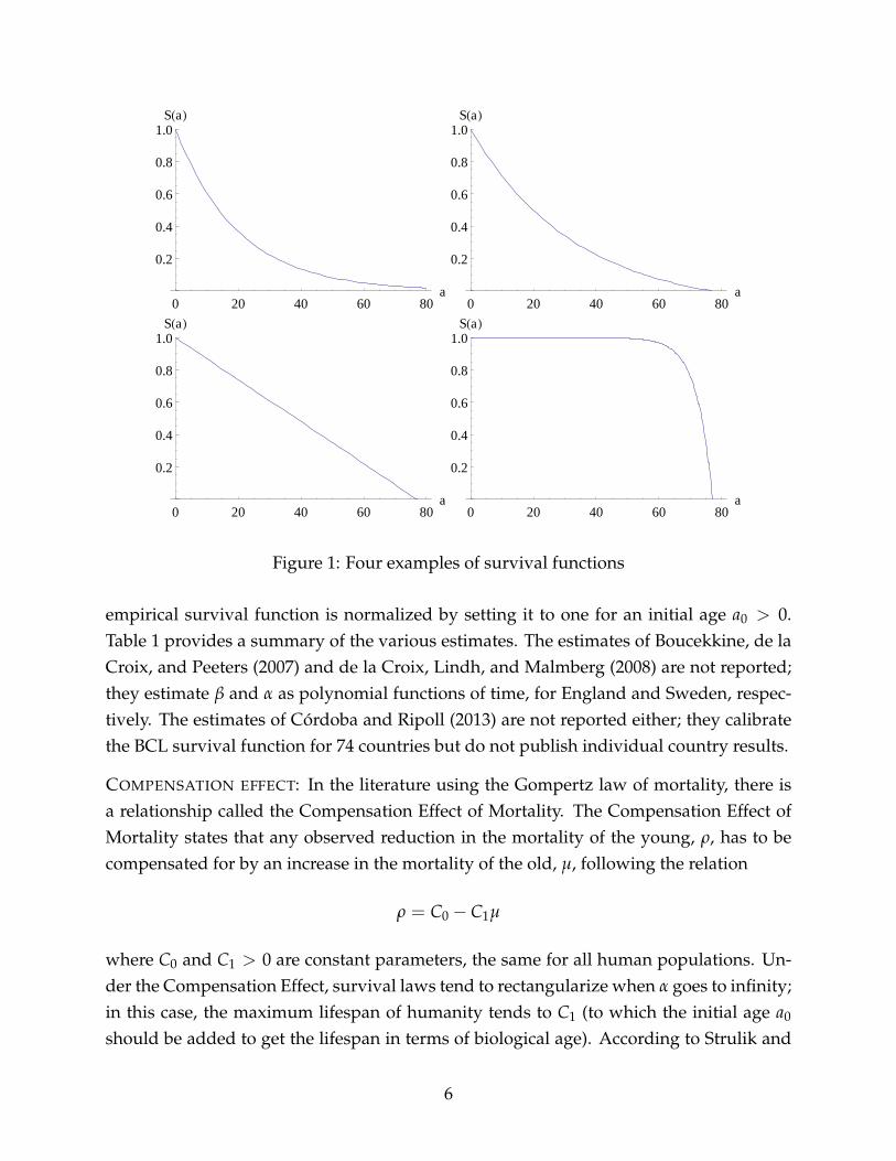
When the cohort of newborns is of size 1, life expectancy is also equal to the size ofthe population P. Second, this two-parameter curve fits the data very well (Mierau andTurnovsky 2014), except for the inflexion point which is observed for very old ages. Third,depending on the value of α and β, the survival function can reproduce several specialcases, as shown in Figure 1. The top left panel shows a survival function with a proba-bility of death independent of age (β = 0.05, α = 0). This is the perpetual youth modelpopularized by Blanchard (1985). In this set-up, there is a positive probability of reachingany age a ∈ R. When β, α > 0, the survival function is convex, as illustrated in the topright panel of Figure 1 for α = 0.1, β = 0.03. When α approaches 1 and β approaches0, the survival function becomes close to linear (see bottom left panel, with α = 0.999and β = 0.000013), which is, for example, a characteristic of the Roman Empire.1 Finally,when α > 1 and β < 0, the survival function is concave, like the current survival curvesof modern societies. Letting α increase and β decrease leads to a rectangularization of thefunction. For α very large, survival until the maximum age is almost certain, which is thecase assumed for example by Hazan (2009). The bottom right panel illustrates the casefor α = 5000000 and β = −0.2.

ESTIMATION OF PARAMETERS: The parameters of the BCL survival function have beenestimated on different populations. As this function is only valid for adult survival, the

1From http://www.richardcarrier.info/lifetbl.html, consulted on January 12, 2015,adapted from “Frier’s Life Table for the Roman Empire,” p.144 of T.G. Parkin, Demography and RomanSociety (1992).

5

0 20 40 60 80a

0.2

0.4

0.6

0.8

1.0SHaL

0 20 40 60 80a

0.2

0.4

0.6

0.8

1.0SHaL

0 20 40 60 80a

0.2

0.4

0.6

0.8

1.0SHaL

0 20 40 60 80a

0.2

0.4

0.6

0.8

1.0SHaL

Figure 1: Four examples of survival functions

empirical survival function is normalized by setting it to one for an initial age a0 > 0.Table 1 provides a summary of the various estimates. The estimates of Boucekkine, de laCroix, and Peeters (2007) and de la Croix, Lindh, and Malmberg (2008) are not reported;they estimate β and α as polynomial functions of time, for England and Sweden, respec-tively. The estimates of Cordoba and Ripoll (2013) are not reported either; they calibratethe BCL survival function for 74 countries but do not publish individual country results.

COMPENSATION EFFECT: In the literature using the Gompertz law of mortality, there isa relationship called the Compensation Effect of Mortality. The Compensation Effect ofMortality states that any observed reduction in the mortality of the young, ρ, has to becompensated for by an increase in the mortality of the old, µ, following the relation

ρ = C0 − C1µ

where C0 and C1 > 0 are constant parameters, the same for all human populations. Un-der the Compensation Effect, survival laws tend to rectangularize when α goes to infinity;in this case, the maximum lifespan of humanity tends to C1 (to which the initial age a0

should be added to get the lifespan in terms of biological age). According to Strulik and

6

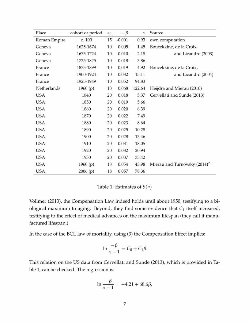
Place cohort or period a0 −β α Source

Roman Empire c. 100 15 -0.001 0.93 own computation

Geneva 1625-1674 10 0.005 1.45 Boucekkine, de la Croix,

Geneva 1675-1724 10 0.010 2.18 and Licandro (2003)

Geneva 1725-1825 10 0.018 3.86

France 1875-1899 10 0.019 4.92 Boucekkine, de la Croix,

France 1900-1924 10 0.032 15.11 and Licandro (2004)

France 1925-1949 10 0.052 94.83

Netherlands 1960 (p) 18 0.068 122.64 Heijdra and Mierau (2010)

USA 1840 20 0.018 5.37 Cervellati and Sunde (2013)

USA 1850 20 0.019 5.66

USA 1860 20 0.020 6.39

USA 1870 20 0.022 7.49

USA 1880 20 0.023 8.64

USA 1890 20 0.025 10.28

USA 1900 20 0.028 13.46

USA 1910 20 0.031 18.05

USA 1920 20 0.032 20.94

USA 1930 20 0.037 33.42

USA 1960 (p) 18 0.054 43.98 Mierau and Turnovsky (2014)2

USA 2006 (p) 18 0.057 78.36

Table 1: Estimates of S(a)

Vollmer (2013), the Compensation Law indeed holds until about 1950, testifying to a bi-ological maximum to aging. Beyond, they find some evidence that C1 itself increased,testifying to the effect of medical advances on the maximum lifespan (they call it manu-factured lifespan.)

In the case of the BCL law of mortality, using (3) the Compensation Effect implies:

ln−β

α− 1= C0 + C1β

This relation on the US data from Cervellati and Sunde (2013), which is provided in Ta-ble 1, can be checked. The regression is:

ln−β

α− 1= −4.21 + 68.6β,

7

with an R2 = 99.6, and a maximum lifespan C1 + a0 of 68.6+20=88.6. The very goodfit indicates that the Compensation Law holds to a large degree, and that most of thechanges in survival are related to a rectangularization process. Let us finally remark thatrectangularization has a particular economic importance. It means that the early increasein longevity benefits adults in their working age, therefore affecting economic incentivesto invest. At later stages, increasing longevity benefits old workers and retired peoplemore, and is probably of less importance as far as incentives are concerned.

Oxborrow and Turnovsky (2015) study the properties of a dynamic general equilibriummodel for an open economy where survival is modelled using various functions. Theyfind that assuming a fully rectangular survival curve or a BCL survival curve deliverssimilar economic responses to macroeconomic shocks, while assuming a constant mor-tality rate a la Blanchard yields very different outcomes (not much in the face of a pro-ductivity shock, but more facing changes in foreign interest rates ). The fact that, usingcurrent data, the BCL and the rectangular curves have similar properties in terms of eco-nomic incentives is not surprising as the rectangularization process of actual survivalfunctions is well advanced. Their conclusion would probably be reversed if they lookedat pre-industrial data where the survival function was close to linear. Then, the constantmortality function and the BCL would yield similar results, which are very different fromthe rectangular curve. As a conclusion, in order to study both periods, pre-industrial andcontemporaneous, the BCL survival function offers the required flexibility.

4 Contact Time Effect

For a long time, knowledge was not written in books or encoded in computer systems butwas embodied in people. Face-to-face communication was key for knowledge transmis-sion and enhancement. Today, even if books and computers have become key, person-to-person interactions remain essential for learning. That is why, after all, we economistsorganize and attend conferences and workshops.

When face-to-face communication does matter to accumulate knowledge, longer livesincrease the contact time between people. This is particularly important as far as appren-ticeship and teaching is concerned. The longer masters live, the more likely they are toaccumulate knowledge and to transmit it to a large number of apprentices. If Robert Lu-cas had died in 1992 at the age of 55, a pre-modern value for longevity, he would have

8

directed 17 Ph.D. dissertations instead of 34.3 Moreover he would not have had the op-portunity to further improve by exchanging ideas beyond the age of 55.

APPRENTICESHIP: I view a model of person-to-person exchange of ideas as crucial formodeling technological progress in the pre-industrial era. Most productive knowledgewas tacit, and was passed on directly from a “teacher” to a “student.” Across societies,much of this knowledge transmission took place within families, i.e. children enteredthe same occupations as their parents and acquired knowledge from working with them.However, the transmission of knowledge across family lines was also important, and here(at least in some areas) institutions such as apprenticeship and journeymanship played animportant role. By adopting a formal model of person-to-person transmission of knowl-edge, de la Croix, Doepke, and Mokyr (2015) help our understanding of the role of suchinstitutional arrangements for the transmission of knowledge and, ultimately, the overallrate of productivity growth. 4

LUCAS’S MODEL: A formal link between productivity growth and longevity is implic-itly provided by Lucas (2009) who builds on earlier contributions by Jovanovic and Rob(1989) and Kortum (1997). In his model, the productivity of any individual evolves as fol-lows. Suppose individuals have the productivity z at date t, viewed as a draw from thedate-t technology frontier, represented by a cumulative distribution function G. Over thetime interval (t, t + h), they get ηh independent draws from another distribution, witha cumulative distribution function H. Assuming that the source of everyone’s ideas isother people in the same economy, G = H. Let y denote the best of these draws. Then att + h, their productivity will be either their original productivity z or the best of their newideas y, whichever is higher: max(z, y).

MINIMUM STABILITY POSTULATE: Each idea y gives the possibility of producing one unitof output with cost x = y−1/θ. The distribution of ideas is assumed to be a Frechetdistribution with shape parameter 1/λt and scale parameter 1/θ:

Pr(Y < y) = exp{λt y−1/θ}

This distribution has the advantage of being preserved by the max operator of the match-

3Computations made using the genealogy module of RePec4In their model, knowledge is represented as the efficiency with which workers can perform tasks. While

there is some scope for new innovation, the main engine of technological progress is the transmission ofproductive knowledge from old to young workers. Young workers learn from elders through a form ofapprenticeship. There is a distribution of knowledge (or productivity) across workers, and when youngworkers learn from multiple old workers, they can adopt the best technique that they have been exposedto. Through this process, average productivity in the economy increases over time.

9

ing process. Let us see how. If ideas are drawn from a Frechet distribution, the corre-sponding costs are distributed following an exponential distribution with rate parameterλt:

Pr(X < x) = Pr(Y > x−θ) = 1− Pr(Y < x−θ) = 1− exp{λtx}.

The exponential distribution satisfies the minimum stability postulate according to whichif x1 and x2 are mutually independent random variables, exponentially distributed withrate parameter λ, then min(x1, x2) is exponentially distributed with rate parameter 2λ.As a consequence, the maximum of two independent random variables, Frechet dis-tributed with parameters (1/θ, 1/λ) will be itself Frechet distributed with parameters(1/θ, 1/(2θλ)). The Frechet distribution is said to satisfy the maximum stability postu-late.

The consequence of this nice property is that it is not necessary to track the entire distribu-tion of knowledge over time, but only the rate parameter of the underlying exponentialdistribution of cost. The only state variable of the model is λt, which is equal to theinverse of the mean cost. Being inversely related to the cost, λt is an indicator which ispositively associated with aggregate knowledge. Along a balanced growth path, λt growsat a constant rate γ, while GDP per capita grows at rate γθ.

INTRODUCING A COHORT STRUCTURE: In addition to these assumptions on knowledgediffusion, Lucas introduces a cohort structure with a stationary population characterizedby the density p(a) giving the density of population aged a in the economy. This impliesage-specific distributions of ideas. Assuming that everyone is met with equal proba-bility, Lucas relates the parameter λt of the aggregate distribution of knowledge to theage-specific distributions. It is through this structure that longevity affects knowledgediffusion. Indeed, if the survival curve is more rectangular, there are more old people inthe economy and the probability of meeting them is higher. As these old people are thosewith the best ideas – as they had more opportunities to improve their knowledge throughthe operator max –, having more old people around accelerates the rate of knowledgediffusion.

In the end, the growth rate of knowledge along a balanced growth path is given by Equa-tion (8) in Lucas (2009):

γ = η∫ a

0p(a)(1− e−γa)da, (4)

where, as explained above, γ is the growth rate of knowledge, η is a parameter measuringthe frequency of contacts and the ability to learn from others, and p(a) is the density of

10

population aged a. p(a) can be computed with the BCL survival function as:

p(a) =S(a)∫ a

0 S(x)dx=

β(e−βa − α

)1− α + α ln α

. (5)

Only in the case where α = 0, one can solve Equation (4) for γ. It yields two solutions,γ = 0, and γ = η − β. Growth depends negatively on the constant death rate β. In themore general case, numerical solutions must be used.

QUANTIFICATION: From the model above, what can be concluded is that the idea-processingrate η and the demographic parameters α and β combine to determine the rate γ of tech-nological change. Together with the Frechet scale parameter 1/θ, they determine thegrowth rate of GDP per capita γθ. This set-up can now be used to quantify the effect oflonger lives on GDP growth. I proceed in four steps.

1. Following Lucas (2009), θ is a parameter which can be estimated from the varianceof earnings across workers. I take the value estimated by Lucas which is equal to0.5.

2. η is now calibrated to give a realistic growth rate with a recent estimate of the sur-vival function. I consider the growth rate of the last century to be about 2% peryear. Given the value of θ, it requires a growth of knowledge λt of 4%. I take theα and β estimated on the cohort born in 1930 in the USA (β = −0.037, α = 33.42).Equations (4) and (5) are solved with these parameters to find the value of η withsuch a growth. It gives η = 0.0588.

3. Next, I compute what the growth rate would be if the survival parameters fromcohorts born one century before are imputed. I take θ = 0.5, η = 0.0588, the α and β

estimated on the cohort born in 1840 in the USA (β = −0.018, α = 5.37), and solvefor γ which leads to γ = 0.0366, implying an annual growth rate of GDP per capitaof 1.83%. This is the annual growth obtained with the 20th century characteristicsas implicitly contained in η and θ, but a 19th century survival level.

4. The same exercise is repeated with pre-industrial levels of the survival parameters.I still take θ = 0.5, η = 0.0588, together with the α and β estimated on the cohortborn in 1625-1674 in Geneva (β = −0.005, α = 1.45), and solve for γ which leads toγ = 0.0245, implying an annual growth rate of GDP per capita of 1.22%.

Column (a) of Table 2 summarizes the results. The relatively short lives of people before

11

(a) (b) (c) (d)Model Lucas Lucas Ben-Porath Ben-PorathBenchmark calibration 1930 1650 1930 1650

1650−→1850 + 0.0061 + 0.0074 +0.0030 + 0.00601850−→1930 + 0.0017 + 0.0017 +0.0010 + 0.0019

1650−→1930 + 0.0078 + 0.0091 + 0.0040 + 0.0079

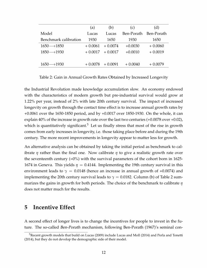
Table 2: Gain in Annual Growth Rates Obtained by Increased Longevity

the Industrial Revolution made knowledge accumulation slow. An economy endowedwith the characteristics of modern growth but pre-industrial survival would grow at1.22% per year, instead of 2% with late 20th century survival. The impact of increasedlongevity on growth through the contact time effect is to increase annual growth rates by+0.0061 over the 1650-1850 period, and by +0.0017 over 1850-1930. On the whole, it canexplain 40% of the increase in growth rate over the last two centuries (+0.0078 over +0.02),which is quantitatively significant.5 Let us finally stress that most of the rise in growthcomes from early increases in longevity, i.e. those taking place before and during the 19thcentury. The more recent improvements in longevity appear to matter less for growth.

An alternative analysis can be obtained by taking the initial period as benchmark to cal-ibrate η rather than the final one. Now calibrate η to give a realistic growth rate overthe seventeenth century (=0%) with the survival parameters of the cohort born in 1625-1674 in Geneva. This yields η = 0.4144. Implementing the 19th century survival in thisenvironment leads to γ = 0.0148 (hence an increase in annual growth of +0.0074) andimplementing the 20th century survival leads to γ = 0.0182. Column (b) of Table 2 sum-marizes the gains in growth for both periods. The choice of the benchmark to calibrate η

does not matter much for the results.

5 Incentive Effect

A second effect of longer lives is to change the incentives for people to invest in the fu-ture. The so-called Ben-Porath mechanism, following Ben-Porath (1967)’s seminal con-

5Recent growth models that build on Lucas (2009) include Lucas and Moll (2014) and Perla and Tonetti(2014), but they do not develop the demographic side of their model.

12

tribution, belongs to this category. According to this theory, the return to investment ineducation depends on the length of time during which education will be productive, i.e.a longer active life makes initial investment in human capital more profitable. Longer ed-ucation makes future income higher. Provided that human capital is an engine of growth,this may in turn sustain permanent income growth. The first authors to put this argumentat work in an endogenous growth model were de la Croix and Licandro (1999). Furthercontributions are in Kalemli-Ozcan, Ryder, and Weil (2000), Boucekkine, de la Croix, andLicandro (2002), Soares (2005) and Cervellati and Sunde (2014). Quantifications of theeffect can be found in de la Croix, Lindh, and Malmberg (2008) and Cordoba and Ripoll(2013). A complementary mechanism argues that longer lives give stronger incentives tosave and invest. Following the intuition of the life-cycle hypothesis, Nicolini (2004) claimsthat the increase in adult life expectancy must have implied less farmer impatience andcould have caused more investment in nitrogen stock and land fertility, the increase inagricultural land, and higher production per acre in hyphen 18th century England.

With these models, the same exercise as with the “contact time” model can be repeated:calibrate the set-up to modern growth, and then feed in the mortality conditions of thepre-industrial era keeping the other parameters constant and compare the growth rates.Let us first summarize the set-up linking mortality to growth through education incen-tives.

THE HOUSEHOLD PROBLEM: An individual born at time t, ∀t ≥ 0, has the followingexpected utility: ∫ t+a

tc(t, z) S(z− t) e−$(z−t)dz, (6)

where c(t, z) is the consumption of a generation t member at time z and $ is the pure timepreference parameter. Risk neutrality is assumed for simplicity.

There is a unique material good, the price of which is normalized to 1, which can beused for consumption. Every working household produces a quantity of good y(t) usinghuman capital h(t) according to the following simple technology: y(t) = h(t). A house-hold’s human capital depends on the time spent on education, T, on the average humancapital H(t) of the society at birth, and on the state of technology A:

h(t) = AH(t)T. (7)

With H(t), the typical externality which positively relates the future quality of the agentto the cultural ambience of the society (through for instance the quality of the school)

13

is introduced. Technology parameter A is a scale parameter that allows to match theobserved growth rate of human capital and output.

Equation (7) relates the human capital of an individual to the human capital of the societywhen this individual started his/her education (“at birth”). This implies that, along abalanced growth path with T constant and H(t) growing, old workers are less productivethan younger ones at any instant t, because they were educated long before, when averagehuman capital was not as high as today. This contrasts with the contact time approach,in which old workers are those with the highest skills (on average) as they had moreopportunities to improve their knowledge by meeting people than young workers.

The inter-temporal budget constraint of the agent born at t is:

∫ t+a

tc(t, z)R(t, z)dz =

∫ t+a

t+Th(t)R(t, z)dz. (8)

The left-hand side is the current cost of of all future contingent life-cycle consumptions.The right-hand side is the current value of contingent earnings. R(t, z) is the contingentprice paid by members of generation t to receive one unit of the physical good at time zin the case where they are still alive. By definition, R(t, t) = 1.

Individuals enter the labor market at age T with human capital h(t), and produce h(t)per unit of time. They work until death.6

The problem of the representative individual from generation t is to select a consumptioncontingent plan and the duration of his or her education to maximize the expected utilitysubject to the inter-temporal budget constraint, and given the per capita human capitaland the sequence of contingent wages and contingent prices. The corresponding first-order necessary conditions for a maximum lead to the following optimal rule for T:

T S(T) e−$T =∫ a

TS(a) e−$a da, (9)

The left-hand side is related to the opportunity cost of postponing the entry in the labormarket, while the right-hand side is the marginal benefit of increasing education mea-sured by the increase in the discounted flow of future wages.

AGGREGATE HUMAN CAPITAL: The productive aggregate stock of human capital is com-

6In the original version of Boucekkine, de la Croix, and Licandro (2002), they have a disutility of laborincreasing with age and they choose a retirement age optimally.

14

puted from the human capital of all generations currently at work:

Y(t) = H(t) =∫ t−T

t−aS(t− z)h(z)dz, (10)

where t− T (= t− T along a BGP) is the last generation that entered the job market at tand t− a is the oldest generation still alive at t. The average human capital at the root ofthe externality (7) is obtained by dividing the aggregate human capital by the size of thepopulation:

H(t) =H(t)

P. (11)

Hence, the dynamics of human capital are given by:

H(t) =∫ t−T

t−aS(t− z)

AH(z)TP

dz, (12)

and its growth rate g, along a balanced growth path, should satisfy:

1 =ATP

∫ a

TS(z)e−gzdz. (13)

As shown in Boucekkine, de la Croix, and Licandro (2002), a rise in life expectancy (ei-ther through an increase in α or a drop in β) increases the optimal length of schooling.Moreover, along a balanced growth path, a rise in life expectancy has a positive effecton economic growth for low levels of life expectancy and a negative effect on economicgrowth for high levels of life expectancy. Intuitively, the total effect of an increase in lifeexpectancy results from combining three factors: (a) agents die on average later, thus thedepreciation rate of aggregate human capital decreases; (b) agents tend to study morebecause the expected flow of future wages has risen, and the human capital per capitaincreases; and (c) the economy consists more of old agents who received their schoolinga long time ago. The first two effects have a positive influence on the growth rate, but thethird effect has a negative influence.

QUANTIFICATION: I now proceed with the quantitative analysis in four steps.

1. First, the pure rate of time preference $ is set to 4% per year.

2. Next, A is calibrated to give a realistic growth rate with a recent estimate of thesurvival function. I consider that the growth rate of the last century is about 2% peryear. Given the value of $, and taking the α and β estimated on the cohort born in

15

1930 in the USA (β = −0.037, α = 33.42), Equations (9) and (13) are solved to findA = 0.1723. Along this balanced growth path, T = 20.8, which is too high.7

3. Next, I compute what the growth rate would be if the survival parameters fromcohorts born one century before are imputed. Taking $ = 0.04, A = 0.1723, and the α

and β estimated on the cohort born in 1840 in the USA (β = −0.018, α = 5.37), I solvefor γ which leads to γ = 0.0190, implying an annual growth rate of GDP per capitaof 1.9%. This is the annual growth obtained with the 20th century characteristics asimplicitly contained in η and θ, but a 19th century survival level.

4. The same exercise is repeated with pre-industrial levels of the survival parameters.Still taking $ = 0.04, A = 0.1723, together with the α and β estimated on the cohortborn in 1625-1674 in Geneva (β = −0.005, α = 1.45), and solving for γ, I findγ = 0.016, i.e. an annual growth rate of GDP per capita of 1.6%. Schooling in thissimulation is T = 15.8.

What can be concluded from this exercise is that the rectangularization of the survivalcurve can be held responsible for one-fifth of the increase in growth rates over the lasttwo centuries (explaining +0.4% over +2%), and one-fourth of the increase in schooling(5 years over 20). Column (c) of Table 2 summarizes these results. The effects are smallerthan with the contact time model. If, instead of calibrating the parameter A to reproduce2% of growth in the twentieth century, A is chosen to reproduce the absence of growthin the seventeenth century, the results are magnified as shown in column (d) of Table 2.Longevity increases account for an increase in annual growth of +0.6% between 1650 and1850 and +0.79% between 1650 and 1930.

Similar results have been debated in the literature. Assuming a perfectly rectangularsurvival function, Hazan (2009) argues that if it was true that longevity increased school-ing investment through the incentive mechanism of Ben-Porath (1967), an increase inexpected lifetime working hours should also be observed, while what is observed on USdata is that lifetime labor supply actually decreased over the last century. This observa-tion led him to conclude that the Ben-Porath mechanism cannot be responsible for theobserved rise in education and growth.

It is easy to understand that Hazan (2009)’s critique cannot be true in general. Considerthe following example illustrated in Figure reffig:hazan. Households live for three peri-ods. In period 1, they can either work or get education. In periods 2 and 3, they work. If

7There are several ways to fix this problem: lower the return to schooling, introduce a fixed retirementage, or assume that some part of the schooling was achieved before age a0.

16

22

11 11

40

20

education

ageage

survivalsurvival

11

period 1 period 2 period 3 period 1 period 2 period 3

Figure 2: Example with Increasing Longevity & Schooling but Decreasing Lifetime LaborSupply

they do not get education, their income per period is 22. If they get an education, theirincome per period is 40.

• Suppose first that they have a 50% chance of dying during the second period butif they survive, they live through the third period for sure. If they do not get aneducation, their expected lifetime income is: 22 + 0.5× 22 + 0.5× 22 = 44 and theirexpected lifetime labor supply is: 2. If they get an education, their expected lifetimeincome is: 0.5× 40+ 0.5× 40 = 40 and their expected lifetime labor supply is 1. Thebest choice is to get no education and work 2 units on average.

• Suppose now that they are certain to survive in period 2, but they have a 50% chanceof dying in period 3. This is a shift in the survival function - a rectangularization. Ifthey do not get an education, their expected lifetime income is: 22+ 22+ 0.5× 22 =

55 and their expected lifetime labor supply is: 2.5. If they get an education, theirexpected lifetime income is 40 + 0.5 × 40 = 60 and their expected lifetime laborsupply is: 1.5. It is now best to get an education, as a response to lower mortality,and to work 1.5 units on average.

Hence, to summarize, the drop in mortality has the following consequences: Educationgoes from 0 to 1, income goes from 44 to 60, labor supply goes from 2 to 1.5, and the BenPorath mechanism is compatible with a shorter lifetime labor supply.

More generally, Cervellati and Sunde (2013) show that Hazan (2009)’s claim relies onthe rectangular survival function he assumed, and that the Ben Porath mechanism canbe reconciled with decreasing lifetime labor supply when the survival function is not

17

perfectly rectangular.8

6 Conclusions

In this note, I have made the point that increases in longevity are quantitatively signifi-cant to explain the acceleration of growth over the last two centuries. Hence, beyond geo-graphical, institutional and cultural determinants of growth, demographic factors shouldalso be considered.

References

Ben-Porath, Yoram. 1967. “The production of human capital and the life-cycle of earn-ings.” Journal of Political Economy 75 (4): 352–365.

Blanchard, Olivier. 1985. “Debt, deficits and finite horizons.” Journal of Political Economy93:223–247.

Boucekkine, Raouf, David de la Croix, and Omar Licandro. 2002. “Vintage HumanCapital, Demographic Trends, and Endogenous Growth.” Journal of Economic Theory104 (2): 340–75.

. 2003. “Early mortality declines at the dawn of modern growth.” ScandinavianJournal of Economics 105 (3): 401–418.

. 2004. “Modelling vintage structures with DDEs: principles and applications.”Mathematical Population Studies 11:151–179.

Boucekkine, Raouf, David de la Croix, and Dominique Peeters. 2007. “Early LiteracyAchievements, Population Density and the Transition to Modern Growth.” Journal ofthe European Economic Association 5:183–226.

Bruce, Neil, and Stephen J. Turnovsky. 2013. “Social security, growth, and welfare inoverlapping generations economies with or without annuities.” Journal of Public Eco-nomics 101:12–24.

Cervellati, Matteo, and Uwe Sunde. 2013. “Life Expectancy, Schooling, and LifetimeLabor Supply: Theory and Evidence Revisited.” Econometrica 81 (5): 2055–2086 (09).

8Other mechanisms can also reconcile Ben Porath with the facts, such as imperfect financial markets, seeHansen and Lønstrup (2012).

18

. 2014. “The Economic and Demographic Transition, Mortality, and ComparativeDevelopment.” American Economic Journal Macroeconomics. forthcoming.

Cordoba, Juan Carlos, and Marla Ripoll. 2013. “What explains schooling differencesacross countries?” Journal of Monetary Economics 60 (2): 184–202.

Cummins, Neil. 2014. “Longevity and the Rise of the West: Lifespans of the Euro-pean Elite, 800-1800.” Working papers 0064, European Historical Economics Society(EHES).

de la Croix, David, Matthias Doepke, and Joel Mokyr. 2015. “Clans, Guilds, and Mar-kets: Apprenticeship Institutions and Growth in the Pre-Industrial Economy.” un-published.

de la Croix, David, and Omar Licandro. 1999. “Life expectancy and endogenousgrowth.” Economics Letters 65 (2): 255–263.

. 2015. “The Longevity of Famous People from Hammurabi to Einstein.” Journalof Economic Growth.

de la Croix, David, Thomas Lindh, and Bo Malmberg. 2008. “Swedish economicgrowth and education since 1800.” Canadian Journal of Economics / Revue canadienned’Economique 41 (1): 166–185.

Gompertz, Benjamin. 1825. “On the nature of the function expressive of the law ofhuman mortality, and on a new mode of determining the value of life contingencies.”Philosophical Transactions of the Royal Society of London 115:513–583.

Hansen, Casper Worm, and Lars Lønstrup. 2012. “Can higher life expectancy inducemore schooling and earlier retirement.” Journal of Population Economics 25:1249–1264.

Hazan, Moshe. 2009. “Longevity and Lifetime Labour Supply: Evidence and Implica-tions.” Econometrica 77:1829–1863.

Heijdra, Ben, and Jochen Mierau. 2010. “Growth effects of consumption and labourincome taxation in an overlapping-generations life-cycle model.” Macroeconomic Dy-namics 14:151–175.

Hollingsworth, Thomas. 1977. “Mortality in the British peerage families since 1600.”Population 32:323–352.

Jovanovic, Boyan, and Rafael Rob. 1989. “The Growth and Diffusion of Knowledge.”The Review of Economic Studies 56 (4): 569–82.

Kalemli-Ozcan, Sebnem, Harl E. Ryder, and David N. Weil. 2000. “Mortality decline,

19

human capital investment, and economic growth.” Journal of Development Economics62 (1): 1–23 (June).

Kortum, Samuel S. 1997. “Research, Patenting, and Technological Change.” Econometrica65 (6): 1389–419.

Lucas, Jr., Robert E. 2009. “Ideas and Growth.” Economica 76 (301): 1–19.

Lucas, Jr., Robert E., and Benjamin Moll. 2014. “Knowledge Growth and the Allocationof Time.” Journal of Political Economy 122 (1): 1–51.

Mierau, Jochen O., and Stephen J. Turnovsky. 2014. “Capital accumulation and thesources of demographic change.” Journal of Population Economics 27:857–894.

Nicolini, Esteban. 2004. “Mortality, interest rates, investment, and agricultural produc-tion in 18th century England.” Explorations in Economic History 41 (2): 130–155.

Oxborrow, David, and Stephen J. Turnovsky. 2015. “Closing the Small Open EconomyModel: A Demographic Approach.” University of Washington.

Perla, Jesse, and Christopher Tonetti. 2014. “Equilibrium Imitation and Growth.” Journalof Political Economy 122 (1): 52–76.

Soares, Rodrigo R. 2005. “Mortality Reductions, Educational Attainment, and FertilityChoice.” American Economic Review 95 (3): 580–601 (June).

Strulik, Holger, and Sebastian Vollmer. 2013. “Long-run trends of human aging andlongevity.” Journal of Population Economics 26 (4): 1303–1323.

Vandenbroucke, Jan. 1985. “Survival and expectation of life from the 1400’s to thepresent - A study of the knighthood order of the Golden Fleece.” American Journal ofEpidemiology 22 (6): 1007–1015.

20

ISSN 1379-244X D/2015/3082/12