Diagnosing Multiple Faults - PARC Multiple... · Diagnosing Multiple Faults ... mechanical devices...

ARTIFICIAL INTELLIGENCE 97

Diagnosing Multiple Faults

Johan de KleerIntelligent SystemsLaboratory, XEROXPalo Alto ResearchCenter, Palo Alto, CA 94304, U.S.A.

Brian C. WilliamsArtificial IntelligenceLaboratory, MIT, Cambridge,MA 02139, U.S.A.

Recommendedby JudeaPearl

ABSTRACT

Diagnostictasks require determiningthe differencesbetweena modelof an artifact and the artifactitself. The differencesbetweenthemanifestedbehaviorof the artifact and the predictedbehaviorofthe model guide the searchfor the differencesbetweenthe artifact and its model. The diagnosticprocedurepresentedin this paper is model-based,inferring the behaviorof the compositedevicefrom knowledgeof the structureandfunction of the individual componentscomprisingthe device.The system(GDE—generaldiagnosticengine)has beenimplementedand testedon manyexamplesin the domain of troubleshootingdigital circuits.

This researchmakesseveral novel contributions: First, the systemdiagnosesfailures due tomultiplefaults. Second,failure candidatesare representedand manipulatedin termsofminimal setsof violated assumptions,resulting in an efficient diagnostic procedure. Third, the diagnosticprocedureis incremental,exploiting the iterative nature of diagnosis.Fourth, a clear separationisdrawn betweendiagnosisand behaviorprediction, resulting in a domain (and inferenceprocedure)independentdiagnosticprocedure. Fifth, GDE combinesmodel-basedprediction with sequentialdiagnosis to propose measurementsto localize the faults. The normally required conditionalprobabilities are computedfrom the structure of the device and models of its components.Thiscapability resultsfrom a novel way of incorporatingprobabilities and information theory into thecontextmechanismprovidedby assumption-basedtruth maintenance.

1. Introduction

Engineersand scientists constantly strive to understandthe differencesbe-tweenphysical systemsand their models. Engineerstroubleshootmechanicalsystemsor electricalcircuits to find brokenparts.Scientistssuccessivelyrefine amodel basedon empirical dataduring the processof theory formation. Many

Artificial Intelligence32 (1987) 97—1300004-3702/87/$3.50© 1987, ElsevierSciencePublishersBy. (North-Holland)

98 J. DE KLEER AND B.C. WILLIAMS

everydaycommon-sensereasoningtasksinvolve finding thedifferencebetweenmodelsand reality.

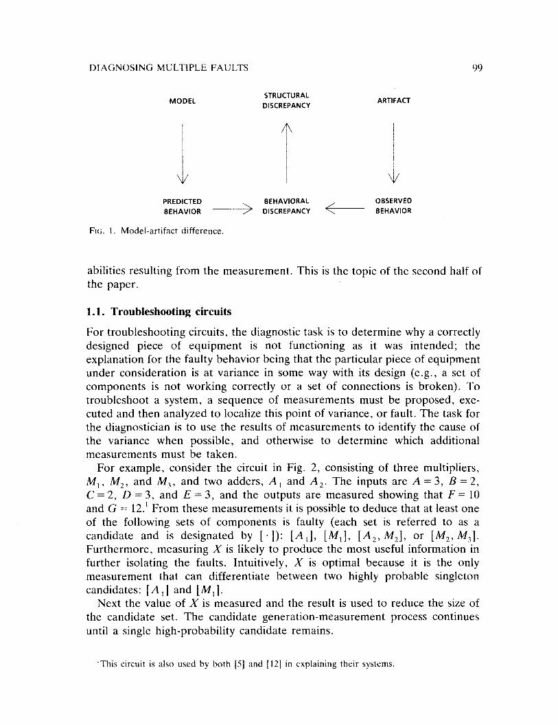
Diagnosticreasoningrequiresa meansof assigningcredit or blameto partsof the model based on observedbehavioral discrepancies.If the task istroubleshooting,then the model is presumedto be correct and all model-artifactdifferencesindicate part malfunctions. If the task is theory formation,then the artifact is presumedto be correct and all model-artifactdifferencesindicate requiredchangesin the model (Fig. 1).

Usually the evidence does not admit a unique model-artifact difference.Thus, the diagnostictask requirestwo phases.The first, mentionedabove,identifies the set of possiblemodel-artifactdifferences.The secondproposesevidence-gatheringteststo refine theset of possiblemodel-artifactdifferencesuntil they accuratelyreflect the actual differences.

This view of diagnosis is very general,.encompassingtroubleshootingmechanicaldevicesand analogand digital circuits, debuggingprograms,andmodeling physical or biological systems. Our approachto diagnosis is alsoindependentof the inference strategy employedto derive predictionsfromobservations.

Earlier researchwork (seeSection6) on model-baseddiagnosisconcentratedon determininga single faulty componentthat explainsall thesymptoms.Thispaperextendsthat researchby diagnosingsystemswith multiple failed compo-nents,andby proposinga sequenceof measurementswhich efficiently localizethe failing components.

When oneentertainsthe possibility of multiple faults, thespaceof potentialcandidatesgrowsexponentiallywith thenumberof faults underconsideration.This work is aimed specifically at developing an efficient general method,referredto as the generaldiagnosticengine(GDE), for diagnosingfailuresdueto any numberof simultaneousfaults. To achievethe neededefficiency, GDE

exploits the featuresof assumption-basedtruth maintenance(ATMS) [8]. This isthe topic of the first half of the paper.

Usually, additionalmeasurementsare necessaryto isolatethesetof compo-nentswhich areactually faulted. The bestnext measurementis the onewhichwill, on average,lead to the discoveryof the faulted set of componentsin aminimum number of measurements.Unlike other probabilistic techniqueswhich require a vast numberof conditional probabilities, GDE need only beprovided with the a priori probabilitiesof individual componentfailure. Usingan ATMS, thisprobabilisticinformationcanbe incorporatedinto GDE suchthat itis straightforwardto computetheconditionalprobabilitiesof thecandidates,aswell as the probabilitiesof the possibleoutcomesof measurements,basedonthe faulty device’s model. This combination of probabilistic inference andassumption-basedtruth maintenanceenablesGDE to apply a minimum entropymethod [1] to determinewhat measurementto make next: the bestmeasure-ment is the one which minimizes the expectedentropy of candidateprob-

DIAGNOSING MULTIPLE FAULTS 99

STRUCTURAL

MODEL DISCREPANCY ARTIFACT_ T _PREDICTED BEHAVIORAL OBSERVEDBEHAVIOR > DISCREPANCY BEHAVIOR

FIG. 1. Model-artifactdifference.

abilities resultingfrom themeasurement.This is the topic of thesecondhalf ofthe paper.

1.1. Troubleshooting circuits

For troubleshootingcircuits, thediagnostictaskis to determinewhy acorrectlydesigned piece of equipment is not functioning as it was intended; theexplanationfor the faulty behaviorbeingthattheparticularpieceof equipmentunderconsiderationis at variance in someway with its design (e.g., a set ofcomponentsis not working correctly or a set of connectionsis broken). Totroubleshoota system,a sequenceof measurementsmust be proposed,exe-cutedandthenanalyzedto localize this point of variance,or fault. The taskforthe diagnosticianis to usethe resultsof measurementsto identify thecauseofthe variance when possible, and otherwise to determinewhich additionalmeasurementsmust be taken.

For example,considerthe circuit in Fig. 2, consistingof threemultipliers,M1, M2, and M3, and two adders,A1 and A2. The inputs areA = 3, B = 2,C = 2, D = 3, and E 3, and the outputs are measuredshowing that F = 10andG = 12.1 From thesemeasurementsit is possibleto deducethat at leastoneof the following sets of componentsis faulty (each set is referred to as acandidateand is designatedby [.]): [A1], [M1], [A2, M,], or [M2, M1].Furthermore,measuringX is likely to producethe most useful information infurther isolating the faults. Intuitively, X is optimal becauseit is the onlymeasurementthat can differentiate between two highly probable singletoncandidates:[A1] and [MI].

Next the value of X is measuredand the result is usedto reducethe size ofthe candidateset. The candidategeneration-measurementprocesscontinuesuntil a single high-probability candidateremains.

‘This circuit is also used by both [5] and [12] in explaining their systems.


3

2 10

2

12

3

FIG. 2. A familiar circuit.

1.2. Somebasic presuppositions

Although GDE considersmultiple faults andprobabilisticinformation, it sharesmanyof the basicpresuppositionsof othermodel-basedresearch.We presumethat the act of taking a measurement(i.e., making an observation)has noaffect on the faulty device. We presumethat once a quantityis measuredto bea certain value, that the quantity remainsat the value. This is equivalenttoassumingthat no component’s(correct or faulty) functioningdependson thepassageof time. For example,this rules out flip-flops as well as intermittentcomponentswhich spontaneouslychangetheir behavior.We presumethat if acomponentis faulty, the distribution of input-output valuesbecomesrandom(i.e., contains no information). We do not presumethat if a component isfaulty, that it must be exhibiting this faulty behavior—it may exhibit faultybehavior on some other set of inputs. Thesepresuppositionssuggestfuturedirectionsfor research,andwe areextendingGDE in thesedirections.

2. A Theory of Diagnosis

The remainderof this paperpresentsa general,domain-independent,diagnos-tic engine(GDE) which, when coupledwith a predictive inferencecomponentprovides a powerful diagnosticprocedurefor dealing with multiple faults. Inaddition the approachis demonstratedin the domain of digital electronics,using propagationasthe predictive inferenceengine.


2.1. Model-artifact differences

The modelof the artifactdescribesthe physicalstructureof the devicein termsof its constituents.Eachtype of constituentobeyscertainbehavioralrules. Forexample,a simple electrical circuit consistsof wires, resistorsand so forth,wherewires obey Kirchhoff’s CurrentLaw, resistorsobey Ohm’s Law, and soon. In diagnosis, it is given that the behaviorof the artifact differs from itsmodel. It is then the task of the diagnostician to determine what thesedifferencesare.

The model for the artifact is a description of its physical structure, plusmodels for eachof its constituents.A constituentis a very general concept,including components,processesand even steps in a logical inference. Inaddition, eachconstituenthasassociatedwith it a set of one or morepossiblemodel-artifactdifferenceswhich establishesthe grain size of the diagnosis.

Diagnosistakes(1) the physicalstructure,(2) modelsfor eachconstituent,(3) a setof possiblemodel-artifactdifferences,and (4) a set of measurements,and producesa set of candidates,eachof which is a set of differenceswhichexplainsthe observations.

Our diagnosticapproachis basedon characterizingmodel-artifactdifferencesas assumptionviolations.A constituentis guaranteedto behaveaccordingto itsmodel only if none of its associateddifferencesare manifested,i.e., all theconstituent’sassumptionshold. If any of theseassumptionsare false, thentheartifact deviates from its model, thus, the model may no longer apply. Animportant ramification of this approach[4,5,10,12,29] is that we need onlyspecify correct modelsfor constituents—explicitfault models are not needed.

Reasoningaboutmodel-artifactdifferencesin termsof assumptionviolationsis very general.For example,in electronicsan assumptionmight be the correctfunctioning of eachcomponentand the absenceof any short circuits; in ascientificdomaina faulty hypothesis;in a commonsensedomainan assumptionsuchas persistence,defaultsor Occam’srazor.

2.2. Detectionof symptoms

We presume(asis usually the case)that the model-artifactdifferencesarenotdirectly observable.2Instead, all assumptionviolations must be inferred in-directly from behavioral observations.In Section 2.7 we presenta generalinference architecturefor this purpose,but for the moment we presumeaninferenceprocedurewhich makesbehavioralpredictionsfrom observationsandassumptionswithout beingconcernedabout the procedure’sdetails.

Intuitively, a symptomis any difference betweena prediction madeby theinferenceprocedureandan observation.Considerour examplecircuit. Given

21n practicethe diagnosticiancan sometimesdirectly observea malfunctioningcomponentbylooking for a crack or burn mark.


the inputs, A = 3, B = 2, C = 2, D = 3, andE = 3, by simplecalculation(i.e.,the inference procedure),F = X X V= A X C + B X D = 12. However, F ismeasuredto be 10. Thus “F is observedto be 10, not 12” is a symptom.Moregenerally,a symptomis any inconsistencydetectedby the inferenceprocedureandmay occurbetweentwo predictions(inferred from distinct measurements)aswell as a measurementanda prediction(inferredfrom someothermeasure-ments).

2.3. Conflicts

The diagnosticprocedureis guided by the symptoms.Each symptomtells usaboutoneor moreassumptionsthatarepossiblyviolated(e.g.,componentthatmay be faulty). Intuitively, a conflict is a set of assumptionswhich supportasymptom, and thus leads to an inconsistency.In this electronicsexample,aconflict is a set of componentswhich cannot all be functioning correctly.Consider the example symptom “F is observedto be 10, not 12.” Thepredictionthat F = 12 dependson the correct operationof A1, M1, and M2,i.e., if A1, M1, and M, werecorrectly functioning, thenF = 12. SinceF is not12, at leastone of A1, M1, and M, is faulted. Thus theset (At, M1, M2~is aconflict for the symptom (conflicts are indicatedby (~)). Becausethe infer-enceis monotonicwith thesetof assumptions,the set (A1, A2, M1, M,), andany other supersetof (A ~, M1, M2) areconflicts aswell; however,no subsetsof (A ~ M1, M2) are necessarilyconflicts since all the componentsin theconflict were neededto predict the value at F.

A measurementmight agree with one prediction and yet disagree withanother,resulting in a symptom.For example,startingwith the inputsB = 2,C = 2, D = 3, andE = 3, andassumingA-,, M2, andM3 arecorrectly function-ing we calculateG to be 12. However,startingwith theobservationF = 10, theinputsA = 3, C = 2, and E = 3, andassumingthat A1, A2, M1, and M3, (i.e.,ignoring M.,) are correctly functioning we calculate G = 10. Thus, when G ismeasuredto be 12, even though it agreeswith the first prediction, it stillproducesa conflict basedon the second:(A ~, ~, M~,M3).

For complex domains any single symptom can give rise to a large set ofconflicts, including the set of all componentsin the circuit. To reduce thecombinatoricsof diagnosisit is essentialthat thesetof conflicts be representedand manipulatedconcisely. If a set of componentsis a conflict, then everysupersetof that set must also be a conflict. Thus the set of conflicts can berepresentedconciselyby only identifying the minimal conflicts, whereaconflictis minimal if it has no propersubsetwhich is alsoaconflict. This observationiscentral to the performanceof our diagnosticprocedure.The goal of conflictrecognition is to identify the completesetof minimal conflicts.3

3Representingthe conflict spacein termsof minimal conflicts is analogousto the idea of versionspacesfor representingplausiblehypothesesin singleconcept learning [19].


2.4. Candidates

A candidate is a particularhypothesisfor how the actual artifactdiffers fromthe model. For example “A, and M, are broken” is a candidatefor the twosymptomsobservedfor our examplecircuit. Ultimately, the goal of diagnosisisto identify, and refine, the set of candidatesconsistentwith the observationsthus far.

A candidateis representedby a set of assumptions(indicatedby [.]). Theassumptionsexplicitly mentionedarefalse, while the onesnot mentionedaretrue. A candidatewhich explains the current set of symptomsis a set ofassumptionssuch that if every assumptionfails to hold, then every knownsymptom is explained.Thus eachset representinga candidatemust have anonemptyintersectionwith every conflict.

For electronics, a candidate is a set of failed components,where anycomponentsnot mentionedare guaranteedto be working. Before any mea-surementshavebeentaken we know nothingabou.tthe circuit. The candidatespaceis theset of candidatesconsistentwith the observations.The size of theinitial candidatespacegrows exponentiallywith the numberof components.Any componentcould be working or faulty, thusthecandidatespacefor Fig. 2initially consistsof 2~= 32 candidates.

It is essentialthat candidatesbe representedconciselyas well. Notice that,like conflicts, candidateshave the property that any supersetof a possiblecandidatefor a setof symptomsmust be a possiblecandidateaswell. Thus thecandidatespacecan be representedby the minimal candidates.Representingand manipulatingthecandidatespacein termsof minimal candidatesis crucialto our diagnosticapproach.Although thecandidatespacegrowsexponentiallywith the numberof potentiallyfaulted components,it is usually thecasethatthesymptomscan be explainedby relatively few minimal candidates.

The goal of candidategeneration is to identify the completeset of minimalcandidates.The spaceof candidatescan be visualized in terms of a subset-supersetlattice (Fig. 3). The minimal candidatesthendefine a boundarysuchthat everything from the boundaryup is a valid candidate,while everythingbelow is not.

Given no measurementsevery componentmight be working correctly, thusthe single minimal candidateis the empty set, [ ], which is the root of thelattice at the bottom of Fig. 3.

To summarize,the set of candidatesis constructedin two stages:conflictrecognitionand candidategeneration.Conflict recognition usesthe observa-tions made along with a model of the device to constructa completeset ofminimal conflicts. Next, candidategenerationusesthesetof minimal conflictsto constructa completeset of minimal candidates.Candidategenerationis thetopic of thenext section,while conflict recognitionis discussedin Section2.6.


(Al ,A2,Ml Mi, M3(

[Al Ml ,M2,M3I (A2,Ml ,M2,M31 (Al ,A2,Ml Mi] (Al,Ai,Ml ,M3( (Al ,A2,M2,M3(

IMI,M2,M3( IA1.M1,M2l (Ai.Ml.M2( (Al,Ml,M3l (A2,Ml,M31 [Al,M2,M3] (Al,A2,Ml( 1A2,M2,M31 (Al,Ai.Mi1 (Al,A2.M3(

—[Ml,M21 (Ml,M3( (Al,Ml( (M2,M3( (A2,MlJ (Al,Mi( 1A2,M2( (Al.M3] (A2,M3( (Al.A21

(Ml( (M2( (M3( (Al] (Au

FIG. 3. Initial candidatespace for the circuit example.

2.5. Candidate generation

Diagnosisis an incrementalprocess;asthe diagnosticiantakesmeasurementshe continually refines the candidatespaceandthen usesthis to guide furthermeasurements.Within a single diagnosticsessionthe total set of candidatesmust decreasemonotonically. This correspondsto having the minimal candi-datesmove monotonicallyup through the candidatesupersetlattice towardsthe candidatecontainingall components.Similarly, the total set of conflictsmust increasemonotonically.This correspondsto having theminimal conflictsmove monotonically down through a conflict supersetlattice towards theconflict representedby theemptyset. Candidatesaregeneratedincrementally,using the new minimal conflict(s) andtheold minimal candidate(s)to generatethe new minimal candidate(s).

The set of minimal candidates is incrementally modified as follows.Whenevera new minimal conflict is discovered,any previousminimal candi-date which doesnot explain the new conflict is replacedby one or moresupersetcandidateswhich are minimal basedon this new information. This isaccomplishedby replacing the old minimal candidatewith a set of new


tentativeminimal candidateseachof which containstheold candidateplus oneassumptionfrom the new conflict. Any tentative new candidatewhich issubsumedor duplicatedby anotheris eliminated;the remainingcandidatesareaddedto the setof new minimal candidates.

Considerour example. initially there are no conflicts, thus the minimalcandidate[ ] (i.e., everythingis working) explainsall observations.We havealready seenthat the single symptom “F = 10 not 12” producesone conflict(A1, M1, M2). This rules out the single minimal candidate[ ]. Thus, itsimmediatesupersetscontainingoneassumptionof the conflict [A1], [M1J, and[M,] are considered.None of theseare duplicatedor subsumedas therewereno otherold minimal candidates.The new minimal candidatesare [A1], [M1],and [M,]. This situation is depicted with the lattice in Fig. 4. All candidatesabove the line labeled by the conflict “Cl: (A1, M1, M2)” are valid candi-dates.

The secondconflict (inferredfrom observationG = 12), (A ~,A.,, M1, M3),only eliminates minimal candidate[M2]; the unaffectedminimal candidates

(Al.A2,Ml,M2,M3]

(Al ,Ml .M2,M3] [A2,Ml ,M2.M3] (Al .Ai.Ml.M2( (Al ,A2,Ml ,Mu( (Al .A2.MLM3(

[Ml,M2,M3( (Al,Ml,M2( (A2.Ml,Mi( (Al,Ml.M31 (A2.Ml.M31 (Al,M2,M3( (Al,A~,Ml] (A2,M2,M31 (Al,Ai,M2( (Al,A2.M3)

FIG. 4. Candidatespaceafter measurements.


[M1], and [A ~1remain. However, to completethe set of minimal candidateswe must consider the immediate supersetsof [M,] which cover the newconflict: [A1, M,], [A,, M,], [M(, M,], and [M2, M3]. Each of thesecandi-datesexplainsthenew conflict, however, [A1, M7] and [M1, M,] aresupersetsof the minimal candidates[A1] and [M1j, respectively.Thus thenew minimalcandidatesare [A,, M1], and [M,, M3}, resultingin theminimal candidateset:[A1], [M1], [A,, M,], and [M2, M3]. The line labeled by conflict “C2:(A1, A,, M1, M3)” in Fig. 4 showsthecandidateseliminatedby theobserva-tion G = 12 alone, and the line labeled “Cl & C2” shows the candidateseliminatedasa resultof both measurements(F = 10 andG = 12). The minimalcandidatewhich split the lattice into valid and eliminated candidatesarecircled.

Candidategenerationhas several interestingproperties.First, the set ofminimal candidatesmay increaseor decreasein size asa result of a measure-ment;however,a candidate,onceeliminatedcanneverreappear.As measure-mentsaccumulateeliminatedminimal candidatesarereplacedby largercandi-dates.Second,if an assumptionappearsin every minimal candidate(and thusevery candidate),then that assumptionis necessarilyfalse. Third, the presup-positionthat thereis only a single fault (exploitedin all previousmodel-basedtroubleshooting strategies), is equivalent to assuming all candidatesaresingletons.In this case,the set of candidatescan be obtainedby intersectingall theconflicts.

2.6. Conflict recognition strategy

The remainingtask involves incrementallyconstructingthe conflicts usedbycandidategeneration.In this sectionwe first presenta simplemodelof conflictrecognition.This approachis then refinedinto an efficient strategy.

A conflict can be identified by selectinga setof assumptions,referredto asan environment,and testing if they are inconsistentwith the observations.4Ifthey are, then the inconsistentenvironmentis a conflict. This requiresaninferencestrategyC(oBs,ENV) which given the set of observationsOBS madethus far, and the environmentENV, determineswhether the combination isconsistent. In our example, after measuringF = 10, and before measuringG = 12, C({F= 10), (A1, M1, M2}) (leaving off the inputs) is false indicatingthe conflict (A 1’ M1, M2). This approachis refined asfollows:

Refinement1: Exploitingminimality. To identify thesetof minimal inconsis-tent environments(and thusthe minimal conflicts), we beginour searchat the

4An environmentshouldnot be confusedwith a candidateor conflict. An environmentis a set ofassumptionsall of which are assumedto be true (e.g., M~and M, are assumedto be workingcorrectly), a candidate is a set of assumptionsall of which are assumedto be false (e.g..componentsM1 and M, are not functioning correctly). A conflict is a set of assumptions,at leastoneof which is false.Intuitively an environmentis the set of assumptionsthat definea “contextS’ ina deductiveinferenceengine,in thiscasethe engineis usedfor predictionandthe assumptionsareaboutthe lack of particular model-artifactdifferences.


emptyenvironment,moving up along its parents.This is similar to the searchpattern used during candidategeneration. At each environmentwe applyC(oBs, ENv) to determinewhether or not ENV is a conflict. Before a newenvironmentis explored,all otherenvironmentswhich area subsetof thenewenvironmentmust be exploredfirst. If the environmentis inconsistent,then itis a minimal conflict andits supersetsare not explored.If an environmenthasalreadybeen exploredor is a supersetof a conflict, then C is not run on theenvironmentand its supersetsare not explored.

We presumethe inferencestrategyoperatesentirely by inferring hypotheti-cal predictions(e.g., valuesfor variablesin environmentsgiven the observa-tions made).Let P(oBs,ENv) be all behavioralpredictionswhich follow fromtheobservationsOBS given the assumptionsENV. For example,P({A = 3, B =

2, C=2, D=3}, {A1, M1, M2}) produces{A=3, B=2, C=2, D=3,X=6,Y=6, F=12}.

C can now be implementedin termsof P. If P computestwo distinct valuesfor a quantity(or moresimply both x and ix), thena symptomis manifestedand ENV is a conflict.

Refinement2: Monotonicity of measurements.If input values are keptconstant,measurementsare cumulative and our knowledgeof the circuit’sstructuregrows monotonically. Given a new measurementM, P(oBsU {M},ENV) is alwaysa supersetof P(oBs,ENv). Thusif we cachethevaluesof everyP,when a new measurementis madewe needonly infer the incrementaladditionto the set of predictions.

Refinement3: Monotonicity for assumptions.Analogousto Refinement2,the set of predictionsgrows monotonically with the environment.If a set ofpredictionsfollows from theenvironment,then the additionof any assumptionto that environmentonly expands this set. Therefore P(oBs,ENv) containsP(oBs,E) for every subset E of ENV. This makes the computation ofP(oBs,ENV) very simple if all its subsetshavealreadybeenanalyzed.

Refinement4: Redundantinferences.P must be run on a large numberof(overlapping)environments.Thus, the samerule will be executedover andover again on the samefacts. All of this overlapcan be avoidedby utilizingideas of truth maintenancesuchthat everyinferenceis recordedas a depen-dency andno inferenceis ever performedtwice [11].

Refinement5: Exploiting the sparsenessof the search space. The fourrefinementsallow the strategy to ignore (i.e., to the extent of not evengeneratingits name)any environmentwhich doesn’tcontainsomeinterestinginferencesabsentin everyoneof its subsets.If everyenvironmentcontainedanew unique inference,then we would still be faced computationallywith anexponentialin thenumberof potentialmodel-artifactdifferences.However,inpractice, as the componentsare weakly connected,the inferencerules areweakly connected.Therefore,it is more efficient to associateenvironmentswith rules than vice versa. Our strategydependson this empirical property.For example,in electronicsthe only assumptionsetsof interestwill be setsof

108 1. DE KLEER AND B.C. WILLIAMS

componentswhich areconnectedandwhosesignalsinteract—typicallycircuitsare explicitly designedso that componentinteractionsare limited.

2.7. Inference procedure architecture

To completelyexploit the ideasdiscussedin the precedingsectionwe needtomodify and augmentthe implementationof P. We presumethat P meets(orcan be modified to) the two basiccriteriafor utilizing truth maintenance:(1) adependency(i.e., justification) can be constructedfor eachinference,and(2)belief or disbeliefin a datumis completelydeterminedby thesedependencies.In addition, we presumethat, during processing,whenevermore than oneinference is simultaneouslypermissible, that the actual order in which theseinferencesare performed is irrelevant and that this order can be externallycontrolled (i.e., by our architecture).Finally, we presumethat the inferenceprocedureis monotonic.MostAl inferenceproceduresmeetthesefour generalcriteria. For example,manyexpertrule-basedsystems,constraintpropagation,demon invocation, taxonomicreasoning,qualitative simulations, natural de-duction systems,andmanyforms of resolutiontheoremproving fit this generalframework.

We associatewith every prediction, V, the set of environments,ENvs(V),from which it follows (i.e., ENvS(V) {env V E P(oBs,env)}). We call this setthe supporting environmentsof the prediction. Exploiting the monotonicityproperty, it is only necessaryto representtheminimal (undersubset)support-ing environments.

Considerour example after the measurementsF = 10 and G = 12. In thiscase we can calculate X = 6 in two different ways. First, V = B x D = 6assumingM2 is functioning correctly. Thus, one of its supportingenviron-ments is {M,}. Second,Y=G—Z=G—(CxE)=6 assumingA, and M3are working. Therefore the supporting environments of V= 6 are{{M~}{A~,M3}}. Any set of assumptionsusedto derive Y= 6 is a supersetofoneof thesetwo.

By exploitingdependenciesno inferenceis everdonetwice. If thesupportingenvironmentsof prediction change,then the supportingenvironmentsof itsconsequentsare updatedautomatically by tracing the dependenciescreatedwhen the rule was first run. This achievesthe consequenceof a deductionwithout rerunningthe rule.

We control the inferenceprocesssuchthat whenevermore than onerule isrunnable, the one producinga predictionin the smaller supportingenviron-ment is performed first. A simple agenda mechanism suffices for this.Whenevera symptomis recognized,theenvironmentis markeda conflict andall rule execution stops on that environment. Using this control schemepredictions are always deducedin their minimal environment,achievingthedesiredproperty that only minimal conflicts (i.e., inconsistentenvironments)aregenerated.


In this architectureP can be incomplete(in practice it usually is). The onlyconsequenceof incompletenessis that fewer conflicts will be detectedandthusfewer candidateswill be eliminated than the ideal—no candidatewill bemistakenlyeliminated.

3. Circuit Diagnosis

Thus far we have describeda very generaldiagnosticstrategy for handlingmultiple faults, whose application to a specific domain dependsonly on theselectionof the function P. In this section,we demonstratethe power of thisapproach,by applying it to the problem of circuit diagnosis.

For our examplewe makea numberof simplifying presuppositions.First, weassumethat the model of a circuit is describedin termsof a circuit topologyplus a behavioraldescriptionof eachof its components.Second,that the onlytype of model-artifact differenceconsideredis whetheror not a particularcomponentis working correctly. Finally, all observationsaremadein termsofmeasurementsat a component’sterminals.

Measurementsare expensive, thus not every value at every terminal isknown. Instead,some values must be inferred from other values and thecomponentmodels. Intuitively, symptomsare recognizedby propagatingoutlocally through componentsfrom the measurementpoints, using the compo-nentmodelsto deducenew values.The applicationof eachmodelis basedonthe assumptionthat its correspondingcomponentis working correctly. If twovaluesarededucedfor thesamequantityin differentways, thena coincidencehasoccurred.If the two valuesdiffer then thecoincidenceis a symptom.Theconflict then consistsof every componentpropagatedthrough from the mea-surementpoints to the point of coincidence(i.e., thesymptomimplies that atleastone of the componentsusedto deducethe two values is inconsistent).Note however, if the two coinciding values are the same, then it is notnecessarilythe case that the componentsinvolved in the predictions arefunctioning correctly. Instead,it may be that the symptom simply does notmanifestitself at that point. Also, it might be that oneof thesecomponentsisfaulty, but doesnot manifest its fault, given the current set of inputs. (Forexample,an inverterwith an outputstuck at one will not manifesta symptomgiven an input of zero.)Thus if the coincidingvaluesarein agreementthennoinformation is gained.

3.1. Constraint propagation

Constraintpropagation[33, 34] operateson cells, values,andconstraints.Cellsrepresentstate variables such as voltages, logic levels, or fluid flows. Aconstraintstipulatesa condition that thecells mustsatisfy.For example,Ohm’slaw, v = iR, is representedas a constraintamongthe threecells v, i, andR.


Given a set of initial values, constraintpropagationassignseachcell a valuethat satisfies the constraints. The basic inference step is to find a constraint thatallows it to determine a value for a previously unknown cell. For example, if ithas discovered values v = 2 and i = 1, then it usesthe constraint v = iR tocalculatethe value R = 2. In addition, the propagatorrecordsR’s dependencyon v, i and the constraintv = iR. The newly recordedvalue may causeotherconstraintsto trigger andmorevaluesto bededuced.Thus,constraintsmay beviewed as a set of conduitsalongwhich valuescan be propagatedout locallyfrom the inputsto other cells in the system.The recordeddependenciestraceout a particularpath through the constraintsthat the inputs have taken. Asymptomis manifestedwhen two different valuesarededucedfor thesamecell(i.e., a logical inconsistencyis identified). In this eventdependenciesare usedto constructthe conflict.

Sometimesthe constraintpropagationprocessterminatesleaving somecon-straintsunusedandsomecellsunassigned.This usuallyarisesasaconsequenceof insufficient information aboutdeviceinputs. However,this can alsoariseastheconsequenceof logical incompletenessin the propagator.

In thecircuit domain,thebehaviorof eachcomponentis modeledasa setofconstraints.For example,in analyzinganalogcircuits the cells representcircuitvoltagesandcurrents,the valuesarenumbers,andtheconstraintsaremathe-matical equations.In digital circuits, the cells representlogic levels,thevaluesare0 and 1, andthe constraintsare Booleanequations.

Considerthe constraintmodel for the circuit of Fig. 2. Thereare ten cells:A, B, C, D, E, X, V. Z, F, and G, five of which areprovided the observedvalues:A = 3, B = 2, C = 2, D = 3, andE = 3. Thereare threemultipliers andtwo adderseachof which is modeledby a single constraint:M1 : X = A x C,M2:Y=BxD, M3:ZCXE,A1:F—X+Y, andA2:G=Y+Z. Thefollowing is a list of deductionsand dependenciesthat the constraintprop-agatorgenerates(a dependencyis indicated by (component:antecedents)):

X=6 (M1:A=3,C=2),

Y=6 (M,:B=2,D=3),

Z=6 (M3:C=2,E=3),

F=12 (A1:X=6,Y=6),

G=12 (A-,:Y=6,Z=6).

A symptom is indicated when two values are determinedfor the samecell(e.g., measuring F to be 10 not 12). Each symptom leads to new conflict(s)(e.g., in this example the symptom indicates a conflict (A1, M1, M,)).

This approach has some important properties. First, it is not necessary forthe starting points of these paths to be inputs or outputs of the circuit. A pathmay begin at any point in the circuit where a measurement has been taken.


Second, it is not necessary to make any assumptions about the direction thatsignals flow through components. In most digital circuits a signal can only flowfrom inputs to outputs. For example, a subtractor cannot be constructed bysimply reversing an input and the output of an adder since it violates thedirectionality of signal flow. However, the directionality of a component’ssignal flow is irrelevant to our diagnostic technique;a componentplacesaconstraintbetweenthe valuesof its terminalswhich can be usedin any waydesired.To detectdiscrepancies,informationcan flow alonga path through acomponent in any direction. For example, although the subtractor does notfunction in reverse, when we observe its outputs we can infer what its inputsmust have been.

3.2. GeneraLized constraint propagation

Each step of constraint propagation takes a set of antecedent values andcomputes a consequent. We have built a constraint propagator within ourinference architecture which explores minimal environments first. This guideseach step during propagation in an efficient manner to incrementally constructminimal conflicts and candidates for multiple faults.

Consider our example. Weensure that propagations in subset environmentsare performed first, therebyguaranteeingthat theresultingsupportingenviron-ments and conflicts are minimal. We use ~x,e1, e2, . . .]~to representtheassertionx with its associatedsupportingenvironments.Before any measure-mentsor propagationstakeplace,given only the inputs, the databaseconsistsof: ~A = 3, { }~,~B = 2, { }1I~ ~C= 2, { }~,~D = 3, { }~,and ~E = 3, { }~.Observethat when propagatingvaluesthrough a component,the assumptionfor that componentis addedto the dependency,and thus to the supportingenvironment(s)of the propagatedvalue. PropagatingA and C through M1 weobtain: ~X = 6, {M1}11. The remaining propagationsproduce: IIY = 6, {M,}1l,~Z=6,{M3}~,~F= 12, {A1, M1, M.,}~,and ~G= 12, {A,, M2, M3}]l.

Suppose we measure F to be 10. This adds ~F= 10, { }]I to the database.Analysis proceedsas follows (starting with the smallerenvironmentsfirst):~X=4, (A1, M2}~,and IIY=4, {A1, M1}~.Now the symptom between~F=10, { }]I and ~F= 12, (A1, M1, M2}~is recognizedindicating a new minimalconflict: (A1, M(, M,). Thus the inferencearchitecturepreventsfurtherprop-agationin the environment(A1, M1, M2} and its supersets.The propagationgoesone more step: ~G= 10, {A1, A.,, M1, M3}E. There are no more infer-encesto be made.

Next, suppose we measure G to be 12. Propagation gives: ~Z= 6,{A,, M7}~, ~Y_—6,{A,, M3}~, ftZ=8, {A1, A,, M1}1j, and ~X=4,(A1, A,, M3}]~. The symptom “G = 12 not 10” produces the conflict(A1, A,, M1, M3). The final databasestateis shownbelow.~

5The justificationsare not shownbut are the sameas those in Section 3.1.


ftA=3,{ }~,~B=2,{ }L~C=2,{ }fl,~D=3,{ }]1~~E=3,{ }]1~~F=10,{ H~ftG=12,{ }~, (1)~X=4, (A1, M,} (A1, A,, M3}J~~X=6, {M1}fl,~Y=4, {A~, M1}fl,ftV = 6, {M2} {A,, M3}fl~Z= 8, {A1, A,, M1H,

6, {M3} {A,, M,}fl.

This results in two minimal conflicts:

(A1, M1, M,), (A1, A,, M1, M3).

The algorithm discussedin Section2.5 usesthe two minimal conflicts toincrementallyconstructthe set of minimal candidates.Given new measure-ments the propagation/candidategenerationcycle continuesuntil the candi-datespacehas beensufficiently constrained.

4. Sequential Diagnosis

In order to reduce the set of remaining candidates the diagnostician mustperform measurements[14] which differentiateamong the remainingcandi-dates.This sectionpresentsa methodfor choosinga next measurementwhichbestdistinguishesthe candidates,i.e., that measurementwhich will, on aver-age, lead to the discoveryof the actual candidatein a minimum numberofsubsequent measurements.

4.1. Possible measurements

The conflict recognition strategy(via P(0BS,ENV)) identifies all predictions foreach environment. The results of this analysis provides the basis for adifferential diagnosisprocedure,allowing ODE to identify possiblemeasure-mentsand their consequences.

Consider how measuring quantity x, could reduce the candidate space. GDE’s

database(e.g., (1)) explicitly representsx,’s values and their supportingenvironments:

E[x~= Vik, e~kI,. . . , eikrnlj


If x1 is measured to be V,k, then the supporting environments of any valuedistinct from the measurement are necessarily conflicts. If V,k is not equal toany of x,’s predicted values, then every supportingenvironment for eachpredictedvalue of x1 is a conflict. Given GDE’s database, it is simple to identifyusefulmeasurements,their possibleoutcomes,andthe conflicts resultingfromeachoutcome.Furthermore,the resulting reductionof the candidatespaceiseasily computedfor eachoutcome.

Consider the example of the previous section. X = 4 in environments(A1, M,} and {A1, A,, M3}, while X=6 in environment {M1). Measuring Xhasthreepossibleoutcomes:(1) X = 4 in which case(M1) is aconflict andthenew minimal candidate is [M1], (2) X= 6 in which case (A1, M,) and(A 1’ A2, M3) are conflicts and thenew minimal candidatesare [A ~ [M,, M3]and [A,, M,], or (3) X~4and X~6in which case (M1), (A1, M,) and(A1, A2, M3) are conflicts and [A1, M1], [M1, M2, M3], and [A,, M1, M,] areminimal candidates.

The minimal candidatesare a computationalconveniencefor representingthe entire candidate set. For presentation purposes, in the following wedispensewith the idea of minimal candidatesandconsiderall candidates.

Thediagnosticprocessdescribedin thesubsequentsectionsdependscritical-ly on manipulatingthreesets: (1) RIk is thesetof (calledremaining)candidatesthat would remain if x1 were measuredto be 1~

ik~(2) S,k is the set of (calledselected) candidatesin which x~must be Vik (equivalently, the candidatesnecessarilyeliminatedif x, is measurednot to be vlk), and (3) U, is theset of(called uncommitted)candidateswhich do not predict a value for x, (equival-ently, the candidateswhich would not be eliminatedindependentof thevaluemeasuredfor x1). This set R~kis coveredby thesetsSIk and U1:

R~k=S1kUUt, SlkflUl=~.

4.2. Lookahead versus myopic strategies

Section 4.1 describes how to evaluate the consequences of a hypotheticalmeasurement.By cascading this procedure, we could evaluate the con-sequences of any sequence of measurements to determine the optimal nextmeasurement(i.e., theonewhich is expectedto eliminatethecandidatesin theshortest sequenceof measurement).This can be implementedas a classicdecisiontree analysis,but thecomputationalcostof this analysisis prohibitive.Instead we use a one-step lookahead strategy based on Shannon entropy[1,20,26]. Given a particular stagein the diagnosticprocesswe analyzetheconsequencesof eachsingle measurementto determinewhich oneto performnext. To accomplishthis we needan evaluationfunction to determinefor eachpossible outcome of a measurementhow difficult it is (i.e., how manyadditional measurements are necessary) to identify the actual candidate. Fromdecisionand information theory we know that a very good costfunction is the


entropy (H) of the candidate probabilities:

H=—~p1logp1,

wherep, is the probability that candidateC, is the actual candidategiven thehypothesizedmeasurementoutcome.

Entropy has severalimportant properties(see a referenceon informationtheory [30] for a more rigorous account).If everycandidateis equally likely,we have little information to provide discrimination—His at a maximum. Asone candidatebecomesmuch more likely than the rest H approachesaminimum. H estimatesthe expectedcost of identifying the actualcandidateasfollows. The cost of locating a candidateof probability p, is proportional tolog p~(cf. binary searchthroughp~’objects).The expectedcostof identify-ing the actual candidateis thus proportionalto thesum of theproductof theprobability of each candidatebeing the actual candidateand the cost ofidentifying that candidatei.e., ~ p, log p~= —E p, log p,. Unlikely candi-dates,althoughexpensiveto find, occurinfrequentlyso they contributelittle tothe cost: p1 log p~ approaches 0 as p, approaches0. Conversely, likelycandidates,althoughthey occurfrequently,areeasyto find so contributelittleto thecost:p, log p~1approaches0 asp, approaches1. Locating candidatesinbetweenthesetwo extremesis more costly becausethey occurwith significantfrequencyandthe cost of finding them is significant.

4.3. Minimum entropy

Undertheassumptionthat everymeasurementis of equalcost, theobjectiveofdiagnosisis to identify the actualcandidatein a minimum numberof measure-ments. This sectionshows how the entropy cost function presentedin theprevious section is utilized to choose the best next measurement.As thediagnosisprocessis sequential,theseformulas describethe changesin quan-tities as a consequenceof making a single measurement.

The bestmeasurementis the onewhich minimizes the expectedentropyofcandidateprobabilities resulting from the measurement.Assuming that theprocessof taking a measurementdoesn’t influence the value measured,theexpectedentropyHe(xi) after measuringquantityx, is given by:

He(xi) = p(x~ = vlk)H(xI = V~k).

Where v,1, . . . ~Virfl are all possible values6for x1, and H(x, = vlk) is the6Theseresultsare easily generalizedto accountfor an infinite numberof possiblevaluessince,

although a quantity may take on an infinite numberof possiblevalues,only a finite numberofthesewill be predictedas the consequencesof other quantitiesmeasured.Further the entropyresulting from the measurementof a value not predicted is independentof that value. Thus thesystemneverhas to deal with more than a finite set of expectedentropies.


entropyresultingif x, is measuredto be VIk. H(x, = VIk) can becomputedfromthe information available.

At eachstep, we computeH(x1 = ulk) by determiningthe new candidateprobabilities,p from the currentprobabilitiesp1 and the hypothesizedresultx, = V

1k. The initial probabilitiesarecomputedfrom empirical data(seeSection

4.4). When x, is measured to be VIk, the probabilitiesof the candidatesshift.Some candidateswill be eliminated, reducing their posterior probability tozero. The remainingcandidatesR~kshift their probabilities according to (seeSection4.5):

p1 , lES~k,p(x1 = V~k)

Pi p1/m , 1EU,.

P(XlV~k)

If everycandidatepredicts a value for x~,then p(x, = vlk) is the combinedprobabilitiesof all the candidatespredictingx1 = V~k.To the extent that LI, isnot empty, theprobability p(x, = v~k) canonly be approximatedwith error

p(x1 = V~k)= P(51k) + Elk, 0< 81k <p(U~),

E~ p(U~)

where,

P(5lk) ~ p1. p(U1) ~ p1.CJESZk C

1EU~

At any stageof the diagnosticprocessonly some (say the first n of the mpossible) of the Ulk are actually predicted (i.e., those with nonempty S~k)for x,.If a candidatedoesnot predict a value for a particularx~,we assumeeachpossibleV~kis equally likely7:

Elk = p(U1)/m.So,

p(x, = U~k)= p(S,k) + p(U1)/m

Notice that for unpredictedvaluesS1k is empty, so p(x, = v,k) = p(L11) /m.

7We could assumethat if a componentwere faulted (i.e., a memberof the actualcandidate),then its current observedinputsand outputswould be inconsistentwith its model. Undersuchanassumption,the distribution would be skewedaway from those V,k predicted from the set ofassumptionsof the candidate(i.e., viewing a candidateasan environment).We do notmake thisassumptionbecausea componentmay appearto be functioning correctly, but actually be faultedproducingincorrectoutputs for a different set of inputs.


The expectedentropycan be computedfrom predictedquantities:

He(Xi) = ~ (p(x1= VIk) + Elk)H(xl = vlk) + Ek=( k=n+1

where H~is the expectedentropy if x. is measuredto have an unpredictedvalue (i.e., all but the candidatesU, are eliminated):

H~=—~ plogp.C

1E U,

H~.and Elk are independentof the unpredictedvalue measured,thusrewriting we obtain:

He(Xi) = (p(x~ = VIk) + elk)H(xI = V~k)+ (m—n) p(U1)H~..

Substitutingand simplifying gives:

He(xi) = H + Z~~He(xj).

Where H is the currententropy,and IXHe(xi) is:

np(U,) p(U1)L1 p(x, = V,k) log p(x, = v.k) + p(U,) log p(LJ,) — logk=1 m m

The expectedentropycan be calculatedfrom thecurrentcandidateprobabilitydistribution—thereis no necessityto explicitly constructthepossibleposteriorprobability distributions and compute their entropies. Thus the best, onaverage,measurementis the onethat minimizes~H~(x1).

The choiceof basefor the logarithm doesnot affect the relative order ofcosts. Purely for convenienceGDE computes base e (this correspondstomeasurements,on average,having e known outcomes).To obtain a positivecost, GDE adds one to this equation. This cost indicates the quality of ahypothesizedmeasurement.The cost is theexpectedincreasein total (i.e., inthe entirediagnosticsession)numberof measurementsthat needto bemadetoidentify thecandidateafter makingthemeasurement.A costof 1 indicatesthatno information at all is obtained.A cost of 0 is ideal as it indicatesperfectinformation gain.

4.4. Independenceof faults

The initial probabilities of candidatesare computed from the initial prob-abilities of componentfailure (obtainedfrom their manufactureror by observa-


tion). We make the assumption that components fail independently. (Thisapproach could be extended to dependent faults except that voluminous data isrequired.) The initial probability that a particular candidate C~is the actualcandidate Ca is given by:

p~=U p(cECa) II (l~p(cECa)).cEC, c~C,

4.5. The conditional probability of a candidate

Given measurementoutcomex1 = V,k, the probability of a candidateis com-putedvia Bayes’ rule (seeSection6.6.):

p(x~= Vlk~Cl)p(Cl)p(Cjx1 = ulk) = p(x, = V,k)

Wherep1 = p(C) wherep = p(C1~x1= V,k). There arethreecasesfor evaluat-ing p(x, = VIkIC,). If C1 predictsx. = W,k where W,k ~ V,k, then theconditionalprobability is 0:

p(x1 = V~kICl)= 0, if CI~’Rlk.

If 141k = Vik, then the conditional probability is 1:

p(x, = VIk~CI)= 1 , if C1 E S,k

In the third case,C1 predictsno value for x.. We assumethat everypossiblevalue for x, (there are m of them) is equally likely:

p(xl=V,klC,)=1/m, ifC1EU1.

Substitutingtheseprobabilitiesinto Bayes’ rule we obtain:

0, ifCl~’Rlk,

p(C,)if CIESk,

P(C1(x, = VIk) = p(x, = ulk)

p(C,)7mifC1EU,,

p(x = Vlk)

wherep(x, = V.k) =p(Slk) +p(LJ,)/m


The estimatep(x, = Vik C1) = i/rn is suspectandintroducesvariouscompu-tational complexities.Fortunately,U, containsprimarily low probability candi-datesand thusany error tendsto be minor. On average,thecandidatesin U.are nonminimal (becauseminimal candidatestend to assignvaluesto most ofthe device’s variables)and as nonminimal candidateshave lower probabilitythan minimal candidates,thecandidatesin LI, haverelatively lower probability.In practice,using P(x, = Vik C1) = 1 for C1 E R.k greatlysimplifies thecomputa-tions and rarely affects the numberof measurementsrequired.

4.6. Examples

This section presents a series of examples to illustrate some of the intuitions

behind our technique.

4.6.1. Cascaded inverters: a = 1

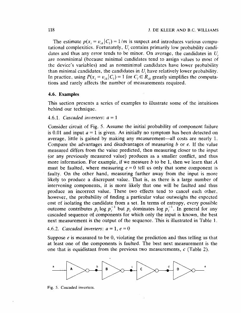
Considercircuit of Fig. 5. Assumethe initial probability of componentfailureis 0.01 and input a = 1 is given. As initially no symptomhas beendetectedonaverage,little is gained by making any measurement—allcosts are nearly 1.Comparethe advantagesand disadvantagesof measuringb or e. If the valuemeasureddiffers from the value predicted,thenmeasuringcloser to the input(or any previously measuredvalue) producesas a smaller conflict, and thusmore information.For example,if we measureb to be 1, thenwe learnthat Amust be faulted, where measuringe = 0 tell us only that somecomponentisfaulty. On the other hand, measuringfurther away from the input is morelikely to produce a discrepant value. That is, as there is a large number ofintervening components, it is more likely that one will be faulted and thusproduce an incorrect value. These two effects tend to cancel each other,however, the probability of finding a particular value outweighs the expectedcost of isolating the candidate from a set. In terms of entropy, every possibleoutcome contributes p, log p~ but p, dominates log pa’. In general for anycascaded sequence of components for which only the input is known, the bestnext measurement is the output of the sequence. This is illustrated in Table 1.

4.6.2. Cascaded inverters: a = 1, e = 0

Supposee is measuredto be 0, violating thepredictionandthustelling us thatat least one of the components is faulted. The best next measurement is theone that is equidistantfrom the previoustwo measurements,c (Table 2).

Fig. 5. Cascadedinverters.


TABLE 1. Expected TABLE 2. Expected TABLE 3. Expectedcosts after a = 1 with costs after a = 1, e = costs after a = 1, e =

p = 0.01 0 with p = 0.01 1 with p = 0.01

a Ib 0.98c 0.96d 0.94e 0.93

a 1b 0.45c 0.31d 0.44e I

a 1b 0.999C 0.999d 0.999e 1

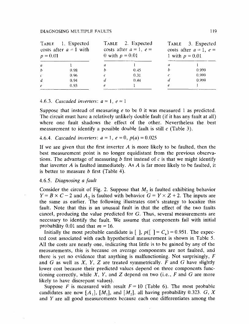
4.6.3. Cascadedinverters: a = 1, e = 1

Suppose that instead of measuring e to be 0 it was measured 1 as predicted.The circuit must have a relatively unlikely double fault (if it has any fault at all)where one fault shadows the effect of the other. Nevertheless the bestmeasurementto identify a possibledouble fault is still c (Table 3).

4.6.4. Cascaded inverters: a = 1, e = 0, p(a) = 0.025

If we are given that the first inverter A is more likely to be faulted, then thebestmeasurementpoint is no longer equidistantfrom the previousobserva-tions. The advantage of measuring b first insteadof c is that we might identifythat inverter A is faulted immediately.As A is far morelikely to be faulted, itis better to measureb first (Table 4).

4.6.5. Diagnosinga fault

Consider the circuit of Fig. 2. Suppose that M, is faulted exhibiting behaviorV = B x C —2 andA2 is faulted with behaviorG = V x Z + 2. The inputsarethe same as earlier. The following illustrates GDE’s strategy to localize thisfault. Note that this is an unusual fault in that the effect of the two faultscancel,producingthe value predictedfor G. Thus, severalmeasurementsarenecessaryto identify the fault. We assumethat componentsfail with initialprobability 0.01 andthat rn = 16.

Initially the most probablecandidateis [], p([ ] = Ca) = 0.951. The expec-ted cost associatedwith eachhypotheticalmeasurementis shownin Table 5.All the costs are nearlyone, indicating that little is to be gainedby any of themeasurements,this is becauseon averagecomponentsare not faulted, andthere is yet no evidencethat anything is malfunctioning.Not surprisingly, Fand G as well as X, V, Z are treatedsymmetrically.F and G have slightlylower cost becausetheir predictedvaluesdependon threecomponentsfunc-tioning correctly, while X, V, and Z dependon two (i.e., F and G aremorelikely to have discrepantvalues).

SupposeF is measuredwith result F = 10 (Table 6). The most probablecandidatesare now [A1], [M1], and [M2], all having probability 0.323. G, Xand Y are all good measurementsbecauseeachone differentiatesamongthe


TABLE 4. Expectedcosts after a = 1, e =

0 with p(a) = 0.025

a 1b 0.33C 0.36d 0.53e 1

high-probability single-fault candidates. Each high-probability candidate pre-dicts Z = 6 so measuringZ provides little new information. G is a slightlybetterpoint to measurebecausethecandidatesaremorebalancedbetweenG’stwo predictedoutcomes(the best measurementis one whosepredictedout-comesall haveequal probability andwhich cover all the candidates).

Next, supposeG is measuredwith result G = 12 (Table 7). The mostprobablecandidatesare now [A ~]and [M1] both with probability 0.478. Atthis point X is thebestmeasurementbecauseit splits thetwo high-probabilitycandidates.

Next, supposeX is measuredwith result X = 6 (Table8). This resultsin asingle high-probability candidate[A1] with probability 0.942. The next sevenmost likely candidatesare: [A1, M3J, [A1, M2], [A1, M1}, [A1, A2], [A2, M,],and [M.,, M3], all with probability 0.00951.

Next, supposeY is measuredwith result V = 4. M2 is now necessarilyfaultedand at least one other fault exists. The costs are now as shown in Table 9.

Finally, supposeZ is measuredwith result Z = 6. There are six remainingcandidates: [A2, M2] with probability 0.970, [A2, M1, M1], [A1, A,, M,},[A2, M2, M3], with probabilities0.0098, [A ~,A2, M1, M2], [A ~,A.,, M2, ~ 1’[A2, M1, M2, M3], with probabilities 0.0001, and [A1, A2, M1, M2, M3] withprobability 0.000001.ComponentsM2 andA2 are necessarilyfaulted, andA1,M1, andM3 are possibly faulted,eachwith probability 0.01. No measurementpointsremain in the circuit, so no further informationcan be obtained.

TABLE 7. Costsafter TABLE 8. Costs afterF=l0, G=12 F=10, G=12, and

F 1G 1x 0.28Y 0.94z 0.97

TABLE 9. Costs afterF=10, G=12, X=

X=6 6,andV=4

F 1G 1X 1Y 0.90z 0.94

F 1G 1X 11’ 1z 0.141

TABLE 5. Initial ex- TABLE 6. Costsafterpectedcosts F = 10

F 0.88G 0.88X 0.95Y 0.95Z 0.95

F 1G 0.28X 0.34Y 0.34Z 0.95


4.7. Logical incompleteness

In practice, for diverse reasons,the underlying inferenceprocessis usuallyincomplete.One of theconsequencesof this incompletenessis that it becomesmoredifficult to evaluatethe resultsof hypotheticalmeasurements—theLI, arelarger than ideal. As any incompletenessdegradesODE’S performance,it isinstructiveto examinethe sourcesand types of this incompleteness.

An often avoidableform of incompletenessoccurswhen theconflict recogni-tion strategymissessomeconflicts. This was discussedearlier. Herewe assumethe conflict recognitionstrategyis complete.U, will be larger than ideal only ifthe prediction processis incomplete. This incompletenessmanifestsitself intwo ways. First, an incompleteinferenceprocessmay result in missingpredic-ted values and missing supporting environments. As a consequence,thehypothesizedconflicts resulting from measuringa quantitywill be incomplete.For example, consider an inverter which is incompletelymodeledby a rulewhichpredicts its outputfrom its input, but not its input from its output. Eventhoughthe inverter’soutput is measuredto beone, thepredictionthatits inputis zero is not made.Thus,ODE doesnotconsidermeasuringits input. A secondsourceof incompletenessis inherentin the x, = Vik representation—theremaybe many additionalpropertiesthat could be inferred aboutx,, but asthereisno way to representthemthey cannotbe usedby our strategy.For example,itcannot representx ~ 1. Thus, although x ~ 1 might be derivable from anenvironment,ODE cannotforeseetheresulting conflict when considering,say,x2.

Assuming the basic conflict recognition strategy is complete, both thesesourcesof incompletenesscan be avoided at prohibitive computationalcosts.The first sourceof incompletenesscan be avoidedwith a completeinferenceprocess.The secondsourceof incompletenesscan be avoidedwith a moregeneralrepresentation.8

5. Pragmatics

5.1. Most probable candidates

Computingall candidatesis computationallyprohibitive. In practice it is onlynecessaryto computethe more probablecandidates.There is no way to tellwhethera single candidateactually hasa high probability without knowing theoverall normalizationfactor. This suggestsusing abest-firstsearchof the latticeto find candidatesin increasingorder of probability. This searchis arbitrarily

8Assumingthe numberof possiblevaluesfor quantitiesare finite, GDE could hypothesizeeachpossiblemeasurementoutcome,run its completeinferenceprocedureandpreciselycomputetheR~kfrom which the S,k could then be computed.


stoppedfor candidatesbelow somethresholdfraction (e.g., ~ of the highestprobability candidate).Although the most probable candidateis a minimalcandidate,the remainingminimal candidatesneednot be very probable.

5.2. When to stop making measurements

If thereare manypoints in a devicethat could be measuredchoosingthebestpoint to measurecan be computationallyexpensive.A heuristicis to makethefirst reasonablemeasurementwhose cost is computed to be less than 1 —

log 0.5 = 0.7 asthis measurementon average,splits thecandidatespacein half.The point at which measurementshould stop dependsgreatly on the

seriousnessof a misdiagnosisas well as on the a priori probabilities ofcomponentfailure. When a candidateis found whoseprobability approachessome threshold(e.g., 0.9), diagnosiscan stop. If the cost of misdiagnosisishigh, then the thresholdshouldbe increased.

6. Comparison to Other Work

6.1. Circuit diagnosisbased on structure and behavior

Work in the Al communityon model-basedhardwarediagnosishasgrown outof a desire to move away from the domain and devicespecific fault modelsusedin traditional circuit diagnosis.9Instead,duringcandidategenerationthemodel-basedapproachreasonsfrom a small setof componentbehaviormodelsplus the structure of the device. The requirementfor device specific faultmodels is eliminatedby basing the diagnosticapproachsolely on the know-ledge that, if a component’sbehavior is inconsistentwith its model, then itmust be faulty. This resultsin a domain independentdiagnostictechnique.Anumberof systemshave followed this approachfor diagnosingboth analog(e.g., LOCAL [10] andsOPHIE [4]) anddigital circuits (e.g., HT [5] andDART [12]).

Our work naturally extendsthis approachalong a numberof dimensions.First, unlike earlierapproaches,our work is aimedspecifically at copingwiththe problem of diagnosingmultiple faults. Earlier work focusedprimarily onthe casewhereall symptomscould be explainedby a single componentbeingfaulty. As Davis points out, the obvious extensionto his work to handlemultiple faults resultsin an algorithm which is exponentialin the numberofpotential faults. As our approachrepresentsthe candidatespaceimplicitly intermsof theminimal candidates,we needonly be concernedwith the growthof this smaller set. Typically the size of eachminimal candidateis relativelysmall (i.e., the symptom can usually be explained by one, two or three

9SeeDavis’ [5], Sections5.1., 12.1. and13 for a discussionof traditionalcircuit diagnosisand theadvantagesof the model-basedapproach.Also see[161.


componentsbeingsimultaneouslyfaulty), thusin practiceour approachtendsto grow with the squareor cubeof the numberof potential faults.

Second,our approachto diagnosisis inferenceprocedureindependent,aswell as domain independent.LOCAL, SOPHIE, and Davis’ system all representcircuit knowledgeasconstraintsandthenusesomeform of constraintpropaga-tion to infer circuit quantitiesand their dependencies.The motivation behindthis approach is that constraints naturally reflect the local interaction ofbehavior in the real world. Theseare similar (althoughnot identical) to theconstraintpropagationtechniqueusedto demonstrateODE in this paper.

On the other hand, DART expressescircuit knowledgeas logical propositionsand uses an inference system based on resolution residue to infer circuitproperties.This samegeneralinferenceprocedureallowsDART to deducewhichcomponentsaresuspectandhow to changecircuit inputsto reducethesuspectset to a singleton.Such a resolution-basedinferencestrategycan be incorpo-ratedinto the candidategenerationandconflict recognitionportion of ODE byrecording, for eachresolution step, the dependenceof the resolvent on theformulas used to perform the resolution. Then, as in the casefor constraintpropagation, ODE can guide the inference processin identifying minimalcandidatesfirst.

Resolutionis highlightedashavinganadvantageoverconstraintpropagationin that it is logically completewith respectto afirst-order theory, wheremostconstraintpropagatorsarenot. However,this can be misleading.A significantcomputationalcost is incurred using a logically completeinferencestrategy,such as resolution. Yet a logically complete inference strategy does notguaranteethat the set of predictionswill alsobe complete.For examplein ananalogdomain,producingexact predictionsoften involves solving systemsofhigher-ordernonlinear differential equations.As this type of equationis notgenerally solvable with known techniques,completenessin the predictor iscurrently beyond our reach. In practice propagationof constraints(withoutsymbolic algebra) provides a good compromisebetween completenessandcomputationalexpense.

Third, our approachis incremental.This is crucialasdiagnosisis an iterativeprocessof making observations,refining hypotheses,andthen using this newknowledgeto guide further observations.

Finally, our approachis unique in that it combinesmodel-basedreasoningwith probabilistic information in a sequentialprobing strategy. SOPHIE alsoproposesmeasurementsto localize the failing component,but is basedon anad hoc half-split method. Its design is basedon the presuppositionthat thecircuit containsasingle fault. Thus, candidategenerationis trivial (setintersec-tion), and identifying good measurementsis easy.

6.1.1. Possibleextensions

Representingandmanipulatingcandidatesin termsof minimal candidatesgivesus a significantcomputationaladvantageover previousapproaches;however,


eventhis representationcan grow exponentiallyin theworstcase.To effective-ly cope with very large devices,additional techniquesmust be incorporated.

One approachinvolves groupingcomponentsinto largermodulesandmod-ifying the candidategenerationstrategyto deal with hierarchicaldecomposi-tions. Although we have not implementedthis, the strategiesproposedbyDavis and Genesereth,as they are model-based,apply. Their basic idea is totroubleshootat the most abstractlevel in the hierarchyfirst and only analyzethe contentsof a module when there is reasonableevidenceto suspectit. Ifthereis no conflict involving themodule, then thereis no reasonto suspectit.

Complexity is directly related to the numberof hypothetical faults enter-tained. Thus anotherapproach,proposedby Davis, involves enumeratingandlayering categoriesof failures based on their likelihood. Troubleshootingbeginsby consideringfaults in the most likely categoryfirst, moving to lesslikely categoriesif thesefail to explain the symptoms.ODE usesa variation onthis approachwhereby candidatescan be enumeratedbasedon their likeli-hood. However,no theoryhas beendevelopedaboutfailure categories.

LOCAL andSOPHIE alsoaddressanumberof issueswhich ODE doesnot. LOCAL

and SOPHIE usecorroborationsaswell asconflicts to eliminate candidates.Totake advantageof corroborations,SOPHIE includes an exhaustiveset of faultmodesfor eachcomponent.As a consequence,SOPHIE can identify a compo-nentasbeingunfaultedby determiningthatit is not operatingin any of its faultmodes(i.e., noneof thecomponentsfault modescan explain the failure, andwe know all the component’smodesof failure, so the componentmust beworking). Thus, SOPHIE reducesthe candidatespacefrom both sides: conflictseliminate candidatesthat do not explain a conflict, and corroborationselimi-natecandidateswhich include known working components.

In addition, SOPHIE and LOCAL dealt with the problem of imprecisemodelsandvaluesaswell. This makesconstraintpropagationvery difficult becauseitis hard to tell whethertwo differing valuescorroborateor conflict within theprecisionof the analysis.

ODE proposesoptimal measurementsgiven a fixed set of inputs. BothShirley’s system [31] and DART generatetest vectorsto localize circuit faults.This approachis useful in caseswhere it is both difficult to make internalmeasurements,and easyto changecircuit inputs. Both approachesproducetestswhicharelikely to give useful information;however,no seriousattemptismadeat selectingtheoptimal tests.A fairly simpleextensioncan be madetoour costfunction to accountfor tests,by takinginto consideration,for examplethe costof modifying the inputs.

In Shirley’s approach,eachtest isolatesa single potentially faulted compo-nent by using known good componentsto guide the input signals to the faultycomponent and the output of that component to a point which can bemeasured.However,it is not alwayspossibleto routethe test signalssuchthatall othersuspectsareavoided.Using the informationconstructedby ODE, this


approachcan be modified, so that testsare constructedfirst for componentswhich are most likely to be faulted, while propagatingthe signal alonga pathwith the lowest probability of having a faulty component.

6.2. Counterfactuals

Ginsberg[13] points out how David Lewis’ possibleworld semanticscould beapplied to diagnosis. Each component is modeled by a counterfactual,astatementsuch as “if p. then q,” wherep is expectedto be false. Thus A I ismodeledby the counterfactual“if A1 fails, then F = X + Y need not hold.”Counterfactualsare evaluatedby consideringa “possible world” that is assimilar aspossibleto the real world wherep is true. The counterfactualis trueif q holds in sucha possibleworld. In this framework themost similar worlds(i.e., those closestto the one in which the circuit functions correctly) corre-sponddirectly to our minimal candidates.A most similar world is onein whichas few of the p’s (e.g., “A1 fails”) as possible becometrue. Thus, in thisinstanceGinsbergusescounterfactualsfor hypotheticals.

Ginsberg’s approacheshandlesmultiple faults, but he does not discussmeasurementstrategiesor probabilities. Both could be integratedinto hisapproach.

6.3. Reiter

Reiter [29] has been independently exploring many of the ideas incorporated inODE. His theory of diagnosis provides a formal account of our “intuitive”techniquesfor conflict recognition and candidategeneration. However, histheory doesnot include a theory of measurementsnor how to exploit prob-abilistic information.

Reiter’s theory usesMcCarthy’s [18] AB predicate.Reiter writes 1AB(A ~)(i.e., adderA1 is not ABnormal), while we write A1 (i.e., the assumptionthatadderA1 is working correctly). Under this mapping, Reiter’s definition ofdiagnosisis equivalentto our definition of minimal candidate,and his defini-tion of conflict set is equivalentto our definition of conflict.

Reiter proposes (unimplemented)a diagnostic algorithm based on histheory. This architectureis quite different from ODE’s. The theoremprover ofhis architecture correspondsroughly to our inference engine. While ODE’S

procedurefirst computesall minimal conflicts resulting from a new measure-ment before updating the candidatespace,Reiter’s algorithm interminglesconflict recognitionwith candidategenerationto guidethe theoremproving to“preventthe computationof inessentialvariantsof refutations,without impos-ing any constraintson the natureof the underlyingtheoremproving system.”Given ODE’S inferencearchitecture(and the necessityto choosethe bestnextmeasurement),ODE avoidsalmostall theseinessentialvariantsandalso avoidsmuch of the computationReiter’s architecturedemands.


6.4. sNeps

SNePS[17] incorporatesa belief revisionsystemSN~BRwhich reasonsabouttheconsistencyof hypotheses.This belief revision systemhas been[6] applied tofault detection in circuits. Some of the basic conceptsused in the SN~PS

approachare similar to those used in ODE—both use an assumption-basedbelief revision system (see[9] for a comparison).As describedin [6] SNePS isweaker than either ODE or Reiter’s approach.In GDE’s terminology, s~e~soperatesin a single environment,detectingsymptoms(and henceconflicts) foronly thosevariablesaboutwhich a userquery is made.The systemprovidesnomechanismsto detectall symptoms(and thus all conflicts), to identify candi-dates, to propose measurements,or to exploit probabilistic information.However,thereseemsno reason,in principle that themethodsof ODE cannotbe incorporatedinto their system.

6.5. IN-ATE and FIS

IN-ATE [7] and FIS [24] are expert systemshells specifically designedfor faultdiagnosis.Although neither is purely model-based(i.e., not purely within thestructure-function paradigm), they are the only other electronic diagnosissystemswe are awareof that proposemeasurements,and thusit is instructiveto compare them with GDE.

IN-ATE incorporatestwo formal criteria to determinethebestnext measure-ment: minimum entropy (as in ODE) and gammaminiaverageheuristicsearch[32]. Wechose minimum entropy (as FIS does) in GDE because it was the bestevaluation function which is efficiently computable (i.e., it is based on one-Steplookahead). The gammaminiaverage heuristic search is a multi-step lookaheadprocedure and hence computationally expensive to apply. Nevertheless, thereis no reason,in principle, it could not be incorporatedinto GDE.

Unlike GDE, IN-ATE and FIS can exploit a variety of kinds of knowledge (e.g.,fault trees,expert-suppliedrules, hierarchy) in the diagnostic process. How-ever, viewedfrom thepure model-basedapproach,they arelimited in predic-tive power and as a consequencecan only estimatethe probabilities for theirpredictions.

As IN-ATE is not model-based,it doesnot constructexplicit value predictionsas does GDE. Instead, it predicts whether a particular measurement outcomewill be “good” or “bad.” (This, in itself, presentsdifficulties because ameasurement,being “good” or “bad” is relative to the observationsbeingcompared to. However, IN-ATE takes “good” and “bad” as absolute.)Thesepredictionsare computedby analyzingexpert-suppliedempirical associationsbasedon “good” and “bad.” IN-ATE incorporatesa heuristic rule generatorwhich exploits connectivity information, but it, at a minimum, must beprovided with the definitions of “good” and “bad” for the test points. In thisapproach,the numberof test points is limited to thoseexplicitly mentionedin


rules (or for which “good” and“bad” areexternallydefined).With this limitedSet of test points full search (i.e., gamma miniaveragesearch) becomesplausible. FIS exploits more model knowledge, propagatingqualitative valuessuch as {hi, ok, lo} through the circuit topology via expert-suppliedcausalrules. The propagated values are always relative to fixed expert-suppliedvalues. Thus neither FIS nor IN-ATE can analyzehypotheticalfaults.

All three systems must compute probabilities for their predictions. ODE

directly computesthe probability of the predictionsfrom the probabilitiesofthe candidatesinvolved. IN-ATE has a much more difficult time determininggood/badprobabilities becauseit cannotdeterminethe candidatespaceandtheir associatedprobabilities. Instead it uses the expert-suppliedrules topropagateprobabilities (much like MYCIN) and Dempster—Shaferto combinethe resulting evidence.FIS’ definition of candidateprobability is similar toODE’S, however, as it cannot perform hypothetical reasoning it can onlyestimatethe probabilitiesof its predictions.

6.6. Medical diagnosis

There has been extensive researchon the diagnostic task in the medicaldecision making community. Although most of this researchis not model-based,its concern with identifying the diseases causing symptoms and sub-sequentlyproposing information-gatheringqueriesis analogousto ours.

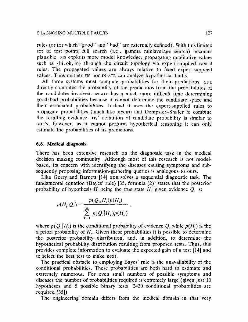
Like Gorry and Barnett [14] GDE solves a sequentialdiagnostictask. Thefundamentalequation (Bayes’ rule) [35, formula (2)] statesthat the posteriorprobability of hypothesisH, being the true state HT given evidenceQ, is:

p(Q,JH1)p(H1)p(H~,JQ1)’

k

wherep(Q1IH~,.) is theconditionalprobability of evidenceQ, while p(H1

) is thea priori probability of H1. Given theseprobabilities it is possible to determinethe posterior probability distribution, and, in addition, to determine thehypotheticalprobability distribution resulting from proposedtests.Thus, thisprovides complete information to evaluatethe expectedgain of a test [14] andto select the best test to makenext.

The practical obstacle to employing Bayes’ rule is the unavailability of theconditional probabilities. These probabilities are both hard to estimate andextremely numerous. For even small numbersof possible symptoms anddiseasesthe numberof probabilities requiredis extremelylarge (given just 10hypothesesand 5 possible binary tests, 2420 conditional probabilities arerequired[35]).

The engineering domain differs from the medical domain in that very


accuratemodels exist basedon the structure of the (faulty) system. Thus,exploiting model-basedreasoning, ODE computes these conditional prob-abilities directly rather than dependingon empirical results. Another advan-tageof themodel-basedapproachfor engineeringis that thepotentialtestsarecomputedin thecourseof the analysisinsteadof havingthem supplieda priori.

Early research[14] presumedthat the patienthad only one disease.This isanalogousto the single-fault assumptionin circuit diagnosis. More recentresearchallows for multiple simultaneousdiseases.Bayes’ rule can also beappliedto this multimembershipclassificationproblem[2, 3] but thenumberofconditionalprobabilitiesrequiredbecomesexponentiallylarger than the single-diseasecase(which already is a large number). Again, ODE computestheseconditional probabilitiesby model-basedreasoning.

The conceptof set covering used in [21, 22, 23, 25, 27, 28] is similar to thecandidategenerationphaseof our diagnostic approach. The irredundant setcoverof thegeneralsetcoveringtheory (osC)of Reggiacorrespondsdirectly toour notion of minimal candidates.The primary differenceis that we consider,in theory, every possiblecover to be an explanationfor the symptomswhileOSC considers only the minimal candidatesas explanations.Although oscincorporatesacrudeheuristicstrategyfor proposingnewmeasurements,as theconditional probabilities are available to ODE, the preferred approach,minimum entropy,can be applied.

ACKNOWLEDGMENT

Daniel G. Bobrow, Randy Davis, Kenneth Forbus, Matthew Ginsberg, Frank Halasz, WalterHainscher,Tad Hogg, RameshPatil, Leah Ruby, Mark Shirley and Jeff Van Baalen,provideduseful insights. We especiallythank Ray Reiter for his clear perspectiveand many productiveinteractions.Lenore JohnsOnand DenisePawsonhelpededit draftsand preparefigures.

REFERENCES

1. Ben-Bassat,M., Myopic policies in sequentialclassification, IEEE Trans. Comput. 27 (1978)170—178.

2. Ben-Bassat,M., Multimembershipand multiperspectiveclassification: Introduction,applica-tions, and a Bayesianmodel, IEEE Trans. Syst.Man Cybern. 6 (1980) 331—336.

3. Ben-Bassat,M. Campbell, D.B., Macneil A.R. and Weil, M.H., Pattern-basedinteractivediagnosisof multiple disorders:The MEDAS system,IEEE Trans. Pattern Anal. Mach. Intel!.2 (1980) 148—160.

4. Brown, iS., Burton, R.R. and de Kleer, J., Pedagogical,natural languageand knowledgeengineeringtechniquesin SOPHIE I, II and III, in: D. Sleemanand J.S. Brown (Eds.),Intelligent Tutoring Systems(AcademicPress,New York, 1982) 227—282.

5. Davis, R., Diagnostic reasoningbasedon structureand behavior, Artifical Intelligence 24(1984) 347—410.

6. Campbell, S.S. and Shapiro, S.C., Using belief revision to detectfaults in circuits, SNeRGTech. Note No. 15, Departmentof Computer Science,SUNY at Buffalo, NY, 1986.


7. Cantone,R.R., Lander,W.B., Marrone,M.P. andGaynor,M.W., IN-ATE: Fault diagnosisasexpertsystemguided search, in: L. BoIc andM.J. Coombs(Eds.), Computer Expert Systems(Springer,New York, 1986).

8. de Kleer, I., An assumption-basedTMS, Artifical Intelligence28 (1986) 127—162.9. de Kleer, J., Problemsolving with the ATMS, Artifical Intelligence28 (1986) 197—224.

10. de Kleer, J.. Local methodsof localizing faults in electroniccircuits, Artificial IntelligenceLaboratory,Al Memo 394, MIT, Cambridge,MA, 1976.

11. Doyle, J., A truth maintenancesystem,Artificial Intelligence 12 (1979) 231—272.12. Genesereth,M.R., The use of designdescriptionsin automateddiagnosis,Artificial Intellig-

ence24 (1984) 411—436.13. Ginsberg,ML., Counterfactuals,Artificial Intelligence30 (1986)35—79.14. Gorry, G.A. and Barnett,G.O., Experiencewith a mode! of sequentialdiagnosis,Comput.

Biomedical Res. 1 (1968) 490—507.15. Hamscher,W. and Davis, R., Diagnosingcircuits with state:An inherently underconstrained

problem, in: Proceedings AAAJ-84,Austin, TX (1984) 142—147.16. Hamscher,W. and Davis, R., Issuesin diagnosisfrom first principles,Artificial Intelligence

Laboratory,Al Memo 394, MIT, Cambridge,MA, 1986.17. Martins, J.P. and Shapiro, S.C., Reasoningin multiple belief spaces,in: Proceedings IJCAI-

83, Karlsruhe,F.R.G., 1983.18. McCarthy, J., Applications of circumscription to formalizing common-senseknowledge,

Artificial Intelligence 28 (1986) 89—116.19. Mitchell, T., Version spaces:An approachto conceptlearning, Computer Science Depart-

ment, STAN-CA-78-711,StanfordUniversity, Palo Alto, CA, 1970.20. Pearl, J., Entropy, information and rationaldecision,Policy Anal. Inf. Syst.3 (1979)93—109.21. Peng,Y.P. andReggia,J.A., Plausibility of diagnostichypotheses:the natureof simplicity, in:

ProceedingsAAAI-86, Philadelphia,PA (1986) 140—145.22. Peng,Y.P. andReggia,J.A., A probabilistic causalmodel for diagnosticproblem-solving;Part

1: Integratingsymbolic causalinferencewith numeric probabilistic inference,DepartmentofComputerScience,University of Maryland, College Park, MD, 1986.

23. Peng,Y.P. andReggia,J.A., A probabilisticcausalmodelfor diagnosticproblem-solving;Part2: Diagnostic strategy,Departmentof Computer Science,University of Maryland, CollegePark, MD, 1986.

24. Pipitone, F., The FIS electronicstroubleshootingsystem,IEEE Computer (1986) 68—75.25. Pople, H., The formationof compositehypothesesin diagnosticproblemsolving: An exercise

in synthetic reasoning,in: Proceedings IJCAI-77, Cambridge,MA (1977) 1030—1037.26. Quinlan, J.R., Learning efficient classificationproceduresand their application to chessend

games, in: R.S. Michalski, J.G. Carbonell and T.M. Mitchell, (Eds.), Machine Learning(Tioga, Palo Alto, CA, 1983) 463—482.

27. Reggia, J.A. and Nau, D.S., An abductive non-monotoniclogic, in: Workshop on Non-monotonic Reasoning, New Paltz, NY, 1984.

28. J.A. Reggia,Nau, D.S., and Wang, P.Y,, Diagnosticexpertsystemsbasedon a set coveringmodel, mt. J. Man-Mach. Stud. 19 (1983) 437—460.

29. Reiter. R., A theory of diagnosisfrom first principles,Artificial Intelligence32 (1987) 57—95(this issue).

30. Shannon,CE., A mathematicaltheory of communication, Bell Syst. Tech. J. 27 (1948)379—623.

31. Shirley, M.H. and Davis R., Generatingdistinguishingtestsbasedon hierarchicalmodelsandsymptominformation, in: Proceedings IEEE International Conference on Computer Design,Rye, NY, 1983.

32. Slagle,JR. and Lee, R.C.T., Application of game tree searchingtechniquesto sequentialpattern recognition,Commun. ACM 14 (1971) 103—110.

130 3. DE KLEER AND B.C. WILLIAMS

33. Steele,G.L., The definition and implementationof a computerprogramminglanguagebasedon constraints,Al Tech. Rept. 595, MIT, Cambridge,MA, 1979.

34. Sussman,G.J. and Steele, G.L., CONSTRAINTS: A language for expressingalmost-hierarchicaldescriptions,Artificial Intelligence 14 (1980) 1—39.

35. Szolovitz, P. and Pauker,S.G., Categoricalandprobabilistic reasoningin medical diagnosis,Artificial Intelligence 11(1978)115—144.

36. Williams, B.C., Doing time: Puttingqualitative reasoningon firmer ground,in: ProceedingsAAAI-86, Philadelphia,PA (1986) 105—112.

Received September 1985; revisedversion receivedJuly 1986

Diagnosing Multiple Faults - PARC Multiple... · Diagnosing Multiple Faults ... mechanical devices...

Documents

Transcript of Diagnosing Multiple Faults - PARC Multiple... · Diagnosing Multiple Faults ... mechanical devices...