Di erential Equations with Linear Algebra · PDF fileall derivative works based upon it must...
157
Differential Equations with Linear Algebra Ben Woodruff December 20, 2011
Transcript of Di erential Equations with Linear Algebra · PDF fileall derivative works based upon it must...

Differential Equations with Linear Algebra
Ben Woodruff
December 20, 2011
i
c©This work is licensed under the Creative Commons Attribution-ShareAlike 3.0 United States License. You may copy, distribute, display, and per-form this copyrighted work but only if you give credit to Ben Woodruff andall derivative works based upon it must be published under the Creative Com-mons Attribution-Share Alike 3.0 United States License. Please attribute toBen Woodruff, Mathematics Faculty at Brigham Young University - Idaho,[email protected]. To view a copy of this license, visit
http://creativecommons.org/licenses/by-sa/3.0/us/
or send a letter to Creative Commons, 171 Second Street, Suite 300, San Fran-cisco, California, 94105, USA.

Contents
1 Review 11.1 Basics . . . . . . . . . . . . . . . . . . . . . . . . . . . . . . . . . 1
1.1.1 Derivatives . . . . . . . . . . . . . . . . . . . . . . . . . . 11.1.2 Integrals . . . . . . . . . . . . . . . . . . . . . . . . . . . . 2
1.2 Ordinary Differential Equations . . . . . . . . . . . . . . . . . . . 41.3 General Functions . . . . . . . . . . . . . . . . . . . . . . . . . . 5
1.3.1 General Derivatives . . . . . . . . . . . . . . . . . . . . . 61.3.2 The General Chain Rule . . . . . . . . . . . . . . . . . . . 6
1.4 Gradient Fields, Potentials, Exact Differential Forms . . . . . . . 81.4.1 How do you find a potential? . . . . . . . . . . . . . . . . 9
1.5 Preparation . . . . . . . . . . . . . . . . . . . . . . . . . . . . . . 111.6 Problems . . . . . . . . . . . . . . . . . . . . . . . . . . . . . . . 121.7 Solutions . . . . . . . . . . . . . . . . . . . . . . . . . . . . . . . 13
2 Linear Algebra Arithmetic 142.1 Basic Notation . . . . . . . . . . . . . . . . . . . . . . . . . . . . 14
2.1.1 Matrices . . . . . . . . . . . . . . . . . . . . . . . . . . . . 142.1.2 Vectors . . . . . . . . . . . . . . . . . . . . . . . . . . . . 152.1.3 Magnitude and the Dot Product . . . . . . . . . . . . . . 16
2.2 Multiplying Matrices . . . . . . . . . . . . . . . . . . . . . . . . . 172.2.1 Linear Combinations . . . . . . . . . . . . . . . . . . . . . 172.2.2 Matrix Multiplication . . . . . . . . . . . . . . . . . . . . 182.2.3 Alternate Definitions of Matrix Multiplication . . . . . . . 19
2.3 Linear Systems of Equations . . . . . . . . . . . . . . . . . . . . . 202.3.1 Gaussian Elimination . . . . . . . . . . . . . . . . . . . . 212.3.2 Reading Reduced Row Echelon Form - rref . . . . . . . . 25
2.4 Rank and Linear Independence . . . . . . . . . . . . . . . . . . . 262.4.1 Linear Combinations, Spans, and RREF . . . . . . . . . . 28
2.5 Determinants . . . . . . . . . . . . . . . . . . . . . . . . . . . . . 282.5.1 Geometric Interpretation of the determinant . . . . . . . 292.5.2 Zero Determinants and Linear Dependence . . . . . . . . 30
2.6 The Matrix Inverse . . . . . . . . . . . . . . . . . . . . . . . . . . 312.7 Eigenvalues and Eigenvectors . . . . . . . . . . . . . . . . . . . . 322.8 Preparation . . . . . . . . . . . . . . . . . . . . . . . . . . . . . . 352.9 Problems . . . . . . . . . . . . . . . . . . . . . . . . . . . . . . . 362.10 Projects . . . . . . . . . . . . . . . . . . . . . . . . . . . . . . . . 382.11 Solutions . . . . . . . . . . . . . . . . . . . . . . . . . . . . . . . 39
3 Linear Algebra Applications 423.1 Kirchoff’s Electrial Laws . . . . . . . . . . . . . . . . . . . . . . . 42
3.1.1 Cramer’s Rule . . . . . . . . . . . . . . . . . . . . . . . . 443.2 Find Best Fit Curves . . . . . . . . . . . . . . . . . . . . . . . . . 45
ii

CONTENTS iii
3.2.1 Interpolating Polynomials . . . . . . . . . . . . . . . . . . 453.2.2 Least Squares Regression . . . . . . . . . . . . . . . . . . 46
3.3 Partial Fraction Decompositions . . . . . . . . . . . . . . . . . . 503.3.1 Finding the correct form . . . . . . . . . . . . . . . . . . . 503.3.2 Integrating Rational Functions . . . . . . . . . . . . . . . 52
3.4 Markov Process . . . . . . . . . . . . . . . . . . . . . . . . . . . . 523.4.1 Steady State Solutions . . . . . . . . . . . . . . . . . . . . 53
3.5 The Second Derivative Test . . . . . . . . . . . . . . . . . . . . . 543.6 Preparation . . . . . . . . . . . . . . . . . . . . . . . . . . . . . . 573.7 Problems . . . . . . . . . . . . . . . . . . . . . . . . . . . . . . . 573.8 Solutions . . . . . . . . . . . . . . . . . . . . . . . . . . . . . . . 59
4 First Order ODEs 624.1 Basic Concepts and Vocabulary . . . . . . . . . . . . . . . . . . . 624.2 Modeling Basics . . . . . . . . . . . . . . . . . . . . . . . . . . . 63
4.2.1 Exponential Model . . . . . . . . . . . . . . . . . . . . . . 634.2.2 Newton’s Law of Cooling . . . . . . . . . . . . . . . . . . 634.2.3 Mixing Model . . . . . . . . . . . . . . . . . . . . . . . . . 64
4.3 Basic Methods . . . . . . . . . . . . . . . . . . . . . . . . . . . . 644.3.1 Separable . . . . . . . . . . . . . . . . . . . . . . . . . . . 644.3.2 Exact Differential Forms . . . . . . . . . . . . . . . . . . . 654.3.3 Integrating Factors (What to do if it isn’t exact) . . . . . 654.3.4 Linear ODEs - a common special form . . . . . . . . . . . 664.3.5 u-Substitutions (How to make it exact) . . . . . . . . . . 67
4.4 Finding Laplace Transforms and Inverses . . . . . . . . . . . . . 684.4.1 Finding the Laplace Transform - Review . . . . . . . . . . 684.4.2 Finding an Inverse Laplace Transform . . . . . . . . . . . 69
4.5 Solving IVPs . . . . . . . . . . . . . . . . . . . . . . . . . . . . . 704.5.1 The Transform of a derivative . . . . . . . . . . . . . . . . 70
4.6 Preparation . . . . . . . . . . . . . . . . . . . . . . . . . . . . . . 714.7 Problems . . . . . . . . . . . . . . . . . . . . . . . . . . . . . . . 714.8 Solutions . . . . . . . . . . . . . . . . . . . . . . . . . . . . . . . 71
5 Homogeneous ODEs 725.1 An Example - Hooke’s Law . . . . . . . . . . . . . . . . . . . . . 725.2 Basic Notation and Vocabulary . . . . . . . . . . . . . . . . . . . 725.3 Laplace Transforms . . . . . . . . . . . . . . . . . . . . . . . . . . 73
5.3.1 The s-shifting theorem . . . . . . . . . . . . . . . . . . . . 735.3.2 Solving ODEs with Laplace transforms . . . . . . . . . . . 74
5.4 Homogeneous Constant Coefficient ODEs . . . . . . . . . . . . . 755.4.1 Summary . . . . . . . . . . . . . . . . . . . . . . . . . . . 77
5.5 Hooke’s law again . . . . . . . . . . . . . . . . . . . . . . . . . . 785.5.1 Free Oscillation - Two imaginary roots . . . . . . . . . . . 785.5.2 Damped Motion - Three cases . . . . . . . . . . . . . . . 79
5.6 Existence and Uniqueness - the Wronskian . . . . . . . . . . . . . 805.7 Preparation . . . . . . . . . . . . . . . . . . . . . . . . . . . . . . 82
6 Non Homogeneous ODEs 836.1 An example - Hooke’s Law . . . . . . . . . . . . . . . . . . . . . 836.2 Theory . . . . . . . . . . . . . . . . . . . . . . . . . . . . . . . . . 846.3 Method of Undetermined Coefficients . . . . . . . . . . . . . . . . 846.4 Hooke’s Law Again . . . . . . . . . . . . . . . . . . . . . . . . . . 876.5 Electric circuits . . . . . . . . . . . . . . . . . . . . . . . . . . . . 896.6 Comparing the two models - saving money . . . . . . . . . . . . . 90

CONTENTS iv
6.7 Preparation . . . . . . . . . . . . . . . . . . . . . . . . . . . . . . 91
7 Laplace Transforms 927.1 The big idea . . . . . . . . . . . . . . . . . . . . . . . . . . . . . . 927.2 Finding Laplace Transforms and Their Inverses . . . . . . . . . . 93
7.2.1 Finding the Laplace Transform . . . . . . . . . . . . . . . 937.2.2 Finding an Inverse Laplace Transform . . . . . . . . . . . 937.2.3 Shifting Theorems and The Heaviside Function . . . . . . 94
7.3 Solving IVPs . . . . . . . . . . . . . . . . . . . . . . . . . . . . . 967.3.1 The Transform of a derivative . . . . . . . . . . . . . . . . 967.3.2 Solving IVPs - Lots of examples . . . . . . . . . . . . . . 967.3.3 How to handle initial conditions that are not at t = 0 . . 97
7.4 Impulses and the Dirac Delta function δ(t− a) . . . . . . . . . . 987.5 Convolutions, and Transfer Theorems . . . . . . . . . . . . . . . 99
7.5.1 Convolutions . . . . . . . . . . . . . . . . . . . . . . . . . 997.5.2 Transform Theorems . . . . . . . . . . . . . . . . . . . . . 99
7.6 Preparation . . . . . . . . . . . . . . . . . . . . . . . . . . . . . . 1017.7 Problems . . . . . . . . . . . . . . . . . . . . . . . . . . . . . . . 102
8 Power Series 1048.1 Taylor Polynomials and Series . . . . . . . . . . . . . . . . . . . . 104
8.1.1 Radius of convergence . . . . . . . . . . . . . . . . . . . . 1078.1.2 Euler’s Formula . . . . . . . . . . . . . . . . . . . . . . . . 108
8.2 Power Series . . . . . . . . . . . . . . . . . . . . . . . . . . . . . . 1098.2.1 Notation and Calculus . . . . . . . . . . . . . . . . . . . . 1098.2.2 Examples . . . . . . . . . . . . . . . . . . . . . . . . . . . 1098.2.3 Shifting Indices . . . . . . . . . . . . . . . . . . . . . . . . 110
8.3 Series Solutions to ODEs . . . . . . . . . . . . . . . . . . . . . . 1108.4 Preparation . . . . . . . . . . . . . . . . . . . . . . . . . . . . . . 1148.5 Problems . . . . . . . . . . . . . . . . . . . . . . . . . . . . . . . 1158.6 Solutions . . . . . . . . . . . . . . . . . . . . . . . . . . . . . . . 115
9 Special Functions 1169.1 Preparation . . . . . . . . . . . . . . . . . . . . . . . . . . . . . . 117
10 Systems of ODEs 11810.1 Definitions and Theory for Systems of ODEs . . . . . . . . . . . 118
10.1.1 The Eigenvalue approach to Solving Linear systems ofODEs . . . . . . . . . . . . . . . . . . . . . . . . . . . . . 119
10.1.2 Using an Inverse Matrix . . . . . . . . . . . . . . . . . . . 12010.2 Jordan Canonical Form . . . . . . . . . . . . . . . . . . . . . . . 12010.3 The Matrix Exponential . . . . . . . . . . . . . . . . . . . . . . . 123
10.3.1 The Matrix Exponential for Diagonal Matrices - expo-nentiate the diagonals . . . . . . . . . . . . . . . . . . . . 124
10.3.2 Nilpotent Matrices - Matrices where An = 0 for some n . 12510.3.3 Matrices in Jordan Form . . . . . . . . . . . . . . . . . . 12610.3.4 Jordan form gives the matrix exponential for any matrix. 127
10.4 Systems of ODEs . . . . . . . . . . . . . . . . . . . . . . . . . . . 12710.4.1 Dilution - Tank Mixing Problems . . . . . . . . . . . . . . 12710.4.2 Solving a system of ODEs . . . . . . . . . . . . . . . . . . 12910.4.3 Higher Order ODEs - Solved via a system . . . . . . . . . 13010.4.4 Spring Systems . . . . . . . . . . . . . . . . . . . . . . . . 13110.4.5 Electrical Systems . . . . . . . . . . . . . . . . . . . . . . 132
10.5 Preparation . . . . . . . . . . . . . . . . . . . . . . . . . . . . . . 13310.6 Problems . . . . . . . . . . . . . . . . . . . . . . . . . . . . . . . 133

CONTENTS v
11 Fourier Series 13611.1 Basic Definitions . . . . . . . . . . . . . . . . . . . . . . . . . . . 136
11.1.1 Examples . . . . . . . . . . . . . . . . . . . . . . . . . . . 13711.2 Orthogonality of Trigonometric functions . . . . . . . . . . . . . 138
11.2.1 Half-Wave Rectifier . . . . . . . . . . . . . . . . . . . . . . 13811.3 Even and Odd Functions . . . . . . . . . . . . . . . . . . . . . . . 13911.4 Identities . . . . . . . . . . . . . . . . . . . . . . . . . . . . . . . 14011.5 Where do people use Fourier Series . . . . . . . . . . . . . . . . . 14111.6 Preparation . . . . . . . . . . . . . . . . . . . . . . . . . . . . . . 14211.7 Problems . . . . . . . . . . . . . . . . . . . . . . . . . . . . . . . 142
12 Partial Differential Equations 14512.1 Basic Definitions . . . . . . . . . . . . . . . . . . . . . . . . . . . 14512.2 Derivation of the one dimensional wave equation . . . . . . . . . 14612.3 Solution of the wave equation . . . . . . . . . . . . . . . . . . . . 147
12.3.1 Separate Variables . . . . . . . . . . . . . . . . . . . . . . 14712.3.2 Solve Multiple ODEs . . . . . . . . . . . . . . . . . . . . . 14712.3.3 Combine the solutions using superposition . . . . . . . . . 14712.3.4 Summary . . . . . . . . . . . . . . . . . . . . . . . . . . . 148
12.4 Solution of the heat equation . . . . . . . . . . . . . . . . . . . . 14812.5 Preparation . . . . . . . . . . . . . . . . . . . . . . . . . . . . . . 14912.6 Problems . . . . . . . . . . . . . . . . . . . . . . . . . . . . . . . 14912.7 Solutions . . . . . . . . . . . . . . . . . . . . . . . . . . . . . . . 150

Chapter 1
Review
This section covers the following ideas.
1. Graph basic functions by hand. Compute derivatives and integrals, inparticular using the product rule, quotient rule, chain rule, integration byu-substitution, and integration by parts (the tabular method is useful forsimplifying notation). Explain how to find a Laplace transform.
2. Explain how to verify a function is a solution to an ODE, and illustratehow to solve separable ODEs.
3. Explain how to use the language of functions in high dimensions and howto compute derivatives using a matrix. Illustrate the chain rule in highdimensions with matrix multiplication.
4. Graph the gradient of a function together with several level curves toillustrate that the gradient is normal to level curves.
5. Explain how to test if a differential form is exact (a vector field is conser-vative) and how to find a potential.
1.1 Basics
You should understand how to graph by hand basic functions. If you havenot spent much time graphing functions by hand, then please spend some timegraphing the following functions:
x2, x3, x4,1
x, sinx, cosx, tanx, arctanx, lnx, ex, e−x
You should also practice shifting and rescaling function. For example the graph(x− h)2
a2+
(y − k)2
b2= 1 is an ellipse shifted from the origin h units right and
k units up. The graph of y = 2 sinx is formed by doubling the amplitude. Thegraph of y = sin(2x) if formed by halving the period. I suggest that you spendtime graphing y = A sin(B(x − C)) + D for various values of A,B,C,D (forhomework), and describe how each constant changes the shape of the function(the period is 2π
B , amplitude is A, and the origin is moved from (0, 0) to (C,D)).
1.1.1 Derivatives
You should know all the derivatives of the basic functions listed in the previoussection. In addition, you should know derivatives of the remaining trigonometric
1

CHAPTER 1. REVIEW 2
functions and trigonometric inverse functions (such as arccos(x)), as well asrules regarding exponents ax and logarithms loga x of any base. The followingrules are crucial as well.
1. Power rule (xn)′ = nxn−1
2. Sum and difference rule (f ± g)′ = f ′ ± g′
3. Product and quotient rule (fg)′ = fg′ + f ′g
4. Chain rule (arguably the most important) (f ◦ g)′ = f ′(g(x)) · g′(x)
Be able to use the chain rule to do implicit differentiation.
Example 1.1. To find the derivative of arcsin(x), first rewrite the expressionas x = sin y. Then differentiate both sides implicitly with respect to x, giving1 = cos(y)y′ (where the chain rule is used to get y′). Solving for y′ givesy′ = 1
cos(y) . The expression x = sin y means that y is the central angle of a
triangle with x as the opposite edge and 1 as the hypotenuse. This makes theadjacent edge
√1− x2. Hence y′ = 1
cos y = 1√1−x2
.
1.1.2 Integrals
You should be able to integrate all the functions listed in the derivative section.In addition you should know the following integration techniques
• u- substitution - The key is to pick the right u, solve for dx, and thencompute the simpler integral.
Example 1.2. To solve∫e3xdx, first notice that we know how to inte-
grate eu, so let u = 3x. Then du = 3dx, or dx = du3 . Substitution yields∫
e3xdx =∫eu du3 = 1
3eu + C = 1
3e3x + C.
• Integration by parts - Recall the formula∫udv = uv −
∫vdu. It is
essentially the product rule (you can see that by differentiating both sidesgiving udv = d(uv)− vdu).
Example 1.3. To compute∫x sin(2x)dx, we first pick for u a function
which simplifies upon differentiation, and for dv the rest of the inte-grand. The choice u = x, dv = sin 2xdx will do. This gives du = 1dxand v = − cos 2x
2 . Integration by parts gives∫x sin(2x)dx = −x cos 2x
2 −∫− cos 2x
2 dx = −x cos 2x2 + sin 2x
4 .
Integration by parts is needed to find the following integrals:∫xexdx,∫
x2 sinxdx,∫ex sinx, and
∫lnx. The Laplace Transform section will
give you lots of practice with this.
There are other methods of integration, but we will only need to focuson integration by substitution and integration by parts. The following twosections illustrate the tabular method which is an organizational tool to helpwith integration by parts, and the Laplace transform which is one of the keytools used by engineers to solve ODEs.
The tabular method
The tabular method is an organizational tool which simplifies integration byparts. This method gives you a convenient way to sort the information frommultiple integration by parts into a simple table, so that you can find theintegral without much work.

CHAPTER 1. REVIEW 3
Example 1.4. I’ll illustrate this method with the same example as above,where f(x) = x sin(2x). Create a table with two sides. On the left side placea factor from your integral which will get simpler with differentiation. In thiscase we place x on the left because after 2 derivatives it will become zero. Onthe right side place the rest of the integrand, which is sin(2x) in our example.Differentiate the left hand side one or more times. Stop differentiation when
D I
+ x sin(2x)− 1 − cos(2x)/2+ 0 − sin(2x)/4
further differentiation will no longer simplify the problem. In this case wedifferentiated twice because we obtained 0. Now integrate the right side thesame number of times. Multiply every other term on the left side by −1,starting with the second (this comes because of the minus in integration byparts, and you can see it in our table as the +,−,+ on the left of the table).Now multiply each term on the left by the term one row lower on the right(multiply diagonally down to the right), and sum the products. In our examplewe obtain +(x)(− cos(2x)/2)− (1)(− sin(2x)). The solution is found by add tothe last step the integral of the product of the bottom row (if is zero, then thispart can be skipped). In our case, the product of the bottom row is zero, soour solution is simply
∫x sin(2x) = +(x)(− cos(2x)/2)− (1)(− sin(2x)).
Example 1.5. As another example let’s compute∫
lnxdx. Since we don’tknow how to integrate lnx, but we can differentiate it, we’ll place lnx on theleft side. Since there is nothing left in the integrand and lnx = lnx · 1, weplace a 1 on the right side. The derivative of lnx is 1/x. The integral of 1 isx. Alternate the sign by placing a minus next to 1/x. Now multiply lnx by
D I
+ lnx 1− 1/x xx to obtain x lnx. The product of the bottom row is − 1
xx = −1 so we add∫−1dx = −x to obtain
∫lnxdx = x lnx− x.
Laplace Transforms
The Laplace transform of a function f(t) defined for t ≥ 0 is F (s) = L(f) =∫∞0e−stf(t)dt, provided this improper integral exists (in which case we say the
integral converges). Remember that to compute an improper integral you haveto compute limits as the variable approaches infinity. The function f(t) is calledthe inverse Laplace transform of F (s), and we write f(t) = L−1(F ). We will usethe Laplace transform throughout the semester to help us solve many problemsrelated to mechanical systems, electrical networks, and more. For now, we justneed to know how to compute it (as it gives a good way to practice integrationby parts)
If you have forgotten how to compute limits at infinity, then here is a brief
review. We can compute limt→∞
1
t= 0 since 1
t gets really small as t gets large.
The function et approaches ∞ as t → ∞, but it approaches 0 as t → −∞.This can be seen by looking at the graph of of et which continues to increaseforever as t increases, but has a horizontal asymptote of y = 0 as t → −∞.
We will need to be able to compute limits such as limt→∞
te−st = limt→∞
tt
est. If
you try taking the limits of both the top and bottom separately, you obtain∞∞ (provided s > 0). This is called an indeterminant form, and L’Hopital’srule says that you can examine such limits by taking the derivative of the top
and the bottom separately and then taking a limit. This gives limt→∞
t
e−st=
limt→∞
1
(−s)e−st=
1
∞= 0.
Example 1.6. If f(t) = 1, then F (s) =∫∞
0e−st1dt = e−st
−s∣∣∞0
= 1s , where the
integral converges provided s > 0.
CHAPTER 1. REVIEW 4
Example 1.7. If f(t) = eat, then F (s) =∫∞
0e−steatdt =
∫∞0e−(s−a)tdt =
e−(s−a)t
−(s−a)
∣∣∞0
= 1s−a , where the integral converges provided s > a.
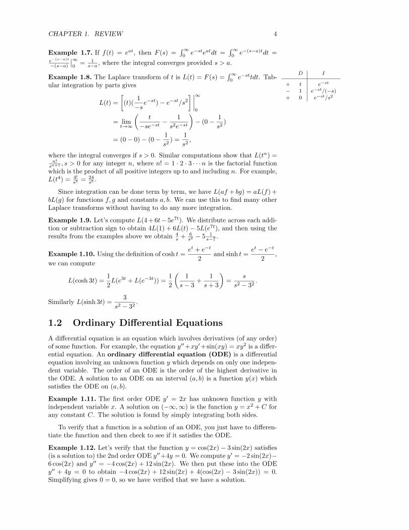
Example 1.8. The Laplace transform of t is L(t) = F (s) =∫∞
0e−sttdt. Tab-
ular integration by parts gives
D I
+ t e−st
− 1 e−st/(−s)+ 0 e−st/s2
L(t) =
[(t)(
1
−se−st)− e−st/s2
] ∣∣∣∣∞0
= limt→∞
(t
−se−st− 1
s2e−st
)− (0− 1
s2)
= (0− 0)− (0− 1
s2) =
1
s2,
where the integral converges if s > 0. Similar computations show that L(tn) =n!sn+1 , s > 0 for any integer n, where n! = 1 · 2 · 3 · · ·n is the factorial functionwhich is the product of all positive integers up to and including n. For example,L(t4) = 4!
s5 = 24s5 .
Since integration can be done term by term, we have L(af + bg) = aL(f) +bL(g) for functions f, g and constants a, b. We can use this to find many otherLaplace transforms without having to do any more integration.
Example 1.9. Let’s compute L(4 + 6t− 5e7t). We distribute across each addi-tion or subtraction sign to obtain 4L(1) + 6L(t)− 5L(e7t), and then using theresults from the examples above we obtain 4
s + 6s2 − 5 1
s−7 .
Example 1.10. Using the definition of cosh t =et + e−t
2and sinh t =
et − e−t
2,
we can compute
L(cosh 3t) =1
2L(e3t + L(e−3t)) =
1
2
(1
s− 3+
1
s+ 3
)=
s
s2 − 32.
Similarly L(sinh 3t) =3
s2 − 32.
1.2 Ordinary Differential Equations
A differential equation is an equation which involves derivatives (of any order)of some function. For example, the equation y′′+xy′+sin(xy) = xy2 is a differ-ential equation. An ordinary differential equation (ODE) is a differentialequation involving an unknown function y which depends on only one indepen-dent variable. The order of an ODE is the order of the highest derivative inthe ODE. A solution to an ODE on an interval (a, b) is a function y(x) whichsatisfies the ODE on (a, b).
Example 1.11. The first order ODE y′ = 2x has unknown function y withindependent variable x. A solution on (−∞,∞) is the function y = x2 + C forany constant C. The solution is found by simply integrating both sides.
To verify that a function is a solution of an ODE, you just have to differen-tiate the function and then check to see if it satisfies the ODE.
Example 1.12. Let’s verify that the function y = cos(2x)− 3 sin(2x) satisfies(is a solution to) the 2nd order ODE y′′+4y = 0. We compute y′ = −2 sin(2x)−6 cos(2x) and y′′ = −4 cos(2x) + 12 sin(2x). We then put these into the ODEy′′ + 4y = 0 to obtain −4 cos(2x) + 12 sin(2x) + 4(cos(2x) − 3 sin(2x)) = 0.Simplifying gives 0 = 0, so we have verified that we have a solution.

CHAPTER 1. REVIEW 5
Typically a solution to an ODE involves an arbitrary constant C. There isoften an entire family of curves which satisfy a differential equation, and theconstant C just tells us which curve to pick. A general solution of an ODEis an infinite class of solutions of the ODE. A particular solution is one ofthe infinitely many solutions of an ODE. Often an ODE comes with an initialcondition y(x0) = y0 for some values x0 and y0. We can use these initialconditions to find a particular solution of the ODE. An ODE, together with aninitial condition, is called an initial value problem (IVP).
Example 1.13. The IVP y′ = 2x, y(2) = 1 has general solution y = x2 + C.Since y = 1 when x = 2, we have 1 = 22 + C which means C = −3. Hence thesolution to our IVP is y = x2 − 3.
The most basic differential equation to solve is one in which you can “sep-arate” the variables. The idea is to rearrange the equation in the differentialform f(y)dy = g(x)dx, where you separate the x and y terms so that they ap-pear on different sides of the equation. Integrating each side gives the generalsolution.
Example 1.14. Separate the ODE y′ = x2
2y by writing 2y dydx = x2 or 2ydy =
x2dx. Integrating both sides gives a general solution y2 + C1 = x3/3 + C2, orsimply y2 = x3/3 + C (since the difference of two arbitrary constants is justa constant). Here we can solve for y to obtain y = ±
√x3/3 + C. Because
we solved for y, we call this an explicit solution to the ODE. The solutiony2 = x3/3 + C is called an implicit solution (where y is given implicitly ratherthan explicitly as a function of x).
Example 1.15. Divide the differential equation y′ = ky on both sides by y.Then multiply both sides by the differential dx to obtain 1
ydy = kdx. Inte-
gration on both sides yields ln |y| = kx + c. Exponentiating both sides gives|y| = ekx+c = ekxec. Now ec is a positive constant, so we rename that constantto be C and obtain |y| = cekx. Removing the absolute values on y just multipliesC by ±1. This shows that the general solution to y′ = ky is y(x) = Cekx.
1.3 General Functions
A function is a set of instructions (a relation) involving two sets (called thedomain and range). A function gives a rule that assigns to each element of thedomain exactly one element in the range. It is customary to write f : D → Rwhen we want to specify exactly what the domain and range are. Often thedomain and range are subsets of Rn (Euclidean n-space). If n = 2 then R2 is thecoordinate plane. The domain and range do not have to be the same dimension.In multivariable calculus, you studied function of the form f : Rn → Rm wheren and m were 1, 2, or 3. The following list is provided as a reminder andsummary of much of what you did in multivariable calculus.
1. Functions of the form f : R → R as in f(x) = x2 are studied in firstsemester calculus.
2. Functions of the form f : R→ R2 as in ~r(t) = 〈3 cos(t), 2 sin(t)〉 are calledparametric curves. They are plotted in the plane by making a t, x, y table.
3. Functions of the form f : R→ R3 as in ~r(t) = 〈cos(t), sin(t), t〉 are calledspace curves. They are plotted in 3D by making a t, x, y, z table.

CHAPTER 1. REVIEW 6
4. Functions of the form f : R2 → R as in f(x, y) = 9 − x2 − y2 oftenrepresent surfaces, temperature, or density. We will use them to studydifferential equations. We often graph these as surfaces in 3D or use levelcurves (contour plots, isotherms (constant temperature), isobars (constantpressure) ) to describe these surfaces in 2D.
5. Functions of the form f : R3 → R as in f(x, y, z) = x2 + y2 + z2 are usedto describe temperature, density, or other measurable quantities at everypoint in space. We graph with 3D level surfaces.
6. Functions of the form f : R2 → R2 or f : R3 → R3 either representvector fields or transformations. Think of polar, cylindrical, or spheri-cal coordinate. Also think of gravity or some other force field, such as~F (x, y) = 〈−y, x〉 (counterclockwise rotation) or ~F (x, y, z) = 〈x, y, z〉 (ra-
dial outward force). Graphs of planar vector fields ~F (x, y) = 〈M,N〉 aremade by drawing the vector 〈M,N〉 with its base at (x, y).
7. Functions of the form f : R2 → R3 such as ~r(u, v) =⟨u, v, 9− u2 − v2
⟩are called parametric surfaces. They are crucial to the development ofelectromagnetism and describing surfaces in space. We will not use themmuch in this class.
8. Functions of the form f : R3 → R2 such as ~F (t, x, y) = 〈f1, f2〉 werenot studied in multivariable calculus. They will be useful as we studymechanical systems and electrical networks.
1.3.1 General Derivatives
Recall that to compute partial derivatives, we hold all but one variable constantand then differentiate with respect to that variable. Partial derivatives can beorganized into a matrix Df where each column represents the partial derivativeof f with respect to each variable. This matrix, called the derivative or totalderivative, takes us into our study of linear algebra. Some examples of functionsand their derivatives appear in Table 1.1. When the output dimension is one,the matrix has only one row and the derivative is often called the gradient off , written ∇f .
In multivariate calculus, we focused our time on learning to graph and an-alyze each of these types of functions. As a review, I suggest that you practicedrawing each of these types of functions, and remembering how to take theirderivatives.
1.3.2 The General Chain Rule
The chain rule in multivariable calculus is easy to remember if you understandmatrix multiplication. To multiply matrices A and B, the ijth entry of thematrix is found by dotting the ith row of A by the jth column of B.
Example 1.16. The product of a row matrix and a column matrix is simplythe dot product of two vectors. Notice that the number of columns of the firstmatrix must match the number of rows of the second matrix.[
1 2] [5
6
]= 〈1, 2〉 · 〈5, 6〉 = 1 · 5 + 2 · 6 = 17
Example 1.17. For larger matrices, the new matrix is found by dotting eachrow with each column. The number of the row and the number of the column

CHAPTER 1. REVIEW 7
Function Derivative
f(x) = x2 Df(x) = [2x]
~r(t) = 〈3 cos(t), 2 sin(t)〉 D~r(t) =
[−3 sin t2 cos t
]
~r(t) = 〈cos(t), sin(t), t〉 D~r(t) =
− sin tcos t
1
f(x, y) = 9− x2 − y2 Df(x, y) = ∇f(x, y) = [−2x −2y]
f(x, y, z) = x2 + y + xz2 Df(x, y, z) = ∇f(x, y, z) =[2x+ z2 1 2xz
]~F (x, y) = 〈−y, x〉 D~F (x, y) =
[0 −11 0
]
~F (r, θ, z) = 〈r cos θ, r sin θ, z〉 D~F (r, θ, z) =
cos θ −r sin θ 0sin θ r cos θ 0
0 0 1
~r(u, v) =
⟨u, v, 9− u2 − v2
⟩D~r(u, v) =
1 00 1−2u −2v
Table 1.1: The table above shows the (matrix) derivative of various functions.Each column of the matrix corresponds a partial derivative of the function.When the output of a function is a vector, partial derivatives are vectors whichare placed in columns of the matrix. The order of the columns matches theorder in which you list the variables.
is the location of the dot product in the new matrix.
[1 23 4
] [5 06 1
]=
[1 2
] [56
] [1 2
] [01
][3 4
] [56
] [3 4
] [01
] =
[5 + 12 0 + 215 + 24 0 + 4
]=
[17 239 4
].
The chain rule in first semester calculus is (f ◦g)′(x) = f ′(g(x))g′(x). Oftenwe remember “the derivative of the outside function times the derivative of theinside function.” In multivariable calculus, often the formula df
dt = fxxt + fyytis given for a function f(x, y), where x and y depend on t (so that r(t) =〈x(t), y(t)〉 is a curve traced out in the plane as t increases). Written in matrixform, the chain rule is
df
dt=[fx fy
] [xtyt
]= Df ·Dr,
which is the (matrix) product of the derivatives, just as it was in first semestercalculus.
Example 1.18. Let f(x, y, z) = x2 + 3y + 5z where x = u+ v, y = u− v, andz = uv. The equations for x, y, and z describe a parametric surface ~r(u, v) =〈x, y, z〉 = 〈u+ v, u− v, uv〉. The function f ◦ ~r(u, v) describes how f changesas u or v changes. Hence we can ask what is fu and fv. To find them, we use thechain rule and multiply the derivatives of f and ~r together. The derivatives of
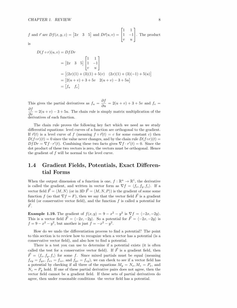
CHAPTER 1. REVIEW 8
f and ~r are Df(x, y, z) =[2x 3 5
]and D~r(u, v) =
1 11 −1v u
. The product
is
D(f ◦ r)(u, v) = DfDr
=[2x 3 5
] 1 11 −1v u
=[(2x)(1) + (3)(1) + 5(v) (2x)(1) + (3)(−1) + 5(u)
]=[2(u+ v) + 3 + 5v 2(u+ v)− 3 + 5u
]=[fu fv
]
This gives the partial derivatives as fu =∂f
∂u= 2(u + v) + 3 + 5v and fv =
∂f
∂v= 2(u+ v)− 3 + 5u. The chain rule is simply matrix multiplication of the
derivatives of each function.
The chain rule proves the following key fact which we need as we studydifferential equations: level curves of a function are orthogonal to the gradient.If ~r(t) is a level curve of f (meaning f ◦ ~r(t) = c for some constant c) thenD(f ◦r)(t) = 0 since the value never changes, and by the chain rule D(f ◦r)(t) =DfDr = ∇f · r′(t). Combining these two facts gives ∇f · r′(t) = 0. Since thedot product of these two vectors is zero, the vectors must be orthogonal. Hencethe gradient of f will be normal to the level curve.
1.4 Gradient Fields, Potentials, Exact Differen-tial Forms
When the output dimension of a function is one, f : Rn → R1, the derivativeis called the gradient, and written in vector form as ∇f = 〈fx, fy, fz〉. If a
vector field ~F = 〈M,N〉 (or in 3D ~F = 〈M,N,P 〉) is the gradient of some some
function f (so that ∇f = F ), then we say that the vector field ~F is a gradientfield (or conservative vector field), and the function f is called a potential for~F .
Example 1.19. The gradient of f(x, y) = 9 − x2 − y2 is ∇f = 〈−2x,−2y〉.This is a vector field ~F = 〈−2x,−2y〉. So a potential for ~F = 〈−2x,−2y〉 isf = 9− x2 − y2, but another is just f = −x2 − y2.
How do we undo the differentiation process to find a potential? The pointto this section is to review how to recognize when a vector has a potential (is aconservative vector field), and also how to find a potential.
There is a test you can use to determine if a potential exists (it is often
called the test for a conservative vector field). If ~F is a gradient field, then~F = 〈fx, fy, fz〉 for some f . Since mixed partials must be equal (meaningfxy = fyx, fxz = fzx, and fyz = fzy), we can check to see if a vector field hasa potential by checking if all three of the equations My = Nx,Mz = Px, andNz = Py hold. If one of these partial derivative pairs does not agree, then thevector field cannot be a gradient field. If these sets of partial derivatives doagree, then under reasonable conditions the vector field has a potential.

CHAPTER 1. REVIEW 9
Example 1.20. Consider the vector field⟨x+ yz, y + xz + z2, xy + 2yz + z2
⟩.
We compute〈x+ yz , y + xz + z2 , xy + 2yz + z2
⟩My = z Nx = z Px = yMz = y Nz = x+ 2z Py = x+ 2z
and hence we know this vector field has a potential because My = Nx,Mz = Px,and Nz = Py. We’ll show how to find a potential in a moment.
The vocabulary of vector fields parallels the vocabulary of differential forms.A differential form is an expression of the form Mdx+Ndy+Pdz (very similarto 〈M,N,P 〉). The differential of a function f is the expression df = fxdx +fydy + fzdz (similar to the gradient). If a differential form is the differential A differential form is exact
precisely when the correspondingvector field is a gradient field.
of a function f , then the differential form is said to be exact (similar to sayinga vector field is a gradient field). Again, the function f is called a potentialfor the differential form. Notice that Mdx+Ndy + Pdz is exact if and only if~F = 〈M,N,P 〉 is a gradient field. We will be using the language of differentialforms throughout the semester.
Example 1.21. The differential form xdx + zdy + ydz is exact because thedifferential of x2/2 + yz is d(x2/2 + yz) = xdx+ zdy + ydz.
Example 1.22. The differential form −ydx+xdy is not exact because My = −1does not equal Nx = 1.
1.4.1 How do you find a potential?
Consider the function f = x2/2 + xyz+ y2/2 + yz2 + z3/3 + 25. Its differentialis df = (x + yz)dx + (y + xz + z2)dy + (xy + 2yz + z2)dz. If we erase f andjust keep the differential form (x+ yz)dx+ (y+xz+ z2)dy+ (xy+ 2yz+ z2)dz,can we recover f? The first component x+ yz should equal fx, so integrate itwith respect to x. Similarly, integrate the second component y + xz + z2 withrespect to y and the third component xy + 2yz + z2 wit respect to z. Thesethree integrals are∫
(x+ yz)dx
∫(y + xz + z2)dy
∫(xy + 2yz + z2)dz
=x2
2+ xyz =
y2
2+ xyz + yz2 = xyz + yz2 +
z3
3.
Notice that each integral contains an xyz term, and the last two integrals bothhave a yz2 term. The reason xyz appears in each integral is that it has all threevariables in it, and so its partial derivative with respect to all three variablesis not zero. The yz2 does not appear in the first integral because it has nox in it, and hence its partial derivative with respect to x is zero. A potentialfor f is now obtained by adding together the three integrals, but realizingthat you do not need to replicate the repeated terms. A potential is hencef(x, y, z) = x2/2+xyz+y2/2+yz2 +z3/3. We did not recover the 25 from theoriginal function. A potential is not unique; if a potential f exists then f + Cis a potential for any constant C.
Example 1.23. Consider the vector field ~F =⟨2xy + x, x2 − 3z,−3y + z2
⟩.
Since My = 2x = Nx,Mz = 0 = Px, and Nz = −3 = Py, the field ~F has apotential. Integrate all three functions simultaneously, ignoring the constants,to get
∫Mdx = x2y + x2/2,
∫Ndy = x2y + −3yz, and
∫Pdz = −3yz + z3/3.
Since x2y and −3yz appear in multiple integrals, we include them once in thesum to obtain for a potential f = x2y + x2/2− 3yz + z3/3.
CHAPTER 1. REVIEW 10
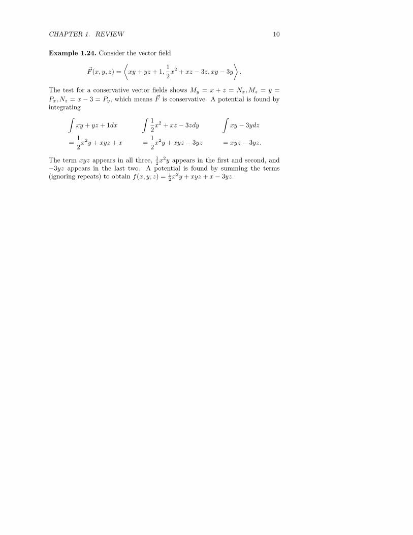
Example 1.24. Consider the vector field
~F (x, y, z) =
⟨xy + yz + 1,
1
2x2 + xz − 3z, xy − 3y
⟩.
The test for a conservative vector fields shows My = x + z = Nx,Mz = y =
Px, Nz = x − 3 = Py, which means ~F is conservative. A potential is found byintegrating∫
xy + yz + 1dx
∫1
2x2 + xz − 3zdy
∫xy − 3ydz
=1
2x2y + xyz + x =
1
2x2y + xyz − 3yz = xyz − 3yz.
The term xyz appears in all three, 12x
2y appears in the first and second, and−3yz appears in the last two. A potential is found by summing the terms(ignoring repeats) to obtain f(x, y, z) = 1
2x2y + xyz + x− 3yz.

CHAPTER 1. REVIEW 11
1.5 Preparation
This chapter covers the following ideas. When you create your lesson plan, it should contain examples whichillustrate these key ideas. Before you take the quiz on this unit, meet with another student out of class andteach each other from the examples on your lesson plan.
1. Graph basic functions by hand. Compute derivatives and integrals, in particular using the productrule, quotient rule, chain rule, integration by u-substitution, and integration by parts (the tabularmethod is useful for simplifying notation). Explain how to find a Laplace transform.
2. Explain how to verify a function is a solution to an ODE, and illustrate how to solve separable ODEs.
3. Explain how to use the language of functions in high dimensions and how to compute derivatives usinga matrix. Illustrate the chain rule in high dimensions with matrix multiplication.
4. Graph the gradient of a function together with several level curves to illustrate that the gradient isnormal to level curves.
5. Explain how to test if a differential form is exact (a vector field is conservative) and how to find apotential.
Most days of class we will present in groups some material you have prepared, or work problems similarto the preparation problems below. Typically there will be 4 problems for each day. Each member of thegroup should prepare one of these problems and then in class you will have the opportunity to teach yourgroup what you have learned as you work through problems. You will occasionally select a problem which isentirely new to you, which you have never seen modeled before. If this occurs, you should look for examplessimilar to this problem in the text, and follow those examples to learn how to do this problem. You will beexercising your faith to then go and teach the class something you have never before seen modeled, and yourconfidence will grow. These problems will normally be the 4th one listed on the preparation problems, so Isuggest that as a group you alternate who takes this problem so that you all get a chance to grow. As timepermits, I will post hand written solutions to these problems on the course website.
Here are the preparation problems for this unit. Problems that come from Schaum’s Outlines are precededby a chapter number. The problems that start with an H are located just below this list. Realize thatsometimes the method of solving the problem in Schaum’s Outlines will differ from how we solve the problemin class.
Preparation Problems (click for handwritten solutions)
Day 1 21.5, 21.29, 4.2, 4.8
Day 2 1.2, 1.7, H.1c, H.2b
Day 3 H.3c, H.4a, H.5b, H.4c
Aside from learning the terms “Laplace Transforms” and “Separable ODEs” (both of which only requirethat you practice your integration), this unit contains material which is review material. The amount andtype of reviewing that we each needs to do will be unique. Remember that your homework assignment is todo enough of each type of problem to master the material we are learning (with a minimum of 7 problemsper day of class). Pick problems that will help you develop your skills. The following problems relate towhat we are studying in class. Section numbers correspond to problems from Schaum’s Outlines DifferentialEquations by Rob Bronson. The suggested problems are a minimum set of problems to attempt.
CHAPTER 1. REVIEW 12
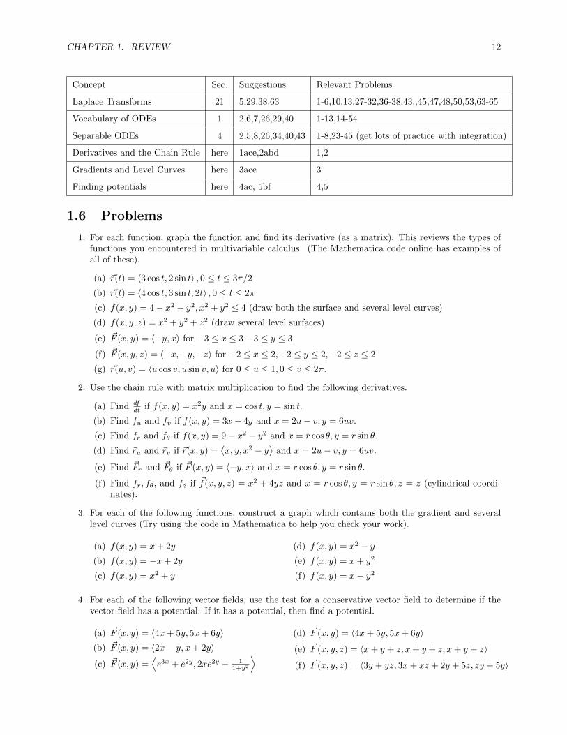
Concept Sec. Suggestions Relevant Problems
Laplace Transforms 21 5,29,38,63 1-6,10,13,27-32,36-38,43,,45,47,48,50,53,63-65
Vocabulary of ODEs 1 2,6,7,26,29,40 1-13,14-54
Separable ODEs 4 2,5,8,26,34,40,43 1-8,23-45 (get lots of practice with integration)
Derivatives and the Chain Rule here 1ace,2abd 1,2
Gradients and Level Curves here 3ace 3
Finding potentials here 4ac, 5bf 4,5
1.6 Problems
1. For each function, graph the function and find its derivative (as a matrix). This reviews the types offunctions you encountered in multivariable calculus. (The Mathematica code online has examples ofall of these).
(a) ~r(t) = 〈3 cos t, 2 sin t〉 , 0 ≤ t ≤ 3π/2
(b) ~r(t) = 〈4 cos t, 3 sin t, 2t〉 , 0 ≤ t ≤ 2π
(c) f(x, y) = 4− x2 − y2, x2 + y2 ≤ 4 (draw both the surface and several level curves)
(d) f(x, y, z) = x2 + y2 + z2 (draw several level surfaces)
(e) ~F (x, y) = 〈−y, x〉 for −3 ≤ x ≤ 3 −3 ≤ y ≤ 3
(f) ~F (x, y, z) = 〈−x,−y,−z〉 for −2 ≤ x ≤ 2,−2 ≤ y ≤ 2,−2 ≤ z ≤ 2
(g) ~r(u, v) = 〈u cos v, u sin v, u〉 for 0 ≤ u ≤ 1, 0 ≤ v ≤ 2π.
2. Use the chain rule with matrix multiplication to find the following derivatives.
(a) Find dfdt if f(x, y) = x2y and x = cos t, y = sin t.
(b) Find fu and fv if f(x, y) = 3x− 4y and x = 2u− v, y = 6uv.
(c) Find fr and fθ if f(x, y) = 9− x2 − y2 and x = r cos θ, y = r sin θ.
(d) Find ~ru and ~rv if ~r(x, y) =⟨x, y, x2 − y
⟩and x = 2u− v, y = 6uv.
(e) Find ~Fr and ~Fθ if ~F (x, y) = 〈−y, x〉 and x = r cos θ, y = r sin θ.
(f) Find fr, fθ, and fz if ~f(x, y, z) = x2 + 4yz and x = r cos θ, y = r sin θ, z = z (cylindrical coordi-nates).
3. For each of the following functions, construct a graph which contains both the gradient and severallevel curves (Try using the code in Mathematica to help you check your work).
(a) f(x, y) = x+ 2y
(b) f(x, y) = −x+ 2y
(c) f(x, y) = x2 + y
(d) f(x, y) = x2 − y(e) f(x, y) = x+ y2
(f) f(x, y) = x− y2
4. For each of the following vector fields, use the test for a conservative vector field to determine if thevector field has a potential. If it has a potential, then find a potential.
(a) ~F (x, y) = 〈4x+ 5y, 5x+ 6y〉(b) ~F (x, y) = 〈2x− y, x+ 2y〉
(c) ~F (x, y) =⟨e3x + e2y, 2xe2y − 1
1+y2
⟩(d) ~F (x, y) = 〈4x+ 5y, 5x+ 6y〉
(e) ~F (x, y, z) = 〈x+ y + z, x+ y + z, x+ y + z〉
(f) ~F (x, y, z) = 〈3y + yz, 3x+ xz + 2y + 5z, zy + 5y〉
CHAPTER 1. REVIEW 13
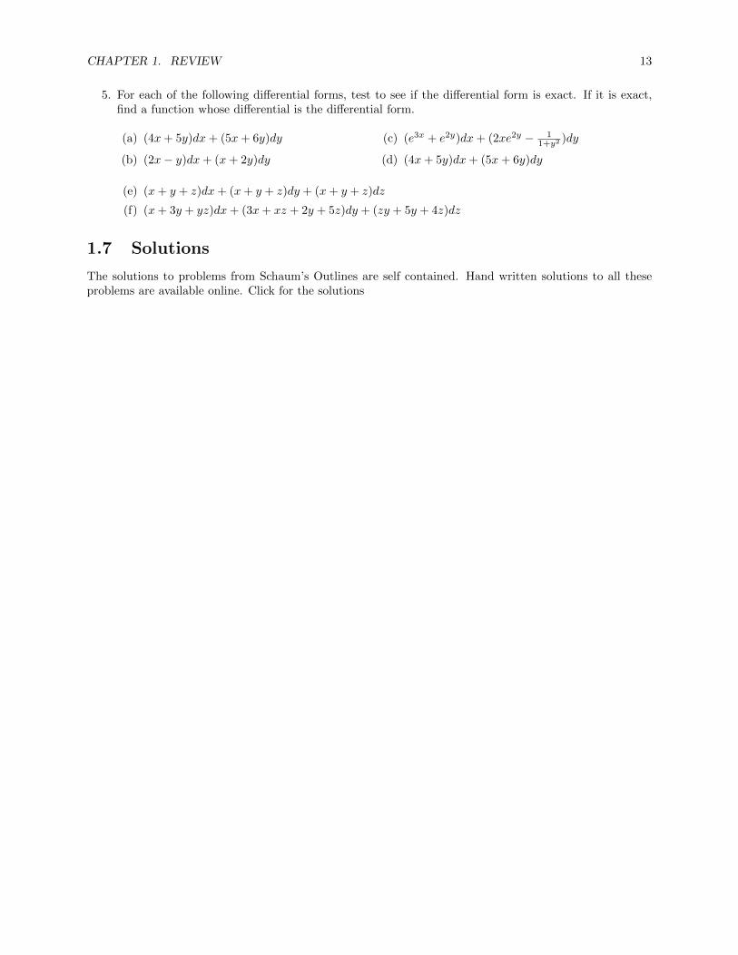
5. For each of the following differential forms, test to see if the differential form is exact. If it is exact,find a function whose differential is the differential form.
(a) (4x+ 5y)dx+ (5x+ 6y)dy
(b) (2x− y)dx+ (x+ 2y)dy
(c) (e3x + e2y)dx+ (2xe2y − 11+y2 )dy
(d) (4x+ 5y)dx+ (5x+ 6y)dy
(e) (x+ y + z)dx+ (x+ y + z)dy + (x+ y + z)dz
(f) (x+ 3y + yz)dx+ (3x+ xz + 2y + 5z)dy + (zy + 5y + 4z)dz
1.7 Solutions
The solutions to problems from Schaum’s Outlines are self contained. Hand written solutions to all theseproblems are available online. Click for the solutions

Chapter 2
Linear Algebra Arithmetic
This chapter covers the following ideas.
1. Be able to use and understand matrix and vector notation, addition, scalarmultiplication, the dot product, matrix multiplication, and matrix trans-posing.
2. Use Gaussian elimination to solve systems of linear equations. Define anduse the words homogeneous, nonhomogeneous, row echelon form, andreduced row echelon form.
3. Find the rank of a matrix. Determine if a collection of vectors is linearlyindependent. If linearly dependent, be able to write vectors as linearcombinations of the preceding vectors.
4. For square matrices, compute determinants, inverses, eigenvalues, andeigenvectors.
5. Illustrate with examples how a nonzero determinant is equivalent to hav-ing independent columns, an inverse, and nonzero eigenvalues. Similarlya zero determinant is equivalent to having dependent columns, no inverse,and a zero eigenvalue.
The next unit will focus on applications of these ideas. The main goal of thisunit is to familiarize yourself with the arithmetic involved in linear algebra.
2.1 Basic Notation
Most of linear algebra centers around understanding matrices and vectors. Thefirst chapter of this text contains a brief introduction to the arithmetic involvedwith matrices and vectors. The second chapter will show you many of the usesof the ideas we are learning. You will be given motivation for all of the ideaslearned here, as well as real world applications of these ideas, before the end ofthe second chapter. For now, I want you become familiar with the arithmeticof linear algebra so that we can discuss how all of the ideas in this chapter showup throughout the course.
2.1.1 Matrices
A matrix of size m by n has m rows and n columns. We normally write Matrix size isrow by column.
14

CHAPTER 2. LINEAR ALGEBRA ARITHMETIC 15
matrices using capital letters, and use the notation
A =
a11 · · · a1n
a21 · · · a2n
.... . .
...am1 · · · amn
= [ajk],
where ajk is the entry in the jth row, kth column.We say two matrices A and B are equal if ajk = bjk for all j and k. We
add and subtract matrices of the same size entry wise, and perform scalarmultiplication cA by multiplying every entry in the matrix by the scalar c. If thenumber of rows and columns are equal, then we say the matrix is square. Themain diagonal of a square (n×n) matrix consists of the entries a11, a22, . . . , ann,and the trace is the sum of the entries on the main diagonal (
∑ajj).
Example 2.1. If A =
[1 30 2
]and B =
[3 −10 4
], then
A− 2B =
[1− 2 · 3 3− 2 · (−1)0− 2 · 0 2− 2 · 4
]=
[−5 50 −6
].
The main diagonal of B consists of the entries b11 = 3 and b22 = 4, which meansthe trace of B is 3 + 4 = 7 (the sum of the entries on the main diagonal).
The transpose of a matrix A = [ajk] is a new matrix AT = [akj ] formed by transpose
interchaning the rows and columns.
Example 2.2. The transpose of A is illustrated below.
A =
[0 1 −11 0 2
]AT =
0 11 0−1 2
.
2.1.2 Vectors
Vectors represent a magnitude in a given direction. We can use vectors tomodel forces, acceleration, velocity, probabilities, electronic data, and more.We can use matrices to represent vectors. A row vector is a 1 × n matrix. Acolumn vector is an m×1 matrix. Textbooks often write vectors using bold facefont. By hand (and in this book) we add an arrow above them. The notationv = ~v = 〈v1, v2, v3〉 can represent either row or column vectors. Many differentways to represent vectors are used throughout different books. In particular,we can represent the vector 〈2, 3〉 in any of the following forms
〈2, 3〉 = 2i + 3j = (2, 3) =[2 3
]=
[23
]=(2 3
)=
(23
)The notation (2, 3) has other meanings as well (like a point in the plane, oran open interval), and so when you use the notation (2, 3), it should be clearfrom the context that you working with a vector. To draw a vector 〈v1, v2〉, one
Both vectors represent 〈2,−3〉,regardless of where we start.
option is to draw an arrow from the origin (the tail) to the point (v1, v2) (thehead). However, the tail does not have to be placed at the origin.
The principles of addition and subtraction of matrices apply to vectors(which can be though of as row or column matrices). For example 〈1, 3〉 −2 〈−1, 2〉+ 〈4, 0〉 = 〈1− 2(−1) + 4, 3− 2(2) + 0〉 = 〈7,−1〉. We will often writevectors using column notation as in[
13
]− 2
[−12
]+
[40
]=
[1− 2(−1) + 43− 2(2) + 0
]=
[7−1
].

CHAPTER 2. LINEAR ALGEBRA ARITHMETIC 16
Vector addition is performed geometrically by placing the tail of the second Vector Addition
~u
~v
~v
~u+ ~v
Scalar Multiplication
~u
2~u
− 12~u
Vector Subtraction
~u
~v
−~v
~u− ~v
~u− ~v
vector at the head of the first. The resultant vector is the vector which startsat the tail of the first and ends at the head of the second. This is called theparallelogram law of addition. The sum 〈1, 2〉 + 〈3, 1〉 = 〈4, 3〉 is illustrated tothe right.
Scalar multiplication c~u (c is a scalar and ~u is a vector) is equivalent tostretching (scaling) a vector by the scalar. The product 2~u doubles the lengthof the vector. If the scalar is negative then the vector turns around to point inthe opposite direction. So the product − 1
2~u is a vector half as long as ~u, andpointing in the opposite direction (as illustrated on the right).
To subtract to vectors ~u−~v, we use scalar multiplication and vector addition.We write ~u − ~v = ~u + (−~v), which means we turn ~v around and then add itto ~u. The same parallelogram law of addition applies geometrically, howeverthe result ~u − ~v can be seen as the vector connecting the heads of the twovectors when their tails are both placed on the same spot, with the directionpointing towards the head of ~u. When I see a vector difference ~u − ~v, I liketo think “head minus tail” to help remind me that the head of ~u − ~v is at thetip of ~u whereas the tail of the difference is at the head of ~v. The difference〈1, 2〉 − 〈3, 1〉 = 〈−2, 1〉 is illustrated to the right.
2.1.3 Magnitude and the Dot Product
The length of a vector is found using the Pythagorean theorem: c2 = a2 + b2.The magnitude (or length) of the vector 〈2, 3〉 is simply the hypotenuse of atriangle with side lengths 2 and 3, hence | 〈2, 3〉 | =
√22 + 32 =
√13. We
denote magnitude with absolute value symbols, and compute for ~u = (u1, u2)the magnitude as |~u| =
√u2
1 + u22. In higher dimensions we extend this as
|~u| =√u2
1 + u22 + u2
3 + · · ·u2n =
√√√√ n∑i=1
u2i .
A unit vector is a vector with length 1. In many books unit vectors are A unit vector u has length |~u| = 1
written with a hat above them, as u. Any vector that is not a unit vectorcan be rewritten as a scalar times a unit vector, by dividing the vector by itsmagnitude. This allows us to write any vector as a magnitude times a direction(unit vector).
Example 2.3. The length of ~u = 〈2, 1,−3〉 is√
22 + 12 + (−3)2 =√
4 + 1 + 9 =√
14. A unit vector in the direction of ~u is1√14〈2, 1,−3〉 =
⟨2√14,
1√14,−3√14
⟩.
We can rewrite ~u as a magnitude times a direction by writing Every vector can be rewritten asa magnitude times direction (unitvector).
~u = |~u| ~u|~u|
=√
14
⟨2√14,
1√14,−3√
14
⟩.
The dot product of two vectors ~u = 〈u1, u2, . . . , un〉 and ~v = 〈v1, v2, . . . , vn〉is the scalar ~u · ~v = u1v1 + u2v2 + · · · + unvn =
∑uivi. Just multiply corre-
sponding components and then add the products.
Example 2.4. The dot product of[1 3 −2
]and
[2 −1 4
]is[
1 3 −2]·[2 −1 4
]= (1)(2) + (3)(−1) + (−2)(4) = −9.
We use the dot product to find lengths and angles in all dimensions. Wewill also use it multiply matrices. The rest of this section explains how to use
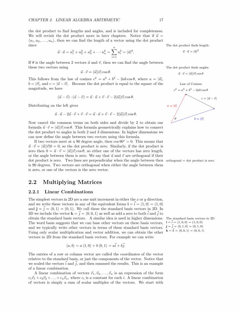
CHAPTER 2. LINEAR ALGEBRA ARITHMETIC 17
the dot product to find lengths and angles, and is included for completeness.We will revisit the dot product more in later chapters. Notice that if ~u =〈u1, u2, . . . , un〉, then we can find the length of a vector using the dot productsince The dot product finds length:
~u · ~u = |~u|2~u · ~u = u21 + u2
2 + u23 + · · ·u2
n =
n∑i=1
u2i = |~u|2.
If θ is the angle between 2 vectors ~u and ~v, then we can find the angle betweenthese two vectors using The dot product finds angles:
~u · ~v = |~u||~v| cos θ~u · ~v = |~u||~v| cos θ.
This follows from the law of cosines c2 = a2 + b2 − 2ab cos θ, where a = |~u|,b = |~v|, and c = |~u− ~v|. Because the dot product is equal to the square of the Law of Cosines
c2 = a2 + b2 − 2ab cos θ
a = |~u|
b = |~v|
c = |~u− ~v|
θ
magnitude, we have
(~u− ~v) · (~u− ~v) = ~u · ~u+ ~v · ~v − 2|~u||~v| cos θ.
Distributing on the left gives
~u · ~u− 2~u · ~v + ~v · ~v = ~u · ~u+ ~v · ~v − 2|~u||~v| cos θ.
Now cancel the common terms on both sides and divide by 2 to obtain ourformula ~u · ~v = |~u||~v| cos θ. This formula geometrically explains how to connectthe dot product to angles in both 2 and 3 dimensions. In higher dimensions wecan now define the angle between two vectors using this formula.
If two vectors meet at a 90 degree angle, then cos 90◦ = 0. This means that~u · ~v = |~u||~v|0 = 0, so the dot product is zero. Similarly, if the dot product iszero then 0 = ~u · ~v = |~u||~v| cos θ, so either one of the vectors has zero length,or the angle between them is zero. We say that ~u and ~v are orthogonal if theirdot product is zero. Two lines are perpendicular when the angle between then orthogonal = dot product is zero
is 90 degrees. Two vectors are orthogonal when either the angle between themis zero, or one of the vectors is the zero vector.
2.2 Multiplying Matrices
2.2.1 Linear Combinations
The simplest vectors in 2D are a one unit increment in either the x or y direction,and we write these vectors in any of the equivalent forms i =~i = 〈1, 0〉 = (1, 0)and j = ~j = 〈0, 1〉 = (0, 1). We call these the standard basis vectors in 2D. In3D we include the vector k = ~j = 〈0, 0, 1〉 as well as add a zero to both~i and ~j toobtain the standard basis vectors. A similar idea is used in higher dimensions. The standard basis vectors in 3D
i =~i = 〈1, 0, 0〉 = (1, 0, 0)
j = ~j = 〈0, 1, 0〉 = (0, 1, 0)
k = ~k = 〈0, 0, 1〉 = (0, 0, 1)
The word basis suggests that we can base other vectors on these basis vectors,and we typically write other vectors in terms of these standard basis vectors.Using only scalar multiplication and vector addition, we can obtain the othervectors in 2D from the standard basis vectors. For example we can write
〈a, b〉 = a 〈1, 0〉+ b 〈0, 1〉 = a~i+ b~j.
The entries of a row or column vector are called the coordinates of the vectorrelative to the standard basis, or just the components of the vector. Notice thatwe scaled the vectors~i and ~j, and then summed the results. This is an exampleof a linear combination.
A linear combination of vectors ~v1, ~v2, . . . , ~vn is an expression of the formc1~v1 + c2~v2 + . . .+ cn~vn, where ci is a constant for each i. A linear combinationof vectors is simply a sum of scalar multiples of the vectors. We start with

CHAPTER 2. LINEAR ALGEBRA ARITHMETIC 18
some vectors, stretch each one by some scalar, and then sum the result. Muchof what we will do this semester (and in many courses to come) relates directlyto understanding linear combinations.
Example 2.5. Let’s look at a physical application of linear combinations thatyou use every day when you drive. When you place your foot on the acceleratorof your car, the car exerts a force ~F1 pushing you forward. When you turn thesteering wheel left, the car exerts a force ~F2 pushing you left. The total forceacting on you is the vector sum of these forces, or a linear combination ~Ftotal =~F1 + ~F2. If ~T represents a unit vector pointing forward, and ~N represents a unitvector pointing left, then we can write the total force as the linear combination
~Ftotal = |~F1|~T + |~F2| ~N.
To understand motion, we can now focus on finding just the tangential force~T and normal force ~N , and then we can obtain other forces by just looking atlinear combinations of these two.
2.2.2 Matrix Multiplication
One of the key applications of linear combinations we will make throughout thesemester is matrix multiplication. Let’s introduce the idea with an example.
Example 2.6. Consider the three vectors
101
,
02−3
, and
211
. Let’s multiply
the first vector by 2, the second by -1, and the third by 4, and then sum theresult. This gives us the linear combination
2
101
− 1
02−3
+ 4
211
=
1029
We will define matrix multiplication so that multiplying a matrix on the right bya vector corresponds precisely to creating a linear combination of the columnsof A. We now write the linear combination above in matrix form1 0 2
0 2 11 −3 1
2−14
=
1029
.We define the matrix product A~x (a matrix times a vector) to be the linear Matrix multiplication A~x
combination of columns of A where the components of ~x are the scalars in thelinear combination. For this to make sense, notice that the vector ~x must havethe same number of entries as there are columns in A. Symbolically, let ~vi be
the ith column of A so that A =[~a1 ~a2 · · · ~an
], and let ~x =
x1
x2
. . .xn
. Then
the matrix product is the linear combination The product A~x gives us linearcombinations of the columns of A.
A~x =[~a1 ~a2 · · · ~an
] x1
x2
. . .xn
= ~a1x1 + ~a2x2 + · · ·+ ~anxn.
This should look like the dot product. If you think of A as a vector of vectors,then A~x is just the dot product of A and ~x.

CHAPTER 2. LINEAR ALGEBRA ARITHMETIC 19
We can now define the product of two matrices A and B. Let ~bj represent Matrix multiplication AB
the jth column of B (so B =[~b1 ~b2 · · · ~bn
]). The product AB of two
matrices Am×n and Bn×p is a new matrix Cm×p = [cij ] where the jth column
of C is the product A~bj . To summarize, the matrix product AB is a new matrixwhose jth column is a linear combinations of the columns of A using the entriesof the jth column of B to perform the linear combinations. We need someexamples.
Example 2.7. A row matrix times a column matrix is equivalent to the dotproduct of the two when treated as vectors.
[1 2
] [56
]=[1 · 5 + 2 · 6
]=[17]
Example 2.8. In this example the matrix A has 3 rows, so the product shouldhave three rows. The matrix B has 2 columns so we need to find 2 differentlinear combinations giving us 2 columns in the product.1 2
3 45 6
[−2 01 3
]=
135
(−2) +
246
(1)
135
(0) +
246
(3)
=
0−2−4
61218
Example 2.9. Note that AB and BA are usually different.
A =
[12
]B =
[3 4
]AB =
[3 46 8
]BA = [11]
Even if the product CD is defined, the product DC does not have to be. Inthis example D has 3 columns but C has only 2 rows, and hence the productDC is not defined (as you can’t form a linear combination of 3 vectors withonly 2 constants).
C =
[1 23 4
]D =
[0 1 −11 0 2
]CD =
[2 1 34 3 5
]DC is undefined
The identity matrix is a square matrix which has only 1’s along the diagonal, The identity matrix behaves likethe number 1, in thatAI = IA = A.
and zeros everywhere else. We often use In to mean the n by n identity matrix.The identity matrix is like the number 1, in that AI = A and IA = A for anymatrix A. If A is a 2 by 3 matrix, then AI3 = A and I2A = A (notice that thesize of the matrix changes based on the order of multiplication. If A is a squarematrix, then AI = IA = A.
2.2.3 Alternate Definitions of Matrix Multiplication
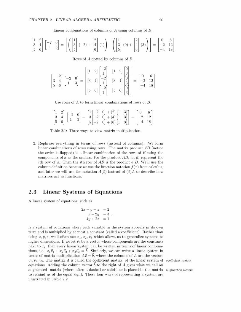
I have introduced matrix multiplication in terms of linear combinations of vec-tors. My hope is that by doing so you immediately start thinking of linearcombinations whenever you encounter matrix multiplication (as this is whatit was invented to do). There are many alternate ways to think of matrixmultiplication. Here are two additional methods. Table 2.1 illustrates all three.
1. “Row times column approach.” The product AB of two matrices Am×nand Bn×p is a new matrix Cm×p = [cij ] where cij =
∑nk=1 aikbkj is the
dot product of the of the ith row of A and the jth column of B. Wikipediahas an excellent visual illustration of this approach.
CHAPTER 2. LINEAR ALGEBRA ARITHMETIC 20
Linear combinations of columns of A using columns of B.1 23 45 6
[−2 01 3
]=
135
(−2) +
246
(1)
135
(0) +
246
(3)
=
0−2−4
61218
Rows of A dotted by columns of B.
1 23 45 6
[−2 01 3
]=
[1 2
] [−21
][3 4
] [−21
][5 6
] [−21
][1 2
] [03
][3 4
] [03
][5 6
] [03
]
=
0−2−4
61218
Use rows of A to form linear combinations of rows of B.1 23 45 6
[−2 01 3
]=
1[−2 0
]+ (2)
[1 3
]3[−2 0
]+ (4)
[1 3
]5[−2 0
]+ (6)
[1 3
] =
0−2−4
61218
Table 2.1: Three ways to view matrix multiplication.
2. Rephrase everything in terms of rows (instead of columns). We formlinear combinations of rows using rows. The matrix product ~xB (noticethe order is flopped) is a linear combination of the rows of B using thecomponents of x as the scalars. For the product AB, let ~ai represent theith row of A. Then the ith row of AB is the product ~aiB. We’ll use thecolumn definition because we use the function notation f(x) from calculus,and later we will use the notation A(~x) instead of (~x)A to describe howmatrices act as functions.
2.3 Linear Systems of Equations
A linear system of equations, such as
2x+ y − z = 2x− 2y = 3
4y + 2z = 1,
is a system of equations where each variable in the system appears in its ownterm and is multiplied by at most a constant (called a coefficient). Rather thanusing x, y, z, we’ll often use x1, x2, x3 which allows us to generalize systems tohigher dimensions. If we let ~vi be a vector whose components are the constantsnext to xi, then every linear system can be written in terms of linear combina-tions, i.e. x1~v1 + x2~v2 + x3~v3 = ~b. Similarly, we can write a linear system interms of matrix multiplication A~x = ~b, where the columns of A are the vectors~v1, ~v2, ~v3. The matrix A is called the coefficient matrix of the linear system of coefficient matrix
equations. Adding the column vector ~b to the right of A gives what we call anaugmented matrix (where often a dashed or solid line is placed in the matrix augmented matrix
to remind us of the equal sign). These four ways of representing a system areillustrated in Table 2.2
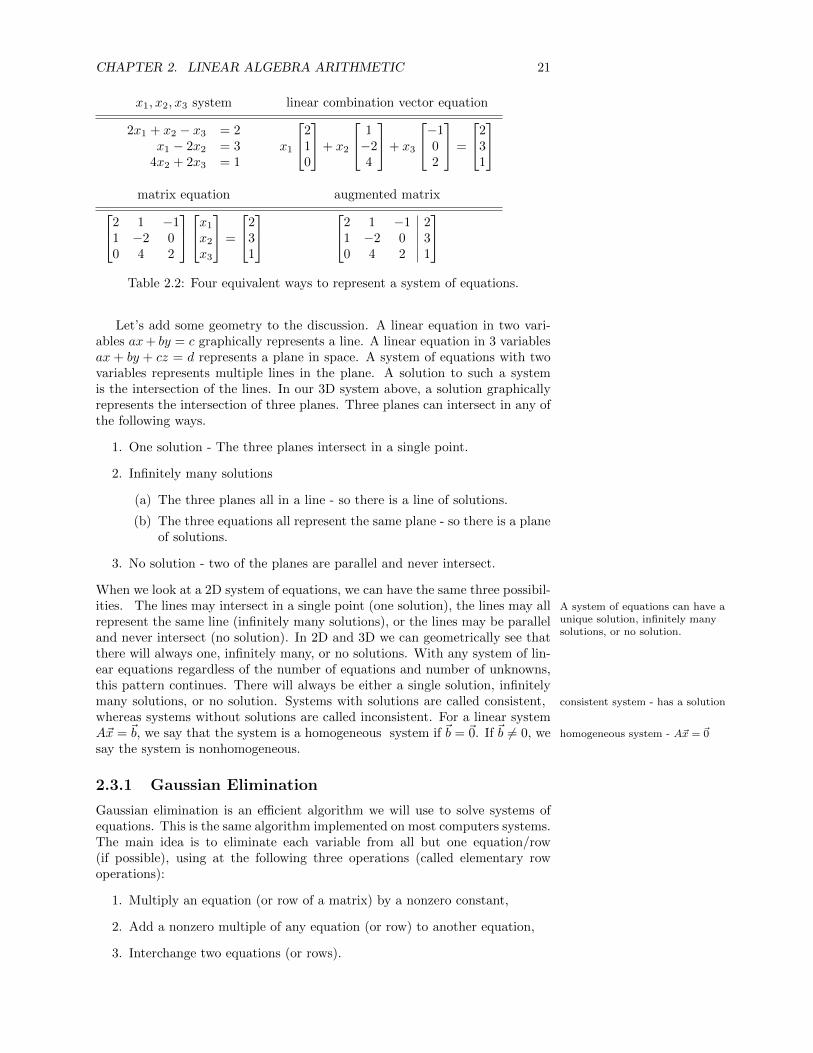
CHAPTER 2. LINEAR ALGEBRA ARITHMETIC 21
x1, x2, x3 system linear combination vector equation
2x1 + x2 − x3 = 2x1 − 2x2 = 3
4x2 + 2x3 = 1x1
210
+ x2
1−24
+ x3
−102
=
231
matrix equation augmented matrix2 1 −1
1 −2 00 4 2
x1
x2
x3
=
231
2 1 −1 21 −2 0 30 4 2 1
Table 2.2: Four equivalent ways to represent a system of equations.
Let’s add some geometry to the discussion. A linear equation in two vari-ables ax+ by = c graphically represents a line. A linear equation in 3 variablesax + by + cz = d represents a plane in space. A system of equations with twovariables represents multiple lines in the plane. A solution to such a systemis the intersection of the lines. In our 3D system above, a solution graphicallyrepresents the intersection of three planes. Three planes can intersect in any ofthe following ways.
1. One solution - The three planes intersect in a single point.
2. Infinitely many solutions
(a) The three planes all in a line - so there is a line of solutions.
(b) The three equations all represent the same plane - so there is a planeof solutions.
3. No solution - two of the planes are parallel and never intersect.
When we look at a 2D system of equations, we can have the same three possibil-ities. The lines may intersect in a single point (one solution), the lines may all A system of equations can have a
unique solution, infinitely manysolutions, or no solution.
represent the same line (infinitely many solutions), or the lines may be paralleland never intersect (no solution). In 2D and 3D we can geometrically see thatthere will always one, infinitely many, or no solutions. With any system of lin-ear equations regardless of the number of equations and number of unknowns,this pattern continues. There will always be either a single solution, infinitelymany solutions, or no solution. Systems with solutions are called consistent, consistent system - has a solution
whereas systems without solutions are called inconsistent. For a linear systemA~x = ~b, we say that the system is a homogeneous system if ~b = ~0. If ~b 6= 0, we homogeneous system - A~x = ~0
say the system is nonhomogeneous.
2.3.1 Gaussian Elimination
Gaussian elimination is an efficient algorithm we will use to solve systems ofequations. This is the same algorithm implemented on most computers systems.The main idea is to eliminate each variable from all but one equation/row(if possible), using at the following three operations (called elementary rowoperations):
1. Multiply an equation (or row of a matrix) by a nonzero constant,
2. Add a nonzero multiple of any equation (or row) to another equation,
3. Interchange two equations (or rows).
CHAPTER 2. LINEAR ALGEBRA ARITHMETIC 22
These three operations are the operations learned in college algebra when solv-ing a system using a method of elimination. Gaussian elimination streamlineselimination methods to solve generic systems of equations of any size. Theprocess involves a forward reduction and (optionally) a backward reduction.The forward reduction creates zeros in the lower left corner of the matrix. Thebackward reduction puts zeros in the upper right corner of the matrix. Weeliminate the variables in the lower left corner of the matrix, starting with col-umn 1, then column 2, and proceed column by column until all variables whichcan be eliminated (made zero) have been eliminated. Before formally statingthe algorithm, let’s look at a few examples.
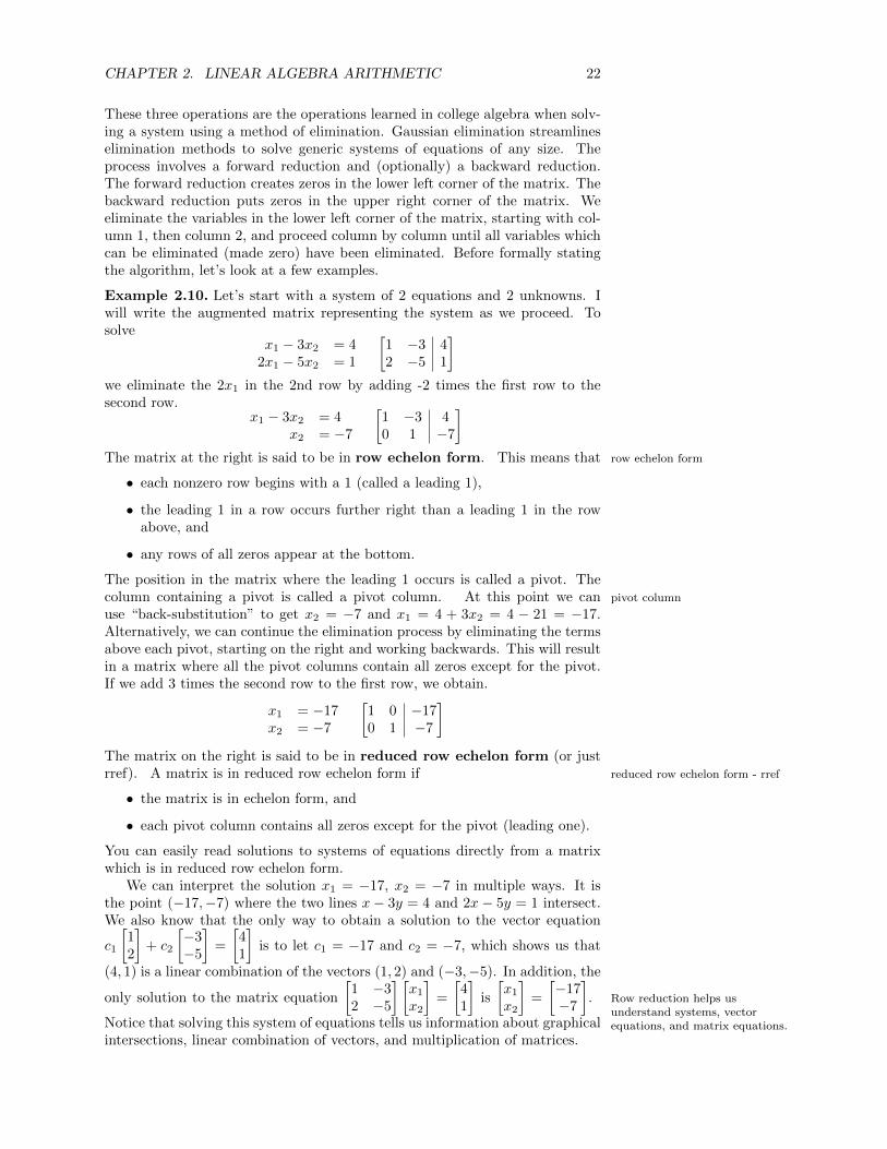
Example 2.10. Let’s start with a system of 2 equations and 2 unknowns. Iwill write the augmented matrix representing the system as we proceed. Tosolve
x1 − 3x2 = 42x1 − 5x2 = 1
[1 −3 42 −5 1
]we eliminate the 2x1 in the 2nd row by adding -2 times the first row to thesecond row.
x1 − 3x2 = 4x2 = −7
[1 −3 40 1 −7
]The matrix at the right is said to be in row echelon form. This means that row echelon form
• each nonzero row begins with a 1 (called a leading 1),
• the leading 1 in a row occurs further right than a leading 1 in the rowabove, and
• any rows of all zeros appear at the bottom.
The position in the matrix where the leading 1 occurs is called a pivot. Thecolumn containing a pivot is called a pivot column. At this point we can pivot column
use “back-substitution” to get x2 = −7 and x1 = 4 + 3x2 = 4 − 21 = −17.Alternatively, we can continue the elimination process by eliminating the termsabove each pivot, starting on the right and working backwards. This will resultin a matrix where all the pivot columns contain all zeros except for the pivot.If we add 3 times the second row to the first row, we obtain.
x1 = −17x2 = −7
[1 0 −170 1 −7
]The matrix on the right is said to be in reduced row echelon form (or justrref). A matrix is in reduced row echelon form if reduced row echelon form - rref
• the matrix is in echelon form, and
• each pivot column contains all zeros except for the pivot (leading one).
You can easily read solutions to systems of equations directly from a matrixwhich is in reduced row echelon form.
We can interpret the solution x1 = −17, x2 = −7 in multiple ways. It isthe point (−17,−7) where the two lines x− 3y = 4 and 2x− 5y = 1 intersect.We also know that the only way to obtain a solution to the vector equation
c1
[12
]+ c2
[−3−5
]=
[41
]is to let c1 = −17 and c2 = −7, which shows us that
(4, 1) is a linear combination of the vectors (1, 2) and (−3,−5). In addition, the
only solution to the matrix equation
[1 −32 −5
] [x1
x2
]=
[41
]is
[x1
x2
]=
[−17−7
]. Row reduction helps us
understand systems, vectorequations, and matrix equations.Notice that solving this system of equations tells us information about graphical
intersections, linear combination of vectors, and multiplication of matrices.
CHAPTER 2. LINEAR ALGEBRA ARITHMETIC 23
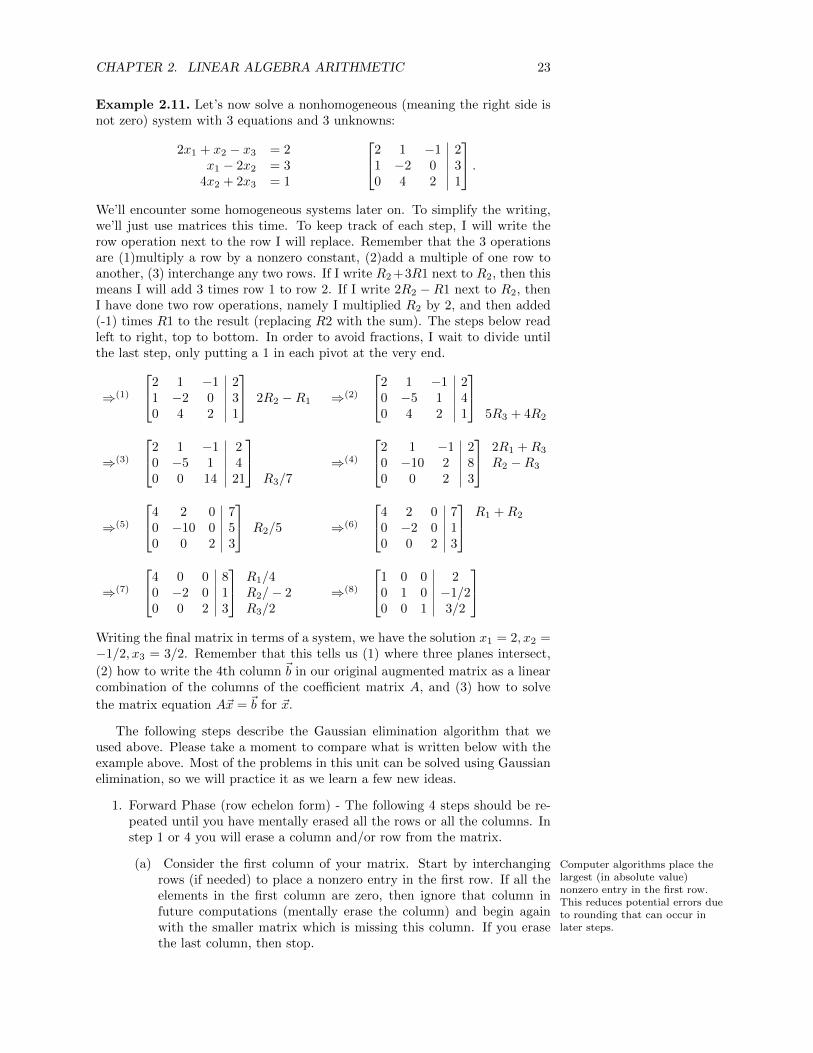
Example 2.11. Let’s now solve a nonhomogeneous (meaning the right side isnot zero) system with 3 equations and 3 unknowns:
2x1 + x2 − x3 = 2x1 − 2x2 = 3
4x2 + 2x3 = 1
2 1 −1 21 −2 0 30 4 2 1
.We’ll encounter some homogeneous systems later on. To simplify the writing,we’ll just use matrices this time. To keep track of each step, I will write therow operation next to the row I will replace. Remember that the 3 operationsare (1)multiply a row by a nonzero constant, (2)add a multiple of one row toanother, (3) interchange any two rows. If I write R2 +3R1 next to R2, then thismeans I will add 3 times row 1 to row 2. If I write 2R2 −R1 next to R2, thenI have done two row operations, namely I multiplied R2 by 2, and then added(-1) times R1 to the result (replacing R2 with the sum). The steps below readleft to right, top to bottom. In order to avoid fractions, I wait to divide untilthe last step, only putting a 1 in each pivot at the very end.
⇒(1)
2 1 −1 21 −2 0 30 4 2 1
2R2 −R1 ⇒(2)
2 1 −1 20 −5 1 40 4 2 1
5R3 + 4R2
⇒(3)
2 1 −1 20 −5 1 40 0 14 21
R3/7
⇒(4)
2 1 −1 20 −10 2 80 0 2 3
2R1 +R3
R2 −R3
⇒(5)
4 2 0 70 −10 0 50 0 2 3
R2/5 ⇒(6)
4 2 0 70 −2 0 10 0 2 3
R1 +R2
⇒(7)
4 0 0 80 −2 0 10 0 2 3
R1/4R2/− 2R3/2
⇒(8)
1 0 0 20 1 0 −1/20 0 1 3/2
Writing the final matrix in terms of a system, we have the solution x1 = 2, x2 =−1/2, x3 = 3/2. Remember that this tells us (1) where three planes intersect,
(2) how to write the 4th column ~b in our original augmented matrix as a linearcombination of the columns of the coefficient matrix A, and (3) how to solve
the matrix equation A~x = ~b for ~x.
The following steps describe the Gaussian elimination algorithm that weused above. Please take a moment to compare what is written below with theexample above. Most of the problems in this unit can be solved using Gaussianelimination, so we will practice it as we learn a few new ideas.
1. Forward Phase (row echelon form) - The following 4 steps should be re-peated until you have mentally erased all the rows or all the columns. Instep 1 or 4 you will erase a column and/or row from the matrix.
(a) Consider the first column of your matrix. Start by interchanging Computer algorithms place thelargest (in absolute value)nonzero entry in the first row.This reduces potential errors dueto rounding that can occur inlater steps.
rows (if needed) to place a nonzero entry in the first row. If all theelements in the first column are zero, then ignore that column infuture computations (mentally erase the column) and begin againwith the smaller matrix which is missing this column. If you erasethe last column, then stop.

CHAPTER 2. LINEAR ALGEBRA ARITHMETIC 24
(b) Divide the first row (of your possibly smaller matrix) row by itsleading entry so that you have a leading 1. This entry is a pivot,and the column is a pivot column. [When doing this by hand, it isoften convenient to skip this step and do it at the very end so thatyou avoid fractional arithmetic. If you can find a common multipleof all the terms in this row, then divide by it to reduce the size ofyour computations. ]
(c) Use the pivot to eliminate each nonzero entry below the pivot, byadding a multiple of the top row (of your smaller matrix) to thenonzero lower row.
(d) Ignore the row and column containing your new pivot and return Ignoring rows and columns isequivalent to incrementing rowand column counters in acomputer program.
to the first step (mentally cover up or erase the row and columncontaining your pivot). If you erase the last row, then stop.
2. Backward Phase (reduced row echelon form - often called Gauss-Jordanelimination) - At this point each row should have a leading 1, and youshould have all zeros to the left and below each leading 1. If you skippedstep 2 above, then at the end of this phase you should divide each row byits leading coefficient to make each row have a leading 1.
(a) Starting with the last pivot column. Use the pivot in that columnto eliminate all the nonzero entries above it, by adding multiples ofthe row containing the pivot to the nonzero rows above.
(b) Work from right to left, using each pivot to eliminate the nonzeroentries above it. Nothing to the left of the current pivot columnchanges. By working right to left, you greatly reduce the number ofcomputations needed to fully reduce the matrix.
Example 2.12. As a final example, let’s reduce
0 1 1 −2 71 3 5 1 62 0 4 3 −8−2 1 −3 0 5
to
reduced row echelon form (rref). The first step involves swapping 2 rows. Weswap row 1 and row 2 because this places a 1 as the leading entry in row 1.
(1) Get a nonzero entry in upper left (2) Eliminate entries in 1st column
⇒
0 1 1 −2 71 3 5 1 62 0 4 3 −8−2 1 −3 0 5
R1 ↔ R2
⇒
1 3 5 1 60 1 1 −2 72 0 4 3 −8−2 1 −3 0 5
R3 − 2R1
R4 + 2R1
(3) Eliminate entries in 2nd column (4) Make a leading 1 in 4th column
⇒
1 3 5 1 60 1 1 −2 70 −6 −6 1 −200 7 7 2 17
R3 + 6R2
R4 − 7R2
⇒
1 3 5 1 60 1 1 −2 70 0 0 −11 220 0 0 16 −32
R3/(−11)R4/16
(5) Eliminate entries in 4th column (6) Row Echelon Form
⇒
1 3 5 1 60 1 1 −2 70 0 0 1 −20 0 0 1 −2
R4 −R3
⇒
1 3 5 1 60 1 1 −2 70 0 0 1 −20 0 0 0 0
At this stage we have found a row echelon form of the matrix. Notice that weeliminated nonzero terms in the lower left of the matrix by starting with thefirst column and working our way over column by column. Columns 1, 2, and

CHAPTER 2. LINEAR ALGEBRA ARITHMETIC 25
4 are the pivot columns of this matrix. We now use the pivots to eliminate theother nonzero entries in each pivot column (working right to left). Recall that a matrix is in reduced
row echelon (rref) if:
1. Nonzero rows begin with aleading 1.
2. Leadings 1’s on subsequentrows appear further rightthan previous rows.
3. Rows of zeros are at thebottom.
4. Zeros are above and beloweach pivot.
(7) Eliminate entries in 4th column (8) Eliminate entries in 2nd column
⇒
1 3 5 1 60 1 1 − 2 70 0 0 1 −20 0 0 0 0
R1 −R3R2 + 2R3 ⇒
1 3 5 0 80 1 1 0 30 0 0 1 −20 0 0 0 0
R1 − 3R2
(9) Reduced Row Echelon Form (10) Switch to system form
⇒
1 0 2 0 −10 1 1 0 30 0 0 1 −20 0 0 0 0
⇒
x1 + 2x3 = −1x2 + x3 = 3
x4 = −20 = 0
We have obtained the reduced row echelon form. When we write this matrixin the corresponding system form, notice that there is not a unique solution tothe system. Because the third column did not contain a pivot column, we canwrite every variable in terms of x3 (the redundant equation x3 = x3 allows usto write x3 in terms of x3). We are free to pick any value we want for x3 andstill obtain a solution. For this reason, we call x3 a free variable, and write our Free variables correspond to non
pivot columns. Solutions can bewritten in terms of free variables.
infinitely many solutions in terms of x3 as
x1 = −1− 2x3
x2 = 3− x3
x3 = x3
x4 = −2
or by letting x3 = t
x1 = −1− 2tx2 = 3− tx3 = tx4 = −2
.
By choosing a value (such as t) for x3, we can write our solution in so called parametric form
parametric form. We have now given a parametrization of the solution set,where t is an arbitrary real number.
2.3.2 Reading Reduced Row Echelon Form - rref
From reduced row echelon form you can read the solution to a system imme-diately from the matrix. Here are some typical examples of what you will seewhen you reduce a system that does not have a unique solution, together withtheir solution. The explanations which follow illustrate how to see the solutionimmediately from the matrix.1 2 0 1
0 0 1 30 0 0 0
[1 0 4 −50 1 −2 3
] 1 0 2 00 1 −3 00 0 0 1
(1− 2x2, x2, 3) (−5− 4x3, 3 + 2x3, x3) no solution,0 6= 1
Example 2.13. In the first example, columns 1 and 3 are the pivot columns.Since column 2 is not a pivot column, we’ll let x2 be a free variable and writethe solution in terms of x2. Rewriting the first matrix in system form yieldsx1 + 2x2 = 1, x3 = 3, or solving for each variable in terms of x2 we havex1 = 1 − x2, x3 = 3. Adding to this system the redundant equation x2 = x2,
we have in vector form
x1
x2
x3
=
1− 2x2
x2
3
=
103
+ x2
−210
. Sometimes it’s
useful to use a different variable, such as x2 = t, and then write the solution inparametric form as (x1, x2, x3) = (1−2t, t, 3), where t is any real number. Thissolution is a line in space.

CHAPTER 2. LINEAR ALGEBRA ARITHMETIC 26
Example 2.14. In the second example, the first and second columns are pivotcolumns, so x3 is a free variable. The solution can be written in the formx1
x2
x3
=
−5− 4x3
3 + 2x3
x3
=
−530
+ x3
−421
. Again the last column appears in
the solution, and then the opposite of the third column together with a 1 in thethird spot gives us the vector which is multiplied by x3.
Example 2.15. In the third example, the first, second, and fourth columnsare pivot columns. Because the last column is a pivot column, we obtain theequation 0 = 1, which is absurd. Hence the system is inconsistent and has nosolution.
Example 2.16. The ideas above generalize to higher dimensions. Here are twolarge rref matrices and their solutions.
0 1 0 2 0 00 0 1 3 0 10 0 0 0 1 40 0 0 0 0 0
x1
x2
x3
x4
x5
=
00104
+ x1
10000
+ x4
0−2−310
0 1 0 2 0 0 00 0 1 3 0 1 00 0 0 0 1 4 00 0 0 0 0 0 0
x1
x2
x3
x4
x5
x6
=
000000
+ x1
100000
+ x4
0−2−3100
+ x6
00−10−41
Each non pivot column corresponds to one of the vectors in the sum above.
2.4 Rank and Linear Independence
The rank of a matrix is the number of pivot columns of the matrix. To find therank of a matrix, you reduce the matrix using Gaussian elimination until youdiscover the pivot columns.
Recall that a linear combination of vectors ~v1, ~v2, . . . , ~vn is an expression ofthe form c1~v1 + c2~v2 + . . . + cn~vn, where ci is a constant for each i. A linearcombination of vectors is a sum of scalar multiples of the vectors. Also recallthat a linear combination of vectors is really just matrix multiplication, A~c,where the columns of A are the vectors ~vi and ~c = (c1, c2, . . . , cn). We will tryto emphasis this in what follows.
First we need another definition. The span of a set of vectors is all possiblelinear combinations of the vectors. We often write this as span{~v1, ~v2, . . . , ~vn}.In terms of matrices, the span of a set of vectors is all possible vectors ~b suchthat A~x = ~b for some ~x where the vectors are placed in the columns of A.
Example 2.17. 1. The span of the vector (1, 0, 0) is vectors of the forma(1, 0, 0) = (a, 0, 0) which is the x axis, a line through the origin.
2. The span of the vectors (1, 0, 0) and (0, 1, 0) is the set of vectors in 3Dof the form a(1, 0, 0) + b(0, 1, 0) = (a, b, 0) which is the xy-plane, a planethrough the origin.
3. The span of (2, 0, 1) and (−1,−2, 3) is the set of vectors
a(2, 0, 1)+b(−1,−2, 3) = (2a−b,−2b, a+3b) =
201
−1−23
[ab
]=
2a− b−2ba+ 3b
.

CHAPTER 2. LINEAR ALGEBRA ARITHMETIC 27
This is again a plane in 3D that passes through the origin.
Geometrically you can obtain the span of vectors by adding together allpossible stretches of the given vectors. The span of a set of vectors will bea line, a plane, or some higher dimensional version of these objects (called ahyperplane) which passes through the origin.
We say that a set of vectors is linearly independent if the only solution to linearly independent
the homogeneous system c1~v1 + c2~v2 + . . . + cn~vn = ~0 is the trivial solutionc1 = c2 = · · · = cn = 0. Otherwise we say the vectors are linearly dependent,and it is possible to write one of the vectors as a linear combination of theothers. We say the vectors are dependent because one of them depends on (canbe obtained as a linear combination of) the others. In terms of spans, we sayvectors are linearly dependent when one of them is in the span of the othervectors.
Example 2.18. The vectors (1, 0) and (0, 1) are independent, whereas the vec-tors (2, 4) and (3, 6) are dependent (notice that (3, 6) = 3
2 (2, 4) is just a linearcombination of (2, 4)). The vectors (1, 2, 0), (2, 0, 3), and (3,−2, 6) are depen-dent because there is a nonzero linear combination of the three vectors thatyields the zero vector
−1(1, 2, 0) + 2(2, 0, 3)− 1(3,−2, 6) = (0, 0, 0).
Alternatively we know the vectors are dependent because we can write the thirdvector is a linear combination of the first two since
−1(1, 2, 0) + 2(2, 0, 3) = (3,−2, 6).
In matrix form we need to solve the homogeneous system When solving a homogeneoussystem of equations, the columnof zeros at the right contributesno new information, and so isoften ommitted.
120
203
3−26
c1c2c3
=
000
120
203
3−26
000
rref−−−→
100
010
−120
000
whose reduced row echelon form tells us that column 3 is not a pivot column.This is precisely why the third column can be written as a linear combinationof the first two, and the numbers in column 3 tell us precisely what coefficients(−1 and 2) to use writing the third column as a linear combination of the pivotcolumns.
An easy way to test if vectors are linearly independent is to create a matrixA where each column represents one of the vectors. The vectors are linearlyindependent if A~c = ~0 means ~c = 0. Row reduce the matrix to reduced rowechelon form. The vectors are linearly independent if and only if each column ofA is a pivot column (forcing ~c to be zero). If a column is not a pivot column, thenthe vector corresponding to that column can be written as a linear combinationof the preceding vectors using the coefficients in that column.
Example 2.19. The vectors [1 3 5], [−1 0 1], and [0 3 1] are linearly indepen-
dent, as the reduced row echelon form of
1 −1 03 0 35 1 1
is
1 0 00 1 00 0 1
, and each
column is a pivot column.
Example 2.20. The vectors [1 3 5], [−1 0 1], and [1 6 11] are linearly dependent,
as the reduced row echelon form of
1 −1 13 0 65 1 11
is
1 0 20 1 10 0 0
, and column
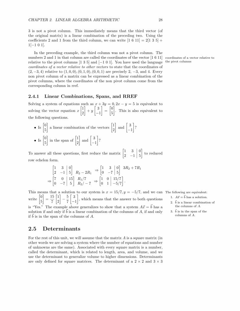
CHAPTER 2. LINEAR ALGEBRA ARITHMETIC 28
3 is not a pivot column. This immediately means that the third vector (ofthe original matrix) is a linear combination of the preceding two. Using thecoefficients 2 and 1 from the third column, we can write [1 6 11] = 2[1 3 5] +1[−1 0 1].
In the preceding example, the third column was not a pivot column. Thenumbers 2 and 1 in that column are called the coordinates of the vector [1 6 11] coordinates of a vector relative to
the pivot columnsrelative to the pivot columns [1 3 5] and [−1 0 1]. You have used the languagecoordinates of a vector relative to other vectors to state that the coordinates of(2,−3, 4) relative to (1, 0, 0), (0, 1, 0), (0, 0, 1) are precisely 2, −3, and 4. Everynon pivot column of a matrix can be expressed as a linear combination of thepivot columns, where the coordinates of the non pivot column come from thecorresponding column in rref.
2.4.1 Linear Combinations, Spans, and RREF
Solving a system of equations such as x + 3y = 0, 2x − y = 5 is equivalent to
solving the vector equation x
[12
]+ y
[3−1
]=
[05
]. This is also equivalent to
the following questions.
• Is
[05
]a linear combination of the vectors
[12
]and
[3−1
]?
• Is
[05
]in the span of
[12
]and
[3−1
]?
To answer all these questions, first reduce the matrix
[1 3 02 −1 5
]to reduced
row echelon form.[1 3 02 −1 5
]R2 − 2R1
⇒[1 3 00 −7 5
]3R2 + 7R1
⇒[7 0 150 −7 5
]R1/7R2/− 7
⇒[1 0 15/70 1 −5/7
].
This means that a solution to our system is x = 15/7, y = −5/7, and we can The following are equivalent:
1. A~x = ~b has a solution.
2. ~b is a linear combination ofthe columns of A.
3. ~b is in the span of thecolumns of A.
write
[05
]=
15
7
[12
]− 5
7
[3−1
], which means that the answer to both questions
is “Yes.” The example above generalizes to show that a system A~x = ~b has asolution if and only if ~b is a linear combination of the columns of A, if and onlyif ~b is in the span of the columns of A.
2.5 Determinants
For the rest of this unit, we will assume that the matrix A is a square matrix (inother words we are solving a system where the number of equations and numberof unknowns are the same). Associated with every square matrix is a number,called the determinant, which is related to length, area, and volume, and weuse the determinant to generalize volume to higher dimensions. Determinantsare only defined for square matrices. The determinant of a 2 × 2 and 3 × 3

CHAPTER 2. LINEAR ALGEBRA ARITHMETIC 29
matrix can be computed as follows:
det
[a bc d
]=
∣∣∣∣a bc d
∣∣∣∣ = ad− bc∣∣∣∣∣∣a b cd e fg h i
∣∣∣∣∣∣ = adet
∣∣∣∣e fh i
∣∣∣∣− bdet
∣∣∣∣d fg i
∣∣∣∣+ cdet
∣∣∣∣d eg h
∣∣∣∣= a(ei− hf)− b(di− gf) + c(dh− ge)
We use vertical bars next to a matrix to state we want the determinant. Noticethe negative sign on the middle term of the 3 × 3 determinant. Also, noticethat we had to compute three determinants of 2 by 2 matrices in order to findthe determinant of a 3 by 3.
The determinant in general is defined recursively in terms of minors (deter-minants of smaller matrices) and cofactors. This method is called the cofactorexpansion of the determinant. The minor Mij of a matrix A is the determinant The determinant is a linear
combination of the cofactors.of the the matrix formed by removing row i and column j from A. We definea cofactor to be Cij = (−1)i+jMij . To compute the determinant, first pick arow or column. We define the determinant to be
∑nk=1 aikCik (if we chose row
i) or alternatively∑nk=1 akjCkj (if we chose column j). You can pick any row
or column you want, and then compute the determinant by multiplying eachentry of that row or column by its cofactor, and then summing the results. A
+ − + · · ·− + − · · ·+ − + · · ·...
......
. . .
sign matrix
sign matrix keeps track of the (−1)j+k term in the cofactor. All you have to dois determine if the first entry of your expansion has a plus or minus, and thenalternate the sign as you expand. We will eventually prove why you can pickany row or column. For now, just become comfortable with the arithmetic.
Example 2.21. Let’s find the determinant of the matrix A =
1 2 0−1 3 42 −3 1
in two ways. First we will use a cofactor expansion along the top row (so thefirst term is positive).
detA = 1
∣∣∣∣ 3 4−3 1
∣∣∣∣− 2
∣∣∣∣−1 42 1
∣∣∣∣+ 0
∣∣∣∣−1 32 −3
∣∣∣∣= 1(3 + 12)− 2(−1− 8) + 0(3− 6) = 33
Now we’ll use the second column (so the first term is negative).
|A| = −2
∣∣∣∣−1 42 1
∣∣∣∣+ 3
∣∣∣∣1 02 1
∣∣∣∣− (−3)
∣∣∣∣ 1 0−1 4
∣∣∣∣= −(2)(−1− 8) + (3)(1− 0)− (−3)(4− 0) = 33
The number 33 is the volume of a 3 dimensional parallelepiped created fromthe columns of A, as described in the next section.
2.5.1 Geometric Interpretation of the determinant
Consider the 2 by 2 matrix
[3 10 2
]whose determinant is 3 · 2 − 0 · 1 = 6.
Draw the column vectors
[30
]and
[12
]with their base at the origin. These + −
Area = 6
∣∣∣∣3 10 2
∣∣∣∣ = 6 and
∣∣∣∣1 32 0
∣∣∣∣ = −6
The determinant gives area anddirection.
two vectors give the edges of a parallelogram whose area is the determinant 6.If I swap the order of the two vectors in the matrix, then the determinant of

CHAPTER 2. LINEAR ALGEBRA ARITHMETIC 30[1 32 0
]is −6. The reason for the difference is that the determinant not only
keeps track of area, but also order. Starting at the first vector, if you canturn counterclockwise through an angle smaller than 180◦ to obtain the secondvector, then the determinant is positive. If you have to turn clockwise instead,then the determinant is negative. This is often termed “the right-hand rule,” asrotating the fingers of your right hand from the first vector to the second vectorwill cause your thumb to point up precisely when the determinant is positive.
For a 3 by 3 matrix, the columns give the edges of a three dimensional
The determinant of a 3 by 3matrix gives the volume of theparallelepiped created by usingthe columns of the matrix as thethree parallel edges.
parallelepiped and the determinant produces the volume of this object. Thesign of the determinant is related to orientation. If you can use your right handand place your index finger on the first vector, middle finger on the secondvector, and thumb on the third vector, then the determinant is positive.
Example 2.22. Consider the matrix A =
100
020
003
. Starting from the origin,
each column represents an edge of the rectangular box 0 ≤ x ≤ 1, 0 ≤ y ≤ 2,0 ≤ z ≤ 3 with volume (and determinant) V = lwh = (1)(2)(3) = 6. The signof the determinant is positive because if you place your index finger pointing inthe direction (1,0,0) and your middle finger in the direction (0,2,0), then yourthumb points upwards in the direction (0,0,3). If you interchange two of the
columns, for example B =
020
100
003
, then the volume doesn’t change since
the shape is still the same. However, the sign of the determinant is negativebecause if you point your index finger in the direction (0,2,0) and your middlefinger in the direction (1,0,0), then your thumb points down in the direction(0,0,-3). If you repeat this with your left hand instead of right hand, then yourthumb points up.
2.5.2 Zero Determinants and Linear Dependence
Because the determinant helps us find area in 2D, we can use this idea to helpus understand when two vectors in 2D are linearly dependent. If two vectorsare dependent, then one is a linear combination of the other, hence a multipleof the other. This means that the parallelogram formed by the two vectorshas no area (as the two vectors lie on the same line). So if the vectors aredependent, the determinant is zero. Similarly, if the determinant is zero, thenthe vectors must lie on the same line and hence are linearly dependent. In 3D,three vectors being linearly dependent implies that one of the vectors lies in aplane or line spanned by the other two. Any object in 3D that lies in a planeor line has no volume so the determinant is zero. Similarly, if the determinantof a 3 by 3 matrix is zero, then the column vectors must lie in the same planeand hence are linearly dependent. We now have a geometric interpretation forthe key fact that For a square matrix A, the
following are equivalent:
1. The determinant is zero.
2. The columns are linearlydependent.
3. The rref of A is not I.
The determinant of a matrix is zero if and only if the columns arelinearly dependent.
The homeworks asks you to compute determinants of matrices as well as rowreduce them so that you can verify this fact in various settings. Notice that thecolumns of a square matrix are linearly independent if and only if the reducedrow echelon form of the matrix is the identity matrix. This shows us that thedeterminant of a square matrix is nonzero if and only if the reduced row echelonform of the matrix is the identity matrix.
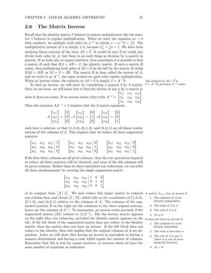
CHAPTER 2. LINEAR ALGEBRA ARITHMETIC 31
2.6 The Matrix Inverse
Recall that the identity matrix I behaves in matrix multiplication like the num-ber 1 behaves in regular multiplication. When we solve the equation ax = bwith numbers, we multiply both sides by a−1 to obtain x = a−1b = 1
ab. Themultiplicative inverse of a is simply 1/a, because a 1
a = 1aa = 1. We have been
studying linear systems of the form A~x = ~b. It would be nice if we could justdivide both sides by A, but there is no such thing as division by a matrix ingeneral. If we look only at square matrices, then sometimes it is possible to finda matrix B such that BA = AB = I, the identity matrix. If such a matrix Bexists, then multiplying both sides of A~x = ~b on the left by the matrix B yieldsBA~x = B ~B, or I~x = ~x = B~b. The matrix B is then called the inverse of A,and we write it as A−1, the same symbol we used with regular multiplication.When an inverse exists, the solution to A~x = ~b is simply ~x = A−1~b. The solution to A~x = ~b is
~x = A−1~b, provided A−1 exists.To find an inverse, we will start by considering a general 3 by 3 matrix.Once we are done, we will know how to find the inverse of any n by n matrix or
state it does not exists. If an inverse exists, then write A−1 =
c11 c12 c13
c21 c22 c23
c31 c32 c33
.
Then the equation AA−1 = I requires that the 3 matrix equations
A
c11
c21
c31
=
100
, Ac12
c22
c32
=
010
, Ac13
c23
c33
=
001
each have a solution, or that (1, 0, 0), (0, 1, 0), and (0, 0, 1) are all linear combi-nations of the columns of A. This requires that we reduce all three augmentedmatricesa11 a12 a13 1
a21 a22 a23 0a31 a32 a33 0
a11 a12 a13 0a21 a22 a23 1a31 a32 a33 0
a11 a12 a13 0a21 a22 a23 0a31 a32 a33 1
.If the first three columns are all pivot columns, then the row operations requiredto reduce all three matrices will be identical, and none of the 4th columns willbe pivot columns. Rather than do three equivalent row reductions, we can solveall three simultaneously by creating the single augmented matrixa11 a12 a13 1 0 0
a21 a22 a23 0 1 0a31 a32 a33 0 0 1
or in compact form
[A I
]. We now reduce this larger matrix to reduced A matrix An×n has an inverse if
1. The columns of A arelinearly independent.
2. The rank of A is n
3. The rref of A is I.
4. |A| 6= 0.
It does not have an inverse if
1. The columns of A arelinearly dependent.
2. The rank is less than n
3. The rref of A is not I(there is a row of zerosalong the bottom).
4. |A| = 0.
row echelon form and obtain[I B
], which tells us the coordinates of (1, 0, 0),
(0, 1, 0), and (0, 0, 1) relative to the columns of A. The columns of the aug-mented portion B on the right are the solutions to the three original systems,hence are the columns of A−1. To summarize, an inverse exists precisely if theaugmented system [A|I] reduces to [I|A−1]. The the inverse matrix appearson the right after row reduction, provided the identity matrix appears on theleft. If the left block of the augmented matrix does not reduce to the identitymatrix, then the matrix does not have an inverse. If the left block does notreduce to the identity, then this implies that the original columns of A are de-pendent. Later we will show that having an inverse is equivalent to having anonzero determinant and having a rank which equals the number of columns.Remember that this is true for square matrices, or systems where we have thesame number of equations as unknowns.

CHAPTER 2. LINEAR ALGEBRA ARITHMETIC 32
Example 2.23. To find the inverse of
[1 23 4
]we reduce
[1 2 1 03 4 0 1
]. Reduc-
tion gives
[1 0 −2 10 1 3/2 −1/2
]. The inverse is the right block
[−2 13/2 −1/2
]. Examples involving larger
matrices are in the homework.Remember that you can solvesystems by finding an inverse ofthe coefficient matrix.
You can always check your result by computing AA−1 to see if it is I, for ex-
ample
[1 23 4
] [−2 13/2 −1/2
]=
[1 00 1
]. Using this inverse, the solution to the
system
{1x+ 2y = 4
3x+ 4y = 0is A−1~b =
[−2 13/2 −1/2
] [40
]=
[−86
].
2.7 Eigenvalues and Eigenvectors
Let’s start by looking at an example to motivate the language we are about to
introduce. Consider the matrix A =
[2 11 2
]. When we multiply this matrix
by the vector ~x =
[11
], we obtain
[2 11 2
] [11
]=
[33
]= 3~x. Multiplication
by the matrix A was miraculously the same as multiplying by the number 3.Symbolically we have A~x = 3~x. Not every vector ~x satisfies this property, for
by ~x =
[10
]gives
[2 11 2
] [10
]=
[21
], which is not a multiple of ~x =
[10
]. Our
main goal in this section is to answer the following two questions:
1. For which nonzero vectors ~x (eigenvectors) is it possible to write A~x = λ~x?
2. Which scalars λ (eigenvalues) satisfy A~x = λ~x?
Now for some definitions. Let A be a square n×n matrix. An eigenvector is eigenvector
a nonzero vector ~x such that A~x = λ~x (matrix multiplication reduces to scalarmultiplication) for some scalar λ called an eigenvalue. We avoid letting ~x be the eigenvalue
zero vector because A~0 = λ~0 no matter what λ is. We can rewrite the equationA~x = λ~x as ~0 = A~x− λ~x = A~x− λI~x and then factor to obtain
(A− λI)~x = ~0.
In other words, we need to find a λ so that there are nonzero solutions to thehomogeneous system of equations, or equivalently we need to pick a λ so thatthe columns of A − λI are linearly dependent. With the correct λ, we knowthat A−λI has no inverse, and so it also means that det(A−λI) = 0. This lastequation is the key equation we will solve, since it does not contain the vector~x anymore. The expression det(A− λI) is called the characteristic polynomialof A. It is a polynomial of degree n, and hence there are at most n eigenvalues characteristic polynomial
(which correspond to the zeros of the polynomial). To find the eigenvalues andeigenvectors, we
1. solve det(A− λI) = 0 to obtain the eigenvalues, and then
2. for each eigenvalue, we solve (A− λI)~x = ~0 to obtain the eigenvectors.
As a way to check your work, the following two facts can help.
• The sum of the eigenvalues equals the trace of the matrix (the sum of the The trace and determinant areequal to the sum and product ofthe eigenvalues.
diagonal elements).
• The product of the eigenvalues equals the determinant.

CHAPTER 2. LINEAR ALGEBRA ARITHMETIC 33
Example 2.24. To find the eigenvalues of
[2 11 2
], first subtract λ from each
diagonal entry
[2− λ 1
1 2− λ
], and then find the determinant. Factor to get
(2−λ)(2−λ)− 1 = λ2− 4λ+ 3 = (λ− 1)(λ− 3). The zeros are 1 and 3, so theeigenvalues are λ = 1, 3. As a check, the trace of this matrix is 2 + 2 = 4 andthe sum of the eigenvalues is 1 + 3. In addition, the determinant is 4 − 1 = 3which equals the product of the eigenvalues.
When λ = 1, we compute A − λI =
[1 11 1
]. We solve the equation (A −
λI)~x = 0 by reducing the augmented matrix
[1 1 01 1 0
]to its rref
[1 1 00 0 0
]. Since we are solving a
homogeneous system A~x = ~0, wecould avoid writing the lastcolumn of zeros.
Since x2 is a free variable, we solve x1 + x2 = 0 for x1 to obtain the equations
x1 = −x2, x2 = x2, and then write our solution in vector form
[x1
x2
]= x2
[−11
]for some x2 6= 0 . There are infinitely many eigenvectors corresponding to λ = 1.
A particular eigenvector is
[−11
]and all the rest are a linear combination of
this one.
When λ = 3, we compute A − λI =
[−1 11 −1
]. Reducing
[−1 1 01 −1 0
]gives
[1 −1 00 0 0
], which means the eigenvectors are of the form x2
[11
]for some
x2 6= 0. A particular eigenvector corresponding to λ = 3 is
[11
], and all others
are a linear combination of this one.
Finding eigenvalues and eigenvectors requires that we compute determi-nants, find zeros of polynomials, and then solve homogeneous systems of equa-tions. You know you are doing the problem correctly if you get infinitely manysolutions to the system (A − λI)~x = 0 for each lambda (i.e. there is at leastone row of zeros along the bottom).
Eigenvalues and eigenvectors show up in many different places in engineer-ing, computer science, physics, chemistry, and mathematics. We will be ex-ploring how eigenvectors appear throughout linear algebra as the semester pro-gresses. For now we’ll just focus on being able to find them.
Example 2.25. Let’s find the eigenvalues and eigenvectors of the matrix A =2 1 41 2 40 0 1
. Subtracting λ from the diagonals gives
2− λ 1 41 2− λ 40 0 1− λ
.
The determinant of this matrix is easiest to compute if you expand along the
third row to get 0−0+(1−λ)
∣∣∣∣2− λ 11 2− λ
∣∣∣∣. Computing the 2 by 2 determinant
gives (1− λ)[(2− λ)(2− λ)− 1] = (1− λ)(λ− 1)(λ− 3), so the eigenvalues are1, 1, 3 (1 is a repeated root). As a check, their sum is 1 + 1 + 3 = 5 and thetrace of A is 2 + 2 + 1 = 5 as well. For larger matrices, determinants are notalways easy to check, so just checking the trace is a fast way to make sure youare on the right path.
When λ = 1, we compute A − λI =
1 1 41 1 40 0 0
. Reducing the system
(A−λI)~x = 0 yields
1 1 4 00 0 0 00 0 0 0
, which has two free variables. The solution
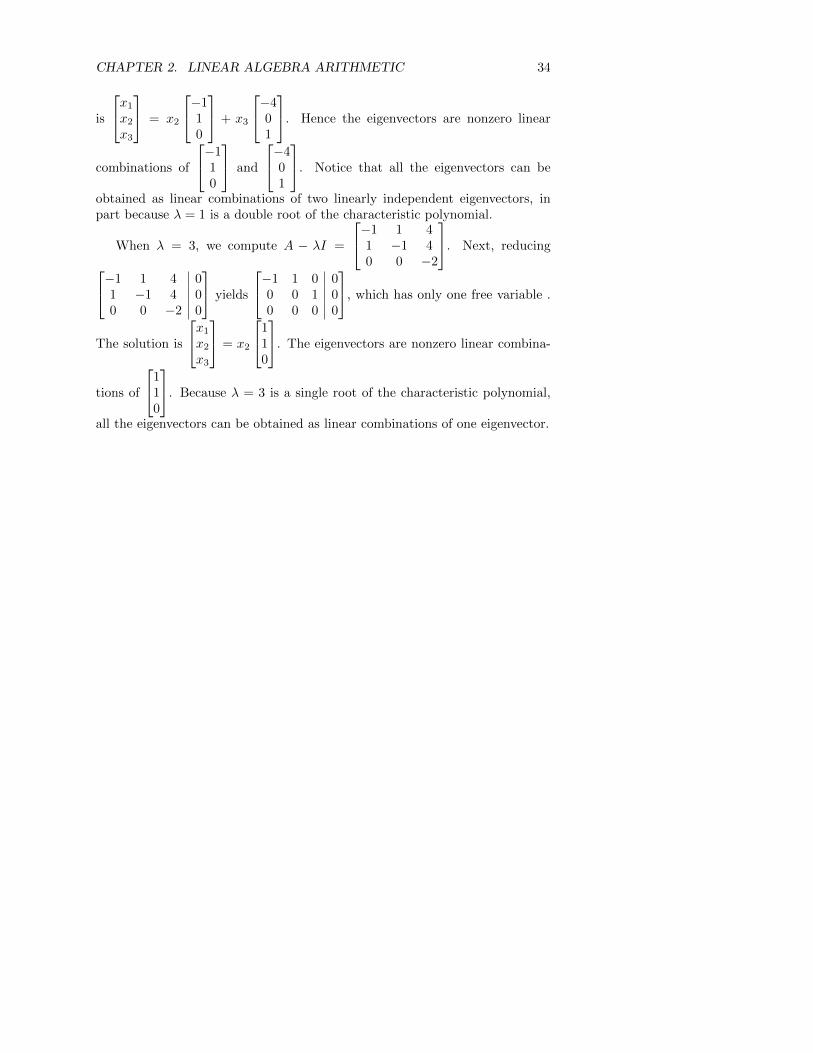
CHAPTER 2. LINEAR ALGEBRA ARITHMETIC 34
is
x1
x2
x3
= x2
−110
+ x3
−401
. Hence the eigenvectors are nonzero linear
combinations of
−110
and
−401
. Notice that all the eigenvectors can be
obtained as linear combinations of two linearly independent eigenvectors, inpart because λ = 1 is a double root of the characteristic polynomial.
When λ = 3, we compute A − λI =
−1 1 41 −1 40 0 −2
. Next, reducing−1 1 4 01 −1 4 00 0 −2 0
yields
−1 1 0 00 0 1 00 0 0 0
, which has only one free variable .
The solution is
x1
x2
x3
= x2
110
. The eigenvectors are nonzero linear combina-
tions of
110
. Because λ = 3 is a single root of the characteristic polynomial,
all the eigenvectors can be obtained as linear combinations of one eigenvector.
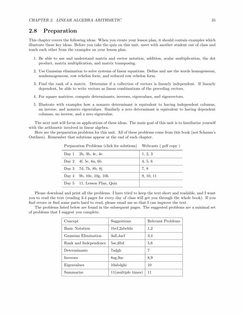
CHAPTER 2. LINEAR ALGEBRA ARITHMETIC 35
2.8 Preparation
This chapter covers the following ideas. When you create your lesson plan, it should contain examples whichillustrate these key ideas. Before you take the quiz on this unit, meet with another student out of class andteach each other from the examples on your lesson plan.
1. Be able to use and understand matrix and vector notation, addition, scalar multiplication, the dotproduct, matrix multiplication, and matrix transposing.
2. Use Gaussian elimination to solve systems of linear equations. Define and use the words homogeneous,nonhomogeneous, row echelon form, and reduced row echelon form.
3. Find the rank of a matrix. Determine if a collection of vectors is linearly independent. If linearlydependent, be able to write vectors as linear combinations of the preceding vectors.
4. For square matrices, compute determinants, inverses, eigenvalues, and eigenvectors.
5. Illustrate with examples how a nonzero determinant is equivalent to having independent columns,an inverse, and nonzero eigenvalues. Similarly a zero determinant is equivalent to having dependentcolumns, no inverse, and a zero eigenvalue.
The next unit will focus on applications of these ideas. The main goal of this unit is to familiarize yourselfwith the arithmetic involved in linear algebra.
Here are the preparation problems for this unit. All of these problems come from this book (not Schaum’sOutlines). Remember that solutions appear at the end of each chapter.
Preparation Problems (click for solutions) Webcasts ( pdf copy )
Day 1 2h, 3b, 4c, 4e 1, 2, 3
Day 2 4f, 5c, 6a, 6b 4, 5, 6
Day 3 7d, 7h, 8b, 8j 7, 8
Day 4 9b, 10e, 10g, 10h 9, 10, 11
Day 5 11, Lesson Plan, Quiz
Please download and print all the problems. I have tried to keep the text short and readable, and I wantyou to read the text (reading 3-4 pages for every day of class will get you through the whole book). If youfind errors or find some parts hard to read, please email me so that I can improve the text.
The problems listed below are found in the subsequent pages. The suggested problems are a minimal setof problems that I suggest you complete.
Concept Suggestions Relevant Problems
Basic Notation 1bcf,2abehln 1,2
Gaussian Elimination 3all,4acf 3,4
Rank and Independence 5ac,6bd 5,6
Determinants 7adgh 7
Inverses 8ag,9ac 8,9
Eigenvalues 10abdghi 10
Summarize 11(multiple times) 11
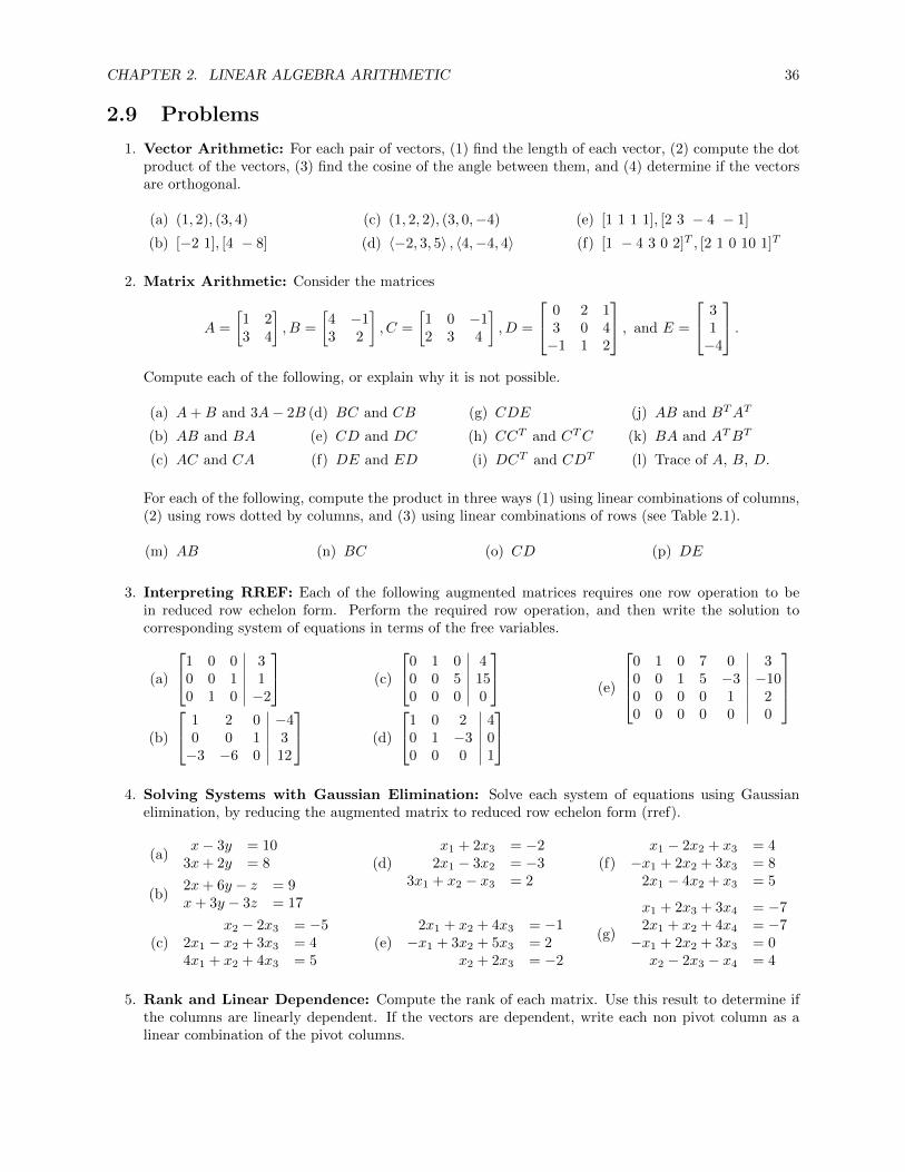
CHAPTER 2. LINEAR ALGEBRA ARITHMETIC 36
2.9 Problems
1. Vector Arithmetic: For each pair of vectors, (1) find the length of each vector, (2) compute the dotproduct of the vectors, (3) find the cosine of the angle between them, and (4) determine if the vectorsare orthogonal.
(a) (1, 2), (3, 4)
(b) [−2 1], [4 − 8]
(c) (1, 2, 2), (3, 0,−4)
(d) 〈−2, 3, 5〉 , 〈4,−4, 4〉(e) [1 1 1 1], [2 3 − 4 − 1]
(f) [1 − 4 3 0 2]T , [2 1 0 10 1]T
2. Matrix Arithmetic: Consider the matrices
A =
[1 23 4
], B =
[4 −13 2
], C =
[1 0 −12 3 4
], D =
0 2 13 0 4−1 1 2
, and E =
31−4
.Compute each of the following, or explain why it is not possible.
(a) A+B and 3A− 2B
(b) AB and BA
(c) AC and CA
(d) BC and CB
(e) CD and DC
(f) DE and ED
(g) CDE
(h) CCT and CTC
(i) DCT and CDT
(j) AB and BTAT
(k) BA and ATBT
(l) Trace of A, B, D.
For each of the following, compute the product in three ways (1) using linear combinations of columns,(2) using rows dotted by columns, and (3) using linear combinations of rows (see Table 2.1).
(m) AB (n) BC (o) CD (p) DE
3. Interpreting RREF: Each of the following augmented matrices requires one row operation to bein reduced row echelon form. Perform the required row operation, and then write the solution tocorresponding system of equations in terms of the free variables.
(a)
1 0 0 30 0 1 10 1 0 −2
(b)
1 2 0 −40 0 1 3−3 −6 0 12
(c)
0 1 0 40 0 5 150 0 0 0
(d)
1 0 2 40 1 −3 00 0 0 1
(e)
0 1 0 7 0 30 0 1 5 −3 −100 0 0 0 1 20 0 0 0 0 0
4. Solving Systems with Gaussian Elimination: Solve each system of equations using Gaussianelimination, by reducing the augmented matrix to reduced row echelon form (rref).
(a)x− 3y = 10
3x+ 2y = 8
(b)2x+ 6y − z = 9x+ 3y − 3z = 17
(c)x2 − 2x3 = −5
2x1 − x2 + 3x3 = 44x1 + x2 + 4x3 = 5
(d)x1 + 2x3 = −2
2x1 − 3x2 = −33x1 + x2 − x3 = 2
(e)2x1 + x2 + 4x3 = −1−x1 + 3x2 + 5x3 = 2
x2 + 2x3 = −2
(f)x1 − 2x2 + x3 = 4
−x1 + 2x2 + 3x3 = 82x1 − 4x2 + x3 = 5
(g)
x1 + 2x3 + 3x4 = −72x1 + x2 + 4x4 = −7−x1 + 2x2 + 3x3 = 0x2 − 2x3 − x4 = 4
5. Rank and Linear Dependence: Compute the rank of each matrix. Use this result to determine ifthe columns are linearly dependent. If the vectors are dependent, write each non pivot column as alinear combination of the pivot columns.

CHAPTER 2. LINEAR ALGEBRA ARITHMETIC 37
(a)
1 2 34 −2 13 0 4
(b)
1 −1 −1−2 3 53 1 9
(c)
1 3 −1 9−1 −2 0 −52 1 3 −2
(d)
1 3 12 12 0 −6 3−1 1 8 −40 2 10 2
6. Linear Independence: In each problem, determine if the vectors given are linearly independent. If
the vectors are linearly dependent, write one of the vectors as a linear combination of the others.
(a) [2,−1, 0], [1, 0, 3], [3, 2, 4]
(b) [1, 2,−3, 4], [3,−2,−1,−2], [5,−2,−3,−1]
(c) [0, 1, 1, 1], [1, 0, 1, 1], [1, 1, 0, 1], [1, 1, 1, 0]
(d) [1, 0,−1,−2], [1, 2, 3, 0], [0, 1,−1, 2], [2, 0, 1,−5]
7. Determinants: Find the determinant of each matrix. For 3 by 3 matrices, compute the determinantin 2 different ways by using a cofactor expansion along a different row or column.
(a)
[1 23 4
]
(b)
[4 35 9
]
(c)
2 1 00 2 11 0 2
(d)
3 1 −21 −1 42 2 1
(e)
2 3 −11 0 04 2 5
(f)
5 1 −32 −1 21 4 −1
(g)
2 1 −6 80 3 5 40 0 1 50 0 0 −4
(h)
3 2 5 −10 8 4 20 −1 0 00 −5 3 −1
(i)
1 1 1 12 −1 1 1−1 1 2 −21 1 −1 −1
(j)
1 1 1 12 2 2 20 2 1 −11 0 −2 1
For the following matrices, compute the determinant and use your answer to determine if the columnsare linearly independent.
(k) Use the matrix from 5a (l) Use the matrix from 5b (m) Use the matrix from 5d
8. Inverse: Find the inverse of each matrix below.
(a)
[1 23 4
](b)
[−2 43 −5
](c)
[0 1−1 0
](d)
[2 34 5
]
(e)
[7 32 1
]
(f)
1 0 20 1 00 0 4
(g)
1 0 20 1 0−1 1 4
(h)
3 0 30 −1 10 3 −4
(i)
1 2 −12 3 −20 3 2
(j)
−2 0 5−1 0 34 1 −1
(k)
2 1 11 2 11 1 2
(l)
[a bc d
]9. Solve systems using an inverse: Solve each system by using an inverse from above.
(a)
{x1 + 2x2 = 3
3x1 + 4x2 = 4using 8a.
(b)
{−2x1 + 4x2 = 4
3x1 − 5x2 = −2using 8b.
(c)
1x1 + 2x3 = 2x2 = 3
−x1 + x2 + 4x3 = 1using 8g.
(d)
−2x1 + 5x3 = −2−x1 + 3x3 = 1
4x1 + x2 − x3 = 3using 8j.
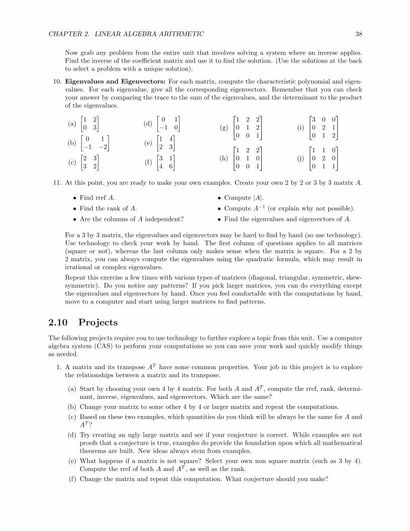
CHAPTER 2. LINEAR ALGEBRA ARITHMETIC 38
Now grab any problem from the entire unit that involves solving a system where an inverse applies.Find the inverse of the coefficient matrix and use it to find the solution. (Use the solutions at the backto select a problem with a unique solution).
10. Eigenvalues and Eigenvectors: For each matrix, compute the characteristic polynomial and eigen-values. For each eigenvalue, give all the corresponding eigenvectors. Remember that you can checkyour answer by comparing the trace to the sum of the eigenvalues, and the determinant to the productof the eigenvalues.
(a)
[1 20 3
](b)
[0 1−1 −2
](c)
[2 33 2
](d)
[0 1−1 0
](e)
[1 42 3
](f)
[3 14 6
](g)
1 2 20 1 20 0 1
(h)
1 2 20 1 00 0 1
(i)
3 0 00 2 10 1 2
(j)
1 1 00 2 00 1 1
11. At this point, you are ready to make your own examples. Create your own 2 by 2 or 3 by 3 matrix A.
• Find rref A.
• Find the rank of A.
• Are the columns of A independent?
• Compute |A|.• Compute A−1 (or explain why not possible).
• Find the eigenvalues and eigenvectors of A.
For a 3 by 3 matrix, the eigenvalues and eigenvectors may be hard to find by hand (so use technology).Use technology to check your work by hand. The first column of questions applies to all matrices(square or not), whereas the last column only makes sense when the matrix is square. For a 2 by2 matrix, you can always compute the eigenvalues using the quadratic formula, which may result inirrational or complex eigenvalues.
Repeat this exercise a few times with various types of matrices (diagonal, triangular, symmetric, skew-symmetric). Do you notice any patterns? If you pick larger matrices, you can do everything exceptthe eigenvalues and eigenvectors by hand. Once you feel comfortable with the computations by hand,move to a computer and start using larger matrices to find patterns.
2.10 Projects
The following projects require you to use technology to further explore a topic from this unit. Use a computeralgebra system (CAS) to perform your computations so you can save your work and quickly modify thingsas needed.
1. A matrix and its transpose AT have some common properties. Your job in this project is to explorethe relationships between a matrix and its transpose.
(a) Start by choosing your own 4 by 4 matrix. For both A and AT , compute the rref, rank, determi-nant, inverse, eigenvalues, and eigenvectors. Which are the same?
(b) Change your matrix to some other 4 by 4 or larger matrix and repeat the computations.
(c) Based on these two examples, which quantities do you think will be always be the same for A andAT ?
(d) Try creating an ugly large matrix and see if your conjecture is correct. While examples are notproofs that a conjecture is true, examples do provide the foundation upon which all mathematicaltheorems are built. New ideas always stem from examples.
(e) What happens if a matrix is not square? Select your own non square matrix (such as 3 by 4).Compute the rref of both A and AT , as well as the rank.
(f) Change the matrix and repeat this computation. What conjecture should you make?
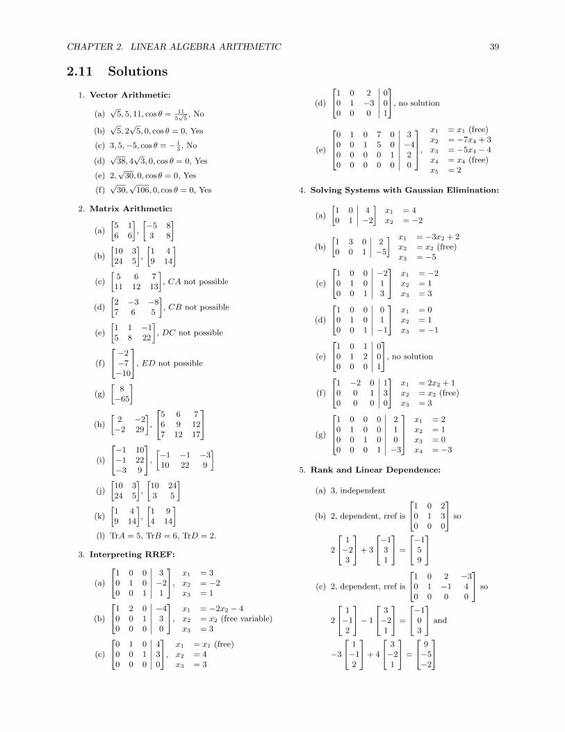
CHAPTER 2. LINEAR ALGEBRA ARITHMETIC 39
2.11 Solutions
1. Vector Arithmetic:
(a)√
5, 5, 11, cos θ = 11
5√
5, No
(b)√
5, 2√
5, 0, cos θ = 0, Yes
(c) 3, 5,−5, cos θ = − 13, No
(d)√
38, 4√
3, 0, cos θ = 0, Yes
(e) 2,√
30, 0, cos θ = 0, Yes
(f)√
30,√
106, 0, cos θ = 0, Yes
2. Matrix Arithmetic:
(a)
[5 16 6
],
[−5 83 8
](b)
[10 324 5
],
[1 49 14
](c)
[5 6 711 12 13
], CA not possible
(d)
[2 −3 −87 6 5
], CB not possible
(e)
[1 1 −15 8 22
], DC not possible
(f)
−2−7−10
, ED not possible
(g)
[8−65
]
(h)
[2 −2−2 29
],
5 6 76 9 127 12 17
(i)
−1 10−1 22−3 9
,
[−1 −1 −310 22 9
]
(j)
[10 324 5
],
[10 243 5
](k)
[1 49 14
],
[1 94 14
](l) TrA = 5, TrB = 6, TrD = 2.
3. Interpreting RREF:
(a)
1 0 0 30 1 0 −20 0 1 1
,x1 = 3x2 = −2x3 = 1
(b)
1 2 0 −40 0 1 30 0 0 0
,x1 = −2x2 − 4x2 = x2 (free variable)x3 = 3
(c)
0 1 0 40 0 1 30 0 0 0
,x1 = x1 (free)x2 = 4x3 = 3
(d)
1 0 2 00 1 −3 00 0 0 1
, no solution
(e)
0 1 0 7 0 30 0 1 5 0 −40 0 0 0 1 20 0 0 0 0 0
,
x1 = x1 (free)x2 = −7x4 + 3x3 = −5x4 − 4x4 = x4 (free)x5 = 2
4. Solving Systems with Gaussian Elimination:
(a)
[1 0 40 1 −2
]x1 = 4x2 = −2
(b)
[1 3 0 20 0 1 −5
] x1 = −3x2 + 2x2 = x2 (free)x3 = −5
(c)
1 0 0 −20 1 0 10 0 1 3
x1 = −2x2 = 1x3 = 3
(d)
1 0 0 00 1 0 10 0 1 −1
x1 = 0x2 = 1x3 = −1
(e)
1 0 1 00 1 2 00 0 0 1
, no solution
(f)
1 −2 0 10 0 1 30 0 0 0
x1 = 2x2 + 1x2 = x2 (free)x3 = 3
(g)
1 0 0 0 20 1 0 0 10 0 1 0 00 0 0 1 −3
x1 = 2x2 = 1x3 = 0x4 = −3
5. Rank and Linear Dependence:
(a) 3, independent
(b) 2, dependent, rref is
1 0 20 1 30 0 0
so
2
1−23
+ 3
−131
=
−159
(c) 2, dependent, rref is
1 0 2 −30 1 −1 40 0 0 0
so
2
1−12
− 1
3−21
=
−103
and
−3
1−12
+ 4
3−21
=
9−5−2

CHAPTER 2. LINEAR ALGEBRA ARITHMETIC 40
(d) 3, dependent, rref is
1 0 −3 00 1 5 00 0 0 10 0 0 0
so
−3
12−10
+ 5
3012
+ 0
13−42
=
12−6810
6. Linear Independence:
(a)
2 1 3−1 0 20 3 4
rref−−→
1 0 00 1 00 0 1
, independent
(b)
1 3 52 −2 −2−3 −1 −34 −2 −1
→
1 0 12
0 1 32
0 0 00 0 0
, dependent
1
2
12−34
+3
2
3−2−1−2
=
5−2−3−1
(c) Independent. Placing the vectors in columns
of a 4 by 4 matrix reduces to the identity, sothere are 4 pivot columns.
(d)
1 1 0 20 2 1 0−1 3 −1 1−2 0 2 −5
→
1 0 0 32
0 1 0 12
0 0 1 −10 0 0 0
,
dependent
3
2
10−1−2
+1
2
1230
−
01−12
=
201−5
7. Determinants:
(a) −2
(b) 21
(c) 9
(d) −28
(e) −17
(f) −58
(g) −24
(h) −30
(i) 24
(j) 0
8. Inverse:
(a)
[−2 132− 1
2
](b)
[52
232
1
](c)
[0 −11 0
](d)
[− 5
232
2 −1
](e)
[1 −3−2 7
]
(f)
1 0 − 12
0 1 0
0 0 14
(g)
23
13− 1
3
0 1 016− 1
616
(h)
13
3 1
0 −4 −10 −3 −1
(i)
−6 72
12
2 −1 0
−3 32
12
(j)
−3 5 011 −18 1−1 2 0
(k)
34− 1
4− 1
4
− 14
34− 1
4
− 14− 1
434
(l)
1
ad− bc
[d −b−c a
]9. Solve systems using an inverse:
(a)
[−2 132− 1
2
] [34
]=
[−252
](b)
[52
232
1
] [4−2
]=
[64
]
(c)
23
13− 1
3
0 1 016− 1
616
231
=
230
(d)
−3 5 011 −18 1−1 2 0
−213
=
11−37
4
10. Eigenvalues and Eigenvectors:
(a) λ2 − 4λ+ 3, for λ = 3 eigenvectors are
[11
]x2
where x2 6= 0, for λ = 1 eigenvectors are[10
]x1 where x1 6= 0.
(b) λ2 + 2λ + 1, for λ = −1 eigenvectors are[−11
]x2 where x2 6= 0
(c) λ2 − 4λ − 5, for λ = −1 eigenvectors are[−11
]x2 where x2 6= 0, for λ = 5 eigenvec-
tors are
[11
]x2 where x2 6= 0
(d) λ2 + 1, for λ = i eigenvectors are
[−i1
]x2
where x2 6= 0, for λ = −i eigenvectors are[i1
]x2 where x2 6= 0
(e) λ2 − 4λ− 5, for λ = 5 eigenvectors are
[11
]x2
where x2 6= 0, for λ = −1 eigenvectors are[−21
]x2 where x2 6= 0
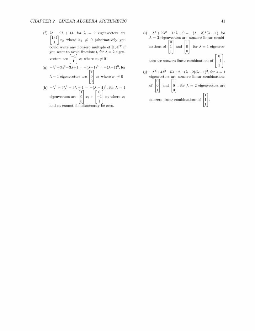
CHAPTER 2. LINEAR ALGEBRA ARITHMETIC 41
(f) λ2 − 9λ + 14, for λ = 7 eigenvectors are[1/41
]x2 where x2 6= 0 (alternatively you
could write any nonzero multiple of [1, 4]T ifyou want to avoid fractions), for λ = 2 eigen-
vectors are
[−11
]x2 where x2 6= 0
(g) −λ3+3λ2−3λ+1 = −(λ−1)3 = −(λ−1)3, for
λ = 1 eigenvectors are
100
x1 where x1 6= 0
(h) −λ3 + 3λ2 − 3λ + 1 = −(λ − 1)3, for λ = 1
eigenvectors are
100
x1 +
0−11
x3 where x1
and x3 cannot simultaneously be zero.
(i) −λ3 + 7λ2 − 15λ+ 9 = −(λ− 3)2(λ− 1), forλ = 3 eigenvectors are nonzero linear combi-
nations of
011
and
100
, for λ = 1 eigenvec-
tors are nonzero linear combinations of
0−11
.
(j) −λ3 +4λ2−5λ+2− (λ−2)(λ−1)2, for λ = 1eigenvectors are nonzero linear combinations
of
001
and
100
, for λ = 2 eigenvectors are
nonzero linear combinations of
111
.

Chapter 3
Linear AlgebraApplications
This chapter covers the following ideas.
1. Find the currents in electrical systems involving batteries and resistors,using both Gaussian elimination and Cramer’s rule.
2. Find interpolating polynomials. Use the transpose and inverse of a matrixto solve the least squares regression problem of fitting a line to a set ofdata.
3. Find the partial fraction decomposition of a rational function. Utilize thisdecomposition to integrate rational functions.
4. Describe a Markov process. Explain how an eigenvector of the eigenvalueλ = 1 is related to the limit of powers of the transition matrix.
5. Explain how to generalize the derivative to a matrix. Use this generaliza-tion to locate optimal values of the function using the second derivativetest. Explain the role of eigenvalues and eigenvectors in the second deriva-tive test.
3.1 Kirchoff’s Electrial Laws
Gustav Kirchoff discovered two laws of electricity that pertain to the conserva-tion of charge and energy. To describe these laws, we must first discuss voltage,resistance, and current. Current is the flow of electricity, and often it can becompared to the flow of water. As a current passes across a conductor, it en-counters resistance. Ohm’s law states that the product of the resistance R andcurrent I across a conductor equals the voltage V , i.e. RI = V . If the voltageremains constant, then a large resistance corresponds to a small current. Aresistor is an object with high resistance which is placed in an electrical systemto slow down the flow (current) of electricity. Resistors are measured in termsof ohms, and the larger the ohms, the smaller the current. Figure 3.1 illustratestwo introductory electrical systems.
In this diagram, wires meet at nodes (illustrated with a dot). Batteries andvoltage sources (represented by or other symbols) supply a voltage of Evolts. At each node the current may change, so the arrows and letters i representthe different currents in the electrical system. The electrical current on eachwire may or may not follow the arrows drawn (a negative current means that
42

CHAPTER 3. LINEAR ALGEBRA APPLICATIONS 43
E R2
R1
R3
i1
i2
i3
E R2
R1
R3
R4 R5
R6
i1
i2
i3
i4
i5
i6
Two Loop System Three Loop System
Figure 3.1: Electrical Circuit Diagrams.
the current flows opposite the arrow). Resistors are depicted with the symbol, and the letter R represents the ohms.
Kirchoff discovered two laws. They both help us find current in a system,provided we know the voltage of any batteries, and the resistance of any resis-tors.
1. Kirchoff’s current law states that at every node, the current flowing inequals the current flowing out (at nodes, current in = current out).
2. Kirchoff’s voltage law states that on any loop in the system, the directedsum of voltages supplied equals the directed sum of voltage drops (inloops, voltage in = voltage out).
Let’s use Kirchoff’s laws to generate a system of equations for the two loopsystem.
1. First we will examine Kirchoff’s current law. At the first node (top mid-dle), current i1 flows in while i2 and i3 flow out. Kirchoff’s current lawstates that i1 = i2 + i3 or i1 − i2 − i3 = 0. At the second node, both i2and i3 are flowing in while i1 flows out. This means that i2 + i3 = i1 or−i1 + i2 + i3 = 0. This second equation is the same as multiplying bothsides of the first by −1 (so we say the 2nd equation depends on the first).
2. We now look at Kirchoff’s voltage law. Pick a loop and work your wayaround the loop in a clockwise fashion. Each time you encounter a batteryor resistor, include a term for the voltage supplied E on the left side of anequation, and the voltage drop (resistance times current Ri) on the right.If you encounter a battery or resistor as you work against the current,then times that term by −1. The left loop has a battery with voltage Eand the resistor contributes a drop in voltage of R1i2 volts. An equationfor the first loop is E = R1i1 + R2i2. On the right loop we encounteralong current i3 a resistor with resistance R3 ohms. While working ourway against the arrow drawn on i2, we encounter an R2 ohm resistor.There are no batteries on the second loop. The two resistors give us theequation 0 = −R2i2 +R3i3.
We can now write a system of equations involving the unknowns i1, i2, i3, putit in matrix form, and then solve
i1 − i2 − i3 = 0−i1 + i2 + i3 = 0R1i1 +R2i2 = E−R2i2 +R3i3 = 0
matrix form−−−−−−−→
1 −1 −1 0−1 1 1 0R1 R2 0 120 −R2 R3 0
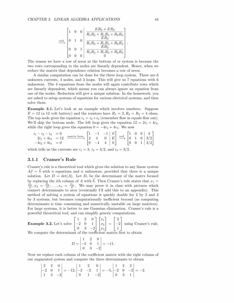
CHAPTER 3. LINEAR ALGEBRA APPLICATIONS 44
rref−−→
1 0 0ER2 + ER3
R1R2 +R1R3 +R2R3
0 1 0ER3
R1R2 +R1R3 +R2R3
0 0 1ER2
R1R2 +R1R3 +R2R3
0 0 0 0
.
The reason we have a row of zeros at the bottom of or system is because thetwo rows corresponding to the nodes are linearly dependent. Hence, when wereduce the matrix that dependence relation becomes a row of zeros.
A similar computation can be done for the three loop system. There are 6unknown currents, 4 nodes, and 3 loops. This will give us 7 equations with 6unknowns. The 4 equations from the nodes will again contribute rows whichare linearly dependent, which means you can always ignore an equation fromone of the nodes. Reduction will give a unique solution. In the homework, youare asked to setup systems of equations for various electrical systems, and thensolve them.
Example 3.1. Let’s look at an example which involves numbers. SupposeE = 12 (a 12 volt battery) and the resistors have R1 = 2, R2 = R3 = 4 ohms.The top node gives the equation i1 = i2 +i3 (remember flow in equals flow out).We’ll skip the bottom node. The left loop gives the equation 12 = 2i1 + 4i2,while the right loop gives the equation 0 = −4r2 + 4r3. We now
i1 − i2 − i3 = 02i1 + 4i2 = 12−4i2 + 4i3 = 0
matrix form−−−−−−−→
1 −1 −1 02 4 0 E0 −4 4 0
rref−−→
1 0 0 30 1 0 3/20 0 1 3/2
which tells us the currents are i1 = 3, i2 = 3/2, and i3 = 3/2.
3.1.1 Cramer’s Rule
Cramer’s rule is a theoretical tool which gives the solution to any linear systemA~x = ~b with n equations and n unknowns, provided that there is a uniquesolution. Let D = det(A). Let Di be the determinant of the matrx formed
by replacing the ith column of A with ~b. Then Cramer’s rule states that x1 =D1
D , x2 = D2
D , . . . , xn = Dn
D . We may prove it in class with pictures whichconnect determinants to area (eventually I’ll add this to an appendix). Thismethod of solving a system of equations is quickly doable for 2 by 2 and 3by 3 systems, but becomes computationally inefficient beyond (as computingdeterminants is time consuming and numerically unstable on large matrices).For large systems, it is better to use Gaussian elimination. Cramer’s rule is apowerful theoretical tool, and can simplify generic computations.
Example 3.2. Let’s solve
1 2 0−2 0 10 3 −2
x1
x2
x3
=
2−21
using Cramer’s rule.
We compute the determinant of the coefficient matrix first to obtain
D =
∣∣∣∣∣∣1 2 0−2 0 10 3 −2
∣∣∣∣∣∣ = −11.
Next we replace each column of the coefficient matrix with the right column ofour augmented system and compute the three determinants to obtain∣∣∣∣∣∣
2 2 0−2 0 11 3 −2
∣∣∣∣∣∣ = −12,
∣∣∣∣∣∣1 2 0−2 −2 10 1 −2
∣∣∣∣∣∣ = −5,
∣∣∣∣∣∣1 2 2−2 0 −20 3 1
∣∣∣∣∣∣ = −2.
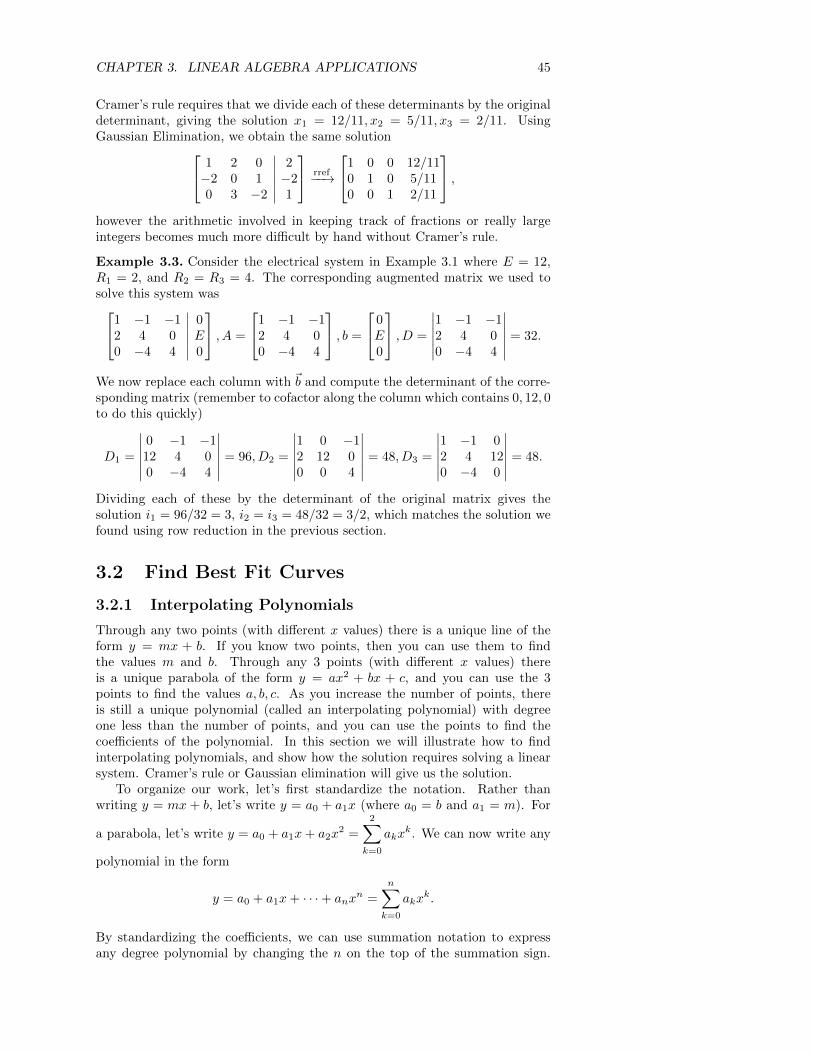
CHAPTER 3. LINEAR ALGEBRA APPLICATIONS 45
Cramer’s rule requires that we divide each of these determinants by the originaldeterminant, giving the solution x1 = 12/11, x2 = 5/11, x3 = 2/11. UsingGaussian Elimination, we obtain the same solution 1 2 0 2
−2 0 1 −20 3 −2 1
rref−−→
1 0 0 12/110 1 0 5/110 0 1 2/11
,however the arithmetic involved in keeping track of fractions or really largeintegers becomes much more difficult by hand without Cramer’s rule.
Example 3.3. Consider the electrical system in Example 3.1 where E = 12,R1 = 2, and R2 = R3 = 4. The corresponding augmented matrix we used tosolve this system was1 −1 −1 0
2 4 0 E0 −4 4 0
, A =
1 −1 −12 4 00 −4 4
, b =
0E0
, D =
∣∣∣∣∣∣1 −1 −12 4 00 −4 4
∣∣∣∣∣∣ = 32.
We now replace each column with ~b and compute the determinant of the corre-sponding matrix (remember to cofactor along the column which contains 0, 12, 0to do this quickly)
D1 =
∣∣∣∣∣∣0 −1 −112 4 00 −4 4
∣∣∣∣∣∣ = 96, D2 =
∣∣∣∣∣∣1 0 −12 12 00 0 4
∣∣∣∣∣∣ = 48, D3 =
∣∣∣∣∣∣1 −1 02 4 120 −4 0
∣∣∣∣∣∣ = 48.
Dividing each of these by the determinant of the original matrix gives thesolution i1 = 96/32 = 3, i2 = i3 = 48/32 = 3/2, which matches the solution wefound using row reduction in the previous section.
3.2 Find Best Fit Curves
3.2.1 Interpolating Polynomials
Through any two points (with different x values) there is a unique line of theform y = mx + b. If you know two points, then you can use them to findthe values m and b. Through any 3 points (with different x values) thereis a unique parabola of the form y = ax2 + bx + c, and you can use the 3points to find the values a, b, c. As you increase the number of points, thereis still a unique polynomial (called an interpolating polynomial) with degreeone less than the number of points, and you can use the points to find thecoefficients of the polynomial. In this section we will illustrate how to findinterpolating polynomials, and show how the solution requires solving a linearsystem. Cramer’s rule or Gaussian elimination will give us the solution.
To organize our work, let’s first standardize the notation. Rather thanwriting y = mx + b, let’s write y = a0 + a1x (where a0 = b and a1 = m). For
a parabola, let’s write y = a0 + a1x+ a2x2 =
2∑k=0
akxk. We can now write any
polynomial in the form
y = a0 + a1x+ · · ·+ anxn =
n∑k=0
akxk.
By standardizing the coefficients, we can use summation notation to expressany degree polynomial by changing the n on the top of the summation sign.

CHAPTER 3. LINEAR ALGEBRA APPLICATIONS 46
Now that our notation is organized, let’s use it to find a polynomial through 3points.
Example 3.4. Let’s find a parabola through the three points (0, 1), (2, 3), (4, 7).The polynomial is y = a0 +a1x+a2x
2 and our job is to find the three constantsa0, a1, a2. Since we have three points, we put these points into the equation toobtain the three equations
a0 = 1 a0 + 2 a1 + 4 a2 = 3 a0 + 4 a1 + 16 a2 = 7
This is a linear system with 3 equations and 3 unknowns. We now write thesystem in matrix form and reduce it1 0 0 1
1 2 4 31 4 16 7
rref−−→
1 0 0 10 1 0 1/20 0 1 1/4
.The reduce row echelon form tells us that the coefficients are a0 = 1, a1 =1/2, a2 = 1/4, which means our parabola is y = 1 + 1
2x + 14x
2. Cramer’s rulegives D = 16, D1 = 16, D2 = 8, D3 = 4, and so a0 = 16/16 = 1, a1 = 8/16 =1/2, a2 = 4/16 = 1/4, the same as with Gaussian elimination.
Once you have obtained your interpolating polynomial, you can always checkyour work by putting the points back into your new equation. When x = 0 wehave y = 1 + 0 + 0 = 1, when x = 2 we have 1 + 1 + 1 = 3, and when x = 4 wehave 1 + 2 + 4 = 7, which means the parabola passes through the three points(0,1), (2,3), and (4,7) as needed.
In the example above, notice that powers of x appear as the coefficients ofour coefficient matrix, and we augment that matrix by the y values. This isthe general pattern for finding an interpolating polynomial. The diagram belowshows the general method for finding an interpolating polynomial through threepoints.
(x1, y1), (x2, y2), (x3, y3)x01 = 1 x1
1 x21 y1
1 x12 x2
2 y2
1 x13 x2
3 y3
rref−−→
1 0 0 a0
0 1 0 a1
0 0 1 a2
y = a0 + a1x+ a2x
2
Finding an interpolating polynomial through 4 points is very similar, you justhave to add one more row and column to the matrix and repeat the process.
(x1, y1), (x2, y2), (x3, y3), (x4, y4)1 x1
1 x21 x3
1 y1
1 x12 x2
2 x32 y2
1 x13 x2
3 x33 y3
1 x14 x2
4 x34 y4
rref−−→
1 0 0 0 a0
0 1 0 0 a1
0 0 1 0 a2
0 0 0 1 a3
y = a0 + a1x+ a2x
2 + a3x3
This pattern generalizes to
all dimensions. Remember that the x values must be different (a functionrequires only one output for each input). Once you have obtained your
solution, remember that you can easily check if your solution is correct byplugging the points into your equation.
3.2.2 Least Squares Regression
Interpolating polynomials give a polynomial which passes through every pointlisted. While they pass through every point in a set of data, the more points
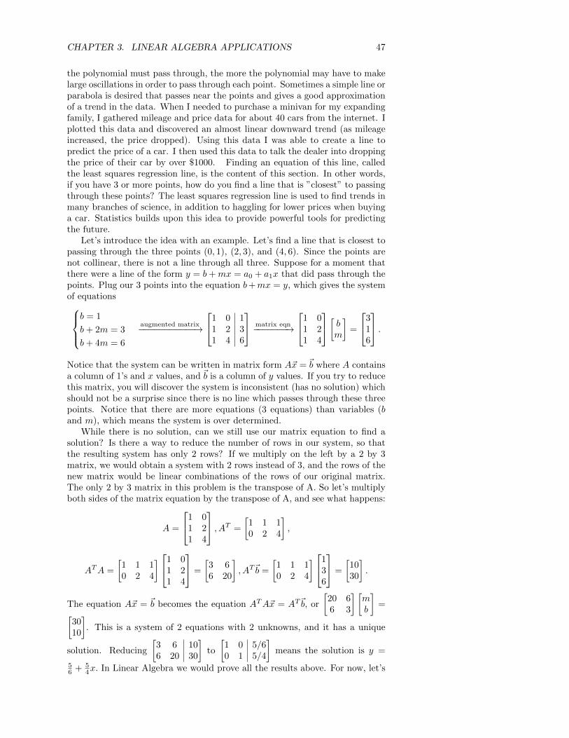
CHAPTER 3. LINEAR ALGEBRA APPLICATIONS 47
the polynomial must pass through, the more the polynomial may have to makelarge oscillations in order to pass through each point. Sometimes a simple line orparabola is desired that passes near the points and gives a good approximationof a trend in the data. When I needed to purchase a minivan for my expandingfamily, I gathered mileage and price data for about 40 cars from the internet. Iplotted this data and discovered an almost linear downward trend (as mileageincreased, the price dropped). Using this data I was able to create a line topredict the price of a car. I then used this data to talk the dealer into droppingthe price of their car by over $1000. Finding an equation of this line, calledthe least squares regression line, is the content of this section. In other words,if you have 3 or more points, how do you find a line that is ”closest” to passingthrough these points? The least squares regression line is used to find trends inmany branches of science, in addition to haggling for lower prices when buyinga car. Statistics builds upon this idea to provide powerful tools for predictingthe future.
Let’s introduce the idea with an example. Let’s find a line that is closest topassing through the three points (0, 1), (2, 3), and (4, 6). Since the points arenot collinear, there is not a line through all three. Suppose for a moment thatthere were a line of the form y = b+mx = a0 + a1x that did pass through thepoints. Plug our 3 points into the equation b+mx = y, which gives the systemof equations
b = 1
b+ 2m = 3
b+ 4m = 6
augmented matrix−−−−−−−−−−−→
1 0 11 2 31 4 6
matrix eqn−−−−−−−→
1 01 21 4
[ bm
]=
316
.Notice that the system can be written in matrix form A~x = ~b where A containsa column of 1’s and x values, and ~b is a column of y values. If you try to reducethis matrix, you will discover the system is inconsistent (has no solution) whichshould not be a surprise since there is no line which passes through these threepoints. Notice that there are more equations (3 equations) than variables (band m), which means the system is over determined.
While there is no solution, can we still use our matrix equation to find asolution? Is there a way to reduce the number of rows in our system, so thatthe resulting system has only 2 rows? If we multiply on the left by a 2 by 3matrix, we would obtain a system with 2 rows instead of 3, and the rows of thenew matrix would be linear combinations of the rows of our original matrix.The only 2 by 3 matrix in this problem is the transpose of A. So let’s multiplyboth sides of the matrix equation by the transpose of A, and see what happens:
A =
1 01 21 4
, AT =
[1 1 10 2 4
],
ATA =
[1 1 10 2 4
]1 01 21 4
=
[3 66 20
], AT~b =
[1 1 10 2 4
]136
=
[1030
].
The equation A~x = ~b becomes the equation ATA~x = AT~b, or
[20 66 3
] [mb
]=[
3010
]. This is a system of 2 equations with 2 unknowns, and it has a unique
solution. Reducing
[3 6 106 20 30
]to
[1 0 5/60 1 5/4
]means the solution is y =
56 + 5
4x. In Linear Algebra we would prove all the results above. For now, let’s

CHAPTER 3. LINEAR ALGEBRA APPLICATIONS 48
just use these tools. In Excel you can create a scatterplot of data nd then rightclick to automatically have the computer find the least square regression line.
In general, a least squares regression problem is solved by (1) assuming theform of a solution (y = b + mx), (2) putting your values of x and y into the
system to get a matrix equation A~x = ~b, (3) multiply both sides by AT , and (4)solving the simplified system, using elimination or Cramer’s rule. Since thesesimplified systems will always be 2 by 2 systems, Cramer’s rule provides anextremely quick solution.
Example 3.5. Let’s find the least squares regression line which passes nearestthe four points (0, 0), (−1, 2), (−2, 4), and (0,−1). We are after an equationof the form y = b + mx. The four points give the equations b = 0, b − m =2, b− 2m = 4, b = −1. In matrix form we write
1 01 −11 −21 0
[ bm]
=
024−1
, A =
1 01 −11 −21 0
,~b =
024−1
,AT =
[1 1 1 10 −1 −2 0
], ATA =
[4 −3−3 5
], AT~b =
[5−10
].
We now need to solve the matrix equation
[4 −3−3 5
] [bm
]=
[5−10
]. Cramer’s
rule gives the solution as
b =
∣∣∣∣ 5 −3−10 5
∣∣∣∣∣∣∣∣ 4 −3−3 5
∣∣∣∣ =−5
11, m =
∣∣∣∣ 4 5−3 −10
∣∣∣∣∣∣∣∣ 4 −3−3 5
∣∣∣∣ =−25
11.
The least square regression line is y = − 511 −
2511x.
A Quick 2 by 2 Inverse
Finding the least square regression line requires solving the system ATA~x =AT~b for ~x. Symbolically we can solve this system by multiplying both sides onthe left by (ATA)−1 (this inverse will exist), giving the solution
~x
[bm
]= (ATA)−1AT~b.
For 2 by 2 matrices, there is quick way to find the inverse. To find the
inverse of a 2 by 2 matrix A =
[a bc d
], we need to solve the system
[a b 1c d 0
]to find the first column of the inverse and
[a b 0c d 1
]to find the second column.
Cramer’s rule gives the formula
A−1 =
∣∣∣∣1 b0 d
∣∣∣∣ /|A| ∣∣∣∣0 b1 d
∣∣∣∣ /|A|∣∣∣∣a 1c 0
∣∣∣∣ /|A| ∣∣∣∣a 0c 1
∣∣∣∣ /|A|
=1
|A|
[d −b−c a
]
To find the inverse of a 2 by 2 matrix, just interchange the diagonal entries,change the sign on the others, and divide by the determinant.

CHAPTER 3. LINEAR ALGEBRA APPLICATIONS 49
Example 3.6. Let’s repeat the introductory example from the last section byusing an inverse to find the line closest to passing through the three points(0, 1), (2, 3), and (4, 6). The matrix equation and relevant matrices are1 0
1 21 4
[ bm
]=
316
, A =
1 01 21 4
,~b =
136
,AT =
[1 1 10 2 4
], ATA =
[3 66 20
], AT~b =
[1030
].
The inverse of (ATA) is1
60− 36
[20 −6−6 3
], which means our solution is[
bm
]= (ATA)−1AT b =
1
24
[20 −6−6 3
] [1030
]=
1
24
[2030
]=
[5/65/4
].
We of course obtained the same solution y = 56 + 5
4x.
The advantage of using an inverse to solve a least square regression problemis that the product W = (ATA)−1AT can be computed once, and then solutions
to the least squares regression problem are found by the simple product ~x = W~b.A different set of data points where the x values remain the same but the yvalues change can then be solved by just changing ~b and using the same resultsas before.
Example 3.7. Let’s find the least square regression line for the two data sets
1. (0, 2), (2, 1), and (4, 3)
2. (0, 6), (2, 3), and (4,−1)
Notice that both of the data sets have the same x values as the previous example.Hence we can still use
A =
1 01 21 4
, AT =
[1 1 10 2 4
], ATA =
[3 66 20
], (ATA)−1 =
1
24
[20 −6−6 3
].
The change occurred with the y values, which means that ~b changed for eachproblem. Before solving either, we compute
W = (ATA)−1AT =1
24
[20 −6−6 3
] [1 1 10 2 4
]=
1
24
[20 8 −4−6 0 6
]We can now solve both problems rapidly, by multiplying by W .
1. The y values are 2, 1, 3, so we compute
1
24
[20 8 −4−6 0 6
]213
=1
24
[366
]
which means that our line is (after simplifying fractions) y = 32 + 1
4x.
2. The y values are 6, 3,−1, so we compute
1
24
[20 8 −4−6 0 6
] 63−1
=1
24
[148−42
]
which means that our line is (after simplifying fractions) y = 376 −
74x.

CHAPTER 3. LINEAR ALGEBRA APPLICATIONS 50
3.3 Partial Fraction Decompositions
A partial fraction decomposition is a method of breaking a complex rationalfunction up into the sum of smaller simpler functions to work with. We willbe using partial fraction decompositions to rapidly solve differential equationsthroughout the semester (using Laplace transforms). For now, we will startby gaining practice with partial fraction decompositions by integrating rationalfunctions. To illustrate their value, let’s start with an example.
Example 3.8. Let’s find the integral of the function f(x) =2x+ 1
(x− 2) (x− 3).
The denominator is the product of two linear functions. Is it possible to breakup the function into two simpler functions, namely can we write
2x+ 1
(x− 2) (x− 3)=
A
x− 2+
B
x− 3
for unknown constants A and B? If we multiply both sides by the originaldenominator, we obtain (cancel the common factors)
2x+ 1 = A(x− 3) +B(x− 2).
Now expand the right hand side and collect the terms which have the samepowers of x,
2x+ 1 = (A+B)x+ (−3A− 2B).
Both sides of the equation above represent lines. In order for the two lines tobe the same line, they must have the same slope and intercept. This means wecan create an equation for each power of x by equating the coefficients on bothsides of the equation. This gives us the two equations
2 = A+B 1 = −3A− 2B.
This is a linear system and Gaussian elimination or Cramer’s rule will solve it:[1 1 2−3 −2 1
]rref−−→
[1 0 −50 1 7
]
The solution is A = −5, B = 7 and so2x+ 1
(x− 2) (x− 3)=−5
x− 2+
7
x− 3. Finish
by integrating each term separately to obtain∫2x+ 1
(x− 2) (x− 3)dx =
∫−5
x− 2dx+
∫7
x− 3dx = −5 ln |x− 2|+ 7 ln |x− 3|.
3.3.1 Finding the correct form
The general process for finding a partial fraction decomposition requires thatyou start with an appropriate guess for the final form, multiply both sides bythe original denominator, collect like powers of x on both sides, and then solvethe corresponding linear system. How do you pick an appropriate guess to beginwith? Before giving the full idea, let’s look at a simple example involving onlyintegers and fractions, before generalizing to polynomials.
The fraction 16 = 1
2·3 can be written as a sum of two fractions with sim-pler denominators as 1
6 = 12 −
13 . The prime factors of 6 are 2 and 3, so we
decompose the more complicated fraction 16 into two simpler fractions whose
denominators are the factors of 6. The fraction 59 = 5
3·3 has a repeated factorof 3 in the denominator, and can be written as 5
9 = 13 + 2
32 . This simplifies the

CHAPTER 3. LINEAR ALGEBRA APPLICATIONS 51
numerators so that they are all less than the denominator. Improper fractions(a larger numerator than denominator) are written in proper form and then wedecompose the remainder, as in 14
9 = 1 + 59 which then becomes 1 + 1
3 + 29 after
decomposing the fraction.In a similar manner, the way we decompose a rational function depends on
the factors of the denominator. If the degree of th numerator is larger than thedenominator, you start by performing long division to force the degree of thenumerator to be smaller than the denominator. Then find the factors of thedenominator. The appropriate guess for your partial fraction decomposition
1. Include a term for every factor of the denominator.
2. The numerator of each term is one degree less than the degree of thefactor (so constants go above linear factors, and linear terms go abovequadratic factors).
3. If a factor is a repeated factor, then it should be included each time, withan increasing power in the denominator.
A proper partial fraction decomposition form will have the same number ofunknowns as the degree of the denominator.
Example 3.9. Let’s illustrate the ideas above by picking the appropriate par-tial fraction decomposition form for the following rational functions:
1.2x+ 3
x2 − 1
2.x+ 1
x3 + x
3.3x+ 2
x2 + 2x+ 1
4.x4 + 2x− 1
x(x− 1)3(x2 + 4x+ 5)(x2 + 1)2
For the first, the denominator factors as two linear terms (x − 1)(x + 1).Since both of these are linear, we place constants above each one to obtain
2x+ 3
x2 − 1=
A
x− 1+
B
x+ 1.
There are two unknowns, which matches the degree of the denominator.The denominator of the second factors as x(x2 + 1). The quadratic term
does not factor any more over real number (its zeros are ±√−1), so we place a
linear guess above it. This gives
x+ 1
x3 + x=A
x+Bx+ C
x2 + 1.
On the third, the denominator factors as (x+1)2. Because this is a repeatedfactor, it get’s included twice, but each time we include it we increase the poweron the denominator. Because the factor is linear, we place a constant aboveeach term. This gives
3x+ 2
x2 + 2x+ 1=
A
x+ 1+
B
(x+ 1)2.

CHAPTER 3. LINEAR ALGEBRA APPLICATIONS 52
On the last example, the denominator is already factored. Each quadraticfactor needs a linear term placed above it. The form is
x4 + 2x− 1
x(x− 1)3(x2 + 4x+ 5)(x2 + 1)2=A
x+
H
x− 1+
I
(x− 1)2+
J
(x− 1)3
+Bx+ C
x2 + 4x+ 5+Dx+ E
x2 + 1+
Fx+G
(x2 + 1)2.
Notice that there are 10 unknowns, which is the degree of the denominator.
3.3.2 Integrating Rational Functions
A rational function is the quotient of two polynomials, r(x) = p(x)q(x) . If we
can factor the denominator into products of linear and quadratic terms, thenwe can always integrate the rational function by performing a partial fractiondecomposition and then integrating each term. The three key integrals used toare
∫1
x−adx = ln |x − a|,∫
1x2+1dx = arctanx, and
∫x
x2+1dx = 12 ln(x2 + 1).
You may have to complete the square and perform a u-substitution to reducethe integrals to one of these 3 key integrals.
Example 3.10. Let’s compute∫ −x2+2 x+5
(x2+1)(x−3)dx, using the form
−x2 + 2x+ 5
(x2 + 1) (x− 3)=Ax+B
x2 + 1+
C
x− 3.
In this case the denominator doesn’t factor into a product of linear terms, so thequadratic term x2 + 1 has a linear term Ax+B in the numerator. Multiplyingboth sides by the denominator and collecting powers of x gives
−x2 + 2x+ 5 = (A+ C)x2 + (B − 3A)x+ (C − 3B).
Equating the coefficients of x on each side gives the three equations
5 = C − 3B, 2 = B − 3A,−1 = A+ C
Rewriting in matrix form and reducing the matrix gives us 0 −3 1 5−3 1 0 21 0 1 −1
rref−−→
1 0 0 −6/50 1 0 −8/50 0 1 1/5
.We can now integrate using our solution to obtain∫
−x2 + 2x+ 5
(x2 + 1) (x− 3)dx =
∫1
5
(−6x− 8
x2 + 1
)+
1
5
(1
x− 3
)dx
= −6
5
∫x
x2 + 1dx− 8
5
∫1
x2 + 1dx+
1
5
∫1
x− 3dx
= − 6
10ln |x2 + 1| − 8
5arctanx+
1
5ln |x− 3|+ C.
3.4 Markov Process
Matrices can be used to model a process called a Markov Process. To fit thiskind of model, a process must have specific states, and the matrix which modelsthe process is a transition matrix which specifies how each state will changethrough a given transition. An example of a set of states is “open” or “closed”

CHAPTER 3. LINEAR ALGEBRA APPLICATIONS 53
in an electrical circuit, or “working properly” and “working improperly” foroperation of machinery at a manufacturing facility. A car rental company whichrents vehicles in different locations can use a Markov Process to keep track ofwhere their inventory of cars will be in the future. Stock market analystsuse Markov processes and a generalization called stochastic processes to makepredictions about future stock values.
Example 3.11. Let’s illustrate a Markov Process related to classifying landin some region as “Residential,” “Commercial,” or “Industrial.” Suppose ina given region over a 5 year time span that 80% of residential land will re-main residential, 10% becomes commercial, and 10% becomes industrial. Forcommerical land, 70% remains commercial, 20% becomes residential, and 10%becomes industrial. For industrial land, 70% remains industrial, 30% becomescommercial, and 0% becomes residential. To find what happens at the end of a5 year period, provided we know the current R, C, and I values, we could justcompute
Rnew = .8R+ .2C + 0ICnew = .1R+ .7C + .3IInew = .1R+ .1C + .7I
matrix form−−−−−−−→
Rnew
Cnew
Inew
=
.8 .2 0.1 .7 .3.1 .1 .7
RCI
The matrix on the right above is called the transition matrix of the Markovprocess. It is a matrix where each column relates to one of the “states,” and
R C I
to Rto Cto I
.8 .2 0.1 .7 .3.1 .1 .7
Transition Matrix
the numbers in that column are the proportions of the column state that willchange to the row state through the transition (the ordering on row and columnstates is the same). We calculate the next “state” by multiplying our currentstate by the transition matrix. If current land use is about 50% residential,30% commercial, and 20% industrial, then 5 years later the land use would be.8 .2 0
.1 .7 .3
.1 .1 .7
503020
=
463222
If the same transitions in land use continue, we can multiply the previous pro-jection (state) by the transition matrix to obtain a 10 and 15 year projectionfor land use:.8 .2 0
.1 .7 .3
.1 .1 .7
463222
=
43.233.623.2
.8 .2 0.1 .7 .3.1 .1 .7
43.233.623.2
=
41.2834.823.92
10 Year Projection 15 Year Projection
As we continue to multiply on the left by our transition matrix, each time weadd 5 more years to our projection. This projection is valid as long as the sametrends continue.
3.4.1 Steady State Solutions
Consider the land use example from above. Let ~x0 be our initial state. If ourtransition matrix A remains the same forever, what will eventually happen tothe proportion of land devoted to residential, commercial, or industrial use?We can write each new state as powers of the transition matrix A by writing~x1 = A~x0, ~x2 = A~x1 = AA~x0 = A2~x0, ~x3 = A3~x0, and ~xn = An~x0. Whathappens to the product An~x0 as n → ∞? Can we reach a state ~x = (R,C, I)such that A~x = ~x, the next state is the same as the current? If this occurs, thenany future transitions will not change the state either. This state ~x is called a
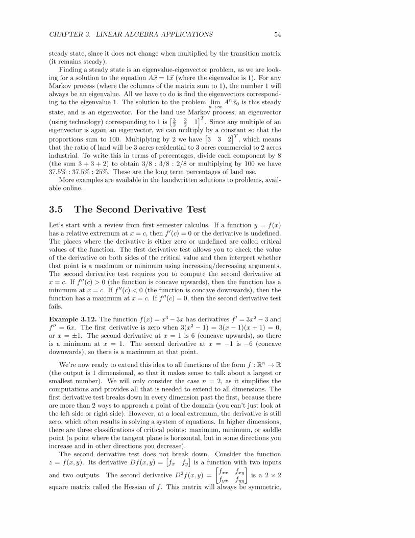
CHAPTER 3. LINEAR ALGEBRA APPLICATIONS 54
steady state, since it does not change when multiplied by the transition matrix(it remains steady).
Finding a steady state is an eigenvalue-eigenvector problem, as we are look-ing for a solution to the equation A~x = 1~x (where the eigenvalue is 1). For anyMarkov process (where the columns of the matrix sum to 1), the number 1 willalways be an eigenvalue. All we have to do is find the eigenvectors correspond-ing to the eigenvalue 1. The solution to the problem lim
n→∞An~x0 is this steady
state, and is an eigenvector. For the land use Markov process, an eigenvector
(using technology) corresponding to 1 is[
32
32 1
]T. Since any multiple of an
eigenvector is again an eigenvector, we can multiply by a constant so that the
proportions sum to 100. Multiplying by 2 we have[3 3 2
]T, which means
that the ratio of land will be 3 acres residential to 3 acres commercial to 2 acresindustrial. To write this in terms of percentages, divide each component by 8(the sum 3 + 3 + 2) to obtain 3/8 : 3/8 : 2/8 or multiplying by 100 we have37.5% : 37.5% : 25%. These are the long term percentages of land use.
More examples are available in the handwritten solutions to problems, avail-able online.
3.5 The Second Derivative Test
Let’s start with a review from first semester calculus. If a function y = f(x)has a relative extremum at x = c, then f ′(c) = 0 or the derivative is undefined.The places where the derivative is either zero or undefined are called criticalvalues of the function. The first derivative test allows you to check the valueof the derivative on both sides of the critical value and then interpret whetherthat point is a maximum or minimum using increasing/decreasing arguments.The second derivative test requires you to compute the second derivative atx = c. If f ′′(c) > 0 (the function is concave upwards), then the function has aminimum at x = c. If f ′′(c) < 0 (the function is concave downwards), then thefunction has a maximum at x = c. If f ′′(c) = 0, then the second derivative testfails.
Example 3.12. The function f(x) = x3 − 3x has derivatives f ′ = 3x2 − 3 andf ′′ = 6x. The first derivative is zero when 3(x2 − 1) = 3(x − 1)(x + 1) = 0,or x = ±1. The second derivative at x = 1 is 6 (concave upwards), so thereis a minimum at x = 1. The second derivative at x = −1 is −6 (concavedownwards), so there is a maximum at that point.
We’re now ready to extend this idea to all functions of the form f : Rn → R(the output is 1 dimensional, so that it makes sense to talk about a largest orsmallest number). We will only consider the case n = 2, as it simplifies thecomputations and provides all that is needed to extend to all dimensions. Thefirst derivative test breaks down in every dimension past the first, because thereare more than 2 ways to approach a point of the domain (you can’t just look atthe left side or right side). However, at a local extremum, the derivative is stillzero, which often results in solving a system of equations. In higher dimensions,there are three classifications of critical points: maximum, minimum, or saddlepoint (a point where the tangent plane is horizontal, but in some directions youincrease and in other directions you decrease).
The second derivative test does not break down. Consider the functionz = f(x, y). Its derivative Df(x, y) =
[fx fy
]is a function with two inputs
and two outputs. The second derivative D2f(x, y) =
[fxx fxyfyx fyy
]is a 2 × 2
square matrix called the Hessian of f . This matrix will always be symmetric,

CHAPTER 3. LINEAR ALGEBRA APPLICATIONS 55
in that the transpose of the matrix equals itself (because fxy = fyx). At acritical point (where the first derivative is zero), the eigenvalues of D2f givethe directional second derivative in the direction of a corresponding eigenvector.The largest eigenvalue is the largest possible value of the second derivative inany direction and the smallest eigenvalue is the smallest possible value of thesecond derivative in any direction.
The second derivative test is the following. Start by finding all the the second derivative test witheigenvaluescritical points (places where the derivative is zero). Then find the eigenvalues of
the second derivative. Each eigenvalue represents the 2nd directional derivativein the direction of a corresponding eigenvector. In every other direction, thedirectional 2nd derivative is between the smallest and largest eigenvalue.
1. If the eigenvalues are all positive at a critical point, then in every directionthe function is concave upwards. The function has a minimum at thatcritical point.
2. If the eigenvalues are all negative at a critical point, then in every directionthe function is concave downwards. The function has a maximum there.
3. If there is a positive eigenvalue and a negative eigenvalue, the functionhas a saddle point there.
4. If either the largest or smallest eigenvalue is zero, then the second deriva-tive test fails.
Eigenvalues are the key numbers needed to generalize optimization to all di-mensions. A proof of this fact is beyond the scope of this class.
Example 3.13. For the function f(x, y) = x2 + xy + y2, the gradient is Df =[2x+ y x+ 2y
], which is zero only at x = 0, y = 0 (solve the system of
equations 2x + y = 0, x + 2y = 0). The Hessian is D2f =
[2 11 2
]. The
eigenvalues are found by solving 0 = det
[2− λ 1
1 2− λ
]= (2 − λ)2 − 1 =
4 − 4λ + λ2 − 1 = (λ − 3)(λ − 1), so λ = 3, 1 are the eigenvalues. Since botheigenvalues are positive, the function is concave upwards in all directions, sothere is a minimum at (0, 0).
The eigenvectors of the Hessian help us understand more about the graph ofthe function. An eigenvector corresponding to 3 is (1,1), and corresponding to1 is (-1,1). These vectors are drawn in figure 3.2, together with two parabolaswhose 2nd derivatives are precisely 3 and 1. The parabola which opens upwardsthe most quickly has a 2nd derivative of 3. The other parabola has a secondderivative of 1. In every other direction, the 2nd derivative would be between1 and 3.
Example 3.14. For the function f(x, y) = x3 − 3x + y2 − 4y, the gradient isDf =
[3x2 − 3 2y − 4
], which is zero at x = 1, y = 2 or x = −1, y = 2. Hence
there are two critical points, so we have to find two sets of eigenvalues. The
Hessian is D2f =
[6x 00 2
]. When x = −1, y = 2, the eigenvalues of
[−6 00 2
]are λ = −6, 2. Since one is positive and one is negative, there is a saddle
point at (−1, 2). When x = 1, y = 2, the eigenvalues of
[6 00 2
]are λ = 6, 2.
Since both are positive, there is a minimum at (−1, 2) (as in every direction thefunction is concave upwards).

CHAPTER 3. LINEAR ALGEBRA APPLICATIONS 56
Figure 3.2: The eigenvectors of the second derivative tell you the directionsin which the 2nd derivative is largest and smallest. At each critical point,two eigenvectors are drawn as well as a parabola whose second derivative (theeigenvalue) matches the second derivative of the surface in the correspondingeigenvector direction.
Again the eigenvectors help us understand how the function behaves, asillustrated in figure 3.2. At (1,2) we have an eigenvector (1,0) corresponding to6, and (0,1) corresponding to 2. In both eigenvector directions the function isconcave upwards, but opens more stepply in the (1,0) direction as 6 is biggerthan 2. At (-1,2) the we have an eigenvector (1,0) corresponding to -6, and(0,1) corresponding to 2. The functions opens stepply downwards in the (1,0)direction, and upwards in the (0,1) direction.
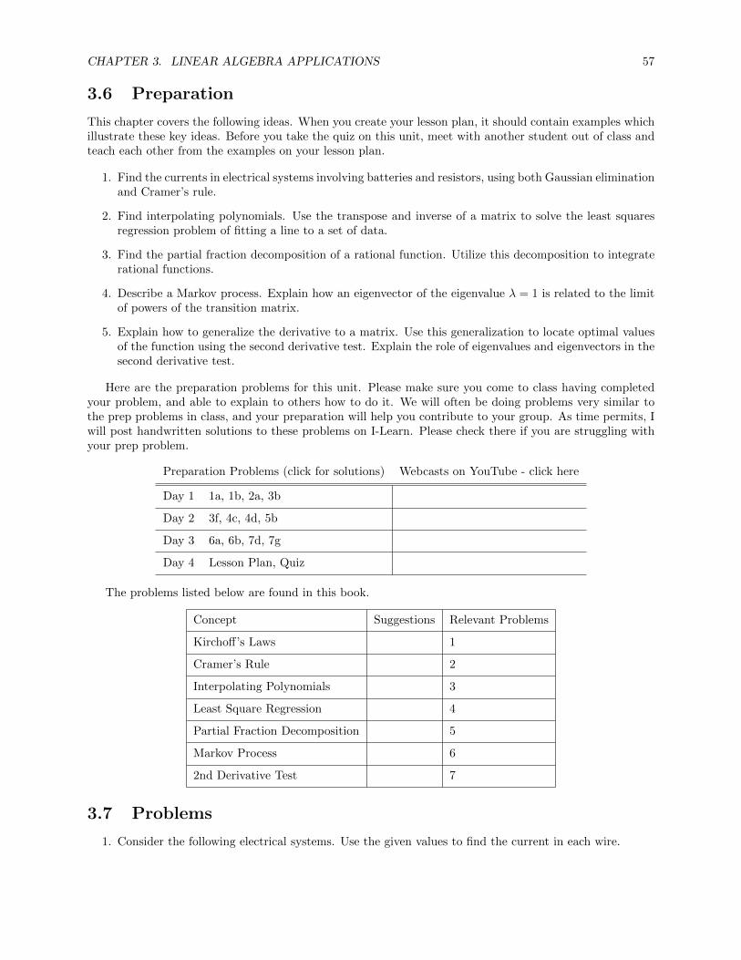
CHAPTER 3. LINEAR ALGEBRA APPLICATIONS 57
3.6 Preparation
This chapter covers the following ideas. When you create your lesson plan, it should contain examples whichillustrate these key ideas. Before you take the quiz on this unit, meet with another student out of class andteach each other from the examples on your lesson plan.
1. Find the currents in electrical systems involving batteries and resistors, using both Gaussian eliminationand Cramer’s rule.
2. Find interpolating polynomials. Use the transpose and inverse of a matrix to solve the least squaresregression problem of fitting a line to a set of data.
3. Find the partial fraction decomposition of a rational function. Utilize this decomposition to integraterational functions.
4. Describe a Markov process. Explain how an eigenvector of the eigenvalue λ = 1 is related to the limitof powers of the transition matrix.
5. Explain how to generalize the derivative to a matrix. Use this generalization to locate optimal valuesof the function using the second derivative test. Explain the role of eigenvalues and eigenvectors in thesecond derivative test.
Here are the preparation problems for this unit. Please make sure you come to class having completedyour problem, and able to explain to others how to do it. We will often be doing problems very similar tothe prep problems in class, and your preparation will help you contribute to your group. As time permits, Iwill post handwritten solutions to these problems on I-Learn. Please check there if you are struggling withyour prep problem.
Preparation Problems (click for solutions) Webcasts on YouTube - click here
Day 1 1a, 1b, 2a, 3b
Day 2 3f, 4c, 4d, 5b
Day 3 6a, 6b, 7d, 7g
Day 4 Lesson Plan, Quiz
The problems listed below are found in this book.
Concept Suggestions Relevant Problems
Kirchoff’s Laws 1
Cramer’s Rule 2
Interpolating Polynomials 3
Least Square Regression 4
Partial Fraction Decomposition 5
Markov Process 6
2nd Derivative Test 7
3.7 Problems
1. Consider the following electrical systems. Use the given values to find the current in each wire.

CHAPTER 3. LINEAR ALGEBRA APPLICATIONS 58
E R2
R1
R3
i1
i2
i3
E R2
R1
R3
R4 R5
R6
i1
i2
i3
i4
i5
i6
(a) E = 12, R1 = 2, R2 = 2, R3 = 2.
(b) E = 12, R1 = 2, R2 = 3, R3 = 3.
(c) E = 12, R1 = 2, R2 = 3, R3 = 6.
(d) E = 12, R1 = 1, R2 = 2, R3 = 2.
(e) E = 9, R1 = 3, R2 = 1, R3 = 2.
(f) E = 6, R1 = 1, R2 = 1, R3 = 2.
(g) E = 12, R1 = 1, R2 = 1, R3 = 1, R4 = 1, R5 = 1, R6 = 1
(h) E = 12, R1 = 2, R2 = 1, R3 = 3, R4 = 4, R5 = 2, R6 = 3
2. Use Cramer’s rule to find solutions to the following linear systems. If Cramer’s rule fails, explain why.
(a) 2x+ 3y = 0, x− 2y = 1
(b) x+ y = 2, x− y = 3
(c) 3x+ y = 6, x+ 3y = 2
(d) 2x+ y = 1, 4x+ 2y = 2
(e) x+ y = 0, 2x− y + z = 1, x+ z = 0
(f) x+ 2y = 3, x− y + z = 0, x+ 3y + z = 1
(g) y + 2z = 1, x− z = 3, 2x+ y = 1
3. In each of the following scenarios, find a polynomial of least degree which passes through the givenpoints. Then plot the points and the polynomial.
(a) (1, 2), (3, 3)
(b) (0, 1), (2, 3), (−1, 4)
(c) (1, 1), (2, 2), (−1, 5)
(d) (1, 2), (3, 3), (5, 6)
(e) (1, 2), (3, 3), (5, 5)
(f) (0, 1), (1, 3), (−1, 4), (2, 4)
4. For each set of data points, find an equation of the least squares regression line. Plot the points andthe line on the same axes.
(a) (0, 0), (1, 3), (1, 2)
(b) (1, 1), (2, 1), (3, 2)
(c) (1, 2), (3, 0), (5, 1)
(d) (0, 0), (1, 3), (1, 2), (4, 5)
(e) (0, 0), (1, 3), (1, 2), (4,−5)
(f) (−1, 2), (1, 3), (2, 5), (3, 3)
(g) Challenge: Find an equation of the least squaresregression parabola y = ax2+bx+c which passesthrough the points (0, 0), (1, 3), (1, 2), (4, 5).[Hint, you will need a 4 by 3 matrix for A in-stead of an n by 2. Use the transpose to reducethe size of the matrix to a 3 by 3 matrix, andthen solve.]
5. Compute each integral by finding a partial fraction decomposition.
(a)
∫1
(x− 3)(x+ 2)dx
(b)
∫2x+ 3
(x− 3)(x+ 2)dx
(c)
∫x
(x+ 1)(x− 2)dx
(d)
∫x2 + 2
x2(x− 2)dx
(e)
∫1
(x2 + 1)(x− 2)dx
(f)
∫x+ 1
(x2 + 1)x2dx
6. Markov Process - In each scenario, write the transition matrix. If an initial state is given, then findthe next two states. Finish by finding a steady state solution and use it to answer the question at theend.

CHAPTER 3. LINEAR ALGEBRA APPLICATIONS 59
(a) In a certain town, there are 3 types of land zones: residential, commercial, and industrial. Thecity has been undergoing growth recently, and the city has noticed the following trends. Every 5years, 10% of the older residential land gets rezoned as commercial land, while 5% gets rezonedas industrial. The other 85% remains residential. For commercial land, 70% remains commercial,while 10% becomes residential and 20% becomes industrial. For industrial land, 60% remainsindustrial, while 25% becomes commercial and 15% becomes residential. Currently the percent ofland in each zone is 40% residential, 30% commercial, and 30% industrial. What will the percentdistribution be in 5 years? In 10 years? If this trend continues indefinitely, what percent of theland will eventually be residential?.
(b) Suppose we own a car rental company which rents cars in Idaho Falls and Rexburg. The last fewweeks have shown a weekly trend that 60% of the cars rented in Rexburg will remain in Rexburg(the other 40% end up in IF), whereas 80% of the cars rented in Idaho Falls will remain in IdahoFalls. If there are currently 60 cars in Rexburg and 140 cars in IF, how many will be in each citynext week? In two weeks? In three weeks? If this trend continues indefinitely, about how manycars should you expect to find in Rexburg each week?
(c) Repeat the previous problem if 40% of the cars rented in Rexburg will remain in Rexburg (theother 60% end up in IF), whereas 80% of the cars rented in Idaho Falls will remain in Idaho Falls.
(d) Repeat the previous problem if 70% of the cars rented in Rexburg will remain in Rexburg (theother 30% end up in IF), whereas 80% of the cars rented in Idaho Falls will remain in Idaho Falls.
(e) A school cafeteria regularly offers 3 types of meals to its students. One of the meals is always apizza/salad combo, One is always hamburgers and fries, and one is a daily special which changesdaily. In an attempt to understand student preferences, the school discovered the following infor-mation. If a student has a hamburger one day, then there is a 30% chance they will try the dailyspecial the next day, and a 40% percent chance they will have the salad bar. If they have thesalad bar, then there is a 30% chance they’ll switch to the daily special, and a 40% chance they’llswitch to the hamburger. If the have the daily special, then there is a 50% chance they’ll get thedaily special the next day, a 20% chance they’ll switch to pizza, and a 30% chance they’ll switchto hamburger. If this trend continues, what percent of the students will eat each type of meal?
[While this problem is highly rigged, there is a branch of applied mathematics which is studied byfinancial analysts call stochastic processes which models such a scenario. This modeling processcan help predict how a new restaurant will perform in a city, sometimes predict stock marketfluctuations, and more. The study of stochastic processes begins with a Markov process and thenintroduces statistics and probability to help predict what happens when trends change.]
7. For each function, find the location of all critical points. Then use the second derivative test todetermine if each critical point corresponds to a maximum, minimum, or saddle point. Graph thefunction in 3D to verify your results, and locate the eigenvectors and eigenvalues in the picture.
(a) f(x, y) = x2 + xy + y2
(b) f(x, y) = x2 + 4xy + y2
(c) f(x, y) = x2 + 2xy + y2
(d) f(x, y) = x2 − 4x+ y2 + 2y + 1
(e) f(x, y) = x2 − 2x+ xy + y2
(f) f(x, y) = x2 + xy + 3y2
(g) f(x, y) = x3− 3x+ y2− 2y (2 critical points)
(h) f(x, y) = x3−3x+y3−3y2 (4 critical points)
3.8 Solutions
Remember that the Technology introduction has astep-by-step guide for solving many of these problems.
1. Kirchoff’s Laws1 −1 −1 0R1 R2 0 E0 −R2 R3 0
(a) (4, 2, 2)
(b) (24/7, 12/7, 12/7)
(c) (3, 2, 1)
(d) (6, 3, 3)
(e) (27/11, 18/11, 9/11)
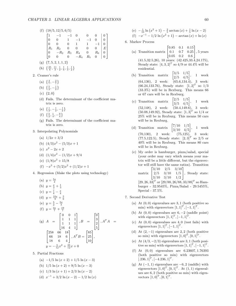
CHAPTER 3. LINEAR ALGEBRA APPLICATIONS 60
(f) (18/5, 12/5, 6/5)1 −1 −1 0 0 0 00 0 1 −1 −1 0 00 0 0 1 1 −1 0R1 R2 0 0 0 0 E0 −R2 R3 R4 0 R6 00 0 0 −R4 R5 0 0
(g) {7, 5, 2, 1, 1, 2}(h)
{256, 11
3, 12, 16, 13, 12
}2. Cramer’s rule
(a){
37,− 2
7
}(b)
{52,− 1
2
}(c) {2, 0}(d) Fails. The determinant of the coefficient ma-
trix is zero.
(e){
12,− 1
2,− 1
2
}(f)
{52, 14,− 9
4
}(g) Fails. The determinant of the coefficient ma-
trix is zero.
3. Interpolating Polynomials
(a) 1/2x+ 3/2
(b) (4/3)x2 − (5/3)x+ 1
(c) x2 − 2x+ 2
(d) (1/4)x2 − (1/2)x+ 9/4
(e) (1/8)x2 + 15/8
(f) −x3 + (5/2)x2 + (1/2)x+ 1
4. Regression (Make the plots using technology)
(a) y = 5x2
(b) y = x2
+ 13
(c) y = 74− x
4
(d) y = 10x9
+ 56
(e) y = 52− 5x
3
(f) y = 3x7
+ 197
(g) A =
0 0 11 1 11 1 116 4 1
, B =
0325
, ATA =
258 66 1866 18 618 6 4
, ATB =
852510
,
y = − 512x2 + 35
12x+ 0
5. Partial Fractions
(a) −1/5 ln (x+ 2) + 1/5 ln (x− 3)
(b) 1/5 ln (x+ 2) + 9/5 ln (x− 3)
(c) 1/3 ln (x+ 1) + 2/3 ln (x− 2)
(d) x−1 + 3/2 ln (x− 2)− 1/2 ln (x)
(e) − 110
ln(x2 + 1
)− 2
5arctan (x) + 1
5ln (x− 2)
(f) −x−1 − 1/2 ln(x2 + 1
)− arctan (x) + ln (x)
6. Markov Process
(a) Transition matrix
0.85 0.1 0.150.1 0.7 0.250.05 0.2 0.6
, 5 years
(41.5,32.5,26), 10 years: (42.425,33.4,24.175),Steady state: [4, 3, 2]T so 4/9 or 44.4% will beresidential.
(b) Transition matrix
[3/5 1/52/5 4/5
], 1 week
(64,136), 2 week: (65.6,134.4), 3 week:(66.24,133.76), Steady state: [1, 2]T so 1/3(33.3%) will be in Rexburg. This means 66or 67 cars will be in Rexburg.
(c) Transition matrix
[2/5 1/53/5 4/5
], 1 week
(52,148), 2 week: (50.4,149.6), 3 week:(50.08,149.92), Steady state: [1, 3]T so 1/4 or25% will be in Rexburg. This means 50 carswill be in Rexburg.
(d) Transition matrix
[7/10 1/53/10 4/5
], 1 week
(70,130), 2 week: (75,125), 3 week:(77.5,122.5), Steady state: [2, 3]T so 2/5 or40% will be in Rexburg. This means 80 carswill be in Rexburg.
(e) My order is hamburger, pizza/salad, special(your order may vary which means your ma-trix will be a little different, but the eigenvec-tor will still have the same ratios). Transition
matrix
3/10 2/5 3/102/5 3/10 1/53/10 3/10 1/2
, Steady state:
[29, 26, 33]T or [29/88, 26/88, 33/88]T so Ham-burger - 32.9545%, Pizza/Salad - 29.5455%,Special - 37.5%.
7. Second Derivative Test
(a) At (0, 0) eigenvalues are 3, 1 (both positive somin) with eigenvectors [1, 1]T , [−1, 1]T .
(b) At (0, 0) eigenvalues are 6,−2 (saddle point)with eigenvectors [1, 1]T , [−1, 1]T .
(c) At (0, 0) eigenvalues are 4, 0 (test fails) witheigenvectors [1, 1]T , [−1, 1]T .
(d) At (2,−1) eigenvalues are 2, 2 (both positiveso min) with eigenvectors [1, 0]T , [0, 1]T .
(e) At (4/3,−2/3) eigenvalues are 3, 1 (both posi-tive so min) with eigenvectors [1, 1]T , [−1, 1]T .
(f) At (0, 0) eigenvalues are 6.23607, 1.76393(both positive so min) with eigenvectors[.236, 1]T , [−4.236, 1]T .
(g) At (−1, 1) eigenvalues are −6, 2 (saddle) witheigenvectors [1, 0]T , [0, 1]T . At (1, 1) eigenval-ues are 6, 2 (both positive so min) with eigen-vectors [1, 0]T , [0, 1]T .

CHAPTER 3. LINEAR ALGEBRA APPLICATIONS 61
(h) At (−1, 0) eigenvalues are −6,−6 (both nega-tive so max) with eigenvectors [1, 0]T , [0, 1]T .At (−1, 2) eigenvalues are −6, 6 (saddle)with eigenvectors [1, 0]T , [0, 1]T . At (1, 0)
eigenvalues are 6,−6 (saddle) with eigenvec-tors [1, 0]T , [0, 1]T . At (1, 2) eigenvalues are6, 6 (both positive so min) with eigenvectors[1, 0]T , [0, 1]T .
Chapter 4
First Order ODEs
This chapter covers the following ideas. When you create your lesson plan, itshould contain examples which illustrate these key ideas. Before you take thequiz on this unit, meet with another student out of class and teach each otherfrom the examples on your lesson plan.
1. Be able to interpret the basic vocabulary of differential equations. Inparticular, interpret the terms ordinary differential equation (ODE), ini-tial value, initial value problem (IVP), general solution, and particularsolution.
2. Use the three step modeling process (express, solve, and interpret) toanalyze exponential growth and decay, Newton’s law of cooling, mixing,and the logistics equation.
3. Identify and solve separable ODES and exact differential forms. Use in-tegrating factors and substitutions to solve additional ODEs.
4. Use Laplace transforms to solve first order ODEs.
4.1 Basic Concepts and Vocabulary
A differential equation is an equation which involves derivatives (of any order)of some function. For example, the equation y′′ + xy′ + sin(xy) = xy2 is adifferential equation. An ordinary differential equation (ODE) is a differ-ential equation involving a function y(x) whose domain is one dimensional. Asolution to an ODE on an interval J = (a, b) is a function y(x) defined on theinterval J which satisfies the ODE. To verify that a function is a solution to anODE, calculate derivatives and put them in the ODE. If the resulting equationis an identity for all x ∈ J , then you have a solution. The order of an ODE isthe largest order derivative that appears in the ODE.
Typically a solution to an ODE involves an arbitrary constant C. There isoften an entire family of curves which satisfy a differential equation, and theconstant C just tells us which curve to pick. A general solution of an ODEis all possible solutions of the ODE. A particular solution is one of infinitelymany solutions of an ODE. Often an ODE comes with an initial conditiony(x0) = y0 for some values x0 and y0. We can use these initial conditions to finda particular solution of the ODE. An ODE, together with an initial condition,is called an initial value problem (IVP).
Example 4.1. The ODE y′ = ky has the general solution y = cekx for x ∈(−∞,∞). We check that this is a solution by calculating d
dxcekx = kcekx =
62

CHAPTER 4. FIRST ORDER ODES 63
ky. This is a first order ODE because only the first derivative and no higherderivatives appear in the ODE. If the initial condition y(0) = 3 were also in theproblem, then the particular solution to this IVP is found by solving for c inthe equation 3 = cek0. This simplifies to c = 3, so y(x) = 3ekx is the solutionto the IVP y′ = ky, y(0) = 3.
4.2 Modeling Basics
Many quantities in the world can be described in terms of rates of change.Differential equations arise in any physical model where rates of change arepart of the model. Modeling requires that we (1) express quantities in termsof mathematical equations, (2) solve those equations, and (3) interpret theresults in the context of our original problem. The first and third steps requirehuman intervention, while the second step can often be solved with the aid oftechnology. We will start by looking at three models: exponential growth anddecay, Newton’s law of cooling, and mixing. I will illustrate steps (1) and (3)first, and then in the next section we will focus on methods of solving.
4.2.1 Exponential Model
Exponential growth and decay models radioactive decay, retirement investing,carbon dating, population growth, and more. The model is based on the princi-ple that the rate of change of a quantity is directly proportional to the quantityitself. The rate of decay of a radioactive isotope is proportional to the amountof the isotope that remains. The rate of increase in a retirement investment isproportional to how much money is in the retirement investment. If you doublean investment, then it should grow twice as quickly. We now follow the threesteps.
1. (Express) The derivative is proportional to the quantity itself can be ex-pressed mathematically by the formula y′(x) = ky(x), where k is someconstant.
2. (Solve) The general solution to this ODE is y(x) = cekx. (Solved inexample 4.2)
3. (Interpret) When x = 0, we have y = c. This means that c is the initialamount of a radioactive isotope, or the initial investment in a retirementportfolio. The constant k helps us determine how quickly an isotopedecays (k < 0), or how quickly an investment grows (k > 0).
4.2.2 Newton’s Law of Cooling
One version of Newton’s law of cooling states that the rate of change of temper-ature dT
dt of a body (which conducts heat well) is proportional to the differencebetween the current temperature T (t) of the body and the temperature TA ofthe surrounding atmosphere (which is assumed to be constant).
1. (Express) Newton’s law of cooling can be expressed mathematically asdTdt = k(T − TA) for some constant k. If T > TA, then the temperatureneeds to drop, so we know k < 0. If T < TA, then the temperature needsto rise, so k < 0 gives k(T − TA) > 0 as the product of two negatives. Inall cases, the constant k will hence be negative.
2. (Solve) The general solution to this ODE is y = TA + cekt (solved inExample 4.3).

CHAPTER 4. FIRST ORDER ODES 64
3. (Interpret) When t = 0, we have T (0) = TA + c. This means thatc = T (0) − TA is the initial difference in temperature. Since k is alwaysnegative, as t→∞ the temperature T (t) approaches TA, the temperatureof the surrounding atmosphere.
4.2.3 Mixing Model
We will encounter mixing problems throughout the semester of the followingtype. Suppose a 5000 gallon tank contains a solution of water which initiallycontains 200 lbs of salt. The tank has an inflow valve, and an outflow value.Suppose 30 gallons of water (with 3 lbs of salt per gallon) are pumped into thetank each minute. The mixture is evenly spread throughout the entire tankby constant stirring. At the same time, 30 gallons of the stirred mixture flowthrough the outflow valve each minute. Find the amount of salt in the tank attime t.
1. (Express) If we let y(t) be the amount of salt in the tank at any time t,then y′ = (flow in)− (flow out). The flow in is
flow in =30 gal
min
∣∣∣∣3 lbs
gal=
90 lbs
minof salt.
The amount of salt lost per minute is proportional to the amount of saltin the tank. Since the tank holds 5000 gallons, and the outflow is 30gal/min, we loose 30
5000 of the water in the tank each minute. Since themixture is evenly stirred, this means that 30
5000 of what currently is in thetank (which is y lbs) should leave every minute. So our flow out is
flow out =30 gal
min
5000 gal
∣∣∣∣y lbs =30
5000y
lbs
minof salt.
Hence y′ = 90− 305000y. The initial condition is y(0) = 200 lbs.
2. (Solve) The general solution is y(t) = 15000 + ce(−3/500)t. Using y(0) =200, we find 200 = 15000 + c, or c = −14800. So y(t) = 15000 −14800e(−3/500)t.
3. (Interpret) The salt content starts at 200 lbs and grows to a maximum of15000 lbs as t → ∞. The quantity grows more rapidly at the beginningthan at the end.
4.3 Basic Methods
The modeling process often results in a differential equation. We will learnvarious methods of solving these differential equations. Software can solve thedifferential equations in this course, however, the differential equations you mayencounter in the future might not be solvable by any of the methods in thistextbook or by software. Understanding the ideas and processes which go intothese methods will give you building blocks which you may need to creativelysolve new differential equations.
4.3.1 Separable
The most basic differential equation to solve is one in which you can “separate”the variables. The idea is to rearrange the equation in the form f(y)dy =g(x)dx, where you separate the x and y terms so that they appear on differentsides of the equation. The solution is found by integrating each side.

CHAPTER 4. FIRST ORDER ODES 65
Example 4.2: Exponential Model Solution. Divide the differential equa-tion y′ = ky on both sides by y. Then multiply both sides by the differentialdx to obtain 1
ydy = kdx. Integration on both sides yields ln |y| = kx+ c. Expo-
nentiating both sides gives |y| = ekx+c = ekxec. Now ec is a positive constant,so we rename that constant to be c and obtain |y| = cekx for c > 0. Removingthe absolute values on y allows c to be any nonzero constant. If c = 0, then theequation y = 0 satisfies the differential equation y′ = ky, so we can let c = 0as well. This shows that a general solution to y′ = ky is y(x) = cekx for anyconstant c.
Example 4.3: Newton’s Law of Cooling Solution. The differential equa-tion for Newton’s law of cooling, dTdt = k(T−TA), is another separable ODE. Re-arrange the equation as 1
T−TAdT = kdt. Integration yields ln |T −TA| = kt+ c.
Exponentiation gives |T − TA| = ekt+c = ektec = cekt. Removing absolutevalues as before gives T = TA + cekt as a general solution.
4.3.2 Exact Differential Forms
Recall that a vector field ~F = 〈M,N〉 is called a gradient field if there exists
a function f(x, y), called a potential for F , which satisfies ∇f = ~F . Recall
also that ~F = 〈M,N〉 has a potential (under suitable conditions) if and only ifMy = Nx (test for exactness). Similarly, a differential form Mdx+Ndy is said
to be exact if there exists a function f(x, y) which satisfies df = Df(x, y)
[dxdy
]=
Mdx + Ndy. If a first order differential equation can be written in the formMdx+Ndy = 0, and that differential form is exact, then a general solution tothe ODE is f(x, y) = c for any constant c, where f is a potential for 〈M,N〉. A general solution to
Mdx+Ndy = 0 is f = c where fis a potential for 〈M,N〉 and c isan arbitrary constant.
This is because the level curves of the potential (f = c) are orthogonal to thegradient of the potential, which is precisely what 〈M,N〉 · 〈dx, dy〉 = 0 means.
Example 4.4. The differential equation 3xy′ = 2x−3y can be rewritten in thedifferential form (3y − 2x)dx+ 3xdy = 0. We calculate My = ∂
∂y (3y − 2x) = 3
and Nx = ∂∂x (3x) = 3. Since My = Nx, a potential exists. We integrate both
terms and obtain ∫Mdx = 3xy − x2
∣∣∣∣ ∫Ndy = 3xy.
Summing the integrals and ignoring duplicates, we obtain f = 3xy − x2 as apotential. The general solution of 3xy′ = 2x − 3y is 3xy − x2 = c for anyconstant c. We have written the solution implicitly (without solving explicitly
for y). Solving for y gives the explicit solution y = c+x2
3x , however you may notalways be able to solve for y.
Notice that if a differential equation is separable f(y)dy = g(x)dx, then itrepresents an exact differential form, namely−g(x)dx+f(y)dy = 0 has potential−∫g(x)dx +
∫f(y)dy. Every separable differential equation can be solved by
considering exact differential forms. In fact, the goal of every method below Solving an exact ODE is the BIGIDEA.is to rewrite the ODE so that it is an exact differential form, which means that
finding a potential is the BIG IDEA of this unit.
4.3.3 Integrating Factors (What to do if it isn’t exact)
Not every differential equation, when written in differential form Mdx+Ndy =0 is exact. However, by multiplying both sides by an appropriate factor (calledan integrating factor), often we can make the ODE exact.

CHAPTER 4. FIRST ORDER ODES 66
Example 4.5. The differential form −kydx+dy = 0 (which models exponentialgrowth) is not exact. However, if you multiply both sides by e−kx, then thedifferential form −ke−kxydx + e−kxdy = 0 is exact with potential f = ye−kx,and hence the solution is ye−kx = c or y = cekx as before. Alternatively, wecould multiply both sides of −kydx + dy = 0 by 1
y . This gives the differential
form −kdx + 1ydy = 0, which is exact with potential f = −kx + ln |y|. The
general solution is thus −kx + ln |y| = c which becomes ln |y| = kx + c andsimplifies to y = cekx as before. In either case we multiplied a non exactdifferential form by a factor (called an integrating factor) to obtain an exactdifferential form.
Essentially every method we look at for this unit can be solved by findingan appropriate integrating factor and then finding a potential to get the generalsolution. So how do we find an appropriate integrating factor? If a differentialform Mdx+Ndy is not exact, then we seek a function F so that FMdx+FNdyis exact. To simplify our work, we will consider two cases: (1) F is a functionwhich depends on only x, or (2) F is a function which depends on only y.
1. If F = F (x), then for FMdx+FNdy to be exact we must have (FM)y =(FN)x, which is equivalent to FNy = FMx + FxM . Rearranging (sep-
arating F from the other terms) gives 1F Fx =
My−Nx
N . Integrating both
sides yields ln |F | =∫ My−Nx
N dx. Solving for F gives F (x) = e∫ My−Nx
N dx.
The preceding formula will give us our integrating factor as long asMy−Nx
Ndepends only on x.
2. If F = F (y), then for FMdx+FNdy to be exact we must have (FM)y =(FN)x, which is equivalent to FMy + FyM = FNx. Rearranging gives1F Fy =
Nx−My
M . Integrating both sides yields ln |F | =∫ Nx−My
M dx, and
solving for F gives F (y) = e∫ Nx−My
M dy. The preceding formula will give
us our integrating factor as long asNx−My
M depends only on y.
Observation 4.1. IfMy −Nx
Ndepends on x, then e
∫ My−NxN dx is an integrating
factor. IfNx −My
Mdepends on y, then e
∫ Nx−MyM dy is an integrating factor.
Example 4.6. To solve the differential equation (x + y)dx + 3xdy = 0, we
compute My − Nx = 1 − 3 = −2. Division by N givesMy−Nx
N = −23x . Hence
F = e∫−2/(3x)dx = e−2/3 ln(x) = x−2/3. Then the differential form (x1/3 +
x−2/3y)dx+ 3x1/3dy = 0 has potential 3x4/3
4 + 3x1/3y. So a general solution is
3x4/3
4 + 3x1/3y = c or y =c− 3x4/3
4
3x1/3 .
4.3.4 Linear ODEs - a common special form
A linear ODE is an ODE of the form y′+ p(x)y = q(x). It is linear in y and y′.The linear ODE y′+p(x)y = 0 is separable, hence can be solved. If q(x) is not 0,we rewrite the linear ODE in differential form, getting (p(x)y−q(x))dx+dy = 0.
SinceMy−Nx
N = (p(x)− 1)/1 = p(x) only depends on x, we use the integrating
factor F (x) = e∫pdx to solve the differential equation.
Example 4.7. To solve y′ + 2xy = 3x, we multiply by the integrating factorF (x) = e
∫2xdx = ex
2
, and obtain (2xyex2 − 3xex
2
)dx+ ex2
dy = 0. A potential
is u = yex2 − 3
2ex2
, so the general solution is yex2 − 3
2ex2
= c, or y = ce−x2
+ 32 .

CHAPTER 4. FIRST ORDER ODES 67
4.3.5 u-Substitutions (How to make it exact)
If an appropriate integrating factor cannot be found to make an ODE exact,then sometimes a substitution will get the job done. Which substitution tomake may require ingenuity. However, sometimes the appropriate substitu-tion to make can be seen by examining the function itself to see if there arecomplex parts which could be simplified by a substitution. We will illustratethis approach with three common substitutions. This process is very similar tou-substitution from first semester calculus.
Homogeneous ODEs, u = y/x
Some ODE’s can be reduced to separable form by using the substitution u =y/x. If an ODE of the form y′ = f(x, y) satisfies yprime = f(tx, ty) (replacingeach x and y with tx or ty does nothing), then we call the ODE a homogeneousfirst order ODE. In such cases, the substitution u = y/x will reduce the ODEto separable form. If an ODE has y/x terms or x/y terms in it, try this kind ofsubstitution. We substitute y = ux and y′ = xu′ + u and then try to separatevariables or find an integrating factor. Rather than memorizing these equations,it is easiest to just carry out the computations each time.
Example 4.8. The differential equation 4xyy′ = x2 + y2 is equivalent to 4y′ =xy+ y
x . Replacing each y with ux, and y′ with xu′+u, we obtain 4xu′+4u = 1u+u.
This is equivalent to 4xu′ = 1u − 3u = 1−3u2
u . Separating variables we obtain
4u1−3u2u
′ = 1x . Integration on both sides yields
4
−6ln |1 − 3u2| = ln |x| + c.
Exponentiating both sides eliminates the absolute values and gives the equation(1−3u2)−2/3 = cx (this c is different than the first). Now substitute back in u =
y/x and solve for y, to obtain 1−3(y/x)2 = cx−3/2, or y = ±x√
1/3− cx−3/2 =
±1/3√
3x2 − c√x (again c has changed) as a solution for any constant c.
Bernoulli Equations, u = y1−n
A Bernoulli equation is an ODE of the form y′+ p(x)y = r(x)yn. To solve suchan ODE, let u = y1−n. This means u′ = (1−n)y−ny′ = (1−n)y−n(ryn−py) =(1− n)(r − py1−n) = (1− n)(r − pu). By using this transformation, the ODEbecome a linear ODE of the form u′+ (1−n)p(x)u = (1−n)r(x). Hence it hasan integrating factor and can be solved as before. Again, it is easiest to carryout the computation with each example, rather than learn this general formula.
Example 4.9. We’ll solve the equation y′ + y = 3y2. First the substitutionu = y1−2 = y−1 gives u′ = (−1)y−2y′ = (−1)y−2(3y2 − y) = (−1)(3 − y−1) =(−1)(3−u). So we have the linear ODE u′−u = −3, which in differential formbecomes (3 − u)dx + du = 0. We compute (Mu − Nx)/N = −1, and so ourintegrating factor is F (x) = e−x. The differential form (3e−x−ue−x)dx+e−xduis exact and has potential f = −3e−x + ue−x. Hence a solution is written
implicitly as −3e−x + 1y e−x = c or explicitly as y = e−x
c+3e−x = 1cex+3 .
Logistic Equation - A Bernoulli Model
The logistic equation is dydt = Ay−By2. It is used to model population growth,
spread of disease, and other quantities which have an upper bound. If B = 0,then we obtain the exponential model which we can already solve. This typeof growth occurs with small populations where there is plenty of space to grow.The term −By2 is added to the model to prevent overgrowth, and places apopulation maximum on the model. To solve the logistic equation, we let u =
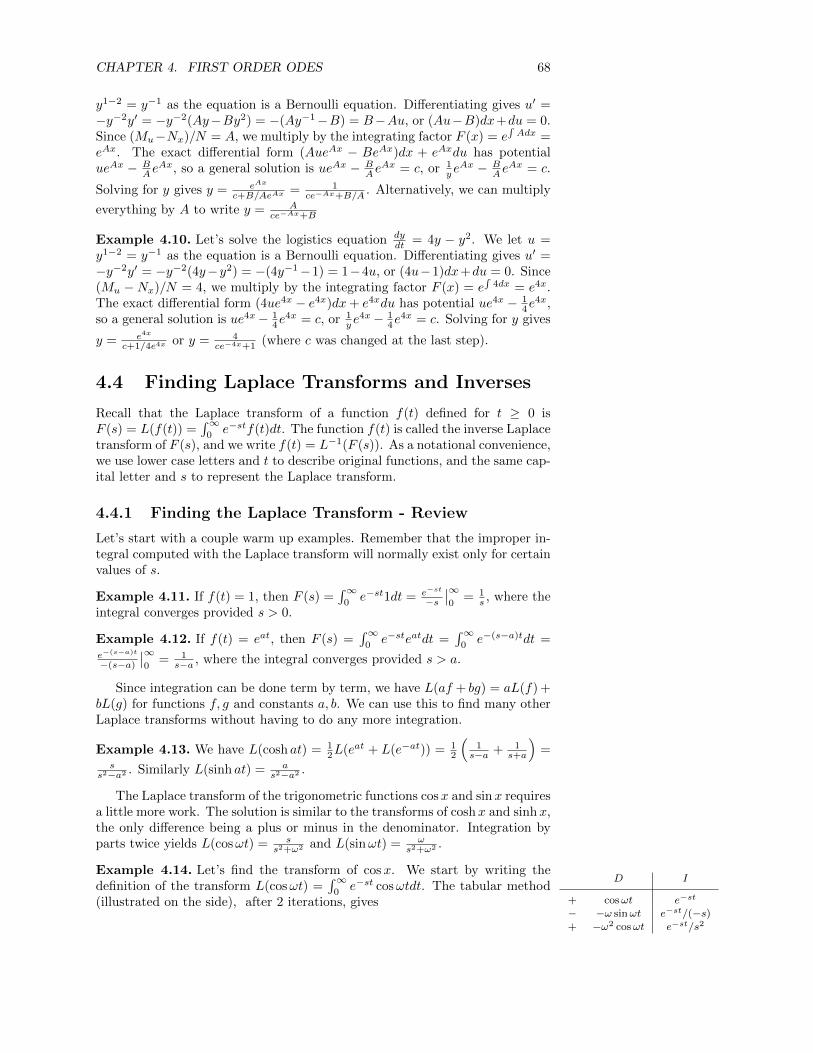
CHAPTER 4. FIRST ORDER ODES 68
y1−2 = y−1 as the equation is a Bernoulli equation. Differentiating gives u′ =−y−2y′ = −y−2(Ay−By2) = −(Ay−1−B) = B−Au, or (Au−B)dx+du = 0.Since (Mu−Nx)/N = A, we multiply by the integrating factor F (x) = e
∫Adx =
eAx. The exact differential form (AueAx − BeAx)dx + eAxdu has potentialueAx − B
AeAx, so a general solution is ueAx − B
AeAx = c, or 1
y eAx − B
AeAx = c.
Solving for y gives y = eAx
c+B/AeAx = 1ce−Ax+B/A
. Alternatively, we can multiply
everything by A to write y = Ace−Ax+B
Example 4.10. Let’s solve the logistics equation dydt = 4y − y2. We let u =
y1−2 = y−1 as the equation is a Bernoulli equation. Differentiating gives u′ =−y−2y′ = −y−2(4y−y2) = −(4y−1−1) = 1−4u, or (4u−1)dx+du = 0. Since(Mu −Nx)/N = 4, we multiply by the integrating factor F (x) = e
∫4dx = e4x.
The exact differential form (4ue4x − e4x)dx+ e4xdu has potential ue4x − 14e
4x,so a general solution is ue4x− 1
4e4x = c, or 1
y e4x− 1
4e4x = c. Solving for y gives
y = e4x
c+1/4e4x or y = 4ce−4x+1 (where c was changed at the last step).
4.4 Finding Laplace Transforms and Inverses
Recall that the Laplace transform of a function f(t) defined for t ≥ 0 isF (s) = L(f(t)) =
∫∞0e−stf(t)dt. The function f(t) is called the inverse Laplace
transform of F (s), and we write f(t) = L−1(F (s)). As a notational convenience,we use lower case letters and t to describe original functions, and the same cap-ital letter and s to represent the Laplace transform.
4.4.1 Finding the Laplace Transform - Review
Let’s start with a couple warm up examples. Remember that the improper in-tegral computed with the Laplace transform will normally exist only for certainvalues of s.
Example 4.11. If f(t) = 1, then F (s) =∫∞
0e−st1dt = e−st
−s∣∣∞0
= 1s , where the
integral converges provided s > 0.
Example 4.12. If f(t) = eat, then F (s) =∫∞
0e−steatdt =
∫∞0e−(s−a)tdt =
e−(s−a)t
−(s−a)
∣∣∞0
= 1s−a , where the integral converges provided s > a.
Since integration can be done term by term, we have L(af + bg) = aL(f) +bL(g) for functions f, g and constants a, b. We can use this to find many otherLaplace transforms without having to do any more integration.
Example 4.13. We have L(cosh at) = 12L(eat + L(e−at)) = 1
2
(1s−a + 1
s+a
)=
ss2−a2 . Similarly L(sinh at) = a
s2−a2 .
The Laplace transform of the trigonometric functions cosx and sinx requiresa little more work. The solution is similar to the transforms of coshx and sinhx,the only difference being a plus or minus in the denominator. Integration byparts twice yields L(cosωt) = s
s2+ω2 and L(sinωt) = ωs2+ω2 .
Example 4.14. Let’s find the transform of cosx. We start by writing thedefinition of the transform L(cosωt) =
∫∞0e−st cosωtdt. The tabular method
(illustrated on the side), after 2 iterations, gives
D I
+ cosωt e−st
− −ω sinωt e−st/(−s)+ −ω2 cosωt e−st/s2

CHAPTER 4. FIRST ORDER ODES 69
f(t) F (s) provided
11
ss > 0
tnn!
sn+1s > 0
eat1
s− as > a
f ′ sL(f)− f(0)
f(t) F (s) provided
cos(wt)s
s2 + ω2s > 0
sin(wt)ω
s2 + ω2s > 0
cosh(wt)s
s2 − ω2s > |ω|
sinh(wt)ω
s2 − ω2s > |ω|
Table 4.1: Table of Laplace Transforms
∫ ∞0
e−st cosωtdt
=(cosωte−st/(−s) + ω sinωte−st/s2
) ∣∣∞0−∫ ∞
0
ω2 cosωte−st/s2dt
= 1/s− ω2/s2
∫ ∞0
e−st cosωtdt.
Replacing each integral above with L(cosωt) gives
L(cosωt) = 1/s− ω2/s2L(cosωt).
We have written the original integral in terms of itself. To simplify we combinelike terms (1 + ω2/s2)L(cosωt) = 1
s , or (s2 + ω2)L(cosωt) = s, and then wesolve for the transform L(cosωt) = s
s2+ω2 . The computation of L(sinx) is verysimilar, but results with an ω in the numerator instead of s.
Integration by parts also shows that L(tn) = n!sn+1 for integers n. For con-
venience, table 4.1 summarizes the Laplace Transforms we will use most often.Feel free to use this table as you find Laplace transforms and their inverses.With practice, you will memorize this table.
4.4.2 Finding an Inverse Laplace Transform
If the Laplace transforms of two functions are the same, then the two functionsmust be the same. This fact allows us to invert the Laplace transform andobtain the only function with a given Laplace transform. Inverting a Laplacetransform often involves matching the transformed function up with a functionfrom a table, and then using the table to invert the transform. We’ll illustratethis with a few examples.
Example 4.15. To find the inverse Laplace transform of F (s) =7
s3, first notice
that2
s3is the transform of t2. We rewrite F (s) =
7
s3=
7
2
2!
s3, and then find the
inverse transform as L−1(F (s)) =7
2t2.
Example 4.16. To find the inverse Laplace transform of F (s) =3s+ 4
s2 + 25, we
notice that the transforms of cos(5t) and sin(5t) are s/(s2 +52) and 5/(s2 +52).We rewrite
F (s) =3s+ 4
s2 + 25= 3
s
s2 + 25+
4
5
5
s2 + 25,

CHAPTER 4. FIRST ORDER ODES 70
and then the inverse transform is 3 cos(5t) +4
5sin(5t).
Example 4.17. To find the inverse Laplace transform of F (s) =3s+ 1
s2 + 3s+ 2,
we start by factoring the denominator as (s2 + 3s + 2) = (s + 2)(s + 1). Wethen use a partial fraction decomposition to write
3s+ 1
s2 + 3s+ 2=
A
s+ 2+
B
s+ 1.
Multiplication on both sides by s2 + 3s+ 2 gives
(3)s+ (1) = A(s+ 1) +B(s+ 2) = (A+B)s+ (A+ 2B).
Since the left and right sides are both linear equations of s, the coefficients mustbe equal so we must have 3 = A+B and 1 = A+ 2B. The solution is B = −2
and A = 5. This means that F (s) = 51
s+ 2−2
1
s+ 1, which means the Laplace
inverse is f(t) = 5e−2t − 2e−t.
4.5 Solving IVPs
4.5.1 The Transform of a derivative
The Laplace transform of a derivative is, using integration by parts,
L(f ′) =
∫ ∞0
e−stf ′(t)dt = (e−stf(t))∣∣∞0
+ s
∫ ∞0
e−stf(t)dt = sL(f)− f(0).
We can use this formula to solve ODEs.Here’s the big idea. Given an ODE, take the Laplace transform of each
side, giving what is called the subsidiary equation. This equation can be solvedfor L(y) = Y (s) using only algebra. You then compute L−1(Y (s)) to find thesolution to the IVP y(t). This may involve finding a partial fraction decompo-sition. Laplace transforms reduce many IVPs to a 3 step process (1) convertto the subsidiary equation, (2) use algebra to solve for Y , performing a partialfraction decomposition if needed, (3) find inverse Laplace transform.
The following two examples represent the basic ideas used to solve prettymuch every Laplace transform problem. We will be revisiting this idea through-out the semester.
Example 4.18. To solve the IVP y′ + 2y = 0, y(0) = 1 we start by takingthe Laplace transform of each side. This gives the subsidiary equation sL(y)−y(0) + 2L(y) = 0, or using the notation L(y) = Y , we have sY − 1 + 2Y = 0.Solving for Y gives the equation Y = 1
s+2 . The inverse Laplace transform of
both sides gives y(t) = e−2t.
Example 4.19. To solve the IVP y′ + 2y = 3, y(0) = 1, take the Laplace
transform of each side. This gives the subsidiary equation sY − 1 + 2Y =3
s.
Solving for Y gives the equation Y =s+ 3
s(s+ 2). The partial fraction decom-
positions+ 3
s(s+ 2)=
A
s+
B
s+ 2requires we solve s + 3 = A(s + 2) + Bs, or
1 = A + B, 3 = 2A giving A = 3/2 and B = −1/2. Our subsidiary equation
is now Y =3
2
1
s− 1
2
1
s+ 2. The inverse Laplace transform of both sides gives
y(t) =3
2− 1
2e−2t.

CHAPTER 4. FIRST ORDER ODES 71
4.6 Preparation
This chapter covers the following ideas. When you create your lesson plan, it should contain examples whichillustrate these key ideas. Before you take the quiz on this unit, meet with another student out of class andteach each other from the examples on your lesson plan.
1. Be able to interpret the basic vocabulary of differential equations. In particular, interpret the termsordinary differential equation (ODE), initial value, initial value problem (IVP), general solution, andparticular solution.
2. Use the three step modeling process (express, solve, and interpret) to analyze exponential growth anddecay, Newton’s law of cooling, mixing, and the logistics equation.
3. Identify and solve separable ODES and exact differential forms. Use integrating factors and substitu-tions to solve additional ODEs.
4. Use Laplace transforms to solve first order ODEs.
Here are the preparation problems for this unit. Please make sure you come to class having completedyour problem, and able to explain to others how to do it. We will often be doing problems very similar tothe prep problems in class, and your preparation will help you contribute to your group.
Preparation Problems (from Schaum’s Outlines) (click for solutions)
Day 1 5.5,5.21,6.4,7.4
Day 2 7.10,7.17,4.11,6.16
Day 3 22.1-3,24.1,24.14,7.7
Day 4 Lesson Plan, Quiz
Concept Sec. Suggested Relevant
Separable Review 4 42 1-8,23-45
Exact 5 5,11,26,29,34 1-13,24-40,56-65
Integrating Factors 5 21,22,41,47 21,22,41-42,47-49,51,55
Linear 6 4,13,20,32,51 1-6,9-15,20-36,43-49,50-57
Homogeneous 4, 11,12,48 11-17,46-54
Bernoulli 6 16,53 16,17,37-42,53
Applications 7 4[27],6[33],1[38] 1-6 [26-44]7 10[48],17[67],7[88] 8-10 [45-50],16-18[65-70], 7[87-88]
Laplace Review 21 19,32,33[use table] 4-7,10-12,27-35
Inverse Transforms 22 1,2,3,6,13,15 1-3,6,15,17,20-28,42,42,45-47
Solving ODEs 24 1,14,19(parfrac) 1,2,11,14,15,19-19,22,24,25,38-42
4.7 Problems
All the problems for this unit come from Schaum’s Outlines Differential Equations by Rob Bronson.
4.8 Solutions
Every problem in Schaum’s Outlines has a solution provided.

Chapter 5
Homogeneous ODEs
This chapter covers the following ideas. When you create your lesson plan, itshould contain examples which illustrate these key ideas. Before you take thequiz on this unit, meet with another student out of class and teach each otherfrom the examples on your lesson plan.
1. Explain Hooke’s Law in regards to mass-spring systems. Construct andsolve differential equations which represent this physical model, with orwithout the presence of a damper.
2. Understand the vocabulary and language of higher order ODEs, suchas homogeneous, linear, coefficients, superposition principle, basis, linearindependence.
3. Solve homogeneous linear ODE’s with constant coefficients (with andwithout Laplace transforms). In addition, create linear homogeneousODE’s given a basis of solutions, or the roots of the characteristic equa-tion.
4. Explain how the Wronskian can be used to determine if a set of solutionsis linear independent. Briefly mention the existence and uniqueness the-orems in relation to linear ODEs, and give a reason for their importance.
5.1 An Example - Hooke’s Law
The force F of a spring is proportional to the distance y of the spring from theequilibrium point y = 0, and the force acts opposite the direction of motion.This is represented by the equation F = −ky for a positive constant k, calledthe spring constant. Since force equals mass times acceleration (one of Newton’slaws of motion), we have my′′ = −ky or my′′+ky = 0. This is our introductoryexample of a 2nd order ODE. If a damper (called a dashpot) is placed in amass-spring system , then the damper applies a force (via friction) which isproportional to the velocity of the spring. This gives the 2nd order ODE my′′+cy′ + ky = 0 for some constants m, c, and k. We will develop general methodsof solving 2nd order linear ODEs, and then return to mass-spring systems tostudy the applications.
5.2 Basic Notation and Vocabulary
A second order linear differential equation is an ODE which can be written inthe form y′′+p(x)y′+q(x)y = r(x). It is linear in y and its derivatives, and the
72

CHAPTER 5. HOMOGENEOUS ODES 73
coefficients of the linear ODE are p(x) and q(x). A higher order linear ODE canbe written in the same form y(n)+an−1(x)y(n−1)+· · ·+a1(x)y′+a0(x)y = r(x).If r(x) = 0, we say the linear ODE is homogeneous, otherwise we say it is nonhomogeneous.
Superposition principle: If y1 and y2 are two solutions of a homogeneouslinear ODE (on some interval J), then so is y1 + y2. In particular, any linearcombination c1y1 + c2y2 of y1 and y2 are solutions to the homogeneous linearODE. The general solution of an nth order homogeneous linear ODE is all linearcombinations y = c1y1 + c2y2 + · · · + cnyn of n linearly independent solutionsy1, y2, . . . , yn (called a basis of solutions). To solve a 2nd order homogeneouslinear ODE, all that must be done is find 2 linearly independent solutions andthen the general solution is all linear combinations of these two solutions. Tosolve an nth order homogeneous linear ODE, you just have to find n linearlyindependent solutions, and then a general solution is all linear combinationsof these two solutions. In other words, the set of solutions of a homogeneouslinear ODE is the span of n linearly independent solutions (this is very similarto what we learned about column and row spaces, where pivot columns servedas a basis of solutions, and the other columns are all linear combinations of thepivot columns).
5.3 Laplace Transforms
The theory of Laplace transforms will give us a simple way to solve linear ODEsof any order. We will start by adding one new transform rule, the s-shiftingtheorem, to our list of rules, and then we will use Laplace transforms to solvesome higher order ODEs.
5.3.1 The s-shifting theorem
In Table 5.1, we add one more Laplace transform to what we learned in thefirst order ODE section. The s-shifting theorem states that
L(eatf(t)) = F (s− a)
or alternatively L−1(F (s− a)) = eatf(t). For example, we compute
L(e3t cos(πt)) =s− 3
(s− 3)2 + π2
(replace s in L(cosπt) = ss2+π2 with s− 3) and
L(t2e−5t) =2!
(s+ 5)3
(replace s in L(t2) = 2!s3 with s + 5). In other words, multiplication of the
function f(t) by eat results in replace s with s − a when you compute thetransform.
The reason the s-shifting theorem is true is because (here’s the 3 step proof)
L(eatf(t)) =
∫ ∞0
e−st(eatf(t))dt =
∫ ∞0
e−(s−a)tf(t)dt = F (s− a).
We need to compute inverse Laplace transforms using the s shifting theorem.The following examples illustrate how this is done.

CHAPTER 5. HOMOGENEOUS ODES 74
f(t) F (s) provided
11
ss > 0
tnn!
sn+1s > 0
eat1
s− as > a
f ′ sL(f)− f(0)
eatf(t) F (s− a)
f(t) F (s) provided
cos(wt)s
s2 + ω2s > 0
sin(wt)ω
s2 + ω2s > 0
cosh(wt)s
s2 − ω2s > |ω|
sinh(wt)ω
s2 − ω2s > |ω|
Table 5.1: Table of Laplace Transforms
Example 5.1. The inverse Laplace transform of 3(s−4)3 is related to the inverse
transform of 3s3 . The transform of t2 is 2
s3 , so the inverse transform of 3s3 = 3
22s3
is 32 t
2. Because there was an s − 4 in the original denominator, we have tomultiply by e4t to obtain the inverse Laplace transform of 3
(s−4)3 as 32 t
2e4t.
Example 5.2. The inverse Laplace transform of s−2(s−4)2+1 is found by first ob-
taining an s−4 in the numerator and then breaking the fraction into two parts,s−4+4−2(s−4)2+1 = s−4
(s−4)2+1 + 2 1(s−4)2+1 . We then compute the inverse transform as
e4t cos(t) + 2e4t sin(t).
To use the s shifting theorem, you have to get good at adding zero to aproblem (as I did in the previous example with −4 + 4). You may also have tocomplete the square in the denominator.
Example 5.3. To find the inverse transform ofs+ 2
s2 + 4s+ 13, first complete the
square in the denominator s2 + 4s+ 13 = s2 + 4s+ 4− 4 + 13 = (s+ 2)2 + 9.Since the transform of cos 3t is s
s2+9 , the inverse transform of s+2(s+2)2+9 is simply
e−2t cos 3t (using the shifting theorem).
5.3.2 Solving ODEs with Laplace transforms
In the first order ODE unit, we showed that the Laplace transform of a deriva-tive is, using integration by parts,
L(f ′) =
∫ ∞0
e−stf ′(t)dt = (e−stf(t))∣∣∞0
+ s
∫ ∞0
e−stf(t)dt = sL(f)− f(0).
We can use this formula to get the following rules for higher order derivatives.
L(f ′′) = sL(f ′)− f ′(0) = s[sL(f)− f(0)]− f ′(0) = s2L(f)− sf(0)− f ′(0)
L(f ′′′) = s3L(f)− s2f(0)− sf ′(0)− f ′′(0)
L(f ′′′′) = s4L(f)− s3f(0)− s2f ′(0)− sf ′′(0)− f ′′′(0)
We’ll use these formulas to solve ODEs and help us discover patterns which willgreatly simplify solving higher order linear ODEs.
Example 5.4. To solve the ODE y′′ + 8y′ + 15y = 0 (no initial conditionsare given), we start by taking the Laplace transform of both sides. This gives

CHAPTER 5. HOMOGENEOUS ODES 75
s2Y − sy(0)− y′(0) + 8(sY − y(0)) + 15Y = 0. Solving for Y gives
Y =sy(0) + y′(0) + 8y(0)
s2 + 8s+ 15.
The denominator factors into the product (s + 5)(s + 3), so we use a partialfraction decomposition to write
Y =sy(0) + y′(0) + 8y(0)
(s+ 5)(s+ 3)=
A
s+ 3+
B
s+ 5.
Without initial conditions, we will avoid solving the problem in general. How-ever, the inverse transform of the right side is simply Ae−3x + Be−5x (if x isthe independent variable instead of t). A general solution to the ODE is justy = Ae−3x + Be−5x for some constants A and B. Letting A = 0 or B = 0, wehave found two solutions to our ODE, namely y1 = e−3x and y2 = e−5x. Thesetwo solutions form a basis for solutions, and a general solution is all linear com-binations of them, namely y = c1e
−3x + c2e−5x. If we had been given initial
conditions, we could have use them to find c1 and c2.
Notice in the example above that the solution involves the sum of two ex-ponential functions. The powers in the exponents came from the roots of thedenominator when performing a partial fraction decomposition. We can findthe denominator quickly by replacing each derivative of y with s to the samepower. Notice that y′′+ 8y′+ 15y became s2 + 8s+ 15. We will find that for allhomogeneous ODEs of any order, the solution will involve sums of exponentialand trigonometric functions, obtained by analyzing the roots of this polynomial.
5.4 Homogeneous Constant Coefficient ODEs
We now consider the homogeneous linear ODE y′′+ay′+by = 0 (the coefficientsp(x) and q(x) are constants). The solution method begins by guessing the so-lution is of a certain form (thanks to the Laplace transform method above),and then observing how close our guess was. A solution to y′ + ay = 0 is anexponential function y = e−ax, so perhaps a solution to y′′ + ay′ + by = 0is g = eλx for some constant λ (λ is the standard notation because eventu-ally we will see that this number is an eigenvalue of a matrix). We calculateg′ = λeλx and g′′ = λ2eλx. The function g is a solution to our ODE if and onlyif g′′ + ag′ + by = eλx(λ2 + aλ + b) = 0. So g = eλx is a solution if an only ifλ is a zero of the characteristic equation λ2 + aλ + b = 0. This same prin- characteristic equation
ciple applies to higher order linear homogeneous ODEs. Factoring polynomials(and using the quadratic equation) are important tools in solving homogeneouslinear ODEs with constant coefficients. We will start by focusing on 2nd orderhomogeneous ODEs, but the principles we learn generalize to any order ODE.Recall that there are three possible cases for roots of a quadratic equation: tworeal, one double, or two complex conjugate roots. After illustrating the solutiontechnique in each case, we’ll show why that solution technique is valid by usingLaplace transforms.
Example 5.5: Two real roots. For the differential equation, y′′+8y′+15y =0, the characteristic equation is λ2 + 8λ + 15 = (λ + 5)(λ + 3). The roots ofthis equation are λ = −5,−3 so both y1 = e−5x and y2 = e−3x are solutionsof the ODE (compare this with the example in the Laplace transform section).Since these two solutions are linearly independent (neither is a multiple of theother), a general solution to this ODE is y = c1e
−5x + c2e−3x.
CHAPTER 5. HOMOGENEOUS ODES 76
If the initial conditions are y(0) = −3 and y′(0) = 2, then we can find theconstants c1 and c2. First, let’s compute the derivative y′ = −5c1e
−5x−3c2e−3x.
We know that if x = 0 then y = −3 and y′ = 2, so plugging these intoour equations for y and y′ gives the system of equations −3 = c1 + c2 and2 = −5c1 − 3c2. Using Gaussian elimination or Cramer’s rule, the solution tothis system is c1 = 7/2 and c2 = −13/2. Hence the solution to the IVP isy = 7
2e−5x − 13
2 e−3x.Alternatively, we can use Laplace transforms if we know the initial condi-
tions. The Laplace transform of both sides of y′′+8y′+15y = 0 with y(0) = −3and y′(0) = 2 is
s2Y − s(−3)− 2 + 8(sY − (−3)) + 15Y = 0.
Solving for Y gives Y =−3s− 22
s2 + 8s+ 15. Using a partial fraction decomposition,
we write−3s− 22
s2 + 8s+ 15=
A
s+ 3+
B
s+ 5or −3s − 22 = A(s + 5) + B(s + 3),
which means −3 = A+B,−22 = 5A+3B. Cramer’s rule gives the solution A =∣∣∣∣ −3 1−22 3
∣∣∣∣ / ∣∣∣∣1 15 3
∣∣∣∣ = 13−2 and B =
∣∣∣∣1 −35 −22
∣∣∣∣ / ∣∣∣∣1 15 3
∣∣∣∣ = −7−2 , so our partial fraction
decomposition is −13/2s+3 + 7/2
s+5 . The inverse transform gives y = − 132 e−3x+ 7
2e−5x,
the same as before.
In general, when you have two distinct real roots, a general solutions consistsof the sum of two exponential functions, where the roots of the characteristicequation λ1, λ2 are the coefficients in the exponent, so a general solution isy = c1e
λ1x + c2eλ2x.
Example 5.6: One real double root. For the differential equation, y′′ +4y′ + 4y = 0, the characteristic equation is λ2 + 4λ + 4 = (λ + 2)2. The onlyroot λ = −2 is a double root. One of the solutions is y1 = e−2x. To obtainthe other solution, Laplace transforms (the next paragraph) suggest that wemultiply this solution by x so that a solution is y2 = xe−2x, which you caneasily verify is a solution (just take two derivatives, and put them back into theODE). Since we now have two linearly independent solutions, a general solutionis y = c1e
λx + c2xeλx = c1e
−2x + c2xe−2x.
Why do we multiply by x? Take the Laplace transform of both sides ofy′′ + 4y′ + 4y = 0 to obtain the subsidiary equation s2Y − sy(0) − y′(0) +
4(sY − y(0)) + 4Y = 0. Solving for Y gives Y =sy(0) + 4y(0) + y′(0)
s2 + 4s+ 4=
sy(0) + 4y(0) + y′(0)
(s+ 2)2. Because there is an s + 2 in the denominator, we need
to obtain an s+ 2 in the numerator as well (to use the s-shifting theorem), sowe write
Y =sy(0) + 4y(0) + y′(0)
(s+ 2)2=A(s+ 2) +B
(s+ 2)2=
A
s+ 2+
B
(s+ 2)2
(this is a partial fraction decomposition). The Laplace inverse of the last lineis Ae−2x +Bxe−2x, using the s-shifting theorem on the second part (since theLaplace inverse of 1
s2 is x, and replacing s with s− (−2) means I multiply x bye−2x).
In general, whenever the characteristic equation has a double root, the sub-sidiary equation will be of the form Y = A
s−λ + B(s−λ)2 which means the solution
will be Aeλx + Bxe−λx. So if you have a double root, just remember that asecond linearly independent solution is obtained by multiplying by x.
CHAPTER 5. HOMOGENEOUS ODES 77
Example 5.7: Two complex roots. For the differential equation, y′′+ 6y′+13y = 0 the characteristic equation is λ2 + 6λ + 13. The roots (using the
quadratic equation) are λ =−6±√
(−6)2−4(1)(13
2(1) = −3±√−16/2 = 3±2i, which
are complex roots. These complex roots have an interpretation. We can verifythat two solutions to our ODE are y1 = e−3x cos(2x) and y2 = e−3x sin(2x) (theshifting theorem from Laplace transforms shows why in the next paragraph).Hence the general solution is y = c1e
−3x cos(2x) + c2e−3x sin(2x). In general, if
the roots of the characteristic equation are a± bi, then two solutions are
y1 = eax cos(bx) and y2 = eax sin(bx).
A general solution is hence y = c1eax cos(bx) + c2e
ax sin(bx).Let’s use Laplace transforms to show why the above is true. The Laplace
transform of both sides of y′′+ 6y′+ 13y = 0 gives s2Y − sy(0)−y′(0) + 6(sY −
y(0)) + 13Y = 0. Solving for Y gives Y =sy(0) + 6y(0) + y′(0)
s2 + 6s+ 13. Completing
the square on the denominator gives Y = sy(0)+6y(0)+y′(0)(s+3)2+4 . Because there is an
s+ 3 in the denominator, we need to obtain an s+ 3 in the numerator as well(to use the s-shifting theorem), so we write
Y =sy(0) + 6y(0) + y′(0)
(s+ 3)2 + 4=A(s+ 3) +B
(s+ 3)2 + 4=
A(s+ 3)
(s+ 3)2 + 4+
B
(s+ 3)2 + 4
(this is a partial fraction decomposition). To find the Laplace inverse of thelast line, recall that the inverse of s
s2+4 is cos(2x) and the inverse of 2s2+4
is sin(2x), so the inverse of A(s+3)(s+3)2+4 + B
(s+3)2+4 = A (s+3)(s+3)2+4 + B
22
(s+3)2+4 is
Ae−3x cos(2x) + B2 e−3x sin(2x), using the s-shifting theorem. Since B is just
a constant anyway, we ignore the division by 2 to obtain a general solutiony = c1e
−3x cos(2x) + c2e−3x sin(2x).
In general, whenever the characteristic equation has two complex roots a±bi,the subsidiary equation will be of the form Y = A(s−a)
(s−a)2+b2 + B(s−a)2+b2 which
means the solution will be Aeax cos(bx) + B2 e
ax sin(bx). So if you have a com-plex pair of roots, just remember that two linearly independent solutions areeax cos(bx) and eax sin(bx).
5.4.1 Summary
To find the solution of a 2nd order homogeneous ODE with constant coefficients,find the roots of the characteristic equation and then the general solution isgiven in the following table.
Root type General solution
Two real roots λ1, λ2 y = c1eλ1x + c2e
λ2x
One real root λ y = c1eλx + c2xe
λx
Two complex conjugate roots λ = a± bi y = c1eax cos(bx) + c2e
ax sin(bx)
To find the solution to a higher order homogeneous ODE with constantcoefficients, just factor the characteristic equation. Each distinct real root con-tributes an exponential function eλx to the solution. If a root appears k times,then eλx, xeλx, . . . , xk−1eλx are k linearly independent solutions to the ODE(Laplace transforms gives this result). Remember, just keep multiplying by xuntil you have k different solutions. Each complex root will appear in conjugate
CHAPTER 5. HOMOGENEOUS ODES 78
pairs, so each complex root contributes two solutions eax cos(bx) and eax sin(bx)to a general solution. If a complex root appears k times, then multiply the pre-vious two solutions by x until you have k pairs of solutions. Laplace Transformsshow why these results are valid.
Example 5.8. Suppose the characteristic equation of your ODE is
λ4(λ− 2)3(λ2 + 4)2(λ2 + 2λ+ 10) = 0.
First notice that the degree of this polynomial is 13, so there should be 13linearly independent solutions. The zeros of this equation are 0, 2, ±2i, −1±3i(counting multiplicities there are 13 roots). The root λ = 0 yields the solutione0x = 1. Since λ = 0 has multiplicity 4, the four functions e0x = 1, x(1), x2(1),and x3(1) are all terms in a general solution. The root λ = 2 adds the threeterms e2x, xe2x, and x2e2x. The pair ±2i adds the terms cos 2x, sin 2x, x cos 2x,and x sin 2x (the last two come become the roots are repeated). The last pair−1± 3i adds the terms e−x cos 3x and e−x sin 3x. A general solution is (noticethere are 13 terms)
y = c1 + c2x+ c3x2 + c4x
3
+ c5e2x + c6xe
2x + c7x2e2x
+ c8 cos 2x+ c9 sin 2x+ c10x cos 2x+ c11x sin 2x
+ c12e−x cos 3x+ c13e
−x sin 3x.
5.5 Hooke’s law again
Recall the setup from the introduction. The ODE my′′ + cy′ + ky = 0 modelsthe motion of a mass-spring system, giving the distance y(t) from equilibriumat time t of an object with mass m that is placed on the end of a spring withmodulus k (spring constant). A dashpot applies a frictional force proportionalto the speed of motion, its strength represented by the coefficient of frictionc. Let’s start by examining the mass-spring system where friction is neglected(without a damper), and then what happens with damping.
5.5.1 Free Oscillation - Two imaginary roots
The mass-spring system satisfies the differential equation my′′ + ky = 0. Sincem and k are both positive, the roots of the equation mλ2 + k = 0 will always
be imaginary, namely λ = ±√−km = ±i
√km . So the position of the end of the
spring can be written as y = A cos(ωt) +B sin(ωt) where ω =√
km and A and
B are constants.Recall from trigonometry the fact that we can always write the sum of two
sine or cosine functions with the same period as a a single trigonometric functionwith a new amplitude and possibly a shift. In symbols, we write
A cos(ωt) +B sin(ωt) = C cos(ωt− φ),
where the amplitude is C =√A2 +B2 with a phase shift φ = arctan(B/A). In
the language of linear algebra, a linear combination of sine and cosine functionsis a single trigonometric function with amplitude A and phase shift φ. Thismakes it easy to see that the solution of a mass spring system is in fact aharmonic oscillation, with a fixed amplitude, period, and phase shift. However,

CHAPTER 5. HOMOGENEOUS ODES 79
Over Damped Critically Damped Under Damped
Two distinct real roots One double root Two complex roots
y = c1eλ1t + c2e
λ2t y = c1eλt + c2te
λt y = c1eαt cosβt+ c2e
αx sinβt
Table 5.2: The three cases of damped motion.
the equation A cos(ωt) +B sin(ωt) is much easier to work with when trying tofind solutions to initial value problems.
Example 5.9. Let’s solve the IVP y′′ + 4y = 0, y(0) = 2, y′(0) = 3, givingthe period and amplitude of the solution, and writing the solution in the formy = C cos(ωt − φ). The characteristic equation is λ2 + 4 = 0 whose roots are±2i. A general solution is y = A cos 2t+B sin 2t. Since y(0) = 2, we know that2 = A cos 0 + B sin 0 = A which means A = 2. We compute y′ = −2A sin 2t +2B cos 2t and then plug y′(0) = 3 into y′ to obtain 3 = −2A sin 0+2B cos 0 = 2Bwhich means B = 3/2. The previous two calculations give the solution as
y = 2 cos 2t+3
2sin 2t.
The period is T = 2π/ω = 2π/2 = π. The amplitude is C =√A2 +B2 = Recall the period of a sine or
cosine curve of the form sin(ωt)or cos(ωt) is T = 2π
ω.
√4 + 9/4 =
√25/4 = 5/2. The phase shift is φ = arctan(3/4) ≈ .6435 rad or
36.87◦. We can now write our solution in the form
y =5
2cos
(2t− arctan
3
4
).
Remember that with any problem, you can always check your answer bytaking derivatives, and plugging in the initial conditions. Using the singletrigonometric form of our solution, we compute y′ = −5 sin(2t − arctan(3/4))and y′′ = −10 cos(2t − arctan(3/4)) and plug them into the ODE to obtainy′′ + 4y = −10 cos(2t − arctan(3/4)) + 10 cos(2t − arctan(3/4)) = 0. Pluggingin the initial conditions we obtain y(0) = 5
2 cos(− arctan 3
4
)= 5
2 cos arctan 34 .
Note that arctan 34 is the angle of a triangle whose opposite edge is length 3, and
adjacent edge is length 4. The hypotenuse of this triangle is 5, and its cosine is 45
while its sine is 35 . This means y(0) = 5
245 = 2 and y′(0) = −5 sin(− arctan 3
4 ) =5 sin arctan 3
4 = 5 35 = 3 as desired. We have shown that our solution satisfies
both the ODE and the initial conditions, hence is the solution to our IVP.
5.5.2 Damped Motion - Three cases
If friction is present (possibly in the form of a damper or a dashpot), thenthe mass-spring system satisfies the differential equation my′′ + cy′ + ky = 0.The constant c must always be positive, just as m and k are positive. Thecharacteristic equation in this present setup yields one of three possible solutiontypes shown in Table 5.2. We will just illustrate each type and then comparethe graphical solutions.
Example 5.10. If m = 10, c = 80, k = 150, then the differential equationbecomes y′′ + 8y′ + 15y = 0. The general solution is y = c1e
−5t + c2e−3t. This
case is called over damping, and occurs whenever there are two distinct rootsof the characteristic polynomial. Both roots are negative, so the position of thespring will exponentially approach zero (equilibrium). The term correspondingto the root which is furthest from zero vanishes very quickly, so the root closerto zero determines how quickly the spring returns to equilibrium.

CHAPTER 5. HOMOGENEOUS ODES 80
Example 5.11. If m = 10, c = 40, k = 40, then the differential equation be-comes y′′+4y′+4y = 0. There is only one real root, and the general solution isy = c1e
−2t+c2te−2t. The solution approaches zero rapidly, essentially following
the exponential function towards zero. This kinds of system is called criticallydamped. Such systems appear rarely in nature because the combinations ofm, c, and k must be perfectly aligned to obtain a double root. Most real lifesystems are either over damped or under damped.
Example 5.12. If m = 10, c = 60, k = 130, then the differential equationbecomes y′′ + 6y′ + 13y = 0. With two complex roots, a general solution isy = e−3t(c1 cos(2t) + c2 sin(2t)). A system with two imaginary zeros is said tobe under damped, because the damping is not enough to prevent oscillation. Wecan rewrite the position in an under damped system as y = Ce−αx cos(ωt−φ),which shows that the spring will oscillate, with a decreasing amplitude followinga multiple of the exponential function e−3x. The oscillation will eventuallybecome so small as to ignore it all together.
To understand the difference between these three types of damping, imag-ine for a moment that you just installed new shocks on your car (they are overdamped). As you drive along the freeway, any bumps that you feel are imme-diately damped away so that you hardly feel them (your car slowly returns toequilibrium). As time passes on, your shocks wear out (the damping force isreduced) and you find that when you hit bumps on the road your car morequickly returns to equilibrium (you feel a more rapid jolt). Eventually, theshocks in your car wear out enough that when you hit a bump in the road youfeel an up and down motion in the car. At this point your shocks are now underdamped.
5.6 Existence and Uniqueness - the Wronskian
A second order homogeneous linear ODE of the form y′′ + p(x)y′ + q(x)y = 0with variable coefficients p(x) and q(x) satisfies some interesting properties. Ifthe coefficients are continuous functions on some interval, and x0 is in thatinterval, then an initial value problem y(x0) = K0, y
′(0) = K1 (1) always hasa solution, and (2) that solution is unique. This theorem is crucial because itmeans there always is a solution, and if you find the solution then it is unique.In addition, if the coefficients are continuous functions on some interval, thenthe ODE will always have a general solution, and it can be found by taking allpossible linear combinations of two linearly independent solutions (which arecalled a basis of solutions). Again this means that a general solution exists, andis in some sense unique.
We now focus on how to determine if two solutions are linearly independent.If y1 and y2 are two solutions of a 2nd order homogeneous linear ODE, then
their Wronskian is W (y1, y2) = det
[y1 y2
y′1 y′2
]. Two solutions on an interval
are linearly dependent on that interval if and only if their Wronskian is zeroat some point in that interval (and hence the Wronskian is equal to zero atevery point on the interval). We will prove this fact, using linear algebra andthe uniqueness theorems of differential equations. If the solutions are linearlydependent, then one solution is a multiple of the other, hence the Wronskian iszero immediately. Now suppose the Wronskian is zero at some point x0, andthen show the solutions are linearly dependent on the entire interval. Usingfacts learned from linear algebra, the determinant being zero means that thereis a nontrivial solution k1, k2 to the system of equations k1y1(x0) + k2y2(x0) =

CHAPTER 5. HOMOGENEOUS ODES 81
0, k1y′1(x0) + k2y
′2(x0) = 0. Let y = k1y1(x) + k2y2(x). This is a solution
to the the ODE, and it satisfies k1y1(x0) + k2y2(x0) = 0. Since the functiony = 0 satisfies the initial conditions y(x0) = 0, y′(x0) as well, we see thaty = k1y1(x) + k2y2(x) = 0 for all x by the uniqueness of a solution to an IVP.Hence we have a nontrivial solution to the equation k1y1(x) + k2y2(x) = 0 forall x, and so y1 and y2 are linearly dependent.
Example 5.13. Two solutions of the differential equation y′′ + 4y′ + 4y = 0are y1 = e−2x and y2 = xe−2x. The Wronskian is
W (y1, y2) =
∣∣∣∣ e−2x xe−2x
−2e−2x −2xe−2x + e−2x
∣∣∣∣= (e−2x)(−2xe−2x + e−2x)− (xe−2x)(−2e−2x)
= e−4x(−2x+ 1 + 2x)
= e−4x
which is never zero. Because the two functions are both solutions to an ODE,and because the Wronskian is not zero, the two solutions are linearly indepen-dent. This idea generalizes to higher order ODEs.

CHAPTER 5. HOMOGENEOUS ODES 82
5.7 Preparation
This chapter covers the following ideas. When you create your lesson plan, it should contain examples whichillustrate these key ideas. Before you take the quiz on this unit, meet with another student out of class andteach each other from the examples on your lesson plan.
1. Explain Hooke’s Law in regards to mass-spring systems. Construct and solve differential equationswhich represent this physical model, with or without the presence of a damper.
2. Understand the vocabulary and language of higher order ODEs, such as homogeneous, linear, coeffi-cients, superposition principle, basis, linear independence.
3. Solve homogeneous linear ODE’s with constant coefficients (with and without Laplace transforms). Inaddition, create linear homogeneous ODE’s given a basis of solutions, or the roots of the characteristicequation.
4. Explain how the Wronskian can be used to determine if a set of solutions is linear independent. Brieflymention the existence and uniqueness theorems in relation to linear ODEs, and give a reason for theirimportance.
Here are the preparation problems for this unit. All of these problems come from Schaum’s Outlines.
Preparation Problems
Day 1 8.33-35, 9.1, 9.7, 9.12
Day 2 10.12, 13.9, 14.2, 14.5
Day 3 21.54, 22.36, 24.26, 8.18
Day 4 Lesson Plan, Quiz
Here are the homework problems which line up with the material we are learning. Remember yourassignment is to do at least 7 per day (2 of those with Mathematica). On the application problems, graphyour solutions so that you can see what is going on.
Concept Sec Suggestions Relevant Problems
Vocabulary of ODEs 8* 33-35 1-3,33-35
2nd Order Homogeneous 9* 1,7,12,21,27,40 1-15, 17-45
nth Order Homogeneous 10* 3,7,8,9,12,18,37,41,44,49 All
IVPs (Homogeneous) 13 9 4,9,13
Applications 14 2,3,5,29,31,34,41-43 1-8,26-43
Laplace Transforms 21* 26, 54 14(c),15(b),25,26,54-58,
Inverse Transforms 22* 7, 34-36,38,read 12 and 18,44 6-10,15-19,29-30,32-53
Solving ODES 24 26,44 5,26,31,36,43,44
Wronskian and Theory 8* 9,10,18,20,43,48,53,58 5-10, 13-20, 31,36-64
*The problems in these sections are quick problems. It is important to do lots of them to learn thepattern used to solve ODEs. You may be able to finish 7 problem in under 30 minutes or less. Please domore, so that when you encounter these kinds of problems in the future you can immediately give an answerand move forward. You’ll notice that the suggested list is more than 7 per day (that’s because there aretons of really quick problems you can do).

Chapter 6
Non Homogeneous ODEs
This chapter covers the following ideas. When you create your lesson plan, itshould contain examples which illustrate these key ideas. Before you take thequiz on this unit, meet with another student out of class and teach each otherfrom the examples on your lesson plan.
1. Explain Hooke’s Law in regards to mass-spring systems, where there is anexternal force. Construct and solve differential equations which representthis physical model, with or without the presence of a damper and be ableto interpret how solutions change based on changes in the model.
2. Understand the theory which relates solutions of homogeneous linearODE’s to non homogeneous ODEs.
3. Use the method of undetermined coefficients to solve non homogeneouslinear ODEs.
4. Explain Kirchhoff’s voltage law, Ohm’s law, and how to model electricalcircuits using 2nd order non homogeneous linear ODEs. Illustrate howresults about circuits can be translated into results about mass-springsystems.
6.1 An example - Hooke’s Law
Second order non homogeneous linear ODEs occur in mass-spring systems whenthere is an outside force, such as a machine applying pressure, bumps in a roadcausing vertical motion on shock absorbers, etc. If a spring is involved in somekind of moving object, then forces will be applied to the spring from outsidethe system. If we let r(t) represent the external force (sometimes called thedriving, or input force), then the sum of the forces acting on the spring is−ky − cy′ + r(t), so Newton’s 2nd law F = ma = my′′ gives the differentialequation my′′ = −cy′−ky+ r(t), or my′′+ cy′+ky = r(t). The solution y(t) iscalled the output or response of the system to the driving force. Solving sucha system in general can be a difficult task. We will discuss the ideas behindsolving such ODE’s in general first, and then focus on a special case where thedriving force is periodic of the form r(t) = F0 cosωt. Near the end of this bookin the Fourier series chapter, we will show how the solutions to this simpleperiodic force can give solutions to any period force.
83
CHAPTER 6. NON HOMOGENEOUS ODES 84
6.2 Theory
If yp is a particular solution to a non homogeneous linear ODE, and yc is asolution to the corresponding homogeneous linear ODE, then yc+yp is a solutionto the non homogeneous linear ODE. We call yp a particular solution, and ycwe call a complementary solution. If y1 and y2 are two particular solutions toa non homogeneous linear ODE, then the difference y1 − y2 is a solution to thecorresponding homogeneous ODE. This is because if you put both of them intothe ODE, you will get out the same driving force, so if you subtract them, youwill get out out zero. This means that y2 = y1 + yc for some solution yc of thehomogeneous linear ODE. This shows the following.
Theorem 6.1. A general solution to a non homogeneous linear ODE is y =yc+yp where yp is a particular solution to the ODE and yc is a general solutionof the corresponding homogeneous linear ODE.
To solve a non homogeneous linear ODE, we first find a single solutionyp to the ODE and then add to it a general solution of the correspondinghomogeneous ODE. If we can guess a particular solution and we know howto find homogeneous solutions (from the previous chapter), then we can finda general solution of a non homogeneous ODE. The existence and uniquenesstheorems apply to non homogeneous ODEs.
Example 6.1. Consider the non homogeneous ODE y′′+4y = 8x. The functionyp = 2x is a particular solution to this ODE, since y′′p = 0 and then 4(2x) = 8x(before this chapter ends you will learn how to discover yp = 2x, but for nowlet’s just use it to illustrate an idea). Removing the driving force 8x gives thecorresponding homogeneous ODE y′′ + 4y = 0. The characteristic equationof this homogeneous ODE is λ2 + 4 = 0, whose solutions are λ = ±2i. Ageneral solution to the homogeneous ODE is yc = c1 cos 2x + c2 sin 2x. Ageneral solution to the non homogeneous ODE is found by simply summing theparticular yp and complementary yc solutions, giving
y = yp + yc = 2x+ yc = c1 cos 2x+ c2 sin 2x.
6.3 Method of Undetermined Coefficients
If a linear ODE can be written in the form y′′ + ay′ + by = r(x), where r(x)is an exponential function, a polynomial, a cosine or sine, or sums or productsof such functions, then we will be able to find particular solutions to the ODEby making educated guesses. The idea is to notice that derivatives of thesetypes of functions involve functions similar to themselves. To find a particularsolution, we chose as our guess a function which is very similar to r(x), whichhas unknown coefficients which we then determine by taking derivatives ofour guess, substituting them into our ODE, and then solving for the unknowncoefficients. Table 6.1 illustrates the type of guesses that should be made basedon what form r(x) takes. There are three key rules needed to use this table tomake appropriate guesses, the product rule, modification rule, and sum rule.
• Product Rule: If r(x) contains a term which is the produce of termsin Table 6.1, then include in yp a product of the corresponding guesses,giving each term in the product it’s own undetermined coefficient.
• Modification Rule: Select a single term in r(x). After applying theproduct rule (if needed), if the guess from Table 6.1 contains a term whichis a solution to the corresponding homogeneous ODE, then multiply the
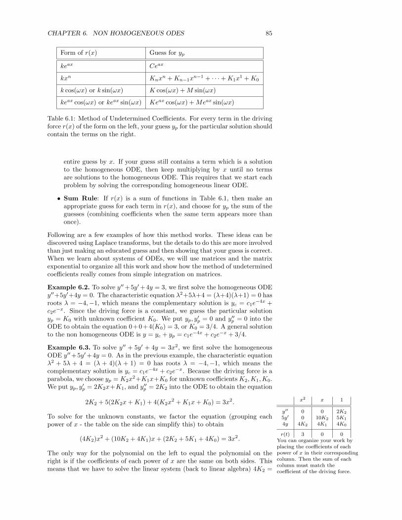
CHAPTER 6. NON HOMOGENEOUS ODES 85
Form of r(x) Guess for yp
keax Ceax
kxn Knxn +Kn−1x
n−1 + · · ·+K1x1 +K0
k cos(ωx) or k sin(ωx) K cos(ωx) +M sin(ωx)
keax cos(ωx) or keax sin(ωx) Keax cos(ωx) +Meax sin(ωx)
Table 6.1: Method of Undetermined Coefficients. For every term in the drivingforce r(x) of the form on the left, your guess yp for the particular solution shouldcontain the terms on the right.
entire guess by x. If your guess still contains a term which is a solutionto the homogeneous ODE, then keep multiplying by x until no termsare solutions to the homogeneous ODE. This requires that we start eachproblem by solving the corresponding homogeneous linear ODE.
• Sum Rule: If r(x) is a sum of functions in Table 6.1, then make anappropriate guess for each term in r(x), and choose for yp the sum of theguesses (combining coefficients when the same term appears more thanonce).
Following are a few examples of how this method works. These ideas can bediscovered using Laplace transforms, but the details to do this are more involvedthan just making an educated guess and then showing that your guess is correct.When we learn about systems of ODEs, we will use matrices and the matrixexponential to organize all this work and show how the method of undeterminedcoefficients really comes from simple integration on matrices.
Example 6.2. To solve y′′+5y′+4y = 3, we first solve the homogeneous ODEy′′+5y′+4y = 0. The characteristic equation λ2+5λ+4 = (λ+4)(λ+1) = 0 hasroots λ = −4,−1, which means the complementary solution is yc = c1e
−4x +c2e−x. Since the driving force is a constant, we guess the particular solution
yp = K0 with unknown coefficient K0. We put yp, y′p = 0 and y′′p = 0 into the
ODE to obtain the equation 0+0+4(K0) = 3, or K0 = 3/4. A general solutionto the non homogeneous ODE is y = yc + yp = c1e
−4x + c2e−x + 3/4.
Example 6.3. To solve y′′ + 5y′ + 4y = 3x2, we first solve the homogeneousODE y′′+5y′+4y = 0. As in the previous example, the characteristic equationλ2 + 5λ + 4 = (λ + 4)(λ + 1) = 0 has roots λ = −4,−1, which means thecomplementary solution is yc = c1e
−4x + c2e−x. Because the driving force is a
parabola, we choose yp = K2x2+K1x+K0 for unknown coefficients K2,K1,K0.
We put yp, y′p = 2K2x+K1, and y′′p = 2K2 into the ODE to obtain the equation
2K2 + 5(2K2x+K1) + 4(K2x2 +K1x+K0) = 3x2.
To solve for the unknown constants, we factor the equation (grouping each
x2 x 1
y′′ 0 0 2K2
5y′ 0 10K2 5K1
4y 4K2 4K1 4K0
r(t) 3 0 0You can organize your work byplacing the coefficients of eachpower of x in their correspondingcolumn. Then the sum of eachcolumn must match thecoefficient of the driving force.
power of x - the table on the side can simplify this) to obtain
(4K2)x2 + (10K2 + 4K1)x+ (2K2 + 5K1 + 4K0) = 3x2.
The only way for the polynomial on the left to equal the polynomial on theright is if the coefficients of each power of x are the same on both sides. Thismeans that we have to solve the linear system (back to linear algebra) 4K2 =
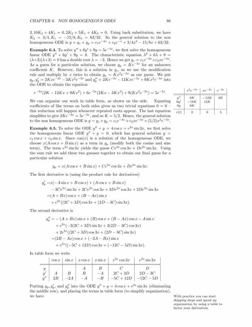
CHAPTER 6. NON HOMOGENEOUS ODES 86
3, 10K2 + 4K1 = 0, 2K2 + 5K1 + 4K0 = 0. Using back substitution, we haveK2 = 3/4,K1 = −15/8,K0 = 63/32. So the general solution to the nonhomogeneous ODE is y = yc + yp = c1e
−4x + c2e−x + 3/4x2 − 15/8x+ 63/32.
Example 6.4. To solve y′′ + 6y′ + 9y = 5e−3x, we first solve the homogeneouslinear ODE y′′ + 6y′ + 9y = 0. The characteristic equation λ2 + 6λ + 9 =(λ+3)(λ+3) = 0 has a double root λ = −3. Hence we get yc = c1e
−3x+c2xe−3x.
As a guess for a particular solution, we choose yp = Ke−3x for an unknowncoefficient K. However, this is a solution in yc, so we use the modificationrule and multiply by x twice to obtain yp = Kx2e−3x as our guess. We putyp, y
′p = 2Kxe−3x− 3Kx2e−3x and y′′p = 2Ke−3x− 12Kxe−3x + 9Kx2e−3x into
the ODE to obtain the equation
e−3x(2K − 12Kx+ 9Kx2) + 6e−3x(2Kx− 3Kx2) + 9(Kx2e−3x) = 5e−3x.
We can organize our work in table form, as shown on the side. Equating
x2e−3x xe−3x e−3x
y′′ 9K −12K 2K6y′ −18K 12K9y 9K
r(t) 0 0 5
coefficients of like terms on both sides gives us two trivial equations 0 = 0 –this reduction will happen whenever repeated roots appear. The last equationsimplifies to give 2Ke−3x = 5e−3x, and so K = 5/2. Hence, the general solutionto the non homogeneous ODE is y = yc+yp = c1e
−3x+c2xe−3x+(5/2)x2e−3x.
Example 6.5. To solve the ODE y′′ + y = 4 cosx + e2x sin 3x, we first solvethe homogeneous linear ODE y′′ + y = 0, which has general solution y =c1 cosx + c2 sinx. Since cos(x) is a solution of the homogeneous ODE, wechoose x(A cosx + B sinx) as a term in yp (modify both the cosine and sineterm). The term e2x sin 3x yields the guess Ce2x cos 3x + De2x sin 3x. Usingthe sum rule we add these two guesses together to obtain our final guess for aparticular solution
yp = x(A cosx+B sinx) + Ce2x cos 3x+De2x sin 3x.
The first derivative is (using the product rule for derivatives)
y′p =x(−A sinx+B cosx) + (A cosx+B sinx)
− 3Ce2x sin 3x+ 2Ce2x cos 3x+ 3De2x cos 3x+ 2De2x sin 3x
=(A+Bx) cosx+ (B −Ax) sinx
+ e2x((2C + 3D) cos 3x+ (2D − 3C) sin 3x).
The second derivative is
y′′p =− (A+Bx) sinx+ (B) cosx+ (B −Ax) cosx−A sinx
+ e2x(−3(2C + 3D) sin 3x+ 3(2D − 3C) cos 3x)
+ 2e2x((2C + 3D) cos 3x+ (2D − 3C) sin 3x)
=(2B −Ax) cosx+ (−2A−Bx) sinx
+ e2x((−5C + 12D) cos 3x+ (−12C − 5D) sin 3x).
In table form we write
cosx sinx x cosx x sinx e2x cos 3x e2x sin 3x
y A B C Dy′ A B B −A 2C + 3D 2D − 3Cy′′ 2B −2A −A −B −5C + 12D −12C − 5D
Putting yp, y′p, and y′′p into the ODE y′′ + y = 4 cosx + e2x sin 3x (eliminating
the middle row), and placing the terms in table form (to simplify organization),we have With practice you can start
skipping steps and speed uporganization by using a table tofactor your derivatives.

CHAPTER 6. NON HOMOGENEOUS ODES 87
cosx sinx x cosx x sinx e2x cos 3x e2x sin 3x
y′′ 2B −2A −A −B −5C + 12D −12C − 5Dy A B C D
r(t) 4 0 0 0 0 1
Summing the columns and equating coefficients gives the 4 non trivial equations2B = 4, −2A = 0, −4C + 12D = 0, −12C − 4D = 1 (notice that two of theequations vanished, which always happens when the modification rule is used).These four equations immediately shows that B = 2 and A = 0. Using Cramer’srule gives C = −3/40 and D = −1/40. The general solution is
y = yc + yp = c1 cosx+ c2 sinx+ 2x sinx− 3
40e2x cos 3x− 1
40e2x sin 3x.
6.4 Hooke’s Law Again
We now return to the mass-spring system where the driving force r(t) is notzero in the differential equation my′′ + cy′ + ky = r(t). We will examine aperiodic (with period 2π
ω ) driving force of the form r(t) = F0 cosωt for someconstants F0 and ω. The number ω is called the angular frequency. We will givea general solution to this ODE, and then explore how F0 and ω can influencethe solution. In particular, we will discover how resonance (large oscillations)can occur. The collapse of the Tacoma Narrows bridge in 1940 provides a visualillustration of how resonance must be accounted for in mechanical design, as theforces from wind generated vorticies pushed and pulled on the bridge structureat just the right frequency to cause the bridge to collapse (see wikipedia or Billah,
K.; R. Scanlan (1991). “Resonance, Tacoma Narrows Bridge Failure, and Undergraduate
Physics Textbooks”).The quadratic equation tells us that the zeros of the characteristic equation
mλ2 + cλ+ k = 0 are
λ =−c±
√c2 − 4mk
2m.
If c 6= 0, then the complementary solution will not contain a cosωx or sinωx,which means that the modification rule will not be needed when selecting yp.
If c = 0, then the roots are ±√k
m, so as long as
√k/m 6= ω we do not
need to worry about the modification rule. We’ll assume for the moment thatthe modification rule does not need to be used, and then consider the caseω =
√k/m afterwards.
Using the method of undetermined coefficients, we guess the solution
yp(t) = a cosωt+ b sinωt.
Differentiation gives
y′p(t) = −aω sinωt+ bω cosωt and y′′p (t) = −aω2 cosωt− bω2 sinωt.
Substitution into the ODE gives m(−aω2 cosωt − bω2 sinωt) + c(−aω sinωt +bω cosωt) + k(a cosωt + b sinωt) = F0 cosωt. Factoring the left side gives(−amω2 + bcω + ak) cosωt+ (−bmω2 − acω + bk) sinωt = F0 cosωt (the tableon the right organizes our work). Hence we have the linear system
cosωt sinωt
my′′ −amω2 −bmω2
cy′ bcω −acωky ak bk
r(t) F0 0
{(k −mω2)a+ bcω = F0
−acω + (k −mω2)b = 0→[(k −mω2) cω−cω (k −mω2)
] [ab
]=
[F0
0
],
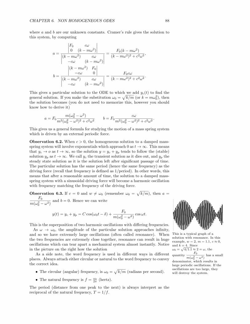
CHAPTER 6. NON HOMOGENEOUS ODES 88
where a and b are our unknown constants. Cramer’s rule gives the solution tothis system, by computing
a =
∣∣∣∣F0 cω0 (k −mω2)
∣∣∣∣∣∣∣∣(k −mω2) cω−cω (k −mω2)
∣∣∣∣ =F0(k −mω2)
(k −mω2)2 + c2ω2,
b =
∣∣∣∣(k −mω2) F0
−cω 0
∣∣∣∣∣∣∣∣(k −mω2) cω−cω (k −mω2)
∣∣∣∣ =F0cω
(k −mω2)2 + c2ω2.
This gives a particular solution to the ODE to which we add yc(t) to find thegeneral solution. If you make the substitution ω0 =
√k/m (or k = mω2
0), thenthe solution becomes (you do not need to memorize this, however you shouldknow how to derive it)
a = F0m(ω2
0 − ω2)
m2(ω20 − ω2)2 + c2ω2
b = F0cω
m2(ω20 − ω2)2 + c2ω2
.
This gives us a general formula for studying the motion of a mass spring systemwhich is driven by an external periodic force.
Observation 6.2. When c > 0, the homogeneous solution to a damped mass-spring system will involve exponentials which approach 0 as t→∞. This meansthat yc → o as t→∞, so the solution y = yc + yp tends to follow the (stable)solution yp as t→∞. We call yc the transient solution as it dies out, and yp thesteady state solution as it is the solution left after significant passage of time.The particular solution has the same period (hence the same frequency) as thedriving force (recall that frequency is defined as 1/period). In other words, thismeans that after a reasonable amount of time, the solution to a damped mass-spring system with a sinusoidal driving force will become a harmonic oscillationwith frequency matching the frequency of the driving force.
Observation 6.3. If c = 0 and w 6= ω0 (remember ω0 =√k/m), then a =
F0
m(ω20 − ω2)
and b = 0. Hence we can write
y(t) = yc + yp = C cos(ω0t− δ) +F0
m(ω20 − ω2)
cosωt.
This is the superposition of two harmonic oscillations with differing frequencies.As ω → ω0, the amplitude of the particular solution approaches infinity,
20 40 60 80 100 120 140
-15
-10
-5
5
10
15
This is a typical graph of asolution with resonance. In thisexample, w = 2, m = 1.1, c ≈ 0,and k = 4. Sinceω0 =
√4/1.1 ≈ 2 = ω, the
quantityF0
m(ω20 − ω2)
has a small
denominator, which results inlarge periodic oscillations. If theoscillations are too large, theywill destroy the system.
and so we have extremely large oscillations (often called resonance). Whenthe two frequencies are extremely close together, resonance can result in hugeoscillations which can tear apart a mechanical system almost instantly. Noticein the picture on the right how the solution
As a side note, the word frequency is used in different ways in differentplaces. Always attach either circular or natural to the word frequency to conveythe correct idea.
• The circular (angular) frequency, is ω0 =√k/m (radians per second).
• The natural frequency is f = ω0
2π (hertz).
The period (distance from one peak to the next) is always interpret as thereciprocal of the natural frequency, T = 1/f .
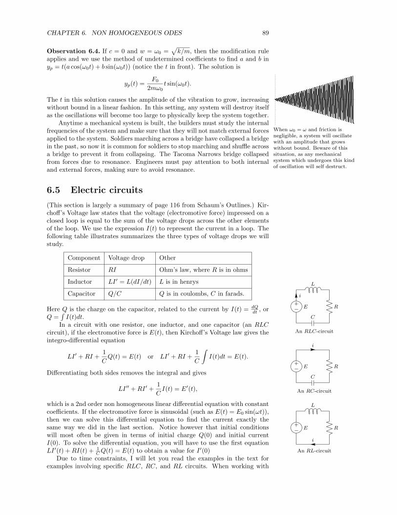
CHAPTER 6. NON HOMOGENEOUS ODES 89
Observation 6.4. If c = 0 and w = ω0 =√k/m, then the modification rule
applies and we use the method of undetermined coefficients to find a and b inyp = t(a cos(ω0t) + b sin(ω0t)) (notice the t in front). The solution is
yp(t) =F0
2mω0t sin(ω0t).
The t in this solution causes the amplitude of the vibration to grow, increasingwithout bound in a linear fashion. In this setting, any system will destroy itselfas the oscillations will become too large to physically keep the system together.
Anytime a mechanical system is built, the builders must study the internal
20 40 60 80 100 120 140
-100
-50
50
100
When ω0 = ω and friction isnegligible, a system will oscillatewith an amplitude that growswithout bound. Beware of thissituation, as any mechanicalsystem which undergoes this kindof oscillation will self destruct.
frequencies of the system and make sure that they will not match external forcesapplied to the system. Soldiers marching across a bridge have collapsed a bridgein the past, so now it is common for soldiers to stop marching and shuffle acrossa bridge to prevent it from collapsing. The Tacoma Narrows bridge collapsedfrom forces due to resonance. Engineers must pay attention to both internaland external forces, making sure to avoid resonance.
6.5 Electric circuits
(This section is largely a summary of page 116 from Schaum’s Outlines.) Kir-choff’s Voltage law states that the voltage (electromotive force) impressed on aclosed loop is equal to the sum of the voltage drops across the other elementsof the loop. We use the expression I(t) to represent the current in a loop. Thefollowing table illustrates summarizes the three types of voltage drops we willstudy.
Component Voltage drop Other
Resistor RI Ohm’s law, where R is in ohms
Inductor LI ′ = L(dI/dt) L is in henrys
Capacitor Q/C Q is in coulombs, C in farads.
Here Q is the charge on the capacitor, related to the current by I(t) = dQdt , or
Q =∫I(t)dt.
In a circuit with one resistor, one inductor, and one capacitor (an RLC
E R
i
L
C
An RLC-circuit
E R
i
C
An RC-circuit
E R
i
L
An RL-circuit
circuit), if the electromotive force is E(t), then Kirchoff’s Voltage law gives theintegro-differential equation
LI ′ +RI +1
CQ(t) = E(t) or LI ′ +RI +
1
C
∫I(t)dt = E(t).
Differentiating both sides removes the integral and gives
LI ′′ +RI ′ +1
CI(t) = E′(t),
which is a 2nd order non homogeneous linear differential equation with constantcoefficients. If the electromotive force is sinusoidal (such as E(t) = E0 sin(ωt)),then we can solve this differential equation to find the current exactly thesame way we did in the last section. Notice however that initial conditionswill most often be given in terms of initial charge Q(0) and initial currentI(0). To solve the differential equation, you will have to use the first equationLI ′(t) +RI(t) + 1
CQ(t) = E(t) to obtain a value for I ′(0)Due to time constraints, I will let you read the examples in the text for
examples involving specific RLC, RC, and RL circuits. When working with

CHAPTER 6. NON HOMOGENEOUS ODES 90
RC-circuits, you differentiate both sides to obtain a first order ODE, and initialconditions are generally given as initial charge. When working with an RL-circuit, you don’t need to differentiate E(t), and the initial current is generallygiven for initial conditions. One key observation to make is that when you aregiven initial conditions for the charge and current, you use these to find initialconditions for the current’s derivative. Even when Q(0) = 0 and I(0) = 0, wemay find that I ′(0) 6= 0. Use the equation involving Q to find I ′(0). (Problem14.13 provides an excellent example of how this can occur.)
6.6 Comparing the two models - saving money
Mechanical models are expensive to build. Electrical models are fairly simpleto build and measure. If you need to create a mechanical system, it mayprove beneficial financially to start with an electrical model. Engineers spendanother semester on this idea in system dynamics. Hydraulic systems are alsovery closely related. In bridging between mechanical and electrical systems, wecompare the following variables.
Mechanical System m c k r(t) = F0 cosωt y(t)
Electrical System L R 1/C E′(t) = E0ω cosωt I(t)
Solving a problem in one system (either mechanical or electrical) can provideuseful results in the other.
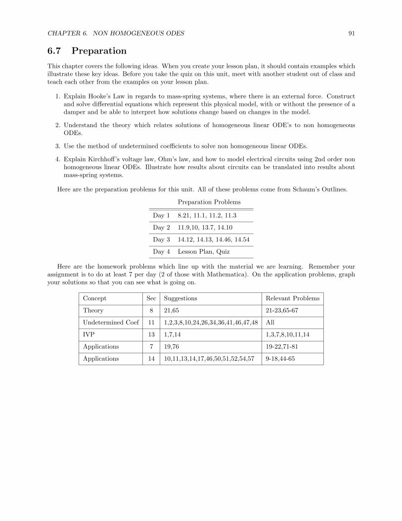
CHAPTER 6. NON HOMOGENEOUS ODES 91
6.7 Preparation
This chapter covers the following ideas. When you create your lesson plan, it should contain examples whichillustrate these key ideas. Before you take the quiz on this unit, meet with another student out of class andteach each other from the examples on your lesson plan.
1. Explain Hooke’s Law in regards to mass-spring systems, where there is an external force. Constructand solve differential equations which represent this physical model, with or without the presence of adamper and be able to interpret how solutions change based on changes in the model.
2. Understand the theory which relates solutions of homogeneous linear ODE’s to non homogeneousODEs.
3. Use the method of undetermined coefficients to solve non homogeneous linear ODEs.
4. Explain Kirchhoff’s voltage law, Ohm’s law, and how to model electrical circuits using 2nd order nonhomogeneous linear ODEs. Illustrate how results about circuits can be translated into results aboutmass-spring systems.
Here are the preparation problems for this unit. All of these problems come from Schaum’s Outlines.
Preparation Problems
Day 1 8.21, 11.1, 11.2, 11.3
Day 2 11.9,10, 13.7, 14.10
Day 3 14.12, 14.13, 14.46, 14.54
Day 4 Lesson Plan, Quiz
Here are the homework problems which line up with the material we are learning. Remember yourassignment is to do at least 7 per day (2 of those with Mathematica). On the application problems, graphyour solutions so that you can see what is going on.
Concept Sec Suggestions Relevant Problems
Theory 8 21,65 21-23,65-67
Undetermined Coef 11 1,2,3,8,10,24,26,34,36,41,46,47,48 All
IVP 13 1,7,14 1,3,7,8,10,11,14
Applications 7 19,76 19-22,71-81
Applications 14 10,11,13,14,17,46,50,51,52,54,57 9-18,44-65

Chapter 7
Laplace Transforms
This chapter covers the following ideas. When you create your lesson plan, itshould contain examples which illustrate these key ideas. Before you take thequiz on this unit, meet with another student out of class and teach each otherfrom the examples on your lesson plan.
1. Explain how to compute Laplace transforms and inverse Laplace trans-forms. Explain and use both shifting theorems, and be able to provethem.
2. Use Laplace transforms to solve IVP’s.
3. Describe the Dirac delta function, and use it in solving ODEs. Illustratewhat the Dirac delta function does to a system by applying it to examplesin mass-spring systems and electrical networks.
4. Explain what a convolution is, and how it relates to Laplace transforms.Be able to use the Transform theorems related to differentiating and in-tegrating functions or their transforms.
7.1 The big idea
The Laplace transform is a tool which became popular in the last 100 yearsbecause of the work of engineers. The Laplace transform has the ability toconvert a differential equation into an algebraic equation which can be solvedpurely with algebra. The Laplace transform can be applied to functions whichare not continuous, which makes it extremely useful in real world applications.For example, if a hammer hits a mass-spring system, or an electrical switchis turned on or off, the Laplace transform can handle the complications whichthese simple changes bring to an ODE. The methods we have learned beforerequire that our driving forces are continuously differentiable functions.
The big idea in this unit is a three step process.
1. Convert and ODE into an algebraic equation using the Laplace transform.
2. Solve the corresponding algebraic equation (which often means you haveto use a partial fraction decomposition and completing the square).
3. Use an inverse Laplace transform to find the solution of the ODE.
The first part of this unit will focus on finding Laplace transforms and theirinverses. The second part will focus on solving ODEs. The third part will focus
92

CHAPTER 7. LAPLACE TRANSFORMS 93
on what happens when we apply impulses to a system (such as a hammer blow,or a bolt of lightning). The fourth part will focus on some theoretical aspectsof the Laplace Transform.
7.2 Finding Laplace Transforms and Their In-verses
The Laplace transform of a function f(t) defined for t ≥ 0 is F (s) = L(f(t)) =∫∞0e−stf(t)dt. The function f(t) is called the inverse Laplace transform of
F (s), and we write f(t) = L−1(F (s)). As a notational convenience, we uselower case letters and t to describe original functions, and the same capitalletter and s to represent the Laplace transform. Provided the function f is“nice” (of exponential order, see pg 448), it will have a Laplace transform forlarge enough s.
7.2.1 Finding the Laplace Transform
If f(t) = 1, then F (s) =∫∞
0e−st1dt = e−st
−s∣∣∞0
= 1s , provided s > 0. If
f(t) = eat, then F (s) =∫∞
0e−steatdt =
∫∞0e−(s−a)tdt = e−(s−a)t
−(s−a)
∣∣∞0
= 1s−a ,
provided s > a. The improper integral computed with the Laplace transformwill normally exist only for certain values of s.
Since integration can be done term by term, we have L(af + bg) = aL(f) +bL(g) for functions f, g and constants a, b. We can use this to find manyother Laplace transforms without having to do any more integration. We
have L(cosh at) = 12L(eat + L(e−at)) = 1
2
(1s−a + 1
s+a
)= s
s2−a2 . Similarly
L(sinh at) = as2−a2 .
D I
+ cosωt e−st
− −ω sinωt e−st/(−s)+ −ω2 cosωt e−st/s2
Integration by parts twice yields L(cosωt) =s
s2+ω2 and L(sinωt) = ωs2+ω2 . To see
this, write L(cosωt) =∫∞
0e−st cosωtdt.
The tabular method gives∫∞
0e−st cosωtdt =(
cosωte−st/(−s) + ω sinωte−st/s2) ∣∣∞
0−∫∞
0ω2 cosωte−st/s2dt =
1/s − ω2/s2∫∞
0e−st cosωtdt, which means L(cosωt) = 1/s − ω2/s2L(cosωt).
This means (1 + ω2/s2)L(cosωt) = 1s , or (s2 + ω2)L(cosωt) = s or L(cosωt) =
ss2+ω2 . Integration by parts also shows that L(tn) = n!
sn+1 for integers n.For convenience, the following table summarizes the Laplace Transforms we
will use most often.
f(t) tn t0 = 1 eat cos(wt) sin(wt) cosh(wt) sinh(wt) u(t− a)
F(s) n!/sn+1 1/s 1/(s− a) s/(s2 + w2) w/(s2 + w2) s/(s2 − w2) w/(s2 − w2) e−as/ss > 0 s > 0 s > a s > 0 s > 0 s > |w| s > |w| s > 0
7.2.2 Finding an Inverse Laplace Transform
If the Laplace transforms of two functions are the same, then the two functionmust be the same as well. This allows us to invert the Laplace transform andobtain the only function with a given Laplace transform. Inverting a Laplacetransform often involves matching the transformed function up with a functionfrom a table, and then using the table to invert the transform.
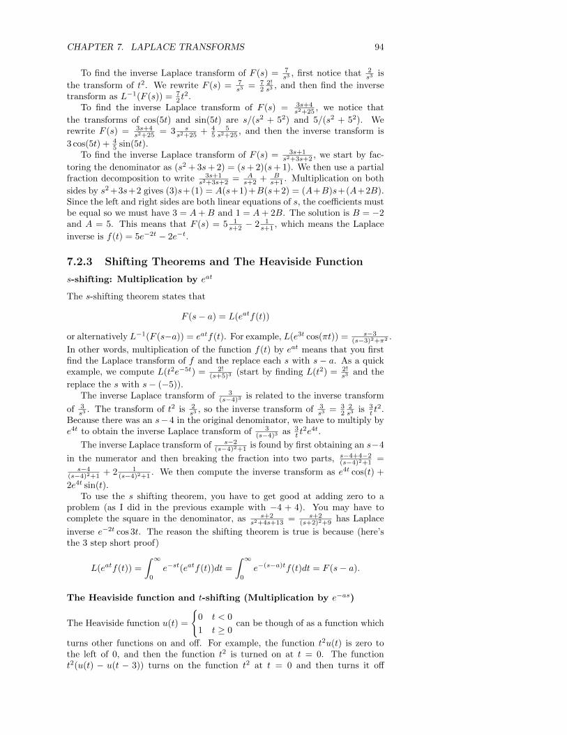
CHAPTER 7. LAPLACE TRANSFORMS 94
To find the inverse Laplace transform of F (s) = 7s3 , first notice that 2
s3 is
the transform of t2. We rewrite F (s) = 7s3 = 7
22!s3 , and then find the inverse
transform as L−1(F (s)) = 72 t
2.To find the inverse Laplace transform of F (s) = 3s+4
s2+25 , we notice that
the transforms of cos(5t) and sin(5t) are s/(s2 + 52) and 5/(s2 + 52). Werewrite F (s) = 3s+4
s2+25 = 3 ss2+25 + 4
55
s2+25 , and then the inverse transform is
3 cos(5t) + 45 sin(5t).
To find the inverse Laplace transform of F (s) = 3s+1s2+3s+2 , we start by fac-
toring the denominator as (s2 + 3s+ 2) = (s+ 2)(s+ 1). We then use a partialfraction decomposition to write 3s+1
s2+3s+2 = As+2 + B
s+1 . Multiplication on both
sides by s2 +3s+2 gives (3)s+(1) = A(s+1)+B(s+2) = (A+B)s+(A+2B).Since the left and right sides are both linear equations of s, the coefficients mustbe equal so we must have 3 = A+B and 1 = A+ 2B. The solution is B = −2and A = 5. This means that F (s) = 5 1
s+2 − 2 1s+1 , which means the Laplace
inverse is f(t) = 5e−2t − 2e−t.
7.2.3 Shifting Theorems and The Heaviside Function
s-shifting: Multiplication by eat
The s-shifting theorem states that
F (s− a) = L(eatf(t))
or alternatively L−1(F (s−a)) = eatf(t). For example, L(e3t cos(πt)) = s−3(s−3)2+π2 .
In other words, multiplication of the function f(t) by eat means that you firstfind the Laplace transform of f and the replace each s with s − a. As a quickexample, we compute L(t2e−5t) = 2!
(s+5)3 (start by finding L(t2) = 2!s3 and the
replace the s with s− (−5)).The inverse Laplace transform of 3
(s−4)3 is related to the inverse transform
of 3s3 . The transform of t2 is 2
s3 , so the inverse transform of 3s3 = 3
22s3 is 3
t t2.
Because there was an s− 4 in the original denominator, we have to multiply bye4t to obtain the inverse Laplace transform of 3
(s−4)3 as 3t t
2e4t.
The inverse Laplace transform of s−2(s−4)2+1 is found by first obtaining an s−4
in the numerator and then breaking the fraction into two parts, s−4+4−2(s−4)2+1 =
s−4(s−4)2+1 + 2 1
(s−4)2+1 . We then compute the inverse transform as e4t cos(t) +
2e4t sin(t).To use the s shifting theorem, you have to get good at adding zero to a
problem (as I did in the previous example with −4 + 4). You may have tocomplete the square in the denominator, as s+2
s2+4s+13 = s+2(s+2)2+9 has Laplace
inverse e−2t cos 3t. The reason the shifting theorem is true is because (here’sthe 3 step short proof)
L(eatf(t)) =
∫ ∞0
e−st(eatf(t))dt =
∫ ∞0
e−(s−a)tf(t)dt = F (s− a).
The Heaviside function and t-shifting (Multiplication by e−as)
The Heaviside function u(t) =
{0 t < 0
1 t ≥ 0can be though of as a function which
turns other functions on and off. For example, the function t2u(t) is zero tothe left of 0, and then the function t2 is turned on at t = 0. The functiont2(u(t) − u(t − 3)) turns on the function t2 at t = 0 and then turns it off

CHAPTER 7. LAPLACE TRANSFORMS 95
at t = 3. The Heaviside function can be used to piece together piecewisecontinuous functions by using this “on-off” approach. For example, the function
f(t) =
0 t < 0
t2 0 ≤ t ≤ 1
2− t 1 < t ≤ πcos t π < t
can be written using the Heaviside function as f(t) =
t2[u(t) − u(t − 1)] + (2 − t)[u(t − 1) − u(t − π)] + cos t[u(t − π)]. This sectiondescribes how to compute Laplace transforms and inverse transforms of suchpiecewise defined functions. Such functions are needed to model turning ona switch in an electrical network, modifying the driving force in a mechanicalspring system, and many other practical applications.
The t-shifting theorem states
L(f(t− a)u(t− a)) = e−asF (s)
or L−1(e−asF (s)) = f(t − a)u(t − a), where F (s) = L(f(t)). This theorem iseasiest to use when computing inverse transforms, as it says that multiplicationof F (s) by e−as means that you multiply the inverse of F (s) by u(t) and thenreplace all the t’s with t− a. For example we can find the inverse transform ofF (s) = 2
s2+4e−3s by first noting that the inverse transform of 2
s2+4 is sin(2t),
and so we multiply by u(t) and replace each t with t−3 to obtain L−1(F (s)) =sin(2(t − 3))u(t − 3). This is just the curve sin(2t) which has been shifted 3units to the right and turned on at t = 3.
Notice that the t-shifting theorem has an e−as, while the s shifting the-orem has an eat. Pay attention to this sign difference. The reason the t-shifting theorem is true is because
∫∞0f(t − a)u(t − a)e−stdt =
∫∞af(t −
a)e−stdt. By the substitution w = (t − a), this becomes∫∞
0f(w)e−sw+adw =
e−as∫∞
0f(w)e−swdw = e−asF (s). Again it is a fairly short proof.
To use the t-shifting theorem to compute forward Laplace transforms, youhave to rewrite f(t) in terms of t−a. For example, the function t2 for t > 1 and0 otherwise is written f(t) = t2u(t−1). To use the second shifting theorem, wewrite f(t) = t2u(t−1) = ((t−1)+1)2u(t−1) = ((t−1)2 +2(t−1)+1)2u(t−1).Notice how I purposefully inserted a −1+1 next to the t. The shifting theoremthen gives F (s) =
(2s3 + frac2s2 + 1
s
)e−s. Our function f(t − 1) = (t − 1)2 +
2(t − 1) + 1 is simply f(t) = t2 + 2t + 1 whose transform is 2s3 + frac2s2 + 1
s ,which we then multiply by e−s to complete the transform. An alternate versionof this transformation uses the formula
L(f(t)u(t− a)) = e−asL(f(t+ a))
(meaning replace each t with t + a and then find the transform and multiplyby e−as). This formula shows that L(t2u(t− 1)) = e−sL((t+ 1)2) = e−sL(t2 +2t+ 1)) = e−s
(2s3 + 2
s2 + 1s
)as before.
Both shifting theorems can be applied simultaneously. If F (s) = (s−3)e−2s
(s−3)2+ω2 ,
then without the e−2s the inverse transform would be e3t cos(ωt) by the s-shifting theorem. The t-shifting theorem says that the inverse transform ise3(t−2) cos(ω(t − 2))u(t − 2) (multiply by u(t) and then replace each t witht − 2). Remember that with the s shifting theorem you change the sign, butwith the t shifting theorem you do not. This is the most common mistake.

CHAPTER 7. LAPLACE TRANSFORMS 96
7.3 Solving IVPs
7.3.1 The Transform of a derivative
The Laplace transform of a derivative is, using integration by parts,
L(f ′) =
∫ ∞0
e−stf ′(t)dt = (e−stf(t))∣∣∞0
+ s
∫ ∞0
e−stf(t)dt = sL(f)− f(0).
We can use this formula to get
L(f ′′) = sL(f ′)− f ′(0) = s[sL(f)− f(0)]− f ′(0) = s2L(f)− sf(0)− f ′(0).
These two formulas can be used to find new Laplace transforms and (mostimportantly) solve ODEs.
7.3.2 Solving IVPs - Lots of examples
We can use the differentiation theorem to solve IVPs. Given an ODE, take theLaplace transform of each side, giving what is called the subsidiary equation.This equation can be solved for L(y) = Y (s) using only algebra. You thencompute L−1(Y (s)) to find the solution to the IVP y(t). This may involvefinding a partial fraction decomposition. Laplace transforms reduce many IVPsto a 3 step process (1) convert to the subsidiary equation, (2) use algebra tosolve for Y , performing a partial fraction decomposition if needed, (3) findinverse Laplace transform.
To solve the homogeneous IVP y′ + 2y = 0, y(0) = 1 we start by takingthe Laplace transform of each side. This gives the subsidiary equation sL(y)−y(0) + 2L(y) = 0, or using the notation L(y) = Y , we have sY − 1 + 2Y = 0.Solving for Y gives the equation Y = 1
s+2 . The inverse Laplace transform of
both sides gives y(t) = e−2t.To solve the nonhomogeneous IVP y′ + 2y = 3, y(0) = 1, take the Laplace
transform of each side. This gives the subsidiary equation sY − 1 + 2Y = 3s .
Solving for Y gives the equation Y = s+3s(s+2) . The partial fraction decomposition
s+3s(s+2) = A
s + Bs+2 requires we solve s+ 3 = A(s+ 2) +Bs, or 1 = A+B, 3 = 2A
giving A = 3/2 and B = −1/2. Our subsidiary equation is now Y = 32
1s−
12
1s+2 .
The inverse Laplace transform of both sides gives y(t) = 32 −
12e−2t. These two
examples represent the basic ideas used to solve pretty much every Laplacetransform problem.
Now for a problem with a Heaviside function. Consider the IVP y′′ + 4y =u(t − 5), y(0) = 0, y′(0) = 1, which represents a mass-spring system with nofriction which has a constant driving force of magnitude 3 applied at time t = 5.Take the Laplace transform of each side to obtain. s2Y − sy(0)− y′(0) + 4Y =e−4s
s or (s2 + 4)Y = 1 + e−5s
s . Solving for Y gives the equation Y = 1s2+4 +
1s(s2+4)e
−5s. The partial fraction decomposition 1s(s2+4) = A
s + Bs+Cs2+4 becomes
0s2 +0s+1 = A(s2 +4)+Bs2 +Cs = (A+B)s2 +(C)s+(4A). We obtain the 3equations 0 = A+B, 0 = C, 1 = 4A whose solution is A = 1/4, B = −1/4, C =
0. Our subsidiary equation is now Y = 12
2s2+4 +
[14
1s −
14
ss2+4
]e−5s. The inverse
Laplace transform of both sides gives y(t) = 12 sin(2t)+[ 1
4−14 cos(2(t−5))]u(t−
5), using the t-shifting theorem.For a more involved example, to solve the IVP y′′+ 4y′+ 3y = 30e2t, y(0) =
1, y′(0) = 3, take the Laplace transform of each side. This gives the subsidiaryequation s2Y − sy(0) − y′(0) + 4(sY − y(0)) + 3Y = 30
s−2 . Solving for Y gives
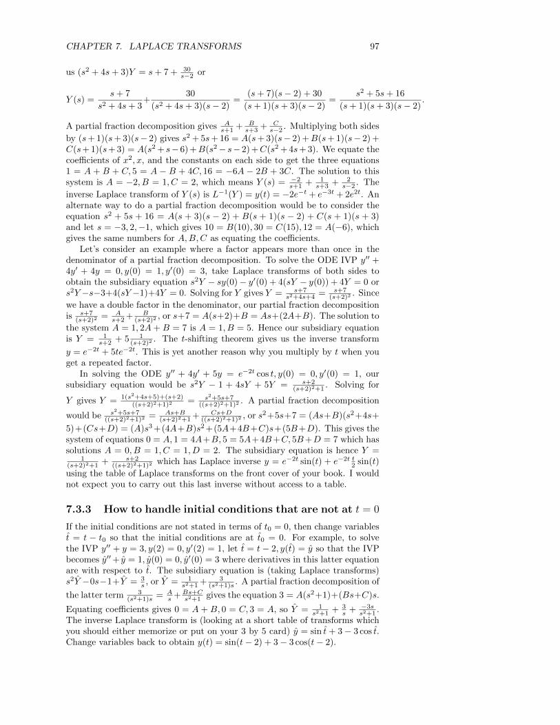
CHAPTER 7. LAPLACE TRANSFORMS 97
us (s2 + 4s+ 3)Y = s+ 7 + 30s−2 or
Y (s) =s+ 7
s2 + 4s+ 3+
30
(s2 + 4s+ 3)(s− 2)=
(s+ 7)(s− 2) + 30
(s+ 1)(s+ 3)(s− 2)=
s2 + 5s+ 16
(s+ 1)(s+ 3)(s− 2).
A partial fraction decomposition gives As+1 + B
s+3 + Cs−2 . Multiplying both sides
by (s+ 1)(s+ 3)(s− 2) gives s2 + 5s+ 16 = A(s+ 3)(s− 2) +B(s+ 1)(s− 2) +C(s+ 1)(s+ 3) = A(s2 + s− 6) +B(s2− s− 2) +C(s2 + 4s+ 3). We equate thecoefficients of x2, x, and the constants on each side to get the three equations1 = A + B + C, 5 = A − B + 4C, 16 = −6A − 2B + 3C. The solution to thissystem is A = −2, B = 1, C = 2, which means Y (s) = −2
s+1 + 1s+3 + 2
s−2 . The
inverse Laplace transform of Y (s) is L−1(Y ) = y(t) = −2e−t + e−3t + 2e2t. Analternate way to do a partial fraction decomposition would be to consider theequation s2 + 5s + 16 = A(s + 3)(s − 2) + B(s + 1)(s − 2) + C(s + 1)(s + 3)and let s = −3, 2,−1, which gives 10 = B(10), 30 = C(15), 12 = A(−6), whichgives the same numbers for A,B,C as equating the coefficients.
Let’s consider an example where a factor appears more than once in thedenominator of a partial fraction decomposition. To solve the ODE IVP y′′ +4y′ + 4y = 0, y(0) = 1, y′(0) = 3, take Laplace transforms of both sides toobtain the subsidiary equation s2Y − sy(0)− y′(0) + 4(sY − y(0)) + 4Y = 0 ors2Y −s−3+4(sY −1)+4Y = 0. Solving for Y gives Y = s+7
s2+4s+4 = s+7(s+2)2 . Since
we have a double factor in the denominator, our partial fraction decompositionis s+7
(s+2)2 = As+2 + B
(s+2)2 , or s+7 = A(s+2)+B = As+(2A+B). The solution to
the system A = 1, 2A+B = 7 is A = 1, B = 5. Hence our subsidiary equationis Y = 1
s+2 + 5 1(s+2)2 . The t-shifting theorem gives us the inverse transform
y = e−2t + 5te−2t. This is yet another reason why you multiply by t when youget a repeated factor.
In solving the ODE y′′ + 4y′ + 5y = e−2t cos t, y(0) = 0, y′(0) = 1, oursubsidiary equation would be s2Y − 1 + 4sY + 5Y = s+2
(s+2)2+1 . Solving for
Y gives Y = 1(s2+4s+5)+(s+2)((s+2)2+1)2 = s2+5s+7
((s+2)2+1)2 . A partial fraction decomposition
would be s2+5s+7((s+2)2+1)2 = As+B
(s+2)2+1 + Cs+D((s+2)2+1)2 , or s2+5s+7 = (As+B)(s2+4s+
5)+(Cs+D) = (A)s3 +(4A+B)s2 +(5A+4B+C)s+(5B+D). This gives thesystem of equations 0 = A, 1 = 4A+B, 5 = 5A+4B+C, 5B+D = 7 which hassolutions A = 0, B = 1, C = 1, D = 2. The subsidiary equation is hence Y =
1(s+2)2+1 + s+2
((s+2)2+1)2 which has Laplace inverse y = e−2t sin(t) + e−2t t2 sin(t)
using the table of Laplace transforms on the front cover of your book. I wouldnot expect you to carry out this last inverse without access to a table.
7.3.3 How to handle initial conditions that are not at t = 0
If the initial conditions are not stated in terms of t0 = 0, then change variablest = t − t0 so that the initial conditions are at t0 = 0. For example, to solvethe IVP y′′ + y = 3, y(2) = 0, y′(2) = 1, let t = t− 2, y(t) = y so that the IVPbecomes y′′+ y = 1, y(0) = 0, y′(0) = 3 where derivatives in this latter equationare with respect to t. The subsidiary equation is (taking Laplace transforms)s2Y −0s−1+Y = 3
s , or Y = 1s2+1 + 3
(s2+1)s . A partial fraction decomposition of
the latter term 3(s2+1)s = A
s +Bs+Cs2+1 gives the equation 3 = A(s2+1)+(Bs+C)s.
Equating coefficients gives 0 = A + B, 0 = C, 3 = A, so Y = 1s2+1 + 3
s + −3ss2+1 .
The inverse Laplace transform is (looking at a short table of transforms whichyou should either memorize or put on your 3 by 5 card) y = sin t+ 3− 3 cos t.Change variables back to obtain y(t) = sin(t− 2) + 3− 3 cos(t− 2).

CHAPTER 7. LAPLACE TRANSFORMS 98
7.4 Impulses and the Dirac Delta function δ(t−a)
The Dirac delta function is defined as the “function” δ(t − a) =
{0 t 6= a
∞ t = a,
which satisfies∫∞
0δ(t − a)dt = 1, and has the sifting property
∫∞0g(t)δ(t −
a)dt = g(a). I put “function” in quotes because Dirac delta is really a “distri-bution,” and is technically studied using limits. Consider the function fk(t−a)which has value k for a < t < t + 1
k , yet is zero elsewhere. The integral∫∞0fk(t)dt =
∫ a+1/k
akdt = 1 for all k, so the function fk(t − a) is essentially
a short impulse of magnitude k over a time interval of length 1/k (so that thetotal area under the curve is 1). The Dirac delta distribution is studied byconsidering limits of fk as k → ∞. The limit lim
k→∞fk(t − a) is point-wise the
zero function, so it should have no area underneath. The Dirac delta functionis defined so that it behaves like the limit of the fk functions, but has a posi-tive area under it when your integral bounds include a. The reason we studythis function is because it is used to describe events which happen instanta-neously as in a hammer blow, flickering a light switch, when lightning strikes,or if a driving force is applied instantaneously at t = a. In other words, ifthe force is turned on and then off essentially instantaneously, then the Diracdelta “function” is used instead of the Heaviside function. The Laplace trans-form of the Dirac delta distribution comes easily from the “sifting” property,as∫∞
0e−stδ(t− a)dt = e−as.
One way of thinking about the Dirac delta distribution is that it representsderivative of the unit impulse function. The IVP y′ = δ(t − 3), y(0) = 0 hassubsidiary equation sY = e−3s or Y = 1
se−3s. The Laplace inverse is y(t) =
u(t−3). In other words, at time 3 a hammer hits the constant solution y(t) = 0and causes a jump upwards of 1 unit. The derivative of such a jump is undefinedin terms of what we learned in first semester calculus, but the Dirac deltadistribution allows us to define the “derivative” of a jump discontinuity. TheIVP y′ = 4δ(t − 3), y(0) = 0 would have solution y = 4u(t − 3) which wouldresult in a jump upwards of 4 units.
As an example, the IVP y′′+ 2y′+ 2y = (1−u(t− 3))et + 30δ(t− 6), y(0) =0, y′(0) = 0 has an input force equal to et for 0 < t < 3, and then at t = 6it receives an impulse of 30 units. The corresponding subsidiary equation iss2Y −0s−0 + 2sY −0 + 2Y = 1
s−1 + e−3sL(et+3) + 30e−6s, or (s2 + 2s+ 2)Y =1s−1−e
−3se3 1s−1 +30e−6s. Since the zeros of s2+2s+2 are imaginary, we cannot
factor it any further and so we complete the square to obtain s2 + 2s + 2 =(s+ 1)2 + 1. We have
Y (s) =1
(s− 1)((s+ 1)2 + 1)−e−3se3 1
(s− 1)((s+ 1)2 + 1)+30e−6s 1
(s+ 1)2 + 1.
Partial fractions gives1
(s− 1)((s+ 1)2 + 1)=
A
s− 1+B(s+ 1) + C
(s+ 1)2 + 1, where I
purposefully wrote B(s + 1) + C as we will have to get a multiple of s + 1in the numerator anyways when we compute the inverse transform which willinvolve the first shifting theorem and a cosine. Multiplying both sides by thedenominator on the left gives 1 = A(s2 + 2s + 2) + (B(s + 1) + C)(s − 1) =s2(A + B) + s(2A + B + C) + (2A − B − C), which means 0 = A + B, 0 =2A + C, 1 = 2A − B − C. So B = −A,C = −2A, and the solution is A =1/5, B = −1/5, C = −2/5. This means we can write

CHAPTER 7. LAPLACE TRANSFORMS 99
Y (s) =(
15(s−1) −
(s+1)5((s+1)2+1) −
25((s+1)2+1)
)y(t) =
(15et − 1
5e−t cos(t)− 2
5e−t sin(t)
)−e−3se3
(1
5(s−1) −(s+1)
5((s+1)2+1) −2
5((s+1)2+1)
)−e3u(t− 3)
(15et−3 − 1
5e−(t−3) cos(t− 3)− 2
5e−(t−3) sin(t− 3)
)+30e−6s 1
(s+1)2+1 +30e−(t−6) sin(t− 6)
I will be creating more problems for you to practice these ideas. Once theproblems are made, I will email you and let you know where to get them. Mostof the problems related to the Dirac delta distribution will involve mass springsystems, or electrical networks.
7.5 Convolutions, and Transfer Theorems
7.5.1 Convolutions
The Laplace transform of the product f · g of two functions is not the productof the Laplace transforms of each (L(fg) 6= L(f)L(g)). Instead, the Laplace
inverse of H(s) = L(f)L(g) is equal to a quantity h(t) = f ∗g(t) =∫ t
0f(p)g(t−
p)dp called the convolution of f and g (the proof involves interchanging theorder of integration on a double integral). The variable p is a dummy variableof integration, and could be called anything else (some books uses τ , but I findit really hard to distinguish between t and τ when I’m writing on paper, soI use p instead). The convolution satisfies various properties (commutative,distributive, associative), however f ∗ 1 6= f , and f ∗ f may be negative.
If H(s) = 1s2(s−1) = 1
s21s−1 = F (s)G(s), where f(t) = t and g(t) =
et, then the inverse Laplace transform of H(s) is the convolution of f and
g. We compute h(t) =∫ t
0pet−pdp = et
∫ t0pe−pdp = et (−pe−p − e−p)
∣∣t0
=et (−te−t − e−t + 1) = −t−1+et. The convolution is an alternate approach (in-stead of a partial fraction decomposition) to finding inverse Laplace transforms.A mass-spring system with ODE my′′ + cy′ + ky = f(t), y(0) = 0, y′(0) = 0has subsidiary equation s2mY + scY + kY = F (s) or Y = 1
ms2+cs+kF (s) =W (s)F (s), where W (s) is called the transfer function of the system. Engineersoften study mass-spring systems by letting w(t) = L−1(W (s)) (called the weightfunction) and then writing the solution using the convolution y(t) = w(t)∗f(t).This gives an extremely easy way to represent the solution of a mass-springsystem, with a single integral (though the integral may be rather complex).This formula is called Duhamel’s principle for the system.
7.5.2 Transform Theorems
The transfer theorems we will focus on essentially give us rules for computingtransforms and inverse transforms of derivatives an integrals. The key transformtheorem we have already been using is L(y′) = sY − y(0). We will now look atL(∫ydt), L−1(F ′(s)), and L−1(
∫F (s)ds).
The Laplace transform of f ∗ 1 =∫ t
0f(p)1dp is F (s)
s , which is immedi-
ate by the convolution theorem since L(1) = 1s . This can be used to find
transforms of integrals, namely L(∫ t
0f(t)dt) = F
s (remember that the trans-form of a derivative resulted in multiplying by s, so it seems reasonable thetransform of an integral should involve division by s). Remember that the
voltage drop due to a capacitor is V = QC , where Q(t) =
∫ t0I(t)dt for the
current I(t). Hence the charge is Q(t) = I(t) ∗ 1, the convolution of i and
1, which means that Q(s)C = I
sC . Hence the subsidiary equation of the ODE

CHAPTER 7. LAPLACE TRANSFORMS 100
LI ′+RI+ QC = E(t) for a power source supplying E(t) volts with I(0) = 0 and
Q(0) = 0 is L(sI − I(0)) +RL(I) + L(I)sC = L(E).
The derivative of a transform satisfies the rule L(−tf(t)) = F ′(s). This can
be used to show that L(−t cos(t)) = dds
ss2+1 = 1−s2
(s2+1)2 , or that L(−t sin(wt)) =dds
ws2+w2 = 2ws
(s2+w2)2 (which we used in one of the examples early on in the unit).
The integral of a transform satisfies the rule L(f(t)t
)=∫∞sF (p)dp, pro-
vided limt→0+f(t)t exists and is finite. I will provide more examples of this as
time goes on.There are many other things known about Laplace transforms. This is
just an introduction to the subject. Laplace transforms replace ODEs withequations which can be solved algebraically. Some people argue that for thisreason Laplace transforms are more advantageous than the classical methodswe previously learned. You trade the method of undetermined coefficients for apartial fraction decomposition. You trade solving the homogeneous system forfactoring the denominator before performing the partial fraction decomposition.Initial values are automatically taken care of which is nice when using Laplacetransforms. In addition, Laplace transforms increase the types of functions youcan include as inputs to an ODE, so that non continuous functions and impulsescan be included.
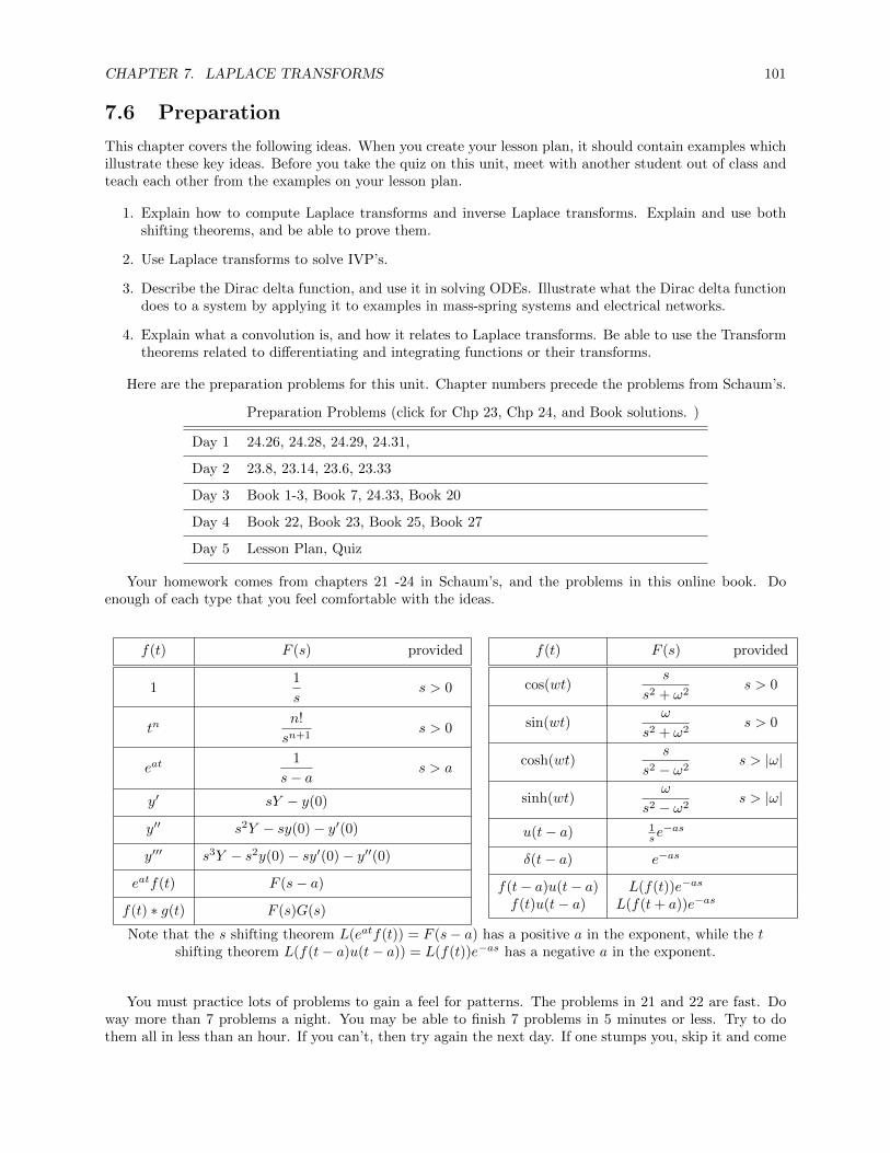
CHAPTER 7. LAPLACE TRANSFORMS 101
7.6 Preparation
This chapter covers the following ideas. When you create your lesson plan, it should contain examples whichillustrate these key ideas. Before you take the quiz on this unit, meet with another student out of class andteach each other from the examples on your lesson plan.
1. Explain how to compute Laplace transforms and inverse Laplace transforms. Explain and use bothshifting theorems, and be able to prove them.
2. Use Laplace transforms to solve IVP’s.
3. Describe the Dirac delta function, and use it in solving ODEs. Illustrate what the Dirac delta functiondoes to a system by applying it to examples in mass-spring systems and electrical networks.
4. Explain what a convolution is, and how it relates to Laplace transforms. Be able to use the Transformtheorems related to differentiating and integrating functions or their transforms.
Here are the preparation problems for this unit. Chapter numbers precede the problems from Schaum’s.
Preparation Problems (click for Chp 23, Chp 24, and Book solutions. )
Day 1 24.26, 24.28, 24.29, 24.31,
Day 2 23.8, 23.14, 23.6, 23.33
Day 3 Book 1-3, Book 7, 24.33, Book 20
Day 4 Book 22, Book 23, Book 25, Book 27
Day 5 Lesson Plan, Quiz
Your homework comes from chapters 21 -24 in Schaum’s, and the problems in this online book. Doenough of each type that you feel comfortable with the ideas.
f(t) F (s) provided
11
ss > 0
tnn!
sn+1s > 0
eat1
s− as > a
y′ sY − y(0)
y′′ s2Y − sy(0)− y′(0)
y′′′ s3Y − s2y(0)− sy′(0)− y′′(0)
eatf(t) F (s− a)
f(t) ∗ g(t) F (s)G(s)
f(t) F (s) provided
cos(wt)s
s2 + ω2s > 0
sin(wt)ω
s2 + ω2s > 0
cosh(wt)s
s2 − ω2s > |ω|
sinh(wt)ω
s2 − ω2s > |ω|
u(t− a) 1se−as
δ(t− a) e−as
f(t− a)u(t− a) L(f(t))e−as
f(t)u(t− a) L(f(t+ a))e−as
Note that the s shifting theorem L(eatf(t)) = F (s− a) has a positive a in the exponent, while the tshifting theorem L(f(t− a)u(t− a)) = L(f(t))e−as has a negative a in the exponent.
You must practice lots of problems to gain a feel for patterns. The problems in 21 and 22 are fast. Doway more than 7 problems a night. You may be able to finish 7 problems in 5 minutes or less. Try to dothem all in less than an hour. If you can’t, then try again the next day. If one stumps you, skip it and come

CHAPTER 7. LAPLACE TRANSFORMS 102
back later. Once you feel confident, chapters 23 (on convolutions and the heaviside function) and 24 (solvingIVPS) will help you use the Laplace transforms to solve ODEs. The online book contains some additionalproblems to help you cement your understanding. I’ve included a table that summarizes the transforms weuse most often.
7.7 Problems
Make sure you try some of each type of problem from chapters 21-24 (except for the last set of problems in23). The new ideas involve convolutions and the Heaviside (unit step) function in 23. Once you have triedsome of each of these, use this page to give you more practice.
I Find the Laplace transform of each of the following, and use Mathematica to check your answer.
1. f(x) = 8e−3x cos 2x− 4e4x sin 5x+ 3e7xx5
2. f(x) = xu(x− 4) + δ(x− 6)
3. f(x) = e3xu(x− 2) + 7δ(x− 4)
II Find the inverse Laplace transform of each of the following, and use Mathematica to check your answer.Many of these will require you to use a partial fraction decomposition.
4.s
(s+ 3)2 + 25+
2
(s− 2)4e−3s
5.s
s2 + 4s+ 13e−4s
6.1
s(s2 + 1)e−5s
7.1
s2(s2 + 1)e−3s
8.2s+ 1
(s− 1)2(s+ 1)e−7s
9.1
(s− 1)(s+ 2)(s− 3)e−4s
III Use Laplace transforms to find the position y(t) of an object or current current I(t) in each of thefollowing scenarios. I will give you the constants m, c, k and the driving force r(t), or I will give youthe inductance L, resistance R, capacitance C, and voltage source E(t), as well as any relevant initialconditions. Your job is to use Laplace transforms to find the solution. Use Mathematica to checkyour solution, and draw the graph of y(t) or I(t) and the steady-state (steady periodic) solution to seehow the Heaviside and Dirac delta functions affect the graph. The point here is to see these two newfunctions affect solutions. I suggest that you do all of these problems with the computer, so you canquickly see the effects of a Heaviside function or Dirac delta distribution.
10. m = 1, c = 0, k = 4, r(t) = u(t− 1), y(0) = 1, y′(0) = 0
11. m = 1, c = 0, k = 4, r(t) = δ(t− 3), y(0) = 1, y′(0) = 0
12. m = 1, c = 0, k = 4, r(t) = 7u(t− 3), y(0) = 1, y′(0) = 0
13. m = 1, c = 0, k = 4, r(t) = 7u(t− 3) + 11δ(t− 5), y(0) = 1, y′(0) = 0
14. m = 1, c = 0, k = 4, r(t) = 7tu(t− 3), y(0) = 1, y′(0) = 0
15. m = 1, c = 0, k = 4, r(t) = 7, y(0) = 1, y′(0) = 0

CHAPTER 7. LAPLACE TRANSFORMS 103
16. m = 1, c = 0, k = 4, r(t) = 7, y(π) = 1, y′(π) = 0
17. m = 1, c = 3, k = 2, r(t) = u(t− 2), y(0) = 0, y′(0) = 0
18. m = 1, c = 3, k = 2, r(t) = δ(t− 2), y(0) = 0, y′(0) = 0
19. m = 1, c = 3, k = 2, r(t) = 4u(t− 1), y(0) = 0, y′(0) = 0
20. m = 1, c = 3, k = 2, r(t) = 4u(t− 1) + 10δ(t− 2), y(0) = 0, y′(0) = 0
21. m = 1, c = 3, k = 2, r(t) = 4tu(t− 1), y(0) = 0, y′(0) = 0
22. L = 0, R = 2, C = 1/5, E(t) = 12u(t− 2), Q(0) = 0 (use first order ODE)
23. L = 1, R = 2, C = 0, E(t) = 12u(t− 2), I(0) = 0 (use first order ODE)
24. L = 1, R = 2, C = 1/5, E(t) = 12, Q(0) = 0, I(0) = 0 (first find I ′(0).)
25. L = 1, R = 2, C = 1/5, E(t) = 12u(t− 2), Q(0) = 0, I(0) = 0
26. L = 1, R = 2, C = 1/5, E(t) = e3tu(t− 2), Q(0) = 0, I(0) = 0
27. L = 1, R = 2, C = 1/5, E(t) = 4 cos(3t), Q(0) = 0, I(0) = 0
28. L = 1, R = 4, C = 1/4, E(t) = u(t− 3), Q(0) = 0, I(0) = 0
29. L = 1, R = 4, C = 1/4, E(t) = e−2t, Q(0) = 0, I(0) = 0
IV Find transforms and inverse transforms of the following, using the transform theorems.
30. We will skip this section. Don’t worry about this objective.
Chapter 8
Power Series
This chapter covers the following ideas. When you create your lesson plan, itshould contain examples which illustrate these key ideas. Before you take thequiz on this unit, meet with another student out of class and teach each otherfrom the examples on your lesson plan.
1. Find and explain the use of Taylor polynomials, Talyor series, and Maclau-rin series. Give examples for various common functions.
2. Explain how to use the ratio test to find the radius of convergence of apower series.
3. Derive Euler’s formula, and use it to explain why complex roots a± bi of2nd order ODE result in the solutions eax cos(bx) and eax sin(bx).
4. Explain how to differentiate, integrate, add, multiply, compose, and shiftindices of power series.
5. Use the power series method to solve ODEs at ordinary points.
8.1 Taylor Polynomials and Series
Recall that the tangent line to a function f(x) at x = c is a line through(c, f(c)) with slope f ′(c). An equation of this line (obtained using the point-slope form y − y0 = m(x− x0))is y − f(c) = f ′(c)(x− c), or in slope interceptform y = f(c) + f ′(c)(x − c). The tangent line provides an approximation tothe function for values of x close to c. As x gets far from c, the approximationgets worse. In this section our main goal is to learn how to create betterapproximations to a function, using polynomials. Calculators use these ideasto evaluate numbers such as π, e, and ln 2.
Rather than use a line to approximate a function, we could instead use aparabola, a cubic function, or a polynomial of any degree. If we use a parabola(which we will call P2(x)) to approximate f(x) at x = 0, then we want theparabola to pass through (0, f(0)), have the same slope at 0 as f , and have thesame concavity at 0 as f . This means we need to satisfy the three equationsP2(0) = f(0), P ′2(0) = f ′(0), P ′′2 (0) = f ′′(0). Since P2(x) is a parabola, wecan write P2(x) = a0 + a1x + a2x
2 for the three unknowns a0, a1, a2. We nowhave three equations and three unknowns, so we solve this system of equations.Since P2(0) = f(0), we have a0 + 0 + 0 = f(0). The derivative of P2 is P ′2(x) =a1 + 2a2x, which at 0 needs to equal f ′(0). This means a1 + 0 = f ′(0). Thesecond derivative is P ′′2 (x) = 2a2, and so we have 2a2 = f ′′(0). From these three
104
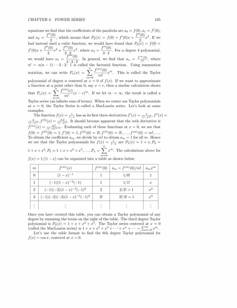
CHAPTER 8. POWER SERIES 105
equations we find that the coefficients of the parabola are a0 = f(0), a1 = f ′(0),
and a2 =f ′′(0)
2, which means that P2(x) = f(0) + f ′(0)x +
f ′′(0)
2x2. If we
had instead used a cubic function, we would have found that P3(x) = f(0) +
f ′(0)x +f ′′(0)
2x2 +
f ′′′(0)
3 · 2x3, where a3 =
f ′′′(0)
3 · 2. For a degree 4 polynomial,
we would have a4 =f ′′′′(0)
4 · 3 · 2. In general, we find that an = f(n)(0)
n! , where
n! = n(n − 1) · · · 3 · 2 · 1 is called the factorial function. Using summation
notation, we can write Pn(x) =
n∑m=0
f (m)(0)
m!xm. This is called the Taylor
polynomial of degree n centered at x = 0 of f(x). If we want to approximatea function at a point other than 0, say x = c, then a similar calculation shows
that Pn(x) =
n∑m=0
f (m)(c)
m!(x − c)m. If we let m → ∞, the result is called a
Taylor series (an infinite sum of terms). When we center our Taylor polynomialsat x = 0, the Taylor Series is called a MacLaurin series. Let’s look at someexamples.
The function f(x) = 11−x has as its first three derivatives f ′(x) = 1
(1−x)2 , f′′(x) =
2(1−x)3 , f
(3)(x) = 3·2(1−x)4 . It should become apparent that the mth derivative is
f (m)(x) = m!(1−x)m+1 . Evaluating each of these functions at x = 0, we see that
f(0) = f (0)(0) = 1, f ′(0) = 1, f (2)(0) = 2!, f (3)(0) = 3!, . . . , f (m)(0) = m!, . . ..To obtain the coefficient am, we divide by m! to obtain am = 1 for all m. Hencewe see that the Taylor polynomials for f(x) = 1
1−x are P1(x) = 1 + x, P2 =
1 + x+ x2, P3 = 1 + x+ x2 + x3, . . . , Pn =
n∑m=0
xm. The calculations above for
f(x) = 1/(1− x) can be organized into a table as shown below:
m f (m)(x) f (m)(0) am = f (m)(0)/m! amxm
0 (1− x)−1 1 1/0! 1
1 (−1)(1− x)−2(−1) 1 1/1! x
2 (−1)(−2)(1− x)−3(−1)2 2 2/2! = 1 x2
3 (−1)(−2)(−3)(1− x)−3(−1)2 3! 3!/3! = 1 x3
......
......
...
Once you have created this table, you can obtain a Taylor polynomial of anydegree by summing the terms on the right of the table. The third degree Taylorpolynomial is P3(x) = 1 + x + x2 + x3. The Taylor series centered at x = 0(called the MacLaurin series) is 1 + x+ x2 + x3 + · · ·+ xn + · · · =
∑∞m=0 x
m.Let’s use the table format to find the 6th degree Taylor polynomial for
f(x) = cosx, centered at x = 0.

CHAPTER 8. POWER SERIES 106
m f (m)(x) f (m)(0) am = f (m)(0)/m! amxm
0 cosx 1 1/0! = 1 1
1 − sinx 0 0/1! = 0 0
2 − cosx −1 −1/2! − 12!x
2
3 sinx 0 0/3! = 0 0
4 cosx 1 1/4! 14!x
4
5 − sinx 0 1/5! = 0 0
6 − cosx −1 −1/6! − 16!x
6
Summing the right column give the 6th degree Taylor polynomial as P6(x) =1− 1
2x2 + 1
4!x4 − 1
6!x6. Notice that 1
6! is extremely small, so the 6th order termdoesn’t change the value of P6(x) much for small values of x.
What if we want to center the Taylor polynomial at a point other than zero.The table format below illustrates this for the 3rd degree Taylor polynomial off(x) = sinx, centered at x = π.
m f (m)(x) f (m)(π) am = f (m)(π)/m! am(x− π)m
0 sinx 0 0/1! = 0 0
1 cosx −1 −1/1! − 11! (x− π)1
2 − sinx 0 0/2! = 0 0
3 − cosx 1 1/3! 13! (x− π)3
Summing the last column means the 3rd degree Taylor polynomial centered atx = π is P3(x) = − 1
1! (x− π)1 + 13! (x− π)3.
The graphs of several Taylor polynomials centered at x = 0 for the func-tions ex, 1
1−x , cosx, and sinx are shown below. The higher the order of thepolynomial, the closer it is to the actual function.
f(x) = ex f(x) = 11−x f(x) = cosx f(x) = sinx
As you increase the degree of a Taylor polynomial, you should expect to seethat your accuracy of approximating a function increases. This is true forcosx, sinx, ex, polynomials, and combination of these functions obtained throughaddition, subtraction, or multiplication. You can also divide any two of thesefunction and still obtain good approximations, but vertical asymptotes pose aproblem.
The function 11−x has a vertical asymptote at x = 1. When we create Taylor
polynomials centered at x = 0, those polynomials follow the function up the lefthand side of the vertical asymptote, causing the polynomials to tend towardinfinity at x = 1 as you increase the degree of the polynomial. In the picture
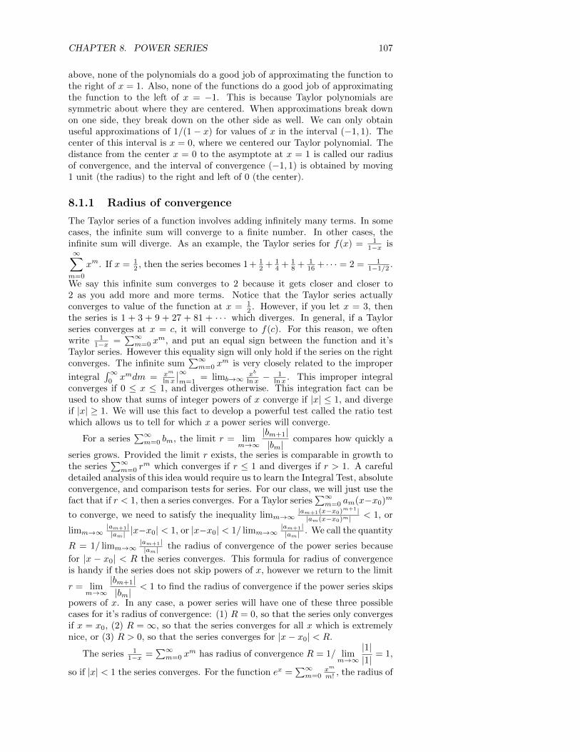
CHAPTER 8. POWER SERIES 107
above, none of the polynomials do a good job of approximating the function tothe right of x = 1. Also, none of the functions do a good job of approximatingthe function to the left of x = −1. This is because Taylor polynomials aresymmetric about where they are centered. When approximations break downon one side, they break down on the other side as well. We can only obtainuseful approximations of 1/(1 − x) for values of x in the interval (−1, 1). Thecenter of this interval is x = 0, where we centered our Taylor polynomial. Thedistance from the center x = 0 to the asymptote at x = 1 is called our radiusof convergence, and the interval of convergence (−1, 1) is obtained by moving1 unit (the radius) to the right and left of 0 (the center).
8.1.1 Radius of convergence
The Taylor series of a function involves adding infinitely many terms. In somecases, the infinite sum will converge to a finite number. In other cases, theinfinite sum will diverge. As an example, the Taylor series for f(x) = 1
1−x is∞∑m=0
xm. If x = 12 , then the series becomes 1 + 1
2 + 14 + 1
8 + 116 + · · · = 2 = 1
1−1/2 .
We say this infinite sum converges to 2 because it gets closer and closer to2 as you add more and more terms. Notice that the Taylor series actuallyconverges to value of the function at x = 1
2 . However, if you let x = 3, thenthe series is 1 + 3 + 9 + 27 + 81 + · · · which diverges. In general, if a Taylorseries converges at x = c, it will converge to f(c). For this reason, we oftenwrite 1
1−x =∑∞m=0 x
m, and put an equal sign between the function and it’sTaylor series. However this equality sign will only hold if the series on the rightconverges. The infinite sum
∑∞m=0 x
m is very closely related to the improper
integral∫∞
0xmdm = xm
ln x
∣∣∞m=1
= limb→∞xb
ln x −1
ln x . This improper integralconverges if 0 ≤ x ≤ 1, and diverges otherwise. This integration fact can beused to show that sums of integer powers of x converge if |x| ≤ 1, and divergeif |x| ≥ 1. We will use this fact to develop a powerful test called the ratio testwhich allows us to tell for which x a power series will converge.
For a series∑∞m=0 bm, the limit r = lim
m→∞
|bm+1||bm|
compares how quickly a
series grows. Provided the limit r exists, the series is comparable in growth tothe series
∑∞m=0 r
m which converges if r ≤ 1 and diverges if r > 1. A carefuldetailed analysis of this idea would require us to learn the Integral Test, absoluteconvergence, and comparison tests for series. For our class, we will just use thefact that if r < 1, then a series converges. For a Taylor series
∑∞m=0 am(x−x0)m
to converge, we need to satisfy the inequality limm→∞|am+1(x−x0)m+1||am(x−x0)m| < 1, or
limm→∞|am+1||am| |x−x0| < 1, or |x−x0| < 1/ limm→∞
|am+1||am| . We call the quantity
R = 1/ limm→∞|am+1||am| the radius of convergence of the power series because
for |x − x0| < R the series converges. This formula for radius of convergenceis handy if the series does not skip powers of x, however we return to the limit
r = limm→∞
|bm+1||bm|
< 1 to find the radius of convergence if the power series skips
powers of x. In any case, a power series will have one of these three possiblecases for it’s radius of convergence: (1) R = 0, so that the series only convergesif x = x0, (2) R = ∞, so that the series converges for all x which is extremelynice, or (3) R > 0, so that the series converges for |x− x0| < R.
The series 11−x =
∑∞m=0 x
m has radius of convergence R = 1/ limm→∞
|1||1|
= 1,
so if |x| < 1 the series converges. For the function ex =∑∞m=0
xm
m! , the radius of

CHAPTER 8. POWER SERIES 108
convergence is R = 1/ limm→∞
|1/(m+ 1)!||1/m!|
= 1/ limm→∞
m
m+ 1= ∞ which means
that the Taylor series for ex converges for all x. We have the series cosx =∑∞m=0
1(2m)!x
2m which skips powers of x. Hence we solve limm→∞
|x2(m+1)/(2(m+ 1))!||x2m/(2m)!|
<
1 which is equivalent to |x2| limm→∞(2m)!
(2m+2)(2m+1)(2m)! < 1 or 0 < 1 which is
always true so the radius of convergence is ∞ and the Taylor series convergesfor all x. You should show that this is true for sinx as well.
Let’s find the radius of convergence of the power series
∞∑n=0
(3n+ 2)(−5)n
(n+ 1)(7n2 + 3)23n+1x2n.
We compute an+1 = (3(n+1)+2)(−5)n+1
((n+1)+1)(7(n+1)2+3)23(n+1)+1x2(n+1). Dividing by an can
get ugly unless we organize our work, for example by placing common termsdirectly above and below each other as shown below.∣∣∣∣an+1
an
∣∣∣∣ =
∣∣∣∣∣ (3(n+ 1) + 2) (−5)n+1 (n+ 1) (7n2 + 3) 23n+1 x2(n+1)
(3n+ 2) (−5)n ((n+ 1) + 1) (7(n+ 1)2 + 3) 23(n+1)+1 x2n
∣∣∣∣∣=
∣∣∣∣∣ (3n+ 5) (−5)n(−5) (n+ 1) (7n2 + 3) 23n2 x2nx2
(3n+ 2) (−5)n (n+ 2) (7(n+ 1)2 + 3) 23n24 x2n
∣∣∣∣∣=
∣∣∣∣∣ (3n+ 5) (−5) (n+ 1) (7n2 + 3) 1 x2
(3n+ 2) 1 (n+ 2) (7(n+ 1)2 + 3) 23 1
∣∣∣∣∣Recall that the limit of a product can be found by computing each individuallimit and the multiplying the result together. Also, the limit as n → ∞ ofa quotient of two polynomials of the same degree is precisely the quotient of
their leading coefficients. This means we can compute limn→∞
(3n+ 5)
(3n+ 2)= 1,
limn→∞
(n+ 1)
(n+ 2)= 1, and lim
n→∞
(7n2 + 3)
(7(n+ 1)2 + 3)= 1, which gives
limn→∞
∣∣∣∣∣ (3n+ 5) (−5) (n+ 1) (7n2 + 3) 1 x2
(3n+ 2) 1 (n+ 2) (7(n+ 1)2 + 3) 23 1
∣∣∣∣∣ =
∣∣∣∣1(−5)(1)(1)
(1
8
)x2
∣∣∣∣ =5
8x2.
We then solve the equation 58x
2 < 1 for x to obtain |x| ≤√
85 , so the radius of
convergence is√
85 .
8.1.2 Euler’s Formula
We now show eix = cosx + i sinx. We know ex =
∞∑m=0
1
m!xm for all x, and it
can be shown that this formula is valid as well for all complex numbers. If we
replace x with ix, then we obtain eix =
∞∑m=0
1
m!(ix)m. The powers of i satisfy
i0 = 1, i1 = i, i2 = −1, i3 = −i, i4 = 1, i5 = i, and cycle through the numbers

CHAPTER 8. POWER SERIES 109
1, i,−1,−i. Hence we have for all x Euler’s formula
eix = 1 + ix− 1
2!x2 − i 1
3!x3 +
1
4!x4 + i
1
5!x5 − 1
6!x6 − i 1
7!x7 + · · ·
=
(1− 1
2!x2 +
1
4!x4 − 1
6!x6 + · · ·
)+ i
(x− 1
3!x3 +
1
5!x5 − 1
7!x7 + · · ·
)=
( ∞∑m=0
(−1)m
(2m)!x2m
)+ i
( ∞∑m=0
(−1)m
(2m+ 1)!x2m+1
)= cos(x) + i sin(x).
Who cares? Well, if the roots of the second order ODE my′′ + cy′ + ky = 0are complex, i.e. λ = a± bi, then y1 = eax+bix = eax(cos bx+ i sin bx) and y2 =eax−bix = eax(cos(−bx) + i sin(−bx)) = eax(cos bx − i sin bx) are two complexsolutions of the ODE (recall that cos(−x) = cos(x) [cosine is an even function]and sin(−x) = − sinx [sine is an odd function]). The superposition principlefor ODEs says that linear combinations are solutions, so y1+y2
2 = eax cos bx
and y1−y22i = eax sin bx are two real solutions. This is why we use eax cos bx
and eax sin bx as solutions when the roots of the characteristic equation areimaginary.
8.2 Power Series
8.2.1 Notation and Calculus
Rather than starting with a function f(x) and calculating the Taylor series,we now reverse the process. We will define a power series centered at x = cto be an expression of the form f(x) =
∑m=0 am(x − c)m, and the domain
of f is all x for which the series converges. We will almost always centerour power series at x = 0, so we write f(x) =
∑m=0 amx
m. The radius ofconvergence is still computed the same. If the power series has a positive orinfinite radius of convergence when centered at x = c, then we say that thefunction f(x) =
∑m=0 am(x− x0)m is analytic at c.
If a power series f(x) =∑m=0 am(x − x0)m has a finite radius of conver-
gence, then we can differentiate and integrate the power series term by term.The resulting power series f ′(x) =
∑m=0mam(x− x0)m−1 =
∑m=1mam(x−
x0)m−1 and∫f(x)dx = C +
∑m=0
amm+1 (x − x0)m+1 have the same radius of
convergence as f . If two power series centered at the same point both convergeat x, then you can add them (by adding their coefficients), and multiply them(using the distributive laws of multiplication). In addition, you can composepower series, though this may change the radius of convergence. The mostcommon composition is to replace x with a(x)k for some constants a and k.
8.2.2 Examples
Since1
1− x=
∞∑m=0
xm has radius of convergence R = 1, we can differentiate
and obtain1
(1− x)2=
∞∑m=1
mxm−1 = 1 + 2x + 3x2 + 4x3 + · · · , which has
radius of convergence R = 1 as well. Replacing x with x = −x gives1
1 + x=
∞∑m=0
(−1)mxm = 1−x+x2−x3 +x4 + · · · . Replacing x with −x2 gives1
1 + x2=
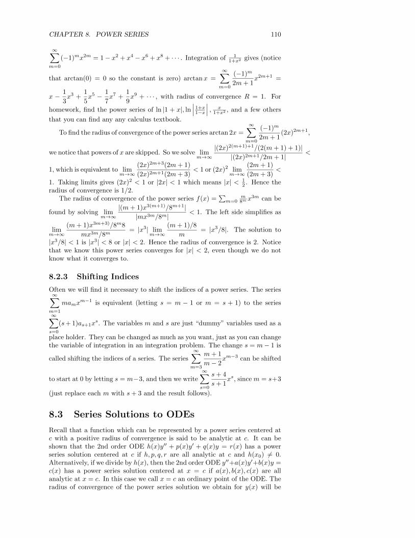
CHAPTER 8. POWER SERIES 110
∞∑m=0
(−1)mx2m = 1− x2 + x4 − x6 + x8 + · · · . Integration of 11+x2 gives (notice
that arctan(0) = 0 so the constant is zero) arctanx =
∞∑m=0
(−1)m
2m+ 1x2m+1 =
x − 1
3x3 +
1
5x5 − 1
7x7 +
1
9x9 + · · · , with radius of convergence R = 1. For
homework, find the power series of ln |1 + x|, ln∣∣∣ 1+x
1−x
∣∣∣ , x1+x2 , and a few others
that you can find any any calculus textbook.
To find the radius of convergence of the power series arctan 2x =
∞∑m=0
(−1)m
2m+ 1(2x)2m+1,
we notice that powers of x are skipped. So we solve limm→∞
|(2x)2(m+1)+1/(2(m+ 1) + 1)||(2x)2m+1/2m+ 1|
<
1, which is equivalent to limm→∞
(2x)2m+3(2m+ 1)
(2x)2m+1(2m+ 3)< 1 or (2x)2 lim
m→∞
(2m+ 1)
(2m+ 3)<
1. Taking limits gives (2x)2 < 1 or |2x| < 1 which means |x| < 12 . Hence the
radius of convergence is 1/2.The radius of convergence of the power series f(x) =
∑m=0
m8mx
3m can be
found by solving limm→∞
|(m+ 1)x3(m+1)/8m+1||mx3m/8m|
< 1. The left side simplifies as
limm→∞
(m+ 1)x3m+3)/8m8
mx3m/8m= |x3| lim
m→∞
(m+ 1)/8
m= |x3/8|. The solution to
|x3/8| < 1 is |x3| < 8 or |x| < 2. Hence the radius of convergence is 2. Noticethat we know this power series converges for |x| < 2, even though we do notknow what it converges to.
8.2.3 Shifting Indices
Often we will find it necessary to shift the indices of a power series. The series∞∑m=1
mamxm−1 is equivalent (letting s = m − 1 or m = s + 1) to the series
∞∑s=0
(s+ 1)as+1xs. The variables m and s are just “dummy” variables used as a
place holder. They can be changed as much as you want, just as you can changethe variable of integration in an integration problem. The change s = m− 1 is
called shifting the indices of a series. The series
∞∑m=3
m+ 1
m− 2xm−3 can be shifted
to start at 0 by letting s = m−3, and then we write
∞∑s=0
s+ 4
s+ 1xs, since m = s+3
(just replace each m with s+ 3 and the result follows).
8.3 Series Solutions to ODEs
Recall that a function which can be represented by a power series centered atc with a positive radius of convergence is said to be analytic at c. It can beshown that the 2nd order ODE h(x)y′′ + p(x)y′ + q(x)y = r(x) has a powerseries solution centered at c if h, p, q, r are all analytic at c and h(x0) 6= 0.Alternatively, if we divide by h(x), then the 2nd order ODE y′′+a(x)y′+b(x)y =c(x) has a power series solution centered at x = c if a(x), b(x), c(x) are allanalytic at x = c. In this case we call x = c an ordinary point of the ODE. Theradius of convergence of the power series solution we obtain for y(x) will be
CHAPTER 8. POWER SERIES 111
at least as big as the smallest radius of convergence of a(x), b(x), c(x). This isthe general theory which motivates everything else we do with regards to seriessolutions to ODEs.
The power series method essentially requires that you (1) write y =
∞∑n=0
anxn,
(2) take derivatives y =
∞∑n=0
nanxn−1 and y =
∞∑n=0
n(n− 1)anxn−2, (3) replace
each function or derivative in your ODE with the appropriate power series (com-puting MacLaurin series of functions which occur) (4) shift the indices on eachsum to obtain a recurrence relation for the unknown constants an, and then (5)solve the recurrence relation for the largest an and use this relation to generatethe constants. The following 4 examples illustrate how to find solutions usingthe power series method. Some of these problems you already can solve withoutpower series methods, however we will start with simpler problems to which youalready know the answer before we venture into new problems.
Consider the ODE y′ = ky. Let y =
∞∑m=0
amxm. Then we compute y′ =
∞∑m=0
mamxm−1 =
∞∑m=1
mamxm−1. Notice that we can start at m = 1 instead
of m = 0 because when you put m = 0 into the sum you get zero, so why notjust start one term later and skip the 0 term. Inserting these series into the
ODE gives
∞∑m=1
mamxm−1 = k
∞∑m=0
amxm =
∞∑m=0
kamxm. For this equality to
hold, we must have the coefficient of each power x equal on each side of theequation. To simplify the calculations, we shift the indices on the power serieson the left by letting m− 1 = s, and on the right by letting m = s. This gives∞∑s=0
(s + 1)as+1xs =
∞∑s=0
kasxs, which means that (s + 1)as+1 = kas for all s.
This gives the recurrence relation as+1 = kas(s+1) . The variable a0 can be chosen
to be anything we want, but then a1 = ka01 , a2 = k2a0
2! , a3 = k3a03! , am = kma0
m! .So we have our solution as
y(x) = a0+a0k
1!x1+a0
k2
2!x2+· · · = a0
(1 +
1
1!(kx)1 +
1
2!(kx)2 + · · ·
)= a0
∞∑m=0
1
m!(kx)m = a0e
kx,
where the last equality comes because we recognize that this is the Maclaurinseries of ekx.
Consider the ODE y′ = xy. Let y =
∞∑m=0
amxm. Then we compute
y′ =
∞∑m=0
mamxm−1 =
∞∑m=1
mamxm−1 (again we start at 1 because m = 0
just gives us zero). Inserting these series into the ODE gives
∞∑m=1
mamxm−1 =
x
∞∑m=0
amxm =
∞∑m=0
amxm+1. Writing out the first few terms, we have
1a1x0 + 2a2x
1 + 3a3x2 + 4a4x
3 + · · · = a0x1 + a1x
2 + a2x3 + a3x
4.
Since x0 appears only on the left side of the equation, we have a1 = 0. Hence the
left side can be written
∞∑m=2
mamxm−1. We shift indices by letting s = m − 1
CHAPTER 8. POWER SERIES 112
(m = s + 1) on the left side and s = m + 1 on the right side. This gives∞∑s=1
(s+ 1)as+1xs =
∞∑s=1
as−1xs. Equating the coefficients of xs (for s ≥ 1) gives
(s + 1)as+1 = as−1, or as+1 = as−1
(s+1) for s ≥ 1. For s = 1, 2, 3, 4, 5, 6, . . . we
have a2 = a0(2) , a3 = a1
(3) = 0, a4 = a2(4) = a0
(2·4) , a5 = 0, a6 = a0(2·4·6) = a0
233! , . . ..
Notice that am = 0 for odd m, and a2m = a02mm! . If m = 0, we can still
write a2m = a02m,m! = a0, which means we can write y =
∑∞m=0
a02mm!x
2m =
a0
∑∞m=0
1m!
(x2
2
)m= a0e
x2/2.
Now consider the ODE y′′ + y = 0. Let y =
∞∑m=0
amxm. Then we com-
pute y′ =
∞∑m=0
mamxm−1 =
∞∑m=1
mamxm−1 and y′′ =
∞∑m=1
m(m − 1)amxm−2 =
∞∑m=2
m(m − 1)amxm−2 (we can start the second derivative at m = 2 because
putting m = 0 or m = 1 into the series gives 0). Inserting these power series intothe ODE gives
∑∞m=2m(m−1)amx
m−2+∑∞m=0 amx
m = 0. Shifting the indiceson the first sum using s = m− 2 (or m = s+ 2) and second sum using m = sgives
∑∞s=0(s+2)(s+1)as+2x
s+∑∞s=0 asx
s = 0. We need to have the sum of thecoefficients of xs sum to zero, so we have (s+2)(s+1)as+2 +as = 0. This meansas+2 = − as
(s+2)(s+1) for s ≥ 0. This recurrence relation does not specify a0 or
a1, so we have two constants we can choose arbitrarily. For s = 0, 1, 2, 3, . . .,we have a2 = −a02! , a3 = −a13! , a4 = a0
4! , a5 = a15! , a6 = −a06! , a7 = −a17! . . .. The
sign changes in groups of two, which suggests we should split the series intoeven and odd powers. This can be summarized as a2m = (−1)m a0
(2m)! and
a2m+1 = (−1)m a1(2m+1)! . This means that the solution to the ODE is
y(x) = a0 + a1x− a01
2!x2 − a1
1
3!x3 + a0
1
4!x4 + a1
1
5!x5 + · · ·
= a0
(1− 1
2!x2 +
1
4!x4 + · · ·
)+ a1
(x− 1
3!x3 +
1
5!x5 + · · ·
)= a0
( ∞∑m=0
(−1)m
(2m)!x2m
)+ a1
( ∞∑m=0
(−1)m
(2m+ 1)!x2m+1
)= a0 cos(x) + a1 sin(x).
The last equality can be discovered by recognizing that the series are theMacLaurin series for cosine and sine.
As our last example, consider the ODE y′′+2xy′+y = 0. Let y =
∞∑m=0
amxm.
Then we compute y′ =
∞∑m=0
mamxm−1 =
∞∑m=1
mamxm−1 and y′′ =
∞∑m=1
m(m−
1)amxm−2 =
∞∑m=2
m(m−1)amxm−2. Inserting these power series into the ODE
and multiplying the middle series by 2x gives
∞∑m=2
m(m− 1)amxm−2 +
∞∑m=1
2mamxm + y =
∞∑m=0
amxm = 0.
We shift the index on the first series by letting s = m − 2 and s = m for the
CHAPTER 8. POWER SERIES 113
last two. This gives
∞∑s=0
(s+ 2)(s+ 1)as+2xs +
∞∑s=1
2sasxs +
∞∑s=0
asxs = 0.
Notice that the second series starts at s = 1 whereas the other two start ats = 0. Hence we look at the coefficients of x0 separately than the rest of thecoefficients. We notice that (2)(1)a2 +a0 = 0, or a2 = −a0
12! . For s ≥ 1 we have
(s+2)(s+1)as+2 +2sas+as = 0, or as+2 = −as 2s+1(s+2)(s+1) . The first few terms
are a2 = −a012! , a3 = −as 3
(3)(2) , a4 = a01·54! , a5 = a1
3·75! , a6 = −a0
1·5·96! ,−a7 =
a13·7·11
7! . Since the even and odd coefficients am depend on a0 and a1, we write
a2m = a0(−1)m 1·5·9···(4m−3)(2m)! and a2m+1 = a1(−1)m 3·7·11···(4m−1)
(2m+1)! . Hence we
have found a solution as
y(x) = a0
(1− 1
2t2 +
5
24t4 − 1
16t6 +
13
896t8 + · · ·
)+ a1
(t− 1
2t3 +
7
40t5 − 11
240t7 +
11
1152t9 + · · ·
)= a0
(1 +
∞∑m=1
(−1)m1 · 5 · 9 · · · (4m− 3)
(2m)!x2m
)+ a1
(x+
∞∑m=1
(−1)m3 · 7 · 11 · · · (4m− 1)
(2m+ 1)!x2m+1
).
This is not a simple elementary function for which we know a power series. Theradius of convergence is R =∞. We will learn how to express this function interms of Bessel functions and Gamma functions when we start studying specialfunctions in the next learning module. Hence, we leave our solution in terms ofa power series and cannot continue any further.
As you work problems in the homework, I want you to find general formulasfor the mth coefficient am. Mathematica has code you can use to check if youranswers are correct, as well as show you many of the steps in the computation.
CHAPTER 8. POWER SERIES 114
8.4 Preparation
This chapter covers the following ideas. When you create your lesson plan, it should contain examples whichillustrate these key ideas. Before you take the quiz on this unit, meet with another student out of class andteach each other from the examples on your lesson plan.
1. Find and explain the use of Taylor polynomials, Talyor series, and Maclaurin series. Give examplesfor various common functions.
2. Explain how to use the ratio test to find the radius of convergence of a power series.
3. Derive Euler’s formula, and use it to explain why complex roots a± bi of 2nd order ODE result in thesolutions eax cos(bx) and eax sin(bx).
4. Explain how to differentiate, integrate, add, multiply, compose, and shift indices of power series.
5. Use the power series method to solve ODEs at ordinary points.
Here are the preparation problems for this unit. Chapter numbers precede the problems from Schaum’s.
Preparation Problems (click for solutions)
Day 1 1, 11, 18, 20
Day 2 25, 29, 43, Schaum’s 27:3
Day 3 46, Schaum’s 27:29, Schaum’s 27:36, Schaum’s 27:41
The homework for this unit comes from the Power Series chapter in this online book. Please makesure you print the appropriate pages from the problem book, as well as the corresponding section from thetextbook.
Make sure you try a few of each type of problem, ASAP. I suggest that the first night you try one of eachtype of problem. It’s OK if you get stuck and don’t know what to do, as long as you decide to learn howto do it and then return to the ones where you got stuck. Eventually do enough of each type to master theideas. The only section in Schaum’s with relevant problems is chapter 27.
Most engineering textbooks assume you have seen Taylor series and power series before (in math 113),but many of you have not. If you have your old Math 215 book, you can find many relevant problems andexplanations from section 11.5 (Ratio Test) and 11.8 (Taylor Series).
For reference, here are a few key functions and their Taylor series centered at x = 0 (so their MacLaurinseries).
1. ex =
∞∑n=0
1
n!xn, R =∞
2. cos(x) =
∞∑n=0
(−1)n
(2n)!x2n, R =∞
3. sin(x) =
∞∑n=0
(−1)n
(2n+ 1)!x2n+1, R =∞
4.1
1− x=
∞∑n=0
xn, R = 1
5. cosh(x) =
∞∑n=0
1
(2n)!x2n, R =∞
6. sinh(x) =
∞∑n=0
1
(2n+ 1)!x2n+1, R =∞

CHAPTER 8. POWER SERIES 115
8.5 Problems
(I) For each of the following, find a Talyor poly-nomial of degree n centered at x = c of thefunction f(x).
1. e4x, n = 3, c = 0
2. cos(x), n = 4, c = π
3. cos(2x), n = 4, c = 0
4. sin( 12x), n = 5, c = 0
5. 1x , n = 3, c = 1
6. lnx, n = 3, c = 1
7. ln(1− x), n = 4, c = 0
8. ln(1 + x), n = 4, c = 0
(II) Find the radius of convergence of each powerseries.
9.
∞∑n=0
1
3nxn
10.
∞∑n=0
(−1)n
4n+1xn
11.
∞∑n=0
n
2nx3n
12.
∞∑n=0
3n+ 1
n2 + 4xn
13.
∞∑n=0
(−4)nn
n2 + 1x2n
14.
∞∑n=0
n
2nx2n
15.
∞∑n=0
(−1)n
n!xn
16.
∞∑n=0
n!
10nx2n
(III) For each function, find the MacLaurin seriesand state the radius of convergence.
17. f(x) = ex
18. f(x) = cosx
19. f(x) = sinx
20. f(x) =1
1− x
21. f(x) =1
1 + x
22. f(x) = coshx
23. f(x) = sinhx
(IV) Prove the following formulas are true by con-sidering power series. These formulas will al-low us to eliminate complex numbers in futuresections.
24. eix = cosx+ i sinx (called Euler’s formula)
25. cosh(ix) = cosx
26. cos(ix) = coshx
27. sinh(ix) = i sinx
28. sin(ix) = i sinhx
(V) Use MacLaurin series of known functions to findthe MacLaurin series of these functions (by in-tegrating, differentiating, composing, or multi-plying together two power series). Then statethe radius of convergence.
29. f(x) = x2e3x
30. f(x) = x2
e3x [hint, use negative exponents]
31. f(x) = cos 4x
32. f(x) = x sin(2x)
33. f(x) = x1+x
34. f(x) = 11+x2
35. f(x) = arctanx [hint, integrate the previous]
36. f(x) = arctan(3x)
(VI) Shift the indices on each sum so that it beginsat n = 0.
37.
6∑n=3
n+ 2
38.
8∑n=2
n2
39.
∞∑n=4
2n
40.
∞∑n=2
xn
41.
∞∑n=1
nanxn
42.
∞∑n=2
n(n− 1)anxn−2
(VII) Solve the following ODEs by the power seriesmethod. With some, initial conditions are given(meaning you know y(0) = a0 and y′(0) = a1).Identify the function whose MacLaurin seriesequals the power series you obtain.
43. y′ = 3y
44. y′ = 2xy
45. y′′ + 4y = 0
46. y′′ − 9y = 0, y(0) = 2, y′(0) = 3
47. y′′ + 4y′ + 3y = 0, y(0) = 1, y′(0) = −1
(VII) Determine whether the given values of x areordinary points or singular points of the givenODE.
48. Chapter 27, problems 26-34 (these are reallyquick).
(VIII) Solve the following ODEs by the power seriesmethod. State the recurrence relation used togenerate the terms of your solution, and writeout the first 5 nonzero terms of your solution.
49. Chapter 27, problems 35-47 (or from the workedproblems).
8.6 Solutions
Handwritten solutions are available online. Click forsolutions.

Chapter 9
Special Functions
This section needs revamping. Until I have time to revamp it, Schaum’s Outlinesprovides a great explanation of these topics.The name of this chapter is “Special Functions.” These are functions whichshow up as the solution to problems of real world interest whose solution is afunction which does not appear in regular calculus. Many of these functions canonly be represented using series. This chapter covers the following objectives:
1. Explain the Frobenius method and use it to solve ODEs where zero is aregular singular point.
2. Solve Legendre’s equation and derive Legendre polynomials.
3. Solve Bessel’s equation giving solutions of the first kind, and write solu-tions to ODEs in terms of Bessel functions.
4. Describe the Gamma function and how it generalizes the factorial. Beable to prove various relationships related to the Gamma function.
116
CHAPTER 9. SPECIAL FUNCTIONS 117
9.1 Preparation
The name of this module is “Special Functions.” These are functions which show up as the solution toproblems of real world interest whose solution is a function which does not appear in regular calculus. Manyof these functions can only be represented using series. When you make your lesson plan, make sure thatyou have an example illustrating each idea.
1. Explain the Frobenius method and use it to solve ODEs where zero is a regular singular point.
2. Solve Legendre’s equation and derive Legendre polynomials.
3. Solve Bessel’s equation giving solutions of the first kind, and write solutions to ODEs in terms of Besselfunctions.
4. Describe the Gamma function and how it generalizes the factorial. Be able to prove various relationshipsrelated to the Gamma function.
Preparation Problems (click for solutions)
Day 1 28.4, 28.5, 28.6, 28.9
Day 2 27.12, 29.4, 28.10, 28.14
Day 3 30.4, 30.6, 30.8, 30.9
Section numbers correspond to problems from Schaum’s Outlines Differential Equations by Rob Bronson.The suggested problems are a minimum set of problems to attempt.
Concept Sec. Suggested Relevant
Frobenius Method* 28:1-4, 5-10, 12,14,16,18-20
Legendre Polynomials 27:11-13; 29:4,6,8,11,12,15
Bessel Functions 30:9,11,12,26, 27,
Gamma Functions 30:1-8, 24, 25
Substitutions 28:22-23, 34-38; 30:30,31
Here are some vocabulary reminders to help you.
• Remember, a function is said to be analytic at x = c if it has a power series solution centered at x = cwith a positive radius of convergence. Polynomials, exponentials, trig function, and rational functionswhose denominator is not zero at x = c are all analytic.
• The point x = c is called an ordinary point of the differential equation y′′ + P (x)y′ +Q(x)y = r(x) ifboth coefficients P (x) and Q(x) are analytic at x = c. We can solve ODEs at regular points by usingthe power series method.
• The point x = c is called a singular point of the ODE y′′ + P (x)y′ +Q(x)y = r(x) if either coefficientP (x) or Q(x) is not analytic at x = c. In general, we can’t solve ODEs at singular points.
• The point x = c is called a regular singular point of the ODE y′′+P (x)y′+Q(x)y = r(x) it is singularand if (x − c)P (x) and (x − c)2Q(x) are both analytic. We can use the Frobenius method to solve
ODEs at regular singular points. The big idea is to guess a solution of the form y = xλ∞∑n=0
anxn and
then solve for λ and the remaining coefficients as in the power series method. The indicial equation isthe first equation resulting from matching coefficients, and it’s roots λ1 and λ2 determine the type ofsolution.
Chapter 10
Systems of ODEs
This chapter covers the following ideas. When you create your lesson plan, itshould contain examples which illustrate these key ideas. Before you take thequiz on this unit, meet with another student out of class and teach each otherfrom the examples on your lesson plan.
1. Explain the basic theory of systems of linear ODEs and the Wronskianfor systems.
2. Convert higher order ODEs to first order linear systems.
3. Explain how to use eigenvalues and eigenvectors to diagonalize matrices.When not possible, use generalized eigenvectors to find Jordan canonicalform.
4. Find the matrix exponential of a square matrix, and use it to solve linearhomogeneous and nonhomogeneous ODEs.
5. Give applications of systems of ODEs. In particular be able to setup sys-tems of ODE related to dilution, electricity, and springs (use the computerto solve complex systems).
10.1 Definitions and Theory for Systems of ODEs
Problems in the real world often involving combining many differential equa-tions which interact with each other, resulting in a system of ODEs. Beforeembarking on a description of the solution techniques and real world applica-tions, let’s look at an example. In what follows, we will generally let t be theindependent variable, as ~x we’ll use for talking about eigenvectors.
Consider the system of ODE’s y′1(t) = 2y1(t) + y2(t) and y′2(t) = y1(t) +
2y2(t). This system can be written in matrix form as
[y′1y′2
]=
[2 11 2
] [y1
y2
]. We
can summarize this in vector and matrix form by writing ~y′ = A~y. Since thesystem of ODEs ~y′ = A~y is similar to the ODE y′ = Ay whose solution involvesan exponential function, we can guess that a solution to ~y′ = A~y will be of the
form
[x1
x2
]eλt for some constant vector ~x =
[x1
x2
]and constant λ. Differentiating
and substituting into the ODE gives λ~xeλt = A~xeλt, or λ~x = A~x. In otherwords, we need a scalar λ and a vector ~x such that multiplying ~x on the left bya matrix A is equivalent to multiplying by a constant λ. This is an eigenvalue
and eigenvector problem. The matrix A =
[2 11 2
]has eigenvalues λ1 = 1 and
118
CHAPTER 10. SYSTEMS OF ODES 119
λ2 = 3, with corresponding eigenvectors ~x1 =
[1−1
]and ~x2 =
[11
](check this
is true). Hence, two solutions to the system of ODE’s are
[y1
y2
]=
[1−1
]et
and
[y1
y2
]=
[11
]e3t. The general solution to this ODE is found using the
superposition principle, and considering any linear combination of these two
solutions. In other words, the general solution is
[y1
y2
]= c1
[1−1
]et+c2
[11
]e3t =[
c1et + c2e
3t
−c1et + c2e3t
].
We now discuss the general case. A first order system of n ODEs can bewritten
y′1 = f1(t, y1, . . . , yn), y′2 = f2(t, y1, . . . , yn), . . . , y′n = fn(t, y1, . . . , yn),
or equivalently ~y′ = ~f(t, ~y). It is said to be linear if it can be written in the formy′1 = a11(t)y1 + a12(t)y2 + · · ·+ a1n(t)yn + g1(t), . . . , y′n = an1(t)y1 + an2(t)y2 +· · · + ann(t)yn + gn(t), or equivalently ~y′ = A~y + ~g. An initial value problemfor a system consists of a system of ODEs and n given initial conditions of theform y1(t0) = K1, . . . , yn(t0) = Kn. Provided all fi are continuous, or aij arecontinuous, then the solution to an IVP exists and is unique.
We will focus on linear systems. We say a linear system ~y′ = A~y + ~g ishomogeneous if ~g = ~0 (~y′ −A~y = ~0). The superposition principle says that anylinear combination of two solutions to a homogeneous linear system of ODEs isagain a solution. A basis of solutions, written ~y1, ~y2, . . . , ~yn, is a set of n linearlyindependent solutions. The general solution is ~y = c1~y1+c2~y2+· · ·+cn~yn = Y ~c,where Y is a matrix whose columns are the vectors ~yi. The Wronskian of nsolutions is the determinant of Y (the matrix whose columns are the solutions).If the Wronskian is ever zero on an interval, then it is identically zero and thesolutions are dependent. If it is nonzero at a point in an interval, then thesolutions are linearly independent.
10.1.1 The Eigenvalue approach to Solving Linear sys-tems of ODEs
If a homogeneous linear system of ODEs has constant coefficients, then thesystem can be written in the form ~y′ = A~y, where A is a matrix with constants.Following the key example in the Definitions and Theory section, we can guessthat a solution is of the form ~xeλt for some λ and vector ~x. Hence we haveλ~xeλt = A~xeλt, or λ~x = A~x, which is an eigenvalue problem. We find that ~xeλt
is a solution of the systems of ODEs for any eigenvalue λ with a correspondingeigenvector ~x. This is the general theory. In particular, if the eigenvaluesare λ1, . . . , λn (whether there are repeats or not), and there are n linearlyindependent eigenvectors ~xi, then the general solution is ~y = c1~x1e
λ1t + · · · +cn~xne
λnt.
Example 10.1. Consider the system of ODEs y′1 = 2y1 +y2, y′2 = y1 +2y2 from
the key example, but add in the initial conditions y1(0) = 3, y2(0) = 4. Since theeigenvalues are 1 and 3 with eigenvectors [1,−1], [1, 1], the general solution is[y1
y2
]= c1
[1−1
]et + c2
[11
]e3t =
[1 1−1 1
] [et 00 e3t
] [c1c2
]. The initial conditions
give us the matrix equation
[34
]=
[1 1−1 1
] [1 00 1
] [c1c2
]=
[1 1−1 1
] [c1c2
], which
can be solved using Cramer’s rule (which we have done for much of the semester)
CHAPTER 10. SYSTEMS OF ODES 120
or by using an inverse matrix. If we let Q =
[1 1−1 1
], then the constants c1
and c2 are found by writing ~c = Q−1~y(0), or[c1c2
]=
[1 1−1 1
]−1 [34
]=
1
2
[1 −11 1
] [34
]=
1
2
[−17
],
or c1 = − 12 , c2 = 7
2 . Hence the solution to our IVP is
[y1
y2
]= − 1
2
[1−1
]et +
72
[11
]e3t =
[− 1
2et + 7
2e3t
12et + 7
2e3t
].
10.1.2 Using an Inverse Matrix
In the applications unit (the last page) it gives a formula for the inverse of a 2by 2 matrix: [
a bc d
]=
1
|A|
[d −b−c a
].
We’ll be using this fact often in most of what follows.In the previous example, we used the inverse matrix to find our constants
from our initial conditions. Notice that the general solution was written in theform ~y = QD~c where Q is a matrix whose columns are the eigenvectors of A,and D is a diagonal matrix with eλt on the diagonals for our eigenvalues λ.We then wrote ~c = Q−1~y(0), which means we could write our solution in theform ~y = QDQ−1~y(0). The matrix QDQ−1 is called the matrix exponential ofAt, and we will soon show that it equals eAt, where we place a matrix in theexponent of e. If we are given initial conditions, then we can find a solution toour IVP system ~y′ = A~y by using the following 4 step process:
1. Find the eigenvalues of A to create D (put eλt on the diagonals).
2. Find the eigenvectors to create Q (put your eigenvectors in the columns).
3. Find the inverse of Q (quick for 2 by 2 matrices, use a computer foranything larger).
4. Compute the product ~y = QDQ−1~y(0) = eAt~y(0) and you’re done.
This will solve every homogeneous ODE we have encountered all semester,provided the roots of our characteristic equation are distinct and real. Most ofthe rest of this document deals with what to do in the case of a double root,complex roots, and nonhomogeneous systems. We will use the ideas in the nextsection on Jordan form to develop a powerful solution technique which combinesall the ideas we have learned throughout the entire semester.
10.2 Jordan Canonical Form
The matrix
[2 11 2
]has eigenvalues λ = 1, 3 and eigenvectors
[−11
],
[11
](check
this). Let Q =
[−1 11 1
]be a matrix whose columns are linearly independent
eigenvectors of A. Then the product Q−1AQ =
[1 00 3
]is a diagonal matrix
whose entries are the eigenvalues of A (written in the same order in whichthe eigenvectors were listed in Q. This process (finding Q and multiplying

CHAPTER 10. SYSTEMS OF ODES 121
J = Q−1AQ) is called diagonalizing a matrix, and is always possible for ann × n matrix which has n linearly independent eigenvectors. Notationally weoften write Q−1AQ = J for the diagonal matrix J , and J is called a Jordancanonical form for A.
2 1 0 00 2 1 00 0 2 00 0 0 3
If A has an eigenvalue λ which occurs k times (we say it’s
algebraic multiplicity is k), but does not have k linearly inde-pendent eigenvectors (the geometric multiplicity is less thank), then we call the eigenvalue defective. In this case, it isimpossible to diagonalize A. However, it is possible to find amatrix J whose diagonal entries are the eigenvalues and theonly nonzero terms are a few 1’s which are found directly abovethe defective eigenvalues. The matrix on the right is a Jordan canonical formfor a matrix whose eigenvalues are 2, 2, 2, and 3 where 2 is a defective eigen-value. To find this matrix J , we need to find generalized eigenvectors, whichare vectors which satisfy (A − λI)r~x = ~0 for some r. If ~x is a vector whichsatisfies this equation for r but not for r − 1, then we call r the rank of theeigenvector ~x. We will focus our examples on 2× 2 and 3× 3 matrices. It canbe shown that if the algebraic multiplicity of an eigenvector is k, then therewill be k linearly independent generalized eigenvalues, which we can then useto obtain the Jordan form.
This paragraph explains a method for finding generalized eigenvectors. Theexamples which follow illustrate this idea. Skim read this paragraph, try theexamples, and then come back and read it again. A generalized eigenvector~vr of rank r satisfies (A − λI)r~vr = ~0 but not (A − λI)r−1~vr = ~0. If welet ~vr−1 = (A − λI)~vr, then ~vr−1 is a generalized eigenvector of rank r − 1.The equation ~vr−1 = (A − λI)r~vr gives us a way of solving for ~vr based upon~vr−1. Similarly, we could use ~vr−2 to obtain ~vr−1. If we repeat this processuntil we get back to ~v1 (which is an actual eigenvector), then we can writeall of the generalized eigenvectors in terms of a basis of eigenvectors. If ~v1
is an eigenvector, then we solve (A − λI)~v2 = ~v1 to find ~v2. We then solve(A−λI)~v3 = ~v2 to find ~v3. Continue this process to obtain a chain of generalizedeigenvectors ~v1, ~v2, . . . , ~vr which are then inserted in the matrix Q to obtainJordan form.
Example 10.2. LetA =
[0 1−1 −2
]. The characteristic polynomial is
∣∣∣∣−λ 1−1 −2− λ
∣∣∣∣ =
λ2 + 2λ + 1 = (λ + 1)2. A double eigenvalue is λ = −1. To find the eigenvec-
tors we compute A − λI =
[1 1−1 −1
]. The only eigenvectors are multiples of
~v1 =
[1−1
]. Hence there is only one linearly independent eigenvector for the
double root −1, which means −1 is a defective eigenvalue. In order to findJordan Form, we must find a generalized eigenvector of rank 2.
We solve the equation (A−λI)~v2 = ~v1 by row reducing the matrix
[1 1 1−1 −1 −1
],
which gives the solution x1 + x2 = 1 (notice we just augmented A − λI byour eigenvector). The vectors [1, 0] and [0, 1] both satisfy this system, so wecan pick either vector as ~v2 (it doesn’t matter which one you pick). Now let
Q =[~v1 ~v2
]. The Jordan form is then Q−1AQ ==
[−1 10 −1
].
The example above gives a general method for finding Jordan form. Startby finding the eigenvalues. For each eigenvalue, find a basis of eigenvectors.For each eigenvector in this basis, use the equation ~vk−1 = (A − λI)r~vk toobtain a chain of generalized eigenvectors {~v1, ~v2, . . . , ~vr} corresponding to that

CHAPTER 10. SYSTEMS OF ODES 122
eigenvector (the chain stops when the equation ~vk−1 = (A − λI)r~vk has nosolution, which will always occur). Once you have completed this, you will findthat the total number of generalized eigenvectors you have obtained matchesthe size of the matrix, and that the vectors are linearly independent (provingthis is not difficult, but beyond the scope of our class). Place the vectors into thecolumns of Q (keeping the chains together) and then the product Q−1AQ = Jwill give you a Jordan form, where each chain of vectors corresponds to a blockmatrix on the diagonal whose diagonal entries are the eigenvalue and 1’s abovethe main diagonal.
Example 10.3. Consider the matrix A =
4 −4 101 0 50 0 2
. The characteristic
polynomial is −λ3 + 6λ2 − 12t+ 8 = (2− λ)3, so A has one eigenvalue, namely
λ = 2. We compute A−2I =
2 −4 101 −2 50 0 0
. Row reduction gives
1 −2 50 0 00 0 0
,
so two linearly independent eigenvectors are
210
and
−501
. We currently
have only 2 linearly independent vectors, so we have to find a third. We solve
(A−2I)v2 =
210
by row reducing
2 −4 10 21 −2 5 10 0 0 0
to obtain
1 −2 5 10 0 0 00 0 0 0
,
which means ~v2 =
100
is a generalized eigenvector since 1 − 2(0) + 5(0) = 1.
We now have three independent vectors, so we can use them to form the matrix
Q. We have Q =
2 1 −51 0 00 0 1
. The inverse of Q is
0 1 01 −2 50 0 1
(using a
computer). Matrix multiplication gives Q−1AQ =
2 1 00 2 00 0 2
as the Jordan
Form.As a side note, if we try to find any more generalized eigenvectors, we
will fail because we will get inconsistent systems. Reduction of the matrix2 −4 10 11 −2 5 00 0 0 0
gives
1 −2 5 00 0 0 10 0 0 0
which means there is no rank 3 eigen-
vector in the first chain. Row reduction of the matrix
2 −4 10 −51 −2 5 00 0 0 1
gives1 −2 5 00 0 0 10 0 0 0
which has no solution, meaning that the second chain is only
one long, and there are no generalized eigenvectors of rank 2 for the secondeigenvector.
Example 10.4. Consider the matrix
1 2 20 1 00 0 1
. Because it is upper trian-
gular, the eigenvalues are the entries on the diagonal, namely λ = 1 is aneigenvalue with algebraic multiplicity 3. To find the eigenvectors, we note that

CHAPTER 10. SYSTEMS OF ODES 123
the matrix A − I =
0 2 20 0 00 0 0
has only 1 pivot, so it has 2 free variable, or
two linearly independent eigenvectors
100
and
01−1
. Since there are only 2
linearly independent eigenvectors, we need to find a third. Row reduction of0 2 2 10 0 0 00 0 0 0
shows that
01/20
is a generalized eigenvector. Hence we let
Q =
1 0 00 1/2 10 0 −1
and then compute Q−1 =
1 0 00 2 20 0 −1
. Then a Jordan
Canonical form is J = Q−1AQ =
1 1 00 1 00 0 1
.
Example 10.5. Consider the matrix A =
1 2 20 1 20 0 1
. Because it is upper
triangular, λ = 1 is a triple eigenvalue. To find the eigenvectors, we note
that the matrix A − I =
0 2 20 0 20 0 0
has 2 pivots, so one linearly independent
eigenvector
100
. Since there is only one linearly independent eigenvector, we
need to find two linearly independent generalized eigenvectors. Row reduction of0 2 2 10 0 2 00 0 0 0
shows that
01/20
is a rank 2 generalized eigenvector. Replacing
the 4th column of the previous calculation with this rank 2 eigenvector gives us
the matrix
0 2 2 00 0 2 1/20 0 0 0
, which shows that
0−1/41/4
is a rank 3 generalized
eigenvector (just reduce the matrix to discover this). Let Q =
1 0 00 1/2 −1/40 0 1/4
and then compute Q−1 =
1 0 00 2 20 0 4
. Jordan Canonical form is J = Q−1AQ =1 1 00 1 10 0 1
.
10.3 The Matrix Exponential
What we are about to learn in this unit is a very powerful tool which essentiallyencompasses and explains almost every idea in an introductory ODE class.Before we start learning about the matrix exponential, let’s first review thesolution of a linear ODE of the form y′ = ay + f(t), where a is a constant.To solve this ODE, we need to find an integrating factor, so we rewrite theODE in differential form as (−ay − f(t))dt + dy = 0. We compute (My −Nt)/N = −a, so our integrating factor is e
∫−a dt = e−at. Multiplying both
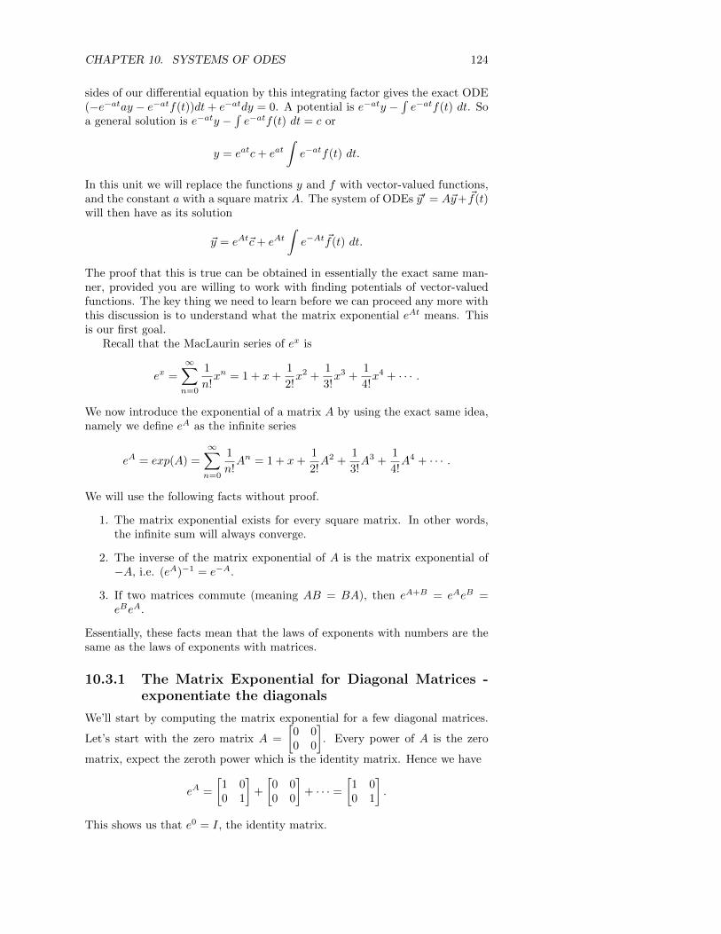
CHAPTER 10. SYSTEMS OF ODES 124
sides of our differential equation by this integrating factor gives the exact ODE(−e−atay − e−atf(t))dt+ e−atdy = 0. A potential is e−aty −
∫e−atf(t) dt. So
a general solution is e−aty −∫e−atf(t) dt = c or
y = eatc+ eat∫e−atf(t) dt.
In this unit we will replace the functions y and f with vector-valued functions,and the constant a with a square matrix A. The system of ODEs ~y′ = A~y+ ~f(t)will then have as its solution
~y = eAt~c+ eAt∫e−At ~f(t) dt.
The proof that this is true can be obtained in essentially the exact same man-ner, provided you are willing to work with finding potentials of vector-valuedfunctions. The key thing we need to learn before we can proceed any more withthis discussion is to understand what the matrix exponential eAt means. Thisis our first goal.
Recall that the MacLaurin series of ex is
ex =
∞∑n=0
1
n!xn = 1 + x+
1
2!x2 +
1
3!x3 +
1
4!x4 + · · · .
We now introduce the exponential of a matrix A by using the exact same idea,namely we define eA as the infinite series
eA = exp(A) =
∞∑n=0
1
n!An = 1 + x+
1
2!A2 +
1
3!A3 +
1
4!A4 + · · · .
We will use the following facts without proof.
1. The matrix exponential exists for every square matrix. In other words,the infinite sum will always converge.
2. The inverse of the matrix exponential of A is the matrix exponential of−A, i.e. (eA)−1 = e−A.
3. If two matrices commute (meaning AB = BA), then eA+B = eAeB =eBeA.
Essentially, these facts mean that the laws of exponents with numbers are thesame as the laws of exponents with matrices.
10.3.1 The Matrix Exponential for Diagonal Matrices -exponentiate the diagonals
We’ll start by computing the matrix exponential for a few diagonal matrices.
Let’s start with the zero matrix A =
[0 00 0
]. Every power of A is the zero
matrix, expect the zeroth power which is the identity matrix. Hence we have
eA =
[1 00 1
]+
[0 00 0
]+ · · · =
[1 00 1
].
This shows us that e0 = I, the identity matrix.
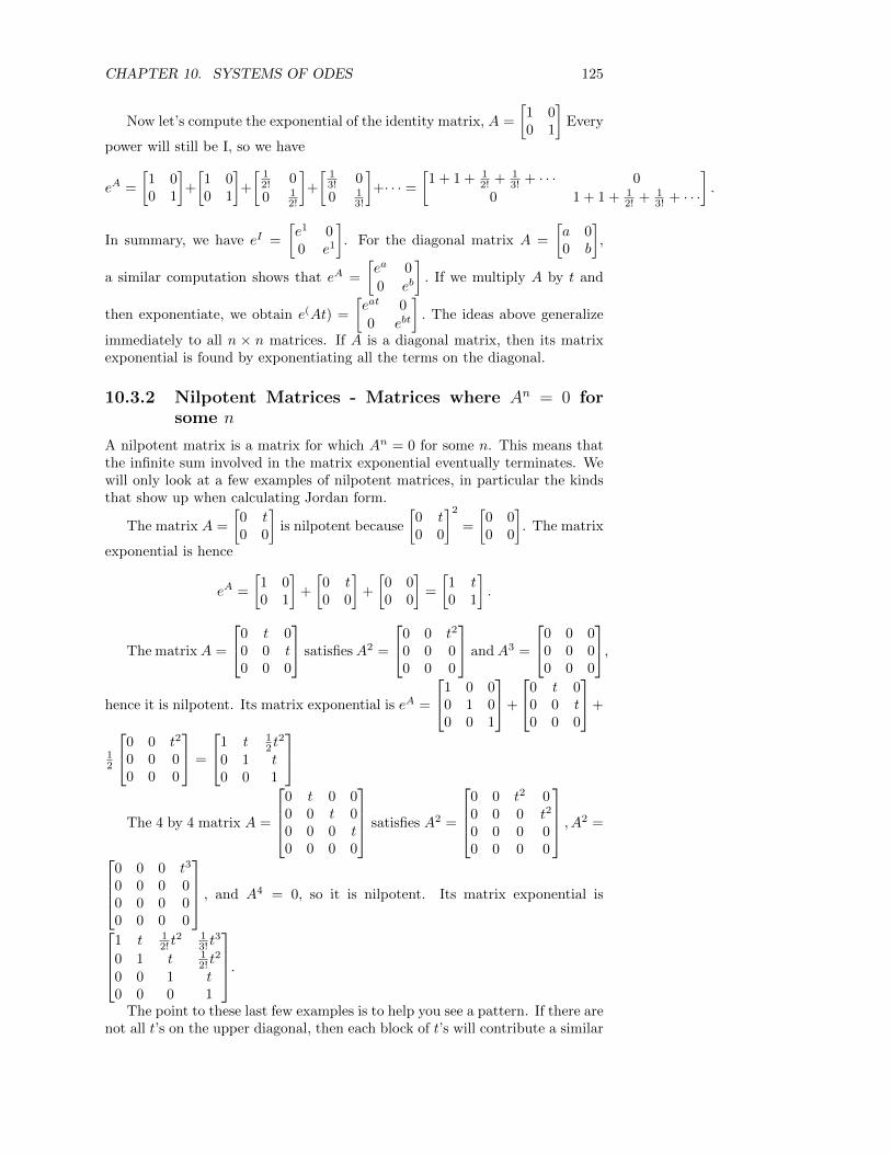
CHAPTER 10. SYSTEMS OF ODES 125
Now let’s compute the exponential of the identity matrix, A =
[1 00 1
]Every
power will still be I, so we have
eA =
[1 00 1
]+
[1 00 1
]+
[12! 0
0 12!
]+
[13! 0
0 13!
]+· · · =
[1 + 1 + 1
2! + 13! + · · · 0
0 1 + 1 + 12! + 1
3! + · · ·
].
In summary, we have eI =
[e1 00 e1
]. For the diagonal matrix A =
[a 00 b
],
a similar computation shows that eA =
[ea 0
0 eb
]. If we multiply A by t and
then exponentiate, we obtain e(At) =
[eat 0
0 ebt
]. The ideas above generalize
immediately to all n × n matrices. If A is a diagonal matrix, then its matrixexponential is found by exponentiating all the terms on the diagonal.
10.3.2 Nilpotent Matrices - Matrices where An = 0 forsome n
A nilpotent matrix is a matrix for which An = 0 for some n. This means thatthe infinite sum involved in the matrix exponential eventually terminates. Wewill only look at a few examples of nilpotent matrices, in particular the kindsthat show up when calculating Jordan form.
The matrix A =
[0 t0 0
]is nilpotent because
[0 t0 0
]2
=
[0 00 0
]. The matrix
exponential is hence
eA =
[1 00 1
]+
[0 t0 0
]+
[0 00 0
]=
[1 t0 1
].
The matrixA =
0 t 00 0 t0 0 0
satisfiesA2 =
0 0 t2
0 0 00 0 0
andA3 =
0 0 00 0 00 0 0
,
hence it is nilpotent. Its matrix exponential is eA =
1 0 00 1 00 0 1
+
0 t 00 0 t0 0 0
+
12
0 0 t2
0 0 00 0 0
=
1 t 12 t
2
0 1 t0 0 1
The 4 by 4 matrix A =
0 t 0 00 0 t 00 0 0 t0 0 0 0
satisfies A2 =
0 0 t2 00 0 0 t2
0 0 0 00 0 0 0
, A2 =
0 0 0 t3
0 0 0 00 0 0 00 0 0 0
, and A4 = 0, so it is nilpotent. Its matrix exponential is
1 t 1
2! t2 1
3! t3
0 1 t 12! t
2
0 0 1 t0 0 0 1
.
The point to these last few examples is to help you see a pattern. If there arenot all t’s on the upper diagonal, then each block of t’s will contribute a similar
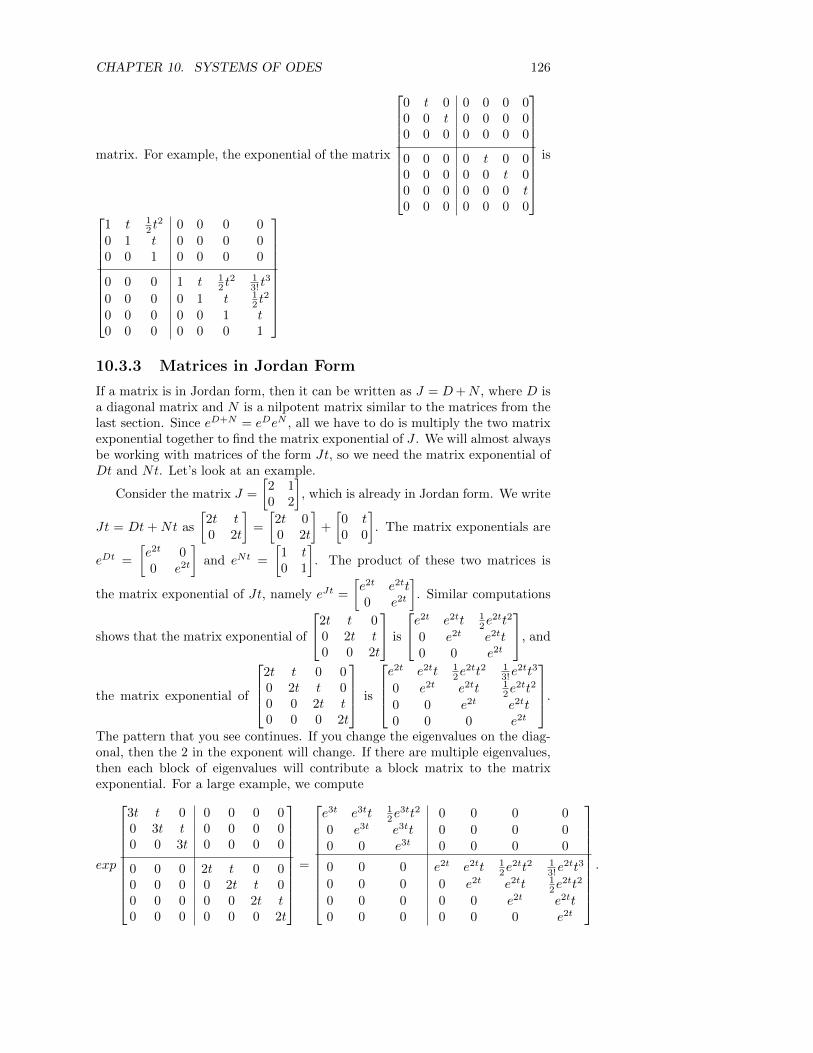
CHAPTER 10. SYSTEMS OF ODES 126
matrix. For example, the exponential of the matrix
0 t 0 0 0 0 00 0 t 0 0 0 00 0 0 0 0 0 0
0 0 0 0 t 0 00 0 0 0 0 t 00 0 0 0 0 0 t0 0 0 0 0 0 0
is
1 t 12 t
2 0 0 0 00 1 t 0 0 0 00 0 1 0 0 0 0
0 0 0 1 t 12 t
2 13! t
3
0 0 0 0 1 t 12 t
2
0 0 0 0 0 1 t0 0 0 0 0 0 1
10.3.3 Matrices in Jordan Form
If a matrix is in Jordan form, then it can be written as J = D+N , where D isa diagonal matrix and N is a nilpotent matrix similar to the matrices from thelast section. Since eD+N = eDeN , all we have to do is multiply the two matrixexponential together to find the matrix exponential of J . We will almost alwaysbe working with matrices of the form Jt, so we need the matrix exponential ofDt and Nt. Let’s look at an example.
Consider the matrix J =
[2 10 2
], which is already in Jordan form. We write
Jt = Dt + Nt as
[2t t0 2t
]=
[2t 00 2t
]+
[0 t0 0
]. The matrix exponentials are
eDt =
[e2t 00 e2t
]and eNt =
[1 t0 1
]. The product of these two matrices is
the matrix exponential of Jt, namely eJt =
[e2t e2tt0 e2t
]. Similar computations
shows that the matrix exponential of
2t t 00 2t t0 0 2t
is
e2t e2tt 12e
2tt2
0 e2t e2tt0 0 e2t
, and
the matrix exponential of
2t t 0 00 2t t 00 0 2t t0 0 0 2t
is
e2t e2tt 1
2e2tt2 1
3!e2tt3
0 e2t e2tt 12e
2tt2
0 0 e2t e2tt0 0 0 e2t
.
The pattern that you see continues. If you change the eigenvalues on the diag-onal, then the 2 in the exponent will change. If there are multiple eigenvalues,then each block of eigenvalues will contribute a block matrix to the matrixexponential. For a large example, we compute
exp
3t t 0 0 0 0 00 3t t 0 0 0 00 0 3t 0 0 0 0
0 0 0 2t t 0 00 0 0 0 2t t 00 0 0 0 0 2t t0 0 0 0 0 0 2t
=
e3t e3tt 12e
3tt2 0 0 0 0
0 e3t e3tt 0 0 0 00 0 e3t 0 0 0 0
0 0 0 e2t e2tt 12e
2tt2 13!e
2tt3
0 0 0 0 e2t e2tt 12e
2tt2
0 0 0 0 0 e2t e2tt0 0 0 0 0 0 e2t
.

CHAPTER 10. SYSTEMS OF ODES 127
10.3.4 Jordan form gives the matrix exponential for anymatrix.
We now consider the matrix exponential of any matrix A. Start by finding Qand J so thatQ−1AQ = J is a Jordan form forA. This means thatA = QJQ−1.Notice that A2 = QJQ−1QJQ−1 = QJ2Q−1, A3 = QJQ−1QJQ−1QJQ−1 =QJ3Q−1, and An = QJnQ−1. This means that the matrix exponential of A is
eA =
∞∑n=0
1
n!An =
∞∑n=0
1
n!QJnQ−1 = Q
( ∞∑n=0
1
n!Jn
)Q−1 = QeJQ−1.
So if we can find the matrix exponential of a matrix in Jordan form, and we cancompute Q and Q−1, then we can find the matrix exponential of any matrix. Wewill never go beyond 2 by 2 and 3 by 3 matrices when we do problems in class,but theoretically you now have the tools for computing matrix exponentials ofany matrix. If we need to find the matrix exponential of At, then we can findthe matrix exponential of Jt and get exp(At) = Q exp(Jt) Q−1.
As an example, let’s consider the matrix A =
[2 11 2
]whose eigenvalues
are 1 and 3, with eigenvectors [−1, 1], [1, 1]. We then have Q =
[−1 11 1
]and
J =
[1 00 3
]so exp(Jt) =
[et 00 e3t
]and the matrix exponential of At is
exp(At) = QeJtQ−1 =
[−1 11 1
] [et 00 e3t
](−1
2
)[1 −1−1 −1
]=
(−1
2
)[−et − e3t et − e3t
et − e3t −et − e3t
]For an example with a repeated eigenvalue, let’s consider the matrix A =[
0 1−9 6
]. We can compute Q =
[1 − 1
3
3 0
]and J =
[3 10 3
]. The matrix
exponential of Jt is
[e3t e3tt0 e3t
]. We then have
exp (At) = exp
([0 1t−9t 6t
])=
[1 − 1
3
3 0
] [e3t e3tt0 e3t
] [0 1
3
−3 1
]=
[e3t − 3e3tt e3tt−9e3tt 3e3tt+ e3t
].
If the eigenvalues are irrational or complex, the computations are still thesame. When the eigenvalues are complex, Euler’s formula eix = cosx + i sinxor the identities cosh ix = cosx, sinh ix = i sinx can be used to simplify thematrix exponential so that it contains no imaginary components. Consider the
matrix A =
[0 1−4 0
]. We can compute Q =
[1 13i −3i
]and J =
[3i 00 −3i
].
The matrix exponential of Jt is
[eit 00 e−it
]. We then have
exp (At) = exp
([0 1t−9t 0
])=
[1 13i −3i
] [e3it 00 e−3it
]1
−6i
[−3i −1−3i 1
]=
[cos(3t) 1
3 sin 3t−3 sin(3t) cos 3t
].
Due to time constraints, we’ll have to finish this example in class.
10.4 Systems of ODEs
10.4.1 Dilution - Tank Mixing Problems
Before we start solving systems, let’s look at an example application to see whythey are useful. Systems are used to understand the motion of moving parts in

CHAPTER 10. SYSTEMS OF ODES 128
a machine, the flow of electricity in a complex network, and many more places.Lets focus on a dilution problem with multiple tanks, so we can see how thesystems of ODEs are created. We won’t be solving any of the ODEs below byhand, rather we will just set them up and let the computer solve them.
Suppose that two tanks are connected via tubes so that the water in thetanks can circulate between each other. Both tanks contain 50 gallons of water.The first tank contains 100lbs of salt, while the second tank is pure water. Thetubes connecting the tanks allow 3 gallons of water to flow from the first tankto the second tank each minute. Similarly, 3 gallons of water are allowed toflow from tank 2 to tank 1 each minute. As soon as water enters either tank, amixing blade ensures that the salt content is perfectly mixed into the tank. Theproblem we want to solve is this: how much salt is in each tank at any giventime t. We know that after sufficient time, we should have 50lbs in each tank(since 100 lbs spread evenly between two tanks will give 50 lbs in each tank).
Let y1(t) be the salt content in lbs in tank 1, and y2(t) be the salt contentin tank 2, where t is given in minutes and y1 and y2 are given in lbs. Weknow that 3 gallons of water flows out of each tank each minute, and 3 gallonsflows in each minute. Let’s focus on tank 1 for a minute and determine it’soutflow and inflow rates. The only water coming into tank 1 each minutecomes from tank 2. We know that 3 out of the 50 gallons from tank 2 willenter tank 1, so the fraction 3
50 represents the proportion of water leavingtank 2 and entering tank 1. This means that the inflow rate for tank 1 is350y2. Similarly, the outflow rate for tank 1 is 3
50y2. Combining these gives adifferential equation y′1 = 3
50y2 − 350y1. Examining tank 2 gives the equation
y′2 = 350y1 − 3
50y2. We now have a system of ODEs
{y′1 = 3
50y2 − 350y1
y′2 = 350y1 − 3
50y2
or in matrix form
[y′1y′2
]=
[−3/50 3/503/50 −3/50
] [y1
y2
]+
[00
], which a first order
homogeneous linear system of ODEs. The intial conditions are y1(0) = 100 andy2(0) = 0.
Consider a similar problem, with these modifications. Each tank still has 50galls, with 100 lbs of salt in tank 1. Each minute, 2 gallons of water containing4lbs per gallon are dumped into tank 1 from an outside source. The pump intank 1 causes 5 gallons per minute to leave tank 1 and enter tank 2. The pumpin tank 2 cause only 3 gallons per minute to flow back into tank 1. The extra2 gallons per minute which flow into tank 2 from the tank 1 pipes flow out ofthe system via a drainage pipe. How much water is in each tank at any giventime?
The flow into tank 1 comes from 2 parts. Each minute 2 gallons containing4 lbs/gal enters the tank, so 8 lbs will enter. In addition, 3/50 ths of thesalt in tank 2 will enter tank 1. The outflow is 5/50 ths the salt in tank1, since 5 gal are flowing toward tank 2 each minute. This gives the ODEy′1 = 8+3/50y2−5/50y1. The inflow in the second tank is 5/50 ths of y1, and theoutflow is 3/50 ths of y2 toward tank 1 plus 2/50 ths of y2 toward drainage. Thismeans we have y′2 = 5/50y1 − 5/50y2. In matrix form we can write the system
as
{y′1 = 3
50y2 − 350y1
y′2 = 350y1 − 3
50y2
or in matrix form
[y′1y′2
]=
[−5/50 3/505/50 −5/50
] [y1
y2
]+[
80
], which is a nonhomogeneous linear system of ODEs, with intial conditions
y1(0) = 100 and y2(0) = 0. In general, a non homogeneous system will occurwhen the rates of change are influenced by things outside the system, like extrasalt being dumped into the system from somewhere else.
Now let’s change the size of the tanks, to see how size affects the prob-

CHAPTER 10. SYSTEMS OF ODES 129
lem. Let tank 1 contain 100 gallons and tank 2 contain 50 gallons. Dump 3gallons, with 5lbs of salt per gallon, into tank 1 each minute. Pumps cause6 gallons to flow from tank 1 to tank 2, and 3 gallons to flow from tank 2 totank 1. This leaves 3 gallons per minute to leave via a drain pipe in tank 2.The corresponding system of ODEs would be y′1 = (3)(5) + 3/50y2 − 6/100y1
and y′2 = 6/100y1 − 6/50y2. In matrix form we can write this as
[y′1y′2
]=[
−6/100 3/506/100 −6/50
] [y1
y2
]+
[150
].
As a final example, let’s consider 3 tanks. Suppose tank 1 contains 100gallons with 300 lbs of salt. Tank 2 contains 50 gallons with 20 lbs of salt, andtank 3 contains 30 gallons of pure water. Pumps allows 2 gallons per minuteto flow each direction between tank 1 and tank 2. Another set of pumps allows3 gallons per minute to flow between tanks 1 and 3. There are no pumpsconnecting tank 2 and tank 3. Let’s set up a system of ODEs in matrix formwhose solution would give us the salt content in each tank at any given time. Fortank 1, we have an inflow of 2/50 y2 plus 3/40 y3. The outflow is 5/100 y1 (2 galtoward tank 2 and 3 toward tank 3). Continuing in this fashion, we eventually
obtain the matrix equation
y′1y′2y′3
=
−5/100 2/50 3/402/100 −2/50 03/100 0 −3/40
y1
y2
y3
, which is
a homogeneous linear first order system of ODEs.
10.4.2 Solving a system of ODEs
We are now ready to solve systems of ODEs. Recall at the beginning of theunit that the solution to the ODE y′ = ay+ f(t) is y = eatc+ eat
∫e−atf(t) dt.
In terms of systems, we can solve the linear system of ODEs with constantcoefficient matrix A given by ~y′ = A~y + ~f(t) using the solution
~y = eAt~c+ eAt∫e−At ~f(t) dt.
If the system is homogeneous, meaning ~f(t) = ~0, then the solution is simply~y = eAt~c. If the initial conditions are ~y(0) = ~y0, then the constant vector ~cmust equal the initial conditions. If the system is nonhomogeneous, then wewill have to use the initial conditions to find ~c. Let’s look at a few examples.
Homogeneous: f~(t) = 0
Let’s start by solving the system of ODEs given by
[y′1y′2
]=
[3 10 3
] [y1
y2
]. Since
the coefficient matrix A =
[3 10 3
]is already in Jordan form, we know the
matrix exponential of A times t is exp(At) =
[e3t te3t
0 e3t
]. Hence we have as
a solution to our ODE
[y1
y2
]=
[e3t te3t
0 e3t
] [c1c2
]=
[c1e
3t + c2te3t
c2e3t
]. Without
using matrix form, a general solution would be y1 = c1e3t + c2te
3t, y2 = c2e3t.
To check our solution, we compute y′1 = 3c1e3t+3c2te
3t+c2e3t and y′2 = 3c2e
3t.The system of ODEs requires that y′1 = 3y1 + y2 = 3(c1e
3t + c2te3t) + (c2e
3t)(which is correct), and that y′2 = 3y2 = 3(c2e
3t) (which is also correct).In the previous problem, let’s add the initial conditions y1(0) = 2 and
y2(0) = 7. Recall that e0 = I, so plugging in t = 0 into our vector equation
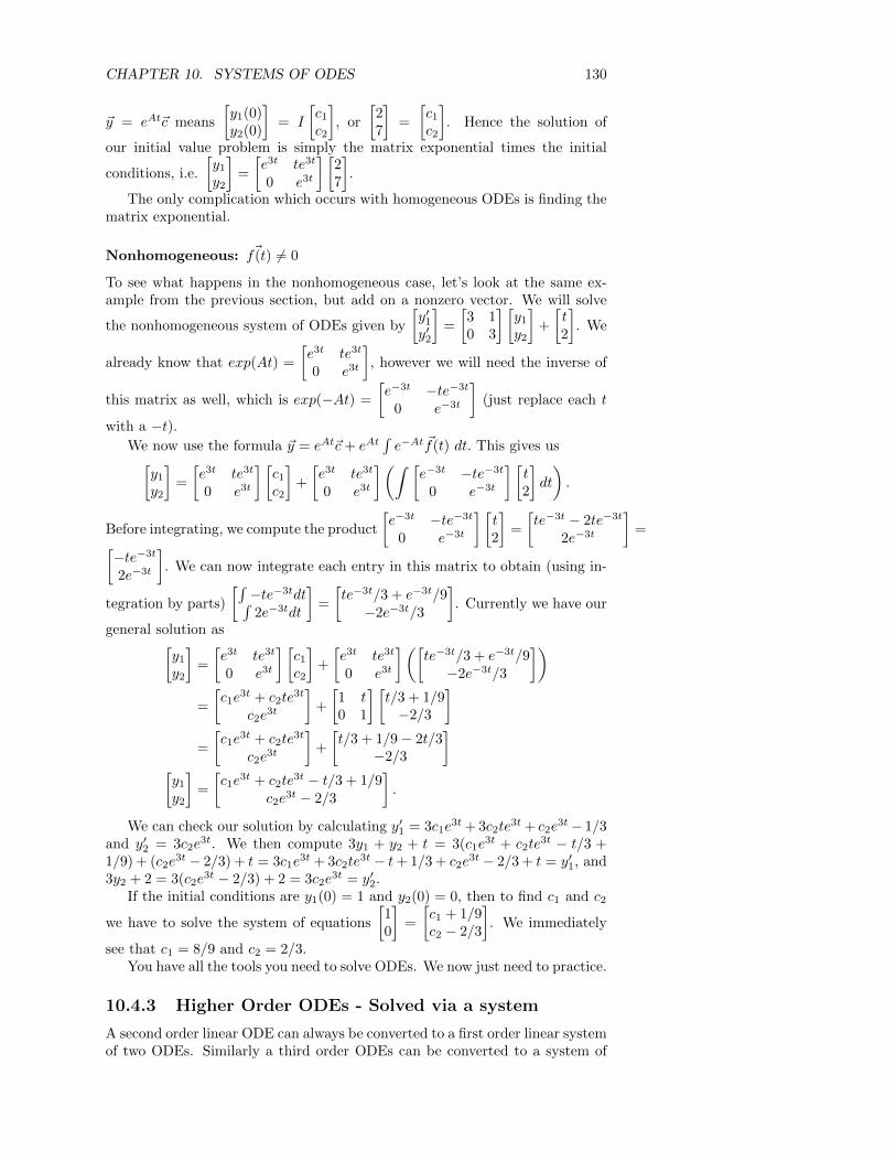
CHAPTER 10. SYSTEMS OF ODES 130
~y = eAt~c means
[y1(0)y2(0)
]= I
[c1c2
], or
[27
]=
[c1c2
]. Hence the solution of
our initial value problem is simply the matrix exponential times the initial
conditions, i.e.
[y1
y2
]=
[e3t te3t
0 e3t
] [27
].
The only complication which occurs with homogeneous ODEs is finding thematrix exponential.
Nonhomogeneous: f~(t) 6= 0
To see what happens in the nonhomogeneous case, let’s look at the same ex-ample from the previous section, but add on a nonzero vector. We will solve
the nonhomogeneous system of ODEs given by
[y′1y′2
]=
[3 10 3
] [y1
y2
]+
[t2
]. We
already know that exp(At) =
[e3t te3t
0 e3t
], however we will need the inverse of
this matrix as well, which is exp(−At) =
[e−3t −te−3t
0 e−3t
](just replace each t
with a −t).We now use the formula ~y = eAt~c+ eAt
∫e−At ~f(t) dt. This gives us[
y1
y2
]=
[e3t te3t
0 e3t
] [c1c2
]+
[e3t te3t
0 e3t
](∫ [e−3t −te−3t
0 e−3t
] [t2
]dt
).
Before integrating, we compute the product
[e−3t −te−3t
0 e−3t
] [t2
]=
[te−3t − 2te−3t
2e−3t
]=[
−te−3t
2e−3t
]. We can now integrate each entry in this matrix to obtain (using in-
tegration by parts)
[∫−te−3tdt∫2e−3tdt
]=
[te−3t/3 + e−3t/9−2e−3t/3
]. Currently we have our
general solution as[y1
y2
]=
[e3t te3t
0 e3t
] [c1c2
]+
[e3t te3t
0 e3t
]([te−3t/3 + e−3t/9−2e−3t/3
])=
[c1e
3t + c2te3t
c2e3t
]+
[1 t0 1
] [t/3 + 1/9−2/3
]=
[c1e
3t + c2te3t
c2e3t
]+
[t/3 + 1/9− 2t/3
−2/3
][y1
y2
]=
[c1e
3t + c2te3t − t/3 + 1/9
c2e3t − 2/3
].
We can check our solution by calculating y′1 = 3c1e3t + 3c2te
3t + c2e3t− 1/3
and y′2 = 3c2e3t. We then compute 3y1 + y2 + t = 3(c1e
3t + c2te3t − t/3 +
1/9) + (c2e3t − 2/3) + t = 3c1e
3t + 3c2te3t − t+ 1/3 + c2e
3t − 2/3 + t = y′1, and3y2 + 2 = 3(c2e
3t − 2/3) + 2 = 3c2e3t = y′2.
If the initial conditions are y1(0) = 1 and y2(0) = 0, then to find c1 and c2
we have to solve the system of equations
[10
]=
[c1 + 1/9c2 − 2/3
]. We immediately
see that c1 = 8/9 and c2 = 2/3.You have all the tools you need to solve ODEs. We now just need to practice.
10.4.3 Higher Order ODEs - Solved via a system
A second order linear ODE can always be converted to a first order linear systemof two ODEs. Similarly a third order ODEs can be converted to a system of
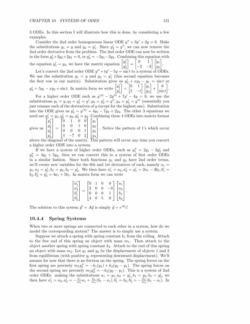
CHAPTER 10. SYSTEMS OF ODES 131
3 ODEs. In this section I will illustrate how this is done, by considering a fewexamples.
Consider the 2nd order homogeneous linear ODE y′′ + 3y′ + 2y = 0. Makethe substitutions y1 = y and y2 = y′1. Since y′2 = y′′, we can now remove the2nd order derivative from the problem. The 2nd order ODE can now be writtenin the form y′2+3y2+2y1 = 0, or y′2 = −2y1−3y2. Combining this equation with
the equation y′1 = y2, we have the matrix equation
[y′1y′2
]=
[0 1−2 −3
] [y1
y2
].
Let’s convert the 2nd order ODE y′′+ ty′− 5y = sin t to a system of ODEs.We use the substitution y1 = y and y2 = y′1 (this second equation becomesthe first row in our matrix). Substitution gives us y′2 + xy2 − y1 = sin t or
y′2 = 5y1 − xy2 + sin t. In matrix form we write
[y′1y′2
]=
[0 15 −t
] [y1
y2
]+
[0
sin t
].
For a higher order ODE such as y(4) − 2y′′′ + 7y′ − 4y = 0, we use thesubstitutions y1 = y, y2 = y′1 = y′, y3 = y′2 = y′′, y4 = y′3 = y′′′ (essentially youjust rename each of the derivatives of y except for the highest one). Substitutioninto the ODE gives us y′4 = y(4) = 4y1 − 7y2 + 2y4. The other 3 equations weneed are y′1 = y2, y
′2 = y3, y
′3 = y4. Combining these 4 ODEs into matrix format
gives us
y′1y′2y′3y′4
=
0 1 0 00 0 1 00 0 0 14 −7 0 2
y1
y2
y3
y4
. Notice the pattern of 1’s which occur
above the diagonal of the matrix. This pattern will occur any time you converta higher order ODE into a system.
If we have a system of higher order ODEs, such as y′′1 = 2y1 − 3y′2 andy′′2 = 4y1 + 5y2, then we can convert this to a system of first order ODEsin a similar fashion. Since both functions y1 and y2 have 2nd order terms,we’ll create new variables for the 0th and 1st derivatives of each, namely a1 =y1, a2 = y′1, b1 = y2, b2 = y′2. We then have a′1 = a2, a
′2 = y′1 = 2a1 − 3b2, b
′1 =
b2, b′2 = y′2 = 4a1 + 5b1. In matrix form we can write
a′1a′2b′1b′2
=
0 1 0 02 0 0 −30 0 0 14 0 5 0
a1
a2
b1b2
.The solution to this system ~y′ = A~y is simply ~y = eAt~c.
10.4.4 Spring Systems
When two or more springs are connected to each other in a system, how do wemodel the corresponding motion? The answer is to simply use a system.
Suppose we attach a spring with spring constant k1 from the ceiling. Attachto the free end of this spring an object with mass m1. Then attach to theobject another spring with spring constant k2. Attach to the end of this springan object with mass m2. Let y1 and y2 be the displacement of objects 1 and 2from equilibrium (with positive yi representing downward displacement). We’llassume for now that there is no friction on the spring. The spring forces on thefirst spring are precisely m1y
′′1 = −k1(y1) + k2(y2 − y1). The spring forces on
the second spring are precisely m2y′′2 = −k2(y2 − y1). This is a system of 2nd
order ODEs. making the substitutions a1 = y1, a2 = y′1, b1 = y2, b2 = y′2, wethen have a′1 = a2, a
′2 = − k1
m1a1 + k2
m1(b1 − a1), b′1 = b2, b
′2 = − k2
m2(b1 − a1). In

CHAPTER 10. SYSTEMS OF ODES 132
matrix form we can writea′1a′2b′1b′2
=
0 1 0 0
− k1m1− k2
m10 k2
m10
0 0 0 1k2m2
0 − k2m2
0
a1
a2
b1b2
.The solution to this system ~y′ = A~y is simply ~y = eAt~c. The process abovegeneralizes to any mass spring system.
10.4.5 Electrical Systems
When multiple loops occur in an electrical system involving resistors, inductors,and capacitors, how do we model the corresponding current? We use a system.Remember that Kirchoff’s current law states that at each node, the current inequals the current out. In addition, Kirchoff’s voltage laws states that alongeach loop, the voltage supplied equals the voltage suppressed. Each resistorcontributes a voltage drop of RI ohms, each capacitor a drop of 1
C
∫Idt farads,
and each inductor a voltage drop of LI ′ Henrys.Consider the electrical network on the right, where R1 = 1, R2 = 2, R3 =
3, L = 4, C = 15 , E = 12. Kirchoff’s current law states that I1 = I2 + I3. On
the left loop, Kirchoff’s voltage law states that E = R1I1+R2I2+LI ′1 or usingthe given numbers we have 12 = I1 + 2I2 + 4I ′1. On the right loop, Kirchoff’svoltage law states that 0 = I3R3 + 1
C
∫I3dt−R2I2 or differentiating and using
the given numbers we have 0 = 3I ′3+5I3−2I ′2. We now need to solve this systemfor I ′1, I
′2, and I ′3. Solving the second equation for I ′1 gives I ′1 = 1
4 (12−I1−2I2).Taking derivatives of the first equation gives I ′1 = I ′2 + I ′3, which means we canreplace I ′2 in the third equation with I ′2 = I ′1− I ′3 = 1
4 (12− I1− 2I2)− I ′3. Thisgives us the equation 0 = 3I ′3 +5I3−2I ′2 = 3I ′3 +5I3−2
(14 (12− I1 − 2I2)− I ′3
).
Solving for I ′3 gives us I ′3 = 15
(−5I3 + 1
2 (12− I1 − 2I2)). Since I ′2 = I ′1− I ′3, we
now use the information we have for I ′1 and I ′3 to write I ′2 = 14 (12− I1− 2I2)−
15
(−5I3 + 1
2 (12− I1 − 2I2)). This gives us the system of ODEs in matrix form
asI ′1 = 1
4 (12− I1 − 2I2)
I ′2 = 14 (12− I1 − 2I2)− 1
5
(−5I3 + 1
2 (12− I1 − 2I2))
I ′3 = 15
(−5I3 + 1
2 (12− I1 − 2I2))
I ′1I ′2I ′3
=
− 14 − 1
2 0
− 14 + 1
10 − 12 + 1
10 1
− 110 − 1
5 −1
I1I2I3
+
3
3− 65
65
Since we have written our ODE in the form ~y′ = A~y+ ~f , the solution is simply~y = eAt~c+ eAt
∫e−At ~fdt. A computer can quickly solve this system.

CHAPTER 10. SYSTEMS OF ODES 133
10.5 Preparation
This chapter covers the following ideas. When you create your lesson plan, it should contain examples whichillustrate these key ideas. Before you take the quiz on this unit, meet with another student out of class andteach each other from the examples on your lesson plan.
1. Explain the basic theory of systems of linear ODEs and the Wronskian for systems.
2. Convert higher order ODEs to first order linear systems.
3. Explain how to use eigenvalues and eigenvectors to diagonalize matrices. When not possible, usegeneralized eigenvectors to find Jordan canonical form.
4. Find the matrix exponential of a square matrix, and use it to solve linear homogeneous and nonhomo-geneous ODEs.
5. Give applications of systems of ODEs. In particular be able to setup systems of ODE related todilution, electricity, and springs (use the computer to solve complex systems).
Preparation Problems (click for solutions)
Day 1 1, 2a, 2b, 3a
Day 2 3d, 4cghj, 5a, 5c
Day 3 6a, 7ag, 8b, 8c,
Day 4 9a, 9b, 10a, 11a
The accompanying problems will serve as our problems set for this unit. Handwritten solutions to mostof these problems area available online (click for solutions). You can use the technology introduction to checkany answer, as well as give a step-by-step solution to any of the problems. However, on problems where thesystem is not diagonalizable, the matrix Q used to obtain Jordan form is not unique (so your answer maydiffer a little, until you actually compute the matrix exponential QeJtQ−1 = eAt).
10.6 Problems
1. Solve the linear ODE y′ = ay(t) + f(t), wherea is a constant and f(t) is any function of t.You will need an integrating factor, and yoursolution will involve the integral of a function.
2. For each system of ODEs, solve the system us-ing the eigenvalue approach. Find the Wron-skian and compute its determinant to show thatyour solutions are linearly independent.
(a) y′1 = 2y1 + 4y2, y′2 = 4y1 + 2y2, y1(0) =
1, y2(0) = 4
(b) y′1 = y1 + 2y2, y′2 = 3y1, y1(0) = 6, y2(0) =
0
(c) y′1 = y1 + 4y2, y′2 = 3y1 + 2y2, y1(0) =
0, y2(0) = 1
(d) y′1 = y2, y′2 = −3y1 − 4y2, y1(0) =
1, y2(0) = 2
3. (Jordan Form) For each matrix A, find matrices
Q,Q−1, and J so that Q−1AQ = J is a Jordancanonical form of A.
(a)
[1 20 3
](b)
[0 1−1 −2
]
(c)
1 2 20 1 20 0 1
(d)
1 2 20 1 00 0 1
(e)
[0 1−1 0
]
4. For each of the following matrices A which arealready in Jordan form, find the matrix expo-nential. Note that if t follows a matrix, thatmeans you should multiply each entry by t.

CHAPTER 10. SYSTEMS OF ODES 134
(a)
[2 00 3
](b)
[2 00 3
]t
(c)
2 0 00 3 00 0 4
(d)
2 0 00 3 00 0 4
t
(e)
[0 10 0
]t
(f)
[4 10 4
]t
(g)
0 1 00 0 10 0 0
t
(h)
5 1 00 5 10 0 5
t
(i)
0 1 0 0 00 0 1 0 00 0 0 0 00 0 0 0 10 0 0 0 0
t
(j)
3 1 0 0 00 3 1 0 00 0 3 0 00 0 0 −2 10 0 0 0 −2
t
5. For each of the following matrices, find the ma-trix exponential. You will have to find the Jor-dan form.
(a)
[0 1−3 4
](b)
[0 1−6 −5
](c)
[0 1−1 −2
](d)
[0 1−4 −4
]
(e)
[0 1−1 0
](f)
[0 1−4 0
](g)
[0 10 3
](h)
[2 44 2
]6. Set up an initial value problem in matrix for-
mat for each of the following scenarios (mixingtank, dilution problems). Solve each one withthe computer.
(a) Tank 1 contains 30 gal, tank 2 contains 40.Pumps allow 5 gal per minute to flow ineach direction between the two tanks. Iftank 1 initially contains 20lbs of salt, andtank 2 initially contains 120 lbs of salt,how much salt will be in each tank at anygiven time t. Remember, you are just sup-posed to set up the IVP, not actually solveit (the eigenvalues are not very pretty).
(b) Three tanks each contain 100 gallons ofwater. Tank 1 contains 400lbs of saltmixed in. Pumps allow 5 gal/min to circu-late in each direction between tank 1 and
tank 2. Another pump allows 4 gallons ofwater to circulate each direction betweentanks 2 and 3. How much salt is in eachtank at any time t?
(c) Four tanks each contain 30 gallons. Be-tween each pair of tanks, a set of pumpsallows 1 gallon per minute to circulate ineach direction (so that each tank has a to-tal of 3 gallons leaving and 3 gallons enter-ing). Tank 1 contains 50lbs of salt, tank 2contains 80 lbs of salt, tank 3 contains 10lbs of salt, and tank 4 is pure water. Howmuch salt is in each tank at time t?
(d) Tank 1 contains 80 gallons of pure water,and tank 2 contains 50 gallons of pure wa-ter. Each minute 4 gallons of water con-taining 3lbs of salt per gallon are added totank 1. Pumps allow 6 gallons per minuteof water to flow from tank 1 to tank 2,and 2 gallons of water to flow from tank2 to tank 1. A drainage pipe removes 4gallons per minute of liquid from tank 2.How much salt is in each tank at any timet?
7. Convert each of the following high order ODEs(or systems of ODEs) to a first order linear sys-tem of ODEs. Which are homogeneous, andwhich are nonhomogeneous?
(a) y′′ + 4y′ + 3y = 0
(b) y′′ + 4y′ + 3y = 4t
(c) y′′ + ty′ − 2y = 0
(d) y′′ + ty′ − 2y = cos t
(e) y′′′ + 3y′′ + 3y′ + y = 0
(f) y′′′′ − 4y′′′ + 6y′′ − 4y′ + y = t
(g) y′′1 = 4y′1 + 3y2, y′2 = 5y1 − 4y2.
(h) Chapter 17, problems 1-20, in Schaum’s
8. Solve the following homogeneous systems ofODEs, or higher order ODEs, with the giveninitial conditions.
(a) y′1 = 2y1, y′2 = 4y2, y1(0) = 5, y2(0) = 6
(b) y′1 = 2y1 + y2, y′2 = 2y2, y1(0) =
−1, y2(0) = 3
(c) y′′ + 4y′ + 3y = 0, y(0) = 0, y′(0) = 1
(d) y′′ + 2y′ + y = 0, y(0) = 2, y′(0) = 0
(e) y′1 = 2y1 + y2, y′2 = y1 + 2y2, y1(0) =
2, y2(0) = 1
(f) y′1 = y2, y′2 = −y1, y1(0) = 1, y2(0) = 2
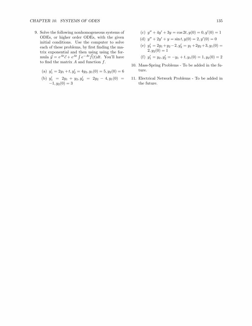
CHAPTER 10. SYSTEMS OF ODES 135
9. Solve the following nonhomogeneous systems ofODEs, or higher order ODEs, with the giveninitial conditions. Use the computer to solveeach of these problems, by first finding the ma-trix exponential and then using using the for-mula ~y = eAt~c + eAt
∫e−At ~f(t)dt. You’ll have
to find the matrix A and function f .
(a) y′1 = 2y1 + t, y′2 = 4y2, y1(0) = 5, y2(0) = 6
(b) y′1 = 2y1 + y2, y′2 = 2y2 − 4, y1(0) =
−1, y2(0) = 3
(c) y′′ + 4y′ + 3y = cos 2t, y(0) = 0, y′(0) = 1
(d) y′′ + 2y′ + y = sin t, y(0) = 2, y′(0) = 0
(e) y′1 = 2y1 +y2−2, y′2 = y1 +2y2 +3, y1(0) =2, y2(0) = 1
(f) y′1 = y2, y′2 = −y1 + t, y1(0) = 1, y2(0) = 2
10. Mass-Spring Problems - To be added in the fu-ture.
11. Electrical Network Problems - To be added inthe future.
Chapter 11
Fourier Series
This chapter covers the following ideas. When you create your lesson plan, itshould contain examples which illustrate these key ideas. Before you take thequiz on this unit, meet with another student out of class and teach each otherfrom the examples on your lesson plan.
1. Define period, and how to find a Fourier series of a function of period 2πand 2L.
2. Explain how to find Fourier coefficients using Euler formulas, and be ableto explain why the Euler formulas are correct.
3. Give conditions as to when a Fourier series will exist, and explain the dif-ference between a Fourier series and a function at points of discontinuity.
4. Give examples of even and odd functions, and correspondingly developFourier cosine and sine series. Use these ideas to discuss even and oddhalf-range expansions.
11.1 Basic Definitions
A function f(x) is said to be periodic with period p if f(x + p) = f(x) for allx in the domain of f . This means that the function will repeat itself every punits. The trig functions sinx and cosx are periodic with period 2π, as wellas with period 4π, 6π, 8π, etc. The fundamental period is the smallest positiveperiod of a function. The function sinnx is periodic, with fundamental period2πn , though it also has period 2π.
If two functions are period with the same period, then any linear combina-tion of those functions is periodic with the same period. In particular, the suma0 +
∑∞n=1(an cosnx + bn sinnx) has period 2π. This sum is called a Fourier
series, where ai, bi are called Fourier coefficients. Given a function f(x) whichhas period 2π, we write
f(x) = a0 +
∞∑n=1
(an cosnx+ bn sinnx)
where the Fourier coefficients of f(x) are given by the Euler formulas
a0 =1
2π
∫ π
−πf(x)dx, an =
1
π
∫ π
−πf(x) cos(nx)dx, bn =
1
π
∫ π
−πf(x) sin(nx)dx
136
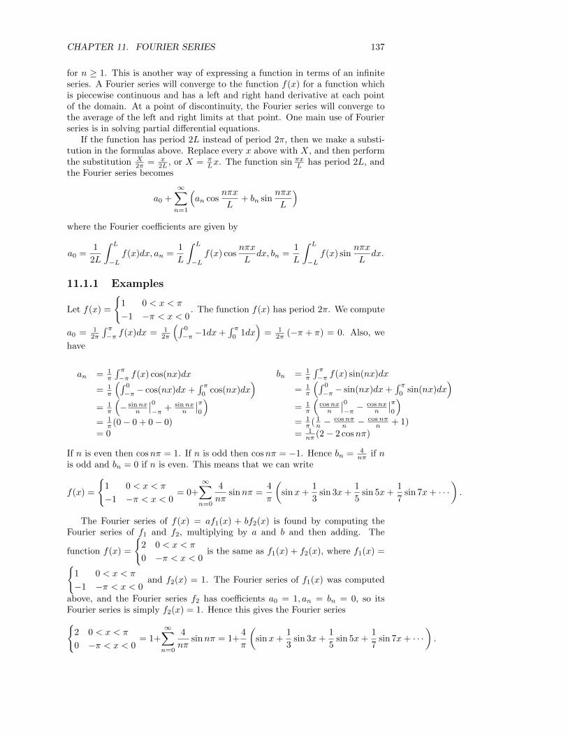
CHAPTER 11. FOURIER SERIES 137
for n ≥ 1. This is another way of expressing a function in terms of an infiniteseries. A Fourier series will converge to the function f(x) for a function whichis piecewise continuous and has a left and right hand derivative at each pointof the domain. At a point of discontinuity, the Fourier series will converge tothe average of the left and right limits at that point. One main use of Fourierseries is in solving partial differential equations.
If the function has period 2L instead of period 2π, then we make a substi-tution in the formulas above. Replace every x above with X, and then performthe substitution X
2π = x2L , or X = π
Lx. The function sin πxL has period 2L, and
the Fourier series becomes
a0 +
∞∑n=1
(an cos
nπx
L+ bn sin
nπx
L
)where the Fourier coefficients are given by
a0 =1
2L
∫ L
−Lf(x)dx, an =
1
L
∫ L
−Lf(x) cos
nπx
Ldx, bn =
1
L
∫ L
−Lf(x) sin
nπx
Ldx.
11.1.1 Examples
Let f(x) =
{1 0 < x < π
−1 −π < x < 0. The function f(x) has period 2π. We compute
a0 = 12π
∫ π−π f(x)dx = 1
2π
(∫ 0
−π −1dx+∫ π
01dx
)= 1
2π (−π + π) = 0. Also, we
have
an = 1π
∫ π−π f(x) cos(nx)dx
= 1π
(∫ 0
−π − cos(nx)dx+∫ π
0cos(nx)dx
)= 1
π
(− sinnx
n
∣∣0−π + sinnx
n
∣∣π0
)= 1
π (0− 0 + 0− 0)= 0
bn = 1π
∫ π−π f(x) sin(nx)dx
= 1π
(∫ 0
−π − sin(nx)dx+∫ π
0sin(nx)dx
)= 1
π
(cosnxn
∣∣0−π −
cosnxn
∣∣π0
)= 1
π ( 1n −
cosnπn − cosnπ
n + 1)
= 1nπ (2− 2 cosnπ)
If n is even then cosnπ = 1. If n is odd then cosnπ = −1. Hence bn = 4nπ if n
is odd and bn = 0 if n is even. This means that we can write
f(x) =
{1 0 < x < π
−1 −π < x < 0= 0+
∞∑n=0
4
nπsinnπ =
4
π
(sinx+
1
3sin 3x+
1
5sin 5x+
1
7sin 7x+ · · ·
).
The Fourier series of f(x) = af1(x) + bf2(x) is found by computing theFourier series of f1 and f2, multiplying by a and b and then adding. The
function f(x) =
{2 0 < x < π
0 −π < x < 0is the same as f1(x) + f2(x), where f1(x) ={
1 0 < x < π
−1 −π < x < 0and f2(x) = 1. The Fourier series of f1(x) was computed
above, and the Fourier series f2 has coefficients a0 = 1, an = bn = 0, so itsFourier series is simply f2(x) = 1. Hence this gives the Fourier series{
2 0 < x < π
0 −π < x < 0= 1+
∞∑n=0
4
nπsinnπ = 1+
4
π
(sinx+
1
3sin 3x+
1
5sin 5x+
1
7sin 7x+ · · ·
).
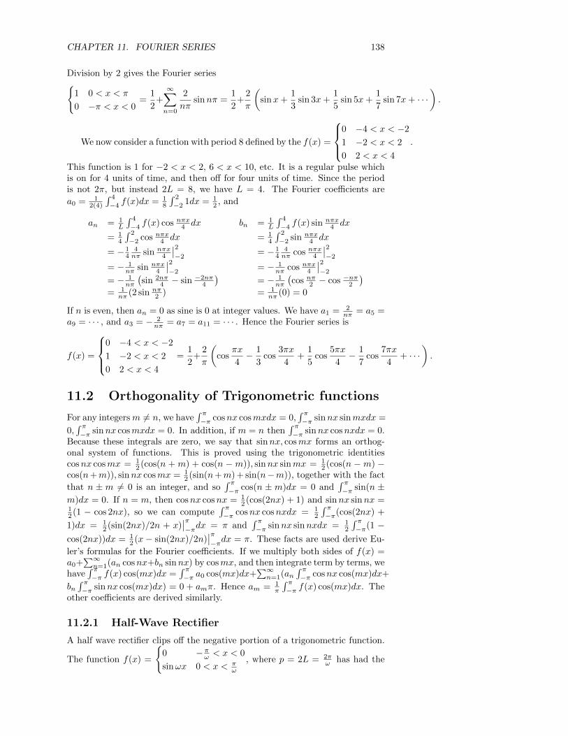
CHAPTER 11. FOURIER SERIES 138
Division by 2 gives the Fourier series{1 0 < x < π
0 −π < x < 0=
1
2+
∞∑n=0
2
nπsinnπ =
1
2+
2
π
(sinx+
1
3sin 3x+
1
5sin 5x+
1
7sin 7x+ · · ·
).
We now consider a function with period 8 defined by the f(x) =
0 −4 < x < −2
1 −2 < x < 2
0 2 < x < 4
.
This function is 1 for −2 < x < 2, 6 < x < 10, etc. It is a regular pulse whichis on for 4 units of time, and then off for four units of time. Since the periodis not 2π, but instead 2L = 8, we have L = 4. The Fourier coefficients are
a0 = 12(4)
∫ 4
−4f(x)dx = 1
8
∫ 2
−21dx = 1
2 , and
an = 1L
∫ 4
−4f(x) cos nπx4 dx
= 14
∫ 2
−2cos nπx4 dx
= − 14
4nπ sin nπx
4
∣∣2−2
= − 1nπ sin nπx
4
∣∣2−2
= − 1nπ
(sin 2nπ
4 − sin −2nπ4
)= 1
nπ (2 sin nπ2 )
bn = 1L
∫ 4
−4f(x) sin nπx
4 dx
= 14
∫ 2
−2sin nπx
4 dx
= − 14
4nπ cos nπx4
∣∣2−2
= − 1nπ cos nπx4
∣∣2−2
= − 1nπ
(cos nπ2 − cos −nπ2
)= 1
nπ (0) = 0
If n is even, then an = 0 as sine is 0 at integer values. We have a1 = 2nπ = a5 =
a9 = · · · , and a3 = − 2nπ = a7 = a11 = · · · . Hence the Fourier series is
f(x) =
0 −4 < x < −2
1 −2 < x < 2
0 2 < x < 4
=1
2+
2
π
(cos
πx
4− 1
3cos
3πx
4+
1
5cos
5πx
4− 1
7cos
7πx
4+ · · ·
).
11.2 Orthogonality of Trigonometric functions
For any integersm 6= n, we have∫ π−π cosnx cosmxdx = 0,
∫ π−π sinnx sinmxdx =
0,∫ π−π sinnx cosmxdx = 0. In addition, if m = n then
∫ π−π sinnx cosnxdx = 0.
Because these integrals are zero, we say that sinnx, cosmx forms an orthog-onal system of functions. This is proved using the trigonometric identitiescosnx cosmx = 1
2 (cos(n + m) + cos(n −m)), sinnx sinmx = 12 (cos(n −m) −
cos(n+m)), sinnx cosmx = 12 (sin(n+m) + sin(n−m)), together with the fact
that n ± m 6= 0 is an integer, and so∫ π−π cos(n ± m)dx = 0 and
∫ π−π sin(n ±
m)dx = 0. If n = m, then cosnx cosnx = 12 (cos(2nx) + 1) and sinnx sinnx =
12 (1 − cos 2nx), so we can compute
∫ π−π cosnx cosnxdx = 1
2
∫ π−π(cos(2nx) +
1)dx = 12 (sin(2nx)/2n + x)
∣∣π−πdx = π and
∫ π−π sinnx sinnxdx = 1
2
∫ π−π(1 −
cos(2nx))dx = 12 (x− sin(2nx)/2n)
∣∣π−πdx = π. These facts are used derive Eu-
ler’s formulas for the Fourier coefficients. If we multiply both sides of f(x) =a0+
∑∞n=1(an cosnx+bn sinnx) by cosmx, and then integrate term by terms, we
have∫ π−π f(x) cos(mx)dx =
∫ π−π a0 cos(mx)dx+
∑∞n=1(an
∫ π−π cosnx cos(mx)dx+
bn∫ π−π sinnx cos(mx)dx) = 0 + amπ. Hence am = 1
π
∫ π−π f(x) cos(mx)dx. The
other coefficients are derived similarly.
11.2.1 Half-Wave Rectifier
A half wave rectifier clips off the negative portion of a trigonometric function.
The function f(x) =
{0 −π
ω < x < 0
sinωx 0 < x < πω
, where p = 2L = 2πω has had the
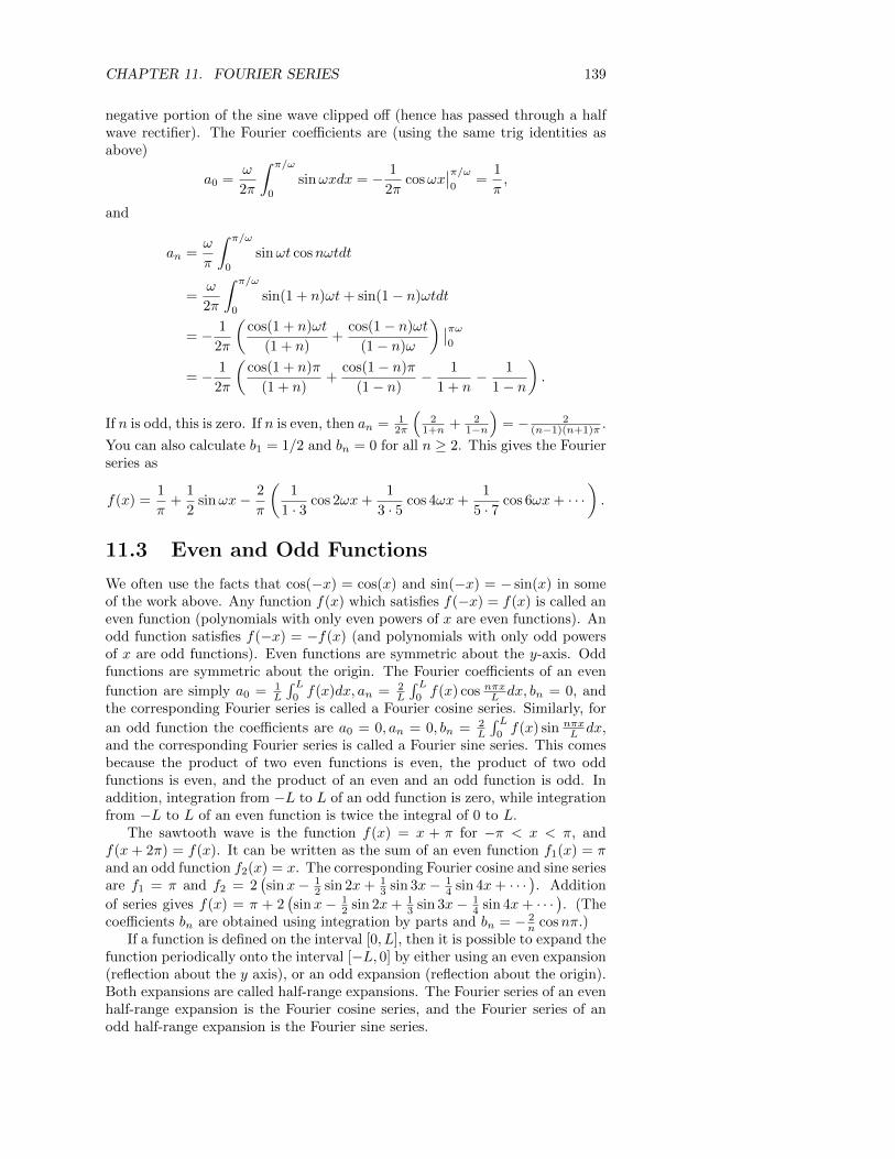
CHAPTER 11. FOURIER SERIES 139
negative portion of the sine wave clipped off (hence has passed through a halfwave rectifier). The Fourier coefficients are (using the same trig identities asabove)
a0 =ω
2π
∫ π/ω
0
sinωxdx = − 1
2πcosωx
∣∣π/ω0
=1
π,
and
an =ω
π
∫ π/ω
0
sinωt cosnωtdt
=ω
2π
∫ π/ω
0
sin(1 + n)ωt+ sin(1− n)ωtdt
= − 1
2π
(cos(1 + n)ωt
(1 + n)+
cos(1− n)ωt
(1− n)ω
) ∣∣πω0
= − 1
2π
(cos(1 + n)π
(1 + n)+
cos(1− n)π
(1− n)− 1
1 + n− 1
1− n
).
If n is odd, this is zero. If n is even, then an = 12π
(2
1+n + 21−n
)= − 2
(n−1)(n+1)π .
You can also calculate b1 = 1/2 and bn = 0 for all n ≥ 2. This gives the Fourierseries as
f(x) =1
π+
1
2sinωx− 2
π
(1
1 · 3cos 2ωx+
1
3 · 5cos 4ωx+
1
5 · 7cos 6ωx+ · · ·
).
11.3 Even and Odd Functions
We often use the facts that cos(−x) = cos(x) and sin(−x) = − sin(x) in someof the work above. Any function f(x) which satisfies f(−x) = f(x) is called aneven function (polynomials with only even powers of x are even functions). Anodd function satisfies f(−x) = −f(x) (and polynomials with only odd powersof x are odd functions). Even functions are symmetric about the y-axis. Oddfunctions are symmetric about the origin. The Fourier coefficients of an even
function are simply a0 = 1L
∫ L0f(x)dx, an = 2
L
∫ L0f(x) cos nπxL dx, bn = 0, and
the corresponding Fourier series is called a Fourier cosine series. Similarly, for
an odd function the coefficients are a0 = 0, an = 0, bn = 2L
∫ L0f(x) sin nπx
L dx,and the corresponding Fourier series is called a Fourier sine series. This comesbecause the product of two even functions is even, the product of two oddfunctions is even, and the product of an even and an odd function is odd. Inaddition, integration from −L to L of an odd function is zero, while integrationfrom −L to L of an even function is twice the integral of 0 to L.
The sawtooth wave is the function f(x) = x + π for −π < x < π, andf(x+ 2π) = f(x). It can be written as the sum of an even function f1(x) = πand an odd function f2(x) = x. The corresponding Fourier cosine and sine seriesare f1 = π and f2 = 2
(sinx− 1
2 sin 2x+ 13 sin 3x− 1
4 sin 4x+ · · ·). Addition
of series gives f(x) = π + 2(sinx− 1
2 sin 2x+ 13 sin 3x− 1
4 sin 4x+ · · ·). (The
coefficients bn are obtained using integration by parts and bn = − 2n cosnπ.)
If a function is defined on the interval [0, L], then it is possible to expand thefunction periodically onto the interval [−L, 0] by either using an even expansion(reflection about the y axis), or an odd expansion (reflection about the origin).Both expansions are called half-range expansions. The Fourier series of an evenhalf-range expansion is the Fourier cosine series, and the Fourier series of anodd half-range expansion is the Fourier sine series.
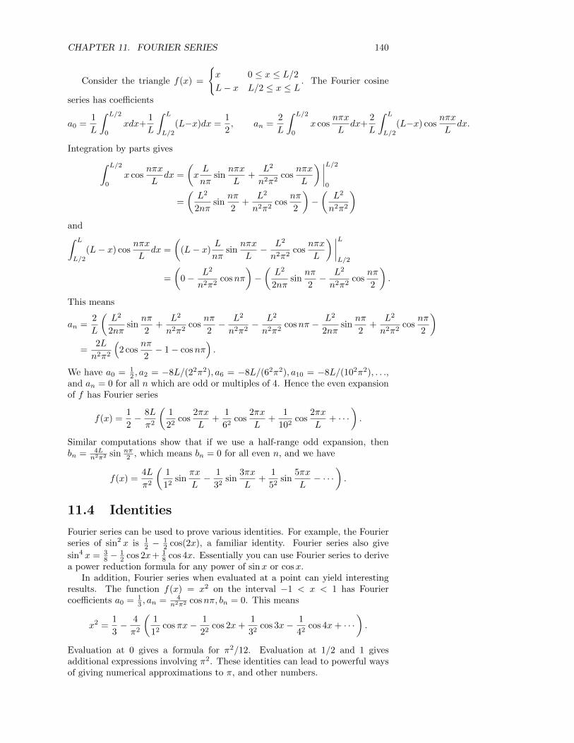
CHAPTER 11. FOURIER SERIES 140
Consider the triangle f(x) =
{x 0 ≤ x ≤ L/2L− x L/2 ≤ x ≤ L
. The Fourier cosine
series has coefficients
a0 =1
L
∫ L/2
0
xdx+1
L
∫ L
L/2
(L−x)dx =1
2, an =
2
L
∫ L/2
0
x cosnπx
Ldx+
2
L
∫ L
L/2
(L−x) cosnπx
Ldx.
Integration by parts gives∫ L/2
0
x cosnπx
Ldx =
(xL
nπsin
nπx
L+
L2
n2π2cos
nπx
L
) ∣∣∣∣L/20
=
(L2
2nπsin
nπ
2+
L2
n2π2cos
nπ
2
)−(
L2
n2π2
)and∫ L
L/2
(L− x) cosnπx
Ldx =
((L− x)
L
nπsin
nπx
L− L2
n2π2cos
nπx
L
) ∣∣∣∣LL/2
=
(0− L2
n2π2cosnπ
)−(L2
2nπsin
nπ
2− L2
n2π2cos
nπ
2
).
This means
an =2
L
(L2
2nπsin
nπ
2+
L2
n2π2cos
nπ
2− L2
n2π2− L2
n2π2cosnπ − L2
2nπsin
nπ
2+
L2
n2π2cos
nπ
2
)=
2L
n2π2
(2 cos
nπ
2− 1− cosnπ
).
We have a0 = 12 , a2 = −8L/(22π2), a6 = −8L/(62π2), a10 = −8L/(102π2), . . .,
and an = 0 for all n which are odd or multiples of 4. Hence the even expansionof f has Fourier series
f(x) =1
2− 8L
π2
(1
22cos
2πx
L+
1
62cos
2πx
L+
1
102cos
2πx
L+ · · ·
).
Similar computations show that if we use a half-range odd expansion, thenbn = 4L
n2π2 sin nπ2 , which means bn = 0 for all even n, and we have
f(x) =4L
π2
(1
12sin
πx
L− 1
32sin
3πx
L+
1
52sin
5πx
L− · · ·
).
11.4 Identities
Fourier series can be used to prove various identities. For example, the Fourierseries of sin2 x is 1
2 −12 cos(2x), a familiar identity. Fourier series also give
sin4 x = 38 −
12 cos 2x+ 1
8 cos 4x. Essentially you can use Fourier series to derivea power reduction formula for any power of sinx or cosx.
In addition, Fourier series when evaluated at a point can yield interestingresults. The function f(x) = x2 on the interval −1 < x < 1 has Fouriercoefficients a0 = 1
3 , an = 4n2π2 cosnπ, bn = 0. This means
x2 =1
3− 4
π2
(1
12cosπx− 1
22cos 2x+
1
32cos 3x− 1
42cos 4x+ · · ·
).
Evaluation at 0 gives a formula for π2/12. Evaluation at 1/2 and 1 givesadditional expressions involving π2. These identities can lead to powerful waysof giving numerical approximations to π, and other numbers.

CHAPTER 11. FOURIER SERIES 141
11.5 Where do people use Fourier Series
Besides mathematicians who like studying infinite series for fun, Fourier serieshave an extremely useful application in the telecommunications and graphicsindustry (cell phones, internet, land lines, JPG, MP3, radio communication,etc.). Radio waves can be thought of as periodic vibrations of space, sentby a radio transmitter. These vibrations are sent out in all directions, andare captured by antennae. Your radio receiver computes Fourier integrals tocompute the coefficients of the signal received. The FCC dictates at whatfrequency people are allowed to broadcast. We will discuss this more in classwith an animation.
In addition, Fourier series play a major role in modeling heat transfer. Engi-neers use Fourier series to model the transfer of heat in jet engines, car engines,space craft, and any other device which could fail because it overheats. You canlearn more about this topic in a course on partial differential equations. We’lltake up a brief study of partial differential equations in the next chapter, andbriefly show where Fourier series appear.
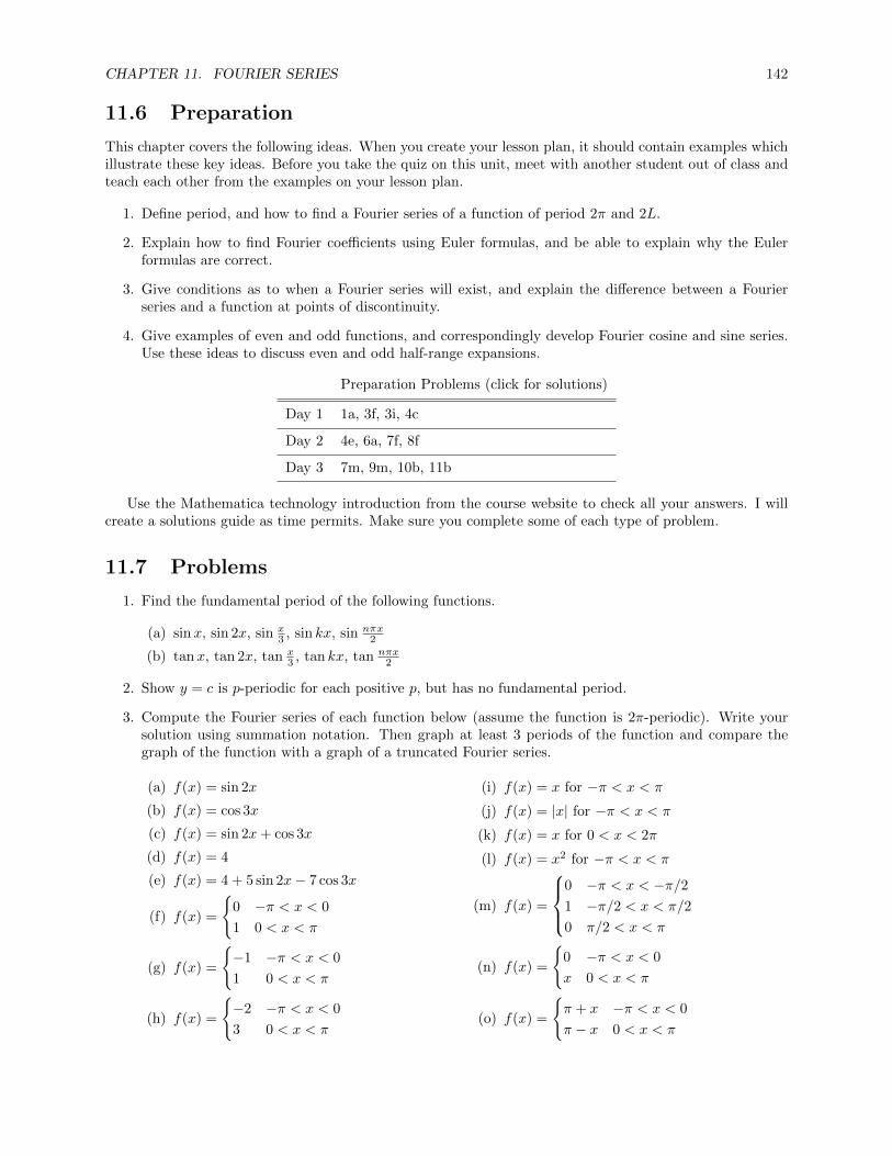
CHAPTER 11. FOURIER SERIES 142
11.6 Preparation
This chapter covers the following ideas. When you create your lesson plan, it should contain examples whichillustrate these key ideas. Before you take the quiz on this unit, meet with another student out of class andteach each other from the examples on your lesson plan.
1. Define period, and how to find a Fourier series of a function of period 2π and 2L.
2. Explain how to find Fourier coefficients using Euler formulas, and be able to explain why the Eulerformulas are correct.
3. Give conditions as to when a Fourier series will exist, and explain the difference between a Fourierseries and a function at points of discontinuity.
4. Give examples of even and odd functions, and correspondingly develop Fourier cosine and sine series.Use these ideas to discuss even and odd half-range expansions.
Preparation Problems (click for solutions)
Day 1 1a, 3f, 3i, 4c
Day 2 4e, 6a, 7f, 8f
Day 3 7m, 9m, 10b, 11b
Use the Mathematica technology introduction from the course website to check all your answers. I willcreate a solutions guide as time permits. Make sure you complete some of each type of problem.
11.7 Problems
1. Find the fundamental period of the following functions.
(a) sinx, sin 2x, sin x3 , sin kx, sin nπx
2
(b) tanx, tan 2x, tan x3 , tan kx, tan nπx
2
2. Show y = c is p-periodic for each positive p, but has no fundamental period.
3. Compute the Fourier series of each function below (assume the function is 2π-periodic). Write yoursolution using summation notation. Then graph at least 3 periods of the function and compare thegraph of the function with a graph of a truncated Fourier series.
(a) f(x) = sin 2x
(b) f(x) = cos 3x
(c) f(x) = sin 2x+ cos 3x
(d) f(x) = 4
(e) f(x) = 4 + 5 sin 2x− 7 cos 3x
(f) f(x) =
{0 −π < x < 0
1 0 < x < π
(g) f(x) =
{−1 −π < x < 0
1 0 < x < π
(h) f(x) =
{−2 −π < x < 0
3 0 < x < π
(i) f(x) = x for −π < x < π
(j) f(x) = |x| for −π < x < π
(k) f(x) = x for 0 < x < 2π
(l) f(x) = x2 for −π < x < π
(m) f(x) =
0 −π < x < −π/21 −π/2 < x < π/2
0 π/2 < x < π
(n) f(x) =
{0 −π < x < 0
x 0 < x < π
(o) f(x) =
{π + x −π < x < 0
π − x 0 < x < π
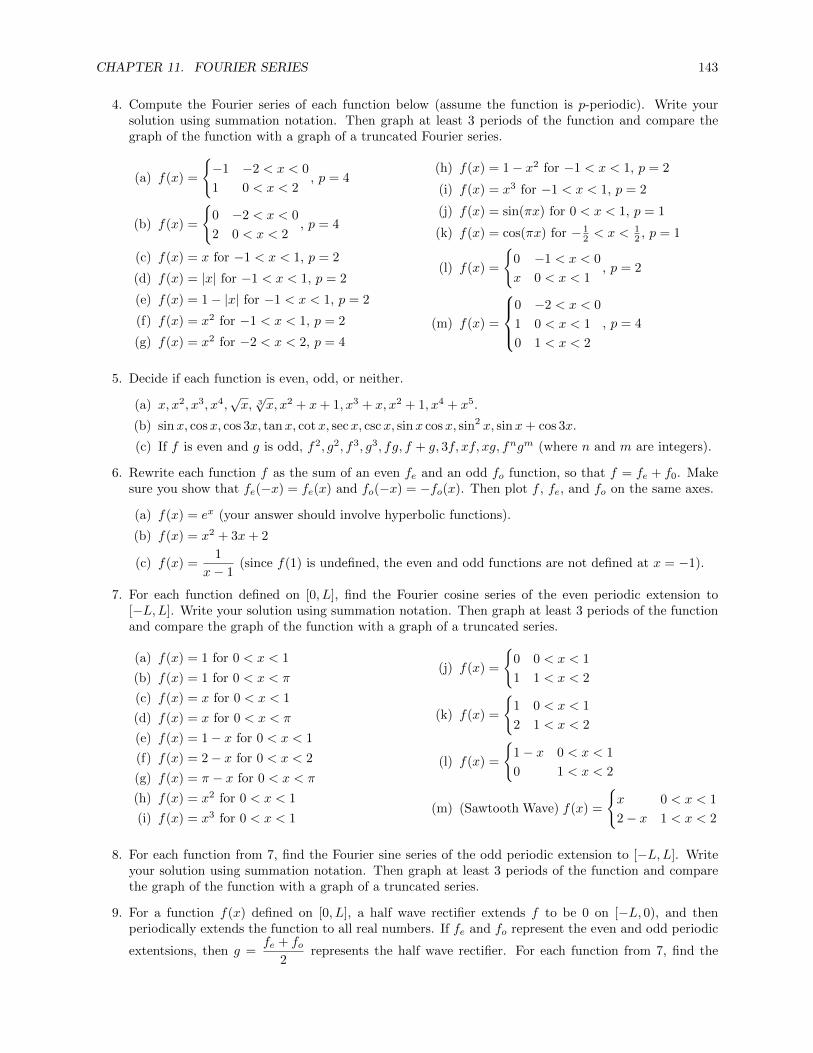
CHAPTER 11. FOURIER SERIES 143
4. Compute the Fourier series of each function below (assume the function is p-periodic). Write yoursolution using summation notation. Then graph at least 3 periods of the function and compare thegraph of the function with a graph of a truncated Fourier series.
(a) f(x) =
{−1 −2 < x < 0
1 0 < x < 2, p = 4
(b) f(x) =
{0 −2 < x < 0
2 0 < x < 2, p = 4
(c) f(x) = x for −1 < x < 1, p = 2
(d) f(x) = |x| for −1 < x < 1, p = 2
(e) f(x) = 1− |x| for −1 < x < 1, p = 2
(f) f(x) = x2 for −1 < x < 1, p = 2
(g) f(x) = x2 for −2 < x < 2, p = 4
(h) f(x) = 1− x2 for −1 < x < 1, p = 2
(i) f(x) = x3 for −1 < x < 1, p = 2
(j) f(x) = sin(πx) for 0 < x < 1, p = 1
(k) f(x) = cos(πx) for − 12 < x < 1
2 , p = 1
(l) f(x) =
{0 −1 < x < 0
x 0 < x < 1, p = 2
(m) f(x) =
0 −2 < x < 0
1 0 < x < 1
0 1 < x < 2
, p = 4
5. Decide if each function is even, odd, or neither.
(a) x, x2, x3, x4,√x, 3√x, x2 + x+ 1, x3 + x, x2 + 1, x4 + x5.
(b) sinx, cosx, cos 3x, tanx, cotx, secx, cscx, sinx cosx, sin2 x, sinx+ cos 3x.
(c) If f is even and g is odd, f2, g2, f3, g3, fg, f + g, 3f, xf, xg, fngm (where n and m are integers).
6. Rewrite each function f as the sum of an even fe and an odd fo function, so that f = fe + f0. Makesure you show that fe(−x) = fe(x) and fo(−x) = −fo(x). Then plot f , fe, and fo on the same axes.
(a) f(x) = ex (your answer should involve hyperbolic functions).
(b) f(x) = x2 + 3x+ 2
(c) f(x) =1
x− 1(since f(1) is undefined, the even and odd functions are not defined at x = −1).
7. For each function defined on [0, L], find the Fourier cosine series of the even periodic extension to[−L,L]. Write your solution using summation notation. Then graph at least 3 periods of the functionand compare the graph of the function with a graph of a truncated series.
(a) f(x) = 1 for 0 < x < 1
(b) f(x) = 1 for 0 < x < π
(c) f(x) = x for 0 < x < 1
(d) f(x) = x for 0 < x < π
(e) f(x) = 1− x for 0 < x < 1
(f) f(x) = 2− x for 0 < x < 2
(g) f(x) = π − x for 0 < x < π
(h) f(x) = x2 for 0 < x < 1
(i) f(x) = x3 for 0 < x < 1
(j) f(x) =
{0 0 < x < 1
1 1 < x < 2
(k) f(x) =
{1 0 < x < 1
2 1 < x < 2
(l) f(x) =
{1− x 0 < x < 1
0 1 < x < 2
(m) (Sawtooth Wave) f(x) =
{x 0 < x < 1
2− x 1 < x < 2
8. For each function from 7, find the Fourier sine series of the odd periodic extension to [−L,L]. Writeyour solution using summation notation. Then graph at least 3 periods of the function and comparethe graph of the function with a graph of a truncated series.
9. For a function f(x) defined on [0, L], a half wave rectifier extends f to be 0 on [−L, 0), and thenperiodically extends the function to all real numbers. If fe and fo represent the even and odd periodic
extentsions, then g =fe + fo
2represents the half wave rectifier. For each function from 7, find the
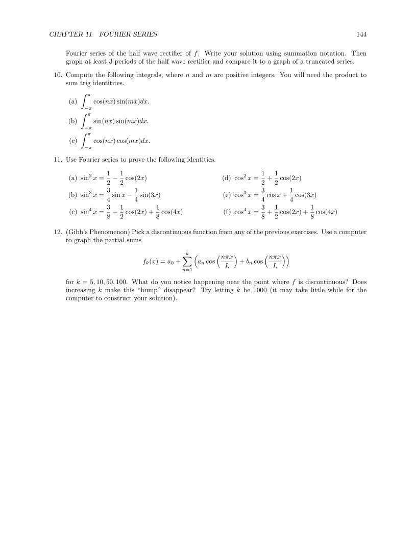
CHAPTER 11. FOURIER SERIES 144
Fourier series of the half wave rectifier of f . Write your solution using summation notation. Thengraph at least 3 periods of the half wave rectifier and compare it to a graph of a truncated series.
10. Compute the following integrals, where n and m are positive integers. You will need the product tosum trig identitites.
(a)
∫ π
−πcos(nx) sin(mx)dx.
(b)
∫ π
−πsin(nx) sin(mx)dx.
(c)
∫ π
−πcos(nx) cos(mx)dx.
11. Use Fourier series to prove the following identities.
(a) sin2 x =1
2− 1
2cos(2x)
(b) sin3 x =3
4sinx− 1
4sin(3x)
(c) sin4 x =3
8− 1
2cos(2x) +
1
8cos(4x)
(d) cos2 x =1
2+
1
2cos(2x)
(e) cos3 x =3
4cosx+
1
4cos(3x)
(f) cos4 x =3
8+
1
2cos(2x) +
1
8cos(4x)
12. (Gibb’s Phenomenon) Pick a discontinuous function from any of the previous exercises. Use a computerto graph the partial sums
fk(x) = a0 +
k∑n=1
(an cos
(nπxL
)+ bn cos
(nπxL
))for k = 5, 10, 50, 100. What do you notice happening near the point where f is discontinuous? Doesincreasing k make this “bump” disappear? Try letting k be 1000 (it may take little while for thecomputer to construct your solution).
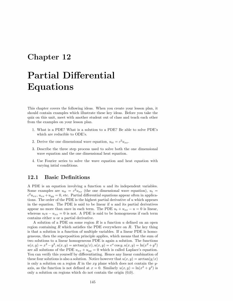
Chapter 12
Partial DifferentialEquations
This chapter covers the following ideas. When you create your lesson plan, itshould contain examples which illustrate these key ideas. Before you take thequiz on this unit, meet with another student out of class and teach each otherfrom the examples on your lesson plan.
1. What is a PDE? What is a solution to a PDE? Be able to solve PDE’swhich are reducible to ODE’s.
2. Derive the one dimensional wave equation, utt = c2uxx.
3. Describe the three step process used to solve both the one dimensionalwave equation and the one dimensional heat equation.
4. Use Fourier series to solve the wave equation and heat equation withvarying intial conditions.
12.1 Basic Definitions
A PDE is an equation involving a function u and its independent variables.Some examples are utt = c2uxx (the one dimensional wave equation), ut =c2uxx, uxx+uyy = 0, etc. Partial differential equations appear often in applica-tions. The order of the PDE is the highest partial derivative of u which appearsin the equation. The PDE is said to be linear if u and its partial derivativesappear no more than once in each term. The PDE ut + uxx − u = 0 is linear,whereas utu − uxx = 0 is not. A PDE is said to be homogeneous if each termcontains either u or a partial derivative.
A solution of a PDE on some region R is a function u defined on an openregion containing R which satisfies the PDE everywhere on R. The key thingis that a solution is a function of multiple variables. If a linear PDE is homo-geneous, then the superposition principle applies, which means that the sum oftwo solutions to a linear homogeneous PDE is again a solution. The functionsu(x, y) = x2− y2, u(x, y) = arctan(y/x), u(x, y) = ex cos y, u(x, y) = ln(x2 + y2)are all solutions of the PDE uxx + uyy = 0 which is called Laplace’s equation.You can verify this yourself by differentiating. Hence any linear combination ofthese four solutions is also a solution. Notice however that u(x, y) = arctan(y/x)is only a solution on a region R in the xy plane which does not contain the y-axis, as the function is not defined at x = 0. Similarly u(x, y) = ln(x2 + y2) isonly a solution on regions which do not contain the origin (0,0).
145

CHAPTER 12. PARTIAL DIFFERENTIAL EQUATIONS 146
Some PDEs can be solved by ODE methods. The PDE uxy = 3ux canbe solved as follows. If we let ux = p, then we have py = 3p. A solution isp = Ce3y, where C is a constant with respect to y. That means that C could beany function of x. Hence we have ux = p = C(x)e3y. Integration with respectto x gives u(x, y) =
∫C(x)dxe3y + D(y), where the constant D could be a
function of y. As another example, uyy−u = 0 does not involve any derivativeswith respect to x. A solution using ODE techniques is u = A cos y + B sin y.However A and B are constants with respect to y, which means they could beany functions of x. A solution in general is thus u(x, y) = A(x) cos y+B(x) sin ywhere A(x), B(x) are any functions of x. We will use this basic idea in thehomework to review solution techniques for every type of ODE.
12.2 Derivation of the one dimensional wave equa-tion
We now derive the one dimensional wave equation utt = c2uxx. This PDEmodels the motion of a vibrating string of length L which is fixed at two end-points. The function u(t, x) will give the vertical position of a vibrating stringat any t for any x along the string. We require that the string is fixed atu(t, 0) = u(t, L) = 0 for all time (these two conditions are called boundaryconditions). In order to know the position of the string for all time, we need toknow its initial position u(0, x) = f(x) and initial velocity ut(0, x) = g(x) forall x. The boundary and initial conditions should give us enough informationto find the position for all t, x. We now make three simplifying assumptions sothat we can model the motion of a vibrating string using PDEs. (1) The den-sity of the string is constant and the string is perfectly elastic. (2) The tensionin the string created by the attachment at the endpoints is so strong that theforce due to gravity can be neglected. (3) Motion is always perpendicular tothe segment connecting the endpoints, so that the bit of string x units awayfrom the left endpoint will only move vertically, never horizontally.
Pick two points at distances x and x + ∆x away from the left endpoint.Since motion is always vertical, the horizontal components of tension in bothdirections are the same in magnitude throughout the entire wire. Call thismagnitude T . Let ~T1 be the tension pulling the string at x toward the leftendpoint and ~T2 the tension pulling the string at x + ∆x toward the rightendpoint. Let α be the acute angle between ~T1 and the horizontal, so thatthe horizontal component of the tension is |T1| cosα. Similarly let β be the
acute angle between ~T2 and the horizontal, so that the horizontal component ofthe tension is |T2| cosβ. This means T = |T1| cosα = |T2| cosβ. Now Newton’ssecond law of motion says that F = ma. The vertical components of force actingon the segment of string between x and x+ ∆x are approximately −|T1| sinα+|T2| sinβ, which by Newton’s second law is the mass ρ∆x (where ρ is the densityper unit length) times the acceleration utt at some point between x and x+∆x.We have the equation |T2| sinβ − |T1| sinα = ρ∆xutt. Divide both sides byT = |T1| cosα = |T2| cosβ, giving the equation tanβ − tanα = ρ∆x
T utt. Recallthat tanα is the slope of the curve at x, which equals ux
∣∣x=x
. Similarly tanβ =
ux∣∣x=x+∆x
. Division by ∆x gives the equation 1∆x (ux
∣∣x=x+∆x
−ux∣∣x=x
) = ρT utt.
The limit as ∆x → 0 of the quantity on the left is precisely the definition ofthe partial derivative of ux with respect to x. Hence taking limits gives usuxx = ρ
T utt. This is commonly written utt = Tρ uxx = c2uxx, where c2 reminds
us that the constant Tρ must be positive.

CHAPTER 12. PARTIAL DIFFERENTIAL EQUATIONS 147
12.3 Solution of the wave equation
The following solution of the wave equation is a general technique which is usefulin various places in modeling. It involves three steps: (1) separate variable, (2)solve multiple ODEs, (3) combine the solutions using superposition. Recall theboundary conditions u(t, 0) = u(t, L) = 0 and initial conditions u(0, x) = f(x),ut(0, x) = g(x) from before. We seek a solution u(t, x) of utt = c2uxx whichsatisfies all of these conditions.
12.3.1 Separate Variables
We assume that our solution satisfies u(t, x) = G(t)F (x), i.e. the variables tand x can be separated. If this is true, then the PDE utt = c2uxx becomesFGtt = c2FxxG or FG = c2F ′′G, where the dots mean derivative with respectto t and the primes mean derivatives with respect to F . We can rewrite the
equation as Gc2G = F ′′
F . The left side of this equation does not change if xchanges, and the right side does not change if t changes, which means that it
must be constant, or Gc2G = F ′′
F = p for some constant k. This gives us two
equations Gc2G = k and F ′′
F = k, or G = kc2G and F ′′ = kF , which are bothODEs.
12.3.2 Solve Multiple ODEs
We first solve F ′′ = kF , or F ′′ − kF = 0, and along the way show that k < 0.The characteristic equation is λ2 − k = 0. If k = 0, then the solution isF (x) = ax+b. However the conditions u(t, 0) = u(t, L) = 0 require that F (0) =0 = F (L), which means that both a and b are 0, or F (x) = 0 which is a useless
solution. Similarly, if k > 0 then the solution is F (x) = Ae−√kx +Be
√kx. The
boundary conditions F (0) = 0 = F (L) give the system of equations A+B = 0
and Ae−√kL + Be
√kL = 0 which has solution A = 0 = B, which again gives
the useless solution F (x) = 0. If k < 0, then letting k = −p2 the solutionis F (x) = A cos(px) + B sin(px). The boundary conditions F (0) = 0 = F (L)give 0 = A and 0 = B sin(pL). This means that pL = nπ or p = nπ
L , as thesine function is zero at any integer multiple of π. This means that for everyinteger n we have a solution Fn(x) = B sin nπx
L of the first ODE. Recall alsothat k = −p2
n must be negative. Because it simplifies our work later on, we letB = 1 and write Fn(x) = sin nπx
L , though any multiple of Fn would also be asolution.
The second ODE G = kc2G can be rewritten G + p2nc
2G = 0, or lettingλn = pnc we have G+λ2
nG = 0. Solutions to this ODE are Gn(t) = An cosλnt+Bn sinλnt for arbitrary constants An andBn. For each n we thus have a solutionun(t, x) = Gn(t)Fn(t) of the original PDE.
12.3.3 Combine the solutions using superposition
The solution un(t, x) = Gn(t)Fn(t) of the wave equation in general will not sat-isfy the initial conditions u(0, x) = f(x), ut(0, x) = g(x). So to find a solutionwhich does, we add together these solutions and then solve for the constantsAn and Bn. A finite sum of solutions will always be a solution, and the in-finite sum u(t, x) =
∑∞n=1 un(t, x) =
∑∞n=1Gn(t)Fn(t) =
∑∞n=1(An cosλnt +
Bn sinλnt) sin nπxL will be a solution under suitable convergence and differen-
tiability conditions. Letting t = 0 and recalling u(0, x) = f(x), we now solvef(x) =
∑∞n=1An sin nπx
L which is a Fourier sine series of f(x). This means that
we can solve for An = 2L
∫ L0f(x) sin nπx
L dx. Taking a derivative with respect to

CHAPTER 12. PARTIAL DIFFERENTIAL EQUATIONS 148
t gives∑∞n=1(−λnAn sinλnt+ λnBn cosλnt) sin nπx
L . Let t = 0 to obtain fromthe initial condition ut(0, x) = g(x) the equation g(x) =
∑∞n=1 λnBn sin nπx
L ,the Fourier sine series of g(x). From the Euler formulas we obtain λnBn =2L
∫ L0g(x) sin nπx
L dx, or Bn = 2ncπ
∫ L0g(x) sin nπx
L dx. We now have a solutionu(t, x) =
∑∞n=1(An cosλnt + Bn sinλnt) sin nπx
L , where λn = nπL c and An and
Bn are obtained from Euler formulas. This solution is only valid under certaincircumstances, which we will not take time to discuss in detail here. A coursein analysis would provide enough details.
12.3.4 Summary
Notice how we separated the PDE, solved individual ODEs, and then usedsuperposition and Fourier series to come up with a complete solution. Thistechnique is a standard tool which you should become familiar with. You willbe able to practice it one more time as you solve the heat equation in the nextsection.
When the initial velocity g(x) is zero, the solution u(t, x) =∑∞n=1(An cosλnt+
Bn sinλnt) sin nπxL can be written in a much nicer manner. Since g(x) = 0, we
have Bn = 0. Using the trig identity cos(A) sin(B) = 12 (sin(A+B)+sin(A−B)),
we write
∞∑n=1
An cosλnt sinnπx
L=
1
2
( ∞∑n=1
An sinnπ
L(x+ ct) +
∞∑n=1
An sinnπ
L(x− ct)
)=
1
2(f∗(x+ ct) + f∗(x− ct)) ,
where f∗ is the odd periodic extension of f . So a solution of the wave equationwhen the initial velocity is zero is found by simply creating the odd periodicextension of f , and then moving the wave left and right where c determines thespeed at which the waves travel, and then halving the sum of these two waves.
12.4 Solution of the heat equation
The one dimensional heat equation is the PDE ut = c2uxx. It models thetemperature of a one dimensional object at any time t. There are two problemswe will solve. First, suppose the rod is L units long, is kept at temperature 0at both endpoints u(t, 0) = u(t, L) = 0, and has initial temperature u(0, t) =f(x) for 0 ≤ x ≤ L. Second, suppose the rod has insulated endpoints (noheat can escape through the endpoints) and has initial temperature u(0, x) =f(x). Experiments show that the boundary conditions for an insulated rod areux(t, 0) = 0 = ux(t, L). As hints for solutions, your solution should involvea Fourier sine series for the first problem, and a Fourier cosine series for thesecond one. I will provide solutions for these problems online.
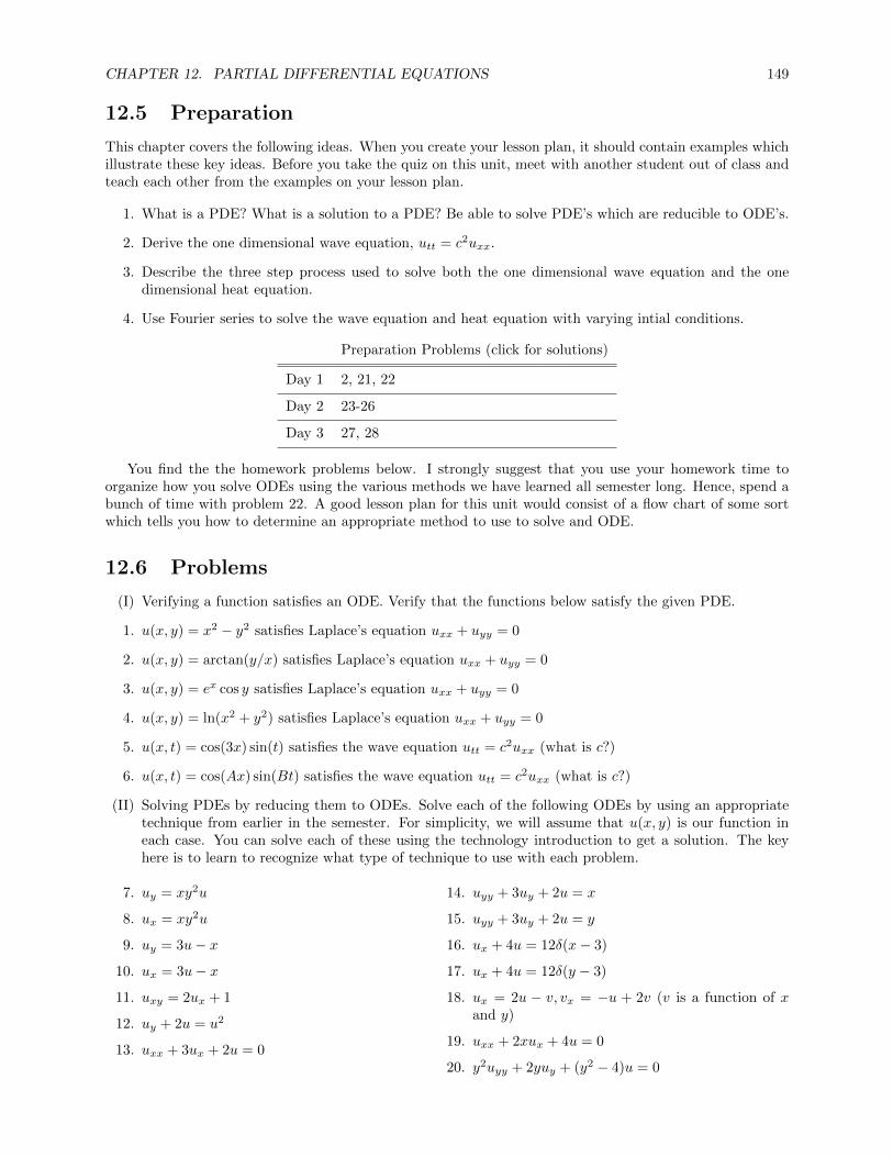
CHAPTER 12. PARTIAL DIFFERENTIAL EQUATIONS 149
12.5 Preparation
This chapter covers the following ideas. When you create your lesson plan, it should contain examples whichillustrate these key ideas. Before you take the quiz on this unit, meet with another student out of class andteach each other from the examples on your lesson plan.
1. What is a PDE? What is a solution to a PDE? Be able to solve PDE’s which are reducible to ODE’s.
2. Derive the one dimensional wave equation, utt = c2uxx.
3. Describe the three step process used to solve both the one dimensional wave equation and the onedimensional heat equation.
4. Use Fourier series to solve the wave equation and heat equation with varying intial conditions.
Preparation Problems (click for solutions)
Day 1 2, 21, 22
Day 2 23-26
Day 3 27, 28
You find the the homework problems below. I strongly suggest that you use your homework time toorganize how you solve ODEs using the various methods we have learned all semester long. Hence, spend abunch of time with problem 22. A good lesson plan for this unit would consist of a flow chart of some sortwhich tells you how to determine an appropriate method to use to solve and ODE.
12.6 Problems
(I) Verifying a function satisfies an ODE. Verify that the functions below satisfy the given PDE.
1. u(x, y) = x2 − y2 satisfies Laplace’s equation uxx + uyy = 0
2. u(x, y) = arctan(y/x) satisfies Laplace’s equation uxx + uyy = 0
3. u(x, y) = ex cos y satisfies Laplace’s equation uxx + uyy = 0
4. u(x, y) = ln(x2 + y2) satisfies Laplace’s equation uxx + uyy = 0
5. u(x, t) = cos(3x) sin(t) satisfies the wave equation utt = c2uxx (what is c?)
6. u(x, t) = cos(Ax) sin(Bt) satisfies the wave equation utt = c2uxx (what is c?)
(II) Solving PDEs by reducing them to ODEs. Solve each of the following ODEs by using an appropriatetechnique from earlier in the semester. For simplicity, we will assume that u(x, y) is our function ineach case. You can solve each of these using the technology introduction to get a solution. The keyhere is to learn to recognize what type of technique to use with each problem.
7. uy = xy2u
8. ux = xy2u
9. uy = 3u− x
10. ux = 3u− x
11. uxy = 2ux + 1
12. uy + 2u = u2
13. uxx + 3ux + 2u = 0
14. uyy + 3uy + 2u = x
15. uyy + 3uy + 2u = y
16. ux + 4u = 12δ(x− 3)
17. ux + 4u = 12δ(y − 3)
18. ux = 2u − v, vx = −u + 2v (v is a function of xand y)
19. uxx + 2xux + 4u = 0
20. y2uyy + 2yuy + (y2 − 4)u = 0
CHAPTER 12. PARTIAL DIFFERENTIAL EQUATIONS 150
21. For each of the problems above, write the type of technique you need to use to solve it. Write a guidefor yourself to know what method you should use based on what you see in the PDE.
22. Construct an example of a PDE which needs each of the following ODE solution techniques to solve.Then solve the PDE. You can count each technique a homework problem: Separable, Exact, IntegratingFactor, Linear, Bernoulli, Homogeneous with constant coefficients, Nonhomogeneous with constantcoefficients, Laplace Transforms, Power Series, Frobenius Method, Matrix exponential.
(IV) Solving the Wave Equation. The first 4 problems in this section ask you to repeat the derivation ofthe wave equation. The solutions are in the lecture notes. The last few problems ask you to solve thewave equation using some given initial conditions.
23. Derive the one dimensional wave equation utt = c2uxx, with boundary conditions u(t, 0) = u(t, L) = 0and initial conditions u(0, x) = f(x), ut(0, x) = g(x).
24. Separate variables on the 1D wave equation to obtain 2 ODEs.
25. Solve both of the ODEs from the previous step.
26. Use superposition and Fourier series to obtain a general solution to the wave equation.
27. If the length of the string is L = 1, its initial position is u(0, x) = x(1− x), and the initial velocity isut(0, x) = 0 (meaning the string is released with no initial velocity), find and graph the position of thestring at any time t.
28. If L = 2, u(0, x) =
{x 0 ≤ x ≤ 1
2− x 1 ≤ x ≤ 2, and ut(0, x) = 0, repeat the previous problem.
12.7 Solutions
(I) Verifying a function satisfies an ODE.
1. Just take derivatives.
2. Just take derivatives.
3. Just take derivatives.
4. Just take derivatives.
5. Just take derivatives. c = 1/3
6. Just take derivatives. c = B/A
(II) Solving PDEs by reducing them to ODEs. I’ll list the technique as well as the solution.
7. Separate variables, then integrate both sides. u(x, y)→ exy3
3 c1[x]
8. Separate variables, then integrate both sides. u(x, y)→ ex2y2
2 c1[y]
9. Find an integrating factor, or find yh and guess yp = A, where the constant A could be a function of x.u(x, y)→ e3yc1[x] + x
3
10. Find an integrating factor, or find yh and guess yp = Ax+B, where the constants A and B could be functionsof y. u(x, y)→ e3xc1[y] + x
3+ 1
9
11. Let z = ux, and then solve zy = 2x + 1. After that, solve z = ux. z = u(x, y) → e2yc1[x] − 12
andu(x, y)→ e2y
∫c1[x]dx− 1
2x+ c2[y] = e2yc3[x]− 1
2x+ c2[y].
12. Use a Bernoulli substitution. This will require that you let w = u1−2. u(x, y)→ − 2
e2c1[x]+2y−1
13. Find yh by getting the roots of the characteristic polynomial. u(x, y)→ e−2xc1[y] + e−xc2[y]
14. Find yh and then guess yp = A, where A is a function of x. u(x, y)→ e−2yc1[x] + e−yc2[x] + x2
15. Find yh and then guess yp = Ay+B, where A and B are functions of x. u(x, y)→ e−2yc1[x]+e−yc2[x]+ 14(2y−3)
16. Use Laplace transforms, just remember that all your constants are functions of y. The transform of δ(x− 3) ise−3s. u(x, y)→ c(x)e−4x + 12e−4(x−3)u(x− 3)

CHAPTER 12. PARTIAL DIFFERENTIAL EQUATIONS 151
17. Use Laplace transforms, and notice that δ(y − 3) is a constant here, so its transform is δ(y−3)s
u(x, y) →c(x)e−4x + 12e−4(x−3)u(x− 3)
18. This is a system where y is just assumed to be a constant. Find the matrix exponential. The matrix exponential
is
(et
2+ e3t
2et
2− e3t
2et
2− e3t
2et
2+ e3t
2
)The solution is
(u(x, y)→ c1[y]e
x
2+ 1
2c1[y]e3x + c2[y]e
x
2− 1
2c2[y]e3x
v(x, y)→ c1[y]ex
2− 1
2c1[y]e3x + c2[y]e
x
2+ 1
2c2[y]e3x
)19. uxx + 2xux + 4u = 0 Use a power series, since the coefficients depend on variable we are differentiating with
respect to. Your solution will look like u(x, y) =∑∞n=1 an(y)xn, where an is a function of y.
20. y2uyy + 2yuy + (y2 − 4)u = 0 Use the Frobenius method. We have variable coefficients and the y2 in frontof uyy causes this to not be ordinary at y = 0, but it is regular singular at y = 0. Your series will looklike u1(x, y) = yλ
∑∞n=1 an(x)yn where each coefficient an is a function of x. This is Bessel’s equation, where
p = 2. The solution in general is c1(x)B1[y, 2] + c2(x)B2[y, 2] where B1 and B2 are the two independent Besselequations that come from the Frobenius method, and the constants c1 and c2 could be any function of x.
21. For each of the problems above, write the type of technique you need to use to solve it. Write a guide foryourself to know what method you should use based on what you see in the PDE.
22. Construct an example of a PDE which needs each of the following ODE solution techniques to solve. Thensolve the PDE. You can count each technique a homework problem: Separable, Exact, Integrating Factor,Linear, Bernoulli, Homogeneous with constant coefficients, Nonhomogeneous with constant coefficients, LaplaceTransforms, Power Series, Frobenius Method, Matrix exponential.
(IV) Solving the Wave Equation. The first 4 problems in this section ask you to repeat the derivation of the waveequation. The solutions are in the lecture notes. The last few problems ask you to solve the wave equationusing some given initial conditions.
23. Derive the one dimensional wave equation utt = c2uxx, with boundary conditions u(t, 0) = u(t, L) = 0 andinitial conditions u(0, x) = f(x), ut(0, x) = g(x).
24. Separate variables on the 1D wave equation to obtain 2 ODEs.
25. Solve both of the ODEs from the previous step.
26. Use superposition and Fourier series to obtain a general solution to the wave equation.
27. If the length of the string is L = 1, its initial position is u(0, x) = x(1−x), and the initial velocity is ut(0, x) = 0(meaning the string is released with no initial velocity), find and graph the position of the string at any time t.
28. If L = 2, u(0, x) =
{x 0 ≤ x ≤ 1
2− x 1 ≤ x ≤ 2, and ut(0, x) = 0, repeat the previous problem.