DEPARTMENT OF AGRICULTURAL ECONOMICS, EXTENSION EDUCATION & RURAL SOCIOLOGY

COLLEGE OF AGRICULTURE CSK HP KRISHI VISHVAVIDYALAYA, PALAMPUR 176 062

September, 2011

SOCIO ECONOMIC SURVEY (SES) ON

DHAULA SIDHA HYDRO ELECTRIC PROJECT (DSHEP)

66 MW DISTRICT HAMIRPUR, HIMACHAL PRADESH

S K CHAUHAN H R SHARMA VIRENDER KUMAR

Final Report on SJVNL Funded Research Project

Dhaula Sidha Temple

Livestock farming –A reality of socio

economic fabric

Storage of maize stalk -Balehu

Research Report 54

ACKNOWLEDGEMENT

We, a team of Agroeconomists, wish to thank the SJVNL for funding the “Social Economic Survey

(SES)” study of Dhaula Sidha Hydro Electric Project (DSHEP) 66 MW, Hamirpur being executed by

SJVN Limited, a corporate venture. Our special thanks are due to Mr. Nand Lal, Director, SJVNL,

Shimla for his initiative, advice and valuable support during course of the completion of the study. We

are also thankful to Er. Sushil Mahajan, Head of DSHEP, Hamirpur, Er Sushil Sagar Sharma, Er. D.

Sarveshwar, Er. Avdesh Prasad and Er. Surinder Paul for their advice, support and help in the

coordination of various activities of the study.

Our sincere thanks are to the Vice-Chancellor and Director of Research of CSK Himachal Pradesh

Agricultural University, Palampur and Head Department of Agricultural Economics, Extension

Education & Rural Sociology who provided all assistance and facilities to accomplish the study.

Sample farmers, in the project area deserve our sincere thanks for their kind cooperation in providing

required data about different aspects of their livelihood. The senior and junior research fellows namely

Arvind, Kulbhushan, Dalvinder, Kusma and Sakshi, who worked in the project, deserve special

appreciations for their hard work, dedication, paying number of visits and sincere efforts. We are also

very much indebted to all the administrative and supporting staff of different offices in the University,

especially to the staff of our Department. Last but not the least, we remain thankful to all those who

helped either directly or indirectly to bring out this report in time

Palampur Research Team

September 21 , 2011 S K Chauhan

H R Sharma

Virender Kumar

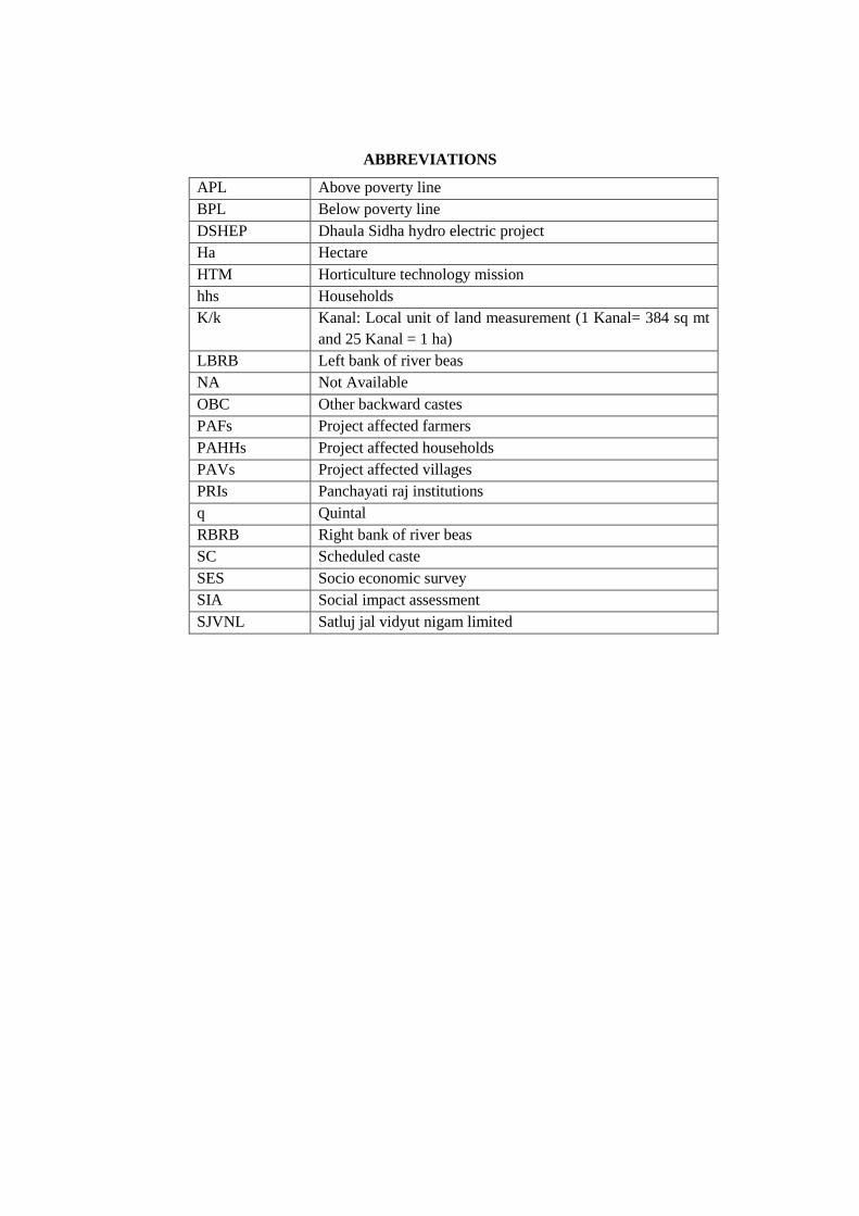
ABBREVIATIONS

APL Above poverty line

BPL Below poverty line

DSHEP Dhaula Sidha hydro electric project

Ha Hectare

HTM Horticulture technology mission

hhs Households

K/k Kanal: Local unit of land measurement (1 Kanal= 384 sq mt

and 25 Kanal = 1 ha)

LBRB Left bank of river beas

NA Not Available

OBC Other backward castes

PAFs Project affected farmers

PAHHs Project affected households

PAVs Project affected villages

PRIs Panchayati raj institutions

q Quintal

RBRB Right bank of river beas

SC Scheduled caste

SES Socio economic survey

SIA Social impact assessment

SJVNL Satluj jal vidyut nigam limited

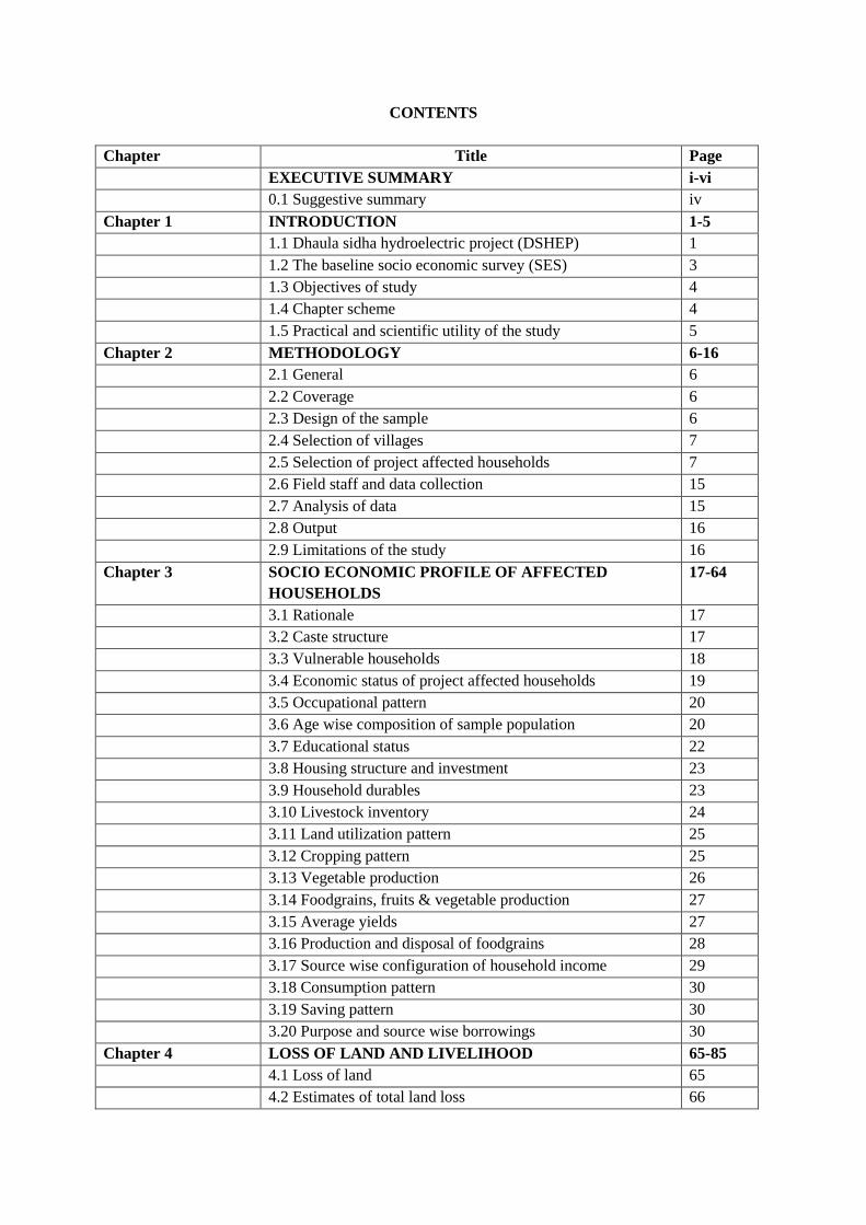
CONTENTS

Chapter Title Page

EXECUTIVE SUMMARY i-vi

0.1 Suggestive summary iv

Chapter 1 INTRODUCTION 1-5

1.1 Dhaula sidha hydroelectric project (DSHEP) 1

1.2 The baseline socio economic survey (SES) 3

1.3 Objectives of study 4

1.4 Chapter scheme 4

1.5 Practical and scientific utility of the study 5

Chapter 2 METHODOLOGY 6-16

2.1 General 6

2.2 Coverage 6

2.3 Design of the sample 6

2.4 Selection of villages 7

2.5 Selection of project affected households 7

2.6 Field staff and data collection 15

2.7 Analysis of data 15

2.8 Output 16

2.9 Limitations of the study 16

Chapter 3 SOCIO ECONOMIC PROFILE OF AFFECTED

HOUSEHOLDS

17-64

3.1 Rationale 17

3.2 Caste structure 17

3.3 Vulnerable households 18

3.4 Economic status of project affected households 19

3.5 Occupational pattern 20

3.6 Age wise composition of sample population 20

3.7 Educational status 22

3.8 Housing structure and investment 23

3.9 Household durables 23

3.10 Livestock inventory 24

3.11 Land utilization pattern 25

3.12 Cropping pattern 25

3.13 Vegetable production 26

3.14 Foodgrains, fruits & vegetable production 27

3.15 Average yields 27

3.16 Production and disposal of foodgrains 28

3.17 Source wise configuration of household income 29

3.18 Consumption pattern 30

3.19 Saving pattern 30

3.20 Purpose and source wise borrowings 30

Chapter 4 LOSS OF LAND AND LIVELIHOOD 65-85

4.1 Loss of land 65

4.2 Estimates of total land loss 66

4.3 Physical and financial estimates of output realized from the

land to be lost

67

4.4 Dependence on natural resources 67

4.5 Estimates of loss of land by alternative classification of

sample affected households

68

4.6 Compensation and rehabilitation plan 69

Chapter 5 SUMMARY AND CONCLUSION 86-92

5.1 Introduction 86

5.2 Main objectives 87

5.3 Methodology 87

5.4 Main findings 88

LIST OF TABLES

Table No. Title Page

Table 0.1 Salient socio-economic characteristics of project affected households v

Table 0.2 Salient land related characteristics of project affected households vi

Table 2.1 List of project affected villages considered for socio economic survey in the

command area of DSHEP

7

Table 2.2 Sampling plan for project affected villages on LBRB 8

Table 2.3 Sampling plan for project affected villages on RBRB 9

Table 2.4 Classification of project affected sample households 9

Table 2.5 Group wise classification of project affected sample households 10

Table 2.6 Classification of sample farmers and all PAFs for deriving estimate 10

Table 2.7 Classification of project affected sample households 10

Table 2.8 List of project affected sample households on LBRB 11

Table 2.9 List of project affected sample households on RBRB 13

Table 1a Distribution of heads of households among castes on LBRB (No.) 32

Table 1b Distribution of heads of households in different castes across groups on LBRB

(No.)

32

Table 1c Distribution of heads of households among castes on RBRB (No.) 32

Table 1d Distribution of heads of households in different castes across groups on RBRB

(No.)

33

Table 2a Distribution of vulnerable heads of households among different categories of

vulnerability on LBRB (No.)

33

Table 2b Distribution of vulnerable heads of households among different categories of

vulnerability on LBRB (No.)

33

Table 2c Distribution of vulnerable heads of households among different categories of

vulnerability on RBRB (No.)

34

Table 2d Distribution of vulnerable heads of households across groups on RBRB (No.) 34

Table 3a Distribution of above poverty line and below poverty line heads of households

across castes on LBRB (No.)

35

Table 3b Distribution of above poverty line and below poverty line heads of households

across castes on RBRB (No.)

35

Table 4a Occupational profile of sample households on LBRB (No.) 36

Table 4b Occupational profile of sample households on RBRB (No.) 36

Table 5a Age wise distribution of sample population on LBRB (No.) 37

Table 5b Age wise distribution of sample population on RBRB (No.) 38

Table 6a. Educational status of sample population on LBRB (No.) 39

Table 6b Educational status of sample population on RBRB (No.) 40

Table 7a Types of buildings owned by sample households on LBRB (No.) 41

Table 7b Types of buildings of owned by sample households on RBRB (No.) 42

Table 8a Investment on buildings by sample households on LBRB (Lakh Rs./hh) 43

Table 8b Investment on buildings by sample households on RBRB (Lakh Rs. /hh) 44

Table 9a Inventory of household durables possessed by sample households on LBRB 45

Table 9b Inventory of household durables possessed by sample households on RBRB 47

Table 10a Livestock inventory of sample households on LBRB 49

Table 10b Livestock inventory of sample households on RBRB 50

Table 11a Land Utilization Pattern of sample households on LBRB (ha/hh) 51

Table 11b Land Utilization Pattern of sample households on RBRB (ha/hh) 51

Table 12a Cropping pattern on sample households of LBRB (in ha / household) 52

Table 12b Cropping pattern on sample households of RBRB (in ha / household) 52

Table 13a Area, production and income from vegetables and spice production on LBRB 53

Table 13b Area, production and income from vegetables and spice production on RBRB 54

Table 14a Production of crops on sample households of LBRB (q/hh) 55

Table 14b Production of crops on sample households of RBRB (q/hh) 55

Table 15a Average yield of crops on sample farms on LBRB (q/ha) 56

Table 15b Average yield of crops on sample farms on RBRB (q/ha) 56

Table 16a Production and disposal of foodgrains on sample households on LBRB (q /hh) 57

Table 16b Production and disposal of foodgrains on sample households on RBRB (q /hh) 57

Table 17a Source wise composition of annual household income of sample households on

LBRB (Rs./hh)

58

Table 17b Source wise composition of annual household income of sample households on

RBRB (Rs./hh)

59

Table 18a Consumption pattern of sample households on LBRB (Rs/hh/yr) 60

Table 18b Consumption pattern of sample households on RBRB (Rs/hh/yr) 61

Table19a Saving pattern of sample households on LBRB (Rs/Yr) 63

Table19b Saving pattern of sample households on RBRB (Rs/Yr) 63

Table 20a Purpose wise borrowings of sample households on LBRB 63

Table 20b Purpose wise borrowings of sample households on RBRB 63

Table 21a Source wise amount borrowed by sample households on LBRB 64

Table 21b Source wise amount borrowed by sample households on LBRB 64

Table 22a Land loss due to project by sample households on LBRB (ha/hh) 72

Table 22b Land loss due to project by sample households on RBRB (ha/hh) 72

Table 23a Existing land, land loss and land remaining with sample households on LBRB

(ha/hh)

73

Table 23b Existing land, land loss and land remaining with sample households on RBRB

(ha/hh)

74

Table 24a Estimates of total land loss by project affected households on LBRB (ha) 75

Table 24b Estimates of total land loss by project affected households on RBRB (ha) 76

Table 25a Physical and financial estimates of output realized from the land to be lost on

LBRB (qty in q and value in Rs/ hh/year)

77

Table 25b Physical and financial estimates of output realized from the land to be lost on

RBRB (qty in q and value in Rs/ hh/year)

77

Table 26a Physical and financial estimates of output realized from the land to be lost on

LBRB assuming 50% rise in production levels ((qty in q and value in Rs/

hh/year)

78

Table 26b Physical and financial estimates of output realized from the land to be lost on

RBRB assuming 50% rise in production levels ((qty in q and value in Rs/

hh/year)

78

Table 27a Dependence of the sample households on natural resources on LBRB 79

Table 27b Dependence of the sample households on natural resources on RBRB 80

Table 28a Land holding of sample households on LBRB (ha/hh) 81

Table 28b Land holding of sample households on RBRB (ha/hh) 81

Table 29a Expected land loss by sample households on LBRB (in ha/hh) 82

Table 29b Expected land loss by sample households on RBRB (in ha/hh) 82

Table 30a Land remaining with sample households on LBRB (in ha/hh) 83

Table 30b Land remaining with sample households on RBRB (in ha/hh) 83

Table 31a Estimates of total land loss by project affected households on LBRB (ha) 84

Table 31b Estimates of total land loss by project affected households on RBRB (ha) 84

Table 32a Estimates of production and other losses on LBRB ( Rs/hh) 85

Table 32b Estimates of production and other losses on RBRB ( Rs/hh) 85

LIST OF FIGURES

Figure

No.

Title Between page

Fig 1.1 Map of the project affected villages under DSHEP, 66MW, Hamirpur 2

Fig 2.1 Group wise distribution of project affected households 10-11

Fig 2.2 Distribution of project affected households by farm size category 10-11

Fig 3.1 Caste wise distribution of project affected households 33-34

Fig 3.2 Distribution of project affected households by vulnerable category 33-34

Fig 3.3 Distribution of project affected households by economic status category 35-36

Fig 3.4 Occupational distribution of project affected households 36-37

Fig 3.5 Gender wise distribution of project affected population 38-39

Fig 3.6 Cropping pattern in project affected area 52-53

Fig 3.7 Average yield of crops in project affected area 56-57

Fig 3.8 Source wise household income of project affected households 59-60

Fig 4.1 Status of land in project affected households 74-75

Fig 4.2 Estimates of production and other losses on LBRB 85-86

Fig.4.3 Estimates of production and other losses on RBRB 85-86

LIST OF PHOTOGRAPHS

Title

Glimpses of socio economic life

Effects of project on private assets and public facilities

i

EXECUTIVE SUMMARY

A Socio Economic Survey (SES) of the proposed Dhaula Sidha Hydro Electric Project

(DSHEP), 66 MW on the boundary of Hamirpur-Kangra district has been carried out to assess

the socio economic profile of the different groups of project affected households in the project

affected villages and to suggest a rehabilitation plan on the basis of estimates of loss of land

and other privileges enjoined upon by the stake holders. The proposed project will affect

households in 44 villages (41 inhabited and 3 uninhabited) in 19 panchayats (11 panchayats

on the left bank and 8 panchayats on the right bank). In terms of households while at least 713

households (440 on left bank and 273 on right bank) would be affected directly in terms of

losing their land, 2160 households (1452 on the left bank and 708 on the right bank) would be

affected indirectly in terms of losing access to various infrastructural facilities like road,

education, health, drinking and irrigation water, etc. The estimated submergence area will

spread across 15-16 km upto Bir-Bagerha in river Beas, 2 km upto Paprola in Neugal khud

and 4 kms upto Gurorhu in Pung khud tributaries of Beas.

The SES survey was carried out in all the inhabited villages to have a wide coverage of all

affected villages. A sample of 100 project affected households was chosen with a minimum of

at least one household from each project affected village to document various socio economic

characteristics among different groups based on the land that would be lost. The survey

revealed that the caste structure of project affected households is dominated by general castes

comprising Rajput and Brahmans followed by households of other backward castes on the left

bank and those of scheduled castes on the right bank. A majority of the vulnerable households

were headed by widows and disables on the left bank of which one–half were in Group I. In

comparison, on the right bank, only widows headed such households of which three-fourths

were in Group III. Further the incidence of poverty, measured by the proportion of households

below poverty line, was high on the right bank as compared to the left bank. Service, both in

private and public sectors, followed by daily paid labour were major occupations of the

sample households on both sides of the river. Agriculture, including crop and animal

husbandry, was being practiced by 16.39% of sample households on the left and 12.82% of

the households on the right bank (Table 0.1).

Some important results that emerged are: first, more than one-fifth of the total population

comprised children below 5 years of age and those above 60 years of age; second, the

proportion of school going population between 6-18 years of age comprised 20 to 21% of

ii

the total population; third, the proportion of labour force actively engaged in various

economic activities was 57 to 58 % and in total work force the proportion of females was

higher than males; fourth, the overall family size was about 7 persons per households; fifth,

the sex ratio (females per 1000 males) was 839 (Table 0.1).

The overall literacy level of population was 88% which was as high as 93 to 94% among

males as against 81 to 82% among their male counterparts. Further, while most of the

females were educated from primary to senior secondary levels, the educated males were

more evenly distributed across different levels of education, say from primary level to post

graduate and technically as well as professionally qualified levels. The underlying message is

the need for making efforts to impart higher and vocational education to women to enhance

their knowledge and skills.

The average investment on buildings was Rs. 6.32 lakh on the left bank and Rs 5.89 lakh on

the right bank with the highest proportion of investment on residential buildings. The average

value of durables per household residing on the left bank was nearly 2.3 times as compared to

an average value of durables per household on the right bank which, among other things,

could be attributed to high economic status on account of better infrastructure and

connectivity.

The average size of land holding on the right bank of river Beas was 1.55 ha with the highest

of 3.10 ha in group III and the lowest 0.52 ha in group I. And among different categories of

land, the uncultivated land accounted for 29.03% of total land. The cropping pattern was

dominated by maize in kharif season and wheat in rabi season in all the project affected

villages on both sides of the river. More importantly, however, the farmers have recently

started diversifying their cropping patterns towards fodder (chari/bajra and oats) and

vegetable crops and the farmers were growing two crops in a year thereby utilizing the

available net sown area more intensively. Further, on an average, each project affected

household was growing more than 1 qt of vegetables produce which in monetary terms

amounted to Rs 1596 on left bank and Rs 1266 on right bank.

Among fruits, indigenous and grafted mangoes were very common and almost each

household owned one or two big trees of indigenous mango which almost fulfilled their

requirements in terms of preparing pickle, mango papad, sauce, jam and amchoor. The

average yields of different crops were low as compared to district and state level average

yields. However, one of the most important factor for low yields is the damage caused to

iii

crops by monkeys and wild boars; such losses have been estimated to be Rs 6250/ha to Rs

7500/ ha. In absolute terms, the marketable and marketed surplus together was 9.30 q per

household on the left bank and 12.76 q on the right bank.

The average annual gross household income was higher (Rs. 2,89,228) on the right bank in

comparison to Rs. 2,15,442 on the left bank. Among different sources, the contribution of the

services was the highest followed by pension. The farm income accounted for 16% and 25%

on the right bank and left bank, respectively. The per capita income was substantially higher

(Rs. 41,318) on the right bank as compared to the left bank (Rs. 32,643). The annual

household expenditure was Rs. 76,375 per household on the left bank in comparison to Rs.

72,141 on the right bank (Table 0.1).

The project affected sample households belonged to small category with an average size of

land holding 1.23 ha out of which they would on an average lose 0.36 ha. This loss of land

would reduce their average size of holding to 0.87 ha pushing them to the category of

marginal households. In a similar vein, on the right bank of river Beas, group I and group II

project affected households belonged to marginal category in that they owned less than 1

hectare and after losing some land they would remain marginal farmers. In comparison,

households in group III were small households with an average of 1.98 ha; after loosing

nearly one-fourth of their land they would be left with 1.50 ha and retain the status of small

households. Taking all households together, the average size of existing land holding was

1.55 ha (small category) after losing 0.26 ha they will be left with 1.29 ha. Further, our

estimates shows that households belonging to group I, group II and group III would

respectively lose 7.84 hectares, 14.52 hectares and 45.60 hectares of different types of land

like cultivated land, grassland, etc amounting to a total of 67.96 ha. Likewise, on the right

bank the households in group I, group II and group III would loose 10.86 ha, 24.15 ha and

132.44 ha of their private land which amounted to 167.45 ha (Table 0.2).

The total loss on account of losing land would be Rs. 6228 and Rs. 4338 per household per

year on the left bank and the right bank, respectively. In terms of loss per hectare, it amounted

to Rs. 17,300 on the left bank and Rs. 16,685 on the right bank with an overall average of Rs.

16,986. The financial loss under the assumption of 50% rise in production level due to

adoption of technology like availability of irrigation, improved variety seeds of crops and

seedlings, improved grass sticks, etc and cultivation under protected environment in future

say after five years amounted to nearly Rs. 9342 and Rs. 6508 per household on the left bank

and the right bank, respectively.

iv

0.1 Suggestive summary

The project affected households in case of DSHEP project would not be rendered completely

landless & homeless and would continue to stay on their land and home in their respective

villages in the aftermath of the completion of the project. Thus the rehabilitation plan in their

case implies compensating them for the loss of their private land and loss of livelihoods on

account of losing access to common property resources like grazing land, forest land, river

bed, etc.

Therefore, to compensate the project affected households, we recommend that in

addition to paying project affected households the market price of their land, they

should be paid annually the amount equivalent to the value of crop output which they

have been currently harvesting and the monetary value of different outputs which

affected households have been deriving from public land and other sources of

livelihood that would be lost as a consequent of construction of the dam.

Further, since the productivity of land increases over the years thanks to the

availability of new technologies and infrastructural facilities like irrigation, the

amount paid in lieu of production and livelihood loss from public land and the river

should be raised annually by a certain amount which may be determined/fixed in view

of the past increases in the productivity of land, say over the past ten years.

Further, such payments may be made on the basis of the amount of crop production

and other livelihoods lost by different categories of households. For example, all those

households who are losing land up to 0.12 ha may be paid an amount equal to the

average loss of households belonging to group-I, those losing between 0.12-0.28 ha

(group-II) may be paid an amount equal to the average loss of the households in

group-II and those losing more than 0.28 ha of land may be paid an amount equal to

average of households in group-III.

v

Table 0.1 Salient socio-economic characteristics of project affected households

Sr.

No.

Particulars Left Bank of River

Beas (n=61)

Right Bank of

River Beas (n=39)

Overall study

area (n=100)

1 Project affected villages (No.) 30 14 44

2 First village Jungle Jihan Bulli Jungle Jihan –

Bulli

3 Last village Bir Bagerha Jagrupnagar Bir Bagerha-

Jagrupnagar

4 Main tributaries in which water

will rise

Pung khud upto 4

km

Nuegal khud upto

2 km

Pung and

Neugal khuds

5 Topography of villages 13 hilly and 17

plain

5 hilly and 9 plain 18 hilly and 26

plains

6 Project affected households as

per panchayat records (No.)

440 273 713

7 Project affected population 2176 1436 3612

8 Sample villages (No.) 27 14 41

9 Sample households (No.) 61 39 100

10 Sample selected (% of PAHHs) 14.00 14.00 14.00

11 Group category of households

(No. & %)

61(100) 39 (100) 100 (100)

Group I (upto 0.12 ha) 24 (39.34) 17 (43.59) 41 (41.00)

Group II (0.12 – 0.28 ha) 17 (27.87) 07 (17.95) 24 (24.00)

Group III (> 0.28 ha) 20 (32.79) 15 (38.46) 35 (35.00)

12 Categories of sample PAHHs in

PAVs (%)

100 100 100

Marginal (Upto 1 ha) 47.54 53.85 50.00

Small (1-2 ha) 34.43 35.90 35.00

Medium (2-10 ha) 18.03 7.69 14.00

Large (> 10 ha) - 2.56 1.00

13 Caste structure (%) 100 100 100

General 68.85 69.23 69.00

Scheduled caste 6.56 25.64 14.00

OBCs 24.59 05.13 17.00

14 Occupational pattern (%) 100 100 100

Agriculture 16.39 12.82 15.00

Service 39.34 30.77 36.00

Pension 18.03 20.51 19.00

Shop keeping 9.85 7.69 9.00

Daily paid labour 16.39 28.21 21.00

15 APL households (No. & %) 49 (80.33) 29 (74.36) 78 (78.00)

16 BPL households (No. & %) 12 (19.67) 10 (25.64) 22 (22.00)

17 Vulnerable hhs (No. & %) 8 (13.11) 4 (10,26) 12 (12.00)

Disabled 4 (50.00) - 4 (33,33)

Widow 4 (50.00) 4 (100.00) 8 (66,67)

18 Sample population (No.) 406 269 675

Sample male population (No.) 214 153 367

Sample female population (No.) 192 116 308

Sex ratio (F/1000M) 894 762 839

19 Average family size 6.6 7.0 6.8

vi

20 Literacy per cent 87.94 88.45 88.14

21 Investment on buildings (Lakh

Rs/hh)

6.32 5.89 6.15

22 Investment on livestock (Rs/hh) 15,211 15, 010 15,133

23 Investment on household

durables (Rs/hh)

73, 888 31, 960 57, 536

24 Annual gross household income

(Rs/hh)

215442 289228 244219

25 Consumption expenditure

(Rs/hh/yr)

76,375 72,141 74,730

Source: Field survey, 2011

Table 0.2 Salient land related characteristics of project affected households

Sr.

No.

Particulars Left Bank of River

Beas (n=61)

Right Bank of

River Beas (n=39)

Overall study

area (n=100)

1 Existing average land holding

size (ha/hh)

1.23 1.55 1.35

2 Land to be lost (ha/hh) 0.36 0.26 0.32

3 Land remaining (ha/hh) 0.87 1.29 1.03

4 Estimates of total land loss (ha) 167.45 67.96 235.41

5 Value of total loss (Lakh Rs/yr) 28.97 13.02 41.99

6 Production loss (Rs/hh/yr) 6228 4338 5491

7 Other loss (Rs/hh/yr) 4919 6816 5659

8 Total loss (Rs/hh/yr) 11147 11154 11150

9 Production loss from land to be

lost (Rs/ha)

17300 16685 17159

10 Major crops grown Maize, paddy,

wheat

Maize, paddy,

wheat

Maize, paddy,

wheat

11 Cropping pattern (%)

Maize 40.56 40.43 40.51

Paddy 05.59 05.67 05.62

Wheat 46.15 46.81 46.41

Cropping intensity 198.61 198.95 198.74

12 Average yield of crops (q/ha)

Maize 12.50 16.75 14.71

Paddy 10. 25 10.75 10.44

Wheat 13.25 17.00 15.40

Source: Field survey, 2011

………..

1

……CHAPTER 1

INTRODUCTION

1.1 Dhaula Sidha hydro electric project

The 66 MW Dhaula Sidha Hydro Electric Project (DSHEP) is under construction by the

Satluj Jal Vidyut Nigam Limited (SJVNL), a public sector undertaking of the Govt. of India

and Govt. of Himachal Pradesh. The proposed project will be a run of, the river project on

the river Beas, with a dam near famous temple Dhaula Sidha at Sonotu and near by villages,

namely, Jungle Jihan on the left bank and Bulli on the right bank in district Hamirpur and

Kangra, respectively. The back water of the proposed dam may go to Bir Bagehra above

Sujanpur Tihra which is nearly 15 -16 km from the actual dam site. There will be two main

khuds joining the dam area, Pung khud near Bhaleth and Neugal khud near Sujanpur Tihra.

Both these khuds are perennial in nature. The catchment of Neugal khud is more than Pung

khud. The creation of dam will shift the water in these two khuds and some villages situated

along these khuds are likely to be affected. The dam area will lie along the Hamirpur-

Palampur & Nadaun-Sujanpur national highways and partially also along the Sujanpur Tihra-

Sandhol state highway. The project is proposed to be carried out in Hamirpur and Kangra

districts of Himachal Pradesh where Dhaula Sidha Hydro Electric Project (DSHEP) is

proposed to be constructed on river Beas. As many as 44 villages will be affected due to its

construction on both sides of the river Beas and two main tributaries namely Pung khud and

Neugal khud joining the river at Sujanpur and Bhaleth, respectively (Fig 1.1)

Tihra Sujanpur founded by Raja Abhay Chand, the king of ruling Katoch dynasty of Kangra

in 1748 AD, is famous for International Holi Fair held at big circular ground. Similarly,

Nadaun, where Maharaja Sansar Chand of Kangra used to held his court during summer, was

headquarter of Nadaun Jagir in old princely days. Hamirpur derived its present name from

Katoch dynasty king named Hamir Chand who ruled from 1700 AD to 1740 AD. The DSHEP

was first proposed to be constructed during the British period and then in 1960, before the

execution of BSL and the Pong dam projects.

2

Fig 1.1 Map of the project affected villages under DSHEP, 66 MW, Hamirpur

3

1.2 The baseline socio economic survey (SES)

The Royal Commission on Agriculture (RCA) 1928 stressed the need and desirability for socio-

economic investigations and wherever possible, for resurveys, to assess the nature and degree of

economic changes. Efforts on these directions were made very soon thereafter. Resultantly, since

the beginning of the five- year plans, baseline surveys have become, in India, a regular and

common feature. To begin with, very little is known about the socio-economic conditions and the

basic quantitative data has been estimated more on surmises (guesses), general observations and

limited enquiries. The baseline Socio Economic Survey (SES) estimates, depict the level of

economic status of the target groups/farmers and the farm economy at a point of time. In the

recent past, Himachal Pradesh has achieved considerable success in the execution of various

hydroelectric projects which have been implemented by the state sector viz; H P State Electricity

Board (HPSEB), central sector Rajiv Gandhi Gramin Vidyutikaran Yojana (RGGVY), joint

venture (SJVNL) and independent power producers like M/S Jai Parkash Industries Ltd and M/S

Rajasthan Spinning & Weaving Mills, etc. The execution of these projects has been criticized in

that the displaced people have not been properly rehabilitated. Further, the execution of these

projects has also affected the area under forest and the grazing area. Keeping all these in view, it

is important to conduct a base line study to examine the real impacts of such projects.

The main objectives of the present base line study in the command area of Dhaula Sidha Hydro

Electric Project (DSHEP) are to furnish a sound informative foundation of carefully ascertained

facts which will help assessing the impact of the hydro electric project on the socio-economic

conditions of the people in the area. This impact can be examined by undertaking repeat surveys

in the same area in future which will serve as a basis for taking appropriate decisions by

administrators, the extension agencies, and the policy makers to safeguard the interests of the

varied groups, particularly the farming community. The base line socio economic survey of area

is neither an end in itself nor the objective. The ultimate goal is the evaluation of the impact of

activity or proposed plan from time to time on the livelihoods of the people. With this

background, The Department of Agricultural Economics, Extension Education & Rural

Sociology of CSK HPKV got opportunity through SJVNL,

4

Hamirpur to carry out the base line socio economic survey (SES) in the command area of the

above stated project with the following specific objectives.

1.3 Objectives of study

The objective of the study was to assess the socio economic profile of the different categories of

project affected households in the project affected villages. The study will enable the project

developer to chalk out resettlement and rehabilitation action plan for the mitigation of any

adverse impact. Moreover, specifically the objectives of the study were limited to the

following:

i. To identify the villages likely to be affected by the project activities

ii. To identify the families residing in the command area of the project and those who are

likely to be affected directly or indirectly

iii. To prepare socio economic profile of the households likely to be affected and the

affect of project activities on their socio economic status

iv. To suggest resettlement and rehabilitation action plan for the mitigation of

displacement effect.

The first two objectives have been achieved under SIA report submitted during March, 2011.

1.4 Chapter scheme

The study has been systematically planned and presented in multiple chapters. For example,

Chapter-1 describes the introduction and the project objectives. Chapter-2 present the material

and methods covering the procedure of selection of sample, the size of sample, the household

schedule, parameters of data collection and analytical framework, etc. Chapter 3 gives detail of

major findings in terms of various parameters like the caste structure, age wise family

composition, economic status, gender wise educational status and literacy level, housing

structure, investment pattern, cropping pattern, crop yields, crop production, fruits and vegetable

production, consumption pattern, household income, etc. The 4th

chapter includes the

rehabilitation plan revealing the land utilization pattern, loss of land & land remaining, physical

and financial estimates of output realized from the land to be lost both at the existing levels and

under assumptions of 50% increase in price level. Finally, Chapter 5 of the report carries

summary and conclusion.

5

The executive summary of findings along with important data on findings has been given in the

beginning to provide ready insight to readers. The survey schedules, list of sample project

affected farmers; etc are appended at the end of report

1.5 Practical and scientific utility of the study

The study will be of utmost importance to planners and future policy makers to understand the

impact of hydroelectric project on the farm economy in the later stage. The results of the report

will be extremely helpful in knowing the socio-economic status of families living in the

command area of the hydro power project. The insights gained from the study would also help

various other stakeholders. For example, the research scholars and scientists will also get

feedback on the problems and prospects which would help them prioritizing future research

agenda. The extension agencies will get necessary insights for the dissemination of information

pertaining to agriculture production technologies and marketing. The credit institutions would

come to know the credit requirements and would, therefore, help preparing plans in extending

financial help to the farmers.

6

CHAPTER 2

METHODOLOGY

2.1 General

The scientific and systematic methodology is an essential component of sound research work. It

directly influences the validity and generalisability of research findings. In the field of social

sciences, formulation of hypotheses, research design and techniques of measurement of variables

to test proposed hypotheses are integral components of a well conceived and laid out project

proposal. In the literature on methodologies in social sciences, there are five main approaches,

namely, sample surveys, rapid appraisal, participant observation, case studies and participatory

learning and action to conduct a scientific research inquiry. The adoption of a particular approach

or amalgam of different approaches, however, is contingent on a variety of factors most notably,

the objectives of the proposed research inquiry, the proposed use of the findings, the level of

required reliability of results, complexity of the research area/programme and, of course, the

availability of resources like money, men/human and time. This chapter describes the different

aspects of methodology followed and techniques employed in carrying out the present socio

economic investigation. While doing so, the methodology adopted in similar socio-economic

investigations has been taken into account.

2.2 Coverage

The present socio-economic survey (SES) is restricted to the command area of Dhaula Sidha

Hydro Electric Project (DSHEP), 66 MW Hamirpur, Himachal Pradesh. The area consists of 44

villages (41 inhabited) in Kangra and Hamirpur districts which formed the population for the

present study.

2.3 Design of the sample

The sampling design adopted for the study is two- stage random sampling with village as the

primary sampling unit and household whose land to be lost on account of construction of a dam

area due to commissioning of DSHEP in the project affected villages as the secondary and

ultimate sampling unit. Since the command area of the

7

DSHEP is situated on both sides of river Beas in Khundian & Jaisinghpur tehsils of Kangra and

Nadaun & Sujanpur tehsils of Hamirpur districts, it is a homogenous tract as for as rainfall, soil

type, cropping pattern, etc, are concerned.

2.4 Selection of villages

The Sr. Manager (Construction), DSHEP Hamirpur, Himachal Pradesh vide letter No.

SJ/SM/Const./DSHEP/10-118-20 dated 30th July, 2010 sent us the list of villages in the

command area of the project. The list contained 44 villages, 30 on the left bank and 14 on the

right bank of river Beas. As far as selection of villages is concerned, all the inhabited villages

were chosen for the study to have a wide coverage of the area. The list of the project affected

villages is presented in Table 2.1.

Table 2.1 List of project affected villages considered for socio economic survey in the command

area of DSHEP

Sr.

No.

Village Sr. No. Village Sr. No. Village

Left bank of river Beas Right bank of river Beas

1 J Jihan 16 Miana 1 Bulli

2 Bumblu 17 Miharhpur 2 Tipri

3 Amli 18 Chauki 3 Kayorh

4 Balehu 19 Darhla 4 Chauki

5 Baari 20 Kharsaal 5 Dalli

6 Mathan 21 Gaagla 6 Bhalunder

7 Laungni 22 Haar 7 Daadu

8 Dhaned 23 Matyal 8 Nicheli Bherhi

9 Bhadryana 24 Balla Girthan 9 Paprola

10 Gahliyan 25 Sujanpur 10 Alampur

11 Ropa 26 Tihra 11 Baag

12 Sarohal 27 Riyah 12 Liyunda

13 Gurorhu 28 Palahi 13 Sai

14 Kanerarh 29 Samona 14 Jagrupnager

15 Tikkar 30 Bir Bagerha

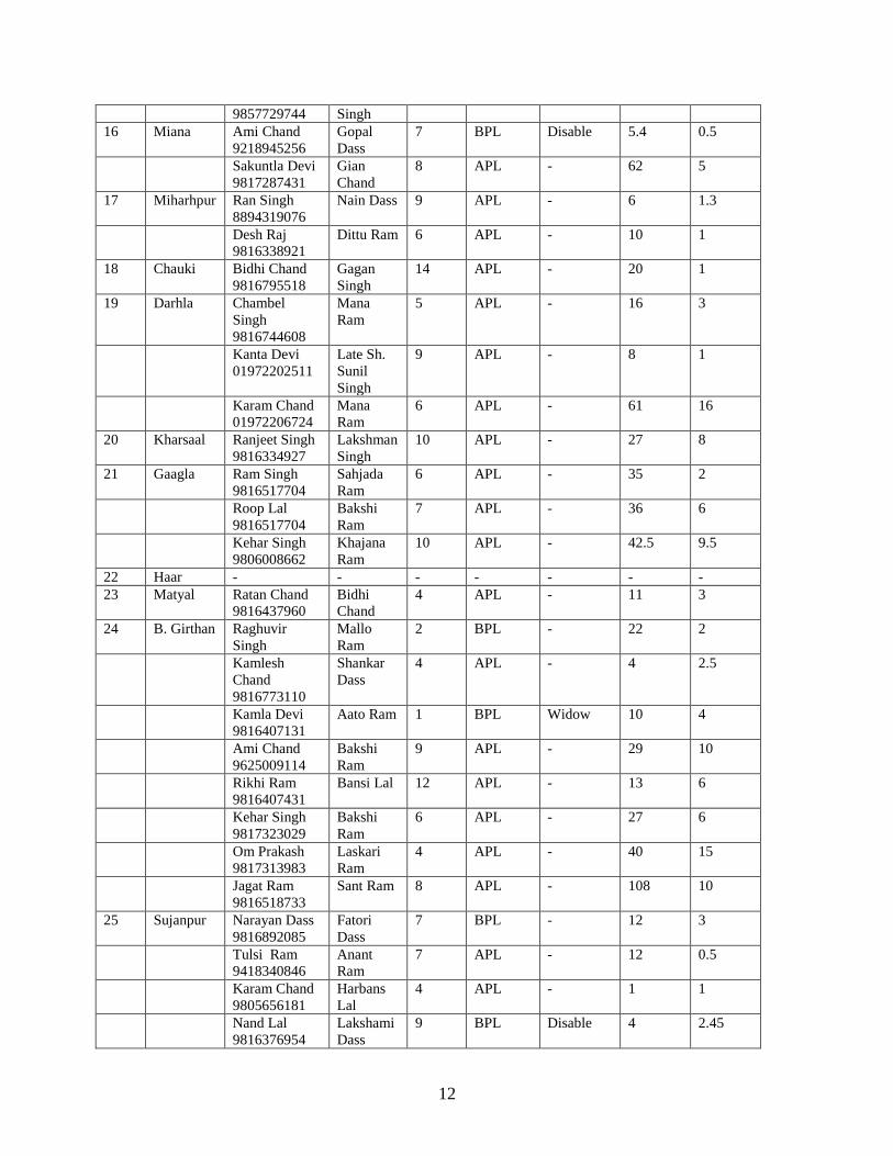
2.5 Selection of project affected households

In each of the project affected village, a complete list of project affected households (not joint land

khata holders) was prepared in consultation with the villagers, who were mostly representatives of

PRIs. A sample of 100 directly project affected households (losing land) was selected

proportionately from all the actual 37 project affected villages losing land following simple random

8

sampling procedure with a minimum of at least one household from each of the affected villages

(Table 2.2 and Table 2.3). The households were post stratified into three categories, namely,

Group I, Group II and Group III using cube- root cumulative frequency method (Table 2.4). The

households losing up to 3 kanal (0.12 ha) of land (1200 m2) were designated as Group I, those

losing 3 to 7 kanals (0.12 to 0.28 ha) land (1200 to 2800 m2) were classified as Group II and those

losing more than 7 kanal (0.28ha) were included in Group III. The per cent distribution of sample

PAFs is given in Table 2.5 and Fig 2.1. The classification of sample farmers and all PAFs for

deriving estimate is depicted in Table 2.6. The details of socio-economic profile of affected

households have been prepared in terms of these three categories of households. However, the

distribution of sample project affected households as per standard classification of marginal, small,

semi-medium, medium and large is presented in Table 2.7 and Fig 2.2. The list and brief detail of

selected households revealing their contact numbers, economic category, existing land, the land to

be lost, etc on both sides of the river is given in Table 2.8 and Table 2.9.

Table 2.2 Sampling plan for project affected villages on LBRB

Sr.

No.

Village Total

households

Project affected

households

Sample

taken

Group-

I

Group-II Group-III

1 J Jihan 18 3 1 - 1 -

2 Bumblu 46 - - - - -

3 Amli Nil - - - - -

4 Balehu 26 20 3 1 - 2

5 Baari 58 7 1 - 1 -

6 Mathan 12 11 1 - - 1

7 Longni 58 52 7 2 - 5

8 Dhaned 22 18 2 2 - -

9 Bhadryana 43 8 1 - 1 -

10 Gahliyan 14 10 1 - - 1

11 Ropa 12 5 1 - 1 -

12 Sarohal 45 12 2 - 1 1

13 Gurorhu 46 12 2 - 1 1

14 Kanerarh - - - - - -

15 Tikkar 85 11 1 1 - -

16 Miana 17 15 2 1 1 -

17 Miharhpur 73 12 2 2 - -

18 Chauki 24 10 1 1 - -

19 Darhla 75 20 3 2 - 1

20 Kharsaal 28 5 1 - - 1

21 Gaagla 47 22 3 1 1 1

22 Haar - - - - - -

23 Matyal 26 11 1 1 - -

24 B Girthan 56 56 8 2 4 2

25 Sujanpur 592 30 4 4 - -

9

26 Tihra 240 - - - - -

27 Riyah 60 - - - - -

28 Palahi 35 15 2 - 1 1

29 Samona 50 40 6 3 1 2

30 B Bagerha 84 35 5 1 3 1

Total 1892 440 61 24 17 20

Source: Field survey, 2011

Table 2.3 Sampling plan for project affected villages on RBRB

Sr.

No.

Village Total

households

Project

affected

households

Sample

taken

Group-I Group-II Group-III

1 Bulli 35 27 4 2 - 2

2 Tipri 31 31 4 3 - 1

3 Kayorh 31 31 4 1 2 1

4 Chauki 36 32 4 1 - 3

5 Dalli 25 12 2 1 - 1

6 Bhalunder 150 12 2 1 - 1

7 Daadu 20 15 2 1 1 -

8 N Bherhi 50 25 4 3 1 -

9 Paprola 66 40 6 2 1 3

10 Alampur 160 10 1 - 1 1

11 Baag 71 4 1 - - 1

12 Liyunda 82 - - - - -

13 Sai 133 27 4 1 1 2

14 Jagrupnager 91 7 1 1 - -

Total 981 273 39 17 7 15

Note: Total project affected HHs = 713 (LBRB = 440, RBRB = 273) Thus sample of 61 and

39=100 from LBRB and RBRB, respectively

Source: Field survey, 2011

Table 2.4 Classification of project affected sample households

Class Interval

(Land to be

lost in k)

Class interval

(Land area to

be lost in ha)

Frequency

(f)

Cube root

frequency

(3/F)

Cumulative

cube-root

frequency

Group

Upto 1 Upto 0.04 17

(10LB+07RB)

2.57 2.57 Group I

1-2 0.04 - 0.08 10 (07+03) 2.15 4.72 Group I

2-3 0.08 – 0.12 14 (07+07) 2.41 7.13 Group I

3-4 0.12 – 0.16 8 (06+02) 2 9.13 Group II

4-5 0.16 – 0.20 3 (02+01) 1.44 10.57 Group II

5-6 0.20 – 0.24 8 (05+03) 2.0 12.57 Group II

6-7 0.24 – 0.28 5 (04+01) 1.70 14.27 Group II

7-8 0.28 – 0.32 7 (03+04) 1.91 16.18 Group III

8-9 0.32 – 0.36 2 (01+01) 1.25 17.43 Group III

9-10 0.36 – 0.40 6 (03+03) 1.81 19.24 Group III

>10 > 0.40 22 (13+07) 2.80 22.04 Group III

Total 100 (61+39) - - -

10

Table 2.5 Group wise classification of project affected sample households

Sr.

No.

Particulars Group I

(up to 0.12 ha)

Group II

(0.12 – 0.28 ha)

Group III

(> 0.28 ha)

Overall

1 Left Bank 24

(39.34)

17

(27.87)

20

(32.79)

61

(100)

2 Right Bank 17

(43.59)

7

(17.95)

15

(38.46)

39

(100)

3 Total 41

(41.00)

24

(24.00)

35

(35.00)

100

(100)

Note: Figures in parentheses are percentages of total

Source: Field survey, 2011

Table 2.6 Classification of sample farmers and all PAFs for deriving estimate

Class interval

(Land to be

lost in k)

Left Bank

(Sample)

Right Bank

(Sample)

Total

sample

Left

Bank

(All)

Right

Bank

(All)

Total

PAFs

Group

Upto 1 10 7 17 72 49 121 GroupI

1-2 7 3 10 50 21 71 GroupI

2-3 7 7 14 50 49 99 GroupI

3-4 6 2 8 43 14 57 GroupII

4-5 2 1 3 14 7 21 GroupII

5-6 5 3 8 36 21 57 GroupII

6-7 4 1 5 29 7 36 GroupII

7-8 3 4 7 22 28 50 GroupIII

8-9 1 1 2 7 7 14 GroupIII

9-10 3 3 6 22 21 43 GroupIII

>10 13 7 20 95 49 144 GroupIII

Total 61 39 100 440 273 713 GroupIII

Table 2.7 Classification of project affected sample households

Sr .

No

Land area interval Category Left bank Right bank Total

1 Upto 1 ha Marginal 29

(47.54)

21

(53.85)

50

(50.00)

2 1-2 ha Small 21

(34.43)

14

(35.90)

35

(35.00)

3 2 - 4 ha Semi medium 6

(9.84)

1

(2.56)

7

(7.00)

4 4 -10 ha Medium 5

(8.19)

2

(5.13)

7

(7.00)

5 Above 10 ha Large - 1

(2.56)

1

(1.00)

Total - 61

(100)

39

(100)

100

(100)

Note: Figures in parentheses are percentages of total

Source: Field survey, 2011

11

Table 2.8 List of project affected sample households on LBRB

Sr.

No

Village Name with

contact no.

Father’s /

Husband

Name

Family

size

(No.)

Category Vulnerable

category

Total

land (k)

Land to

be lost

1 Jungle

Jihan

Pyar Chand Gian

Chand

4 BPL Disable 21 4

2 Bumblu - - - - - - -

3 Amli - - - - - - -

4 Balehu Ajeet Singh

01972313164

Khabbo

Ram

12 APL - 23 2

Munshi Ram

9816969889

Ranu Ram 11 APL - 29 8

Shali Ram

01972206267

Kanehia

Lal

16 APL - 91 20

5 Baari Mehar Singh

8894436802

Jai Singh 10 APL Disable 30 6

6 Mathan Sunil Kumar

9816206519

Roop

Singh

5 APL - 43 15

7 Laungni Tarsem Singh

8894261733

Bakshi

Ram

6 APL - 18 3

Krishani Devi

8679289822

Pyar

Chand

1 BPL Widow 7 1

Hans Raj

9817326793

Rangeela

Ram

9 APL - 111 70

Ishwar Dass

9816357617

Shiv Dyal 9 APL - 42 12

Prabhu Ram

01972206070

Sukh Ram 8 APL - 50 13

Prithi Chand

9805252148

Sant Ram 9 APL - 35 32

Puran Chand

01972206060

Koka

Ram

9 APL - 20 16

8 Dhaned Rakesh Kumar

9816362551

Durga

Dass

4 APL - 25 2

Jagdih Chand

01972221232

Pinnu

Ram

6 APL - 38 2

9 Bhadryana Prahalad

Singh

9736152236

Sant Ram 4 APL - 9 4

10 Gahliyan Kamlesh

Kumari

9418667203

Kapoor

Singh

7 APL Widow 110 80

11 Ropa Dhyan Singh

01972206094

Mansa

Ram

5 APL - 15 7

12 Sarohal Kishori Lal

9418208129

Sufi Ram 8 APL - 28 6

Som Nath

9816922163

Tulsi Ram 9 APL - 38 20

13 Gurorhu Baldev Singh

9816337965

Paras

Ram

4 APL - 25 7

Rikhi Ram Paras

Ram

4 APL - 46 9

14 Kanerarh - - - - - - -

15 Tikkar Bimla Devi Janak 5 APL Widow 146 1

12

9857729744 Singh

16 Miana Ami Chand

9218945256

Gopal

Dass

7 BPL Disable 5.4 0.5

Sakuntla Devi

9817287431

Gian

Chand

8 APL - 62 5

17 Miharhpur Ran Singh

8894319076

Nain Dass 9 APL - 6 1.3

Desh Raj

9816338921

Dittu Ram 6 APL - 10 1

18 Chauki Bidhi Chand

9816795518

Gagan

Singh

14 APL - 20 1

19 Darhla Chambel

Singh

9816744608

Mana

Ram

5 APL - 16 3

Kanta Devi

01972202511

Late Sh.

Sunil

Singh

9 APL - 8 1

Karam Chand

01972206724

Mana

Ram

6 APL - 61 16

20 Kharsaal Ranjeet Singh

9816334927

Lakshman

Singh

10 APL - 27 8

21 Gaagla Ram Singh

9816517704

Sahjada

Ram

6 APL - 35 2

Roop Lal

9816517704

Bakshi

Ram

7 APL - 36 6

Kehar Singh

9806008662

Khajana

Ram

10 APL - 42.5 9.5

22 Haar - - - - - - -

23 Matyal Ratan Chand

9816437960

Bidhi

Chand

4 APL - 11 3

24 B. Girthan Raghuvir

Singh

Mallo

Ram

2 BPL - 22 2

Kamlesh

Chand

9816773110

Shankar

Dass

4 APL - 4 2.5

Kamla Devi

9816407131

Aato Ram 1 BPL Widow 10 4

Ami Chand

9625009114

Bakshi

Ram

9 APL - 29 10

Rikhi Ram

9816407431

Bansi Lal 12 APL - 13 6

Kehar Singh

9817323029

Bakshi

Ram

6 APL - 27 6

Om Prakash

9817313983

Laskari

Ram

4 APL - 40 15

Jagat Ram

9816518733

Sant Ram 8 APL - 108 10

25 Sujanpur Narayan Dass

9816892085

Fatori

Dass

7 BPL - 12 3

Tulsi Ram

9418340846

Anant

Ram

7 APL - 12 0.5

Karam Chand

9805656181

Harbans

Lal

4 APL - 1 1

Nand Lal

9816376954

Lakshami

Dass

9 BPL Disable 4 2.45

13

26 Tihra - - - - - - -

27 Riyah - - - - - - -

28 Palahi Baba Ram

9816122860

Shambhu

Ram

6 APL - 7 4

Prabhu Ram

9816765966

6 BPL - 11 11

29 Samona Ratto Kumar Bhundu

Ram

6 BPL - 7 0.5

Jai Ram

9816340195

7 APL - 9 2

Hem Raj

9418919921

4 APL - 6 3

Kamla Devi

9805351622

Ranjha

Ram

5 BPL - 13 7

Rikhi Ram

9805592108

10 APL - 20 8

Kioshori Lal 6 APL - 55 40

30 Bir

Bagerha

Mani Ram

Thakur

Munshi

Ram

3 APL - 13 1

Ravinder

Kumar

9816379999

Khajana

Ram

2 APL - 29 4

Paras Ram Ranjha

Ram

6 APL - 26 4

Jyoti Prakash

9736805732

Mangat

Ram

5 BPL - 69 5

Rakesh Kumar

9816874828

Sadhu

Ram

5 APL - 24 10

Source: Field survey, 2011

Table 2.9 List of project affected sample households on RBRB Sr.

No

Village Name with

contact no.

Father’s /

Husband

Name

Family

size

(No.)

Category Vulnerable

category

Total

land (k)

Land to

be lost

1 Bulli Ratto Ram

9805300686

Bagho

Ram

6 BPL - 10 3

Rattan Chand

9816701816

Marchu

Ram

10 BPL - 11 3

Pawar Singh

9816798134

Sohan

Singh

4 BPL - 70 15

Man Chand

9816926502

Krishan

Chand

8 APL - 148 36.5

2 Tipri Prithi Chand

9817156373

Kansi Ram 2 BPL - 16.5 2

Satya Devi

8894545728

Baisakhi

Ram

12 BPL - 45 3

Karam Chand

9805128588

Khajana

Ram

3 BPL - 6 3

Kaushlya Devi

9817166234

W/O Ami

Chand

5 APL - 130 14

3 Kayorh Shali Ram

9418761339

Gulab

Singh

5 APL - 6 3

Julfi Ram

01972203092

Khalehu

Ram

10 APL - 18 10

14

Karam Chand

9816577281

Khajana

Ram

6 APL - 27 5

Gian Chand

Sant Ram 4 BPL - 24 6

4 Chauki Nirmla Devi

9625123900

Subhkaran 2 BPL Widow 13 2

Simro Devi

9816227181

Ram Singh 9 APL Widow 80 15

Om Prakash

9816555736

Sukh Ram 3 APL - 37 8

Ghungar Ram

9816335019

Ram Singh 10 APL - 40 12

5 Dalli Jagdish Chand

9816334969

Sunder Lal 11 APL - 9 1

Gian Chand

9816126072

Shingar

Singh

12 APL - 40 9.4

6 Bhalunder Hakam Chand

9816363471

Shri Ram

ji

10 APL - 3.5 0.50

Vipin Kumar

9816871590

Sadhu

Ram

5 BPL - 10.3 10.3

7 Daadu Kailasha Devi

9816480323

Bhoop

Singh

4 APL - 1.5 0.5

Sansar Chand

9816904562

Mehar

Singh

9 APL - 50 4

8 Nichali

Bherhi

Parbhat Chand

9736181363

Dyal

Chand

10 APL - 27 2.5

Madan Lal

Sharma

09625721363

Paemanand

Sharma

7 APL - 23.5 0.5

Roop Singh

9418121152

Tara

Chand

5 APL - 20 2.5

Kultar Singh Bachitar

Singh

14 APL - 351 7

9 Paprola Devi Singh

9736181363

Kapoor

Minhas

7 APL - 4 0.75

Mohinder

Singh

9805118977

Kansi Ram 6 APL - 10 1

Mansa Devi

9805207199

Mast Ran 13 BPL Widow 10 8

Kalan Devi

9805444050

Baragi

Ram

9 BPL Widow 10 8

Kalyan Chand

9817747449

Ragi Ram 7 APL - 30 10

Munsi Ram

9418562279

Khajana

Ram

10 APL - 31 6

10 Alampur Chanderkant

Walia

01894271169

Shamsher

Singh

10 APL - 25.5 4

11 Baag Kanshi Ram

9805839349

6 APL - 30.45 11.5

12 Liyunda - - - - - - -

13 Sai Bidhi Chand

9805730501

Chaudhary

Ram

7 APL - 25 6

Ajaib Singh Chuhar 4 APL - 40 8

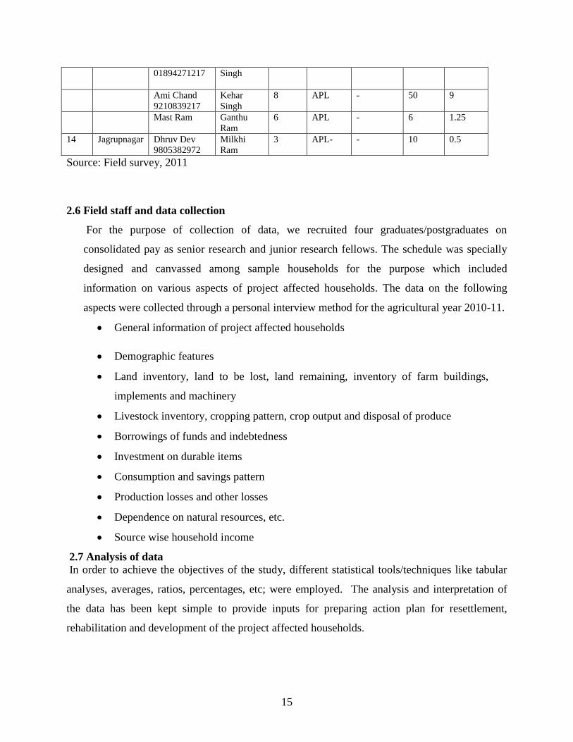
15

01894271217

Singh

Ami Chand

9210839217

Kehar

Singh

8 APL - 50 9

Mast Ram Ganthu

Ram

6 APL - 6 1.25

14 Jagrupnagar Dhruv Dev

9805382972

Milkhi

Ram

3 APL- - 10 0.5

Source: Field survey, 2011

2.6 Field staff and data collection

For the purpose of collection of data, we recruited four graduates/postgraduates on

consolidated pay as senior research and junior research fellows. The schedule was specially

designed and canvassed among sample households for the purpose which included

information on various aspects of project affected households. The data on the following

aspects were collected through a personal interview method for the agricultural year 2010-11.

General information of project affected households

Demographic features

Land inventory, land to be lost, land remaining, inventory of farm buildings,

implements and machinery

Livestock inventory, cropping pattern, crop output and disposal of produce

Borrowings of funds and indebtedness

Investment on durable items

Consumption and savings pattern

Production losses and other losses

Dependence on natural resources, etc.

Source wise household income

2.7 Analysis of data

In order to achieve the objectives of the study, different statistical tools/techniques like tabular

analyses, averages, ratios, percentages, etc; were employed. The analysis and interpretation of

the data has been kept simple to provide inputs for preparing action plan for resettlement,

rehabilitation and development of the project affected households.

16

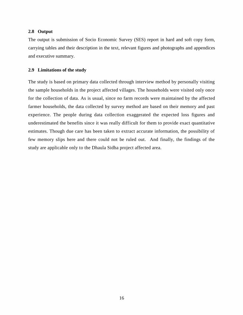
2.8 Output

The output is submission of Socio Economic Survey (SES) report in hard and soft copy form,

carrying tables and their description in the text, relevant figures and photographs and appendices

and executive summary.

2.9 Limitations of the study

The study is based on primary data collected through interview method by personally visiting

the sample households in the project affected villages. The households were visited only once

for the collection of data. As is usual, since no farm records were maintained by the affected

farmer households, the data collected by survey method are based on their memory and past

experience. The people during data collection exaggerated the expected loss figures and

underestimated the benefits since it was really difficult for them to provide exact quantitative

estimates. Though due care has been taken to extract accurate information, the possibility of

few memory slips here and there could not be ruled out. And finally, the findings of the

study are applicable only to the Dhaula Sidha project affected area.

17

CHAPTER 3

SOCIO ECONOMIC PROFILE OF PROJECT AFFECTED HOUSEHOLDS

3.1 Rationale

The present chapter, using household data, seeks to understand, among other things, the socio-

economic profile of sample households in Dhaula Sidha hydro electric project affected villages.

In the context of an agrarian economy, the socio-economic features of any set of population like

age structure, family size and composition, the educational status, etc determine, inter alia,

response of agrarian population to new innovations and their attitude and ability to switch over to

more risky crops and enterprises. These features of population, therefore, broadly determine the

pre-conditions for agricultural development of any region. The extent to which new technologies,

crops and enterprises are actually adopted and practiced is, however, determined by a host of

other important factors like the structure of incentives, institutions and infrastructure. It is,

therefore, important to understand various socio-economic features of sample population. Against

this background, the present chapter discusses some important socio-economic aspects of sample

households such as caste structure, vulnerable households, economic status, sex wise average size

of family, distribution of households according to average size of family, age wise distribution of

family members, educational status, farm assets, livestock inventory, occupational pattern, source

and composition of household income, consumption pattern, and so on.

3.2 Caste structure

Table 1a shows the caste wise distribution of sample head of households on left bank of river Beas. Of the

total sample households, more than two-thirds (68.85%) of the households belonged to general castes

followed by other backward classes (OBCs) with 24.59% and scheduled castes (6.56%). In a similar vein,

the distribution of sample households in terms of amount of land lost, Table 1b shows that 39.34%

households belonged to Group I category followed by Group III (32.79%) and Group II (27.87%).

Table 1c gives caste wise distribution of affected sample households on right bank of river Beas. As may

be seen from the table, in all the categories of households i.e. group I, group II and group III; a

preponderant majority of households belonged to general category followed by scheduled caste and other

backwards castes. At the overall level, 69.23% households belonged to general castes, 25.64% to

scheduled castes and 5.13% to other backward castes (Fig 3.1). Further, the distribution of households of

different castes across different groups (Table 1d) shows that among households of general category

18

44.44% were in group I followed by 37.03% in group III and 18.53% in group II. Among scheduled caste

affected households, 50% belonged to group I, 40% to group III and 10% to group II. As far as households

of other backward castes are concerned, while one-half (50%) of these belonged to group III, the

remaining one-half were in group II. In sum, caste wise distribution of project affected households shows

that on both sides of river Beas, more than two-thirds of the households (nearly 69%) belonged to general

castes comprising Rajput and Brahmans followed by households of other backward castes on the left bank

and those of scheduled castes on the right bank. The distribution of households across three groups shows

that while on the left bank nearly two-fifths (39.34%) of the households were in group I, nearly one-third

(32.79%) were in group III in terms of losing land. Likewise, on the right bank, nearly 44 % of the

households belonged to group I followed by 38.47% in group-III and around18% in group-II.

3.3 Vulnerable households

Table 2a presents the distribution of heads of vulnerable households into different categories belonging to

different groups and all households together on left bank of river Beas. The table reveals that of the total

sample of 61 heads of project affected households, 8 (13.11%) belonged to vulnerable category. The

proportion of disables households headed by disables and those headed by widows was the same i.e., of

50.00%. None of the household was headed by unmarried girls and orphans. The distribution of

vulnerable households according to the severity of the effect, given in Table 2b, shows that 50.00% of the

households belonged to group I followed by 337.50% who belonged to group II. There was only one

vulnerable household (12,50) who belonged to group III.

As far as households on the right bank of the river Beas are concerned, Table 2c shows that there were

10.26% (4) vulnerable households in the project affected villages; out of these households, cent per cent

households were headed by widows. And among these vulnerable households, 25.00% belonged to group

I and 75.00 to group III (Table 2d). In brief, all the vulnerable households were headed by widows and

disables on the left bank of which one–half were in group I. In comparison, on the right bank, only

widows headed such households of which three-fourth were in group III. The distribution of project

affected household by vulnerable category is also depicted through Fig 3.2.

3.4 Economic status of project affected households

Table 3a and 3b portray economic status of the project affected sample households. As may be noted from

Table 3a, of the total sample of 61 project affected households on left bank of river Beas, four-fifths were

above poverty line (APL) while remaining one-fifth (19.67%) were below poverty line (BPL). The table

further shows that as high as 79.59% of the households above poverty line came from general castes.

Likewise, one-half of the BPL households belonged to other backward casts and one-fourth each to

general category and scheduled caste category. In terms of the amount of land that would be lost, group I

19

and group III each accounted for 36.73 per cent of the APL households. Among BPL households, one-

half belonged to group I and nearly one-third to Group II. On the right bank of the river Beas, nearly

three-fourths of the sample households were above poverty line (APL) and remaining one-fourth were

below poverty line (BPL) households. Further, more than three-fifths of the households above poverty line

belonged to general castes, nearly one-tenth were scheduled castes and remaining 6.90% came from other

backward castes (OBCs). In the BPL category, 70% belonged to scheduled castes and 30% to general

category. None of the BPL category household belonged to OBCs. And, on the right bank of river Beas,

among general category APL households, more than 41.67% were in group I, 37.50% were in group III

whereas 20.83% came from group II. Thus it can be concluded that the incidence of poverty, measured by

the proportion of households below poverty line, was high (25.64%) on the right bank as compared to left

bank (19.67%). The distribution of project affected households by economic status category is also shown

in Fig 3.3.

3.5 Occupational pattern

Table 4a and 4b show the occupational pattern of project affected sample households. These tables reveal

that service both in public and private sectors was the major occupation of the households on both sides of

river Beas. For example, 30.77% of the households on right bank and 39.34% on left bank reported

service as their major occupation. Daily paid labour was another important occupation of the sample

households on the right bank which was being practiced by 28.21% of the total households. In comparison,

on the left bank, 16% of the households reported daily paid labour as their main occupation. Agriculture

which encompasses crops and animal husbandry including dairying was the major occupation of 16.39%

households on the left bank and 12.82% on the right bank. The sample households who reported pension

as their main source of income accounted for 18.03% on the left bank and 20.51% on the right bank. A

more or less similar occupational pattern was in evidence insofar as households falling under different

groups were concerned. On the whole, service both in private and public sectors followed by daily paid

labour were major occupations of sample households on both sides of the river. Agriculture, including

crop and animal husbandry, was being practiced by 16.39% of sample households in left and 12.82% of

the households in right bank of river Beas (Fig 3.4).

3.6 Age wise composition of sample population

Age wise composition of sample population in the study area is depicted in Table 5a and Table 5b. A

close perusal of the table 5a shows that out of the total population of 406, the male and female population

respectively accounted for 52.71 % and 47.29 %. The gender wise distribution of project affected

population given in Fig 3.5 shows that males were 54.37% against 45.53% of females. As far as age

composition is concerned, 38.42% of total persons were in the age group of 18-40 years followed by

20

21.18% who were in the age group of 6-18 years and 18% in the age group of 18-40 years. The children

below 5 years accounted for 9.36% of the total population whereas the share of those above 60 years was

12.81%. In case of female population, while their proportion in children and old age category was less

than their male counter parts, the proportion of females in the age group of 18-60 years was higher than

males. And it is this age group of population which contributes more towards households’ economy in

terms of providing active labour force services. The distribution of population into different groups which

indicate the amount of land that would be lost, Table 5a shows that there were 148, 102 and 156 persons

in group I, group II and group III, respectively and that in all categories, the proportion of males was

marginally higher than females. The average family size of project affected households in group I, group

II and group III respectively was 6.0, 6.0 and 7.8 persons with an overall average figure of 6.6 persons. An

important feature which emerges from the table is the higher average family size of households in group

III who would most severely be affected in terms of the amount of land that they would lose.

Table 5b shows the age composition of population of sample households who reside on the right bank of

the river Beas. The total population comprised of 269 persons with 153 (56.88%) males and 116 (43.12%)

females. More than one-third of the population was in the age group of 18-40 years, and the proportion of

female in this age group was higher (39.66%) than males (32.68%). The pattern of age composition

among different groups of project affected households was broadly similar. As regards average family size,

it was 6.5 persons in group I, 7.3 in group II and 7.5 in group III. The overall average family size of

households on right bank of river Beas was 7 persons per household comprising 4 males and 3 females. In

broad terms, two important results need reiteration: first, more than one-fifth of the total population

comprised children below 5 years of age and those above 60 years of age; second, the proportion of school

going population between 6-18 years of age comprised 20 to 21% of the total population; third, the

proportion of labour force actively engaged in various economic activities was 57 to 58 % and in total

workforce, the proportion of females was higher than males; fourth, the overall family size was 7 persons

per households; fifth, the sex ratio (females per 1000 males) was 894 and 762 on left bank and right bank,

respectively, while for all households taken together the sex ratio was 839.

3.7 Educational status

Table 6a and Table 6b present educational status of project affected sample population on both sides of the

river Beas. As may be seen from two tables, 7% to 8% of the population was non-school going. The

overall literacy rate was nearly 88%. And among males the literacy level was 93-94% males as compared

to 81-82% among females. Among households categorized according to the amount of land that would be

lost, the literate percentage of population on RBRB varied from 87.23% in group I to 89.72% in group III

households with an overall literacy level of 88.45%. In terms of levels of education, education up to

21

primary level was more among females than males. Further, as much as 19% of people had education up

to matriculation level followed by those educated up to senior secondary and middle standard who each

accounted for 17%. One-tenth of the total population was educated up to graduate. And the proportion of

those who had done post-graduation and those who were technically qualified were negligible. More

importantly, however, in almost all educational levels, females lagged much behind their male

counterparts implying gender discrimination. Across different category of project affected households on

left bank of the river Beas, the literacy level of population varied from 85.26% among households of

group II to as high as 90.98% among those in group I. In all the categories, the level of male literacy was

above 90% in comparison to female literacy which varied between 77% and 86%. In case of different

levels of education, at the overall level, the distribution of male population according to different levels

was more even as compared to distribution of female who were mostly concentrated in primary to senior

secondary levels.

To conclude, the overall literacy level of population was 88% which was as high as 93 to 94% among

males as against 81 to 82% among their male counterparts. Further while most of the females were

educated from primary to senior secondary levels, the educated males were more evenly distributed across

different levels of education, say from primary level to post graduate and technically as well as

professionally qualified levels. The underlying message is the need for making efforts to impart higher

education and vocational education to women to enhance their knowledge and skills.

3.8 Housing structure and investment

The details of various buildings like house, stable, cattle shed, store, business shop and agro industry (atta

chakki & gharat) have been brought in Tables 7a and 7b. The tables bring out a number of interesting

patterns. For example, out of 61 sample households situated on the left bank, 33 households (54.10%)

owned kachcha houses whereas 28 (45.90%) possessed pucca houses. More than half of the households

(55 %) in group I owned pucca houses while 64.71 % of households in group II had kachcha houses. On

the right bank of the river, a reverse trend was noted, for example, the proportion of households

possessing pucca houses was higher (51.28%) compared those owing kachcha houses (48.72 %). In case

of cattle sheds, on both sides of the river, more than 94% were kachcha structures. Among others, the

structures like stable for horses/ponies, store for preserving foodgrains & agricultural implements were

possessed by a very few households. In addition, one atta chakki and one gharat were also found among

sample households. Similarly, buildings meant for running business like shop keeping numbered 3 on the

right bank and 1 on the left bank. Further, the investment on all types of buildings mentioned above

amounted to Rs. 5.89 lakh on the right side and Rs. 6.32 lakh on the left side (Table 8a and Table 8b).

Again residential houses accounted for the highest proportion of total investment which varied from 82%

on the right bank to 85% on the left bank. Among different groups of households, the investment on

22

buildings was the highest in group II on the right side and group III on the left side which respectively

amounted to Rs 9.90 lakh and Rs 8.70 lakh per household, respectively. The average investment on

buildings was Rs. 5.89 lakh on the right bank and Rs 6.32 lakh on the left bank with the highest proportion

of investment on residential buildings.

3.9 Household durables

The household durables possessed by the sample households along with their monetary value have been

presented in Table 9a and Table 9b. Table 9a reveals that on the left bank of the river Beas the total

present value of household items such as communication means (telephones/cell phones) kitchen

appliances (cooking gas, gas cylinder, refrigerator, pressure cooker, dining set, etc.), entertainment sources

like radio, tap recorder & television and the means of conveyance & goods carrier like bicycle, scooter,

car, jeep/utility van, etc. increased from Rs. 37,996 in respect of households in group I to Rs. 1,53,953 in

case of households in group III. At the overall level, the present value of all durables was assessed at Rs.

73,888. In comparison, however, there was no clear cut pattern in the value of the household durables

possessed by the households belonging to different groups on the right bank of the river (Table 9b). For

example, across different groups, the value of all household durables was Rs. 34,594, Rs 33,407 and Rs

29,853 in group I, group II and group III households. At the overall level, the average value of all durables

per household was Rs. 31,960 which was around one-third in comparison to the value of household

durables possessed by households residing on the left bank of river Beas. Among different items (Table

9a), conveyance means accounted for the largest share in the value of all durables. Cots and television

each accounted for 6.44 and 7.49% of the total investment. On the right bank, however, cots and

refrigerator each accounted for nearly 15% whereas television’s share in total value was as high as 15.66%.

In conclusion, means of conveyance followed by drawing room & bed room items and recreation items

were the major items of household durables. The average value of durables per household residing in the

left bank was nearly 2.3 times as compared to an average value of durables per household in the right bank

which, among other things, could be attributed to high economic status on account of better infrastructure

and connectivity.

3.10 Livestock inventory

Livestock rearing is the most important economic activity and provides a regular and relatively more

secure source of household income and employment. Table 10a and Table 10b present details on livestock

inventory including investment pattern on the project affected households. It can be seen from the tables

that, on an average, each sample household reared 2 to 3 animals. In monetary terms, the investment made

on these animals amounted to Rs. 15,211 per household on the left bank and Rs. 15,010 per household on

the right bank. One of the interesting patterns emerging from these tables is that the number of animals

reared per household and the amount of investment made on them increased from group I to group III on

23

both sides of the river. Among animals, buffaloes were the most important animals accounting for nearly

one-third of the total investment on livestock on the right bank and more than 70% on the left bank.

Equines (horses & ponies) were maintained in large number on the right bank primarily on account of

poor means of transport facilities. There were 12 horses/ponies on all the 39 sample households which in

monetary terms amounted to Rs. 1, 68,000 accounting for 28.70% of the total investment. In brief, the

average number of animals reared by the sample households was 2.70 on the left bank and 2.23 on the

right bank whose monetary valued stood at Rs. 15,211 and Rs. 15,010, respectively. And among different

animals, buffaloes particularly of murrah breed were the most important.

3.11 Land utilization pattern

As is well known, the land is the most important asset whose distribution determines, to a large extent,

the economic status of households. In an agrarian economy, land not only determines the social &

economic status of a household but access to different institutions as well. Table 11a shows land

utilization pattern of the affected households on the left bank. As may be seen from the table average size

of land holding varied from 0.74 ha per household in group I to as high as 1.95 ha per household in group

III; at the overall level, the average size of land holding was 1.23 ha per household. It can further be seen

from the table that more than one-half of the land holding was under cultivation and in group III (most

affected category) the percentage of cultivated land was 60.20 while the per cent of cultivated land was

58.11 in group I and 54.63 in group II with an overall average of 58.06 per cent. Area under grassland

ranged from about one-fourth in group II households to approximately one-third in group III with an

overall average of 29.04% of total holding. Table 11b depicts land utilization pattern on various groups of

project affected sample households on the right bank of river Beas. The table shows that the average size

of land holding on the right bank of river Beas was 1.55 ha with the highest of 3.10 ha in group III and the

lowest 0.52 ha in group I. And among different categories of land, the uncultivated land accounted for

29.03% of total land.

3.12 Cropping pattern

Table 12a and 12b gives details of crops grown by the sample project affected households on both sides of

the river Beas. As may be seen from the tables, maize is the most important crop grown during the kharif

season on both sides of the river; it was evident from the fact that maize occupied around two-fifths of the

total cropped area on both sides of river Beas (Fig 3.6). Among households belonging to different groups,

no neat was discernible. However, in absolute terms, the area allocated to maize crops increased from

group I to group III category households. Wheat was the most important crop raised in rabi season which

accounted for 46.15% of the cropped area on the left bank and 46.81% on right bank. Again the amount of

area devoted to wheat increased from group I to group III on both sides of river Beas. Paddy was not very

important crop which is evident from fact that it accounted for 5.59% of the cultivated area in the left bank

24

of the river and 5.67% on the right bank. Fodder crops comprising chari /bajra in kharif and oats &

barseem in rabi occupied nearly 5 to 6% of the cropped area on both sides. The area under pulses was

negligible. Vegetable cultivation was gaining popularity wherever irrigation facility is available; currently

1.41 and 1.42 % of the cropped area was devoted for the production of vegetables on left bank and right

bank, respectively. The cropping intensity was nearly 200 suggesting that the farmers took two crops

during a year and the cultivated land was almost equally allocated under kharif and rabi crops. On the

whole, the cropping pattern was dominated by maize in kharif season and wheat in rabi season in all the

project affected villages on both sides of the river. More importantly, however, the farmers have recently

started diversifying their cropping patterns towards fodder (chari/bajra and oats) and vegetable crops. And

the farmers were growing two crops in a year thereby fully utilizing the available net sown area.

3.13 Vegetable production

It is customary in the project affected villages to grow vegetables; some farmers grow on a very small area

while others cultivate it on a significant proportion of cultivated area for meeting their own requirements.

With the increase in irrigation infrastructure facilities and the introduction of protected cultivation, the

farmers have started growing vegetable for market and are increasingly allocating more and more area to

these crops. The data on the area under different vegetable crops have been presented in Table 13a and

Table 13b. As may be seen from the tables, potato, carrot, radish, cauliflower, cabbage, lady finger,

colocasia, cucumber, pumpkin, turmeric, garlic, coriander, ginger and onion were the important vegetables

raised by project affected households on both sides of the river Beas. Among these crops, potato followed

by turmeric, lady finger and cauliflower were the important vegetable crops on LBRB while radish

followed by lady finger, cauliflower and potato were the important crops grown on the right bank of river

Beas. Further, on an average, each project affected household was growing more than 1 q of vegetables

produce which in monetary terms amounted to Rs 1596 on left bank of river Beas and Rs 1266 on right

bank of river Beas.

3.14 Foodgrains, fruits & vegetable production

The details on foodgrains (cereals and pulses), fruits and vegetable production have been presented in

Table 14a and Table 14b. It can be seen from the tables that while the foodgrain production per

households was higher (25.32 q) on right side than 17.27 q on the left bank. Among cereals, wheat crop

was the major contributor towards foodgrain production followed by maize on both sides of river Beas.

On the left bank of river Beas, the contribution of wheat was more than one-half whereas on the right bank

of river Beas it was nearly 45%. Similarly, maize accounted for 42.04% and 38.15 % of foodgrain

production on the left bank and the right bank of the river, respectively. Among fruit, indigenous and

25

grafted mangoes were very common and almost each household owned one or two big trees of indigenous

mango which almost fulfilled their requirements in terms of preparing pickle, mango papad, sauce, jam

and amchoor. Vegetable production was nearly 1 quintal per household.

3.15 Average yields

Table 15a and Table 15b show the average yield of crops (cereals & pulses and fruits & vegetables) on

sample project affected households. It can be observed from the tables that average yield of maize varied

from 12.50 q/ha on left bank to 16.75 q/ha on right bank. These are the average yields that have been

realized by the farmers, though actual yields were high around 25 q/ha but due to damage caused by wild

animals mostly the monkeys and wild boars, 6.25-7.50 q/ha loss suffered by the farmers which in value

terms amounted to Rs. 6250 to Rs. 7500 /ha. Wheat, the most important rabi crop, gave an average yield

of 13.25 q to 17 q/ha. Paddy was not an important crop of the area and its average yield was 10.25 to

10.75 q/ha. The average yields of maize, paddy and wheat are also depicted in Fig 3.7. Average yield of

pulses was low ranging varying 3.75 q/ha on the left bank to 7.50 q/ha on the right bank. The vegetable

growing was becoming an important activity in areas where irrigation facility is available; these crops

gave average yield in the range of 55.25 q to 64.50 q/ha. The yield of barley though not grown on a

significant area was 10.75 q/ha on the right bank to 17.25 q/ha on the left bank. As far as individual

groups are concerned, there was no specific pattern. To sum up, the average yields of different crops were

low as compared to district and state level average yields However, one of the most important factor for

low yields is the damage caused to crops by monkeys and wild boars; such losses have estimated to be Rs

6250/ha to Rs 7500/ ha

3.16 Production and disposal of food grains

The details of production and disposal of foodgrains which include cereals and pulses on different types

of project affected households on both sides of river Beas have been given in Table 16a and Table 16b.

The tables show that the average production as well as marketable surplus of food grains increased from

group I to group III. The estimates of production of food grains reveal that a household produced 17.26 q

on the left side and 22.01 q on the right side. The production of food grains across groups on the left side

of the river Beas varied widely from 10.59 q in group I to 28.81 q in group III on the left hand side of river

Beas. The corresponding figures on right side were 6.80 and 38.01 q, respectively. The amount of

marketable surplus was 2.23 q per household on the right bank and 1.63 q per household on the left side.

In per cent terms, the marketable surplus ranged from 4% to 13% on the left bank and 2% to 13 % on the

right bank. The marketed surplus was 44% on the left bank and 48% on the right bank. The marketed

surplus i.e. quantity actually sold as a proportion of marketable surplus was 54% on the left bank and 58%

26

on the right bank. Similarly, the quantity of food grains consumed at home accounted for 27% on the right

bank and 33% on the left bank. The per cent share of food grains consumed at home was the highest in

group I might be due to low level of production. In sum, the average production of food grains varied from

17 to 22 q per household; out of the total production per household 27 to 33% was consumed at home and

54 to 58% was marketable/marketed surplus. In absolute terms, the marketable and marketed surplus

together was 9.30 q per household on the left bank and 12.76 q on the right bank.

3.17 Source wise configuration of household income

Tables 17a and 17b show the source wise composition of annual household income of project affected

households on both sides of the river Beas. A perusal of the table reveals that off farm income sources like

service, pension, shop keeping and daily paid labour were the important sources of households income;

these sources taken together contributed as high as three-fourths of total household income on the left

bank and more than four-fifths on the right bank. The gross household income from farm sources was

assessed at Rs. 45,339 on right bank and Rs 53,550 on left bank which respectively accounted for 16%

and 25% of the gross household income. Among farm income sources, while crops and animal husbandry

including dairying were relatively more important, fruits and vegetables contributed negligible amount.

Among off-farm sources, services in public and private sectors accounted for the highest share (41.66% on

right bank and 45.23% on left bank). Among households belonging to different groups according to the

amount of land to be lost, the table shows that gross annual household income was highest in group II

(Rs.4,68,032) on the right bank and group III (Rs.2,20,136) on the left bank. However, per capita income

was the highest of Rs. 64,114 in group II category on the right bank and Rs. 35,798 in group I on the left

bank. The average per capita income for overall situation including households of both the left and right

bank was Rs. 32,643 and Rs. 41,318 which was significantly lower than the average per capita income of

Rs. 58,000 for the state as a whole. In sum, the average annual gross household income was higher (Rs.

2,89,228) on the right bank in comparison to Rs. 2,15,442 on the left bank. Among different sources, the

contribution of the services was the highest followed by pension. The farm income accounted for 16% on

the right bank and 25% on the left bank with overall average of about 21% (Fig 3.8). The per capita

income was substantially higher (Rs. 41,318) on the right bank as compared to the left bank (Rs. 32,643).

3.18 Consumption pattern

Consumption pattern of the sample households is shown in Tables 18a and 18b. The table shows that the

household consumption expenditure on various items was Rs. 76,375 per annum in the left bank in

comparison to Rs. 72,141 on the right bank. Likewise, the per capita consumption expenditure was Rs.

11,572 on the left bank and Rs. 10,305 on the right bank. Further, the per capita consumption expenditure

27

on left bank was found increasing from group I to group III while no specific pattern between per capita

expenditure and households in different groups was in evidence on the right bank. Among different items

of expenditure, milk was the most important item which accounted for 20.10% of total expenditure on the

right bank and 24.29% on the left bank. Clothing was next important item accounting for 6.93% of the

household expenditure on the left bank and 7.87 % on the right bank. Cereals like rice and wheat and

vegetables were other important items of expenditure. In brief, the annual household expenditure was Rs.

76,375 per household on the left bank in comparison to Rs. 72,141 on the right bank. The per capita

expenditure was higher (Rs. 11,572) on the left bank than Rs. 10,305 on the right bank.

3.19 Saving pattern

Savings have been estimated by deducting the gross household consumption expenditure and gross

household income. The estimates have been shown in Table 19a and Table 19b. As may be seen from the

tables, that while nearly two-thirds of the gross household income was being saved by households on the

left bank, three-fourths of gross household income was being saved by those on the right bank. Among

households belonging to different group categories, those on the right bank did save as high as four-fifths

of their household income on the right bank which could be attributed to higher household income in case

of the latter as compared to the former.

3.20 Purpose and source wise borrowings

Table 20a and Table 20b present purpose wise borrowings of sample households on the left side and the

right side of the river, respectively. It can be seen from Table 20a that on the left bank, 8 (13.12%) out of

61 households borrowed money for purposes like agriculture, dairy farming, agricultural machinery,

construction of house, running business, personal vehicle and social ceremonies like marriage, education

of children, etc. The amount of money borrowed for the purpose of agriculture like polyhouse per

household was Rs 1, 09,500. The maximum amount of Rs 2, 50,000 was borrowed by one household for

the purchase of tractor trolley and thrasher. Similarly, the amount borrowed for running commercial dairy

was Rs 50,000 per household. In a similar vein, on the right side, there was only one household who

borrowed Rs 20,000 for the construction of a house (Table 20b).

As far as sources of borrowing is concerned, Table 21a and Table 21b reveals that commercial banks

followed by state horticulture Department (under HTM scheme) were the two major sources of finance on

the left bank of river Beas whereas on the right bank of river there was only one borrower who had

borrowed from village cooperative society for this purpose.

28

Table 1a Distribution of heads of households among castes on LBRB (No.)

Sr.

No.

Caste Group I

(upto 0.12 ha)

Group II

(0.12 – 0.28 ha)

Group III

(> 0.28 ha)

Total

1 General

16

(66.66)

11

(64.71)

15

(75.00)

42

(68.85)

2 Scheduled caste 2

(8.34)

1

(5.88)

1

(5.00)

4

(6.56)

3 Other backward

classes

6

(25.00)

5

(29.41)

4

(20.00)

15

(24.59)

Total 24

(100)

17

(100)

20

(100)

61

(100)

Note: Figures in parentheses are percentages of column total

Source: Field survey, 2011

Table 1b Distribution of heads of households in different castes across groups on LBRB (No.)

Sr. No. Caste Group I

(upto 0.12 ha)

Group II

(0.12 – 0.28 ha)

Group III

(> 0.28 ha)

Total

1 General

16

(38.09 )

11

(25.19 )

15

( 35.72 )

42

(100)

2 Scheduled caste 2

(50.00)

1

(25.00)

1

(25.00)

4

(100)

3 Other backward

classes

6

(40.00 )

5

(33.33 )

4

(26.67)

15

(100)

Total 24

(39.34)

17

(27.87)

20

(32.79)

61

(100)

Note: Figures in parentheses are percentages of row total.

Source: Field survey, 2011

Table 1c Distribution of heads of households among castes on RBRB (No.)

Sr. No. Caste Group I

(upto 0.12 ha)

Group II

(0.12 – 0.28 ha)

Group III

(> 0.28 ha)

Total

1 General

12

(70.59)

5

(71.43)

10

(66.67)

27

(69.23)

2 Scheduled caste 5

(29.41)

1

(14.29)

4

(26.67)

10

(25.64)

3 Other backward

classes

- 1

(14.28)

1

(6.66)

2

(5.13)

Total 17

(100)

7

(100)

15

(100)

39

(100)

Note: Figures in parentheses are percentages of column total.

Source: Field survey, 2011

29

Table 1d Distribution of heads of households in different castes across groups on RBRB (No.)

Sr. No. Caste Group I

(upto 0.12 ha)

Group II

(0.12 – 0.28 ha)

Group III

(> 0.28 ha)

Total

1 General

12

(44.44)

5

(18.53)

10

(37.03)

27

(100)

2 Scheduled caste 5

(50.00)

1

(10.00)

4

(40.00)

10

(100)

3 Other backward

classes

- 1

(50.00)

1

(50.00)

2

(100)

4 Total 17

(43.59)

7

(17.94)

15

(38.47)

39

(100)

Note: Figures in parentheses are percentages of row total

Table 2a Distribution of vulnerable heads of households among different categories of vulnerability on

LBRB (No.)

Sr. No. Category Group I

(upto 0.12 ha)

Group II

(0.12 – 0.28 ha)

Group III

(> 0.28 ha)

Total

1 Disable 2

(50.00)

2

(66.67)

- 4

(50.00)

2 Widow 2

(50.00)

1

(33.33)

1

(100.00)

4

(50.00)

3 Total 4

(100)

3

(100)

1

(100)

8

(100)

Note: Figures in parentheses are percentages of column total

Source: Field survey, 2011

Table 2b Distribution of vulnerable heads of households among different categories of vulnerability on

LBRB (No.)

Sr. No. Category Group I

(upto 0.12 ha)

Group II

(0.12 – 0.28 ha)

Group III

(> 0.28 ha)

Total

1 Disable 2

(50.00)

2

(50.00)

-

4

(100)

2 Widow 2

(50.00)

1

(25.00)

1

(25.00)

4

(100)

3 Total 4

(50.00)

3

(37.50)

1

(12.50)

8

(100)

Note: Figures in parentheses are percentages of row total

Source: Field survey, 2011

30

Table 2c Distribution of vulnerable heads of households among different categories of vulnerability on

RBRB (No.)

Sr No. Category Group I (upto 0.12 ha)

Group II (0.12 – 0.28 ha)

Group III (> 0.28 ha)

Total

1 Disable -

-

-

-

2 Widow 1

(100.00)

-

3

(100.00)

4

(100.00)

3 Total 1

(100)

-

3

(100)

4

(100)

Note: Figures in parentheses are percentages of column total

Source: Field survey, 2011

Table 2d Distribution of vulnerable heads of households across groups on RBRB (No.)

Sr No. Category Group I (upto 0.12 ha)

Group II (0.12 – 0.28 ha)

Group III (> 0.28 ha)

Total

1 Disable -

-

-

-

2 Widow 1

(25.00)

-

3

(75.00)

4

(100)

3 Total 1

(25.00)

-

3

(75.00)

4

(100)

Note: Figures in parentheses are percentages of horizontal total

Source: Field survey, 2011

Table 3a Distribution of above poverty line and below poverty line heads of households across castes on

LBRB (No.)

Sr.

No.

Economic category Group I (upto 0.12 ha)

Group II (0.12 – 0.28 ha)

Group III (> 0.28 ha)

Total

1 Above Poverty Line

(APL)

18

(100)

13

(100)

18

(100)

49

(100)

General

15

(83.33)

9

(69.22)

15

(83.33)

39

(79.59)

Scheduled caste -

1

(11.11)

-

1

(2.04)

Other backward

classes

3

(16.67)

3

(23.07)

3

(16.67)

9

(18.37)

2 Below Poverty Line

(BPL)

6

(100)

4

(100)

2

(100)

12

(100)

General

1

(16.67)

2

(50.00)

-

3

(25.00)

Scheduled caste 2

(33.33)

- 1

(50.00)

3

(25.00)

Other backward

classes

3

(50.00)

2

(50.00)

1

(50.00)

6

(50.00)

Note: Figures in parentheses are percentages of total under respective economic class

Source: Field survey, 2011

31

Table 3b Distribution of above poverty line and below poverty line heads of households across castes on

RBRB (No.)

Sr.

No.

Economic category Group I

(upto 0.12 ha)

Group II

(0.12 – 0.28 ha)

Group III

(> 0.28 ha)

Total

1 Above Poverty Line

(APL)

12

(100)

6

(100)

11

(100)

29

(100)

General

10

(83.33)

5

(83.33)

9

(81.82)

24

(82.76)

Scheduled caste 2

(16.67)

-

1

(9.09)

3

(10.34)

Other backward

classes

-

(0.00)

1

(16.67)

1

(9.09)

2

(6.90)

2 Below Poverty Line

(BPL)

5

(100)

1

(100)

4

(100)

10

(100)

General

2

(40.00)

-

1

(25.00)

3

(30.00)

Scheduled caste 3

(60.00)

1

(100.00)

3

(75.00)

7

(70.00)

Other Backward

Classes

-

-

-

-

Note: Figures in parentheses are percentages of total under respective economic class

Source: Field survey, 2011

Table 4a Occupational profile of sample households on LBRB (No.)

Sr. Occupation Group I

(upto 0.12 ha)

Group II

(0.12 – 0.28 ha)

Group III

(> 0.28 ha)

Total

1 Agriculture 1.00

(4.17)

7.00

(41.18)

2.00

(10.00)

10.00

(16.39)

2 Government service 5.00

(20.83)

3.00

(17.65)

3.00

(15.00)

11.00

(18.03)

3 Private service 6.00

(25.00)

3.00

(17.64)

4.00

(20.00)

13.00

(21.31)

4 Pension 4.00

(16.67)

3.00

(17.65)

4.00

(20.00)

11.00

(18.03)

5 Shop keeping 3.00

(12.50)

- 3.00

(15.00)

6.00

(9.85)

6 Daily paid labour 5.00

(20.83)

1.00

(5.88)

4.00

(20.00)

10.00

(16.39)

Total 24.00

(100)

17.00

(100)

20.00

(100)

61.00

(100)

Note: Figures in parentheses are percentages of total

Source: Field survey, 2011

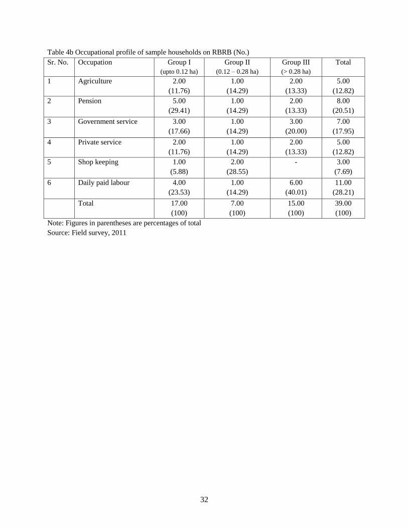
32

Table 4b Occupational profile of sample households on RBRB (No.)

Sr. No. Occupation Group I

(upto 0.12 ha)

Group II

(0.12 – 0.28 ha)

Group III

(> 0.28 ha)

Total

1 Agriculture 2.00

(11.76)

1.00

(14.29)

2.00

(13.33)

5.00

(12.82)

2 Pension 5.00

(29.41)

1.00

(14.29)

2.00

(13.33)

8.00

(20.51)

3 Government service 3.00

(17.66)

1.00

(14.29)

3.00

(20.00)

7.00

(17.95)

4 Private service 2.00

(11.76)

1.00

(14.29)

2.00

(13.33)

5.00

(12.82)

5 Shop keeping 1.00

(5.88)

2.00

(28.55)

- 3.00

(7.69)

6 Daily paid labour 4.00

(23.53)

1.00

(14.29)

6.00

(40.01)

11.00

(28.21)

Total 17.00

(100)

7.00

(100)

15.00

(100)

39.00

(100)

Note: Figures in parentheses are percentages of total

Source: Field survey, 2011

33

Table 5a Age wise distribution of sample population on LBRB (No.)

Sr.

No.

Age

interval

(Years)

Group I

(upto 0.12 ha)

Group II

(0.12 – 0.28 ha)

Group III

(> 0.28 ha)

Total

Male Female Total Male Female Total Male Female Total Male Female Total

1 Upto 5 10

(12.05)

9

(13.85)

19

(12.84)

4

(7.85)

3

(5.88)

7

(6.86)

7

(8.75)

5

(6.58)

12

(7.69)

21

(9.81)

17

(8.85)

38

(9.36)

2 6-18 17

(20.48)

6

(9.23)

23

(15.54)

13

(25.49)

11

(21.57)

24

(23.53)

18

(22.50)

21

(27.63)

39

(25.00)

48

(22.43)

38

(19.79)

86

(21.18)

3 18-40 33

(39.76)

28

(43.08)

61

(41.22)

19

(37.25)

20

(39.22)

39

(38.24)

28

(35.00)

28

(36.84)

56

(35.90)

80

(37.38)

76

(39.59)

156

(38.42)

4 40-60 12

(14.46)

16

(24.61)

28

(18.92)

9

(17.65)

12

(23.53)

21

(20.59)

13

(16.25)

12

(15.79)

25

(16.03)

34

(15.89)

40

(20.83)

74

(18.23)

5 >60 11

(13.25)

6

(9.23)

17

(11.48)

6

(11.76)

5

(9.80)

11

(10.78)

14

(17.50)

10

(13.16)

24

(15.38)

31

(14.49)

21

(10.94)

52

(12.81)

6 Total 83

(100)

65

(100)

148

(100)

51

(100)

51

(100)

102

(100)

80

(100)

76

(100)

156

(100)

214

(100)

192

(100)

406

(100)

7 Average

family size

3.4 2.6 6.0 3.0 3.0 6.0 4.0 3.8 7.8 3.5 3.1 6.6

8 Sex ratio

(F/1000M)

- - 776 - - 1000 - - 950 - - 894

Note: Figures in parentheses are percentages of total.

Source: Field survey, 2011

34

Table 5b Age wise distribution of sample population on RBRB (No.)

Sr.

No.

Age

interval

(Years)

Group I

(upto 0.12 ha)

Group II

(0.12 – 0.28 ha)

Group III

(> 0.28 ha)

Total

Male Female Total Male Female Total Male Female Total Male Female Total

1 Upto 5 11

(18.65)

4

(8.51)

15

(14.42)

-

1

(5.26)

1

(1.96)

6

(9.68)

1

(2.00)

7

(6.25)

17

(11.11)

6

(5.16)

23

(8.55)

2 6-18 8

(13.56)

8

(17.03)

16

(15.38)

14

(43.75)

-

14

(27.45)

14

(22.58)

9

(18.00)

23

(20.54)

36

(23.53)

17

(14.66)

53

(19.70)

3 18-40 21

(35.59)

15

(31.91)

36

(34.62)

6

(18.75)

10

(52.64)

16

(31.37)

23

(37.10)

21

(42.00)

44

(39.29)

50

(32.68)

46

(39.66)

96

(35.69)

4 40-60 9

(15.25)

17

(36.17)

24

(23.08)

7

(21.87)

4

(21.05)

11

(21.57)

13

(20.97)

12

(24.00)

25

(22.31)

29

(18.95)

33

(28.45)

62

(23.05)

5 >60 10

(16.95)

3

(6.38)

13

(12.50)

5

(15.63)

4

(21.05)

9

(17.65)

6

(9.67)

7

(14.00)

13

(11.61)

21

(13.73)

14

(12.07)

35

(13.01)

6 Total 59

(100)

47

(100)

104

(100)

32

(100)

19

(100)

51

(100)

62

(100)

50

(100)

112

(100)

153

(100)

116

(100)

269

(100)

7 Average

family

size

3.6 2.9 6.5 4.6 2.7 7.3 4.1 3.4 7.5 4.0 3.0 7.0

8 Sex ratio

(F/1000M)

- - 807 - - 594 - - 806 - - 762

Note: Figures in parentheses are percentages of total.

Source: Field survey, 2011

35

Table 6a. Educational status of sample population on LBRB (No.)

Sr.

No.

Education Group I

(upto 0.12 ha)

Group II

(0.12 – 0.28 ha)

Group III

(> 0.28 ha)

Total

Male Female Total Male Female Total Male Female Total Male Female Total

1 Illiterate 4

(4.82)

8

(12.31)

12

(8.05)

3

(5.88)

11

(21.57)

14

(13.73)

6

(7.50)

13

(17.11)

19

(12.18)

13

(6.07)

32

(16.67)

45

(11.08)

2 Primary 12

(14.46)

10

(15.38)

22

(14.76)

5

(9.80)

13

(25.49)

18

(17.65)

7

(8.75)

13

(17.11)

20

(12.82)

24

(11.21)

36

(18.75)

60

(14.78)

3 Middle 10

(12.06)

9

(13.84)

19

(12.75)

9

(17.65)

5

(9.80)

14

(13.73)

15

(18.75)

18

(23.67)

33

(21.15)

34

(15.88)

32

(16.67)

66

(16.26)

4 Matriculation 21

(25.30)

10

(15.38)

31

(20.80)

19

(37.25)

14

(27.46)

33

(32.35)

26

(32.50)

15

(19.74)

41

(26.28)

66

(30.84)

39

(20.31)

105

(25.86)

5 Sr. Secondary 20

(24.08)

15

(23.08)

35

(23.49)

7

(13.74)

5

(9.80)

12

(11.76)

9

(11.25)

8

(10.53)

17

(10.90)

36

(16.82)

28

(14.58)

64

(15.76)

6 Graduate 6

(7.23)

5

(7.69)

12

(8.06)

3

(5.88)

- 3

(2.94)

6

(7.50)

3

(3.94)

9

(5.78)

15

(7.01)

8

(4.17)

23

(5.67)

7 Post graduate 2

(2.41)

- 2

(1.34)

-

- - 2

(2.50)

1

(1.32)

3

(1.92)

4

(1.88)

1

(0.52)

5

(1.23)

8 Technical

qualification

- - -

1

(1.96)

- 1

(0.98)

3

(3.75)

1

(1.32)

4

(2.56)

4

(1.88)

1

(0.52)

5

(1.23)

9 Non school

going

8

(9.64)

8

(12.32)

16

(10.75)

4

(7.84)

3

(5.88)

7

(6.86)

6

(7.50)

4

(5.26)

10

(6.41)

18

(8.41)

15

(7.81)

33

(8.13)

10 Total 83

(100)

65

(100)

149

(100)

51

(100)

51

(100)

102

(100)

80

(100)

76

(100)

156

(100)

214

(100)

192

(100)

406

(100)

11 Literacy (%) 94.66 85.96 90.98 93.62 77.08 85.26 91.89 81.94 86.99 93.37 81.92 87.94

Note: Figures in parentheses are percentages of total

Source: Field survey, 2011

36

Table 6b Educational status of sample population on RBRB (No.)

Sr.

No.

Education Group I

(upto 0.12 ha)

Group II

(0.12 – 0.28 ha)

Group III

(> 0.28 ha)

Total

Male Female Total Male Female Total Male Female Total Male Female Total

1 Illiterate 4

(6.77)

8

(17.02)

12

(11.32)

2

(6.25)

4

(21.05)

6

(11.76)

2

(3.23)

9

(18.00)

11

(9.82)

8

(5.23)

21

(18.10)

29

(10.78)

2 Primary 7

(11.86)

13

(27.66)

20

(18.86)

4

(12.50)

1

(5.26)

5

(9.80)

8

(12.90)

11

(22.00)

19

(16.96)

19

(12.42)

25

(21.55)

44

(16.36)

3 Middle 4

(6.78)

4

(8.51)

8

(7.55)

7

(21.88)

4

(21.05)

11

(21.57)

11

(17.74)

15

(30.00)

26

(23.21)

22

(14.38)

23

(19.83)

45

(16.73)

4 Matriculation 14

(23.73)

6

(12.76)

20

(18.88)

6

(18.74)

3

(15.79)

9

(17.65)

13

(20.98)

10

(20.00)

23

(20.54)

33

(21.57)

19

(16.40)

52

(19.33)

5 Sr. Secondary 12

(20.33)

7

(14.89)

19

(17.93)

6

(18.75)

4

(21.05)

10

(19.62)

15

(24.19)

1

(2.00)

16

(14.29)

33

(21.57)

12

(10.33)

45

(16.73)

6 Graduate 7

(11.88)

6

(12.78)

13

(12.26)

3

(9.38)

2

(10.54)

5

(9.80)

7

(11.29)

2

(4.00)

9

(8.04)

17

(11.11)

10

(8.62)

27

(10.04)

7 Post graduate - - - 1

(3.13)

- 1

(1.96)

- 2

(4.00)

2

(1.79)

1

(0.65)

2

(1.72)

3

(1.12)

8 Technical

qualification

2

(3.39)

- 2

(1.88)

3

(9.37)

- 3

(5.88)

1

(1.61)

- 1

(0.89)

6

(3.92)

- 6

(2.22)

9 Non school

going

9

(15.26)

3

(6.38)

12

(11.32)

- 1

(5.26)

1

(1.96)

5

(8.06)

- 5

(4.46)

14

(9.15)

4

(3.45)

18

(6.69)

10 Total 59

(100)

47

(100)

106

(100)

32

(100)

19

(100)

51

(100)

62

(100)

50

(100)

112

(100)

153

(100)

116

(100)

269

100)

11 Literacy (%) 92.00 81.82 87.23 93.75 77.78 88.00 96.49 82.00 89.72 94.25 81.25 88.45

Note: Figures in parentheses are percentages of total.

Source: Field survey, 2011

37

Table 7a Types of buildings owned by sample households on LBRB (No.)

Sr.

No.

Particulars Group I

(upto 0.12 ha)

Group II

(0.12 – 0.28 ha)

Group III

(> 0.28 ha)

Total

1 House Kachcha 13

(54.17)

11

(64.71)

9

(45.00)

33

(54.10)

Pucca 11

(45.83)

6

(35.29)

11

(55.00)

28

(45.90)

Sub-total 24

(100)

17

(100)

20

(100)

61

(100)

2 Stable Kachcha 1

(100)

- - 1

(100)

Pucca - - - -

Sub-total 1

(100)

- - 1

(100)

3 Cattle shed Kachcha 18

(100)

13

(92.86)

18

(90.00)

49

(94.23)

Pucca - 1

(7.14)

2

(10.00)

3

(5.77)

Sub-total 18

(100)

14

(100)

20

(100)

52

(100)

4 Store Kachcha 1

(100)

- - 1

(100)

Pucca - - - -

Sub-total 1

(100)

- - 1

(100)

5 Business

shop

Rented out 1

(100)

- 2

(100)

3

(75.00)

Own

running

- 1

(100)

- 1

(25.00)

Sub-total 1

(100)

1

(100)

2

(100)

4

(100)

6 Agro

industry

Atta chakki - - - -

Gharat 1

(100)

- - 1

(100)

Sub-total 1

(100)

- - 1

(100)

Total 46

(100)

32

(100)

42

(100)

120

(100)

Note: Figures in parentheses are percentages of total in each category.

Source: Field survey, 2011

38

Table 7b Types of buildings owned by sample households on RBRB (No.)

Sr.

No.

Particulars Group I

(upto 0.12 ha)

Group II

(0.12 – 0.28 ha)

Group III

(> 0.28 ha)

Total

1 House Kachcha 8

(47.06)

2

(28.57)

9

(60.00)

19

(48.72)

Pucca 9

(52.94)

5

(71.43)

6

(40.00)

20

(51.28)

Sub-total 17.

(100)

7

(100)

15

(100)

39

(100)

2 Cattle shed Kachcha 14

(100)

6

(100)

13

(92.86)

33

(97.06)

Pucca - - 1

(7.14)

1

(2.94)

Sub-total 14

(100)

6.

(100)

14

(100)

34

(100)

3 Store Kachcha - 1

(100)

1

(100)

2

(100)

Pucca - - - -

Sub-total

-

1

(100)

1

(100)

2

(100)

4 Business shop Rented out - 1

(33.33)

- 1

(33.33)

Own

running

- 2

(66.67)

- 2

(66.67)

Sub-total

-

3

(100) -

3

(100)

5 Agro industry Atta

chakki

- - 1

(100)

1

(100)

Sub-total

- -

1.00

(100)

1.00

(100)

Total

31

(100)

17

(100)

31

(100)

79

(100)

Note: Figures in parentheses are percentages of total in each category.

Source: Field survey, 2011

39

Table 8a Investment on buildings by sample households on LBRB (Lakh Rs./hh)

Sr.

No.

Particulars

Group I

(upto 0.12 ha)

Group II

(0.12 – 0.28 ha)

Group III

(> 0.28 ha)

Total

1 House Kachcha 1.60

(29.86)

1.68

(34.40)

1.56

(17.93)

1.61

(25.45)

Pucca 3.13

(58.25)

2.19

(44.90)

5.86

(67.36)

3.76

(59.49)

2 Stable Kachcha 0.02

(0.39)

- - 0.01

(0.13)

Pucca - - - -

3 Cattle

shed

Kachcha 0.60

(11.18)

0.54

(11.04)

0.93

(10.69)

0.69

(10.93)

Pucca -

0.12

(2.41)

0.15

(1.72)

0.08

(1.30)

4 Store Kachcha 0.02

(0.31)

-

-

0.01

(0.10)

Pucca -

-

-

-

5 Business

shop

Rented out -

-

0.20

(2.30)

0.07

(1.04)

Own

running

- 0.35

(7.24)

- 0.10

(1.56)

6 Agro

industry

Atta chakki

- - - -

Total 5.36

(100)

4.87

(100)

8.70

(100)

6.32

(100)

Note: Figures in parentheses are percentages of total in each category.

Source: Field survey, 2011

40

Table 8b Investment on buildings by sample households on RBRB (Lakh Rs. /hh)

Sr.

No.

Particulars Group I

(upto 0.12 ha)

Group II (0.12

(0.12 – 0.28 ha)

Group III

(> 0.28 ha)

Total

1 House Kachcha 0.57

(12.71)

0.64

(6.49)

1.18

(21.08)

0.82

(13.90)

Pucca 3.35

(74.71)

6.71

(67.82)

3.49

(62.42)

4.01

(68.13)

2 Cattle

shed

Kachcha 0.56

(12.58)

0.60

(6.06)

0.64

(11.49)

0.60

(10.22)

Pucca -

-

0.03

(0.60)

0.01

(0.22)

3 Store Kachcha - 0.09

(0.87)

0.01

(0.24)

0.02

(0.35)

Pucca -

-

-

-

4 Business

shop

Rented -

0.29

(2.89)

-

0.05

(0.87)

Own running - 1.57

(15.87)

- 0.28

(4.79)

5 Agro

industry

Atta chakki -

-

0.23

(4.17)

0.09

(1.52)

Gharat -

-

-

-

Total 4.49

(100)

9.90

(100)

5.60

(100)

5.89

(100)

Note: Figures in parentheses are percentages of total in each category.

Source: Field survey, 2011

41

Table 9a Inventory of household durables possessed by sample households on LBRB

Sr.

No.

Particulars Group I (upto 0.12 ha) Group II (0.12 – 0.28 ha) Group III (> 0.28 ha) Total

No. Purchased

price

(Rs)

Present

value

(Rs)

No. Purchased

price

(Rs)

Present

value

(Rs)

No. Purchased

price

(Rs)

Present

value

(Rs)

No. Purchased

price

(Rs)

Present

value

(Rs)

1 Telephone 3

(0.63)

3000

(0.24)

3000

(0.33)

3

(0.74)

2100

(0.16)

2100

(0.22)

7

(1.32)

20500

(0.55)

9500

(0.36)

13

(0.91)

25600

(0.41)

14600

(0.32)

2 Mobile 51

(10.72)

121500

(9.80)

61700

(6.77)

27

(6.63)

68400

(5.35)

52700

(5.52)

44

(8.27)

115400

(3.09)

79200

(3.03)

124

(8.66)

307800

(4.89)

195100

(4.33)

3 Table 39

(8.19)

33300

(2.69)

18100

(1.98)

33

(8.11)

23638

(1.85)

18300

(1.92)

40

(7.52)

35500

(0.95)

21000

(0.80)

113

(7.89)

92938

(1.48)

57700

(1.28)

4 Chairs 93

(19.54)

29500

(2.38)

19900

(2.18)

107

(26.29)

31300

(2.45)

24650

(2.58)

154

(28.95)

70800

(1.89)

31300

(1.20)

358

(25.00)

133600

(2.12)

77050

(1.71)

5 Cots 59

(12.39)

178100

(14.37)

99800

(10.94)

61

(14.99)

101200

(7.91)

76800

(8.04)

49

(9.21)

137800

(3.69)

112800

(4.32)

171

(11.94)

420100

(6.68)

290400

(6.44)

6 Radio &

tape

recorder

6

(1.26)

11500

(0.93)

7200

(0.79)

4

(0.98)

4500

(0.35)

3600

(0.38)

9

(1.68)

9600

(0.26)

7600

(0.29)

19

(1.33)

25600

(0.41)

18400

(0.41)

7 Television 22

(4.62)

183200

(14.78)

110500

(12.12)

19

(4.67)

128000

(10.01)

96600

(10.12)

25

(4.70)

173700

(4.65)

124500

(4.76)

67

(4.68)

493900

(7.85)

337600

(7.49)

8 Bicycle - - - 1

(0.25)

2000

(0.16)

1800

0.19)

6

(1.13)

9000

(0.24)

6700

0.26)

7

(0.49)

11000

(0.17)

8500

(0.19)

9 Scooter 4

(0.84)

149000

(12.02)

103000

11.30)

3

(0.74)

153000

(11.96)

105000

(11.00)

4

(0.75)

160000

(4.28)

98000

3.74)

11

(0.77)

462000

(7.34)

306000

(6.79)

10 Car - - - 2

(0.49)

485000

(37.93)

380000

(39.80)

2

(0.38)

650000

(17.39)

450000

(17.19)

4

(0.28)

1135000

(18.04)

830000

(18.42)

12 Jeep/Utility

van

- - - - - - 4

(0.75)

1900000

(50.84)

1350000

(51.58)

4

(0.28)

1900000

(30.21)

1350000

(29.95)

13 Sewing

machine

21

(4.41)

26900

(2.17)

162000

(17.77)

16

(3.93)

22400

(1.75)

17800

(1.86)

15

(2.82)

19100

(0.51)

16600

(0.63)

52

(3.62)

68400

(1.09)

196400

(4.36)

14 Washing 5 47000 30000 1 12000 6000 6 45000 37000 12 104000 73000

42

machine (1.05) (3.79) (3.29) (0.25) (0.94) (0.63) (1.13) (1.20) (1.42) (0.84) (1.65) (1.62)

15 Cooking gas 22

(4.62)

58500

(4.72)

43500

(4.77)

13

(3.19)

19900

(1.56)

14800

(1.55)

16

(3.01)

24600

(0.66)

17800

(0.68)

52

(3.63)

104500

(1.66)

77300

(1.72)

16 Gas cylinder 10

(2.10)

21000

(1.69)

20600

(2.26)

15

(3.69)

19400

(1.52)

15900

(1.67)

19

(3.57)

29200

(0.78)

25700

(0.98)

45

(3.14)

71200

(1.13)

63700

(1.41)

17 Refrigerator 20

(4.20)

173000

(13.95)

118000

(12.94)

10

(2.46)

71000

(5.56)

61000

(6.39)

19

(3.57)

180500

(4.83)

109500

(4.18)

50

(3.49)

436500

(6.94)

297500

(6.60)

18 Fan 70

(14.71)

78000

(6.29)

49300

(5.41)

53

(13.01)

55000

(4.30)

45900

(4.80)

65

(12.22)

74500

(1.99)

57700

(2.20)

189

(13.20)

208700

(3.32)

153700

(3.41)

19 Dining

table/ sofa

set

7

(1.48)

80000

(6.45)

51500

(5.65)

4

(0.98)

58500

(4.57)

15000

(1.57)

7

(1.32)

58000

(1.55)

45500

(1.74)

8

(1.26)

196500

(3.12)

112000

(2.48)

20 Pressure

cooker

44

(9.24)

46300

(3.73)

13800

(1.50)

35

(8.60)

21400

(1.67)

16800

(1.76)

41

(7.71)

24300

(0.65)

16800

(0.64)

123

(8.59)

93500

(1.49)

48200

(1.07)

21 Total 476

(100)

1239800

(100)

911900

(100)

407

(100)

1278738

(100)

954750

(100)

532

(100)

3737500

(100)

2617200

(100)

1432

(100)

6290838

(100)

4507150

(100)

22 Per

household

- 51658 37996 - 75220 56162 - 219853 153953 103128 73888

Note: Figures in parentheses are percentages of total

Field survey, 2011

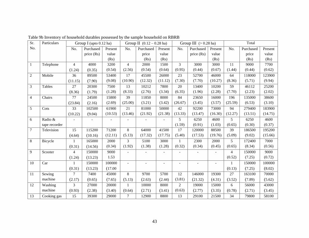
43

Table 9b Inventory of household durables possessed by the sample household on RBRB

Sr.

No.

Particulars Group I (upto 0.12 ha) Group II (0.12 – 0.28 ha) Group III (> 0.28 ha) Total

No. Purchased

price (Rs)

Present

value

(Rs)

No. Purchased

price

(Rs)

Present

value

(Rs)

No. Purchased

price (Rs)

Present

value

(Rs)

No. Purchased

price

(Rs)

Present

value

(Rs)

1 Telephone 4

(1.24)

4000

(0.35)

3200

(0.54)

4

(2.56)

2000

(0.54)

1500

(0.64)

3

(0.95)

3000

(0.44)

3000

(0.67)

11

(1.44)

9000

(0.44)

7700

(0.62)

2 Mobile 36

(11.15)

89500

(7.90)

53400

(9.08)

17

(10.90)

45500

(12.32)

26000

(11.12)

23

(7.30)

52700

(7.70)

46000

(10.27)

64

(8.36)

118000

(5.71)

123900

(9.94)

3 Tables 27

(8.36)

20300

(1.79)

7500

(1.28)

13

(8.33)

10212

(2.76)

7800

(3.34)

20

(6.35)

13400

(1.96)

10200

(2.28)

59

(7.70)

46112

(2.23)

25200

(2.02)

4 Chairs 77

(23.84)

24500

(2.16)

15800

(2.69)

39

(25.00)

11850

(3.21)

8000

(3.42)

84

(26.67)

23650

(3.45)

16000

(3.57)

196

(25.59)

135000

(6.53)

38600

(3.10)

5 Cots 33

(10.22)

102500

(9.04)

61900

(10.53)

21

(13.46)

81000

(21.92)

50000

(21.38)

42

(13.33)

92200

(13.47)

73000

(16.30)

94

(12.27)

279400

(13.51)

183900

(14.75)

6 Radio &

tape recorder

- - - - - - 5

(1.59)

6250

(0.91)

4600

(1.03)

5

(0.65)

6250

(0.30)

4600

(0.37)

7 Television 15

(4.64)

115200

(10.16)

71200

(12.11)

8

(5.13)

64000

(17.32)

41500

(17.75)

17

(5.40)

120000

(17.53)

88500

(19.76)

39

(5.09)

186500

(9.02)

195200

(15.66)

8 Bicycle 1

(0.31)

165000

(14.56)

2000

(0.34)

3

(1.92)

5100

(1.38)

3000

(1.28)

1

(0.32)

2300

(0.34)

2000

(0.45)

5

(0.65)

172400

(8.34)

7000

(0.56)

9 Scooter 4

(1.24)

150000

(13.23)

9000

1.53

- - - - - - 4

(0.52)

150000

(7.25)

9000

(0.72)

10 Car 1

(0.31)

150000

(13.23)

100000

(17.00

- - - - - - 1

(0.13)

150000

(7.25)

100000

(8.02)

11 Sewing

machine

7

(2.17)

7400

(0.65)

45000

(7.65)

8

(5.13)

9700

(2.63)

5700

(2.44)

12

(3.81)

146000

(21.32)

19300

(4.31)

27

(3.52)

163100

(7.89)

70000

(5.62)

12 Washing

machine

3

(0.93)

27000

(2.38)

20000

(3.40)

1

(0.64)

10000

(2.71)

8000

(3.41)

2

(0.63)

19000

(2.77)

15000

(3.35)

6

(0.78)

56000

(2.71)

43000

(3.45)

13 Cooking gas 15 39300 29000 7 12900 8800 13 29100 21500 34 79800 58100

44

(4.64) (3.48) (4.93) (4.49) (3.49) (3.76) (4.13) (4.25) (4.80) (4.44) (3.86) (4.66)

14 Gas cylinder 4

(1.24)

6200

(0.55)

5500

(0.94)

8

(5.13)

10900

(2.95)

7800

(3.34)

12

(3.81)

20300

(2.96)

32300

(7.21)

23

(3.00)

35800

(1.73)

44100

(3.54)

15 Refrigerator 13

(4.01)

121000

(10.68)

84000

(14.28)

6

(3.85)

67000

(18.13)

41500

(17.75)

11

(3.49)

86000

(12.56)

65500

(14.63)

28

(3.66)

262000

(12.67)

182000

(14.60)

16 Fan 47

(14.55)

48100

(4.24)

39600

(6.73)

- - (0.00) 43

(13.65)

43900

(6.41)

32900

(7.35)

89

(11.62)

90800

(4.37)

71700

(5.76)

17 Sofa set/

dining table

5

(1.55)

46500

(4.11)

30500

(5.19)

3

(1.92)

30000

(8.12)

19000

(8.12)

3

(0.95)

14500

(2.12)

10500

(2.34)

11

(1.44)

91000

(4.40)

60000

(4.81)

18 Pressure

cooker

31

(9.60)

16900

(1.49)

10500

(1.78)

18

(11.54)

9300

(2.52)

5250

(2.25)

24

(7.62)

12400

(1.81)

7500

(1.68)

70

(9.14)

37100

(1.79)

22450

(1.80)

19 Total 323

(100)

1133400

(100)

588100

(100)

156

(100)

369462

(100)

233850

(100)

315

(100)

684700

(100)

447800

(100)

766

(100)

2068262

(100)

1246450

(100)

20 Per

household

- 66671 34594 - 52780 33407 - 45647 29853 - 53032 31960

Note: Figures in parentheses are percentages of total

Source: Field survey, 2011

Table 10a Livestock inventory of sample households on LBRB

Sr.

No.

Particulars Group I (upto 0.12 ha) Group II (0.12 – 0.28 ha) Group III (> 0.28 ha) Total

No. Value (Rs.) No. Value (Rs.) No. Value (Rs.) No. Value (Rs.)

1 Cow in milk 1

(1.96)

8000.00

(2.48)

-

(0.00)

-

(0.00)

1

(1.56)

16000.00

(4.32)

2

(1.21)

24000

(2.59)

Cow dry -

-

- - - - - -

2 Buffalo in milk 18

(35.29)

180000

(55.74)

9

(18.00)

90000

(38.30)

19

(29.69)

190000

(51.35)

46

(27.88)

460000

(49.57)

Buffalo dry 6

(11.76)

48000

(14.87)

8

(16.00)

64000

(27.23)

11

(17.19)

88000

(23.78)

25

(15.15)

200000

(21.55)

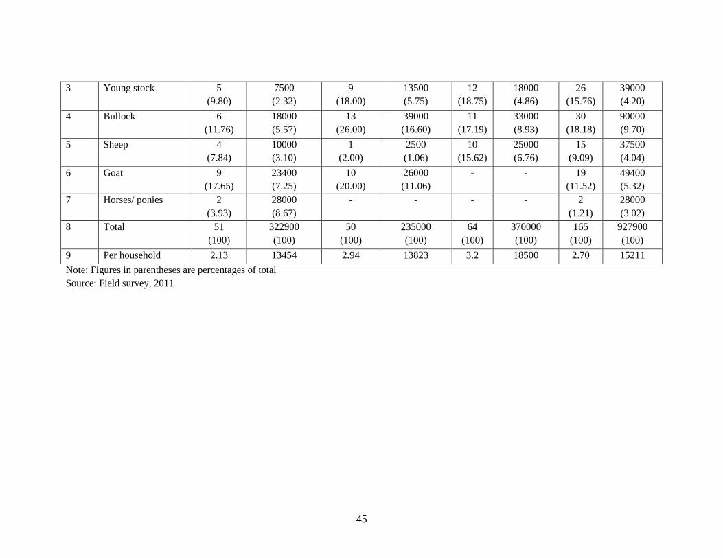
45

3 Young stock 5

(9.80)

7500

(2.32)

9

(18.00)

13500

(5.75)

12

(18.75)

18000

(4.86)

26

(15.76)

39000

(4.20)

4 Bullock 6

(11.76)

18000

(5.57)

13

(26.00)

39000

(16.60)

11

(17.19)

33000

(8.93)

30

(18.18)

90000

(9.70)

5 Sheep 4

(7.84)

10000

(3.10)

1

(2.00)

2500

(1.06)

10

(15.62)

25000

(6.76)

15

(9.09)

37500

(4.04)

6 Goat 9

(17.65)

23400

(7.25)

10

(20.00)

26000

(11.06)

- - 19

(11.52)

49400

(5.32)

7 Horses/ ponies 2

(3.93)

28000

(8.67)

- - - - 2

(1.21)

28000

(3.02)

8 Total 51

(100)

322900

(100)

50

(100)

235000

(100)

64

(100)

370000

(100)

165

(100)

927900

(100)

9 Per household 2.13 13454 2.94 13823 3.2 18500 2.70 15211

Note: Figures in parentheses are percentages of total

Source: Field survey, 2011

46

Table 10b Livestock inventory of sample households on RBRB

Sr.

No.

Particulars Group I (upto 0.12 ha) Group II (0.12 – 0.28 ha) Group III (> 0.28 ha) Total

No. Value (Rs.) No. Value (Rs.) No. Value (Rs.) No. Value

(Rs.)

1 Cow in milk 3

(12.00)

24000

(20.48)

3

(20.00)

24000

(18.36)

8

(17.02)

64000

(18.96)

14

(16.09)

112000

(19.13)

Cow dry 1

(4.00)

6000

(5.12)

1

(6.67)

6000

(4.59)

5

(10.64)

30000

(8.88)

7

(8.05)

42000

(7.17)

2 Buffalo in milk 2

(8.00)

20000

(17.06)

3

(20.00)

30000

(22.95)

6

(12.77)

60000

(17.78)

11

(12.64)

110000

(18.79)

Buffalo dry 4

(16.00)

32000

(27.30)

1

(6.67)

8000

(6.12)

5

(10.64)

40000

(11.85)

10

(11.49)

80000

(13.67)

3 Young stock 6

(24.00)

9000

(7.68)

1

(6.67)

1500

(1.15)

8

(17.02)

12000

(3.56)

15

(17.24)

22500

(3.84)

4 Bullock 7

(28.00)

21000

(17.92)

2

(13.32)

5200

(3.98)

4

(8.51)

12000

(3.56)

13

(14.94)

38200

(6.53)

5 Sheep -

-

-

-

3

(6.38)

7500

(2.22)

3

(3.46)

7500

(1.28)

6 Goat 2

(8.00)

5200

(4.44)

-

-

-

-

2

(2.30)

5200

(0.89)

7 Horses/ ponies -

-

4

(26.67)

56000

(42.85)

8

(17.02)

112000

(33.19)

12

(13.79)

168000

(28.70)

8 Total 25

(100)

117200

(100)

15

(100)

130700

(100)

47

(100)

337500

(100)

87

(100)

585400

(100)

9 Per household 1.47 6894 2.14 18671 3.13 22500 2.23 15010

Note: Figures in parentheses are percentages of total

Source: Field survey, 2011

47

Table 11a Land Utilization Pattern of sample households on LBRB (ha/hh)

Sr. No. Particulars Group I

(upto 0.12 ha)

Group II

(0.12 – 0.28 ha)

Group III

(> 0.28 ha)

Overall

1 Cultivated 0.43

(58.11)

0.59

(54.63)

1.18

(60.20)

0.72

(58.06)

Irrigated 0.15

(20.27)

0.21

(19.44)

0.55

(28.57)

0.3

(24.19)

Unirrigated 0.28

(37.84)

0.38

(35.19)

0.63

(32.14)

0.42

(33.87)

2 Uncultivated including

fruit trees

0.07

(9.46)

0.22

(20.37)

0.05

(2.55)

0.11

(8.87)

Irrigated 0.01

(1.35)

0.02

(1.85)

0

(0.00)

0.01

(0.81)

Unirrigated 0.06

(8.11)

0.20

(18.52)

0.05

(2.55)

0.1

(8.06)

3 Grassland 0.23

(31.08)

0.26

(24.08)

0.6

(30.62)

0.36

(29.04)

4 Wasteland (forestry trees) 0.01

(1.35)

- 0.12

(6.12)

0.04

(3.23)

5 Total 0.74

(100)

1.07

(100)

1.95

(100)

1.23

(100)

Note: Figures in parentheses are percentages of total

Source: Field survey, 2011

Table 11b Land utilization pattern of sample households on RBRB (ha/hh)

Sr. No. Particulars Group I

(upto 0.12 ha)

Group II

(0.12 – 0.28 ha)

Group III

(> 0.28 ha)

Overall

1 Cultivated 0.32

(61.54)

0.79

(25.48)

1.10

(55.56)

0.71

(45.81)

Irrigated 0.15

(28.85)

0.14

(4.52)

0.23

(11.62)

0.18

(11.61)

Unirrigated 0.17

(32.69)

0.65

(20.97)

0.87

(43.94)

0.53

(34.19)

2 Uncultivated including

fruit trees

0.05

(9.62)

0.78

(21.61)

0.83

(40.91)

0.48

(29.03)

Irrigated 0.04

(7.69)

0.21

(6.77)

- 0.05

(3.23)

Unirrigated 0.01

(1.92)

0.57

(18.39)

0.83

(41.92)

0.43

(27.75)

3 Grassland 0.15

(28.84)

0.22

(7.10)

0.05

(2.52)

0.12

(7.74)

4 Wasteland (forestry trees) - 1.31

(42.26)

- 0.24

(15.48)

48

5 Total 0.52

(100)

3.10

(100)

1.98

(100)

1.55

(100)

Note: Figures in parentheses are percentages of total

Source: Field survey, 2011

Table 12a Cropping pattern on sample households of LBRB (in ha / hh)

Sr. No. Crops Group I

(upto 0.12 ha)

Group II

(0.12 – 0.28 ha)

Group III

(> 0.28 ha)

Overall

1 Maize 0.39

(43.82)

0.47

(40.45)

0.9

(38.14)

0.58

(40.56)

2 Paddy 0.02

(2.25)

0.05

(4.30)

0.18

(7.63)

0.08

(5.59)

3 Pulses - - - -

4 Oilseed - 0.01

(1.40)

- -

5 Fodder 0.04

(4.49)

0.07

(6.01)

0.15

(6.36)

0.08

(5.59)

6 Vegetables 0.02

(2.25)

0.01

(0.84)

0.03

(1.27)

0.02

(1.41)

7 Wheat 0.41

(46.07)

0.55

(47.00)

1.07

(45.34)

0.66

(46.15)

8 Barley 0.01

(1.12)

- 0.03

(1.26)

0.01

(0.70)

9 Total 0.89

(100)

1.16

(100)

2.36

(100)

1.43

(100)

10 Cropping intensity

(%)

206.98 196.61 200.00 198.61

Note: Figures in parentheses are percentages of total

Source: Field survey, 2011

Table 12b Cropping pattern on sample households of RBRB (in ha / hh)

Sr. No. Crops Group I

(upto 0.12 ha)

Group II

(0.12 – 0.28 ha)

Group III

(> 0.28 ha)

Overall

1

Maize

0.28

(43.75)

0.71

(45.15)

0.84

(38.36)

0.57

(40.43)

2

Paddy

- - 0.21

(9.59)

0.08

(5.67)

3

Pulses

- - - -

4

Oilseed

- - 0.01

(0.46)

-

5

Fodder

0.10

(15.63)

0.06

(3.50)

0.03

(1.37)

0.07

(4.96)

49

6 Vegetables

0.01

(1.56)

0.03

(1.80)

0.02

(0.91)

0.02

(1.42)

7 Wheat

0.25

(39.06)

0.77

(49.04)

1.07

(48.85)

0.66

(46.81)

8 Barley

- 0.01

(0.51)

0.01

(0.46)

0.01

(0.71)

9

Total

0.64

(100)

1.57

(100)

2.19

(100)

1.41

(100)

10 Cropping intensity

(%)

200.00 198.73 199.09 198.59

Note: Figures in parentheses are percentages of total

Source: Field survey, 2011

50

Table 13a Area, production and income from vegetables and spice production on LBRB

Sr.

No

Particulars Group I (upto 0.12 ha) Group II (0.12 – 0.28 ha) Group III (> 0.28 ha) Total

Area

(k)

Prod.

(q)

Income

(Rs.)

Area

(k)

Prod. (q) Income

(Rs)

Area

(k)

Prod.

(q)

Income

(Rs)

Area

(k)

Prod.

(q)

Income

(Rs)

1 Potato 2.40

(24.49)

7.35

(33.64)

5145

(19.63)

0.50

(20.00)

2.30

(28.75)

2240

(18.04)

2.20

(16.24)

2.40

(6.50)

2190

(3.73)

5.10

(19.73)

12.05

(18.05)

9575

(9.83)

2 Carrot - - - - - - 0.50

(3.69)

0.50

(1.36)

750

(1.28)

0.50

(1.93)

0.50

(0.75)

750

(0.77)

3 Radish 0.85

(8.67)

2.60

(11.90)

1820

(6.94)

0.25

(10.00)

1.10

(13.75)

1280

(10.31)

0.25

(1.85)

5.00

(13.55)

6890

(11.73)

1.35

(5.22)

8.70

(13.03)

9990

(10.26)

4 Cauliflower 1.45

(14.80)

1.35

(6.18)

1350

(5.15)

0.10

(4.00)

0.05

(0.63)

40

(0.32)

0.80

(5.90)

6.80

(18.43)

6050

(10.30)

2.35

(9.09)

8.20

(12.28)

7440

(7.64)

5 Cabbage 0.15

(1.53)

2.00

(9.15)

1600.

(6.10)

- - - 0.25

(1.85)

3.00

(8.13)

2400

(4.09)

0.40

(1.55)

5.00

(7.49)

4000

(4.11)

6 Lady

Finger

1.05

(10.71)

2.20

(10.07)

2850

(10.87)

0.35

(14.00)

0.20

(2.50)

300

(2.42)

1.60

(11.81)

2.30

(6.23)

3450

(5.87)

3.00

(11.61)

4.70

(7.04)

6600

(6.78)

7 Colocasia 0.30

(3.06)

0.45

(2.06)

750

(2.86)

0.20

(8.00)

0.70

(8.75)

2100

(16.91)

1.25

(9.23)

6.10

(16.53)

3050

(5.19)

1.75

(6.77)

7.25

(10.86)

5900

(6.06)

8 Cucumber

- - - 0.05

(2.00)

1.00

(12.50)

1000

(8.05)

0.20

(1.48)

0.50

(1.36)

500

(0.85)

0.25

(0.97)

1.50

(2.25)

1500

(1.54)

9 Pumpkin 0.05

(0.51)

0.20

(0.92)

200

(0.76)

0.10

(4.00)

1.50

(18.75)

1800

(14.49)

0.50

(3.69)

3.00

(8.13)

300

(0.51)

0.65

(2.51)

4.70

(7.04)

2300

(2.36)

10 Turmeric 0.35

(3.57)

0.40

(1.83)

1700

(6.48)

0.25

(10.00)

0.60

(7.50)

2400

(19.32)

3.10

(22.88)

4.70

(12.74)

18800

(32.01)

3.70

(14.31)

5.70

(8.54)

22900

(23.52)

11 Garlic 0.60

(6.13)

1.10

(5.03)

4700

(17.93)

0.30

(12.00)

0.04

(0.50)

160

(1.29)

0.90

(6.64)

1.20

(3.25)

5400

(9.19)

1.80

(6.96)

2.34

(3.51)

10260

(10.54)

12 Coriander 1.00

(10.20)

0.50

(2.29)

500

(1.91)

0.05

(2.00)

0.01

(0.13)

100

(0.81)

0.20

(1.48)

0.10

(0.27)

250.00

(0.43)

1.25

(4.84)

0.61

(0.91)

850

(0.87)

13 Ginger 0.55

(5.61)

0.65

(2.97)

1700

(6.48)

- - - 0.30

(2.21)

0.5

(1.36)

2500

(4.26)

0.85

(3.29)

1.15

(1.72)

4200

(4.31)

14 Onion 1.05

(10.72)

3.05

(13.96)

3900

(14.88)

0.35

(14.00)

0.50

(6.25)

1000

(8.05)

1.5

(11.07)

0.80

(2.17)

6200.00

(10.56)

2.90

(11.22)

4.35

(6.52)

11100

(11.40)

15 Total 9.80 21.85 26215 2.50 8.00 12420 13.55 36.90 58730.00 25.85 66.75 97365

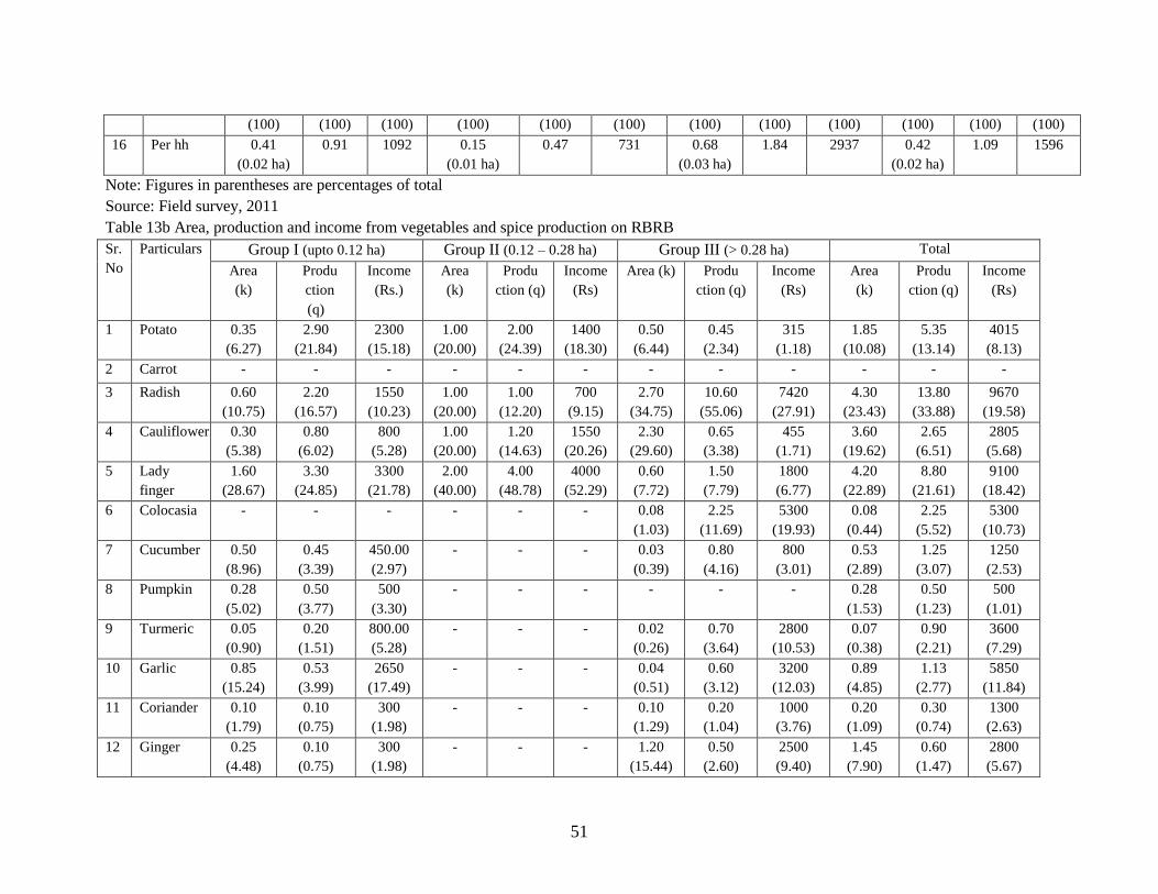
51

(100) (100) (100) (100) (100) (100) (100) (100) (100) (100) (100) (100)

16 Per hh 0.41

(0.02 ha)

0.91 1092 0.15

(0.01 ha)

0.47 731 0.68

(0.03 ha)

1.84 2937 0.42

(0.02 ha)

1.09 1596

Note: Figures in parentheses are percentages of total

Source: Field survey, 2011

Table 13b Area, production and income from vegetables and spice production on RBRB

Sr.

No

Particulars Group I (upto 0.12 ha) Group II (0.12 – 0.28 ha) Group III (> 0.28 ha) Total

Area

(k)

Produ

ction

(q)

Income

(Rs.)

Area

(k)

Produ

ction (q)

Income

(Rs)

Area (k) Produ

ction (q)

Income

(Rs)

Area

(k)

Produ

ction (q)

Income

(Rs)

1 Potato 0.35

(6.27)

2.90

(21.84)

2300

(15.18)

1.00

(20.00)

2.00

(24.39)

1400

(18.30)

0.50

(6.44)

0.45

(2.34)

315

(1.18)

1.85

(10.08)

5.35

(13.14)

4015

(8.13)

2 Carrot - - - - - - - - - - - -

3 Radish 0.60

(10.75)

2.20

(16.57)

1550

(10.23)

1.00

(20.00)

1.00

(12.20)

700

(9.15)

2.70

(34.75)

10.60

(55.06)

7420

(27.91)

4.30

(23.43)

13.80

(33.88)

9670

(19.58)

4 Cauliflower 0.30

(5.38)

0.80

(6.02)

800

(5.28)

1.00

(20.00)

1.20

(14.63)

1550

(20.26)

2.30

(29.60)

0.65

(3.38)

455

(1.71)

3.60

(19.62)

2.65

(6.51)

2805

(5.68)

5 Lady

finger

1.60

(28.67)

3.30

(24.85)

3300

(21.78)

2.00

(40.00)

4.00

(48.78)

4000

(52.29)

0.60

(7.72)

1.50

(7.79)

1800

(6.77)

4.20

(22.89)

8.80

(21.61)

9100

(18.42)

6 Colocasia -

-

-

- - - 0.08

(1.03)

2.25

(11.69)

5300

(19.93)

0.08

(0.44)

2.25

(5.52)

5300

(10.73)

7 Cucumber 0.50

(8.96)

0.45

(3.39)

450.00

(2.97)

- - - 0.03

(0.39)

0.80

(4.16)

800

(3.01)

0.53

(2.89)

1.25

(3.07)

1250

(2.53)

8 Pumpkin 0.28

(5.02)

0.50

(3.77)

500

(3.30)

- - - - - - 0.28

(1.53)

0.50

(1.23)

500

(1.01)

9 Turmeric 0.05

(0.90)

0.20

(1.51)

800.00

(5.28)

- - - 0.02

(0.26)

0.70

(3.64)

2800

(10.53)

0.07

(0.38)

0.90

(2.21)

3600

(7.29)

10 Garlic 0.85

(15.24)

0.53

(3.99)

2650

(17.49)

- - - 0.04

(0.51)

0.60

(3.12)

3200

(12.03)

0.89

(4.85)

1.13

(2.77)

5850

(11.84)

11 Coriander 0.10

(1.79)

0.10

(0.75)

300

(1.98)

- - - 0.10

(1.29)

0.20

(1.04)

1000

(3.76)

0.20

(1.09)

0.30

(0.74)

1300

(2.63)

12 Ginger 0.25

(4.48)

0.10

(0.75)

300

(1.98)

- - - 1.20

(15.44)

0.50

(2.60)

2500

(9.40)

1.45

(7.90)

0.60

(1.47)

2800

(5.67)

52

13 Onion 0.70

(12.54)

2.20

(16.57)

2200

(14.52)

- - 0.20

(2.57)

1.00

(5.19)

1000

(3.76)

0.90

(4.90)

3.20

(7.86)

3200

(6.48)

14 Total 5.58

(100)

13.28

(100)

15150

(100)

5.00

(100)

8.20

(100)

7650.00

(100)

7.77

(100)

19.25

(100)

26590

(100)

18.35

(100)

40.73

(100)

49390

(100)

15 Per hh 0.33

(0.01ha)

0.78 891 0.71

(0.03ha)

1.17 1093 0.52

(0.02ha)

1.28 1773 0.47

(0.02ha)

1.04 1266

Note: Figures in parentheses are percentages of total

Source: Field survey, 2011

53

Table14a Production of crops on sample households of LBRB (q/hh)

Sr. No. Crop Group I

(upto 0.12 ha)

Group II

(0.12 – 0.28 ha)

Group III

(> 0.28 ha)

Overall

I Foodgrain

1 Maize 5.13 6.09 10.82 7.26

2 Paddy 0.19 0.59 1.70 0.80

3 Pulses 0.01 - -

4 Oilseed 0.10 - 0.04

5 Wheat 5.14 6.34 15.80 8.95

6 Barley 0.13 0.06 0.49 0.22

7 Sub-total 10.59 13.19 28.81 17.27

II Fruit & Vegetable

1 Fruit 0.01 - - 0.02

2 Vegetable 0.91 0.47 1.84 1.09

3 Sub-total 0.92 0.47 1.84 1.11

Source: Field survey, 2011

Table14b Production of crops on sample households of RBRB (q/hh)

Sr.

No.

Crop Group I

(upto 0.12 ha)

Group II

(0.12 – 0.28 ha)

Group III

(> 0.28 ha)

Overall

I Foodgrain

1 Maize 3.77 13.64 14.49 9.66

2 Paddy - 2.26 0.87

3 Pulses - 0.02 0.01

4 Oilseed - 0.09 3.33

5 Wheat 3.03 10.91 21.06 11.38

6 Barley - 0.11 0.14 0.07

7 Sub-total 6.80 24.66 38.06 25.32

II Fruit & Vegetable

1 Fruit - - - -

2 Vegetable 0.78 1.17 1.28 1.04

3 Sub-total 0.78 1.17 1.28 1.04

Source: Field survey, 2011

Table 15a Average yield of crops on sample farms on LBRB (q/ha)

Sr. No. Crops Group I Group II Group III Overall

54

(upto 0.12 ha) (0.12 – 0.28 ha) (> 0.28 ha)

1 Maize 13.25 13.00 12.00 12.50

2 Paddy 12.50 12.50 9.50 10.25

3 Pulses - 4.25 - 3.75

4 Oilseed - 9.00 - 9.00

5 Fruits 16.25 - - 16.25

6 Vegetable 55.75 80.00 68.00 64.50

7 Wheat 12.50 11.00 14.75 13.25

8 Barley 19.25 18.75 17.50 17.25

Source: Field survey, 2011

Table 15b Average yield of crops on sample households of RBRB (q/ha)

Sr. No. Crops Group I

(upto 0.12 ha)

Group II

(0.12 – 0.28 ha)

Group III

(> 0.28 ha)

Overall

1 Maize 13.25 19.25 17.25 16.75

2 Paddy - - 10.75 10.75

3 Pulses - - 7.50 7.50

4 Oilseed - - 10.75 10.75

5 Fruits - - - -

6 Vegetable 59.50 41.00 22.00 55.25

7 Wheat 12.25 14.25 19.25 17.00

8 Barley - 13.25 10.00 10.75

Source: Field survey, 2011

Table 16a Production and disposal of foodgrains on sample households on LBRB (q /hh)

Sr. No. Particulars Group I

(upto 0.12 ha)

Group II

(0.12 – 0.28 ha)

Group III

(> 0.28 ha)

Overall

1 Production 10.59

(100)

13.09

(100)

28.81

(100)

17.26

(100)

2 Home consumption 5.07

(47.88)

5.37

(41.04)

6.47

(22.45)

5.61

(32.52)

3 Kept for seed 1.24

(11.74)

1.01

(7.69)

3.51

(12.20)

1.92

(11.14)

4 Kind payment 0.14

(1.29)

0.55

(4.18)

0.67

(2.33)

0.43

(2.47)

5 Sold (marketed plus) 3.71

(35.00)

5.48

(41.86)

14.28

(49.57)

7.67

(44.43)

6 Marketable surplus 0.43

(4.09)

0.69

(5.24)

3.87

(13.44)

1.63

(9.45)

Note: Figures in parentheses are percentages of total

Source: Field survey, 2011

Table 16b Production and disposal of foodgrains on sample households on RBRB (q /hh)

Sr. No. Particulars Group I

(upto 0.12 ha)

Group II

(0.12 – 0.28 ha)

Group III

(> 0.28 ha)

Overall

55

1 Production 6.80

(100)

24.66

(100)

38.01

(100)

22.01

(100)

2 Home consumption 4.82

(70.80)

7.46

(30.24)

6.63

(17.46)

5.99

(27.22)

3 Kept for seed 0.59

(8.70)

1.37

(5.54)

6.15

(16.19)

2.87

(13.04)

4 Kind payment 0.14

(2.07)

0.50

(2.03)

0.62

(1.63)

0.39

(1.77)

5 Sold (marketed plus) 1.15

(16.90)

13.37

(54.22)

19.83

(52.18)

10.53

(47.84)

6 Marketable surplus 0.10

(1.53)

1.96

(7.97)

4.77

(12.54)

2.23

(10.14)

Note: Figures in parentheses are percentages of total

Source: Field survey, 2011

Table 17a Source wise composition of annual household income of sample households on LBRB

(Rs./hh)

Sr. No Source Group I

(upto 0.12 ha)

Group II

(0.12 – 0.28 ha)

Group III

(> 0.28 ha)

Overall

I Farm income

1 Agriculture 16513

(7.69)

48211

(22.87)

49162

(22.33)

36051

(16.73)

2 Animal Husbandry 16063

(7.48)

7971

(3.78)

21555

(9.79)

15608

(7.24)

3 Fruits 250

(0.12)

706

(0.33)

- 295

(0.14)

4 Vegetable 1092

(0.50)

731

(0.35)

2937

(1.34)

1596

(0.75)

5 Sub-Total 33918

(15.79)

57619

(27.33)

73654

(33.46)

53550

(24.86)

II Off farm income

1 Govt. / private service 107983

(50.27)

97694

(46.33)

84600

(38.43)

97449

(45.23)

2 Pension 32236

(15.01)

45373

(21.52)

34512

(15.68)

36643

(17.01)

3 Shop keeping 17750

(8.27)

- 10200

(4.63)

10328

(4.79)

4 Daily paid labour 22900

(10.66)

10165

(4.82)

17170

(7.80)

17472

(8.11)

5 Others (contractor,

commission agent, black smith,

etc)

-

-

-

-

6 Sub-total 180869

(84.21)

153232

(72.67)

146482

(66.54)

161892

(75.14)

III Grand-total 214787

(100)

210851

(100)

220136

(100)

215442

(100)

56

IV Per capita income 35798 35142 28223 32643

Note: Figures in parentheses indicate percentages of total

Source: Field survey, 2011

Table 17b Source wise composition of annual household income of sample households on RBRB

(Rs./hh)

Sr. No Source Group I

(upto 0.12 ha)

Group II

(0.12 – 0.28 ha)

Group III

(> 0.28 ha)

Overall

I Farm income

1 Agriculture 13494

(5.10)

41227

(8.81)

31378

(13.42)

25350

(8.76)

2 Animal Husbandry 8259

(3.12)

27626

(5.90)

20293

(8.68)

16364

(5.66)

3 Fruits - 7143

(1.53)

2800

(1.20)

2359

(0.82)

4 Vegetable 891

(0.34)

1093

(0.23)

1773

(0.75)

1266

(0.44)

5 Sub-total 22643

(8.56)

77089

(16.47)

56245

(24.05)

45339

(15.68)

II Off farm income

1 Govt. / private service 120118

(45.42)

205714

(43.95)

81200

(34.72)

120513

(41.66)

2 Pension 66212

(25.04)

99429

(21.24)

12800

(5.47)

51631

(17.85)

3 Shop keeping 40235

(15.21)

32571

(6.96)

3200

(1.38)

24615

(8.51)

4 Daily paid labour 15247

(5.77)

27086

(5.79)

47087

(20.13)

29618

(10.24)

5 Others (contractor,

commission agent,

black smith, etc)

-

(0.00)

26143

(5.59)

33333

(14.25)

17513

(6.06)

6 Sub-total 241812

(91.44)

390943

(83.53)

177620

(75.95)

243890

(84.32)

III Grand total 264455

(100)

468032

(100)

233865

(100)

289228

(100)

IV Per capita income 40686 64114 31182 41318

Note: Figures in parentheses indicate percentages of total

Source: Field survey, 2011

Table 18a Consumption pattern of sample households on LBRB (Rs/hh/yr)

Sr. No. Items Group I

(upto 0.12 ha)

Group II

(0.12 – 0.28 ha)

Group III

(> 0.28 ha)

Overall

1 Rice 4613

(6.29)

4765

(6.21)

5418

(6.79)

4919

(6.44)

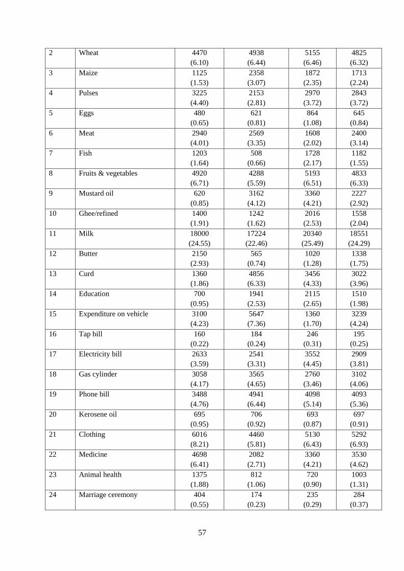
57

2 Wheat 4470

(6.10)

4938

(6.44)

5155

(6.46)

4825

(6.32)

3 Maize 1125

(1.53)

2358

(3.07)

1872

(2.35)

1713

(2.24)

4 Pulses 3225

(4.40)

2153

(2.81)

2970

(3.72)

2843

(3.72)

5 Eggs 480

(0.65)

621

(0.81)

864

(1.08)

645

(0.84)

6 Meat 2940

(4.01)

2569

(3.35)

1608

(2.02)

2400

(3.14)

7 Fish 1203

(1.64)

508

(0.66)

1728

(2.17)

1182

(1.55)

8 Fruits & vegetables 4920

(6.71)

4288

(5.59)

5193

(6.51)

4833

(6.33)

9 Mustard oil 620

(0.85)

3162

(4.12)

3360

(4.21)

2227

(2.92)

10 Ghee/refined 1400

(1.91)

1242

(1.62)

2016

(2.53)

1558

(2.04)

11 Milk 18000

(24.55)

17224

(22.46)

20340

(25.49)

18551

(24.29)

12 Butter 2150

(2.93)

565

(0.74)

1020

(1.28)

1338

(1.75)

13 Curd 1360

(1.86)

4856

(6.33)

3456

(4.33)

3022

(3.96)

14 Education 700

(0.95)

1941

(2.53)

2115

(2.65)

1510

(1.98)

15 Expenditure on vehicle 3100

(4.23)

5647

(7.36)

1360

(1.70)

3239

(4.24)

16 Tap bill 160

(0.22)

184

(0.24)

246

(0.31)

195

(0.25)

17 Electricity bill 2633

(3.59)

2541

(3.31)

3552

(4.45)

2909

(3.81)

18 Gas cylinder 3058

(4.17)

3565

(4.65)

2760

(3.46)

3102

(4.06)

19 Phone bill 3488

(4.76)

4941

(6.44)

4098

(5.14)

4093

(5.36)

20 Kerosene oil 695

(0.95)

706

(0.92)

693

(0.87)

697

(0.91)

21 Clothing 6016

(8.21)

4460

(5.81)

5130

(6.43)

5292

(6.93)

22 Medicine 4698

(6.41)

2082

(2.71)

3360

(4.21)

3530

(4.62)

23 Animal health 1375

(1.88)

812

(1.06)

720

(0.90)

1003

(1.31)

24 Marriage ceremony 404

(0.55)

174

(0.23)

235

(0.29)

284

(0.37)

58

25 Birthday party 130

(0.18)

141

(0.18)

153

(0.19)

140

(0.18)

26 Religious function 98

(0.13)

124

(0.16)

120

(0.15)

112

(0.15)

27 Fairs & festivals 244

(0.33)

132

(0.17)

243

(0.30)

212

(0.28)

28 Total 73305

(100)

76699

(100)

79784

(100)

76375

(100)

29 Per capita expenditure 12217 12783 10929 11572

Note: Figures in parentheses are percentages of total

Source: field survey, 2011

Table 18b Consumption pattern of households on RBRB (Rs/hh/yr)

Sr. No. Items Group I

(upto 0.12 ha)

Group II

(0.12 – 0.28 ha)

Group III

(> 0.28 ha)

Overall

1 Rice 4606

(7.50)

4886

(5.25)

4860

(6.53)

4754

(6.59)

2 Wheat 4362

(7.10)

3394

(3.64)

4464

(5.99)

4228

(5.86)

3 Maize 1976

(3.22)

1543

(1.66)

1960

(2.63)

1892

(2.62)

4 Pulses 2859

(4.65)

3086

(3.31)

3360

(4.51)

3092

(4.29)

5 Egg 508

(0.83)

11314

(12.15)

864

(1.16)

2585

(3.58)

6 Meat 1976

(3.22)

5040

(5.41)

4256

(5.72)

3403

(4.72)

7 Fish 254

(0.41)

2057

(2.21)

2208

(2.97)

1329

(1.84)

8 Fruits & vegetables 5294

(8.62)

4886

(5.25)

5604

(7.53)

5340

(7.40)

9 Mustard oil 3049

(4.96)

3429

(3.68)

3200

(4.30)

3175

(4.40)

10 Ghee/refined 1525

(2.48)

1234

(1.00)

1600

(2.15)

1502

(2.08)

11 Milk 12212

(19.88)

16800

(18.04)

16016

(21.51)

14498

(20.10)

12 Butter 720

(1.17)

1200

(1.29)

720

(0.97)

806

(1.12)

13 Curd 2174

(3.54)

3429

(3.68)

3648

(4.90)

2966

(4.11)

14 Education 1606

(2.61)

1571

(1.69)

1370

(1.84)

1509

(2.09)

15 Expenditure on

vehicle

2668

(4.34)

6857

(7.36)

- 2394

(3.32)

16 Tap bill 155 206 224 191

59

(0.25) (0.22) (0.30) (0.26)

17 Electricity bill 2384

(3.88)

2571

(2.76)

1948

(2.62)

2250

(3.12)

18 Gas cylinder 2341

(3.81)

3814

(4.09)

2480

(3.33)

2659

(3.69)

19 Phone bill 2753

(4.48)

3857

(4.14)

3600

(4.83)

3277

(4.54)

20 Kerosene oil 472

(0.77)

394

(0.42)

500

(0.67)

469

(0.65)

21 Clothing 5506

(8.96)

5829

(6.26)

5800

(7.79)

5677

(7.87)

22 Medicine 629

(1.02)

4457

(4.79)

4267

(5.73)

2715

(3.76)

23 Animal health 424

(0.69)

771

(0.83)

600

(0.81)

554

(0.77)

24 Marriage ceremony 115

(0.19)

273

(0.29)

247

(0.33)

194

(0.27)

25 Birthday party 212

(0.34)

69

(0.07)

93

(0.13)

141

(0.19)

26 Religious function 297

(0.48)

97

(0.10)

217

(0.29)

230

(0.32)

27 Fairs & festivals 362

(0.59)

83

(0.09)

360

(0.48)

311

(0.43)

28 Total 61441

(100)

93147

(100)

74465

(100)

72141

(100)

29 Per capita expenditure 9452 12760 9929 10305

Note: Figures in parentheses are percentages of total

Source: Field survey, 2011

Table 19a Saving pattern of sample households on LBRB (Rs/Yr)

Sr. Particular Group I

(upto 0.12 ha)

Group II

(0.12 – 0.28 ha)

Group III

(> 0.28 ha)

Total

1 Gross household

income

214787

(100)

210851

(100)

220136

(100)

215442

(100)

2 Gross household

consumption

expenditure

73305

(34.13)

76699

(36.38)

79784

(36.24)

76375

(35.45)

3 Gross household

saving (1-2)

141482

(65.87)

134152

(63.62)

140352

(63.76)

139067

(64.55)

Note: Figures in parentheses indicate percentages of total

60

Source: Field survey, 2011

Table 19b Saving pattern of sample households on RBRB (Rs/Yr)

Sr. Particular Group I

(upto 0.12 ha)

Group II

(0.12 – 0.28 ha)

Group III

(> 0.28 ha)

Total

1 Gross household

income

264455

(100)

468032

(100)

233865

(100)

289228

(100)

2 Gross household

consumption

expenditure

61441

(23.23)

93147

(19.90)

74465

(31.84)

72141

(24.94)

3 Gross household

saving (1-2)

203014

(76.77)

374885

(80.10)

159400

(68.16)

217087

(75.06)

Note: Figures in parentheses indicate percentages of total

Source: Field survey, 2011

Table 20a Purpose wise borrowings of sample households on LBRB

Sr. No Purpose Borrowers (No.) Total amount (Rs) Amount (Rs/hh)

1 Agriculture 2 219000 109500

2 Dairy 1 50000 50000

3 Agril machinery 1 250000 250000

4 Business 1 230000 230000

5 Vehicle 1 800000 800000

6 Social ceremony 1 35000 35000

7 House loan 1 80000 80000

Source: Field survey, 2011

Table 20b Purpose wise borrowings of sample households on RBRB

Sr. No Purpose Borrowers (No.) Total amount (Rs) Amount (Rs/hh)

1 Agriculture - - -

2 Dairy - - -

3 Agril machinery - - -

4 Business - - -

5 Vehicle - - -

6 Social ceremony - - -

7 House loan 1 20000 20000

Source: Field survey, 2011

Table 21a Source wise amount borrowed by sample households on LBRB

Sr.

No Source Group I

(upto 0.12 ha)

Group II

(0.12 – 0.28 ha)

Group III

(> 0.28 ha)

Total

No Amount

(Rs/hh)

No Amount

(Rs/hh) No Amount

(Rs/hh) No Amount

(Rs/hh)

1 Total sample 24 17 20 61

2 Horticulture

department

1

(4.17)

80000 - - - - 1

(1.64)

80000

61

3 Co-op

society

- - - - - - -

4 Commercial

bank

2

(8.33)

142500 2

(11.70)

124500 3

(15.00)

350000 7

(11.48)

88143

Note: Figures in parentheses are percentages of total sample households

Source: Field survey, 2011

Table 21b Source wise amount borrowed by sample households on RBRB

Sr.

No Source Group I

(upto 0.12 ha)

Group II

(0.12 – 0.28 ha)

Group III

(> 0.28 ha)

Total

No Amount

(Rs/hh)

No Amount

(Rs/hh) No Amount

(Rs/hh) No Amount

(Rs/hh)

1 Total sample 17.00 7.00 15.00 39.00

2 Horticulture

department

- - - - - - - -

3 Co-op society - - - - 1

(6.67)

20000 1

(2.56)

20000

4 Commercial

bank

- - - - - - - -

Note: Figures in parentheses are percentages of total sample

Source: Field survey, 2011

62

CHAPTER 5

SUMMARY AND CONCLUSION

5.1 Introduction

The 66 MW Dhaula Sidha Hydro Electric Project (DSHEP) is under construction by the

Satluj Jal Vidyut Nigam Limited (SJVNL), a public sector undertaking of the Govt. of India

and Govt. of Himachal Pradesh. The proposed project will be a run of the river project on

the river Beas, with a 61 meter height dam near famous temple Dhaula Sidha in village

Sanotu of Nadaun constituency and nearby villages, namely, Jungle Jihan on the left bank

and Bulli on the right bank in district Hamirpur and Kangra, respectively. The estimated

cost of the project would be around Rs 500 crores. It is planned to be constructed on the

basis of live storage system and will have two turbines each with a capacity of 33 MW. The

back water of the proposed dam may reach Bir Bagehra above Sujanpur Tihra which is

nearly 15 -16 km from the actual dam site. There will be two main khuds joining the dam

area, Pung khud near Bhaleth and Neugal khud near Sujanpur Tihra. Both these khuds are

perennial in nature. The catchment area of Neugal khud is more than that of Pung khud. The

creation of dam will shift the water in these two khuds and some villages situated along

these khuds are likely to be affected. The dam area lies along the Hamirpur-Palampur &

Nadaun-Sujanpur national highways and partially also along the Sujanpur Tihra- Sandhol

state highway. As many as 44 villages are expected to be affected due to its construction on

63

both sides of the river Beas and two main tributaries, namely, Pung khud and Neugal khud

joining the river at Sujanpur and Bhaleth, respectively.

The importance of social surveys and resurveys in planning and impact assessment was

emphasized by the Royal Commission on Agriculture (RCA) in 1928. The base line socio-

economic surveys have become a regular and common feature, especially since the beginning

of the five- year plans. In the absence of base line socio-economic surveys, socio-economic

conditions and the basic quantitative data is estimated more on surmises, general observations

and limited enquiries which many times leads to poor planning and implementation. The

baseline Socio Economic Survey (SES) estimates, depict the level of socio-economic status

of the target groups/farmers and the farm economy at a point of time. Given huge potential

for hydro-electricity, the state of Himachal Pradesh has achieved considerable success in the

execution of various hydro electric projects. These projects have been implemented by the

state sector H P State Electricity Board (HPSEB), central sector Rajiv Gandhi Gramin

Vidyutikaran Yojana (RGGVY), joint venture (SJVNL) and independent power producers

like M/S Jai Parkash Industries Ltd and M/S Rajasthan Spinning & Weaving Mills, etc. The

execution of these projects has, however, been criticized in that the displaced people have not

been properly compensated for the loss of their livelihood and rehabilitated.

As mentioned above, the base line surveys and resurveys help assessing the impact of

developmental projects and programmes. It is against this background that the present socio-

economic survey has been planned to understand the socio-economic status of the households

who would be affected by the construction of Dhaula Sidha Hydro Electric Project (DSHEP).

The main objective of the present base line survey is to generate a sound data base which can

be compared with results of re-surveys in the aftermath of the completion of the project at some

future date to assess the impact of project on the socio-economic conditions of the people in the

area. The results will help taking appropriate decisions by administrators, the extension

agencies, and the policy makers to safeguard the interests of the farming community. It is

against this background, that the study was entrusted to the Department of Agricultural

Economics, Extension Education & Rural Sociology, CSK HP Agricultural University,

Palampur by SJVNL to conduct the base line socio economic survey (SES) in the command

area of the (DSHEP) with following specific objectives.

5.2 Main objectives

v. To prepare socio economic profile of the households to be affected and the affect

of project activities on their socio economics status

64

vi. To suggest resettlement and rehabilitation action plan for the mitigation of

displacement effect.

5.3 Methodology

The present socio-economic survey (SES) is restricted to the command area of Dhaula Sidha

Hydro Electric Project (DSHEP), 66 MW Hamirpur (Himachal Pradesh). There are 44

villages in the command area of the project in Kangra and Hamirpur districts. These villages

formed the population for the present study. A two-stage random sampling design with

village as the primary sampling unit and households whose land would be lost on account of

construction of the project as the secondary and ultimate sampling units was followed to

select the sample for the study. At the first stage, all the 37 inhabited villages were chosen for

the study to have a wide coverage of the area.

A sample of 100 households out of those who would be losing land was selected

proportionately from all the project affected villages following simple random sampling

procedure with a minimum of at least one household from each of the affected villages. The

selected households were post stratified into three categories, namely, group I, group II and

group III using cube-root cumulative frequency method. The households losing up to 0.12 ha

(3 kanals/1200 m2) of land were designated as group I, those losing between 0.12 to 0.28 ha (3

to 7 kanals/1200 to 2800 m2) of land were classified as group II and those losing more than

0.28 ha (more than 7 kanals) were included in group III. The socio-economic profile of

affected households covered aspects like demographic features, land inventory, land to be lost

and consequent loss of output, inventory of farm buildings, implements and machinery,

livestock inventory, cropping pattern, crop output and disposal of produce, borrowings of funds

and indebtedness, investment on durable items, consumption pattern, dependence on natural

resources, source wise household income, etc. The data on these aspects were collected through

a personal interview method using a pre-tested schedule/questionnaire for the agricultural year

2010-11. A number of appropriate statistical tools/techniques like tabular analyses, averages,

ratios, percentages, etc; were employed to accomplish the objectives and suggesting an action

plan for the resettlement, rehabilitation and development of the project affected households.

5.4 Main findings

The caste wise distribution of project affected households shows that on both sides of

river Beas, more than two-thirds of the households (nearly 69%) belonged to general

castes comprising Rajput and Brahmans followed by households of other backward

castes on the left bank and those of scheduled castes on the right bank. The

65

distribution of households across three groups shows that while on the left bank

nearly two-fifths (39.34%) of the households were in group I, nearly one-third

(32.79%) were in group III in terms of losing land. Likewise, on the right bank, nearly

44 % of the households belonged to Group I followed by 38.47% in group-III and

around18% in group-II.

The vulnerable households were headed by widows and disables on the left bank of

which one–half were in group I. In comparison, on the right bank, only widows

headed such households of which three-fourth were in group III. Further the incidence

of poverty, measured by the proportion of households below poverty line, was high

(25.64%) on the right bank as compared to left bank (19.67%).

The service both in private and public sectors followed by daily paid labour were

major occupations of sample households on both sides of the river. Agriculture,

including crop and animal husbandry, was being practiced by 16.39% of sample

households in left and 12.82% of the households in right bank of river Beas.

The overall average family size of households on the right bank of the river was 7

persons per households comprising 4 males and 3 females. More importantly, first,

more than one-fifth of the total population comprised children below 5 years of age

and those above 60 years of age, secondly, the proportion of school going population

between 6-18 years of age comprised 20 to 21% of the total population; third, the

proportion of labour force actively engaged in various economic activities was 57 to

58 % and in total workforce, the proportion of females was higher than males; fourth,

the overall family size was 7 persons per households; fifth, the sex ratio (females per

1000 males) was 894 and 762 on the left bank and the right bank respectively, while

for all households taken together the sex ratio was 839.

The overall literacy level of population was 88% which was as high as 93 to 94%

among males as against 81 to 82% among their male counterparts. Further, while

most of the females were educated from primary to senior secondary levels, the

educated males were more evenly distributed across different levels of education, say

from primary level to post graduate and technically as well as professionally qualified

levels. The underlying message is the need for making efforts to impart higher and

vocational education to women to enhance their knowledge and skills.

The average investment on buildings was Rs. 5.89 lakh on the right bank and Rs 6.32

lakh on the left bank with the highest proportion of investment on residential

buildings. The average value of durables per household residing on the left bank was

66

nearly 2.3 times as compared to an average value of durables per household on the

right bank which, among other things, could be attributed to high economic status on

account of better infrastructure and connectivity.

The average number of animals reared by the sample households was 2.70 on the left

bank and 2.23 on the right bank whose monetary valued stood at Rs. 15,211 and Rs.

15,010, respectively. And among different animals, buffaloes particularly of murrah

breed were the most important. Regarding land, the average size of land holding on

the right bank of river Beas was 1.55 ha with the highest of 3.10 ha in group III and

the lowest 0.52 ha in group I. And among different categories of land, the

uncultivated land accounted for 29.03% of total land. The cropping pattern was

dominated by maize in kharif season and wheat in rabi season in all the project

affected villages on both sides of the river. More importantly, however, the farmers

have recently started diversifying their cropping patterns towards fodder (chari/bajra

and oats) and vegetable crops. And the farmers were growing two crops in a year

thereby utilizing the available net sown area more intensively. Further, on an average,

each project affected household was growing more than 1 q of vegetable produce

which in monetary terms amounted to Rs 1596 on the left bank of river Beas and Rs

1266 on the right bank of river Beas.

Among fruits, indigenous and grafted mangoes were very common and almost each

household owned one or two big trees of indigenous mango which almost fulfilled

their requirements in terms of preparing pickle, mango papad, sauce, jam and

amchoor. The average yields of different crops were low as compared to district and

state level average yields. However, one of the most important factors for low yields

is the damage caused to crops by monkeys and wild boars; such losses have estimated

to be Rs 6250/ha to Rs 7500/ ha. In absolute terms, the marketable and marketed

surplus together was 9.30 q per household on the left side and 12.76 q on the right

hand side.

The average annual gross household income was higher (Rs. 2,89,228) on the right

bank in comparison to Rs. 2,15,442 on the left bank. Among different sources, the

contribution of the services was the highest followed by pension. The farm income

accounted for 16% on the right bank and 25% on the left bank. The per capita income

was substantially higher (Rs. 41,318) on the right bank as compared to the left bank

(Rs. 32,643). The annual household expenditure was Rs. 76,375 per household on the

left bank in comparison to Rs. 72,141 on the right bank. The per capita expenditure

67

was higher (Rs. 11,572) on the left bank than Rs. 10,305 on the right bank. Among

households belonging to different group categories, those on the right bank did save

as high as four-fifths of their household income which could be attributed to higher

household income in case of the latter as compared to the former.

At overall situation, the project affected sample households belonged to small

category with an average size of land holding 1.23 ha out of which they would, on an

average lose 0.36 ha. This loss of land would reduce their average size of holding to

0.87 ha pushing them to the category of marginal households. In a similar vein, on the

right bank of river Beas, group I and group II project affected households belonged to

marginal category in that they owned less than 1 hectare and after losing some they

would remain marginal farmers. In comparison, households in group III were small

households with an average of 1.98 ha; after losing nearly one-fourth of their land

they will be left with 1.50 ha and would retain the status of small households. On the

whole, the average size of existing land holding was 1.55 ha (small category) after

losing 0.26 ha they will be left with 1.29 ha. Further, these estimates show that

households belonging to group I, group II and group III would respectively lose 10.86

hectares, 24.15 hectares and 132.44 hectares of different types of land like cultivated

land, grassland, etc amounting to a total of 167.45 ha. Likewise, on the right bank the

households in group I, group II and group III would lose 7.84 ha, 14.52 ha and 45.60

ha of their private land which amounted to 67.96 ha.

The total loss on account of losing land would be Rs. 6228 and Rs. 4338 per

household per year on the left bank and the right bank, respectively. In terms of loss

per hectare, it amounted to Rs. 17,300 on the left bank and Rs. 16,685 on the right

bank with an overall average of Rs. 17,159. The financial loss under the assumption

of 50% rise in production level due to adoption of technology like availability of

irrigation, improved variety seeds of crops and seedlings, improved grass sticks, etc

and cultivation under protected environment in future say after five years amounted to

nearly Rs. 9342 and Rs. 6508 per household on the left bank and the right bank,

respectively.

Given the existing land acquisition act and the current policy to compensate the

project affected households, each project affected household would be paid the market

price of the different types of land that would be affected by the construction of the

project. This policy for land compensation is being followed by different agencies

acquiring land for different purposes, notwithstanding ongoing disputes on current

68

prevailing market price that are paid to farmers. The SJVNL is, therefore, expected to

pay the current market price of the land that would be acquired from the project

affected households. We, however, feel very strongly that since land is a major source

of livelihood, one-time payment even on the market prices to the project affected

households may not be enough to compensate and protect their livelihoods. As is well

known, the farmers lack awareness and are not able to invest the compensation

amount in assets yielding long term gains. Not only that land is a perennial source of

livelihood and one-time payment, howsoever generous that may be, is not enough.

Further, since the project affected households would not be rendered completely

landless, they would continue to stay on their land in their respective villages in the

aftermath of the completion of the project. Thus the rehabilitation plan in their case

implies compensating them for the loss of their private land and loss of livelihoods on

account of losing access to common property resources like grazing land, forest land,

river bed, etc.

In view of this, we recommend that in addition to paying project affected households

the market price of their land, they should be paid annually the amount equivalent to

the value of crop output which they have been currently harvesting and the monetary

value of different output which affected households have been deriving from public

land and other sources of livelihood that would be lost as a consequent of construction

of the dam. Further, since the productivity of land increases over the years thanks to

the availability of new technologies and infrastructural facilities like irrigation, the

amount paid in lieu of production and livelihood loss from public land and the river

should be raised annually by a certain amount which may be determined/fixed in view

of the past increases in the productivity of land, say over the past ten years. Further,

such payments may be made on the basis of the amount of crop production and other

livelihoods lost by different categories of households. For example, all those

households who are losing land up to 0.12 ha may be paid an amount equal to the

average loss of households belonging to group-I, those losing between 0.12-0.28 ha

(group-II) may be paid an amount equal to the average loss of the households in

group-II and those losing more than 0.28 ha of land may be paid an amount equal to

average of households in group-III.