Theses - Daytona Beach Dissertations and Theses

5-2008

Development, Verification, and Future Applications of a 3-DoF Development, Verification, and Future Applications of a 3-DoF

Entry and Descent Simulation Tool Entry and Descent Simulation Tool

Shaun Deacon Embry-Riddle Aeronautical University - Daytona Beach

Follow this and additional works at: https://commons.erau.edu/db-theses

Part of the Aeronautical Vehicles Commons

Scholarly Commons Citation Scholarly Commons Citation Deacon, Shaun, "Development, Verification, and Future Applications of a 3-DoF Entry and Descent Simulation Tool" (2008). Theses - Daytona Beach. 39. https://commons.erau.edu/db-theses/39

This thesis is brought to you for free and open access by Embry-Riddle Aeronautical University – Daytona Beach at ERAU Scholarly Commons. It has been accepted for inclusion in the Theses - Daytona Beach collection by an authorized administrator of ERAU Scholarly Commons. For more information, please contact commons@erau.edu.

DEVELOPMENT, VERIFICATION, AND FUTURE APPLICATIONS OF A 3-

DOF ENTRY AND DESCENT SIMULATION TOOL

By

Shaun Deacon

A Thesis Submitted to the

Department of Aerospace Engineering

in Partial Fulfillment of the Requirements for the Degree of

Master of Science in Aerospace Engineering

Embry-Riddle Aeronautical University

Daytona Beach, Florida

May 2008

UMI Number: EP32011

INFORMATION TO USERS

The quality of this reproduction is dependent upon the quality of the copy •

submitted. Broken or indistinct print, colored or poor quality illustrations

and photographs, print bleed-through, substandard margins, and improper

alignment can adversely affect reproduction.

In the unlikely event that the author did not send a complete manuscript

and there are missing pages, these will be noted. Also, if unauthorized

copyright material had to be removed, a note will indicate the deletion.

®

UMI UMI Microform EP32011

Copyright 2011 by ProQuest LLC All rights reserved. This microform edition is protected against

unauthorized copying under Title 17, United States Code.

ProQuest LLC 789 East Eisenhower Parkway

P.O. Box 1346 Ann Arbor, Ml 48106-1346

DEVELOPMENT, VERIFICATION, AND FUTURE APPLICATIONS OF A 3-

DOF ENTRY AND DESCENT SIMULATION TOOL

By

Shaun Deacon

This thesis was prepared under the direction of the candidate's thesis committee chairman, Dr. Bogdan Udrea, Department of Aerospace Engineering, and has been approved by the members of the thesis committee. It was submitted to the Department of Aerospace Engineering and was accepted in partial fulfillment of the requirements for the degree of Master of Science in Aerospace Engineering.

S COMMITTEE:

Dr. Bogdan Udrea Chairman

.tea*. Dv. Hamilton Hagar

v Member 4^* Dr. Eric Perrell

Member

Dr. Yi! Graduate Program Coordinator, Aerospace Engineering

{. Habib Eslarni Department Chair, Aerospace Engineering

Date

*7/oA ate

Dr. Christina Frederick-Recascino Vice President for Research and Federal Programs

r- x -ns Date

11

ACKNOWLEDGEMENTS

The author would like to express heartfelt thanks to the Thesis Chairman, Dr. Bogdan Udrea, without whom, this research would have gone nowhere. Thank you for providing confidence and direction when I had none.

Appreciation and gratitude also goes out to the other members of my committee, Doctors Hagar and Perrell, both for appearing on my committee and for the help in getting to this point.

in

ABSTRACT

Author: Shaun Deacon

Title: Development, Verification, and Future Applications of a 3-DoF Entry and

Descent Simulation Tool

Institution: Embry-Riddle Aeronautical University

Degree: Master of Science in Aerospace Engineering

Year: 2008

With any space related mission, the unknown effects are often some of the most important design considerations. These effects must be accounted for in some fashion, and often lead to mission elements being centered around gathering information on the unknown.

It is the purpose of this research to develop and test a tool for simulation of entry, descent, and landing, (EDL) and to present a brief analysis of possible dispersion patterns related to autonomous radiosonde deployment on the surface of Mars.

The EDL simulation tool is written in Matlab. The aerodynamic information used by the tool is obtained with the use of HEAT/TK. HEAT/TK is an aerodynamic coefficient solver written by The Boeing Company, and distributed by the US Air Force. The simulation tool is validated against data from the mission planning analysis for Mars Exploration Rovers, as well as telemetry data from the MERs. The results compare favorably with most results being within 7% of the published results.

The radiosonde mission is designed to use the MER EDL system. The mission deploys six radiosondes, contained within pods, when the EDL system reaches a specified velocity. Dispersion patterns for the radiosondes follow the expected general trends established by the EDL Monte Carlo analysis.

IV

TABLE OF CONTENTS

ACKNOWLEDGEMENTS i«

ABSTRACT iv

LIST OF FIGURES vii

LIST OF TABLES viii

NOMENCLATURE ix

Introduction 1

Overview 2

Introduction 2

Methodology 2

Modeling Simplifications 3

Results Comparison 4

Example of Simulation Application 4

Conclusion and Recommendations 4

Planetary Entry Flight Dynamics 5

Introduction 5

Definition of Coordinate Systems 5

Equations of Motion 8

Aerodynamics 9

Introduction and Assumptions 10

Atmospheric Modeling 11

Drag Modeling 15

Aeroshell Modeling 17

Modeling of the EDL system with deployed parachute 23

Wind Modeling 27

Wind Generation 27

Wind Resolution 29

Conclusion 29

EATEM Simulator Validation and Verification 30

Introduction 30

v

Setup and Assumptions 30

EATEM Simulation Results 34

Monte Carlo Landing Dispersion Analysis Results 39

Conclusion 47

Development of a Martian Radiosonde Mission 48

Introduction 48

Setup 48

Results 48

Conclusion 50

Conclusion and Recommendations 51

APPENDIX A

LIST OF ACRONYMS 54

APPENDIX B

CREATION OF HEAT/TK INPUT FILES 56

APPENDIX C

HEAT/TK ORIENTATION INFORMATION 58

APPENDIX D

.Geo File Conversion Script and Help File 60

VI

LIST OF FIGURES

Figure 1: Diagram of the planet based coordinate frames 5

Figure 2: Definition of rotating planet and body frame coordinate systems. [3] 7

Figure 3: Mars atmospheric temperature curve fitting 13

Figure 4: Mars atmospheric density curve fitting 14

Figure 5: HEAT/TK simulations using Modified Newtonian analysis methods 16

Figure 6: HEAT/TK simulations using Dahlem Buck Empirical analysis methods 17

Figure 7: Side view of the MER aeroshell 18

Figure 8: Three dimensional view of the MER aeroshell mock up 19

Figure 9: Matlab plot of the data output from HEAT/TK 21

Figure 10: Matlab curve fitting results using a Power Law fit 22

Figure 11: Gaussian distribution used in wind generation 28

Figure 12: MER Spirit mission timeline 31

Figure 13: Combined plot set of axial force vs. time and altitude 35

Figure 14: Altitude vs. speed, with zoomed views from the post parachute phase 36

Figure 15: Combined plot set of altitude and speed vs. time 37

Figure 16: Plot of the axial force vs. time for EATEM and MER IMU data 38

Figure 17: EATEM landing ellipse created by the presence of winds 40

Figure 18: EATEM landing ellipse created by the presence of spacecraft effects 41

Figure 19: EATEM landing ellipse created by the presence of atmospheric effects (JPL

development model) 42

Figure 20: EATEM landing ellipse created by the presence of atmospheric effects (JPL

updated model) 43

Figure 21: EATEM landing ellipse created by the presence of navigation errors 44

Figure 22: EATEM landing ellipse created by the presence of all expected errors 45

Figure 23: EATEM landing ellipse created by the presence of all expected errors, with

root-sum-square margins included 47

Figure 24: Initial dispersion results of the Martian radiosondes 49

Figure 25: Radiosonde Monte Carlo dispersion simulation 50

vn

LIST OF TABLES

Table 1: HEAT/TK output for various angles of attack 10

Table 2: HEAT/TK output for Mach numbers ranging from 1.1 to 50 20

Table 3: Compilation of aerodynamic data 26

Table 4: Monte Carlo analysis variables 33

Table 5: Comparison of EATEM results with official benchmarks 39

Table 6: Monte Carlo landing ellipse margins 46

via

NOMENCLATURE

Arefaeroshell = cross sectional reference area for the initial aeroshell

Arefbackshell = cross sectional reference area for the entry craft backshell

Areflander = cross sectional reference area for the deployed lander

Arefpara = cross sectional reference area for the deployed parachute

Cd = coefficient of drag

Cdaeroshell = coefficient of drag for the initial aeroshell

C-dbacksheii = coefficient of drag for the entry craft backshell

Cdlander = coefficient of drag for the deployed lander

Cdpara = coefficient of drag for the deployed parachute

b̂ackshell = diameter of the entry craft backshell

Dlander = diameter of the deployed lander

Dpara = diameter of the deployed parachute

FT = tangent force, includes drag (N)

FN = normal force, includes lifting forces (N)

g= gravity (m/s2)

LID= lift to drag ratio

m = mass (kg)

p = pressure (Pascals)

p = density (kg/m3)

5, = body term, combination of reference area and drag coefficient

T = temperature (K)

V = velocity (m/s)

a = angle of attack (deg)

(0=angular rotation of the planet (rad/s)

7=flight path angle (rad)

y/ = heading angle (rad)

0 = lattitude (rad)

6 = longitude (rad)

£ = angle between thrust and velocity vector (rad)

a = angle between lift and defined axis X! (rad)

ix

Introduction

In any space based mission design effort, the unknown factors present the greatest challenge to the design. The inability to know how design changes will affect the mission can have disastrous consequences. To combat and potentially eliminate such deficiencies, large amounts of effort are put into the creation and refinement of simulation environments in which the missions can be studied. These environments allow for investigation of design trade offs, analysis of the effects caused hardware and vehicle design changes, mission feasibility studies, and many other testing aspects which dominate the space mission design efforts.

The Entry Analysis Tool for Exploration Missions (EATEM) represents the first step in the creation of an in-house simulation environment with which to launch more aggressive space based research. EATEM is a three degree of freedom simulation tool, which models the entry vehicle dynamics from initial atmospheric interface until the * termination conditions of the simulation are met.

The intended advantage of EATEM is that it represents a simplified, yet fairly robust platform for the modeling of entry dynamics.EATEM currently only supports missions to Mars which use the Mars Exploration Rover aeroshell. However, the code structure is modular which allows for straightforward adaptation to other planets (with atmospheres) and/or new entry vehicle geometry definitions.

The EATEM simulator is composed of two main parts: a routine which integrates the equations of motion, and another series of routines which handles the flight aerodynamics. Each of these routines uses the respective planet and body coordinate systems, and the subsequent transformations between are detailed with the coordinate systems.

Following the explanation of the EATEM simulation tool, validation and verification test cases are examined, and results are displayed. With the validation and verification of the simulator concluded, the potential application of EATEM is examined briefly with respect to previous work on Martian radiosondes. Further application possibility is examined but no analysis details are presented.

1

Overview

Introduction

This section is included in an effort to provide the reader with a background and to present the general approach without the rigorous detail which is present in the main body of the thesis.

Methodology

The modeling approach begins with the definitions of the fluid through which the craft will be traveling. The base Mars atmospheric model is taken from information provided by the NASA Glenn Research Center. This model allows for the calculation*of pressure and temperature based on altitude, but requires the use of the Ideal Gas Law for the calculation of density. This model presents inconsistencies which occur at break points defined in the model. These inconsistencies, as well as the requirement of the use of Ideal Gas Law, are removed through the use of curve fitting techniques, and the final model is based solely on current altitude.

The flight aerodynamics are governed by the allowable degrees of freedom (DoF). The simulator is limited to 3 DoF, which allows for the removal of the moment coefficients and moves the focus on to the modeling of the vehicle drag.

The flight trajectory is broken into four main sections, each having its own required approach to the modeling of the vehicle drag. The first portion of the trajectory is the high altitude section. This is the entry phase in which the craft is above 60 km. During this phase, the density is extremely low, and free molecular flow occurs. The second phase is lower altitude descent and it spans the trajectory from below 60km until the parachute systems deploy. During this regime, the flow transforms from free molecular flow to general hypersonic flow and to low supersonic flow, shortly before the parachute deployment. The trajectory under the parachute provides the most challenge as changes occur in both the vehicle geometry and the overall trajectory shape. During this phase, the heat shield is ejected and the lander un-spools from the backshell. This EDL systems deployment ends with formation of a 3 body system consisting of the parachute, backshell, and suspended lander. This phase also sees rapid shift in the flight path angle (fpa) of the craft which works to orient the craft for landing. The last phase, covering retrorocket firing, is brief and lasts only a couple of seconds. It serves to slow the craft down to a velocity sufficiently low as to allow for the survival of the lander at touchdown.

Each of these phases requires alterations in the way the drag is modeled. High altitude modeling uses a constant coefficient determined from the use of analysis software. Lower altitude descent uses a combination of a constant coefficient and a Cd vs.

2

Mach number model after the craft has transcended into the hypersonic regime. The last two phases share a drag model in which the constant coefficients are defined through the use of average values obtained from the available literature. The retrorockets simply add an addition drag term during the time in which they are present.

The next development item in this simulation environment is the modeling of exterior forces which act upon the body. These forces take the form of winds which help to push the craft away from the intended target. Modeling of these winds is important in the choice of landing sites.

Wind patterns on Mars are not well known. Large amounts of data exist only for the previously used landing sites of interest. In the absence of this data, random number generation is used instead. Static wind generation in this simulation environment uses a Gaussian distribution in which the 3 a end points are defined by the Mars safe landing protocols.

Modeling Simplifications

There are several simplifications found in the simulation environment. Some of these are dependent upon the nature of the simulation, while others are more resource dependent.

The simulation environment only supports 3 DoFs. The lack of the additional 3 DoFs removes the application of lifting forces as attitude changes and other effects due to the lift can not be tracked, and pushes the craft into zero-lift ballistic flight. Confirmation that the use of this assumption does not significantly alter the simulation is handled through the use of the drag analysis software.

The parachute deployment systems transform the craft from a single aeroshell into a 3 body dynamical system. However, current modeling limitations prevent the incorporation of this 3 body system into the current drag analysis software. As such, the system is treated as a single rigid body with constant aerodynamic coefficients.

The 3 body system also houses another simulation simplification. During normal flight, the deployment of all parachute and lander occurs as a sequence of events over an approximate duration of 40 seconds. In the simulation, this series is treated a step function, and deployment occurs between time steps.

Wind modeling presents its own set of simplifications. For most of the entry prior to the parachute deployment, the density of the atmosphere is too low for the winds that due exist to have a significant impact. As such, winds are not considered until after the parachute deployment has happened.

3

Results Comparison

Results presented in this research take one of two forms. The first is a direct comparison of the trajectory parameters calculated by the simulator with those published by official sources. The second is through an overview of the touchdown location variations caused by changes to the initial simulation inputs. The source of the comparison data is the same in both cases.

The trajectory comparisons are covered through the combination of NASA pre-mission planning details and post mission reconstruction work handled by Desai. These comparisons focus on flight characteristics at key points in the trajectory and the results generally compare within 7 %.

The landing dispersion analysis comparisons are done with the aid of NASA pre -mission planning ellipses. The resulting simulation ellipses are sorted by the inputs which are used to produce them, and are compared against similar figures provided within ttie NASA documentation. Results in this section compare with varied success but the final data compares within 2%.

Example of Simulation Application

Post validation and verification, the research turns towards application of the simulation environment. Initial work in this area is done with the analysis of radiosonde deployment patterns.

This work examines the capability of the simulation tool to model the trajectory of the radiosondes packages post deployment, and to track the characteristics of interest until landing. The analysis allows for the quick determination of impact velocity and initial displacement spread of the packages.

Following this, variable models are introduced into the ejection charges used to propel the radiosondes away from the craft. Landing dispersion analysis, similar that carried out in the validation and verification testing, is shown to illustrate the usefulness of the tool in establishing acceptable error tolerances in design parameters.

Conclusion and Recommendations

The paper concludes with a recap of the success of the initial simulation testing. Further applications are examined and future work is recommended.

4

Planetary Entry Flight Dynamics

Introduction

Entry, Descent, and Landing (EDL) of a spacecraft is governed entirely by the flight dynamics involved. The term flight dynamics covers a range of concepts, but for the purposes of this research, it will be confined to the following topics: definition of the coordinate systems, development of the equations of motion, and application of the flight aerodynamics.

Definition of Coordinate Systems

EATEM uses a combination of Cartesian and Spherical coordinate systems. The coordinate systems used in EATEM are taken from Hypersonic and Planetary Entry * Flight Mechanics [3], and have been adapted as needed. The coordinates systems are described below and illustrated in Figure 1 and Figure 2.

Local horizontal plane [LhP]

Legend OXYZ - Planet centered inertia) Ox'y'z' - Planet centered rotating Ox^Zi - Planet centered passing through vehicle CoM

Figure 1 Diagram of the planet based coordinate frames

In Figure 1, the OXYZ coordinate system represents the inertial, planet center frame of reference, with the origin located at the center of the planet. The coordinate axes are defined as follows:

5

• Origin : Center of mass of the planet • OX : Points through the equator and towards a chosen, inertial point in

space • OY : Completes the right handed coordinate frame created by OXZ • OZ : Points through the geographic north pole

The Ox'y'z' axis system defines the rotating planet frame of reference. The axis definitions are given below:

• Origin : Center of mass of the planet • Ox': Points through the intersection between the prime meridian and

the equator. • Oy': Completes the right handed coordinate frame created by Ox'z' • Oz' : Points through the geographic north pole

Coordinate frame OxiyiZi is detailed in Figure 2, which shows the relationship between the rotating planet and the craft more clearly.

Figure 1 also introduces three spherical coordinate variables: r, 9, and (p. The variable r represents the radius, cp the current latitude, and 9 the current longitude. These variables are components of the state vector which EATEM tracks, and define the location of the entry vehicle.

Figure 2 shows the relationship between the coordinate frames associated with the rotating planet and those of the entry vehicle. This relationship is shown through the use of the lift-drag plane, and the local horizontal and vertical planes.

6

LI FT-DRAQ, PLANE

VERTICAL PLANE

HORIZONTAL PLANE

Figure 2: Definition of rotating planet and body frame coordinate systems. [3]

As mentioned above, the Ox'y'z' coordinate system in Figure 2 represents the rotating planet frame of reference. Coordinate system OxiyiZ] is defined by the following set of axes:

• Origin : Center of mass of the planet • Oxi: Points from the origin through the center of mass of the vehicle • Oyi : Aligns with the drag • Oz! : Completes the right handed coordinate system

Figure 2 introduces two more components of the state vector: y and v|/. The flight path angle is represented by y and is the rotation the vertical plane undergoes to move from planet to body frames. The heading angle is represented by v|/, and shows the similar rotation of the horizontal plane.

Two additional angles, o and 8, are introduced in Figure 2, where a represents the rotation of the lift vector about the velocity vector and 8 is the angle in the vertical plane that exists between the thrust and velocity vectors.

The transformation between the rotating planet frame and the lift-drag plane, as shown in Figure 2, is given by the following transformation equation.

7

Or

X

y

z

=

cosy

-sin ycos y/

-sin/sin ^

sin y

cos /cos y/

cos^in^"

0

-sin^

cos^

*1

v i

,z\

(2)

Equations of Motion

Simulations carried out through the use of EATEM are governed by a system of six ordinary differential equations which represent a spherical coordinate approach to the flight tracking of the craft. The equations of motion (EoMs), define the movement of the entry vehicle with respect to the inertial reference frame.

The equations of motion are integrated in a routine which uses a Runge-Kutta formulation to numerically solve for each time step. One of Matlab's built in integration solvers, ode23, is used to carry out the analysis. Ordinarily this solver is for crude error tolerances, but testing showed that at time steps of 0.1 seconds or less, the results did not vary significantly from those obtained by ode45, a solver with higher tolerances.

The equations of motion that govern the simulation are provided below. They are taken from reference [3].

8

— = —F r-gsin/+tf>2rcos^(sin/cos^-cos/sin0sin^) (3) dt m

V— = — FAfcos<7-gcosx+—cos/+26>Vcos0cos^ (4) dt m r

+ Q)2r cos0(cos ycos (/> - sin /sin 0sin y/)

Trdy/ 1 FNsine V2 , . T7, , . . ,-> ,-,. V—^ = - cos/cosy/'tan^+2ft>V(tan/cos0sin^-sin0) (5) dt

dr

dt dO dt

d<j>

dt

m cos y r

cos/

Vsin/

V cos ycos y/

rcosip

V cos /sin y r

(6)

(7) *

(8)

The components terms found in the above equation set and their respective units are as follows: m represents the mass of the object and is given in kilograms; FT is the

tangential force and is given in Newtons; FN is the normal force and is given in Newtons; V is the velocity of the craft and is in meters per second, g is the gravitational acceleration and is in meters per second squared; 0) is the angular speed of the planet and is in radians per second; / is the flight path angle and is radians; y/ is the heading angle and is radians; <p is the planet based latitude and is in radians; 0 is the planet based longitude and is in radians; £ is the angle between the thrust and velocity vector and is in radians; and G is the angle between lift and the defined axis xi and it is also given in radians.

The equations of motion are fed a state vector which sets the initial conditions for all variables in the integration routine. This state vector contains tracking information for the six variables that are integrated in the EoMs as well as the mass. Gravity, normal and tangential forces, epsilon, sigma, and omega are tracked independently and passed in and out of the equations of motion as needed. All input variables are updated at each time step.

Aerodynamics

This section presents the development and implementation of the flight aerodynamic considerations in EATEM.

9

Introduction and Assumptions

As with all entry trajectories that involve an atmosphere, the aerodynamics play an important role in the dynamics of the entry craft. The aerodynamics routines detailed in this section are used to generate the lift and drag forces that the craft experiences, and which are used in the EoMs, equations 3 -8.

EATEM's aerodynamics routines consist of three distinct, main parts. These include the modeling of the Martian atmosphere, the modeling of entry vehicle drag forces, and the modeling of near surface winds.

The aerodynamics routines of the EATEM simulator work under a set of case limiting assumptions which detail the flight and fluid characteristics. The justification for these assumptions is generally taken from the references provided and is detailed below.

The first governing assumption is that the craft is involved in zero lift, pure ballistic flight. This assumption removes lift entirely as well as other considerations such as lift induced drag and attitude variation due to varying lifting forces. Zero lift flight also removes the need to track and manage attitude changes which, in turn, speeds up the drag routine calculation time.

The zero lift assumption is validated through a combination of HEAT/TK modeling and MER reconstruction work done by Desai [7]. HEAT/TK is an update to the Supersonic Hypersonic Arbitrary Body program created by The Boeing Company and distributed by the US Air Force. In his reconstruction work, Desai [4] shows that the MER aeroshell has a maximum angle of attack of about three degrees and a normal range of less than one degree. Feeding this information into HEAT/TK yields the following sets of results.

Table 1: HEAT/TK output for various angles of attack

Mach

a = 0° cd L/D

a = l° cd L/D

a = 2° cd L/D

a = 3° Cd L/D

2

1.78099

0

1.78037

0.0146J

1.77851

0.0292

1.77543

0.0439

5

1.57497

0

1.57438

0.0145

1.57263

0.029

1.56791

0.0435

10

1.54589

0

1.54531

0.0145

1.54356

0.029

1.54066

0.0434

15

1.54051

0

1.53992

0.0145

1.53818

0.0289

1.53528

0.0434

20

1.53862

0

1.53804

0.0145

1.5363

0.0289

1.5334

0.0434

10

The HEAT-TK data results, shown in Table 1, point toward the following conclusions. First, the coefficient of drag is not greatly influenced by the minor angle of attack variance, as the results from Table 1 vary by only 0.00556. Secondly, the lift to drag ratio is less than .05 for all values in the four tables.

The second governing assumption is with regard to the allowable side slip of the craft. The drag force is assumed to be entirely axial for the duration of the pre-parachute descent. Any possible wind influence is ignored during this phase.

The reasoning for this assumption is multi-faceted. First, the speed of the entry craft during the pre-parachute phase far exceeds any wind contribution. Even if the altitude range over which a constant wind exists is several kilometers, time spent in the region, especially in the upper atmosphere, is only a matter of seconds. This presents very little time for the winds to generate an acceleration of the body. Secondly, the geometry of the craft is compact at this point in the flight; it presents a very small cross section for the winds to act upon and consequently further reducing the acceleration created. Lastly, the atmospheric density at the majority of the altitudes seen during this phase is small. The density does not increase significantly enough for wind effects, sufficient to alter the trajectory of the craft, to occur until thirty kilometers and below. Gusts, in particular, are much more common at the lower altitudes.

The last governing assumption is of inherent craft stability. It is assumed that there are no extra measures required to assure craft stability, and that the measures taken during launch do not affect the simulation.

This assumption comes from both the mission design and the previous ballistic flight assumption. The mission used for verification of the simulator uses a spin stabilization method in place of any control systems. As seen in Desai's work [4], the craft becomes unstable at some key points in the descent but the craft's spin soon corrects these minor attitude variations.

Atmospheric Modeling

The EATEM simulator currently only has one available atmospheric model. This model is a time independent view of the Martian atmosphere. The density variations which normally occur based on local entry time are not accounted for in this model.

The model's basis is taken from the readily available model presented by NASA's Glenn Research Center. The model, as originally taken from NASA, is shown below [12].

11

h<1000

T = -23.4- (0.00222) h

p = 699e((-o^)h)

/? = p/(0.192l(J + 273.l))

h>1000

T = -31-(0.000998)h

p = 699e((-000009)h)

/? = p/(0.192l(r + 273.l))

(9)

(10)

(ID

(12)

(13)

(14)

In equations 9 through 14, the variables have the following units: T is in degrees Celsius, p is in Pascals, and p is in kilograms per cubic meter.

Initial work using this model showed inconsistencies that needed to be corrected. The first inconsistency encountered was a temperature jump of one degree between sections of the model. This problem was compounded by the fact that the NASA model reached zero Kelvin before the defined atmospheric interface point located at 125 kilometers above the mean equatorial radius of Mars.

Revision of these issues brought about the desire to remove the break at 7 km from the model if possible. To accomplish this, Matlab's curve fitting capabilities were utilized.

The model revision began with recreating the model as a data set inside Matlab. It is immediately apparent that the pressure term does not vary between sections of the above model, so that portion of the original model was left intact. The temperature was curve fitted using a simple linear expression. To avoid issues with the zero Kelvin temperature results, the model was truncated at one hundred kilometers above the mean equatorial radius. The new model was continued out until the one hundred and twenty five kilometer reference height. The results are shown below in Figure 3.

12

Temperature Variation Model 300

250.

200

I 150 8.

100

50

New Mode! NASA Model

4 6 8 10 12 Altitude (m)

Figure 3: Mars atmospheric temperature curve fitting. x 10

14 4

The density transformation was a bit more involved than the temperature transfer. The old model called for the calculation of two input parameters to determine the density. The goal became to alter this model to be purely altitude dependent.

Upon plotting the density information, it is clear that the data follows an exponential trend. Using Matlab, an exponential model was created from the data set. As with the temperature, the original model was truncated at one hundred kilometers above the mean equatorial radius to prevent division by zero errors. The results are shown in Figure 4 below.

13

Density Variation Model 0.015

— New Model NASA Model

0.01

E

0.005

0 0 2 4 6 8 10 12 14

Altitude (m) x 1 Q 4

Figure 4: Mars atmospheric density curve fitting.

With the new models in place, there remains one minor problem to resolve. The new temperature model still does not remove the zero Kelvin error. This point was conceded as un-removable without changing the nature of the model, so a break point in the code was defined. The background temperature of space is approximately two Kelvin. While the proximity of the local sun most likely makes the real value higher than two Kelvin, the model was truncated at the altitude in which the local temperature was found to be two Kelvin. From this height on, the temperature is assumed to be a constant two Kelvin.

Combining all of the new models yields the following atmospheric model, with the original units still intact.

14

fc<112027

T = (-2.219999999999993E-03)h + 2.506999999999997E02

p = 699e((-^-o5)h)

p = (1.447478775902356E-02)e((-7"3373382836542E-05)h)

h> 112027

T = 2

p = 699e((-^H

p = (1.447478775902356E-02)e((-7"3373382836542E-°5)h)

(15)

(16)

(17)

(18)

(19)

(20)

The atmospheric code module in EATEM is very straightforward. It takes the state vector, xO, and the radius of the currently selected planet as inputs and calculates a current altitude h. Based on the model presented in equations 15 through 20, it then returns a temperature, density, and pressure, and speed of sound for that time step.

Drag Modeling

The drag modeling in the EATEM simulator is based largely on results from the HEAT/TK analysis software. For initial verification purposes, HEAT/TK was run with a variety of analysis methods over a large range of Mach numbers. This testing was an attempt to both get a handle on the software parameters as well as establish a baseline familiarity with the various analysis methods it offered. HEAT/TK's set up offers a windward and leeward analysis method choice, with each having its own specific calculation routines. The initial testing carried out checked the effectiveness of most method pairs and helped to define a baseline of relationships between the analysis types. The data from these test runs was plotted for easier comparison, and two example sets are shown below. In the examples below, the title of the figure gives the windward analysis methodology and the curve labels, found in the legend, give the leeward.

15

Modified Newt/ PrandtlMeyer

Van Dyke Shock Exp

5 6 mach number

Figure 5: HEAT/TK simulations using Modified Newtonian analysis methods.

As can be seen in Figure 5, the Modified Newtonian example, the curves are free of anomalies and show the Van Dyke set to be the more conservative of the two. However, in Figure 6, the Dahiem Buck example given below, an anomaly occurs with the leeward use of Modified Newtonian. Below Mach two, this method is unusable.

16

Van Dyke Mod Newt Shock Exp

2 f -—•«=-

5 1'5

1

0.5

2 3 4 5 6 7 8 9 10 mach number

Figure 6: HEAT/TK simulations using Dahlein Buck Empirical analysis methods.

Examining both figures together, it is clear to see that the results obtained from the Modified Newtonian methods are the generally more conservative estimate. While this comparison is shown for only the two above cases, the trend shown carried over through out the initial testing work. This led to the adoption of the Newtonian approach as the first run analysis method.

The use of HEAT/TK after this initial phase requires the acceptance of one key assumption. HEAT/TK is only capable of testing in either air or helium. The atmosphere of Mars is mostly carbon dioxide, which will alter the Knudsen number slightly due to the difference in molecular mean free path. The resolution of the free molecular regime and the subsequent comparisons to the approximates used currently will the subject of future work.

Aeroshell Modeling

In order to create an accurate drag model, the vehicle which will be used must first be chosen. The validation and verification of the EATEM simulator is done by comparison with the Mars Exploration Rover Missions. As such, the entry vehicle developed for the EATEM simulator is a close approximation of the MER aeroshell which is shown below.

Dahiem Buck Empincaf

17

«-20°A

Figure 7: Side view of the MER aeroshell.

Based on the data in Figure 7, taken from reference [9], a three dimensional model of the aeroshell was constructed in Catia. However, Catia does not support the file type required for HEAT/TK, so the file was imported from Catia into Gridgen and the file extension issue resolved from there. Figure 8, shown below, is the completed version of the MER aeroshell mock up.

18

£"XyJ"y*

Figure 8: Three dimensional view of the MER aeroshell mock up.

With the aeroshell rendered and ready to be entered into HEAT/TK, there remains one parameter to define. HEAT/TK calculates total drag forces and resolves the coefficient of drag post run using a combination of specified fluid and body properties. Since HEAT/TK uses local Mach number in its calculations, the fluid properties are handled, leaving only the body properties to define.

The vehicle reference area is the single body contributor to the coefficient of drag calculation, and thus, is the only concern at this point. Reference area, by definition, is arbitrary, but must be consistent between tests. Based on this, it was chosen to use the

19

generally accepted value of the maximum cross sectional area rather than to define a value unique to the current testing.

To generate the data required for drag simulation, HEAT/TK was run for a range of Mach numbers from 1.1 to 50. The first Mach interval was 0.4, with all subsequent intervals, until Mach twenty, being 0.5. From Mach twenty one to Mach twenty five, the interval was 1.0. And the Mach range from twenty five to fifty was handled as one interval. The Mach range was started at 1.1 due to the limitations of HEAT/TK. The program can not resolve solutions at the sonic limit.

Mach

1.1 1.5 2

2.5 3

3.5 4

4.5 5

5.5 6

6.5 7

7.5 8

Table 2: HEAT/TK output for Mach numbers rangin

c d -ModNewt

2.34837

1.97226

1.78099 1.69238 1.64434

1.61541

1.59681 1.58407

1.57497

1.56824 1.56312

1.55913

1.55598 1.55343 1.55134

Mach

8.5 9

9.5 10

10.5 11

11.5 12

12.5 13

13.5 14

14.5 15

15.5

c d -ModNewt

1.54961 1.54816

1.54694

1.54589 1.54499

1.54421 1.54353

1.54293 1.5424

1.54193 1.54152

1.54114

1.54081 1.54051

1.54023

g from 1.1 to 50 Mach

16 16.5 17

17.5 18

18.5 19

19.5 20 21 22 23 24 25 50

c d -ModNewt

1.53998 1.53978

1.53955

1.53936 1.53919

1.53903

1.53888

1.53875 1.53862

1.5384

1.5382

1.53803

1.53788 1.53775

1.53659

Table 2 shows the output from the HEAT/TK drag simulations, using Modified Newtonian Theory. While the interval range produces a lot of data points, the Mach interval of 0.5 is still too large for accurate modeling. To alleviate this, the data was sent to Matlab's curve fitting tool, in-order to generate a function which could return a coefficient of drag for any specified Mach number.

20

2.3

2.2

2.1

"8 I 1.9

1.8

1.7 . *

1.6 '

1.5 10 15 20 25 30 35 40 45 50 Mach Number

Figure 9: Matlab plot of the data output from HEAT/TK.

Figure 9 shows the initial, non-fitted Cd vs. Mach data. It appears initially to be an exponential trend, but attempts to fit the curve in this manner failed. The data from Mach ten onward has too little variance in Cd value and the exponential trend fails to match it. Due to nature of the right side of the curve, a power law fit was tested and the results are shown below.

21

2.3

2.2

10 15 20 25 30 35 40 45 50 Mach Number

Figure 10: Matlab curve fitting results using a Power Law fit.

Figure 10 shows the results of the power law fit. The equation in Figure 10 is of the form a *xh +c and produces an R-squared value of almost one. The coefficients and final drag formulation are shown below.

a = 0.9839

£ = -2.013

c = 1.537

Cd = 0.9839*Mach -2 0H + 1.537 (21)

While Equation 21 produces a good fit for the current data, it does not cover all ranges of Mach numbers. For this reason, the drag model is split at the Mach value of fifty, and a constant Cd value of 1.53659 is used for all Mach numbers above this value. From Table 2, the coefficient of drag at Mach twenty five and Mach fifty varies by only .00116. This minor variance allows for the flat truncation post Mach fifty with very little concern about on its impact upon the overall model.

With the aeroshell drag coefficient model in place, the drag experienced by the aeroshell is calculated using the following formulation.

~>~>

" I ^daeroshell^refaeroshell *• '

Drag=^pV2S] (23)

Modeling of the EDL system with deployed parachute

After the parachute and lander deployment occur, the modeling of the drag experienced by the three body system does not allow for the use of as straightforward and clean an approach as the initial aeroshell only configuration. As such, there are several simplifications which are used the development of the model.

First, under true flight conditions, the vehicle deploys the parachute, and over the next forty seconds, the parachute fully inflates, the heat shield is jettisoned and the lanfler un-spools from the backshell. In EATEM, this whole phase is truncated into a single step, where the parachute is fully deployed, the heat shield is jettisoned, and the lander is extended. This step function approach to the modeling is due to the inability to predict the continuously changing dynamics of the deploying EDL systems.

During this phase, the craft's EDL system is comprised of three distinct pieces: the parachute, the backshell, and the lander. All three pieces are connected by cables and create a semi-rigid, three body system. For the purposes of the EATEM simulator, this three body system has been modified to be modeled as a single rigid body consisting of contributions from the three main parts.

This rigid assumption is an expansion of the design parameters for the MER backshell. For the Transverse Impulse Rocket System (TIRS) rockets to be able to function properly, and control the vehicle's horizontal velocity, the backshell had to be stabilized so that it would not drift far outside of the plane in which vehicle side slip would occur. This stabilization removes some of the possible pendulum oscillation and leaves the EATEM simplification to only remove the pendulum motion of the lander-backshell system.

Since the entry vehicle assembly is modeled as a single body, the drag is modeled in the same fashion. The drag force calculation is based on the fluid properties which are multiplied by a single body term, Si. Si is the summation of each piece's coefficient of drag multiplied by its reference area. Each reference area is defined in the same fashion as the MER aeroshell mock up. The formulation found in Equation 22 is expanded to fit this summation approach as seen in Equation 24.

" 1 = *-dpara™rejpara "" ̂ dbackshell \efbadahell """ *-dlanderAreflander (24)

23

After this update to the body term is made, the original drag formulation from Equation 23 is employed.

Unlike in the pre-parachute phase, there is no easy way to model the body terms found in S1 during this portion of the descent. The post parachute phase spans the subsonic, transonic, and supersonic regimes. Even if a working mock up of the craft could be rendered, the resources to model the drag, as done with HEAT/TK, are not present at this time. Based on this, research was done to find average or technically accepted static values for the necessary drag coefficients.

Witkowski's work [2] was used as the basis for the parachute modeling. His paper detailed both pre-flight and post flight, reconstruction ranges for the MER parachute. The pre-flight range was determined to be from a Cd value of 0.384 to 0.488, while the post flight determination was higher at a Cd value of 0.43 to 0.52. Using a combination of the two, a conservative estimation for the parachute Cdpara of 0.45 was chosen.

Witkowski's works also gives direct values for the dimensions of the parachute. Using the same methodology for reference area as was previously defined for the aeroshell, a max diameter value, Dpaia, of 14.1 meters was decided upon. This yielded a parachute reference area, ArefPara, of 156.145 m2.

A direct reference to the MER backshell could not be found. However, the MER aeroshell is very close to that of the Mars Pathfinder (MPF). The geometry is nearly identical, which allows for the use of Desai's work [7]. In this flight reconstruction, Desai shows the average coefficient of drag to be 1.33. This value is used as the backshell model, resulting in a Cdbacksheii of 1.33.

The dimensions for the backshell are easily determined. The heat shield jettison removes the front portion of the aeroshell, but leaves the remaining shell intact as the backshell. This leaves the max cross sectional area unchanged and the values of 2.65 meters for Dbacksheii and 5.515 m for Arefbacksheii are used.

The lander has the same problem as the backshell; a direct reference which gave specific values for the coefficient of drag could not be found. Desai's work on the MPF reconstruction [7]gives an average value for the MPF lander, but unlike the backshell, there is not a direct correlation between the two. The MER lander is larger than its MPF counterpart and has a higher mass. However, the geometry is similar enough that the coefficient of drag from the MPF can still be used within a small margin of error. This yields a Caiander value of 1.072.

The lander reference area is another quantity to which is not easy to affix a value. In this case, the information from the Mars Pathfinder reconstruction can not be used, and a direct reference to the MER lander area can not be found. In the end, initial values taken from the Jet Propulsion Laboratory (JPL) pre-flight parachute drop testing [11] are settled upon. JPL's test did not exactly model the lander craft, but kept to a similar geometry profile while keeping the diameter consistent to the actual lander. Since the

24

diameter is the value of importance to the simulation, the differences are not overly important. The values finally assigned in the drag simulation for D^der and Arefiander respectively, are 1.6 meters and 2.01 m2.

The final portion of the EDL is the firing of the retrorockets. The MER aeroshell is equipped with three Rocket Assisted Descent (RAD) motors, each having a total impulse of approximately thirty three thousand Newton-seconds [1].

The RADs are set to fire based on ground acquisition data gathered from equipment on the backshell. Once an adjusted ground level (AGL) of 120 meters is determined, the rockets fire. As mentioned previously, the backshell is stabilized which keeps the RADs force aligned, and prevents significant lateral acceleration from occurring.

The EATEM simulator models the RAD motors as an additional component in the drag force. The RADs are set at a cant angle of 28.5 degrees from the backshell center* line, and this angle is taken into consideration when resolving the thrust produced along the drag vector. The RADs are spaced 120 degrees apart so that the horizontal components of thrust produced will negate each other. EATEM ignores the possibility of small time delays between individual RAD motor firings.

The RADs are added to the normally calculated drag term during the time step immediately after the altitude dips below one hundred and twenty meters above AGL. This additional RAD term is present for a specified thrust duration. In the MER based simulations, this term is two seconds.

The last deviation of the simulator from real flight experiences involves the landing procedures. In real flight, the landing airbags deploy shortly before the RADs fire. This causes a slight increase in the drag of the entry craft. However, due to the small time duration and the limited effect on the overall system, the EATEM simulator does not model the deployment of the airbags.

The reasoning for this is two fold. First, the simulator is not designed to test the successful survival of actual landing; it is only designed to model the craft until just before the point of touch down, or some otherwise specified termination condition is met. With the relatively low velocity during the operational time of the airbags, the removal of this EDL sub-system represents only a minimal change during the last few seconds of flight. The second reason is that the aerodynamic effect of deployed airbags could not be effectively modeled, and a generalized drag coefficient could not be determined from the literature.

The EATEM drag simulation ends with the programmed termination condition. In the MER based simulations, this aspect of mission design is fixed at a value of twelve meters AGL, and the simulation uses this value as a hard coded event. When the integration routines reach twelve meters, the simulation terminates.

25

For ease of reference, Table 3 provides a quick reference list of the parameters detailed in the preceding paragraphs.

Table 3: Compilation of aerodynamic data

Diameters Aeroshell Backshell

Lander Parachute

Reference Areas Aeroshell Backshell

Lander Parachute

Cd Values Aeroshell Backshell

Lander Parachute

2.65 m 2.65 m 1.6 m

14.1m

5.515 m2

5.515 m2

2.01 m2

156.145 m2

see model 1.33

1.072 0.45

The drag module in EATEM is a bit more complex than the atmospheric module. It has a large number of inputs which consists of the following: the state vector, xO, the density, the speed of sound, the defined reference areas of the body components, the time step size, the parachute and RAD initiation and termination conditions and the wind components resolved into the body frame coordinate system.

The drag module computes the local flight Mach number and checks the current speed, taken from the state vector, versus the parachute deployment conditions. From there, the module determines the initial Cd value using either the aeroshell or the deployed EDL inputs based on the current speed. The code then creates the body term S1, and resolves the drag using formulation found in Equation 23. If the wind inputs are nonzero, the code computes the updated drag term. Horizontal winds are resolved as lifting forces.

If the RAD initiation conditions are met, the axially aligned thrust is added to the drag force term. This action turns on the RAD duration counter, and continues until the duration counter has exceeded the proscribed duration.

The drag module passes the drag, the lift, and the RAD thruster duration counter back out to the main EATEM code.

26

Wind Modeling

The EATEM simulator uses random generation functions to determine wind patterns. The random distribution is based on the Gaussian Normal distribution. Winds in the EATEM simulator exist both as DC or steady state winds, as well as gusts. Before the flight integrations begin, the wind generation routine is run.

Wind Generation

Wind generation, as described above, is handled via a random number based system. The first portion of the wind generation represents the static wind conditions during descent. The distribution of the static winds is based on recent Mars atmospheric research. This research covers both the expected averages as well as the upper extremes found during the period of study. The upper extremes found in this research violate the Mars landing protocols which require no more than thirty meters per second static wind patterns, so the value of thirty meters per second was adopted as a pseudo cap, or more specifically as the magnitude which occurs at the three sigma point. Using this distribution, the static wind patterns are set such that the average returned magnitude is near the four to seven meter per second average generally found at the acceptable landing locations. This last part does not remove the chance for winds to exceed thirty meters per second, but it does limit the chances of occurrence to less than one percent. Figure 11, which illustrates the wind distribution model, appears below.

27

0.45 Wind Model Normal Distribution

0.4 /*~v

0.35 / \

0.3 > / \

0.25 / \

0.2 / \

0.15 / \

0.1 • / \

°-05 -30 m/s / \ 30 m/s Negative % / \ P o s i t i w 3 a

- 4 - 3 - 2 - 1 0 1 2 3 4

Figure 11: Gaussian distribution used in wind generation

Using the static wind distribution, as detailed above, the wind module generates a magnitude, and a set of unit vectors to describe the direction of the wind. The magnitude is generated from the normalized deviation value generated by the randn function in Matlab multiplied by the model standard deviation. The unit vectors are generated using a uniform distribution with a modification to allow for both positive and negative signs.

Gust generation is handled differently from static winds. The gust generation section of the wind routine checks versus a predefined probability of occurrence. If the probability criterion is not met, then there is no gust generated for the current iteration. This value is checked only once for the entire simulation.

If a gust is found to be present, the model follows the same procedure as the static winds. However, the distribution it uses differs, and it has a few limiting factors. The wind gusts distribution is setup so that if a three sigma gust and a three sigma static wind happen concurrently, the total magnitude is one hundred meters per second. Otherwise, gust generation uses a three sigma value of seventy five meters per second. Gust winds also have a limited duration, which is determined using a uniform distribution. This limit is fifteen seconds, and is completely arbitrary at this point in the research.

The gust wind generation routine has one more randomly determined component, the delay timer. As EATEM currently only allows for one gust per simulation, the delay

timer is based on a uniform distribution in which the random number that is produced does not exceed the total simulation time between parachute deployment and simulation termination. This input requires the code to be run one time with the winds turned off to establish a working parameter.

Wind Resolution

The wind module creates winds in the rotating planet frame of reference, Ox y z (see Figure 1). However, their resolution as drag and side slip components requires that the winds be expressed in the craft's frame of reference. This is achieved through the inverse of the transformation listed in Equation 1. To avoid the addition of more terms to the existing EoMs, the unused lift vector is rotated to the horizontal plane and used to resolve craft side slip. From this point forward, lift will refer to and generally be used in place of side slip.

With the winds resolved in the body reference frame, the lifting angle, sigma, is calculated through the comparison of the normal of the total lift vector and the body frame x component of lift. Logic in the code handles the quadrant assignment based upon the signs of the component vectors.

Normally, the side slip would be monitored and TIRS rocket motors would on standby to correct overly large horizontal velocities. However, these systems have been disabled in the EATEM simulation as the potential for side slip is one of the components of study.

Conclusion

With the development of the flight dynamics information complete, the simulator is ready for testing. In the proceeding section, the simulator is tested against the validation and verification cases.

29

EATEM Simulator Validation and Verification

Introduction

In order for any new analysis tool to be deemed effective, the results from the tool must be verified, and shown to be accurate. It is the purpose of this section to present both the methodology and the results of this validation.

Setup and Assumptions

Validation and verification of the EATEM simulator is done through a comparison of the simulation results to the Mars Exploration Rover mission. The comparison is done, where available, with both NASA EDL pre-launch projections as * well as with Monte Carlo post mission reconstruction work done by Desai. For the axial force specifically, real Inertial Measurement Unit (IMU) data from the descending craft will be used.

Simulation validation and verification is carried out without the planet rotation being considered. The sources used for validation also neglect this term.

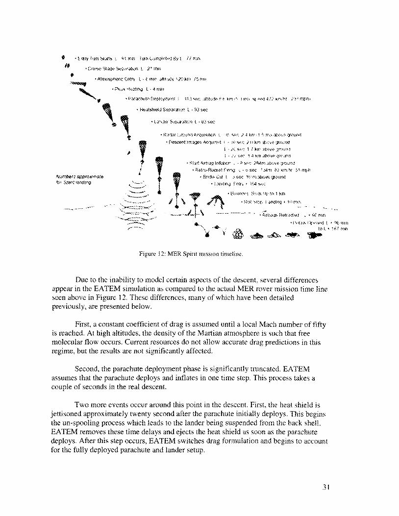
Figure 12 shows the predicted timeline for the Spirit (MER 1) mission. The values and times shown in the figure are estimated, and may not reflect changes made prior to launch.

30

• - tn i t y fym blarls t «>1 wn t umt *m j * *WJ i i y l ' . ' »

i $ F * Ctu*» Slat* S«witw*s l 2*111111

• AlmospHem; E«rv L • C mw Mu>H 120 km /5 n

X » P w M«3?irnj L - 4 roirt

• f - \v*3«>- £}*{*3|>iwit I 11 i sec al &&*•*> M t a ^ 1 mis <* »«f 4,f? M"*W «*? * mptit

• htealshieW Separata L - 93 wc

• la**Jef Separate! t - H i sec

• f>est»nt images Acqof&jl I - . « sec i u Kn -ifoeve ground

I - X *sc t ? kir afcov? gsmtrk}

1 - / / w 1 4 to «ihr>w»i}roiiniJ

• Start *,trtwp tnftatrr . • ft s**e JWm .*t:c>\-# ijtourwt

• SetJO-Rooiel f i f o j i - ts sec *3&-ft &l tart t* $1 r r f *

Mrafiers aospftMffmafe " I I B > B « i ^ M i * sec turn abowe ground

& Sjxwvwtfig ^ " l - T W ' l . i n d n ^ fnir> * i W sec

• t \ m n m Ho i&UHf t i km

> A»tw>j«. R«lMd«J v * w? mm

•tvtaiM)rvrv*d. I »«&«mn to L •> W mm

Figure 12: MER Spirit mission timeline.

Due to the inability to model certain aspects of the descent, several differences appear in the EATEM simulation as compared to the actual MER rover mission time line seen above in Figure 12. These differences, many of which have been detailed previously, are presented below.

First, a constant coefficient of drag is assumed until a local Mach number of fifty is reached. At high altitudes, the density of the Martian atmosphere is such that free molecular flow occurs. Current resources do not allow accurate drag predictions in this regime, but the results are not significantly affected.

Second, the parachute deployment phase is significantly truncated. EATEM assumes that the parachute deploys and inflates in one time step. This process takes a couple of seconds in the real descent.

Two more events occur around this point in the descent. First, the heat shield is jettisoned approximately twenty second after the parachute initially deploys. This begins the un-spooling process which leads to the lander being suspended from the back shell. EATEM removes these time delays and ejects the heat shield as soon as the parachute deploys. After this step occurs, EATEM switches drag formulation and begins to account for the fully deployed parachute and lander setup.

31

Third, the MERs deploy parachutes based on the measurement of dynamic pressure. However, due to EATEM's limited Mars atmospheric model, EATEM deploys the parachute based on defined speed of four and twenty meters per second. The value for this speed comes from the parachute design deployment speed based on target flight Mach number.

Fourth, the post parachute craft is treated a single, rigid body. It is not allowed to oscillate or produce any pendulum type motion. Efforts were made to make the real craft follow this assumption, but the actual MER flight still exhibits some of this motion.

Lastly, the camera and ground acquisition systems can not be simulated currently in the code. Therefore, the firing of the retrorockets is based entirely on altitude and is not subject to the uncertainty in the MER acquisition system.

With the simulation controls in place, the initial conditions are left to define. The initial conditions are set without respect to retrograde or posigrade entry considerations. The simulation begins with the following initial conditions in the state vector.

• Altitude 125 km • FPA -11.5 degs • Velocity 5.7 km/s • Heading Angle 0 deg • Longitude 0 deg • Latitude 0 deg • Mass 845 kg

Finally, the simulation is run using a time step of one tenth of a second to increase overall accuracy of results.

The second portion of the simulation validation is carried out through the comparison of Monte Carlo analysis results. The Monte Carlo analysis method gives variable of interest a random variance model, similar in form to the wind generation routine, but having a different standard deviation, and the simulation is repeated a large number of times. In the case of EDL simulations, Monte Carlo results generally take the form of a landing foot print, which describes the spread of the landing projected landing area. The results of EATEM's dispersion analysis are compared against the JPL landing ellipses [8].

For the analysis carried out through the use of EATEM, the parameters being varied fall into one of four categories: spacecraft uncertainties, atmospheric uncertainties, navigation uncertainties, and wind uncertainties. Table 4 shows the variable breakdown as well as their respective variation.

32

Table 4: Monte Carlo analysis variables Variable Variation 3a Range

Spacecraft Uncertainties

Parachute Deployment Speed hp (m/s) RAD Initiation Altitude Mm) RAD Thrust TR (kN)

Aeroshell Cd, hypersonic

Aeroshell Cd, supersonic

Lander Cd

Backshell Cd

Parachute Cd

5%

25%

5%

5%

10%

20%

5%

12%

399 < hp< 441

90 < hr < 150

25.65 < TR < 28.35

Model Dependent *

Model Dependent * •

0.8576 < 1.072 < 1.2864

1.2635 < 1.33 < 1.3965

0.396 < 0.45 < 0.504

Atmospheric Uncertainties

Density above 60km

Density below 60km

Winds above 60km

Winds below 60km

45%

15%

80 m/s

40 m/s

Model Dependent *

Model Dependent *

Simulation Dependent **

Simulation Dependent **

Navigation Uncertainties

Entry Flight Path Angle (FPA)

1.04% -11.38 < FPA < -11.62

Wind Uncertainties

Wind Patterns o ** -100 < wind < 100 **

* Entries with this notation are models which do not have a fixed value. The range values show a rough estimate from a middle value. ** Entries with this notation are system which contain inherent randomization, and as such, do not have specific Monte Carlo variation attached.

33

The percent variations, in Table 4, are defined so that the range is nearly identical to that used by Desai [6]. Minor differences occur in the navigation variables, however. The EATEM fpa variation is defined by the maximum allowable error in the fpa prior to entry maneuvers as outlined by D'Amario [5]. This number varies between Spirit and Opportunity (MER1 and MER2) and Desai uses the median number. EATEM uses the Spirit value to match more completely with the previous validation work.

Desai also incorporates other navigation errors which are not encompassed by EATEM. EATEM does not allow initial heading angle variations or in flight moment induced changes.

The landing dispersion analysis is set up in 5 stages. The first stage establishes the landing foot print created by the wind generation. The next three stages attempt to establish the individual contributions to the landing foot print of the three variable types of interests. The last stage shows the combined effect of all variations.

The landing dispersion analysis is carried out in two thousand run sets. Each iteration of the code establishes a range and cross range value. The range represents the arc that would be inscribed upon the surface of the planet during the flight. The cross range represents the arc of lateral deviation from range.

EATEM Simulation Results

Figure 13, Figure 14, Figure 15, and Figure 16 show the visually important flight tracking parameters captured during the simulation. Plots are combined into a single figure when there is a common axis variable.

34

x 10

x 10

20 40 60 80 Altitude (km)

100 120

Figure 13: Combined plot set of axial force vs. time and altitude.

Figure 13 shows the axial force the entry craft undergoes. This force is the combination of all drag, wind, and thrust effects. The first peak is the natural deceleration due to frictional forces; the second peak is the parachute deployment; and, the third peak is the retro-rocket firing.

35

500 1000 1500 2000 2500 3000 3500 4000 4500 5000 5500 Speed {m/s)

Figure 14 Altitude vs speed, with zoomed views from the post parachute phase

Figure 14 shows the current speed of the entry craft with respect to height. This figure shows the minimal effects of the atmosphere until below sixty kilometers. The first zoomed view shows the effects of the parachute decelerator systems. The second zoom shows the RAD decelerator systems and the subsequent acceleration due to gravity.

36

100 150 200 Ms)

250 300

Figure 15: Combined plot set of altitude and speed vs. time.

Figure 15 displays the altitude and speed tracking as the EDL time elapses. The black and gold marker shows the point of parachute deployment.

With the general results established, the comparison between EATEM simulation and the established work can begin. The first comparison is with the IMU axial force data and the EATEM simulation results.

37

x 10

IMU DATA EATEM DATA

EATEM and MER1 (Spirit) IMU Data

Parachute Deployment

Figure 16: Plot of the axial force vs time for EATEM and MER IMU data.

Figure 16 verifies that the EATEM simulations captured, at the very least, the general trends expected during EDL. The time and force offsets are expected as the atmospheric model in EATEM is still very limited. The only major point of discrepancy occurs at the second peak, or parachute deployment point. This reasoning for this time delay is multi-faceted. First, EATEM* s simulation is based from the nominal deployment numbers. Changes in the atmosphere from the expected models, forced the late deployment of the Spirit's parachute almost a kilometer below the expected altitude. Secondly, EATEM treats the parachute deployment as a step function, where as the IMU data displays the mortar fire and subsequent deployment time delay. The close alignment of the post parachute terminal velocity lends credibility to assumptions which govern the post parachute drag model.

The verification comparison is between EATEM, the NASA pre-flight numbers, and the work of Desai post flight. NASA's pre-flight numbers are taken from "Using Inertial Measurements for the Reconstruction Of 6-DOF Entry, Descent, and Landing Trajectory and Attitude Profiles" [11], and represent completely preflight simulation results. Desai's numbers are taken from "Mars Exploration Rovers Entry, Descent, and Landing Trajectory Analysis" by Desai and Knocke [6]. Desai's numbers are from post flight Monte Carlo simulation means. Table 5 shows the breakdown for each point of comparison.

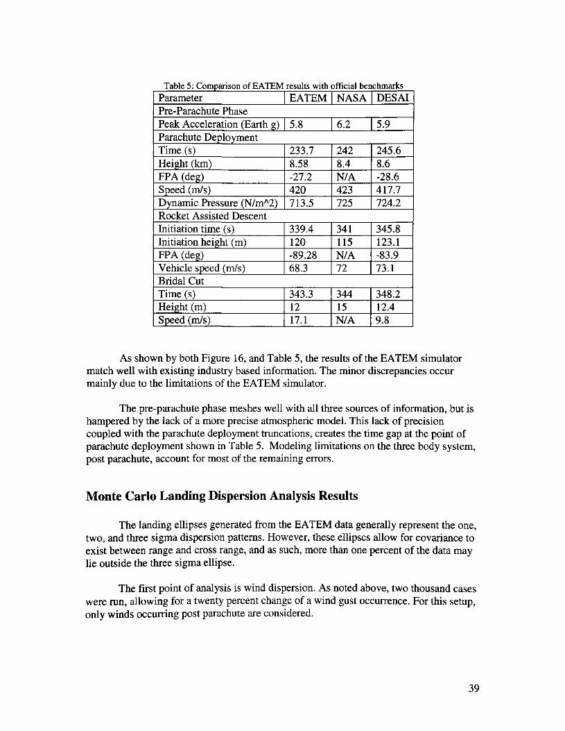
Table 5: Comparison of EATEM results with official benchmarks Parameter EATEM NASA DESAI Pre-Parachute Phase Peak Acceleration (Earth g) 5.8 6.2 5.9 Parachute Deployment Time (s) Height (km) FPA (deg) Speed (m/s) Dynamic Pressure (N/mA2)

233.7 8.58 -27.2 420 713.5

242 8.4 N/A 423 725

245.6 8.6 -28.6 417.7 724.2

Rocket Assisted Descent Initiation time (s) Initiation height (m) FPA (deg) Vehicle speed (m/s)

339.4 120 -89.28 68.3

341 115 N/A 72

345.8 123.1 -83.9 73.1

Bridal Cut Time (s) Height (m) Speed (m/s)

343.3 12 17.1

344 15 N/A

348.2 12.4 9.8

As shown by both Figure 16, and Table 5, the results of the EATEM simulator match well with existing industry based information. The minor discrepancies occur mainly due to the limitations of the EATEM simulator.

The pre-parachute phase meshes well with all three sources of information, but is hampered by the lack of a more precise atmospheric model. This lack of precision coupled with the parachute deployment truncations, creates the time gap at the point of parachute deployment shown in Table 5. Modeling limitations on the three body system, post parachute, account for most of the remaining errors.

Monte Carlo Landing Dispersion Analysis Results

The landing ellipses generated from the EATEM data generally represent the one, two, and three sigma dispersion patterns. However, these ellipses allow for covariance to exist between range and cross range, and as such, more than one percent of the data may lie outside the three sigma ellipse.

The first point of analysis is wind dispersion. As noted above, two thousand cases were run, allowing for a twenty percent change of a wind gust occurrence. For this setup, only winds occurring post parachute are considered.

39

2.5

2

1.5

1

| 0.5

I °

b

-1

-1.5

-2

Landing Site Dispersion - MER Lander With Navigation Effects

O O Simulation results

% (39.4%)

2 0 {86.5%)

3 0 (98.9%)

3o (JPL)

°o °

O

-2.5 -3 -2 -1 0 1

range (km)

Figure 17: EATEM landing ellipse created by the presence of winds.

As seen in Figure 17, the wind dispersion created by EATEM is slightly smaller than that found by JPL. JPL's ellipse, at the three sigma range, is 3 kilometers range by 1 kilometer cross range. EATEM returns a 2 km range by 1 km cross range. The EATEM wind data is created with only the post parachute wind routines running. The JPL data is from wind vs. altitude models which are much more sophisticated than the single magnitude wind approach used in EATEM.

The next criterion is the spacecraft effects contribution to the landing ellipse. This data is from a two thousand run case, and uses the parameter variations found in Table 4.

40

-p 1

o -1

-2

-3

Landing Site Dispersion - MER Lander With Spacecraft Effects

O Simulation results — — % (39.4%)

2 0 (86.5%)

3o(98.9%)

— — 30 (JPL)

\ f

-4 - 8 - 6 - 4 - 2 0 2 4 6 8

range (km)

Figure 18: EATEM landing ellipse created by the presence of spacecraft effects.

Figure 18 shows a flattened ellipse from the EATEM data. The spacecraft effects which could cause a cross range movement are not considered in EATEM. This limitation not withstanding, the EATEM results return a 12km by 0 km ellipse. JPL's numbers yield a 13km by 3 km ellipse. JPL's cross range results are due to the additional three degrees of freedom taken into account by their simulation tools.

The next data set revolves around the atmospheric uncertainties. Again, two thousand iterations were run using the variations initially described.

41

E

-2

Landing Site Dispersion - MER Lander With Atmospheric Effects

O Simulation results O _ 1 o (39.4%)

20(86.5%)

3o (98.9%)

O | Q J - - 3 0 (JPL)

0 O

-6 -30 -20 -10 0

range (km) 10 20 30

Figure 19: EATEM landing ellipse created by the presence of atmospheric effects (JPL development model).

In Figure 19, the three sigma ellipse from the JPL development model is smaller than the one created by EATEM. JPL's ellipse is 38 km by 0.1 km while EATEM returns a 46 km by 3.4 km model. The updated JPL model, taken from Mars Global Surveyor data, shows a higher degree of uncertainty and is shown against the EATEM data in Figure 20.

42

Landing Site Dispersion - MER Lander With Atmospheric Effects

O Simulation results O _ _ _ 1(y (39,4%)

— — - 20 (86.5%)

30(98.9%)

— — 3 0 (JPL)

-30 -20 -10 0 range (km)

10 20 30

Figure 20: EATEM landing ellipse created by the presence of atmospheric effects (JPL updated model).

Figure 20 shows the updated JPL model results. This new level of uncertainty produces a larger ellipse than previous, at 59 km by 0.1 km. Figure 19 and Figure 20 also show a discrepancy between the JPL analysis and EATEM. The JPL atmospheric effects only consider density variations. This is why there is little to no cross track on the JPL ellipses. The EATEM data considers the larger wind variance (separate variance than that of the wind ellipses) listed in the Monte Carlo variables of Desai's work [6]. These winds produce the 3.4 km cross track seen in the figures,

Figure 19 and Figure 20 also show the level of uncertainty which exists in the Martian atmospheric models. The atmospheric effects dominate the others, and provide the largest portion of variability.

The next area of uncertainty analysis revolves around the navigation parameters. Two thousand runs and the resulting ellipses are shown below.

43

5 Landing Site Dispersion - MER Lander With Navigation Effects

Simulation results

• 10 (39.4%)

•20(86.5%)

• 3o (98.9%)

30 (JPL)

o::a:==::= i, > o i o

1 -1 w

<j

-2

-3

-4

-5 -20 -15 -10 -5 0 5 10 15 20

range (km)

Figure 21: EATEM landing ellipse created by the presence of navigation errors.

Figure 21 shows the addition of extra navigation variance information in the JPL ellipses. EATEM's simulations only include an entry fpa variation as this is the only condition about which detailed information could be found. As a result, EATEM's simulation has no cross track results to match with JPL. The range results however, show that the JPL ellipse is slightly larger, and this is to be expected as the JPL results use an average result between the two MERs that is higher than the allowable error for the Spirit EDL which EATEM uses. EATEM produces a 27 km by 0 km ellipse while the JPL ellipse measures 32 km by 3 km.

With all of the sub-ellipses defined, it is time to examine the combined effects. As with previous cases, two thousand runs have been compiled, and the data is presented in Figure 22.

44

10 Landing Site Dispersion - MER Lander With Alt Effects

O Simulation results

S 2

w

8 o

10(39.4%)

20 (86.5%)

3o (98.9%)

30 (JPL)

-4

-6 O -40 -30 -20 -10 0 10 20 30 40 50 60

range (km)

Figure 22: EATEM landing ellipse created by the presence of all expected errors

Figure 22 shows a larger total ellipse from EATEM's data than that of JPL. This is due primarily to the fact that the EATEM atmospheric ellipse is larger than that of JPL. However, the numbers still compare well with JPL having a 54 km by 4 km ellipse and EATEM returning a 56 km by 5 km ellipse. The JPL simulations used the developmental atmospheric model over the updated one. JPL simulations using the updated model produce an ellipse on the order of 74 km by 6 km.

As the Monte Carlo system is entirely random, it is not conceivable to think that it covers the worst case scenarios in this small amount of simulations. To account for the fact that not all possible worst case scenarios occur together, the final ellipse is margined to account for the un-presented and/or un-modeled error. This is accomplished by taking the root-sum-square of the individual error contributors and adding the result to the un-margined ellipse. This process is accomplished with the following formula, and assumes no correlation in the errors.

mar; gin = Jj>,2 (25)

Many of the values for error contributions are taken directly from the JPL information [8] as they involve parameters which can not be simulated in or are outside

45

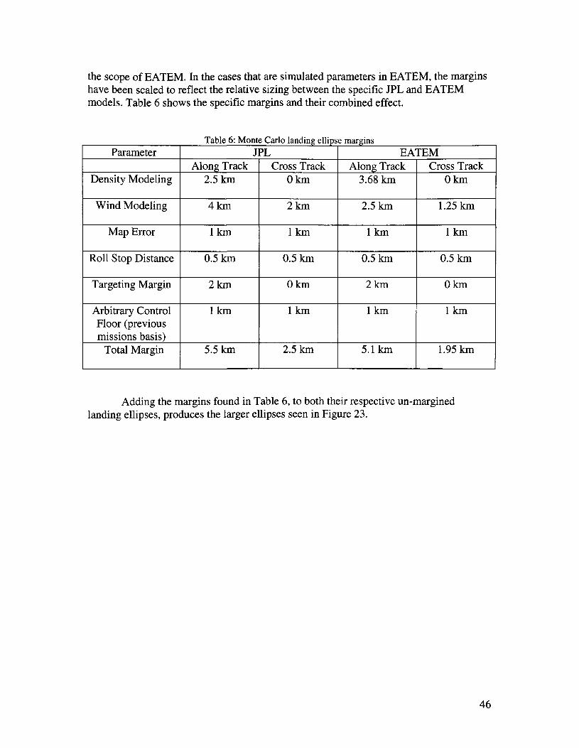
the scope of EATEM. In the cases that are simulated parameters in EATEM, the margins have been scaled to reflect the relative sizing between the specific JPL and EATEM models. Table 6 shows the specific margins and their combined effect.

Table 6: Monte Carlo landing ellipse margins Parameter

Density Modeling

Wind Modeling

Map Error

Roll Stop Distance

Targeting Margin

Arbitrary Control Floor (previous missions basis)

Total Margin

J]

Along Track 2.5 km

4km

1km

0.5 km

2km

1km

5.5 km

PL Cross Track

0km

2km

1km

0.5 km

0km

1km

2.5 km

EATEM Along Track

3.68 km

2.5 km

1km

0.5 km

2km

1km

5.1km

Cross Track 0km

1.25 km

1km

0.5 km

0km

1km

1.95 km

Adding the margins found in Table 6, to both their respective un-margined landing ellipses, produces the larger ellipses seen in Figure 23.

46

Landing Site Dispersion - MER Lander With Margined Ellipses

25 — — 3o margined (JPL)

20 • 3o margined (EATEM)

15

10

-10

-15

-20

-25

-30 -20 -10 0 10 20 30 range (km)

Figure 23" EATEM landing ellipse created by the presence of all expected errors, with root-sum-square margins included.

The addition of the margins to the ellipses produces ellipses that are more closely matched. While not immediately obvious in the picture, due to the scale of the ellipse, the two ellipses are off by about 1 km by 0.1 km, resulting in an EATEM margined ellipse of 66 km by 8.9 km and a JPL margined ellipse of 65 km by 9 km. The addition of the margins create a values of 3.57 range and 5.33 cross range for EATEM, and 3.61 range and 6.77 cross range for JPL.

Conclusion

The simulation trials effectively demonstrated the accuracy of the results produced by EATEM. In the single loop case, where small perturbations can significantly alter the results, the differences found between EATEM and the validation and verification sources were small, and mostly within acceptable engineering tolerances. The Monte Carlo analysis results show even more promise, in that the results were overall closer to the verification source.

47

Development of a Martian Radiosonde Mission

Introduction

The purpose of creating the EATEM simulator was to have a platform to carry out first iteration design work. EATEM represents a quick option for the initial testing of concepts and sizing trade offs. An example of this work will be shown using a previous research topic of mine based in the development of autonomous Martian radiosondes, where a significant portion of the investigation revolves around deployment methods and dynamics.

Setup

The Mars radiosonde deployment mission is adapted from the MER configuration already validated in EATEM. The new mission removes the lander from the configuration and replaces it with six radiosonde packages, leaving enough free mass to account for additional structure requirements, deployment mechanisms, and propulsive effects.

The new mission follows the same entry conditions as the MER and proceeds along the same trajectory until the parachute deployment phase is reached. From there, the craft descends in two pieces, parachute and body, until the RAD altitude is reached. The RADs fire until the craft is decelerated to a velocity of approximately five meters per second, at which point, the radiosondes are ejected from the body via pyrotechnic devices. After this point, the simulation follows the radiosondes until touchdown.

Further, small scale, Monte Carlo dispersion analysis is carried out on the radiosonde dispersion patterns.

Results

The study of the radiosonde deployment tracks the craft from the last two second of simulation EDL until the radiosondes touch down on the surface of Mars. The RAD system on the MERs slows the craft down to approximately five meters per second, before the radiosondes are discharged via pyrotechnics. For these simulations, given the relative size of the objects, and the small time duration, wind effects have been removed.

The trajectories of the falling radiosonde packages are shown below in Figure 24.

48

80

60

40

20

0

50

50

-50 -50

Figure 24: Initial dispersion results of the Martian radiosondes.

As seen in Figure 24, EATEM allows for quick testing of design parameters. Design parameters such as radiosonde mass, expulsive force, expulsion angle, and craft velocity at ejection can be easily adapted and changed inside the code, to test relative and combined effects. Design requirements, such as radiosonde impact velocity, are already tracked and can be monitored as desired to meet requirements.

Applying Monte Carlo analysis, a two dimensional spread pattern can be found. The results of a small scale Monte Carlo simulation are show in Figure 25. For this analysis, the force produced by the deploying mortars is allowed to vary by five percent.

49

80

60

40

20

-i# *•

o -20

-40

-60l

-80--100 -80 -60 -40 -20 0 20

range (m) 40 60 80 100

Figure 25: Radiosonde Monte Carlo dispersion simulation.

This approach shows the expected landing regions based on the current error tolerancing and allows for quick determination of required refinements. Once nominal spread tolerancing is achieved, existing code effects can be turned on to track deployment spread based on the entire mission.

Conclusion

The application of EATEM shown in this section is only a quick view of the design benefits that EATEM presents. The modular format allows for quick adaptation of the code to design specifications, and presents a quick and efficient tool for initial design considerations. This work shows that EATEM achieved its initial design goal of creating versatile environment in which research and analysis can be carried out.

50

Conclusion and Recommendations

EATEM represents a validated, first run, EDL analysis tool. The results difference between EATEM and the NASA based simulation sources is small, generally 7% or less, with most of the error being expected and explained by the nature of the simplifications made in EATEM.

Aside from its initial design concepts involving Mars based entry missions, EATEM is set up so that it can be easily adapted for any extra-planetary EDL design by the simple addition of new atmospheric models and planetary science information.

The entry vehicle selection can be expanded in a similar fashion by the creation and analysis of new vehicle geometries.

EATEM's usefulness is not limited to the EDL scenario. EATEM can be adapted for areas of research such as guided missile analysis, missile or craft interception, and rendezvous trajectories.

While EATEM represents a large step forward, there is still much work to be done in the expansion of the simulator. Many of the simplifications in EATEM can be removed with further time and resources.

The first major step is the conversion of EATEM from a 3 DoF simulation to a 6 DoF of freedom simulation. This step does not immediately require more resources, as the drag program HEAT/TK provides moment coefficient information. It will however, require many more drag models, as well as more state vector inputs and tracking.

The second recommended upgrade to EATEM revolves around the parachute deployment. Mathematical models exist which can track deployment progress and forces present during deployment, but their development and implementation is not a quick process, and was beyond the scope of this initial work.

The third upgrade to EATEM is in the post parachute body modeling. The current grouping of the three bodies into a single rigid body needs to be removed, and the three bodies allowed to move independently within the defined constrains of the system. These changes will force modifications to many of the models currently used by EATEM, and may represent the most ambitious of the upgrades to EATEM.

The last major piece of future work for EATEM revolves around the numerical integration routines. During the large scale Monte Carlo analysis, situations occur which cause the craft's velocity to become very small. When this occurs, the integrators have a problem resolving the tolerances and either a simulation stall or a bad data point can occur. This problem is compounded by the necessity to further reduce the time step below 0.1 seconds during some aspects of mission design. Resolution of this issue is required before any detailed parametric sizing can be accurately carried out.

51

REFERENCES [I] Adle, M., Erickson, J.K., Manning, R., "Mars Exploration Rover: Launch, Cruise,

Entry, Descent, and Landing" 55th International Astronautical Congress, Vancouver, Canada, Oct. 4, 2004.

[2] Bruno, Robin, Cruz, Juan, Kandis, Mike, Witkowski, Allen., "Mars Exploration Rover Parachute System Performance,'''' 18th AIAA Aerodynamic Decelerator Systems Technology Conference and Seminar, Munich, Germany, May 2005.

[3] Busemann, Adolf, Culp, Robert D., Vinh, Nguyen X. Hypersonic and Planetary Entry Flight Mechanics. Ann Arbor: University of Michigan Press, 1980.

[4] Cheatwood, F.M., Desai, Presun N., Schoenenberger, Mark, " Mars Exploration Rover Six-Degree-of-Freedom Entry Trajectory Analysis," Journal of Spacecraft and Rockets Vol. 43, No. 5 (2006).

[5] D' Amario, Louis A., " Mars Exploration Rover Navigation" AIAA/AAS Astrodynamics Specialist Conference and Exhibit, Providence, RI, Aug. 2004.

[6] Desai, Prasun N., Knocke, Philip C, "Mars Exploration Rovers Entry, Descent, and Landing Trajectory Analysis," AIAA/AAS Astrodynamics Specialist Conference and Exhibit, Providence, RI, Aug. 2004.

[7] Desai, Prasun N., Lisano, Michael E., Schofield, John T., "Flight Reconstruction of the Mars Pathfinder Disk-Gap-Band Parachute Drag Coefficient," 17th AIAA Aerodynamic Decelerator Systems Technology Conference and Seminar, Monterey, California, May 2003.

[8] Desai, Prasun N., et al, "Mars Exploration Rovers Landing Dispersion Analysis," AIAA/AAS Astrodynamics Specialist Conference and Exhibit, Providence, RI, Aug. 2004.

[9] Eloret Corporation, "Planetary Mission Entry Vehicles: Quick Reference Guide," ver. 3, 2006.

[10] Kass, D.M., et al, "Analysis of atmospheric mesoscale models for entry, descent, and Landing," Journal of Geophysical Research. Vol. 108 (2003).

[II] Lisano, Michael E., Wawrzyniak, Geoffrey G., "Using Inertial Measurements for the Reconstruction Of 6-DOF Entry, Descent, and Landing Trajectory and Attitude Profiles," AAS/AIAA Space Flight Mechanics Meetings, San Antonio, TX, Jan. 2002.

52

[12] Benson, Tom, "Mars Atmospheric Model," Glenn Research Center. 2006. NASA. 8 May 2008. http://www.grc.nasa. gov/WWW/K-12/airplane/atmosmrm.html

[13] Pointwise, "Gridgen User's Manual," 2006.

[14] Rafkin, Scot C.R., "Preliminary Atmospheric Hazard Assessment for Mars Science Laboratory Entry, Descent, and Landing," PowerPoint presentation. Southwest Research Institute, 8 May 2008. http://marsoweb.nas.nasa.gov/landingsites/msl/workshops/Ist workshop/talks/wed-AM/08-Rafkin atmosphere.ppt

[15] The Boeing Company, "Hypersonic Engineering Aerothermodynamic Trajectory Tool Kit (HEAT-TK): Software User's Manual" Jan. 2005.

53

APPENDIX A

LIST OF ACRONYMS

54

AGL = adjusted ground level

CFD = computation fluid dynamics

DoF = degree of freedom

EATEM = Entry Analysis Tool for Exploration Missions

EDL = entry, descent, and landing

EoMs = equations of motion

FPA = flight path angle

HEAT/TK = computation fluid dynamics analysis software

LMU = inerital measurement unit

JPL = Jet Propulsion Laboratory

MER = Mars Exploration Rover

RADs = rocket assisted descent motors

TIRS = transverse impulse rocket system

55

APPENDIX B

CREATION OF HEAT/TK INPUT FILES

56

HEAT/TK uses the .geo file extension. Currently there are no modern software packages available that support this file extension. To alleviate this problem, a conversion script and instructions are provided below.

FORTRAN Script and Compilation

The conversion script is written in FORTRAN and is entitled p3d_geo.f. Compiling this script requires the use of the Intel Fortran compiler which is available for free in the Linux operating environment. Successful compilation should result in a p3d_geo executable.

File Creation and Conversion

To begin the conversion process, the file must be saved in the plot3d format. This can be accomplished through the use of Gridgen or through a variety of other modeling software. The file must be saved to the same folder as the conversion script.

Running the conversion script without specifying any input arguments will allow the user to enter the desired choices after each prompt. It is recommended that the user use this option in the beginning.

The script will ask the user for the name of the file to be converted. The script will look for the full file name so the extension, p3d, can not be left off. After this, it will ask for the name of the output file desired. Once again, the file extension, in this case .geo, can not be left off. The script will then ask for the scale factors desired. If the original model is to scale, the scale factor is one. Last, the script will ask if an inversion of the axis is needed. This option is a one or zero (yes / no) choice. After this point, if there are no errors, the .geo file will be successfully created.

Recommendations

It is recommended that in the creation of the plot3d file, that the user only exports the surface domains. HEAT/TK has a limited number of allowable subsections and the creation of blocks which have thickness, severely curtails the ability to model the object.

Exporting only the domains can be achieved by the following in Gridgen. Select the I/O tab. Next, select the grid points export command, followed by the domain surfaces tab. Type in the name of the output file, and then click on the domains that are to be exported.

57

APPENDIX C

HEAT/TK ORIENTATION INFORMATION

58

Below is pictured the definition of the coordinate system in which HEAT/TK operates.

Cross-section

Flow direction

Streamwise

59

APPENDIX D

.Geo File Conversion Script and Help File

60

program p3d_geo (Code)

parameter (imax=2 00,jmax=20 0,maxobj=100) real x(imax,j max,maxobj),y(imax,j max,maxobj), & z(imax,jmax,maxobj) integer ni(maxobj),nj(maxobj)

character ofile*80,ifile*80,ans*10,string*80 o

narg=nargs() "5

if(narg.eq.1) then % interactive prompts

ans='q!' % prompt for the name of the input file

write(*,*)'**** input the name of the plot3d input file ****' read(*,'(a)') ifile if (ifile.eq.ans) goto 999

% open input file 1 open(unit=10,file=ifile,status='old',iostat=ios)

if( ios .ne. 0 ) then write(*,*)'**** error opening p3d input file ****' write(*,*)'**** reenter file or q! to exit ****' read(*,'(a)') ifile if (ifile.eq.ans) goto 999 goto 1

endif %

write(*,'(//,'' input the name of the Geo output file'')') read(*,'(a)') ofile

% open geo output file 2 open(unit=ll,file=ofile,status='unknown',iostat=ios)

if( ios .ne. 0 ) then write(*,*)'**** error opening geo file ****' write (*,*) '**** reenter file or q! to exit ****' read(*,'(a)') ofile if (ofile.eq.ans) goto 999 goto 2

endif

write(6,*) write(6,*) '**** Enter X,Y,Z Scale Factors, Enter XSF,YSF,ZSF' read(5,*) xsf,ysf,zsf

write (6,*) write(6,*) '**** Flip order? (l=yes, 0=no) Enter IF, JF' write(6,*) '**** for example if enter 1,0 reveres' write(6,*) ' order of i points'

read(5,*) iflip,jflip

else arguments entered on command line, use those for file names

iflip=0

61

jflip=0 nf=l i = l

50 continue call getarg(i,string)

write(6,'(i3,lx,a40)') i,string if(string.eq.'-x' .or. string.eq.'-X1) then

call getarg(i+l,string) i = i + l read(string, ' (f15.0) ') xsf

elseif(string.eq.'-y' .or. string.eq.'-Y') then call getarg(i+l,string) i=i+l read(string, ' (f15.0) ') ysf

elseif(string.eq.'-z' .or. string.eq.'-Z') then call getarg(i+1,string) i = i+l read(string, ' (fl5.0) ') zsf

elseif(string.eq.'-i' .or. string.eq. ' -I •) then iflip=l

elseif(string.eq.'-j' .or. string.eq.'-J') then jflip-1

else if(nf.eq.l) then

ifile=string nf=nf+l

else ofile=string

endif endif i = i+l if(i.lt.narg) goto 50

error check on files if(ifile.eq.'') then

write(*.*) '**** need to enter input file on ', & 'command line ****'

stop endif if(ofile.eq.'') ofile='output.geo1

write (6,200 0) ifile,ofile,xsf,ysf,zsf,iflip,jflip 00 format('**** input = 'a80/

& .**** ouput = 'a80//

& .**** xscale ='fl0.3/

& <**** Yscale ='fl0.3/

& i**** zscale ='fl0.3/

& i**** ifiip ='i2/

& i**** jflip ='i2/) open(unit=10,file=ifile,status='old',iostat=ios) if(ios.ne.O) then write(6,2010) stop

endif open(unit=ll,file=ofile,status='unknown',iostat=ios) if(ios.ne.O) then write(6,2010)

stop endif

2010 format(/'**** Error opening files ****< &i**** check command line inputs ****</) endif

% rewind 10 rewind 11

% % read p3d file % >>>> format is Ascii multi grid, kmax=l no iblank grid file ft. o

read(10,*) nmax do i=l,nmax

read(10,*) ni(i),nj(i),nk enddo

do n=1,nmax read(10,*) ((x(i,j,n), i=l,ni(n)),j=l,nj(n)),

& ((y(i,j,n), i=l,ni(n)),j=l,nj(n)), & ((z(i,j,n), i=l,ni(n)),j=l,nj(n)) enddo

% % write geo file

% loop on all grids do n=1,nmax

ib=l ie=ni(n) ii=l if(iflip.eq.1) then ie=l ib=ni(n) ii=-l

endif jb=l je=nj(n) ji = l if (jflip.eq.l) then je=l jb=nj(n) ji=-l

endif

write(11,500)'BODY' 500 format('BODY001'al5/'01',18X,'1')

do j=jb,je,ji do i=ib,ie,ii

icode=0 if(j.eq.jb .and. i.eq.ib ) icode=2 if(j.ne.jb .and. i.eq.ib) icode=l if(j.eq.je .and. i.eq.ie) icode=3

xl=xsf*x(i,j,n) yl=ysf*y(i,j,n)

63

zl=zsf*z(i,j,n) write(ll,22)xl,yl,zl,icode

22 format(3fl0.4,il,lx) % % 60 end do

end do enddo

write(6,*) '**** Geo File written successfully! **** 999 stop

end

64

Program p3d_geo.exe (help file)

This program reads a plots 3d frile from a grid generation program

such as Gridgen and convetes it to a geo file that can be read into Heat-TK

Options

if run p3d_geo.exe with no options program is interactive.

if run p3d_geo.exe from command line can specify option

p3d_geo.exe -X xscale -Y yscale -Z zscale -i -j input_file output_file

xscale, yscale, zscale are scale factors that the input file x,y,z coordinates are multiplied by. Can use to re-orient or scale the complete geometry.

-X xscale - optional, x scale factor -y yscale - optional, y scale factor -z zscale - optional, z scale factor

-i - optional, if input reverese the order of the i points -j - optional, if input reverese the order of the j points

input_file - mandatory input if commande line driven, complete file name output_file - optional output file name

David Adamczak AFR1WAAA david.adacmzak@wpafb.af.mil

11/04

example inputs

p3d_geo.exe -x -1.0 test.p3d output.geo

p3d_geo.exe -x -1.0 -y 2.0 -z 2.0 -i test.p3d