McCreery Page 1

Development Potential: The Joint Influence of High Population Growth

and a Weak Economic Base

Dr. Anna C. McCreery Ph.D. in Environmental Science (June 2012)

Ohio State University http://annamccreery.wordpress.com/

Fundamentals of Geographic Information Systems (Autumn 2009)

Applications of GIS – Final Project Assignment Information: Students will perform a spatial analysis exercise, given only the criteria to use for reaching a conclusion. Objectives are to explore a data set and the geographic distribution of the variables, to arrive at several conclusions, and to

produce four maps showing those conclusions visually. Other objectives include learning to design and perform the necessary data analysis in a vector-based or raster-based GIS. Data export utilities to other applications, such as Microsoft Access or Excel, will be learned for developing a

more complete statistical analysis of spatial data.

   

McCreery Page 2

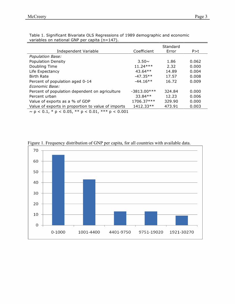
Problem Definition and Preliminary Non-Spatial Analysis This study examines how a country’s population growth and the strength of its economic base influences the potential for future economic growth. To put this in context, the geographic distribution of countries with different demographic and economic conditions will be examined. The clear historical link between spatial location and current economic conditions in many African, Asian, and South American countries can be linked to oppressive colonial regimes that still affect these countries today. Furthermore, countries in the Northern Hemisphere might have different demographic and economic conditions than countries in the Southern hemisphere, due to variation in natural resources and historical patterns. This project will therefore also examine the degree of spatial autocorrelation of demographic and economic conditions between countries, to determine whether the location of a country influences its other attributes. This study begins with a non-spatial analysis of country-specific data, looking for significant bivariate relationships between demographic variables, economic variables, and Gross National Product (GNP) per capita (the distribution of GNP per capita is shown in Figure 1). The results of this preliminary analysis are presented in Table 1. In terms of the population base, several factors were tested. Population density has a weakly significant positive effect, as it is a simple indicator of the amount of human resources that a country has available. Second, very high population growth (as indicated by the doubling time of the population) could produce one of two possible effects: 1) a country with a very high population growth might not be able to keep up economically with that growth; or 2) a higher doubling time might indicate a very vibrant country, with high numbers of immigrants seeking economic opportunities in a quickly growing economy. This second option is more likely, since doubling time has a positive significant effect on GNP per capita. Third, longer life expectancy is associated with higher GNP per capita. Finally, both higher current birth rates and higher past birth rates (measured as the percent of the population under age 15) have a negatively impact GNP per capita. Taken as a whole, these factors imply that countries with quickly growing populations and a large percentage of children tend to be less developed (i.e. have lower GNP per capita).1 Next, there were several economic factors that influence GNP per capita in bivariate regressions. The percent of the population dependent on agriculture can be used as a proxy measure of the level of industrialization of a country’s economy. A higher proportion of population dependent on agriculture would indicate a less industrialized country, and these countries have significantly lower GNP per capita. The percent of the population in urban areas has a significant positive influence on GNP per capita, likely because urban areas act as economic centers, and more modernized countries have fewer rural residents. Trade was also found to be important: higher export values are associated with higher per capita GNP (when measured as a percent of GDP or when measured in proportion to the value of imports).2

Taken together, these results demonstrate the importance of population growth, industrialization, and trade balance in determining GNP per capita. Higher population growth and a lower industrial base are associated with a lower GNP per capita.

1 Other demographic factors that were also tested and not found significant in a bivariate regression are: the growth rate (measures at 1989 or 1980), percent of the population between ages 15-64, and the death rate. 2 The influence of the energy balance, or difference between energy consumption and production, was also tested but not significant.

McCreery Page 3

Table 1. Significant Bivariate OLS Regressions of 1989 demographic and economic variables on national GNP per capita (n=147).

Independent Variable Coefficient Standard

Error P>t Population Base: Population Density 3.50~ 1.86 0.062 Doubling Time 11.24*** 2.32 0.000 Life Expectancy 43.64** 14.89 0.004 Birth Rate -47.35** 17.57 0.008 Percent of population aged 0-14 -44.16** 16.72 0.009 Economic Base: Percent of population dependent on agriculture -3813.00*** 324.84 0.000 Percent urban 33.84** 12.23 0.006 Value of exports as a % of GDP 1706.37*** 329.90 0.000 Value of exports in proportion to value of imports 1412.33** 473.91 0.003 ~ p < 0.1, * p < 0.05, ** p < 0.01, *** p < 0.001

Figure 1. Frequency distribution of GNP per capita, for all countries with available data.

McCreery Page 4

Methodology For conceptual clarity, countries were classified according to their economic conditions and population growth. Countries with high population growth are those with birth rate at least 37 births per 1000 women and at least 33% of the population under age 15, while low population growth countries are lower on both criteria. Countries were also classified as poor economic conditions, good economic conditions, or other. Countries with poor economic conditions have at least 50% of their population dependent on agriculture and a trade balance where imports exceed exports by at least 10%, while countries with good economic conditions have less than 50% of their population dependent on agriculture and a trade balance where exports exceed imports by at least 10%. These economic and demographic variables were chosen because they have a statistically significant effect on GNP per capita in 1989, so it is likely that they will also affect economic growth in future years. These the geographic distribution of these conditions are shown on a series of maps, discussed below.

Data Preparation and GIS Visualization All of the data for this project was taken from the datasets provided to the class for individual projects. GIS data conversion and visualization techniques were used to create a series of maps showing the geographic distribution of different population and economic conditions, to examine the spatial auto-correlation of development potential. Specific data transformations are detailed in the appendix. The following maps show the results:

1. 1989 Birth Rate: Map displaying birth rate in each country, and highlighting countries with a very quickly growing population (countries with birth rate at least 37 and at least 33% of the population under 15 years old)

2. Agricultural Dependence and Population Growth: Map showing percent of population dependent on agriculture, highlighting countries with very quickly growing populations

3. Balance of Imports versus Exports: Map showing trade balance by countries, highlighting countries with high population growth

4. Potential for Future Economic Growth: Map showing countries with poor economic conditions and high population growth, countries with good economic conditions and low population growth, countries with good economic conditions (regardless of population) and countries with poor economic conditions (regardless of population)

Discussion

Examination of the four maps shows noticeable patterns in the data. First, the 1989 Birth Rate map (see below) shows a clear geographic pattern in birth rates, with higher birth rates concentrated in the Southern Hemisphere. Furthermore, the highest birth rates in the world (above 37 births per 1000 women) occur primarily in Africa, with a few countries in Asia, Latin America, and South America that also have very high birth rates. This map also outlines countries with high birth rates and at least 33% of the population under age 15. The second map, on agricultural dependence, seems to follow the same geographic pattern. Specifically, countries with a high percent of the population dependent on agriculture (>50%) are mostly in the Southern Hemisphere, and are primarily located in Africa.

McCreery Page 5

Next, the map for trade balance (titled Balance of Imports versus Exports, below) shows more geographic variation. The level of spatial autocorrelation of trade balances is clearly lower than the level of spatial autocorrelation of agricultural dependence and birth rates. African countries have a variety of different trade balances, unlike agricultural dependence and birth rates which are high throughout the continent. Just by looking at the map there does not seem to be any clear spatial pattern in the distribution of trade balances. The overall picture for economic development potential, however, is clear. A glance at the final map, Potential for Future Economic Growth, shows distinct geographic patterns. Countries with high population growth and poor economic conditions do not have the resource to improve their economy, despite international development efforts, and they will be further hampered by high population growth. These countries may not have the funds to educate their citizens, or possibly even feed them adequately, and they will therefore not have the human capital needed to grow their economy in the future. Although a few of these countries are in Latin America and Southern Asia, they are almost all located in Africa. The concentration of these countries in Africa demonstrates the spatial autocorrelation of these attributes, and the intersection of difficulties faced by many African nations. The final map also shows that there are some countries where future economic growth could be considerable. These countries have good economic conditions in the current data, and they are not hampered by high population growth. Indeed, the lower population growth could be an asset, since it will allow these countries to invest in good education for all their young citizens. These countries are not concentrated in any geographic location. However, there does seem to be some spatial autocorrelation for countries with good economic conditions, regardless of their population growth. Even a country with high population growth has the potential for high economic growth if its current economy is strong enough. Although it is a somewhat weaker spatial-autocorrelation, countries with strong economics, and therefore higher development potential, are clustered in South America and the Northern coast of Africa.

Conclusions After the injustices of colonialism and the abusive treatment of many Southern hemisphere countries by European powers, it is important to consider whether former colonies have been able to overcome the weight of history. This analysis shows that in some parts of the world they have not – many former colonies in Africa are struggling with slow economies and high population growth, and they could be facing continued dire economic conditions in the future. This is even after many of them have been independent nations for decades, and despite efforts to encourage development taken by the World Bank and other international bodies. Several South Asian nations are also facing difficult circumstances, and this region of the world could also be feeling the negative effects of the history of colonialism. Former colonies in the Americas seem to be doing better – many countries in South America have good economic conditions, and apart from a few countries in Latin America the economic and demographic conditions of these countries show promise for continuing economic improvements. Overall, these issues are important because understanding the geographic distribution of economic and demographic conditions is useful for understanding world power relationships both now and in the future. This sort of spatial analysis is also useful for targeting development aid to the geographic regions where it is most needed.

LegendCountriesBirth Rate

no birth rate data

0 - 18.6

18.7 - 28.0

28.1 - 36.9

37.0 - 44.8

44.9 - 54.0

High population growth

1989 Birth Rate :

0 50 10025 Decimal Degrees

Geographic Coordinate System: GCS WGS 1984

Datum: D WGS 1984

In this map, high population growth is defined as a birth rate ofat least 37 and at leat 33% of the population under age 15.

LegendHigh population growth

Countriesno agricultural dependence data

Percent of population dependent on agriculture1-10%

11-25%

26-50%

51-75%

Greater than 75%

Agricultural Dependence and Population Growth

:0 50 10025 Decimal Degrees

Geographic Coordinate System: GCS WGS 1984

Datum: D WGS 1984

In this map, high population growth is defined as a birth rate ofat least 37 and at leat 33% of the population under age 15.

Balance of Imports versus Exports

:0 50 10025 Decimal Degrees

Geographic Coordinate System: GCS WGS 1984

Datum: D WGS 1984

In this map, high population growth is defined as a birth rate ofat least 37 and at leat 33% of the population under age 15.

LegendHigh population growth

Countriesno trade data

Trade BalanceExports Exceed Imports by greater than 50%

Exports Exceed Imports by 10-50%

Either Side by 10%

Imports Exceed Exports by 10-50%

Imports Exceed Exports by greater than 50%

LegendGood economic conditions & low population growth

Good economic conditions

Poor economic conditions & high population growth

Poor economic conditions

all other countries

This map displays the countries that are most likely to see changes intheir economic situation in the future, either good or bad. Countries withgood economic conditions (defined as <50% of the population dependenton agriculture and exports exceeding imports by at least 10%) and lowpopulation growth (defined as birth rate <37 and <33% of the populationunder age 15) are likely to have future economic growth. Countries withpoor economic conditions (defined as >50% of the population dependenton agriculture and imports exceeding exports by at least 10%) and highpopulation growth (defined as birth rate at least 37 and at least 33% of thepopulation under age 15) are likely to continue struggling economically,and economic conditions could even get worse. The other countries areharder to predict

:0 50 10025 Decimal Degrees

Geographic Coordinate System: GCS WGS 1984 Datum: D WGS 1984

Potential for Future Economic Growthbased on current economic conditions and population growth

McCreery                                    Page  10  

Appendix: Data Preparation and GIS Operations The operations performed on these data are quite simple. First the join function was used to join the demographic data file to the country map layer. A series of new data layers were then created for countries with a specific set of attributes, using the following steps:

1. Select the countries with specific attributes. For example, for high population growth, use select by attribute to select countries with birth rate ≥ 37 and population under 15 ≥ 33%. As another example, for trade balance the countries with the required trade balance were selected manually.

2. Export this selection to a new data layer. The constructed data layers are as follows:

1. High population growth: only countries with Birth rate ≥ 37 and % of population under 15 years old ≥ 33%

2. Low population growth: only countries with Birth rate < 37 and % of population under 15 years old < 33%

3. Agriculture-Dependent: only countries with > 50% of the population dependent on agriculture

4. Agriculture-Independent: only countries with < 50% of population dependent on agriculture

5. Poor economic conditions: only countries that have > 50% of population dependent on agriculture and imports exceeding exports by at least 10%

6. Good economic conditions: only countries with <50% of population dependent on agriculture and exports exceeding imports by at least 10%

7. Poor economic conditions and high population growth: only countries that fulfill the criteria for layer 1 and layer 5

8. Good economic conditions and low population growth: only countries that fulfill the criteria for layer 2 and layer 6.