Development of vehicle emissions models for Australian ...
130
i Development of vehicle emissions models for Australian conditions Sicong Zhu B.Eng., M.Sc. A thesis submitted for the degree of Doctor of Philosophy at The University of Queensland in 2014 School of Civil Engineering
Transcript of Development of vehicle emissions models for Australian ...

i
Development of vehicle emissions models for Australian
conditions
Sicong Zhu
B.Eng., M.Sc.
A thesis submitted for the degree of Doctor of Philosophy at
The University of Queensland in 2014 School of Civil Engineering

ii
Abstract
Microscopic simulation models such as AIMSUN, VISSIM and/or PARAMICS have the
ability to output emissions based on default values for emission factors derived mainly from
European test data. Emission algorithms in those models are based on overseas vehicle
emissions datasets, which do not reflect the different Australian vehicles, fuels, climate and
fleet composition. The proposed research provides a set of emission algorithms to be used in
conjunction with traffic simulation modelling, to better represent local conditions.
Macro level models based on average vehicle speeds may not be appropriate for use at a more
localized and detailed level when vehicle speed profiles may change significantly. Emission
rates for a number of vehicles were compared using Australian data based on dynamometer
testing. The results show that only CO2 shows a strong correlation with average speed. All
other pollutants show very low levels of correlation. On the other hand, an evaluation of
several micro level emissions models has been undertaken by applying them to the results of
Australian vehicle emissions measured in the field. A number of models have been analysed
and the results compared. Power based models have some significant shortcomings and their
use is not consistent with our finding that there are significant variations in emissions for
small changes in vehicle power. The results highlight the need to model acceleration,
deceleration and cruising stages of the urban cycle separately. A speed based approach, such
as that followed in by the AIMSUN traffic simulation model, was found to have merit based
on the evaluation results discussed here. The current research investigates the gap between
estimated emissions and actual measurements using an Australian emissions dataset and the
widely used micro-simulation model AIMSUN. The results indicate that the model
adequately predicts CO2 emissions. However, the likely errors associated with the prediction
of other pollutants are significantly greater. As a result, the thesis puts forward improved
emissions estimation relationships for use with micro-simulation models. Using Australian
emissions data, it was possible to improve the estimation ability of existing micro-simulation
models.
The thesis discusses the limitations of existing emissions estimation approaches at the micro
level. A methodology to establish emission models for predicting emission pollutants other
than CO2 is proposed. The models adopt a genetic algorithm approach to select the predicting
variables. The approach is capable of solving combinatorial optimisation problems. Overall,

iii
the emission prediction results reveal that the proposed new models outperform conventional
equations.
There is a need to match emission modelling estimation to the accuracy levels of confidence
in the outputs of transport models. In order to quantify the likely level of uncertainty attached
to forecasts of emissions, an analysis of errors needs to be undertaken. The two major sources
of error are the deficiency inherent in the model structure itself and the uncertainty in the
input data used. This thesis deals with both of these error types in relation to CO2 emissions
modelling using a case-study from Brisbane, Australia. To estimate input data uncertainty, an
analysis of different traffic conditions using Monte Carlo simulation is shown here. Model
structure induced uncertainties are also quantified by statistical analysis for a number of
traffic scenarios. To arrive at an optimal overall CO2 prediction, the interaction between the
two components was taken into account. Since a more complex model does not necessarily
yield higher overall accuracy, a balanced solution needs to be found. The results obtained
suggest that the CO2 model used in the analysis produces low overall uncertainty under free
flow traffic conditions. However, when average traffic speeds approach congested conditions,
there are significant errors associated with emissions estimates.
Using different scenarios for different road configurations and traffic conditions, the results
of applying the new approach are compared with those obtained by using default emissions
parameters commonly found in a simulation package.
The enhancement of emission predictions rests to a large extent on the further improvements
to traffic micro-simulation models. The results obtained suggest that the new approach
produces low overall errors under several traffic conditions. The accuracy of emissions
predictions is, to a large extent, dependent on the errors associated with transport model
outputs and on the accuracy of the emissions models themselves.

iv
Declaration by author
This thesis is composed of my original work and contains no material previously published or
written by another person, except where due reference has been made in the text. I have
clearly stated the contribution by others to jointly-authored works that I have included in my
thesis.
I have clearly stated the contribution of others to my thesis as a whole, including statistical
assistance, survey design, data analysis, significant technical procedures, professional
editorial advice, and any other original research work used or reported in my thesis. The
content of my thesis is the result of work I have carried out since the commencement of my
research higher degree candidature and does not include a substantial part of work that has
been submitted to qualify for the award of any other degree or diploma in any university or
other tertiary institution. I have clearly stated which parts of my thesis, if any, have been
submitted to qualify for another award.
I acknowledge that an electronic copy of my thesis must be lodged with the University
Library and, subject to the General Award Rules of The University of Queensland,
immediately made available for research and study in accordance with the Copyright Act
1968.
I acknowledge that copyright of all material contained in my thesis resides with the copyright
holder(s) of that material. Where appropriate I have obtained copyright permission from the
copyright holder to reproduce material in this thesis.
Sicong Zhu
May 2014

v
Publications during candidature
Refereed Journal Papers
S. Zhu, L.S. Tey and L. Ferreira. 2014. modelling vehicle emissions using a genetic algorithm
approach. Transportation Research Part C (Forthcoming)
S. Zhu, I. Kim, and L. Ferreira. 2014. Analysis of vehicle acceleration profiles for emissions
modelling at signalised intersections. Transportation Research Part C (Forthcoming)
S. Zhu and L. Ferreira. 2013. Framework to quantify errors in micro-scale emissions models.
Transportation Research Part D, Volume 21, Page 19–25.
S. Zhu and L. Ferreira. 2012. Evaluation of vehicle emissions models for micro-simulation
modelling: using CO2 as a case study. Journal of Transport and Road Research, Volume 21,
Issue 3, Page 3-18.
P.Bover, S. Zhu and L. Ferreira. 2012. Modelling vehicle emissions for Australian conditions.
Journal of Transport and Road Research. Volume 22 Issue 4, Page 7-21.
L.Tey, S. Zhu, L. Ferreira and G. Wallis. 2014. Micro-simulation modelling of driver
behaviour towards alternative warning devices at railway level crossings. Accident Analysis
& Prevention, Volume 71, Page177-182.
L,Tey., G,Wallis., S,Cloete., L, Ferreira., S, Zhu. 2013. evaluating driver behaviour towards
innovative warning devices at railway level crossings using a driving simulator. Journal of
Transportation Safety & Security, Volume 5, Page 118-130.
Z, Ma., L. Ferreira., M. Mesbah and S, Zhu. 2014. Modelling distributions of travel time
variability for bus operations. Jounral of Advanced Transportation. (Accepted)
Refereed Conference Papers
S. Zhu and L. Ferreira. 2013. Quantifying traffic related emissions using micro-simulation
model outputs. 36th
Australasian Transport Research Forum, Brisbane.
S. Zhu and L. Ferreira. 2012. Assessing the uncertainty in micro-simulation model outputs.
35th
Australasian Transport Research Forum, Perth.

vi
Publications included in this thesis
No publications included
Contributions by others to the thesis
No contributions by others.
Statement of parts of the thesis submitted to qualify for the award of another degree
None.

vii
Acknowledgements
This research would not have been possible without the advice, encouragement and support
of many people. I would like to take this opportunity to extend my sincere gratitude and
appreciation to all those who made this PhD thesis possible.
I would like to extend my sincere gratitude to Professor Luis Ferreira, my Principal Advisor,
for his endless patience, expert advice, optimistic attitude and critical support during my
difficult times. My special words of thanks should also go to Professor Phil Charles, my
Associate Advisor. I would also like to acknowledge Professor Mark Hickman for his kind
support and Dr Mahmoud Mesbah who has always supported my tutorial work.
I thank my fellow postgraduate students of the transport group at the University of
Queensland. My best wishes to them for future career and family life.
Keywords
Traffic simulation, vehicle emission modeling, Genetic Algorithm, uncertainty quantification,
Urban drive cycle and Monte Carlo simulation.
Australian and New Zealand Standard Research Classifications (ANZSRC)
090507, Transport Engineering, 100%
Fields of Research (FoR) Classification
0905, Civil Engineering, 100%

viii

1
TABLE OF CONTENTS
CHAPTER INTRODUCTION ............................................................................................................................. 5 1
1.1 BACKGROUND .............................................................................................................................................. 5
1.2 RESEARCH QUESTION ..................................................................................................................................... 6
1.3 RESEARCH SIGNIFICANCE ................................................................................................................................. 6
1.4 MAIN THESIS CONTRIBUTIONS ......................................................................................................................... 7
1.5 RESEARCH OBJECTIVES .................................................................................................................................... 7
1.6 STRUCTURE OF THIS THESIS .............................................................................................................................. 7
CHAPTER LITERATURE REVIEW ...................................................................................................................... 9 2
2.1 INTRODUCTION ............................................................................................................................................. 9
2.2 VEHICLES EMISSION POLLUTANTS ...................................................................................................................... 9
2.2.1 Background ..................................................................................................................................... 9
2.2.2 Factors affecting transportation pollutants .................................................................................. 11
2.2.3 Vehicle emission standards in Australia ........................................................................................ 12
2.3 VEHICLE EMISSIONS DATA TESTING .................................................................................................................. 16
2.4 VEHICLE DRIVING CYCLES ............................................................................................................................... 18
2.5 REVIEW OF DEVELOPMENT METHODS FOR DRIVE CYCLES ...................................................................................... 26
2.6 SUMMARY ................................................................................................................................................. 27
CHAPTER DATA SOURCE AND EMISSIONS MODELLING EVALUATION ......................................................... 28 3
3.1 INTRODUCTION ........................................................................................................................................... 28
3.2 EMISSIONS MODELS REVIEW .......................................................................................................................... 28
3.2.1 Macro emissions modelling .......................................................................................................... 29
3.2.2 Micro emission modelling ............................................................................................................. 32
3.3 SUMMARY ................................................................................................................................................. 45
CHAPTER RESEARCH METHODOLOGY ......................................................................................................... 46 4
4.1 BACKGROUND: OVERVIEW ON RESEARCH METHODOLOGY ................................................................................... 47
4.2 MODEL DEVELOPMENT ................................................................................................................................. 48
4.3 UNCERTAINTY ANALYSIS ................................................................................................................................ 49
4.3.1 Uncertainty of un-signalised traffic flow....................................................................................... 49
4.3.2 Signalised traffic flow at intersection ........................................................................................... 50
4.4 INTERACTIONS BETWEEN MODEL DEVELOPMENT AND UNCERTAINTY ANALYSIS ......................................................... 50
4.5 SUMMARY ................................................................................................................................................. 52
CHAPTER A PROPOSED NEW EMISSIONS MODEL ..................................................................................... 53 5
5.1 INTRODUCTION ........................................................................................................................................... 53
5.2 DATA SOURCES, SELECTION AND VALIDATION .................................................................................................... 54
5.3 DEVELOPMENT OF EMISSIONS MODELS ............................................................................................................ 54
5.4 MODEL DEVELOPMENT OUTCOMES ................................................................................................................. 58
5.4.1 General ......................................................................................................................................... 58
5.4.2 Validating the proposed models ................................................................................................... 61
5.5 PARALLELED GENETIC ALGORITHM .................................................................................................................. 64
5.6 SUMMARY ................................................................................................................................................. 65
CHAPTER FRAMEWORK TO QUANTIFY ERRORS IN MICRO-SCALE EMISSIONS MODELS ............................ 66 6
6.1 INTRODUCTION ........................................................................................................................................... 66

2
6.2 DATA SOURCES AND VALIDATION .................................................................................................................... 66
6.2.1 Emission data and modelling ........................................................................................................ 66
6.2.2 Traffic micro-simulation data ....................................................................................................... 67
6.3 UNCERTAINTY QUANTIFICATION METHODOLOGY ................................................................................................ 69
6.3.1 Uncertainty definition ................................................................................................................... 69
6.3.2 Input variables assumptions ......................................................................................................... 70
6.4 UNCERTAINTY QUANTIFICATION ..................................................................................................................... 72
6.4.1 Model input errors ........................................................................................................................ 72
6.4.2 Quantifying model specification errors ......................................................................................... 76
6.5 SUMMARY ................................................................................................................................................. 76
CHAPTER PROPOSED NEW MODEL: APPLICATIONS ..................................................................................... 79 7
7.1 INTRODUCTION ........................................................................................................................................... 80
7.2 METHODOLOGY .......................................................................................................................................... 81
7.3 CASE-STUDIES ............................................................................................................................................. 82
7.3.1 Motorway example ....................................................................................................................... 82
7.3.2 Intersection example ..................................................................................................................... 85
7.4 UPDATING AIMSUN EQUATIONS TO AUSTRALIAN CONDITIONS .............................................................................. 88
7.5 SUMMARY ................................................................................................................................................. 93
CHAPTER 8 CONCLUSIONS ............................................................................................................................. 94
8.1 MAIN FINDINGS .......................................................................................................................................... 94
8.2 RESEARCH LIMITATION AND FUTURE RESEARCH .................................................................................................. 96
REFERENCES ................................................................................................................................................... 97
APPENDIX A ASSESSING THE UNCERTAINTY IN MICRO-SIMULATION MODEL OUTPUTS ........................... 102
INTRODUCTION ......................................................................................................................................... 102 A.1
PAST WORKS ............................................................................................................................................ 102 A.2
METHODOLOGY ........................................................................................................................................ 102 A.3
DATASET DESCRIPTION ............................................................................................................................... 104 A.4
UNCERTAINTY ANALYSIS .............................................................................................................................. 106 A.5
SUMMARY ............................................................................................................................................... 110 A.6
APPENDIX B ANALYSIS OF VEHICLE ACCELERATION PROFILES FOR EMISSIONS MODELLING AT SIGNALISED
INTERSECTIONS............................................................................................................................................ 112
INTRODUCTION ......................................................................................................................................... 112 B.1
METHODOLOGY ........................................................................................................................................ 112 B.2
B.2.1 Driving simulator experiment (Kim, 2013) .................................................................................. 112
B.2.2 The Markov process and estimation of the transition matrix ..................................................... 113
ACCELERATION BEHAVIOUR ANALYSIS ............................................................................................................ 114 B.3
B.3.1 Data collection and vehicle operation classification ................................................................... 114
B.3.2 Transition matrix estimation....................................................................................................... 117
B.3.3 Acceleration profile reconstruction ............................................................................................. 117
B.3.4 Acceleration/speed profile selection ........................................................................................... 119
B.4 ACCELERATION/SPEED PROFILE APPLICATION ....................................................................................... 120
B.5 SUMMARY ............................................................................................................................................. 122

3
List of Figures
FIGURE 1.1 THESIS FLOW CHART ..................................................................................................................... 8
FIGURE 2.2 FUEL CONSUMPTION, EMISSIONS AND ACCELERATION (RAKHA ET AL., 2003) ............................. 11
FIGURE 2.3 OVERVIEW OF VEHICLE EMISSIONS MEASUREMENT FACILITY (ORBITAL, 2009) ....................... 17
FIGURE2.4 PORTABLE EMISSIONS MEASUREMENT SYSTEM SETUP (ON-BOARD DIAGNOSTIC) ....................... 18
FIGURE2.5 PORTABLE EMISSIONS MEASUREMENT SYSTEM SETUP ............................................................... 18
FIGURE 2.6 THE EUROPEAN DRIVE CYCLE: ECE AND EUDC ........................................................................ 19
FIGURE 2.7 THE ENTIRE ECE TEST DRIVE CYCLE (SAMUEL ET AL., 2002) ..................................................... 20
FIGURE 2.8 ARTEMIS DRIVING CYCLE ........................................................................................................ 21
FIGURE 2.10 JC08 DRIVE CYCLE (WALSH, 2011) ........................................................................................... 23
FIGURE 2.11 ADR 37 PROFILE (ZITO AND PRIMERANO, 2005) ....................................................................... 23
FIGURE 2.12 ADR 79/01 PROFILE (ZITO AND PRIMERANO, 2005) .................................................................. 24
FIGURE 2.13 FLOW CHART FOR DEVELOPING CUEDC (NISE 2, 2009) ......................................................... 25
FIGURE 2.14 CUEDC FOR LIGHT DUTY GASOLINE VEHICLES (NISE 2, 2009) ................................................ 26
FIGURE3.1 HYDROCARBON EMISSION DATASET OF THE COLD START CONDITION ........................................ 41
FIGURE 3.2 HYDROCARBON EMISSION DATASET UNDER HOT STABILISED CONDITIONS ................................. 41
FIGURE 3.3 MATCHING THE SIMULATED AIMSUN SPEED PROFILE TO CUEDC ........................................... 44
FIGURE 3.4 COMPARISON OF CO2 AIMSUN PREDICTIONS WITH AVERAGED OBSERVED DATA ..................... 44
FIGURE 3.5 HC EMISSION PREDICTION COMPARISONS................................................................................... 44
FIGURE 4.1 THESIS FLOW CHART ................................................................................................................... 46
FIGURE 4.2 RESEARCH METHODOLOGY OUTLINE .......................................................................................... 47
FIGURE 4.3 MODEL COMPLEXITY AND ERRORS ........................................................................................... 51
FIGURE 4.4 INTERACTIONS BETWEEN MODELLING DEVELOPMENT AND UNCERTAINTY ANALYSIS ................. 52
FIGURE 5.1 FLOWCHART OF GENETIC ALGORITHM ....................................................................................... 57
FIGURE 5.2 AN INDIVIDUAL CHROMOSOME ................................................................................................... 57
FIGURE 5.3 MAXIMUM AND AVERAGED FITNESS OVER GENERATIONS ........................................................... 58
FIGURE 5.4 NEW MODEL PREDICTED VS. MEASURED HC ............................................................................... 60
FIGURE 5.5 NEW MODEL RESIDUALS .............................................................................................................. 60
FIGURE 6.1 PACIFIC HIGHWAY NETWORK MAP AND SELECTED DETECTORS. ................................................. 68
FIGURE 6.2 ERROR DISTRIBUTIONS – FREE FLOW STAGE .............................................................................. 73
FIGURE6.3 ACCELERATION TRANSITIONAL STAGE ERROR DISTRIBUTION ..................................................... 75
FIGURE6.4 CONGESTED STAGE ERROR DISTRIBUTION ................................................................................... 75
FIGURE 7.1 THESIS FLOW CHART ................................................................................................................... 79
FIGURE 7.2 FRAMEWORK FOR THE MICRO-SCALE EMISSION MODEL APPLICATION ....................................... 82
FIGURE 7.3 PACIFIC HIGHWAY NETWORK DIAGRAM ..................................................................................... 83
FIGURE 7.4 EMISSION PROFILES FOR THE MOTORWAY .................................................................................. 84
FIGURE 7.5 MOTORWAY SECTION VEHICLE COUNTS AND AVERAGE SPEED .................................................... 85
FIGURE 7.6 CLEVELAND NETWORK MAP ........................................................................................................ 85
FIGURE 7.7 SIMULATED EMISSION PROFILES FOR SIGNALISED INTERSECTION .............................................. 87
FIGURE 7.8 TRAFFIC AT THE INTERSECTION .................................................................................................. 87
FIGURE 7.9 NOX EMISSION PREDICTIONS FOR THE SAME SAMPLE OF LCV VEHICLES .................................... 89
FIGURE 7.10 PERFORMANCE OF VOC EMISSION PREDICTIONS ...................................................................... 91
FIGURE 7.11 PERFORMANCE OF CO EMISSION PREDICTIONS ........................................................................ 92

4
List of Tables
TABLE 2.1AUSTRALIAN EMISSION STANDARDS ................................................................................................................. 13
TABLE 2.2 LIGHT-DUTY VEHICLE AND LIGHT-DUTY TRUCK -- CLEAN FUEL FLEET EXHAUST EMISSION STANDARDS (EPA, 2005) ..... 14
TABLE 2.2 LIGHT-DUTY VEHICLE AND LIGHT-DUTY TRUCK -- CLEAN FUEL FLEET EXHAUST EMISSION STANDARDS (CONTINUED) .... 15
TABLE2.3 EUROPEAN EMISSION STANDARDS FOR PASSENGER CARS (CATEGORY M*), G/KM .................................................... 16
TABLE 3.1 EMISSIONS MODELS ASSESSED ....................................................................................................................... 33
TABLE 3.2 SELECTED VEHICLES FOR MODEL COMPARISONS ................................................................................................. 39
TABLE 5.1: RESULTS OF MODEL DEVELOPMENT – GOODNESS OF FIT, R2 ............................................................................... 59
TABLE 5.2 HC MODELLING VALIDATION, R2 ................................................................................................................... 61
TABLE 5.3 CO MODELLING VALIDATION, R2 ................................................................................................................... 62
TABLE 5.4 NOX MODELLING VALIDATION, R2 .................................................................................................................. 64
TABLE 6.1 CORRELATION COEFFICIENT BETWEEN SPEED AND ACCELERATION (CUEDC) .......................................................... 71
TABLE 6.2 SIMULATION PARAMETERS FOR DIFFERENT STAGES ........................................................................................... 73
TABLE 6.3 UNCERTAINTIES QUANTIFICATION SUMMARY ................................................................................................... 76
TABLE 7.1 SAMPLE OUTPUTS OF MICRO-SIMULATION OUTPUTS .......................................................................................... 81
TABLE 7.2 EVOLUTION OF THE GOODNESS OF FIT PARAMETERS ........................................................................................... 90
TABLE 7.3 NEW MODEL PARAMETERS FOR AUSTRALIAN CONDITIONS ................................................................................... 92

5
Introduction Chapter 1.
1.1 Background
The concern with air quality standards has prompted road and transport authorities to pay
more attention to the development of enhanced traffic management and infrastructure
strategies mainly to mitigate the adverse health and other environmental impacts of road
traffic. Quantitative travel demand and emissions models are necessary for the evaluation of
future transport/land use options, as well as for the management of existing transport systems.
The modelling of emissions is seen as an increasingly important tool in transportation
planning and management. The application of Intelligent Transport System (ITS) has also
been a potential solution to reduce emissions and improve air quality. The combination of
traffic simulation and vehicle emissions modelling is increasingly seen as providing the tools
to evaluate ITS applications.
Emissions models can be broadly divided into two categories, namely: micro and macro level
models. Micro models predict emissions at the individual vehicle level and may involve a
complete driving cycle for each vehicle. They require a large amount of data and are often
based on instantaneous measurements. Traffic-based micro models predict emissions from
vehicles operating in a street network from information such as vehicle speeds, number of
stops, idling times, and acceleration and deceleration times. Emission factors are provided for
the various vehicle/engine technologies given these network characteristics. Macro models
give the average emissions for a group of vehicles. These models use statistics such as
vehicle-kilometre travelled (VKT) and average vehicle speed to calculate the overall level of
emissions usually at a study area level. The advantages of average speed models include the
fact that they can be used with a smaller experimental database than modal modelling or
engine mapping approaches. Strategic travel demand models tend to be large and regional in
nature whereas micro simulation models are mainly used for detailed tactical or operational
testing of options. The accuracy demanded by emissions models is not usually matched in
either strategic or detailed simulation models (Ferreira, 2007).
Currently, microscopic simulation models such as AIMSUN, VISSIM and PARAMICS have
the ability to output emissions data based on default values for emission factors derived
mainly from European test data. Emission algorithms in those models are based on overseas
vehicle emissions datasets, which do not reflect the different Australian vehicles, fuels,
climate and fleet composition. For example, Australia has:
A larger proportion of vehicles with six and eight cylinder engines;
A significantly lower percentage of diesel cars;
Different composition of fuels;
Different emission standards;

6
Vehicles with different calibration of engine management systems;
Vehicles with different configuration of emission reduction technologies (e.g. size,
location of catalysts, catalyst material)
Other emission behaviour aspects.
1.2 Research question
The current thesis is concerned with answering the question:
Can emissions models be developed, based on Australian data and conditions, which are
suited for use in conjunction with the outputs of existing traffic models?
Predictions of the pollution impacts of mode and route choice decisions need to be considered
in conjunction with conventional travel demand modelling outputs. In order to evaluate the
environmental impacts generated by the implementation of particular transportation
management schemes over a period of time and to make sound policy-related decisions based
on such evaluations, environmental emissions models need to be developed as accurate and
reliable assessment tools.
In light of the strong relationship between carbon dioxide (CO2) emissions and fuel
consumption (Akcelik and Besley, 2003), fuel consumption and emission estimation can be
critical for comprehensive transportation planning. These require more accurate tools to
quantify environmental impacts so that project evaluation can adequately address community
expectations. There is a need to match emission estimation to accurate levels of confidence in
the outputs of transport models.
Given these considerations, the current research develops models to predict vehicle emissions
under various traffic conditions using an Australian vehicle fleet emissions inventory
database.
1.3 Research significance
There are three main reasons why this research is significant, namely:
(i) There is room for improvement in the field of vehicular traffic environmental impact
predictions. Current models fail to take into consideration the differences across vehicles that
populate an entire fleet. Current state of-the-art models estimate fuel consumption and
emission outputs based on typical driving cycles with most models being based on average
speeds that do not consider other changes that occur during the driving cycle, such as vehicle
acceleration and deceleration.
(ii) Australia does not currently have standard models for estimating vehicle emissions unlike
other countries such as the United States (US). The models developed by other countries are
based on their own traffic conditions and vehicle fleet characteristics and are therefore
inappropriate for use in Australia.

7
(iii) There is an absence of a methodology to quantify emission modelling reliability in terms
of the uncertainty attached to prediction outcomes. The reliability of any proposed new
emissions models should be evaluated using an analysis of the expected errors that are
attached to the inputs used.
1.4 Main Thesis contributions
The main areas in which this thesis makes a significant contribution to new knowledge are:
(1) Enhancing the predicted reliability of emissions models using the outputs of traffic
simulation models. The modelling of all pollutants has been improved by the application of
new models;
(2) A methodology for the quantification of emission predictions is proposed. This is
achieved by the use of traffic micro-simulation coupled with new emissions models. The
likely uncertainty in the estimation of emissions is related to the error analysis of
micro-simulation outputs for several traffic flow scenarios.
1.5 Research objectives
The aim of this study is to develop a new emissions modelling approach at micro level, to
deliver reliable estimates of all the main pollutants.
In order to achieve the aim, the following objectives have been defined:
i. To review emissions models at the micro and macro levels and identify advantages
and shortcomings of different modelling approaches;
ii. To review traffic models at the micro and macro levels to achieve compatibility with
the most appropriate emissions models, in terms of prediction accuracy and modelling
scale;
iii. To evaluate driving cycles under varied traffic conditions and validate the emission
datasets from the Australian national in-service emissions study (NISE2);
iv. To establish new emissions models by implementing a Genetic Algorithm (GA)
approach to optimise the process of selecting explanatory variables;
v. To determine an appropriate level of pollutant modelling complexity by comparing
the errors due to the new model specification with those due to input data uncertainty;
and
vi. To apply the new emissions models to a Brisbane traffic network, using as input data
the outputs from a traffic simulation model.
1.6 Structure of this thesis
The outline of the thesis is shown in Figure 1.1. Chapter 2 outlines all related factors
associated with traffic induced emission, including emission introduction, testing method,

8
driving cycle development. Chapter 3 reviews the existing research regarding emission
modelling at macro and micro levels. After the reviews, the research methodology is
proposed in Chapter 4. It not only improves emission modelling accuracy but also considers
the input uncertainty, in order to deliver an optimised overall prediction. Chapters 5 and 6
describe the two components respectively, namely GA-based modelling development and
overall uncertainty quantification using the Monte Carlo method. The proposed new emission
model is integrated with micro traffic-simulation in Chapter 7. Finally, Chapter 8 draws the
conclusions from the results obtained here and discusses related potential future research
topic.
Figure 1.1 Thesis flow chart
Introduction Chapter 1
Literature Review
Gaseous emission and particulate matter
Emission testing
Drive cycle
Literature Review:
Emission Modelling Classification
Emissions Models Evaluation
Chapter 4 Research Methodology
Chapter 5 Chapter 6 Emission Model
Development
Modelling Uncertainty
Analysis
Applications:
Motorway links
Signalised Intersections
Chapter 8 Conclusions
Chapter 2 Chapter 3
Chapter 7

9
Literature Review Chapter 2.
2.1 Introduction
Vehicle induced emissions are a major source of air pollution in metropolitan areas. A large
portion of air pollution has adverse human health impacts. It is recognised that road transport
is one of the major pollution sources for urban dwellers (Ahrens, 2003). This chapter deals
with the following topics: the origin of vehicle emission pollutants and their classification are
introduced in the next section; this is followed by a brief description of emission testing
methods. Finally, a number of drive cycles currently in use in different countries are
reviewed.
2.2 Vehicles emission pollutants
2.2.1 Background
Road transport emits air pollution from the combustion of liquid or gaseous fossil fuels.
Although thousands of air pollutants from road traffic can be identified, most of them can be
classified in the following major groups according to their origins and formation processes:
Products of incomplete combustion, including carbon monoxide (CO), particulate matter (PM)
and hydrocarbons (HCs);
Products of high-temperature combustion processes, including nitrogen oxides (NOx);
By-products of combustion due to impurities in the fuel, including heavy metals and sulphur
oxides (SOx);
Non-combustible products, including evaporative hydrocarbons when HC in the fuel escapes
into air; diurnal emission from standing vehicle fuel evaporation.
“Road vehicles are the dominant emission source, if not the most important, anthropogenic
source of air pollution in urban areas” (Fenger, 1999). Moreover, traffic-induced pollutants
are emitted in close proximity to human receptors, which increases exposure levels. By means
of an example, Figure 2.1 shows the estimated relative contribution of road traffic to
anthropogenic emissions of key primary air pollutants in the South-East Queensland Region,
for 2000.

10
Figure 2.1 Road traffic and air pollution in SEQ (BCC/QGEPA, 2004)
PM can be classified into three categories by particle diameter, namely, PM 1 (diameter <1
μm) is ultra-fine; PM 2.5 (diameter <2.50 μm) is fine; and PM 10 (diameter <10 μm) consists
of coarse particles. The majority of ultra-fine PM is emitted by vehicles. Most anthropogenic
pollution sources are combustion-related and generate particles with diameters<1 μm
(Jamriska and Morawska, 2001). For different engines, the emission properties are slightly
different with each other. Particles emitted from diesel engines are in the size range 20-130
nm and from petrol engines in the range 20-60 nm (Morawska et al., 2008a). Therefore, a
large proportion of the PM in urban air is found in the ultra-fine size range (Morawska et al.,
1998). Overall, “it has been shown that in urban environments the smallest particles make the
highest contribution to the total particle number concentrations, while only a small
contribution to particle volume or mass” (Morawska et al., 2008a). In contrast, “almost all
particles in the coarse particle mode originate from natural and anthropogenic mechanical
processes, including grinding, breaking and wear of material and dust re-suspension”
(Morawska et al., 2008b).
Several researchers have reported significant health risks associated with exposure to PM,
which is common in urban areas (Pope et al., 2002; Pope and Dockery, 2006). Among the PM
categories, those small enough to lodge deep in the lungs where they can do serious damage
are of the most concern (American Lung Association, 2004).

11
2.2.2 Factors affecting transportation pollutants
Travel–related Factors
Travel-related factors include vehicle-operating modes, speeds and acceleration (deceleration).
Figure 2.2 illustrates four different types of vehicle emission measurements under different
accelerations. Panis et al. (2006b) suggest that the emission data plot reveals a clear
distinction in the scatter for acceleration and deceleration. Different researchers are divided on
the mechanism of emission modelling. Some of them consider that emissions models should
be physical, depending on the tractive power of a vehicle. Others think emission is correlated
with speed and acceleration. Both points of view will be discussed in detail in Chapter 3.
Figure 2.2 Fuel consumption, emissions and acceleration (Rakha et al., 2003)
(a) Fuel consumption, (b) HC, (c) CO, (d) NOx.
Driver–related factors
Driver behaviour varies greatly with different drivers and traffic conditions. For example,
aggressive drivers may exert sharp accelerations more frequently than their less aggressive
counterparts in congested conditions. Sharp accelerations impose heavy loads on the engine
and thus result in higher emission levels.

12
Vehicle –related factors
Air pollutant emissions and fuel consumption vary substantially with vehicle design
characters, which include; vehicle size and weight, engine type, transmission type, presence
and type of emission control technology, auxiliary systems, and aerodynamic characteristics.
The European Climate Change Working Group estimated that the use of air conditioning
systems under „average‟ European conditions would cause an increase in fuel consumption of
between 4% and 8% by 2020 (Rakha et al., 2011) . Ageing is a critical cause of progressive
deterioration of emission standards for individual vehicles. During vehicle use, the converter
is exposed to heat, which causes the metal particles to agglomerate and grow, and their overall
surface area to decrease. As a result, catalytic activity deteriorates. The problem has been
exacerbated in recent years by the trend to install catalytic converters closer to the engine,
which ensures immediate activation of the catalyst on engine start-up, but also places
demanding requirements on the catalyst's heat resistance (Nishihata et al., 2002). Australian
vehicle test data show a significant gap between catalytic converted and non-catalytic
converted emissions (Orbital, 2009). Vehicle emissions also vary with ambient temperature.
At colder temperatures, engine and emission control systems need more time to heat up,
increasing cold start emissions.
2.2.3 Vehicle emission standards in Australia
Australia has a commitment to match emissions standards with those developed by the UN
Economic Commission for Europe wherever possible. The emission standards now in place
reflect that commitment. The codes of emissions have been compliant with the Australia
Design Rules since 1970s. Table 2.1 provides details of past and current standards and shows
the relationship between Australian standards.

13
Table 2.1Australian emission standards
Standard Date Introduced # Exhaust Emission Limits (petrol vehicles) Source Standard /
Test Method
HC CO NOx
ADR26 1/1/72 NA 4.5% by vol NA Idle CO test
ADR27 1/1/74 8.0 - 12.8
g/test
100 - 220 g/test &
4.5% by vol
NA ECE 'Big Bag'
ADR27A 1/7/76 2.1 g/km 24.2 g/km 1.9 g/km US '72 FTP
ADR27B 1/1/82 2.1 g/km 24.2 g/km 1.9 g/km US '72 FTP
ADR27C + 1/1/83 2.1 g/km 24.2 g/km 1.9 g/km US '72 FTP
ADR37/00 1/2/86 0.93 g/km 9.3 g/km 1.93 g/km US '75 FTP
ADR37/01 1/1/97 - 1/1/99 0.26 g/km 2.1 g/km 0.63 g/km US '75 FTP
ADR79/00 1/1/03 - 1/1/04 0.25*g/km 2.2 g/km 0.25* g/km UN ECE
R83/04 (Euro
2)
ADR79/01 1/1/05 - 1/1/06 0.2 g/km 2.3 g/km 0.15 g/km UN ECE
R83/05
(Euro 3)
ADR79/02 1/7/08 - 1/7/10 0.1 g/km 1.0 g/km 0.08 g/km UN ECE
R83/05
(Euro 4)
Where:
Two dates specified: first date applies to vehicle models produced on or after
that date, with all new vehicles required to comply by the second date.
+ ADR27C introduced a number of administrative changes, based on
procedures of ADR37/00.
* ADR 79/00 has a combined HC+NOx limit of 0.5, so the HC:NOx split is
indicative only "NA" means no limit applies.

14
United States emission standards (CFR Title 40)
In the US, emission standards are managed by the Environmental Protection Agency (EPA)
at national level, except in California where the California Air Resource Board (CARB) has
its own standard system. Table 2.2 shows current EPA emission standards for passenger cars
and light commercial vehicles (<3.5 tons).
Table 2.2 Light-Duty Vehicle and Light-Duty Truck -- Clean Fuel Fleet Exhaust
Emission Standards (EPA, 2005)
Vehicle
Type
Emissions
Category
Useful Life
Standard
Test Weight
(lbs)
NMOG
(g/mi)
NOx
(g/mi)
CO
(g/mi)
Formaldehyde
(g/mi)
PM
(g/mi)b
LDVs
TLEV
Intermediate
All
0.125 0.4 3.4 0.015 -
LEV 0.075c 0.2 3.4
c 0.015
c -
ULEV 0.04 0.2c 1.7 0.008 -
TLEV
Full
0.156 0.6 4.2 0.018 0.08
LEV 0.090c 0.3 4.2
c 0.018 0.08
c
ULEV 0.055 0.3c 2.1 0.011 0.04
LLDTs
TLEV
Intermediate
0-3750
LVW
0.0125 0.4 3.4 0.015 -
LEV 0.075c 0.2 3.4
c 0.015
c -
ULEV 0.04 0.2c 1.7 0.008 -
TLEV
3751-5750
LVW
0.16 0.7 4.4 0.018c -
LEV 0.100c 0.4 4.4
c 0.018
c -
ULEV 0.05 0.4c 2.2 0.009 -
TLEV
Full
0-3750
LVW
0.156 0.6 4.2 0.018 0.08
LEV 0.090c 0.3 4.2
c 0.018
c 0.08
c
ULEV 0.055 0.3c 2.1 0.011 0.04
TLEV
3751-5750
LVW
0.2 0.9 5.5 0.023 0.08
LEV 0.130c 0.5 5.5
c 0.023
c 0.08
c
ULEV 0.07 0.5c 2.8 0.013 0.04

15
Table 2.3 Light-Duty Vehicle and Light-Duty Truck -- Clean Fuel Fleet Exhaust
Emission Standards (Continued)
HLDTs
LEV
Intermediate
0-3750
LVW 0.125
c 0.4
d 3.4
c 0.015
c -
ULEV ALVW 0.075 0.2c, d
1.7 0.008 -
LEV 3751-5750 0.160c 0.7
d 4.4
c 0.018
c -
ULEV ALVW 0.1 0.4c, d
2.2 0.009 -
LEV 5751+ 0.195c 1.1
d 5.0
c 0.022
c -
ULEV ALVW 0.117 0.6c, d
2.5 0.011 -
LEV
Full
0-3750
LVW 0.180
c 0.6 5.0
c 0.022
c 0.08
c
ULEV ALVW 0.107 0.3c 2.5 0.012 0.04
LEV 3751-5750 0.230c 1 6.4
c 0.027
c 0.10
c
ULEV ALVW 0.143 0.5c 3.2 0.013 0.05
LEV 5751+ 0.280c 1.5 7.3
c 0.032
c 0.12
c
ULEV ALVW 0.167 0.8c 3.7 0.016 0.06
Notes:
a These standards have in effect been superseded by newer, more stringent
standards in 40 Code of Federal Regulations (CFR) Part 86. See Manufacturer
Guidance Letter CCD-05-12, July 21, 2005.
b Applies to diesel vehicles only.
c Applies to Inherently Low Emission Vehicles.
d Does not apply to diesel vehicles.
European Union emission standards
EU emission regulations for new light duty vehicles (passenger car and light commercial
vehicles <3.5 tons) are specified in the Directive 70/220/EEC. The standards have evolved
from Euro 1 to Euro 6 in the last two decades, demonstrated in Table 2.3.
Euro 1 standards (also known as EC 93): Directives 91/441/EEC (passenger cars only) or
93/59/EEC (passenger cars and light trucks)
Euro 2 standards (EC 96): Directives 94/12/EC or 96/69/EC

16
Euro 3/4 standards (2000/2005): Directive 98/69/EC, further amendments in 2002/80/EC
Euro 5/6 standards (2009/2014): Regulation 715/2007 (“political” legislation) and
Regulation 692/2008
Table2.4 European emission standards for passenger cars (Category M*), g/km
Tier Date CO THC NMHC NOx HC+NOx PM
Diesel
Euro 1† July 1992 2.72 (3.16) - - - 0.97 (1.13) 0.14 (0.18)
Euro 2 January 1996 1.0 - - - 0.7 0.08
Euro 3 January 2000 0.64 - - 0.50 0.56 0.05
Euro 4 January 2005 0.50 - - 0.25 0.30 0.025
Euro 5 September 2009 0.500 - - 0.180 0.230 0.005
Euro 6 (future) September 2014 0.500 - - 0.080 0.170 0.005
Petrol (Gasoline)
Euro 1† July 1992 2.72 (3.16) - - - 0.97 (1.13) -
Euro 2 January 1996 2.2 - - - 0.5 -
Euro 3 January 2000 2.3 0.20 - 0.15 - -
Euro 4 January 2005 1.0 0.10 - 0.08 - -
Euro 5 September 2009 1.000 0.100 0.068 0.060 - 0.005**
Euro 6 (future) September 2014 1.000 0.100 0.068 0.060 - 0.005**
* Before Euro 5, passenger vehicles > 2500 kg were type approved as light commercial vehicles N1-I
** Applies only to vehicles with direct injection engines
*** A number standard is to be defined as soon as possible and at the latest upon entry into force of Euro 6
2.3 Vehicle emissions data testing
The most common method of emissions testing uses dynamometers. During the test, the
vehicle runs on a roller according to a specific driving cycle, while a set of instruments record
real-time emissions from the tailpipe. Pre-catalyst results are recorded as “modal” data, this
being a second-by-second recording of instantaneous emissions. Likewise modal data is
recorded for tailpipe (post-catalyst) emissions. The emissions are typically sampled raw using

17
exhaust gas analysers with high range detectors. No compensation is made for ambient levels
for these raw readings. In addition, “bagged” results are obtained for the tailpipe sample. “Bag”
sampling of emissions is typically used for certification tests and relies upon “bagging” a
dilute proportion of the tailpipe emission sample for subsequent measurement. The sample
bag usually measures the emissions for a complete phase of the test. The bagging process
requires specialised sampling equipment and this makes the process expensive compared to
the modal integration method. Figure 2.3 illustrates the process.
Another testing method, an on-board diagnostic, can be conducted under actual road
conditions. For example, the OEM-2100 system, a Portable Emissions Measurement System,
can be set up in approximately 15 minutes on most motor vehicles. It interfaces with the
vehicle in two ways: (1) it obtains engine data from an on-board diagnostic link found on
most vehicles manufactured since the early 1990s; and (2) it obtains a small sample of engine
exhaust using a sampling probe. The device simultaneously records engine data and measures
the concentration of several gases in the vehicle‟s exhaust, including carbon monoxide,
hydrocarbons, nitric oxide, carbon dioxide, and oxygen. Figures 2.4 and 2.5 demonstrate how
an on-board system connects with a vehicle. The instrument reports engine and emissions data
every second and the data are retrieved for later analysis (Unal et al., 2003)
Figure 2.3 Overview of Vehicle Emissions Measurement Facility (Orbital, 2009)

18
Figure2.4 Portable Emissions Measurement System setup (on-board diagnostic)
Figure2.5 Portable Emissions Measurement System setup
2.4 Vehicle driving cycles
To simulate real vehicle driving conditions, different agencies have developed various
speed-time profiles to represent real driving behaviour under dynamometer testing conditions.
European ECE driving cycle
The emission test procedure for European passenger cars was defined by ECE regulation 15.
The ECE+EUDC test cycle is performed on a chassis dynamometer. The whole cycle is used
for emission certification of light duty vehicles in Europe, consisting of four ECE 15
segments and one Extra Urban Driving Cycle. The ECE 15 cycle is an urban driving cycle
(UDC). It was devised to represent city driving conditions. It is characterised by low vehicle
speed, low engine load, and low exhaust gas temperature, shown in Figure 2.6(a). The Extra
Urban Driving Cycle (EUDC) segment has been added after the fourth ECE15 cycle to
account for more aggressive, high speed driving modes, as shown in Figure 2.6(b). The
maximum speed of the EUDC cycle is 120 km/h. An alternative EUDC cycle for
low-powered vehicles has been also defined with a maximum speed limited to 90 km/h. The
entire cycle is illustrated in Figure 2.7.

19
Figure 2.6 (a) ECE 15 Cycle (Samuel et al., 2002)
Figure 2.6 (b) The EUDC Cycle (Samuel et al., 2002)
Figure 2.6 The European drive cycle: ECE and EUDC
0
10
20
30
40
50
60
0 9
18
27
36
45
54
63
72
81
90
99
10
8
11
7
12
6
13
5
14
4
15
3
16
2
17
1
18
0
18
9
Spee
d (
Km
/h)
Time (s)
ECE
0
20
40
60
80
100
120
140
0
17
34
51
68
85
10
2
11
9
13
6
15
3
17
0
18
7
20
4
22
1
23
8
25
5
27
2
28
9
30
6
32
3
34
0
35
7
37
4
39
1
Spee
d (
Km
/h)
Time (s)
EUDC

20
Note: BS, beginning of cycle; ES, end of cycle
Figure 2.7 The entire ECE test drive cycle (Samuel et al., 2002)
European ARTEMIS cycle(André, 2004)
Firstly, observations of vehicle uses and operating conditions are obtained by the
instrumentation and monitoring of a representative and relatively large sample of private cars.
A simple approach is based mainly on the visualisation of the driving cycles as a function of
instantaneous speed and acceleration. A vehicle trip dataset is classified into typical segments
according to their speed-acceleration distribution. In order to describe the class through
overall parameters, central segments are selected as representative of varied classes. As a
result, 12 typical and contrasted driving situations were identified with their respective share.
The next step is based on the analysis of the kinematical content of the cycles, through the
2-dimensional distribution of the instantaneous speed and acceleration. Finally, the cycle is
established by juxtaposing representative kinematic segments of driving classes. Figure 2.8
(a), (b) and (c) demonstrate the ARTEMIS drive cycles under different scenarios.

21
Figure 2.8(a) ARTEMIS urban driving cycles(André, 2004)
Figure 2.8(b) ARTEMIS rural-road driving cycles (André, 2004)
Figure 2.8(c) ARTEMIS motorway driving cycles (André, 2004)1
1 The red line represents 130 km/hr speed version
Figure 2.8 ARTEMIS driving cycle

22
US drive cycles
The Federal Test Procedure 75 (FTP-75) has been used for emission certification of light
duty vehicles in the US. From 2000, vehicles have to be additionally tested on two
Supplemental Federal Test Procedures (SFTP) designed to address shortcomings with the
FTP-75 in the representation of aggressive, high speed driving and the use of air
conditioning. The FTP-75 cycle is derived from the FTP-72 cycle by adding a third phase of
505 seconds, identical to the first phase of FTP-72 but with a hot start. The third phase starts
after the engine has been stopped for 10 minutes. Thus, the entire FTP-75 cycle consists of
the following phases: cold start; transient; and hot start, as shown in Figure 2.9.
Figure 2.9 TP-75 Cycle (Samuel et al., 2002)
Japanese drive cycles
In 2010, Japan introduced a new test cycle, the JC10. Compared with the previous test cycle,
the length of JC10 cycle is longer. The cycle accounts for more aggressive driving behaviours,
with higher average and maximum speeds. The cycle is illustrated in Figure 2.10.
0
20
40
60
80
100
06
51
30
19
52
60
32
53
90
45
55
20
58
56
50
71
57
80
84
59
10
97
51
04
01
10
51
17
01
23
51
30
01
36
51
43
01
49
51
56
01
62
51
69
01
75
51
82
0
Spee
d (
Km
/h)
Time (s)
Federal Test Procedure 75

23
Figure 2.10 JC08 drive cycle (Walsh, 2011)
Australian drive cycles
Australian Design Rules (ADR) 37/xx Drive Cycle
An FTP cycle can be split into a transient portion and a stabilised portion. It is set to test a
series of mechanical performances (EPA, 1989). Phase 1 consists of 505 seconds transient
phase, which includes a brief high speed highway component; phase 2 is start-stop slower
speed transient phase meant to replicate congested traffic; and phase 3 is a repeat of phase 1
but initiated with a hot start. The ADR37 time-speed profile is shown in Figure 2.11.
Figure 2.11 ADR 37 profile (Zito and Primerano, 2005)
0
10
20
30
40
500 5
10
15
20
25
30
35
40
45
50
55
60
65
70
75
80
85
90
95
10
0
10
5
11
0
11
5
12
0
12
5
13
0
13
5
Spee
d (
Km
/h)
Time (s)
JC 10

24
ADR 79/01
ADR 79/01 adopts the ECE 83/04 drive cycle. The prototype was introduced in the early
1990s to test light duty vehicles with catalytic converters. It has two phases: phase 1 consists
of four duplicated urban modes of driving; and phase 2 is an extra-urban driving cycle to
account for more aggressive high speed driving modes. The maximum velocity of this phase
reaches 120 km/h. The ADR79 time-speed profile is shown in Figure 2.12.
Figure 2.12 ADR 79/01 profile (Zito and Primerano, 2005)
Composite urban emissions drive cycle (CUEDC, NISE2, 2009)
To obtain a truly representative national driving cycle, data were collected from the Brisbane,
Sydney, Melbourne, Adelaide and Perth metropolitan areas. The methodology was proposed
by Lin and Niemeier (2003), and adopted and used in several applications (Biona and Culaba,
2006; Hung et al., 2007). The first step of drive cycle development is the composite urban
emissions drive cycle (CUEDC) categorised into six phases by driving pattern. The
Markov-chain approach is used to construct the stochastic cycle based on the transition
probability from one modal event to another.
The drive cycle is built to represent a comprehensive drive cycle in Australia on varied road
conditions; this cycle consists of four components, including residential road, arterial road,
freeway and congested conditions. Due to the time gap between consecutive phases, each one
can be taken as an independent distinct cycle. The flow chart of the methodology is shown in
Figure 2.13. From GPS measurements and GIS processing, instantaneous speed, acceleration,

25
position, and road flow category can be derived. After the data acquisition, the dataset is
disaggregated into six phases. To establish a national drive cycle, parameters of each phase
are weighted by the estimated number of trips in each state. The CUEDC time-speed profile is
shown in Figure 2.14.
Figure 2.13 Flow Chart for developing CUEDC (NISE 2, 2009)

26
Figure 2.14 CUEDC for light duty gasoline vehicles (NISE 2, 2009)
2.5 Review of development methods for drive cycles
The drive cycle, which is a key building block for emissions modelling, should be
representative of vehicle daily travel patterns. For emission modelling at the macro-scale, the
emission/fuel consumption rate is determined by the average value of measurements when
driving through a cycle. At the micro level, the cycle links the instantaneous emissions with
vehicle operational variables (i.e. speed and acceleration). As a result, different countries
have developed various cycles based on the results of large travel surveys. The
methodologies can be classified as follows:
(1) Stochastic: instantaneous speed data is deconstructed into operational components (i.e.
acceleration, deceleration, cruising), then the cycle is constructed by Markov Chain (Lin and
Niemeier, 2003).
(2) Semi-Stochastic: According to André (2004), the instantaneous speed data is also
deconstructed into components. However, the average sub-cycle is selected in each
component, and those selected are combined into a drive cycle.
0
10
20
30
40
50
60
70
80
90
100
0 200 400 600 800 1000 1200 1400 1600 1800
Sp
eed
(km
/h)
Time (secs)
Petrol CUEDC
Residential
Arterial
Freeway
Congested

27
(3) Empirical: Based on the statistical results of the vehicle‟s travel, the cycle consists of
polygon-like blocks to describe the relationship between speed and time (Samuel et al.,
2002).
The Markov Chain represents well the stochastic nature of driver behaviours. The stochastic
method, which the CUEDC has adopted, has been applied successfully in different
countries(Biona and Culaba, 2006) . The four different components of the cycle enable it to
represent urban traffic patterns in Australia. All of these features indicate that the CUEDC is
a promising drive cycle for Australian conditions.
2.6 Summary
Generally, gaseous emissions, namely HC, CO, NOx and particulate matter in various sizes
are the major hazardous pollutants. Vehicle emissions vary subject to vehicle loading, driver
behaviour, vehicle specification and other factors. The vehicle emission‟s intensity can be
measured by indoor dynamometer testing or mobile on-board equipment. As they closely
correlate with emission modelling at either the macro or micro levels, the drive cycles that
represent daily travel have been reviewed and compared here. This chapter has presented the
main findings of a state-of-the-art literature review conducted on vehicle emissions and their
testing methods. The main aim of appraising the literature was to set up the working scope
and reveal the collection method of emission data for further emission modelling.
28
Data Source and Emissions Modelling Evaluation Chapter 3.
3.1 Introduction
Historically, car-following and traffic flow models have been developed using different
theoretical bases. This has given rise to two main kinds of models of traffic dynamics,
namely: microscopic representations, based on the description of the individual behaviour of
each vehicle; and macroscopic representations describing traffic as a continuous flow obeying
global rules (Bourrel and Lesort, 2003). Strategic travel demand models tend to be large and
regional in nature, whereas micro simulation models are used for detailed tactical or
operational testing of options. Taking the highest macroscopic level as an example, the total
vehicle flow and the average speed over an entire network may be all that is provided (Barth
and Scora, 2006). At the lowest level of the hierarchy, high-resolution microscopic
transportation models typically produce second-by-second vehicle trajectories (e.g. location,
speed and acceleration). Hence, traffic modelling and emission modelling should be
compatible in terms of accuracy and aggregation levels. For instance, driving cycles used for
vehicle emission testing are specified on a second-by-second speed-time profile. Microscopic
traffic models should integrate real time emission prediction models, which are able to utilise
high-resolution transportation modelling results, thereby generating potentially more precise
emission estimates. This chapter provides a detailed review and evaluation of emissions
models at both the micro and the macro levels.
3.2 Emissions models review
Emissions models range from elemental approaches, which cater for the main elements of an
urban movement (acceleration, deceleration, cruising and idling), to aggregate models based
on average speed as the only variable. The former are suitable for use in conjunction with
micro-simulation of traffic flow and for single intersection deterministic models. Strategic
transport models output vehicle flows and average link speeds on road and public transport
network links. Flows are categorised by vehicle type, typically passenger cars; and
commercial vehicles (disaggregated by light, medium and heavy commercial vehicles), as
well as bus flows and bus speeds. Thereby, Smit et al. (2009) proposed a classification of
emissions models based on the way driving behaviour is incorporated, namely:
Models which incorporate speed-time profiles in their development phase (Type 1);
Models that generate speed-time profiles as part of the emission modelling process
(Type 2); and
Models that require speed-time profiles data as input (Type 3).
Several emissions models, at micro and macro scales, are reviewed in section 3.2.1 and
section 3.2.2, respectively, in order to find a promising approach to address the research
question.

29
3.2.1 Macro emissions modelling
Typical relationships are of the type shown in Equation 3.1.
F = A + (B/V) + C*V+ D*V2
Equation 3.1
Where:
V=average speed (km/h);
F=fuel (l/100 km); and
A, B, C and D are coefficients which depend on vehicle type and road link type.
According to Akcelik and Besley (2003) the fuel consumption is highly correlated with
CO2 emissions. In contrast, other pollutants, including HC CO NOx have weak correlation
with fuel consumption.
There are several reasons to predict fuel consumption and air quality impacts of
transport/land use, namely: to estimate the total energy impact of projects or strategies; to
estimate the changes in transport modal energy efficiency levels; and to estimate the
greenhouse gas impacts either at the total study area aggregation or at more disaggregated
levels (in both time and space). Some environmental impacts have local, regional and global
effects, as well as short- and long-term effects (e.g. air pollution with its impact on local
residents‟ health and on global warming). The macro-level of emissions models is suitable
to provide large scale area (regional or corridor) impacts.
US MOBILE6 (EPA, 2003)
The MOBILE6 model was developed by the US EPA and is the latest of the MOBILE
models. MOBILE6 was developed using recent vehicle-emission testing data collected by
the EPA, CARB, and automobile manufacturers, as well as inspection and maintenance tests
conducted in various states. The emissions for specific classes of vehicle are a product of
traffic volume and emission factors.The latter, which are, at the core of macro emissions
models, can be adjusted for different facility types and different average speeds based on
vehicle testing over a series of facility cycles. A methodology, known as named running
exhaust factor, quantifies emission rate by using a serial of adjustment factors, which are
influenced by surrounding environment, vehicle usage and fleet status.
Mobile 6 running exhaust factor methodology:
[ ] ∑ [ ] * [LA4 emission
rate+ Tampering offset + Aggressive Driving +Air Conditioning]*[Temperature
Adjustment]*[Speed Adjustment]*[Fuel adjustment]

30
VISUM (PTV, 2005)
In the strategic transport demand modelling package, VISUM, emissions are determined on
the basis of emission factors from the Swiss Federal Office for the Environment. The
calculation of the pollution emission values is carried out internally by the program on the
basis of direction; volume values for both directions are later added. The emissions are
calculated for every car and every truck (HGV), with every value multiplied by the number
of vehicles (link volume for HGVs or cars). For every pollutant a regression curve is used of
the form:
Equation 3.2
Where:
V: Speed (km/h)
The parameters A, B, C, D, E and F were determined separately for different pollutants for
cars and HGVs for the reference years 1990, 1992, and 2000.
COPERT 4 (André and Rapone, 2009)
This model provides the methodology, emission factors and relevant activity data to enable
exhaust emissions to be calculated for the following categories of road vehicles:
• Passenger cars
• Light-duty vehicles (1) (< 3.5 t)
• Heavy-duty vehicles (2) (> 3.5 t) and buses
• Mopeds and motorcycles
The summation approach for exhaust emissions uses the following general equation:
∑ ∑ Equation 3.3
Where:
= emission of pollutant i [g],
= fuel consumption of vehicle category j using fuel m [kg],
= fuel consumption-specific emission factor of pollutant i for vehicle category j and
fuel m [g/kg].

31
The fuels to be considered include gasoline, diesel, LPG and natural gas. This equation
requires the fuel consumption/sales statistics to be split by vehicle category, as national
statistics do not provide vehicle category details.
Artemis emission model - European Union (Cantú-Paz, 1998)
Essentially, this model measures total emissions of a given pollutant from a road traffic
source as the product of a specific emission factor and a quantity of traffic activity. Compared
with other emissions models, the emission factor is determined by the vehicle‟s kinematic
content in modelling area. An approach based on kinematic similarity is developed. The
approach consists of three main steps:
(i) Identify cycles by kinematic content through the construction of a classification
scheme.
(ii) Select of appropriate cycles to represent each group; determine the appropriate emission
factor for specified traffic activities.
(iii) Determine the corrections to develop reference emission factors.
Macro-level models: summary
The common macro-level modelling approach used to produce a mobile source emission
inventory is based on two processing steps. The first step consists of determining a set of
emission factors that specify the rate at which emissions are generated, and the second step
is to produce an estimate of vehicle activity. The emission inventory is then calculated by
multiplying the results of these two steps together. This methodology has two major
shortcomings:
(1) Inaccurate characterisation of actual driving behaviour
The current methods used for determining emission factors are based on average driving
characteristics embodied in a pre-determined driving cycle which is used to certify vehicles
for compliance of emission standards and from which most of the emissions‟ data are based.
This drive cycle does not represent Australian driving behaviour.
(2) The emissions factor methodology does not represent properly actual conditions
The non-representative nature of the US FTP driving cycle tests is exacerbated by the
procedure used for collecting and analysing emissions (Barth et al., 1996). Dynamometer
tail-pipe measurements are used as base values to reconstruct statistically the relationship
between emission rates and average vehicle speeds. These “averaged speeds” are at variance
with the vehicle operation at the micro level, under Australian conditions. For example,

32
frequent and sharp accelerations (or decelerations) can be found in the urban phase of the
CUEDC drive cycle.
Hence, the relationship between vehicle use and each individual pollutant is, for the most part,
complex and difficult to quantify using average emission factors. Whilst greenhouse gases
are directly related to fuel consumption, other pollutants show no such direct correlation.
Typical Australian based macro emission factors for particle and gaseous pollutants, by
vehicle class, road type and average speed have been summarised by Ferreira (2007). Keogh
et al.(2010) have undertaken an analysis of over 600 particle emission factors in the
international literature. This has resulted in the development of statistical models that can
estimate average particle emission factors for light duty vehicles (mainly passenger cars),
heavy vehicles and buses. Having obtained estimates of total pollutants for each road link, it
is possible to use detailed estimates of exposure by linking emission estimates with
dispersion models and land use adjacent to transport links, to arrive at exposure impacts on
the local population. As an intermediate stage, it may be worthwhile to arrive at measures of
environmental impact by weighting link-based emissions according to the likely population
exposure.
3.2.2 Micro emission modelling
Type 3 (micro-level) models typically simulate traffic systems on a vehicle-by-vehicle basis,
updating speed, acceleration and other variables on a second-by-second basis. These models
require a large amount of data and are often based on instantaneous measurements. Macro
models (Type 1) give the average emissions for a group of vehicles. Typically, these models
use vehicle-kilometres travelled (VKT) and average vehicle speed to calculate the overall
level of emissions. The matching between traffic modelling outputs and emission modelling
means making sure there is compatibility between the levels of uncertainty attached to the
inputs (and outputs) of both types of models.
There have been a number of modelling approaches proposed to estimate future vehicle
emissions in conjunction with the outputs of transport models. One such approach is the use
of engine power as the main predictive basis. Another is the use of vehicle speed and
acceleration as predictive variables. Three main modelling approaches were reviewed, namely:
power-based; speed-based; and hybrid models. A review of microscopic emissions models
has been undertaken using the results of Australian vehicle emissions measured in the field.
As shown in Table 3.1, those three approaches were covered by seven different models which
have been analysed by the same dataset from NISE2 and the emission prediction results
compared.

33
Table 3.1 Emissions models assessed
Model
General approach Reference
Power-based
1: CSIRO (Leung and Williams, 2000)
2: CMEM (Barth and Scora, 2006)
3:VT-CPFM (Rakha et al., 2011)
Speed-based
4: Energy and emissions model (VT) (Ahn et al., 2002)
5: Instantaneous traffic emissions (Int Panis et al., 2006b)
Hybrid
6: Micro-scale modelling (Qi et al., 2004)
7: Micro-scale modelling (Smit and McBroom, 2009)
3.2.2.1 Power-based models
Model 1: CSIRO, (Leung and Williams, 2000)
The performance of a power-based fuel consumption and exhaust emissions model has been
evaluated. The model was found to predict fuel consumption well when compared with
on-road and dynamometer tests. Average exhaust emissions including HC and CO were also
well predicted.
The tractive power equation has the form shown in Equation 3.4.
Equation 3.4
Where:

34
inertial and gravitational resistance
M (kg) is the inertia mass of vehicle; V (km/h) the vehicle speed; a (m/ ) the vehicle
acceleration, Cd the aerodynamic drag coefficient; A (m2) the vehicle frontal area; and the
road gradient.
The emission rate equation is given by:
Equation 3.5
Where :
represents the idle emission rate
represents the emission rate per unit power output.
As the emission rate increases with the fuel consumption rate, is expected to be a function
of engine capacity and thus can be expressed as a product of and EC.
The intersect of Equation 3.5 reflects idling emission (or fuel consumption) when power
equals zero. This model shows a theoretical link between emissions and instantaneous power.
For macro-scale emission modelling, this approach can provide an adequate estimate of
emissions. However, the results are based on statistical average values for power, fuel
consumption and emissions. For micro-scale modelling, it is important to be able to account
for variations in vehicle characteristics, such as age and the use of catalytic converters.
Some parameters, such as vehicle aerodynamic drag coefficient, were not available to
estimate Equation 3.4. Therefore, instead of instantaneous power, vehicle specific power
(VSP) was used, which is defined as the engine power output per vehicle unit mass expressed
as a function of vehicle speed, road grade, and acceleration (Frey et al., 2006). Model 1 was
evaluated using Equation 3.6.

35
VSP = [ ( ) ]
Equation 3.6
Where:
VSP = vehicle specific power (kW/ ton)
A and V are as defined in Equation 3.4.
Model 2: Comprehensive Modal Emissions Model (CMEM), (Barth and Scora, 2006) .
Model 2 is a physical, power-demand model based on a parameterised analytical
representation of emissions production. The emission process is divided into different
components that correspond to physical phenomena associated with vehicle operation and
emissions. Each component is modelled as an analytical representation consisting of various
parameters that are characteristic of the process (Barth et al., 1996). In developing these
models, both engine-out and tailpipe emissions of over 300 vehicles were measured in a
laboratory at a second-by-second level of resolution along three drive cycles (Barth et al.,
1996). However, the establishment of this type of model is data intensive. To compute the
real-time emission rate, a large number of physical variables need to be collected or measured
and a second-by-second vehicle speed-time profile is required as input.
Model 3: Virginia Tech Comprehensive Power-Based Fuel Consumption Model (Barth and
Scora, 2006)
The Virginia Tech Comprehensive Power-Based Fuel Consumption Model-1 and Model -2
(VT-CPFM-1 and VT-CPFM-2) address the two deficiencies in existing models, namely: the
ability to result in a non-bang–bang control (on–off controller) and the ability to calibrate the
model parameters using publicly available fuel consumption and vehicle driveline data. The
use of a second-order model with a positive second order parameter is used to ensure that a
bang–bang control does not result from the application of the model. Addition of higher than
second-order parameters would add to the complexity of the model and thus not allow for
model calibration using the US EPA city and highway cycles. Consequently, a second-order
model provides a good compromise between model accuracy and applicability.

36
VT-CPFM-1:
VT-CPFM-2:
Equation 3.7
Where:
, , a2 and , , and are vehicle-specific model constants that are calibrated for
each vehicle
is the engine idling speed (rpm)
is the instantaneous engine output power.
3.2.2.2 Speed-based models
Model 4: Microscopic energy and emissions model (Virginia Tech) (Ahn et al., 2002)
Model 4 is based on the relationship between emissions and vehicle speed established by Ahn
et al.(2002).The results indicate that vehicle emissions and fuel consumption rate increase as
speed increases, and occur even when the vehicle is in deceleration mode. This phenomenon
cannot be explained by power-based models which assume idling conditions for negative
tractive effort (Biggs and Akcelik, 1986). For Model 4, the final regression includes linear
quadratic and cubic speed and acceleration terms. As Rakha et al. (2003) have pointed out, the
model provides the least number of terms with a relatively good fit to the original data (R2>
0.92) for all measures of effectiveness (MOE). However, the regression equation includes a
high number of terms (16). The regression results are sensitive to the testing method used,
namely the driving cycle and the sample of vehicles chosen to represent the fleet composition.
Model 4 has a set of equations produced for each MOE, as shown in Equation 3.8.
∑ ∑
Equation 3.8
Where:
MOE = Instantaneous fuel consumption and other pollutants;
Model regression coefficient for MOE e at speed power i and
acceleration power j

37
Speed (m/s)
Acceleration (m/ )
Model 5: Instantaneous traffic emissions (Int Panis et al., 2006b)
Model 5 is a simplification of Model 4 consisting of only six variables. Emission
functions for each vehicle are derived with instantaneous speed and acceleration as
parameters use non-linear multiple regression techniques. The model has been
calibrated using data from 25 vehicles (6 buses, 2 trucks and 17cars). Since the data
revealed a clear distinction in emissions for acceleration and deceleration phases, the
entire dataset was categorised into three components, namely: acceleration greater
than 0.5 m/ ; deceleration less than -0.5 m/ cruising and idling within 0.5
m/ and -0.5 m/ , respectively. The model can be used to estimate NOx, volatile
organic compounds (VOC), CO2 and PM. Model 3 has the form shown in Equation
3.9
[
]
Equation 3.9
Where:
and are the instantaneous speed and acceleration of vehicle n at time t; is
a lower limit of emission (g/s) specified for each vehicle and pollutant type; and to are
emission constants specific for each vehicle and pollutant type determined by the regression
analysis.
3.2.2.3 Hybrid models
Model 6: Micro-scale modelling (Qi et al., 2004)
Model 6 incorporates acceleration and deceleration into a single vehicle emission model. The
calibration was based on a testing program of 327 vehicles over three cycles. This model
adopts lagged acceleration (or deceleration) variables. Nine terms in the equation represent
acceleration (or deceleration) of one to nine seconds before current time. Two variables, T‟
and T”, are introduced to represent the duration of acceleration and deceleration since its
inception, respectively. The model takes the form shown in Equation 3.10.

38
E + + + + + +
…….
Equation 3.10
Where:
E : Emission rate
Kinetic powe
Acceleration at time t seconds
: Acceleration at time (t-9) seconds
: Duration that deceleration has been continuously executed since
inception
Duration that acceleration has been continuously executed since
inception
Model 7: Micro-scale model (Smit and McBroom, 2009)
This recently developed model is similar in principle to model 6 Australian emissions
measurement data (Orbital, 2009) was used to calibrate the model which consists of two parts,
namely: (1) relating emissions to the instantaneous speed, acceleration and instantaneous
power; and (2) relating historic power change to the current emission rate. Model 7 has the
form shown in Equation 3.11.
+ + + + + + (t)
Equation 3.11
Where:
The definition of terms for this model are shown below
Instantaneous speed at time: V(t)
Acceleration at time: A(t)=V(t)-V(t-1)
Instantaneous power at the wheels: P(t)
Delta power over last three seconds

39
Delta power over last nine seconds
Oscillation power over last nine seconds
+…..+
Logarithm of distance normalised total absolute difference in speed (TAD) over last 9
seconds at time
∑
Error term or Residual :
3.2.3 Micro-scale model comparison results
These models are applied to the NISE2 dataset, which covers a range of vehicle sizes and ages.
Eight average-aged passenger vehicles (which had travelled approximately
50,000-100,000km each), as listed in Table 3.2, were used here for model assessment.
Table 3.2 Selected vehicles for model comparisons
Vehicle(1) Odometer (km) Engine Displacement
(L) Transmission Mass (kg)
Mazda 323 75,615 1.6 Manual 1215
Echo 53,859 1.5 Manual 921
Vectra 81,666 2.0 Auto 1317
Mazda 323 62,229 1.8 Manual 1142
Camry 81,783 2.2 Auto 1395
Tarago 90,749 2.4 Auto 1615
Pulsar 65,120 1.6 Manual 1067
Commodore 95,979 3.8 Auto 1654
Note: (1)
All vehicles have 4 cylinders except the Commodore (V6).

40
Each chosen vehicle was „driven‟ through the speed profile of the CUEDC, which is
simulated using a purpose specific program and is presented in Figure 2.14. Gaseous
emission rates for CO2, CO, HC and NOx were recorded second-by-second in addition to
instantaneous speed. The CUEDCs were developed to represent typical vehicle journeys in a
given study area. To obtain a representative Australian driving cycle, data were collected
from the Brisbane, Sydney, Melbourne, Adelaide and Perth metropolitan areas (Orbital,
2009).
This cycle consists of four components, representing conditions on residential roads, arterial
roads, freeways, as well as highly congested conditions. Due to the time gap between
consecutive phases, each component can be taken as an independent distinct cycle. The
emissions data described above was validated and verified before further analysis. Cold start
and abnormal emissions were separated since they represent significant characteristics to hot
stabilised conditions (Weilenmann et al., 2009). Figures 3.1 and 3.2 demonstrate the
significant differences between the two datasets of the same vehicle. The integrity of the data
was validated by a series of comparisons (Favez et al., 2009), namely: comparisons between
two ways of collecting emission data; comparison between emission rates for different
vehicles of the same category; and comparisons with European emission standards for new
vehicles. The instantaneous emission measurements were averaged over those vehicles.

41
Figure3.1 Hydrocarbon emission dataset of the cold start condition
Figure 3.2 Hydrocarbon emission dataset under hot stabilised conditionsAn evaluation of the
reviewed models included the analysis of a number of statistical measures comparing
modelled with measured values for CO2. The measures used include: the coefficient of
correlation, R2, an indicator of overall fitting; the root mean square error (RMSE); and the
number of instances of negative emissions estimates. RMSE is given by:

42
√∑ [ ]
Equation 3.12
Where:
: emission estimation for time t
: emission measurement for time t
m : Emission type
T : No of measurements
Table 3.3 Overall model results
Model R2 RMSE No of negative predictions Make-up method
Model 1 0.76 0.69 91 N/A
Model 2 0.64 0.85 0 N/A
Model 4: Acceleration 0.92 0.44 0
Model 4: Deceleration 0.86 0.28 0
Model 4: Whole 0.93 0.38 0
Logarithm of emission data
before regression analysis
Model 5: Acceleration 0.86 0.57 0
Model 5: Cruising & idling 0.89 0.39 0
Model 5: Deceleration 0.10 0.10 0
Model 5: Whole 0.92 0.40 0
Assign a specific value to
minus estimation
Model 6 0.91 0.43 51 N/A
Model 7 0.91 0.42 44
Square root of emission data
before regression analysis
Table 3.3 shows the overall evaluation results. Speed-based models are more efficient in
estimating emissions. In general, power-based models underperform, whilst hybrid models

43
produce more satisfying results. Between the two speed-based approaches, model 3 yields the
highest values of statistical performance. However, this model has high levels of
multicolinearity. In addition, its complex structure is a limiting factor for practical
application.
The „instantaneous traffic emissions‟ model (model 5) has been adopted by the AIMSUN
traffic simulation model. The latter adopts European fleet derived coefficients to calculate
instantaneous emission for specified types of vehicles (TSS, 2010). In the current paper, the
AIMSUN emission methodology was adopted and each vehicle was „driven‟ through the
speed profile of the CUEDC drive cycle. A purpose specific program was developed to
simulate the CUEDC in AIMSUN. Figures 3.3 (a) and (b) show the simulated and the actual
cycles, respectively. The AIMSUN default settings are derived from European vehicle
emission tests. To have a considerate evaluation of AIMSUN emission module, the pollutant
emission predictions using the AIMSUN default settings were compared with the average of
observed emissions from the NISE2 database (Orbital, 2009), using eight vehicles as
representative of the current Australian passenger vehicle fleet. Figure 3.4 shows the
goodness of fit obtained (R2=0.8).
a.Simulated AIMSUN instantaneous speed profile
b. Australian Composite Urban Emissions Drive Cycle (petrol CUEDC)
0
10
20
30
40
50
60
70
80
90
100
0 200 400 600 800 1000 1200 1400 1600 1800
Sp
eed
(km
/h)
Time (secs)

44
Figure 3.3 Matching the simulated AIMSUN speed profile to CUEDC
Figure 3.4 Comparison of CO2 AIMSUN predictions with averaged observed data
(a) Secondly CUEDC HC emissions prediction using AIMSUN
(b) Estimated emissions using AIMSUN default coefficients
(c) Averaged Observed data (NISE2 dataset)
Figure 3.5 HC emission prediction comparisons

45
For other pollutants, such as HC, PM and NOx, AIMSUN does not display
second-by-second emission predictions properly. It was therefore necessary to calculate
emissions manually using the instantaneous emissions model equation. Further investigation
of pollutants other than CO2 reveals that emission predictions are rather less robust. For
instance, Figure 3.5 demonstrates that the HC emission prediction using AIMSUN (Figure
3.5 (a) and (b)) varies significantly from the average of observed HC emissions for the eight
selected vehicles (Figure 3.5 (c)).The gap between NISE2 data observations and predictions
by the current transportation simulation emissions module shows the European vehicle
emission dataset derived coefficients are not applicable to the Australian fleet.
3.3 Summary
This chapter reviewed the macro and micro level emissions models, which are integrated with
corresponding traffic models. The micro level models were classified and evaluated in terms
of the modelling approach, accuracy and robustness. The initial results for CO2 show that the
speed-based model of Panis et al. (2006b) is a promising approach with several advantages.
However, the modelling of other pollutants remains a challenge for current emissions models.
To deliver a reliable solution of emission estimation, Chapter 4 introduces the research
methodology and Chapter 5 proposes a new set of models for other pollutants.

46
Research Methodology Chapter 4.
Based the review of the relevant literature (Chapter 2) and on the results of the evaluation of
existing models (Chapter 3), this chapter presents the research methodology and introduces
the contributions of this thesis.
Introduction Chapter 1
Literature Review
Gaseous emission and particulate matter
Emission testing
Literature Review:
Emission Modelling Classification
Emissions Models Evaluation
Chapter 4 Research Methodology
Chapter 5 Chapter 6 Emissions Model
Development
Modelling Uncertainty Analysis
Applications:
Motorway links
Signalised Intersections
Chapter 8 Conclusions
Chapter 2 Chapter 3
Chapter 7
Figure 4.1 Thesis flow chart

47
4.1 Background: Overview on research methodology
The methodology was designed to achieve the stated research objects. The process is outlined
in Figure 4.2. The main research tasks include the development of new emissions models, as
well as the analysis of uncertainties presented in the outcomes of those models. The current
chapter also deals with the way in which model development and uncertainty analysis
influence each other.
Figure 4.2 Research methodology outline
Genetic algorithm based variable selection
Model specification uncertainty quantification
Research task 2: Emission model
development
(Section 4.2)
Research task 3: Emission modelling uncertainty
(Section 4.2)
Emission testing and verification, driving cycle development
Emission modelling
Outcomes:
GA based explanatory variables selection algorithm
New emissions prediction models
Input uncertainty quantification
Outcomes:
Overall prediction uncertainty on emission prediction
Modelling strategy and state of the art
Research task 4: Emissions model application
Preliminary work: Research task 1
Emission testing and verification, driving cycle development
Results
1 Promising CO2 prediction at the micro-scale
2 Shortcomings of other pollutants prediction accuracy

48
4.2 Model development
Historically, traffic flow models have been developed using different theoretical basis. “This
has given rise to two main kinds of models of traffic dynamics, namely: microscopic
representations, based on the description of the individual behaviour of each vehicle; and
macroscopic representations describing traffic as a continuous flow obeying global rules”
(Toledo, 2007). Taking the highest macroscopic level as an example, the total vehicle flow
over an entire network may provide the average speed only (Barth et al., 1996) .
Correspondingly, a number of emissions models deliver the predictions based on the
aggregated traffic model outputs, for example the ARTEMIS in Europe and MOBILE6 from
the US.(André and Rapone, 2009; EPA, 2003). The common macro-level modelling approach
used to produce a mobile source emission inventory is based on two processing steps. The
first step consists of determining a set of emission factors that specify the rate at which
emissions are generated, and the second step is to produce an estimate of vehicle activity. The
emission inventory is then calculated by multiplying the results of these two steps together.
This methodology has two major shortcomings, namely:
Inaccurate characterisation of traffic activities; and
Emissions factors which may not represent actual conditions adequately.
At the lowest level of the hierarchy, microscopic transportation models typically produce
second-by-second vehicle trajectories (location, speed and acceleration). Driving cycles used
for vehicle emission testing are also specified on a second-by-second speed-time profile.
Microscopic models should be integrated with real time emission prediction models which
are able to utilise high resolution transportation modelling results, thereby generating
potentially more precise emission estimates. Several commercial micro-simulation traffic
packages are widely used to estimate emissions (TSS, 2010).There have been a number of
modelling approaches at the micro-level proposed to estimate future vehicle emissions in
conjunction with the outputs of transport models. One such approach is the use of engine
power as the main predictive basis. Another is the use of vehicle speed and acceleration as
predictive variables. There are three main types of modelling approaches, namely:
power-based, speed-based, and hybrid models, shown in Table 3.1 (Zhu and Ferreira,
2012b). The instantaneous traffic emissions model, a speed-based approach which utilises
the micro-simulation result as an input, was found to have merit based on the evaluation
results. New models are put forward in Chapter 5, based on the structure of existing models
reviewed earlier. The new approach uses a GA to optimise the combination of explanatory
variables, in terms of accuracy and robustness.

49
4.3 Uncertainty analysis
The degree of confidence obtained from model results is the conventional definition for
modelling uncertainty by Klauer and Brown, (2004). According to Walker et al (2003), the
main uncertainty sources for environmental modelling can be characterized as:
Input uncertainty: In terms of external driving factors and system data that are input into
the model, such as predicted speeds and accelerations in the case of emission modelling.
Model structure errors: the conceptual uncertainty due to incomplete understanding and
simplified descriptions of modelled processes as compared to observed data.
Parameter uncertainty: the inaccurate parameters calibration leads to a downgrade of
output solution.
In the current research, parameter uncertainty has been minimised by the use of locally
derived data to calibrate the model. Hence, to quantify the overall modelling uncertainty, the
analysis focuses on the effects of model structure errors; input data errors; and the interaction
between the two. The modelling structure or specification errors can be estimated using
residual analysis, by quantifying the differences between modelled results and measured
emissions. Traffic micro-simulation consists of two distinct scenarios, namely, un-signalised
traffic flow on motorway sections and at signalised intersections. The difficulty of motorway
traffic simulation is due to the speed break-down, when vehicle numbers approach capacity.
In contrast, there are two challenges posed by the simulation of queues at the micro-scale
level for signalised intersections, namely: the acceleration profile of the leading vehicle in the
queue (Li et al., 2004); and the headway of the following vehicles (Jin et al., 2009). The
quantification of input data errors is presented in detail in Appendix A and an overview of the
approach is presented in Chapter 6.
4.3.1 Uncertainty of un-signalised traffic flow
Limited research has been undertaken on the validation of motorway traffic flow simulation,
in terms of the gap between prediction and measurement for vehicle speeds for each modelled
time period. The performance of these types of models, with respect to their ability to predict
average speeds and traffic volumes, is dependent on several external and internal factors.
This chapter focuses on uncertainty induced by internal factors in the form of the driver
behaviour model used. Theoretically, micro-simulation has two core algorithms, namely:
car-following and lane-changing, which are the main drivers of overall model accuracy.
Panwai and Dia (2005) undertook a comparative evaluation of car-following behaviour in a
number of traffic simulation models to validate their reliability. The results point to similar
performance for the psychophysical spacing models used in VISSIM and PARAMICS with
better performance reported for the Gipps-based models implemented. Hidas (2006) confirms
the findings and points out that lane-changing behaviour is a challenge for prediction
accuracy. In most models, lane-changing behaviour requires two stages, namely:
consideration of lane-changing and execution. The improvement of lane-changing may be
facilitated in two major directions: an increase in the level of detail in the specification of
models to better capture the complexity and sophistication of human decision-making
processes; and an improvement in the quality of data used to calibrate these models (Toledo,

50
2007). Zhu and Ferreira (2012a) have assessed model output uncertainty for varied traffic
flow conditions. Chapter 6 provides a detailed account of that analysis.
4.3.2 Signalised traffic flow at intersection
Insufficient research has been documented on the leading vehicle acceleration behaviour at
intersections. Generally, an assumption of constant acceleration is implemented by most
micro-simulation packages. The deceleration and acceleration behaviour at intersections
affects the emission intensity significantly (Minoura et al., 2009). On the other hand, Wang et
al. (2004) have assumed that drivers normally accelerate with a polynomial decreasing
relationship with speed. Long (2000) has concluded that linearly decreasing acceleration rates
better represent both maximum vehicle acceleration capabilities and actual motorist
behaviour.
The initial and primary challenge is data collection, since high-resolution and
accurate-positioned vehicle trajectory datasets are difficult to obtain in practice. Currently,
there are two ways to collect trajectory data, namely, vehicle-mounted GPS and
feature-capture camera (Gordon et al., 2012). The data accuracy of both methods is subject to
weather and surrounding environments, with downgrading reliability of the leading vehicle‟s
acceleration behaviour. The issue is significant for both traffic simulation and modelling of
vehicle fuel consumption and emissions, which rely on the acceleration characteristics of
vehicles starting from idling. The major proportion of vehicle emissions occurs at the
intersection approaches, due to the final acceleration to cruising speed and to the stop-and-go
cycles (EPA, 2003). Through the evaluation of a driving simulator dataset, an analysis of the
acceleration profile of the leading vehicle was undertaken to improve the vehicle trajectory
prediction. The results of that analysis are shown in Appendix B.
4.4 Interactions between model development and uncertainty analysis
This thesis defines the modelling robustness as the degree of modelling accuracy able to
withstand input uncertainties. There are two main types of errors associated with emission
forecasts which rely on transport models outputs, namely input data errors and emission
model specification errors. The former have to do with uncertainty in forecasts of vehicle
movement data, such as instantaneous speed and acceleration. Input data related uncertainty
shows very different characteristics for different traffic flow conditions (Zhu and Ferreira,
2012a). Specification errors are due to the fact that the models cannot account for emission
behaviour in a precise manner. An important issue is the trade-off between model
specification accuracy and input data accuracy. As model complexity increases, more
variables are needed and the input related errors increases. “The latter may negate the
increased accuracy derived from an improved model specification” (Smit et al., 2009).
Therefore, there is an optimum level of modelling detail for a certain application. This
optimum is highlighted in Figure 4.3, which shows graphically the relationship between
model complexity, input data errors and model specification errors. Besides CO2, current
modelling of gaseous pollutants (CO HC NOx) is to the left of the optimum level, with more

51
significant modelling specification errors, while CO2 modelling is to the right of the optimum
level.
Figure 4.3 Model complexity and errors
The reliability of emission prediction relies on two factors, namely accuracy and robustness.
On one hand, the modelling accuracy can be improved by more complex modelling
formulations. On the other hand, the robustness of model complexity tends to be negated by
the increasing input errors. The analysis of emission uncertainties will be introduced in
Chapter 6. The results of uncertainty analysis evaluate the overall performance with regard to
input errors and specification errors. Specifically, Figure 4.4 demonstrates how model
development and uncertainty analysis interact as both cause and effect.

52
Figure 4.4 Interactions between modelling development and uncertainty analysis
4.5 Summary
To minimise the overall modelling uncertainty, emission modelling has to take the input
uncertainties into consideration. This is especially so for the case of CO2 modelling. For the
other gaseous pollutants, namely, CO, HC and NOx, the priority is to improve the modelling
accuracy. Therefore, Chapters 5 and 6 address the two main areas, namely:
(1) Model development
A new emission model using GA to select its main variables will be discussed in detail in
Chapter 5.
(2) Uncertainty analysis
Both existing emissions models and the proposed new models were evaluated using a new
methodology based on the Monte Carlo simulation. Chapter 6 puts forward an evaluation,
which deals with both data inputs and specification errors.
Chapter 5: Emission model development Chapter 6: Emission modelling uncertainty
New models are evaluated in Chapter 6
Uncertainty of results provides the model establishment strategy

53
A Proposed New Emissions Model Chapter 5.
5.1 Introduction
There is a need to match emission estimations accuracy with the outputs of transport models.
The overall error rate in long-term traffic forecasts resulting from strategic transport models
is likely to be significant. Micro-simulation models, whilst of high-resolution in nature, may
have similar measurement errors if they use the outputs of strategic models to obtain traffic
demand predictions. This chapter discusses the limitations of existing emissions micro-level
estimation approaches. Emissions models for predicting emission pollutants other than CO2
are proposed. A GA approach is adopted to select the predicting variables for the new model.
The approach is capable of solving combinatorial optimisation problems. Overall, the
emission prediction results reveal that the proposed new models outperform conventional
equations in terms of accuracy and robustness.
There are three main types of modelling approaches, namely; power-based, speed-based, and
hybrid models. Two models from each category, as shown in Chapter 3, have been analysed
(Zhu and Ferreira, 2012b). It was found that power-based models have some significant
shortcomings and their use is not consistent with the finding that there are significant
variations in emissions for small changes in vehicle power. The results from speed-based
models highlight the need to model acceleration, deceleration and cruising stages of the urban
cycle separately. The instantaneous traffic emissions model, a speed-based approach which
utilises the micro-transportation simulation result as an input, was found to have merits based
on the evaluation results. More complex models, whilst theoretically more desirable, may
mean additional input measurement errors, such that the overall effect may not yield more
accurate estimates (Smit et al., 2009).
The instantaneous traffic emissions model developed by Int Panis et al. (2006b) has been
adopted by the AIMSUN traffic simulation model (TSS, 2010). The model, shown in
Equation 5.1, has been reviewed and its merits mentioned in Chapter 3.
)()()()()()i(,max)( 62
542
321 iAiVfiAfiAfiVfVffEtE nnnnnnon -----Equation 5.1 ... (3)
Where:
E0 (i) = a lower limit of emission (g/s) specified for each vehicle and pollutant type;
Vn (i) = instantaneous speed of vehicle n at time i;
An (i) = acceleration of vehicle n at time i;
f1 to f6 = emission constants specific for each vehicle and pollutant type determined by
regression analysis.

54
5.2 Data sources, selection and validation
The data used for analysis in the current chapter were extracted from the NISE2 dataset
(Orbital, 2009), which was developed using a petrol CUEDC. The cycle is established to
represent daily driving behaviours by the Markov process. The emission rates for CO2, CO,
HC and NOx of the test-bed vehicles from the NISE2 fleet, which travels on the composite
urban driving cycle (CUEDC), were recorded second-by-second in addition to the
instantaneous speed. Prior to analysis, the integrity of the emission measurements from
NISE2 was reconfirmed and corrected to enhance the reliability of the instantaneous
emissions using the method followed by Smit et al. (2010). In addition, cold start affected
datasets were filtered prior to analysis by adopting an approach recommended by Favez et
al. (2009). Table 3.2 demonstrates a composite car, consisting of eight average-aged
passenger vehicles shortlisted from the NISE database (which had travelled approximately
50,000-100,000 km each).
5.3 Development of emissions models
The current chapter proposes a methodology to improve those results. The concept is briefly
described below. Based on the reviews in Chapter 3, microscopic models use a combination
of instantaneous velocity and acceleration to predict various gaseous pollutants including HC
and CO. The latter are primarily formed during in-cylinder combustion processes depending
on many factors such as air-fuel ratio, cylinder temperature and pressure, and engine speed
(Heywood, 1988). The formation of HC and CO rises in a rich fuel environment. Thus, the
fact of high correlation between CO2 emission rate and fuel consumption was taken into
account in the modelling of these gaseous pollutants. In addition, vehicle acceleration or
deceleration leads to substantial change in fuel injection per combustion cycle. The change in
air-fuel ratio forces the engine to adapt to a new equilibrium and tends to lead to a transient
variation in pollutant formation (North et al., 2006). This effect may be compounded by
dynamic effects in the catalyst and exhaust system, such as catalyst malfunctioning, which
can cause a sudden increase of the pollutant emissions. For these reasons, modelling of HC
and CO, as the products of incomplete fuel combustion, should take the time-lag effect
described above into consideration. Hence, several lag variables (i.e., variables at previous
time steps of i-1, i-2, i-3 or i-4 seconds) of the time-lag effect are introduced into the models
as predicting variables.
A range of variables for the instantaneous and lag velocity, acceleration and CO2 emission
rate were selected and tested:

55
[B0 Vi Ai Vi2 Ai
2 ViAi Vi
3 Ai
3 ViAi
2 Vi
2Ai
Vi-1 Vi-2 Vi-3 Vi-4 Ai-1 Ai-2 Ai-3 Ai-4 Rate_CO2i
Rate_CO2i-1 Rate_CO2i-2 Rate_CO2i-3 Rate_CO2i-4 ]
Where:
B0 = constant;
Vi = velocity at time i;
Ai = acceleration at time i;
Rate_CO2i = CO2 emission rate at time i.
A total of 23 candidate variables were identified. An exhaustive enumeration method is not a
practical alternative, while step-wise and stage-wise regression procedures produce only local
optimum solutions (Chatterjee et al., 1996). The solution to such a combinatorial optimisation
problem can be obtained by using an enumerative technique such as GA. GA is a stochastic
search process that mimics the natural process of „survival of the fittest‟ through the
manipulation of a population of chromosomes (possible solutions) (Vladisavljevic et al.,
2007). As a result, the elite individual solution is a balanced one with high accuracy and
consisting of strong statistically related variables. The GA programme was compiled using
Matlab 7.9. A selective weighted fitness for the GA, Equation 5.2, was used to implement an
automated variables selection procedure to build the calibration models based on least-square
regression.
N
OPFitness
N
ii
i
1
2
1 -------Equation5. 2
Where
iiii VariableP
Pi = estimated instantaneous emission rate at time i;
Oi = observed instantaneous emission rate at time i;
αi = binary logic control parameter after regression analysis;
{
βi = coefficient derived from regression analysis;
N = number of observations.

56
Pi is the prediction of emission rate as a product of selected coefficients and the
corresponding candidate variables whose p-value of the t-statistical analysis is lower than
0.05. The reciprocal relationship of root-mean-square error enables the accurate prediction of
solutions with high fitness values.
Figure 5.1 shows the flow chart of the GA application. Firstly, chromosomes that represent
feasible solutions of a non-linear optimisation problem are randomly generated to form the
initial population following the fitness test (Equation 5.2). Each chromosome symbolises a
potential solution to the emission modelling problem. Figure 5.2 demonstrates an example of
an individual chromosome consisting of 23 bits. Each bit represents a corresponding variable
in the list of all potential variables. The dichotomous data on each bit are either „included in
the model‟ valued 1 or „not included in the model‟ valued 0. The size of the solution is
therefore 223
. In determining the fitness value, the chromosome tends to take more variables
for better prediction accuracy. This may include irrelevant candidate variables that undermine
the robustness of the model. To avoid this happening, the calculation of the emission rate
prediction, Pi, was limited to those statistically significant variables (p < .05). In order to
achieve acceptable solutions, the calculations of the fitness values and selection of
chromosomes continued. This procedure evolves through many generations by a natural
genetic process. The genetic process includes three types of operation, namely, crossover,
selection, and mutation (Mitchell, 1998). It repeats until the number of iterations exceeds a
predefined limit. The number of chromosomes in a population and the number of iterations
are set to 600 and 100, respectively.

57
Figure 5.1 Flowchart of genetic algorithm
Figure 5.2 An individual chromosome
Figure 5.3 shows the maximum and averaged fitness reached over the iterations. The
averaged fitness for each generation increases substantially at the beginning and reaches
stability towards the end. These results indicate that the evolving chromosomes improve the
accuracy of the solution until eventually a saturated condition is reached. Hence the elite
chromosome can be justified as the optimal solution.
Initial Generation
Select variables by individual chromosome and calculate the fitness for
each individual chromosome in the evolvement
New Generation
End Criteria
Return elite individual chromosome (Combination of variables)

58
Figure 5.3 Maximum and averaged fitness over generations
5.4 Model development outcomes
5.4.1 General
The proposed GA approach was applied to the HC pollutant for different driving modes:
namely, acceleration, cruising, and deceleration. The models for the emission rate, Y, from
the ultimate chromosome are presented in Equations 5.3, 5.4 and 5.5, respectively. All the
predicting variables selected are statistically significant at p < .05. Both the instantaneous
traffic emissions model (Equation 5.1) and the newly modified equation parameters were
calibrated by least square regression on the same test-bed dataset that was used to develop the
new model. To conduct meaningful comparisons of modelling-induced error, the goodness of
fit, R2, for the three driving modes, between the newly modified model and the model
(Equation 5.1) are shown in Table 5.1.
The proposed new approach significantly improved the modelling results for HC, although
the prediction accuracy for the deceleration component was relatively low. The deceleration
component accounts for 42% of total driving cycle duration, but the summation of HC
deceleration component only takes up 25% of total cycle measurements. As a result, the
deceleration component does not play an important role as a percentage of total emissions.
Due to the multidimensionality of the solution search space, the GA method is not necessary
to lead to a global optimum when formulated as an optimisation problem. Because size of
chromes is limited, GA has a tendency to converge towards local optima rather than the
global optimum. This means that it is not wise to sacrifice short-term fitness in order to gain
longer-term fitness. To tackle this issue, the proposed GA methodology relies on the fitness
function, which enables quantification of individual solution appropriateness in terms of the
statistical significance of both model accuracy and shortlisted variables.

59
To test the fitness function, the size of the population was increased to 2,000 in order to
enable more potential solutions to search in the multidimensional space; the results being
similar to those previously presented. Moreover, taking the HC acceleration component as an
example, the proposed new equation R2
is slightly lower than the theoretical maximum value
by which an individual chromosome includes all candidature variables. Hence, the new
equation selected by the new algorithm is a close approximation to the global optimum.
Table 5.1: Results of model development – Goodness of fit, R2
R2
Driving Mode
Overall Acceleration Cruising Deceleration
GA-based model 0.80 0.65 0.75 0.15
Equation5.1 model 0.69 0.47 0.60 0.08
37615
2
4
3
3210 2_2_ iiiiiiiii CORateBCORateBVBAVBVBAVBABBY
------- Equation 5.3 (Acceleration component)
3101984726
2
5
3
43
2
210 2_2_2_ iiiiiiiiiiii CORateBCORateBCORateBVBVBAVBVBAVBVBABBY
------- Equation 5.4 (Cruising component)
35
2
4
3
3
2
210 iiiiii ABAVBVBVBVBBY
------- Equation 5.5 (Deceleration component)
Where:
Y = emission rate (g/s) for each vehicle and pollutant type;
Vi = velocity at time i;
Ai = acceleration at time i;
Rate_CO2i = CO2 emission rate at time i;
B1 to Bn = emission coefficients for each vehicle and pollutant type.

60
The same experimental dataset was used to test the prediction accuracy of the model. Figure
5.4 shows the correlation between modelling predictions and HC measurements, and Figure
5.5 illustrates the corresponding residuals plots.
Figure 5.4 New model predicted vs. measured HC
Figure 5.5 New model residuals

61
5.4.2 Validating the proposed models
The proposed new models were validated on different sets of data with various vehicle size
and make for different age ranges, namely: new vehicles with mileages from 1,000-11,000km;
middle-aged vehicles with mileages from 75,000-95,000km; and older vehicles with mileages
from 130,000-140,000km.
Comparisons of the goodness of fit, R2, of the overall modelling results for the three vehicle
age ranges, between the proposed new models (summation of Equations 5.3 to 5.5) and the
instantaneous traffic emissions model (Equation 5.1) are shown in Tables 5.2 (a) to (c),
respectively. Overall, the emission prediction results show that the proposed new models
provide improved results. The new models are more robust and accurate for HC prediction.
Table 5.2 HC Modelling validation, R2
Table 5.2 (a): HC Modelling validation, R2: (New vehicles)
Vehicles
Civic Getz Yaris Tiida Corolla
GA-based model 0.37 0.77 0.54 0.45 0.41
Equation5.1 model 0.28 0.70 0.45 0.34 0.31
Table 5.2 (b): HC Modelling validation, R2 (Middle-aged vehicles)
Vehicles
323 Echo Vectra 323 Camry Tarago Pulsar Commodore
GA-based model 0.68 0.59 0.84 0.51 0.82 0.80 0.41 0.84
Equation 5.1 model 0.61 0.55 0.79 0.44 0.80 0.72 0.38 0.80
Table 5.2 (c): HC Modelling validation, R2 (Older vehicles)
Vehicles
Festiva Lancer Astra Civic Astra Lancer Pulsar
GA-based model 0.69 0.74 0.61 0.23 0.79 0.85 0.62
Equation5.1 model 0.56 0.69 0.53 0.16 0.67 0.82 0.27

62
The proposed methodology was also applied to other pollutants, including CO and NOx. The
new CO emission prediction equations for acceleration, cruising, and deceleration
components, are shown in Equations 5.6, 5.7 and 5.8, respectively. The overall R2
for the
entire test-bed dataset is 0.70. In Table 5.3, the modelling results using the proposed new
models (summation of Equations 5.6 to 5.8) and the instantaneous traffic emissions model
(Equation 5.1) are compared for the same vehicle fleet demonstrated in Table 3.2.
47625
2
4
2
3
3
2
2
10 2_2_ iiiiiiiii CORateBCORateBVBAVBAVBVBVBBY
------- Equation 5.6 (Acceleration)
2716
2
5
3
43
2
210 iiiiiiiii ABVBAVBVBAVBVBABBY
310198 2_2_2_ iii CORateBCORateBCORateB
------ Equation 5.7 (Cruising)
42
2
10 2_ iii CORateBAVBBY
------- Equation 5.8 (Deceleration)
Table 5.3 CO Modelling validation, R2
Table 5.3 (a): CO Modelling validation, R2: (New vehicles)
Vehicles
Civic Getz Yaris Tiida Corolla
Modified model 0.39 0.77 0.54 0.43 0.41
Original model 0.21 0.39 0.36 0.20 0.18
Table 5.3 (b): CO Modelling validation, R2 (Middle-aged vehicles)
Vehicles
323 Echo Vectra 323 Camry Tarago Pulsar Commodore
Modified model 0.68 0.60 0.84 0.53 0.82 0.80 0.41 0.84
Original model 0.44 0.36 0.43 0.28 0.58 0.24 0.37 0.51

63
Table 5.3 (c): CO Modelling validation, R2 (Older vehicles)
Vehicles
Festiva Lancer Astra Civic Astra Lancer Pulsar
Modified model 0.66 0.74 0.60 0.22 0.79 0.85 0.61
Original model 0.58 0.28 0.16 0.13 0.27 0.29 0.13
New NOx emission prediction equations for acceleration, cruising, and deceleration
components are shown in Equations 5.9, 5.10 and 5.11, respectively. The overall R2
for the
entire test-bed dataset is 0.82. Table 5.4 shows the modelling results using the proposed new
models (summation of Equations 5.9 to 5.11) and the instantaneous traffic emissions model
(Equation 5.1) are compared for the same fleet, demonstrated in Table 3.2.
26
2
5
2
4
3
3
3
2
2
10 iiiiiiii ABAVBAVBABVBVBBY
39287 2_2_2_ iii CORateBCORateBCORateB
------- Equation 5.9
4948
2
7
2
6
3
54
2
3210 iiiiiiiiiiii ABVBAVBAVBABAVBABABVBBY
31321211110 2_2_2_2_ iiii CORateBCORateBCORateBCORateB
------- Equation 5.10
434210 2_ iiii CORateBABAVBBY
------- Equation 5.11

64
Table 5.4 NOx Modelling validation, R2
Table 5.4 (a): NOx Modelling validation, R2: (New vehicles)
Vehicles
Civic Getz Yaris Tiida Corolla
Modified model 0.39 0.71 0.51 0.43 0.36
Original model 0.11 0.31 0.18 0.20 0.08
Table 5.4 (b): NOx Modelling validation, R2 (Middle-aged vehicles)
Vehicles
323 Echo Vectra 323 Camry Tarago Pulsar Commodore
Modified model 0.66 0.54 0.84 0.53 0.82 0.80 0.41 0.83
Original model 0.52 0.14 0.55 0.26 0.34 0.26 0.41 0.56
Table 5.4 (c): NOx Modelling validation, R2 (Older vehicles)
Vehicles
Festiva Lancer Astra Civic Astra Lancer Pulsar
Modified model 0.70 0.74 0.61 0.29 0.79 0.83 0.58
Original model 0.71 0.44 0.15 0.44 0.15 0.76 0.32
5.5 Paralleled genetic algorithm
Cantú-Paz (1998)classified parallel GAs into three main types, namely:
Global single-population master-slave GA
Single-population fine-grained GA
Multiple-population coarse grained GA

65
Single-population fine-grained GAs and multiple-population coarse grained GAs are suitable
to tackle dynamic function optimisation problems (Luque, 2011). That approach has an
important role in optimising complex functions whose optima vary in time (learning-like
process). In a master-slave GA there is a single population, but the evaluation of fitness is
distributed among several processors. Matlab enables the full functionality of the parallel
language features by creating a special job on a pool of workers, and connecting the pool to
the Matlab client (MathWorks, 2012). Distributed synchronous GA is based on distribution of
the workload among processors during the fitness function evaluation phase followed by
single central population regeneration. Hence, the massive fitness computations are assigned
to workers in order to improve the computation efficiency.
5.6 Summary
Past research on modelling vehicle emissions other than CO2 reveal relatively weak
prediction results. The proposed methodology was applied to all NISE2 pollutants, including
HC CO and NOx. The current chapter proposes a GA-based methodology to determine the
contributing variables, including lag ones, for predicting vehicle emissions. Except
deceleration mode, the GA-based methodology deliver accurate modelling equation for each
operation mode and each pollution. This method provides a new approach to the selection of
a combination of variables among a large potential set. The applications of the new models
show enhanced results for modelling vehicle emissions, supporting the new variable selection
methodology using GA. The modified fitness function for the proposed GA demonstrates the
ability to establish a balanced multivariate model. In addition, the improved HC prediction
results – obtained by introducing „historical‟ CO2 emission rates – support the time-lag effect
hypothesis. Compared with the theoretical maximum value of modelling fitness, the new
modelling equation can deliver a goodness of fit result which is close to the global optimum.
The proposed GA methodology offers a solution for a combinatorial optimisation problem,
providing high modelling accuracy with statistically significant relationships between the
selected predicting variables and the dependant variable.

66
Framework to Quantify Errors in Micro-Scale Emissions Models Chapter 6.
6.1 Introduction
Quantitative travel demand and emissions models are necessary for the environmental
evaluation of future transport and land use options, as well as for the management of existing
transport systems. This requires more accurate tools to quantify CO2 and fuel consumption
prediction uncertainty so that project evaluation can adequately address community
expectations of prediction reliability. Moreover, there is a need to match the levels of
uncertainty attached to estimates of emissions models with the uncertainties which are likely
to be present in transport model outputs. The error analysis framework put forward in this
chapter is aimed at the use of micro-simulation traffic flow models in conjunction with
compatible emissions predictive relationships. Although the pollutant chosen to exemplify the
framework is CO2, the methodology may be applied to other pollutants.
There are two main types of errors associated with emission forecasts which rely on transport
models outputs, namely input data errors and emission model specification errors. The former
have to do with uncertainty in forecasts of vehicle travelling data, such as instantaneous speed
and acceleration. Specification errors are due to the fact that the models cannot account for
emission behaviour in a precise manner. An important issue is the trade-off between model
specification accuracy and input data accuracy. Therefore, there is an optimum level of
modelling detail for a certain application. This optimum is highlighted in Figure 4.2 Research
methodology outline, which shows graphically the relationship between model complexity,
input data errors and model specification errors.
This chapter is organised as follows. The next section outlines the Australian emissions
dataset used in this analysis. This is followed by a discussion of the uncertainty quantification
methodology. The subsequent sections provide the uncertainty analysis results; and final
conclusions based on the results highlighted in the chapter.
6.2 Data sources and validation
6.2.1 Emission data and modelling
The data used for the analysis presented in this chapter were extracted from the NISE2
(Orbital, 2009) dataset. The instantaneous emission observations used the same composite
vehicle as described in Chapters 3 and 5 and listed in Tables 3.3 and 5.1, which are similar
to Australian vehicle fleet characteristics, in terms of mileage and age (ABS, 2009).
The instantaneous traffic emissions model has been adopted by the AIMSUN traffic
simulation model (TSS, 2010). The model 5 is reviewed in Section 3.2.2.As discussed in
section 4.5, in order to lower overall model error in the case of CO2 modelling, it is necessary
to focus on reducing input data errors, since the model is already well specified. In contrast,

67
the results point to more effort being needed to improve model specification for other
pollutants.
[
]
---Equation 6.1
Where:
and are the instantaneous speed and acceleration of vehicle n at time t; is
a lower limit of emission (g/s) specified for each vehicle and pollutant type; and to are
emission constants specific for each vehicle and pollutant type determined by the regression
analysis.
6.2.2 Traffic micro-simulation data
The uncertainty in the outputs of motorway micro-simulation was analysed by Zhu and
Ferreira (2012a) (see the details in Appendix A). This was done by comparing predicted
results with field average speed data obtained from motorway loop detectors at the 1-minute
disaggregated level. The Queensland based traffic operations system records real time data by
using 1-minute average speed measurements and other road section performance indicators,
such as flow count and density (DTMR, 2010). In order to extract the speed information
covering several traffic conditions, the datasets were collected in different sections in terms of
distance to Brisbane CBD, in March 2012. They are shown in Figure 6.1. A detailed
AIMSUN traffic micro-simulation model has recently been calibrated using data obtained
from those loop detectors (Chung et al., 2011).

68
Figure 6.1 Pacific highway network map and selected detectors.
The Taguchi statistical method(Logothetis, 1988) was applied to three traffic flow stages to
establish the relationships between modelled vehicle speeds and measured speeds, on a
minute-by-minute basis. The results show close agreement between modelled and actual
speeds under free flow conditions. In contrast, the transitional stage between free flow speeds
and queuing shows a higher level of error. As traffic volumes increase, the quality of model
outputs shows statistically significant negative correlation with average speeds and a negative
exponential equation has been fitted. When volumes reach saturation levels, the flow
break-down phenomenon leads to large model errors.
Detector B (2 km to CBD) Detector A (1.4 km to CBD)
Detector C (6 km to CBD)
Detector E (20.3 km to CBD) Detector D (20 km to CBD)
Inbound

69
6.3 Uncertainty quantification methodology
6.3.1 Uncertainty definition
The degree of confidence obtained from model results is the conventional definition for
modelling uncertainty Klauer and Brown (2004). According to Walker et al (2003), the main
uncertainty sources for environmental modelling are:
Input uncertainty: in terms of external driving factors and system data that are input into
the model, such as predicted speeds and accelerations in case of CO2 modelling.
Model structure errors: the conceptual uncertainty due to incomplete understanding and
simplified descriptions of modelled processes as compared to observed data.
Parameter uncertainty: the inaccurate parameter calibration leads to a downgrade of
output solution.
In the current analysis, parameter uncertainty has been minimised by the use of locally
derived data to calibrate the model. Hence, to quantify the overall modelling uncertainty, the
analysis focuses on the effects of model structure errors; input data errors; and the interaction
between the two. The modelling structure or specification errors can be estimated using
residual analysis, by quantifying the differences between modelled results and measured
emissions. The quantification of input data errors is presented in a later section (see Appendix
A).
Selection of Uncertainty assessment methodology
A review of environmental modelling uncertainty by Refsgaard et al. (2007), points to the use
of error propagation relationships and Monte Carlo simulation as potential methodologies to
quantify input data uncertainties for CO2 modelling. Propagation equations are valid only if
the following conditions are met:
(1) The uncertainties have Gaussian (normal) distributions;
(2) The uncertainties for non-linear models are relatively small; and
(3) The uncertainties have no significant covariance;
As will be demonstrated in this chapter, these requirements are not satisfied in the present
investigation. In contrast, Monte Carlo simulation is a more robust approach, as it can
simulate the structure of the distributions of model outputs. In its simplest form, this
distribution is mapped by calculating the deterministic results for a large number of random

70
draws from the individual distribution functions of input data and parameters of the model
(Gentle, 2003). The quality of Monte Carlo analysis relies on random number generator
quality. The random samples used here in the Monte Carlo simulation were generated by
Matlab functions. The reliability of the random number generator approach has been
confirmed by Kroese et al., (2011). According to Muthén and Muthén (2002), the random
sample size, another critical factor, should be no less than 10,000. Finally, the CO2
uncertainties distribution, generated by the Monte Carlo method, should be able to be
reproduced strictly in different simulation runs.
6.3.2 Input variables assumptions
In Equation 6.1, speed (v) and acceleration (a) are critical input variables for instantaneous
emission modelling. Theoretically, the errors in each input variable need to be quantified by
comparison between simulation outputs and field measurements at the disaggregated level.
Such speed and acceleration data requires high-resolution instantaneous measurements at the
individual vehicle level, which are too data-intensive to be available. High-resolution average
speed errors can be considered as approximation to instantaneous values. Field surveys from
a motorway in Brisbane, show that the errors between micro-simulation estimations and
measured data, in terms of minute-by-minute average vehicle speed, follow a normal
distribution for different traffic conditions. Based on data observed in a Brisbane section of
motorway, the speeds estimated by a micro-simulation model (AIMSUN) show differences
when compared to measured data for all but free flow traffic conditions. However, the trend
of simulated average speeds is broadly consistent with loop detector measurements in the
transition stage from free flow to queuing. Therefore, the simulated accelerations are assumed
to be an unbiased estimation following a normal distribution with zero mean.
Sub-sets of data from the CUEDC were used to investigate driving behaviour under several
scenarios. Table 6.1 shows the standard deviations and the correlation coefficients between
speed and acceleration for each scenario. In order to undertake Monte Carlo simulation, it is
important to evaluate the covariance among the input variables (EPA, 1997). Generally,
disregarding the correlation between variables in a Monte Carlo simulation results in a
dispersion of simulation output standard variance (Touran and Wiser, 1992). Hence, the
correlation between acceleration and speed must be taken into considerations when evaluating
different traffic conditions. In the CUEDC, the correlation coefficients between speed and
acceleration show distinct differences for each level of acceleration, as shown in Table 6.1.

71
Table 6.1 Correlation Coefficient between Speed and Acceleration (CUEDC)
Acceleration standard deviation (m/s2) Correlation coefficient
Acceleration component (A>0.5m/s2) 0.41 -0.414
Cruising component (-0.5m/s2<A<0.5m/s
2) 0.20 0.015
Deceleration component (A<-0.5m/s2) 0.42 0.233
Congested phase (fourth phase of CUEDC ) 0.70 0.10
In the case of correlated variables, random samples may be generated by the algorithm
proposed by Touran and Wiser (1992) and shown below.
Generate Z ~ Normal distribution
Compute the Cholesky decomposition C such that CTC = ∑
Set X = CTZ
Where:
∑ : Covariance matrix of speed and acceleration
Z = (Za Zv)T . Zv and Za are speed and acceleration vectors.
C is the lower triangle matrix of Cholesky decomposition.
X consists of correlated speed and acceleration vectors, following respective normal
distribution.
In order to investigate the CO2 modelling uncertainties under several vehicle speed conditions,
the following four emissions scenarios were considered:
Scenario 1: Free flow stage – speed error follows a normal distribution with zero
mean; acceleration is assumed to be zero.
Scenario 2(a): Acceleration stage – simulated speed has systematic error following a
normal distribution, acceleration has significant correlation with speed.

72
Scenario 2(b): Acceleration stage – simulated speed has systematic error following a
normal distribution; the samples of acceleration are generated regardless of the
correlation between speed and acceleration.
Scenario 3: Congestion stage – simulated speed error follows a normal distribution;
acceleration has some correlation with speed.
To quantify the input-induced uncertainties, two random samples have been generated,
representing speed and acceleration as the inputs to Equation 6.1. The following Monte Carlo
simulation method was used:
For i=1 to n
Generate Xi
Set
Where:
Xi: Random samples;
: CO2 model estimations using Equation 6.1, based on simulated traffic model outputs;
: CO2 model estimations using Equation 6.1, based on predetermined traffic conditions;
: Input induced uncertainties.
6.4 Uncertainty quantification
6.4.1 Model input errors
Table 6.2 shows a summary of the data assumed for the error analysis presented here. This
data, which is based on the results of field surveys (see Appendix A for details), includes
assumptions about measured vehicle speeds and standard deviations, as well as the
corresponding acceleration results, for each scenario modelled. The correlation between
speed and acceleration is taken into consideration in Scenarios 2(a) and 3.

73
Table 6.2 Simulation Parameters for Different Stages
Variables Scenario 1 Scenario 2(a) Scenario 2(b) Scenario 3
Vehicle speed 21 m/s 16 m/s 16 m/s 10 m/s
Speed standard deviation 1.31 m/s 2 m/s 2 m/s 1.47 m/s
Acceleration 0 m/s2 1 m/s
2 1 m/s
2 0 m/s
2
Acceleration standard deviation 0 m/s2 0.3 m/s
2 0.3 m/s
2 0 m/s
2
Simulated speed biases 0 m/s 4 m/s 4 m/s 0.7 m/s
Correlation coefficient
(speed/acceleration) NA -0.414 NA 0.10
Figure 6.2 Error distributions – Free flow stage
Figure 6.2 shows a histogram of input data-induced uncertainties for the free flow stage. The
range between the two vertical lines represents the 95% confidence area. The results confirm
that the CO2 estimation errors follow a normal distribution with zero mean, according to the
Kolmogorov–Smirnov test.
CO2 Error (g/s)
F
requ
ency

74
Figure 6.3 (a) shows a histogram of input data-induced uncertainties in the acceleration stage,
when there is correlation between speed and acceleration. The errors associated with the
modelled speed and acceleration estimations lead to a distribution of CO2 uncertainties, where
the mean value is 1.3 g/s. The systematic errors from speed estimation result in higher values
of uncertainty, compared with the results of free flow condition. The dataset of uncertainties
follows a normal distribution, according to the Kolmogorov–Smirnov test. Figure 6.3 (b)
shows a histogram of input induced uncertainties, when the correlation between speed and
acceleration is ignored. The results highlight the difference between Scenario 2(a) and
Scenario 2(b). The negative correlation between speed and acceleration reduces the
occurrence of extreme estimation values, hence decreasing the overall error variation.
Figure 6.3 [a] Correlated variables,
CO2 Error (g/s)
F
requ
ency

75
Figure 6.3 [b] uncorrelated variables
Figure6.3 Acceleration transitional stage error distribution
Figure6.4 Congested stage error distribution
CO2 Error (g/s)
F
requ
ency
CO2 Error (g/s)
F
requ
ency

76
Figure 6.4 shows a histogram of uncertainties for the congested stage. As discussed earlier,
Equation 6.1 yields a low value of CO2 estimates under congested traffic flow conditions.
This leads to a large number of instances where the CO2 estimation is set by Equation 6.1 to
the minimum value. Hence, a large number of errors occur at low values, as shown in Figure
6.4. The latter also shows that the error distribution has a long tail due to the fact that the
acceleration is assumed to have a higher standard deviation for congested conditions.
6.4.2 Quantifying model specification errors
The use of locally derived data using Australian vehicles in combination with Equation 6.1,
has led to an improvement in the overall CO2 model estimates. As a result, errors due to
parameter estimation were reduced. The modelling residuals between estimations and
observed data were assumed to be model induced errors. Several residual sub-sets were
selected from the entire CUEDC, for each traffic scenario. The distributions of these residual
sub-sets were difficult to test, due to the limited size of the sub-sample. The statistical
properties of model specification error, as well as the corresponding input data errors, are
shown in Table 6.3. The latter shows that the two types of errors are closely aligned for the
case of free flow traffic conditions. This highlights that the combination of model
specification and data input is close to optimal for those traffic conditions. On the other hand,
other traffic flow conditions show that input data errors are significantly more important that
model specification errors.
Table 6.3 Uncertainties Quantification Summary
Input-induced Model-induced
Mean (g/s) Standard Deviation (g/s) Mean (g/s) Standard Deviation (g/s)
Free flow Stage <0.01 0.18 0.08 0.34
Transitional Stage 1.30 1.80 -0.09 0.65
Congested Stage 0.38 1.32 <0.01 0.46
6.5 Summary
Vehicle CO2 emissions have significant economic and environmental implications for
transportation planning and policy, mainly through their impact on greenhouse gases.
Sophisticated micro-level CO2 emissions models have been developed with the aim of
producing predictions with higher levels of accuracy. In order to quantify the likely level of
uncertainty attached to such forecasts, an analysis of errors, which is seldom done in practice,
needs to be undertaken. The two major sources of error are the deficiency inherent in the
model structure itself and the uncertainty in the input data used. This chapter deals with both
of these error types in relation to CO2 emissions modelling.

77
Appendix A concludes that model uncertainty shows very different characteristics for
different traffic flow conditions. Model output uncertainty shows distinctly different
characteristics for different traffic flow conditions. The results show the close agreement
between modelled and actual speeds under free flow conditions, the speed prediction
uncertainties can be considered to follow zero-mean normal distribution (white noise). In
contrast, the transitional stage between free flow and queuing shows a higher level of
discrepancy. As traffic volumes increase, the quality of model outputs shows statistically
significant negative correlation with average speeds. When volumes reach saturation levels,
the flow break-down phenomenon leads to large model errors.
To estimate input data uncertainty effects, the chapter quantifies such effects for different
traffic conditions using Monte Carlo simulation. Model structure induced uncertainties are
also quantified by statistical analysis for a number of traffic scenarios. To arrive at an optimal
CO2 emission modelling outcome, the interaction between two components was taken into
account. Since a more complex model does not necessarily yield higher overall accuracy, a
compromise solution needed to be found. The results obtained here suggest that the CO2
model used in the analysis, produces low overall uncertainty under free flow traffic
conditions. However, when average traffic speeds approach congested conditions, there are
significant errors associated with emission estimates.
This chapter focused on the quantification of errors associated with the outputs of
un-signalised models on a micro-scale. In particular, the estimation of CO2 emissions by such
models was used as an example. The uncertainties likely to be present in the input data
needed to calibrate the models, as well as the specification errors inherent in the models, have
been discussed here. It was demonstrated that Monte Carlo simulation analysis could be used
successfully to quantify model uncertainties for the outputs of the widely used AIMSUN
micro-simulation model. For the signalised traffic, the feature of uncertainties associated with
the outputs of micro-simulation model is fundamentally different, when compared with the
un-signalised counterpart.
The common assumption in traffic simulation models is that of constant acceleration for the
leading vehicle moving from a stationary position at an intersection. In contrast, Appendix B
shows that assumption to be unrealistic, following the results of 40 drivers in a driving
simulator experiment. The high-resolution data from the driving simulator show significant
differences for acceleration behaviour between participants. Hence, typical acceleration
profiles are necessary to replace the current constant acceleration assumption for
micro-simulation models. The randomness of acceleration behaviour can be simulated by the
Markov process. Therefore, the acceleration profile can be reconstructed using a Markov
process and the corresponding statistical features of the acceleration operation. The new
acceleration profile can play a pivotal role in emission estimation. The instantaneous
emission modelling at an intersection is highly dependent on acceleration behaviours
(Minocha, 2005; Pandian et al., 2009). Compared with other data collection methods used to
establish the driving cycle (Lin and Niemeier, 2003), the high-resolution driving simulator
data, including detailed acceleration/brake pedal movements, provides a more certain

78
operational state classification. This would deliver a more reliable simulation of vehicle
trajectory and emissions profile. Appendix B provides a new methodology to build the
speed/acceleration profile by 3-Dimension simulator data.

79
Proposed New Model: Applications Chapter 7.
The prediction of environmental impacts of local traffic management and transport planning
measures is usually undertaken using the outputs of transport and traffic models, either at the
strategic or the micro-level of detail. The accuracy of emissions predictions is, to a large
extent, dependent on the errors associated with transport model outputs and on the accuracy
of the emissions models themselves.
Introduction Chapter 1
Literature Review
Gaseous emission and particulate matter
Emission testing
Literature Review:
Emission Modelling Classification
Emissions Models Evaluation
Chapter 4 Research Methodology
Chapter 5 Chapter 6 Emissions Model Development Modelling Uncertainty Analysis
Applications:
Motorway links
Signalised Intersections
Chapter 8 Conclusions
Chapter 2 Chapter 3
Chapter 7
Figure 7.1 Thesis flow chart

80
Chapter 5 put forward a new approach to forecasting vehicle emissions using the outputs of
micro-simulation traffic models and a set of emission equations based on the analysis of an
Australian test dataset. In the current chapter the new model is applied to a case study in
Brisbane. Using different scenarios for different road configurations and traffic conditions,
the results of applying the new approach are compared with those obtained by using default
emissions parameters commonly found in a simulation package. The results obtained suggest
that the new approach produces low overall errors under several traffic conditions.
7.1 Introduction
Vehicle emissions have become a major source of gaseous emissions and fine particles
(PM2.5) in major cities due to a rapid growth in the vehicle population. PM2.5 is responsible
for harmful effects on human health. NOx is another important pollutant which is also well
known as a major precursor to photochemical formation of ozone (O3).
Historically, car-following and traffic flow models have been developed using different
theoretical bases. “This has given rise to two main kinds of models of traffic dynamics,
namely: microscopic representations, based on the description of the individual behaviour of
each vehicle; and macroscopic representations describing traffic as a continuous flow
obeying global rules”(Toledo, 2007). Driving cycles used for vehicle emission testing are
also specified on a second-by-second speed-time profile. Microscopic models should be
integrated with real time emission prediction models which are able to utilise high resolution
transportation modelling results, thereby generating potentially more precise emission
estimates. Several commercial micro-simulation traffic packages are widely used to estimate
the emissions (TSS, 2010). There have been a number of proposed modelling approaches at
the micro-level to estimate future vehicle emissions in conjunction with the outputs of
transport models.
Furthermore, an integration of emission modelling and dispersion can deliver an estimation
of pollutant concentration, a more meaningful result for environmental protection. For
example, a modelling system for predicting urban air pollution in the Helsinki metropolitan
area integrates the EMME/2 strategic modelling package with a more comprehensive
population activities model, which covers spatial and time distribution of population (Kousa
et al., 2002).
To apply any emission model in a given area, the population exposures to air pollutants relies
on the modelling of emission intensity and population activities. According to Kousa et al.
(2002), exposure models have been classified by the modelling methodology of traffic
emission and dispersion, namely, statistical, mathematical and stochastic. The stochastic
approach attempts to include a treatment of the inherent uncertainties in the model, for
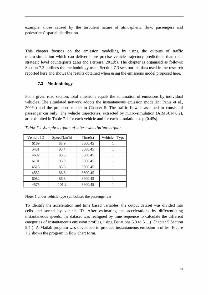
81
example, those caused by the turbulent nature of atmospheric flow, passengers and
pedestrians‟ spatial distribution.
This chapter focuses on the emission modelling by using the outputs of traffic
micro-simulation which can deliver more precise vehicle trajectory predictions than their
strategic level counterparts (Zhu and Ferreira, 2012b). The chapter is organised as follows:
Section 7.2 outlines the methodology used. Section 7.3 sets out the data used in the research
reported here and shows the results obtained when using the emissions model proposed here.
7.2 Methodology
For a given road section, total emissions equals the summation of emissions by individual
vehicles. The simulated network adopts the instantaneous emission model(Int Panis et al.,
2006a) and the proposed model in Chapter 5. The traffic flow is assumed to consist of
passenger car only. The vehicle trajectories, extracted by micro-simulation (AIMSUN 6.2),
are exhibited in Table 7.1 for each vehicle and for each simulation step (0.45s).
Table 7.1 Sample outputs of micro-simulation outputs
Note: 1 under vehicle type symbolises the passenger car
To identify the acceleration and time based variables, the output dataset was divided into
cells and sorted by vehicle ID. After estimating the accelerations by differentiating
instantaneous speeds, the dataset was realigned by time sequence to calculate the different
categories of instantaneous emission profiles, using Equations 5.3 to 5.11( Chapter 5 Section
5.4 ). A Matlab program was developed to produce instantaneous emission profiles. Figure
7.2 shows the program in flow chart form.
Vehicle ID Speed(km/h) Time(s) Vehicle Type
6169 88.9 3600.45 1
5431 93.4 3600.45 1
4602 95.5 3600.45 1
6101 95.9 3600.45 1
4516 85.3 3600.45 1
4552 86.8 3600.45 1
6082 86.8 3600.45 1
4575 101.2 3600.45 1

82
Figure 7.2 Framework for the micro-scale emission model application
7.3 Case-studies
The proposed new emissions models have been applied to two scenarios in Brisbane, namely, a
section of motorway and a section of signalised arterial road. Significant amounts of emissions are
generated at both locations. In addition, the dynamic nature of motorway traffic (Johnson and Ferreira,
2001) and the stop-start behaviour of traffic flow at intersections provide a series of challenges to
modelling accuracy (Li et al., 2004). For the motorway simulation, the transition between congestion
and free flow leads to a significant gap between simulated results and actual measurements (Zhu and
Ferreira, 2012a). The new emission model can also be used to analyse traffic flow at
signalised intersections. The deceleration and acceleration event behaviours at an intersection affect
the emission intensity significantly (Minoura et al., 2009). Generally, the simulation of queues poses a
number of challenges, namely: the acceleration profile of the leading vehicle in the queue and the
headway of the following vehicles. Currently, constant acceleration is assumed by most simulation
packages. However, Long (2000) has shown that linearly decreasing acceleration rates better
represent both maximum vehicle acceleration capabilities and actual motorist behaviour. For the
headway problem, Jin et al. (2009) have found that the distributions of the departure headways at each
position in a queue are shown to approximately follow a log-normal distribution and the
corresponding mean values level out gradually.
7.3.1 Motorway example
The section of motorway used for the study is part of the Pacific Motorway in Brisbane,
selected from a large set of potential locations to avoid the merging and diverging effects on
the mainstream motorway traffic flow (TRB, 2010). The chosen section consists of three
lanes. Its distance to the CBD of Brisbane is shown in Figure 7.3. Figure 7.4 demonstrates
Simulation Outputs by Micro-simulation
Input Variables by Emission Model
e.g. Speed, Acceleration and Vehicle type
Extract
Match Set of Coefficients by Fleet Characters
e.g. Vehicle type, Engine type, Age
Produce
Emission Prediction Inventories, including
Fuel consumption, Gaseous Emission and PM

83
profiles of varied gaseous emissions by the instantaneous emission model and the proposed
new model. Figure 7.5 illustrates the real-time vehicle counts and average speed on the
motorway section. They show that the emissions are correlated with the traffic volume in the
case of continuous traffic flow.
Figure 7.3 Pacific highway network diagram
(a) HC emission profile by the instantaneous emission model (Int Panis et al., 2006b)
Selected Section (20 km to CBD)

84
(b)HC emission profile using the proposed emission model (Zhu et al., 2013)
(c) CO emission profile using the proposed emission model (Zhu et al., 2013)
(d) NOx emission profile using the proposed emission model (Zhu et al., 2013)
Figure 7.4 Emission profiles for the motorway
(a) Traffic flow on the motorway section (three lanes)

85
(b) Average speed on the motorway section (three lanes)
Figure 7.5 Motorway section vehicle counts and average speed
7.3.2 Intersection example
The signalled intersection of Cleveland-Redland Bay Rd and Benfer Rd has been previously
modelled using the VISSIM package (Galiza and Tavassoli, 2009). One north-bound lane
was selected here to be the test-bed site. A major proportion of vehicle emissions occur at the
intersection approaches, due to the final acceleration to cruising speed and to the stop-and-go
cycles (EPA, 2003). Figure 7.6 shows the location of the network under study. Figure 7.7
demonstrates varied simulated profiles of gaseous emissions by the instantaneous emission
model and the proposed new model. Figure 7.8 illustrates the traffic queue at the intersection.
In contrast to the motorway case, the emissions at the intersection vary dramatically. The
acceleration (start-go) at the intersection accounts for a significant share of emissions.
Figure 7.6 Cleveland network map
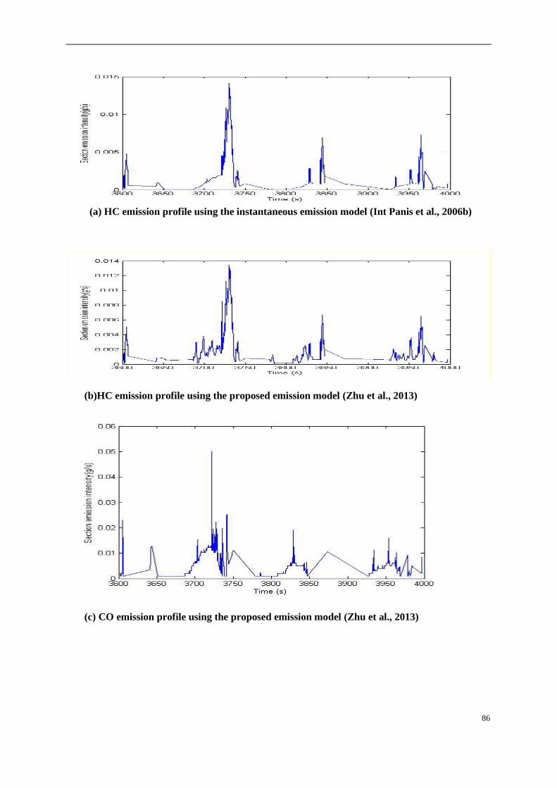
86
(a) HC emission profile using the instantaneous emission model (Int Panis et al., 2006b)
(b)HC emission profile using the proposed emission model (Zhu et al., 2013)
(c) CO emission profile using the proposed emission model (Zhu et al., 2013)

87
(d) NOx emission profile using the proposed emission model (Zhu et al., 2013)
Figure 7.7 Simulated emission profiles for a signalised intersection
(a) Total traffic at the intersection (one lane)
(b) Total queued traffic at the intersection (one lane)
Figure 7.8 Traffic at the intersection

88
7.4 Updating Aimsun equations to Australian conditions
The updating of „default‟ parameters used in AIMSUN to represent the Australian vehicle
fleet characteristics has been undertaken as part of the current research. The following two
main steps were performed:
(1) The NISE2 dataset was used in conjunction with the CUEDC (1800 seconds) as
described in Chapter 2. For each vehicle, the average speed, acceleration and emission rate
were used for each second of time interval. Average values for these variables were derived
by vehicle category. The NISE2 tested light-duty petrol vehicles were divided according to a
matrix of vehicle categories, based mainly on engine capacity and the number of cylinders.
The six vehicle categories used were:
Small passenger (PV-S)
Medium passenger (PV-M)
Large passenger (PV-L)
Compact sport utility (SUV-C)
Large sport utility (SUV-L)
Light Commercial (LCV)
For each category, non-linear multiple regression was used to estimate the best-fit parameters
for the AIMSUN model (Equation 3.6).
(2) Having established new parameters for each pollutant, the resulting predictive models
were validated with the NISE2 dataset vehicles that were not used in the calibration process.
The recalibrated NOx emissions model was developed using all NISE2 vehicles with the
exception of 10 vehicles in each category, which were used to validate the model. The results
of using the improved model with these „validation‟ vehicles are shown in Figure 7.9(a) for
the LCV vehicle category. Figure 7.9(b) shows the corresponding results obtained when
AIMSUN default parameters were used.

89
Figure 7.9(a): NOx emission predictions for the same sample of LCV vehicles (using the new
parameters)
Figure 7.9(b): NOx emission predictions for the same sample of LCV vehicles (using the
AIMSUN default parameters)
Figure 7.9 NOx emission predictions for the same sample of LCV vehicles
The summary results for all vehicle categories are shown in Table 7.2. There has been a
significant improvement in the predictive ability of the recalibrated model, with the
coefficient of determination (R2) increasing to more than 0.6 for most vehicle categories.
R² = 0.7952
0
0.01
0.02
0.03
0.04
0.05
0 0.01 0.02 0.03 0.04 0.05 0.06 0.07
NIS
E2
ob
serv
ati
on
s (g
)
AIMSUN prediction (g)
New parameters
R² = 0.1816
0
0.01
0.02
0.03
0.04
0.05
0 0.001 0.002 0.003 0.004 0.005 0.006
NIS
E2
ob
serv
ati
on
s (g
)
AIMSUN prediction (g)
Default parameters

90
Table 7.2 Evolution of the goodness of fit parameters
To calibrate new parameters for the estimation of VOC and CO, the NISE2 dataset was used
which included a total of 40 vehicles for validation purposes. Figure 7.10 and Figure 7.11
show the overall comparison of the model and observed results, when the new parameters are
used. They also show the performance of the model for all vehicles combined and for LCVs
separately. A significant improvement is seen when compared with the use of the original
default parameters.
Figure 7.10 (a): VOC emission predictions for all vehicles
R² = 0.7092
0
0.003
0.006
0.009
0.012
0 0.0005 0.001 0.0015 0.002 0.0025 0.003 0.0035 0.004 0.0045 0.005
NIS
E2
ob
serv
ati
on
s (g
)
AIMSUN prediction (g)
All vehicles
R-Sq. (R2) Total cycle emissions (g)
Ratio New
Ratio Pollutant Vehicle Default New
AIMSUN
default AIMSUN new
NISE2
Average
NOx
PV-S 35% 63%
1.57
7.74 2.79 0.56 2.77
PV-M 1% 26% 9.45 3.21 0.49 2.94
PV-L 12% 52% 12.62 8.89 0.18 1.42
SUV-C 12% 54% 8.85 4.35 0.36 2.03
SUV-L 28% 67% 16.91 6.67 0.24 2.54
LCV 18% 80% 20.75 12.73 0.12 1.63

91
Figure 7.10(b): VOC emission predictions for LCVs
Figure 7.10 Performance of VOC emission predictions
Figure 7.11(a): CO emission predictions for all vehicles
R² = 0.7304
0
0.004
0.008
0.012
0.016
0.02
0 0.001 0.002 0.003 0.004 0.005 0.006 0.007 0.008 0.009 0.01
NIS
E2 o
bse
rvat
ion
s (g
)
AIMSUN prediction (g)
LCV vehicles
R² = 0.5775
0
0.05
0.1
0.15
0.2
0.25
0 0.01 0.02 0.03 0.04 0.05 0.06 0.07 0.08 0.09 0.1
NIS
E2
ob
serv
ati
on
s (g
)
AIMSUN prediction (g)
All vehicles

92
Figure 7.11(b): CO emission predictions for LCVs
Figure 7.11 Performance of CO emission predictions
Finally, Table 7.3 shows the new set of parameters that have been determined for each of the
pollutants. For NOx, every category has its own set of parameters, whereas for VOC and CO
there are two set of parameters, namely, those representing the LCV category and those
representing all other vehicle categories.
Table 7.3 New model parameters for Australian conditions
Pollutant Vehicle
category
Acceleration
(a) E0 f1 f2 f3 f4 f5 f6
NOx
PV-S (a≥-0.5 m/s2) 0.001 1.00E-03 8.01E-05 9.35E-06 -3.00E-03 1.00E-03 1.00E-03
(a<-0.5 m/s2) 0.001 1.00E-03 2.77E-05 4.31E-06 1.00E-03 0.00E+00 2.36E-05
PV-M (a≥-0.5 m/s2) 0.001 1.00E-03 9.03E-05 1.39E-05 -3.00E-03 1.00E-03 1.00E-03
(a<-0.5 m/s2) 0.001 1.00E-03 9.93E-05 4.80E-06 1.00E-03 1.00E-03 3.60E-05
PV-L (a≥-0.5 m/s2) 0 1.00E-03 0.00E+00 3.35E-05 -1.00E-03 1.00E-03 0.00E+00
(a<-0.5 m/s2) 0.002 -5.00E-03 9.84E-05 4.24E-05 -3.00E-03 1.00E-03 1.00E-03
SUV-C (a≥-0.5 m/s2) 0.001 1.00E-03 0.00E+00 1.73E-05 -2.00E-03 1.00E-03 1.00E-03
(a<-0.5 m/s2) 0 1.00E-03 -5.11E-05 7.50E-06 1.00E-03 0.00E+00 -2.71E-07
SUV-L (a≥-0.5 m/s2) 0.002 2.00E-03 -9.22E-05 3.61E-05 -2.00E-03 1.00E-03 2.00E-03
(a<-0.5 m/s2) 0.001 2.00E-03 0.00E+00 1.08E-05 3.00E-03 1.00E-03 5.26E-05
LCV (a≥-0.5 m/s2) 0 1.00E-03 -6.07E-05 5.13E-05 -2.00E-03 1.00E-03 2.00E-03
(a<-0.5 m/s2) 0.001 2.00E-03 3.75E-05 1.57E-05 1.00E-03 1.00E-03 9.41E-05
VOC
ALL (a≥-0.5 m/s2) 0 7.55E-04 8.92E-05 -2.04E-06 -2.05E-04 2.45E-04 1.21E-04
(a<-0.5 m/s2) 0 5.98E-04 1.13E-04 -3.92E-06 -2.30E-04 -8.23E-05 2.27E-05
LCV (a≥-0.5 m/s2) 0 2.16E-03 2.12E-04 -5.13E-06 -6.87E-04 3.79E-04 2.32E-04
(a<-0.5 m/s2) 0 1.75E-03 3.86E-04 -1.35E-05 -7.98E-04 -1.99E-04 1.06E-04
CO
ALL (a≥-0.5 m/s2) 0 6.64E-03 1.46E-03 -5.69E-06 -1.37E-02 4.66E-03 3.36E-03
(a<-0.5 m/s2) 0 2.75E-03 2.23E-03 -6.45E-05 -6.97E-03 -2.49E-03 3.94E-04
LCV (a≥-0.5 m/s2) 0 1.89E-02 3.00E-03 1.95E-06 -5.72E-02 1.70E-02 8.89E-03
(a<-0.5 m/s2) 0 4.13E-03 7.21E-03 -2.41E-04 -2.47E-02 -8.12E-03 1.11E-03
R² = 0.4656
0
0.2
0.4
0.6
0.8
1
0 0.05 0.1 0.15 0.2 0.25
NIS
E2
ob
serv
ati
on
s (g
)
AIMSUN prediction (g)
LCV vehicles

93
7.5 Summary
Because the lagged variables were unavailable at the beginning of simulation, the proposed
new model underestimates the emission intensity for the un-signalised traffic condition. The
two scenarios tested here show very different emission profiles. The acceleration component
of the new model shows more sensitive reactions to vehicle acceleration, compared with the
single-equation instantaneous model (the instantaneous emissions model).
Instead of the proposed new models, the coefficient localisation of the equation has resulted
in a reduction of the measurement related error in the models, as the results have shown
moderate improvements in the predictive ability of the models. However, the overall levels of
accuracy present in such predictions remain poor, compared with the results in Table 5.3
-Table 5.5.
The profiles shown here for gaseous emission intensity demonstrate the advantage of
emission micro-simulation modelling. The high-resolution predictions are more reliable due
to the ability to deal with the dynamic nature of the vehicle trajectories. The emissions results
for the motorway example depend on dynamic traffic conditions. On the other hand, the
emissions results for the intersection example are mainly related to vehicle acceleration
behaviour. The proposed new model is robust under varied traffic operations, despite the fact
that the added model complexity means increased potential estimation forecasting errors. On
the level of individual vehicle operation, there is a substantial gap between traffic simulation
and traffic flow measurement for both signalised and non-signalised traffic. Therefore, the
enhancement of emission predictions rests to a large extent on further improvements to traffic
micro-simulation models.

94
Conclusions Chapter 8.
8.1 Main findings
General
Predictions of the pollution impacts of mode and route choice decisions need to be considered
in conjunction with conventional travel demand modelling outputs. In order to evaluate the
environmental impacts generated by the implementation of particular transportation
management schemes over a period of time and make sound policy-related decisions based
on such evaluations, environmental emissions models need to be developed as accurate and
reliable assessment tools.
This thesis has reviewed macro and micro level emissions models which are integrated with
corresponding traffic models. Strategic travel demand models tend to be large and regional in
nature, whereas micro simulation models are used for detailed tactical or operational testing
of options. Hence, microscopic traffic models should integrate real time emission prediction
models, which are able to utilise high-resolution transportation modelling results, thereby
generating potentially more precise emission estimates. The micro level models have been
classified and evaluated here in terms of modelling approach, accuracy and robustness. The
modelling approaches are classified into three types, namely: power based; speed based; and
hybrid models. A review of microscopic emissions models has been undertaken using the
results of Australian vehicle emissions measured in the field. It was found that the
„instantaneous traffic emissions‟ (model 5) produced the best overall result of modelling
evaluations.
Development of emissions model
A comprehensive review of the relevant literature was undertaken (Chapter 3). It was found
that the modelling of gaseous pollutants, namely CO, HC and NOx continues to present
significant challenges. Based on the reviews in Chapter 3, microscopic models use a
combination of instantaneous velocity and acceleration to predict various gaseous pollutants
including HC and CO. A range of variables for the instantaneous and lag velocity,
acceleration and CO2 emission rate were selected and tested. As a result, this thesis proposes
a GA-based methodology to select the most appropriate explanatory variables, including
lagging variables, to predict vehicle emissions. This method provides a new approach to the
selection of a combination of variables among a large potential set. The new models deliver
not only more accurate predictions but also robust performance for several types of vehicles.
The approach is capable of solving combinatorial optimisation problems. To improve
computational efficiency, distributed synchronous GA is based on distribution of workload
among processors during the fitness function evaluation phase followed by a single central
population regeneration. Hence, the massive fitness computations are assigned to workers in
order to improve the computation efficiency.

95
Moreover, the proposed GA methodology provides a solution for a combinatorial
optimisation problem, providing high modelling accuracy with statistically significant
relationships between the selected predicting variables and the dependant variable.
Uncertainty analysis
To arrive at an optimal emissions modelling outcome, the interaction between two
components namely, input data and model specification, needs to be taken into account. A
more complex model may negate the overall modelling accuracy by increasing input data
uncertainties. Hence, a compromise solution needs to be found. The two types of errors
exhibit distinct characteristics for each stage of driving behaviour. Under free traffic flow
conditions, the two types of errors are closely aligned and the overall accuracy of model
outputs is close to its optimum level. However, the input data errors provide the main source
of estimated uncertainty for traffic flow conditions of transition to congestion and very
congested stages.
The micro-simulation modelling of congested and near congested traffic flow conditions
yield significantly less robust estimates than is the case with free flow conditions. Model
input data related to average vehicle speeds and accelerations at the micro-scale level, are
critical to reduce overall emissions estimation errors. The profiles show more sensitive
reactions to vehicle acceleration, compared with the single-equation instantaneous model.
This is particularly so for congested and near congested stages of the simulation. For
applications of micro-simulation models dealing with urban congested conditions, the largest
gain in terms of the likely accuracy of emissions estimates would seem to rest with
improvement in input data reliability. Int Panis et al.‟s (2006b) emission model has several
advantages for CO2 modelling, including good prediction accuracy and concise modelling
structure. The complexity of emission modelling structures may not yield increased overall
accuracy until the uncertainties attached to the input data can be significantly improved.
Emission modelling application
In Chapter 7, the new emission model was applied to a case study in Brisbane. Using
different scenarios for different road configurations and traffic conditions, the results of
applying the new approach were compared with those obtained by using default emissions
parameters commonly found in a simulation package. The high-resolution profiles for
gaseous emission intensity demonstrate the advantage of emission micro-simulation
modelling. The high-resolution predictions are more reliable due to the ability to deal with
the dynamic nature of vehicle trajectories. The proposed new model is robust under varied
traffic operations, despite the fact that the added model complexity means increased potential
estimation forecasting errors.

96
8.2 Research limitation and future research
Emissions model development
Despite the significant overall improvements for the modelling of gaseous pollutants, the
models proposed here produce relatively low accuracy in predicting emissions for the
deceleration mode. In addition, the accuracy of the new model may be compromised when
driving with loads or in hilly terrain. Future research should focus on extending the modelling
scope to include the full set of PM. Further investigations need to be put forward on the
ageing effect of engines and catalytic converters along with emission modelling of emerging
vehicle technologies, such as hybrid engine technology.
Modelling uncertainty
As was demonstrated in Chapter 6, Monte Carlo simulation is an effective methodology to
address the quantification of modelling uncertainty. However, the uncertainties of input
variables, such as vehicle speed and acceleration, need to be verified by high-resolution field
data for the motorway scenario. For the signalised intersection scenario, the acceleration
behaviour of the leading vehicles at intersections, as well as the following car headways are
significant for queue simulation and emissions estimation. The assumption of constant
acceleration was found to deviate substantially from observations collected by a driving
simulator study. The latter also shows that the acceleration characteristics are significantly
different between participants. In the case of signalised intersection flows, the emissions
modelling is dependent on complex vehicle interactions, including queue discharging. Future
enhancement of emission predictions rests to a large extent on further improvements to traffic
micro-simulation models.
Modelling applications
The proposed emission model underestimates the emission intensity due to the absence of lag
variables at the beginning of the simulation period. To overcome this problem, the emission
model could be efficiently and effectively integrated with micro-simulation software.
The two scenarios based on different traffic conditions, show very different instantaneous
emission profiles. At the level of individual vehicle operation, there is a substantial gap
between traffic simulation and traffic flow measurement for both signalised and
non-signalised traffic flow conditions. The emission results for the motorway example
depend on dynamic traffic conditions. On the other hand, the emission results for the
intersection example are mainly related to acceleration behaviour of the queued vehicles. In
Appendix B, a new acceleration profile is proposed to simulate the leading vehicle in a queue.
The resultant emission predictions are significantly different from the common
constant-acceleration profile. Also, it could replace the constant-acceleration assumption.
Moreover, a stochastic simulation approach, instead of a deterministic profile, may be
adopted by traffic simulation packages to fit with the randomness of acceleration behaviours
of the leading vehicle.

97
References
Abaza, K., Ashur, S., Al-Khatib, I., 2004. Integrated Pavement Management System with a
Markovian Prediction Model. Journal of Transportation Engineering 130(1), 24-33.
ABS, 2009. Motor vehicle census, In: 9309.0. Australian Bureau of Statistics, Canberra.
Ahn, K., Rakha, H., Trani, A., Van Aerde, M., 2002. Estimating vehicle fuel consumption
and emissions based on instantaneous speed and acceleration levels. Journal of
Transportation Engineering 128(2), 182-190.
Ahrens, C.D., 2003. Meteorology today: an introduction to weather, climate, and the
environment. Thomson/Brooks/Cole.
Akcelik, R., Besley, M., 2003. Operating cost, fuel consumption and emission models in
aaSidra and aaMotion, 25th Conference of Australian Institutes of Transport Research
(CAITR), University of South Australia, Adelaide, Australia.
André, M., 2004. The ARTEMIS European driving cycles for measuring car pollutant
emissions. Science of The Total Environment 334–335(0), 73-84.
André, M., Rapone, M., 2009. Analysis and modelling of the pollutant emissions from
European cars regarding the driving characteristics and test cycles. Atmospheric Environment
43(5), 986-995.
Barth, M., An, F., Norbeck, J., Ross, M., 1996. Modal emissions modeling: A physical
approach. Transportation Research Record(1520), 81-88.
Barth, M., Scora, G., 2006. Comprehensive modal emissions model (CMEM), User‟s Guide,
Version 3.01. University of California, Riverside.
BCC/QGEPA, 2004. Air Emissions inventory South-East Queensland Region, In: Agency,
B.C.C.a.Q.G.E.P. (Ed.), Brisbane, Queensland.
Biggs, D.C., Akcelik, R., 1986. An energy related model of instantaneous fuel consumption.
Traffic Engineering & Control 27(6), 320-325.
Biona, J.B.M., Culaba, A., 2006. Drive cycle development for tricycles. Clean Technologies
and Environmental Policy 8(2), 131-137.
Bourrel, E., Lesort, J.-B., 2003. Mixing microscopic and macroscopic representations of
traffic flow: Hybrid model based on Lighthill-Whitham-Richards theory. Transportation
Research Record: Journal of the Transportation Research Board 1852(-1), 193-200.
Cantú-Paz, E., 1998. A survey of parallel genetic algorithms. Calculateurs paralleles,
reseaux et systems repartis 10(2), 141-171.
Chatterjee, S., Laudato, M., Lynch, L.A., 1996. Genetic algorithms and their statistical
applications: an introduction. Computational Statistics & Data Analysis 22(6), 633-651.
Chowdhury, D., Santen, L., Schadschneider, A., 2000. Statistical physics of vehicular traffic
and some related systems. Physics Report 329(4-6), 199-329.
Chung, E., Rahman, M., Bevrani, K., Jiang, R., 2011. Evaluation of Queensland Department
of Transport and Main Roads Managed Motorways. Smart Transport Research Centre,
Queensland University of Technology, Brisbane
DTMR, 2010. Guidelines for the configuration and placement of vehicle detection sensors,
Traffic and Road Use Management Manual. Department of Transport and Main
Roads.Queensland Government, Brisbane , Australia.
DTMR, 2011. Pacific Motorway M1 Project location map. DTMR.
EPA, 1989. Federal Test Procedure.
EPA, 1997. Risk Assessment Forum, Guiding Principles for Monte Carlo Analysis.
EPA/630/R-97/001.
EPA, 2003. User's Guide to MOBILE6.1 and MOBILE6.2; Mobile Source Emission Factor
Model, EPA420-R-03-010. EPA, Washington, DC.

98
EPA, 2005. Clean Fuel Fleet Exhaust Emission Standards, In: Office of Transportation and
Air Quality , E.P.A. (Ed.), United States
Favez, J.-Y., Weilenmann, M., Stilli, J., 2009. Cold start extra emissions as a function of
engine stop time: Evolution over the last 10 years. Atmospheric Environment 43(5),
996-1007.
Fenger, J., 1999. Urban air quality. Atmospheric Environment 33(29), 4877-4900.
Ferreira, L., 2007. Using strategic transport models to predict energy, climate change and air
quality impacts, Portfolio Transport Modelling Team. Queensland Transport, Brisbane.
Frey, H.C., Rouphail, N.M., Zhai, H., 2006. Speed-and facility-specific emission estimates
for on-road light-duty vehicles on the basis of real-world speed profiles. Transportation
Research Record: Journal of the Transportation Research Board 1987(-1), 128-137.
Galiza, R., Tavassoli, A., 2009. REDLAND BAY RD UPGRADE: MICRO-SIMULATION
MODEL (VISSIM). ITS Research Laboratory, UQ Brisbane, QLD
Gentle, J.E., 2003. Random Number Generation and Monte Carlo Methods.
Springer-Verlag,Inc. , New York.
Godley, S.T., Triggs, T.J., Fildes, B.N., 2002. Driving simulator validation for speed research.
Accident Analysis & Prevention 34(5), 589-600.
Gordon, T., Bareket, Z., Kostyniuk, L., Barnes, M., Hagan, M., Kim, Z., Cody, D.,
Skabardonis, A., 2012. Site-Based Video System Design and Development.
Heywood, J.B., 1988. Internal Combustion Engine Fundamentals McGraw-Hill, New York.
Hidas, P., 2006. Evaluation and further development of car following models in microscopic
traffic simulation, pp. 287-296.
Hourdakis, J., Michalopoulos, P.G., Kottommannil, J., 2003. Practical Procedure for
Calibrating Microscopic Traffic Simulation Models, pp. 130-139.
Hung, W.T., Tong, H.Y., Lee, C.P., Ha, K., Pao, L.Y., 2007. Development of a practical
driving cycle construction methodology: A case study in Hong Kong. Transportation
Research Part D: Transport and Environment 12(2), 115-128.
Int Panis, L., Broekx, S., Liu, R., 2006a. Modelling instantaneous traffic emission and the
influence of traffic speed limits. Science of the Total Environment 371(1-3), 270-285.
Int Panis, L., Broekx, S., Liu, R., 2006b. Modelling instantaneous traffic emission and the
influence of traffic speed limits. Science of The Total Environment 371(1–3), 270-285.
Isaacson, D.L., Madsen, R.W., 1985. Markov chains: theory and applications. RE Krieger
Publishing Company.
Jamriska, M., Morawska, L., 2001. A model for determination of motor vehicle emission
factors from on-road measurements with a focus on submicrometer particles. Science of The
Total Environment 264(3), 241-255.
Jin, X., Zhang, Y., Wang, F., Li, L., Yao, D., Su, Y., Wei, Z., 2009. Departure headways at
signalized intersections: A log-normal distribution model approach. Transportation Research
Part C: Emerging Technologies 17(3), 318-327.
Johnson, L., Ferreira, L., 2001. Modelling particle emissions from traffic flows at a freeway
in Brisbane, Australia. Transportation Research Part D: Transport and Environment 6(5),
357-369.
Keogh, D.U., Kelly, J., Mengersen, K., Jayaratne, R., Ferreira, L., Morawska, L., 2010.
Derivation of motor vehicle tailpipe particle emission factors suitable for modelling urban
fleet emissions and air quality assessments. Environmental Science and Pollution Research
17(3), 724-739.
Kerner, B.S., 2004. Three-phase traffic theory and highway capacity. Physica A: Statistical
Mechanics and its Applications 333(1-4), 379-440.

99
Kim, I., Ferreira, L, Tey, LS and Wallis, G, 2013. Integration of driving simulator and traffic
simulation to analyse behavior at railway crossings, Proceedings of the Institution of
Mechanical Engineers, Part F: Journal of Rail and Rapid Transit.
Klauer, B., Brown, J.D., 2004. Conceptualising imperfect knowledge in public decision
making: ignorance, uncertainty, error and 'risk situations'. Environmental Research,
Engineering and Management 27(1), 124-128.
Kousa, A., Kukkonen, J., Karppinen, A., Aarnio, P., Koskentalo, T., 2002. A model for
evaluating the population exposure to ambient air pollution in an urban area. Atmospheric
Environment 36(13), 2109-2119.
Kroese, D.P., Taimre, T., Botev, Z.I., 2011. Handbook of Monte Carlo Methods. John Wiley
and Sons,Inc. , New Jersey.
Leung, D.Y.C., Williams, D.J., 2000. Modelling of motor vehicle fuel consumption and
emissions using a power-based model. Environmental Monitoring and Assessment 65(1-2),
21-29.
Li, X., Li, G., Pang, S.-S., Yang, X., Tian, J., 2004. Signal timing of intersections using
integrated optimization of traffic quality, emissions and fuel consumption: a note.
Transportation Research Part D: Transport and Environment 9(5), 401-407.
Lin, J., Niemeier, D.A., 2003. Estimating regional air quality vehicle emission inventories:
Constructing robust driving cycles. Transportation Science 37(3), 330-346.
Logothetis, N., 1988. Role of data transformation in taguchi analysis. Quality and Reliability
Engineering International 4(1), 49-61.
Logothetis, N., Haigh, A., 1988. CHARACTERIZING AND OPTIMIZING
MULTI-RESPONSE PROCESSES BY THE TAGUCHI METHOD. Quality and Reliability
Engineering International 4(2), 159-169.
Long, G., 2000. Acceleration Characteristics of Starting Vehicles. Transportation Research
Record: Journal of the Transportation Research Board 1737(-1), 58-70.
Luque, G., 2011. Parallel genetic algorithms: theory and real world applications.
Springer-Verlag, Berlin.
MathWorks, 2012. MATLAB Documentation.
Minocha, V.K., 2005. Discussion of “Impact Stops on Vehicle Fuel Consumption and
Emissions” by Hesham Rakha and Yonglian Ding. Journal of Transportation Engineering
131(7), 571-571.
Minoura, H., Takekawa, H., Terada, S., 2009. Roadside nanoparticles corresponding to
vehicle emissions during one signal cycle. Atmospheric Environment 43(3), 546-556.
Mitchell, M., 1998. An Introduction to Genetic Algorithms. Mit Press, Cambridge, MA.
Morawska, L., Keogh, D.U., Thomas, S.B., Mengersen, K., 2008a. Modality in ambient
particle size distributions and its potential as a basis for developing air quality regulation.
Atmospheric Environment 42(7), 1617-1628.
Morawska, L., Ristovski, Z., Jayaratne, E.R., Keogh, D.U., Ling, X., 2008b. Ambient nano
and ultrafine particles from motor vehicle emissions: Characteristics, ambient processing and
implications on human exposure. Atmospheric Environment 42(35), 8113-8138.
Morawska, L., Thomas, S., Bofinger, N., Wainwright, D., Neale, D., 1998. Comprehensive
characterization of aerosols in a subtropical urban atmosphere: Particle size distribution and
correlation with gaseous pollutants. Atmospheric Environment 32(14-15), 2467-2478.
Muthén, L.K., Muthén, B.O., 2002. How to use a Monte Carlo study to decide on sample size
and determine power. Structural Equation Modeling 9(4), 599-620.
Nishihata, Y., Mizuki, J., Akao, T., Tanaka, H., Uenishi, M., Kimura, M., Okamoto, T.,
Hamada, N., 2002. Self-regeneration of a Pd-perovskite catalyst for automotive emissions
control. Nature 418(6894), 164-167.

100
North, R.J., Noland, R.B., Ochieng, W.Y., Polak, J.W., 2006. Modelling of particulate matter
mass emissions from a light-duty diesel vehicle. Transportation Research Part D: Transport
and Environment 11(5), 344-357.
Orbital, 2009. Second national in-service emissions study (NISE2): light duty petrol vehicle
emissions testing. Road and Traffic Authority of New South Wales.
Pandian, S., Gokhale, S., Ghoshal, A.K., 2009. Evaluating effects of traffic and vehicle
characteristics on vehicular emissions near traffic intersections. Transportation Research
Part D: Transport and Environment 14(3), 180-196.
Panwai, S., Dia, H., 2005. Comparative evaluation of microscopic car-following behavior.
IEEE Transactions on Intelligent Transportation Systems 6(3), 314-325.
PTV, A., 2005. VISUM User Manual Version 9.3. PTV AG
Qi, Y., Teng, H., Yu, L., 2004. Microscale Emission Models Incorporating Acceleration and
Deceleration. Journal of Transportation Engineering 130(3), 348-359.
Rakha, H., Ahn, K., Trani, A., 2003. Comparison of MOBILE5a, MOBILE6, VT-MICRO,
and CMEM models for estimating hot-stabilized light-duty gasoline vehicle emissions.
Canadian Journal of Civil Engineering 30(6), 1010-1021.
Rakha, H.A., Ahn, K., Moran, K., Saerens, B., Bulck, E.V.d., 2011. Virginia Tech
Comprehensive Power-Based Fuel Consumption Model: Model development and testing.
Transportation Research Part D: Transport and Environment 16(7), 492-503.
Refsgaard, J.C., van der Sluijs, J.P., Højberg, A.L., Vanrolleghem, P.A., 2007. Uncertainty in
the environmental modelling process - A framework and guidance. Environmental Modelling
and Software 22(11), 1543-1556.
Samuel, S., Austin, L., Morrey, D., 2002. Automotive test drive cycles for emission
measurement and real-world emission levels - A review. Proceedings of the Institution of
Mechanical Engineers, Part D: Journal of Automobile Engineering 216(7), 555-564.
Smit, R., Dia, H., Morawska, L., 2009. Road traffic emission and fuel consumption modelling:
trends, new developments and future challenges, in: Traffic Related AirPollution. Nova USA
Smit, R., McBroom, J., 2009. Use of microscopic simulation models to predict traffic
emissions. Road and Transport Research 18(2), 49-54.
Toledo, T., 2007. Driving behaviour: Models and challenges. Transport Reviews 27(1),
65-84.
Toledo, T., Koutsopoulos, H.N., Davol, A., Ben-Akiva, M.E., Burghout, W., Andréasson, I.,
Johansson, T., Lundin, C., 2003. Calibration and Validation of Microscopic Traffic
Simulation Tools: Stockholm Case Study, pp. 65-75.
Touran, A., Wiser, E.P., 1992. Monte Carlo technique with correlated random variables.
Journal of Construction Engineering and Management 118(2), 258-272.
TRB, 2010. Highway Capacity Manual 2010. Transportation Research Board 500 Fifth St.
NW, Washington, D.C. 20001.
TSS, 2010. Aimsun 6.1 manual. Transport Simulation System, Barcelona, Spain.
Unal, A., Rouphail, N., Frey, H., 2003. Effect of Arterial Signalization and Level of Service
on Measured Vehicle Emissions. Transportation Research Record: Journal of the
Transportation Research Board 1842(-1), 47-56.
Vladisavljevic, I., Martin, P.T., Stevanovic, A., 2007. Integration of mathematical and
physical simulation to calibrate car-following behaviour of unimpaired and impaired drivers.
World Review of Intermodal Transportation Research 1(4), 403-418.
Walker, W.E., Harremoe, S., P., Rotmans, J., Van der Sluijs, J.P., Van Asselt, M.B.A.,
Janssen, P., Krayer von Krauss, M.P., 2003. Defining uncertainty a conceptual basis for
uncertainty management in model-based decision support. Integrated Assessment 4(1), 5-17.
Walsh, M.P., 2011. Automobiles and Climate Policy in the Rest of the OECD. Cars and
Carbon: Automobiles and European Climate Policy in a Global Context, 355.

101
Wang, J., Dixon, K., Li, H., Ogle, J., 2004. Normal acceleration behavior of passenger
vehicles starting from rest at all-way stop-controlled intersections. Transportation Research
Record: Journal of the Transportation Research Board 1883(1), 158-166.
Weilenmann, M., Favez, J.-Y., Alvarez, R., 2009. Cold-start emissions of modern passenger
cars at different low ambient temperatures and their evolution over vehicle legislation
categories. Atmospheric Environment 43(15), 2419-2429.
Zhu, S., Ferreira, L., 2012a. Assessing the uncertainty in micro-simulation model outputs,
Australasian Transport Research Forum, Perth.
Zhu, S., Ferreira, L., 2012b. Evaluation of vehicle emissions models for micro-simulation
modelling: using CO2 as a case study. Road and Transport Research 21(3), 3-18.
Zhu, S., Tey, L.-S., Ferreira, L., 2013. Modelling Vehicle Gaseous Emissions Using a
Genetic Algorithm Approach-Based on Australian emission data Transportation Research
Part C: Emerging Technologies.
Zito, R., Primerano, F., 2005. NISE2 –Contract 2 Drive Cycle Development Methodology
and Results. Orbital Engine Company and Department of the Environment and Heritage.

102
Appendix A. Assessing the uncertainty in micro-simulation model outputs
(Zhu and Ferreira, 2012a)
Introduction A.1
Micro simulation traffic models continue to be widely used as tools to analyse current and
future road system performance. Such models tend to operate by concentrating on the
movement of individual vehicles in the traffic stream on a second by second basis. The
likely errors associated the outputs of such models are usually thought to be significantly
lower than the „coarser‟ models with deal with the movement of groups of vehicles over an
average time period. The predicted vehicle speeds and the traffic volumes are the most
important traffic indicators, and primary inputs of other models such as emission estimation.
This appendix evaluates the uncertainty in the outputs of micro level models by comparing
those outputs with field data obtained from loop detectors on disaggregated level.
Past works A.2
Currently, limited research has been put forward on the validation of micro simulation
outputs, in terms of the gap between prediction and measurement for vehicle speeds for each
modelled time period. The performance of these types of models, with respect to their ability
to predict average speeds and traffic volumes, is depended on several external and internal
factors. This research focuses on uncertainty induced by internal factors in the form of the
driver behaviour model used. Theoretically, micro simulation has two core algorithms,
namely: car-following and lane-changing, which are the main drivers of overall model
accuracy. Panwai and Dia (2005) undertook a comparative evaluation of car-following
behaviour in a number of traffic simulation models to validate their reliability of the
AIMSUN, PARAMICS, and VISSIM models). The results point to similar performance for
the psychophysical spacing models used in VISSIM and PARAMICS with better
performance reported for the Gipps-based models implemented. Hidas (2006) confirms the
findings and points out that lane-changing behaviour is a challenge for prediction accuracy.
In most models, lane-changing behaviour requires two stages, consideration of lane-
changing and execution. The improvement of lane-changing may be facilitated in two major
directions: an increase in the level of detail in the specification of models to better capture the
complexity and sophistication of human decision-making processes; and an improvement in
the quality of data used to calibrate such these models (Toledo, 2007).
Methodology A.3
This research evaluates the uncertainty in the outputs of micro simulation models by
comparing predicted results with field average speed data obtained from motorway loop
detectors at the 1-minute disaggregated level. Currently, the Queensland based traffic
operations system records real time data by using 1-minute average speed measurements and
other road section performance indicators, such as flow count and density (DTMR, 2010). For
major facilities, such as the Pacific motorway, this data is collected from a network of loop

103
detectors established by the Department of Transport and Main Roads (DTMR, 2011). A
detailed Aimsun traffic micro-simulation model has recently been calibrated using data
obtained from those loop detectors(Chung et al., 2011). Although loop detector data has its
shortcomings, it is the only available extensive data set for model calibration purposes. This
research assumes that detector measurement error can be neglected, after the more obvious
instances of missing or spurious data has been omitted. An initial primary visual check
indicates that the uncertainty in the model outputs is likely to be associated with traffic flow
conditions, such as the level of congestion. Particularly, the fundamental traffic theory is
qualitatively different from empirical traffic flow analysis on over-saturated conditions
(Chowdhury et al., 2000).
Hence, a new traffic flow theory has been proposed, in which flow is classified into three
conditions, namely: free flow; „synchronised ‟ flow and queuing (Kerner, 2004).
Synchronized flow refers to non-interrupted traffic flow without a long period of queuing.
There is a tendency to a synchronization of vehicle speeds across different lanes on a
multi-lane road in this flow.
To evaluate the uncertainty on different traffic conditions, the Taguchi method, an offline
quality control technique, is introduced in this research (Logothetis and Haigh, 1988). This
technique classifies the source of uncertainty into outer and inner noise. In this research, the
former includes the external sources to micro simulation model outputs, such as in traffic
conditions, driving behaviour variations and traffic management strategies. The current
research has focused on the inner noise induced by the simulation algorithm itself. The
performance of system output is evaluated using equation (1).
NSR=
----------------- (1)
Where:
: Speed output expectation
: Absolute output error
NSR: Noise-to-signal ratio, percentage of error to prediction.
The model for the relationship between the output ( ) and its error ( ) is formulated as:
NSR= -------------------- (2)
Where:
: Speed Output expectation
NSR: Noise-to-signal ratio
k and : Coefficients
Equation 2 may have a Box-Cox transformation to produce an improved fitting (Logothetis,
1988).
= -------------------- (3)
The speed prediction uncertainty is defined here as the difference between loop detector
measurement and simulation model output. To have a meaningful simulation speed prediction,
it is necessary to undertaken a calibration of the model parameters to minimize the internal
noise. In engineering practise, calibration uses simulated and actual measurements including

104
traffic volumes, vehicle occupancies and speeds. The deviation between actual and measured
values is minimised by adjusting the simulation parameters through trial-and-error. The
simulation parameters are classified into two main categories, namely: global (those that
affect the performance of the entire model) and local (those that affect only specific sections
of the roadway). Hourdakis et al. (2003) suggest the global parameters are calibrated first
followed by local parameter calibration. Examples of global parameters are the vehicle
characteristics, such as desired speed, maximum acceleration/deceleration, simulation step;
and driver reaction time). Link speed limits and capacities are local parameters. Toledo et al.
(2003) point out the calibration process should begin with disaggregate data including
information on detailed driver behaviour, such as vehicle trajectories of the subject and
surrounding vehicles. Aggregate data (e.g. time headways, speeds, flows, etc.) are used to
fine-tune parameters and estimate general parameters in the simulation. The application of
the Aimsun model to a section of the Pacific Motorway studied here, follows established
calibration methodology (Chung et al., 2011). To minimize the effects of external impacts on
the uncertainty results, the measurement data was selected according to three main criteria, as
shown below.
(1) Quality of instantaneous traffic flow simulated and measured outputs
The quality of simulated flow count was evaluated using Equation (4):
√
----------------------- (4)
Where:
n : Number of observed values
o : Observed value
e : Simulated value
(2) Detector location
To avoid the merging and diverging effects on the mainstream motorway traffic flow, the
selected detectors were around 460 metres away from on-ramp and off-ramp(TRB, 2010).
(3) Incidents affected data
Comparing with minute-by-minute traffic data on other days, the datasets with unusual and
non-recurring traffic congested patterns were excluded to remove incident-induced results.
Dataset description A.4
After detailed validation, three detector groups C/D/E satisfied all three criteria and were
selected from a large set of potential locations. The location of all selected detectors are
shown in Figure 1. The distance to the CBD of Brisbane is also shown in Figure 1. The
selected datasets were used to investigate the relationship between the simulated speed output
and its uncertainty as the flow moves from free flow to highly congested conditions.

105
Detectors A and B were used to investigate free flow and queuing status. The analysis was
undertaken for each minute of both actual measured outputs and simulation model results.
Figure 1: Pacific highway network map and selected detectors
Detector B (2 km to CBD) Detector A (1.4 km to CBD)
Detector C (6 km to CBD)
Detector E (20.3 km to CBD) Detector D (20 km to CBD)
Inbound

106
Uncertainty analysis A.5
Numerous datasets from different locations along the motorway indicate that the uncertainty
in average speeds follows closely a normal distribution under off-peak time periods with free
flow conditions, when tested using the Kolmogorov-Smirnov test. Using detector B as an
example, Figure 2(a) and 2(b) demonstrate the flow and speed results for both the measured
values and simulation outputs during an off-peak period. As a result, the coefficient k is 0 in
Equation 2, showing non-correlation between speed prediction and uncertainty. The
uncertainty expectation is a very low 1.9 km/h with a standard deviation of 4.7 km/h.
Figure 2(a): Simulation and measurement speed during non-peak period
Figure 2(b): Simulation and measurement flow count during non-peak period
-20
0
20
40
60
80
100
12
:00
:00
12
:11
:00
12
:22
:00
12
:33
:00
12
:44
:00
12
:55
:00
13
:06
:00
13
:17
:00
13
:28
:00
13
:39
:00
13
:50
:00
14
:01
:00
14
:12
:00
14
:23
:00
14
:34
:00
14
:45
:00
14
:56
:00
15
:07
:00
15
:18
:00
15
:29
:00
15
:40
:00
15
:51
:00
Spe
ed
(km
/h)
Time
Simulation
Measurment
Error
0
5
10
15
20
25
30
12
:10
:00
12
:21
:00
12
:32
:00
12
:43
:00
12
:54
:00
13
:05
:00
13
:16
:00
13
:27
:00
13
:38
:00
13
:49
:00
14
:00
:00
14
:11
:00
14
:22
:00
14
:33
:00
14
:44
:00
14
:55
:00
15
:06
:00
15
:17
:00
15
:28
:00
15
:39
:00
15
:50
:00
Ve
hic
le c
ou
nt/
min
Time
Measurment
Simulation

107
The vehicle speed related results obtained when measured data for one peak period is
compared with simulation outputs are shown in Figure 3(a) and (b). In the latter, they present
and sort the datasets in the descending order of vehicle speed. In the transitional stage
between free flow and highly congested conditions at detector C, the relationship between
uncertainty and average speed can be fitted using Equation 3. In this case the following
results were obtained:
k= -4.29 and 7.15
Due to traffic speed fluctuations, linear regression analysis shows R2
(Coefficient of
determination) reaches 0.65, and the simulated speed is statistical significant with NSR.
Hence, minus exponential relationship between simulation speed and its NSR is established.
Similarly, the negative correlations during the transitional stage have been replicated at other
locations. Figure 3(b) demonstrates another example from detector E data.
Figure 3(a): Simulation and measurement speed during transitional stage (detector C)
Figure 3(b): Simulation and measurement speed during transitional stage (detector E)
0102030405060708090
5:4
0:0
0
5:4
6:0
0
5:3
7:0
0
6:0
4:0
0
6:0
3:0
0
5:5
6:0
0
5:4
9:0
0
6:1
8:0
0
5:5
2:0
0
5:5
3:0
0
5:5
5:0
0
6:0
6:0
0
6:0
7:0
0
6:1
4:0
0
6:0
9:0
0
6:1
0:0
0
6:2
2:0
0
6:2
3:0
0
Spe
ed
(K
m/h
)
Time
Simulation
Error
-10
0
10
20
30
40
50
60
70
80
90
5:3
8:0
05
:36
:00
5:2
9:0
05
:35
:00
5:3
4:0
05
:57
:00
5:3
9:0
06
:12
:00
9:5
7:0
05
:46
:00
5:5
4:0
05
:58
:00
6:0
1:0
06
:11
:00
6:0
4:0
05
:56
:00
9:5
3:0
06
:03
:00
5:5
5:0
06
:07
:00
5:5
9:0
08
:48
:00
8:3
7:0
0
Spe
ed
(K
m/h
)
Time
Simulation
Error

108
When traffic flow reaches capacity, unstable conditions prevail and simulation results appear
to be much less reliable. For over-saturated conditions, both queuing and „synchronized‟ flow
conditions were found at different locations during periods. Figure 4 shows the speed
measurements at detector C during the peak-hour. The results from the three inbound lanes at
this detector show highly synchronized speeds across all lanes.
Figure 4: Detector C measured speeds in the morning peak hour
Figures 5(a) and 5(b) demonstrate modelled and measured vehicle speeds and volumes,
respectively. The results related to detector C and a 3-hour morning peak period. The
modelled traffic volume results show good agreement with measured values. The modelled
vehicle speeds, when compared with measured values, follow a normal distribution. The
uncertainty expectation is estimated at 23.2 km/h with a standard deviation is 10.4 km/h.
Figure 5(a): Simulated and measured average speeds: morning peak period (detector C)
0
10
20
30
40
50
60
70
80
6:3
0:0
0
6:3
7:0
0
6:4
4:0
0
6:5
1:0
0
6:5
8:0
0
7:0
5:0
0
7:1
2:0
0
7:1
9:0
0
7:2
6:0
0
7:3
3:0
0
7:4
0:0
0
7:4
7:0
0
7:5
4:0
0
8:0
1:0
0
8:0
8:0
0
8:1
5:0
0
8:2
2:0
0
8:2
9:0
0
8:3
6:0
0
8:4
3:0
0
8:5
0:0
0
8:5
7:0
0
Spe
ed
(km
/h)
Time
Detector C Lane 1
Detector C Lane 2
Detector C Lane 3
-40
-20
0
20
40
60
80
100
120
5:0
1:0
0
5:1
6:0
0
5:3
1:0
0
5:4
6:0
0
6:0
1:0
0
6:1
6:0
0
6:3
1:0
0
6:4
6:0
0
7:0
1:0
0
7:1
6:0
0
7:3
1:0
0
7:4
6:0
0
8:0
1:0
0
8:1
6:0
0
8:3
1:0
0
8:4
6:0
0
9:0
1:0
0
9:1
6:0
0
9:3
1:0
0
9:4
6:0
0
Spe
ed
(km
/h)
Time
Simulation
Measurement
Error

109
Figure 5(b): Simulated and measured traffic flow: morning peak period (detector C)
Similarly, Figures 6(a) and 6(b) demonstrate minute-by-minute traffic volumes and average
speeds respectively. The data was collected at detector A in the morning peak direction.
Traffic moves into queuing conditions for long periods, speed prediction uncertainty follows
a normal distribution. The error expectation is 7.2 km/h with a standard deviation of 5.3
km/h, indicating the significant difference between queuing and „synchronized‟ flow, as
defined earlier.
Figure 6(a): Simulated and measured average speed during peak hours (detector A)
0
5
10
15
20
25
30
35
40
45
5:0
1:0
0
5:1
4:0
0
5:2
7:0
0
5:4
0:0
0
5:5
3:0
0
6:0
6:0
0
6:1
9:0
0
6:3
2:0
0
6:4
5:0
0
6:5
8:0
0
7:1
1:0
0
7:2
4:0
0
7:3
7:0
0
7:5
0:0
0
8:0
3:0
0
8:1
6:0
0
8:2
9:0
0
8:4
2:0
0
8:5
5:0
0
9:0
8:0
0
9:2
1:0
0
9:3
4:0
0
9:4
7:0
0
10
:00
:00
Co
un
t V
eh
/min
Time
Simulation
Measurement
-10
0
10
20
30
40
50
60
7:2
0:0
0
7:2
5:0
0
7:3
0:0
0
7:3
5:0
0
7:4
0:0
0
7:4
5:0
0
7:5
0:0
0
7:5
5:0
0
8:0
0:0
0
8:0
5:0
0
8:1
0:0
0
8:1
5:0
0
8:2
0:0
0
8:2
5:0
0
8:3
0:0
0
8:3
5:0
0
8:4
0:0
0
8:4
5:0
0
8:5
0:0
0
8:5
5:0
0
9:0
0:0
0
Spe
ed
(km
/h)
Time
Simulation
Measurment
Error

110
Figure 6(b): Simulated and measured flow count during peak hours (detector A)
Summary A.6
The research concludes that model uncertainty shows very different characteristics for
different traffic flow conditions. The Taguchi statistical method was applied to three traffic
flow stages to establish the relationships between modelled vehicle speeds and measured
speeds, on a minute-by-minute basis. Model output uncertainty shows very different
characteristics for different traffic flow conditions. The Taguchi statistical method was
applied to three traffic flow stages to establish the relationships between modelled vehicle
speeds and measured speeds, on a minute-by-minute basis. The results show the close
agreement between modelled and actual speeds under free flow conditions, the speed
prediction uncertainties can be considered to follow zero-mean normal distribution (white
noise).
In contrast, the transitional stage between free flow and queuing shows a higher level of
discrepancy. As traffic volumes increase, the quality of model outputs shows statistically
significant negative correlation with average speeds and a negative exponential equation has
been fitted. When volumes reach saturation levels, the flow break-down phenomenon leads to
large model errors.
For over-saturation traffic flow, the simulation algorithm follows the fundamental theory,
therefore neglects the existence „synchronised‟ flow condition. The simulation has an
acceptable solution on queue condition prediction. Figure 7 gives a big picture for the
relationship between uncertainty and simulated speed prediction.
0
5
10
15
20
25
30
35
7:2
0:0
0
7:2
5:0
0
7:3
0:0
0
7:3
5:0
0
7:4
0:0
0
7:4
5:0
0
7:5
0:0
0
7:5
5:0
0
8:0
0:0
0
8:0
5:0
0
8:1
0:0
0
8:1
5:0
0
8:2
0:0
0
8:2
5:0
0
8:3
0:0
0
8:3
5:0
0
8:4
0:0
0
8:4
5:0
0
8:5
0:0
0
8:5
5:0
0
9:0
0:0
0
Flo
w c
ou
nt
(Ve
hic
le/m
in)
Time
Simulation
Measurment

111
Figure 7: Relationship between speed prediction and uncertainty
Saturation
Free flow
Speed
Synchronized flow
Queuing
Uncertainty (absolute error term)
0

112
Appendix B. Analysis of vehicle acceleration profiles for emissions
modelling at signalised intersections (Zhu et al., 2014)
Introduction B.1
Currently, very limited research has been done on leading vehicle acceleration behaviour at
intersections. Generally, an assumption of constant acceleration is implemented by most
micro-simulation packages. However, Wang et al. (2004) have assumed that drivers normally
accelerate with a polynomial decreasing relationship with speed. Long (2000) has concluded
that linearly decreasing acceleration rates better represent both maximum vehicle acceleration
capabilities and actual motorist behaviour. The initial and primary challenge is data collection:
high-resolution and accurately-positioned vehicle trajectory datasets are difficult to obtain in
practice. Currently, there are two ways to collect trajectory datasets, namely, use of a
vehicle-mounted GPS and a feature-capture camera (Gordon et al., 2012). The data accuracy
of both methods is subject to surrounding environments, which downgrade the reliability of
the leading vehicle acceleration behaviour. The issue is significant for both traffic simulation
and modelling of vehicle fuel consumption and emissions, which rely on the acceleration
characteristics of vehicles starting from idling. The major proportion of vehicle emissions
occurs at intersection approaches, due to the final acceleration to cruising speed and to the
stop-and-go cycles. The deceleration and acceleration behaviour at intersections affects the
emission intensity significantly (Minoura et al., 2009). The challenges posed by the
simulation of queues at a micro-scale level are the acceleration profile of the leading vehicle
in the queue (Li et al., 2004) and the headway of the following vehicles (Jin et al., 2009).
This research focuses on using the outputs of a vehicle-simulator to establish an
acceleration/speed cycle, which can deliver more precise vehicle trajectory predictions at an
intersection. The research is organised as follows: Section 2 outlines the methodology used;
Section 3 sets out the data used in the research and proposes a new speed/acceleration profile;
and finally, the main conclusions are discussed in Section 4.
Methodology B.2
B.2.1 Driving simulator experiment (Kim, 2013)
Participants
Forty male and female licensed drivers were selected to participate in the experiment ranging
in age from 19 to 77 years. Participants completed four drives including one practice drive.
Apparatus and stimuli
Experimentation was conducted using a driving simulator composed of an automatic Holden
Commodore vehicle. When seated in the simulator vehicle, the driver was immersed in a

113
virtual environment which included a 180 degree front field of view composed of three
screens, simulated rear view mirror images on LCD screens, surround sound for engine and
environmental noise, real car cabin and simulated vehicle motion. The road and environment
were developed to create a sense of realistic traffic around the driven car.
Figure 1 Driving simulator at Carrs-Q
The simulator software also enabled the creation of realistic road networks with a
combination of straight and curvy sections with intersections. The participant sat in the
driver‟s seat of the car, and drove using two pedals (brake and accelerator only) and a
steering wheel which provided force feedback.
B.2.2 The Markov process and estimation of the transition matrix
Given the randomness of driving acceleration behaviour, there are several successful Markov
chain applications to establish representative speed cycles (Biona and Culaba, 2006; Lin and
Niemeier, 2003). By definition, the Markov process is a discrete time stochastic process {Zγ},
γ = 1,2,... , T with state space S = (Abaza et al., 2004 . . . , K) ,such that for every step γ and
all states S1, S2,... , Sγ (Isaacson and Madsen, 1985)
P{ Zγ= Sγ | Zγ-1= Sγ-1 } ------- Equation 1
In other words, the probability of the current state being Sγ depends on the previous state only.
The conditional probability, transferring from state 2 to state 1, P{Zγ = 1|Zγ-1=2}, is called
transition probability and is typically denoted as P21. A Markov chain with K states will have
K2 transition probabilities.

114
11 1
1
k
k kk
P P
P
P P
Let N21 be the total number of repeated observations where the condition is {Zγ = 1|Zγ-1=2}
∑ ------- Equation 2
Where
N is the total observations of all transitional conditions.
The flowchart in Figure 2 reconstructs the acceleration profile using the Markov process.
Figure 2 Methodology of acceleration profile establishment using the Markov process.
Acceleration behaviour analysis B.3
B.3.1 Data collection and vehicle operation classification
An acceleration process is defined as the period starting with the idling condition and ending
when speed reaches the maximum cruising speed. The leading vehicle trajectories were
collected at an intersection in increments of 0.05 seconds. The dataset consisted of vehicle
speed, acceleration, acceleration pedal movement and brake pedal movement. This dataset
has been classified into 4 different states according to the criteria shown in Table 1.
Speed data partition
Transition matrix estimation
State sequence
Speed/Acceleration profile
State space
Transition Matrix
Acceleration Distribution

115
Table 1. Vehicle operation classification
Operation state Definition
1 Transition Brake pedal movement =0; Acceleration pedal movement =0 and Speed>0
2 Acceleration Brake pedal movement =0 and Acceleration pedal movement >0
3 Idling Brake pedal movement =0; Acceleration pedal movement =0 and Speed=0
4 Brake Brake pedal movement >0 and Acceleration pedal movement =0
Significant variation was observed between the driving behaviour of each participant. The
dynamic speed profiles of three participants are illustrated in Figure 3. The results confirm
the findings of Wang et al. (2004), that the constant acceleration assumption does not reflect
realistic, actual driver behaviour. After analysing 40 different driver simulator runs, it was
found that the process consists of only two main operational states, namely, transition (state 1)
and acceleration (state 2). The acceleration dispersion does not result merely from how
drivers accelerate but whether they accelerate, which does make the most significant
contribution. Therefore, when facing a distinctly different speed profile due to acceleration
behaviour, the statistical fitting is not able to generate any meaningful results.

116
Figure 3 Selective speed profiles at an intersection

117
B.3.2 Transition matrix estimation
The probability of state-transition is estimated using Equation 2, by classification and
analysing operational state sequences of all participants. The transition matrix consists of 4
state-transition probabilities as shown in Figure 4.
Figure 4. Transition matrix and state transitions by Markov process
B.3.3 Acceleration profile reconstruction
The first step in reconstructing the acceleration profile is to re-establish state space using the
transition matrix. The state space starts from state 1, and lasts for the average time of the
acceleration processes defined in Section 3.1. Each step is 0.05 seconds.
{1 1 2 2 2 ……2 1 1 1 1 2……. 2 2 2}
Where:
1 is transition operation state
2 is acceleration operation state
Once the state space is established, the acceleration profile can be reconstructed by sampling
the acceleration values from the two operational acceleration distributions. The sampling
procedure is defined as following
Y= f (X) ------- Equation (3)
Where:
Transition State (1) Acceleration State (2)
P11:0.9526 P22:0.9968 P12:0.0475
P21:0.0032
0.9526 0.0475
0.0032 0.9968P

118
f(x) is cumulative distribution function of operational acceleration
Y is the probability
X is the acceleration
The acceleration distributions of both states, based on the datasets of all participants, are
shown in Figure 5. For each part of the state space, the corresponding acceleration is
calculated by generation of uniform-distribution random numbers as input of the reversed
cumulative distribution function. Finally, the sample acceleration profile is generated from
the sampling.
{0.369 0.366 1.303 3.576 0.987 2.721 2.257….1.09 0.054 0.388 0.005
2.036….0.004 0.989 0.420} (unit: m/s2)
(a) Acceleration state acceleration distribution

119
(b) Transition state acceleration distribution
Figure 5 Acceleration distributions (two operational states)
B.3.4 Acceleration/speed profile selection
A larger number of profile candidates can be produced by the Markov process. In order to
select the most appropriate acceleration profile it is necessary to use a number of performance
measures such as average acceleration, acceleration variation and transition time percentage.
Selection criteria are put forward to evaluate performance measures, which are combined in
Equation 4. The selected cycle is obtained through the process of minimising the differences
between individual cycles and the overall average for all participants.
2 2 2( ) ( ( )) ( ( )) ( ( ))PM i CP i AA i AD i ------- Equation
(4)
Where:
i=1 ,2 ,3……nth
candidate cycle . is the differential operator .
PM: Overall performance measurement
CP: Cycle transition proportion
AA: Cycle average acceleration
AD: Cycle acceleration standard deviation
The proposed cycle is illustrated in Figure 6.

120
Figure 6 Proposed speed-time profile
B.4 Acceleration/speed profile application
The proposed speed profile can replace the constant-acceleration assumption at intersections.
Furthermore, the stochastic Markov process can be applied using simulation software instead
of the static constant-acceleration assumption. Besides the improvement of the vehicle
trajectory prediction, it also affects calculations of fuel consumption and emissions
significantly. An instantaneous traffic emissions model, developed by Int Panis et al. (Int
Panis et al., 2006b), has been adopted by the AIMSUN traffic simulation model (TSS, 2010).
This model integrates traffic simulation results with emission prediction equations. Thus,
emission functions for each vehicle have been derived with instantaneous speed and
acceleration as parameters using nonlinear multiple regression techniques. The model, shown
in Equation 5, was calibrated using data from 25 vehicles (6 buses, 2 trucks and 17 cars) in
Europe.
)()()()()()(,max)( 6
2
54
2
321 tatvftaftaftvftvffEtE nnnnnnon -------Equation 5 ... (3)
Where:
E0 (t) = a lower limit of emission (g/s) specified for each vehicle and pollutant type;
Vn (t) = instantaneous speed of vehicle n at time t;
an (t) = acceleration of vehicle n at time t;

121
f1 to f6 = emission constants specific for each vehicle and pollutant type determined by the
regression analysis.
Two scenarios are generated using different speed profiles. One is the representative speed
profile proposed in Section 3.4 while the other is based on the constant acceleration
assumption. Figure 7 shows two CO2 emission profiles calculated by Equation 5. The total
emissions are 27.5g and 87.5g for the constant acceleration scenario and the Markov
scenario, respectively. It also shows that the emission prediction is over-idealised under the
constant acceleration assumption.
Figure 7 (a) CO2 emission profile using Markov process
Figure 7 (b) CO2 emission profile using constant acceleration

122
B.5 Summary
The common assumption in traffic simulation models is constant acceleration for the leading
vehicle moving from a stationary position at an intersection. This research has shown that to
be unrealistic using the results of 40 drivers in a driving simulator experiment. The
high-resolution data from the driving simulator show significant differences for acceleration
behaviour between participants. Hence, a typical acceleration profile is necessary to replace
the current constant acceleration assumption for micro-simulation models. The randomness
of acceleration behaviour can be simulated by the Markov process. Therefore, the
acceleration profile can be reconstructed using a Markov process and the corresponding
statistical features of the acceleration operation. Compared with other data collection
methods used to establish the driving cycle (Lin and Niemeier, 2003), the high-resolution
driving simulator data, including detailed acceleration/brake pedal movements, provides a
more certain operational state classification.
However, the proposed speed/acceleration profile is based on simulator data, which may
deviate from actual driving conditions (Godley et al., 2002). This research does not take
turning manoeuvres and the influences of traffic management into consideration. The
selection criteria of candidate driving cycles can be customised to improve the statistical fit
using more realistic acceleration behaviour under various traffic conditions. The
improvements to the methodology rely on the collection of vehicle trajectory data at a high
level of resolution.