INDIANA UNIVERSITY

Development of Two Tools to Measure and Correct Betatron

Tunes and Measure Transverse Emittances in the Fermilab

Antiproton Accumulator

A DISSERTATION

SUBMITTED TO THE GRADUATE SCHOOL

IN PARTIAL FULFILLMENT OF THE REQUIREMENTS

for the degree

Masters of Science

Field of Physics

By

Allan Sondgeroth

Bloomington Indiana

May 2004

c Copyright by Allan Sondgeroth 2004

All Rights Reserved

ii

Contents

Acknowledgements v

ABSTRACT vi

Chapter 1. Introduction 1

1.1. Why Make an Antiproton Source? 1

1.2. Target station 3

1.3. Debuncher 4

1.4. Accumulator 5

1.5. Modes of Operation 13

1.6. Tools Used for Measurements 17

1.7. Accumulator Betatron Tunes 23

1.8. Transverse Emittances 26

Chapter 2. Tunes vs Revolution Frequency Moving Beam with ARF-3 28

2.1. VSA Setup 30

2.2. Measuring the Beam Revolution Frequency and Width 30

2.3. Calculating the Bunching Voltage 33

iii

2.4. Bunching the Beam 34

2.5. Measuring the Sidebands 34

2.6. Plotting the Data 37

2.7. Options After the Initial Measurement 39

2.8. Replot the Data 41

2.9. Corrections Using the Simulation Code 41

Chapter 3. Tunes and Emmitances Measuring Sideband Power 47

3.1. Power Measurement Method 47

3.2. Coupled Tunes at the Core Revolution Frequency 50

3.3. Proof of Principle 51

Chapter 4. Tune Correction Coe¢ cients and the Lattice Model 55

4.1. Stacking Lattice Coe¢ cients 55

4.2. Shot Lattice Coe¢ cients 58

Chapter 5. Summary and Conclusions 73

References 76

iv

Acknowledgements

I�d like to thank Elvin Harms and Dave McGinnis for allowing me the time to

work on this project and paper. I�d like to thank Paul Derwent for his guidence

throuout this process and I�d like to thank Steve Werkema for helping me to

understand the intricacies of the lattice measurements and model.

v

ABSTRACT

Development of Two Tools to Measure and Correct Betatron Tunes and Measure

Transverse Emittances in the Fermilab Antiproton Accumulator

Allan Sondgeroth

Tunes and emittances are both important beam parameters that must be known

and controlled in a circular particle accelerator, especially a storage ring such as

the Fermilab Accumulator. This thesis presents the development of two tools used

to measure and correct the tunes across the Fermilab Accumulator momentum

aperture. One of the tools also measures the emittances across momentum aperture.

vi

CHAPTER 1

Introduction

1.1. Why Make an Antiproton Source?

The Fermilab Tevatron began operation as an 800 GeV �xed target machine,

but the eventual goal was to use it as a proton-antiproton collider. Building on the

CERN innovations and experiences, Fermilab began construction of an antiproton

source. The �rst colliding beams in the Tevatron were established late in 1985

during a study period following a �xed target run. The antiproton source was

commissioned and the �rst collider run began late in 1986. With a center of mass

energy of 1.8 TeV (900 GeV on 900 GeV),the world�s highest energy accelerator

was again found at Fermilab. During Tevatron Run I, from 1992 through 1996,

physics data was collected by to detector facilities, CDF and D0. Tevatron Run II

began in 2001 and continues to date.

Luminosity is a measure of the number of collisions at an experiment. It is

a function of beam intensity and beam emittance, which is related to the size

of the beam. Through a series of improvements to Fermilab�s accelerators, there

has been steady improvement in the Tevatron�s luminosity. During the 1988-89

1

Collider run, the design luminosity of 1.0x1030cm�2sec�1was achieved. Since that

time the luminosity has increased by more than a factor of 60. With the addition of

the Main Injector and other accelerator improvements, the luminosity is expected

to increase by another factor of 2. The addition of the Recycler ring should bring

further improvements, perhaps as much as another factor of 2.

The FNAL Antiproton Source[1] is comprised of a series of beamlines leading

from an upstream accelerator known as the Main Injector ( MI ) through a series

of beamlines( P1, P2 and AP-1 ), the target station ( Section 1.2 ), a beamline

connecting the target station to the Debuncher ring(AP-2), the Debuncher ring (

Section 1.3 ), a beamline connecting the Debuncher and the Accumulator ring(DtoA),

the Accumulator ring ( Section 1.4 ) and a beamline connecting the Accumulator to

AP-1(AP-3). In a process called stacking ( Section 1.5.1 ) antiprotons are created,

accumulated, and stored in the Accumulator.

The largest bottleneck in a proton-antiproton collider is the time required

to accumulate the required number of antiprotons. The process is inherently

ine¢ cient, typically for every 105protons striking a target, only 1 or 2 antiprotons

are captured and stored. It takes hours to build up a suitable stack to use for a

colliding beams store. The performance of the antiproton source greatly a¤ects

the quality and duration of stores in the Tevatron. A loss of stored antiprotons or

a beam with large emittances would contribute to a low integrated luminosity.

2

An undesirable tune value could lead to large emittances and beam loss. This

paper outlines methods for measuring and measurements of the tunes for all beam

energies in the Accumulator. Chapter 2 presents a method for calculating the

tunes by measuring sideband frequencies at various revolution frequencies. The

beam is moved using radio frequency ( RF ) cavities. Chapter 3 presents a

method for calculating tunes and emittances by measuring integrated sideband

power. Chapter 4 presents the lattice model and correction algorithms used to

vary tunes and emittances.

1.2. Target station

The actual production and collection of antiprotons occur in a specially designed

vault. The major components as seen by the incoming beam are:

� A stack of nickel disks, separated by copper cooling disks with channels

for air �ow to provide heat transfer. Standard sized target disks are about

10 cm in diameter and 2 cm thick. All disks have a hole in the middle

to direct the air �ow out of the assembly. The disks are held in a �xture

that is encased in a thin titanium jacket. Motion control allows targeting

of a speci�c disk.

� Immediately downstream of the target module is the Collection lens module.

The lens is designed to collect a portion of the secondary particles coming

3

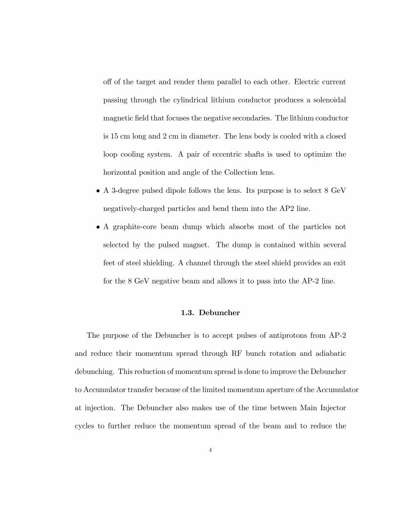
o¤ of the target and render them parallel to each other. Electric current

passing through the cylindrical lithium conductor produces a solenoidal

magnetic �eld that focuses the negative secondaries. The lithium conductor

is 15 cm long and 2 cm in diameter. The lens body is cooled with a closed

loop cooling system. A pair of eccentric shafts is used to optimize the

horizontal position and angle of the Collection lens.

� A 3-degree pulsed dipole follows the lens. Its purpose is to select 8 GeV

negatively-charged particles and bend them into the AP2 line.

� A graphite-core beam dump which absorbs most of the particles not

selected by the pulsed magnet. The dump is contained within several

feet of steel shielding. A channel through the steel shield provides an exit

for the 8 GeV negative beam and allows it to pass into the AP-2 line.

1.3. Debuncher

The purpose of the Debuncher is to accept pulses of antiprotons from AP-2

and reduce their momentum spread through RF bunch rotation and adiabatic

debunching. This reduction of momentum spread is done to improve the Debuncher

to Accumulator transfer because of the limited momentum aperture of the Accumulator

at injection. The Debuncher also makes use of the time between Main Injector

cycles to further reduce the momentum spread of the beam and to reduce the

4

transverse size of the beam through stochastic cooling[2]. This cooling greatly

improves the e¢ ciency of the Debuncher to Accumulator transfer.

1.4. Accumulator

1.4.1. Function

The purpose of the Accumulator is to accumulate antiprotons. This accumulation

is accomplished by momentum stacking successive pulses of antiprotons from the

Debuncher over several hours or days. Both radio frequency ( RF ) and stochastic

cooling systems are used in the momentum stacking process. The RF decelerates

the recently injected pulses of antiprotons from the injection energy to the edge of

the stack tail. The stack tail momentum cooling system sweeps the beam deposited

by the RF away from the edge of the tail and decelerates it towards the dense

portion of the stack, known as the core. Additional cooling systems keep the pbars

in the core at the desired momentum and minimize the transverse beam size.

What follows is a chronological sequence of events that takes place in the

Accumulator:

(1) Unbunched antiprotons are extracted from the Debuncher, transferred

down the Debuncher to Accumulator ( DtoA ) line, and injected into the

Accumulator with a kinetic energy 8 GeV. The beam is transferred in

the horizontal plane by means of a kicker and pulsed magnetic septum

5

combination in each machine (in order: D:EKIK, D:ESEPV, A:ISEP2V,

A:ISEP1V and A:IKIK). Extraction in the Debuncher occurs just before

another antiproton pulse arrives from the target.

(2) The Accumulator injection kicker puts the injected antiproton pulse onto

the injection closed orbit which is roughly 80mm to the outside of the

central orbit. The kicker is located in a high dispersion region so the higher

energy injected beam is displaced to the outside of the Accumulator. This

kicker is unique in that there is a shutter which moves into the aperture

between the injection orbit and the circulating stacktail and stack. The

shutter is in this position only when the kicker �res. The shutter�s purpose

is to shield the circulating antiprotons already in the Accumulator from

fringe �elds created when the kicker �res. Figure 1.1 diagrams a spectrum

analyzer display of the Accumulator longitudinal beam distribution. It

shows the relative location of the shutters in revolution frequency (which

relates to the horizontal position in a dispersive region)

(3) After the injected pbars have been kicked onto the injection closed orbit,

the shutter is opened and a 53 MHz RF system known as ARF-1 captures

the beam in 84 bunches. ARF-1 then decelerates the beam by approximately

60 MeV to the edge of the stack tail, beyond the space occupied by the

kicker shutter. The RF is adiabatically turned o¤ as the edge of the tail

6

Figure 1.1. Spectrum Analyzer trace of a signal from a longitudinalSchottky detector showing the Accumulator momentum apertureduring atiproton stacking.

is approached and the now unbunched pbars are deposited into the stack

tail.

(4) The stack tail momentum cooling system now acts on the pbars. This

system decelerates the beam towards the stack core which is approximately

-150MeV from the injection orbit (or ~63 mm to the inside of the Accumulator

central orbit in a high dispersion region).

(5) After approximately 30 minutes, the antiprotons in the stack tail have

been decelerated into the domain of the core cooling systems. Six stochastic

7

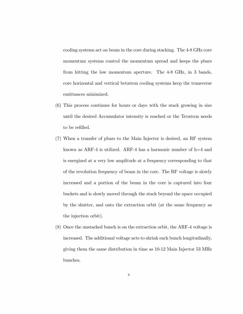
cooling systems act on beam in the core during stacking. The 4-8 GHz core

momentum systems control the momentum spread and keeps the pbars

from hitting the low momentum aperture. The 4-8 GHz, in 3 bands,

core horizontal and vertical betatron cooling systems keep the transverse

emittances minimized.

(6) This process continues for hours or days with the stack growing in size

until the desired Accumulator intensity is reached or the Tevatron needs

to be re�lled.

(7) When a transfer of pbars to the Main Injector is desired, an RF system

known as ARF-4 is utilized. ARF-4 has a harmonic number of h=4 and

is energized at a very low amplitude at a frequency corresponding to that

of the revolution frequency of beam in the core. The RF voltage is slowly

increased and a portion of the beam in the core is captured into four

buckets and is slowly moved through the stack beyond the space occupied

by the shutter, and onto the extraction orbit (at the same frequency as

the injection orbit).

(8) Once the unstacked bunch is on the extraction orbit, the ARF-4 voltage is

increased. The additional voltage acts to shrink each bunch longitudinally,

giving them the same distribution in time as 10-12 Main Injector 53 MHz

bunches.

8

(9) Like its injection counterpart, the extraction kicker has a shutter to shield

the remaining stack from fringe �elds. The extraction kicker shutter closes,

then the kicker is �red. The de�ection imparted by the kicker provides

su¢ cient horizontal displacement to place the kicked beam in the �eld

region of a Lambertson magnet which bends the beam up out of the

Accumulator and into the AP3 line.

1.4.2. Lattice

The Accumulator �ring�actually resembles a triangle with �attened corners.

The lattice has been designed with the following constraints in mind:

� The Accumulator must be capable of storing an antiproton beam over

many hours.

� There must be several long straight sections of lengths up to 16 m with

small transverse beam sizes to accommodate stochastic cooling pickups

and kickers.

� Some of these sections must have low dispersion, others with dispersion

of about 9 m (high dispersion).

� Betatron cooling pick-ups and kickers must be an odd multiple of �/2

apart in betatron phase (i.e. the number of betatron oscillations) and

far enough apart physically so that a chord drawn across the ring will be

9

signi�cantly shorter than the arc. Cooling pickup signals must arrive at

the kickers on the same turn in time to act on the particles that created

the signal.

The end result is that the Accumulator has an unconventional triangular shape

that includes 6 straight sections with alternately low and high dispersion.

The dispersion function (often written �x or �y) describes the contribution

to the transverse size of a particle beam as a result of its momentum spread.

Dispersion is caused in large part by bending magnets, as di¤erent momenta

particles are bent at di¤erent angles as a function of the momentum. In a low

dispersion area, the beam size is almost entirely de�ned by the � function and

the normalized emittance of the beam. In a high dispersion region, the beam size

is de�ned by the � function and normalized emittance as well as the dispersion

function. In the case of the Accumulator, the horizontal � function is small in the

high dispersion regions in addition to the large horizontal dispersion function so

the beam size is dominated by �ppand the position errors are dominated by o¤

momentum particles. As a result, the beam size is very small in the low dispersion

areas and very wide horizontally in the high dispersion areas (there is very little

vertical dispersion due to the fact that there are only small vertical trim dipoles

in the Accumulator).

10

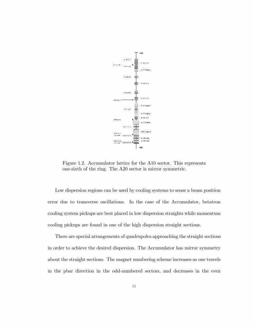
Figure 1.2. Accumulator lattice for the A10 sector. This representsone-sixth of the ring. The A20 sector is mirror symmetric.

Low dispersion regions can be used by cooling systems to sense a beam position

error due to transverse oscillations. In the case of the Accumulator, betatron

cooling system pickups are best placed in low dispersion straights while momentum

cooling pickups are found in one of the high dispersion straight sections.

There are special arrangements of quadrupoles approaching the straight sections

in order to achieve the desired dispersion. The Accumulator has mirror symmetry

about the straight sections. The magnet numbering scheme increases as one travels

in the pbar direction in the odd-numbered sectors, and decreases in the even

11

1 5 8 .0 3 30

M o n A p r 26 1 4 :2 7 :5 0 2 0 0 4 O p tiM - M A IN : - Y :\L a t tic e s \A c c um u la t or \So urc e \AC C U M U LA TO R .opt

75

0

10

-2

BE

TA

_X&

Y[m

]

DIS

P_X

&Y

[m]

B E TA _ X B E TA _ Y D IS P _X D IS P _Y

Figure 1.3. Plot of the beta and dispersion funtions for 2 sectors ofthe Accumulator. The red trace is �x. The green trace is �y andthe blue trace is Dx.

sectors. The lattice of one sector ( one-sixth ) of the Accumulator is shown in

Figure 1.2. The beta functions and dispersion for 2 sectors of the Accumualtor are

shown in Figure 1.3 .

The Accumulator straight sections are full of specialized devices. A10 contains

core betatron cooling pickup tanks, Schottky and other diagnostic pickups, damper

pickups and kickers as well as the beam current transformer for measuring the

circulating beam intensity. The injection and extraction kickers are found in

straight section A20 as are the pickup arrays for the 4-8 GHz core momentum

cooling system. In A30 reside the extraction Lambertson magnetic septum, the

stack tail momentum, 2-4 GHz core momentum, and core betatron cooling kickers.

12

Section A40 contains a beam scraper used for measuring �p/p and a set of

�ying wires for making high dispersion measurements of the beam size. A50

contains transverse scrapers. The various Accumulator RF cavities are also found

in A50. Just upstream of the actual straight section is the kicker tank for the 4-8

GHz core momentum system and a set of �ying wires for making low dispersion

measurements of the beam size. Straight section A60 contains all of the stochastic

cooling pickups for the stack tail momentum systems and the 2-4 GHz core momentum

cooling.

The Accumulator is operated in two con�gurations, a stacking lattice and a

shot lattice. The slip factor �( eta ), the amount one particle slips past another

in longitudinal phase space as particles travel around the ring, is changed between

the two con�gurations by ramping the �elds in the magnetic elements. For the

stacking lattice � = -0.012 which optimizes the stacktail cooling and allows for the

highest stacking rates. For the shot lattice � = -0.024 which lowers the emittances

of the beam and produces better beam brightness for the Tevatron.

1.5. Modes of Operation

The Antiproton source can be oriented into several modes of operation based

on the needs of users. In addition to antiproton stacking and unstacking, several

operating modes were created that utilize protons. Protons provide a convenient

13

source of relatively high intensity beam for tune-up and studies. For the RF tune

measurement method, the beam can be protons or antiprotons circulating in the

Accumulator.

1.5.1. Antiproton Stacking

Protons are accelerated in the Main Injector to 120 GeV. After the protons are

bunch rotated, the short bunch length beam is extracted from the Main Injector.

Beam is transported, through a series of beamlines, into the AP-1 line (see Figure

1.4). The protons move down the AP-1 line into the target vault where the

beam strikes a nickel target. Downstream of the target, 8 GeV antiprotons, as

well as other negative secondaries, are focused with the collection lens and are

momentum selected with a pulsed magnet. Particles that are o¤-momentum or

positively charged are absorbed in a beam dump. The secondary beam travels

to the Debuncher via the AP2 line where most of the secondaries, that are not

antiprotons, decay away. Of the remaining secondaries, most are lost in the

�rst dozen turns in the Debuncher. Only the small fraction of antiprotons with

appropriate energy survive to circulate in the Debuncher. For every million protons

on target, only ~20 antiprotons circulate in the Debuncher. After debunching and

cooling in the Debuncher, the antiprotons pass through the D to A line and into

the Accumulator. Successive pulses of antiprotons arriving into the Accumulator

14

Figure 1.4. Path of antiprotons in stacking mode.

are �stacked� over several hours or days into the core by ARF-1 and stochastic

cooling. Stacking cycles are at least 1.5 seconds in duration and may be extended

to improve the stacking rate with larger stacks.

15

Figure 1.5. Path of protons in reverse proton mode.

1.5.2. Reverse Protons

8-GeV protons from the Main Injector are transported, through a series

of beamlines, into the AP-1 line. Beam is bent into the AP-3 line bypassing the

vault. After passing through AP-3 the beam continues through a C-magnet and the

�eld region of the extraction Lambertson which bends the beam upward into the

Accumulator at A30. The extraction kicker in A20 de�ects the beam horizontally

onto the closed orbit of the Accumulator( see Figure 1.5 ).

16

Figure 1.6. ARF-3 RF structure.

Reverse protons are used in Collider mode to tune up the AP-1 and AP-3 lines

prior to an antiproton transfer from the Accumulator to the Main Injector. Reverse

proton mode is also used for high intensity studies in both rings and all beamlines.

If desired, particles can be extracted from the Accumulator and sent down the D

to A line into the Debuncher. Beam can then be injected backwards into the AP-2

line and transported to the target vault.

1.6. Tools Used for Measurements

1.6.1. ARF-3

ARF-3 is a h = 2 ( 1:26MHz ) RF cavity ( Figure 1.6 ) that is used to move

the beam to various revolution frequencies in the Accumulator for measurements

and studies.

17

The low level amplitude input to ARF-3 comes from either a digital to analog

converter ( DAC ) or a programmable ramp card. The frequency inputs are

provided by a digital synthesizer.

1.6.2. Vector Signal Analyzer

Signals from the Schottky detectors ( Section 1.6.5 ) can be displayed on

a Hewlett Packard HP 89440A DC-1800 MHz Vector Signal Analyzer ( VSA ).

A coaxial relay multiplexer is used to connect the Schottky detector to the VSA.

The HP 89440A is capable of measuring rapidly time-varying signals and addresses

problems dealing with complex modulated signals that cannot be de�ned in terms

of simple AM, FM, or RF. It uses a large parallel digital �lter array at its input and

performs a Fast Fourier Transform (FFT) to display an amplitude versus frequency

spectrum[3].

1.6.3. ACNET

The accelerator controls network ( ACNET ) is a general term used to describe

the overall controls system. There is a VAX cluster provided for code development

of console applications and for using several of the control system public facilities.

This cluster is called ADCON.

18

1.6.3.1. Architecture. The control system consists of four main components:

front-ends, centrals, consoles and the network that ties them all together. Front-ends

are the computers that bridge between the hardware (e.g. power supply control

cards, analog read-backs, etc.) and the rest of the control system. Centrals are

the machines that provide centralized, shared tasks such as databases, shared

�les, alarm reporting, etc. Consoles are the computers that an end-user (e.g. an

Accelerator Operator) uses to control the accelerator. They provide a user interface

to present accelerator data. Consoles communicate with the front-ends and the

centrals to acquire and scale data. The network is the hardware and software that

connect consoles, centrals and front-ends; allowing them a means to communicate

with each other.

1.6.3.2. Consoles. A console is the machine and system software that provide

the human interface to the accelerator. There are a �xed number of processes that

de�ne a console including several system tasks and a �xed number of application

programs.

There are two main kinds of applications that run on a console: Primary

Application (PA) and Secondary Application (SA). PAs run with character-based

windows and take keyboard input. SAs runs with graphics based windows and

usually do not use keyboard input. There are 3 PAs and 3 SAs allowed to run on

19

a given console. SAs are started from an existing PA. PAs also have the ability to

use two dedicated screens which are pixel based, for graphics and text display.

1.6.3.3. Devices. Devices are an important logical construct within the

control system. A device is the common way to address a physical channel (hardware).

More speci�cally, �device�refers to an ACNET device in the database. A device is

identi�ed by a unique integer (called a device index, or DI) or a name. Devices are

de�ned to have some set of properties (PIs): reading, setting, basic status, basic

control, analog alarm, digital alarm, etc. By addressing a DI/PI combination one

can read or set that part of a device. Device properties can also have scaling

information stored in the database.

1.6.4. Programmer Tools

There are a large set of library routines provided for the console application

programmer. This library is called CLIB (Console LIBrary). CLIB contains

routines for user interface, data acquisition and program control.

1.6.5. Schottky Signals

A charged particle passing through a resonant stripline detector or a resonant

cavity creates a short signal pulse. A particle beam is made up of many charged

20

particles. Each particle creates a short signal pulse. This collection of pulses is

known as a Schottky signal ( a more complete description is given in Section 3.1).

There are three Schottky detectors used in the Accumulator. The vertical,

horizontal and longitudinal detectors are located in the A10 straight section. The

vertical and horizontal transverse pickups are approximately 24 inches long and

2 inches in diameter. These pickups detect transverse beam oscillations. The

vertical pickup has the striplines above and below the beam with outputs on the

top and bottom, the horizontal pickup is rotated 90�. The transverse pickups are

a stainless steel tube with a slot cut along much of the long dimension (see Figure

1.7 ). The pickup is held by ceramic rings, which also electrically insulate it from

the outer housing.

Signals from each plate are fed through to a 3/8-inch heliax cable, which is run

to the AP-10 service building. The detectors resonate at a frequency determined

by the length of the strip inside the cylinder plus the coaxial cable between the

output connector and a capacitor. Connectors in the middle are used to inject a

signal for tuning the device to the frequency of interest. Horizontal and vertical

pickups are mounted on motorized stands so that the device can be centered with

respect to the beam.

The longitudinal pickups are larger, 37 inches in length and 3.4 inches in

diameter. These pickups are tuned quarter-wave cavities that are made by separating

21

Figure 1.7. Diagram of a Schottky detector.

a stainless steel tube into two sections with a ceramic across the gap. Charged

particles crossing the gap produce Schottky signals. The longitudinal detectors are

tuned with plungers or sliding sleeves on the center element.

The Schottky detectors used in the Antiproton Source are tuned to the 126th

harmonic of the beam�s revolution frequency. There are several reasons for choosing

the 126th harmonic for the design of the Schottky detectors. The spectral power

contribution from the 53.1 MHz bunch structure (from ARF-1 in the Accumulator)

is minimized by using a frequency located between 53.1 MHz (h=84) and its

second harmonic at 106.2 MHz (h=168). The resulting signal from the revolution

harmonic for the Accumulator core would be 126*.628881 MHz = 79.239 MHz.

The physical size of the detector must also be taken into account. The aperture

22

must be large enough to not restrict beam transmission. Limited space available

in the rings limits the pickup length to only 1 or 2 m. Schottky detectors designed

for the 126th harmonic �t both of these size constraints. For example, recall that

the longitudinal Schottky pickups are 1/4 wavelength long. The physical length of

the cavity as built is 0.94 meters which would result in a resonant frequency of:

(1.1) f =velocity

length~3E8m=s

4 � :94m~79:75MHz

That works well for the Accumulator.

1.7. Accumulator Betatron Tunes

As particles travel around the ring they oscillate about the machine design

trajectory. This motion is termed a betatron oscillation. The number of betatron

oscillations per revolution is termed the betatron tune. There is a betatron tune

for both the x and y planes. The integer number of betatron tunes are measured by

changing the magnetic �eld of one dipole and counting the oscillations on a beam

position monitor ( BPM ) display. The plots in Figure 1.8 show 6 full oscillations

( Qx ) about the design and 8 full oscillations ( Qy ) about the design orbit in the

y plane.

23

Figure 1.8. Di¤erence orbits showing oscillations about the machinedesign orbit caused by dipole de�ections. The plot on the left showsa horizontal de�ection. The plot on the right shows a verticalde�ection.

The fractional parts of the peak tunes ( qx, qy ) on the core revolution frequency

are calculated from Schottky dectector signals, as displayed in Figure 1.9 , using

Equation 1.2. Here qx is calculated to be 0:6969 and qy is calculated to be 0:6845.

(1.2) qx =Pxfrev

qy =Pyfrev

where Px, Py and frev are the horizontal sideband peak frequency, vertical

sideband peak frequency and core revolution frequency respectively. Combining

the integer tune measurements with the fractional tune measurements shows that

Qx + qx = 6:6969 and Qy + qy = 8:6845.

24

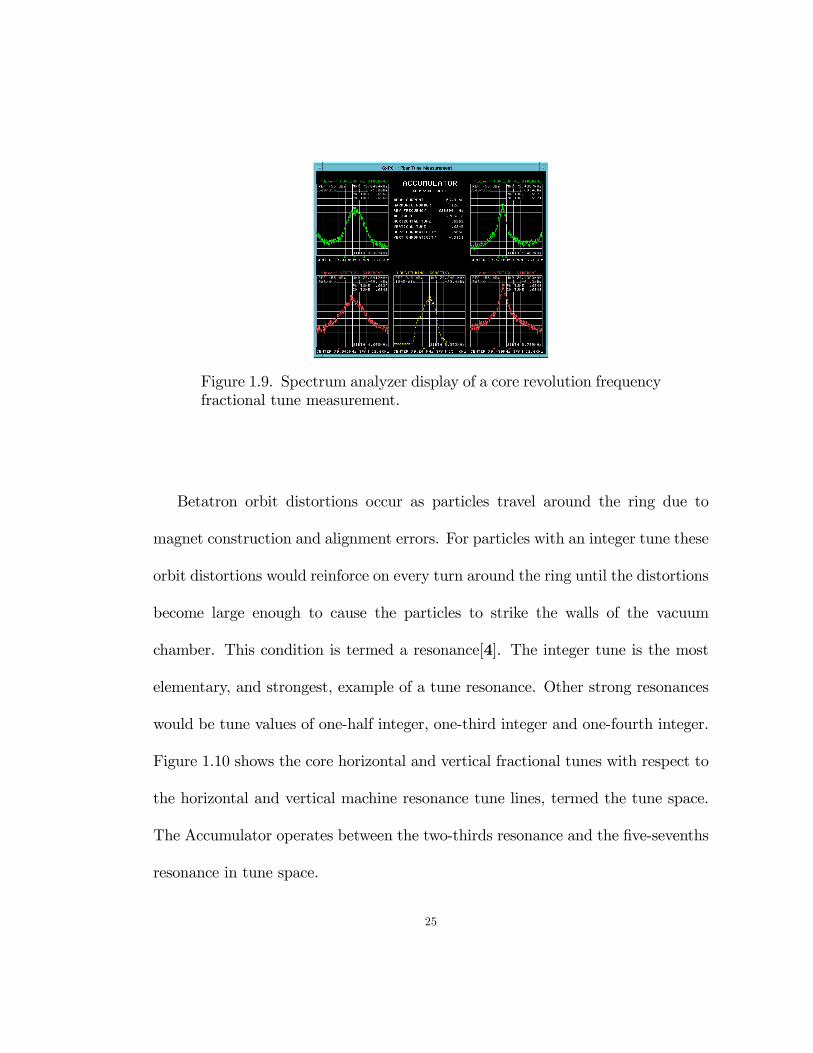
Figure 1.9. Spectrum analyzer display of a core revolution frequencyfractional tune measurement.

Betatron orbit distortions occur as particles travel around the ring due to

magnet construction and alignment errors. For particles with an integer tune these

orbit distortions would reinforce on every turn around the ring until the distortions

become large enough to cause the particles to strike the walls of the vacuum

chamber. This condition is termed a resonance[4]. The integer tune is the most

elementary, and strongest, example of a tune resonance. Other strong resonances

would be tune values of one-half integer, one-third integer and one-fourth integer.

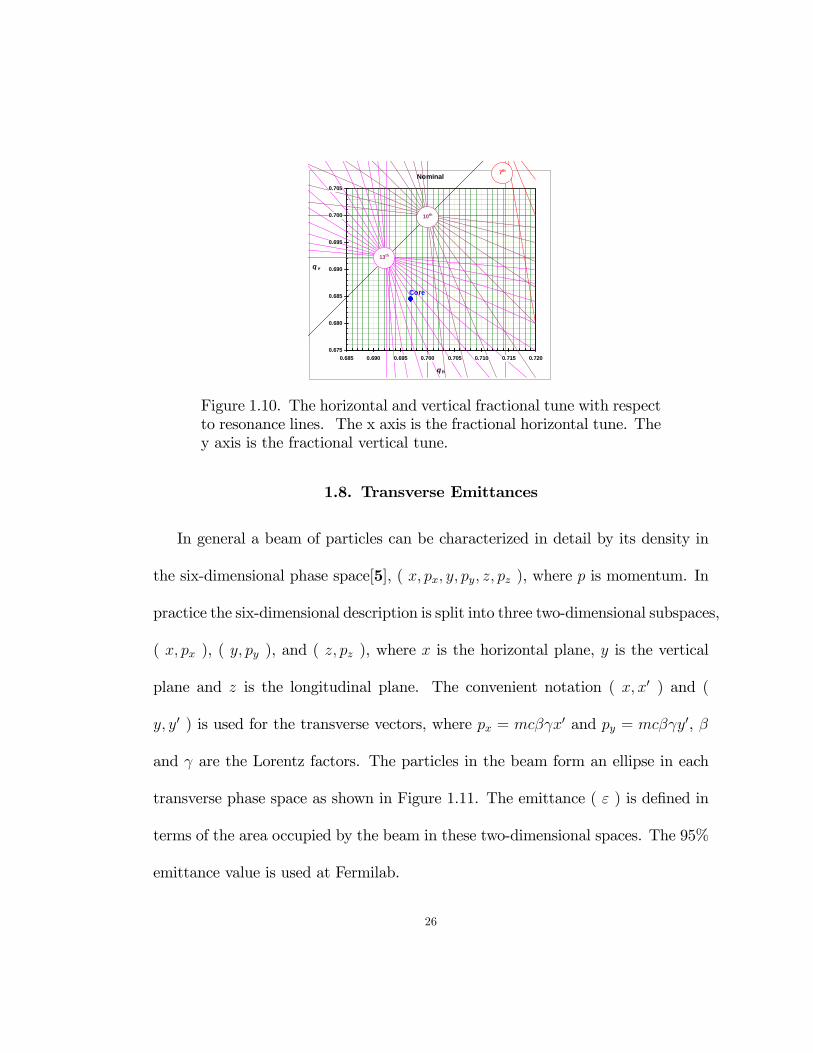
Figure 1.10 shows the core horizontal and vertical fractional tunes with respect to

the horizontal and vertical machine resonance tune lines, termed the tune space.

The Accumulator operates between the two-thirds resonance and the �ve-sevenths

resonance in tune space.

25

Nominal

0.675

0.680

0.685

0.690

0.695

0.700

0.705

0.685 0.690 0.695 0.700 0.705 0.710 0.715 0.720

q h

q v

7th

10th

13th

Core

Figure 1.10. The horizontal and vertical fractional tune with respectto resonance lines. The x axis is the fractional horizontal tune. They axis is the fractional vertical tune.

1.8. Transverse Emittances

In general a beam of particles can be characterized in detail by its density in

the six-dimensional phase space[5], ( x; px; y; py; z; pz ), where p is momentum. In

practice the six-dimensional description is split into three two-dimensional subspaces,

( x; px ), ( y; py ), and ( z; pz ), where x is the horizontal plane, y is the vertical

plane and z is the longitudinal plane. The convenient notation ( x; x0 ) and (

y; y0 ) is used for the transverse vectors, where px = mc� x0 and py = mc� y0, �

and are the Lorentz factors. The particles in the beam form an ellipse in each

transverse phase space as shown in Figure 1.11. The emittance ( " ) is de�ned in

terms of the area occupied by the beam in these two-dimensional spaces. The 95%

emittance value is used at Fermilab.

26

Figure 1.11. Horizontal phase space as it relates to the Lorentz factors.

Large transverse emittances in the stack could lead to beam loss, poor brightness

and low luminosity in the Tevatron. The transvers emittances of the stack are

monitored on a consistant basis by a dedicated system and are normalized to the

number of antiprotons in the stack. Transverse emittance sizes range from 0 � mm

mr with no stack to 1:7 � mm mr and 1:3 � mm mr for horizontal and vertical,

respectively, with a stack size of 200mA.

27

CHAPTER 2

Tunes vs Revolution Frequency Moving Beam with ARF-3

The tunes vs revolution frequency moving beam with ARF-3 ( RF method ) is

used when the Antiproton Source is not in stacking operations. Beam is expected

to be circulating in the Accumulator. The beam is bunched, using ARF-3, and

moved in steps through a frequency range in the momentum aperture. Schottky

detectors are connected, one at a time, to a VSA. Trace data is stored and a

contour plot is displayed showing the sideband tunes versus revolution frequency.

Protons or antiprotons may be used. Antiprotons are used when the stack is

small, such as just after a store has begun. Protons are used when the machine

is con�gured in the reverse proton mode. One measurement, using both upper

and lower sidebands, takes approximately 25 minutes. This includes bunching the

beam, making the measurements, moving the beam back to the original revolution

frequency and debunching the beam.

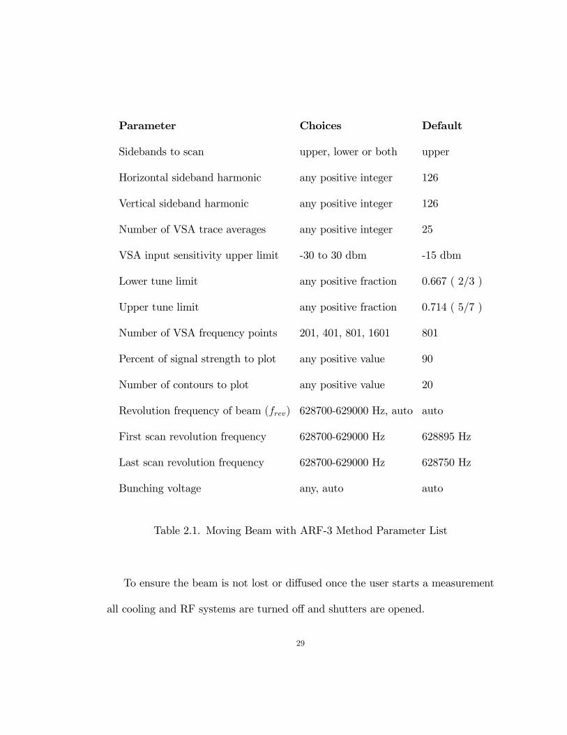
An ACNET program written in C was created to accomplish this task. Table

2.1 lists user controlled parameters.

28

Parameter Choices Default

Sidebands to scan upper, lower or both upper

Horizontal sideband harmonic any positive integer 126

Vertical sideband harmonic any positive integer 126

Number of VSA trace averages any positive integer 25

VSA input sensitivity upper limit -30 to 30 dbm -15 dbm

Lower tune limit any positive fraction 0.667 ( 2/3 )

Upper tune limit any positive fraction 0.714 ( 5/7 )

Number of VSA frequency points 201, 401, 801, 1601 801

Percent of signal strength to plot any positive value 90

Number of contours to plot any positive value 20

Revolution frequency of beam (frev) 628700-629000 Hz, auto auto

First scan revolution frequency 628700-629000 Hz 628895 Hz

Last scan revolution frequency 628700-629000 Hz 628750 Hz

Bunching voltage any, auto auto

Table 2.1. Moving Beam with ARF-3 Method Parameter List

To ensure the beam is not lost or di¤used once the user starts a measurement

all cooling and RF systems are turned o¤ and shutters are opened.

29

2.1. VSA Setup

The VSA is initialized and setup as follows;

� Set to vector mode

� GPIB data format set to 64 bit real

� Number of frequency points set

� Trace coordinates set to log-magnitude

� Upper limit of the analyzer input�s sensitivities range set to �15 dBm

� Number of averages set

� Averaging turned on

If the current revolution frequency or the bunching volts are set to auto the

following steps are taken;

� Center frequency set to 79.2288 MHz

� Span set to 26 KHz

2.2. Measuring the Beam Revolution Frequency and Width

If the current revolution frequency or the bunching voltage are set to auto, the

longitudinal Schottky detector is connected to the VSA. This setup will allow the

VSA to sense the entire momentum aperture. A delay is given to allow the VSA

to average. The display is paused and the trace recorded. The program scans

30

through the trace data, point by point, to �nd the VSA frequency at the peak of

the spectrum. The revolution frequency is calculated using Equation 2.1,

(2.1) PBeam = PV SA � 126

where PV SA is the VSA frequency of the signal peak and PBeam is the revolution

frequency of the signal peak

The frequency width of the beam is needed to calculate the amount of voltage

required to bunch the beam. The beam width is de�ned to be the frequency

span of the points at or above a 10 dB power level above the noise �oor of the

signal. To calculate the noise �oor the VSA measurements are restarted and the

center frequency is set to 79.5432 MHz. This frequency is between the 126th and

127th harmonic where there is no beam signal. A delay is given to allow the VSA to

average. The display is paused and the trace recorded. The noise �oor is calculated

using Equations 2.2.

(2.2) NF = NAve + (2�NRMS)

where

31

NAve = NSum � (SP � 1);

NRMS =pNSum2 � (SP � 2)

and NSum is the sum of all VSA points, NAve is the noise average, MV SA is the

VSA point measurements minus Nave, NSum2 is the sum of all (MV SA)2, NRMS is

the rms noise, NF is the noise �oor and SP is the number of VSA signal points.

Once the noise �oor is calculated the frequencies in the array containing the

beam are converted to revolution frequencies and the trace is searched. Since the

Accumulator operates above transition the high energy, low frequency, side of the

beam is found by comparing the power at each VSA point to the noise �oor power

starting from the peak moving down in frequency and including each point until

the power is less than 10 dB above the noise �oor. Likewise, the low energy, high

frequency, side of the beam is found by comparing the power at each VSA point to

the noise �oor power starting from the peak moving up in frequency and including

each point until power is less than 10 dB above the noise �oor. The beam width

is the di¤erence between these two frequencies.

32

2.3. Calculating the Bunching Voltage

The bunching voltage is calculated using Equations 2.3.

(2.3) VRF = (1:2

64!RF

"L�s)2(2�h

�

ecEs)

where,

Es =q(pc)2 + (mpc2)2;

s =Esmpc2

;

�s =

s1� 1

2s;

"L =�2sEs�(frev�f 2rev

);

!RF = 2�hfrev

and h is the RF harmonic, p is the orbit beam momentum, � is the lattice slip

factor, frev is the beam revolution frequency, �frev is the beam width, L is the

33

orbit length,mp is the antiproton mass, c is the speed of light,Es is the synchronous

energy, s is the relativistic gamma, �s is the relativistic beta, "L is the longitudinal

emittance, !RF is the angular RF frequncy and ec is the electron charge.

2.4. Bunching the Beam

Depending on the initial setup the beam is adiabatically bunched, using the

relationships in Equations 2.4 , at either the calculated or user selected revolution

frequency.

(2.4) V (t) =V0

(1� !sAt)2

where

!s =

s�frev!RF ec

V0

�2sEs

and V0 is the intitial voltage, A is the adiabatic constant, t is the time and V (t) is

the voltage at given time t.

2.5. Measuring the Sidebands

The beam is moved, using the ARF3 system, to the revolution frequency of the

�rst scan point. The VSA is connected to the horizontal Schottky detector. As the

tune of the beam increases the sidebands move further away from the revolution

34

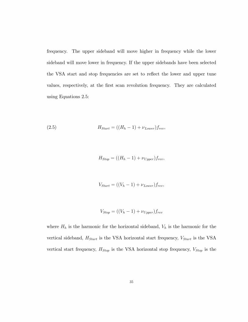
frequency. The upper sideband will move higher in frequency while the lower

sideband will move lower in frequency. If the upper sidebands have been selected

the VSA start and stop frequencies are set to re�ect the lower and upper tune

values, respectively, at the �rst scan revolution frequency. They are calculated

using Equations 2.5:

(2.5) HStart = ((Hh � 1) + �Lower)frev;

HStop = ((Hh � 1) + �Upper)frev;

VStart = ((Vh � 1) + �Lower)frev;

VStop = ((Vh � 1) + �Upper)frev

where Hh is the harmonic for the horizontal sideband, Vh is the harmonic for the

vertical sideband, HStart is the VSA horizontal start frequency, VStart is the VSA

vertical start frequency, HStop is the VSA horizontal stop frequency, VStop is the

35

VSA vertical stop frequency, �Lower is the lower tune limit and �Upper is the upper

tune limit.

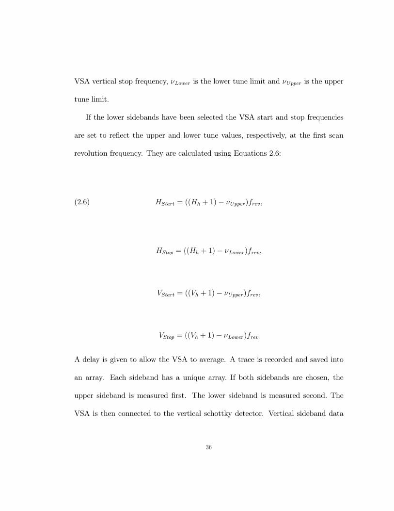
If the lower sidebands have been selected the VSA start and stop frequencies

are set to re�ect the upper and lower tune values, respectively, at the �rst scan

revolution frequency. They are calculated using Equations 2.6:

(2.6) HStart = ((Hh + 1)� �Upper)frev;

HStop = ((Hh + 1)� �Lower)frev;

VStart = ((Vh + 1)� �Upper)frev;

VStop = ((Vh + 1)� �Lower)frev

A delay is given to allow the VSA to average. A trace is recorded and saved into

an array. Each sideband has a unique array. If both sidebands are chosen, the

upper sideband is measured �rst. The lower sideband is measured second. The

VSA is then connected to the vertical schottky detector. Vertical sideband data

36

is recorded in the same fashion. The bunched beam is then moved in frequency to

subsequent points. At each point the above process is repeated.

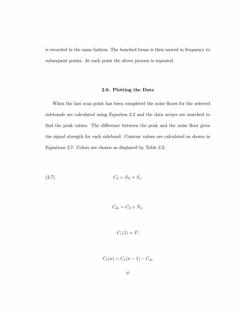
2.6. Plotting the Data

When the last scan point has been completed the noise �oors for the selected

sidebands are calculated using Equation 2.2 and the data arrays are searched to

�nd the peak values. The di¤erence between the peak and the noise �oor gives

the signal strength for each sideband. Contour values are calculated as shown in

Equations 2.7. Colors are chosen as displayed by Table 2.2:

(2.7) Cd = S% � Ss;

Cdv = Cd �Nc;

Cv(1) = P;

Cv(n) = Cv(n� 1)� Cdv

37

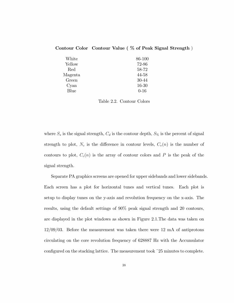
Contour Color Contour Value ( % of Peak Signal Strength )

White 86-100Yellow 72-86Red 58-72

Magenta 44-58Green 30-44Cyan 16-30Blue 0-16

Table 2.2. Contour Colors

where Ss is the signal strength, Cd is the contour depth, S% is the percent of signal

strength to plot, Nc is the di¤erence in contour levels, Cv(n) is the number of

contours to plot, Cc(n) is the array of contour colors and P is the peak of the

signal strength.

Separate PA graphics screens are opened for upper sidebands and lower sidebands.

Each screen has a plot for horizontal tunes and vertical tunes. Each plot is

setup to display tunes on the y-axis and revolution frequency on the x-axis. The

results, using the default settings of 90% peak signal strength and 20 contours,

are displayed in the plot windows as shown in Figure 2.1.The data was taken on

12/09/03. Before the measurement was taken there were 12 mA of antiprotons

circulating on the core revolution frequency of 628887 Hz with the Accumulator

con�gured on the stacking lattice. The measurement took ~25 minutes to complete.

38

Figure 2.1. Horizontal and vertical sideband tunes. The verticalaxis shos the fractional tune value between the two-thirds and�ve-sevenths resonances. The horizontal axis shows the Accumulatorrevolution frequency. The injection frequency is 628765 Hz and thecore revolution frequency is 628888 Hz. 90% of the peak signalstrength and 20 contours are plotted. The plot on the left are theupper sidebands. The plot on the right are the lower sidebands.

Coupling is evident near the core revolution frequency, especially in the vertical

tune measurement.

2.7. Options After the Initial Measurement

After the intial measurement is complete the user may choose to do any of the

following:

� Save the measurement for later analysis.

� Make another measurement moving the beam in the opposite direction.

� Replot the data using di¤erent signal depths and number of contours (

Section 2.8 ).

39

� Move the beam back to the original revolution frequency and debunch.

� Use a model of the lattice to simulate changes in the tunes vs revolution

frequency ( Section 2.9 ).

40

Figure 2.2. Upper horizontal and vertical sideband tunes. 70% ofthe peak signal strength and 50 contours are plotted.

2.8. Replot the Data

By changing the depth of the signal and number of contours to plot the user can

explore di¤erent aspects of the measurement. Figure 2.2 shows the upper sidebands

with 70% of the peak signal depth and 50 contours plotted. While Figure 2.2 is a

cleaner plot and more clearly shows the features near the peak signal values the

plot for the vertical upper sideband in Figure 2.1 shows the evidence of coupling

with the horizontal plane near the core.

2.9. Corrections Using the Simulation Code

The simulation code stores the peak tune value at each scan point into a

separate array. The user is allowed to make changes to the currents in the quadruploes,

41

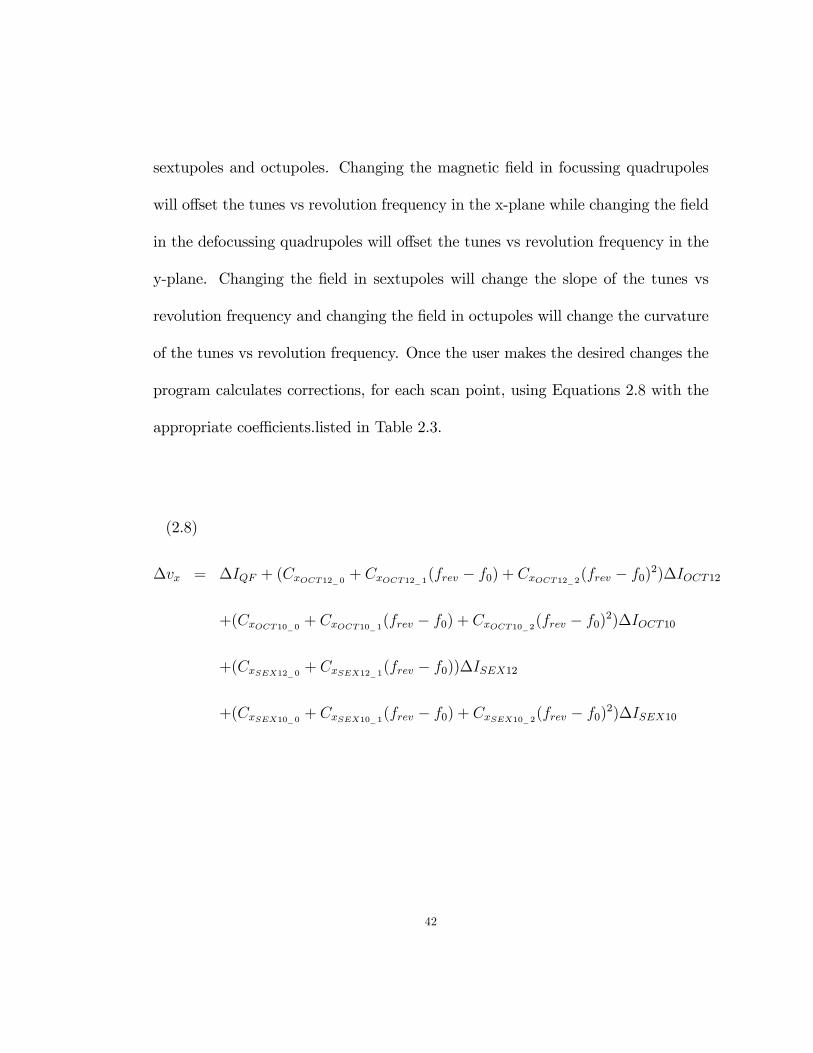
sextupoles and octupoles. Changing the magnetic �eld in focussing quadrupoles

will o¤set the tunes vs revolution frequency in the x-plane while changing the �eld

in the defocussing quadrupoles will o¤set the tunes vs revolution frequency in the

y-plane. Changing the �eld in sextupoles will change the slope of the tunes vs

revolution frequency and changing the �eld in octupoles will change the curvature

of the tunes vs revolution frequency. Once the user makes the desired changes the

program calculates corrections, for each scan point, using Equations 2.8 with the

appropriate coe¢ cients.listed in Table 2.3.

(2.8)

�vx = �IQF + (CxOCT12_0 + CxOCT12_1(frev � f0) + CxOCT12_2(frev � f0)2)�IOCT12

+(CxOCT10_0 + CxOCT10_1(frev � f0) + CxOCT10_2(frev � f0)2)�IOCT10

+(CxSEX12_0 + CxSEX12_1(frev � f0))�ISEX12

+(CxSEX10_0 + CxSEX10_1(frev � f0) + CxSEX10_2(frev � f0)2)�ISEX10

42

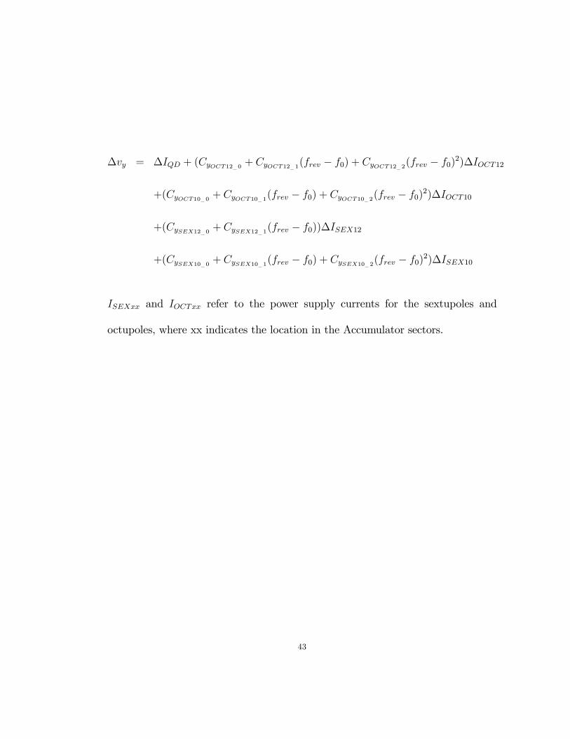
�vy = �IQD + (CyOCT12_0 + CyOCT12_1(frev � f0) + CyOCT12_2(frev � f0)2)�IOCT12

+(CyOCT10_0 + CyOCT10_1(frev � f0) + CyOCT10_2(frev � f0)2)�IOCT10

+(CySEX12_0 + CySEX12_1(frev � f0))�ISEX12

+(CySEX10_0 + CySEX10_1(frev � f0) + CySEX10_2(frev � f0)2)�ISEX10

ISEXxx and IOCTxx refer to the power supply currents for the sextupoles and

octupoles, where xx indicates the location in the Accumulator sectors.

43

Coe¢ cient Stacking Lattice Value Shot Lattice Value

CxOCT12_0 8:07835� 10�2 �6:38059� 10�2CxOCT12_1 5:98993� 10�4 �5:07452� 10�6CxOCT12_2 4:25182� 10�5 �2:84701� 10�5CxOCT10_0 �1:78816� 10�1 3:71805� 10�2CxOCT10_1 �8:59186� 10�4 2:95619� 10�6CxOCT10_2 �1:54145� 10�4 1:30559� 10�5CxSEX12_0 �5:92861� 10�3 �3:38680� 10�3CxSEX12_1 2:15582� 10�3 �3:26972� 10�3CxSEX10_0 �2:22532� 10�2 �3:23140� 10�3CxSEX10_1 �7:42469� 10�3 �2:85976� 10�3CxSEX10_2 �2:06370� 10�7 �1:97485� 10�11CyOCT12_0 �1:10022� 10�1 �1:10022� 10�1CyOCT12_1 �7:06975� 10�4 �7:06975� 10�4CyOCT12_2 �6:19865� 10�5 �6:19865� 10�5CyOCT10_0 4:36403� 10�2 �7:81030� 10�2CyOCT10_1 3:13166� 10�4 �6:21317� 10�6CyOCT10_2 3:30681� 10�5 �2:74259� 10�5CySEX12_0 �3:80515� 10�2 1:30859� 10�3CySEX12_1 �3:59078� 10�3 1:26337� 10�3CySEX10_0 3:32594� 10�2 1:53831� 10�3CySEX10_1 1:72438� 10�3 1:36137� 10�3CySEX10_2 �3:93965� 10�6 �1:21451� 10�11

Table 2.3. Stacking and shot lattice tune correction equation coe¢ cients

The stacking lattice coe¢ cients were calculated from �ts to measured data. The

shot lattice coe¢ cients were derived using a tune circuits model. The coe¢ cient

calculations are outlined in Chapter 4.

44

2.9.1. Example of Predicted Corrections

Figure 2.3 shows the corrections predicted by the simulation code with a

10 A change in the octupole windings on the multipole magnets in the Ax10

locations, where x indicates Accumulator sectors 1 through 6, and a -10A change

in the octupole windings on the multipole magnets in the Ax12 locations. The

Accumulator was con�gured on the stacking lattice. The algorithms predicted that

the horizontal tunes should be lower by ~0:010 units near the core and injection

frequencies and the vertical tunes should be higher by ~0:005 units near the core

and by ~0:010 near the injection frequencies. The plots in Figure 2.4 shows the

tunes across the aperture before the correction and after the correction. The

measured and predicted corrections match well.

Using the RF method a user could measure the tunes back and forth across

the aperture as many times as they wished while making corrections after each

measurement. This method provides the Antiproton Source Group with a powerful

diagnostic tool.

45

Figure 2.3. Tune measurements and correction predictions. Theyellow trace shows the measured peak tune values for each scanpoint. The blue curve shows the change to the tunes predicted bythe correction algorithms.

Figure 2.4. The plot on the left is the measured tunes before thecorrections were applied. The plot on the right is the tunes afterthe corrections were applied. The algorithms predicted that thehorizontal tunes should be lower by ~0:005 units near the core andinjection frequencies. The algorithms predicted that the verticaltunes should be higher by ~0:010 units near the core and by ~0:010near the injection frequencies. The measurements agree with thepredictions.

46

CHAPTER 3

Tunes and Emmitances Measuring Sideband Power

A method similar to one developed at CERN by S. van der Meer[6] and applied

to the Accumulator by Rui Alves-Pires[7] in 1993 is presented here as a proof of

principle.

3.1. Power Measurement Method

Schottky described the statistical current �uctuations caused by a �nite number

of charge carriers in 1918[6]. He showed that the noise, termed Scottky noise,

produced by each charge carrier is independent of the other charge carriers. Schottky

noise is incoherent. For particles in a storage ring, such as the Accumulator,

Schottky noise is a collection of signal pulses in the time domain, which corresponds

to a spectrum of lines in the frequency domain. The lines occur at harmonics of

the revolution frequency since the particles, circulating in the accelerator, pass

repeatedly through the Schottky detector. The combined response from all the

particles in the ring is smeared over a �nite frequency range at each harmonic.

This frequency range is related to the momentum spread of the beam by Equation

47

3.1,

(3.1)df

f=dp

p�

where � (the slip factor) is �xed by the Accumulator lattice. Each particle contributes

power to each sideband independently as they circulate around the ring. The

upper and lower sideband frequencies of the particles can be calculated from the

revolution frequency as shown in Equations 3.2.

(3.2) f+ = (n+ q)frev and f� = (n� q)frev

where n is the harmonic number, q is the fractional tune, frev, f+ and f� are the

revolution, upper, and lower sideband frequencies of the particles, respectively.

Conversely the revolution frequency and tune of the particles can be calculated

from the sideband frequencies using Equations 3.3 and 3.4 respectively:

(3.3) frev =f+ + f�2n

;

48

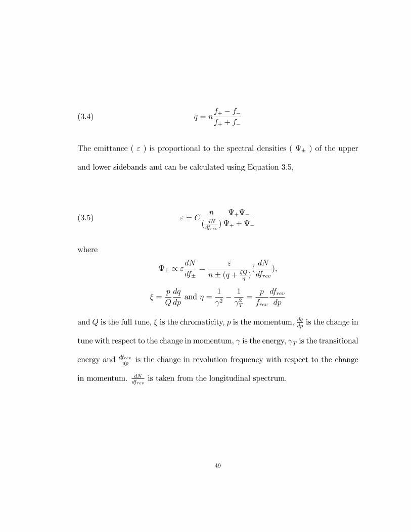
(3.4) q = nf+ � f�f+ + f�

The emittance ( " ) is proportional to the spectral densities ( � ) of the upper

and lower sidebands and can be calculated using Equation 3.5,

(3.5) " = Cn

( dNdfrev

)

+�+ +�

where

� / "dN

df�=

"

n� (q + �Q�)(dN

dfrev);

� =p

Q

dq

dpand � =

1

2� 1

2T=

p

frev

dfrevdp

and Q is the full tune, � is the chromaticity, p is the momentum, dqdpis the change in

tune with respect to the change in momentum, is the energy, T is the transitional

energy and dfrevdp

is the change in revolution frequency with respect to the change

in momentum. dNdfrev

is taken from the longitudinal spectrum.

49

Figure 3.1. Coupling at the core revolution frequency. The ploton the left shows the vertical sideband as seen on the horizontalSchottky detector display. The plot on the left shows the horizontalsideband as seen on the vertical Schottky detector display.

3.2. Coupled Tunes at the Core Revolution Frequency

In the current running mode, the fractional Accumulator tunes at the core

revolution frequency are qx = 0:6969 and qy = 0:6845. The tunes are close enough

to be termed coupled. The plots in Figure 3.1 show the coupling in the upper

sidebands. The vertical sideband is visible on a display of the horizontal schottky

detector as shown in the plot on the left. Conversely, the horizontal sideband is

visible on a display of the vertical schottky detector as shown in the plot on the

right. Coupling the tunes leads to more e¢ cient transvere cooling and a higher

beam quality for collisions in the Tevatron but renders the S. van der Meer method

of measuring tunes and emittances impractical. Therefore this technique is only

used during special study periods where the core tunes are decoupled.

50

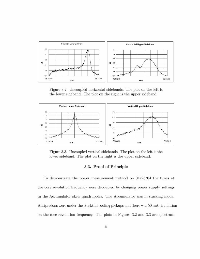
Figure 3.2. Uncoupled horizontal sidebands. The plot on the left isthe lower sideband. The plot on the right is the upper sideband.

Figure 3.3. Uncoupled vertical sidebands. The plot on the left is thelower sideband. The plot on the right is the upper sideband.

3.3. Proof of Principle

To demonstrate the power measurement method on 04/23/04 the tunes at

the core revolution frequency were decoupled by changing power supply settings

in the Accumulator skew quadrupoles. The Accumulator was in stacking mode.

Antiprotons were under the stacktail cooling pickups and there was 50 mA circulation

on the core revolution frequency. The plots in Figures 3.2 and 3.3 are spectrum

51

analyzer traces of transverse Schottky detector signals showing the uncoupled

sidebands.

An ACNET program was written in C to analyze the trace data. The program

scans the upper sideband, in each transverse plane, and integrates the power,

from the starting frequency of the sideband, to pre-determined frequency points

throughout the sideband. For each of these points the program searches through

the lower sideband for the frequency point with the same amount of integrated

power. Revolution frequencies, tunes and emittances for these power points are

calculated using Equations 3.3 , 3.4 and 3.5 , respectively, with the corresponding

upper and lower sideband frequencies. Figure 3.4 shows the calculated tunes

through the revolution frequencies covered by the stacktail cooling system. Figure

3.5 shows the calculated emittances through the revolution frequencies covered by

the stacktail cooling system. In Equation 3.5 C is the calibration constant. The

measurement at the core revolution frequency is calibrated to the emittance size

measured by the dedicated system. For a 50mA stack "x = 0:779�mmmr and

"y = 0:430�mmmr. Therfore C = 1:194 � 10�2 for the horizontal measurement

and C = 7:174� 10�3 for the vertical measurement.

52

-110

-105

-100

-95

-90

-85

-80

-75

0.68

0.685

0.69

0.695

0.7

Tunes Through the Stacktail

Stacktail Trace VerticalTunesHorizontal Tunes

Hz

628823 628914628868

Figure 3.4. The red trace is the longitudinal Schottky stack signal.The stacktail extends from the core region to ~628830Hz, near thecentral orbit. The green trace is the calculated horizontal tunes. Theblue trace is the calculated vertical tunes.

-110

-105

-100

-95

-90

-85

-80

-75

0

0.2

0.4

0.6

0.8

1

Emittances Through the Stacktail

Stacktail Trace Vertical EmittancesHorizontal Emittances

Hz

628823 628914628868

Figure 3.5. The red trace is the longitudinal Schottky stack signal.The green trace is the calculated horizintal emittances. The bluetrace is the calculated vertical emittances.

53

Emittances and tunes can be calculated during stacking operations proving to

be an advantge over the RF method in some situations. For example, if the stack

rate is zero or lower than expected, while stacking in the Accumulator, the tunes

could be decoupled and the power measurement method could be used to locate

any resonances in the tunes under the stacktail cooling system indicating a possible

problem with a magnet. Another use could be to decouple the tunes for a complete

stacking cycle and using the power measurement method at several stack sizes to

characterize tunes and emittances with respect to the number of antiprotons in

the stack. However, since the stacktail cooling system only covers approximately

half of the momentum aperture, the power measurement method cannot measure

the tunes near the injection revolution frequencies.

54

CHAPTER 4

Tune Correction Coe¢ cients and the Lattice Model

The sextupoles and octupoles located in the Ax10 and Ax12 locations, where x

indicates Accumulator sectors 1 through 6, ( Figure 1.2 ) are wound on a common

frame. These magnets are termed multipoles. The sextupole and octupole �elds

are formed by the shape and location of separate windings, rather than the number

of poles, and are powered by separate supplies. Since the multipoles are located in

the high dispersion straight sections di¤erent momentum particles will experience

di¤erent �eld strengths and exhibit di¤erent tunes. The sextupole and octupole

�elds in the multipoles are termed tune circuits.

The correction equation coe¢ cients for the stacking ( Section 4.1 ) and shot (

Section 4.2 ) lattices were derived using two separate methods[8].

4.1. Stacking Lattice Coe¢ cients

The stacking lattice coe¢ cients were derived by applying a �t to measured

data. The measurements of the tune circuits were made in the months between

December 2001 and April 2002. For each tune circuit the tunes at predetermined

revolution frequencies were measured at several power supply settings. From the

55

SEX10 Stacking Lattice

y = -3.93965E-09x2 + 1.72438E-06x + 3.32594E-05

y = -2.06376E-10x2 - 7.42469E-06x - 2.22532E-05

-0.0006

-0.0004

-0.0002

0.0000

0.0002

0.0004

0.0006

-80 -60 -40 -20 0 20 40 60

f rev - f 0 (Hz)

dq/d

I

HorizontalVerticalvh

Figure 4.1. Fits to dqdIcurves for the sextupoles in the Ax10 locations

on the stacking lattice.

SEX12 Stcaking Lattice

y = -3.59078E-06x - 3.80515E-05

y = 2.15582E-06x - 5.92861E-06

-0.0003

-0.0002

-0.0001

0.0000

0.0001

0.0002

0.0003

-80 -60 -40 -20 0 20 40 60

f rev - f 0 (Hz)

dq/d

I

HorizontalVerticalvh

Figure 4.2. Fits to dqdIcurves for the sextupoles in the Ax12 locations

on the stacking lattice.

resulting data tune changes with respect to current changes ( dqdI) were calculated.

Fits were applied to the dqdIcurves: Figures 4.1 and 4.2 shows the �ts, including the

56

OCT10 Stacking Lattice

y = 3.30681E-08x2 + 3.13166E-07x + 4.36403E-05

y = -1.54145E-07x2 - 8.59186E-07x - 1.78816E-04

-0.0012

-0.0010

-0.0008

-0.0006

-0.0004

-0.0002

0.0000

0.0002

0.0004

-80 -60 -40 -20 0 20 40 60

f rev - f 0 (Hz)

dq/d

I

HorizontalVerticalvh

Figure 4.3. Fits to dqdIcurves for the octupoles in the Ax10 locations

on the stacking lattice.

OCT12 Stacking Lattice

y = -6.19865E-08x2 - 7.06975E-07x - 1.10022E-04

y = 4.25182E-08x2 + 5.58993E-07x + 8.07835E-05

-0.0006

-0.0004

-0.0002

0.0000

0.0002

0.0004

0.0006

-80 -60 -40 -20 0 20 40 60

f rev - f0(Hz)

dq/d

I

HorizontalVerticalvh

Figure 4.4. Fits to dqdIcurves for the octupoles in the Ax12 locations

on the stacking lattice.

correction equation coe¢ cients, for the sextupoles. Figures 4.3 and 4.4 shows the

�ts, including the correction equation coe¢ cients, for the octupoles.

57

4.2. Shot Lattice Coe¢ cients

The development and operation of the shot lattice was established in the

months of May and June of 2002. Unlike on the stacking lattice no study time

was given to measure the tune circuits on the shot lattice. Another method was

needed to derive the tune correction equation coe¢ cients for the shot lattice. The

solution was to take the following steps:

� Develop a tune circuits model using MathCad.

� Compare the model to the the measured stacking lattice dqdIcurves using

the stacking lattice functions.

� Enter the shot lattice functions into the model to create shot lattice dqdI

curves.

� Apply �ts to the shot lattice dqdIcurves to produce the shot lattice tune

correction equation coe¢ cients.

To develop the model and the correction algorithms ( Subsection 4.2.7 ) many

parameters were de�ned and calculated as outlined through Subsection 4.2.6.

58

4.2.1. De�ne Constants, Units and Accelerator Parameters

Electron Charge ec = 1:60217733� 10�19C

Speed of Light c = 299792458 ms

Electron Volt eV = ecV, MeV = 106 eV

Antiproton Mass mp = 938:27231MeVc2

Number of Accumulator Lattice Sections NSec = 6

� �1��frevfrev

Central Orbit Momentum p0 = 8803:89MeVc

Central Orbit Circumference L0 = 474:0535m

Central Orbit Revolution Frequency f0 = 628840Hz

Core Revolution Frequency fc = 628888Hz

Extraction Orbit Revolution Frequency fe = 628765Hz

Dipole Field B0 = 16815:752G

Central Orbit Radius of Curvature in Main Dipoles � = p0B0ec

= 17:463754m

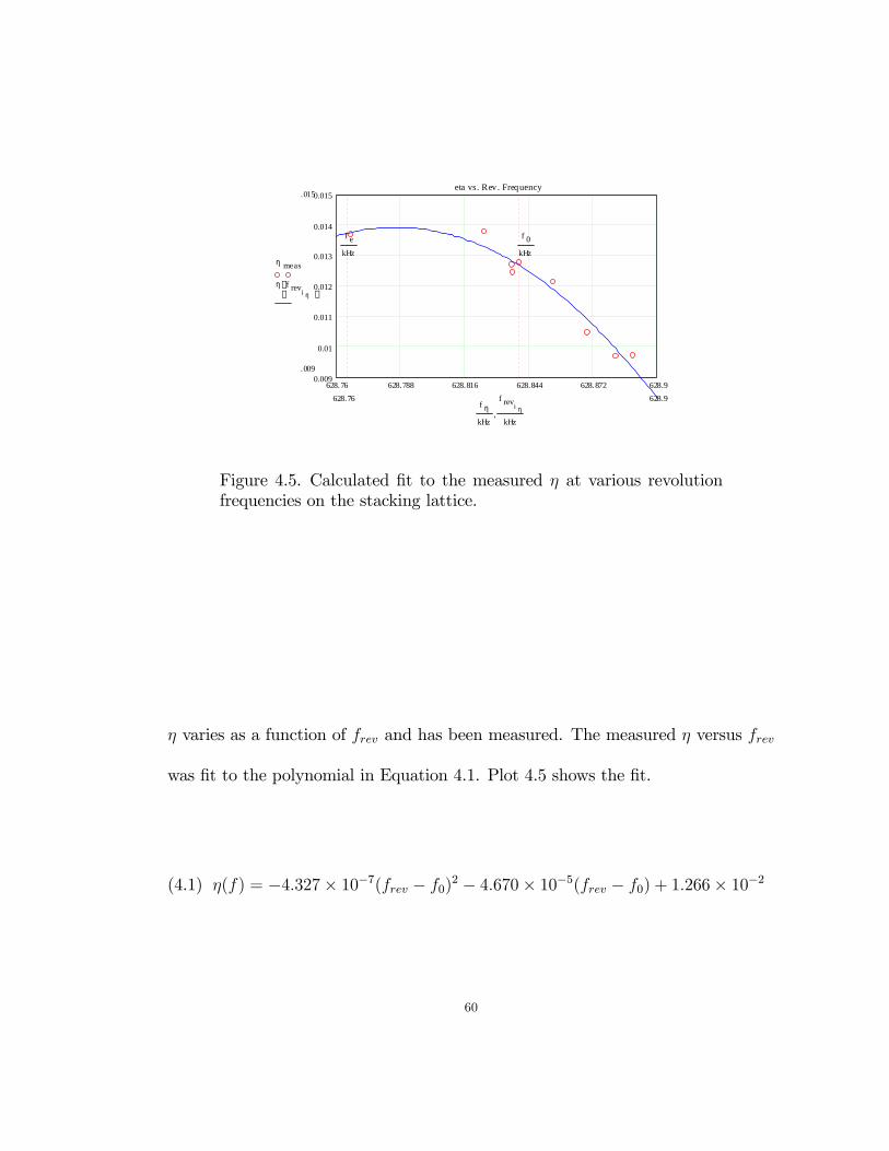
4.2.2. � on the Stacking Lattice

The quantity � is constant across the momentum aperture on the shot lattice,

however, it is not constant across the momentum aperture on the stacking lattice.

59

628.76 628.788 628.816 628.844 628.872 628.90.009

0.01

0.011

0.012

0.013

0.014

0.015eta vs. Rev . Frequency

.015

.009

η meas

η f revi η

628.9628.76

f e

kHz

f 0

kHz

f η

kHz

f revi η

kHz,

Figure 4.5. Calculated �t to the measured � at various revolutionfrequencies on the stacking lattice.

� varies as a function of frev and has been measured. The measured � versus frev

was �t to the polynomial in Equation 4.1. Plot 4.5 shows the �t.

(4.1) �(f) = �4:327� 10�7(frev � f0)2 � 4:670� 10�5(frev � f0) + 1:266� 10�2

60

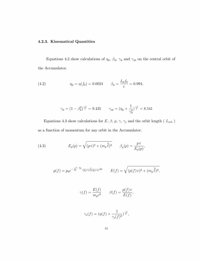
4.2.3. Kinematical Quantities

Equations 4.2 show calculations of �0, �0, 0 and t0 on the central orbit of

the Accumulator.

(4.2) �0 = �(f0) = 0:0024 �0 =L0f0c

= 0:994;

0 = (1� �20)�12 = 9:435 t0 = (�0 +

1

20)�12 = 8:541

Equations 4.3 show calculations for E, �, p, , t and the orbit length ( Lorb )

as a function of momentum for any orbit in the Accumulator.

(4.3) Ep(p) =

q(p c)2 + (mp

2c)2 �p(p) =

p c

Ep(p);

p(f) = p0e�R f�f00

1(f0+x)�(f0+x)

dxE(f) =

q(p(f) c)2 + (mp

2c)2;

(f) =E(f)

mpc2�(f) =

p(f) c

E(f);

t(f) = (�(f) +1

t(f)2)�12 ;

61

Lorb(f) = L0e�R ff0

1x�(x) t(x)

2 dx;

�p(f) =p(f)� p0

p0;

pc = p(fc) = 8743:718MeV

c

4.2.4. Multipole Parameters

Stength in the multipole magnets as a function of power supply current for

the quadrupole, sextupole and octupole �elds are shown in Equations 4.4, 4.5 and

4.6,respectively.

B1(IS; IO) = (2:030764� 10�6 TA)IS + (2:486613� 10�4

T

A)IO(4.4)

+(3:523344� 10�7 TA2)ISIO + (�4:4� 10�9

T

A3)ISI

2O;

B1(IS; IO;�IS;�IO) = B1(IS +�IS; IO +�IO)�B1(IS; IO)

62

B2(I) = (1:097079� 10�6 T

mA2)I2(4.5)

�(1:193167� 10�2 T

mA)I � 6:006515� 10�2 T

m;

B2(I;�I) = B2(I +�I)�B2(I);

(4.6) B3(�I) = (3:127722� 10�1T

m2A)�I

4.2.5. Bus Currents

The sextupole power supply current in the Ax10 locations, where x refers

to sectors 1 through 6, is nominally set to 404A. The sextupole power supply

current in the Ax12 locations is nominally set to 581A.The octupole power supply

current in the Ax10 locations is nominally set to 52:01A and 64:04A in the Ax12

locations. The possibility of a polarity change must be included and is de�ned as

PolarityiM = �1(�1)iM .

63

4.2.6. Stacking Lattice Parameters at the Multipole Magnets

In the Ax10 locations �x is 45:527m, �y is 12:568m and Dx is 7:758m. In the

Ax12 locations �x is 18:486m, �y is 29:554m and Dx is 6:976m.

4.2.7. Correction Algorithms

Equations 4.7 shows the developed tune circuits model.

��x0(�;�ISEX ;�IOCT )(4.7)

=NSecec4�p0

[(1� �)XiM

(PolarityiM�xiMB1(ISEXiM ; IOCTiM ;�ISEXiM ;�IOCTiM ))

+�XiM

(PolarityiM�xiMDxiM

B2(ISEX�{M ;�ISEXiM ))

+1

2�2XiM

(PolarityiM�xiMD2xiMB3(�IOCTiM )];

��y0(�;�ISEX ;�IOCT )

=NSecec4�p0

[(1� �)XiM

(PolarityiM�yiMB1(ISEXiM ; IOCTiM ;�ISEXiM ;�IOCTiM ))

+�XiM

(PolarityiM�yiMDxiM

B2(ISEX�{M ;�ISEXiM ))

+1

2�2XiM

(PolarityiM�yiMD2xiMB3(�IOCTiM )]

64

0.62876 0.62877 0.62879 0.6288 0.62882 0.62883 0.62884 0.62886 0.62887 0.62889 0.62890.001

8 .10 4

6 .10 4

4 .10 4

2 .10 4

0

2 .10 4

4 .10 4

6 .10 4

8 .10 4

0.001SEX10

.001

.001−

0

δν xm

δν x1

δν ym

δν y1

0.629.62876

f 0MHz

f revMHz

fMHz

,f revMHz

,f

MHz,

Figure 4.6. Model predictions compared to measured dqdIdata for

sextupoles in the Ax10 locations on the stacking lattice.

4.2.8. Compare Fits to Measured Values on the Stacking Lattice

The plots in Figures 4.6 and 4.7 show the measured data compared to the model

prediction for a 1A change in the Ax10 and Ax12 location sextupoles, respectively.

The model predictions match the measured data well. Figures 4.8 and 4.9 show

the measured data compared to the model prediction for a 1A change in the Ax10

and Ax12 location octupoles, respectively. The model predictions match well for

the Ax12 octupoles. The model diverges from the measurements by as much as

20% near the injection region for the Ax10 octupoles. This has not been a problem

during operations.

65

0.62876 0.62877 0.62879 0.6288 0.62882 0.62883 0.62884 0.62886 0.62887 0.62889 0.62890.001

8 .10 4

6 .10 4

4 .10 4

2 .10 4

0

2 .10 4

4 .10 4

6 .10 4

8 .10 4

0.001SEX12

.001

.001−

0

δν xm

δν x1

δν ym

δν y1

0.629.62876

f 0

MHz

f rev

MHz

f

MHz,

f rev

MHz,

f

MHz,

Figure 4.7. Model predictions compared to measured dqdIdata for

sextupoles in the Ax12 locations on the stacking lattice.

0.62876 0.62877 0.62879 0.6288 0.62882 0.62883 0.62884 0.62886 0.62887 0.62889 0.62890.001

8 .10 4

6 .10 4

4 .10 4

2 .10 4

0

2 .10 4

4 .10 4

6 .10 4

8 .10 4

0.001OCT10

.001

.001−

0

δν xm

δν x2

δν ym

δν y2

0.629.62876

f 0MHz

f revMHz

fMHz

,f revMHz

,f

MHz,

Figure 4.8. Model predictions compared to measured dqdIdata for

octupoles in the Ax10 locations on the stacking lattice.

66

0.62876 0.62877 0.62879 0.6288 0.62882 0.62883 0.62884 0.62886 0.62887 0.62889 0.62890.001

8 .10 4

6 .10 4

4 .10 4

2 .10 4

0

2 .10 4

4 .10 4

6 .10 4

8 .10 4

0.001OCT12

.001

.001−

0

δν xm

δν x3

δν ym

δν y3

0.629.62876

f 0

MHz

f re v

MHz

f

MHz,

f re v

MHz,

f

MHz,

Figure 4.9. Model predictions compared to measured dqdIdata for

octupoles in the Ax12 locations on the stacking lattice.

4.2.9. Predicted Tune Changes on the Shot Lattice

The shot lattice functions in the Ax10 locations are �x = 23:511m, �y =

11:192m and Dx = 8:519m. In the Ax12 locations they are �x = 12:289m,

�y = 29:554m and Dx = 7:462m. Using these lattice functions in the model

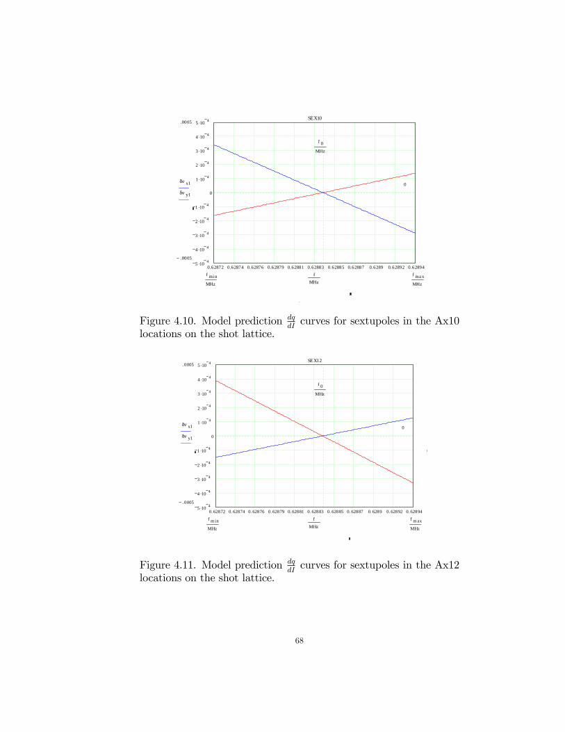
will give predicted tune changes on the shot lattice. Figures 4.10 and 4.11 show

the model prediction for a 1A change in the Ax10 and Ax12 location sextupoles,

respectively. Figures 4.12 and 4.13 show the model prediction for a 1A change in

the Ax10 and Ax12 location octupoles, respectively.

67

0.62872 0.62874 0.62876 0.62879 0.62881 0.62883 0.62885 0.62887 0.6289 0.62892 0.628945 .10 4

4 .10 4

3 .10 4

2 .10 4

1 .10 4

0

1 .10 4

2 .10 4

3 .10 4

4 .10 4

5 .10 4 SEX10.0005

.0005−

0δν x1

δν y1

f ma xMHz

f mi nMHz

f 0MHz

fMHz

Figure 4.10. Model prediction dqdIcurves for sextupoles in the Ax10

locations on the shot lattice.

0. 62872 0. 62874 0. 62876 0. 62879 0. 62881 0. 62883 0. 62885 0. 62887 0. 6289 0. 62892 0. 628945 .10 4

4 .10 4

3 .10 4

2 .10 4

1 .10 4

0

1 .10 4

2 .10 4

3 .10 4

4 .10 4

5 .10 4 SEX12.0005

.0005−

0δν x1

δν y1

f m ax

MHz

f m in

MHz

f 0

MHz

f

MHz

Figure 4.11. Model prediction dqdIcurves for sextupoles in the Ax12

locations on the shot lattice.

68

0.62872 0.62874 0.62876 0.62879 0.62881 0.62883 0.62885 0.62887 0.6289 0.62892 0.628945 .10 4

4 .10 4

3 .10 4

2 .10 4

1 .10 4

0

1 .10 4

2 .10 4

3 .10 4

4 .10 4

5 .10 4 OCT10.0005

.0005−

0δν x1

δν y1

f maxMHz

f minMHz

f 0MHz

fMHz

Figure 4.12. Model prediction dqdIcurves for octupoles in the Ax10

locations on the shot lattice.

0.62872 0.62874 0.62876 0.62879 0.62881 0.62883 0.62885 0.62887 0.6289 0.62892 0.628945 .10 4

4 .10 4

3 .10 4

2 .10 4

1 .10 4

0

1 .10 4

2 .10 4

3 .10 4

4 .10 4

5 .10 4 OCT12.0005

.0005−

0δν x1

δν y1

f m ax

MHz

f m in

MHz

f 0

MHz

f

MHz

Figure 4.13. Model prediction dqdIcurves for octupoles in the Ax12

locations on the shot lattice.

69

SEX10 Shot Lattice

y = -1.21451E-14x2 + 1.36137E-06x + 1.53831E-06

y = -1.97485E-14x2 - 2.85976E-06x - 3.23140E-06

-0.0006

-0.0004

-0.0002

0.0000

0.0002

0.0004

0.0006

-80 -60 -40 -20 0 20 40 60

f rev - f 0 (Hz)

dq/d

I

HorizontalVerticalvh

Figure 4.14. Fits to dqdIcurves predicted by the model for the

sextupoles in the Ax10 locations on the shot lattice.

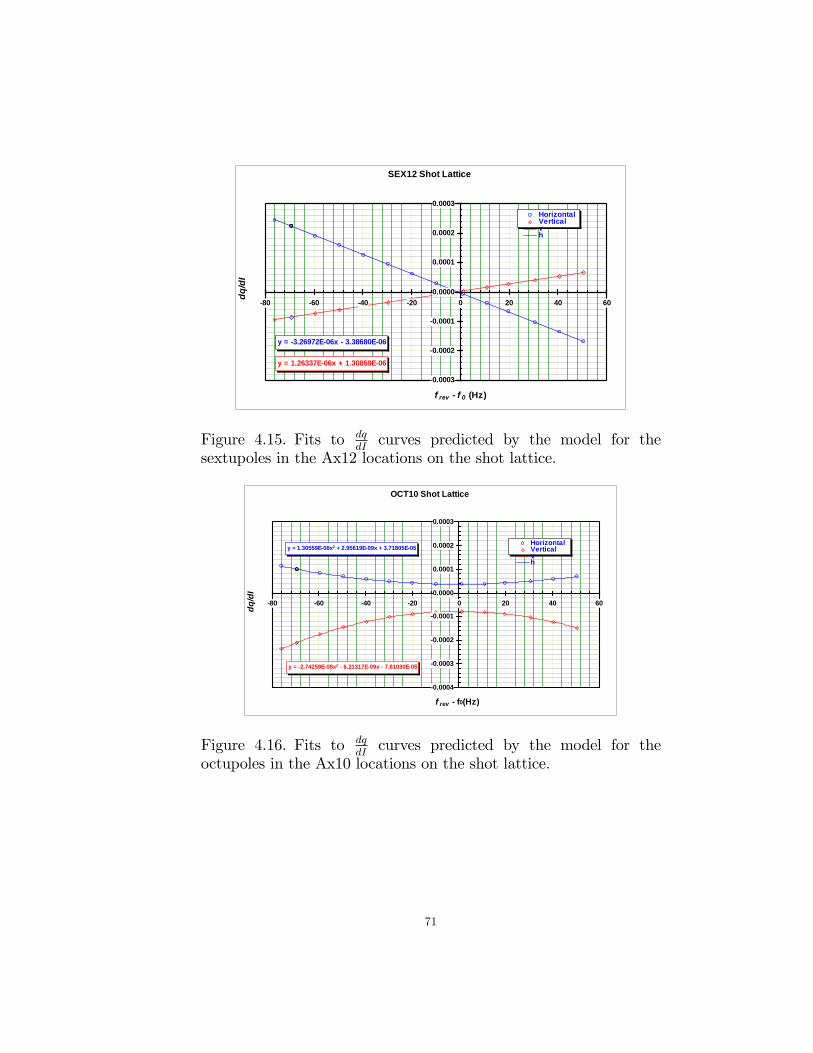
4.2.10. Fits to the Shot Lattice dqdICurves

Figures 4.14 and 4.15 show the �ts, including the tune correction equation

coe¢ cients, to the shot lattice model prediction for a 1A change in the Ax10 and

Ax12 location sextupoles, respectively.

Figures 4.16 and 4.17 show the �ts, including the tune correction equation

coe¢ cients, to the shot lattice model prediction for a 1A change in the Ax10 and

Ax12 location octupoles, respectively.

70

SEX12 Shot Lattice

y = 1.26337E-06x + 1.30859E-06

y = -3.26972E-06x - 3.38680E-06

-0.0003

-0.0002

-0.0001

0.0000

0.0001

0.0002

0.0003

-80 -60 -40 -20 0 20 40 60

f rev - f 0 (Hz)

dq/d

I

HorizontalVerticalvh

Figure 4.15. Fits to dqdIcurves predicted by the model for the

sextupoles in the Ax12 locations on the shot lattice.

OCT10 Shot Lattice

y = -2.74259E-08x2 - 6.21317E-09x - 7.81030E-05

y = 1.30559E-08x2 + 2.95619E-09x + 3.71805E-05

-0.0004

-0.0003

-0.0002

-0.0001

0.0000

0.0001

0.0002

0.0003

-80 -60 -40 -20 0 20 40 60

f rev - f0(Hz)

dq/d

I

HorizontalVerticalvh

Figure 4.16. Fits to dqdIcurves predicted by the model for the

octupoles in the Ax10 locations on the shot lattice.

71

OCT12 Shot Lattice

y = -2.84701E-08x2 - 5.07452E-09x - 6.38059E-05

y = 1.10004E-08x2 + 1.96009E-09x + 2.46537E-05

-0.0003

-0.0003

-0.0002

-0.0002

-0.0001

-0.0001

0.0000

0.0001

0.0001

0.0002

0.0002

-80 -60 -40 -20 0 20 40 60

f rev - f0 (Hz)

dq/d

I

HorizontalVerticalvh

Figure 4.17. Fits to dqdIcurves predicted by the model for the

octupoles in the Ax12 locations on the shot lattice.

72

CHAPTER 5

Summary and Conclusions

It is important to know the tunes and emittances across the momentum aperture

of an accelerator, especially a storage ring such as the Accumulator. Methods and

tools must be developed to correct for any anomalies and to keep the machine

operating within a stable space.

To measure the tunes across the aperture during Tevatron Run I beam would

be bunched and moved with RF, by hand, to various revolution frequencies. Tunes

would be calculated one at a time from Schottky detector spectrum analyzer traces.

The tunes were manually entered into a separate simulation code to predict and

apply any corrections. The measurements would then be taken again. The method

was similar in nature to the RF method described in Chapter 2, however, it would

take two knowledgable people four to eight hours to setup and execute. During

special circumstances the Accumulator would run with no coupling at the core

revolution frequency. The method �rst developed by S. van der Meer and adapted

by Rui Alves-Pires in 1993, for the Accumulator at Fermilab, was used in the

instances. During the current collider run the Accumulator runs with coupling at

73

the core frequency so this power measurement method, as described in Chapter

3.1 becomes di¢ cult.

In the beginning of Tevatron Run II, as in Run I, beam was bunched and moved

with RF by hand, although a VSA was now available. This was an improvement,

especially in the display of the data, yet there were still limitations. Two experienced

people were needed, only two sidebands could be recorded during a measurement,

data would have to be stored in a �le on the VSA or transfered to a �oppy

disk for later analysis and tune values were calculated, by hand, and manually

entered into a separate simulation. The RF method described in Chapter 2 is a

vast improvement. Once a person is familiar with the software a two sideband

measurement would take one person 10 to 15 minutes to execute. A four sideband

measurement would take 20 to 30 minutes. Peak values are automatically loaded

into the simulation code so a second measurement could be done within minutes.

Data can be stored in a �le on the controls system which could be analyzed by

anyone with a console.

Using the program written to move the beam using ARF-3 is now the primary

method for measuring the tunes across the aperture and will be used for maintaining

the tunes as well as measuring and adjusting tunes for any Accumulator lattice

changes. One such change will happen in the near future. The Recycler ring is

currently being commissioned. When it is integrated into daily operations the

74

Accumulator will no longer transfer antiprotons to the Tevatron for collider stores.

The Accumulator will transfer antiprotons to the Recycler where larger stacks can

be accumulated. There is a ~40 MeV energy di¤erence between the Accumulator

and the Recycler. Since the Recycler uses permanent magnets the energy in the

Recycler is �xed. 8 GeV energies in all of the other machines will need to be

adjusted to match the Recycler energy. This adjustment will require a change to

the Accumulator lattice. Measuring and adjusting the tunes across the aperture

will be essential during this change. The RF method will be the method used.

Although the power measurement method is not the primary tool used to

measure the tunes across the aperture it does have two advantages over the RF

method. Emittances are calculated and tunes are measured during stacking operations.

This could prove to be useful. For example, if the stack rate is zero or lower than

expected while stacking in the Accumulator the tunes could be decoupled and the

power measurement method could be used to locate any possible resonances in the

tunes across the aperture indicating a possible problem with a magnet. Another use

could be to decouple the tunes for a complete stacking cycle and using the power

measurement method at several stack sizes to characterize tunes and emittances

with respect to the number of antiprotons in the stack.

These two methods of measuring the tunes across the aperture compliment

each other and give the Antiproton Source Group great versatility.

75

References

[1] Elvin Harms and Jim Morgan, The Antiproton Source Rookie Book, FermiNational Accelerator Laboratory, August 1999.

[2] A. V. Tollestrup and G. Dugan, Physics of High Energy Particle Accelerators,AIP Conf. Proc. 105, New York, 1983.

[3] Hewlitt Packard 89440A DC to 1.8 GHz Data Sheet.

[4] S. Y. Lee, Accelerator Physics, ( World Scienti�c Publishing, Singapore, 1999).

[5] D. A. Edwards and M. J. Syphers, An Introduction to the Physics of HighEnergy Accelerators, ( John Wiley and Sons, Inc, N. Y., 1993 ).

[6] S. van der Meer DIAGNOSTICS WITH SCHOTTKY NOISE, Lecture given atthe Joint US-CERN School on Beam Observation, Diagnosis and Correction,October 1988, Capri, Italy.

[7] Rui Alves-Pires Measurement of Transverse Emittances as a Function ofRevolution Frequency and Beam Current in the Accumulator, Pbar Note #548,Fermi National Accelerator Laboratory, August 1993.

[8] S. Werkema, private communications.

[9] Fermilab Personnel, DESIGN REPORT TEVATRON 1 PROJECT, FermiNational Accelerator Laboratory, September 1984.

76