HSE Health & Safety

Executive

Development of theoretical model for simulating FLT overturn ­

Rate of steering response - Fixed geometry vehicle

Prepared by Frazer-Nash Consultancy Ltd for the Health and Safety Executive 2004

RESEARCH REPORT 291

HSE Health & Safety

Executive

Development of theoretical model forsimulating FLT overturn ­

Rate of steering response - Fixed geometry vehicle

S A Challener A F Wylie

Frazer-Nash Consultancy Ltd Stonebridge House

Dorking Business Park Dorking

Surrey RH4 1HJ

This report describes the development of an analytical model that can be used to assess the stability of fork lift trucks undergoing steering manoeuvres.

The work has been carried out by Frazer-Nash Consultancy Limited (FNC) on behalf of the Health and Safety Executive (HSE) under contract number 4524/R36.197. The work builds on work previously undertaken for HSE that looked at the stability of fork lift trucks under steady state cornering conditions.

The model has demonstrated the two features that were of particular interest, namely the effect of rear wheel steering on the path taken and the effect of rate of change of steer angle on stability.

• The model shows that rear wheel steer leads to a tightening up of the turning radius of the rear wheel

on straightening out from a turn. Depending on the conditions, this may mean that the truck is more

likely to roll over when exiting the turn than when continuing the turn under steady state conditions.

• This change of turning radius causes a roll moment to be applied to the truck. The more rapid this

change is, the greater the roll moment produced, under certain conditions this can lead to the truck

rolling over.

The model is able to rapidly analyse the stability of a wide configuration of trucks under different steering manoeuvres and can give an insight into the mechanisms involved in fork lift truck rollover.

It has been demonstrated that this model could be used to quickly ascertain whether a particular manoeuvre was ‘safe’ and consequently it could be used in conjunction with a control system, fitted to a truck, which would prevent the vehicle from being operated outside its safe envelope. However, before this can be achieved, the model requires validation against physical test results.

This report and the work it describes were funded by the Health and Safety Executive (HSE). Its contents, including any opinions and/or conclusions expressed, are those of the authors alone and do not necessarily reflect HSE policy.

HSE BOOKS

© Crown copyright 2004

First published 2004

ISBN 0 7176 2928 7

All rights reserved. No part of this publication may bereproduced, stored in a retrieval system, or transmitted inany form or by any means (electronic, mechanical,photocopying, recording or otherwise) without the priorwritten permission of the copyright owner.

Applications for reproduction should be made in writing to:Licensing Division, Her Majesty's Stationery Office, St Clements House, 2-16 Colegate, Norwich NR3 1BQ or by e-mail to hmsolicensing@cabinet-office.x.gsi.gov.uk

ii

CONTENTS

1. INTRODUCTION 5

2. DESCRIPTION 6

2.1 MODEL CAPABILITY OVERVIEW 6

2.2 DEVELOPMENT PROCESS 6

2.3 SOLUTION APPROACH 6

2.4 MODEL INPUTS 7

2.5 MODEL OUTPUTS 8

3. MODEL DETAILS 9

3.1 AXIS SYSTEMS 9

3.2 FORCES 9

3.3 ACCELERATIONS AND INTEGRATION 11

3.4 SUSPENSION 12

4. EXAMPLES 13

4.1 TURNING AT LIMIT OF STABILITY 13

4.2 STEERING ANGLE OF 65 DEGREES 15

4.3 THE EFFECT OF RATE OFAPPLICATION OF TURN 17

4.4 THE EFFECT OF APPLIED DRIVING FORCE 18

4.5 TRUCK UNDERTAKING A SHARP TURN WITH NO LOAD 19

4.6 TRUCK UNDERTAKING A SHARP TURN WITH LOAD IN THE DOWNPOSITION 21

4.7 TRUCK UNDERTAKING A SHARP TURN WITH A RAISED LOAD 22

5. CONCLUSIONS 23

6. REFERENCES 24

iii

iv

1. INTRODUCTION

This report describes the development of an analytical model that can be used to assess the stability of fork lift trucks undergoing steering manoeuvres.

The work has been carried out by Frazer-Nash Consultancy Limited (FNC) on behalf of the Health and Safety Executive (HSE) under contract number 4524/R36.197. The work builds on work previously undertaken for HSE that looked at the stability of fork lift trucks under steady state cornering conditions.

The aim of this piece of work was to model the fork-lift truck as it follows a pre-defined course. Having this modelling ability allows for the investigation of the following two effects:

· Previous work (Reference 1) has proposed that, for a rear-wheel steer vehicle with Ackermann steering geometry, the centre of gravity of follows a path with a smaller radius of curvature when exiting a corner than was experienced in the turn. This means the vehicle is more likely to roll-over as it exits the turn.

· Anecdotal evidence suggests fork-lift trucks become more likely to rollover as the rate of turn of the steering wheel increases.

The objectives of this work are:

· To enable the modelling of trucks with a wide variety of three and four wheeled configuration with various geometries performing a large number of manoeuvres, on flat and sloping ground.

· To produce a simulation tool which is quick to run and easy to use.

5

2.1

2. DESCRIPTION

This section describes the model that has been developed.

MODEL CAPABILITY OVERVIEW

The model that has been developed allows a user to simulate a very large variety of physical cases. In summary the model can be used to model the behaviour of the following:

· Three and four wheel trucks

· Front or rear wheel drive

· Front or rear wheel steer

· Any manoeuvre, based on a time history of steering angle and force from the driven wheels

· With or without a load on the forks

· Sloping ground

· Rigid or pivoting rear axle

The model runs quickly (approximately 5 seconds) and has a good graphical user interface (GUI). This makes it particularly suitable for the investigation of the effects on stability of differences in truck geometry and mass parameters, load conditions and steering manoeuvres. Screen shots of the GUI are shown in Figure 1 and Figure 2.

2.2 DEVELOPMENT PROCESS

The model was developed using a two stage process. In the first stage the underlying physics was modelled with a FORTRAN computer simulation. When this was found to be working satisfactorily, the model was incorporated into the existing steady state IDL model. IDL is an extremely powerful complete computing environment for the interactive analysis and visualisation of data.

Previous work, which also was developed using IDL, is described in Reference 2. The original model took largely similar inputs to the current model and calculated the rate at which a truck would roll-over for a given truck geometry, mass and speed. However this model only considered a constant bend radius and the tyres where not modelled in any detail.

2.3 SOLUTION APPROACH

The model solves the equations of motion of a truck undergoing steering manoeuvres. These equations are solved using a time stepping method of numerical integration that can be summarised as follows:

· The slip angle at each tyre is calculated, based on the current truck velocity and steering input.

· The side forces at each tyre are calculated from the slip angles (based on data supplied by tyre manufacturers)

· The trucks forward, sideways, roll, pitch and yaw accelerations are calculated from the tyre side forces and the driving force.

6

2.4

· The accelerations are integrated to give the linear and angular velocity and position of the truck.

· The time is updated and the loop repeated

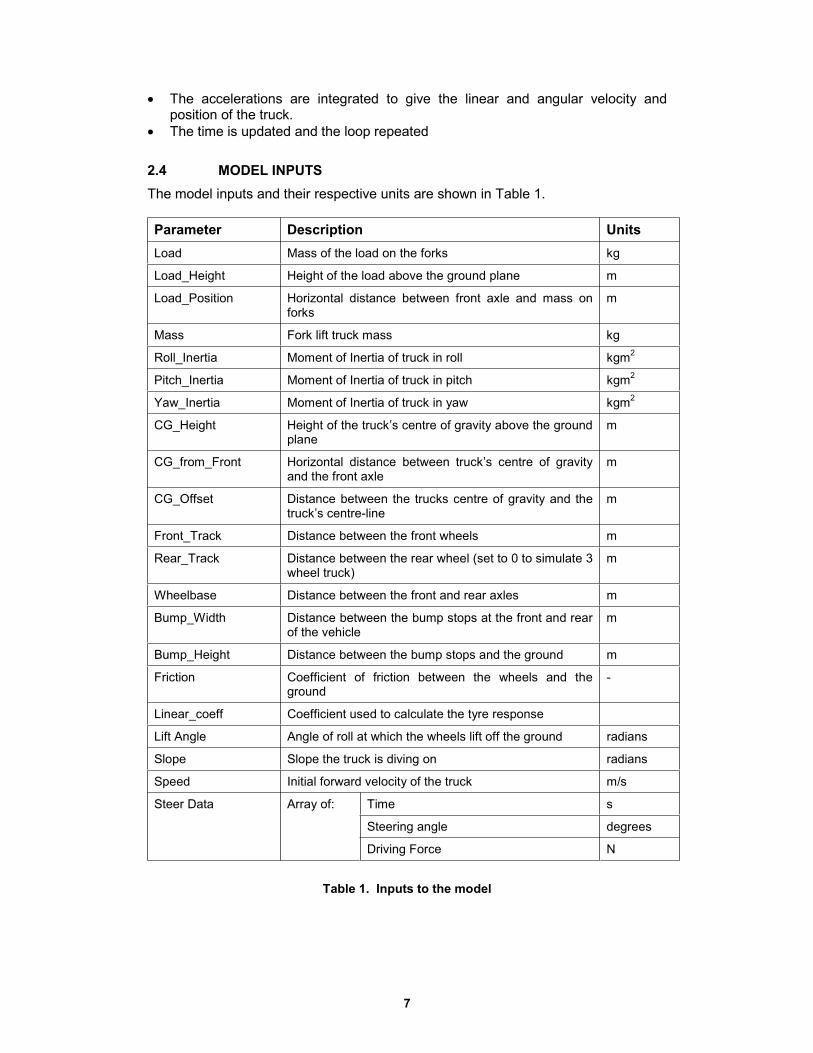
MODEL INPUTS

The model inputs and their respective units are shown in Table 1.

Parameter Description Units

Load Mass of the load on the forks kg

Load_Height Height of the load above the ground plane m

Load_Position Horizontal distance between front axle and mass on forks

m

Mass Fork lift truck mass kg

Roll_Inertia Moment of Inertia of truck in roll kgm 2

Pitch_Inertia Moment of Inertia of truck in pitch kgm 2

Yaw_Inertia Moment of Inertia of truck in yaw kgm 2

CG_Height Height of the truck’s centre of gravity above the ground m plane

CG_from_Front Horizontal distance between truck’s centre of gravity m and the front axle

CG_Offset Distance between the trucks centre of gravity and the m truck’s centre-line

Front_Track Distance between the front wheels m

Rear_Track Distance between the rear wheel (set to 0 to simulate 3 m wheel truck)

Wheelbase Distance between the front and rear axles m

Bump_Width Distance between the bump stops at the front and rear m of the vehicle

Bump_Height Distance between the bump stops and the ground m

Friction Coefficient of friction between the wheels and the ground

-

Linear_coeff Coefficient used to calculate the tyre response

Lift Angle Angle of roll at which the wheels lift off the ground radians

Slope Slope the truck is diving on radians

Speed Initial forward velocity of the truck m/s

Steer Data Array of: Time s

Steering angle degrees

Driving Force N

Table 1. Inputs to the model

7

2.5

The truck data can be written to and read from data files. Similarly steering manoeuvres can be written to and read from files so that different combinations of truck and conditions can readily be analysed.

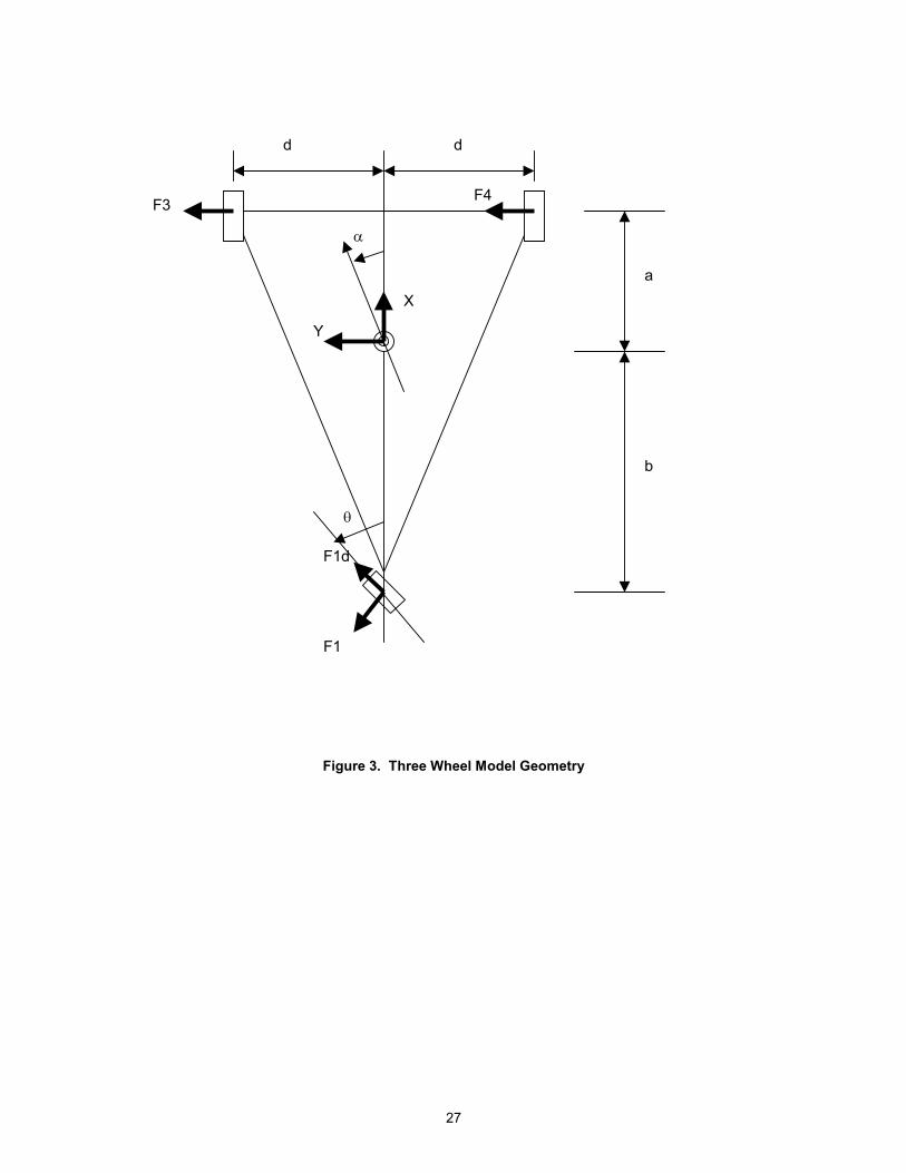
The basic model in three wheel configuration is shown in Figure 3.

MODEL OUTPUTS

The GUI used to set up the models also displays the results after the analysis has been run. The GUI can be used to print the outputs or to select numerical values from the results. The following outputs can be displayed in the GUI as outputs. These are all plotted against time, except where indicated.

· Steer Angle

· Driving Force

· Tyre Characteristics (Side force versus slip angle)

· CG Path (in XY space)

· Front Axle Path (in XY space)

· Rear Axle Path (in XY space)

· Roll Angle

· Yaw Angle

· Forward Speed

· Wheel Loads

· Slip Angles

· Tyre Forces

· Wheel Paths (in XY space)

In addition, animations showing the motion of the truck can be produced.

The conditions at the limit of rollover can be extracted and applied to the steady state model to determine the time taken for complete rollover to occur. This is simple to perform. The truck geometry file can be read by the steady state model as well as the steered model. The forward velocity of the truck when one wheel lifts off the ground (i.e. when the analysis stops) should be taken from the steered model and applied to the steady state model.

8

3. MODEL DETAILS

3.1 AXIS SYSTEMS

The truck is modelled in a local axis system where the x axis is forwards, the y axis is sideways to the left and the z axis is upwards (see Figure 3). In addition, a global axis system is used to calculate the truck position, direction of travel and orientation so that the path that the truck takes can be determined.

3.2 FORCES

The forces acting on the truck consist of the following

· Gravity.

· Vertical forces at the wheels.

· Side forces at the wheels due to the slip angle between direction of travel and orientation of the wheel and the vertical force on the wheel.

· Driving force at the front or rear wheels.

3.2.1 Gravity

When the truck is modelled on level ground the gravitational force acts vertically through the centre of gravity and remains constant.

If a slope is included in the model the simulation holds the truck on the slope all the time, hence the truck is modelled at the point where the slope is most likely to cause the truck to roll over. The gravitational force is modelled inclined towards the centre of the turn, acting through the centre of gravity.

3.2.2 Vertical Forces

The static vertical forces at the wheels are given by

w1s = mass*g*a/(a+b) w3s = 0.5*mass*g*b/(a+b) w4s = 0.5*mass*g*b/(a+b)

Where a and b are dimensions shown in Figure 1.

Dynamically, the wheel forces are changed by truck roll and pitch. This effect is controlled by the spring and damper rates, rstiff and rdamp.

w1 = w1s - pstiff*pang*a - pdamp*pvel*a

w3 = w3s - rstiff*rang*d - rdamp*rvel*d + 0.5*pstiff*pang*a +

0.5*pdamp*pvel*a

w4 = w4s + rstiff*rang*d + rdamp*rvel*d + 0.5*pstiff*pang*a +

0.5 *pdamp*pvel*a

In the above equations rang and rvel are the roll angle and velocity and pang and pvel are the pitch angle and velocity.

9

If a wheel force becomes negative, it is set to zero and the other wheel forces modified to maintain the correct total force.

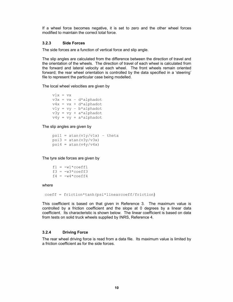
3.2.3 Side Forces

The side forces are a function of vertical force and slip angle.

The slip angles are calculated from the difference between the direction of travel and the orientation of the wheels. The direction of travel of each wheel is calculated from the forward and lateral velocity at each wheel. The front wheels remain oriented forward; the rear wheel orientation is controlled by the data specified in a ‘steering’ file to represent the particular case being modelled.

The local wheel velocities are given by

v1x = vxv3x = vx – d*alphadot v4x = vx + d*alphadot v1y = vy – b*alphadot v3y = vy + a*alphadot v4y = vy + a*alphadot

The slip angles are given by

psi1 = atan(v1y/v1x) – theta

psi3 = atan(v3y/v3x)

psi4 = atan(v4y/v4x)

The tyre side forces are given by

f1 = -w1*coeff1 f3 = -w3*coeff3 f4 = -w4*coeff4

where

coeff = friction*tanh(psi*linearcoeff/friction)

This coefficient is based on that given in Reference 3. The maximum value is controlled by a friction coefficient and the slope at 0 degrees by a linear data coefficient. Its characteristic is shown below. The linear coefficient is based on data from tests on solid truck wheels supplied by INRS, Reference 4.

3.2.4 Driving Force

The rear wheel driving force is read from a data file. Its maximum value is limited by a friction coefficient as for the side forces.

10

3.2.5 Total Forces

The total vertical force is zero.

The total forward and lateral forces and roll, pitch and yaw moments are given by

Fx = -f1*sin(theta) + f1d*cos(theta) Fy = f1*cos(theta) + f1d*sin(theta) + f3 + f4 Mx = (f1*cos(theta) + f1d*sin(theta) + f3 + f4)*h –

(w4 – w3)*d*cos(rang)

My = ((f1*sin(theta1) + f2*sin(theta2) - f1d*cos(theta))*h +

(w1 + w2)*b - (w3 + w4)*a)

Mz = (f3 + f4)*a – (f1*cos(theta) + f1d*sin(theta))*b.

3.3 ACCELERATIONS AND INTEGRATION

The accelerations are given by

Ax = Fx/m Ay = Fy/m Alphaddot = Mz/iz Rollddot = Mx/ix Pitchddot = My/iy

The global accelerations are calculated by rotating the local accelerations by alpha.

Xddot = Ax*cos(alpha) - Ay*sin(alpha) Yddot = Ax*sin(alpha) + Ay*cos(alpha)

The velocities are obtained by integrating the accelerations and the displacements by integrating the velocities. This integration is performed using a Runge-Kutta routine from Numerical Recipes, Reference 5.

11

3.4 SUSPENSION

A dynamic model, such as the one created can only operate effectively if springs are introduced. For the model developed here these springs represent the vertical stiffness of the tyres. The springs are modelled with some damping in order to control the frequency response of the model. Arbitrary values for the springs have been chosen, these represent wheel lift at 0.02 radians of body roll for the truck. The damping is set such that the truck is critically damped.

12

4.1

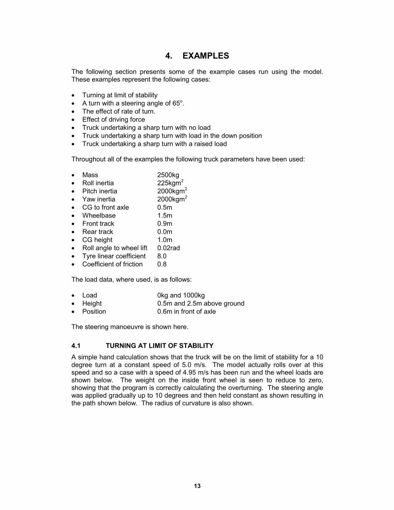
4. EXAMPLES

The following section presents some of the example cases run using the model. These examples represent the following cases:

· Turning at limit of stability

· A turn with a steering angle of 65o.

· The effect of rate of turn.

· Effect of driving force

· Truck undertaking a sharp turn with no load

· Truck undertaking a sharp turn with load in the down position

· Truck undertaking a sharp turn with a raised load

Throughout all of the examples the following truck parameters have been used:

· Mass 2500kg

· Roll inertia 225kgm2

· Pitch inertia 2000kgm2

· Yaw inertia 2000kgm2

· CG to front axle 0.5m

· Wheelbase 1.5m

· Front track 0.9m

· Rear track 0.0m

· CG height 1.0m

· Roll angle to wheel lift 0.02rad

· Tyre linear coefficient 8.0

· Coefficient of friction 0.8

The load data, where used, is as follows:

· Load 0kg and 1000kg

· Height 0.5m and 2.5m above ground

· Position 0.6m in front of axle

The steering manoeuvre is shown here.

TURNING AT LIMIT OF STABILITY

A simple hand calculation shows that the truck will be on the limit of stability for a 10 degree turn at a constant speed of 5.0 m/s. The model actually rolls over at this speed and so a case with a speed of 4.95 m/s has been run and the wheel loads are shown below. The weight on the inside front wheel is seen to reduce to zero, showing that the program is correctly calculating the overturning. The steering angle was applied gradually up to 10 degrees and then held constant as shown resulting in the path shown below. The radius of curvature is also shown.

13

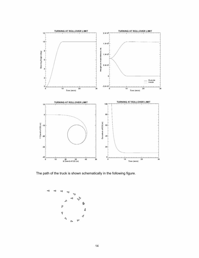
The path of the truck is shown schematically in the following figure.

14

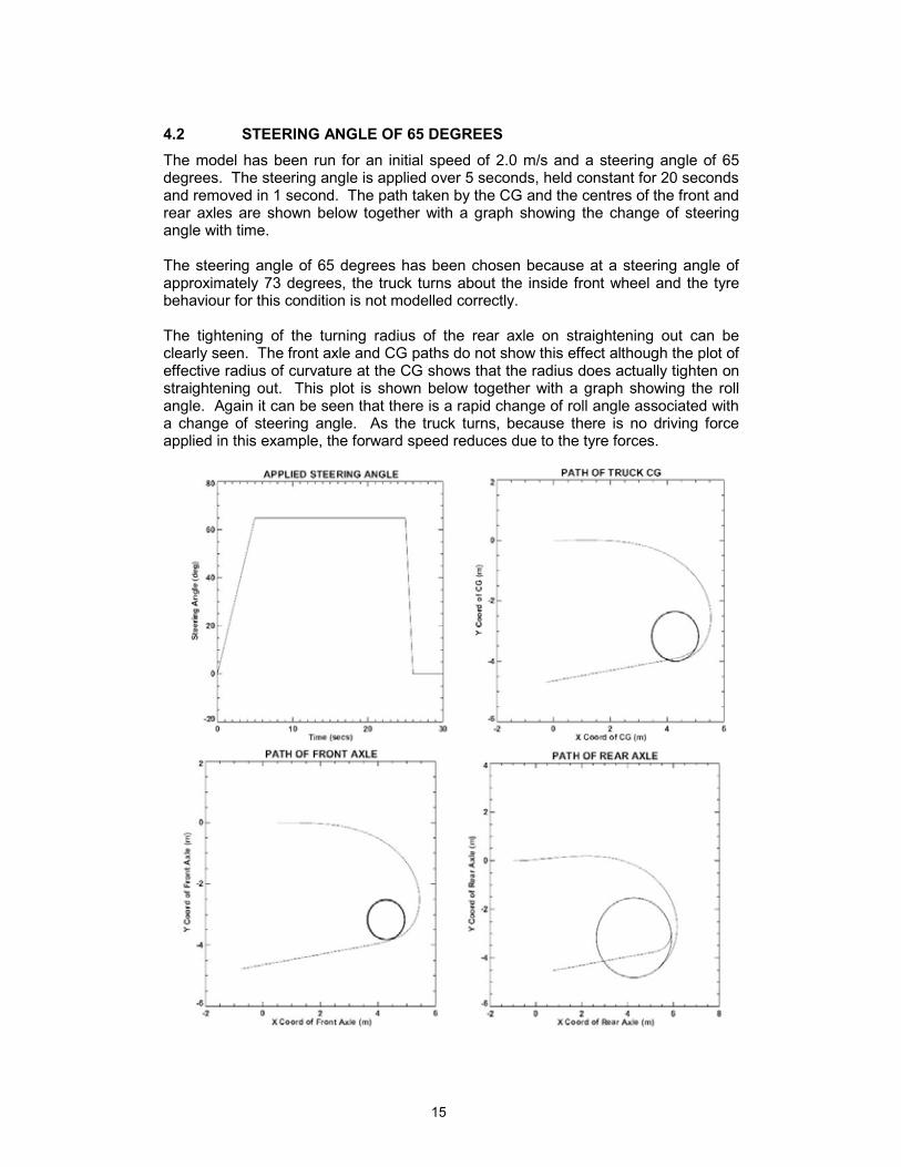
4.2 STEERING ANGLE OF 65 DEGREES

The model has been run for an initial speed of 2.0 m/s and a steering angle of 65 degrees. The steering angle is applied over 5 seconds, held constant for 20 seconds and removed in 1 second. The path taken by the CG and the centres of the front and rear axles are shown below together with a graph showing the change of steering angle with time.

The steering angle of 65 degrees has been chosen because at a steering angle of approximately 73 degrees, the truck turns about the inside front wheel and the tyre behaviour for this condition is not modelled correctly.

The tightening of the turning radius of the rear axle on straightening out can be clearly seen. The front axle and CG paths do not show this effect although the plot of effective radius of curvature at the CG shows that the radius does actually tighten on straightening out. This plot is shown below together with a graph showing the roll angle. Again it can be seen that there is a rapid change of roll angle associated with a change of steering angle. As the truck turns, because there is no driving force applied in this example, the forward speed reduces due to the tyre forces.

15

Path of the Vehicle

16

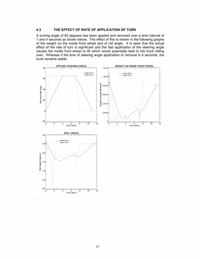
4.3 THE EFFECT OF RATE OF APPLICATION OF TURN

A turning angle of 65 degrees has been applied and removed over a time interval of 1 and 4 seconds as shown below. The effect of this is shown in the following graphs of the weight on the inside front wheel and of roll angle. It is seen that the actual effect of the rate of turn is significant and the fast application of the steering angle causes the inside front wheel to lift which would potentially lead to the truck rolling over. Whereas if the time of steering angle application or removal is 4 seconds, the truck remains stable.

.

17

4.4 THE EFFECT OF APPLIED DRIVING FORCE

The 65 degree steering angle case has been repeated with a driving force applied to the rear wheel in an attempt to maintain a constant speed during the constant part of the turn. The force applied is shown in the graph that also shows the applied steering angle. A Graph of forward speed and roll angle are also presented. It can be seen that the speed (i.e. forward component of velocity) reduces as the truck begins to turn, it remains more or less constant during the turn and then increases as the truck straightens out back to the initial speed.

For this case the steering angle was removed more slowly, over a time interval of 10 seconds because a faster change of steering angle caused the truck to roll over. Even at the chosen rate it can be seen that the weight on the inside front wheel reduces briefly to zero.

18

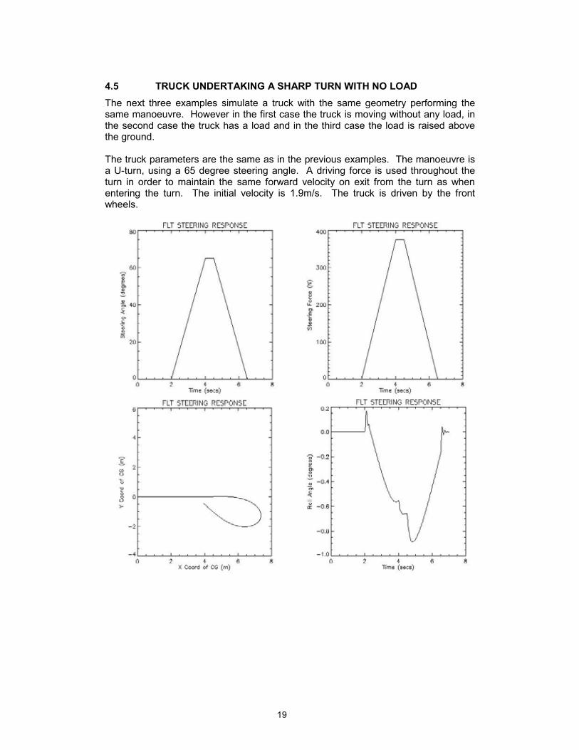
4.5 TRUCK UNDERTAKING A SHARP TURN WITH NO LOAD

The next three examples simulate a truck with the same geometry performing the same manoeuvre. However in the first case the truck is moving without any load, in the second case the truck has a load and in the third case the load is raised above the ground.

The truck parameters are the same as in the previous examples. The manoeuvre is a U-turn, using a 65 degree steering angle. A driving force is used throughout the turn in order to maintain the same forward velocity on exit from the turn as when entering the turn. The initial velocity is 1.9m/s. The truck is driven by the front wheels.

19

20

4.6 TRUCK UNDERTAKING A SHARP TURN WITH LOAD IN THE DOWN POSITION

This example is exactly the same as the previous example, with the exception that the truck is carrying a 1000kg load on the forks. The centre of gravity of the load is held 0.5m above the ground plane.

The results from this model show a that the truck has a greatly increased stability, due to the action of the load on the forks. This load increases the weight on the front wheels and means that the minimum load on the inside wheel is over 5000N (c.f. 500N in the previous example). This wheel that is loaded the lightest is the rear wheel, since this is on the centre-line of the vehicle this wheel is affected least by the turn of the vehicle.

21

4.7 TRUCK UNDERTAKING A SHARP TURN WITH A RAISED LOAD

This example is the same as the previous two examples, except that the 1000kg load is now raised 2.5m above the ground plane. As the wheel load graph shows the inside wheel of the truck is close to lifting off the ground, i.e. reaching the rollover condition.

22

5. CONCLUSIONS

The model has demonstrated the two features that were of particular interest, namely the effect of rear wheel steering on the path taken and the effect of rate of change of steer angle on stability.

1. The model shows that rear wheel steer leads to a tightening up of the turning radius of the rear wheel on straightening out from a turn. Depending on the truck geometry, this may mean that the truck is more likely to roll over when exiting the turn than when continuing the turn under steady state conditions, assuming that the velocity remains constant.

2. This change of turning radius causes a roll moment to be applied to the truck. The more rapid this change is the greater the roll moment produced. Under certain conditions this can lead to the truck rolling over.

The combination of the software and the graphical user interface makes analysis of FLT’s extremely efficient. The model is able to rapidly analyse the stability of a wide configuration of trucks under different steering manoeuvres.

It is believed that this package can be used with confidence to predict the behaviour of FLT’s in any given manoeuvre.

It is also possible that, in the future, this package could form an important development tool that can be used to develop control software for the speed of the truck so that in any configuration the FLT remains stable. Should this be achieved it would provide a significant improvement in FLT safety.

23

6. REFERENCES

1. O CRICHTON Mathematical Simulation of Ackermann Steering Geometry and its Implications to Fork Lift Truck Stability HSE SME 902/292/01 R33.11 IR/L/FE/94/07

2. FNC REPORT Simulations of Three and Four Wheeled Vehicles FNC 5352/19708R Issue 1

3. The Dynamics of Vehicles on Roads and on Tracks, edited Zhiyun Shen

4. Institut National de Recherche et de Securite, Fax. From J Rebelle, dated 18/06/2003

5. Numerical Recipes in Fortran Cambridge University Press

24

Figure 1 Graphical User Interface for Steering Model

25

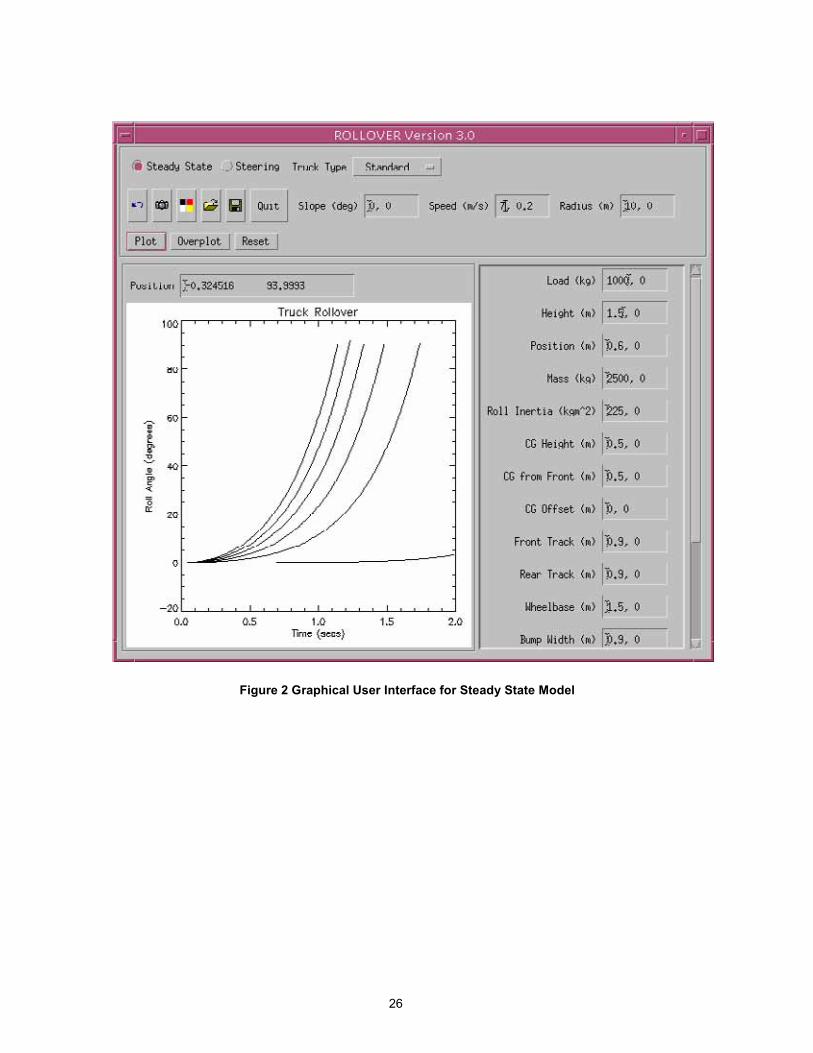
Figure 2 Graphical User Interface for Steady State Model

26

d d

F3

F1

F4

a

b

a

q

F1d

X

Y

Figure 3. Three Wheel Model Geometry

27

Printed and published by the Health and Safety ExecutiveC30 1/98

Printed and published by the Health and Safety Executive C1.10 11/04

ISBN 0-7176-2928-7

RR 291

78071 7 629282£10.00 9