SANDIA REPORT SAND2013-10712 Unlimited Release December 2013

Development of the Sandia Cooler

Program Manager: Imane Khalil

Authors: Terry A. Johnson, Jeff P. Koplow, Wayne L. Staats, Dita B. Curgus, Michael T. Leick, Daniel Matthew, Mark D. Zimmerman Energy Systems Engineering and Analysis Department 8366 Marco Arienti and Patricia E. Gharagozloo Thermal Fluids Science and Engineering Department 8365 Ethan Hecht Hydrogen and Combustion Technology Department 8367 Nathan Spencer Multi-Physics Modeling and Simulation Department 8259 Justin W. Vanness and Ryan Gorman Cyber-Physical Systems Department 8136 Prepared by Sandia National Laboratories Albuquerque, New Mexico 87185 and Livermore, California 94550

Sandia National Laboratories is a multi-program laboratory managed and operated by Sandia Corporation, a wholly owned subsidiary of Lockheed Martin Corporation, for the U.S. Department of Energy's National Nuclear Security Administration under contract DE-AC04-94AL85000.

2

Issued by Sandia National Laboratories, operated for the United States Department of Energy by

Sandia Corporation.

NOTICE: This report was prepared as an account of work sponsored by an agency of the United

States Government. Neither the United States Government, nor any agency thereof, nor any of

their employees, nor any of their contractors, subcontractors, or their employees, make any

warranty, express or implied, or assume any legal liability or responsibility for the accuracy,

completeness, or usefulness of any information, apparatus, product, or process disclosed, or

represent that its use would not infringe privately owned rights. Reference herein to any specific

commercial product, process, or service by trade name, trademark, manufacturer, or otherwise,

does not necessarily constitute or imply its endorsement, recommendation, or favoring by the

United States Government, any agency thereof, or any of their contractors or subcontractors. The

views and opinions expressed herein do not necessarily state or reflect those of the United States

Government, any agency thereof, or any of their contractors.

Printed in the United States of America. This report has been reproduced directly from the best

available copy.

Available to DOE and DOE contractors from

U.S. Department of Energy

Office of Scientific and Technical Information

P.O. Box 62

Oak Ridge, TN 37831

Telephone: (865) 576-8401

Facsimile: (865) 576-5728

E-Mail: reports@adonis.osti.gov

Online ordering: http://www.osti.gov/bridge

Available to the public from

U.S. Department of Commerce

National Technical Information Service

5285 Port Royal Rd.

Springfield, VA 22161

Telephone: (800) 553-6847

Facsimile: (703) 605-6900

E-Mail: orders@ntis.fedworld.gov

Online order: http://www.ntis.gov/help/ordermethods.asp?loc=7-4-0#online

3

SAND2013-10712

Unlimited Release

December 2013

Development of the Sandia Cooler

Program Manager: Imane Khalil

Terry A. Johnson, Jeff P. Koplow, Wayne L. Staats, Dita B. Curgus, Michael T. Leick, Daniel

Matthew, Mark D. Zimmerman

Energy Systems Engineering and Analysis Department 8366

Marco Arienti and Patricia E. Gharagozloo

Thermal Fluids Science and Engineering Department 8365

Ethan Hecht

Hydrogen and Combustion Technology Department 8367

Nathan Spencer

Multi-Physics Modeling and Simulation Department 8259

Justin W. Vanness and Ryan Gorman

Cyber-Physical Systems Department 8136

Sandia National Laboratories

PO Box 969

Livermore, CA 94551-0969

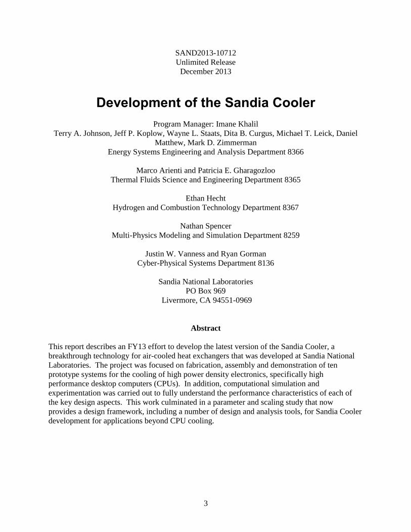
Abstract

This report describes an FY13 effort to develop the latest version of the Sandia Cooler, a

breakthrough technology for air-cooled heat exchangers that was developed at Sandia National

Laboratories. The project was focused on fabrication, assembly and demonstration of ten

prototype systems for the cooling of high power density electronics, specifically high

performance desktop computers (CPUs). In addition, computational simulation and

experimentation was carried out to fully understand the performance characteristics of each of

the key design aspects. This work culminated in a parameter and scaling study that now

provides a design framework, including a number of design and analysis tools, for Sandia Cooler

development for applications beyond CPU cooling.

4

ACKNOWLEDGMENTS

The authors wish to acknowledge the support and expertise of Kent Smith (8366) in the

fabrication of a number of components used in the various test assemblies as well as the Sandia

Cooler impellers and baseplates.

The authors also would like to recognize Isaac Ekoto (8367) and Adam Ruggles (8351) for the

use of their lab and their expertise, advice, and hard work in carrying out and post-processing

Particle Image Velocimetry (PIV) measurements of the Sandia Cooler impellers.

5

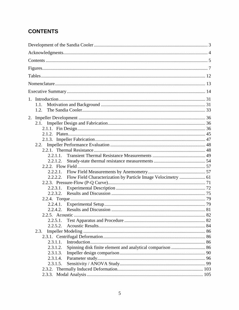
CONTENTS

Development of the Sandia Cooler ................................................................................................. 3

Acknowledgments........................................................................................................................... 4

Contents .......................................................................................................................................... 5

Figures............................................................................................................................................. 7

Tables ............................................................................................................................................ 12

Nomenclature ................................................................................................................................ 13

Executive Summary ...................................................................................................................... 14

1. Introduction ............................................................................................................................. 31

1.1. Motivation and Background ......................................................................................... 31 1.2. The Sandia Cooler......................................................................................................... 33

2. Impeller Development ............................................................................................................ 36 2.1. Impeller Design and Fabrication ................................................................................... 36

2.1.1. Fin Design ............................................................................................................. 36

2.1.2. Platen..................................................................................................................... 45 2.1.3. Impeller Fabrication .............................................................................................. 47

2.2. Impeller Performance Evaluation ................................................................................. 48 2.2.1. Thermal Resistance ............................................................................................... 48

2.2.1.1. Transient Thermal Resistance Measurements ............................................. 49

2.2.1.2. Steady-state thermal resistance measurements ............................................ 54 2.2.2. Flow Field ............................................................................................................. 57

2.2.2.1. Flow Field Measurements by Anemometry ................................................. 57

2.2.2.2. Flow Field Characterization by Particle Image Velocimetry ...................... 61

2.2.3. Pressure-Flow (P-Q Curve)................................................................................... 71 2.2.3.1. Experimental Description ............................................................................ 72

2.2.3.2. Results and Discussion ................................................................................ 75 2.2.4. Torque ................................................................................................................... 79

2.2.4.1. Experimental Setup ...................................................................................... 79 2.2.4.2. Results and Discussion ................................................................................ 81

2.2.5. Acoustic ................................................................................................................ 82 2.2.5.1. Test Apparatus and Procedure ..................................................................... 82 2.2.5.2. Acoustic Results........................................................................................... 84

2.3. Impeller Modeling ........................................................................................................ 86 2.3.1. Centrifugal Deformation ....................................................................................... 86

2.3.1.1. Introduction .................................................................................................. 86

2.3.1.2. Spinning disk finite element and analytical comparison ............................. 86

2.3.1.3. Impeller design comparison ......................................................................... 90 2.3.1.4. Parameter study ............................................................................................ 96 2.3.1.5. Sensitivity / ANOVA Study......................................................................... 99

2.3.2. Thermally Induced Deformation......................................................................... 103 2.3.3. Modal Analysis ................................................................................................... 105

6

2.3.4. Heat Transfer and Fluid Dynamics ..................................................................... 107

2.3.4.1. Model Development and Validation .......................................................... 107 Effect of turbulent Prandtl number ............................................................................ 110 2.3.4.2. Parameter Optimization Study ................................................................... 117

2.3.4.3. Scaling Study ............................................................................................. 131

3. Baseplate development ......................................................................................................... 138 3.1. Baseplate Design and Fabrication ............................................................................... 138

3.1.1. Stator Mounting Scheme..................................................................................... 139 3.1.2. Solid Baseplates .................................................................................................. 140

3.1.3. Vapor Chamber Baseplates ................................................................................. 140 3.2. Baseplate Thermal Resistance .................................................................................... 141

4. Air bearing ............................................................................................................................ 143 4.1. Overview of Spiral Groove Air Bearings ................................................................... 143

4.2. Initial Designs and Evaluation .................................................................................... 145 4.2.1. Air bearing for V3 and V4 impellers .................................................................. 145

4.2.2. Air bearing for V5 impeller ................................................................................ 146 4.2.3. Experimental Evaluation ..................................................................................... 147

4.3. Final Design and Validation ....................................................................................... 150 4.4. Air Bearing Thermal Resistance ................................................................................. 151

4.4.1. Experimental Evaluation ..................................................................................... 151

4.4.2. Computational Simulation .................................................................................. 153 4.5. Alternate Design: Magnetic Lift ................................................................................. 155

4.5.1. Introduction ......................................................................................................... 155 4.5.2. Magnetic bearing design ..................................................................................... 156

4.5.2.1. Potential bearing configurations ................................................................ 156

4.5.2.2. Magnet sizing and materials ...................................................................... 158

4.5.2.3. Thermal effect on lift force ........................................................................ 159 4.5.3. Experimental setup.............................................................................................. 159 4.5.4. Results ................................................................................................................. 160

4.5.5. Conclusion .......................................................................................................... 162

5. Anti-friction coating.............................................................................................................. 163

5.1. Background and Requirements ................................................................................... 163 5.2. Candidate Coating Evaluation .................................................................................... 164

5.2.1. Test Apparatus and Procedures ........................................................................... 164 5.2.2. Low Energy i-Kote Performance ........................................................................ 166 5.2.3. Standard i-Kote Performance .............................................................................. 170 5.2.4. Start-stop Cycling with i-Kote and Super MoS2 ................................................ 174 5.2.5. Conclusions ......................................................................................................... 181

6. Motor and controller ............................................................................................................. 182 6.1. Overview of Motor Selection...................................................................................... 182

6.2. Motor Controller Development................................................................................... 182 6.2.1. COTS Motor Controller Evaluation.................................................................... 182 6.2.2. Custom VVVF Motor Controller Development ................................................. 190

6.2.2.1. Waveform Selection................................................................................... 192 6.2.2.2. Startup Performance................................................................................... 193

7

6.2.2.3. Circuit Design ............................................................................................ 194

7. Conclusions and recommendations....................................................................................... 194

References ................................................................................................................................... 198

Distribution ................................................................................................................................. 201

FIGURES

Figure 1. Sandia Cooler. .............................................................................................................. 14 Figure 2. Version 4 impeller (left), version 5 impeller (center), and version 6 impeller (right). . 15 Figure 3. Test stands to measure impeller thermal resistance. Thermal decay (left) and steady-

state (right) methods were both used. ........................................................................................... 16

Figure 4. V4, V5 and V6 thermal resistance for speeds of 1000-5000 rpm. ................................ 17

Figure 5. Test stand for P-Q curve measurement. ........................................................................ 18 Figure 6. Several data points show the performance of the version 6 impeller, as compared to

versions 5 and 4. ........................................................................................................................... 18 Figure 7. Experimental setup for torque measurements. .............................................................. 19

Figure 8. Torque measurements and quadratic fits for V4, V5 and V6 impellers. ...................... 19 Figure 9. Typical acoustic measurement setup with the fan or impeller mounted on a pedestal in

the middle of the anechoic chamber. ............................................................................................ 20

Figure 10. Experimental setup for baseplate thermal resistance measurements. .......................... 21 Figure 11. Three spiral groove air bearing designs: V4 (left), V5 (middle), and final (right). ..... 22

Figure 12. Thermal resistance of the air bearing as a function of gap height, for several rotation

speeds. For reference, the resistance of a stagnant air layer is also shown. ................................. 23 Figure 13. i-Kote after 10,000 cycles (left) and friction torque data (right) during cycling. ........ 24

Figure 14. Motor rotor magnet array, flux ring and bearing integrated into impeller platen. ...... 24

Figure 15. 64-bit pulse density modulation synthesis of a sine wave. The motor controller for the

Sandia Cooler uses 4096-bit PDM synthesis. The above public domain image is available at

http://commons.wikimedia.org/wiki/File%3APulse-density_modulation_2_periods.gif. ........... 26

Figure 16. Components for CPU Cooler demonstration units nearly complete. .......................... 26

Figure 17. Impeller design tool. .................................................................................................... 27 Figure 18. Example of an impeller CFD model domain using periodic boundary conditions. .... 28 Figure 19. CFD models have been experimentally validated. ...................................................... 29 Figure 20. A conventional heat sink employs one or more fans and an array of fins. In this

particular example, cylindrical heat pipes are used to improve the heat transfer from the base to

the extended surfaces (adapted from [8]). ..................................................................................... 32 Figure 21. Sandia Cooler. ............................................................................................................ 33 Figure 22. V1 impeller. ................................................................................................................. 36

Figure 23. V3 impeller design. ..................................................................................................... 37 Figure 24. V4 impeller. ................................................................................................................. 38 Figure 25. V5 impeller. ................................................................................................................. 38 Figure 26: A prototypical heat-sink-impeller with fins that follow a logarithmic spiral. ............. 40

Figure 27. Mathematica impeller design tool. .............................................................................. 41 Figure 28. Thermal resistance parameter study for 4” diameter impeller. ................................... 43 Figure 29. V6 impeller. ................................................................................................................. 44

8

Figure 30. Rotor mounting features incorporated into impeller platen. ....................................... 45

Figure 31. Fixture for machining platen surface profile. .............................................................. 46 Figure 31. Twenty cold-forged V4 impellers. .............................................................................. 47 Figure 33. Progressively higher aspect ratio tools were used to machine the V5 impeller. ......... 48

Figure 32. Experimental Setup. .................................................................................................... 49 Figure 33. First step in data analysis. ............................................................................................ 52 Figure 34. Thermal Resistance of Heat-Sink-Impellers V4, V5, and V6. .................................... 53 Figure 35. V4, V5 and V6 thermal resistance for speeds of 1000-5000 rpm. .............................. 53 Figure 36. Experimental setup for measuring thermal resistance of Sandia Cooler impellers. A

thin film heater provides heat at a given power for the impeller to dissipate. As the impeller

rotates, the temperature difference between the inlet air and impeller is measured as a function of

power............................................................................................................................................. 55 Figure 37. Typical data stream for impeller thermal resistance measurements. Top frame shows

speed and power, middle frame shows data and fit using lumped capacitance model, and bottom

frame shows steady-state thermal resistances and averages of that data. ..................................... 56

Figure 38. Thermal resistance of the version 4 (left) and version 5 (right) impellers as a function

of rotation speed. Different colors represent differences in the sensor used, or the analysis

method, as described in the legend. .............................................................................................. 57 Figure 39. Version 4 impeller cross-sectional area, flow velocity profile at 2,500 rpm. ............. 60 Figure 40. Version 4 impeller cross-sectional area, flow velocity profile at 5,000 rpm. ............. 61

Figure 41. Particle image velocimetry setup................................................................................. 62 Figure 42. Example of seeded flow, version 4 impeller at 5,000 rpm. ........................................ 63

Figure 43. Raw data, version 4 impeller at 2,500 rpm. ................................................................. 64 Figure 44. Mask, version 4 impeller at 2,500 rpm. ....................................................................... 65 Figure 45. Masked data, version 4 impeller at 2,500 rpm. ........................................................... 65

Figure 46. Instantaneous snapshot after partial masking, version 4 impeller at 2,500 rpm. ........ 66 Figure 47. Statistical mean image, version 4 impeller at 2,500 rpm. .......................................... 67

Figure 48. Statistical mean image, version 4 impeller at 5,000 rpm. .......................................... 68 Figure 49. Statistical mean image, version 5 impeller at 2,500 rpm. .......................................... 69

Figure 50. Statistical mean image, version 5 impeller at 5,000 rpm. .......................................... 70 Figure 51. Perspective error due to out-of-plane flow and camera position. ............................... 71

Figure 54. Experimental setup for fan curve measurements. Valves and flow boosters allowed

the resistance of the system to be varied. Screens in sieves were used to straighten the flow and

prevent jetting onto the impeller. .................................................................................................. 73 Figure 55. Measured errors in mean pressure as the pressure tap position was varied (left), and as

the gap between the plenum and impeller was varied (right). ...................................................... 74 Figure 52. Dimensionless fan curves for the version 4 (left) and version 5 (right) impellers. Data

is shown by the points, colored by the rotational speed, as shown in the legend, and the line is a

best fit curve to all of the data. ...................................................................................................... 76 Figure 53. Data and fan curves for the version 4 (left) and version 5 (right) impellers. Data is

shown by the points, colored by the rotational speed, as shown in the legend, and the fits are re-

dimensioned from the single dimensionless data fit. .................................................................... 76 Figure 54. Data and fan curves for the version 4 (left) and version 5 (right) impellers operating in

the reversed (clockwise) direction. Data is shown by the points, colored by the rotational speed,

as shown in the legend, and the fits are re-dimensioned from the single dimensionless data fit. 77

9

Figure 55. Performance of version 4 and 5 impellers (scaled to 110 mm) are shown by the lines.

The points show the static pressure and free delivery rates of several axial fans manufactured by

Sunon. ........................................................................................................................................... 78 Figure 56. Several data points show the performance of the version 6 impeller, as compared to

versions 5 and 4. ........................................................................................................................... 78 Figure 57. Comparison of measured and predicted impeller free delivery rates for the V4, V5,

and V6 impellers. .......................................................................................................................... 79 Figure 58. Experimental setup for torque measurements. ............................................................ 80 Figure 59. Example speed decay curve and fit to data. ................................................................ 80

Figure 60. Torque measurements and quadratic fits for versions 4, 5 and 6 impellers. .............. 81 Figure 61. Comparison of measured and predicted torque for V4, V5, and V6 impellers. ......... 82 Figure 62. Typical acoustic measurement setup with the fan or impeller mounted on a ............. 83 Figure 63. Meshes for a simple spinning disk with (a) one (b) two and (c) four elements through

the thickness of the disk. ............................................................................................................... 87

Figure 64. Analytical and finite element calculated displacements for a spinning disk with one

(1t), two (2t), and four (4t) elements through the thickness of the disk. ...................................... 88 Figure 65. Finite element calculated displacements for a spinning disk with one (1t), two (2t),

and four (4t) elements through the thickness of the disk. ............................................................. 88 Figure 66. Displacement contour plot of the spinning disk magnified by a factor of 200,000x. 89 Figure 67. Geometry of the version 4 and version 5 impeller designs. ....................................... 91

Figure 68. Meshed geometry of the version 4 and version 5 impeller designs. .......................... 92 Figure 69. Axial displacement contour plots of the version 4 and 5 impeller designs magnified

by a factor of 1000x. ..................................................................................................................... 93 Figure 70. Comparison of the maximum axial displacement as a function of rotational velocity

between the version 4 and 5 impellers. ......................................................................................... 94

Figure 71. Axial displacements as a function of radial position for both the version 4 and

version 5 impellers for rotational velocities ranging from 1000 to 3000 rpm in 100 rpm

increments. A rotational velocity of 2500 rpm is emphasized. ................................................... 94 Figure 72. Meshed geometry of the V6 impeller. ......................................................................... 95

Figure 73. Maximum axial displacements of all three impeller designs. ..................................... 95 Figure 74. Parameter trends affecting the impeller gap distance. ................................................ 97

Figure 75. Zoomed in parameter trends. ....................................................................................... 97 Figure 76. Plots of each factor colored separately by blue, green, or red for low, medium, and

high levels. .................................................................................................................................. 101 Figure 77. Plots of each factor at their low (blue), medium (green), and high (red) levels with the

other factors held constant at their medium/nominal level. ........................................................ 102 Figure 78. Version 5 (a) mapped temperature distribution and (b) resulting axial displacements.

..................................................................................................................................................... 104

Figure 79. Axial displacements of the version 5 impeller due to thermal gradients during the

operational cooling process for one calculated temperature distribution. .................................. 105

Figure 80. Version 5 impeller mode shapes and corresponding frequencies. ........................... 106 Figure 81. Version 5 (a) isolated fin geometry, (b) first mode, and (c) second mode with the base

of the fin having a fixed displacement boundary condition. ....................................................... 107 Figure 82. Version 6 (a) isolated fin geometry, (b) first mode, and (c) second mode with the base

of the fin having a fixed displacement boundary condition. ....................................................... 107 Figure 83. CFX view of the periodic impeller’s slice used in the simulations. .......................... 108

10

Figure 84. Solid domain with the two halves of a fin. ................................................................ 109

Figure 85. Streamlines of the gas flow past the impeller at two different pseudo- times in the

simulation. Lines generated from the instantaneous velocity vectors. ....................................... 110 Figure 86. Schematic view of rotating boundary layer (pressure surface). From Yamawaki et al.,

International Journal of Heat and Fluid Flow 23, 2002. ............................................................. 111 Figure 87. Thermal boundary layer development. ...................................................................... 111 Figure 88. Heat flux contour at the walls of the impeller’s channel. .......................................... 112 Figure 89. Sensitivity of thermal resistance to the Turbulent Prandtl number. .......................... 113 Figure 90. Example of radial slices taken to extract simulation data. ........................................ 114

Figure 91. Comparison of the radial velocity field from anemometry measurements and from the

simulation at steady state for V4. The two rectangles indicate the position of the impeller in this

view. ............................................................................................................................................ 114 Figure 92. Detail above the impeller with ensemble-averaged PIV data. .................................. 115 Figure 93. RANS turbulent kinetic energy. ................................................................................ 115

Figure 94. Root Mean Square values of the radial and axial components of velocity from the

PIV measurements. ..................................................................................................................... 116 Figure 95. Thermal resistance as a function of rotational speed. ................................................ 117

Figure 96: CFD model domains and boundary conditions. ........................................................ 119 Figure 97. The convergence of mass flow rate, torque, and thermal resistance for designs 1-23 of

batch 2 in the parametric study. .................................................................................................. 120

Figure 98: CFD parameter study results from batch 1 at 2500 rpm. The circle on each surface

indicates the design with the optimal value. ............................................................................... 122

Figure 99: Thermal resistance vs. power consumption for batch 1 at 2500 rpm. ....................... 123 Figure 100: Thermal resistance and relative mass flow for the batch 1 designs operating at 5 W

of power consumption................................................................................................................. 124

Figure 101: The velocity field (shown with vectors) and temperature field (shown with color

according to the legends) for each of the designs in batch 1, operating at 2500 rpm. ................ 125

Figure 102: Thermal resistance and pumping power for the batch 2 designs. ........................... 127 Figure 103: The thermal resistances of the batch 2 designs operating at 5 W of power

consumption. The brackets on the right of the bars indicate the power law exponent (A) of the

designs......................................................................................................................................... 128

Figure 104: Interrupted fin designs, called “v6a” and “v6b,” compared to v4 and v5. .............. 131 Figure 105. Impeller thermal conductance (1/R) and shaft power as a function of scale factor

with a constant fin tip speed........................................................................................................ 133 Figure 106. Effect of fin height on thermal conductance and shaft power for constant fin tip

speed. .......................................................................................................................................... 134 Figure 107. UA/P versus fin tip speed for scaled V6 designs. ................................................... 134 Figure 108. Thermal conductance per volume versus shaft power per volume. ........................ 135

Figure 109. Air flow rate as a function of shaft power and fin tip speed. .................................. 136 Figure 110. Scaling laws fit to impeller air flow rate, torque and power. .................................. 137

Figure 111. Comparison of correlation values with CFD results for torque, air flow rate, and

thermal conductance. .................................................................................................................. 138 Figure 112. New motor stator mount and shaft. ......................................................................... 139 Figure 117. As-installed stator/shaft assembly. .......................................................................... 139 Figure 118. Conceptual design of vapor chamber baseplate. ..................................................... 141 Figure 113. Experimental setup for baseplate thermal resistance measurements. ...................... 142

11

Figure 114. Thermal resistance measurements of the Sandia Cooler system. The left plot is for a

10 µm air bearing gap, the right plot for a 30 µm gap. ............................................................... 143 Figure 115. Example of a flat spiral groove thrust bearing [1]. .................................................. 144 Figure 116. Initial spiral groove pattern used with V3 and V4 impellers. .................................. 145

Figure 117. V5 baseplate with new spiral groove pattern. ......................................................... 147 Figure 118. Predicted gap height using the V4 and V5 baseplates without preload. ................. 147 Figure 119. Test apparatus for air bearing performance evaluation. .......................................... 148 Figure 120. Eddy current displacement sensor and calibration setup. ........................................ 149 Figure 121. Air bearing test results compared to theoretical calculations. ................................. 150

Figure 122. Final spiral groove design. ...................................................................................... 151 Figure 123. Photo and sketch of the experimental setup for air bearing thermal resistance

measurements. ............................................................................................................................. 152 Figure 124. Thermal resistance of the air bearing as a function of gap height, for several rotation

speeds. For reference, the resistance of a stagnant air layer is also shown. ............................... 153

Figure 125. Computational mesh of air bearing gap. .................................................................. 154

Figure 126. Cartoon of deformed fluid region. ........................................................................... 155 Figure 127. Results of the measured and predicted thermal enhancement versus angular shear

rate with and without deformation. ............................................................................................. 155 Figure 128: Conceptual rendering of magnetic lift design using alignment of steel rings. ....... 158 Figure 129: Stock ring magnet embedded in modified baseplate. ............................................. 160

Figure 130: Static repulsive force between stock commercial magnets versus separation

distance. ...................................................................................................................................... 161

Figure 131: Air gap measurements at 1500rpm. ........................................................................ 162 Figure 132: Air gap measurements at 3750rpm. ........................................................................ 162 Figure 133. Torque measurement and wear testing setup. .......................................................... 165

Figure 134. Impeller substitute coated with low energy deposition i-Kote, prior to installation.

..................................................................................................................................................... 166

Figure 135: Friction torque versus rotational speed for first set of coated parts. ...................... 168 Figure 136: Friction torque versus time for wear test. ............................................................... 169

Figure 137: Wear patterns of substitute impeller (left) and baseplate (right). ........................... 170 Figure 138: Parts coated using standard deposition, prior to installation. ................................. 171

Figure 139: Parts coated using standard deposition, after 16 hours at 1000rpm. ...................... 171 Figure 140: Friction torque versus rotational speed for low energy and standard (high energy)

deposition. Data for high energy deposition taken immediately after installation, prior to wear-

in. ................................................................................................................................................ 172 Figure 141: Wear test at 1000rpm with 10N preload, standard deposition coating. ................. 173 Figure 142: Coating wear effect with no preload. ..................................................................... 173 Figure 143: Coating wear effect with 5N preload. .................................................................... 174

Figure 144: Coating wear effect with 10N preload. .................................................................. 174 Figure 145: Condition of i-Kote baseplate substitute at various points during cycle testing. ... 176

Figure 146: Condition of i-Kote impeller substitute at various points during cycle testing. ..... 177 Figure 147: Condition of Super MoS2 baseplate substitute at various points during cycle testing.

..................................................................................................................................................... 178 Figure 148: Condition of Super MoS2 impeller substitute at various points during cycle testing.

..................................................................................................................................................... 179

12

Figure 149: Friction torque data for i-Kote during cycle testing (cycles 10,001-15,000 shown

separately for clarity). ................................................................................................................. 180 Figure 150: Friction torque data for Super MoS2 during cycle testing. .................................... 181 Figure 151. Motor stator mounted on baseplate. ........................................................................ 182

Figure 152. Voltage across all three motor phases at 1500 RPM at ~ 50% Duty Cycle. ........... 184 Figure 153. Voltage across all three motor phases at full power. ............................................... 185 Figure 154. DP.D control software. ............................................................................................ 186 Figure 155. Motor mounted on hysteresis brake test bed. .......................................................... 188 Figure 156. DPflex user control box. ......................................................................................... 190

Figure 157: VVVF test setup. ..................................................................................................... 192 Figure 158: Custom VVVF Motor Control Simulator. ............................................................... 193

TABLES

Table 1. Dimensions of impellers and fins. .................................................................................. 16 Table 2. Scaling law equations for impeller performance based on CFD results. ........................ 30

Table 3. Biot numbers for the latest impeller designs. ................................................................. 51 Table 4. Example of measured flow rates at a single point. ......................................................... 59 Table 5. Acoustic measurements of COTS CPU Coolers. ............................................................ 84

Table 6. Acoustic measurements of V5 impeller. ......................................................................... 85 Table 7. Acoustic comparison between V4 and V5 impellers. ..................................................... 85

Table 8. Summary of parameter values comparing version 4 and version 5 impellers. ............... 92 Table 9. Summary of parameters and values used in the parameter study. Highlighted values are

considered as “baseline.” .............................................................................................................. 96

Table 10. Factor levels selected for a sensitivity study of the axial displacements. .................... 99 Table 11. Parametric Study Geometry and Performance. ........................................................... 129

Table 12. Results of the Preliminary Impeller Scaling Study. .................................................... 132 Table 13. Scaling Laws. .............................................................................................................. 136

Table 14. Parameters of the initial spiral groove design. ............................................................ 146 Table 15. Parameters for the V5 baseplate spiral groove air bearing. ........................................ 146

Table 16. Parameters for the final spiral groove air bearing....................................................... 150

13

NOMENCLATURE

CFD computational fluid dynamics

dB decibel

DOE Department of Energy

OEM Original Equipment Manufacturer

SNL Sandia National Laboratories

VVVF Variable Voltage Variable Frequency

14

EXECUTIVE SUMMARY

This report describes an FY13 effort to develop the latest version of the Sandia Cooler, a

breakthrough technology for air-cooled heat exchangers that was developed at Sandia National

Laboratories (see Figure 1). The project was focused on fabrication, assembly and

demonstration of ten prototype systems for the cooling of high power density electronics,

specifically high performance desktop computers (CPUs). In addition, computational simulation

and experimentation was carried out to fully understand the performance characteristics of each

of the key design aspects. This work culminated in a parameter and scaling study that now

provides a design framework, including a number of design and analysis tools, for Sandia Cooler

development for applications beyond CPU cooling.

The key to the technology is the heat-sink impeller which consists of a disc-shaped impeller

populated with fins on its top surface. The impeller functions like a hybrid of a conventional

finned metal heat sink and a fan. Air is drawn down into the central region without fins, and

expelled in the radial direction through the dense array of fins. The primary breakthrough in this

device is that air accelerates past the heat sink fins due to the rotating reference frame of the

impeller. This acceleration thins the boundary layer of air next to the fin surfaces, which

significantly enhances heat transfer from the fins to the air. The enhanced heat transfer is what

allows the Sandia Cooler to be much more compact than other technologies.

Figure 1. Sandia Cooler.

A high-efficiency brushless motor is used to impart rotation (several thousand rpm) to the heat-

sink-impeller. A brushless motor was chosen for the significant increase in lifetime, compared to

brushed motors, as well as for low noise. The motor is also much more compact because it does

not require the Hall-effect sensors typically used to provide feedback as to motor orientation.

The motor being used is commercially available and inexpensive, but provides enough torque to

start and spin the impeller up to speeds in excess of 5000 rpm.

15

At start-up, the impeller contacts the baseplate and static, and then sliding friction occurs

between the two surfaces before the air bearing provides enough lift for separation. To minimize

that friction, an anti-friction coating is incorporated into the two mating surfaces. Once the

impeller is spinning fast enough (~1000 rpm), a spiral-groove air bearing lifts the impeller above

the baseplate to provide a stable, frictionless interface. The air bearing is self-sustaining and the

gap height is controlled by the spring pre-load. A gap height of 10 microns reduces the thermal

resistance to a manageable fraction of the total thermal resistance budget.

The air bearing grooves are machined into the baseplate, which also houses the wire-wound

stator for the brushless motor. In addition to these functions, the baseplate serves to transfer heat

from the source, in this case a CPU, to the impeller. To achieve the very low thermal spreading

resistance required, a vapor chamber (heat pipe) produced by a commercial vendor is used.

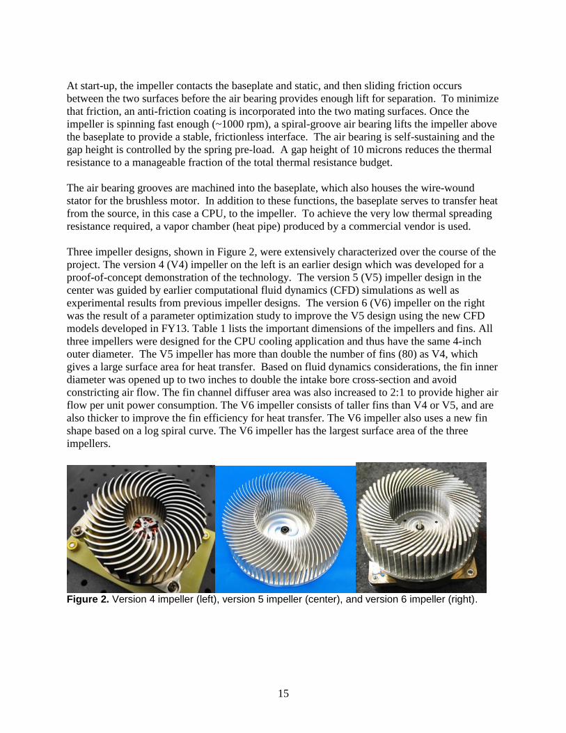
Three impeller designs, shown in Figure 2, were extensively characterized over the course of the

project. The version 4 (V4) impeller on the left is an earlier design which was developed for a

proof-of-concept demonstration of the technology. The version 5 (V5) impeller design in the

center was guided by earlier computational fluid dynamics (CFD) simulations as well as

experimental results from previous impeller designs. The version 6 (V6) impeller on the right

was the result of a parameter optimization study to improve the V5 design using the new CFD

models developed in FY13. Table 1 lists the important dimensions of the impellers and fins. All

three impellers were designed for the CPU cooling application and thus have the same 4-inch

outer diameter. The V5 impeller has more than double the number of fins (80) as V4, which

gives a large surface area for heat transfer. Based on fluid dynamics considerations, the fin inner

diameter was opened up to two inches to double the intake bore cross-section and avoid

constricting air flow. The fin channel diffuser area was also increased to 2:1 to provide higher air

flow per unit power consumption. The V6 impeller consists of taller fins than V4 or V5, and are

also thicker to improve the fin efficiency for heat transfer. The V6 impeller also uses a new fin

shape based on a log spiral curve. The V6 impeller has the largest surface area of the three

impellers.

Figure 2. Version 4 impeller (left), version 5 impeller (center), and version 6 impeller (right).

16

Table 1. Dimensions of impellers and fins.

OD 4.0” 4.0” 4.0”

ID 1.5” 2.0” 2.0”

Fin Height 1.0” 0.95” 1.18”

# Fins 36 80 55

Shape Intersecting arcs Arcs Log spiral

Fin Width Variable 0.030” uniform Variable

Surface area 820 cm2 1150 cm2 1220 cm2

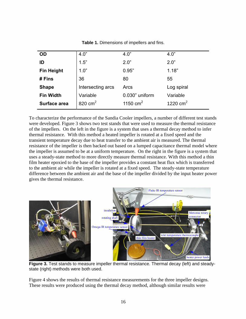
To characterize the performance of the Sandia Cooler impellers, a number of different test stands

were developed. Figure 3 shows two test stands that were used to measure the thermal resistance

of the impellers. On the left in the figure is a system that uses a thermal decay method to infer

thermal resistance. With this method a heated impeller is rotated at a fixed speed and the

transient temperature decay due to heat transfer to the ambient air is measured. The thermal

resistance of the impeller is then backed out based on a lumped capacitance thermal model where

the impeller is assumed to be at a uniform temperature. On the right in the figure is a system that

uses a steady-state method to more directly measure thermal resistance. With this method a thin

film heater epoxied to the base of the impeller provides a constant heat flux which is transferred

to the ambient air while the impeller is rotated at a fixed speed. The steady-state temperature

difference between the ambient air and the base of the impeller divided by the input heater power

gives the thermal resistance.

Figure 3. Test stands to measure impeller thermal resistance. Thermal decay (left) and steady-state (right) methods were both used.

Figure 4 shows the results of thermal resistance measurements for the three impeller designs.

These results were produced using the thermal decay method, although similar results were

17

found for V4 and V5 with the steady-state method. The plot in Figure 4 shows thermal

resistance in °C/W as a function of impeller rotational speed from 1000 to 5000 rpm. Dots

indicate the actual measured data points while curves were fit to the V4 (blue) and V5 (red)

points. The data shows that the V5 design provides the lowest thermal resistance at a given speed

resulting in a ~30% decrease over the V4 design. The V6 impeller (green) has a thermal

resistance that falls between the V4 and V5 designs.

Figure 4. V4, V5 and V6 thermal resistance for speeds of 1000-5000 rpm.

Figure 5 shows a test stand assembled to characterize the relationship between pressure drop and

air flow rate for the impellers, also known as a P-Q curve. A typical experiment consisted of

setting a system resistance using the combination of flow booster settings and butterfly valve

position, and then varying the rotation speed of the impeller in discrete steps. A steady flow rate

and pressure, enabled by the mesh sieve flow straighteners and large plenum, were quickly

reached as the impeller reached the rotation speed. Six rotation speeds were tested, up to 3750

rpm for the V4 and V5 impellers and the system resistance was varied from the static pressure

condition (zero flow) to beyond the free flow condition (zero pressure drop). The V6 impeller

was tested over a reduced range of pressures and flows for comparison purposes only.

Figure 6 shows the P-Q curves for V4 and V5 along with two data points at each rotational speed

for the V6 impeller. All three impellers produce about the same static pressures, but the V5

provides higher flow rates throughout the range of pressures and speeds. The V6 impeller

produces the lowest flow rates.

18

Figure 5. Test stand for P-Q curve measurement.

Figure 6. Several data points show the performance of the version 6 impeller, as compared to versions 5 and 4.

The majority of the power consumed by the motor when the Sandia Cooler is in operation is used

to overcome the torque required to rotate the impeller through the air. Designs with a lower

torque requirement are preferred to minimize motor power. Figure 7 shows the test stand

assembled to measure the impeller torque as a function of rotational speed. The impellers were

mounted on a near frictionless air bearing shaft and brought up to speed using a jet of air applied

to the fins. Like the thermal decay measurement, this method used the decay in impeller speed

19

over time to infer the torque on the impeller at each speed. Speed was measured by using a

phototransistor to count the pulses observed as a black mark on the shaft interrupted the

reflection of a HeNe laser.

Figure 7. Experimental setup for torque measurements.

Figure 8 shows the results of the torque measurements for the three impellers. The V5 impeller

requires the highest torque at a given speed. The V6 impeller requires slightly lower torque than

V5 while V4 requires significantly less.

Figure 8. Torque measurements and quadratic fits for V4, V5 and V6 impellers.

Since silent operation is one of the keynote features of the Sandia Cooler, it is of great

importance to ensure that future designs are at least as quiet, and preferably quieter, to the human

ear than previous configurations and comparable cooling units in industry. Several acoustics

experiments were set up to measure the noise output of the latest impeller designs and a couple

of commonly used processor cooling fans. We examined the V4, V5, and V6 impellers along

with an i7-960 LGA1366 fan, which comes with the Intel Core i7 Processor, and with a Noctua

NHD14 fan, which is commonly used in high-performance computers.

20

Figure 9 shows a typical acoustic measurement setup with an impeller (V4) mounted on a

vibrationally damped pedestal in the center of an anechoic chamber. A type 2250 sound level

meter by Brüel & Kjær and an Extech 407730 sound level meter were used for the tests

depending on availability. The OEM and the Noctua coolers were tested at 1V increments

between 5 and 12V (maximum speed). The impellers were tested at speeds that ranged from

1400 rpm up to 5000 rpm, although most measurements were made between 2000 and 4000 rpm.

The measurements showed that the OEM cooler was slightly quieter than the Noctua model,

however the Noctua cooler uses two fans and is significantly better in thermal performance. Both

devices are very quiet and only about 10 dBa above the 20 dBa noise floor at full power. The

impellers were found to be fairly similar to each other in noise output, although the V4 impeller

was slightly quieter than V5 and V6. All three, however, were noticeably louder than the

commercial units, producing sound levels between 20 to 30 dBa higher than ambient at speeds

between 2000 rpm and 4000 rpm partially because of motor noise and mechanical vibration

induced by torque ripple. The later development of a motor controller that provides high-fidelity

sinusoidal excitation, based on a pulse density (PDM) modulated Class-D amplifier, proved

extremely effective in reducing these components of noise. Follow-on acoustic measurements

will be undertaken in 2014 to document the extremely low dBa levels generated by the Sandia

Cooler at typical operating speeds with this new motor controller system.

Figure 9. Typical acoustic measurement setup with the fan or impeller

mounted on a pedestal in the middle of the anechoic chamber.

Overall, these tests indicated that the V5 impeller had the best performance. The combination of

pressure-flow capability and low thermal resistance outweigh the higher shaft power required for

a given speed. While both V5 and V6 impellers improved over the V4 design, slightly better

21

performance and comparatively easier fabrication made V5 the choice over V6 for the final

demonstration units.

Vapor chamber baseplates for the final demonstration units were procured through Thermacore,

a company specializing in heat pipe and vapor chamber design. The external dimensions were

supplied by Sandia to meet the mounting requirements of an Intel Core i7 processor as well as

the motor stator mount. The internal details of the vapor chamber design were considered trade

secrets (e.g. wick structure, internal support, working fluid, etc.) and were determined by

Thermacore to meet the requirements of the application. However, the performance of the vapor

chamber baseplates was verified at Sandia using an experimental apparatus similar to that shown

in the diagram in Figure 10. A V5 impeller was used rather than a surrogate impeller and fan.

The heater block at the bottom was used to simulate the heat from a CPU and thermocouples

inserted into holes at the top of the heater and the top of the baseplate were used for thermal

resistance calculations. Both a vapor chamber and a solid copper baseplate were tested and the

results showed that the vapor chamber was approximately 0.030 °C/W lower than the copper

baseplate. Based on thermal model predictions, the copper baseplate was found to have a

thermal resistance of about 0.04 °C/W. Thus, the vapor chamber thermal resistance, at

approximately 0.01 °C/W, is a significant improvement.

Figure 10. Experimental setup for baseplate thermal resistance measurements.

In addition to transferring the CPU heat to the spinning impeller, the baseplate houses the spiral

groove air bearing that the impeller rides on. A succession of designs were evaluated this year

and are shown in Figure 11. The design on the left is the original spiral groove design developed

for the V3 and V4 impellers. This air bearing was made up of grooves that used a large fraction

of the baseplate surface area and were quite deep at about 80 microns. This air bearing provided

more lift than necessary and had high thermal resistance because of the large, deep grooves. The

V5 design, shown in the middle picture, was an improvement over the previous design with

shallower (25 m) grooves that covered a smaller surface area. Both sets of grooves were

designed using an online calculator (http://www.tribology-abc.com ) based on previously

published equations for spiral groove air bearings [1]. However, experimental evaluation of these

air bearings showed some discrepancy between the predicted and measured lift. Based on the

experimental evaluation of the V4 and V5 baseplates and a more detailed investigation into spiral

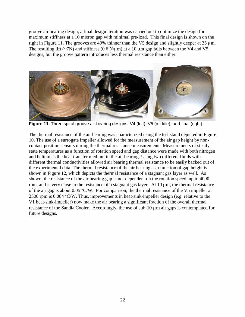
22

groove air bearing design, a final design iteration was carried out to optimize the design for

maximum stiffness at a 10 micron gap with minimal pre-load. This final design is shown on the

right in Figure 11. The grooves are 40% thinner than the V5 design and slightly deeper at 35 m.

The resulting lift (~7N) and stiffness (0.6 N/m) at a 10 m gap falls between the V4 and V5

designs, but the groove pattern introduces less thermal resistance than either.

Figure 11. Three spiral groove air bearing designs: V4 (left), V5 (middle), and final (right).

The thermal resistance of the air bearing was characterized using the test stand depicted in Figure

10. The use of a surrogate impeller allowed for the measurement of the air gap height by non-

contact position sensors during the thermal resistance measurements. Measurements of steady-

state temperatures as a function of rotation speed and gap distance were made with both nitrogen

and helium as the heat transfer medium in the air bearing. Using two different fluids with

different thermal conductivities allowed air bearing thermal resistance to be easily backed out of

the experimental data. The thermal resistance of the air bearing as a function of gap height is

shown in Figure 12, which depicts the thermal resistance of a stagnant gas layer as well. As

shown, the resistance of the air bearing gap is not dependent on the rotation speed, up to 4000

rpm, and is very close to the resistance of a stagnant gas layer. At 10 m, the thermal resistance

of the air gap is about 0.05 °C/W. For comparison, the thermal resistance of the V5 impeller at

2500 rpm is 0.084 °C/W. Thus, improvements in heat-sink-impeller design (e.g. relative to the

V1 heat-sink-impeller) now make the air bearing a significant fraction of the overall thermal

resistance of the Sandia Cooler. Accordingly, the use of sub-10-m air gaps is contemplated for

future designs.

23

Figure 12. Thermal resistance of the air bearing as a function of gap height, for several rotation speeds. For reference, the resistance of a stagnant air layer is also shown.

When the impeller begins rotating from rest, before the air bearing can produce enough lift for

levitation, the impeller and baseplate are in contact. To reduce the static and sliding friction

between the two surfaces, prevent galling, and minimize wear, a dry ceramic anti-friction coating

is applied to the impeller and baseplate. A number of anti-friction coating options were

considered for this application, but i-Kote, a coating patented by Tribologix Inc., was chosen for

this application (1) because it provides a very low coefficient of friction, (2) it has an extremely

low wear rate, (3) unlike some dry anti-friction coatings, i-Kote is insensitive to environmental

variables such as relative humidity, (4) the wear in process allows in situ generation of extremely

flat/parallel surfaces, and (5) none of the i-Kote constituent materials are expensive. i-Kote is a

mixture of molybdenum disulfide, graphite, and other constituents that form a chemical bond to

the metal substrate. The thickness of the i-Kote coating is typically 2.5 microns, and the i-Kote

deposition process is self-limiting, characterized by maximum thickness of 4 m. After an initial

wear-in process the wear rate is claimed to be extremely small (5 x 10-17

m3 N

-1 m

-1), and it is the

properly worn in coating that provides the extremely low coefficient of friction claimed by

Tribologix.

The i-Kote coating was evaluated on a test rig using surrogate parts made to match the impeller

and baseplate in terms of contact dimensions, flatness, surface finish, and perpendicularity of

shaft and bearing holes. The surrogate baseplate was mounted to one flange of a reaction torque

sensor, whose other flange was mounted to the housing of a drive motor. The drive motor was

coupled to a shaft assembly that spun the surrogate impeller, which was spring loaded, against

the surrogate baseplate. The impeller rotation was then cycled to simulate starting and stopping

the Sandia Cooler. The cycle consisted of starting from rest, ramping to a nominal 1000rpm in

10s, and cutting power to the motor for 10s to bring the impeller to rest. This was done with a

5N pre-load. Figure 13 shows the coating on the surrogate baseplate after 10,000 of these cycles

still completely intact. Friction torque data was collected during cycle testing, and is shown in

the plot on the right. i-Kote provides low static friction torque and sliding friction torque that

decreases with cycling.

24

Figure 13. i-Kote after 10,000 cycles (left) and friction torque data (right) during cycling.

The Sandia Cooler utilizes a brushless, sensorless DC motor based on the Motrolfly DM2203

brushless motor. This motor is comprised of a 12 pole stator and a rotor consisting of 14 NdFeB

rare earth magnets to drive the impeller at speeds up to 5000rpm. The stator is incorporated into

the baseplate as shown in the V4 and V5 baseplates in Figure 11. The rotor magnet array and

bearing are integrated into the impeller as shown below in Figure 14. The stator winding type

(DLRK) requires less copper windings per stator tooth, which is a critical factor due to space

constraints of this compact design. To reduce the footprint and cost even further, no Hall effect

rotor position sensors are used to control motor commutation. The Sandia Cooler is also unique

compared to other brushless motor applications (such as cooling fans) because it requires a large

initial torque to overcome the friction between the impeller and baseplate experienced at startup

and has a relatively large moment of inertia. The need for high start-up torque, silent operation,

and high brushless motor efficiency required development of a custom variable voltage variable

frequency (VVVF) motor controller with closed-loop control of motor torque angle to ensure

operation near unity power factor.

Figure 14. Motor rotor magnet array, flux ring and bearing integrated into impeller platen.

The motor controller generates three voltage waveforms of equal amplitude with precise phase

relationships and ramps the waveform’s frequency from 0 Hz to the final operating electrical

frequency over a predetermined time interval (e.g. 25 seconds at a ramp rate of 100 rpm/sec). To

provide high startup torque relative to the size of the motor (up to 60 m N m), the rms voltage

delivered to motor windings is initially set at 200 to 300% typical operating voltage. Once the

25

rotor reaches a predetermined rpm threshold (e.g. 500 rpm, after 5 seconds), the excitation

voltage is stepped down (e.g. to 150% typical operating voltage) to prevent over-heating of the

motor windings. Once the motor has nearly finished ramping up to the set point rpm (e.g. 2500

rpm), the rotor torque angle PID control loop is activated. The PID controller lowers the

excitation amplitude further, eventually settling at an rms voltage that corresponds to a torque

angle of nearly 90 degrees, and a power factor of approximately unity.

To investigate different waveform characteristics for the controller, we used an amplified three-

channel arbitrary waveform generator to determine base line performance for motor efficiency

and motor noise under pure sinusoidal excitation (ignoring the fact that these waveforms could

not be generated with high electrical efficiency), to judge the efficacy of various pseudo-

sinusoidal waveforms in conjunction with Class D amplification (e.g. in a MOSFET H-bridge).

These studies resulted in the adoption of 4 kilobit pulse density modulation (PDM), which incurs

no measureable penalty in motor efficiency or motor noise relative to true sinusoidal excitation.

The new brushless motor controller board for the Sandia Cooler comprises:

1) a custom designed VCO circuit with 1000:1 tuning range for clock generation,

2) a set of three EEPROMs that store the PDM bit sequences for the 0, 120, and 240 degree

phases,

3) MOSFET driver circuitry that includes anti-shoot-through delay generation for high-

efficiency MOSFET operation,

4) A set of six full H-bridge MOSFET modules to provide push-pull excitation of the three

motor phases,

5) Supervisory circuitry to control starting, ramp up and transmission to closed-loop PID

control,

6) Phase detection circuitry for determination of rotor torque angle,

7) A PID control system that adjusts excitation amplitude to maintain a nearly 90 degree

torque angle and damp residual torque ripple during normal operation,

8) Supervisory circuitry to detect fault conditions such as loss of synchronism, rotor lock, or

stator winding overheating.

implemented in the form of circuitry that will later allow the entire motor controller to

manufactured as a single low cost application specific integrated circuit (ASIC). The above

circuitry has been prototyped and tested in the form of six circuit sub modules, and we are

currently awaiting fabrication the final printed circuit board by an outside vendor. A fully

detailed description of the motor controller circuit will be provided in a subsequent report.

26

Figure 15. 64-bit pulse density modulation synthesis of a sine wave. The motor controller for the Sandia Cooler uses 4096-bit PDM synthesis. The above public domain image is available at

http://commons.wikimedia.org/wiki/File%3APulse-density_modulation_2_periods.gif.

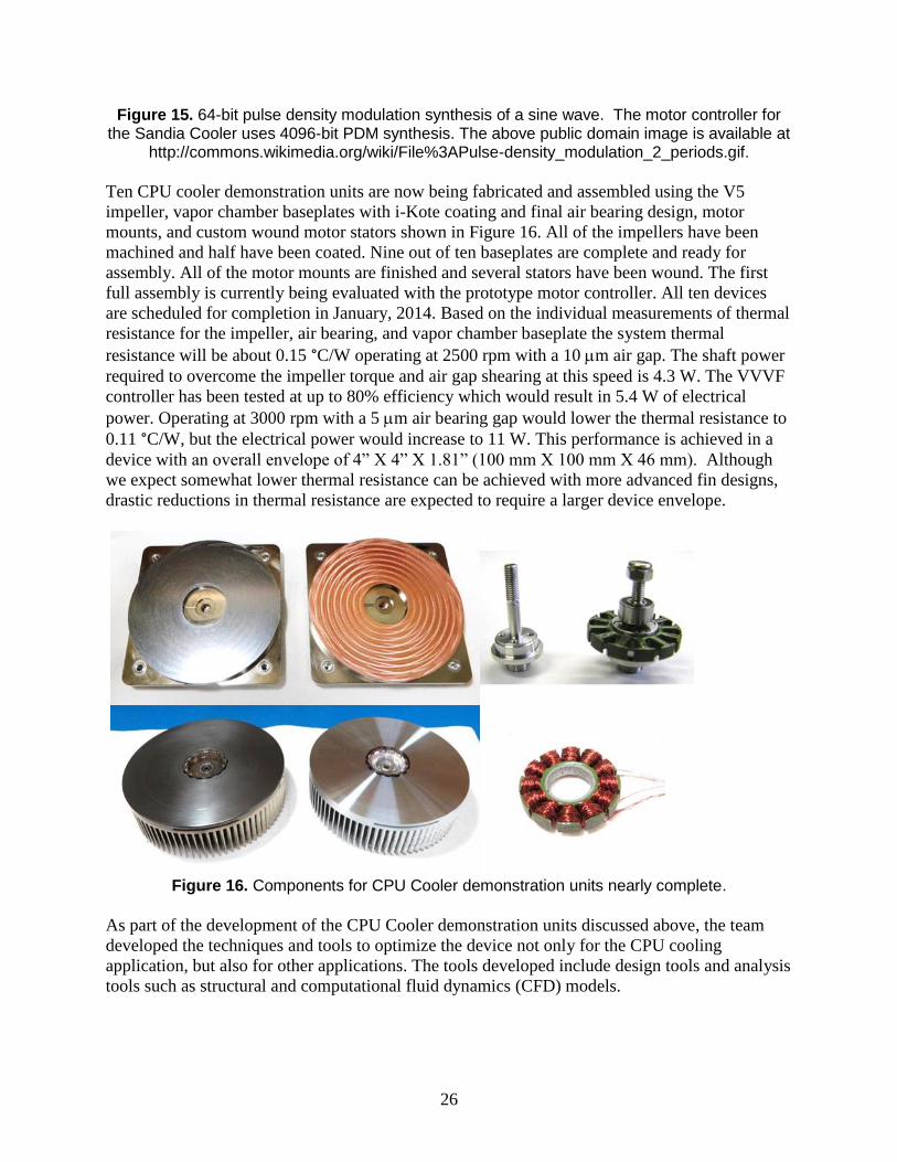
Ten CPU cooler demonstration units are now being fabricated and assembled using the V5

impeller, vapor chamber baseplates with i-Kote coating and final air bearing design, motor

mounts, and custom wound motor stators shown in Figure 16. All of the impellers have been

machined and half have been coated. Nine out of ten baseplates are complete and ready for

assembly. All of the motor mounts are finished and several stators have been wound. The first

full assembly is currently being evaluated with the prototype motor controller. All ten devices

are scheduled for completion in January, 2014. Based on the individual measurements of thermal

resistance for the impeller, air bearing, and vapor chamber baseplate the system thermal

resistance will be about 0.15 °C/W operating at 2500 rpm with a 10 m air gap. The shaft power

required to overcome the impeller torque and air gap shearing at this speed is 4.3 W. The VVVF

controller has been tested at up to 80% efficiency which would result in 5.4 W of electrical

power. Operating at 3000 rpm with a 5 m air bearing gap would lower the thermal resistance to

0.11 °C/W, but the electrical power would increase to 11 W. This performance is achieved in a

device with an overall envelope of 4” X 4” X 1.81” (100 mm X 100 mm X 46 mm). Although

we expect somewhat lower thermal resistance can be achieved with more advanced fin designs,

drastic reductions in thermal resistance are expected to require a larger device envelope.

Figure 16. Components for CPU Cooler demonstration units nearly complete.

As part of the development of the CPU Cooler demonstration units discussed above, the team

developed the techniques and tools to optimize the device not only for the CPU cooling

application, but also for other applications. The tools developed include design tools and analysis

tools such as structural and computational fluid dynamics (CFD) models.

27

An impeller design tool was developed using Mathematica [2] to enable rapid geometric

parameterization of a design with real-time feedback on the effects of parameter changes.

Assuming a log spiral shape to the fins, an impeller can be expressed with a set of 7 parameters:

outer radius, inner radius, fin height, sweep angle, number of fins, fin width at leading edge, and

power law exponent. The Mathematica tool, shown in Figure 17, allows the user to modify these

parameters via slider bars in the upper left corner of the tool. Calculated quantities including the

surface area of the fins, the entrance and exit width of the air channels, the area ratio of the air

channels, the cross-sectional area of the fins, and the percentage of the cross-section occupied by

the fins are shown in the upper right corner. This tool was used to parameterize a number of

designs that were then analyzed using CFD tools to determine the thermal resistance, shaft

torque, and air flow rate.

Figure 17. Impeller design tool.

These CFD tools were built using the CFD software platform ANSYS CFX (V14.0). Simulations

were carried out by coupling the solid domain (impeller fins and plate) with the fluid domain

(surrounding air) using the conjugate heat transfer method. As shown in Figure 18, the models

take advantage of the geometrical symmetry of the impeller by using rotationally periodic

boundary conditions where only one fin and the adjacent channel are included. The models also

use a rotational reference frame for the impeller with a fixed outer reference frame. Turbulence

and boundary layers were modeled by solving the RANS (Reynolds-Averaged Navier Stokes)

equations: the Shear Stress Transport model was selected as the most appropriate for the given

28

rotational flow. Models like that shown in Figure 18 were developed for a number of different

impeller geometries this year. These models provide significant insight into impeller

performance providing flow field details and air temperature distribution, torque and power

consumption as a function of rotation speed, heat transfer coefficients and overall thermal

resistance, and impeller temperature distribution and fin efficiency.

Figure 18. Example of an impeller CFD model domain using periodic boundary conditions.

To provide confidence in the results of these models, significant model validation was carried

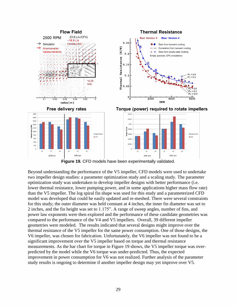
out. Figure 19 summarizes the primary comparisons that were made between CFD model results

and experimental measurements. In addition to the impeller performance tests for thermal

resistance, air flow, and torque that were described above, air velocity measurements were made

using hot wire anemometry to compare to the CFD predictions. The figure shows that the overall

agreement between simulations and experiments was quite good.

29

Figure 19. CFD models have been experimentally validated.

Beyond understanding the performance of the V5 impeller, CFD models were used to undertake

two impeller design studies: a parameter optimization study and a scaling study. The parameter

optimization study was undertaken to develop impeller designs with better performance (i.e.

lower thermal resistance, lower pumping power, and in some applications higher mass flow rate)

than the V5 impeller. The log spiral fin shape was used for this study and a parameterized CFD

model was developed that could be easily updated and re-meshed. There were several constraints

for this study; the outer diameter was held constant at 4 inches, the inner fin diameter was set to

2 inches, and the fin height was set to 1.175”. A range of sweep angles, number of fins, and

power law exponents were then explored and the performance of these candidate geometries was

compared to the performance of the V4 and V5 impellers. Overall, 39 different impeller

geometries were modeled. The results indicated that several designs might improve over the

thermal resistance of the V5 impeller for the same power consumption. One of those designs, the

V6 impeller, was chosen for fabrication. Unfortunately, the V6 impeller was not found to be a

significant improvement over the V5 impeller based on torque and thermal resistance

measurements. As the bar chart for torque in Figure 19 shows, the V5 impeller torque was over-

predicted by the model while the V6 torque was under-predicted. Thus, the expected

improvement in power consumption for V6 was not realized. Further analysis of the parameter

study results is ongoing to determine if another impeller design may yet improve over V5.

2500 RPM

Simulations Anemometer measurements

23.6 L/s (CFX) ~18.9 L/s (measured)

*4.35 m/s

*

Free delivery rates Torque (power) required to rotate impellers

Thermal Resistance Flow Field

30

The second study carried out using the CFD tools was a study of the performance of impellers

scaled beyond the 4” diameter required for CPU cooling. The goal of this study was to develop

insight and scaling laws for impeller performance based on the CFD results. Initially, a fairly

sparse set of simulations was run given time and resource constraints. The V6 impeller geometry

was used as the baseline with a diameter of 4”, fin height of 1.175”, and speed of 2500 rpm. The

impeller diameter was then scaled by 1.5X with heights at 0.5X, 1X, and 1.5X. Simulations

were carried out for these configurations with rotational speed at 2/3X, 1X, 1.2X, and 2X. Then

the impeller diameter was scaled by 2X with heights at 1X and 2X. These simulations were

completed with rotational speeds at 0.5X, 1X, and 2X. Not all combinations of these scales and

speeds were modeled. Thermal resistance, torque, and air flow rate were extracted from the CFD

results for each case and analyzed. The ultimate result from this analysis was a set of scaling law

equations for impeller performance similar to the more common fan affinity laws. These simple

power law correlations, shown in Table 2, can be used to provide an estimate of the performance

of an impeller without the use of costly CFD simulations.

Table 2. Scaling law equations for impeller performance based on CFD results.

Thermal conductance

Shaft torque

Shaft power

Air flow rate

31

1. INTRODUCTION

1.1. Motivation and Background

Worldwide, the number of personal computers is over a billion and that number is expected to

increase to 4 billion PCs by 2020 [3]. Chip makers have continued to follow Moore’s Law and

double the number of transistors packed into microprocessors every year such that the number is

currently over 2 billion. This increase in transistor density, combined with higher clock speeds,

has caused the heat dissipation in central processing units (CPUs) to increase from 30 W in the

early 1990s [4] to 130 W in 2011 (for an Intel Core i7 CPU [5]). This heat dissipation is caused

both by transistor leakage current, which occurs whenever the CPU is powered, and by clock

speed during operation. As transistor number continues to increase, the former becomes more

and more important. Currently, computers are at the point where thermal management imposes

significant limitations on computing power.

Furthermore, CPU cooling technologies have not advanced at the same rate as the CPU heat

dissipation requirements. The International Technology Roadmap for Semiconductors (ITRS) [6]

predicts that current air cooling technology will be incapable of meeting the increasing demands

of CPUs: “The high junction-to-ambient thermal resistance resulting from an air-cooled heat sink

provides inadequate heat removal capability at the necessary junction temperatures for ITRS

projections at the end of this roadmap.” This is in large part due to the fact that air cooling

technology has not changed significantly in decades. The conventional approach for air cooling

is to spread the heat from the source into a finned heat sink through which a fan blows air. Fan

and heat sink designs have changed little since the introduction of the computer. This issue was

summarized by DARPA in a 2008 call for research proposals on new ideas for air-cooled heat

exchanger technology: “Over the last 40 years, CMOS, telecommunications, active sensing and

imaging and other technologies have undergone tremendous technological innovation. Over this

same historical period the technologies, designs and performance of air-cooled heat exchangers

has remained unchanged. The performance data for today’s state of the art heat exchangers and

blowers is, in many cases, based on measurements performed in the 1960s.”[7]

Thus, for CPU cooling, the current state-of-the-art is becoming inadequate to meet the thermal

management needs of many high performance systems. This has led to the development of many

aftermarket CPU coolers. These systems are targeted at PC users that want to push the

performance of their computers by over-clocking. An example of a high-end, aftermarket CPU

cooler is shown in Figure 20. In this case, cylindrical heat pipes are in contact with the heated

surface to bring thermal energy to the extended surfaces with minimal temperature drop. This

thermal energy flows from the heat pipes into the fins, where it is transferred through convection

into the stream of air induced by the two fans.

32

Figure 20. A conventional heat sink employs one or more fans and an array of fins. In this particular example, cylindrical heat pipes are used to improve the heat transfer from the base to the extended surfaces (adapted from [8]).

The system shown in Figure 20 has a much lower thermal resistance (about 0.10 C/W) than a

conventional OEM CPU cooler (e.g. 0.30 C/W for the Intel Core 2 Duo E4400 stock CPU cooler

(http://www.frostytech.com/articleview.cfm?articleid=2335&page=4)). However, this decrease

in thermal resistance is primarily achieved by an increase in volume. The Noctua unit is more

than five times larger than the standard unit. The addition of heat pipes enables the CPU heat to

be spread to this larger volume heat sink. This solution is more complex and costly and,

unfortunately, not all computers have the space for such a device.

This brings up another issue in air cooling technologies; heat sinks are subject to volume

constraints. However, minimum volume traditionally comes at the expense of thermal

performance. So, while reductions in thermal resistance can be made with conventional

technologies by increasing volume, there is a limit to that approach that for many systems has

already been reached.

With traditional air-cooled heat exchangers reaching a limit, many applications have resorted to

more exotic cooling solutions such as liquid-cooled manifolds, spray-cooled enclosures, and

vapor-compression refrigeration. Compared to air cooling, these systems are complex, power

hungry, and costly. An air-cooled heat sink can be a self-contained unit that doesn’t require any

fluid connections. This means that the heat sink always remains dry near the electronics, which

can be damaged by some cooling fluids. Also, many locations, such as an office, are simply not

equipped to handle liquid cooling with external connections. The simplicity of air cooling

inherently reduces its installed cost in a system. This is evidenced by the widespread use of air

cooling.

33

1.2. The Sandia Cooler

This work reports on a fundamentally different approach to air-cooled heat exchangers that was

developed at Sandia National Laboratories [9] called the Sandia Cooler. Figure 21 shows the

latest version of the Sandia Cooler. The key to the technology is the heat-sink impeller which

consists of a disc-shaped impeller populated with fins on its top surface. The impeller functions

like a hybrid of a conventional finned metal heat sink and a fan. Air is drawn in the downward

direction into the central region having no fins, and expelled in the radial direction through the

dense array of fins. A high efficiency brushless motor is used to impart rotation (e.g. 2000 to

3000 rpm) to the heat-sink-impeller.

Figure 21. Sandia Cooler.

This rotating heat exchanger geometry places the thermal boundary layer in an accelerating

frame of reference. Placing the boundary layer in this non-inertial frame of reference adds a new

force term to the Navier-Stokes equations, whose steady-state solution governs the functional

form of the heat-sink-impeller flow field [10]. At a rotation speed of several thousand rpm, the

magnitude of this centrifugal force term is such that as much as a factor of ten reduction in

average boundary layer thickness is predicted [11]. The centrifugal force generated by rotation

acts on all surfaces simultaneously, and all portions of the finned heat sink are subject to the

resulting boundary layer thinning effect. This effect leads directly to an increase in the

convective heat transfer coefficient of the Sandia Cooler as compared to conventional

technology. It is the rotation of the heat sink that also provides a potent remedy to the

longstanding problems of heat exchanger fouling, condensate retention, and frosting. Rather

than having stationary finned surfaces that can accumulate dust and retain moisture, the Sandia

Cooler’s fins are constantly moving in an accelerating reference frame that expels particulates

and condensed liquid.

For the CPU cooling application, the base plate functions as a stationary heat spreader mounted

to the CPU case. During operation, the impeller is suspended above the baseplate by a thin (~10

34

m) air gap, much like the puck on an air hockey table. Heat then flows from the stationary

baseplate across the air gap to the rotating heat-sink-impeller. This air gap is produced by a

hydrodynamic air bearing. The air gap is passively regulated such that if the air gap distance

increases, the air pressure in the gap region drops, which causes the air gap distance to decrease.

This built-in negative feedback provides excellent mechanical stability and an extremely stiff

effective spring constant. Due to the relatively large surface area and thin gap, the thermal

resistance of the air bearing is only a small fraction of the overall Sandia Cooler thermal

resistance.

A sensorless, brushless DC motor integrated into the baseplate and impeller provides the torque

for rotating the impeller. Sensorless, meaning there are no Hall-effect sensors which provide

feedback as to motor orientation, so that the motor is much more compact. Brushless motors are

typically selected for cooling applications for the significant increase in lifetime compared to

brushed motors, which are typically limited to 5,000 hours because of brush wear. In contrast,

brushless motor cooling fans with operating lifetimes of 200,000 hours are now commercially

available (see for example

http://db.sanyodenki.co.jp/product_db_e/coolingfan/dcfan/longlife_read.html). In addition, if

equipped with an appropriate brushless motor controller, brushless motors operate quieter than

their brushed counterparts and generate much lower electromagnetic interference (EMI). The

motor currently being used in the Sandia Cooler is based on replacement parts (stator and rotor

magnets) from a commercial product that are readily available and inexpensive, but provides

enough torque to start and spin the impeller up to speeds in excess of 5000 rpm.

When the device is started from rest, the impeller contacts the baseplate with gravitational as

well as a spring pre-load force. Overcoming the static and then sliding friction that occurs

between the two surfaces before the air bearing provides enough lift is challenging. To minimize

that friction we incorporate an anti-friction coating into the two mating surfaces.

The air bearing grooves are machined into the cooler baseplate. The baseplate also houses the

wire wound stator for the brushless motor. In addition to these functions, the baseplate serves to

transfer heat from the CPU to the impeller. Because the heat source has a much smaller footprint

than the impeller, the baseplate must have a very low thermal spreading resistance. Because not

even a copper baseplate would be conductive enough to meet the thermal resistance

requirements, a vapor chamber (the same technology used in heat pipes) produced by a

commercial vendor is used instead.

This report describes an effort, carried out primarily in FY13, to develop the design shown in

Figure 21 including fabrication, assembly and demonstration of ten prototype systems. In

addition, work was carried out, through computational simulation and experimentation, to fully

understand the performance characteristics of each of the key aspects of the design. This work

culminated in a parameter and scaling study that has provided a design framework for Sandia

Cooler development for applications beyond CPU cooling. In addition, a number of design and

analysis tools resulted.

Previous impeller designs and the design philosophy for new fin versions will be described first.

Then the experimental characterization of several versions of the heat sink impeller, one

35

developed in previous years (V4) and two new impellers (V5 and V6), will be described in

detail. The heat transfer and fluid dynamic properties measured include thermal resistance, flow

field, pressure-flow curves, shaft torque, and acoustic noise.

Computational simulation of the impellers included mechanical deformation due to centrifugal

forces and thermal expansion, modal analysis, and extensive, coupled heat transfer and fluid

dynamics. Model development will be described and results will be discussed in terms of the

implications for the current design as well as for future designs for new applications.

The design and fabrication of several baseplate versions will be described next including solid

metal baseplates as well as vapor chambers. Then, experimental characterization of the heat

spreading characteristics of the baseplates will be shown. The development of the design for the

air bearing grooves follows. Again, several successive versions were developed and

characterized for lift and stiffness as well as thermal resistance. In addition, an alternative design

to the air bearing, magnetic lift, will be explained and an experimental demonstration shown.

The anti-friction coating used to enable startup and minimize wear of the contacting surfaces

between the baseplate and the impeller was provided by a commercial vendor. However, a

comprehensive evaluation process was undertaken to ensure that the coating provided the

necessary friction coefficient and was robust. This evaluation actually included two slightly

different anti-friction coatings from Tribologix, Inc. Results for startup torque, friction, and

durability tests will be discussed.

As mentioned previously, a design based on a COTS motor was selected for the CPU cooler

application. However, no COTS motor controller was found that could operate the motor as

required for startup. Available COTS motor controllers also generated objectionable levels of

motor noise, and provided relatively low brushless motor efficiency. Thus, two parallel

development efforts will be described to produce a robust motor controller for this design. One

effort was based on modifying a COTS controller so that the necessary startup torque could be

applied before transitioning into a speed control mode. The second effort was the development

of a custom controller based on a Variable Voltage Variable Frequency (VVVF) control scheme.

This second path was ultimately chosen as the final motor controller configuration. The design

and fabrication of this custom VVVF controller will be described in the final section.

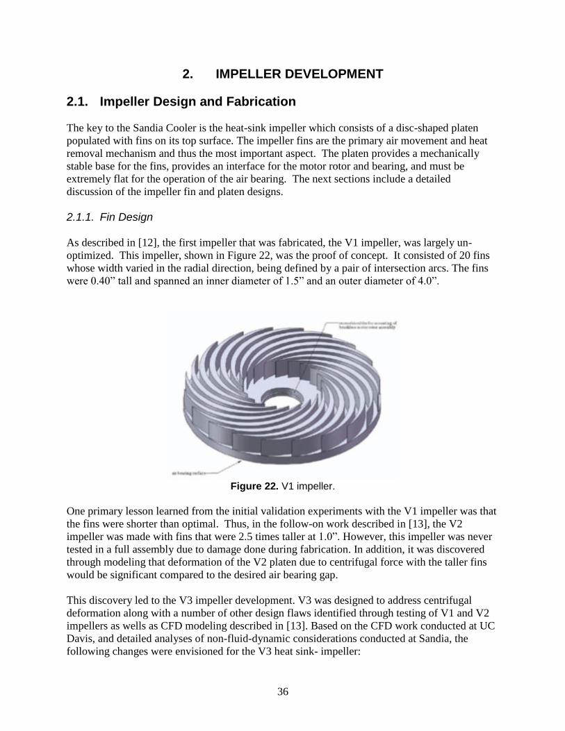
36

2. IMPELLER DEVELOPMENT

2.1. Impeller Design and Fabrication

The key to the Sandia Cooler is the heat-sink impeller which consists of a disc-shaped platen

populated with fins on its top surface. The impeller fins are the primary air movement and heat

removal mechanism and thus the most important aspect. The platen provides a mechanically

stable base for the fins, provides an interface for the motor rotor and bearing, and must be

extremely flat for the operation of the air bearing. The next sections include a detailed

discussion of the impeller fin and platen designs.

2.1.1. Fin Design

As described in [12], the first impeller that was fabricated, the V1 impeller, was largely un-

optimized. This impeller, shown in Figure 22, was the proof of concept. It consisted of 20 fins

whose width varied in the radial direction, being defined by a pair of intersection arcs. The fins

were 0.40” tall and spanned an inner diameter of 1.5” and an outer diameter of 4.0”.

Figure 22. V1 impeller.

One primary lesson learned from the initial validation experiments with the V1 impeller was that

the fins were shorter than optimal. Thus, in the follow-on work described in [13], the V2

impeller was made with fins that were 2.5 times taller at 1.0”. However, this impeller was never

tested in a full assembly due to damage done during fabrication. In addition, it was discovered

through modeling that deformation of the V2 platen due to centrifugal force with the taller fins

would be significant compared to the desired air bearing gap.

This discovery led to the V3 impeller development. V3 was designed to address centrifugal

deformation along with a number of other design flaws identified through testing of V1 and V2

impellers as wells as CFD modeling described in [13]. Based on the CFD work conducted at UC

Davis, and detailed analyses of non-fluid-dynamic considerations conducted at Sandia, the

following changes were envisioned for the V3 heat sink- impeller:

37

1) The incorporation of a shroud to solve the problem of centrifugal deformation.

2) Increasing the fin height from 0.40" to l.00" (as in the version 2 heat-sink-impeller).

3) Increasing the number of fins from 20 to 60.

4) Rounding of the leading edge geometry to minimize sensitivity to angle of attack.

5) Flaring of the channel cross-sectional area to add the functionality of a diffuser.

6) Fabrication of the heat-sink-impeller from copper rather than aluminum.

7) Drastic reduction of air flow obstruction by the brushless motor assembly.

Figure 23. V3 impeller design.

The V3 impeller (Figure 23) was conceived as a two-piece assembly with top and bottom pieces

having 30 fins each which would mesh together to make a 60 fin device. As described in [13],

the incorporation of a solid shroud on the top of the impeller essentially eliminated centrifugal

deformation. However, due to the anticipated fabrication complexity and budget constraints, a

V3 impeller was never produced. Instead, a simpler design, the V4 impeller, was fabricated and

used for a second demonstration system. The V4 impeller, shown in Figure 24, consisted of a

single piece with 36, 1-inch tall fins. These fins were also arc shaped like previous versions and

the impeller was made from aluminum. Centrifugal deformation of this impeller would be

compensated by machining the bottom surface as will be described later.

38

Figure 24. V4 impeller.

With the two-piece V3 design never fully developed, the lessons learned from early impeller

experiments and modeling were not fully implemented until the V5 design. The improvements

meant for V3 along with more lessons learned from the assembly of the V4 prototype were all

taken into account in the V5 impeller design.

The V5 impeller is shown in Figure 25. Like the previous four versions, this impeller was

developed for CPU cooling and thus maintained the 4.0” outer diameter. However, most of the

other aspects of this impeller were different. To increase heat transfer surface area, this impeller

includes more than double the number of fins of the V4 design with 80 fins. Moreover, the V5

fins are a constant 0.030” thickness, rather than variable thickness like previous versions.

Although the fins are slightly shorter than the V4 fins at 0.95”, the aspect ratio is much higher.

This fin design results in a better balance between conduction and convection heat transfer.

Figure 25. V5 impeller.

Based on fluid dynamics considerations, the fin inner diameter was opened up to two inches to

double the intake bore cross-sectional to avoid constricting air flow. Also, the fin channel

diffuser area ratio was increased to 2:1 to provide higher air flow per unit power consumption.

39

While the V5 impeller is still meant to be cold-forged for production, it was designed for rapid

in-house CNC fabrication and modification. QC-10 aluminum [14] was chosen to develop this

impeller due to an excellent combination of machinability and thermal conductivity. In addition,

a number of improvements were made for the integration of the brushless DC motor that will be

described below.

The V5 impeller design was the result of several years of development and a number of design

revisions. Thus, the primary goal for the project in FY13 was to develop an operational Sandia

Cooler prototype based on the V5 impeller. That was to include fabricating multiple copies of the

impeller and evaluating the thermal and pumping performance of the impeller which will be

described in subsequent sections.

In addition to developing the V5 design, a related goal was to fully understand the performance

through physical and computational simulation so that it might be improved in future

generations. The experiments and CFD analysis toward this end will be described later. In

addition to CFD though, other tools were developed to aid with respect to fin design and several

new fin designs were developed in an attempt to further improve over the V5 design.

Firstly, a fin design tool was developed using Mathematica [2] to enable rapid geometric

parameterization of a design with real-time feedback on the effects of parameter changes. The

tool was developed with the assumption that the fin shape, rather than the intersection of arcs,

would follow a logarithmic spiral so that the fin angle relative to a radial line (φ) is constant.

Figure 26 shows the geometry of a prototypical impeller with this fin shape. The pressure side

(the convex side) of the fin was defined, with the angle θ from the x-axis as the parameter, as

follows:

[

] [

], Equation 1

where x and y are the horizontal and vertical positions of the curve and c is a parameter defining

the curvature of the log spiral. The parameter c is related to the fin angle relative to a radial line

(φ) as follows:

. Equation 2

The width of each fin was defined by (1) the width at the leading edge and (2) a power law

function defining how the fin thickness varies with radius:

(

)

, Equation 3

where w is the fin width, r is the radius, A is the power law exponent (a parameter that

determines how the fin width varies with radius), and the subscript 1 refers to quantities at the

leading edge of the fin. The equation of the suction side of the fin can be determined by vector

addition of the pressure side equation and the product of w(r) and the unit normal vector. The

pressure and suction sides of the fin are joined by fillets that are tangent to the inner and outer

40

radii (r1 and r2). The impeller, then, can be expressed with a set of 7 parameters: outer radius r2,

inner radius r1, height b, sweep angle φ, number of fins Z, fin width at leading edge w1, and

power law exponent A.

Figure 26: A prototypical heat-sink-impeller with fins that follow a logarithmic spiral.

41

Figure 27. Mathematica impeller design tool.

Figure 27 shows the Mathematica tool. A top view of the impeller is shown in the central region

of the tool. The seven adjustable parameters are controlled via slider bars in the upper left corner

of the tool. Because prototype impellers are CNC machined, end mill diameter and aspect ratio

are defined rather than explicitly defining fin height. In this way, a geometry that can be

fabricated is ensured. Fin height is then calculated and displayed in the upper right corner of the

tool along with a number of additional characteristics of the impeller. These calculated quantities

include the surface area of the fins, the entrance and exit width of the air channels, the area ratio

of the air channels, the cross-sectional area of the fins, and the percentage of the cross-section

occupied by the fins.

Both the calculated quantities and the top view of the current impeller design update

automatically as the various slider bars are adjusted. This allows the user to visualize the effects

42

of various parameters and understand the ranges through which a reasonable design can be

achieved. For example, some combinations of parameters will result in a design that could not

be fabricated because the channel widths between fins would be too small. Also, for a given set

of constraints, the tool allows the user to maximize fin surface area or obtain a desired air

channel area ratio.

This tool was developed not only to allow for the design and visualization of different impeller

geometries, but to inform other performance calculation tools. The inputs and outputs of this

tool were used to set the ranges and increments for a CFD parameter study, for instance, as will

be discussed in Section 2.3.4.2. They were also used along with another analytical tool to predict

the impeller geometry for minimum thermal resistance.

This second tool was developed using Mathcad 15.0 and was created as a simpler method than

3D CFD models to predict the thermal resistance of various impeller designs. The calculations

combine a heat transfer coefficient correlation and a fin efficiency analysis to predict overall

thermal resistance. The heat transfer coefficient correlation is largely empirical, but similar to a

turbulent Nusselt number with the fluid parameters lumped into a single constant. This heat

transfer correlation is shown below in Equation 16,

, Equation 4

where rave is the average radius of the fins in meters and speed is in rpm. A standard fin

efficiency analysis is then carried out (see Mills pg. 85-89) to determine the parameter which

accounts for the fact that the temperature of the impeller surface has a gradient and is, on

average, lower than the platen temperature. The thermal resistance of the impeller is then

calculated as R = 1/hA, where A is the total impeller surface area. This set of equations was

found to provide reasonable agreement (within 10%) to thermal resistance values obtained

through experiment and CFD over a range of speeds, impeller diameters and fin geometries.

These Mathematica and Mathcad tools were used to perform a study for the 4-inch diameter

impeller geometry to determine minimum thermal resistance. Five geometric parameters were

varied including number of fins, inner fin radius, fin height, fin width at leading edge, and power

law exponent. Reasonable ranges and combinations of these parameters were determined using

the Mathematica tool. Outer diameter and log spiral angle (30deg) were kept constant. Fin

parameters were then fed to the Mathcad model to calculate thermal resistance for a rotational

speed of 2500 rpm. Figure 28 shows the study results for thermal resistance as a function of the

five parameters.

43

Figure 28. Thermal resistance parameter study for 4” diameter impeller.

In Figure 28, thermal resistance is denoted by color in the array of 3D contour plots. All 7 plots

have the same scale with a thermal resistance range of 0.15 to 0.07. Each plot shows thermal

resistance as a function of fin width at leading edge, power law exponent, and fin height for fixed

values of number of fins and fin inner radius. Fin width was varied from 0.020” to 0.050”, fin

height was varied from 0.85” to 1.15”, and the power law exponent varied from 0 to 2. The

columns represent the three values used for number of fins: 40, 60 and 80 fins. Rows represent

the three values used for fin inner radius: 0.75”, 1.0”, and 1.25”. Not every combination of these

parameters was possible for two reasons. First, for the 40 fin case, a limitation in the range of

the slider bars in the Mathematica tool wouldn’t allow the lower left corner of the matrix to be

filled out. However, since this region trends toward higher thermal resistance, it was ignored.

Second, the upper right corner could not be filled out due to the minimum air channel width

constraint. For example, an 80 fin design with an inner fin radius of 0.75” would result in a

channel width between fins that was too small to machine.

The results of this study identified several effects of the five parameters. Increasing the number

of fins has a strong effect on reducing thermal resistance due to increased surface area.

Reducing the inner fin radius also reduces thermal resistance for the same reason. Thickening

the fins by increasing the width at the inner radius and growing the width with radial location

both reduce thermal resistance by increasing the fin efficiency. This is more important as the fin

44

height increases. Finally, fin height has competing effects. Increasing fin height also increases

surface area which lowers thermal resistance. But, taller fins have lower fin efficiency. Overall,

the surface area increase seems to outweigh the fin efficiency decrease, so taller fins are better

especially for thicker fins. However, this is only true within the range of heights considered.

Overall, the analysis indicated that surface area is the most important driver to lower thermal

resistance, as might be anticipated. A high surface area coupled with the highest possible fin

efficiency produced the lowest thermal resistance designs. High surface area is achieved with a

large number of fins, the minimum fin inner radius that can be fabricated, and a height near the

maximum of the range studied. The highest fin efficiency is then achieved at the maximum

thickness possible as a function of radius. Note that the V5 fin design is close to this description

for minimum thermal resistance. In fact, the Mathcad tool predicts a thermal resistance for the

V5 impeller at 2500 rpm of 0.084 which is very close to the measured value that will be

described later. Out of the 146 cases that were considered in the Mathcad parameter study, only

27 designs had a lower thermal resistance than V5 with the lowest value being 0.067.

Finally, we point out that the Mathcad calculations, while verified with a few experimental

results, are for guiding engineering judgment rather than as absolute predictors of performance.

In addition, the Mathcad analysis tells us nothing about several other performance parameters

that are key to a successful impeller design which include air flow delivery rate, torque and

power consumption, and noise. For the fluid dynamics parameters and more accurate thermal

resistance predictions we relied on the more complex CFD calculations which will be described

in Sections 2.1.4.1 and 2.3.4.2. Section 2.3.4.2 describes a CFD parameter study that was used in

conjunction with the Mathcad analysis to develop an improvement to the V5 impeller. The result

was the V6 impeller shown in Figure 29.

Figure 29. V6 impeller.

The V6 impeller consists of 55 log spiral fins that are taller than the V4 or V5 fins at 1.175”.

Like V5, these fins span an inner diameter of 2.0” and an outer diameter of 4.0”. The log spiral

shape has a sweep angle of 45°, a leading edge width of 0.034”, and a power law exponent of

45

1.5. The CFD calculations discussed in Section 2.3.4.2 indicated that this design would have a

comparable thermal resistance to V5 at 2500 rpm, but significantly lower power requirement. At

the same 5W of shaft power the V6 impeller thermal resistance was predicted to be 20% lower

than V5. Experimental characterization of the V4, V5, and V6 impellers will be discussed in

Section 2.2.

In addition to the parameter studies to develop optimized fin designs, several concepts for fin

configurations originally contemplated in the first patent application for the Sandia Cooler were

investigated this year. These configurations were termed “interrupted fin” designs since the

underlying concept was to interrupt the fluid boundary layer next to the fin surfaces to increase

the convective heat transfer coefficient and further improve the impeller thermal resistance. An

initial performance assessment of two interrupted fin designs will be described in Section

2.3.4.2.

2.1.2. Platen

As mentioned previously, the impeller platen has the following functions: provide a thermally

conductive and mechanically stable base for the fins, provide an interface for the permanent

magnet rotor and radial bearing assembly, and maintain a flat bottom surface for proper

operation of the air bearing and control of the air gap. Material selection, either aluminum or

copper, and a reasonable thickness (~0.25”) satisfy the first requirement. As the interface for the

brushless motor, several modifications were made to the V5 design to improve over previous

designs. Rather than attaching the off-the-shelf rotor to the platen, the rotor was integrated into

the platen design. This change eliminated numerous alignment problems, minimized motor

noise, minimized air flow obstruction, and eliminated a path for dust to enter the air gap.

There were a number of problems when installing off-the-shelf rotor assemblies into the

impellers. The rotor magnet array needed to be parallel to the bottom surface of the impeller

and, subsequently, the bearing’s axis of rotation perpendicular to this surface. To accomplish

this, the rotor of the original motor was eliminated and the necessary features were incorporated

into the impeller that allowed direct installation of the magnets, flux ring, and bearing while

insuring adequate tolerances in a highly manufacturable design (Figure 30). Along with solving

the aforementioned problems, this new design allowed the motor cavity to be sealed. Having the

motor cavity sealed prevents the ingress of dust and other contaminants, and helps reduce motor

noise. The revised design provided a number of benefits while eliminating the associated issues

with alignment, vibration, and noise.

Figure 30. Rotor mounting features incorporated into impeller platen.

46

Due to the centrifugal forces acting on the fins of the impeller at operating speed, the impeller

deforms and the bottom surface becomes slightly concave. As will be discussed in Section

2.3.1.3, the V5 impeller operating at 2500 rpm develops a maximum displacement of ~8 m.

This deformation causes a variation in the air gap between the impeller and the baseplate,

adversely affecting heat transfer and air bearing functionality. To counteract this effect,

compensating the bottom surface of the impeller with a convex profile specific for the operating

speed allows the bottom surface to become flat once it is up to speed. The convex profile also

reduces the effective torque radius for sliding friction, thereby reducing starting torque

requirements.

However, creating such a precise convex profile presents some challenges when using common

machining practices. Work holding becomes an issue when trying to achieve such a contour;

required clamping forces distort the part causing asymmetric deformation upon releasing the

clamps after machining. As a solution to this issue, a fixture was designed and fabricated that

would produce adequate clamping force but cylindrically symmetric deformation as shown in

Figure 31. With in-situ measurements of deflection due to fixturing, appropriately compensated

3-axis tool paths were created that would give the desired contour upon release from the fixture.

While this method showed potential, it was difficult in practice to achieve the desired precision

for the surface profile. Also, customized compensation profiles and 3-axis tool paths were

required for each new impeller design due to different centrifugal and fixturing deflection

profiles. Due to the complexity of this method and the resulting scallops that are inherent to 3-

axis surfacing, a completely different approach was used on the V5 impellers. A custom fixture

Figure 31. Fixture for machining platen surface profile.

47

was fabricated for mounting the impeller to the CNC spindle and registering to the impeller

bearing’s inner race to insure concentricity and the rotor features to insure perpendicularity. The

spindle was then gradually brought up to speed and a tool mounted to the worktable was

traversed across the bottom surface of the impeller at the appropriate feed rate to insure proper

chip load and surface finish. In this way, the bottom surface of the impeller was allowed to

deform at the intended operating speed and then cut flat. This method proved to be very

successful and is simple enough for implementation in mass production. Once impeller profiles

were cut using this method, the surface profile was inspected using a precision dial indicator.

The measured profiles matched well with the predicted deformation, as will be discussed in

Section 2.3.1.3.

2.1.3. Impeller Fabrication

For mass production, Sandia Cooler impellers are intended to be cold-forged. To demonstrate

the viability of this manufacturing process, the V4 impeller was cold-forged and 20 such

impellers were fabricated as a proof-of-concept for the mass-manufacturing process (Figure 32).

Each of the heat-sink-impellers was stamped out of a single rough-cut billet of 6063 aluminum

(later black-nickel plated for aesthetics). The cold forging process takes ~10 seconds to complete

and is carried out at room temperature. For the V4 impellers, the hardened steel die set cost

~$10k to fabricate. Each die set has a lifetime of several hundred thousand process cycles and

multiple cavity dies would be used for mass production. The hydraulic press used for forging

these parts costs ~$250k, but that cost could be amortized over millions of parts. Between the die

set and the press, the manufacturing costs would only be a few dimes per impeller. The

successful completion of these parts demonstrated that the Sandia Cooler could be produced at a

competitive cost compared to current CPU cooling technology.

Figure 32. Twenty cold-forged V4 impellers.

48

However, for design development and rapid turn-around prototyping, cold-forging is not

practical and the impellers had to be CNC machined. Due to complexity, small feature size, and

tight tolerances, most machine shops would not bid on the job. Thus, all of the V5 impellers were

fabricated at Sandia using a Haas OM-2A CNC vertical 4-axis mill with a 30,000 rpm spindle.

Milling the high aspect ratio fin channels was the most challenging aspect. Tool availability and

durability limited the number of fins, channel width, and fin height that could be achieved. The

V5 impeller pushed the limit in this respect. Investigation of the current state-of-the-art tooling

lead to selection of Harvey Tool high aspect ratio end mills. Due to tool deflection and breakage

associated with high aspect ratio end mills, each operation required custom tool paths that CAM

software could not generate. After these paths were created in CAD software and loaded into the

CAM software, optimization of spindle speed, feed rate, and cutting depth had to be done for

each tool. To minimize fabrication time, an assortment of endmills of the same diameter was

used starting with a stub flute endmill, and progressing in length to the most extreme aspect ratio

endmill as shown in Figure 33. This process drastically reduced the machining time.

With this process and mill, a V5 impeller could be fabricated in roughly three days with

excellent quality control. The addition of a new 75,000 rpm air-spindle reduced the fin cutting

operation time by a factor of three. This was invaluable for producing ten copies of the V5

impeller.

2.2. Impeller Performance Evaluation

2.2.1. Thermal Resistance

One of the most important characteristics of the Sandia Cooler is the thermal performance. A

typical metric for thermal performance in electronics cooling applications is the thermal

Figure 33. Progressively higher aspect ratio tools were used to machine the V5 impeller.

49

resistance, which is the temperature difference between the cooled surface and the ambient air

divided by the heat dissipated. While the overall thermal resistance of the Sandia Cooler is

important and was measured, in this section, we also describe measurements of the thermal

resistances of individual components. The different components to the system include the

baseplate, which mounts to the device that will be cooled, the air bearing between the baseplate

and the impeller, and the impeller itself. By measuring the thermal resistance of individual

components in addition to the overall system, highly thermally resistive components can be

identified and improved upon. In addition, it is also often easier to measure the thermal

resistance of an individual component than the overall system. This also allows comparisons to

be made on new designs of one aspect of the system; for example, when a new impeller is

designed and manufactured, its thermal resistance can be measured and compared to the thermal

resistance of the previous impeller versions to see if improvements have been made. Two

different methods were used to measure impeller thermal resistance: a transient method and a

steady-state method.

2.2.1.1. Transient Thermal Resistance Measurements

Test Apparatus and Procedure

The impeller (1 of Figure 34) was mounted on a shaft (13 of Figure 34) and, using a motor

control assembly (8-10 of Figure 34), it was rotated at predetermined speeds up to 6,000 rpm at

increments of approximately 250 rpm. The impeller was heated to a uniform temperature of

50oC by a heat gun (not shown). Then, the external heat source was turned off and, using an

infrared probe (3 of Figure 34), the temperature of the heat-sink-impeller was measured once

every second. The thermal decay was recorded using data acquisition software and the collected

decay data was fit to a mathematical lumped capacitance model of the thermal decay. Heat losses

down the shaft were deemed negligible because the contact area was very small and the time

period for heat transfer to occur was relatively short.

Figure 34. Experimental Setup.

50

Control and Data Acquisition

The set up for speed control and to record data was fairly simple. An MPI MX 8340 Servo

Driver PRO controller was used to set the speed and a TEKIN Race Legal Type S motor was

used to drive the shaft. To measure the temperature of the impeller, a FLUKE 80T-IR sensor was

used. The temperature probe was pointed at the platen (the bottom surface of the impeller) and

the time sampling was set to 1 second. The probe was connected to an Agilent DSO6034

Oscilloscope for data acquisition and the recorded decay was transferred to Excel and later to

Mathematica for analysis. The probe voltage to temperature conversion factor was calibrated in

the lab and checked against the factory calibration. Only a slight difference was found between

the two calibrations.

Data Analysis

As mentioned earlier, the lumped capacitance model was used to calculate the resistance R at

each rotational speed. A dimensionless parameter called the Biot number indicates whether the

lumped capacitance model is applicable to a given heat transfer case. The Biot number is the

ratio of the internal resistance of a body to heat conduction to its external resistance to heat

convection. In general, as long as the Biot number is less than 0.1 the variation of temperature is

small enough that the lumped capacitance model is applicable. If this condition is satisfied, the

fluctuation of temperature in the body is within 5%. If the criterion Bi < 0.1 is not met, the

model can still be used but the results will be much less accurate.

Due to the complex shape of the impellers, to calculate the Biot numbers, they were broken

down into their platen and fins. Therefore, two Biot numbers were calculated for each impeller

to justify using the lumped capacitance model. The Biot number can be calculated as,

Bi =hLc

k Equation 5

Where h is the convective heat transfer coefficient, k is the thermal conductivity of the impeller,

and Lc is a characteristic length, which, in general, is the ratio of the object’s volume to its

surface area, as shown in Equation 6:

Lc =V

As. Equation 6

Biot numbers were calculated for the V4 and V5 impellers. For the platens, the thickness was

used for Lc since only the top surface is cooled. For the fins, Lc = 6.6x10-4

m for V4 and 3.7x10-

4 m for V5. The convective heat transfer coefficients h were calculated using the resistance R

values at around 3,000 rpm along with the surface area of the impellers.

h =1

RAs Equation 7

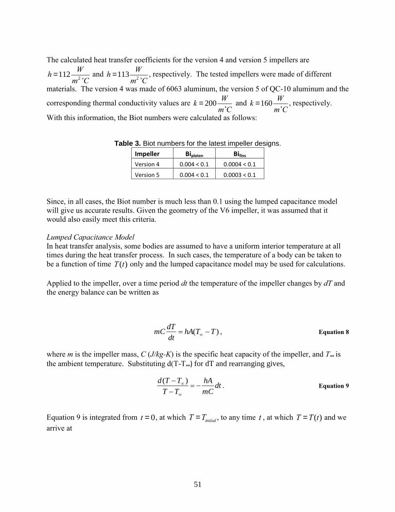
51

The calculated heat transfer coefficients for the version 4 and version 5 impellers are

h =112W

m2 C and h =113

W

m2 C, respectively. The tested impellers were made of different

materials. The version 4 was made of 6063 aluminum, the version 5 of QC-10 aluminum and the

corresponding thermal conductivity values are k = 200W

m C and k =160

W

m C, respectively.

With this information, the Biot numbers were calculated as follows:

Table 3. Biot numbers for the latest impeller designs.

Impeller Biplaten Bifins

Version 4 0.004 < 0.1 0.0004 < 0.1

Version 5 0.004 < 0.1 0.0003 < 0.1

Since, in all cases, the Biot number is much less than 0.1 using the lumped capacitance model

will give us accurate results. Given the geometry of the V6 impeller, it was assumed that it

would also easily meet this criteria.

Lumped Capacitance Model

In heat transfer analysis, some bodies are assumed to have a uniform interior temperature at all

times during the heat transfer process. In such cases, the temperature of a body can be taken to

be a function of time T (t) only and the lumped capacitance model may be used for calculations.

Applied to the impeller, over a time period dt the temperature of the impeller changes by dT and

the energy balance can be written as

)( TThAdt

dTmC , Equation 8

where m is the impeller mass, C (J/kg-K) is the specific heat capacity of the impeller, and T∞ is

the ambient temperature. Substituting d(T-T∞) for dT and rearranging gives,

dtmC

hA

TT

TTd

)(. Equation 9

Equation 9 is integrated from t = 0, at which T =Tinitial , to any time t , at which T =T(t) and we

arrive at

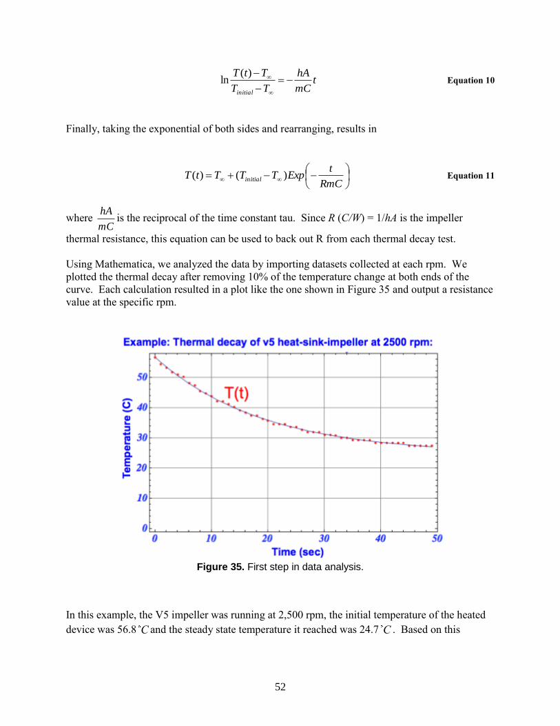
52

tmC

hA

TT

TtT

initial

)(ln Equation 10

Finally, taking the exponential of both sides and rearranging, results in

RmC

tExpTTTtT initial )()( Equation 11

where mC

hAis the reciprocal of the time constant tau. Since R (C/W) = 1/hA is the impeller

thermal resistance, this equation can be used to back out R from each thermal decay test.

Using Mathematica, we analyzed the data by importing datasets collected at each rpm. We

plotted the thermal decay after removing 10% of the temperature change at both ends of the

curve. Each calculation resulted in a plot like the one shown in Figure 35 and output a resistance

value at the specific rpm.

Figure 35. First step in data analysis.

In this example, the V5 impeller was running at 2,500 rpm, the initial temperature of the heated

device was 56.8 C and the steady state temperature it reached was 24.7 C . Based on this

53

information, a resistance value of R= 0.082K /Wwas calculated. This procedure was repeated

for each speed for all three impellers and the results are shown in Figure 36.

Thermal Resistance Results and Conclusion

The thermal resistance (R) values of each decay curve, corresponding to individual rpm settings,

are summarized in the final plot shown in figure 37. The blue dots mark the R values for the V4

impeller, the green ones mark the V6 impeller and the red ones mark those for the V5 impeller.

Figure 36. Thermal Resistance of Heat-Sink-Impellers V4, V5, and V6.

Figure 37. V4, V5 and V6 thermal resistance for speeds of 1000-5000 rpm.

54

Thermal resistance values between 1000 and 5000 rpm are shown expanded in Figure 37. The

thermal resistance of the V5 impeller is about 30% lower than the V4 impeller. The difference

between the two impellers is likely due to the overall surface area of V5 being 41% greater than

V4. The V6 thermal resistance lies between that of V4 and V5 and is slightly higher than was

predicted by our CFD model.

2.2.1.2. Steady-state thermal resistance measurements

While the thermal decay method was a fairly simple method to measure impeller thermal

resistance, a more direct method with less potential for error was desired. Thus, a new

experiment was designed and assembled to measure the thermal resistance of the impellers. This

method was a steady-state heat transfer method that more directly simulated the way the Sandia

Cooler would be used for CPU cooling. A heater was adhered to the bottom surface of the

impeller, covered in with insulation and then mounted on a rotating shaft. The contact area

between the shaft and the base of the impeller is very small, which leads to insignificant

conduction through the shaft. The power leads to the heater were fed through two of the fins of

the impeller, into a one-foot-long piece of 5/32 in. hex tubing where they were mated with a

Mercotac model 205 rotary electrical connector. Two IR sensors pointed at the impeller gave

readings of temperature. One sensor was a Fluke 80T-IR temperature probe, and the other was an

Omega OS36-01 sensor. A type-K thermocouple also measured the temperature of the inlet air.

This experimental setup is shown in Figure 38. An Agilent 34970A data logger was used to log

data. The voltage and current applied to the heater were measured as well as the rotation speed,

and the three temperatures previously described. The voltage measurements were corrected for a

0.2 resistance in the heater wiring (including the rotary connector). The current was determined

by measuring the voltage drop across a 0.05 current sensing resistor.

55

Two methods were used to analyze the data. In the lumped capacitance analysis, it was assumed

that conduction in the aluminum impeller is very fast. By making this assumption, a heat

balance on the impeller can be written as

where is the power to the heater (W), is the mass of the impeller (kg), is the heat capacity

(903 J/kg-K for aluminum), is the impeller temperature (K), is time (s), is the convective

heat transfer coefficient (W/m2-K), is the surface area of the impeller (m

2), and is the

temperature of the inlet air (K). If we transform the temperature through the relation , this equation becomes the ODE

to which the solution can be found using an integrating factor, as

(

) [ ∫

(

) ]

With the measured data for the temperature difference and the power to the heater, the

quantity , which is the thermal resistance, was determined using a least squares fit. The

data, and a typical fit is shown in Figure 37, for the version 5 impeller spinning at 2500 RPM.

Figure 38. Experimental setup for measuring thermal resistance of Sandia Cooler impellers. A thin film heater provides heat at a given power for the impeller to dissipate. As the impeller rotates, the temperature difference between the inlet air and impeller is measured as a function of power.

56

As shown in the middle frame, the lumped capacitance model follows the data for quite well,

as the power is varied in time.

A steady-state analysis of this data was also performed. In this analysis, first a Gaussian window

using 15 data points was used to smooth the temperature difference data. Then a central

difference approximation with fourth order error was used to determine the derivative of the

smoothed data. The steady-state data points considered were those where the power to the heater

was greater than 15 Watts, the rate of change of the temperature difference data was less than

0.005 K/s, and the rate of change of the power data was less than 0.005 W/s. For each of these

data points, the thermal resistance of the impeller was calculated by dividing the temperature

difference by the power to the heater. Finally, an average value of the thermal resistance was

calculated over all of the power variations for a given rotation speed. The data and average

values are shown in the bottom frame of Figure 37. As shown, the steady-state measurements

agree quite well with the lumped capacitance fit.

Figure 39. Typical data stream for impeller thermal resistance measurements. Top frame shows speed and power, middle frame shows data and fit using lumped capacitance model, and bottom frame shows steady-state thermal resistances and averages of that data.

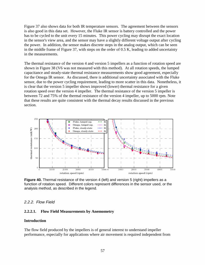
57

Figure 37 also shows data for both IR temperature sensors. The agreement between the sensors

is also good in this data set. However, the Fluke IR sensor is battery controlled and the power

has to be cycled to the unit every 15 minutes. This power cycling may disrupt the exact location

in the sensor's view area, and the sensor may have a slightly different voltage output after cycling

the power. In addition, the sensor makes discrete steps in the analog output, which can be seen

in the middle frame of Figure 37, with steps on the order of 0.5 K, leading to added uncertainty

in the measurements.

The thermal resistance of the version 4 and version 5 impellers as a function of rotation speed are

shown in Figure 38 (V6 was not measured with this method). At all rotation speeds, the lumped

capacitance and steady-state thermal resistance measurements show good agreement, especially

for the Omega IR sensor. As discussed, there is additional uncertainty associated with the Fluke

sensor, due to the power cycling requirement, leading to more scatter in this data. Nonetheless, it

is clear that the version 5 impeller shows improved (lower) thermal resistance for a given

rotation speed over the version 4 impeller. The thermal resistance of the version 5 impeller is

between 72 and 75% of the thermal resistance of the version 4 impeller, up to 5000 rpm. Note

that these results are quite consistent with the thermal decay results discussed in the previous

section.

2.2.2. Flow Field

2.2.2.1. Flow Field Measurements by Anemometry

Introduction

The flow field produced by the impellers is of general interest to understand impeller

performance, especially for applications where air movement is required independent from

Figure 40. Thermal resistance of the version 4 (left) and version 5 (right) impellers as a function of rotation speed. Different colors represent differences in the sensor used, or the analysis method, as described in the legend.

58

heat dissipation. However, more importantly, these experiments provide model validation

data for the CFD calculations. This is critical since we rely on our CFD models to design new

impeller geometries.

Anemometry experiments were done to measure the flow field around the version 4 impeller.

Both, the entry and the exit flow were examined. When compared to other instruments for

flow measurements, thermal anemometers have very high frequency-response and very good

spatial resolution, which makes them a useful tool for characterizing turbulent flow. They

rely on a heated probe element that is inserted into the airstream where the speed of the

airflow is to be measured. These hot-wire equipped instruments have a very fine wire, on the

order of several micrometers thin, that is electrically heated to some temperature above that

of the ambient air. As air flows past the wire the temperature of the wire drops and since the

wire’s electrical resistance depends on its temperature, a relationship can be obtained

between the resistance of the wire and the measured speed of the airflow.

While these types of instruments can measure the speed of the airflow, they are not able to

provide information regarding the direction of the flow. We wanted to be able to draw a

vector field that represents the flow around the impeller so the direction of the flow was also

of interest. To obtain results with approximate directions, we took several measurements at

different angles at each point examined and used the angular direction corresponding to the

highest speed value.

Test Procedure

The impeller was mounted on a shaft at a 90 degree angle, its axis of rotation being

horizontal, and the anemometer was clamped on a traverse with the probe positioned at the

center of the impeller, about 5 mm away from the top of the fins. The impeller was then

rotated at 2,500 and 5,000 rpm and the speed of the airflow was recorded at numerous points,

both at the entrance and exit, with spacing of 5mm from each other. By turning the probe

from 0 to 90 degrees in increments of 10 degrees, we got 10 speed measurements at each

point. These measurements were used to predict the direction of the flow in a plane and the

highest value was recorded with its angular direction.

As an example, in the case of the version 4 impeller, at 2,500 rpm, we took 10 measurements

at the center of the impeller 5 mm above the fins. The list of collected data is shown in Table

4. Based on the angle at the highest speed measured (marked in green in the table) the vector

(circled in red in Figure 41) was drawn to represent the flow velocity at that point.

59

Table 4. Example of measured flow rates at a single point.

Probe Angle Speed (m/s)

0 4.23

10 4.22

20 4.34

30 4.35

40 4.04

50 3

60 0.71

70 0.91

80 1.52

90 1.46

Control and Data Acquisition

An MPI MX 8340 Servo Driver PRO controller was used to set the speed and a TEKIN Race

Legal Type S motor was used to drive the shaft. The anemometer was held in position by

optical mounts and an optical dial attached to the probe was used for rotating it 10 degrees at

a time. The anemometer used was one by TSI, the Alnor Velometer AVM 440. The data

recorded was the statistics given by the anemometer, based on settings of 1 minute for

sampling time and a time constant of 5 sec. This means, the average of 12 measurements

within a one minute period was displayed by the anemometer and 10 of those averaged

values were recorded at every point examined, one for each angle, as listed in Table 4. As

mentioned above, the angle corresponding to the highest speed measured was recorded, thus

providing a speed and direction, or velocity, which was used to draw the vectors.

Anemometry Results

The final images of the flow characteristics of the impeller at 2,500 and 5,000 rpm are shown in

Figure 41 and Figure 42, respectively, where the purple boxes represent the cross-section of the

impeller from the center to the edge of the fins. These results show that at 2,500 rpm the highest

speed is just above 6 m/s and occurs at the exit at the base of the impeller, while the next fastest

airflow is seen at the entrance, at the center and top of the impeller where the suction takes place.

With the impeller running at 5,000 rpm the flow rate reached above 10 m/s at places where we

expected the fastest airflow, similar to the case at 2,500 rpm.

60

Figure 41. Version 4 impeller cross-sectional area, flow velocity profile at 2,500 rpm.

The above results were subsequently compared to modeling data. While the out of plane

component of the velocity is not part of the data collected by anemometry, there is reasonable

agreement between the image acquired by this experiment and the modeling results (see Section

2.3.4.1).

61

Figure 42. Version 4 impeller cross-sectional area, flow velocity profile at 5,000 rpm.

2.2.2.2. Flow Field Characterization by Particle Image Velocimetry

The process for measuring the impeller flow field using anemometry for V4 proved to be a

tedious task. For the V5 impeller, another experiment was set up to image the flow field

using Particle Image Velocimetry (PIV), which is an optical method to collect flow field data

over a 2D plane, rather than point by point.

Introduction

PIV is used to measure entire velocity fields using a double pulsed laser sheet, a particle-

seeded flow, and a high-speed digital camera to record the images. Laser pulses are used to

avoid blurred images as a result of the fast movement of the particles in the airflow. The

camera takes two images with a temporal spacing on the order of microseconds and the

distance particles travel during the elapsed time is calculated. Finally, from the known delta t

and the measured displacement the velocity is calculated. Hundreds or thousands of

snapshots of the instantaneous velocity are typically created and statistically averaged to

create a vector field characterizing the airflow.

Preliminary 2D PIV measurements were taken to characterize the flow field created by the

version 4 and version 5 impellers. While 3D measurements are possible with two cameras,

the 2D method is less complex using a single camera. This method was used to evaluate the

62

viability of a new flow seeding method and to get an idea whether the collected data could be

used for model validation.

Experimental Hardware

Figure 43 shows the equipment used to carry out these experiments including an optical

traverse, a laser, a seeder, a camera, and a power unit to control the speed of the impeller. To

generate the laser sheet we used a Quanta-Ray PIV Yag laser. The seeder was a custom

designed unit that was developed on a trial and error basis. The basic idea was to use dry ice

and water to create a fog with fine particles with a fairly uniform size distribution. Adding

water to a container of dry ice worked great for a short period time, but didn’t provide lasting

output since the dry ice froze into one piece, limiting the surface area and the production of

fog. A second design used a water mister to add a measured amount of water to the dry ice,

but the sprayer we tested didn’t have fine enough flow control to create a sustained fog

output. Rather than pursue this design further, we found that using heated water worked

quite well for the necessary time needed to run the experiments. Since connecting to a hot

water line in the lab proved complicated, we decided to feed the dry ice manually with hot

water that was heated separately. The final design is pictured in Figure 43. Our seeder

consisted of a simple container to hold dry ice with a center tube and a 10 cm exit diameter

where the fog could escape and sink into the area of the flow field as shown in Figure 44. A

high-speed, double exposure LaVision Interline CCD camera was used to capture and store

the images.

Figure 43. Particle image velocimetry setup.

63

Figure 44. Example of seeded flow, version 4 impeller at 5,000 rpm.

Test Procedure, Control and Data Acquisition

For this experiment, the impeller was mounted on a traverse with its axis of rotation being

vertical. A container of dry ice was held in position about 6 inches above the impeller and a

double pulse laser sheet of about 2 inches in height was directed to highlight the seeded area

in the airflow just above the impeller. This seeded area is the field of view, which the camera

focused on and recorded the raw data from. The fog was generated by adding hot water to

the dry ice, which was gravity fed into the area to be seeded. The laser-illuminated images

were captured and stored by the camera. Several hundred images were recorded to be post-

processed and to create a statistical mean image of the vector field. During image processing

the raw data was first masked. All data, such as random erroneous vectors due to scatter or

noise, needs to be removed to create the instantaneous velocity snapshots. These

instantaneous images are then averaged to arrive at a mean flow field that is representative of

the 2D flow above the impeller.

Particle Image Velocimetry Results

The following results show the raw data recorded by the camera, the instantaneous vector field

after partial masking, and the mean, or statistical average, of the vector fields. All images have

“Radial Distance” on the x-axis (where 0 represents the center of the impeller, just under the red

line that marks the center of rotation) and “Axial Distance” on the y-axis, with the scale showing

64

“Counts” from 0 (dark blue) to 1000 (red). All of the post-processing was done using Davis 7.2

software. Figure 45 is the raw image recorded by the camera with no processing. This image is

then processed based on this image processing equation,

I (x,y) = R(x,y) - B (x,y) - Dc (x,y) Equation 12

where I is the image we need to start the masking process, R represents the raw, recorded data, B

is a background image, which is the mean of 100 images recorded with the camera lens simply

exposed to light, and Dc stands for the “dark current” image, which is the mean of 25 images

recorded with the cap on the camera lens. From the raw image we subtract the Dc and B images

to arrive at image I, which we use to generate a mask, such as the one shown in Figure 46. To

create the right mask is crucial. The mask removes erroneous or noisy data that can skew the

final results. Mask creation is a time consuming trial and error process. If too little data is

removed, there will be a significant amount of noise left over and if too much is removed, a

larger than ideal portion of the raw data will be lost, both of which give less accurate results.

Figure 45. Raw data, version 4 impeller at 2,500 rpm.

65

Figure 46. Mask, version 4 impeller at 2,500 rpm.

By multiplying the mask by I we arrive at the image shown in Figure 47, which is then ready for

PIV processing where the instantaneous snapshots and the mean images can be created.

Figure 47. Masked data, version 4 impeller at 2,500 rpm.

66

Figure 48 shows an example of what an instantaneous velocity profile looks like after partial

masking. This image is the result of the vectors being thinned out for easier viewing. Only one

sixteenth of the vectors are displayed; the rest of them were eliminated. In this image we can see

that they point in the general direction of the flow, towards the center of the impeller where the

airflow is sucked in. However, since this is an instantaneous snapshot, it is highly turbulent. The

vectors are color coded for speed and, as the legend shows, most of them are at a speed of 7-8

m/s, which are green-yellow color on the scale of 0 (dark blue) to 15 (red).

Mean images are shown in Figures 49-52 and are statistical averages of 500 snapshots each.

This averaging was done not only to remove the effect of turbulence, but also because each

image does not contain seeds at every location. In fact, because of the nature of the flow field,

some locations have much fewer samples to average than others meaning some vectors in the

final, mean image were calculated based on hundreds of samples whereas for others there was

only a handful of samples.

Figure 48. Instantaneous snapshot after partial masking, version 4 impeller at 2,500 rpm.

67

Figure 49. Statistical mean image, version 4 impeller at 2,500 rpm.

68

Figure 50. Statistical mean image, version 4 impeller at 5,000 rpm.

69

Figure 51. Statistical mean image, version 5 impeller at 2,500 rpm.

70

Figure 52. Statistical mean image, version 5 impeller at 5,000 rpm.

Note that in all four figures the velocity vectors show the air flow accelerating downward and

toward the central open bore of the impeller as expected. The maximum velocity occurs directly

above the bore and is for the most part uniformly downward and symmetric about the axis. For

the 2500 rpm cases, the maximum velocity is about 3.5 m/s. For the 5000 rpm cases it is about 7

m/s.

The V5 cases appear to have more noise perhaps due to lower density seeding. The V4 cases,

especially at 2500 rpm show a bit of perspective error. Perspective error is a bias introduced

from the camera lens’ perspective and out of plane motion of the seeds. The bias is due to the

third component of velocity affecting the in plane velocity calculations. As explained in Figure

53, the flow perpendicular to the field of view is out of the plane on one side of the center of

rotation and into the plane on the other side. This results in an additional horizontal velocity

component that gets added to the actual velocity. It’s not clear why this shows up more clearly

in the plot of V4 at 2500 rpm.

71

Figure 53. Perspective error due to out-of-plane flow and camera position.

Summary and Conclusions

Hot wire anemometry and PIV were carried out to validate the CFD model predictions for

the flow fields of the V4 and V5 impellers. The flow field of the V4 impeller was examined

using both methods while that of the V5 impeller was only tested with PIV experiments.

Comparison of the results from the two methods for the V4 impeller indicates about a 20%

discrepancy between the resulting velocity vectors. For example, the highest speeds at the

intake are about 9m/s according to the anemometry results and about 7m/s in the PIV results.

This difference could be due to the limited accuracy of the anemometer or the perspective

error in PIV measurements, or a combination of those two. The degree of uncertainty in the

two methods is not known. In Section 2.3.4.1, these results are compared to the flow fields

calculated with CFD models and good qualitative agreement is found.

2.2.3. Pressure-Flow (P-Q Curve)

A P-Q curve or fan curve is a measure of the relationship between pressure and flow for a system

that is moving a gas (typically air). A system into which a fan is mounted will have a flow

resistance, which is a function of the geometry. If the geometry allows no air flow through the

fan, the maximum pressure drop across the fan will develop. This is known as the static

pressure. If the geometry is completely open, the maximum flow rate through the fan will be

reached, which is known as the free delivery rate. Fan curves were measured for several

versions of the Sandia Cooler impellers. The data presented in this section can be used to

determine the flow characteristics in a cooling application, where the cooling units may be

constrained by an enclosure. Comparisons to computational fluid dynamics simulations, state-

of-the-art fans, and amongst the impeller versions may also be made from this data.

72

2.2.3.1. Experimental Description

The experimental approach was to create a large volume from which the impellers were to draw

the air, and measure the flowrate and pressure drop across the fan as a function of impeller

speed. The setup can be seen in Error! Reference source not found.. As shown, a series of

commercial sieves were modified to make up the flow plenum from which the impeller drew air.

The fine mesh (140 and 20 mesh) sieves served to straighten and spread the inlet flow and

minimize jetting onto the impeller. By drawing air from a large volume (12" diameter by 8"

height, to the screen nearest the impeller), the flow to the impeller was made to be as natural as

possible, with the constraint that the inlet and outlet needed to be separated. The system

resistance was varied using a combination of a flow booster and butterfly valve. Using a flow

booster (Nortel Manufacturing AM750, or AM1000, for low and high flowrates, respectively)

allowed measurements to be made all the way out to the free delivery point (and beyond into the

unphysical, under normal operations, negative pressure regime). A turbine flowmeter (Omega

FTB-934 or FTB-938, for low and high flowrates, respectively) was used to measure the air

flow. A differential pressure transducer (Omega PX275-05DI) was used to measure the pressure

drop across the impeller. The rotation speed was controlled by a DC motor (Pittmann

14204S005) and a variable power supply (Circuit Specalisits 3646A) that was computer

controlled. The rotation speed was not directly measured during the pressure-flow

measurements, but was characterized using a stroboscope and related to the motor voltage

through the relationship where is in volts and in rpm. The voltage to the motor

was measured throughout the course of the experiments. LabView was used for data acquisition

on all of the sensors, and for control of the rotation speed.

73

A typical experiment consisted of setting a system resistance using the combination of flow

booster settings and butterfly valve position, and then varying the rotation speed of the impeller

in discrete steps. A steady flowrate and pressure (within the noise on the measurements) were

quickly reached as the impeller reached the rotation speed. A 15 second dwell time was found to

be sufficient for each of the rotation speeds. Six rotation speeds were tested, up to 3750 rpm,

which were randomly selected (to minimize hysteresis in the data) twice in each run. After each

of the rotation speeds was selected twice, the system resistance was varied, and the procedure

repeated.

Two potential sources of error in the pressure measurement were explored. First, the position of

the pressure tap was varied from its original position, which was near the outer radius of the flow

plenum along the baseline of the plenum. The position of this pressure tap within the flow

plenum was moved horizontally, along the base of the plenum closer to the impeller, vertically,

along the outer radius of the plenum, and to a position directly over the impeller. As shown in

Error! Reference source not found., the pressure measurement was repeatable to within 5%,

with the exception of when the pressure tap was directly over the impeller, and some of the

Figure 54. Experimental setup for fan curve measurements. Valves and flow boosters allowed the resistance of the system to be varied. Screens in sieves were used to straighten the flow and prevent jetting onto the impeller.

74

measurements at zero rpm. At zero rpm, the measured pressures are near 0, and a small change

in absolute pressure is characterized by a large relative error in pressure measurement. When the

pressure tap is directly over the impeller, there is a larger flow rate of air, which will cause a

dynamic pressure to be measured on top of the static pressure in the plenum. The goal of the

original placement of the pressure tap was to minimize the dynamic pressure measurement, so

that the static pressure (which is measured) is the total pressure measurement. The large

discrepancy between the measurements directly above the fan and the other measurements

confirm that there is a large dynamic pressure directly above the fan. The small difference (on

the order of 5%) between the measurements at different positions along the plenum walls is

taken to be the accuracy of these measurements.

The second potential source of error in the pressure measurements considered was the gap

between the impeller fins and the plenum. Due to some wobble of the impeller on the motor, it

was not possible to minimize this gap with the copper frame of the plenum. A rubber gasket was

affixed to the bottom of the plenum, allowing a much tighter seal to be made. With the rubber

gasket, the error in the pressure measurement shown in Error! Reference source not found.,

described as minimal gap, is less than 5% different than without the gasket. The other curves

shown in Error! Reference source not found., described as 1/16 in. gap, are the error in

pressure measurements when the vertical gap between the impeller and the bottom of the plenum

was approximately 1/16 in. As shown, this gap has a very minimal effect on the pressure

measurements, with all of the data falling within the 5% error range.

To make the pressure-flow analysis applicable to a wide range of conditions and allow

extrapolation to conditions (e.g. rotation speeds) that were not tested, the data was first non-

dimensionalized. The maximum velocity of the impeller is at the outer edge, with a tangential

velocity equal to where is the impeller diameter, and is the rotational

velocity. If the volume of air in the impeller fins were to be expelled at this rate, the maximum

theoretical flowrate would be measured. The maximum volumetric flowrate is the product of the

maximum flowrate and the area of the outer circumference of the impeller, , where is

the height of the impeller fins (note that this neglects the space taken up by the fins). The

dimensional flowrate is normalized by this value, and the expression for the dimensionless

Figure 55. Measured errors in mean pressure as the pressure tap position was varied (left), and as the gap between the plenum and impeller was varied (right).

75

flowrate is

where is the dimensional volumetric flowrate. Similarly, the maximum theoretical pressure

that can develop is the dynamic pressure of the air exiting the impeller fins at the maximum fluid

velocity, . The dimensionless pressure is therefore given by

where is the dimensional pressure, and is the density of the air in the impeller. The

maximum value for both the dimensionless flowrate, , and dimensionless pressure, , are 1.

2.2.3.2. Results and Discussion

The V4 and V5 impellers were fully characterized using this P-Q apparatus while limited

measurements were made for V6 for comparison purposes only. The dimensionless flowrate is

plotted as a function of the dimensionless pressure for both the version 4 and version 5 impellers

in Figure 52. The data for all of the rotational speeds collapses onto one curve when it is non-

dimensionalized, although at the lowest rotational speeds, some outliers appear. As the rotation

speed decreases, the magnitude of the pressure and flowrate that develop decrease, increasing the

relative uncertainty in these measurements, since the uncertainties are based on the full-scale

value of the sensor. In addition, as the rotation speed decreases, the error in and increase

due to the inverse scaling of these values with . The data shown in Figure 52 continues well

into negative values, where the flow booster was introducing more air into the plenum than the

free delivery rate. While this data is not important for a practical system that will operate only in

the positive pressure range, the fan curves continue smoothly into this region. Near zero

pressure drop, and into the negative pressure regime, there were two stable operating pressures

for the impellers, depending on whether the operation point was approached from a higher

pressure (rotation speed), or a lower pressure. These plots also include a best fit line to all of the

data. A non-linear least squares fit was found to a complex curve. The curve is two parabolas

that merge into each other through a sigmoid function. The data was weighted based on the

calculated errors, causing the lower rotational speeds to have less weight. The negative pressure

points also included additional assumed error, due to the two stable operating pressures that were

observed.

The dimensional data and fit, re-dimensioned for each of the rotational speeds, are shown in

Error! Reference source not found.. The agreement between the re-dimensioned fit and the

data is quite good, across the range of rotational speeds tested. Both the version 4 and version 5

impellers have a shoulder at about 2/3 of the free delivery flowrate where the pressure curve

becomes very steep briefly before leveling off slightly again out to the free delivery rate. In an

application, these pressure-flow curves can be used to guide design.

76

In addition to these forward rotation experiments, the impellers were also operated in the

reversed (clockwise) rotation direction. The pressure flow curves in the reversed direction are

shown in Error! Reference source not found.. The data was analyzed in a similar fashion, by

nondimensionalizing, fitting one curve to the dimensionless data, and then redimensionalizing

the fit. The impellers have worse performance when rotating in this direction, as shown by lower

free delivery rates and static pressure drops. This performance decrease is due to the curvature

of the impeller fins, which is aerodynamically unfavorable when the impellers are spinning in the

Figure 56. Dimensionless fan curves for the version 4 (left) and version 5 (right) impellers. Data is shown by the points, colored by the rotational speed, as shown in the legend, and the line is a best fit curve to all of the data.

Figure 57. Data and fan curves for the version 4 (left) and version 5 (right) impellers. Data is shown by the points, colored by the rotational speed, as shown in the legend, and the fits are re-dimensioned from the single dimensionless data fit.

77

clockwise direction.

Figure 58. Data and fan curves for the version 4 (left) and version 5 (right) impellers operating in the reversed (clockwise) direction. Data is shown by the points, colored by the rotational speed, as shown in the legend, and the fits are re-dimensioned from the single dimensionless data fit.

As an example comparison, the version 4 and 5 impellers (rotating in the correct, counter-

clockwise, direction) are compared to each other and some typical axial fans manufactured by

Sunon in Figure 59. This comparison highlights the power of non-dimensionalizing the data and

fits, because a direct comparison can be made to axial fans that are slightly larger than the Sandia

Cooler impellers, and were operated at different rotation speeds, by changing the dimensions

used to rescale the data. A couple of features become apparent in this graphic where different

devices are directly compared on the same axes. The version 5 impeller has a larger static

pressure and free delivery rate than the version 4 impeller. A larger static pressure means that

the impeller will have better performance in a more constrained environment. Both the version 4

and version 5 impellers greatly improve on the static pressure as compared to the axial fans, for

a given rotation speed, suggesting that these devices will outperform an axial fan in a more

constrained environment. Finally, we see that the axial fans have a much greater free delivery

rate than the impellers. With the Sandia cooler design, the boundary layer on the impeller fins is

very thin and does not require as much flow as an axial fan blowing across heat fins to achieve

the same level of heat transfer to the air.

78

Figure 59. Performance of version 4 and 5 impellers (scaled to 110 mm) are shown by the lines. The points show the static pressure and free delivery rates of several axial fans manufactured by Sunon.

Finally, as the version 6 impeller was developed, it was quickly screened on the pressure flow

experiment. This data is shown in Figure 60. Several data points show the performance of the

version 6 impeller as compared to versions 5 and 4.

Figure 60. Several data points show the performance of the version 6 impeller, as compared to versions 5 and 4.

The static pressure of the version 6 impeller is very similar, if not slightly greater than the static

pressure of both the version 5 and version 4 impellers. However, this impeller has a somewhat

lower free delivery rate than both the version 5 and 4 impellers. This effect was predicted by

CFD simulations as shown in Figure 61.

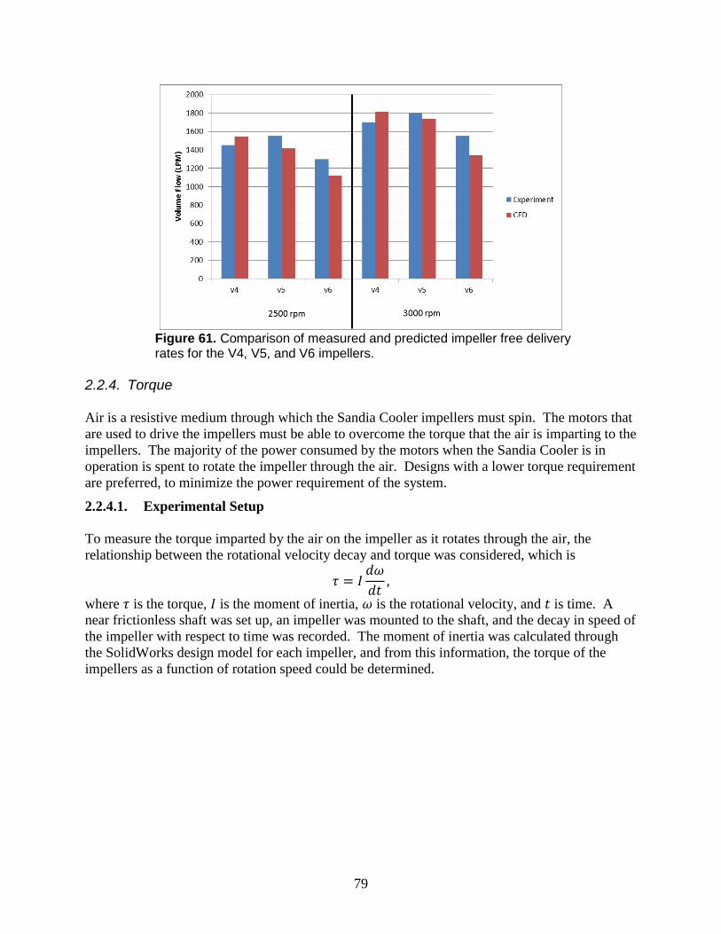
79

Figure 61. Comparison of measured and predicted impeller free delivery rates for the V4, V5, and V6 impellers.

2.2.4. Torque

Air is a resistive medium through which the Sandia Cooler impellers must spin. The motors that

are used to drive the impellers must be able to overcome the torque that the air is imparting to the

impellers. The majority of the power consumed by the motors when the Sandia Cooler is in

operation is spent to rotate the impeller through the air. Designs with a lower torque requirement

are preferred, to minimize the power requirement of the system.

2.2.4.1. Experimental Setup

To measure the torque imparted by the air on the impeller as it rotates through the air, the

relationship between the rotational velocity decay and torque was considered, which is

where is the torque, is the moment of inertia, is the rotational velocity, and is time. A

near frictionless shaft was set up, an impeller was mounted to the shaft, and the decay in speed of

the impeller with respect to time was recorded. The moment of inertia was calculated through

the SolidWorks design model for each impeller, and from this information, the torque of the

impellers as a function of rotation speed could be determined.

80

Figure 62. Experimental setup for torque measurements.

The experimental setup is shown in Figure 62. The nearly frictionless shaft was achieved

through an air bearing with a slight slope to it. The air jet shown on the right hand side of the

figure overcame the gravitational force from the slight slope, which prevented the shaft from

sliding out of the air bearing. The impeller speed was measured by counting the pulses observed

as a HeNe laser reflected off the shaft. A dark patch was drawn on the shaft using a marker,

which dimmed the reflected light once per revolution. A phototransistor was wired in series with

a variable resistor, and the resistance was set to achieve sharp, measurable, change in voltage

drop across the phototransistor as the shaft rotated. The pulse frequency from the voltage drop

phototransistor was measured and recorded as a function of time using LabView.

Figure 63. Example speed decay curve and fit to data.

A typical experiment involved rotating the impeller using a jet of air, and measuring the speed as

a function of time, recording data such as that shown in Figure 63Error! Reference source not

found.. The model for the decay in speed was

(

)

(

)

(

)

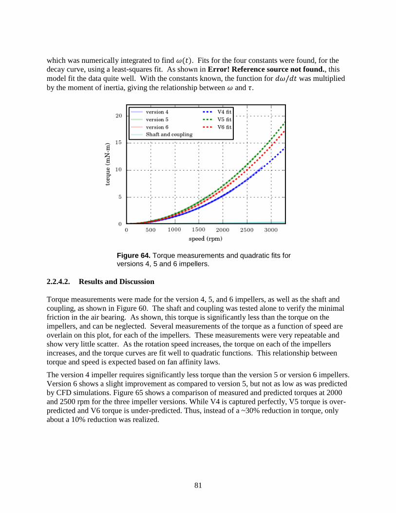
81

which was numerically integrated to find . Fits for the four constants were found, for the

decay curve, using a least-squares fit. As shown in Error! Reference source not found., this

model fit the data quite well. With the constants known, the function for was multiplied

by the moment of inertia, giving the relationship between and .

2.2.4.2. Results and Discussion

Torque measurements were made for the version 4, 5, and 6 impellers, as well as the shaft and

coupling, as shown in Figure 60. The shaft and coupling was tested alone to verify the minimal

friction in the air bearing. As shown, this torque is significantly less than the torque on the

impellers, and can be neglected. Several measurements of the torque as a function of speed are

overlain on this plot, for each of the impellers. These measurements were very repeatable and

show very little scatter. As the rotation speed increases, the torque on each of the impellers

increases, and the torque curves are fit well to quadratic functions. This relationship between

torque and speed is expected based on fan affinity laws.

The version 4 impeller requires significantly less torque than the version 5 or version 6 impellers.

Version 6 shows a slight improvement as compared to version 5, but not as low as was predicted

by CFD simulations. Figure 65 shows a comparison of measured and predicted torques at 2000

and 2500 rpm for the three impeller versions. While V4 is captured perfectly, V5 torque is over-

predicted and V6 torque is under-predicted. Thus, instead of a ~30% reduction in torque, only

about a 10% reduction was realized.

Figure 64. Torque measurements and quadratic fits for versions 4, 5 and 6 impellers.

82

Figure 65. Comparison of measured and predicted torque for V4, V5, and V6 impellers.

2.2.5. Acoustic

For the CPU cooling application and many others, fan noise is an important performance aspect.

A device that demonstrates low thermal resistance at the expense of high noise may not be

marketable to many consumers. While early impeller prototypes exhibited low noise, at least

qualitatively to those in witness, detailed and dedicated acoustic characterization was not carried

out. With the V5 design, the improved thermal resistance and air flow seemed to be

accompanied by louder operation. A ringing tone could be perceived by ear that seemed to

correlate to a resonance in the impeller fins. This was accompanied by a white noise sound

associated with the air flow.

Thus, it was desired to make acoustic measurements of our impellers and compare them to

commercially available CPU cooling technology. Since silent operation is one of the keynote

features of the Sandia Cooler, it is of great importance to ensure that future designs are at least as

quiet, and preferably quieter, to the human ear than previous configurations and comparable

cooling units in industry. Several acoustics experiments were set up to measure the noise output

of the latest impeller designs and a couple of commonly used processor cooling fans. We

examined the version 4, version 5, and the version 6 impellers along with an i7-960 LGA1366

fan, which comes with the Intel Core i7 Processor and Noctua NHD14 fan, which is commonly

used in high performance computers.

2.2.5.1. Test Apparatus and Procedure

Ideally, acoustics measurements are made in an environment with a very low noise floor, to

ensure that the collected data reflects sound emitted by the device to be characterized without a

lot of noise disturbance from the background. Anechoic chambers are specifically designed to

provide such an environment by absorbing sound reflections and blocking external noise sources

through acoustic insulation. While a true acoustic anechoic chamber was not available at Sandia,

an RF anechoic chamber does exist at the Livermore campus. This chamber was designed to

absorb radio frequency wavelengths for antenna characterization, but also works quite well for

83

acoustic attenuation. The measurements described below were all conducted in this chamber

which is shown in Figure 66. The ceiling, walls, and a portion of the floor are covered in the

pyramidal RF absorbent material shown in the figure.

Figure 66. Typical acoustic measurement setup with the fan or impeller mounted on a pedestal in the middle of the anechoic chamber.

Figure 66 also shows a sound level meter, a V4 impeller, and motor controller in a typical

configuration that was used to test the various devices. Two types of sound level meters were

used during the course of the experiments, depending on availability. The type 2250 sound level

meter by Brüel & Kjær has data acquisition capabilities built in and the Extech 407730 sound

level meter was connected to an Agilent Infinium 54854 oscilloscope to monitor and record the

corresponding frequency responses. The sound level meters were mounted on a tripod and

positioned relative to the fixed device to be measured. To follow ISO standards, the sound level

meter was set 1 meter from the fan or impeller for many of the tests. The device to be tested was

set on a surface about two feet in height, which was rubberized to help reduce vibration. The rest

of the equipment, such as a power supply and/or data acquisition unit, was placed on the floor to

ensure the least amount of interference with the sound waves.

Before taking measurements on any of the devices, the noise level of the background and, in case

of the impellers, that of the motor running by itself were recorded. These gave us reference

84

points reflecting the ambient noise level. To assess the noise level of the devices, we measured

and recorded the dB(A) levels 1 m away in most cases and, in some cases, a distance of just 12

inches to increase the signal to noise level.

The tests were not run remotely so there were 2-4 people present at any given time. Each test had

a duration of 10 seconds to one minute during which an attempt was made to be silent.

However, some noise was certainly due to personnel and other equipment in the room which

might have affected the test results. Most of the tests were repeated two to three times to help

reduce these errors and we did not judge them to be significant.

For the OEM and the Noctua coolers, the fans are rated for 12 V and for our tests we ran them at

1V increments between 5 and 12V. The voltage was set using a power supply and monitored

just upstream of the fans with a voltmeter, while the actual fan speed was confirmed with a

stroboscope. Using the Type 2250 sound level meter, we measured and recorded the dB(A)

levels twice at each voltage to check for consistency.

The various impellers that were measured were operated either mounted directly on a brushless

DC motor or mounted on a baseplate as they would for normal operation. Impellers were tested

at speeds that ranged from 1400 rpm up to 5000 rpm, although most measurements were made

between 2000 and 4000 rpm since that is the likely operating range. The stroboscope was used to

verify impeller speed prior to each measurement.

2.2.5.2. Acoustic Results

Initially, the conventional CPU coolers were measured and compared to the V5 impeller. These

measurements were made with the B&K 2250 meter. The background was measured at about 20

dBA with this meter. Results for the two off-the-shelf coolers are shown in Table 5 as a function

of power supply voltage. For a given voltage, the OEM cooler is slightly quieter than the Noctua

model, however the Noctua cooler uses two fans and is significantly better in thermal

performance. Both devices are very quiet and only about 10 dBA above ambient at full power.

Table 5. Acoustic measurements of COTS CPU Coolers.

OEM Noctua

Voltage dB(A) dB(A) ambient 19.7 20.3

5 21 20.9 6 21.9 21.6 7 22.9 22.3 8 23.2 22.8 9 23.5 24.3

10 24.5 27.1 11 26.7 28.5 12 28.3 30.5

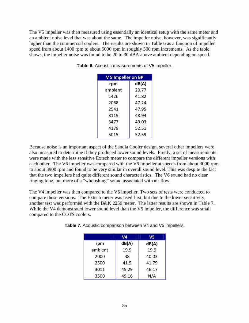
85

The V5 impeller was then measured using essentially an identical setup with the same meter and

an ambient noise level that was about the same. The impeller noise, however, was significantly

higher than the commercial coolers. The results are shown in Table 6 as a function of impeller

speed from about 1400 rpm to about 5000 rpm in roughly 500 rpm increments. As the table

shows, the impeller noise was found to be 20 to 30 dBA above ambient depending on speed.

Table 6. Acoustic measurements of V5 impeller.

V 5 Impeller on BP

rpm dB(A)

ambient 20.77

1426 41.82

2068 47.24

2541 47.95

3119 48.94

3477 49.03

4179 52.51

5015 52.59

Because noise is an important aspect of the Sandia Cooler design, several other impellers were

also measured to determine if they produced lower sound levels. Firstly, a set of measurements

were made with the less sensitive Extech meter to compare the different impeller versions with

each other. The V6 impeller was compared with the V5 impeller at speeds from about 3000 rpm

to about 3900 rpm and found to be very similar in overall sound level. This was despite the fact

that the two impellers had quite different sound characteristics. The V6 sound had no clear

ringing tone, but more of a “whooshing” sound associated with air flow.

The V4 impeller was then compared to the V5 impeller. Two sets of tests were conducted to

compare these versions. The Extech meter was used first, but due to the lower sensitivity,

another test was performed with the B&K 2250 meter. The latter results are shown in Table 7.

While the V4 demonstrated lower sound level than the V5 impeller, the difference was small

compared to the COTS coolers.

Table 7. Acoustic comparison between V4 and V5 impellers.

V4 V5

rpm dB(A) dB(A)

ambient 19.9 19.9

2000 38 40.03

2500 41.5 41.79

3011 45.29 46.17

3500 49.16 N/A

86

Overall, the acoustic results discussed above were disappointing. Quiet operation is a design

goal for the Sandia Cooler. Thus, work is ongoing to improve over these results. Firstly, motor

noise can be reduced in two ways; by adding acoustic damping material to the motor mount and

by using a cleaner drive waveform. The latter should be accomplished by the custom motor

controller that will be discussed in Section 6. Secondly, the ringing that is due to the vibration of

impeller fins can be dampened. A design for this dampening mechanism is currently underway.

Finally, a study of the aero-acoustic characteristics of the impeller could result in a fin shape that

produces less noise at a given rotational speed. Currently, this study is beyond the scope of our

funding but could be pursued in the future.

2.3. Impeller Modeling

2.3.1. Centrifugal Deformation

2.3.1.1. Introduction

Part of the Sandia Cooler design effort includes maintaining the critical gap distance of the air

bearing on which the impeller rotates. As the impeller increases in rotational velocity,

centripetal forces act upon the impeller. Calculations of the resulting deflections from these

forces show that the impeller deflects downward in a concave manner, reducing the air bearing

gap. The target gap for the air bearing is currently 10 microns at 2500 rpm. Preliminary

calculations indicated that the deflections due to the centripetal forces are close to 10 microns.

Therefore, further analysis provided in this report is of interest to the design team to account for

the deflections of the impeller.

All of the finite element calculations were performed using the Sierra Structural Mechanics [15]

software developed internally at Sandia National Laboratories. Meshes consist of eight node

hexahedral elements. The analysis is static with the nodal displacements at the center axle region

fixed. The software calculates centripetal forces resulting from rotations about a specified axis

and automatically applies them as external forces to all nodes in the mesh.

A simplified model of a spinning disk is first used for comparison to an analytical solution for

calculating radial displacements. Next, a comparison of the lateral displacements is made

between several impeller designs. Then effects of air pressure loads, material selection, and

thickness variations are explored. A sensitivity study of the various parameters for a selected

design follows.

2.3.1.2. Spinning disk finite element and analytical comparison

A solution for the radial displacements, u(r), of a spinning disk with a central hole is given by

[16]:

[

]

where the variables, their descriptions, and assigned values for this problem are listed as:

87

Poison’s Ratio 0.3

Density 2.52×10-4

lb·s2/in

4

Rotational velocity in rad/sec 2500 rpm (~261.8 rad/sec)

E Elastic modulus 107 psi

r Radial position [0.05 0.25 0.5 0.75 1 1.25 1.5 1.75 2] in

a Inner radius 0.0455 in

b Outer radius 2 in

A simple model of the disk was created and meshed with one, two, and four elements through

the thickness of the disk for a simple mesh refinement study. The meshes are shown in Figure

67, and the resulting displacements calculated by both the analytical and Sierra Structural

Mechanics solutions are shown in Figure 68. The lateral displacements are shown in Figure 69,

without an analytical solution for comparison. A contour plot of magnified displacements is

shown in Figure 70 to illustrate the thinning effect of the spinning disk.

(a)

(b)

(c)

Figure 67. Meshes for a simple spinning disk with (a) one (b) two and (c) four elements through the thickness of the disk.

88

Figure 68. Analytical and finite element calculated displacements for a spinning disk with one (1t), two (2t), and four (4t) elements through the thickness of the disk.

Figure 69. Finite element calculated displacements for a spinning disk with one (1t), two (2t), and four (4t) elements through the thickness of the disk.

0 0.5 1 1.5 20

0.5

1

1.5

2

2.5x 10

-6 Spinning Disk Radial Displacement

Radial Position (in)

Ra

dia

l D

isp

lace

me

nt (i

n)

Analytical

1t

2t

4t

0 0.2 0.4 0.6 0.8 1 1.2 1.4 1.6 1.8 2-2.5

-2

-1.5

-1

-0.5

0x 10

-7 Spinning Disk Out of Plane Displacements

Radial Position (in)

Ou

t o

f P

lan

e D

isp

lace

me

nt (in

)

1t

2t

4t

89

Figure 70. Displacement contour plot of the spinning disk magnified by a factor of 200,000x.

Surface constrained in all directions at the axle location

90

2.3.1.3. Impeller design comparison

V4, V5, and V6 designs were analyzed for centripetal deformation. First, V4 and V5 were

modeled for comparison. This comparison serves two purposes. One is to compare the analysis

methodology with results previously generated and the second is to compare the results between

the different designs. The previous results were not provided for inclusion in this work, but

personal communication from the design team indicates that they are similar to their satisfaction.

The geometric definition for each design is shown in Figure 71. The finite element meshes are

shown in Figure 72. Material properties and rotational velocities are summarized in Table 8.

Resulting contour plots of the lateral deflections are shown in Figure 73, but will hereafter be

referred to as "axial" deflections, which is a natural term to fit the geometry of the impeller. The

maximum axial deflections as a function of rotational velocity are shown in Figure 74, and the

axial deflections as a function of radial position (approximately every 0.25”) are shown in Figure

75. Although the geometry and material properties used in the model are specified in the English

inch-pound-second (ips) system, the displacements shown in Figures 74-75 are converted to

microns for more direct comparison to the design specification of a 10 micron air bearing gap.

Referring to Figure 74, there appears to be a quadratic relationship between maximum

displacement and rotational speed for both impellers. The V4 impeller is predicted to have about

25% larger displacement than the V5 impeller for any given speed. The predicted maximum

axial displacement for the V5 impeller operating at 2500 rpm is approximately 8 m, close to the

total target air gap of 10 m. The deflection as a function of radial position in Figure 75 shows

the profile that the surface takes if not machined. As discussed previously in Section 2.1.3, the

procedure to compensate for this deflection is to spin an impeller up to the desired operating

speed on a precision spindle and pass a cutting tool across the surface to cut it flat. At 2500 rpm,

the V5 impeller surface would have 8 m of material removed from the outer radius compared to

the inner radius. At rest, this would result in a slightly convex surface. As previously

mentioned, measurements of impeller surfaces that have been cut in this fashion show this

convex shape, validating these modeling results.

91

Impeller Version 4

Impeller Version 5

Figure 71. Geometry of the version 4 and version 5 impeller designs.

92

Impeller Version 4

Impeller Version 5

Figure 72. Meshed geometry of the version 4 and version 5 impeller designs.

Table 8. Summary of parameter values comparing version 4 and version 5 impellers.

Parameter Value

Elastic Modulus 10 × 106 psi

Poisons Ratio 0.36

Density 2.53 × 10-4

lb·s2/in

4

Rotational Velocities 1000 to 3000 rpm in 100 rpm increments

93

Impeller Version 4

Impeller Version 5

Figure 73. Axial displacement contour plots of the version 4 and 5 impeller designs magnified by a factor of 1000x.

94

Figure 74. Comparison of the maximum axial displacement as a function of rotational velocity between the version 4 and 5 impellers.

Figure 75. Axial displacements as a function of radial position for both the version 4 and version 5 impellers for rotational velocities ranging from 1000 to 3000 rpm in 100 rpm increments. A rotational velocity of 2500 rpm is emphasized.

1000 1200 1400 1600 1800 2000 2200 2400 2600 2800 3000-15

-10

-5

0Axial Displacement wrt Rotational Velocity

Rotational Velocity (rpm)

Axia

l D

isp

lace

me

nt (m

icro

ns)

Version 4

Version 5

0 0.2 0.4 0.6 0.8 1 1.2 1.4 1.6 1.8 2-15

-10

-5

0Axial Displacement wrt Radial Position

Radial Position (microns)

Axia

l D

isp

lace

me

nt (m

icro

ns)

Increasing

Version 4

Version 5

95

The V6 impeller, shown meshed in Figure 76, consists of 55 fins which are thicker and taller

than the V4 or V5 fins. Figure 77 shows a comparison of axial displacements for the three

impeller versions reported in this work. Due to the larger fins, it is observed that the axial

displacement for the version 6 impeller exceeds that of the V4 and V5 impellers. At 2500 rpm

the deflection is greater than the 10 micron desired air gap with the standard 0.25" thick platen.

Another set of simulations were run with a 0.375" thick platen, resulting in a 3X reduction in

axial displacement, which is also shown in Figure 77.

Figure 76. Meshed geometry of the V6 impeller.

Figure 77. Maximum axial displacements of all three impeller designs.

1000 1200 1400 1600 1800 2000 2200 2400 2600 2800 3000-16

-14

-12

-10

-8

-6

-4

-2

0 Max Axial Displacement wrt Rotational Velocity

Rotational Velocity (rpm)

Axia

l D

isp

lace

me

nt (m

icro

ns)

Version 4

Version 5

Version 6

Version 6 3/8" thick

96

2.3.1.4. Parameter study

The version 5 impeller geometry was used in a parameter study to investigate how material

selection, thickness, and blade pressure influence the observed deflection. The parameters and

their assigned values are summarized in Table 9. Ensembles of simulations were in three main

steps. The first step ran a full factorial matrix varying the rotational velocities, aluminum or

copper selection, and applied blade pressures. Next, the 0.125” and 0.375” disk thicknesses were

run, again in a full factorial ensemble varying the rotational velocity with the thicknesses.

Finally, a thickness profile tapered with the intent of compensating for the observed “baseline”

displacements of the 0.25” aluminum impeller at 2500 rpm was run at all rotational velocities.

The results are partially shown in Figure 78. Only one set of rotational velocity curves are

shown because they are similar in trends to the other sets. The intent of the figure is to show

how the “baseline” case compares to other rotational velocities, pressure loads on the blades, a

copper impeller, different disk thicknesses, and finally the tapered cross-sectional profile.

Because the thinner impeller disk experiences significant deflection, the axes are rescaled in

Figure 79 to capture more detail for the rest of the results.

Table 9. Summary of parameters and values used in the parameter study. Highlighted values are considered as “baseline.”

Parameter Values

Rotational velocity 1000 to 3000 rpm in 100 rpm increments (2500 rpm)

Pressure on concave side of blade 0, -15, -30, -45, -60 Pa

Pressure on top of blade 0, 15, 30, 45, 60 Pa

Material property selection Aluminum

(E=10×106 psi, n = 0.36, density = 2.53×10

-4 lb·s

2/in

4)

Copper

(E=16×106 psi, n = 0.343, density = 7.43×10

-4 lb·s

2/in

4)

Disk thickness 0.125”, 0.250”, 0.375”

Tapered profile Linear taper starting at a radial distance of 0.5” and

reaching an offset of 0.00031” at the edge (2.0” radial

distance).

97

Figure 78. Parameter trends affecting the impeller gap distance.

Figure 79. Zoomed in parameter trends.

0 0.2 0.4 0.6 0.8 1 1.2 1.4 1.6 1.8 2-60

-50

-40

-30

-20

-10

0

10Reduction in Gap wrt Radial Position

Radial Position (in)

Re

du

ctio

n in

Ga

p (

mic

ron

s)

Base Line

Rotational Velocity

Pressure

Copper

Thickness

Taper Profile

0.2 0.4 0.6 0.8 1 1.2 1.4 1.6 1.8 2

-10

-8

-6

-4

-2

0

Reduction in Gap wrt Radial Position

Radial Position (in)

Re

du

ctio

n in

Ga

p (

mic

ron

s)

Base Line

Rotational Velocity

Pressure

Copper

Thickness

Taper Profile

98

The results of this parameter study show several important effects. Firstly, the applied pressures

to the impeller blades have a negligible effect on the deformation of the disk. Secondly, the

choice of aluminum over copper has a significant structural advantage in reducing the amount of

axial displacement. Thirdly, the selected thicknesses strongly affect the observed displacements,

with the thinner disk undergoing significantly greater axial displacement. The values indicate a

cubic relationship between thickness and maximum displacement. Finally, tapering the disk's

thickness to account for calculated axial displacement does result in maintaining a nearly flat

surface with relatively small errors on the order of +/-1 micron.

99

2.3.1.5. Sensitivity / ANOVA Study

A sensitivity study is performed to provide an indication on how sensitive the axial displacement

is to possible variations in the different parameters. Based on the previous work, the selected

factors / parameters are the rotational velocity, disk thickness, Poison’s ratio, elastic modulus,

and density of the material. Three levels / values are used for each factor. The range for each

factor is selected with the intent of realistically bounding the values which may be expected

during operation and manufacturing. However, additional research or expert opinion was not

obtained for each parameter, so the bounds remain an arbitrary estimate at this point. The

selected factors and levels are summarized in Table 10, with some explanation for their selection.

Table 10. Factor levels selected for a sensitivity study of the axial displacements.

Factor Levels Notes

Rotational Velocity 2475, 2500, 2525 rpm +/ 1% of 2500 rpm

Disk Thickness 0.248, 0.250, 0.252 in Thickness manufactured within +/- 2 mil

Poison’s Ratio 0.3, 0.33, 0.36 +/- ~10% of 0.33

matweb.com reported values:

aluminum: 0.36

aluminum 6061-T6, 6061-T6: 0.33

Elastic Modulus 9.5, 10, 10.5×106 psi +/- 5% of 10×10

6 psi

matweb.com reported values:

aluminum: 9.86×106

psi

aluminum 6061-T6; 6061-T6: 10×106

psi

aluminum 7075-T6, T651: 10.4×106

psi

Density 2.394×10-4

, 2.52×10-4

,

2.646×10-4

lb·s2/in

4

+/- 5% of 2.52×10-4

lb·s2/in

4

matweb.com reported values:

aluminum: 2.53×10-4

lb·s2/in

4

aluminum 6061-T6, 6061-T6: 2.53×10-4

lb·s2/in

4

aluminum 7075-T6, T651: 2.64×10-4

lb·s2/in

4

A full factorial design of experiments matrix was evaluated with the selected factors and levels

for a total of 243 simulations in this sensitivity study. An analysis of variation (ANOVA)

calculation was performed on the maximum axial displacements observed in each simulation.

The p-values for the null hypothesis on the main effects were all nearly 0, indicating that each

factor was significant in the observed axial displacements (typically p < 0.05 indicates

significance).

Plots of the displacements as a function of radial position were generated in two ways in order to

visualize the impact of each factor. The first way is to plot all the results and color each series

either blue, green, or red depending on whether the low, medium, or high value of the selected

factor is being displayed. This technique results in a separate plot for each factor shown in

Figure 80. It should be noted that the sequence of plotting was for low, then medium, and then

high values. Therefore, the red color often covers the green and blue colors. One insight from

100

these plots is that there are not distinct bands of each color, further indicating that all the factors

are significant. Also, the range of displacements due to possible uncertainty in the design

parameters is illustrated. The second way the results are displayed is in a similar series of plots

which contain only the low, medium, and high values for a single factor while holding the other

factors at their medium/nominal target value. Thus the range of displacements due to the single

factor is illustrated, as shown in Figure 81.

This initial sensitivity study indicated that the axial displacements may vary up to 2.9 m based

upon the selected bounds of considered design parameters. Updated knowledge of the

manufacturing tolerances and operation of the device will likely change this possible variation.

Other aspects may warrant investigation as well if tight operational tolerances are required.

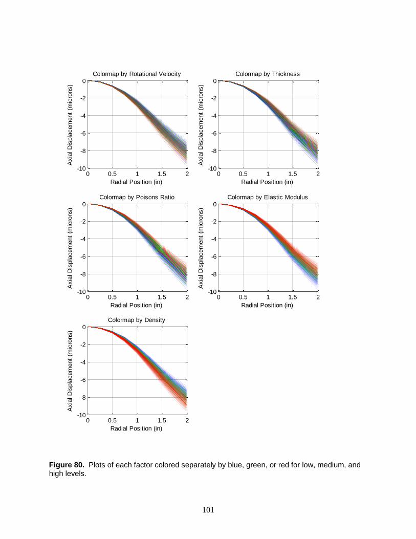
101

Figure 80. Plots of each factor colored separately by blue, green, or red for low, medium, and high levels.

0 0.5 1 1.5 2-10

-8

-6

-4

-2

0Colormap by Rotational Velocity

Radial Position (in)

Axia

l D

ispla

cem

ent

(mic

rons)

0 0.5 1 1.5 2-10

-8

-6

-4

-2

0Colormap by Thickness

Radial Position (in)

Axia

l D

ispla

cem

ent

(mic

rons)

0 0.5 1 1.5 2-10

-8

-6

-4

-2

0Colormap by Poisons Ratio

Radial Position (in)

Axia

l D

ispla

cem

ent

(mic

rons)

0 0.5 1 1.5 2-10

-8

-6

-4

-2

0Colormap by Elastic Modulus

Radial Position (in)

Axia

l D

ispla

cem

ent

(mic

rons)

0 0.5 1 1.5 2-10

-8

-6

-4

-2

0Colormap by Density

Radial Position (in)

Axia

l D

ispla

cem

ent

(mic

rons)

102

Figure 81. Plots of each factor at their low (blue), medium (green), and high (red) levels with the other factors held constant at their medium/nominal level.

0 0.5 1 1.5 2-10

-8

-6

-4

-2

0Factor: Rotational Velocity

Radial Position (in)

Axia

l D

ispla

cem

ent

(mic

rons)

0 0.5 1 1.5 2-10

-8

-6

-4

-2

0Factor: Thickness

Radial Position (in)

Axia

l D

ispla

cem

ent

(mic

rons)

0 0.5 1 1.5 2-10

-8

-6

-4

-2

0Factor: Poisons Ratio

Radial Position (in)

Axia

l D

ispla

cem

ent

(mic

rons)

0 0.5 1 1.5 2-10

-8

-6

-4

-2

0Factor: Elastic Modulus

Radial Position (in)

Axia

l D

ispla

cem

ent

(mic

rons)

0 0.5 1 1.5 2-10

-8

-6

-4

-2

0Factor: Density

Radial Position (in)

Axia

l D

ispla

cem

ent

(mic

rons)

103

2.3.2. Thermally Induced Deformation

Centrifugal forces are not the only source of impeller deformation during operation. Whether

used in a cooling or heating application, the impeller works by transferring heat between the

ambient air and the base of the platen. Within the impeller the heat is transferred via conduction

through the aluminum platen and fins. Thus, a temperature gradient develops, the magnitude of

which depends on the amount of heat transferred, the impeller design, and the impeller speed.

Non-uniform thermal expansion results from this temperature gradient which will produce

deformation of the impeller.

In order to characterize the magnitude of this thermally induced deformation, the structural

model used in the previous analysis was utilized. A case was run with the V5 impeller assuming

a temperature gradient resulting from a heat load of 150 W with the impeller operating at 2500

rpm. The temperature gradient was calculated from a CFD model simulating these conditions.

The temperatures were then mapped to the structural model first by approximating the radial

gradient in the platen out to the inner fin radius. A vertical gradient was then applied from the

base of the platen up through the fins. This approach provided a reasonable approximation to the

actual temperature distribution.

The temperature distribution and resulting displacement due to thermal strains is shown in Figure

82. Temperatures are shown in °F and displacements were calculated with zero strain at 72 °F.

Note that the surface of the hole in the platen was constrained to zero displacement. Although the

temperature distribution is based on a relatively crude mapping, the temperature differences are

not very large. Therefore, for design scoping purposes a finer temperature distribution was not

pursued. A line plot of the axial displacements on the base of the platen as a function of radial

position is shown in Figure 83. As Figure 83 shows, the platen bows up, which is the opposite of

the effect due to the centrifugal force. Conceptually this occurs because the lower surface is

hotter; causing more expansion then the upper surface. The total displacement from the edge of

the hole to the outer radius of the platen is nearly 3 microns. This is a significant fraction of the

deformation caused by the rotational speed. Based on these results, thermal gradients must be

taken into account when determining how to compensate the platen surface to maintain a

constant air bearing gap.

104

(a)

(b)

Figure 82. Version 5 (a) mapped temperature distribution and (b) resulting axial displacements.

105

Figure 83. Axial displacements of the version 5 impeller due to thermal gradients during the

operational cooling process for one calculated temperature distribution.

2.3.3. Modal Analysis

The mode shapes and frequencies of the version 5 impeller were calculated using the same finite

element meshes and material properties as described in Section 3 with the Sierra Structural

Dynamics code [17]. A fixed boundary condition is specified at the nodes on the interior of the

impeller's center through hole (contacting surface for the axle shaft). The calculated modes up to

about 2600 Hz occur at about 437, 707, 1493, 1682, 2414, 2556, 2586, 2590, and 2598 Hz. The

corresponding mode shapes are shown in Figure 84.

0 0.2 0.4 0.6 0.8 1 1.2 1.4 1.6 1.8 2-1.5

-1

-0.5

0

0.5

1

1.5

2

Radial Position (inches)

Axia

l D

isp

lace

me

nt o

f L

ow

er

Pla

tte

n S

urf

ace

(m

icro

ns)

Thermal Strain Deformation of V5 Design

106

437 Hz

1682 Hz

2586 Hz

707 Hz

2414 Hz

2590 Hz

1493 Hz

2556 Hz

2598 Hz

Figure 84. Version 5 impeller mode shapes and corresponding frequencies.

Of particular interest is the mode at 2590 Hz, which is similar in shape to the first mode of an

isolated fin with the fixed boundary condition applied where it contacts the spinning disk, as

shown in Figure 85. The interest in this particular mode is due to a concern that vibration

resulting primarily from fin excitation is responsible for undesirable noise generation at some

rotational velocities. The ringing sound from the V5 impeller, in particular, is thought to be due

to excitation of the fin natural frequency.

The version 6 fin geometry and first two mode shapes, with the fin base having a fixed

displacement, are shown in Figure 86. The natural frequency of the first mode of the V5 fin is

lower than the first mode of the V6 fin, but only by about 10% (2699 Hz versus 2989 Hz).

107

However, the mode shapes are different. The first mode of the V5 fin actually resembles the

second mode of the V6 fin and vice versa. An explanation of this behavior may be attributed to

the difference in height and thickness of the fins affecting the mode shape order. Nevertheless,

the modal frequencies of the two fins are not significantly different. Yet, the acoustic emissions

of the two impellers seem different by ear.

It should be noted that while isolating the fins is instructive to their behavior, actual performance

will be dependent on the entire device, including the platen, shaft, and attachments (as can be

seen for the platen and fin case in Figure 84). The relative importance of each part of the entire

platen will change depending on the mass and stiffness of each contributing part. For example,

as the platen's stiffness increases, then the isolated fin case with a fixed base is approached.

(a) Isolated Fin

(b) First Mode 2699 Hz

(c) Second Mode 3688 Hz

Figure 85. Version 5 (a) isolated fin geometry, (b) first mode, and (c) second mode with the base of the fin having a fixed displacement boundary condition.

(a) Isolated Fin

(b) First Mode 2989 Hz

(c) Second Mode 3458 Hz

Figure 86. Version 6 (a) isolated fin geometry, (b) first mode, and (c) second mode with the base of the fin having a fixed displacement boundary condition.

2.3.4. Heat Transfer and Fluid Dynamics

2.3.4.1. Model Development and Validation

108

This section describes the validation activity carried out with the CFD software platform ANSYS

CFX (V14.0). This activity led to identifying and correcting features of the baseline

computational model, particularly with respect to the effect of turbulence on thermal diffusivity.

The validation included data from anemometry and particle image velocimetry (PIV) of the

airflow near the impeller, as well as data from temperature measurements of the impeller surface

in transient and steady state experiments. The two impeller geometries considered for this study

were Version 4 (V4) and Version 5 (V5), shown in Figure 87.

Figure 87. CFX view of the periodic impeller’s slice used in the simulations.

The main elements of the CFD simulation are listed in the following. Several variants of the

computational settings were also carried out to assess the robustness of the numerical method,

but are mostly not reported here.

The simulations were carried out by coupling the solid domain (impeller fins and plate)

with the fluid domain (surrounding air) using the conjugate heat transfer method. To

apply a specific thermal load to the impeller, two methods were considered: constant heat

flux to the bottom plate (with a reference value of Wplate = 18,500 W/m2); or constant

temperature, i.e. Tplate = 290 K, maintained at the same surface. In both cases, as cooler

air enters from the top of the computational domain, warmer air leaves the impeller’s

channel. We found that the thermal resistance of the impeller,

R =Tplate -Tair

Wplate ,

does not depend substantially on the method used to apply the thermal load.

The thermal properties of the solid domain were set according to the impeller version:

6063 aluminum for V4, and QC-10 aluminum for V5.

The impeller and the inner portion of the fluid domain were part of a rotational reference

frame spinning at the impeller’s nominal rotational speed; the outer flow domain was

stationary (frozen rotor). This arrangement was assessed to be the most stable and to lead

to the steady-state solution more quickly.

109

The model takes advantage of the geometrical symmetry of the impeller by using

rotationally periodic boundary conditions: as shown in Figure 87, only one fin and the

adjacent channel are calculated. Figure 88 shows an example where the fin is divided in

two halves with periodic walls and a central channel. Alternatively, the air channel can be

split in two periodic halves and the metal is in the middle of the computational domain.

It is noted that modeling a single fin precludes the simulation of fluid-dynamic effects

that could take place in the full impeller. Most of these effects, such as rotating flow

instability, would however appear only in time-accurate simulations (which were not part

of the current task).

Figure 88. Solid domain with the two halves of a fin.

All the verification simulations were run to steady state for the assigned rotational speed.

Even in steady-state mode, a start-up vortex ring can be observed at the tip of the fin

because of the sudden rotation imposed to the impeller. Figure 89a shows that the ring is

later advected outside of the domain by the air entrained by the impeller. This transient

needs to be concluded before the solution can be considered stationary. Even then, the

stationary solution can be interpreted only in a time-averaged sense: oscillations in the

thermal flux or in the propeller’s torque may still occur because of periodic vortex

shedding (shown in Figure 89b).

Turbulence and boundary layers were modeled by solving the RANS (Reynolds-

Averaged Navier Stokes) equations: the Shear Stress Transport model was selected as the

most appropriate for the given rotational flow.

110

The Reynolds analogy is used to calculate heat transfer at the boundary layer. This model

postulates a similarity between modeled momentum diffusion and scalar diffusion

(specifically, heat). The key parameter in the analogy is the turbulent Prandtl number.

The fluid Prandtl number (sometimes referred to as “laminar” Pr) is the ratio of

momentum diffusivity (kinematic viscosity) to thermal diffusivity: it is a well-defined

thermodynamic property. The turbulent Prandtl number is instead a model parameter

defined as the ratio between the momentum eddy diffusivity and the heat transfer eddy

diffusivity,

Prt =n tkt .

The parameter kt is needed to solve the energy equation. From experimental data, Prt has

an average value of 0.85, but ranges from 0.7 to 0.9 depending on the fluid in question in

non-rotational flow. The default value in CFX is 0.9. In general, there is no “universal”

value of Prt, as this model parameter varies from point to point in turbulent flow. This

aspect is discussed in more detail in the following section.

(a) (b)

Figure 89. Streamlines of the gas flow past the impeller at two different pseudo- times in the simulation. Lines generated from the instantaneous velocity vectors.

Effect of turbulent Prandtl number

By including the effects of turbulence on the boundary layer, the thermal transport from the

entrained air to the fin surface was perhaps the most challenging mechanism to model. In

general, boundary layers in turbomachinery rotors are subject to Coriolis forces, which can

contribute directly to the development of secondary flows (Figure 90). The same forces can also

indirectly increase or suppress turbulence production in the boundary layers on fins. It is also

found that buoyancy enhances the turbulent heat transfer on both the pressure and the suction

side boundary layers.

111

Figure 90. Schematic view of rotating boundary layer (pressure surface). From Yamawaki et al., International Journal of Heat and Fluid Flow 23, 2002.

Evidence of streamwise vortices caused by the Coriolis force was found in the CFX simulations

as well, as shown on Figure 91. When the Coriolis force acts toward the wall, heat transfer in a

laminar boundary layer is dramatically enhanced (see Yamawaki et al., International Journal of

Heat and Fluid Flow 23, 2002 and references therein). This can be explained by the generation of

streamwise vortices and by the resulting enhancement of the transverse convection of energy.

Existing analyses and experimental investigations on this topic are only for straight channels, but

there is evidence of varying heat flux magnitude on the impeller fin in Figure 92.

Figure 91. Thermal boundary layer development.

112

Figure 92. Heat flux contour at the walls of the impeller’s channel.

From a practical standpoint, enhanced heat fluxes can manifest as a smaller Prt. In direct

numerical simulations of fully developed rotating channel flow about the spanwise axis,

Brethouwer et al. (Journal of Physics: Conference Series 318, 2011) found that the turbulent

Prandtl number of a passive scalar is close to one when rotation is absent, but it is much smaller

when rotation is present. The Reynolds number based on the bulk mean velocity Ub and the

channel width h,

 

Reb =Ubh

n ,

and the non-dimensional rotational number,

,

are the two main parameters that appear to control Prt. As observed by Brethouwer et al., the

turbulent Prandtl number becomes very small in certain regions of the channel flow, but returns

to the regular range when Rob is sufficiently small.

While the result above may not be valid in general, we did find a strong dependence of the

thermal resistance on Prt. Figure 93 displays a set of calculations for V4 and V5. Reynolds and

rotational numbers of V4 and V5 are different for the same rotational speed because of their

different channel width (the value of Ub was estimated directly from the simulation). In this

parametric study, the turbulent Prandtl number was incrementally decreased from 0.9 to 0.01 at a

fixed RPM. The measured values of R for the two impellers are added to this diagram to show

that the effective, rotational turbulent Prandtl number may, in effect, depend on Reb and Rob.

Based on these results, subsequent calculations were carried out with Prt set to a value of 0.2,

rather than the default value of 0.9.

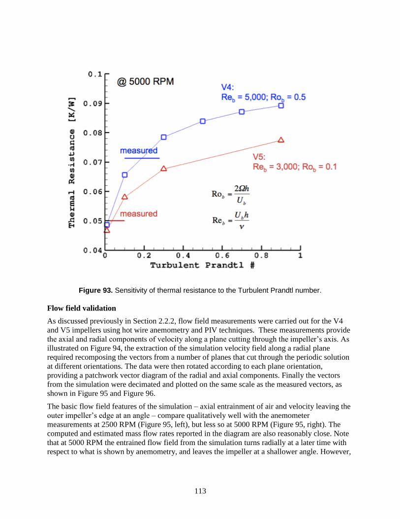
113

Figure 93. Sensitivity of thermal resistance to the Turbulent Prandtl number.

Flow field validation

As discussed previously in Section 2.2.2, flow field measurements were carried out for the V4

and V5 impellers using hot wire anemometry and PIV techniques. These measurements provide

the axial and radial components of velocity along a plane cutting through the impeller’s axis. As

illustrated on Figure 94, the extraction of the simulation velocity field along a radial plane

required recomposing the vectors from a number of planes that cut through the periodic solution

at different orientations. The data were then rotated according to each plane orientation,

providing a patchwork vector diagram of the radial and axial components. Finally the vectors

from the simulation were decimated and plotted on the same scale as the measured vectors, as

shown in Figure 95 and Figure 96.

The basic flow field features of the simulation – axial entrainment of air and velocity leaving the

outer impeller’s edge at an angle – compare qualitatively well with the anemometer

measurements at 2500 RPM (Figure 95, left), but less so at 5000 RPM (Figure 95, right). The

computed and estimated mass flow rates reported in the diagram are also reasonably close. Note

that at 5000 RPM the entrained flow field from the simulation turns radially at a later time with

respect to what is shown by anemometry, and leaves the impeller at a shallower angle. However,

114

the comparison in Figure 96 with the PIV data above the impeller suggests the discrepancies also

exist between PIV and anemometry results.

Figure 94. Example of radial slices taken to extract simulation data.

Figure 95. Comparison of the radial velocity field from anemometry measurements and from the simulation at steady state for V4. The two rectangles indicate the position of the impeller in this view.

115

Figure 96. Detail above the impeller with ensemble-averaged PIV data.

The PIV measurements enable the assessment of the fluctuating component of velocity in the

simulation. The fluctuating component can be derived from the turbulent model, specifically the

local turbulent kinetic energy, kRANS, shown in Figure 97.

Figure 97. RANS turbulent kinetic energy.

116

Figure 98. Root Mean Square values of the radial and axial components of velocity from the PIV measurements.

One can attempt to compare kRANS with the fluctuating kinetic energy estimated from the root

mean square values of the PIV axial and radial velocities, as displayed on Figure 98. This

approach is questionable, since the tangential velocity is not known: in the plot, it is assumed that

the RMS of axial and radial velocity contribute 2/3 of the total fluctuating kinetic energy.

Moreover, the PIV data are only preliminary measurements – for instance, they are not

symmetric with respect to the impeller’s axis and probably not very reliable above 10 m2/s

2.

With these caveats, comparison of the plots in in Figure 97 and Figure 98 suggests that the

RANS kinetic energy is strongly under-estimated. We verified that increasing the inlet turbulent

intensity did not succeed in increasing the turbulent intensity of the entrained flow. This point

remains an issue that will need to be revisited when additional PIV data become available.

Thermal resistance validation

As described in Section 2.2.1, two different techniques were used to measure impeller thermal

resistance. The first, “transient cooling”, required measuring the temperature decay of the

impeller’s plate after an initial heating. The second, “steady-state heating”, consisted in

establishing a constant heat flux to the bottom of the impeller and in measuring its steady-state

temperature. In both cases the rotational speed was maintained constant, but the latter approach

is essentially identical to how the CFX simulations were run. Data points from both techniques

are displayed in Figure 99; the continuous lines in the diagram are the correlation derived from

the transient cooling points for V4 (blue) and V5 (red). It is worth noting the dispersion of the

measurements, particularly for V5.

Also plotted are the simulation values of resistance. With reference to the previous section, the

triangular symbols correspond to simulations with the default turbulent Prandtl number, Prt =

0.9, for non-rotational flow. A second set (square symbols) was obtained with Prt = 0.3, and

another point, at 5000 RPM, was calculated with Prt = 0.01. Obviously, the simulations capture

the trend of decreasing resistance with increasing rotational speed. They also correctly capture

the different performance of the two impellers, with V5 offering a lower resistance than V4 over

117

the full range of speeds. However, the results become rather sensitive to the parameter Prt once

the rotational number Rob becomes sufficiently large. This behavior is consistent with the

experimental and numerical behavior of rotating channels described above. Based on these

observations, a constant value of Prt,rot = 0.2, instead of the default value, was used for

subsequent calculations including the parameter optimization and scaling studies which will be

discussed in the following sections.

Figure 99. Thermal resistance as a function of rotational speed.

2.3.4.2. Parameter Optimization Study

A parametric study was undertaken to develop impeller designs that have better performance (i.e.

lower thermal resistance, lower pumping power, and in some applications higher mass flow rate)

than the V5 impeller. First, a prototypical form of the impeller was assumed that could be

represented with a small number of parameters. A CFD model of this impeller was developed,

and based on this CFD model two sets of runs were performed in which certain geometrical

parameters were varied for each design. These candidate geometries were compared to the

performance of the v4 and v5 impellers. Finally, several alternative designs that departed from

the prototypical impeller geometry (in favor of an interrupted-fin geometry) were preliminarily

118

explored. These designs exhibited low thermal resistance without a corresponding increase in

power consumption and would likely be a fruitful direction for future study.

Impeller Geometry

In this study, the outer diameter was held at a constant value of approximately 101 mm (4 in).

The inner radius was set to r1=r2/2. The fin height was set to the maximum height that could be

machined with either a 20-to-1 or a 25-to-1 aspect ratio endmill (thus, the height was determined

by the minimum width of the flow channel). The sweep angle, number of fins, and power law

exponent were explored in the parametric study.

The impeller geometry was calculated using the Mathematica tool, described in Section 2.1.1,

which provided immediate visual feedback of surface area (As), total fin footprint area (Afp),

total fin perimeter (Pf), minimum flow channel width, and fin height (b, based on a desired

maximum endmill aspect ratio). Subsequently, the key parameters were entered into a

parametrically-driven (via a design table) SolidWorks model. This geometry was imported to

ANSYS Workbench, where it was processed by ANSYS Meshing and, finally, input to ANSYS

CFX for analysis.

CFD Model

Domain and Boundary Conditions

The CFD model consisted of a single unit cell of the impeller, with a solid domain, a rotating

fluid domain, and a stationary fluid domain, as shown in Figure 100. It was assumed that the

flow would be rotationally periodic; accordingly, the model used periodic boundary conditions

on the lateral faces of each domain. The solid portion of the heat-sink-impeller is also included in

the model using the ANSYS conjugate heat transfer capability. The bottom face of the heat-sink-

impeller was given a prescribed temperature, to mimic the thermal boundary condition of a vapor

chamber heat pipe. The Menter SST fluid model with the total energy equation is used in the

fluid domains. Note that the various domains have multiple regions; this is merely done for the

sake of the meshing software, which has a preference for fully prismatic solid bodies. The

interfaces between these regions fully conserve all simulated quantities. The top, side, and

bottom openings of the model used the “opening/entrainment” boundary condition, which

constrains either the static pressure (for outward flow) or total pressure (for inward flow) but

allows flow in any direction. The “opening” boundary condition (as opposed to a velocity inlet /

pressure outlet combination, for example) ensures that the flow through the system is entirely

driven by the impeller, making it representative of a CPU-cooling application. In the figure, the

gray region is a stationary frame while the pink region is a rotating frame. A “frozen rotor”

reference frame change model was used between the rotating and stationary domains.

119

Figure 100: CFD model domains and boundary conditions.

Convergence Criteria

The convergence of the CFD model was determined by monitors of the quantities of interest:

mass flow rate, torque, and thermal resistance. Based on a study of the convergence behavior, it

was determined that approximately 1000 iterations ensured consistency in the results of interest

and yielded reasonable flow fields and temperature distributions. Additionally, 1000 iterations

provided enough time in the simulation to allow a startup vortex to convect downstream, away

from the impeller. The convergence behavior for batch 2 of the parametric study (discussed

below) is shown in Figure 101. The plots in Figure 101 indicate normalized mass flow, torque,

and thermal resistance; the scale shows +/- 15% compared to the final value. In most of the

cases, the convergence monitors were stable and approached the final value with small changes.

However, in cases 6 and 14, the simulations were terminated prematurely to avoid a numerical

instability in which the convergence monitors oscillated about their final value shown in Figure

101. Results from designs 6 and 14 should therefore be used with caution. Another point to note

in Figure 101 is that initially, the model proceeds with no heat transfer (i.e. isothermal) for the

first 600 iterations to reduce computation time and allow the flow field to establish itself. At

iteration 601, the solver restarts with heat transfer, initialized by the fluid dynamic solution at

600 iterations. This restart sometimes causes the parameters of interest to abruptly change prior

to converging.

Opening

T=Tamb

Opening

T=Tamb

Periodic

Interface

Impeller

Axis of

Rotation

Stationary Domain

Rotating Domain

T=Tamb

+25 ºC

120

Figure 101. The convergence of mass flow rate, torque, and thermal resistance for designs 1-23 of batch 2 in the parametric study.

Post Processing

Three quantities of interest were extracted from the CFD models: mass flow rate through the

impeller, aerodynamic torque (excluding the drag torque associated with the air gap), and

thermal resistance of the heat-sink-impeller from the bottom of the impeller to the ambient

surroundings. The mass flow rate was calculated using the massFlow function in ANSYS CFD-

post. The mass flow rate was determined at a surface coplanar to the top fin surface, with a

diameter extending to the outer diameter of the fin. The torque was calculated using the torque_y

function in CFD-post, and was calculated for all of the solid surfaces touching the air in the

simulation. The mass flow rate and torque computed from the CFD simulations were multiplied

by the number of fins to determine the overall quantities.

The thermal resistance was determined as follows. First, an area integral (areaInt function) of the

heat flux on the bottom surface of the impeller yielded the heat transfer per fin. The heat transfer

per fin was then multiplied by the number of fins to obtain the total heat transfer. The

temperature difference between the bottom of the impeller and the ambient (in these simulations,

this temperature difference was 25 °C) was then divided by the total heat transfer to obtain the

overall thermal resistance.

Parametric Study

Different impeller designs at the same speed tend to yield results that are difficult to interpret, as

the designer must choose the relative importance of the various figures of merit (i.e. thermal

121

resistance and pumping power). After each initial constant-speed simulation, a second simulation

was run where the rotational speed of each impeller was rescaled to a new value. This value of

the rotational speed was chosen so the pumping power, which is often an important constraint in

a CPU cooler, would be equal to a reference value (in this study, 5 W was chosen as the

reference power consumption). The fan affinity laws (e.g. White, 2003) were used to scale the

rotational speed to achieve this power consumption:

(

)

where ω is the rotational speed, W is the power consumption, and the subscripts refer to the

initial CFD run (1) and the second, rescaled CFD run (2). W2 was chosen to be the reference

value of 5 W, ω1 was 2500 rpm, and W1 was the power consumption result from the first CFD

run. ω2 was the rescaled rotational speed for the second simulation, intended to produce a result

with 5 W of power consumption. Thus, for each design, performance metrics were examined at

2500 rpm and also at 5 W of power consumption.

The parametric study was broken into two batches. The first batch explored the effects of the

number of fins and the sweep angle, but allowed the fin height to vary. This variable height was

found to be undesirable, since many end uses have an explicit constraint on the height. The

second batch focused on impeller designs with nearly incidence-free entry, and thus most of the

designs in batch 2 had a sweep angle of 45 degrees. The fin height was held constant in batch 2.

Batch 2 also explored the effect of increasing the power law exponent (A).

Batch 1: Setup

In the first set of runs the number of fins and the sweep angle were varied. This run consisted of

impellers with 30, 40, 50, and 60 fins and sweep angles of 15, 30, 45, and 60 degrees. In this first

batch, the thermal conductivity of the aluminum impellers was set to the default value in the

CFX material library (k=237 W/m·K). The turbulent Prandtl number was set to the default value

of Prt=0.9.

The convergence of the batch 1 simulations was achieved by allowing the solver to perform 800

iterations. In contrast to the batch 2 simulations (whose convergence is shown in Figure 101),

only a single run was performed and the energy equation was included for all of the iterations. It

was subsequently determined that much of the convergence could be accomplished without

solving the energy equation, presumably because the small absolute temperature changes in the

air have little effect on the flow field.

As a benchmark for comparison, the v4 and v5 impellers were also simulated using analogous

CFD domains, but with thermal conductivity values specific to the aluminum alloys used in the

v4 and v5 impellers (v4 was made of 6063 alloy, while v5 was made of QC-10 alloy).

Additionally, as will be discussed below, the turbulent Prandtl number was set to 0.2 rather than

0.9 for the v4 and v5 benchmarks. As it turns out, the effects of thermal conductivity and

turbulent Prandtl number tend to counteract each other, so the results from batch 1 compare

almost directly to the v4 and v5 benchmarks despite having different values of k and Prt.

However, this subtle point is relatively moot because the results from batch 2 (which used k and

Prt values consistent with the benchmark cases) showed significantly better performance than

batch 1.

122

Batch 1: Results

The results from batch 1 – thermal resistance, mass flow rate, power consumption, and

coefficient of performance (the ratio of heat transfer to power consumption) – are shown in

Figure 102.

Figure 102 shows how the various figures of merit often tend to have optima (indicated by a blue

circle in each plot) at different design points.

Figure 102: CFD parameter study results from batch 1 at 2500 rpm. The circle on each surface indicates the design with the optimal value.

Figure 103 shows the thermal resistance and power consumption (torque · speed) for the designs

in batch 1. Both thermal resistance and power consumption should be low in a good heat-sink-

impeller design; thus, points closer to the origin represent better designs. The relative weighting

of these figures of merit depends on the application, making impossible an a priori judgment of

competing designs at the same rotational speed. In Figure 103, for example, some of the designs

have a slightly higher thermal resistance than the v5 design, but simultaneously have lower

power consumption. The best designs compare favorably to v5; however, some of these designs

are impractically tall. Furthermore, the designs explored in batch 2 have markedly better

performance. To ensure an appropriately balanced comparison of the designs, the rotational

speed was scaled according to the relation introduced above and re-simulated so that each design

would consume about 5 W of power.

123

Figure 103: Thermal resistance vs. power consumption for batch 1 at 2500 rpm.

Figure 104 shows such a comparison of the batch 1 designs at 5 W of power consumption. The

plot on the left shows contours of thermal resistance (interpolated from the 16 data points), with

the lowest thermal resistance (shown with an x) close to the 50-fin, 45-degree-sweep design. On

the right plot, the thermal resistances and mass flow rates of the entire data set are normalized to

a range from 0 to 1 and shown in filled contours (thermal resistance) and grayscale contour lines

(mass flow). The area around the 50-fin, 45-degree design is circled because this area exhibits

low thermal resistance and high mass flow. Interestingly, the optimal design point in Figure 104

is different from any of the optima in the 2500 rpm runs (

Figure 102), reinforcing the point that an objective method of weighting the various figures of

merit is important in interpreting these parametric studies. The numerical values corresponding

to the points in

Figure 102, Figure 103, and Figure 104 are shown in Figure 105 below.

0 1 2 3 4 5 6 70

0.02

0.04

0.06

0.08

0.1

0.12

0.14

0.16

0.18

Therm

al R

esi

stance

(K/W

)

Power Consumption (W)

30 fins

50 fins60 fins

40 fins

15°

v5

v4

15°

15°

15°

30°

30°

30°30°

45°60°

60°

45°

45°45°

The fill color of each marker is proportional to the mass flow rate, with white representing the maximum mass flow rate (30 fins, 45 degree angle).

124

Figure 104: Thermal resistance and relative mass flow for the batch 1 designs operating at 5 W of power consumption.

Figure 105 shows the velocity field (shown with vectors) and the temperature field (shown with

color according to the legends) for each of the designs in batch 1, operating at 2500 rpm. The

temperature of the solid fins is also indicated by color according to the legends. In these CFD

runs, a startup vortex develops and convects downstream as the number of solver iterations

increases. As discussed above, the number of iterations was chosen to allow this startup vortex to

convect far downstream so as to exert minimal influence on the simulation result. In several of

the cases shown in Figure 105, remnants of the startup vortex can be seen in the temperature

field, but the associated velocity vectors are very small and the quantities of interest typically

achieved satisfactory convergence and showed little variation as the number of iterations

increased beyond 800. In each of the vector fields, a small amount of the exiting flow

recirculates into the impeller inlet, but this was found to have a very small effect on the

temperature of the incoming air.

125

Figure 105: The velocity field (shown with vectors) and temperature field (shown with color according to the legends) for each of the designs in batch 1, operating at 2500 rpm.

Batch 2: Setup

In batch 2, several geometrical parameters were explored: (1) the number of fins, (2) the sweep

angle, and (3) the power law exponent. The fin width at the leading edge was varied so that a

3/64 inch diameter, 25-to-1 aspect ratio endmill could machine the impeller (i.e. at the narrowest

point of the flow channel, typically the entry, the flow channel is 3/64 in. wide and 1.177 in. tall).

The outer diameter of the fins was 101.3 mm (3.990 in.), allowing for the impeller to be

machined from a 4 inch diameter disc and leaving a 0.005 in. “shelf” around the outer periphery

of the fins. The inner diameter of the fins was 50.8 mm (2.000 in.). For each design, the

rotational speed was set to 2500 rpm, and a second run was performed at a speed that resulted in

approximately 5 W of power consumption.

126

Batch 2 consisted of 3 parts. First, in designs 1-7, the sweep angle was set to 45, the power law

exponent was set to 1, and the number of fins was varied as 40, 45, 50, 55, 60, 65, 70. Second,

designs 8-14 were identical to designs 1-7 except for the power law exponent, which was

changed from 1 to 1.5. Finally, designs 15-23 attempted to zero in on the most promising of the

previous designs by varying both the number of fins and the sweep angle around nominal values

of 55 fins and 45 degrees. At the same time, the power law exponent was set to 1.75 based on

previous results and another reduced-order model of the impeller. Accordingly, in designs 15-23,

the sweep angle was set to 40, 45, 50, the power law exponent was set to 1.75, and the number of

fins was set to 50, 55, 60, for a total of 9 designs. Table 11 shows a summary of the geometries

explored in batch 1 and batch 2.

The motivation for focusing on the 45 degree sweep angle in batch 2 came from a lesson learned

in batch 1, where post-processing revealed that most of the designs with a 45 degree sweep angle

had an entry flow in the rotating frame that followed the fin contour and suggested a low

incidence loss. Incidence loss occurs when the relative velocity vector into the fin channel does

not match the fin angle. Improper incidence can result in undesirable phenomena such as

separation at the leading edge of the fin, which gives rise to a loss in total pressure (i.e.

irreversible loss) and also potential for higher aeroacoustic noise levels. Since the heat-sink-

impellers in this study operate at the free delivery point (i.e. they do not pump against a resistive

system), the angle of incidence does not change with the rotational speed. The volume flow tends

to scale with the rotational speed; thus, as the rotational speed increases, the volume flow

increases proportionally and the incidence angle remains invariant.

In batch 2, several of the shortcomings of batch 1 were addressed. First, in preserving a 20-to-1

aspect ratio, the absolute height of the fins in batch 1 varied considerably. This variance in height

led to many designs that were thought to be impractically tall. Ultimately, this height variance

resulted from the choice to constrain the fin width at the leading edge, because as the number of

fins increased the space occupied by the fins at the inner radius increased, leading to smaller

flow channels (and through the aspect ratio constraint, shorter fins). In batch 2, the height of the

fins was constrained and the fin width at the leading edge was adjusted accordingly.

Batch 2 also contained some differences from batch 1 in the CFD simulation parameters. First,

the thermal conductivity of the aluminum impellers in batch 2 was 160 W/m·K. This is the

thermal conductivity of QC-10 aluminum alloy (Alcoa, 2010), which was anticipated to be the

alloy used to machine prototype impellers. Next, the turbulent Prandtl number (Prt) was set to 0.2

rather than the default value of 0.9 as suggested in the section on model validation. Finally, the

convergence behavior in batch 2 was altered (as discussed above) to use a 2-part strategy. First, a

fluid dynamic simulation (i.e. isothermal) was run for 600 iterations; subsequently, the full

simulation (i.e. with heat transfer) was initialized with the result of the fluid dynamic simulation

and allowed to run an additional 400 iterations. This 2-part strategy reduced the computational

burden of the CFD runs.

Batch 2: Results

The results from batch 2 are shown in Figure 106 and Figure 107, with the underlying data

shown in Table 11. Figure 106 shows the thermal resistance and pumping power for the batch 2

127

designs at 2500 rpm. Designs 8-14, which were identical to designs 1-7 except for the power law

exponent (A) of 1.5 rather than 1, shifted toward the origin, indicating improvement in both

thermal resistance and power consumption. This improvement in performance motivated the

A=1.75 power law exponent for designs 15-23, which explored small changes in the number of

fins and the sweep angle. Many of the designs in batch 2 have a lower thermal resistance and

power consumption than the v5 design. In general, increasing the power law exponent (A) had

the effect of decreasing both thermal resistance and pumping power, suggesting that the

increased fin efficiency associated with a larger footprint area has a beneficial effect. However,

the small difference between the A=1.5 and A=1.75 designs indicates diminishing returns , and

the A=1.75 designs are often more difficult to prototype due to the smaller air channel width.

The fill color of each marker is proportional to the mass flow rate, with white representing the

maximum mass flow rate (design 7).

Figure 106: Thermal resistance and pumping power for the batch 2 designs.

Figure 107 shows the thermal resistance of the batch 2 designs operating at 5 W of power

consumption. While Figure 106 shows the tradeoff between thermal resistance and power

consumption, Figure 107 shows a rigorous comparison of only the thermal resistance without

introducing the subjective, application-specific discussion of weighting factors for each figure of

merit. Design 17 has the lowest thermal resistance (0.097 K/W), but several other designs also

have thermal resistances under 0.110 K/W (designs 9-16 and 19-23). Design 11 was selected as

the V6 impeller design, as it was thought to be a good compromise between performance and

manufacturability.

128

Figure 107: The thermal resistances of the batch 2 designs operating at 5 W of power consumption. The brackets on the right of the bars indicate the power law exponent (A) of the designs.

Table 11 shows the input geometry, derived geometry (surface area As, fin footprint area Afp, and

total fin perimeter Pf), and performance (speed, power consumption, thermal resistance, and

pumping power) at both 2500 rpm rotational speed and 5 W power consumption, for batch 1,

batch 2, and the benchmark v4 and v5 cases. The optimum values in each column are

highlighted.

129

Table 11. Parametric Study Geometry and Performance.

Alternative Designs

In addition to the parametric study, which explored the effects of changing the geometry of the

heat-sink-impeller topology specified above, several alternative topologies were briefly explored.

These topologies explored the concept of boundary layer restarting, whereby the fin surface is

interrupted to force the boundary layer to restart. This restarting keeps the boundary layer thin

and leads to a higher heat transfer coefficient. First, a design (called v6a) with a fin profile

similar to v5 but split into 3 rows of fins was simulated (the middle row was offset to achieve a

staggering effect). Next, an extreme and aerodynamically unusual fan design (called v6b)

consisting of a “forest” of cylindrical pins was simulated. This design would likely be insensitive

to the entry angle of the flow, which may make it suitable for variable speed applications with a

restricted inlet. Simulations of these alternative designs are compared with simulations of v4 and

v5 in Figure 108.

Batch Design Z (-) φ (deg) A (-) w1 (mm) b (mm) As (m2) Afp (m2) Pf (m) W (W) R (K/W) V (L/s) ω (rpm) R (K/W) V (L/s)

1 1 30 15 1. 0.89 89.5 0.144 1.030E-03 1.596 6.07 0.184 32.4 2344 0.184 28.2

1 2 40 15 1. 0.89 61.7 0.133 1.370E-03 2.128 5.19 0.149 28.9 2469 0.150 28.9

1 3 50 15 1. 0.89 45.4 0.122 1.710E-03 2.660 4.73 0.134 27.3 2547 0.133 27.6

1 4 60 15 1. 0.89 34.6 0.113 2.050E-03 3.192 4.02 0.130 24.2 2688 0.125 26.5

1 5 30 30 1. 0.89 79.5 0.141 1.140E-03 1.766 5.17 0.174 33.2 2473 0.166 31.8

1 6 40 30 1. 0.89 54.0 0.129 1.520E-03 2.354 4.36 0.143 30.4 2617 0.140 31.7

1 7 50 30 1. 0.89 39.1 0.117 1.900E-03 2.943 3.90 0.134 27.4 2716 0.129 29.9

1 8 60 30 1. 0.89 29.3 0.106 2.280E-03 3.531 3.14 0.134 24.0 2920 0.123 28.7

1 9 30 45 1. 0.89 61.5 0.133 1.390E-03 2.134 4.15 0.154 34.4 2659 0.147 38.5

1 10 40 45 1. 0.89 40.7 0.118 1.860E-03 2.846 3.42 0.138 29.8 2837 0.126 35.9

1 11 50 45 1. 0.89 28.5 0.104 2.320E-03 3.557 2.46 0.144 22.8 3168 0.115 30.6

1 12 60 45 1. 0.89 20.5 0.090 2.790E-03 4.268 1.64 0.149 15.7 3622 0.120 24.6

1 13 30 60 1. 0.89 37.5 0.113 1.960E-03 2.966 2.08 0.154 26.2 3348 0.120 35.1

1 14 40 60 1. 0.89 23.0 0.094 2.610E-03 3.954 1.35 0.164 14.8 3869 0.124 25.0

1 15 50 60 1. 0.89 14.5 0.075 3.260E-03 4.943 0.72 0.225 7.5 4770 0.142 16.8

1 16 60 60 1. 0.89 8.9 0.057 3.920E-03 5.931 0.33 0.473 3.4 6173 0.185 10.7

2 1 40 45 1. 1.67 29.9 0.090 3.480E-03 2.892 2.25 0.138 18.1 3242 0.118 23.9

2 2 45 45 1. 1.36 29.9 0.100 3.200E-03 3.246 2.22 0.131 19.0 3293 0.111 25.7

2 3 50 45 1. 1.11 29.9 0.110 2.910E-03 3.601 2.61 0.128 21.2 3151 0.112 27.3

2 4 55 45 1. 0.90 29.9 0.121 2.610E-03 3.955 2.81 0.123 23.1 3086 0.110 29.0

2 5 60 45 1. 0.73 29.9 0.131 2.310E-03 4.310 2.88 0.120 24.3 3063 0.107 30.3

2 6 65 45 1. 0.58 29.9 0.141 2.000E-03 4.664 2.94 0.113 25.2 2838 0.105 28.7

2 7 70 45 1. 0.45 29.9 0.152 1.680E-03 5.019 3.59 0.121 28.0 2804 0.114 31.6

2 8 40 45 1.5 1.50 29.9 0.092 3.940E-03 2.932 1.65 0.151 12.8 3626 0.120 19.7

2 9 45 45 1.5 1.28 29.9 0.102 3.790E-03 3.287 1.62 0.135 13.6 3592 0.108 20.7

2 10 50 45 1.5 1.05 29.9 0.112 3.460E-03 3.638 1.98 0.130 16.3 3420 0.108 23.2

2 11 55 45 1.5 0.86 29.9 0.122 3.120E-03 3.989 2.24 0.120 19.0 3263 0.103 25.7

2 12 60 45 1.5 0.70 29.9 0.132 2.770E-03 4.340 2.67 0.117 21.5 3124 0.102 27.4

2 13 65 45 1.5 0.56 29.9 0.143 2.400E-03 4.690 2.93 0.112 24.3 3000 0.102 29.6

2 14 70 45 1.5 0.44 29.9 0.153 2.020E-03 5.041 2.94 0.109 25.3 2857 0.101 28.8

2 15 50 40 1.75 1.06 29.9 0.105 3.630E-03 3.406 1.90 0.130 16.1 3490 0.103 23.3

2 16 55 40 1.75 0.94 29.9 0.115 3.520E-03 3.733 2.02 0.123 16.7 3400 0.101 23.5

2 17 60 40 1.75 0.83 29.9 0.125 3.400E-03 4.059 2.15 0.116 17.6 3305 0.097 24.2

2 18 50 45 1.75 0.95 29.9 0.113 3.520E-03 3.655 2.02 0.136 15.6 3373 0.115 21.9

2 19 55 45 1.75 0.83 29.9 0.123 3.390E-03 4.009 1.93 0.128 16.0 3423 0.106 22.9

2 20 60 45 1.75 0.68 29.9 0.133 3.040E-03 4.358 2.17 0.118 18.8 3271 0.100 25.5

2 21 50 50 1.75 0.83 29.9 0.122 3.370E-03 3.984 1.95 0.127 15.7 3399 0.104 22.6

2 22 55 50 1.75 0.67 29.9 0.134 2.990E-03 4.371 2.08 0.116 18.6 3292 0.098 25.6

2 23 60 50 1.75 0.52 29.9 0.145 2.550E-03 4.758 2.89 0.116 22.9 3060 0.104 28.6

- v4 36 - - 0.72 25.4 0.082 2.060E-03 3.129 1.85 0.161 22.2 3481 0.135 31.5

- v5 80 - - 0.76 24.1 0.115 1.740E-03 4.681 3.51 0.129 24.6 2813 0.122 28.2

Performance at 2500 rpm Performance at 5 WDerived GeometryInput Geometry

130

Figure 108 shows that while v5 has a reduced thermal resistance compared to v4, the power

consumption increases significantly. In contrast, designs v6a and v6b have an even further

reduction in thermal resistance while maintaining power consumption levels on par with v4.

Interestingly, v6a and v6b achieve their low thermal resistances with less surface area than v5.

Of course, this supports the hypothesis that forcing the boundary layer to restart increases the

heat transfer coefficient (U); although the new designs have less surface area than v5, the heat

transfer coefficient increases enough compared to v5 that the net conductance (UA) of the new

designs is higher. Additionally, the lower mass flow rates of the new designs imply that the

temperature increase of the air flowing through the heat exchanger is larger; that is, the heat

exchanger effectiveness (ε=(Tout-Tin)/(Twall-Tin)) is higher in the new designs than in v4 or v5. In

fact, the effectiveness increases from 17% in v4 to 22% in v5; the effectiveness of v6a and v6b is

41%, and 58%, respectively. This indicates a more efficient use of the air flow, contributing to

the lower power consumption levels seen in Figure 108.These initial CFD results of the

alternative designs suggest that interrupted fins are a promising area for further study.

131

Figure 108: Interrupted fin designs, called “v6a” and “v6b,” compared to v4 and v5.

2.3.4.3. Scaling Study

To determine the effect of scaling the geometry of the Sandia cooler, a study was conducted to

determine how the thermal resistance, flow rate, and torque respond to variations in the impeller

size. To conduct the scaling analysis, the V6 impeller geometry was used. The model was run

with a turbulent Prandtl number of 0.2 and aluminum thermal conductivity of 160 W/m/K. The

model was carried out to 3000 iterations to ensure convergence.

This was an initial study with a somewhat limited matrix of simulations. With a baseline

diameter of 10 cm, fin height of 3 cm, and speed of 2500 rpm, the impeller diameter was scaled

by 1.5X with heights at 0.5X, 1X, and 1.5X. Simulations were carried out for these

132

configurations with rotational speed at 2/3X, 1X, 1.2X, and 2X. Then the impeller diameter was

scaled by 2X with heights at 1X and 2X. These simulations were completed with rotational

speeds at 0.5X, 1X, and 2X. Note that not all combinations of these scales and speeds were

modeled. The results of the study are shown below in Table 12. The table shows the thermal

resistance R, torque, and air flow rate calculated from the CFD results for each case run. Also

listed are the scale factors in each dimension, the resulting fin height and impeller diameter, the

speed, and the heat applied to the impeller platen.

Table 12. Results of the Preliminary Impeller Scaling Study.

x

scalin

g

y

scaling

z

scaling

RPM R

(K/W)

Torqu

e (J)

Mass

Flow

(kg/s)

H

(cm)

D (cm) Tot

heat

[W]

2 2 2 5000 0.0165 1.3531 0.4755 6 20 1511

2 2 2 2500 0.0222 0.3307 0.2308 6 20 1125

2 2 2 1250 0.0315 0.0791 0.1107 6 20 794

2 1.5 2 2500 0.0280 0.2425 0.1660 4.5 20 892

2 1 2 2500 0.0300 0.1431 0.1512 3 20 832

2 1 2 1250 0.0534 0.0379 0.0612 3 20 468

1.5 0.5 1.5 1666 0.1188 0.0122 0.0214 1.5 15 209

1.5 0.5 1.5 2500 0.0823 0.0282 0.0337 1.5 15 304

1.5 0.5 1.5 3000 0.0710 0.0410 0.0412 1.5 15 350

1.5 0.5 1.5 5000 0.0467 0.0993 0.0872 1.5 15 534

1.5 1 1.5 1666 0.0791 0.0210 0.0385 3 15 317

1.5 1 1.5 2500 0.0612 0.0498 0.0605 3 15 406

1.5 1 1.5 3000 0.0536 0.0726 0.0737 3 15 468

1.5 1 1.5 5000 0.0302 0.2234 0.1339 3 15 826

1.5 1.5 1.5 1666 0.0506 0.0328 0.0588 4.5 15 494

1.5 1 1.5 1666 0.0822 0.0218 0.0388 3 15 304

1.5 1 1.5 2500 0.0583 0.0539 0.0601 3 15 429

1 1 1 2500 0.0966 0.0092 0.0255 3 10 259

133

An analysis of these 18 cases was then carried out to determine trends and scaling laws that

could then be used for impeller design. The first trend investigated was the relationship between

thermal resistance and shaft power for cases where the V6 impeller was scaled uniformly in all

three dimensions with inverse scaling of speed. Scaling speed inversely keeps the fin tip speed

(speed at the outer diameter or *r) constant. In the table, these cases are the original V6 design

at 2500 rpm, the 15 cm diameter version at 1666 rpm, and the 20 cm version at 1250 rpm.

Plots of thermal conductance (1/R or UA where A is the footprint area) and shaft power as a

function of scale factor are shown in Figure 109. Over this limited scale range, the plots show a

nearly linear relationship between scale factor and 1/R and power. Translated, this means that

there is a fixed relationship between thermal resistance and shaft power for a uniformly scaled

impeller.

Figure 109. Impeller thermal conductance (1/R) and shaft power as a function of scale factor with a constant fin tip speed.

For clarity, let’s consider an example. Based on the CFD results, if four of the 10cm impellers

were used at 2500 rpm they would cover an area of 314 cm2, provide a combined R of 0.025

°C/W, and require a shaft power of about 10 W. This same performance could be achieved with

one 20 cm diameter impeller operating at 1250 rpm. Note that this impeller covers the same area

of 314 cm2, also provides an R of 0.025 and requires a shaft power of 10 W. This simple

analysis provides an easy way to consider the impeller size, number and speed required to meet

application requirements.

Now we consider the effect of variable fin height. The fin height to diameter ratio of the original

V6 design was used as the maximum for the study, but smaller ratios were investigated. The 15

cm diameter design was run with three fin heights, 1.5, 3.0, and 4.5 cm. The 20 cm diameter

design was run with fin heights of 3.0 and 6.0 cm. Shaft power and thermal conductance as a

function of fin height for constant tip speed are shown in Figure 110 for these impellers. The

plots show that for both power and thermal conductance change linearly with fin height. The

result is that the same thermal performance per Watt of shaft power is achieved with shorter fins.

However, shorter fins provide worse thermal performance per footprint area. Thus, for a given

application, if a lower thermal conductance is needed it is more efficient to run an impeller

slower, since shaft power is proportional to the cube of speed, rather than with shorter fins.

134

Finally, the results indicate that relative to diameter, the fin heights considered in this study may

be shorter than optimum since performance increased with fin height to the maximum value

considered.

Figure 110. Effect of fin height on thermal conductance and shaft power for constant fin tip speed.

In the above analyses we have considered the thermal conductance of the impellers per Watt of

shaft power (UA/P) as a performance metric. Figure 111 shows this metric plotted against fin tip

speed for the scaling study cases in Table 12. The plot shows that UA/P has an inverse power

law relationship to fin tip speed and increases continuously with decreasing speed.

Figure 111. UA/P versus fin tip speed for scaled V6 designs.

Since, for almost any application, maximizing UA/P will be a high priority, Figure 111 suggests

that the optimum impeller design will be based on the lowest fin tip speed practical for the

application (i.e. required UA, footprint, volume, etc.).

135

Another potentially useful way to look at the data is shown in Figure 112 where UA is plotted

versus power with both normalized by impeller volume. This plot shows families of curves at

different fin tip speeds. The plot shows that the same thermal performance can be achieved at a

fin tip speed of 1.3 m/s for 2.5 times less power as at a tip speed of 1.96 m/s. The range of

UA/vol at a given tip speed is largely due to the variable fin heights with short fins providing

lower thermal conductance. To restate the conclusion above, for a required R and an allowable

space, the best design will be the result of scaling and/or numbering up an optimized impeller

geometry operating at the slowest possible speed.

Figure 112. Thermal conductance per volume versus shaft power per volume.

While thermal performance is the most important metric for impeller performance, air flow may

also be important for some applications. Figure 113 shows air flow rate for the three fin tip

speeds simulated versus shaft power. Other than one outlier, the curves show that air flow

increases linearly with shaft power for each fixed fin tip speed. Since higher fin tip speeds result

in less air flow per power, air flow is also most efficiently produced at lower fin tip speeds.

136

Figure 113. Air flow rate as a function of shaft power and fin tip speed.

Beyond the trends discussed so far, the CFD scaling study was used to assess the applicability of

generalized scaling laws. For axial fans, for instance, fan affinity laws have been found for the

main performance characteristics. These laws are shown in Table 13 for flow rate, pressure

drop, torque and power [18]. For axial fans, these laws show power law dependencies on

rotation speed and fan diameter. For the Sandia Cooler we would expect similar dependencies.

However, as discussed above, impeller fin height has also been found to affect these parameters.

By substituting fin height for a diameter dependence it was found that similar scaling laws apply

to the results in Table 12. These scaling laws are shown in the second column of Table 13.

Table 13. Scaling Laws.

Axial Fans Impellers

Volumetric air flow rate

Pressure drop

Torque

Pumping power

Figure 114 shows the CFD results for flow rate, torque, and power for all 18 cases plotted as a

function of these scaling laws. For example, the plot in the upper left shows the air mass flow

rate plotted against the product of fin height, speed, and impeller diameter squared. The fact that

each set of data is fit to a high degree of accuracy with a linear function shows the validity of the

law. For air flow, Figure 114 shows that the equation,

,

fits the CFD simulation results for air flow rate to an R2 value of 0.993. Here, h and d are fin

height and impeller diameter in cm and is rotational speed in rad/s. Similar equations can be

assembled from the plots of torque and power. Along with an expression for thermal resistance,

this set of equations can be used to determine the performance of different impeller geometries.

137

Figure 114. Scaling laws fit to impeller air flow rate, torque and power.

For thermal resistance, an empirical power law correlation was developed for the scaled V6

results. The equation, in terms of thermal conductance, is given by,

.

This set of equations was then used to calculate impeller torque, air flow rate, and thermal

conductance for the simulation results in Table 12. It was found that a few minor modifications

were necessary to get the best agreement to all values for torque and air flow rate. The final

equations are,

, and

.

Note that since shaft power is torque multiplied by speed that,

.

Figure 115 shows that with these correlations, the CFD results can be reproduced to within 15%

for torque and air flow, and within 20% for thermal conductance.

138

Figure 115. Comparison of correlation values with CFD results for torque, air flow rate, and thermal conductance.

The overall result from this analysis is a set of simple power law correlations that can be used to

provide a coarse estimate of the performance of an impeller without the use of costly CFD

simulations.

3. BASEPLATE DEVELOPMENT

3.1. Baseplate Design and Fabrication

The baseplate of the Sandia Cooler, in its role as a CPU cooling device, has several functions.

Firstly, the baseplate is the mechanical and thermal interface to the CPU. Thus, the baseplate

designs described in this report are designed to be bolted directly to the motherboard of an Intel

Core i7 processor as described in [13]. Secondly, the baseplate acts as a heat spreader to

distribute heat from the relatively small processor footprint to the 4-inch diameter heat sink

impeller. In order to efficiently do so, a heat pipe or vapor chamber design is required rather than

a solid aluminum or copper baseplate. That being said, the original baseplates which were used

with the V1-V4 impellers were solid, primarily due to the lead time and expense of fabricating

custom vapor chamber baseplates in small quantities. Both solid and vapor chamber baseplate

designs will be discussed in more detail below. The third function of the Sandia Cooler baseplate

is to house the motor stator and shaft that drives the impeller. The design for this interface

evolved over several designs and the final version will be described next. Finally, the last

function of the baseplate is to provide a mating air bearing surface to the impeller. The air

bearing design is discussed separately in a later section.

139

3.1.1. Stator Mounting Scheme

Early baseplate designs directly incorporated the off-the-shelf brushless motor stators and shafts.

Unfortunately, the manufacturing tolerances and quality control of these assemblies was

inadequate. Problems arose from the registration scheme used to get the stator’s pole array

parallel to the top surface of the baseplate and, subsequently, insure the motor’s shaft was

perpendicular to this surface of the baseplate. Due to the tolerances of the original motor’s

bearing hub, it was nearly impossible to meet both of these requirements. Instead, the bearing

hub was eliminated and a new component was designed to alleviate the aforementioned

problems. This new component is shown in Figure 116. This redesigned stator assembly

provides precise mechanical registration for reduced vibration and allows for easy swapping of

stators for performance optimization.

Figure 116. New motor stator mount and shaft.

Figure 117. As-installed stator/shaft assembly.

140

Figure 117 shows an installed assembly. The new component uses a registration surface that

mates to a corresponding registration surface in the baseplate. With tight tolerances insuring the

shaft was perpendicular to the registration surface and the stator mounting surface was parallel to

this registration feature, this part eliminated the associated issues with alignment, vibration, and

noise. Along with solving these problems, the new design provides a few additional advantages.

Integrating the shaft in this part eliminated a previous design conflict with the shaft integral to

the baseplate allowing for ease of final machining of the baseplate top surface for flatness, while

preserving extremely tight tolerances. With a simple cap that clamps the stator to this

component, the ability to easily change stators allows the optimization of brushless motor

efficiency. The revised design achieved all goals in a highly manufacturable two-piece

assembly.

3.1.2. Solid Baseplates

The original V1 baseplate, described in [12], was a disc shaped 7075 aluminum part that

incorporated a static air bearing and position sensors. This baseplate was designed primarily for

proof-of-concept validation experiments. Subsequent designs incorporated mounting features for

mating to a CPU as well as hydrodynamic air bearing grooves. The next design that was

fabricated was made from OFHC copper and was used with the V4 impeller for demonstration

purposes.

The next and final solid baseplate design was the V5 design. Three solid copper V5 baseplates

were fabricated and used for a number of different experiments and demonstrations of the Sandia

Cooler in FY13. However, the relatively high thermal resistance of these solid baseplates limited

the performance of the Sandia Cooler. Thus, a vapor chamber version was developed and

fabricated and will be described next.

3.1.3. Vapor Chamber Baseplates

Early calculations indicated that the spreading resistance of a solid copper baseplate would be

unacceptably high (0.04 °C/W) to meet the Sandia Cooler design goals. To decrease the thermal

resistance of this component, a vapor chamber needed to be incorporated into the baseplate

(analogous to the heat pipe assemblies used in common CPU coolers). An initial vapor chamber

baseplate design was conceptualized by Sandia for the V3 impeller. This design is discussed in

some detail in [13].

With the availability of funding, the vapor chamber baseplate design was revisited. A detailed

CAD model, based on the solid copper V5 baseplate, was developed to convey the desired

functionality. Due to the complexity of developing a vapor chamber design, an external vendor

was sought to finalize the design and fabricate the parts. Thermacore Inc. was the company with

the desired expertise that became a collaborative partner in the design of this vapor chamber.

Because the details of the baseplate design were considered trade secrets (e.g. wick structure,

working fluid, etc.), only the conceptual design is shown in Figure 118. The ultimate design met

some constraints not normally present in heat pipe design. Due to the geometry of the baseplate,

the internal wick structure needed to be functional in a variety of orientations. Also, variations in

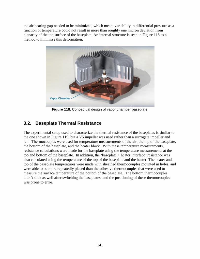
141

the air bearing gap needed to be minimized, which meant variability in differential pressure as a

function of temperature could not result in more than roughly one micron deviation from

planarity of the top surface of the baseplate. An internal structure is seen in Figure 118 as a

method to minimize this deformation.

3.2. Baseplate Thermal Resistance

The experimental setup used to characterize the thermal resistance of the baseplates is similar to

the one shown in Figure 119, but a V5 impeller was used rather than a surrogate impeller and

fan. Thermocouples were used for temperature measurements of the air, the top of the baseplate,

the bottom of the baseplate, and the heater block. With these temperature measurements,

resistance calculations were made for the baseplate using the temperature measurements at the

top and bottom of the baseplate. In addition, the ‘baseplate + heater interface’ resistance was

also calculated using the temperature of the top of the baseplate and the heater. The heater and

top of the baseplate temperatures were made with sheathed thermocouples mounted in holes, and

were able to be more repeatedly placed than the adhesive thermocouples that were used to

measure the surface temperature of the bottom of the baseplate. The bottom thermocouples

didn’t stick as well after switching the baseplates, and the positioning of these thermocouples

was prone to error.

Figure 118. Conceptual design of vapor chamber baseplate.

142

Figure 119. Experimental setup for baseplate thermal resistance measurements.

The experimental procedure for these measurements was to zero the distance sensors at room

temperature, then spin the impeller up to a given speed. Either a spring or a spacer were used

with a nut to set the gap at a given rotation speed. The power to the heaters was then varied,

generally up to 200 W, and the temperatures were monitored. Both a thermal inertia model, and

a steady-state model were used to calculate the thermal resistances. The steady-state thermal

resistance was the steady-state temperature difference between two locations divided by the

power to the heaters. Steady-state resistances were within 12% of the inertial calculations.

Because the inertial calculations used more data points to fit the data, the resistances reported are

those calculated using the inertial model.

In Figure 114, the differences in thermal resistances of the two different baseplates are directly

compared, for both a 10 and 30 µm air bearing gap. Due to the errors in the individual

‘baseplate’ resistances due to the surface mount thermocouples, a more accurate comparison of

the thermal resistance of the copper and vapor chamber baseplates can be made by comparing

the ‘baseplate + heater interface’ resistances. For both of the gaps, the resistances of the

‘baseplate + heater interface’ were very similar and approximately 0.030 °C/W lower for the

vapor chamber than the copper baseplate. The copper baseplate was previously analyzed using

analytical and finite element calculations and found to have a thermal resistance of about 0.04

C/W. Thus, the vapor chamber is a significant improvement.

143

4. AIR BEARING

4.1. Overview of Spiral Groove Air Bearings

As briefly discussed in Section 1.2, the Sandia Cooler design incorporates an air bearing as a

frictionless, low thermal resistance support between the stationary baseplate and the spinning

impeller. It was recognized that having a gap between the impeller and baseplate filled with a

low thermal conductivity fluid such as air presents a potential design obstacle. However, early

design development calculations showed that the torque required due to the shearing resistance

of a liquid at several thousand rpm would make motor power requirements impractically high. In

contrast, calculations for very thin (tens of microns) air gaps indicated that the thermal resistance

would be non-negligible, but a fraction of the total thermal resistance budget.

With the assumption of an air gap separating the baseplate and the impeller, the question was

how to support the impeller and control and maintain a desired gap thickness. For early

prototype development, a static air bearing was used [12] in which pressurized gas was injected

through the holes drilled through the baseplate at the center and, in some cases, at radial

locations. Pressures of tens of psi (due to the use of flow metering orifice hardware) and gas

flow rates of order 10 sccm were required to levitate impellers above baseplates to evaluate

design performance.

While other potential mechanisms were considered to maintain and control the air gap

(mechanical bearings and magnetic forces, for example), an air bearing has several advantages.

One important advantage is that the air gap is not maintained by using extremely tight

mechanical tolerances. Much like an air hockey puck on an air hockey table, or a hard disk

read/write head, the air gap distance is self-regulating. If the air gap distance increases, the air

pressure in the gap region drops, which causes the air gap distance to decrease. This built in

negative feedback provides excellent mechanical stability and an extremely stiff effective spring

constant. The stiffness of an air bearing is another important advantage which provides resistance

to external disturbances such as shock and vibration.

Figure 120. Thermal resistance measurements of the Sandia Cooler system. The left plot is for a 10 µm air bearing gap, the right plot for a 30 µm gap.

144

However, since supplying pressurized gas to the device during operation is largely impractical, a

hydrodynamic air bearing, where the air bearing is created by the rotational motion of the

impeller, was required for a practical design. Such a hydrodynamic air bearing can be achieved

using a series of shallow grooves in one of the mating surfaces of the air bearing. In fact, the

spiral groove air bearing is a concept that was developed decades ago and is used in a number of

commercial applications including inertial gyroscopes, face seals, optical spinners and

turbomachinery.

The first full development of the design of spiral groove bearings was by Muijderman in his

1966 text [1], although the concept was first discussed in the 1920s and studied in more detail in

the 1940s and 1950s. Muijderman developed the spiral groove thrust bearing design in pursuit of

a high speed, low friction bearing capable of high load capacity. In his book, Muijderman

develops equations for pressure, load carrying capacity and frictional torque for several different

configurations of flat, spherical and conical thrust bearings. While a number of more recent

works on the subject have been published [19-22], Muijderman’s equations were found to

sufficient and relevant for our design.

Figure 121. Example of a flat spiral groove thrust bearing [1].

An image of a spiral groove thrust bearing from Muijderman’s book is shown in Figure 121. In

brief, the spiral groove air bearing works through the pumping of a viscous fluid by the rotation

of the surface containing the grooves with respect to the mating surface. Depending on the

groove orientation and the direction of rotation, the fluid will be pumped toward or away from

the axis of rotation. Thus, only one rotation direction results in a positive pressure developed

between the mating parts which creates lift between them. This positive pressure lift matches the

opposing gravitational force of the lifted object at some gap where the fluid leakage from the gap

offsets the pumping action of the grooves. Thus, there is an optimum groove depth for a desired

load and gap height. The equations developed in [1] allow for the calculation of this optimum

groove geometry, and were used to develop the air bearing groove designs discussed in the next

sections.

145

4.2. Initial Designs and Evaluation

4.2.1. Air bearing for V3 and V4 impellers

The first baseplate to incorporate a spiral groove air bearing was used with the V3 and V4

versions of the heatsink impeller and is shown in Figure 122. For the purposes of this report we

will refer to this as the V4 baseplate. Muijderman’s equations in the form of an online calculator

(http://www.tribology-abc.com ) were used to design this first air bearing groove pattern. For

the log spiral groove geometry, the parameters that define the grooves and the air bearing

performance are shown in Table 14. Number of grooves, groove depth, groove angle, inner to

outer radius ratio, and ridge width to groove width ratio are the parameters required to

completely define the groove geometry. The calculator then determines the rotational speeds

required for the specified grooves to initially lift a given load and then support the load with a

given gap height. Thus, the tool could be used to find the groove geometry required to produce a

gap height of 10 microns at a speed of 2500 rpm, for instance, but that was not the design intent.

The intent was to create an air bearing that was stiff and relatively insensitive to changes in

impeller speed. To accomplish this, the air bearing was designed to be able to produce greater

lifting force than the impeller weight at the desired operating height. As briefly described in

Section 1.2, a preload supplied by a compression spring mounted on the impeller shaft and

applied to the impeller bearing would then be used to set the operating gap height. This allowed

for maximum stiffness of the air bearing and the ability to operate the Sandia Cooler in any

orientation by changing the pre-load.

Figure 122. Initial spiral groove pattern used with V3 and V4 impellers.

146

Table 14. Parameters of the initial spiral groove design.

Parameters

Ø_Impeller 101.6 mm

Groove Depth 81 μm

λ, r_Inner/r_Outer 0.75

α, Groove Angle 15°

k, # of Grooves 15

, ridge width/groove width 1.0

Calculation Results

Lift off speed 136 rpm

Gap at 2500 rpm 50 μm

4.2.2. Air bearing for V5 impeller While the V4 baseplate provided a hydrodynamic air bearing that functioned properly, it

provided too much lifting force at operating RPM which resulted in a significant pre-load

required to maintain the desired 10 micron gap. Nor was it optimized for minimum thermal

resistance. The groove surface area and depth were both larger than required for the best air

bearing performance which hindered heat transfer since a large fraction of the baseplate to platen

surface area consisted of an additional 81 microns of air gap due to the groove depth.

With the revised design for the solid copper baseplates described above in Section 5.1.2., a new

groove geometry was also developed. This groove design was an effort to provide good stiffness

with less thermal resistance and less sensitivity to impeller speed. This iteration also produced a

more ideal gap, with “lift off” occurring at a lower RPM. The design parameters are shown in

Table 15 and the grooves shown in Figure 123.

Table 15. Parameters for the V5 baseplate spiral groove air bearing.

Parameters

Ø_Impeller 101.6 mm

Groove Depth 25 μm

λ, r_Inner/r_Outer 0.9

α, Groove Angle 15°

k, # of Grooves 15

, ridge width/groove width 1.0

Calculation Results

Lift off speed 39 rpm

Gap at 2500 rpm 24 μm

147

Figure 123. V5 baseplate with new spiral groove pattern.

Figure 124 shows the calculated gap height for both the V4 and V5 baseplates as a function of

impeller rotational speed based on just supporting the weight of the impeller. Note the much

larger gap height, and thus load carrying capacity, of the initial design and the steeper slope with

impeller speed. The newer design was more carefully designed considering the goals for the

final Sandia Cooler device.

Figure 124. Predicted gap height using the V4 and V5 baseplates without preload.

4.2.3. Experimental Evaluation

With the expansion of the project in FY13, budget was available to perform a more extensive

characterization of air bearing performance than had previously been possible. To this end, a test

apparatus was assembled to measure gap height as a function of rotational speed to compare to

the theoretical predictions. Figure 125 shows the experimental setup which included a surrogate

impeller and displacement sensors. The surrogate impeller was used for several reasons. The

148

primary reason was that a surrogate could be easily fabricated with flat and parallel top and

bottom surfaces so that the top could be used as the target for the non-contact displacement

sensors. With a finned impeller the target would have to be the bottom surface which would have

required mounting the sensors in the baseplate which was undesirable. In addition, the simple flat

surrogate did not suffer from the centrifugal deformation that the finned impellers were subject

to which would make gap determination difficult.

Figure 125. Test apparatus for air bearing performance evaluation.

Two non-contact displacement sensors were used to measure the air gap distance between the top

surface of the base plate and the bottom surface of the surrogate impeller. This was accomplished

by “zeroing” the sensor values with the two plates in contact. The displacement of the top

surface of the surrogate was then assumed to equal the gap height. These sensors are eddy

current displacement sensors (Keyence, Model EX-305V, 0.4 m resolution, 1000 m dynamic

range), and are shown more clearly in Figure 126. The model 305V sensor has a sampling rate of

40 kHz, which ensures adequate bandwidth to record mechanical vibration waveforms in

addition to average air gap distance. The 5-mm-diameter cylindrical sensor heads were mounted

inside Teflon sleeves for shielding and positioned using optical mounting hardware above the

surrogate plate. Because the displacement measurement relies on eddy currents, these sensors are

designed to be used with iron or steel targets. The response is quite non-linear for aluminum,

which the surrogate was constructed from. However, through calibration (see Figure 126) we

found that the sensors could be linearized over an acceptable range of displacements for our

purposes.

149

Figure 126. Eddy current displacement sensor and calibration setup.

Both the V4 and V5 baseplates were tested with this system over a range of rotational speeds

from 2500 to 4000 rpm. A static air bearing was used to initially lift the surrogate impeller while

an off-the-shelf motor controller was used to bring the surrogate up to speed. The surrogate was

designed to have the same mass and rotational inertia as the V5 impeller. These tests were run

without a spring pre-load to determine the gap height at speed. Figure 127 shows the test results

for the two air bearing designs compared to the theoretical calculations. Although the slope of

the gap height as a function of speed is captured quite well, the absolute value does not match the

prediction, especially for the V4 design. This may be due to discrepancies between the as-built

geometry and the specified parameters such as groove depth and width or to the simplifying

assumptions that are built into the theoretical equations. Nevertheless, the trends in the air

bearing performance are captured, if not perfectly.

150

Figure 127. Air bearing test results compared to theoretical calculations.

4.3. Final Design and Validation

Based on the experimental evaluation of the V4 and V5 baseplates and a more detailed

investigation into spiral groove air bearing design, a final design iteration was carried out to

optimize the design for maximum stiffness at a 10 micron gap with minimal pre-load. The

parameters for the final air bearing design are shown in Table 16. It was found that load capacity

is maximized when the gap height is approximately 1/3 the groove depth, so a depth of 35

microns was specified. Load carrying capacity also increases with number of grooves up to about

fifteen, so that number was kept the same. However, for fifteen grooves the optimum groove

angle was found to be 12 degrees. Load capacity and stiffness are most sensitive to and

increase dramatically as decreases. Through calculation and experiment it was determined that

for a reasonable pre-load and good stiffness, of 0.9 was optimal. Finally, analysis showed that

for close to 1, a greater than one is best. Thus, the new design uses ridges that are 40% wider

than the grooves. This combination of parameters gave a greater load capacity and stiffness than

the V5 design while simultaneously minimizing the thermal resistance due to the grooves.

Figure 128 shows a CAD image of the new grooves.

Table 16. Parameters for the final spiral groove air bearing.

Parameters

Ø_Impeller 101.6 mm

Groove Depth 35 μm

λ, r_Inner/r_Outer 0.9

α, Groove Angle 12°

k, # of Grooves 15

, ridge width/groove width 1.4

151

Figure 128. Final spiral groove design.

4.4. Air Bearing Thermal Resistance

4.4.1. Experimental Evaluation

An air bearing is used to transfer heat from a stationary reference frame of the object being

cooled to the rotational reference frame of the Sandia cooler impeller, which dissipates the heat.

The thermal resistance of the air bearing is a significant portion of the thermal resistance of the

entire Sandia cooler system. In this section, an experiment to measure the air bearing resistance

and results of those experiments are presented.

A photo and sketch of the air bearing thermal resistance setup is shown in Figure 129. To isolate

the effects of the air bearing and the impeller, a surrogate impeller with a flat upper and lower

surface was used. Heat from the insulated heater block flowed through the baseplate, air bearing,

surrogate impeller, and then to the air. Heat transfer to the air was enhanced by mounting an

axial fan above the surrogate impeller. By using an axial fan and the flat surrogate impeller, the

heat transfer to the air was not a function of the rotation speed of the impeller. In this way, the

effect of rotation speed on the thermal resistance of the air bearing was separated from the

changes in resistance due to the enhanced cooling of the impeller as the rotation speed increases.

Locations and names of the temperature measurements are shown in red, with the type of sensor

and number of sensors shown in parenthesis. The position sensors are labeled in blue.

Measurements of steady-state temperatures as a function of rotation speed and gap distance were

made with both nitrogen and helium as the heat transfer medium in the air bearing. Using two

different fluids with different thermal conductivities allowed air bearing thermal resistance to be

easily backed out of the experimental data.

152

The most challenging aspect of this experiment was precisely setting and maintaining the air

bearing gap as different characteristics of the system changed (temperature, rotation speed, and

gas in the air bearing). Thermal expansion caused significant movement of the distances to the

surfaces being measured. Grooves for a hydrodynamic air bearing as the impeller rotates caused

the lifting force of the surrogate impeller to be a function of rotation speed. The difference in

viscosity of nitrogen as compared to helium also affects the lifting force. For these reasons, the

experimental procedure involved first heating the system to a steady temperature with heater

power set to 75 W. Then the distance sensors were zeroed, by adjusting the height of the post

onto which they were mounted. A gas was chosen (either nitrogen or helium) and the gas was

allowed to flow into the air bearing gap. The surrogate impeller was then spun up, and a nut and

spacer (metal tubing) were used to set the gap. By looking at the difference between the eddy

current sensors and the LVDT, the gap could be set to a fair degree of precision. Wobble in the

surrogate impeller prevented precisions greater than ±5 µm. After setting the air bearing gap with

a given gas, the impeller speed was varied. This procedure was repeated with both nitrogen and

helium flowing into the air bearing gap, and as the gap was varied from 10-25 µm. The steady-

state temperatures were determined for each rotation speed, gap, and gas.

The maximum theoretical resistance of the air bearing gap would occur with a stagnant gas layer.

This thermal resistance would be due to conduction in the gas, equal to where

is the gap height, is the thermal conductivity of the gas, and is the area for conduction. If the

rotation of the impeller (or surrogate impeller) enhances the mixing, the resistivity of the gap

would be expected to decrease. Assuming that this enhancement would be the same for both

helium and nitrogen, the resistance of the gap when nitrogen (or air) is in the gap can be

calculated through the equation,

(

),

Figure 129. Photo and sketch of the experimental setup for air bearing thermal resistance measurements.

153

where TN2 is the temperature difference when N2 is used, THe is the temperature difference

when He is used, P is the heater power, and kN2 and kHe are the thermal conductivities of N2 and

He respectively. This equation is analogous to that on pg. 25 of [12] if the heat leakage is

neglected.

Calculating the resistance in this manner overcomes the challenges of measuring the temperature

difference directly on either side of the air bearing gap, and allows any two temperature locations

to be used, as long as they are on either side of the air bearing.

The thermal resistance of the air bearing as a function of gap height is shown in Figure 124. This

depicts the thermal resistance of a stagnant gas layer as well. As shown, the resistance of the air

bearing gap is not dependent on the rotation speed, up to 4000 rpm, and is very close to the

resistance of a stagnant gas layer. At 10 mm, the thermal resistance of the air gap is about 0.05

°C/W. This value is a significant fraction of the overall thermal resistance of the Sandia Cooler.

Recall that the thermal resistance of the V5 impeller at 2500 rpm is just 0.084 °C/W. Lowering

the thermal resistance of the air bearing gap can best be accomplished by narrowing the gap as

much as possible, or by purging the gap region with a trickle flow of gas having much higher

thermal conductivity than air, such as helium or hydrogen.

4.4.2. Computational Simulation

In a previous report [12], the measured thermal resistance of the air bearing gap for Version 1

was found to decrease with increasing angular velocity of the impeller. In an effort to examine

and exploit the cause of the enhancement, a computational fluid dynamics study was conducted

of the air gap. In this study, the thermal resistance of the air gap was determined by simulating

various angular speeds and comparing to the pure conduction case to determine the

enhancement.

The model was set-up to correspond to the Version 1 experimental set-up. In this case, no

grooves or coatings were present on the base plate or platen to facilitate the air bearing. The air

flow applied to the air bearing was found to be negligible for our calculations. The meshed gap

is shown in Figure 131. To compare with the data from the previous report, the angular shear

rate, S, is calculated as the angular velocity, ω, divided by the gap thickness, d, and is compared

Figure 130. Thermal resistance of the air bearing as a function of gap height, for several rotation speeds. For reference, the resistance of a stagnant air layer is also shown.

154

with the enhancement factor, ε, which is the effective thermal conductivity of the gap, keff,

divided by the thermal conductivity of air in the gap, kair. The effective thermal conductivity is

calculated by Fourier’s Law keff = q”∙d/(Tbottom - Ttop), where q” is the applied heat flux (18500

W/m2), Tbottom is the temperature of the bottom surface in the gap and Ttop (40 ºC) is the

temperature of the top surface in the gap. The thermal boundary conditions applied are the heat

flux on the bottom surface and constant uniform temperature on the top surface. The flow

boundaries are a rotating wall for the top surface, a stationary wall for the bottom surface, an

entrainment opening for the outer surface and a free slip wall for the inner surface.

Figure 131. Computational mesh of air bearing gap.

When the simulation was run for the range of angular velocity of interest (0-10,000 RPM) no

enhancement was shown over the base thermal conductivity. Thus, we concluded that the

perceived enhancement was not due to the fluidics, but must be due to another component. In

another previous report [13], it was shown that the V2 impeller had a large amount of

deformation as it was spinning causing the outer edges to bow downwards, which increased with

increasing angular velocity. This deformation of the gap region could cause a decrease in the

thermal resistance.

To include the deformation in the model, the portion of the gap was deformed to imitate the

measured deformation. A gap size of 50 µm was assumed. A linear profile was assumed from

the radial midpoint at the top of the gap to the outer radius down the predicted maximum

deformation at the specified angular velocity. Figure 132 shows a schematic of the deformed

gap.

155

Figure 132. Cartoon of deformed fluid region.

The results from the model with and without deformation compared to the experimental data are

shown in Figure 133. The results follow the same trend as the measured curve.

Figure 133. Results of the measured and predicted thermal enhancement versus angular shear rate with and without deformation.

From this study, we concluded that the apparent thermal resistance enhancement with angular

velocity at a specified gap height was due to the reduced gap height at the edges, which

intensified with higher angular velocity.

4.5. Alternate Design: Magnetic Lift

4.5.1. Introduction

Magnetic lift was investigated as an alternative to the hydrodynamic air bearing for maintaining

the air gap between the impeller and baseplate. The hydrodynamic air bearing has many positive

attributes making it nearly ideal in this application. It is elegantly simple and inexpensive,

requiring only that shallow spiral grooves be created in one face. Because of the way it operates,

the lift force is indexed to the surfaces, ensuring parallelism during operation. The air bearing

also provides remarkably high and nonlinear stiffness, increasing with smaller air gaps, thereby

providing stability. The one main drawback to the hydrodynamic air bearing is associated with

156

the speed dependence of the lift force. For air gap regulation, a spring force is applied on the

impeller toward the baseplate. Once up to speed, the lift force of the air bearing overcomes the

spring force, lifts the impeller, and due to its high stiffness, equilibrates with the spring force at

the desired air gap. With the impeller at rest, this spring force must be balanced by a normal

force between the surfaces, which creates additional friction. With the relatively large diameter

of the impeller and baseplate, the resulting friction torque is difficult to overcome with a motor

optimized for the much lower torque required to spin the impeller once lifted. In contrast,

magnetic lift would provide a lift force independent of speed, allowing near zero starting torque.

In this way, it would also reduce or eliminate demands on an anti-friction coating. However,

many of the positive attributes of the air bearing are lost. Magnetic lift would not provide

stiffness as high as the air bearing, and changes to the demagnetization curves with temperature

mean the lift force will change with temperature. These factors make air gap regulation more

challenging. Additionally, magnetic lift would be more costly and complex, and if magnets are

embedded in the surfaces, heat transfer performance would be degraded.

To investigate the feasibility of magnetic lift, the overall strategy was as follows. Potential

configurations for magnetic lift were first investigated. An experiment was then assembled using

commercially available ring magnets to allow operation of a surrogate impeller at speed.

Dynamic measurements of the air gap at different speed and lift force conditions were made to

assess the stability of operation. Meanwhile, preliminary design work was carried out using a

static 2D axisymmetric finite element method magnetic solver software, FEMM. Measurements

of lift force versus magnet separation distance were made on the commercial magnet experiment

to validate FEMM simulation results. With this information, pathways to feasible

implementation of magnetic lift were identified.

4.5.2. Magnetic bearing design

4.5.2.1. Potential bearing configurations

Several possibilities exist for creating magnetic lift, both static and dynamic. Only magnetostatic

lift configurations are considered for this application, as dynamic magnetic lift would suffer a

similar starting torque issue as the hydrodynamic air bearing, with inherent eddy current drag

while coming up to speed. Two ring magnets in repulsion is one configuration for static

magnetic lift which can be easily implemented in this application, and will be the primary focus

for this work. In this scheme, one ring magnet would be embedded in the impeller and one in the

baseplate, with similar poles facing one another. With appropriately sized magnets, this can

provide the required lift force. The force profile is similar to an air bearing in that stiffness

increases with decreasing gap, but the stiffness is not nearly as high. The bonded NdFeB design

discussed below has a stiffness around 0.04 N/µm near its operating point, while an air bearing at

a 10µm air gap is in the range of 0.2 to 5 N/µm depending on groove design and rotational

speed.

Alternative magnetic bearing configurations were briefly considered to see whether higher

stiffness could be achieved, since this would be beneficial for air gap regulation. One possibility

is shown in Figure 134. This configuration would use a single, axially magnetized ring magnet

positioned between two steel rings. The steel rings guide magnetic flux to a ‘C’ shaped ring

attached to the impeller. The path of lowest magnetic reluctance occurs with the baseplate rings

157

and impeller ring aligned. When the rings are not aligned, a magnetic force is created trying to

pull them into alignment. Thin teeth are machined into the rings so that a small change in axial

position is a significant fraction of the tooth width, thereby increasing the sensitivity to axial

position. The steel rings on the baseplate are biased upward relative to the impeller ring in order

to create the desired lift. The air gap between impeller and baseplate would then be adjusted

using a spring force or spacer on the inner race of the impeller bearing. It should be noted that

this configuration relies on the ‘C’ shaped ring being concentric with the rings on the baseplate.

If not, a radial magnetic force will be created trying to pull them together at one side, which

could add significant radial load to the bearing. FEMM modeling indicates that reasonably high

stiffness can be achieved using this configuration, around 0.2 N/µm. A fully dense sintered

neodymium-iron-boron (NdFeB) magnet was used in the simulations, and the rings would need

to be machined to fairly close tolerances, so this configuration comes with more cost and

complexity compared with magnets in repulsion, and especially compared with a hydrodynamic

air bearing. For this reason, it was not pursued further, but it remains a potential alternative. The

remainder of this work only considers the aforementioned configuration of two magnets in

repulsion.

158

Figure 134: Conceptual rendering of magnetic lift design using alignment of steel rings.

4.5.2.2. Magnet sizing and materials

Large diameter ring magnets are desired for stability of the impeller. Due to the brittle nature of

magnetic materials, thin sections at large diameter are difficult to manufacture. For this

application, minimizing the volume occupied while maintaining adequate lift would suggest the

use of high energy product fully dense rare earth magnets. However, at a diameter of around

three inches, the cross section of magnet required to achieve the desired lift becomes quite small.

These magnets, if they could be manufactured, would be expensive and extremely fragile.

Despite intuition, fully dense rare earth magnets do not seem well suited for the application.

Similar issues would be found with most magnetic materials. An attractive alternative in this

case would be bonded magnetic materials, consisting of magnetic powder contained within a

polymer matrix. Magnetic properties of bonded materials are reduced relative to fully dense

magnetic materials, so bonded rare earth magnets would likely be required instead of the less

Baseplate

Impeller

Steel ring fixed on impeller

Ring magnet (magnetized axially)

Steel rings fixed to baseplate (biased upward to create lift on impeller)

Thin teeth increase sensitivity to axial position

Air gap

159

expensive bonded ferrite. FEMM modeling results suggest that bonded NdFeB magnets with

9MGOe energy product occupying 3% of the baseplate and impeller surface area would provide

around 14N of lift force. A similar lift force with bonded ferrite (2MGOe energy product) would

take over 10% of the surface area. To put the magnet cost in perspective, the volume of bonded

NdFeB material required is estimated as 0.50cc, versus 0.27cc of fully dense sintered NdFeB

contained in the motor magnets. As for implementation, bonded magnetic material could be

injected into grooves in the impeller and baseplate and machined flat during the facing

operations. Selection of a binder with coefficient of thermal expansion as close as possible to

copper and aluminum would ensure dimensional stability of the magnets relative to the baseplate

and impeller.

4.5.2.3. Thermal effect on lift force

Magnetic properties of permanent magnet materials change with temperature, typically described

by a set of demagnetization curves. The implication with this application is that the lift force

will decrease with temperature, creating further complication with air gap regulation. Regulation

accomplished by a spring force on the impeller would be susceptible to changes in air gap due to

changes in magnetic properties with temperature. A possible alternative is to set the air gap

using a spacer contacting the inner race of the bearing, adjusted by means of a locknut on the

shaft. This method has its own set of challenges. Thermal expansion issues could be mitigated

by using a spacer of low thermal expansion material, with length chosen such that expansion of

the shaft cancels expansion of the impeller and baseplate to maintain nearly constant air gap with

temperature. Use of a spacer would also be susceptible to mechanical wear of the bearing,

causing the air gap to widen over time. Despite the problems, use of a spacer is likely to be more

feasible than a spring when using magnets for lift.

4.5.3. Experimental setup

Commercially available 3.50” OD x 3.00” ID x 0.079” thick axially magnetized N40 NdFeB ring

magnets were obtained for experimental testing. These dimensions and material provided much

more strength than required, but they were the most reasonable stock magnets found at the time.

A baseplate and surrogate impeller were modified with grooves to embed the magnets. To

compensate for the excessive strength of the magnets, the grooves were made deeper than the

magnet thickness, such that the magnet faces were below the mating surfaces. The impeller

magnet was fixed, while the baseplate magnet position was adjustable using three set screws

from below, which allowed operation with different lift force. A picture of the modified

baseplate with magnet installed is shown in Figure 135 below. Magnetic lift force measurements

for model validation were made with the impeller at rest by adding weights until contact was

detected. For air gap measurements, an inductive displacement sensor was positioned to read the

top surface of the surrogate impeller. The sensor was calibrated against a micrometer, and a

partial range of the sensor was chosen for optimum linearity. Within this range, the sensor

matched the micrometer to within 1µm. Prior to each test, a zero point was obtained by reading

the sensor output with the impeller held against the baseplate. Readings were taken at eight

angular positions of the impeller and averaged to account for imperfect parallelism of the top and

bottom surfaces.

160

Figure 135: Stock ring magnet embedded in modified baseplate.

4.5.4. Results

Static lift force measurements using the commercial magnets are shown in Figure 136, along

with FEMM model results. Model results closely match the measurements, indicating that the

model is well-suited for an initial investigation of magnet sizing and materials. Model

calculations at small separation distances show the extent to which these stock commercial

magnets are oversized, providing an order of magnitude larger force than required when brought

within close proximity. Stiffness, seen as the slope of the force curve, is seen to drop off quickly

with increasing separation distance as well. For air gap regulation with spring preload, a lift

force with high sensitivity to axial position is necessary. Use of a spacer for regulation relaxes

this constraint, as the lift force must only hold the impeller against the spacer. A high stiffness is

still desirable from the perspective of stability and reducing axial load on the bearing, but is not

as critical.

161

Figure 136: Static repulsive force between stock commercial magnets versus separation distance.

Air gap measurements with the impeller running at 1500rpm and 3750rpm are shown in Figure

137 and Figure 138. Each line represents data taken at a different setting of the adjustment

locknut, with nominal air gaps of 10, 20, and 30µm. At 1500rpm, similar magnitudes of

oscillation are seen for the three different gap settings. The lower speed oscillation corresponds

to the frequency of operation, with amplitude around 1.5µm for all three air gaps at 1500rpm. At

3750rpm rpm, the amplitude of oscillation is seen to increase with larger air gaps, from around

1.5µm at 10µm air gap to around 5µm at 30µm air gap. At both rotational speeds, higher

frequency oscillations around 300Hz were seen with amplitude around 2µm. The frequency and

magnitude of these oscillations appear independent of rotational speed, though a slight shift to

higher frequency with larger air gap was noticed. A precise explanation for these oscillations

was not determined, but they are not believed to be artifacts of the measurement device.

162

Figure 137: Air gap measurements at 1500rpm.

Figure 138: Air gap measurements at 3750rpm.

4.5.5. Conclusion

Magnetic lift was investigated as an alternative for maintaining the air gap between the baseplate

and impeller. The main benefits associated with magnetic lift compared with a hydrodynamic air

bearing are a result of its lift force being independent of rotational speed. In applications where a

163

wide range of operating speeds is desired, this would provide consistent air gap regulation.

Perhaps more importantly, it enables near zero starting torque, and there is no need to rely on an

anti-friction coating. An anti-friction coating may still be desired for surface protection, but

coating wear would not be a limitation on the number of startup cycles. Despite these benefits,

magnetic lift suffers more difficult air gap regulation than with a hydrodynamic air bearing,

along with added cost and complexity. Nonetheless, the experiments conducted show that

magnetic lift can provide stable operation under the range of operating conditions expected for

the device. Bonded NdFeB was identified as a pathway to reasonable magnet size and feasible

implementation. Though not an inexpensive material, the amount required is comparable to the

amount used in the drive motor for the device. Considering all of these aspects, in applications

requiring a wide range of operating speed, where motor starting torque is insufficient, or with

large numbers of start-stop cycles, magnetic lift provides an attractive alternative to a

hydrodynamic air bearing.

5. ANTI-FRICTION COATING

5.1. Background and Requirements

When the Sandia Cooler is started from rest, the impeller will be contacting the baseplate with

gravitational as well as the spring pre-load force. Overcoming the static and then sliding friction

that occurs between the two surfaces before the air bearing provides enough lift is a challenge for

the brushless motor. To minimize that friction we incorporate an anti-friction coating into the

two mating surfaces which enables the motor to initiate impeller rotation to the point that the air

bearing lifts the impeller from the baseplate surface. In addition to lowering friction, the coating

prevents galling and wear of the impeller and baseplate surfaces during starts and stops.

A number of anti-friction coating options were considered for this application. While many

possibilities exist that could meet several of our requirements, few could meet all of them. i-

Kote, a coating patented by Tribologix Inc., was chosen for this application (1) because it

provides a very low coefficient of friction, (2) it has an extremely low wear rate, (3) unlike some

dry anti-friction coatings, i-Kote is insensitive to environmental variables such as relative

humidity, (4) the wear in process allows in situ generation of extremely flat/parallel surfaces, and

(5) none of the i-Kote constituent materials are expensive. i-Kote is a mixture of molybdenum

disulfide, graphite, and other constituents that form a chemical bond to the substrate (nickel-

plated QC-10 aluminum in this case). The thickness of the i-Kote coating is typically 2.5 microns

with a maximum thickness of 4 m (the chemical deposition process is self-limiting). Once the

i-Kote coating goes through its initial wear-in process the wear rate is supposed to be extremely

small (5 x 10-17

m3 N

-1 m

-1), and it is the properly worn in coating that provides the extremely

low coefficient of fiction claimed by Tribologix. One drawback is the i-Kote is sensitive to

exposure to water, solvents, finger prints, and other contaminants.

The strategy for preventing contamination of the coating and air gap region is to leave the heat-

sink-impeller and base plate fully assembled and in positive contact. When the device is not in

operation the two surfaces are clamped together by the air gap spring, thereby preventing the

ingress of contaminants. During operation, sub-10-micron particles that attempt to enter the air

gap region will be entrained in the air flow and tend to be centrifuged out because they are 3 to 4

164

orders of magnitude denser than air. Extremely small particles may be able to settle down in the

boundary layer of the base plate if they can somehow find their way there. These particles may

however be entrained in the air flow during startup and shutdown (at which time the air gap

distance sweeps through the 0 to 10 micron range).

5.2. Candidate Coating Evaluation

5.2.1. Test Apparatus and Procedures

Anti-friction coating evaluation was performed on a test rig using surrogate parts made to match

the impeller and baseplate in terms of contact dimensions, flatness, surface finish, and

perpendicularity of shaft and bearing holes. The impeller substitute was adjusted in thickness to

match the impeller mass. The rotational inertia was within 8% of the impeller, which was

deemed an adequate representation given that the torque measurement being made is not

sensitive to that parameter. Both the impeller substitute and baseplate substitute were made of

6061-T6 aluminum. Nickel plating is required prior to application of the anti-friction coating, so

it was not necessary to use materials identical to the impeller and baseplate. No spiral grooves

were machined into the substitute parts, so the normal contact force between them does not

change with speed. The impeller substitute was made with a flat profile, not including the

convex correction for centrifugal deformation used on the real impeller. No appreciable axial

deformation is expected with the substitute impeller since the fins are not present. The flat

profile gives conservative overestimates of the static and low-speed friction torque as a result of

the equivalent torque radius being larger than it would be with a convex profile.

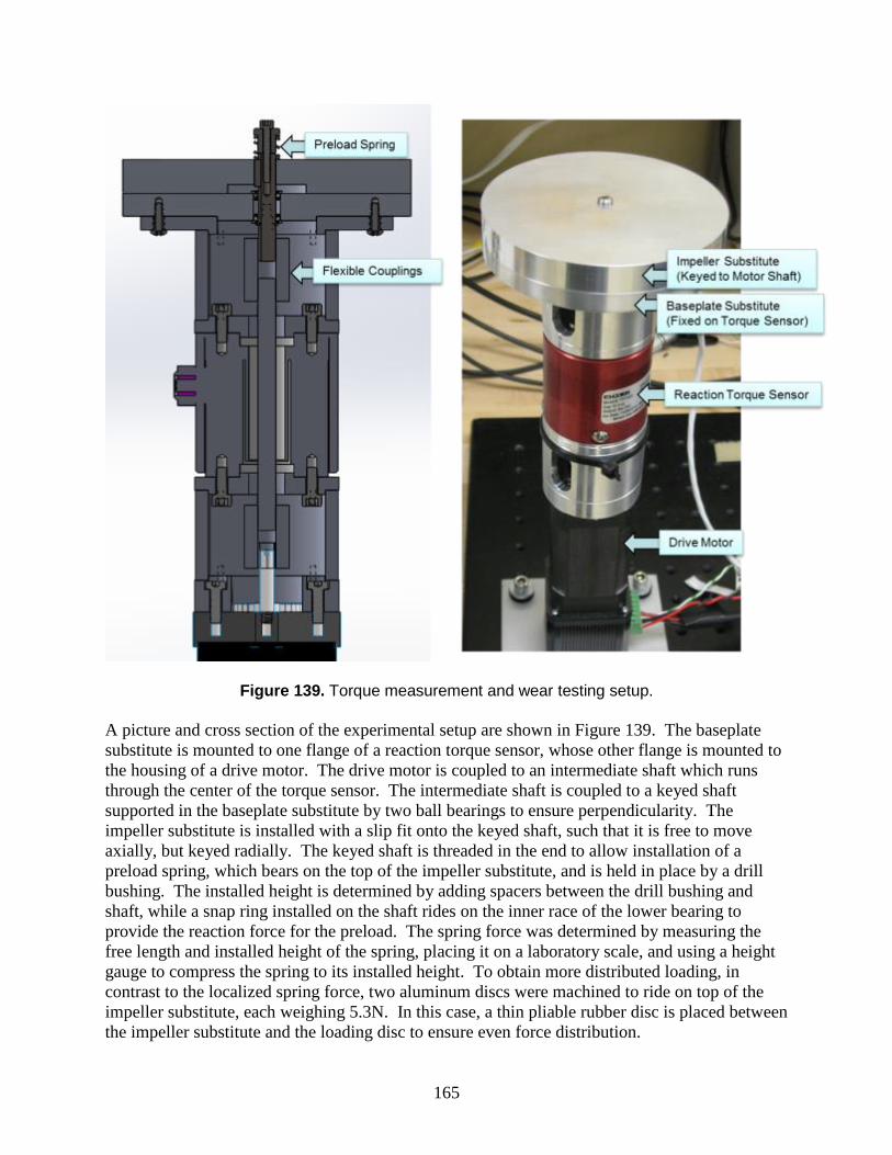
165

Figure 139. Torque measurement and wear testing setup.

A picture and cross section of the experimental setup are shown in Figure 139. The baseplate

substitute is mounted to one flange of a reaction torque sensor, whose other flange is mounted to

the housing of a drive motor. The drive motor is coupled to an intermediate shaft which runs

through the center of the torque sensor. The intermediate shaft is coupled to a keyed shaft

supported in the baseplate substitute by two ball bearings to ensure perpendicularity. The

impeller substitute is installed with a slip fit onto the keyed shaft, such that it is free to move

axially, but keyed radially. The keyed shaft is threaded in the end to allow installation of a

preload spring, which bears on the top of the impeller substitute, and is held in place by a drill

bushing. The installed height is determined by adding spacers between the drill bushing and

shaft, while a snap ring installed on the shaft rides on the inner race of the lower bearing to

provide the reaction force for the preload. The spring force was determined by measuring the

free length and installed height of the spring, placing it on a laboratory scale, and using a height

gauge to compress the spring to its installed height. To obtain more distributed loading, in

contrast to the localized spring force, two aluminum discs were machined to ride on top of the

impeller substitute, each weighing 5.3N. In this case, a thin pliable rubber disc is placed between

the impeller substitute and the loading disc to ensure even force distribution.

166

The coatings investigated were commercially available thin solid film lubricants applied by

Tribologix Inc., known as i-Kote and Super MoS2. Containing molybdenum disulfide and

graphite chemically bonded to the substrate, these coatings have a controllable thickness with a

self-limiting maximum of 4 microns. After an initial period of wear-in, the wear rate is claimed

to be extremely small. The friction is also expected to decrease as the parts wear in. Though

literature is available on the friction and wear characteristics of similar coatings, testing was

warranted in this case due to the unusual operating conditions. This application is different from

typical applications of the coating in that the contact force is small and applied over a large area,

so the contact pressures are much lower than typically seen. Test procedures were adapted as

experience was gained with the coatings. Initial tests used continuous operation at constant

speed for quicker wear simulation. Later tests were designed to approximate the start-stop

cycling during which the surfaces are in direct sliding contact.

5.2.2. Low Energy i-Kote Performance

The first set of parts was sent to Tribologix for i-Kote application. The coated parts had a

uniform light gray matte appearance prior to installation, as seen in Figure 140. The parts were

installed in the test rig and run through a slow ramp in speed to measure the friction torque

response. They were then run at constant speed for increasingly longer durations to look for

evidence of wear-in. The impeller substitute was taken off periodically to allow visual

inspection of the surfaces. Fine black dust was generated as the surfaces gained a shinier

appearance.

Figure 140. Impeller substitute coated with low energy deposition i-Kote, prior to installation.

Figure 141 shows the friction torque versus rotational speed for the first set of coated parts

tested. Data for bare aluminum parts is shown for comparison. The bare parts show stick-slip

friction throughout the range of speeds tested, as seen in the noisy torque measurement, along

167

with rapid surface wear and galling. The coated parts, meanwhile, show stick-slip behavior only

at low speed. In this region, the friction torque drops off rapidly with increasing speed, and

reaches very low levels by about 400rpm. At this point, the friction torque is an order of

magnitude lower than with bare metal parts, and a slow increase in friction torque with

increasing rotational speed is seen. Static friction torque values of around 25, 60, and 80mNm

were seen for 0, 5, and 10N preload. Assuming uniform loading, these numbers give static

friction coefficients of 0.28, 0.21, and 0.17. Calculated static and kinetic friction values were

lower for higher preload, reflecting the non-uniform spring load applied at the center of the disc

and its effect of reducing the torque radius at which the friction is applied. Static friction

coefficients in the range of 0.17 to 0.28 are higher than the vendor would have expected and

higher than desirable for ease of starting the motor. Visual inspection of wear-in patterns

indicated that contact was initially localized near the outer radius. As the coating wore-in,

evidence of contact was seen farther inward on the discs. This bias toward a larger radius of

contact is likely to have resulted in larger friction torque than would be seen with a perfectly

even force distribution. For perspective, the difference between a force applied at the inner

contact radius of 0.546” versus the outer contact radius of 2.000” is a factor of 3.67 difference in

torque. Besides the radius of contact issue, it is well documented that friction coefficients for

MoS2 solid film lubricants generally decrease with increasing contact pressure [23]. While few

studies report results for such low contact pressures, a friction coefficient somewhat higher than

normal should be expected.

168

Figure 141: Friction torque versus rotational speed for first set of coated parts.

To obtain quicker accumulation of cycles for preliminary assessment of coating wear, the parts

were run together at constant speed rather than simulating start-stop cycling. Friction torque was

monitored for evidence of any change in the coating. After around 6 hours of operation at 1000

rpm, a rise in friction torque was seen, accompanied by much more noise in the data, as seen in

Figure 142. Based on the claimed wear rate of the worn-in coating, 6 hours of operation at 1000

rpm should correspond to ~10 nm of wear at the outer radius. It is well-documented that most of

the thickness of a MoS2 coating is lost early in its sliding life [24], so despite the initial 4µm

thickness, it is expected that <1µm is left to wear at the low rate. Nonetheless, the wear

characteristics seen were not as good as anticipated. Upon consulting with the vendor, it was

learned that a lower energy ion source was used for deposition compared with their standard

process used for the more commonly coated stainless steel and titanium. This was suggested as a

169

possible reason for the sub-optimal wear characteristics. Indeed, studies have been published

showing that endurance depends on the orientation of the crystalline material, and that the

orientation is affected by the ion-to-atom ratio [25]. Parts were sent back to the vendor to be

stripped and have the standard coating applied.

Figure 142: Friction torque versus time for wear test.

Figure 143 shows the wear patterns observed for the substitute baseplate and impeller. A ring of

high wear can be seen near the outer radius on the substitute impeller. While increased wear

may be expected at the outer radius due to longer distance traveled, in this case there seemed to

be preferential contact as a result of imperfections in flatness. The baseplate substitute appears

to have two high spots near the outer radius, thought to be caused by deflection experienced on

installation. Care was taken in subsequent tests not to over-tighten installation screws.

170

Figure 143: Wear patterns of substitute impeller (left) and baseplate (right).

5.2.3. Standard i-Kote Performance

Figure 144 shows the parts coated using the vendor’s standard deposition process prior to

installation. A notable difference is seen visually between these parts and the first set of coated

parts in Figure 145. The low energy coating appeared a uniform matte gray over the whole

surface, whereas the high energy coating is speckled with darker and shinier gray and black. The

high energy coated parts were run through the same set of wear tests in order to have a direct

comparison.

171

Figure 144: Parts coated using standard deposition, prior to installation.

Figure 145 shows the wear pattern of the parts coated with the standard, higher energy

deposition. Interestingly, the wear pattern began at the inner radius, versus on the outer radius

with the previous iteration (

Figure 143), despite being the same parts. Contact at the inner radius, as seen during tests of the

standard coating, would be expected due to the spring preload applied at the center. Further

testing using dead weights to obtain evenly distributed preload resulted in an even wear-in

pattern, confirming that the spring preload was causing the wear to be concentrated near the

inner radius.

Figure 145: Parts coated using standard deposition, after 16 hours at 1000rpm.

172

The friction and wear characteristics with the standard deposition were notably different from the

low energy deposition. Figure 146 shows the measured friction torque versus rotational speed

for the first iteration low energy coating and the second iteration standard coating. Data for the

standard coating was taken immediately after installation, prior to wear-in. Static friction

measured was 25 to 50% lower than with the low energy coating, depending on the spring

preload force. However, friction torque dropped off much more slowly with increasing

rotational speed, and the data remained noisy throughout the range of speed measured.

Figure 146: Friction torque versus rotational speed for low energy and standard (high energy) deposition. Data for high energy deposition taken immediately after installation, prior to wear-in.

The standard coating was run through the same constant speed wear tests as the low energy

coating. Figure 147 shows friction torque data for the 1000rpm wear test. Compared with

Figure 142 above, the higher friction torque and noise with this coating are evident. However,

the coating lasts throughout the 16 hour test with no apparent failure. In fact, the friction torque

appears to decrease with time. After these tests, the friction torque versus speed measurements

were repeated, showing changes from the fresh coating. Figures 148 through 150 show the

difference between the fresh (initial) and worn (final) coating. Friction torque appears to drop

off more quickly with increasing speed, as seen with the low energy coating. The worn coating

also shows a further reduction in static friction in the cases with spring preload.

173

Figure 147: Wear test at 1000rpm with 10N preload, standard deposition coating.

Figure 148: Coating wear effect with no preload.

174

Figure 149: Coating wear effect with 5N preload.

Figure 150: Coating wear effect with 10N preload.

5.2.4. Start-stop Cycling with i-Kote and Super MoS2

With initial experience working with the coatings, the next set of tests was focused on start-stop

cycling more representative of the intended application. The cycle consisted of starting from

rest, ramping to a nominal 1000rpm in 10s, and cutting power to the motor for 10s to bring the

impeller to rest. Based on prior testing, the friction torque with a 10N preload seemed beyond

the motor’s starting capability. It also tended to concentrate wear to a small ring near the center.

175

For these reasons, a 5N spring preload was chosen for the remaining tests. The 1000rpm peak

was chosen to approximate the speed at which the hydrodynamic lift force counteracts the spring

preload and impeller mass. The ramp rate was considered reasonably achievable based on motor

control work available at the time. Two sets of parts were coated, one with the standard i-Kote

and one with a Sb2O3 and Au-doped MoS2 coating which was suggested as another possibility

during a teleconference with Tribologix. This coating, which Tribologix sells as ‘Super MoS2’,

has similar friction but better wear properties than pure MoS2, particularly in humid air where the

oxygen and water vapor typically degrade the coating [26].

Figures 151 through 154 show the condition of the i-Kote and Super MoS2 coatings at various

intervals during cycle testing. For both coatings, the wear patterns show contact that is

distributed reasonably well across the mating surfaces. This suggests that the baseplates were

not experiencing significant deflection due to over-tightening of the installation screws, and that

the impeller deflection with 5N preload was more manageable than with 10N preload.

Nonetheless, with increased cycling, it became clear that wear was concentrated near the inner

radius due to the spring load. While the i-Kote appears to wear uniformly across the surfaces,

the Super MoS2 develops several discrete rings of wear. Friction torque data was collected

during cycle testing, and is shown in Figures 155 and 156. The i-Kote provided a slightly lower

static friction torque than the Super MoS2 but was much slower to drop off with speed,

particularly in the early cycles. With increased cycling, the static friction for i-Kote remained

consistent, while the sliding friction torque became smoother (less spread in the data) and lower

in magnitude. After around 13600 cycles, the sliding friction showed an abrupt increase, which

can be seen as two distinct curves in Figure 155. For Super MoS2, the static friction torque

began to increase with cycling, while the sliding friction torque remained consistently low.

176

Figure 151: Condition of i-Kote baseplate substitute at various points during cycle testing.

i-Kote after 2500

cycles

i-Kote after 5000

cycles

i-Kote after 10000

cycles

i-Kote after 15000

cycles

177

Figure 152: Condition of i-Kote impeller substitute at various points during cycle testing.

i-Kote after 2500

cycles

i-Kote after 5000

cycles

i-Kote after 10000

cycles

i-Kote after 15000

cycles

178

Figure 153: Condition of Super MoS2 baseplate substitute at various points during cycle testing.

Super MoS2 after 2500

cycles

Super MoS2 after 5000

cycles

Super MoS2 after 10000

cycles Super MoS2 after 15000

cycles

179

Figure 154: Condition of Super MoS2 impeller substitute at various points during cycle testing.

Super MoS2 after 2500

cycles

Super MoS2 after 5000

cycles

Super MoS2 after 10000

cycles

Super MoS2 after 15000

cycles

180

Figure 155: Friction torque data for i-Kote during cycle testing

(cycles 10,001-15,000 shown separately for clarity).

181

Figure 156: Friction torque data for Super MoS2 during cycle testing.

5.2.5. Conclusions

Anti-friction coatings were studied for application to the Sandia cooler. Measured static friction

torque was higher than would be expected based on published friction coefficients. This is

thought to be partly due to the low contact pressure, but also influenced by uneven contact

changing the effective torque radius at which the friction acts. In the final application, the

convex profile of the impeller used to correct for centrifugal deformation will also ensure that

contact between the impeller and baseplate at startup is focused near the center, at a smaller

torque radius. The measurements presented here, therefore, should be considered conservative

overestimates of the startup torque required. Nonetheless, these results suggest that 10N preload

is likely beyond the startup capabilities of the motor. Cycle testing of i-Kote and Super MoS2

showed both coatings lasting over 10,000 cycles with 5N preload without significant degradation

in performance. i-Kote was seen to improve in performance as cycling continued before finally

degrading. Super MoS2 was consistently smooth and showed lower sliding torque throughout

the 15,000 cycles tested, but showed higher static friction than i-Kote. Considering motor torque

limitations, i-Kote is a better choice, and based on these simulated conditions, it is expected to

perform adequately in terms of surface protection, friction, and longevity.

182

6. MOTOR AND CONTROLLER

6.1. Overview of Motor Selection

The Sandia Cooler utilizes a custom wound 3 phase-WYE connected, brushless, sensorless DC

motor (see Figure 157). This motor is comprised of a 12 pole, DLRK (Distributed - Lucas,

Retzbach and Kühfuss) stator and a rotor consisting of 14 NdFeB rare earth magnets to drive the

impeller at speeds up to 5000rpm. This arrangement allows for an electronic gear ratio of 7:1,

thus providing more torque at the required rpm range, as well as a more precise 8.57 degrees of

movement per step. The DLRK winding requires less copper windings per stator tooth, which is

a critical factor due to space constraints of this compact design. To reduce the footprint and cost

even further, no rotor position sensors (hall effect) are used and a sensorless control technique is

therefore required to control motor commutation.

Figure 157. Motor stator mounted on baseplate.

The brushless DC motor requires a motor controller to supply coordinated voltage waveforms to

each of its three-phases to generate the torque needed to spin the impeller. The Sandia Cooler is

unique compared to other brushless DC motor control applications because it requires a large

initial torque to overcome the friction between the impeller and baseplate experienced at startup

and has a relatively large moment of inertia. This, coupled with the lack of rotor position sensors,

makes it particularly challenging for a motor controller to get impeller to spin from rest. Two

motor controllers, a consumer off-the-shelf motor controller and a custom-made variable-voltage

variable-frequency motor controller, were identified as potential candidates suitable for the

application. Each was developed and tested for performance.

6.2. Motor Controller Development

6.2.1. COTS Motor Controller Evaluation

One of the goals of the program was to utilize a relatively inexpensive and compact commercial

off the shelf (COTS) motor control unit that could be easily tuned to optimally drive motors with

183

a varying range of voltage and torque constants, under a multitude of startup frictional and

inertial loads. Several COTS motor control drive units were selected as a best fit for this

particular motor based on several critical criteria that include motor windings, voltage and

current requirements, cost, size, and ease of setup and tuning. The DPFlex motor controller,

manufactured by Allied Motion Technologies, Inc. (Agile Systems Inc.) of Ontario Canada, was

chosen over other units for several specific reasons. There are a multitude of COTS controllers

that are available, however most of these units : 1) utilize Hall effect sensor or rotary optical

encoder based control, 2) are targeted for much larger motors and are not easily scaled down to

this particular motor size, 3) lack simple and easily adaptable software, 4) have fixed pole and

voltage constraints, and 5) are relatively large. The DPFlex controller has the ability to run on a

wide array of bus voltages and can be modified through a combination of minor hardware and

software/firmware changes from the manufacturer. It can also run as a standalone unit without

computer connectivity and has analog speed control through a potentiometer or other dc inputs.

As will be discussed later, the unit also incorporates a more sophisticated startup algorithm that

other COTS sensorless motor controllers do not offer.

In sensorless control, rotor position must be determined using another method, which is typically

based on an algorithm relying on back EMF (electro-motive force) detection, where the voltage

waveform generated by the passage of the permanent magnet rotor across unexcited stator

windings is using to infer the rotational orientation of the rotor relative to the stator. The speed

of the motor and the magnitude of the back EMF signal are directly proportional, therefore at

zero RPM or very low speeds the signal is zero or very close to zero. It is for this reason that

startup in a sensorless BLDC motor setup is the most difficult aspect of control. Actual rotor

position must be first determined, and traditional methods involve passing a high current through

the stator windings, thus forcing the rotor to cog and lock into a position. This method can cause

overshoot and ringing if currents are too high with respect to motor loads. Conversely, if the

current is too low the motor will fail to start. But in particular, the high starting torque

requirements of this application (e.g. compared to a cooling fan) make this traditional approach

to sensorless control problematic.

The DPFlex unit uses a more complex and robust method for startup and it is for this reason it

was chosen over other COTs brushless motor controllers. This technique involves measuring the

phase-to-phase inductance, which is a periodic function of angular rotor position. Under low

load conditions, short opposing current probe pulses generated by the drive send the motor

phases into saturation without actually rotating the motor. This inductance change in each phase

is compiled in a look up table and is used to accurately determine rotor position and rotational

direction. In situations where starting loads are high, due to friction and inertia, the above

process is repeated several times, while the rotor spins at low rpm. Since the motor is spinning at

a low rpm, and the pulse period time is short and the minimum back EMF threshold has not been

reached, position can be determined.

In a six step trapezoidal commutation scheme, only two of the three phases are powered at any

given time. Figure 158 below shows test data of voltage across the three phases of the motor at a

nominal rotational speed of 1500 rpm. Figure 159 shows the voltage across the phases under a

full load, 100% duty cycle condition and demonstrates clearly the trapezoidal motor

commutation. A 16 Volt unit was used with an external bench top power supply set to provide

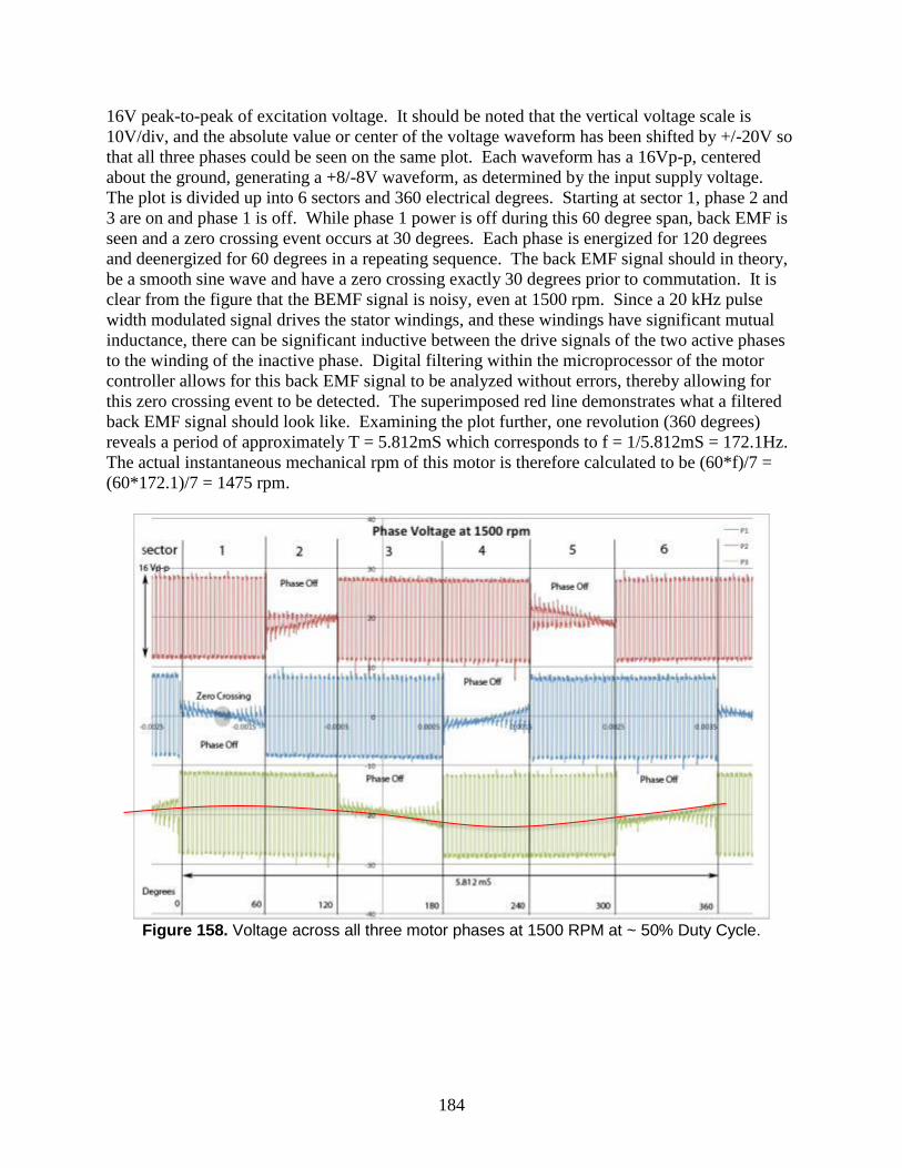
184

16V peak-to-peak of excitation voltage. It should be noted that the vertical voltage scale is

10V/div, and the absolute value or center of the voltage waveform has been shifted by +/-20V so

that all three phases could be seen on the same plot. Each waveform has a 16Vp-p, centered

about the ground, generating a +8/-8V waveform, as determined by the input supply voltage.

The plot is divided up into 6 sectors and 360 electrical degrees. Starting at sector 1, phase 2 and

3 are on and phase 1 is off. While phase 1 power is off during this 60 degree span, back EMF is

seen and a zero crossing event occurs at 30 degrees. Each phase is energized for 120 degrees

and deenergized for 60 degrees in a repeating sequence. The back EMF signal should in theory,

be a smooth sine wave and have a zero crossing exactly 30 degrees prior to commutation. It is

clear from the figure that the BEMF signal is noisy, even at 1500 rpm. Since a 20 kHz pulse

width modulated signal drives the stator windings, and these windings have significant mutual

inductance, there can be significant inductive between the drive signals of the two active phases

to the winding of the inactive phase. Digital filtering within the microprocessor of the motor

controller allows for this back EMF signal to be analyzed without errors, thereby allowing for

this zero crossing event to be detected. The superimposed red line demonstrates what a filtered

back EMF signal should look like. Examining the plot further, one revolution (360 degrees)

reveals a period of approximately T = 5.812mS which corresponds to f = 1/5.812mS = 172.1Hz.

The actual instantaneous mechanical rpm of this motor is therefore calculated to be (60*f)/7 =

(60*172.1)/7 = 1475 rpm.

Figure 158. Voltage across all three motor phases at 1500 RPM at ~ 50% Duty Cycle.

185

Figure 159. Voltage across all three motor phases at full power.

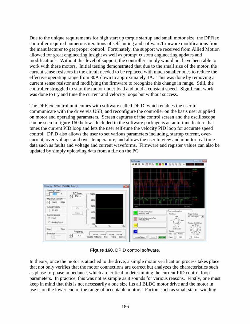
186

Due to the unique requirements for high start up torque startup and small motor size, the DPFlex

controller required numerous iterations of self-tuning and software/firmware modifications from

the manufacturer to get proper control. Fortunately, the support we received from Allied Motion

allowed for great engineering insight as well as prompt custom engineering updates and

modifications. Without this level of support, the controller simply would not have been able to

work with these motors. Initial testing demonstrated that due to the small size of the motor, the

current sense resistors in the circuit needed to be replaced with much smaller ones to reduce the

effective operating range from 30A down to approximately 3A. This was done by removing a

current sense resistor and modifying the firmware to recognize this change in range. Still, the

controller struggled to start the motor under load and hold a constant speed. Significant work

was done to try and tune the current and velocity loops but without success.

The DPFlex control unit comes with software called DP.D, which enables the user to

communicate with the drive via USB, and reconfigure the controller on the basis user supplied

on motor and operating parameters. Screen captures of the control screen and the oscilloscope

can be seen in figure 160 below. Included in the software package is an auto-tune feature that

tunes the current PID loop and lets the user self-tune the velocity PID loop for accurate speed

control. DP.D also allows the user to set various parameters including, startup current, over-

current, over-voltage, and over-temperature, and allows the user to view and monitor real time

data such as faults and voltage and current waveforms. Firmware and register values can also be

updated by simply uploading data from a file on the PC.

Figure 160. DP.D control software.

In theory, once the motor is attached to the drive, a simple motor verification process takes place

that not only verifies that the motor connections are correct but analyzes the characteristics such

as phase-to-phase impedance, which are critical in determining the current PID control loop

parameters. In practice, this was not as simple as it sounds for various reasons. Firstly, one must

keep in mind that this is not necessarily a one size fits all BLDC motor drive and the motor in

use is on the lower end of the range of acceptable motors. Factors such as small stator winding

187

wire gauge, on the order of 30-36AWG have several implications. This translates into phase-to-

phase inductance values on the order of 100 to 800 H and resistance values on the order of 2 to

8 ohms. The datasheet clearly states that the motor have a minimum inductance of 100 H and a

motor time constant = L/R > 150 S. These particular motors typically have a time constant in

the range of 100 to 200 S. Small time constants mean that the motor can respond very quickly

to small changes in current drive, sometimes too quickly for the controller to respond. These

small inductance values coupled with a very limited amount of current of typically less than 3

amps make it difficult for the motor to start under heavy loads.

After numerous conversations with Allied Motion, it was suggested that the physical properties

of the motors and the inertial and frictional loads of the setup be looked at more closely. Data

from two differently wound stators were obtained and motor constants were calculated and

summarized in the tables below. Motor voltage (Kv), motor torque (Kt) and motor back-EMF

(Ke) constants have been calculated and are listed below. Theoretical torque values are shown as

function of maximum current through the windings based on either resistance to voltage

limitations or drive current limits set at 3 Amps. In the case of the 32AWG, for example, rotor

torque is limited by the controller, and not the resistance of the windings. In the case of the

34AWG stator, with increased resistance, the buss voltage becomes a current limiting factor.

Theoretical torque using the 16V driver is calculated to be approximately 25mN-m for both

motors, which is very close to the required starting torque of the impeller. In practice, using the

hysteresis brake as shown in figure 161, these motors both were able to start into a maximum of

about 18 mN-m and maintain speed at that given load.

Two versions of the DPFlex motor control were used, first a 30V/30A (PN 11-F0024-30) was

implemented into a test bed setup using a hysteresis brake as shown in Figure 161. Later a

16V/30A (PN 11-F0012-30) version was eventually found to be a better choice. Numerous tests

were made using the 30V version with various motor configurations in an attempt to match the

best motor speed/torque values with the controller. Using the Ke motor back-EMF constant, the

minimum speed for adequate BEMF voltage is calculated. The controller will not go into closed

velocity loop control until this minimum value has been reached. It was proven that the 30V

version was simply not compatible with our small motors primarily because as was later brought

to our attention, the BEMF voltage required by the controller needs to be at a minimum of 4% of

the buss voltage. In the 30V case, that translates into 1.2V and .64V for the 16V model.

Looking at the charts below, it can be seen that both motors under the 30V controller require a

minimum of at least 1000RPM to produce this voltage. The motor simply cannot accelerate to

this rpm in the given time frame and times out, thus shutting the controller off. The 16V

controller on the other hand requires a minimum speed well below 1000 RPM. Loaded motors

are thus able to accelerate to this minimum speed and go into closed loop before timeout occurs.

188

Figure 161. Motor mounted on hysteresis brake test bed.

Hysteresis Brake

Assembly

3 Phase BLDC

Motor

189

#34AWG with 85 Turns/pole at 2400 RPM

Rp-p = 7.93 Ohm

Phase to Neutral Voltage (VRMS) Kv (rpm/volt) Kt (mN-M/A) Ke (mV/RPM)

2.87 836 12.0 1.20

2.91 824 12.1 1.21

2.97 810 12.4 1.24

Max Current @30V Max Current @16V(A) Max Torque @30V Max Torque @16V

Controller Limited Winding limited mN-m mN-m

3.00 2.02 35.9 24.1

Minimum RPM to meet minimum Reqd BEMF

30V control 16V control

1000 535

#32AWG with 55 Turns/pole at 3522 RPM Rp-p = 3.18 Ohm

Phase to Neutral Voltage (VRMS) Kv (rpm/volt) Kt (mN-M/A) Ke (mV/RPM)

2.79 1260 7.92 0.792

2.85 1240 8.08 0.808

2.77 1270 7.86 0.786

Max Current @30V(A) Max Current @16V(A) Max Torque

Controller Limited

mN-m

3.00 3.00 23.8

Minimum RPM to meet minimum Reqd BEMF

30V control (RPM) 16V control (RPM)

1510 808

The 16 volt version of the DPFlex controller was demonstrated with a 32AWG custom (Sandia

wound) stator in a standalone control box with external setpoint control (See Figure 162).

Velocity control loop tuning is required every time a different impeller with different inertial and

dynamic loads and/or a different motor are placed on the system. Once tuned, these parameters

can be saved on a PC and later uploaded into the device for future use. Once the correct

parameters have been loaded into the controller, computer control is no longer required and the

user may operate the cooler using the custom Sandia made control box, which incorporates a

power supply, on/off switch and a potentiometer to control the setpoint.

190

Figure 162. DPflex user control box.

6.2.2. Custom VVVF Motor Controller Development

The VVVF motor control option differs from the COTS controller in that it does not use

information gained by sensing the motor’s back EMF to coordinate and control the motor or

utilize any advanced starting algorithms. The VVVF controller instead operates the motor similar

to a synchronous AC motor. The controller produces three voltage waveforms of equal amplitude

with precise phase relationships and ramps the waveform’s frequency from zero hertz to the final

operating electrical frequency in a specified amount of time. The initial voltage amplitude is set

sufficiently large to ensure that no slip occurs between the magnetic fields of the rotor and stator

when the motor is started. Once started, the voltage amplitude is adjusted under PID control to a

value that ensures phase lock without overdriving the motor.

The implementation of such a closed-loop control system is extremely importance form the

standpoint of motor efficiency. For example, consider a permanent magnet synchronous motor

with a stator winding resistance of 5 ohms per phase that consumes 2.5 W of electrical power,

and has a back emf of 5.0 V rms at 2500 rpm under typical operating conditioning conditions.

Now consider the consequences of operating at an over-voltage of 2.0 V rms (e.g. 7.0 V rms

excitation instead of 5.0 V rms excitation). A first order analysis indicates that each phase is

subject to an additional power dissipation of (2.0 V rms)2/(5.0 ohms) = 0.80 W per phase,

resulting in 2.4 W of additional resistive heating for the three motor phases. In practice however,

the resulting temperature rise of the stator winding elevates additional resistive losses

considerably, such that the total power delivered to the motor might be 5.5 W; the excess power

dissipation effect has a greater than quadratic dependence on excitation over-voltage. Thus in

this example, operation at 140% of nominal excitation voltage has more than doubled power

consumption.

Open-loop control of stator excitation voltage (e.g. based on operating rpm) is not tractable

because such an open-loop system must operate with a substantial overvoltage margin to avoid

191

stalling due to disturbances, changes in operating temperature (stator winding resistance) because

of variations in thermal loading by the CPU or other device being cooled, and because open-loop

operation in the vicinity of the “drop-out voltage” (where insufficient torque causes rotor

slippage, loss of synchronism, and immediate stalling) tends to be erratic, and is characterized by

high torque ripple.

On the other hand, all of these problems are solved by implementing PID closed-loop of rotor

torque angle, wherein rotor angle is inferred from a sensing coil located in the vicinity of the

circular rotor magnet array (but with negligible coupling to the time-varying magnetic field

generated by the stator windings). Such a passive inductive sensor is extremely inexpensive and

compact, and generates a low-impedance signal that can be easily amplified and filtered to

provide a large-amplitude sinusoidal signal that is synchronous with rotor phase angle.

The other critically important consideration in this application is brushless motor noise, which is

very sensitive the fidelity of the waveform used for excitation. This stems from the fact that pure

sinusoidal excitation of a 3-phase motor generates nominally zero torque ripple. But

commercially available brushless motor controllers for small motors invariably use rectangular,

trapezoidal, and/or pulse width modulated (PWM) waveforms that are rich in harmonics. Such

harmonics generate angular vibration rather than angular rotation, and because of nonlinearities,

difference frequencies between higher harmonics further contribute to vibrational excitation.

Moreover, such vibrations can excite mechanical resonances in the finned heat-sink-impeller,

generating audible ringing. As a result, the acoustic noise generated by early version Sandia

Coolers based on commercially available small brushless motor controllers was objectionable,

both from the standpoint of amplitude and tonality (highly tonal sounds are perceived as more

annoying than acoustic emissions having a broad frequency spectrum).

The solution to this noise problem is pure sinusoidal 3-phase excitation, and sinusoidal excitation

has the further benefit of maximizing motor efficiency. Unfortunately, it is not a simple matter to

a design a circuit to generate a sinusoidal 3-phase waveform that can varied over a large range in

amplitude, and an extremely large range in frequency (three decades) with high output power

and high electrical efficiency. For example, the classic analog phase-shift oscillator can be used

in conjunction with appropriate limiting circuitry to generate three sinusoidal phase winding

currents with the desired 0/60/120 degree phase relationship, but is very difficult to tune over a

wide range in frequency range. Moreover, high fidelity amplification of such signals using power

transistors biased to operate between cut off and saturation invariably results in high power

dissipation, and consequently, low efficiency.

To generate such signals at high power and high efficiency, some form of Class D amplification

must be used, wherein the high power output pass transistors are switched rapidly between

saturation (fully conducting) and cut off (fully blocking) and spend very little time operating in

the linear region between. This raises the question of what type of waveform, when processed by

a Class D amplifier and applied to the stator windings the brushless motor, adequately

approximates a true sinusoid from the standpoint of motor noise and motor efficiency.

192

6.2.2.1. Waveform Selection

The first step in the development process was determining the waveform shape for the controller.

The waveform shape dictates several important factors such as audible noise generation,

efficiency, performance, and robustness. When selecting the waveform, it is also important to

consider the ease of producing the waveform using electronics, the cost to do so, and the size of

the electronics package required to produce the drive waveforms.

The setup shown in Figure 163 was developed to determine the characteristics mentioned above

for various types of waveforms. The test setup consisted of a custom software package (Figure

164) capable of generating an assortment of different waveforms that we were interested in

testing. The waveforms were uploaded to an arbitrary waveform generator that produced the

voltage waveforms for each of the phases of the motor. The waveforms were amplified, routed

through a switch, and connected to their corresponding phases of the motor. The motor shaft was

connected to a hysteresis brake that supplied a known amount of torque and was used to simulate

the startup and operating torques.

Figure 163: VVVF test setup.

193

Figure 164: Custom VVVF Motor Control Simulator.

6.2.2.2. Startup Performance

The first set of tests focused on determining if the VVVF could be used to reliably start the

impeller while resting on the baseplate. Two waveform characteristics, initial voltage and ramp

rate, were initially identified as the key parameters for achieving a successful startup. The test

setup allowed us to quickly adjust these parameters and identify the values that worked best.

The value of the initial waveform voltage was determined to be tradeoff between starting torque

and overheating of the windings. As stated earlier, the initial voltage must be set large enough to

produce sufficient torque to overcome the static starting friction and inertia of the impeller.

However, it was observed that too large of an initial voltage resulted in overheating of the

windings and during the course of ramp up. An IR thermometer was used during all tests to

monitor stator winding temperature.

The motor generates a back EMF that is proportional to the motor speed that opposes the

excitation voltage. Thus back EMF reduces the effective voltage applied to the series impedance

of the stator windings, and in part governs the amount of torque generated by the rotor. The

amount of torque generated by the rotor also has a significant dependence on stator winding

temperature (i.e. series resistance). The custom motor controller software permitted the

excitation voltage schedule during start up to varied ensure high initial start up torque without

subsequent overheating.

The rpm ramp rate of the was selected to limit the amount of rotor torque required for rotor

acceleration (so that most of the rotor torque during start up is available for overcoming contact

friction), while still accelerating the rotor to its operating rpm in a reasonable period of time (e.g.

20 seconds). The ideal ramp rate was identified to be in the neighborhood of 100 rpm/second.

194

The testing concluded that, with the proper choice of ramp rate and initial voltage, a VVVF

motor controller could be used to reliably start the impeller from a dead stop while resting on the

baseplate.

6.2.2.3. Circuit Design

As described earlier, a comprehensive description of the VVVF controller under development

will be provided in a subsequent report.

7. CONCLUSIONS AND RECOMMENDATIONS

This report described work performed primarily in FY13 to develop the V5 version of the Sandia

Cooler, a breakthrough technology for air-cooled heat exchangers that was developed at Sandia

National Laboratories. The primary goal was to fabricate, assemble and demonstrate ten

prototype systems. The components for these systems have largely been fabricated and are

currently being assembled into demonstration units. These prototypes will consist of the V5

impeller, vapor chamber baseplates, i-Kote anti-friction coating and a new air bearing design. All

of the impellers have been machined and half have been coated. Nine out of ten baseplates are

complete and ready for assembly. All of the motor mounts are finished and several stators have

been wound. The first full assembly is currently being evaluated with the prototype VVVF

controller. All ten devices are scheduled for completion in January 2014.

The V5 impeller designed in FY12 was found to be the best of three designs that were

extensively characterized over the course of the project. Of the other two impellers, the V4

impeller designed in FY11 was developed for a proof-of-concept demonstration of the

technology. The V6 impeller designed in FY13 was the result of a parameter optimization study

to improve on the V5 design using the new CFD models developed this year. However,

performance tests indicated that the V5 impeller had the best combination of pressure-flow

capability and low thermal resistance that outweighed the higher shaft power required for a given

speed. While both V5 and V6 impellers improved on the V4 design, slightly better performance

and comparatively easier fabrication made V5 the choice over V6 for the final demonstration

units.

To characterize the performance of the Sandia Cooler, a number of different test stands were

developed. Two test stands were used to measure the thermal resistance of the impellers: one that

uses a thermal decay method to infer thermal resistance, and one that uses a steady-state method

to more directly measure thermal resistance. Results from these tests showed that the V5 design

provided the lowest thermal resistance at a given speed resulting in a ~30% decrease over the V4

design. At 2500 rpm, the thermal resistance of the V5 impeller is 0.084 °C/W.

Another test stand was assembled to characterize the impeller P-Q curves. All three impellers

produced about the same static pressures, but the V5 provided higher flow rates throughout the

range of pressures and speeds. At 2500 rpm, the V5 impeller can produce a static pressure of

about 65 Pa and a free delivery air flow rate of 1550 lpm.

The test stand assembled to measure the impeller torque used the decay in impeller speed over

time to infer the torque on the impeller at each speed. The V5 impeller required the highest

195

torque at a given speed, 10-15% higher than the V6 impeller and about 40% higher than V4. At

2500 rpm the V5 impeller requires about 0.011 N-m of torque and 2.6W of shaft power.

Noise measurements of the impellers indicated they were fairly similar to each other, although

the V4 impeller was slightly quieter than V5 and V6. All three, however, were noticeably louder

than commercial CPU coolers and produced sound levels between 20 to 30 dBa higher than

ambient at speeds between 2000 rpm and 4000 rpm. Since silent operation is one of the keynote

features of the Sandia Cooler, these results were disappointing. But in recent months, the

customized VVVF motor controller incorporating PDM sinusoidal excitation and PID control of

rotor torque angle has been shown to address both the problem of motor noise and fin vibration,

resulting in a drastic decrease in audible noise. Finally, a more complete study of the aero-

acoustics of the impeller, including coupled CFD-acoustics modeling, could be carried out to

develop a fin design that produces lower noise. However, this could be a significant R&D effort

that is beyond the scope of the current Sandia Cooler project.

Vapor chamber baseplates for the demonstration units fabricated by Thermacore were also tested

for thermal resistance using yet another Sandia-developed experimental apparatus. Both a vapor

chamber and a solid copper baseplate were tested and the results showed that the vapor chamber

had a thermal resistance that was approximately 0.01 °C/W. This was a significant improvement

over the thermal resistance of the copper baseplate (0.04 °C/W).

The spiral groove air bearing that levitates the impeller above the baseplate was optimized for

maximum stiffness at a 10 micron gap with minimal pre-load. The final design has grooves that

are 40% thinner than the V5 design and slightly deeper at 35 m. The resulting lift (~7N) and

stiffness (0.6 N/m) at a 10 m gap falls between the V4 and V5 designs, but the groove pattern

introduces less thermal resistance than either. The thermal resistance of the air bearing was

characterized using the test stand used for the baseplate characterization. The thermal resistance

of the air bearing gap was found to be independent of the rotation speed, up to 4000 rpm, and

approximately equal to the resistance of a stagnant gas layer. At 10 m, the thermal resistance of

the air gap is about 0.05 °C/W. The use of smaller air gap distances will likely be viable option

at lower operating rpm (e.g. a 5 m gap distance at 2000 rpm).

After considerable research and extensive testing, i-Kote was chosen as the anti-friction coating

used to reduce the static and sliding friction and minimize galling and wear between the impeller

and baseplate. i-Kote, a proprietary mixture of molybdenum disulfide and graphite patented by

Tribilogix, was evaluated on a test stand using surrogate parts made to match the impeller and

baseplate. Start-stop cycles consisting of starting from rest, ramping to a nominal 1000rpm in

10s, and cutting power to the motor for 10s to bring the impeller to rest were carried out with a

5N pre-load. The i-Kote coating survived 15,000 of these cycles with low static and sliding

friction torque.

A custom VVVF motor controller has been developed to control the brushless, sensorless DC motor used to spin the Sandia Cooler impeller. The motor, based on the Motrolfly DM2203 brushless motor, is comprised of a 12 pole stator and a rotor consisting of 14 NdFeB rare earth magnets to drive the impeller at speeds up to 5000rpm. The custom controller is required to produce the relatively large initial torque to overcome the friction between the

impeller and baseplate experienced at startup, accelerate the large moment of inertia of the

196

impeller, provide high brushless motor efficiency (typically 70%), and very low noise operation,

all without use of Hall effect sensors or rotary optical encoders.

The VVVF controller uses a 4 kbit PDM waveform to drive the phases of the motor which is

essentially imperceptible to the human ear. The waveform frequency is ramped from zero hertz

to the desired operating frequency in a specified amount of time using an initial voltage

amplitude high enough that no slip occurs between the magnetic fields of the rotor and stator

when the motor is started. A feedback loop is then used to control the supplied voltage amplitude

to provide maximum motor efficiency and stability. The motor control circuitry is currently

being prototyped and final printed circuit board layout is nearing completion.

Based on the individual measurements of thermal resistance for the impeller, air bearing, and

vapor chamber baseplate, the system thermal resistance will be about 0.15 °C/W operating at

2500 rpm with a 10 m air gap. The shaft power required to overcome the impeller torque and

air gap shearing at this speed is 4.3 W. The VVVF controller has been tested at up to 80%

efficiency which would result in 5.4 W of electrical power. Operating at 3000 rpm with a 5 m

air bearing gap would lower the thermal resistance to 0.11 °C/W, but the electrical power would

increase to 11 W. This performance is achieved in a device with an overall envelope of 4” X 4”

X 1.81” (100 mm X 100 mm X 46 mm).

In addition to prototype development, computational simulation and experimentation were

performed to fully understand the performance characteristics of each of the key aspects of the

design. This work culminated in a parameter and scaling study that has provided a design

framework, including a number of design and analysis tools, for Sandia Cooler development for

applications beyond CPU cooling.

A Mathematica design tool enables rapid geometric parameterization of an impeller with real-

time feedback on the effects of parameter changes. Impeller outer radius, inner radius, fin

height, sweep angle, number of fins, fin width at leading edge, and power law exponent are set

using slider bars. The tool then calculates the surface area of the fins, the entrance and exit width

of the air channels, the area ratio of the air channels, the cross-sectional area of the fins, and the

percentage of the cross-section occupied by the fins.

Designs parameterized using the Mathematica tool were analyzed with CFD simulations to

determine whether an improvement over the V5 impeller could be found. The CFD models were

developed using Ansys CFX and validated with data from the V4 and V5 impellers. The

parameter study was constrained to 4” outer diameter impellers with the inner diameter of the

fins set to 2 inches. Initial runs were completed with variable heights, but the final set had the fin

height set to 1.175”. A range of sweep angles, number of fins, and power law exponents were

explored and the performance of these candidate geometries was compared to the performance of

the V4 and V5 impellers. Overall, 39 different impeller geometries were modeled. The results

indicated that several designs might improve over the thermal resistance of the V5 impeller for

the same power consumption. One of those designs, the V6 impeller, was chosen for fabrication.

Unfortunately, the V6 impeller was not found to be a significant improvement over the V5

impeller based on torque and thermal resistance measurements. Further analysis of the parameter

study results is ongoing to determine if another impeller design may yet improve over V5.

197

In addition to this study, which only considered fin shape, other methods to improve impeller

performance may exist. The preliminary analysis of discontinuous or “interrupted” fins indicated

an improvement over V5 in both thermal resistance and torque at the same rotational speed. This

concept is currently being revisited and may be further developed. Other performance

enhancements may also be investigated in FY14 including surface area enhancements and

boundary layer perturbation.

The second study carried out using the CFD tools examined the performance of impellers scaled

beyond the 4” diameter required for CPU cooling. The goal of this study was to develop insight

and scaling laws for impeller performance based on the CFD results. Initially, a fairly sparse set

of simulations was run given time and resource constraints. The V6 impeller geometry was used

as the baseline with a diameter of 4”, fin height of 1.175”, and speed of 2500 rpm. The impeller

diameter was then scaled by 1.5X with heights at 0.5X, 1X, and 1.5X. Simulations were carried

out for these configurations with rotational speed at 2/3X, 1X, 1.2X, and 2X. Then the impeller

diameter was scaled by 2X with heights at 1X and 2X. These simulations were completed with

rotational speeds at 0.5X, 1X, and 2X. Not all combinations of these scales and speeds were

modeled. Thermal resistance, torque, and air flow rate were extracted from the CFD results for

each case and analyzed. The ultimate result from this analysis was a set of scaling law equations

for impeller performance similar to the more common fan affinity laws. These simple power law

correlations can be used to provide an estimate of the performance of an impeller without the use

of costly CFD simulations.

198

REFERENCES

[1] E.A. Muijderman, Spiral Groove Bearings, Cleaver-Hume Press Ltd., London, 1966.

[2] Wolfram Research, Inc., Mathematica, Version 8.0, Champaign, IL (2010).

[3] S. E. Thompson and S. Parthasarathy, “Moore’s law: the future of Si microelectronics,”

Materials Today, vol. 9, no. 6, pp. 20 – 25, 2006.

[4] W. Krueger and A. Bar-Cohen, “Optimal numerical design of forced convection heat sinks,”

Components and Packaging Technologies, IEEE Transactions on, vol. 27, pp. 417 – 425, June

2004.

[5] Intel, “Intel core i7 processor family for the LGA2011-0 socket: Thermal/mechanical

specification and design guide,” Tech. Rep. Document Number: 326199-001, Intel Corp.,

November 2011.

[6] “International Technology Roadmap for Semiconductors (ITRS).” http://www.itrs.

net/Links/2010ITRS/Home2010.htm, 2009. Accessed: July 29, 2012.

[7] “Broad agency announcement, microtechnologies for air-cooled exchangers (MACE), BAA

08-15,” Tech. Rep., DARPA MTO, 2008. 205

[8] Noctua, “NH-D14.”

http://www.noctua.at/main.php?show=productview&products_id=34&lng=en. Accessed: July 7,

2012.

[9] Koplow, J. P., HEAT EXCHANGER DEVICE AND METHOD FOR HEAT REMOVAL

OR TRANSFER, US Patent # 8,605,438.

[10] Schlichting H., Boundary Layer Theory, McGraw-Hill, New York, 1979.

[11] Cobb, E. C., Saunders, O. A., “Heat Transfer from a rotating disk”, Proceedings of the

Royal Society of London. Series A, Mathematical and Physical Science, 1956.

[12] J. P. Koplow, "A Fundamentally New Approach to Air-cooled Heat Exchangers," Sandia

National Laboratory Report, SAND2010-0258, January 2010.

[13] J. P. Koplow, “Exploration and Development of Air Bearing Heat Exchanger Technology,”

Sandia National Laboratories report, SAND2011-1986, March 2011.

[14] Alcoa QC-10 Aluminum Alloy Datasheet:

http://www.alcoa.com/mill_products/catalog/pdf/QC-10_brochure.pdf, 2010.

199

[15] "Sierra/Solid Mechanics 4.28 User's Guide," Sandia National Laboratories, Albuquerque,

New Mexico 2013.

[16] P. A. Kelly, "Lecture Notes in Solid Mechanics Part II: Engineering Solid Mechanics," ed.

Auckland, New Zealand: University of Auckland.

[17] G. Reese, D. Segalman, M. K. Bhardwaj, K. Alvin, B. Driessen, K. Pierson, and T. Walsh,

"Salinas -User's Notes," Sandia National Laboratories, Albuquerque, NM SAND99-2801,

February 4, 2013.

[18] White, F. M., Fluid Mechanics – 5th

edition, McGraw-Hill, 2003.

[19] H. Hashimoto and M. Ochiai, “Optimization of Groove Geometry for Thrust Air Bearing to

Maximize Bearing Stiffness,” ASME Journal of Tribology 130 (2008)

[20] H. Hashimoto and T. Namba, “Optimization of Groove Geometry for a Thrust Air Bearing

According to Various Objective Functions,” ASME Journal of Tribology 131 (2009)

[21] C. W. Wong, X. Zhang, S. A. Jacobson, and A. H. Epstein, “A Self-Acting Gas Thrust

Bearing for High-Speed Microrotors,” Journal of Microelectromechanical Systems vol. 13, no. 2

(2004) pp. 158-164

[22] Y. Xue and T. A. Stolarski, “Numerical prediction of the performance of gas-lubricated

spiral groove thrust bearings,” Proceedings of the Institution of Mechanical Engineers, Part J:

Journal of Engineering Tribology, vol. 211, no. 2, (1997) pp. 117-127

[23] H.F. Barry and J.P. Binkelman, “MoS2 lubrication of various metals,” Lubrication Eng., 22

(1966) 139-145.

[24] K.J. Wahl and I.L. Singer, “Material transfer processes in MoS2,” Tribology Letters 1

(1995) 59-66.

[25] L.E. Seitzman, R.N. Bolster, I.L. Singer, “Effects of temperature and ion-to-atom ratio on

the orientation of IBAD MoS2 coatings,” Thin Solid Films 260 (1995) 143-147.

[26] T.W. Scharf, P.G. Kotula, S.V. Prasad, “Friction and wear mechanisms in MoS2/Sb2O3/Au

nanocomposite coatings,” Acta Materialia 58 (2010) 4100–4109.

200

201

DISTRIBUTION

1 MS0899 Technical Library 9536 (electronic copy)

1 MS0359 D. Chavez, LDRD Office 1911

202