
Development of Scientific Applications with the Mobile Robot Programming Toolkit
114
Development of Scientific Applications with the Mobile Robot Programming Toolkit The MRPT reference book by Jose Luis Blanco Claraco Machine Perception and Intelligent Robotics Laboratory University of Malaga Version: October 25, 2010
-
Upload
sixtogerardo -
Category
Documents
-
view
45 -
download
2
Transcript of Development of Scientific Applications with the Mobile Robot Programming Toolkit

Development of ScientificApplications with the MobileRobot Programming Toolkit
The MRPT reference book
by Jose Luis Blanco Claraco
Machine Perception and Intelligent Robotics Laboratory
University of Malaga
Version: October 25, 2010
Familia
Text box
http://www.mrpt.org/downloads/mrpt-book.pdf

ii
Copyright c© 2008-2010 Jose Luis Blanco Claraco and contributors.All rights reserved.
Permission is granted to copy, distribute verbatim copies and print this docu-
ment, but changing or publishing without a written permission from the authors is
not allowed.

Note:
This book is uncompleted. The most up-to-date version will always be availableonline at:
http://www.mrpt.org/The MRPT book
Recent updates:
• Oct 25, 2010: Written chapters §5 and §11.
• Aug 10, 2009: Added description of resampling schemes (§23.3).
• Apr 21, 2009: Updated to MRPT 0.7.0. Added sections on: fixed-size ma-trixes (§7.1.2), metric maps (§19), file formats (§4).

iv

Contents
I First steps 1
1 Introduction 3
1.1 Why a new library? . . . . . . . . . . . . . . . . . . . . . . . 3
1.2 What is MRPT? . . . . . . . . . . . . . . . . . . . . . . . . . 3
1.3 What is this book about? . . . . . . . . . . . . . . . . . . . . 4
1.4 What is this book not about? . . . . . . . . . . . . . . . . . . 4
1.5 How much does it cost? . . . . . . . . . . . . . . . . . . . . . 5
1.6 OS restrictions . . . . . . . . . . . . . . . . . . . . . . . . . . 5
1.7 Robotic software architectures . . . . . . . . . . . . . . . . . . 6
2 Compiling 7
2.1 Binary distributions . . . . . . . . . . . . . . . . . . . . . . . 7
2.2 Prerequisites . . . . . . . . . . . . . . . . . . . . . . . . . . . 8
2.2.1 GNU/Linux . . . . . . . . . . . . . . . . . . . . . . . . 8
2.2.2 Windows . . . . . . . . . . . . . . . . . . . . . . . . . 10
2.3 Compiling . . . . . . . . . . . . . . . . . . . . . . . . . . . . . 10
2.4 Building options . . . . . . . . . . . . . . . . . . . . . . . . . 10
II User guide 11
3 Applications 13
3.1 pf-localization . . . . . . . . . . . . . . . . . . . . . . . . . . . 13
3.1.1 Description . . . . . . . . . . . . . . . . . . . . . . . . 13
3.1.2 Usage . . . . . . . . . . . . . . . . . . . . . . . . . . . 13
3.1.3 Example configuration file . . . . . . . . . . . . . . . . 13
3.2 RawLogViewer . . . . . . . . . . . . . . . . . . . . . . . . . . 14
3.2.1 Description . . . . . . . . . . . . . . . . . . . . . . . . 14
3.2.2 Usage . . . . . . . . . . . . . . . . . . . . . . . . . . . 14
v

vi CONTENTS
3.3 rbpf-slam . . . . . . . . . . . . . . . . . . . . . . . . . . . . . 15
3.3.1 Description . . . . . . . . . . . . . . . . . . . . . . . . 15
3.3.2 Usage . . . . . . . . . . . . . . . . . . . . . . . . . . . 15
3.3.3 Example configuration file . . . . . . . . . . . . . . . . 15
3.4 rawlog-grabber . . . . . . . . . . . . . . . . . . . . . . . . . . 16
3.4.1 Description . . . . . . . . . . . . . . . . . . . . . . . . 16
3.4.2 Usage . . . . . . . . . . . . . . . . . . . . . . . . . . . 16
3.4.3 Configuration files . . . . . . . . . . . . . . . . . . . . 16
4 File formats 19
III Programming guide 21
5 The libraries 23
5.1 Introduction . . . . . . . . . . . . . . . . . . . . . . . . . . . . 23
5.2 Libraries summary . . . . . . . . . . . . . . . . . . . . . . . . 23
5.2.1 mrpt-base . . . . . . . . . . . . . . . . . . . . . . . . . 23
5.2.2 mrpt-opengl . . . . . . . . . . . . . . . . . . . . . . . . 27
5.2.3 mrpt-bayes . . . . . . . . . . . . . . . . . . . . . . . . 27
5.2.4 mrpt-gui . . . . . . . . . . . . . . . . . . . . . . . . . . 27
5.2.5 mrpt-obs . . . . . . . . . . . . . . . . . . . . . . . . . 27
5.2.6 mrpt-scanmatching . . . . . . . . . . . . . . . . . . . . 28
5.2.7 mrpt-topography . . . . . . . . . . . . . . . . . . . . . 28
5.2.8 mrpt-hwdrivers . . . . . . . . . . . . . . . . . . . . . . 28
5.2.9 mrpt-maps . . . . . . . . . . . . . . . . . . . . . . . . 29
5.2.10 mrpt-vision . . . . . . . . . . . . . . . . . . . . . . . . 29
5.2.11 mrpt-slam . . . . . . . . . . . . . . . . . . . . . . . . . 29
5.2.12 mrpt-reactivenav . . . . . . . . . . . . . . . . . . . . . 30
5.2.13 mrpt-hmtslam . . . . . . . . . . . . . . . . . . . . . . 30
5.2.14 mrpt-detectors . . . . . . . . . . . . . . . . . . . . . . 30
6 Your first MRPT program 31
6.1 Source files . . . . . . . . . . . . . . . . . . . . . . . . . . . . 32
6.2 The CMake project file . . . . . . . . . . . . . . . . . . . . . . 33
6.3 Generating the native projects . . . . . . . . . . . . . . . . . 34
6.4 Compile . . . . . . . . . . . . . . . . . . . . . . . . . . . . . . 34
6.5 Summary . . . . . . . . . . . . . . . . . . . . . . . . . . . . . 34
CONTENTS vii
7 Linear algebra 35
7.1 Matrices . . . . . . . . . . . . . . . . . . . . . . . . . . . . . . 35
7.1.1 Declaration . . . . . . . . . . . . . . . . . . . . . . . . 35
7.1.2 Fixed-size matrices . . . . . . . . . . . . . . . . . . . . 37
7.1.3 Storage in files . . . . . . . . . . . . . . . . . . . . . . 37
7.2 Vectors . . . . . . . . . . . . . . . . . . . . . . . . . . . . . . 37
7.2.1 Declaration . . . . . . . . . . . . . . . . . . . . . . . . 37
7.2.2 Resizing . . . . . . . . . . . . . . . . . . . . . . . . . . 38
7.2.3 Storage in files . . . . . . . . . . . . . . . . . . . . . . 38
7.3 Basic operations . . . . . . . . . . . . . . . . . . . . . . . . . 39
7.4 Optimized matrix operations . . . . . . . . . . . . . . . . . . 40
7.5 Text output . . . . . . . . . . . . . . . . . . . . . . . . . . . . 41
7.6 matrices manipulation . . . . . . . . . . . . . . . . . . . . . . 41
7.6.1 Extracting a submatrix . . . . . . . . . . . . . . . . . 41
7.6.2 Extracting a vector from a matrix . . . . . . . . . . . 41
7.6.3 Building a matrix from parts . . . . . . . . . . . . . . 42
7.7 Matrix decomposition . . . . . . . . . . . . . . . . . . . . . . 42
8 Mathematical algorithms 43
8.1 Fourier Transform (FFT) . . . . . . . . . . . . . . . . . . . . 43
8.2 Statistics . . . . . . . . . . . . . . . . . . . . . . . . . . . . . 43
8.3 Spline interpolation . . . . . . . . . . . . . . . . . . . . . . . . 43
8.4 Spectral graph partitioning . . . . . . . . . . . . . . . . . . . 43
8.5 Quaternions . . . . . . . . . . . . . . . . . . . . . . . . . . . . 43
8.6 Geometry functions . . . . . . . . . . . . . . . . . . . . . . . . 43
8.7 Numeric Jacobian estimation . . . . . . . . . . . . . . . . . . 43
9 3D geometry 45
9.1 Introduction . . . . . . . . . . . . . . . . . . . . . . . . . . . . 45
9.2 Homogeneous coordinates geometry . . . . . . . . . . . . . . 45
9.3 Geometry elements in MRPT . . . . . . . . . . . . . . . . . . 45
9.3.1 2D points . . . . . . . . . . . . . . . . . . . . . . . . . 45
9.3.2 3D points . . . . . . . . . . . . . . . . . . . . . . . . . 45
9.3.3 2D poses . . . . . . . . . . . . . . . . . . . . . . . . . 45
9.3.4 3D poses . . . . . . . . . . . . . . . . . . . . . . . . . 45
10 Serialization 49
10.1 The problem of persistence . . . . . . . . . . . . . . . . . . . 49
10.2 Approach used in MRPT . . . . . . . . . . . . . . . . . . . . 49
10.3 Run-time class identification . . . . . . . . . . . . . . . . . . . 51

viii CONTENTS
10.4 Writing new serializable classes . . . . . . . . . . . . . . . . . 52
10.5 Serializing STL containers . . . . . . . . . . . . . . . . . . . . 52
11 Smart Pointers 53
11.1 Overview of memory management . . . . . . . . . . . . . . . 53
11.2 Class hierarchy . . . . . . . . . . . . . . . . . . . . . . . . . . 56
11.3 Handling smart pointers . . . . . . . . . . . . . . . . . . . . . 57
11.3.1 The Create() class factory . . . . . . . . . . . . . . . 57
11.3.2 Testing for empty smart pointers . . . . . . . . . . . . 58
11.3.3 Making multiple aliases . . . . . . . . . . . . . . . . . 59
11.3.4 The clear() method . . . . . . . . . . . . . . . . . . 60
11.3.5 The clear unique() method . . . . . . . . . . . . . . 61
11.3.6 The make unique() method . . . . . . . . . . . . . . . 61
11.3.7 Creating from dynamic memory . . . . . . . . . . . . 62
11.3.8 Never create from stack-allocated memory . . . . . . . 62
12 Images 63
12.1 The central class for images . . . . . . . . . . . . . . . . . . . 63
12.2 Basic image operations . . . . . . . . . . . . . . . . . . . . . . 63
12.3 Feature extraction . . . . . . . . . . . . . . . . . . . . . . . . 63
12.4 SIFT descriptors . . . . . . . . . . . . . . . . . . . . . . . . . 63
13 Rawlog files (datasets) 65
13.1 Format #1: A Bayesian filter-friendly file format . . . . . . . 65
13.1.1 Description . . . . . . . . . . . . . . . . . . . . . . . . 65
13.1.2 Actual contents of a ”.rawlog” file in this format . . . 66
13.2 Format #2: An timestamp-ordered sequence of observations . 66
13.2.1 Description . . . . . . . . . . . . . . . . . . . . . . . . 66
13.2.2 Actual contents of a ”.rawlog” file in this format . . . 66
13.3 Compression of rawlog files . . . . . . . . . . . . . . . . . . . 66
13.4 Generating Rawlog files . . . . . . . . . . . . . . . . . . . . . 67
13.5 Reading Rawlog files . . . . . . . . . . . . . . . . . . . . . . . 68
13.5.1 Option A: Streaming from the file . . . . . . . . . . . 68
13.5.2 Option B: Read at once . . . . . . . . . . . . . . . . . 68
14 GUI classes 69
14.1 Windows from console programs . . . . . . . . . . . . . . . . 69
14.2 Bitmapped graphics . . . . . . . . . . . . . . . . . . . . . . . 69
14.3 3D rendered graphics . . . . . . . . . . . . . . . . . . . . . . . 69
14.4 2D vectorial plots . . . . . . . . . . . . . . . . . . . . . . . . . 69

CONTENTS ix
15 OS Abstraction Layer 71
15.1 Cross platform Support . . . . . . . . . . . . . . . . . . . . . 71
15.2 Function Areas . . . . . . . . . . . . . . . . . . . . . . . . . . 71
15.2.1 Threading . . . . . . . . . . . . . . . . . . . . . . . . . 71
15.2.2 Sockets . . . . . . . . . . . . . . . . . . . . . . . . . . 71
15.2.3 Time and date . . . . . . . . . . . . . . . . . . . . . . 71
15.2.4 String parsing . . . . . . . . . . . . . . . . . . . . . . . 71
15.2.5 Files . . . . . . . . . . . . . . . . . . . . . . . . . . . . 71
16 Probability density functions (pdfs) 73
16.1 Efficient pose sample generator . . . . . . . . . . . . . . . . . 73
17 Random number generators 75
17.1 Generators . . . . . . . . . . . . . . . . . . . . . . . . . . . . 75
17.2 Multiple samples . . . . . . . . . . . . . . . . . . . . . . . . . 75
18 Observations 77
18.1 The generic interface . . . . . . . . . . . . . . . . . . . . . . . 77
18.2 Implemented observations . . . . . . . . . . . . . . . . . . . . 77
18.2.1 Monocular images . . . . . . . . . . . . . . . . . . . . 77
18.2.2 Stereo images . . . . . . . . . . . . . . . . . . . . . . . 77
19 Metric map classes 79
19.1 The generic interface of maps . . . . . . . . . . . . . . . . . . 79
19.2 The “multi-metric map” container . . . . . . . . . . . . . . . 80
19.3 Implemented maps . . . . . . . . . . . . . . . . . . . . . . . . 80
19.4 Configuration block for a multi-metric map . . . . . . . . . . 81
20 Probabilistic Motion Models 83
20.1 Introduction . . . . . . . . . . . . . . . . . . . . . . . . . . . . 83
20.2 Gaussian probabilistic motion model . . . . . . . . . . . . . . 84
20.3 Thrun et al.’s book particle motion model . . . . . . . . . . . 87
21 Sensor Interfaces 89
21.1 Communications . . . . . . . . . . . . . . . . . . . . . . . . . 89
21.1.1 Serial ports . . . . . . . . . . . . . . . . . . . . . . . . 89
21.1.2 USB FIFO with FTDI chipset . . . . . . . . . . . . . 90
21.2 Summary of sensors . . . . . . . . . . . . . . . . . . . . . . . 90
21.3 The unified sensor interface . . . . . . . . . . . . . . . . . . . 91
21.4 How rawlog-grabber works . . . . . . . . . . . . . . . . . . . 91

x CONTENTS
22 Kalman filters 9322.1 Introduction . . . . . . . . . . . . . . . . . . . . . . . . . . . . 9322.2 Algorithms . . . . . . . . . . . . . . . . . . . . . . . . . . . . 9322.3 How to implement a problem as a KF . . . . . . . . . . . . . 93
23 Particle filters 9523.1 Introduction . . . . . . . . . . . . . . . . . . . . . . . . . . . . 9523.2 Algorithms . . . . . . . . . . . . . . . . . . . . . . . . . . . . 95
23.2.1 SIR . . . . . . . . . . . . . . . . . . . . . . . . . . . . 9523.2.2 Auxiliary PF . . . . . . . . . . . . . . . . . . . . . . . 9523.2.3 Optimal PF . . . . . . . . . . . . . . . . . . . . . . . . 9523.2.4 Optimal-rejection sampling PF . . . . . . . . . . . . . 95
23.3 Resampling schemes . . . . . . . . . . . . . . . . . . . . . . . 9523.4 Implementation examples . . . . . . . . . . . . . . . . . . . . 100

Listings
6.1 A very simple MPRT program . . . . . . . . . . . . . . . . . 32
xi

xii LISTINGS

Part I
First steps
1


Chapter 1
Introduction
1.1 Why a new library?
Many good scientific programs and programming libraries exist out there.When working with matrices, vectors, and graphical representations, appli-cations like MATLAB or Octave excel. If one’s needs are efficient imagealgorithms under C and C++, OpenCV or VXL are good bets. Otherlibraries provide Bayesian inference or random number generators for a va-riety of probability distributions. When interfacing a variety of sensors, alow-level language as C is probably one of the best ways to develop a ro-bust and efficient implementation. A problem raises only when a projectrequires performing many or all of these tasks under a single and sensibledevelopment framework, since each library declares its own data structures.For example, an image grabbed by an OpenCV program cannot be directlysent to a MATLAB program which detects features.
The development of mobile robotics software is one of those complexprojects that require having at hand a variety of heterogeneous tools: arobot may capture an image from an IEEE1394 camera, extract featuresfrom it, read odometry information from wheel encoders through a serialport, and then fuse all these data using a Kalman filter in matrix form.This contains tasks which range from low-level code (close to hardware), upto linear algebra.
1.2 What is MRPT?
To face the development of such software, we have created the Mobile RobotProgramming Toolkit, or MRPT. This framework acts as the glue that makes
3

4 CHAPTER 1. INTRODUCTION
possible to interconnect several third-party libraries, but it also implementsseveral features on its own.
Despite the name, MRPT currently comprises several generic libraries inC++ which can be perfectly employed for developing any kind of scientificapplication that requires 2D plots, linear algebra, 3D geometry, Bayesianinference, 3D scene animations, or any combination of them.
In the specific field of mobile robotics, MRPT is aimed to help researchersto design and implement algorithms in the areas of Simultaneous Localiza-tion and Mapping (SLAM), computer vision and motion planning (obstacleavoidance). The libraries include classes for easily managing 3D(6D) ge-ometry, probability density functions (pdfs) over many predefined variables(points and poses, landmarks, maps), Bayesian inference (Kalman filters,particle filters), image processing, path planning and obstacle avoidance,3D visualization of all kind of maps (points, occupancy grids, landmarks,...),and “drivers” for a variety of robotic sensors.
1.3 What is this book about?
This document tries to address the needs of two different kinds of readers:
• Firstable, users of MRPT programs. The toolkit is not only acollection of libraries, but also contains some ready-to-use programs.With those applications, a user can record data from a mobile robot,manipulate the logs if needed, and create point or occupancy grid-maps using state-of-the-art algorithms without typing a single line ofsource code.
• Developers. Users who pretend to integrate their own algorithmsinto MRPT or to use it as a layer on which to develop more powerfulapplications or libraries.
Obviously, many readers may fit within both kinds of readers, but forreasons of clarity, this book is structured into two well-differentiated parts.Part II addresses using existing programs, while Part III discusses morein-deep details required for MRPT programmers.
1.4 What is this book not about?
The intention is that this book does not become one of those boring, andnearly useless hard copies of a library reference. This book pretends to
1.5. HOW MUCH DOES IT COST? 5
let a programmer know what is inside MRPT, as a birth-eye-view. Oncehe or she needs to handle any specific class, the reference documentation(created with Doxygen) will be an invaluable tool, and indeed one of ourmain concerns during the development of MRPT has been an extensive andgood reference documentation, which is available online at the MRPT website1.
But before reading that documentation, the programmer should have agross idea of how things are managed within MRPT, and that is preciselythe aim of this book.
1.5 How much does it cost?
MRPT is free software. Free in both senses: you can use it without anycost, and it is an Open Source project. We have released the sources underGNU General Public License 3. Feel free to modify the sources for yourneeds, to the extent allowed by the aforementioned license. If you want tocontribute with patches or bug reports (or even better, bug fixes!), pleasecontact the authors through the forums in http://www.mrpt.org/.
MRPT is releasedunder GNU GPL 3.
Despite its beginnings at the MAPIR Laboratory in the University ofMalaga, several people world-wide have contributed in different ways to itsdevelopment since its release as an Open Source project. We kindly thankeveryone who has helped in any way, and hope more people continue gettinginvolved in the future2.
1.6 OS restrictions
MRPT is designed to be cross-platform. It works under 32bit and 64bitsystems. Thus, the good news is that any user application developed withMRPT and no other OS-dependant API will also become cross-platformwithout any extra effort.
The libraries are daily tested under Windows 32bit and Linux. In theorythey should also work under any POSIX-compatible system equipped witha decent C++ compiler, like Mac OS X, Solaris, BSDs, etc, but all theseplatforms have not been tested yet3.
1http://www.mrpt.org/2The complete list of authors can be checked out online at
http://www.mrpt.org/Authors3An up-to-date list of systems where MRPT has been completely tested can be found
in http://www.mrpt.org/Supported Platforms

6 CHAPTER 1. INTRODUCTION
1.7 Robotic software architectures
MRPT provides several ready-to-use data structures and algorithms whichcan be directly used to build software aimed to be run on a vehicle or robot.In fact, some MRPT applications (e.g. rawlog-grabber) are designed forthis purpose.
However, intelligent robots usually require a much more complex soft-ware than a single application. Robotic software architectures play the roleof splitting the code into independent programs (or “modules”) which, as awhole, comprise the robot software. In such a framework MRPT might bejust a “low-level” library.
A number of publicly available frameworks exist. In our group, we de-veloped the BABEL system [7], available online for download at [8]. Otherdevelopment environments are the Player project [2], MOOS [10] and CAR-MEN [9].

Chapter 2
Compiling
This chapter explains how to compile the MRPT libraries and applications,and also whether a user may instead prefer a pre-compiled version.
If you are sure you prefer (or have to) compile MRPT from sources, skipthe next section and continue with section 2.2.
2.1 Binary distributions
For Windows users, may want to only use existing MRPT applications,so they do not pretend to develop custom programs based on MRPT. Forsuch users, precompiled binary distributions of MRPT exist and perhapsare a better choice than compiling it from sources. These binary packagesalso allow compiling custom MRPT-based programs, but if the user needsa compiler different that Visual Studio C++, MRPT had to be compiledfrom sources. For Linux users, precompiled packages from the repositoriesare recomendable not only for using MRPT applications, but also for devel-opment.
In the case of 32bit Windows XP/Vista/7, binary packages are availablefor download at the main MRPT download page1. There are packages forGNU/Linux for the following distributions:
• Debian (unstable and testing repository).
• Ubuntu (from version 9.04 ).
• Fedora Core (from version 9 ).
1http://www.mrpt.org/downloads/
7

8 CHAPTER 2. COMPILING
All the packages can be installed by executing:$ sudo apt-get install mrpt-apps mrpt-dev mrpt-doc
or manually from synaptic or the appropriate package manager.
2.2 Prerequisites
As with any mid or large-size software collection, MRPT requires someprograms and libraries to be installed in your system before you can compileit. Next sections explain the required steps for each system, but in generalthe main requisites are:
• CMake: A powerful cross-platform build system.
• wxWidgets: An extensive GUI toolkit.
• OpenCV: A widely-used computer vision library.
2.2.1 GNU/Linux
Debian, Ubuntu
Invoke:sudo apt-get install build-essential cmake libwxgtk2.8-dev libwxbase2.8-dbg
libwxgtk2.8-dbg libftdi-dev libglut3-dev libhighgui-dev lib3ds-dev
libboost-program-options-dev
Note that if version 2.8 of wxWidgets is not available in your distribution,it would have to be installed manually.
Fedora
Invoke as root:yum install gcc gcc-c++ make cmake wxGTK-devel opencv-devel freeglut-devel
lib3ds-devel boost-dev
OpenSUSE
Invoke:sudo zypper install make gcc gcc-c++ cmake cmake-gui pkg-config
zlib-devel wxGTK-devel wxGTK-gl libusb-devel freeglut-devel lib3ds-devel
libboost-program-options
Installing OpenCV on OpenSUSE
2.3. COMPILING 9
Source directory
mrpt-0.6.2
src
include
CMakeLists.txt
…
Binary directory
my-mrpt-bin
lib
bin
CMakeCache.txt
…
CMake
MRPTConfig.cmake
…
GCC
Visual Studio
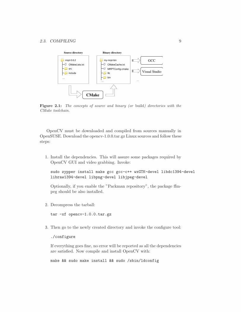
Figure 2.1: The concepts of source and binary (or build) directories with theCMake toolchain.
OpenCV must be downloaded and compiled from sources manually inOpenSUSE. Download the opencv-1.0.0.tar.gz Linux sources and follow thesesteps:
1. Install the dependencies. This will assure some packages required byOpenCV GUI and video grabbing. Invoke:
sudo zypper install make gcc gcc-c++ wxGTK-devel libdc1394-devel
libraw1394-devel libpng-devel libjpeg-devel
Optionally, if you enable the ”Packman repository”, the package ffm-peg should be also installed.
2. Decompress the tarball:
tar -xf opencv-1.0.0.tar.gz
3. Then go to the newly created directory and invoke the configure tool:
./configure
If everything goes fine, no error will be reported as all the dependenciesare satisfied. Now compile and install OpenCV with:
make && sudo make install && sudo /sbin/ldconfig

10 CHAPTER 2. COMPILING
2.2.2 Windows
2.3 Compiling
2.4 Building options
The table summarizes the most important options which can be set throughthe CMake gui (ccmake, cmakesetup, or cmake-gui):
For all platforms/compilers
BUILD_SHARED_LIBS Build static libraries if set to OFF, or dynamic librariesBUILD_EXAMPLES Whether you want to compile all the examples in theMRPT_HAS_BUMBLEBEE To enable integration of the Bumblebee stereo cameraMRPT_ALWAYS_CHECKS_DEBUG If set to ON, additional security checks will be performedMRPT_ALWAYS_CHECKS_DEBUG_MATRICES If set to ON, additional security checks will be performedMRPT_OCCUPANCY_GRID_CELLSIZE Can be either 8 or 16 (bits). The size of each cell in theUSER_EXTRA_CPP_FLAGS You can add here whatever additional flags to be passedMRPT_HAS_ASIAN_FONTS Enables Asian fonts in CCanvas, but increases libraryBUILD_xSENS Whether to use the CMT library for interfacing xSens
Microsoft Visual Studio
CMAKE_MRPT_HAS_VLD Whether to include the Visual Leak Detector (VLK). Default is OFF. If
GNU GCC compiler only
MRPT_ENABLE_LIBSTD_PARALLEL_MODE Enables the experimental GNU libstdc++ parallel mode.MRPT_ENABLE_PROFILING Enables generation of information required for profiling.MRPT_OPTIMIZE_NATIVE Enables optimization for the current architecture (-mtune=nativ
Part II
User guide
11


Chapter 3
Applications
3.1 pf-localization
3.1.1 Description
3.1.2 Usage
3.1.3 Example configuration file
13

14 CHAPTER 3. APPLICATIONS
3.2 RawLogViewer
3.2.1 Description
3.2.2 Usage

3.3. RBPF-SLAM 15
3.3 rbpf-slam
3.3.1 Description
3.3.2 Usage
3.3.3 Example configuration file

16 CHAPTER 3. APPLICATIONS
3.4 rawlog-grabber
3.4.1 Description
rawlog-grabber is a command-line application which uses a generic sensorarchitecture to allow collecting data from a variety of robotic sensors in real-time taking into account the different rates at each sensor may work. Thisprogram creates a thread for each sensor declared in the config file and thensaves the timestamp-ordered observations to a rawlog file - the format ofthose files is explained in Chapter 13.
The valuable utility of this application is to collect datasets from mobilerobots for off-line processing.
3.4.2 Usage
This program is invoked from the command line with:
rawlog -grabber <config_file.ini >
3.4.3 Configuration files
The format of the configuration file is explained in the comments of thefollowing prototype file. Refer also to the directory
MRPT/shared/mrpt/config_files/rawlog-grabber
for more sample files and to the next sections for each specific sensor1.
// ------------------------------------------------------------
// Example config file for rawlog -grabber
//
// ~ The MRPT project ~
// Jose Luis Blanco Claraco (C) 2005 -2008
// ------------------------------------------------------------
// Each section [XXXXX] (except [global ]) sets up a thread in
// the rawlog -grabber standalone application . Each thread collects
// data from one sensor or device , then the main thread groups
// and orders them before streaming everything to a rawlog file.
// The name of the sections can be arbitrary and independent
// of the sensor label. The driver for each sensor is actually
// determined by the field "driver", which must match the name
// of some class in mrpt :: hwdrivers implementing CGenericSensor .
// =======================================================
// Section: Global settings to the application
1However, notice that the most up-to-date documentation will be always available inthe reference of CGenericSensor and their derived classes.

3.4. RAWLOG-GRABBER 17
// =======================================================
[global]
// The prefix can contain a relative or absolute path.
// The final name will be <PREFIX > _date_time.rawlog
rawlog_prefix = dataset
// Milliseconds between thread launches
time_between_launches = 800
// SF =1: Enabled -> Observations will be grouped by time periods.
// SF =0: Disabled -> All the observations are saved independently
// and ordered solely by their timestamps.
use_sensoryframes = 1
// Only if " use_sensoryframes =1": The maximum time difference between
// observations within a single sensory -frame.
SF_max_time_span = 0.25 // seconds
// Observations will be processed at the main thread with this period
GRABBER_PERIOD_MS = 1000 // ms
// Here follow sections for each sensor.
// This is one example for a Hokuyo laser scanner:
// =======================================================
// SENSOR: LASER_2D
// =======================================================
[LASER_2D]
driver = CHokuyoURG
process_rate = 90 ; Hz
sensorLabel = HOKUYO_UTM
pose_x = 0 ; Laser range scaner 3D position
pose_y = 0 ; on the robot (meters)
pose_z = 0.31
pose_yaw = 0 ; Angles in degrees
pose_pitch = 0
pose_roll = 0
COM_port_WIN = COM3
COM_port_LIN = ttyACM0
Specification for: Hokuyo Laser
Specification for: GPS
Specification for: Camera

18 CHAPTER 3. APPLICATIONS
Chapter 4
File formats
In this chapter we summarize the format of MRPT data files which aremanaged by the library itself and some of the applications, sorted by theirmost common file extensions.
• .gridmap (or compressed version .gridmap.gz). A 2D occupancygrid map. These files consist on one COccupancyGridMap2D objectserialized into a binary file. See Chapter 10 for more details on howto serialize and de-serialize objects.
• .ini. Configuration files. The format is plain text, with the filestructured in sections (denoted as [NAME]) and variables within eachsection (denoted by var=value). These files can contain comments,which may start with ; or //.
• .simplemap (or compressed version .simplemap.gz). A collection ofpairs location-observations, from which metric maps can be built eas-ily. The file actually contains a binary serialization of an object ofthe class CSensFrameProbSequence. See Chapter 10 for more de-tails on how to serialize and de-serialize objects. The applicationobservations2map can convert a simplemap file into a set of differentmetric maps (grid maps, point maps,...) and save them to differentfiles. Refer to the documentation of that program for details.
• .rawlog. Robotic datasets. The format of these files is explainedin detail in the Chapter 13. These files can be managed and visual-ized with the application RawlogViewer, or captured from sensors byrawlog-grabber.
19

20 CHAPTER 4. FILE FORMATS

Part III
Programming guide
21

Chapter 5
The libraries
5.1 Introduction
MRPT consists of a set of C++ libraries and a number of ready-to-useapplications. This chapter briefly describes the most interesting part ofMRPT for mobile robotics developers: the libraries.
The large number of C++ templates and classes in MRPT makes ita good idea to split them into a set of libraries or ”modules”, so users canchoose to depend on a part of MRPT only, reducing compile time and futuredependence problems.
The dependence graph in Figure 5.1 shows the currently existing librariesin MRPT. An arrow A→ B means ”A depends on B”. The starred librariesare in an experimental stage and their sources may not be released yet or, ifthey are, changes in the API can be expected in the future without assuringbackward compatibility.
5.2 Libraries summary
5.2.1 mrpt-base
This is the most fundamental library in MRPT, since it provides a vastamount of utilities and OS-abstraction classes upon which the rest of MRPTis built. Here resides critical functionality such as mathematics, linear alge-bra §7.1, serialization §10, smart pointers §11 and multi-threading.
All MRPT classes and functions live within the global namespace mrpt
or one of a series of nested namespaces. This particular library comprisesclasses in a number of different namespaces, briefly described next.
23

24 CHAPTER 5. THE LIBRARIES
Figure 5.1: An overview of the individual libraries within MRPT and their de-pendencies, as of version 0.9.2.
mrpt::poses
This namespace contains a comprehensive collection of geometry-relatedclasses to represent all kind of 2D and 3D geometry transformations indifferent formats (Euler angles, rotation matrices, quaternions), as well asnetworks of pose constrains (as used in GraphSLAM problems).
There are also representations for probability distributions over all ofthese transformations, in a generic way that allow mono and multi-modalGaussians and particle-based representations.
mrpt::utils
The functionality of this namespace includes:
• RTTI (RunTime Type Information): A cross-platform, compiler-independentRTTI system is built around the base class mrpt::utils::CObject.
• Smart pointers: Based on the STLplus library, any class CFoo inher-iting from CObject, automatically has an associated smart pointerclass CFooPtr. MRPT implements advanced smart pointers capable
5.2. LIBRARIES SUMMARY 25
of multi-thread safe usage and smart pointer typecasting with runtimecheck for correct castings (see §11).
• Image handling: The class CImage represents a wrapper around OpenCV’sIplImage data structure, plus extra functionality such as on-the-flyloading of images stored in disk upon first usage (see §12). The in-ternal IplImage is always available so OpenCV functions can be stillused to operate on MRPT images.
• Serialization/Persistence: Object serialization in a simple but powerful(including versioning) format is supported by dozens of MRPT classes,all based on CSerializable.
• Streams: Stream classes (see the base CStream) allow serialization ofMRPT objects. There are classes for transparent GZ-compressed files,sockets, serial ports, etc.
• XML-based databases: Simple databases can be maintained, loadedand saved to files with CSimpleDatabase.
• Name-based argument passing: The structure TParameters can beused to pass a variable number of arguments to functions by name.
• Configuration files: There is one base virtual class (CConfigFileBase)which can be used to read/write configuration files (including basictypes, vectors, matrices,...) transparently from any “configurationsource” (a physical file, a text block created on the fly as a string,etc.).
mrpt::math
MRPT defines a number of generic math containers (described in §7.1),namely:
• Matrices: Dynamic-size and compile-time fixed-size matrices.
• Matrix views: Proxy classes that allow operating on the transpose, apart of, or the diagonal of another matrix as if it was a plain matrixobject.
• Vectors: Dynamic-size vectors, built upon standard STL std::vector.
• Arrays: Fixed-size vectors, just like plain C arrays but with supportfor STL-like iterators and many mathematical operations.

26 CHAPTER 5. THE LIBRARIES
These containers have a number of characteristics in common (e.g. STL-like iterators and typedefs) and can be mixed altogether in operations. Forexample, matrices of any kind can be operated together, a vector can beadded to an array, or the results of a matrix operation stored in a matrixview. Fixed-size containers should be preferred where possible, since theyallow more compile-time optimizations.
Apart from the containers, this namespace contains much more func-tionality:
• A templatized RANSAC algorithm.
• Probability distribution functions.
• Statistics: mean, covariance, covariance of weighted samples, etc...from sets of data.
• A huge amount of geometry-related functions: Lines (TLine3D), planes(TPlane3D), segments, polygons, intersections between them, etc.
• Graph-related stuff: generic directed graphs (CDirectedGraph) andtrees (CDirectedTree).
• PDF transformations (uncertainty propagation): Linearized, unces-ted or MonteCarlo-based propagation of Gaussian distributions of anydimensionality via arbitrary transformation functions.
mrpt::synch
Threading tools can be found here such as critical sections or semaphores.
mrpt::system
Here can be found functions for filesystem managing, watching directories,creating and handling threads in an OS-independent way, etc.
mrpt::compress
This namespace contains the methods needed to compress and decompresswith the GZip algorithm, independently of whether the zlib library exists inthe system or not.
5.2. LIBRARIES SUMMARY 27
5.2.2 mrpt-opengl
This library defines 3D rendering primitive objects that can be combinedinto scene objects. These scenes can be saved to files or visualized in real-time.
Note that all the C++ classes in this library will be always defined, evenif MRPT is built without OpenGL support, thus scene data structures canbe always built and saved to disk or streamed for rendering on other system.
5.2.3 mrpt-bayes
This library provides a templatized Kalman filter (KF) implementation thatincludes the Extended KF (EKF) and the Iterated EKF. It only requiresfrom the user to provide the system models and, optionally, the Jacobians.
5.2.4 mrpt-gui
This library provides three classes for creating and managing GUI windows,each having a specific specialized purpose:
• CDisplayWindow: Displays 2D bitmap images, and optionally sets ofpoints over them, etc.
• CDisplayWindow3D: A powerful 3D rendering window capable of dis-playing an COpenGLScene. It features mouse navigation, Alt+Enterfullscreen switching, multiple viewports, etc.
• CDisplayWindowPlots: Displays one or more 2D vectorial graphs,with an interface resembling MATLAB’s plot commands.
5.2.5 mrpt-obs
In this library there are five key elements or groups of elements:
• Sensor observations: All sensor observations share a common virtualbase class (mrpt::slam::CObservation). There are classes to storelaser scanners, 3D range images, monocular and stereo images, GPSdata, odometry, etc. A concept very related to observations is amrpt::slam::CSensoryFrame, a set of observations which were col-lected approximately at the same instant. Chapter 18 explores theseclasses.

28 CHAPTER 5. THE LIBRARIES
• Rawlogs or datasets: A robotics dataset can be loaded, edited andexplored by means of the class mrpt::slam::CRawlog, as explained inChapter 13.
• Actions: For convenience in many Bayesian filtering algorithms, robotactions (like 2D displacement characterized by an odometry increment)can be represented by means of “actions”.
• Simple maps: A ”simple map” in MRPT is a set of pairs (posi-tion,sensory frame). The advantage of maintaining such a simplemap format instead a metric map is that the metric maps can berebuilt when needed with different parameters from the raw observa-tions, which are never lost.
• CARMEN logs tools: Utilities to read from CARMEN log files andload their observations as MRPT observations1.
5.2.6 mrpt-scanmatching
Within this library (which defines the namespace mrpt::scanmatching) wefind functions in charge of solving the optimization problem of aligning a setof correspondences, both in 2D and in 3D. Note that this does not includesthe iterative ICP algorithm, included instead into the library mrpt-slam.
5.2.7 mrpt-topography
This library provides, in the namespace mrpt::topography, conversion func-tions and useful data structures to handle topographic data, perform geoidtransformations, geocentric coordinates, etc.
5.2.8 mrpt-hwdrivers
This namespace includes several hardware-related classes, from serial portinterfaces, USB FTDI chip interfaces, to more complex ones including han-dling specific proprietary protocols (i.e. SICK and Hokuyo scanners), cam-eras, etc. All classes of this library live in the namespace mrpt::hwdrivers.
1Refer to mrpt::slam::carmen log parse line and the applications carmen2rawlog
and carmen2simplemap

5.2. LIBRARIES SUMMARY 29
5.2.9 mrpt-maps
This library includes (almost) all the maps usable for localization or mappingin the rest of MRPT classes. All the classes are defined in the namespacemrpt::slam. Refer to Chapter 19 for a discussion on these metric maps.
This library also adds new classes (CAngularObservationMesh and CPlanarLaserScan)to the namespace mrpt::opengl, which couldn’t be included in the librarymrpt-opengl due to its heavy dependence on map classes declared here.
It is worth mentioning that one of the most useful map classes, namelymrpt::slam::CMultiMetricMap, is not in this library, but within mrpt-slam.
5.2.10 mrpt-vision
This library includes some wrappers to OpenCV methods and other originalfunctionality:
• The namespace mrpt::vision::pinhole contains several projectionand Jacobian auxiliary functions for projective cameras.
• Sparse Bundle Adjustment algorithms.
• A versatile feature tracker (refer to mrpt::vision::CFeatureTracker KL).
• A generic representation of visual features, with or without patches,with or without a set of descriptors (see mrpt::vision::CFeature).
• A hub for a number of detection algorithms and different descriptors,in the class mrpt::vision::CFeatureExtraction.
5.2.11 mrpt-slam
Interesting algorithms provided by this library, whose classes live in thenamespace mrpt::slam, include:
• mrpt::slam::CMetricMapBuilder: A virtual base for both ICP andRBPF-based SLAM.
• mrpt::slam::CMonteCarloLocalization2D: Particle filter-based (MonteCarlo) localization for a robot in a planar scenario.
• mrpt::slam::CMultiMetricMap: The most versatile kind of metricmap, which contains an arbitrary number of any other maps.

30 CHAPTER 5. THE LIBRARIES
• Kalman Filter-based Range-Bearing SLAM, both in 2D and 3D. Thesealgorithms are demonstrated in the applications 2d-slam-demo andkf-slam, respectively.
• Data association: The nearest neighbor (NN) and the Joint-CompatibilityBranch and Bound (JCBB) algorithms are implemented here as generictemplates.
• Graph-SLAM: Methods to optimize graphs of pose constraints.
5.2.12 mrpt-reactivenav
This library implements the following algorithms in the namespace mrpt::reactivenav:
• Holonomic navigation algorithms: Virtual Force Fields (VFF) andNearness Diagram (ND).
• A complex reactive navigator, using space transformations (PTGs) todrive a robot using an internal simpler holonomic algorithm (refer toclass CReactiveNavigationSystem).
• A number of different PTGs
All these methods are demonstrated in the application ReactiveNaviga-tionDemo.
5.2.13 mrpt-hmtslam
This library includes an implementation of the Hybrid Metric-Topological(HMT) SLAM framework.
5.2.14 mrpt-detectors
A set of generic computer-vision-based detectors are implemented here. De-tectors exist that can fuse observations from different sensors to improve thedetection of, for example, faces.

Chapter 6
Your first MRPT program
At this point, it is assumed that MRPT has been already compiled in anyarbitrary user directory (or, optionally, installed in the system, e.g. usingsynaptic). If this is not the case, refer to Chapter 2 for instalation instruc-tions.
In this chapter you will learn the basics of the CMake building systemand how to use it to create and compile a very simple MRPT program. Thecomplete files of this example can be found within the MRPT packages atMRPT/doc/mrpt_example1.tar.gz1.
1Or downloaded from this link: mrpt example1.tar.gz
31

32 CHAPTER 6. YOUR FIRST MRPT PROGRAM
6.1 Source files
As explained in Chapter 5, MRPT comprises different libraries (base, opengl,slam, etc.), thus the first step is determine which ones your program willneed. As an example, let’s assume only mrpt-base and mrpt-gui areneeded. Then, the first step is to include the corresponding headers inyour program:
#include <mrpt/base.h>
#include <mrpt/gui.h>
using namespace mrpt;
using namespace mrpt::utils;
using namespace mrpt::poses;
using namespace mrpt::gui;
using namespace std;
Obviously, the using namespace statements are not mandatory, butrecommended for code clarity. Note that each library (remember they arelisted in §5) has a main header, named <mrpt/name.h> for the libray mrpt-name.
Now we will see a complete program. This very basic example that onlyuses the library mrpt-base and just creates a pair of 2D (x, y, φ) and 3D(x, y, z, yaw, pitch, roll) poses and computes the composed pose R⊕ C andthe distances between them:
Listing 6.1: A very simple MPRT program
#include <mrpt/base.h>
using namespace mrpt::utils;
using namespace mrpt::poses;
using namespace std;
int main()
{
// Robot pose: 2D (x,y,phi)
CPose2D R(2,1, DEG2RAD (45.0) );
// Camera pose relative to the robot: 6D (x,y,z,yaw ,pitch ,roll ).
CPose3D C( 0.5,0.5,1.5,
DEG2RAD (-90.0), DEG2RAD (0), DEG2RAD ( -90.0) );
cout << "R: " << R << endl;
cout << "C: " << C << endl;
cout << "R+C:" << (R+C) << endl;
cout << "|R-C|= " << R.distanceTo(C) << endl;
return 0;
}
Save this program as test.cpp and half the work is done!
6.2. THE CMAKE PROJECT FILE 33
6.2 The CMake project file
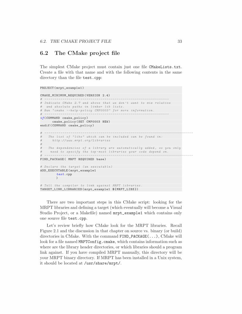
The simplest CMake project must contain just one file CMakeLists.txt.Create a file with that name and with the following contents in the samedirectory than the file test.cpp:
PROJECT(mrpt_example1 )
CMAKE_MINIMUM_REQUIRED (VERSION 2.4)
# --------------------------------------------------------------
# Indicate CMake 2.7 and above that we don ’t want to mix relative
# and absolute paths in linker lib lists.
# Run "cmake --help -policy CMP0003" for more information .
# --------------------------------------------------------------
if(COMMAND cmake_policy)
cmake_policy(SET CMP0003 NEW)
endif(COMMAND cmake_policy)
# --------------------------------------------------------------------------
# The list of "libs" which can be included can be found in:
# http :// www.mrpt.org/ Libraries
#
# The dependencies of a library are automatically added , so you only
# need to specify the top -most libraries your code depend on.
# --------------------------------------------------------------------------
FIND_PACKAGE( MRPT REQUIRED base)
# Declare the target (an executable)
ADD_EXECUTABLE(mrpt_example1
test.cpp
)
# Tell the compiler to link against MRPT libraries.
TARGET_LINK_LIBRARIES (mrpt_example1 ${MRPT_LIBS })
There are two important steps in this CMake script: looking for theMRPT libraries and defining a target (which eventually will become a VisualStudio Project, or a Makefile) named mrpt_example1 which contains onlyone source file test.cpp.
Let’s review briefly how CMake look for the MRPT libraries. RecallFigure 2.1 and the discussion in that chapter on source vs. binary (or build)directories in CMake. With the command FIND_PACKAGE(...), CMake willlook for a file named MRPTConfig.cmake, which contains information such aswhere are the library header directories, or which libraries should a programlink against. If you have compiled MRPT manually, this directory will beyour MRPT binary directory. If MRPT has been installed in a Unix system,it should be located at /usr/share/mrpt/.

34 CHAPTER 6. YOUR FIRST MRPT PROGRAM
6.3 Generating the native projects
Now, a native project must be created to compile your program, where na-tive means a project for your preferred compiler or IDE which is supportedby CMake. Some examples are: Unix makefiles, Visual Studio solutions,Code Blocks projects, Eclipse projects, etc. In any case, create a new di-rectory to make an off-tree build, for example first_mrpt_bin. We willrefer to the directory with the sources (test.cpp and CMakeLists.txt), aspath_first_mrpt_src.
Under Unix or GNU/Linux, go to the new empty directory and invoke:
first_mrpt_bin$ cmake {path_first_mrpt_src }
or, to invoke the NCurses GUI version:
first_mrpt_bin$ ccmake {path_first_mrpt_src }
On Windows, execute cmake-gui or cmakesetup and select the source({path_first_mrpt_src}) and binary (first_mrpt_bin) directories. Notethat in some Linux distributions cmake-gui is also available.
At this point, press the button “configure” in CMake, then “generate”to build your project. If CMake complains about not finding MRPT, setmanually the variable MRPT_DIR to the directory where you compiled MRPT(or /usr/share/mrpt/ if it was installed through synaptic or apt).
6.4 Compile
Once generated the project for your favorite compiler, just manage it asusual. For example, for Unix Makefiles, go to the binary directory andinvoke make. For Visual Studio, open the solution file mrpt-example1.sln
and compile as usual.
6.5 Summary
Creating user applications with MRPT requires adding the correspondingMRPT headers to the sources and creating a CMake project which includesMRPTConfig.cmake using the command FIND_PACKAGE(MRPT REQUIRED {LIBS}).The simple project presented in this chapter could be hopefuly used as abase for the user to create more complex applications.

Chapter 7
Linear algebra
In this chapter you will learn one of the most basic features of MRPT: vectorand matrix manipulation. The basic syntax in many cases will remain veryclose to that used in MATLAB, although the syntax must change a littlefor using the most optimized functions if the application performance is apriority.
In the following, all the required classes can be included in a programwith:
#include <mrpt/core.h>
using namespace mrpt;
using namespace mrpt::math;
using namespace mrpt:: utils;
using namespace mrpt:: system;
Currently there is no support for reading/writing binary MATLAB files,but this limitation is not severe since files saved from MATLAB in plaintext (with the format --ascii) are fully supported.
Notice that, like in C/C++ languages in general, the first element inany sequence has the index 0. This convention also applies to all matricesand vectors in MRPT. As usual, for matrices the first index corresponds torows.
7.1 Matrices
7.1.1 Declaration
MRPT defines two kind of matrices: variable-sized and fixed-sized. Most ofthis chapter will focus on the dynamic-size kind, but most of the operators
35

36 CHAPTER 7. LINEAR ALGEBRA
and methods are applicable to both types of objects.Matrices are implemented as class templates in MRPT, but the following
two types are provided for making programs more readable:
typedef CMatrixTemplateNumeric <float > CMatrixFloat;
typedef CMatrixTemplateNumeric <double > CMatrixDouble ;
A matrix with any given size can be created by passing it at constructiontime, or otherwise it can be resized later as shown in this example:
CMatrixDouble M(2,3); // Create a 2x3 matrix
cout << M(0,0) << endl; // Print out the left -top element
CMatrixDouble A; // Another way of creating
A.setSize (3,4); // a 2x3 matrix
A(2,3) = 1.0; // Change the bottom -right element
A matrix can be resized at any time, and the contents are preserved ifpossible. Notice also in the example how the element at the r’th row andc’th column can be accessed through M(r, c).
Sometimes, predefined values must be loaded into a matrix, and writingall the assignments element by element can be tedious and error prone. Inthose cases, better use this constructor:
const double numbers [] = {
1,2,3,
4,5,6 };
CMatrixDouble N(2,3, numbers );
cout << "Initialized matrix: " << endl << N << endl;
If the size of the vector does not fit exactly the matrix, an exception willraise at run-time. This example above also illustrates how to dump a matrixto the console, which is useful for debugging in case of small matrices.

7.2. VECTORS 37
7.1.2 Fixed-size matrices
When the size of matrices is known a priori, it is advisable to use the al-ternative implementation based on fixed-size matrices1. These objects aremanaged very similarly to dynamic matrices, including most operators andmethods. Naturally, the only difference comes into their declaration:
const double numbers [] = {
1,2,3,
4,5,6 };
CMatrixFixedNumeric <double ,2,3> N ( numbers );
cout << "Initialized matrix: " << endl << N << endl;
Predefined type names exist for double matrices of many common sizes:
CMatrixFixedNumeric <double ,10,3> M;
CMatrixDouble33 A = (~M) * M; // Predefined type for 3x3
Whenever possible, employ fixed-sized matrices, especially for small ma-trices, since the speed gain can be in the order of ten or more for mostoperations.
7.1.3 Storage in files
When managing large matrices, it is useful to load or save them in files.In particular, it would be even more handful to make those files compati-ble with MATLAB. This format exists and is as simple as plain text files.For example, the following small program loads a matrix from a file, thencompute its eigenvectors and save them to a different file:
CMatrixDouble H,Z,D;
H.loadFromTextFile("H.txt"); // H <- ’H.txt’
H.eigenVectors(Z,D); // Z: eigenvectors , D: eigenvalues
Z.saveToTextFile("Z.txt"); // Save Z in ’Z.txt’
7.2 Vectors
7.2.1 Declaration
The base class for vectors is the standard STL container std::vector,such as a user will normally declare and manipulate objects of the types
1This feature is available in MRPT 0.7.0 or newer.

38 CHAPTER 7. LINEAR ALGEBRA
vector_float or vector_double 2, for element types being float or double,respectively:
typedef std::vector <float > vector_float;
typedef std::vector <double > vector_double ;
7.2.2 Resizing
To resize a vector we must use the standard std::vector methods, that is:
vector_double V(5,1); // Create a vector with 5 ones.
V.resize (10);
cout << V << endl; // Print out the vector to console
7.2.3 Storage in files
There is less support yet to vector I/O than in the case of matrices, so it isnormally advisable to use matrices when loading text files, especially whenthe format of the file is unknown (e.g. column vs. row vector).
Reading a vector from a text file
This works for row vectors only:
vector_double v;
loadVector( CFileInputStream("in.txt"), v);
Saving to a text file
The function vectorToTextFile allows saving as a row, as a column, andoptionally, to append at the end of the existing file:
vector_double v(4,0); // [0 0 0 0]
vectorToTextFile(v, "o1.txt"); // Save as row
vectorToTextFile(v, "o2.txt", true); // Append a new row
vectorToTextFile(v, "o3.txt", false , true ); // Save as a column
2One can also use CVectorFloat and CVectorDouble, which have some useful op-erations implemented as methods, but most MRPT interfaces expect the simpler STLcontainers.

7.3. BASIC OPERATIONS 39
Serializing
If you prefer to serialize the vectors in binary form (see chapter 10), thatcan be done as simply as:
vector_double v = linspace (0 ,1 ,100); // [0 ... 1]
CFileOutputStream("dump.bin") << v;
7.3 Basic operations
In this section we will go through a quick summary of unary and binaryoperations for matrices, vectors, or a mix of them. Table 7.3 lists someof the most simple of these operations in common mathematical notation,in C++ using MRPT operators and alternative functional forms. Mostoperations apply indistinctly to dynamic and fixed-size matrices.
Description Operation MRPT C++ 2nd alternativeRead element a←M(i, j) a = M(i,j) a=M.get unsafe(i,j)Write element M(i, j)← a M(i,j) = a M.get unsafe(i,j)=aMatrix inverse M−1 !M M.inv()
Matrix transpose M⊤ ~MMatrix assignment Q←M Q = MMatrix comparison Q = M? Q == M, Q!=M
Matrix sum/substract M +Q, M −Q M+Q, M-QIn place sum M ←M +Q M+=Q
Vector sum/substract v + w, v − w v+w, v-wScalar multiplication M ←Ma M*=aMatrix multiplication MQ M*QMatrix multiplication M ←MQ M = M*Q M.multiply(Q)Matrix/vector mult. Mv M*vMultiply by inverse MQ−1 M/Q
Determinant |M | M.det()
Naturally, some operations carry restrictions on the sizes of the operants (e.g.matrix multiplication). An exception will be thrown if invalid operations are foundin run-time for dynamic-size matrix, while the compiler will complain about theinvalid operation for fixed-size ones.
This table does not contain all the implemented operators, for all the detailsplease refer to:
• mrpt::math
• mrpt::math::CMatrixTemplateNumeric<T>

40 CHAPTER 7. LINEAR ALGEBRA
Other methods which may be easy to remember to those programmers famil-iarized with MATLAB are:
• M.ones(A,B) : Generates a A×B matrix of ones.
• M.zeros(A,B) : Generates a A×B matrix of zeroes.
• M.unit(A) : The A×A unity matrix.
• size(M,1) : Number of rows in M , equivalent to M.getRowCount().
• size(M,2) : Number of columns in M , equivalent to M.getColCount().
• v=linspace(a,b,N) : Generates a vector v with N elements in the range[a, b].
• mean(v), stddev(v) : Mean and standard deviation of the vector v. Thereis also a combined meanAndStd(...).
• cumsum(v) : Cumulative sum of vector v.
• histogram(v,...) : Histogram of a vector. See reference documentation.
As an example of the operators described so far, the equation
R = H · C ·H⊤
can be implemented with the next code fragment:
CMatrixDouble C(3,3);
CMatrixDouble H(5,3);
// C=diag ([1 2 3])
C(0,0) = 1;
C(1,1) = 2;
C(2,2) = 3;
// randomize matrix
mrpt:: random :: matrixRandomUni (H, -1.0 ,1.0);
CMatrixDouble R = H * C * (~H);
However, this operation, like many others have specialized methods which muchbetter performance. These common expressions should be known to take advantageof them, hence they are summarized in the next section.
7.4 Optimized matrix operations
Many common operations with matrices have efficient implementations, as summa-rized in Table ??. In the table M,A,B,C represent matrices while v, w are vectorsand x is a scalar. All these elements must be of the appropriate sizes for the cor-responding operations to make sense. For clarity, some terms in the “operation”column are represented in MATLAB notation.

7.5. TEXT OUTPUT 41
Operation Efficient implementation Remarks
M = M +A⊤ M.add_At(A)
M = M +A+A⊤ M.add_AAt(A) A squareM = AB⊤ M.multiply_ABt(A,B)
M = AA⊤ M.multiply_AAt(A)
M = A⊤A M.multiply_AtA(A)
w = Ab A.multiply_Ab(b,w)
w = A⊤b A.multiply_Atb(b,w)
M = AB M.multiply_result_is_symmetric(A,B) AB symmetricM = ABA⊤ A.multiply_HCHt(B,M) B symmetricM = M +ABA⊤ A.multiply_HCHt(B,M,false,0,true) B symmetricx = ABA⊤ A.multiply_HCHt_scalar(B) B sym., result 1x1M = ABC M.multiply_ABC(A,B,C)
M = ABC⊤ M.multiply_ABCt(A,B,C)
M = AB(r0 : end, c0 : (c0 + c)) A.multiply_SubMatrix(B,M,c0,r0,c)
M = A−1 A.inv_fast(M) Contents of A are lostsum(A(:)) M.sumAll()
7.5 Text output
7.6 matrices manipulation
7.6.1 Extracting a submatrix
For example, the following MATLAB statement:
A = C(6 : 8, 7 : 8);
becomes:
CMatrixDouble C(10 ,10);
CMatrixDouble A(3,2); // Set to the size of the patch to extract
C.extractMatrix (5,6,A)
Notice again how in MATLAB the first elements are referenced as 1 while inMRPT they have 0 as index.
7.6.2 Extracting a vector from a matrix
Extracting a column, for example v = C(:, 3), can be implemented with:
CMatrixDouble C(10 ,10);
vector_double v;
C.extractCol (2,v);
And equivalently for rows, for example v = C(4, :):
CMatrixDouble C(10 ,10);
vector_double v;
C.extractRow (5,v);

42 CHAPTER 7. LINEAR ALGEBRA
7.6.3 Building a matrix from parts
A matrix can be also built from its 4 parts, such as:
M =
(
A BC D
)
with:
CMatrixDouble M;
M.joinMatrix(A,B,C,D);
Many other methods exist (please, see the reference for further details) with self-explaining names: insertRow, appendRow, insertCol, insertMatrix (for insertinga submatrix in a larger matrix), etc.
7.7 Matrix decomposition
Chapter 8
Mathematical algorithms
8.1 Fourier Transform (FFT)
8.2 Statistics
Mean, std, meanAndStd.
8.3 Spline interpolation
8.4 Spectral graph partitioning
8.5 Quaternions
8.6 Geometry functions
8.7 Numeric Jacobian estimation
43

44 CHAPTER 8. MATHEMATICAL ALGORITHMS

Chapter 9
3D geometry
9.1 Introduction
9.2 Homogeneous coordinates geometry
9.3 Geometry elements in MRPT
9.3.1 2D points
9.3.2 3D points
9.3.3 2D poses
9.3.4 3D poses
45

46 CHAPTER 9. 3D GEOMETRY
y
x
Figure 9.1: A point in 2D.

9.3. GEOMETRY ELEMENTS IN MRPT 47
y
x
Figure 9.2: A pose in 2D.
z
x
y
Yaw
(1st)
Pitch
(2nd)
Roll
(3rd)
Arrow indicates
positive direction
Figure 9.3: A pose in 3D.

48 CHAPTER 9. 3D GEOMETRY

Chapter 10
Serialization
10.1 The problem of persistence
Serializing consists of taking an existing object and converting it into a sequenceof bytes, in any given format, such as the contents and state of the object can beafterward reconstructed, or deserialized.
10.2 Approach used in MRPT
There are many C++ libraries for serializing out there (e.g. boost), althoughMRPT uses a simple, custom implementation with the following aims:
1. Simplicity: A few and small core functions only.
2. Versioning: If a class changes along time (something really common), anew version number will be assigned to its serialization, but old stored datacan be still imported.
3. C++ compiler independence: Use only standardized data-lengths. Forexample, a data of type ”int” has different lengths depending on the machine,thus it is not allowed to serialize an ”int” variable without forcing it to aknown length.
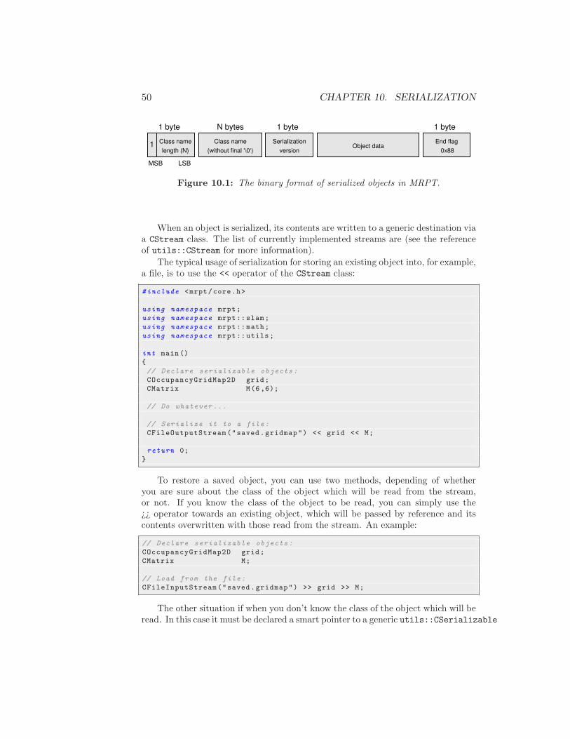
Currently, the only supported format for serialization is binary, i.e. there isno support for XML. The reason is that, for robotic applications, it is typicallymore important to save data size (and transmission times) between a running,real-time system. The actual binary frame for each serialized object is sketched inFigure 10.11.
1In versions before MRPT 0.5.5 the end flag was not present and the first and thirdfields were 4 bytes wide (instead of just 1). However, data saved in the old format can bestill loaded without problems.
49
50 CHAPTER 10. SERIALIZATION
Class name
length (N)
Class name
(without final '\0‘)
1 byte N bytes
Serialization
version
1 byte
Object dataEnd flag
0x88
1 byte
1
MSB LSB
Figure 10.1: The binary format of serialized objects in MRPT.
When an object is serialized, its contents are written to a generic destination viaa CStream class. The list of currently implemented streams are (see the referenceof utils::CStream for more information).
The typical usage of serialization for storing an existing object into, for example,a file, is to use the << operator of the CStream class:
#include <mrpt/core.h>
using namespace mrpt;
using namespace mrpt::slam;
using namespace mrpt::math;
using namespace mrpt::utils;
int main()
{
// Declare serializable objects:
COccupancyGridMap2D grid;
CMatrix M(6,6);
// Do whatever ...
// Serialize it to a file:
CFileOutputStream ("saved.gridmap") << grid << M;
return 0;
}
To restore a saved object, you can use two methods, depending of whetheryou are sure about the class of the object which will be read from the stream,or not. If you know the class of the object to be read, you can simply use the¿¿ operator towards an existing object, which will be passed by reference and itscontents overwritten with those read from the stream. An example:
// Declare serializable objects:
COccupancyGridMap2D grid;
CMatrix M;
// Load from the file:
CFileInputStream("saved.gridmap") >> grid >> M;
The other situation if when you don’t know the class of the object which will beread. In this case it must be declared a smart pointer to a generic utils::CSerializable

10.3. RUN-TIME CLASS IDENTIFICATION 51
object (initialized as NULL to indicate that it is empty), and after using the >>
operator it will point to a newly created object with the deserialized object:
// Declare serializable objects:
CSerializablePtr obj; // NULL pointer
// Load from the file:
CFileInputStream("saved.gridmap") >> obj;
std::cout << "Object class:" << obj ->GetRuntimeClass ()->className;
The next section explains the most important methods of utils::CSerializableand runtime class information. In the case of loading objects of unknown class, itis important to read the MRPT registration mechanism and when you should callit manually.
Note that these code examples do not catch potential exceptions.Apart from using the operators << and >> over a utils::CStream, there are two
independent functions, utils::ObjectToString and utils::StringToObject, whichserialize and deserialize, respectively, an object into a standard STL string (std::string).The difference of these functions with serialization over normal CStream’s is thatthe binary data stream is encoded to avoid null characters (’\0’), such as the re-sulting string can be passed as a char *. Avoid using these functions but whenstrictly necessary, since they introduce an additional processing delay.
10.3 Run-time class identification
All serializable classes must inherit from the virtual class utils::CSerializable, whichprovides standard methods to manage any serializable object without knowing itsreal class. The most common operation is probably to check whether an object isof a given type, which can be performed by:
CSerializablePtr obj;
stream >> obj;
// Test if "obj" points to an object of class "CMatrix ".
if ( IS_CLASS(obj ,CMatrix) )
// Or (old format ):
if ( obj ->GetRuntimeClass () == CLASS_ID( CMatrix ) )
If the class to test is not in the current namespace (and there is not a using namespace NAMESPACE;),you can alternatively use CLASS_ID_NAMESPACE, for example:
if ( obj ->GetRuntimeClass () == CLASS_ID_NAMESPACE ( CMatrix , UTILS) ) ...
The method CSerializable::GetRuntimeClass() actually returns a pointer to aUTILS::TRuntimeClassId data structure, which contains other useful members:
1. The class name as a string:
obj ->GetRuntimeClass ()->className;
52 CHAPTER 10. SERIALIZATION
2. Checking whether a class is a descendent of a given virtual class. An example:
void func( CMetricMap * aMap )
{
if (IS_DERIVED(aMapCPointsMap ))
{
CPointsMap *pMap = (CPointsMap *) aMap;
}
}
Other useful method of any serializable object is CSerializable::duplicate, whichmakes a copy of the object. The internal data, pointers, etc... will be reallyduplicated and the original object can be safely deleted.
10.4 Writing new serializable classes
10.5 Serializing STL containers
MRPT supports serializing arbitrarily complex data structures mixing STL con-tainers, plain data types and MRPT classes. For example:
std::multimap <double ,std::pair <CPose3D , COccupancyGridMap2D > > myVar;
file << myVar;
The code above will compile and work without the need of the user to writeany extra code for the multimap<> type.
In the case of STL containers, the binary format consists on:
• The dump of a std::string with the STL container name (dumped using theserialization format explained above).
• The dump of the strings representing each of the types kept by the container(the key and value for a map, the values for a list, etc...).
• The number of elements in the container (for all containers but std::pair).
• The recursive dump of each of the elements. Here the same may apply ifthe elements are STL containers. For normal MRPT classes, the formatexplained above is used here.

Chapter 11
Smart Pointers
11.1 Overview of memory management
Variables, objects (that is, instantiations of classes) and arrays are the typicalkinds of data managed by any program. Dynamic data on virtually all computerarchitectures, but some embedded systems, can be allocated into memory in twovery different places: in the stack or in the heap.
Stack allocation is always preferred unless there are specific reasons not to use Stack memory
it. This technique implies a very efficient memory reservation method, typically justsubtracting a fixed number to the stack pointer register when calling a function.Correspondingly, freeing memory becomes an addition to the same register. It ishard to imagine a more efficient way to handle the reservation of local memoryneeded in any function or class method. Below follow some examples of stackallocation:
void bar()
{
int counter;
MyClass obj1 , obj2;
double numbers [100];
...
}
On the other hand, we have heap allocation, also known as dynamic memory, Heap memory
where the program must make a request to the operative system to allocate a cer-tain amount of memory on the heap space (the program’s reservoir of memoryspace). These requests may take some time since a gap large enough must befound and problems such as memory fragmentation must be avoided by the alloca-tion algorithm, which must also handle explicit requests from the program to freethe non-needed allocated blocks. The equivalent to the example above with heapallocation would be:
53

54 CHAPTER 11. SMART POINTERS
void bar()
{
int *counter = new int [1];
MyClass *obj1 = new MyClass (), *obj2 = new MyClass ();
double *numbers = new numbers [100];
...
delete [] counter;
delete obj1;
delete obj2;
delete [] numbers;
}
Although the efficiency of heap allocation is far poorer than reserving on thestack, there are three main reasons to employ the former under some circumstances:(i) memory allocation on the stack is typically limited to a few Megabytes, thuslarge memory blocks should be heap allocated, (ii) when the amount of memoryis unknown at compile time and (iii) when the variables are intended to still existwhen the program goes out of the creation scope.
As an illustrative example, refer to the following three functions which areintended to return a newly created object:
// Returning by value
MyClass function1 ()
{
MyClass obj; // Stack alloc
...
return obj;
}
// Returning a pointer (WRONG! DON ’T DO THIS)
MyClass* function2 ()
{
MyClass obj; // Stack alloc
...
return &obj;
}
// Returning a pointer (Correct)
MyClass* function3 ()
{
MyClass *obj = new MyClass (); // Heap alloc
...
return obj;
}
If we analyze the three alternatives, we found that the first and third versionsare perfectly valid but quite different in their inner workings: while the caller tothe first function must make a copy of the returned object, the third one will haveto copy just a pointer value – obviously, the fastest solution. Regarding the secondalternative function2, note that the pointer will be invalid out of the scope of thefunction (it points to the stack space of the function), thus accessing the returnedpointer would lead to undefined behavior, most likely a segmentation fault. To

11.1. OVERVIEW OF MEMORY MANAGEMENT 55
sum up, returning pointers is the fastest way to return objects, but in that case thememory must be dynamic, that is, reserved on the heap.
At this point we have established that, in some cases, pointers to objects al-located in the heap are the most efficient mechanism to transfer objects betweendifferent functions (or even threads) within one program. Now it must be high-lighted the fundamental risk of this idea: memory allocated dynamically must befreed by means of explicit requests by the program. As the complexity of an appli-cation grows, it becomes increasingly difficult to keep track of how many pointers,possibly distributed throughout different threads, refer to the same object, withthe idea of requesting its deletion only after the destruction of the last reference tothe object.
Here is where the concept of smart pointers gets into the scene. A smart pointer Smart pointers
is actually an object itself, but behaves as if it were a plain pointer but has the niceproperty of automatically and transparently maintaining a counter with the numberof active references, or aliases, to the object. Only when the counter reaches zero,the dynamically-allocated object is freed.
Smart pointers in MRPT are based on the wonderful implementation providedby the STLplus C++ Library Collection [11] due to its versatility, clean interfaceand proven robustness1. Next sections describe how to use these smart pointerclasses correctly.
1The only modification to the original STLplus in MRPT is the replacement of thereference counter by a thread-safe atomic counter.

56 CHAPTER 11. SMART POINTERS
11.2 Class hierarchy
Smart pointers are introduced in MRPT mainly by means of the smart pointer classCObjectPtr, which represents a pointer to objects of type CObject (both definedin namespace mrpt::utils in the library mrpt-base).
Most MRPT classes subject to be frequently allocated as dynamic memoryinherit from CObject. In parallel to that hierarchy of classes, a set of MRPTmacros automatically define another hierarchy of smart pointer classes, one for each“normal” class. As a naming convention, names of smart pointer classes are builtby adding the postfix Ptr to the original class name, as illustrated in Figure 11.1.
(a) Hierarchy of classes (b) Hierarchy of smart-pointer classes
Figure 11.1: For each class in the hierarchy of classes (left) there is an associatedsmart pointer class (right).
A useful built-in functionality of MRPT smart pointers is that copy constructorsexist to convert between any two different smart pointer classes. Those construc-tors check, at runtime, the validity of the intended transformation. An incorrectassignment will raise an exception upon execution. The following example illus-trates this feature, assuming the hierarchy of class defined in the previous figure(the Create() method is explained in the next section):
CTrianglePtr ptrTri = CTriangle :: Create (); // Create new object
CPolygonPtr ptrPoly = CPolygonPtr(ptrTri ); // Correct
CPentagonPtr ptrPent = CPentagonPtr(ptrPoly ); // Incorrect
CTrianglePtr ptrTri2 = CTrianglePtr(ptrPoly ); // Correct
Finally, it is very important to remark once again that smart pointers act likepointers but actually are objects themselves. Therefore, both the dot and arrowoperators can be used on them but with quite different intentions:
CTrianglePtr ptrTri = CTriangle :: Create (); // Create new object
ptrTri ->method (); // Invoke method () of the CTriangle class
ptrTri.method (); // Invoke method () of the smart pointer class

11.3. HANDLING SMART POINTERS 57
11.3 Handling smart pointers
11.3.1 The Create() class factory
For each MRPT class CFoo with associated smart pointer CFooPtr, a static methodexists implementing a smart pointer factory. These methods are something equiv-alent to:
class CFoo
{
public:
static CFooPtr Create () { return CFooPtr(new CFoo ()); }
};
Put in words, this method creates a new (dynamically allocated) instance ofthe type CFoo and immediately assigns its memory management to a smart pointerof type CFooPtr, which from that moment on is the interface for the programmerto access the actual object. The process is sketched in Figure 11.2.
Figure 11.2: The construction of a new object and an associated smart pointer bymeans of the Create() static method.

58 CHAPTER 11. SMART POINTERS
11.3.2 Testing for empty smart pointers
Unlike standard pointers, there is no need to initially set smart pointers to a NULL
value to mark them as invalid : the default internal state of the smart pointer alreadyis “NULL valued”-like and behaves accordingly by means of the ! operator:
CFooPtr a;
if (!a)
{
// This code WILL be executed , since "a" is empty.
}
CFooPtr b = CFoo:: Create ();
if (!b)
{
// This code WILL NOT be executed , "b" points to an object.
}
Alternatively, the method present() returns true if the smart pointer actuallypoints to an object:
CFooPtr a;
if (a.present ())
{
// This code WILL NOT be executed , since "a" is empty.
}
CFooPtr b = CFoo:: Create ();
if (b.present ())
{
// This code WILL be executed , "b" points to an object.
}

11.3. HANDLING SMART POINTERS 59
11.3.3 Making multiple aliases
After creating a smart pointer, an arbitrary number of copies can be made from it,and all of them will be aliases of one single object in memory. For instance, afterthese instructions:
CFooPtr a = CFoo:: Create (); // Create object
CFooPtr b = a; // Make a new alias
the actual memory layout would be like:
Figure 11.3: Copying smart pointers become increasing the number of aliases tothe same object.
The copy is very efficient, and totally independent of the complexity of CFoo.Notice how, after the copy, the aliases counter is now increased to two. Therefore,just like when using plain pointers, both a-> and b-> actually dereference to exactlythe same memory address.
If we consider now what happens after the program gets out of the scope wherethe first smart pointer a was created, we arrive to the situation of Figure 11.4,where the aliases counter is back again to one.
Figure 11.4: The number of aliases automatically decreases with each smartpointer variable that is no longer used.
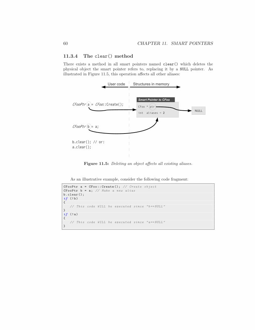
60 CHAPTER 11. SMART POINTERS
11.3.4 The clear() method
There exists a method in all smart pointers named clear() which deletes thephysical object the smart pointer refers to, replacing it by a NULL pointer. Asillustrated in Figure 11.5, this operation affects all other aliases:
Figure 11.5: Deleting an object affects all existing aliases.
As an illustrative example, consider the following code fragment:
CFooPtr a = CFoo:: Create (); // Create object
CFooPtr b = a; // Make a new alias
b.clear ();
if (!b)
{
// This code WILL be executed since "b== NULL"
}
if (!a)
{
// This code WILL be executed since "a== NULL"
}

11.3. HANDLING SMART POINTERS 61
11.3.5 The clear unique() method
In contrast to the previous method, one may want in some situations to free just onealias, without affecting the others. This is done with the clear unique() method:
Figure 11.6: The clear unique() method clears just the referred alias.
11.3.6 The make unique() method
In this case, the affected aliases become independent of the others and a copy ismade of the pointed object, as shown in the following figure:
Figure 11.7: Effects of the make unique() method.

62 CHAPTER 11. SMART POINTERS
11.3.7 Creating from dynamic memory
Apart from the Create() class factory mentioned above, a smart pointer can beassociated to a plain pointer at any given instant by means of the smart pointerclass constructor. For instance, in
CFoo *obj = new CFoo (...);
CFooPtr a(obj);
the smart pointer a now holds the pointer to the object obj, and the programmershould not issue an delete obj; since the smart pointer is the one now in chargeof freeing that memory.
11.3.8 Never create from stack-allocated memory
Unlike in the previous case, which was perfectly valid, don’t ever try to associate asmart pointer to a local variable allocated in the stack, such as in:
CFoo obj;
CFooPtr a(&obj); // Don ’t ever try this.
It is clear that the smart pointer will eventually try to issue a delete on theobject which was not actually dynamically allocated, which will for sure lead to an“invalid free” memory error.

Chapter 12
Images
12.1 The central class for images
The main class for image storage is CImage, which internally fully relies on the IPLformat and OpenCV functions for memory management, format conversions, fileI/O, etc. Basically, it is a wrapper for OpenCV C library functionality with themore attractive appearance of a C++ class and extended with many MRPT-specificalgorithms.
12.2 Basic image operations
12.3 Feature extraction
12.4 SIFT descriptors
63

64 CHAPTER 12. IMAGES

Chapter 13
Rawlog files (datasets)
This chapter describes the two formats for datasets in MRPT’s binary format, called“rawlogs”. Many existing formats can be imported as rawlogs due to its versatilityto cope with a wide range of robotic sensors (see the chapter on Observations formore details).
Rawlog files are the input of many MRPT applications for off-line processing.The application RawlogViewer incorporates several tools to visualize and manipu-late these files.
13.1 Format #1: A Bayesian filter-friendly fileformat
13.1.1 Description
The purpose of a rawlog file is to reflect as accurately as possible all the datagathered by a robot as it moves through an environment, autonomously or manuallyguided.
Under the perspective of Bayesian SLAM methods, these data are divided intwo clearly differentiated groups: actions, and observations, denoted typically asuk and zk in the literature, respectively.
Hence, to ease the implementation of Bayesian methods in MRPT, a rawlogfile is divided in a sequence of actions, observations, actions, observations,... ”Actions” typically include robot motor actuations (odometry), but any kindof user-defined actions can be defined as well (e.g. robot arm actuations). ”Obser-vations” include readings from the rest of robotic sensors: laser scanners, imagesfrom cameras, sonar ranges, etc.
Note that the intention of grouping several observations between two consecu-tive actions is to assure they are gathered approximately at the same time, althougheach individual observation has its own timestamp.
65

66 CHAPTER 13. RAWLOG FILES (DATASETS)
13.1.2 Actual contents of a ”.rawlog” file in this format
A rawlog file is a binary serialization of alternating objects of the classes:
• CActionCollection, one or more actions (e.g. odometry), and
• CSensoryFrame, which stores the observations.
The serialization mechanism of MRPT is explained in Chapter 10.
13.2 Format #2: An timestamp-ordered sequenceof observations
13.2.1 Description
While the previous format is really well-suited for Bayesian approaches with clearlyseparate steps of process action-process observation, in the case of complex datasetswith many different sensors, working at different rates, and possibly without odom-etry (the typical ’action’ in SLAM algorithms), it is more clear to just store datasetsas an ordered list of observations.
13.2.2 Actual contents of a ”.rawlog” file in this format
In this case, the rawlog file is a binary serialization of objects derived from theclass slam::CObservation. In this case, odometry (if present) is also stored as anobservation. The serialization mechanism of MRPT is explained in Chapter 10.
The applications RawLogViewer, rawlog-grabber, and the class slam::CRawlogall support both rawlog formats.
13.3 Compression of rawlog files
Since MRPT 0.6.0 all rawlog files are transparently compressed using thegzip algorithm. The compression level is set to ’minimum’ to reduce as muchas possible the computational load, while still deflating file sizes to approximately33%.
If compatibility with old versions is required, the files can be renamed to.rawlog.gz, then decompressed using standard tools. To enable compressed in-put/output in your code, replace the stream classes by their gzip equivalents:
• CFileInputStream → CFileGZInputStream
• CFileOutputStream → CFileGZOutputStream
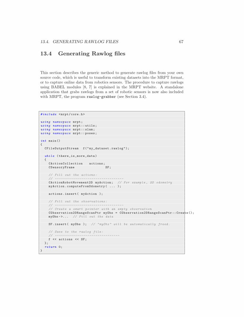
13.4. GENERATING RAWLOG FILES 67
13.4 Generating Rawlog files
This section describes the generic method to generate rawlog files from your ownsource code, which is useful to transform existing datasets into the MRPT format,or to capture online data from robotics sensors. The procedure to capture rawlogsusing BABEL modules [8, 7] is explained in the MRPT website. A standaloneapplication that grabs rawlogs from a set of robotic sensors is now also includedwith MRPT, the program rawlog-grabber (see Section 3.4).
#include <mrpt/core.h>
using namespace mrpt;
using namespace mrpt:: utils;
using namespace mrpt::slam;
using namespace mrpt:: poses;
int main()
{
CFileOutputStream f("my_dataset.rawlog");
while (there_is_more_data )
{
CActionCollection actions;
CSensoryFrame SF;
// Fill out the actions:
// ----------------------------------
CActionRobotMovement2D myAction; // For example , 2D odometry
myAction.computeFromOdometry ( ... );
actions.insert( myAction );
// Fill out the observations :
// ----------------------------------
// Create a smart pointer with an empty observation
CObservation2DRangeScanPtr myObs = CObservation2DRangeScanPtr :: Create ();
myObs ->... // Fill out the data
SF.insert( myObs ); // "myObs" will be automatically freed.
// Save to the rawlog file:
// --------------------------------
f << actions << SF;
};
return 0;
}

68 CHAPTER 13. RAWLOG FILES (DATASETS)
13.5 Reading Rawlog files
13.5.1 Option A: Streaming from the file
This is the preferred mode of operation in general: actions and observations are readsequentially from the file, processed, freed, and so on. In this way only the requiredobjects are loaded in memory at any time, which is mandatory when managinglarge datasets (e.g. containing thousands of embedded images). However, noticethat if images are stored externally the rawlog could be loaded at once withoutproblems.
A typical loop for loading a rawlog in this way is shown next:
CFileGZInputStream rawlogFile(filename ); // "file.rawlog"
CActionCollectionPtr action; // Smrt. pointer to actions
CSensoryFramePtr observations; // Smrt. pointer to observations
size_t rawlogEntry =0;
bool end = false;
// Load action from rawlog:
while ( readActionObservationPair (
rawlogFile ,
action ,
observations ,
rawlogEntry) )
{
// Process action & observations
...
};
// Smart pointers will be deleted automatically.
13.5.2 Option B: Read at once
A rawlog file can be read as a whole using the class slam::CRawlog. Notice thatthis may be impractical for very large datasets (several millions of entries) due tomemory requirements, but for mid-sized datasets it definitively is the easiest wayof loading rawlogs.
CRawlog dataset;
dataset.loadFromRawLogFile (filename );

Chapter 14
GUI classes
14.1 Windows from console programs
14.2 Bitmapped graphics
See mrpt::gui::CDisplayWindow.
14.3 3D rendered graphics
See mrpt::gui::CDisplayWindow3D.
14.4 2D vectorial plots
See mrpt::gui::CDisplayWindowPlots.
69

70 CHAPTER 14. GUI CLASSES

Chapter 15
OS Abstraction Layer
15.1 Cross platform Support
To write cross-platform and cross-compiler code, we need a layer of functions thatact like a minimum set of services found on any OS and compiler. In MRPT, thesemethods are concentrated in the namespace mrpt::system::os, and comprise arange of different areas as enumerated next.
15.2 Function Areas
15.2.1 Threading
15.2.2 Sockets
15.2.3 Time and date
15.2.4 String parsing
15.2.5 Files
71

72 CHAPTER 15. OS ABSTRACTION LAYER
Chapter 16
Probability density functions(pdfs)
16.1 Efficient pose sample generator
73

74 CHAPTER 16. PROBABILITY DENSITY FUNCTIONS (PDFS)

Chapter 17
Random number generators
17.1 Generators
17.2 Multiple samples
75

76 CHAPTER 17. RANDOM NUMBER GENERATORS

Chapter 18
Observations
18.1 The generic interface
18.2 Implemented observations
18.2.1 Monocular images
18.2.2 Stereo images
77

78 CHAPTER 18. OBSERVATIONS
CObservationImage
Reference system on the camera:
CPose3D cameraPose;
z
x
y
Robot on-board
reference system
z
x
y
Focal pointImage plane
Figure 18.1: Representation of single camera observations.
CObservationStereoImages
Reference systems related to both cameras:
CPose3D cameraPose;
z
x
y
Robot on-board
reference system
z
x
y
Left camera’s
focal pointLeft image plane
LEFT CAMERA
z
x
y
Right image plane
RIGHT CAMERA
Right camera’s
focal point
CPose3D rightCameraPose;
(It can be any 3D relation, it does
not need to be at the “right”)
Figure 18.2: Representation of stereo image observations.
Chapter 19
Metric map classes
19.1 The generic interface of maps
All metric maps in MRPT have a common interface to ease polymorphism andgeneric programming. The base class is mrpt::slam::CMetricMap. All the mapclasses are within the namespace mrpt::slam, which is omitted in the rest of thechapter for readability.
We review next only the most important methods of this interface:
bool insertObservation (
const CObservation *obs ,
const CPose3D *robotPose=NULL)
By invoking this method, the map will be updated from the new informationprovided by the passed observation. It is important to remark that not all themaps can process all the kinds of observations. The returned boolean value actuallyindicates whether the map was affected by the observation. For example, insertinga 2D laser scan in an occupancy grid map will update it, while an observation ofgas concentrations will not.
For most kinds of maps, it is crucial to provide a second argument with thelocation of the robot when the observation was taken from. Notice that the relativeposition of the sensor with respect to the robot is already taken into account duringthe process of updating the map, that is, the same robotPose must be used for arobot carrying three different laser scanners, as long as the location of each sensoris correctly annotated within the corresponding observation objects.
double computeObservationLikelihood (
const CObservation *obs ,
const CPose3D &takenFrom)
This important method evaluates the log-likelihood of a given observation, con-ditional to the robot being at the given location in map coordinates. If a given maphave no way to infer any sensible value for the likelihood (e.g. a visual landmark
79

80 CHAPTER 19. METRIC MAP CLASSES
map queried for the likelihood of a laser scanner), an arbitrary constant value willbe returned. This method is at the core of most Bayesian approaches to particlefiltering-based localization and mapping.
void saveMetricMapRepresentationToFile (
const std:: string &filNamePrefix ) const
Useful for debugging, this method dumps one or several files with differentrepresentations of the map.
19.2 The “multi-metric map” container
The most powerful tool when dealing with metric maps is an especial kind of map:the “multi-metric map”. This class offers the interface of a normal metric map, butit holds internally an arbitrary number of other metric maps.
To realize of the potential and simplicity of this approach, imagine programminga method which inserts scans from 3 laser range finders into a 3D point map (so,a point cloud is built incrementally). By just replacing the point map by a multi-metric map, we can now build the point cloud and, at our choice, three occupancygrid maps, once for each height. The original code would need no changes at all.
This is the reason of calling the MRPT map model hierarchical, in the sensethat one map (the multi-metric map) propagates all the calls to the child maps.
19.3 Implemented maps
1. The generic map container: Multi-metric map. Implemented in the classCMultiMetricMap.
2. Beacon maps. A map of 3D beacons with an ID, used for range-only local-ization and SLAM. Implemented in CBeaconMap.
3. 2D gas concentration maps. A planar lattice of gas concentrations, used forgas concentration mapping. See the class CGasConcentrationGridMap2D.
4. 2D height (or elevation) maps. A lattice where each cell keeps the averageelevation (”z” coordinate) of the points sensed within its square area. Seethe class CHeightGridMap2D.
5. Landmark maps. A set of 3D landmarks with IDs and a 3D Gaussian dis-tribution for its position. Used mainly for visual SLAM. Implemented inCLandmarksMap.
6. Occupancy grid maps. A planar occupancy grid map. Occupancy probabil-ities are kept as log-odds for a better dynamic range in the possible valuesof each cell. It is used in many SLAM and particle filter-based localizationprograms. See the class COccupancyGridMap2D.

19.4. CONFIGURATION BLOCK FOR A MULTI-METRIC MAP 81
7. Point maps. A virtual class for maps of 2D or 3D points. It implementsefficient look-up methods based on KD-trees. The derived classes are:KD-tree look-up
is built-in inall point maps. (a) Simple point maps. A type of point map where each point only have
(x,y,z) coordinates. See CSimplePointsMap.
(b) Colored point maps. A type of point map where each point have (x,y,z)coordinates, plus RGB color data. Implemented in CColouredPointsMap.
19.4 Configuration block for a multi-metric map
Typically, all the parameters to configure a multi-metric map can be loaded froma INI-like configuration file (or any other textual input, such as an input box in aGUI). Of course, they can be also hard-coded.
The key structure to use here is TSetOfMetricMapInitializers. The format ofthe configuration files is explained in the reference documentation of:
• TSetOfMetricMapInitializers::loadFromConfigFile.
For practical examples of use, refer also to the INI files locate in the MRPTpackages at MRPT/share/mrpt/config_files/*.

82 CHAPTER 19. METRIC MAP CLASSES

Chapter 20
Probabilistic Motion Models
20.1 Introduction
Within a particle filter, the samples are propagated at each time step using somegiven proposal distribution. A common approach for mobile robots is taking theprobabilistic motion model directly as this proposal.
In MRPT there are two models for probabilistic 2D motion, implemented inmrpt::slam::CActionRobotMovement2D.
To use them just fill out the option structure motionModelConfiguration andselect the method in:
CActionRobotMovement2D::TMotionModelOptions ::modelSelection.
An example of usage would be like:
using namespace mrpt::slam;
using namespace mrpt:: poses;
CPose2D actualOdometryReading (0.20, 0.05, DEG2RAD (1.2) );
// Prepare the "options" structure:
CActionRobotMovement2D actMov;
CActionRobotMovement2D :: TMotionModelOptions opts;
opts.modelSelection = CActionRobotMovement2D :: mmThrun;
opts.thrunModel.alfa3_trans_trans = 0.10f;
// Create the probability density
// distribution (PDF) from a 2D odometry reading:
actMov.computeFromOdometry ( actualOdometryReading , opts );
// For example , draw one sample from the PDF:
CPose2D sample;
actMov.drawSingleSample( sample );
This chapter provides a description of the internal models used by these meth-ods.
83
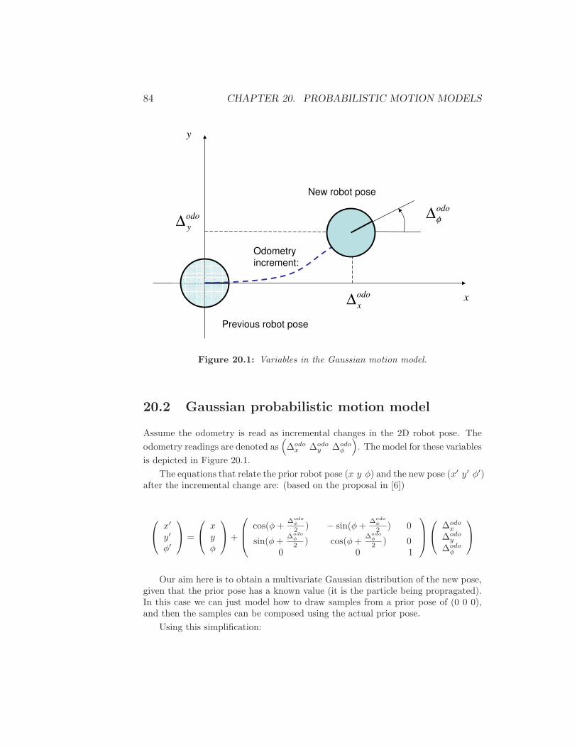
84 CHAPTER 20. PROBABILISTIC MOTION MODELS
x
y
odo
x∆
odo
y∆
odo
φ∆
Previous robot pose
New robot pose
Odometry
increment:
Figure 20.1: Variables in the Gaussian motion model.
20.2 Gaussian probabilistic motion model
Assume the odometry is read as incremental changes in the 2D robot pose. The
odometry readings are denoted as(
∆odox ∆odo
y ∆odoφ
)
. The model for these variables
is depicted in Figure 20.1.
The equations that relate the prior robot pose (x y φ) and the new pose (x′ y′ φ′)after the incremental change are: (based on the proposal in [6])
x′
y′
φ′
=
xyφ
+
cos(φ+∆odo
φ
2 ) − sin(φ+∆odo
φ
2 ) 0
sin(φ+∆odo
φ
2 ) cos(φ+∆odo
φ
2 ) 00 0 1
∆odox
∆odoy
∆odoφ
Our aim here is to obtain a multivariate Gaussian distribution of the new pose,given that the prior pose has a known value (it is the particle being propragated).In this case we can just model how to draw samples from a prior pose of (0 0 0),and then the samples can be composed using the actual prior pose.
Using this simplification:

20.2. GAUSSIAN PROBABILISTIC MOTION MODEL 85
Figure 20.2: Simulation of a Gaussian motion model in RawlogViewer.
x′
y′
φ′
=
cos∆odo
φ
2 − sin∆odo
φ
2 0
sin∆odo
φ
2 cos∆odo
φ
2 00 0 1
∆odox
∆odoy
∆odoφ
= H
∆odox
∆odoy
∆odoφ
The mean of the Gaussian can be simply computed from the composition ofthe prior and the odometry increment. For the covariance, we need to estimatethe variances of the three variables of the odometry increment. We model themas having independent, zero-mean Gaussian errors. The errors will be composed ofterms that capture imperfect odometry and potential drift effects.
We denote as Σ the diagonal matrix having the three variances of the odometryvariables, modeled as:
σ∆odox
= σ∆odoy
= σminxy + α1
√
(∆odox )2 + (∆odo
y )2 + α2|∆odoφ |
σ∆odoφ
= σminφ + α3
√
(∆odox )2 + (∆odo
y )2 + α4|∆odoφ |
The default parameters (loaded in the constructor and available in RawLogViewer)are:

86 CHAPTER 20. PROBABILISTIC MOTION MODELS
α1 = 0.05 meters/meterα2 = 0.001 meters/degreeα3 = 5 degrees/meterα4 = 0.05 degrees/degree
σminxy = 0.01 meters
σminφ = 0.20 degrees
And finally, the covariance of the new pose after the odometry increment (C)is computed by means of:
C = J Σ J t
where J stands for the Jacobian of H.An example of samples obtained using this model with the RawLogViewer
application is represented by Figure 20.2.
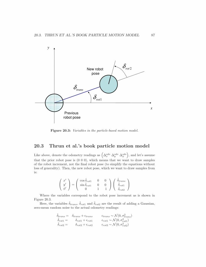
20.3. THRUN ET AL.’S BOOK PARTICLE MOTION MODEL 87
x
y
transδ
Previous
robot pose
New robot
pose
1rotδ
2rotδ
Figure 20.3: Variables in the particle-based motion model.
20.3 Thrun et al.’s book particle motion model
Like above, denote the odometry readings as(
∆odox ∆odo
y ∆odoφ
)
, and let’s assume
that the prior robot pose is (0 0 0), which means that we want to draw samplesof the robot increment, not the final robot pose (to simplify the equations withoutloss of generality). Then, the new robot pose, which we want to draw samples fromis:
x′
y′
φ′
=
cos δrot1 0 0
sin δrot1 0 00 1 1
δtransδrot1δrot2
Where the variables correspond to the robot pose increment as is shown inFigure 20.3.
Here, the variables δtrans, δrot1 and δrot2 are the result of adding a Gaussian,zero-mean random noise to the actual odometry readings:
δtrans = δtrans + ǫtrans ǫtrans ∼ N (0, σ2trans)
δrot1 = δrot1 + ǫrot1 ǫrot1 ∼ N (0, σ2rot1)
δrot2 = δrot2 + ǫrot2 ǫrot2 ∼ N (0, σ2rot2)

88 CHAPTER 20. PROBABILISTIC MOTION MODELS
Figure 20.4: Simulation of a particles motion model in RawlogViewer.
The model described in [12] employs the following approximations for the valuesof the standard deviations required for the equations above:
σrot1 = α1|δrot1|+ α2δtransσtrans = α3δtrans + α4(|δrot1|+ |δrot2|)σrot2 = α1|δrot2|+ α2δtrans
This is the model implemented in CActionRobotMovement2D when setting”CActionRobotMovement2D::TMotionModelOptions::modelSelection” to ”mmThrun”.Actually, a small additional error is summed to each pose component (x, y, φ) toavoid that for a null odometry increment the movement for all the particles becomeexactly zero, which may lead a particle filter to degenerate.
Figure 20.4 shows an example of samples generated using this model, for anexcessively large value of α2 (a very large ”slippage”), generated by the applicationRawLogViewer.

Chapter 21
Sensor Interfaces
This chapter describes the two parts in which classes of the library mrpt-hwdriversare divided: those providing the basis of communications (USB, serial), and thesensors themselves.
21.1 Communications
21.1.1 Serial ports
Even nowadays, lots of devices offer serial ports (or embedded USB-to-serial con-verters) as interfaces due to their simplicity of use. In MRPT, a serial port can bemanaged with the class hwdrivers::CSerialPort. An example of usage would beas follows:
#include <mrpt/hwdrivers.h>
...
CSerialPort ser;
ser.setSerialPortName ("ttyS0"); // or "COM3", ...
ser.setConfig (9600 /* baud */, 0 /*no parity */, 8 /*8 bit words */ );
ser.open ();
if (!ser.isOpen ()) { // Report error }
ser.Read( ... );
ser.Write( ... );
ser.close (); // optional: it closes on destruction anyway
In addition, a serial port implements the generic CStream interface, thus it isperfectly legal to transfer arbitrarily complex objects through a serial connectionas in:
COccupancyGridMap2D map;
ser << map;
However, the most likely use of a serial ports is to send and receive short textualmessages, thus the most useful methods are Read and Write.
89
90 CHAPTER 21. SENSOR INTERFACES
Names of serial ports
In Windows, serial ports appear with names COM1, COM2, COM3, COM4 and \\.\COMXX
for the rest. However, if you pass a name without the prefix \\.\ it will be addedautomatically.
In Linux, a variety of names can be found such as ttyUSB0, ttyS0 or ttyACM0.It is not required to provide the full path to the device (eg. /dev/ttyS0), as inWindows, it will be added transparently.
As follows from above, always keep serial port names as strings, not only as anumber since it will be not enough in a cross-platform application.
Timeouts
Slight changes in the timeouts of your connection can be lead to random and hardto debug errors with no apparent reason. The proper way of setting these delays isthrough the method:
void CSerialPort :: setTimeouts(
int ReadIntervalTimeout ,
int ReadTotalTimeoutMultiplier ,
int ReadTotalTimeoutConstant ,
int WriteTotalTimeoutMultiplier ,
int WriteTotalTimeoutConstant )
where all the fields have the same meaning than in the Windows API1.
21.1.2 USB FIFO with FTDI chipset
21.2 Summary of sensors
1 Search for the COMMTIMEOUTS structure for details.

21.3. THE UNIFIED SENSOR INTERFACE 91
21.3 The unified sensor interface
When implementing a new sensor class, the following execution flow must be keptin mind:
1. Object constructor: Do here basic initialization only. Parameters are still notset (see next step), thus communications must not be set up at this point.
2. CGenericSensor::loadConfig: Load here the parameters specific to yoursensor. Notice that the application rawlog-grabber automatically loads thefollowing parameters (common to all the sensors), thus they must be notloaded at this point:
(a) “process rate”: The rate in Hertz (Hz) at which the sensor threadshould invoke ”doProcess”. Mandatory parameter.
(b) “max queue len”: The maximum number of objects in the observationsqueue (default is 100). If overflow occurs, an error message will be issuedat run-time.
3. CGenericSensor::initialize: Initialize here your connections, send initialcommands to the device, etc.
4. CGenericSensor::doProcess: This method is called over and over againwhile the application is running. Your code must not delay too much andmust always return, i.e. do not insert infinite loops. If a new piece of infor-mation from the sensor is gathered (which may not always occur), use thehelper method CGenericSensor::appendObservation to add it to the “out-put queue”. That is all rawlog-grabber expects from each sensor’s class.Observations must be inserted in the list in the form of smart pointers (referto Chapter 11).
21.4 How rawlog-grabber works

92 CHAPTER 21. SENSOR INTERFACES
Chapter 22
Kalman filters
22.1 Introduction
22.2 Algorithms
22.3 How to implement a problem as a KF
The example bayesianTracking.A more complicated model, the problem of 6D SLAM, is discussed in detail in
[3] and implemented as the application kf-slam within MRPT.
93

94 CHAPTER 22. KALMAN FILTERS
Chapter 23
Particle filters
23.1 Introduction
A good tutorial can be found in [1].
23.2 Algorithms
23.2.1 SIR
23.2.2 Auxiliary PF
23.2.3 Optimal PF
23.2.4 Optimal-rejection sampling PF
The method presented in the paper [4].
23.3 Resampling schemes
A common problem of all particle filters is the degeneracy of weights, which consistsin the unbounded increase of the variance of the weights ω[i] with time. In order toprevent this growth of variance, which entails a loss of particle diversity, one of aset of resampling methods must be employed. The aim of resampling is replacingan old set of N particles by a new one with the same population but where particleshave been duplicated or removed according to their weights. More specifically, theexpected duplication count of the i’th particle, denoted by Ni, must tend to Nω[i].After resampling, all the weights become equal to preserve the importance samplingof the target pdf.
In this section we briefly review four different strategies for resampling a set ofparticles whose normalized weights are given by ω[i] for i = 1, ..., N . The methodsare explained using a visual analogy with a “wheel” whose perimeter is assigned to
95
96 CHAPTER 23. PARTICLE FILTERS
the different particles in such a way that the length associated to the i’th particleis proportional to its weight ω[i]. Therefore, picking a random direction in this“wheel” implies choosing a particle with a probability proportional to its weight.For a more formal description of the methods, please refer to the excellent paperby Douc, Cappe and Moulines [5].

23.3. RESAMPLING SCHEMES 97
[1]ω
[2]ω
[3]ω
[4]ω [5]
ω
[6]ω
Random
Figure 23.1: The multinomial resampling algorithm.
• Multinomial resampling: The most straighforward method, where N in-dependent random numbers are generated to pick a particle from the old set.In the “wheel” analogy, illustrated in Figure 23.1, this method consists ofpicking N independent random directions.
The name of this method comes from the fact that the probability massfunction for the duplication counts Ni is the multinomial distribution withthe weights as parameters.

98 CHAPTER 23. PARTICLE FILTERS
[1]ω[2]
ω
[3]ω
[4]ω
[5]ω
[6]ω
Random
[1]ω
[2]ω
[3]ω
[4]ω [5]
ω
[6]ω
Figure 23.2: The residual resampling algorithm. The shaded areas represent theinteger parts of ω[i]/(1/N). The residual parts of the weights, substracting theseareas, are taken as the modified weights ω[i].
• Residual resampling: This method comprises of two stages. Firstly, parti-cles are sampled deterministically by picking Ni = ⌊Nω[i]⌋ copies of the i’thparticle. Then, multinomial sampling is performed with the residual weights
ω[i] = ω[i] −Ni/N.

23.3. RESAMPLING SCHEMES 99
[1]ω
[2]ω
[3]ω
[4]ω [5]
ω
[6]ω
Random
Random
Random
Random
Random
Random 1N
Figure 23.3: The stratified resampling algorithm. The entire circunference isassociated to the range [0, 1] in the space of the particle weights, hence dividing itinto N equal parts is represented as N circular sectors of 1/N each.
• Stratified resampling: In this method, the “wheel” representing the oldset of particles is divided into N equally-sized segments, as represented inFigure 23.3. Then, N uniform numbers are independently generated likein multinomial sampling, but instead of mapping each draw to the entirecircunference, they are mapped to its corresponding partition.

100 CHAPTER 23. PARTICLE FILTERS
[1]ω
[2]ω
[3]ω
[4]ω [5]
ω
[6]ω
1N
1N
1N
1N
1N
1N
Random
Figure 23.4: The systematic resampling algorithm.
• Systematic resampling: Also called universal sampling, this popular tech-nique draws only one random number, i.e. one direction in the “wheel”, withthe others N − 1 directions being fixed at 1/N increments from the randompick.
23.4 Implementation examples

Bibliography
[1] M.S. Arulampalam, S. Maskell, N. Gordon, T. Clapp, D. Sci, T. Organ, andSA Adelaide. A tutorial on particle filters for online nonlinear/non-GaussianBayesian tracking. IEEE Transactions on Signal Processing, 50(2):174–188,2002.
[2] Several authors. The Player project, 2008.http://playerstage.sourceforge.net/.
[3] J.L. Blanco. Derivation and Implementation of a Full 6D EKF-based Solutionto Bearing-Range SLAM. Technical report, 2008.
[4] J.L. Blanco, J. Gonzalez, and J.A. Fernandez-Madrigal. An optimal filteringalgorithm for non-parametric observation models in robot localization. InIEEE International Conference on Robotics and Automation (ICRA’08), pages461–466, May 2008.
[5] R. Douc, O. Cappe, and E. Moulines. Comparison of resampling schemes forparticle filtering. In Proceedings of the 4th International Symposium on Imageand Signal Processing and Analysis, pages 64–69, 2005.
[6] A.I. Eliazar and R. Parr. Learning probabilistic motion models for mobilerobots. ACM International Conference Proceeding Series, 2004.
[7] Juan-Antonio Fernandez-Madrigal. The babel development system for inte-grating heterogeneous robotic software. Technical report, System Engineeringand Automation Dpt. - University of Malaga (Spain), July 2003.
[8] Juan-Antonio Fernandez-Madrigal. The BABEL website, 2008.http://babel.isa.uma.es/babel2/.
[9] Michael Montemerlo, Nicholas Roy, Sebastian Thrun, Dirk Haehnel, CyrillStachniss, and Jared Glover. The CARMEN robot navigation toolkit, 2008.http://carmen.sourceforge.net/.
[10] Paul Newman et al. The MOOS website, 2008.http://www.robots.ox.ac.uk/ pnewman/TheMOOS/.
[11] Andy Rushton. The STLplus website, 2008.http://stlplus.sourceforge.net/.
101

102 BIBLIOGRAPHY
[12] S. Thrun, W. Burgard, and D. Fox. Probabilistic Robotics. The MIT Press,September 2005.


![Introduction to Scientific Computing · 2.1 Introduction to Scientific Computing Scientific computing – subject on crossroads of physics, chemistry, [social, engineering,...]](https://static.fdocuments.us/doc/165x107/5edc24c2ad6a402d6666af19/introduction-to-scientiic-computing-21-introduction-to-scientiic-computing.jpg)


