FINAL REPORT

DEVELOPMENT OF PROTOTYPEDECISION SUPPORT SYSTEMS

FOR REAL-TIMEFREEWAY TRAFFIC ROUTING:

VOLUME I

BRIAN L. SMITH, Ph.D.FacuIty Research Scientist

CATHERINE C. McGHEESen ior Research Scientist

MICHAEL J. DEMETSKY, Ph.D.Faculty Research Scientist

ADEL W. SADEKGraduate Research Assistant

VIRGINIA TRANSPORTATION RESEARCH COUNCIL

1. Report No.FHWNVTRC 98-R17

Standard Title Pa~e - Report on Federally Funded Project2. Government Accession No. 3. Recipient's Catalog No.

4. Title and SubtitleDevelopment of Prototype Decision Support Systems for Real-Time FreewayTraffic Routing: Volume I

7. Author(s)B.L. Smith, C. C. McGhee, M.J. Demetsky, and A.W. Sadek

9. Performing Organization and Address

Virginia Transportation Research Council530 Edgemont RoadCharlottesville, VA 2290312. Sponsoring Agencies' Name and Address

5. Report DateJune 1998

6. Performing Organization Code

8. Performing Organization Report No.VTRC 98-R17

10. Work Unit No. (TRAIS)

11. Contract or Grant No.1465-03013. Type of Report and Period CoveredFinal October 1995 - December 1997

Virginia Department of Transportation1401 E. Broad StreetRichmond, VA 2321915. Supplementary Notes

FHWA1504 Santa Rosa RoadRichmond, VA 23239

14. Sponsoring Agency Code

16. AbstractFor a traffic management system (TMS) to improve traffic flow, TMS operators must develop effective routing strategies

based on the data collected by the system. The purpose of this research was to build prototype decision support systems (DSS) forthe real-time development of such strategies. We used the freeway system controlled by the Suffolk (Virginia) TMS as a test case.

A routing DSS has (1) a search mechanism that allows the space of possible routing strategies to be explored thoroughly butefficiently, and (2) an evaluation routine that estimates the effectiveness of a particular strategy. We combined the search andevaluation routines to develop two DSS prototypes: a simple shock-wave DSS that required very little input data and a heuristicsearch/dynamic traffic assignment (DTA) DSS that demanded more input and computations but captured traffic dynamics better.

We evaluated the prototypes based on the agreement of their recommended strategies with prior expectations and theirpotential for real-time applications. The results are promising. For the shock-wave DSS, the diversion percentages recommendedagree with prior expectations. For the heuristic search/DTA model, the results are consistent regardless of the start point for thesearch algorithm.

17 Key WordsFreeway traffic management, traffic routing, intelligenttransportation systems, decision support systems, stochasticsearch algorithms

18. Distribution StatementNo restrictions. This document is available to the public throughNTIS, Springfield, VA 22161.

19. Security Classif. (of this report)Unclassified

20. Security Classif. (of this page)Unclassified

21. No. of Pages38

22. Price

Form DOT F 1700.7 (8-72) Reproduction of completed page authorized

FINAL REPORT

DEVELOPMENT OF PROTOTYPE DECISION SUPPORT SYSTEMSFOR REAL-TIME FREEWAY TRAFFIC ROUTING: VOLUME I

Brian L. Smith, Ph.D.Faculty Research Scientist

Catherine C. McGheeSenior Research Scientist

Michael J. Demetsky, Ph.D.Faculty Research Scientist

Adel W. SadekGraduate Research Assistant

(The opinions, findings, and conclusions expressed in thisreport are those of the authors and not necessarily

those of the sponsoring agencies.)

Virginia Transportation Research Council(A Cooperative Organization Sponsored Jointly by the

Virginia Department of Transportation and theUniversity of Virginia)

Charlottesville, Virginia

June 1998VTRC 98-R17

Copyright 1998 by the Virginia Department of Transportation.

11

ABSTRACT

For a traffic management system (TMS) to improve traffic flow, TMS operatorsmust develop effective routing strategies based on the data collected by the system. Thepurpose of this research was to build prototype decision support systems (DSS) for thereal-time development of such strategies. We used the freeway system controlled by theSuffolk (Virginia) TMS as a test case.

A routing DSS has (1) a search mechanism that allows the space of possiblerouting strategies to be explored thoroughly but efficiently, and (2) an evaluation routinethat estimates the effectiveness of a particular strategy. We combined the search andevaluation routines to develop two DSS prototypes: a simple shock-wave DSS thatrequired very little input data and a heuristic search/dynamic traffic assignment (DTA)DSS that demanded more input and computations but captured traffic dynamics better.

We evaluated the prototypes based on the agreement of their recommendedstrategies with prior expectations and their potential for real-time applications. Theresults are promising. For the shock-wave DSS, the diversion percentages recommendedagree with prior expectations. For the heuristic search/DTA model, the results areconsistent regardless of the start point for the search algorithm.

iii

DEVELOPMENT OF PROTOTYPE DECISION SUPPORT SYSTEMSFOR REAL-TIME FREEWAY TRAFFIC ROUTING: VOLUME I

Brian L. Smith, Ph.D.Faculty Research Scientist

Catherine C. McGheeSenior Research Scientist

Michael J. Demetsky, Ph.D.Faculty Research Scientist

Adel W. SadekGraduate Research Assistant

INTRODUCTION

To serve as the foundation for its Smart Travel program, the Virginia Departmentof Transportation (VDOT) made a significant investment in smart traffic centers. Thesecenters, commonly known as traffic management systems (TMSs), monitor freewaytraffic flow with sensors and closed-circuit television (CCTV) and relay travelinformation to motorists via devices such as variable message signs (VMS). The primarypurpose of a TMS is to enable urban freeways to operate as safely and efficiently aspossible.

To fulfill this purpose, TMS operators must make sound decisions based on thedata collected by the system. TMSs use advanced software to process raw data to provideoperators with information to support their decision making. Although significantresearch has been dedicated to developing improved TMS hardware, relatively little efforthas gone into developing improved decision support software to assist TMS operators.

One of the most important decisions operators must make is how to "control"traffic flow. Operators attempt to do this by influencing the route choice of motoriststhrough providing traveler information. By influencing route choice, TMS operators canattempt to distribute traffic flow evenly over the entire network, resulting in better overallnetwork performance. However, developing sound system routing strategies is a complextask that must effectively address two fundamental tasks:

1. Searching. A search mechanism is required that allows the "space" of allpossible routing strategies to be explored efficiently but thoroughly (the needfor an efficient search algorithm is especially true for a complex urbanfreeway network, where the number of possible routing strategies is extremelylarge).

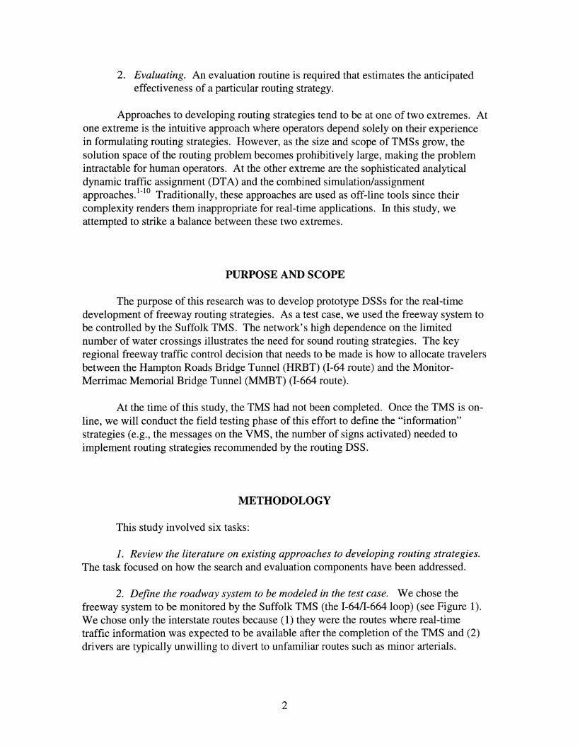
2. Evaluating. An evaluation routine is required that estimates the anticipatedeffectiveness of a particular routing strategy.

Approaches to developing routing strategies tend to be at one of two extremes. Atone extreme is the intuitive approach where operators depend solely on their experiencein formulating routing strategies. However, as the size and scope of TMSs grow, thesolution space of the routing problem becomes prohibitively large, making the problemintractable for human operators. At the other extreme are the sophisticated analyticaldynamic traffic assignment (DTA) and the combined simulation/assignmentapproaches. I

-IO Traditionally, these approaches are used as off-line tools since their

complexity renders them inappropriate for real-time applications. In this study, weattempted to strike a balance between these two extremes.

PURPOSE AND SCOPE

The purpose of this research was to develop prototype DSSs for the real-timedevelopment of freeway routing strategies. As a test case, we used the freeway system tobe controlled by the Suffolk TMS. The network's high dependence on the limitednumber of water crossings illustrates the need for sound routing strategies. The keyregional freeway traffic control decision that needs to be made is how to allocate travelersbetween the Hampton Roads Bridge Tunnel (HRBT) (1-64 route) and the Monitor­Merrimac Memorial Bridge Tunnel (MMBT) (1-664 route).

At the time of this study, the TMS had not been completed. Once the TMS is on­line, we will conduct the field testing phase of this effort to define the "information"strategies (e.g., the messages on the VMS, the number of signs activated) needed toimplement routing strategies recommended by the routing DSS.

METHODOLOGY

This study involved six tasks:

1. Review the literature on existing approaches to developing routing strategies.The task focused on how the search and evaluation components have been addressed.

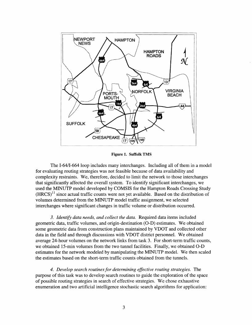
2. Define the roadway system to be modeled in the test case. We chose thefreeway system to be monitored by the Suffolk TMS (the 1-64/1-664 loop) (see Figure 1).We chose only the interstate routes because (1) they were the routes where real-timetraffic information was expected to be available after the completion of the TMS and (2)drivers are typically unwilling to divert to unfamiliar routes such as minor arterials.

2

NEWPORTNEWS

SUFFOLK

HAMPTON jROADS 1

9t£

Figure 1. Suffolk TMS

The I-64/I-664 loop includes many interchanges. Including all of them in a modelfor evaluating routing strategies was not feasible because of data availability andcomplexity restraints. We, therefore, decided to limit the network to those interchangesthat significantly affected the overall system. To identify significant interchanges, weused the MINUTP model developed by COMSIS for the Hampton Roads Crossing Study(HRCS)ll since actual traffic counts were not yet available. Based on the distribution ofvolumes determined from the MINUTP model traffic assignment, we selectedinterchanges where significant changes in traffic volume or distribution occurred.

3. Identify data needs, and collect the data. Required data items includedgeometric data, traffic volumes, and origin-destination (O-D) estimates. We obtainedsome geometric data from construction plans maintained by VDOT and collected otherdata in the field and through discussions with VDOT district personnel. We obtainedaverage 24-hour volumes on the network links from task 3. For short-term traffic counts,we obtained I5-min volumes from the two tunnel facilities. Finally, we obtained O-Destimates for the network modeled by manipulating the MINUTP model. We then scaledthe estimates based on the short-term traffic counts obtained from the tunnels.

4. Develop search routines for determining effective routing strategies. Thepurpose of this task was to develop search routines to guide the exploration of the spaceof possible routing strategies in search of effective strategies. We chose exhaustiveenumeration and two artificial intelligence stochastic search algorithms for application:

3

(1) genetic algorithms (GAs), which are based on the principle of survival of the fittest,12and (2) simulated annealing (SA), which is analogous to the process of atoms rearrangingthemselves in a cooling metal. 13

5. Develop evaluation tools for testing the effectiveness ofalternate routingstrategies generated by the search routine. We examined two approaches that vary inaccuracy, input requirements, and computational demands: (1) a simplified shock-wavemodel, and (2) a detailed dynamic macroscopic model of the region.

6. Develop and evaluate prototype routing DSSs. In this task, we combined thesearch and evaluation routines developed under tasks 4 and 5 to develop two routingdecision support prototypes. We paired exhaustive enumeration with the simplifiedshock-wave model, resulting in a simple DSS that required very little input data. On theother hand, we linked GAs and SA to the detailed dynamic macroscopic model to yield aDSS that was more demanding in terms of input and computational requirements butpromised to be more accurate than the shock-wave model. We evaluated the tools basedon the agreement of their recommended strategies with prior expectations and theirpotential for real-time applications.

RESULTS

Literature Review

A number of avenues are being investigated by researchers in the United States,Europe, and Japan for developing effective decision support tools for real-time trafficrouting. Approaches to developing routing strategy can be broadly classified into twocategories: (1) the analytical dynamic traffic assignment (DTA) approach,I-6 and (2) thecombined simulation/assignment approach.7

-10 Traditionally, these approaches have been

used as off-line analysis tools and not in real-time applications.

Analytical DTA Approach

In this approach, the routing problem is formulated as a mathematicalprogramming model, commonly referred to as a DTA model. In a mathematicalprogramming approach, a mathematical model is constructed for the system underconsideration. This model takes the form of a system of equations and relatedmathematical expressions (commonly referred to as constraints) that describe how thesystem functions. Within this system of equations, the quantifiable decisions that need tobe made and that affect the performance of the system are represented as decisionvariables whose values need to be determined. Solving a mathematical model involvesdetermining the values for the decision variables that will optimize the system's

4

performance. The system's measure of performance to be optimized is typicallyexpressed as a mathematical function called the objective function. 14

For a DTA model, the decision variables are typically the time-varying trafficvolume assigned to each link (roadway segment) of the network. The objective functionexpresses the measure of highway network performance to be optimized (e.g., the totaltravel time for all vehicles), whereas the set of constraints attempts to model traffic flowin the region through the use of macroscopic traffic flow theory concepts. Theformulated model is then solved, typically using a non-linear programming (NLP)technique, to obtain the routing strategy that will optimize the objective function.

There are two types of DTA models: (1) user-optimal or user-equilibrium models,and (2) system-optimal models. In user-equilibrium formulations, each user attempts tominimize his or her travel time. These models are typically based on a dynamicgeneralization of Wardrop's principle, which states that the individual costs along utilizedroutes connecting an origin to a destination are equal and minimal. In other words,people use paths of minimum cost. The goal behind user-equilibrium formulations is toreplicate the patterns of traffic flows resulting from users' independent path choicedecisions, and hence they are mainly used to predict traffic.

The system-optimal formulation, on the other hand, attempts to determine howtraffic should be distributed in the network so as to optimize a systemwide criterion.Although the travel times of alternate routes might be unequal, the total travel time for allthe vehicles in the system is minimal. It is this second type of dynamic assignment modelthat is more relevant to the real-time traffic routing problem for a centrally managednetwork similar to the one considered in this study. The Merchant and Nemhauser (M-N)model, l which is considered by many as the seminal work on system-optimal DTAmodels, illustrates the analytical DTA approach best.

Merchant and Nemhauser Model

The M-N model addresses the case of single-destination networks in whichtravelers from multiple origins are traveling to one destination. The purpose is tooptimally assign traffic over a period of time known as the planning horizon. In the M-Nformulation, the planning horizon is divided into equal time intervals of suitably smalllength {i I i =0,1, ... I}. Each link of the network is assigned a cost function (hij) and anexit function gj. When xij is the number of vehicles on linkj at the beginning of timeperiod i, it is assumed that a cost hij(xij) is incurred and an amount of traffic gj(xij) exitsfrom the link.

To model traffic dynamics, the function gj(x) will typically have to be concaveover some part of its domain (Figure 2). This leads to non-convex model formulationsthat cannot be easily solved using traditional analytical approaches. The function hij(x),

on the other hand, should be nonnegative, nondecreasing, continuous, and convex to

5

/

"//

//

"//

//

//

//

/

//

//

"//

//

//

//

//

//

C - Capacity of link aa

u - Flow of link aa 9a -Exit flow from link a

Figure 2. Examples of Exit Functions

represent the increase in travel cost with congestion. An example of a cost function is hij(x) =x for all i andj, which gives the total number of vehicle-periods spent on thenetwork.

The objective function of the M-N model is expressed as:

minimize

This function attempts to minimize the total cost as defined by the function hij(Xl}) over alllinks over all time periods. Optimizing this function is subject to four groups ofconstraints.

1. The state equations. Denoting the number of vehicles admitted onto linkjduring the ith period by dij (the decision variables), and assuming that the external inputsare known for each time period Fi (q) and that the volume admitted onto a link cannotleave that link in the same time interval, the fundamental state equations can be writtenas:

i =0,1, ..., I - 1 (1)

This equation states that the number of vehicles on linkj during time interval (i + 1) isequal to the number of vehicles that were on that link during the previous time interval(xij) minus the volume that exited from the link, gj(xij), plus the volume admitted on thatlink, dij.

2. The flow conservation constraints. The flow conservation equations at eachnode are given as:

(2)

where A(q) is the set of links pointing out of node q, B(q) is the set of links pointing intonode q, and Fi(q) is the external travel demand (number of vehicles) at node q. These

6

equations reflect the fact that nodes cannot "store" vehicles. Therefore, the number ofvehicles leaving a node during an interval must equal the number of vehicles entering thenode.

3. The initial conditions. These are given as:

(3)

which define the number of vehicles that were initially on each link, j, of the network.

4. The non-negativity constraints. These are expressed as:

d .. >OI} -

These constraints require that the decision variables, du, and the state variables, xu' arenonnegative. A negative value is physically impossible for the number of vehiclesadmitted, or present, on a link.

(4)

(5)

The M-N model formulation represents a discrete time, nonlinear, and nonconvexmathematical programming problem and, therefore, cannot be directly solved using NLPtechniques. To allow for the application of such techniques, Carey3 modified the modelby introducing traffic flow control or congestion control constraint that can be used tokeep the actual outflow from a link below the natural or the unrestricted capacity levelgiven by the function gj(xu). In the real world, this corresponds to having a traffic signalor ramp metering system regulating traffic entry into the different segments. Althoughsuch a modification allows for solving the model using traditional NLP techniques, therecould be many instances in practice where one does not wish to consider traffic controls(e.g., an unmetered freeway). Carey also extended the formulation to handle multipledestinations. 16 Such an extension, however, renders the problem nonconvex once againand hence precludes its solution using traditional NLP methods.

Limitations

The analytical DTA approach places less weight on the evaluation than on thesearch. Traffic flow is represented by a set of mathematical equations and inequalities.In addition, various assumptions are typically made in formulating these equations tofacilitate model solution using traditional NLP techniques. Given the "constraints"placed on the evaluation component, the analytical approach cannot fully capture trafficdynamics. Among the problems that have been reported by researchers in this regard are:

• The violation of the first in, first out (FIFO) property, which means that thesolution may involve holding traffic on one path in favor of traffic on other

7

paths for a significant time. This is unrealistic from an operations point ofview.

• The inability ofsome models to capture traffic spillback and lane blockageeffects.

• The inability to capture dynamic traffic flow phenomena such as queueformation and discharge and congestion buildup and dissipation.

On the other hand, the approach emphasizes the search aspect by attempting tolocate the optimal solution. For a complex urban freeway network, finding the optimalsolution is computationally intensive. In most cases, such complexity renders DTAmodels inappropriate for real-time applications.

Combined Simulation/Assignment ApproachOverview

This approach puts more weight on the evaluation than on the search aspect of theproblem. Two of the best known examples of this approach are the INTEGRATIONmodel developed by Van Aerde7,s and the DYNASMART model developed byMahmassani et a1.9

,lO These models are typically mesoscopic in nature, which means thatvehicles are treated as separate entities carrying a set of attributes for assignment purposesbut they travel from the entrance to the exit of a section based on speed-density-capacityrelationships and not according to car-following logic as in microscopic simulation.

The combined simulation/assignment approach represents an attempt to overcomethe limitations of the purely analytical approach in modeling traffic dynamics. In thisapproach, a simulation model (the evaluation component) is used to model traffic flow(simulation allows for more accurate modeling of traffic flow phenomena such as queueformation and dissipation). An assignment procedure (the search procedure) then assignsvehicles to the shortest path based on the travel time obtained from the simulation model.To allow for capturing the dynamic nature of the problem, the shortest paths arerecalculated frequently (every 5 seconds in case of the INTEGRATION model).

Limitations

Simulation-assignment models are rather slow and, therefore, are not suited forreal-time applications. Moreover, it is not envisioned that computer advancements in theforeseeable future will completely address this problem.

These models are mainly intended for solving user-equilibrium modelformulations and, therefore, cannot be easily adapted to address system optimalassignments.

8

Despite the fact that they represent an improvement over analytical models incapturing traffic dynamics, they still have problems fully capturing true traffic dynamicsbecause of their mesoscopic nature.

The Roadway System

The first step in developing the routing decision support tools was to define thehighway network to be considered for modeling. This network had to include the majorfacilities in the area that were to be managed by the Suffolk TMS. The selected networkis shown in Figure 3.

70

60

..-.. 50~Q) 40~co~ 30Q)UJ

:::J 20

10

0

-----.--------.

--+- Correct

-B- Incorrect

A None

------ No data

1993 1994 1995

Year

1996 1997

Figure 3. Network Selected for Modeling

As can be seen, the scope of the network selected is composed of the loop formedby 1-64 and 1-664, along with 1-264 and 1-464. The network selected, given the locationof the VMSs of the Suffolk TMS, will allow for routing traffic originating from Route 44,1-464, and Route 17 as it enters the loop.

Given the scope of the network, the next step was to identify the location of thoseaccess/exit points where traffic volume changes significantly. This required a carefulstudy of the variation in traffic volumes along the different road segments of the network.To do this, we used the travel demand model developed by COMSIS Corporation for theHRCS. This model was developed using the MINUTP travel demand forecastingsoftware (version 96A). Validation checks were made to ensure that the model wasreplicating observed travel patterns. For most of the screen- and cut-lines considered, thedeviation of assigned volumes from the observed counts was less than 15 percent.

From the results of the MINUTP traffic assignment step, we estimated the dailyvolume on each link of the system. We then used these volumes to identify the

9

significant access/exit points. Tables 1 through 7 give the significant access/exit pointsselected along with the 24-hour traffic volume entering and leaving the system at eachpoint.

Figure 4 shows the location of these points along the network selected formodeling.

o Nodes

D Links

~

~ ~~~5..a--=@§]~~~~~~~~~~~~~F(@ @)

Figure 4. Location of AccesslExit Points with Significant Volume Changes

10

Table 1. Significant Access/Exit Points Along Segment of 1-64 from 1-64/Rt. 44 Junctionto 1-64/1-664 Junction

VTRC Model Entering Volume Exiting VolumeNode Description Node Number (veh.lday) (veh.lday)

Exit 284 - I-64/Rt. 44 Junction 12 103080 47800

Exit 282 - NorthHampton (Rt. 13) 11 24047 8567Exit 281 - Military Hwy. (Rt. 165) 10 7587 15473

Exit 279 - Norview Ave. 9 13153 8513Exit 278 - Chesapeake Blvd. (Rt. 194) 8 3093 9540Exit 277 - Tidewater Dr. (Rt. 168) 7 15833 2787Exit 276 - 1564 6 20020 37073Exit 274 - Bay Ave. 5 3260 13333Exit 273 - 4th View 4 3187 7420Exit 268 - Mallory St. (Rt. 169) 3 12673 860Exit 265 - Lasalle Ave. 2 14793 5100Exit 264 - 1-64/1-664 Junction 1 0 93007

Table 2. Significant Access/Exit Points Along Segment of 1-64 from 1-64/Rt. 44 Junctionto 1-64/1-664 Junction (WB)

VTRCModel Entering Volume Exiting VolumeNode Description Node Number (veh.lday) (veh.lday)

Exit 286 - Indian River 31 9567 12547Exit 289 - Greenbrier 30 7000 3233Exit 290 - Battlefield Blvd. 29 6580 4920Exit 291 - 1-464 16 22740 15567Exit 296 - Rt. 17 18 5660 5913

Table 3. Significant Access/Exit Points Along Segment of 1-64 from 1-64/Rt. 44 Junctionto 1-64/1-664 Junction (EB)

VTRC Model Entering Volume Exiting VolumeNode Description Node Number (veh.lday) (veh.lday)

Exit 286 - Indian River 13 25620 1100Exit 289 - Greenbrier 14 5260 3613Exit 290 - Battlefield Blvd. 15 12140 9127Exit 291 - 1-464 16 22740 15567Exit 296 - Rt. 17 18 5660 5913

11

Table 4. Significant Access/Exit Points Along 1-664

VTRC Model Node Entering Volume Exiting VolumeNode Description Number (veh.lday) (veh.lday)

Exit 13 - Military Hwy. (Rt. 13,58,460) 27 5453 18867Exit 12 26 500 2247Exit 10 - Taylor St/Exit 9 - I-1641Exit 8 - Rt. 135 25 5407 6147Exit 5 24 10027 387Intersection wI Roanoke Ave. 23 7313 467

Table 5. Significant Access/Exit Points Along 1-264 (WB)

VTRCModel Entering Volume Exiting VolumeNode Description Node Number (veh.lday) (veh.lday)

Military Hwy. (Rt. 13) 37 8047 20600Balientine Blvd. 36 10473 3807Brambleton Ave. 35 0 181271-264/1-464 Junction 22 35793 25307Intersection wI Rt. 17 34 1767 22293Portsmouth (Rt. 337) 33 893 11853Victory Blvd. 32 567 6440

Table 6. Significant Access/Exit Points Along 1-264 (EB)

VTRC Model Entering Volume Exiting VolumeNode Description Node Number (veh.lday) (veh.lday)

Military Hwy. (Rt. 13) 19 26400 3027Balientine Blvd. 20 4300 3107Brambleton Ave. 21 26973 9131-264/1-464 Junction 22 35793 25307

Table 7. Significant Access/Exit Points Along 1-464

VTRC Model Node Entering Volume Exiting VolumeNode Description Number (WB) (veh.lday) (veh.lday)

1-264/1-464 Junction 22 35793 25307Exit 291 - 1-464 16 22740 15567

Data Collection

The data required for developing the routing strategy decision support tools can bedivided into three main categories: (1) freeway geometries, (2) traffic volumes, and (3)O-D estimates.

12

Freeway Geometries

We extracted geometric data from construction plans for the selected freewaysystem. Data items collected were:

• length of freeway segments (links)

• number of lanes for each segment

• width of lanes

• length of acceleration and deceleration lanes

• location of lane add/drop.

Traffic Volumes

Estimated average 24-hour volumes on the different links of the network wereavailable from the results of the MINUTP model traffic assignment step. For short-termtraffic volumes, data were available only for the two tunnels in the region, since the TMSwas not yet operational. We obtained traffic volumes, by lane, in 15-minute incrementsfor 1 year from the two tunnel facilities.

For the winter, Figure 5 shows the variation of traffic volume with the time of theday for weekdays during a typical winter month for the westbound direction of the

1000

900

.........C 800-ean 700~-....J:

~600

----CD 500E::s

~400

CJ 300Eca... 200I-

LO LO LO ~ LO LO LO LO LO LO LO II) II) LO II) LO II) II) LO II) II) II) LO

0 N ~ ~ an cO ~ co m 0 N ~ ~ an cO ~ co m 0 N N ~'l"'"" N N N

Time of Day

-Man

-Tues

Wed

Thu

-Fri

Figure 5. Volume Variation with Time of Day (Winter Weekdays)

13

HRBT. The evening peak period extends from around 3:30 P.M. to around 6:00 P.M.,

whereas the morning peak occurs between 6:30 A.M. and 9:00 A.M. In general, theevening peak traffic was heavier than the morning peak. Table 8 gives the peak hourtraffic volume for the evening peak period, along with the ratio of the peak hour volumeto the daily volume, k. Values for k were 0.08 to 0.09. For weekends, there appears tobe only one extended peak period (Figure 6). Values for k, however, were still around0.08.

Table 8. Peak Hour Traffic Volume on Weekdays During Winter

Monday Tuesday Wednesday Thursday FridayPeak hour 15:45-16:45 16:45-17:45 16:15-17:15 15:30-16:30 15:30-16:30Volume (veh./hr) 3251 3398 3236 3407 3709Daily volume 37238 39431 37951 41811 46293The ratio, k 0.087 0.086 0.085 0.081 0.080

800

~700

Cee600

It)...........c: 500~.........CD 400E:::s

~ 300

U

IE 200ca~

100

0LO LO LO LO...... ...... ...... ......a N cVi

-~-_. ----~ .......:

.

LO LO LO LO LO LO LO LO LO LO LO LO LO LO LO LO LO LO LO LO...... ...... ...... ...... ...... ...... ...... ...... ...... ...... ...... ...... ...... ...... ...... ...... ...... ...... ......~ ~ ~ ~ ~ m a ~ N cVi ~ ~ ~ ~ ~ m 0 ~ N cVi

...... ...... ...... ...... ...... ...... ...... ...... ...... ...... N N N N

Time of Day

Figure 6. Volume Variation with Time of Day (Winter Weekends)

For the summer, Figure 7 depicts volume variation on weekdays during a typicalsummer month. The morning and evening peak periods are quite discernible for allweekdays except Friday. For Friday, the peak period is longer. Similar to the wintermonths, the evening peak traffic is heavier than the morning peak. For weekends, thesingle extended peak period can once again be discerned (Figure 8). As seen in Table 9,although the daily summer volumes are larger than the winter volumes, peak hourvolumes are almost the same. This is obviously a direct result of the increase inrecreational traffic during the summer months. The increase in recreational traffic alsoexplains the lower k ratio values.

14

-Man

--- Tues

Wed

" Thu

-Fri

..._ _.~_ ~._ - _ - _- _ _._._ _._ ··_·····..· ····..·1

!i

II!

,v~1\ I~ I

t- ", U

~r\!

\'!li, ~

'"V

Io-t+tt-Htt+ttt+t+H-HI++t+t+t+t+tt+1rt+t+t+t+++++t-H+++t+t+++++H-H++++H+++++-lH-+++++H+++++-ll+H+t+I~ ~ ~ ~ ~ ~ ~ ~ ~ ~ ~ ~ ~ ~ ~ ~ ~ ~ ~ ~ ~ ~ ~ ~~~~~~~~~~~~~~~~~~~~~~~~~

o~NM~~m~mmo~NM~~m~mmo~NM~ ~ ~ ~ ~ ~ ~ ~ ~ ~ N N N N

900

100

1000

Time of Day

Figure 7. Volume Variation with Time of Day (Summer Weekdays)

200

300

400I Sat I'~Sun

a~ ~ ~ ~ ~ ~ ~ ~ ~ ~ ~ ~ ~ ~ ~ ~ ~ ~ ~ ~ ~ ~ ~ ~

~ ~

0 N M~ .n m ~ m m 0 N M~ .n m ~ m m 0 N N MN N N

Time of Day

900-r--"---~---------------~---~

100

800.........c

8e 700

It)

:!: 600.c~........ 500CDE:s

~uIEca~

Figure 8. Volume Variation with Time of Day (Summer Weekends)

Table 9. Peak Hour Traffic Volume on Weekdays During Summer

Monday Tuesday Wednesday Thursday FridayPeak hour 16:45-17:45 15:15-16:15 16:00-17:00 15:15-16:15 16:00-17:00Volume (veh./hr) 3073 3301 3406 3483 3344Daily volume 40639 40471 43071 45772 48680The ratio, k 0.076 0.082 0.079 0.076 0.069

15

Origin-Destination Estimates

The development of effective routing strategies for a network requires a goodestimate of the origins and destinations of the trips using the network. The HRCSMINUTP model was a valuable resource in this regard. However, the model, with nearly1,450 zones and more than 12,000 links, covered a larger area than the network selectedfor modeling. There was thus a need to extract the O-D matrix for the network of interest(such a matrix is typically referred to as a freeway interchange matrix since it gives thedistribution of trips between the on- and off-ramps of the freeway network). Table 10lists the network's major generators and attraction zones.

Table 10. Network Major Generators and Attraction Zones

VTRC Model Entering Volume Exiting VolumeNode Description Node Number (veh.lday) (veh.lday)

Exit 264 - I-64/I-664 Junction 1 0 93007Exit 276 - I-64/I564 Junction (Naval Base) 6 20020 37073Exit 284 - I-64/Rt. 44 Junction 12 103080 47800Exit 291 - I-64/I-464 Junction 16 22740 15567I-264/I-464 Junction 22 35793 25307I-264/Rt. 13 Intersection 19/37 34447 23627I-264/Brambleton Ave. Intersection 21/35 26973 19040

However, although the compiled matrix gave the daily trips between each O-Dpair, real-time routing required O-D matrices for shorter time intervals (typically 15­minute intervals). To address this, the matrix was appropriately scaled based on theshort-term traffic counts obtained from the tunnels. Scaling an O-D matrix based on justtwo points is admittedly not desirable. Nevertheless, the availability of traffic data fromthe Suffolk TMS, once it is on-line, will provide for more precise estimates in the future.

Search Routines for Determining Effective Routing Strategies

The purpose of this task was to investigate different approaches to developing thesearch component of the routing strategy development methodology. The search routineis responsible for guiding the exploration of possible routing strategies in search of aneffective strategy.

Overview ofSearch Techniques

Search techniques can be broadly classified into three groups: (1) exhaustiveenumeration, (2) mathematical programming techniques, and (3) heuristic approaches.Exhaustive enumeration searches through all possible combinations of values for thedecision variables and hence can be practically used only when the search space of theproblem is very small.

16

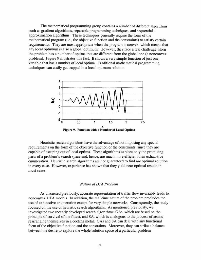
The mathematical programming group contains a number of different algorithmssuch as gradient algorithms, separable programming techniques, and sequential­approximation algorithms. These techniques generally require the form of themathematical program (i.e., the objective function and the constraints) to satisfy certainrequirements. They are most appropriate when the program is convex, which means thatany local optimum is also a global optimum. However, they face a real challenge whenthe problem has a number of optima that are different from the global one (a nonconvexproblem). Figure 9 illustrates this fact. It shows a very simple function of just onevariable that has a number of local optima. Traditional mathematical programmingtechniques can easily get trapped in a local optimum solution.

4---------------------3 -------- ----- -- ------ ----- -- ----- -- -- -- ------ --------- ------ ------ --- -------

2

O-t---------=---:w--------....-t--I-----.....-.J----t-I------t

-1 ------ -- ------- --- ----- ------- -- ------ ---- -- ----- ----- --------- --- --- -------

2.521.50.5-2 ------+-----+-------+------+-----.1

oX

Figure 9. Function with a Number of Local Optima

Heuristic search algorithms have the advantage of not imposing any specialrequirements on the form of the objective function or the constraints, since they arecapable of escaping out of local optima. These algorithms explore only the promisingparts of a problem's search space and, hence, are much more efficient than exhaustiveenumeration. Heuristic search algorithms are not guaranteed to find the optimal solutionin every case. However, experience has shown that they yield near optimal results inmost cases.

Nature ofDTA Problem

As discussed previously, accurate representation of traffic flow invariably leads tononconvex DTA models. In addition, the real-time nature of the problem precludes theuse of exhaustive enumeration except for very simple networks. Consequently, the studyfocused on the use of heuristic search algorithms. As mentioned previously, weinvestigated two recently developed search algorithms: GAs, which are based on theprinciple of survival of the fittest, and SA, which is analogous to the process of atomsrearranging themselves in a cooling metal. GAs and SA can deal with any functionalform of the objective function and the constraints. Moreover, they can strike a balancebetween the desire to explore the whole solution space of a particular problem

17

and the need to focus on the most promising parts of this space. Therefore, they are wellsuited to solve combinatorial optimization problems such as the one in this study.

Genetic Algorithms

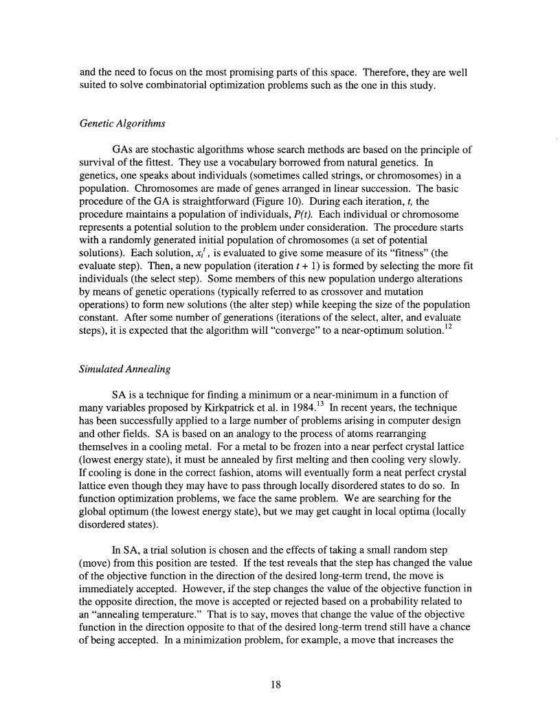
GAs are stochastic algorithms whose search methods are based on the principle ofsurvival of the fittest. They use a vocabulary borrowed from natural genetics. Ingenetics, one speaks about individuals (sometimes called strings, or chromosomes) in apopulation. Chromosomes are made of genes arranged in linear succession. The basicprocedure of the GA is straightforward (Figure 10). During each iteration, t, theprocedure maintains a population of individuals, pet). Each individual or chromosomerepresents a potential solution to the problem under consideration. The procedure startswith a randomly generated initial population of chromosomes (a set of potentialsolutions). Each solution, x/ , is evaluated to give some measure of its "fitness" (theevaluate step). Then, a new population (iteration t + 1) is formed by selecting the more fitindividuals (the select step). Some members of this new population undergo alterationsby means of genetic operations (typically referred to as crossover and mutationoperations) to form new solutions (the alter step) while keeping the size of the populationconstant. After some number of generations (iterations of the select, alter, and evaluatesteps), it is expected that the algorithm will "converge" to a near-optimum solution. 12

Simulated Annealing

SA is a technique for finding a minimum or a near-minimum in a function ofmany variables proposed by Kirkpatrick et al. in 1984.13 In recent years, the techniquehas been successfully applied to a large number of problems arising in computer designand other fields. SA is based on an analogy to the process of atoms rearrangingthemselves in a cooling metal. For a metal to be frozen into a near perfect crystal lattice(lowest energy state), it must be annealed by first melting and then cooling very slowly.If cooling is done in the correct fashion, atoms will eventually form a neat perfect crystallattice even though they may have to pass through locally disordered states to do so. Infunction optimization problems, we face the same problem. Weare searching for theglobal optimum (the lowest energy state), but we may get caught in local optima (locallydisordered states).

In SA, a trial solution is chosen and the effects of taking a small random step(move) from this position are tested. If the test reveals that the step has changed the valueof the objective function in the direction of the desired long-term trend, the move isimmediately accepted. However, if the step changes the value of the objective function inthe opposite direction, the move is accepted or rejected based on a probability related toan "annealing temperature." That is to say, moves that change the value of the objectivefunction in the direction opposite to that of the desired long-term trend still have a chanceof being accepted. In a minimization problem, for example, a move that increases the

18

Initialize P(t)

Evaluate P(t)

t =t + 1

Select P(t) from P(t - 1)

Alter P(t) throughmutation & crossover

Figure 10. GA Procedure

objective function value (an uphill move) may be accepted as part of the full series of thedownhill moves for which the general trend is to decrease the value of the objectivefunction. It is argued that such controlled uphill steps allow one to break away fromconfigurations leading to locally optimal solutions, and hence increases the likelihood ofeventually obtaining a higher quality solution.

The probability, P, of accepting these uphill moves is given by the followingequation, borrowed from the annealing process:

P =exp ( -illi/kT) (6)

where k is Boltzmann's constant, T is the temperature, and illi is the change in energy.For optimization problems, the energy, E, of equation (6) corresponds to the value of theobjective function, and since the temperature is a numerical value that controls theprobability of accepting uphill moves, the Boltzmann constant is not needed in thecomputation. The SA algorithm starts by initially setting the temperature at a high value,and then it periodically decrements such a value. While T is high, the optimizationroutine is free to accept many varied solutions, but as it drops, this freedom diminishesuntil the search is over. The success of the SA technique is, therefore, heavily dependenton the selection of a proper annealing schedule. An annealing schedule is the sequenceof temperatures and the amount of time or number of iterations at each temperatureneeded to reach equilibrium at that temperature.

Evaluation Tools for Testing Effectiveness of Alternate Routing Strategies

The objective of this task was to explore different approaches for modeling trafficflow in the region that can be used in evaluating the effectiveness of the alternate routingstrategies generated by the search algorithm. We developed two models that vary in

19

complexity and input requirements: (1) a shock-wave model developed for a very simpleversion of the highway network; and (2) a detailed dynamic, macroscopic, deterministicmodel of the region.

Shock-Wave Model

The purpose here was to develop an evaluation tool that (1) was simple to use, (2)required input data that were readily available, and (3) was capable of real-timeexecution. The tool was developed for a very simple network consisting of just tworoutes and for one specific routing scenario that frequently faces traffic operators atSuffolk TMS (Figure 11). This scenario involves routing westbound traffic originatingfrom Route 44 with destinations in Newport News when an incident occurs on theHampton-Roads Tunnel segment. The tool would help the user determine the percentage oftraffic that needs to be diverted to the MMBT and would give an estimate of the expectedtime required for flow to return to normal.

AlternateRoute 2

Figure 11. Network Considered for Shock-Wave Model

The tool is based on shock wave analysis and macroscopic traffic flow theoryprinciples. To allow for developing a simple tool with the minimum input requirements,a number of simplifying assumptions had to be made (these assumptions should beexpected to affect the accuracy of the results).

20

Assumptions

We made the following assumptions while developing the tool:

• Entering and exiting volumes between the origin (Route 44/1-64 interchange)and the destination (1-64/1-664 junction) are ignored.

• Traffic volumes are assumed constant over the planning horizon considered.

• The recommended diversion percentage remains the same until flow returns tonormal (i.e., remains constant throughout the planning horizon).

• The expected duration of an incident can be estimated.

• Traffic volumes using 1-264 and 1-464 are not treated as a part of the systemmodeled.

• A Greenshield's model I? for capturing traffic flow dynamics is assumed with

the following parameters: ajam density of 83.9 vehicles/kmllane (135vehicles/mi/lane) and a free-flow speed of 112.6 kmIhr (70 mph).

Shock-Wave Theory

The use of shock-wave analysis to model traffic congestion was first introducedby Lighthill and Whitham. 18 Shock waves are defined as boundary conditions in thetime-space domain that mark a discontinuity in flow-density conditions. One mayconsider the example of a pretimed signal-controlled intersection. At some distanceupstream of the signal and immediately downstream of the signal, free-flow conditionsexist. However, just upstream of the signal during the red phase, vehicles will be stoppedand densities will be high. As a result, there will be a discontinuity as vehicles join therear of the queue (backward forming shock wave) and as vehicles are discharged from thefront of the standing queue (backward recovery shock wave) when the signal turns green(see Figure 12). These two shock waves are backward moving because over time thediscontinuity is propagating in the opposite direction of the moving traffic. The firstshock wave is a forming wave because it is causing an increase in the congested part, andthe second is a recovery wave because it is causing a decrease in the congested area. I?

The shock wave speed between two traffic states is equal to the change in flowdivided by the change in density. Shock waves can be analyzed if a flow densityrelationship is known and traffic flow states are specified.

21

BackwardRecovery

ShockWave

/

JlFrontal

StationaryShockWave

Green

/BackwardForming

ShockWave

Time

Green Red

Figure 12. Shock Waves at Signalized Intersection

Hampton Roads Shock-Wave Evaluation Tool

The goal of the shock-wave evaluation tool is to find the travel time on the HRBTsegment (alternate route 1) and the MMBT segment (alternate route 2) under differentdiversion percentages. The travel time is averaged over the time period spanning fromthe moment an incident is verified to the time needed for traffic flow to return to normalconditions.

For calculating the travel time on the HRBT segment where an incident isassumed to have occurred, a shock-wave analysis is conducted. The shock-wave diagramfor this case is very similar to the one occurring at a signalized intersection (Figure 12).To find the average travel time over the period from the moment the incident is verifiedto the time flow returns to normal, the model traces the trajectories of representativevehicles that are 5 minutes apart, determines the travel time of each vehicle, and thenaverages the results.

For the MMBT segment, calculating the travel does not require shock-waveanalysis since no incident conditions are involved. The procedure simply entails usingthe flow-density-speed relationships to determine the speed corresponding to the trafficvolume on the segment, and hence the travel time.

22

Detailed Dynamic, Macroscopic Model

In this task, the purpose was to develop a more detailed dynamic, macroscopicmathematical model for the Hampton Roads region that could more accurately capturetraffic flow dynamics. This model would then serve as the evaluation component for arouting strategy development methodology. The study team felt that for the model toprovide more accurate results, it should have the following features:

• The model should account for the dynamic nature of traffic demand/supply.

• The model should take into account traffic entering and exiting at the variousaccess/exit points to the network.

• The model should be able to capture spillback and lane blockage effects, aswell as the effects of lane add/drop.

• The model should allow for considering multiple O-D pairs.

• The model should allow for considering more than one routing scenario.

The model has its roots in the modeling framework proposed by Papageorgiou.6 Weintroduced a number of refinements to allow for more accurate representation of trafficdynamics.

Papageorgiou's Modeling Framework

Papageorgiou's model addresses the general case of a multi-origin, multi­destination network. The model is based on the concept of independent splitting rates ateach node, f3njm(k), which give the rate of traffic volume leaving node n and destined tonode j that uses link m during interval k (k =0,1,2, ... is the discrete time index (i.e., f3(k)= (3(k . T)), T being the sample time interval or time step for the dynamic model).

The f3njm(k)s thus define how traffic is distributed among the alternate routes at anode and are given by:

(7)

where qnj(k) is the traffic volume exiting node n and destined to nodej, and qnjm(k) is thevolume exiting node n through link m and destined to node j during interval k. It followstherefore that the f3njm(k) s assume values between 0 and 1.0 and that

(8)m

23

Papageorgiou's model uses exit functions, first introduced by Merchant andNemhauser, l which give the number of vehicles leaving a link as a function of thenumber of vehicles on that link. The state of the system is described in terms of thetraffic density along the different links during each time step.

The formulation of the state equations of a DTA model (equation 1) dictates thatthe sample time interval or time step, T, be chosen so that the maximum distance avehicle travels in one time period is less than the link length. This ensures that allvehicles entering a link during a given interval remain on that link during that timeinterval and hence are justifiably included in estimating the density on that link.

Given (1) an initial state, (2) a demand matrix (O-D matrix), and (3) a specifiedset of the splitting rates, (3(k), the model can be used to describe the dynamic evolution ofthe system. Therefore, the model can be used to evaluate the effectiveness of a particularrouting strategy, as defined by the (3(k), given the initial state and the demand matrix.

Refinements to Papageorgiou's Framework

With Papageorgiou's framework as a starting point, we developed a dynamicmodel for the Hampton Roads network with the following refinements:

1. The model was designed to checkfor the capacities downstream and to admitonly such a volume that would not result in exceeding the downstreamcapacity. Any excess volume is not allowed to exit and thus remains on thelink till downstream capacity becomes available. Such a modification allowedthe model to capture spillback and congestion buildup effects more closely.

2. The model was modified to allow for different splitting rates on the differentapproaches to a node. For example, for the node shown in Figure 13, onemay have three different sets of the {3njm for that node, one set for each of theapproaches A, Band C, instead of just one set for the node as a whole.

3. The model was equipped with the capability to capture the effect of laneadd/drop. For example, in the case where a three-lane section leads into atwo-lane section, the model was designed to ensure that the volume exitingfrom the three-lane segment does not exceed the minimum headwayrequirements for the two-lane segment capacity. This allows the model toapproximate the effect of the shock wave occurring at such sections. Thisrefinement could be viewed as a special case of refinement 1.

24

.-----.-----Approach B

Approach A

------.-----.

Figure 13. Splitting Rates at a Node

Hampton Roads Model

For the Hampton Roads model, the exit function was based on the modifiedGreenshields formula proposed by Chang et al. 19 To satisfy the requirement that themaximum distance a vehicle travels during a time interval should be less than the link'slength, T had to be less than 50 seconds. The evaluation criterion selected to measure thesystem's operational efficiency under a particular routing strategy was the sum of thevehicles left on the network during the final time interval and those vehicles that were notable to depart from an origin node because all the links leaving that node were saturated.As pointed out by Merchant and Nemhauser,l attempting to minimize this sum serves thepurpose of moving vehicles to their destinations as fast as possible and hence has theeffect of reducing the total travel time.

The model was coded in C++. For a specific routing strategy, the programrequired less than 0.50 second to simulate a clock-time period of 20 minutes on aPentium 166 MHz computer. However, before the model can be implemented in the realworld, its exit functions must be calibrated using real-time traffic data. Calibration of anexit function essentially entails determining the function's parameter values that willallow the output of the function to resemble real-world conditions as closely as possible.The calibration process will be performed once the Suffolk TMS traffic data becomeavailable.

Prototype Routing Decision Support Systems

In this task, the search and evaluation routines developed under tasks 4 and 5 werecombined to develop two routing decision support prototypes: (1) a simple shock-waveDSS prototype, and (2) a heuristic searchlDTA DSS prototype. A preliminary evaluation

25

of the two prototypes was then conducted to check the plausibility of their recommendedstrategies and their potential for real-time applications.

Shock-Wave DSS Prototype

The purpose of the shock-wave DSS is to find the diversion percentage that willequate or minimize the difference between the average travel time on the HRBT segmentand the MMBT segment. As previously mentioned, our problem formulation had onlyone decision or control variable (i.e., the split rate at the Rt. 44/1-64 interchange).Moreover, this diversion percentage remained the same from the time an incident wasverified to the time flow returned to normal (i.e., constant splitting rate throughout theplanning horizon). This allowed for the use of exhaustive enumeration, since the size ofthe search space was quite small. The study team used a search routine that simply trieddiversion percentages ranging from 1% to 100% in increments of 1%. For each diversionpercentage, we ran the shock wave model to determine the travel time on the two routesof the network. We then selected the diversion percentage yielding the smallestdifference between the travel time on the two routes.

The shock-wave DSS requires less than 0.50 second of CPU time on a Pentium166-MHz PC and hence is quite capable of real-time execution. Table 11 provides thereader a flavor of the results. The table lists the diversion percentage recommended bythe DSS for the case of (1) an incident with a duration of 20 minutes, (2) an initial queuelength of 3.2 km (2.0 mi) at the time the incident was verified, (3) a traffic volume of3,400 vehicles per hour on the HRBT segment, and (4) three traffic volume levels on theMMBT segment. The table also shows the travel time on the HRBT and the MMBT forboth the case of diversion and the case of no/diversion. Moreover, the table gives thetime savings for the number of vehicles entering the system during a 15-minute periodthat would result if the recommended diversion strategy was implemented.

Table 11. Shock-Wave DSS Results

Diversion No DiversionTime

HRBT MMBT HRBT MMBT savingsMMBT travel travel travel travel (veh

Vol. Diversion time time time time min/ISCase (vehlhr) % (min) (min) (min) (min) min)

1 2000 8 43.4 43.6 44.3 42.2 1652 1600 17 42.8 42.9 44.3 40.2 180.63 1200 26 42.4 42.4 44.3 38.6 475

The DSS equated the travel time on the HRBT and MMBT for the three cases.The time savings increased with the increase in the difference in volumes between thetwo segments, which is quite reasonable. The rather small values for the time savingsresulting from implementing the diversion strategies are to be expected, since the shock-

26

wave DSS considers only a single O-D pair (e.g., traffic from Route 44/ 1-64 interchangeto 1-64/1-664 Junction).

Heuristic Search/DTA Model DSS Prototype

As opposed to the shock-wave DSS search space, the search space for thedynamic macroscopic model is extremely large. For example, for a network with 40independent diversion splits per time interval, and for a planning horizon of 25 minutesdivided into five intervals of 5 minutes each (i.e., a total of 40 x 5 = 200 independentdiversion rates), one would have a total of 100 200 combinations that need to be evaluated(assuming we are considering increments/decrements of 1% for each split rate). Runningthe macroscopic model 100 200 times would require 1.389 x 10396 hours on the Pentium166-MHz PC. This is clearly infeasible from a practical standpoint. There is, therefore, aneed for adopting a heuristic search approach. In addition, there was a need forattempting to reduce the complexity of the problem before applying the search routine.

Simplifying the DTA Problem

From a theoretical standpoint, the size of the DTA problem solution space is sobig as to challenge solution using any search algorithm. Fortunately, however, severalpractical considerations allow for significantly simplifying the problem. We exploitedfour in this study:

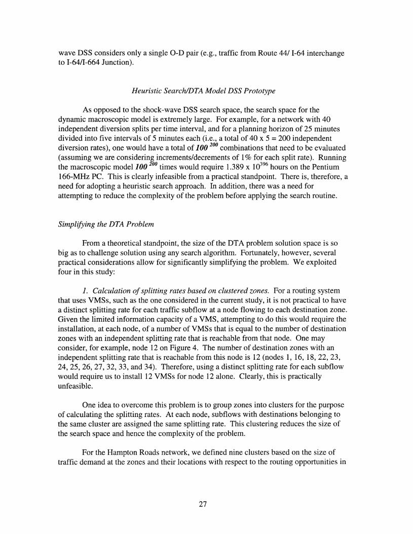
1. Calculation ofsplitting rates based on clustered zones. For a routing systemthat uses VMSs, such as the one considered in the current study, it is not practical to havea distinct splitting rate for each traffic subflow at a node flowing to each destination zone.Given the limited information capacity of a VMS, attempting to do this would require theinstallation, at each node, of a number of VMSs that is equal to the number of destinationzones with an independent splitting rate that is reachable from that node. One mayconsider, for example, node 12 on Figure 4. The number of destination zones with anindependent splitting rate that is reachable from this node is 12 (nodes 1, 16, 18,22,23,24,25,26,27,32,33, and 34). Therefore, using a distinct splitting rate for each subflowwould require us to install 12 VMSs for node 12 alone. Clearly, this is practicallyunfeasible.

One idea to overcome this problem is to group zones into clusters for the purposeof calculating the splitting rates. At each node, subflows with destinations belonging tothe same cluster are assigned the same splitting rate. This clustering reduces the size ofthe search space and hence the complexity of the problem.

For the Hampton Roads network, we defined nine clusters based on the size oftraffic demand at the zones and their locations with respect to the routing opportunities in

27

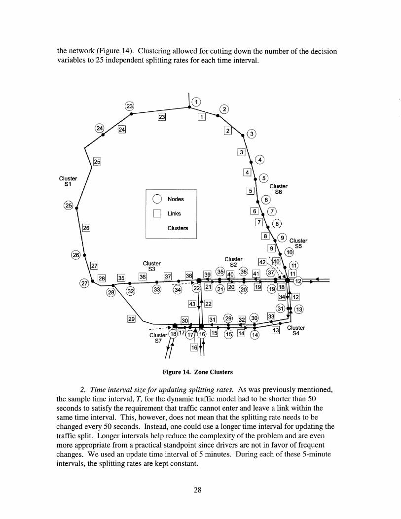
the network (Figure 14). Clustering allowed for cutting down the number of the decisionvariables to 25 independent splitting rates for each time interval.

o[I]®

r71 Cluster~ 86

Cluster83

~ ~

Clusters

o Nodes

D Links

Cluster81

Figure 14. Zone Clusters

2. Time interval size for updating splitting rates. As was previously mentioned,the sample time interval, T, for the dynamic traffic model had to be shorter than 50seconds to satisfy the requirement that traffic cannot enter and leave a link within thesame time interval. This, however, does not mean that the splitting rate needs to bechanged every 50 seconds. Instead, one could use a longer time interval for updating thetraffic split. Longer intervals help reduce the complexity of the problem and are evenmore appropriate from a practical standpoint since drivers are not in favor of frequentchanges. We used an update time interval of 5 minutes. During each of these 5-minuteintervals, the splitting rates are kept constant.

28

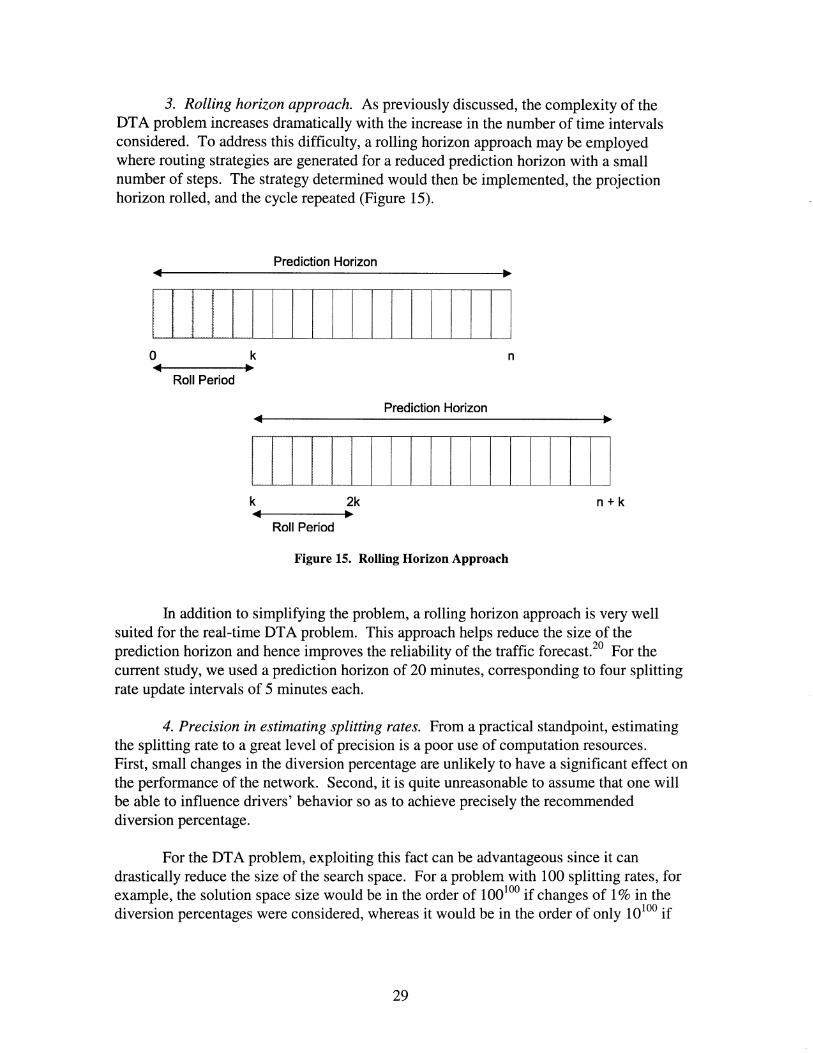
3. Rolling horizon approach. As previously discussed, the complexity of theDTA problem increases dramatically with the increase in the number of time intervalsconsidered. To address this difficulty, a rolling horizon approach may be employedwhere routing strategies are generated for a reduced prediction horizon with a smallnumber of steps. The strategy determined would then be implemented, the projectionhorizon rolled, and the cycle repeated (Figure 15).

Prediction Horizon

o~

Roll Period

k

•Prediction Horizon

2k

•Roll Period

Figure 15. Rolling Horizon Approach

n

n+k

In addition to simplifying the problem, a rolling horizon approach is very wellsuited for the real-time DTA problem. This approach helps reduce the size of theprediction horizon and hence improves the reliability of the traffic forecast. 20 For thecurrent study, we used a prediction horizon of 20 minutes, corresponding to four splittingrate update intervals of 5 minutes each.

4. Precision in estimating splitting rates. From a practical standpoint, estimatingthe splitting rate to a great level of precision is a poor use of computation resources.First, small changes in the diversion percentage are unlikely to have a significant effect onthe performance of the network. Second, it is quite unreasonable to assume that one willbe able to influence drivers' behavior so as to achieve precisely the recommendeddiversion percentage.

For the DTA problem, exploiting this fact can be advantageous since it candrastically reduce the size of the search space. For a problem with 100 splitting rates, forexample, the solution space size would be in the order of 100100 if changes of 1% in thediversion percentages were considered, whereas it would be in the order of only 10100 if

29

10% increments/decrements are assumed. We searched the solution space using 10%increments/decrements for each split percentage.

Implementation Details

GA Program. Developing the program involved the following subtasks:

1. Developing a GA's representation scheme. Solving the DTA or the routingstrategy development problem essentially involves determining the diversion percentageor the independent traffic split at each diversion point. As previously mentioned, thenetwork selected for modeling had 25 independent splitting rates (i.e., diversionpossibilities) for each time interval. Therefore, for a planning horizon of 20 minutesdivided into four intervals of 5 minutes, the problem would involve determining thevalues for 100 splitting rates (25/interval x 4 intervals). In this case, a potential solutionto the problem would be represented as a lOa-element vector as follows:

where each element, Ui, is a real-valued number corresponding to an independent trafficsplit or diversion percentage (i.e., a value between a and 100).

2. Designing an approach for constraints handling. The basic idea in creatingthe initial population was first to determine the upper and lower bounds for each controlvariable and then to select a random number between these bounds for this variable. Thelower bound for our split rates is 0, and the upper bound can be determined from the factthat the sum of splitting rates for a particular O-D pair at a node is equal to 1.0.

3. Designing a selection scheme. Evaluating a GA chromosome (i.e., a potentialsolution for the problem) involved running the dynamic model for the values of the trafficsplits encoded in the chromosome and determining the corresponding value of theobjective function. The selection scheme used to select the more fit individuals from apopulation was the roulette wheel procedure commonly used in GA applications.

4. Designing appropriate genetic operators. The mutation operator was designedto proceed in the following fashion. A gene (a variable from the solution vector) israndomly selected and replaced by a random number selected between that gene'sbounds. Since this may change the bounds for the genes that follow, a check is made toensure that such genes are within their new ranges. If any gene is outside its range, a newrandom number that is within the new bounds replaces it.

The crossover operator was designed to combine the features of two parentchromosomes to form two offspring by swapping corresponding segments of the parents.For example, if the two parents (aI, b l , CI, d l , el, ...) and (a2, b2, C2, d2, e2, ...) arecrossed after the second gene, the offspring (aI, bl, C2, d2, e2, ...) and (a2, b2, CI, dl,

30

el, ...) are produced. Similar to the mutation operator, a check is made to ensure that allgenes are within admissible bounds.

SA Program. The design of the SA program involved the following subtasks:

1. Developing a representation for the problem's potential solutions. As in theGA program representation, a potential solution to the problem was represented as a 100­element vector as follows:

2. Designing a methodfor moving to neighboring points in the solution space(commonly referred to as the neighborhood structure). For moving to neighboring pointsin the solution space, the following procedure is executed. One element (splitting rate)from the solution vector is selected at random. A random number in the range [0,1] isthen generated. If that random number is less than or equal to 0.50, the selected splittingrate is increased by 10%; otherwise, the chosen splitting rate is reduced by 100/0. A checkis then made to ensure that all the variables are within admissible bounds. If any variableis outside the specified range, its value is reset to that of the boundary.

3. Defining an annealing schedule. We modeled the annealing schedule after thatproposed by Golden and Skiscim,21 with minor modifications. The approach is based onthe concept of an epoch that is made up of a prespecified number of accepted moves (k).After an epoch is executed, the resulting solution is saved and testing for equilibrium isperformed. This test compares the most recent objective function value with the valuesfrom all previous epochs at the same temperature. If the objective value of the mostrecent solution is close (a threshold value [0 < E < 1] is usually defined for this purpose)to any previously observed value from epochs at the same temperature, the system isdeclared to be at equilibrium and the next temperature is selected. The temperature isreduced by 20% at each step for a predefined number of steps (x).

Preliminary Evaluation

We coded the SA and GA algorithms in C++ and linked them to the detaileddynamic macroscopic model developed for the Hampton Roads network. For the SAalgorithm, we selected a value of 10 for the initial temperature control parameter afterpreliminary experimentation. We set the other two control parameters at the followingvalues:

number of temperature steps (x) =25

number of moves per epoch (k) =25

31

since these were the values used by Golden and Skiscim.21 For the GA program, weadopted the following control parameter values:

population size =30

probability of crossover =0.40

probability of mutation =0.15

number of generations =500.

These values are among the ones most commonly used in many GA implementations.

We considered two routing problems. In the first, an incident was assumed tohave taken place on link 11, resulting in a 60% reduction in that link's capacity. In thesecond, a 75% capacity reduction was assumed. An important consideration inevaluating the performance of stochastic search algorithms such as the ones considered inthis study is that they should yield consistent results regardless of their start point. To testthis, we tried five runs using a different random number seed for each of the two cases.

SA Results. The SA results are given in Table 12, along with the number ofevaluations performed by the program and its running time on a Pentium 166-MHz pc.As can be seen, the solutions from the five runs were very close. For case 1, the range ofvalues was within less than 0.15% of the best value (8,547), whereas for case 2, the rangewas within less than 0.22%. This shows that the algorithm was yielding consistentresults.

Table 12. SA Results

Problem 1-60% Capacity Reduction Problem 2-75% Capacity ReductionObjective Objective Runningfunction Running function time

Run (veh) No. evaluations time (min) (veh) No. evaluations (min)1 8553 4075 18.8 46065 5512 25.5

2 8549 4775 22.1 46038 5515 25.53 8559 4101 18.9 46125 4904 22.74 8547 4300 19.9 46139 5491 25.45 8554 4726 21.8 46117 5766 26.6

To get a better appreciation of the execution-time characteristics of the algorithm,we plotted the objective function value against the number of evaluations performed bythe program for each of the five runs (Figures 16 and 17). The algorithm seems to getclose to the final value obtained quite early in the search. For case 1, a value within 5%of the best solution was attained in less than 1,450 evaluations for the five runsperformed. For case 2, such a value was attained after 2,250 evaluations. This is quitesignificant for real-time applications since it means that a quick solution may be obtained

32

18000

16000Q)::1

~ 14000c:0

+:i0c: 12000::1

LLQ)>

+:i 100000Q)

:C'0

8000

60000 500 1000 1500 2000 2500 3000 3500 4000 4500 5000

No. Evaluations

Figure 16. SA Results for Case 1

100000

90000

Q)

80000::1

~c:0 70000+:i0C::1

LLQ) 60000>

+:i0Q)

:C' 500000

40000

300000 500 1000 1500 2000 2500 3000 3500 4000

No. Evaluations

Figure 17. SA Results for Case 2

with a minor sacrifice in accuracy. Running the program for 1,450 and 2,250 evaluationsrequires less than 6.7 and 10.4 minutes, respectively, on the Pentium 166MHz PC. It isalso clear from the figures that the better the quality of the start point, the sooner the SAapproaches the final value.

33

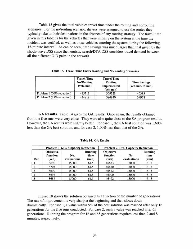
Table 13 gives the total vehicles travel time under the routing and no/routingscenarios. For the no/routing scenario, drivers were assumed to use the routes theytypically take to their destinations in the absence of any routing strategy. The travel timegiven in this table is for the vehicles that were initially on the system at the time theincident was verified, as well as those vehicles entering the system during the following15-minute interval. As can be seen, time savings was much larger than that given by theshock-wave DSS since the heuristic search/DTA DSS considers travel demand betweenall the different O-D pairs in the network.

Table 13. Travel Time Under Routing and NolRouting Scenarios

Travel Time Travel TimeNolRouting Routing Time Savings(veh. min) Implemented (veh min/IS min)

(veh min)Problem 1 (60% reduction) 415711 369328 46383Problem 2 (75% reduction) 424818 384840 39978

GA Results. Table 14 gives the GA results. Once again, the results obtainedfrom the five runs were very close. They were also quite close to the SA program results.However, the SA results were slightly better. For case 1, the SA best solution was 1.60%less than the GA best solution, and for case 2, 1.00% less than that of the GA.

Table 14. GA Results

Problem 1-60% Capacity Reduction Problem 2-75% Capacity ReductionObjective Running Objective Runningfunction No. time function No. time

Run (veh) evaluations (min) (veh) evaluations (min)1 8690 15000 61.5 46633 15000 61.52 8703 15000 61.5 46670 15000 61.53 8690 15000 61.5 46522 15000 61.54 8697 15000 61.5 46900 15000 61.55 8687 15000 61.5 46492 15000 61.5

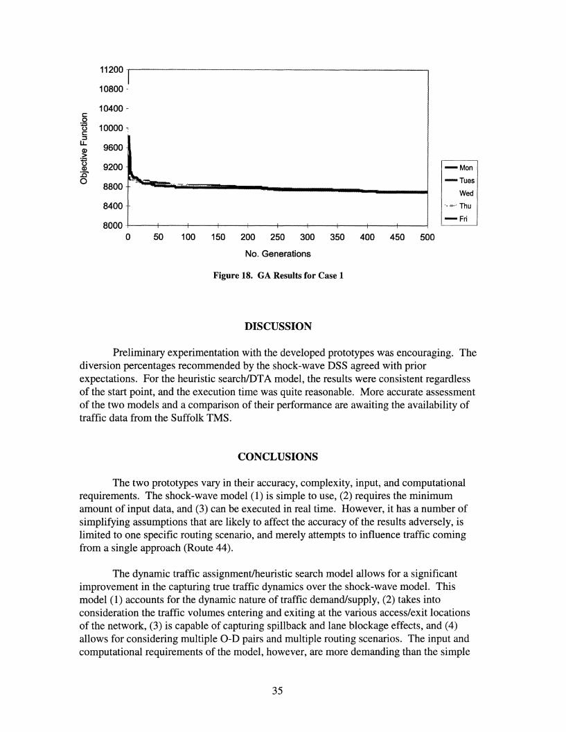
Figure 18 shows the solution obtained as a function of the number of generations.The rate of improvement is very sharp at the beginning and then slows downdramatically. For case 1, a value within 5% of the best solution was reached after only 16generations for the five runs conducted. For case 2, such a value was reached after 65generations. Running the program for 16 and 65 generations requires less than 2 and 8minutes, respectively.

34

11200 I10800 -

10400 -c:.Qts 10000 -:c::3U. 9600Q)

.~U 9200Q)

E~-0

8800

8400

80000 50

-Man

-Tues

Wed

"'''~.u' Thu

-Fri

100 150 200 250 300 350 400 450 500

No. Generations

Figure 18. GA Results for Case 1

DISCUSSION

Preliminary experimentation with the developed prototypes was encouraging. Thediversion percentages recommended by the shock-wave DSS agreed with priorexpectations. For the heuristic searchlDTA model, the results were consistent regardlessof the start point, and the execution time was quite reasonable. More accurate assessmentof the two models and a comparison of their performance are awaiting the availability oftraffic data from the Suffolk TMS.

CONCLUSIONS

The two prototypes vary in their accuracy, complexity, input, and computationalrequirements. The shock-wave model (1) is simple to use, (2) requires the minimumamount of input data, and (3) can be executed in real time. However, it has a number ofsimplifying assumptions that are likely to affect the accuracy of the results adversely, islimited to one specific routing scenario, and merely attempts to influence traffic comingfrom a single approach (Route 44).

The dynamic traffic assignment/heuristic search model allows for a significantimprovement in the capturing true traffic dynamics over the shock-wave model. Thismodel (1) accounts for the dynamic nature of traffic demand/supply, (2) takes intoconsideration the traffic volumes entering and exiting at the various access/exit locationsof the network, (3) is capable of capturing spillback and lane blockage effects, and (4)allows for considering multiple O-D pairs and multiple routing scenarios. The input andcomputational requirements of the model, however, are more demanding than the simple

35

computational requirements of the model, however, are more demanding than the simpleshock-wave model. Nevertheless, it is still suited for quasi real-time applications basedon rolling horizon approaches, where the model will be rerun every 5 or 10 minutes.

RECOMMENDATIONS

1. Since time savings resulting from the implementation of routing strategies increasewith the increase in the number ofalternate routes available, make decisionsregarding the locations for any new VMS in the region after carefully considering theadditional opportunities for routing the new VMS provides.

2. Since traffic data are crucial for developing, calibrating, and evaluating routingDSSs, provide TMSs with the functionality that allows for the easy archival andretrieval ofhistorical traffic data.

3. Since the development of real-time routing strategies is demanding in terms ofcomputational requirements, develop TMSs in afashion that allowsfor incorporatinghigher performance computing resources as they become available.

4. Evaluate and test further the tools developed in this study. To do this, we suggest thata detailed CORSIM simulation model of the network be developed and calibratedonce traffic data become available from the Suffolk TMS. The CORSIM model canthen be used for testing the two developed prototypes and comparing the effectivenessof the routing strategies recommended by each prototype.

5. Since the development ofeffective routing strategies requires tools for the on-lineestimation of O-D matrices, focus future research studies on this area as a means ofimproving upon the existing O-D estimation procedures.

6. Refine the search algorithms. This could involve testing different sets of their controlparameters, trying different annealing schedules to speed up the SA algorithm, oreven designing a hybrid GNSA approach where the GA is used as a preprocessor toperform the initial search before turning the search process over to the SA algorithm.An interesting observation that comes out of the SA results (Figures 16 and 17) is thatif the initial solution is close to the optimum, the speed of convergence is greatlyenhanced. This suggests that the procedure would be greatly aided by some means ofgenerating good initial solutions. The feasibility of adding such functionality to theSAs should be investigated.

7. Once the TMS is on-line, investigate the question ofhow to use motorist informationfor system control by studying how devices such as VMSs can be used to influencedrivers' route selection. The purpose of the study would be to identify the effects ofVMSs on link flows and the extent to which traffic volume shifts because of traveler

36

information. The results would then be used in formulating a set of "information"strategies that could be used to achieve the desired diversion levels.

REFERENCES

1. Merchant, D. K., and G. L. Nemhauser. 1978. A Model and an Algorithm for theDynamic Traffic Assignment Problem. Transportation Science, Vol. 12, No.3, pp.183-199.

2. Ho, J. K. 1980. A Successive Linear Optimization Approach to the Dynamic TrafficAssignment Problem. Transportation Science, Vol. 14, No.4, pp. 295-305.

3. Carey, M. 1987. Optimal Time-Varying Flows on Congested Networks. OperationsResearch, Vol. 35, No.1, pp. 58-69.

4. Friesz, T. L., J. Luque, R Tobin, and B. W. Wie. 1989. Dynamic Network TrafficAssignment Considered as a Continuous Time Optimal Control Problem. OperationsResearch, Vol. 37, No.6, pp. 893-901.

5. Ran, B., D. E. Boyce, and L. J. LeBlanc. 1993. A New Class of InstantaneousDynamic User-optimal Traffic Assignment Models. Operations Research, Vol. 41,No.1, pp. 192-202.

6. Papageorgiou, M. 1990. Dynamic Modeling, Assignment and Route Guidance inTraffic Networks. Transportation Research, Vol. 24B, No.6, pp. 471-495.

7. Van Aerde, M., and S. Yagar. 1988. Dynamic Integrated FreewaylTraffic SignalNetworks: A Routing-based Modeling Approach. Transportation Research, Vol.22A, No.6, pp. 435-443.

8. Yagar, S. 1993. INTEGRATION: A Critique. In Proceedings of the AdvancedTraffic Management Conference, S1. Petersburg, Florida, pp. 71-89.

9. Mahmassani, H. S., S. Peeta, T. Hu, and A. Ziliaskopoulos. 1993. Dynamic TrafficAssignment with Multiple-User Classes for Real-Time ATIS/ATMS Applications.Proceedings of the Advanced Traffic Management Conference, S1. Petersburg,Florida, pp. 91-113.

10. Jayakrishnan, R., H. S. Mahmassani, and T. Hu. 1994. An Evaluation Tool forAdvanced Traffic Information and Management Systems in Urban Networks.Transportation Research, Vol. 2C, pp. 129-147.

37

11. COMSIS Corporation. 1996. Hampton Roads Crossing Study: Compendium ofTechnical Traffic Information. Prepared for the Virginia Department ofTransportation.

12. Michalewicz, Z. 1994. Genetic Algorithms + Data Structures =EvolutionaryPrograms. Springer-Verlag, Berlin, Heidelberg, New York.

13. Kirkpatrick, S., C. D. Gelatt, and M. P. Vecchio 1983. Optimization by SimulatedAnnealing. Science, Vol. 220, pp. 671-680.

14. Hillier, F. S., and G. J. Lieberman. 1986. Introduction to Operations Research.Holden-Day, Inc., Oakland, Calif.

15. Drissi-Kaitouni, 0., and A. Hameda-Benchekroun. 1992. A Dynamic TrafficAssignment Model and Solution Algorithm. Transportation Science, 26, pp. 119­128.

16. Carey, M. 1992. Nonconvexity of the Dynamic Traffic Assignment Problem.Transportation Research, Vol. 26B, No.2, pp. 127-133.

17. May, A. D. 1990. Traffic Flow Fundamentals. Prentice-Hall, Englewood Cliffs,N.J.

18. Lighthill, M. H., and G. B. Whitham. 1957. On Kinematic Waves: A Theory ofTraffic Flow on Long Crowded Roads. Proceedings of the Royal Society, Series A,Vol. 229, pp. 317-345.

19. Chang, G. L., H. S. Mahmassani, and R. Herman. 1985. A Macroparticle TrafficSimulation Model to Investigate Peak-period Commuter Decision Dynamics.Transportation Research Record 1005, pp. 107-120. Transportation Research Board,Washington, D.C.

20. Peeta, S., and H. S. Mahmassani. 1995. Multiple User Classes Real-time TrafficAssignment for Online Operations: A Rolling Horizon Solution Framework.Transportation Research, Vol. 3C, No.2, pp. 83-98.

21. Golden, B. L., and C. C. Skiscim. 1986. Using Simulated Annealing to SolveRouting and Location Problems. Naval Research Logistics Quarterly, Vol. 33, pp.261-279.

38