DEVELOPMENT OF PID CURRENT CONTROL FOR DC … · DEVELOPMENT OF PID CURRENT CONTROL FOR DC MOTOR...

DEVELOPMENT OF PID CURRENT CONTROL FOR DC MOTOR USING

ARDUINO

MOHD KHAIRUL AKLI BIN AB GHANI

A project report submitted in partial

fulfillment of the requirement for the award of the

Degree of Master Electrical Engineering

Faculty of Electrical and Electronic Engineering

Universiti Tun Hussein Onn Malaysia

JULY 2014

ABSTRACT

Power electronic systems have been widely used in varieties of domestic applications

and industrial sector due to its reliability, simple construction and low weight.

Therefore, this project is to design and to develop of PID Current Control that could

be applied for the DC motor. The control technique was called as current control

technique by comparing the output current with the reference current. Thus, the PID

controller will force the output current to follow the reference current by creating the

pulse with modulation (PWM) signals. The PID Controller was developed and

simulated by using MATLAB/Simulink software and then implemented to the

hardware by using Arduino microcontroller board as a digital signal processing

system. The final observation from this project is by using Arduino Uno board, the

current of DC motor can control but in small scale. This is due to the current sensor

that used had range in small scale reading. Lastly, the result of the performance for

this controller was explained in this report by observed in three condition;

simulation, open loop control and closed loop control.

iv

ABSTRAK

Sistem elektronik kuasa telah digunakan secara meluas untuk pelbagai kegunaan

dalam pelbagai bidang kerana sifatnya yang boleh dipercayai, pembinaannya yang

ringkas dan juga sifatnya yang ringan. Oleh yang demikian, projek ini adalah

merekabentuk berkenaan dengan teknik pembangunan pengawal arus PID yang

boleh diaplikasikan kepada motor arus terus. Teknik kawalan yang dinamakan

sebagai pengawal arus ini adalah dengan membandingkan arus keluaran dengan arus

rujukan. Jadi, pengawal PID akan memaksa arus keluaran untuk mengikut arus

rujukan dengan menghasilkan isyarat lebar denyut modulasi. Pengawal PID telah

dibangunkan dan diuji dengan menggunakan perisian MATLAB/Simulink dan

kemudiannya dilaksanakan dalam bentuk sebenar dengan menggunakan Arduino

sebagai sistem pemprosesan isyarat digital. Pemerhatian akhir tentang projek ini

ialah dengan menggunakan papan Ardunio Uno, arus pada motor arus terus boleh di

kawal tetapi hanya dalam skala yang kecil. Ini adalah kerana jenis pengesan arus

yang digunakan adalah dalam skala bacaan yang kecil. Akhir sekali, segala hasil

prestasi untuk pengawal ini telah di terangkan di dalam laporan ini dengan melihat

kepada tiga situasi; simulasi, kawalan gelung terbuka dan kawalan gelung tertutup.

v

CONTENTS

TITLE i

DECLARATION ii

ACKNOWLEDGEMENT iii

ABSTRACT iv

CONTENTS vi

LIST OF TABLES ix

LIST OF FIGURES x

LIST OF SYMBOL AND ABBREVIATIONS xiii

CHAPTER 1 INTRODUCTION 1

1.1 Project Background 1

1.2 Problem Statement 3

1.3 Objectives of Project 4

1.4 Scope of Project 4

CHAPTER 2 LITERATURE REVIEW 6

2.1 Introduction 6

2.2 Direct Current (DC) Motor 6

2.2.1 Block diagram of DC Motor Closed-Loop Control 7

2.2.2 Shunt Wound DC Motor 8

2.3 Three Phase Controlled Rectifier 10

2.4 Three Phase Gate Driver 11

2.5 Controller Method 12

2.5.1 Proportional (P) Controller 12

2.5.2 Proportional-Integral (PI) Controller 13

2.5.3 Proportional-Derivative (PD) Controller 14

2.5.4 Proportional-Integral-Derivative (PID) Controller 14

2.5.5 Characteristic of Proportional (P), Integral (I) and

Derivative (D) Controllers 16

vi

2.5.6 Tuning PID Method 17

2.5.6.1 Manual Tuning Method 17

2.5.6.2 Ziegler–Nichols Tuning Method 18

2.5.6.3 PID Tuning Software Method 19

2.6 MATLAB Software 20

2.7 Arduino 20

2.8 Current Sensor 22

CHAPTER 3 METHODOLOGY 24

3.1 Introduction 24

3.2 Specific Block Diagram of Project 24

3.3 Design Flow 25

3.4 Flowchart 26

3.4.1 General Flowchart of Project 26

3.4.2 Process Flow of System Software 28

3.4.3 Process Flow of System Hardware 29

3.5 Circuit Diagram 30

3.5.1 Three Phase Controlled Rectifier Circuit 30

3.5.1.1 Schematic Circuit 30

3.5.1.2 Layout Diagram 31

3.5.2 Three Phase Gate Driver 32

3.5.2.1 Schematic Circuit 32

3.5.2.2 Layout Circuit 34

3.5.3 Current Sensor Design 35

3.5.4 Controller Design 36

3.6 Experiment Set up 39

CHAPTER 4 RESULTS 40

4.1 Introduction 40

4.2 Simulation Result Analysis 40

4.2.1 Open Loop Simulation Diagram and Results 44

4.2.2 Close Loop Simulation Diagram and Results 47

4.3 Hardware Result Analysis 49

4.3.1 Gate Driver Circuit Analysis 49

4.3.2 Three Phase Rectifier Circuit Analysis 52

vii

4.4 Open Loop Analysis 55

4.5 Closed Loop Analysis 63

CHAPTER 5 DISCUSSION AND CONCLUSION 69

5.1 Discussion and Conclusion 69

5.2 Future Recommendation 70

REFERENCES 71

viii

LIST OF TABLES

2.1 Characteristic of Proportional (P), Integral (I) and Derivative (D)

controllers 16

2.2 Effect of changing control parameter 18

2.3 Ziegler-Nichols tuning method, gain parameters calculation 19

2.4 Advantages and disadvantages of tuning methods 20

2.5 Specification of Arduino Uno Board 21

2.6 Comparison of current sensing method 23

3.1 List of components for gate driver circuit 33

3.2 List of component for the current sensor circuit 36

3.3 Relation current and voltage for current sensor 36

4.1 Comparison output voltage for rectifier 43

4.2 Result for open loop simulation process 46

4.3 Result for close loop simulation process 49

ix

LIST OF FIGURES

1.1 General block diagram of project 3

2.1 Types of DC motor 6

2.2 The block diagram of the DC motor closed-loop control 7

2.3 Equivalent Circuit of Shunt Wound DC motor 8

2.4 Connections of Shunt motor 9

2.5 Three-phase active rectifier system 10

2.6 Three-phase active rectifier system using MOSFET 11

2.7 Proportional controller block diagram 12

2.8 Proportional-Integral controller block diagram 13

2.9 Proportional-Derivative controller block diagram 14

2.10 Proportional-Integral-Derivative controller block diagram 15

2.11 Arduino Uno Board 21

2.12 Typical DC motor block diagram 22

3.1 Specific block diagram of project 24

3.2 Modeling processes 26

3.3 General flowchart of project 27

3.4 Flowchart of system software 28

3.5 Process flow of system hardware 29

3.6 Schematic circuit for three phase controlled rectifier 30

3.7 Layout for three phase controlled rectifier 31

3.8 Hardware development of three phase rectifier 31

3.9 Schematic of three phase gate driver 32

3.10 Layout for three phase gate driver 34

3.11 Hardware development of gate driver 34

3.12 Diagram of current sensor (BB-ACS756) 35

3.13 Schematic of current sensor (BB-ACS756) 35

3.14 The Simulink model for the controller 38

x

3.15 The design of PID current controller 38

3.16 PID controller block parameters 39

3.17 Experiment set up 39

4.1 The full simulation 41

4.2 Three phase rectifier and load model 41

4.3 The model that contained in controller block 42

4.4 Three phase input voltage for rectifier 43

4.5 Output rectifier during uncontrolled condition 44

4.6 Open loop simulation analysis 44

4.7 Result for open loop output current at Iref = 0.2A 45



4.10 Close loop simulation analysis 47

4.11 Result for close loop output current at Iref = 0.2A 47



4.14 The output of PWM signal 50

4.15 Input and output for gate driver 50

4.16 The peak-to-peak voltage output signal of gate driver 51

4.17 The overlap condition 52

4.18 Phase A and phase B input voltage 53

4.19 Phase B and phase C input voltage 53

4.20 Phase A and phase C input voltage 54

4.21 The output of voltage for the rectifier in uncontrolled condition 54

4.22 MATLAB/Simulink model for open loop analysis for 0.2A 55

4.23 PWM output for phase A and phase B when input 0.2508 56

4.24 Output voltage at current sensor when input 0.2508 56

4.25 Rectifier output voltage when Iref open loop = 0.2A 57




4.29 Rectifier output voltage when Iref open loop= 0.3A 60


xi



4.33 Rectifier output voltage when Iref open loop= 0.4A 63

4.34 MATLAB/Simulink model for closed loop analysis 63

4.35 The output voltage at current sensor when Iref = 0.2A 64

4.36 Rectifier output voltage when Iref close loop= 0.2A 65





xii

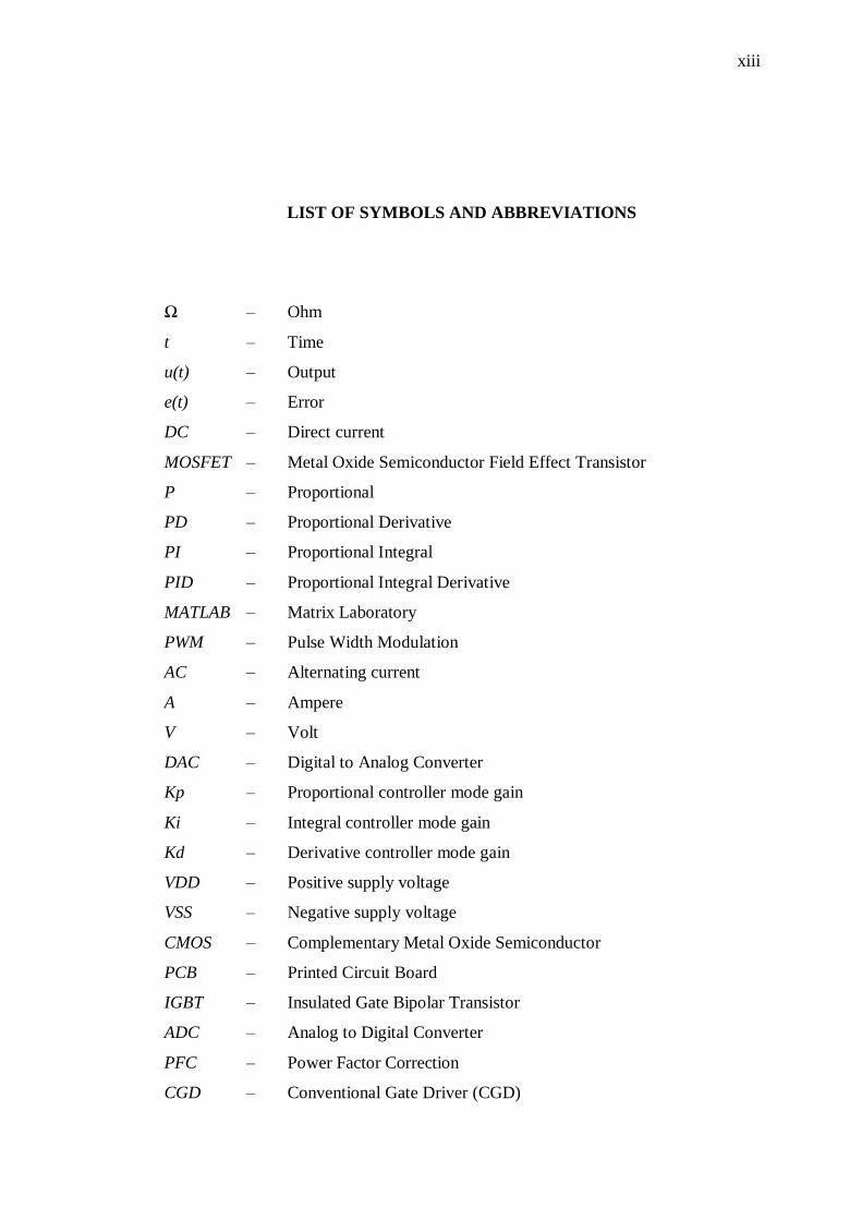
LIST OF SYMBOLS AND ABBREVIATIONS

Ω – Ohm

t – Time

u(t) – Output

e(t) – Error

DC – Direct current

MOSFET – Metal Oxide Semiconductor Field Effect Transistor

P – Proportional

PD – Proportional Derivative

PI – Proportional Integral

PID – Proportional Integral Derivative

MATLAB – Matrix Laboratory

PWM – Pulse Width Modulation

AC – Alternating current

A – Ampere

V – Volt

DAC – Digital to Analog Converter

Kp – Proportional controller mode gain

Ki – Integral controller mode gain

Kd – Derivative controller mode gain

VDD – Positive supply voltage

VSS – Negative supply voltage

CMOS – Complementary Metal Oxide Semiconductor

PCB – Printed Circuit Board

IGBT – Insulated Gate Bipolar Transistor

ADC – Analog to Digital Converter

PFC – Power Factor Correction

CGD – Conventional Gate Driver (CGD)

xiii

CHAPTER 1

INTRODUCTION

1.1 Project Background

Nowadays, almost every mechanical movement around the world is accomplished by

an electric motor. The electric machines are a means of converting energy. Motors

take electrical energy and produce mechanical energy. The direct current (DC) motor

is a device that used in many industries in order to convert electrical energy into

mechanical energy. The result from the availability of speed controllers is wide

range, easily and many ways. In most applications, speed control is very important.

For example, consider the DC motor in radio controller car, if just apply a constant

power to the motor, it is impossible to maintain the desired speed. It will go slower

over rocky road, slower uphill, faster downhill and so on. So, it is important to make

a controller to control the speed of DC motor in desired speed [1]. In this project,

researcher used multifunction DC motor with Shunt Wound DC motor connection

just to know whether this type of motor able to operate or not with this controller.

With the advancement of power electronics, microprocessors and digital

electronics, typical electric drive systems nowadays are becoming more compact,

efficient, cheaper and versatile. The voltage and current applied to the motor can be

changed at will by employing power electronic converters [2]. Before the widespread

use of power electronic rectifier, dc motors were unexcelled in speed control

application [3]. To operating this DC motor, the rectifier is required. Active Rectifier

is widely used in industrial applications because it has many advantages including

unity power factor, low ripple of the DC voltage and low total harmonics distortion.

Due to these features, the active rectifier is a good choice for application in industrial

drives [4]. This rectifier activated by gate driver circuit that charge pump signal to

the gate for MOSFET in rectifier circuit. So, for this project three phase controlled

active rectifier is selected.

The speed of DC motor can be adjusted to a great extent as to provide

controllability easy and high performance. The controllers of the speed that are

conceived for goal to control the speed of DC motor to execute one variety of tasks,

is of several conventional and numeric controller types, the controllers can be:

Proportional (P) Controller, Proportional-Derivative (PD) Controller, Proportional-

Integral (PI) Controller, Proportional-Integral-Derivative (PID) Controller, Fuzzy

Logic Controller, Genetic Algorithm technique, Particle Swarm Optimization

technique or the combination between them: Fuzzy-Neural Networks, Fuzzy-Genetic

Algorithm, Fuzzy-Ants Colony, Fuzzy-Swarm [5]. For this project, with demanding

and sophisticated application, the PID controller is designed accordingly with PWM

current controller to produce a better controller for DC motor. Current sensor had

used as a reference current to compare with setting current that setting in the

MATLAB Simulink Toolbox software.

Due to their functional simplicity and reliability, the PID controller is one of

the most popular controllers in the industry. It provides robust and reliable

performance for most systems if the PID parameters are determined or tuned to

ensure a satisfactory closed-loop performance [6]. A PID controller is designed using

MATLAB Simulink functions to generate a set of coefficients associated with a

desired controller's characteristics [7]. The controller coefficients are then included in

MATLAB Simulink Toolbox functional block diagram that implements the PID

controller. MATLAB has been selected for this work due to the fact that it is one of

the most widely used software and it is almost accessible in all education institutions

around the world [8].

Arduino Uno board microcontroller has been selected to store and run the

program from MATLAB. This Arduino Uno board had chosen due to a simple board,

easy to handle and its affordable cost. This board can be program by using C/C++

programming language, Java or using MATLAB Simulink Toolbox function block.

Figure 1.1 below shows the general block diagram for this project. This

project consists of three phase controlled rectifier, three phase gate driver, Arduino

2

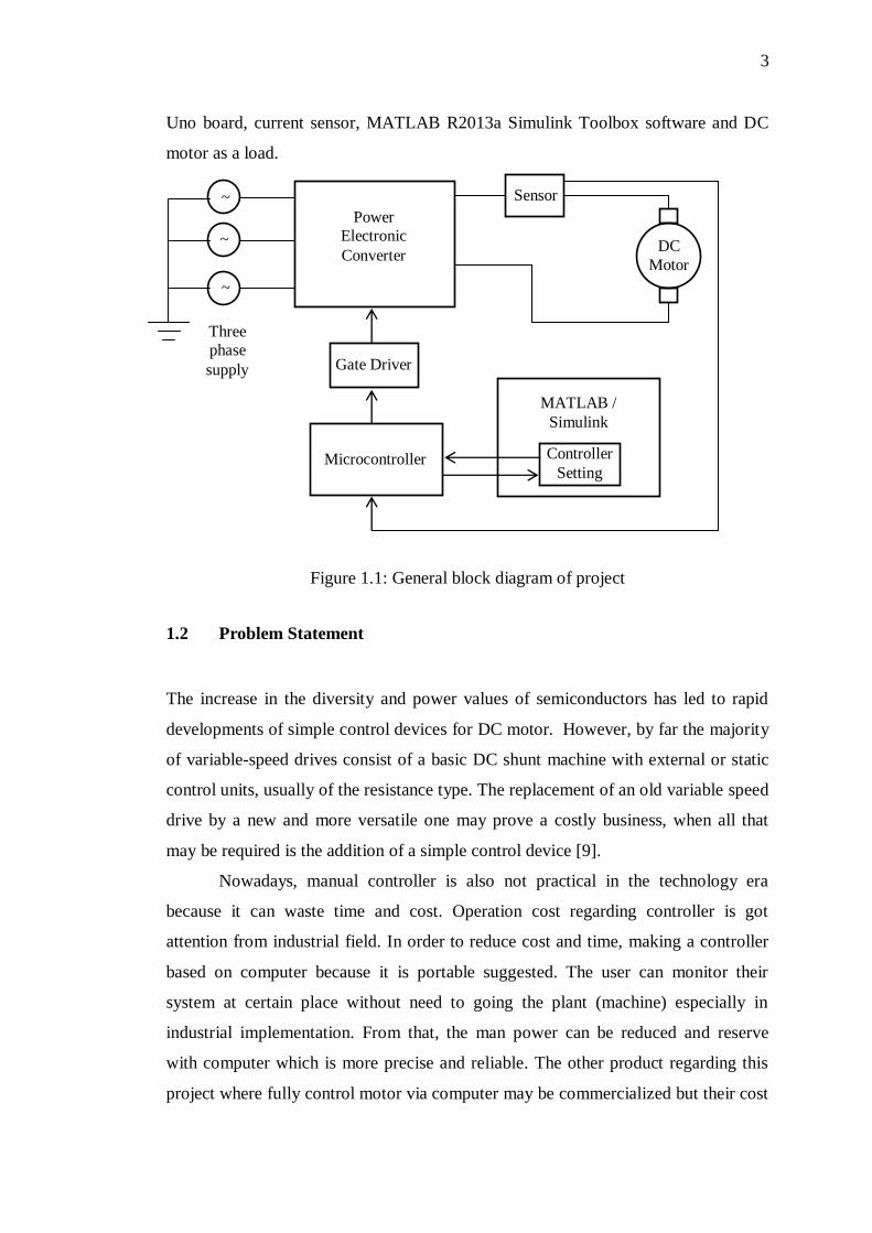
Uno board, current sensor, MATLAB R2013a Simulink Toolbox software and DC

motor as a load.

Figure 1.1: General block diagram of project

1.2 Problem Statement

The increase in the diversity and power values of semiconductors has led to rapid

developments of simple control devices for DC motor. However, by far the majority

of variable-speed drives consist of a basic DC shunt machine with external or static

control units, usually of the resistance type. The replacement of an old variable speed

drive by a new and more versatile one may prove a costly business, when all that

may be required is the addition of a simple control device [9].

Nowadays, manual controller is also not practical in the technology era

because it can waste time and cost. Operation cost regarding controller is got

attention from industrial field. In order to reduce cost and time, making a controller

based on computer because it is portable suggested. The user can monitor their

system at certain place without need to going the plant (machine) especially in

industrial implementation. From that, the man power can be reduced and reserve

with computer which is more precise and reliable. The other product regarding this

project where fully control motor via computer may be commercialized but their cost

Microcontroller

Gate Driver

Power

Electronic

Converter

Sensor

MATLAB /

Simulink

Controller

Setting

DC

Motor

~

~

~

Three

phase

supply

3

is very expensive. The hardware of may be complicated and maintenance cost is

higher [1]. The simple electronic devices can be designed using power electronic

control device to make a speed controller system.

This has led the researchers to consider the design and application of a power

electronic control device to a DC motor. The adaptive PID controller is so designed

that it can be used to overcome the problem in industry like to avoid machine

damages and to avoid slow rise time and high overshoot. This is because when the

starting voltage is high, it is not suitable for machine and can make machine

damages. With the aid of feedback control, the controller monitors the armature

current of the DC motor.

1.3 Objectives of Project

Basically, this project is listing four main objectives.

i. To develop the three phase controlled rectifier.

ii. To develop the three phase gate driver.

iii. To design the PID current control using MATLAB R2013a Simulink Toolbox

function block.

iv. To study the communication between MATLAB R2013a Simulink software

and Arduino Uno board.

1.4 Scope of Project

There are four main points in this project. These scopes parallel with the objectives

of the project.

i. The rating for the three phase rectifier is the direct current (DC) output

between 0V to 240V. For this project, 500V input voltage, 8A maximum

current power MOSFET (IRF840) is selected to be used as switching device

due to the specification of DC motor is 220V input voltage maximum, 1.8A

maximum current and 300W output power.

ii. The rating for the three phase gate driver is (10V-15V) output that meets the

specification of rectifier to activate. The aim of the circuit is to receive output

signal that produced from MATLAB and Arduino Uno board and then deliver

4

the output to rectifier. This gate driver consists of three inputs and six

outputs.

iii. The third point of this project is to design the PID current control using

MATLAB Simulink Toolbox function block. The version of MATLAB

software that used is MATLAB R2013a software. From the PID controller

block, it produced the pulse width modulation (PWM) input signal for gate

driver.

iv. Studying the communication between MATLAB R2013a Simulink software

and Arduino Uno board. This MATLAB R2013a Simulink software and

Arduino Uno board microcontroller should be able to communicate each

other.

5

CHAPTER 2

LITERATURE REVIEW

2.1 Introduction

This chapter will focus on studies, facts and past researches on this project title.

There are several topics that would be taken up for references.

2.2 Direct Current (DC) Motor

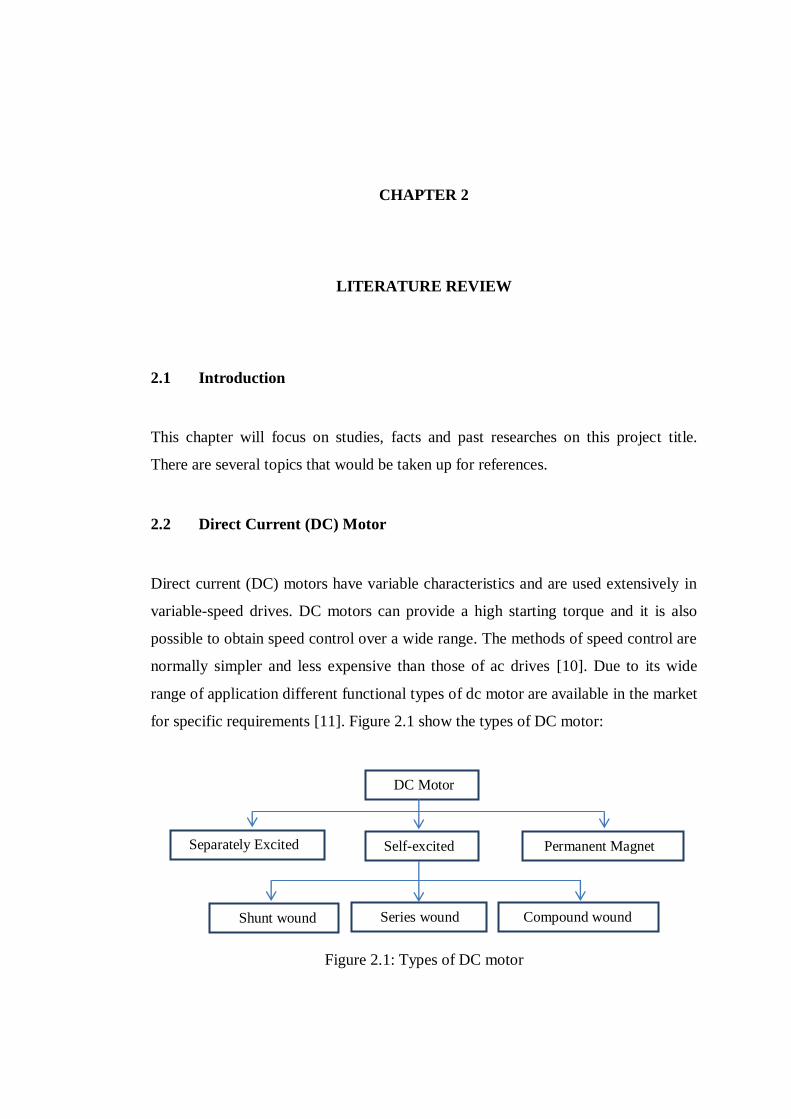
Direct current (DC) motors have variable characteristics and are used extensively in

variable-speed drives. DC motors can provide a high starting torque and it is also

possible to obtain speed control over a wide range. The methods of speed control are

normally simpler and less expensive than those of ac drives [10]. Due to its wide

range of application different functional types of dc motor are available in the market

for specific requirements [11]. Figure 2.1 show the types of DC motor:

Figure 2.1: Types of DC motor

DC Motor

Separately Excited Self-excited Permanent Magnet

Series wound Shunt wound Compound wound

Direct current motors hold the very important status in the electric driving

automatic control system. Relative to the alternating current motor, the performance

of direct current motor's speed control is much better. It is the first choice in the

applications which require wide range of speed regulation and high-precision speed,

and it has been widely used in Computerized Numerical Control machine tools and

process control [12].

DC Motors can be used in various applications and can be used as various

sizes and rates. Today their uses isn’t limited in the car applications (electrics

vehicle), in applications of weak power using battery system (motor of toy) or for the

electric traction in the multi-machine systems too. The speed of DC motor can be

adjusted to a great extent as to provide controllability easy and high performance

[13].

2.2.1 Block diagram of DC Motor Closed-Loop Control

The speed of dc motors changes with the load torque. To maintain a constant speed,

the armature (and or field) voltage should be varied continuously by varying the

delay angle of ac-dc converters or duty cycle of dc-dc converters. In practical

systems it is required to operate the drive at constant torque or constant power; in

addition controlled acceleration and deceleration are required [10]. Nowadays, most

industrial drives operate as closed-loop feedback system due to the system has the

advantages of improves accuracy, fast dynamic response and reduced effect of load

disturbances and system nonlinearities.

Figure 2.2: The block diagram of the DC motor closed-loop control

As it is seen from figure 2.2 the block diagram of the DC motor closed-loop

control, the speed sensor (encoder) measure the speed of the DC motor. In these

loops we have the actual speed of the DC motor with the desired one. The DC speed

PID DC

MOTOR Set

Point

Sensor

7

measurement gives the actual speed value. The error between theoretical and

practical values is corrected with PID controller. The parameters of the PID

controller are determined with MATLAB results which will be explained in the

following sections. The output of the PID controller gives the duty cycle of the

square wave generator [14].

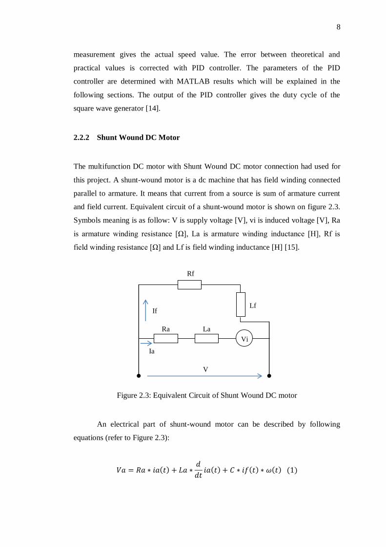
2.2.2 Shunt Wound DC Motor

The multifunction DC motor with Shunt Wound DC motor connection had used for

this project. A shunt-wound motor is a dc machine that has field winding connected

parallel to armature. It means that current from a source is sum of armature current

and field current. Equivalent circuit of a shunt-wound motor is shown on figure 2.3.

Symbols meaning is as follow: V is supply voltage [V], vi is induced voltage [V], Ra

is armature winding resistance [Ω], La is armature winding inductance [H], Rf is

field winding resistance [Ω] and Lf is field winding inductance [H] [15].

Figure 2.3: Equivalent Circuit of Shunt Wound DC motor

An electrical part of shunt-wound motor can be described by following

equations (refer to Figure 2.3):

( )

( ) ( ) ( ) ( )

Rf

Ra La

Lf

Vi

V

If

Ia

8

8

( )

( ) ( )

Here, Va is voltage on armature (i.e. supply voltage V minus brush drops)

[V], ia(t) is armature current [A], if(t) is shunt winding current [A], C is constant

(dimension of product C·if(t) is [V·s-1

]) and ω(t) is angular velocity [rad·s-1

]. Current

i(t) from a source is

( ) ( ) ( ) ( )

To completing the shunt-wound motor description, mechanical equation is

needed:

( ) ( )

( ) ( ) ( )

Where TL is load torque [Nm], J is inertia moment [kg·m2] and D is friction

coefficient [Nm·s·rad-1

].

Figure 2.4 shows the connections of a shunt motor. From these connections,

the field current is constant, since it is connected directly to the supply which is

assumed to be at constant voltage. Hence the flux is approximately constant and,

since also the back e.m.f is almost constant under normal conditions the speed is

approximately constant. It is usual for all practical purpose to regard the shunt motor

as a constant speed machine. It is employed in practice for drives, the speeds of

which are required to be independent of the loads. The speed can be varied by the

inclusion of a variable resistor in series with the field winding as figure 2.4 below

[16].

Figure 2.4: Connections of Shunt motor

Armature

Resistor

Rsh

V

9

2.3 Three Phase Controlled Rectifier

In general, control strategy for switching patterns and their duty cycles on the

rectifier uses voltage or current. Figure 2.5 represents the topology of the three phase

active rectifier proposed. The dynamic model of rectifier consists of a three-phase

network connected to three-phase supply voltage ea , eb , ec by assuming a balanced

three-phase system, the three-phase input line currents ia, ib, ic and va, vb, vc which

represent the three-phase voltages generated by the PWM active rectifier. R and L

are the resistance and inductance of the line, a smoothing capacitor, and the load

represented by a current source [4].

Figure 2.5: Three-phase active rectifier system [4]

A three-phase synchronous controlled rectifier is very efficient rectifier which

uses power MOSFETs in place of passive pn-diodes. The advantage of power

MOSFETs is that the conduction path for the current does not go across a pn

junction. The problem with pn junctions is that they have an inherent, current

independent voltage drop of around 0.7V for silicon. Power MOSFETs have a

continuous n-doped conduction channel in the on state, which has no current

independent voltage drop and behaves like a resistive element. By reducing the

resistance of the channel 1 by cry cooling and paralleling of MOSFETs, arbitrarily

low on-state voltages and corresponding low losses can be achieved. The design

discussed here uses the reverse (body) diodes of the n-channel power MOSFETs for

10

passive rectification which can be switched to active (synchronous) rectification by

applying appropriate gate drive pulses to the power MOSFETs [17].

Figure 2.6: Three-phase active rectifier system using MOSFET [17]

The developing trend in switching power supply system has been aiming

high-efficiency and low-cost power converters. A conventional power supply

commonly has a simple diode rectifier, which consists of several diodes, an output

inductor and a capacitor. However, AC/DC diode converter with low output voltage,

total loss is consumed over 85% by the diodes, and the output inductor; for this

reason, AC/DC power MOSFET rectifier is developed to operate with low power

loss, unity power factor, low harmonic and low output ripple [18].

2.4 Three Phase Gate Driver

There are numerous IC gate drives that are commercially available for gating power

converters. These include pulse-width modulation (PWM) control, power factor

correction (PFC) control, combined PWM and PFC control, current mode control,

bridge driver, servo driver, hall-bridge drivers, stepper motor driver and thyristor

gate driver [10].

Recently, the interest with solid state pulsed power modulator has been

growing because of many advantages such as long life span, rectangular pulse

waveforms and easiness of controlling the pulse width and repetition rate [19].

Efficiency is one of the most important issues among high power converters

where IGBTs are widely used, and the gate drive circuit serving as the interface

11

between the IGBT power switches and the logic-level signals can be optimized to

achieve low losses. Conventional Gate Driver (CGD) circuits have employed fixed

gate voltage and resistor networks, which are selected to minimize switching losses,

suppress cross-talk and EMI noise, and also limit the power device stresses at

switching transients. However, these conflicting requirements are difficult to be

realized in a conventional gate driver [20].

Basically, the purpose of using a gate driver is the application of to charge

pump circuit to the gate of the MOSFET in the rectifier circuit. The gate

requirements for a MOSFET or an IGBT switch are satisfy as follows; i) Gate

voltage must be 10V to 15V higher than the source or emitter voltage. Because the

power drive is connected to the main igh voltage rail +Vs, the gate voltage must be

higher than the rail voltage. ii) The gate voltage that is normally referenced to

ground must be controllable from the logic circuit. Thus, the control signals have to

be level shifted to the source terminal of the power device, which in most

applications swings between the two rails V+. iii) A low-side power device generally

drives the high-side power device that is connected to the high voltage. Thus, there is

one high-side and one low-side power device. The power absorbed by the gate drive

circuitry should be low and it should not significantly affect the overall efficiency of

the power converter [10].

2.5 Controller Method

This part expresses the type of controlled method that most widely used. The

explanation about those controllers aid with block diagrams. The description control

method focused for Proportional (P) controller, Proportional-Integral (PI) controller,

Proportional-Derivative (PD) controller and Proportional-Integral-Derivative (PID)

controller.

2.5.1 Proportional (P) Controller

Figure 2.7: Proportional controller block diagram

Kp Plant Set Point +

- Feedback

12

Ʃ

Proportional (P) controller is mostly used in first order processes with single energy

storage to stabilize the unstable process. The main usage of the P controller is to

decrease the steady state error of the system. As the proportional gain factor K

increases, the steady state error of the system decreases. However, despite the

reduction, P control can never manage to eliminate the steady state error of the

system. As we increase the proportional gain, it provides smaller amplitude and

phase margin, faster dynamics satisfying wider frequency band and larger sensitivity

to the noise. We can use this controller only when our system is tolerable to a

constant steady state error. In addition, it can be easily concluded that applying P

controller decreases the rise time and after a certain value of reduction on the steady

state error, increasing K only leads to overshoot of the system response. P control

also causes oscillation if sufficiently aggressive in the presence of lags and/or dead

time. The more lags (higher order), the more problem it leads. Plus, it directly

amplifies process noise [14].

2.5.2 Proportional-Integral (PI) Controller

Figure 2.8: Proportional-Integral controller block diagram

Proportional-Integral (PI) controller is mainly used to eliminate the steady state error

resulting from P controller. However, in terms of the speed of the response and

overall stability of the system, it has a negative impact. This controller is mostly used

in areas where speed of the system is not an issue. Since PI controller has no ability

to predict the future errors of the system it cannot decrease the rise time and

eliminate the oscillations. If applied, any amount of I guarantees set point overshoot

[14].

P=Kp*e(t)

Process +

- Ʃ Ʃ

e(t) +

+ I=Kiʃe(τ)dτ

13

Set

Point

Feedback

2.5.3 Proportional-Derivative (PD) Controller

Figure 2.9: Proportional-Derivative controller block diagram

The aim of using Proportional-Derivative (PD) controller is to increase the stability

of the system by improving control since it has an ability to predict the future error of

the system response. In order to avoid effects of the sudden change in the value of

the error signal, the derivative is taken from the output response of the system

variable instead of the error signal. Therefore, D mode is designed to be proportional

to the change of the output variable to prevent the sudden changes occurring in the

control output resulting from sudden changes in the error signal. In addition D

directly amplifies process noise therefore D-only control is not used [14].

2.5.4 Proportional-Integral-Derivative (PID) Controller

Proportional-Integral-Derivative (PID) controller has the optimum control dynamics

including zero steady state error, fast response (short rise time), no oscillations and

higher stability. The necessity of using a derivative gain component in addition to the

PI controller is to eliminate the overshoot and the oscillations occurring in the output

response of the system. One of the main advantages of the PID controller is that it

can be used with higher order processes including more than single energy storage

[14].

PID controllers are widely used in industrial practice over 60 years ago. The

invention of PID control is in 1910 (largely owing to Elmer Sperry’s ship autopilot)

and the straightforward Ziegler-Nichols (Z-N) tuning rule in 1942. Today, PID is

used in more than 90% of practical control systems, ranging from consumer

electronics such as cameras to industrial processes such as chemical processes. The

PID controller helps get our output (velocity, temperature, position) where we want

P=Kp*e(t)

Process +

- Ʃ Ʃ

e(t) +

+ D=Kd*de(t)

dt

14

Set

Point

Feedbackk

it, in a short time, with minimal overshoot, and with little error. It also the most

adopted controllers in the industry due to the good cost and given benefits to the

industry. Many nonlinear processes can be controlled using the well-known and

industrially proven PID controller [21].

The control structure used was the PID (Proportional + Integral + Derivative)

as a base for software development. This type of controller was initially chosen,

because it is generally applied to most of the control systems of continuous

processes, proving its usefulness by providing a generally satisfactory control. The

connection among the proportional, integral and derivative actions result in the PID

controller, which can be found in various formats. Among the existing formats, the

one chosen to be implemented in the experiment was parallel PID, since it is the

most common among industrial controllers. Figure 6 shows the block diagram of a

closed loop control system using PID controller [22].

Figure 2.10: Proportional-Integral-Derivative controller block diagram

The figure 2.10 above shows the PID controller block diagram, which has an

adder which is integrates the actions of controllers: proportional, integral and

derivative actions, resulting in the PID controller in parallel. The controller equation

is shown in Equation 5.

( ) ( ) ∫ ( ) ( )

( )

Set

Point

Feedbackk

P=Kp*e(t)

Process

+

- Ʃ

Ʃ

e(t)

+ +

D=Kd*de(t)

dt

I=Kiʃe(τ)dτ

+

15

Where;

t = Time

u(t) = Output

e(t) = Error = set point – process variable

Kp = Proportional controller mode gain

Ki = Integral controller mode gain

Kd = Derivative controller mode gain

Using above equation of the PID controller in time domain it is possible to

develop an equation of a digital PID controller in order to use it on the Arduino. To

approximate the equation 5, a T period sampling rate was used, thus the integral

action is close to the sum of all values of the sampled error multiplied by the period,

and the derivative action multiplied by the difference between the current and

previous error divided by the period.

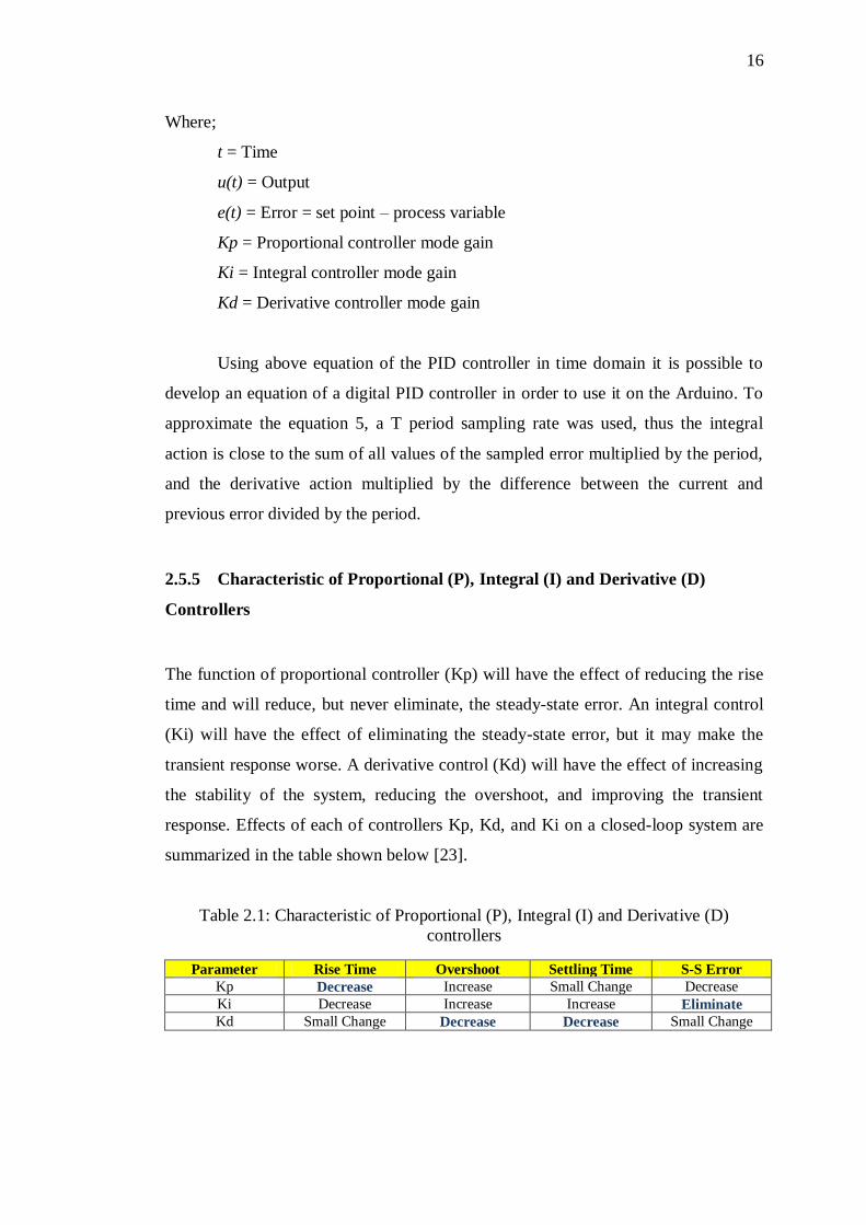
2.5.5 Characteristic of Proportional (P), Integral (I) and Derivative (D)

Controllers

The function of proportional controller (Kp) will have the effect of reducing the rise

time and will reduce, but never eliminate, the steady-state error. An integral control

(Ki) will have the effect of eliminating the steady-state error, but it may make the

transient response worse. A derivative control (Kd) will have the effect of increasing

the stability of the system, reducing the overshoot, and improving the transient

response. Effects of each of controllers Kp, Kd, and Ki on a closed-loop system are

summarized in the table shown below [23].

Table 2.1: Characteristic of Proportional (P), Integral (I) and Derivative (D)

controllers

Parameter Rise Time Overshoot Settling Time S-S Error

Kp Decrease Increase Small Change Decrease

Ki Decrease Increase Increase Eliminate

Kd Small Change Decrease Decrease Small Change

16

Take a note that these correlations may not be exactly accurate, because Kp,

Ki, and Kd are dependent of each other. In fact, by changing one of these variables

can change the effect of the other two. For this reason, the table should only be used

as a reference when you are determining the values for Ki, Kp and Kd.

2.5.6 Tuning PID Method

The meaning of tuning is adjustment of control parameters to the optimum values for

the desired control response. The stability is a basic requirement. However, different

systems have different behaviour, different applications have different requirements,

and requirements may conflict with one another. PID tuning is a difficult problem,

even though there are only three parameters and in principle is simple to describe,

because it must satisfy complex criteria within the limitations of PID control. There

are accordingly various methods for loop tuning, some of them [24]:

i- Manual tuning method,

ii- Ziegler–Nichols tuning method,

iii- PID tuning software methods.

2.5.6.1 Manual Tuning Method

Using manual tuning method, parameters are adjusted by watching system responses.

Kp, Ki, Kd are changed until desired or required system response is obtained. Even

though this method is simple, it should be used by experienced personal. For

example, using One Manual Tuning Method, firstly, Ki and Kd are set to zero. Then,

the Kp is increased until the output of the loop oscillates, after obtaining optimum Kp

value, it should be set to approximately half of that value for a "quarter amplitude

decay" type response. Then, Ki is increased until any offset is corrected in sufficient

time for the process. However, too much Ki will cause instability. Finally, Kd is

increased, until the loop is acceptably quick to reach its reference after a load

disturbance. However, too much Kd also will cause excessive response and

overshoot. A fast PID loop tuning usually overshoots slightly to reach the set point

more quickly; however, some systems cannot accept overshoot, in which case an

over-damped closed-loop system is required, which will require a Kp setting

17

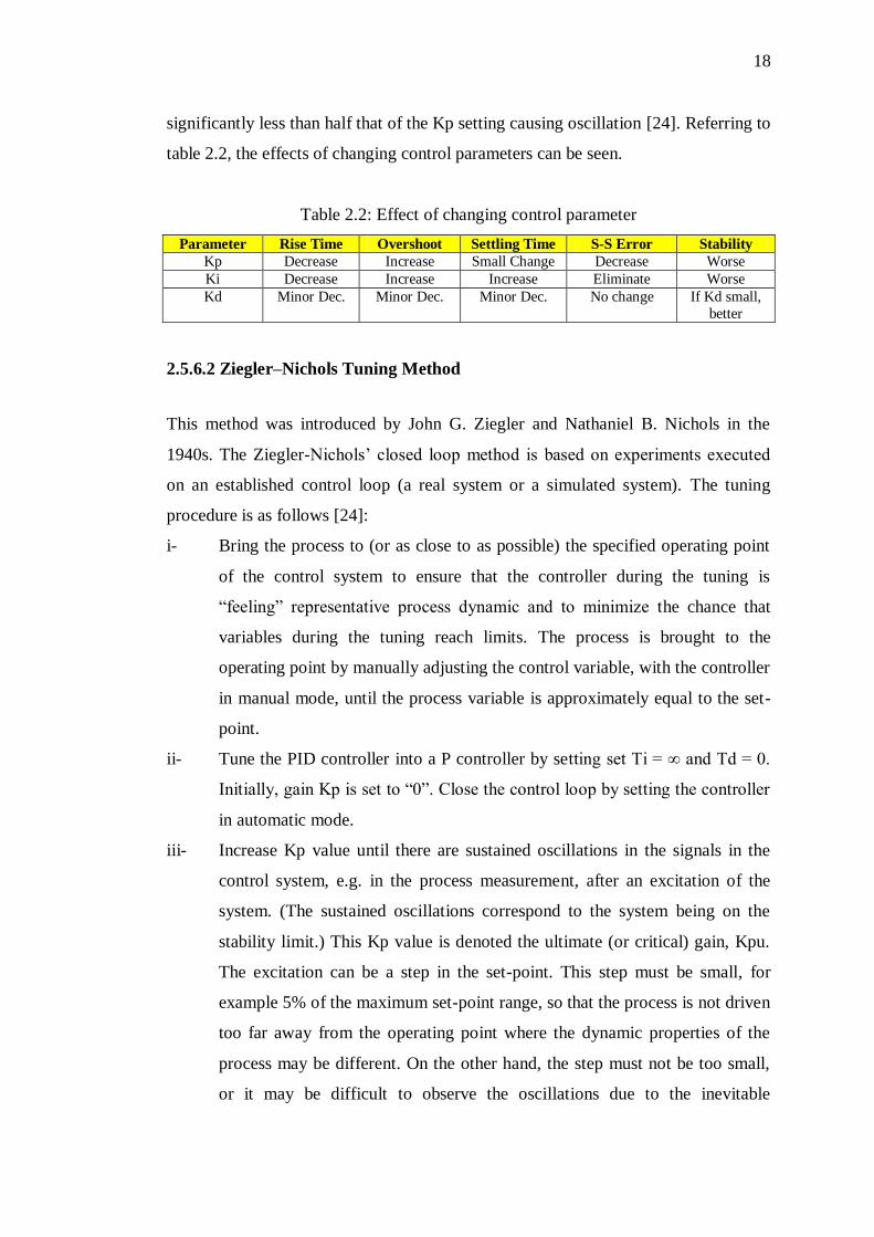
significantly less than half that of the Kp setting causing oscillation [24]. Referring to

table 2.2, the effects of changing control parameters can be seen.

Table 2.2: Effect of changing control parameter

Parameter Rise Time Overshoot Settling Time S-S Error Stability

Kp Decrease Increase Small Change Decrease Worse

Ki Decrease Increase Increase Eliminate Worse

Kd Minor Dec. Minor Dec. Minor Dec. No change If Kd small,

better

2.5.6.2 Ziegler–Nichols Tuning Method

This method was introduced by John G. Ziegler and Nathaniel B. Nichols in the

1940s. The Ziegler-Nichols’ closed loop method is based on experiments executed

on an established control loop (a real system or a simulated system). The tuning

procedure is as follows [24]:

i- Bring the process to (or as close to as possible) the specified operating point

of the control system to ensure that the controller during the tuning is

“feeling” representative process dynamic and to minimize the chance that

variables during the tuning reach limits. The process is brought to the

operating point by manually adjusting the control variable, with the controller

in manual mode, until the process variable is approximately equal to the set-

point.

ii- Tune the PID controller into a P controller by setting set Ti = ∞ and Td = 0.

Initially, gain Kp is set to “0”. Close the control loop by setting the controller

in automatic mode.

iii- Increase Kp value until there are sustained oscillations in the signals in the

control system, e.g. in the process measurement, after an excitation of the

system. (The sustained oscillations correspond to the system being on the

stability limit.) This Kp value is denoted the ultimate (or critical) gain, Kpu.

The excitation can be a step in the set-point. This step must be small, for

example 5% of the maximum set-point range, so that the process is not driven

too far away from the operating point where the dynamic properties of the

process may be different. On the other hand, the step must not be too small,

or it may be difficult to observe the oscillations due to the inevitable

18

measurement noise. This is important that Kpu is found without the control

signal being driven to any saturation limit (maximum or minimum value)

during the oscillations. If such limits are reached, there will be sustained

oscillations for any (large) value of Kp, e.g. 1000000, and the resulting Kp

value is useless (the control system will probably be unstable). One way to

say this is that Kpu must be the smallest Kp value that drives the control loop

into sustained oscillations.

iv- Measure the ultimate (or critical) period Pu of the sustained oscillations.

v- Calculate the controller parameter values according to Table 2.3, and these

parameter values are used in the controller. If the stability of the control loop

is poor, stability is improved by decreasing Kp, for example a 20% decrease.

Table 2.3: Ziegler-Nichols tuning method, gain parameters calculation

Control Type Kp Ki Kd

P 0.5*Ku - -

PI 0.45*Ku 1.2*Kp/Tu -

PID 0.6*Ku 2*Kp/Tu Kp*Tu/8

2.5.6.3 PID Tuning Software Method

There is some prepared software that they can easily calculate the gain parameter. Any

kind of theoretical methods can be selected in some these methods [24]. Here the

examples of software most used:

i- MATLAB Simulink PID Controller Tuning,

ii- BESTune,

iii- Exper Tune etc.

2.5.7 Advantages and Disadvantages of Tuning Methods

Table 2.4 below shows the advantages and disadvantages for three PID tuning

methods [24].

19

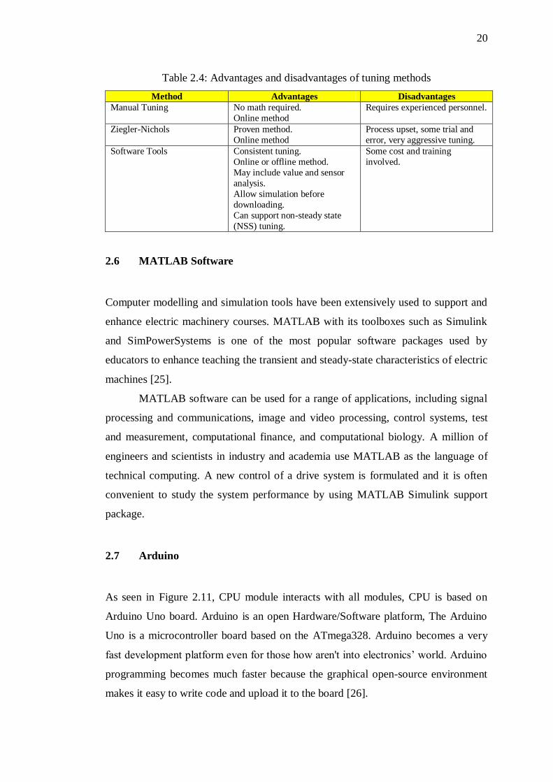
Table 2.4: Advantages and disadvantages of tuning methods

Method Advantages Disadvantages

Manual Tuning - No math required.

- Online method

- Requires experienced personnel.

Ziegler-Nichols - Proven method.

- Online method

- Process upset, some trial and

error, very aggressive tuning.

Software Tools - Consistent tuning.

- Online or offline method.

- May include value and sensor

analysis.

- Allow simulation before

downloading.

- Can support non-steady state

(NSS) tuning.

- Some cost and training

involved.

2.6 MATLAB Software

Computer modelling and simulation tools have been extensively used to support and

enhance electric machinery courses. MATLAB with its toolboxes such as Simulink

and SimPowerSystems is one of the most popular software packages used by

educators to enhance teaching the transient and steady-state characteristics of electric

machines [25].

MATLAB software can be used for a range of applications, including signal

processing and communications, image and video processing, control systems, test

and measurement, computational finance, and computational biology. A million of

engineers and scientists in industry and academia use MATLAB as the language of

technical computing. A new control of a drive system is formulated and it is often

convenient to study the system performance by using MATLAB Simulink support

package.

2.7 Arduino

As seen in Figure 2.11, CPU module interacts with all modules, CPU is based on

Arduino Uno board. Arduino is an open Hardware/Software platform, The Arduino

Uno is a microcontroller board based on the ATmega328. Arduino becomes a very

fast development platform even for those how aren't into electronics’ world. Arduino

programming becomes much faster because the graphical open-source environment

makes it easy to write code and upload it to the board [26].

20

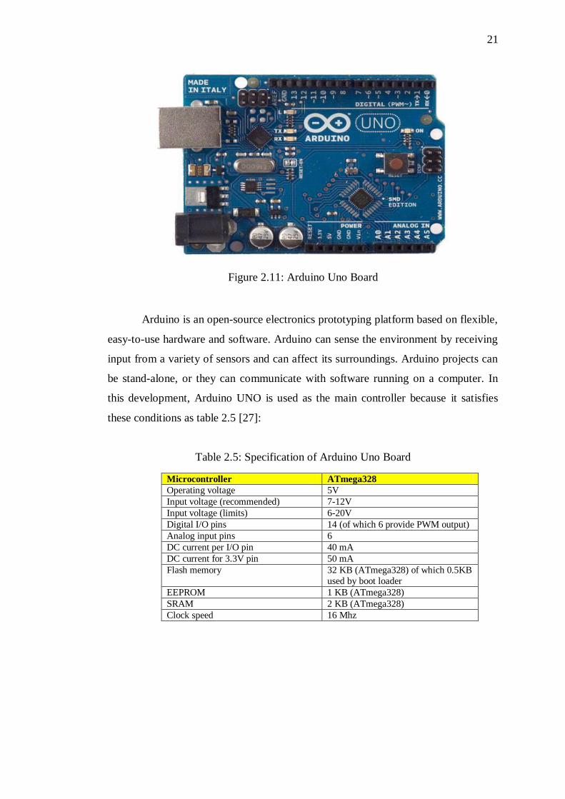
Figure 2.11: Arduino Uno Board

Arduino is an open-source electronics prototyping platform based on flexible,

easy-to-use hardware and software. Arduino can sense the environment by receiving

input from a variety of sensors and can affect its surroundings. Arduino projects can

be stand-alone, or they can communicate with software running on a computer. In

this development, Arduino UNO is used as the main controller because it satisfies

these conditions as table 2.5 [27]:

Table 2.5: Specification of Arduino Uno Board

Microcontroller ATmega328

Operating voltage 5V

Input voltage (recommended) 7-12V

Input voltage (limits) 6-20V

Digital I/O pins 14 (of which 6 provide PWM output)

Analog input pins 6

DC current per I/O pin 40 mA

DC current for 3.3V pin 50 mA

Flash memory 32 KB (ATmega328) of which 0.5KB

used by boot loader

EEPROM 1 KB (ATmega328)

SRAM 2 KB (ATmega328)

Clock speed 16 Mhz

21

2.8 Current Sensor

Sensors are a critical component in a motor control system. They are used to sense

the current, position, speed and direction of the rotating motor. Recent advancements

in sensor technology have improved the accuracy and reliability of sensors, while

reducing the cost. Many sensors are now available that integrate the sensor and

signal-conditioning circuitry into a single package. In most motor control systems,

several sensors are used to provide feedback information on the motor. These sensors

are used in the control loop and to improve the reliability by detecting fault

conditions that may damage the motor. As an example, Figure 2.12 provides a block

diagram of a DC motor control system to show the sensor feedback provided for a

typical motor control [28].

Figure 2.12: Typical DC motor block diagram

Nowadays, there is having three most popular current sensors in motor

control applications:

i- Shunt resistors

ii- Hall-Effect sensors

iii- Current transformers

Shunt resistors are popular current sensors because they provide an accurate

measurement at a low cost. Hall-Effect current sensors are widely used because they

provide a non-intrusive measurement and are available in a small IC package that

combines the sensor and signal-conditioning circuit. Current-sensing transformers

are also a popular sensor technology, especially in high-current or AC line-

Torque

Speed

Direction

Input PICmicro Microcontroller

Driver Motor

Current

Sensor

22

monitoring applications. A summary of the advantages and disadvantages of each of

the current sensors is provided in Table 2.6 [28].

Table 2.6: Comparison of current sensing method

Current sensing method Shunt Resistor Hall-Effect Current Sensing

Transformer

Accuracy Good Good Medium

Accuracy vs. Temperature Good Poor Good

Cost Low High Medium

Isolation No Yes Yes

High Current-Measuring

Capability Poor Good Good

DC Offset Problem Yes No No

Saturation / Hysterisis Problem No Yes Yes

Power Consumption High Low Low

Instrusive Measurement Yes No No

AC/DC Measurement Both Both Only AC

23

CHAPTER 3

METHODOLOGY

3.1 Introduction

This chapter will give explanations about the project methodology. It will be

included the description of the design flow, flowchart (general project, software,

hardware) and the detail explanations for the software system as well as the hardware

system. In this chapter also include the circuit that used for this project.

3.2 Specific Block Diagram of Project

Figure 3.1: Specific block diagram of project

Arduino Uno

Board

3 Phase Gate

Driver

Power

Electronic

Converter

Current

Sensor

MATLAB /

Simulink

PID Current

Controller

DC

Motor

~

~

~

Three

phase

supply

Software

Development Hardware

Development

REFERENCES

[1] Awang M.A.F., “DC Motor Speed Controller,” no. November, 2010.

[2] M. Electric, “Introduction To Electrical Drive.” [Online]. Available:

ftp://ftp.dei.polimi.it/outgoing/Massimo.Ghioni/Power Electronics /Motor

control/motor control overview/INTRODUCTION TO ELECTRICAL

DRIVES.pdf.

[3] S. . Chapman, Electric Machinery Fundamentals, vol. 4th Ed. 2005, pp. 535–

551.

[4] A. I. Technology, M. H. Purnomo, and M. Ashari, “ADVANCED CONTROL

OF ACTIVE RECTIFIER USING SWITCH FUNCTION AND FUZZY

LOGIC FOR NONLINEAR BEHAVIOUR COMPENSATION,” vol. 40, no.

2, pp. 156–161, 2012.

[5] R. G. Kanojiya, “Method for Speed Control of DC Motor,” pp. 117–122, 2012.

[6] C. Xu, D. Huang, Y. Huang, and S. Gong, “Digital PID Controller for

Brushless DC Motor Based on AVR Microcontroller,” no. 1, pp. 247–252,

2008.

[7] J. Tang, “PID CONTROLLER USING THE TMS320C31 DSK WITH ON-

LINE PARAMETER ADJUSTMENT FOR REAL-TIME DC MOTOR

SPEED AND POSITION CONTROL,” pp. 786–791, 2001.

[8] Asiya M. Al-Busaidi, “Development of an Educational Environment for Online

Control of a Biped Robot using MATLAB and Arduino,” pp. 337–344, 2012.

[9] J. Richardson, “New static controller for dc. machines,” vol. 119, no. 11, 1972.

[10] M. H. Rashid, Power Electronics Curcuits, Devices and Applications. 2004,

pp. 640–781.

[11] “Types of DC Motor Separately Excited Shunt Series Compound DC Motor.”

[Online]. Available: http://www.electrical4u.com/.

[12] W. C. M. yongbin, L. Yongxin, “Design of Parameters Self-tuning Fuzzy PID

Control for DC Motor,” pp. 345–348, 2010.

71

[13] R. G. Kanojiya and P. M. Meshram, “Optimal Tuning of PI Controller for

Speed Control of DC motor drive using Particle Swarm Optimization,” no. Dc,

2012.

[14] V. M. V. Rao, “Performance Analysis Of Speed Control Of Dc Motor Using P,

PI, PD And PID Controllers,” vol. 2, no. 5, pp. 60–66, 2013.

[15] M. Mach, P. Grmela, and V. Hajek, “Shunt-Wound Motor Parameter

Estimation by a Genetic Algorithm,” vol. 1003, no. 3, pp. 1003–1006, 2012.

[16] “Types of DC Motor.pdf.” [Online]. Available:

www.most.gov.mm/techuni/media/EP_02021_4.pdf.

[17] M. G. Giiesselmann and M. R. Haider, “Design , Coinstruction and Test of a 3-

Phase Cryogenic Synchronous Rectifier 3-Phase Synchronous Rectifier,” pp.

237–240, 1998.

[18] C.-M. Kung, Y.-S. Hwang, and J.-J. Chen, “Feedforward simple control

technique for on-chip all-digital three-phase AC/DC power-MOSFET

converter with least components,” IET Circuits, Devices Syst., vol. 3, no. 4, pp.

161–171, Aug. 2009.

[19] S. R. Jang and S. H. Ahn, “A Comparative Study of the Gate Driver Circuits

for Series Stacking of Semiconductor Switches,” pp. 326–330, 2010.

[20] Z. Wang, X. Shi, L. M. Tolbert, and B. J. Blalock, “Switching Performance

Improvement of IGBT Modules Using an Active Gate Driver,” pp. 1266–1273,

2013.

[21] M. S. Najib, M. S. Jadin, R. M. Taufika, and R. Ismail, “Design and

Implementation of PID Controller in Programmable Logic Controller for DC

Motor Position Control of the Conveyor System,” pp. 266–270, 2007.

[22] J. M. Neto, S. Paladini, C. E. Pereira, and R. Marcelino, “Remote Educational

Experiment Applied To Electrical Engineering,” 2012.

[23] “Introduction to PID Control Introduction The three-term controller.” [Online].

Available:

http://ee.sharif.edu/~industrialcontrol/Introduction_to_PID_Control.pdf.

[24] K. ARI, F. T. ASAL, and M. COSGUN, “EE 402 DISCRETE TIME SYTEMS

PROJECT REPORT PI , PD , PID.” [Online]. Available:

www.eee.metu.edu.tr/~ee402/2012/EE402RecitationReport_4.pdf.

[25] S. Ayasun and G. Karbeyaz, “DC motor speed control methods using

MATLAB/Simulink and their integration into undergraduate electric

72

machinery courses,” Comput. Appl. Eng. Educ., vol. 15, no. 4, pp. 347–354,

2007.

[26] J. Antonio, “Automatic Control for Laboratory Sterilization Process based on

Arduino Hardware,” no. Figure 2, pp. 130–133, 2012.

[27] Z. Othman, “High-Efficiency Dual-Axis Solar Tracking Developement using

Arduino,” pp. 43–47, 2013.

[28] J. Lepkowski, “Motor Control Sensor Feedback Circuits,” 2003.

73

DEVELOPMENT OF PID CURRENT CONTROL FOR DC … · DEVELOPMENT OF PID CURRENT CONTROL FOR DC MOTOR...

Documents

Transcript of DEVELOPMENT OF PID CURRENT CONTROL FOR DC … · DEVELOPMENT OF PID CURRENT CONTROL FOR DC MOTOR...