Development of new hybrid methods in density functional ...
134
HAL Id: tel-00931866 https://tel.archives-ouvertes.fr/tel-00931866 Submitted on 16 Jan 2014 HAL is a multi-disciplinary open access archive for the deposit and dissemination of sci- entific research documents, whether they are pub- lished or not. The documents may come from teaching and research institutions in France or abroad, or from public or private research centers. L’archive ouverte pluridisciplinaire HAL, est destinée au dépôt et à la diffusion de documents scientifiques de niveau recherche, publiés ou non, émanant des établissements d’enseignement et de recherche français ou étrangers, des laboratoires publics ou privés. Development of new hybrid methods in density functional theory by linear separation of the electron-electron interaction Kamal Sharkas To cite this version: Kamal Sharkas. Development of new hybrid methods in density functional theory by linear separation of the electron-electron interaction. Chemical Sciences. Université Pierre et Marie Curie - Paris VI, 2013. English. tel-00931866
Transcript of Development of new hybrid methods in density functional ...
HAL Id: tel-00931866https://tel.archives-ouvertes.fr/tel-00931866
Submitted on 16 Jan 2014
HAL is a multi-disciplinary open accessarchive for the deposit and dissemination of sci-entific research documents, whether they are pub-lished or not. The documents may come fromteaching and research institutions in France orabroad, or from public or private research centers.
L’archive ouverte pluridisciplinaire HAL, estdestinée au dépôt et à la diffusion de documentsscientifiques de niveau recherche, publiés ou non,émanant des établissements d’enseignement et derecherche français ou étrangers, des laboratoirespublics ou privés.
Development of new hybrid methods in densityfunctional theory by linear separation of the
electron-electron interactionKamal Sharkas
To cite this version:Kamal Sharkas. Development of new hybrid methods in density functional theory by linear separationof the electron-electron interaction. Chemical Sciences. Université Pierre et Marie Curie - Paris VI,2013. English. �tel-00931866�
THESE DE DOCTORATDE L’UNIVERSITE PIERRE ET MARIE CURIE
Specialite :
CHIMIE THEORIQUE
ED 388 - Ecole Doctorale de Chimie Physique et Chimie Analytique deParis Centre
presentee par
M. Kamal SHARKAS
pour obtenir le grade de
DOCTEUR DE L’UNIVERSITE PIERRE ET MARIE CURIE
Sujet de la these:
Developpement de nouvelles methodes hybrides en
theorie de la fonctionnelle de la densite par
separation lineaire de l’interaction electronique.
Soutenue le 10 juillet 2013 devant le Jury compose de :
Prof. Esmaıl ALIKHANI Universite P. et M. Curie - CNRS PresidentProf. Gabor I. CSONKA Budapest University (BUTE) RapporteurProf. Thierry LEININGER Universite de Toulouse - CNRS RapporteurProf. Carlo ADAMO Chimie ParisTech - CNRS ExaminateurDr. Emmanuel FROMAGER Universite de Strasbourg - CNRS ExaminateurDr. Andreas SAVIN Universite P. et M. Curie - CNRS Directeur de theseDr. Julien TOULOUSE Universite P. et M. Curie - CNRS Co-directeur de these

2
Developpement de nouvelles methodes hybrides en
theorie de la fonctionnelle de la densite par
separation lineaire de l’interaction electronique.
Resume
Cette these rassemble des contributions methodologiques aux methodes hybrides en theoriede la fonctionnelle de la densite (DFT). La combinaison de la DFT et de plusieurs meth-odes de fonction d’onde a ete realisee par separation lineaire de l’interaction electroniquedans l’extension multideterminantale de la methode de Kohn-Sham. Afin d’ameliorer lecalcul des effets de correlation de (quasi-)degenerescence des systemes moleculaires, nousavons developpe les hybrides multiconfigurationnels qui combinent la DFT avec un calculde champ autocoherent multiconfigurationnel. Le couplage de la DFT avec une theorie deperturbation Møller-Plesset du deuxieme ordre (MP2) a donne la justification theorique etle developpement d’approximations “double hybrides” qui ont ete testees sur des systemesmoleculaires et etendus.
Mots-cles
theorie de la fonctionnelle de la densite; correlation electronique; hybride multiconfigura-tionnel; approximation double hybride; molecules; cristaux moleculaires.
3

4 RESUME

Development of new hybrid methods in density
functional theory by linear separation of the
electron-electron interaction.
Abstract
This thesis draws together methodological contributions to the hybrid methods in densityfunctional theory (DFT). The combination of DFT and several wave function methodshas been done by linear separation of the electron-electron interaction in the multideter-minantal extension of the Kohn-Sham scheme. Aiming at improving the calculation of(near-)degeneracy correlation effects in molecular systems, we have developed the mul-ticonfigurational hybrids which combine DFT with a multiconfiguration self-consistentfield calculation. The coupling between DFT and second-order Møller-Plesset perturba-tion theory (MP2) has provided the theoretical justification and development of double
hybrid approximations which have been tested for molecular and extended systems.
Keywords
density functional theory; electronic correlation; multiconfigurational hybrid; double hy-brid approximation; molecules; molecular crystals.
5

6 ABSTRACT

Remerciements
Je remercie Olivier Parisel pour m’avoir accueilli dans de bonnes conditions au sein dulaboratoire de Chimie Theorique de l’Universite Pierre et Marie Curie.
Je remercie sincerement mon directeur de these Andreas Savin pour m’avoir encadreet appris. J’ai apprecie ses grandes competences scientifiques, sa disponibilite et sa gen-tillesse.
Je tiens a rendre hommage a Julien Toulouse, mon co-directeur de these, pour m’avoirencadre. J’ai apprecie sa precision, sa patience et son enthousiasme pour la recherche.
Je remercie les membres du jury, Gabor I. Csonka et Thierry Leininger pour avoiraccepte le travail de rapporteurs, ainsi que Carlo Adamo, Esmaıl Alikhani, Roberto Dovesiet Emmanuel Fromager pour avoir accepte d’evaluer ma these. Un merci particulier aRoberto Dovesi qui m’a accueilli au sein du laboratoire de Chimie Theorique a Turin.
I am thankful to Bartolomeo Civalleri (Mimmo), Lorenzo Maschio and all the youngstudents in the theoretical chemistry group for a very pleasant and fructuous stay in Turin.
Enfin, J’adresse ma gratitude a l’ensemble des membres, anciens et actuels, du labo-ratoire de Chimie Theorique; qu’ils m’excusent de ne pas tous les mentionner.
7

8 REMERCIEMENTS
Contents
1 Introduction generale 131.1 Appercu de quelques methodes de calcul de structure electronique . . . . . 13
1.1.1 Methodes de fonction d’onde . . . . . . . . . . . . . . . . . . . . . . 131.1.2 Methodes DFT . . . . . . . . . . . . . . . . . . . . . . . . . . . . . 151.1.3 Methodes hybrides WFT/DFT . . . . . . . . . . . . . . . . . . . . 16
1.2 Developpement de nouvelles methodes hybrides par separation lineaire del’interaction . . . . . . . . . . . . . . . . . . . . . . . . . . . . . . . . . . . 17
2 Models and approximations 292.1 N-electron problem . . . . . . . . . . . . . . . . . . . . . . . . . . . . . . . 29
2.1.1 Separation of space and time . . . . . . . . . . . . . . . . . . . . . . 292.1.2 Separation of nuclear and electronic variables (Born-Oppenheimer
approximation) . . . . . . . . . . . . . . . . . . . . . . . . . . . . . 302.1.3 Spin-orbitals . . . . . . . . . . . . . . . . . . . . . . . . . . . . . . . 312.1.4 Slater determinant . . . . . . . . . . . . . . . . . . . . . . . . . . . 322.1.5 Variational theorem . . . . . . . . . . . . . . . . . . . . . . . . . . . 33
2.2 Hartree-Fock and post Hartree-Fock approximations . . . . . . . . . . . . . 332.2.1 Expectation values with a Slater determinant . . . . . . . . . . . . 332.2.2 Hartree-Fock equations . . . . . . . . . . . . . . . . . . . . . . . . . 34
2.2.2.1 Restricted and unrestricted Hartree-Fock . . . . . . . . . . 362.2.2.2 Solution of the restricted Hartree-Fock equations . . . . . 37
2.2.3 Second quantized form of the Hamiltonian . . . . . . . . . . . . . . 392.2.4 Post Hartree-Fock methods . . . . . . . . . . . . . . . . . . . . . . 40
2.2.4.1 Dynamic correlation . . . . . . . . . . . . . . . . . . . . . 412.2.4.2 Static correlation . . . . . . . . . . . . . . . . . . . . . . . 412.2.4.3 Configuration Interaction . . . . . . . . . . . . . . . . . . 412.2.4.4 Coupled Cluster . . . . . . . . . . . . . . . . . . . . . . . 422.2.4.5 Perturbation Theory . . . . . . . . . . . . . . . . . . . . . 432.2.4.6 Multiconfiguration Self-Consistent Field . . . . . . . . . . 45
2.3 Density Functional Theory (DFT) . . . . . . . . . . . . . . . . . . . . . . . 462.3.1 Hohenberg-Kohn variational theorem . . . . . . . . . . . . . . . . . 462.3.2 Kohn-Sham formulation . . . . . . . . . . . . . . . . . . . . . . . . 472.3.3 Exchange-Correlation energy Exc[n] . . . . . . . . . . . . . . . . . . 49
2.3.3.1 Local Density Approximation . . . . . . . . . . . . . . . . 502.3.3.2 Generalized Gradient and Meta-Generalized Gradient Ap-
proximations . . . . . . . . . . . . . . . . . . . . . . . . . 512.3.3.3 Hybrids . . . . . . . . . . . . . . . . . . . . . . . . . . . . 52
9

10 CONTENTS
2.4 Models and approximations for solids . . . . . . . . . . . . . . . . . . . . . 532.4.1 Periodicity . . . . . . . . . . . . . . . . . . . . . . . . . . . . . . . . 532.4.2 Mean-field crystalline orbital theory . . . . . . . . . . . . . . . . . . 542.4.3 Wave Function Based Electron Correlation Methods for Solids . . . 56
3 A multiconfigurational hybrid density-functional theory 673.1 Abstract . . . . . . . . . . . . . . . . . . . . . . . . . . . . . . . . . . . . . 673.2 Introduction . . . . . . . . . . . . . . . . . . . . . . . . . . . . . . . . . . . 673.3 Theory . . . . . . . . . . . . . . . . . . . . . . . . . . . . . . . . . . . . . . 683.4 Computational details . . . . . . . . . . . . . . . . . . . . . . . . . . . . . 703.5 Results . . . . . . . . . . . . . . . . . . . . . . . . . . . . . . . . . . . . . . 72
3.5.1 O3ADD6 database . . . . . . . . . . . . . . . . . . . . . . . . . . . 723.5.2 Dissociation of diatomic molecules . . . . . . . . . . . . . . . . . . . 74
3.6 Conclusions . . . . . . . . . . . . . . . . . . . . . . . . . . . . . . . . . . . 773.7 Appendix . . . . . . . . . . . . . . . . . . . . . . . . . . . . . . . . . . . . 77
3.7.1 Scaling relations for the derivatives of the density-scaled correlationfunctional . . . . . . . . . . . . . . . . . . . . . . . . . . . . . . . . 77
3.7.2 Asymptotic expansion of the potential energy curve of H2 . . . . . . 78
4 Double-hybrid density-functional theory made rigorous 874.1 Abstract . . . . . . . . . . . . . . . . . . . . . . . . . . . . . . . . . . . . . 874.2 Introduction . . . . . . . . . . . . . . . . . . . . . . . . . . . . . . . . . . . 874.3 Theory . . . . . . . . . . . . . . . . . . . . . . . . . . . . . . . . . . . . . . 884.4 Computational details . . . . . . . . . . . . . . . . . . . . . . . . . . . . . 914.5 Results and discussion . . . . . . . . . . . . . . . . . . . . . . . . . . . . . 924.6 Conclusions . . . . . . . . . . . . . . . . . . . . . . . . . . . . . . . . . . . 964.7 Appendix . . . . . . . . . . . . . . . . . . . . . . . . . . . . . . . . . . . . 99
4.7.1 Density-scaled correlation energy and potential . . . . . . . . . . . 994.7.1.1 Density-scaled local-density approximations . . . . . . . . 994.7.1.2 Density-scaled generalized-gradient approximations . . . . 100
4.7.2 Theoretical reference values for the AE6 and BH6 test sets . . . . . 100
5 Rationale for a new class of double-hybrid approximations in density-functional theory 1075.1 Abstract . . . . . . . . . . . . . . . . . . . . . . . . . . . . . . . . . . . . . 1075.2 Introduction . . . . . . . . . . . . . . . . . . . . . . . . . . . . . . . . . . . 1075.3 Theory . . . . . . . . . . . . . . . . . . . . . . . . . . . . . . . . . . . . . . 1085.4 Results . . . . . . . . . . . . . . . . . . . . . . . . . . . . . . . . . . . . . . 1095.5 Conclusions . . . . . . . . . . . . . . . . . . . . . . . . . . . . . . . . . . . 111
6 Double-hybrid density-functional theory applied to molecular crystals 1156.1 Abstract . . . . . . . . . . . . . . . . . . . . . . . . . . . . . . . . . . . . . 1156.2 Introduction . . . . . . . . . . . . . . . . . . . . . . . . . . . . . . . . . . . 1156.3 Theory . . . . . . . . . . . . . . . . . . . . . . . . . . . . . . . . . . . . . . 116
6.3.1 One-parameter double-hybrid approximations . . . . . . . . . . . . 1166.3.2 Periodic local MP2 . . . . . . . . . . . . . . . . . . . . . . . . . . . 117
6.4 Computational details . . . . . . . . . . . . . . . . . . . . . . . . . . . . . 1196.5 Results and discussion . . . . . . . . . . . . . . . . . . . . . . . . . . . . . 120

CONTENTS 11
6.6 Conclusions . . . . . . . . . . . . . . . . . . . . . . . . . . . . . . . . . . . 123
7 Conclusion generale et perspectives 131

12 CONTENTS
Chapter 1
Introduction generale
Ce chapitre rappelle tout d’abord les modeles principaux de la chimie quantique, puisintroduit les methodes developpees au cours de cette these.
1.1 Appercu de quelques methodes de calcul de struc-
ture electronique
La chimie quantique applique les lois de la mecanique quantique pour extraire les dif-ferentes proprietes physico-chimiques de la matiere a l’echelle moleculaire. Les particulesconsiderees a ce niveau de description sont les noyaux atomiques et les electrons. Dansl’approximation non-relativiste, l’evolution dans le temps d’un ensemble d’electrons et denoyaux est regie par l’equation de Schrodinger dependante du temps. Dans la plupartdes problemes de chimie quantique, le point crucial est la resolution de l’equation deSchrodinger stationnaire, c’est-a-dire la recherche des fonctions propres de l’hamiltoniendu systeme. Les noyaux sont beaucoup plus lourds que les electrons. Ceci nous permetde decoupler le mouvement des electrons de celui des noyaux, c’est ce que l’on appellel’approximation de Born-Oppenheimer. Dans cette approximation, le probleme standardde la chimie quantique est d’obtenir les etats propres de l’hamiltonien electronique, quin’agit que sur les variables electroniques. Parmi ces etats, l’etat fondamental est celui deplus basse energie dans le spectre de l’hamiltonien electronique.
Sauf dans le cas des systemes atomiques ou moleculaires ne comprenant qu’un seulelectron (et d’autres modeles tres simples), on ne peut pas resoudre exactement l’equationde Schrodinger et l’on doit utiliser des methodes d’approximation. Face a ce defi, on peutdistinguer deux familles de methodes. La premiere famille cible le calcul direct de lafonction d’onde du systeme. Ce sont les methodes de fonction d’onde (WFT pour Wave
Function Theory). La deuxieme famille considere que la connaissance de la densite elec-tronique d’un systeme quelconque suffit pour le decrire pleinement. Ce sont les methodesbasees sur la theorie de la fonctionnelle de la densite (DFT pour Density Functional
Theory).
1.1.1 Methodes de fonction d’onde
Deux types de methodes d’approximation sont principalement utilisees : les methodesvariationnelles et les methodes de perturbation. Les methodes variationnelles sont fondees
13
14 CHAPTER 1. INTRODUCTION GENERALE
sur le principe variationnel, qui etablit que, pour l’etat fondamental, l’energie associee atoute fonction d’onde autre que la fonction exacte est toujours superieure a l’energieexacte. Dans les methodes de perturbation, on approche la fonction d’onde exacte sousla forme d’un developpement en serie a partir d’une solution approchee connue.
La methode Hartree-Fock (HF) est souvent la premiere approche utilisee. C’est uneapproximation variationnelle consistant a restreindre les solutions approchees aux seulesfonctions d’onde de type determinant de Slater. Le determinant de Slater est le produit an-tisymetrise d’orbitales moleculaires (OM), developpees sur une base d’orbitales atomiques(OA) selon l’approche CLOA (combinaison lineaire d’orbitales atomiques). Cette methodesuppose que chacun des electrons d’un systeme atomique ou moleculaire est une particuleindependante qui ne subit que le champ moyen des autres electrons. La description quan-titative des proprietes chimiques ne peut se faire correctement qu’en prenant en comptela tendance des electrons a s’eviter instantanement les uns des autres. Ce phenomeneest appele correlation electronique. L’energie de correlation mesure l’erreur sur l’energiecommise en utilisant le determinant de Hartree-Fock pour calculer la valeur moyennede l’hamiltonien electronique. C’est donc la difference entre l’energie electronique non-relativiste exacte et celle de Hartree-Fock. Il faut donc aller au-dela de l’approximationHartree-Fock pour calculer une partie de l’energie de correlation. On peut utiliser plusieurstypes de methodes, dites de fonction d’onde ou post Hartree-Fock, prenant en compte lacorrelation electronique.
La correlation peut etre classee en deux categories : la correlation dynamique et sta-tique (ou non-dynamique). La premiere est associee a la correlation au sein de paireselectroniques, et caracterisee par sa convergence lente avec la taille de la base utilisee.Pour la majorite des molecules dans leur etat fondamental et proches de leur geometried’equilibre, la correlation dynamique est predominante. On inclut aussi dans la cor-relation dynamique les interactions de dispersion, qui sont parfois dominantes dans lescomplexes faiblement lies. La seconde est associee a la presence de niveaux tres prochesen energie (degenerescence ou quasi-degenerescence) dans le systeme et necessite d’utiliserdes fonctions d’onde multideterminantales. Les effets de correlation statique sont souventimportants pour des molecules dans des etats excites ou proches de la dissociation.
En principe, la fonction d’onde exacte peut s’obtenir a partir d’un ensemble complet dedeterminants construits avec une base complete d’OM. Partant du determinant Hartree-Fock, on cherche une meilleure fonction d’onde developpee en combinaison lineaire dudeterminant Hartree-Fock et des determinants construits par excitations d’electrons d’OMoccupees a des OM virtuelles. Dans la methode d’interaction de configurations (IC),les coefficients des determinants dans la combinaison sont determines en appliquant leprincipe variationnel. Si on prend en compte toutes les configurations excitees, il s’agit del’interaction de configurations complete (full CI). Les resultats obtenus par IC completesont les meilleurs resultats que l’on puisse obtenir avec la base d’OA choisie, mais enpratique un calcul IC complet est souvent trop couteux en temps de calcul. Generalement,on utilise le formalisme IC tronque. Par exemple, un calcul CISD, dans lequel on se limitea considerer les excitations simples et doubles, reproduit typiquement 95% de l’energie decorrelation pour les petites molecules dans la geometrie d’equilibre. Pour les moleculesplus grandes ou les etats excites, il devient important de prendre en compte les excitationstriples ou superieures, mais l’absence d’extensivite peut rendre ces approches peu fiables.
Ce probleme d’extensivite est resolu par les methodes de coupled cluster (CC). Cesmethodes consistent a exprimer la fonction d’onde du systeme en utilisant l’ansatz expo-

1.1. APPERCU DE QUELQUES METHODES... 15
nentiel. Elles sont une variante des methodes IC permettant d’optimiser les coefficientsdes configurations par une technique alternative a la methode variationnelle basee sur laprojection de l’equation de Schrodinger sur l’espace de reference.
La methode de perturbation de Møller-Plesset est une autre maniere de calculer lacorrelation dynamique. Elle consiste a appliquer la theorie de perturbation de Rayleigh-Schrodinger standard a la recherche de l’energie fondamentale de l’hamiltonien electron-ique a partir de l’hamiltonien de Hartree-Fock, dont on connait les valeurs et etats propres.On peut developper l’energie jusqu’a un ordre quelconque. En pratique, on utilise les ap-proximations MP2, MP3 et MP4, ou l’energie est developpee jusqu’a l’ordre deux, troiset quatre respectivement.
Les methodes post Hartree-Fock decrites ci-dessus sont monoreferentielles, c’est-a-direqu’elles s’appuient sur une seule configuration obtenue par un calcul Hartree-Fock. Lavalidite de ces methodes est alors mise en question en presence de quasi-degenerescences(distribution des electrons au sein de couches partiellement occupees). Les methodesmultideterminantales MCSCF (MultiConfiguration Self-Consistent Field) fournissent unebonne description de la correlation statique. Ces methodes consistent a minimiser l’energieelectronique avec une fonction d’onde multiconfigurationnelle qui s’ecrit comme somme deplusieurs determinants de Slater. Contrairement aux methodes IC, on optimise simultane-ment les OM et les coefficients des configurations dans un calcul MCSCF. Une variantede MCSCF est CASSCF (Complete Active Space Self-Consistent Field) dans laquelle lafonction d’onde contient toutes les configurations electroniques qui peuvent etre formeesen distribuant les electrons consideres parmi les orbitales d’un espace choisi (IC completedans l’espace considere).
Pour tenir compte a la fois de la correlation dynamique et statique, on peut obtenir unefonction d’onde multideterminantale du type MCSCF puis appliquer un methode multi-referentielle du type MRCI (MultiReference Configuration Interaction), MRCC (MultiRef-
erence Coupled Cluster) ou CASPT2 (Complete Active Space Perturbation Theory).
1.1.2 Methodes DFT
Les methodes issues de la theorie de la fonctionnelle de la densite (DFT) sont la deuxiemeapproche usuelle de la chimie quantique. Elle repose sur la densite electronique, unefonction de 3 variables. Ainsi, la variable principale dans la resolution de l’equation deSchrodinger est reduit de 3N dimensions (avecN le nombre d’electrons) pour les methodesde fonction d’onde a 3 dimensions dans les methodes DFT.
La DFT est une methode variationnelle, basee sur le theoreme de Hohenberg etKohn [1] qui montre que la densite de l’etat fondamental determine (a une constanteadditive pres) le potentiel externe dans l’hamiltonien d’un systeme electronique. Toutesles observables du systeme, en particulier l’energie de l’etat fondamental, sont donc desfonctionnelles de la densite de l’etat fondamental. Sauf pour quelques cas simples, ladependance de la fonctionnelle d’energie exacte vis-a-vis de la densite, pour l’etat fonda-mental, est inconnue. La DFT est en realite le plus souvent appliquee dans le cadre de lamethode de Kohn-Sham [2]. Cette methode se fonde sur l’hypothese de l’existence d’unsysteme fictif d’electrons non-interagissants, qui possede la meme densite electronique quele systeme physique. Dans l’approche de Kohn-Sham de la DFT, toute la difficulte duprobleme a N electrons est concentree dans la recherche d’une expression pour la fonction-nelle dite d’echange-correlation se rapprochant le plus de l’expression exacte. Pour cela,

16 CHAPTER 1. INTRODUCTION GENERALE
il existe plusieurs approximations qui fournissent tres souvent une precision raisonnablepour un faible cout de calcul.
L’approximation de la densite locale (LDA pour Local Density Approximation) proposed’utiliser, en chaque point de l’espace, l’energie d’echange-correlation calculee pour ungaz d’electrons homogene, en supposant que, dans un petit volume entourant le pointconsidere, le systeme est localement homogene. Pour traiter les effets de polarisationde spin, il faut distinguer les densites associees aux deux composantes du spin. Cetteextension de la methode LDA, qui prend en compte les degres de liberte de spin, porte lenom de methode LSDA (Local Spin Density Approximation).
Le point faible de la methode L(S)DA est l’hypothese d’une densite electronique variantlentement dans l’espace. On peut raffiner cette approximation en exprimant les differentstermes d’energie non seulement en fonction de la densite mais aussi de son gradient, ce quel’on appelle les approximations GGA (Generalized gradient approximation) [3–20], et deson Laplacien et/ou la densite d’energie cinetique, ce que l’on appelle les approximationsmeta-GGA [21–34].
1.1.3 Methodes hybrides WFT/DFT
L’etape suivante dans la recherche de l’energie la plus proche possible de l’energie exacte dusysteme est de combiner les avantages des methodes de fonction d’onde et DFT. On parlealors de methodes hybrides. Le developpement de la DFT dans ce sens est toujours tresactif et les modeles theoriques que nous avons elabores au cours de cette these poursuiventcette direction de recherche.
L’approche hybride a ete initiee par Becke [35]. En utilisant l’approche dite de la con-nexion adiabatique, Becke a propose l’introduction partielle de l’echange exact (echangeHartree-Fock) dans la fonctionnelle d’echange-correlation. Les fonctionnelles resultantesportent le nom d’hybrides globales (GH pour Global Hybrid) [20, 36–48]. La portiond’echange exact est determinee de maniere semi-empirique, comme dans la fonction-nelle d’echange-correlation la plus populaire B3LYP [36], ou rationalisee, comme dansla fonctionnelle d’echange-correlation PBE0 [37]. Il existe des fonctionnelles d’echange-correlation dites hybrides locales. La portion d’echange exact depend de la position dansl’espace [49].
Savin et al. [50–58] ont propose l’extension multideterminantale de la methode deKohn-Sham, qui est basee sur la decomposition longue portee/courte portee de l’interactionelectron-electron. Pour effectuer une telle decomposition, on utilise souvent la fonction er-reur standard et son complementaire. La partie courte portee est traitee par les methodesde la densite, qui sont capables de decrire correctement les interactions a courte porteegrace aux fonctionnelles d’echange-correlation de courte portee concues pour ce but. Lapartie longue portee est contenue dans un systeme fictif remplacant celui de Kohn-Sham,qui peut etre, en pratique, traite par un des modeles de la chimie quantique comme lesmethodes Hartree-Fock [59], MCSCF [60, 61], CI [51, 55], CC [62–67], MP2 mono- etmultireferentielle [59, 62, 68–74], RPA (Random Phase Approximation) [75–84], CPMFT(Constrained-Pairing Mean-Field Theory) [85, 86] et DMFT (Density-Matrix Functional
Theory) [87–89].La premiere approximation est de restreindre ce formalisme a des fonctions d’onde
a un seul determinant, donnant une fonctionnelle hybride a separation de portee (RSHpour Range Separated Hybrid) [59] qui consiste a combiner une fonctionnelle d’echange-

1.2. DEVELOPPEMENT DE NOUVELLES METHODES... 17
correlation de courte portee avec une energie d’echange de longue portee de type Hartree-Fock. On remarque clairement que cette approximation n’inclue pas de correlation delongue portee. Une variante proche consiste a n’effectuer la decomposition que sur l’energied’echange. Il est alors possible de combiner une fonctionnelle d’echange de courte porteeavec une energie d’echange de longue portee de type Hartree-Fock (LC pour Long-range
Corrected Hybrid) [90–98], ou d’utiliser une fonctionnelle d’echange de longue porteeavec une fonctionnelle hybridee avec l’echange Hartree-Fock de courte portee (SC pourScreened-Coulomb Hybrid) [99–102]. On peut considerer la portee intermediaire (middle
range) dans la separation du terme d’interaction electron-electron, ce qui a conduit ala creation de la fonctionnelle HISS (Henderson-Izmaylov-Scuseria-Savin) [103]. Il existeaussi des modeles combinant les hybrides LC et GH comme la fonctionnelle CAM-B3LYP(Coulomb-Attenuating Method) [104] dans laquelle on introduit des parametres permet-tant d’incorporer diverses portions d’echange Hartree-Fock a longue et a courte portee.
Le deuxieme niveau d’approximation consiste a utiliser l’approche RSH comme referencesur laquelle on applique des methodes perturbatives a longue portee. Plusieurs meth-odes perturbatives ont ete utilisees dans ce contexte comme la theorie de perturbationde type Møller-Plesset au deuxieme ordre (MP2) de longue portee [59, 62, 68–73], latheorie de perturbation multireference de longue portee [74], l’approche CCSD(T) delongue portee [62–67] et differentes variantes de RPA de longue portee [75–84]. Ces ap-proches sont prometteuses pour decrire efficacement les effets de correlation nonlocaux,tels que ceux impliques dans les complexes de van der Waals, faiblement lies par desforces de dispersion [105]. Ces interactions faibles ne sont pas decrites correctement parles approximations locales (LDA) ou semilocales (GGA, meta-GGA) de l’approche deKohn-Sham de la DFT et plusieurs approches, empiriques ou non, ont par ailleurs eteproposees pour remedier a ces difficultes [106–124].
Les approximations locales ou semilocales habituelles de l’approche de Kohn-Sham dela DFT ne permettent generalement pas de decrire avec precision les systemes ayant desorbitales quasi-degenerees partiellement remplies [53, 125, 126]. De nombreuses approchesont ete proposees pour introduire explicitement le traitement de la correlation statiquedans la DFT (voir [127] pour une revue). Fromager et al. [60] ont utilise l’extension multi-determinantale de la methode de Kohn-Sham pour developper une methode combinant laDFT et l’approche MCSCF, basee sur une separation de portee de l’interaction electron-ique. L’idee est d’utiliser l’approche MCSCF sur la partie de longue portee de l’interactionpour inclure les effets de correlation statique principaux et d’utiliser une fonctionnelle dela densite pour decrire les interactions de courte portee. La methode est designee parMC-srPBE dans laquelle la fonctionnelle PBE de courte portee [63] a ete utilisee. Uneautre maniere d’introduire des effets de correlation statique est de combiner la DFT avecune fonctionnelle de la matrice densite a une particule pour la longue portee [87–89].
1.2 Developpement de nouvelles methodes hybrides
par separation lineaire de l’interaction
Dans cette these, dans l’objectif de disposer de methodes ameliorant la precision de laDFT actuelle, nous avons etudie plusieurs methodes hybrides basees sur une decomposi-tion lineaire de l’interaction electron-electron en introduisant une constante de couplageλ dans l’extension multideterminantale de la methode de Kohn-Sham. Quand λ = 0, le

18 CHAPTER 1. INTRODUCTION GENERALE
couplage s’identifie a la methode de Kohn-Sham, alors que lorsque λ = 1, on retrouveune methode de fonction d’onde. Pour les valeurs intermediaires de λ, cette proce-dure entraıne l’utilisation de la fonctionnelle d’echange-correlation dite complementairemodelisant les interactions qui ne sont pas prises en compte par la methode de fonc-tion d’onde. Les fonctionnelles complementaires peuvent etre deduites directement desfonctionnelles d’echange-correlation habituelles. Ceci represente un avantage pratique surla procedure de la decomposition longue portee/courte portee, dans laquelle on a be-soin de construire des nouvelles fonctionnelles d’echange-correlation de courte portee. Lacontribution d’echange complementaire est du premier ordre par rapport a l’interactionelectron-electron et est donc donnee par une transformation d’echelle (scaling) lineaire del’energie d’echange de Kohn-Sham habituelle. Le traitement rigoureux de la contributionde correlation complementaire fait appel a l’utilisation des relations de transformationd’echelle (scaling) uniforme des coordonnees dans la densite [128–131]. Il est possible denegliger le scaling de la densite, ce qui conduit a des variantes des methodes proposees.
Apres un rappel methodologique dans le chapitre 2, le chapitre 3 propose les meth-odes hybrides multiconfigurationnelles a un parametre. En utilisant la procedure ci-dessus,nous avons developpe une approche [132] combinant un calcul de fonction d’onde multi-configurationnelle complete de facon autocoherente par une fonctionnelle complementairede la densite pour decrire les effets de correlation statique dans la DFT. Cette meth-ode porte le nom de MCDS1H (multiconfigurational density-scaled one-parameterhybrid). Quand on neglige le scaling de la densite, on obtient une methode appeleeMC1H (multiconfigurational one-parameter hybrid). Nous avons implemente cette ap-proche dans le logiciel DALTON [133], en utilisant les fonctionnelles d’echange-correlationPBE [5] et BLYP [3, 4]. Concernant la constante de couplage λ, une etude [132] sur lareaction de cycloaddition de l’ozone avec l’ethylene et l’acetylene montre qu’une bonnevaleur de ce parametre est λ=0.25. Nous avons egalement teste la performance des approx-imations hybrides multiconfigurationnelles pour calculer les courbes d’energie potentiellede cinq molecules diatomiques, H2, Li2, C2, N2 et F2.
Le chapitre 4 expose les approximations doubles hybrides (DH) a un parametre. Nousavons developpe une reformulation rigoureuse de ces approximations DH qui ont ete pro-posees par Grimme [134]. Elles consistent a combiner une fraction (ax) d’energie d’echangeHartree-Fock avec une fonctionnelle d’echange semilocale et une fraction (ac) d’energie decorrelation Møller-Plesset au deuxieme ordre (MP2) avec une fonctionnelle de correlationsemilocale. Dans la premiere approximation double hybride a deux parametres B2-PLYPde Grimme [134], les parametres ax=0.53 et ac=0.27 ont ete optimises sur l’ensemblethermochimique G2/97 [135]. Les doubles hybrides permettent d’atteindre en moyenneune precision proche de la precision chimique pour les proprietes thermochimiques [136],et sont de plus en plus utilisees [137–151]. Cependant, et malgre des tentatives de justi-fication a partir de la theorie de perturbation de Gorling-Levy [145], ces approximationssouffraient jusqu’a present d’un manque de justification theorique.
Notre formulation [152] utilise l’extension multideterminantale de la methode de Kohn-Sham avec separation lineaire de l’interaction. La premiere etape consiste a se limiter ades fonctions d’onde a un seul determinant. Comme deja signale precedemment, la contri-bution de correlation complementaire peut etre calculee soit en considerant le scaling de

1.2. DEVELOPPEMENT DE NOUVELLES METHODES... 19
la densite, donnant l’approximation DS1H (density-scaled one-parameter hybrid), soit ennegligeant le scaling de la densite, donnant l’approximation appelee 1H (one-parameterhybrid). La deuxieme etape consiste a ajouter l’energie de correlation apportee par lesorbitales virtuelles, selon une theorie de perturbation de Rayleigh-Schrodinger non lineaireappliquee sur les references DS1H et 1H. On retrouve a l’ordre 1 l’energie de DS1H et 1H. Al’ordre 2, on obtient les approximations DS1DH (density-scaled one-parameter double-hybrid) et 1DH (one-parameter double-hybrid) respectivement. Dans l’approximationdouble hybride a un parametre 1DH, dans laquelle le scaling de la densite est negligepour la fonctionnelle de correlation, nous avons etabli que la fraction d’energie de cor-relation Møller-Plesset (MP2) est donnee par le carre de la fraction d’energie d’echangeHartree-Fock, ax=λ et ac=λ
2. Les approximations doubles hybrides DS1DH et 1DH ontete implementees dans le logiciel MOLPRO [153], en utilisant les fonctionnelles PBE etBLYP. Le parametre de couplage λ a ete optimise sur des ensembles de tests represen-tatifs d’energies d’atomisation AE6 et de barrieres de reaction BH6 [154]. Nous avonsmene une etude sur des ensembles de tests plus grands pour comparer les performancesde 1DH-BLYP (la meilleure DH a un parametre issue de l’optimisation), B2-PLYP etl’approximation double hybride a separation de portee RSH+lrMP2 [59].
Le chapitre 5 presente une autre famille d’approximations doubles hybrides. Bre-mond et Adamo [155] ont propose l’approximation double hybride PBE0-DH avec unedependance en λ3 pour la fraction d’energie de correlation MP2. En utilisant le for-malisme precedent, nous avons donne une justification theorique [156] de cette formed’approximations doubles hybrides. La fonctionnelle de correlation avec scaling de ladensite peut etre approchee par une interpolation lineaire entre l’energie de correlationMP2 et l’energie de correlation de Kohn-Sham habituelle. En appliquant cette approxi-mation sur le modele DS1DH, on arrive a une nouvelle famille d’approximation LS1DH(linearly scaled one-parameter double-hybrid) ou la fraction de l’energie de correlationMP2 est λ3 ou bien, ac = a3
x. Ceci donne donc une base theorique plus solide pourl’approximation PBE0-DH.
Notre travail a ete poursuivi par Fromager [157] qui a donne la justification theoriquedes approximations doubles hybrides a deux parametres en introduisant une fractiond’echange exact multideterminantal dans l’approximation DS1DH. Ceci demande un traite-ment par la procedure, dite d’optimisation du potentiel effectif (OEP pour Optimized
Effective Potential), donnant une approximation appelee DS2-HF-OEP. La connectionentre cette approximation et les doubles hybrides a deux parametres standard se fait ennegligeant le scaling et les corrections a l’ordre 2 de la densite.
Le chapitre 6 teste, sur un ensemble de cinq cristaux moleculaires, quelques approx-imations doubles hybrides, incluant celles developpees au cours de cette these, qui ontete implementees dans la suite logicielle CRYSTAL09 [158] et CRYSCOR09 [159] pourdes calculs periodiques en base de gaussiennes localisees. Nous avons calcules les energiesreticulaires (ou energies de cohesion, lattice energy) des cristaux d’uree, de formamide,d’acide formique, d’ammoniac, et de dioxyde de carbone. Cette etude montre que les dou-bles hybrides sont capables de reproduire de maniere globalement satisfaisante les energiesreticulaires des systemes avec liaisons hydrogenes, mais elles ont tendance a sous-estimersignificativement l’energie reticulaire du cristal de dioxyde carbone qui est lie en grande

20 CHAPTER 1. INTRODUCTION GENERALE
partie par des interactions de dispersion.
Le chapitre 7 resume les conclusions et les perspectives des developpements de cettethese.

Bibliography
[1] P. Hohenberg and W. Kohn, Phys. Rev. 136, B 864 (1964).
[2] W. Kohn and L. J. Sham, Phys. Rev. A 140, 1133 (1965).
[3] C. Lee, W. Yang and R. G. Parr, Phys. Rev. B 37, 785 (1988).
[4] A. D. Becke, Phys. Rev. A 38, 3098 (1988).
[5] J. P. Perdew, K. Burke and M. Ernzerhof, Phys. Rev. Lett. 77, 3865 (1996).
[6] D. C. Langreth and J. P. Perdew, Solid State Commun. 31, 567 (1979).
[7] D. C. Langreth and J. P. Perdew, Phys. Rev. B 21, 5469 (1980).
[8] J. P. Perdew, A. Ruzsinszky, G. I. Csonka, O. A. Vydrov, G. E. Scuseria, L. A.Constantin, X. L. Zhou and K. Burke, Phys. Rev. Lett. 100, 136406 (2008).
[9] J. P. Perdew and W. Yue, Phys. Rev. B 33, 8800 (1986).
[10] J. P. Perdew, Phys. Rev. B 33, 8822 (1986).
[11] A. D. Becke, J. Chem. Phys. 84, 4524 (1986).
[12] J. P. Perdew, J. A. Chevary, S. H. Vosko, K. A. Jackson, M. R. Pederson, D. J.Singh and C. Fiolhais, Phys. Rev. B 46, 6671 (1992).
[13] F. A. Hamprecht, A. J. Cohen, D. J. Tozer and N. C.Handy, J. Chem. Phys. 109,6264 (1998).
[14] T. Tsuneda, T. Suzumura and K. Hirao, J. Chem. Phys. 110, 10664 (1999).
[15] A. D. Boese, N. L. Doltsinis, N. C. Handy and M. J. Sprik, J. Chem. Phys. 112,1670 (2000).
[16] A. D. Boese and N. C. Handy, J. Chem. Phys. 114, 5497 (2001).
[17] N. C. Handy and A. J. Cohen, Mol. Phys. 99, 403 (2001).
[18] N. C. Handy and A. J. Cohen, J. Chem. Phys. 116, 5411 (2002).
[19] T. W. Keal and D. J. Tozer, J. Chem. Phys. 121, 5654 (2004).
[20] Y. Zhao and D. G. Truhlar, J. Chem. Phys. 128, 184109 (2008).
21
22 BIBLIOGRAPHY
[21] A. D. Becke, J. Chem. Phys. 88, 1053 (1988).
[22] A. D. Becke, Int. J. Quantum. Chem. 52, 625 (1994).
[23] A. D. Becke and M. R. Roussel, Phys. Rev. A 39, 3761 (1989).
[24] J. P. Perdew, S. Kurth, A. Zupan and P. Blaha, Phys. Rev. Lett. 82, 2544 (1999).
[25] J. P. Perdew and L. A. Constantin, Phys. Rev. B 75, 155109 (2007).
[26] J. P. Perdew, A. Ruzsinszky, J. Tao, G. I. Csonka and G. E. Scuseria, Phys. Rev.A 76, 042506 (2007).
[27] J. P. Perdew, A. Ruzsinszky, G. I. Csonka, L. A. Constantin and J. W. Sun, Phys.Rev. Lett. 103, 026403 (2009).
[28] J. Tao, J. P. Perdew, V. N. Staroverov and G. E. Scuseria, Phys. Rev. Lett. 91,146401 (2003).
[29] C. Lee and R. G. Parr, Phys. Rev. A 35, 2377 (1987).
[30] A. D. Becke, J. Chem. Phys. 104, 1040 (1996).
[31] A. D. Becke, J. Chem. Phys. 109, 2092 (1998).
[32] T. van Voorhis and G. E. Scuseria, J. Chem. Phys. 109, 400 (1998).
[33] A. D. Boese and N. C. Handy, J. Chem. Phys. 116, 9559 (2002).
[34] Y. Zhao and D. G. Truhlar, J. Chem. Phys. 125, 194101 (2006).
[35] A. D. Becke, J. Chem. Phys. 98, 1372 (1993).
[36] P. J. Stephens, F. J. Devlin, C. F. Chabalowski and M. J. Frisch, J. Phys. Chem.98, 11623 (1994).
[37] J. P. Perdew, M. Ernzerhof and K. Burke, J. Chem. Phys 105, 9982 (1996).
[38] A. D. Becke, J. Chem. Phys. 107, 8554 (1997).
[39] C. Adamo and V. Barone, J. Chem. Phys. 101, 6158 (1999).
[40] B. J. Lynch, P. L. Fast, M. Harris and D. G. Truhlar, J. Phys. Chem. A 104, 4811(2000).
[41] P. J. Wilson, T. J. Bradly and D. J. Tozer, J. Chem. Phys. 115, 9233 (2001).
[42] A. J. Cohen and N. C. Handy, Mol. Phys. 99, 607 (2001).
[43] X. Xu and W. A. Goddard III, Proc. Natl. Acad. Sci. U.S.A. 229, 2673 (2004).
[44] T. W. Keal and D. J. Tozer, J. Chem. Phys. 123, 121103 (2005).
[45] Y. Zhao, N. E. Schultz and D. G. Truhlar, J. Chem. Theory Comput. 2, 364 (2006).
BIBLIOGRAPHY 23
[46] Y. Zhao and D. G. Truhlar, J. Chem. Theory Comput. 110, 13126 (2006).
[47] Y. Zhao and D. G. Truhlar, J. Chem. Theory Comput. 110, 5121 (2006).
[48] Y. Zhao and D. G. Truhlar, Theor. Chem. Acc. 120, 215 (2008).
[49] J. Jaramillo, G. E. Scuseria and M. Ernzerhof, J. Chem. Phys. 118, 1068 (2003).
[50] H. Stoll and A. Savin, in Density Functional Method in Physics , edited by R. M.Dreizler and J. da Providencia (Plenum, Amsterdam, 1985), pp. 177–207.
[51] A. Savin and H.-J. Flad, Int. J. Quantum. Chem. 56, 327 (1995).
[52] A. Savin, in Recent Advances in Density Functional Theory , edited by D. P. Chong(World Scientific, 1996).
[53] A. Savin, in Recent Developments of Modern Density Functional Theory , edited byJ. M. Seminario (Elsevier, Amsterdam, 1996), pp. 327–357.
[54] T. Leininger, H. Stoll, H.-J. Werner and A. Savin, Chem. Phys. Lett. 275, 151(1997).
[55] R. Pollet, A. Savin, T. Leininger and H. Stoll, J. Chem. Phys. 116, 1250 (2002).
[56] R. Pollet, F. Colonna, T. Leininger, H. Stoll, H.-J. Werner and A. Savin, Int. J.Quantum. Chem. 91, 84 (2003).
[57] A. Savin, F. Colonna and R. Pollet, Int. J. Quantum. Chem. 93, 166 (2003).
[58] J. Toulouse, F. Colonna and A. Savin, Phys. Rev. A 70, 062505 (2004).
[59] J. G. Angyan, I. Gerber, A. Savin and J. Toulouse, Phys. Rev. A 72, 012510 (2005).
[60] E. Fromager, J. Toulouse and H. J. A. Jensen, J. Chem. Phys. 126, 074111 (2007).
[61] E. Fromager, F. Real, P. Wahlin, U. Wahlgren and H. J. A. Jensen, J. Chem. Phys.131, 054107 (2009).
[62] E. Goll, H.-J. Werner and H. Stoll, Phys. Chem. Chem. Phys. 7, 3917 (2005).
[63] E. Goll, H.-J. Werner, H. Stoll, T. Leininger, P. Gori-Giorgi and A. Savin, Chem.Phys. 329, 276 (2006).
[64] E. Goll, H. Stoll, C. Thierfelder and P. Schwerdtfeger, Phys. Rev. A 76, 032507(2007).
[65] E. Goll, H.-J. Werner and H. Stoll, Chem. Phys. 346, 257 (2008).
[66] E. Goll, M. Ernst, F. Moegle-Hofacker and H. Stoll, J. Chem. Phys. 130, 234112(2009).
[67] E. Goll, H.-J. Werner and H. Stoll, Z. Phys. Chem. 224, 481 (2010).
[68] I. C. Gerber and J. G. Angyan, Chem. Phys. Lett. 416, 370 (2005).

24 BIBLIOGRAPHY
[69] I. C. Gerber and J. G. Angyan, J. Chem. Phys. 126, 044103 (2007).
[70] J. G. Angyan, Phys. Rev. A 78, 022510 (2008).
[71] E. Fromager and H. J. A. Jensen, Phys. Rev. A 78, 022504 (2008).
[72] S.Chabbal, H.-J. Werner, H. Stoll and T. Leininger, Mol. Phys. 108, 3373 (2010).
[73] S. Chabbal, D. Jacquemin, C. Adamo, H. Stoll and T. Leininger, J. Chem. Phys.133, 151104 (2010).
[74] E. Fromager, R. Cimiraglia and H. J. A. Jensen, Phys. Rev. A 81, 024502 (2010).
[75] J. Toulouse, I. C. Gerber, G. Jansen, A. Savin and J. G. Angyan, Phys. Rev. Lett.102, 096404 (2009).
[76] W. Zhu, J. Toulouse, A. Savin and J. G. Angyan, J. Chem. Phys. 132, 244108(2010).
[77] J. Toulouse, W. Zhu, J. G. Angyan and A. Savin, Phys. Rev. A 82, 032502 (2010).
[78] J. Toulouse, W. Zhu, A. Savin, G. Jansen and J. G. Angyan, J. Chem. Phys. 135,084119 (2011).
[79] J. G. Angyan, R.-F. Liu, J. Toulouse and G. Jansen, J. Chem. Theory Comput. 7,3116 (2011).
[80] B. G. Janesko, T. M. Henderson and G. E. Scuseria, J. Chem. Phys. 130, 081105(2009).
[81] B. G. Janesko, T. M. Henderson and G. E. Scuseria, J. Chem. Phys. 131, 034110(2009).
[82] B. G. Janesko and G. E. Scuseria, J. Chem. Phys. 131, 154106 (2009).
[83] J. Paier, B. G. Janesko, T. M. Henderson, G. E. Scuseria, A. Gruneis and G. Kresse,J. Chem. Phys. 132, 094103 (2010).
[84] R. M. Irelan, T. M. Henderson and G. E. Scuseria, J. Chem. Phys. 135, 094105(2011).
[85] T. Tsuchimochi, G. E. Scuseria and A. Savin, J. Chem. Phys. 132, 024111 (2010).
[86] T. Tsuchimochi and G. E. Scuseria, J. Chem. Phys. 134, 064101 (2011).
[87] K. Pernal, Phys. Rev. A 81, 052511 (2010).
[88] D. R. Rohr, J. Toulouse and K. Pernal, Phys. Rev. A 82, 052502 (2010).
[89] D. R. Rohr and K. Pernal, J. Chem. Phys. 135, 074104 (2011).
[90] H. Iikura, T. Tsuneda, T. Yanai and K. Hirao, J. Chem. Phys. 115, 3540 (2001).

BIBLIOGRAPHY 25
[91] T. T. Y. Tawada, S. Yanagisawa, T. Yanai and K. Hirao, J. Chem. Phys. 120, 8425(2004).
[92] R. Baer and D. Neuhauser, Phys. Rev. Lett. 94, 043002 (2005).
[93] I. Gerber and J. G. Angyan, Chem. Phys. Lett. 415, 100 (2005).
[94] J.-W. Song, S. Tokura, T. Sato, M. A. Watson and K. Hirao, J. Chem. Phys. 127,154109 (2007).
[95] J.-D. Chai and M. Head-Gordon, J. Chem. Phys. 128, 084106 (2008).
[96] O. A. Vydrov and G. E. Scuseria, J. Chem. Phys. 125, 234109 (2006).
[97] M. A. Rohrdanz, K. M. Martins and J. M. Herbert, J. Chem. Phys. 130, 054112(2009).
[98] J.-W. Song, M. A. Watson and K. Hirao, J. Chem. Phys. 131, 144108 (2009).
[99] J. Heyd, G. E. Scuseria and M. Ernzerhof, J. Chem. Phys. 118, 8207 (2003).
[100] J. Heyd and G. E. Scuseria, J. Chem. Phys. 120, 7274 (2004).
[101] J. Heyd and G. E. Scuseria, J. Chem. Phys. 121, 1187 (2004).
[102] R. Peverati and D. G. Truhlar, Phys. Chem. Chem. Phys. 14, 16187 (2012).
[103] T. M. Henderson, A. F. Izmaylov, G. E. Scuseria and A. Savin, J. Chem. Phys. 127,221103 (2007).
[104] T. Yanai, D. P. Tew and N. C. Handy, Chem. Phys. Lett. 393, 51 (2004).
[105] J. F. Dobson, K. McLennan, A. Rubio, J. Wang, T. Gould, H. M. Le and B. P.Dinte, Aust. J. Chem. 54, 513 (2001).
[106] M. Elstner, P. Hobza, T. Frauenheim, S. Suhai and E. Kaxiras, J. Chem. Phys. 114,5149 (2001).
[107] X. Wu, M. C. Vargas, S. Nayak, V. Lotrich and G. Scoles, J. Chem. Phys. 115,8748 (2001).
[108] Q. Wu and W. Yang, J. Chem. Phys. 116, 515 (2002).
[109] U. Zimmerli, M. Parrinello and P. Koumoutsakos, J. Chem. Phys. 120, 2693 (2004).
[110] S. Grimme, J. Comput. Chem. 25, 1463 (2004).
[111] A. D. Becke and E. R. Johnson, J. Chem. Phys. 122, 154104 (2005).
[112] J. G. Angyan, J. Chem. Phys. 127, 024108 (2007).
[113] T. Sato and H. Nakai, J. Chem. Phys. 131, 224104 (2009).
[114] O. A. von Lilienfeld, I. Tavernelli and U. Rothlisberger, Phys. Rev. Lett. 93, 153004(2004).
26 BIBLIOGRAPHY
[115] J.-D. Chai and M. Head-Gordon, J. Chem. Phys. 131, 174105 (2009).
[116] Y. Lin, C. Tsai, G. Li and J.-D. Chai, J. Chem. Phys. 136, 154109 (2012).
[117] Y. Lin, G. Li, S. Mao and J.-D. Chai, J. Chem. Theory Comput. 9, 263 (2013).
[118] Y. Andersson, D. C. Langreth and B. I. Lundqvist, Phys. Rev. Lett. 76, 102 (1996).
[119] J. F. Dobson and B. P. Dinte, Phys. Rev. Lett. 76, 1780 (1996).
[120] M. Dion, H. Rydberg, E. Schroder, D. C. Langreth and B. I. Lundqvist, Phys. Rev.Lett. 92, 246401 (2004).
[121] M. Kamiya, T. Tsuneda and K. Hirao, J. Chem. Phys. 117, 6010 (2002).
[122] O. A. Vydrov and T. van Voorhis, J. Chem. Phys. 130, 104105 (2009).
[123] O. A. Vydrov and T. van Voorhis, Phys. Rev. Lett. 103, 063004 (2009).
[124] A. Heßelmann, G. Jansen and M. Schutz, J. Chem. Phys. 122, 014103 (2005).
[125] E. J. Baerends, Phys. Rev. Lett. 87, 133004 (2001).
[126] A. J. Cohen, P. Mori-Sanchez and W. Yang, J. Chem. Phys. 129, 121104 (2008).
[127] J. Grafenstein and D. Cremer, Mol. Phys. 103, 279 (2005).
[128] M. Levy and J. P. Perdew, Phys. Rev. A 32, 2010 (1985).
[129] M. Levy, W. Yang and R. G. Parr, J. Chem. Phys. 83, 2334 (1985).
[130] M. Levy, Phys. Rev. A 43, 4637 (1991).
[131] M. Levy and J. P. Perdew, Phys. Rev. B 48, 11638 (1993).
[132] K. Sharkas, A. Savin, H. J. A. Jensen and J. Toulouse, J. Chem. Phys. 137, 044104(2012).
[133] C. Angeli, K. L. Bak, V. Bakken, O. Christiansen, R. Cimiraglia, S. Coriani,P. Dahle, E. K. Dalskov, T. Enevoldsen, B. Fernandez, L. Ferrighi, L. Frediani,C. Hattig, K. Hald, A. Halkier, H. Heiberg, T. Helgaker, H. Hettema, B. Jansik,H. J. A. Jensen, D. Jonsson, P. Jørgensen, S. Kirpekar, W. Klopper, S. Knecht,R. Kobayashi, J. Kongsted, H. Koch, A. Ligabue, O. B. Lutnæs, K. V. Mikkelsen,C. B. Nielsen, P. Norman, J. Olsen, A. Osted, M. J. Packer, T. B. Pedersen,Z. Rinkevicius, E. Rudberg, T. A. Ruden, K. Ruud, P. Salek, C. C. M. Samson,A. S. de Meras, T. Saue, S. P. A. Sauer, B. Schimmelpfennig, A. H. Steindal,K. O. Sylvester-Hvid, P. R. Taylor, O. Vahtras, D. J. Wilson and H.Agren, DAL-TON, a molecular electronic structure program, Release DALTON2011 (2011), seehttp://daltonprogram.org.
[134] S. Grimme, J. Chem. Phys. 124, 034108 (2006).
[135] L. A. Curtiss, K. Raghavachari, P. C. Redfern and J. A. Pople, J. Chem. Phys. 106,1063 (1997).
BIBLIOGRAPHY 27
[136] T. Schwabe and S. Grimme, Phys. Chem. Chem. Phys. 8, 4398 (2006).
[137] J. C. Sancho-Garcıa and A. J. Perez-Jimenez, J. Chem. Phys. 131, 084108 (2009).
[138] A. Tarnopolsky, A. Karton, R. Sertchook, D. Vuzman and J. M. L. Martin, J. Phys.Chem. A 112, 3 (2008).
[139] A. Karton, A. Tarnopolsky, J.-F. Lamere, G. C. Schatz and J. M. L. Martin, J.Phys. Chem. A 112, 12868 (2008).
[140] S. Kozuch, D. Gruzman and J. M. L. Martin, J. Phys. Chem. C 114, 20801 (2010).
[141] S. Kozuch and J. M. L. Martin, Phys. Chem. Chem. Phys. 13, 20104 (2011).
[142] B. Chan and L. Radom, J. Chem. Theory Comput. 7, 2852 (2011).
[143] T. Benighaus, R. A. DiStasio Jr., R. C. Lochan, J.-D. Chai and M. Head-Gordon,J. Phys. Chem. A 112, 2702 (2008).
[144] L. Goerigk and S. Grimme, J. Chem. Theory Comput 7, 291 (2011).
[145] Y. Zhang, X. Xu and W. A. Goddard III, Proc. Natl. Acad. Sci. U.S.A. 106, 4963(2009).
[146] I. Y. Zhang, Y. Luo and X. Xu, J. Chem. Phys. 132, 194105 (2010).
[147] I. Y. Zhang, Y. Luo and X. Xu, J. Chem. Phys. 133, 104105 (2010).
[148] X. Xu and I. Y. Zhang, Int. Rev. Phys. Chem. 30, 115 (2011).
[149] I. Y. Zhang, J. Wu and X. Xu, Chem. Commun. 46, 3057 (2010).
[150] Y. Zhang, X. Xu and Y. S. Jung and W. A. Goddard III, Proc. Natl. Acad. Sci.U.S.A. 108, 19896 (2011).
[151] I. Y. Zhang, N. Q. Su, E. Bremond and C. Adamo, J. Chem. Phys. 136, 174103(2011).
[152] K. Sharkas, J. Toulouse and A. Savin, J. Chem. Phys. 134, 064113 (2011).
[153] H.-J. Werner, P. J. Knowles, G. Knizia, F. R. Manby, M. Schutz, and others,MOLPRO, version 2010.1, a package of ab initio programs, Cardiff, UK, 2010, seehttp://www.molpro.net.
[154] B. J. Lynch and D. G. Truhlar, J. Phys. Chem. A 107, 8996 (2003).
[155] E. Bremond and C. Adamo, J. Chem. Phys. 135, 024106 (2011).
[156] J. Toulouse, K. Sharkas, E. Bremond and C. Adamo, J. Chem. Phys. 135, 101102(2011).
[157] E. Fromager, J. Chem. Phys. 135, 244106 (2011).

28 BIBLIOGRAPHY
[158] R. Dovesi, V. R. Saunders, C. Roetti, R. Orlando, C. M. Zicovich-Wilson, F. Pas-cale, B. Civalleri, K. Doll, N. M. Harrison, I. J. Bush, P. D′Arco and M. Llunell.,CRYSTAL, Release CRYSTAL09 (2009), see http://www.crystal.unito.it.
[159] C. Pisani, M. Schutz, S. Casassa, D. Usvyat, L. Maschio, M. Lorenz and A. Erba,Phys. Chem. Chem. Phys. 14, 7615 (2012).
Chapter 2
Models and approximations
This chapter presents an introduction to and a survey of the quantum many-body problemstudied in this thesis. It describes in a nutshell some aspects of zero-temperature and time-independent wave function and density functional methods, and introduces the notationsused in this thesis.
2.1 N-electron problem
The term ab initio is Latin for from the first principles, implying that an ab initiocalculation is to be done without the use of experimentally-derived inputs except for themass of the electron, m, the magnitude of the charge of the electron, e, and Planck’sconstant, ~. The used units throughout this thesis are called Hartree atomic units (~ =m = e2/(4πε0) = 1).
2.1.1 Separation of space and time
Understanding electron motion and behaviour in atoms, molecules and solids is a keypart of materials science. The relevant equation is the time-dependent Schrodinger waveequation
HΨ(r, t) = i∂
∂tΨ(r, t), (2.1)
where H is the Hamiltonian operator, Ψ(r, t) is the wave function of N interacting elec-trons and r ≡ {r1, r2, ..., rN} stands for the collection of all electronic spatial coordinates.We consider the stationary states that have the form
Ψ(r, t) = Ψ(r)e−iEt, (2.2)
which shows that the wave function can be factored into a product of a space part and atime part and that the time dependence is given by a phase factor. Inserting this wavefunction in Eq (2.1) leads to the time-independent Schrodinger equation
HΨ(r) = EΨ(r), (2.3)
which is the central equation in molecular electronic-structure theory. The properties of asystem are determined by the eigenfunction Ψ and the eigenvalue E of the Hamiltonian,which represents the energy of the system.
29

30 CHAPTER 2. MODELS AND APPROXIMATIONS
2.1.2 Separation of nuclear and electronic variables (Born-Oppenheimerapproximation)
In the nonrelativistic approximation, for a system of N interacting electrons movingaround M nuclei, with ri denoting electronic and Rα denoting nuclear spatial coordi-nates, considering all the terms in atomic units, the Hamiltonian looks like,
H(r,R) = −1
2
N∑
i
∇2i −
M∑
α
1
2Mα
∇2α −
N∑
i
M∑
α
Zα
riα
+N
∑
i
N∑
j>i
1
rij
+M
∑
α
M∑
β>α
ZβZα
Rαβ
. (2.4)
The Laplacian operators ∇2i and ∇2
α involve differentiation with respect to the coordinatesof the ith electron and αth nucleus. Mα is the mass of nucleus α in atomic units, and Zα
is the atomic number of the nucleus α. The distance between the ith electron and theαth nucleus is riα = |riα| = |ri − Rα|; the distance between the ith and jth electron isrij = |rij| = |ri − rj|; and the distance between the αth and βth nucleus is Rαβ = |Rαβ| =|Rα − Rβ|.
The Hamiltonian in Eq (2.4) is composed of five terms: the two first terms are thekinetic energy of the N electrons and the M nuclei, respectively. The Coulomb attractionbetween the electrons and nuclei is represented by term three, and the fourth and fifthterms describe respectively the interelectron and internuclear repulsion energies.
One can simplify this Hamiltonian if one notes the difference in mass between elec-trons and nuclei (a factor of 103 − 105). The nuclei are much heavier than electrons,thus they move more slowly. The electronic problem can be solved for nuclei which aremomentarily clamped to fixed positions in space. Such an approximation is known asthe Born-Oppenheimer (BO) approximation [1]. This approximation decouples electronmotion from the motion of the nuclei then the corresponding total wave function can bewritten as a product of its electronic and nuclear components
Ψtotal(r,R) = Ψel(r;R)Ψnuc(R). (2.5)
The separation of nuclear and electronic coordinates is an essential first step in simpli-fying a molecular Schrodinger equation to the point where actual computation can takeplace. The electronic wave function Ψel(r;R) describes the motion of the electrons and de-pends explicitly on the electronic coordinate r but depends parametrically on the nuclearcoordinates R, and is determined by
Hel(r;R)Ψel(r;R) = Eel(R)Ψel(r;R). (2.6)
The kinetic energy of the nuclei can be neglected and the Coulomb repulsion between thenuclei can be considered constant. The remaining terms in (2.4) are called the electronicHamiltonian
Hel = −1
2
N∑
i
∇2i −
N∑
i
M∑
α
Zα
riα
+N
∑
i
N∑
j>i
1
rij
. (2.7)
The total energy is given by the sum of the electronic energy and the nuclear repulsion
Etotal = Eel +M
∑
α
M∑
β>α
ZβZα
Rαβ
. (2.8)

2.1. N-ELECTRON PROBLEM 31
The nuclear wave function Ψnuc(R) is a solution of the nuclear Schrodinger equation
(
−M
∑
α
1
2Mα
∇2α + Etotal(R)
)
Ψnuc(R) = EΨnuc(R), (2.9)
which is the key equation in theoretical vibrational spectroscopy. Because we will onlyconsider electronic wave functions and Hamiltonians throughout this thesis, we drop thesubscript ’el’.
2.1.3 Spin-orbitals
An orbital is a wave function describing a single electron. For an atom one has atomicorbitals and for a molecule one has molecular orbitals. A spatial orbital ψi(r) is afunction of the position vector r and describes the spatial distribution of the ith electronsuch that |ψi(r)|2dr is the probability of finding the ith electron in the volume dr at theposition r. It is well known that the probability of finding the ith electron in all thespace is one,
∫
|ψi(r)|2dr = 1. We also request that two different spatial orbitals to beorthogonal,
∫
ψi(r)ψj(r)dr = 0. A set of spatial orbitals which has these two propertiesis called orthonormal. In Dirac’s notation
〈ψi|ψj〉 = δij =
{
1 i = j0 i 6= j
(2.10)
The elementary particles are characterized not only by their spatial coordinates butalso by their intrinsic spin s which is a vector quantity. The electron is known to have a spinwith a quantum number 1/2, whose z-component is quantized to take one of two possibleeigenvalues +1/2 or −1/2 corresponding two eigenfunctions α(s) or β(s) respectively.The composition of spatial r = {x, y, z} and spin s coordinates is called the space-spincoordinate, x = {r, s}. With this variable, we define a spin orbital φ(x) as a one-electronwave function which includes the spin of the electron. If the spin-orbit interaction isneglected, the spatial and spin coordinates are independent, and consequently the spinorbital may be written as a product of a spatial orbital and either the α or β spin function
φαi (x) = ψα
i (r)α(s)
φβi (x) = ψβ
i (r)β(s), (2.11)
where we have recognized the fact that the spatial part of a spin orbital may depend onwhether the spin part is α or β. If the spatial orbitals are orthonormal, so are the spinorbitals
〈φi|φj〉 = δij, (2.12)
which is a consequence of the normalization of the spin functions
〈α|α〉 = 〈β|β〉 = 1
〈α|β〉 = 0. (2.13)
32 CHAPTER 2. MODELS AND APPROXIMATIONS
2.1.4 Slater determinant
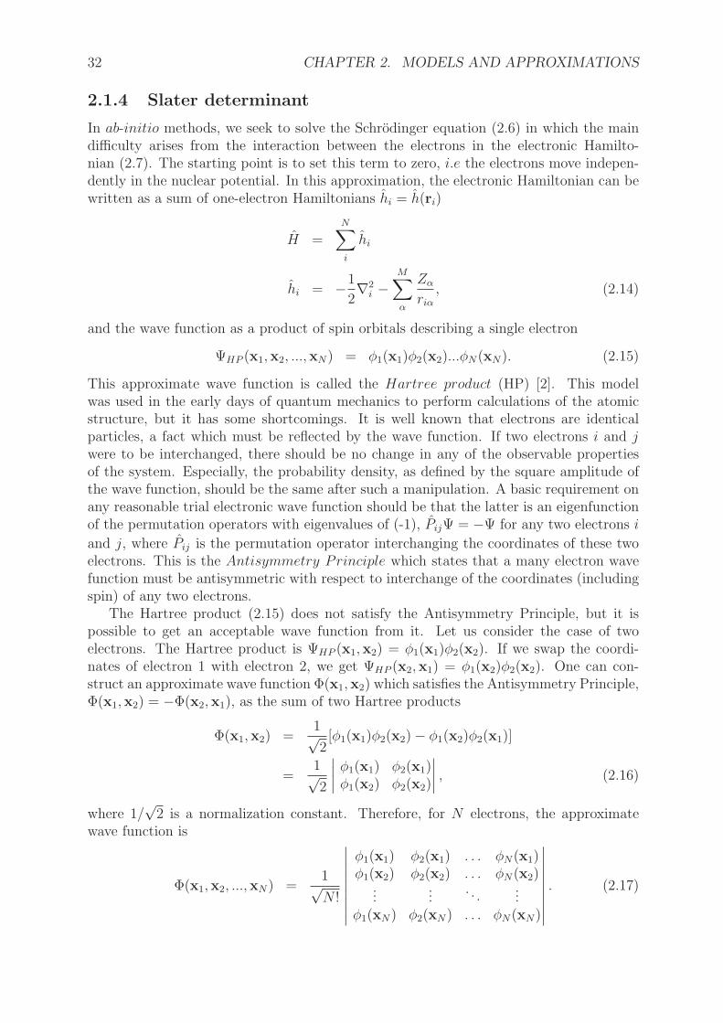
In ab-initio methods, we seek to solve the Schrodinger equation (2.6) in which the maindifficulty arises from the interaction between the electrons in the electronic Hamilto-nian (2.7). The starting point is to set this term to zero, i.e the electrons move indepen-dently in the nuclear potential. In this approximation, the electronic Hamiltonian can bewritten as a sum of one-electron Hamiltonians hi = h(ri)
H =N
∑
i
hi
hi = −1
2∇2
i −M
∑
α
Zα
riα
, (2.14)
and the wave function as a product of spin orbitals describing a single electron
ΨHP (x1,x2, ...,xN ) = φ1(x1)φ2(x2)...φN(xN). (2.15)
This approximate wave function is called the Hartree product (HP) [2]. This modelwas used in the early days of quantum mechanics to perform calculations of the atomicstructure, but it has some shortcomings. It is well known that electrons are identicalparticles, a fact which must be reflected by the wave function. If two electrons i and jwere to be interchanged, there should be no change in any of the observable propertiesof the system. Especially, the probability density, as defined by the square amplitude ofthe wave function, should be the same after such a manipulation. A basic requirement onany reasonable trial electronic wave function should be that the latter is an eigenfunctionof the permutation operators with eigenvalues of (-1), PijΨ = −Ψ for any two electrons i
and j, where Pij is the permutation operator interchanging the coordinates of these twoelectrons. This is the Antisymmetry Principle which states that a many electron wavefunction must be antisymmetric with respect to interchange of the coordinates (includingspin) of any two electrons.
The Hartree product (2.15) does not satisfy the Antisymmetry Principle, but it ispossible to get an acceptable wave function from it. Let us consider the case of twoelectrons. The Hartree product is ΨHP (x1,x2) = φ1(x1)φ2(x2). If we swap the coordi-nates of electron 1 with electron 2, we get ΨHP (x2,x1) = φ1(x2)φ2(x2). One can con-struct an approximate wave function Φ(x1,x2) which satisfies the Antisymmetry Principle,Φ(x1,x2) = −Φ(x2,x1), as the sum of two Hartree products
Φ(x1,x2) =1√2[φ1(x1)φ2(x2) − φ1(x2)φ2(x1)]
=1√2
∣
∣
∣
∣
φ1(x1) φ2(x1)φ1(x2) φ2(x2)
∣
∣
∣
∣
, (2.16)
where 1/√
2 is a normalization constant. Therefore, for N electrons, the approximatewave function is
Φ(x1,x2, ...,xN ) =1√N !
∣
∣
∣
∣
∣
∣
∣
∣
∣
φ1(x1) φ2(x1) . . . φN(x1)φ1(x2) φ2(x2) . . . φN(x2)
......
. . ....
φ1(xN) φ2(xN) . . . φN(xN)
∣
∣
∣
∣
∣
∣
∣
∣
∣
. (2.17)

2.2. HARTREE-FOCK AND POST HARTREE-FOCK APPROXIMATIONS 33
This form of the wave function was applied to the N -electron problem by Slater [3] andis known as a Slater determinant. By writing the wave function in this form, we providea way which automatically satisfies the Pauli Exclusion Principle, i.e. two identicalfermions cannot be found in the same quantum state (having the same spin orbital),which is a corollary of the antisymmetry principle. If φi = φj, two columns are identicalin (2.17), then Φ = 0 according to the determinant property. Because the determinantwave function (2.17) is only a function of the N occupied spin orbitals φi(x), φj(x), ...,φk(x), we introduce the abbreviation Φ = |ij...k〉. The antisymmetry property of Slaterdeterminant is expressed as
|...i...j...〉 = −|...j...i...〉. (2.18)
2.1.5 Variational theorem
Since an exact or almost exact numerical solution of the Schrodinger equation (2.6) isnot in sight and appears hopeless for N>2, approximations must be made. A standardtool for computing approximate solutions of (2.6) is the variation method based on theV ariational Theorem. For any initial trial wave function, Φ, we have
E[Φ] =〈Φ|H|Φ〉〈Φ|Φ〉 ≥ E0 (2.19)
where E0 is the exact ground state energy. Approximate solutions for the ground state(excited states can be treated similarly) can thus be obtained by a minimization of E[Φ]for a reasonable ansatz Φ. By expressing the approximate wave function in terms ofparameters and minimizing the functional (2.19) with respect to these parameters onecan obtain progressively better approximations to the energy and the eigenfunctions ofthe Hamiltonian. The energies obtained are more accurate than the wave functions andrepresent rigorous upper bounds to the exact ground state energy. Quantitatively, if theaccuracy of the approximate wave function assumed is of order δ, the energy is accurateto order δ2.
2.2 Hartree-Fock and post Hartree-Fock approxima-
tions
The essence of the Hartree-Fock method is that the wave function is written as a Slater de-terminant [4]. We will now use this wave function representation to obtain the expectationvalue 〈Φ|H|Φ〉 of the Hamiltonian operator.
2.2.1 Expectation values with a Slater determinant
The electronic Hamiltonian for a many electron system can be written in terms of one-,and two-electron operators
H =N
∑
i
hi +N
∑
i
N∑
j>i
vij, (2.20)
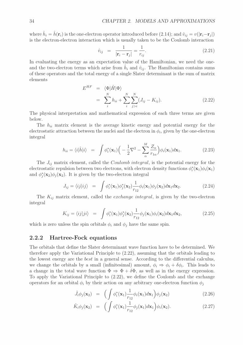
34 CHAPTER 2. MODELS AND APPROXIMATIONS
where hi = h(ri) is the one-electron operator introduced before (2.14); and vij = v(|ri−rj|)is the electron-electron interaction which is usually taken to be the Coulomb interaction
vij =1
|ri − rj|=
1
rij
. (2.21)
In evaluating the energy as an expectation value of the Hamiltonian, we need the one-and the two-electron terms which arise from hi and vij. The Hamiltonian contains sumsof these operators and the total energy of a single Slater determinant is the sum of matrixelements
EHF = 〈Φ|H|Φ〉
=N
∑
i
hii +N
∑
i
N∑
j>i
(Jij −Kij). (2.22)
The physical interpretation and mathematical expression of each three terms are givenbelow.
The hii matrix element is the average kinetic energy and potential energy for theelectrostatic attraction between the nuclei and the electron in φi, given by the one-electronintegral
hii = 〈i|h|i〉 =
∫
φ∗i (x1)
(
− 1
2∇2 −
M∑
α
Zα
r1α
)
φi(x1)dx1. (2.23)
The Jij matrix element, called the Coulomb integral, is the potential energy for theelectrostatic repulsion between two electrons, with electron density functions φ∗
i (x1)φi(x1)and φ∗
j(x2)φj(x2). It is given by the two-electron integral
Jij = 〈ij|ij〉 =
∫
φ∗i (x1)φ
∗j(x2)
1
r12φi(x1)φj(x2)dx1dx2. (2.24)
The Kij matrix element, called the exchange integral, is given by the two-electronintegral
Kij = 〈ij|ji〉 =
∫
φ∗i (x1)φ
∗j(x2)
1
r12φj(x1)φi(x2)dx1dx2, (2.25)
which is zero unless the spin orbitals φi and φj have the same spin.
2.2.2 Hartree-Fock equations
The orbitals that define the Slater determinant wave function have to be determined. Wetherefore apply the Variational Principle to (2.22), assuming that the orbitals leading tothe lowest energy are the best in a general sense. According to the differential calculus,we change the orbitals by a small (infinitesimal) amount, φi ⇒ φi + δφi. This leads toa change in the total wave function Φ ⇒ Φ + δΦ, as well as in the energy expression.To apply the Variational Principle to (2.22), we define the Coulomb and the exchangeoperators for an orbital φi by their action on any arbitrary one-electron function φj
Jiφj(x2) =(
∫
φ∗i (x1)
1
r12φi(x1)dx1
)
φj(x2) (2.26)
Kiφj(x2) =(
∫
φ∗i (x1)
1
r12φj(x1)dx1
)
φi(x2). (2.27)

2.2. HARTREE-FOCK AND POST HARTREE-FOCK APPROXIMATIONS 35
The Coulomb operator simply multiplies the test function by the electrostatic potentialarising from the orbital φi, so it is just an ordinary local multiplicative operator. Bycontrast, the exchange operator is nonlocal, and produces a function which is the productof φi with an electrostatic potential. This potential is determined by the differentialoverlap of the test function with the orbital φi.
Then, we rewrite (2.22) using a symmetric double summation for the Coulomb andthe exchange operators which yields a factor 1/2 in front of them (the Coulomb ”self-interaction” Jii is exactly canceled by the corresponding ”exchange” element Kii)
EHF =N
∑
i
〈φi|h|φi〉 +1
2
N∑
ij
〈φi|Jj − Kj|φi〉. (2.28)
In the minimization of (2.28), the constraint that the spin orbitals remain orthonor-mal (2.12) needs to be enforced. A convenient way to do this is using the method ofLagrange multipliers. The Lagrangian
LHF = EHF −N
∑
ij
λij(〈φi|φj〉 − δij), (2.29)
where λij are the Lagrange multipliers, is stationary with respect to a small change in thespin orbital
δLHF = δEHF −N
∑
ij
λij(〈δφi|φj〉 − 〈φi|δφj〉) = 0. (2.30)
After allowing the spin orbital variation δφ in each orbital of (2.28), we find that theenergy variation is given by variation of the expectation value of a single operator
δEHF =N
∑
i
(〈δφi|Fi|φi〉 − 〈φi|Fi|δφi〉), (2.31)
where Fi ≡ F is the Fock Operator which is identical for all electrons and so we maydrop the index i
F = h+N
∑
j
(Jj − Kj). (2.32)
This operator is associated with the variation of the energy, not the energy itself. Thevariation of the Lagrangian (2.30) reduces to
δLHF =N
∑
i
〈δφi|[
F |φi〉 −N
∑
j
λij|φj〉]
+ c.c. = 0, (2.33)
where c.c. denotes the complex conjugate. The equation (2.33) is only possible if the termin the squared bracket is zero; therefore,
F |φi〉 =N
∑
j
λij|φj〉, (2.34)
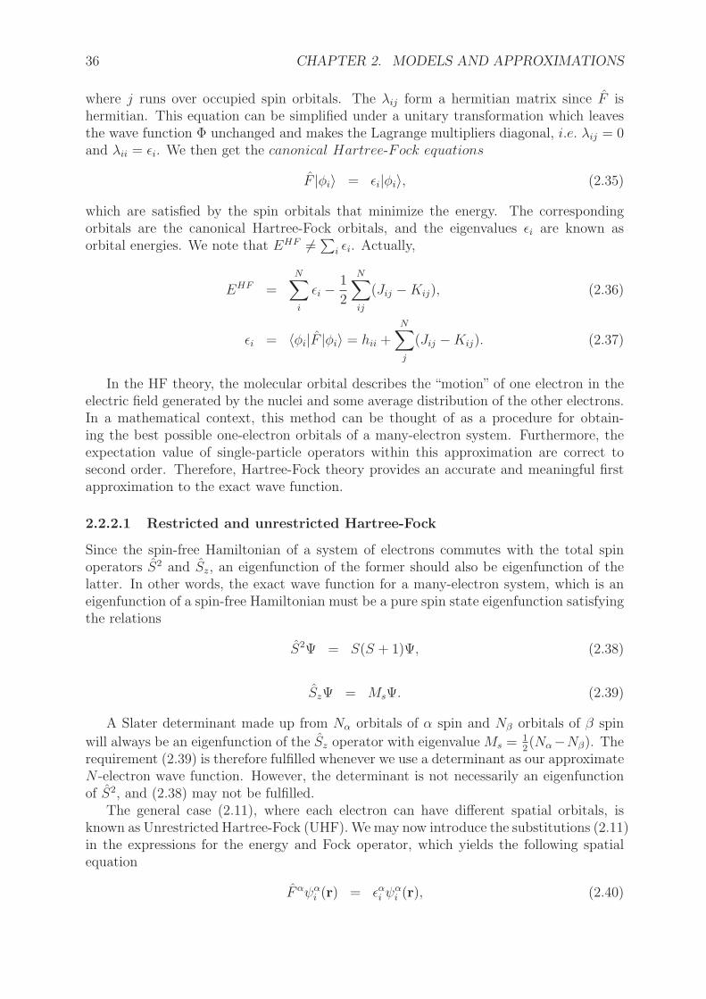
36 CHAPTER 2. MODELS AND APPROXIMATIONS
where j runs over occupied spin orbitals. The λij form a hermitian matrix since F ishermitian. This equation can be simplified under a unitary transformation which leavesthe wave function Φ unchanged and makes the Lagrange multipliers diagonal, i.e. λij = 0and λii = ǫi. We then get the canonical Hartree-Fock equations
F |φi〉 = ǫi|φi〉, (2.35)
which are satisfied by the spin orbitals that minimize the energy. The correspondingorbitals are the canonical Hartree-Fock orbitals, and the eigenvalues ǫi are known asorbital energies. We note that EHF 6= ∑
i ǫi. Actually,
EHF =N
∑
i
ǫi −1
2
N∑
ij
(Jij −Kij), (2.36)
ǫi = 〈φi|F |φi〉 = hii +N
∑
j
(Jij −Kij). (2.37)
In the HF theory, the molecular orbital describes the “motion” of one electron in theelectric field generated by the nuclei and some average distribution of the other electrons.In a mathematical context, this method can be thought of as a procedure for obtain-ing the best possible one-electron orbitals of a many-electron system. Furthermore, theexpectation value of single-particle operators within this approximation are correct tosecond order. Therefore, Hartree-Fock theory provides an accurate and meaningful firstapproximation to the exact wave function.
2.2.2.1 Restricted and unrestricted Hartree-Fock
Since the spin-free Hamiltonian of a system of electrons commutes with the total spinoperators S2 and Sz, an eigenfunction of the former should also be eigenfunction of thelatter. In other words, the exact wave function for a many-electron system, which is aneigenfunction of a spin-free Hamiltonian must be a pure spin state eigenfunction satisfyingthe relations
S2Ψ = S(S + 1)Ψ, (2.38)
SzΨ = MsΨ. (2.39)
A Slater determinant made up from Nα orbitals of α spin and Nβ orbitals of β spin
will always be an eigenfunction of the Sz operator with eigenvalue Ms = 12(Nα−Nβ). The
requirement (2.39) is therefore fulfilled whenever we use a determinant as our approximateN -electron wave function. However, the determinant is not necessarily an eigenfunctionof S2, and (2.38) may not be fulfilled.
The general case (2.11), where each electron can have different spatial orbitals, isknown as Unrestricted Hartree-Fock (UHF). We may now introduce the substitutions (2.11)in the expressions for the energy and Fock operator, which yields the following spatialequation
Fαψαi (r) = ǫαi ψ
αi (r), (2.40)

2.2. HARTREE-FOCK AND POST HARTREE-FOCK APPROXIMATIONS 37
where
Fα = h+N
∑
j
Jj −Nα∑
j
Kαj . (2.41)
For the Fock operator, we must make a distinction depending on whether it operates onan α orbital or a β orbital (the operator Kα
j only acts on the Nα electrons of spin α).Equivalent equations exist for electrons of spin β. The straightforward implementation ofthe α equations (2.40) and the β equivalent ones is known as Unrestricted Hartree-FockTheory, since there is no attempt to impose the constraint (2.38) on the wave function.
A simpler situation occurs when the electronic state under consideration is a spinsinglet (S = Ms = 0, spin multiplicity=1), which necessarily requires an even numberof electrons. The spin orbitals can be required to occur in pairs having the same spatialorbital
φαi (x) = ψi(r)α(s)
φβi (x) = ψi(r)β(s), (2.42)
and
Fψi(r) = ǫiψi(r), (2.43)
where
F = h+
N2
∑
j
(2Jj − Kj). (2.44)
The determinant is then an eigenfunction of the operators Sz and S2. The above ansatz (2.42)therefore ensures correct spin properties for a singlet wave function. The RestrictedHartree-Fock equations (2.43) are simpler to solve than the corresponding UHF ones.Since the α and β orbitals have identical spatial parts, the two Fock operators must alsobe the same (2.44) in this closed shell theory and by only constructing one Fock operator,the work and the memory requirements are reduced.
There is a method for applying RHF equations to an open shell system known asRestricted Open Shell Hartree-Fock (ROHF). In ROHF, the paired electrons are re-stricted to have the same spatial orbital as in RHF and the unpaired electrons are treatedwith different spatial orbitals as in UHF. Such a determinant is an eigenfunction of Sz
and S2 with S = Ms = no
2, where no is the number of the singly occupied spatial orbitals.
2.2.2.2 Solution of the restricted Hartree-Fock equations
The resulting integro-differential equations from the Hartree-Fock approximation can besolved numerically, but in general they are still too complicated to be solved exactly, andfurther approximations are needed. Roothann [5] made the HF approximation more prac-tical for numerical solutions by using the basis set expansion approach, i.e. the techniqueof expanding a spatial molecular orbital (MO) ψi(r) as a Linear Combination of AtomicOrbitals (LCAO) χp(r)
ψi(r) =
Nbasis∑
ν
Cνiχν(r), (2.45)
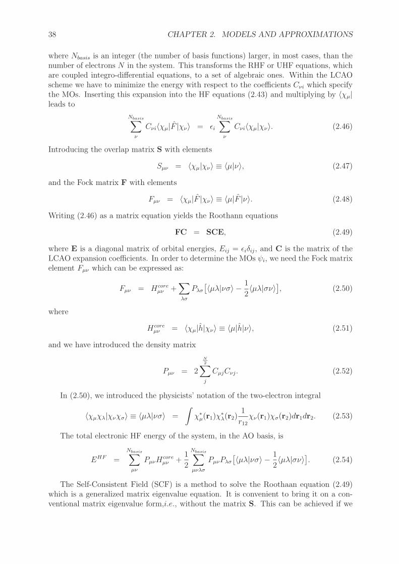
38 CHAPTER 2. MODELS AND APPROXIMATIONS
where Nbasis is an integer (the number of basis functions) larger, in most cases, than thenumber of electrons N in the system. This transforms the RHF or UHF equations, whichare coupled integro-differential equations, to a set of algebraic ones. Within the LCAOscheme we have to minimize the energy with respect to the coefficients Cνi which specifythe MOs. Inserting this expansion into the HF equations (2.43) and multiplying by 〈χµ|leads to
Nbasis∑
ν
Cνi〈χµ|F |χν〉 = ǫi
Nbasis∑
ν
Cνi〈χµ|χν〉. (2.46)
Introducing the overlap matrix S with elements
Sµν = 〈χµ|χν〉 ≡ 〈µ|ν〉, (2.47)
and the Fock matrix F with elements
Fµν = 〈χµ|F |χν〉 ≡ 〈µ|F |ν〉. (2.48)
Writing (2.46) as a matrix equation yields the Roothann equations
FC = SCE, (2.49)
where E is a diagonal matrix of orbital energies, Eij = ǫiδij, and C is the matrix of theLCAO expansion coefficients. In order to determine the MOs ψi, we need the Fock matrixelement Fµν which can be expressed as:
Fµν = Hcoreµν +
∑
λσ
Pλσ
[
〈µλ|νσ〉 − 1
2〈µλ|σν〉
]
, (2.50)
where
Hcoreµν = 〈χµ|h|χν〉 ≡ 〈µ|h|ν〉, (2.51)
and we have introduced the density matrix
Pµν = 2
N2
∑
j
CµjCνj. (2.52)
In (2.50), we introduced the physicists’ notation of the two-electron integral
〈χµχλ|χνχσ〉 ≡ 〈µλ|νσ〉 =
∫
χ∗µ(r1)χ
∗λ(r2)
1
r12χν(r1)χσ(r2)dr1dr2. (2.53)
The total electronic HF energy of the system, in the AO basis, is
EHF =
Nbasis∑
µν
PµνHcoreµν +
1
2
Nbasis∑
µνλσ
PµνPλσ
[
〈µλ|νσ〉 − 1
2〈µλ|σν〉
]
. (2.54)
The Self-Consistent Field (SCF) is a method to solve the Roothaan equation (2.49)which is a generalized matrix eigenvalue equation. It is convenient to bring it on a con-ventional matrix eigenvalue form,i.e., without the matrix S. This can be achieved if we
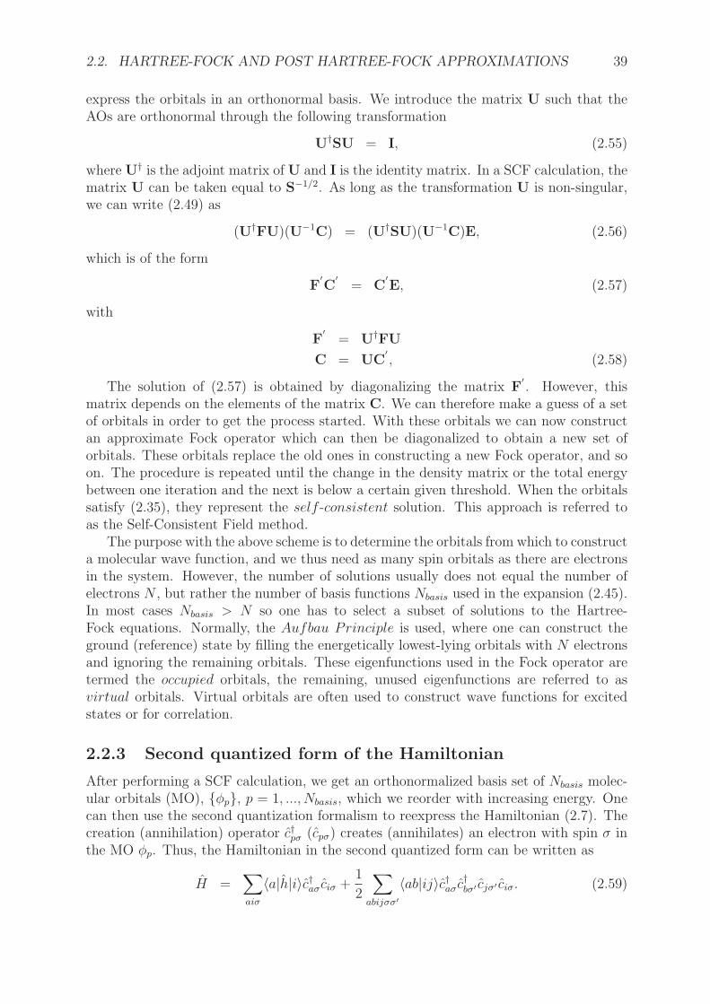
2.2. HARTREE-FOCK AND POST HARTREE-FOCK APPROXIMATIONS 39
express the orbitals in an orthonormal basis. We introduce the matrix U such that theAOs are orthonormal through the following transformation
U†SU = I, (2.55)
where U† is the adjoint matrix of U and I is the identity matrix. In a SCF calculation, thematrix U can be taken equal to S−1/2. As long as the transformation U is non-singular,we can write (2.49) as
(U†FU)(U−1C) = (U†SU)(U−1C)E, (2.56)
which is of the form
F′
C′
= C′
E, (2.57)
with
F′
= U†FU
C = UC′
, (2.58)
The solution of (2.57) is obtained by diagonalizing the matrix F′
. However, thismatrix depends on the elements of the matrix C. We can therefore make a guess of a setof orbitals in order to get the process started. With these orbitals we can now constructan approximate Fock operator which can then be diagonalized to obtain a new set oforbitals. These orbitals replace the old ones in constructing a new Fock operator, and soon. The procedure is repeated until the change in the density matrix or the total energybetween one iteration and the next is below a certain given threshold. When the orbitalssatisfy (2.35), they represent the self -consistent solution. This approach is referred toas the Self-Consistent Field method.
The purpose with the above scheme is to determine the orbitals from which to constructa molecular wave function, and we thus need as many spin orbitals as there are electronsin the system. However, the number of solutions usually does not equal the number ofelectrons N , but rather the number of basis functions Nbasis used in the expansion (2.45).In most cases Nbasis > N so one has to select a subset of solutions to the Hartree-Fock equations. Normally, the Aufbau Principle is used, where one can construct theground (reference) state by filling the energetically lowest-lying orbitals with N electronsand ignoring the remaining orbitals. These eigenfunctions used in the Fock operator aretermed the occupied orbitals, the remaining, unused eigenfunctions are referred to asvirtual orbitals. Virtual orbitals are often used to construct wave functions for excitedstates or for correlation.
2.2.3 Second quantized form of the Hamiltonian
After performing a SCF calculation, we get an orthonormalized basis set of Nbasis molec-ular orbitals (MO), {φp}, p = 1, ..., Nbasis, which we reorder with increasing energy. Onecan then use the second quantization formalism to reexpress the Hamiltonian (2.7). Thecreation (annihilation) operator c†pσ (cpσ) creates (annihilates) an electron with spin σ inthe MO φp. Thus, the Hamiltonian in the second quantized form can be written as
H =∑
aiσ
〈a|h|i〉c†aσ ciσ +1
2
∑
abijσσ′
〈ab|ij〉c†aσ c†bσ′ cjσ′ ciσ. (2.59)

40 CHAPTER 2. MODELS AND APPROXIMATIONS
The sum is over all spatial orbitals and spin σ. The matrix elements 〈a|h|i〉 represent thecore Hamiltonian containing kinetic energy and electron-nuclear attraction, while 〈ab|ij〉are the two-electron repulsion integrals. The Hamiltonian (2.59) is not equal to the usualone (2.7). If Nbasis is infinitely large, the set {φp}, can be complete, and in this limitthe eigenfunctions and eigenvalues of these two Hamiltonians are identical. If Nbasis isfinite, the orbital space is necessarily incomplete and the second quantized Hamiltoniancan be interpreted as the projection of the exact one to a finite subspace spanned by thebasis orbitals. It is possible to formulate the Hamiltonian (2.59) in terms of spin summedexcitation operators Epq, defined as
Epq = c†pαcqα + c†pβ cqβ =∑
σ
c†pσ cqσ. (2.60)
After some manipulations for the second term in (2.59), where we use the known anti-commutator relations for the creation-annihilation operators [6], we can write down theHamiltonian in the operator basis constructed from the excitation operators :
H =∑
ai
〈a|h|i〉Eai +1
2
∑
abij
〈ab|ij〉(EaiEbj − δibEaj). (2.61)
The summations are now over the molecular spatial orbital basis. We note that the numberof electrons does not appear in the definition of the Hamiltonian. All such informationis found in the Slater determinant basis. Using the occupation number formalism, adeterminant Φ can be written as a series of 1 and 0 indicating which spin orbitals areoccupied in the determinant
|Φ〉 = c†p1σ1c†p2σ2
...c†piσi...|0〉 = |n1, n2, ..., ni, ..., n2Nbasis
〉, (2.62)
where ni is the occupation number (0 or 1) for spin orbital piσi and |0〉 is the vacuumstate where all occupations are zero.
2.2.4 Post Hartree-Fock methods
The Hartree-Fock method is one of the simplest methods to solve the Schrodinger equa-tion, where the electrons are moving in the average field of the other electrons, whichis obviously an approximation. In reality the motion of the electrons depends on theinstantaneous positions of all the other electrons, and on average they are further apartthan described by the Hartree-Fock wave function. Therefore, the motion of the electronsis ”correlated”. The phenomenon is known as electron correlation. In the HF approxi-mation, the probability of finding two electrons with parallel spins at the same point inthe space is zero, then the motion of electrons with the same spin is correlated in thisapproximation. Conventionally correlation energy Ec is defined as
Ec = Eexact − EHF , (2.63)
where Eexact is the exact non-relativistic ground state energy, at 0 K, of the system withinthe Born-Oppenheimer approximation, and EHF is the restricted Hartree-Fock energy ina complete basis set.
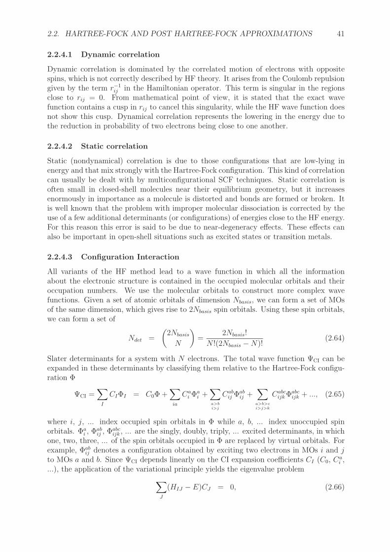
2.2. HARTREE-FOCK AND POST HARTREE-FOCK APPROXIMATIONS 41
2.2.4.1 Dynamic correlation
Dynamic correlation is dominated by the correlated motion of electrons with oppositespins, which is not correctly described by HF theory. It arises from the Coulomb repulsiongiven by the term r−1
ij in the Hamiltonian operator. This term is singular in the regionsclose to rij = 0. From mathematical point of view, it is stated that the exact wavefunction contains a cusp in rij to cancel this singularity, while the HF wave function doesnot show this cusp. Dynamical correlation represents the lowering in the energy due tothe reduction in probability of two electrons being close to one another.
2.2.4.2 Static correlation
Static (nondynamical) correlation is due to those configurations that are low-lying inenergy and that mix strongly with the Hartree-Fock configuration. This kind of correlationcan usually be dealt with by multiconfigurational SCF techniques. Static correlation isoften small in closed-shell molecules near their equilibrium geometry, but it increasesenormously in importance as a molecule is distorted and bonds are formed or broken. Itis well known that the problem with improper molecular dissociation is corrected by theuse of a few additional determinants (or configurations) of energies close to the HF energy.For this reason this error is said to be due to near-degeneracy effects. These effects canalso be important in open-shell situations such as excited states or transition metals.
2.2.4.3 Configuration Interaction
All variants of the HF method lead to a wave function in which all the informationabout the electronic structure is contained in the occupied molecular orbitals and theiroccupation numbers. We use the molecular orbitals to construct more complex wavefunctions. Given a set of atomic orbitals of dimension Nbasis, we can form a set of MOsof the same dimension, which gives rise to 2Nbasis spin orbitals. Using these spin orbitals,we can form a set of
Ndet =
(
2Nbasis
N
)
=2Nbasis!
N !(2Nbasis −N)!(2.64)
Slater determinants for a system with N electrons. The total wave function ΨCI can beexpanded in these determinants by classifying them relative to the Hartree-Fock configu-ration Φ
ΨCI =∑
I
CIΦI = C0Φ +∑
ia
Cai Φa
i +∑
a>b
i>j
Cabij Φab
ij +∑
a>b>c
i>j>k
Cabcijk Φabc
ijk + ..., (2.65)
where i, j, ... index occupied spin orbitals in Φ while a, b, ... index unoccupied spinorbitals. Φa
i , Φabij , Φabc
ijk , ... are the singly, doubly, triply, ... excited determinants, in whichone, two, three, ... of the spin orbitals occupied in Φ are replaced by virtual orbitals. Forexample, Φab
ij denotes a configuration obtained by exciting two electrons in MOs i and jto MOs a and b. Since ΨCI depends linearly on the CI expansion coefficients CI (C0, C
ai ,
...), the application of the variational principle yields the eigenvalue problem
∑
J
(HIJ − E)CJ = 0, (2.66)
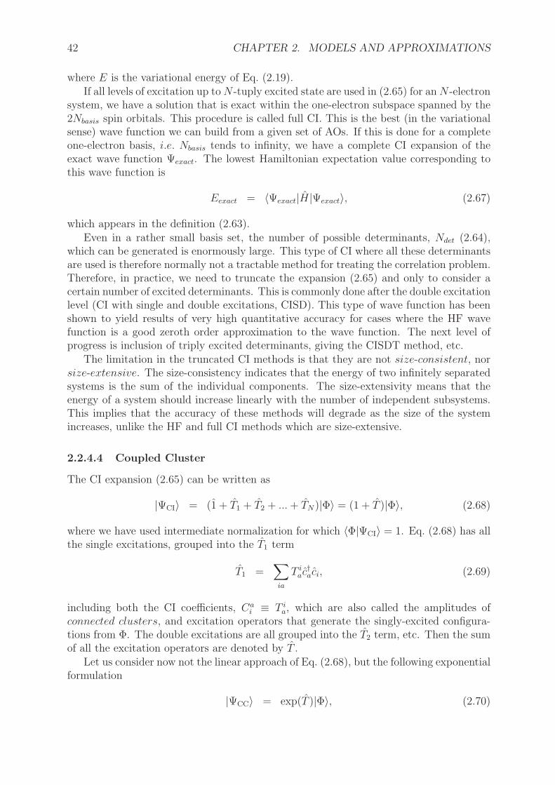
42 CHAPTER 2. MODELS AND APPROXIMATIONS
where E is the variational energy of Eq. (2.19).If all levels of excitation up toN -tuply excited state are used in (2.65) for anN -electron
system, we have a solution that is exact within the one-electron subspace spanned by the2Nbasis spin orbitals. This procedure is called full CI. This is the best (in the variationalsense) wave function we can build from a given set of AOs. If this is done for a completeone-electron basis, i.e. Nbasis tends to infinity, we have a complete CI expansion of theexact wave function Ψexact. The lowest Hamiltonian expectation value corresponding tothis wave function is
Eexact = 〈Ψexact|H|Ψexact〉, (2.67)
which appears in the definition (2.63).Even in a rather small basis set, the number of possible determinants, Ndet (2.64),
which can be generated is enormously large. This type of CI where all these determinantsare used is therefore normally not a tractable method for treating the correlation problem.Therefore, in practice, we need to truncate the expansion (2.65) and only to consider acertain number of excited determinants. This is commonly done after the double excitationlevel (CI with single and double excitations, CISD). This type of wave function has beenshown to yield results of very high quantitative accuracy for cases where the HF wavefunction is a good zeroth order approximation to the wave function. The next level ofprogress is inclusion of triply excited determinants, giving the CISDT method, etc.
The limitation in the truncated CI methods is that they are not size-consistent, norsize-extensive. The size-consistency indicates that the energy of two infinitely separatedsystems is the sum of the individual components. The size-extensivity means that theenergy of a system should increase linearly with the number of independent subsystems.This implies that the accuracy of these methods will degrade as the size of the systemincreases, unlike the HF and full CI methods which are size-extensive.
2.2.4.4 Coupled Cluster
The CI expansion (2.65) can be written as
|ΨCI〉 = (1 + T1 + T2 + ...+ TN)|Φ〉 = (1 + T )|Φ〉, (2.68)
where we have used intermediate normalization for which 〈Φ|ΨCI〉 = 1. Eq. (2.68) has allthe single excitations, grouped into the T1 term
T1 =∑
ia
T iac
†aci, (2.69)
including both the CI coefficients, Cai ≡ T i
a, which are also called the amplitudes ofconnected clusters, and excitation operators that generate the singly-excited configura-tions from Φ. The double excitations are all grouped into the T2 term, etc. Then the sumof all the excitation operators are denoted by T .
Let us consider now not the linear approach of Eq. (2.68), but the following exponentialformulation
|ΨCC〉 = exp(T )|Φ〉, (2.70)

2.2. HARTREE-FOCK AND POST HARTREE-FOCK APPROXIMATIONS 43
which we can expand in a power series
|ΨCC〉 =[
1 + T +1
2T 2 +
1
6T 3 + ...
]
|Φ〉
=[
1 + T1 +(
T2 +1
2T 2
1
)
+(
T3 + T2T1 +1
6T 3
1
)
+ ...]
|Φ〉. (2.71)
If we include all levels of excitation, up to N -fold, the wave function is equivalent to afull CI wave function. However, it is more practical to truncate at some fixed excitationlevel. Suppose one considers only the operators T1 and T2. The exponential expansion inthe exact coupled cluster wave function (2.71) becomes
|ΨCCSD〉 =[
1 + T1 + (T2 +1
2T 2
1 ) + (T1T2 +1
6T 3
1 ) + ...]
|Φ〉, (2.72)
giving the CCSD model (Coupled Cluster Singles and Doubles), which includes not onlysingle and double excitations, but higher excitations termed disconnected clusters, toinfinite order, whose amplitudes are products of the coefficients of the single and doubleexcitations. Indeed, with the exponential ansatz, we retain all disconnected clusters arisingfrom the truncated set of connected ones. Therefore, unlike the CISD method, the CCSDmethod is size-consistent thanks to the disconnected clusters. The next higher level is forT = T1 + T2 + T3 giving the CCSDT model, where we include the triples, and so on.
Due to the nonlinear nature of the wave function (2.71), the number of disconnectedcluster amplitudes grows factorially with the excitation level and obtaining these ampli-tudes by using an equation like (2.66) is not feasible so the variational approach can notbe used as a computational method. The cluster amplitudes can be optimised by substi-tuting ΨCC into the Schrodinger equation and then projecting onto the space of Φ, Φa
i ,Φab
ij , etc. This gives a set of nonlinear simultaneous equations for the cluster amplitudes.
2.2.4.5 Perturbation Theory
The most straightforward method to deal with the dynamical correlation is the many-bodyperturbation theory. In this method, the problem which needs to be solved is assumedto deviate only slightly from a solved one. For treating dynamical correlation, we usenondegenerate Rayleigh-Schrodinger perturbation theory with Møller-Plesset (MP) [7]partitioning of the Hamiltonian
H = H0 + W (2.73)
where H0, the sum of the Fock operators (2.32)
H0 =N
∑
i=1
Fi, (2.74)
is chosen as the reference Hamiltonian. The perturbative operator W can be given as
W = H −N
∑
i=1
Fi (2.75)
= Wee − VHx[Φ], (2.76)
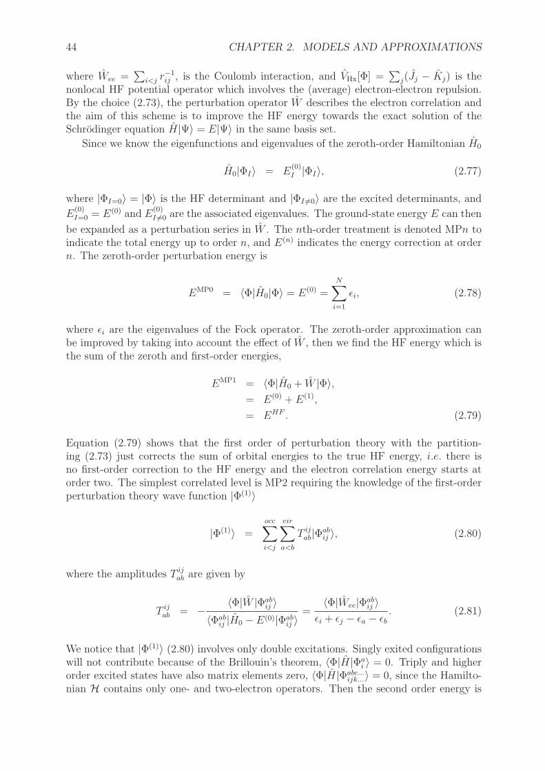
44 CHAPTER 2. MODELS AND APPROXIMATIONS
where Wee =∑
i<j r−1ij , is the Coulomb interaction, and VHx[Φ] =
∑
j(Jj − Kj) is thenonlocal HF potential operator which involves the (average) electron-electron repulsion.By the choice (2.73), the perturbation operator W describes the electron correlation andthe aim of this scheme is to improve the HF energy towards the exact solution of theSchrodinger equation H|Ψ〉 = E|Ψ〉 in the same basis set.
Since we know the eigenfunctions and eigenvalues of the zeroth-order Hamiltonian H0
H0|ΦI〉 = E(0)I |ΦI〉, (2.77)
where |ΦI=0〉 = |Φ〉 is the HF determinant and |ΦI 6=0〉 are the excited determinants, and
E(0)I=0 = E(0) and E
(0)I 6=0 are the associated eigenvalues. The ground-state energy E can then
be expanded as a perturbation series in W . The nth-order treatment is denoted MPn toindicate the total energy up to order n, and E(n) indicates the energy correction at ordern. The zeroth-order perturbation energy is
EMP0 = 〈Φ|H0|Φ〉 = E(0) =N
∑
i=1
ǫi, (2.78)
where ǫi are the eigenvalues of the Fock operator. The zeroth-order approximation canbe improved by taking into account the effect of W , then we find the HF energy which isthe sum of the zeroth and first-order energies,
EMP1 = 〈Φ|H0 + W |Φ〉,= E(0) + E(1),
= EHF . (2.79)
Equation (2.79) shows that the first order of perturbation theory with the partition-ing (2.73) just corrects the sum of orbital energies to the true HF energy, i.e. there isno first-order correction to the HF energy and the electron correlation energy starts atorder two. The simplest correlated level is MP2 requiring the knowledge of the first-orderperturbation theory wave function |Φ(1)〉
|Φ(1)〉 =occ∑
i<j
vir∑
a<b
T ijab|Φab
ij 〉, (2.80)
where the amplitudes T ijab are given by
T ijab = −
〈Φ|W |Φabij 〉
〈Φabij |H0 − E(0)|Φab
ij 〉=
〈Φ|Wee|Φabij 〉
ǫi + ǫj − ǫa − ǫb. (2.81)
We notice that |Φ(1)〉 (2.80) involves only double excitations. Singly exited configurationswill not contribute because of the Brillouin’s theorem, 〈Φ|H|Φa
i 〉 = 0. Triply and higherorder excited states have also matrix elements zero, 〈Φ|H|Φabc...
ijk...〉 = 0, since the Hamilto-nian H contains only one- and two-electron operators. Then the second order energy is
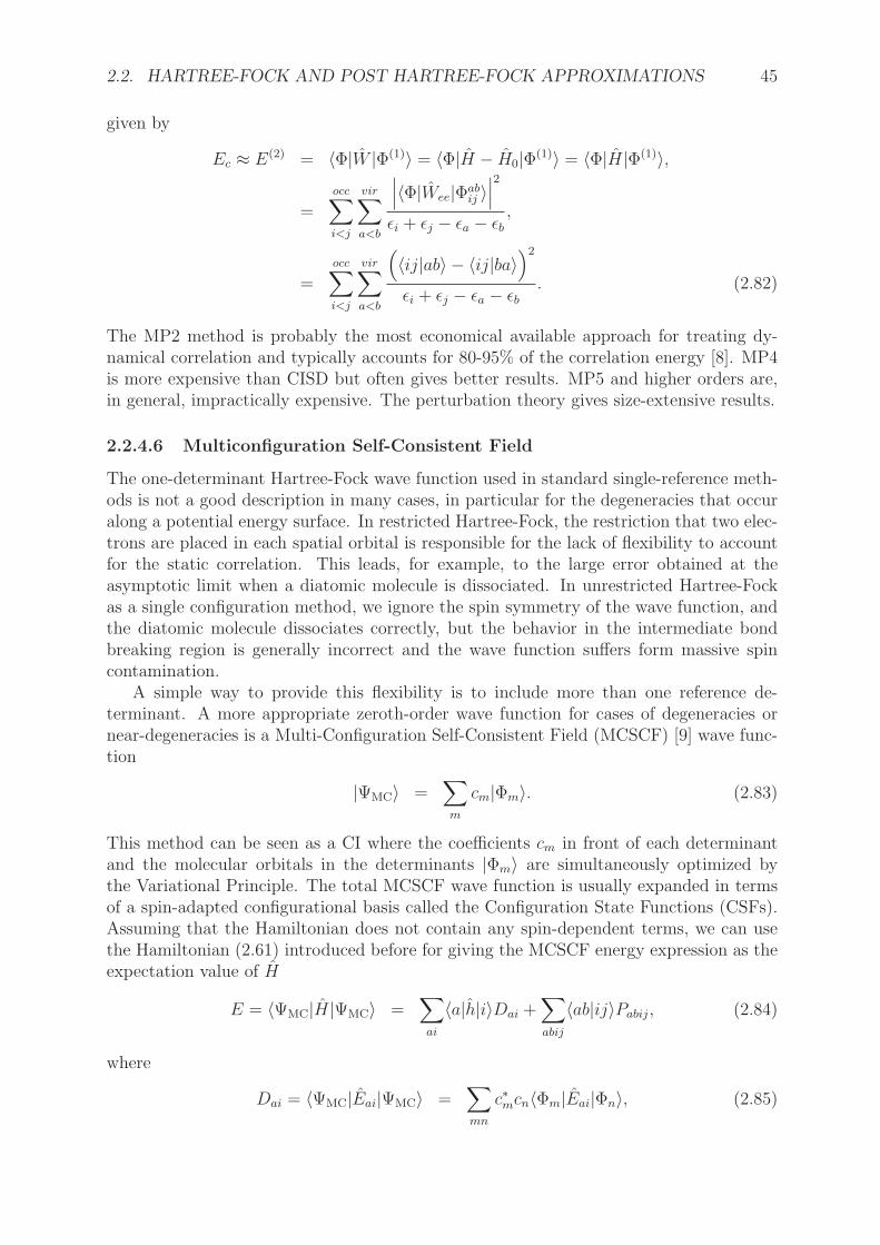
2.2. HARTREE-FOCK AND POST HARTREE-FOCK APPROXIMATIONS 45
given by
Ec ≈ E(2) = 〈Φ|W |Φ(1)〉 = 〈Φ|H − H0|Φ(1)〉 = 〈Φ|H|Φ(1)〉,
=occ∑
i<j
vir∑
a<b
∣
∣
∣〈Φ|Wee|Φab
ij 〉∣
∣
∣
2
ǫi + ǫj − ǫa − ǫb,
=occ∑
i<j
vir∑
a<b
(
〈ij|ab〉 − 〈ij|ba〉)2
ǫi + ǫj − ǫa − ǫb. (2.82)
The MP2 method is probably the most economical available approach for treating dy-namical correlation and typically accounts for 80-95% of the correlation energy [8]. MP4is more expensive than CISD but often gives better results. MP5 and higher orders are,in general, impractically expensive. The perturbation theory gives size-extensive results.
2.2.4.6 Multiconfiguration Self-Consistent Field
The one-determinant Hartree-Fock wave function used in standard single-reference meth-ods is not a good description in many cases, in particular for the degeneracies that occuralong a potential energy surface. In restricted Hartree-Fock, the restriction that two elec-trons are placed in each spatial orbital is responsible for the lack of flexibility to accountfor the static correlation. This leads, for example, to the large error obtained at theasymptotic limit when a diatomic molecule is dissociated. In unrestricted Hartree-Fockas a single configuration method, we ignore the spin symmetry of the wave function, andthe diatomic molecule dissociates correctly, but the behavior in the intermediate bondbreaking region is generally incorrect and the wave function suffers form massive spincontamination.
A simple way to provide this flexibility is to include more than one reference de-terminant. A more appropriate zeroth-order wave function for cases of degeneracies ornear-degeneracies is a Multi-Configuration Self-Consistent Field (MCSCF) [9] wave func-tion
|ΨMC〉 =∑
m
cm|Φm〉. (2.83)
This method can be seen as a CI where the coefficients cm in front of each determinantand the molecular orbitals in the determinants |Φm〉 are simultaneously optimized bythe Variational Principle. The total MCSCF wave function is usually expanded in termsof a spin-adapted configurational basis called the Configuration State Functions (CSFs).Assuming that the Hamiltonian does not contain any spin-dependent terms, we can usethe Hamiltonian (2.61) introduced before for giving the MCSCF energy expression as theexpectation value of H
E = 〈ΨMC|H|ΨMC〉 =∑
ai
〈a|h|i〉Dai +∑
abij
〈ab|ij〉Pabij, (2.84)
where
Dai = 〈ΨMC|Eai|ΨMC〉 =∑
mn
c∗mcn〈Φm|Eai|Φn〉, (2.85)
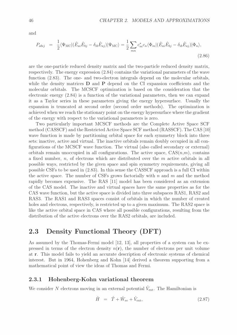
46 CHAPTER 2. MODELS AND APPROXIMATIONS
and
Pabij =1
2〈ΨMC|(EaiEbj − δibEaj)|ΨMC〉 =
1
2
∑
mn
c∗mcn〈Φm|(EaiEbj − δibEaj)|Φn〉,
(2.86)
are the one-particle reduced density matrix and the two-particle reduced density matrix,respectively. The energy expression (2.84) contains the variational parameters of the wavefunction (2.83). The one- and two-electron integrals depend on the molecular orbitals,while the density matrices D and P depend on the CI expansion coefficients and themolecular orbitals. The MCSCF optimization is based on the consideration that theelectronic energy (2.84) is a function of the variational parameters, then we can expandit as a Taylor series in these parameters giving the energy hypersurface. Usually theexpansion is truncated at second order (second order methods). The optimization isachieved when we reach the stationary point on the energy hypersurface where the gradientof the energy with respect to the variational parameters is zero.
Two particularly important MCSCF methods are the Complete Active Space SCFmethod (CASSCF) and the Restricted Active Space SCF method (RASSCF). The CAS [10]wave function is made by partitioning orbital space for each symmetry block into threesets: inactive, active and virtual. The inactive orbitals remain doubly occupied in all con-figurations of the MCSCF wave function. The virtual (also called secondary or external)orbitals remain unoccupied in all configurations. The active space, CAS(n,m), containsa fixed number, n, of electrons which are distributed over the m active orbitals in allpossible ways, restricted by the given space and spin symmetry requirements, giving allpossible CSFs to be used in (2.83). In this sense the CASSCF approach is a full CI withinthe active space. The number of CSFs grows factorially with n and m and the methodrapidly becomes expensive. The RAS [11] model has been considered as an extensionof the CAS model. The inactive and virtual spaces have the same properties as for theCAS wave function, but the active space is divided into three subspaces RAS1, RAS2 andRAS3. The RAS1 and RAS3 spaces consist of orbitals in which the number of createdholes and electrons, respectively, is restricted up to a given maximum. The RAS2 space islike the active orbital space in CAS where all possible configurations, resulting from thedistribution of the active electrons over the RAS2 orbitals, are included.
2.3 Density Functional Theory (DFT)
As assumed by the Thomas-Fermi model [12, 13], all properties of a system can be ex-pressed in terms of the electron density n(r), the number of electrons per unit volumeat r. This model fails to yield an accurate description of electronic systems of chemicalinterest. But in 1964, Hohenberg and Kohn [14] derived a theorem supporting from amathematical point of view the ideas of Thomas and Fermi.
2.3.1 Hohenberg-Kohn variational theorem
We consider N electrons moving in an external potential Vext. The Hamiltonian is
H = T + Wee + Vext, (2.87)

2.3. DENSITY FUNCTIONAL THEORY (DFT) 47
where T and Wee are the kinetic and electron-electron interaction operators, respectively.Vext =
∫
vext(r)n(r)dr, where vext(r) is the scalar (usually electron-nuclear) multiplicativepotential, and n(r) is the density operator. For all densities such that
∫
n(r)dr = N , whicharise from some antisymmetric wave function Ψ, Levy [15, 16] defined the functional
F [n] = minΨ⇒n
〈Ψ|T + Wee|Ψ〉, (2.88)
where the search is constrained to the subspace of all the antisymmetric Ψ that give thedensity n. We denote Ψ[n] to be the minimizing wave function.
F [n] = 〈Ψ[n]|T |Ψ[n]〉 + 〈Ψ[n]|Wee|Ψ[n]〉 = T [n] +Wee[n]. (2.89)
Let E0, Ψ0, and n0 be the ground-state energy, wave function, and density, respectively.Then if we insert Ψ[n] in expression of the total energy
E[n] ≡∫
vext(r)n(r)dr + F [n] = 〈Ψ[n]|T + Wee + Vext|Ψ[n]〉,
≥ E0 = E[n0], (2.90)
we must get a higher number according to the minimum property of the ground state.The ground-state energy can be given as
E0 = minn
{
∫
vext(r)n(r)dr + F [n]}
, (2.91)
where the minimum is taken over all N -representable densities. The minimization (2.91)implies that,
vext(r) =(
− δF [n]
δn(r)
)
n=n0
, (2.92)
which means that, within an additive constant, the ground-state density n0 determinesthe potential vext(r), so it determines the ground-state wave function Ψ0 = Ψ[n0], fromwhich all the ground-state properties can be calculated.
2.3.2 Kohn-Sham formulation
The equations (2.90) and (2.91) in the previous subsection provide a method for calculat-ing ground-state properties such that if a form of F [n] can be found, we have to minimizeE[n] in (2.90) for the potential vext(r) of interest. But the task of finding good approx-imations to F [n] is not easy. There is a problem with the expression of the kinetic partT [n] in terms of the density, which represents the main drawback of the Thomas-Fermiapproach, the old practical application of DFT.
In 1965, Kohn and Sham (KS) [17] introduced a method for evaluating T [n] by re-placing the kinetic energy of the interacting electrons with that of an equivalent non-interacting reference (Kohn-Sham) system whose ground-state density is that of the in-teracting one n0. Assume that n0 is the ground-state density of the non-interactingHamiltonian
HKS = T + VKS, (2.93)
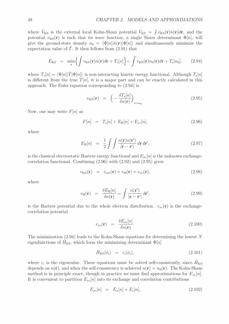
48 CHAPTER 2. MODELS AND APPROXIMATIONS
where VKS is the external local Kohn-Sham potential VKS =∫
vKS(r)n(r)dr, and thepotential vKS(r) is such that its wave function, a single Slater determinant Φ[n], willgive the ground-state density n0 = 〈Φ[n]|n(r)|Φ[n]〉 and simultaneously minimize theexpectation value of T . It then follows from (2.91) that
EKS = minn
{
∫
vKS(r)n(r)dr + Ts[n]}
=
∫
vKS(r)n0(r)dr + Ts[n0], (2.94)
where Ts[n] = 〈Φ[n]|T |Φ[n]〉 is non-interacting kinetic energy functional. Although Ts[n]is different from the true T [n], it is a major part and can be exactly calculated in thisapproach. The Euler equation corresponding to (2.94) is
vKS(r) =(
− δTs[n]
δn(r)
)
n=n0
. (2.95)
Now, one may write F [n] as
F [n] = Ts[n] + EH[n] + Exc[n], (2.96)
where
EH[n] =1
2
∫ ∫
n(r)n(r′)
|r − r′| dr dr′, (2.97)
is the classical electrostatic Hartree energy functional and Exc[n] is the unknown exchange-correlation functional. Combining (2.96) with (2.92) and (2.95) gives
vKS(r) = vext(r) + vH(r) + vxc(r), (2.98)
where
vH(r) =δEH[n]
δn(r)=
∫
n(r′)
|r − r′| dr′, (2.99)
is the Hartree potential due to the whole electron distribution. vxc(r) is the exchange-correlation potential
vxc(r) =δExc[n]
δn(r). (2.100)
The minimization (2.94) leads to the Kohn-Sham equations for determining the lowest Neigenfunctions of HKS, which form the minimizing determinant Φ[n]
HKS|φi〉 = εi|φi〉, (2.101)
where εi is the eigenvalue. These equations must be solved self-consistently, since HKS
depends on n(r), and when the self-consistency is achieved n(r) = n0(r). The Kohn-Shammethod is in principle exact, though in practice we must find approximations for Exc[n].It is convenient to partition Exc[n] into its exchange and correlation contributions
Exc[n] = Ex[n] + Ec[n], (2.102)
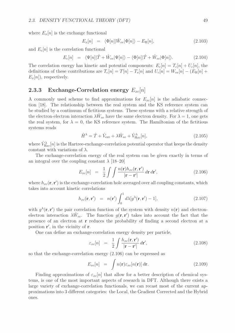
2.3. DENSITY FUNCTIONAL THEORY (DFT) 49
where Ex[n] is the exchange functional
Ex[n] = 〈Φ[n]|Wee|Φ[n]〉 − EH[n], (2.103)
and Ec[n] is the correlation functional
Ec[n] = 〈Ψ[n]|T + Wee|Ψ[n]〉 − 〈Φ[n]|T + Wee|Φ[n]〉. (2.104)
The correlation energy has kinetic and potential components: Ec[n] = Tc[n] + Uc[n], thedefinitions of these contributions are Tc[n] = T [n] − Ts[n] and Uc[n] = Wee[n] − (EH[n] +Ex[n]), respectively.
2.3.3 Exchange-Correlation energy Exc[n]
A commonly used scheme to find approximations for Exc[n] is the adiabatic connec-tion [18]. The relationship between the real system and the KS reference system canbe studied by a continuum of fictitious systems. These systems with a relative strength ofthe electron-electron interaction λWee have the same electron density. For λ = 1, one getsthe real system, for λ = 0, the KS reference system. The Hamiltonian of the fictitioussystems reads
Hλ = T + Vext + λWee + V λHxc[n], (2.105)
where V λHxc[n] is the Hartree-exchange-correlation potential operator that keeps the density
constant with variations of λ.The exchange-correlation energy of the real system can be given exactly in terms of
an integral over the coupling constant λ [18–20]
Exc[n] =1
2
∫ ∫
n(r)hxc(r, r′)
|r − r′| dr dr′, (2.106)
where hxc(r, r′) is the exchange-correlation hole averaged over all coupling constants, which
takes into account kinetic correlations
hxc(r, r′) = n(r′)
∫ 1
0
dλ[gλ(r, r′) − 1], (2.107)
with gλ(r, r′) the pair correlation function of the system with density n(r) and electron-electron interaction λWee. The function g(r, r′) takes into account the fact that thepresence of an electron at r reduces the probability of finding a second electron at aposition r′, in the vicinity of r.
One can define an exchange-correlation energy density per particle,
εxc[n] =1
2
∫
hxc(r, r′)
|r − r′| dr′, (2.108)
so that the exchange-correlation energy (2.106) can be expressed as
Exc[n] =
∫
n(r)εxc[n(r)] dr. (2.109)
Finding approximations of εxc[n] that allow for a better description of chemical sys-tems, is one of the most important aspects of research in DFT. Although there exists alarge variety of exchange-correlation functionals, we can recast most of the current ap-proximations into 3 different categories: the Local, the Gradient Corrected and the Hybridones.
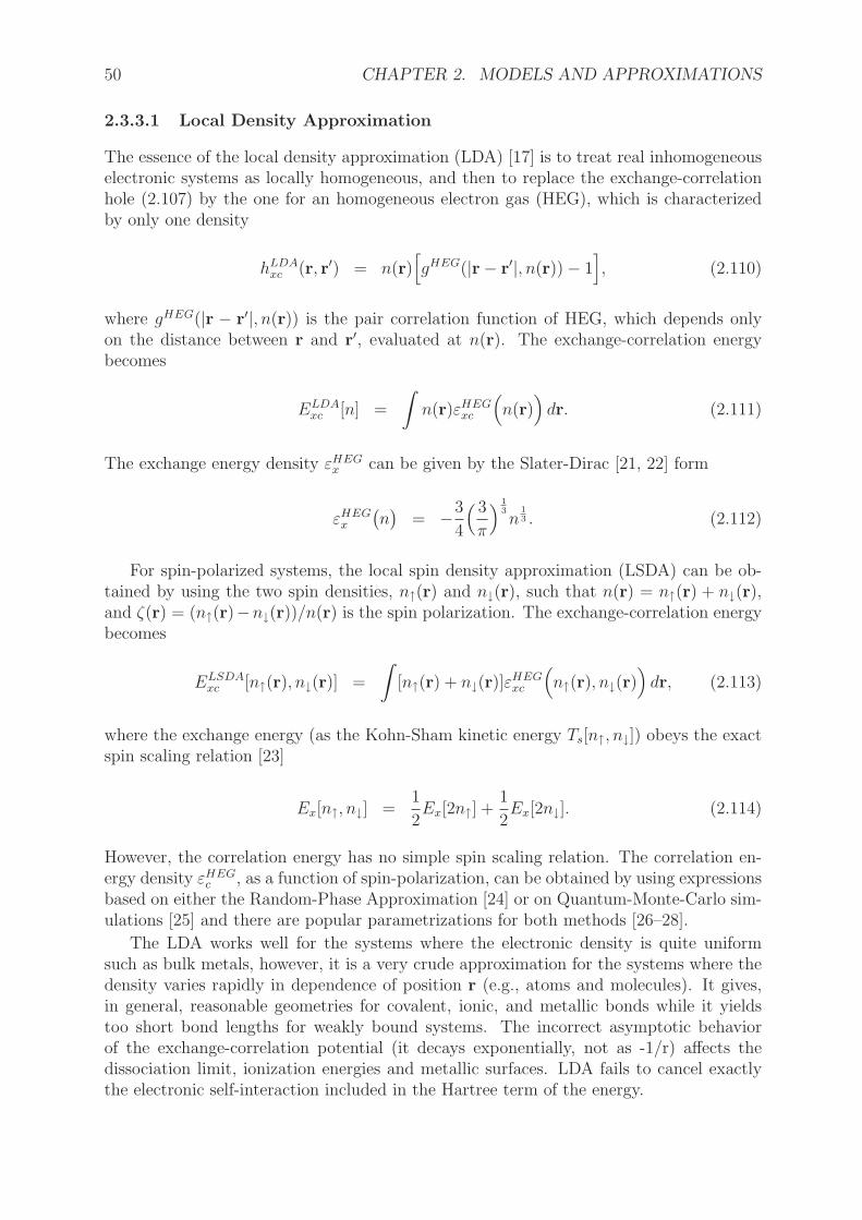
50 CHAPTER 2. MODELS AND APPROXIMATIONS
2.3.3.1 Local Density Approximation
The essence of the local density approximation (LDA) [17] is to treat real inhomogeneouselectronic systems as locally homogeneous, and then to replace the exchange-correlationhole (2.107) by the one for an homogeneous electron gas (HEG), which is characterizedby only one density
hLDAxc (r, r′) = n(r)
[
gHEG(|r − r′|, n(r)) − 1]
, (2.110)
where gHEG(|r − r′|, n(r)) is the pair correlation function of HEG, which depends onlyon the distance between r and r′, evaluated at n(r). The exchange-correlation energybecomes
ELDAxc [n] =
∫
n(r)εHEGxc
(
n(r))
dr. (2.111)
The exchange energy density εHEGx can be given by the Slater-Dirac [21, 22] form
εHEGx
(
n)
= −3
4
( 3
π
)1
3
n1
3 . (2.112)
For spin-polarized systems, the local spin density approximation (LSDA) can be ob-tained by using the two spin densities, n↑(r) and n↓(r), such that n(r) = n↑(r) + n↓(r),and ζ(r) = (n↑(r)−n↓(r))/n(r) is the spin polarization. The exchange-correlation energybecomes
ELSDAxc [n↑(r), n↓(r)] =
∫
[n↑(r) + n↓(r)]εHEGxc
(
n↑(r), n↓(r))
dr, (2.113)
where the exchange energy (as the Kohn-Sham kinetic energy Ts[n↑, n↓]) obeys the exactspin scaling relation [23]
Ex[n↑, n↓] =1
2Ex[2n↑] +
1
2Ex[2n↓]. (2.114)
However, the correlation energy has no simple spin scaling relation. The correlation en-ergy density εHEG
c , as a function of spin-polarization, can be obtained by using expressionsbased on either the Random-Phase Approximation [24] or on Quantum-Monte-Carlo sim-ulations [25] and there are popular parametrizations for both methods [26–28].
The LDA works well for the systems where the electronic density is quite uniformsuch as bulk metals, however, it is a very crude approximation for the systems where thedensity varies rapidly in dependence of position r (e.g., atoms and molecules). It gives,in general, reasonable geometries for covalent, ionic, and metallic bonds while it yieldstoo short bond lengths for weakly bound systems. The incorrect asymptotic behaviorof the exchange-correlation potential (it decays exponentially, not as -1/r) affects thedissociation limit, ionization energies and metallic surfaces. LDA fails to cancel exactlythe electronic self-interaction included in the Hartree term of the energy.
2.3. DENSITY FUNCTIONAL THEORY (DFT) 51
2.3.3.2 Generalized Gradient and Meta-Generalized Gradient Approxima-tions
The exchange-correlation energy in the Generalized Gradient Approximation (GGA), hasthe following form:
EGGAxc [n] =
∫
n(r)εHEGxc
(
n(r))
dr +
∫
Fxc
(
n(r),∇n(r))
dr (2.115)
where the function Fxc is constructed to satisfy a number of known conditions for theexchange-correlation hole (e.g., sum rules, long-range decay, etc.). There are many differ-ent prescriptions for choosing Fxc, each one leads to distinct GGA. Among the numerousGGA functionals [29–46] here are some of the commonly used ones. The Becke 88 ex-change functional (B88) [30] which takes the form of an additional correction to the LDAexchange. It contains one adjustable parameter which was optimized so that the sum ofthe LDA and Becke exchange terms reproduces the exchange energy of six noble gas atoms.The introduction of Becke’s gradient exchange correction in 1988 was an important stepfor the acceptance of DFT as a valuable tool for computational chemistry. However, B88exchange functional is responsible for repulsive potential energy curves for many rare gasdiatomic molecules [47]. The Lee-Yang-Parr (LYP) [29, 48] correlation functional whichhas been derived as a reformulation of the Colle-Salvetti [49] expression for the correla-tion energy of Helium, in term of n and ∇n. This correlation functional is one-electronself-interaction error free, but can not reproduce the correct uniform electron gas like thefunctionals based on (2.115). A popular recipe is to use B88 exchange complementedwith LYP correlation. The Perdew-Burke-Ernzerhof (PBE) exchange-correlation func-tional [31] verifies many of the exact properties for the exchange-correlation hole and doesnot contain any fitting parameters. It retains the correct features of LDA and combinesthem with the inhomogeneity aspects that are supposed to be important for describingreal systems. GGA sometimes overcorrects LDA for bond lengths, binding energies andalso atomic energies. It cannot describe long-range effects. However, hydrogen bonds areusually well accounted for. GGA functionals still do not eliminate the spurious electronself-interaction completely.
The Meta-Generalized Gradient Approximations (meta-GGA) that go beyond GGA,have been suggested to overcome the shortcomings of LDA and GGA methods. Thesefunctionals employ, in addition to the density and its gradient, either the Laplacian of thedensity (∇2n(r)) or the kinetic energy density
τ(r) =1
2
occ∑
α
|∇φα(r)|2. (2.116)
Different meta-GGA functionals have been developed [50–63], for example, the Perdew-Kurth-Zupan-Blaha (PKZB) [53] exchange-correlation functional which depends on twofitted parameters, the nonempirical Tao-Perdew-Staroverov-Scuseria (TPSS) [57] exchange-correlation functional. The TPSS exchange functional can be combined with the Krieger-Chen-Iafrate-Savin (KCIS) [64] correlation functional. These meta-GGA correlation func-tionals are one-electron self-interaction error free. The results obtained using meta-GGAare quite improved with respect to PBE, especially when atomisation energy and metalsurface energy are considered.

52 CHAPTER 2. MODELS AND APPROXIMATIONS
2.3.3.3 Hybrids
Becke [65] employed the adiabatic connection to suggest that the functional should containsome of the exact HF exchange1
EHFx = −1
2
∑
ijσ
∫ ∫
φ∗iσ(r)φjσ(r)φ∗
jσ(r′)φiσ(r′)
|r − r′| dr dr′. (2.117)
Letting Ψλ[n] be the unique antisymmetric ground state wave function of Hλ (2.105), theexchange-correlation energy can be expressed in terms of the coupling constant integra-tion [66]
Exc[n] =
∫ 1
0
Uxc,λ[n] dλ =
∫ 1
0
〈Ψλ[n]|Wee|Ψλ[n]〉 dλ− EH[n]. (2.118)
A possible scheme to construct functionals from the adiabatic connection is to approximatethe integrand Uxc,λ by a model function of λ [65, 67–69]. Integrating (2.118) using thelinear model [65], Uxc,λ[n] = a[n] + b[n]λ, gives rise to
Exc[n] = a+1
2b = Uxc,0 +
1
2(Uxc,1 − Uxc,0), (2.119)
where Uxc,0 = EHFx is the exchange energy of the KS determinant. The potential en-
ergy contribution to the exchange-correlation energy of the fully interacting system wasapproximated by Becke as Uxc,1 ≈ ULDA
xc , leading to the half-and-half functional
Exc[n] =1
2(EHF
x + ELDAx ) +
1
2ULDA
c . (2.120)
The last term in (2.120) is often approximated as ULDAc ≈ ELDA
c in other versions of thehalf-and-half functional. Successively, Becke [67] proposed to parametrize the functionalform to chosen sets of experimental data, leading to the family of the three-parameterhybrid functionals
EB3PW91xc [n] = aEHF
x + (1 − a)ELDAx + b∆EB88
x + EV WNc + c∆EPW91
c . (2.121)
Alternatively, the most widely used B3LYP [70] reads as
EB3LYPxc [n] = aEHF
x + (1 − a)ELDAx + b∆EB88
x + cELY Pc + (1 − c)EV WN
c , (2.122)
where the parameters (a = 0.2, b = 0.72, c = 0.81) in (2.121) and (2.122) were determinedby a least square fit to atomization energies, electron and proton affinities, and the ioniza-tion potentials of the atomic species and molecules in the G2 [71] test set of experimentaldata. B3LYP is successful as a result of some cancellation of errors, despite its knownshortcomings [72]. Many single hybrid functionals have been suggested [46, 73–83]. Singlehybrid functionals are known to improve significantly the accuracy of DFT results in par-ticular for geometries and thermochemistry. They are supposed to compensate partiallythe many-electron self-interaction error by using the exact exchange [72]. So for kinetics,good hybrid functionals tend to have a larger percentage of exact exchange.
1Computed with the Kohn-Sham orbitals and eigenvalues.
2.4. MODELS AND APPROXIMATIONS FOR SOLIDS 53
Range-separated single-hybrid functionals [84, 85] are characterized by the separationof the electron-electron interaction into two parts which may be treated separately
1
r12=
erf(µr12)
r12+
erfc(µr12)
r12, (2.123)
where the parameter µ controls the separation between the long-range (erf(µr12)/r12) andthe short-range (erfc(µr12)/r12) interactions. The long-range corrected functionals [86–95]in which we mix long-range HF with short-range DFT, are known to improve propertiessuch as charge-transfer and Rydberg excitations in TDDFT. The screened functionals [96–99] are obtained when we use short-range HF and long-range DFT, and these hybrids aremore commonly used in solid-state calculations (band gaps, lattice constants, etc).
Besides the HF exchange, unoccupied orbitals and eigenvalues are also used throughthe perturbative double-excitation correlation in the double hybrid functionals. Thesefunctionals are the subject of two articles [100, 101] presented in this thesis, where thetheoretical foundation of types of double hybrid functionals has been provided.
Another class of hybrids, where we combine MCSCF and DFT, was explored throughan article [102] exposed in this thesis. This method is called multiconfigurational hybridfunctional.
2.4 Models and approximations for solids
For molecules in the gas phase, ab initio and DFT methods have become an alternativeto experiments for determining accurately structural and energetic properties. It wouldbe most valuable if predictions of such properties for solids could be made with similaraccuracy. The serious complication in introducing the quantum chemistry techniques intosolid state modeling is, on the molecular scale, the infinite dimension of solids. One wayto overcome this difficulty is to adopt the perfect crystal model in which an ideally crys-talline bulk material is translation-invariant. This can be exploited to define a unit cell.Then one has to enforce periodic boundary conditions (PBC) and solve the correspondingSchrodinger equation accordingly [103–105].
2.4.1 Periodicity
Bloch [106] showed that for a perfect periodic solid, at the same point r in differentrepeating unit cells, the orbitals differ only by a complex phase factor eik.g:
φ(r + g;k) = eik.gφ(r;k), (2.124)
where g = n1a1 + n2a2 + n3a3 (n1, n2, n3 are integers) is a lattice vector describingtranslations in real space and the parallelepiped constructed by the basis vectors a1, a2
and a3 is the primitive unit cell. The wave vector k = k1b1+k2b2+k3b3 (ai.bj = 2πδij) isdefined in the reciprocal space such that each wave vector may be written as k = k′ +nK(n is an integer), where K is a reciprocal lattice vector defined by g.K = 2πn and k′ iswithin the first Brillouin zone (BZ) of reciprocal space.
The function φ(r;k) should not be vanished at infinity and at the same time we have tonormalize it. We can consider a finite crystal of N = N1.N2.N3 cells, having Nj primitive
54 CHAPTER 2. MODELS AND APPROXIMATIONS
cells along the j-th direction (j =1,2,3). Periodic boundary conditions require that
φ(r +mNjaj;k) = φ(r;k), (2.125)
for any integer m and every j. By using (2.124), we find that
eimNjkjbj .aj = 1, (2.126)
which implies that kj = nj/Nj (nj is an integer in the domain 0 ≤ nj < Nj). Therefore,the number of wave vectors
k =n1
N1
b1 +n2
N2
b2 +n3
N3
b3, (2.127)
in the first BZ is finite. When N1, N2, N3 grow to infinity, the wave vector k can beconsidered as a continuous variable such that the summation over k vectors is replacedby three dimensional integration and the number of k points within the first BZ plays arole in the accuracy of the calculations.
2.4.2 Mean-field crystalline orbital theory
If we use the Fockian (2.32) in the Schrodinger equation, the Hartree-Fock level of thetheory is retained. For the molecular case, we should solve the Roothann equations (2.46,2.49). The difficulty in dealing with solids is that the equations (2.46) will have infinitedimension and the expansion (2.45) extends not only over functions centered on atomswithin one primitive unit cell but also over all primitive cells labeled by g
ψi(r) =∑
g
Nbasis∑
µ
Cgµiχµ(r − rµ − g). (2.128)
As N grows to infinity, the direct solution of the equations
∑
g′
Nbasis∑
ν
(F gg′
µν − ǫiSgg′
µν )Cg′
νi = 0, (2.129)
is practically impossible, where F gg′
µν is the Fock matrix element in direct space in thelocal basis set, which is invariant to translation :
F gg′
µν = 〈χµ(r − rµ − g)|F |χν(r − rν − g′)〉 = 〈χµ(r − rµ)|F |χν(r − rν − g′ + g)〉= 〈χµ(r − rµ)|F |χν(r − rν − l)〉, (2.130)
where the linear combination between two lattice vectors, g′ − g = l, is a lattice vector.The same can be said of the overlap matrix element Sgg′
µν . The function χµ(r− rµ) is theµ-th atomic orbital centered at rµ in the (origin or reference) 0-cell and χν(r − rν − l) isthat one in the l-cell. These local functions are in turn defined by a contraction, i.e., afixed linear combination of Gaussian-type functions.
Taking advantage of translation symmetry, we can define k-dependent Bloch functions
φµ(r;k) =1√N
∑
g
eik.gχµ(r − rµ − g), (2.131)
2.4. MODELS AND APPROXIMATIONS FOR SOLIDS 55
where the wave vector k is indicative of different irreducible representations. Conse-quently, the Bloch functions belonging to different k vectors are mutually orthogonal andthe matrix elements between them vanish
Fµν(k,k′) = δ(k − k′)Fµν(k,k) = δ(k − k′)Fµν(k). (2.132)
where k is one of the sampling set points in the first BZ at which the Fock matrix, Fµν(k),is diagonalized. As result, the secular problem reduces to secular problems, one for eachk vector, resembling that of molecules:
Nbasis∑
ν
(
Fµν(k) − ǫi(k)Sµν(k))
Cνi(k) = 0. (2.133)
Their solutions are the single-particle crystalline orbitals (CO) which are linear combina-tions of Bloch functions (2.131)
ψi(r;k) =∑
µ
Cµi(k)φµ(r;k). (2.134)
The coefficients Cµi(k), which determine the crystalline orbitals ψi(r;k), are obtainedwhen solving (2.133) (with the orthonormality condition) for a particular k vector. Thesecoefficients are used to form the density matrix in order to calculate the total energy perunit cell.
While accurate structure predictions for solids are given by the HF-CO theory, thecohesive energies are severely underestimated and the energy-band gaps are too largecompared to experiment [107] in this model which does not account for correlation effects.As another mean field method, periodic density functional theory (DFT) has quicklybecome the main computational tool for the electronic structure of solids. The Hartree-Fock and the Kohn-Sham equations can be solved by expanding the orbitals in one of twomajor kinds of basis set: atom-centered Gaussian-type orbitals (GTO) and plane waves(PW). Both choices yield very similar results if convergence is carefully checked andreached [108, 109]. Transferability of molecular GTO basis functions to periodic systemsshould be done with care, particularly in the case of diffuse functions, to avoid lineardependence in the definition of the wave function. Plane wave basis sets are used alongwith pseudopotentials or projector augmented wave method to account for core electrons.They have many advantages : the basis functions are orthonormal by definition, unbiasedby the atomic positions so that they describe any point in the crystalline cell with thesame quality, thereby having the ability to accurately treat different kinds of structure.The convergence of the calculation with respect to the size of the truncated PW basis setcan be checked by increasing the electronic kinetic energy cutoff.
DFT calculations within the LDA are known to exhibit a significant overbinding,whereas the GGA cohesive energies of solids are generally improved. The underestima-tion of the band gap has been a long-standing problem for density functionals. Thereason for this is the self-interaction error in LDA and GGA. Hybrid functionals combinegradient-corrected approximations with a fraction of exact exchange, which allows im-provement of the performance of GGA functionals for systems where the self-interactionerror may become important. However, calculating the nonlocal exchange energy can bevery expensive in extended systems. This has motivated the development of screened
56 CHAPTER 2. MODELS AND APPROXIMATIONS
hybrids [96–98, 110] which are based on that the long-range contribution of the nonlocalexchange interaction is canceled by long-range correlation effects that are not accountedfor in standard semilocal functionals. These functionals use a finite amount of exact ex-change at short-range, but none in the long-range limit, in order to cut the computationalcost of nonlocal exchange integrals for extended systems. Compared to the semilocaldensity functionals, the screened hybrids yield an improved description of semiconductorband gaps and lattice constants, but still underestimate the gap in insulators.
One of the failures of the one-electron levels of theory, including DFT with standardfunctionals, was observed in the description of long-range dispersion interactions [111,112]. In molecular crystals, this deficiency often leads to severe errors. DFT calculationscan be improved by including an empirical correction to account for van de Waals interac-tions. This empirical correction consists of damped pairwise interatomic potentials of theform −Cn/r
n (n ≥ 6) to describe the attraction that decays at long range as r−6, whilethe attractive terms of order r−8 and r−10 become important at medium range. Thesemethods are called empirical dispersion-corrected density functionals [113–116] and canpredict very reasonable molecular crystal lattice parameters and lattice energies [117–126].However, the damped pairwise correction terms depend on the choice of functional formand the system being treated, which prevents to systematically improve the predictions.Several non-empirical methods for treating dispersion have also been used in molecularcrystals [127–131]. They perform well for predicting crystal lattice energy but they aresignificantly more expensive than conventional DFT methods.
2.4.3 Wave Function Based Electron Correlation Methods forSolids
Attempts have been made to extend the higher correlated methods based on the wavefunction expansion to solid state treatment. The infinite extension of solids implies thatonly size-extensive methods can be applied to study these systems. Periodic second-orderMøller-Plesset perturbation theory (MP2) provides an electron-correlation method withaccuracy unachievable by DFT with the standard LDA, GGA and meta-GGA functionalsfor many systems. Efficient periodic MP2 algorithms have been developed [132–137]. Gen-eralized from the molecular formulation, atomic-orbital Laplace-transformed MP2 method(AO-LT-MP2) [138] permits calculating the MP2 correlation energy for extended systemsusing occupied and virtual space spanned by Bloch functions. Another choice is to usecanonical orbitals expanded in plane waves. This periodic approach is called plane wavebased canonical MP2 [139, 140] which has led to the periodic canonical coupled clustersingles and doubles (CCSD) [141]. As a local correlation method [142–146], periodic localMP2 [147, 148] exploits the local character of dynamical electron correlation hole andgives the total electron correlation energy as a sum of contributions from a truncated listof orbital pairs. In this method, the occupied space is spanned by orthonormal localizedcrystalline orbitals (Wannier functions) generated from the occupied canonical orbitalsby unitary transformation. For the virtual space, LMP2 employs mutually nonorthogonalorbitals obtained from the atomic orbital basis by projecting out the occupied space (pro-jected AOs). Truncation of the virtual space is important to reduce the computationalcosts, where the excitations from an orbital pair are restricted to the PAOs centered in thevicinity of either of the two occupied orbitals. This approximation is known to reduce thebasis set superposition error (BSSE) [149]. To improve the performance further, LMP2

2.4. MODELS AND APPROXIMATIONS FOR SOLIDS 57
can be combined with density fitting techniques [150].Periodic MP2 methods are, in general, very expensive when applied to systems with
medium-sized unit cell. But the recent development of parallel implementations [151, 152]opens the possibility of applications dealing with molecular crystals of chemical interest.These methods are limited to the treatment of non-conducting crystals (limitation ofthe MP2 method itself). For Gaussian orbital based periodic MP2, large and especiallydiffuse basis sets frequently cause linear dependence problems in the periodic Hartree-Fock calculations that precede the MP2 calculations. But the use of diffuse basis sets ismandatory in many cases for the convergence of MP2 energies. Dual-basis set scheme isone way to overcome this difficulty, where a smaller basis set is used for the HF calculationsand then additional basis functions can be allocated in the MP2 correlation calculations.

58 CHAPTER 2. MODELS AND APPROXIMATIONS

Bibliography
[1] M. Born and J. Oppenheimer, Ann. Phys. 84, 457 (1927).
[2] D. R. Hartree, Proc. Camb. Phil. Soc. 24, 111 (1928).
[3] J. C. Slater, Phys. Rev. 34, 1293 (1929).
[4] V. Fock, Physik 61, 126 (1930).
[5] C. C. J. Roothann, Rev. Mod. Phys. 23, 69 (1951).
[6] T. Helgaker, P. Jorgensen and J. Olsen, Molecular Electronic-Structure Theory (Wi-ley, Chichester, 2002).
[7] C. Møller and M. S. Plesset, Phys. Rev. 46, 618 (1934).
[8] R. J. Bartlett, Ann. Rev. Phys. Chem. 32, 359 (1981).
[9] M. W. Schmidt and M. S. Gordon, Ann. Rev. Phys. Chem. 49, 233 (1998).
[10] P. R. T. B. O. Roos and P. E. M. Siegbahn, Chem. Phys. 48, 157 (1980).
[11] P. J. J. Olsen, B. O. Roos and H. J. A. Jensen, J. Chem. Phys. 89, 2185 (1988).
[12] L. H. Thomas, Proc. Camb. Phil. Soc. 23, 542 (1927).
[13] E. Fermi, Z. Phys. 48, 73 (1928).
[14] P. Hohenberg and W. Kohn, Phys. Rev. 136, B 864 (1964).
[15] M. Levy, Proc. Natl. Acad. Sci. U.S.A. 76, 6062 (1979).
[16] M. Levy, Phys. Rev. A 26, 1200 (1982).
[17] W. Kohn and L. J. Sham, Phys. Rev. A 140, 1133 (1965).
[18] J. Harris, Phys. Rev. A 29, 1648 (1984).
[19] D. C. Langreth and J. P. Perdew, Solid State Commun. 17, 1425 (1975).
[20] O. Gunnarsson and B. I. Lundqvist, Phys. Rev. B 13, 4274 (1976).
[21] J. C. Slater, Phys. Rev. 81, 385 (1951).
[22] P. A. M. Dirac, Proc. Camb. Phil. Soc. 26, 376 (1930).
59
60 BIBLIOGRAPHY
[23] J. P. Perdew and S. Kurth, in A Primer in Density Functional Theory , edited byC. Fiolhais, F. Nogueira and M. A. L. Marques (Springer, Berlin, 2003), Vol. 620 ofLecture Notes in Physics, pp. 1–55.
[24] M. Gell-Mann and K. A. Brueckner, Phys. Rev. 106, 364 (1957).
[25] D. M. Ceperley and B. J. Alder, Phys. Rev. Lett. 45, 566 (1980).
[26] J. P. Perdew and Y. Wang, Phys. Rev. B 45, 13244 (1992).
[27] J. P. Perdew and A. Zunger, Phys. Rev. B 23, 5048 (1981).
[28] S. J. Vosko, L. Wilk and M. Nusair, Can. J. Phys. 58, 1200 (1980).
[29] C. Lee, W. Yang and R. G. Parr, Phys. Rev. B 37, 785 (1988).
[30] A. D. Becke, Phys. Rev. A 38, 3098 (1988).
[31] J. P. Perdew, K. Burke and M. Ernzerhof, Phys. Rev. Lett. 77, 3865 (1996).
[32] D. C. Langreth and J. P. Perdew, Solid State Commun. 31, 567 (1979).
[33] D. C. Langreth and J. P. Perdew, Phys. Rev. B 21, 5469 (1980).
[34] J. P. Perdew, A. Ruzsinszky, G. I. Csonka, O. A. Vydrov, G. E. Scuseria, L. A.Constantin, X. L. Zhou and K. Burke, Phys. Rev. Lett. 100, 136406 (2008).
[35] J. P. Perdew and W. Yue, Phys. Rev. B 33, 8800 (1986).
[36] J. P. Perdew, Phys. Rev. B 33, 8822 (1986).
[37] A. D. Becke, J. Chem. Phys. 84, 4524 (1986).
[38] J. P. Perdew, J. A. Chevary, S. H. Vosko, K. A. Jackson, M. R. Pederson, D. J.Singh and C. Fiolhais, Phys. Rev. B 46, 6671 (1992).
[39] F. A. Hamprecht, A. J. Cohen, D. J. Tozer and N. C.Handy, J. Chem. Phys. 109,6264 (1998).
[40] T. Tsuneda, T. Suzumura and K. Hirao, J. Chem. Phys. 110, 10664 (1999).
[41] A. D. Boese, N. L. Doltsinis, N. C. Handy and M. J. Sprik, J. Chem. Phys. 112,1670 (2000).
[42] A. D. Boese and N. C. Handy, J. Chem. Phys. 114, 5497 (2001).
[43] N. C. Handy and A. J. Cohen, Mol. Phys. 99, 403 (2001).
[44] N. C. Handy and A. J. Cohen, J. Chem. Phys. 116, 5411 (2002).
[45] T. W. Keal and D. J. Tozer, J. Chem. Phys. 121, 5654 (2004).
[46] Y. Zhao and D. G. Truhlar, J. Chem. Phys. 128, 184109 (2008).
[47] Y. Zhang, W. Pan and W. Yang, J. Chem. Phys. 107, 7921 (1997).

BIBLIOGRAPHY 61
[48] B. Miehlich, A. Savin, H. Stoll and H. Preuss, Chem. Phys. Lett. 157, 200 (1989).
[49] R. Colle and O. Salvetti, Theor. Chim. Acta 37, 329 (1975).
[50] A. D. Becke, J. Chem. Phys. 88, 1053 (1988).
[51] A. D. Becke, Int. J. Quantum. Chem. 52, 625 (1994).
[52] A. D. Becke and M. R. Roussel, Phys. Rev. A 39, 3761 (1989).
[53] J. P. Perdew, S. Kurth, A. Zupan and P. Blaha, Phys. Rev. Lett. 82, 2544 (1999).
[54] J. P. Perdew and L. A. Constantin, Phys. Rev. B 75, 155109 (2007).
[55] J. P. Perdew, A. Ruzsinszky, J. Tao, G. I. Csonka and G. E. Scuseria, Phys. Rev.A 76, 042506 (2007).
[56] J. P. Perdew, A. Ruzsinszky, G. I. Csonka, L. A. Constantin and J. W. Sun, Phys.Rev. Lett. 103, 026403 (2009).
[57] J. Tao, J. P. Perdew, V. N. Staroverov and G. E. Scuseria, Phys. Rev. Lett. 91,146401 (2003).
[58] C. Lee and R. G. Parr, Phys. Rev. A 35, 2377 (1987).
[59] A. D. Becke, J. Chem. Phys. 104, 1040 (1996).
[60] A. D. Becke, J. Chem. Phys. 109, 2092 (1998).
[61] T. van Voorhis and G. E. Scuseria, J. Chem. Phys. 109, 400 (1998).
[62] A. D. Boese and N. C. Handy, J. Chem. Phys. 116, 9559 (2002).
[63] Y. Zhao and D. G. Truhlar, J. Chem. Phys. 125, 194101 (2006).
[64] J. B. Krieger, J. Chen, G. J. Iafrate and A. Savin, in Electron Correlation and
Materials Properties, edited by A. Gonis and N. Kioussis (Plenum, New York, 1999).
[65] A. D. Becke, J. Chem. Phys. 98, 1372 (1993).
[66] M. Levy and J. P. Perdew, Phys. Rev. A 32, 2010 (1985).
[67] A. D. Becke, J. Chem. Phys. 98, 5648 (1993).
[68] J. P. Perdew, M. Ernzerhof and K. Burke, J. Chem. Phys 105, 9982 (1996).
[69] P. Mori-Sanchez, A. J. Cohen and W. Yang, J. Chem. Phys. 124, 091102 (2006).
[70] P. J. Stephens, F. J. Devlin, C. F. Chabalowski and M. J. Frisch, J. Phys. Chem.98, 11623 (1994).
[71] L. A. Curtiss, K. Raghavachari, G. W. Trucks and J. A. Pople, J. Chem. Phys. 94,7221 (1991).
62 BIBLIOGRAPHY
[72] G. I. Csonka, J. P. Perdew and A. Ruzsinszky, J. Chem. Theory Comput 6, 3688(2010).
[73] A. D. Becke, J. Chem. Phys. 107, 8554 (1997).
[74] C. Adamo and V. Barone, J. Chem. Phys. 101, 6158 (1999).
[75] B. J. Lynch, P. L. Fast, M. Harris and D. G. Truhlar, J. Phys. Chem. A 104, 4811(2000).
[76] P. J. Wilson, T. J. Bradly and D. J. Tozer, J. Chem. Phys. 115, 9233 (2001).
[77] A. J. Cohen and N. C. Handy, Mol. Phys. 99, 607 (2001).
[78] X. Xu and W. A. Goddard III, Proc. Natl. Acad. Sci. U.S.A. 229, 2673 (2004).
[79] T. W. Keal and D. J. Tozer, J. Chem. Phys. 123, 121103 (2005).
[80] Y. Zhao, N. E. Schultz and D. G. Truhlar, J. Chem. Theory Comput. 2, 364 (2006).
[81] Y. Zhao and D. G. Truhlar, J. Chem. Theory Comput. 110, 13126 (2006).
[82] Y. Zhao and D. G. Truhlar, J. Chem. Theory Comput. 110, 5121 (2006).
[83] Y. Zhao and D. G. Truhlar, Theor. Chem. Acc. 120, 215 (2008).
[84] A. Savin and H.-J. Flad, Int. J. Quantum. Chem. 56, 327 (1995).
[85] T. Leininger, H. Stoll, H.-J. Werner and A. Savin, Chem. Phys. Lett. 275, 151(1997).
[86] H. Iikura, T. Tsuneda, T. Yanai and K. Hirao, J. Chem. Phys. 115, 3540 (2001).
[87] J. Toulouse, F. Colonna and A. Savin, Phys. Rev. A 70, 062505 (2004).
[88] J.-W. Song, S. Tokura, T. Sato, M. A. Watson and K. Hirao, J. Chem. Phys. 127,154109 (2007).
[89] J.-W. Song, M. A. Watson, A. Nakata and K. Hirao, J. Chem. Phys. 129, 184113(2008).
[90] J.-W. Song, M. A. Watson and K. Hirao, J. Chem. Phys. 131, 144108 (2009).
[91] T. Yanai, D. P. Tew and N. C. Handy, Chem. Phys. Lett. 393, 51 (2004).
[92] R. Baer and D. Neuhauser, Phys. Rev. Lett. 94, 043002 (2005).
[93] J. Toulouse, F. Colonna and A. Savin, J. Chem. Phys. 122, 014110 (2005).
[94] O. A. Vydrov and G. E. Scuseria, J. Chem. Phys. 125, 234109 (2006).
[95] J.-D. Chai and M. Head-Gordon, J. Chem. Phys. 128, 084106 (2008).
[96] J. Heyd, G. E. Scuseria and M. Ernzerhof, J. Chem. Phys. 118, 8207 (2003).

BIBLIOGRAPHY 63
[97] J. Heyd and G. E. Scuseria, J. Chem. Phys. 121, 1187 (2004).
[98] J. Heyd and G. E. Scuseria, J. Chem. Phys. 120, 7274 (2004).
[99] A. V. Krukau, O. A. Vydrov, A. F. Izmaylov and G. E. Scuseria, J. Chem. Phys.125, 224106 (2006).
[100] K. Sharkas, J. Toulouse and A. Savin, J. Chem. Phys. 134, 064113 (2011).
[101] J. Toulouse, K. Sharkas, E. Bremond and C. Adamo, J. Chem. Phys. 135, 101102(2011).
[102] K. Sharkas, A. Savin, H. J. A. Jensen and J. Toulouse, J. Chem. Phys. 137, 044104(2012).
[103] R. Dovesi, in Quantum-Mechanical Ab-initio Calculation of the Properties of Crys-
talline Materials, edited by C. Pisani (Springer-Verlag, Berlin, 1996), vol. 67, p. 31.
[104] C. Pisani, in Quantum-Mechanical Ab-initio Calculation of the Properties of Crys-
talline Materials, edited by C. Pisani (Springer-Verlag, Berlin, 1996), vol. 67, p. 47.
[105] C. Pisani, R. Dovesi and C. Roetti, in Lecture Notes in Chemistry (Springer-Verlag,Berlin, 1988), vol. 48, p. 193.
[106] F. Bloch, Z. Phys. 52, 555 (1928).
[107] B. Civalleri, D. Presti, R. Dovesi and A. Savin (Royal Society of Chemistry: Chem.Modell., 2012), vol. 9, pp. 168–185.
[108] J. Paier, R. Hirschl, M. Marsman and G. Kresse, J. Chem. Phys. 122, 234102 (2005).
[109] S. Tosoni, C. Tuma, J. Sauer, B. Civalleri and P. Ugliengo, J. Chem. Phys. 127,154102 (2007).
[110] R. Peverati and D. G. Truhlar, Phys. Chem. Chem. Phys. 14, 16187 (2012).
[111] S. Kristyan and P. Pulay, Chem. Phys. Lett. 229, 175 (1994).
[112] P. Hobza, J. Sponer and T. Reschel, J. Comput. Chem. 16, 1315 (1995).
[113] M. Elstner, P. Hobza, T. Frauenheim, S. Suhai and E. Kaxiras, J. Chem. Phys. 114,5149 (2001).
[114] S. Grimme, J. Comput. Chem. 25, 1463 (2004).
[115] S. Grimme, J. Comput. Chem. 27, 1787 (2006).
[116] S. Grimme, J. Antony, S. Ehrlich and H. Krieg, J. Chem. Phys. 132, 154104 (2010).
[117] M. A. Neumann and M.-A. Perrin, J. Phys. Chem. B 109, 15531 (2005).
[118] T. Li and S. Feng, Pharm. Res. 23, 2326 (2006).

64 BIBLIOGRAPHY
[119] B. Civalleri, C. Zicovich-Wilson, L. Valenzano and P. Ugliengo, Cryst. Eng. Comm10, 405 (2008).
[120] P. G. Karamertzanis, G. M. Day, G. W. A. Welch, J. Kendrick, F. J. J. Leusen,M. A. Neumann and S. L. Price, J. Phys. Chem. 128, 244708 (2008).
[121] P. Ugliengo, C. Zicovich-Wilson, S. Tosoni and B. Civalleri, J. Mater. Chem. 19,2564 (2009).
[122] C. M. Zicovich-Wilson, B. Kirtman, B. Civalleri and A. Ramırez-Solıs, Phys. Chem.Chem. Phys. 12, 3289 (2010).
[123] K. Hongo, M. A. Watson, R. S. Sanchez-Carrera, T. Iitaka and A. Aspuru-Guzik,J. Phys. Chem. Lett. 1, 1789 (2010).
[124] D. C. Sorescu and B. M. Rice, J. Phys. Chem. C 114, 6734 (2010).
[125] R. Balu, E. F. C. Byrd and B. M. Rice, J. Phys. Chem. B 115, 803 (2011).
[126] W. Reckien, F. Janetzko, M. F. Peintinger and T. Bredow, J. Comput. Chem. 33,2023 (2012).
[127] M. Dion, H. Rydberg, E. Schroder, D. C. Langreth and B. I. Lundqvist, Phys. Rev.Lett. 92, 246401 (2004).
[128] T. Thonhauser, V. R. Cooper, S. Li, A. Puzder, P. Hyldgaard and D. C. Langreth,Phys. Rev. B. 76, 125112 (2007).
[129] F. Shimojo, Z. Wu, A. Nakano, R. K. Kalia and P. Vashishta, J. Chem. Phys. 132,094106 (2010).
[130] D. Lu, Y. Li, D. Rocca and G. Galli, Phys. Rev. Lett. 102, 206411 (2009).
[131] Y. Li, D. Lu, H.-V. Nguyen and G. Galli, J. Phys. Chem. 114, 1944 (2010).
[132] S. Suhai, Phys. Rev. B 27, 3506 (1983).
[133] J.-Q. Sun and R. J. Bartlett, J. Chem. Phys. 104, 8553 (1996).
[134] S. Hirata and S. Iwata, J. Chem. Phys. 109, 4147 (1998).
[135] S. Hirata and T. Shimazaki, Phys. Rev. B 80, 1 (2009).
[136] Y.-Y. Ohnishi and S. Hirata, J. Chem. Phys. 133, 034106 (2010).
[137] T. Shiozaki and S. Hirata, J. Chem. Phys. 132, 151101 (2010).
[138] P. Y. Ayala, K. N. Kudin and G. E. Scuseria, J. Chem. Phys. 115, 9698 (2001).
[139] M. Marsman, A. Gruneis, J. Paier and G. Kresse, J. Chem. Phys. 130, 184103(2009).
[140] A. Gruneis, M. Marsman and G. Kresse, J. Chem. Phys. 133, 074107 (2010).
BIBLIOGRAPHY 65
[141] A. Gruneis, G. H. Booth, M. Marsman, J. Spencer, A. Alavi and G. Kresse, J.Chem. Theory Comput. 7, 2780 (2011).
[142] S. Saebø and P. Pulay, J. Phys. Chem. 88, 1884 (1988).
[143] M. S. Lee, P. E. Maslen and M. Head-Gordon, J. Phys. Chem. 112, 3592 (2000).
[144] G. E. Scuseria and P. Y. Ayala, J. Phys. Chem. 111, 8330 (1999).
[145] M. Schutz, J. Phys. Chem. 116, 8772 (2002).
[146] H.-J. Werner, F. R. Manby and P. J. Knowles, J. Phys. Chem. 118, 8149 (2003).
[147] C. Pisani, M. Busso, G. Capecchi, S. Casassa, R. Dovesi, L. Maschio, C. Zicovich-Wilson and M. Schutz, J. Phys. Chem. 122, 094113 (2005).
[148] D. Usvyat, L. Maschio, C. Pisani and M. Schutz, Z. Phys. Chem. 224, 441 (2010).
[149] M. Schutz, G. Rauhut and H.-J. Werner, J. Phys. Chem. A 102, 599 (1998).
[150] L. Maschio and D. Usvyat, Phys. Rev. B 78, 073102 (2008).
[151] L. Maschio, J. Chem. Theory Comput. 7, 2818 (2011).
[152] M. D. Ben, J. Hutter and J. VandeVondele, J. Chem. Theory Comput. 8, 4177(2012).

66 BIBLIOGRAPHY
Chapter 3
A multiconfigurational hybriddensity-functional theory
This chapter, written in collaboration with A. Savin, H. J. Aa. Jensen and J. Toulouse,has been published in Journal of Chemical Physics [J. Chem. Phys. 137, 044104 (2012)].
3.1 Abstract
We propose a multiconfigurational hybrid density-functional theory which rigorously com-bines a multiconfiguration self-consistent-field calculation with a density-functional ap-proximation based on a linear decomposition of the electron-electron interaction. Thisgives a straightforward extension of the usual hybrid approximations by essentially addinga fraction λ of exact static correlation in addition to the fraction λ of exact exchange. Testcalculations on the cycloaddition reactions of ozone with ethylene or acetylene and thedissociation of diatomic molecules with the Perdew-Burke-Ernzerhof (PBE) and Becke-Lee-Yang-Parr (BLYP) density functionals show that a good value of λ is 0.25, as inthe usual hybrid approximations. The results suggest that the proposed multiconfigura-tional hybrid approximations can improve over usual density-functional calculations forsituations with strong static correlation effects.
3.2 Introduction
Density-functional theory (DFT) [1] within the Kohn-Sham (KS) scheme [2] is the mostwidely used method for electronic-structure calculations in atomic, molecular and solid-state systems. With the usual approximate density functionals, such as generalized-gradient approximations (GGA) and hybrid approximations mixing in a fraction of Hartree-Fock (HF) exchange, DFT KS generally gives good results for situations in which theso-called dynamic electron correlation dominates the total correlation energy, but it canyield severe errors for systems with strong static correlation, i.e. with partially fillednear-degenerate orbitals (see, e.g., Ref. [3]). It has been argued that the GGA exchangedensity functionals actually mimic some static correlation through their self-interactionerror, though in an imperfect manner (see, e.g., Refs. [4, 5]). There is often indeed apartial cancellation of errors between the self-interaction error which tends to give toolow an energy and the neglect of static correlation which gives too high an energy (see,
67

68 CHAPTER 3. A MULTICONFIGURATIONAL HYBRID...
e.g., Ref. [6]). Hybrid approximations have a smaller self-interaction error and are thusoften worse than pure density functionals for describing systems with static correlation(see, e.g., Ref. [7]).
Several approaches have been proposed to include explicit static correlation in density-functional theory. Artificially breaking (space and spin) symmetry by unrestricted KScalculations is the simplest approach to simulate static correlation (see, e.g., Ref. [8]), andit often leads to reasonable potential energy surfaces but wrong spin densities. Anotherpossible approach consists in replacing the single KS determinant by an ensemble of de-terminants or, equivalently, using fractional occupation numbers for the orbitals [9–22],but a successful and general method based on this idea is still lacking. Configuration-interaction schemes have also been proposed in which modified Hamiltonian matrix ele-ments include information from DFT [23–26]. A lot of approaches consist in adding tothe energy of a partially correlated wave function calculation, including near-degenerateconfiguration state functions coupled by the full Coulombic electron-electron interaction,an energy density functional describing the missing correlation effects [27–62]. In theselast approaches, one must use a density functional which depends on the size of the mul-ticonfigurational expansion, in order to avoid double counting of correlation between thewave function part of the calculation and the density functional. Finally, to avoid anydouble counting of correlation from the beginning, it has been proposed to decompose theCoulombic electron-electron interaction into long-range and short-range components, thelong-range part being treated by a method capable of describing static correlation andthe short-range part being described by a density functional approximation. The meth-ods that have been used for the long-range part are: configuration interaction [63–69],multiconfigurational self-consistent field (MCSCF) [70–72], multireference perturbationtheory [73], constrained-pairing mean-field theory [74, 75], and density-matrix functionaltheory [76–78].
In this work, we explore the possibility to combine MCSCF and DFT based on asimple linear decomposition of the Coulombic electron-electron interaction, in the spiritof the usual hybrid approximations, and similarly to what was recently done for con-structing theoretically justified double-hybrid approximations [79]. This approach givesa straightforward multiconfigurational extension of the standard hybrid approximations,and aims at improving their description of static correlation. After deriving this mul-ticonfigurational hybrid density-functional theory, we test this approach on situationswith strong static correlation effects, namely the cycloaddition reactions of ozone withethylene or acetylene and the dissociation of diatomic molecules, and we compare withother methods, in particular the range-separated multiconfigurational hybrid method ofRefs. [70–72].
3.3 Theory
Using the formalism of the multideterminant extension of the KS scheme (see, e.g.,Refs. [69, 71, 79, 80]), for any coupling constant λ, the exact energy can be expressedas the following minimization over multideterminant wave functions Ψ:
E = minΨ
{
〈Ψ|T + Vext + λWee|Ψ〉 + EλHxc[nΨ]
}
, (3.1)

3.3. THEORY 69
where T is the kinetic energy operator, Vext is a scalar external potential operator (e.g.,nuclei-electron), Wee is the electron-electron interaction operator, and Eλ
Hxc[nΨ] is thecomplement λ-dependent Hartree-exchange-correlation density functional evaluated at thedensity coming from Ψ. The complement density functional, Eλ
Hxc[n] = EHxc[n]−EλHxc[n],
is the difference between the usual KS density functional EHxc[n] and the λ-dependentdensity functional Eλ
Hxc[n] corresponding to the interaction λWee. The Hartree-exchangecontribution is of first order in the electron-electron interaction and is thus linear in λ,
EλHx[n] = (1 − λ)EHx[n], (3.2)
where EHx[n] is the usual KS Hartree-exchange density functional. The correlation con-tribution is obtained by uniform coordinate scaling of the density [81–84],
Eλc [n] = Ec[n] − Eλ
c [n] = Ec[n] − λ2Ec[n1/λ] (3.3)
where Ec[n] is the usual KS correlation functional, Eλc [n] is the correlation functional
corresponding to the interaction λWee, and n1/λ(r) = (1/λ)3n(r/λ) is the scaled density.The theory is so far exact but in practice approximations must be used for the mul-
tideterminant wave function and the density functionals. In Ref. [79], by restricting thesearch in Eq. (4.3) to single-determinant wave functions Φ, we defined the density-scaled
one-parameter hybrid (DS1H) approximation
EDS1H = minΦ
{
〈Φ|T + Vext + λWee|Φ〉 + (1 − λ)EHx[nΦ] + Ec[nΦ] − λ2Ec[nΦ,1/λ]}
,
(3.4)
and, by additionally neglecting density scaling in the correlation functional, Ec[n1/λ] ≈Ec[n], we obtained the one-parameter hybrid (1H) approximation,
E1H = minΦ
{
〈Φ|T + Vext + λWee|Φ〉 + (1 − λ)EHx[nΦ] + (1 − λ2)Ec[nΦ]}
, (3.5)
which is similar to the usual one-parameter hybrid approximations [85, 86], except thatthe correlation functional is weighted by a factor of (1−λ2). Starting from these referencesand applying a second-order Møller-Plesset (MP2) perturbation theory [80, 87, 88], wealso defined the density-scaled one-parameter double-hybrid (DS1DH) and one-parameter
double-hybrid (1DH) approximations [79], which are one-parameter versions of the originaldouble-hybrid approximations [89]. These latter also combine HF exchange and MP2correlation with a semilocal exchange-correlation density functional but with two empiricalparameters.
Here, we follow a different route and use an MCSCF wave function in Eq. (4.3),expanded as a linear combination of configuration state functions ΦI ,
|Ψ〉 =∑
I
cI |ΦI〉, (3.6)
where the coefficients cI and the orbitals are to be simultaneously optimized. With thisform of wave function, we obtain a multiconfigurational density-scaled one-parameter hy-
brid (MCDS1H) approximation,
EMCDS1H = minΨ
{
〈Ψ|T + Vext + λWee|Ψ〉 + (1 − λ)EHx[nΨ] + Ec[nΨ] − λ2Ec[nΨ,1/λ]}
,
(3.7)

70 CHAPTER 3. A MULTICONFIGURATIONAL HYBRID...
and, if density scaling, which is not considered in usual hybrid approximations, is ne-glected, we obtain a multiconfigurational one-parameter hybrid (MC1H) approximation,
EMC1H = minΨ
{
〈Ψ|T + Vext + λWee|Ψ〉 + (1 − λ)EHx[nΨ] + (1 − λ2)Ec[nΨ]}
. (3.8)
Equation (3.7) is the equivalent of the range-separated multiconfigurational hybrid methodof Refs. [70–72], that we will refer to as MC-srDFT, but for a linear separation of theelectron-electron interaction. Notice that, if we were to use no approximations for the wavefunction Ψ and the exchange-correlation density functional, then Eq. (3.7) would give theexact energy, independently of λ. In practice, of course, we must use approximations, andthe energy does depend on λ, which can then be considered as an empirical parameter tobe optimized.
The present scheme has two advantages over the range-separated scheme: (a) Only onelist of two-electron Coulomb integrals is needed and it is just multiplied by λ in the MCSCFpart and by (1 − λ) in the complement Hartree energy, whereas two lists of two-electronintegrals are needed in the range-separated scheme for the long-range MCSCF part andfor the short-range complement Hartree energy; (b) No new exchange and correlationdensity functionals need in principle to be developed since all the existing approximationsdeveloped for the KS scheme can be reused with a simple scaling, whereas new short-rangedensity-functional approximations must be developed in the range-separated scheme.
Equations (3.7) and (3.8) can be seen as straightforward multiconfigurational exten-sions of the usual hybrid approximations. Indeed, the expectation value of λWee over theMCSCF wave function Ψ not only introduces a fraction λ of exact exchange but also afraction of exact static correlation. Defined in the ideal limit of reference energy levels thatare degenerate, the static correlation energy is linear with respect to the electron-electroninteraction, and thus we can consider that the expectation value of λWee introduces alinear fraction λ of static correlation. By contrast, the dynamic correlation energy startsat quadratic order in the electron-electron interaction, so that, for sufficiently small λ, itis justified to neglect it in the wave function expectation value. Moreover, for sufficientlysmall λ, the weight (1 − λ2) is close to 1 and thus Eq. (3.8) includes a nearly completeapproximate correlation energy functional, that is often thought of as correctly describ-ing dynamic correlation. Of course, if the multiconfigurational hybrid approximations ofEq. (3.7) or (3.8) are to be accurate, the fraction (1 − λ) of static correlation energy nottreated by MCSCF must be accounted for by the density functional, possibly through acompensation with the self-interaction error of the scaled exchange functional (1−λ)Ex[n].
3.4 Computational details
The calculations have been performed with a development version of the DALTON 2011program [90], in which the MCDS1H and MC1H approximations have been implementedin the same way than for the MC-srDFT method [70, 71, 91], using the direct restricted-step second-order MCSCF algorithm of Jensen and coworkers [92–97]. For Ex[n] andEc[n], we use two GGA exchange-correlation density functionals, Perdew-Burke-Ernzerhof(PBE) [98] and Becke/Lee-Yang-Parr (BLYP) [99, 100], without spin-density dependence.For implementing the density-scaled correlation functionals in the MCSCF algorithm, weneed the scaling relations for the energy density, and its first- and second-order derivativesthat we give in Appendix 3.7.1. The computational cost of the method is essentially the

3.4. COMPUTATIONAL DETAILS 71
same as for a standard MCSCF calculation, with a small extra cost due to the DFTcontribution.
A good value for the empirical parameter λ in Eqs. (3.7) and (3.8) is determined onthe O3ADD6 benchmark set [101, 102] for the 1,3-dipolar cycloaddition reactions of ozone(O3) with ethylene (C2H4) or acetylene (C2H2) [103–105]. For these two reactions, thereare three stationary points along the reaction coordinate: the van der Waals complex, thetransition state, and the cycloadduct (primary ozonide), all in a closed-shell spin-singletstate. The O3ADD6 set consists of the six energies of these stationary points of the tworeactions, calculated relative to the energy of the separated reactants, and without zero-point vibrational energy correction. Accurate calculations of these energies are difficultand require to handle the subtle balance between static and dynamic correlation effectsalong the reaction coordinate. The ozone reactant, the van der Waals complex, and thetransition state have a strong multiconfigurational character corresponding to the HOMO→ LUMO double excitation in ozone. In the cycloadduct, and to a less extent in thetransition state, the stabilization of the ozone HOMO and the destabilization of the ozoneLUMO greatly reduce this multiconfigurational character. In addition, there are smallnear-degeneracy correlation effects due to the π and π∗ orbitals of the reactive π bond ofethylene and acetylene. For each separate reactant, a complete active space wave functionwith 2 electrons in 2 orbitals [CAS(2,2)] is chosen, the active space corresponding to theHOMO and LUMO orbitals for ozone, and to the HOMO (π) and LUMO (π∗) orbitalsof the reactive π bond for ethylene and acetylene. For the van der Waals complex, thetransition state, and the cycloadduct, a CAS(4,4) wave function is consistently chosen,the active space corresponding to the orbitals that connect to the ones chosen for thereactants in the dissociation limit. We use the aug-cc-pVTZ basis set [106, 107] and thefixed geometries of Ref. [104] optimized using the hybrid meta-GGA exchange-correlationfunctional M05 [108] with the 6-311+G(2df,2p) basis set [109, 110]. The reference valuesfor the energies are from Ref. [104] and were obtained from extensive coupled-clustercalculations extrapolated to the complete basis set limit [103, 104]. We calculate the meanabsolute error (MAE) over the six values as a function of the parameter λ. We compare theMCDS1H and MC1H approximations with (a) some non-hybrid methods: HF, MCSCF,MP2 [111], multireference MP2 (MRMP2) [104, 112], PBE [98], and BLYP [99, 100];(b) some single-hybrid approximations: PBE0 [113, 114], B1LYP [115], and B3LYP [116,117]; (c) some double-hybrid approximations: DS1DH-PBE [79], 1DH-BLYP [79], andB2-PLYP [89], all applied in a spin-restricted formalism. We also compare with therange-separated MC-srPBE multiconfigurational hybrid approximation [70–72] using theshort-range PBE exchange-correlation functional of Ref. [118] and the value of the range-separation parameter µ = 0.40 bohr−1 which was previously determined in Ref. [71].
We also test the MCDS1H and MC1H approximations by computing the potentialenergy curves the five diatomic molecules H2, Li2, C2, N2, and F2, using in each case afull-valence CAS wave function and the cc-pVTZ basis set [106].
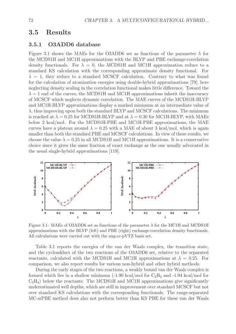
72 CHAPTER 3. A MULTICONFIGURATIONAL HYBRID...
3.5 Results
3.5.1 O3ADD6 database
Figure 3.1 shows the MAEs for the O3ADD6 set as functions of the parameter λ forthe MCDS1H and MC1H approximations with the BLYP and PBE exchange-correlationdensity functionals. For λ = 0, the MCDS1H and MC1H approximation reduce to astandard KS calculation with the corresponding approximate density functional. Forλ = 1, they reduce to a standard MCSCF calculation. Contrary to what was foundfor the calculation of atomization energies using double-hybrid approximations [79], hereneglecting density scaling in the correlation functional makes little difference. Toward theλ = 1 end of the curves, the MCDS1H and MC1H approximations inherit the inaccuracyof MCSCF which neglects dynamic correlation. The MAE curves of the MCDS1H-BLYPand MC1H-BLYP approximations display a marked minimum at an intermediate value ofλ, thus improving upon both the standard BLYP and MCSCF calculations. The minimumis reached at λ = 0.25 for MCDS1H-BLYP and at λ = 0.30 for MC1H-BLYP, with MAEsbelow 2 kcal/mol. For the MCDS1H-PBE and MC1H-PBE approximations, the MAEcurves have a plateau around λ = 0.25 with a MAE of about 3 kcal/mol, which is againsmaller than both the standard PBE and MCSCF calculations. In view of these results, wechoose the value λ = 0.25 in all MCDS1H and MC1H approximations. It is a conservativechoice since it gives the same fraction of exact exchange as the one usually advocated inthe usual single-hybrid approximations [119].
0
2
4
6
8
10
12
0 0.2 0.4 0.6 0.8 1
MA
E (
kca
l/m
ol)
λ
MC1H-BLYPMCDS1H-BLYP
0
2
4
6
8
10
12
0 0.2 0.4 0.6 0.8 1
MA
E (
kca
l/m
ol)
λ
MC1H-PBEMCDS1H-PBE
Figure 3.1: MAEs of O3ADD6 set as functions of the parameter λ for the MC1H and MCDS1Happroximations with the BLYP (left) and PBE (right) exchange-correlation density functionals.All calculations were carried out with the aug-cc-pVTZ basis set.
Table 3.1 reports the energies of the van der Waals complex, the transition state,and the cycloadduct of the two reactions of the O3ADD6 set, relative to the separatedreactants, calculated with the MCDS1H and MC1H approximations at λ = 0.25. Forcomparison, we also report results for various non-hybrid and other hybrid methods.
During the early stages of the two reactions, a weakly bound van der Waals complex isformed which lies in a shallow minimum (-1.90 kcal/mol for C2H2 and -1.94 kcal/mol forC2H4) below the reactants. The MCDS1H and MC1H approximations give significantlyunderestimated well depths, which are still in improvement over standard MCSCF but notover standard KS calculations with the corresponding functionals. The range-separatedMC-srPBE method does also not perform better than KS PBE for these van der Waals
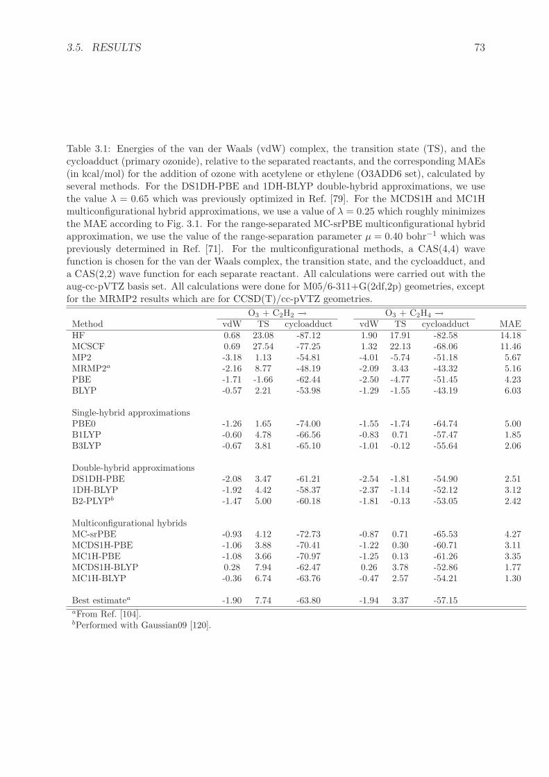
3.5. RESULTS 73
Table 3.1: Energies of the van der Waals (vdW) complex, the transition state (TS), and thecycloadduct (primary ozonide), relative to the separated reactants, and the corresponding MAEs(in kcal/mol) for the addition of ozone with acetylene or ethylene (O3ADD6 set), calculated byseveral methods. For the DS1DH-PBE and 1DH-BLYP double-hybrid approximations, we usethe value λ = 0.65 which was previously optimized in Ref. [79]. For the MCDS1H and MC1Hmulticonfigurational hybrid approximations, we use a value of λ = 0.25 which roughly minimizesthe MAE according to Fig. 3.1. For the range-separated MC-srPBE multiconfigurational hybridapproximation, we use the value of the range-separation parameter µ = 0.40 bohr−1 which waspreviously determined in Ref. [71]. For the multiconfigurational methods, a CAS(4,4) wavefunction is chosen for the van der Waals complex, the transition state, and the cycloadduct, anda CAS(2,2) wave function for each separate reactant. All calculations were carried out with theaug-cc-pVTZ basis set. All calculations were done for M05/6-311+G(2df,2p) geometries, exceptfor the MRMP2 results which are for CCSD(T)/cc-pVTZ geometries.
O3 + C2H2 −→ O3 + C2H4 −→Method vdW TS cycloadduct vdW TS cycloadduct MAEHF 0.68 23.08 -87.12 1.90 17.91 -82.58 14.18MCSCF 0.69 27.54 -77.25 1.32 22.13 -68.06 11.46MP2 -3.18 1.13 -54.81 -4.01 -5.74 -51.18 5.67MRMP2a -2.16 8.77 -48.19 -2.09 3.43 -43.32 5.16PBE -1.71 -1.66 -62.44 -2.50 -4.77 -51.45 4.23BLYP -0.57 2.21 -53.98 -1.29 -1.55 -43.19 6.03
Single-hybrid approximationsPBE0 -1.26 1.65 -74.00 -1.55 -1.74 -64.74 5.00B1LYP -0.60 4.78 -66.56 -0.83 0.71 -57.47 1.85B3LYP -0.67 3.81 -65.10 -1.01 -0.12 -55.64 2.06
Double-hybrid approximationsDS1DH-PBE -2.08 3.47 -61.21 -2.54 -1.81 -54.90 2.511DH-BLYP -1.92 4.42 -58.37 -2.37 -1.14 -52.12 3.12B2-PLYPb -1.47 5.00 -60.18 -1.81 -0.13 -53.05 2.42
Multiconfigurational hybridsMC-srPBE -0.93 4.12 -72.73 -0.87 0.71 -65.53 4.27MCDS1H-PBE -1.06 3.88 -70.41 -1.22 0.30 -60.71 3.11MC1H-PBE -1.08 3.66 -70.97 -1.25 0.13 -61.26 3.35MCDS1H-BLYP 0.28 7.94 -62.47 0.26 3.78 -52.86 1.77MC1H-BLYP -0.36 6.74 -63.76 -0.47 2.57 -54.21 1.30
Best estimatea -1.90 7.74 -63.80 -1.94 3.37 -57.15aFrom Ref. [104].bPerformed with Gaussian09 [120].

74 CHAPTER 3. A MULTICONFIGURATIONAL HYBRID...
systems. A better description of the long-range dispersion correlation would indeed re-quire inclusion of perturbation corrections on top of the active space [73]. As expected, thedouble-hybrid approximations, which include second-order perturbation corrections, tendto perform better for these van der Waals complexes. The best performance is achievedwith MRMP2 which is able to correctly describe both multiconfigurational effects and dis-persion correlations. However, one should keep in mind than the methods MP2, MRMP2,and the double hybrids are most likely less converged with respect to the basis size thanthe other methods.
The activation barriers of the transition states are underestimated (or not presentat all) in KS PBE and BLYP calculations, and to a less extent with the single-hybridand double-hybrid approximations, while they are largely overestimated in MCSCF. Notethat here, contrary to the common case, MCSCF gives higher activation barriers thanHF because the ozone reactant has more static correlation than the transition state.The MCDS1H and MC1H approximations give an improvement of about 5 kcal/mol overthe KS calculations with the corresponding functionals. The range-separated MC-srPBEmethod gives activation barriers which are slightly better than the ones given by MCDS1H-PBE and MC1H-PBE, but largely worse than the ones given by MCDS1H-BLYP andMC1H-BLYP. The values obtained with MCDS1H-BLYP and MC1H-BLYP, as well aswith MRMP2, are all within 1 kcal/mol of the best estimates.
The reaction energies of the formation of the cycloadducts are overestimated in MC-SCF and underestimated in MRMP2 (by about 15 kcal/mol). Zhao et al. observedthat even using a large (14,14) active space does not improve the MRMP2 reaction en-ergy [104]. All the hybrid methods give more reasonable reaction energies. In particular,MC1H-BLYP gives reaction energies within less than 3 kcal/mol of the best estimates.
If we accept to look more closely to the MAE values in spite of the limited statistics,we see that MC1H-BLYP gives overall the smallest MAE with 1.30 kcal/mol. The multi-configurational hybrid MCDS1H-PBE involving the PBE exchange-correlation functionalgives a larger MAE of 3.11 kcal/mol, but turns out to perform better on average thanthe range-separated MC-srPBE method which gives a MAE of 4.27 kcal/mol. Neglectingdensity scaling in the correlation functional of multiconfigurational hybrids seems slightlyfavorable for BLYP and slightly unfavorable for PBE. This is in line with what was foundfor double-hybrid approximations [79], although the MP2 correlation part made it muchmore sensitive to the neglect of the density scaling. Even if the effect of neglecting densityscaling is systematic in giving more negative complement correlation energies Eλ
c [n] forall density functionals, its effect on the MAE depends more on fortuitous compensationof errors for the approximate functional used.
3.5.2 Dissociation of diatomic molecules
We now turn to the calculation of potential energy curves of diatomic molecules. Thisis a harder problem since static correlation effects are dominant at dissociation. For themulticonfigurational hybrids, we report here only the curves of MCDS1H for PBE and ofMC1H for BLYP according to the results of Section 3.5.1, but the differences between thecurves of MCDS1H and MC1H for both BLYP and PBE are in fact very small for thesediatomic molecules.
Figure 3.2 shows the potential energy curve of H2 calculated by hybrid approxima-tions using the PBE and BLYP density functionals. Around the equilibrium internuclear

3.5. RESULTS 75
-1.15
-1.1
-1.05
-1
-0.95
-0.9
-0.85
-0.8
-0.75
0 2 4 6 8 10
Tota
l E
ner
gy (
hart
ree)
Internuclear distance (bohr)
AccurateHF
MCSCFPBE
PBE0MC-srPBE
MCDS1H-PBE
H2
-1.15
-1.1
-1.05
-1
-0.95
-0.9
-0.85
-0.8
-0.75
0 2 4 6 8 10
Tota
l E
ner
gy (
hart
ree)
Internuclear distance (bohr)
AccurateHF
MCSCFBLYP
B1LYPB3LYP
MC1H-BLYP
H2
Figure 3.2: Potential energy curves of H2 calculated by HF, MCSCF, and several methods basedon the PBE (left) or BLYP (right) exchange-correlation density functionals. For the MCDS1Hand MC1H multiconfigurational hybrid approximations, we use a value of λ = 0.25. For therange-separated MC-srPBE multiconfigurational hybrid approximation, we use a value of therange-separation parameter of µ = 0.40 bohr−1. For all multiconfigurational methods, we usea full-valence CAS wave function. The basis set is cc-pVTZ basis. The accurate curve is fromRef. [28].
distance, all DFT-based method, including MCDS1H-PBE and MC1H-BLYP, are accu-rate, which means that they properly describe dynamic correlation. At large distances,the single-hybrid approximations (PBE0, B1LYP, and B3LYP), which include a fractionof HF exchange energy, give less accurate potential energy curves than non-hybrid KScalculations (PBE and BLYP). By inclusion of a fraction of exact static correlation en-ergy, the multiconfigurational hybrids (MCDS1H-PBE, MC-srPBE, and MC1H-BLYP)correct this behavior and give potential energy curves that correctly saturate beyond adistance of about 5 bohr, as the MCSCF curve does. This point is explained by a de-tailed analysis of the asymptotic expansion of the potential energy curves in a minimalbasis in Appendix 3.7.2. However, the MCDS1H-PBE, MC-srPBE, and MC1H-BLYPmethods still display significant errors on the energy of the separated atoms due to thedensity-functional approximations. Indeed, as in restricted KS calculations, the densityfunctionals used in the multiconfigurational hybrids depend only of the total density anddo not give accurate energies in the limit of separated atoms of open-shell character. In anunrestricted KS calculation, the energy at dissociation can be improved by breaking thespin symmetry and therefore introducing a fictitious spin density which helps to describethe separated atoms. In our present implementation of the multiconfigurational hybrids,the spin symmetry is imposed on the MCSCF wave function so that there is no fictitiousspin density to be used in the density functionals.
Figure 3.5.2 shows the potential energy curves of Li2, C2, N2, and F2. The results aresimilar than for H2. Around the equilibrium distance, the MCDS1H-PBE and MC1H-BLYP curves are similar to the standard hybrid or non-hybrid KS calculations. At largedistances, the single-hybrid approximations give a spurious increase of the energy, whereasthe MCDS1H-PBE and MC1H-BLYP curves correctly saturate. The MC1H-BLYP ap-proximation gives good total energies, but again a significant error remains at dissociation,especially for N2. The DS1DH-PBE and MC-srPBE approximation gives curves of verysimilar shape.

76 CHAPTER 3. A MULTICONFIGURATIONAL HYBRID...
-14.98
-14.96
-14.94
-14.92
-14.9
-14.88
2 4 6 8 10 12 14
Tota
l E
ner
gy (
hart
ree)
Internuclear distance (bohr)
AccurateMCSCF
PBEPBE0
MC-srPBEMCDS1H-PBE
Li2
-14.98
-14.96
-14.94
-14.92
-14.9
-14.88
2 4 6 8 10 12 14
Tota
l E
ner
gy (
hart
ree)
Internuclear distance (bohr)
AccurateMCSCF
BLYPB1LYPB3LYP
MC1H-BLYP
Li2
-75.9
-75.8
-75.7
-75.6
-75.5
-75.4
2 3 4 5 6 7 8 9 10
Tota
l E
ner
gy (
hart
ree)
Internuclear distance (bohr)
AccurateMCSCF
PBEPBE0
MC-srPBEMCDS1H-PBE
C2
-75.9
-75.8
-75.7
-75.6
-75.5
-75.4
2 3 4 5 6 7 8 9 10
Tota
l E
ner
gy (
hart
ree)
Internuclear distance (bohr)
AccurateMCSCF
BLYPB1LYPB3LYP
MC1H-BLYP
C2
-109.6
-109.5
-109.4
-109.3
-109.2
-109.1
-109
-108.9
-108.8
-108.7
1 2 3 4 5 6 7 8 9 10
Tota
l E
ner
gy (
hart
ree)
Internuclear distance (bohr)
AccurateMCSCF
PBEPBE0
MC-srPBEMCDS1H-PBE
N2
-109.6
-109.5
-109.4
-109.3
-109.2
-109.1
-109
-108.9
-108.8
1 2 3 4 5 6 7 8 9 10
Tota
l E
ner
gy (
hart
ree)
Internuclear distance (bohr)
AccurateMCSCF
BLYPB1LYPB3LYP
MC1H-BLYP
N2
-199.6
-199.5
-199.4
-199.3
-199.2
-199.1
-199
-198.9
-198.8
-198.7
2 3 4 5 6 7
Tota
l E
ner
gy (
hart
ree)
Internuclear distance (bohr)
AccurateMCSCF
PBEPBE0
MC-srPBEMCDS1H-PBE
F2
-199.6
-199.5
-199.4
-199.3
-199.2
-199.1
-199
-198.9
-198.8
-198.7
2 3 4 5 6 7
Tota
l E
ner
gy (
hart
ree)
Internuclear distance (bohr)
AccurateMCSCF
BLYPB1LYPB3LYP
MC1H-BLYP
F2
Figure 3.3: Potential energy curves of Li2, C2, N2, and F2 calculated with MCSCF and severalmethods based on the PBE (left) or BLYP (right) exchange-correlation density functionals.For the MCDS1H and MC1H multiconfigurational hybrid approximations, we use a value ofλ = 0.25. For the range-separated MC-srPBE multiconfigurational hybrid approximation, weuse a value of the range-separation parameter of µ = 0.40 bohr−1. For all multiconfigurationalmethods, we use a full-valence CAS wave function. The basis set is cc-pVTZ basis. The accuratecurves are from Ref. [28].

3.6. CONCLUSIONS 77
3.6 Conclusions
We have presented a multiconfigurational hybrid density-functional theory which rigor-ously combines MCSCF and DFT based on a linear decomposition of the electron-electroninteraction. It is straightforward extension of the usual hybrid approximations by essen-tially adding a fraction λ of exact static correlation in addition to the fraction λ of exactexchange. Any existing approximate exchange-correlation density functional can be usedin this scheme by using a simple scaling relation with λ. Test calculations on the cy-cloaddition reactions of ozone with ethylene or acetylene and the dissociation of diatomicmolecules with the PBE and BLYP density functionals show that a good value of λ is0.25, as in the usual hybrid approximations.
Interestingly, the results seem to indicate that the present approach based on a sim-ple linear decomposition of the electron-electron interaction is at least as good as therange-separated multiconfigurational hybrid method of Ref. [70–72] for including staticcorrelation in DFT, at least with the approximate density functionals used here. Of course,with better short-range density-functional approximations (in particular, we do not havea short-range version of the LYP correlation functional for comparison), the conclusioncould be different. Also, one should note that hybrid approaches combining perturbationtheory with DFT based on a linear decomposition of the interaction [79] do not have theadvantages of the range-separated hybrid approaches for fast basis-size convergence andexplicit inclusion of long-range van der Waals interactions. For MCSCF, however, basisset convergence is not so much an issue.
The present results suggest that the proposed multiconfigurational hybrid approxi-mations can improve over usual DFT approximations for situations with strong staticcorrelation effects. It remains however to assess the performance of this multiconfigura-tional hybrid method on a larger variety of systems. Future work includes adding thedependence on the spin density in the functionals to be able to properly handle open-shellsystems, and possibly other additional variables such as the on-top pair density as analternative to the spin density for improving the accuracy of closed-shell systems [121].
Acknowledgments
We thank E. Fromager (Strasbourg, France) for discussions. K.S. thanks Professors I.Othman and M. K. Sabra (Atomic Energy Commission of Syria) for their support. Thiswork was part of the French-Danish collaboration project“WADEMECOM.dk”supportedby the French government.
3.7 Appendix
3.7.1 Scaling relations for the derivatives of the density-scaledcorrelation functional
We give the scaling relations for the density-scaled correlation functionalEλc [n] = λ2Ec[n1/λ]
and its derivatives in the case of generalized-gradient approximations (GGA). Starting

78 CHAPTER 3. A MULTICONFIGURATIONAL HYBRID...
from a standard GGA density functional written as
Ec,GGA[n] =
∫
ec (n(r), |∇n(r)|) dr, (3.9)
where |∇n(r)| is the norm of the density gradient, the corresponding scaled functional is
Eλc,GGA[n] =
∫
eλc (n(r), |∇n(r)|) dr, (3.10)
where the energy density is obtained by scaling relation (see Ref. [79])
eλc (n(r), |∇n(r)|) = λ5ec
(
n(r)
λ3,|∇n(r)|λ4
)
. (3.11)
The first-order derivatives of the energy density are
∂eλc
∂n(n(r), |∇n(r)|) = λ2∂ec
∂n
(
n(r)
λ3,|∇n(r)|λ4
)
, (3.12)
and
∂eλc
∂ |∇n| (n(r), |∇n(r)|) = λ∂ec
∂ |∇n|
(
n(r)
λ3,|∇n(r)|λ4
)
.
(3.13)
The second-order derivatives are
∂2eλc
∂n2(n(r), |∇n(r)|) =
1
λ
∂2ec
∂n2
(
n(r)
λ3,|∇n(r)|λ4
)
, (3.14)
∂2eλc
∂ |∇n|2(n(r), |∇n(r)|) =
1
λ3
∂2ec
∂ |∇n|2(
n(r)
λ3,|∇n(r)|λ4
)
, (3.15)
and
∂2eλc
∂n∂ |∇n| (n(r), |∇n(r)|) =1
λ2
∂2ec
∂n∂ |∇n|
(
n(r)
λ3,|∇n(r)|λ4
)
. (3.16)
3.7.2 Asymptotic expansion of the potential energy curve of H2
We consider the H2 molecule in a Slater minimal basis, with a basis function a localizedon the left atom and a basis function b localized on the right atom, both basis functionsbeing identical with exponent ζ = 1. In the large internuclear distance R limit, thetwo molecular orbitals are 1 = (a + b)/
√2 and 2 = (a − b)/
√2. The total restricted
Hartree-Fock (RHF) energy writes
ERHF = 2h11 + J11 +1
R, (3.17)

3.7. APPENDIX 79
where h11 = t11 +v11 is the sum of the kinetic integral t11 = (1|t|1) and the nuclei-electronintegral v11 = (1|vne|1), and J11 = (11|11) is the Coulomb two-electron integral, and 1/Ris the nuclear repulsion energy. By expanding the molecular orbital 1 into the localizedfunctions a and b, and using the symmetry between a and b, it is easy to find the large Rbehavior of all these terms:
t11 = (a|t|a) + (a|t|b) =1
2+O(e−R), (3.18)
and
v11 = (a|vne|a) + (a|vne|b) = −1 − 1
R+O(e−R), (3.19)
and
J11 =(aa|aa)
2+
(aa|bb)2
+ 2(aa|ab) + (ab|ab) =5
16+
1
2R+O(e−R), (3.20)
where O(e−R) stands for exponentially decaying terms in R. For the values of the inte-grals, see Ref. [122]. Adding all the pieces together, it leads to the following asymptoticexpansion of the total RHF energy
ERHF = −11
16− 1
2R+O(e−R). (3.21)
At dissociation, the RHF wave function contains 50% of the incorrect ionic contributionH+...H−, which is responsible for too high an energy and for the spurious electrostaticattraction term −1/2R.
The full configuration interaction (FCI) correlation energy in this basis is found bydiagonalizing the 2 × 2 Hamiltonian matrix, leading to
EFCIc =
1
2
(
E2 − ERHF −√
(E2 − ERHF)2 + 4K212
)
, (3.22)
where E2 = 2h22 + J22 + 1/R is the energy of the double-excited determinant, and K12 =(12|12) is the exchange two-electron integral. The asymptotic behavior of E2 is exactlythe same as the one of ERHF, so that E2 − ERHF vanishes exponentially when R → ∞and the asymptotic behavior of EFCI
c is determined by K12 only: EFCIc = −K12 +O(e−R).
The asymptotic behavior of K12 is
K12 =(aa|aa)
2− (aa|bb)
2=
5
16− 1
2R+O(e−R),
(3.23)
giving for the correlation energy
EFCIc = − 5
16+
1
2R+O(e−R). (3.24)
Adding the asymptotic expansions of Eqs. (3.21) and (3.24) gives the asymptotic expan-sion of the total FCI energy in this basis
EFCI = −1 +O(e−R), (3.25)
80 CHAPTER 3. A MULTICONFIGURATIONAL HYBRID...
which implies that the FCI potential energy curve saturates quickly at large internucleardistance.
In restricted Kohn-Sham (RKS) density-functional theory, the total energy writes
ERKS = 2h11 + 2J11 + Ex + Ec +1
R, (3.26)
where Ex and Ec are the exchange and correlation energies. At large R, it behaves as
ERKS = −3
8+ Ex + Ec +O(e−R). (3.27)
With local or semilocal density-functional approximations, Ex and Ec go exponentially toconstants when R → ∞, so that the asymptotic expansion of ERKS does not contain aspurious term in 1/R.
Single-hybrid approximations introduces a fraction λ of RHF exchange which have thefollowing asymptotic expansion
ERHFx = −J11 = − 5
16− 1
2R+O(e−R), (3.28)
and therefore introduce a wrong −λ/2R term in the total energy,
Ehybrid = −3
8− 5λ
16+ (1 − λ)Ex + Ec −
λ
2R+O(e−R). (3.29)
Single-hybrid approximations thus deteriorate the large R behavior of local or semilocaldensity-functional approximations (see Fig. 3.2). The multiconfigurational hybrid approx-imations introduced in this work correct this behavior by adding a fraction of the FCIcorrelation energy which, in the limit of large R, is just λEFCI
c , the linearity in λ being asignature of static correlation. For example, the MC1H approximation has the followingasymptotic expansion
EMC1H = −3
8− 5λ
8+ (1 − λ)Ex + (1 − λ2)Ec +O(e−R), (3.30)
with no longer any spurious 1/R term, and thus improves the large R behavior (seeFig. 3.2). It is a typical example where exact exchange and static correlation must beconsidered together.
For range-separated density-functional theory, the situation is similar. Range-separatedsingle-hybrid approximations [80, 123–126] include some long-range RHF exchange andtheir asymptotic expansions display a wrong −1/2R term, just as RHF. Their behaviorfor large R is in fact worse than that of usual single-hybrid approximations since the−1/2R term is not weighted by λ. However, the range-separated CI-srDFT [66, 67] orMC-srDFT [70–72] methods add some exact long-range correlation energy which removesthis wrong −1/2R term.
Note that other forms of single-hybrid approximations which do not use RHF exchangeat long range [127, 128] allow one to avoid a wrong −1/2R term in the large R limit.Symmetry breaking is another way to avoid a wrong asymptotic −1/2R term since theunrestricted Hartree-Fock exchange energy does not contain such a term.
The fact that local or semilocal approximations for Ex and Ec do not introduce 1/Rterms is in agreement with the usual conviction that approximate GGA exchange func-tionals not only represent exchange but also static correlation, while approximate GGAcorrelation functionals represent dynamic correlation only [4].

Bibliography
[1] P. Hohenberg and W. Kohn, Phys. Rev. 136, B 864 (1964).
[2] W. Kohn and L. J. Sham, Phys. Rev. 140, A1133 (1965).
[3] W. Koch and M. C. Holthausen, A Chemist’s Guide To Density Functional Theory
(Wiley-VCH, New York, 2001).
[4] O. V. Gritsenko, P. R. T. Schipper and E. J. Baerends, J. Chem. Phys. 107, 5007(1997).
[5] A. D. Becke, J. Chem. Phys. 119, 2972 (2003).
[6] A. J. Cohen, P. Mori-Sanchez and W. Yang, Science 321, 792 (2008).
[7] N. E. Schultz, Y. Zhao and D. G. Truhlar, J. Phys. Chem. A 109, 11127 (2005).
[8] D. Cremer, Mol. Phys. 99, 1899 (2001).
[9] J. Slater, J. Mann, T. Wilson and J. Wood, Phys. Rev. 184, 672 (1969).
[10] M. Levy, Phys. Rev. A 26, 1200 (1982).
[11] E. H. Lieb, Int. J. Quantum. Chem. 24, 24 (1983).
[12] B. I. Dunlap and W. N. Mei, J. Chem. Phys. 78, 4997 (1983).
[13] S. G. Wang and W. H. E. Schwarz, J. Chem. Phys. 105, 4641 (1996).
[14] P. R. T. Schipper, O. V. Gritsenko and E. J. Baerends, Theor. Chem. Acc. 99, 329(1998).
[15] J. D. Goddard and G. Orlova, J. Chem. Phys. 111, 7705 (1999).
[16] M. Filatov and S. Shaik, Chem. Phys. Lett. 304, 429 (1999).
[17] M. Filatov and S. Shaik, J. Phys. Chem. A 103, 8885 (1999).
[18] M. Filatov and S. Shaik, Chem. Phys. Lett. 332, 409 (1999).
[19] M. Filatov, S. Shaik, M. Woeller, S. Grimme and S. Peyerimhoff, Chem. Phys. Lett.316, 135 (2000).
[20] M. Filatov and S. Shaik, J. Phys. Chem. A 104, 6628 (2000).
81

82 BIBLIOGRAPHY
[21] C. A. Ullrich and W. Kohn, Phys. Rev. Lett. 87, 093001 (2001).
[22] K. Y. R. Takeda, S. Yamanaka, Int. J. Quantum. Chem. 93, 317 (2003).
[23] S. Grimme and M. Waletzke, J. Chem. Phys. 111, 5645 (1999).
[24] E. V. Beck, E. A. Stahlberg, L. W. Burggraf and J.-P. Blaudeau, Chem. Phys. 349,158 (2008).
[25] Q. Wu, C.-L. Cheng, and T. Van Voorhis, J. Chem. Phys. 127, 164119 (2007).
[26] Q. Wu, B. Kaduk, and T. Van Voorhis, J. Chem. Phys. 130, 034109 (2009).
[27] G. C. Lie and E. Clementi, J. Chem. Phys. 60, 1275 (1974).
[28] G. C. Lie and E. Clementi, J. Chem. Phys. 60, 1288 (1974).
[29] R. Colle and O. Salvetti, Theor. Chim. Acta 37, 329 (1975).
[30] R. Colle and O. Salvetti, Theor. Chim. Acta 53, 55 (1979).
[31] R. Colle and O. Salvetti, J. Chem. Phys. 79, 1404 (1983).
[32] R. Colle and O. Salvetti, J. Chem. Phys. 93 (1990).
[33] A. Savin, Int. J. Quantum. Chem. 22, 59 (1988).
[34] A. Savin, J. chim. phys. 86, 757 (1989).
[35] A. Savin, in Density functional methods in chemistry , edited by J. Labanowski andJ. Andzelm (Springer-Verlag, New York, 1991), p. 213.
[36] B. Miehlich, H. Stoll and A. Savin, Mol. Phys. 91, 527 (1997).
[37] C. Gutle and A. Savin, Phys. Rev. A 75, 032519 (2007).
[38] F. Moscardo and E. San-Fabian, Int. J. Quantum. Chem. 40, 23 (1991).
[39] E. Kraka, Chem. Phys. 161, 141 (1992).
[40] E. Kraka, D. Cremer and S. Nordholm, in Molecules in Natural Science and
Biomedicine, edited by Z. Maksic and M. Eckert-Maksic (Ellis Horwood, Chich-ester, 1992), p. 351.
[41] W. Wu and S. Shaik, Chem. Phys. Lett. 301, 37 (1999).
[42] H. Stoll, Chem. Phys. Lett. 376, 141 (2003).
[43] F. Ying, P. Su, Z. Chen, S. Shaik and W. Wu, J. Chem. Theory Comput. 8, 1608(2012).
[44] N. O. J. Malcolm and J. J. W. McDouall, J. Phys. Chem. 98, 12579 (1994).
[45] N. O. J. Malcolm and J. J. W. McDouall, J. Phys. Chem. 100, 10131 (1996).

BIBLIOGRAPHY 83
[46] N. O. J. Malcolm and J. J. W. McDouall, J. Phys. Chem. A 101, 8119 (1997).
[47] N. O. J. Malcolm and J. J. W. McDouall, Chem. Phys. Lett. 282, 121 (1998).
[48] J. J. W. McDouall, Mol. Phys. 101, 361 (2003).
[49] P. Borowski, K. D. Jordan, J. Nichols and P. Nachtigall, Theor. Chem. Acc. 99, 135(1998).
[50] J. Grafenstein and D. Cremer, Chem. Phys. Lett. 316, 569 (2000).
[51] J. Grafenstein and D. Cremer, Phys. Chem. Chem. Phys. 2, 2091 (2000).
[52] J. Grafenstein and D. Cremer, Mol. Phys. 103, 279 (2005).
[53] R. Takeda, S. Yamanaka and K. Yamaguchi, Chem. Phys. Lett. 366, 321 (2002).
[54] K. Nakata, T. Ukai, S. Yamanaka, T. Takada and K. Yamaguchi, Int. J. Quantum.Chem. 106, 3325 (2006).
[55] S. Yamanaka, K. Nakata, T. Ukai, T. Takada and K. Yamaguchi, Int. J. Quantum.Chem. 106, 3312 (2006).
[56] T. Ukai, K. Nakata, S. Yamanaka, T. Takada and K. Yamaguchi, Mol. Phys. 105,2667 (2007).
[57] S. Gusarov, P.-A. Malmqvist, R. Lindh and B. O. Roos, Theor. Chim. Acc. 112, 84(2004).
[58] A. J. Perez-Jimenez and J. M. Perez-Jorda, Phys. Rev. A 75, 012503 (2007).
[59] A. J. Perez-Jimenez, J. M. Perez-Jorda, I. de P. R. Moreira and F. Illas, J. Comput.Chem. 28, 2559 (2007).
[60] A. J. Perez-Jimenez, J. M. Perez-Jorda and J. C. Sancho-Garcıa, J. Chem. Phys.127, 104102 (2007).
[61] M. Weimer, F. D. Sala and A. Gorling, J. Chem. Phys. 128, 144109 (2008).
[62] Y. Kurzweil, K. V. Lawler and M. Head-Gordon, Mol. Phys. 107, 2103 (2009).
[63] A. Savin and H.-J. Flad, Int. J. Quantum. Chem. 56, 327 (1995).
[64] A. Savin, in Recent Advances in Density Functional Theory , edited by D. P. Chong(World Scientific, 1996).
[65] A. Savin, in Recent Developments of Modern Density Functional Theory , edited byJ. M. Seminario (Elsevier, Amsterdam, 1996), pp. 327–357.
[66] T. Leininger, H. Stoll, H.-J. Werner and A. Savin, Chem. Phys. Lett. 275, 151(1997).
[67] R. Pollet, A. Savin, T. Leininger and H. Stoll, J. Chem. Phys. 116, 1250 (2002).
84 BIBLIOGRAPHY
[68] A. Savin, F. Colonna and R. Pollet, Int. J. Quantum. Chem. 93, 166 (2003).
[69] J. Toulouse, F. Colonna and A. Savin, Phys. Rev. A 70, 062505 (2004).
[70] J. K. Pedersen and H. J. A. Jensen, unpublished.
[71] E. Fromager, J. Toulouse and H. J. A. Jensen, J. Chem. Phys. 126, 074111 (2007).
[72] E. Fromager, F. Real, P. Wahlin, U. Wahlgren and H. J. A. Jensen, J. Chem. Phys.131, 054107 (2009).
[73] E. Fromager, R. Cimiraglia and H. J. A. Jensen, Phys. Rev. A 81, 024502 (2010).
[74] T. Tsuchimochi, G. E. Scuseria and A. Savin, J. Chem. Phys. 132, 024111 (2010).
[75] T. Tsuchimochi and G. E. Scuseria, J. Chem. Phys. 134, 064101 (2011).
[76] K. Pernal, Phys. Rev. A 81, 052511 (2010).
[77] D. R. Rohr, J. Toulouse and K. Pernal, Phys. Rev. A 82, 052502 (2010).
[78] D. R. Rohr and K. Pernal, J. Chem. Phys. 135, 074104 (2011).
[79] K. Sharkas, J. Toulouse and A. Savin, J. Chem. Phys. 134, 064113 (2011).
[80] J. G. Angyan, I. C. Gerber, A. Savin and J. Toulouse, Phys. Rev. A 72, 012510(2005).
[81] M. Levy and J. P. Perdew, Phys. Rev. A 32, 2010 (1985).
[82] M. Levy, W. Yang and R. G. Parr, J. Chem. Phys. 83, 2334 (1985).
[83] M. Levy, Phys. Rev. A 43, 4637 (1991).
[84] M. Levy and J. P. Perdew, Phys. Rev. B 48, 11638 (1993).
[85] A. D. Becke, J. Chem. Phys. 104, 1040 (1996).
[86] M. Ernzerhof, J. P. Perdew and K. Burke, in Density Functional Theory , edited byR. Nalewajski (Springer-Verlag, Berlin, 1996).
[87] E. Fromager and H. J. A. Jensen, Phys. Rev. A 78, 022504 (2008).
[88] J. G. Angyan, Phys. Rev. A 78, 022510 (2008).
[89] S. Grimme, J. Chem. Phys. 124, 034108 (2006).
[90] C. Angeli, K. L. Bak, V. Bakken, O. Christiansen, R. Cimiraglia, S. Coriani,P. Dahle, E. K. Dalskov, T. Enevoldsen, B. Fernandez, L. Ferrighi, L. Frediani,C. Hattig, K. Hald, A. Halkier, H. Heiberg, T. Helgaker, H. Hettema, B. Jansik,H. J. A. Jensen, D. Jonsson, P. Jørgensen, S. Kirpekar, W. Klopper, S. Knecht,R. Kobayashi, J. Kongsted, H. Koch, A. Ligabue, O. B. Lutnæs, K. V. Mikkelsen,C. B. Nielsen, P. Norman, J. Olsen, A. Osted, M. J. Packer, T. B. Pedersen,Z. Rinkevicius, E. Rudberg, T. A. Ruden, K. Ruud, P. Salek, C. C. M. Samson,
BIBLIOGRAPHY 85
A. S. de Meras, T. Saue, S. P. A. Sauer, B. Schimmelpfennig, A. H. Steindal,K. O. Sylvester-Hvid, P. R. Taylor, O. Vahtras, D. J. Wilson and H.Agren, DAL-TON, a molecular electronic structure program, Release DALTON2011 (2011), seehttp://daltonprogram.org.
[91] J. K. Pedersen, Description of correlation and relativistic effects in calculations of
molecular properties, PhD thesis, University of Southern Denmark, Odense (2004).
[92] H. J. A. Jensen and P. Jørgensen, J. Chem. Phys. 80, 1204 (1984).
[93] H. J. A. Jensen and H. Agren, Chem. Phys. Lett. 110, 140 (1984).
[94] H. J. A. Jensen and H. Agren, Chem. Phys. 104, 229 (1986).
[95] H. J. A. Jensen, P. Jorgensen and H. Agren, J. Chem. Phys. 87, 451 (1987).
[96] H. J. A. Jensen, P. Jørgensen, H. Agren and J. Olsen, J. Chem. Phys. 88, 3834(1988).
[97] H. J. A. Jensen, in Relativistic and Electron Correlation Effects in Molecules and
Solids , edited by G. L. Malli (Plenum, New York, 1994), p. 179.
[98] J. P. Perdew, K. Burke and M. Ernzerhof, Phys. Rev. Lett. 77, 3865 (1996).
[99] A. D. Becke, Phys. Rev. A 38, 3098 (1988).
[100] C. Lee, W. Yang and R. G. Parr, Phys. Rev. B 37, 785 (1988).
[101] L. Goerigk and S. Grimme, J. Chem. Theory Comput 6, 107 (2010).
[102] L. Goerigk and S. Grimme, J. Chem. Theory Comput 7, 291 (2011).
[103] S. E. Wheeler, D. H. Ess and K. N. Houk, J. Phys. Chem. A 112, 1798 (2007).
[104] Y. Zhao, O. Tishchenko, J. R. Gour, W. Li, J. J. Lutz, P. Piecuch and D. G. Truhlar,J. Phys. Chem. A 113, 5786 (2009).
[105] T. Saito, S. Nishihara, Y. Kataoka, Y. Nakanishi, Y. Kitagawa, T. Kawakami,S.Yamanaka, M. Okumura and K. Yamaguchi, J. Phys. Chem. A 114, 12116 (2010).
[106] T. H. Dunning, J. Chem. Phys. 90, 1007 (1989).
[107] R. A. Kendall, T. H. Dunning and R. J. Harrison, J. Chem. Phys. 96, 6796 (1992).
[108] Y. Zhao, N. E. Schultz and D. G. Truhlar, J. Chem. Phys. 123, 161103 (2005).
[109] R. Krishnan, J. S. Binkley, R. Seeger and J. A. Pople, J. Chem. Phys. 72, 650(1980).
[110] A. D. McLean and G. S. Chandler, J. Chem. Phys. 72, 5639 (1980).
[111] C. Møller and M. S. Plesset, Phys. Rev. 46, 618 (1934).
[112] K. Hirao, Chem. Phys. Lett. 190, 374 (1992).
86 BIBLIOGRAPHY
[113] C. Adamo and V. Barone, J. Chem. Phys. 110, 6158 (1999).
[114] C. Adamo and V. Barone, Chem. Phys. Lett. 298, 113 (1998).
[115] C. Adamo and V. Barone, Chem. Phys. Lett. 274, 242 (1997).
[116] A. D. Becke, J. Chem. Phys. 98, 5648 (1993).
[117] V. Barone and C. Adamo, Chem. Phys. Lett. 224, 432 (1994).
[118] E. Goll, H.-J. Werner, H. Stoll, T. Leininger, P. Gori-Giorgi and A. Savin, Chem.Phys. 329, 276 (2006).
[119] J. P. Perdew, M. Ernzerhof and K. Burke, J. Chem. Phys 105, 9982 (1996).
[120] M. J. Frisch, G. W. Trucks, H. B. Schlegel, G. E. Scuseria, M. A. Robb, J. R.Cheeseman, G. Scalmani, V. Barone, B. Mennucci, G. A. Petersson, H. Nakatsuji,M. Caricato, X. Li, H. P. Hratchian, A. F. Izmaylov, J. Bloino, G. Zheng, J. L.Sonnenberg, M. Hada, M. Ehara, K. Toyota, R. Fukuda, J. Hasegawa, M. Ishida,T. Nakajima, Y. Honda, O. Kitao, H. Nakai, T. Vreven, J. A. Montgomery, Jr.,J. E. Peralta, F. Ogliaro, M. Bearpark, J. J. Heyd, E. Brothers, K. N. Kudin,V. N. Staroverov, R. Kobayashi, J. Normand, K. Raghavachari, A. Rendell, J. C.Burant, S. S. Iyengar, J. Tomasi, M. Cossi, N. Rega, J. M. Millam, M. Klene,J. E. Knox, J. B. Cross, V. Bakken, C. Adamo, J. Jaramillo, R. Gomperts, R. E.Stratmann, O. Yazyev, A. J. Austin, R. Cammi, C. Pomelli, J. W. Ochterski, R. L.Martin, K. Morokuma, V. G. Zakrzewski, G. A. Voth, P. Salvador, J. J. Dannenberg,S. Dapprich, A. D. Daniels, A. Farkas, J. B. Foresman, J. V. Ortiz, J. Cioslowskiand D. J. Fox, Gaussian 09 Revision A.1, Gaussian Inc. Wallingford CT 2009.
[121] J. P. Perdew, A. Savin and K. Burke, Phys. Rev. A 51, 4531 (1995).
[122] M. J. S. Dewar and J. Kelemen, J. Chem. Educ. 48, 494 (1971).
[123] H. Iikura, T. Tsuneda, T. Yanai and K. Hirao, J. Chem. Phys. 115, 3540 (2001).
[124] T. Yanai, D. P. Tew and N. C. Handy, Chem. Phys. Lett. 393, 51 (2004).
[125] I. C. Gerber and J. G. Angyan, Chem. Phys. Lett. 415, 100 (2005).
[126] O. A. Vydrov and G. E. Scuseria, J. Chem. Phys. 125, 234109 (2006).
[127] J. Heyd, G. E. Scuseria and M. Ernzerhof, J. Chem. Phys. 118, 8207 (2003).
[128] T. M. Henderson, A. F. Izmaylov, G. E. Scuseria and A. Savin, J. Chem. Phys. 127,221103 (2007).
Chapter 4
Double-hybrid density-functionaltheory made rigorous
This chapter, written in collaboration with J. Toulouse and A. Savin, has been publishedin Journal of Chemical Physics [J. Chem. Phys. 134, 064113 (2011)].
4.1 Abstract
We provide a rigorous derivation of a class of double-hybrid approximations, combin-ing Hartree-Fock exchange and second-order Møller-Plesset correlation with a semilo-cal exchange-correlation density functional. These double-hybrid approximations containonly one empirical parameter and use a density-scaled correlation energy functional. Ne-glecting density scaling leads to an one-parameter version of the standard double-hybridapproximations. We assess the performance of these double-hybrid schemes on represen-tative test sets of atomization energies and reaction barrier heights, and we compare toother hybrid approximations, including range-separated hybrids. Our best one-parameterdouble-hybrid approximation, called 1DH-BLYP, roughly reproduces the two parametersof the standard B2-PLYP or B2GP-PLYP double-hybrid approximations, which showsthat these models are not only empirically close to an optimum for general chemicalapplications but are also theoretically supported.
4.2 Introduction
Density-functional theory (DFT) [1–3] is a powerful approach for electronic-structurecalculations of atoms, molecules and solids. In its Kohn-Sham (KS) formulation, a se-ries of approximations for the exchange-correlation energy have been developed for anever-increasing accuracy: local density approximation (LDA), semilocal approximations(generalized-gradient approximations (GGA) and meta-GGA), hybrid approximations in-troducing Hartree-Fock (HF) exchange, and nonlocal correlation approximations usingvirtual KS orbitals [4].
In this context, Grimme [5] recently introduced the family of so-called double-hybrid
(DH) density-functional approximations which mix HF exchange with a semilocal ex-change density functional and second-order Møller-Plesset (MP2) correlation with a semilo-
87
88 CHAPTER 4. DOUBLE-HYBRID DENSITY-FUNCTIONAL...
cal correlation density functional:
EDHxc = axE
HFx + (1 − ax)Ex[n] + (1 − ac)Ec[n] + acE
MP2c , (4.1)
where the first three terms are calculated in an usual self-consistent hybrid KS calculation,and the last perturbative term evaluated with the previously obtained orbitals is addeda posteriori. The B2-PLYP double-hybrid approximation [5] is obtained by choosing theBecke 88 (B) exchange functional [6] for Ex[n] and the Lee-Yang-Parr (LYP) correlationfunctional [7] for Ec[n], and the empirical parameters ax = 0.53 and ac = 0.27 optimizedfor the G2/97 subset of heats of formation. The mPW2-PLYP double-hybrid approxi-mation [8] uses the modified Perdew-Wang (mPW) exchange functional [9], and has verysimilar optimized parameters ax = 0.55 and ac = 0.25. These two double-hybrid approx-imations reach on average near-chemical accuracy for the thermodynamical data of theG3/05 set [8]. Similar double-hybrid approximations have also been obtained by reopti-mizing the parameters ax and ac for a spin-restricted open-shell version of the method [10]or for different test sets [11, 12]. In particular, targeting both thermochemistry and ki-netics applications has given the reoptimized parameters ax = 0.65 and ac = 0.36 whichdefines the general-purpose B2GP-PLYP double-hybrid approximation [12]. The so-calledmulticoefficient correlation methods combining HF, DFT and MP2 energies can also beconsidered to be a form of double-hybrid approximation [13–15], and the connection wasmade explicit in Ref. [16]. Three- or four-parameter double-hybrid approximations havealso been proposed [17–19], scaling differently the LDA and GGA components of the den-sity functionals, in the style of the first hybrid DFT approximations [20]. For systemswith van der Waals interactions, good accuracy can be obtained by further adding anempirical dispersion term [21] or by increasing the amount of MP2 correlation at longinterelectronic distances [22].
Although the above-mentioned double-hybrid approximations yield very promising re-sults and are already largely used, they suffer from a lack of theoretical justification. Ithas been tried [17] to motivate these approaches by invoking the adiabatic connection for-malism [23] and second-order Gorling-Levy perturbation theory (GL2) [24], but severalunjustified empirical steps remain (e.g., dropping the single-excitation term in the GL2expression). On the contrary, the range-separated double-hybrid RSH+lrMP2 methodof Ref. [25], which combines long-range HF exchange and long-range MP2 correlationwith a short-range exchange-correlation density functional, has been rigorously derivedusing the formally exact multideterminant extension of the Kohn-Sham scheme based onrange separation. In this work, we apply an analogous formalism without range separa-tion which leads to a rigorous derivation of a form of double-hybrid approximation. Inthis double-hybrid scheme, only one empirical parameter appears, the appropriate corre-lation energy functional is obtained by uniform coordinate scaling of the density, and theMP2 correlation energy expression appears naturally without the need to neglect single-excitation contributions. We test the proposed double-hybrid scheme on representativesets of atomization energies and reaction barrier heights, and compare with other hybridapproximations.
4.3 Theory
We consider the usual adiabatic connection of DFT linking the non-interacting Kohn-Sham Hamiltonian (λ = 0) to the exact Hamiltonian (λ = 1) by linearly switching on the
4.3. THEORY 89
Coulombic electron-electron interaction λWee [23],
Hλ = T + Vext + λWee + V λHxc[n], (4.2)
where T is the kinetic energy operator, Vext is a scalar external potential operator (e.g.,nuclei-electron), and V λ
Hxc[n] is the Hartree-exchange-correlation potential operator keep-ing the one-electron density n constant for all values of the coupling constant λ ≥ 0.Using the formalism of the multideterminant extension of the Kohn-Sham scheme (see,e.g., Refs. [25, 26]), for any λ, the exact energy can be expressed as the following mini-mization over multideterminant wave functions Ψ:
E = minΨ
{
〈Ψ|T + Vext + λWee|Ψ〉 + EλHxc[nΨ]
}
, (4.3)
where nΨ is the density coming from Ψ and EλHxc[n] = EHxc[n] − Eλ
Hxc[n] is the com-
plement λ-dependent Hartree-exchange-correlation density functional, i.e. the differencebetween the usual Kohn-Sham density functional EHxc[n] and the λ-dependent densityfunctional Eλ
Hxc[n] corresponding to the Hamiltonian (6.2). This complement density func-tional generates the potential in Eq. (6.2) which keeps the density constant: V λ
Hxc[n] =∫
dr n(r) δEλHxc[n]/δn(r), where n(r) is the density operator. Since the Hartree and ex-
change contributions are first order in the electron-electron interaction, their dependenceon λ is just linear,
EλH[n] = (1 − λ)EH[n], (4.4)
Eλx [n] = (1 − λ)Ex[n], (4.5)
where EH[n] and Ex[n] are the usual Kohn-Sham Hartree and exchange density func-tionals. The correlation contribution is not linear in λ but can be obtained by uniformcoordinate scaling of the density [27–31],
Eλc [n] = Ec[n] − Eλ
c [n] = Ec[n] − λ2Ec[n1/λ], (4.6)
where Ec[n] is the usual Kohn-Sham correlation functional, Eλc [n] is the correlation func-
tional corresponding to the Hamiltonian (6.2), and n1/λ(r) = (1/λ)3n(r/λ) is the scaleddensity.
To avoid possible confusions with previous work, we note that numerous exchange-correlation functional approximations have been constructed using the adiabatic-connectionintegral formula (see, e.g., Refs. [32–43]), Exc[n] =
∫ 1
0Uxc,α dα where Uxc,α is the integrand
(exchange + potential correlation energy) that needs to be approximated. In the samelanguage, the complement exchange-correlation functional used in the present work wouldwrite Eλ
xc[n] =∫ 1
λUxc,α dα. The confusion is possible because Uxc,α has sometimes been
called Exc,α in the literature. Although we do not use in practice this adiabatic-connectionintegral, it should help to clarify that in this work the coupling constant λ is fixed andthe complement correlation functional Eλ
c [n] does include a kinetic correlation energycontribution.
We now define a density-scaled one-parameter hybrid (DS1H) approximation by re-stricting the minimization in Eq. (4.3) to single-determinant wave functions Φ:
EDS1H,λ = minΦ
{
〈Φ|T + Vext + λWee|Φ〉 + EλHxc[nΦ]
}
,
(4.7)

90 CHAPTER 4. DOUBLE-HYBRID DENSITY-FUNCTIONAL...
obtaining an energy which necessarily depends on λ. The minimizing single-determinantwave function Φλ is calculated by the self-consistent eigenvalue equation:
(
T + Vext + λV HFHx [Φλ] + V λ
Hxc[nΦλ ])
|Φλ〉 = Eλ0 |Φλ〉, (4.8)
where V HFHx [Φλ] is the nonlocal HF potential operator evaluated with the DS1H wave
function Φλ and V λHxc[nΦλ ] is the previously introduced local Hartree-exchange-correlation
potential operator evaluated at the DS1H density nΦλ . Evidently, in practice, Eq. (4.8)is decomposed into usual one-particle hybrid KS equations. For simplicity, we will nowrefer to this DS1H wave function and associated density as just Φ and n, respectively, theλ-dependence being implicit. The DS1H energy is thus finally written as
EDS1H,λ = 〈Φ|T + Vext|Φ〉 + EH[n] + λEHFx [Φ] + (1 − λ)Ex[n] + Ec[n] − λ2Ec[n1/λ],
(4.9)
where the full Coulombic Hartree energy EH[n] has been recomposed, EHFx [Φ] is the HF
exchange energy and in practice density-functional approximations must be used for Ex[n]and Ec[n]. In the appendix, we give the explicit formulas for calculating the scaled func-tional Ec[n1/λ] and associated potential for LDA and GGA approximations. Neglectingthe density scaling in the correlation functional, Ec[n1/λ] ≈ Ec[n], in Eq. (4.9) gives anone-parameter hybrid (1H) approximation,
E1H,λ = 〈Φ|T + Vext|Φ〉 + EH[n] + λEHFx [Φ] + (1 − λ)Ex[n] + (1 − λ2)Ec[n],
(4.10)
which has a similar form than the standard one-parameter hybrid functionals such asB1LYP [44] or PBE1PBE (also known as PBE0) [45, 46], except that the correlationenergy in Eq. (4.10) is weighted by (1 − λ2) while in the standard one-parameter hybridfunctionals it is weighted by a factor of 1.
All what is missing in Eq. (4.9) is the correlation energy associated with the scaledinteraction λWee. It can be calculated by a nonlinear Rayleigh-Schrodinger perturbationtheory [25, 47, 48] starting from the DS1H reference. Consider the following energyexpression with the perturbation parameter α:
Eλ,α = minΨ
{
〈Ψ|T + Vext + λV HFHx [Φ] + αλW |Ψ〉 + Eλ
Hxc[nΨ]}
, (4.11)
where λW = λ(
Wee − V HFHx [Φ]
)
is the scaled Møller-Plesset fluctuation perturbation op-
erator. For α = 1, Eq. (4.11) reduces to Eq. (4.3), so Eλ,α=1 is the exact energy, indepen-dently of λ. The sum of the zeroth-order energy and first-order energy correction givessimply the DS1H energy, EDS1H,λ = Eλ,(0) +Eλ,(1). Thanks to the existence of a Brillouintheorem just like in standard Møller-Plesset perturbation theory (see Refs. [25, 47, 48]),only double excitations contribute to the second-order energy correction which has a stan-dard MP2 form,
Eλ,(2) = λ2∑
i<j
a<b
|〈ij||ab〉|2εi + εj − εa − εb
= λ2EMP2c , (4.12)

4.4. COMPUTATIONAL DETAILS 91
where i, j and a, b refer to occupied and virtual DS1H spin-orbitals, respectively, withassociated orbital eigenvalues εk, and 〈ij||ab〉 are the antisymmetrized two-electron inte-grals. Note that the dependence on λ is not simply quadratic since the spin-orbitals andtheir eigenvalues implicitly depend on λ. Our final density-scaled one-parameter double-
hybrid (DS1DH) approximation is then obtained by adding the second-order correctionto the DS1H energy
EDS1DH,λ = EDS1H,λ + Eλ,(2). (4.13)
To summarize, the exchange-correlation energy in the DS1DH approximation is
EDS1DH,λxc = λEHF
x + (1 − λ)Ex[n] + Ec[n] − λ2Ec[n1/λ] + λ2EMP2c . (4.14)
To make connection with the standard double-hybrid approximations, we also define anone-parameter double-hybrid (1DH) approximation, obtained by neglecting the densityscaling in the correlation functional, Ec[n1/λ] ≈ Ec[n],
E1DH,λxc = λEHF
x + (1 − λ)Ex[n] + (1 − λ2)Ec[n] + λ2EMP2c , (4.15)
which exactly corresponds to the double-hybrid approximation of Eq. (6.1) with parame-ters ax = λ and ac = λ2.
4.4 Computational details
Except for the B2-PLYP calculations which were carried out with GAUSSIAN 09 [49], allother calculations have been performed with a development version of the MOLPRO 2008program [50], in which the DS1DH and 1DH approximations have been implemented. ForEx[n] and Ec[n], we use the LDA functional [51] and two GGA functionals, Perdew-Burke-Ernzerhof (PBE) [52] and BLYP [6, 7]. For DS1DH approximations, the correspondingdensity-scaled correlation energy is obtained from the formulas of the appendix. For agiven value of the parameter λ, a self-consistent hybrid calculation is first performed andthe MP2 correlation energy part calculated with the obtained orbitals is then added. Theempirical parameter λ is optimized on the AE6 and BH6 test sets [53]. The AE6 setis a small representative benchmark set of six atomization energies consisting of SiH4,S2, SiO, C3H4 (propyne), C2H2O2 (glyoxal), and C4H8 (cyclobutane). The BH6 set isa small representative benchmark set of forward and reverse hydrogen barrier heights ofthree reactions, OH + CH4 → CH3 + H2O, H + OH → O + H2, and H + H2S → HS+ H2. We compute mean errors (MEs) and mean absolute errors (MAEs) as functions ofthe parameter λ. All the calculations for the AE6 and BH6 sets were performed at theoptimized QCISD/MG3 [54, 55] geometries [56]. The best double-hybrid approximationsare also compared on larger benchmark sets which consist of the set of 49 atomizationenergies of Ref. [57] (G2-1 test set [58, 59] except for the six molecules containing Li,Be, and Na) at MP2(full)/6-31G* geometries, and the DBH24/08 test set [15, 60] of 24forward and reverse reaction barrier heights with QCISD/MG3 geometries. One practicaladvantage of these benchmark sets is that, as for the AE6 and BH6 sets, they come withreference values with zero-point energies removed and which can therefore be directlycompared to the differences of electronic energies. We use the Dunning cc-pVTZ, cc-pVQZ, and aug-cc-pVQZ basis sets [61–64]. Diffuse basis functions are important for
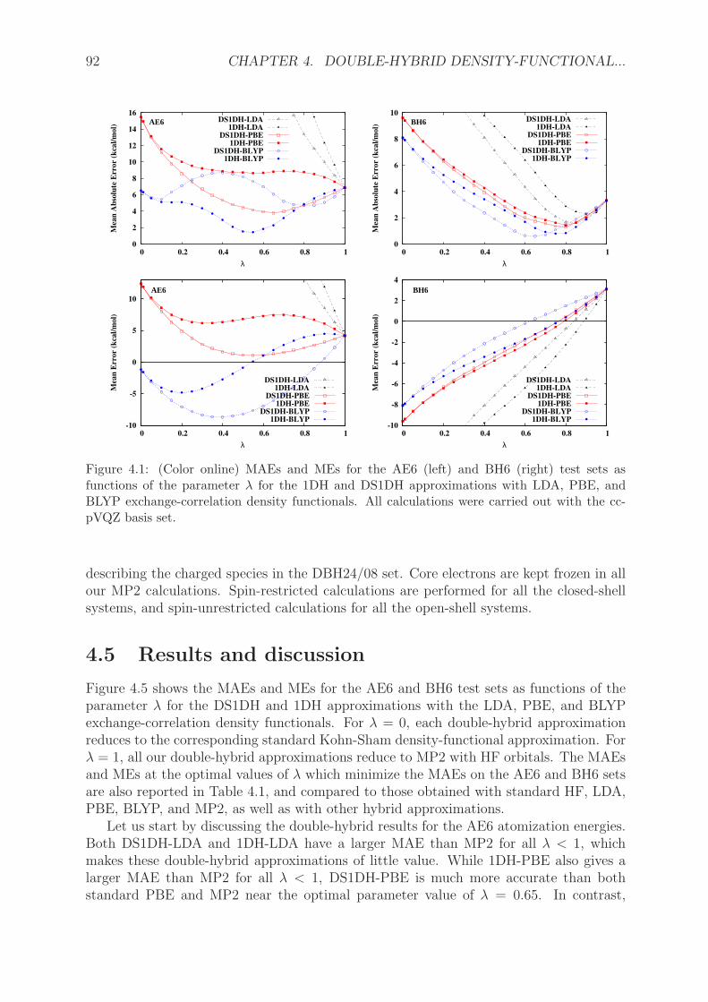
92 CHAPTER 4. DOUBLE-HYBRID DENSITY-FUNCTIONAL...
0
2
4
6
8
10
12
14
16
0 0.2 0.4 0.6 0.8 1
Mea
n A
bso
lute
Err
or
(kca
l/m
ol)
λ
DS1DH-LDA1DH-LDA
DS1DH-PBE1DH-PBE
DS1DH-BLYP1DH-BLYP
AE6
0
2
4
6
8
10
0 0.2 0.4 0.6 0.8 1
Mea
n A
bso
lute
Err
or
(kca
l/m
ol)
λ
DS1DH-LDA1DH-LDA
DS1DH-PBE1DH-PBE
DS1DH-BLYP1DH-BLYP
BH6
-10
-5
0
5
10
0 0.2 0.4 0.6 0.8 1
Mea
n E
rror
(kca
l/m
ol)
λ
DS1DH-LDA1DH-LDA
DS1DH-PBE1DH-PBE
DS1DH-BLYP1DH-BLYP
AE6
-10
-8
-6
-4
-2
0
2
4
0 0.2 0.4 0.6 0.8 1
Mea
n E
rror
(kca
l/m
ol)
λ
DS1DH-LDA1DH-LDA
DS1DH-PBE1DH-PBE
DS1DH-BLYP1DH-BLYP
BH6
Figure 4.1: (Color online) MAEs and MEs for the AE6 (left) and BH6 (right) test sets asfunctions of the parameter λ for the 1DH and DS1DH approximations with LDA, PBE, andBLYP exchange-correlation density functionals. All calculations were carried out with the cc-pVQZ basis set.
describing the charged species in the DBH24/08 set. Core electrons are kept frozen in allour MP2 calculations. Spin-restricted calculations are performed for all the closed-shellsystems, and spin-unrestricted calculations for all the open-shell systems.
4.5 Results and discussion
Figure 4.5 shows the MAEs and MEs for the AE6 and BH6 test sets as functions of theparameter λ for the DS1DH and 1DH approximations with the LDA, PBE, and BLYPexchange-correlation density functionals. For λ = 0, each double-hybrid approximationreduces to the corresponding standard Kohn-Sham density-functional approximation. Forλ = 1, all our double-hybrid approximations reduce to MP2 with HF orbitals. The MAEsand MEs at the optimal values of λ which minimize the MAEs on the AE6 and BH6 setsare also reported in Table 4.1, and compared to those obtained with standard HF, LDA,PBE, BLYP, and MP2, as well as with other hybrid approximations.
Let us start by discussing the double-hybrid results for the AE6 atomization energies.Both DS1DH-LDA and 1DH-LDA have a larger MAE than MP2 for all λ < 1, whichmakes these double-hybrid approximations of little value. While 1DH-PBE also gives alarger MAE than MP2 for all λ < 1, DS1DH-PBE is much more accurate than bothstandard PBE and MP2 near the optimal parameter value of λ = 0.65. In contrast,

4.5. RESULTS AND DISCUSSION 93
Table 4.1: MAEs and MEs (in kcal/mol) on the AE6 and BH6 test sets for several methods.For the single-hybrid DS1H, 1H, PBE1PBE, and B1LYP approximations and the double-hybridDS1DH and 1DH approximations, the results are for the optimal values of λ which minimizethe MAEs of the AE6 and BH6 sets, separately. For the range-separated hybrids, this is therange-separation parameter µ (in bohr−1) which is optimized. All calculations were carried outwith the cc-pVQZ basis set. The reference values [53] are given in the appendix (Table 4.5).
AE6 BH6Method λ or µ MAE ME λ or µ MAE ME
HF 145.1 -145.1 12.2 12.2LDA 76.9 76.9 18.0 -18.0PBE 15.5 12.4 9.61 -9.61BLYP 6.52 -1.18 8.10 -8.10MP2 6.86 4.17 3.32 3.11
Single-hybrid approximations
DS1H-LDA λ = 0.45 5.90 -5.20 λ = 0.50 1.62 -1.621H-LDA λ = 0.45 7.04 1.38 λ = 0.60 1.98 -0.59DS1H-PBE λ = 0.20 5.18 -3.85 λ = 0.45 1.00 0.351H-PBE λ = 0.20 4.43 -2.00 λ = 0.45 0.97 -0.02DS1H-BLYP λ = 0.05 5.71 -3.72 λ = 0.35 1.70 -0.151H-BLYP λ = 0.05 5.62 -3.53 λ = 0.40 1.80 -0.24PBE1PBE λ = 0.30 5.28 -2.06 λ = 0.55 1.22 -0.01B1LYP λ = 0.05 5.52 -3.25 λ = 0.45 1.94 -0.77B3LYP 2.51 -1.95 4.95 -4.95RSHX-PBE(GWS) µ = 0.65 7.78 1.08 µ = 0.55 1.82 -0.33RSHX-PBE(HSE) = LC-ωPBE µ = 0.40 4.57 -1.96 µ = 0.45 1.09 -0.25
Double-hybrid approximations
DS1DH-LDA no minimum∗ λ = 0.85 1.59 0.221DH-LDA no minimum∗ λ = 0.90 2.29 0.27DS1DH-PBE λ = 0.65 3.78 1.30 λ = 0.80 1.32 0.481DH-PBE λ = 0.55† 8.64† 7.06† λ = 0.80 1.42 0.12DS1DH-BLYP λ = 0.80 4.73 -2.52 λ = 0.65 0.60 0.241DH-BLYP λ = 0.55 1.46 0.07 λ = 0.75 0.80 -0.18B2-PLYP 1.39 -1.09 2.21 -2.21RSH-PBE(GWS)+lrMP2 µ = 0.50 3.48 -1.91 µ = 0.70 1.55 0.73∗ There is no minimum for 0 < λ < 1. The global minimum is for λ = 1.0, i.e. MP2.† This is a local minimum. The global minimum is for λ = 1.0, i.e. MP2.
94 CHAPTER 4. DOUBLE-HYBRID DENSITY-FUNCTIONAL...
DS1DH-BLYP appears to be less accurate than 1DH-BLYP. On the AE6 set, the latterleads to the smallest MAE among our one-parameter double-hybrid approximations witha minimal MAE of 1.46 kcal/mol for the optimal parameter λ = 0.55. The B2-PLYPdouble-hybrid gives a similar MAE of 1.39 kcal/mol (though with a ME farther awayfrom zero). In fact, 1DH-BLYP is just an one-parameter version of the B2-PLYP doublehybrid with optimal parameters ax = λ = 0.55 and ac = λ2 ≃ 0.30 very close to theoriginal B2-PLYP parameters ax = 0.53 and ac = 0.27.
The fact that neglecting the density scaling in the correlation functional, Ec[n1/λ] ≈Ec[n] (i.e., going from Eq. (6.3) to Eq. (6.4)), yields a greater accuracy on the AE6 set forthe double-hybrid approximation based on the BLYP functional but worsen the double-hybrid approximation based on the PBE functional can be clarified by looking at the(signed) MEs. It appears that, in both cases, the 1DH approximation always gives amore positive ME in comparison to the DS1DH approximation, at the optimal values ofλ, and in fact also for all λ (not shown). Since DS1DH-PBE gives a positive ME (1.30kcal/mol) at the optimal λ, inherited from the large positive ME of standard PBE (12.4kcal/mol), it follows that neglecting density scaling makes the ME even more positive(7.06 kcal/mol), thus deteriorating the accuracy of this double hybrid. On the contrary,since DS1DH-BLYP gives a negative ME (2.52 kcal/mol) at the optimal λ, inherited fromthe negative ME of standard BLYP (-1.18 kcal/mol), neglecting density scaling makes theME vary in the right direction, reaching a ME of 0.07 kcal/mol and also improving theMAE.
Let us consider now the double-hybrid results for the BH6 barrier heights. The MAEcurves of all the DS1DH and 1DH approximations now display a marked minimum atan intermediate value of λ, thus improving upon both the corresponding standard Kohn-Sham density-functional approximations and MP2. In comparison to AE6, the minimalMAEs for the BH6 set are obtained for larger values of λ, from 0.65 to 0.90, whichis consistent with the commonplace experience that a larger fraction of HF exchangeimproves barrier heights (by decreasing the self-interaction error). For this BH6 set, theDS1DH approximations are found to give smaller MAEs than the 1DH approximationsfor all the three density-functional approximations tested here. The best double-hybridapproximation is DS1DH-BLYP with a minimal MAE of 0.60 kcal/mol at λ = 0.65.The B2-PLYP double-hybrid gives a larger MAE of 2.21 kcal/mol, but it has not beenoptimized for barrier heights.
For each of our three best one-parameter double-hybrid approximations, we have alsodetermined a global optimal value of λ which minimizes the total MAE of the combinedAE6+BH6 set, and which could be used in general applications: λ = 0.65 for DS1DH-PBE giving a total MAE of 2.77 kcal/mol, λ = 0.70 for DS1DH-BLYP giving a totalMAE of 2.94 kcal/mol, and λ = 0.65 for 1DH-BLYP giving a total MAE of 1.75 kcal/mol.Note that the optimal fractions of HF exchange and MP2 correlation in 1DH-BLYP,ax = λ = 0.65 and ac = λ2 ≈ 0.42, roughly reproduce the two parameters of the B2GP-PLYP double hybrid, i.e. ax = 0.65 and ac = 0.36.
For comparison, we have also reported in Table 4.1 the MAEs and MEs obtainedwith the single-hybrid DS1H and 1H approximations, as well as the usual single-hybridfunctionals PBE1PBE [45, 46] and B1LYP [44], both with reoptimization of the fraction ofHF exchange λ, and the standard B3LYP functional [20, 65, 66] without reoptimization ofthe parameters. We have also considered range-separated single-hybrid functionals (alsoknown as long-range corrected functionals [67]), here referred to as RSHX as in Ref. [68],
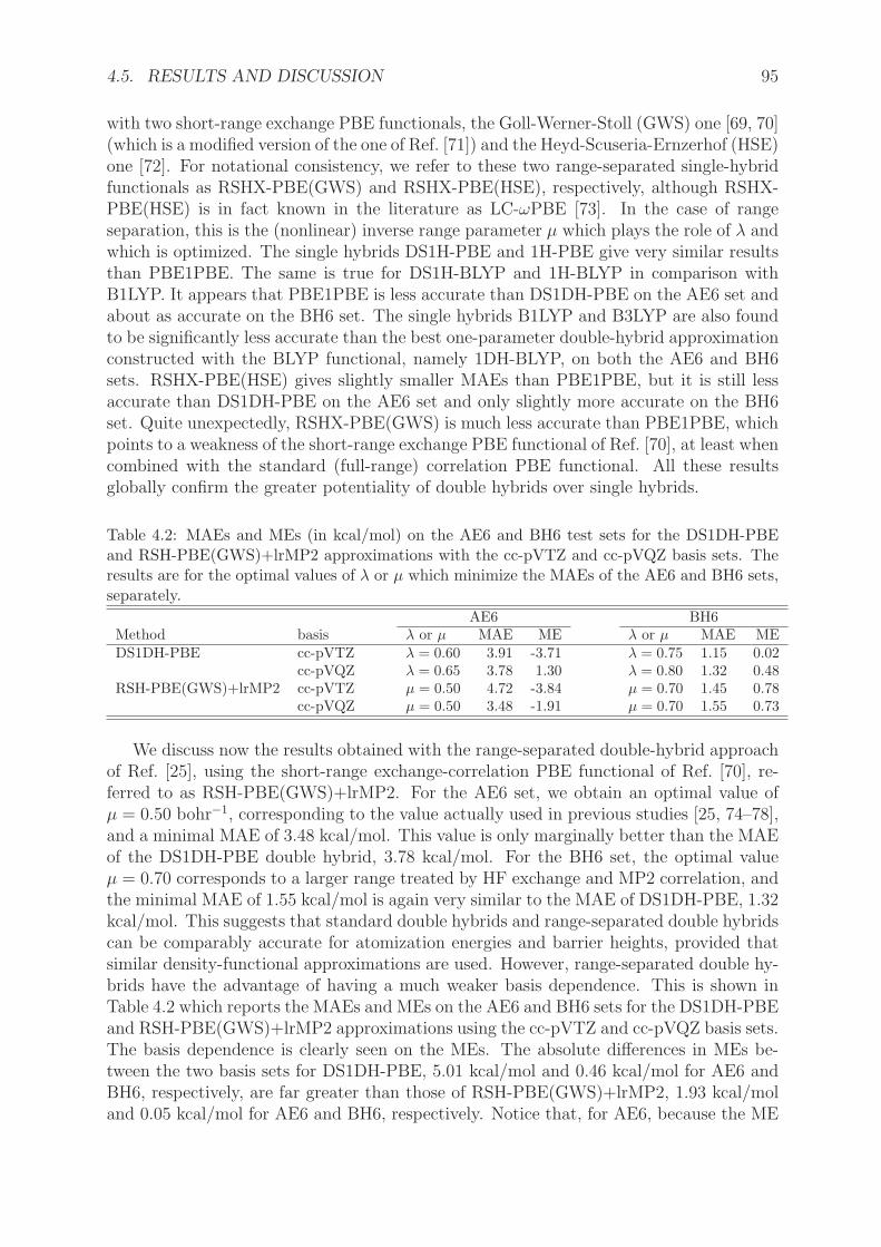
4.5. RESULTS AND DISCUSSION 95
with two short-range exchange PBE functionals, the Goll-Werner-Stoll (GWS) one [69, 70](which is a modified version of the one of Ref. [71]) and the Heyd-Scuseria-Ernzerhof (HSE)one [72]. For notational consistency, we refer to these two range-separated single-hybridfunctionals as RSHX-PBE(GWS) and RSHX-PBE(HSE), respectively, although RSHX-PBE(HSE) is in fact known in the literature as LC-ωPBE [73]. In the case of rangeseparation, this is the (nonlinear) inverse range parameter µ which plays the role of λ andwhich is optimized. The single hybrids DS1H-PBE and 1H-PBE give very similar resultsthan PBE1PBE. The same is true for DS1H-BLYP and 1H-BLYP in comparison withB1LYP. It appears that PBE1PBE is less accurate than DS1DH-PBE on the AE6 set andabout as accurate on the BH6 set. The single hybrids B1LYP and B3LYP are also foundto be significantly less accurate than the best one-parameter double-hybrid approximationconstructed with the BLYP functional, namely 1DH-BLYP, on both the AE6 and BH6sets. RSHX-PBE(HSE) gives slightly smaller MAEs than PBE1PBE, but it is still lessaccurate than DS1DH-PBE on the AE6 set and only slightly more accurate on the BH6set. Quite unexpectedly, RSHX-PBE(GWS) is much less accurate than PBE1PBE, whichpoints to a weakness of the short-range exchange PBE functional of Ref. [70], at least whencombined with the standard (full-range) correlation PBE functional. All these resultsglobally confirm the greater potentiality of double hybrids over single hybrids.
Table 4.2: MAEs and MEs (in kcal/mol) on the AE6 and BH6 test sets for the DS1DH-PBEand RSH-PBE(GWS)+lrMP2 approximations with the cc-pVTZ and cc-pVQZ basis sets. Theresults are for the optimal values of λ or µ which minimize the MAEs of the AE6 and BH6 sets,separately.
AE6 BH6Method basis λ or µ MAE ME λ or µ MAE MEDS1DH-PBE cc-pVTZ λ = 0.60 3.91 -3.71 λ = 0.75 1.15 0.02
cc-pVQZ λ = 0.65 3.78 1.30 λ = 0.80 1.32 0.48RSH-PBE(GWS)+lrMP2 cc-pVTZ µ = 0.50 4.72 -3.84 µ = 0.70 1.45 0.78
cc-pVQZ µ = 0.50 3.48 -1.91 µ = 0.70 1.55 0.73
We discuss now the results obtained with the range-separated double-hybrid approachof Ref. [25], using the short-range exchange-correlation PBE functional of Ref. [70], re-ferred to as RSH-PBE(GWS)+lrMP2. For the AE6 set, we obtain an optimal value ofµ = 0.50 bohr−1, corresponding to the value actually used in previous studies [25, 74–78],and a minimal MAE of 3.48 kcal/mol. This value is only marginally better than the MAEof the DS1DH-PBE double hybrid, 3.78 kcal/mol. For the BH6 set, the optimal valueµ = 0.70 corresponds to a larger range treated by HF exchange and MP2 correlation, andthe minimal MAE of 1.55 kcal/mol is again very similar to the MAE of DS1DH-PBE, 1.32kcal/mol. This suggests that standard double hybrids and range-separated double hybridscan be comparably accurate for atomization energies and barrier heights, provided thatsimilar density-functional approximations are used. However, range-separated double hy-brids have the advantage of having a much weaker basis dependence. This is shown inTable 4.2 which reports the MAEs and MEs on the AE6 and BH6 sets for the DS1DH-PBEand RSH-PBE(GWS)+lrMP2 approximations using the cc-pVTZ and cc-pVQZ basis sets.The basis dependence is clearly seen on the MEs. The absolute differences in MEs be-tween the two basis sets for DS1DH-PBE, 5.01 kcal/mol and 0.46 kcal/mol for AE6 andBH6, respectively, are far greater than those of RSH-PBE(GWS)+lrMP2, 1.93 kcal/moland 0.05 kcal/mol for AE6 and BH6, respectively. Notice that, for AE6, because the ME
96 CHAPTER 4. DOUBLE-HYBRID DENSITY-FUNCTIONAL...
of DS1DH-PBE changes sign when going from the cc-pVTZ to the cc-pVQZ basis, thevariation of the corresponding MAE turns out to be fortuitously small, and so at firstglance this hides the large basis dependence of DS1DH-PBE. Note also that the optimalvalue of the parameter λ is more dependent on the basis than the range-separation pa-rameter µ. For RSH-PBE(GWS)+lrMP2, we have determined a global optimal value ofµ = 0.58 which minimizes the total MAE of the combined AE6+BH6 set, giving a totalMAE of 2.63 kcal/mol. In the appendix, the MAEs and MEs at the optimal values of λare recalculated using more recent reference energy values (Table 4.5) [79] and reportedin Table 4.6. The small deviation between the reference values used in the Tables 4.1 and4.6 does not affect the aforementioned conclusions.
Finally, we compare our best one-parameter double-hybrid approximation 1DH-BLYP(with the optimal parameter λ = 0.65), the standard double hybrid B2-PLYP and therange-separated double hybrid RSH-PBE(GWS)+lrMP2 (with the optimal parameterµ = 0.58) on larger benchmark sets, the 49 atomization energies of the set of Ref. [57](Table 4.3) and the DBH24/08 set of 24 reaction barrier heights (Table 4.4). For the set ofatomization energies in Table 4.3, 1DH-BLYP is somewhat more accurate than B2-PLYP,with a slightly smaller MAE (1.4 vs. 1.6 kcal/mol) and a significantly smaller ME (0.3 vs.-1.0 kcal/mol). By contrast, the range-separated double hybrid RSH-PBE(GWS)+lrMP2gives a MAE as large as 6.5 kcal/mol. This is most likely due to the fact that theshort-range exchange-correlation functional used is based on PBE. Indeed, the previousresults for the AE6 set (Table 4.1) show that PBE is a much less accurate functionalthan BLYP for atomization energies. Unfortunately, there is no short-range exchange-correlation functional based on BLYP available yet. In fact, it is a practical advantageof the double hybrids without range separation that do not require development of newdensity functional approximations. The range-separated coupled-cluster calculations onan extension of the G2/97 set of atomization energies by Goll et al. [70] show that a betteraccuracy can be reached by using a short-range exchange-correlation functional based onthe TPSS functional [80]. For the reaction barrier heights of Table 4.4, 1DH-BLYP is onaverage more accurate than B2-PLYP, with a smaller MAE (1.4 vs. 2.0 kcal/mol) andan even smaller ME (-0.8 vs. -1.8 kcal/mol). The range-separated double hybrid RSH-PBE(GWS)+lrMP2 performs about equally well for the barrier heights, with a MAE of2.1 kcal/mol and a ME of 1.1 kcal/mol.
4.6 Conclusions
We have rigorously derived a class of double-hybrid approximations, combining HF ex-change and MP2 correlation with a semilocal exchange-correlation density functional.These double-hybrid approximations contain only one empirical parameter and uses adensity-scaled correlation energy functional. Neglecting density scaling leads to an one-parameter version of the standard double-hybrid approximations. Calculations on therepresentative test set of atomization energies AE6 show that in practice neglecting den-sity scaling in an approximate functional can either make the double-hybrid method lessaccurate (case of PBE) or more accurate (case of BLYP). Neglecting density scaling alwaysleads to a less accurate double-hybrid method on the representative test set of reactionbarrier heights BH6, for all the density-functional approximations tested here. Our bestone-parameter double-hybrid approximation, 1DH-BLYP, roughly reproduces the two pa-
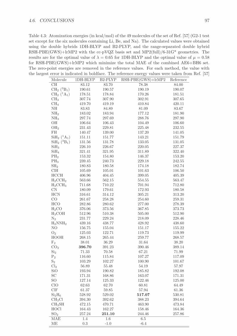
4.6. CONCLUSIONS 97
Table 4.3: Atomization energies (in kcal/mol) of the 49 molecules of the set of Ref. [57] (G2-1 testset except for the six molecules containing Li, Be, and Na). The calculated values were obtainedusing the double hybrids 1DH-BLYP and B2-PLYP, and the range-separated double hybridRSH-PBE(GWS)+lrMP2 with the cc-pVQZ basis set and MP2(full)/6-31G* geometries. Theresults are for the optimal value of λ = 0.65 for 1DH-BLYP and the optimal value of µ = 0.58for RSH-PBE(GWS)+lrMP2 which minimize the total MAE of the combined AE6+BH6 set.The zero-point energies are removed in the reference values. For each method, the value withthe largest error is indicated in boldface. The reference energy values were taken from Ref. [57]
Molecule 1DH-BLYP B2-PLYP RSH-PBE(GWS)+lrMP2 ReferenceCH 83.12 83.70 78.38 84.00CH2 (3B1) 190.61 190.57 190.19 190.07CH2 (1A1) 178.51 178.84 170.26 181.51CH3 307.74 307.90 302.91 307.65CH4 419.70 419.19 410.84 420.11NH 83.83 84.89 81.09 83.67NH2 183.02 183.94 177.12 181.90NH3 297.74 297.69 288.76 297.90OH 106.64 106.43 104.49 106.60OH2 231.43 229.81 225.48 232.55FH 140.47 139.00 137.20 141.05SiH2 (1A1) 151.11 151.77 143.21 151.79SiH2 (3B1) 131.56 131.78 133.05 131.05SiH3 226.10 226.67 220.05 227.37SiH4 321.41 321.95 311.89 322.40PH2 153.32 154.80 146.37 153.20PH3 239.45 240.73 229.18 242.55SH2 180.83 180.58 174.18 182.74ClH 105.69 105.01 101.63 106.50HCCH 406.96 404.45 399.05 405.39H2CCH2 563.66 562.15 554.55 563.47H3CCH3 711.68 710.22 701.94 712.80CN 180.09 179.61 172.93 180.58HCN 316.61 314.12 305.21 313.20CO 261.67 258.28 254.60 259.31HCO 282.86 280.62 277.00 278.39H2CO 376.06 373.56 367.85 373.73H3COH 512.96 510.38 505.00 512.90N2 231.77 229.24 218.09 228.46H2NNH2 439.16 438.77 428.92 438.60NO 156.75 155.04 151.17 155.22O2 125.03 122.71 119.73 119.99HOOH 268.15 265.44 259.77 268.57F2 38.01 36.29 31.64 38.20CO2 396.70 391.23 390.46 389.14Si2 71.33 70.58 67.21 71.99P2 116.60 115.84 107.27 117.09S2 103.29 102.27 100.90 101.67Cl2 56.89 55.48 54.19 57.97SiO 193.94 190.82 185.82 192.08SC 171.31 168.86 163.07 171.31SO 127.14 125.33 122.46 125.00ClO 62.63 62.70 60.81 64.49ClF 61.37 59.85 57.94 61.36Si2H6 528.92 529.02 517.07 530.81CH3Cl 394.30 392.62 388.23 394.64CH3SH 472.15 470.71 463.90 473.84HOCl 164.43 162.27 158.46 164.36SO2 257.24 251.10 244.46 257.86MAE 1.4 1.6 6.5ME 0.3 -1.0 -6.4
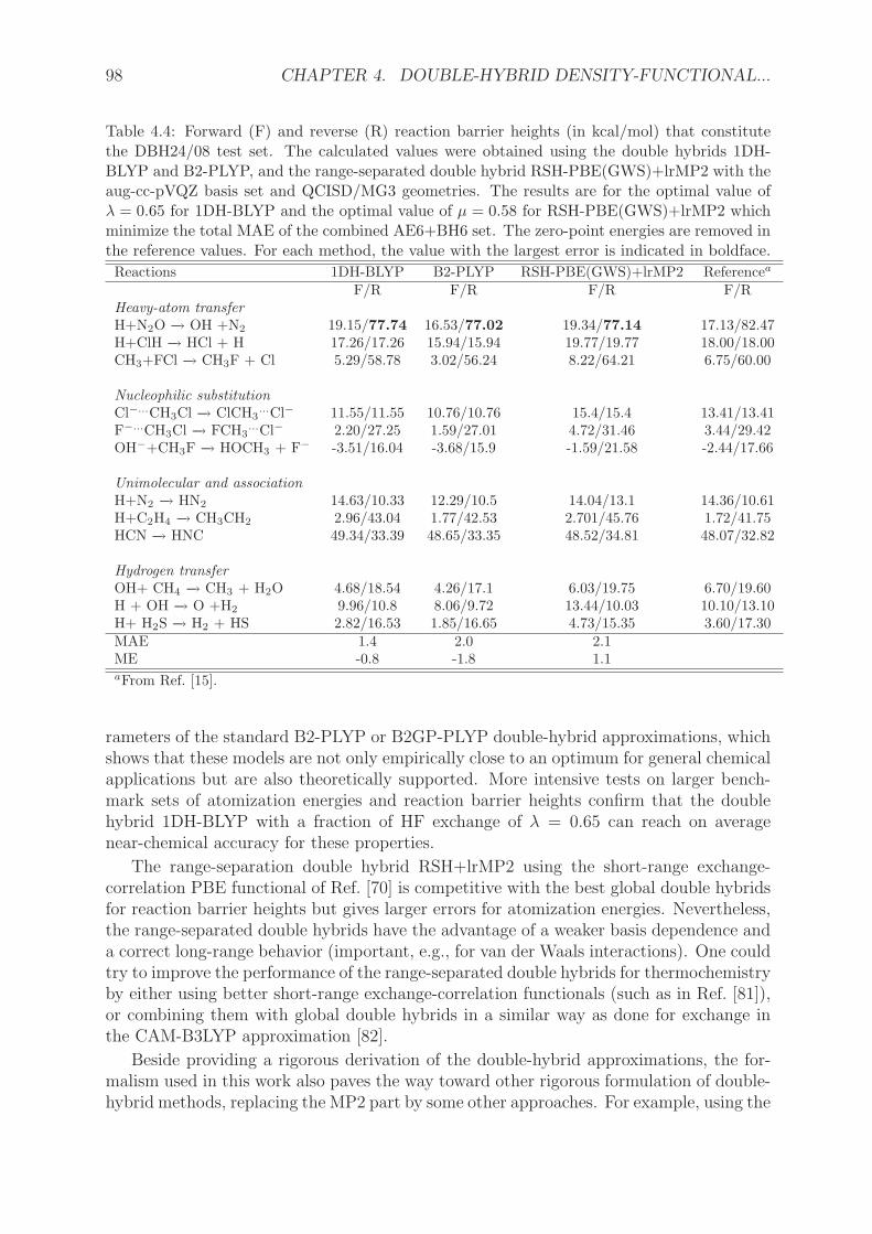
98 CHAPTER 4. DOUBLE-HYBRID DENSITY-FUNCTIONAL...
Table 4.4: Forward (F) and reverse (R) reaction barrier heights (in kcal/mol) that constitutethe DBH24/08 test set. The calculated values were obtained using the double hybrids 1DH-BLYP and B2-PLYP, and the range-separated double hybrid RSH-PBE(GWS)+lrMP2 with theaug-cc-pVQZ basis set and QCISD/MG3 geometries. The results are for the optimal value ofλ = 0.65 for 1DH-BLYP and the optimal value of µ = 0.58 for RSH-PBE(GWS)+lrMP2 whichminimize the total MAE of the combined AE6+BH6 set. The zero-point energies are removed inthe reference values. For each method, the value with the largest error is indicated in boldface.
Reactions 1DH-BLYP B2-PLYP RSH-PBE(GWS)+lrMP2 Referencea
F/R F/R F/R F/RHeavy-atom transfer
H+N2O −→ OH +N2 19.15/77.74 16.53/77.02 19.34/77.14 17.13/82.47H+ClH −→ HCl + H 17.26/17.26 15.94/15.94 19.77/19.77 18.00/18.00CH3+FCl −→ CH3F + Cl 5.29/58.78 3.02/56.24 8.22/64.21 6.75/60.00
Nucleophilic substitution
Cl−...CH3Cl −→ ClCH3...Cl− 11.55/11.55 10.76/10.76 15.4/15.4 13.41/13.41
F−...CH3Cl −→ FCH3...Cl− 2.20/27.25 1.59/27.01 4.72/31.46 3.44/29.42
OH−+CH3F −→ HOCH3 + F− -3.51/16.04 -3.68/15.9 -1.59/21.58 -2.44/17.66
Unimolecular and association
H+N2 −→ HN2 14.63/10.33 12.29/10.5 14.04/13.1 14.36/10.61H+C2H4 −→ CH3CH2 2.96/43.04 1.77/42.53 2.701/45.76 1.72/41.75HCN −→ HNC 49.34/33.39 48.65/33.35 48.52/34.81 48.07/32.82
Hydrogen transfer
OH+ CH4 −→ CH3 + H2O 4.68/18.54 4.26/17.1 6.03/19.75 6.70/19.60H + OH −→ O +H2 9.96/10.8 8.06/9.72 13.44/10.03 10.10/13.10H+ H2S −→ H2 + HS 2.82/16.53 1.85/16.65 4.73/15.35 3.60/17.30MAE 1.4 2.0 2.1ME -0.8 -1.8 1.1aFrom Ref. [15].
rameters of the standard B2-PLYP or B2GP-PLYP double-hybrid approximations, whichshows that these models are not only empirically close to an optimum for general chemicalapplications but are also theoretically supported. More intensive tests on larger bench-mark sets of atomization energies and reaction barrier heights confirm that the doublehybrid 1DH-BLYP with a fraction of HF exchange of λ = 0.65 can reach on averagenear-chemical accuracy for these properties.
The range-separation double hybrid RSH+lrMP2 using the short-range exchange-correlation PBE functional of Ref. [70] is competitive with the best global double hybridsfor reaction barrier heights but gives larger errors for atomization energies. Nevertheless,the range-separated double hybrids have the advantage of a weaker basis dependence anda correct long-range behavior (important, e.g., for van der Waals interactions). One couldtry to improve the performance of the range-separated double hybrids for thermochemistryby either using better short-range exchange-correlation functionals (such as in Ref. [81]),or combining them with global double hybrids in a similar way as done for exchange inthe CAM-B3LYP approximation [82].
Beside providing a rigorous derivation of the double-hybrid approximations, the for-malism used in this work also paves the way toward other rigorous formulation of double-hybrid methods, replacing the MP2 part by some other approaches. For example, using the
4.7. APPENDIX 99
random phase approximation would generate a hybrid method similar to the one proposedin Ref. [83], or using a configuration-interaction or multiconfiguration self-consistent-fieldapproach would lead to a hybrid method capable of dealing with static electron correlation,in a similar but alternative way to the range-separated approaches [84–86].
Acknowledgments
K.S. would like to thank Prof. I. Othman (AEC) for his support. J.T. and A.S. ac-knowledge ANR (contract Wademecom 07-BLAN-0272). We also thank J. G. Angyan fordiscussions.
4.7 Appendix
4.7.1 Density-scaled correlation energy and potential
In this appendix, we give explicit expressions for the density-scaled correlation energyfunctional which appears in Eq. (6.3)
Eλc [n] = λ2Ec[n1/λ], (4.16)
and its associated potential
vλc [n](r) =
δEλc [n]
δn(r). (4.17)
4.7.1.1 Density-scaled local-density approximations
For local-density approximations (LDA),
Ec,LDA[n] =
∫
ec(n(r))dr, (4.18)
where ec is the energy density, the density-scaled correlation energy is obtained as
Eλc,LDA[n] = λ2
∫
ec
(
n1/λ(r))
dr
= λ2
∫
ec
(
n(r/λ)/λ3)
dr
= λ5
∫
ec
(
n(r)/λ3)
dr, (4.19)
where the coordinate transformation r → λr has been used. The associated potential issimply
vλc,LDA[n](r) = λ2dec
dn
(
n(r)/λ3)
.
(4.20)

100 CHAPTER 4. DOUBLE-HYBRID DENSITY-FUNCTIONAL...
4.7.1.2 Density-scaled generalized-gradient approximations
For generalized-gradient approximations (GGA), usually written as a function of the den-sity and the square of density gradient norm |∇rn(r)|2,
Ec,GGA[n] =
∫
ec
(
n(r), |∇rn(r)|2)
dr, (4.21)
the density-scaled correlation energy is
Eλc,GGA[n] = λ2
∫
ec
(
n1/λ(r),∣
∣∇rn1/λ(r)∣
∣
2)
dr,
= λ2
∫
ec
(
n(r/λ)/λ3, |∇rn(r/λ)|2 /λ6)
dr,
= λ5
∫
ec
(
n(r)/λ3, |∇rn(r)|2 /λ8)
dr, (4.22)
where the coordinate transformation r → λr, and consequently ∇r → ∇λr = ∇r/λ, hasbeen used. The associated potential is
vλc,GGA[n](r) = λ2 ∂ec
∂n
(
n(r)/λ3, |∇rn(r)|2 /λ8)
− 2∇r ·[
1
λ3
∂ec
∂ |∇n|2(
n(r)/λ3, |∇rn(r)|2 /λ8)
∇rn(r)
]
.
(4.23)
The same scaling relations apply for spin-dependent functionals Ec[n↑, n↓], i.e. thescaling of the spin densities n↑ and n↓ is the same as the scaling of the total density n,and the scaling of the spin-density gradients |∇n↑|2, |∇n↓|2, and ∇n↑ · ∇n↓ is the sameas the scaling of total density gradient |∇n|2.
4.7.2 Theoretical reference values for the AE6 and BH6 testsets
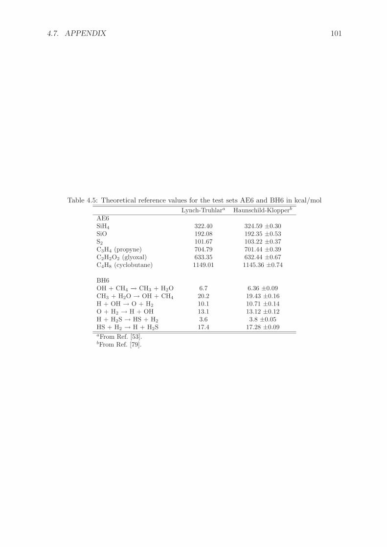
4.7. APPENDIX 101
Table 4.5: Theoretical reference values for the test sets AE6 and BH6 in kcal/mol
Lynch-Truhlara Haunschild-Klopperb
AE6SiH4 322.40 324.59 ±0.30SiO 192.08 192.35 ±0.53S2 101.67 103.22 ±0.37C3H4 (propyne) 704.79 701.44 ±0.39C2H2O2 (glyoxal) 633.35 632.44 ±0.67C4H8 (cyclobutane) 1149.01 1145.36 ±0.74
BH6OH + CH4 −→ CH3 + H2O 6.7 6.36 ±0.09CH3 + H2O → OH + CH4 20.2 19.43 ±0.16H + OH → O + H2 10.1 10.71 ±0.14O + H2 → H + OH 13.1 13.12 ±0.12H + H2S → HS + H2 3.6 3.8 ±0.05HS + H2 → H + H2S 17.4 17.28 ±0.09aFrom Ref. [53].bFrom Ref. [79].

102 CHAPTER 4. DOUBLE-HYBRID DENSITY-FUNCTIONAL...
Table 4.6: MAEs and MEs (in kcal/mol) on the AE6 and BH6 test sets for several methods.For the single-hybrid DS1H, 1H, PBE1PBE, and B1LYP approximations and the double-hybridDS1DH and 1DH approximations, the results are for the optimal values of λ which minimizethe MAEs of the AE6 and BH6 sets, separately. For the range-separated hybrids, this is therange-separation parameter µ (in bohr−1) which is optimized. All calculations were carried outwith the cc-pVQZ basis set. The reference values were taken from Ref. [79].
AE6 BH6Method λ or µ MAE ME λ or µ MAE ME
HF 144.4 -144.4 12.3 12.3LDA 77.6 77.6 17.9 -17.9PBE 16.9 13.0 9.54 -9.54BLYP 5.94 -0.53 8.04 -8.04MP2 8.24 4.82 3.34 3.18
Single-hybrid approximations
DS1H-LDA λ = 0.45 6.47 -4.55 λ = 0.50 1.67 -1.551H-LDA λ = 0.45 8.00 2.03 λ = 0.65 2.10 -1.00DS1H-PBE λ = 0.20 4.67 -3.20 λ = 0.45 0.92 0.421H-PBE λ = 0.20 5.90 -1.36 λ = 0.45 0.94 0.05DS1H-BLYP λ = 0.05 4.84 -3.07 λ = 0.35 1.78 -0.091H-BLYP λ = 0.05 4.73 -2.90 λ = 0.40 1.88 -0.18PBE1PBE λ = 0.30 6.44 -1.41 λ = 0.55 1.20 0.05B1LYP λ = 0.05 4.61 -2.60 λ = 0.45 2.03 -0.71B3LYP 1.97 -1.30 4.88 -4.88RSHX-PBE(GWS) µ = 0.65 9.73 1.73 µ = 0.55 1.85 -0.26RSHX-PBE(HSE) = LC-ωPBE µ = 0.45 5.91 -3.42 µ = 0.45 0.91 -0.14
Double-hybrid approximations
DS1DH-LDA no minimum∗ λ = 0.85 1.51 0.291DH-LDA no minimum∗ λ = 0.90 2.21 0.34DS1DH-PBE λ = 0.65 5.25 1.95 λ = 0.75 1.14 -0.051DH-PBE λ = 0.55† 10.1† 7.71† λ = 0.80 1.34 0.18DS1DH-BLYP λ = 0.75 4.37 -3.21 λ = 0.65 0.36 0.311DH-BLYP λ = 0.55 1.77 0.72 λ = 0.75 0.51 -0.11B2-PLYP 1.72 -0.44 2.14 -2.14RSH-PBE(GWS)+lrMP2 µ = 0.58 3.38 -2.79 µ = 0.58 1.42 -0.2∗ There is no minimum for 0 < λ < 1. The global minimum is for λ = 1.0, i.e. MP2.† This is a local minimum. The global minimum is for λ = 1.0, i.e. MP2.

Bibliography
[1] P. Hohenberg and W. Kohn, Phys. Rev. 136, B 864 (1964).
[2] W. Kohn and L. J. Sham, Phys. Rev. 140, A1133 (1965).
[3] W. Kohn, Rev. Mod. Phys. 71, 1253 (1999).
[4] S. Kummel and L. Kronik, Rev. Mod. Phys. 80, 3 (2008).
[5] S. Grimme, J. Chem. Phys. 124, 034108 (2006).
[6] A. D. Becke, Phys. Rev. A 38, 3098 (1988).
[7] C. Lee, W. Yang and R. G. Parr, Phys. Rev. B 37, 785 (1988).
[8] T. Schwabe and S. Grimme, Phys. Chem. Chem. Phys. 8, 4398 (2006).
[9] C. Adamo and V. Barone, J. Chem. Phys. 108, 664 (1998).
[10] D. C. Graham, A. S. Menon, L. Goerigk, S. Grimme and L. Radom, J. Phys. Chem.A 113, 9861 (2009).
[11] A. Tarnopolsky, A. Karton, R. Sertchook, D. Vuzman and J. M. L. Martin, J. Phys.Chem. A 112, 3 (2008).
[12] A. Karton, A. Tarnopolsky, J.-F. Lamere, G. C. Schatz and J. M. L. Martin, J. Phys.Chem. A 112, 12868 (2008).
[13] Y. Zhao, B. J. Lynch and D. G. Truhlar, J. Phys. Chem. A 108, 4786 (2004).
[14] Y. Zhao, B. J. Lynch and D. G. Truhlar, Phys. Chem. Chem. Phys. 7, 43 (2005).
[15] J. Zheng, Y. Zhao and D. G. Truhlar, J. Chem. Theory Comput. 5, 808 (2009).
[16] J. C. Sancho-Garcıa and A. J. Perez-Jimenez, J. Chem. Phys. 131, 084108 (2009).
[17] Y. Zhang, X. Xu and W. A. Goddard III, Proc. Natl. Acad. Sci. U.S.A. 106, 4963(2009).
[18] I. Y. Zhang, Y. Luo and X. Xu, J. Chem. Phys. 132, 194105 (2010).
[19] I. Y. Zhang, Y. Luo and X. Xu, J. Chem. Phys. 133, 104105 (2010).
[20] A. D. Becke, J. Chem. Phys. 98, 5648 (1993).
103
104 BIBLIOGRAPHY
[21] T. Schwabe and S. Grimme, Phys. Chem. Chem. Phys. 9, 3397 (2007).
[22] T. Benighaus, R. A. DiStasio Jr., R. C. Lochan, J.-D. Chai and M. Head-Gordon, J.Phys. Chem. A 112, 2702 (2008).
[23] J. Harris, Phys. Rev. A 29, 1648 (1984).
[24] A. Gorling and M. Levy, Phys. Rev. B 47, 13105 (1993).
[25] J. G. Angyan, I. C. Gerber, A. Savin and J. Toulouse, Phys. Rev. A 72, 012510(2005).
[26] J. Toulouse, F. Colonna and A. Savin, Phys. Rev. A 70, 062505 (2004).
[27] M. Levy and J. P. Perdew, Phys. Rev. A 32, 2010 (1985).
[28] M. Levy, W. Yang and R. G. Parr, J. Chem. Phys. 83, 2334 (1985).
[29] M. Levy, Phys. Rev. A 43, 4637 (1991).
[30] M. Levy, The Single-Particle Density in Physics and Chemistry, eds. N.H. March
and B.M. Deb (Academic Press, London, 1987).
[31] M. Levy and J. P. Perdew, Phys. Rev. B 48, 11638 (1993).
[32] A. D. Becke, J. Chem. Phys. 98, 1372 (1993).
[33] M. Levy, N. H. March and N. C. Handy, J. Chem. Phys. 104, 1989 (1996).
[34] M. Ernzerhof, Chem. Phys. Lett. 263, 499 (1996).
[35] O. V. Gritsenko, R. van Leeuwen, and E. J. Baerends, Int. J. Quantum Chem.:Quantum Chem. Symp. 30, 1375 (1996).
[36] K. Burke, M. Ernzerhof and J. P. Perdew, Chem. Phys. Lett. 265, 115 (1997).
[37] M. Ernzerhof, J. P. Perdew and K. Burke, Int. J. Quantum Chem. 64, 285 (1997).
[38] M. Seidl, J. P. Perdew and M. Levy, Phys. Rev. A 59, 51 (1999).
[39] A. Seidl, J. P. Perdew and S. Kurth, Phys. Rev. A 62, 012502 (2000).
[40] M. Siedl, J. P. Perdew and S. Kurth, Phys. Rev. Lett. 84, 5070 (2000).
[41] P. Mori-Sanchez, A. J. Cohen and W. Yang, J. Chem. Phys. 124, 091102 (2006).
[42] A. J. Cohen, P. Mori-Sanchez and W. Yang, J. Chem. Phys. 126, 191109 (2007).
[43] A. J. Cohen, P. Mori-Sanchez and W. Yang, J. Chem. Phys. 127, 034101 (2007).
[44] C. Adamo and V. Barone, Chem. Phys. Lett. 274, 242 (1997).
[45] M. Ernzerhof and G. E. Scuseria, J. Chem. Phys. 110, 5029 (1999).
[46] C. Adamo and V. Barone, J. Chem. Phys. 101, 6158 (1999).
BIBLIOGRAPHY 105
[47] E. Fromager and H. J. A. Jensen, Phys. Rev. A 78, 022504 (2008).
[48] J. G. Angyan, Phys. Rev. A 78, 022510 (2008).
[49] M. J. Frisch, G. W. Trucks, H. B. Schlegel, G. E. Scuseria, M. A. Robb, J. R.Cheeseman, G. Scalmani, V. Barone, B. Mennucci, G. A. Petersson, H. Nakatsuji,M. Caricato, X. Li, H. P. Hratchian, A. F. Izmaylov, J. Bloino, G. Zheng, J. L.Sonnenberg, M. Hada, M. Ehara, K. Toyota, R. Fukuda, J. Hasegawa, M. Ishida,T. Nakajima, Y. Honda, O. Kitao, H. Nakai, T. Vreven, J. A. Montgomery, Jr.,J. E. Peralta, F. Ogliaro, M. Bearpark, J. J. Heyd, E. Brothers, K. N. Kudin, V. N.Staroverov, R. Kobayashi, J. Normand, K. Raghavachari, A. Rendell, J. C. Burant,S. S. Iyengar, J. Tomasi, M. Cossi, N. Rega, J. M. Millam, M. Klene, J. E. Knox,J. B. Cross, V. Bakken, C. Adamo, J. Jaramillo, R. Gomperts, R. E. Stratmann,O. Yazyev, A. J. Austin, R. Cammi, C. Pomelli, J. W. Ochterski, R. L. Martin,K. Morokuma, V. G. Zakrzewski, G. A. Voth, P. Salvador, J. J. Dannenberg, S. Dap-prich, A. D. Daniels, A. Farkas, J. B. Foresman, J. V. Ortiz, J. Cioslowski and D. J.Fox, Gaussian 09 Revision A.1, Gaussian Inc. Wallingford CT 2009.
[50] H.-J. Werner, P. J. Knowles, R. Lindh, F. R. Manby, M. Schutz et al., MOLPRO,version 2008.2, a package of ab initio programs (2008), see www.molpro.net.
[51] S. J. Vosko, L. Wilk and M. Nusair, Can. J. Phys. 58, 1200 (1980).
[52] J. P. Perdew, K. Burke and M. Ernzerhof, Phys. Rev. Lett. 77, 3865 (1996).
[53] B. J. Lynch and D. G. Truhlar, J. Phys. Chem. A 107, 8996 (2003).
[54] P. L. Fast, M. L. Sanchez and D. G. Truhlar, Chem. Phys. Lett. 306, 407 (1999).
[55] L. A. Curtiss, P. C. Redfern, K. Raghavachari, V. Rassolov and J. A. Pople, J. Chem.Phys. 110, 4703 (1999).
[56] B. Lynch, Y. Zhao and D. Truhlar, http://comp.chem.umn.edu/database.
[57] P. L. Fast, J. Corchado, M. L. Sanchez and D. G. Truhlar, J. Phys. Chem. A 103,3139 (1999).
[58] L. A. Curtiss, K. Raghavachari, G. W. Trucks and J. A. Pople, J. Chem. Phys. 94,7221 (1991).
[59] L. A. Curtiss, K. Raghavachari, P. C. Redfern and J. A. Pople, J. Chem. Phys. 106,1063 (1997).
[60] J. Zheng, Y. Zhao and D. G. Truhlar, J. Chem. Theory Comput. 3, 569 (2007).
[61] T. H. Dunning, J. Chem. Phys. 90, 1007 (1989).
[62] R. A. Kendall, T. H. Dunning and R. J. Harrison, J. Chem. Phys. 96, 6796 (1992).
[63] D. Woon and T. Dunning, J. Chem. Phys. 98, 1358 (1993).
[64] D. Woon and T. Dunning, J. Chem. Phys. 100, 2975 (1994).
106 BIBLIOGRAPHY
[65] V. Barone and C. Adamo, Chem. Phys. Lett. 224, 432 (1994).
[66] P. J. Stephens, F. J. Devlin, C. F. Chabalowski and M. J. Frisch, J. Phys. Chem. 98,11623 (1994).
[67] H. Iikura, T. Tsuneda, T. Yanai and K. Hirao, J. Chem. Phys. 115, 3540 (2001).
[68] I. C. Gerber and J. G. Angyan, Chem. Phys. Lett. 415, 100 (2005).
[69] E. Goll, H.-J. Werner and H. Stoll, Phys. Chem. Chem. Phys. 7, 3917 (2005).
[70] E. Goll, H.-J. Werner, H. Stoll, T. Leininger, P. Gori-Giorgi and A. Savin, Chem.Phys. 329, 276 (2006).
[71] J. Toulouse, F. Colonna and A. Savin, J. Chem. Phys. 122, 014110 (2005).
[72] J. Heyd, G. E. Scuseria and M. Ernzerhof, J. Chem. Phys. 118, 8207 (2003).
[73] O. A. Vydrov and G. E. Scuseria, J. Chem. Phys. 125, 234109 (2006).
[74] I. C. Gerber and J. G. Angyan, Chem. Phys. Lett. 416, 370 (2005).
[75] I. C. Gerber and J. G. Angyan, J. Chem. Phys. 126, 044103 (2007).
[76] E. Goll, T. Leininger, F. R. Manby, A. Mitrushchenkov, H.-J. Werner and H. Stoll,Phys. Chem. Chem. Phys. 10, 3353 (2008).
[77] W. Zhu, J. Toulouse, A. Savin and J. G. Angyan, J. Chem. Phys. 132, 244108 (2010).
[78] J. Toulouse, W. Zhu, J. G. Angyan and A. Savin, Phys. Rev. A 82, 032502 (2010).
[79] R. Haunschild and W. Klopper, Theor. Chem. Acc. 131, 1112 (2012).
[80] J. Tao, J. P. Perdew, V. N. Staroverov and G. E. Scuseria, Phys. Rev. Lett. 91,146401 (2003).
[81] E. Goll, M. Ernst, F. Moegle-Hofacker and H. Stoll, J. Chem. Phys. 130, 234112(2009).
[82] T. Yanai, D. P.Tew and N. C. Handy, Chem. Phys. Lett. 393, 51 (2004).
[83] A. Ruzsinszky, J. P. Perdew and G. I. Csonka, J. Chem. Theory Comput. 6, 127(2010).
[84] T. Leininger, H. Stoll, H.-J. Werner and A. Savin, Chem. Phys. Lett. 275, 151 (1997).
[85] R. Pollet, A. Savin, T. Leininger and H. Stoll, J. Chem. Phys. 116, 1250 (2002).
[86] E. Fromager, J. Toulouse and H. J. A. Jensen, J. Chem. Phys. 126, 074111 (2007).

Chapter 5
Rationale for a new class ofdouble-hybrid approximations indensity-functional theory
This chapter, written in collaboration with J. Toulouse, Eric Bremond and Carlo Adamo,has been published in Journal of Chemical Physics [J. Chem. Phys. 135, 101102 (2011)].
5.1 Abstract
We provide a rationale for a new class of double-hybrid approximations introduced byBremond and Adamo [J. Chem. Phys. 135, 024106 (2011)] which combine an exchange-correlation density functional with Hartree-Fock exchange weighted by λ and second-orderMøller-Plesset (MP2) correlation weighted by λ3. We show that this double-hybrid modelcan be understood in the context of the density-scaled double-hybrid model proposedby Sharkas et al. [J. Chem. Phys. 134, 064113 (2011)], as approximating the density-scaled correlation functional Ec[n1/λ] by a linear function of λ, interpolating between MP2at λ = 0 and a density-functional approximation at λ = 1. Numerical results obtainedwith the Perdew-Burke-Ernzerhof density functional confirms the relevance of this double-hybrid model.
5.2 Introduction
The double-hybrid (DH) approximations introduced by Grimme [1], after some relatedearlier work [2, 3], are increasingly popular for electronic-structure calculations withindensity-functional theory. They consist in mixing Hartree-Fock (HF) exchange with asemilocal exchange density functional and second-order Møller-Plesset (MP2) correlationwith a semilocal correlation density functional:
EDHxc = axE
HFx + (1 − ax)Ex[n] + (1 − ac)Ec[n] + acE
MP2c , (5.1)
where the first three terms are calculated in a usual self-consistent hybrid Kohn-Sham(KS) calculation, and the last perturbative term is evaluated with the previously obtained
107

108 CHAPTER 5. RATIONALE FOR A NEW CLASS OF DOUBLE-HYBRID...
orbitals and added a posteriori. The two empirical parameters ax and ac can be determinedby fitting to a thermochemistry database. For example, the B2-PLYP double-hybridapproximation [1] is obtained by choosing the Becke 88 (B) exchange functional [4] forEx[n] and the Lee-Yang-Parr (LYP) correlation functional [5] for Ec[n], and the empiricalparameters ax = 0.53 and ac = 0.27 are optimized for the G2/97 subset of heats offormation. Another approach has been proposed in which the perturbative contributionis evaluated with normal B3LYP orbitals rather than orbitals obtained with the weightedcorrelation density functional (1 − ac)Ec[n] [6, 7].
Recently, Sharkas, Toulouse, and Savin [8] have provided a rigorous reformulation ofthe double-hybrid approximations based on the adiabatic-connection formalism, leadingto the density-scaled one-parameter double-hybrid (DS1DH) approximation
EDS1DH,λxc = λEHF
x + (1 − λ)Ex[n] + Ec[n] − λ2Ec[n1/λ] + λ2EMP2c , (5.2)
where Ec[n1/λ] is the usual correlation energy functional evaluated at the scaled densityn1/λ(r) = (1/λ)3n(r/λ). This reformulation shows that only one independent empiricalparameter λ is needed instead of the two parameters ax and ac. The connection with theoriginal double-hybrid approximations can be made by neglecting the density scaling
Ec[n1/λ] ≈ Ec[n], (5.3)
which leads to the one-parameter double-hybrid (1DH) approximation [8]
E1DH,λxc = λEHF
x + (1 − λ)Ex[n] + (1 − λ2)Ec[n] + λ2EMP2c . (5.4)
Equation (6.4) exactly corresponds to the double-hybrid approximation of Eq. (6.1) withparameters ax = λ and ac = λ2.
5.3 Theory
Very recently, Bremond and Adamo [9] have proposed a new class of double-hybrid ap-proximations where the correlation functional is weighted by (1 − λ3) and the MP2 cor-relation energy is weighted by λ3, instead of (1 − λ2) and λ2, respectively. Applying thisformula with the Perdew-Burke-Ernzerhof (PBE) [10] exchange-correlation density func-tional, they have constructed the PBE0-DH double-hybrid approximation which performsreasonably well. In this work, we give a rationale for this class of double-hybrid approx-imations. For this, we start by recalling that the density-scaled correlation functionalEc[n1/λ] tends to the second-order Gorling-Levy (GL2) [11] correlation energy when thedensity is squeezed up to the high-density limit (or weak-interaction limit)
limλ→0
Ec[n1/λ] = EGL2c , (5.5)
which is finite for nondegenerate KS systems. The GL2 correlation energy can be decom-posed as (see, e.g., Ref. [12])
EGL2c = EMP2
c + E∆HFc , (5.6)
where EMP2c is the usual MP2 correlation energy expression
EMP2c = −1
4
∑
ij
∑
ab
|〈φiφj||φaφb〉|2εa + εb − εi − εj
, (5.7)
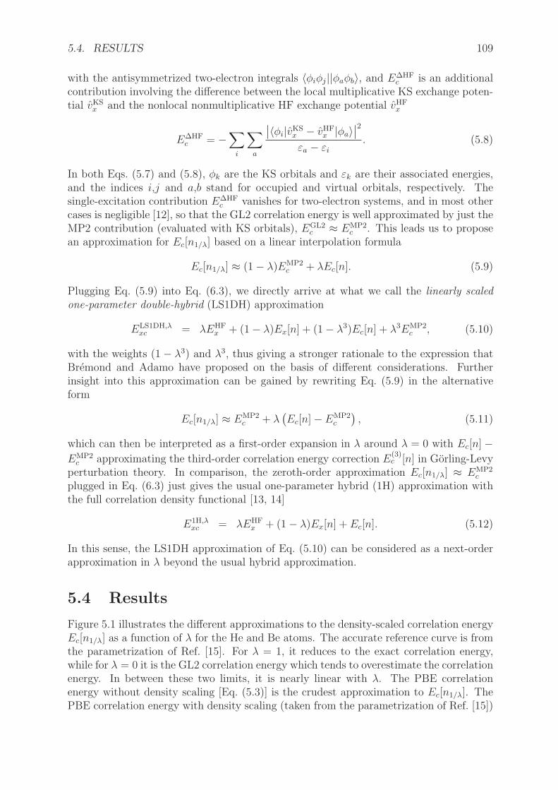
5.4. RESULTS 109
with the antisymmetrized two-electron integrals 〈φiφj||φaφb〉, and E∆HFc is an additional
contribution involving the difference between the local multiplicative KS exchange poten-tial vKS
x and the nonlocal nonmultiplicative HF exchange potential vHFx
E∆HFc = −
∑
i
∑
a
∣
∣〈φi|vKSx − vHF
x |φa〉∣
∣
2
εa − εi
. (5.8)
In both Eqs. (5.7) and (5.8), φk are the KS orbitals and εk are their associated energies,and the indices i,j and a,b stand for occupied and virtual orbitals, respectively. Thesingle-excitation contribution E∆HF
c vanishes for two-electron systems, and in most othercases is negligible [12], so that the GL2 correlation energy is well approximated by just theMP2 contribution (evaluated with KS orbitals), EGL2
c ≈ EMP2c . This leads us to propose
an approximation for Ec[n1/λ] based on a linear interpolation formula
Ec[n1/λ] ≈ (1 − λ)EMP2c + λEc[n]. (5.9)
Plugging Eq. (5.9) into Eq. (6.3), we directly arrive at what we call the linearly scaled
one-parameter double-hybrid (LS1DH) approximation
ELS1DH,λxc = λEHF
x + (1 − λ)Ex[n] + (1 − λ3)Ec[n] + λ3EMP2c , (5.10)
with the weights (1 − λ3) and λ3, thus giving a stronger rationale to the expression thatBremond and Adamo have proposed on the basis of different considerations. Furtherinsight into this approximation can be gained by rewriting Eq. (5.9) in the alternativeform
Ec[n1/λ] ≈ EMP2c + λ
(
Ec[n] − EMP2c
)
, (5.11)
which can then be interpreted as a first-order expansion in λ around λ = 0 with Ec[n] −EMP2
c approximating the third-order correlation energy correction E(3)c [n] in Gorling-Levy
perturbation theory. In comparison, the zeroth-order approximation Ec[n1/λ] ≈ EMP2c
plugged in Eq. (6.3) just gives the usual one-parameter hybrid (1H) approximation withthe full correlation density functional [13, 14]
E1H,λxc = λEHF
x + (1 − λ)Ex[n] + Ec[n]. (5.12)
In this sense, the LS1DH approximation of Eq. (5.10) can be considered as a next-orderapproximation in λ beyond the usual hybrid approximation.
5.4 Results
Figure 5.1 illustrates the different approximations to the density-scaled correlation energyEc[n1/λ] as a function of λ for the He and Be atoms. The accurate reference curve is fromthe parametrization of Ref. [15]. For λ = 1, it reduces to the exact correlation energy,while for λ = 0 it is the GL2 correlation energy which tends to overestimate the correlationenergy. In between these two limits, it is nearly linear with λ. The PBE correlationenergy without density scaling [Eq. (5.3)] is the crudest approximation to Ec[n1/λ]. ThePBE correlation energy with density scaling (taken from the parametrization of Ref. [15])

110 CHAPTER 5. RATIONALE FOR A NEW CLASS OF DOUBLE-HYBRID...
-0.05
-0.048
-0.046
-0.044
-0.042
-0.04
0 0.2 0.4 0.6 0.8 1
Ec [
n1/λ
] (h
art
ree)
λ
AccuratePBE without density scaling
PBE with density scalingLinear interpol. of MP2 and PBE
He
-0.13
-0.12
-0.11
-0.1
-0.09
-0.08
0 0.2 0.4 0.6 0.8 1
Ec [
n1/λ
] (h
art
ree)
λ
AccuratePBE without density scaling
PBE with density scalingLinear interpol. of MP2 and PBE
Be
Figure 5.1: (Color online) Density-scaled correlation energy Ec[n1/λ] for the He (left) and Be(right) atoms as a function of λ. Accurate calculations (from the parametrizations of Ref. [15])are compared with different approximations: PBE without density scaling [Eq. (5.3)], PBE withdensity scaling (from the parametrizations of Ref. [15]), and linear interpolation between MP2(with PBE orbitals) and PBE [Eq. (5.9)]. The MP2 calculations for He and Be (including coreexcitations) have been performed with the cc-pV5Z and cc-pCV5Z basis sets [16, 17], respectively.
0
2
4
6
8
10
12
14
16
0 0.2 0.4 0.6 0.8 1
Mean
Ab
so
lute
Err
or
(kc
al/m
ol)
λ
1DH-PBEDS1DH-PBELS1DH-PBE
AE6
0
2
4
6
8
10
0 0.2 0.4 0.6 0.8 1
Mean
Ab
so
lute
Err
or
(kc
al/m
ol)
λ
1DH-PBEDS1DH-PBELS1DH-PBE
BH6
Figure 5.2: (Color online) Mean absolute errors for the AE6 (left) and BH6 (right) test setsas functions of the parameter λ for the 1DH, and DS1DH, and LS1DH approximations withthe PBE exchange-correlation density functional. All calculations were carried out with thecc-pVQZ basis set.

5.5. CONCLUSIONS 111
gives a nearly linear curve. It is a fairly good approximation for He, but a less goodapproximation for Be where it underestimates the correlation energy for all λ, especiallyat λ = 0. This is due to the presence of static correlation in this system that is notdescribed by the PBE functional. Finally, the linear interpolation of Eq. (5.9) betweenMP2 (evaluated with PBE orbitals) and PBE appears as a good approximation for bothHe and Be. In fact, the linear interpolation is clearly the best approximation for Be, atleast with the PBE functional.
For a more comprehensive comparison of the different approximations, we have per-formed calculations on the AE6 and BH6 test sets [18] with the 1DH, DS1DH, and LS1DHdouble hybrids for the PBE functional, using a development version of the MOLPRO 2010program [19]. The AE6 set is a small representative benchmark set of six atomizationenergies consisting of SiH4, S2, SiO, C3H4 (propyne), C2H2O2 (glyoxal), and C4H8 (cy-clobutane). The BH6 set is a small representative benchmark set of forward and reversebarrier heights of three reactions, OH + CH4 → CH3 + H2O, H + OH → O + H2, andH + H2S → HS + H2. All the calculations are performed at the optimized QCISD/MG3geometries [20]. We use the Dunning cc-pVQZ basis set [21, 22]. Core electrons are keptfrozen in all our MP2 calculations. Spin-restricted calculations are performed for all theclosed-shell systems, and spin-unrestricted calculations for all the open-shell systems. InFig. 5.2, we plot the mean absolute errors (MAE) for the two sets as a function of λ. Forthe AE6 set, the MAEs of the DS1DH and LS1DH approximations are quite similar, andare both much smaller that the MAE of the 1DH approximation for a wide range of λ.For the BH6 set, the LS1DH approximation gives a MAE which is significantly smallerthan those of both DS1DH and 1DH for intermediate values of λ.
As regards the choice of the parameter λ, the present data on the AH6 set gives anoptimal value of λ = 0.75 for the LS1DH double hybrid, with a minimal MAE of 3.59kcal/mol, and for the BH6 set the optimal value is λ = 0.70 giving a minimal MAE of0.73 kcal/mol. However, the MAE is not very sensitive to the value of λ around theoptimal value, and Bremond and Adamo [9] have argued for using λ = 0.5 in definingthe PBE0-DH approximation, using a similar argument as the one used by Becke for his“half-and-half” hybrid [23].
5.5 Conclusions
In summary, we have shown that the new class of double-hybrid approximations namedhere LS1DH [Eq. (5.10)] can be understood as approximating the density-scaled correla-tion functional Ec[n1/λ] by a linear function of λ, interpolating between MP2 at λ = 0and a density-functional approximation at λ = 1. Numerical results obtained with thePBE density functional confirms that the LS1DH approximation is a relevant double-hybrid model, and in fact tends to be more accurate than the DS1DH double-hybridmodel [Eq. (6.3)] in which density scaling is applied to the PBE correlation functional.More generally, it can be expected that the LS1DH double-hybrid model will be moreaccurate than the DS1DH double-hybrid model when applied with a density-functionalapproximation that is inaccurate in the high-density limit. We hope that this work willhelp constructing other theoretically justified double-hybrid approximations.

112 CHAPTER 5. RATIONALE FOR A NEW CLASS OF DOUBLE-HYBRID...
Acknowledgments
We thank A. Savin for discussions. This work was partly supported by Agence Na-tionale de la Recherche (ANR) via contract numbers 07-BLAN-0272 (Wademecom) and10-BLANC-0425 (DinfDFT). Sanofi-Aventis is also acknowledged for financial support.
Bibliography
[1] S. Grimme, J. Chem. Phys. 124, 034108 (2006).
[2] Y. Zhao, B. J. Lynch and D. G. Truhlar, J. Phys. Chem. A 108, 4786 (2004).
[3] Y. Zhao, B. J. Lynch and D. G. Truhlar, Phys. Chem. Chem. Phys. 7, 43 (2005).
[4] A. D. Becke, Phys. Rev. A 38, 3098 (1988).
[5] C. Lee, W. Yang and R. G. Parr, Phys. Rev. B 37, 785 (1988).
[6] Y. Zhang, X. Xu and W. A. Goddard III, Proc. Natl. Acad. Sci. U.S.A. 106, 4963(2009).
[7] I. Y. Zhang and X. Xu, Int. Rev. Phys. Chem 30, 115 (2011).
[8] K. Sharkas, J. Toulouse and A. Savin, J. Chem. Phys. 134, 064113 (2011).
[9] E. Bremond and C. Adamo, J. Chem. Phys. 135, 024106 (2011).
[10] J. P. Perdew, K. Burke and M. Ernzerhof, Phys. Rev. Lett. 77, 3865 (1996).
[11] A. Gorling and M. Levy, Phys. Rev. B 47, 13105 (1993).
[12] E. Engel, in A Primer in Density Functional Theory , edited by C. Fiolhais,F. Nogueira and M. A. L. Marques (Springer, Berlin, 2003), Vol. 620 of LectureNotes in Physics, pp. 56–122.
[13] A. D. Becke, The Journal of Chemical Physics 104 (1996).
[14] M. Ernzerhof, J. P. Perdew and K. Burke, in Density Functional Theory , edited byR. Nalewajski (Springer-Verlag, Berlin, 1996).
[15] F. Colonna and A. Savin, J. Chem. Phys. 110, 2828 (1999).
[16] D. Woon and T. Dunning, J. Chem. Phys. 100, 2975 (1994).
[17] B. P. Prascher, D. E. Woon, T. H. D. J. K. A. Peterson and A. K. Wilson, Theor.Chem. Acc. 128, 69 (2011).
[18] B. J. Lynch and D. G. Truhlar, J. Phys. Chem. A 107, 8996 (2003).
[19] H.-J. Werner, P. J. Knowles, G. Knizia, F. R. Manby, M. Schutz, and others,MOLPRO, version 2010.1, a package of ab initio programs, Cardiff, UK, 2010, seehttp://www.molpro.net.
113

114 BIBLIOGRAPHY
[20] B. Lynch, Y. Zhao and D. Truhlar, http://comp.chem.umn.edu/database.
[21] T. H. Dunning, J. Chem. Phys. 90, 1007 (1989).
[22] D. Woon and T. Dunning, J. Chem. Phys. 98, 1358 (1993).
[23] A. D. Becke, J. Chem. Phys. 98, 1372 (1993).

Chapter 6
Double-hybrid density-functionaltheory applied to molecular crystals
The chapter corresponds to a paper in preparation.
6.1 Abstract
We test the performance of a number of two- and one-parameter double-hybrid approxi-mations, combining semilocal exchange-correlation density functionals with periodic localsecond-order Møller-Plesset (LMP2) perturbation theory, for calculating lattice energiesof a set of molecular crystals: urea, formamide, formic acid, ammonia, and carbon dioxide.All double-hybrid methods perform better than the corresponding Kohn-Sham calcula-tions with the same functionals, but not better than standard LMP2. The one-parameterdouble-hybrid approximations based on the PBEsol density functional gives lattice ener-gies per molecule with an accuracy of about 5 kJ/mol, which is similar to the accuracyof LMP2. The fact that these double-hybrid approximations underestimate the latticeenergy of the carbon dioxide crystal suggests that these approximations miss a part ofdispersion interactions.
6.2 Introduction
The reliable computational prediction of the lattice energies of molecular crystals is im-portant in materials science [1–4]. It requires an accurate treatment of different typesof intermolecular interactions, including electrostatics [5], induction [6, 7], and disper-sion interactions [8]. Kohn-Sham density-functional theory (DFT) [9, 10] using standard(semi)local density functionals can account for electrostatic and induction interactions inmolecular crystals [11–13]. However, these usual semilocal functionals fail to adequatelymodel the dispersion interactions [14–17] which are an important source of attraction evenin the hydrogen-bonded crystals [18]. One possibility for improving the prediction of crys-tal lattice energies is to use empirical [19–28] or non-empirical [29–31] dispersion-correcteddensity functionals.
Another possibility for theoretical prediction of molecular crystal lattice energies is touse wave-function type correlation methods such as second-order Møller-Plesset perturba-tion theory (MP2), coupled-cluster singles doubles with perturbative triples [CCSD(T)],
115
116 CHAPTER 6. DOUBLE-HYBRID DENSITY-FUNCTIONAL...
or symmetry-adapted perturbation theory (SAPT) on finite clusters [32–35]. However,the accurate simulation of a periodic system by a finite cluster is difficult and the resultsmay depend very much on the size of the clusters. More satisfying is the use of fullyperiodic wave-function correlation methods such as MP2 [36–42], the random-phase ap-proximation [41, 43, 44], or quantum Monte Carlo [16]. In particular, the periodic localMP2 (LMP2) method as implemented in the CRYSCOR program [42, 45, 46] is well suitedfor weakly bound systems such as rare-gas solids [47–49] and molecular crystals [50–52].
In the present work, we investigate the performance of a number of double-hybrid(DH) approximations combining semilocal density functionals with periodic LMP2 forprediction of the lattice energies of a set of molecular crystals. The DH approxima-tions have been introduced a few years ago [53] and have proven capable to reach nearchemical accuracy for atomic and molecular properties such as atomization energies, re-action barrier heights, ionization potentials, and electron affinities. To the best of ourknowledge, only DH approximations using two empirical parameters constructed withthe Becke 88 (B) exchange functional [54] and the Lee-Yang-Parr (LYP) correlation func-tional [55] have recently been applied to molecular crystals and no improvement over MP2was found [40]. Here, we test the Perdew-Burke-Ernzerhof (PBE) [56] and the modifiedPBEsol [57] exchange-correlation functionals in the one-parameter DH scheme recentlyproposed by some of us [58].
The paper is organized as follows. In Section 6.3, we review the one-parameter DHapproximations and the main equations of the periodic LMP2 method, and we indicate themodifications made for the present implementation. After giving computational detailson the calculations in Section 6.4, we present and discuss the results obtained with variousDH approximations on five molecular crystals: urea, formamide, formic acid, ammonia,and carbon dioxide. Section 6.6 summarizes our conclusions.
6.3 Theory
6.3.1 One-parameter double-hybrid approximations
After some related earlier work [59, 60], Grimme [53] introduced the procedure which isnow commonly used in DH approximations. First, a normal self-consistent DFT calcu-lation is carried out using a fraction ax of Hartree-Fock (HF) exchange EHF
x , a fraction(1 − ax) of a semilocal exchange density functional Ex[n], and a fraction (1 − ac) of asemilocal correlation density functional Ec[n]. Subsequently, the MP2 correlation energyEMP2
c calculated using the previously generated orbitals is added with the fraction ac. Theresulting exchange-correlation energy can thus be written as
EDHxc = axE
HFx + (1 − ax)Ex[n] + (1 − ac)Ec[n] + acE
MP2c . (6.1)
Many DH approximations relying on this procedure have been developed [53, 61–64].For example, the B2-PLYP approximation [53] is obtained by choosing the B exchangefunctional for Ex[n] and the LYP correlation functional for Ec[n], and the two empiricalparameters ax = 0.53 and ac = 0.27 as optimized for the G2/97 [65] subset of heats offormation.
Recently, a rigorous reformulation of the DH approximations was provided [58] by ap-plying the multideterminant extension of the Kohn-Sham scheme [66, 67] to the adiabatic-
6.3. THEORY 117
connection Hamiltonian
Hλ = T + Vext + λWee + V λHxc[n], (6.2)
which links the non-interacting Kohn-Sham Hamiltonian (λ = 0) to the exact Hamilto-nian (λ = 1). In this expression, T is the kinetic energy operator, Vext is a scalar externalpotential operator (e.g., nuclei-electron), and V λ
Hxc[n] is the Hartree-exchange-correlationpotential operator keeping the one-electron density n constant for all values of the cou-pling constant λ. This leads to the density-scaled one-parameter double-hybrid (DS1DH)approximation
EDS1DH,λxc = λEHF
x + (1 − λ)Ex[n] + Ec[n] − λ2Ec[n1/λ] + λ2EMP2c , (6.3)
whereEc[n1/λ] is the correlation energy functional evaluated at the scaled density n1/λ(r) =(1/λ)3n(r/λ). Neglecting the density scaling in the correlation functional, Ec[n1/λ] ≈Ec[n], leads to one-parameter double-hybrid (1DH) approximation
E1DH,λxc = λEHF
x + (1 − λ)Ex[n] + (1 − λ2)Ec[n] + λ2EMP2c . (6.4)
In comparison to the original DH approximations, only one empirical parameter needs tobe determined. DS1DH and 1DH approximations using the BLYP and PBE exchange-correlation functionals have been constructed and the optimal parameter was found to beabout λ ≈ 0.65 or 0.70 for atomization energies and reaction barrier heights of molecularsystems [58].
6.3.2 Periodic local MP2
We now briefly review the main equations of the periodic local MP2 method that weuse and indicate the required modifications for implementing the one-parameter DH ap-proximations. The implementation of two-parameter DH approximations require obvioussimilar modifications.
The first-order perturbative correction to the HF wave function is written as
|Ψ(1)〉 =1
2
∑
(ij)∈P
∑
(ab)∈[ij]
T ij
ab|Φabij 〉, (6.5)
where Φabij are doubly excited determinants and T ij
ab are the corresponding amplitudes. Inthis expression, the labels (i,j) refer to pairs of occupied Wannier functions (WFs) takenfrom a truncated list P , in which the first WF i is located in the reference unit cell andthe second WF j is restricted within a given distance to the first WF i. The labels (a, b)refer to pairs of mutually non-orthogonal virtual projected atomic orbitals (PAOs) andthe sum is restricted to the pair-domain [ij] of PAOs which are spatially close to at leastone of the WF i or j. This truncation of the virtual space makes the LMP2 method scaleslinearly with the supercell size.
The double excitation amplitudes T ij
ab are obtained by solving the following system oflinear equations [42, 68, 69]
K ij
ab +∑
cd
{
FacTij
cdSdb + SacTij
cdFdb − Sac
[
∑
k
(FikTkj
cd + T ikcdFkj)
]
Sdb
}
= 0, (6.6)
118 CHAPTER 6. DOUBLE-HYBRID DENSITY-FUNCTIONAL...
where K ij
ab = (ia|jb) are the two-electron exchange integrals, Sdb is the overlap betweenPAOs, and Fik and Fdb are elements of the Fock matrix in WF and PAO basis, which isobtained by transformation of the Fock matrix in the atomic orbital (AO) basis
Fµν = hµν + Jµν +Kµν , (6.7)
where hµν , Jµν , and Kµν are the one-electron Hamiltonian, Coulomb, and exchangematrices, respectively. For closed-shell systems, Jµν =
∑
ρσ Pρσ(µν|σρ) and Kµν =(−1/2)
∑
ρσ Pρσ(µρ|σν) where Pρσ is the density matrix and (µν|σρ) are the two-electronintegrals. In the local basis, the occupied-occupied and virtual-virtual blocks of the Fockmatrix are not diagonal, which means that Eq. (6.6) has to be solved iteratively for theamplitudes T ij
ab. When the convergence is reached, the LMP2 correlation energy per unitcell is given as
ELMP2c =
∑
ij∈P
∑
(ab)∈[ij]
K ij
ab(2T ij
ab − T ij
ba). (6.8)
For the one-parameter DH approximations, the Fock matrix of Eq. (6.7) is replacedby
F hybridµν = hµν + Jµν + λKµν + V λ
xc,µν , (6.9)
with the scaled exchange matrix λKµν and the exchange-correlation potential matrix V λxc,µν
corresponding to the density functional used. Note that, because of self consistency, thedensity matrix Pρσ in Jµν and Kµν also depends on λ. This is essentially the only non-trivial modification to be made in the program. Indeed, one can see that using the scaledinteraction λWee of Eq. (6.2) corresponds to scaling the two-electron exchange integrals,K ij
ab → λK ij
ab, in Eq. (6.6), implying the scaling of the amplitudes T ij
ab → λT ij
ab. UsingEq. (6.8), it means that we just need to scale the LMP2 correlation energy by λ2
ELMP2c → λ2ELMP2
c , (6.10)
as it was already indicated in Eqs. (6.3) and (6.4).There is an additional point to consider when using the dual-basis set scheme [70, 71].
The reliable description of the correlated wave functions needs the use of rather large basissets and especially with diffuse functions when treating weakly bound systems. However,such basis sets may lead to linear-dependency problems in the periodic self-consistent-fieldcalculation (SCF) that precedes the LMP2 step. The dual-basis set scheme helps overcomethese difficulties by using a smaller basis for the SCF calculation and additional basisfunctions for the LMP2 calculation. In this scheme, Brillouin’s theorem does not applyin the LMP2 calculation and hence single excitations contribute to the LMP2 correlationenergy
ELMP2c,singles =
∑
ia
FiaTia, (6.11)
where the single excitation amplitudes T ia are determined from
Fia +∑
b
FabTib −
∑
bj
FijTibSba = 0, (6.12)
6.4. COMPUTATIONAL DETAILS 119
where the Fock matrix in these formulas are defined in the large basis set but built fromdensity matrices in the small one (i.e., the indices µ and ν in Fµν run over the largebasis set while the indices ρ and σ in Pρσ belong to the small one) [72]. For the caseof the one-parameter DH approximations, since the two-electron integrals do not explicitappear in Eqs. (6.11) and (6.12), the evaluation of the single excitation contribution do notrequire other modifications than simply using the dual-basis version of the Fock matrix ofEq. (6.9) in Eqs. (6.11) and (6.12). We note, however, that because the one-parameter DHapproximations are based on a nonlinear Rayleigh-Schrodinger perturbation theory [67,73, 74], when Brillouin’s theorem does not apply, there is in principle an additional single-excitation contribution to the second-order correlation energy coming from the second-order functional derivative of the Hartree-exchange-correlation energy, but we neglect thisadditional contribution in this work.
6.4 Computational details
The one-parameter DS1DH and 1DH approximations using the BLYP, PBE, and PBEsolfunctionals, as well as the two-parameter DH approximations, B2-PLYP (ax = 0.53, ac =0.27) [53], B2GP-PLYP (ax = 0.65, ac = 0.36) [63], and mPW2-PLYP (ax = 0.55, ac =0.25) [61], have been implemented in a development version of the CRYSTAL09 [75] andCRYSCOR09 [45, 46] suite of programs. For the DS1DH approximations, the expressionsof the density-scaled correlation energy Ec[n1/λ] and the corresponding potential are givenin the appendix of Ref. [58].
We study five molecular crystals: urea CO(NH2)2, formamide HCONH2, formic acidHCOOH, ammonia NH3 and carbon dioxide CO2. The experimental crystal structureswere used [76–79]. The truncation tolerances of lattice sums for one- and two-electronintegrals were set to 7 7 7 12 40 (TOLINTEG parameters [75]). A grid consisting of 75radial points and up to 974 angular points was used in evaluating the exchange-correlationfunctional. The shrinking factors were set to 4 for the k points grid to sample the irre-ducible Brillouin zone. Each calculation is done in two steps: a periodic SCF hybridcalculation is first performed using CRYSTAL09, and then the periodic LMP2 correlationenergy is calculated using CRYSCOR09 and added to the SCF energy after multiplica-tion by the proper scaling factor. For urea, formamide, and formic acid, we employ thepolarized split-valence double-zeta Gaussian basis set 6-31G(d,p) [80] in the SCF calcu-lations [81]. This basis is then augmented by polarization functions with small exponents(d functions for C, N and O atoms, p functions for H atoms, taken from the aug-cc-pVDZbasis set [82]), and the resulting basis set is denoted by p-aug-6-31G(d,p) [52]. The virtualspace of the extended basis set is employed in the subsequent LMP2 calculation. Whenwe use this dual-basis set technique, the contribution of single excitations to the LMP2correlation energy is evaluated and added. This contribution does not exceed 2% of thecalculated lattice energy. In practice, the dual-basis matrices are obtained through a non-self-consistent SCF (GUESDUAL [75]) which uses the density matrix from a previous SCFrun to allocate the additional basis functions. For ammonia and carbon dioxide, we usethe p-aug-6-31G(d,p) basis set for both the SCF and LMP2 calculations. Core electronsare kept frozen in all LMP2 calculations. The occupied valence orbital space is spanned bythe localized [83] symmetry-adapted [84] mutually orthogonal Wannier functions (WFs)supplied by the PROPERTIES module of CRYSTAL. The virtual orbital space is spanned
120 CHAPTER 6. DOUBLE-HYBRID DENSITY-FUNCTIONAL...
by mutually nonorthogonal PAOs, which are constructed by projecting the individual AObasis functions on the virtual space [68]. The explicit computations cover WF pairs upto distance dij = 12 A, where the two-electron repulsion integrals were evaluated via
the density fitting periodic (DFP) scheme [85] for dij ≤ 8 A and via the multipolar ap-
proximation for 8 < dij ≤ 12 A. The contribution of the WF pairs with dij > 12 A tothe correlation energy was estimated through the Lennard-Jones extrapolation technique.Excitation PAO domains have been restricted to the molecular units.
Single-point, static (i.e. at 0 K) energies are computed to evaluate the counterpoise-corrected lattice energy ECP
LE (V ) per molecule at a given volume V of the unit cell
ECPLE (V ) = Ebulk/Z − E
[bulk]mol+ghosts, (6.13)
where Z is the number of the molecular units in the unit cell, and Ebulk and E[bulk]mol+ghosts are
total energies of the bulk system (per cell) and of the molecule in the crystalline bulk ge-ometry with ghost functions, respectively, at a given cell volume. At least 50 ghost atomssurrounding the central molecule were used. The ghost functions, in the standard Boys-Bernardi counterpoise scheme [86], are supposed to eliminate the inconsistency betweenthe finite basis sets used in the molecular and bulk calculations to obtain basis set super-position error (BSSE) free lattice energies. The structural deformation of the moleculeinduced by the crystal packing is not included, i.e., the difference between the energiesof the isolated molecules in the bulk and in the gas phase conformations is neglected,E
[bulk]mol = E
[gas]mol .
6.5 Results and discussion
The calculated lattice energies of crystalline urea, formamide, ammonia and carbon diox-ide are compared to the experimental sublimation enthalpies after corrections for thermaland zero-point effects [28], while the lattice energy of formic acid is directly comparedto the experimental one [52]. Although this set of five molecular crystals is statisticallysmall, it includes systems ranging from a purely dispersion bound crystal (carbon diox-ide) to structures with hydrogen bonds of varying strengths (urea, formamide, formic acid,ammonia).
To have a first global view of the performance of the different one-parameter DHapproximations and the dependence on the parameter λ, we show in Fig. 6.1 mean absoluteerrors (MAEs) on the five lattice energies as a function of λ for the DS1DH and 1DHmethods using the BLYP, PBE, and PBEsol density functionals. For λ = 0, each methodreduces to a standard periodic Kohn-Sham calculation with the corresponding densityfunctional. For λ = 1, all methods reduce to a standard periodic LMP2 calculation.Kohn-Sham BLYP and PBE calculations at λ = 0 give much larger MAEs (about 32kJ/mol and 16 kJ/mol, respectively) than LMP2 (about 5 kJ/mol).
The DS1DH and 1DH approximations using the BLYP and PBE functionals inheritthe bad performance of these functionals and always give larger MAEs than standardLMP2 for all λ < 1. In contrast, the PBEsol functional (which is a modified version ofthe PBE functional to improve the description of solids) gives a MAE at λ = 0 (about8 kJ/mol) that is comparable to LMP2. Consequently, the DS1DH-PBEsol and 1DH-PBEsol approximations give almost constant MAEs as a function of λ, with a slight
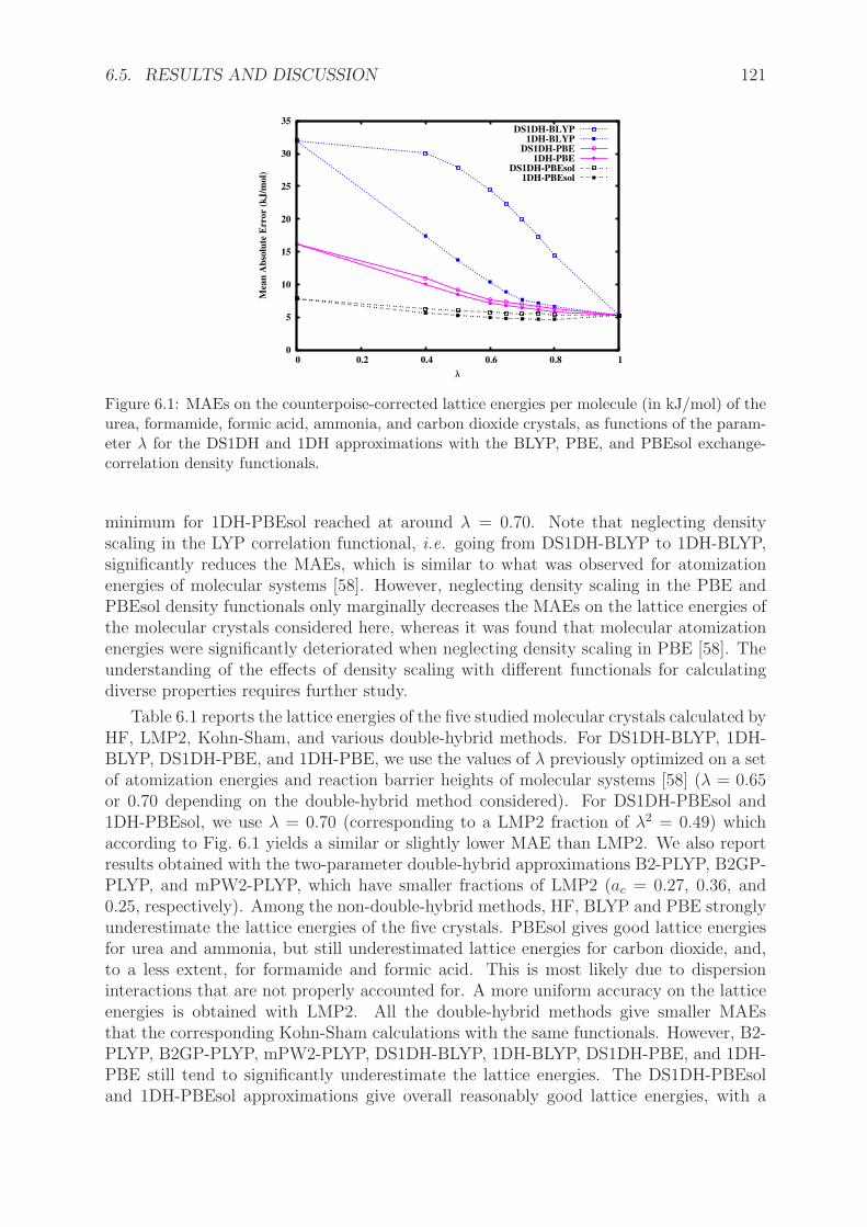
6.5. RESULTS AND DISCUSSION 121
0
5
10
15
20
25
30
35
0 0.2 0.4 0.6 0.8 1
Mea
n A
bso
lute
Err
or
(kJ/m
ol)
λ
DS1DH-BLYP1DH-BLYP
DS1DH-PBE1DH-PBE
DS1DH-PBEsol1DH-PBEsol
Figure 6.1: MAEs on the counterpoise-corrected lattice energies per molecule (in kJ/mol) of theurea, formamide, formic acid, ammonia, and carbon dioxide crystals, as functions of the param-eter λ for the DS1DH and 1DH approximations with the BLYP, PBE, and PBEsol exchange-correlation density functionals.
minimum for 1DH-PBEsol reached at around λ = 0.70. Note that neglecting densityscaling in the LYP correlation functional, i.e. going from DS1DH-BLYP to 1DH-BLYP,significantly reduces the MAEs, which is similar to what was observed for atomizationenergies of molecular systems [58]. However, neglecting density scaling in the PBE andPBEsol density functionals only marginally decreases the MAEs on the lattice energies ofthe molecular crystals considered here, whereas it was found that molecular atomizationenergies were significantly deteriorated when neglecting density scaling in PBE [58]. Theunderstanding of the effects of density scaling with different functionals for calculatingdiverse properties requires further study.
Table 6.1 reports the lattice energies of the five studied molecular crystals calculated byHF, LMP2, Kohn-Sham, and various double-hybrid methods. For DS1DH-BLYP, 1DH-BLYP, DS1DH-PBE, and 1DH-PBE, we use the values of λ previously optimized on a setof atomization energies and reaction barrier heights of molecular systems [58] (λ = 0.65or 0.70 depending on the double-hybrid method considered). For DS1DH-PBEsol and1DH-PBEsol, we use λ = 0.70 (corresponding to a LMP2 fraction of λ2 = 0.49) whichaccording to Fig. 6.1 yields a similar or slightly lower MAE than LMP2. We also reportresults obtained with the two-parameter double-hybrid approximations B2-PLYP, B2GP-PLYP, and mPW2-PLYP, which have smaller fractions of LMP2 (ac = 0.27, 0.36, and0.25, respectively). Among the non-double-hybrid methods, HF, BLYP and PBE stronglyunderestimate the lattice energies of the five crystals. PBEsol gives good lattice energiesfor urea and ammonia, but still underestimated lattice energies for carbon dioxide, and,to a less extent, for formamide and formic acid. This is most likely due to dispersioninteractions that are not properly accounted for. A more uniform accuracy on the latticeenergies is obtained with LMP2. All the double-hybrid methods give smaller MAEsthat the corresponding Kohn-Sham calculations with the same functionals. However, B2-PLYP, B2GP-PLYP, mPW2-PLYP, DS1DH-BLYP, 1DH-BLYP, DS1DH-PBE, and 1DH-PBE still tend to significantly underestimate the lattice energies. The DS1DH-PBEsoland 1DH-PBEsol approximations give overall reasonably good lattice energies, with a
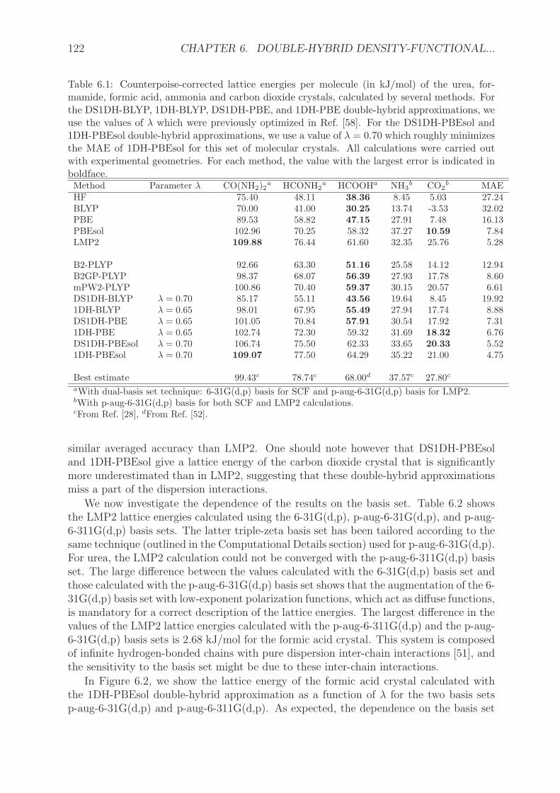
122 CHAPTER 6. DOUBLE-HYBRID DENSITY-FUNCTIONAL...
Table 6.1: Counterpoise-corrected lattice energies per molecule (in kJ/mol) of the urea, for-mamide, formic acid, ammonia and carbon dioxide crystals, calculated by several methods. Forthe DS1DH-BLYP, 1DH-BLYP, DS1DH-PBE, and 1DH-PBE double-hybrid approximations, weuse the values of λ which were previously optimized in Ref. [58]. For the DS1DH-PBEsol and1DH-PBEsol double-hybrid approximations, we use a value of λ = 0.70 which roughly minimizesthe MAE of 1DH-PBEsol for this set of molecular crystals. All calculations were carried outwith experimental geometries. For each method, the value with the largest error is indicated inboldface.Method Parameter λ CO(NH2)2
a HCONH2a HCOOHa NH3
b CO2b MAE
HF 75.40 48.11 38.36 8.45 5.03 27.24BLYP 70.00 41.00 30.25 13.74 -3.53 32.02PBE 89.53 58.82 47.15 27.91 7.48 16.13PBEsol 102.96 70.25 58.32 37.27 10.59 7.84LMP2 109.88 76.44 61.60 32.35 25.76 5.28
B2-PLYP 92.66 63.30 51.16 25.58 14.12 12.94B2GP-PLYP 98.37 68.07 56.39 27.93 17.78 8.60mPW2-PLYP 100.86 70.40 59.37 30.15 20.57 6.61DS1DH-BLYP λ = 0.70 85.17 55.11 43.56 19.64 8.45 19.921DH-BLYP λ = 0.65 98.01 67.95 55.49 27.94 17.74 8.88DS1DH-PBE λ = 0.65 101.05 70.84 57.91 30.54 17.92 7.311DH-PBE λ = 0.65 102.74 72.30 59.32 31.69 18.32 6.76DS1DH-PBEsol λ = 0.70 106.74 75.50 62.33 33.65 20.33 5.521DH-PBEsol λ = 0.70 109.07 77.50 64.29 35.22 21.00 4.75
Best estimate 99.43c 78.74c 68.00d 37.57c 27.80c
aWith dual-basis set technique: 6-31G(d,p) basis for SCF and p-aug-6-31G(d,p) basis for LMP2.bWith p-aug-6-31G(d,p) basis for both SCF and LMP2 calculations.cFrom Ref. [28], dFrom Ref. [52].
similar averaged accuracy than LMP2. One should note however that DS1DH-PBEsoland 1DH-PBEsol give a lattice energy of the carbon dioxide crystal that is significantlymore underestimated than in LMP2, suggesting that these double-hybrid approximationsmiss a part of the dispersion interactions.
We now investigate the dependence of the results on the basis set. Table 6.2 showsthe LMP2 lattice energies calculated using the 6-31G(d,p), p-aug-6-31G(d,p), and p-aug-6-311G(d,p) basis sets. The latter triple-zeta basis set has been tailored according to thesame technique (outlined in the Computational Details section) used for p-aug-6-31G(d,p).For urea, the LMP2 calculation could not be converged with the p-aug-6-311G(d,p) basisset. The large difference between the values calculated with the 6-31G(d,p) basis set andthose calculated with the p-aug-6-31G(d,p) basis set shows that the augmentation of the 6-31G(d,p) basis set with low-exponent polarization functions, which act as diffuse functions,is mandatory for a correct description of the lattice energies. The largest difference in thevalues of the LMP2 lattice energies calculated with the p-aug-6-311G(d,p) and the p-aug-6-31G(d,p) basis sets is 2.68 kJ/mol for the formic acid crystal. This system is composedof infinite hydrogen-bonded chains with pure dispersion inter-chain interactions [51], andthe sensitivity to the basis set might be due to these inter-chain interactions.
In Figure 6.2, we show the lattice energy of the formic acid crystal calculated withthe 1DH-PBEsol double-hybrid approximation as a function of λ for the two basis setsp-aug-6-31G(d,p) and p-aug-6-311G(d,p). As expected, the dependence on the basis set

6.6. CONCLUSIONS 123
Table 6.2: Counterpoise-corrected lattice energies per molecule of the molecular crystal test setwith the LMP2 method with three different basis sets.
Basis set CO(NH2)2 HCONH2 HCOOH NH3 CO2
6-31G(d,p) 95.04 63.51 50.00 26.82 16.16p-aug-6-31G(d,p) 109.88a 76.44a 61.60a 32.35 25.76p-aug-6-311G(d,p) - 77.26a 64.27a 31.78 25.26aWith dual-basis set technique: 6-31G(d,p) basis for SCF.
58
60
62
64
66
68
0 0.2 0.4 0.6 0.8 1
Latt
ice
En
ergy (
kJ/m
ol)
λ
p-aug-6-311G(d,p)p-aug-6-31G(d,p)
REF
formic acid
Figure 6.2: Counterpoise-corrected lattice energy per molecule of the formic acid molecularcrystal as a function of the parameter λ for the 1DH-PBEsol double-hybrid approximation withp-aug-6-31G(d,p) and p-aug-6-311G(d,p) basis sets. The reference value is from Ref. [52].
decreases as λ is reduced from λ = 1 (corresponding to LMP2) to λ = 0 (corresponding toKohn-Sham PBEsol which has a very small basis set dependence). However, at the valueof the parameter used, λ = 0.70, the dependence on the basis set of 1DH-PBEsol is notsignificantly smaller than that of LMP2. This is a disadvantage of the DH approximationsbased on a linear decomposition of the electron-electron interaction, in comparison toDH schemes based on a range separation of the interaction which have a faster basisconvergence [67, 87, 88].
6.6 Conclusions
We have implemented a number of double-hybrid approximations in the CRYSTAL09and CRYSCOR09 suite of programs, and tested them for calculating lattice energies offive molecular crystals: urea, formamide, formic acid, ammonia, and carbon dioxide. Theone-parameter double-hybrid approximations based on the PBEsol density functional,DS1DH-PBEsol and 1DH-PBEsol, with a fraction of HF exchange of λ = 0.70 and afraction of LMP2 correlation of λ2 = 0.49, gives lattice energies per molecule with anaccuracy of about 5 kJ/mol, which is similar to the accuracy of LMP2. The results onthe purely dispersion bound carbon dioxide crystal suggest that the DS1DH-PBEsol and1DH-PBEsol double-hybrid approximations miss a part of dispersion interactions. Thiscould be improved by either adding semi-empirical dispersion corrections [21] or using

124 CHAPTER 6. DOUBLE-HYBRID DENSITY-FUNCTIONAL...
range-separated double-hybrid methods [67].
Acknowledgments
We thank Peter Reinhardt (UPMC, Paris) for helpful discussions and technical assistance.

Bibliography
[1] C. B. Aakerøy and K. R. Seddon, Chem. Soc. Rev. 22, 397 (1993).
[2] P. G. Karamertzanis, P. R. Anandamanoharan, P. Fernandes, P. W. Cains, M. Vick-ers, D. A. Tocher, A. J. Florence and S. L. Price, J. Phys. Chem. B 111, 5326 (2007).
[3] M. D. Gourlay, J. Kendrick and F. J. J. Leusen, Crystal Growth & Design 7, 56(2007).
[4] O.-P. Kwon, B. Ruiz, A. Choubey, L. Mutter, A. Schneider, M. Jazbinsek, V. Gram-lich and P. Gunter, Chem. Mater. 18, 4049 (2006).
[5] D. S. Coombes, S. L. Price, D. J. Willock and M. Leslie, J. Phys. Chem. 100, 7352(1996).
[6] G. G. Ferenczy, G. I. Csonka, G. Naray-szabo and J. G. Angyan, J. Comput. Chem.19, 38 (1998).
[7] G. W. A. Welch, P. G. Karamertzanis, A. J. Misquitta, A. J. Stone and S. L. Price,J. Chem. Theory Comput. 4, 522 (2008).
[8] A. J. Stone and S. Tsuzuki, J. Phys. Chem. B 101, 10178 (1997).
[9] P. Hohenberg and W. Kohn, Phys. Rev. 136, B 864 (1964).
[10] W. Kohn and L. J. Sham, Phys. Rev. 140, A1133 (1965).
[11] C. A. Morrison and M. M. Siddick, Chem.aEur. J. 9, 628 (2003).
[12] A. D. Fortes, J. P. Brodholt, I. G. Wood and L. Vocadlo, J. Chem. Phys. 118, 5987(2003).
[13] X.-H. Ju, H.-M. Xiao and L.-T. Chen, Int. J. Quantum Chem. 102, 224 (2005).
[14] S. Kristyan and P. Pulay, Chem. Phys. Lett. 229, 175 (1994).
[15] P. Hobza, J. Sponer and T. Reschel, J. Comput. Chem. 16, 1315 (1995).
[16] K. Hongo, M. A. Watson, R. S. Sanchez-Carrera, T. Iitaka and A. Aspuru-Guzik, J.Phys. Chem. Lett. 1, 1789 (2010).
[17] Y. Zhao and D. G. Truhlar, J. Chem. Theory Comput. 3, 289 (2007).
[18] S. Tsuzuki, H. Orita, K. Honda and M. Mikami, J. Phys. Chem. B 114, 6799 (2010).
125

126 BIBLIOGRAPHY
[19] M. A. Neumann and M.-A. Perrin, J. Phys. Chem. B 109, 15531 (2005).
[20] T. Li and S. Feng, Pharm. Res. 23, 2326 (2006).
[21] B. Civalleri, C. Zicovich-Wilson, L. Valenzano and P. Ugliengo, Cryst. Eng. Comm10, 405 (2008).
[22] P. G. Karamertzanis, G. M. Day, G. W. A. Welch, J. Kendrick, F. J. J. Leusen, M. A.Neumann and S. L. Price, J. Phys. Chem. 128, 244708 (2008).
[23] P. Ugliengo, C. Zicovich-Wilson, S. Tosoni and B. Civalleri, J. Mater. Chem. 19,2564 (2009).
[24] C. M. Zicovich-Wilson, B. Kirtman, B. Civalleri and A. Ramırez-Solıs, Phys. Chem.Chem. Phys. 12, 3289 (2010).
[25] D. C. Sorescu and B. M. Rice, J. Phys. Chem. C 114, 6734 (2010).
[26] R. Balu, E. F. C. Byrd and B. M. Rice, J. Phys. Chem. B 115, 803 (2011).
[27] W. Reckien, F. Janetzko, M. F. Peintinger and T. Bredow, J. Comput. Chem. 33,2023 (2012).
[28] A. O. de-la Roza and E. R. Johnson, J. Chem. Phys. 137, 054103 (2012).
[29] M. Dion, H. Rydberg, E. Schroder, D. C. Langreth and B. I. Lundqvist, Phys. Rev.Lett. 92, 246401 (2004).
[30] T. Thonhauser, V. R. Cooper, S. Li, A. Puzder, P. Hyldgaard and D. C. Langreth,Phys. Rev. B. 76, 125112 (2007).
[31] F. Shimojo, Z. Wu, A. Nakano, R. K. Kalia and P. Vashishta, J. Chem. Phys. 132,094106 (2010).
[32] M. Alfredsson, L. Ojamae and K. G. Hermansson, Int. J. Qunatum Chem. 60, 767(1996).
[33] T. Ikeda, K. Nagayoshi and K. Kitaura, Chem. Phys. Lett. 370, 218 (2003).
[34] A. L. Ringer and C. D. Sherrill, Chem.aEur. 14, 2542 (2008).
[35] R. Podeszwa, B. M. Rice and K. Szalewicz, Phys. Rev. Lett. 101, 115503 (2008).
[36] J.-Q. Sun and R. J. Bartlett, J. Chem. Phys. 104, 8553 (1996).
[37] P. Y. Ayala, K. N. Kudin and G. E. Scuseria, J. Chem. Phys. 115, 9698 (2001).
[38] M. Marsman, A. Gruneis, J. Paier and G. Kresse, J. Chem. Phys. 130, 184103 (2009).
[39] A. Gruneis, M. Marsman and G. Kresse, J. Chem. Phys. 133, 074107 (2010).
[40] M. D. Ben, J. Hutter and J. VandeVondele, J. Chem. Theory Comput. 8, 4177 (2012).
BIBLIOGRAPHY 127
[41] M. D. Ben, J. Hutter and J. VandeVondele, J. Chem. Theory Comput. , DOI:10.1021/ct4002202 (2013).
[42] C. Pisani, M. Busso, G. Capecchi, S. Casassa, R. Dovesi, L. Maschio, C. Zicovich-Wilson and M. Schutz, J. Phys. Chem. 122, 094113 (2005).
[43] D. Lu, Y. Li, D. Rocca and G. Galli, Phys. Rev. Lett. 102, 206411 (2009).
[44] Y. Li, D. Lu, H.-V. Nguyen and G. Galli, J. Phys. Chem. A 114, 1944 (2010).
[45] L. Maschio, J. Chem. Theory Comput. 7, 2818 (2011).
[46] C. Pisani, M. Schutz, S. Casassa, D. Usvyat, L. Maschio, M. Lorenz and A. Erba,Phys. Chem. Chem. Phys. 14, 7615 (2012).
[47] S. Casassa, M. Halo and L. Maschio, J. Phys.: Conf. Ser 117, 012007 (2008).
[48] M. Halo, S. Casassa, L. Maschio and C. Pisani, Chem. Phys. Lette 467, 294 (2009).
[49] M. Halo, S. Casassa, L. Maschio and C. Pisani, Phys. Chem. Chem. Phys. 11, 586(2009).
[50] L. Maschio, D. Usvyat, M. Schutz and B. Civalleri, J. Chem. Phys. 132, 134706(2010).
[51] L. Maschio, D. Usvyat and B. Civalleri, CrystEngComm 12, 2429 (2010).
[52] L. Maschio, B. Civalleri, P. Ugliengo and A. Gavezzotti, J. Phys. Chem. 115, 11179(2011).
[53] S. Grimme, J. Chem. Phys. 124, 034108 (2006).
[54] A. D. Becke, Phys. Rev. A 38, 3098 (1988).
[55] C. Lee, W. Yang and R. G. Parr, Phys. Rev. B 37, 785 (1988).
[56] J. P. Perdew, K. Burke and M. Ernzerhof, Phys. Rev. Lett. 77, 3865 (1996).
[57] J. P. Perdew, A. Ruzsinszky, G. I. Csonka, O. A. Vydrov, G. E. Scuseria, L. A.Constantin, X. L. Zhou and K. Burke, Phys. Rev. Lett. 100, 136406 (2008).
[58] K. Sharkas, J. Toulouse and A. Savin, J. Chem. Phys. 134, 064113 (2011).
[59] Y. Zhao, B. J. Lynch and D. G. Truhlar, J. Phys. Chem. A 108, 4786 (2004).
[60] Y. Zhao, B. J. Lynch and D. G. Truhlar, Phys. Chem. Chem. Phys. 7, 43 (2005).
[61] T. Schwabe and S. Grimme, Phys. Chem. Chem. Phys. 8, 4398 (2006).
[62] A. Tarnopolsky, A. Karton, R. Sertchook, D. Vuzman and J. M. L. Martin, J. Phys.Chem. A 112, 3 (2008).
[63] A. Karton, A. Tarnopolsky, J.-F. Lamere, G. C. Schatz and J. M. L. Martin, J. Phys.Chem. A 112, 12868 (2008).

128 BIBLIOGRAPHY
[64] J. C. Sancho-Garcıa and A. J. Perez-Jimenez, J. Chem. Phys. 131, 084108 (2009).
[65] L. A. Curtiss, K. Raghavachari, P. C. Redfern and J. A. Pople, J. Chem. Phys. 106,1063 (1997).
[66] J. Toulouse, F. Colonna and A. Savin, Phys. Rev. A 70, 062505 (2004).
[67] J. G. Angyan, I. C. Gerber, A. Savin and J. Toulouse, Phys. Rev. A 72, 012510(2005).
[68] P. Pulay and S. Saebø, Theor. Chim. Acta 69, 357 (1986).
[69] C. Pisani, L. Maschio, S. Casassa, M. Halo, M. Schutz and D. Usvyat, J. Comput.Chem. 29, 2113 (2008).
[70] R. P. Steele and R. A. DiStasio and Y. Shao and J. Kong and M. Head-Gordon, J.Chem. Phys. 125, 074108 (2006).
[71] R. A. DiStasio and R. P. Steele and M. Head-Gordon, Mol. Phys. 105, 2731 (2007).
[72] K. Wolinski and P. Pulay, J. Chem. Phys. 118, 9497 (2003).
[73] J. G. Angyan, Phys. Rev. A 78, 022510 (2008).
[74] E. Fromager and H. J. A. Jensen, Phys. Rev. A 78, 022504 (2008).
[75] R. Dovesi, V. R. Saunders, C. Roetti, R. Orlando, C. M. Zicovich-Wilson, F. Pas-cale, B. Civalleri, K. Doll, N. M. Harrison, I. J. Bush, P. D′Arco and M. Llunell.,CRYSTAL, Release CRYSTAL09 (2009), see http://www.crystal.unito.it.
[76] F. H. Allen, Acta Cryst. B58, 380 (2002).
[77] A. Simon and K. Peters, Acta Cryst. B36, 2750 (1980).
[78] H. Kiefte, R. Penney, S. W. Breckon and M. J. Clouter, J. Chem. Phys. 86, 662(1987).
[79] E. I. Voitovich, A. M. Tolkachev and V. G. Manzhelii, J. Low Temp. Phys. 5, 435(1971).
[80] P. Hariharan and J. Pople, Theoret. Chim. Acta 1973, 213 (28).
[81] W. F. Perger, R. Pandey, M. A. Blanco and J. Zhao, Chem. Phys. Lett. 388, 175(2004).
[82] T. H. Dunning, J. Chem. Phys. 90, 1007 (1989).
[83] C. Zicovich-Wilson, R. Dovesi and V. R. Saunders, J. Chem. Phys. 115, 9708 (2001).
[84] S. Casassa, C. Zicovich-Wilson and C. Pisani, Theor. Chem. Acc. 116, 726 (2006).
[85] L. Maschio and D. Usvyat, Phys. Rev. B 78, 073102 (2008).
[86] S. F. Boys and F. Bernardi, Mol. Phys. 19, 553 (1970).

BIBLIOGRAPHY 129
[87] J. Toulouse, I. C. Gerber, G. Jansen, A. Savin and J. G. Angyan, Phys. Rev. Lett.102, 096404 (2009).
[88] J. Toulouse, W. Zhu, J. G. Angyan and A. Savin, Phys. Rev. A 82, 032502 (2010).

130 BIBLIOGRAPHY
Chapter 7
Conclusion generale et perspectives
L’essence des methodes developpees dans ce travail de these reside dans l’extension mul-tideterminantale de la methode de Kohn-Sham basee sur une decomposition lineairede l’operateur d’interaction bielectronique en deux fragments complementaires λWee et(1 − λ)Wee, dont les proportions dependent d’un parametre λ a fixer. Cette formulationrigoureuse met en jeu un calcul de type fonction d’onde pour la contribution λWee al’energie complete par une fonctionnelle de la densite pour la contribution (1 − λ)Wee.Cette approche est en principe exacte. En pratique, il faut bien sur utiliser des approxi-mations pour la fonction d’onde et les fonctionnelles d’echange et de correlation.
En utilisant cette procedure, nous avons developpe les hybrides multiconfigurationnelsa un parametre avec transformation d’echelle (scaling) de la densite, MCDS1H, ou sansscaling de la densite, MC1H. Ces hybrides combinent la DFT avec la methode MC-SCF pour traiter les effets de correlation statique des systemes moleculaires en theoriede la fonctionnelle de la densite. Cette approche peut etre vue comme une general-isation directe des hybrides habituelles. En effet, la valeur moyenne de λWee sur lafonction d’onde MCSCF introduit essentiellement une fraction λ d’energie de correla-tion statique, en plus d’une fraction λ d’energie d’echange exacte. Il a ete montre qu’unebonne valeur du parametre est λ = 0.25, c’est-a-dire correspondant a la meme fractiond’echange exacte habituellement utilisee pour les hybrides globales. Quelques exemplessur des courbes d’energie potentielle des molecules diatomiques montrent qu’autour de ladistance d’equilibre, les hybrides multiconfigurationnels donnent des energies tres prochesde celles obtenues par les calculs Kohn-Sham standard avec des hybrides globales commePBE0 ou B3LYP. Aux grandes distances internucleaires R, les hybrides globales donnentdes courbes d’energie qui ont une dependance incorrecte en 1/R ce qui est le signe d’unemauvaise description de la correlation statique. Les hybrides multiconfigurationnels cor-rigent ce comportement en introduisant un fraction de correlation statique et donnent descourbes d’energie qui saturent correctement a grande distance comme la courbe MCSCF.Ceci confirme que les hybrides multiconfigurationnels peuvent apporter une ameliorationau traitement des effets de correlation de (quasi-)degenerescence en comparaison auxmethodes Kohn-Sham standard avec des hybrides globales. Dans la presente implemen-tation, il reste neanmoins une erreur significative sur l’energie a la dissociation due auxfonctionnelles d’echange-correlation approchees utilisees qui ne dependent que la densitetotale. Un perfectionnement de la methode pourrait etre obtenu en construisant desfonctionnelles d’echange-correlation dependantes, en plus de la densite electronique, dela densite de spin ou d’une autre quantite comme la densite de paires a la coalescence
131

132 CONCLUSION GENERALE ET PERSPECTIVES
(on-top pair density) afin d’ameliorer l’energie de la molecule dissociee qui a un caracterede couches ouvertes.
La meme procedure nous a permis de mieux comprendre les approximations dou-bles hybrides (DH) et de les justifier theoriquement. Cette approche consiste a traiterl’interaction λWee au niveau Hartree-Fock et ajouter la correlation manquante associeea cette interaction selon une theorie de perturbation Møller-Plesset du deuxieme ordre(MP2). Cela conduit a deux nouvelles formes d’approximations doubles hybrides a unseul parametre empirique λ : DS1DH avec scaling de la densite et 1DH sans scaling dela densite. Les approximations DS1DH-PBE et 1DH-BLYP avec les valeurs optimiseesde λ aportent une amelioration pour les proprietes thermochimiques en comparaison auxmethodes non hybrides correspondantes. Pour les energies d’atomisation, l’approximationdouble hybride a un parametre 1DH-BLYP avec la valeur optimisee sur l’ensemble AE6de λ=0.55 donne des resultats tres proches de ceux de l’approximation double hybride adeux parametres B2-PLYP. De plus, le seul parametre λ de 1DH-BLYP donne des frac-tions d’echange exact et de correlation MP2, ax=λ=0.55 et ac=λ
2 ≈ 0.3, tres prochesde celles optimisees separement pour B2-PLYP, ax=0.53 et ac=0.27. Pour les proprietesthermochimiques et cinetiques, l’approximation double hybride 1DH-BLYP avec la valeuroptimisee sur l’ensemble AE6+BH6 de λ=0.65 peut atteindre en moyenne une preci-sion proche de la precision chimique. Nous avons verifie que ces conclusions restaientvalables sur des ensembles de tests plus grands. L’approximation double hybride a unparametre avec scaling lineaire LS1DH est obtenue du modele DS1DH en approchant lafonctionnelle de la correlation avec scaling, Ec[n1/λ], par une interpolation lineaire entrel’energie de correlation MP2, EMP2
c , et l’energie de correlation de Kohn-Sham habituelle,Ec[n]. L’approximation LS1DH-PBE avec la valeur de λ=0.50 reproduit exactementl’approximation PBE0-DH. Ceci donne donc une base theorique plus solide pour cetteapproximation. Plus generalement, on s’attend a ce que cette approximation LS1DH soitplus precise que l’approximation DS1DH pour des fonctionnelles de correlation qui sontimprecises dans la limite des hautes densites.
En effectuant des calculs sur cinq cristaux moleculaires, nous avons teste les ca-pacites des diverses approximations doubles hybrides a decrire les interactions faiblesdans les solides. Toutes les approximations doubles hybrides sont plus performantesque les methodes DFT correspondantes. La sous-estimation de l’energie reticulaire ducristal d’oxyde de carbone calculee par l’approximation 1DH-PBEsol est due a une par-tie d’interaction de dispersion manquante. L’ajout des corrections de dispersion semi-empiriques ou l’utilisation des approximations doubles hybrides a separation de porteepeuvent etre proposes pour remedier a cette difficulte.
Pour finir, mentionnons que cette approche basee sur la separation lineaire de l’interactionelectronique presente deux avantages pratiques sur l’approche de la decomposition longueportee/courte portee de l’energie en theorie de la fonctionnelle de la densite : (a) Il suffitd’une seule liste d’integrales bielectroniques coulombiennes multipliees par λ pour le calculde type fonction d’onde et par (1-λ) pour l’energie de Hartree complementaire, alors quepour la decomposition longue portee/courte portee il faut une liste d’integrales calculeesavec l’interaction de longue portee pour le calcul de type fonction d’onde, et une listed’integrales calculees avec l’interaction de courte portee pour l’energie de Hartree courteportee; (b) Les fonctionnelles d’echange-correlation complementaires sont obtenues desfonctionnelles habituelles par des relations de transformation d’echelle, alors que pour la
133
decomposition longue portee/courte portee il faut developper des nouvelles fonctionnellesd’echange-correlation de courte portee. Quant a la performance, les deux methodes sontsouvent proches. Les approximations MCDS1H-PBE (λ=0.25) et MC-srPBE (µ=0.40)donnent des courbes d’energie potentielle tres similaires pour les molecules diatomiquesconsiderees dans cette these. L’approximation double hybride a separation de porteeRSH+lrMP2 donne des barrieres de reaction comparables a celles obtenues avec la doublehybride globale 1DH-BLYP, mais les energies d’atomisation calculees par l’approximationRSH+lrMP2 sont moins bonnes que celles donnees par l’approximation 1DH-BLYP. No-tons qu’une amelioration de la fonctionnelle de courte portee pourrait changer ces conclu-sions. Cependant, la dependance vis-a-vis de la taille de la base est plus faible pour lesmethodes basees sur la decomposition longue portee/courte portee que pour celles baseessur la decomposition lineaire. En plus, la decomposition longue portee/courte porteepermet de traiter explicitement les effets de correlation de longue portee telles que lesinteractions de dispersion de van der Waals. Il serait interessant de poursuivre l’idee dela combinaison d’une approximation double hybride a separation de portee avec une ap-proximation double hybride globale a la maniere de ce qui a ete fait pour la fonctionnelleCAM-B3LYP pour les hybrides simples. Ceci nous permettrait de coupler les approxima-tions doubles hybrides globales avec des methodes connues pour leur efficacite a traiterles interactions de longue portee comme l’approximation des phases aleatoires.