Development of high efficiency Axial Flux Motor for Shell Eco-marathon

John Ola Buøy

Master of Energy and Environmental Engineering

Supervisor: Robert Nilssen, ELKRAFT

Department of Electric Power Engineering

Submission date: June 2013

Norwegian University of Science and Technology

AbstractIn 2011 Lubna Nasrin designed an optimized in-wheel axial flux motor for the competition Shell Eco-

Marathon. A motor was built for the 2012 competition by Fredrik V. Endresen. Testing of this motor

showed however that the performance was nothing like the one anticipated by Nasrin. The conclusion

was that the production methods were not good enough and this was the main reason for the poor

result.

A new motor was built for use in the 2013 competition. Several design improvements over the old

motor which was built in 2010 has been made. Litz wire is used in the stator and Halbach array

permanent arrangement in the rotors. Rims, axle and other mechanical parts have also been made

brand new this year to try to make the best possible design.

The assembly didn’t go without problems, but in the end the motor was fit to the car and tested. It was

used in the competition where the team ended up with a third place in the battery electric class.

Several tests were performed on the motor to identify how well it performed compared to the FEM

results. Question marks have however been raised when it comes to the results of the test due to

problems aligning the motor in the test bench. The results indicate rather high rotational losses, but also

an induced voltage 35% lower than anticipated. This should not be critical though as the theoretical

efficiency, rotational losses discarded, still is 99% with this value.

The high eddy current and friction losses measured do however ruin the real efficiency of the machine.

Sammendrag I 2011 designet Lubna Nasrin en optimalisert aksial fluks motor for bruk i Shell Eco-Marathon. Fredrik V.

Endresen bygde en motor i 2012 basert på dette designet. Testene som ble utført viste derimot at

ytelsen ikke var i nærheten av det som Lubna hadde estimert. Det ble konkludert med at

produksjonsmetodene var for dårlige og dette var hovedårsaken til det heller dårlige resultatet.

En ny motor ble bygd for konkurransen i 2013. I forhold til den gamle motoren som ble bygd i 2010 har

det nye designet mange forbedringer. Statorviklingene består av Litz wire og permanentmagnetene er

bygd opp som et Halbach array. Alt ble bygd nytt i år, felger, aksling og andre mekaniske deler for å

kunne optimalisere mest mulig.

Byggingen skulle dog vise seg å bli en utfordring også i år, men motoren ble ferdig og testet på bilen.

Den ble brukt i 2013 konkurransen der årets team endte med en tredjeplass i den batterielektriske

klassen.

Flere tester ble utført for å kartlegge ytelsen på den nye motoren sammenlignet med designet.

Resultatene ble dessverre ikke helt til å stole på da det viste seg vanskelig å få satt motoren riktig opp i

testbenken. Rotasjonstapene er mye større enn beregnet og ødelegger virkningsgraden på motoren.

Også den motinduserte spenninga er lavere enn beregnet med 35 %. Dette i seg selv skal likevel ikke

være kritisk fordi den teoretiske virkningsgraden er fremdeles 99 % med denne verdien når

rotasjonstapene er neglisjert.

List of figures Figure 1: The 2012 motor. ................................. 1

Figure 2: 3D model from Maxwell showing one

pole pair. ............................................................ 3

Figure 3: Air gap mesh. ...................................... 3

Figure 4: Induced voltage in the winding. .......... 3

Figure 5: Contour plot with lines. ...................... 4

Figure 6: B-field distribution in phi-axis. ............ 4

Figure 7: Radial B-field. ...................................... 4

Figure 8: Axial direction B-field. ......................... 4

Figure 9: Magnetic force between two poles. ... 5

Figure 10: Equivalent geometry of Halbach. ...... 6

Figure 11: Demagnetization curve with load line.

........................................................................... 6

Figure 12: Wave winding. .................................. 8

Figure 13: The end turns of the top phase is

always crossing on top. ...................................... 8

Figure 14: Prototype stator mold. ..................... 8

Figure 15: The top phase is finished and ready

for the mold. ...................................................... 8

Figure 16: The complete three-phase winding is

ready to be casted in epoxy. .............................. 8

Figure 17: Prototype stator finished. ................. 9

Figure 18: Final mold for casting the stator. ...... 9

Figure 19: Bending of the end turns. ................. 9

Figure 20: Epoxy casting. ................................... 9

Figure 21: Finished stator. ............................... 10

Figure 22: Stator mounted on the axle and

placed inside the wheel. .................................. 10

Figure 23: 90 degree Halbach. ......................... 11

Figure 24: 45 degree Halbach. ......................... 11

Figure 25: B-field in the middle of the air gap. 11

Figure 26: CNC machining. ............................... 12

Figure 27: Mold to glue magnets together. ..... 12

Figure 28: Finished with a powerful top part to

hold the magnets in plase. ............................... 12

Figure 29: Jig for assembling magnets. ............ 12

Figure 30: Steel in all directions was the only

way to keep the magnets in place. .................. 13

Figure 31: Halbach in the making. ................... 13

Figure 32: Gluing finished. ............................... 13

Figure 33: Finished rotor plate with magnets. 13

Figure 34: The old motor was also modified to

work with encoder. .......................................... 15

Figure 35: The new motor with encoder fitted

and cable going through the axle. ................... 15

Figure 36: Test setup. ...................................... 16

Figure 37: Mechanical loss as function of

rotational speed. .............................................. 16

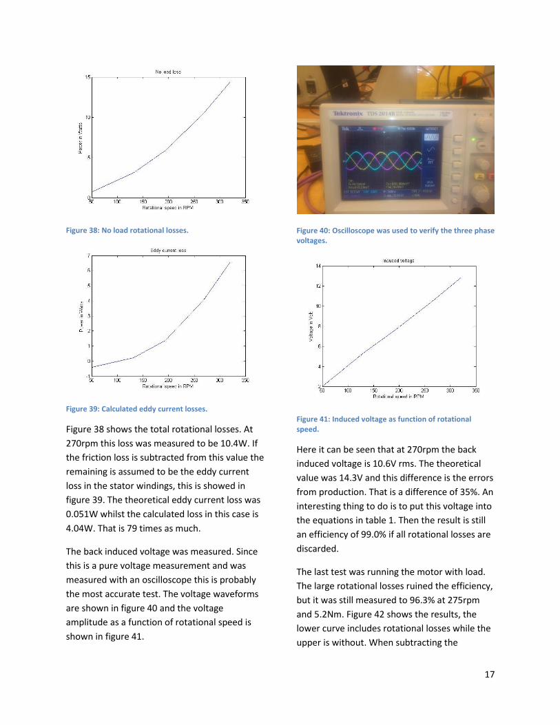
Figure 38: No load rotational losses. ............... 17

Figure 39: Calculated eddy current losses. ...... 17

Figure 40: Oscilliscope was used to verify the

three phase voltages. ....................................... 17

Figure 41: Induced voltage as function of

rotational speed. .............................................. 17

Figure 42: Efficiency of the motor. .................. 18

Figure 43: Efficiency of the motor controller. . 18

Figure 44: Crossing the finish line. ................... 20

Figure 45: At display in DNV's main office in

Oslo. ................................................................. 20

List of symbols

T Torque

P Power

I Phase current

ω Rotational speed rad/s

e Induced voltage

n Rotational speed rpm

Stw Stator thickness

Do Outer diameter of magnet ring

Di Inner diameter of magnet ring

kD Diameter ratio

Flux linkage

t time

B Magnetic field strength

A Area

Permeability in vacuum

Permeance coefficient

Equivalent magnet length

Equivalent air gap area

Equivalent air gap length

Equivalent magnet area

σ Electric conductivity

Br Remanent flux density

l Slot length

w Average slot width

R Electrical resistance

F Force

kf Friction coefficient

dbearing Equivalent diameter of ball bearing

cf Air drag coefficient

Mass density

R Radius

Contents Introduction .................................................................................................................................................. 1

Is it possible to build a motor with such a high efficiency? ...................................................................... 1

2013 Design ................................................................................................................................................... 2

Motor parameters .................................................................................................................................... 2

3D model in Maxwell ................................................................................................................................ 3

Magnet forces ........................................................................................................................................... 5

Magnetic loading ...................................................................................................................................... 5

Stator............................................................................................................................................................. 7

Rotors .......................................................................................................................................................... 11

Losses .......................................................................................................................................................... 14

Encoder ....................................................................................................................................................... 15

Testing ......................................................................................................................................................... 16

Results ..................................................................................................................................................... 16

Batteries ...................................................................................................................................................... 18

Motor controller ......................................................................................................................................... 19

The competition .......................................................................................................................................... 20

Conclusions ................................................................................................................................................. 21

Future work ................................................................................................................................................. 21

Acknowledgements ..................................................................................................................................... 23

References .................................................................................................................................................. 24

Appendixes .................................................................................................................................................. 25

A1: Simulation results ............................................................................................................................. 25

A2: Table of B-field values from Maxwell ............................................................................................... 26

A3: Demagnetization curve of NdFeB N52 ............................................................................................. 27

1

Introduction In the 2011 spring semester Lubna Nasrin

designed an optimized axial flux motor for the

DNV Fuel Fighter as her master thesis [1]. This

design incorporated several improvements over

the previous one, like carbon fiber rotor plates,

Halbach permanent magnet arrangement, the

use of Litz wire in the stator winding and a more

precise simulation model to ensure the motor

would get the designed back EMF. Her design

basically showed half the weight compared to

the previous motor and an efficiency of over

97%, a number which also encounters the

friction losses.

Nasrin’s design was a very good basis for the

2012 team to work with.

A high efficiency propulsion system is much

needed for the car to be competitive. Therefore

the 2012 team decided to build a motor based

on the design of Nasrin. Figure 1 shows the end

result of this work. Sadly the production proved

to be more difficult than they anticipated and

the result was not good enough to be used in

the competition [2]. That being said, the work

that Fredrik V. Endresen put into this attempt

shows the possibility with a design like this and

maybe most importantly he has discovered

several aspect when it comes to the physical

interpretation of a design which might not be

easy and therefore the effort needed in this

part of project should not be underestimated.

Figure 1: The 2012 motor.

Is it possible to build a motor with

such a high efficiency? A car named Aurora had a similar motor built

for a similar type of competition in Australia. It’s

about building a solar powered car which

should drive across the continent. They

developed a motor with similar technology as

the 2012 motor and achieved an efficiency of

97.9% [3], [4]. That is however without rolling

friction. They say the rolling friction belongs to

the wheel, not the motor itself. With friction

included the same motor was tested to an

efficiency of 95.7% [5]. Nasrin’s design takes

rolling friction into account, but it looks like she

has underestimated the value for this loss,

which will be explained later in the test results.

This year there have been more focus on the

production process, and some of the

mechanical students have been directly

involved in the motor project. They do have

more experience with materials, the use of

machines and industrial manufacturing

methods and are able to provide help for

practical problems.

2

2013 Design Like the 2010-2012 motors the 2013 car

featured an in-wheel axial flux motor. This type

of motor is better suited for low speed direct

drive than similar radial flux machines [6] and

[7].

The team decided to go with a single motor

configuration. Due to lack of resources and time

restrictions not very large modifications could

be done to the motor controller and therefore

the double motor configuration was

abandoned. For next year’s team a master

student in drives and power electronics could

look into details about building a custom motor

controller.

Motor parameters To find the best design the criteria used was 5

Nm and 270rpm. This should be the operating

point for the motor when the car was cruising

at a steady 28km/h. However these values are

not critical because the design which is the

most efficient at this operating point would also

be the most efficient at other operating points

since all possibilities considered here is the

same type of motor, just different geometries.

That means they’ll behave the same.

To identify the most efficient design Maxwell 3D

was used to simulate the flux linkage and

thereby induced voltage. This number was then

used in a series of equations to estimate the

performance of the machine.

The loading of this machine is low and since

there is no iron in rotor or stator it is assumed

to be completely linear.

Table 1: Design parameters of the chosen geometry.

T [Nm] 5,000

Pout = 3*e*i = T*w [W] 141,4

If [|A] 3,282

ω = n/60*2*pi [rad/s] 28,274

e = (e/N)*n [V], rms 14,357

n [rpm] 270,0

e/N [V/rpm], rms 0,053

# pole pairs 24,0

# phases 3,000

# slots per pole per phase, q 1,000

Stw [mm] 8,700

Do [mm] 320,0

Di [mm] 210,0

kD 0,656

Wire fill factor 0,550

Slot fill factor 0,455

Slot width, inner diameter [mm] 4,581

Slot width, outer diameter [mm] 6,981

Inner end turn length [mm] 30,0

Outer end turn length [mm] 40,0

Copper resistivity [siemens/mm], 60*C 50302,4

Copper area [mm^2] 10,961

Wire length per phase [mm] 8160,0

Phase resistivity [ohm} 0,015

Copper loss [W] 0,478

Eddy current losses [W] 0,050

Mechanical losses [W] 2,820

Efficiency [%] 97,700

Efficiency without mechanical loss [%] 99,628

3

3D model in Maxwell To ensure proper simulation results 3D

modeling was chosen as the primary tool.

Figure 2 shows the model in Maxwell.

Figure 2: 3D model from Maxwell showing one pole pair.

Figure 3 shows the mesh used in the simulation.

Many nodes were needed in the air gap to give

accurate simulation results.

Figure 3: Air gap mesh.

Transient solution was used to calculate

induced voltage in the winding. Figure 4 shows

the graph with the peak value of the voltage

marked.

Figure 4: Induced voltage in the winding.

A model for how the weight affects the

performance of the car has not been developed.

Bigger magnets would mean a higher magnetic

field and therefore a more efficient motor, but

the extra weight would be negative for the

performance. That means it was not easy to

know how big the magnets should be. The old

motor weighted 21kg including rim. With 10kg

of magnets in the new motor the weight would

be almost similar. Nasrin’s design was lighter

than this but with the track parameters and the

knowledge about the winning car from last year

the belief was that weight is secondary.

The decision was made to go with 10kg of

magnets and end up with a very powerful

motor and a weight similar to the old motor.

Simulations were done to find the best use of

these 10kg and the results are showed in

appendix A1.

Varying air gap was tried, but even though the

simulations were promising the idea of a

thinner stator was abandoned because an error

in the stator production would be more severe.

Figure 4 shows the induced voltage calculated

by Maxwell. This was checked by running a

magneto static analysis, finding the maximum

average B-field in the windings and then

calculating the amplitude of the induced voltage

by the formula below (Hanselmann, 1993).

(1)

4

With 270rpm the time to move from one pole

to another is 0.0046s. So is 0.0023s. is

the area of the coil times average B-field and

is zero.

The area of one coil is 0.000954m2.

The average B-field was found looking at the

variation of the field along three lines in the air

gap, shown in the contour plot in figure 5. The

center point where the lines meet is in the

middle of the air gap.

Figure 5: Contour plot with lines.

The following figures show the distribution of

the B-field along these lines. In the center point

the field strength is 0.96T.

Figure 6: B-field distribution in phi-axis.

In the phi-axis the field is sinusoidal as shown in

figure 6. The average value of this is 0.644 times

the peak value in the center point.

Figure 7: Radial B-field.

The average in the radial axis was calculated

manually from the data table with all the points.

The average was found to be 0.881 times the

value in the center point. The distribution is

shown in figure 7 and the data table is found in

appendix A2.

Figure 8: Axial direction B-field.

In the z-axis the field is symmetric as shown in

figure 8, and the average value was calculated

to be 1.111 times the value in the center point.

Then the average B-field is estimated to be

And the induced voltage

e

This gives an rms value of 8.87V compared to

the value from Maxwell of 14.36V it’s a lot

lower.

Another thing was tried. The line spanning the

radial direction was moved to the point where

the field was equal to the average value in both

5

phi-axis and z-axis. It was moved 1.6 degrees in

phi-direction and 3.15mm in the z-direction.

Then the average B-field along the line was

calculated to be 0.735T. Using this value the

back induced voltage becomes 10.69V. Still

lower than what Maxwell calculates, but it looks

like that the variation in phi-axis is lower when

the line is moved out from the center.

With the test results later in the report in mind

and the fact that production was not perfect it

is assumed that the values that Maxwell

calculates are the correct values.

Magnet forces The magnets on the two rotor plates will try to

close the air gap. Bearings, rotor plates and the

glue to hold the magnets have to be

dimensioned for this force.

This force can be estimated by the following

formula (Endresen, 2012):

(2)

With the average field strength 0.735T

calculated earlier and the total area of

0.0458m2 the force becomes 9.8kN in total.

This was also simulated in Maxwell to be 316N

per pole pair as shown in figure 9 and thereby

7.6kN total force. This value was used when the

thickness of the aluminum plates for the rotors

was chosen.

Figure 9: Magnetic force between two poles.

Magnetic loading High grade magnets have a non-linear

magnetization curve. Too high loading will

demagnetize them, but even if they are not

destroyed the performance is low if they

operate outside the best operating point.

The magnetization curve for the NdFeB N52

magnets is shown in Appendix A3.

The magnetic loading can be calculated from

the formula below (Hanselmann, 1993). This

value is thought of as the slope of a line going

from origin and crossing the demagnetization

curve.

(3)

Finding the equivalent values for area and

length of the magnet in a Halbach array is not

the easiest task, but an approximation is to just

use the length of a half circle through the

magnets to find the length and use the surface

area of one pole as the equivalent area. This is

shown in figure 10 and table 2 on the next page.

We see that longer magnets and wider air gap

gives a higher Pc while a longer air gap and

wider magnets gives a lower Pc. Here the width

of the air gap is assumed to be the same as the

magnets, but in real life this would not be the

case. This would lead to a lower operating

point.

6

With the equivalent values at the middle radius

given in table below the permeance coefficient

becomes 1.9. The load line is plotted in figure

11.

Table 2: Equivalent values of Halbach array.

Parameter Equivalent Value

lm 20.4mm

Ag 357.5mm2

g 10.7mm

Am 357.5mm2

Pc 1.9

Figure 10: Equivalent geometry of Halbach.

Figure 11: Demagnetization curve with load line.

This estimate shows that the magnet array

should operate above the knee of the curve and

not loose performance.

7

Stator The two most promising methods for stator

design were Litz wire and solid conductors

water cut from a copper plate.

Litz wires have been used earlier to prevent

losses because of eddy currents and proximity

effect. This is based on the skin depth, which

basically means the current do not flow in the

center of the conductor at high frequencies.

This leads to higher losses because the copper is

badly utilized. These wires are used in many

high frequency applications. Litz wires work

because there are many thin strands which is

insulated from each other and then twisted.

This gives a uniform current distribution and

eddy currents are heavily damped.

The water cut windings would have a much

better fill factor than the Litz wire, which would

reduce the copper losses. The fill factor in the

slots could almost be doubled with regards to

Nasrin’s design with Litz wire because the area

doesn’t need to be constant and there is almost

no insulation. The drawback of this design is the

eddy currents.

To estimate the eddy current loss the equation

below (Hanselmann, 1993) can be used.

(4)

This number can then be estimated for Nasrin’s

design with a total of 144 slots. For one solid

conductor in the slot this loss equals 22.3W per

slot and thus 3222W for the whole machine at

the rated speed of 25km/h. This loss is not

dependent on the loading of the machine, but

the speed. To achieve the right back EMF in

Nasrin’s design four turns are needed. If the

width are divided into four series connected

conductors the eddy current loss are reduced to

189W. This was verified in Maxwell 3D and later

a water cut winding was made and tested in the

lab by a fellow student to give the same result

[8].

Due to the calculation and simulation results it

was decided to use Litz wire. With the super

strong permanent magnets the induced voltage

per turn was very high. Therefore it was decided

to only have two turns. In addition it was

initially a thought that this would lead to an

easier production process.

The wire used was custom made by New

England wire technology in the USA. The

specification was Type 2 Litz 7 AWG 7X30/30

SPN. This means it has a copper area equal to a

7 AWG, which is the same as 10.5mm2. It is

made up by 7 twisted strands which again are

made up by 30 twisted 30 AWG wires. That

means it is 210 strands twisted in two levels.

This was pressed into a rectangular wire with

the dimensions 4.3mmx4.5mm to accurately fit

into the slots in the machine.

The fill factor of this wire is then 55.2% and the

slot fill factor would then equal 45.6%.

Epoxy was used to give the winding mechanical

integrity and a way of mounting it to the axle.

This was bought from Lindberg & Lund. 17110

Araldite DBF together with the hardener

HY956B 11796 Ren HY956 MP was used

because of the relatively easy handling. It would

not be necessary with vacuum or hardening at

temperatures above room temperature.

Wave winding arrangement was used due to

the short end turn length compared to the

active length of the winding and therefore the

quite efficient design. Figure 5 shows the

winding before its being casted in epoxy.

8

The windings were done in such a way that they

could be laid down phase by phase in the mold.

This meant the end turns of the different

phases did not cross each other and this can be

seen in figure 12.

Figure 12: Wave winding.

Figure 13: The end turns of the top phase is always crossing on top.

In figure 13 a paper with all holes marked can

be seen. This was used as a guideline so the

wires would not crash with any of them after

the stator was casted in epoxy.

The mold was made in Polystone which is a

quite stiff plastic material. A small prototype of

the stator was first made to see if this worked

at all. This mold was made as a two-piece

design and not for vacuum casting. Details of

this work can be seen in figure 14 to 17.

A wooden plate was also machined with slots so

one winding at a time could be made. When

one phase was finished it was moved over to

the mold and the next phase was made. This is

seen in figure 8 and 9.

Figure 14: Prototype stator mold.

Figure 15: The top phase is finished and ready for the mold.

Figure 16: The complete three-phase winding is ready to be casted in epoxy.

9

Figure 17: Prototype stator finished.

Figure 17 shows the final result of the work with

the prototype. It was a success and it was

decided to use the same technique for the real

stator.

A problem was discovered when the big stator

mold was to be made. The bottom part was

supposed to be machined down in a CNC mill.

This was not possible to do because of internal

stress in the plate that basically bent the whole

plate. Therefore a three-piece mold was made.

This solved the problem because the slots for

the end turns and a spacer ring at the outside

were the only machining necessary. Figure 18

shows the final mold. The spacer ring was

machined from a Lexan plate and was 8.7mm

thick.

Figure 18: Final mold for casting the stator.

Figure 19: Bending of the end turns.

Because of the stiffer Litz wire for the real

stator tools had to be used to bend the end

turns. This can be seen in figure 19. Care had to

be taken not to damage the wires in the

process.

When the windings was placed in the mold it

had to be pressed together to ensure it

wouldn’t be too thick. The hydraulic press was

used for this to put the wires in the right place.

During casting powerful clamps was used as

figure 20 shows.

Bits of fire sticks were used between the wires

to ensure even displacement between them.

Figure 20: Epoxy casting.

The final result can be seen in figure 21 and 22.

The thickness should be 8.7mm, but was found

to vary a bit, and was 9mm at the thickest point.

10

But with 1mm air gap at each side this was no

thought of as a major problem.

There are mainly two reasons for this. The most

important one is that the windings were a bit

too tight at the inner diameter. From the start

the goal was to put as much copper in there as

possible. Therefore the slot width at the inner

diameter was used as a parameter and the

winding is just a bit smaller than this value.

What should have been used is the slot width

inside of the inner end turns. This would have

provided more space at the inner diameter. A

steel mold would however solve this problem

because it would not bend as much as the

Polystone mold. In the future a steel mold

should be made anyway to ensure that

everything is in place. Another thing that’s

important with the stator mold is slip angle. The

mold used didn’t have enough slip angles, so it

was very hard to get the cast out of the mold.

Air at high pressure was blown into the center

holes, but this wasn’t enough

Figure 21: Finished stator.

Figure 22: Stator mounted on the axle and placed inside the wheel.

The resistance in the windings was measured

after the stator was finished to ensure that

everything still worked. The result is shown in

table 3. Since the exact length of wire in each

phase was not measured the theoretical value is

not known, but 9.5m of 10.5mm2 copper wire

should have a resistance of 15.8mΩ. The middle

winding was shorter than the lower and upper

winding so that’s why it has a lower resistance.

Table 3: Resistance of phase windings.

Winding Resistance mΩ

A 16.3

B 15.8

C 16.2

When looking at the stator it can be seen that it

is not perfect. The wires do not lie in a

completely straight line or completely axially.

This lowers the induced voltage as the winding

factor gets lower. Since the number of poles is

so high the number of electrical degrees the

windings is skewed gets quite high quite fast

with small errors in production.

11

Rotors The motor should have a double rotor with

permanent magnet configuration. Nasrin

proposed to use Halbach arrays because of the

higher flux density compare to a conventional

north south configuration [1] and [9].

Endresen put together a pair of nice rotors with

90° N42 Halbach array. After simulations in

Maxwell it was found that a 45° array would

increase the back induced voltage by 9.8%

compared to a 90° array of the same size and

magnet grade. This is similar with the findings in

[10]. Figure 23 shows a 90° array and figure 24

shows a 45° array. The magnets in the 45° array

would be half the size, and twice as many would

be needed.

Figure 23: 90 degree Halbach.

Figure 24: 45 degree Halbach.

Drawbacks with the 45° array are more

complicated assembly and the higher material

cost. The cost was not really an issue because of

the proper funding of the project and the motor

development. The assembly should however be

an important part of the process to get the

motor finished before the race.

A 45° array of NdFeB N52 magnets was ordered

from Ningbo Xinfeng Magnet Industry Co.,ltd in

China. They would have a Br of 1.43T and was

one of the most powerful magnet grades

available.

Figure 25 shows the field strength in the middle

of the air gap with this magnet array simulated

in Maxwell. The powerful magnets did push 1T

through the conductors.

Figure 25: B-field in the middle of the air gap.

Assembly of the magnet array proved to be

more challenging than anticipated. In figure 24

it can be seen that there are especially three

magnets per pole that are not very good

friends. There is one pointing directly up and

the two neighbors of this magnet do also point

up, but in a 45° angle. These three had to be

forced together if the array was to be stable.

With two rings this meant that 96 of these

groups had to be glued together before the final

array could be assembled.

This work wouldn’t have been so hard if the

magnets had arrived in time. But because of

problems with placing the order, holidays and

manufacturing process the magnets arrived

very late. So late that several team members

had to work almost nonstop from the day the

magnets arrived and until the rotor plates were

glued and done if the new motor was to be

finished before the race.

The magnets were ordered on 5th of February,

but arrived in Trondheim on 3th of May. The car

was supposed to leave for Rotterdam on 11th of

May, just over one week later.

To be able to assemble the three difficult

magnets tools had to be made. The initial

12

thought was that steel was not a good idea

since it’s magnetic. A mold with two slots was

designed. The slots were wide enough for two

and three magnets to fit, respectively. This way

two magnets could be glued together first and

then the third could be added. This was milled

in a piece of aluminum in the Makino CNC mill.

Figure 26 to 28 shows this first mold. Figure 28

show the top part as well that should keep the

magnets flat while there was screws on the side

that pressed them together.

Figure 26: CNC machining.

Figure 27: Mold to glue magnets together.

Figure 28: Finished with a powerful top part to hold the magnets in place.

This first mold did not work. The magnets did

not want to stay in the slots and there was too

much pressure for the glue to work properly.

This mold could however not be made in steel

because it would be almost impossible to get

the magnets out of the slots after gluing.

Figure 29: Jig for assembling magnets.

Therefore new tools had to be designed. Figure

29 shows a jig that was made to be able to put

together the magnets. A slot was milled in a

steel plate where the magnets just fitted into.

The jig had these two arms that pushed the

magnets together and a rod was put on top to

hold them down to the plate. This process can

be seen in figure 30. Steel was chosen because

that was the only way the magnets wanted to

13

stay together long enough for the glue to do its

magic.

Figure 30: Steel in all directions was the only way to keep the magnets in place.

When this was done the array could be put

together. Figure 31 shows the progression. The

ring on top is aluminum. The glue used between

the magnets and the rotor plates was AW4858-

HW4858-SP from Lindberg & Lund.

Figure 31: Halbach in the making.

Figure 32 and 33 shows the final rotor rings.

There were some problems with the magnet

rings. The jig that was used to put the three

magnets together was made in a hurry and it

didn’t glue the magnets completely true. This

meant that the magnets didn’t quite fit into the

slots that were already machined in the rotor

plates. The rotor plates and the rim were

machined for free at a local company called

Delproduct AS as a part of a sponsorship deal

with the DNV Fuel Fighter team.

This leads to several problems. The side facing

the stator was uneven and the 1mm air gap was

not enough space. The side facing the plate was

also uneven and the glue didn’t get to work that

well. Some magnets came loose and had to be

glued again.

The most serious problem was that the

magnets was skewed a bit and that meant the

last magnet in the array didn’t fit. So it had to

be replaced with a steel piece instead.

Machining of the magnet was tried, but it got

too hot and was thereby destroyed.

Figure 32: Gluing finished.

Figure 33: Finished rotor plate with magnets.

A simulation was done with 1.5mm air gap on

each side and the induced voltage decreased by

14

6.4%. The exact value for the air gap in the

motor is not known, but it’s closer to 2mm on

each side after spacing because it was difficult

to find thinner spacers and at the same time

have enough room for the stator.

Also on the side, in the radial direction, the

design had a 1mm gap between stator and the

magnets. This was a mistake. Because of the

uneven magnet array the stator touched in this

direction as well and the corners of the magnets

had to be grinded down. This value is not critical

for the performance in any way and should

have been made at least 2mm to ensure

enough space.

The team wanted to finish the new motor badly

due to all the new mechanical parts associated

with it. The new aluminum rims were

completely true, easier to handle than the old

carbon fiber rims and could withstand the air

pressure in the tires of 5 bars with no problems.

Losses The different losses are estimated by analytical

calculations. Copper loss is calculated from the

needed phase current and the resistivity in the

winding which again is a result of copper area

and wire length.

(5)

In this design this loss at 5Nm is 0,535W.

The Litz wire that was used had 210 strand each

with a diameter of 0.255mm. With 2 turns, 3

phases and 48 poles the eddy current loss at

270rpm with a flux density of 1T becomes

0.051W when using equation 4.

The friction and windage losses are calculated

from the following equations [11] and [1]

(6)

( )

(

) (7)

The friction loss is estimated to be 2.80W with a

load of 120N, weight of rotors, equal to 0.01

and equivalent diameter of 25mm for the SKF

hybrid ceramic bearings. Windage loss was

estimated to be 0.023W so the total mechanical

loss is then 2.82W.

This is higher than the value first estimated in

Nasrin’s thesis, but should be more accurate

since it’s the model of the bearings that are

used in the motor. This means that the friction

loss used in the analysis is too low. All the

values in the appendix use the value 1.6W

which is what Lubna calculated. The theoretical

efficiency of the design used here is reduced

from 98.43% to 97.70% due to this.

15

Encoder Previous years the motor has been run by a

sensor less algorithm. This is not an ideal way of

operating a synchronous motor. To get

maximum torque of a given current in the stator

windings the angle between the field in the

rotor and stator should be as close to 90° as

possible. This cannot be done if the controller

can adjust the voltage vectors quickly if the

angle passes 90° - it would lose synchronism.

Therefore it was decided to use an optical

encoder with the motor. To find a suitable

encoder was challenging. In this axial flux motor

the axle is standing still and most encoders out

there was supposed to fit on the axle. Therefore

a different solution had to be made. What the

team ended up with was to buy loose parts

from US Digital in the USA. The EM1 read head

together with the 2” disc and proper hardware

to make this fit to the motor controller, like

differential board and proper cables were

ordered. Figure 34 shows the modified old

motor and figure 35 shows the new motor with

encoder installed.

Discs with 2500 slots were ordered. This was a

mistake as the motor control software would

have liked a proper computer number, i.e. 2048

much better. The reason for this is that the

controller needed to divide this number and

2500 did not give an even number which lead to

miscalculations. Help from Smart Motor to

identify this and rewrite the software did solve

this problem in the end.

With limited space inside the motor it was

decided to have the encoder disc on the

outside. A plastic cover was made to protect the

disc. The hole in the axle was made big enough

for the cable to go through and into the car.

Figure 34: The old motor was also modified to work with encoder.

Figure 35: The new motor with encoder fitted and cable going through the axle.

16

Testing To verify the performance of the final result the

motor was setup in a test rig. A DC motor was

mounted as load and a torque transducer was

used to measure output power. A Harmonics

analyzer was used to measure power going into

the motor from the motor controller and a DC

power meter measured the power going into

the motor controller. In addition an oscilloscope

was used to check voltages and output values

from the equipment. The test setup is showed

in figure 36.

Figure 36: Test setup.

The following tests were performed:

- Dummy stator test

- No load test with real stator

- Performance test

This way the hope was to identify the different

losses in the motor. When running with the

dummy stator only the mechanical losses are

present. This is useful when doing the no load

test with the real stator because if the

mechanical losses are subtracted from that

result what’s left is the eddy current loss.

Results All results that are based on the output torque

have to be used with caution. Because of the

placement of the encoder on the outside of the

rotor plate there wasn’t really possible to fit the

adapter for the torque sensor in a good way. A

vacuum formed plastic cup was placed outside

of the encoder and holes were drilled in the

plastic to be able to fit the torque adapter. This

solution wasn’t very good because the two

motors have to be mounted very accurate. A

flex coupling was used on the axial flux motor,

but it could be seen when the motor was

running that the adapter was not in line with

the test setup.

Figure 37 shows the mechanical losses. This is

friction and windage loss. At 270rpm this loss

was measured to be 6.4W which is 227% of the

calculated loss of 2.82W.

Figure 37: Mechanical loss as function of rotational speed.

17

Figure 38: No load rotational losses.

Figure 39: Calculated eddy current losses.

Figure 38 shows the total rotational losses. At

270rpm this loss was measured to be 10.4W. If

the friction loss is subtracted from this value the

remaining is assumed to be the eddy current

loss in the stator windings, this is showed in

figure 39. The theoretical eddy current loss was

0.051W whilst the calculated loss in this case is

4.04W. That is 79 times as much.

The back induced voltage was measured. Since

this is a pure voltage measurement and was

measured with an oscilloscope this is probably

the most accurate test. The voltage waveforms

are shown in figure 40 and the voltage

amplitude as a function of rotational speed is

shown in figure 41.

Figure 40: Oscilloscope was used to verify the three phase voltages.

Figure 41: Induced voltage as function of rotational speed.

Here it can be seen that at 270rpm the back

induced voltage is 10.6V rms. The theoretical

value was 14.3V and this difference is the errors

from production. That is a difference of 35%. An

interesting thing to do is to put this voltage into

the equations in table 1. Then the result is still

an efficiency of 99.0% if all rotational losses are

discarded.

The last test was running the motor with load.

The large rotational losses ruined the efficiency,

but it was still measured to 96.3% at 275rpm

and 5.2Nm. Figure 42 shows the results, the

lower curve includes rotational losses while the

upper is without. When subtracting the

18

rotational losses measured earlier the efficiency

is calculated to 100.7% so the number looks to

be a bit optimistic. And the fact that at 310rpm

and 4.75Nm the efficiency is down to 87%

clearly shows that the measurements are not

conclusive.

Figure 42: Efficiency of the motor.

Figure 43: Efficiency of the motor controller.

Figure 43 shows the efficiency of the modified

motor controller from Smart Motor. It varies

from 78.7% at 230rpm and 4.34Nm to 88.9% at

310rpm and 4.75Nm. This shows that the

controller is more efficient at higher loads.

Batteries A123 Lithium Ion batteries with a nominal

voltage of 46.2V and in three different sizes

were provided by Gylling Teknikk. Last year’s

team thought the batteries could not provide

enough power without having too much voltage

drop.

The medium and the large battery were tested

with a variable resistor with 15A load current.

The medium battery had initially a voltage of

46.64V. With 15A current drawn from the

battery the voltage went down to 43.35V.

The big battery had initially a voltage of 46.78V.

With 15A current drawn from the battery the

voltage went down to 44.5V.

So this proves the batteries should be able to

keep the voltage quite stiff even if the motor

controller draws 650W.

The batteries had built in automatic BMS.

However this did not include thermal cut off

which had to be in place to meet the 2013

regulations. This was solved by soldering a

thermal fuse in series with the battery

management system and placing it just at the

end of the battery. The thermal fuse would melt

at 72°C.

19

Motor controller The motor controller that was used was

provided by Smart Motor. It a controller

originally built for use in a submarine, the

Hugin. Earlier years the team did not have much

control of the digital signal processor software.

This has led to problems because every time a

change had to be made it had to go through

Smart Motor.

Therefore some effort from the guys working at

Smart Motor was put into making a software

package that could be used by the students and

giving the team control of everything necessary.

This worked out very well and the code was

quite understandable as it did hide most of the

lower layers in the code and at the same time

provide a control of all needed parameters in a

structured way.

The controller hardware had to be modified to

work with the encoder since earlier teams had

run a senseless algorithm and the encoder card

was not installed in the motor controller. The

cooler had to be cut to make space for the extra

circuit board. At the same time high

performance cooling paste and aluminum

screws was installed.

Because this controller is made for a submarine

it has more functionality than this project

requires. A quite high no load loss of almost

10W was measured for the controller alone.

After investigating where the heat was

produced and discussing with Smart Motor it

was decided to remove the integrated circuits

and mosfets originally used to control the

rudders. As it turned out these circuits was

active anyway and did draw some power.

Approximately 2W was saved by doing this.

To ensure an efficient way of driving the motor

a lot of time went into tuning the current

regulators. Because the inductance of this

ironless machine is very low there is not much

filtering at the output of the controller and

therefore difficult to produce a stable sine

wave. By using a debugger program called

Active DSP and using the scope function there

to see the current wave form the best

parameters for the built in PI-regulator was

found. To begin with the motor produced a lot

of noise, inverter noise because of vibrations in

the stator due to the sudden current spikes.

To make it perfect was impossible so an idea

was to try adding small inductances in series

with the motor to increase the filtering

capabilities. There would be some loss in the

inductances, but it the thought was that the

system would be more efficient. Looking at the

Csiro motor again, it can be seen that this motor

is delivered with a set of inductances.

Sadly due to time constraints and difficulties

with the electric system right before the

competition this test had to be abandoned.

20

The competition As already mentioned the week before the race

was very stressful. The electronic system did

not work properly and the car did not pass the

technical inspection. A faulty signal cable was

found eventually after trying to replace almost

everything. Then the car worked brilliantly, but

all optimization of the car had to be abandoned

due to this. Only one attempt was completed,

on the last day, which led to third place in the

competition. The team thinks this could be

improved by just optimizing the software,

driving controls and tactics in general. The car

crossing the finish line can be seen in figure 44.

After the race we spoke to a French guy who

earlier had been participating for the French

team which won the competition and now was

working as a marshal during the event. He

meant the car should be ready two months

before the competition so that everything could

be tested properly and optimized. In the battery

electric class the software and driving strategy

is quite important since no time is needed to

make the power source, the battery, to work

properly.

The conclusion was that our car looks really

good, and most likely the car itself was one of

the most high tech at the event, but we didn’t

win because we didn’t have the proper control

software and driving strategy.

Figure 44: Crossing the finish line.

Figure 45: At display in DNV's main office in Oslo.

Still we managed to get two prizes - the design

award and the PR award. So even if we didn’t

manage to do everything that we wanted and

what it takes to win the battery electric class

the project was a success with the third place

on track and two off track awards. After the

race the car and awards was on display at DNV,

the projects most important sponsor, in Oslo,

shown in figure 45.

21

Conclusions Building a new motor was successful in the end.

The motor was used in the competition and

performed well. The building did not go without

problems and the most severe ones were due

to time restrictions. If the magnet had arrived

on time the team could have spent more time

building a revised jig and managed to glue them

completely true.

Most effort went into building the stator as this

part was thought of as the most difficult to

produce from the start. This production method

worked very well, and with some revised

parameters for the Litz wire and a stiffer mold it

could be perfect. The stator used in the motor is

not very bad, but together with the

irregularities in the magnet arrangements the

air gap had to be made bigger to make sure the

stator did not scratch the magnets.

The tests performed on the motor are not

conclusive. The measure rotational losses are a

lot higher than anticipated. Together with the

knowledge about the adapter used for the

torque transducer and the difficulties aligning

the motor in the test bench the results have to

be treated carefully. The test of the induced

voltage does however indicate a fairly high

performance. This test does show the flux

linkage and the error of 35% can be the

production errors.

The flux linkage would be lower due to some

irregularities in the stator windings, the skewed

and a bit broken magnets and the increased air

gap. There is no reason to believe that if the

production went completely smooth the

induced voltage would be lower than in the

design.

The high rotational losses have to be

investigated more. The bearings could have

more friction due to the axial loads the magnets

produce, but also the eddy current losses are a

lot higher than anticipated.

Future work Firstly it’s important to repeat the words from

the French guy who has been on the winning

team. The car should be finished a long time

before the competition so the team has time to

optimize everything. In the battery electric class

the driving strategy and control software is one

of the most important parts for a good result.

This motor could be tested again with a revised

torque adapter. To identify the magnitude of

the friction and eddy current losses would be

important to know what to do with the next

design.

A complete car model should be made and

analyzed. This way the next team could get

better understanding of the weight penalty

compared to raw efficiency in the motor. This

way a better optimization algorithm can be

developed.

To completely understand the sereneness of

the eddy current losses a FE-model should be

made. This has not been done so far because of

problems with the mesh in the air gap when the

wires become so thin, but a method of making

this should be investigated. PhD. Candidate

Zhaoqiang Zhang can probably be of good help

in this field.

To decrease system losses the motor could be

designed with a bit higher induced voltage. The

low voltage and high current stator produced

here would lead to higher copper losses in

cables, connections and controller. With the

stiff battery voltage the induced voltage in the

motor could be a bit higher.

22

Development of a new motor controller is the

next step. It could be done by the help from

Smart Motor and a master student in the field

of power electronics and drives. An efficiency of

more than 90% should be possible.

For a new motor development for 2014 a new

stator mold should be made. Epoxy casting

works well. The mold should be made in steel,

this is possible to machine in the Makino CNC

mill, to ensure a completely stiff mold. The size

of the Litz wire should be revised to ensure

there is enough space at the inner diameter. To

use the hydraulic press a bit is good, but not as

much as we needed to do. Finding a way of

making the windings completely true would be

a good improvement. This is especially for a

high pole machine like this where the winding

factor is easily affected.

A Litz wire with thinner strands should be used

if calculations or simulations show that this

could decrease the eddy current losses

measured in this motor and the measurements

are trustworthy.

New magnets should be bought. Halbach array

should be considered again. If 45° array is to be

used again it’s important to consider the gluing

process of the three problematic magnets. They

need to be completely true and the glue would

add a little bit to the width of the complete

magnet array. Glue should be used between all

the magnets. This way they could be glued

together to a ring before gluing them onto the

rotor plates. Then the slots guiding the magnets

on the plates to ensure they are centered can

be made accurately.

To make this simpler a 90° array can be used

and the performance will not be that much

lower. Especially if one anticipates that

production of the 45° array might not go

completely smooth.

Make sure to investigate holydays in China and

production capabilities early when ordering

high grade permanent magnets. Ideally the

magnets should be ordered before Christmas so

they would arrive in Norway in the first part of

February. The same if a custom made Litz wire

is to be used.

With a new rim or modifications to the old rim

the outer diameter could be made even bigger

because this design has room for M6 bolts going

through the rotor plates and the rim to hold the

wheel together. These screws are not needed as

the magnets will hold the plates in place.

The last thing is the air gap in the radial

direction that should be made bigger. 2mm

here is nice comfort to be sure that if the stator

touch it’s in the axial direction. This would lead

to a bit longer end winding, but the difference is

very small compared to other losses.

23

Acknowledgements I would like to thank my supervisor Professor

Robert Nilssen for his support, guidelines and

suggestions during this time period here at

NTNU.

I would like to thank PhD. Candidate Zhaoqiang

Zhang for his help and support about 3D

modeling, especially Ansys Maxwell, and

machine design in general.

The whole 2013 DNV Fuel Fighter team

deserves huge thanks for letting me participate

in this interesting project, and especially the

two mechanical engineers Fredrik Pettersen and

Magnus Holmefjord who has helped with the

mechanical design of the motor and assembly.

Big thanks to the sponsors and supporters of

the DNV Fuel Fighter project.

I would like to say thank you to my fellow

students for a good time here at NTNU and

suggestions for the work.

I would also like to thank my friends and family

for supporting me during this work.

John Ola Buøy

June 2013

Trondheim, Norway

24

References 1 Improved Version of Energy Efficient Motor for Shell Eco Marathon, Lubna Nasrin Master Thesis 2011. 2 Electric Motor Development for Shell Eco-Marathon, Fredrik Vihovde Endresen,

Master thesis, 2012.

3 Design of an in-wheel motor for a solar-powered vehicle, H.C.Lovatt, V.S. Ramsden and B.C. Mecrow, 1998. 4 Csiro, CSIRO Solar Car Surface Magnet Motor Kit, http://www.csiro.au/resources/pf11g.html 5 Axial Flux Permanent Magnet Motor Csiro. R. Al Zaher, 2010. 6 A comparison between axial-flux and the

radial-flux structures for PM synchronous

motors. Cavagnino, A., Lazzari, M., Profumo, F.,

Tenconi, A., 2001.

7 Analysis and Performance of Axial Flux Permanent-Magnet Machine With Air-Cored Nonoverlapping Concentrated Stator Windings,

Maarten J. Kamper, Member, IEEE, Rong-Jie Wang, and Francois G. Rossouw, 2008. 8 Analysis of a novel coil design for axial flux machines. S. Lomheim, 2013. 9 Improvement of Axial Flux Permanent Magnet Machine using Halbach Arrays, Astrid Røkke , Project Work, 2006. 10 The Effect of Roll Angle on the Performance of Halbach Arrays D. Maybury, C. Nanji, M. Scannell,; Magnetic Component Engineering, Inc. F. Spada; University of California-San Diego, Center for Magnetic Recording Research, 2008. 11 SKF, calculation of bearing friction. http://www.skf.com/group/products/bearings-units-housings/spherical-plain-bearings-bushings-rod-ends/general/friction/index.html

25

Appendixes

A1: Simulation results

The back induced voltage of the given geometry was calculated in Maxwell 3D. This value was then put into the equations and the efficiency at 5Nm and 270rpm was calculated.

Design Do [mm]

Di [mm]

Stw [mm]

Hm [mm] Halbach

Air gap [mm]

Back-emf [V]

Efficiency [%]

Old motor 315 205 6 10 No 2 0,31 95,823

Old motor 315 205 6 10 No 1 0,34 96,374

Lubna's design 315 247 8,7 8 90 1 0,233 97,638

New design 320 210 6,7 15 45 1 0,595 98,442

New design 2 320 210 7,7 15 45 1 0,554 98,44

New design 3 320 210 8,2 15 45 1 0,534 98,435

New design 4 320 210 8,7 15 45 1 0,517 98,433

New design 5 320 210 9,7 15 45 1 0,484 98,422

New design 6 320 210 8,7 17 45 1 0,528 98,451

New design 7 320 210 8,7 13 45 1 0,5 98,402

New design 8 320 150 8,7 11 45 1 0,598 98,273

New design 9 320 170 8,7 12 45 1 0,598 98,339

New design10 320 190 7,7 13 45 1 0,602 98,428

New design11 320 190 8,7 13 90 1 0,51 98,322

New design12 320 190 8,7 13 45 1 0,56 98,417

New design13 320 243 8,7 20 45 1 0,416 98,372

New design14 320 225 8,7 17 45 1 0,477 98,425

New design15 320 210 8,7 15 45 1,5 0,484 98,369

26

A2: Table of B-field values from Maxwell

27

N35

N38

N40

N42

N45

N48

N50

N52

35M

38M

40M

42M

48M

50M

35H

38H

40H

42H

45H

48H

35SH

38SH

40SH

42SH

45SH

28UH

30UH

33UH

35UH

38UH

40UH

Cop

yri

gh

t b

y H

KC

M E

ng

ine

eri

ng

, In

sta

nt U

pda

te -

Cop

y 1

2 J

un

e 2

01

3 2

0:2

6:5

3

A3: Demagnetization curve of NdFeB N52

Néodyme (NdFeB) N52

Update 12 June 2013

BH-diagram (de-magnetisation curve)

ENERGY PRODUCT = Hd*Bd = 52 Mega Gauss * Oersted (MGO)

Grade N52 Residual Induction Br 14.3-14.8 (1430-1480) KG (mT)

Coercive Force Hcb 10.0 (796) kOe(KA/m)

Intrinsic Coercive Force Hcj 11.0 (876) kOe(KA/m)

Energy Product BHmax 50-53 (398-422) MGO(KJ/m3)

Max. Operating Temp. 60 °C

For the description of the properties of magnets practical and theoretical

comparisons need to be done. Magnetic materials preferably are conditioned and

measured in electro magnetic fields.

The BH-diagram is used to determine a characteristical figure - the so called ENERGY PRODUCT : BHmax = Mega Gauss *

Oersted (MGsOe or MGO) This regards to the largest possible rectangle area below the Br/Hcb-curve.

For e.g. Neodymium N45 it is 45 MGO.

The values in table (e.g. 43...46) relate to the tolerances in production.

The BH-Diagramm shows how strong an electro magnetic field (H) must be in order de-magnetize a permanent magnet with a field (B).