Development of Fluidity Measurement Technique and ...

Development of Fluidity Measurement Technique

and Automation of Measurement Station

PAPER WITHIN: Product Development and Materials Engineering AUTHOR: Pratheek Ullal TUITOR: Nils-Eric Andersson JÖNKÖPING: May 2019

Developing the existing Fluidity Measurement Station by automating the operation and measuring the fluidity digitally with MATLAB Image Processing Tools.

Postadress: Besöksadress: Telefon: Box 1026 Gjuterigatan 5 036-10 10 00 (vx) 551 11 Jönköping

Preface

This exam work has been carried out at the School of Engineering in Jönköping in the subject area Product Development and Materials Engineering. The work is a part of the Master of Science program. The author takes full responsibility for opinions, conclusions, and findings presented. Examiner: Roland Stolt Supervisor: Nils-Eric Andersson Scope: 30 credits (second cycle) Date: June 2019.

Acknowledgment

I would like to express my gratitude to Bryne AB, Sweden for hosting the thesis at the company and all the facilities provided to make this thesis a success. I would like to offer my special thanks to Tomas Liljenfors (Ph.D.) Managing Director, for being my supervisor during the entire thesis period at Bryne AB. I am grateful for the assistance given by Alexander Lyrbo (B.Sc.) Mechanical Engineer, during the thesis. I am particularly thankful to the Department of Product development and Materials Engineering at Jonkoping University, Sweden for providing the opportunity to carry out the thesis at Bryne AB. I am grateful for the supervision provided by Nils-Eric Anderson (Ph.D.) Product development and materials Engineering, Jonkoping University, Sweden during the thesis. Pratheek Ullal Jönköping, June 2019

Abstract

1

Abstract

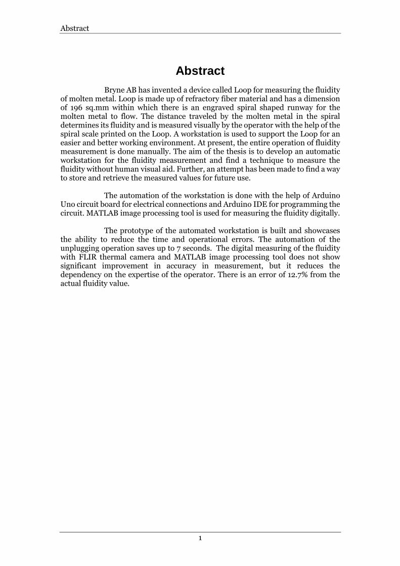
Bryne AB has invented a device called Loop for measuring the fluidity of molten metal. Loop is made up of refractory fiber material and has a dimension of 196 sq.mm within which there is an engraved spiral shaped runway for the molten metal to flow. The distance traveled by the molten metal in the spiral determines its fluidity and is measured visually by the operator with the help of the spiral scale printed on the Loop. A workstation is used to support the Loop for an easier and better working environment. At present, the entire operation of fluidity measurement is done manually. The aim of the thesis is to develop an automatic workstation for the fluidity measurement and find a technique to measure the fluidity without human visual aid. Further, an attempt has been made to find a way to store and retrieve the measured values for future use.

The automation of the workstation is done with the help of Arduino Uno circuit board for electrical connections and Arduino IDE for programming the circuit. MATLAB image processing tool is used for measuring the fluidity digitally.

The prototype of the automated workstation is built and showcases the ability to reduce the time and operational errors. The automation of the unplugging operation saves up to 7 seconds. The digital measuring of the fluidity with FLIR thermal camera and MATLAB image processing tool does not show significant improvement in accuracy in measurement, but it reduces the dependency on the expertise of the operator. There is an error of 12.7% from the actual fluidity value.

Summary

2

Keywords

Product Development, Fluidity in casting Process, MATLAB image processing Tool, Automation, Arduino, Maynard Operation Sequence Technique, Archimedean Spiral.

Contents

3

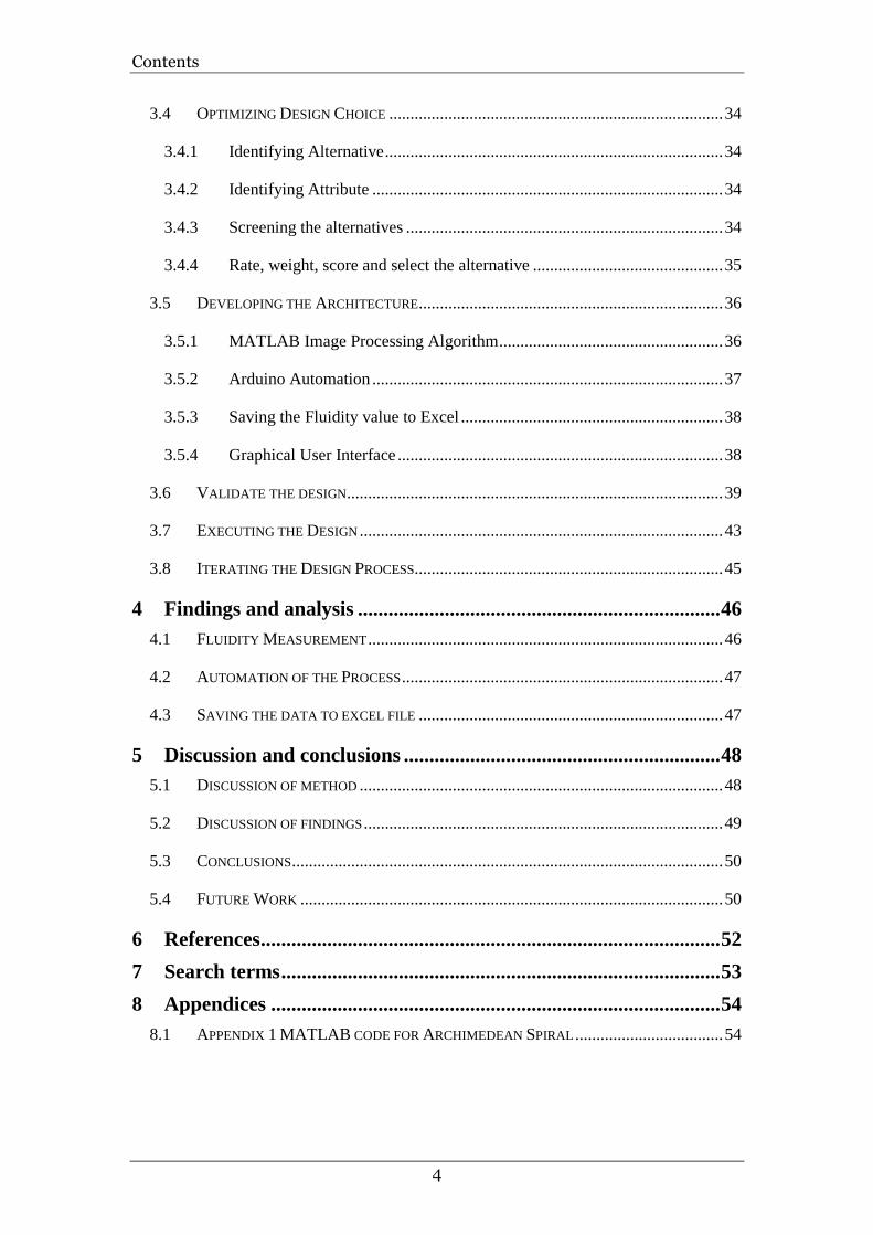
Contents

1 Introduction .......................................................................................... 7

1.1 BACKGROUND ....................................................................................................... 7

1.2 PURPOSE AND RESEARCH QUESTIONS .................................................................... 8

1.2.1 Purpose.......................................................................................................... 8

1.2.2 Research Question ........................................................................................ 8

1.3 DELIMITATIONS ..................................................................................................... 8

1.4 OUTLINE ................................................................................................................ 8

2 Theoretical background ..................................................................... 9

2.1 FLUIDITY ............................................................................................................... 9

2.2 BRYNE AB, LOOP .............................................................................................. 11

2.3 ARCHIMEDEAN SPIRAL ........................................................................................ 15

2.4 MATLAB- IMAGE PROCESSING TOOL................................................................. 17

2.5 THERMAL IMAGING CAMERA ............................................................................... 19

2.6 MICROCONTROLLER FOR AUTOMATION................................................................ 20

2.7 MAYNARD OPERATION SEQUENCE TECHNIQUE ................................................... 22

3 Method and implementation ........................................................... 23

3.1 PROBLEM DEFINITION .......................................................................................... 24

3.1.1 Definition .................................................................................................... 24

3.1.2 Context ........................................................................................................ 25

3.1.3 Functional Requirement .............................................................................. 25

3.2 MEASURE THE NEED AND SET TARGETS .............................................................. 26

3.2.1 Operation Time for Manual Fluidity Measurement .................................... 26

3.2.2 Temperature v/s Fluidity Relation .............................................................. 27

3.2.3 Measurement and operational errors ........................................................... 28

3.3 EXPLORE THE DESIGN SPACE ............................................................................... 29

Contents

4

3.4 OPTIMIZING DESIGN CHOICE ............................................................................... 34

3.4.1 Identifying Alternative ................................................................................ 34

3.4.2 Identifying Attribute ................................................................................... 34

3.4.3 Screening the alternatives ........................................................................... 34

3.4.4 Rate, weight, score and select the alternative ............................................. 35

3.5 DEVELOPING THE ARCHITECTURE ........................................................................ 36

3.5.1 MATLAB Image Processing Algorithm ..................................................... 36

3.5.2 Arduino Automation ................................................................................... 37

3.5.3 Saving the Fluidity value to Excel .............................................................. 38

3.5.4 Graphical User Interface ............................................................................. 38

3.6 VALIDATE THE DESIGN......................................................................................... 39

3.7 EXECUTING THE DESIGN ...................................................................................... 43

3.8 ITERATING THE DESIGN PROCESS ......................................................................... 45

4 Findings and analysis ....................................................................... 46

4.1 FLUIDITY MEASUREMENT .................................................................................... 46

4.2 AUTOMATION OF THE PROCESS ............................................................................ 47

4.3 SAVING THE DATA TO EXCEL FILE ........................................................................ 47

5 Discussion and conclusions .............................................................. 48

5.1 DISCUSSION OF METHOD ...................................................................................... 48

5.2 DISCUSSION OF FINDINGS ..................................................................................... 49

5.3 CONCLUSIONS ...................................................................................................... 50

5.4 FUTURE WORK .................................................................................................... 50

6 References .......................................................................................... 52

7 Search terms ...................................................................................... 53

8 Appendices ........................................................................................ 54

8.1 APPENDIX 1 MATLAB CODE FOR ARCHIMEDEAN SPIRAL ................................... 54

Contents

5

List of Tables

Table 1: Chemical Composition of AES Fiber ......................................................... 11 Table 2: Physical Properties ................................................................................... 11 Table 3: Thermal Conductivity ............................................................................... 11 Table 4: Dimension of the components .................................................................. 12 Table 5: Basic MOST activity sequence model ...................................................... 22 Table 6: Must and Should Functional Requirements ........................................... 25 Table 7: Activities and time taken ......................................................................... 26 Table 8: Screening of Concepts.............................................................................. 34 Table 9: Five-point scale rating ............................................................................. 35 Table 10: Percentage weight and Score calculation ............................................... 35 Table 11: Image Processing steps ........................................................................... 40 Table 12: Fluidity Measurements .......................................................................... 42 Table 13: Hardware and Pin connection ............................................................... 43 Table 14: Trial 1 ...................................................................................................... 45 Table 15: Trial 2 ..................................................................................................... 46

List of Figures

Figure 1: Spiral Test[11] ........................................................................................... 9 Figure 2: Vacuum Test[11] ....................................................................................... 9 Figure 3: Measuring the length with printed scale [14] ......................................... 10 Figure 4: Sand Mold a) Drag b) Cope c) Pouring Basin d) Steel Stopper [14] ....... 10 Figure 5: LOOP assembly ....................................................................................... 12 Figure 6: Cope with Entry and Vent hole ............................................................... 12 Figure 7: Drag with spiral engraved ....................................................................... 12 Figure 8: Stopper .................................................................................................... 12 Figure 9: Filler (Cup) .............................................................................................. 12 Figure 10: Step 2 ..................................................................................................... 13 Figure 11: Step 1 ...................................................................................................... 13 Figure 12: Step 3 ..................................................................................................... 13 Figure 13: Step 4 ..................................................................................................... 13 Figure 14: Opened Loop drag spiral channel.......................................................... 13 Figure 15: LOOP drag with a spiral of solidified metal. ......................................... 13 Figure 16: Fluidity Measurement Station ............................................................... 14 Figure 17: Archimedean spiral represented on a polar graph [15] ......................... 16 Figure 18: Three 360° turnings of one arm of an Archimedean spiral [15] ........... 16 Figure 19: True Color Image showing pixel intensities [16] ................................... 17 Figure 20: Gray Scale Image with pixel intensities between 0 and 1[16] .............. 18 Figure 21: Binary Image showing 1 as white pixel and 0 as black pixel [16] .......... 18 Figure 22: After filling holes[16] ............................................................................. 18 Figure 23: Before filling holes[16] .......................................................................... 18 Figure 24: 8-connected pixel[16] ............................................................................ 19 Figure 25: 4-connected pixel[16] ............................................................................ 19 Figure 26: Electromagnetic Spectrum[17]............................................................. 20 Figure 27: Thermal Imaging Camera[17] .............................................................. 20 Figure 28: Arduino Uno Microcontroller ............................................................... 21 Figure 29: Raspberry Pi B+ .................................................................................... 21 Figure 30: Classification of the entire system ....................................................... 24 Figure 31: Unopened loop ...................................................................................... 28 Figure 32: Opened loop ......................................................................................... 28

https://d.docs.live.net/487d970d7490cb9a/jonkoping/jonkoping%20univertisy%20study%20material/TEUV24%20Thesis/Thesis/Files/Thesis%20report.docx#_Toc10551686































Contents

6

Figure 33: Color image of Loop ............................................................................. 29 Figure 34: Thermal Image ..................................................................................... 29 Figure 35: Polar cordinate method ........................................................................ 30 Figure 36: Cartesian Coordinate System ............................................................... 30 Figure 37: Converting color image to binary image ............................................... 31 Figure 38: Loop with Thermocouple atached along the spiral. ............................. 31 Figure 39: Servo motor with a crank lever mechanism ......................................... 32 Figure 40: Electromagnetic linear actuator .......................................................... 32 Figure 41: Integration of Arduino and MATLAB into one app with GUI ............. 33 Figure 42: Flow chart and MATLAB code for image processing .......................... 36 Figure 43: Flowchart and Arduino code for unplugging automation ....................37 Figure 44: MATLAB code for saving data in excel file .......................................... 38 Figure 45: Graphical User Interface ...................................................................... 38 Figure 46: Archimedian Spiral Graph ................................................................... 39 Figure 47: Loop with 8mm channel....................................................................... 39 Figure 48: Scale model .......................................................................................... 39 Figure 49: Printed scale on the Loop ..................................................................... 39 Figure 53: Fluidity measuring station ................................................................... 44 Figure 50: Measuring station fixed with Arduino, servomotor and thermocouple ................................................................................................................................ 44 Figure 51: Flir one pro thermal camera ................................................................. 44 Figure 52: Temporary measuring station with camera at the bottom .................. 44















Introduction

7

1 Introduction Bryne AB is a Swedish manufacturing and consultation company within the field of material development and technology [1]. Bryne AB offers unique analysis tool 'LOOP' which is used to measure the fluidity of the liquid aluminum at the cast house [2]. Loop is made up of Alkaline Earth Silicate (AES) fiber material and has a dimension of 196 sq.mm within which there is an engraved spiral shaped runway for the molten metal to flow. The distance traveled by the molten metal in the spiral determines its fluidity and is measured visually by the operator with the help of the spiral scale printed on the Loop. A workstation is used to support the Loop for an easier and better working environment. The aim of the thesis is to develop an automatic workstation for the fluidity measurement and find a technique to measure the fluidity without human visual aid. Further, an attempt has been made to find a way to store and retrieve the measured values for future use. This thesis report is carried out in partial fulfillment for the award of Master of Science (120 credits) in Product Development and Materials Engineering of the Jonkoping University, Sweden during the year 2017-2019. The project report has been approved as it satisfies the academic requirements in respect of thesis work prescribed for the Master of Science Degree.

1.1 Background

Casting is a process in which molten metal or an alloy is introduced into a mold where it solidifies in the shape of the mold cavity [3]. The ability of the metal and the alloy to cast without any defects is known as Castability [4]. Fluidity is one of the parameters that influence the Castability of the metal or alloy [5]. Fluidity is the distance flown in a constant cross section by the molten metal before it solidifies. Fluidity depends on various factors such as metal composition, impurities, oxides and temperature. Fluidity affects the surface finish and other mechanical properties in the cast product. Hence there is a requirement to maintain the fluidity at the desired level. Fluidity can be measured by different methods. One of the methods is the spiral loop. There are different technique and material to produce the spiral loop and to measure the fluidity. One such device is the LOOP, invented at Bryne AB. LOOP is made up of AES fiber and has a dimension of 196sq.mm, within which there is an engraved spiral shaped runway for the molten metal to flow. The distance traveled by the molten metal in the spiral determines its fluidity and is measured visually by the operator with the help of the spiral scale printed on the Loop. A workstation is used to support the Loop for the easier and better working environment. But there are several operations during the measurement process using LOOP which consumes time. Hence there is a need for automation. Also, the accuracy of measurement is less with a human visual aid. Hence there is a need for digital readout, which can also be saved and retrieved when required. The use of digital storage creates possibilities for statistical analysis and process control. This requirement directs us to study and find a way to automate the existing process and develop better measurement technique. This development in the existing product would help the cast house to measure the fluidity faster and accurately which would result in better casting products and hence the profit.

Introduction

8

1.2 Purpose and Research questions

The following purpose and research question have been formulated to identify difficulties and establish knowledge of research.

1.2.1 Purpose At present, the measurement of the liquid aluminum takes place at a low rate since all the operation is done manually and the measurement done differs with each operator at the caste house. Hence there is a need for some automation to reduce the time as well as for accurate measurement. Also, the measured values which are stored can be retrieved and used accordingly.

1.2.2 Research Question

1. How can we automate the existing operation of fluidity measurement? 2. How can we measure the fluidity of the liquid aluminum digitally? 3. How can the calculated values be stored and retrieved?

1.3 Delimitations

The thesis focuses on the possible alternative method for human visual aid for the fluidity measurement.

1. The thesis will not cover optimal fluidity for various metal and alloys. 2. The thesis will not cover the reliability of the fluidity value in the casting

process. 3. The thesis will not cover the diagnosis for the bad fluidity.

1.4 Outline

The report covers the theoretical background for the thesis which includes the principle behind the fluidity and the spiral. It also includes information about the software, hardware, and tools used to develop and solve the problem. Following chapters include the method and implementation of the developed design where it focuses on the different concepts and the method to select and eliminate the concepts based on the requirement. Next the findings of the thesis are displayed and finally, conclusions are drawn with future development ideas.

Theoretical background

9

2 Theoretical background

2.1 Fluidity

The quality of the melt is one of the important factors that lead to good casting. Hence, the control and prediction of the melt properties and its characteristics is necessary. The most frequently used tools to achieve this in aluminum casting plants are Thermal analysis (cooling curve), Reduced Pressure test, K-mold, Tatur test, Spiral test, Alscan for hydrogen measurement and PoDFA apparatus [6]. One of the significant properties that influence the casting products is the fluidity of the melt.

The term fluidity is used to indicate the distance a molten metal can flow in a mold of a constant cross-section area before it solidifies [7]. The fluidity depends on many factors such as Chemical composition, Solidification range, Viscosity, Heat of fusion, Heat transfer coefficient, Mold and metal mass density, Specific heat and Surface tension [8]. There are no standard or reliable values for pure metal or alloys. However, fluidity tests are important for respective cast houses or respective batch of melt for the optimization of the above-mentioned factors that affect the fluidity [9]. The first fluidity test was conducted in 1902 [10], and since then many types of equipment for fluidity testing has been developed and modified [11] [12]. The most popular fluidity test is the Archimedean spiral shaped mold test which measures the length the metal flows inside a narrow channel as shown in Figure 1 and the vacuum Fluidity test where the metal flows inside a narrow channel when sucked from a crucible by using a vacuum pump as shown in Figure 2 [13]. Since the spiral test is compact and portable, it has been extensively used.

Figure 1: Spiral Test[11]

Figure 2: Vacuum Test[11]


10

The Archimedean spiral shaped mold setup has three basic sections,

• The narrow channel where the liquid metal flow. • The entry point through which the liquid metal enters the narrow channel. • The vent which is provided for the gases to escape.

The above type of setup can be created in several ways. One type of setup is shown in Figure 4 where the mold is made of quartz sand [14]. The different components in the setup include a) quartz sand drag which has the Archimedean spiral cavity b) quartz sand cope which is placed over the drag c) quartz sand pouring basin which is placed over the cope d) stopper, made of steel is used to block the entry point to stop the liquid metal until temperature reduces and reaches the desired value. When the temperature reaches the desired value, the stopper is pulled out allowing the liquid aluminum to flow in the drag and solidify. After solidification, the sand mold is opened, and the casting is measured using a scale printed on the paper as shown in Figure 3. The temperature is measured with the K-type thermocouple which is attached to the stopper.

The disadvantage of the sand mold is that it is heavy and time-consuming. To overcome this, Bryne AB has invented the same spiral with the product name LOOP. The Loop is made up of a material called AES fiber which can withstand temperature up to 1100 degree Celsius. It has low thermal conductivity, which means the metal can flow longer before solidification resulting in higher precision. The properties throughout the AES fiber remains constant, unlike the sand mold which differs in properties due to the change in packing, humidity, and composition. The material is lightweight which makes it possible to transport without risking the product to fall apart. The material is sustainable, eco-friendly and safe for the operator. The spiral is engraved by CNC milling process which gives the possibility for faster manufacturing and mass production. The chemical composition of AES fiber, Physical properties, and thermal conductivity is discussed in the next section.

Figure 3: Measuring the length with printed scale [14]

Figure 4: Sand Mold a) Drag b) Cope c) Pouring Basin d) Steel Stopper [14]


11

2.2 Bryne AB, LOOP

LOOP is made up of compressed Alkaline Earth Silicate (AES fiber). The chemical composition in percentage is given in Table 1. The physical properties of the LOOP are given in Table 2. The thermal conductivity is given in Table 3.

Table 1: Chemical Composition of AES Fiber

Sr.no Chemical Composition Percentage

1 SiO2 60-67 2 Cao 27-33 3 MgO 3-7 4 Al2O3 <1 5 Fe2O3 <0.6

Table 2: Physical Properties

Sr.no Physical Properties Values

1 Color White/beige 2 Melting Point >1330oC 3 Density 270 kg/m3

4 Modulus of rupture >700 kPa 5 Highest recommended user temp 1100 oC

Table 3: Thermal Conductivity

Sr.no Temperature in oC 4

1 400 0.07 2 600 0.10 3 800 0.14

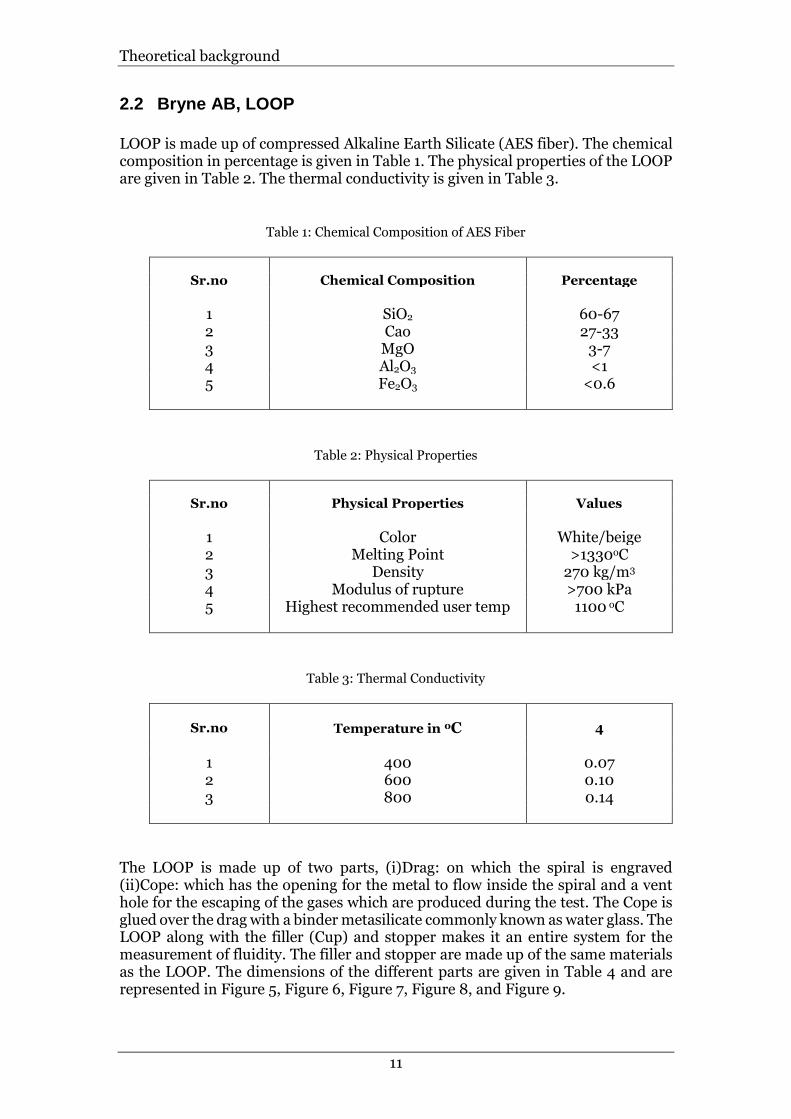
The LOOP is made up of two parts, (i)Drag: on which the spiral is engraved (ii)Cope: which has the opening for the metal to flow inside the spiral and a vent hole for the escaping of the gases which are produced during the test. The Cope is glued over the drag with a binder metasilicate commonly known as water glass. The LOOP along with the filler (Cup) and stopper makes it an entire system for the measurement of fluidity. The filler and stopper are made up of the same materials as the LOOP. The dimensions of the different parts are given in Table 4 and are represented in Figure 5, Figure 6, Figure 7, Figure 8, and Figure 9.


12

Table 4: Dimension of the components

Sr.no Dimensions Values

1 Drag 196x196x8 mm 2 Cope 196x196x6 mm 3 Filler (Cup) Ø65 x 50 x Ø80 mm

4 Entrance Hole Ø20 5 Vent Hole Ø20

Figure 7: Drag with spiral engraved Figure 6: Cope with Entry and Vent hole

Figure 9: Filler (Cup) Figure 8: Stopper

Figure 5: LOOP assembly


13

The measurement of the fluidity using LOOP is done in four simple steps:

1. Place the loop on the table. The plug A is mounted on the entry hole in the cope B. The cup C is placed at the center of the entry hole and a thermocouple D is placed inside the cup to measure the temperature (Figure 11).

2. The melted metal is poured into the cup (Figure 10). 3. When the temperature of the melt reduces to the desired level, the plug is

pulled straight up allowing the metal to flow inside the spiral (Figure 12). 4. As the metal runs inside the spiral it burns the AEF, turning it to brown

color. The upper side of the cope is printed with the measuring spiral scale which indicates the length the metal has flown before solidification (Figure 13)[1].

Figure 11: Step 1 Figure 10: Step 2

Figure 12: Step 3 Figure 13: Step 4

Figure 14: Opened Loop drag spiral channel

Figure 15: LOOP drag with a spiral of solidified metal.


14

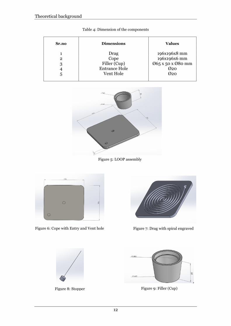
The opened loop drag with spiral channel is shown in Figure 14. Loop drag with a solidified spiral is shown in Figure 15. The width of the channel is 8mm and the depth of the channel is 4mm. The thickness of the wall between each channel is 4mm. The total length of the channel is 1988mm. There are total 38 markings along the channel with each marking at 50mm from each other. Loop is read using the marks and named, for example, 30.2 when the metal has traveled the distance of 30.2. The measurement station is 1 meter in height, 2 meters in length and 1.5 meters in width with the flaps extended as shown in Figure 16. It is made up of stainless steel and is portable. It has provisions for mounting the thermocouple and base support to place the temperature readout machine. At the bottom, it has space for the loop, cups and other necessary items.

Figure 16: Fluidity Measurement Station


15

2.3 Archimedean Spiral

The spiral shape that has been used in the Loop is originally known as the Archimedean Spiral. It is named after the 3rd century BC Greek Mathematician Archimedes. This spiral can be defined as “The locus of points corresponding to the locations over time of a point moving away from a fixed point with a constant speed along a line that rotates with constant angular velocity” [15]. This spiral can be represented by the polar coordinates (r, θ) in the equation (1) where we assume that the curve is traced out exactly once, that is one loop. Here r is the length of the radius from the center or beginning of the spiral, 𝜃 is the angular position, f is the constant, and 𝛼, 𝛽 are the maximum and the minimum angle between which the spiral is drawn.

𝑟 = 𝑓𝜃 𝛼 ≤ 𝜃 ≤ 𝛽 (1) Writing the equation (1) in terms of a set of parametric equations we get equation(2) and equation(3) where x and y are the distance in x and y-direction in cartesian coordinate.

𝑥 = 𝑟 𝑐𝑜𝑠𝜃 (2)

𝑦 = 𝑟 𝑠𝑖𝑛𝜃 (3)

The small change in distance x and y with the change of 𝜃 can be obtained by differentiating the above equation with respect to θ , we get equation (4) and equation(5).

𝑑𝑥

𝑑𝜃=

𝑑𝑟

𝑑𝜃𝑐𝑜𝑠𝜃 − 𝑟𝑠𝑖𝑛𝜃 (4)

𝑑𝑦

𝑑𝜃=

𝑑𝑟

𝑑𝜃𝑠𝑖𝑛𝜃 + 𝑟𝑐𝑜𝑠𝜃 (5)

Next, the approximate arc length can be found out by the Pythagoras theorem

(𝑑𝑥

𝑑𝜃)

2

+ (𝑑𝑦

𝑑𝜃)

2

= (𝑑𝑟

𝑑𝜃𝑐𝑜𝑠𝜃 − 𝑟𝑠𝑖𝑛𝜃)

2

+ (𝑑𝑟

𝑑𝜃𝑠𝑖𝑛𝜃 + 𝑟𝑐𝑜𝑠𝜃)

2

= (𝑑𝑟

𝑑𝜃)

2

𝑐𝑜𝑠2 𝜃 − 2𝑟 𝑑𝑟

𝑑𝜃 𝑐𝑜𝑠𝜃 𝑠𝑖𝑛𝜃 + 𝑟2𝑠𝑖𝑛2 𝜃

+ (𝑑𝑟

𝑑𝜃)

2

𝑐𝑜𝑠2 𝜃 − 2𝑟 𝑑𝑟

𝑑𝜃 𝑐𝑜𝑠𝜃 𝑠𝑖𝑛𝜃 + 𝑟2𝑠𝑖𝑛2 𝜃

= (𝑑𝑟

𝑑𝜃)

2

(𝑐𝑜𝑠2 𝜃 + 𝑠𝑖𝑛2 𝜃) + 𝑟2(𝑐𝑜𝑠2 𝜃 + 𝑠𝑖𝑛2 𝜃)

(𝑑𝑥

𝑑𝜃)

2

+ (𝑑𝑦

𝑑𝜃)

2

= 𝑟2 + (𝑑𝑟

𝑑𝜃)

2

(6)

(𝑑𝑥

𝑑𝜃)

2

+ (𝑑𝑦

𝑑𝜃)

2

= 𝑑𝑠2 (7)


16

Where 𝑑𝑠2 = 𝑟2 + (𝑑𝑟

𝑑𝜃)

2

.

The arc length formula for the spiral in polar coordinates is then given by adding all the 𝑠 . That is integrating 𝑑𝑠 we get equation (8) where L is the entire length of the spiral.

𝐿 = ∫ 𝑑𝑠 (8)

Where,

𝑑𝑠 = √𝑟2 + (𝑑𝑟

𝑑𝜃)

2

𝑑𝜃 (9)

The arc length for multiple loops n with the loop starting at a distance a from the origin and having constant distance b between each arm can be obtained by the equation (10).

𝐿 = ∫ √𝑟2 + (𝑑𝑟

𝑑𝜃)

2

𝑑𝜃𝜃2

𝜃1

(10)

Where,

𝑟 = 𝑎 + 𝑏𝜃

(11)

And 𝜃1, 𝜃2 are the minimum and maximum angle within which the spiral is drawn.

Figure 18: Three 360° turnings of one arm of an Archimedean spiral [15]

Figure 17: Archimedean spiral represented on a polar graph [15]


17

2.4 MATLAB- Image Processing Tool

Designed by Cleve Moler and Developed by MathWorks with its first release in the year 1984, MATLAB is a functional, imperative, procedural, array and object-oriented numerical computing environment and programming language which allows matrix manipulation, plotting of functions and data, implementation of algorithms and creation of user interface. It can also be used for the interfacing with programs written in other languages including C, C++, C#, Java, Fortran, and Python. The supported operating system is Windows, macOS, and Linux with the platform IA-32, x86-64. The latest version of MATLAB R2019a was released on March 20, 2019. There are many add-on products to the MATLAB such as Control System Toolbox, Data Acquisition Toolbox, Image Processing Toolbox, etc [16]. Image Processing Toolbox™ is used for image processing, analysis, visualization, and algorithm development with the help of a comprehensive set of reference-standard algorithms and workflow apps. The toolbox supports processing of 2D, 3D, and large images and can perform image segmentation, image enhancement, noise reduction, geometrical transformation and image registration using deep learning. The four basic types of images that Image Processing Toolbox handles are Binary images, Indexed Images, Grayscale Images, and True Color Images. Import, Export, and Conversion includes converting between image types, such as RGB (true color), Binary, Gray Scale and Indexed [16]. Images in MATLAB are stored in a two-dimensional matrix. Images are made up of pixels whose intensity can be varied. Each element of the matrix corresponds to a single discrete pixel of the image. True color images (also called as RGB image) are represented by three-dimensional array since the true color image is made up of 24 bits which are distributed among Red, Green, and Blue with 8 bits each and are designated to three planes respectively showing the pixel intensities (Figure 19). Grayscale images can be obtained by representing the intensity values within range 0 to 1 in a data matrix ( Figure 20). Binary Image is stored as a logical array and assumes one of only two discrete values 1 or 0 where one represents white and o represents black (Figure 21) [16].

Figure 19: True Color Image showing pixel intensities [16]


18

The threshold level is usually used during the conversion of grayscale image to a binary image. For example, if we specify the threshold level as 0.4, the pixels with the intensity below 0.4 in the grayscale image turns into black and the rest turns into white. Sometimes the converted binary images need to be modified so that the holes or the dark spaces within certain boundaries are filled. This can be done with

Figure 20: Gray Scale Image with pixel intensities between 0 and 1[16]

Figure 21: Binary Image showing 1 as white pixel and 0 as black pixel [16]

Figure 23: Before filling holes[16] Figure 22: After filling holes[16]


19

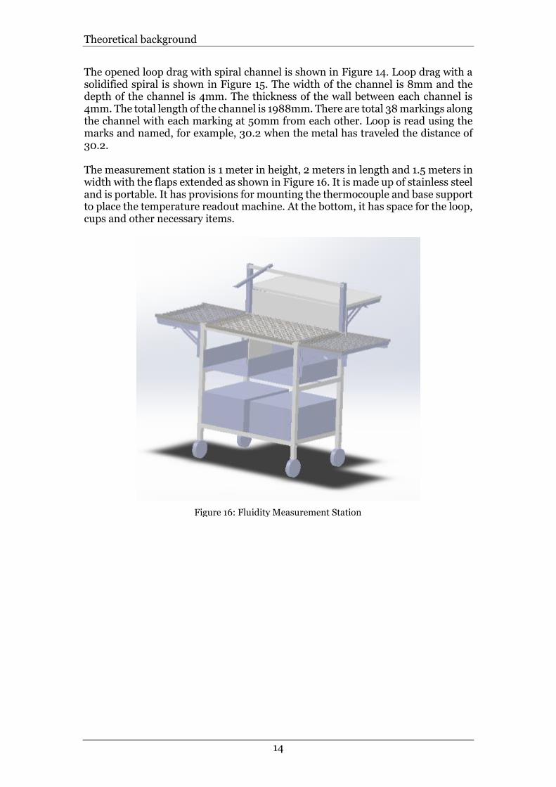
the inbuilt command ‘imfill’. Figure 22, Figure 23 shows before and after the imfill operation [16]. For two dimensional images, there are two ways in which the pixel gets connected to its neighboring pixel, 4-connected and 8-connected. In 4-connected, the adjacent pixels in the horizontal or vertical direction get connected if the edges of the pixel touch (Figure 25). In 8-connected, the horizontal, vertical, or diagonal direction get connected if the edges or corners of pixel touch (Figure 24).

2.5 Thermal Imaging Camera

All substance in the universe is made up of atoms. The atom itself is made up of particles such as an electron, proton, neutron, etc. When an atom absorbs energy one or more electron changes their position from lower energy level to a higher level within the atom. When the same electron returns to its original position an electromagnetic wave is produced. The electromagnetic spectrum consists of x-rays, ultraviolet, visible light, infrared, microwaves and radio waves (Figure 26). Electromagnetic radiation emitted due to the heat of material are called thermal radiation [17]. Thermal radiation can have the wavelength corresponding to the visible and infrared region of the electromagnetic spectrum. Although the visible light can be detected by a normal camera the infrared radiation needs to be converted into a color image. The infrared radiation lies between the visible and microwave in the electromagnetic spectrum. The difference in temperature produces different intensity and wavelength in the infrared region. These infrared radiations can be converted into images known as thermal images with appropriate hardware and software. The basic principle is shown in Figure 27 where the infrared radiation (A) radiated by the object is focused onto an infrared detector (C) by the optic lens (B). The detector will send the information into the sensor (D) which then processes the data from the sensor to produce an image with the help of complex algorithms which is then viewed on the LCD screen or the viewfinder (E). There are several properties that need to be considered during the thermal imaging such as thermal conductivity, emissivity, reflection, etc [18]. The difference in thermal conductivity between two different types of material can show a large temperature difference in a certain situation which might sometimes lead to wrong inferences and conclusion for the diagnosis. Emissivity is the efficiency with which an object emits infrared radiations. To read the correct temperature, setting the right emissivity is very important. The thermal radiation gets reflected like that of the visible light, and hence can affect the measurement of the temperature.

Figure 25: 4-connected pixel[16]

Figure 24: 8-connected pixel[16]


20

Some of the parameters that are to be considered for obtaining a good thermal image are thermal sensitivity, accuracy, camera resolution, and software. The smallest temperature difference that the sensor can detect is called the thermal sensitivity. For example, 0.7-degree Celsius thermal sensitivity is better than 0.9-degree Celsius thermal sensitivity. The camera resolution delivers image quality. More the resolution clearer is the image. The clear image helps to see, measure and understand more accurately.

2.6 Microcontroller for automation.

The microcontroller is like a small computer in a single integrated circuit. It is mainly used for controlling the products and devices automatically. A typical microcontroller includes a processor, memory and input/output peripherals. The processor capacity of a microcontroller can be chosen according to its application. The options range from 4-bit, 8 bit, 16 bit, 32 bit, or 64 bit. The input/output peripheral include analog to digital converters, universal serial bus (USB) connectivity, and Liquid Crystal Display (LCD) controllers. Two of the most popular microcontrollers producing company is the Arduino and Raspberry Pi. Arduino is a company known for manufacturing single-board microcontrollers and microcontroller kits for building digital devices and interactive objects which can sense and control both physically and digitally. It also provides open source software for programming of microcontroller kits known as Arduino IDE [19]. Arduino Uno is one of a well-known microcontroller board. It is an 8-bit microcontroller and has 12 kilobytes of RAM. It has 14 digital input/output pins and 6 analog inputs. The codes can in uploaded into the microcontroller with

Figure 26: Electromagnetic Spectrum[17]

Figure 27: Thermal Imaging Camera[17]


21

the help of a USB port in the board. The other parts of the microcontroller are shown in Figure 28. Raspberry Pi is developed by the Raspberry Pi foundation. Raspberry Pi model B+ is one of the microcontroller board. It comes with a 64-bit microprocessor and 1GB of RAM. It has 8 input/output pins and several other ports such as HDMI port, SD card port, USB port, and Audio jack. The other parts of Raspberry Pi B+ are shown in Figure 29 below. The choice of the microcontroller is done based on its application and complexity.

Figure 28: Arduino Uno Microcontroller

Figure 29: Raspberry Pi B+


22

2.7 Maynard Operation Sequence Technique

Maynard operation sequence technique or MOST is a technique used to set or determine the standard time that is needed by a worker to perform a task. Time measurement units (TMU) is assigned to the individual motion element that is obtained by breaking the main task. 100000 TMU is equivalent to one hour [20]. There are many variations in MOST but the commonly used MOST is the Basic MOST. It was released in Sweden in 1972. The Basic MOST are used for the operations that take time between one to ten minutes. Other types of MOST are MiniMOST, MaxiMOST, and AdminMOST. Table 5 shows the general move activity sequence model for Basic MOST.

Table 5: Basic MOST activity sequence model

General Move activity sequence model = A B G A B P A

Index A = Action

distance B = Body motion

G = Gain control

P = Placement

0 Close <= 5 cm Hold, Toss

1 Within reach,>

2in

Grasp light object using one or two

hands

Lay aside loose fit

3 1 or 2 steps Bend and arise

with a 50% occurrence

Grasp object that is heavy, or obstructed, or

hidden, or interlocked

Adjustments, Light

pressure, double

placement

6 3 or 4 steps Bend and arise

with a 100% occurrence

A position with care, or precision, or the blind, or obstructed,

or heavy pressure.

10 5 to 7 steps Sit or Stand

16 8 to 10 steps

Through the door, or climb

on or off, or Stand and

Bend, or Bend and sit

The time for each task is obtained by adding the index for the task and multiplying it with 0.36. For example, time taken for placing a coffee cup from one table to another can be calculated as follows: Action distance to grab the cup is within reach therefor index is A1. Next, there is no need to bend or raise body motion, therefore B0. Next, gaining control of the cup with one hand G1. And finally placing the object on the table by laying it aside P1. So, the total index is A1+B0+G1+P1=3. And the total time taken for this task is 3 x 0.36 = 1.08 sec.

Method and implementation

23

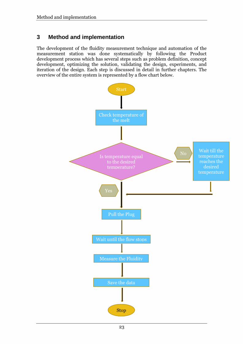
3 Method and implementation The development of the fluidity measurement technique and automation of the measurement station was done systematically by following the Product development process which has several steps such as problem definition, concept development, optimizing the solution, validating the design, experiments, and iteration of the design. Each step is discussed in detail in further chapters. The overview of the entire system is represented by a flow chart below.

Start

Check temperature of the melt

Is temperature equal to the desired temperature?

Pull the Plug

Wait till the temperature reaches the

desired temperature

No

Yes

Measure the Fluidity

Save the data

Stop

Wait until the flow stops


24

3.1 Problem definition

3.1.1 Definition The measurement of the liquid aluminum at the cast house takes place at a low rate All the operations mentioned in section 2.2 are done manually. The measurement which is done visually by the operator differs with each operator at the caste house. Hence there was a need for some automation of the manual operations to reduce the time as well as for accurate measurement. Also, the measured values were needed to be stored and retrieved for statistical analysis and process control. Hence the entire system was classified into three sections as shown in Figure 30. The boxes with blue color indicate that they will be focused in this thesis and are expected to be completed.

1. Measurement: Digital reading of the fluidity value and measurement of temperature.

2. Automation: Automation of the operation carried out for the measurement of the fluidity.

3. Integration: Saving and retrieval of the obtained values.

Figure 30: Classification of the entire system

Definition

Automation

Unplugging at right temperature

Valve opening of crucible at right

temperature.

Placing the loop and the cup at the right

position

Placing the used loop and cup at the right

position

Measurement

Measuring the Fluidity

Measuring the temperature

Measuring the speed of metal filling

Measuring the rate of decrease in

temperature inside the loop

Integration

Saving and retrieving the information and

results

Integration of automation and measurement

Creating the Graphical User Interface


25

3.1.2 Context This section describes the circumstances, events and the places where the developed product will be handled and used. The developed system will be used at the cast house by different operators. The cast houses have different ovens with different alloy composition and temperature. Each oven is placed at a certain distance apart from each other. Several trials are needed from each oven during the experiment, hence there was a need for several LOOPs. During the trials, the information such as the alloy type, temperature, time, batch number, date, oven number, and fluidity needs to be recorded. The functions that need to be incorporated in the developed product so that it can be used in the above context are listed in the next section.

3.1.3 Functional Requirement The functional requirements include those functions that the owner and the user of the system feel it must or should contain. These functional requirements are found out by discussing it with the owner at the company and the operator at the cast houses. Since the developed system will be used at the cast house, the system must be robust and resistant to high temperature. The system must be lightweight, compact and mobile so that it can be moved from one oven to another. The results must be precise, accurate and reliable. It must be user-friendly and easy to understand so that every operator can use the system. There should be enough space to store the loop in the station and enough table area to perform the experiment. The new system (includes automation, measurement, and integration mentioned in section 3.1.1) must be faster and cost-efficient. It was also desirable to have the system to be aesthetically appealing. It should be easy to maintain since maintenance directly influences time and cost. Table 6 shows the list of must and should functional requirements.

Table 6: Must and Should Functional Requirements

Sr.no Must Should

1 Compact and Portable Aesthetic 2 Faster Space to store loop, cup, stopper 3 Cost efficient Easy maintenance 4 User-friendly Instant Analysis of results 5 Robust 6 Precise and accurate

The functional requirement that is mentioned above needs to be satisfactory and should achieve some set target. Next section deals with measuring and setting targets so that the final system that is developed is better than the existing system and shows significant improvement than the former system.


26

3.2 Measure the Need and Set Targets

Measuring and setting target helps to understand the performance of the existing system in all its attributes. Different attributes (Functional Requirement) needs to be measured in different methods. For instance, the fastest of the two machines can be compared by the time taken by it to perform its respective task. One such example is measuring the operation time for manual fluidity measurement as discussed in the next section.

3.2.1 Operation Time for Manual Fluidity Measurement The operation time taken for the steps of fluidity measurement can be determined by using Maynard Operation Sequence Technique (MOST). MOST has many methods that are classified according to its applicability as mentioned in section 2.7. Basic MOST is one such technique that can be used in this context. The steps (discussed in section Bryne AB, LOOP) can be subdivided into several steps and the time taken for each step can be calculated as follows by using the Table 5: Basic MOST activity sequence model

Table 7: Activities and time taken

Sr.no Activities Index Time(sec) = Total Index * 10 *0.036

1 Place the LOOP on the table A1B0G1P1 1.08 2 Place the plug on the entry hole A1B0G1P3 1.8 3 Place the cup at the center of the hole A1B0G1P1 1.08 4 Place the thermocouple A1B0G1P3 1.8 5 Take the metal in the scoop A3B3G3P6 5.4

6 Measure the temperature of the metal in the scoop.

A1B0G1P1 1.08

7 Wait until it reaches the desired temperature T1

Variable 5

8 Pour the metal into the cup. A1B3G3P3 3.6

9 Measure the temperature of metal inside the cup.

A1B0G1P1 1.08

10 Wait until it reaches the desired temperature.

Variable 5

11 Pull the plug straight up when the temperature reaches the desired temperature.

A1B0G1P1 1.08

12 Wait until the metal flows into the spiral 7 13 Measure the reading visually A1B0G1P1 1.08

14 Note down the reading and other details in the notebook.

A1B0G1P1 1.08

15 Keep the Loop aside A1B0G1P1 1.08

Total 38.24

Since we are dealing with molten metal which is at a temperature of more than 700 degree Celsius, it is highly recommended that we slow down the body movements to avoid any accidents. Hence activities such as 5, 6, 7 and 8 should be performed


27

carefully. Therefore, these activities were added with 5 seconds each for the calculation of the total time. This time was determined by doing several experiments at the cast house. After considering the conditions the total time would be 58.24 seconds. This is the approximate total time that is needed for one trial of fluidity measurement. Therefore, if there are 10 trials in one batch (Oven), we would need around 6000 seconds (100 minutes) to perform all the trials without considering the time taken for miscellaneous activities. By measuring the time taken for one trial (60 seconds), we now know that the time taken by the automated system must be below 60 seconds. Hence, our target time for one trial must be below 60 seconds.

3.2.2 Temperature v/s Fluidity Relation One of the important factors that change the fluidity of the melt (molten alloy) is the temperature. Graph 1 shows the increase in fluidity with an increase in temperature. These data are recorded from the experiments conducted by Bryne AB. With higher temperature, the melt takes more time to solidify which gives the metal a chance to flow further. Also, with higher temperature the viscosity of the melt decreases. Hence it is important that the metal flows into the loop at the same temperature for every trial. This will ensure the consistency and the reliability on the result. One of the reasons for the difference in entry temperature of the melt into the loop is delayed or advanced unplugging. For example, if the unplugging is done at a temperature of 668 degree Celsius instead of 670 degree Celsius, the fluidity value decreases from 26 to 25. This variation might result in improper analysis in the long run.

Graph 1: Temperature v/s Fluidity ( Internal experimental data)

Hence, the new system that needs to be developed should be able to accurately measure the temperature with sensitivity of at least 0.50 degree Celsius ( target for temperature sensitivity) and the automation of the unplugging operation needs to be quick enough to respond (target for efficient mechanism) when the temperature reached the desired set unplugging temperature.


28

3.2.3 Measurement and operational errors During manual operation committing errors are evident. The errors can be done during any measurement or during the operation. For example, the Fluidity readout from an unopened loop (Figure 31) is 27.5 and opened loop (Figure 32) is 27.3. The difference in the readout value is 0.2. Although the deviation is very small in this example the two readings can vary as much as 1.5 to -1.5. The deviation can be caused by several reasons such as:

a) Improper noting down of the measured values. b) Visibility errors on the loop. c) Approximation errors between different operators.

Although the deviation (Graph 2) of most of the readings is between +0.5 to -0.5, some of the values exceed +1.5 to -1.5. This can affect the result during determining variation in the fluidity at the cast house.

Graph 2: Deviation in fluidity reading

With this, we were able to determine the accuracy of the digital reading that was planned to develop. Hence, the target that was expected to achieve with the digital reading was less than +/- 0.5 deviation.

Figure 32: Opened loop Figure 31: Unopened loop


29

3.3 Explore the Design Space

In this section, we try to explore different possibility and ideas that could be used to solve the problems. Considering the context and functional requirements, several concepts were developed for measuring the fluidity and for the automation. Some of the concepts and ideas are given below:

1) Measuring the fluidity a) Image Processing: One of the methods to measure the fluidity can be by

using the digital image of the used loop that is captured by the camera after the flow of the metal in the spiral has stopped. The images can be of two types: i) Color Image: Deep Learning image recognition method is required to

measure the fluidity with the digital color image. In this method, hundreds of previously captured digital test images are stored in the database with the respective fluidity value. The digital color images that are captured during the experiment for the measurement of fluidity needs to be compared with the previously stored images, which are done with the deep learning algorithm. The challenges of this method include large data storage and high-quality images.

ii) Thermal Image: The thermal images display the distinct color and path of the metal flow inside the loop. The endpoint of the loop is much clearly visible than that of the digital color image with a high thermal sensitive camera. By using the position of the end point of the loop we can use different methods to measure the fluidity.

Figure 33: Color image of Loop

Figure 34: Thermal Image


30

(1) Polar coordinate method: The thermal image captured during the experiment can possibly be overlapped with the polar coordinate scale as shown in Figure 35. In polar coordinate scale, space is divided into 36 parts with an angle of 10 degrees each and each arm is divided into 10 division with 1 centimeter between two division. The position of the end point of the loop is then determined by measuring the angle and the distance in the arm. This coordinate can be then used in the Archimedean spiral formula to calculate the fluidity. The below figure represents just an idea of a polar coordinate method.

(2) Cartesian Coordinate method: The thermal image captured during

the experiment can possibly be overlapped with the cartesian coordinate scale as shown in Figure 36. In this method, the scale is divided into 400 squares with each square having the area of 10 square millimeters. The position of the end point of the loop is then determined by the X coordinate and the Y coordinate. This coordinate values can be then used in the Archimedean spiral formula to calculate the fluidity.

Figure 35: Polar cordinate method

Figure 36: Cartesian Coordinate System


31

(3) MATLAB Image Processing: The thermal image captured is sent into the image processing algorithm which uses the image processing tool to calculate the fluidity by comparing it to the reference image and its respective fluidity. This is done in several steps. First, the image is resized into the desired dimension, next it is converted into a grayscale image and then into binary. The threshold level is used to differentiate between the white and black pixel. Next, the area of the white pixel is measured and compared with the white pixel of the reference image thus calculating the fluidity.

Figure 37: Converting color image to a binary image

b) Thermocouple: The thermocouple can possibly be placed along the spiral path at a certain distance from each other. When the temperature of the furthest thermocouple has increased to a large value, we can interpret that the molten metal has flown till that point thus determining the fluidity of the melt. This method was practically not feasible since we needed lots of thermocouples that needs to be attached to every loop that was not reusable. Also, the distance of thermocouple between successive loop is small which can lead to a false temperature value. Figure 38 shows the idea of the loop with the thermocouple attached. The red dots along the spiral represents the thermocouple.

These are some of the concepts to measure the fluidity of the molten metal/alloy using the Loop. All concepts have their own advantages and disadvantages which will be looked into during the selection of one of the concepts from the above-mentioned concepts.

Figure 38: Loop with Thermocouple attached along the spiral.


32

2) Automation of the unplugging operation

a) Servo Motor: When the temperature is reduced to a certain degree, the plug can be pulled with a Crank lever mechanism which is connected to a servo motor. The input of the temperature value and the output of the servomotor can be achieved by integrating the thermocouple and the servomotor with the Arduino hardware and software. By using Arduino, the servo motor is programmed such that it rotates to a certain degree when the temperature value is sent into the system. Figure 39 shows the servo motor with the crank lever mechanism.

Figure 39: Servo motor with a crank lever mechanism

b) Electromagnet: A linear actuator solenoid can be used, to which the plug is

connected. When the electricity is passed into a solenoid it retracts linearly which in turn will pull out the plug. Figure 40 shows the electromagnetic linear actuator.

Figure 40: Electromagnetic linear actuator

These are some of the concepts for unplugging operation during the measurement of fluidity.


33

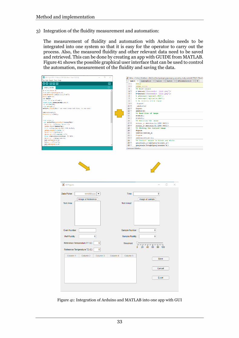
3) Integration of the fluidity measurement and automation: The measurement of fluidity and automation with Arduino needs to be integrated into one system so that it is easy for the operator to carry out the process. Also, the measured fluidity and other relevant data need to be saved and retrieved. This can be done by creating an app with GUIDE from MATLAB. Figure 41 shows the possible graphical user interface that can be used to control the automation, measurement of the fluidity and saving the data.

Figure 41: Integration of Arduino and MATLAB into one app with GUI


34

3.4 Optimizing Design Choice

Out of the several concepts mentioned in section 3.3, we had to choose one concept for further development. The selection of the concept was done using the Pugh analysis (Pugh 1991) to select one concept. Different stages in this analysis that were performed are mentioned below. We focused on selecting one concept for the fluidity measurement technique.

3.4.1 Identifying Alternative Different concepts were identified and were put into a table as shown below.

Deep learning of color image

Polar coordinate

Method

Cartesian coordinate

Method

MATLAB Image

Processing Thermocouple

3.4.2 Identifying Attribute The attributes against which the concepts were compared were identified.

• Cost efficient • Data storage requirement • Easy to develop the algorithm/hardware • Easy to understand

3.4.3 Screening the alternatives The screening step was an early elimination of the alternatives by simple rating or scoring system to filter out the more efficient concepts that needed to be looked upon in detail. By taking one of the concepts as reference concept and comparing other concepts to it +, 0 or – were marked as shown in Table 8 where +,0,- refers to better, equal and worse than the reference concept. Here Polar Coordinate method was taken as the reference concept and received 0 for each row. After the initial screening, the concept of deep learning and thermocouple was eliminated.

Table 8: Screening of Concepts

Attributes

Deep learning of color image

Polar coordinate

Method (Reference

concept)

Cartesian coordinate

Method

MATLAB Image

Processing

Thermocouple

Cost efficient - 0 0 0 -

Data storage - 0 0 + +

Ease to develop algorithm/hardware

0 0 0 + -

Ease to understand - 0 - 0 -

Net Score -3 0 -1 2 -2

Rank 5 2 3 1 4


35

3.4.4 Rate, weight, score and select the alternative After the initial screening, a more detailed rating scale was used to choose from the remaining concept. To begin with we have a five-point scale rating for a comparison between the remaining alternatives as shown the Table 9. Next, we assigned percentage weight for the attributes as shown in Table 10 where the highest percentage share was given to the most important attribute. Later, the score was calculated for each of the concepts. The concept with the highest score was selected for development. Here, MATLAB image processing had the highest score and was selected for further development. Similarly, the concept of servo motor with a crank lever mechanism as selected for the automation process.

Table 9: Five-point scale rating

Relative performance Rating Much worse than the reference 1 Worse than the reference concept 2 Same as reference concept 3 Better than the reference concept 4 Much better than reference concept 5

Table 10: Percentage weight and Score calculation

Attributes Weigh

ts Polar coordinate Method (Reference concept)

Cartesian coordinate Method

MATLAB Image Processing

Rating

1. Weighted Score

Rating

2. Weighted Score

Rating

3. Weighted Score

Cost efficient 40% 4. 3 5. 1.2 6. 3 7. 1.2 8. 3 9. 1.2

Data storage 30% 10. 3 11. 0.9 12. 3 13. 0.9 14. 3 15. 0.9

Ease to develop algorithm/hard

ware

10% 16. 3 17. 0.3 18. 2 19. 0.2 20. 4 21. 0.4

Ease to understand

20% 3 0.6 2 0.4 4 0.8

Total Score 3 2.7 3.3

Rank 2 3 1

Continue No No Develo

p


36

3.5 Developing the Architecture

After selecting MATLAB image processing, it was time to develop it. The images that were captured with the thermal camera were needed to be processed so that we achieve the goal of measuring the fluidity. This was divided into two parts (i) image processing algorithm (ii) Thermal Image Capturing.

3.5.1 MATLAB Image Processing Algorithm The algorithm uses the inbuilt commands to process the image. During the fluidity testing at the cast house, the first image was captured, and the fluidity was measured visually. The first captured image and the fluidity value is taken as the reference image for rest of the fluidity measurement for that batch.

Clculate the fluidity of the Test Image

Enter the Fluidity value of the reference image

Lable the image and Determine the area of white pixel

Reference Test Image Test Image

Complement the binary image


Convert into binary image


Select the threshold level


Convert the image into Gray Scale Image


Resize the image


Determine Size of the Image


Capture Thermal Image of


%% Read images a=imread('Reference test image.png'); b=imread('Test image.png');

%% Read Size of image size(a); size(b);

%% Resizing the image resize_a=imresize(a,[288 563]); resize_b=imresize(b,[288 563]);

%% Convert images to black and white grayscale_a=rgb2gray(resize_a); grayscale_b=rgb2gray(resize_b);

%% Selecting the threshold level level=0.4 %% converting to binary image binary0=imbinarize(grayscale_a,level); binary1=imbinarize(grayscale_b,level);

%%creating complementary image complement0=imcomplement(binary0); complement1=imcomplement(binary1);

%% Labeling the image label0=bwlabel(complement0); Stats0=regionprops(label0,'Area'); Stats0(1); area_values0=[Stats0.Area];

label1=bwlabel(complement1); Stats1=regionprops(label1,'Area'); Stats1(1); area_values1=[Stats1.Area];

%% Fluidity calculation refreadout=40.7650 refFluidity=refreadout*50 Fluidity=(area_values1*refFluidity)/ar

ea_values0; FluidityReadout=Fluidity/50;

Figure 42: Flow chart and MATLAB code for image processing


37

3.5.2 Arduino Automation Arduino IDE is an open software that was used for programming the microcontroller. The temperature was sensed by the thermocouple and the signal was sent into the Arduino by the max6675 module. The servomotor was programmed to rotate 180 degrees when the temperature decreases to a set level. The Serial Output (SO) from the max6675 was read by the Arduino, the Chip Select (CS) selects the module and tells the Arduino to supply an output that was synchronized with the clock and Serial Clock (SCK) was the input from the Arduino.

Measure the temperature of melt in

the cup

Compare the temperature with the

set temprrature

Is the temperature in the cup =< set temperature?

No

Wait till the temperature

decreases

Yes

Turn the servo motor and pull

the plug

Return to initial position after 1

min

#include "max6675.h" #include<Servo.h> Servo myServo; int angle; int soPin = 4;//serial out int csPin = 5;// chip select CS pin int sckPin = 6;// serial clock pin MAX6675 thermocouple(sckPin, csPin, soPin); void setup() { Serial.begin(9600); Serial.println("Thermocouple"); myServo.attach(9); delay(200); } void loop() { Serial.print("C = "); Serial.print(thermocouple.readCelsius()); if (thermocouple.readCelsius()<=670){ angle=179; myServo.write(angle); delay(1000); } else if(thermocouple.readCelsius()>27) { angle=0; myServo.write(angle); delay(1000); }

Figure 43: Flowchart and Arduino code for unplugging automation


38

3.5.3 Saving the Fluidity value to Excel The data such as the fluidity, temperature, date and time is saved in the excel sheet from the MATLAB. This is a part of automation. After the calculation of fluidity, all the relevant data is automatically saved into the excel file. This data can be retrieved when required for analysis. This solves the problem of manually updating the information and errors caused during the entering of information.

3.5.4 Graphical User Interface This is a sample of graphical user interface that will be developed. It shows the necessary data that are required to be input during the fluidity measurement.

%%saving to Excel t=now; date=

datetime(t,'ConvertFrom','datenum

'); Temperature1=700; Temperature2=690; fileName='Experiment.xlsx'; T=table(date,Temperature1,Tempera

ture2,CalFluidity); writetable(T,fileName)

Figure 44: MATLAB code for saving data in excel file

Figure 45: Graphical User Interface


39

3.6 Validate the design

The developed design needs to be verified so that it works during the actual experimental setup. The total length of the loop is 1988.2 mm. The total reading on the loop is 1988.2/50 which is equal to 39.764. Width of the channel is 8mm. The thickness of the wall in between the channel is 4mm. The total number of loops is 6.75. By using the above parameters and Archimedean formula, a graph was plotted in the MATLAB which resembles the Loop as shown in Figure 46. The fluidity measurement scale is shown in the below Figure 49.

Figure 46: Archimedian Spiral Graph

Figure 47: Loop with 8mm channel

Figure 48: Scale model

Figure 49: Printed scale on the Loop

For validating the MATLAB Image processing algorithm, computer-generated image of the loop was used. Here the computer-generated image refers to the image of the spiral that was created in SolidWorks. The two images were used as the input in the image processing algorithm. The image was then processed and finally, the fluidity was calculated. The various steps and the resulting image are shown in Table 11 below.


40

Table 11: Image Processing steps

Reference Image Trial Image

Step 1: Input the color/Thermal Image

Step 2: Resize the Input Image

Step 3: Convert into Grayscale Image

Step 4: Convert into Binary Image


41

Step 5: Complement the Binary Image

Step 6: Labeling

Step 8: Determining the area of the white pixel

30271 13585

Step 9: Calculating the fluidity

39.6750 17.8053

We can clearly observe that the results are accurate by comparing the measuring scale on the loop with the calculated fluidity value. With this, we were able to validate the algorithm. Table 12 shows the fluidity measurement for different length of the spiral.


42

Table 12: Fluidity Measurements

Test Image Area of the white pixel Fluidity

5125 6.5614

8263 10.7320

23079 29.6734

24645 31.7547

28627 37.0471


43

Automation of the pulling of the plug was done with the help of Arduino Uno microcontroller. The Arduino Uno microcontroller, max6675 module, K-type thermocouple (sensitivity=0.25 degree Celsius, range -270 to 1200 degree Celsius) , servomotor ( pulling capacity =4.1 kg, Dimension=41x20x36 mm, rotation 180 degrees, weight 37g) and respective pin connections which were used for the automation is shown in the table below. Using Arduino IDE open source software, the code was written for rotation of the servomotor when the set temperature is reached.

Table 13: Hardware and Pin connection

Pin connection for servo motor Servo Motor

Pin connection for Max6675 module with thermocouple

Max6675 module and thermocouple

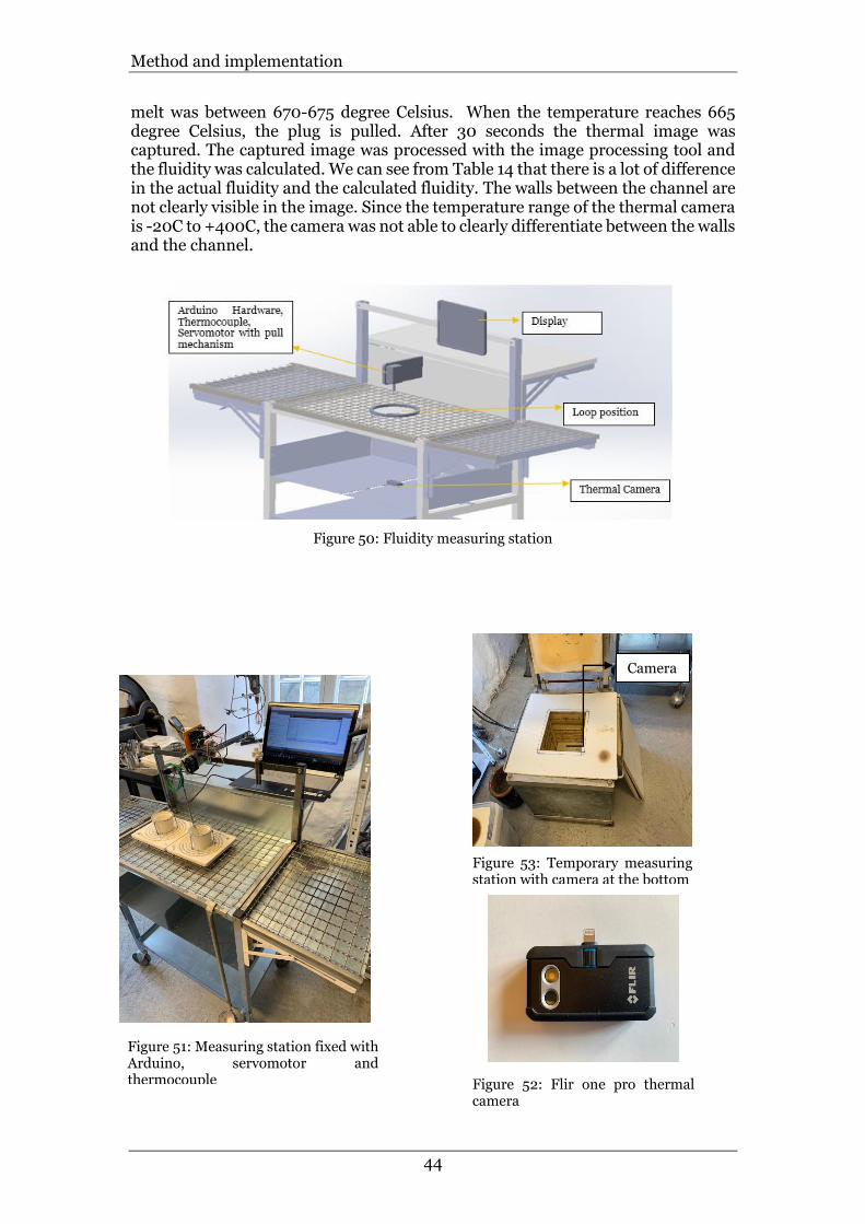
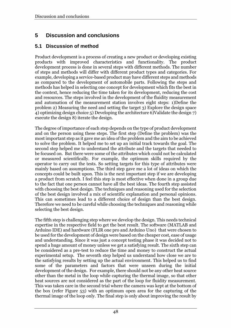
3.7 Executing the Design

After validating the design, the design is executed. In this stage we set up the actual experimental environment. The FLIR one pro thermal camera was used for capturing the thermal image (Figure 52). The specification of the thermal Camera is a) thermal sensitivity 70mK b) temperature range -20C-+400C c)IR resolution 480 x 640. The thermal camera was placed below the loop at a distance of 500mm as shown in Figure 53. The hardware was temporarily attached to the fluidity measurement station as shown in Figure 51. The loop with a channel width of 8mm and wall thickness in between the channel of 4mm is used. The temperature of the


44

melt was between 670-675 degree Celsius. When the temperature reaches 665 degree Celsius, the plug is pulled. After 30 seconds the thermal image was captured. The captured image was processed with the image processing tool and the fluidity was calculated. We can see from Table 14 that there is a lot of difference in the actual fluidity and the calculated fluidity. The walls between the channel are not clearly visible in the image. Since the temperature range of the thermal camera is -20C to +400C, the camera was not able to clearly differentiate between the walls and the channel.

Figure 52: Flir one pro thermal camera

Figure 51: Measuring station fixed with Arduino, servomotor and thermocouple

Figure 53: Temporary measuring station with camera at the bottom

Camera

Figure 50: Fluidity measuring station


45

Table 14: Trial 1

3.8 Iterating the Design Process

The results from trial 1 were not impressive, hence we needed some improvement. For trial 2, by using a loop with a wall thickness of 9mm and channel width of 8mm the second test was performed. The thermal camera was placed below the loop at a distance of 500mm. The set temperature to pull out the plug was 665 degree Celsius and the image was captured after 30 seconds of pulling the plug. The captured thermal image was better than the image captured from trial 1 with the loop wall thickness of 4mm. Due to the higher wall thickness, the camera could distinguish between the wall and the channel. Also, the background of the image was darkened to obtain a clearer picture of the loop. This gave a better result than the previous test as shown in Table 15.

Reference Color Image Test Color Image

Fluidity =27.4 Fluidity = 15.4

Fluidity = 27.4 Fluidity= 8.8 Error = 6.6

Findings and analysis

46

4 Findings and analysis

4.1 Fluidity Measurement

The measurement of fluidity was done by capturing the image with Flair one pro Thermal Camera with the following specification: (i) thermal sensitivity 70mK (ii) temperature range -20C-+400C (iii) IR resolution 480 x 640. The Image was processed with MATLAB image processing Tool. First, the validity of the image processing algorithm was done with the computer-generated image which gave an accurate result as shown in Table 12. Next, trial 1 was conducted by setting up the actual experimental environment as mentioned in section 3.7.In trial 1 we could see that the error was approximately 42% which was quite large (refer Table 14). Trial 2 was conducted by keeping all the parameters same except the wall thickness between the spiral channel which was increased to 9mm (refer 3.8). The wall and the channel could be clearly differentiated. But the thickness of the channel is not uniform along the spiral in the image. This produces some amount of errors in fluidity measurement. Compared to the results from trial 1 the error decreased to 12.7% in trial 2. The results for trial 2 are shown in Table 15.

Table 15: Trial 2

Reference Color Image Test Color Image

Fluidity =23.6 Fluidity = 17.2

Findings and analysis

47

It was also found that there are other factors that need to be considered to get an accurate result and the possible methods to control these are discussed in section 5.2. The factors are mentioned below:

1. The temperature of the molten metal which flows inside the spiral is an important factor since the color and the intensity of the pixel in the image differs for different temperature.

2. The waiting time before clicking the thermal image should be the same for the reference image and the successive test images to ensure a similar condition for every trial and increase the accuracy.

3. The distance between the camera and the loop must be the same for every trial since the change in the distance will change the amount of white pixel of the image.

4.2 Automation of the Process

The automation of the unplugging operation is done with the help of Arduino Uno microcontroller, K type thermocouple for temperature detection and servomotor. The automation saved approximately 7 seconds of the operator for each trial. The coordination between the temperature detection and the rotation was accurate when the delay (time between two consecutive temperature reading) is between 0.5 to 1 seconds. This ensured that the temperature of the metal during the entry into the loop was same for each trial by unplugging at the set temperature which also means that the error caused by the operator during the unplugging is reduced. But when the delay is increased to 2 seconds the unplugging was done at a lower temperature than the desired unplugging temperature. This is due to the delay between the two readings of temperature. It was also observed that the temperature response of the two types of thermocouples differs. This was due to the sensitivity and the geometry of the thermocouple. The thermocouple with the larger diameter takes longer time than the thin thermocouple to respond to the temperature change.

4.3 Saving the data to excel file

The data such as the measured fluidity value, temperature, date, time, etc are stored into the excel file from the MATLAB. However, it was observed that the values that are stored during the trial were overwritten during each trial. Due to this, it was not possible to retrieve the values of previous trials.

Fluidity = 23.6 Fluidity = 15.01

Error = 2.19

Discussion and conclusions

48

5 Discussion and conclusions

5.1 Discussion of method

Product development is a process of creating a new product or developing existing products with improved characteristics and functionality. The product development process is done in several steps with different methods. The number of steps and methods will differ with different product types and categories. For example, developing a service-based product may have different steps and methods as compared to the development of automobile parts. Following the steps and methods has helped in selecting one concept for development which fits the best in the context, hence reducing the time taken for its development, reducing the cost and resources. The steps involved in the development of the fluidity measurement and automation of the measurement station involves eight steps: 1)Define the problem 2) Measuring the need and setting the target 3) Explore the design space 4) optimizing design choice 5) Developing the architecture 6)Validate the design 7) execute the design 8) iterate the design.

The degree of importance of each step depends on the type of product development and on the person using these steps. The first step (Define the problem) was the most important step as it gave me an idea of the problem and the aim to be achieved to solve the problem. It helped me to set up an initial track towards the goal. The second step helped me to understand the attribute and the targets that needed to be focused on. But there were some of the attributes which could not be calculated or measured scientifically. For example, the optimum skills required by the operator to carry out the tests. So setting targets for this type of attributes were mainly based on assumptions. The third step gave me a lot of ideas on which the concepts could be built upon. This is the next important step if we are developing a product from scratch. I feel this step is most effective when done in a group due to the fact that one person cannot have all the best ideas. The fourth step assisted with choosing the best design. The techniques and reasoning used for the selection of the best design involved a mix of scientific explanation and personal opinions. This can sometimes lead to a different choice of design than the best design. Therefore we need to be careful while choosing the techniques and reasoning while selecting the best design.

The fifth step is challenging step where we develop the design. This needs technical expertise in the respective field to get the best result. The software (MATLAB and Arduino IDE) and hardware (FLIR one pro and Arduino Uno) that were chosen to be used for the development of design were based on the cheaper cost, ease of usage and understanding. Since it was just a concept testing phase it was decided not to spend a huge amount of money unless we get a satisfying result. The sixth step can be considered as a pre-test to reduce the time and money to construct the actual experimental setup. The seventh step helped us understand how close we are to the satisfying results by setting up the actual environment. This helped us to find some of the parameters and factors that were unseen during the initial development of the design. For example, there should not be any other heat source other than the metal in the loop while capturing the thermal image, so that other heat sources are not considered as the part of the loop for fluidity measurement. This was taken care in the second trial where the camera was kept at the bottom of the box (refer Figure 53) with an optimum open area for the capturing of the thermal image of the loop only. The final step is only about improving the result by


49

optimizing the parameters. We could change only the thickness of the wall which gave a better result. But we can also use a better camera with higher thermal sensitivity ( one of the parameters to obtain good thermal image).

The above-mentioned steps give us the flexibility to maneuver according to the requirement. This method ( eight steps ) is suitable for the development of a new product since we cannot get the right design with a single attempt. This method can also be considered as a pre-engineering step since it mainly focuses on how to select a concept before developing it with the perfect design. This type of method and steps will not be effective if we already have the right design but need small changes.

5.2 Discussion of findings

The digital measurement of the fluidity of molten metal was not accurate enough at present to make it an alternative for the visual measurement. One of the reasons for the error caused was due to the low thermal sensitivity of the camera. Due to the low thermal sensitivity of the camera, it was not able to recognize the small temperature difference between the molten metal and the thin walls of the spiral. Hence while setting the threshold value in image processing, some part of the walls were also considered as the molten metal (spiral channel). This caused the extra addition of the white pixels which in turn increases the area and hence fluidity value. The second trial gave a better result due to the higher wall thickness. Higher wall thickness has two advantages a) clear visual between the channels and b) it takes more time for the heat to transfer from the molten metal to the wall. Due to this reason, the image showed a clearer distinction between the walls and the channel and help in reducing the error in calculating the fluidity as compared to the trial 1. Trial 2 also showed the difference in the width of the walls and the channel due to the reason of low thermal sensitivity. Hence higher thermal sensitive camera and higher wall width can help to reduce the error to a large extent. The other reason also can be due to the different material thickness.

The temperature of the molten metal during its entry into the spiral needs to be same for the successive trial. This is because every degree of temperature has its respective color in the thermal image. The difference in the temperature for the successive trials causes the changes in the color which in turn changes the threshold level for each image. It might be helpful if we could assign a value of the threshold for each degree of temperature (which means each color). So that during the experiment we could set the threshold by knowing the temperature for each trial and reduce the error. The waiting time for capturing the image after the metal has stopped flowing must be the same for each successive trial. This is due to the heat conduction from the molten metal to the Loop. As soon as the metal flows into the loop the heat transfer takes place from the metal to the surrounding material in the loop (to the walls) which increases the temperature and hence will show a color change in the thermal image. When the waiting time is kept constant for each trial the heat transfer is expected to be the same and hence will show a similar color for trial which will help us to use the same threshold value. This will ensure the same condition for the image processing and produces better accuracy. The distance between the camera and the loop must be the same for every trial. The change in the distance between the two will be similar to zooming in or zooming out effect. When the camera is kept closer to the loop the area covered by the color image will be larger and vice versa. When the area is large the fluidity reading will be larger than the actual.


50

The automation of the unplugging process showed that it can save the time of the operator and also it can eliminate the error (delay) caused by the operator while unplugging at the set temperature. However, the mechanism used for the unplugging could be improved so that during the unplugging there is no much disturbance in the molten metal contained in the cup. The disturbance in the molten metal can hinder the laminar flow of the metal when it enters the cup. It would also be better if we can use the same plug (stopper) which is directly connected to the mechanism instead of connecting new stopper for each trial as it is done today.

5.3 Conclusions

Automation and digital measurement of fluidity are definitely a step forward in the process of measuring fluidity as compared to the present manual method. The automation of unplugging operation saves approximately 7 seconds of the operator. It also reduces the error during the manual unplugging and ensures that the metal flows into the spiral at the same temperature for each trial. Which means that the variation of fluidity caused due to the difference in temperature of the metal while entering the spiral is eliminated. The digital measurement with image processing is not accurate as of now. There is an error of 12.7% between the actual fluidity and the fluidity measured by image processing. However, by using a better thermal camera (with better thermal sensitivity, broader range, better resolution) and the better algorithm it is expected to show a better result with higher accuracy. At present, it is difficult to conclude if the digital measurement of fluidity will be more accurate than the manual measurement of fluidity. However, the digital measurement will reduce the dependency on the operator’s skill and knowledge since the digital measurement is based on the calculation done by the system instead of human approximation. Apart from these, the automation and the digital measurement will prove to be safer than the manual operation since the operator is less exposed to the high-temperature molten metal. The system will prove to be user-friendly since the data related to the experiments will be saved automatically and handled digitally rather than noting down manually.

5.4 Future Work

Although an attempt has been made to demonstrate the effectiveness of automation and digital measurement, there are further works that need to be considered for the complete success of the fluidity measurement. Further work includes:

1. Automation of valve opening of the crucible at the set temperature: This can be done similar to that of unplugging operation. The crucible should have a valve which can be opened and closed for a certain amount of time at the desired temperature. This automation will ensure that the same volume of molten metal is filled into the cup at the same temperature at each trial.


51

2. Placing and retrieving of the new and used loop with a cup: This automation will make the process faster and will save the time of the operator. This is complex automation.

3. Creating a graphical user interface and creating an application which integrates the automation and measurement.

4. The automatic image capturing and transfer to the application, with an advanced thermal camera.

5. Saving the data to a universal database, so that we can have access to data from different cast house for analysis.

6. Measuring the speed of metal filling inside the loop. 7. Measuring the rate of decrease in the temperature inside the loop and

plotting the temperature curve.

References

52

6 References

[1] ”Bryne AB,” Bryne AB, [Online]. Available: http://bryne.se/. [Använd 19 02 2019].

[2] T. Liljenfors, ”Device for Measuring Fluidity of Molten Metal”. Sweden Patent WO2017176184AI, 12 10 2017.

[3] P.Groover och Mikell, ”Fundamentals Of Modern Manufacturing,” John Wiley & Sons,Inc, 2010, pp. 205-206.

[4] L. Arnberg och M. D. Sabatino, ”Castability of aluminium alloys,” Transactions of The Indian Institute of Metals, vol. 62, nr 4-5, pp. 1-5, 2009.

[5] M. C. Flemings, Solidification Process, New York: McGraw-Hill, 1974.

[6] M. B.Djurdjevic, Z. Odanovic och J. P. Krsyic, ”Melt Quality Control At Aluminium Casting Plants,” Association of Metallurgical Engineers of Serbia, Belgrade, 2010.

[7] M. Flemings, ”Solidification Processing,” i Materials Transactions, McGraw Hill, 2005, pp. 895-900.

[8] M. D. Sabatino, Fluidity of Aluminium Foundry Alloys, Trondheim: Norwegian University of Science and Technology, 2005.

[9] M. D. Sabatino, S. Shankar, D. Apellal och L.Arnberg, Influence of temperature and alloying elements on the fluidity of AL-Si alloys, 2005.

[10] T. D. West, Metallurgy of cast iron, Cleveland, 1902.

[11] M. D. Sabatino, F. Syvertsen, L. Arnberg och A. Nordmark, ”An improved method for fluidity measurement by gravity casting of spirals in sand molds,” International Journal of Cast Metals Research, vol. 18, nr 1, pp. 59-62, 2005.

[12] A.L.Krynitsky, ”AFS trans,” 1953, pp. 399-477.

[13] M. D. Sabatino och S. Akhtar, ”State of the art characterization tools for Al foundry alloys,” Metallurgical Science and Technology, vol. 30, 2012.

[14] D. Caliari, G. Timelli, F. Bonollo, P. Amalberto och P. Giordano, ”Fluidity of Aluminium Foundry Alloys: development of a Testing Procedure,” La metallurgia Italiana, 2015.

[15] ”wolfram Mathworld,” [Online]. Available: http://mathworld.wolfram.com/ArchimedesSpiral.html. [Använd 16 04 2019].

[16] Mathworks, ”Matlab Documentation,” [Online]. Available: https://se.mathworks.com/help/matlab/. [Använd 16 04 2019].

[17] M. J.Hobbs, C. Zhu, M. P.Grainer, J. R.Willmott och C. H. Tan, ”Quantitative traceable temperature measurement using novel thermal imaging camera,” Optics Express, vol. 28, nr 19, 2018.

[18] F. S. AB, Thermal Imaging Guidebook For Industrial Application, 2011.

[19] Arduino, ”Arduino Dodumentation,” Arduino, [Online]. Available: https://www.arduino.cc. [Använd 13 05 2019].

[20] J.Senthil och G.Haripriya, ”Time Analysis with Most Technique,” International Journal of chemical science, vol. 14, nr 2, pp. 519-526, 2016.

Search terms

53

7 Search terms

Abstract .............................................. 1

Acknowledgment ........................... 1

Aesthetic ........................................... 24

Alexander Lyrbo ................................. 1

Archimedean Spiral .......................... 15

Arduino ............................................. 20

attributes ............................................ 34

Automation ....................................... 49

Background ......................................... 7

Basic MOST ...................................... 25

Binary Image ..................................... 17

Bryne AB ............................................ 1

Cartesian Coordinate method ............ 29

Castability ........................................... 7

Casting ................................................ 7

Chemical Composition of AES Fiber

....................................................... 11

Color Image ...................................... 28

Compact ............................................ 24

concepts ............................................. 28

Contents ............................................. 3

Context .............................................. 24

Definition .......................................... 23

Delimitations ....................................... 8

diagnosis ............................................. 8

Dimension of the components .......... 12

Electromagnet ................................... 31

emissivity .......................................... 19

Examiner ............................................. 2

excel .................................................. 37

fiber ..................................................... 7

FLIR .................................................... 1

Fluidity ................................................ 9

Functional Requirement .................... 24

functional requirements .................... 24

Grayscale images .............................. 17

Image Processing .............................. 28

Image Processing Tool ...................... 17

improvement ....................................... 1

Integration ......................................... 32

Introduction ......................................... 7

Iterate ................................................ 45

Jönköping ............................................ 2

Keywords ......................................... 2

LOOP .................................................. 7

Managing Director .............................. 1

Master of Science ............................... 2

MATLAB ......................................... 17

MATLAB Image Processing ............ 30

Method and implementation ............. 22

microcontroller ................................. 42

MOST ............................................... 24

Nils-Eric Andersson ............................ 2

operator ............................................... 1

optimal fluidity ................................... 8

Outline ................................................ 8

Physical Properties ............................ 11

Polar coordinate method ................... 29

polar coordinates ............................... 15

Pratheek Ullal ..................................... 1

Preface .............................................. 2

Product Development ....................... 20

Product Development and Materials

Engineering ..................................... 2

Purpose ............................................... 8

radiation ............................................ 19

rating ................................................. 34

refractory ............................................. 7

reliability ............................................. 8

Research Question .............................. 8

Roland Stolt ........................................ 2

School of Engineering ........................ 2

Scope ................................................... 2

screening ........................................... 33

Servo Motor ...................................... 31

Supervisor ........................................... 2

Sweden ................................................ 1

thermal conductivity ......................... 19

Thermal Conductivity ....................... 11

Thermal Image ............................ 19, 28

Thermocouple ................................... 30

Thomas Liljenfors ............................... 1

True color images ............................. 17

validating .......................................... 38

viewfinder ......................................... 19

workstation ......................................... 1

Search terms


8 Appendices

8.1 Appendix 1 MATLAB code for Archimedean Spiral

clc(); clear all %% Dimentions of the loop widthofflow=8; widthofwall=4; Noofloops=6.75; iradius=3.5; oradius=iradius+widthofflow; avgradius=(oradius+iradius)/2; outerradius=oradius+((widthofflow+widthofwall)*Noofloops); %% limits or integrals lowerlimit=0; upperlimit=2*pi*Noofloops; armdistance=widthofflow+widthofwall; b=armdistance/(2*pi); %% length Calculation x=0:0.01:upperlimit; r1=iradius+(b*x); r2=oradius+(b*x); r=avgradius+(b*x); diffr=b; %% length of inner loop f1=sqrt((iradius+b*x).^2+diffr.^2); z1=@(x)sqrt((iradius+b*x).^2+diffr.^2); q1=integral(z1,0,upperlimit); polarplot(x,f1); pax=gca; pax.ThetaDir='clockwise'; %% length of outer loop f2=sqrt((oradius+b*x).^2+diffr.^2); z2=@(x)sqrt((oradius+b*x).^2+diffr.^2); q2=integral(z2,0,upperlimit); hold on polarplot(x,f2); pax=gca; pax.ThetaDir='clockwise'; %% length of average loop f=sqrt((avgradius+b*x).^2+diffr.^2); z=@(x)sqrt((avgradius+b*x).^2+diffr.^2); q=integral(z,0,upperlimit); polarplot(x,f,'--'); pax=gca; pax.ThetaDir='clockwise'; hold off %% readouts qavg=(q1+q2)/2 totalReading=qavg/50 calreading=totalReading-1;

Development of Fluidity Measurement Technique and ...

Documents

Transcript of Development of Fluidity Measurement Technique and ...