Development of Design Guidelines for Proper Selection · PDF fileDEVELOPMENT OF DESIGN...
94
STATE HIGHWAY ADMINISTRATION RESEARCH REPORT DEVELOPMENT OF DESIGN GUIDELINES FOR PROPER SELECTION OF GRADED AGGREGATE BASE IN MARYLAND STATE HIGHWAYS Ahmet H. Aydilek, Intikhab Haider, Zulkuf Kaya, Altan Cetin, and Mustafa Hatipoglu UNIVERSITY OF MARYLAND, COLLEGE PARK Project number SP109B4G FINAL REPORT January 2015 MD-15- SP109B4G-1
Transcript of Development of Design Guidelines for Proper Selection · PDF fileDEVELOPMENT OF DESIGN...
STATE HIGHWAY ADMINISTRATION
RESEARCH REPORT
DEVELOPMENT OF DESIGN GUIDELINES FOR PROPER SELECTION OF GRADED AGGREGATE BASE
IN MARYLAND STATE HIGHWAYS
Ahmet H. Aydilek, Intikhab Haider, Zulkuf Kaya, Altan Cetin, and Mustafa Hatipoglu
UNIVERSITY OF MARYLAND, COLLEGE PARK
Project number SP109B4G
FINAL REPORT
January 2015
MD-15- SP109B4G-1

The contents of this report reflect the views of the authors who are responsible for the facts and the accuracy of the data presented herein. The contents do not necessarily reflect the official views or policies of the Maryland State Highway Administration. This report does not constitute a standard, specification, or regulation.

ii
Technical Report Documentation Page 1. Report No. MD-15-SP109B4G-1
2. Government Accession No. 3. Recipient's Catalog No.
4. Title and Subtitle Development of Design Guidelines for Proper Selection of Graded Aggregate
Base in Maryland State Highways
5. Report Date January, 2015 6. Performing Organization Code
7. Author/s Ahmet H. Aydilek, Intikhab Haider, Altan Cetin, Zulkuf Kaya, and Mustafa Hatipoglu.
8. Performing Organization Report No.
9. Performing Organization Name and AddressUniversity of Maryland 1171, Glenn L. Martin Hall, University of Maryland College Park, MD-20742
10. Work Unit No. (TRAIS) 11. Contract or Grant No.
SP109B4G
12. Sponsoring Organization Name and AddressMaryland State Highway Administration Office of Policy & Research 707 North Calvert Street Baltimore MD 21202
13. Type of Report and Period Covered
Final Report
14. Sponsoring Agency Code(7120) STMD - MDOT/SHA
15. Supplementary Notes 16. Abstract The mechanical and drainage properties of graded aggregate base material are the level one input in mechanistic pavement design. Maryland State Highway Administration (SHA) is in need of guidelines for evaluation of stiffness and drainage characteristics of graded aggregate base (GAB) stone delivered at highly variable gradations to the construction sites. To fulfill the current need, the mechanical and drainage properties of several Maryland GAB materials were evaluated in the laboratory and field. The resilient modulus and hydraulic conductivity test results obtained in the laboratory were compared to the field moduli and hydraulic conductivity. The effect of moisture content on resilient modulus was also evaluated. Summary resilient modulus, SMR values at Optimum Moisture Content (OMC) minus 2% were higher than those at OMC, with few exceptions; however, the permanent deformations increased with moisture beyond OMC. The control of moisture content within 2% of OMC would not significantly affect the resilient modulus and permanent deformation in construction. It was also concluded that an addition of 4-6% fines over the SHA specification limit of 8% resulted in 2-5 times decrease in the laboratory-based GAB hydraulic conductivities and an increase in time for 50% completion of the drainage from the highway base. The required base thickness increased 2.6 to 7 times as a result of fines increased from 2 to 14% for selected GAB materials evaluated. It is recommended that resilient modulus, permanent deformation, as well as hydraulic conductivity of GAB materials, are evaluated for designing a highway base with adequate stiffness and drainage performance.
17. Key Words Graded Aggregate Base, GAB, RCA, Drainage, Hydraulic Conductivity
18. Distribution Statement: No restrictions This document is available from the Research Division upon request.
19. Security Classification (of this report) None
20. Security Classification (of this page) None
21. No. Of Pages 72
22. Price
Form DOT F 1700.7 (8-72) Reproduction of form and completed page is authorized.

iii
TABLE OF CONTENTS
1. INTRODUCTION ........................................................................................................ 1
2. MATERIALS ................................................................................................................ 4
3. METHODS .................................................................................................................... 8
3.1 Laboratory Geomechanical Tests ................................................................................. 8
3.2 Laboratory Hydraulic Conductivity Tests. .................................................................. 11
3.3 Field Tests. .............................................................................................................. 12
3.3.1 Light Weight Deflectometer ............................................................................... 12
3.3.2 Geogauge. ......................................................................................................... 14
3.3.3 Field Hydraulic Conductivity Tests ..................................................................... 15
4.1 CBR Tests. .............................................................................................................. 16
4.2. Resilient Modulus Tests ........................................................................................... 19
4.3. Permanent Deformation Tests ................................................................................... 27
4.4. Laboratory Hydraulic Conductivity Tests .................................................................. 29
5. PRACTICAL IMPLICATIONS .................................................................................. 46
5.1 Highway Base Design............................................................................................... 46
5.2. Effect of Hydraulic Conductivity on Highway Base Design ......................................... 47
5.3. Cost Calculations .................................................................................................... 64
6. CONCLUSIONS........................................................................................................... 65
IMPLEMENTATION PLAN AND GUIDELINES FOR PAVEMENT DESIGN. ......... 67
REFERENCES ................................................................................................................. 70
APPENDIX A ................................................................................................................... 74
APPENDIX B ................................................................................................................... 78
APPENDIX C ................................................................................................................... 85
ABBREVIATION AND ACRONYMS ........................................................................... 88

1
1. INTRODUCTION Millions of tons of graded aggregate base (GAB) materials are used in construction of highway
base layers in Maryland due to their satisfactory mechanical properties. The fines content of a
GAB material is highly variable and is often related to crushing process, stockpiling in the quarry,
transportation and during construction at the site. The crushing of the stone at the quarry generally
does not decrease the mechanical strength and stiffness of the material delivered to the site.
However, the Maryland State Highway Administration (SHA) is experiencing difficulties in
achieving proper drainage through the base layers due to occasionally high fines content of the
delivered GABs. The presence of excessive water in pavement systems is one of the main causes
of pavement distress, which decreases the service life of the pavement structures significantly
(NCHRP 1997). The relatively impervious base-course materials may shorten the service life of
highways and increase the deterioration of the upper surface (asphalt layer) of pavements (NCHRP
1997).
Drainage in pavements can only be achieved with a properly designed and constructed
system that consists of all essential drainage components and a base layer with adequate
drainability and sufficient structural stability. The presence of free moisture in pavement layers has
been found responsible for many premature failures observed in both flexible and rigid pavements
(Abhijit et.al 2011). Diefenderfer et. al. (2001) present six adverse effects of excess water in
pavement life: reduction in shear strength of the unbound material, increase in differential swelling
of expansive subgrade soil, movement of fines in base and subbase layers, frost-heave and thaw
weakening, cracking in rigid pavements, and stripping of asphalt in flexible pavement. Erlingsson
et al. (2009) used heavy vehicle simulator to show that the rate of rutting depth increased in all
layers of flexible pavement structure when the groundwater table was raised. Dawson (2009) has

2
also shown that poor drainage poses significant adverse effects on the condition of roadways. Free
moisture in the pavement sub layers largely occurs due to infiltration of rainwater and melted snow
through pavement surface joints or cracks. To mitigate the moisture-induced distresses, it is
imperative to drain free moisture out of pavement structures as quickly as possible via a good
drainage system. Although the performance of a subsurface drainage system depends on all of its
individual components, the hydraulic conductivity of a highway base layer can be critical for its
adequate drainage (NCHRP 1997). Several factors, including physical and chemical properties of
aggregates, geometry of pavements, climatic conditions, and pavement surface conditions, affect
the minimum hydraulic conductivity of a highway base layer or the time to achieve a certain
percentage of drainage in the pavement structure (Casagrande and Shanon, 1952).
In addition to a high quality drainage system, highway base layers should also have
satisfactory mechanical properties such as high resistance to permanent (plastic) deformation
under normal traffic loading. Therefore, it is imperative to consider structural stability in the
optimization of highway base materials. Traditionally, the California bearing ratio (CBR) test has
been used to quantify the structural stability of highway base materials due to its simplicity;
however, it does not represent the stiffness of soils at low strains. Accordingly, SHA is no longer
evaluating the pavement performance solely based on CBR test results. The resilient modulus is
arguably superior to static tests, such as CBR, due to its capability of characterizing the response
of pavement material under repeated loading that simulates traffic loading conditions (AASHTO T
307). The resilient modulus test provides an essential input parameter for the pavement design and
the permanent deformation test provides information on the rutting potential of a pavement
material in field conditions.

3
There is no agreement on the minimum value of hydraulic conductivity or the time to
achieve a given percentage of drainage; however, hydraulic conductivity and the appropriate
drainage time are the indicators of pavement service life. Similarly, the minimum structural
stability required for a permeable aggregate base is not well established in the previous studies and
design guidelines. Therefore, there is a need to identify a range of gradation for highway base
materials that can provide a better characterization of structural stability along with the high
quality drainage in highway base layers.
To respond to this need, a battery of tests was conducted on graded aggregate base (GAB)
course materials, in the laboratory as well as in the field. Recycled concrete aggregates (RCAs)
and their mixtures with select GABs were also included in the laboratory testing program since
beneficial reuse of RCA brings economic advantages due to a decrease in its disposal associated
with clogging of landfill leachate collection systems. California bearing ratio (CBR), resilient
modulus, permanent deformation and hydraulic conductivity tests were conducted to investigate
the engineering properties of GAB, RCA and their mixtures, and to study the effect of curing time
on RCA. The effect of winter conditions were also evaluated by performing resilient modulus
tests on the RCA specimens after a series of freeze-thaw cycles.

4
2. MATERIALS The graded aggregate base materials (GABs) included in the current testing program are
commonly used as highway base materials by the Maryland State Highway Administration (SHA).
GAB contains coarse and fine aggregate particles as well as fines (clay and silt). Generally, the
ratio between coarse and fine aggregate particles varies between 1:1 and 7:3. Seven GAB materials
were collected from different quarries in Maryland/Virginia and tested in the laboratory. GABs
used in the current study were named: A,B,C,D,E,F,G. The petrographic data shows that all
GAB materials used in this study had different mineralogy (Table 1). All GAB materials met the
SHA and AASHTO M-147 specifications and were classified as high quality base materials (A-1-a
(0) according to AASHTO Soil Classification System.
The gradations of all selected GAB materials were within the tolerance limits of SHA
specifications except few fractions of materials from the T quarry (Figure 1). The index properties
of GAB materials are shown in Table 1. All GAB materials were non-plastic and their as-received
fines content ranged from 6.9% to10%. According to SHA specifications, the fines content of the
GAB materials used in highway base layers must be less than 8% (SHA 2012). The absorption of
fine and coarse aggregates of GAB materials varied between 0.89 and 5.33% and 0.4 and 0.79%
respectively (Table 1). The Los Angeles abrasion values of all GABs were below 30%, except B-
GAB. Petrographic and mineralogical nature (marble, high CaCO3 content) of quarry ‘B’ GAB
may have caused the relatively higher loss during the abrasion tests as marble stone tends to be
easily crushed under impact loading.

5
Table 1: Physical and chemical properties of the GAB and RCA materials
GA
B
Materials
Physical Properties chemical Properties
d (Pcf) OMC (%) Gs Absorption LA MD SS PD
SiO2 Al2O3 Fe2O3 CaO
Imp Vib Imp Vib F C F (%)
C (%)
% % % % % % %
A 152.3 157.2 5.80 4.70 2.55 2.77 5.33 0.78 16.40 21.90 1.60 Meta Basalt 60.88 13.27 9.43 2.93
B 152.1 154.6 4.20 4.10 2.70 2.79 1.75 0.40 53.04 24.76 0.53 Carbonate Marble 44.10 3.04 1.57 26.83
C 158.1 - 5.40 - 2.86 2.99 3.18 0.79 22.20 7.50 0.73 Basalt 38.39 9.48 7.18 5.80
D 148.8 - 5.20 - 2.75 2.79 1.32 0.58 22.90 11.50 0.60 Prasiolite 2.36 0.70 1.31 29.31
E 146.6 - 4.70 - 2.60 2.68 2.63 0.51 25.20 12.20 2.02 Carbonate-Siliceous Rock 11.90 1.95 0.85 31.67
F 157.8 162.6 5.30 4.80 2.91 3.01 0.89 0.49 26.90 18.50 2.20 Gneiss 47.71 15.61 10.95 11.90
G 154.7 157 4.80 4.50 2.72 2.83 3.09 0.55 23.60 7.56 1.10 Carbonate Dolomite 50.73 12.93 10.92 10.67
RC
GA
B
Plant A 128.4 - 9.50 - 2.29 2.49 9.23 4.20 55.20 16.80 15.70 - 51.54 4.61 2.55 16.94
Plant B 128.2 - 9.50 - 2.29 2.53 9.05 4.19 47.40 18.40 14.26 : 61.24 4.02 1.87 13.06
ϒd: maximum dry density, Imp: impact compactor, Vib: vibratory compactor, Gs: specific gravity, F: fine contents, C: Coarse contents, LA: Los Angeles abrasion test , MD: Micro deval test , SS: loss in Sodium Sulfate test, PD: Petrographic Description.

6
The micro deval values of GAB materials were 7.5- 24.8%. The A and B GABs yielded high
micro deval values (21.9 and 24.8%, respectively), indicating that these GAB materials were not
durable under moist conditions. Mineralogical natures and shapes of the A and B GABs particles
could be the reason for high micro deval values. The percentage loss in sodium sulfate test for the
GAB materials ranged from 0.6 to 2.2%, meaning that all GAB materials had good resistance
against freezing and thawing process.
Two Maryland RCA materials, named A and B, were also included in the laboratory testing
program. RCAs were generated from the demolition of concrete structures and stockpiled in
Plants A and B located in Maryland. The fines content of materials A and B were measured as 6
and 9%, respectively, and grain size distribution curves of both materials were within the SHA
GAB limits (Figure 1). The absorption values of both RCAs were 4.2%; however, the Los Angeles
abrasion of A exceeded the specification limit of 50%. The percent losses based on sodium sulfate
tests were 15.7 and 14.3% for A and B, respectively, and exceeded the SHA specification limit of
12%, which could be due to a reaction of sodium sulfate with cement contents present in material.
The physical and chemical properties of the two RCA materials are summarized in Table 1.

7
0
20
40
60
80
100
0.010.1110100
A
F
B
G
C
D
E
GAB Upper Limit
GAB Lower LimitPe
rce
nt
fin
er
#2
00
#3
0
3/4
1 1/
2
1/2
3/8 #4
Particle size (mm)
(a)
0
20
40
60
80
100
0.010.1110100
RCA--Plant A
RCA--Plant B
SHA Upper Limit
SHA Lower Limit
Pe
rce
nt
fin
er
Paticle size (mm)
#20
0
#30
3/4
1 1/
2
1/2
3/8 #4
(b)
FIGURE 1: Gradation of (a) GAB materials, and (b) RCA materials.
8
3. METHODS:
3.1 Laboratory Geomechanical Tests
The California bearing ratio (CBR) test is a penetration test for evaluation of the mechanical
behavior of road base and subbase course layers. The CBR tests were performed on A, G, F, and B
GAB materials, the two RCA materials, and their mixtures with G and A GABs. G and A GABs
were blended with two RCAs at 75:25, 50:50, and 25:75 ratios by weight. These ratios cover big
range of test results. Two types of compaction methods were utilized to observe the effect of
compaction on CBR: impact Modified Proctor compaction (ASTM D1557) and vibratory
compaction (ASTM D7382). The specimens for vibratory compaction were prepared in three
equal layers using a vibration frequency of 55 Hz for 605 seconds per layer. A BOSCH 11248
EVS model vibratory hammer was used. All specimens were compacted at their optimum
moisture contents (OMC). Table 1 provides the optimum moisture contents (OMCs) and
maximum dry unit weights (d) of the GAB and RCA materials. All CBR tests were conducted by
following the methods outlined in AASHTO T-193 and ASTM D 1883. The specimens were un-
soaked and the tests were performed at a strain rate of 0.05 in/min.
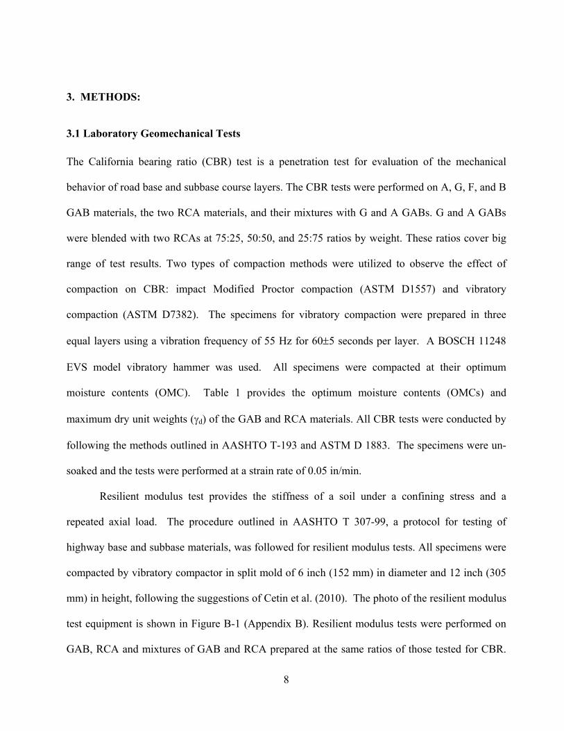
Resilient modulus test provides the stiffness of a soil under a confining stress and a
repeated axial load. The procedure outlined in AASHTO T 307-99, a protocol for testing of
highway base and subbase materials, was followed for resilient modulus tests. All specimens were
compacted by vibratory compactor in split mold of 6 inch (152 mm) in diameter and 12 inch (305
mm) in height, following the suggestions of Cetin et al. (2010). The photo of the resilient modulus
test equipment is shown in Figure B-1 (Appendix B). Resilient modulus tests were performed on
GAB, RCA and mixtures of GAB and RCA prepared at the same ratios of those tested for CBR.

9
Each sample was compacted in six layers at their optimum moisture contents (OMC) and
maximum dry densities using a vibratory compactor (ASTM D73820). RCA specimens were
removed from the molds after compaction, sealed in plastic wrap, and cured at 100% relative
humidity and controlled temperature 70 3.6F (21 2 OC) for 1, 7 and 28 days before testing. In
order to evaluate the effect of moisture contents on resilient modulus (MR), specimens of all GABs
were prepared and tested at 2% below and 2% above the OMC. Resilient modulus tests were also
performed on GAB samples collected from the construction sites. The field samples were collected
from the locations where geogauge, nuclear density gauge, and light weight deflectometer (LWD)
tests were conducted. The laboratory resilient modulus tests were conducted on field-retrieved
GAB samples prepared at their field gradations, moisture contents, and compaction levels.
To determine the climate effects on the mechanical properties of RCAs, specimens were
prepared at OMC and maximum dry density in split molds and cured for 28 days before subjecting
them to 1, 4, 8, 16, and 20 cycles of freezing and thawing (F-T) per ASTM D6035. Each F-T cycle
consisted of exposing each specimen to -2.2F (-19°C) for 24 hours, followed by room temperature
(~68°F) for another 24 hours. The effect of F-T cycling on the engineering properties of recycled
materials was determined by conducting resilient modulus tests after selection of the
corresponding F-T cycles. Duplicate specimens were tested for most of the resilient modulus tests
as quality control.
A Geocomp LoadTrac-II loading frame and associated hydraulic power unit system was
used to load the specimens. The specimens were subjected to conditioning before the actual test
loading under the confining and axial stress of 15 Psi (103 kPa) for 500 repetitions. Confining
stress was kept between 3 Psi (20.7 KPa) and 20Psi (138 kPa) during loading stages, and the
deviator stress was increased from 3 Psi (20.7 kPa) to 40 Psi (276 kPa) and applied 100 repetitions

10
at each step. The detailed information about the load sequences are provided in Table A-1
(Appendix A). The loading sequence, confining pressure, and data acquisition were controlled by a
personal computer equipped with RM 5.0 software. Deformation data were measured with
external linear variable displacement transducers (LVDTs) that had a measurement range of 0 to 2
inch (50.8 mm).
Resilient moduli from the last five cycles of each test sequence were averaged to obtain
resilient modulus for each load sequence. This nonlinear behavior of unbound granular material
was defined in this study using the model developed by Witczak and Uzan (1988) which
recommended the following formula:
32
31
k
a
d
k
aaR pp
pkM
(1)
where MR is resilient modulus, k1, k2, and k3 are constants, is isotropic confining pressure, d is
the deviator stress, and pa is atmospheric pressure. A summary resilient modulus (SMR) was
computed at a bulk stress of 30 Psi (208 KPa), following the guidelines provided in NCHRP 1-
28A. With few exceptions, high R2 values (R2 >0.9) were obtained from regression analyses
performed on the model.
AASHTO T-307 test guidelines were followed to run the permanent deformation tests.
During the permanent deformation test, same preconditioning load sequence of resilient modulus
tests was followed. After the preconditioning stage, the specimens were subjected to 10,000 load
repetitions under 15 Psi (103.4 kPa) confining pressure and 30 Psi (206.8 kPa) deviator stresses.
Permanent deformation tests were performed until either 10,000 load repetitions were completed
or the permanent deformation of the tested specimen was exceeded the original length of the

11
specimen by 5%. A series of laboratory tests were also performed to study the effect of moisture
content (OMC, OMC-2%, and OMC+2%) on permanent deformation.
3.2 Laboratory Hydraulic Conductivity Tests.
Hydraulic conductivities of the different GAB materials were determined using a rigid-wall
permeameter that was specifically developed for testing of asphalt and GAB specimens (Kutay et
al. 2007). The GAB specimens were compacted in the mold having dimension of 8 inch (203 mm)
diameter and 8 inch (203 mm) height by using a vibratory compactor in four to six equal layers.
The test set-up allows application of a wide range of hydraulic gradients and accommodates high
flow rates that are associated with testing of permeable specimens, and significantly minimizes
sidewall leakage. The unique design also eliminates the use of valves, fittings and smaller diameter
tubing, all of which contribute to head losses that interfere with the test measurements, yet follows
all recommendations in ASTM D2434 (Figure B-2, Appendix B).
The permeameter was placed in a bath to maintain constant tail water elevation. The tub
rim was located a few millimeters above the specimen top. As the water flows out of the reservoir
tube through the specimen, air bubbles emerge from the bottom of the bubble tube. The constant
total head difference through the specimen (H) was the height difference between the bottom of
the bubble tube and the top of the water bath, and was used to calculate the hydraulic gradient (i).
The total flow rate through the specimen (Q) was determined by noting the water elevation drop in
the reservoir tube and multiplying it with the inner area of the reservoir tube (A). Finally, the
vertical hydraulic conductivities (k) were calculated using Darcy’s law.

12
3.3 Field Tests.
A series of geogauge, nuclear gauge and light weight deflectometer (LWD) measurements were
conducted on the highway test sections constructed with five different GABs. The construction
sites were located at MD 200, the Inter County connector (ICC) (A GAB), I-695 (B GAB), I-295
(D GAB), MD 725 (G GAB), MD 231 (C GAB). Samples were collected from each test site
following the procedures outlined in AASHTO T-2. The field-retrieved samples were transported
to the laboratory and subjected to resilient modulus and hydraulic conductivity tests to compare
their physical and mechanical properties with those collected from the quarries. The grain size
distribution curves of the field-retrieved samples are shown in Figure 2. All gradations lie within
the SHA upper and lower gradation limits, except two samples of the T- GAB material, indicating
that the test sections were generally built by conforming to the SHA guidelines.
3.3.1 Light Weight Deflectometer Light weight deflectometer (LWD) is designed to determine the surface modulus, a response of the
underlying structure in terms of a transient deflection to the dynamic stress applied through a
circular bearing plate. Test locations at the construction site were selected on the basis of geometry
of the road. A series of density and moisture content measurements were performed via nuclear
density gauge (Figure B-3, Appendix B) at the same locations where LWD tests were executed.
The test procedure outlined in ASTM E2583 was followed to conduct the LWD tests.
Zorn® ZFG 3000 light weight deflectometer (with GPS) was used for measurements. The base
plate of the LWD equipment was placed on a flat and smooth surface, and dynamic load on the
ground was applied by dropping 22lb (10kg) load from a height of 18 inches (0.5 m). These

13
measurements were at least three times at the same location and an average of the measurements
was recorded as the modulus value of the tested location.
0
20
40
60
80
100
0.010.1110100
SHA lower limit
SHA upper limit
FieldretrievedOriginal quarry
Per
cen
t fi
ner
Particle size (mm)
1/1
2
3/8
#4
#3
0
#2
00
3/4
A-GAB
0
20
40
60
80
100
0.010.1110100
SHA lower limit
SHA upper limit
FieldretrievedOriginal quarry
Per
cen
t fi
ner
Particle size (mm)
1/1
2
3/8
#4
#3
0
#2
00
3/4
G-GAB
0
20
40
60
80
100
0.010.1110100
SHA lower limit
SHA upper limit
FieldretrievedOriginal quarry
Per
cen
t fi
ner
Particle size (mm)
1/1
2
3/8
#4
#3
0
#2
00
3/4
D-GAB
0
20
40
60
80
100
0.010.1110100
SHA lower limit
SHA upper limit
FieldretrievedOriginal quarry
Per
cen
t fi
ner
Particle size (mm)
1/1
2
3/8
#4
#3
0
#2
00
3/4
B-GAB
0
20
40
60
80
100
0.010.1110100
SHA lower limit
SHA upper limit
FieldretrievedOriginal quarry
Per
cen
t fi
ner
Particle size (mm)
1/1
2
3/8
#4
#3
0
#2
00
3/4
C-GAB
FIGURE 2: Gradation of field retrieved samples.

14
This deflection response is a composite response from the underlying structure within the zone of
influence, which is dictated by a combination of the plate diameter, applied dynamic load and
characteristics of the underlying materials. The zone of influence for the test may extend to a depth
equal to 1-1.5 times the plate diameter, i.e. testing undertaken with a 12 inches (300 mm) plate is
likely to have a zone of influence between 12 inches and 18 inches (300 and 450 mm) deep. The
following model was used to calculate the LWD-based modulus:
o
oo dafE 21 (2)
where Eo is surface modulus Psi , f is plate rigidity factor, v is Poisson’s ratio (~0.35), σo is
maximum contact stress Psi , a is plate radius (in), and do is maximum deflection (in).
LWD used in the study had a fixed-drop height, and deflection was measured via an
accelerometer mounted rigidly within the middle of the bearing plate. According to ASTM E2583,
the initial 1-3 drops were considered to provide a ‘seating pressure’ to ensure good contact, and
further drops were used to determine the surface modulus. A photo of the equipment is given in
Figure B-4 (Appendix B).
3.3.2 Geogauge. Geogauge was used to determine the stiffness and Young’s modulus of GAB materials at the same
locations where LWD and nuclear gauge tests were performed (Figure B-5, Appendix B).
Geogauge was placed on the ground, and slightly rotated to achieve sufficient contact between the
foot of the geogauge and ground. On hard or rough surfaces, seating of the foot was assisted by the
use of less than (10 mm) 1/4" thickness of moist sand.

15
Geogauge is a hand-portable instrument that provides stiffness and material modulus
(NCHRP 10-65). The device measures the force imparted to the soil and records the resulting
surface deflection as a function of frequency. Stiffness, force over deflection, follows directly from
the impedance. Geogauge imparts very small displacements to the ground (< 1.27 x 10⁻⁶ m or <5 x
10-5 in) at 25 steady state frequencies between 100 and 196 Hz. Stiffness is determined at each
frequency and the average stiffness for the 25 frequencies is displayed in lb/in. The entire process
takes about one minute. At these low frequencies, the impedance at the surface is stiffness-
controlled and is proportional to the shear modulus of the soil. The stiffness, K (lb/in), is
calculated using the following equation:
)1(
77.12
REP
K (3)
where P (lb) is load, δ (inch) is deflection, R (in) is radius of the contact ring, E (lb/in2) is shear
modulus and υ is Poisson ratio.
3.3.3 Field Hydraulic Conductivity Tests
A series of borehole hydraulic conductivity tests were conducted at the construction sites,
following the procedure outlined in ASTM D6391 (Figure B-6, Appendix B). The first stage of
the test method was employed as it provides the vertical hydraulic conductivity. Bentonite was
used as a sealant around the borehole, and tests were performed on the basis of falling head
method. Furthermore, GAB samples were collected from each test site and compacted to field
density and water content upon transporting to laboratory. A series of laboratory hydraulic
conductivity tests were performed on the field-retrieved samples by following the procedures
outlined in Section 3.2.
16
4. RESULTS AND ANALYSIS
4.1 CBR Tests.
Table 2 shows the CBR results for GAB materials. The CBR of BLGAB was the highest (218)
among others while the R- GAB resulted in the lowest CBR (68). The reason for such variation in
CBR values of GAB materials could be different gradations, packing arrangement of particles and
fines content. It is well-known that the structural stability of an unbound aggregate is affected by
its particle size distribution (gradation), particle shape, packing arrangements, and angularity of the
coarse particles (White et al. 2002). The CBRs of all GABs prepared with impact compaction
method are significantly lower than those prepared with the vibratory compaction. Fines content
increased due to crushing of the coarse aggregate during the impact compaction process as shown
in Figure A-1 (Appendix A). Siswosoebrotho et al. (2005) showed that coarse materials contained
more than 4% fines content decreased the CBR value since excessive fines caused reduction in
interlocking between the angular aggregates, which may have influenced the strength of the coarse
material. The data by Bennert and Maher (2005) also revealed that an increase in fines content
decreases the CBR values significantly, consistent with the findings obtained in the current study.
Therefore, all GABs were compacted by a vibratory hammer before performing resilient modulus,
permanent deformation, and hydraulic conductivity tests.
Table 3a shows that the RCA specimens cured for 1 day resulted in lower CBR than those
subjected to 7 day-curing. Poon et al. (2006) stated that unhydrated cement content retained
within the adhered mortar was the cause of self-cementing in RCA used as unbound base. Table 3b
presents the results of CBR tests performed on mixtures of RCA and GABs.

17
Table 2: CBR, SMR, power fitting parameters and plastic strain of the GAB materials
GAB Material
CBR Average SMR (Psi) Mean power model fitting parameters
(Standard deviation) ϵ Plastic strain (%) Impact
Compt. Vibratory
compaction
Field- retriev
ed
Lab OMC-2
(%)
Lab OMC (%)
Lab OMC+
2 (%)
k1 (σ) k2(σ) k3(σ)
A 58 68 21464 27991 26105 21900 1025 (216)
0.88 (.09)
-0.22 (0.07)
0.035
B 85 150 23495 25525 37273 21464 803.9 (310)
1.08 (0.28)
-0.15(0.13)
0.03
C NA NA 23205 18274 14648 17259 663.5 (183)
0.96 (0.27)
-0.15(0.08)
0.07
D NA NA 32197 18854 17404 17984 894.4 (118)
0.72 (0.09)
-0.11(0.09)
0.045
E NA NA NT 21319 19434 12618 666.6 (139)
0.96 (0.12)
-0.10(0.02)
0.09
F 175 200 NT 20304 12618 NT 679.9 (278)
1.07 (0.25)
-0.16(0.06)
0.06
G 121 218 19579 18854 16533 17259 1121 (606)
0.91 (0.33)
-0.16(0.09)
0.04
Notes: CBR: California bearing ratio, SMR: summary resilient modulus, OMC: optimum moisture content, ϵplastic: plastic strain of specimens after 10,000 repeated load cycles. NA: Not analyzed.

18
Table 3a. Effect of curing time and freeze-thaw cycles on CBR and SMR of the two RCAs.
RCA
CBR SMR (psi) Mean power model fitting parameters
(Standard deviation) Curing Time
Freezing and Thawing Cycles
1 day
7 days
0 4 8 12 14 20 k1 k2 k3
A 148 167 14793 16533 14503 NA 20304 31181 355.8 (17.2)
1.40(0.09)
-0.18(0.09)
B 114 131 17694 17694 17839 18274 NA 18854 493.3 (35.2)
1.18(0.07)
-0.13(0.07)
Table 3b. CBR, SMR and power model fitting parameters of RCA/GAB mixtures.
RCA/GAB mixtures
CBR SMR (psi)
Power model fitting parameters
k1 k2 k3
25A75G 282 20304 1495 0.80 -0.04 50A50G 319 21755 543.5 1.30 -0.10 75A25G 301 37708 492.3 1.29 -0.11 25A75A 209 23205 1430 0.82 -0.20 50A50A 131 18854 356.5 1.54 -0.17 75A25A 154 40608 478.1 1.45 -0.34 25B75G NA 49310 452.3 1.36 -0.05 50B50G NA 40608 1689 0.68 -0.08 75B25G NA 17404 2313 0.53 -0.18 25B75A 141 10152 510.61 1.29 -0.18 50B50A 194 17404 450.63 1.27 -0.11 75B25A 189 21755 356.25 1.39 -0.21
Notes: A: RCA from Plant A, B: RCA from Plant B, NA: Not analyzed,
19
BL-based mixtures resulted in higher CBRs but a consistent trend cannot be observed with CBR
value and percent RCA addition.
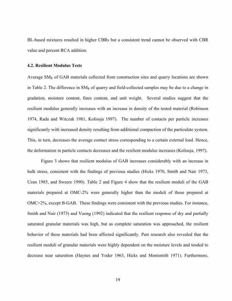
4.2. Resilient Modulus Tests
Average SMR of GAB materials collected from construction sites and quarry locations are shown
in Table 2. The difference in SMR of quarry and field-collected samples may be due to a change in
gradation, moisture content, fines content, and unit weight. Several studies suggest that the
resilient modulus generally increases with an increase in density of the tested material (Robinson
1974, Rada and Witczak 1981, Kolisoja 1997). The number of contacts per particle increases
significantly with increased density resulting from additional compaction of the particulate system.
This, in turn, decreases the average contact stress corresponding to a certain external load. Hence,
the deformation in particle contacts decreases and the resilient modulus increases (Kolisoja, 1997).
Figure 3 shows that resilient modulus of GAB increases considerably with an increase in
bulk stress, consistent with the findings of previous studies (Hicks 1970, Smith and Nair 1973,
Uzan 1985, and Sweere 1990). Table 2 and Figure 4 show that the resilient moduli of the GAB
materials prepared at OMC-2% were generally higher than the moduli of those prepared at
OMC+2%, except B-GAB. These findings were consistent with the previous studies. For instance,
Smith and Nair (1973) and Vuong (1992) indicated that the resilient response of dry and partially
saturated granular materials was high, but as complete saturation was approached, the resilient
behavior of these materials had been affected significantly. Past research also revealed that the
resilient moduli of granular materials were highly dependent on the moisture levels and tended to
decrease near saturation (Haynes and Yoder 1963, Hicks and Monismith 1971). Furthermore,

20
Dawson et al. (1996) studied a range of well-graded unbound aggregates and determined that,
below the
0
20000
40000
60000
80000
100000
0 20 40 60 80 100 120 140 160
G
F
C
D
E
A
B
y = 87.801 + 595.94x R2= 0.89895
y = -705.54 + 600.36x R2= 0.95716
y = 9620.4 + 388.76x R2= 0.95887
y = 12674 + 377.62x R2= 0.92609
y = 3088.6 + 496.15x R2= 0.97694
y = 13142 + 706.3x R2= 0.83176
y = 5585.3 + 920.28x R2= 0.89961
Res
ilien
t m
od
ulu
s (P
si)
Bulk stress (Psi)
FIGURE 3: GAB resilient moduli at different loading sequences

21
10000
15000
20000
25000
30000
35000
40000
0 2 4 6 8 10
A
B
G
E
D
C
F
SM
R (P
si)
Moisture Content (%)
FIGURE 4: Effect of moisture content on SMR values of GABs.

22
optimum moisture content, stiffness tended to increase apparently due to development of suction.
Beyond the optimum moisture content, as the material became more saturated and excess pore
water pressure was developed, the trend was shifted and stiffness started to decline rapidly.
An exception to the observed trend in Figure 4 was with the B-GAB material, which
experienced a maximum SMR when compacted at its optimum moisture content. Thom and Brown
(1987) observed a similar behavior in testing of select aggregates and attributed it to lubricating
effect of moisture on particles that would decrease the deformation of the aggregate assembly and
yield a resilient modulus increase.
Figure 5 shows the effect of fines content and gravel/sand ratio on the resilient moduli of
A-GAB material, respectively. SMR increased 2-2.5 times with an increase in fines content from 2
to 8% by weight, and then gradually decreased with further addition of fines (Figure 5a). A nearly
bell-shaped relationship can be observed when the gravel-to-sand ratio is plotted against SMr
(Figure 5b). SMr increases nearly 1.4 times with a change in G/S ratio from 1.5 to 1.7, and reaches
its maximum value at the optimum G/S value of ~1.7. Further decrease in sand fractions makes
the material unstable depending on the gravel size distribution. Similar observations were made
by Xiao et al. (2009) on testing three aggregates with different petrography. Previous studies
reported that the resilient modulus of granular materials generally tended to decrease with an
increase in fines content (Thom and Brown 1987; Kamal et al. 1993). Jorenby and Hicks (1986)
also showed that initially an increase in fines content provided higher stiffness in granular
materials and then a considerable reduction in stiffness was observed as more fines content were
added to a crushed aggregate.
The trends in Figure 5 can be explained by the influence of fines addition to packing of the
particles in a soil matrix. Figure 6 shows the hypothetical packing arrangements of coarse

23
0
5000
10000
15000
20000
25000
30000
0 3 6 9 12 15
SM
R (
Psi
)
Fines content (%)
Y = M0 + M1*x + ... M8*x8 + M9*x9
-1129.6M0
8555.7M1
-915.88M2
29.212M3
0.62776R2
(a)
5000
10000
15000
20000
25000
30000
35000
40000
1.4 1.5 1.6 1.7 1.8 1.9
SM
R (
Ps
i)
Gravel/Sand Ratio
Y = M0 + M1*x + ... M8*x8 + M9*x9
4.7669e+6M0
-8.9467e+6M1
5.6008e+6M2
-1.1643e+6M3
0.61876R2
(b)
FIGURE 5: Effect of (a) fines content, and (b) gravel-to-sand ratio on SMR of A GAB.

24
Large G/S Optimum G/S Small G/S
(a) (b) (c) FIGURE 6: Arrangement of particles in a soil matrix with the variation of fines. (a) No or small fines content (large G/S ratio), (b) dense graded (optimum G/S), and (c) high fines content (small G/S) (After Yoder and Witczak 1975, and Xiao et al. 2012)

25
Particles with varying fine contents in a soil matrix. Coarse aggregates can be interlocked with
each other yielding lower density and large voids due to lack of fines, as shown in Figure 6a. This
kind of soil matrix is referred to as gap graded gradation, and brings several advantages. The
matrix provides good drainage and is less susceptible to frost and heave processes. Xiao et al.
(2012) claimed that the GABs at this state may develop an unstable permanent deformation
behavior. The soil matrix shown in Figure 6b is classified as dense-graded in which most of the
voids between the aggregates are filled with fines but coarse particles are still in contact with each
other. The grain-to-grain contact and void filling with fines are the possible reasons for the
strength gain in this state. This soil matrix provides higher density which yields higher stiffness yet
decreases the hydraulic conductivity. On the other hand, the compaction of such a soil matrix is
moderately difficult. There is no grain-to-grain contact of aggregates in a soil matrix shown in
Figure 6c. It has reasonably low density and hydraulic conductivity and the coarse particles are
floating in the fine particles. The compaction of this kind of soil matrix is easier; however, its
stability can easily be affected by adverse water conditions.
The initial improvement in stiffness observed in the current study was attributed to
increased contacts during pore filling as explained (Figure 6b). Addition of excessive fines
gradually displaced the coarse particles in the soil matrix and caused stiffness to decrease (Figure
6c). The initial increase in resilient modulus with an increase in fines content was due to packing
of aggregates which decreased the recoverable strain of the material and resulted in stiff material
(Figure 5b).
Resilient modulus tests were also performed on RCAs and mixtures prepared at varying
RCA-to-GAB ratios. It can be seen from Figure 7 and Table 3b that 100%RCA and 100%GAB
provide relatively higher MR values as compared to their mixtures, with few exceptions. Similar

26
0
2 0 0 0 0
4 0 0 0 0
6 0 0 0 0
8 0 0 0 0
1 0 0 0 0 0
1 2 0 0 0 0
0 2 0 4 0 6 0 8 0 1 0 0
B G (7 5 -2 5 ) B G (5 0 -5 0 ) B G (2 5 -7 5 )R C G A B 'B 'G -G A B
Re
silie
nt
mo
du
lus
(Psi
)
B u lk s tre s s (P s i)
0
2 0 0 0 0
4 0 0 0 0
6 0 0 0 0
8 0 0 0 0
1 0 0 0 0 0
0 2 0 4 0 6 0 8 0 1 0 0
R C G A B 'B 'B A (7 5 -2 5 )B A (5 0 -5 0 ) B A (2 5 -7 5 )A -G A B
Res
ilie
nt
mo
du
lus
(Psi
)
B u lk s t re s s (P s i )
0
2 0000
4 0000
6 0000
8 0000
1 0 000 0
0 2 0 4 0 60 80 1 00
A G (75 -25 )A G (50 -50 )A G (25 -75 )R C G A B 'A 'G -G A B
Res
ilie
nt
mo
du
lus
(Psi
)
B u lk s tress ( P s i)
0
2 0 0 00
4 0 0 00
6 0 0 00
8 0 0 00
1 0 0 00 0
0 2 0 4 0 6 0 8 0 1 0 0
R C G A B 'A 'A A (7 5 -2 5 )A A (5 0 -5 0 )A A (2 5 -7 5 )A -G A B
Res
ilie
nt
mo
du
lus
(Psi
)
B u lk s tre s s (P s i)
FIGURE 7: Resilient moduli of recycled aggregate A and B, and their mixtures with two GABs.

27
observations were made by Kazmee et al. (2012) who attributed this behavior to poor packing of
particles and change in gradation parameters. Table 3a indicates that the SMR of RCAs tend to
increase with an increase in freezing and thawing cycles. The trends are reported by Bozyurt et.al
(2011). The stiffness increase in the current study is attributed to the continuation of hydration
(cementation) reactions in RCA during the freeze-thaw cycles.
4.3. Permanent Deformation Tests
Granular materials exhibit permanent deformation if they are subjected to repetitive loading for
extended periods of time. The permanent deformation values are strongly dependent on rigidity,
shear stress and load capacity of the granular materials. Use of the resilient modulus by itself is not
sufficient to fully characterize the mechanical behavior of a pavement structure and should be
coupled with permanent deformation tests (Khogali and Mohammad, 2004).
Figure 8 shows the variation of cumulative permanent axial strain (plastic strain) with
applied number of load repetitions. To model the relationship between the applied number of load
repetitions and plastic strain, a power model was used:
baNP (4)
where a, b are fitting parameters; P is the cumulative permanent axial strain and N is the number
load repetitions. The permanent deformation (i.e., plastic strain) depends on the packing
arrangement of particles, grain size distribution, and particle contact area. Table 2 shows the
plastic strain of all GAB materials used in the current study. The E-GAB had the maximum plastic
strain (0.09%) while T- GAB had the minimum plastic strain (0.03%) among all GAB materials
after 10,000 repeated cycles of loading, which may be attributed to the gravel contents of

28
0
0.02
0.04
0.06
0.08
0.1
0 2000 4000 6000 8000 10000
G F C D E A B
y = 0.0057315 * x^(0.22031) R2= 0.96927
y = 0.010909 * x^(0.20494) R2= 0.95451
y = 0.0081745 * x^(0.24811) R2= 0.96024
y = 0.011369 * x^(0.17083) R2= 0.93148
y = 0.0099292 * x^(0.24348) R2= 0.97282
y = 0.0088956 * x^(0.16364) R2= 0.94868
y = 0.0058739 * x^(0.18826) R2= 0.88511
Pla
sti
c s
trai
n (
%)
Number of repeated load cycles
FIGURE 8: Plastic strain of GABs under repeated load cycles. All specimens are compacted at OMC.

29
the two GABs. The K- GAB matrix has higher gravel content (56% versus 46%) and thus includes
more voids (Figure 6a). Such a matrix, due to lack of good amount of fines and sand, includes
gravel-to-gravel contact only and may experience more deformation during repeated loading (Xiao
et al. 2012).
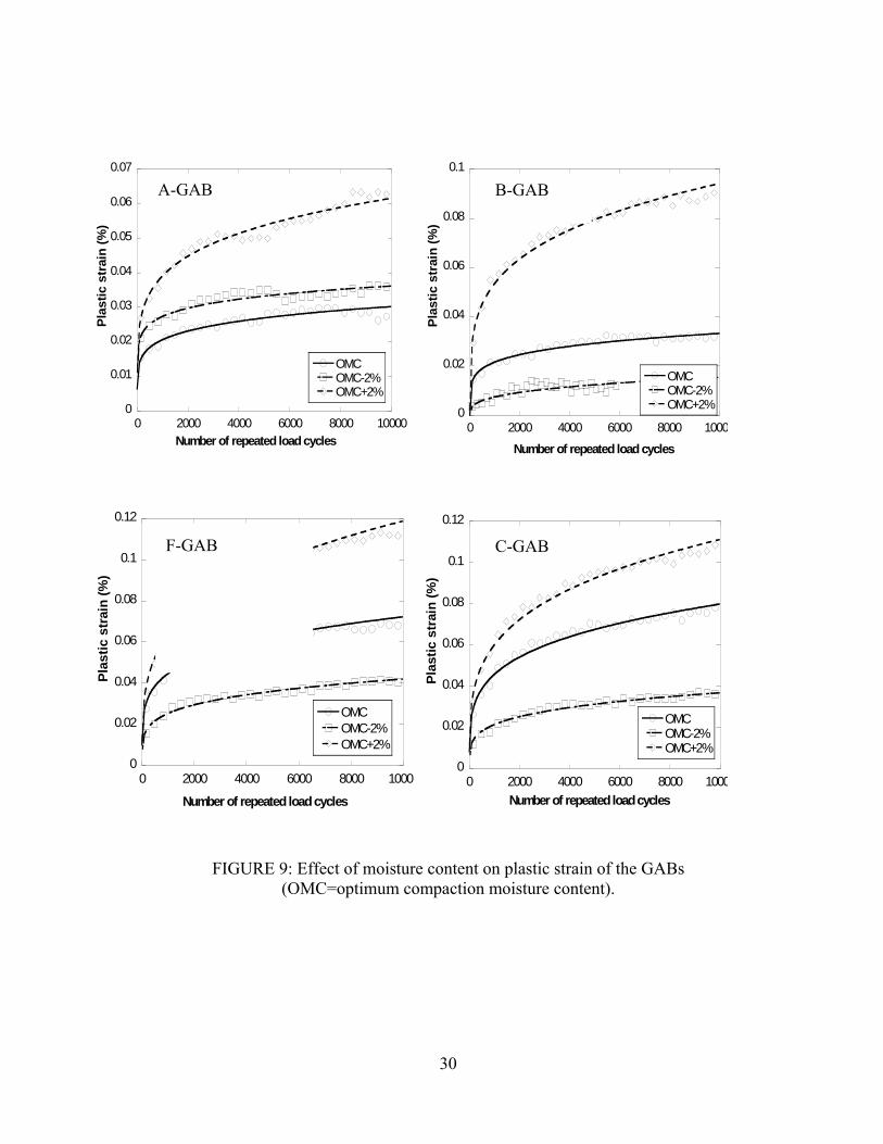
The data in Figure 9 suggest that GABs compacted wet of optimum are more susceptible to
structural rutting. Khogali et al. (2004) also observed 2-3 times increase in permanent
deformations of roadway bases due to fluctuations in groundwater table. Uthus (2007) reported
that dry density, degree of saturation, and stress level seemed to be the key parameters for
influencing the permanent deformation behavior, along with mineralogy, fines content and grain
size distributions of the granular materials. Increase in moisture content from OMC-2% to OMC
for all GABs yielded approximately the same amount of plastic strain under long term repetitive
loads (Figure 9). The addition of moisture above OMC caused pore water pressure increase under
repeated loading and resulted in excessive deformations.
As shown in Figure10, the permanent deformation of GAB increases upon mixing with
RCA, suggesting higher likelihood of rutting of a pavement system built with GAB/RCA blends.
Similar observations were made by Kazmee et al (2011). It is also noted that the plastic strain in
individual GAB and RCA materials is less than their mixtures. This could be due to poor packing
arrangement of particles when these two materials are mixed.
4.4. Laboratory Hydraulic Conductivity Tests
Table 4 summarizes the hydraulic conductivities of seven GABs tested in the laboratory and in-
situ. In-situ hydraulic conductivities are only 0.76-1.64 and 0.6-1.48 times higher than the
laboratory-measured hydraulic conductivities of the samples collected from the quarries and field
30
0
0.01
0.02
0.03
0.04
0.05
0.06
0.07
0 2000 4000 6000 8000 10000
OMCOMC-2%OMC+2%
Pla
stic
str
ain
(%
)
Number of repeated load cycles
0
0.02
0.04
0.06
0.08
0.1
0 2000 4000 6000 8000 1000
OMCOMC-2%OMC+2%
Pla
stic
str
ain
(%
)Number of repeated load cycles
0
0.02
0.04
0.06
0.08
0.1
0.12
0 2000 4000 6000 8000 10000
OMCOMC-2%OMC+2%
Pla
sti
c st
rain
(%
)
Number of repeated load cycles
0
0.02
0.04
0.06
0.08
0.1
0.12
0 2000 4000 6000 8000 1000
OMCOMC-2%OMC+2%
Pla
sti
c s
trai
n (
%)
Number of repeated load cycles
FIGURE 9: Effect of moisture content on plastic strain of the GABs (OMC=optimum compaction moisture content).
A-GAB B-GAB
F-GAB C-GAB

31
0
0.2
0.4
0.6
0.8
1
0 2000 4000 6000 8000 10000
A25-A75A50-A50A75-A25RCGAB 'A'A-GAB
Pla
stic
str
ain
(%
)
Number of repeated load cycles
RCA-Plant A
0
0.1
0.2
0.3
0.4
0 200 400 600 800 1000
A25-B75A50-B50A75-B25RCGAB 'B'A-GABI
Pla
stic
str
ain
(%
)
Number of repeated load cycles
RCA-Plant B
FIGURE 10: Plastic strain of recycled concrete aggregates A and B, and their mixtures with A- GAB

32
Table 4: Mean hydraulic conductivity of GAB materials tested in the laboratory and in-situ.
GAB Material k laboratory of quarry
samples, ft/day (cm/s)
k laboratory of field-retrieved samples
(ft/day)
k in-situ
(ft/day)
A 77
(2.73 x 10⁻²) 71
(2.52 x 10⁻²) 59
(2.07 x 10⁻²)
B 19
(6.57 x 10⁻³) 20
(7.23 x 10⁻³) 20
(7.05 x 10⁻³)
C 2
(5.66 x 10⁻⁴) 2
(6.30 x 10⁻⁴) 3
(9.30 x 10⁻⁴)
D 42
(1.48 x 10⁻²) 20
(6.90 x 10⁻³) 12
(4.25 x 10⁻³)
E 11
(3.92 x 10⁻³) NA NA
F 4
(1.48 x 10⁻³) NA NA
G 36
(1.28 x 10⁻²) 37
(1.30 x 10⁻²) 18
(6.20 x 10⁻³) NA: Not analyzed
33
test locations, respectively. The difference is less than an order of magnitude, suggesting that the
laboratory and field hydraulic conductivities are comparable.
In order to study the effect of fines content on hydraulic conductivity, gradations of A- and
B-GAB materials were adjusted by following two different approaches. First, gradation was
adjusted between the US. No #4 and #30 sieves and the rest of the fractions were kept constant
(Figure 11a). Figure 12a shows that such an adjustment does not significantly alter hydraulic
conductivity of R- GAB. These results confirm the commonly observed trend that the coarser
portion of sand in GAB (e.g., between the U.S. #4 and #30 sieves) does not have a significant
effect on hydraulic conductivity and flow is mainly controlled by smaller particles in the gradation
(Cote and konrad 2003). Therefore, at the second stage, adjustments were made for the fractions
between the 3/8-inch (9.5-mm) and 1/2-inch, (12.7-mm) and 3/4-inch (19-mm) sieves to
represent a more widespread change in grain size distribution (Figures 11b and 11c). The data in
Table 5 reveal that A- and B-GABs hydraulic conductivities reduced 5 and 50 times, respectively,
as a result of such fines content adjustment from 2 to 16% (Figures 12b and 12c). Similar
observations were reported by Siswosoebrotho et. al. (2005) during testing of unbound granular
materials.
Figure 13 shows that hydraulic conductivities of A- and B-GAB materials increase up to 5
and 50 times, respectively, with nearly 14% increase in gravel content for both materials. Similar
magnitudes of increase in hydraulic conductivity were observed when gravel-to-sand (G/S) ratio
was varied between 1.45 and 1.85 R-GAB and 0.82 and 1.14 for T-GAB (Figure 14). Analysis of
the trends in Figure 14 shows that the soil matrix is porous and leads to higher hydraulic
conductivities when G/S ratio >1.7 for R and G/S>1.05 for B GABs. It is believed that the
minimum porosities are achieved at these gravel-

34
0
10
20
30
40
50
60
70
80
90
100
0.010.1110100
Original quarry2% fines6% fines8% fines10% fines12% fines14% finesSHA Upper Limit SHA Lower Limit
Per
cen
t fi
ner
Particle size (mm)
#200
#30
3/4
1 1/
2
1/2
3/8 #4
A- GAB
(a)
0
10
20
30
40
50
60
70
80
90
100
0.010.1110100
Original quarry2% fines4% fines6% fines8% fines10% fines12% fines14% fines16% finesSHA Upper Limit SHA Lower Limit
Per
cen
t fi
ner
Particle size (mm)
#20
0
#3
0
3/4
1 1
/2
1/2
3/8 #4
A- GAB
(b)
0
10
20
30
40
50
60
70
80
90
100
0.010.1110100
Original quarry2% fines4% fines6% fines8% fines10% fines12% fines14% fines16% finesSHA Upper Limit SHA Lower Limit
Pe
rcen
t fi
ner
Particle size (mm)
#200
#3
0
3/4
1 1/
2
1/2
3/8 #4
B-GAB
(c)
FIGURE 11: Change in gradations of (a) A- GAB due to adjustment between #30 to #4 sieves, and (b) A and (c) B GABs due to adjustment between 3/4in to #4 sieves.

35
10
100
1000
0 2 4 6 8 10 12 14 16
Hyd
rau
lic
co
nd
uct
ivit
y (
ft/d
ay)
Fines Content (%)
(a)
A- GAB
1
10
100
1000
0 2 4 6 8 10 12 14 16
Hy
dra
uli
c co
nd
uct
ivit
y (f
t/d
ay)
Fines content (%)
SHA upper limit for gradation
SHA lower limit for gradation
A- GAB
(b)
Y = M0 + M1*x + ... M8*x8 + M9*x9
102.64M0
-11.351M1
0.38988M2
0.91896R2
0.1
1
10
100
0 2 4 6 8 10 12 14 16
y = 89.928 * x (-2.1883) R2= 0.73377
Hyd
rau
lic
con
du
cti
vity
(ft
/day
)
Fines content (%)
SHA upper limit for gradation
SHA lower limit for gradation
B- GAB
(c)
FIGURE 12: Effect of fines on hydraulic conductivity of (a) A GAB due to adjustment between #30 and #4 (0.6 mm and 4.75 mm sieves), and (b) A and (c) B GABs due to adjustment between 3/4in to #4 sieves.

36
10
20
30
40
50
60
70
80
90
45 50 55 60 65 70
y = 0.081814 * e (0.10709x) R2= 0.90999 H
ydra
uli
c co
nd
uct
ivit
y (f
t/d
ay)
Gravel content (%)
(a)
5
10
15
35 40 45 50 55 60
y = 5.3859e-7 * e (0.32115x) R2= 0.94017
Hy
dra
uli
c co
nd
uct
ivit
y (f
t/d
ay)
Gravel content (%)
(b)
FIGURE13: Effect of gravel content on hydraulic conductivity of
(a) A and (b) B GABs

37
Table 5: Effect of gradation parameters on SMR and hydraulic conductivity of GAB materials.
Material FC D10 D30 D60 D50 Sand Gravel G/S SMR k
(%) in in in in (%) (%) Ratio Psi cm/s ft/day
A- GAB Change in
Fines content is adjusted in sand portion of gradation
2 0.007 0.084 0.404 0.280 34.4 63.6 1.17 - 1.01
x 10-2 29
6 0.009 0.067 0.394 0.256 34.4 59.6 1.27 - 2.56
x 10-2 73
8 0.008 0.071 0.394 0.256 34.4 57.6 1.33 - 3.85
x 10-2 109
10 0.006 0.067 0.394 0.256 34.4 55.6 1.38 - 3.40
x 10-2 96
12 0.004 0.079 0.394 0.256 34.4 53.6 1.44 - 6.33
x 10-2 179
14 0.004 0.079 0.394 0.256 34.4 51.6 1.56 - 3.83
x 10-2 109
A- GAB Change in
fines content is adjusted in
coarse portion of gradation
2 0.016 0.106 0.421 0.307 34.4 63.6 1.85 12502 3.12
x 10-2 88
4 0.009 0.087 0.409 0.280 34.4 61.6 1.79 21493 1.92
x 10-2 54
6 0.006 0.075 0.394 0.268 34.4 59.6 1.73 18883 1.83
x 10-2 52
8 0.005 0.067 0.366 0.244 34.4 57.6 1.67 26076 1.04
x 10-2 29
10 0.003 0.051 0.354 0.228 34.4 55.6 1.62 18375 1.11
x 10-2 31
12 0.002 0.045 0.323 0.209 34.4 53.6 1.56 21247 1.14
x 10-2 32
14 0.001 0.038 0.307 0.199 34.4 51.6 1.5 19231 6.33
x 10-3 18
16 0.001 0.032 0.280 0.169 34.4 49.6 1.44 - 6.40
x 10-3 18
B- GAB, Change in
fines content is adjusted in
coarse portion of gradation
2 0.006 0.035 0.354 0.205 45.8 52.2 1.14 - 3.67
x 10-3 10
4 0.005 0.030 0.323 0.193 45.8 50.2 1.1 - 2.71
x 10-3 8
6 0.004 0.024 0.295 0.157 45.8 48.2 1.05 - 1.17
x 10-3 3
8 0.004 0.020 0.276 0.126 45.8 46.2 1.01 - 4.22
x 10-4 1
10 0.003 0.017 0.236 0.106 45.8 44.2 0.97 - 4.60
x 10-4 1
12 0.002 0.014 0.213 0.091 45.8 42.2 0.92 - 6.44
x 10-5 0.2
14 0.002 0.012 0.185 0.075 45.8 40.2 0.88 - 7 x 10⁻⁵
0.2
16 0.002 0.010 0.157 0.063 45.8 38.2 0.83 - 7.32
x 10-5 0.2
A- GAB QG 7.6 0.005 0.071 0.394 0.256 34.4 58.03 1.69 190 2.73
x 10-2 77
B GAB QG 8.6 0.005 0.020 0.276 0.126 45.8 45.6 1 257 6.57 x 10⁻³
19

38
SHA Spec. LL
0 0.016 0.118 0.472 0.374 36 64 1.78 - 3.19
x 10-2 90
SHA.Spec UL
8 0.004 0.033 0.236 0.126 48 44 0.92 - 3.84
x 10-3 11
FC: Fines contents, D10,D30,D50,D60 : Diameter of particles @ 10,30,50,60 passing percentage finer respectively, G/S: Gravel to Sand ratio, SMR: Summary Resilient Modulus, k : hydraulic conductivity, QG: quarry gradation, LL: Lower limit of SHA specified Gradation, UL: Upper Limit of SHA specified gradation

39
10
20
30
40
50
60
70
80
90
1.4 1.5 1.6 1.7 1.8 1.9
Hyd
rau
lic
con
du
ctiv
ity
(ft/
day
)
Gravel/sand ratio
(a)
Y = M0 + M1*x + ... M8*x8 + M9*x9
1006.2M0
-1333.7M1
450.88M2
0.92424R2
3.75
7.5
11.2
15
0.8 0.85 0.9 0.95 1 1.05 1.1 1.15
y = 6.0696e-7 * e (14.579x) R2= 0.95304
Hyd
rau
lic
con
du
cti
vit
y (
ft/d
ay)
Gravel/sand ratio
(b)
FIGURE14: Effect of gravel/sand ratio on hydraulic conductivity of
(a) A and (b) B GABs

40
to-sand ratios due to optimum packing of the GAB medium. Xiao et al. (2012) also reported
minimum porosity achievements at G/S=1.56-1.68 and G/S~1.5, respectively, for GABs with
varying petrography.
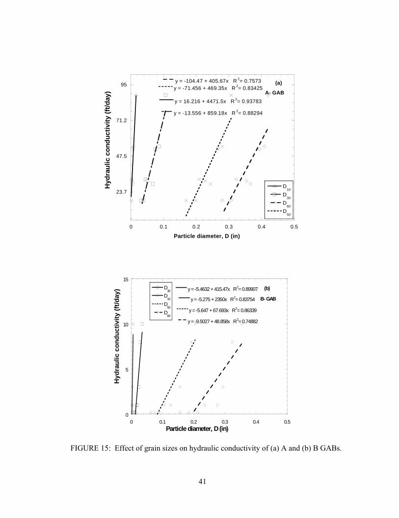
Figure 15 shows that hydraulic conductivites of R and B GABs increased up to 5 and 50
times, respectively, with increasing characeterictic grain sizes of the soil (i.e., D10, D30 , D50 and
D60). The hydraulic conductivity seems to be more sensitive to the smaller grain sizes (D10 and
D30) as compared to larges sizes (D50 and D60), consistent with the previous studies that finer sizes
play a major role in hydraulic conductivity changes (FHWA 2005).
41
23.7
47.5
71.2
95
0 0.1 0.2 0.3 0.4 0.5
D10
D30
D60
D50
y = -104.47 + 405.67x R 2= 0.7573 y = -71.456 + 469.35x R 2= 0.83425
y = 16.216 + 4471.5x R 2= 0.93783
y = -13.556 + 859.18x R 2= 0.88294 H
ydra
uli
c co
nd
uc
tivi
ty (
ft/d
ay)
Particle diameter, D (in)
A- GAB
(a)
0
5
10
15
0 0.1 0.2 0.3 0.4 0.5
D30
D10
D50
D60
y = -5.4632 + 415.47x R2= 0.89907
y = -5.275 + 2350x R2= 0.83754
y = -5.647 + 67.693x R2= 0.86339
y = -9.5027 + 48.858x R2= 0.74882
Hy
dra
uli
c c
on
du
ctiv
ity
(ft
/day
)
Particle diameter, D (in)
B- GAB
(b)
FIGURE 15: Effect of grain sizes on hydraulic conductivity of (a) A and (b) B GABs.
42
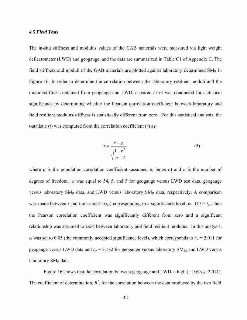
4.5 Field Tests
The in-situ stiffness and modulus values of the GAB materials were measured via light weight
deflectometer (LWD) and geogauge, and the data are summarized in Table C1 of Appendix C. The
field stiffness and moduli of the GAB materials are plotted against laboratory determined SMR in
Figure 16. In order to determine the correlation between the laboratory resilient moduli and the
moduli/stiffness obtained from geogauge and LWD, a paired t-test was conducted for statistical
significance by determining whether the Pearson correlation coefficient between laboratory and
field resilient modulus/stiffness is statistically different from zero. For this statistical analysis, the
t-statistic (t) was computed from the correlation coefficient (r) as:
2
1 2
n
r
rt
(5)
where ρ is the population correlation coefficient (assumed to be zero) and n is the number of
degrees of freedom. n was equal to 54, 5, and 5 for geogauge versus LWD test data, geogauge
versus laboratory SMR data, and LWD versus laboratory SMR data, respectively. A comparison
was made between t and the critical t (tcr) corresponding to a significance level, α. If t > tcr, then
the Pearson correlation coefficient was significantly different from zero and a significant
relationship was assumed to exist between laboratory and field resilient modulus. In this analysis,
was set to 0.05 (the commonly accepted significance level), which corresponds to tcr = 2.011 for
geogauge versus LWD data and tcr = 3.182 for geogauge versus laboratory SMR, and LWD versus
laboratory SMR data.
Figure 16 shows that the correlation between geogauge and LWD is high (t=9.6>tcr=2.011).
The coefficient of determination, R2, for the correlation between the data produced by the two field

43
0
5000
10000
15000
20000
25000
30000
35000
0 10000 20000 30000 40000 50000
y = 0.42795x
LW
D m
od
ulu
s (P
si)
Geogauge Young's modulus (Psi)
r = 0.81t = 9.6 > t
cr = 2.011
0
5000
10000
15000
20000
25000
30000
35000
0 50000 100000 150000 200000 250000
y = 0.094929x
LW
D m
od
ulu
s (P
si)
Geogauge stiffness (lb/in)
r = 0.81t = 9.6 > t
cr = 2.011
80000
90000
100000
110000
120000
130000
140000
150000
20000 22000 24000 26000 28000 30000 32000
y = 4.5302x
Mea
n g
eog
aug
e st
iffn
ess
(lb
/in
)
Mean SMR(Psi)
r = 0.95t = 5.3 > t
cr = 3.182
18000
20000
22000
24000
26000
28000
30000
32000
20000 22000 24000 26000 28000 30000 32000
y = 0.98693x
Mea
n g
eo
ga
ug
e Y
ou
ng
's m
od
ulu
s (
Ps
i)
M ean SMR
(Psi)
r = 0.91t = 3.8 > t
cr = 3.182
6 0 0 0
8 0 0 0
1 0 0 0 0
1 2 0 0 0
1 4 0 0 0
1 6 0 0 0
1 8 0 0 0
6 0 0 0 8 0 0 0 1 0 0 0 0 1 2 0 0 0 1 4 0 0 0 1 6 0 0 0 1 8 0 0 0 2 0 0 0 0
y = 0 .7 7 9 9 3 x
Mea
n L
WD
mo
du
lus
(P
si)
M e a n MR
@ L W D B u lk S t r e s s (P s i)
B - G A B
A -G A B
D -G A B
C -G A B
G -G A B
r = 0 .9 7t = 6 .9 > t
c r = 3 .1 8 2
FIGURE 16: Comparison of laboratory and field moduli.

44
equipment was fair (R2>0.65). The differences in induced stress and depth of influence of the
applied load provided by LWD, and geogauge could be the possible reasons for the observed
correlation. Previous studies showed that applied stress level was the factor that had the most
significant impact on the resilient properties of granular materials (Kolisoja (1997). Significantly
higher R2 values were observed for the correlations between the mean laboratory SMR and LWD
or geogauge data (R2=0.83-0.97). In addition, t values that were obtained from statistical analyses
(t>tcr= 3.182) indicate that reasonably good correlations exist between the geogauge and laboratory
SMR as well as LWD and laboratory MR data at LWD bulk stress level. All regression lines were
forced to pass through the zero intercept because of rationality of relations.
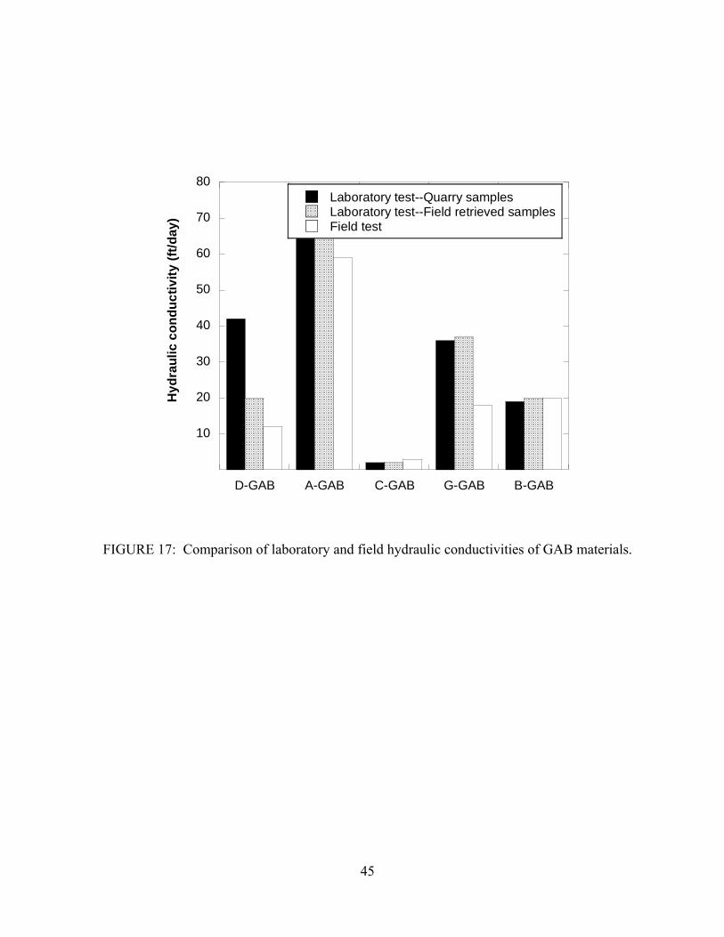
Figure 17 shows the field and laboratory hydraulic conductivity test results. The
differences in the laboratory and field hydraulic conductivity values are negligible considering the
anisotropy in the field. The drainage qualities of the GAB materials tested in the laboratory and
field can be considered as “fair to good” according to the hydraulic conductivity range provided in
AASHTO Guide (1993).
45
10
20
30
40
50
60
70
80
D-GAB A-GAB C-GAB G-GAB B-GAB
Laboratory test--Quarry samplesLaboratory test--Field retrieved samplesField test
Hy
dra
uli
c c
on
du
cti
vit
y (f
t/d
ay)
FIGURE 17: Comparison of laboratory and field hydraulic conductivities of GAB materials.

46
5. PRACTICAL IMPLICATIONS
5.1 Highway Base Design
Resilient modulus test results were used to estimate the thickness of the base layer in a pavement
by following the procedures defined in the AASHTO Guide (1993). The 50 million ESAL value
was assumed for this analysis. The overall standard deviation (So) and reliability (ZR) were
assumed to be 0.35 and 95%, respectively. Structural numbers (SN) were back-calculated using
the following equation:
(6)
where ∆PSI is design serviceability loss and MR is the roadbed material effective resilient
modulus. The values were selected as 5000Psi, based on Huang (1993). An asphalt layer
thickness of 8 inches (203.2 mm) was selected. The resilient modulus of asphalt was assumed to
be 430000Psi (2965 Mpa), which corresponded to a layer coefficient of a1 = 0.44 according to
AASHTO Guide (1993). A resilient modulus of 15000lb (103 Mpa) (corresponding to a structural
coefficient of a3 = 0.08) and a thickness of 6 inch (152.4 mm) (D3) were assumed for the subbase
layer. The laboratory-based SMR values vary between 17000 psi (120 Mpa) and 30500 psi (210
Mpa) which correspond to a layer coefficient (a2) of 0.08-0.14 according to AASHTO pavement
design guidelines (1993). SMr of 30000lb (206.84 Mpa) and a2 of 0.12, the two values commonly
used by SHA in absence of measurement, fall within this range. Finally, the base thicknesses were
calculated using the following formula:
07.8log32.2110944.0
5.12.4log20.01log36.9log 1019.5
1010018
RR M
SN
PSISNSZW
47
m2a
mD3
a1D1aSN
2D2
33 (7)
where m2 and m3 are drainage modification factors for base and subbase layer, respectively, and
were chosen as 1.2, 1.0, 0.8, 0.6 for excellent, good, fair, and poor drainage conditions,
respectively, within the pavement system (Huang 1993). D1, D2, and D3 are the layer thicknesses of
asphalt layer, base layer, and subbase layer, respectively.
It can be concluded from Table 6 that an increase in the base layer coefficient yields a
decrease in required thickness of base layer while all other factors are kept constant. On the other
hand, the decrease in drainage modification factor increases the required thickness of the base
course. The effects of layer coefficient and drainage modification factor of GAB on the required
design thickness are also reflected in Figure 18.
5.2. Effect of Hydraulic Conductivity on Highway Base Design
Federal Highway Administration (FHWA) software DRIP (Drainage Requirement in Pavements)
was used to evaluate the effect of hydraulic conductivity on drainage time and minimum required
thickness of highway base layers. For the purpose of analysis, a typical cross section of highway
having width (W) of 24 ft (two lanes, each 12 ft wide) was selected. The longitudinal slope (S)
and cross slope (Sx) were considered as 2%, and the resultant length of flow path (LR =
W*[1+(S/Sx)2]1/2) was calculated.
The largest source of water is the rain water that enters the pavement surface through
cracks and joints in the surface. Two methods have been used to determine surface infiltration of
water: the infiltration ratio method (Cedergren et al. 1973) and the crack infiltration method

48
(Ridgeway 1976). The infiltration ratio method is highly empirical and depends on both the
infiltration ratio and rainfall rate. The crack infiltration method, on the other hand, is based on the
Table 6. Effect of change in layer coefficient and drainage modification factor on the required base thickness in pavement design.
a2 m3 = m2 D2 (in) Cost /mile ($)
0.08
0.6 24.8 594173
0.8 17.1 409742
1 12.5 299065
1.2 9.4 225311
0.10
0.6 19.9 475300
0.8 13.7 327794
1 10.0 239252
1.2 7.5 180192
0.12
0.6 16.6 396084
0.8 11.4 273161
1 8.3 199408
1.2 6.3 150239
0.14
0.6 14.2 339474
0.8 9.8 234165
1 7.1 170868
1.2 5.4 128763
Notes: a2: base layer coefficient, m2 : base layer drainage modification factor, m3: subbase layer drainage modification factor, D2: required base thickness

49
5
10
15
20
25
0.50.60.70.80.911.11.21.3
a2 = 0.08
a2 = 0.10
a2 = 0.12
a2 = 0.14
Re
qu
ired
bas
e th
ick
ne
ss
(in
)
Base course drainage modification factor (m2)
FIGURE 18: Variation of required base thickness with the change in layer coefficient and drainage
modification factor.
50
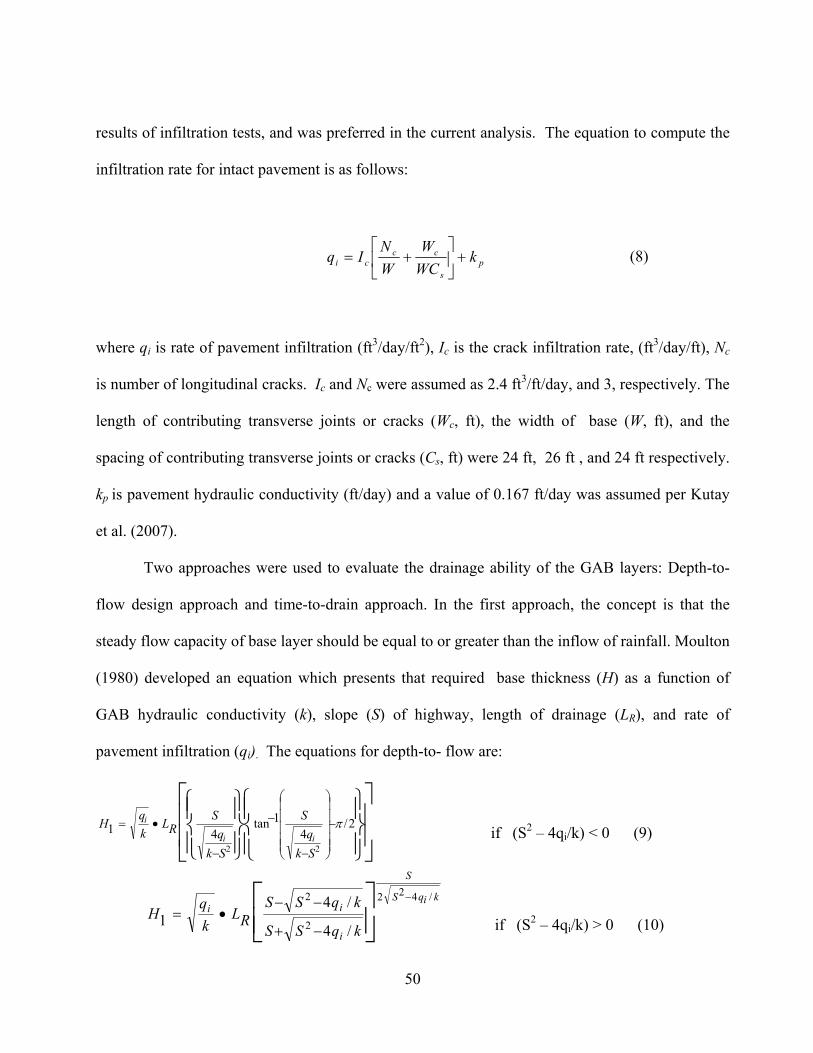
results of infiltration tests, and was preferred in the current analysis. The equation to compute the
infiltration rate for intact pavement is as follows:
ps
ccci k
WC
W
W
NIq
(8)
where qi is rate of pavement infiltration (ft3/day/ft2), Ic is the crack infiltration rate, (ft3/day/ft), Nc
is number of longitudinal cracks. Ic and Nc were assumed as 2.4 ft3/ft/day, and 3, respectively. The
length of contributing transverse joints or cracks (Wc, ft), the width of base (W, ft), and the
spacing of contributing transverse joints or cracks (Cs, ft) were 24 ft, 26 ft , and 24 ft respectively.
kp is pavement hydraulic conductivity (ft/day) and a value of 0.167 ft/day was assumed per Kutay
et al. (2007).
Two approaches were used to evaluate the drainage ability of the GAB layers: Depth-to-
flow design approach and time-to-drain approach. In the first approach, the concept is that the
steady flow capacity of base layer should be equal to or greater than the inflow of rainfall. Moulton
(1980) developed an equation which presents that required base thickness (H) as a function of
GAB hydraulic conductivity (k), slope (S) of highway, length of drainage (LR), and rate of
pavement infiltration (qi). The equations for depth-to- flow are:
2/4
1tan41
22
Sk
q
S
Sk
q
SRL
k
qH
ii
i
if (S2 – 4qi/k) < 0 (9)
kiqS
S
i
ii
kqSS
kqSSRL
k
qH
/422
2
2
/4
/41
if (S2 – 4qi/k) > 0 (10)

51
1
1
RL
k
qH i
if (S2 – 4qi/k) = 0 (11)
where S and LR were assumed as 0.0283 and 36.8 ft respectively. The highway geometry is
beyond the scope of this work, thus a sensitivity analysis was conducted with respect to hydraulic
conductivity (k) only. The laboratory quarry GAB hydraulic conductivities listed in Table 4 were
used in the analysis. The results shown in Figure 19 indicate that the required base thickness is
more influenced from GAB permeability’s at k < 300ft/day.
0
10
20
30
40
50
60
70
80
0 500 1000 1500 2000 2500 3000 3500 4000
Req
uir
ed b
ase
th
ickn
ess
(in
)
Hydraulic conductivity (ft/day)
FIGURE 19: Variation in required base thickness with base course hydraulic conductivity

52
The second approach for design of the GAB layers includes a series of calculations for the
time to drain 50% of the infiltrating water. The AASHTO pavement design guideline (1993)
categorizes the base layer as excellent, good, fair, and poor based on time for 50% drainage. The
following equations developed by Casagrande and Shannon (1952) and Barber and Sawyer (1952)
and embedded in the DRIP software were used to calculate the time to drain a specified percentage
of the infiltrating water:
Casagrande and Shannon (1952)
kH
Ln
SU
USSS
S
SSS
St e
2
1
111
1
12113/1
1122
122ln
1ln
4.02.1
if U > 0.5 (12)
kH
Ln
S
USSUS
St e
2
1
12113/1
1
2ln2
4.02.1
if U ≤ 0.5 (13)
Barber and Sawyer (1952)
kH
Ln
SU
USSS
SSSt e
2
1
111
1
211 4.21
2.1log15.1
4.21log48.05.0
if 0.5 U 1.0 (14)
kH
Ln
S
USUSt e
2
1
21
8.41log48.0
if 0 U 0.5 (15)
where t is time (hours) for percent drainage, U, to be reached, S1 is dimensionless slope factor (=
H/LS). L and ne are width and effective porosity of the GAB layers and were taken as 24ft (7.3 m)
and 20- 70% of total porosity, respectively.

53
A series of analysis was performed to gage the influence of U, H, and k on time-to-drain.
U and H varied between 0 and 98%, and 2 inch to 24 inch (5 and 60 cm), respectively. A unit
weight of 140 Pcf (2242.5 kg/m3) and specific gravity of 2.70 for GAB were used. The water in
the voids cannot be drained by gravity flow due to capillary action present in the soil matrix, thus,
effective porosities were assumed to be 20-70% of the total porosities (Moulton 1980) and utilized
in the analysis. Four different gradations of A- and B-GAB materials, with fines content of 2, 4,
8, and 14%, along with the lower and upper SHA gradation limits were used in the drainage
calculations. A-GAB hydraulic conductivities ranging from 88ft/day to 18ft/day (6.4 x 10⁻³ to 3.12
x 10-2 cm/s) that correspond to 2-16% fines content were utilized. The corresponding T- GAB
hydraulic conductivities ranged from 10ft/day to 0.2ft/day (3.67 x 10⁻³ to 7.32 x 10⁻⁵ cm/s).
The results are shown in Figures 20-23. The time-to-drain does not change significantly up
to 50% drainage, and an exponential increase in drainage time exists for 50%<U<98% (Figures 20
and 22). Moreover, when the base thickness of R- GAB was increased from 2 inches to 24 inches
(6 to 60 cm), 57% and 48% decreases in drainage time were observed based on Barber and Sawyer
(1952) and Casagrande and Shannon (1952) methods, respectively (Figure 21). The corresponding
decreases in drainage time for T- GAB were 45% and 54%, respectively (Figure 23).
The driving factor for time-to-drain of a highway base is the GAB hydraulic conductivity.
The required base layer thickness (Moulton method 1980) with respect to hydraulic conductivity
values obtained at 2-14% fines are shown for R- GAB in Figure 24 and Table 7. At a specific base
thickness of 12in (0.3m), the time-to-drain (at U=50%) increases three times with change of fines
content from 2 to 14% (24h to 75h, changing the corresponding AASHTO drainage quality
classification from Good to Fair (Table 7). The corresponding increase in time-

54
0
200
400
600
800
1000
1200
0 20 40 60 80 100
2% fines4% fines8% fines14% finesSHA upper limitSHA lower limit
Tim
e to
dra
in (
ho
urs
)
Drainage (%)
Barber and Sawyer Method
(a)
(H=0.3 m)
A-GAB
0
200
400
600
800
1000
1200
0 20 40 60 80 100
2% fines4% fines8% fines14% finesSHA upper limitSHA lower limit
Tim
e to
dra
in (
ho
urs
)
Drainage (%)
Casagrande and Shannon Method
(b)
(H=0.3 m)
A-GAB
FIGURE 20: Variation in time to drain with percent drainage and fines content for A GAB: (a)
Barber and Sawyer Method, and (b) Casagrande and Shannon Method. H= 0.3 m was used throughout the analysis

55
0
50
100
150
200
0 5 10 15 20 25
2% fines4% fines8% fines14% finesSHA upper limitSHA lower limit
Tim
e t
o d
rain
at
U=
50
% (
ho
urs
)
Base thickness (in)
Barber and Sawyer Method
(a)
A-GAB
0
50
100
150
200
250
0 5 10 15 20 25
2% fines4% fines8% fines14% finesSHA upper limitSHA lower limit
Tim
e to
dra
in a
t U
=5
0%
(h
ou
rs)
Base thickness (in)
Casagrande and Shannon Method
(b)
A-GAB
FIGURE 21: Variation in time to drain with base thickness and fines content for A GAB: (a)
Barber and Sawyer Method, and (b) Casagrande and Shannon Method.

56
0
1000
2000
3000
4000
5000
6000
7000
0 20 40 60 80 100
2% fines4% fines8% fines14% finesSHA upper limitSHA lower limit
Tim
e to
dra
in (
ho
urs
)
Drainage (%)
Barber and Sawyer Method
(a)
(H=0.3 m)
B-GAB
0
1000
2000
3000
4000
5000
6000
7000
0 20 40 60 80 100
2% fines4% fines8% fines14% finesSHA upper limitSHA lower limit
Tim
e to
dra
in (
ho
urs
)
Drainage (%)
Casagrande and Shannon Method
(b)
(H=0.3 m)
B-GAB
FIGURE 22: Variation in time to drain with percent drainage and fines content for B GAB: (a)
Barber and Sawyer Method, and (b) Casagrande and Shannon Method. H= 0.3 m was used throughout the analysis
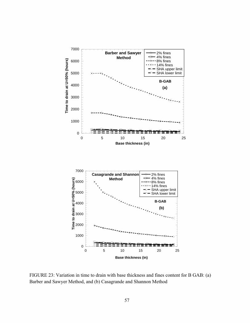
57
0
1000
2000
3000
4000
5000
6000
7000
0 5 10 15 20 25
2% fines4% fines8% fines14% finesSHA upper limitSHA lower limit
Tim
e t
o d
rain
at
U=
50
% (
ho
urs
)
Base thickness (in)
Barber and Sawyer Method
(a)
B-GAB
0
1000
2000
3000
4000
5000
6000
7000
0 5 10 15 20 25
2% fines4% fines8% fines14% finesSHA upper limitSHA lower limit
Tim
e to
dra
in a
t U
=50
% (
ho
urs
)
Base thickness (in)
Casagrande and Shannon Method
(b)
B-GAB
FIGURE 23: Variation in time to drain with base thickness and fines content for B GAB: (a) Barber and Sawyer Method, and (b) Casagrande and Shannon Method

58
20
30
40
50
60
70
80
20
25
30
35
40
45
50
55
10 20 30 40 50 60 70 80 90
Time to drain
Base thickness
y = 525.97 * x^(-0.67727) R2= 0.99818
y = 302.87 * x^(-0.59473) R2= 0.99934 T
ime
to
dra
in a
t U
=50
% (
ho
urs
)R
eq
uire
d b
as
e th
ickn
ess
(in)
Hydraulic conductivity (ft/day)
14% fines
8% fines
4% fines
2% fines
FIGURE 24: Influence of hydraulic conductivity on required base thickness (Moulton method) and time-to-drain of highway base layers constructed with (a) A-Quarry, and (b) B-Quarry GABs.
A-GAB

59
Table 7. Effect of fines content and GAB type on required base thickness and time to drain.
Material Gradation Hydraulic
conductivity ft/day (cm/s)
Time to drain at U=50% (hours)
AASHTO classification
for quality of drainage
R-Q
uarr
y
2% FC 88 (3.12 x 10⁻²) 24 Good
4% FC 54 (1.92 x 10⁻²) 36 Fair
8% FC 29 (1.04 x 10⁻²) 52 Fair
14% FC 18 (6.33 x 10⁻³) 75 Fair
Quarry 77 (2.73 x 10⁻²) 48 Fair
T-Q
uarr
y
2% FC 10 (3.67 x 10⁻³) 218 Poor
4% FC 8 (2.71 x 10⁻³) 263 Poor
8% FC 1 (4.22 x 10⁻⁴) 1262 Poor
14% FC 0.001 (7 x 10⁻⁵) 3768 Poor
Quarry 19 (6.57 x 10⁻³) 77 Fair
E-GAB Quarry 11 (3.92 x 10⁻³) 138 Fair
G-GAB Quarry 36 (1.28 x 10⁻²) 35 Fair F-GAB Quarry 4 (1.48 x 10⁻³) 430 Poor C-GAB Quarry 2 (5.66 x 10⁻⁴) 1121 Poor
D-GAB Quarry 42 (1.48 x 10⁻²) 33 Fair SHA lower limit 90 (3.19 x 10⁻²) 29 Good
SHA upper limit 11 (3.84 x 10⁻³) 140 Fair

60
to-drain for T-GAB was from 218 hours to 3768 hours (Table 7). A 17 times increase in time-to-
drain indicated that material was clogged by fines. It can also be seen from Figures 11 and 12 that
T- GAB stays out of the SHA gradation limits and experience unacceptable hydraulic
conductivities when the fines content was greater than 6%.
Figure 25 and 26 present the variation in time-to-drain with percent drainage and base
thickness for all GABs. The F and C GABs materials took long time to drain as compared to
others due to their relatively lower hydraulic conductivities (Table 4). The effect of hydraulic
conductivity on drainage performance and required base thickness can clearly be seen in Figure
27. The GAB materials with lower hydraulic conductivities yielded higher time-to-drain at
U=50% and required large base thicknesses for construction.

61
0
200
400
600
800
1000
1200
0 20 40 60 80 100
ABEGFCDSpec.Upper LimitSpec.Lower Limit
Tim
e to
dra
in (
ho
urs
)
Drainage (%)
Barber and Sawyer Method
(a)
(H=0.3 m)
0
200
400
600
800
1000
1200
0 20 40 60 80 100
ABEGFCDSpec.Upper LimitSpec.Lower Limit
Tim
e to
dra
in (
ho
urs
)
Drainage (%)
Casagrande and Shannon Method
(b)
(H=0.3 m)
FIGURE 25: Variation in time to drain with percent drainage and GAB type: (a) Barber and
Sawyer Method, and (b) Casagrande and Shannon Method. H= 0.3 m was used throughout the analysis

62
0
500
1000
1500
0 5 10 15 20 25
ABEGFCDSpec.Upper LimitSpec.Lower Limit
Tim
e t
o d
rain
at
U=
50%
(h
ou
rs)
Base thickness (in)
Barber and Sawyer Method
(a)
0
500
1000
1500
2000
0 5 10 15 20 25
ABEGFCDSpec.Upper LimitSpec.Lower Limit
Tim
e t
o d
rain
at
U=
50%
(h
ou
rs)
Base thickness (in)
Casagrande and Shannon
Method
(b)
FIGURE 26: Variation in time to drain with base thickness and GAB type: (a) Barber and Sawyer Method, and (b) Casagrande and Shannon Method.

63
0
50
100
150
200
250
0 10 20 30 40 50 60 70 80
y = 341.47 * x^(-0.58672) R2= 0.9952
Re
qu
ire
d b
ase
th
ick
ne
ss
(in
)
Hydraulic conductivity (ft/day)
A-GAB
D-GAB
B-GAB
E-GAB
F-GAB
C-GAB
G-GAB
0
200
400
600
800
1000
1200
0 10 20 30 40 50 60 70 80
y = 1494.4 * x (-0.9457) R2= 0.99753
Tim
e to
dra
in a
t U
= 5
0%
(h
ou
rs)
Hydraulic conductivity (ft/day)
A-GABD-GABB-GAB
E-GAB
F-GAB
C-GAB
G-GAB
Thickness of base (H) = 0.3m
FIGURE 27: Effect of GAB hydraulic conductivity on (a) required base thickness, and (b) time to
drain at 50% drainage.
64
5.3. Cost Calculations
A simple cost analysis was performed on all GAB materials. The design thicknesses of the base
layers (Table 6) were calculated using Equation 6 by assuming a pavement structural number (SN)
of 5 based on 50 million ESAL value, a layer coefficient (a1) of 0.44 for the asphalt layer, and a
layer coefficient (a3) of 0.08 for the subbase layer. The layer coefficient of base layer (a2) was
varied between 0.08 and 0.14 based on laboratory SMR of the GAB materials, and the drainage
coefficient of both base and subbase (m1 and m2) were assumed to remain in a range of 0.6-1.2.
The average unit price of the GAB material was considered to be $80/m3 ($10/ yd3 per 6-in lift
thickness) following the 2013 price index table issued by Maryland SHA. The listed unit price of a
GAB material includes material, hauling, transportation and laying costs only.
Lane widths in the United States can range from 11.5 ft (low volume roads) to 15 ft
(highway ramps), and a typical design lane width of 12ft (3.65 m) was selected for the cost
analysis in the current study. A two-lane roadway was considered. The cost analysis summarized
in Table 6 indicates that the GAB cost decreases with increasing drainage modification factor or
layer coefficient, and vice versa. It can be seen from Figure 28 that the cost decreases 62% with
the increase in quality of drainage from poor to excellent or time-to-drain from 10 to 0.08 days. A
42% cost decrease is noticeable with a layer coefficient increase of 0.08 to 0.14. The construction
cost of 1-mile highway varies from $128763 to $594173, which indicates that proper selection of a
highway base layer coefficient and drainage modification factor has a significant impact on the
construction costs.

65
0.5
1
1.5
2
2.5
3
3.5
4
10 7 1 0.08
Poor Fair Good Excellent
a2 =0.08
a2=0.10
a2 = 0.12
a2=0.14
Time to drain water from the base layer (days)
Quality of Drainage
Co
st
of
GA
B la
yer
X 1
05 $
FIGURE 28: Effect of time to drain and quality of drainage on the cost of GAB layer.
6. CONCLUSIONS
The structural stability and drainability of pavement structures depend on the mechanical and
hydraulic characteristics of graded aggregate base (GAB) materials. A research study was
conducted to evaluate the drainage and mechanical properties of GAB materials utilized in
Maryland highways. In addition to seven GAB materials, two recycled concrete GAB materials
and their selected mixtures were studied. The observations are summarized as follows:

66
1) The GAB resilient modulus, Mr. increased when fines content was varied between 2 and 8%
and, started decreasing with further fines addition. SMr was maximized when the fines
content was ~8% and gravel-to-sand ratio was 1.6-1.7. A minimum gravel content of 70%
(>4.75 mm) by weight and a maximum fines content of 8% by weight should be specified
for highway base construction with the GABs tested. This can be controlled by avoiding
segregation of the GABs and their proper mixing by pig mill at the construction site.
2) The GAB resilient modulus generally decreased with moisture addition above OMC during
compaction. SMr values at OMC-2% were higher than those at OMC, with few exceptions.
On the other hand, the permanent deformations (i.e., a measure of structural rutting) were
doubled with 2% increase in moisture contents from the OMCs; however, no significant
change in permanent deformations occurred at OMC-2%. The findings suggest that the
field compaction mositure content should be as close to OMC as possible.
3) The RCAs experienced 0.98 to 2.1 times increase in SMR with increasing freeze-thaw cycles
due to ongoing hydration process during freezing and thawing. The SMR of RCAs
mixtures were lower than the ones for 100%RCA and 100%GAB materials, with few
exceptions. Similarly, permanent deformations of the mixtures were generally higher than
those obtained for pure GAB or RCA.
4) An addition of 4-6% fines over the SHA specification limit of 8% resulted in 2-5 times
decrease in the laboratory-based GAB hydraulic conductivities and led to an increase in
time for 50% completion of the drainage from the highway base (from 50 hr to 75 hr). The
required base thickness based on Moulton method (1979) was also increased 2.5 times as a
result of the reduction in GAB hydraulic conductivity. The laboratory and field hydraulic
67
conductivities were generally comparable and ratio of the laboratory-to-field hydraulic
conductivity was 0.6-3.5.
5) The correlation between the mean laboratory and field stiffness/modulus values were fair to
acceptable (R2=0.65 to 0.9); however, further research is required to improve the accuracy
of correlation between the laboratory and field stiffness/modulus values.
6) If percentage of fine materials is not carefully controlled during construction process, the
base layer built with GAB materials may experience clogging which may, in turn, initiate
the deterioration of the upper pavement layer (asphalt layer). Considering the hydraulic
conductivity, resilient modulus and permanent deformation data of the current study, the
fines content should be limited to 8% and gravel-to-sand ratio should be kept between 1.6
and 1.7.
7) A simple cost analysis suggested that improper selection of layer coefficient and drainage
modification factor for the base layer may lead to immature failure or uneconomical design. In
cases where clogging of the base is of concern, a drainage analysis should be conducted in
addition to geomechanical testing for cost-based selection of the layer coefficient.
IMPLEMENTATION PLAN AND GUIDELINES FOR PAVEMENT DESIGN.
1. Based on the resilient moduli (MR) of graded aggregate base (GAB) materials of seven
quarries located in different districts of Maryland, the corresponding layer coefficient can be
used in the pavement design for new construction.
2. The variation in moisture content more than 2% above or below the optimum moisture
content could cause significant change in the resilient modulus of the GAB material. The
field moisture content of a GAB material should be controlled well during compaction
process.

68
3. The resilient modulus of GAB is stress dependent provided density, gradation and moisture
content are kept constant. Thus, the representative design resilient modulus of GAB material
should be selected based on the stress level in the GAB layer, thickness of pavement
structure and loading conditions.
4. Fines content greater than 8% by weight could cause the clogging of a GAB material,
resulting in immature failure due to development of excessive pore water pressure in the
GAB layer.
5. The drainage of GAB depends on a number of factors: compaction level, gradation, void
ratio, porosity, particle shape, hydraulic gradient, and road geometry. Thus, it is important
to run at least one test on the JMF conditions and road geometry to analysis the drainage
ability of a specific GAB material.
6. The resilient moduli results are calibrated with a model given in AASHTO Pavement
Design Guide. By using the k1, k2, k3 coefficients, the resilient moduli of seven quarries can
be estimated at different stress levels. On the other hand, the drainage modification factors
being used in pavement design are also calculated based on the time to drain for 50%
drainage by DRIP software. The drainage modification factors can be used in pavement
design.
7. The structural coefficient of all GAB materials varies in between 0.08 to 0.14 based on their
resilient moduli at maximum optimum density, moisture content and 208 kPa bulk stress.
8. The geometry of road, fines content, gradation, porosity and hydraulic conductivity are the
factors which affect the drainage capacity of GAB material. To estimate the drainage
capacity of a GAB material, the above mentioned factors should be considered and DRIP

69
software should be run to find the time to drain at 50% drainage to define a drainage
modification factor.
9. SHA should consider including resilient modulus and hydraulic conductivity tests in the
aggregate bulletin to develop the database for other quarries that are not tested in this
research study.
10. The layer coefficient of a GAB material used in pavement design should be based on the
laboratory resilient modulus at OMC, Max density, JMF gradation and given stress level.
The drainage modification factor should be based on the laboratory hydraulic conductivity
value and time to drain at 50% drainage, geometry of road. At the time of preparation of
JMF of GAB material, the resilient modulus and hydraulic conductivity properties can be
optimized for a specific GAB material by running few tests in the laboratory.
11. There are three levels of inputs in the MEPDG design for GAB material. For level # 1 input,
we have to run laboratory testing on GAB material to obtain the resilient modulus and
hydraulic conductivity. For Level # 2, correlation between index properties and resilient
modulus and hydraulic conductivity are available, which can be used for level 2 input. Level
# 3 inputs are default values of GAB materials. The selection of level is based on the type
of the highway studied.

70
REFERENCES AASHTO Guide (1993). Guide for design of pavement structures. American Association of
State Highway and Transportation Officials, Washington D.C. AASHTO Specification (2010). Standard specification for transportation materials and methods
of sampling and testing. American Association of State Highway and Transportation Officials, Washington D.C.
ASTM. Specification (2010). Annual Books of ASTM Standards, Road and Paving Materials. American Standards of Testing Materials.
Abhijit.P., Patil,.J. (2011). Effects of bad drainage on roads. Civil and Environmental Research, IISTE, Vol 1, No.1. India
Barber, E.S and Sawyer, C.L. (1952). Highway subdrainage: Proceedings of Highway Research Board. pp 643-666.
Bozyurt, O., Keene,A., Tinjum,J.M., Edil,T.B. (2012). Freez-thaw effects on stiffness of unbound recycled road base. Transportation Research Board Annual Meeting. Washington D.C.
Bennert,T., Maher, A. (2005). The development of a performance specification for granular base and subbase material. Federal Highway Authority, FHWA-NJ-2005-003. New Jersey.
Cetin, B., Aydilek, A.H., Guney. Y. (2010). Stabilization of recycled base materials with high carbon fly ash. Resources, Conservation and Recycling 54. pp 878-892
Casagrande, A., Shannon, W.L. (1952). Base course drainage for airport pavements. Proceedings of American Society of Civil Engineers. Vol.77, pp.792-814.
Cedergren, H.R., Arman, J.A., O'Brien, K.H. (1973). Development of guidelines for the design of subsurface drainage systems for highway pavement structural sections. Federal Highway Administration. FHWA-RD-73-14.
Christopher, B. R., and McGuffey, V.C. (1997). NCHRP synthesis of highway practice no.239: Pavement subsurface drainage systems. National Research Council, Washington, D.C.
Dawson, A. R., Thom, N. H., and Paute, J. L. (1996). Mechanical characteristics of unbound granular materials as a function of condition. Flexible Pavements, Proc., Eur. Symp. Rotterdam, Netherlands, pp 35-44.
Dawson, A.R. (2009). Introduction. in: Water in Road Structure. Ch. 1. Springer. p 436 Diefenderfer.P., Abhijit.P., Patil,.J. (2001). Six adverse effects of bad drainage on roads. Civil
and Environmental Research, Vol 1, No.1. India Erlingsson, S., Baltzer, S., Baena, J. and Bjarnason, G (2009). Measurement techniques for
water: water in road structures. Ch. 3. Springer. p 436. Haynes, J. G., and Yoder, E. J. (1963). Effects of repeated loading on gravel and crushed stone
base course materials used in the aasho road test. Highway Research Record 39. Hicks, R. G. (1970). Factors influencing the resilient properties of granular materials. PhD
Thesis. Berkeley: University of California. Hicks, R. G. and Monismith, C. L. (1971). Factors influencing the resilient properties of
granular materials. Highway Research Record 345. pp 15-31. Jorenby, B. N., and Hicks, R. G. (1986). Base course contamination limits. Transportation
Research Record 1095. pp 86-101.

71
Kamal, M. A., Dawson, A. R., Farouki, O. T., Hughes, D. A. B. (1993). Field and laboratory evaluation of the mechanical behaviour of unbound granular materials in pavements. Transportation Research Record 1406. pp. 88-97.
Kazmee, H., Tutumluer, E., Mishra,D. (2012). Effects of material blending on strength, modulus and deformation characteristics of recycled concrete aggregates. Transportation Research Board Meeting. Washington D.C
Khogali, W. E., and Mohammed, E. H. (2004). Novel approach for characterization of unbound materials. Transportation Research Record 1874. pp 38-44.
Kolisoja, P. (1997). Resilient deformation characteristics of granular materials. PhD Thesis. University of Technology, Tampere.
Kutay,M.E., Aydilek, A.H., Masad,E., Harman,T. (2007). Computational and experimental evaluation of hydraulic conductivity anisotropy in hot-mix asphalt. International Journal of Pavement Engineering, Vol. 8, No. 1, pp 29–43.
Moulton, L.K. (1980). Highway subdrainage design. Federal Highway Administration, FHWA-TS-80-224. Washington D.C
NCHRP 1-28A. (2003). Harmonized test methods for laboratory determination of resilient modulus for flexible pavement design. Asphalt concrete material. Vol. II
NCHRP 626. (2009). NDT technology for quality assurance of HMA pavement construction. Transportation Research Board.
NCHRP 10-65 (2006). Nondestructive Testing technology for quality control and acceptance of flexible pavement Construction. Transportation Research Board.
Poon, C.S., Shui, Z.H., Lam, L., Fok.H. (2004). Influence of moisture states of natural and
recycled aggregates on the slump and compressive strength of concrete. Cement and Concrete Research. Vol.34, pp 31-36.
Rada, G., and Witczak, M. W. (1981). Comprehensive evaluation of laboratory resilient moduli results for granular material. Transportation Research Record. 810. pp 23-33. Washington D.C.
Ridgeway, H.H. (1976). Infiltration of water through the pavement surface. Transportation Research Record 616,TRB, National Research Council, Washington D.C. pp 98-100.
Robinson, R.G. (1974). Measurement of the elastic properties of granular materials using a resonance method. TRRL Supplementary Report.No. 111UC,
Smith, W. S., and Nair, K. (1973). Development of procedures for characterization of untreated granular base coarse and asphalt-treated base course materials. Federal Highway Administration, FHWA-RD-74-61.Washington D.C.
Sweere, G. T. H. (1990). Unbound granular basis for roads, PhD Thesis. University of Delft, The Netherlands.
Thom, N. H., and Brown, S. F. (1987). Effect of moisture on the structural performance of a crushed-limestone road base. Transportaton Research Record 1121. pp 50-56 Washington D.C..
Siswosoebrotho,B.I., Widodo.P, Augusta.E. (2005) .The influence of fines content and plasticity on the strength and permeability of aggregate for base course material. Eastern Asia Society for Transportation Studies. Indonesia, Vol 5, pp 845-856.
Uzan, J. (1985). Characterization of granular material. Transportation Research Record 1022, pp 52-59. Washington D.C.

72
Uthus, L. (2007). Deformation properties of unbound granular aggregates, PhD Thesis. Department of civil and transportation engineering, Norwegian University of Science and Technology.
Vuong, B. (1992). Influence of density and moisture content on dynamic stress-strain behavior of a low plasticity crushed rock. Road and Transportation Research, TR 1(2). pp 88-100.
White, D., Bergeson, K., and Jahren, C. (2002). Embankment quality: phase III. Department of Civil and Construction Engineering, Iowa State University, final report, Iowa DOT Project TR-401, CTRE Project 97-08,
Witczak, M.W. and Uzan, J. (1988). The universal airport pavement design system. Report I of IV. University of Maryland.
Xiao,Y., Tutumluer, E., Qian, Y. (2012). Gradation effects influencing mechanical properties of aggregate base and granular subbase in Minnesota. Transportaton Research Board Meeting. Washington D.C.

73
APPENDIX

74
APPENDIX A
COMPACTION AND RESILIENT MODULUS TESTING

75
0
20
40
60
80
100
0.010.1110100
Per
cent
Fin
er
Particle Size, mm
Virgin
Vibratory Comp.
Impact Comp.
(a)
0
20
40
60
80
100
0.010.1110100
Per
cent
Fin
er
Particle Size, mm
VirginVibratory Comp.Impact Comp.
(b)
0
20
40
60
80
100
0.010.1110100
Per
cent
Fin
er
Particle Size, mm
VirginVibratory Comp.Impact Comp.
(c)
0
20
40
60
80
100
0.010.1110100
Per
cent
Fin
er
Particle Size, mm
VirginVibratory Comp.Impact Comp.
(d)
FIGURE A.1: Particle degradation of GAB materials due to vibratory and impact compaction: (a) A-GAB (b) B-GAB (c) G-GAB (d) CH-GAB

76
Table A.1 AASHTO T 307-99 resilient modulus testing sequence for base and subbase
materials.
Sequence No.
Confining Pressure,
S3
(Psi)
Maximum Axial
Stress, Smax
(Psi)
Cyclic Stress, Scyclic
(Psi)
Constant Stress,
0.1 Smax (Psi)
Cycles
0 14.993 14.993 13.4995 1.4935 500 1 3.0015 3.0015 2.697 0.3045 100 2 3.0015 6.003 5.4085 0.5945 100 3 3.0015 9.0045 8.1055 0.899 100 4 5.0025 5.0025 4.495 0.5075 100 5 5.0025 9.9905 8.99 1.0005 100 6 5.0025 14.993 13.4995 1.4935 100 7 9.9905 9.9905 8.99 1.0005 100 8 9.9905 19.9955 17.9945 2.001 100 9 9.9905 29.986 26.9845 3.0015 100 10 14.993 9.9905 8.99 1.0005 100 11 14.993 14.993 13.4995 1.4935 100 12 14.993 29.986 26.9845 3.0015 100 13 19.9955 14.993 13.4995 1.4935 100 14 19.9955 19.9955 17.9945 2.001 100 15 19.9955 39.991 35.989 4.002 100

77
STEP-BY-STEP RESILIENT MODULUS TEST PROCEDURE
1) Turn on Geocomp Load Trac II
2) Turn the air pressure pump on
3) Measure the specimen height and diameter
4) Place the porous stone on bottom plate
5) Place the filter paper on bottom porous stone
6) Place the specimen on bottom plate
7) Place the filter paper on top of the specimen
8) Place the porous stone on filter paper
9) Place the top plate on top of the specimen
10) Place rubber membrane over specimen using a mold
11) Place two O- rings on both bottom and top of the plates to hold the membrane in place
12) Plug the drainage tubes on top plate.
13) Place the cell on bottom cap
14) Place cover plate, it should not be tight
15) Place LVDT on top of chamber
16) Screw cover plate with three rods carefully
17) Plug air supply hose into cell
18) Log into PC and open the Resilient modulus RM version 5.0 software
19) Input Specimen height, diameter, and weight.
20) Input the loading and pressure data which is designed for base and subbase test protocol
21) Click on the load calibration menu and check the applied load with the load data that you
entered
22) Click run test and save the file.
78
APPENDIX B
PICTURES OF EQUIPMENT USED IN THE CURRENT RESEARCH STUDY

79
FIGURE B.1 (a) Resilient Modulus Testing Equipment (b) Vibratory compactor.
(b)
(a)

80
FIGURE B-2: Bubble tube constant head permeameter
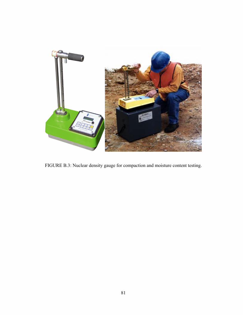
81
FIGURE B.3: Nuclear density gauge for compaction and moisture content testing.
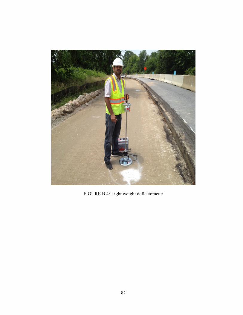
82
FIGURE B.4: Light weight deflectometer
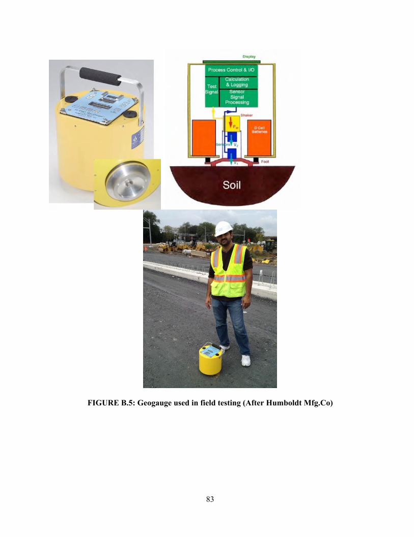
83
FIGURE B.5: Geogauge used in field testing (After Humboldt Mfg.Co)

84
D
SealCasing
ScaleStandpipe
H
( ) S
Zw
Dc
FIGURE B.6: Field hydraulic conductivity test on GAB. (ASTM D6391--Stage 1)

85
APPENDIX C
FIELD TEST RESULTS

86
Table C.1 Field Tests Results.
Quarry Name
Geogauge LWD Nuclear Density GaugeYoung's Modulus
(Psi)
Stiffness (lb./in)
Modulus (Psi)
Density (Pcf)
Moist (%)
A-V1 32407.0 126536.7 10213.0 149.9 4.7 A-V2 32602.7 148006.8 12326.1 139.3 6.4 A-V3 33744.1 153146.0 11822.8 142.2 7.1 A-V4 27448.4 124538.2 9843.2 147.4 4.7 A-V5 26562.2 120541.1 7276.2 145.9 4.3 A-V6 30795.7 139727.1 10165.2 142.4 4
A-VII1 31444.0 142696.4 12910.6 152.5 0.2 A-VII2 30807.3 139841.3 15995.4 155.8 0.7
A-VII3 33687.6 152860.4 12759.7 148.5 1 B-1 201111.1 25251.2 137.5 4.4 B-2 29596.3 143952.6 19215.0 137.1 4.8 B-3 191803.6 18458.0 146.4 3.6 B-4 46057.2 209048.2 31333.7 151.2 2.9 B-5 41169.7 186835.8 24459.3 151.9 2.9 D-1 11051.3 50135.0 8271.1 156.3 6.2 D-2 13883.7 148463.6 3792.5 153.7 5.8 D-3 20182.4 91590.6 5870.8 152.1 6.7 D-4 9174.6 41626.9 3023.9 155.9 7.1 D-5 28241.7 128192.6 12445.0 155.1 6.3 D-6 21313.6 96729.8 3276.2 154.3 6.7 D-7 6285.6 28550.7 2319.0 152.6 6.8
D-So1 22282.4 101126.6 12311.6 152.8 6.2 D-So2 21413.7 97186.6 6007.1 156.7 5.5 D-So3 21686.3 98442.8 8694.5 151.9 5.7 D-So4 12909.1 58586.0 4546.7 153.5 5.2 D-So5 27622.4 104609.8 9782.3 152.1 6.2 D-So6 22645.0 102782.5 6690.2 159.2 5.4 D-So7 16527.6 75031.2 2517.7 152.6 6.8 D-So8 16624.8 75488.1 3002.1 152.6 4.5 D-So9 27317.9 123339.0 16762.6 154.9 7.8 D-So10 30159.0 136872.1 17181.7 151.5 7.1 D-So11 17780.7 80684.3 12548.0 151.0 6.5 D-So12 17290.5 78514.4 8482.8 152.1 6.3 B-695-1 20037.3 90905.4 11016.5 149.0 5.1 B-695-2 19135.3 86851.2 10392.8 142.6 4.6

87
B-695-3A 20914.8 94902.5 5873.7 146.6 4.1
B-695-3B 25209.1 114431.2 8021.6 142.8 5.2 B-695-4 20862.6 94674.1 7550.3 144.6 4.9
G-1 19908.3 90391.5 8169.5 151.7 5.2
G-2 23193.2 105295.0 8758.4 151.4 6.6 G- 3 24286.7 110262.8 7915.7 150.6 6.8
G-4 29448.3 133674.4 12970.0 147.9 6
G-5 24575.3 111576.1 7442.9 156.9 5.7 G-6 25918.3 117628.9 9962.1 152.4 5.5
C-1 18675.5 84738.5 7728.6
C-2 14765.5 67037.0 7411.0
C-3 28794.3 131732.9 10893.2
C-4 15870.6 72062.0 5553.2
C-5 19064.2 86508.6 4321.9
C-6 19847.4 90106.0 6897.6
88
APPENDIX D
ABBREVIATIONS AND ACRONYMS

89
ϒd: Maximum dry density
Imp: Impact compactor
Vib: Vibratory compactor
Gs: Specific gravity
F: Fine contents
C: Coarse contents
LA: Los Angeles abrasion test
MD: Micro deval test
SS: Loss in Sodium Sulfate test
PD: Petrographic Description
MR : Resilient modulus
k1, k2, and k3 : Constants
sotropic confining pressure
d: Deviator stress
pa: Atmospheric pressure
SMR: Summary resilient modulus
Eo: Surface modulus
f: Plate rigidity factor
v: Poisson’s ratio
σo: Maximum contact stress
a: Plate radius (in)
do: Maximum deflection (in).
P: Load
δ: Deflection,
R: Radius of the contact ring
E: Shear modulus and
CBR: California bearing ratio
OMC: Optimum moisture content
ϵplastic: Plastic strain of specimens
NA: Not analyzed.
90
A: RCA from Plant A
B: RCA from Plant B
FC: Fines content
G/S: Gravel-to-sand ratio,
k: Hydraulic conductivity
a2: Base layer coefficient,
m2: Base layer drainage modification factor
m3: Subbase layer drainage modification factor
D2: Required base thickness
∆PSI : Design serviceability loss
So: Overall standard deviation
ZR: Reliability
SN = Structural numbers
D1, D2, and D3 : Layer thicknesses of asphalt layer, base layer, and subbase layer
S: Longitudinal slope
Sx : Cross slope
LR: Resultant length of flow path
qi: Rate of pavement infiltration (m3/day/m2),
Ic: Crack infiltration rate, (m3/day/m),
Nc: Number of longitudinal cracks.
kp: Pavement hydraulic
H: Base thickness
t: Time for percent drainage, U, to be reached
S1: Dimensionless slope factor (H/LS).
L: Width of GAB
ne: Effective porosity of the GAB