Development of Curved-Plate Elements for the Exact ...mln/ltrs-pdfs/NASA-99-tm209512.pdf · August...

August 1999

NASA/TM-1999-209512

Development of Curved-Plate Elements forthe Exact Buckling Analysis of CompositePlate Assemblies Including Transverse-Shear Effects

David M. McGowanLangley Research Center, Hampton, Virginia

The NASA STI Program Office ... in Profile

Since its founding, NASA has been dedicated tothe advancement of aeronautics and spacescience. The NASA Scientific and TechnicalInformation (STI) Program Office plays a keypart in helping NASA maintain this importantrole.

The NASA STI Program Office is operated byLangley Research Center, the lead center forNASAÕs scientific and technical information. TheNASA STI Program Office provides access to theNASA STI Database, the largest collection ofaeronautical and space science STI in the world.The Program Office is also NASAÕs institutionalmechanism for disseminating the results of itsresearch and development activities. Theseresults are published by NASA in the NASA STIReport Series, which includes the followingreport types:

· TECHNICAL PUBLICATION. Reports of

completed research or a major significantphase of research that present the results ofNASA programs and include extensivedata or theoretical analysis. Includescompilations of significant scientific andtechnical data and information deemed tobe of continuing reference value. NASAcounterpart of peer-reviewed formalprofessional papers, but having lessstringent limitations on manuscript lengthand extent of graphic presentations.

· TECHNICAL MEMORANDUM. Scientific

and technical findings that are preliminaryor of specialized interest, e.g., quick releasereports, working papers, andbibliographies that contain minimalannotation. Does not contain extensiveanalysis.

· CONTRACTOR REPORT. Scientific and

technical findings by NASA-sponsoredcontractors and grantees.

· CONFERENCE PUBLICATION. Collected

papers from scientific and technicalconferences, symposia, seminars, or othermeetings sponsored or co-sponsored byNASA.

· SPECIAL PUBLICATION. Scientific,

technical, or historical information fromNASA programs, projects, and missions,often concerned with subjects havingsubstantial public interest.

· TECHNICAL TRANSLATION. English-

language translations of foreign scientificand technical material pertinent to NASAÕsmission.

Specialized services that complement the STIProgram OfficeÕs diverse offerings includecreating custom thesauri, building customizeddatabases, organizing and publishing researchresults ... even providing videos.

For more information about the NASA STIProgram Office, see the following:

· Access the NASA STI Program Home Pageat http://www.sti.nasa.gov

· E-mail your question via the Internet to

[email protected] · Fax your question to the NASA STI Help

Desk at (301) 621-0134 · Phone the NASA STI Help Desk at

(301) 621-0390 · Write to:

NASA STI Help Desk NASA Center for AeroSpace Information 7121 Standard Drive Hanover, MD 21076-1320

National Aeronautics andSpace Administration

Langley Research Center Hampton, Virginia 23681-2199

August 1999

NASA/TM-1999-209512

Development of Curved-Plate Elements forthe Exact Buckling Analysis of CompositePlate Assemblies Including Transverse-Shear Effects

David M. McGowanLangley Research Center, Hampton, Virginia

Available from:

NASA Center for AeroSpace Information (CASI) National Technical Information Service (NTIS)7121 Standard Drive 5285 Port Royal RoadHanover, MD 21076-1320 Springfield, VA 22161-2171(301) 621-0390 (703) 605-6000

The use of trademarks or names of manufacturers in this report is for accurate reporting and does not constitute anofficial endorsement, either expressed or implied, of such products or manufacturers by the National Aeronauticsand Space Administration.

DEVELOPMENT OF CURVED-PLATE ELEMENTS FOR THE EXACT

BUCKLING ANALYSIS OF COMPOSITE PLATE ASSEMBLIES INCLUDING

TRANSVERSE-SHEAR EFFECTS

ABSTRACT

The analytical formulation of curved-plate non-linear equilibrium equations including

transverse-shear-deformation effects is presented. The formulation uses the principle of

virtual work. A unified set of non-linear strains that contains terms from both physical

and tensorial strain measures is used. Linearized, perturbed equilibrium equations

(stability equations) that describe the response of the plate just after buckling occurs are

then derived after the application of several simplifying assumptions. These equations

are then modified to allow the reference surface of the plate to be located at a distance zc

from the centroidal surface. The implementation of the new theory into the VICONOPT

exact buckling and vibration analysis and optimum design computer program is described

as well. The terms of the plate stiffness matrix using both classical plate theory (CPT)

and first-order shear-deformation plate theory (SDPT) are presented. The necessary steps

to include the effects of in-plane transverse and in-plane shear loads in the in-plane

stability equations are also outlined. Numerical results are presented using the newly

implemented capability. Comparisons of results for several example problems with

different loading states are made. Comparisons of analyses using both physical and

tensorial strain measures as well as CPT and SDPT are also made. Results comparing the

computational effort required by the new analysis to that of the analysis currently in the

VICONOPT program are presented. The effects of including terms related to in-plane

transverse and in-plane shear loadings in the in-plane stability equations are also

examined. Finally, results of a design-optimization study of two different cylindrical

shells subject to uniform axial compression are presented.

ii

TABLE OF CONTENTS

ABSTRACT . . . . . . . . . . . . . . . . . . . . . . . . . . . . . . . . . . . . . . . . . . . . . . . . . . . . . . . . . . . . . . . . . . . . . . . i

TABLE OF CONTENTS . . . . . . . . . . . . . . . . . . . . . . . . . . . . . . . . . . . . . . . . . . . . . . . . . . . . . . . ii

LIST OF TABLES . . . . . . . . . . . . . . . . . . . . . . . . . . . . . . . . . . . . . . . . . . . . . . . . . . . . . . . . . . . . . .iv

LIST OF SYMBOLS . . . . . . . . . . . . . . . . . . . . . . . . . . . . . . . . . . . . . . . . . . . . . . . . . . . . . . . . . . vii

CHAPTER I . . . . . . . . . . . . . . . . . . . . . . . . . . . . . . . . . . . . . . . . . . . . . . . . . . . . . . . . . . . . . . . . . . . . . 1

INTRODUCTION... . . . . . . . . . . . . . . . . . . . . . . . . . . . . . . . . . . . . . . . . . . . . . . . . . . . . . . . . . . . . . . . . . . . . . . . . . . . . . . . . 1

1.1 Purpose of Study ... . . . . . . . . . . . . . . . . . . . . . . . . . . . . . . . . . . . . . . . . . . . . . . . . . . . . . . . . . . . . . . . . . . . . . . . . . 1

1.2 Literature Review ... . . . . . . . . . . . . . . . . . . . . . . . . . . . . . . . . . . . . . . . . . . . . . . . . . . . . . . . . . . . . . . . . . . . . . . . . 4

1.3 Scope of Study... . . . . . . . . . . . . . . . . . . . . . . . . . . . . . . . . . . . . . . . . . . . . . . . . . . . . . . . . . . . . . . . . . . . . . . . . . . . 10

CHAPTER II . . . . . . . . . . . . . . . . . . . . . . . . . . . . . . . . . . . . . . . . . . . . . . . . . . . . . . . . . . . . . . . . . . . 12

ANALYTICAL FORMULATION ... . . . . . . . . . . . . . . . . . . . . . . . . . . . . . . . . . . . . . . . . . . . . . . . . . . . . . . . . . . . 12

2.1 Plate Geometry, Loadings, and Sign Conventions.. . . . . . . . . . . . . . . . . . . . . . . . . . . . . . . . . . . . 12

2.2 Strain-Displacement Relations .. . . . . . . . . . . . . . . . . . . . . . . . . . . . . . . . . . . . . . . . . . . . . . . . . . . . . . . . . . 13

2.3 Equilibrium Equations .. . . . . . . . . . . . . . . . . . . . . . . . . . . . . . . . . . . . . . . . . . . . . . . . . . . . . . . . . . . . . . . . . . . . 16

2.4 Stability Equations .. . . . . . . . . . . . . . . . . . . . . . . . . . . . . . . . . . . . . . . . . . . . . . . . . . . . . . . . . . . . . . . . . . . . . . . . 19

2.5 Stability Equations Transformed to the Plate Reference Surface .. . . . . . . . . . . . . . . . . . . 23

2.6 Constitutive Relations .. . . . . . . . . . . . . . . . . . . . . . . . . . . . . . . . . . . . . . . . . . . . . . . . . . . . . . . . . . . . . . . . . . . . 27

CHAPTER III . . . . . . . . . . . . . . . . . . . . . . . . . . . . . . . . . . . . . . . . . . . . . . . . . . . . . . . . . . . . . . . . . . 31

IMPLEMENTATION INTO VICONOPT . . . . . . . . . . . . . . . . . . . . . . . . . . . . . . . . . . . . . . . . . . . 31

3.1 Simplifications to the Theory.. . . . . . . . . . . . . . . . . . . . . . . . . . . . . . . . . . . . . . . . . . . . . . . . . . . . . . . . . . . . . 31

3.2 Continuity of Rotations at a Plate Junction .. . . . . . . . . . . . . . . . . . . . . . . . . . . . . . . . . . . . . . . . . . . . 32

iii

3.3 Derivation of the Curved-Plate Stiffness Matrix .. . . . . . . . . . . . . . . . . . . . . . . . . . . . . . . . . . . . . . 36

3.4 The Wittrick-Williams Eigenvalue Algorithm ... . . . . . . . . . . . . . . . . . . . . . . . . . . . . . . . . . . . . . . 42

CHAPTER IV . . . . . . . . . . . . . . . . . . . . . . . . . . . . . . . . . . . . . . . . . . . . . . . . . . . . . . . . . . . . . . . . . . 44

NUMERICAL RESULTS... . . . . . . . . . . . . . . . . . . . . . . . . . . . . . . . . . . . . . . . . . . . . . . . . . . . . . . . . . . . . . . . . . . . . . . 44

4.1 Convergence of the Segmented-Plate Approach ... . . . . . . . . . . . . . . . . . . . . . . . . . . . . . . . . . . . . 44

4.2 Buckling of Curved Plates With Widely Varying Curvatures.. . . . . . . . . . . . . . . . . . . . . . . 46

4.3 Buckling of an Unsymmetrically Laminated Curved Plate .. . . . . . . . . . . . . . . . . . . . . . . . . . 48

4.4 Effect of N22 Terms in the In-Plane Stability Equations .. . . . . . . . . . . . . . . . . . . . . . . . . . . . . 49

4.5 Design Optimization of a Cylindrical Shell Subject to Uniaxial Compression .. . . 53

CHAPTER V . . . . . . . . . . . . . . . . . . . . . . . . . . . . . . . . . . . . . . . . . . . . . . . . . . . . . . . . . . . . . . . . . . . 56

CONCLUDING REMARKS ... . . . . . . . . . . . . . . . . . . . . . . . . . . . . . . . . . . . . . . . . . . . . . . . . . . . . . . . . . . . . . . . . . . 56

REFERENCES . . . . . . . . . . . . . . . . . . . . . . . . . . . . . . . . . . . . . . . . . . . . . . . . . . . . . . . . . . . . . . . . . 59

APPENDIX A . . . . . . . . . . . . . . . . . . . . . . . . . . . . . . . . . . . . . . . . . . . . . . . . . . . . . . . . . . . . . . . . . . 63

MATRICES FOR DETERMINING CHARACTERISTIC ROOTS ... . . . . . . . . . . . . . . . . . . . . . 63

iv

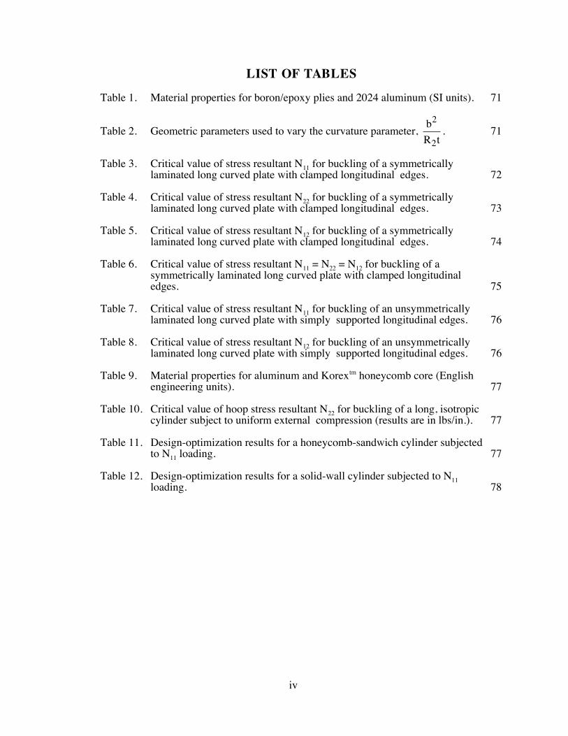
LIST OF TABLES

Table 1. Material properties for boron/epoxy plies and 2024 aluminum (SI units). 71

Table 2. Geometric parameters used to vary the curvature parameter, bR t

2

2. 71

Table 3. Critical value of stress resultant N11 for buckling of a symmetricallylaminated long curved plate with clamped longitudinal edges. 72



Table 6. Critical value of stress resultant N11 = N22 = N12 for buckling of asymmetrically laminated long curved plate with clamped longitudinaledges. 75

Table 7. Critical value of stress resultant N11 for buckling of an unsymmetricallylaminated long curved plate with simply supported longitudinal edges. 76

Table 8. Critical value of stress resultant N12 for buckling of an unsymmetricallylaminated long curved plate with simply supported longitudinal edges. 76

Table 9. Material properties for aluminum and Korextm honeycomb core (Englishengineering units). 77

Table 10. Critical value of hoop stress resultant N22 for buckling of a long, isotropiccylinder subject to uniform external compression (results are in lbs/in.). 77

Table 11. Design-optimization results for a honeycomb-sandwich cylinder subjectedto N11 loading. 77

Table 12. Design-optimization results for a solid-wall cylinder subjected to N11loading. 78

v

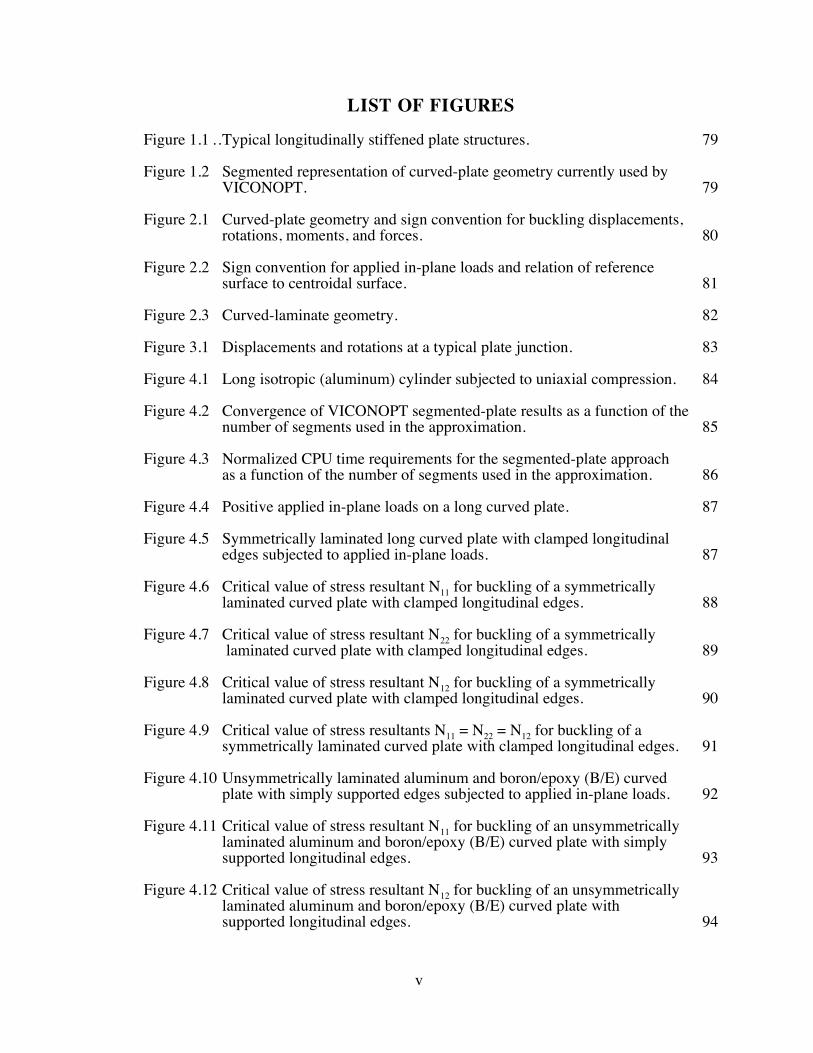
LIST OF FIGURES

Figure 1.1 ..Typical longitudinally stiffened plate structures. 79

Figure 1.2 Segmented representation of curved-plate geometry currently used byVICONOPT. 79

Figure 2.1 Curved-plate geometry and sign convention for buckling displacements,rotations, moments, and forces. 80

Figure 2.2 Sign convention for applied in-plane loads and relation of referencesurface to centroidal surface. 81

Figure 2.3 Curved-laminate geometry. 82

Figure 3.1 Displacements and rotations at a typical plate junction. 83

Figure 4.1 Long isotropic (aluminum) cylinder subjected to uniaxial compression. 84

Figure 4.2 Convergence of VICONOPT segmented-plate results as a function of thenumber of segments used in the approximation. 85

Figure 4.3 Normalized CPU time requirements for the segmented-plate approachas a function of the number of segments used in the approximation. 86

Figure 4.4 Positive applied in-plane loads on a long curved plate. 87

Figure 4.5 Symmetrically laminated long curved plate with clamped longitudinaledges subjected to applied in-plane loads. 87

Figure 4.6 Critical value of stress resultant N11 for buckling of a symmetricallylaminated curved plate with clamped longitudinal edges. 88

Figure 4.7 Critical value of stress resultant N22 for buckling of a symmetrically laminated curved plate with clamped longitudinal edges. 89

Figure 4.8 Critical value of stress resultant N12 for buckling of a symmetricallylaminated curved plate with clamped longitudinal edges. 90

Figure 4.9 Critical value of stress resultants N11 = N22 = N12 for buckling of asymmetrically laminated curved plate with clamped longitudinal edges. 91

Figure 4.10 Unsymmetrically laminated aluminum and boron/epoxy (B/E) curvedplate with simply supported edges subjected to applied in-plane loads. 92

Figure 4.11 Critical value of stress resultant N11 for buckling of an unsymmetricallylaminated aluminum and boron/epoxy (B/E) curved plate with simplysupported longitudinal edges. 93

Figure 4.12 Critical value of stress resultant N12 for buckling of an unsymmetricallylaminated aluminum and boron/epoxy (B/E) curved plate withsupported longitudinal edges. 94

vi

Figure 4.13 Isotropic (aluminum) long cylindrical tube subjected to uniform externalpressure loading. 95

Figure 4.14 Cylindrical shell subjected to uniform axial compression (N11 loading). 96

Figure 4.15 Optimized cylinder mass as a function of the applied loading for acylindrical shell. 97

vii

LIST OF SYMBOLS

A extensional stiffness matrix

a upper half of the eigenvectors of matrix R , associated with displacements

B coupling stiffness matrix

B , C , E ,

F , G , H coefficients used to select physical or tensor strains

b lower half of the eigenvectors of matrix R , associated with forces

b plate width (arc length)

C matrix whose columns contain the eigenvectors of matrix R

c single eigenvector of matrix R

D bending stiffness matrix

d vector of displacement amplitudes at the two edges of a plate

ds arc length of a line element in a body before deformation

ds* arc length of a line element in a body after deformation

Eii YoungÕs modulus in the i-i direction

E matrix used to define vector d , see Eq. (3.19)

F matrix used to define vector f , see Eq. (3.20)

f vector of force amplitudes at the two edges of a plate

fi body forces

G12 in-plane shear stiffness

G13, G23 transverse shear stiffnesses

hij coefficient of the partially inverted constitutive relations, see Eqs. (3.11) and

(3.12)

I identity matrix

I moment of inertia

i imaginary number, square root of -1

viii

K plate stiffness matrix

k transverse-shear compliance matrix

M11, M22, M12 applied (prebuckling) moment resultants

m11, m22, m12 perturbation values of moment resultants just after buckling has occurred

Ä , Ä , Äm m m11 22 12 moment resultants

N11, N22, N12 applied (prebuckling) stress resultants

n11, n22, n12 perturbation values of stress resultants just after buckling has occurred

Ä , Ä , Än n n11 22 12 stress resultants

Ã , Ãn n22 12 effective forces per unit length at an edge x2 = constant

nl number of layers in a general curved laminate

P coefficient matrix of the set of first-order plate differential equations,

see Eq. (3.14)

p applied external pressure

p2, p3 perturbation values of the applied pressure load in the buckled state in

the x2- and x3-directions

Q lamina reduced stiffness matrix

Q lamina reduced transformed stiffness matrix

Q1, Q2 applied (prebuckling) shear stress resultants

q1, q2, perturbation values of shear stress resultants just after buckling has

occurred

Ä , Äq q1 2 shear stress resultants

Ãq 2 effective transverse shear force per unit length at an edge x2 = constant

R matrix whose eigenvalues are the characteristic roots of the plate

differential equations, see Eq. (3.16b)

R1, R2 radii of lines of principal curvature

ix

T coefficient matrix of the set of first-order plate differential equations, see Eq.

(3.14)

Ti surface tractions

t plate thickness

U1, U2 prebuckling displacements

u1, u2 perturbation values of displacements just after buckling has occurred

v volume

w normal displacement in the x3-direction

Z vector of the forces and displacements in the plate

z vector containing the amplitudes of the forces and displacements in the plate

assuming a sinusoidal variation in the x1-direction

zc distance from the plate centroidal surface to the plate reference surface

zk distance from laminate reference surface to the kth layer in the laminate

Greek

a1, a2 Lam� parameters

b angle included by a curved plate

e vector containing strains e11, e22, and g12

e11, e22 in-plane direct strains

e12, g12 in-plane shear strains

e13, g13 transverse shear strains

e23, g23 transverse shear strains

f1, f2 rotations

x

fn rotation about the normal to the plate middle surface

k11, k22 middle surface changes in curvatures

k12 middle surface twisting curvature

l half wavelength of buckling mode

n PoissonÕs ratio

qk angular orientation of ply k in a laminate with respect to the laminate

coordinate system

r density

s vector containing stresses s11, s22, and t12

s11, s22 in-plane direct stresses

t12 in-plane shear stress

x1, x2, x3 coordinate measures in the 1-, 2-, and 3-directions, respectively

Subscripts and Superscripts

cr critical value for buckling

k kth layer in a laminated composite plate

n normal to middle surface

1, 2, 3 1-, 2-, and 3-directions, respectively

¡ value at centroidal surface

1

CHAPTER I

INTRODUCTION

1.1 Purpose of Study

Longitudinally stiffened plate structures occur frequently in aerospace vehicle

structures. These structures can typically be represented by long, thin, flat or curved

plates that are rigidly connected along their longitudinal edges, see Figure 1.1. The

designs for these structures often exploit the increased structural efficiency that can be

obtained by the use of advanced composite materials. Therefore, the plates used to

represent the structure may consist of anisotropic laminates. The buckling and vibration

behavior of this type of structure must be understood to design the structure.

Additionally, to satisfy the current demands for more cost-effective and structurally

efficient aerospace vehicles, these structures are frequently optimized to obtain an

optimal design that satisfies either buckling or vibration constraints or a combination of

these two constraints. There is a need for analytical tools that can provide the analysis

capability required to optimize panel designs.

The VICONOPT computer code [1] is an exact analysis and optimum design

program that includes the buckling and vibration analyses of prismatic assemblies of flat,

in-plane-loaded anisotropic plates. The code also includes approximations for curved and

tapered plates, discrete supports, and transverse stiffeners. Anisotropic composite

laminates having fully populated A , B and D stiffness matrices may be analyzed. Either

classical plate theory (CPT) or first-order transverse-shear-deformation plate theory

(SDPT) may be used [2]. The analyses of the plate assemblies assume a sinusoidal

response along the plate length. The analysis used in the code is referred to as ÒexactÓ

2

because it uses stiffness matrices that result from the exact solution to the differential

equations that describe the behavior of the plates.

Currently, VICONOPT approximates a curved plate by subdividing it into a series of

flat-plate segments that are joined along their longitudinal edges to form the complete

curved-plate structure, see Figure 1.2. This procedure is analogous to the discretization

approach used in finite element analysis. The code uses exact stiffnesses for the flat-plate

segments and enforces continuity of displacements and rotations at the segment

connections. Thus, the analyst must ensure that an adequate number of flat-plate

segments is used in the analysis. The next logical step in the development of the

VICONOPT code is to eliminate the need to approximate curved-plate geometries by

flat-plate segments by adding the capability to analyze curved-plate segments exactly.

By adding this capability, the accuracy of the solutions can be improved. Furthermore,

since the curvature of a plate is modeled directly, there will be no need to determine if a

sufficient amount of flat-plate segments have been used to model the curved plate.

Another benefit of adding this capability is that the computational efficiency of the code

will be improved since only one stiffness calculation for the entire curved plate is

required, rather than the several that are currently required for the individual flat plates

that are used to approximate the curved plate. This improvement in computational

efficiency is important for structural optimization. In this report, the capability to analyze

curved-plate segments exactly has been added to the VICONOPT code. The present

report will describe the methodology used to accomplish this enhancement of the code

and will present results obtained utilizing this new capability.

The procedure used in the present report is an extension of the procedure described in

[2]. This procedure involves deriving the appropriate differential equations of

equilibrium for the analysis of fully anisotropic curved plates, including transverse-shear-

deformation effects. These coupled equations are of eighth-order if transverse-shear

effects are neglected, and of tenth-order if transverse-shear effects are included. For the

3

analysis of flat plates, the coupling of these equations occurs through the laminate

extension-bending B matrix; however, coupling can also be produced by including

curvature terms in the equilibrium equations. The numerical solution technique that was

developed in [2] to solve such systems of equations will apply for either type of coupling,

and the stiffnesses of the plates are derived from the numerical solution to these

equations.

Several features have been added to the VICONOPT code as part of the present

report. The current version of VICONOPT only analyzes flat-plate elements based on a

tensorial strain-displacement relation. However, the choice of strain-displacement

relations can affect the contribution of prebuckling forces in curved plates. Therefore, a

unified set of nonlinear strain-displacement relations that contains terms from both

physical and tensorial strain measures is used to derive the plate equilibrium equations.

The unified set of strains is used throughout the derivation of the equilibrium equations,

and the selection of either physical or tensorial strains is achieved by appropriately

setting coefficients in the equilibrium equations equal to one or zero. The option to use

physical strain-displacement relations for the analysis of flat plates is included as well.

Another addition is the treatment of the effects of in-plane transverse and in-plane shear

loadings in the in-plane equilibrium equations. These effects are currently ignored in the

VICONOPT code (see [1]). In the present report, an in-plane transverse loading, denoted

N22, is a loading that acts perpendicular to the longitudinal edges of the plate. The

present study has added the option to include the effects of these loadings in the in-plane

equilibrium equations. Finally, either CPT or SDPT may be used. The SDPT used in

VICONOPT and in the present report uses the usual first-order assumption that straight

lines originally normal to the centroidal surface are assumed to remain straight and

inextensional but not necessarily normal to the centroidal surface during deformation of

the plate. All of these features have been implemented such that they are available for

use in the analysis of both flat and curved plates.

4

1.2 Literature Review

The buckling and vibration analysis of assemblies of prismatic plates has received a

great deal of attention over the last thirty years. One method of analysis for this class of

structure that has been studied extensively is the finite-strip method, FSM [3]. A popular

application of this method involves determining a stiffness matrix for each individual

plate in the assembly and then assembling those individual matrices into a global stiffness

matrix for use in determining the response of the entire structure. This method is

therefore analogous in form to the finite element method [4]. The main difference

between the two methods is that the finite element method discretizes the individual

plates into elements in both the longitudinal and transverse directions. The stiffness

matrix for each individual element is then calculated and assembled into a global stiffness

matrix. In the FSM, the response of the plate in the longitudinal direction is represented

as a continuously differentiable smooth series that satisfies the boundary conditions at the

two ends of the plate. Therefore, discretization of the structure is only required to be

performed in the transverse direction, and depending on the method being used,

discretization of the individual plates may or may not be required [3].

The work in the area of finite strip analysis of assemblies of prismatic plates may be

broadly classified based upon different characteristics of the analysis method used. One

classification distinguishes whether the properties of the individual plates are derived by

direct solution to the equations of equilibrium or by application of potential energy or

virtual work principles, i.e., exact versus approximate methods. Another classification

distinguishes whether classical plate theory (CPT) or first-order shear-deformation plate

theory (SDPT) is used in the analysis. Finally, a distinction may be made as to whether

or not complex quantities are used in the development of the individual stiffness matrices.

A review of the literature in the area of finite strip analysis methods is presented below.

Approximate methods are discussed separately from exact methods.

5

The approximate FSM was first proposed for the static analysis of plate bending by

Cheung in 1968 [5]. The approximate FSM involves subdividing each plate into a series

of finite-width strips that are linked together at their longitudinal edges in a manner

similar to that depicted in Figure 1.2. Separate expressions for in-plane and out-of-plane

displacements as well as rotations about the in-plane x and y axes over the middle surface

of each strip are assumed. Each of these fundamental quantities are expressed as a

summation of the products of longitudinal series and transverse polynomials [3]. The

longitudinal series are typically sinusoidal and are selected to satisfy displacement

conditions at the transverse edges of each strip that match the desired plate boundary

conditions along those edges. The potential energy of an individual finite strip is then

evaluated, and the total potential energy of the plate is obtained by summing the potential

energies of the individual strips. Following the application of any appropriate zero-

displacement boundary conditions at the longitudinal edges, the potential energy is

minimized with respect to each plate degree of freedom to generate the equilibrium

equations for the plate. Displacements are then calculated for a given loading condition

using this system of equations.

The analysis of [5] utilized CPT for the static bending analysis of isotropic plates. In

1971, Cheung and Cheung [6] applied the approximate FSM to the analysis of natural

vibrations of thin, flat-walled structures with different combinations of the standard edge

boundary conditions (i.e., clamped, simply supported, or free). Their analysis was based

upon CPT and the displacements in the longitudinal direction were approximated using

the normal modes of Timoshenko beam theory to allow for various boundary conditions

on the transverse edges.

Przemieniecki [7] used an approximate FSM based upon CPT to calculate the initial

buckling of assemblies of flat plates subjected to a biaxial stress state. This method only

considered local buckling modes since it assumed that the line junctions between plates

remained straight during buckling. Plank and Wittrick [8] extended the work of

6

Przemieniecki by considering global as well as local modes and by admitting a more

general loading state that included uniform transverse and longitudinal shear stress and

longitudinal direct stress that varies linearly across the width of the plate. When in-plane

shear loading is present, a spatial phase difference occurs between the perturbation forces

and displacements which occur at the edges of the plates during buckling. This phase

difference causes skewing of the nodal lines and is accounted for in [8] by defining the

magnitude of these quantities using complex quantities. This method is referred to as a

complex finite strip method.

In 1977, Dawe [9 and 10] used an approximate FSM based upon CPT for the static

and linear buckling analysis of curved-plate assemblies. The plates studied were

isotropic, and in-plane shear loads were not allowed. Morris and Dawe extended this

analysis to study the free vibration of curved-plate assemblies in 1980 [11].

All of the analyses discussed thus far have been based upon CPT. In 1978, Dawe

[12] presented an approximate FSM based upon SDPT [13] for the vibration of isotropic

plates with a pair of opposite edges simply supported. Roufaeil and Dawe [14] and

Dawe and Roufaeil [15] extended this analysis to the vibration and buckling,

respectively, of isotropic and transversely isotropic plates with general boundary

conditions. The latter two analyses admitted the general boundary conditions through the

use of the normal modes of Timoshenko beam theory, as was done in [6].

In 1986, Craig and Dawe [16] considered the vibration of single symmetrically

laminated plates using an approximate FSM based upon SDPT. Dawe and Craig [17]

then extended this analysis to study the buckling of single symmetrically laminated plates

subject to uniform shear stress and direct in-plane stress. This analysis allowed for

anisotropic material properties. General boundary conditions were once again admitted

through the use of the normal modes of Timoshenko beam theory. The analysis of [17]

was extended in 1987 to the vibration of complete plate assemblies [18]. However, it

was shown in this work that the problem size increased dramatically as attempts to

7

increase the accuracy of the solution were made by further subdivision of the component

plates.

In 1988, Dawe and Craig [19] presented a complex FSM based upon SDPT for the

buckling and vibration of prismatic plate structures in which the component plates could

consist of anisotropic laminates and could be subject to in-plane shear loads. This work

also made use of substructuring to create ÒsuperstripsÓ that eliminated the internal

degrees-of-freedom from each component plate. This analysis was later extended to

consider finite-length structures [20 and 21] and to add multi-level substructuring to

couple several ÒsuperstripsÓ to further decrease the problem size. Dawe and Peshkam

[22] also developed a complementary analysis to that presented in [20 and 21] for long

plate structures. Analyses using both SDPT and CPT were presented. This work also

added the capability to define eccentric connections of component plates.

Wittrick laid the groundwork for the exact FSM in 1968 [23]. The basic assumption

in this work is that the deformation of any component plate varies sinusoidally in the

longitudinal direction. Using this assumption, a stiffness matrix may be derived that

relates the amplitudes of the edge forces and moments to the corresponding edge

displacements and rotations for a single component plate. For the exact FSM, this

stiffness matrix is derived directly from the equations of equilibrium that describe the

behavior of the plate. In [23], Wittrick developed an exact stiffness matrix for a single

isotropic, long flat plate subject to uniform axial compression. His analysis used CPT.

Wittrick and Curzon [24] extended this analysis to account for the spatial phase

difference between the perturbation forces and displacements which occur at the edges of

the plate during buckling due to the presence of in-plane shear loading. This phase

difference is accounted for by defining the magnitude of these quantities using complex

quantities. Wittrick [25] then extended his analysis to consider flat isotropic plates under

any general state of stress that remains uniform in the longitudinal direction (i.e.,

combinations of bi-axial direct stress and in-plane shear). A method very similar to that

8

described in [23] was presented by Smith in 1968 [26] for the bending, buckling, and

vibration of plate-beam structures.

In 1972, Williams [27] presented two computer programs, GASVIP and VIPAL to

compute the natural frequencies and initial buckling stress of prismatic plate assemblies

subjected to uniform longitudinal stress or uniform longitudinal compression,

respectively. GASVIP was used to set up the overall stiffness matrix for the structure,

and VIPAL demonstrated the use of substructuring. In 1974, Wittrick and Williams [28]

first reported on the VIPASA computer code for the buckling and vibration analyses of

prismatic plate assemblies. This code allowed for isotropic or anisotropic plates as well

as a general state of stress (including in-plane shear). The complex stiffnesses described

in [8] were incorporated, as well as allowances for eccentric connections between

component plates. This code also incorporated an algorithm, referred to as the Wittrick-

Williams algorithm, for determining any natural frequency or buckling load for any given

wavelength [29]. The development of this algorithm was necessary because the complex

stiffnesses described above are transcendental functions of the load factor and half

wavelength of the buckling modes of the structure. The eigenvalue problem for

determining natural frequencies and buckling load factors is therefore transcendental.

Further discussion of the Wittrick-Williams algorithm will be presented in Chapter III.

In 1973, Viswanathan and Tamekuni [30 and 31] presented an exact FSM based upon

CPT for the elastic stability analysis of composite stiffened structures subjected to biaxial

inplane loads. The structure is idealized as an assemblage of laminated plate elements

(flat or curved) and beam elements. The analysis assumes that the component plates are

orthotropic. The transverse edges are assumed to be simply supported, and any

combination of boundary conditions may be applied to the longitudinal edges. The

analysis was included in an associated computer code, BUCLAP2. Viswananthan,

Tamekuni, and Baker extended this analysis in [32] to consider long curved plates

subject to any general state of stress, including in-plane shear loads. Anisotropic material

9

properties were also allowed. This analysis utilized complex stiffnesses as described in

[8]. The analyses described in [26, 28, and 32] are very similar. The differences between

the three are discussed in [28].

When applied in-plane shear loads or anisotropy is present, the assumption of a

sinusoidal variation of deformation in the longitudinal direction is only exact for

structures that are infinitely long. Significant errors for structures of finite length can

occur due to the skewing of nodal lines. In 1983, Williams and Anderson [33] presented

modifications to the eigenvalue algorithm described in [29]. The modifications presented

in [33] allowed the buckling mode corresponding to a general loading to be represented

as a series of sinusoidal modes in combination with Lagrangian multipliers to apply point

constraints at any location on those edges. Each sinusoidal mode is represented by an

exact stiffness matrix. This technique allows infinitely long structures supported at

repeating intervals with anisotropy or applied in-plane shear loads to be analyzed. Thus,

a panel supported at its transverse edges is approximated by one with a series of point

supports along those edges. These modifications formed the basis for the computer code

VICON (VIpasa with CONstraints) described in [34]. However, the analysis capability

of VICON was limited to plates analyzed with CPT having a zero B matrix. The VICON

code was later modified to include structures supported by Winkler foundations [35]. An

optimum design feature was also added in 1990 [36 and 37], and the VICONOPT

(VICON with OPTimization) code was introduced.

Anderson and Kennedy [2] incorporated SDPT into VICONOPT in 1993. A

numerical approach to obtain exact plate stiffnesses that include the effects of transverse-

shear deformation was presented. The generality of VICONOPT was also expanded in

[2] to allow for the analysis of laminates with fully populated A , B , and D stiffness

matrices.

10

1.3 Scope of Study

The analytical formulation of the curved-plate non-linear equilibrium equations

including transverse-shear-deformation effects are presented in Chapter II. A unified set

of non-linear strains that contains terms from both physical and tensorial strain measures

is used. The equilibrium equations are derived using the principle of virtual work

following the method presented by Sanders [38 and 39]. Linearized, perturbed

equilibrium equations that describe the response of the plate just after buckling occurs are

then derived after the application of several simplifying assumptions. Modifications to

these equations that allow the reference surface of the plate to be located at a distance zc

from the centroidal surface are then made.

In Chapter III, the implementation of the new theory into the VICONOPT code is

described. A derivation of the terms of the plate stiffness matrix using MATHEMATICA

[40] is presented. The form of these terms for both CPT and SDPT is discussed. The

necessary steps to include the effects of in-plane transverse and in-plane shear loads in

the in-plane equilibrium equations are also outlined.

In Chapter IV, numerical results are presented using the newly implemented

capability. A convergence study using the current segmented-plate approach in

VICONOPT is performed for a simple example problem to obtain baseline results for use

in future comparisons. Results comparing the computational effort required by the new

analysis to that of the analysis currently in the VICONOPT program are also presented.

Comparisons of results for several example problems with different loading states are

then made. Comparisons of analyses using both physical and tensorial strain measures as

well as CPT and SDPT are made. The effects of including terms related to in-plane

transverse and in-plane shear loads in the in-plane stability equations are also examined.

In Chapter V, the characteristics of the newly implemented curved-plate elements in

VICONOPT is presented. A brief summary of the effects of several analytical features

11

that have been implemented into VICONOPT is given. Finally, potential future work in

this area is discussed.

12

CHAPTER II

ANALYTICAL FORMULATION

In this chapter, the non-linear equilibrium equations are derived for a curved plate

including transverse-shear effects. A unified set of non-linear strains that contain terms

from both physical and tensorial strain measures is used. The equilibrium equations are

derived using the principle of virtual work following the method presented by Sanders

[38 and 39]. Linearized stability equations that describe the response of the plate just

after buckling occurs are then derived following the application of several simplifying

assumptions. Modifications to these equations that allow the reference surface of the

plate to be located at a distance zc from the centroidal surface are then made.

2.1 Plate Geometry, Loadings, and Sign Conventions

The geometry of the basic plate element being studied is given in Figure 2.1. This

figure depicts the orthogonal curvilinear coordinate system (x1, x2, x3) used in the present

analysis. The x1- and x2-axes shown in the figure are along lines of principal curvature

and they have radii of curvature R1 and R2, respectively. The x2-axis is normal to the

middle surface of the plate. The first fundamental form of the plate middle surface is

given by

ds d d212

12

22

22= +a x a x (2.1)

where a1 and a2 are the Lam� parameters. The coordinates x1 and x2 are measured as arc

lengths along the x1- and x2-axes, respectively. The result of measuring the coordinates

13

in this manner is that a1 = a2, = 1. The sign conventions for buckling displacements,

moments, rotations, and forces are also shown in Figure 2.1. The sign convention for the

applied in-plane loadings being considered and the relation of the reference surface of the

plate to the centroidal surface of the plate are shown in Figure 2.2. Note that that

centroidal surface can be offset from the reference surface by a distance zc. The

centroidal surface is defined to be located at the centroid of the face of the panel that is

normal to the x1-axis. The loading N22 shown in this figure is referred to in the present

report as an in-plane transverse loading.

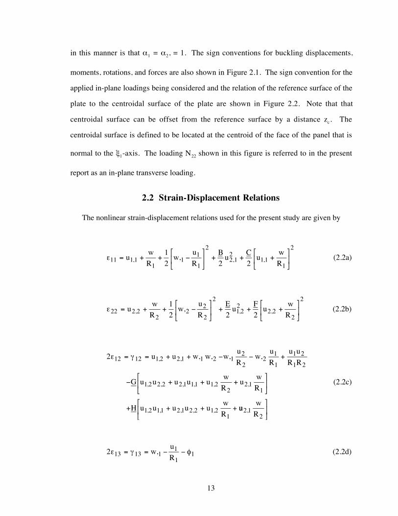
2.2 Strain-Displacement Relations

The nonlinear strain-displacement relations used for the present study are given by

e11 1 11

11

1

2

2 12

1 11

212 2 2

= + + -é

ëê

ù

ûú + + +

é

ëê

ù

ûúu

wR

wuR

Bu

Cu

wR, , ,, (2.2a)

e22 2 22

22

2

2

1 22

2 22

212 2 2

= + + -é

ëê

ù

ûú + + +

é

ëê

ù

ûúu

wR

wu

RE

uF

uw

R, , ,, (2.2b)

2 12 12 1 2 2 1 1 2 12

22

1

1

1 2

1 2

1 2 2 2 2 1 11 1 22

2 11

1 2 11 2 1 2 2 1 21

e g= = + + - - +

- + + +é

ëê

ù

ûú

+ + + +

u u w w wu

Rw

u

R

u u

R R

G u u u u uw

Ru

wR

H u u u u uwR

, ,

, , , , , ,

, , , , ,

, , , ,

uuw

R2 12

,é

ëê

ù

ûú

(2.2c)

2 13 13 11

11e g f= = - -w

u

R, (2.2d)

14

2 23 23 22

22e g f= = - -w

u

R, (2.2e)

where the following notation for partial derivatives is used: ¶

¶x

uui

ji j= , . The

displacement quantities in Eqs. (2.2a) through (2.2e) are displacements of the centroidal

surface of the plate. The constants B , C , E , F , and H are set equal to one and G is set

equal to zero in Eqs. (2.2a) through (2.2e) to use tensorial strain measures. The constants

B , E , and G are set equal to one and C , F , and H are set equal to zero to use physical

strain measures. Note that the linear portions of the tensorial and physical strain

measures are identical. To obtain Donnell theory from the strain-displacement relations

in Eqs. (2.2a) through (2.2e) the constants B , C , E , F , G , and H must be set equal to zero,

and all terms involving the quantities u

Rand

u

R1

1

2

2 must be neglected. SanderÕs theory

[39] may be obtained by setting the constants B , C , E , F , G , and H equal to zero and

adding the term 12

2fn to Eqs. (2.2a) and (2.2b), where fn is the rotation about the normal

to the plate middle surface.

The tensorial strain measures used in the present study are those of Novozhilov [41].

These strains are obtained by taking the difference between the square of the arc length of

a line element in a body after deformation, (ds*)2, and before deformation (ds)2. The

tensorial strain measures, ejk, are defined by the relationship

12

2 2ds ds d djk j k*( ) - ( )é

ëêùûú

= e x x i, j = 1, 3 (2.3)

The repeated indices in Eq. (2.3) indicate summation over i and j. The physical strain

measures are strains that can be measured in the laboratory. The physical strains used in

15

the present report are derived in a manner similar to that presented by Stein in [42] and

they were communicated to the author in lines of curvature coordinates by Dr. Michael P.

Nemeth.1. Physical extensional strains are defined as the ratio of the change in arc length

of a line element in a body, ds*, to the original length of that line element, ds,

e jjj j

j

ds ds

dsj=

( ) - ( )

( )=

*

,1 2 (no summation) (2.4a)

Physical shearing strains are defined as the change in the angles between three line

elements that are orthogonal before deformation and are oriented in the direction of three

unit vectors, Ã *e j , after deformation. The physical shearing strains are defined by the

following expressions

sin Ã Ã * *g g12 12 1 2( ) » = ·e e (2.4b)

sin Ã Ã , * *g gj j je e j3 3 3 1 2( ) » = · = (2.4c)

The definitions for the changes in curvatures of the centroidal surface used for both

theories are

k f11 1 1= - , (2.5a)

k f22 2 2= - , (2.5b)

k f f12 1 2 2 1= - +( ), , (2.5c)

These changes in curvatures are equivalent to those given by Sanders in [39] with the

terms involving rotations about the normal neglected.

1 Mechanics and Durability Branch, Structures and Materials, NASA Langley Research Center, Hampton, VA,

16

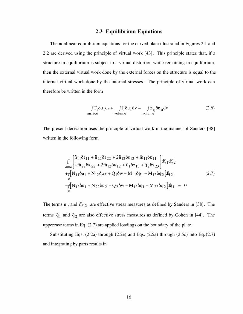
2.3 Equilibrium Equations

The nonlinear equilibrium equations for the curved plate illustrated in Figures 2.1 and

2.2 are derived using the principle of virtual work [43]. This principle states that, if a

structure in equilibrium is subject to a virtual distortion while remaining in equilibrium,

then the external virtual work done by the external forces on the structure is equal to the

internal virtual work done by the internal stresses. The principle of virtual work can

therefore be written in the form

T u ds f u dv dvi isurface

i ivolume

ij ijvolume

d d s deò + ò = ò (2.6)

The present derivation uses the principle of virtual work in the manner of Sanders [38]

written in the following form

Ä Ä Ä Ä

Ä Ä Ä Ä

n n n m

m m q qd d

N u N u Q w M M d

N u N u Q w

area

c

11 11 22 22 12 12 11 11

22 22 12 12 1 13 2 231 2

11 1 12 2 1 11 1 12 2 2

12 1 22 2 2

2

2

de de de dk

dk dk dg dgx x

d d d df df x

d d d

+ + +

+ + + +

é

ëê

ù

ûúòò

+ + + - -[ ]ò

- + + - MM M dc

12 1 22 2 1 0df df x-[ ]ò =

(2.7)

The terms �12 and Äm12 are effective stress measures as defined by Sanders in [38]. The

terms Äq1 and Äq2 are also effective stress measures as defined by Cohen in [44]. The

uppercase terms in Eq. (2.7) are applied loadings on the boundary of the plate.

Substituting Eqs. (2.2a) through (2.2e) and Eqs. (2.5a) through (2.5c) into Eq. (2.7)

and integrating by parts results in

17

-òò + + -æ

èç

ö

ø÷ + -

æ

èç

ö

ø÷ +

é

ëê

æ

èç

+ +é

ëê

ù

ûú

æ

èç

ö

ø÷ + ( )

- +

arean n

n

Rw

u

R

n

Rw

u

R

q

R

C n uwR

E n u

G n uw

Ä ÄÄ

,Ä

,Ä

Ä Ä

Ä

, ,

,,

, ,

,

111 12 211

11

1

1

12

12

2

2

1

1

11 111 1

22 1 2 2

12 2 2 RRn u

H n uwR

n u u

2 212 2 1 1

12 111 2

12 1 2 1 1

ìíî

üýþ

é

ëê

ù

ûú + [ ]

æ

èçç

ö

ø÷÷

+ +ìíî

üýþ

é

ëê

ù

ûú + [ ]

æ

èçç

ö

ø÷÷

ù

û

úú

,, ,

,,

, ,

Ä

Ä Ä d

+ + + -æ

èç

ö

ø÷ + -

æ

èç

ö

ø÷ +

é

ëê

+ ( ) + +é

ëê

ù

ûú

æ

èç

ö

ø÷

- +ìíî

Ä ÄÄ

,Ä

,Ä

Ä Ä

Ä

, ,

, , ,,

,

n nn

Rw

u

R

n

Rw

u

R

q

R

B n u F n uw

R

G n uwR

12 1 22 222

22

2

2

12

21

1

1

2

2

11 2 1 1 22 2 22 2

12 111

üüýþ

é

ëê

ù

ûú + [ ]

æ

èçç

ö

ø÷÷

+ +ìíî

üýþ

é

ëê

ù

ûú + [ ]

æ

èçç

ö

ø÷÷

ù

û

úú

,, ,

,,

, ,

Ä

Ä Ä

112 1 2 2

12 2 22 1

12 2 1 2 2

n u

H n uw

Rn u ud

+ + - +æ

èç

ö

ø÷ + -

æ

èç

ö

ø÷

é

ëê

ù

ûú

é

ë

êê

+ -æ

èç

ö

ø÷

é

ëê

ù

ûú + -

æ

èç

ö

ø÷

é

ëê

ù

ûú

+

Ä ÄÄ Ä

Ä ,

Ä , Ä ,

Ä

, ,,

, ,

q qn

R

n

Rn w

u

R

n wu

Rn w

u

R

n w

11 2 211

1

22

211 1

1

1 1

22 22

2 212 2

2

2 1

12 ,,Ä

ÄÄ

Ä

,,

,, ,

, ,

11

1 2

11

1 111

22

2 22 2 12

1 2

2

2 1

1

121 2

1

2 1

2

-æ

èç

ö

ø÷

é

ëê

ù

ûú + +

æ

èç

ö

ø÷

- +æ

èç

ö

ø÷ + +

æ

èç

ö

ø÷

- +æ

èç

ö

ø÷

ù

ûú

u

R

Cn

RwR

u

Fn

Rw

Ru Gn

u

R

u

R

Hnu

R

u

Rwd

18

+ + -[ ] + + -[ ]ö

ø

÷÷

Ä Ä Ä Ä Ä Ä, , , ,m m q m m q d d111 12 2 1 1 12 1 22 2 2 2 1 2df df x x

+ + + +æ

èç

ö

ø÷ - +

é

ëê

ù

ûú

æ

èçò N n Cn u

wR

Gn u Hn u uc

11 11 11 111

12 2 1 12 1 2 1Ä Ä Ä Ä, , , d

+ + + - +æ

èç

ö

ø÷ + +

æ

èç

ö

ø÷

é

ëê

ù

ûúN n Bn u Gn u

wR

Hn uw

Ru12 12 11 2 1 12 11

112 2 2

22Ä Ä Ä Ä, , , d

+ + + +æ

èç

ö

ø÷ + +

æ

èç

ö

ø÷

é

ëê

ù

ûúQ q n w

uR

n wuR

w1 1 11 11

112 2

2

2Ä Ä , Ä , d

- +[ ] - +[ ]ö

ø

÷÷

M m M m d11 11 1 12 12 2 2Ä Ädf df x

+ + + - +æ

èç

ö

ø÷ + +

æ

èç

ö

ø÷

é

ëê

ù

ûú

æ

èçò N n En u Gn u

wR

Hn uwR

uc

12 12 22 1 2 12 2 22

12 111

1Ä Ä Ä Ä, , , d

+ + + +æ

èç

ö

ø÷ - +

é

ëê

ù

ûúN n Fn u

wR

Gn u Hn u u22 22 22 2 22

12 1 2 12 2 1 2Ä Ä Ä Ä, , , d

+ + + +æ

èç

ö

ø÷ + +

æ

èç

ö

ø÷

é

ëê

ù

ûúQ q n w

uR

n wuR

w2 2 12 11

122 2

2

2Ä Ä , Ä , d

- +[ ] - +[ ] öø÷ =M m M m d12 12 1 22 22 2 1 0Ä Ädf df x (2.8)

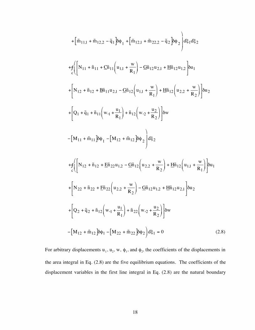
For arbitrary displacements u1, u2, w, f1, and f2, the coefficients of the displacements in

the area integral in Eq. (2.8) are the five equilibrium equations. The coefficients of the

displacement variables in the first line integral in Eq. (2.8) are the natural boundary

19

conditions for an edge x1 = constant, and the coefficients of the displacement variables in

the second line integral are the natural boundary conditions for an edge x2 = constant.

2.4 Stability Equations

A set of perturbation equilibrium equations that govern the stability of the plate,

referred to herein as the stability equations, may now be written by taking the difference

between the equilibrium equations evaluated for an equilibrium state just prior to

buckling and an adjacent (perturbed) equilibrium state just after buckling has occurred.

Let the prebuckling state be represented by:

Ä , Ä , Ä , Ä ,

Ä , Ä , Ä , Ä ,

, ,

n N n N n N m M

m M m M q Q q Q

U U W

11 11 22 22 12 12 11 11

22 22 12 12 1 1 2 2

1 2

= - = - = - = -

= - = - = - = - (2.9)

The minus signs in the loading terms reflect the sign convention used in which the

applied loads are opposite in direction to the loads that develop after buckling. Let the

perturbed state just after buckling has occurred be represented by:

Ä , Ä , Ä ,

Ä , Ä , Ä ,

Ä , Ä , , ,

n n N n n N n n N

m m M m m M m m M

q q Q q q Q u U u U w W

11 11 11 22 22 22 12 12 12

11 11 11 22 22 22 12 12 12

1 1 1 2 2 2 1 1 2 2

= - = - = -

= - = - = -

= - = - + + +

(2.10)

where the lower case variables are perturbation variables. Taking the difference between

the two equilibrium states represented by Eqs. (2.9) and (2.10), linearizing the resulting

equations for the perturbation variables, and applying the following simplifying

assumptions:

1) Prebuckling deformations, moments, and transverse-shear stresses are

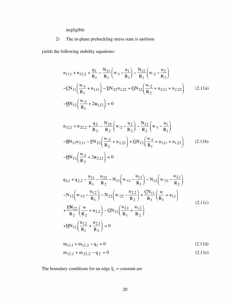
20

negligible

2) The in-plane prebuckling stress state is uniform

yields the following stability equations:

n nq

R

N

Rw

u

R

N

Rw

u

R

CNw

Ru EN u GN

w

Ru u

HNw

R

111 12 21

1

11

11

1

1

12

12

2

2

111

1111 22 1 22 12

2

22 11 2 22

122

12

, ,

, , , ,

, ,

, ,

,

+ + - -æ

èç

ö

ø÷ - -

æ

èç

ö

ø÷

- +æ

èç

ö

ø÷ - + + +

æ

èç

ö

ø÷

- + uu112 0,æ

èç

ö

ø÷ =

(2.11a)

n nq

R

N

Rw

u

R

N

Rw

u

R

BN u FNw

Ru GN

w

Ru u

HNw

R

12 1 22 22

2

22

22

2

2

12

21

1

1

11 2 11 222

22 22 12

1

1111 1 22

121

22

, ,

, , , ,

, ,

, ,

,

+ + - -æ

èç

ö

ø÷ - -

æ

èç

ö

ø÷

- - +æ

èç

ö

ø÷ + + +

æ

èç

ö

ø÷

- + uu2 12 0,æ

èç

ö

ø÷ =

(2.11b)

q qn

R

n

RN w

u

RN w

u

R

N wu

RN w

u

R

CN

RwR

u

F

11 2 211

1

22

211 11

11

112 21

2 1

2

12 121 2

122 22

2 2

2

11

1 111

, ,, ,

, ,,

, ,

, ,

+ - - - -æ

èç

ö

ø÷ - -

æ

èç

ö

ø÷

- -æ

èç

ö

ø÷ - -

æ

èç

ö

ø÷ + +

æ

èç

ö

ø÷

+NN

Rw

Ru GN

u

R

u

R

HNu

R

u

R

22

2 22 2 12

2 1

1

1 2

2

121 2

1

2 1

20

+æ

èç

ö

ø÷ - +

æ

èç

ö

ø÷

+ +æ

èç

ö

ø÷ =

,, ,

, ,

(2.11c)

m m q11 1 12 2 1 0, ,+ - = (2.11d)

m m q12 1 22 2 2 0, ,+ - = (2.11e)

The boundary conditions for an edge x1 = constant are

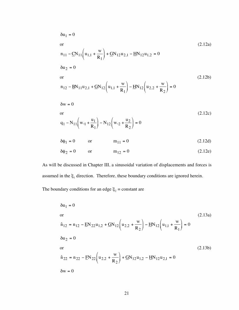
21

du1 0=

or (2.12a)

n CN uwR

GN u HN u11 11 1 11

12 2 1 12 1 2 0- +æ

èç

ö

ø÷ + - =, , ,

du2 0=

or (2.12b)

n BN u GN uwR

HN uw

R12 11 2 1 12 1 11

12 2 22

0- + +æ

èç

ö

ø÷ - +

æ

èç

ö

ø÷ =, , ,

dw = 0

or (2.12c)

q N wuR

N wuR1 11 1

1

112 2

2

20- +

æ

èç

ö

ø÷ - +

æ

èç

ö

ø÷ =, ,

df1 0= or m11 0= (2.12d)

df2 0= or m12 0= (2.12e)

As will be discussed in Chapter III, a sinusoidal variation of displacements and forces is

assumed in the x1 direction. Therefore, these boundary conditions are ignored herein.

The boundary conditions for an edge x2 = constant are

du1 0=

or (2.13a)

Ã , , ,n n EN u GN uw

RHN u

wR12 12 22 1 2 12 2 2

212 11

10= - + +

æ

èç

ö

ø÷ - +

æ

èç

ö

ø÷ =

du2 0=

or (2.13b)

Ã , , ,n n FN uw

RGN u HN u22 22 22 2 2

212 1 2 12 2 1 0= - +

æ

èç

ö

ø÷ + - =

dw = 0

22

or (2.13c)

Ã , ,q q N wuR

N wuR2 2 12 1

1

122 2

2

20= - +

æ

èç

ö

ø÷ - +

æ

èç

ö

ø÷ =

df1 0= or m12 0= (2.13d)

df2 0= or m22 0= (2.13e)

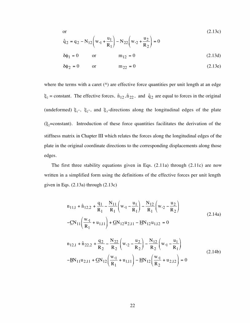
where the terms with a caret (^) are effective force quantities per unit length at an edge

x2 = constant. The effective forces, Ã , Ã , Ãn n and q12 22 2 are equal to forces in the original

(undeformed) x1-, x2-, and x3-directions along the longitudinal edges of the plate

(x2=constant). Introduction of these force quantities facilitates the derivation of the

stiffness matrix in Chapter III which relates the forces along the longitudinal edges of the

plate in the original coordinate directions to the corresponding displacements along those

edges.

The first three stability equations given in Eqs. (2.11a) through (2.11c) are now

written in a simplified form using the definitions of the effective forces per unit length

given in Eqs. (2.13a) through (2.13c)

n nq

R

N

Rw

u

R

N

Rw

u

R

CNw

Ru GN u HN u

111 12 21

1

11

11

1

1

12

12

2

2

111

1111 12 2 11 12 112 0

, ,

, , ,

Ã , ,

,

+ + - -æ

èç

ö

ø÷ - -

æ

èç

ö

ø÷

- +æ

èç

ö

ø÷ + - =

(2.14a)

n nq

R

N

Rw

u

R

N

Rw

u

R

BN u GNw

Ru HN

w

Ru

12 1 22 22

2

22

22

2

2

12

21

1

1

11 2 11 121

1111 12

1

22 12 0

, ,

, , ,

Ã , ,

, ,

+ + - -æ

èç

ö

ø÷ - -

æ

èç

ö

ø÷

- + +æ

èç

ö

ø÷ - +

æ

èç

ö

ø÷ =

(2.14b)

23

q qnR

nR

N wu

RN w

u

R

CNR

wR

uGN u

R

HN u

R

1 1 2 211

1

22

211 11

1 1

112 21

2 1

2

11

1 11 1

12 2 1

1

12 1 2

10

, ,, ,

,, ,

ÃÃ

, ,+ - - - -æ

èç

ö

ø÷ - -

æ

èç

ö

ø÷

+ +æ

èç

ö

ø÷ - + =

(2.14c)

This form of these stability equations will be used herein. Note that Eq. (2.14b) contains

the perturbation variables n12 and q2. These variables are related to the effective forces,

Ã Ãn and q12 2 , through Eqs. (2.13a) and (2.13c).

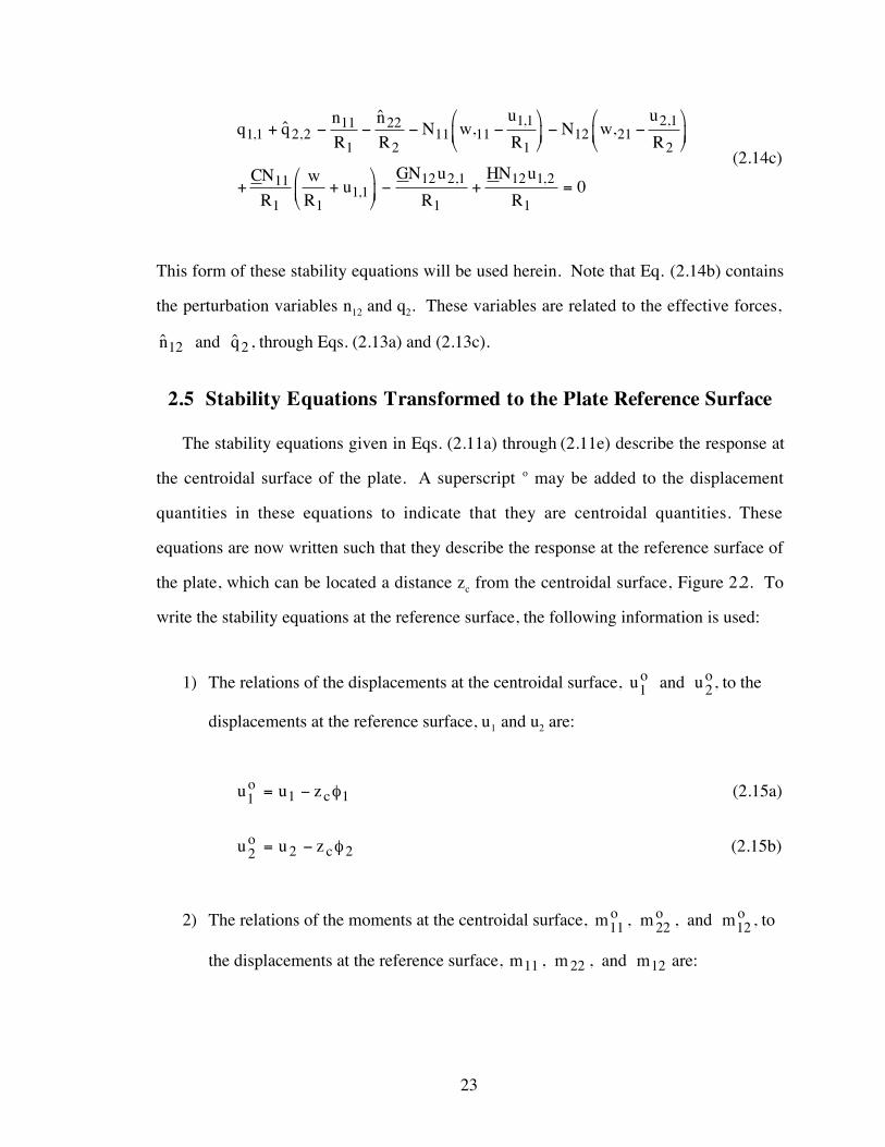
2.5 Stability Equations Transformed to the Plate Reference Surface

The stability equations given in Eqs. (2.11a) through (2.11e) describe the response at

the centroidal surface of the plate. A superscript o may be added to the displacement

quantities in these equations to indicate that they are centroidal quantities. These

equations are now written such that they describe the response at the reference surface of

the plate, which can be located a distance zc from the centroidal surface, Figure 2.2. To

write the stability equations at the reference surface, the following information is used:

1) The relations of the displacements at the centroidal surface, u and uo o1 2 , to the

displacements at the reference surface, u1 and u2 are:

u u zoc1 1 1= - f (2.15a)

u u zoc2 2 2= - f (2.15b)

2) The relations of the moments at the centroidal surface, m m and mo o o11 22 12, , , to

the displacements at the reference surface, m m and m11 22 12, , are:

24

m m z noc11 11 11= - (2.15c)

m m z noc22 22 22= - (2.15d)

m m z noc12 12 12= - (2.15e)

3) The following quantities do not vary with z:

N N N n n n q q and w11 22 12 11 22 12 1 2, , , , , , , ,

4) The applied in-plane stresses, N11, N22, and N12 act at the centroidal surface.

Substitution of Eqs. (2.15a) through (2.15e) into Eqs. (2.14a) through (2.14c) and Eqs.

(2.11d) and (2.11e) yields the following equations

n nq

R

N

Rw

u z

R

N

Rw

u z

R

CNwR

u z GN u z

HN u z

c c

c c

c

111 12 21

1

11

11

1 1

1

12

12

2 2

2

111

11 11

12 2 2 11

12 1 1

, ,

,,

,

,

Ã , ,+ + - --æ

èç

ö

ø÷ - -

-æ

èç

ö

ø÷

- + -æ

èç

ö

ø÷ + -[ ]

- -[ ]

f f

f f

f 1212 0=

(2.16a)

n nq

R

N

Rw

u z

R

N

Rw

u z

R

BN u z GNw

Ru z

HNw

Ru

c c

c c

12 1 22 22

2

22

22

2 2

2

12

21

1 1

1

11 2 2 11 121

11 1 11

121

22

, ,

, ,

Ã , ,

,

,

+ + - --æ

èç

ö

ø÷ - -

-æ

èç

ö

ø÷

- -( ) + + -[ ]æ

èç

ö

ø÷

- +

f f

f f

--[ ]æ

èç

ö

ø÷ =zcf2 12 0

(2.16b)

25

q qn

R

n

RN w

u z

R

N wu z

R

CN

Rw

Ru z

GN u z

R

HN

c

cc

c

11 2 211

1

22

211 1

1 1

1 1

12 22 2

2 1

11

1 11 1 1

12 2 2 1

1

, ,,

, ,,

,

ÃÃ

,

,

+ - - - --æ

èç

ö

ø÷

- --æ

èç

ö

ø÷ + + -[ ]

æ

èç

ö

ø÷

+-[ ]

+

f

ff

f 1212 1 1 2

10

u z

R

c-[ ]=

f ,

(2.16c)

m m z n n qc11 1 12 2 11 1 12 2 1 0, , , ,+ - +( ) - = (2.16d)

m m z n n qc12 1 22 2 12 1 22 2 2 0, , , ,+ - +( ) - = (2.16e)

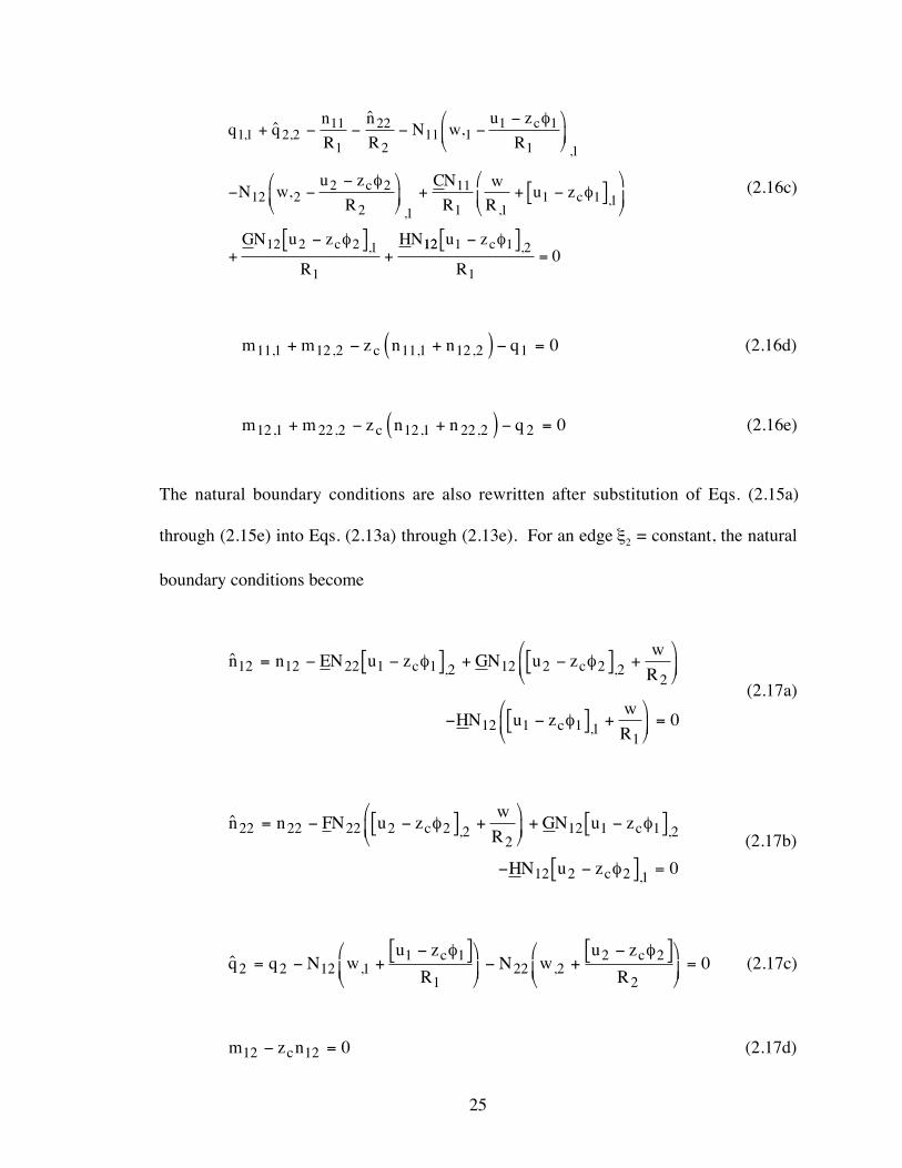
The natural boundary conditions are also rewritten after substitution of Eqs. (2.15a)

through (2.15e) into Eqs. (2.13a) through (2.13e). For an edge x2 = constant, the natural

boundary conditions become

Ã, ,

,

n n EN u z GN u zw

R

HN u zwR

c c

c

12 12 22 1 1 2 12 2 2 22

12 1 1 11

0

= - -[ ] + -[ ] +æ

èç

ö

ø÷

- -[ ] +æ

èç

ö

ø÷ =

f f

f

(2.17a)

Ã, ,

,

n n FN u zw

RGN u z

HN u z

c c

c

22 22 22 2 2 22

12 1 1 2

12 2 2 1 0

= - -[ ] +æ

èç

ö

ø÷ + -[ ]

- -[ ] =

f f

f

(2.17b)

Ã , ,q q N wu z

RN w

u z

Rc c

2 2 12 11 1

122 2

2 2

20= - +

-[ ]æ

èç

ö

ø÷ - +

-[ ]æ

èç

ö

ø÷ =

f f(2.17c)

m z nc12 12 0- = (2.17d)

26

m z nc22 22 0- = (2.17e)

The last two stability equations, Eqs. (2.16d) and (2.16e), are now rewritten by

substituting expressions for the quantities n n11 1 12 2, ,+( ) and n n12 1 22 2, ,+( ) that can

be obtained using Eqs. (2.16a) and (2.16b), respectively, and the definitions for the

effective forces per unit length, Eqs. (2.17a) through (2.17c). The definitions for the

effective forces are needed since the terms n12 and n22 that appear in the two above are the

perturbation values, not the effective forces. Substitution of the expressions for the two

quantities above into Eqs. (2.16d) and (2.16e), respectively, yields the final form of the

last two stability equations

m m q zq

R

N

Rw

u z

R

N

Rw

u z

RCN

wR

u z

EN u z GNw

cc

cc

c

111 12 2 11

1

11

11

1 1

1

12

12

2 2

211

111 1

1

22 1 1 22 12

, ,

, ,,

,

,

,

,

+ - +é

ëê - -

-æ

èç

ö

ø÷

- --æ

èç

ö

ø÷ - + -

æ

èç

ö

ø÷

- -( ) +

f

ff

f 22

22 2 11

2 2 22 122

11 1 122 0

Ru z

u z HNw

Ru z

c

c c

æ

èç + -[ ]

+ -[ ] ) - + -[ ]æ

èç

ö

ø÷

ù

ûú =

f

f f

,

, ,,

(2.18a)

m m q zq

R

N

Rw

u z

R

N

Rw

u z

RBN u z

FNw

Ru z GN

w

cc

cc

c

12 1 22 2 22

2

22

22

2 2

2

12

21

1 1

111 2 2 11

222

22 2 22 12

, ,

,

,

,

,

,

+ - +é

ëê - -

-æ

èç

ö

ø÷

- --æ

èç

ö

ø÷ - -( )

- + -[ ]æ

èç

ö

ø÷ +

f

ff

f,,

,

,

, ,

1

11 1 11

1 1 22 121

22 2 122 0

Ru z

u z HNw

Ru z

c

c c

+ -[ ]æ

èç

+ -[ ] ) - + -[ ]æ

èç

ö

ø÷

ù

ûú =

f

f f

(2.18b)

27

The stability equations in the form given in Eqs. (2.16a) through (2.16c) and Eqs. (2.18a)

and (2.18b) are those implemented into the VICONOPT code.

2.6 Constitutive Relations

The present analysis allows for generally laminated composite materials. The

geometry of a general, curved laminate is given in Figure 2.3. As shown in the figure,

the number of layers in the laminate is nl, and the width of the laminate is b. The radius

of curvature of the x2-axis, R2 is shown in the figure as well. . The radius of curvature of

the x1-axis, R1 is not shown; however, its direction may be inferred from that of R2. The

lamina coordinate system is the (x1Õ, x2Õ, x3) system and the laminate coordinate system is

the (x1, x2, x3) system. The lamina coordinate system is aligned with the principal

material direction of the lamina, and the laminate coordinate system is aligned with the

principal geometric directions of the laminate. The coordinate system for the kth lamina

is oriented at an angle qk with respect to the laminate coordinate system. The stress-strain

relations in the lamina coordinate system for a lamina of orthotropic material in a state of

plane stress are

s

s

t

e

e

g

11

22

12

11 12

12 22

66

11

22

12

0

0

0 0

©

©

©

©

©

©

ì

íï

îï

ü

ýï

þï

=

é

ë

êêê

ù

û

úúú

ì

íï

îï

ü

ýï

þï

Q Q

Q Q

Q

(2.19)

where the [Q] matrix is referred to as the reduced stiffness matrix for the lamina and is

defined in [45] in terms of the elastic engineering constants of the lamina. These

relations may be written in the laminate coordinate system by use of transformation

matrices as defined in [45]. The transformed relations are

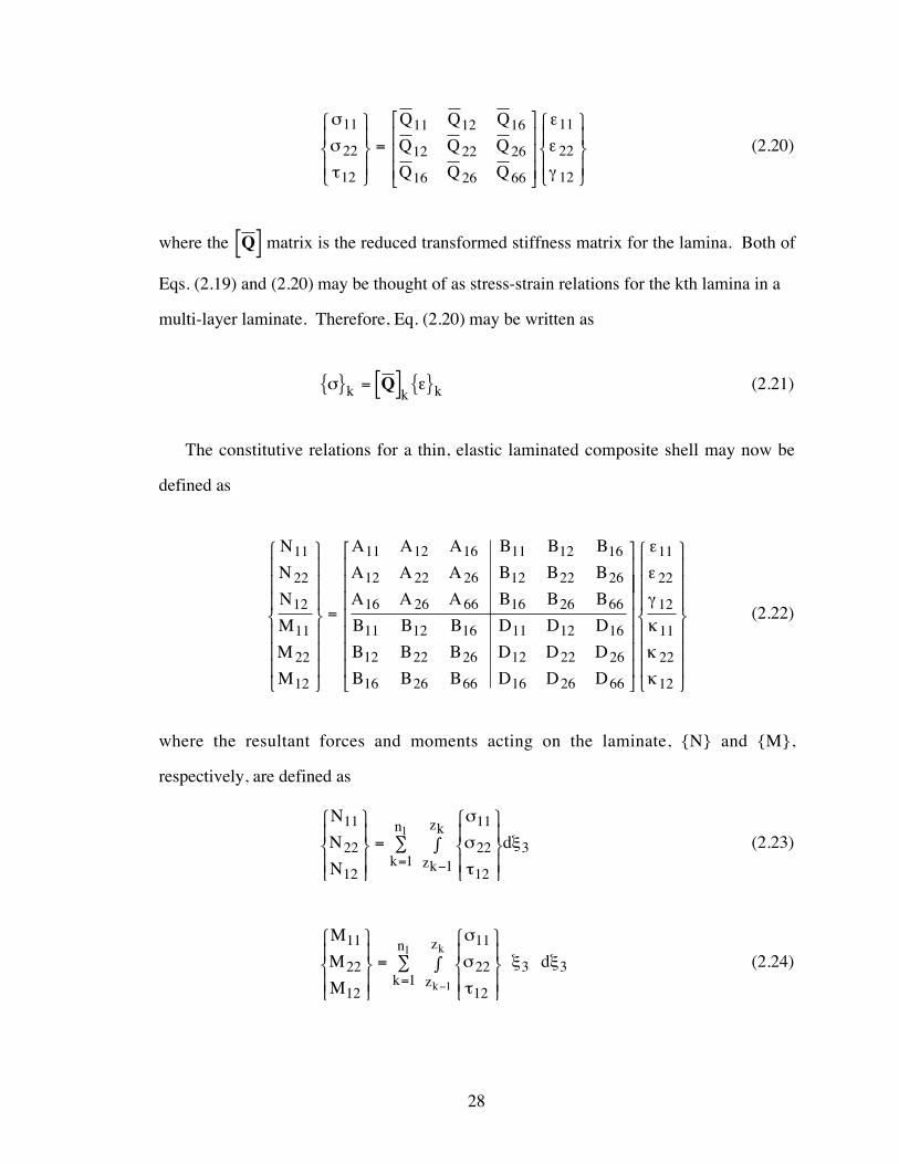
28

s

s

t

e

e

g

11

22

12

11 12 16

12 22 26

16 26 66

11

22

12

ì

íï

îï

ü

ýï

þï

=

é

ë

êêê

ù

û

úúú

ì

íï

îï

ü

ýï

þï

Q Q Q

Q Q Q

Q Q Q

(2.20)

where the Q[ ] matrix is the reduced transformed stiffness matrix for the lamina. Both of

Eqs. (2.19) and (2.20) may be thought of as stress-strain relations for the kth lamina in a

multi-layer laminate. Therefore, Eq. (2.20) may be written as

s e{ } = [ ] { }k k kQ (2.21)

The constitutive relations for a thin, elastic laminated composite shell may now be

defined as

N

N

N

M

M

M

A A A B B B

A A A B B B

A A A B B B

B B B D D D

B B B D D D

B B B D D D

11

22

12

11

22

12

11 12 16 11 12 16

12 22 26 12 22 26

16 26 66 16 26 66

11 12 16 11 12 16

12 22 26 12 22 26

16 26 66 16 26 66

ì

í

ïïï

î

ïïï

ü

ý

ïïï

þ

ïïï

=

é

ë

êêêêêêê

ù

û

úúúúúúúú

ì

í

ïïï

î

ïïï

ü

ý

ïïï

þ

ïïï

e

e

g

k

k

k

11

22

12

11

22

12

(2.22)

where the resultant forces and moments acting on the laminate, {N} and {M},

respectively, are defined as

N

N

N

dzk

zk

k

nl11

22

12

11

22

12

311

ì

íï

îï

ü

ýï

þï

=

ì

íï

îï

ü

ýï

þï

òå-=

s

s

t

x (2.23)

M

M

M

dz

z

k

n

k

kl11

22

12

11

22

12

3 31 1

ì

íï

îï

ü

ýï

þï

=

ì

íï

îï

ü

ýï

þï

òå-=

s

s

t

x x (2.24)

29

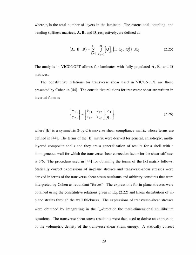
where nl is the total number of layers in the laminate. The extensional, coupling, and

bending stiffness matrices, A, B, and D, respectively, are defined as

A B D Q, , , , ( ) = [ ] ( )òå-= k

zk

zk

k

nld1 3 3

2

113x x x (2.25)

The analysis in VICONOPT allows for laminates with fully populated A , B , and D

matrices.

The constitutive relations for transverse shear used in VICONOPT are those

presented by Cohen in [44]. The constitutive relations for transverse shear are written in

inverted form as

g

g13

23

11 12

12 22

1

2

ìíî

üýþ

=é

ëê

ù

ûúìíî

üýþ

k k

k k

q

q(2.26)

where [k] is a symmetric 2-by-2 transverse shear compliance matrix whose terms are

defined in [44]. The terms of the [k ] matrix were derived for general, anisotropic, multi-

layered composite shells and they are a generalization of results for a shell with a

homogeneous wall for which the transverse shear correction factor for the shear stiffness

is 5/6. The procedure used in [44] for obtaining the terms of the [k] matrix follows.

Statically correct expressions of in-plane stresses and transverse-shear stresses were

derived in terms of the transverse-shear stress resultants and arbitrary constants that were

interpreted by Cohen as redundant ÒforcesÓ. The expressions for in-plane stresses were

obtained using the constitutive relations given in Eq. (2.22) and linear distribution of in-

plane strains through the wall thickness. The expressions of transverse-shear stresses

were obtained by integrating in the x3-direction the three-dimensional equilibrium

equations. The transverse-shear stress resultants were then used to derive an expression

of the volumetric density of the transverse-shear strain energy. A statically correct

30

expression of the area density of the transverse-shear strain energy was then obtained by

integrating in the x3-direction this volumetric density. The transverse-shear constitutive

relations given in Eq. (2.26) were then derived by applying CastiglianoÕs theorem of least

work [46] by minimizing the area density of the transverse-shear strain energy with

respect to the redundant forces mentioned previously.

31

CHAPTER III

IMPLEMENTATION INTO VICONOPT

In this chapter, the implementation of the present theory into the VICONOPT code is

described. Additional simplifications made to the theory are described first. A

discussion of the use of the transverse-shear strain, g13, as a fundamental displacement

variable in the problem to maintain continuity of rotations at plate junctions is then

presented. The derivation of an expression for the curved-plate stiffness matrix is

described. The terms of matrices that are needed to calculate this stiffness matrix were

obtained using MATHEMATICA [40], and they are presented in Appendix A. The terms

for both CPT and SDPT are presented, and the terms that result from the inclusion of

direct in-plane transverse and in-plane shear loads in the in-plane stability equations are

specified. As stated previously, the implementation of the curved-plate theory into

VICONOPT follows very closely the method presented in Reference [2]. Therefore, the

following discussion is necessarily similar to that presented in that reference.

3.1 Simplifications to the Theory

Before proceeding with the derivation of the curved-plate stiffness matrix, a

discussion of several simplifications to be implemented is presented. First, the theory

implemented into the VICONOPT code considers structures that are prismatic in the

longitudinal direction. Therefore, for the curved plates being considered in the present

report, the radius of curvature in the longitudinal direction, R1, is infinite; and any terms

involving the quantity 1

1R are zero. Although these terms are set equal to zero for the

calculation of the terms of the stiffness matrix, they are retained for completeness in the

32

theory presented in this chapter. Another simplification to the theory involves limiting

the capability to locate the reference surface a distance zc from the centroidal surface.

This capability has only been implemented for the case where the effects of N22 and N12

loads in the in-plane stability equations are neglected. The expressions for the stiffness

terms that result when N22 and N12 are included in the in-plane stability equations and zc

is non-zero are prohibitively long. Therefore, in the derivation to follow, only the

following two cases are presented:

1) N22 and N12 are included in the in-plane stability equations and zc is zero (i.e.,

reference surface is coincident with the centroidal surface); and ,

2) N22 and N12 are neglected in the in-plane stability equations and zc is non-zero (i.e.,

reference surface may be translated from the centroidal surface).

3.2 Continuity of Rotations at a Plate Junction

One important issue to be addressed in the analysis of plate assemblies is the

continuity of rotations at a plate junction. The original VIPASA code is based upon CPT,

and the theory only treats four degrees of freedom (DOF) at a longitudinal plate edge.

These DOF are the three displacement quantities, u1, u2, and w, and a rotation about the

x1-axis, f2. Maintaining continuity of these DOF at a typical plate junction is very

straightforward. However, when SDPT is considered, there are five DOF at a

longitudinal plate edge. These DOF are the four from CPT as well as an additional

rotation, f1, that results from the inclusion of transverse-shear deformation. Another

problem that must be addressed is that when two plates are joined together such that one

is rotated at an arbitrary angle, q, to the other, rotations about the normals to the

centroidal surfaces of the two plates must be included to satisfy continuity of rotations.

This rotation, fn, is not accounted for in the present plate theory. The procedure used in

33

VICONOPT to maintain continuity of rotations follows that used by Cohen in [47]. This

procedure introduces the shear strain, g13, as a fundamental displacement variable instead

of the rotation, f1. The justification for using this approach is described subsequently.

The displacements and rotations at a typical plate junction are shown in Figure 3.1.

The two plates, numbered 1 and 2, are shown viewed along the 1-axis, and it is obvious

that the u1 displacements are easily matched regardless of the orientation of plate 2. The

displacements and rotations for which continuity must be maintained are u2, w, f1, and fn.

Upon inspection of Figure 3.1(a), the following expressions for coplanar plates (q = 0)

may be written as

u u21

22= (3.1a)

w w1 2= (3.1b)

f f11

12= (3.1c)

f fn n1 2= (3.1d)

where the superscripts 1 and 2 refer to the plate numbers. Similarly, upon inspection of

Figure 3.1(b), the following expressions for q = +90o may be written as

u w21 2= (3.2a)

w u122= - (3.2b)

f f11 2= - n (3.2c)

f fn1

12= (3.2d)

34

Finally, upon inspection of Figure 3.1(c), the following expressions for arbitrary q may

be written as

u u w21

22 2= +cos sinq q (3.3a)

w w cos u sin1 222= -q q (3.3b)

f f q f q11

12 2= -cos sinn (3.3c)

f f q f qn n1 2

12= +cos sin (3.3d)

The rotation about the normal of a line element originally directed along the x1-axis is

shown in [48] to be

f¶

¶xnu

= 2

1(3.4)

Using this definition, Eqs. (3.3c) and (3.3d) are written as

f f q q11

12

2 12= -cos sin,u (3.5a)

u u2 11

2 12

12

, , cos sin= +q f q (3.5b)

Using Eqs. (3.3a) and (3.3b) and the definition for g13, Eq. (2.2d), the previous two

equations may be written as

g q g131

132= cos (3.6a)

0 132= -sin q g (3.6b)

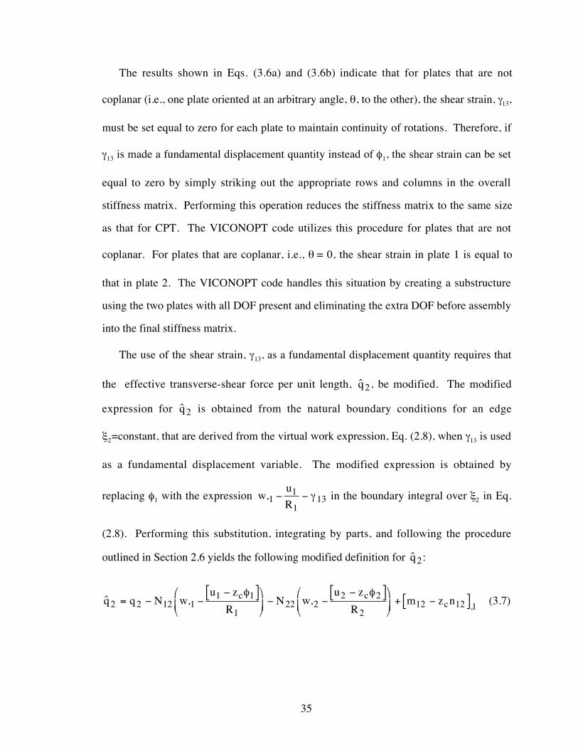
35

The results shown in Eqs. (3.6a) and (3.6b) indicate that for plates that are not

coplanar (i.e., one plate oriented at an arbitrary angle, q, to the other), the shear strain, g13,

must be set equal to zero for each plate to maintain continuity of rotations. Therefore, if

g13 is made a fundamental displacement quantity instead of f1, the shear strain can be set

equal to zero by simply striking out the appropriate rows and columns in the overall

stiffness matrix. Performing this operation reduces the stiffness matrix to the same size

as that for CPT. The VICONOPT code utilizes this procedure for plates that are not

coplanar. For plates that are coplanar, i.e., q = 0, the shear strain in plate 1 is equal to

that in plate 2. The VICONOPT code handles this situation by creating a substructure

using the two plates with all DOF present and eliminating the extra DOF before assembly

into the final stiffness matrix.

The use of the shear strain, g13, as a fundamental displacement quantity requires that

the effective transverse-shear force per unit length, Ãq2 , be modified. The modified

expression for Ãq2 is obtained from the natural boundary conditions for an edge

x2=constant, that are derived from the virtual work expression, Eq. (2.8), when g13 is used

as a fundamental displacement variable. The modified expression is obtained by

replacing f1 with the expression wu

R,1

1

113- - g in the boundary integral over x2 in Eq.

(2.8). Performing this substitution, integrating by parts, and following the procedure

outlined in Section 2.6 yields the following modified definition for Ãq2 :

Ã , , ,q q N wu z

RN w

u z

Rm z nc c

c2 2 12 11 1

122 2

2 2

212 12 1= - -

-[ ]æ

èç

ö

ø÷ - -

-[ ]æ

èç

ö

ø÷ + -[ ]

f f(3.7)

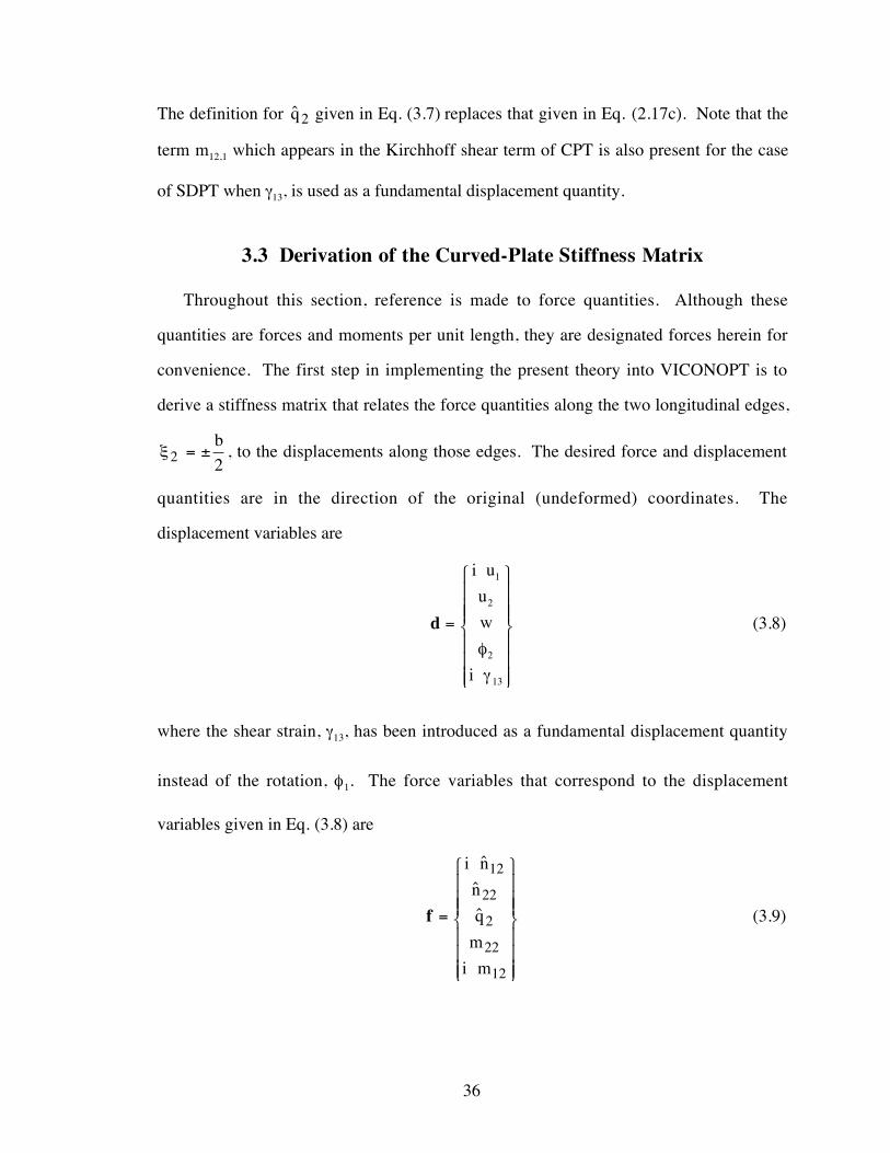
36

The definition for Ãq2 given in Eq. (3.7) replaces that given in Eq. (2.17c). Note that the

term m12,1 which appears in the Kirchhoff shear term of CPT is also present for the case

of SDPT when g13, is used as a fundamental displacement quantity.

3.3 Derivation of the Curved-Plate Stiffness Matrix

Throughout this section, reference is made to force quantities. Although these

quantities are forces and moments per unit length, they are designated forces herein for

convenience. The first step in implementing the present theory into VICONOPT is to

derive a stiffness matrix that relates the force quantities along the two longitudinal edges,

x 2 2= ±

b, to the displacements along those edges. The desired force and displacement

quantities are in the direction of the original (undeformed) coordinates. The

displacement variables are

d =

ì

í

ïïï

î

ïïï

ü

ý

ïïï

þ

ïïï

i u

u

w

i

1

2

2

13

f

g

(3.8)

where the shear strain, g13, has been introduced as a fundamental displacement quantity

instead of the rotation, f1. The force variables that correspond to the displacement

variables given in Eq. (3.8) are

f =

ì

í

ïïï

î

ïïï

ü

ý

ïïï

þ

ïïï

i n

n

q

m

i m

Ã

Ã

Ã

12

22

2

22

12

(3.9)

37

Note that the effective forces at the boundaries, defined by Eqs. (2.17a) and (2.17b) and

Eq. (3.7), are being used as the force quantities since, as discussed in Chapter II, they are

equal to the forces in the direction of the original (undeformed) coordinates.

The problem may now be reduced to ordinary differential equations in y by assuming

that the response of the plate in the longitudinal x1-direction varies sinusoidally.

Therefore, if the displacements and forces in the plate are now considered to be functions

of x2, the variables of Eqs. (3.8) and (3.9) may be written as

Z zx xp x

lx1 2

12, exp

( ) =

æèç

öø÷ ( )

i(3.10)

where

zd

f=

ìíî

üýþ

and l is the half-wavelength of the response in the x1-direction. Since a sinusoidal

variation in the x1-direction is assumed, the vector z will involve the amplitudes of the

displacement and force quantities. The imaginary number, i, has been used in Eqs. (3.8)

and (3.9) to account for the spatial phase shift that occurs between the perturbation forces

and displacements which occur at the edges of the plates during buckling for orthotropic

plates without shear loading and to result in real plate stiffnesses when using the

exponential expression of Eq. (3.10).

The next step in the derivation is to express all unknowns in terms of z. A partially

inverted form of the constitutive relations, Eq. (2.22), is used to express the required

quantities as functions of the fundamental variables in d and f or terms that may be

derived from the fundamental variables. The partially inverted constitutive relations are

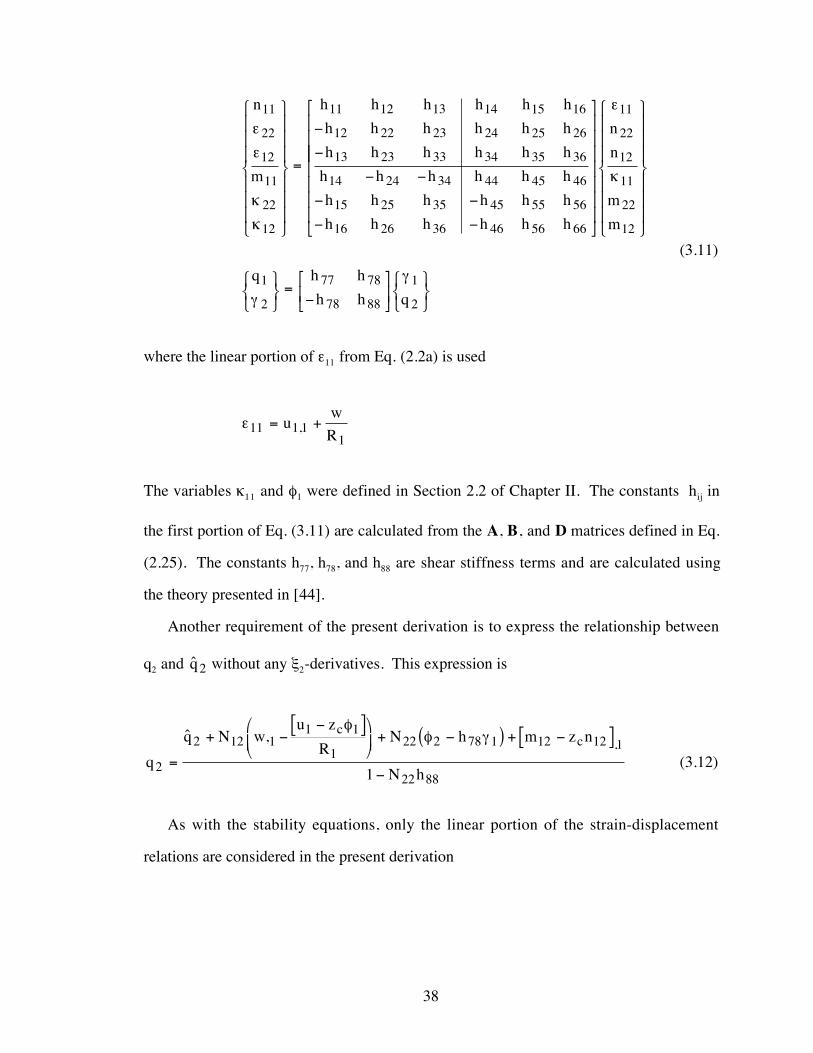
38

n

m

h h h h h h

h h h h h h

h h h h h h

h h h h h h

h h h h h h

h h h h h h

11

22

12

11

22

12

11 12 13 14 15 16

12 22 23 24 25 26

13 23 33 34 35 36

14 24 34 44 45 46

15 25 35 45 55 56

16 26 36 46 56 66

e

e

k

k

ì

í

ïïï

î

ïïï

ü

ý

ïïï

þ

ïïï

=

-

-

- -

- -

- -

é

ë

êêêêêêêê

ù

û

úúúúúúú

ì

í

ïïï

î

ïïï

ü

ý

ïïï

þ

ïïï

ìíî

üýþ

=-

é

ëê

ù

ûúìíî

üýþ

e

k

g

g

11

22

12

11

22

12

1

2

77 78

78 88

1

2

n

n

m

m

q h h

h h q

(3.11)

where the linear portion of e11 from Eq. (2.2a) is used

e11 1 11

= +uw

R,

The variables k11 and f1 were defined in Section 2.2 of Chapter II. The constants hij in

the first portion of Eq. (3.11) are calculated from the A, B, and D matrices defined in Eq.

(2.25). The constants h77, h78, and h88 are shear stiffness terms and are calculated using

the theory presented in [44].

Another requirement of the present derivation is to express the relationship between

q2 and Ãq2 without any x2-derivatives. This expression is

q

q N wu z

RN h m z n

N h

cc

2

2 12 11 1

122 2 78 1 12 12 1

22 881=

+ --[ ]æ

èç

ö

ø÷ + -( ) + -[ ]

-

Ã , ,

ff g

(3.12)

As with the stability equations, only the linear portion of the strain-displacement

relations are considered in the present derivation

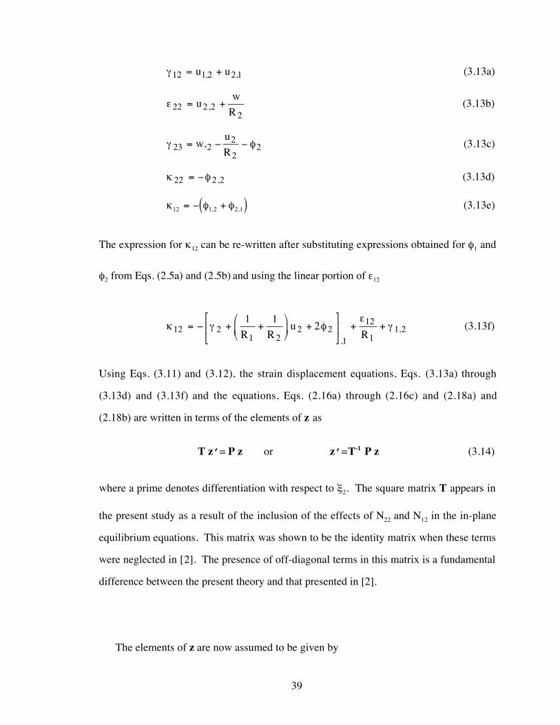
39

g12 1 2 2 1= +u u, , (3.13a)

e 22 2 22

= +uw

R, (3.13b)

g f23 22

22= - -w

u

R, (3.13c)

k f22 2 2= - , (3.13d)

k f f12 1 2 2 1= - +( ), , (3.13e)

The expression for k12 can be re-written after substituting expressions obtained for f1 and

f2 from Eqs. (2.5a) and (2.5b) and using the linear portion of e12

k g fe

g12 21 2

2 21

12

11 2

1 12= - + +

æ

èç

ö

ø÷ +

é

ëê

ù

ûú + +

R Ru

R,

, (3.13f)

Using Eqs. (3.11) and (3.12), the strain displacement equations, Eqs. (3.13a) through

(3.13d) and (3.13f) and the equations, Eqs. (2.16a) through (2.16c) and (2.18a) and

(2.18b) are written in terms of the elements of z as

T zÕ= P z or zÕ=T-1 P z (3.14)

where a prime denotes differentiation with respect to x2. The square matrix T appears in

the present study as a result of the inclusion of the effects of N22 and N12 in the in-plane

equilibrium equations. This matrix was shown to be the identity matrix when these terms

were neglected in [2]. The presence of off-diagonal terms in this matrix is a fundamental

difference between the present theory and that presented in [2].

The elements of z are now assumed to be given by

40

z ci

bj j=æèç

öø÷exp

b x 2 (3.15)

where b is a characteristic root of the differential equation. The number of values of b is

equal to the order of the differential equation system. Substitution of Eq. (3.15) into Eq.

(3.14) results in the following equation

(R - bI ) c = 0 (3.16a)

where

R T P1= -b (3.16b)

and I is the identity matrix. The vector c consists of the cj of Eq. (3.15). The matrix R is

obtained by premultiplying P by T-1. The eigenvalues of the matrix R are the

characteristic roots of the differential equation. This matrix is not symmetric; however, it

can be made real by multiplication or division of appropriate rows and columns by the

imaginary number, i. The elements of the matrices T and P are given in Appendix A for

both SDPT and CPT.

For each eigenvalue of R , there exists an eigenvector, c. A matrix C may be defined

with columns as the eigenvectors, c, the upper half of each column, denoted a , will be

associated with displacements, and the lower half, denoted b , will be associated with

forces. The form of C is therefore

Ca a . . . a

b b . . . b1 2 j

1 2 j=

é

ëê

ù

ûú (3. 17)

The next step in the derivation is to write the amplitudes of the displacements and forces

at the two edges of the plate. Quantities evaluated at x 2 2= -

b are identified with a

41

superscript 1 and quantities evaluated at x 2 2= +

b are identified with a superscript 2 as

follows:

d a ri

j jk kk

k

N1

1 2=

-æèç

öø÷å

=exp

b(3.18a)

d a ri

j jk kk

k

N2

1 2=

æèç

öø÷å

=exp

b(3.18b)

f b ri

j jk kk

k

N1

1 2=

-æèç

öø÷å

=exp

b(3.18c)

f b ri

j jk kk

k

N2

1 2= æ

èç

öø÷å

=exp

b(3.18d)

where the rk are constants determined from the edge values and N is the order of the

differential equation. Equations (3.18a)-(3.18d) may be written in matrix form as

d

dE r

1

2

ìíî

üýþ

= (3.19)

f

fF r

1

2

ìíî

üýþ

= (3.20)

Eliminating r from Eqs. (3.19) and (3.20) yields

f

fK

d

d

1

2

1

2

ìíî

üýþ

=ìíî

üýþ

(3.21)

where K is the stiffness matrix given by

K = F E-1 (3.22)

As for the case of CPT, K is real and symmetric for orthotropic plates without in-

plane shear loading, and it is Hermitian otherwise. Reference [2] presents a discussion of

42

techniques used to ensure that accurate numerical results for K are obtained from Eq.

(3.22).

3.4 The Wittrick-Williams Eigenvalue Algorithm

A brief discussion of the analysis procedure used in VICONOPT is in order. As

previously mentioned, VICONOPT uses a specialized algorithm for determining any

natural frequency or buckling load for any given wavelength [29]. The development of

this algorithm was necessary because the complex stiffnesses defined in the previous

section are transcendental functions of the load factor and half wavelength of the

buckling modes of the structure. The eigenvalue problem for determining natural

frequencies and buckling load factors is therefore transcendental.

The iterative analysis procedure used in VICONOPT is described in [36]. For this

procedure, the plate stiffnesses for a given wavelength are evaluated at a series of trial

values of the eigenvalue being determined until convergence is attained. This eigenvalue

is either the load factor for buckling or the natural frequency for vibration, and it is

different than the eigenvalues of the R matrix of Eq. (3.16b). Unless otherwise specified

by the user, the default initial trial value used in the VICONOPT code is one. For each

trial value of the eigenvalue considered, the analysis requires the plate stiffnesses as well

as the number of eigenvalues that lie below the trial value for the entire plate assembly

assuming the longitudinal edges of each individual to be clamped. A complete

description of the eigenvalue algorithm is given in [28]. Determining the number of

eigenvalues exceeded by a plate with clamped edges is very difficult except for very

specialized cases. Therefore, the procedure developed in [28] is used. This procedure

subdivides each plate into sub-elements with a small enough width such that none of the

eigenvalues of the sub-elements with clamped edges lie below the trial value. A sub-

elements is then used as a substructure and is repeatedly doubled until the original plate

element is obtained. Using a simple procedure at each doubling step [29], the number of

43

eigenvalues that lie below the trial value for the complete plate is returned. This

procedure is repeated for each plate in the assembly. Using this information and other

information obtained from the stiffness matrix of the entire assembly, the total number of

eigenvalues for the entire plate assembly that lie below the trial value is obtained. An

iterative procedure is then used to refine the trial value until the desired eigenvalue is

calculated to within the accuracy required.

One important piece of information required for the analysis procedure described

herein is the number of subdivisions required for each plate. As seen in Appendix A, all

of the terms of the R matrix are proportional to the plate width, b. Therefore, all of the

eigenvalues of R are proportional to b. Furthermore, it is important to note that an

eigenvalue equal to p corresponds to buckling or vibration with simply supported

longitudinal edges. By successively halving the value for b until all the real eigenvalues

of R are less than p, a value for the width of the sub-elements for which no eigenvalues

lie below the eigenvalue for simply supported edges is determined. This width also

guarantees that no eigenvalues for the sub-elements lie below the eigenvalue for clamped

edges. This width is that used in the iterative analysis procedure described previously.

44

CHAPTER IV

NUMERICAL RESULTS

In this chapter, numerical results are presented using the newly implemented curved-

plate analysis capability in VICONOPT. Results from several example problems are

presented to verify the results obtained with this new capability. A convergence study

using the segmented-plate approach in VICONOPT is performed for an isotropic

cylindrical shell subjected to uniaxial compression to identify a suitable number of

segments to be used when comparing results. Results comparing the computational effort

required by the new analysis to that of the analysis currently in the VICONOPT program

are also presented for this example. Comparisons of results for several curved plates

analyzed in Ref. [32] are then made. The effects of including terms related to in-plane

transverse loads in the in-plane stability equations are examined using a long cylindrical

tube subjected to in-plane transverse loading. Finally, the curved-plate analysis is used to

conduct a design-optimization study of a honeycomb-sandwich cylindrical shell

subjected to uniaxial compression. Comparisons of analyses using both physical and

tensorial strain measures are made for selected examples, and, where appropriate, results

using CPT and SDPT are compared.

4.1 Convergence of the Segmented-Plate Approach

The convergence of results using the segmented-plate approach in VICONOPT is

examined for the case of an aluminum cylindrical shell subjected to uniaxial

compression, see Figure 4.1. The values of the material properties used for this example

are E = 10.0 x 106 psi and n12 = 0.33. The wall thickness, t, is 0.1 in., and the radius, R2 is

60 in. As shown in Reference [49], the critical value for the stress resultant, N cr11 , for

the axisymmetric buckling of a long isotropic cylindrical shell is

45

NEt

Rlb incr11

2

2 1223 1

1019 354=-( )

=n

. / . (4.1)

For n12 = 0.33, the critical half wavelength, lcr, for axisymmetric buckling is shown in

[49] to be

l pn

crR t

R t in=-( )

= = . . .22 2

1224 2

12 11 74 4 255 (4.2)

Results illustrating the convergence of the VICONOPT segmented-plate results for

N cr11 as a function of the number of segments used to approximate the cylinder are

shown in Figure 4.2. In this figure, the results of the segmented-plate analysis are shown

as the solid curve. The theoretical value obtained from Reference [49] is shown as the

dashed horizontal line. The value obtained using the present curved-plate analysis with

two curved-plate elements is shown as the open symbol. All results in this figure are

calculated for the value of lcr given in Eq. (4.2). The VICONOPT results presented in

this figure are obtained using CPT with tensorial strain measures. As shown in Figure

4.2, the segmented-plate results converge to the theoretical value when 120 segments are

used. Therefore, to ensure that converged results are obtained when the segmented-plate

approach is used to analyze the remaining example problems, sixty segments will be used

when analyzing curved plates with an included angle of 180 degrees or less, and 120

segments will be used when analyzing full cylinders.

This example problem is also used to study the computational requirements of the

new curved-plate analysis in relation to the segmented-plate approach. A plot of

normalized CPU time as a function of the number of plate segments used in the

approximation is shown in Figure 4.3 for the segmented-plate analysis using either CPT

or SDPT. The normalized CPU time shown in this figure is the CPU time required for

46

the segmented-plate analyses normalized with respect to the CPU time required for the

curved-plate analysis using two curved-plate elements. The horizontal dashed line is at a

normalized CPU time of 1.0, and it represents the curved-plate analysis results. As

shown in the figure, to achieve convergence with 120 flat-plate segments requires

approximately 3.5 times and 16.7 times as much CPU time as the curved-plate analysis

for CPT and SDPT, respectively. (For the analysis using SDPT, G12 = G13 = G23). One

consideration to note at this time is that the segmented-plate analysis in VICONOPT is

implemented to handle the general case of variable geometry, stiffness and loading in the

x2-direction. This approach is therefore not as computationally efficient as it could be for

the case of constant curvature, stiffness, and loading in that direction (as is the case for

the curved-plate analysis). One approach to determining the additional computational

efficiency that may be obtained with the segmented-plate analysis involves defining a

single, small flat plate that is repeatedly doubled using the substructuring capability in

VICONOPT until the curved-plate segment is obtained. This technique is referred to

herein as ÔdoublingÕ. Results relating the computational effort of this approach to the

curved-plate analysis indicate that further reduction in the computational effort required

for the segmented-plate analysis can be obtained using this technique. This result occurs

because the in-plane and out-plane equations are uncoupled in the segmented-plate

analysis, and analytical expressions for the plate stiffnesses can be used. However, this

approach is currently not automated in the VICONOPT code, and a separate ÔdoublingÕ

effort would have to be made for every curved-plate segment in any given analytical

model.

4.2 Buckling of Curved Plates With Widely Varying Curvatures

The example problems presented in the next two sections are taken from Ref. [32],

and they are used to verify the results obtained using the new curved-plate analysis in

VICONOPT. The positive sense of the applied in-plane loadings to be considered in all

47

of the following examples is given in Figure 4.4. The first example problem considered

studies the buckling of a symmetrically laminated curved plate with clamped longitudinal

edges as a function of the curvature of the plate. The geometry of the plate is shown in

Figure 4.5. As shown in the figure, the plate is constructed from symmetrically

laminated boron/epoxy plies with a [0/90/±45]s layup. To allow for direct comparison of

results with those presented in [32], the SI units are used for this example and the

example in the following section. The material properties for a boron/epoxy ply are

given in Table 1.

The following loadings are considered for this example problem: N11 only, N22 only,

N12 only, and combined N11 = N22 = N12. The buckling of this plate subject to these four

different loadings was investigated while varying the value of the curvature parameter,

bR t

2

2, from 1 to 1000. The values of b, R2, and b used for these analyses are summarized

in Table 2. Both physical and tensorial strains are used with the new curved-plate

analysis, while physical strains only are used for the segmented-plate analysis. The

analysis of [32] uses physical strains. All analysis results presented in this section are for

CPT. The terms involving N22 and N12 are included in the in-plane stability equations for

all analyses. The results of this study are presented in Table 3 for N11 loading, in Table 4

for N22 loading, in Table 5 for N12 loading, and in Table 6 for combined N11 = N22 = N12

loading. The critical values of the stress resultants presented in these tables were

calculated using for the values of l

b given in the tables. These values of

l

b were

presented in Reference [32]. The critical values of these stress resultants are also plotted

as a function of the curvature parameter in Figure 4.6 through Figure 4.9, respectively.

As shown in these tables, the present analysis compares very well with that presented in

[32] and with the segmented-plate analysis for widely varying values of the curvature

48

parameter. As shown in Tables 3 - 6, there is no appreciable difference in the results

obtained using physical and tensorial strains.

4.3 Buckling of an Unsymmetrically Laminated Curved Plate

This example problem includes the effect of bending-stretching coupling and shear-

extension coupling on the buckling of an unsymmetrically laminated curved plate with

simply supported longitudinal edges. The geometry of the curved plate is shown in

Figure 4.10. As shown in the figure, the laminate being studied consists of a 0.0508-cm.-

thick layer of 2024 aluminum that is reinforced on the inner surface with pairs of ±45o

boron/epoxy plies. The material properties for 2024 aluminum are given in Table 1. For

this example, the number of pairs of ±45o boron/epoxy plies is increased from one to

seven. The analyses used for this example are identical to those used for the previous

example. The critical values for buckling of the stress resultants N11 and N12 are

presented in Tables 7 and 8, respectively. These values are also plotted as a function of

the number of boron/epoxy plies used in the laminate in Figure 4.11 and Figure 4.12,

respectively. The agreement between all the analyses is very good. As with the previous

example, there is no appreciable difference in the results obtained using physical and

tensorial strains. Results were also computed using SDPT. However, for the case of

seven pairs of pairs of ±45o boron/epoxy plies, the R/t ratio is still approximately 300,

and the effects of transverse-shear deformation are minimal. Therefore, as expected, the

critical values for buckling of the stress resultants N11 and N12 were slightly less than

those for CPT, but the differences were less than 0.2 percent. With regards to the CPU

time requirements for this example, the segmented-plate analysis using SDPT required

approximately 35 times as much CPU time as the curved-plate analysis for the case of 14

boron/epoxy plies. Furthermore, the results obtained using the ÔdoublingÕ approach

described in Section 4.1 indicate that the computational efficiencies offered by that

approach were not realized for this example problem. This result occurs because the

49

coupling that occurs due to the unsymmetric laminate prevents the in-plane and out-of-

plane equations from being uncoupled, and the same numerical approach for calculating

the plate stiffnesses as that used for the curved-plate analysis must be used.

4.4 Effect of N22 Terms in the In-Plane Stability Equations

As stated previously, the original segmented-plate analysis in the VICONOPT code

neglects the effects of the terms involving N22 and N12 in the in-plane stability equations.

This example problem illustrates the effect these terms may have on the buckling of an

isotropic (aluminum) long cylindrical tube subjected to uniform external pressure. The

material properties in English units for aluminum are given in Table 9. The geometry of

this example problem is shown in Figure 4.13. As shown in the figure, only half of the

tube is modeled since the buckling mode being studied is symmetric (i.e., two full waves

in the circumferential direction). The pressure load is modeled as an applied N22 hoop

loading. The value of the external pressure that would generate this hoop load is obtained

from the following expression [49]

pN

R= 22

2(4.3)

Simitses [50] presents a detailed discussion of the buckling of a thin circular ring

uniformly compressed by external pressure. When considering the behavior of the

pressure load as the ring buckles, Simitses describes three possible cases. In Case 1, the

pressure load is assumed to remain normal to the deflected surface. This loading is

referred to as a live pressure load. In Case 2, the pressure load is assumed to remain

parallel to its original direction. This loading is referred to as a dead pressure load. In

Case 3, the pressure load is assumed to always be directed toward the center of curvature

of the ring. This loading is referred to as a centrally directed pressure load. Only Cases 1

and 2 will be discussed in the present report.

50

In Reference [50], Simitses presents in-plane and out-of-plane stability equations for

the thin circular ring which may be rewritten in the notation used in the present report as

nq

Rp w

u

Rpcr22 2

2

22

2

22 0, ,+ - -

æ

èç

ö

ø÷ - = (4.4)

qn

Rp R w u pcr2 2

22

22 22 2 2 3 0, ,,- - -( ) - = (4.5)

where p2 and p3 are the perturbation values of the applied pressure load in the buckled

state in the x2- and x3-directions, respectively. For the case of a live pressure load in

which the applied pressure is assumed to remain normal to the deflected surface, p2 and

p3 are (for small deformations)

p p wu

Rand pcr2 2

2

23 0= - -

æ

èç

ö

ø÷ =, (4.6)

For the case of a dead pressure load in which the applied pressure is assumed to remain

parallel to its original direction, p2 and p3 are

p and p2 30 0= = (4.7)

Substituting Eqs. (4.3) and (4.6) into Eqs. (4.4) and (4.5), yields the following stability

equations for the case of live pressure loading:

nq

R22 22

20, + = (4.8)

qn

RN w

u

Rcr2 222

222 22

2 2

20,

,,- - -æ

èç

ö

ø÷ = (4.9)

51

Substituting Eqs. (4.3) and (4.7) into Eqs. (4.4) and (4.5), yields the following stability

equations for the case of dead pressure loading:

nq

R

N

Rw

u

Rcr

22 22

2

22

22

2

20, ,+ - -

æ

èç

ö

ø÷ = (4.10)

qn

RN w

u

Rcr2 222

222 22

2 2

20,

,,- - -æ

èç

ö

ø÷ = (4.11)

For live pressure, the critical value of pressure is shown in [50] to be

pEI

Rcr =

3

23 (4.12)

Therefore,

NEI

Rcr2222

3= (4.13)

For dead pressure, the critical value of pressure is shown in [50] to be

pEI

Rcr =

4

23 (4.14)

Therefore,

NEI

Rcr2222

4= (4.15)

52

As discussed in Reference [49], results for the case of a long cylindrical tube uniformly

compressed by external pressure, may be obtained by considering an elemental ring of

unit width and using Eqs. (4.12) through (4.15) with E replaced by E/(1-n2) and I

replaced by t3/12.

External pressure loads are not included in the present analysis. However, an

equivalent N22 loading may be calculated using Eq. (4.3). The present analysis treats the

applied loads as dead loads since no effort is made to modify the applied loads as the

plate deforms. The stability equations in the x2 and x3 directions, Eqs. (2.11b) and

(2.11c) for the present analysis are written for a thin circular ring subjected to N22 loading

by ignoring any terms that involve N12, x1, or derivatives with respect to x1. These

equations are

nq

R

N

Rw

u

RFN

w

Ru22 2

2

2

22

22

2

222

2

22 22 0, ,,

,+ - -

æ

èç

ö

ø÷ - +

æ

èç

ö

ø÷ = (4.16)

qn

RN w

u

R

FN

Rw

Ru2 2

22

222 22

2 2

2

22

2 22 2 0,

,,,- - -

æ

èç

ö

ø÷ + +

æ

èç

ö

ø÷ = (4.17)

Comparing Eqs. (4.9), (4.11), and (4.17), reveals that if physical strains are used in the

present analysis (i.e., F = 0), the out-of-plane stability equation is identical to that given

by Simitses for both live and dead pressure loads. Furthermore, the in-plane stability

equation for the live pressure load case is recovered by the present analysis if the N22

term is neglected in Eq. (4.16). The dead pressure load case is seen to be recovered when

the N22 term is included in Eq. (4.16). Comparing Eqs. (4.6), (4.7), and (4.16), shows that

53

for the case of physical strains, the remaining term involving N22 is actually equivalent to

the component of a live pressure load in the x2 direction (see Eq. (4.6)).

Buckling results for this example are presented in Table 10. The VICONOPT results

presented in this table are for physical strains. As previously discussed, the VICONOPT

result when the N22 term is neglected in the in-plane stability equation corresponds to the

case of live pressure load, and the VICONOPT result when the N22 term is included in the

in-plane stability equation corresponds to the case of dead pressure load. The results for

physical strains for the segmented-plate analysis always equal those for the case of dead

pressure load since the N22 term in the in-plane stability equation also involves 1/R2 and it

therefore drops out of that equation altogether. These results illustrate the dramatic effect

that the N22 and N12 terms in the in-plane stability equations can have on the buckling

results for curved plates.

4.5 Design Optimization of a Cylindrical Shell Subject to Uniaxial

Compression

The final example utilizes the new curved-plate analysis with the design optimization

capability of VICONOPT to perform a structural optimization of two different cylindrical

shell concepts subject to uniform axial compression (N11 loading). The two concepts are

solid-wall construction and honeycomb-sandwich construction. The geometry of this

example problem is shown in Figure 4.14. As shown in the figure, the facesheets of the

honeycomb-sandwich concept are aluminum, and the core is KorexTM aramid paper

honeycomb core [51]. The solid-wall concept is aluminum. The material properties used

for the facesheets and core are presented in Table 9.

Before results for this example are presented, a discussion of the modeling technique

used to model this cylinder is presented. An analysis of a complete cylinder was

performed using only one plate element with the new curved-plate analysis capability in

54

VICONOPT. The cylinder is modeled by defining a repetitive cross-section in which

there is only one node that is connected to itself. However, numerical problems were

encountered when analyzing closed cylinders with very small wavelengths. The

following procedure was used to avoid this problem. First, a 45¡ arc segment is defined.

Second, a 90¡ arc segment is defined as a substructure by connecting the original 45¡ arc

segment to itself. Similarly, a 180¡ arc segment is constructed from two 90¡ arcs.

Finally, a 360¡ arc is constructed from two 180¡ arcs. This substructure is then used to

define the repetitive cross-section of the cylinder as previously discussed. This modeling

technique is used for all closed cylinders analyzed in the present report, and no numerical

problems were encountered when using this technique.

The design variables for the structural optimization are the thicknesses of the

facesheets and the core for the sandwich concept and the wall thickness for the solid-wall

construction. There is no minimum-gage restriction for any design variables. The

nominal values for these variables are 0.1 in., 0.5 in., and 0.1 in., respectively. The

design constraints are that the strain in the facesheets or the solid wall cannot exceed

0.005 in/in and that the stress in the core cannot exceed 115 psi in the x1-direction and 55

psi in the x2-direction. The results of this study, including the mass of the optimized

cylinder and the final values of the design variables are given in Table 11 for the

honeycomb-sandwich concept and in Table 12 for the solid-wall concept. Results from

both CPT and SDPT are given in these tables. The optimized mass values are also

plotted as a function of the applied loading in Figure 4.15. As seen in the tables and the

figure, the values for optimized mass obtained using CPT are slightly less than those for

SDPT for the honeycomb-sandwich cylinder as the applied loading is increased.

However, the values for core thickness obtained using CPT are significantly less than

those for SDPT for the honeycomb-sandwich cylinder as the applied loading is increased.

These results are expected because CPT results in an overly stiff approximation since the

55

effects of transverse-shear deformation are neglected. This overly stiff approximation

results in higher buckling loads for a given core thickness. Therefore, the core thickness

and the optimum mass obtained is less than that obtained using SDPT. The optimized

mass values for the solid-wall construction are much greater than those for the

honeycomb-sandwich construction. The results for CPT and SDPT are nearly identical

for the solid-wall construction, as expected.

56

CHAPTER V

CONCLUDING REMARKS

The VICONOPT computer code is an exact analysis and optimum design program

that includes the buckling and vibration analyses of prismatic assemblies of flat, in-plane-

loaded anisotropic plates. In the present report, the capability to analyze curved-plate

segments exactly has been added to the VICONOPT code. Non-linear curved-plate

equilibrium equations have been formulated using the principle of virtual work, and

linearized stability equations that describe the response of the plate just after buckling

occurs were derived following the application of several simplifying assumptions.

Finally, modifications to these equations were made to allow the reference surface of the

plate to be located at a distance zc from the centroidal surface.

The analysis methodology described in the present report improves upon the existing

methodology in the VICONOPT code (referred to herein as the segmented-plate analysis)

which requires that curved-plate segments be subdivided into several flat-plate elements

that must be subsequently joined at their longitudinal edges to approximate the curved-

plate geometry. The new analysis formulation allows either classical plate theory (CPT)

or first-order shear deformation plate theory (SDPT) to be used. Furthermore, anisotropic

laminates having fully populated A , B, and D stiffness matrices may be analyzed. The

analysis described in the present report is an example of an exact finite-strip method

(FSM) since it uses a stiffness matrix that is derived by direct solution to the stability

equations.

One additional capability that has been incorporated into the VICONOPT code as part

of the present report is the option to use plate elements (flat or curved) that are based

upon nonlinear strain-displacement relations that contain terms from either physical or

tensorial strain measures. A second capability that has been added is the ability to

57

include the effect of terms associated with in-plane transverse and in-plane shear loading

in the in-plane stability equations. The original VICONOPT code neglects these terms.

Results from the present curved-plate analysis capability compare very well with a

closed-form solution and the existing segmented-plate analysis for the buckling of a long

isotropic cylinder. The present analysis also compares well with results from the

literature for symmetrically laminated curved plates with widely varying curvatures and

with unsymmetrically laminated plates that include the effect of extensional-bending and

shear-extension coupling. No appreciable effects of using tensorial versus physical

strains are noted in these examples. The present curved-plate analysis was also shown to

require significantly less computational effort than the segmented-plate analysis. An

alternate approach for the segmented-plate analysis that offers additional computational

savings for certain classes of problems has been investigated. However, this approach

requires greater user effort, and it is currently not implemented in the VICONOPT code.

A significant effect of either including or neglecting the terms associated with an

applied in-plane transverse loading (i.e., N22 loading) in the in-plane stability equations

was noted when analyzing a long cylindrical tube subjected to uniform external pressure.

The symmetry of the buckling mode for this problem allowed it to be modeled as a half

cylinder, and the pressure load was simulated with an equivalent hoop (N22) loading. The

buckling results for this problem were shown to change by a factor of 3/4 when the terms

associated with the N22 loading were neglected in the in-plane stability equations. This

result illustrates the effect that the treatment of the in-plane stability equations can have

on the buckling results for curved plates.

Finally, the present curved-plate analysis was used to conduct a design-optimization

study of two different cylindrical shells subject to uniform axial compression (N11

loading). One shell was constructed from a honeycomb-sandwich wall construction, and

the other was a solid-wall construction. The values of mass for the optimized solid-wall

design were consistently higher than those for the honeycomb-sandwich construction.

58

However, there was no difference between results using CPT and SDPT for the solid-wall

cylinder. The values of mass for the optimized honeycomb-sandwich cylinder using CPT

were slightly less than those for SDPT as the applied loading was increased. However,

the values of core thickness for the optimized honeycomb-sandwich cylinder using CPT

were significantly less than those for SDPT as the applied loading was increased. This

trend occurred because CPT results in an overly stiff approximation since the effects of

transverse-shear flexibility are neglected. This overly stiff approximation results in

higher buckling loads and, thus, a lower optimum mass.

One area for future work includes retaining the curvature terms in the longitudinal

direction and implementing the capability to analyze shells of revolution. The analysis

can also be modified to allow vibration analyses to be performed. Another enhancement

that can be made to the present analysis is to remove the restriction that when the terms

associated with in-plane transverse and in-plane shear loading are retained in the in-plane

stability equations, the centroidal surface and reference surface must coincide.

59

REFERENCES

1. Williams, F. W.; Kennedy, D.; Anderson, M. S.; and Edwards, D. A.: ÒUser Manualfor VICONOPT,Ó Release 1.3, April 1996.

2. Anderson, M. S.; and Kennedy, D.: ÒInclusion of Transverse Shear Deformation inthe Exact Buckling and Vibration Analysis of Composite Plate Assemblies,ÓPresented at the AIAA/ASME/ASCE/AHS/ASC 32nd Structures, StructuralDynamics and Materials Conference, Dallas, Texas, April 13-15, 1992. AIAA PaperNo. 92-2287.

3. Cheung, Y. K.: The Finite Strip Method in Structural Analysis, Pergamon Press,Oxford, England, 1976.

4. Zienkiewicz, O. C.: The Finite Element Method in Engineering Science, McGrawHill, London, England, 1971.

5. Cheung, Y. K.: ÒThe Finite Strip Method in the Analysis of Elastic Plates with TwoOpposite Simply Supported Ends,Ó Proceedings of the Institute of Civil Engineers ,Vol. 40, No. 1, 1968.

6. Cheung, M. S.; and Cheung, Y. K.: ÒNatural Vibrations of Thin Flat-WalledStructures With Different Boundary Conditions,Ó Journal of Sound and Vibration ,Vol. 18, 1971, pp. 325-337.

7. Przemieniecki, J. S.: ÒFinite Element Structural Analysis of Local Instability,ÓAIAA Journal , Vol. 11, 1973, pp. 33-39.

8. Plank, R. J.; and Wittrick, W. H.: ÒBuckling Under Combined Loading of Thin Flat-Walled Structures By a Complex Finite-Strip Method,Ó International Journal forNumerical Methods in Engineering , Vol. 8, 1974, pp. 323-339.

9. Dawe, D. J.: ÒStatic Analysis of Diaphragm-Supported Cylindrical Shells Using aCurved Finite Strip,Ó International Journal for Numerical Methods in Engineering ,Vol. 11, 1977, pp. 1347-1364.

10. Dawe, D. J.: ÒFinite Strip Buckling Analysis of Curved Plate Assemblies UnderBiaxial Loading,Ó International Journal for Numerical Methods in Engineering , Vol.13, 1977, pp. 1141-1155.

11. Morris, I. R.; and Dawe, D. J.: ÒFree Vibration of Curved-Plate Assemblies WithDiaphragm Ends,Ó Journal of Sound and Vibration , Vol. 73, 1980, pp. 1-17.

12. Dawe, D. J.: ÒFinite Strip Models for Vibration of Mindlin Plates,Ó Journal ofSound and Vibration , Vol. 59, 1978, pp. 441-452.

13. Mindlin, R. D.: ÒInfluence of Rotatory Inertia and Shear on Flexural Motions ofIsotropic Elastic Plates,Ó Journal of Applied Mechanics , Vol. 18, 1951, pp. 31-38.

60

14. Roufaeil, O. L.; and Dawe, D. J.: ÒVibration Analysis of Rectangular Mindlin Platesby the Finite Strip Method,Ó Computers & Structures , Vol. 12, 1980, pp. 833-842.

15. Dawe, D. J.; and Roufaeil, O. L.: ÒBuckling of Rectangular Mindlin Plates,ÓComputers & Structures , Vol. 15, 1982, pp. 461-471.

16. Craig, T. J.; and Dawe, D. J.: ÒFlexural Vibration of Symmetrically LaminatedComposite Rectangular Plates Including Transverse Shear Effects,Ó InternationalJournal of Solids and Structures , Vol. 22, No. 2, 1986, pp. 155-169.

17. Dawe, D. J.; and Craig, T. J.: ÒThe Vibration and Stability of SymmetricallyLaminated Composite Rectangular Plates Subjected to In-Plane Stresses,ÓComposite Structures , Vol. 5, 1986, pp. 281-307.

18. Craig, T. J.; and Dawe, D. J.: ÒVibration of Shear-Deformable Laminated PlateStructures by the Finite Strip Method,Ó Computers & Structures , Vol. 27, No. 1,1987, pp. 61-72.

19. Dawe, D. J.; and Craig, T. J.: ÒBuckling and Vibration of Shear DeformablePrismatic Plate Structures by a Complex Finite Strip Method,Ó International Journalof Mechanical Sciences , Vol. 30, No. 2, 1988, pp. 77-99.

20. Dawe, D. J.; and Peshkam, V.: ÒBuckling and Vibration of Finite-Length CompositePrismatic Plate Structures With Diaphragm Ends, Part I: Finite Strip Formulation,ÓComputer Methods in Applied Mechanics and Engineering , Vol. 77, 1989, pp. 1-30.

21. Peshkam, V.; and Dawe, D. J.: ÒBuckling and Vibration of Finite-Length CompositePrismatic Plate Structures With Diaphragm Ends, Part II: Computer Programs andBuckling Applications,Ó Computer Methods in Applied Mechanics and Engineering ,Vol. 77, 1989, pp. 227-252.

22. Dawe, D. J.; and Peshkam, V.: ÒBuckling and Vibration of Long Plate Structures byComplex Finite Strip Methods,Ó International Journal of Mechanical Sciences , Vol.32, No. 9, 1990, pp. 743-766.

23. Wittrick, W. H.: ÒA Unified Approach to the Initial Buckling of Stiffened Panels inCompression,Ó The Aeronautical Quarterly , Vol. 19, 1968, pp. 265-283.

24. Wittrick, W. H.; and Curzon, P. L. V.: ÒStability Functions for the Local Bucklingof Thin Flat-Walled Structures with the Walls in Combined Shear andCompression,Ó Aeronautical Quarterly , November 1968, vol. 19, pp. 327-351.

25. Wittrick, W. H.: ÒGeneral Sinusoidal Stiffness Matrices for Buckling and VibrationAnalysis of Thin Flat-Walled Structures,Ó International Journal of MechanicalSciences , Vol. 10, 1968, pp. 949-966.

26. Smith, C. S.: ÒBending, Buckling and Vibration of Orthotropic Plate-BeamStructures,Ó Journal of Ship Research , Vol. 12, 1968, pp. 249-268.

61

27. Williams, F. W.: ÒComputation of Natural Frequencies and Initial Buckling Stressesof Prismatic Plate Assemblies,Ó Journal of Sound and Vibration , Vol. 21, 1972, pp.87-106.

28. Wittrick, W. H.; and Williams, F. W.: ÒBuckling and Vibration of Anisotropic orIsotropic Plate Assemblies Under Combined Loadings,Ó International Journal ofMechanical Sciences , Vol. 16, 1974, pp. 209-239.

29. Wittrick, W. H.; and Williams, F. W.: ÒAn Algorithm for Computing CriticalBuckling Loads of Elastic Structures,Ó Journal of Structural Mechanics , Vol. 1,1973, pp. 497-518.

30. Viswanathan, A. V.; and Tamekuni, M.: ÒElastic Buckling Analysis For CompositeStiffened Panels and other Structures Subjected to Biaxial Inplane Loads,Ó NASACR-2216, 1973.

31. Viswanathan, A. V.; Tamekuni, M.; and Tripp, L. L.: ÒElastic Stability of BiaxiallyLoaded Longitudinally Stiffened Composite Structures,Ó Proceedings of theAIAA/ASME/SAE 14th Structures, Structural Dynamics, and Materials Conference,Williamsburg, VA, March 20-22, 1973. AIAA Paper No. 73-367.

32. Viswanathan, A. V.; Tamekuni, M.; and Baker, L. L.: ÒElastic Stability ofLaminated, Flat and Curved, Long Rectangular Plates Subjected to CombinedLoads,Ó NASA CR-2330, 1974.

33. Williams, F. W.; and Anderson, M. S.: ÒIncorporation of Lagrangian Multipliersinto an Algorithm for Finding Exact Natural Frequencies or Critical BucklingLoads,Ó International Journal of Mechanical Sciences , Vol. 25, 1983, No. 8, pp.579-584.

34. Anderson, M. S.; Williams, F. W.; and Wright, C. J.: ÒBuckling and Vibration ofany Prismatic Assembly of Shear and Compression Loaded Anisotropic Plates withan Arbitrary Supporting Structure,Ó International Journal of Mechanical Sciences ,Vol. 25, No. 8, 1983, pp. 585-596.

35. Kennedy, D.; and Williams, F. W.: ÒVibration and Buckling of Anisotropic PlateAssemblies with Winkler Foundations,Ó Journal of Sound and Vibration , Vol. 138,No. 3, 1990, pp. 501-510.

36. Williams, F. W.; Kennedy, D.; and Anderson, M. S.: ÒAnalysis Features ofVICONOPT, an Exact Buckling and Vibration Program for Prismatic Assemblies ofAnisotropic Plates,Ó Proceedings of the 31st AIAA/ASME/ASCE/AHS/ASCStructures, Structural Dynamics and Materials Conference, Long Beach, California,pp. 920-929, April 1990. AIAA Paper 90-0970.

37. Butler, R.; and Williams, F. W.: ÒOptimum Design Features of VICONOPT, anExact Buckling and Vibration Program for Prismatic Assemblies of AnisotropicPlates,Ó Proceedings of the 31st AIAA/ASME/ASCE/AHS/ASC Structures,Structural Dynamics and Materials Conference, Long Beach, California, pp. 1289-1299, April 1990. AIAA Paper 90-1068.

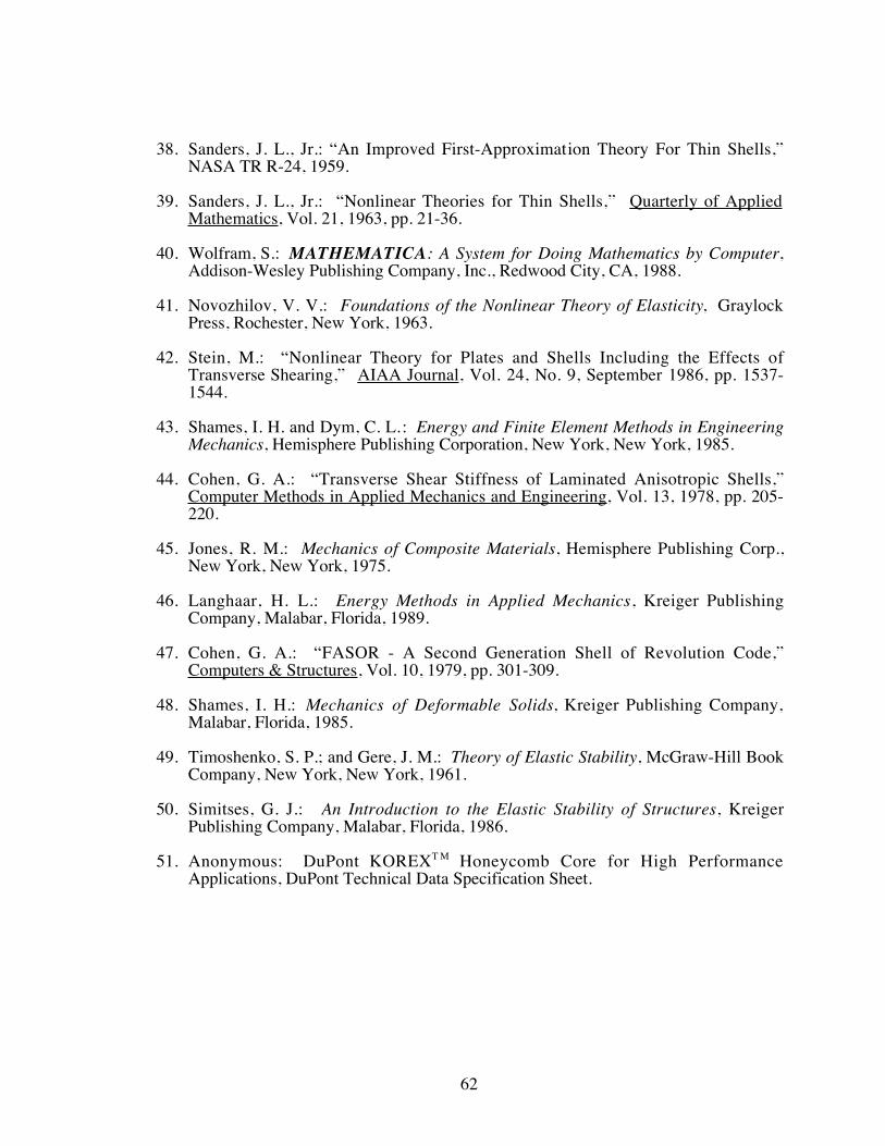
62

38. Sanders, J. L., Jr.: ÒAn Improved First-Approximation Theory For Thin Shells,ÓNASA TR R-24, 1959.

39. Sanders, J. L., Jr.: ÒNonlinear Theories for Thin Shells,Ó Quarterly of AppliedMathematics , Vol. 21, 1963, pp. 21-36.

40. Wolfram, S.: MATHEMATICA: A System for Doing Mathematics by Computer,Addison-Wesley Publishing Company, Inc., Redwood City, CA, 1988.

41. Novozhilov, V. V.: Foundations of the Nonlinear Theory of Elasticity, GraylockPress, Rochester, New York, 1963.

42. Stein, M.: ÒNonlinear Theory for Plates and Shells Including the Effects ofTransverse Shearing,Ó AIAA Journal , Vol. 24, No. 9, September 1986, pp. 1537-1544.

43. Shames, I. H. and Dym, C. L. : Energy and Finite Element Methods in EngineeringMechanics, Hemisphere Publishing Corporation, New York, New York, 1985.

44. Cohen, G. A.: ÒTransverse Shear Stiffness of Laminated Anisotropic Shells,ÓComputer Methods in Applied Mechanics and Engineering , Vol. 13, 1978, pp. 205-220.

45. Jones, R. M.: Mechanics of Composite Materials, Hemisphere Publishing Corp.,New York, New York, 1975.

46. Langhaar, H. L.: Energy Methods in Applied Mechanics, Kreiger PublishingCompany, Malabar, Florida, 1989.

47. Cohen, G. A.: ÒFASOR - A Second Generation Shell of Revolution Code,ÓComputers & Structures , Vol. 10, 1979, pp. 301-309.

48. Shames, I. H.: Mechanics of Deformable Solids, Kreiger Publishing Company,Malabar, Florida, 1985.

49. Timoshenko, S. P.; and Gere, J. M.: Theory of Elastic Stability, McGraw-Hill BookCompany, New York, New York, 1961.

50. Simitses, G. J.: An Introduction to the Elastic Stability of Structures, KreigerPublishing Company, Malabar, Florida, 1986.

51. Anonymous: DuPont KOREXT M Honeycomb Core for High PerformanceApplications, DuPont Technical Data Specification Sheet.

63

APPENDIX A

MATRICES FOR DETERMINING CHARACTERISTIC ROOTS

The eigenvalues of matrix R in Eq. (3.16a) are the characteristic roots of the

differential equations describing the behavior of the plate. The 10-by-10 matrix R is

calculated from the matrices T and P as shown in Eq. (3.16b). The non-zero elements of

the T matrix are

t t t t t t t t3 3 4 4 5 5 6 6 7 7 8 8 9 9 10 10 1,*

,*

, ,*

,*

,*

,*

,= = = = = = = =

t E h N G h N11 33 22 23 121,* = - -( ) t F h N G h N1 2 23 22 33 12,

* = - +

t E h N G h N2 1 23 22 22 12,* = - -( ) t F h N G h N2 2 22 22 23 121,

* = - -( )

t E h N G h N4 1 35 22 25 12,* = - t F h N G h N4 2 25 22 35 12,

* = -

t E h N G h N5 1 36 22 26 12, = - -( ) t F h N G h N5 2 26 22 36 12, = - +

tb

E H h N N G H h N E h N G h N6 1 33 22 12 23 122

13 22 12 12,* = - - +( )a

tb

F H h N N G H h N F h N G h N6 2 23 22 12 33 122

12 22 13 12,* = - - +( )a

tb

E H h N N G H h N E N7 1 23 22 12 22 122

22, = - -( )a

tb

F H h N N G H h N G N7 2 22 22 12 23 122

12, = - +( )a

tb

tb

E h N G h N8 1 10 1

2

2 34 22 24 12,*

, = = -( )a a

tb

tb

F h N G h N8 2 10 2

2

2 24 22 34 12,*

, = = -( )a a

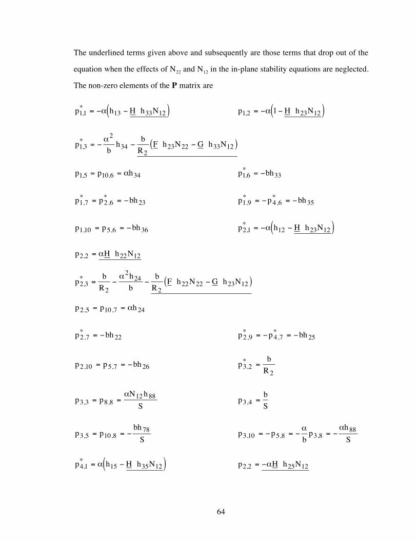
64

The underlined terms given above and subsequently are those terms that drop out of the

equation when the effects of N22 and N12 in the in-plane stability equations are neglected.

The non-zero elements of the P matrix are

p h H h N11 13 33 12,* = - -( )a p H h N1 2 23 121, = - -( )a

pb

hb

RF h N G h N1 3

2

342

23 22 33 12,* = - - -( )a

p p h1 5 10 6 34, ,= = a p bh1 6 33,* = -

p p bh1 7 2 6 23,*

,*= = - p p bh1 9 4 6 35,

*,

*= - = -

p p bh1 10 5 6 36, ,= = - p h H h N2 1 12 23 12,* = - -( )a

p H h N2 2 22 12, = a

pb

R

h

bb

RF h N G h N2 3

2

224

222 22 23 12,

* = - - -( )a

p p h2 5 10 7 24, ,= = a

p bh2 7 22,* = - p p bh2 9 4 7 25,

*,

*= - = -

p p bh2 10 5 7 26, ,= = - pb

R3 22

,* =

p pN h

S3 3 8 812 88

, ,= =a

pbS3 4, =

p pbh

S3 5 10 878

, ,= = - p pb

ph

S3 10 5 8 3 888

, , ,= - = - = -a a

p h H h N4 1 15 35 12,* = -( )a p H h N2 2 25 12, = -a

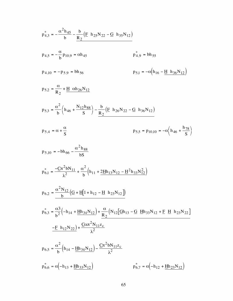
65

ph

bb

RF h N G h N4 3

245

225 22 35 12,

* = - - -( )a

pb

p h4 5 10 9 45, ,= - =a

a p bh4 9 55,* =

p p bh4 10 5 9 56, ,= - = p h H h N5 1 16 36 12, = - -( )a

pR

H h N5 22

26 12, = +a

a

pb

hN h

Sb

RF h N G h N5 3

2

4612 88

226 22 36 12, = +æ

èöø- -( )a

pS5 4, = +aa

p p hh

S5 5 10 10 4678

, ,= = - +æè

öø

a

p bhh

bS5 10 66

288

, = - -a

pC bN

bh Hh N H h N6 1

211

2

2

11 13 122

33 1222,

* =-

+ + -( )p

l

a

pN

bG H h H h N6 2

212

12 23 121, = + + -[ ]( )a

pb

h Hh NR

N Gh G Hh N F H h N

F h NC N zc

6 3 2 14 34 122

12 13 33 12 23 22

12 22

211

2

3,

*

= - +( ) + - +[ ](

- ) +

a a

ap

l

pb

h Hh NC bN zc

6 5

2

14 34 12

211

2, = -( ) -a p

l

p h Hh N6 6 13 33 12,* = - +( )a p h Hh N6 7 12 23 12,

* = - +( )a

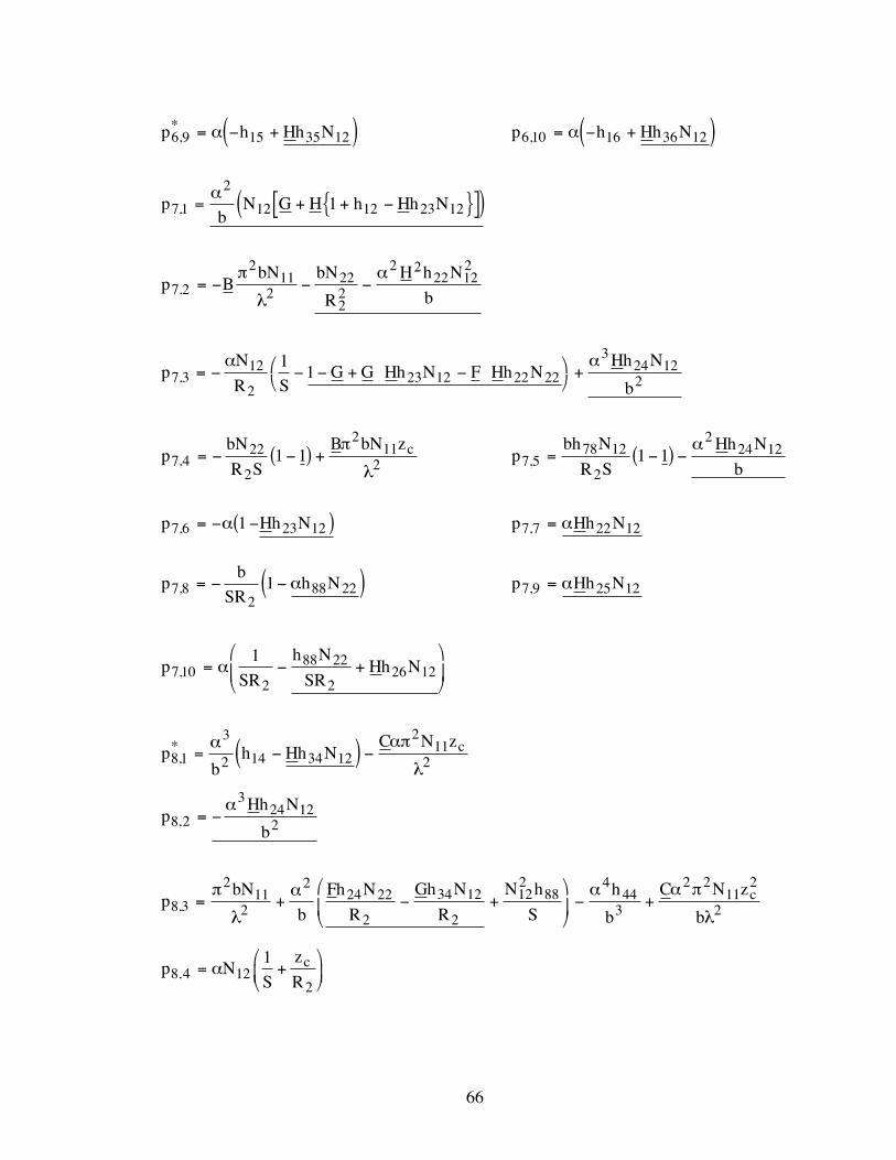
66

p h Hh N6 9 15 35 12,* = - +( )a p h Hh N6 10 16 36 12, = - +( )a

pb

N G H h Hh N7 1

2

12 12 23 121, = + + -{ }[ ]( )a

p BbN bN

R

H h N

b7 2

211

222

22

2 222 12

2

, = - - -p

l

a

pN

R SG G Hh N F Hh N

Hh N

b7 3

12

223 12 22 22

324 122

11, = - - - + -æ

èöø+

a a

pbN

R S

B bN zc7 4

22

2

211

21 1, = - -( ) +p

lp

bh N

R S

Hh N

b7 578 12

2

224 121 1, = -( ) -

a

p Hh N7 6 23 121, = - -( )a p Hh N7 7 22 12, = a

pb

SRh N7 8

288 221, = - -( )a p Hh N7 9 25 12, = a

pSR

h N

SRHh N7 10

2

88 22

226 12

1, = - +

æ

èç

ö

ø÷a

pb

h Hh NC N zc

8 1

3

2 14 34 12

211

2,* = -( ) -a ap

l

pHh N

b8 2

324 122, = -

a

pbN

b

Fh N

R

Gh N

R

N h

S

h

b

C N z

bc

8 3

211

2

224 22

2

34 12

2

122

884

443

2 211

2

2, = + - +æ

èç

ö

ø÷ - +

p

l

a a a p

l

p NS

z

Rc

8 4 122

1, = +

æ

èç

ö

ø÷a

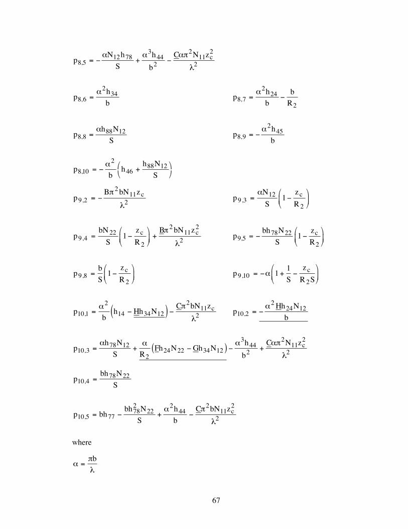
67

pN h

S

h

b

C N zc8 5

12 783

442

211

2

2, = - + -a a ap

l

phb8 6

234

, =a

phb

bR8 7

224

2, = -

a

ph N

S8 888 12

, =a

ph

b8 9

245

, = -a

pb

hh N

S8 10

2

4688 12

, = - +æè

öø

a

pB bN z c

9 2

211

2, = -p

lp

N

S

z

Rc

9 312

21, = -æ

èç

ö

ø÷

a

pbN

S

z

R

B bN zc c9 4

22

2

211

2

21, = -æ

èç

ö

ø÷ +

p

lp

bh N

S

z

Rc

9 578 22

21, = - -æ

èç

ö

ø÷

pbS

z

Rc

9 82

1, = -æ

èç

ö

ø÷ p

S

z

R Sc

9 102

11

, = - + -æ

èç

ö

ø÷a

pb

h Hh NC bN zc

10 1

2

14 34 12

211

2, = -( ) -a p

lp

Hh N

b10 2

224 12

, = -a

ph N

S RFh N Gh N

h

b

C N zc10 3

78 12

224 22 34 12

344

2

211

2

2, = + -( ) - +a a a ap

l

pbh N

S10 478 22

, =

p bhbh N

S

h

b

C bN zc10 5 77

782

222

442

112

2, = - + -a p

l

where

ap

l=

b

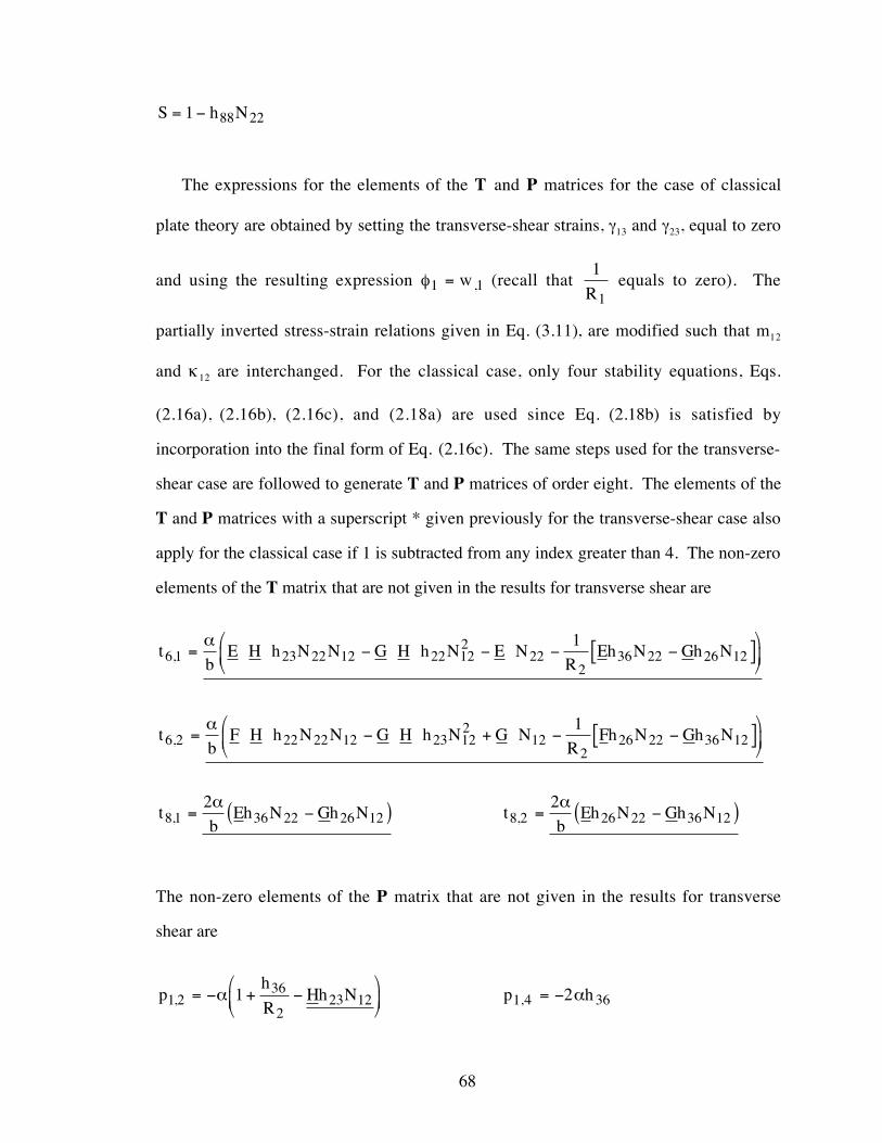
68

S h N= -1 88 22

The expressions for the elements of the T and P matrices for the case of classical

plate theory are obtained by setting the transverse-shear strains, g13 and g23, equal to zero

and using the resulting expression f1 1= w, (recall that 1

1R equals to zero). The

partially inverted stress-strain relations given in Eq. (3.11), are modified such that m12

and k12 are interchanged. For the classical case, only four stability equations, Eqs.

(2.16a), (2.16b), (2.16c), and (2.18a) are used since Eq. (2.18b) is satisfied by

incorporation into the final form of Eq. (2.16c). The same steps used for the transverse-

shear case are followed to generate T and P matrices of order eight. The elements of the

T and P matrices with a superscript * given previously for the transverse-shear case also

apply for the classical case if 1 is subtracted from any index greater than 4. The non-zero

elements of the T matrix that are not given in the results for transverse shear are

tb

E H h N N G H h N E NR

Eh N Gh N6 1 23 22 12 22 122

222

36 22 26 121

, = - - - -[ ]æ

èç

ö

ø÷

a

tb

F H h N N G H h N G NR

Fh N Gh N6 2 22 22 12 23 122

122

26 22 36 121

, = - + - -[ ]æ

èç

ö

ø÷

a

tb

Eh N Gh N8 1 36 22 26 122

, = -( )at

bEh N Gh N8 2 26 22 36 12

2, = -( )a

The non-zero elements of the P matrix that are not given in the results for transverse

shear are

ph

RHh N1 2

36

223 121, = - + -

æ

èç

ö

ø÷a p h1 4 362, = - a

69

ph

RHh N2 2

26

222 12, = - -

æ

èç

ö

ø÷a p h2 4 262, = - a

p b3 4, = ph

RHh N4 2

56

225 12, = -

æ

èç

ö

ø÷a

p h4 4 562, = a

pN

bG H h

h

RH h N

h

bR5 2

212

1236

223 12

216

21, = + + + -é

ëê

ù

ûú

æ

èç

ö

ø÷ -

a a

pb

h Hh N5 4

2

16 36 122

, =-

-( )a

pNb

G H hhR

H h Nh

bR6 1

212

1236

223 12

216

21, = + + + -é

ëê

ù

ûú

æ

èç

ö

ø÷ -

a a

pb

h

RHN h Hh N

B bN6 2

266

22 12 26 22 12

211

22, = + -[ ]æ

èç

ö

ø÷ -

a p

l

pb

h

RHh N

N

RG G Hh N F Hh N

Gh

R

Fh N

R

N

R

6 3 246

224 12

12

223 12 22 22

36

2

26 22

22

12

2

31, = +

æ

èç

ö

ø÷ + + - + +

æ

èç

ö

ø÷

- -

a a

a a

pb

h

RHh N

bN

R

B bN zc6 4

266

226 12

22

2

211

22

1 1, = +æ

èç

ö

ø÷ - -( ) +a p

l

ph

RHh N6 5

36

223 121, = - + -

æ

èç

ö

ø÷a p

h

RHh N6 6

26

222 12, = - -

æ

èç

ö

ø÷a

pb

R6 72

, = - ph

RHh N6 8

56

225 12, = - -

æ

èç

ö

ø÷a

70

pb

h Hh NC N zc

7 1

3

2 14 34 12

211

2, = -( ) -a ap

l

pb

h

RHh N7 2

3

246

224 12, = - +

æ

èç

ö

ø÷

a

pbN

bRFh N GN h

h

b

C N z

bc

7 3

211

2

2

224 22 12 34

444

3

2 211

2

2, = + -( ) - +p

l

a a a p

l

p Nh

b

N z

Rc

7 4 12

346

212

2

2, = - +a

a ap

hb7 5

234

, =a

ph

bb

R7 6

224

2, = -

ap

h

b7 8

245

, = -a

pb

hz

RHh Nc

8 1

2

162

36 122 2, = -é

ëê

ù

ûú -

æ

èç

ö

ø÷

a

pbR

hz

RHh N

B bN zc c8 2

2

266

226 12

211

22 2, = - -é

ëê

ù

ûú -

æ

èç

ö

ø÷ -

a p

l

ph

b

z

RN

z

R RFh N Gh Nc c

8 3

346

22

122 2

26 22 36 122 12

, = - -æ

èç

ö

ø÷ + -

æ

èç

ö

ø÷ + -( )a

aa

ph

b

z

RbN

z

R

B bN zc c c8 4

266

222

2

211

2

22

2 1, = - -æ

èç

ö

ø÷ + -

æ

èç

ö

ø÷ +

a p

l

p hz

Rc

8 5 362

2, = -æ

èç

ö

ø÷a p h

z

Rc

8 6 262

2, = -æ

èç

ö

ø÷a

p bz

Rc

8 72

1, = -æ

èç

ö

ø÷ p h

z

Rc

8 8 562

2, = -æ

èç

ö

ø÷a

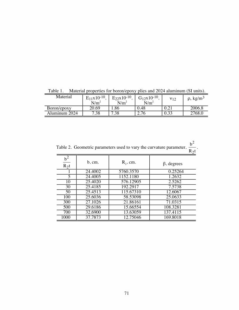
71

Table 1. Material properties for boron/epoxy plies and 2024 aluminum (SI units).Material E11x10-10,

N/m2E22x10-10,

N/m2G12x10-10,

N/m2n12 r, kg/m3

Boron/epoxy 20.69 1.86 0.48 0.21 2006.8Aluminum 2024 7.38 7.38 2.76 0.33 2768.0

Table 2. Geometric parameters used to vary the curvature parameter, bR t

2

2.

bR t

2

2b, cm. R2, cm. b, degrees

1 24.4002 5760.3570 0.252645 24.4005 1152.1180 1.2632

10 25.4020 576.12905 2.526230 25.4185 192.2917 7.573850 25.4513 115.67310 12.6067

100 25.6036 58.53098 25.0633300 27.1026 21.86161 71.0315500 29.6186 15.66554 108.3281700 32.6900 13.63059 137.4115

1000 37.7873 12.75046 169.8018

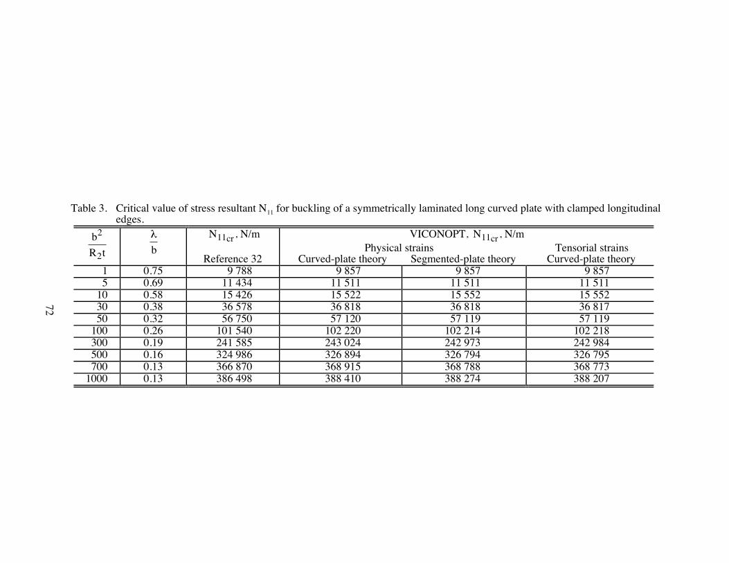
72

Table 3. Critical value of stress resultant N11 for buckling of a symmetrically laminated long curved plate with clamped longitudinaledges.

bR t

2

2

l

b

N cr11 , N/m

Reference 32

VICONOPT, N cr11 , N/mPhysical strains Tensorial strains

Curved-plate theory Segmented-plate theory Curved-plate theory1 0.75 9 788 9 857 9 857 9 8575 0.69 11 434 11 511 11 511 11 511

10 0.58 15 426 15 522 15 552 15 55230 0.38 36 578 36 818 36 818 36 81750 0.32 56 750 57 120 57 119 57 119

100 0.26 101 540 102 220 102 214 102 218300 0.19 241 585 243 024 242 973 242 984500 0.16 324 986 326 894 326 794 326 795700 0.13 366 870 368 915 368 788 368 773

1000 0.13 386 498 388 410 388 274 388 207

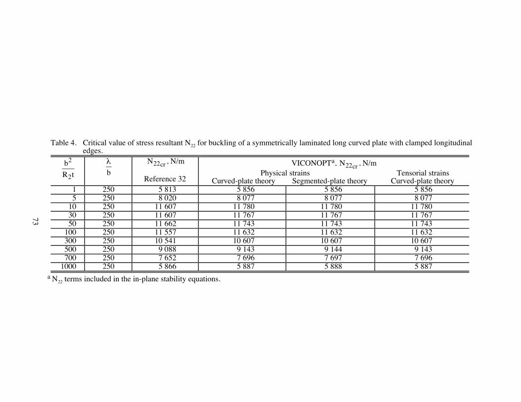
73

Table 4. Critical value of stress resultant N22 for buckling of a symmetrically laminated long curved plate with clamped longitudinaledges.

bR t

2

2

l

b

N cr22 , N/m

Reference 32

VICONOPTa, N cr22 , N/mPhysical strains Tensorial strains

Curved-plate theory Segmented-plate theory Curved-plate theory1 250 5 813 5 856 5 856 5 8565 250 8 020 8 077 8 077 8 077

10 250 11 607 11 780 11 780 11 78030 250 11 607 11 767 11 767 11 76750 250 11 662 11 743 11 743 11 743

100 250 11 557 11 632 11 632 11 632300 250 10 541 10 607 10 607 10 607500 250 9 088 9 143 9 144 9 143700 250 7 652 7 696 7 697 7 696

1000 250 5 866 5 887 5 888 5 887a N22 terms included in the in-plane stability equations.

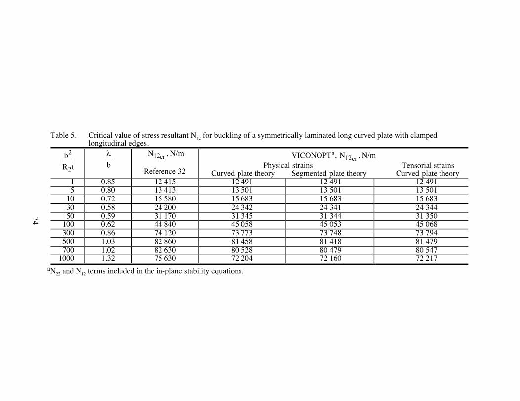
74

Table 5. Critical value of stress resultant N12 for buckling of a symmetrically laminated long curved plate with clampedlongitudinal edges.

bR t

2

2

l

b

N cr12 , N/m

Reference 32

VICONOPTa, N cr12 , N/mPhysical strains Tensorial strains


10 0.72 15 580 15 683 15 683 15 68330 0.58 24 200 24 342 24 341 24 34450 0.59 31 170 31 345 31 344 31 350

100 0.62 44 840 45 058 45 053 45 068300 0.86 74 120 73 773 73 748 73 794500 1.03 82 860 81 458 81 418 81 479700 1.02 82 630 80 528 80 479 80 547

1000 1.32 75 630 72 204 72 160 72 217aN22 and N12 terms included in the in-plane stability equations.

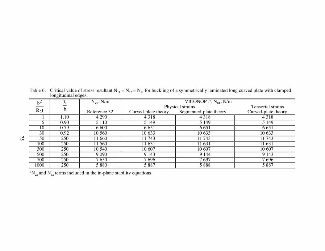
75

Table 6. Critical value of stress resultant N11 = N22 = N12 for buckling of a symmetrically laminated long curved plate with clampedlongitudinal edges.

bR t

2

2

l

b

Ncr, N/m

Reference 32

VICONOPTa, Ncr, N/mPhysical strains Tensorial strains


10 0.79 6 600 6 651 6 651 6 65130 0.92 10 560 10 633 10 633 10 63350 250 11 660 11 743 11 743 11 743

100 250 11 560 11 631 11 631 11 631300 250 10 540 10 607 10 607 10 607500 250 9 090 9 143 9 144 9 143700 250 7 650 7 696 7 697 7 696

1000 250 5 880 5 887 5 888 5 887aN22 and N12 terms included in the in-plane stability equations.

76

Table 7. Critical value of stress resultant N11 for buckling of an unsymmetrically laminated long curved plate with simplysupported longitudinal edges.

N cr11 , N/m VICONOPT, N cr11 , N/mPhysical strains Tensorial strains

Number of B/E plies Reference 32 Curved-plate theory Segmented-plate theory Curved-plate theory2 24 545 24 981 24 969 24 9734 40 000 41 367 41 336 41 3476 63 636 64 331 64 265 64 2898 92 727 94 318 94 198 94 241

10 129 545 131 905 131 708 131 77512 177 273 177 722 177 416 177 51714 232 727 232 424 231 976 232 118

Table 8. Critical value of stress resultant N12 for buckling of an unsymmetrically laminated long curved plate with simplysupported longitudinal edges.

N cr12 , N/m VICONOPT, N cr12 , N/mPhysical strains Tensorial strains

Number of B/E plies Reference 32 Curved-plate theory Segmented-plate theory Curved-plate theory2 7 273 8 070 8 066 8 0704 14 318 16 346 16 336 16 3456 26 818 28 830 28 811 28 8298 43 182 46 229 46 194 46 229

10 66 818 69 265 69 205 69 26412 95 454 98 668 98 573 98 66614 130 454 135 180 135 037 135 177

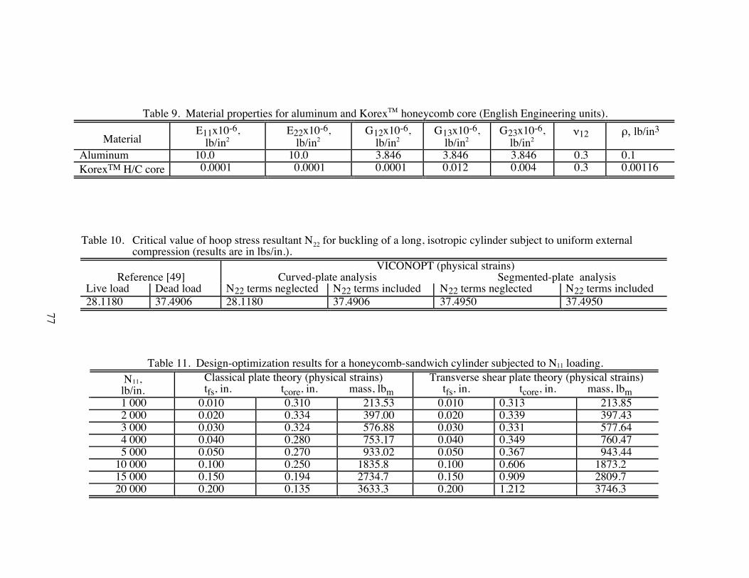
77

Table 9. Material properties for aluminum and KorexTM honeycomb core (English Engineering units).

MaterialE11x10-6,

lb/in2E22x10-6,

lb/in2G12x10-6,

lb/in2G13x10-6,

lb/in2G23x10-6,

lb/in2n12 r, lb/in3

Aluminum 10.0 10.0 3.846 3.846 3.846 0.3 0.1KorexTM H/C core 0.0001 0.0001 0.0001 0.012 0.004 0.3 0.00116

Table 10. Critical value of hoop stress resultant N22 for buckling of a long, isotropic cylinder subject to uniform externalcompression (results are in lbs/in.).

Reference [49]VICONOPT (physical strains)

Curved-plate analysis Segmented-plate analysisLive load Dead load N22 terms neglected N22 terms included N22 terms neglected N22 terms included28.1180 37.4906 28.1180 37.4906 37.4950 37.4950

Table 11. Design-optimization results for a honeycomb-sandwich cylinder subjected to N11 loading.N11,lb/in.

Classical plate theory (physical strains)tfs, in. tcore, in. mass, lbm

Transverse shear plate theory (physical strains)tfs, in. tcore, in. mass, lbm

1 000 0.010 0.310 213.53 0.010 0.313 213.852 000 0.020 0.334 397.00 0.020 0.339 397.433 000 0.030 0.324 576.88 0.030 0.331 577.644 000 0.040 0.280 753.17 0.040 0.349 760.475 000 0.050 0.270 933.02 0.050 0.367 943.44

10 000 0.100 0.250 1835.8 0.100 0.606 1873.215 000 0.150 0.194 2734.7 0.150 0.909 2809.720 000 0.200 0.135 3633.3 0.200 1.212 3746.3

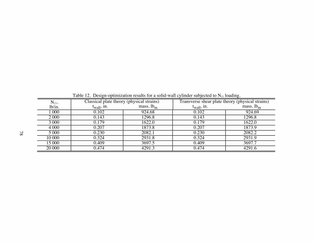
78

Table 12. Design-optimization results for a solid-wall cylinder subjected to N11 loading.N11,lb/in.

Classical plate theory (physical strains)twall, in. mass, lbm

Transverse shear plate theory (physical strains)twall, in. mass, lbm

1 000 0.102 924.68 0.102 924.692 000 0.143 1296.8 0.143 1296.83 000 0.179 1622.0 0.179 1622.04 000 0.207 1873.8 0.207 1873.95 000 0.230 2082.1 0.230 2082.2

10 000 0.324 2931.8 0.324 2931.915 000 0.409 3697.5 0.409 3697.720 000 0.474 4291.3 0.474 4291.6

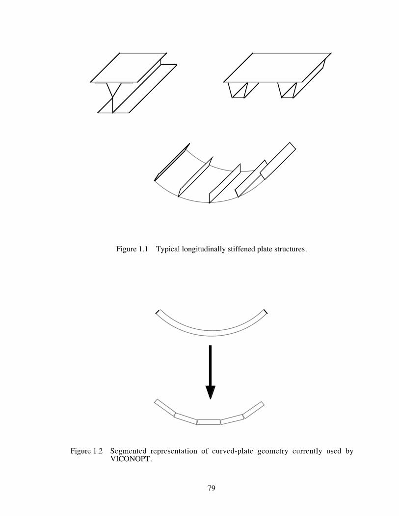
79

Figure 1.1 Typical longitudinally stiffened plate structures.

Figure 1.2 Segmented representation of curved-plate geometry currently used byVICONOPT.

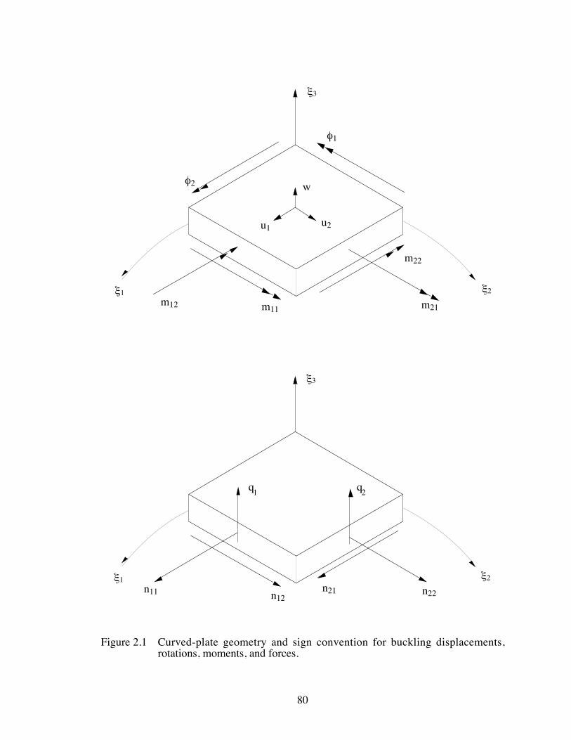
80

x1

w

u1 u2

f2

f1

m12 m11

m22

m21

n11 n12n21 n22

q1 q2

x3

x2

x1

x3

x2

Figure 2.1 Curved-plate geometry and sign convention for buckling displacements,rotations, moments, and forces.

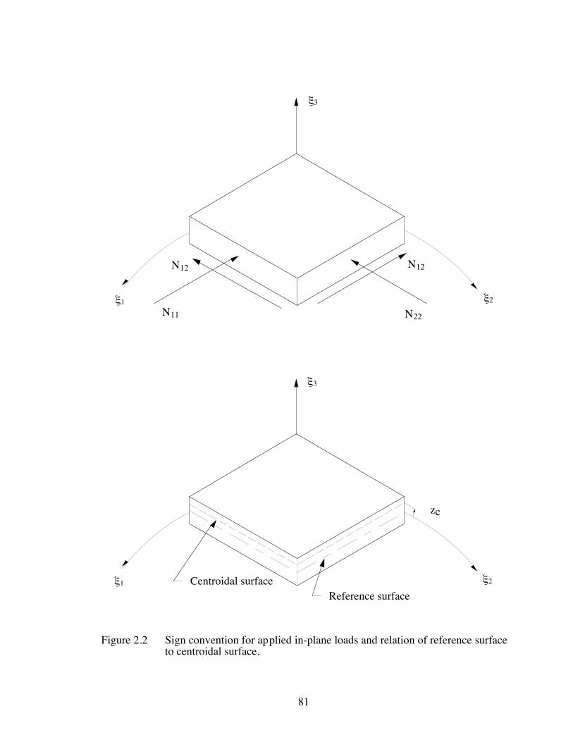
81

x1

x3

x2

x1

x3

x2Centroidal surface Reference surface

N11

N12

N22

N12

zc

Figure 2.2 Sign convention for applied in-plane loads and relation of reference surfaceto centroidal surface.

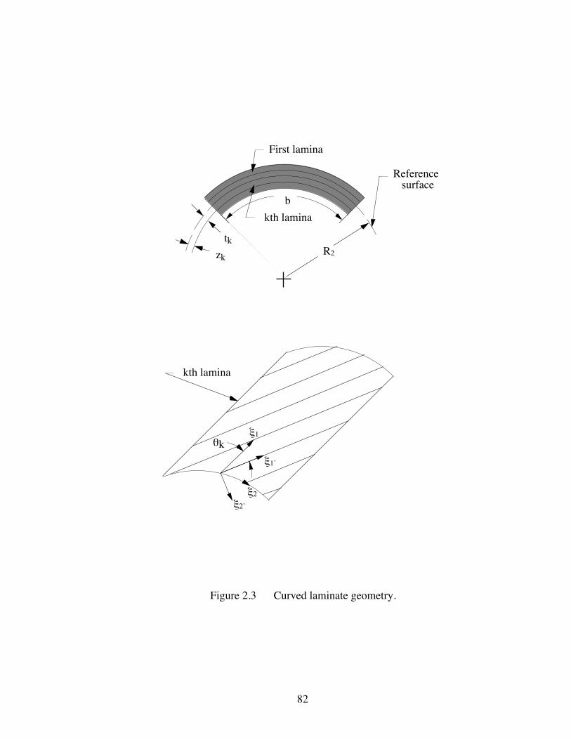
82

First lamina

kth lamina

R2zk

tk

kth lamina

x1Õ

x1qk

Reference surface

b

x2

x2Õ

Figure 2.3 Curved laminate geometry.

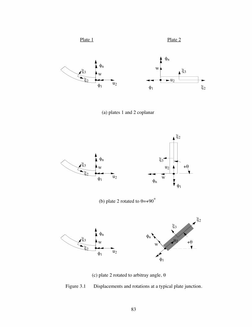
83

x3

x2 u2f1

w

fn

x3

x2 u2f1

w

fn

x3

x2 u2f1

w

fn

+q

+q

x3

x2

u2

f1

w

fn

x3

fnw

f1

u2

x2

u2w

fn

x3

f1

Plate 1 Plate 2

(a) plates 1 and 2 coplanar

(b) plate 2 rotated to q=+90¡

(c) plate 2 rotated to arbitray angle, q

x2

Figure 3.1 Displacements and rotations at a typical plate junction.

84

E Û= Û10.0 x 106 psin12 �= Û0.33

r �= Û0.1 lb/in.3

60.0 in.

0.10 in. N11

Figure 4.1 Long isotropic (aluminum) cylinder subjected to uniaxial compression.

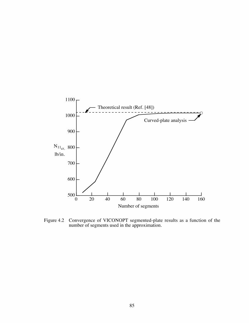
85

1100

1000

900

800

700

600

500160140120100806040200

N11cr,

Number of segments

Theoretical result (Ref. [48])

Curved-plate analysis

lb/in.

Figure 4.2 Convergence of VICONOPT segmented-plate results as a function of thenumber of segments used in the approximation.

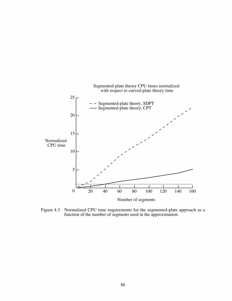
86

25

20

15

10

5

16014012010080604020

Segmented-plate theory, SDPT Segmented-plate theory, CPT

Normalized CPU time

Segmented-plate theory CPU times normalized with respect to curved-plate theory time

Number of segments

0

Figure 4.3 Normalized CPU time requirements for the segmented-plate approach as afunction of the number of segments used in the approximation.

87

N11

N22

N12x1, u1

x2, u2x3, w

Figure 4.4 Positive applied in-plane loads on a long, curved plate.

25.4 cm

b

b

R2

Boron/epoxy[0/90/±45]s

nominal ply thickness = 0.014 cm.

Figure 4.5 Symmetrically laminated curved plate with clamped longitudinal edgessubjected to applied in-plane loads.

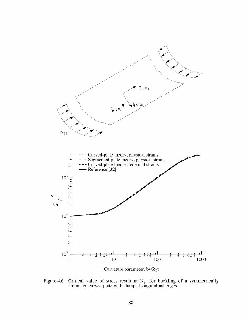
88

103

2

3

456

104

2

3

456

105

2

34

12 3 4 5 6 7

102 3 4 5 6 7

1002 3 4 5 6 7

1000

Curved-plate theory, physical strains Segmented-plate theory, physical strains Curved-plate theory, tensorial strains Reference [32]

N11cr,

N/m

Curvature parameter, b2/R2t

N11

x1, u1

x2, u2x3, w

Figure 4.6 Critical value of stress resultant N11 for buckling of a symmetricallylaminated curved plate with clamped longitudinal edges.

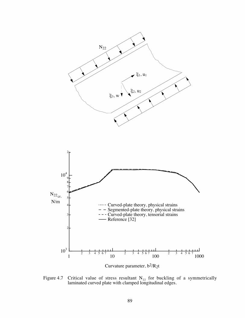
89

103

2

3

4

5

6

789

104

2

12 3 4 5 6 7

102 3 4 5 6 7

1002 3 4 5 6 7

1000


N22cr,

N/m


N22

x1, u1

x2, u2x3, w


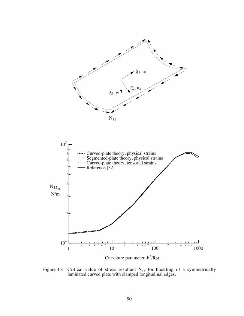
90

104

2

3

4

5

6

7

8

9105

12 3 4 5 6 7

102 3 4 5 6 7

1002 3 4 5 6 7

1000


N12cr,

N/m


N12

x1, u1

x2, u2x3, w


91

103

2

3

4

5

6

789

104

2

12 3 4 5 6 7

102 3 4 5 6 7

1002 3 4 5 6 7

1000


Ncr,

N/m


N11

N22

N12x1, u1

x2, u2x3, w

Figure 4.9 Critical value of stress resultant N11=N22=N12 for buckling of a symmetricallylaminated curved plate with clamped longitudinal edges.

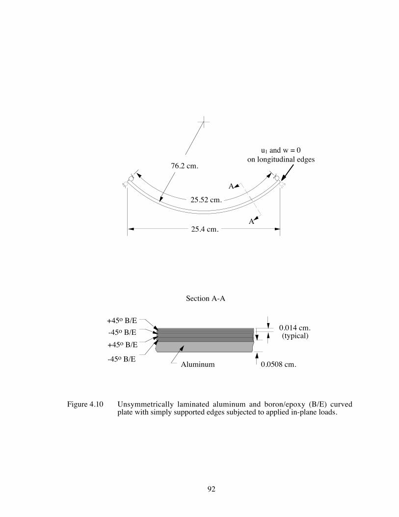
92

0.014 cm.(typical)

0.0508 cm.Aluminum-45o B/E

+45o B/E

-45o B/E

+45o B/E

Section A-A

76.2 cm.

25.4 cm.

A

A

25.52 cm.

u1 and w = 0on longitudinal edges

Figure 4.10 Unsymmetrically laminated aluminum and boron/epoxy (B/E) curvedplate with simply supported edges subjected to applied in-plane loads.

93

250,000

200,000

150,000

100,000

50,000

1412108642


N11cr,

N/m

Number of boron/epoxy plies

N11

0

x1, u1

x2, u2x3, w

Figure 4.11 Critical value of stress resultant N11 for buckling of an unsymmetricallylaminated aluminum and boron/epoxy (B/E) curved plate with simplysupported longitudinal edges.

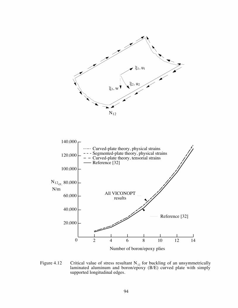
94

140,000

120,000

100,000

80,000

60,000

40,000

20,000

1412108642


N12cr,

N/m

Number of boron/epoxy plies

N12

Reference [32]

All VICONOPTresults

0

x1, u1

x2, u2x3, w

Figure 4.12 Critical value of stress resultant N12 for buckling of an unsymmetricallylaminated aluminum and boron/epoxy (B/E) curved plate with simplysupported longitudinal edges.

95

t = 0.1 in.

N22, equivalent hoop load

u1 restrained along longitudinal edges

R2 = 10.0 in.

E Û= Û10.0 x 106 psin12 �= Û0.33

r �= Û0.1 lb/in3

N22, equivalent hoop load

External pressure, p

Figure 4.13 Isotropic (aluminum) long cylindrical tube subjected to uniform externalpressure loading.

96

R2=60 in

240 in.

N11

A

A

Section A-ASolid wall

Section A-AHoneycomb sandwich

Aluminum

Aluminumfacesheets

KorexTM

honeycomb core

0.1 in. nom.

0.1 in. nom.

0.5 in. nom.

Simply supported ends

Figure 4.14 Cylindrical shell subjected to uniform axial compression (N11 loading).

97

20,00015,00010,0005,000

4,500

4,000

3,500

3,000

2,500

2,000

1,500

1,000

500

Solid wall, classical and transverse shear H/C sandwich, transverse shear H/C sandwich, classical

0

Mass, lbm

Applied N11 loading, lb/in.

N11

240 in.

R2=60 in.

tcore = 0.135 in.

tcore = 1.212 in.

Figure 4.15 Optimized cylinder mass as a function of the applied loading for acylindrical shell.

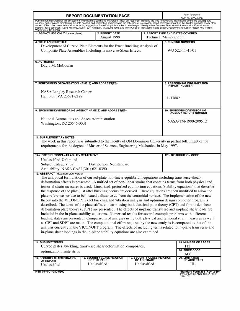
REPORT DOCUMENTATION PAGE Form ApprovedOMB No. 0704-0188

Public reporting burden for this collection of information is estimated to average 1 hour per response, including the time for reviewing instructions, searching existing datasources, gathering and maintaining the data needed, and completing and reviewing the collection of information. Send comments regarding this burden estimate or any otheraspect of this collection of information, including suggestions for reducing this burden, to Washington Headquarters Services, Directorate for Information Operations andReports, 1215 Jefferson Davis Highway, Suite 1204, Arlington, VA 22202-4302, and to the Office of Management and Budget, Paperwork Reduction Project (0704-0188),Washington, DC 20503.1. AGENCY USE ONLY (Leave blank) 2. REPORT DATE

August 19993. REPORT TYPE AND DATES COVERED

Technical Memorandum4. TITLE AND SUBTITLE

Development of Curved-Plate Elements for the Exact Buckling Analysis ofComposite Plate Assemblies Including Transverse-Shear Effects

5. FUNDING NUMBERS

WU 522-11-41-01

6. AUTHOR(S)David M. McGowan

7. PERFORMING ORGANIZATION NAME(S) AND ADDRESS(ES)

NASA Langley Research CenterHampton, VA 23681-2199

8. PERFORMING ORGANIZATIONREPORT NUMBER

L-17882

9. SPONSORING/MONITORING AGENCY NAME(S) AND ADDRESS(ES)

National Aeronautics and Space AdministrationWashington, DC 20546-0001

10. SPONSORING/MONITORINGAGENCY REPORT NUMBER

NASA/TM-1999-209512

11. SUPPLEMENTARY NOTESThe work in this report was submitted to the faculty of Old Dominion University in partial fulfillment of therequirements for the degree of Master of Science, Engineering Mechanics, in May 1997.

12a. DISTRIBUTION/AVAILABILITY STATEMENTUnclassified-UnlimitedSubject Category 39 Distribution: NonstandardAvailability: NASA CASI (301) 621-0390

12b. DISTRIBUTION CODE

13. ABSTRACT (Maximum 200 words)The analytical formulation of curved-plate non-linear equilibrium equations including transverse-shear-deformation effects is presented. A unified set of non-linear strains that contains terms from both physical andtensorial strain measures is used. Linearized, perturbed equilibrium equations (stability equations) that describethe response of the plate just after buckling occurs are derived. These equations are then modified to allow theplate reference surface to be located a distance zc from the centroidal surface. The implementation of the newtheory into the VICONOPT exact buckling and vibration analysis and optimum design computer program isdescribed. The terms of the plate stiffness matrix using both classical plate theory (CPT) and first-order shear-deformation plate theory (SDPT) are presented. The effects of in-plane transverse and in-plane shear loads areincluded in the in-plane stability equations. Numerical results for several example problems with differentloading states are presented. Comparisons of analyses using both physical and tensorial strain measures as wellas CPT and SDPT are made. The computational effort required by the new analysis is compared to that of theanalysis currently in the VICONOPT program. The effects of including terms related to in-plane transverse andin-plane shear loadings in the in-plane stability equations are also examined.

14. SUBJECT TERMSCurved plates, buckling, transverse shear deformation, composites,

15. NUMBER OF PAGES112

optimization, finite strips 16. PRICE CODEA06

17. SEC U RITY CL ASSIF IC AT ION O F REPO R TUnclassified

18. SEC U RITY CL ASSIF IC AT ION O F TH IS PA GEUnclassified

19. SECURITY CLASSIFICATION OF ABSTRACTUnclassified

20. LIMITATION OF ABSTRACT UL

NSN 7540-01-280-5500 Standard Form 298 (Rev. 2-89)Prescribed by ANSI Std. Z-39-18298-102

Development of Curved-Plate Elements for the Exact ...mln/ltrs-pdfs/NASA-99-tm209512.pdf · August...

Documents

Transcript of Development of Curved-Plate Elements for the Exact ...mln/ltrs-pdfs/NASA-99-tm209512.pdf · August...