Development of Asphalt Dynamic Modulus Master Curve Using...
65
Development of Asphalt Dynamic Modulus Master Curve Using Falling Weight Deflectometer Measurements Final Report June 2014 Sponsored by Iowa Highway Research Board (IHRB Project TR-659) Iowa Department of Transportation (InTrans Project 13-471)
Transcript of Development of Asphalt Dynamic Modulus Master Curve Using...

Development of Asphalt Dynamic Modulus Master Curve Using Falling Weight Deflectometer MeasurementsFinal ReportJune 2014
Sponsored byIowa Highway Research Board(IHRB Project TR-659)Iowa Department of Transportation(InTrans Project 13-471)
About the Institute for Transportation
The mission of the Institute for Transportation (InTrans) at Iowa State University is to develop and implement innovative methods, materials, and technologies for improving transportation efficiency, safety, reliability, and sustainability while improving the learning environment of students, faculty, and staff in transportation-related fields.
Disclaimer Notice
The contents of this report reflect the views of the authors, who are responsible for the facts and the accuracy of the information presented herein. The opinions, findings and conclusions expressed in this publication are those of the authors and not necessarily those of the sponsors.
The sponsors assume no liability for the contents or use of the information contained in this document. This report does not constitute a standard, specification, or regulation.
The sponsors do not endorse products or manufacturers. Trademarks or manufacturers’ names appear in this report only because they are considered essential to the objective of the document.
Non-Discrimination Statement
Iowa State University does not discriminate on the basis of race, color, age, ethnicity, religion, national origin, pregnancy, sexual orientation, gender identity, genetic information, sex, marital status, disability, or status as a U.S. veteran. Inquiries regarding non-discrimination policies may be directed to Office of Equal Opportunity, Title IX/ADA Coordinator, and Affirmative Action Officer, 3350 Beardshear Hall, Ames, Iowa 50011, 515-294-7612, email [email protected].
Iowa Department of Transportation Statements
Federal and state laws prohibit employment and/or public accommodation discrimination on the basis of age, color, creed, disability, gender identity, national origin, pregnancy, race, religion, sex, sexual orientation or veteran’s status. If you believe you have been discriminated against, please contact the Iowa Civil Rights Commission at 800-457-4416 or the Iowa Department of Transportation affirmative action officer. If you need accommodations because of a disability to access the Iowa Department of Transportation’s services, contact the agency’s affirmative action officer at 800-262-0003.
The preparation of this report was financed in part through funds provided by the Iowa Department of Transportation through its “Second Revised Agreement for the Management of Research Conducted by Iowa State University for the Iowa Department of Transportation” and its amendments.
The opinions, findings, and conclusions expressed in this publication are those of the authors and not necessarily those of the Iowa Department of Transportation.
Technical Report Documentation Page
1. Report No. 2. Government Accession No. 3. Recipient’s Catalog No.
IHRB Project TR-659
4. Title and Subtitle 5. Report Date
Development of Asphalt Dynamic Modulus Master Curve Using Falling
Weight Deflectometer Measurements
June 2014
6. Performing Organization Code
7. Author(s) 8. Performing Organization Report No.
Kasthurirangan Gopalakrishnan, Sunghwan Kim, Halil Ceylan, and Orhan
Kaya
InTrans Project 13-471
9. Performing Organization Name and Address 10. Work Unit No. (TRAIS)
Institute for Transportation
Iowa State University
2711 South Loop Drive, Suite 4700
Ames, IA 50010-8664
11. Contract or Grant No.
12. Sponsoring Organization Name and Address 13. Type of Report and Period Covered
Iowa Highway Research Board
Iowa Department of Transportation
800 Lincoln Way
Ames, IA 50010
Final Report
14. Sponsoring Agency Code
TR-659
15. Supplementary Notes
Visit www.intrans.iastate.edu for color pdfs of this and other research reports.
16. Abstract
The asphalt concrete (AC) dynamic modulus (|E*|) is a key design parameter in mechanistic-based pavement design
methodologies such as the American Association of State Highway and Transportation Officials (AASHTO) MEPDG/Pavement-
ME Design. The objective of this feasibility study was to develop frameworks for predicting the AC |E*| master curve from
falling weight deflectometer (FWD) deflection-time history data collected by the Iowa Department of Transportation (Iowa
DOT). A neural networks (NN) methodology was developed based on a synthetically generated viscoelastic forward solutions
database to predict AC relaxation modulus (E(t)) master curve coefficients from FWD deflection-time history data. According to
the theory of viscoelasticity, if AC relaxation modulus, E(t), is known, |E*| can be calculated (and vice versa) through numerical
inter-conversion procedures. Several case studies focusing on full-depth AC pavements were conducted to isolate potential
backcalculation issues that are only related to the modulus master curve of the AC layer. For the proof-of-concept demonstration,
a comprehensive full-depth AC analysis was carried out through 10,000 batch simulations using a viscoelastic forward analysis
program. Anomalies were detected in the comprehensive raw synthetic database and were eliminated through imposition of
certain constraints involving the sigmoid master curve coefficients.
The surrogate forward modeling results showed that NNs are able to predict deflection-time histories from E(t) master curve
coefficients and other layer properties very well. The NN inverse modeling results demonstrated the potential of NNs to
backcalculate the E(t) master curve coefficients from single-drop FWD deflection-time history data, although the current
prediction accuracies are not sufficient to recommend these models for practical implementation. Considering the complex nature
of the problem investigated with many uncertainties involved, including the possible presence of dynamics during FWD testing
(related to the presence and depth of stiff layer, inertial and wave propagation effects, etc.), the limitations of current FWD
technology (integration errors, truncation issues, etc.), and the need for a rapid and simplified approach for routine
implementation, future research recommendations have been provided making a strong case for an expanded research study.
17. Key Words 18. Distribution Statement
dynamic modulus—FWD—HMA— master curve—neural networks—
relaxation modulus—viscoelastic
No restrictions.
19. Security Classification (of this
report)
20. Security Classification (of this
page)
21. No. of Pages 22. Price
Unclassified. Unclassified. 63 NA
Form DOT F 1700.7 (8-72) Reproduction of completed page authorized

DEVELOPMENT OF ASPHALT DYNAMIC MODULUS
MASTER CURVE USING FALLING WEIGHT
DEFLECTOMETER MEASUREMENTS
Final Report
June 2014
Principal Investigator
Halil Ceylan
Associate Professor, Civil, Construction, and Environmental Engineering (CCEE)
Director, Program for Sustainable Pavement Engineering and Research (PROSPER)
Institute for Transportation, Iowa State University
Co-Principal Investigators
Kasthurirangan Gopalakrishnan
Senior Research Scientist, CCEE, Iowa State University
Sunghwan Kim
Research Assistant Professor, CCEE, Iowa State University
Research Assistant
Orhan Kaya
Authors
Kasthurirangan Gopalakrishnan, Sunghwan Kim, Halil Ceylan, and Orhan Kaya
Sponsored by the Iowa Highway Research Board
(IHRB Project TR-659) and
the Iowa Department of Transportation
(InTrans Project 13-471)
Preparation of this report was financed in part
through funds provided by the Iowa Department of Transportation
through its Research Management Agreement with the
Institute for Transportation
A report from
Institute for Transportation
Iowa State University
2711 South Loop Drive, Suite 4700
Ames, IA 50010-8664
Phone: 515-294-8103 Fax: 515-294-0467
www.intrans.iastate.edu

v
TABLE OF CONTENTS
ACKNOWLEDGMENTS ............................................................................................................. ix
EXECUTIVE SUMMARY ........................................................................................................... xi
INTRODUCTION ...........................................................................................................................1
Background ..........................................................................................................................1 Objectives and Scope ...........................................................................................................2
OVERVIEW OF ASPHALT MASTER CURVE AND FWD BACKCALCULATION ...............3
Dynamic Modulus (E*) Master Curve of Asphalt Mixtures ..............................................3 FWD Backcalculation ..........................................................................................................6
DEVELOPMENET OF FRAMEWORK FOR DERIVING AC MASTER CURVE FROM FWD
DATA ................................................................................................................................12
Case Studies .......................................................................................................................15
PROOF-OF-CONCEPT DEMONSTRATION:COMPREHENSIVE FULL-DEPTH AC
PAVEMENT ANALYSIS .................................................................................................25
Development of Comprehensive Synthetic Database ........................................................25 Synthetic Database: Data Pre-processing ..........................................................................27 Neural Networks Forward Modeling .................................................................................31
Neural Networks Inverse Modeling Considering only D0, D8, and D12 ..........................33 Neural Networks Inverse Modeling Considering Data from all FWD Sensors: Partial
Pulse (Pre-Peak) Time Histories ........................................................................................37 Neural Networks Inverse Modeling Considering Data from all FWD Sensors: Full Pulse
Time Histories ....................................................................................................................39
SUMMARY AND CONCLUSIONS ............................................................................................41
FUTURE RESEARCH RECOMMENDATIONS ........................................................................43
REFERENCES ..............................................................................................................................47

vii
LIST OF FIGURES
Figure 1. AC layer damage master curve computation in MEPDG/Pavement ME Design Level 1
(NCHRP 2004).....................................................................................................................2
Figure 2. Laboratory AC dynamic modulus (E*) test protocol ......................................................4 Figure 3. Illustration of typical FWD deflection measurements (Goktepe et al. 2006) ...................7 Figure 4. Schematic representation of the frequency domain fitting for dynamic load
backcalculation (Goktepe et al. 2006) .................................................................................9 Figure 5. Schematic representation of dynamic time domain fitting for dynamic load
backcalculation (Goktepe et al. 2006) .................................................................................9 Figure 6. Schematic of synthetic database development approach using the viscoelastic forward
analysis tool .......................................................................................................................13
Figure 7. Schematic of neural networks approach to predict AC E(t) master curve from FWD
deflection-time history data ...............................................................................................14
Figure 8. Compound graphs summarizing descriptive statistics, histograms, box plots, and
normal probability plots for variable inputs in the synthetic datasets ...............................17 Figure 9. Typical deflection-time history generated by the VE forward analysis program at one
location. Only the left half of the deflection-time history data was considered in NN
inverse modeling in this study. ..........................................................................................18 Figure 10. Box and whisker plots of D0, D8, and D12 deflection-time histories generated by VE
forward analysis simulations for the case studies ..............................................................18 Figure 11. NN prediction of E(t) master curve coefficients from D0 time history data using 100
datasets (case study #1): (a) c1, (b) c2, (c) c3, (d) c4 ........................................................21
Figure 12. NN prediction of E(t) master curve coefficients from D0, D8, and D12 time history
data using 100 datasets (case study #2): (a) c1, (b) c2, (c) c3, (d) c4 ................................22
Figure 13. NN prediction of E(t) master curve coefficients from differences in magnitudes
between D0 and D12 time history data (SCI) using 100 datasets (case study #3): (a) c1,
(b) c2, (c) c3, (d) c4 ...........................................................................................................23 Figure 14. Graphical statistical summaries of Tac, Hac, and Esub in the comprehensive raw
synthetic database ..............................................................................................................26
Figure 15. Graphical statistical summaries of c1, c2, c3, and c4 in the comprehensive raw
synthetic database ..............................................................................................................26
Figure 16. D0 deflection-time history (from time interval 1 to 20) outputs from 10,000 VE
forward analysis simulations..............................................................................................27 Figure 17. D8 deflection-time history (from time interval 1 to 20) outputs from 10,000 VE
forward analysis simulations..............................................................................................28 Figure 18. D12 deflection-time history (from time interval 1 to 20) outputs from 10,000 VE
forward analysis simulations..............................................................................................28
Figure 19. Graphical statistical summaries of Tac, Hac, and Esub in the processed synthetic
database ..............................................................................................................................29 Figure 20. Graphical statistical summaries of c1, c2, c3, and c4 in the processed synthetic
database ..............................................................................................................................29 Figure 21. D0 deflection-time history (from time interval 1 to 20) outputs in the processed
synthetic database ..............................................................................................................30 Figure 22. D8 deflection-time history (from time interval 1 to 20) outputs in the processed
synthetic database ..............................................................................................................30
viii
Figure 23. D12 deflection-time history (from time interval 1 to 20) outputs in the processed
synthetic database ..............................................................................................................31 Figure 24. NN forward modeling regression results for predicting D0 deflection-time history data
from E(t) master curve coefficients ...................................................................................32
Figure 25. NN forward modeling regression results for predicting D8 deflection-time history data
from E(t) master curve coefficients ...................................................................................32 Figure 26. NN forward modeling regression results for predicting D12 deflection-time history
data from E(t) master curve coefficients ............................................................................33 Figure 27. Inputs, outputs, and generic network architecture details for the NN inverse mapping
models considering only D0, D8, and D12 ........................................................................33 Figure 28. NN prediction of E(t) master curve coefficient, c1, from D0, D8, and D12 time history
data using the processed synthetic database ......................................................................34 Figure 29. NN prediction of E(t) master curve coefficient, c2, from D0, D8, and D12 time history
data using the processed synthetic database ......................................................................35 Figure 30. NN prediction of E(t) master curve coefficient, c3, from D0, D8, and D12 time history
data using the processed synthetic database ......................................................................36 Figure 31. NN prediction of E(t) master curve coefficient, c4, from D0, D8, and D12 time history
data using the processed synthetic database ......................................................................37 Figure 32. Inputs, outputs, and generic network architecture details for the NN inverse mapping
models considering data from all FWD sensors and pre-peak time history data ...............38
Figure 33. An example of time delay (dynamic behavior) in FWD deflection-time histories (top)
and the shifting of deflection pulses to the left (bottom) (Kutay et al. 2011) ....................43
Figure 34. Overall proposed approach for backcalculating the AC E(t) master curve from FWD
deflection-time history data using an evolutionary global optimization search scheme ...45
LIST OF TABLES
Table 1. Summary of input ranges used in the generation of 100 VE forward analysis scenarios
for case studies ...................................................................................................................16 Table 2. Summary of input ranges used in the generation of 10,000 VE forward analysis
scenarios for comprehensive full-depth AC analysis.........................................................25 Table 3. NN prediction of E(t) master curve coefficients, c1, c2, c3, and c4, from D0, D8, D12,
D18, D24, D36, D48, D60, and D72 pre-peak deflection-time history data .....................39 Table 4. NN prediction of E(t) master curve coefficients, c1, c2, c3, and c4, from D0, D8, D12,
D18, D24, D36, D48, D60, and D72 full pulse deflection-time history data ....................40

ix
ACKNOWLEDGMENTS
The authors would like to thank the Iowa Highway Research Board (IHRB) and the Iowa
Department of Transportation (Iowa DOT) for sponsoring this research. The project technical
advisory committee (TAC) members from the Iowa DOT, including Scott Schram, Chris Brakke,
Ben Behnami, and Jason Omundson, are gratefully acknowledged for their guidance, support,
and direction throughout the research.
The authors would like to extend their sincerest appreciation to Emin Kutay, Karim Chatti, and
Sudhir Varma at Michigan State University (MSU) for their timely technical support and
detailed discussions on viscoelastic forward analysis and dynamic backcalculation.

xi
EXECUTIVE SUMMARY
The asphalt concrete (AC) dynamic modulus (|E*|) is a key design parameter in the American
Association of State Highway and Transportation Officials (AASHTO) Mechanistic-Empirical
Pavement Design Guide (MEPDG)/AASHTOWare Pavement-ME Design. The standard
laboratory procedures for AC dynamic modulus testing and development of a master curve
require time and considerable resources. The objective of this feasibility study was to develop
frameworks for predicting the AC relaxation modulus (E(t)) or dynamic modulus master curve
from routinely collected falling weight deflectometer (FWD) time history data. According to the
theory of viscoelasticity, if the AC relaxation modulus, E(t), is known, |E*| can be calculated
(and vice versa) through numerical inter-conversion procedures.
The overall research approach involved the following steps:
Conduct numerous viscoelastic (VE) forward analysis simulations by varying E(t) master
curve coefficients, shift factors, pavement temperatures, and other layer properties
Extract simulation inputs and outputs and assemble a synthetic database
Train, validate, and test neural network (NN) inverse mapping models to predict E(t) master
curve coefficients from single-drop FWD deflection-time histories
A computationally efficient VE forward analysis program developed by Michigan State
University (MSU) researchers was adopted in this study to generate the synthetic database. The
VE forward analysis program accepts pavement temperature and layer properties (AC E(t)
master curve, Eb/sub, h, μ,) and outputs surface deflection-time histories. Several case studies
were conducted to establish detailed frameworks for predicting the AC E(t) master curve from
single-drop FWD time history data. Case studies focused on full-depth AC pavements as a first
step to isolate potential backcalculation issues that are only related to the modulus master curve
of the AC layer. For the proof-of-concept demonstration, a comprehensive full-depth AC
analysis was carried out through 10,000 batch simulations of a VE forward analysis program.
Anomalies were detected in the comprehensive raw synthetic database and were eliminated
through imposition of certain constraints on the sum of E(t) sigmoid coefficients, c1 + c2.
Except for the first two or three time intervals, deflection-time histories at all other time intervals
considered in the analysis were predicted by NNs with very high accuracy (R-values greater than
0.97). The NN inverse modeling results demonstrated the potential of NNs to predict the E(t)
master curve coefficients from single-drop FWD deflection-time history data. However, the
current prediction accuracies are not sufficient to recommend these models for practical
implementation.
Considering the complex nature of the problem with many uncertainties involved, including the
possible presence of dynamics during FWD testing (related to the presence and depth of stiff
layer, inertial and wave propagation effects, etc.), the limitations of current FWD technology
(integration errors, truncation issues, etc.), and the need for a rapid and simplified approach for

xii
routine implementation, future research recommendations have been provided that make a strong
case for an expanded research study.

1
INTRODUCTION
Background
The new American Association of State Highway and Transportation Officials (AASHTO)
pavement design guide (Mechanistic-Empirical Pavement Design Guide [MEPDG]) and the
associated software (AASHTOWare Pavement ME Design, formerly known as DARWin ME)
represents a major advancement in pavement design and analysis. The MEPDG employs the
principle of a master curve based on time-temperature superposition principles to characterize
the viscoelastic-plastic property of asphalt materials. The MEPDG recommends the use of
asphalt dynamic modulus, |E*|, as the design parameter. The dynamic modulus master curve is
constructed from multiple values of measured dynamic modulus at different temperature and
frequency conditions. The standard laboratory procedure for dynamic modulus testing requires
time and considerable resources.
State agencies, faced with the challenge of implementing the MEPDG/Pavement ME Design, are
looking to field testing as a possibility for obtaining values for use in new design. The laboratory
testing requirements are extensive, and the idea of obtaining default regional properties for
specific materials and structures in the field is attractive. Falling weight deflectometer (FWD)
testing has become the predominant method for characterizing in situ material properties for
rehabilitation design. The state of the practice in FWD analysis involves static backcalculation of
pavement layer moduli, although FWD measurements capture the entire time history of
deflections under dynamic loading conditions.
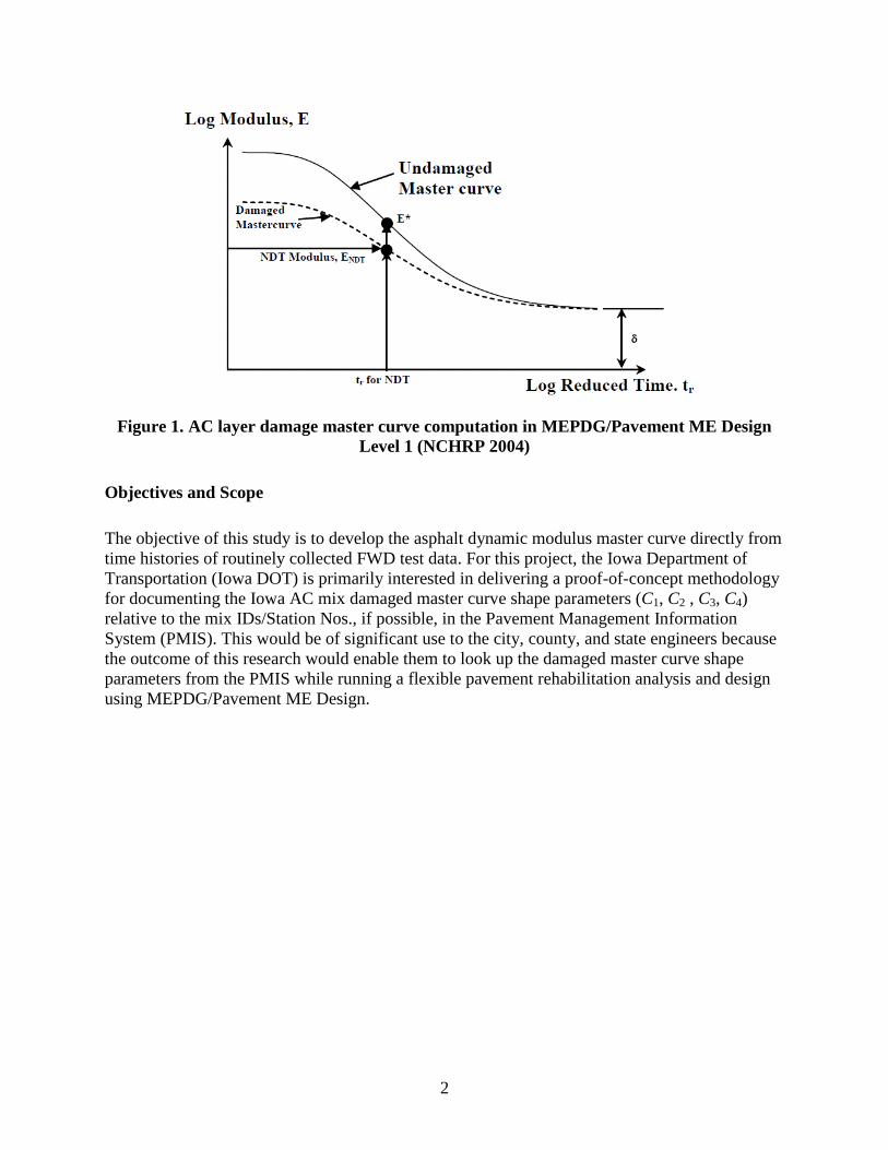
In the MEPDG/Pavement ME Design flexible pavement rehabilitation analysis (NCHRP 2004,
ASHTO 2008, AASHTO 2012), the pre-overlay damaged master curve of the existing asphalt
concrete (AC) layer is determined by first calculating an “undamaged” modulus and then
adjusting this modulus for damage using the pre-overlay condition. The undamaged AC master
curve is derived from its aggregate gradation and laboratory-tested asphalt binder
properties/asphalt binder grade using Witczak’s dynamic modulus predictive equation. Both
aggregate gradation and asphalt binder properties/asphalt binder grade may be obtained from
construction records or testing of field-cored samples. To characterize the damage in the existing
pavement at the time of overlay, MEPDG/Pavement ME Design allows the input of
backcalculated moduli from nondestructive testing (NDT) with frequency and temperature under
the Level 1 rehabilitation input option. The process is shown schematically in Figure 1.
If the damaged |E*| master curve of the AC in an in-service pavement can be derived from the
time histories of routinely collected FWD deflection data, it would not only save lab time and
resources, but it could also lead to a more accurate prediction of the pavement’s remaining
service life.
2
Figure 1. AC layer damage master curve computation in MEPDG/Pavement ME Design
Level 1 (NCHRP 2004)
Objectives and Scope
The objective of this study is to develop the asphalt dynamic modulus master curve directly from
time histories of routinely collected FWD test data. For this project, the Iowa Department of
Transportation (Iowa DOT) is primarily interested in delivering a proof-of-concept methodology
for documenting the Iowa AC mix damaged master curve shape parameters (C1, C2 , C3, C4)
relative to the mix IDs/Station Nos., if possible, in the Pavement Management Information
System (PMIS). This would be of significant use to the city, county, and state engineers because
the outcome of this research would enable them to look up the damaged master curve shape
parameters from the PMIS while running a flexible pavement rehabilitation analysis and design
using MEPDG/Pavement ME Design.

3
OVERVIEW OF ASPHALT MASTER CURVE AND FWD BACKCALCULATION
Dynamic Modulus (E*) Master Curve of Asphalt Mixtures
The E* value is one of the asphalt mixture stiffness measures that determines the strains and
displacements in a flexible pavement structure as it is loaded or unloaded. The asphalt mixture
stiffness can alternatively be characterized via the flexural stiffness, creep compliance, relaxation modulus, and resilient modulus. The E* value is one of the primary material property inputs required in the MEPDG/Pavement ME Design procedure (NCHRP 2004,
ASHTO 2008, AASHTO 2012).
Definition of AC Dynamic Modulus (E*)
The definition of E* comes from the complex modulus (E*), consisting of both a real and
imaginary component, as shown in the following equation:
21* iEEE (1)
Here, 1i , E1 is the storage modulus part of the complex modulus, and E2 is the loss
modulus part of the complex modulus. The E* value can be mathematically defined as the
magnitude of the complex modulus, as shown in the following equation:
2
2
2
1* EEE (2)
E* is also determined experimentally as the ratio of the applied stress amplitude to the strain
response amplitude under a sinusoidal loading, as shown in the following equation:
o
oE
*
(3)
Here, 0 is the average stress amplitude and 0 is the average recoverable strain. The E* value
of the asphalt mixture is strongly dependent upon temperature (T) and loading rate, defined
either in terms of frequency (f) or load time (t).
Figure 2 illustrates how the dynamic modulus can be determined in the laboratory. The peak
points of applied load and strain response at each of the test frequencies and temperatures are
utilized to determine the dynamic modulus under given conditions. The measured dynamic
moduli at different frequencies and temperatures are utilized to construct the AC master curve.
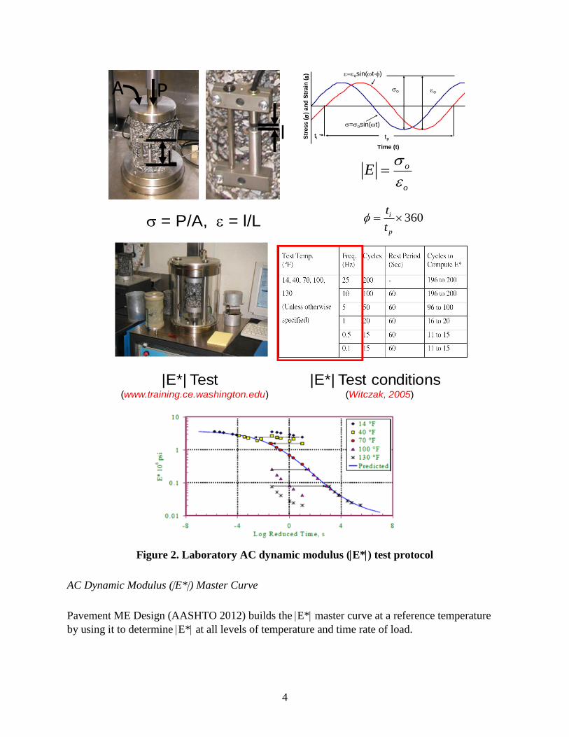
4
Figure 2. Laboratory AC dynamic modulus (E*) test protocol
AC Dynamic Modulus (E*) Master Curve
Pavement ME Design (AASHTO 2012) builds the E* master curve at a reference temperature
by using it to determine E* at all levels of temperature and time rate of load.
PA
L
l
= P/A, = l/L
Time (t)
Str
ess (
) an
d S
train
()
ti
o
=osin(wt)
osin(wt-f)
o
tp
o
o
E
360i
p
t
tf
|E*| Test (www.training.ce.washington.edu)
|E*| Test conditions (Witczak, 2005)
5
The E* master curves are constructed using frequency-temperature (or time-temperature)
superposition concepts represented by shift factors. The combined effects of temperature and
loading rate can be represented in the form of a master curve relating E* to a reduced frequency
(fr) or a reduced time (tr) by a sigmoidal function. Each of the parameters (i.e., a reduced
frequency [fr] or a reduced time [tr]) utilizes a sigmoidal function equation of the E* master
curve. However, the various equations of a sigmoidal function for the E* master curve have
been reported in the literature (Pellinen et al. 2004, Schwartz 2005, Witczak 2005, Kutay et al.
2011). For clarification, in this study, the sigmoidal function equation using a reduced frequency
(fr) is defined as the dynamic modulus E* master curve equation, while the sigmoidal function
equation using a reduced time (tr) is defined as the relaxation modulus E(t) master curve
equation. From the theory of viscoelasticity, E* and E(t) can be converted from each into the
other through numerical procedures (Park and Schapery 1999). The dynamic modulus E*
master curve equation using a reduced frequency (fr) in this study is described as follows:
3 4
21 ( log( ))
*1 rC C f
CLog E C
e
(4)
Where,
fr = reduced frequency of loading at reference temperature
C1 = minimum value of E*
C1 + C2 = maximum value of E*
C3 and C4 = parameters describing the shape of the sigmoidal function
The function parameters C1 and C2 in general depend on the aggregate gradation and mixture
volumetrics, while the parameters C3 and C4 depend primarily on the characteristics of the
asphalt binder (Schwartz 2005). The reduced frequency (fr ) can be shown in the following form:
( )a ( )r Tf f T (5)
Where,
f = frequency of loading at desired temperature
T = temperature of interest
aT(T) = shift factor as a function of temperature
The equations widely used to express the temperature-shift factor of aT(T) include Williams-
Landel-Ferry equations, the Arrhenius equations, and the second-order polynomial equations
(Pellinen et al. 2004, Witczak 2005, Kutay et al. 2011, Varma et al. 2013b). The shift factor utilized in this study is the logarithm of the shift factor computed by using a second-order polynomial (Kutay et al. 2011, Varma et al. 2013b), described as follows:
2 2
1 2log(a ( )) ( ) (T T )T ref refT a T T a (6)
6
Where,
Tref = reference temperature, 19C (or 66.2°F)
a1 and a2 = the shift factor polynomial coefficients
The values for C1, C2, C3, C4, and aT(T) in a sigmoidal function of master curve are all
simultaneously determined from test data using nonlinear optimization techniques, e.g., the
Solver function in Excel software. The relaxation modulus E(t) using a reduced time (tr) can be
converted from the dynamic modulus E* using a reduced frequency (fr) through numerical
procedures (Park and Schapery 1999) and described as follows:
3 4
21 ( log(t ))
( (t))1 rc c
cLog E c
e
(7)
Where,
tr = reduced time at reference temperature
c1, c2, c3, and c4 = the relaxation modulus E(t) coefficients
FWD Backcalculation
Static FWD Backcalculation Approaches
The FWD backcalculation procedure involves two calculation directions, namely forward and
inverse. In the forward direction of analysis, theoretical deflections are computed under the
applied load and the given pavement structure using assumed pavement layer moduli. In the
inverse direction of analysis, these theoretical deflections are compared with measured
deflections, and the assumed moduli are then adjusted in an iterative procedure until the
theoretical and measured deflection basins match acceptably well. The moduli derived in this
way are considered representative of the pavement response to load and can be used to calculate
stresses or strains in the pavement structure for analysis purposes. This is an iterative method of
solving the inverse problem and will not have a unique solution in most cases.
In the FWD test, an impulse load within the range of 6.7 to 156 kN is impacted on the pavement
surface, and associated surface deflection values in the time domain are measured at different
locations (usually at six or seven locations) by geophones. Figure 3 illustrates the typical result
of an FWD test. In general, deflection-time history curves for each geophone exhibit Haversine
behavior, and peak values of these curves for each geophone are used to plot the deflection basin
curve. Static FWD backcalculation methods utilize only peak values of deflection-time history
curves to compute moduli values.
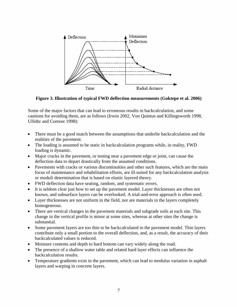
7
Figure 3. Illustration of typical FWD deflection measurements (Goktepe et al. 2006)
Some of the major factors that can lead to erroneous results in backcalculation, and some
cautions for avoiding them, are as follows (Irwin 2002, Von Quintus and Killingsworth 1998,
Ullidtz and Coetzee 1998):
There must be a good match between the assumptions that underlie backcalculation and the
realities of the pavement.
The loading is assumed to be static in backcalculation programs while, in reality, FWD
loading is dynamic.
Major cracks in the pavement, or testing near a pavement edge or joint, can cause the
deflection data to depart drastically from the assumed conditions.
Pavements with cracks or various discontinuities and other such features, which are the main
focus of maintenance and rehabilitation efforts, are ill-suited for any backcalculation analysis
or moduli determination that is based on elastic layered theory.
FWD deflection data have seating, random, and systematic errors.
It is seldom clear just how to set up the pavement model. Layer thicknesses are often not
known, and subsurface layers can be overlooked. A trial-and-error approach is often used.
Layer thicknesses are not uniform in the field, nor are materials in the layers completely
homogeneous.
There are vertical changes in the pavement materials and subgrade soils at each site. This
change in the vertical profile is minor at some sites, whereas at other sites the change is
substantial.
Some pavement layers are too thin to be backcalculated in the pavement model. Thin layers
contribute only a small portion to the overall deflection, and, as a result, the accuracy of their
backcalculated values is reduced.
Moisture contents and depth to hard bottom can vary widely along the road.
The presence of a shallow water table and related hard layer effects can influence the
backcalculation results.
Temperature gradients exist in the pavement, which can lead to modulus variation in asphalt
layers and warping in concrete layers.
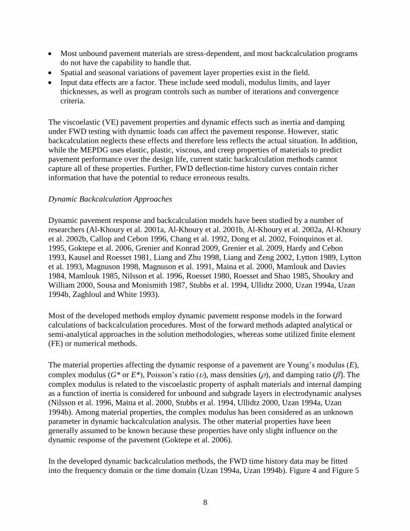
8
Most unbound pavement materials are stress-dependent, and most backcalculation programs
do not have the capability to handle that.
Spatial and seasonal variations of pavement layer properties exist in the field.
Input data effects are a factor. These include seed moduli, modulus limits, and layer
thicknesses, as well as program controls such as number of iterations and convergence
criteria.
The viscoelastic (VE) pavement properties and dynamic effects such as inertia and damping
under FWD testing with dynamic loads can affect the pavement response. However, static
backcalculation neglects these effects and therefore less reflects the actual situation. In addition,
while the MEPDG uses elastic, plastic, viscous, and creep properties of materials to predict
pavement performance over the design life, current static backcalculation methods cannot
capture all of these properties. Further, FWD deflection-time history curves contain richer
information that have the potential to reduce erroneous results.
Dynamic Backcalculation Approaches
Dynamic pavement response and backcalculation models have been studied by a number of
researchers (Al-Khoury et al. 2001a, Al-Khoury et al. 2001b, Al-Khoury et al. 2002a, Al-Khoury
et al. 2002b, Callop and Cebon 1996, Chang et al. 1992, Dong et al. 2002, Foinquinos et al.
1995, Goktepe et al. 2006, Grenier and Konrad 2009, Grenier et al. 2009, Hardy and Cebon
1993, Kausel and Roesset 1981, Liang and Zhu 1998, Liang and Zeng 2002, Lytton 1989, Lytton
et al. 1993, Magnuson 1998, Magnuson et al. 1991, Maina et al. 2000, Mamlouk and Davies
1984, Mamlouk 1985, Nilsson et al. 1996, Roesset 1980, Roesset and Shao 1985, Shoukry and
William 2000, Sousa and Monismith 1987, Stubbs et al. 1994, Ullidtz 2000, Uzan 1994a, Uzan
1994b, Zaghloul and White 1993).
Most of the developed methods employ dynamic pavement response models in the forward
calculations of backcalculation procedures. Most of the forward methods adapted analytical or
semi-analytical approaches in the solution methodologies, whereas some utilized finite element
(FE) or numerical methods.
The material properties affecting the dynamic response of a pavement are Young’s modulus (E),
complex modulus (G* or E*), Poisson’s ratio (), mass densities (), and damping ratio (). The complex modulus is related to the viscoelastic property of asphalt materials and internal damping
as a function of inertia is considered for unbound and subgrade layers in electrodynamic analyses
(Nilsson et al. 1996, Maina et al. 2000, Stubbs et al. 1994, Ullidtz 2000, Uzan 1994a, Uzan
1994b). Among material properties, the complex modulus has been considered as an unknown
parameter in dynamic backcalculation analysis. The other material properties have been
generally assumed to be known because these properties have only slight influence on the
dynamic response of the pavement (Goktepe et al. 2006).
In the developed dynamic backcalculation methods, the FWD time history data may be fitted
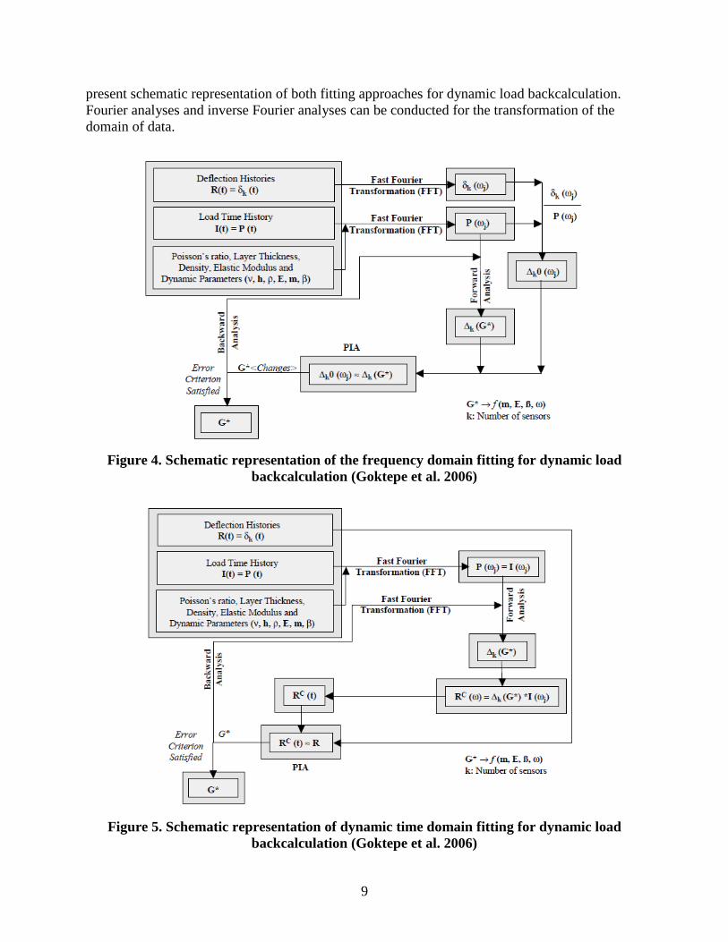
into the frequency domain or the time domain (Uzan 1994a, Uzan 1994b). Figure 4 and Figure 5
9
present schematic representation of both fitting approaches for dynamic load backcalculation.
Fourier analyses and inverse Fourier analyses can be conducted for the transformation of the
domain of data.
Figure 4. Schematic representation of the frequency domain fitting for dynamic load
backcalculation (Goktepe et al. 2006)
Figure 5. Schematic representation of dynamic time domain fitting for dynamic load
backcalculation (Goktepe et al. 2006)
10
In frequency domain fitting, the applied load and deflection response time histories are
transformed into the frequency domain by using a Fourier transformation. The compliance
function of the complex deflection function divided by the complex load function is the
measured complex unit response of the pavement at each frequency. Similarly to static
backcalculation methods, an iterative procedure is carried out to find the set of complex moduli
that will generate the calculated complex unit response close to the measured one. In time
domain fitting, the impulse load time histories should be transformed into the frequency domain
data in order to input the available forward model into the frequency domain. Inverse Fourier
transformations should be carried out to compare calculated and measured deflections in the time
domain.
Some advantages of developed dynamic backcalculation procedures include considering asphalt
viscoelastic properties and obtaining more precise results than static procedures. However, some
of the limitations of current dynamic backcalculation procedures include the following (Goktepe
et al. 2006, Grenier and Konrad 2009):
The current dynamic backcalculation procedures have more complexity and greater
computational expense.
The error minimization scheme can fall into a local minimum (which may not be the absolute
minimum), depending on the complexity of the error function.
The uniqueness of the solution is not always guaranteed and depends on the number of
unknown parameters and the correlation between these parameters.
Because many observations are used in the dynamic approach, correlations between
unknown parameters are usually low, which is not the case in the static approach that uses
only the deflection basin.
Viscoelastic Backcalculation Approach
Although many static and dynamic backcalculation approaches have been proposed in the past,
only fewer recent studies have attempted to develop dynamic backcalculation approaches to
derive the AC E* master curve from FWD defection-time history data.
Kutay et al. (2011) developed a methodology that backcalculates the damaged dynamic modulus
|E*| master curve of asphalt concrete by utilizing the time histories of FWD surface deflections.
A computationally efficient layered viscoelastic forward solution, referred to as LAVA, was
employed iteratively to backcalculate the AC E(t) master curve (which can then be converted to
the |E*| master curve using numerical inter-conversion procedures) based on FWD deflection-
time history data. Certain information such as the thickness of each layer (AC, base, subbase,
etc.), the modulus, and the Poisson’s ratio of the layers under the AC layer are required for
backcalculation of E(t). Specifically, the number of layers and thickness of each layer, modulus
and Poisson’s ratio of unbound layers, and Poisson’s ratio of the AC layer are required as inputs.
Using simulated examples of two pavement structures, Kutay et al. (2011) demonstrated that it is
possible to backcalculate certain portions of the E(t) master curve using deflection-time histories
11
from a typical FWD test. The study noted that the proposed backcalculation algorithm is
independent of layer geometry because the layer structure and the thickness of the asphalt layer,
for the cases analyzed, did not have an influence on the backcalculated E(t) or |E*| master curves.
The authors also proposed modifications to the current FWD technology to enable longer FWD
pulses and to ensure more reliable readings in the tail regions of the FWD deflection-time
histories.
As a follow-up to the work by Kutay et al. (2011), Varma et al. (2013a) estimated and proposed
a set of temperatures at which FWD tests should be conducted to be able to maximize the portion
of the E(t) curve that can be accurately backcalculated. A genetic algorithm–based (GA-based)
viscoelastic backcalculation algorithm was proposed that is capable of predicting E(t) and |E*|
master curves as well as time-temperature superposition shift factors from a set of FWD
deflection-time histories at different temperatures. The study concluded that deflection-time
histories from FWD tests conducted between 68–104 °F (20–40 °C) are useful in accurately
estimating the entire E(t) or |E*| master curve.
Varma et al. (2013b) considered FWD deflection-time history data from a single FWD drop
combined with the temperature gradient across the AC layer at the time of FWD testing in their
GA-based viscoelastic backcalculation approach, referred to as BACKLAVA. The study
concluded that, unless a stiff layer (bedrock) exists close to the pavement surface that can
contribute to the dynamics in the FWD test, BACKLAVA is capable of inferring E(t)/|E*| master
curve coefficients (including shift factors) as well as the linear elastic moduli of the base and
subgrade layers.
12
DEVELOPMENET OF FRAMEWORK FOR DERIVING AC MASTER CURVE FROM
FWD DATA
Based on the research team’s discussions with the Iowa DOT’s Office of Special Investigations
and Bituminous Materials Office regarding the specific objectives of this project, the Iowa DOT
is eventually interested in documenting the Iowa AC mix damaged master curve coefficients
relative to the mix IDs/Station Nos., if possible, in the Pavement Management Information
System (PMIS). This would be of significant use to the city, county, and state engineers because
the outcome of this research would enable them to look up the damaged master curve shape
parameters from the PMIS while running a flexible pavement rehabilitation analysis and design
using MEPDG/Pavement ME Design. As a first and foundational step, this feasibility research
study focused on establishing frameworks for predicting the AC E(t) master curve coefficients
from FWD time history data.
Based on a comprehensive literature review, the existing direct, indirect, and derivative
approaches to damaged master curve determination using FWD time history data were
synthesized in the previous section. This section describes the development of a detailed
framework as a first step in a proof-of-concept demonstration for deriving the AC |E*| master
curve coefficients from single-drop FWD time history data.
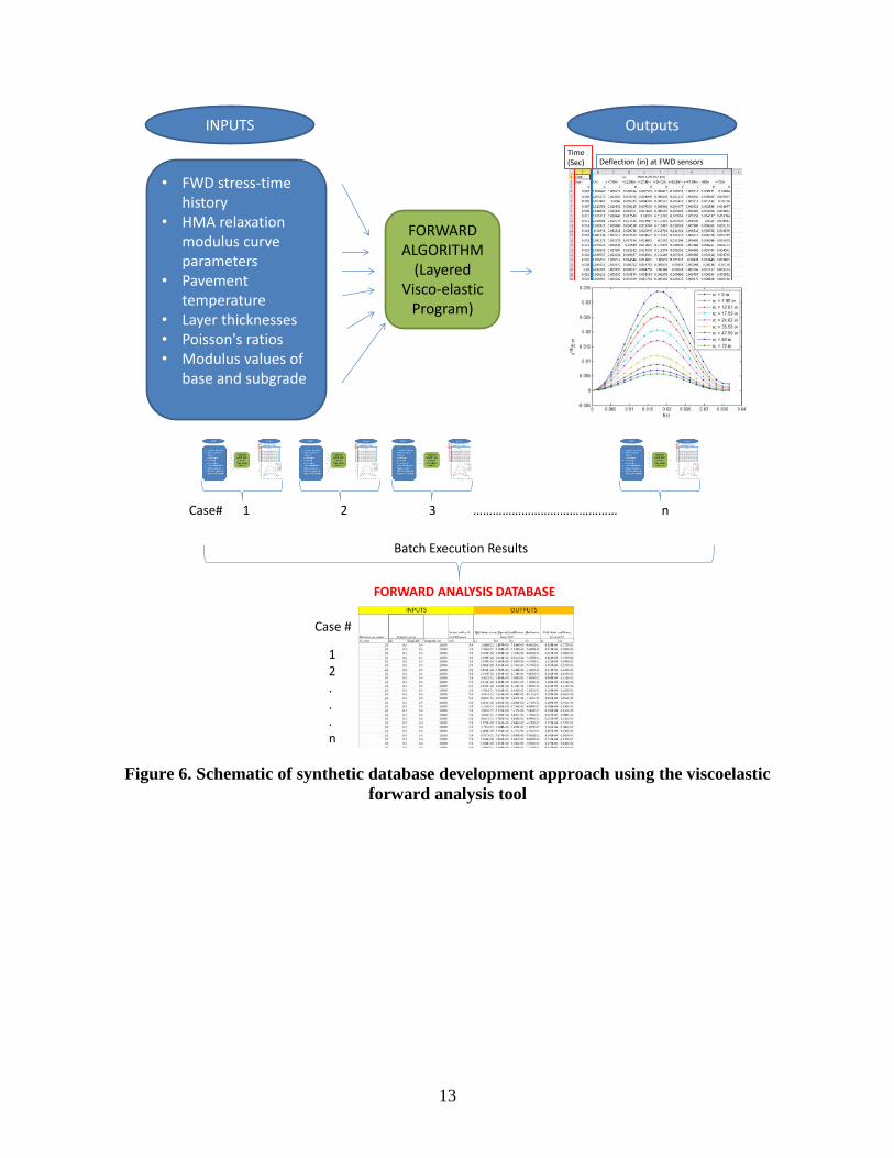
In the proposed approach, a layered viscoelastic forward analysis tool is first used to generate a
database of AC master curve (input)–pavement surface deflection time history (output) scenarios
for a variety of pavement layer thicknesses and pavement temperatures (see Figure 6). In the
second step, the neural network (NN) methodology is employed to map the AC surface
deflection time history data (generated through a forward-layered viscoelastic analysis model) to
(damaged) AC relaxation modulus master curve shape parameters (see Figure 7).
13
Figure 6. Schematic of synthetic database development approach using the viscoelastic
forward analysis tool
INPUTS
FORWARD ALGORITHM
(Layered Visco-elastic
Program)
• FWD stress-time history
• HMA relaxation modulus curve parameters
• Pavement temperature
• Layer thicknesses• Poisson's ratios• Modulus values of
base and subgrade
Outputs
Time (Sec) Deflection (in) at FWD sensors
1 2 3 n………………………………………Case#
FORWARD ANALYSIS DATABASE
Case #
12...n
Batch Execution Results
14
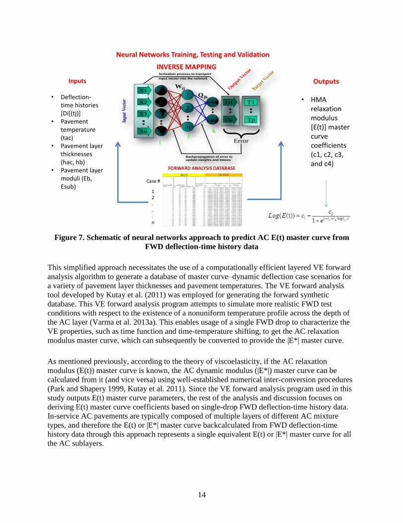
Figure 7. Schematic of neural networks approach to predict AC E(t) master curve from
FWD deflection-time history data
This simplified approach necessitates the use of a computationally efficient layered VE forward
analysis algorithm to generate a database of master curve–dynamic deflection case scenarios for
a variety of pavement layer thicknesses and pavement temperatures. The VE forward analysis
tool developed by Kutay et al. (2011) was employed for generating the forward synthetic
database. This VE forward analysis program attempts to simulate more realistic FWD test
conditions with respect to the existence of a nonuniform temperature profile across the depth of
the AC layer (Varma et al. 2013a). This enables usage of a single FWD drop to characterize the
VE properties, such as time function and time-temperature shifting, to get the AC relaxation
modulus master curve, which can subsequently be converted to provide the |E*| master curve.
As mentioned previously, according to the theory of viscoelasticity, if the AC relaxation
modulus (E(t)) master curve is known, the AC dynamic modulus (|E*|) master curve can be
calculated from it (and vice versa) using well-established numerical inter-conversion procedures
(Park and Shapery 1999, Kutay et al. 2011). Since the VE forward analysis program used in this
study outputs E(t) master curve parameters, the rest of the analysis and discussion focuses on
deriving E(t) master curve coefficients based on single-drop FWD deflection-time history data.
In-service AC pavements are typically composed of multiple layers of different AC mixture
types, and therefore the E(t) or |E*| master curve backcalculated from FWD deflection-time
history data through this approach represents a single equivalent E(t) or |E*| master curve for all
the AC sublayers.
Neural Networks Training, Testing and Validation
INVERSE MAPPING
Inputs
• Deflection-time histories [Di[(tj)]
• Pavement temperature (tac)
• Pavement layer thicknesses (hac, hb)
• Pavement layer moduli (Eb, Esub)
Outputs
• HMA relaxation modulus [E(t)] master curve coefficients (c1, c2, c3, and c4)
2
3
n
11
1
m
2
p
X1
X2
X3
Xn
O1
Op
T1
Tp
Error
Activation process to transport
input vector into the network
i
kj
Wij
Qjk
Backpropagation of error toupdate weights and biases
15
The backcalculation of shift factors for the master curve requires knowledge of the temperature
profile at the time of the FWD testing, which translates into additional dimensions of complexity
in the forward analysis and database generation using the current approach. Therefore,
considering the limited project duration and lack of development time, the current approach is
restricted to the backcaclulation of AC E(t) master curve coefficients. However, it is
recommended that future research efforts include backcalculation of shift factors for the master
curve from FWD deflection-time history data.
Case Studies
First, a preliminary (screening) analysis was carried out for full-depth AC through various case
studies to verify the feasibility of the NN approach, identify the promising input features and NN
parameters for inverse modeling, and identify associated modeling challenges. The primary goal
of these case studies was to answer the question: Are NNs capable of learning/mapping the
complex, nonlinear relationship between AC E(t) master curve coefficients and FWD time
history data? These case studies (as well as the rest of the report) focus on full-depth AC
pavements as a first step to isolate potential backcalculation issues that are only related to the
modulus master curve of the AC layer.
Among the several case studies conducted by the research team, three case studies are reported
here that systematically varied the inputs for the NN inverse modeling: (1) consider only FWD
D0 time history data; (2) consider FWD D0, D8, and D12 time history data; (3) consider only
FWD Surface Curvature Index (D0–D12). Here D0, D8, and D12 refer to deflection-time history
data recorded at an offset of 0, 8, and 12 inches, respectively, from the center of the FWD
loading plate. It is expected that the effect of viscoelasticity will be more pronounced in the
sensors closest to the load plate. Further, some studies have reported that the addition of further
sensors in the backcalculation process tends to increase the error in E(t) predictions (Varma et al.
2013a). However, future research should consider all sensors in the standard FWD configuration
to elaborately investigate their influence on the accuracy of the backcalculated E(t) master curve
and unbound layers.
Development of Synthetic Database
As mentioned previously, the VE forward analysis program outputs pavement surface deflection-
time histories based on the following inputs: FWD stress-time history, AC E(t) master curve
coefficients and shift factors, pavement temperature, pavement layer thicknesses and Poisson’s
ratios, and unbound layer moduli. The FWD stress-time history for a standard 9 kip loading was
used for these case studies and for other analyses discussed in the rest of the report. For full-
depth AC analysis, the inputs were reduced to AC E(t) master curve coefficients (c1, c2, c3, and
c4) and shift factors (a1 and a2), pavement temperature (Tac), AC layer thickness (Hac), subgrade
layer modulus (Esub), AC Poisson’s ratio (μac), and subgrade Poisson’s ratio (μsub).
Because the goal of this exercise was to quickly verify the feasibility of the NN approach, certain
inputs were blocked out from the modeling by assigning them constant values for all simulations.
This enabled a more focused evaluation of the ability of the NNs in modeling the relationship
16
between the E(t) master curve and deflection-time histories. A synthetic database consisting of
100 scenarios was generated through batch simulations of the VE forward analysis program
using the input ranges summarized in Table 1. The min-max ranges of E(t) master curve
coefficients and shift factors are based on the Michigan State University (MSU) E(t) database of
100+ hot-mix asphalt (HMA) mixtures (Varma et al. 2013a).
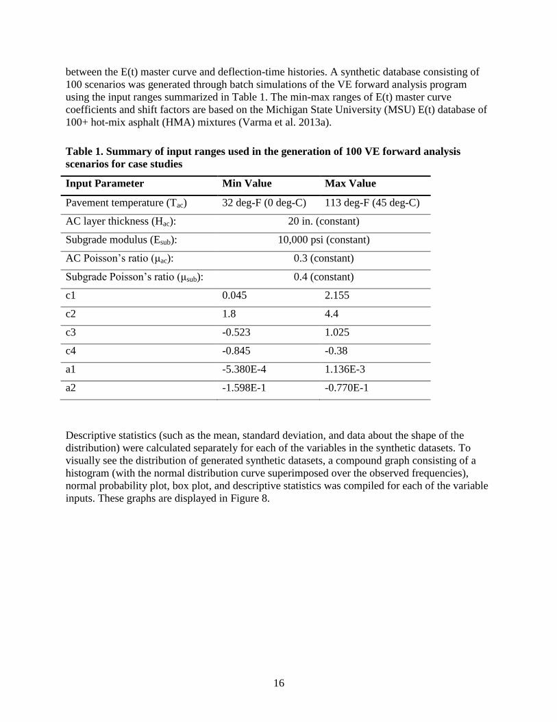
Table 1. Summary of input ranges used in the generation of 100 VE forward analysis
scenarios for case studies
Input Parameter Min Value Max Value
Pavement temperature (Tac) 32 deg-F (0 deg-C) 113 deg-F (45 deg-C)
AC layer thickness (Hac): 20 in. (constant)
Subgrade modulus (Esub): 10,000 psi (constant)
AC Poisson’s ratio (μac): 0.3 (constant)
Subgrade Poisson’s ratio (μsub): 0.4 (constant)
c1 0.045 2.155
c2 1.8 4.4
c3 -0.523 1.025
c4 -0.845 -0.38
a1 -5.380E-4 1.136E-3
a2 -1.598E-1 -0.770E-1
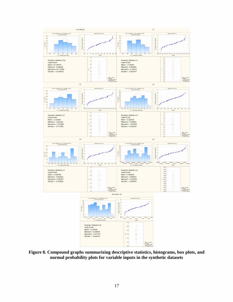
Descriptive statistics (such as the mean, standard deviation, and data about the shape of the
distribution) were calculated separately for each of the variables in the synthetic datasets. To
visually see the distribution of generated synthetic datasets, a compound graph consisting of a
histogram (with the normal distribution curve superimposed over the observed frequencies),
normal probability plot, box plot, and descriptive statistics was compiled for each of the variable
inputs. These graphs are displayed in Figure 8.
17
Figure 8. Compound graphs summarizing descriptive statistics, histograms, box plots, and
normal probability plots for variable inputs in the synthetic datasets
Tac (deg-C)
K-S d=.10643, p> .20; Lilliefors p<.01
Expected Normal
-10 0 10 20 30 40 50
X <= Category Boundary
0
5
10
15
20
25
30
35
No
. o
f o
bs.
Mean = 23.146 Mean±SD = (9.9879, 36.3041) Mean±1.96*SD = (-2.6439, 48.9359)-10
0
10
20
30
40
50
60
Tac
Normal P-Plot: Tac
-5 0 5 10 15 20 25 30 35 40 45 50
Value
-3
-2
-1
0
1
2
3
Exp
ect
ed
No
rma
l Va
lue
Summary Statistics:Tac
Valid N=100
Mean= 23.145975
Minimum= 0.546636
Maximum= 44.774360
Std.Dev.= 13.158101
c1
K-S d=.09698, p> .20; Lilliefors p<.05
Expected Normal
-0.5 0.0 0.5 1.0 1.5 2.0 2.5
X <= Category Boundary
0
5
10
15
20
25
30
35
No
. o
f o
bs.
Mean = 1.1026 Mean±SD = (0.461, 1.7441) Mean±1.96*SD = (-0.1549, 2.36)-0.4
-0.2
0.0
0.2
0.4
0.6
0.8
1.0
1.2
1.4
1.6
1.8
2.0
2.2
2.4
2.6
c1
Normal P-Plot: c1
-0.2 0.0 0.2 0.4 0.6 0.8 1.0 1.2 1.4 1.6 1.8 2.0 2.2 2.4
Value
-3
-2
-1
0
1
2
3
Exp
ect
ed
No
rma
l Va
lue
Summary Statistics:c1
Valid N=100
Mean= 1.102562
Minimum= 0.050683
Maximum= 2.135515
Std.Dev.= 0.641574
c2
K-S d=.11699, p<.15 ; Lilliefors p<.01
Expected Normal
1.5 2.0 2.5 3.0 3.5 4.0 4.5
X <= Category Boundary
0
5
10
15
20
25
30
No
. o
f o
bs.
Mean = 3.1434 Mean±SD = (2.3696, 3.9172) Mean±1.96*SD = (1.6268, 4.66)1.5
2.0
2.5
3.0
3.5
4.0
4.5
5.0
c2
Normal P-Plot: c2
1.6 1.8 2.0 2.2 2.4 2.6 2.8 3.0 3.2 3.4 3.6 3.8 4.0 4.2 4.4 4.6
Value
-3
-2
-1
0
1
2
3
Exp
ect
ed
No
rma
l Va
lue
Summary Statistics:c2
Valid N=100
Mean= 3.143426
Minimum= 1.821228
Maximum= 4.372656
Std.Dev.= 0.773780
c3
K-S d=.07703, p> .20; Lilliefors p<.15
Expected Normal
-0.8 -0.6 -0.4 -0.2 0.0 0.2 0.4 0.6 0.8 1.0 1.2
X <= Category Boundary
0
2
4
6
8
10
12
14
16
18
20
22
No
. o
f o
bs.
Mean = 0.292 Mean±SD = (-0.1391, 0.7231) Mean±1.96*SD = (-0.5529, 1.137)-0.8
-0.6
-0.4
-0.2
0.0
0.2
0.4
0.6
0.8
1.0
1.2
1.4
c3
Normal P-Plot: c3
-0.6 -0.4 -0.2 0.0 0.2 0.4 0.6 0.8 1.0 1.2
Value
-3
-2
-1
0
1
2
3
Exp
ect
ed
No
rma
l Va
lue
Summary Statistics:c3
Valid N=100
Mean= 0.292020
Minimum= -0.518842
Maximum= 1.015026
Std.Dev.= 0.431103
c4
K-S d=.12893, p<.10 ; Lilliefors p<.01
Expected Normal
-0.9 -0.8 -0.7 -0.6 -0.5 -0.4 -0.3 -0.2 -0.1 0.0
X <= Category Boundary
0
5
10
15
20
25
No
. o
f o
bs.
Mean = -0.4368 Mean±SD = (-0.6906, -0.1829) Mean±1.96*SD = (-0.9343, 0.0607)-1.0
-0.8
-0.6
-0.4
-0.2
0.0
0.2
c4
Normal P-Plot: c4
-0.9 -0.8 -0.7 -0.6 -0.5 -0.4 -0.3 -0.2 -0.1 0.0
Value
-3
-2
-1
0
1
2
3
Exp
ect
ed
No
rma
l Va
lue
Summary Statistics:c4
Valid N=100
Mean= -0.436766
Minimum= -0.820522
Maximum= -0.050877
Std.Dev.= 0.253829
a1
K-S d=.11197, p<.20 ; Lilliefors p<.01
Expected Normal
-0.0008-0.0006
-0.0004-0.0002
0.00000.0002
0.00040.0006
0.00080.0010
0.0012
X <= Category Boundary
0
2
4
6
8
10
12
14
16
18
20
No
. o
f o
bs.
Mean = 0.0003 Mean±SD = (-0.0002, 0.0008) Mean±1.96*SD = (-0.0007, 0.0013)-0.0008
-0.0006
-0.0004
-0.0002
0.0000
0.0002
0.0004
0.0006
0.0008
0.0010
0.0012
0.0014
0.0016
a1
Normal P-Plot: a1
-0.0006-0.0004
-0.00020.0000
0.00020.0004
0.00060.0008
0.00100.0012
Value
-3
-2
-1
0
1
2
3
Exp
ect
ed
No
rma
l Va
lue
Summary Statistics:a1
Valid N=100
Mean= 0.000294
Minimum= -0.000532
Maximum= 0.001093
Std.Dev.= 0.000504
Summary: a2
K-S d=.09302, p> .20; Lilliefors p<.05
Expected Normal
-0.17-0.16
-0.15-0.14
-0.13-0.12
-0.11-0.10
-0.09-0.08
-0.07
X <= Category Boundary
0
2
4
6
8
10
12
14
16
18
No
. o
f o
bs.
Mean = -0.1206 Mean±SD = (-0.1452, -0.096) Mean±1.96*SD = (-0.1688, -0.0724)-0.18
-0.16
-0.14
-0.12
-0.10
-0.08
-0.06
a2
Normal P-Plot: a2
-0.17-0.16
-0.15-0.14
-0.13-0.12
-0.11-0.10
-0.09-0.08
-0.07
Value
-3
-2
-1
0
1
2
3
Exp
ect
ed
No
rma
l Va
lue
Summary Statistics:a2
Valid N=100
Mean= -0.120594
Minimum= -0.158848
Maximum= -0.077472
Std.Dev.= 0.024574
18
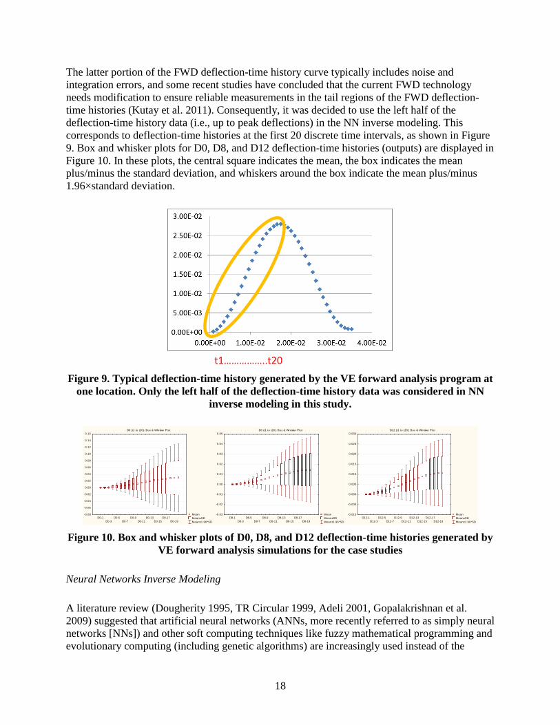
The latter portion of the FWD deflection-time history curve typically includes noise and
integration errors, and some recent studies have concluded that the current FWD technology
needs modification to ensure reliable measurements in the tail regions of the FWD deflection-
time histories (Kutay et al. 2011). Consequently, it was decided to use the left half of the
deflection-time history data (i.e., up to peak deflections) in the NN inverse modeling. This
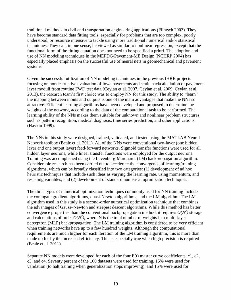
corresponds to deflection-time histories at the first 20 discrete time intervals, as shown in Figure
9. Box and whisker plots for D0, D8, and D12 deflection-time histories (outputs) are displayed in
Figure 10. In these plots, the central square indicates the mean, the box indicates the mean
plus/minus the standard deviation, and whiskers around the box indicate the mean plus/minus
1.96×standard deviation.
Figure 9. Typical deflection-time history generated by the VE forward analysis program at
one location. Only the left half of the deflection-time history data was considered in NN
inverse modeling in this study.
Figure 10. Box and whisker plots of D0, D8, and D12 deflection-time histories generated by
VE forward analysis simulations for the case studies
Neural Networks Inverse Modeling
A literature review (Dougherity 1995, TR Circular 1999, Adeli 2001, Gopalakrishnan et al.
2009) suggested that artificial neural networks (ANNs, more recently referred to as simply neural
networks [NNs]) and other soft computing techniques like fuzzy mathematical programming and
evolutionary computing (including genetic algorithms) are increasingly used instead of the
t1……………..t20
D0 (t1 to t20): Box & Whisker Plot
Mean
Mean±SD
Mean±1.96*SD
D0-1
D0-3
D0-5
D0-7
D0-9
D0-11
D0-13
D0-15
D0-17
D0-19
-0.08
-0.06
-0.04
-0.02
0.00
0.02
0.04
0.06
0.08
0.10
0.12
0.14
0.16
D8 (t1 to t20): Box & Whisker Plot
Mean
Mean±SD
Mean±1.96*SD
D8-1
D8-3
D8-5
D8-7
D8-9
D8-11
D8-13
D8-15
D8-17
D8-19
-0.03
-0.02
-0.01
0.00
0.01
0.02
0.03
0.04
0.05
D12 (t1 to t20): Box & Whisker Plot
Mean
Mean±SD
Mean±1.96*SD
D12-1
D12-3
D12-5
D12-7
D12-9
D12-11
D12-13
D12-15
D12-17
D12-19
-0.010
-0.005
0.000
0.005
0.010
0.015
0.020
0.025
0.030
19
traditional methods in civil and transportation engineering applications (Flintsch 2003). They
have become standard data fitting tools, especially for problems that are too complex, poorly
understood, or resource intensive to tackle using more traditional numerical and/or statistical
techniques. They can, in one sense, be viewed as similar to nonlinear regression, except that the
functional form of the fitting equation does not need to be specified a priori. The adoption and
use of NN modeling techniques in the MEPDG/Pavement-ME Design (NCHRP 2004) has
especially placed emphasis on the successful use of neural nets in geomechanical and pavement
systems.
Given the successful utilization of NN modeling techniques in the previous IHRB projects
focusing on nondestructive evaluation of Iowa pavements and static backcalculation of pavement
layer moduli from routine FWD test data (Ceylan et al. 2007, Ceylan et al. 2009, Ceylan et al.
2013), the research team’s first choice was to employ NN for this study. The ability to “learn”
the mapping between inputs and outputs is one of the main advantages that make the NNs so
attractive. Efficient learning algorithms have been developed and proposed to determine the
weights of the network, according to the data of the computational task to be performed. The
learning ability of the NNs makes them suitable for unknown and nonlinear problem structures
such as pattern recognition, medical diagnosis, time series prediction, and other applications
(Haykin 1999).
The NNs in this study were designed, trained, validated, and tested using the MATLAB Neural
Network toolbox (Beale et al. 2011). All of the NNs were conventional two-layer (one hidden
layer and one output layer) feed-forward networks. Sigmoid transfer functions were used for all
hidden layer neurons, while linear transfer functions were employed for the output neurons.
Training was accomplished using the Levenberg-Marquardt (LM) backpropagation algorithm.
Considerable research has been carried out to accelerate the convergence of learning/training
algorithms, which can be broadly classified into two categories: (1) development of ad hoc
heuristic techniques that include such ideas as varying the learning rate, using momentum, and
rescaling variables; and (2) development of standard numerical optimization techniques.
The three types of numerical optimization techniques commonly used for NN training include
the conjugate gradient algorithms, quasi-Newton algorithms, and the LM algorithm. The LM
algorithm used in this study is a second-order numerical optimization technique that combines
the advantages of Gauss–Newton and steepest descent algorithms. While this method has better
convergence properties than the conventional backpropagation method, it requires O(N2) storage
and calculations of order O(N2), where N is the total number of weights in a multi-layer
perceptron (MLP) backpropagation. The LM training algorithm is considered to be very efficient
when training networks have up to a few hundred weights. Although the computational
requirements are much higher for each iteration of the LM training algorithm, this is more than
made up for by the increased efficiency. This is especially true when high precision is required
(Beale et al. 2011).
Separate NN models were developed for each of the four E(t) master curve coefficients, c1, c2,
c3, and c4. Seventy percent of the 100 datasets were used for training, 15% were used for
validation (to halt training when generalization stops improving), and 15% were used for
20
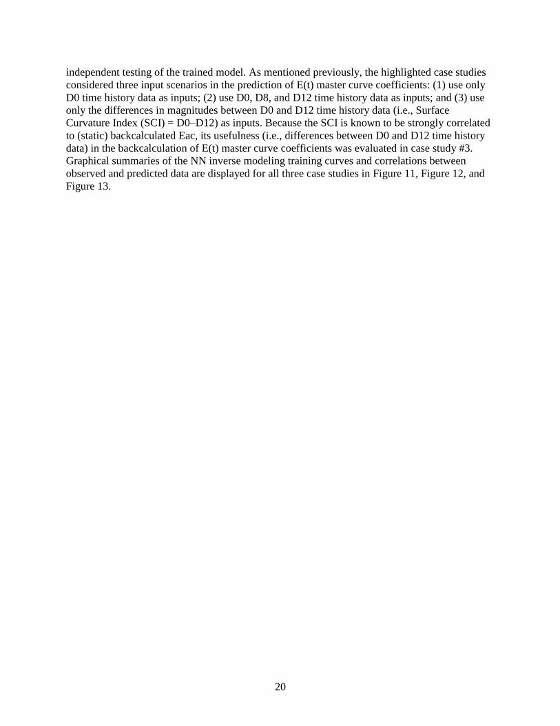
independent testing of the trained model. As mentioned previously, the highlighted case studies
considered three input scenarios in the prediction of E(t) master curve coefficients: (1) use only
D0 time history data as inputs; (2) use D0, D8, and D12 time history data as inputs; and (3) use
only the differences in magnitudes between D0 and D12 time history data (i.e., Surface
Curvature Index (SCI) = D0–D12) as inputs. Because the SCI is known to be strongly correlated
to (static) backcalculated Eac, its usefulness (i.e., differences between D0 and D12 time history
data) in the backcalculation of E(t) master curve coefficients was evaluated in case study #3.
Graphical summaries of the NN inverse modeling training curves and correlations between
observed and predicted data are displayed for all three case studies in Figure 11, Figure 12, and
Figure 13.
21
(a)
(b)
(c)
(d)
Figure 11. NN prediction of E(t) master curve coefficients from D0 time history data using
100 datasets (case study #1): (a) c1, (b) c2, (c) c3, (d) c4
22
(a)
(b)
(c)
(d)
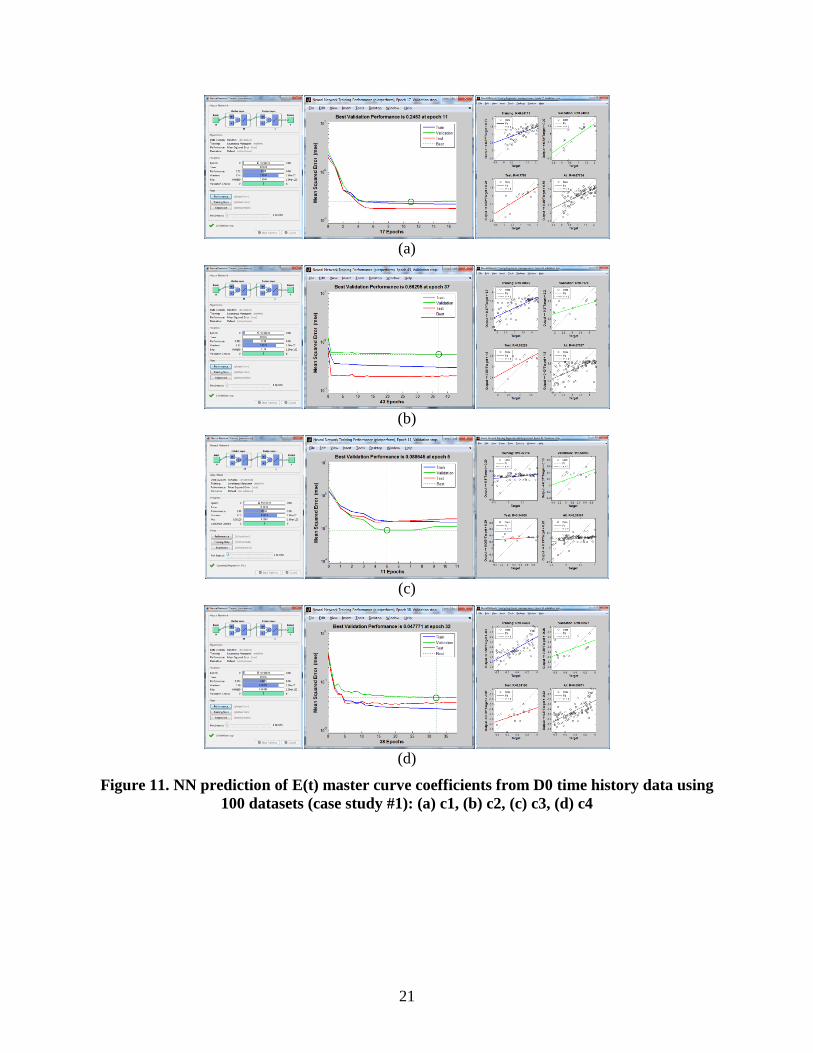
Figure 12. NN prediction of E(t) master curve coefficients from D0, D8, and D12 time
history data using 100 datasets (case study #2): (a) c1, (b) c2, (c) c3, (d) c4
23
(a)
(b)
(c)
(d)
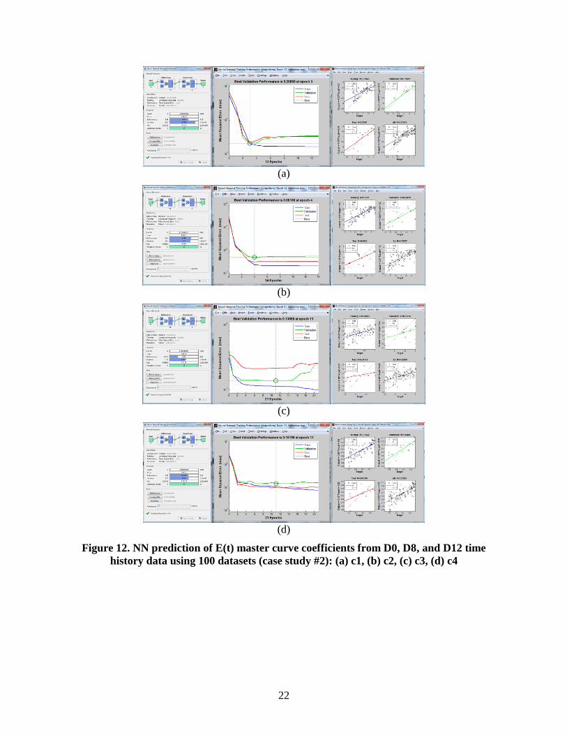
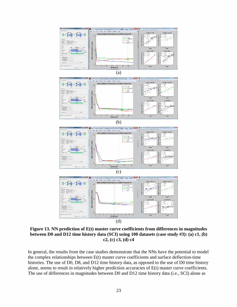
Figure 13. NN prediction of E(t) master curve coefficients from differences in magnitudes
between D0 and D12 time history data (SCI) using 100 datasets (case study #3): (a) c1, (b)
c2, (c) c3, (d) c4
In general, the results from the case studies demonstrate that the NNs have the potential to model
the complex relationships between E(t) master curve coefficients and surface deflection-time
histories. The use of D0, D8, and D12 time history data, as opposed to the use of D0 time history
alone, seems to result in relatively higher prediction accuracies of E(t) master curve coefficients.
The use of differences in magnitudes between D0 and D12 time history data (i.e., SCI) alone as

24
an input in NN inverse modeling did not increase the prediction accuracies and is therefore not
recommended for future analysis. Future analysis should also consider the effect of including
deflection-time history data from all sensors in the standard FWD configuration (D0, D8, D12,
D18, D24, D36, D48, D60, and D72) on the prediction accuracies.
25
PROOF-OF-CONCEPT DEMONSTRATION:COMPREHENSIVE FULL-DEPTH AC
PAVEMENT ANALYSIS
Development of Comprehensive Synthetic Database
The focused case studies carried out and discussed in the previous section established the
framework for deriving the AC E(t) or |E*| master curve based on a single FWD test performed
at a single temperature, thereby fulfilling the main objective of this study. In this section, the
proposed methodology is further explored through a comprehensive forward and inverse analysis
of full-depth AC. A comprehensive synthetic database consisting of 10,000 datasets was
generated through batch simulations of the VE forward analysis program by randomly varying
the inputs within the min-max ranges, summarized in Table 2.
Table 2. Summary of input ranges used in the generation of 10,000 VE forward analysis
scenarios for comprehensive full-depth AC analysis
Input Parameter Min Value Max Value
Pavement temperature (Tac) 32 deg-F (0 deg-C) 113 deg-F (45 deg-C)
AC layer thickness (Hac): 5 in. 45 in.
Subgrade modulus (Esub): 5,000 psi 20,000 psi
AC Poisson’s ratio (μac): 0.3 (constant)
Subgrade Poisson’s ratio (μsub): 0.4 (constant)
c1 0.045 2.155
c2 1.8 4.4
c3 -0.523 1.025
c4 -0.845 -0.38
a1 -5.380E-4 1.136E-3
a2 -1.598E-1 -0.770E-1
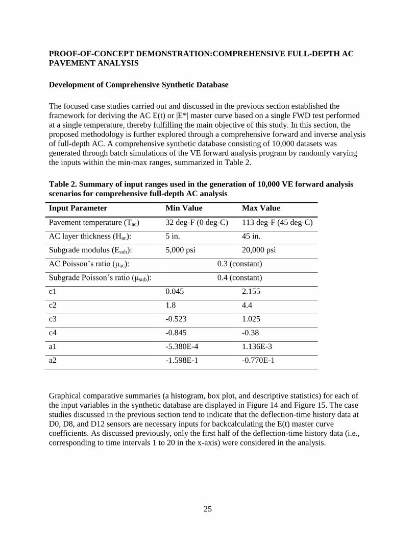
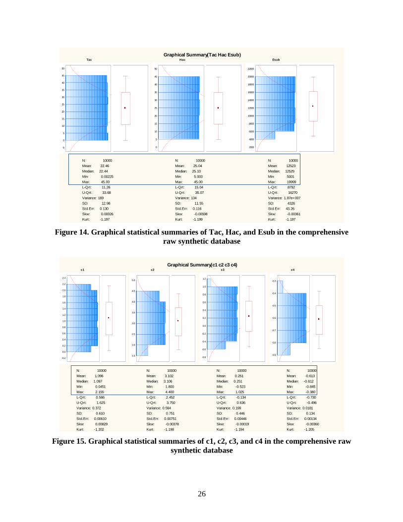
Graphical comparative summaries (a histogram, box plot, and descriptive statistics) for each of
the input variables in the synthetic database are displayed in Figure 14 and Figure 15. The case
studies discussed in the previous section tend to indicate that the deflection-time history data at
D0, D8, and D12 sensors are necessary inputs for backcalculating the E(t) master curve
coefficients. As discussed previously, only the first half of the deflection-time history data (i.e.,
corresponding to time intervals 1 to 20 in the x-axis) were considered in the analysis.
26
Figure 14. Graphical statistical summaries of Tac, Hac, and Esub in the comprehensive
raw synthetic database
Figure 15. Graphical statistical summaries of c1, c2, c3, and c4 in the comprehensive raw
synthetic database
Graphical Summary(Tac Hac Esub)Tac
-5
0
5
10
15
20
25
30
35
40
45
50
-5
0
5
10
15
20
25
30
35
40
45
50
N: 10000
Mean: 22.46
Median: 22.44
Min: 0.00225
Max: 45.00
L-Qrt: 11.26
U-Qrt: 33.68
Variance: 169
SD: 12.98
Std.Err: 0.130
Skw: 0.00026
Kurt: -1.197
95% Conf SD
Lower: 12.80
Upper: 13.16
95% Conf Mean
Lower: 22.21
Upper: 22.72
Hac
0
5
10
15
20
25
30
35
40
45
50
0
5
10
15
20
25
30
35
40
45
50
N: 10000
Mean: 25.04
Median: 25.10
Min: 5.003
Max: 45.00
L-Qrt: 15.04
U-Qrt: 35.07
Variance: 134
SD: 11.55
Std.Err: 0.116
Skw: -0.00598
Kurt: -1.199
95% Conf SD
Lower: 11.40
Upper: 11.72
95% Conf Mean
Lower: 24.82
Upper: 25.27
Esub
2000
4000
6000
8000
10000
12000
14000
16000
18000
20000
22000
2000
4000
6000
8000
10000
12000
14000
16000
18000
20000
22000
N: 10000
Mean: 12523
Median: 12529
Min: 5001
Max: 19999
L-Qrt: 8792
U-Qrt: 16270
Variance: 1.87e+007
SD: 4326
Std.Err: 43.26
Skw: -0.00361
Kurt: -1.197
95% Conf SD
Lower: 4266
Upper: 4386
95% Conf Mean
Lower: 12438
Upper: 12608
Graphical Summary(c1 c2 c3 c4)c1
-0.2
0.0
0.2
0.4
0.6
0.8
1.0
1.2
1.4
1.6
1.8
2.0
2.2
2.4
-0.2
0.0
0.2
0.4
0.6
0.8
1.0
1.2
1.4
1.6
1.8
2.0
2.2
2.4
N: 10000
Mean: 1.096
Median: 1.097
Min: 0.0451
Max: 2.155
L-Qrt: 0.566
U-Qrt: 1.625
Variance: 0.372
SD: 0.610
Std.Err: 0.00610
Skw: 0.00829
Kurt: -1.202
95% Conf SD
Lower: 0.602
Upper: 0.619
95% Conf Mean
Lower: 1.085
Upper: 1.108
c2
1.5
2.0
2.5
3.0
3.5
4.0
4.5
5.0
1.5
2.0
2.5
3.0
3.5
4.0
4.5
5.0
N: 10000
Mean: 3.102
Median: 3.106
Min: 1.800
Max: 4.400
L-Qrt: 2.452
U-Qrt: 3.750
Variance: 0.564
SD: 0.751
Std.Err: 0.00751
Skw: -0.00378
Kurt: -1.198
95% Conf SD
Lower: 0.740
Upper: 0.761
95% Conf Mean
Lower: 3.088
Upper: 3.117
c3
-0.8
-0.6
-0.4
-0.2
0.0
0.2
0.4
0.6
0.8
1.0
1.2
-0.8
-0.6
-0.4
-0.2
0.0
0.2
0.4
0.6
0.8
1.0
1.2
N: 10000
Mean: 0.251
Median: 0.251
Min: -0.523
Max: 1.025
L-Qrt: -0.134
U-Qrt: 0.636
Variance: 0.199
SD: 0.446
Std.Err: 0.00446
Skw: -0.00019
Kurt: -1.194
95% Conf SD
Lower: 0.440
Upper: 0.452
95% Conf Mean
Lower: 0.242
Upper: 0.260
c4
-0.9
-0.8
-0.7
-0.6
-0.5
-0.4
-0.3
-0.9
-0.8
-0.7
-0.6
-0.5
-0.4
-0.3
N: 10000
Mean: -0.613
Median: -0.612
Min: -0.845
Max: -0.380
L-Qrt: -0.730
U-Qrt: -0.496
Variance: 0.0181
SD: 0.134
Std.Err: 0.00134
Skw: -0.00360
Kurt: -1.205
95% Conf SD
Lower: 0.133
Upper: 0.136
95% Conf Mean
Lower: -0.615
Upper: -0.610
27
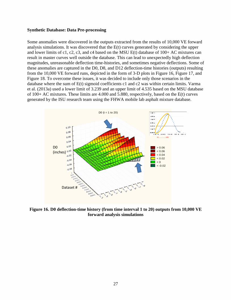
Synthetic Database: Data Pre-processing
Some anomalies were discovered in the outputs extracted from the results of 10,000 VE forward
analysis simulations. It was discovered that the E(t) curves generated by considering the upper
and lower limits of c1, c2, c3, and c4 based on the MSU E(t) database of 100+ AC mixtures can
result in master curves well outside the database. This can lead to unexpectedly high deflection
magnitudes, unreasonable deflection time-histories, and sometimes negative deflections. Some of
these anomalies are captured in the D0, D8, and D12 deflection-time histories (outputs) resulting
from the 10,000 VE forward runs, depicted in the form of 3-D plots in Figure 16, Figure 17, and
Figure 18. To overcome these issues, it was decided to include only those scenarios in the
database where the sum of E(t) sigmoid coefficients c1 and c2 was within certain limits. Varma
et al. (2013a) used a lower limit of 3.239 and an upper limit of 4.535 based on the MSU database
of 100+ AC mixtures. These limits are 4.000 and 5.880, respectively, based on the E(t) curves
generated by the ISU research team using the FHWA mobile lab asphalt mixture database.
Figure 16. D0 deflection-time history (from time interval 1 to 20) outputs from 10,000 VE
forward analysis simulations
D0 (t = 1 to 20)
1
8 0 1
1 6 0 1
2 4 0 1
3 2 0 1
4 0 0 1
4 8 0 1
5 6 0 1
6 4 0 1
7 2 0 1
8 0 0 1
8 8 0 1
9 6 0 1 D0-1
D0-3
D0-5
D0-7
D0-9
D0-11
D0-13
D0-15
D0-17
D0-19
-0.08
-0.06
-0.04
-0.02
0.00
0.02
0.04
0.06
0.08
0.10
> 0.06
< 0.06
< 0.04
< 0.02
< 0
< -0.02
D0 (inches)
Dataset #
t1……………..t20
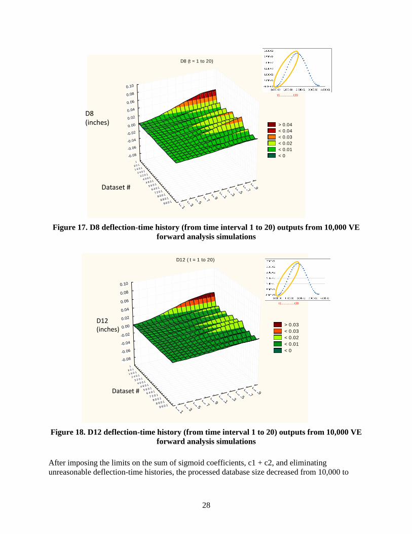
28
Figure 17. D8 deflection-time history (from time interval 1 to 20) outputs from 10,000 VE
forward analysis simulations
Figure 18. D12 deflection-time history (from time interval 1 to 20) outputs from 10,000 VE
forward analysis simulations
After imposing the limits on the sum of sigmoid coefficients, c1 + c2, and eliminating
unreasonable deflection-time histories, the processed database size decreased from 10,000 to
D8 (t = 1 to 20)
1
8 0 1
1 6 0 1
2 4 0 1
3 2 0 1
4 0 0 1
4 8 0 1
5 6 0 1
6 4 0 1
7 2 0 1
8 0 0 1
8 8 0 1
9 6 0 1 D8-1
D8-3
D8-5
D8-7
D8-9
D8-11D8-13
D8-15
D8-17
D8-19
-0.08
-0.06
-0.04
-0.02
0.00
0.02
0.04
0.06
0.08
0.10
> 0.04
< 0.04
< 0.03
< 0.02
< 0.01
< 0
D8 (inches)
Dataset #
t1……………..t20
D12 ( t = 1 to 20)
1
8 0 1
1 6 0 1
2 4 0 1
3 2 0 1
4 0 0 1
4 8 0 1
5 6 0 1
6 4 0 1
7 2 0 1
8 0 0 1
8 8 0 1
9 6 0 1 D12-1D12-3
D12-5
D12-7
D12-9
D12-11
D12-13
D12-15
D12-17
D12-19
-0.08
-0.06
-0.04
-0.02
0.00
0.02
0.04
0.06
0.08
0.10
> 0.03
< 0.03
< 0.02
< 0.01
< 0
D12 (inches)
Dataset #
t1……………..t20
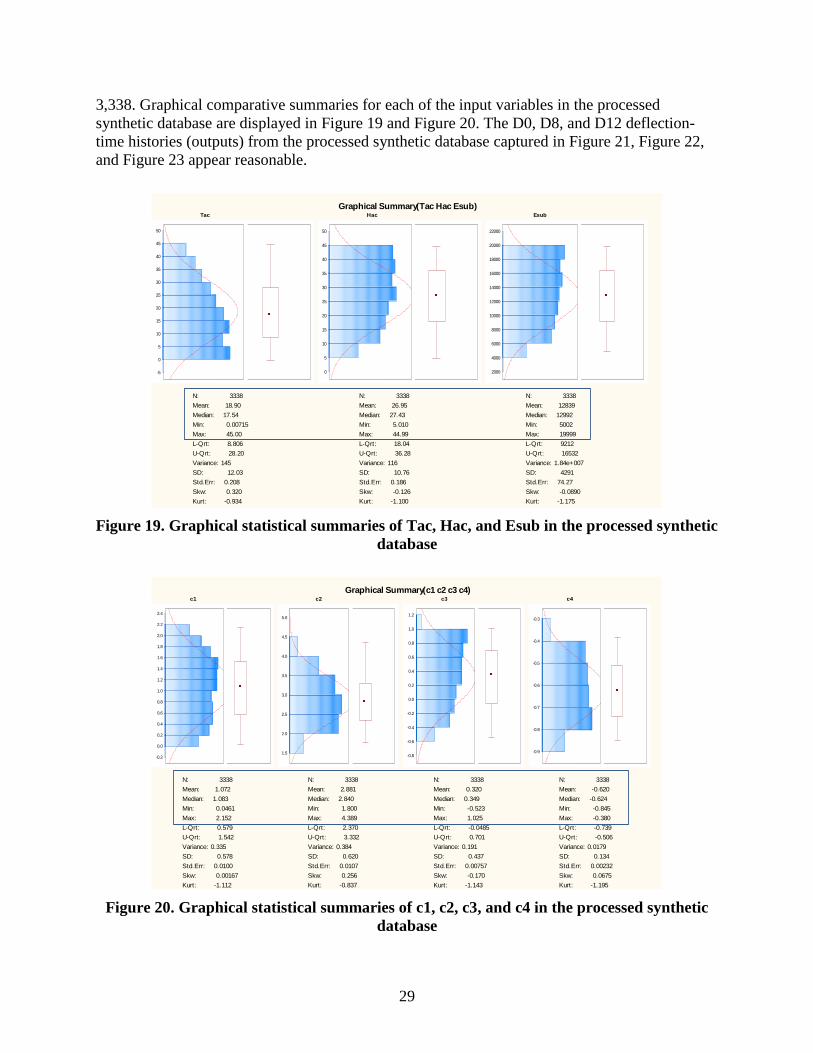
29
3,338. Graphical comparative summaries for each of the input variables in the processed
synthetic database are displayed in Figure 19 and Figure 20. The D0, D8, and D12 deflection-
time histories (outputs) from the processed synthetic database captured in Figure 21, Figure 22,
and Figure 23 appear reasonable.
Figure 19. Graphical statistical summaries of Tac, Hac, and Esub in the processed synthetic
database
Figure 20. Graphical statistical summaries of c1, c2, c3, and c4 in the processed synthetic
database
Graphical Summary(Tac Hac Esub)Tac
-5
0
5
10
15
20
25
30
35
40
45
50
-5
0
5
10
15
20
25
30
35
40
45
50
N: 3338
Mean: 18.90
Median: 17.54
Min: 0.00715
Max: 45.00
L-Qrt: 8.806
U-Qrt: 28.20
Variance: 145
SD: 12.03
Std.Err: 0.208
Skw: 0.320
Kurt: -0.934
95% Conf SD
Lower: 11.75
Upper: 12.33
95% Conf Mean
Lower: 18.49
Upper: 19.30
Hac
0
5
10
15
20
25
30
35
40
45
50
0
5
10
15
20
25
30
35
40
45
50
N: 3338
Mean: 26.95
Median: 27.43
Min: 5.010
Max: 44.99
L-Qrt: 18.04
U-Qrt: 36.28
Variance: 116
SD: 10.76
Std.Err: 0.186
Skw: -0.126
Kurt: -1.100
95% Conf SD
Lower: 10.51
Upper: 11.03
95% Conf Mean
Lower: 26.59
Upper: 27.32
Esub
2000
4000
6000
8000
10000
12000
14000
16000
18000
20000
22000
2000
4000
6000
8000
10000
12000
14000
16000
18000
20000
22000
N: 3338
Mean: 12839
Median: 12992
Min: 5002
Max: 19999
L-Qrt: 9212
U-Qrt: 16532
Variance: 1.84e+007
SD: 4291
Std.Err: 74.27
Skw: -0.0890
Kurt: -1.175
95% Conf SD
Lower: 4191
Upper: 4397
95% Conf Mean
Lower: 12693
Upper: 12984
Graphical Summary(c1 c2 c3 c4)c1
-0.2
0.0
0.2
0.4
0.6
0.8
1.0
1.2
1.4
1.6
1.8
2.0
2.2
2.4
-0.2
0.0
0.2
0.4
0.6
0.8
1.0
1.2
1.4
1.6
1.8
2.0
2.2
2.4
N: 3338
Mean: 1.072
Median: 1.083
Min: 0.0461
Max: 2.152
L-Qrt: 0.579
U-Qrt: 1.542
Variance: 0.335
SD: 0.578
Std.Err: 0.0100
Skw: 0.00167
Kurt: -1.112
95% Conf SD
Lower: 0.565
Upper: 0.593
95% Conf Mean
Lower: 1.052
Upper: 1.092
c2
1.5
2.0
2.5
3.0
3.5
4.0
4.5
5.0
1.5
2.0
2.5
3.0
3.5
4.0
4.5
5.0
N: 3338
Mean: 2.881
Median: 2.840
Min: 1.800
Max: 4.389
L-Qrt: 2.370
U-Qrt: 3.332
Variance: 0.384
SD: 0.620
Std.Err: 0.0107
Skw: 0.256
Kurt: -0.837
95% Conf SD
Lower: 0.605
Upper: 0.635
95% Conf Mean
Lower: 2.860
Upper: 2.902
c3
-0.8
-0.6
-0.4
-0.2
0.0
0.2
0.4
0.6
0.8
1.0
1.2
-0.8
-0.6
-0.4
-0.2
0.0
0.2
0.4
0.6
0.8
1.0
1.2
N: 3338
Mean: 0.320
Median: 0.349
Min: -0.523
Max: 1.025
L-Qrt: -0.0485
U-Qrt: 0.701
Variance: 0.191
SD: 0.437
Std.Err: 0.00757
Skw: -0.170
Kurt: -1.143
95% Conf SD
Lower: 0.427
Upper: 0.448
95% Conf Mean
Lower: 0.305
Upper: 0.335
c4
-0.9
-0.8
-0.7
-0.6
-0.5
-0.4
-0.3
-0.9
-0.8
-0.7
-0.6
-0.5
-0.4
-0.3
N: 3338
Mean: -0.620
Median: -0.624
Min: -0.845
Max: -0.380
L-Qrt: -0.739
U-Qrt: -0.506
Variance: 0.0179
SD: 0.134
Std.Err: 0.00232
Skw: 0.0675
Kurt: -1.195
95% Conf SD
Lower: 0.131
Upper: 0.137
95% Conf Mean
Lower: -0.625
Upper: -0.616
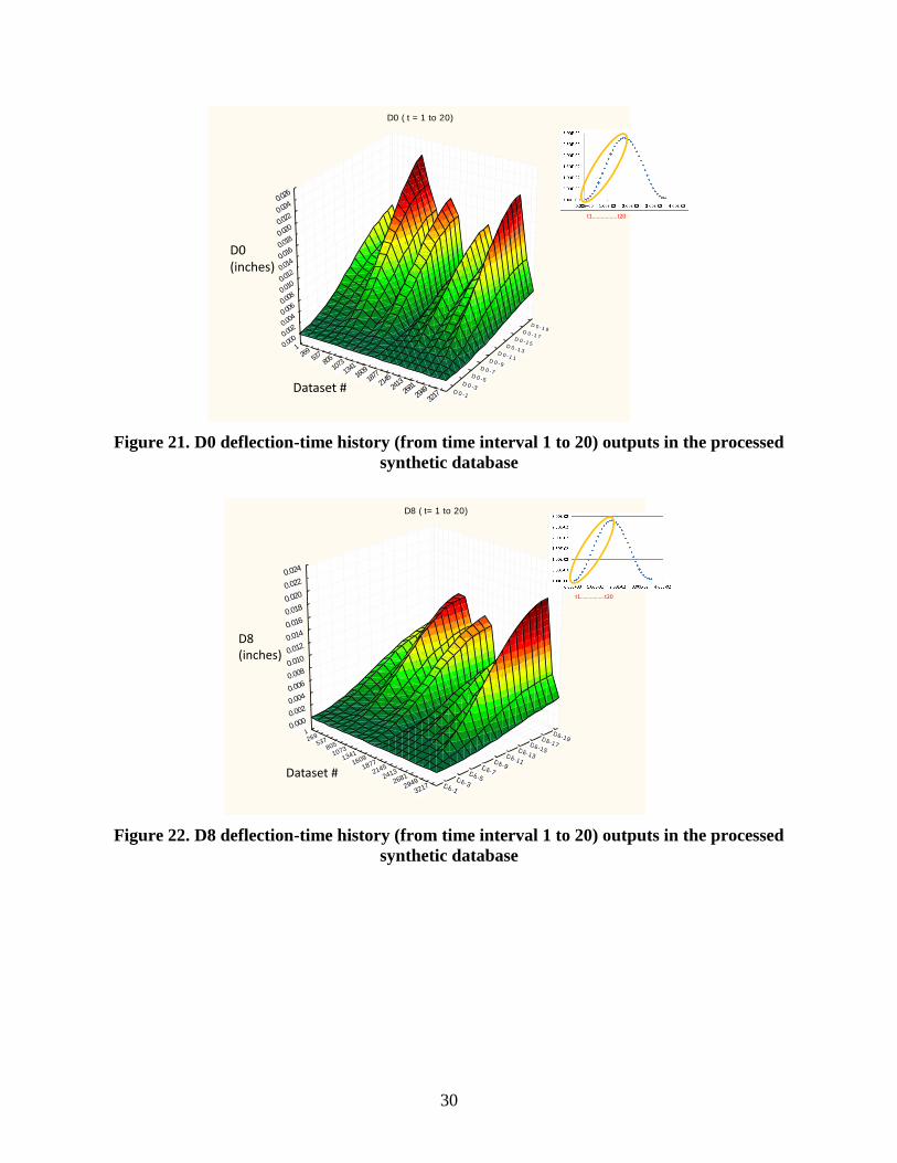
30
Figure 21. D0 deflection-time history (from time interval 1 to 20) outputs in the processed
synthetic database
Figure 22. D8 deflection-time history (from time interval 1 to 20) outputs in the processed
synthetic database
D0 ( t = 1 to 20)
126
953
780
5
1073
1341
1609
1877
2145
2413
2681
2949
3217
D 0 -1
D 0 -3
D 0 -5
D 0 -7
D 0 -9
D 0 -1 1
D 0 -1 3
D 0 -1 5
D 0 -1 7
D 0 -1 9
0.000
0.002
0.004
0.006
0.008
0.010
0.012
0.014
0.016
0.018
0.020
0.022
0.024
0.026
D0 (inches)
Dataset #
t1……………..t20
D8 ( t= 1 to 20)
1269
537805
1073
1341
1609
1877
2145
2413
2681
2949
3217 D8-1
D8-3
D8-5
D8-7
D8-9
D8-11
D8-13
D8-15
D8-17
D8-19
0.0000.0020.0040.0060.0080.0100.0120.0140.0160.0180.0200.0220.024
D8 (inches)
Dataset #
t1……………..t20
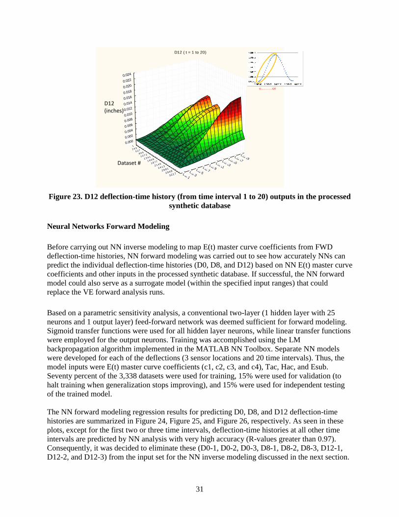
31
Figure 23. D12 deflection-time history (from time interval 1 to 20) outputs in the processed
synthetic database
Neural Networks Forward Modeling
Before carrying out NN inverse modeling to map E(t) master curve coefficients from FWD
deflection-time histories, NN forward modeling was carried out to see how accurately NNs can
predict the individual deflection-time histories (D0, D8, and D12) based on NN E(t) master curve
coefficients and other inputs in the processed synthetic database. If successful, the NN forward
model could also serve as a surrogate model (within the specified input ranges) that could
replace the VE forward analysis runs.
Based on a parametric sensitivity analysis, a conventional two-layer (1 hidden layer with 25
neurons and 1 output layer) feed-forward network was deemed sufficient for forward modeling.
Sigmoid transfer functions were used for all hidden layer neurons, while linear transfer functions
were employed for the output neurons. Training was accomplished using the LM
backpropagation algorithm implemented in the MATLAB NN Toolbox. Separate NN models
were developed for each of the deflections (3 sensor locations and 20 time intervals). Thus, the
model inputs were E(t) master curve coefficients (c1, c2, c3, and c4), Tac, Hac, and Esub.
Seventy percent of the 3,338 datasets were used for training, 15% were used for validation (to
halt training when generalization stops improving), and 15% were used for independent testing
of the trained model.
The NN forward modeling regression results for predicting D0, D8, and D12 deflection-time
histories are summarized in Figure 24, Figure 25, and Figure 26, respectively. As seen in these
plots, except for the first two or three time intervals, deflection-time histories at all other time
intervals are predicted by NN analysis with very high accuracy (R-values greater than 0.97).
Consequently, it was decided to eliminate these (D0-1, D0-2, D0-3, D8-1, D8-2, D8-3, D12-1,
D12-2, and D12-3) from the input set for the NN inverse modeling discussed in the next section.
D12 ( t = 1 to 20)
1
2 6 9
5 3 7
8 0 5
1 0 7 3
1 3 4 1
1 6 0 9
1 8 7 7
2 1 4 5
2 4 1 3
2 681
2 949
3217 D12-1
D12-3
D12-5
D12-7
D12-9
D12-11
D12-13
D12-15
D12-17
D12-19
0.0000.0020.0040.0060.0080.0100.0120.0140.016
0.018
0.020
0.022
0.024
D12 (inches)
Dataset #
t1……………..t20
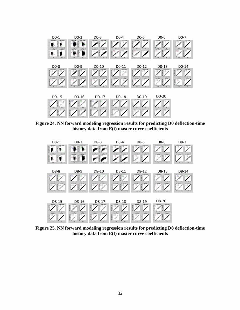
32
Figure 24. NN forward modeling regression results for predicting D0 deflection-time
history data from E(t) master curve coefficients
Figure 25. NN forward modeling regression results for predicting D8 deflection-time
history data from E(t) master curve coefficients
D0-1 D0-2 D0-3 D0-4 D0-5 D0-6 D0-7
D0-8 D0-9 D0-10 D0-11 D0-12 D0-13 D0-14
D0-15 D0-16 D0-17 D0-18 D0-19 D0-20
D8-1 D8-2 D8-3 D8-4 D8-5 D8-6 D8-7
D8-8 D8-9 D8-10 D8-11 D8-12 D8-13 D8-14
D8-15 D8-16 D8-17 D8-18 D8-19 D8-20
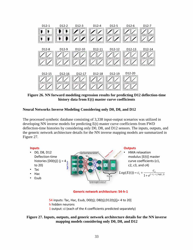
33
Figure 26. NN forward modeling regression results for predicting D12 deflection-time
history data from E(t) master curve coefficients
Neural Networks Inverse Modeling Considering only D0, D8, and D12
The processed synthetic database consisting of 3,338 input-output scenarios was utilized in
developing NN inverse models for predicting E(t) master curve coefficients from FWD
deflection-time histories by considering only D0, D8, and D12 sensors. The inputs, outputs, and
the generic network architecture details for the NN inverse mapping models are summarized in
Figure 27.
Figure 27. Inputs, outputs, and generic network architecture details for the NN inverse
mapping models considering only D0, D8, and D12
D12-1 D12-2 D12-3 D12-4 D12-5 D12-6 D12-7
D12-8 D12-9 D12-10 D12-11 D12-12 D12-13 D12-14
D12-15 D12-16 D12-17 D12-18 D12-19 D12-20
Inputs• D0, D8, D12
Deflection-time histories [D0(tj)] (j = 4 to 20)
• Tac• Hac• Esub
Outputs• HMA relaxation
modulus [E(t)] master curve coefficients (c1, c2, c3, and c4)
3 4
21 ( log(t ))
( (t))1 rc c
cLog E c
e
Generic network architecture: 54-h-1
54 inputs: Tac, Hac, Esub, D0(tj); D8(tj);D12(tj)[j= 4 to 20]h hidden neurons1 output: ci (each of the 4 coefficients predicted separately)
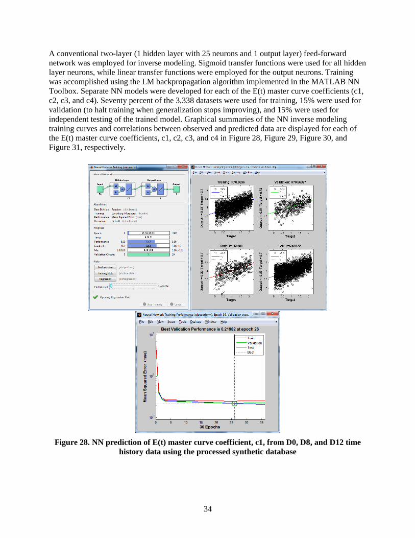
34
A conventional two-layer (1 hidden layer with 25 neurons and 1 output layer) feed-forward
network was employed for inverse modeling. Sigmoid transfer functions were used for all hidden
layer neurons, while linear transfer functions were employed for the output neurons. Training
was accomplished using the LM backpropagation algorithm implemented in the MATLAB NN
Toolbox. Separate NN models were developed for each of the E(t) master curve coefficients (c1,
c2, c3, and c4). Seventy percent of the 3,338 datasets were used for training, 15% were used for
validation (to halt training when generalization stops improving), and 15% were used for
independent testing of the trained model. Graphical summaries of the NN inverse modeling
training curves and correlations between observed and predicted data are displayed for each of
the E(t) master curve coefficients, c1, c2, c3, and c4 in Figure 28, Figure 29, Figure 30, and
Figure 31, respectively.
Figure 28. NN prediction of E(t) master curve coefficient, c1, from D0, D8, and D12 time
history data using the processed synthetic database
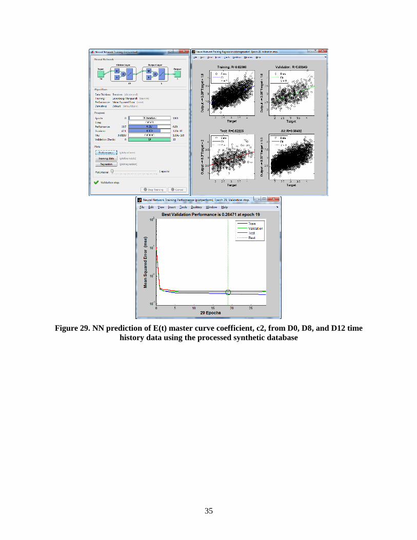
35
Figure 29. NN prediction of E(t) master curve coefficient, c2, from D0, D8, and D12 time
history data using the processed synthetic database
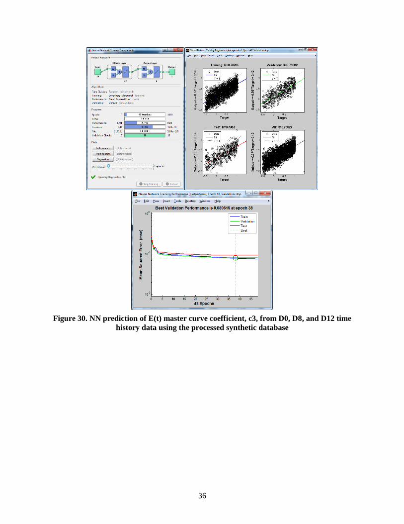
36
Figure 30. NN prediction of E(t) master curve coefficient, c3, from D0, D8, and D12 time
history data using the processed synthetic database
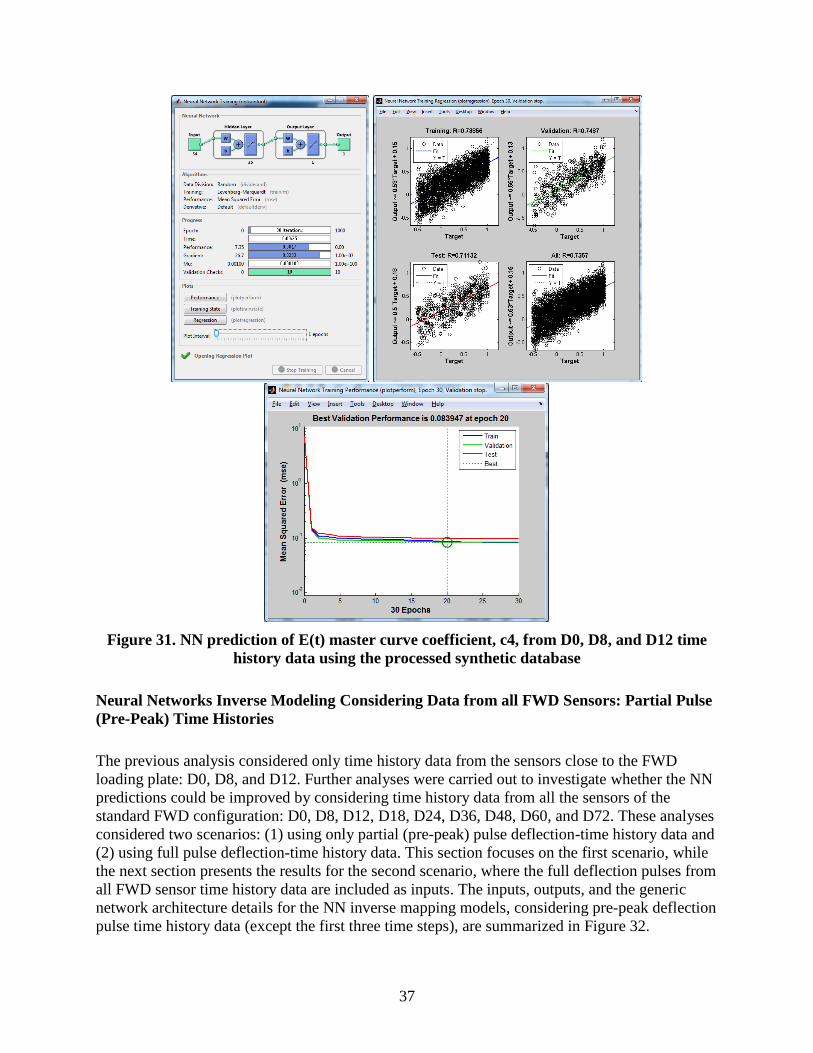
37
Figure 31. NN prediction of E(t) master curve coefficient, c4, from D0, D8, and D12 time
history data using the processed synthetic database
Neural Networks Inverse Modeling Considering Data from all FWD Sensors: Partial Pulse
(Pre-Peak) Time Histories
The previous analysis considered only time history data from the sensors close to the FWD
loading plate: D0, D8, and D12. Further analyses were carried out to investigate whether the NN
predictions could be improved by considering time history data from all the sensors of the
standard FWD configuration: D0, D8, D12, D18, D24, D36, D48, D60, and D72. These analyses
considered two scenarios: (1) using only partial (pre-peak) pulse deflection-time history data and
(2) using full pulse deflection-time history data. This section focuses on the first scenario, while
the next section presents the results for the second scenario, where the full deflection pulses from
all FWD sensor time history data are included as inputs. The inputs, outputs, and the generic
network architecture details for the NN inverse mapping models, considering pre-peak deflection
pulse time history data (except the first three time steps), are summarized in Figure 32.
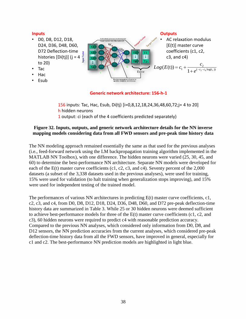
38
Figure 32. Inputs, outputs, and generic network architecture details for the NN inverse
mapping models considering data from all FWD sensors and pre-peak time history data
The NN modeling approach remained essentially the same as that used for the previous analyses
(i.e., feed-forward network using the LM backpropagation training algorithm implemented in the
MATLAB NN Toolbox), with one difference. The hidden neurons were varied (25, 30, 45, and
60) to determine the best-performance NN architecture. Separate NN models were developed for
each of the E(t) master curve coefficients (c1, c2, c3, and c4). Seventy percent of the 2,000
datasets (a subset of the 3,338 datasets used in the previous analyses), were used for training,
15% were used for validation (to halt training when generalization stops improving), and 15%
were used for independent testing of the trained model.
The performances of various NN architectures in predicting E(t) master curve coefficients, c1,
c2, c3, and c4, from D0, D8, D12, D18, D24, D36, D48, D60, and D72 pre-peak deflection-time
history data are summarized in Table 3. While 25 or 30 hidden neurons were deemed sufficient
to achieve best-performance models for three of the E(t) master curve coefficients (c1, c2, and
c3), 60 hidden neurons were required to predict c4 with reasonable prediction accuracy.
Compared to the previous NN analyses, which considered only information from D0, D8, and
D12 sensors, the NN prediction accuracies from the current analyses, which considered pre-peak
deflection-time history data from all the FWD sensors, have improved in general, especially for
c1 and c2. The best-performance NN prediction models are highlighted in light blue.
Inputs• D0, D8, D12, D18,
D24, D36, D48, D60, D72 Deflection-time histories [Di(tj)] (j = 4 to 20)
• Tac• Hac• Esub
Outputs• AC relaxation modulus
[E(t)] master curve coefficients (c1, c2, c3, and c4)
3 4
21 ( log(t ))
( (t))1 rc c
cLog E c
e
Generic network architecture: 156-h-1
156 inputs: Tac, Hac, Esub, Di(tj) [i=0,8,12,18,24,36,48,60,72;j= 4 to 20]h hidden neurons1 output: ci (each of the 4 coefficients predicted separately)
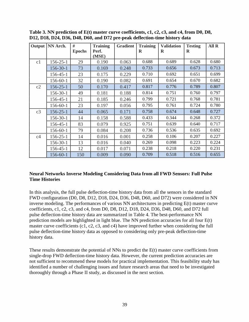
39
Table 3. NN prediction of E(t) master curve coefficients, c1, c2, c3, and c4, from D0, D8,
D12, D18, D24, D36, D48, D60, and D72 pre-peak deflection-time history data
Output NN Arch. #
Epochs
Training
Perf.
(MSE)
Gradient Training
R
Validation
R
Testing
R
All R
c1 156-25-1 29 0.190 0.063 0.688 0.689 0.628 0.680
156-30-1 73 0.169 0.248 0.733 0.656 0.673 0.713
156-45-1 23 0.175 0.229 0.710 0.692 0.651 0.699
156-60-1 32 0.190 0.082 0.691 0.654 0.670 0.682
c2 156-25-1 50 0.170 0.417 0.817 0.776 0.789 0.807
156-30-1 49 0.181 0.188 0.814 0.751 0.760 0.797
156-45-1 21 0.185 0.246 0.799 0.721 0.768 0.781
156-60-1 23 0.197 0.056 0.795 0.761 0.724 0.780
c3 156-25-1 44 0.065 0.171 0.758 0.674 0.648 0.727
156-30-1 14 0.158 0.588 0.433 0.344 0.268 0.372
156-45-1 83 0.079 0.925 0.751 0.639 0.640 0.717
156-60-1 79 0.084 0.208 0.736 0.536 0.635 0.692
c4 156-25-1 14 0.016 0.001 0.258 0.106 0.207 0.227
156-30-1 13 0.016 0.040 0.269 0.098 0.223 0.224
156-45-1 12 0.017 0.071 0.238 0.218 0.220 0.231
156-60-1 150 0.009 0.090 0.709 0.518 0.516 0.655
Neural Networks Inverse Modeling Considering Data from all FWD Sensors: Full Pulse
Time Histories
In this analysis, the full pulse deflection-time history data from all the sensors in the standard
FWD configuration (D0, D8, D12, D18, D24, D36, D48, D60, and D72) were considered in NN
inverse modeling. The performances of various NN architectures in predicting E(t) master curve
coefficients, c1, c2, c3, and c4, from D0, D8, D12, D18, D24, D36, D48, D60, and D72 full
pulse deflection-time history data are summarized in Table 4. The best-performance NN
prediction models are highlighted in light blue. The NN prediction accuracies for all four E(t)
master curve coefficients (c1, c2, c3, and c4) have improved further when considering the full
pulse deflection-time history data as opposed to considering only pre-peak deflection-time
history data.
These results demonstrate the potential of NNs to predict the E(t) master curve coefficients from
single-drop FWD deflection-time history data. However, the current prediction accuracies are
not sufficient to recommend these models for practical implementation. This feasibility study has
identified a number of challenging issues and future research areas that need to be investigated
thoroughly through a Phase II study, as discussed in the next section.
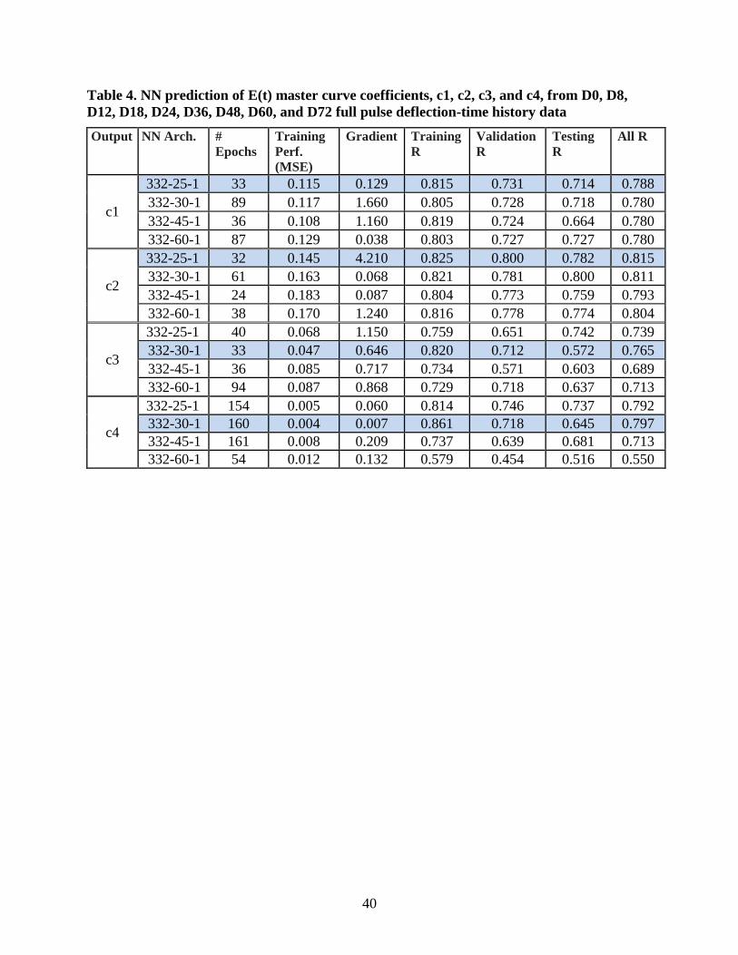
40
Table 4. NN prediction of E(t) master curve coefficients, c1, c2, c3, and c4, from D0, D8,
D12, D18, D24, D36, D48, D60, and D72 full pulse deflection-time history data
Output NN Arch. #
Epochs
Training
Perf.
(MSE)
Gradient Training
R
Validation
R
Testing
R
All R
c1
332-25-1 33 0.115 0.129 0.815 0.731 0.714 0.788
332-30-1 89 0.117 1.660 0.805 0.728 0.718 0.780
332-45-1 36 0.108 1.160 0.819 0.724 0.664 0.780
332-60-1 87 0.129 0.038 0.803 0.727 0.727 0.780
c2
332-25-1 32 0.145 4.210 0.825 0.800 0.782 0.815
332-30-1 61 0.163 0.068 0.821 0.781 0.800 0.811
332-45-1 24 0.183 0.087 0.804 0.773 0.759 0.793
332-60-1 38 0.170 1.240 0.816 0.778 0.774 0.804
c3
332-25-1 40 0.068 1.150 0.759 0.651 0.742 0.739
332-30-1 33 0.047 0.646 0.820 0.712 0.572 0.765
332-45-1 36 0.085 0.717 0.734 0.571 0.603 0.689
332-60-1 94 0.087 0.868 0.729 0.718 0.637 0.713
c4
332-25-1 154 0.005 0.060 0.814 0.746 0.737 0.792
332-30-1 160 0.004 0.007 0.861 0.718 0.645 0.797
332-45-1 161 0.008 0.209 0.737 0.639 0.681 0.713
332-60-1 54 0.012 0.132 0.579 0.454 0.516 0.550
41
SUMMARY AND CONCLUSIONS
The AC dynamic modulus (|E*|) is a key design parameter in the AASHTO MEPDG/Pavement-
ME Design. The standard laboratory procedures for AC dynamic modulus testing and
development of the master curve require time and considerable resources. The objective of this
feasibility study was to develop frameworks for predicting the AC dynamic modulus master
curve from routinely collected FWD time history data. The Iowa DOT is eventually interested in
documenting the Iowa AC mix damaged master curve coefficients relative to the mix IDs/Station
Nos., if possible, in the PMIS. This would be of significant use to the city, county, and state
engineers because the outcome of this research would enable them to look up the damaged
master curve shape parameters from the PMIS while running a flexible pavement rehabilitation
analysis and design using MEPDG/Pavement ME Design. As a first and foundational step, this
feasibility research study focused on establishing frameworks for predicting AC E(t) master
curve coefficients from FWD time history data. According to the theory of viscoelasticity, if the
AC relaxation modulus, E(t), is known, |E*| can be calculated (and vice versa) through numerical
inter-conversion procedures.
The overall research approach involved the following steps:
Conduct numerous VE forward analysis simulations by varying E(t) master curve
coefficients, shift factors, pavement temperatures, and other layer properties
Extract simulation inputs and outputs and assemble a synthetic database
Train, validate, and test NN inverse mapping models to predict E(t) master curve coefficients
from single-drop FWD deflection-time histories
A computationally efficient VE forward analysis program developed by MSU researchers was
adopted in this study to generate the synthetic database. The VE forward analysis program
accepts pavement temperature and layer properties (AC E(t) master curve, Eb/sub, h, μ,) and
outputs surface deflection-time histories. Several case studies were conducted to establish
detailed frameworks for predicting the AC E(t) master curve from single-drop FWD time history
data. Case studies focused on full-depth AC pavements as a first step to isolate potential
backcalculation issues that are only related to the modulus master curve of the AC layer. For the
proof-of-concept demonstration, a comprehensive full-depth AC analysis was carried out
through 10,000 batch simulations of a VE forward analysis program. Anomalies were detected in
the comprehensive raw synthetic database and were eliminated through imposition of certain
constraints on the sum of E(t) sigmoid coefficients, c1 + c2.
NN forward modeling was carried out to see how accurately NNs can predict the individual
deflection-time histories (D0, D8, and D12) based on NN E(t) master curve coefficients and
other inputs in the processed synthetic database. If successful, the NN forward model could also
serve as a surrogate model (within the specified input ranges) that could replace the VE forward
analysis runs. Except for the first two or three time intervals, deflection-time histories at all other
time intervals were predicted by NN analysis with very high accuracy (R-values greater than
0.97). The NN inverse modeling results demonstrated the potential of NNs to predict the E(t)
master curve coefficients from single-drop FWD deflection-time history data. However, the

42
current prediction accuracies are not sufficient to recommend these models for practical
implementation. Some recommendations are presented in the next section for an expanded Phase
II research project to arrive at high-accuracy E(t) master curve backcalculation models.
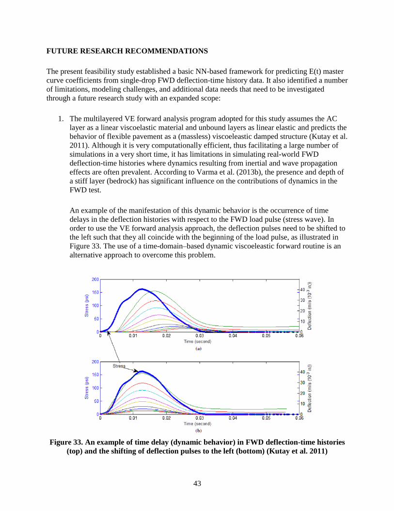
43
FUTURE RESEARCH RECOMMENDATIONS
The present feasibility study established a basic NN-based framework for predicting E(t) master
curve coefficients from single-drop FWD deflection-time history data. It also identified a number
of limitations, modeling challenges, and additional data needs that need to be investigated
through a future research study with an expanded scope:
1. The multilayered VE forward analysis program adopted for this study assumes the AC
layer as a linear viscoelastic material and unbound layers as linear elastic and predicts the
behavior of flexible pavement as a (massless) viscoeleastic damped structure (Kutay et al.
2011). Although it is very computationally efficient, thus facilitating a large number of
simulations in a very short time, it has limitations in simulating real-world FWD
deflection-time histories where dynamics resulting from inertial and wave propagation
effects are often prevalent. According to Varma et al. (2013b), the presence and depth of
a stiff layer (bedrock) has significant influence on the contributions of dynamics in the
FWD test.
An example of the manifestation of this dynamic behavior is the occurrence of time
delays in the deflection histories with respect to the FWD load pulse (stress wave). In
order to use the VE forward analysis approach, the deflection pulses need to be shifted to
the left such that they all coincide with the beginning of the load pulse, as illustrated in
Figure 33. The use of a time-domain–based dynamic viscoeleastic forward routine is an
alternative approach to overcome this problem.
Figure 33. An example of time delay (dynamic behavior) in FWD deflection-time histories
(top) and the shifting of deflection pulses to the left (bottom) (Kutay et al. 2011)
44
2. The proposed NN-based framework computes E(t) master curve coefficients based on
single-drop FWD test data (i.e., single FWD test performed at a single temperature).
Using this approach, it is only possible to accurately backcalculate certain portions of the
E(t), i.e., at high frequencies (short times). Note that the post-peak portion of the
deflection-time history curve is generally not considered reliable due to FWD integration
errors, which leaves limited information for backcalculating the entire E(t) master curve.
Kutay et al. (2011) and Varma et al. (2013a) noted that E(t) (|E*|) can be backcalculated
accurately up to about t = 0.1 sec (f = 10-3
Hz) using the deflection-time histories from a
typical single-drop FWD test. They further noted that, in order to accurately predict the
entire E(t) master curve, longer pulse durations need to be employed in the FWD test
(which will result in long-duration deflection-time history) or FWD tests need to be
conducted at different pavement temperatures (during different times of the day or
seasons) and use the concept of time-temperature superposition. Varma et al. (2013a)
concluded that deflection-time histories from FWD tests conducted between 68–104 °F
(20–40 °C) are useful in accurately estimating the entire E(t) or |E*| master curve.
If the prediction of E(t) from single-drop FWD test data is desirable (which is most often
the case), Varma et al. (2013b) recommends using deflection-time history data from
FWD tests conducted under an AC layer temperature gradient of preferably 41 °F (5 °C)
or more. Future research should consider the use of the enhanced VE forward analysis
tool recommended by Varma et al. (2013b) for synthetic database generation because it
attempts to simulate more realistic FWD test conditions with respect to the presence of an
uneven temperature distribution across the depth of the AC layer.
3. This feasibility study was restricted to the prediction of E(t) master curve coefficients
based on single-drop FWD test performed at a single temperature. Consequently, the
prediction of time-temperature superposition shift factors (a1 and a2) was omitted. Again,
by including the AC temperature profile information at the time of FWD testing in the
generation of the synthetic database using the enhanced VE forward analysis program
proposed by Varma et al. (2013b), it may be possible to backcalculate the entire E(t)
master curve, including the shift factors, from FWD deflection-time histories.
4. Apart from the use of NNs for the inverse analysis of viscoelastic asphalt layer properties
from FWD time history data, future research should also consider the use of an
evolutionary global optimization technique in combination with the VE forward solver.
For instance, Varma et al. (2013b) proposed the use of a GA-based optimization scheme
in combination with a VE forward solver to backcalculate E(t) master curve coefficients
and shift factors from FWD time history data. Such an approach involves minimizing the
differences between the responses calculated from the forward analysis and those from
the FWD test by varying the pavement layer properties until a best match is achieved.
The researchers for the present project have successfully employed this approach for
static backcalculation with different evolutionary optimization techniques such as GA
(Gopalakrishnan 2012), particle swarm optimization (PSO) (Gopalakrishnan 2010),
covariance matrix adaptation evolution strategy (CMA-ES) (Gopalakrishnan and Manik
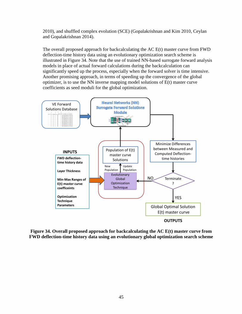
45
2010), and shuffled complex evolution (SCE) (Gopalakrishnan and Kim 2010, Ceylan
and Gopalakrishnan 2014).
The overall proposed approach for backcalculating the AC E(t) master curve from FWD
deflection-time history data using an evolutionary optimization search scheme is
illustrated in Figure 34. Note that the use of trained NN-based surrogate forward analysis
models in place of actual forward calculations during the backcalculation can
significantly speed up the process, especially when the forward solver is time intensive.
Another promising approach, in terms of speeding up the convergence of the global
optimizer, is to use the NN inverse mapping model solutions of E(t) master curve
coefficients as seed moduli for the global optimization.
Figure 34. Overall proposed approach for backcalculating the AC E(t) master curve from
FWD deflection-time history data using an evolutionary global optimization search scheme
Minimize Differences between Measured and Computed Deflection-
time histories
Population of E(t) master curve
Solutions
Global Optimal SolutionE(t) master curve
Terminate?
YES
Evolutionary Global
Optimization Technique
NO
Update Population
FWD deflection-time history data
Layer Thickness
Min-Max Ranges of E(t) master curve coefficeints
Optimization Technique Parameters
New Population
INPUTS
OUTPUTS
VE Forward Solutions Database

47
REFERENCES
AASHTO. (2008). Mechanistic-empirical pavement design guide, interim edition: a manual of
practice. American Association of State Highway and Transportation Officials,
Washington, D.C.
AASHTO. (2012). AASHTOWare Pavement ME Design. American Association of State
Highway and Transportation Officials, Washington, D.C.
<http://www.darwinme.org/MEDesign/Index.html> (March, 2013).
Adeli, H. (2001). Neural networks in civil engineering: 1989-2000. Computer-Aided Civil and
Infrastructure Engineering, Vol. 16, pp. 126-142.
Al-Khoury, R., Scarpas, A., Kastergen, C., and Blaauwendraad, J. (2001a). “Spectral Element
Technique for Efficient Parameter Identification of Layered Media, Part I: Forward
Calculation.” International Journal of Solids and Structures, Vol. 38, pp. 1605–1623.
Al-Khoury, R., Scarpas, A., Kastergen, C., and Blaauwendraad, J. (2001b). “Spectral Element
Technique for Efficient Parameter Identification of Layered Media, Part II: Inverse
Calculation.” International Journal of Solids and Structures, Vol. 38, pp. 8753–8772.
Al-Khoury, R., Scarpas, A., Kastergen, C., and Blaauwendraad, J. (2002a). “Spectral Element
Technique for Efficient Parameter Identification of Layered Media, Part III: Viscoelastic
Aspects.” International Journal of Solids and Structures, Vol. 39, pp. 2189–2201.
Al-Khoury, R., Scarpas, A., Kastergen, C., and Blaauwendraad, J. (2002b). “Poroelastic Spectral
Element for Wave Propagation and Parameter Identification in Multi-layer Systems.”
International Journal of Solids and Structures, Vol. 39, pp. 4073–4091.
Beale, M.H., Hagan, M.T., and Demuth, H.B. (2011). Neural Network ToolboxTM
User’s Guide,
MathWorks, Inc., Natick, MA.
Callop, A. C. and Cebon, D. (1996) “Stiffness Reductions of Flexible Pavements due to
Cumulative Fatigue Damage,” Journal of Transportation Engineering, Vol. 122, pp. 131-
139.
Ceylan, H., Guclu, A., Bayrak, M. B., and Gopalakrishnan, K. (2007). “Nondestructive
Evaluation of Iowa Pavements-Phase I”. Center for Transportation Research and
Education, Iowa State University, Ames, IA.
Ceylan, H., Gopalakrishnan, K., Kim, S., Guclu, A. and Bayrak, M. B. (2009). Non-Destructive
Evaluation of Iowa Pavements Phase 2: Development of a Fully Automated Software
System for Rapid Analysis/Processing of the Falling Weight Deflectometer Data. Final
Report. CTRE Project 04-177 Phase 2, Prepared for the Iowa Highway Research Board,
Center for Transportation Research and Education (CTRE), Iowa State University, Ames,
Iowa, February 2009.
Ceylan, H., Gopalakrishnan, K., and Kim, S. (2013). “Improving the Accuracy and Usability of
Iowa Falling Weight Deflectometer Data”. InTrans Project 11-415, Institute for
Transportation, Iowa State University.
Ceylan, H. and Gopalakrishnan, K. (2014). “Finite Element based Hybrid Evolutionary
Optimization Approach to Solving Rigid Pavement Inversion Problem”. Engineering
with Computers, Vol. 30, pp. 1-13.
Chang, D. W., Kang, Y. V., Roesset, J. M., and Stokoe II, K. H. (1992). ”Effect of Depth to
Bedrock on Deflection Basins Obtained with Dynaflect and Falling Weight
Deflectometer Tests,” Transportation Research Record, 1355, pp. 8–16.
48
Dong, Q. X., Hachiya, Y., Takahashi, O., Tsubokawa, Y. and Matsui, K. (2002). “An Efficient
Backcalculation Algorithm of Time Domain for Large-scale Pavement Structures Using
Ritz vectors,” Finite Elem Anal Des. Vol. 38, pp. 1131–1150.
Dougherity, M. (1995). “A review of neural networks applied to transport”. Transportation
Research, Part C, Vol. 3, No. 4, pp. 247-260.
Flintsch, G. W. (2003). “Soft computing applications in pavement and infrastructure
management: state-of-the-art”. CD-ROM Proceedings of the 82nd Annual Meeting of the
Transportation Research Board, National Research Council, Washington, D.C.
Foinquinos, R., Roesset, J. M., and Stokoe II, K. H. (1995). “Response of Pavement Systems to
Dynamic Loads Imposed by Nondestructive Tests,” Transportation Research Record,
1504, pp. 57–67.
Goktepe, A. B., Agar, E., Lav, A. H. (2006). “Advances in Backcalculating the Mechanical
Properties of Flexible pavements,” Advances in Engineering Software, Vol. 37, pp. 421–
431.
Gopalakrishnan, K., Kim, S., and Ceylan, H. (2009) “Hot Mix Asphalt Dynamic Modulus
Prediction Models Using Kernel Machines.” Intelligent Engineering Systems through
Artificial Neural Networks (the ANNIE 2009), Dagli, C. H., Bryden, K. M., Corns, S.
M., Gen, M., Tumer, K., and Suer, G. (Eds.), Vol.19, pp. 131–138, American Society of
Mechanical Engineers, New York.
Gopalakrishnan, K. (2010). “Neural Networks-Swarm Intelligence Hybrid Nonlinear
Optimization Algorithm for Pavement Moduli Backcalculation”. ASCE Journal of
Transportation Engineering, Vol. 136, No. 6, pp. 528-536.
Gopalakrishnan, K. and Manik, A. (2010). “Co-Variance Matrix Adaptation Evolution Strategy
for Pavement Backcalculation”. Construction and Building Materials, Vol. 24, pp. 2177-
2187.
Gopalakrishnan, K. and Kim, S. (2010). “Global Optimization of Pavement Structural
Parameters during Backcalculation Using Hybrid Shuffled Complex Evolution
Algorithm”. ASCE Journal of Computing in Civil Engineering, Vol. 24, No. 5, pp. 441-
451.
Gopalakrishnan, K. (2012). “Instantaneous Pavement Condition Evaluation Using
Nondestructive Neuro-Evolutionary Approach”. Structure & Infrastructure Engineering,
Vol. 8, No. 9, 2012.
Grenier, S., Konrad, J-M., and LeBoeuf, D. (2009). “Dynamic Simulation of Falling Weight
Deflectometer Tests on Flexible Pavements Using the Spectral Element Method: Forward
Calculations,” Can. J. Civ. Eng., Vol. 36, pp. 944–956.
Grenier, S., and Konrad, J-M. (2009). “Dynamic Interpretation of Falling Weight Deflectometer
Tests on Flexible Pavements Using the Spectral Element Method: Backcalculation,” Can.
J. Civ. Eng., Vol. 36, pp. 957–968.
Hardy, M. S. A. and Cebon, D. (1993). “Response of Continued Pavements to Moving Dynamic
Loads,” J Eng Mech. Vol. 119, No. 9, pp. 1762–1780.
Haykin, S. (1999). Neural networks: A comprehensive foundation. Prentice-Hall Inc., NJ, USA.
Irwin, L. (2002). “Backcalculation: An Overview and Perspective.” Proceedings of the
FWD/Backanalysis Workshop, 6th International Conference on the Bearing Capacity of
Roads, Railways and Airfields (BCRA 2002), Lisbon, Portugal.
Kausel, E., and Roesset, J.M. (1981). “Stiffness Matrices for Layered Soils,” Bulletin of the
Seismological Society of America, Vol. 71, Issue 6, pp. 1743–1761.
49
Kutay, E., Chatti, K., and Lei, L. (2011). “Backcalculation of Dynamic Modulus Mastercurve
from Falling Weight Deflectometer Surface Deflections”. Transportation Research
Record: Journal of the Transportation Research Board, Vol. 2227, pp. 87-96.
Liang, R. and Zeng, S. (2002). “Efficient Dynamic Analysis of Multilayered System during
Falling Weight Deflectometer Experiments,” Journal of Transportation Engineering, Vol.
128, No. 4, pp. 366-374.
Liang, R, Y. and Zhu, J. X. (1998). “Efficient Computational Algorithms for Forward and
Backward analysis of a Dynamic Pavement System,” Comput Struct 69, pp. 255–263.
Lytton, R. L., (1989). “Backcalculation of Pavement Layer Properties,” In NDT of Pavements
and Backcalculation of Moduli, First Volume, ASTM STP 1026. Edited by A. J. Bush III
and G. Y. Baladi. American Society for Testing and Materials, West Conshohochen, Pa.
pp. 7–38.
Lytton, R.L., Uzan, J., Frenando, E.G., Roque, R., Hiltunen, D., and Stoffels, S.M. (1993).
“Development and Validation of Performance Prediction Models and Specifications for
ASPHALT Binders and Paving mixes,” Report SHRP-A-357. Strategic Highway
Research Program, National Research Council, Washington, D.C.
Magnuson, A.H., Lytton, R.L., and Briggs, R. (1991). “Comparison of Computer Predictions and
Field Data for Dynamic Analysis of Falling Weight Deflectometer Data,” Transportation
Research Record, 1293, pp. 61–71.
Magnuson, A. H. (1998). “Computer Analysis of Falling Weight Deflectometer Data, Part I.
Vertical Displacement Computations on the Surface of a Uniform Surface Pressure
Distribution,” Research Report No.1215-1F, Texas Transportation Institute, Collage
Station.
Maina, J. W., Yokota, H., Mfinanga, D. A. and Masuda, S. (2000). “Dynamic Backcalculation
and Overlay Design Based on FWD Data,” In Nondestructive Testing of Pavements and
Backcalculation of Moduli, Third Volume, ASTM STP 1375. Edited by S.D. Tayabji and
E.O. Lukanen. American Society for Testing and Materials, West Conshohochen, Pa. pp.
95–109.
Mamlouk, M. S. and Davies, G. D. (1984). “Elasto-dynamic Analysis of Pavement Deflections,”
Journal of Transportation Engineering, Vol. 110, No.6, pp.536-567.
Mamlouk, M.S. (1985). “Use of Dynamic Analysis in Predicting Field Multilayer Pavement
Moduli,” Transportation Research Record, 1043, pp. 113-121.
National Cooperative Highway Research Program (NCHRP). (2004). Guide for mechanistic-
empirical design of new and rehabilitated pavement structures, <http://trb.org/mepdg>,
NCHRP 1-37A Final Report, Transportation Research Board, Washington, D.C.
Nilsson, R. N., Oost, I., and Hopman, P. C. (1996). “Visco-elastic Analysis of Full Scale
Pavements: Validation of VEROAD,” Transportation Research Record, 1539, pp. 81–87.
Park, S. W., and R. A. Schapery. (1999). Methods of Interconversion Between Linear
Viscoelastic Material Functions, Part I: A Numerical Method Based on Prony Series.
International Journal of Solids and Structures, Vol. 36, pp. 1653–1675.
Pellinen, T., Witczak, M., and Bonaquist, R. (2004) Asphalt Mix Master Curve Construction
Using Sigmoidal Fitting Function with Non-Linear Least Squares Optimization. Recent
Advances in Materials Characterization and Modeling of Pavement Systems, ASCE, pp.
83-101.
50
Roesset, J. M. (1980). “Stiffness and Damping Coefficients of Foundations,” In Proceedings of
ASCE National Convention on Dynamic Response of Pile Foundations, Analytical
Aspects. Edited by M.W. O'Neal and K. Dobry, New York , pp. 1–30.
Roesset, J. M. and Shao, K. Y. (1985). “Dynamic Interpretation of Dynaflect and falling Weight
Deflectometer tests,” Transportation Research Record, 1022, pp. 7–16.
Schwartz, C. W. (2005). Evaluation of the Witczak dynamic modulus prediction model. CD-
ROM, Presented at 84th Annual Transportation Research Board Meeting, Transportation
Research Board, Washington, D.C.
Shoukry, S. N. and William, G. W. (2000). “Performance Evaluation of Backcalculation
Algorithms through Three Dimensional Finite-element Modeling of Pavement
Structures,” Transportation Research Record, 1655, pp. 152–160.
Sousa, J. B. and Monismith, C. L. (1987). “Dynamic Response of Paving Materials,”
Transportation Research Record, 1136, pp. 57–68.
Stubbs, N., Torpunuri, V.S., Lytton, R.L., and Magnuson, A.H. (1994). “A Methodology to
Identify Material Properties in Pavements Modeled as Layered Viscoelastic Halfspaces
(Theory),” In Nondestructive Testing of Pavements and Backcalculation of Moduli,
Second Volume, ASTM STP 1198. In H.L. Von Quintus, A.J. Bush III, and G.Y. Baladi.
American Society for Testing and Materials, West Conshohochen, Pa. pp. 53–67.
Transportation Research (TR) Circular (1999). “Transportation Research Circular No. E-C012 -
Use of Artificial Neural Networks in Geomechanical and Pavement Systems,”
Transportation Research Circular, Prepared by A2K05(3) Subcommittee on Neural Nets
and Other Computational Intelligence–Based Modeling Systems, Transportation
Research Board, National Research Council, Washington, D.C., 18 p.
Ullidtz, P. and Coetzee, N. F. (1999). “Analytical Procedures in NDT Pavement Evaluation.”
CD-ROM Proceedings of the Annual Meeting of the Transportation Research Board,
Washington, D.C.
Ullidtz, P. (2000). “Will nonlinear Backcalculation Help,” In Nondestructive Testing of
Pavements and Backcalculation of Moduli, Third Volume, ASTM STP 1375. Edited by
S.D. Tayabji and E.O. Lukanen. American Society for Testing and Materials, West
Conshohochen, Pa. pp. 14–22.
Uzan, J. (1994a). “Dynamic Linear Back Calculation of Pavement Material Properties,” Journal
of Transportation Engineering, Vol. 120, No. 1.
Uzan, J. (1994b). “Advanced Backcalculation Techniques,” In Nondestructive Testing of
Pavements and Backcalculation of Moduli, Second Volume, ASTM STP 1198. In H.L.
Von Quintus, A.J. Bush III, and G.Y. Baladi. American Society for Testing and
Materials, West Conshohochen, Pa. pp. 3–37.
Varma,,S., Kutay, M. E. and Chatti, K. (2013a) “Data Requirements from Falling Weight
Deflectometer Tests for Accurate Backcalculation of Dynamic Modulus Master curve of
Asphalt Pavements”. 2013 Airfield & Highway Pavement Conference, pp. 1-11.
Varma, S., Kutay, E., and Levenberg, E. (2013b). “Viscoelastic Genetic Algorithm for Inverse
Analysis of Asphalt Layer Properties from Falling Weight Deflections”. Transportation
Research Record: Journal of the Transportation Research Board, Vol. 2369, pp. 38-46.
Von Quintus, H. L. and Killingsworth, B. (1998). “Comparison of Laboratory and In situ
Determined Elastic Layer Moduli.” Presented at the Annual Transportation Research
Board Meeting, Washington, D.C.

51
Witczak, M. W. (2005). Simple performance tests: Summary of Recommended Methods and
Database. National Cooperative Highway Research Program Report 547, Transportation
Research Board, Washington, D.C.
Zaghloul, S. M., and White, T. D. (1993). “Use of a Three Dimensional Dynamic Finite Element
Program for the Analysis of Flexible Pavement,” Transportation Research Record, 1388,
pp. 60–69.