DEVELOPMENT OF AN ULTRA-HIGH EFFICIENCY GAS TURBINE …
213
DEVELOPMENT OF AN ULTRA-HIGH EFFICIENCY GAS TURBINE ENGINE (UHEGT) WITH STATOR INTERNAL COMBUSTION: DESIGN, OFF-DESIGN, AND NONLINEAR DYNAMIC OPERATION A Dissertation by SEYED MOSTAFA GHOREYSHI Submitted to the Office of Graduate and Professional Studies of Texas A&M University in partial fulfillment of the requirements for the degree of DOCTOR OF PHILOSOPHY Chair of Committee, Meinhard T. Schobeiri Committee Members, J.N. Reddy Alan Palazzolo Jean-Luc Guermond Head of Department, Andreas A. Polycarpou December 2018 Major Subject: Mechanical Engineering Copyright © 2018 Seyed Mostafa Ghoreyshi
Transcript of DEVELOPMENT OF AN ULTRA-HIGH EFFICIENCY GAS TURBINE …

DEVELOPMENT OF AN ULTRA-HIGH EFFICIENCY GAS TURBINE
ENGINE (UHEGT) WITH STATOR INTERNAL COMBUSTION: DESIGN,
OFF-DESIGN, AND NONLINEAR DYNAMIC OPERATION
A Dissertation
by
SEYED MOSTAFA GHOREYSHI
Submitted to the Office of Graduate and Professional Studies of
Texas A&M University
in partial fulfillment of the requirements for the degree of
DOCTOR OF PHILOSOPHY
Chair of Committee, Meinhard T. Schobeiri
Committee Members, J.N. Reddy
Alan Palazzolo
Jean-Luc Guermond
Head of Department, Andreas A. Polycarpou
December 2018
Major Subject: Mechanical Engineering
Copyright © 2018 Seyed Mostafa Ghoreyshi

ii
ABSTRACT
An Ultra-High Efficiency Gas Turbine (UHEGT) technology is developed in this
study. In UHEGT, the combustion process is no longer contained in isolation between the
compressor and turbine, rather distributed in multiple stages and integrated within the
High-Pressure (HP)-turbine stator rows. Fundamental issues of aero-thermodynamic
design, combustion, and heat transfer are addressed in this study. The aero-thermodynamic
study shows that the UHEGT-concept improves the thermal efficiency of gas turbines by
5-7% above the current most advanced gas turbine engines, such as Alstom GT24. The
designed thermodynamic cycle has a 45% thermal efficiency and includes a six-stage
turbine with three stages of stator internal combustion. Meanline approach is used to
preliminary design the entire flow path in the turbine. Multiple configurations are designed
and simulated via Computational Fluid Dynamics (CFD) to achieve the optimum
combustion system for UHEGT. Flow patterns, temperature distributions, secondary
losses, etc. are among the parameters studied in the results. The final configuration for the
combustion system includes two rows of injectors placed before the stator rows in the first
three turbine stages. The current injector configuration provides a highly uniform
temperature distribution at the rotor inlet, low pressure loss, and low emissions compared
to the other cases. Different approaches are numerically studied to lower the stator blade
surface temperature distribution in UHEGT from which indexing (clocking) is shown to
be very effective.

iii
In the final part of this study, a dynamic simulation is performed on the entire engine
using the nonlinear generic code GETRAN developed by Schobeiri. The simulations are in
2D (space-time) and include the complete gas turbine engine. The system performance is
studied under variable design and off-design conditions. The results show that most of the
system parameters fluctuate with similar patterns to the fuel schedule. However, the
amplitudes of the fluctuations are different and there is a time lag in the response profiles
relative to the fuel schedules. It is shown that thermal efficiency variations are smaller
compared to the other parameters which means the system performs in efficiencies close to
the design point throughout the entire cycle.

iv
DEDICATION
I dedicate my dissertation to my parents whom without their support I would never
be able to succeed in this path. I also dedicate this dissertation to my wife, Nadia, whose
love and companionship gave me the motivation and will to work harder and better to
complete this work.

v
ACKNOWLEDGMENTS
I would like to state my greatest appreciation for my research adviser, Dr.
Schobeiri, whom I have learned so much from in the past few years. His knowledge,
guidance, and support gave me the power to succeed throughout this research. I would
also like to thank my committee members, Drs. Reddy, Palazzolo, and Guermond for their
help and guidance. I like to acknowledge the Mechanical Engineering Department and
Dale Adams Enterprises Inc. for supporting this project, and the High-Performance
Research Computing (HPRC) center at Texas A&M University for providing the
commercial softwares.
I would like to thank my friends and co-researchers Dr. Rezasoltani and Dr. Cand.
Nikparto whose experience guided me along this path. Also, thanks to all my friends in
Texas A&M University who made this experience enjoyable along the way. At the end, I
would like to thank my wife and family for their patience and continuous love and support
which made all this possible.

vi
NOMENCLATURE
Bh Blade height (m)
C Blade chord (m)
Cax Blade axial chord (m)
Cf Friction coefficient
Cp Static pressure coefficient
D Diameter (m)
Dh Hydraulic diameter (m)
h Static enthalpy (J/kg)
hs Isentropic enthalpy (J/kg)
H Total enthalpy (J/kg)
K Kinetic energy (J)
lm Specific load (J/kg)
M Mach number
�� Mass flow rate (kg/s)
mf Fuel mass flow rate (kg/s)
N Rotational velocity (rpm)
P Static pressure (Pa)
Pstag Stagnation pressure (Pa)
Ptot Total pressure (Pa)
R Radius

vii
Re Reynolds number
S Entropy (J/kg.K)
T Static temperature (K)
Tc Coolant temperature (K)
Tij Shear stress tensor (N/m2)
Ts Isentropic temperature (K)
Ttot Total temperature (K)
Tw Wall temperature (K)
T∞ Mainstream temperature (K)
U Blade circumferential velocity (m/s)
V Velocity (m/s)
Vj Cooling jet velocity (m/s)
Vm Meridional velocity (m/s)
Vu Circumferential velocity (m/s)
W Relative velocity (m/s)
�� Power (Watt)
X Axial location (m)
XL Length (m)
Greek
α Flow angle (deg)
β Blade metal angle (deg)

viii
γ Heat capacity ratio
η Efficiency
ηp Polytropic efficiency
ηs Isentropic efficiency
ηth Thermal efficiency
κ Heat capacity ratio
λ Load coefficient
μ Meridional velocity ratio
ν Circumferential velocity ratio
π Pressure ratio
ρ Density (kg/m3)
τw Wall shear stress (N/m2)
ϕ Flow coefficient
ϕWE Weak extinction equivalence ratio
ψ Isentropic load coefficient
Abbreviations
BL Baseline
CAES Compressed Air Energy Storage
CFD Computational Fluid Dynamics
CMB Combustion Chamber
EDM Eddy Dissipation Model

ix
GT Gas Turbine
HP High Pressure
INJ Injectors
LE Leading Edge
LP Low Pressure
M Million (Mega)
NUI Non-Uniformity Index
ppmv parts per million volume
PS Pressure Surface
R Rotor
S Stator
SS Suction Surface
TIT Turbine Inlet Temperature
UHEGT Ultra-High Efficiency Gas Turbine

x
CONTRIBUTORS AND FUNDING SOURCES
Contributors
This work was supported by a dissertation committee consisting of Professor
Schobeiri (adviser) and Professors Reddy and Palazzolo of the Department of Mechanical
Engineering and Professor Guermond of the Department of Mathematics.
The compressor data and design were provided by Erie Widyanto of the
Department of Mechanical Engineering and were published in 2015 in a thesis listed in
the Biographical Sketch.
All other work conducted for the dissertation was completed by the student
independently.
Funding Sources
Graduate study was supported by the Department of Mechanical Engineering from
Texas A&M University and Dale Adams Enterprises Inc.

xi
TABLE OF CONTENTS
ABSTRACT .......................................................................................................................ii
DEDICATION .................................................................................................................. iv
ACKNOWLEDGMENTS .................................................................................................. v
NOMENCLATURE .......................................................................................................... vi
CONTRIBUTORS AND FUNDING SOURCES .............................................................. x
TABLE OF CONTENTS .................................................................................................. xi
LIST OF FIGURES ......................................................................................................... xiv
LIST OF TABLES .......................................................................................................... xxi
CHAPTER I INTRODUCTION: GAS TURBINE ENGINE ........................................ 1
I.1. Gas Turbine Structure and Components ............................................................ 1
I.1.1. Turbine ......................................................................................................... 2 I.2. Gas Turbine Applications................................................................................... 3
I.2.1 Power Generation ........................................................................................... 3
I.2.2 Aircraft Engine ............................................................................................... 3 I.3. Efficiency Evolution of Gas Turbines ................................................................ 5
I.3.1. Alternative Performance Improvement Strategies ....................................... 7
CHAPTER II UHEGT: CONCEPT AND BACKGROUND ........................................ 9
II.1. Sequential Combustion: Background and Evolution of Technology ................. 9 II.2. The UHEGT Concept ....................................................................................... 12
II.2.1. Applications of UHEGT-Technology ........................................................ 19
II.2.2. Reheat Advantages in Gas Turbines .......................................................... 20 II.3. Alternative Combustor Technologies............................................................... 21
CHAPTER III RESEARCH OBJECTIVES ................................................................ 26
III.1. General Outline ................................................................................................ 26
III.2. Major Study Phases .......................................................................................... 26 III.2.1. Phase I: Combustion System Requirements and Design Process ........... 26

xii
III.2.2. Phase II: Turbine Cycle and Flow Path Design ...................................... 30 III.2.3. Phase III: UHEGT Simulation and Analysis .......................................... 31
III.2.4. Phase IV: Dynamic Simulation of the Engine ........................................ 31
CHAPTER IV DESIGN AND SIMULATION OF A SINGLE STAGE SAMPLE
TURBINE WITH STATOR INTERNAL COMBUSTION ........................................ 33
IV.1. UHEGT Combustion System: Important Design Parameters .......................... 33 IV.1.1. Controlled Fuel and Air Mixing by Vortex Generation ......................... 33
IV.1.2. Flame Stability ........................................................................................ 36 IV.1.3. Temperature Distribution at Rotor Inlet ................................................. 39
IV.2. Single Stage Turbine Design ............................................................................ 39
IV.3. Injector Design and Geometry ......................................................................... 40 IV.3.1. Injector Configuration 1 ......................................................................... 41 IV.3.2. Injector Configuration 2 ......................................................................... 44 IV.3.3. Injector Configuration 3 ......................................................................... 45
IV.4. Mesh Generation .............................................................................................. 47 IV.5. Numerical Method and Boundary Conditions ................................................. 50
IV.6. Results and Discussion ..................................................................................... 52 IV.6.1. Injector Configuration 1 ......................................................................... 52 IV.6.2. Injector Configuration 2 ......................................................................... 62
IV.6.3. Injector Configuration 3 ......................................................................... 64 IV.6.4. Further Discussion on Different Injector Configurations ....................... 70
CHAPTER V DESIGN AND SIMULATION OF THE MULTISTAGE UHEGT .... 76
V.1. Turbine Stage Design ....................................................................................... 76
V.2. Cycle Design .................................................................................................... 79 V.3. Turbine Geometry and Blade Profiling ............................................................ 83
V.4. Results and Discussion ..................................................................................... 84 V.5. Reducing the Stator Blade Surface Temperature ............................................. 97
V.5.1. Introduction and Methodology ................................................................... 97
V.5.2 Results and Discussion ............................................................................. 102
CHAPTER VI ENGINE SIMULATION IN DESIGN, OFF-DESIGN AND
DYNAMIC OPERATION ......................................................................................... 113
VI.1. Introduction .................................................................................................... 113 VI.2. Theoretical Background ................................................................................. 114
VI.2.1. The Engine Structure ............................................................................ 114 VI.2.2. Governing Equations ............................................................................ 116 VI.2.3. Numerical Approach ............................................................................. 119 VI.2.4. Engine Components and Simulation Schematics ................................. 120
VI.3. Results and Discussion ................................................................................... 127 VI.3.1. Sinusoidal Fuel Schedule ...................................................................... 127

xiii
VI.3.2. Gaussian Fuel Schedule ........................................................................ 136 VI.3.3. Step Function Fuel Schedule ................................................................ 144
CHAPTER VII CONCLUSION ................................................................................ 153
REFERENCES ........................................................................................................... 159
APPENDIX A SAMPLE DESIGN CODES .............................................................. 177
A.1. Turbine Stage Flow Path Design (FORTRAN) ............................................. 177 A.2. Blade Profiling (FORTRAN) ......................................................................... 184

xiv
LIST OF FIGURES
Figure 1. GE-Alstom (former Brown Boveri) heavy duty power generation gas
turbine GT13E2 with gross output of 203 MW; Reprinted from GE Power
[2]. ....................................................................................................................... 1
Figure 2. A three-stage high pressure research turbine at TPFL. The blades are
cylindrical with tip shroud to reduce the tip leakage losses; Reprinted from
Schobeiri [1]. ...................................................................................................... 2
Figure 3. Siemens SGT-800 power generation gas turbine (57.0 MW); Reprinted
from Siemens [3]. ............................................................................................... 4
Figure 4. Rolls Royce Trent 1000 aircraft engine. Three-spool, high-bypass ratio gas
turbine, designed and optimized for the Boeing 787 Dreamliner; Reprinted
from Rolls Royce [4]. ......................................................................................... 4
Figure 5. Efficiency comparison between a conventional (blue curve) and a reheat
(green curve) gas turbine; Reprinted from Schobeiri [5]. ................................... 6
Figure 6. Brown Boveri (GE-Alstom) GT 24/26 with two combustion stages and a
reheat turbine stage; Reprinted from GE Power [2]. .......................................... 6
Figure 7. Compressed air energy storage facility, Huntorf, Germany: (1) LP-Gear,
HP-Compressor train, (2) electric motor/generator, (3) gas turbine with two
combustion chambers and two multi-stage turbines, (4) air storage;
Reprinted from Schobeiri [12]. ......................................................................... 10
Figure 8. CAES gas turbine engine; Reprinted from Schobeiri [12]. .............................. 11
Figure 9. Process comparison for (a) baseline-conventional GT, (b) GT-24, and (c)
UHEGT (four stages); detailed processes are: compression 1–2, combustion
2–3, 4–5, 6–7, and 8–9, expansion: 3–4, 5–6, 7–8, and 9–10; Reprinted
from Schobeiri [8]. ............................................................................................ 14
Figure 10. (a) Thermal efficiency and (b) specific work comparison of baseline GT,
GT-24, and different UHEGT configurations; Reprinted from Ref. [15]. ....... 17
Figure 11. Technology change from conventional GT to more advanced GT24/26 and
the most advanced engine with an integrated UHEGT technology: (a)
conventional technology, (b) New technology, and (c) UHEGT technology;
Reprinted from Ref. [15]. ................................................................................. 18

xv
Figure 12. Brown Boveri’s Multi Injection Burner in the GT8 annular combustor;
Reprinted from Ref. [9]. ................................................................................... 23
Figure 13. EV burner by Alstom; Reprinted from Döbbeling et al. [9]. .......................... 23
Figure 14. Conventional combustion chamber: Typical primary-zone configuration
with inlet swirler; Reprinted from Lefebvre [33]. ............................................ 34
Figure 15. Effects of different parameters on weak extinction limit in a bluff-body
stabilized flame using liquid fuel sources: (a) Effect of mainstream velocity,
(b) effect of air pressure, (c) effect of inlet flow temperature, (d) effect of
approach stream Mach number. ΦWE is weak extinction equivalence ratio,
BG and θ are the flame holder blockage and angle, respectively; Reprinted
from Refs. [60]-[62]. ......................................................................................... 38
Figure 16. Pressure coefficient distribution along suction and pressure surfaces for the
single-stage turbine stator blade. ...................................................................... 41
Figure 17. Injector configuration 1: cylindrical fuel injectors extended from hub to
shroud. .............................................................................................................. 42
Figure 18. Injector configuration 1: computational domain. ........................................... 42
Figure 19. Single-stage sample turbine with injector configuration 1. ............................ 43
Figure 20. Injector configuration 2: cylindrical fuel injectors implemented inside the
stator blades. ..................................................................................................... 44
Figure 21. Injector configuration 3: (a) single layer and (b) multilayer vortex
generators; (c) gaseous fuel injector in the center of the swirler. ..................... 45
Figure 22. Injector configuration 3: computational domain. ........................................... 46
Figure 23. Single-stage sample turbine with injector configuration 3. ............................ 46
Figure 24. Computational grid: (a) structured hexahedral grid over the blade
components, (b) boundary layer grid near the blade leading edge, (c)
boundary layer grid near the blade trailing edge, (d) tetrahedral elements
near the injector surface combined with hexahedral grid in the main
domain. ............................................................................................................. 48
Figure 25. Grid independence study results: velocity and temperature distribution on
the midspan line at the exit of stator in configuration 1 for three different
grid sizes. .......................................................................................................... 49

xvi
Figure 26. Injector configuration 1: Mid-span velocity distribution in stationary
frame. ................................................................................................................ 53
Figure 27. Injector configuration 1: Mid-span velocity vectors in relative frame. .......... 54
Figure 28. Injector configuration 1: Fuel injector, velocity vectors and Von-Karman
vortices. ............................................................................................................. 54
Figure 29. Injector configuration 1: Mid-span temperature distribution. ........................ 55
Figure 30. Injector configuration 1: Temperature distribution before and after stator
and rotor. ........................................................................................................... 56
Figure 31. Injector configuration 1: Temperature distribution at the rotor inlet (Non-
uniformity=9.2%). ............................................................................................ 57
Figure 32. Injector configuration 1: Meridional temperature distribution. ...................... 57
Figure 33. Modified injector configuration 1: Temperature distribution at the rotor
inlet (Non-uniformity=5.1%). ........................................................................... 59
Figure 34. Modified injector configuration 1: Meridional temperature distribution. ...... 59
Figure 35. Injector configuration 1: Average temperature profile. .................................. 60
Figure 36. Injector configuration 1: Average fuel mass fraction profile. ........................ 61
Figure 37. Injector configuration 2, blade inlet and fuel injectors: Velocity vectors. ..... 63
Figure 38. Injector configuration 2, fuel injectors: Temperature contours show the
fuel ejection from the cutting surface into the flow field. ................................ 63
Figure 39. Injector configuration 2: Mid-span temperature distribution. ........................ 64
Figure 40. Modified injector configuration 2: Mid-span temperature distribution. ......... 65
Figure 41. Vortex breakdown in a swirling flow approaching stator blades. Midspan
velocity streamlines (a), and velocity vectors (b), from Ref. [15]. ................... 66
Figure 42. Injector configuration 3: Mid-span velocity distribution in stationary
frame. ................................................................................................................ 66
Figure 43. Injector configuration 3: Mid-span velocity vectors in relative frame. .......... 67
Figure 44. Injector configuration 3: Temperature distribution at span=0.6. .................... 69

xvii
Figure 45. Injector configuration 3: Temperature distribution before and after stator
and rotor. ........................................................................................................... 70
Figure 46. Injector configuration 3: Temperature distribution at the rotor inlet. ............. 71
Figure 47. Injector configuration 3: Meridional temperature distribution. ...................... 71
Figure 48. Injector configuration 3: Average temperature profile. .................................. 72
Figure 49. Injector configuration 3: Average fuel mass fraction profile. ........................ 73
Figure 50. A sample axial turbine stage (left) with corresponding velocity diagrams
(right); (V and W show the absolute and relative velocities, respectively);
Reprinted from Ref. [1]. ................................................................................... 77
Figure 51. UHEGT thermodynamic cycle: Pressure ratio for compressor and each
turbine stage, fuel mass flow rate for each combustion stage, corresponding
total power for each component, and the cycle thermal efficiency are
shown. ............................................................................................................... 81
Figure 52. Six-stage UHEGT turbine with three stages of stator internal combustion. ... 85
Figure 53. Computational domain for the 3-stage assembly: the domain has 10 total
components which include 3 injector rows, 3 stators, 3 rotors, and an inlet
extension. .......................................................................................................... 85
Figure 54. Midspan blade loading on the first stator: pressure coefficient distribution
on suction and pressure surfaces. ...................................................................... 86
Figure 55. Midspan streamlines in relative frame for the three-stage assembly. ............. 89
Figure 56. Midspan Mach number in relative frame for the three-stage assembly. ......... 90
Figure 57. Midspan static temperature distribution in stage 1. ........................................ 92
Figure 58. Midspan static temperature distribution in stage 2. ........................................ 93
Figure 59. Midspan static temperature distribution in stage 3. ........................................ 94
Figure 60. Temperature distribution at different axial locations: (a) stage 1 rotor inlet,
(b) stage 2 rotor inlet, (c) stage 3 rotor inlet, (d) stage 3 exit. .......................... 95
Figure 61. Average fuel mass fraction changes with axial location. ................................ 97
Figure 62. Numerical domain for CFD simulation in configuration 1. The injectors’
circumferential locations will be adjusted in configurations 2 and 3. ............ 101

xviii
Figure 63. Stator blade with film cooling holes in configuration 4: 3D view (left) and
side view (right). ............................................................................................. 101
Figure 64. Midspan Mach number distribution and velocity vectors for configuration
1. The distribution is similar for the other configurations as well. ................. 104
Figure 65. Midspan temperature distribution for the four configurations. ..................... 105
Figure 66. Stator blade surface temperature distribution for all configurations:
Configuration 1 represents the basic case with uniformly distributed
injectors in the circumferential direction; Configurations 2 and 3 represent
the case with the indexed injectors; Configuration 4 represents the film
cooled stator blade. ......................................................................................... 107
Figure 67. Film cooling effectiveness contours on stator blade, configuration 4: PS
(left), SS (right). .............................................................................................. 108
Figure 68. Rotor inlet temperature distribution for the four configurations. ................. 110
Figure 69. UHEGT, cross section of the complete assembly. The assembly consists of
three main components: Compressor on the left, connection piece in the
middle, and turbine on the right. ..................................................................... 114
Figure 70. UHEGT, 3D model of the rotor and casing. ................................................. 115
Figure 71. Simulation schematic of UHEGT (by Schobeiri). ........................................ 116
Figure 72. Discretized flow path with changing cross section S=S(x); Reprinted from
Schobeiri [1]. .................................................................................................. 117
Figure 73. System components and their modular representation; Reprinted from
Schobeiri [1]. .................................................................................................. 121
Figure 74. Representation of an adiabatic turbine component in the row-by-row
calculation. Each stage is decomposed into two rows that are connected via
the middle plenum. ......................................................................................... 123
Figure 75. Tubular combustion chamber; Reprinted from Schobeiri [31]. .................... 124
Figure 76. UHEGT injector component: Front view (top) and left view (bottom). ....... 125
Figure 77. Schedule applied through fuel valve to the injector component. .................. 126
Figure 78. Sinusoidal fuel schedule. .............................................................................. 127
Figure 79. Sinusoidal schedule: Compressor sets’ mass flow rates. .............................. 129

xix
Figure 80. Sinusoidal schedule: Turbine sets’ mass flow rates. ..................................... 129
Figure 81. Sinusoidal schedule: Turbine inlet temperatures. ......................................... 130
Figure 82. Sinusoidal schedule: Turbine exit temperatures. .......................................... 130
Figure 83. Sinusoidal schedule: Compressor sets’ power consumptions. ...................... 132
Figure 84. Sinusoidal schedule: Turbine sets’ power generations. ................................ 132
Figure 85. Sinusoidal schedule: Total power for each component. ............................... 133
Figure 86. Sinusoidal schedule: Engine thermal efficiency. .......................................... 134
Figure 87. Sinusoidal schedule: Non-dimensional shaft rotational speed. .................... 134
Figure 88. Sinusoidal schedule: Plena pressure. ............................................................ 135
Figure 89. Sinusoidal schedule: Plena temperature. ...................................................... 135
Figure 90. Gaussian fuel schedule. ................................................................................. 136
Figure 91. Gaussian schedule: Compressor sets’ mass flow rates. ................................ 137
Figure 92. Gaussian schedule: Turbine sets’ mass flow rates. ....................................... 138
Figure 93. Gaussian schedule: Turbine inlet temperatures. ........................................... 138
Figure 94. Gaussian schedule: Turbine exit temperatures. ............................................ 139
Figure 95. Gaussian schedule: Compressor sets’ power consumptions. ........................ 140
Figure 96. Gaussian schedule: Turbine sets’ power generations. .................................. 140
Figure 97. Gaussian schedule: Total power for each component................................... 141
Figure 98. Gaussian schedule: Engine thermal efficiency. ............................................ 142
Figure 99. Gaussian schedule: Non-dimensional shaft rotational speed. ....................... 142
Figure 100. Gaussian schedule: Plena pressure. ............................................................ 143
Figure 101. Gaussian schedule: Plena temperature. ....................................................... 143
Figure 102. Step function fuel schedule: Injector 1. ...................................................... 144
Figure 103. Step function fuel schedule: Injectors 2 and 3. ........................................... 145

xx
Figure 104. Step function schedule: Compressor sets’ mass flow rates. ....................... 146
Figure 105. Step function schedule: Turbine sets’ mass flow rates. .............................. 146
Figure 106. Step function schedule: Turbine inlet temperatures. .................................. 147
Figure 107. Step function schedule: Turbine exit temperatures. .................................... 147
Figure 108. Step function schedule: Compressor sets’ power consumptions. ............... 148
Figure 109. Step function schedule, turbine sets’ power generations: Turbines 1 to 3.. 149
Figure 110. Step function schedule, turbine sets’ power generations: Turbine 4. ......... 149
Figure 111. Step function schedule: Total power for each component. ......................... 150
Figure 112. Step function schedule: Engine thermal efficiency. ................................... 151
Figure 113. Step function schedule: Non-dimensional shaft rotational speed. .............. 151
Figure 114. Step function schedule: Plena pressure. ...................................................... 152
Figure 115. Step function schedule: Plena temperature. ................................................ 152

xxi
LIST OF TABLES
Table 1. Single-stage turbine parameters ......................................................................... 40
Table 2. Comparison of different UHEGT injector configurations ................................. 75
Table 3. Turbine stage parameters at the mean section for UHEGT ............................... 83
Table 4. Comparison between turbine stage power productions calculated by 2D and
CFD simulations ............................................................................................... 96
Table 5. Total pressure loss values in the injector rows ................................................... 96
Table 6. Comparison of the performance parameters between different
configurations ................................................................................................. 111

1
CHAPTER I
INTRODUCTION: GAS TURBINE ENGINE
I.1. Gas Turbine Structure and Components
Gas Turbine (GT) engines are types of Turbomachinery devices that transform the
total energy of the working fluid into kinetic energy and vice versa. A gas turbine engine
typically has three main components: compressor, combustion chamber, and turbine. In
compressor, the mechanical power is transferred to the working fluid (air) to increase its
pressure. In combustion chamber, the fuel is added to the working fluid and makes its
temperature to increase through combustion process. Finally, the high pressure-high
temperature combustion gas goes through turbine where its total energy is transformed to
mechanical energy and rotates the shaft [1]. Figure 1 shows a gas turbine and the main
corresponding components.
Figure 1. GE-Alstom (former Brown Boveri) heavy duty power generation gas turbine
GT13E2 with gross output of 203 MW; Reprinted from GE Power [2].

2
I.1.1. Turbine
The turbine component in the gas turbine is responsible for extracting the total
energy from the working fluid (combustion gas) and converting it into mechanical energy
which can be used for power or thrust generation. In an axial turbine, this process happens
through consecutive stages consisting of stator and rotor rows. The stator blades, which
are stationary and attached to the turbine casing, are responsible for deflecting the high
pressure-high temperature combustion gas to an appropriate angle to enter the rotor row.
In addition, the deflection process causes the flow to accelerate in the stator channel. The
working fluid then enters rotor where its energy is used to rotate the blades and the main
shaft. This process is repeated in multiple stages until the gas reaches the exit conditions.
Figure 2. A three-stage high pressure research turbine at TPFL. The blades are cylindrical
with tip shroud to reduce the tip leakage losses; Reprinted from Schobeiri [1].

3
Figure 2 shows a three-stage high pressure research turbine at Turbomachinery
Performance and Flow Research Laboratory (TPFL). The rotor blades are cylindrical with
tip shroud to reduce the tip leakage losses in this design.
I.2. Gas Turbine Applications
I.2.1 Power Generation
One of the main uses of gas turbines is in power generation plants. Gas turbines
have high thermal efficiencies, use air as the working fluid, and have high exhaust
temperature. Those characteristics make them very popular for power generation. The
high exhaust temperature makes it possible to use the gas turbine in a combined cycle
where the exhaust gas is used as a heat source for additional power generation via a steam
turbine. The combined cycle can reach astounding net efficiencies of higher than 60%.
Figure 3 shows a power generation industrial gas turbine engine, SGT-800 by Siemens.
I.2.2 Aircraft Engine
Gas turbines play a very important role in transportation as they are the main
propulsion system for all size aircrafts. The primary function of an aircraft gas turbine is
to generate thrust. Typically, aircraft gas turbines are designed as Turbofans which contain
two (or more) spools (shafts). The HP-spool includes HP-turbine which drives the HP-
compressor via the connecting shaft. The LP-spool contains the LP-turbine which drives

4
Figure 3. Siemens SGT-800 power generation gas turbine (57.0 MW); Reprinted from
Siemens [3].
Figure 4. Rolls Royce Trent 1000 aircraft engine. Three-spool, high-bypass ratio gas turbine,
designed and optimized for the Boeing 787 Dreamliner; Reprinted from Rolls Royce [4].

5
the main fan which is the main provider of thrust in a high-bypass ratio engine. The bypass
ratio is defined as the ratio of air mass flow bypassing the engine core (turbine and
combustion chamber) to the air mass flow going through the engine core. Figure 4 shows
the Rolls Royce Trent 1000 engine with bypass ratio of 10:1.
I.3. Efficiency Evolution of Gas Turbines
The basic cycle efficiency of the gas turbines prior to 1986 was in the range of
32%-35% [5]. To achieve higher efficiencies, Turbine Inlet Temperature (TIT) has to be
substantially increased which requires extensive amount of cooling in the front turbine
stages. Studies in [6]-[8] show that a significant efficiency improvement can be achieved
by introducing the reheat concept in CAES-turbine design. Figure 5 quantitively shows
the efficiency improvement achieved using the reheat concept. The blue curve in this
figure represents the efficiency of a relatively advanced GT with conventional
thermodynamic cycle. The green curve, on the other hand, represents the efficiency of a
generic reheat gas turbine [5]. This concept was adopted by Brown Boveri1 company in
GT24/26 engine, shown in Figure 6. As shown in this figure, GT24/26 has two combustion
stages and a reheat turbine stage. The background and evolution of this concept is
discussed in further details in the next chapter.
1 Former Brown Boveri (BBC), then Asea Brown Boveri (ABB), now GE-Alstom.

6
Figure 5. Efficiency comparison between a conventional (blue curve) and a reheat (green
curve) gas turbine; Reprinted from Schobeiri [5].
Figure 6. Brown Boveri (GE-Alstom) GT 24/26 with two combustion stages and a reheat
turbine stage; Reprinted from GE Power [2].

7
I.3.1. Alternative Performance Improvement Strategies
Premix Combustion: In 1970’s the engine pollution gained attraction and different
methods were developed to reduce NOx emission of gas turbines. The lean premix burning
concept was introduced which created a step towards low NOx combustion [9]. It was
realized that to achieve a low emission combustion process, the mixing process of fuel
and air could be separated from the combustion process itself and also combustion could
take place under very lean conditions. So, the goal was first to create a lean and
homogeneous mixture of fuel and air and then to burn it. Döbbeling et al. [9] from Alstom
performed some tests on a premix swirl combustor in conjunction with GASL in
Westbury, US. Approximately 10 ppm NOx was measured at the exit with 100% premix
oil, which was compared to the 60 ppm NOx in case of 92% premix oil and 8% diffusion
oil. This demonstrated the clear superiority of lean premix burning. If fuel and air are not
adequately premixed before combustion, it leads to creation of so-called hot-spot regions
which will likely cause an increase in NOx emission [10]. In lean premixed combustion,
the engine operates in equivalence ratio close to the lean blow-out limit in order to
maintain NOx and CO emission at low levels. For instance, as for natural gas, the
stoichiometric fuel air ratio is 1:17.2 and the lean blow-out limit is in the range of 0.1-0.4
depending on the performing conditions. Examples of lean blow-out limits are shown in
Figure 15 for a number liquid fuel sources. A lean fuel and air mixture may also lead to
unstable combustion. So, there should be a tradeoff between low emissions and flame
stability [10].

8
Water Injection: Water or steam injection into the flame was a normal practice to
reduce the NOx emissions. An example is one of the former BBC single-combustion
chamber gas turbine engines [9]. The injected mass flow of water would be in the same
order as the fuel mass flow rate. Although the output power of the gas turbine increased
with higher amount of water injection, the efficiency of the cycle dropped. Another
disadvantage was that demineralized water and steam were not available in many cases
[9].

9
CHAPTER II1
UHEGT: CONCEPT AND BACKGROUND
II.1. Sequential Combustion: Background and Evolution of Technology
Conventional gas turbines have a multistage compressor followed by a combustion
chamber and a multistage turbine. To substantially increase the thermal efficiency, in
1986, Schobeiri [6] introduced a multi-stage combustion process into gas turbines in a
Brown Boveri2 report. In this process, the combustion takes place in sequential steps along
the turbine stages, which leads to the elimination of the combustion chamber as a single
separate unit.
The idea behind the concept above is based on the well-known reheat process in
steam turbines. In this process, after the steam exits from the high pressure stages,
additional superheated steam is added to the main flow. The reheated steam flow then
passes the intermediate and low pressure turbine stages. The addition of the hot steam
improves the performance of the system and increases the average temperature of heat
addition, making the cycle closer to the ideal Carnot cycle [11].
1 Part of the materials are reprinted with permission from “The Ultrahigh Efficiency Gas Turbine Engine
with Stator Internal Combustion,” by Meinhard T. Schobeiri and Seyed M. Ghoreyshi, 2016. ASME Journal
of Engineering for Gas Turbines and Power Vol. 138, no. 2, Copyright © 2016 by ASME. 2 Former Brown Boveri (BBC), then Asea Brown Boveri (ABB), now GE-Alstom.

10
Based on this concept, a change of technology was suggested to increase the gas
turbine efficiency without a significant increase in Turbine Inlet Temperature (TIT). This
idea was utilized for the first time in order to develop a gas turbine for a compressed air
energy storage (CAES) in Huntorf, Germany. Figure 7 and Figure 8 show the schematic
of the CAES facility which is described more in details by Schobeiri [12], Schobeiri and
Haselbacher [13], and Schobeiri [14]. CAES gas turbine was designed and manufactured
by Brown Boveri (BBC) in 1978. The facility has been operating since then as an
emergency power generator. Different components are: 1- Compressor gear train, 2-
electric motor generator unit, 3- gas turbine, 4- underground compressed air storage.
Figure 7. Compressed air energy storage facility, Huntorf, Germany: (1) LP-Gear, HP-
Compressor train, (2) electric motor/generator, (3) gas turbine with two combustion
chambers and two multi-stage turbines, (4) air storage; Reprinted from Schobeiri [12].

11
Figure 8. CAES gas turbine engine; Reprinted from Schobeiri [12].
The main component of the CAES facility is the gas turbine shown in Figure 8. It
contains a high pressure (HP) combustion chamber followed by a multi-stage HP-turbine
and a low pressure (LP) combustion chamber followed by a multi-stage LP turbine. A
detailed study of this gas turbine showed a significant improvement in thermal efficiency
in the order of 5-7% in comparison with the one with one combustion chamber [12].
Although this standard efficiency improvement method was routinely used in compressed
air energy storage facilities, until the late eighties it did not find its way into the power
generation and aircraft gas turbine industry. The reason for that was the inherent problem
of adding a typical large volume combustion chamber to the engine. It could cause
different design integrity and operational problems which made the engine manufacturer

12
unwilling to implement this technology. So, prior to late eighties, implementing the reheat
process by adding a conventional combustion chamber was not a feasible option. But the
significant improvement in efficiency motivated Brown Boveri to make a radical change
to stay ahead in the increasingly intense global competition. In an intensive effort, a new
combustion technology was developed and integrated into a new gas turbine engine with
one reheat stage turbine followed by a second combustion and a multi-stage turbine which
significantly improved the thermal efficiency [15]-[18].
Although the addition of the second combustion chamber brought a significant
efficiency improvement, increasing the number of combustion chambers above two,
would result in unforeseeable design integrity problems. In the following section, the new
UHEGT technology is introduced which describes how to overcome the problems of
implementation of multiple combustion chambers in gas turbines.
II.2. The UHEGT Concept
The concept of the Ultra High Efficiency Gas Turbine (UHEGT) was developed
by M.T. Schobeiri, the former Chief of Aero-Thermodynamic Gas Turbine Design Group
at Brown Boveri. The new developed technology introduces a gas turbine in which the
combustion process is distributed along the turbine stator rows. This allows the
elimination of combustion chambers as a separate unit form the turbine leading to high
thermal efficiencies that cannot be achieved by conventional gas turbines. Schobeiri [7],
[8] proposed a patent which demonstrates that the UHEGT-concept can improve the

13
thermal efficiency of gas turbines from 5% to 7% above the current highest efficiency gas
turbines such as ABB GT24/26 (at full load: 40.5%).
To demonstrate the innovative claim of the UHEGT-concept, a study is conducted
comparing three conceptually different power generation gas turbine engines: a
conventional gas turbine (single shaft, single combustion chamber), a gas turbine with
sequential combustion (GT24/26), and a UHEGT [8]. The evolution of the gas turbine
process that represents the efficiency improvement is shown in Figure 9.
In this study, the working fluid is an ideal reacting mixture of methane and air. The
compression and each expansion processes is specified with polytropic efficiencies of
90% and 88%, respectively. The energy exchange at each section is calculated based on
the static enthalpy difference between inlet and exit. The total net power is computed by
adding turbine powers of all stages and subtracting the total compressor power and the
power due to the bearing losses. The thermal efficiency is the ratio of the total net power
to the fuel energy.
Figure 9a shows a conventional single combustion process in which thermal
efficiency is around 32-36% (based on the different turbine inlet temperatures).
Substantial efficiency improvement was achieved by introducing a single reheat turbine
stage as shown in Figure 9b. By utilizing a higher compression ratio in GT24/26 and a
two-stage combustion process, the efficiency of the machine was considerably improved
without any significant increase in TIT. The cross-hatched area refers to the baseline
process and the simple-hatched area translates to the net work increase. This will lead to

14
thermal efficiency gain, which in case of the ABB-GT24/26, resulted in 6 to 7% efficiency
improvement [8].
Figure 9. Process comparison for (a) baseline-conventional GT, (b) GT-24, and (c) UHEGT
(four stages); detailed processes are: compression 1–2, combustion 2–3, 4–5, 6–7, and 8–9,
expansion: 3–4, 5–6, 7–8, and 9–10; Reprinted from Schobeiri [8].

15
A detailed dynamic engine simulation of the ABB-GT24/26 gas turbine engine
showed a thermal efficiency of 𝜂𝑇𝐻=40.5%. The corresponding measured efficiency for
GT-26 was reported as 38.2%. The difference of 2.3% is attributed to numerous failures
associated with compressor blade distress in the form of cracking. The failures occurred
at the start of the engine operation [19]. This efficiency improvement was achieved despite
the following facts: (a) The compressor pressure ratio is far greater than the optimal
conventional one (𝜋𝑜𝑝𝑡 𝐺𝑇24 ≈ 2 × 𝜋𝑜𝑝𝑡 𝐵𝐿) causing the compressor efficiency to
decrease. The latter is because of reduced blade height associated with an increase in
secondary flow losses. (b) The introduction of a second combustion chamber inherently
causes additional total pressure losses.
A further efficiency improvement is achieved by eliminating the combustion
chambers altogether and placing the combustion process inside the stator blade passages.
Figure 9c schematically shows the thermodynamic process of this gas turbine engine,
where the combustion is placed inside the stator flow passage of a multi-stage turbine.
Starting from the compressor exit pressure, Figure 9c, point 2, fuel is added inside the
stator flow passage raising the total temperature, to point 3. The expansion in the stator is
followed by the expansion through the first turbine rotor flow passage, point 4. The same
expansion processes are repeated in the following turbine stator and rotor blade passages
(points 5 through 9). The cross-hatched area refers to the baseline process, whereas the
simple-hatched area represents the net work gain which leads to thermal efficiency
improvement. Aero-thermodynamic calculations show that for a UHEGT with three
stator-internal combustions, a thermal efficiency of above 45% can be achieved.

16
Increasing the number of stator internal combustion to 4, raises the efficiency above 47%
[15].
A detailed quantitative calculation of each process is presented in Figure 10. In
this figure, the compression ratio is increased while the maximum cycle temperature (TIT)
is kept constant. These figures represent a comparison between the thermal efficiencies
and specific works of baseline GT, the GT24/26, and a UHEGT with three and four stator-
internal combustions, UHEGT-3S and UHEGT-4S, respectively. Maximum temperature
for all cycles are the same and equal to TIT=1200 C. As shown in Figure 10a, for UHEGT-
3S (with three stator internal combustion stages), a thermal efficiency above 45% is
calculated [15]. This exhibits an increase of at least 5% above the efficiency of the most
advanced current gas turbine engine, GT24/26. Increasing the number of stator internal
combustion to 4, curve labeled with UHEGT-4S, raises the efficiency above 47% which
can bring an enormous efficiency increase compared to the existing gas turbine engines.
It should be noted that UHEGT-concept requires an optimization of the compressor
pressure ratio. As shown in Figure 10a, the optimum pressure ratio for the current UHEGT
is around 35 to 40 which is higher than the optimum pressure ratio for a single combustor
engine (15-20).
Figure 10b shows the specific work comparison for the gas turbines discussed
above. Compared to GT-24, UHEGT-technology has about 20% higher specific work,
making this technology very suitable for aircraft engines, stand-alone as well as combined
cycle power generation applications. This efficiency increase can be established at a
compressor pressure ratio of 𝜋𝑈𝐻𝐸𝐺𝑇 = 35 − 40, which can be achieved easily by existing

17
Figure 10. (a) Thermal efficiency and (b) specific work comparison of baseline GT, GT-24,
and different UHEGT configurations; Reprinted from Ref. [15].
GT-24
Baseline GT
UHEGT-4S
UHEGT-3S
w(K
J/k
g)
10 20 30 40 500
100
200
300
400
500
600
(b)
GT-24
=
38
UHEGT-4S
UHEGT-3S
Measured Th
=38.2% [7]
Baseline GT
Th
=47.5%
Th
=45.3%
th
0 10 20 30 40 500.2
0.3
0.4
0.5
(a) TIT = 1200C
for all three GTs

18
Figure 11. Technology change from conventional GT to more advanced GT24/26 and the
most advanced engine with an integrated UHEGT technology: (a) conventional technology,
(b) New technology, and (c) UHEGT technology; Reprinted from Ref. [15].

19
compressor design technology with a conventional polytropic efficiency of around 90%
[15]. Figure 11 represents at one glance the evolution associated with the change of
technology as discussed. Starting with the conventional design in Figure 11a, through
GT24/26 in Figure 11b, and the UHEGT with a multi-stage compressor and internal
combustion within the first, second, third, and fourth stators as shown in Figure 11c.
II.2.1. Applications of UHEGT-Technology
The UHEGT-technology is equally applicable to the core of civil and military
aircraft engines with single, twin and three spools as well as power generation gas turbine
engines. The elimination of the combustion chamber in UHEGT results in a much shorter
shaft with a more stable rotor dynamic operation [15]. In aircraft engine applications, in
addition to an increased thermal efficiency, the UHEGT design results in higher engine
thrust/weight ratio which can lead to considerable fuel savings. With reduced fuel
consumption, a consolidated turbine inlet temperature and less CO2 output, the application
of the UHEGT to aircraft and power generation gas turbines significantly contributes to
environmental protection. UHEGT configuration also allows the unburned fuel particles
to be further burned in the following rotor passages which results in further mixing and
makes a complete combustion possible. For supersonic applications, the UHEGT-
technology brings additional advantages, namely the elimination of the afterburner and
reduction of NOx as a result of reduced fuel consumption and distributed combustion.
Thus, this technology development describes a breakthrough in power and thrust
generation gas turbines [15].

20
II.2.2. Reheat Advantages in Gas Turbines
Asea Brown Boveri (ABB)1 introduced a new generation of high efficiency gas
turbines with two sequential combustion stages in the mid 90’s (GT24/GT26), shown in
Figure 6. In addition to high efficiency, these gas turbine engines have shown superior
flexibility in operation and low emission since their launch [20], [21]. Since the 80’s, the
advantages of reheat process in gas turbines are discussed in multiple studies by ABB
researchers [6], [9], [21], [22]. GT24/GT26 engines use an EV (EnVironmental) burner in
the first combustion stage and an SEV (Sequential EnVironmental) burner in the second
combustion stage. Combination of the two concepts of low emission EV-burner and
sequential combustion in a single shaft engine, GT24/GT26, created a machine with high
power density and small footprint. In these engines, a reheat combustor makes a more
efficient use of the oxygen by burning twice in lean premix mode. High peak flame
temperatures which lead to increase in NOx are avoided in a double stage combustion
engine. In addition, the unburned fuel particles from the first combustion stage will be
burned in the next combustor. The other reason for the low NOx-emission in a reheat
engine, is that second stage combustion occurs at lower O2 and higher H2O levels
compared to the first one [21]. This allows for the second combustor to operate at a high
flame temperature and produce lower NOx compared to a single combustor at the same
temperature. With regards to the engine flexibility, the reheat concept allows the
combustors to work at a different temperature without a significant effect on the total
1 Now GE-Alstom

21
output power. Another advantage to the reheat engine is that the benefits of premix
combustion can be used in the entire load range. In these engines, the first combustor
operates at constant flame temperature through the entire load range, while the premixed
second combustor is used to change loads [21].
II.3. Alternative Combustor Technologies
Cottle and Polanka [23] studied the Ultra-Compact Combustor (UCC) technology.
UCC is based on the previously introduced concept of inter-turbine burner (ITB) [24]-
[26]. The concept in these type of combustors is to bring the combustion process into the
turbine blade channels in order to simulate the theoretical constant temperature work
extraction in the ideal (Carnot) cycle. UCC operates by diverting a portion of the
compressor exit flow into a cavity around the engine outer diameter. The cavity is used as
the primary combustion zone. The burning mixture is brought back into the main axial
flow by use of radial guide vanes or similar mechanisms. Although there are some
advantages in these type of combustors, they face some challenges such as inward radial
migration of the flow in the core turbine passage [23].
In a combustor called “Multi Injection Burner” developed by Brown Boveri [9]
and shown in Figure 12, the complete cross section area of the annular combustor is
utilized by using a large number of small burners. Subsequently the flame length and
residence time is shortened which will lead to lower NOx emissions. The short length of
flame causes a short length combustor which leads to lower cooling air consumption and
higher air flow to the burners. Also, some ports for quenching air were arranged near to

22
the swirlers to reduce the high gas temperature immediately after burning. Brown Boveri’s
GT-8 was equipped with this type of combustor in 1988 along with several other BBC gas
turbine engines [9]. Results showed that 70 ppm NOx was generated at the exit which
showed that first, combustion was still taking place near stoichiometry conditions and
second, the short residence time was not quite enough for bringing down the NOx levels.
Alstom also introduced annular premix combustor in GT13E2 (shown in Figure 1) in
which multiple singular burners are distributed along the turbine entry circumference. This
arrangement has several advantages including an automatic cross ignition along the
burners, the possibility to run with some burners turned off, and highly uniform gas
temperature at turbine inlet.
EV burner introduced by Alstom1 and first applied to GT11 in 1993 uses the vortex
breakdown of a strongly swirling flow to stabilize the premix flame [27]. As shown in
Figure 13, the EV burner consists of two half cone shells with an offset to each other in
order to create a tangential slot for air and fuel. The swirl strength of the air flow increases
in axial direction in a way that vortex breakdown occurs near the exit of the burner.
Upstream of the vortex breakdown, the core flow is strongly accelerated which creates a
barrier against flashback. Downstream of the vortex breakdown an inner recirculation
zone is created which plays an important part in stabilizing the flame. Modern versions of
EV burner have brought down the NOx and CO emissions to very low levels (25 vppm
NOx) [9].
1 Former Brown Boveri (BBC), now GE-Alstom.

23
Figure 12. Brown Boveri’s Multi Injection Burner in the GT8 annular combustor; Reprinted
from Ref. [9].
Figure 13. EV burner by Alstom; Reprinted from Döbbeling et al. [9].

24
Following the introduction of sequential combustion into Alstom gas turbines in 1990, a
second EV burner called SEV burner was utilized after the first expansion process. In the
SEV burner, carrier air which is extracted from compressor is used to enhance premixing
and as an ignition controller [9].
One of the recently introduced concepts in gas turbine combustion is the Shockless
Explosion Combustion (SEC). SEC, suggested by Bobusch et al. [28], intends to enable
the approximate constant volume combustion (aCVC) in the gas turbine engine. In aCVC,
combustion process takes place in constant volume instead of constant pressure which can
theoretically lead to thermal efficiency improvement. Reichel et al. [29] performed an
experimental investigation of an SEC system. SEC is based on a periodic combustion
process which intends to create a lasting pressure wave inside a combustion tube.
Combustion of the fuel-air mixture takes place in phase with the pressure wave raising the
pressure at the tube inlet. After that, when the pressure at the tube inlet gets below the
plenum pressure (suction wave), the tube is filled with the compressor air. After filling the
tube with a small portion of pure air, fuel is injected into the tube to create a nearly
homogeneous combustible mixture. The pure air packet is used to separate the fresh fuel-
air mixture from the hot gases of the previous combustion cycle in order to prevent
premature combustion. The entire packet of fresh fuel-air mixture undergoes a spatially
quasi-homogeneous autoignition process due to the high temperature of the compressor
air. In this process, the combustion takes place in a constant volume process with an
increase in pressure and temperature. Because of the homogeneity of the ignition process,

25
no shock waves occur and the losses associated with a detonation wave are not present
[29].

26
CHAPTER III
RESEARCH OBJECTIVES
III.1. General Outline
This study aims to design and simulate a complete UHEGT engine. This system
includes a multistage compressor and a multistage combustion unit combined with a
multistage turbine. To achieve the goals of this study, major phases are outlined as follows:
1- Design and simulation of a combustion system that is compatible with UHEGT
requirements.
2- Cycle, flow path, and solid design for the UHEGT along with implementation of the
combustion units.
3- Simulation and analysis of the turbine stages with stator internal combustion via CFD.
4- Simulation of the entire system performance at design, off-design and dynamic
operation with GETRAN.
Each of these phases will be discussed in details in the following sections.
III.2. Major Study Phases
III.2.1. Phase I: Combustion System Requirements and Design Process
The main question in developing the UHEGT technology is: How to distribute the
combustion process along multiple gas turbine stages in a practical way? The key to

27
answer this question lies in the design of combustors that can be implemented in the engine
stator rows along multiple stages without creating structural problems. The appropriate
fuel injectors would have some characteristics similar to the currently used fuel injectors
in industry along with new features that makes them fit for our specific design. The main
requirements for a combustion system for UHEGT are summarized as follows and will be
discussed in further details in the next chapter:
1- Small volume occupation: one of the major goals of UHEGT is to combine the
combustion process into the stator rows of the turbine stages. So, a UHEGT
combustion unit must occupy as minimum volume as possible to make this
integration possible.
2- Enable sequential combustion: the most important requirement for a UHEGT
combustor is to provide the conditions for sequential combustion. The combustion
units need to be designed in a way that they could be integrated into the turbine
stator rows in multiple stages. This integration removes the combustion chamber
as a separate unit and makes it possible for the reheat process to take place along
the turbine stages.
3- Provide a stable combustion: combustion stability is one of the main features of
any practical combustor. The unit needs to maintain the flame in high air speeds
and a wide enough range of fuel/air ratios during the engine’s full or part load
performance.
4- Uniform temperature distribution at the rotor inlet: one of the most important
factors determining the engine performance is the temperature uniformity at the

28
rotor entrance. A UHEGT combustion unit needs to provide a temperature
distribution at the rotor inlet which is as uniform as possible.
5- Utilize inherent secondary flows in the channel: there are different patterns of
secondary flows existent in the turbine channel flow path. A UHEGT combustion
unit must be able to utilize these vortices in order to enhance the mixing between
fuel and air particles.
6- Induce additional vortices: proper mixing between fuel and air particles is a very
important factor in enabling a stable combustion. In order to achieve that goal,
UHEGT fuel injectors must be able to induce additional vortices in the flow path.
These vortices along with the inherent existent vortices in the flow channel, will
help providing a stable combustion process in UHEGT.
7- Low pressure loss: combustor pressure loss is the main contributor to the total loss
in a gas turbine engine. UHEGT has multiple combustion stages. Therefore, it is
very important that the combustors are designed in way to minimize the pressure
loss. This will help to achieve the highest possible efficiency from the engine.
8- Low pollutant emission: to comply with environmental standards, UHEGT
combustors will have to achieve minimum levels of air pollutants (such as NOx
and CO) emission. As discussed before, enabling a reheat system, bringing down
flame peak temperature, bringing down TIT, and enabling proper mixing between
fuel and air particles are some of the factors that can be utilized to achieve this
goal.

29
9- Keep the high temperature away from the blade surfaces, shaft and casing: it is
preferred in the integrated UHEGT combustion process, that the hot zone is kept
away from the blade surfaces, shaft and casing as much as possible. This makes it
easier for these areas to be cooled and also protects them against possible damage.
These parameters will be discussed in further details in section IV.1. Each of the factors
discussed above need to be measured accurately and compared to modern day
conventional gas turbine combustors in order to assess how well they satisfy the
requirements. To achieve this goal, different types of 3D injector models will be designed.
These models will then be implemented in a single stage turbine row that performs in
conditions similar to UHEGT (the single stage turbine is designed based on the same
principles as the complete UHEGT which will be discussed later). This unit is taken to
grid generation and will be simulated with CFD. The CFD simulations will take place in
real-time and include rotor motion and complete combustion modeling. The results of the
CFD simulations will provide all of the necessary factors such as temperature distribution
at rotor inlet, pressure loss, output emissions, and others. Based on the CFD results each
design will be evaluated. Different types of combustion units will be simulated by this
method and the results are compared to each other. Moreover, different modifications are
applied to each model based on the strong and weak features that they demonstrate in the
outcome. At the end of this phase of the project, a preliminary design for the fuel injectors
has been obtained. This design satisfies the requirements of UHEGT, but it is also subject
to further modifications as the complete system is simulated in the following phases.

30
III.2.2. Phase II: Turbine Cycle and Flow Path Design
Cycle design is the first step in designing the multistage turbine for UHEGT. The
UHEGT cycle is based on the reheat principle which means subsequent combustion and
expansion processes take place in the system. The turbine cycle determines all the major
flow parameters (such as pressure, temperature, fuel/air ratio, etc) at each section of the
machine. This cycle will be optimized by varying different parameters such as compressor
pressure ratio, turbine inlet temperature, turbine stages pressure ratios, and others. The
main objective of the optimization process is to achieve the cycle with the highest
efficiency and power output which fits within the manufacturing and performance limits
of UHEGT. Details of the cycle design process will be discussed in the next chapter. Based
on the designed cycle, all of the turbine stage parameters are calculated. These parameters
include mean diameter, blade heights, blade angles, stage load and flow coefficients,
degree of reaction and others. By determining all of these parameters, the flow path
through the turbine stages is determined.
After the flow path along the turbines stages is determined, the data is taken for
solid design. The first step in this process is blade profiling. All of the stator and rotor
blades are profiled based on the calculated inlet and outlet metal angles. Free vortex flow
rule is applied to the blades for radial equilibrium and standard base profiles and chord to
spacing ratios are used which are going to be further discussed in the next chapter. After
the solid design and assembly is complete, it will be taken to mesh generation and CFD
simulation.

31
III.2.3. Phase III: UHEGT Simulation and Analysis
At this point, UHEGT includes multiple turbine stages from which the first three
or four of them have stator internal combustion. The following turbine stages will be used
for further expansion to the atmospheric pressure. In order to make the CFD simulation
feasible, only the high pressure turbine stages that include stator internal combustion will
be modeled. The rest of the machine is similar to a conventional gas turbine engine, so it
is not necessary to simulate that portion. Each combustion unit, stator row, and rotor row
needs be meshed separately. After that, all of the units will be imported to the CFD
simulation software (ANSYS CFX). A real-time unsteady simulation which includes rotor
motions and full combustion modeling will be performed on the system. Velocity patterns,
temperature distribution, pressure loss, pollutant emissions, and other parameters will be
studied as a result of this multi-stage CFD simulation.
Based on the simulation results, the turbine blades and combustion units will be
modified. These modifications include changing the shape, size, location, and arrangement
of the combustors, changing fuel distribution patterns, modifying the flow path by
changing the blade angles, number of the blades, etc. The temperature distribution over
blade surfaces will be studied in this phase as well and appropriate strategies will be
developed to control the blade surface temperature distribution.
III.2.4. Phase IV: Dynamic Simulation of the Engine
In this section, the entire UHEGT engine will be simulated using a time-dependent
unsteady code (GETRAN) developed by Schobeiri and described in NASA reports [30]-

32
[32] and Schobeiri’s text book [1]. As we know, a full four-dimensional space-time
simulation of the gas turbine engine as a whole is not feasible at the current computational
capacities. However, GETRAN enables us to perform a two-dimensional space-time
simulation for the entire gas turbine engine in variable design and off-design conditions.
These simulations help us to understand the engine response in dynamic operation in
different conditions such as start-up, shut down, load change, variable fuel schedules, etc.

33
CHAPTER IV
DESIGN AND SIMULATION OF A SINGLE STAGE SAMPLE TURBINE WITH
STATOR INTERNAL COMBUSTION
In this chapter, different configurations for the UHEGT combustion unit are
designed and implemented in a single stage test turbine which performs at similar
conditions as the first stage of a multistage UHEGT. The configurations are simulated via
Computational Fluid Dynamics (CFD) and the results are investigated to develop the
optimum combustion system for UHEGT.
IV.1. UHEGT Combustion System: Important Design Parameters
IV.1.1. Controlled Fuel and Air Mixing by Vortex Generation
In conventional combustion chambers, shown in Figure 14, majority of the
compressed air (primary air) goes through a swirler vane and enters the relatively large
combustion zone via a diffuser. The sudden expansion at the combustor inlet generates a
primary vortex that facilitates the fuel and air mixing. Going through the mixing zone,
secondary air is added and mixed with the combustion gas to accomplish a stable
combustion [15].

34
Figure 14. Conventional combustion chamber: Typical primary-zone configuration with
inlet swirler; Reprinted from Lefebvre [33].
The mixture and dilution zones occupy a large portion of the combustor. Thornburg et al.
[34] employed a fueled-cavity type flame holder in a turbine vane with an angled injection
of air and fuel from the outer casing. His case and many similar cases were critically
investigated by Schobeiri and Ghoreyshi [15], [16] using Navier-Stokes simulations; none
of them delivered results that can be applied to gas turbine engines.
Inherent Vortices in Turbine: One of the essential features for properly mixing the
fuel with the combustion air is the existence of vortices that are inherently present in a
turbine. The flow through a turbine stage is highly turbulent and inherently unsteady due
to the stator rotor interactions. Comprehensive studies by Schobeiri and his co-researchers
among others [35]-[39] in the past twenty years show the significance of the effect of
unsteady wakes, turbulence and inlet flow conditions on the turbine blade aerodynamics
and heat transfer. At the hub and tip regions, the adjacent blades cause a system of vortices
(horseshoe and passage vortices) that induce secondary flow. Furthermore, for unshrouded
rotor blades, the pressure differences at the blade tip generate the tip clearance vortices. It

35
should also be noted that the type of flow field with lean flames is only marginally
influenced by the flame compared to the case without reaction [40]-[42]. In other words,
the existence of the flame in the flow domain, does not fundamentally change the flow
patterns.
Additional Vortex Generation: As mentioned before, swirl flow associated with
vortex breakdown is one of the most effective ways to induce flow recirculation. Vortex
breakdown can be defined as a change in the structure of a vortex initiated by variation of
tangential to axial velocity ratio [43], [44]. It causes flow recirculation in the core region
of the combustor which moves the combustion products upstream to better mix with the
incoming air and fuel [33]. Vortex breakdown, its physics, stability, and its application in
combustor design are reported in the papers by Keller et al. [45], Schobeiri [35] and Keller
et al. [46], as well as its other characteristics in [47], [48]. Gupta et al. [49] thoroughly
reviewed swirl flows, their characteristics, and their applications in flame stabilization in
their book ‘Swirl Flows’. Lucca-Negro and O'Doherty [44] reviewed studies undertaken
on vortex breakdown in the second half of 20th century. Anacleto et al. [50] performed an
experimental investigation on swirl flow and flame structure in a lean premixed
combustor. They investigated the effects of different parameters such as swirl number (as
defined by Beer and Chigier [51]) on flame stability and pollutant emission in a model
combustion chamber. Duwig et al. [52] numerically and experimentally studied flow
dynamics and flame structure in a swirling partially premixed operation on a simplified
model combustor. Galley et al. [53] performed a similar experimental study on a model
combustion chamber. Wurm et al. [54], [55] investigated the impact of swirl flow on

36
combustor liner cooling performance. They performed their experiments on a model test
section in which the interaction between swirl flow and coolant flow is studied. Beard et
al. [56] performed an experimental and numerical study on the effects of combustor swirl
on a high pressure turbine efficiency. Their results show that there can be about 1%
efficiency drop due to combustor swirl, but it could be recovered by appropriate design.
Agbonzikilo et al. [10] studied fuel injection into a radial swirler of a Dry Low Emission
(DLE) gas turbine combustor using experimental and numerical simulations. They
concluded that fuel injection into the suction side of the radial swirler slot will enhance
the mixing of fuel and air due to lower pressure and secondary flows near the suction side.
IV.1.2. Flame Stability
One of the major requirements for a gas turbine combustor is to maintain the
combustion process over a wide range of operating conditions. The good stability
performance of a combustor can be described in two ways: either by the range of fuel/air
ratio that provides a stable combustion or the maximum air velocity that the system can
tolerate without flame extinction [33]. In other words, if the combustor can handle a larger
range of fuel/air ratio or higher speed of combustion air without losing the flame, it has a
better stability performance.
Among different approaches to stabilize the flame, bluff-body stabilization is often used
as an effective method in variable combustion systems. A Bluff-body flame holder can be
defined as a geometrical obstacle placed in the path of the reactive mixture; introducing
turbulence, secondary flows, and low speed recirculation zones into the domain [33], [57].

37
They enhance flame stability and are especially practical in flowing combustible mixtures.
Some of their applications include afterburners of ramjet and turbojet systems and
supplementary firing in industrial boilers and heat recovery steam generators [57]. Many
researches have studied the effects of different parameters on flame stability in a bluff-
body stabilized combustion. Lefebvre and his coworkers [58], [59] have provided
equations for predicting stability limits in terms of bluff-body dimension, blockage ratio,
pressure, temperature, velocity and other parameters. Figure 15 a-d shows the effects of
different parameters on flame stability based on the experimental studies by Lefebvre and
his coworkers [60]-[62]. The vertical axes on these figures represent the weak extinction
limit which is defined as the minimum equivalence ratio required to enable a stable
combustion. Thus, a lower weak extinction limit means a higher stability range for the
flame. Equivalence ratio, φ, is defined as the mixture fuel/air ratio divided by the
stoichiometric fuel/air ratio for each type of fuel. Different independent affecting
parameters are presented on the horizontal axes as well. As shown in Figure 15 and based
on Lefebvre’s conclusion [33], following parameters can improve the stability
performance of a combustion system:
1. Higher gas pressure
2. Higher gas temperature
3. Lower Mach number
4. Lower turbulence intensity
5. Equivalence ratio close to unity
6. Higher flameholder size and lower blockage

38
Figure 15. Effects of different parameters on weak extinction limit in a bluff-body stabilized
flame using liquid fuel sources: (a) Effect of mainstream velocity, (b) effect of air pressure,
(c) effect of inlet flow temperature, (d) effect of approach stream Mach number. ΦWE is weak
extinction equivalence ratio, BG and θ are the flame holder blockage and angle, respectively;
Reprinted from Refs. [60]-[62].
The issue of stability becomes less critical in industrial gas turbines as the pressure and
temperature values are higher in these systems. Moreover, using gaseous fuels increases
the stability performance as fuel drop size, atomization, and two phase flows will not be
an issue anymore [33].
(a) (b)
(c) (d)

39
IV.1.3. Temperature Distribution at Rotor Inlet
The effects of non-uniform temperature distribution after combustion chamber on
the engine performance have been investigated by many authors [63]-[68]. One of the
effects of temperature non-uniformity at the turbine inlet is the reduction in efficiency and
power production of the rotor row. That is a result of non-uniform distribution of high-
enthalpy flow over the rotor blades which prevents full extraction of power from the
combustion gas by the blades [15]. Furthermore, turbine inlet temperature distortions or
so-called hot-streaks can cause flow unsteadiness and adversely affect the engine
performance [66]. Increase in the blade thermal load, overheating, and thermal fatigue are
other consequences of non-uniform temperature distribution at the rotor inlet [65], [69]-
[73]. There have also been studies in blade stress analysis which take the effects of blade
temperature distribution into account (Jafari et al. [74], [75]). Moreover, a uniform
temperature distribution can reduce hot spots and bring down the NOx emissions. It is also
worth mentioning that temperature non-uniformities will not have a sever adverse effect
on the stator row. That is because the guide vanes are stationary and no power extraction
takes place in the stator. Therefore, the design should mainly focus on achieving a uniform
temperature distribution at the rotor inlet.
IV.2. Single Stage Turbine Design
Table 1 shows different parameters for the single stage test turbine used in this
chapter for all the numerical investigations. The stage is designed to have a swirl-free flow
at the inlet and exit planes.

40
Table 1. Single-stage turbine parameters
Parameter Value
Inlet total pressure 𝑃𝑖𝑛 = 35 𝑏𝑎𝑟
Inlet total temperature 𝑇𝑖𝑛 = 887.2 K
Turbine inlet temperature 𝑇𝐼𝑇 ≈ 1250 K
Total mass flow �� = 76.3 𝑘𝑔/𝑠
Fuel mass flow 𝑚𝑓 = 0.61 𝑘𝑔/𝑠
Mean diameter 𝐷𝑚 = 500 𝑚𝑚
Blade number 𝑁 = 36
Blade height 𝐻 = 50 𝑚𝑚
Blade chord 𝐶 = 76 𝑚𝑚
Degree of reaction R = 0.5
Stagger angle 𝛾 = 45°
Blade inlet metal angle 𝛽1 = 90°
Blade exit metal angle 𝛽2 = 19.7°
Figure 16 shows the static pressure coefficient distribution for the stator blade
which is defined as,
𝐶𝑃 =
𝑃 − 𝑃𝑠𝑡𝑎𝑔
1/2𝜌𝑉2 (4.1)
The blade profile shown in this figure remains constant from hub to tip for both stator and
rotor rows.
IV.3. Injector Design and Geometry
Different configurations are designed for UHEGT combustion system at this stage. These
configurations integrate the combustion unit with the stator row of the single-stage turbine
described before. The main requirements for UHEGT combustion units are described in
section III.2.1. The designs are mostly based on the concept of bluff-body flame holders
as explained in section IV.1.2. The introduced UHEGT combustion units or Fuel Injectors

41
Figure 16. Pressure coefficient distribution along suction and pressure surfaces for the
single-stage turbine stator blade.
takes advantage of the inherent secondary flow vortices inside the turbine blade channel
which will be enhanced by vortex filaments generated by a number of integrated vortex
generator fuel nozzles. Three of the main injector configurations are discussed in details
in the following sections.
IV.3.1. Injector Configuration 1
In this configuration, gaseous fuel is injected from cylindrical tubes extended from
hub to shroud, shown in Figure 17.

42
Figure 17. Injector configuration 1: cylindrical fuel injectors extended from hub to shroud.
Fuel enters the tube from the main fuel line located on the casing and it is injected into the
domain through small injection holes on the top and bottom. In the current design, the
sizes of the injection holes are the same, but they can also vary in size to allow different
fuel-air ratios at different radial locations. Figure 18 shows the numerical domain for this
geometry. Periodic boundary conditions are utilized in order to reduce the size of
computational domain by simulating only one blade from each row. In this configuration,
flow over cylinders creates Von Karman vortices along with Coanda effect. The interact-
Figure 18. Injector configuration 1: computational domain.

43
ion of Von Karman vortices and the Coanda effect causes the fuel particle to stay longer
in vortical motion to facilitate better mixing with the compressed air and enhance flame
stability.
Figure 19 shows a sample single-stage turbine with current configuration. As
shown in this figure and Figure 18, two rows of fuel injectors are located before the stator
row. These injector rows are staggered compared to each other in order to bring down the
flow blockage and pressure loss while enhancing the mixing between fuel and air particles
and temperature uniformity.
Figure 19. Single-stage sample turbine with injector configuration 1.

44
IV.3.2. Injector Configuration 2
In this configuration a new type of stator blade is utilized to enable the combustion
process inside the blade. The corresponding blade is designed by Schobeiri and his co-
workers [76] in order to reduce the incidence losses associated with strong off-design
operations. This design presents an appropriate space for implementation of injectors
inside the blade. As shown in Figure 20, the blade is hollowed for the purpose of creating
the space for combustion. The leading edge of the blade is opened in order to take in the
incoming air into the blade. The cross section increases in this area to produce a diffuser
effect. Two half cylinders facing each other are placed inside the hollow blade. The fuel
Figure 20. Injector configuration 2: cylindrical fuel injectors implemented inside the stator
blades.

45
is injected into the half cylinder body and exits from the cutting surface into the flow
domain. Multiple slots are opened on suction and pressure surfaces as well as the blade
trailing edge. The hot gas mixture exits from those slots and flows toward the rotor.
IV.3.3. Injector Configuration 3
In this configuration, axial swirlers are designed for vortex generation as shown in
Figure 21. The vane profiles are based on a Bezier curve with inlet and exit angle of 90
and 45 degrees, respectively. In the single layer vortex generator shown in Figure 21a, the
vanes are scaled from hub to tip to maintain a constant chord to spacing ratio. Figure 21b
shows a multilayer vortex generator which can be used to achieve different swirl numbers
at different radial locations. The fuel is injected in the center of the vortex generator
through a gaseous fuel injector as shown in Figure 21c.
Figure 21. Injector configuration 3: (a) single layer and (b) multilayer vortex generators; (c)
gaseous fuel injector in the center of the swirler.

46
Figure 22. Injector configuration 3: computational domain.
Figure 23. Single-stage sample turbine with injector configuration 3.

47
Figure 22 shows the numerical domain for this configuration. In this design
swirlers are placed right before the stator blades injecting fuel and air into the blade
channels. The swirler is positioned in the middle of two adjacent blades, thus minimizing
direct interaction between the flame and stator blades. Figure 23 shows a sample single-
stage turbine with the current configuration.
IV.4. Mesh Generation
The grids are generated using the commercial software ANSYS ICEM CFD 17.1.
Each stator, rotor, or injector component is treated as a separate unit in the grid generation
process. For the stator and rotor units, fully structured hexahedral grids are generated as
shown in Figure 24a. They incorporate boundary layer (BL) grids near the blade and hub
and shroud surfaces. BL grids near the blade leading and trailing edges are shown in Figure
24b and Figure 24c, respectively. Based on the utilized turbulence model (SST) and the
mainstream Reynolds number (RE=2.8E6), the corresponding y+ value of the first
boundary layer node is kept in the order of 1 over all of the blade surfaces. Inside the
boundary layers, between 16 to 22 nodes are distributed with a growth factor of 1.1 to 1.2.
For the injector components, a tetrahedral grid with hexa core is generated as shown in
Figure 24d. In this type of grid, fine tetrahedral elements are generated near the injector
surfaces and domain boundaries, and they are combined with a hexahedral grid in the main
domain. Meshing strategy and parameters are based on many previous studies [77]-[87].
A grid study is performed on the single stage turbine with injector configuration
type 1 to evaluate grid independency of the simulation results. The grid is refined until the

48
Figure 24. Computational grid: (a) structured hexahedral grid over the blade components,
(b) boundary layer grid near the blade leading edge, (c) boundary layer grid near the blade
trailing edge, (d) tetrahedral elements near the injector surface combined with hexahedral
grid in the main domain.

49
Figure 25. Grid independence study results: velocity and temperature distribution on the
midspan line at the exit of stator in configuration 1 for three different grid sizes.
velocity and temperature distributions at rotor inlet are almost independent from the grid
size. Figure 25 shows the velocity and temperature distributions on the mid-span line at
the rotor inlet for three different grid sizes. The corresponding number of elements for the
stator component in each grid is shown in the figure. According to the results, grid size 2
can properly capture the Mountains and Valleys in velocity and temperature profiles.
Moreover, the maximum difference between the results of grids 2 and 3 is less than 0.5%
which is acceptable for the purposes of the current simulations. Therefore, considering
Theta (deg)
Ve
locity
(m/s
)
Te
mp
era
ture
(K)
1 2 3 4 5 6300
330
360
390
420
1000
1100
1200
1300
1400
Grid 1 velocity (stator number of elements: 2.0 M)
Grid 2 velocity (stator number of elements: 4.1 M)
Grid 3 velocity (stator number of elements: 9.7 M)
Grid 1 temperature (stator number of elements: 2.0 M)
Grid 2 temperature (stator number of elements: 4.1 M)
Grid 3 temperature (stator number of elements: 9.7 M)

50
accuracy and the cost of calculation, grid size 2 has been selected for all simulations in
this study. Total number of elements for a single stage simulation (including inlet
extension, injectors, stator, and rotor) in configuration 1 is 12.2 M.
IV.5. Numerical Method and Boundary Conditions
ANSYS CFX 17.1 is used for the CFD simulations. As mentioned before, periodic
boundary conditions are used to reduce the size of the computational domain. Rotational
periodic boundary condition around the turbine axis of rotation simulates a complete row
of blades for each component. In order to establish the unsteady simulation, a steady
solution with frozen rotor interface between the stator and rotor components is used as the
initial guess. In frozen rotor, the frame of reference is changed but the relative orientation
of the components across the interface is fixed [88]. The interfaces are changed to
Transient Rotor Stator as the unsteady solution is started. In this approach, the transient
relative motion between the sliding components on each side of the connection is
simulated. It accounts for all interaction effects between the components that are in relative
motion with regards to each other, i.e. stators and rotors. The interface position is updated
at each timestep, as the relative position of the grids on each side of the interface changes
[88]. The interface between the stationary components such as injectors and stator is a
general connection with no change in relative frame positions. For the boundary
conditions, total pressure and total temperature are specified at the inlet along with the
mass flow rate at the exit. Hub, shroud, blade, and injector surfaces are assumed as no slip
adiabatic walls.

51
The fuel, methane (CH4), is injected in each injector as an ideal gas with the mass
flow rates mentioned before. The solution is performed for an ideal gas reacting mixture
of air and methane. The combustion is simulated based on the Eddy Dissipation Model
(EDM). This turbulence-chemistry interaction model is based on the work of Magnussen
and Hjertager [89]. The Eddy Dissipation model tracks each individual chemical species
with its own transport equation and is very suitable for fast combustion modeling. This
model is flexible in that new materials, such as additional fuels, can be added to the
simulation without complications [88].
For the turbulence simulation, the shear stress transport (SST) k-ω model is
utilized along with automatic wall function. This model is based on the turbulent viscosity
proposed by Menter [90] which adds a cross diffusion term in the ω-equation. In many
cases, SST model shows a better performance compared to the standard k-ε model [91].
For the energy equation, the total energy model is utilized which accounts for the kinetic
energy effects in the equation. These effects are significant in the current flow conditions
which represent a compressible flow with high Mach number. For numerical discretization
of the momentum and energy equations, the CFX advection scheme of High Resolution is
used along with an automatic timescale. The high resolution scheme uses a blend factor
to combine the first and second order advection schemes. The blend factor values vary
throughout the domain based on the local solution field [88]. Each solution cycle is defined
by the third stage rotor blade passing through 1 pitch and it is divided into 20 timesteps.
The convergence criteria require the global root mean square residuals for momentum and
energy equations to reach values below 10-5. The unsteady solution initiates upon the

52
results of the steady solution and it runs for multiple cycles before the final results are
exported.
IV.6. Results and Discussion
In this section the results of the main three injector configurations are studied and
compared to each other to select the optimum configuration for UHEGT. The single stage
turbine (previously described in this chapter) exhibits the main test platform for all CFD
investigations presented bellow in conjunction with the geometry optimization of various
injectors.
IV.6.1. Injector Configuration 1
Figure 26 and Figure 27 show the computed mid-span velocity contours in the
stationary frame and velocity vectors in the relative frame, respectively. As shown in
Figure 27, fluid particles follow the metal angle with little deviation. It should be noted
that the velocity vectors are shown in the relative frame for each component which is
stationary for stator and rotating with the shaft rotational speed for rotor. That change in
the frame of reference is why the vectors’ direction suddenly change from stator to rotor.
Figure 28 shows the velocity vectors around the fuel injectors in which the Von
Karman vortices and Coanda effect are observable. Fuel particles move forward and
backward among these vortices, which helps them to further mix with air particles.

53
Figure 26. Injector configuration 1: Mid-span velocity distribution in stationary frame.
The amount of torque on each blade is 156.7 N.m and the total power is 6.1 MW. Figure
29 shows the resulted mid-span temperature distribution. As shown in this figure, most of
the combustion process takes place before the stator and the temperature distribution at
rotor is very uniform. Figure 30 and Figure 31 show the temperature distribution before
and after stator and rotor blades and the temperature distribution at rotor inlet,
respectively. As seen in these figures, the temperature distribution at the rotor inlet is
relatively uniform. The Non-Uniformity Index defined as (Tmax-Tmin)/Tave is equal to 9.2%
at this cross section. The temperature gradient in radial direction shows that the
temperature is slightly higher near the hub compared to the shroud. That is because of the

54
Figure 27. Injector configuration 1: Mid-span velocity vectors in relative frame.
Figure 28. Injector configuration 1: Fuel injector, velocity vectors and Von-Karman vortices.

55
higher fuel concentration close to the hub due to the lower cross section area. It is
noticeable that in rotor, as result of rotation and due to buoyancy effects, the higher density
(lower temperature) fluid moves towards the shroud and vice versa. The buoyancy force
is caused by centrifugal acceleration in rotor. The effect of this phenomenon can be clearly
seen in the temperature contours after the rotor and it is approved by previous studies [69].
Moreover, adding a distance between the injection holes and the endwalls can help to
protect them from the high flame temperature.
Figure 29. Injector configuration 1: Mid-span temperature distribution.

56
Figure 30. Injector configuration 1: Temperature distribution before and after stator and
rotor.
Figure 32 shows the meridional temperature distribution. The temperature is
averaged in circumferential direction and it is presented from hub to shroud and from inlet
to outlet. As shown in this figure, maximum temperature is reached before the stator
leading edge which means that most of the fuel is burned quickly after the injection.

57
Figure 31. Injector configuration 1: Temperature distribution at the rotor inlet (Non-
uniformity=9.2%).
Figure 32. Injector configuration 1: Meridional temperature distribution.

58
Moreover, there is a temperature gradient in radial direction which shows a higher
temperature near the hub. This is because of the lower cross section area close to the hub
which causes higher fuel concentration, as mentioned before.
In order to overcome the temperature gradient in radial direction and improve
temperature distribution at the rotor inlet, a modification is performed in the fuel injection
pattern. In this method, fuel injection is linearly increased from hub to shroud to provide
an injection pattern proportional to the corresponding radial location. This modification is
applied via boundary conditions in the CFD simulation by defining variable inlet velocities
on the fuel injection holes. In reality, this modification can be applied using variable sizes
for the injection holes. Figure 33 and Figure 34 show the corresponding temperature
distribution at the rotor inlet and meridional temperature distribution, respectively. As
seen in Figure 33, the temperature distribution in radial direction is considerably improved
by this modification. The Non-uniformity is reduced to 5.1% which is far below
conventional combustion chambers which could have more than 40% non-uniformity at
the rotor inlet [70], [71]. Figure 34 reveals that the temperature gradient in radial direction
is almost eliminated and a consistent temperature distribution is observed from hub to
shroud. It should be noted that the mid-span velocity and temperature distributions
maintain a similar pattern before and after this modification.

59
Figure 33. Modified injector configuration 1: Temperature distribution at the rotor inlet
(Non-uniformity=5.1%).
Figure 34. Modified injector configuration 1: Meridional temperature distribution.

60
Figure 35 and Figure 36 show the average temperature and average fuel mass
fraction changes with regards to streamwise location from inlet to exit. As shown in Figure
35, temperature rises very fast after the fuel injection and reaches its maximum right before
the stator leading edge. The temperature decreases along the stator due to increase in
kinetic energy and it falls in rotor because of power extraction. Figure 36 shows the pattern
of fuel burning which indicates most of the fuel particles are burned before the stator
leading edge. It should be noted that since the combustion process is completed right after
the fuel injection, the injectors could be moved further close to the stator leading edge to
Figure 35. Injector configuration 1: Average temperature profile.

61
Figure 36. Injector configuration 1: Average fuel mass fraction profile.
make the engine more compact. However, the blade material temperature limits need to
be taken into careful consideration.
Total pressure loss due to secondary flows and friction in the injector segment for
this configuration is slightly higher than 1% which is quite suitable for a single-stage
combustion unit. Moreover, NOx emission at the stage outlet is 0.5 ppm which is totally
acceptable based on the regulated standard emissions [92]. According to the results, this
configuration provides a very suitable design option for UHEGT.

62
IV.6.2. Injector Configuration 2
An infinite blade height (2D) simulation is performed on the second configuration
including the stator blade and fuel injectors to provide a general pattern of velocity and
temperature distributions. Figure 37 and Figure 38 show the velocity vectors and
temperature distribution inside the blade and around the injectors. As shown in Figure 37,
the flow expands at the blade inlet due to an increase in cross section. This reduces the air
velocity and makes it more appropriate for combustion [33]. Secondary flows are
generated as the flow passes the injectors which helps the mixing between the combustion
gas particles.
Figure 39 shows the temperature contours in the domain. As shown in this figure,
the temperature distribution after the stator is not uniform. The high non-uniformity at
stator outlet can adversely affect the turbine performance. In order to improve the
temperature distribution at this area, two external injectors are added to the combination
which is shown in Figure 40. This modification helps to achieve a more uniform
temperature distribution at the exit.
This Figure 40 configuration provides a very compact space for combustion
unit/stator combination and it can lead to small engine sizes. But, it needs to be noted that
placing the injectors inside the blade creates a very high flame temperature near the blade
internal surface, and also takes out the option for blade internal cooling. Therefore, at this
point configuration 2 is not considered an optimum design option for UHEGT.

63
Figure 37. Injector configuration 2, blade inlet and fuel injectors: Velocity vectors.
Figure 38. Injector configuration 2, fuel injectors: Temperature contours show the fuel
ejection from the cutting surface into the flow field.

64
Figure 39. Injector configuration 2: Mid-span temperature distribution.
IV.6.3. Injector Configuration 3
Figure 41 shows a swirling flow approaching the stator blades. The recirculation
zone in the core in which fluid particles travel upstream due to vortex breakdown can be
clearly seen in this figure [15].

65
Figure 40. Modified injector configuration 2: Mid-span temperature distribution.
Figure 42 and Figure 43 show the derived mid-span velocity contours in the
stationary frame and velocity vectors in the relative frame for injector configuration 3. As
shown in Figure 43, fluid particles follow the blade metal angle with little deviation. A
portion of the air goes through the swirler and attains a rotational velocity component. The
rotating air is mixed with the fuel injected in the center of the swirler and burns to a high
temperature. The rest of the air which does not pass through the swirler keeps its axial

66
Figure 41. Vortex breakdown in a swirling flow approaching stator blades. Midspan velocity
streamlines (a), and velocity vectors (b), from Ref. [15].
Figure 42. Injector configuration 3: Mid-span velocity distribution in stationary frame.

67
Figure 43. Injector configuration 3: Mid-span velocity vectors in relative frame.
velocity direction and surrounds the flame.
The amount of torque on each blade is 142.9 N.m and the total power is 5.2 MW.
Figure 44 shows the temperature distribution at span=0.6. As shown in this figure,
temperature rises along the stator and the early stages of rotor blade due to fuel burning.
Figure 45 and Figure 46 show the temperature distribution before and after stator and rotor
blades and the temperature distribution at rotor inlet, respectively. As shown in these
figures, at the rotor inlet there is a cold flow near the endwalls and a hot core in the middle.
Lower temperature near hub and shroud can be a positive factor because it protects the
endwalls from the hot flame radiation [66]. But despite swirling flow, in this case the hot

68
core does not mix completely with the surrounding flow. Therefore the temperature
distribution at rotor inlet is not quite uniform which can adversely affect the turbine
performance. The non-uniform temperature distribution in this case results in 14.7% lower
power generation compared to configuration 1. That is because the high enthalpy
combustion gases are not distributed properly around the rotor blades. The reason behind
the low mixing between the hot core and the surrounding flow can be the high pressure
and density of the fluid. In the simulated models with very low inlet pressure (1.5 bar),
more mixing was observed. The low amount of mixing causes the temperature in the core
to rise very high. This generates a very hot flow near the blade surfaces which is not
favorable with regards to blade material and manufacturing.
Figure 47 shows the meridional temperature distribution. As shown in this figure,
maximum temperature is reached at the early stages of rotor blade which means the
combustion process is taking place up to that area. Also it is seen that the hot core is not
expanded and mixed with the surrounding flow as explained before. The other
phenomenon is that the hot fluid in center does not follow the centerline. This is most
likely due to the swirling flow and it causes the maximum temperature to occur at about
span=0.6.
Figure 48 and Figure 49 show the average temperature and average fuel mass
fraction changes with regards to streamwise location from inlet to exit, respectively. As
shown in Figure 48, temperature rises at a high rate after the fuel injection. The rate of
temperature rise decreases as it approaches the stator blade. That is because of the increase
of kinetic energy in stator. After the stator trailing edge the temperature increases with a

69
Figure 44. Injector configuration 3: Temperature distribution at span=0.6.
high rate up to the rotor leading edge. In the early stages of the rotor blade, temperature is
still rising which indicates that the fuel particles are still burning in this area. After
temperature reaches its maximum and all the fuel is burned, temperature starts to decrease
along the remaining parts of rotor blade. That is because of power extraction in rotor.
Figure 49 shows the pattern in which the fuel is burned along the stator and rotor blades.
Total pressure loss due to secondary flows and friction in the injector segment for
this configuration is around 1% which is considered a good value for a single-stage
combustion unit. With regards to pollutant emissions, NOx concentration at the stage outlet
is around 120 ppm which is slightly higher than the regulated 100 ppm NOx emission for
industrial engines under 50 MW [92].

70
Figure 45. Injector configuration 3: Temperature distribution before and after stator and
rotor.
IV.6.4. Further Discussion on Different Injector Configurations
In order to achieve the optimum design for UHEGT, numerous configurations have
been designed and investigated numerically. These configurations utilize vortex
generation to enhance the mixing between air and fuel particles. They present a
combination of combustion unit, stator and rotor components for the first stage of a high

71
Figure 46. Injector configuration 3: Temperature distribution at the rotor inlet.
Figure 47. Injector configuration 3: Meridional temperature distribution.

72
Figure 48. Injector configuration 3: Average temperature profile.
pressure UHEGT. Transient numerical simulations which include both combustion
process and rotor motion are performed on each configuration. Velocity, pressure, and
temperature distributions, fuel mass fraction, power generation, pressure losses, and
pollutant emissions are investigated in the domains. Three of these configurations are
presented in this study.
In the first configuration, fuel is injected into the domain through cylindrical tubes
extended from hub to shroud. Flow over cylindrical tubes creates Von Karman vortices
which help the mixing between fuel and air particles. This configuration provides a very

73
Figure 49. Injector configuration 3: Average fuel mass fraction profile.
uniform combustion process, a good mixing between air and fuel, and a highly uniform
temperature distribution at the rotor inlet. Temperature distribution at the rotor inlet is
considerably improved using linearly increasing fuel injection from hub to shroud. As a
result, this configuration generates more than 17% higher power compared to
configuration 3 which is quite noticeable. It was also observed that due to rotation and
buoyancy effects, the lower temperature (higher density) fluid particles move toward the
shroud in rotor and vice versa. This configuration has a low pressure loss and very low
pollutant emission and provides a very suitable design option for UHEGT.

74
Configuration 2 presents a total new design for the blade and injectors. It enables
the combustion process to take place inside the stator blades which leads to a very compact
engine. Cylindrical fuel injectors are placed inside the stator blades and multiple slots are
opened on suction and pressure surfaces and the trailing edge. The hot flow exits those
slots and flows toward the rotor. Temperature distribution at rotor inlet was improved by
adding external injectors. It needs to be noted that in this design, temperature near the
blade internal surface may get too high and the blade cannot be cooled internally.
In the third configuration, axial swirlers are placed before the stator row for the
purpose of vortex generation. This configuration provides a hot core in the center of the
domain and low temperature flow near the endwalls. Although the cold flow near hub and
shroud can be helpful by protecting them from the hot flame radiation, the hot core is
highly concentrated in the center of the domain. So the temperature distribution at rotor
inlet is not quite uniform which have negative effects on the engine performance and
reduces the amount of power generated by rotor. Moreover, since all the fuel is injected
in the center, it takes some time for fuel particles to mix with air and burn. Therefore it
was observed that the burning process continues up to the early stages of the rotor blades.
The non-uniform temperature distribution causes the temperature in the core and near the
blade surfaces to rise very high which is not a favorable design parameter. Another
observed phenomenon is that the hot core does not follow the centerline of the domain
and it is deviated towards the shroud, which is most likely due to the swirling flow. This
configuration has a slightly higher than standard NOx emission and low pressure loss.

75
Table 2 presents a comparison between the advantages and disadvantages of
different UHEGT configurations.
Table 2. Comparison of different UHEGT injector configurations
Advantages Disadvantages
Config 1
Highly uniform temperature
distribution at rotor inlet, uniform
combustion, low pressure loss, low
pollutant emission
--
Config 2 Compact engine size
Non-uniform temperature distribution
at rotor inlet (if used without external
injectors), high temperature near the
blade internal surface, no possibility
for blade internal cooling
Config 3 Low pressure loss, low temperature
near the endwalls
Non-uniform temperature distribution
at rotor inlet, high temperature in the
core and near the blade surfaces, high
pollutant emission
As shown in this table and by looking at temperature distributions at different locations,
fuel burning patterns, power generation, pressure loss, and pollutant emission, modified
configuration 1 in which the fuel is injected into the domain through cylindrical tubes is
considered the optimum design for UHEGT among current options. Additional
modifications such as moving the injectors closer to the blades and adding a distance
between the injection holes and the endwalls can further improve the characteristics of this
configuration.

76
CHAPTER V
DESIGN AND SIMULATION OF THE MULTISTAGE UHEGT
In this chapter, a complete UHEGT engine with a multistage compressor, a
multistage turbine, and multiple stages of stator internal combustion integrated within the
HP-turbine stages is developed. The turbine is designed as a single spool turboshaft power
generation system and could also be modified for aero-industry in future. The HP-turbine
stages with stator internal combustion and rotor motion are simulated and analyzed via
Computational Fluid Dynamics (CFD).
V.1. Turbine Stage Design
The high pressure and temperature gas in a gas turbine is guided through the stator
blades where it gains the proper angle and velocity; then it passes through the rotor in
which it transfers mechanical energy to the shaft. Figure 50 shows a sample axial turbine
stage with corresponding velocity diagrams [1].
The turbine stages are designed based on a 1D/2D approach also known as
meanline calculation. In [1], it was shown that the compressor and turbine stages of axial,
radial or mixed geometry can be described in a unique manner by a few dimensionless
parameters only, which are:

77
𝜇 =𝑉𝑚2
𝑉𝑚3 , 𝜈 =
𝑅2
𝑅3=
𝑈2
𝑈3 , 𝜙 =
𝑉𝑚3
𝑈3 , 𝜆 =
𝑙𝑚
𝑈32 , 𝑟𝑒𝑎𝑐𝑡𝑖𝑜𝑛 =
Δℎ𝑟
Δℎ𝑠 + Δℎ𝑟 (5.1)
Figure 50. A sample axial turbine stage (left) with corresponding velocity diagrams (right);
(V and W show the absolute and relative velocities, respectively); Reprinted from Ref. [1].
In which μ is the meridional velocity ratio, ν is the circumferential velocity ratio, ϕ is the
flow coefficient, λ is the load coefficient, reaction is the degree of reaction, Vm is the
meridional (axial) velocity, U is the blade circumferential velocity, and lm is the specific

78
load of the stage. Introducing the above dimensionless parameters into the equations of
continuity, moment of momentum, and degree of reaction, the stage is fully defined by the
following set of equations [1],
𝑐𝑜𝑡𝑔𝛼2 − 𝑐𝑜𝑡𝑔𝛽2 =𝜈
𝜇𝜙 (5.2.a)
𝑐𝑜𝑡𝑔𝛼3 − 𝑐𝑜𝑡𝑔𝛽3 =1
𝜙 (5.2.b)
𝑟𝑒𝑎𝑐𝑡𝑖𝑜𝑛 = 1 +𝜙2
2𝜆[1 + 𝑐𝑜𝑡𝑔2𝛼3 − 𝜇2(1 + 𝑐𝑜𝑡𝑔2𝛼2)] (5.2.c)
𝜆 = 𝜙(𝜇𝜈𝑐𝑜𝑡𝑔𝛼2 − 𝑐𝑜𝑡𝑔𝛽3) − 1 (5.2.d)
In which, α and β show the flow’s absolute and relative angles at stator and rotor,
respectively (Figure 50). The above equations include 9 unknown parameters from which
5 of them should be assumed and the other 4 will be calculated by solving the Eq. 5.2a-d.
All the mixture properties such as enthalpy, entropy, γ, Cp, etc at different pressures,
temperatures, and fuel/air ratios are calculated using a FORTRAN gas table developed by
Schobeiri [1]. At the inlet of each stage, the inlet conditions (i.e. pressure and temperature)
are known from the previous stage. Based on the stage desired pressure ratio and a
preliminary assumed isentropic efficiency, the exit pressure and temperature of the stage
are calculated. The final isentropic efficiency is found after implementation of all
individual losses [1]. In order to come up with the appropriate values for 5 of the unknown
parameters in Eq. 5.2a-d, the stage geometry (i.e. mean diameter and blade height),
rotational speed, and α2 values are specified. Moreover, μ and ν are calculated assuming
average blade height and velocity at the middle section of the stage. The remaining

79
unknown parameters (α3, β2, β3 and r) are calculated by solving the equation set of 5.2a-d.
In this process, we tried to distribute the stage load coefficients, λ, properly over different
stages. To achieve this goal, the initial assumptions are modified in a trial and error process
until the desired values are acquired. Finally, in order to maintain radial equilibrium from
hub to shroud, the free vortex flow equation is applied as described in [1]. In this process,
after calculation of all the stage parameters at the mean diameter, the free vortex law is
applied at hub and shroud sections to calculate the corresponding blade angles. All of the
stage design and calculation processes are performed in an in-house FORTRAN code
developed for this study (Appendix A).
V.2. Cycle Design
As the system is designed to use natural gas as the main source of fuel, the
thermodynamic cycle is based on the methane air mixture. A 3-stage combustion process
is considered for the current design. It provides enough room for reheat while not making
the system too complicated. The process starts at near atmospheric pressure and
temperature. Based on the previous and current calculations, and as shown in Figure 10a,
the optimum compressor pressure ratio for a 3-stage combustion UHEGT is around 40:1.
So, the compressor is set up as one unit with the pressure ratio of 40:1 and an estimated
isentropic efficiency of 90%. The next design factor is the turbine inlet temperature. In the
Brayton cycle (which describes the process in conventional gas turbines), increasing the
TIT leads to an increase in the cycle efficiency. But on the other hand, a higher TIT
requires a higher amount of cooling air and a more complicated cooling system which can

80
lead to a total efficiency loss. Another disadvantage of high TIT is an increase in the
pollutant emissions as a results of the higher flame temperatures [21]. It will also make
the manufacturing process more difficult as the system requires more advanced and
expensive materials. In UHEGT, high thermal efficiencies can be achieved without a
dramatic increase in TIT. TIT=1500 K is considered as the maximum temperature limit in
the current cycle design. This temperature limit allows us to achieve the main objectives
of the design which are high thermal efficiency, high output power, and low emissions,
without the downsides of a super high TIT system. It should be noted that the highly
advanced Mitsubishi GT G-series with TIT close to 1800 K has less than five percentage
point thermal efficiency compared to UHEGT [93].
The next deciding factor in cycle design for UHEGT is the distribution of pressure
ratios on different turbine stages. An optimization program is developed in FORTRAN to
calculate what combination of the pressure ratios produces the best performance for the
system. The results show that the maximum cycle efficiency is achieved when the first
two turbine stages have a pressure ratio of between 1.4-2 each; with the rest of the pressure
applied on the following stages. It is also shown that higher pressure ratio in the first two
stages results in higher output power. As both high efficiency and output power are
important factors in the design, a compromise between the two criteria results in an
optimum outcome. Other than that, we tried to maintain a reasonable balance between the
fuel flow rates injected in each combustion stage. Therefore, we avoided injecting too
much (more than 50%) or too low (less than 10%) of the total fuel mass flow in any of the
three combustion stages. Considering all of the parameters above, Figure 51 shows the

81
final thermodynamic cycle for the current UHEGT design. In this figure, the
corresponding pressure ratios for the compressor and each turbine stage are specified.
Each combustion stage is shown by the symbol MF and its corresponding fuel mass flow
Figure 51. UHEGT thermodynamic cycle: Pressure ratio for compressor and each turbine
stage, fuel mass flow rate for each combustion stage, corresponding total power for each
component, and the cycle thermal efficiency are shown.
Entropy [kJ/kgK]
Tem
pera
ture
[K]
6 6.5 7 7.5 8 8.5 9200
400
600
800
1000
1200
1400
1600
MF(1)=2.30 kg/sMF(2)=1.32 kg/sMF(3)=1.32 kg/s
T3: PR=1.66
T4: PR=1.79
T5: PR=2.03
T6: PR=2.62
Turbine power: 192.6 MWCompressor power: 98.7 MWCombustion energy: 207.5 MWThermal Efficiency= 45.3%
T2: PR=1.55
T1: PR=1.55MF1
MF2
MF3
Comp: PR=40

82
rate. On the bottom side of this figure, the turbine output power, compressor input power,
and the total fuel energy are shown. The cycle thermal efficiency is calculated as,
𝜂𝑡ℎ =
𝑊𝑡𝑢𝑟𝑏 − 𝑊𝑐𝑜𝑚𝑝
𝑄𝑓𝑢𝑒𝑙 (5.3)
The incoming air at atmospheric pressure and temperature (1 atm, 300 K) and mass flow
rate of 150 kg/s passes through the compressor with the pressure ratio of 40:1. The high
pressure air is injected with 2.3 kg/s of fuel flow in the first combustion stage. The high
pressure and temperature gas then expands in the first turbine stage with the pressure ratio
of 1.55:1. After that, the gas passes through the second combustor and the same
combustion-expansion process takes place again. After the final combustion stage, the gas
reaches its highest temperature (1500 K). At this point, it has expanded through the first
two turbine stages and is at the pressure of 15.5 bar. The high pressure hot gas then
expands through the last turbine set which consists of four turbine stages. At the exit point,
the mixture is at atmospheric pressure and a relatively high temperature (869.1 K). The
exit gas could be used in a following power cycle (combined system) to considerably
increase efficiency. After the cycle design is finalized, all of the stage parameters are
calculated as explained in the previous section. Table 3 shows the turbine stage parameters
at mean section for the current design. The rotational speed is N=6000 rpm and the hub
diameter is Dhub=0.5 m for all stages. The geometry of the turbine is discussed in the next
section.

83
Table 3. Turbine stage parameters at the mean section for UHEGT
stage 1 stage 2 stage 3 stage 4 stage 5 stage 6
Power (MW) 23.7 26.0 32.5 33.1 35.9 41.4
Pressure ratio 1.55 1.55 1.66 1.79 2.03 2.62
Vin (m/s) 88.1 126.2 144.3 137.5 138.4 142.9
Vout (m/s) 102.9 120.2 137.5 138.4 142.9 191.4
Mout 0.23 0.20 0.25 0.25 0.27 0.34
Reaction 0.64 0.47 0.45 0.48 0.50 0.38
λ 1.40 1.45 1.66 1.51 1.37 1.29
φ 0.31 0.35 0.39 0.37 0.35 0.42
Bh1 (mm) 50.0 60.0 87.2 132.5 198.4 310.0
Bh3 (mm) 60.0 87.2 132.5 198.4 310.0 450.0
α2 (deg) 15.0 16.0 16.0 16.0 16.0 16.0
α3 (deg) 137.4 120.5 128.1 125.9 123.2 99.6
β2 (deg) 75.4 53.1 44.6 50.2 55.5 48.2
β3 (deg) 167.0 163.8 163.5 163.8 164.2 158.6
Chord (mm) (stator/rotor) 80.0 100.0 120.0 140.0 160.0 180.0
Blade number (stator/rotor) 60 48 40 32 30 28
V.3. Turbine Geometry and Blade Profiling
After all of the stage parameters are determined, blades need to be aerodynamically
profiled. In order to do that, the geometrical parameters including blade metal angles,
blade heights, and mean diameters are imported into a separate FORTRAN code. Based
on the equations explained previously, radial equilibrium is applied at the hub and shroud
sections to modify the blade angles. The blade chords are specified based on the
conventional values as a linearly increasing number through the six stages. The chord to
spacing ratios of about 1.4 and 1.2 are applied to the high pressure (HP) and low pressure
(LP) turbine stages, respectively. The blade number for each stage is then calculated based
on the chord to spacing ratio. Bezier camberlines, detailed in [1], are generated for all of

84
the stator and rotor blades at hub, mean, and tip sections. After that, standard base profiles
are superimposed on each camberline to generate suction and pressure surfaces. The
maximum thickness increases 20% from tip to hub in each blade in order to overcome the
higher torque near the hub.
The profiles at hub, mean and tip sections are imported into SolidWorks. The 3D
model of each blade is generated and all components are assembled together. Figure 52
shows the cross section of the six-stage turbine with three stages of stator internal
combustion. The numerical domain generated for the CFD simulation is shown in Figure
53. This domain represents the first three stages of the system which includes 3 injector
rows, 3 stators, 3 rotors, and an inlet extension. Periodic boundary conditions are used in
each component in order to bring down the size of the computational domain to include
only one blade and its corresponding injectors at each row. The design of the injectors is
based on the single stage simulations which will be discussed in the next section.
The mesh generation process, numerical method and boundary conditions are
similar to the single stage turbine described in the previous chapter. The total number of
elements for the computational domain of the 3-stage assembly is more than 25 m. For
further details, please refer to the sections IV.4 and IV.5.
V.4. Results and Discussion
Figure 54 shows the blade loading (static pressure coefficient distribution, 𝐶𝑃 =
𝑃−𝑃𝑠𝑡𝑎𝑔1
2𝜌𝑉2
) over the first stator’s suction and pressure surfaces. This diagram shows a high
amount of pressure difference between the suction and pressure surfaces which means a

85
Figure 52. Six-stage UHEGT turbine with three stages of stator internal combustion.
Figure 53. Computational domain for the 3-stage assembly: the domain has 10 total
components which include 3 injector rows, 3 stators, 3 rotors, and an inlet extension.

86
proper load is applied on the blade. As seen in this figure, the stagnation point is not located
exactly on the LE and it is slightly moved towards the pressure side. That is due to
incidence angle between the inlet flow and the blade metal angle which will be discussed
more in the following.
Figure 54. Midspan blade loading on the first stator: pressure coefficient distribution on
suction and pressure surfaces.
Figure 55 shows the midspan streamlines in the relative frame of reference over
the three stages. As shown in this figure, streamlines follow the blade metal angles very
X/Cax
CP
0 0.2 0.4 0.6 0.8 1
-12
-10
-8
-6
-4
-2
0
SS
PS
LE
stagnation point

87
closely and the incidence angles are minimized. To achieve the current flow pattern,
multiple steps of modification are applied to the blades. In the original case, the deviation
angle at the exit of each stator and rotor row caused a huge incidence angle at the inlet of
the next component. This caused the flow to not follow the next component’s inlet metal
angle which created big flow separations and reduced the generated power by up to 75%.
The effects of exit deviation angle seemed to be more intense due to the high rotational
speed and high exit metal angles. These factors make the small deviation angle (below 6
degrees) to amplify in the following component and create large incidence angles (up to
45 degrees). In order to fix this problem, the stagger angles of each stator and rotor
components are slightly modified (each blade was rotated 5-6 degrees). This change in the
stagger angle makes up for the deviation angle at the exit of each component, reducing the
incidence angle at the following component. As shown in Figure 55, by applying this
modification the incidence angle in all components are minimized and the separations are
dramatically reduced.
Figure 56 shows the midspan Mach number distribution in the relative frame over
the three stages. Different parameters are noticeable in this figure. First is the local
maximum Mach numbers which occurs at the throats. The Mach numbers are kept under
1 to prevent sonic flow which could lead to shock and increasing losses. The next
parameter to notice is the approach stream Mach number. As shown in Figure 56, the
average approach stream Mach number over the first injectors is about 0.1. Based on the
experiments run by Baxter and Lefebvre [62], this Mach number allows for an appropriate
margin of flame stability in a bluff body stabilized combustion. The first combustion stage

88
is the most critical one with regards to the flame stability since it has the lowest
temperature among the three combustion stages. As the gas moves on along the turbine
stages and reaches the second and third injectors, the average approach stream Mach
number increases to about 0.2. Although the higher Mach number provides a lower
stability margin, but with the incoming temperatures of above 1200 K at the second and
third injectors, the combustion process will most likely be stable (according to similar
studies [60]).
The next noticeable parameter in Figure 56 is the clocking of the injectors and
turbine stator blades. Wakes from the upstream injectors impinge on the following
injectors and stator blades. In conventional gas turbines, clocking (indexing) is considered
a way of influencing the flow by changing the circumferential position of rotor-rotor rows
and stator-stator rows relative to each other [94]. It has been shown that clocking can affect
the turbine efficiency by up to 1% [95]. This efficiency variation is called clocking effect.
In UHEGT, clocking concept could be extended to define adjusting of the circumferential
location of the injector rows with regards to each other and the following stator blades.
Therefore, it is considerable from two aspects: the first is how the two adjacent injector
rows are clocked relative to each other; and the second is how the injectors are clocked
relative to the following stator rows. In the current design, the two injector rows in each
stage are aligned in a way that the wakes from the first row do not impinge on the injectors
in the second row. This prevents the wakes from being combined with each other which
could contribute to increasing losses. It would cause stronger wakes approaching the stator
blades generating stronger secondary flows and separations. The second aspect is the

89
clocking of the injector rows with the following stator blades. Many studies have been
performed on the interactions between the wakes produced by blades or rods on the
following sets of blades [94]-[96]. They study the stage performance and efficiency and
how they could be improved by clocking the blades. This topic will be a subject of study
in section V.5.
Last but not the least, is the amplification of the injector wakes that approach the
stator blades’ pressure surfaces. This phenomenon can be seen in all of the three stages in
Figure 56, but it is mostly visible in the third stage. As seen in the picture, the injector
wakes that are approaching the stator blades’ pressure surfaces in the third stage, become
larger as they get closer to the surface. This is due to the high pressure in the wake core
being combined with the high pressure near the pressure surface. This phenomenon
amplifies the pressure in the wake core and results in stronger wakes near the blades’
pressure sides.
Figure 55. Midspan streamlines in relative frame for the three-stage assembly.

90
Figure 56. Midspan Mach number in relative frame for the three-stage assembly.
Figure 57, Figure 58, and Figure 59 show the midspan static temperature
distributions in the three stages. It is seen that the combustion takes place in a short space
after the fuel is injected and the hot gas is mixed with the main stream as it moves along
the channel. A relatively uniform temperature distribution is achieved by the end of each
stator row. That creates a uniform temperature distribution near the rotor blades which
improves engine efficiency and performance.
As seen in Figure 57 to Figure 59, the temperature near the stator blade LE’s could
go up to 1800 K. The high temperature in some areas on the stator blade surfaces could be
managed in three ways: (1) indexing the fuel injectors in order to minimize the direct
interaction of injector wakes with the stator blade surfaces. For example, in the first stage,
this could be done by indexing the one injector which generates a wake hitting the stator
LE; (2) use of thermal-barrier coating in some areas on the stator blades. Such coatings
are introduced and investigated in many studies such as Padture et al. [97] and Clarke et

91
al. [98]; (3) design and implementation of a cooling system for the stator blades.
Showerhead film cooling may be applied to the stator leading edge area. Different
approaches in reducing stator blade surface temperature will be further studied in the next
section.
The main factor that affects the rotor performance is the temperature non-
uniformity at the rotor inlet. Figure 60a-c shows the temperature distributions at the inlet
of each rotor stage. The Non-Uniformity Index (NUI) defined as (Tmax-Tmin)/Tave is shown
for each section. In the calculation of NUI, the thin areas with low temperature near hub
and shroud surfaces are excluded. That is because those thin layers are generated
intentionally through design to protect the endwalls from the high flame temperature.
Based on the results, as the gas moves through the turbine stages, the non-uniformity index
may slightly rise. That is due to two reasons: (1) the inlet gas temperatures at the second
and third injectors are not fully uniform due to the combustion and incoming non-
uniformity from the previous stage. That adds up to the non-uniformity caused by the new
injectors which will lead to higher non-uniformity at the next rotor inlet; (2) as the
combustion gases pass through rotor, higher density (lower temperature) fluid moves
towards the shroud and vice versa. That causes more temperature non-uniformity at the
inlet of the next injector which transfers to the rotor inlet. Considering all of the above,
the temperature non-uniformity at the inlet of each rotor is quite acceptable. In
conventional combustion chambers, the turbine inlet temperature non-uniformity can be
up to 40% ([70], [71]) which shows that the current design is performing very well in
comparison. Figure 60d shows the temperature distribution at the exit of the third stage.

92
As seen in this figure, the lower temperature fluid which has higher density has moved
towards the shroud and the higher temperature fluid has moved towards the hub. As
explained before, this is due to the centrifugal effect as the flow passes through the rotor
components.
Table 4 compares the power generated by each turbine stage based on 2D and 3D
calculations. The numbers in the first column show the expected values from the 1D/2D
design process which are calculated based on the expected enthalpy drop in each stage.
The numbers in the second column show the resulted power values from the CFD calcula-
Figure 57. Midspan static temperature distribution in stage 1.

93
Figure 58. Midspan static temperature distribution in stage 2.
tion. In CFD, the power is calculated based on the torque applied to each blade and the
shaft rotational speed (�� = 𝑇. 𝜔). As shown in this table, the power values differ by less
than 10% between the two calculation methods. This difference is in the acceptable range
and shows a good agreement between the two methods. The difference in the power values
is due to the intrinsic differences between 2D and 3D simulations in modeling parameters
such as flow patterns, flow angles, average velocity, temperature values, secondary flows,
etc. Moreover, the isentropic efficiencies of the blades were estimated in the 1D/2D design

94
process (not calculated based on the loss models). This is also partially responsible for the
difference between the 2D and CFD power values.
Table 5 shows the total pressure loss for each of the three injectors. As seen in this
table, the first stage which has 4 injectors per blade has the lowest amount of pressure loss.
As the number of injectors increases in the second and third injector units (6 per blade),
their pressure losses go up. Another reason for higher pressure losses over the second and
third injectors, is larger wakes and vortices as it was observed in Figure 56. The wakes in
Figure 59. Midspan static temperature distribution in stage 3.

95
Figure 60. Temperature distribution at different axial locations: (a) stage 1 rotor inlet, (b)
stage 2 rotor inlet, (c) stage 3 rotor inlet, (d) stage 3 exit.

96
Table 4. Comparison between turbine stage power productions calculated by 2D and CFD
simulations
2D design power (MW) CFD calculated power (MW) Difference (%)
Stage 1 23.7 21.5 -9.3
Stage 2 26.0 23.6 -9.2
Stage 3 32.5 34.9 +7.4
Table 5. Total pressure loss values in the injector rows
Total pressure loss (%)
Injector row 1 0.8
Injector row 2 1.9
Injector row 3 2.5
those regions are larger because of lower mainstream pressure. The total pressure loss in
all of the three injector components is about 5% which is an acceptable value in
comparison with conventional combustion chambers.
Figure 61 shows the average fuel mass fraction in terms of the axial (streamwise)
location. As shown in this figure, the fuel particles burn immediately after they are injected
into the domain. So the fuel mass fraction goes to near 0% before the flow has reached the
stator LE. This provides a proper space for the hot gas to mix with the mainstream flow
along the stator channel. When the combustion gas reaches the rotor, the mixture has
reached a relatively uniform temperature distribution which provides a proper working
environment for rotor. NOx emission at the system exit is 107 ppmv. Considering the high
load of the system and multiple steps of fuel injection, and based on the regulated standard
emissions (mentioned in [92]), and also in comparison with other studies (Kroniger et al.
[99]), the NOx emission of the current system is completely in the acceptable range.

97
Figure 61. Average fuel mass fraction changes with axial location.
Further modifications such as reducing temperature non-uniformities could lead to lower
emissions in future.
V.5. Reducing the Stator Blade Surface Temperature
V.5.1. Introduction and Methodology
One of the issues that we have faced in the design process of UHEGT, is the high
temperature on the blade surfaces, especially in stator. Bringing the combustion process
into the stator channel makes the blades exposed to the hot combustion gases and
X [m]
CH
4m
ass
fra
ctio
n[%
]
0 0.2 0.4 0.6 0.80
0.2
0.4
0.6
0.8
1
stator3 LE
stator1 LE
stator2 LE

98
vulnerable to being overheated. To resolve this issue, besides use of thermal-barrier
coating and other new materials and manufacturing technologies [97], blade surface
temperature needs to be reduced. Two different cooling approaches for stator blades are
studied in this section: one is indexing the fuel injectors relative to each other and the
stator blades, the other is using film cooling. Both approaches will be discussed in the
following paragraphs.
UHEGT uses the inherent vortices in stator channel along with induced vortices
by the specifically designed injectors to enhance mixing between air and fuel particles and
increase flame stability [15]-[17]. The wakes produced by the injectors carry on the hot
combustion gases along the stator channel. These wakes interact with the stator blade
surfaces and cause them to exceed their material limits at certain areas. To control the
temperature distribution on the blade surfaces, indexing (clocking) method could be used.
In this method, the location of the injectors relative to each other and to the stator blades
will be adjusted in a way that results in lower temperature distribution over the blade
surface. The concept of indexing between the stator and rotor blades of consecutive turbine
stages has been studied before by different scholars [94]-[96]. Indexing in conventional
gas turbines is considered a way of influencing the flow by changing the circumferential
position of rotor-rotor rows and stator-stator rows relative to each other. It is shown that
clocking can affect the turbine efficiency by up to 1% which is called clocking effect. But,
indexing in the current context (between the fuel injectors and stator blades) is a new
concept which will be studied in this section.

99
Another approach to controlling the blade surface temperature is Film Cooling.
Film cooling has been used as a common method in recent years to overcome the
constantly increasing cycle temperatures in gas turbines and their negative effects on the
blade material. The source of the cooling fluid is usually the compressor output air which
has high enough pressure to be injected through the cooling holes and low enough
temperature to protect the blade material from overheating. Many scholars have studied
different film cooling methods and different ways to optimize them. Studies by Schobeiri
and coworkers [100], [101], Nirmalan and Hylton [102], Heidmann and co-workers [103],
[104], Abuaf and co-workers [105], Jafari et al. [106], Khodabandeh et al. [107], and
Volino and co-workers [108]-[110] are only a few examples of the many studies taken
place by different scholars on film cooling methods, hole shape design, blowing ratio
effects, and combination of unsteady wakes with film cooling. In the current study, one
set of film cooling holes on the leading edge and three sets of film cooling holes on each
suction and pressure surface of the stator blade will be used to analyze the effects of film
cooling in UHEGT.
The first stage of the six-stage UHEGT turbine described previously in this chapter
and shown in Figure 52 is used for simulations and analysis in the current section. Four
different configurations are studied in this section via Computational Fluid Dynamics
(CFD). The first configuration represents the basic scenario which is used as a reference
case to evaluate the other configurations. The second and third configurations use indexing
approach in order to bring down the stator blade surface temperature. The fourth
configuration uses film cooling approach to reduce the surface temperature. Different

100
performance parameters such as blade surface temperature, rotor inlet temperature
distribution, total pressure loss, and total power generation are compared between
different configurations to evaluate them. Finally, the pros and cons of each approach are
discussed and the best method for controlling the blade surface temperature in UHEGT is
designated.
Figure 62 shows the numerical domain used for CFD simulation in the first
scenario presented by configuration 1. In this configuration, four injectors are uniformly
distributed in front of each stator blade in the circumferential direction. The
circumferential location of the injectors relative to the stator blade has not been taken into
consideration in this case. In configuration 2, which is designed based on the results of
configuration 1, one of the injectors that is located right in front the stator LE is removed.
The remaining three injectors are circumferentially distributed between the two adjacent
blades while keeping a certain circumferential distance between the injectors and the blade
LE (about 0.5 degrees on each side). In configuration 3, four injectors are distributed
between the two adjacent blades while still keeping a certain circumferential distance
between the injectors and the blade LE. The corresponding positioning of the injectors
will be further discussed in the RESULTS AND DISCUSSION section with additional
details and figures.
Configuration 4 uses a different approach in reducing the blade surface
temperature and that is film cooling. As shown in Figure 63, one set of film cooling is
applied to the blade leading edge along with three sets of cooling holes on each suction

101
and pressure surfaces. 1.5% of the total compressor air output is diverted into the hollow
stator blade and injected through the cooling holes (Dhole=1 mm). An ejection angle of 35
Figure 62. Numerical domain for CFD simulation in configuration 1. The injectors’
circumferential locations will be adjusted in configurations 2 and 3.
Figure 63. Stator blade with film cooling holes in configuration 4: 3D view (left) and side
view (right).

102
degrees is applied to the cooling holes on the suction and pressure surfaces at each
location. This will help to prevent the cooling jets from lift off or separation from the
surface [100]. The blowing ratio (𝑀 =𝜌𝑗𝑉𝑗
𝜌∞𝑉∞) for the cooling jets is about 1. This blowing
ratio has been chosen because it provides enough power for the jet to penetrate the main
flow while preventing it from separating from the blade surface. Moreover, the mixing
losses are minimum at this blowing ratio [100], [101].
V.5.2 Results and Discussion
Figure 64 shows the midspan Mach number distribution and velocity vectors in
configuration 1. As shown in this figure, the flow is closely following the blade metal
angle and the incidence angle is minimized in stator and rotor. The maximum Mach
number in the rotor throat does not exceed 0.85 which represents a subsonic flow along
the entire passage. Moreover, the approaching flow Mach number is about 0.1 which
provides a suitable environment to achieve a stable combustion process [60], [62]. The
Mach number distribution and velocity vectors in configurations 2 to 4 are similar to
configuration 1 with slight differences. Therefore, the figures have not been presented
independently to avoid repetition. Moreover, it should be mentioned that the stage power
calculated by the CFD simulation in configuration 1 (23.0 MW) only slightly differs from
the results of meanline calculation (22.1 MW). Similar agreement is observed in other
parameters such as velocity, pressure, temperature, etc. This further validates the results
of both simulations, considering the two methods use completely different approaches and
tools to solve the problem.

103
Figure 65 shows the midspan temperature distribution in the four configurations.
As shown in the figure on top left, the temperature is uniformized along the stator channel
and a uniform temperature distribution is achieved over the rotor. But, due to a direct
interaction between one of the injectors’ wakes and the stator blade, the temperature on
the blade surface is increased to a high level (above 1600 K). This would negatively affect
the overall performance of the system by requiring the stator blade to be cooled down due
to material limitations. In order to avoid the direct interaction between the stator blade and
the injectors wakes, the injectors are indexed relative to the stator blade in the second and
third configurations. In the second configuration which is shown in Figure 65 top right,
the one injector that was located in front of the stator LE in the previous configuration is
removed. In this scenario, three injectors are distributed in the circumferential space
between the two adjacent stator blades and a certain circumferential distance is kept
between the injectors and the LE’s of the blades. The results show that a cool layer of flow
is preserved near the stator blade surface in this case. The temperature in this layer is
nearly the same as the compressor exit temperature which can completely protect the blade
from the high flame temperature. On the other hand, it is seen that the temperature
distribution over the rotor in this configuration is not as uniform as configuration 1, which
can adversely affect the system performance. In configuration 3, shown in Figure 65
bottom left, four injectors are distributed in the circumferential space between the two
adjacent blades while keeping a certain circumferential distance from the LE’s of the
blades. Adding one injector between the two blades could potentially increase the
temperature uniformity over the rotor blades. As seen in the figure, the cool layers of air

104
near the stator blade surfaces are still preserved in this case, but the temperature
distribution over the rotor is not significantly improved compared to configuration 2. This
shows that adding the number of injectors between the two blades, cannot necessarily
increase the temperature uniformity in the rotor channel. Configuration 4 takes a different
approach to bringing down the blade surface temperature and that is to use film cooling.
In this configuration, the injectors are located at the same positions as configuration 1. But
1.5 percent of the incoming compressor air is diverted into the film cooling holes
distributed on the stator LE, SS, and PS. Figure 65 bottom right, represents the midspan
Figure 64. Midspan Mach number distribution and velocity vectors for configuration 1. The
distribution is similar for the other configurations as well.

105
Config. 1: Midspan temperature distribution Config. 2: Midspan temperature distribution
Config. 3: Midspan temperature distribution Config. 4: Midspan temperature distribution
Figure 65. Midspan temperature distribution for the four configurations.

106
temperature distribution for this case. The results show a similar pattern for this
configuration and configuration 1 at this scale. But a closer look at the blade surface
temperature distribution in the next figure will reveal how much difference the film
cooling holes are actually making in bringing down the blade surface temperature.
Figure 66 shows the blade surface temperature on stator PS and SS for all different
configurations. As shown in this figure, for configuration 1, temperature would go up to
1600 K on the suction side. This temperature is relatively high and requires the blade to
be cooled down due to material limitations. In configurations 2 and 3, as shown in the
picture, indexing the injectors and the stator blade has led to a significant reduction in the
blade surface temperature. The temperature on these surfaces is nearly as low as the
compressor air temperature which is ideal for the blade surfaces and completely protects
them from the high temperature of the combustion gas. This demonstrates the high
effectiveness of the indexing method in order to control the temperature distribution on
the blade surfaces. The results for the film cooled blade in configuration 4 are shown in
the last part of Figure 66. As shown in this picture, the cooling fluid has successfully
brought down the blade surface temperature in all locations. In the areas near the film
cooling holes the temperature is dropped significantly, while in the farther areas the
temperature drop is relatively lower. Figure 67 shows the film cooling effectiveness (𝜂 =
𝑇∞−𝑇𝑤
𝑇∞−𝑇𝑐) contours on stator blade pressure and suction surfaces in configuration 4. As shown
in this figure, film cooling effectiveness has its maximum value at about 1 at the exit of
each cooling hole. By getting further away from the cooling holes, the values are reduced.
The minimum film cooling effectiveness is about 0.1 which takes place on the suction

107
Config 1 – PS Config 2, 3 – PS Config 4 - PS
Config 1 - SS Config 2, 3 - SS Config 4 - SS
Figure 66. Stator blade surface temperature distribution for all configurations:
Configuration 1 represents the basic case with uniformly distributed injectors in the
circumferential direction; Configurations 2 and 3 represent the case with the indexed
injectors; Configuration 4 represents the film cooled stator blade.

108
Figure 67. Film cooling effectiveness contours on stator blade, configuration 4: PS (left), SS
(right).
surface near the TE. The maximum surface temperature is reduced by about 100 degrees
in this area.
By comparing the results of configurations 2 and 3 with configuration 4, all shown
in Figure 66, it is clear that although film cooling method is effective in bringing down
the blade surface temperature, it is not as highly effective as the indexing method. Using
indexing in configurations 2 and 3, the blade surface temperature has been completely
brought down to near compressor air temperature which is regularly used for cooling. But
in configuration 4 which uses film cooling, the temperature drop is not as strong as the
previous two configurations. This further proves the high effectiveness of the indexing
method in lowering the stator blade surface temperature.

109
Now it is time to take a look at the temperature distribution at the rotor inlet
resulted from different configurations which is shown in Figure 68. As shown in this
figure, the temperature at this section is highly uniform in configuration 1, relatively
uniform in configuration 4, and less uniform in configurations 2 and 3. The Non-
Uniformity Index (NUI, defined as (Tmax-Tmin)/Tave) is 4.1, 26.2, 27.2, and 6.3 percent for
configurations 1 to 4, respectively. This shows that although configurations 2 and 3 are
very successful in lowering the blade surface temperature, they produce a relatively non-
uniform temperature distribution at the rotor inlet compared to the other cases. The higher
temperature non-uniformity at rotor inlet could potentially affect the system performance
adversely by reducing rotor power production and causing thermal fatigue. This will be
further discussed in the following paragraphs. Moreover, due to centrifugal (buoyancy)
effect on the flow in rotor, higher density (lower temperature) flow moves towards the
shroud and vice versa [111]-[113].
Table 6 shows a comparison between different performance parameters resulted
from different configurations. The average stator surface temperatures are shown in the
second column. The results show that indexing the injectors with the stator blade in
configurations 2 and 3 significantly brings down the blade surface temperature. In
configuration 2, the average blade surface temperature is about the compressor output air
temperature which is commonly used for cooling. This temperature is ideal for the blade
metal and completely protects it from the hot gases in the main channel. Moreover, using
film cooling in configuration 4, the average surface temperature is reduced by about 107
degrees which is noticeable and shows the effectiveness of the utilized film cooling meth-

110
Config. 1: Rotor inlet temperature Config. 2: Rotor inlet temperature
Config. 3: Rotor inlet temperature Config. 4: Rotor inlet temperature
Figure 68. Rotor inlet temperature distribution for the four configurations.

111
Table 6. Comparison of the performance parameters between different configurations
Average stator
surface temp. (K)
Rotor inlet temp.
NUI (%)
Rotor power
generation (MW)
Total pressure loss
over injectors (%)
Config 1 1341.0 4.1 23.0 0.68
Config 2 855.2 26.2 22.5 0.57
Config 3 887.0 27.2 22.8 0.73
Config 4 1233.7 6.3 22.8 0.69
od. In the third and fourth columns of the table, rotor inlet temperature non-uniformity
index and rotor power production values can be observed. Based on the results, the non-
uniformity index is much higher in configurations 2 and 3. This higher NUI means more
hotspots which could negatively affect the rotor blade material [66], [69]. However, NUI
at the current levels for configurations 2 and 3 is still lower than many industrial engines
which could have nonuniformities as high as 40% and more ([70], [71]). Moreover, as
seen in the fourth column, the higher NUI in configurations 2 and 3 does not lower the
power generated by rotor. The injectors total pressure loss values are also compared in the
last column of the table. Based on the results, configuration 2, which uses the least number
of injectors per blade (3), produces the least amount of total pressure loss. That would be
even more considerable when the injectors are used in the second and third turbine stages
in UHEGT where the pressure loss caused by injectors tends to be higher [17]. Also, it is
seen that configuration 3 has a slightly higher pressure loss compared to configuration 1.
That is because of the injectors in the second row of configuration 3 are located close to
each other.
Overall, based on the results, configuration 2 produces the best temperature
distribution over the stator blade surface, generates the least amount of total pressure loss

112
over the injectors, uses the lowest number of injectors per blade, generates almost the same
amount of power as other configurations, and it is the easiest configuration to manufacture.
No further cooling would be required while using this configuration. Therefore,
configuration 2 can be considered as the best option in reducing the stator blade surface
temperature among the cases studied in this research. However, it should be noted that
higher NUI in configuration 2 compared to other configurations leads to more hotspots in
rotor which could negatively affect the rotor blade material and blade life [66], [69].
Therefore, if this configuration is used, rotor surface temperature should be studied
closely, and appropriate cooling strategy should be employed. The second-best option
would be configuration 4 which uses film cooling and effectively reduces the average
surface temperature by more than 100 degrees. This configuration produces a highly
uniform temperature distribution at the rotor inlet as well.
Finally, it should be mentioned that for the second and third turbine stages with
stator internal combustion, a similar approach could be used to optimize the temperature
distribution. Based on the results presented in section V.4, the temperature distribution in
each stage is mainly dependent on the arrangement of the burners in the same stage. That
means most hotspots are damped and the temperature distribution is more uniform at the
exit of each stage due to the interactions with rotor. Therefore, the fuel injectors need to
be indexed based on the flow patterns and temperature distribution in each stage.
Moreover, use of film cooling is recommended for the rotor blades.

113
CHAPTER VI
ENGINE SIMULATION IN DESIGN, OFF-DESIGN AND DYNAMIC
OPERATION
VI.1. Introduction
A gas turbine engine goes through variable performance conditions throughout its
life which include design and off-design conditions such as start-up, shutdown, load
change, change of altitude, etc. Operating in the dynamic state requires changing the fuel
mass flow regularly or randomly. To simulate the engine as a whole through these variable
conditions, we cannot use four-dimensional space-time CFD simulations because they are
too heavy and cannot run the entire engine model at once in the current computational
capacities. The best alternative in this situation is a 2D space-time simulation. This type
of simulation enables us to study the entire engine at the same time through variable time-
dependent conditions. For this purpose, the computer code GETRAN developed by
Schobeiri and described in NASA reports [30]-[32], Schobeiri’s text books [1], [5] and
articles [114], [115] is used. GETRAN is a generic modular non-linear code in FORTRAN
which is developed to simulate the dynamic behavior of single- and multi-spool high
pressure core engines, turbofan engines, and power generation gas turbines. The
theoretical background including engine structure, governing equations, and certain

114
component geometries for the current simulation will be discussed in the following
sections.
VI.2. Theoretical Background
VI.2.1. The Engine Structure
3D Model: Figure 69 shows the cross section of the complete UHEGT model with
a six-stage turbine and three stages of stator internal combustion. This engine was
designed and analyzed via CFD in the previous chapter. As shown in Figure 69, the
assembly consists of three main components: compressor on the left, connection piece in
the middle, and turbine on the right. The compressor is created by and taken from
Widyanto [116]. Different components such as inlet nozzle, exit diffuser, shaft, casing,
blades, injectors, journal bearings, etc. can be seen in this figure. Figure 70 shows the 3D
model of the rotor and casing.
Figure 69. UHEGT, cross section of the complete assembly. The assembly consists of three
main components: Compressor on the left, connection piece in the middle, and turbine on
the right.

115
Figure 70. UHEGT, 3D model of the rotor and casing.
GETRAN Simulation Schematic: Figure 71 shows the simulation schematic for this
engine which will be used for the simulation via GETRAN. As shown in this figure, the
system is a single-spool single-shaft engine with four sets of compressor rows, three
combustors which represent the injector rows, four sets of turbines which have six stages
overall, three controllers, fourteen plena, an inlet nozzle, an exit diffuser, a generator, fuel
and bypass valves, and multiple pipes. GETRAN is a fully modular code which can take
any number and combination of components in the system. These components are coupled
to one another via plena. Each component sends and receives information (i.e. mass flow,

116
Figure 71. Simulation schematic of UHEGT (by Schobeiri).
total pressure, total temperature, etc.) to and from the corresponding plena. The plenum
acts as a mixing hub for all the incoming data and it exports the information to the
receiving components. Each component is represented by a set of Partial Differential
Equations (PDEs) in its corresponding module. The PDEs include the continuity,
momentum, and energy equations in each corresponding thermo-fluid region plus
conduction PDE in the metal areas in between. The governing equations are discussed in
the next section.
VI.2.2. Governing Equations
Conservation of Mass: For an unsteady flow, the conservation of mass is described
as [1],

117
𝜕𝜌
𝜕𝑡= −∇ ∙ (𝜌𝑽) (6.1)
With V as velocity and 𝜌 as density. This equation in 2D space-time is translated as,
𝜕𝜌
𝜕𝑡= −
𝜕
𝜕𝑥(
��
𝑠) (6.2)
In which x is the axial location, �� is the mass flow rate, and S=S(x) is the cross-sectional
area. To develop a numerical solution for this PDE, the flow field is uniformly divided
into discrete zones with prescribed length Δ𝑋 [1]. Figure 72 shows a discretized flow path
with changing cross section S=S(x). Based on the discretized flow path, the conservation
of mass is approximated as,
𝜕𝜌𝑘
𝜕𝑡= −
1
ΔX(
��𝑖+1
𝑆𝑖+1−
��𝑖
𝑆𝑖) (6.3)
Figure 72. Discretized flow path with changing cross section S=S(x); Reprinted from
Schobeiri [1].

118
In which the index k refers to the axial position at Δ𝑋/2.
Equation of Motion: The equation of momentum in the index notation is described
as,
𝜕(𝜌𝑉𝑖)
𝜕𝑡= −
𝜕
𝜕𝑥𝑗(𝜌𝑉𝑖𝑉𝑗) −
𝜕𝑝
𝜕𝑥𝑖+
𝜕𝑇𝑖𝑗
𝜕𝑥𝑗 (6.4)
In which the divergence of shear stress tensor ∇ ∙ 𝑇 = 𝑒𝑖𝜕𝑇𝑖𝑗/𝜕𝑥𝑗 represents the shear
force acting on the surface of the element. In a one-dimensional flow, the only non-zero
term is related to the wall shear stress 𝜏𝑤 that can be expressed in terms of friction
coefficient cf as,
𝜏𝑤 = 𝑐𝑓
𝜌
2𝑉2 (6.5)
Considering that the shear stress is zero outside of the boundary layer, and by replacing
Δ𝑦 by the characteristic length hydraulic diameter Dh, after inserting all variables and
simplification, the momentum equation for a discretized domain will be approximated as
[1],
𝜕��𝑘
𝜕𝑡= −
1
Δx(��𝑖+1𝑉𝑖+1 − ��𝑖𝑉𝑖 + 𝑝𝑖+1𝑆𝑖+1 − 𝑝𝑖𝑆𝑖)
+ (��𝑘𝑉𝑘 + 𝑃𝑘𝑆𝑘
𝑆𝑘) (
𝑆𝑖+1 − 𝑆𝑖
Δ𝑥) − 𝑐𝑓
��𝑘2
2𝐷ℎ𝑘𝜌𝑘𝑆𝑘
(6.6)
The Energy Equation: The energy equation can be expressed in terms of total
enthalpy H in index notation as,

119
𝜕𝐻
𝜕𝑡= −𝑘𝑉𝑖
𝜕𝐻
𝜕𝑥𝑖
−𝜅 − 1
𝜌((𝐻 + 𝐾)
𝜕(𝜌𝑉𝑖)
𝜕𝑥𝑖+
𝑉𝑖 ∙ 𝜕(𝜌𝑉𝑖)
𝜕𝑡)
−𝜅
𝜌(
𝜕��𝑖
𝜕𝑥𝑖−
𝜕(𝑉𝑗𝑇𝑖𝑗)
𝜕𝑥𝑖)
(6.7)
In which K is the kinetic energy, k is the fluid conductivity, and 𝜅 is the heat capacity ratio.
In a one-dimensional flow, the work by shear stress compared to the enthalpy is negligible.
Thus, after simplification, the energy equation in terms of total enthalpy for a discretized
flow path can be approximated as [1],
𝜕𝐻
𝜕𝑡= −𝜅𝑘
��𝑘
𝜌𝑘𝑆𝑘(
𝐻𝑖+1 − 𝐻𝑖
Δ𝑥)
− (𝜅 − 1
𝜌)
𝑘
[(𝐻𝑘 + 𝐾𝑘
Δ𝑥) (
��𝑖+1
𝑆𝑖+1−
��𝑖
𝑆𝑖) +
��𝑘
𝜌𝑘𝑆𝑘2
𝜕��𝑖+1
𝜕𝑡]
−𝜅𝑘
𝜌𝑘(
Δ�� + Δ𝐿
Δ𝑉)
(6.8)
VI.2.3. Numerical Approach
The above equations on all components create a system of coupled PDEs that need
to be solved using a numerical approach. An implicit method described below will be used
for this purpose. The system of PDEs can be represented by a system of Ordinary
Differential Equations (ODEs) as,
𝑑𝑋
𝑑𝑡= 𝐺(𝑋, 𝑡) (6.9)

120
In which X is the state vector. Knowing the X vector at time t, it can be approximated at
time t+dt by,
𝑋𝑡+Δ𝑡 = 𝑋𝑡 +
1
2Δ𝑡(𝐺𝑡+Δ𝑡 + 𝐺𝑡) (6.10)
which can be rewritten in terms of a nonlinear function 𝐹(𝑋𝑡+Δ𝑡) as,
𝑋𝑡+Δ𝑡 − 𝑋𝑡 −
1
2Δ𝑡(𝐺𝑡+Δ𝑡 + 𝐺𝑡) = 𝐹(𝑋𝑡+Δ𝑡) (6.11)
This equation can be used to determine Xt+dt based on Xt. The iteration process will
continue until the vector converges or the maximum number of iteration is achieved. In
case the vector is not converged by the maximum number of iterations, the time interval
Δ𝑡 will be halved and the process is repeated [1].
VI.2.4. Engine Components and Simulation Schematics
As mentioned before, the current model includes four sets of compressor rows,
three combustors which represent the injector rows, four sets of turbines which have six
stages overall, three controllers, fourteen plena, an inlet nozzle, an exit diffuser, a
generator, fuel and bypass valves, and multiple pipes. Engine Schematics or modular
representations are vital for the proper description and simulation of the engine
components. The schematics are important in that they portray the spatial location of each
component in the system and the corresponding inlet and outlet flows. Figure 73 shows
some of the system components and their modular representations. Detailed analysis
method for common components such as inlet nozzle, exit diffuser, pipes, valves, etc. can
be found in [30] and [1]. The models for these components are developed based on the

121
user defined geometries and matched with the combination of other major components
(i.e. compressor, turbine, combustion chamber, etc.).
Compressor: For the compressor, a global compressor is used where performance
is obtained from polynomial maps. In the current model, there are four sets of global
compressors where the coefficients are specified and taken from Schobeiri [31]. Values
for pressure, temperature, and cross section area are specified at the inlet and exit of each
Figure 73. System components and their modular representation; Reprinted from Schobeiri
[1].

122
compressor set. These values are based on the compressor designed by Widyanto [116].
Further details regarding the compressor simulation model and performance maps can be
found in [1] and [30].
Turbine: There are four sets of turbines in the current design: the first three stages
which are preceded with injector rows create turbine sets 1 to 3, and the last three stages
with conventional gas expansion create turbine set 4. For the turbine, a row-by-row
calculation method is used, in which the turbine performance is directly computed based
on each stator and rotor row’s geometry. In this method, the geometrical parameters such
as mean diameter, blade height, and inlet and exit angles for each stator and rotor row are
specified in the input file. Figure 74 shows the schematic representation of consecutive
adiabatic turbine stages in row-by-row calculation. As shown in this figure, each stage is
decomposed into two rows that are connected with each other via the middle plenum.
More details regarding the row-by-row calculation process for turbine can be found in [1].
Injector Rows: In order to model the injector rows in UHEGT, a tubular
combustion chamber, shown in Figure 75, is modified. For this purpose, the combustion
chamber is scaled down in both axial and radial directions. Two independent scale factors
are used in axial and radial directions for each combustion stage. The resulted combustion
volume at each stage will be equal to the combustion volume at the corresponding injector
row. Figure 76 shows a schematic representation of the injector components in UHEGT
used in the current simulations. The combustion volume is calculated based on the length,
width, and height of the injector component as shown in the figure. Based on the structure

123
Figure 74. Representation of an adiabatic turbine component in the row-by-row calculation.
Each stage is decomposed into two rows that are connected via the middle plenum.

124
of the current rows of injectors in UHEGT, the combustor model is created to simply
represent the combustion volume without much focus on the geometrical details inside the
combustion unit. The main goal in this process is to simulate the temperature increase in
the combustible flow as it passes over the injector rows. Figure 77 schematically
represents the fuel schedule applied through fuel valve to the injector component.
In the injector components, the temperature in the primary combustion zone is
Figure 75. Tubular combustion chamber; Reprinted from Schobeiri [31].

125
Figure 76. UHEGT injector component: Front view (top) and left view (bottom).

126
Figure 77. Schedule applied through fuel valve to the injector component.
determined by [1],
𝜕𝑇𝑜𝑖+1
𝜕𝑡=
1
𝑉𝜌𝑖+1𝑐𝑝𝑖+1
(∑ ��𝑖𝑘 [𝜅𝑖+1 (𝑐𝑝𝑖𝑇𝑜𝑖
)𝑘
− 𝑐𝑝𝑖+1𝑇𝑜𝑖+1
]
𝐾
𝑘=1
)
+1
𝑉𝜌𝑖+1𝑐𝑝𝑖+1
[(1 − 𝜅𝑖+1)��𝑖+1𝑐𝑝𝑖+1𝑇𝑜𝑖+1
− 𝜅𝑖+1��𝐺]
− (1 − 𝜅𝑖+1
𝑐𝑝𝑖+1
) (��
𝜌2𝑆2)
𝑖+1
𝜕��𝑖+1
𝜕𝑡
(6.12)
The mixing components in this equation are specified with index k changing from 1 to the
number of species in the combustion process, K.

127
VI.3. Results and Discussion
In this section, different fuel schedules are applied to the engine and its unsteady
response is studied in each case. The variations are selected in a way to represent the cases
that the engine goes through in actual performance conditions. All the simulations start at
the steady performance of the engine at the design point.
VI.3.1. Sinusoidal Fuel Schedule
In this scenario, a sinusoidal fuel schedule is applied to all injectors as shown in
Figure 78. The sinusoidal schedule represents regular changes in the fuel flow rate that
may take place in power plants or aircrafts. The schedule ranges from 90% to 110% in 60
s periods over a total time period of 200 s. The Amplitude value for each profile is shown
Figure 78. Sinusoidal fuel schedule.
Time (s)
Fuel(k
g/s
)
0 50 100 150 2001.0
1.5
2.0
2.5
3.0
Injector 1
Injector 2,3
Amplitude (10%)

128
in the plot as well.
Figure 79 and Figure 80 show the compressor and turbine mass flow rates. As
shown in these figures, the compressor and turbine mass flow rates fluctuate with the
similar pattern as the fuel schedule. However, there are a few important parameters that
need to be discussed. The first thing to notice is that at the beginning (the first fluctuation
cycle), the response is not quite similar to the second and third fluctuation cycles. That is
because of the Transient response that exists in the system as it starts on the new fuel
schedule. This transient response is usually damped away quickly and what remains is the
steady fluctuations due to the driving profile (fuel schedule). The next important parameter
is the time lag between the mass flow rate responses and the fuel schedule. These delays
represent the reaction time of the engine and the control system. In other words, they
describe how long it takes each component to adjust itself to the changes in fuel schedule.
The next factor to notice is the amplitude values for different profiles. As shown in Figure
79 and Figure 80, the amplitudes of the compressor and turbine mass flow rates are about
3%. These values are less than half of the fuel schedule amplitude (10%) which shows that
the turbine and compressor flow rates do not oscillate as intensely as the fuel.
Figure 81 and Figure 82 show the inlet and exit temperature distributions for each
turbine set. As shown in these figures, the temperature profiles fluctuate with amplitudes
of about 5-6%. The fluctuation amplitudes are slightly increased in the later turbine stages
which is due to the fuel injection in the second and third injector rows.

129
Figure 79. Sinusoidal schedule: Compressor sets’ mass flow rates.
Figure 80. Sinusoidal schedule: Turbine sets’ mass flow rates.
Time (s)
Co
mp
resso
rM
ass
Flo
ws
(kg
/s)
0 50 100 150 200150
155
160
165
170
Compressor 1,2,3
Compressor 4
Time (s)
Tu
rbin
eM
ass
Flo
ws
(kg
/s)
0 50 100 150 200150
160
170
180
Turbine 1
Turbine 2
Turbine 3
Turbine 4

130
Figure 81. Sinusoidal schedule: Turbine inlet temperatures.
Figure 82. Sinusoidal schedule: Turbine exit temperatures.
Turbine 1&2: Tin
Time (s)
Tu
rbin
eIn
letT
em
pera
ture
s(K
)
0 50 100 150 2001300
1400
1500
1600
1700
1800Turbine 1
Turbine 2
Turbine 3
Turbine 4
Turbine 1&2: Tout
Time (s)
Tu
rbin
eE
xit
Tem
pera
ture
s(K
)
0 50 100 150 200800
900
1000
1100
1200
1300
1400
1500
Turbine 1
Turbine 2
Turbine 3
Turbine 4

131
Figure 83 and Figure 84 show the compressor and turbine sets’ power distributions,
respectively. As shown in the figures, power values for these components fluctuate with
an approximately 7-10% amplitude which is close to the fuel flow fluctuation amplitude.
It should also be noted that Turbine 4 which consists of three turbine stages produces a
much higher amount of power compared to the other turbine sets with one stage each.
Figure 85 shows the total power distributions for turbine, compressor, and
generator. The generator power (net power) is calculated by subtracting compressor power
from turbine power and reducing mechanical and winding losses. As seen in this figure,
the fluctuation amplitudes for turbine, compressor, and generator total powers are
approximately 7%, 8%, and 10%, respectively.
Figure 86 shows the engine thermal efficiency which is calculated by dividing the
generator power by the total fuel energy. As shown in this figure, the efficiency fluctuates
between 44% and 46%. That means the range of fluctuations in efficiency is relatively
lower than the other parameters. In other words, the system’s efficiency does not drop
noticeably, and it performs near the design point efficiency (45%) throughout the entire
cycle.
Figure 87 shows the non-dimensional shaft rotational speed. The amplitude is
3.9% which is relatively low compared to the fuel schedule. The total moment of inertia
about the axis of rotation for all rotating components including shaft, rotor blades,
generator, etc. is shown in the figure. The moment of inertia determines the shaft response
and the intensity of the fluctuations in rotational speed.
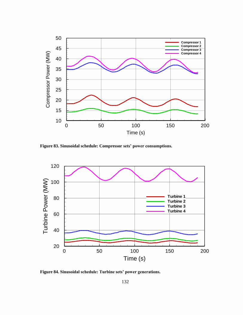
132
Figure 83. Sinusoidal schedule: Compressor sets’ power consumptions.
Figure 84. Sinusoidal schedule: Turbine sets’ power generations.
Time (s)
Co
mp
resso
rP
ow
er
(MW
)
0 50 100 150 20010
15
20
25
30
35
40
45
50Compressor 1
Compressor 2
Compressor 3
Compressor 4
Time (s)
Tu
rbin
eP
ow
er
(MW
)
0 50 100 150 20020
40
60
80
100
120
Turbine 1
Turbine 2
Turbine 3
Turbine 4

133
Figure 85. Sinusoidal schedule: Total power for each component.
Finally, Figure 88 and Figure 89 show the pressure and temperature distribution in
all 14 plena, respectively. As seen in the first figure, the pressure values in plena 1 to 5 do
not fluctuate at all. That shows fuel schedule does not affect the pressure values in the
compressor significantly. Starting at plenum 6, which is the inlet of the first injector row,
pressure in the following plena fluctuate with an amplitude of about 4%. Regarding the
temperature, as shown in Figure 89, except the inlet plena 1 and 2, all other plena
temperatures fluctuate under the influence of the fuel schedule. However, the amplitudes
of the compressor temperature fluctuations are lower than the injector and turbine. As the
Time (s)
Po
we
r(M
W)
0 50 100 150 20060
80
100
120
140
160
180
200
220
Turbine
Compressor
Generator

134
Figure 86. Sinusoidal schedule: Engine thermal efficiency.
Figure 87. Sinusoidal schedule: Non-dimensional shaft rotational speed.
Time (s)
Th
erm
alE
ffic
ien
cy
0.0 50.0 100.0 150.0 200.00.40
0.42
0.44
0.46
0.48
0.50
Time (s)
/
0
0 50 100 150 2000.80
0.85
0.90
0.95
1.00
1.05
1.10
1.15
1.20
Total Moment of Inertia: Ixx
= 4608.0 kg.m2

135
Figure 88. Sinusoidal schedule: Plena pressure.
Figure 89. Sinusoidal schedule: Plena temperature.
Time (s)
Ple
nu
mP
ressu
re(b
ar)
0 50 100 150 200 2500
10
20
30
40
50
Plenum 1
Plenum 2
Plenum 3
Plenum 4
Plenum 5
Plenum 6
Plenum 7
Plenum 8
Plenum 9
Plenum 10
Plenum 11
Plenum 12
Plenum 13
Plenum 14
Time (s)
Ple
nu
mT
em
pera
ture
(K)
0 50 100 150 200 250200
400
600
800
1000
1200
1400
1600
1800
Plenum 1
Plenum 2
Plenum 3
Plenum 4
Plenum 5
Plenum 6
Plenum 7
Plenum 8
Plenum 9
Plenum 10
Plenum 11
Plenum 12
Plenum 13
Plenum 14

136
flow moves towards the later stages, the intensity of the fluctuations increases due to
injection of more fuel.
VI.3.2. Gaussian Fuel Schedule
In the second scenario, a Gaussian fuel schedule is applied to the injectors as shown
in Figure 90. This schedule represents the random load changes in the power plants and
aircrafts which have been shown to follow a Gaussian (normal) distribution pattern [1].
The schedule ranges from 100% to 110% in 50 s periods over a total time period of 200 s.
As shown in the figure, the amplitude in this case is measured from the top point to the
minimum part of the profile which is the flat section at 100%. The same amplitude
measurement technique is used in all the following diagrams in this section.
Figure 90. Gaussian fuel schedule.
Time (s)
Fuel(k
g/s
)
0 50 100 150 2001.0
1.5
2.0
2.5
3.0
Injector 1
Injector 2,3
Amplitude (10%)

137
Figure 91 and Figure 92 show the compressor and turbine mass flow rates. As
shown in these figures, the mass flow rates fluctuate with amplitudes of about 3%. Also,
the flat parts in the fuel schedule are not reproduced in the mass flow rates.
Figure 93 and Figure 94 show the inlet and exit temperature distributions for each
turbine set. As shown in these figures, temperature values fluctuate with amplitudes of
about 5-6% which are relatively higher than the mass flow rate fluctuation amplitudes. It
is interesting to notice that in contrast to the mass flow rates, the rising sections in the
temperature profiles are shorter than the descending sections. That means while the fuel
schedule is flat, the temperatures continue to drop.
Figure 91. Gaussian schedule: Compressor sets’ mass flow rates.
Time (s)
Co
mp
resso
rM
ass
Flo
ws
(kg
/s)
0 50 100 150 200160
165
170
Compressor 1,2,3
Compressor 4

138
Figure 92. Gaussian schedule: Turbine sets’ mass flow rates.
Figure 93. Gaussian schedule: Turbine inlet temperatures.
Time (s)
Tu
rbin
eM
ass
Flo
ws
(kg
/s)
0 50 100 150 200160
170
180Turbine 1
Turbine 2
Turbine 3
Turbine 4
Turbine 1&2: Tin
Time (s)
Tu
rbin
eIn
letT
em
pera
ture
s(K
)
0 50 100 150 2001300
1400
1500
1600
1700
1800
Turbine 1
Turbine 2
Turbine 3
Turbine 4

139
Figure 94. Gaussian schedule: Turbine exit temperatures.
Figure 95 and Figure 96 show the compressor and turbine sets’ power
distributions, respectively. Moreover, Figure 97 shows the total power for turbine,
compressor, and generator. As seen in this figure, the fluctuation amplitudes for turbine,
compressor, and generator are approximately 5%, 5%, and 8%, respectively. It is also
noticeable that the generator power profile looks very similar to the fuel schedule.
Figure 98 shows the engine thermal efficiency. It is seen that in the beginning of
the cycle, efficiency drops about 2% compared to the design point efficiency (45%). After
that it oscillates between 42% and 43%. The reason for this decline is that the engine is
performing on a higher average fuel flow compared to the design point. The net increase
in the average fuel causes the cycle to move from the design point and reduces efficiency.
Turbine 1&2: Tout
Time (s)
Tu
rbin
eE
xit
Tem
pera
ture
s(K
)
0 50 100 150 200800
900
1000
1100
1200
1300
1400
1500
1600
Turbine 1
Turbine 2
Turbine 3
Turbine 4

140
Figure 95. Gaussian schedule: Compressor sets’ power consumptions.
Figure 96. Gaussian schedule: Turbine sets’ power generations.
Time (s)
Co
mp
resso
rP
ow
er
(MW
)
0 50 100 150 20010
15
20
25
30
35
40
45
50
Compressor 1
Compressor 2
Compressor 3
Compressor 4
Time (s)
Tu
rbin
eP
ow
er
(MW
)
0 50 100 150 20020
40
60
80
100
120
140
Turbine 1
Turbine 2
Turbine 3
Turbine 4

141
Figure 97. Gaussian schedule: Total power for each component.
Figure 99 shows the non-dimensional shaft rotational speed. The amplitude is
2.0% which is relatively lower than the other parameters. An overall increase in the
average shaft rotational speed is observed which is due to the increase in the average
amount of fuel.
Finally, Figure 100 and Figure 101 show the pressure and temperature distribution
in all 14 plena, respectively. As seen in the first figure, the pressure values do not fluctuate
strongly, and fluctuation amplitudes are below 2%. However, the fluctuations in the temp-
Time (s)
Po
we
r(M
W)
0 50 100 150 20080
100
120
140
160
180
200
220
240
Turbine
Compressor
Generator

142
Figure 98. Gaussian schedule: Engine thermal efficiency.
Figure 99. Gaussian schedule: Non-dimensional shaft rotational speed.
Time (s)
Th
erm
alE
ffic
ien
cy
0.0 50.0 100.0 150.0 200.00.40
0.42
0.44
0.46
0.48
Time (s)
/
0
0 50 100 150 2000.90
0.95
1.00
1.05
1.10
Total Moment of Inertia: Ixx
= 4608.0 kg.m2

143
Figure 100. Gaussian schedule: Plena pressure.
Figure 101. Gaussian schedule: Plena temperature.
Time (s)
Ple
nu
mP
ressu
re(b
ar)
0 50 100 150 200 2500
10
20
30
40
50Plenum 1
Plenum 2
Plenum 3
Plenum 4
Plenum 5
Plenum 6
Plenum 7
Plenum 8
Plenum 9
Plenum 10
Plenum 11
Plenum 12
Plenum 13
Plenum 14
Time (s)
Ple
nu
mT
em
pera
ture
(K)
0 50 100 150 200 250200
400
600
800
1000
1200
1400
1600
1800Plenum 1
Plenum 2
Plenum 3
Plenum 4
Plenum 5
Plenum 6
Plenum 7
Plenum 8
Plenum 9
Plenum 10
Plenum 11
Plenum 12
Plenum 13
Plenum 14

144
erature values are stronger as seen in Figure 101. Moreover, due to the increase in the
average fuel flow in the system, average temperature values for most plena are increased.
VI.3.3. Step Function Fuel Schedule
In this simulation, the fuel flow rate is increased by 5% in all injectors through a
step function as shown in Figure 102 and Figure 103. The step function represents sudden
changes taking place during the engine performance time. The current simulation runs for
a total of 400 seconds and the responses in all components are studied.
Figure 102. Step function fuel schedule: Injector 1.
Time (s)
Fuel(k
g/s
)
0 5 10 15 20 25 30 35 40 45 502.2
2.3
2.4
2.5
2.6
Amplitude (5%)

145
Figure 103. Step function fuel schedule: Injectors 2 and 3.
Figure 104 and Figure 105 show the compressor and turbine mass flow rates. As
seen in these figures, the increase in fuel at first causes the mass flow rates to go higher
than the steady response (overshoot), reach a maximum point and eventually come down
to the steady state value. The mass flow rates in these components increase by about 1%
due to the increase in fuel flow.
Figure 106 and Figure 107 show the inlet and exit temperature distributions for
each turbine set. As shown in these figures, the steady amplitudes of the temperatures are
above 10% which is more than double the fuel amplitude.
Time (s)
Fuel(k
g/s
)
0 5 10 15 20 25 30 35 40 45 501.2
1.3
1.4
1.5
Amplitude (5%)

146
Figure 104. Step function schedule: Compressor sets’ mass flow rates.
Figure 105. Step function schedule: Turbine sets’ mass flow rates.
Time (s)
Co
mp
resso
rM
ass
Flo
ws
(kg
/s)
0 50 100 150 200 250 300 350 400160
165
170
Compressor 1,2,3
Compressor 4
Time (s)
Tu
rbin
eM
ass
Flo
ws
(kg
/s)
0 50 100 150 200 250 300 350 400160
170
180
Turbine 1
Turbine 2
Turbine 3
Turbine 4

147
Figure 106. Step function schedule: Turbine inlet temperatures.
Figure 107. Step function schedule: Turbine exit temperatures.
Turbine 1&2: Tin
Time (s)
Tu
rbin
eIn
letT
em
pera
ture
s(K
)
0 50 100 150 200 250 300 350 4001300
1400
1500
1600
1700
1800
Turbine 1
Turbine 2
Turbine 3
Turbine 4
Turbine 1&2: Tout
Time (s)
Tu
rbin
eE
xit
Tem
pera
ture
s(K
)
0 50 100 150 200 250 300 350 400800
900
1000
1100
1200
1300
1400
1500
1600
Turbine 1
Turbine 2
Turbine 3
Turbine 4

148
Figure 108 to Figure 110 show the power distributions for each compressor and
turbine set. As shown in the figures, power values for all turbines and compressors
increase due to the increase in fuel. Figure 111 shows the total power for turbine,
compressor, and generator. Although the powers of turbine and compressor increase with
increase of fuel, these changes cancel each other out and the net power remains almost
constant. That means the increase in fuel has not resulted in the proportional increase in
the net power which implies a drop in efficiency.
Figure 112 shows the engine thermal efficiency. As it was discussed before, the
efficiency is dropped by about 2%. This decline is due to the increase in amount of fuel
that changes the thermodynamic cycle from the design conditions.
Figure 108. Step function schedule: Compressor sets’ power consumptions.
Time (s)
Co
mp
resso
rP
ow
er
(MW
)
0 50 100 150 200 250 300 350 40010
15
20
25
30
35
40
45
50
Compressor 1
Compressor 2
Compressor 3
Compressor 4

149
Figure 109. Step function schedule, turbine sets’ power generations: Turbines 1 to 3.
Figure 110. Step function schedule, turbine sets’ power generations: Turbine 4.
Time (s)
Tu
rbin
eP
ow
er
(MW
)
0 50 100 150 200 250 300 350 40020
25
30
35
40
45
50Turbine 1
Turbine 2
Turbine 3
Time (s)
Tu
rbin
eP
ow
er
(MW
)
0 100 200 300 400100
105
110
115
120
125
130
Turbine 4

150
Figure 111. Step function schedule: Total power for each component.
Figure 113 shows the non-dimensional shaft rotational speed. The rotational speed
increases by 11% as a result of the increased fuel flow.
Finally, Figure 114 and Figure 115 show the pressure and temperature distribution
in all 14 plena, respectively. As seen in the first figure, the pressure values increase by 5-
10% in different stages. On the other hand, temperature values in compressors are
increased by about 5% contrary to turbines and injectors in which temperatures are
increased by about 10%.
Time (s)
Po
we
r(M
W)
0 50 100 150 200 250 300 350 40080
100
120
140
160
180
200
220
240
Turbine
Compressor
Generator

151
Figure 112. Step function schedule: Engine thermal efficiency.
Figure 113. Step function schedule: Non-dimensional shaft rotational speed.
Time (s)
Th
erm
alE
ffic
ien
cy
0.0 50.0 100.0 150.0 200.00.40
0.42
0.44
0.46
0.48
Time (s)
/
0
0 50 100 150 200 250 300 350 4000.90
0.95
1.00
1.05
1.10
1.15
1.20
Total Moment of Inertia: Ixx
= 4608.0 kg.m2

152
Figure 114. Step function schedule: Plena pressure.
Figure 115. Step function schedule: Plena temperature.
Time (s)
Ple
nu
mP
ressu
re(b
ar)
0 50 100 150 200 250 300 350 4000
10
20
30
40
50Plenum 1
Plenum 2
Plenum 3
Plenum 4
Plenum 5
Plenum 6
Plenum 7
Plenum 8
Plenum 9
Plenum 10
Plenum 11
Plenum 12
Plenum 13
Plenum 14
Time (s)
Ple
nu
mT
em
pera
ture
(K)
0 50 100 150 200 250 300 350 400200
400
600
800
1000
1200
1400
1600
1800Plenum 1
Plenum 2
Plenum 3
Plenum 4
Plenum 5
Plenum 6
Plenum 7
Plenum 8
Plenum 9
Plenum 10
Plenum 11
Plenum 12
Plenum 13
Plenum 14

153
CHAPTER VII
CONCLUSION
The Ultra-High Efficiency Gas Turbine Engine (UHEGT) is introduced, designed,
and simulated in this study. UHEGT is based on the concept of sequential combustion
(reheat) in the gas turbine engine. In UHEGT, the combustion process is no longer
contained in isolation between the compressor and turbine, rather distributed and
integrated within stator rows of the HP-turbine stages. As shown in this study, this
technology substantially increases the thermal efficiency of the engine. Additionally, it
significantly increases the engine power output, reduces pollutant emissions, and reduces
the engine size and weight.
In the first part of this research, a comprehensive aerothermodynamic study is
conducted which shows that the UHEGT technology increases the engine efficiency by 5-
7% compared to current most advanced gas turbine engines such as Alstom’s GT 24/26.
Moreover, the total output power is significantly increased due to an increase in the total
amount of fuel combined with higher thermal efficiency. Based on all the important
parameters including thermal efficiency, total power, fuel flow rate in each combustion
stage, Turbine Inlet Temperature (TIT), etc., the complete thermodynamic cycle for the
system is developed. The final system has a six-stage turbine with three stages of stator
internal combustion and a compressor with pressure ratio of 40:1. The thermodynamic

154
efficiency of more than 45% is achieved in this cycle. Based on the thermodynamic cycle,
1D/2D (meanline) approach is used to design the entire flow path for the turbine.
In the next section, different injector configurations are designed and studied to
develop the optimum combustion system for UHEGT. The important parameters for a
suitable combustion unit for UHEGT are: enabling sequential combustion, utilizing
inherent secondary flows and induced vortices to provide a stable combustion
environment, provide uniform temperature distribution at the rotor inlet, etc. The studies
are performed on a single-stage turbine via Computational Fluid Dynamics (CFD) and the
simulations are unsteady and include multispecies combustion process along with rotor
motion. The flow field is analyzed based on different parameters such as velocity patterns,
Mach number, pressure, and temperature distribution, losses and emissions, etc. The final
configuration for the combustion system includes two rows of injectors placed before the
stator rows in the first three turbine stages. The injectors are hollow tubes extended from
hub to shroud with slots on top and bottom for fuel injection. Three or four injectors per
stator blade are included in each combustion stage. This configuration provides a highly
uniform temperature distribution at the rotor inlet, low pressure loss, low emissions, small
weight and volume, and ease of manufacturing compared to the other cases. Von Karman
vortices and the Coanda effect help to enhance the mixing between fuel and air particles
and increase combustion stability.
In the next section, a complete CFD model is developed to simulate multiple stages
of the UHEGT turbine with stator internal combustion. Flow patterns, secondary flow
losses, temperature distribution, and pollutant emissions are studied in the results in order

155
to investigate the interactions between consecutive combustion and turbine stages. The
flow paths are modified based on the CFD results in order to reduce separation and
pressure losses while enabling maximum mixing of fuel and air and reducing temperature
non-uniformities. The results show that:
1. There is a deviation angle at the exit of each stator or rotor component. This
deviation transforms to a large incidence angle in the following component. The stagger
angle for each component is slightly modified in order to make up for the deviation.
2. The injector wakes become larger as they move towards the blades’ pressure sides
which is due to the higher resistance against the flow in that area.
3. Injector wakes are larger in the lower pressure turbine stages. This causes the
injector pressure loss to increase in the second and third stages.
4. Combustion takes place mostly before the gas reaches the stator leading edge. The
hot gases are mixed with the mainstream flow along the stator channel.
5. Highly uniform temperature distribution is achieved at the inlet of each rotor stage
(non-uniformity is below 10%).
6. There is a good agreement between the meanline and CFD calculations for
different parameters.
Since the combustion process is brought into the turbine stages in UHEGT, the
stator blades are exposed to high temperature gases and are prone to be overheated. That
is one of the main phenomena observed in the simulation results discussed before. The
next part of this research is dedicated to investigation of different methods to reduce the
stator blade surface temperature. Two different approaches in this regard are numerically

156
studied: the first is based on indexing (clocking) fuel injectors relative to each other and
the stator blades and the second is based on using film cooling. Four different
configurations are designed and simulated via CFD to evaluate the effectiveness of the
two approaches. Based on the results, the configuration with indexing approach provides
the best option in lowering the stator blade surface temperature. This configuration brings
down the average stator blade surface temperature to near the compressor air temperature
which is ideal for the blade material. The blade surface is completely protected against the
hot combustion gases in this configuration. However, this configuration produces a higher
temperature non-uniformity compared to the other configurations. The higher non-
uniformity could negatively affect the rotor blade material, but it does not noticeably
reduce the amount of power generated by the rotor. Moreover, this configuration uses the
lowest number of injectors per blade, produces the least amount of total pressure loss, and
is the easiest configuration to manufacture. Therefore, the indexing in this configuration
is the best option in reducing the stator blade surface temperature among the cases studied
in this research. Film cooling approach can be considered the second-best option in
controlling the blade surface temperature. This approach successfully brings down the
average stator blade surface temperature by more than 100 degrees and produces a highly
uniform temperature distribution at the rotor inlet. For the second and third turbine stages
with stator internal combustion, a similar indexing approach could be used to optimize the
temperature distribution. The fuel injectors need to be indexed based on the flow patterns
and temperature distribution in each stage. Moreover, use of film cooling is recommended
for the rotor blades.

157
In the last part of this research, a dynamic simulation is performed on the entire
engine using the nonlinear generic code GETRAN developed by Schobeiri [1], [30]. The
simulations are in 2D (space-time) and include majority of the engine components, i.e.
compressor, turbine, injectors, diffuser, control system, pipes, etc. The time-dependent
simulations are performed in variable design and off-design conditions that engine goes
through during its performance. Three main conditions are simulated via fuel schedules
applied through fuel valves which include sinusoidal, Gaussian, and step function. The
results show that fluctuations in the fuel flow rate lead to fluctuations with similar patterns
in the majority of the system parameters such as compressor and turbine mass flow rates,
temperatures, pressures, power, shaft speed, etc. However, the fluctuation profiles in
different parameters are different in amplitude and typically have a time lag compared to
the fuel schedules. The time lag represents the reaction time of the engine and the control
system to adjust itself to the changes in fuel flow. Regarding the intensity of the fluctuations,
usually mass flow rates of turbine and compressor and shaft rotational speed fluctuate with
lower amplitudes compared to the fuel schedule. The intensity of fluctuation in those
parameters are directly affected by the rotating shaft moment of inertia. On the other hand,
the fluctuation amplitudes in temperatures, and compressor and turbine powers usually
tend to be higher. It is also seen that generator (or net) power has a very similar fluctuation
pattern to the fuel schedule, both in shape of the profile and intensity of the fluctuation.
Regarding the thermal efficiency, it is seen that the range of the changes is relatively lower
than the other parameters. That means the system performs near the design point efficiency
throughout the entire cycle. However, an increase in the total average fuel in the system

158
causes the average thermal efficiency to drop slightly. That is due to the thermodynamic
cycle being moved from the design point conditions. It is also seen that the first fluctuation
cycle in the each response profile is slightly different than the following cycles. That is
due to the transient response in the beginning of the oscillation which will be damped
quickly.

159
REFERENCES
[1] Schobeiri, M. T. Turbomachinery Flow Physics and Dynamic Performance. 2nd
and enhanced ed., Springer (2012).
[2] GE Power, URL https://www.gepower.com.
[3] Siemens, URL https://www.siemens.com.
[4] Rolls-Royce, URL https://www.rolls-royce.com.
[5] Schobeiri, M. T. Gas Turbine Design, Components and System Design Integration.
Springer (2018).
[6] Schobeiri, M. T. “Prozessoptimierung fur die Kombianlagen.” BBC–Internal
Classified Report No. BBC-TN-86-112. 1986.
[7] Schobeiri, M. T. “The Ultra-High Efficiency Gas Turbine Engine with Stator
Internal Combustion, UHEGT.” US Patent pending, No. 1389-TEES-99. 1999.
[8] Schobeiri, Meinhard T. "Ultra-High Efficiency Gas Turbine (UHEGT) with Stator
Internal Combustion." US patent application. No. US 14/595,417. 2014.
[9] DÃķbbeling, Klaus, Hellat, Jaan and Koch, Hans. "25 years of bbc/abb/alstom lean
premix combustion technologies." ASME Journal of Engineering for Gas Turbines
and Power Vol. 129, no. 1 (2007): pp. 2-12. DOI 10.1115/1.2181183.
[10] Agbonzikilo, F. E., Owen, I., Stewart, J., Sadasivuni, S. K., Riley, M., and
Sanderson, V. “Experimental and Numerical Investigation of Fuel–Air Mixing in
a Radial Swirler Slot of a Dry Low Emission Gas Turbine Combustor.” ASME J.
Eng. Gas Turbines Power Vol. 138, no. 6 (2016): pp. 061502.

160
[11] Moran, M. J., Shapiro, H. N., Boettner, D. D., Bailey, M. B. Fundamentals of
Engineering Thermodynamics. 7th Edition, John Wiley & Sons (2011).
[12] Schobeiri, M. T. “Dynamisches Verhalten der Luftspeichergasturbine Huntorf bei
einem Lastabwurf mit Schnellabschaltung,” Brown Boveri, Technical Report No.
TA-58. 1982.
[13] Schobeiri, T. and Haselbacher, H. “Transient Analysis of Gas Turbine Power
Plants, Using the Huntorf Compressed Air Storage Plant as an Example.”
Proceedings of ASME 1985 International Gas Turbine Conference and Exhibit.
pp. V003T10A015-V003T10A015. March 1985.
[14] Schobeiri, T. “A general Computational method for simulation and prediction of
transient behavior of gas Turbines.” Proceedings of ASME 1986 International Gas
Turbine Conference and Exhibit. pp. V001T01A070-V001T01A070. June 1986.
[15] Schobeiri, Meinhard T. and Ghoreyshi, Seyed M. "The Ultrahigh Efficiency Gas
Turbine Engine with Stator Internal Combustion." ASME Journal of Engineering
for Gas Turbines and Power Vol. 138, no. 2 (2016): pp. 021506. DOI
10.1115/1.4031273.
[16] Schobeiri, Meinhard T. and Ghoreyshi, Seyed M. “UHEGT, the Ultra-High
Efficiency Gas Turbine Engine with Stator Internal Combustion.” Proceedings of
the ASME Turbo Expo 2015: Turbine Technical Conference and Exposition. pp.
V003T06A019-V003T06A019. Montreal, Quebec, Canada, June 15–19, 2015.
DOI 10.1115/GT2015-43447.

161
[17] Ghoreyshi, Seyed M. and Schobeiri, Meinhard T. “Numerical Simulation of the
Multistage Ultra-High Efficiency Gas Turbine Engine, UHEGT.” Proceedings of
ASME Turbo Expo 2017: Turbomachinery Technical Conference and Exposition.
pp. V003T06A034-V003T06A034. Charlotte, North Carolina, USA, June 26–30,
2017. DOI 10.1115/GT2017-65029.
[18] Ghoreyshi, Seyed M. and Schobeiri, Meinhard T. “A Numerical Study on
Reducing the Stator Blade Surface Temperature in the Ultra-High Efficiency Gas
Turbine Engine by Indexing Fuel Injectors and Using Film Cooling.” Proceedings
of ASME Turbo Expo 2018: Turbomachinery Technical Conference and
Exposition. Oslo, Norway, June 11–15, 2018.
[19] EPRIGEN. “Thermal Performance of the ABB GT24 Gas Turbine in Peaking
Service at the Gilbert Station of GPU Energy.” EPRIGEN, Palo Alto, CA. 1998.
[20] Savic, S., Lindvall, K., Papadopoulos, T., and Ladwig, M. “The Next Generation
KA24/GT24 from Alstom, the Pioneer in Operational Flexibility.” Alstom Power
Industry Seminar. Newport, RI, USA, 2011.
[21] Güthe, Felix, Hellat, Jaan and Flohr, Peter. "The reheat concept: the proven
pathway to ultralow emissions and high efficiency and flexibility." ASME Journal
of Engineering for Gas Turbines and Power Vol. 131, no. 2 (2009): pp. 021503.
DOI 10.1115/1.2836613.
[22] Eroglu, Adnan, Flohr, Peter, Brunner, Philipp and Hellat, Jaan. “Combustor design
for low emissions and long lifetime requirements.” Proceedings of ASME Turbo

162
Expo 2009: Power for Land, Sea, and Air. Paper No. GT2009-59540, pp. 435-444.
Orlando, Florida, USA, June 8–12, 2009. DOI 10.1115/GT2009-59540.
[23] Cottle, Andrew E. and Polanka, Marc D. “Numerical and Experimental Results
from a Common-Source High-G Ultra-Compact Combustor.” Proceedings of the
ASME Turbo Expo 2016: Turbomachinery Technical Conference and Exposition.
pp. V04AT04A013-V04AT04A013. Seoul, South Korea, June 13-17, 2016. DOI
10.1115/GT2016-56215.
[24] Zelina, Joseph, Sturgess, Geoff and Shouse, Dale. “The Behavior of an Ultra-
Compact Combustor (UCC) Based on Centrifugally-Enhanced Turbulent Burning
Rates.” Proceedings of 40th AIAA/ASME/SAE/ASEE Joint Propulsion Conference
and Exhibit. AIAA 2004-3541. Fort Lauderdale, FL, 2004. URL
https://doi.org/10.2514/ 6.2004-3541.
[25] Sirignano, W. A. and Liu, F. “Performance Increases for Gas-Turbine Engines
Through Combustion Inside the Turbine.” Journal of Propulsion and Power Vol.
15, no. 1 (1999): pp. 111-118. URL https://doi.org/10.2514/2.5398.
[26] Sirignano, W. A., Dunn-Rankin, D., Liu, F., Colcord, B. and Puranam, S. “Turbine
Burners: Performance Improvement and Challenges of Flameholding.” AIAA
Journal Vol. 50, no. 8 (2012): pp. 1645-1669. DOI 10.2514/1.J051562.
[27] Zajadatz, M., Lachner, R., Bernero, S., Motz, C., & Flohr, P. “Development and
design of ALSTOM’S staged fuel gas injection EV burner for NOx reduction.”
Proceedings of ASME Turbo Expo January 2007: Power for Land, Sea, and Air.
pp. 559-567. January 2007.

163
[28] Bobusch, B. C., Berndt, P., Paschereit, C. O., & Klein, R. “Shockless explosion
combustion: An innovative way of efficient constant volume combustion in gas
turbines.” Combustion Science and Technology Vol. 186, no. 10-11 (2014): pp.
1680-1689.
[29] Reichel, T. G., Schäpel, J. S., Bobusch, B. C., Klein, R., King, R., & Paschereit,
C. O. “Shockless Explosion Combustion: Experimental Investigation of a New
Approximate Constant Volume Combustion Process.” Journal of Engineering for
Gas Turbines and Power Vol. 139, no. 2 (2017): pp. 021504.
[30] Schobeiri, M. T. “Final Report on GETRAN: The GEneric, Modularly Structured
Computer Code for Simulation of the Transient Behavior of Single- and Multi-
spool Aero and Power Generation Gas Turbine Engines.” Volume I: Technical
Report, submitted to NASA Lewis Research Center. December, 1995.
[31] Schobeiri, M. T. “Final Report on GETRAN: The GEneric, Modularly Structured
Computer Code for Simulation of the Transient Behavior of Single- and Multi-
spool Aero and Power Generation Gas Turbine Engines.” Volume II: Technical
Report, submitted to NASA Lewis Research Center. December, 1995.
[32] Schobeiri, M. T. “Final Report on GETRAN: The GEneric, Modularly Structured
Computer Code for Simulation of the Transient Behavior of Single- and Multi-
spool Aero and Power Generation Gas Turbine Engines.” Volume III: Technical
Report, submitted to NASA Lewis Research Center. December, 1995.
[33] Lefebvre, A. H. and Ballal, D. R. Gas Turbine Combustion: Alternative Fuels and
Emissions. Third Edition. CRC press, Taylor and Francis. 2010.

164
[34] Thornburg, H., Sekar, B., Zelina, J., Lin, C., and Holder, R. “Prediction of Inter-
Turbine Burner (ITB) Performance with Curved Radial Vane Cavity at Various
Equivalence Ratios.” ASME Paper No. GT2008-50192. 2008.
[35] Schobeiri, M. T. “On the Stability Behavior of Vortex Flows in Turbomachinery.”
Z. Flugwiss. Weltraumforsch. Vol. 13 (1989): pp. 233–239 (in German).
[36] Schobeiri, M. T., and Ozturk, B. “Experimental Study of the Effect of the Periodic
Unsteady Wake Flow on Boundary Layer Development, Separation, and Re-
Attachment Along the Surface of a Low Pressure Turbine Blade.” ASME J.
Turbomach. Vol. 126, no. 4 (2004): pp. 663–676.
[37] Schobeiri, M. T., and Chakka, P. “Prediction of Turbine Blade Heat Transfer and
Aerodynamics Using Unsteady Boundary Layer Transition Model.” Int. J. Heat
Mass Transfer Vol. 45, no. 4 (2002): pp. 815–829.
[38] Schobeiri, M. T., Read, K., and Lewalle, J. “Effect of Unsteady Wake Passing
Frequency on Boundary Layer Transition, Experimental Investigation and
Wavelet Analysis.” ASME J. Fluids Eng. Vol. 125, no. 2 (2003): pp. 251–266.
[39] Wright, L., and Schobeiri, M. T. “The Effect of Periodic Unsteady Flow on
Boundary Layer and Heat Transfer on a Curved Surface.” ASME J. Heat Transfer
Vol. 121, no. 1 (1999): pp. 22–33.
[40] Claypole, T. “Coherent Structures in Swirl Generators and Combustors.”
Proceedings of the ASME Symposium Vortex Flows. Winter Annual Meeting,
Chicago, IL, Nov. 16–21, 1980.

165
[41] Lilley, D. “Swirl Flows in Combustion: A Review.” AIAA Journal Vol. 15, no. 8
(1977): pp. 1063–1078.
[42] Claypole, T., and Syred, N. “The Effect of Swirl Burner Aerodynamics on NOx
Formation.” Symp. (Int.) Combust. 18(1) (1981): pp. 81–89.
[43] Farber, J., Koch, R., Bauer, H., Hase, M., and Krebs, W. “Effects of Pilot Fuel and
Liner Cooling on the Flame Structure in a Full Scale Swirl-Stabilized Combustion
Setup.” ASME J. Eng. Gas Turbines Power Vol. 132, no. 9 (2010): p. 091501.
[44] Lucca-Negro, O., and O’Doherty, T. “Vortex Breakdown: A Review.” Prog.
Energy Combust. Sci. Vol. 27, no. 4 (2001): pp. 431–481.
[45] Keller, J., Egli, W., and Althaus, R. “Vortex Breakdown as a Fundamental Element
of Vortex Dynamics.” Z. Angew. Math. Phys. Vol. 39, no. 3 (1988): pp. 404–440.
[46] Keller, J. J., Sattelmayer, T., and Thueringer, F. “Double-Cone Burners for Gas
Turbine Type 9 Retrofit Application.” 19th International Congress on Combustion
Engines. CIMAC, Florence. 1991.
[47] Kazemi, A. and Curet, O. "PIV measurements and flow characteristics
downstream of mangrove root models." In APS Division of Fluid Dynamics
Meeting Abstracts. 2016.
[48] Kazemi, A., Van de Riet, K. and Curet, O. M. "Hydrodynamics of mangrove-type
root models: the effect of porosity, spacing ratio and flexibility." Bioinspiration &
biomimetics Vol. 12, no. 5 (2017): 056003.
[49] Gupta, A. K., Lilley, D. G., and Syred, N. Swirl Flows. Abacus, Tunbridge Wells,
Kent, England (1984).

166
[50] Anacleto, P. M., Fernandes, E. C., Heitor, M. V., and Shtork, S. I. “Swirl Flow
Structure and Flame Characteristics in a Model Lean Premixed Combustor.”
Combust. Sci. Technol. Vol. 175, no. 8 (2003): pp. 1369–1388.
[51] Beer, J. M., and Chigier, N. A. Combustion Aerodynamics, Wiley, Halstead Press
Division, New York (1972).
[52] Duwig, C., Ducruix, S., and Veynante, D. “Studying the Stabilization Dynamics
of Swirling Partially Premixed Flames by Proper Orthogonal Decomposition.”
ASME J. Eng. Gas Turbines Power Vol. 134, no. 10 (2012): p. 101501.
[53] Galley, D., Ducruix, S., Lacas, F., and Veynante, D. “Mixing and Stabilization
Study of a Partially Premixed Swirling Flame Using Laser Induced Fluorescence.”
Combust. Flame Vol. 158, no. 1 (2011): pp. 155–171.
[54] Wurm, B., Schulz, A., Bauer, H., and Gerendas, M. “Impact of Swirl Flow on the
Cooling Performance of an Effusion Cooled Combustor Liner.” ASME J. Eng. Gas
Turbines Power Vol. 134, no. 12 (2012): p. 121503.
[55] Wurm, B., Schulz, A., & Bauer, H. J. “A new test facility for investigating the
interaction between swirl flow and wall cooling films in combustors.” Proceedings
of ASME Turbo Expo 2009: Power for Land, Sea, and Air. pp. 1397-1408. January
2009.
[56] Beard, P., Smith, A., and Povey, T. “Effect of Combustor Swirl on Transonic High
Pressure Turbine Efficiency.” ASME J. Turbomach. Vol. 136, no. 1 (2014): p.
011002.
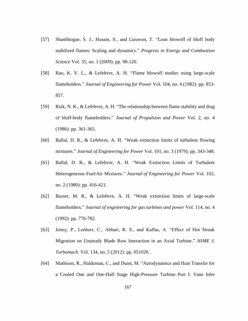
167
[57] Shanbhogue, S. J., Husain, S., and Lieuwen, T. “Lean blowoff of bluff body
stabilized flames: Scaling and dynamics.” Progress in Energy and Combustion
Science Vol. 35, no. 1 (2009): pp. 98-120.
[58] Rao, K. V. L., & Lefebvre, A. H. “Flame blowoff studies using large-scale
flameholders.” Journal of Engineering for Power Vol. 104, no. 4 (1982): pp. 853-
857.
[59] Rizk, N. K., & Lefebvre, A. H. “The relationship between flame stability and drag
of bluff-body flameholders.” Journal of Propulsion and Power Vol. 2, no. 4
(1986): pp. 361-365.
[60] Ballal, D. R., & Lefebvre, A. H. “Weak extinction limits of turbulent flowing
mixtures.” Journal of Engineering for Power Vol. 101, no. 3 (1979): pp. 343-348.
[61] Ballal, D. R., & Lefebvre, A. H. “Weak Extinction Limits of Turbulent
Heterogeneous Fuel/Air Mixtures.” Journal of Engineering for Power Vol. 102,
no. 2 (1980): pp. 416-421.
[62] Baxter, M. R., & Lefebvre, A. H. “Weak extinction limits of large-scale
flameholders.” Journal of engineering for gas turbines and power Vol. 114, no. 4
(1992): pp. 776-782.
[63] Jenny, P., Lenherr, C., Abhari, R. S., and Kalfas, A. “Effect of Hot Streak
Migration on Unsteady Blade Row Interaction in an Axial Turbine.” ASME J.
Turbomach. Vol. 134, no. 5 (2012): pp. 051020.
[64] Mathison, R., Haldeman, C., and Dunn, M. “Aerodynamics and Heat Transfer for
a Cooled One and One-Half Stage High-Pressure Turbine–Part I: Vane Inlet

168
Temperature Profile Generation and Migration.” Proceedings of ASME Turbo
Expo 2010: Power for Land, Sea and Air. Jun. 14–18, 2010, Glasgow.
[65] Mathison, R. M., Haldeman, C. W., & Dunn, M. G. “Aerodynamics and Heat
Transfer for a Cooled One and One-Half Stage High-Pressure Turbine–Part II:
Influence of Inlet Temperature Profile on Blade Row and Shroud.” Journal of
Turbomachinery Vol. 134, no. 1 (2012): pp. 011007.
[66] Simone, S., Montomoli, F., Martelli, F., Chana, K., Qureshi, I., and Povey, T.
“Analysis on the Effect of a Nonuniform Inlet Profile on Heat Transfer and Fluid
Flow in Turbine Stages.” ASME J. Turbomach. Vol. 134, no. 1 (2012): p. 011012.
[67] Barringer, M., Thole, K., and Polanka, M. “Effects of Combustor Exit Profiles on
Vane Aerodynamic Loading and Heat Transfer in a High Pressure Turbine.” ASME
J. Turbomach. Vol. 131, no. 2 (2009): p. 021008.
[68] Khanal, B., He, L., Northall, J., and Adami, P. “Analysis of Radial Migration of
Hot-Streak in Swirling Flow Through High-Pressure Turbine Stage.” ASME J.
Turbomach. Vol. 135, no. 4 (2013): p. 041005.
[69] Shang, Tonghuo and Epstein, Alan H. “Analysis of Hot Streak Effects on Turbine
Rotor Heat Load.” ASME J. Turbomach Vol. 119, no. 3 (1997): pp. 544–553. DOI
10.1115/1.2841156.
[70] Qureshi, I., Beretta, A., and Povey, T. “Effect of Simulated Combustor
Temperature Nonuniformity on HP Vane and End Wall Heat Transfer: An
Experimental and Computational Investigation.” ASME J. Eng. Gas Turbines
Power Vol. 133, no. 3 (2011): p. 031901.

169
[71] Wang, J., Ge, N., & Sheng, C. “Analysis of swirling flow effects on the
characteristics of unsteady hot-streak migration.” Chinese Journal of Aeronautics
(2016).
[72] Błachnio, J., & Pawlak, W. I. “Non-uniformity of the combustor exit flow
temperature in front of the gas turbine.” acta mechanica et automatica Vol. 8, no
4 (2014): pp. 209-213.
[73] Barzegarian, R., Aloueyan, A., and Yousefi, T. "Thermal performance
augmentation using water based Al2O3-gamma nanofluid in a horizontal shell and
tube heat exchanger under forced circulation." International Communications in
Heat and Mass Transfer Vol. 86 (2017): 52-59.
[74] Jafari, M. M., Atefi, G. A. and Khalesi, J. “Advances in nonlinear stress analysis
of a steam cooled gas turbine blade.” Latin American Applied Research Vol. 42,
no. 2 (2012): pp. 167-175.
[75] Atefi, G. A., Jafari, M. M., Khalesi, J., & Soleymani, A. “The thermoelastic stress
analysis of a gas turbine blade with cooling.” In 13th Annual & 2nd Int. Fluid Dyn.
Conf. 2010.
[76] Chibli, H. A., Abdelfattah, S. A., Schobeiri, M. T., & Kang, C. “An experimental
and numerical study of the effects of flow incidence angles on the performance of
a stator blade cascade of a high pressure steam turbine.” Proceedings of ASME
Turbo Expo 2009: Power for Land, Sea, and Air. pp. 821-830. January 2009.
[77] Schobeiri, M. T., & Nikparto, A. “A comparative numerical study of aerodynamics
and heat transfer on transitional flow around a highly loaded turbine blade with

170
flow separation using rans, urans and les.” Proceedings of ASME Turbo Expo
2014: Turbine Technical Conference and Exposition. pp. V05CT17A001-
V05CT17A001. June 2014.
[78] Rezasoltani, M., Lu, K., Schobeiri, M., and Han, J. C. “A Combined Experimental
and Numerical Study of the Turbine Blade Tip Film Cooling Effectiveness Under
Rotation Condition.” ASME J. Turbomach. Vol. 137, no. 5 (2015): p. 051009.
[79] Nikparto, A., & Schobeiri, M. T. “Numerical and Experimental Investigation of
Aerodynamics on Flow Around a Highly Loaded Low-Pressure Turbine Blade
with Flow Separation Under Steady and Periodic Unsteady Inlet Flow Condition.”
Proceedings of ASME Turbo Expo 2016: Turbomachinery Technical Conference
and Exposition. pp. V05AT13A010-V05AT13A010. June 2016.
[80] Nikparto, A., & Schobeiri, M. T. “Investigation of Aerodynamics and Heat
Transfer of a Highly Loaded Turbine Blade Using the Universal Intermittency
Function.” Proceedings of ASME Turbo Expo 2017: Turbomachinery Technical
Conference and Exposition. pp. V02DT46A030-V02DT46A030). June 2017.
[81] Nikparto, Ali and Schobeiri, Meinhard T. “Combined numerical and experimental
investigations of heat transfer of a highly loaded low-pressure turbine blade under
periodic inlet flow condition.” Proceedings of IMechE, Part A: Journal of Power
and Energy (2018). DOI https://doi.org/10.1177/0957650918758158.
[82] Mortazavi, Farzam and Palazzolo, Alan. “Prediction of Rotordynamic
Performance of Smooth Stator-Grooved Rotor Liquid Annular Seals Utilizing

171
Computational Fluid Dynamics.” ASME Journal of Vibration and Acoustics Vol.
140, no. 3 (2017): pp. 031002-031002-031009. DOI 10.1115/1.4038437.
[83] Mortazavi, Farzam, Riasi, Alireza and Nourbakhsh, Ahmad. “Numerical
Investigation of Back Vane Design and Its Impact on Pump Performance.” ASME
Journal of Fluids Engineering Vol. 139, no. 12 (2017): pp. 121104-121104-
121109. DOI 10.1115/1.4037281.
[84] Ghoreyshi, Mostafa, Saidi, Mohamad S., Navabi, Mohamad A., Firoozabadi,
Bahar D. and Shabanian, Reza. “Numerical investigation of antegrade flow effects
on flow pulsations in Fontan operation.” International Journal of Biomedical
Engineering and Technology Vol. 10, no. 3 (2012): pp. 221-238. URL
https://doi.org/10.1504/IJBET. 2012.050291.
[85] Jafari, M., Afshin, H., Farhanieh, B. and Bozorgasareh, H. "Numerical
aerodynamic evaluation and noise investigation of a bladeless fan." Journal of
Applied Fluid Mechanics Vol. 8, no. 1 (2015): 133-142.
[86] Jafari, M., Afshin, H., Farhanieh, B. and Bozorgasareh, H. "Experimental and
Numerical Investigation of a 60cm Diameter Bladeless Fan." Journal of Applied
Fluid Mechanics Vol. 9, no. 2 (2016).
[87] Jafari, Mohammad, Afshin, Hossein, Farhanieh, Bijan and Sojoudi, Atta.
"Numerical investigation of geometric parameter effects on the aerodynamic
performance of a Bladeless fan." Alexandria Engineering Journal Vol. 55, no. 1
(2016): 223-233.
[88] ANSYS. “ANSYS CFX-Solver Modeling Guide.” Release 15.0. Nov. 2013.

172
[89] Magnussen, B. F., and Hjertager, B. H. “On mathematical modeling of turbulent
combustion with special emphasis on soot formation and combustion.” In
Symposium (International) on Combustion Vol. 16, No. 1 (1977): pp. 719-729,
Elsevier.
[90] Menter, F. R. “Two-equation eddy-viscosity turbulence models for engineering
applications.” AIAA journal Vol. 32, no. 8 (1994): pp. 1598-1605.
[91] Mansouri, Z., Aouissi, M., & Boushaki, T. “A Numerical Study of Swirl Effects
on the Flow and Flame Dynamics in a Lean Premixed Combustor.” International
Journal of Heat and Technology Vol. 34, No. 2 (2016): pp. 227-235.
[92] Lefebvre, A.H. “The Role of Fuel Preparation in Low-Emission Combustion.”
Journal of Engineering for Gas Turbines and Power Vol. 117 (1995): pp 617-654.
[93] Mitsubishi. “MHPS Gas Turbine M501G/M701G.” Mitsubishi Hitachi Power
Systems, LTD. Technical Report.
[94] König, S., Stoffel, B., & Schobeiri, M. T. “Experimental investigation of the
clocking effect in a 1.5-stage axial turbine—part i: Time-averaged results.”
Journal of Turbomachinery Vol. 131, no. 2 (2009): pp. 021003.
[95] Huber, F. W., Johnson, P. D., Sharma, O. P., Staubach, J. B., and Gaddis, S. W.
“Performance Improvement Through Indexing of Turbine Airfoils: Part 1—
Experimental Investigation.” ASME J. Turbomach. Vol. 118 (1996): pp. 630–635.
[96] Griffin, L. W., Huber, F. M., and Sharma, O. P. “Performance Improvement
Through Indexing Turbine Airfoils: Part 2—Numerical Simulation.” ASME J.
Turbomach. Vol. 118 (1996): pp. 636–642.

173
[97] Padture, N. P., Gell, M., & Jordan, E. H. “Thermal barrier coatings for gas-turbine
engine applications.” Science Vol. 296, no. 5566 (2002): pp. 280-284.
[98] Clarke, D. R., Oechsner, M., & Padture, N. P. “Thermal-barrier coatings for more
efficient gas-turbine engines.” MRS bulletin Vol. 37, no. 10 (2012): pp. 891-898.
[99] Kroniger, D., Wirsum, M., Horikawa, A., Okada, K., & Kazari, M. “NOx
Correlation for an Industrial 10 MW Non-Premixed Gas Turbine Combustor for
High Hydrogen Fuels.” In ASME Turbo Expo June 2016: Turbomachinery
Technical Conference and Exposition. pp. V04AT04A012-V04AT04A012. June
2016.
[100] Nikparto, Ali and Schobeiri, Meinhard T. “Experimental Investigation of Film-
Cooling Effectiveness of a Highly Loaded Turbine Blade Under Steady and
Periodic Unsteady Flow Conditions.” ASME Journal of Heat Transfer Vol. 139,
no. 7 (2017): pp. 072201. DOI 10.1115/1.4035651.
[101] Nikparto, Ali, Rice, Tyler and Schobeiri, Meinhard T. "Experimental and
Numerical Investigation of Heat Transfer and Film Cooling Effectiveness of A
Highly Loaded Turbine Blade Under Steady And Unsteady Wake Flow
Condition." Proceedings of ASME Turbo Expo 2017: Turbomachinery Technical
Conference and Exposition. pp. V05CT19A029-V05CT19A029. Charlotte, North
Carolina, USA, June 26–30, 2017. DOI 10.1115/GT2017-65012.
[102] Nirmalan, N. V. and Hylton, L. D. " An Experimental Study of Turbine Vane Heat
Transfer with Leading Edge and Downstream Film Cooling." ASME Journal of
Turbomachinery Vol. 112, no. 3 (1990): pp. 477-487. DOI 10.1115/1.2927683.

174
[103] El-Gabry, Lamyaa A., Thurman, Douglas R., Poinsatte, Philip E. and Heidmann,
James D. "Turbulence and Heat Transfer Measurements in an Inclined Large Scale
Film Cooling Array: Part I— Velocity and Turbulence Measurements."
Proceedings of ASME 2011 Turbo Expo: Turbine Technical Conference and
Exposition. pp. 541-550. Vancouver, British Columbia, Canada, June 6–10, 2011.
DOI 10.1115/GT2011-46491.
[104] Thurman, Douglas R., El-Gabry, Lamyaa A., Poinsatte, Philip E. and Heidmann,
James D. "Turbulence and Heat Transfer Measurements in an Inclined Large Scale
Film Cooling Array: Part II—Temperature and Heat Transfer Measurements."
Proceedings of ASME 2011 Turbo Expo: Turbine Technical Conference and
Exposition. pp. 551-558. Vancouver, British Columbia, Canada, June 6–10, 2011.
DOI 10.1115/GT2011-46498.
[105] Abuaf, N., Bunker, R. and Lee, C. P. "Heat transfer and film cooling effectiveness
in a linear airfoil cascade." ASME Journal of Turbomachinery Vol. 119, no. 2
(1997): pp. 302-309. DOI 10.1115/1.2841113.
[106] Jafari, M. M., Atefi, G., Khalesi, J. and Soleymani, A. “A new conjugate heat
transfer method to analyse a 3D steam cooled gas turbine blade with temperature-
dependent material properties.” Proceedings of the IMechE, Part C: Journal of
Mechanical Engineering Science Vol. 226, no. 5 (2012): pp.1309-1320.
DOI:10.1177/0954406211418734.
[107] Khodabandeh, Erfan, Ghaderi, Mohsen, Afzalabadi, Abolfazl, Rouboa, Abel and
Salarifard, Amir. “Parametric Study of Heat Transfer in an Electric Arc Furnace

175
and Cooling System.” Applied Thermal Engineering Vol. 123 (2017): pp. 1190-
1200.
[108] Womack, K. M., Volino, R. J., and Schultz, M. P. “Measurements in Film Cooling
Flows With Periodic Wakes.” ASME J. Turbomach. Vol. 130, no. 4 (2008): p.
041008.
[109] Coulthard, S. M., Volino, R. J., and Flack, K. A. “Effect of Jet Pulsing on Film
Cooling—Part I: Effectiveness and Flow-Field Temperature Results.” ASME J.
Turbomach. Vol. 129, no. 2 (2007): pp. 232–246.
[110] Womack, K. M., Volino, R. J., and Schultz, M. P. “Combined Effects of Wakes
and Jet Pulsing on Film Cooling.” ASME J. Turbomach. Vol. 130, no. 4 (2008): p.
041010.
[111] Soong, C. Y. “Thermal buoyancy effects in rotating non-isothermal flows.”
International Journal of Rotating Machinery Vol. 7, no. 6 (2001): pp. 435-446.
DOI http://dx.doi.org/10.1155/S1023621X01000380.
[112] Ghasemi, Arman, Dardel, Morteza and Ghasemi, Mohammad Hassan. “Collective
Effect of Fluid's Colioris Force and Nano-Scale's Parameter on Instability Pattern
and Vibration Characteristic of Fluid-Conveying Carbon Nanotubes.” Journal of
Pressure Vessel Technology Vol. 137, no. 3 (2015): pp. 031301. DOI
10.1115/1.4029522.
[113] Ghasemi, Arman, Dardel, Morteza and Ghasemi, Mohamad Hassan. "Control of
the non-linear static deflection experienced by a fluid-carrying double-walled
carbon nanotube using an external distributed load." Proceedings of the Institution

176
of Mechanical Engineers, Part N: Journal of Nanoengineering and Nanosystems
226, no. 4 (2012): 181-190.
[114] Schobeiri, M. T., Attia, M, Lippke, C. “Nonlinear Dynamic Simulation of Single
and Multi-spool Core Engines, Part I: Theoretical Method.” AIAA, Journal of
Propulsion and Power Vol. 10, No. 6 (1994): pp. 855- 862.
[115] Schobeiri, M. T., Attia, M, Lippke, C. “Nonlinear Dynamic Simulation of Single
and Multi-spool Core Engines, Part II: Modeling and Simulation Cases.” AIAA
Journal of Propulsion and Power Vol. 10, No. 6 (1994): pp. 863-867.
[116] Widyanto, Erie. “Design of Multi-Stage Compressor Using Streamline Curvature
Method.” Thesis for Degree of Master of Science. Texas A&M University (2015).

177
APPENDIX A
SAMPLE DESIGN CODES
A.1. Turbine Stage Flow Path Design (FORTRAN)
C =======================================
C TURBINE STAGE DESIGN
C =======================================
REAL MAIR,MTOT,MFTOT,MF
COMMON/GAS/ NG,NGC,NGE,NGS
COMMON/VAR/ MAIR,MTOT,MFTOT,PRATIO_COMBUST,XW,HU,ETA_T,ETA_C
COMMON/MATRIX/ P(20),T(20),H(20),S(20),RHO(20),MF(20),C_GAS(20)
DIMENSION Z(13)
REAL LM(10),W(10),RHO1(10),RHO3(10),PHI(10),R(10),H1(10),H3(10)
REAL U3(10),V1(10),V3(10),MU(10),NU(10),BH1(10),BH3(10)
REAL LAMBDA(10),ALPHA2(10),ALPHA3(10),BETA2(10),BETA3(10)
REAL DM1(10),DM2(10),DM3(10),MDOT(10),C_GAS3(10),MACH3(10)
REAL R_A(10),ALPHA3_A(10),BETA2_A(10),BETA3_A(10)
REAL PRATIO_TURB(10),A_TURB(10),LAMBDA_SUM
REAL R_HUB(10),R_HUB_A(10),PHI_HUB(10),LAMBDA_HUB(10),NU_HUB(10)
COMMON PI
PI=3.14159
NOUT1=1
NOUT2=2
NOUT3=3
NOUT4=4
NOUT5=5
OPEN(UNIT=NOUT1,FILE='CYCLE.DAT')
OPEN(UNIT=NOUT2,FILE='STAGE_PARAM.DAT')
OPEN(UNIT=NOUT3,FILE='GEOMETRY.DAT')
OPEN(UNIT=NOUT4,FILE='STATOR_DATA.DAT')
OPEN(UNIT=NOUT5,FILE='ROTOR_DATA.DAT')
NG = -1 !INPUT: XB AND XW, OUTPUT: R
NGC = 1 !INPUT: TEPMERATURE, OUTPUT: CP
NGE = 3 !INPUT: TEMPERATURE AND PRESSURE, OUTPUT: ENTROPY
NGS = 5 !INPUT: ENTROPY AND PRESSURE, OUTPUT: TEMPERATURE
MAIR=150.0
MF(1)=2.301
MF(2)=1.32

178
MF(3)=1.32
HU=42.0E6/1000.0
ETA_C=0.90
ETA_T=0.88
XW=0.0
MTOT=MAIR
MFTOT=0.0
PRATIO_COMP=40.0
PRATIO_COMBUST=.98
PRATIO_TURB_ALL=PRATIO_COMP*(PRATIO_COMBUST**3)
MDOT(1)=MAIR+MF(1)
MDOT(2)=MAIR+MF(1)+MF(2)
DO 10 I=3,6
MDOT(I)=MAIR+MF(1)+MF(2)+MF(3)
10 CONTINUE
P(1)=.9861 !COMP INLET
T(1)=288.21
CALL PROPERTIES(1)
CALL COMPRESSOR(1,PRATIO_COMP)
DHUB=1.0
OMEGA_N=6000.0
OMEGA=OMEGA_N*2*PI/60
BH1(1)=.05
DM1(1)=DHUB+BH1(1)
DO 20 I=1,6
DRATIO=0.99-(I-1)*.015
DM3(I)=DM1(I)/DRATIO
DM3(1)=1.06
DM3(5)=1.31
DM3(6)=1.45
BH3(I)=DM3(I)-DHUB
U3(I)=0.5*DM3(I)*OMEGA
BH1(I+1)=BH3(I)
DM1(I+1)=DM3(I)
20 CONTINUE
DO 30 I=1,6
A_TURB(I)=1.0/6
PRATIO_TURB(I)=PRATIO_TURB_ALL**(A_TURB(I))
30 CONTINUE
DO 40 ITR=1,100
MTOT=MAIR
MFTOT=0.0
CALL COMBUSTOR_MF(2,MF(1))
CALL TURBINE(3,PRATIO_TURB(1))
CALL COMBUSTOR_MF(4,MF(2))

179
CALL TURBINE(5,PRATIO_TURB(2))
CALL COMBUSTOR_MF(6,MF(3))
CALL TURBINE(7,PRATIO_TURB(3))
CALL TURBINE(8,PRATIO_TURB(4))
CALL TURBINE(9,PRATIO_TURB(5))
CALL TURBINE(10,PRATIO_TURB(6))
LM(1)=1000.*(H(3)-H(4))
LM(2)=1000.*(H(5)-H(6))
LM(3)=1000.*(H(7)-H(8))
LM(4)=1000.*(H(8)-H(9))
LM(5)=1000.*(H(9)-H(10))
LM(6)=1000.*(H(10)-H(11))
LAMBDA_SUM=0.0
DO 50 I=1,6
LAMBDA(I)=LM(I)/U3(I)**2
LAMBDA_SUM=LAMBDA_SUM+LAMBDA(I)
50 CONTINUE
IF (ITR.EQ.100) GOTO 40
A_TURB_SUM=0.0
DO 60 I=1,6
D_LAMBDA=LAMBDA(I)-LAMBDA_SUM/6.0
A_TURB(I)=A_TURB(I)-D_LAMBDA*.01
A_TURB_SUM=A_TURB_SUM+A_TURB(I)
60 CONTINUE
DO 70 I=1,6
A_TURB(I)=A_TURB(I)/A_TURB_SUM
PRATIO_TURB(I)=PRATIO_TURB_ALL**(A_TURB(I))
70 CONTINUE
40 CONTINUE
C WRITE(*,*) A_TURB(1),A_TURB(2),A_TURB(3)
C 1 ,A_TURB(4),A_TURB(5),A_TURB(6)
PRATIO_TURB(1)=PRATIO_TURB_ALL**(0.12)
PRATIO_TURB(2)=PRATIO_TURB_ALL**(0.12)
PRATIO_TURB(3)=PRATIO_TURB_ALL**(0.14)
PRATIO_TURB(4)=PRATIO_TURB_ALL**(0.16)
PRATIO_TURB(5)=PRATIO_TURB_ALL**(0.195)
PRATIO_TURB(6)=PRATIO_TURB_ALL**(0.265)
MTOT=MAIR
MFTOT=0.0
CALL COMBUSTOR_MF(2,MF(1))
CALL TURBINE(3,PRATIO_TURB(1))
CALL COMBUSTOR_MF(4,MF(2))
CALL TURBINE(5,PRATIO_TURB(2))
CALL COMBUSTOR_MF(6,MF(3))
CALL TURBINE(7,PRATIO_TURB(3))

180
CALL TURBINE(8,PRATIO_TURB(4))
CALL TURBINE(9,PRATIO_TURB(5))
CALL TURBINE(10,PRATIO_TURB(6))
LM(1)=1000.*(H(3)-H(4))
LM(2)=1000.*(H(5)-H(6))
LM(3)=1000.*(H(7)-H(8))
LM(4)=1000.*(H(8)-H(9))
LM(5)=1000.*(H(9)-H(10))
LM(6)=1000.*(H(10)-H(11))
RHO1(1)=RHO(3)
RHO3(1)=RHO(4)
RHO1(2)=RHO(5)
RHO3(2)=RHO(6)
RHO1(3)=RHO(7)
RHO3(3)=RHO(8)
RHO1(4)=RHO(8)
RHO3(4)=RHO(9)
RHO1(5)=RHO(9)
RHO3(5)=RHO(10)
RHO1(6)=RHO(10)
RHO3(6)=RHO(11)
C_GAS3(1)=C_GAS(4)
C_GAS3(2)=C_GAS(6)
C_GAS3(3)=C_GAS(8)
C_GAS3(4)=C_GAS(9)
C_GAS3(5)=C_GAS(10)
C_GAS3(6)=C_GAS(11)
DO 80 I=1,6
LAMBDA(I)=LM(I)/U3(I)**2
V1(I)=MDOT(I)/(RHO1(I)*PI*DM1(I)*BH1(I))
V3(I)=MDOT(I)/(RHO3(I)*PI*DM3(I)*BH3(I))
PHI(I)=V3(I)/U3(I)
MU(I)=.5*(V1(I)+V3(I))/V3(I)
NU(I)=.5*(DM1(I)+DM3(I))/DM3(I)
W(I)=MDOT(I)*LM(I)
ALPHA2(I)=16.0*PI/180
ALPHA2(1)=15.0*PI/180
R(I)=.5/LAMBDA(I)*
1 ( MU(I)**2*PHI(I)**2/TAN(ALPHA2(I))**2*(NU(I)**2-1)
2 -2*MU(I)*NU(I)*PHI(I)*LAMBDA(I)/TAN(ALPHA2(I))
3 +LAMBDA(I)**2+2*LAMBDA(I)-PHI(I)**2*(MU(I)**2-1) )
BETA2(I)=ACOT( 1/TAN(ALPHA2(I))-NU(I)/(MU(I)*PHI(I)) )
BETA3(I)=ACOT( MU(I)*NU(I)/TAN(ALPHA2(I))-(LAMBDA(I)+1)/PHI(I) )
ALPHA3(I)=ACOT(1/PHI(I)+1/TAN(BETA3(I)))
MACH3(I)=V3(I)/SIN(ALPHA3(I))/C_GAS3(I)

181
80 CONTINUE
PWC=(H(2)-H(1))*MAIR/1.0E3
PWT=(W(1)+W(2)+W(3)+W(4)+W(5)+W(6))/1.0E6
PCM=HU*(MF(1)+MF(2)+MF(3))/1.0E3
ETA_TH=(PWT-PWC)/PCM*100
WRITE(*,*) PWC,PWT,PCM,ETA_TH
C =======================================
C OUTPUT
P(12)=P(1)
DO 90 N=1,11
WRITE(NOUT1,200) P(N),T(N),H(N),S(N),RHO(N),P(N)/P(N+1)
90 CONTINUE
DO 100 I=1,6
WRITE(NOUT2,*) "STAGE: ",I
WRITE(NOUT2,*) "INLET VELOCITY (m/s): ",V1(I)
WRITE(NOUT2,*) "OUTLET VELOCITY (m/s): ",V3(I),MACH3(I)
WRITE(NOUT2,*) "LAMBDA: ",LAMBDA(I)
WRITE(NOUT2,*) "R: ",R(I)
WRITE(NOUT2,*) "MU: ",MU(I)
WRITE(NOUT2,*) "NU: ",NU(I)
WRITE(NOUT2,*) "PHI: ",PHI(I)
WRITE(NOUT2,*) "POWER (MW): ",W(I)/1.0E6
WRITE(NOUT2,*) "ALPHA2 (deg): ",ALPHA2(I)*180/PI
WRITE(NOUT2,*) "ALPHA3 (deg): ",ALPHA3(I)*180/PI
WRITE(NOUT2,*) "BETA2 (deg): ",BETA2(I)*180/PI
WRITE(NOUT2,*) "BETA3 (deg): ",BETA3(I)*180/PI
WRITE(NOUT2,*)
WRITE(NOUT3,*) I,DHUB/2,DM1(I)/2,(DM1(I)+BH1(I))/2,BH1(I)
IF (I.EQ.1) WRITE(NOUT4,*) 90.0,ALPHA2(I)*180/PI
1 ,BH1(I)*1000,BH3(I)*1000
IF (I.GT.1) WRITE(NOUT4,*) ALPHA3(I-1)*180/PI,ALPHA2(I)*180/PI
1 ,BH1(I)*1000,BH3(I)*1000
WRITE(NOUT5,*) BETA2(I)*180/PI,BETA3(I)*180/PI
1 ,BH1(I)*1000,BH3(I)*1000
100 CONTINUE
WRITE(NOUT3,*) 7,DHUB/2,DM3(6)/2,(DM3(6)+BH3(6))/2,BH3(6)
200 FORMAT(8(1X,E12.5))
STOP
END
C =======================================
C SUBROUTINES
C =======================================
FUNCTION ACOT(XNUM)
COMMON PI
ACOT=ATAN(1/XNUM)
IF (ACOT.LT.0) ACOT=ACOT+PI

182
RETURN
END
C =======================================
SUBROUTINE COMPRESSOR(I,PRATIO)
REAL MAIR,MTOT,MFTOT,MF
COMMON/GAS/ NG,NGC,NGE,NGS
COMMON/VAR/ MAIR,MTOT,MFTOT,PRATIO_COMBUST,XW,HU,ETA_T,ETA_C
COMMON/MATRIX/ P(20),T(20),H(20),S(20),RHO(20),MF(20),C_GAS(20)
DIMENSION Z(13)
P(I+1)=P(I)*PRATIO
XB=MFTOT/MAIR
CALL GASPRO(NG,XB,XW,RG,Z)
CALL GASPRO(NGS,S(I),P(I+1),TSO,Z)
CALL GASPRO(NGC,TSO,0.0,CPO,Z)
HSO=TSO*CPO
H(I+1)=H(I)+(HSO-H(I))/ETA_C
T(I+1)=H(I+1)/CPO
CALL GASPRO(NGE,T(I+1),P(I+1),S(I+1),Z)
RHO(I+1)=P(I+1)*1E5/(T(I+1)*RG)
RETURN
END
C =======================================
SUBROUTINE COMBUSTOR(I,TOUT)
REAL MAIR,MTOT,MFTOT,MF
COMMON/GAS/ NG,NGC,NGE,NGS
COMMON/VAR/ MAIR,MTOT,MFTOT,PRATIO_COMBUST,XW,HU,ETA_T,ETA_C
COMMON/MATRIX/ P(20),T(20),H(20),S(20),RHO(20),MF(20),C_GAS(20)
DIMENSION Z(13)
P(I+1)=P(I)*PRATIO_COMBUST
T(I+1)=TOUT
XB=MFTOT/MAIR
DO 10 ITR=1,50
CALL GASPRO(NG,XB,XW,RG,Z)
CALL GASPRO(NGC,T(I+1),0.0,CPO,Z)
H(I+1)=T(I+1)*CPO
MF(I)=MTOT*(H(I+1)-H(I))/(HU-H(I+1))
XB=(MFTOT+MF(I))/MAIR
10 CONTINUE
MTOT=MTOT+MF(I)
MFTOT=MFTOT+MF(I)
CALL GASPRO(NGE,T(I+1),P(I+1),S(I+1),Z)
RHO(I+1)=P(I+1)*1E5/(T(I+1)*RG)
RETURN
END
C =======================================
SUBROUTINE COMBUSTOR_MF(I,MF_VAL)

183
REAL MAIR,MTOT,MFTOT,MF,MF_VAL
COMMON/GAS/ NG,NGC,NGE,NGS
COMMON/VAR/ MAIR,MTOT,MFTOT,PRATIO_COMBUST,XW,HU,ETA_T,ETA_C
COMMON/MATRIX/ P(20),T(20),H(20),S(20),RHO(20),MF(20),C_GAS(20)
DIMENSION Z(13)
P(I+1)=P(I)*PRATIO_COMBUST
MFTOT=MFTOT+MF_VAL
XB=MFTOT/MAIR
H(I+1)=(MTOT*H(I)+MF_VAL*HU)/(MTOT+MF_VAL)
CPO=1.0
DO 10 ITR=1,50
T(I+1)=H(I+1)/CPO
CALL GASPRO(NG,XB,XW,RG,Z)
CALL GASPRO(NGC,T(I+1),0.0,CPO,Z)
10 CONTINUE
MTOT=MTOT+MF_VAL
CALL GASPRO(NGE,T(I+1),P(I+1),S(I+1),Z)
RHO(I+1)=P(I+1)*1E5/(T(I+1)*RG)
RETURN
END
C =======================================
SUBROUTINE TURBINE(I,PRATIO)
REAL MAIR,MTOT,MFTOT,MF
COMMON/GAS/ NG,NGC,NGE,NGS
COMMON/VAR/ MAIR,MTOT,MFTOT,PRATIO_COMBUST,XW,HU,ETA_T,ETA_C
COMMON/MATRIX/ P(20),T(20),H(20),S(20),RHO(20),MF(20),C_GAS(20)
DIMENSION Z(13)
P(I+1)=P(I)/PRATIO
XB=MFTOT/MAIR
CALL GASPRO(NG,XB,XW,RG,Z)
CALL GASPRO(NGS,S(I),P(I+1),TSO,Z)
CALL GASPRO(NGC,TSO,0.0,CPO,Z)
HSO=TSO*CPO
H(I+1)=H(I)+(HSO-H(I))*ETA_T
T(I+1)=H(I+1)/CPO
CALL GASPRO(NGE,T(I+1),P(I+1),S(I+1),Z)
RHO(I+1)=P(I+1)*1E5/(T(I+1)*RG)
C_GAS(I+1)=( CPO*1000/(CPO*1000-RG)*RG*T(I+1) )**0.5
RETURN
END
C =======================================
SUBROUTINE PROPERTIES(I)
REAL MAIR,MTOT,MFTOT,MF
COMMON/GAS/ NG,NGC,NGE,NGS
COMMON/VAR/ MAIR,MTOT,MFTOT,PRATIO_COMBUST,XW,HU,ETA_T,ETA_C
COMMON/MATRIX/ P(20),T(20),H(20),S(20),RHO(20),MF(20),C_GAS(20)
DIMENSION Z(13)

184
XB=MFTOT/MAIR
CALL GASPRO(NG,XB,XW,RG,Z)
CALL GASPRO(NGC,T(I),0.0,CPO,Z)
H(I)=T(I)*CPO
CALL GASPRO(NGE,T(I),P(I),S(I),Z)
RHO(I)=P(I)*1E5/(T(I)*RG)
RETURN
END
C =======================================
SUBROUTINE PROPERTIES1(I)
REAL MAIR,MTOT,MFTOT,MF
COMMON/GAS/ NG,NGC,NGE,NGS
COMMON/VAR/ MAIR,MTOT,MFTOT,PRATIO_COMBUST,XW,HU,ETA_T,ETA_C
COMMON/MATRIX/ P(20),T(20),H(20),S(20),RHO(20),MF(20),C_GAS(20)
DIMENSION Z(13)
XB=MFTOT/MAIR
CPO=1.0
DO 10 ITR=1,50
T(I)=H(I)/CPO
CALL GASPRO(NG,XB,XW,RG,Z)
CALL GASPRO(NGC,T(I),0.0,CPO,Z)
10 CONTINUE
P(I)=RHO(I)*RG*T(I)/1E5
CALL GASPRO(NGE,T(I),P(I),S(I),Z)
CALL GASPRO(NGS,S(I-1),P(I),TSO,Z)
CALL GASPRO(NGC,TSO,0.0,CPO,Z)
HSO=TSO*CPO
ETA_T=(H(I)-H(I-1))/(HSO-H(I-1))
RETURN
END
A.2. Blade Profiling (FORTRAN)
C =======================================
C STATOR BEZIER BLADE PROFILING
C =======================================
REAL P0(2),P1(2),P2(2),GAMMA(6),CHORD(6),XLE(6),BH1(6),BH3(6)
REAL XS(1001),YS(1001),XP(1001),YP(1001)
REAL XS1(1001),YS1(1001),XP1(1001),YP1(1001),XC1(1001),YC1(1001)
COMMON /CURVES/ T(1001),XC(1001),YC(1001)
COMMON /PI_NUM/ PI
PI=3.14159
NOUT1=1

185
OPEN(UNIT=NOUT1,FILE='CAMBER.TXT')
NOUT2=2
OPEN(UNIT=NOUT2,FILE='SUCTION.TXT')
NOUT3=3
OPEN(UNIT=NOUT3,FILE='PRESSURE.TXT')
NIN20=20
OPEN(UNIT=111,FILE='SPH1.TXT')
OPEN(UNIT=112,FILE='SPH2.TXT')
OPEN(UNIT=113,FILE='SPH3.TXT')
OPEN(UNIT=114,FILE='SPH4.TXT')
OPEN(UNIT=115,FILE='SPH5.TXT')
OPEN(UNIT=116,FILE='SPH6.TXT')
OPEN(UNIT=121,FILE='SPM1.TXT')
OPEN(UNIT=122,FILE='SPM2.TXT')
OPEN(UNIT=123,FILE='SPM3.TXT')
OPEN(UNIT=124,FILE='SPM4.TXT')
OPEN(UNIT=125,FILE='SPM5.TXT')
OPEN(UNIT=126,FILE='SPM6.TXT')
OPEN(UNIT=131,FILE='SPT1.TXT')
OPEN(UNIT=132,FILE='SPT2.TXT')
OPEN(UNIT=133,FILE='SPT3.TXT')
OPEN(UNIT=134,FILE='SPT4.TXT')
OPEN(UNIT=135,FILE='SPT5.TXT')
OPEN(UNIT=136,FILE='SPT6.TXT')
OPEN(UNIT=211,FILE='SSH1.TXT')
OPEN(UNIT=212,FILE='SSH2.TXT')
OPEN(UNIT=213,FILE='SSH3.TXT')
OPEN(UNIT=214,FILE='SSH4.TXT')
OPEN(UNIT=215,FILE='SSH5.TXT')
OPEN(UNIT=216,FILE='SSH6.TXT')
OPEN(UNIT=221,FILE='SSM1.TXT')
OPEN(UNIT=222,FILE='SSM2.TXT')
OPEN(UNIT=223,FILE='SSM3.TXT')
OPEN(UNIT=224,FILE='SSM4.TXT')
OPEN(UNIT=225,FILE='SSM5.TXT')
OPEN(UNIT=226,FILE='SSM6.TXT')
OPEN(UNIT=231,FILE='SST1.TXT')
OPEN(UNIT=232,FILE='SST2.TXT')
OPEN(UNIT=233,FILE='SST3.TXT')
OPEN(UNIT=234,FILE='SST4.TXT')
OPEN(UNIT=235,FILE='SST5.TXT')
OPEN(UNIT=236,FILE='SST6.TXT')
C STAGE PARAMETERS
DHUB=1000.0
DO 5 ISECT=1,3
OPEN(UNIT=NIN20,FILE='STATOR_DATA.DAT')
WRITE(NOUT1,*) 'ZONE'
WRITE(NOUT2,*) 'ZONE'
WRITE(NOUT3,*) 'ZONE'
DO 10 ISTG=1,6

186
READ(NIN20,*) ALPHA1,ALPHA2,BH1(ISTG),BH3(ISTG)
ALPHA1=ALPHA1*PI/180
ALPHA2=ALPHA2*PI/180
IF (ISECT.EQ.1) THEN
ALPHA1=ACOT( (DHUB+BH1(ISTG))*COT(ALPHA1)/DHUB )
ALPHA2=ACOT( (DHUB+.5*(BH1(ISTG)+BH3(ISTG)))*COT(ALPHA2)/DHUB )
END IF
IF (ISECT.EQ.3) THEN
ALPHA1=ACOT( (DHUB+BH1(ISTG))*COT(ALPHA1)/(DHUB+2*BH1(ISTG)) )
ALPHA2=ACOT( (DHUB+.5*(BH1(ISTG)+BH3(ISTG)))*COT(ALPHA2)
1 /(DHUB+2*.5*(BH1(ISTG)+BH3(ISTG))) )
END IF
GAMMA(1)=45.0*PI/180
GAMMA(2)=65.0*PI/180
IF (ISTG.GT.2) GAMMA(ISTG)=60.0*PI/180
CHORD(ISTG)=80.0+(ISTG-1)*20.0
XLE(1)=0.0
IF (ISTG.GT.1 .AND. ISTG.LT.4) XLE(ISTG)=XLE(ISTG-1)+
1 2*CHORD(ISTG-1)*SIN(GAMMA(ISTG-1))+120.0
IF (ISTG.GT.3) XLE(ISTG)=XLE(ISTG-1)+
1 2*CHORD(ISTG-1)*SIN(GAMMA(ISTG-1))+80.0
C CAMBERLINE
PHI1=PI/2+GAMMA(ISTG)-ALPHA1
PHI2=PI/2-GAMMA(ISTG)+ALPHA2
WRITE(*,*) ALPHA1*180/PI,ALPHA2*180/PI,PHI1*180/PI,PHI2*180/PI
P0(1)=0.0
P0(2)=0.0
P1(1)=1.0/(1+COT(PHI1)/COT(PHI2))
P1(2)=COT(PHI1)/(1+COT(PHI1)/COT(PHI2))
P2(1)=1.0
P2(2)=0.0
DO 20 I=1,1001
ZETA=(I-1)*.001
XC(I)=(1-ZETA)**2*P0(1)+2*(1-ZETA)*ZETA*P1(1)+ZETA**2*P2(1)
YC(I)=(1-ZETA)**2*P0(2)+2*(1-ZETA)*ZETA*P1(2)+ZETA**2*P2(2)
20 CONTINUE
C SUPERIMPOSITION
CALL BASE_PRF_INT
DO 30 I=2,1001
THETA=ATAN((YC(I)-YC(I-1))/(XC(I)-XC(I-1)))
TFACTOR=1.2*(1+(3-ISECT)*.1)
XS(I)=XC(I)-.5*TFACTOR*T(I)*SIN(THETA)
YS(I)=YC(I)+.5*TFACTOR*T(I)*COS(THETA)
XP(I)=XC(I)+.5*TFACTOR*T(I)*SIN(THETA)
YP(I)=YC(I)-.5*TFACTOR*T(I)*COS(THETA)
30 CONTINUE
C FLIP, ROTATION, SCALING, MOVE
YCSUM=0.0
DO 40 I=1,1001
YC(I)=-YC(I)

187
YS(I)=-YS(I)
YP(I)=-YP(I)
XC1(I)=CHORD(ISTG)*(COS(PI/2-GAMMA(ISTG))*XC(I)
1 -SIN(PI/2-GAMMA(ISTG))*YC(I))+XLE(ISTG)
YC1(I)=CHORD(ISTG)*(SIN(PI/2-GAMMA(ISTG))*XC(I)
1 +COS(PI/2-GAMMA(ISTG))*YC(I))
XS1(I)=CHORD(ISTG)*(COS(PI/2-GAMMA(ISTG))*XS(I)
1 -SIN(PI/2-GAMMA(ISTG))*YS(I))+XLE(ISTG)
YS1(I)=CHORD(ISTG)*(SIN(PI/2-GAMMA(ISTG))*XS(I)
1 +COS(PI/2-GAMMA(ISTG))*YS(I))
XP1(I)=CHORD(ISTG)*(COS(PI/2-GAMMA(ISTG))*XP(I)
1 -SIN(PI/2-GAMMA(ISTG))*YP(I))+XLE(ISTG)
YP1(I)=CHORD(ISTG)*(SIN(PI/2-GAMMA(ISTG))*XP(I)
1 +COS(PI/2-GAMMA(ISTG))*YP(I))
YCSUM=YCSUM+YC1(I)
40 CONTINUE
YCAVE=YCSUM/1001
NCOUNTER_P=100+10*ISECT+ISTG
NCOUNTER_S=200+10*ISECT+ISTG
DO 50 I=1,1001
WRITE(NOUT1,*) XC1(I),YC1(I)-YCAVE,DHUB/2+BH1(ISTG)*.5*(ISECT-1)
1 +(XC1(I)-XLE(ISTG))/(CHORD(ISTG)*SIN(GAMMA(ISTG)))
2 *(BH3(ISTG)-BH1(ISTG))*.5*.5*(ISECT-1)
WRITE(NOUT2,*) XS1(I),YS1(I)-YCAVE,DHUB/2+BH1(ISTG)*.5*(ISECT-1)
1 +(XS1(I)-XLE(ISTG))/(CHORD(ISTG)*SIN(GAMMA(ISTG)))
2 *(BH3(ISTG)-BH1(ISTG))*.5*.5*(ISECT-1)
WRITE(NOUT3,*) XP1(I),YP1(I)-YCAVE,DHUB/2+BH1(ISTG)*.5*(ISECT-1)
1 +(XP1(I)-XLE(ISTG))/(CHORD(ISTG)*SIN(GAMMA(ISTG)))
2 *(BH3(ISTG)-BH1(ISTG))*.5*.5*(ISECT-1)
WRITE(NCOUNTER_P,*) XP1(I),YP1(I)-YCAVE,DHUB/2+BH1(ISTG)*.5*
1 (ISECT-1)+(XP1(I)-XLE(ISTG))/(CHORD(ISTG)*SIN(
2 GAMMA(ISTG)))*(BH3(ISTG)-BH1(ISTG))*.5*.5*(ISECT-1)
WRITE(NCOUNTER_S,*) XS1(I),YS1(I)-YCAVE,DHUB/2+BH1(ISTG)*.5*
1 (ISECT-1)+(XS1(I)-XLE(ISTG))/(CHORD(ISTG)*SIN(
2 GAMMA(ISTG)))*(BH3(ISTG)-BH1(ISTG))*.5*.5*(ISECT-1)
50 CONTINUE
10 CONTINUE
CLOSE(NIN20)
5 CONTINUE
STOP
END
C =======================================
C SUBROUTINES
C =======================================
FUNCTION COT(ANGLE)
COT=1.0/TAN(ANGLE)
RETURN

188
END
C =======================================
FUNCTION ACOT(XNUM)
COMMON /PI_NUM/ PI
ACOT=ATAN(1/XNUM)
IF (ACOT.LT.0) ACOT=ACOT+PI
RETURN
END
C =======================================
SUBROUTINE BASE_PRF_INT !THIS SUBROUTINE INTERPOLATES THE
1 !BASE PROFILE FOR CAMBERLINE POINTS
COMMON /CURVES/ T(1001),XC(1001),YC(1001)
NIN21=21
OPEN(UNIT=NIN21,FILE='2_2.txt')
T(1)=0.0
XF=0.0
DO 10 I=2,1001
20 IF (XF.LT.XC(I)) THEN
XF0=XF
TF0=TF
READ(NIN21,*) XF,TF
GO TO 20
END IF
T(I)=TF0+(XC(I)-XF0)/(XF-XF0)*(TF-TF0)
10 CONTINUE
CLOSE(NIN21)
RETURN
END
C =======================================
C ROTOR BEZIER BLADE PROFILING
C =======================================
REAL P0(2),P1(2),P2(2),GAMMA(6),CHORD(6),XLE(6),BH1(6),BH3(6)
REAL XS(1001),YS(1001),XP(1001),YP(1001)
REAL XS1(1001),YS1(1001),XP1(1001),YP1(1001),XC1(1001),YC1(1001)
COMMON /CURVES/ T(1001),XC(1001),YC(1001)
COMMON /PI_NUM/ PI
PI=3.14159
NOUT1=1
OPEN(UNIT=NOUT1,FILE='CAMBER.TXT')
NOUT2=2
OPEN(UNIT=NOUT2,FILE='SUCTION.TXT')
NOUT3=3
OPEN(UNIT=NOUT3,FILE='PRESSURE.TXT')
NIN20=20
OPEN(UNIT=111,FILE='RPH1.TXT')
OPEN(UNIT=112,FILE='RPH2.TXT')
OPEN(UNIT=113,FILE='RPH3.TXT')
OPEN(UNIT=114,FILE='RPH4.TXT')

189
OPEN(UNIT=115,FILE='RPH5.TXT')
OPEN(UNIT=116,FILE='RPH6.TXT')
OPEN(UNIT=121,FILE='RPM1.TXT')
OPEN(UNIT=122,FILE='RPM2.TXT')
OPEN(UNIT=123,FILE='RPM3.TXT')
OPEN(UNIT=124,FILE='RPM4.TXT')
OPEN(UNIT=125,FILE='RPM5.TXT')
OPEN(UNIT=126,FILE='RPM6.TXT')
OPEN(UNIT=131,FILE='RPT1.TXT')
OPEN(UNIT=132,FILE='RPT2.TXT')
OPEN(UNIT=133,FILE='RPT3.TXT')
OPEN(UNIT=134,FILE='RPT4.TXT')
OPEN(UNIT=135,FILE='RPT5.TXT')
OPEN(UNIT=136,FILE='RPT6.TXT')
OPEN(UNIT=211,FILE='RSH1.TXT')
OPEN(UNIT=212,FILE='RSH2.TXT')
OPEN(UNIT=213,FILE='RSH3.TXT')
OPEN(UNIT=214,FILE='RSH4.TXT')
OPEN(UNIT=215,FILE='RSH5.TXT')
OPEN(UNIT=216,FILE='RSH6.TXT')
OPEN(UNIT=221,FILE='RSM1.TXT')
OPEN(UNIT=222,FILE='RSM2.TXT')
OPEN(UNIT=223,FILE='RSM3.TXT')
OPEN(UNIT=224,FILE='RSM4.TXT')
OPEN(UNIT=225,FILE='RSM5.TXT')
OPEN(UNIT=226,FILE='RSM6.TXT')
OPEN(UNIT=231,FILE='RST1.TXT')
OPEN(UNIT=232,FILE='RST2.TXT')
OPEN(UNIT=233,FILE='RST3.TXT')
OPEN(UNIT=234,FILE='RST4.TXT')
OPEN(UNIT=235,FILE='RST5.TXT')
OPEN(UNIT=236,FILE='RST6.TXT')
C STAGE PARAMETERS
DHUB=1000.0
DO 5 ISECT=1,3
OPEN(UNIT=NIN20,FILE='ROTOR_DATA.DAT')
WRITE(NOUT1,*) 'ZONE'
WRITE(NOUT2,*) 'ZONE'
WRITE(NOUT3,*) 'ZONE'
DO 10 ISTG=1,6
READ(NIN20,*) BETA2,BETA3,BH1(ISTG),BH3(ISTG)
BETA2=BETA2*PI/180
BETA3=BETA3*PI/180
IF (ISECT.EQ.1) THEN
BETA2=ACOT( (DHUB+.5*(BH1(ISTG)+BH3(ISTG)))*COT(BETA2)/DHUB )
BETA3=ACOT( (DHUB+BH3(ISTG))*COT(BETA3)/DHUB )
END IF
IF (ISECT.EQ.3) THEN
BETA2=ACOT( (DHUB+.5*(BH1(ISTG)+BH3(ISTG)))*COT(BETA2)
1 /(DHUB+2*.5*(BH1(ISTG)+BH3(ISTG))) )
BETA3=ACOT( (DHUB+BH3(ISTG))*COT(BETA3)/(DHUB+2*BH3(ISTG)) )

190
END IF
BETA2=PI-BETA2
BETA3=PI-BETA3
GAMMA(1)=45.0*PI/180
GAMMA(2)=65.0*PI/180
IF (ISTG.GT.2) GAMMA(ISTG)=60.0*PI/180
CHORD(ISTG)=80.0+(ISTG-1)*20.0
XLE(1)=CHORD(1)*SIN(GAMMA(1))+40.0
IF (ISTG.GT.1 .AND. ISTG.LT.4) XLE(ISTG)=XLE(ISTG-1)+CHORD(ISTG-1)
1 *SIN(GAMMA(ISTG-1))+CHORD(ISTG)*SIN(GAMMA(ISTG))+120.0
IF (ISTG.GT.3) XLE(ISTG)=XLE(ISTG-1)+CHORD(ISTG-1)
1 *SIN(GAMMA(ISTG-1))+CHORD(ISTG)*SIN(GAMMA(ISTG))+80.0
C CAMBERLINE
PHI1=PI/2+GAMMA(ISTG)-BETA2
PHI2=PI/2-GAMMA(ISTG)+BETA3
WRITE(*,*) BETA2*180/PI,BETA3*180/PI,PHI1*180/PI,PHI2*180/PI
P0(1)=0.0
P0(2)=0.0
P1(1)=1.0/(1+COT(PHI1)/COT(PHI2))
P1(2)=COT(PHI1)/(1+COT(PHI1)/COT(PHI2))
P2(1)=1.0
P2(2)=0.0
DO 20 I=1,1001
ZETA=(I-1)*.001
XC(I)=(1-ZETA)**2*P0(1)+2*(1-ZETA)*ZETA*P1(1)+ZETA**2*P2(1)
YC(I)=(1-ZETA)**2*P0(2)+2*(1-ZETA)*ZETA*P1(2)+ZETA**2*P2(2)
20 CONTINUE
C SUPERIMPOSITION
CALL BASE_PRF_INT
DO 30 I=2,1001
THETA=ATAN((YC(I)-YC(I-1))/(XC(I)-XC(I-1)))
TFACTOR=1.2*(1+(3-ISECT)*.1)
XS(I)=XC(I)-.5*TFACTOR*T(I)*SIN(THETA)
YS(I)=YC(I)+.5*TFACTOR*T(I)*COS(THETA)
XP(I)=XC(I)+.5*TFACTOR*T(I)*SIN(THETA)
YP(I)=YC(I)-.5*TFACTOR*T(I)*COS(THETA)
30 CONTINUE
C ROTATION, SCALING, MOVE
YCSUM=0.0
DO 40 I=1,1001
XC1(I)=CHORD(ISTG)*(COS(GAMMA(ISTG)-PI/2)*XC(I)
1 -SIN(GAMMA(ISTG)-PI/2)*YC(I))+XLE(ISTG)
YC1(I)=CHORD(ISTG)*(SIN(GAMMA(ISTG)-PI/2)*XC(I)
1 +COS(GAMMA(ISTG)-PI/2)*YC(I))
XS1(I)=CHORD(ISTG)*(COS(GAMMA(ISTG)-PI/2)*XS(I)
1 -SIN(GAMMA(ISTG)-PI/2)*YS(I))+XLE(ISTG)
YS1(I)=CHORD(ISTG)*(SIN(GAMMA(ISTG)-PI/2)*XS(I)
1 +COS(GAMMA(ISTG)-PI/2)*YS(I))
XP1(I)=CHORD(ISTG)*(COS(GAMMA(ISTG)-PI/2)*XP(I)
1 -SIN(GAMMA(ISTG)-PI/2)*YP(I))+XLE(ISTG)

191
YP1(I)=CHORD(ISTG)*(SIN(GAMMA(ISTG)-PI/2)*XP(I)
1 +COS(GAMMA(ISTG)-PI/2)*YP(I))
YCSUM=YCSUM+YC1(I)
40 CONTINUE
YCAVE=YCSUM/1001
NCOUNTER_P=100+10*ISECT+ISTG
NCOUNTER_S=200+10*ISECT+ISTG
DO 50 I=1,1001
WRITE(NOUT1,*) XC1(I),YC1(I)-YCAVE,
1 DHUB/2+.5*(BH1(ISTG)+BH3(ISTG))*.5*(ISECT-1)
2 +(XC1(I)-XLE(ISTG))/(CHORD(ISTG)*SIN(GAMMA(ISTG)))
3 *(BH3(ISTG)-BH1(ISTG))*.5*.5*(ISECT-1)
WRITE(NOUT2,*) XS1(I),YS1(I)-YCAVE,
1 DHUB/2+.5*(BH1(ISTG)+BH3(ISTG))*.5*(ISECT-1)
2 +(XS1(I)-XLE(ISTG))/(CHORD(ISTG)*SIN(GAMMA(ISTG)))
3 *(BH3(ISTG)-BH1(ISTG))*.5*.5*(ISECT-1)
WRITE(NOUT3,*) XP1(I),YP1(I)-YCAVE,
1 DHUB/2+.5*(BH1(ISTG)+BH3(ISTG))*.5*(ISECT-1)
2 +(XP1(I)-XLE(ISTG))/(CHORD(ISTG)*SIN(GAMMA(ISTG)))
3 *(BH3(ISTG)-BH1(ISTG))*.5*.5*(ISECT-1)
WRITE(NCOUNTER_P,*) XP1(I),YP1(I)-YCAVE,
1 DHUB/2+.5*(BH1(ISTG)+BH3(ISTG))*.5*(ISECT-1)
2 +(XP1(I)-XLE(ISTG))/(CHORD(ISTG)*SIN(GAMMA(ISTG)))
3 *(BH3(ISTG)-BH1(ISTG))*.5*.5*(ISECT-1)
WRITE(NCOUNTER_S,*) XS1(I),YS1(I)-YCAVE,
1 DHUB/2+.5*(BH1(ISTG)+BH3(ISTG))*.5*(ISECT-1)
2 +(XS1(I)-XLE(ISTG))/(CHORD(ISTG)*SIN(GAMMA(ISTG)))
3 *(BH3(ISTG)-BH1(ISTG))*.5*.5*(ISECT-1)
50 CONTINUE
10 CONTINUE
CLOSE(NIN20)
5 CONTINUE
STOP
END
C =======================================
C SUBROUTINES
C =======================================
FUNCTION COT(ANGLE)
COT=1.0/TAN(ANGLE)
RETURN
END
C =======================================
FUNCTION ACOT(XNUM)
COMMON /PI_NUM/ PI
ACOT=ATAN(1/XNUM)
IF (ACOT.LT.0) ACOT=ACOT+PI
RETURN

192
END
C =======================================
SUBROUTINE BASE_PRF_INT !THIS SUBROUTINE INTERPOLATES THE
1 !BASE PROFILE FOR CAMBERLINE POINTS
COMMON /CURVES/ T(1001),XC(1001),YC(1001)
NIN21=21
OPEN(UNIT=NIN21,FILE='2_2.txt')
T(1)=0.0
XF=0.0
DO 10 I=2,1001
20 IF (XF.LT.XC(I)) THEN
XF0=XF
TF0=TF
READ(NIN21,*) XF,TF
GO TO 20
END IF
T(I)=TF0+(XC(I)-XF0)/(XF-XF0)*(TF-TF0)
10 CONTINUE
CLOSE(NIN21)
RETURN
END