Development of Advanced Reliability Assessment Models with ...
190
Development of Advanced Reliability Assessment Models with Applications in Integrity Management of Onshore Energy Pipelines KONSTANTINOS PESINIS A thesis submitted in partial fulfilment of the requirements of the University of Greenwich for the degree of Doctor of Philosophy June 2018
Transcript of Development of Advanced Reliability Assessment Models with ...
Development of Advanced Reliability Assessment Models
with Applications in Integrity Management of Onshore
Energy Pipelines
KONSTANTINOS PESINIS
A thesis submitted in partial fulfilment of the
requirements of the University of Greenwich
for the degree of Doctor of Philosophy
June 2018

i
DECLARATION
“I certify that the work contained in this thesis, or any part of it, has not been accepted in
substance for any previous degree awarded to me, and is not concurrently being submitted
for any degree other than that of Doctor of Philosophy being studied at the University of
Greenwich. I also declare that this work is the result of my own investigations, except where
otherwise identified by references and that the contents are not the outcome of any form of
research misconduct.”
Student Supervisor
Konstantinos Pesinis
Dr Kong Fah Tee

ii
ACKNOWLEDGEMENTS
The kind support received from my supervisor, Dr Kong Fah Tee during the several
milestones of my research studies is appreciated. Many thanks go to my family for their
support throughout my studies. I would also like to thank Cynthia for the constant
encouragement and support in all aspects.
iii
ABSTRACT
This thesis addresses some of the predominant engineering challenges involved in the
reliability-based integrity management of energy pipelines. The aim is to conjointly consider
realistic safety threats and integrity management strategies, such as in-line inspections,
criteria for excavation and direct assessment of energy pipelines. Towards this, advanced
algorithmic model-based approaches are developed and proposed, based on fundamental
principles of structural reliability analyses, stochastic degradation processes, machine
learning through Bayesian statistics, multivariate data analysis, hazard modelling and interval
probabilities, in an effort to quantify uncertainties that impose threats and define risks to the
integrity of energy pipelines.
First, the quantification of failure probabilities for onshore gas pipelines subjected to external
metal-loss corrosion is addressed. The probabilistic methodology proposed is based on a
robust integration of stochastic processes within a structural reliability analysis (SRA)
framework. It comprehensively accounts for the temporal uncertainty of multiple metal-loss
corrosion defects and efficiently predicts long-term time-dependent reliability at the pipe
segment level. The application of the methodology is illustrated through two case studies,
based on two distinct inspection and maintenance strategies. In specific, an industry-
consistent maintenance strategy is considered in one of them, namely External Corrosion
Direct Assessment (ECDA). The reliability, originally evaluated at the segment level, is
incorporated in an investigation of the influence of imperfect ECDA actions at the system
level. The methodology is also applied considering a realistic maintenance and repair strategy
based on in-line inspections (ILI). Again, it deals with multiple metal-loss corrosion defects,
facilitates the identification of the critical ones and provides expected reliability forecasts for
the whole lifecycle of the pipe segment.
Second, two distinct statistical models are proposed that can account for multiple integrity
threats, since historical failures form an integral part of informed integrity management
strategies. For the implementation actual incidents are employed, derived from the Pipeline
and Hazardous Material Safety Administration (PHMSA) database, which contains data of
incidents of existing gas transmission pipelines, providing useful insights into their state at
the time of the analysis. In both statistical models, a non-repairable system approach is
considered, as opposed to the repairable system approach commonly adopted in energy
pipeline studies. In the first one, a well-established approach from reliability and survival
iv
analysis is employed, known as nonparametric predictive inference (NPI). This method
provides interval probabilities, also known as imprecise reliability, in that probabilities and
survival functions are quantified via upper and lower bounds. The focus is on the rupture of a
future pipe segment, due to a specific cause among a range of competing risks. The second
statistical methodology adopts a parametric hybrid empirical hazard model, complemented
with a robust data processing technique, i.e. the non-linear quantile regression, for reliability
analysis and prediction. It provides inferences on the complete lifecycle reliability of the
average pipe segment of a region under study. For the purpose of cross-verification, the
results of the second statistical model are compared with these of the second aforementioned
structural reliability model, which is based on the ILI maintenance and repair strategy.
Finally, a robust methodology for estimation of small posterior failure probabilities for gas
pipelines based on available inspection data is presented. The analysis of the data is based on
the BUS (Bayesian Updating with Structural reliability methods), which sets an analogy
between Bayesian updating and a reliability problem. The structural reliability method
adopted is Subset Simulation (SuS) and the whole analysis is referred to as BUS-SuS. Two
case studies are carried out to illustrate and validate the proposed methodology. In the first
case study, hierarchical BUS-SuS is implemented on an existing gas pipeline containing
metal-loss corrosion defects and is validated against field data. The reliability of the pipe
segment is evaluated in terms of three distinctive failure modes, namely small leak, large leak
and rupture. In the second case study, the Bayesian updating is conducted by using BUS-SuS
in conjuction with the data augmentation (DA) technique. Simulated data, corresponding to
an existing gas pipeline with high-pH stress corrosion cracking (SCC) features and constant
internal pressure loading, are employed to illustrate and validate the proposed model.
Furthermore, the dependence among the growths of different crack features is taken into
account, using the Gaussian copula. At the end, the sensitivity of both the stochastic growth
model and pipe segment reliability to different dependence scenarios is investigated. All the
aforementioned proposed methodologies aim to assist pipeline operators in decision making
and informed implementation of integrity management strategies.
Keywords: Energy pipelines, structural reliability analysis, statistical analysis, stochastic
process, metal-loss corrosion, stress corrosion cracking, Bayesian updating, competing risks,
historical failure data, non-repairable systems approach.
v
CONTENTS
Development of Advanced Reliability Assessment Models with Applications in Integrity
Management of Onshore Energy Pipelines ..............................................................................
DECLARATION ................................................................................................................... i
ACKNOWLEDGEMENTS................................................................................................... ii
ABSTRACT ........................................................................................................................ iii
CONTENTS ......................................................................................................................... v
LIST OF FIGURES ........................................................................................................... viii
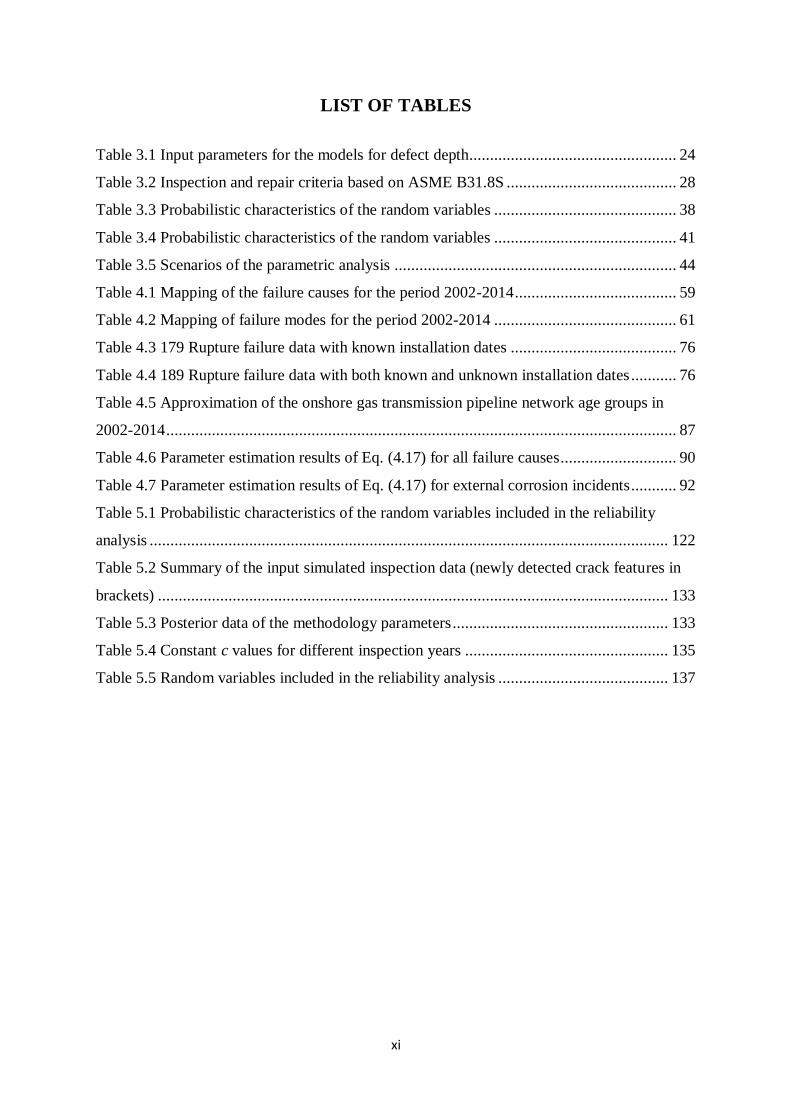
LIST OF TABLES ............................................................................................................... xi
LIST OF APPENDICES ..................................................................................................... xii
LIST OF SYMBOLS ......................................................................................................... xiii
1. Introduction ....................................................................................................................... 1
1.1 Background ................................................................................................................. 1
1.2 Objectives and Research Significance .......................................................................... 4
1.3 Scope of Study ............................................................................................................. 4
1.4 Thesis Format .............................................................................................................. 6
2. Literature Review .............................................................................................................. 7
3. Structural Reliability Analyses for Predictions in Energy Pipelines ................................. 18
3.1 Introduction ............................................................................................................... 18
3.2 Physical Model .......................................................................................................... 20
3.2.1 Stochastic Generation of Metal-loss Corrosion Defects ....................................... 20
3.2.2 Stochastic Growth of Defects .............................................................................. 21
3.2.3 Time-dependent Internal Pressure Model ............................................................. 24
3.2.4 Time-dependent Reliability Evaluation for Pipe Segment with Multiple Defects . 25
3.3 Maintenance Plan for the 1st Case Study based on In-line Inspections ....................... 27
3.3.1 Uncertainties of ILI Tools ................................................................................... 29
3.3.2 Effect of Maintenance on Pipe Segment Reliability ............................................. 29
3.4 Maintenance Plan for the 2nd Case Study based on ECDA ........................................ 30
3.4.1 Pipeline System Reliability Prediction based on SSA .......................................... 30
3.4.2 Linear Approximations ........................................................................................ 36
3.5 Numerical Application for the 1st Case Study based on In-line Inspections ................ 36
3.5.1 Results and Discussion ........................................................................................ 38
3.6 Numerical Application for the 2nd Case Study based on ECDA ................................. 39
3.6.1. Results and Discussions ...................................................................................... 44
vi
3.7 Conclusions ............................................................................................................... 53
4. Statistical Analyses for Reliability Predictions in Energy Pipelines ................................. 56
4.1 Introduction ............................................................................................................... 56
4.2 Competing Risks Analysis of Failures based on the NPI Approach ............................ 57
4.2.1 General................................................................................................................ 57
4.2.2 PHMSA Rupture Incidents from 2002-2014 ........................................................ 58
4.2.3 NPI for Competing Failure Causes ...................................................................... 63
4.3 Statistical Analysis based on a Parametric Hybrid Methodology ................................ 68
4.3.1 General................................................................................................................ 68
4.3.2 Hazard Functions and Corresponding Reliability ................................................. 69
4.3.3 Non-linear Quantile Regression ........................................................................... 72
4.4 Case Study based on the NPI methodology ................................................................ 74
4.4.1 General................................................................................................................ 74
4.4.2 Results and Discussion ........................................................................................ 76
4.5. Case Study based on the Parametric Hybrid Methodology ........................................ 85
4.5.1. General ............................................................................................................... 85
4.5.2 Results and Discussions....................................................................................... 88
4.6 Conclusions ............................................................................................................... 94
5. Bayesian Analysis of Pipeline Reliability Based on Imperfect Inspection Data ................ 96
5.1 Introduction ............................................................................................................... 96
5.2 Uncertainties Associated with ILI Data ...................................................................... 98
5.3 Stochastic Models for Corrosion Defect Generation and Growth.............................. 100
5.3.1 Generation of both Detected and Undetected Corrosion Defects ........................ 100
5.3.2 Stochastic Growth of Corrosion Defects ............................................................ 101
5.3.3 Correlations among stochastic degradations through Gaussian copula ............... 102
5.4 Bayesian Updating of the Stochastic Generation and Growth Models ...................... 103
5.4.1 Prior Distributions and Hierarchical Representation of the Deterioration Model 103
5.4.2 General Formulation .......................................................................................... 105
5.4.3 Constant c ......................................................................................................... 108
5.4.4 Likelihood Function for the Growth Model of Detected Corrosion Defects ........ 109
5.4.5 Likelihood Function for the Generation Model of Corrosion Defects ................. 110
5.5 Time-dependent Reliability Analysis ....................................................................... 110
5.5.1 Limit State Functions for Metal-Corrosion Defects ............................................ 110
5.5.2 Limit State Functions for High-pH SCC Defects ............................................... 111
5.5.3 System Reliability Analysis ............................................................................... 112
vii
5.6 Metal-loss Corrosion Case Study ............................................................................. 115
5.6.1 General.............................................................................................................. 115
5.6.2 Application and Validation of the Methodology ................................................ 116
5.6.3 Comparisons of Growth Models and Time-dependent Reliability Analysis ........ 120
5.7 High-pH SCC Case Study ........................................................................................ 129
5.7.1 Model Feasibility Study..................................................................................... 129
5.7.2 Numerical Application ...................................................................................... 130
5.7.3 Validation of Bayesian Formulation .................................................................. 132
5.7.4 Parametric and Reliability Analyses .................................................................. 135
5.8 Conclusions ............................................................................................................. 138
6. Conclusions, Research Achievements and Future Works ............................................... 141
6.1 General Conclusions ................................................................................................ 141
6.1.1 Structural Reliability Analyses for Predictions in Energy Pipelines.................... 141
6.1.2 Statistical Analyses for Reliability Predictions in Energy Pipelines.................... 143
6.1.3 Bayesian Analysis of Pipeline Reliability based on Imperfect Inspection Data ... 144
6.2 Research Achievements ........................................................................................... 146
6.3 Recommendations for future study ........................................................................... 148
REFERENCES ................................................................................................................. 149
Appendix A: Step-by-Step Procedure for Estimating the Posterior Failure Probabilities
Conditional on the ILI Data ............................................................................................... 167
Appendix B: List of Publications ....................................................................................... 169
viii
LIST OF FIGURES
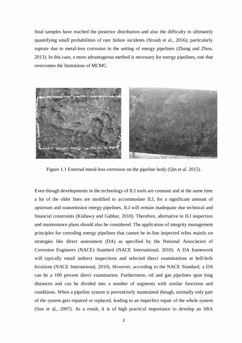
Figure 1.1 External metal-loss corrosion on the pipeline body ............................................... 2
Figure 1.2 Direct Assessment of the pipeline condition in the field ........................................ 3
Figure 2.1 Dimensions of a typical metal-loss corrosion defect on pipeline (Al-Amin and
Zhou, 2013) .......................................................................................................................... 8
Figure 3.1 Poisson Square Wave Process model .................................................................. 22
Figure 3.2 Illustration of stochastic Poisson Square Wave Process and time-independent
power law defect growth models ......................................................................................... 22
Figure 3.3 Stochastic Ferry-Borges model for internal pressure of gas pipelines .................. 24
Figure 3.4 Reliability updating based on inspection information .......................................... 30
Figure 3.5 Example of conditional reliability of a pipeline system with multiple imperfect
repairs ................................................................................................................................. 32
Figure 3.6 Example of multi-component series system ........................................................ 33
Figure 3.7 Linear approximations to determine the exact time of reliability falling to 0.9 .... 35
Figure 3.8 Results of the structural reliability approach ....................................................... 38
Figure 3.9 Illustration of the NHPP ..................................................................................... 41
Figure 3.10 Simulated time-dependent internal pressure based on the PSWP model ............ 42
Figure 3.11 Time-dependent reliability prediction for an externally corroded 12m pipe
segment ............................................................................................................................... 44
Figure 3.12 Comparison of reliability with and without PM ................................................ 45
Figure 3.13 (a-c) Comparison of reliability predictions in terms of the proportional constant
λο of the defect generation model ........................................................................................ 48
Figure 3.14 (a-c) Comparisons of reliability predictions in terms of the generation rate λ of
the PSWP internal pressure model ....................................................................................... 50
Figure 3.15a Comparisons of reliability predictions in temrs of the reliability threshold Rth . 51
Figure 3.15b Comparisons of reliability predictions in terms of the reliability threshold Rth . 52
Figure 4.1 Bath-tub failure pattern ....................................................................................... 68
Figure 4.2 Bath-tub failure pattern for gas transmission pipelines ........................................ 69
Figure 4.3 NPI lower and upper survival functions for a future pipeline segment with t in
weeks .................................................................................................................................. 80
Figure 4.4 NPI conditional (EC, MF) lower and upper survival functions for a future pipeline
segment with t in weeks ...................................................................................................... 81
ix
Figure 4.5 NPI conditional (IC, ED, OTHER) lower and upper survival functions for a future
pipeline segment with t in weeks ......................................................................................... 82
Figure 4.6 NPI conditional (PDP, EM) lower and upper survival functions for a future
pipeline segment with t in weeks ......................................................................................... 83
Figure 4.7 Rupture hazard bar chart of the onshore gas transmission pipeline network in
2002-2014 ........................................................................................................................... 86
Figure 4.8 Hazard function curve for τq = 0.99 quantile (all failure causes).......................... 88
Figure 4.9 Reliability function against rupture of the average segment of the onshore gas
transmission pipeline netwotrk in 2002-2014 ...................................................................... 89
Figure 4.10 Hazard bar chart for rupture due to external metal-loss corrosion ...................... 90
Figure 4.11 Comparison of the reliability function curves of the two different methodologies
........................................................................................................................................... 92
Figure 5.1 Measurement error band and corresponding probability...................................... 97
Figure 5.2 Hierarchical Bayesian HGP-based model for the jth inspection of the ith defect . 103
Figure 5.3 ILI-reported depths in 2000, 2004, 2007 and field-measured depths in 2010 for
each of the seventeen defects ............................................................................................. 114
Figure 5.4 Comparison of the HGP model predictions with the field-measured depths in 2010
......................................................................................................................................... 115
Figure 5.5 Predicted growth path of defect 4 based on the HGP model .............................. 116
Figure 5.6 Predicted growth path of defect 9 based on the HGP model .............................. 117
Figure 5.7 Comparison of the NHGP model predictions with the field measured depths in
2010 .................................................................................................................................. 117
Figure 5.8 ILI-reported depths in 2004, 2007, 2009 and 2011 for each of the ten defects ... 118
Figure 5.9 Initial defect lengths of the 10 defects derived from the ILI in 2011.................. 120
Figure 5.10 Comparisons of the growth path predictions of the NHGP- and HGP-based
models for four random defects ......................................................................................... 121
Figure 5.11 Marginal posterior PDFs of depth predictions of four defects in years 2011, 2016
and 2021 ........................................................................................................................... 123
Figure 5.12(a-c) Comparison of small leak, large leak and rupture probabilities associated
with different corrosion growth (NHGP, HGP) and different simulation methods for
reliability evaluations (BUS-SuS, MC) .............................................................................. 125
Figure 5.13 Four stages of high-pH SCC ........................................................................... 127
Figure 5.14 Comparison of predicted and actual number of crack features ......................... 132
Figure 5.15 Comparison of predicted and actual depths of crack features at year 15 .......... 132

x
Figure 5.16 Comparison of the predicted and actual depths of crack features at year 15 for
different correlation coefficients between stochastic growths ............................................ 134
Figure 5.17 Posterior system reliability at inspection times, based on the proposed
methodology and Monte Carlo, for different correlation scenarios among stochastic growths
of the crack features .......................................................................................................... 136
xi
LIST OF TABLES
Table 3.1 Input parameters for the models for defect depth.................................................. 24
Table 3.2 Inspection and repair criteria based on ASME B31.8S ......................................... 28
Table 3.3 Probabilistic characteristics of the random variables ............................................ 38
Table 3.4 Probabilistic characteristics of the random variables ............................................ 41
Table 3.5 Scenarios of the parametric analysis .................................................................... 44
Table 4.1 Mapping of the failure causes for the period 2002-2014 ....................................... 59
Table 4.2 Mapping of failure modes for the period 2002-2014 ............................................ 61
Table 4.3 179 Rupture failure data with known installation dates ........................................ 76
Table 4.4 189 Rupture failure data with both known and unknown installation dates ........... 76
Table 4.5 Approximation of the onshore gas transmission pipeline network age groups in
2002-2014 ........................................................................................................................... 87
Table 4.6 Parameter estimation results of Eq. (4.17) for all failure causes............................ 90
Table 4.7 Parameter estimation results of Eq. (4.17) for external corrosion incidents ........... 92
Table 5.1 Probabilistic characteristics of the random variables included in the reliability
analysis ............................................................................................................................. 122
Table 5.2 Summary of the input simulated inspection data (newly detected crack features in
brackets) ........................................................................................................................... 133
Table 5.3 Posterior data of the methodology parameters .................................................... 133
Table 5.4 Constant c values for different inspection years ................................................. 135
Table 5.5 Random variables included in the reliability analysis ......................................... 137

xii
LIST OF APPENDICES
Appendix A: Step-by-Step Procedure for Estimating the Posterior Failure Probabilities
Conditional on the ILI Data ............................................................................................... 164
Appendix B: List of Publications ....................................................................................... 166

xiii
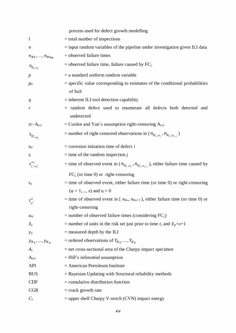
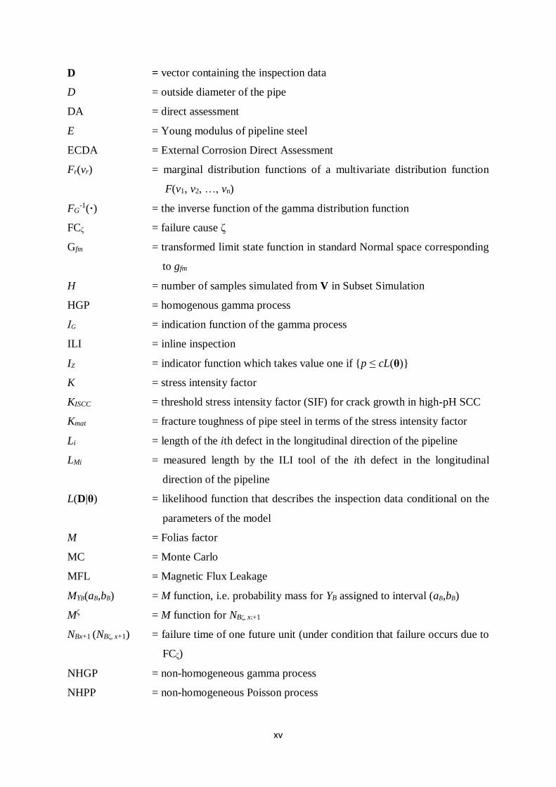
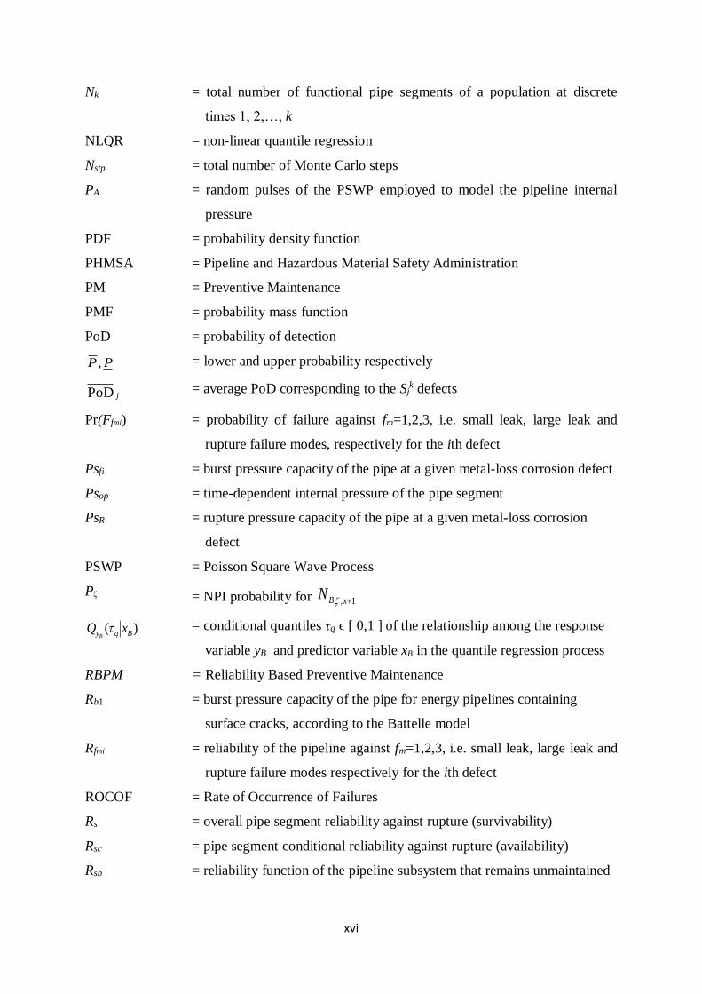
LIST OF SYMBOLS
ai = random variable (exponent) of the parameterized stochastic process used
to characterise the growth of the ith defect
c = a positive constant that ensures cL(θ) ≤ 1 for all θ
cl2 = constant biases of the ILI tools related to the measured lengths
cl2 = non-constant biases of the ILI tools related to the measured lengths
c1, …, cvΒ = right-censored observations
c1j = constant biases associated with the ILI tool of the jth inspection with
regard to the measured depths
c2j = non-constant biases associated with the ILI tool of the jth inspection
with regard to the measured depths
Bscc ,...,1 = right-censored observations in (nBω, nBω+1), ω= 0,…, uB
,
,1, ,...,Bscc = right-censored observations in (
1,,,
BB nn ), ωζ = 0,…, uBζ
dij = actual field-measured depth of the ith defect
dt = defect depth detection threshold of the ILI tool
f (·) = probability density function of the random variable ·
f(θ) = joint prior distribution of the parameters θ
f(θ|D) = posterior probability distribution of the model parameters conditional on
the inspection data
f p(·) = probability mass function of the random variable ·
g1 = limit state function for the corrosion defect penetrating the pipe wall and
causing a small leak
g2 = limit state function for plastic collapse under internal pressure at the
defect causing large leak
g3 = limit state function for unstable defect extension in the axial direction
causing rupture of the pipeline
h(t) = hazard function
i = random defect out of the total s detected defects
iid = independent and identically distributed
j = random inspection out of the total l inspections
kA = random variable (proportionality factor) of the parameterized stochastic
xiv
process used for defect growth modelling
l = total number of inspections
n = input random variables of the pipeline under investigation given ILI data
𝑛𝐵1,…, 𝑛𝐵𝑢𝐵 = observed failure times
,Bn = observed failure time, failure caused by FCζ
p = a standard uniform random variable
p0 = specific value corresponding to estimates of the conditional probabilities
of SuS
q = inherent ILI tool detection capability
r = random defect used to enumerate all defects both detected and
undetected
rc–A(x) = Coolen and Yan’s assumption right-censoring A(x)
,Bs = number of right-censored observations in (
1,,,
BB nn )
ti0 = corrosion initiation time of defect i
tj = time of the random inspection j
*,t = time of observed event in (
1,,,
BB nn ), either failure time caused by
FCζ (or time 0) or right-censoring
tψ = time of observed event, either failure time (or time 0) or right-censoring
(ψ = 1,..., x) and t0 = 0
*t = time of observed event in [ nBω, nBω+1 ), either failure time (or time 0) or
right-censoring
uBζ = number of observed failure times (considering FCζ)
�̃�𝑡 = number of units in the risk set just prior to time t, and �̃�0=x+1
yij = measured depth by the ILI
𝑦𝐵1, … , 𝑦𝐵𝑥 = ordered observations of 𝑌𝐵1, … , 𝑌𝐵𝑥
Ac = net cross-sectional area of the Charpy impact specimen
A(x) = Hill’s inferential assumption
API = American Petroleum Institute
BUS = Bayesian Updating with Structural reliability methods
CDF = cumulative distribution function
CGR = crack growth rate
Cv = upper shelf Charpy V-notch (CVN) impact energy
xv
D = vector containing the inspection data
D = outside diameter of the pipe
DA = direct assessment
E = Young modulus of pipeline steel
ECDA = External Corrosion Direct Assessment
Fr(vr) = marginal distribution functions of a multivariate distribution function
F(v1, v2, …, vn)
FG-1(·) = the inverse function of the gamma distribution function
FCζ = failure cause ζ
Gfm = transformed limit state function in standard Normal space corresponding
to gfm
H = number of samples simulated from V in Subset Simulation
HGP = homogenous gamma process
ΙG = indication function of the gamma process
ILI = inline inspection
IZ = indicator function which takes value one if {p ≤ cL(θ)}
K = stress intensity factor
KISCC = threshold stress intensity factor (SIF) for crack growth in high-pH SCC
Kmat = fracture toughness of pipe steel in terms of the stress intensity factor
Li = length of the ith defect in the longitudinal direction of the pipeline
LMi = measured length by the ILI tool of the ith defect in the longitudinal
direction of the pipeline
L(D|θ) = likelihood function that describes the inspection data conditional on the
parameters of the model
M = Folias factor
MC = Monte Carlo
MFL = Magnetic Flux Leakage
MYB(aB,bB) = M function, i.e. probability mass for YB assigned to interval (aB,bB)
Mζ = M function for NBζ, xζ+1
NBx+1 (NBζ, x+1) = failure time of one future unit (under condition that failure occurs due to
FCζ)
NHGP = non-homogeneous gamma process
NHPP = non-homogeneous Poisson process
xvi
Nk = total number of functional pipe segments of a population at discrete
times 1, 2,…, k
NLQR = non-linear quantile regression
Nstp = total number of Monte Carlo steps
PA = random pulses of the PSWP employed to model the pipeline internal
pressure
PDF = probability density function
PHMSA = Pipeline and Hazardous Material Safety Administration
PM = Preventive Maintenance
PMF = probability mass function
PoD = probability of detection
PP , = lower and upper probability respectively
jPoD = average PoD corresponding to the Sjk defects
Pr(Ffmi) = probability of failure against fm=1,2,3, i.e. small leak, large leak and
rupture failure modes, respectively for the ith defect
Psfi = burst pressure capacity of the pipe at a given metal-loss corrosion defect
Psop = time-dependent internal pressure of the pipe segment
PsR = rupture pressure capacity of the pipe at a given metal-loss corrosion
defect
PSWP = Poisson Square Wave Process
Pζ = NPI probability for 1, xBN
)( Bqy xQB = conditional quantiles τq ϵ [ 0,1 ] of the relationship among the response
variable yB and predictor variable xB in the quantile regression process
RBPM = Reliability Based Preventive Maintenance
Rb1 = burst pressure capacity of the pipe for energy pipelines containing
surface cracks, according to the Battelle model
Rfmi = reliability of the pipeline against fm=1,2,3, i.e. small leak, large leak and
rupture failure modes respectively for the ith defect
ROCOF = Rate of Occurrence of Failures
Rs = overall pipe segment reliability against rupture (survivability)
Rsc = pipe segment conditional reliability against rupture (availability)
Rsb = reliability function of the pipeline subsystem that remains unmaintained
xvii
Rth = predefined reliability threshold for the entire pipeline
SCC = Stress Corrosion Cracking
SMTS = Specified Minimum Tensile Strength
SMYS = Specified Minimum Yield Stress
Sj = total number of defects on the pipe segment at the time of the jth
inspection
Sj0 = number of defects that have initiated prior to the (j-1)th inspection
Sjk = number of defects that have initiated between the (j-1)th and jth
inspection
Sjkde = number of detected defects by the ILI tool that form part of the total
number Sjk
Sjkun = number of undetected defects by the ILI tool that form part of the total
number Sjk
SRA = Structural Reliability Analysis
SSA = Split System Approach
S(t) = total number of expected defects on the pipe segment over [0, t]
SuS = Subset Simulation
Tζ = unit’s random time to failure under condition that failure occurs due to
FCζ
Tm = time of the mth PM action
TMT = given decision horizon for a preventive maintenance strategy
YB = random quantity used in definition of M-function
𝑌𝐵1, … , 𝑌𝐵𝑥+1 = random quantities used in general formulation of A(x)
Uja = random pulse heights of ja duration of the PSWP
UC = standard uniformly distributed variable of the Copula functions
UT = Ultrasonic Thickness device
UTS = ultimate tensile strength of the pipeline material
V = transformed space with independent standard Normal random variables
corresponding to the original random variables p and θ
ZA = number of pulses of the PSWP process
αFT = multiplier of the non-linear relationship in the NLQR
α(t-ti0)κ = the time-dependent shape parameter of the gamma process
α2 = scale parameter of the Weibull distribution
xviii
βFT = exponent of the non-linear relationship in the NLQR
βi = rate parameter of the gamma process associated with the ith defect
β2 = shape parameter of the Weibull distribution
γ(▪) = the incomplete gamma function
γ1-6 (ξ1-6) = distribution parameters of the prior distributions of model parameters
𝛿𝜔𝜁∗
𝜔𝜁 = 1 if ))(( **
ttt is a failure time or 0 if a right-censoring time
εij = random scattering error associated with the actual depth of the ith defect
reported by the jth inspection
εli = random scattering errors related to the measured length of the ith defect
η = density of corrosion defects
ηA = safety factor associated with internal pressure-related excavation criteria
θ = vector of random variables of the physical pipeline model
λΑ(τ) = instantaneous generation rate of corrosion defects
λ = mean occurrence rate per unit time (or Poisson rate) of the PSWP
μ = mean of the probability distribution of the random scattering error εij
associated with the reported defect i in the jth inspection
ξA = safety factor associated with wall thickness-related excavation criteria
ρjq = correlation coefficient between the random scattering errors associated
with the jth and the qth inspections
σ = standard deviation of the probability distribution of the random
scattering error εij associated with the reported defect i in the jth
inspection
σf = material flow stress of the pipeline
σj = standard deviation of the random scattering errors associated with the
ILI tool used in inspection j
σy = pipe’s material ultimate yield strength
υΒζ = number of right-censored observations (considering FCζ)
Δαij = the time-dependent shape parameter associated with Δdij
Δdij = the growth of the ith defect among two consecutive ILIs
Z = observation event {p ≤ cL(θ)}in terms of the Bayesian updating
Λ(t) = expected number of defects generated over [0, t]
Σε = covariance matrix of the random scattering error
Φ -1 (▪) = the inverse of the standard normal distribution function

xix
Φn (▪; R) = the n-variate standard normal distribution function with (n x n) matrix of
correlation coefficients R
1
1. Introduction
1.1 Background
Pipelines are the safest and most economic means of transporting hydrocarbons (e.g. crude
oil and natural gas) around the globe. Degradation is considered an inevitable part of the
operating lifecycle of pipelines, even for newly built ones, as it typically is for
infrastructure. A sudden breakdown can lead to loss of productivity or severe accident with
large environmental, economic and social implications. As a result, comprehensive
maintenance and rehabilitation plans should be available, as part of a structured reliability-
based integrity management program. The success of such programs, depends primarily on
how well threats and failure mechanisms are defined. Integrity threats should be
considered in conjunction with realistic maintenance strategies including in-line (ILI)
inspections, criteria for excavating and repairing defects and direct assessment. Structural
reliability analysis (SRA) can have a key role in the reliability-based integrity
management. It offers an efficient way of directly assessing the loads and capacity of a
pipeline, considering the separate effect of each random variable on the pipeline condition
(Barone and Frangopol, 2014). When it comes to SRA models, the uncertainties regarding
material and geometrical properties, environmental factors and the models themselves are
accounted for probabilistically, towards obtaining realistic forecasts of failure probabilities
(Frangopol and Soliman, 2016). The results from the SRA can be used in real industry
practice for the development of safe and cost-effective integrity management strategies.
According to incident data from the literature, external corrosion has been identified as the
predominant gradual deterioration process (UKOPA, 2014). In addition, stress corrosion
cracking (SCC) also poses a major threat to the safe operation and structural integrity of
energy pipelines. Bayesian data analysis is a very advantageous way of updating SRA
models given corrosion ILI data and has been used considerably in energy pipelines’
literature over the past decade (Maes et al., 2009; Pandey and Lu, 2013; Al-Amin and
Zhou, 2014; Qin et al., 2015; Zhang and Zhou, 2013; Caleyo et al., 2015). The analytical
estimation of the high-dimensional integrals typically involved in Bayesian updating is not
feasible in pipeline problems and therefore Markov Chain Monte Carlo (MCMC) sampling
techniques are commonly adopted to numerically perform this task (Al-Amin and Zhou,
2014). The limitations of these methods include the uncertainty around ensuring that the
2
final samples have reached the posterior distribution and also the difficulty in ultimately
quantifying small probabilities of rare failure incidents (Straub et al., 2016); particularly
rupture due to metal-loss corrosion in the setting of energy pipelines (Zhang and Zhou,
2013). In this case, a more advantageous method is necessary for energy pipelines, one that
overcomes the limitations of MCMC.
Figure 1.1 External metal-loss corrosion on the pipeline body (Qin et al. 2015).
Even though developments in the technology of ILI tools are constant and at the same time
a lot of the older lines are modified to accommodate ILI, for a significant amount of
upstream and transmission energy pipelines, ILI will remain inadequate due technical and
financial constraints (Kishawy and Gabbar, 2010). Therefore, alternative to ILI inspection
and maintenance plans should also be considered. The application of integrity management
principles for corroding energy pipelines that cannot be in-line inspected relies mainly on
strategies like direct assessment (DA) as specified by the National Association of
Corrosion Engineers (NACE) Standard (NACE International, 2010). A DA framework
will typically entail indirect inspections and selected direct examinations at bell-hole
locations (NACE International, 2010). However, according to the NACE Standard, a DA
can be a 100 percent direct examination. Furthermore, oil and gas pipelines span long
distances and can be divided into a number of segments with similar functions and
conditions. When a pipeline system is preventively maintained though, normally only part
of the system gets repaired or replaced, leading to an imperfect repair of the whole system
(Sun et al., 2007). As a result, it is of high practical importance to develop an SRA

3
methodology that includes imperfect DA strategies for a pipeline system that cannot be
inspected with ILI tools.
Figure 1.2 Direct Assessment of the pipeline condition in the field (NACE
International, 2010).
The validation of SRA based on historical failure data is key to gaining confidence on the
results, provided the uncertainties associated with both methods are properly taken into
account. Previous studies that employed historical failure data of energy pipelines,
evaluated the failure probabilities in the rate of occurrence of failure (ROCOF) sense for
repairable systems (Caleyo et al, 2008; Nessim et al, 2009). In brief, the repairable system
approach assumes that upon failure, the system is restored to operation by repairing or
even replacing some parts of the system, instead of replacing the entire system. Thus, the
failure rate refers to a sequence of failure times within a time interval, as opposed to a
single time to failure distribution. However, the ROCOF failure rate can be evaluated only
for a limited period of time, i.e. for as long as incident data are available. In an alternative
approach, the pipeline times to failure can be grouped according to a non-repairable
systems approach. The failed pipes are defined as non-repairable segments functioning
within a repairable system, which is the entire pipeline network. In other words, the
lifetime of a pipe segment is a random variable described by a single time to failure. Such
analyses of historical failure data are advantageous in that they can provide a complete
4
picture of energy pipeline reliability and can be directly comparable to SRA predictions for
cross-verification and corroboration of the results.
1.2 Objectives and Research Significance
The aim is to develop technically comprehensive methods that can explicitly define safety
threats in the context of realistic pipeline integrity management strategies, in order to
accurately evaluate the pipeline remaining life as a function of uncertainties in pipeline
operating conditions. The objectives of the study reported in this thesis include: 1)
development of model-based methodologies that incorporate stochastic processes within a
structural reliability analysis (SRA) framework and predict time-dependent reliability for
corroding pipelines, with the consideration of realistic, industry consistent inspection and
maintenance techniques, 2) development of methodologies that estimate failure
probabilities in a non-repairable approach setting, based on robust statistical analyses of
historical incidents, 3) development of methodologies to evaluate small (<10 -6) failure
probabilities for corroding pipelines conditional on ILI data, by employing the developed
probabilistic SRA framework, 4) cross-verification of the SRA and statistical
methodologies 5) validation of the methodologies conditional on ILI data, based on actual
data. It is anticipated that the research outcome of this study will assist energy pipeline
operators in implementing informed integrity management plans, based on reliability and
safety. This can be of great value not only to the pipeline industry, but also to the
communities in the proximity of energy pipelines.
1.3 Scope of Study
This study consists of a relevant literature review in Chapter 2 and three core topics that
are presented in Chapters 3 to 5 respectively and form the main body of the thesis. In
Chapter 3, a probabilistic methodology for onshore gas pipelines with corrosion defects is
proposed, based on a structural reliability analysis (SRA) framework. The application of
the SRA methodology is illustrated through two case studies that consider two different
maintenance strategies. In the first application, the non-homogeneous Poisson process is
used to model the generation of new defects and a parameterized stochastic process (i.e. a
non-linear function of two random variables) is used to model the growth of defects. The
5
internal pressure loading is modelled as a Poisson square wave stochastic process. External
Corrosion Direct Assessment (ECDA) is utilised as an industry-consistent maintenance
strategy. The second case study implements the SRA methodology with the consideration
of a realistic maintenance and repair strategy based on in-line inspections (ILI). The non-
homogeneous Poisson process models the generation of new defects and a robust non-
linear stochastic process, namely Poisson square wave process, is used to model the
growth of defects. The internal pressure loading is modelled as a discrete Ferry-Borges
stochastic process. The probability of detection (PoD) and measurement error of the
inspection tools are also incorporated in the methodology. The results are validated against
a statistical model presented subsequently in Chapter 4. In specific, two statistical models
are proposed in Chapter 4, based on historical failure data of onshore gas transmission
pipelines from the Pipeline and Hazardous Material Safety Administration (PHMSA)
database. The first statistical methodology is based on a well-established non-repairable
system approach, namely nonparametric predictive inference (NPI). It provides imprecise
probabilities and survival functions via upper and lower bounds, due to a specific cause
among a range of competing ones. The second case study concerns the application of a
novel statistical methodology, based on a parametric hybrid empirical hazard model and a
robust data processing technique (i.e. non-linear quantile regression) with regards to the
PHMSA historical failure data. Reliability inferences correspond to the complete lifecycle
reliability of the average pipe segment of the respective region under study. The results
from the latter are compared with the ILI-based SRA methodology proposed in Chapter 3
for the purpose of cross-verification. Finally, in Chapter 5 a new methodology for
estimation of small posterior failure probabilities based on Bayesian analysis of ILI data is
presented. Two case studies are conducted to illustrate and validate the proposed
methodology. Firstly, the methodology is applied in an existing gas pipeline containing
metal-loss corrosion defects and is validated against field data. The reliability conditional
on the inspection data is evaluated directly with a single method. In the second case study,
Bayesian updating is carried out in conjunction with a data augmentation (DA) technique,
for simulated data of high-pH stress corrosion cracking (SCC). The interdependence of
crack growths is addressed through the Gaussian copula method. Both numerical
applications of Chapter 5 are carried out within a realistic, industry-consistent context.

6
1.4 Thesis Format
This thesis consists of six chapters in total. Chapter 1 presents a brief introduction of the
background, objectives and scope of study. Chapter 2 reviews the literature with respect to
the relevant research area of this thesis. Chapters 3 to 5 forms the main body of the thesis,
each of which addresses a distinct topic. These constitute the core of the published papers
and submitted manuscripts, as listed in Appendix B. The conclusions and main
contributions of the research of this thesis, as well as the proposed future works are
discussed in Chapter 6.
7
2. Literature Review
Energy pipeline infrastructure grows about 3-4 percent per year globally. Worldwide, most
energy pipelines have been in place for at least 20 years; more than 50 percent of pipelines
were installed in the period 1950-1970 (Kiefner and Rosenfeld, 2012). In literature, old
pipelines refer to those that were constructed prior to the 1970’s (Kishawy and Gabbar,
2010). These are considered of lower standards, in terms of material and external coating,
compared to more recent ones. However, gradual deterioration of the pipeline condition is
considered inevitable, even for contemporary pipelines, as it typically is for all engineering
structures. As a result, comprehensive maintenance and rehabilitation plans should be
readily available, as part of a structured integrity management program. The effectiveness
of an integrity management program depends on many factors, including how well threats
and failure mechanisms have been identified (Kishawy and Gabbar, 2010).
According to statistical analyses and incident data, external corrosion is the predominant
gradual deterioration process for onshore energy pipelines (EGIG, 2015; CONCAWE,
2015; UKOPA, 2014; AER, 2013). However, other factors such as third-party activity,
material or construction imperfections, geotechnical hazards, incorrect operation and
inadequate design, among others, can lead to ultimate failure modes such as leaks and
ruptures (Caleyo et al., 2008; El-Abbasy et al., 2014). Nonetheless, the efforts to evaluate
pipeline reliability in the literature thus far, either account only for corrosion as a failure
mechanism (Li et al., 2009; Zhou, 2010; Lecchi, 2011; Valor et al., 2013; Zhang and Zhou,
2013) or inevitably entail a level of subjectivity due to their prominently conceptual nature
(Peng et al., 2009; El-Abbasy et al., 2014). Failures of onshore energy pipelines due to
external corrosion can be further distinguished in metal-loss and stress corrosion cracking
(SCC) failures (EGIG, 2015; CONCAWE, 2015; UKOPA, 2014; PHMSA, 2015).
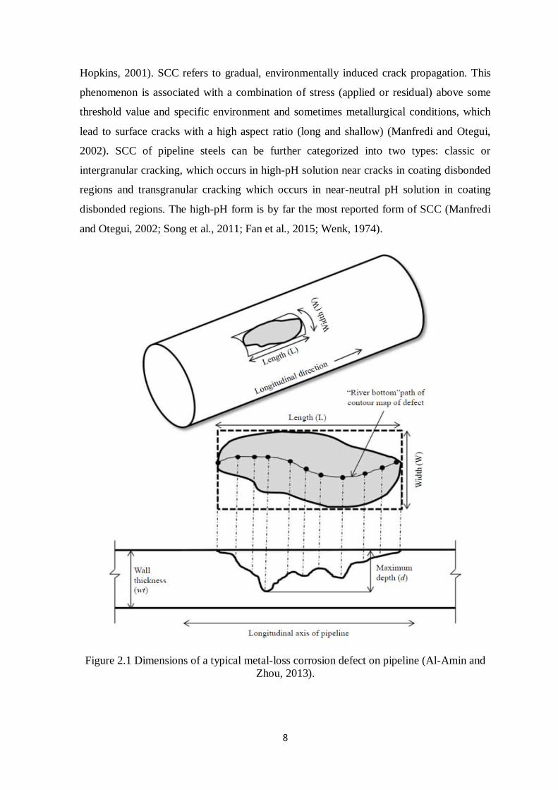
Metal-loss corrosion defects typically have an irregular depth profile and extend
irregularly in both longitudinal and circumferential directions, as illustrated in Figure 2.1
(Cosham and Hopkins, 2001). Metal-loss corrosion may occur as a single defect or a
cluster of adjacent defects, separated by full wall thickness areas and it typically has a
length and width less than or equal to three times the full wall thickness (Kiefner and
Veith, 1989). The main difference compared to SCC is that metal-loss defects are ‘blunt’.
That is, the minimum radius equals or exceeds half of the pipe wall thickness and defects
that have a width greater than their local depth (Stephens and Leis, 2000; Cosham and
8
Hopkins, 2001). SCC refers to gradual, environmentally induced crack propagation. This
phenomenon is associated with a combination of stress (applied or residual) above some
threshold value and specific environment and sometimes metallurgical conditions, which
lead to surface cracks with a high aspect ratio (long and shallow) (Manfredi and Otegui,
2002). SCC of pipeline steels can be further categorized into two types: classic or
intergranular cracking, which occurs in high-pH solution near cracks in coating disbonded
regions and transgranular cracking which occurs in near-neutral pH solution in coating
disbonded regions. The high-pH form is by far the most reported form of SCC (Manfredi
and Otegui, 2002; Song et al., 2011; Fan et al., 2015; Wenk, 1974).
Figure 2.1 Dimensions of a typical metal-loss corrosion defect on pipeline (Al-Amin and
Zhou, 2013).
9
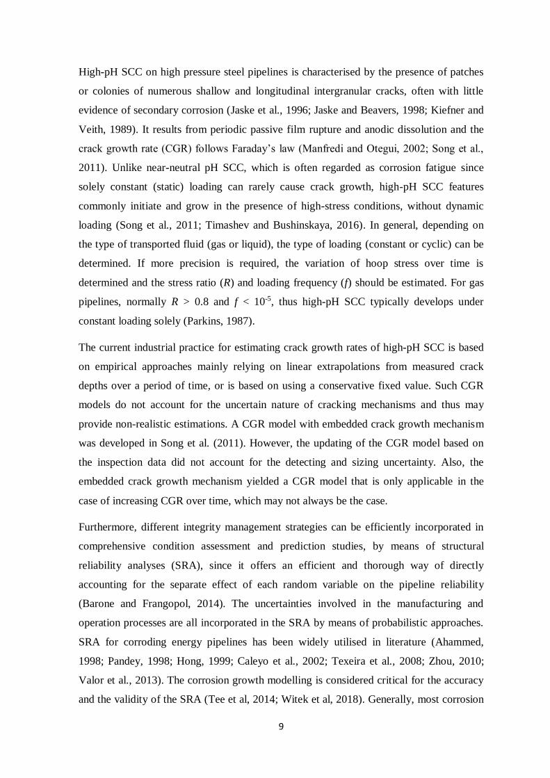
High-pH SCC on high pressure steel pipelines is characterised by the presence of patches
or colonies of numerous shallow and longitudinal intergranular cracks, often with little
evidence of secondary corrosion (Jaske et al., 1996; Jaske and Beavers, 1998; Kiefner and
Veith, 1989). It results from periodic passive film rupture and anodic dissolution and the
crack growth rate (CGR) follows Faraday’s law (Manfredi and Otegui, 2002; Song et al.,
2011). Unlike near-neutral pH SCC, which is often regarded as corrosion fatigue since
solely constant (static) loading can rarely cause crack growth, high-pH SCC features
commonly initiate and grow in the presence of high-stress conditions, without dynamic
loading (Song et al., 2011; Timashev and Bushinskaya, 2016). In general, depending on
the type of transported fluid (gas or liquid), the type of loading (constant or cyclic) can be
determined. If more precision is required, the variation of hoop stress over time is
determined and the stress ratio (R) and loading frequency (f) should be estimated. For gas
pipelines, normally R > 0.8 and f < 10-5, thus high-pH SCC typically develops under
constant loading solely (Parkins, 1987).
The current industrial practice for estimating crack growth rates of high-pH SCC is based
on empirical approaches mainly relying on linear extrapolations from measured crack
depths over a period of time, or is based on using a conservative fixed value. Such CGR
models do not account for the uncertain nature of cracking mechanisms and thus may
provide non-realistic estimations. A CGR model with embedded crack growth mechanism
was developed in Song et al. (2011). However, the updating of the CGR model based on
the inspection data did not account for the detecting and sizing uncertainty. Also, the
embedded crack growth mechanism yielded a CGR model that is only applicable in the
case of increasing CGR over time, which may not always be the case.
Furthermore, different integrity management strategies can be efficiently incorporated in
comprehensive condition assessment and prediction studies, by means of structural
reliability analyses (SRA), since it offers an efficient and thorough way of directly
accounting for the separate effect of each random variable on the pipeline reliability
(Barone and Frangopol, 2014). The uncertainties involved in the manufacturing and
operation processes are all incorporated in the SRA by means of probabilistic approaches.
SRA for corroding energy pipelines has been widely utilised in literature (Ahammed,
1998; Pandey, 1998; Hong, 1999; Caleyo et al., 2002; Texeira et al., 2008; Zhou, 2010;
Valor et al., 2013). The corrosion growth modelling is considered critical for the accuracy
and the validity of the SRA (Tee et al, 2014; Witek et al, 2018). Generally, most corrosion
10
growth models reported in literature can be categorised as random-variable based,
stochastic process-based models, fuzzy models, interval models and imprecise probability
models (Hong, 1999; Timashev, 2008; Caleyo et al., 2009; Maes et al., 2009; Zhang and
Zhou, 2013; Senouci et al., 2014; Opeyemi et al., 2015; Fang et al, 2015; Shafiee and
Ayudiani, 2015; Chaves et al., 2016; Melchers, 2016; Melchers and Ahammed, 2016;
Asadi and Melchers, 2017; Witek, 2018).
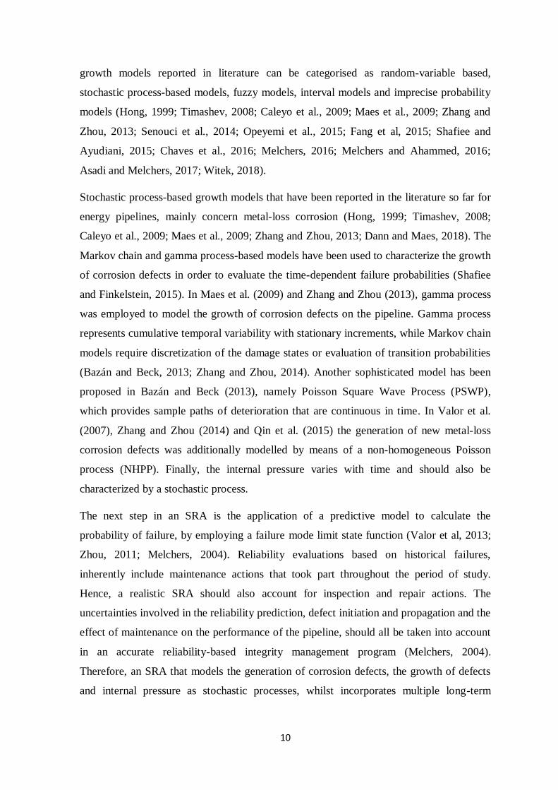
Stochastic process-based growth models that have been reported in the literature so far for
energy pipelines, mainly concern metal-loss corrosion (Hong, 1999; Timashev, 2008;
Caleyo et al., 2009; Maes et al., 2009; Zhang and Zhou, 2013; Dann and Maes, 2018). The
Markov chain and gamma process-based models have been used to characterize the growth
of corrosion defects in order to evaluate the time-dependent failure probabilities (Shafiee
and Finkelstein, 2015). In Maes et al. (2009) and Zhang and Zhou (2013), gamma process
was employed to model the growth of corrosion defects on the pipeline. Gamma process
represents cumulative temporal variability with stationary increments, while Markov chain
models require discretization of the damage states or evaluation of transition probabilities
(Bazán and Beck, 2013; Zhang and Zhou, 2014). Another sophisticated model has been
proposed in Bazán and Beck (2013), namely Poisson Square Wave Process (PSWP),
which provides sample paths of deterioration that are continuous in time. In Valor et al.
(2007), Zhang and Zhou (2014) and Qin et al. (2015) the generation of new metal-loss
corrosion defects was additionally modelled by means of a non-homogeneous Poisson
process (NHPP). Finally, the internal pressure varies with time and should also be
characterized by a stochastic process.
The next step in an SRA is the application of a predictive model to calculate the
probability of failure, by employing a failure mode limit state function (Valor et al, 2013;
Zhou, 2011; Melchers, 2004). Reliability evaluations based on historical failures,
inherently include maintenance actions that took part throughout the period of study.
Hence, a realistic SRA should also account for inspection and repair actions. The
uncertainties involved in the reliability prediction, defect initiation and propagation and the
effect of maintenance on the performance of the pipeline, should all be taken into account
in an accurate reliability-based integrity management program (Melchers, 2004).
Therefore, an SRA that models the generation of corrosion defects, the growth of defects
and internal pressure as stochastic processes, whilst incorporates multiple long-term
11
integrity management strategies and quantifies the relevant uncertainties is of great
practical importance.
The corrosion defect growth rate is pivotal and must be accurately modelled when the
interval for in-line inspection (ILI), pressure testing and direct assessment is to be
determined. The corrosion growth model can also be a key parameter in identifying
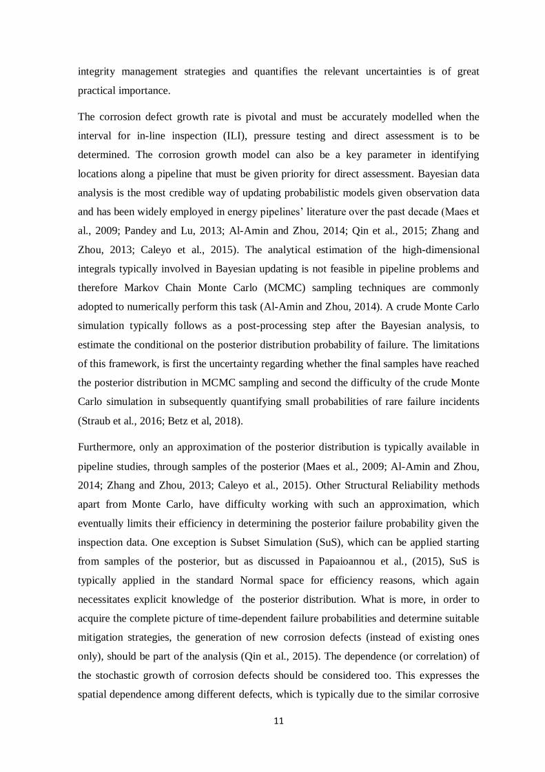
locations along a pipeline that must be given priority for direct assessment. Bayesian data
analysis is the most credible way of updating probabilistic models given observation data
and has been widely employed in energy pipelines’ literature over the past decade (Maes et
al., 2009; Pandey and Lu, 2013; Al-Amin and Zhou, 2014; Qin et al., 2015; Zhang and
Zhou, 2013; Caleyo et al., 2015). The analytical estimation of the high-dimensional
integrals typically involved in Bayesian updating is not feasible in pipeline problems and
therefore Markov Chain Monte Carlo (MCMC) sampling techniques are commonly
adopted to numerically perform this task (Al-Amin and Zhou, 2014). A crude Monte Carlo
simulation typically follows as a post-processing step after the Bayesian analysis, to
estimate the conditional on the posterior distribution probability of failure. The limitations
of this framework, is first the uncertainty regarding whether the final samples have reached
the posterior distribution in MCMC sampling and second the difficulty of the crude Monte
Carlo simulation in subsequently quantifying small probabilities of rare failure incidents
(Straub et al., 2016; Betz et al, 2018).
Furthermore, only an approximation of the posterior distribution is typically available in
pipeline studies, through samples of the posterior (Maes et al., 2009; Al-Amin and Zhou,
2014; Zhang and Zhou, 2013; Caleyo et al., 2015). Other Structural Reliability methods
apart from Monte Carlo, have difficulty working with such an approximation, which
eventually limits their efficiency in determining the posterior failure probability given the
inspection data. One exception is Subset Simulation (SuS), which can be applied starting
from samples of the posterior, but as discussed in Papaioannou et al., (2015), SuS is
typically applied in the standard Normal space for efficiency reasons, which again
necessitates explicit knowledge of the posterior distribution. What is more, in order to
acquire the complete picture of time-dependent failure probabilities and determine suitable
mitigation strategies, the generation of new corrosion defects (instead of existing ones
only), should be part of the analysis (Qin et al., 2015). The dependence (or correlation) of
the stochastic growth of corrosion defects should be considered too. This expresses the
spatial dependence among different defects, which is typically due to the similar corrosive
12
environment (e.g. surrounding soils), similar pipe properties (e.g. wall thickness, yield
strength and tensile strength) at the defects’ location and the fact that defects are subjected
to the same internal pressure (Zhou et al., 2012).
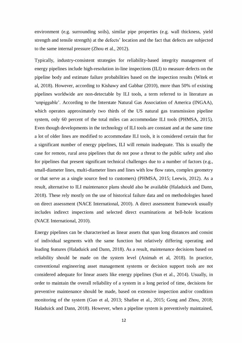
Typically, industry-consistent strategies for reliability-based integrity management of
energy pipelines include high-resolution in-line inspections (ILI) to measure defects on the
pipeline body and estimate failure probabilities based on the inspection results (Witek et
al, 2018). However, according to Kishawy and Gabbar (2010), more than 50% of existing
pipelines worldwide are non-detectable by ILI tools, a term referred to in literature as
‘unpiggable’. According to the Interstate Natural Gas Association of America (INGAA),
which operates approximately two thirds of the US natural gas transmission pipeline
system, only 60 percent of the total miles can accommodate ILI tools (PHMSA, 2015).
Even though developments in the technology of ILI tools are constant and at the same time
a lot of older lines are modified to accommodate ILI tools, it is considered certain that for
a significant number of energy pipelines, ILI will remain inadequate. This is usually the
case for remote, rural area pipelines that do not pose a threat to the public safety and also
for pipelines that present significant technical challenges due to a number of factors (e.g.,
small-diameter lines, multi-diameter lines and lines with low flow rates, complex geometry
or that serve as a single source feed to customers) (PHMSA, 2015; Leewis, 2012). As a
result, alternative to ILI maintenance plans should also be available (Haladuick and Dann,
2018). These rely mostly on the use of historical failure data and on methodologies based
on direct assessment (NACE International, 2010). A direct assessment framework usually
includes indirect inspections and selected direct examinations at bell-hole locations
(NACE International, 2010).
Energy pipelines can be characterised as linear assets that span long distances and consist
of individual segments with the same function but relatively differing operating and
loading features (Haladuick and Dann, 2018). As a result, maintenance decisions based on
reliability should be made on the system level (Animah et al, 2018). In practice,
conventional engineering asset management systems or decision support tools are not
considered adequate for linear assets like energy pipelines (Sun et al., 2014). Usually, in
order to maintain the overall reliability of a system in a long period of time, decisions for
preventive maintenance should be made, based on extensive inspection and/or condition
monitoring of the system (Guo et al, 2013; Shafiee et al., 2015; Gong and Zhou, 2018;
Haladuick and Dann, 2018). However, when a pipeline system is preventively maintained,
13
normally only part of the system is repaired or replaced, leading to an imperfect actions
when it comes to the whole system (Sun, et al, 2007; Finkelstein and Shafiee, 2017). For
large scale engineering systems like pipelines though, it is not sufficient to estimate the
next inspection and preventive maintenance (PM) time, but it is also necessary to define
multiple inspection and PM times over a decision horizon, which is normally a long period
of time. This enables decision makers to adequately plan various resources such as
economic, human and logistic.
Relevant studies of maintenance strategies based on pipeline reliability, either focused
only on a single defect to derive the reliability of the pipeline (Gomes, et al, 2013) or
required the number of defects to be a priori known from ILI results (Lecchi, 2011; Zhang
and Zhou, 2013). Hong (1999) and Zhang and Zhou (2014) employed the homogeneous
Poisson process (HPP) and the non-HPP subsequently to generate the number of defects
on a single pipeline segment and then find the optimal interval in a periodic inspection
plan. Hong (1999) estimated the probability of failure with regard to a defect-based
maintenance and repair strategy, as opposed to a segment-based strategy. Zhang and Zhou
(2014) did not deal with the overall probability of failure but only estimated the optimal
interval based on cost and did not consider multiple segments via system reliability. On the
other hand, studies in literature relevant to DA, have so far accounted only for the
Bayesian updating of data relevant to uncertainties of inspection tools and of active
corrosion defects’ characteristics (Van Os, 2006; Francis et al., 2006; Francis et al., 2009;
Van Brugel et al., 2011). Recently, Valor et al. (2014) and Caleyo et al. (2015), proposed
practical methodologies with regards to the analysis of field data from random sampling
for unpiggable underground pipelines. However, according to the NACE Standard, when
applying a DA, pipeline operators can adopt a 100 percent direct examination, instead of
indirect inspections and selected sampling direct examinations at bell-hole locations.
Previous works that consider a system of pipe segments include De Leon and Macias
(2005), Straub and Faber (2005) and Hong et al. (2014). De Leon and Macias (2005)
studied the effect of spatial correlation on the failure probability of corroded pipelines. It
was found that the correlation degree between failure modes at two pipeline segments,
increases with the degree of correlation of the initial corrosion depths of defects of these
segments. In addition, for a small number of segments (<5), the correlation was found to
be insignificant. Straub and Faber (2005) considered system effects for the inspection
planning of steel structures subjected to fatigue deterioration. The system representation
14
was made by considering a number of ‘hot spots’ in the structure, which have been chosen
as more failure prone or of higher failure consequences. However, it was concluded that
for corroded pipelines, in principle ‘all spots are hot’ and as a result the spatial variability
of the deterioration mechanisms should be exhaustively considered. Still though, the
number of ‘hot spots’ is expected to be very large and therefore some level of
simplification should be normal. Hong et al. (2014) studied the dependency of the
stochastic degradations of multiple components of engineering systems and their effect on
the system probability of failure. The result indicated importance solely for parallel
systems and not for series systems, like pipelines. In conclusion, system reliability
predictions for unpiggable corroding gas pipelines, with the consideration of imperfect
repairs, had not been dealt with in the literature, to the best of the author’s knowledge.
Furthermore, a comparison between SRA and statistical analyses has always been
challenging, for practical reasons. Pipeline historical failure data are scarce and generic, in
that they do not account for the wide variety of parameters and conditions associated with
different pipelines (Kiefner et al., 2001; Nessim et al., 2009). However, the validation of
failure probability calculations (SRA) based on historical failure data is key to gaining
confidence on the results, provided the uncertainties associated with both methods are
properly considered. Collection of incident data and database development for statistical
analyses and probability prediction of future events is a well established practice when it
comes to energy pipelines (AER, 2013; UKOPA, 2014; EGIG, 2015; CONCAWE, 2015;
PHMSA, 2015). Probabilistic data driven models are complicated, in that they usually
require substantial amounts of data for proper development (Dann and Huyse, 2018). In
practice, pipeline operators prefer to use quantitative models like these in order to assess
risk. However, often there is not enough actual data to yield meaningful results and expert
judgment is required to estimate missing data, or to make conservative assumptions. The
results of a probabilistic model are generally expressed as the probability of an event being
realised. Afterwards, the probability rating can be compared with the overall reliability
history of the operator’s pipeline, with the level of desired performance and also industry-
acceptable thresholds (Kishawy and Gabbar, 2010; Frangopol and Soliman, 2016).
Reliability prediction based on historical failure data, on the other hand, is realised by
assuming and defining a direct comparison among the values of each pipe segment with a
reference pipeline that summarises the average conditions of the area where the pipeline
system operates (Caleyo et al., 2008; Nessim et al., 2009). Other relative reliability ranking
15
models identify all of the reliability variables that contribute to the likelihood of a failure
with respect to a specific threat, such as external corrosion or third-party damage. The
models usually provide a system to numerically rank the conditions that could be
associated with a model variable, as well as to evaluate the relative contribution of each
variable. These could be related to the physical characteristics of the facility, the nature of
recurring problems and the root cause of major problems for instance (Caleyo et al., 2015).
Most of the information stem from historical failure data or expert knowledge. Thereafter,
a numerical weighting factor can be determined. For example, age is a driving variable that
must be considered, as many failure causes are time-based damage mechanisms and also
because as pipelines grow older, their probability of failure naturally increases. These
models are particularly valuable in determining the relative impact of each threat on a
particular pipe segment. They allow pipeline operators to assess integrity threats
independently or to compare them. In summary, relative risk ranking models provide a
consistent approach to assessing the integrity of and assigning a reliability factor to a pipe
segment. These models are very valuable in aiding operators to prioritize pipe segments
according to the need for assessment but are not considered to be entirely quantitative
(Baker, 2008). Therefore, they are not suggested when accurate results are desirable (Valor
et al., 2014).
The implementation of probabilistic risk models and subsequent mitigation strategies can
be considerably assisted by the pipeline incident and mileage data available at different
databases from around the world (Tee et al., 2014). One of the most distinguished is the
Pipeline and Hazardous Material Safety Administration (PHMSA) of the United States
Department of Transportation (DOT), which collects information on incidents of gas and
liquid pipelines that were regulated by PHMSA and met the appropriate criteria. PHMSA
pipeline incident database includes information regarding each reported incident and the
pipeline involved in the incident, along with annual reports from gas and liquid pipeline
operators about the total pipeline mileage, transported commodities and installation dates.
Golub et al. (1996) analysed the PHMSA incident data on the gas transmission pipelines
between 1970 and 1993 and later Kiefner et al. (2001) also analysed the incidents on the
gas transmission and gathering pipelines from 1985 to 1997 as reported in the PHMSA
database. Similar analyses have been conducted in the past from data derived from other
relevant databases, such as the United Kingdom Onshore Pipeline Operators’ Association
(UKOPA) or the European Gas pipeline Incident data Group (EGIG) (UKOPA, 2014;
16
EGIG, 2015; CONCAWE, 2015). It is noted that the principal legislation governing the
safety of pipelines is goal setting requiring that pipelines are designed, constructed and
operated so that the risks are as low as is reasonably practicable (ALARP) (Papadakis,
2000). In the UK pipeline industry in particular, there are many well established standards,
covering design, operations and maintenance of sector major accident hazard pipelines,
which can be used to demonstrate risks are ALARP (UKOPA, 2014). For natural gas
major accident hazard pipelines the Institution of Gas Engineers and Managers (IGEM)
series of recommendation on transmission and distribution practice is advocated by the
British Standard Code of Practice for Pipelines, such as IGE/TD/1 and IGE/TD/13
(Goodfellow et al., 2008). Lam and Zhou (2016) analysed the PHMSA database in an
effort to derive inferences about the condition of gas transmission pipelines in the US and
to develop relevant failure frequencies for assessing the risk of onshore gas transmission
pipelines. Also, they proposed a probability of ignition model for ruptures, based on the
above-mentioned incidents reported in the PHMSA database for the period from 2002 to
2013.
Additional studies that utilized historical failure data for reliability analysis of energy
pipelines, evaluated the failure probabilities in the rate of occurrence of failures (ROCOF)
approach for repairable systems (Caleyo et al., 2008; Nessim et al., 2009). This means that
upon failure, the system is restored to operation by repairing or even replacing some parts
of the system, instead of replacing the entire system. The ROCOF failure rate considers a
sequence of failure times within a time interval, as opposed to a single time to failure
distribution (Ascher and Feingold, 1984; Leemis, 1995). However, the ROCOF failure rate
can be characterised only for a limited period of time, i.e. for as long as incident data are
available. In practice, in most databases available incident data that are fairly consistent,
usually do not cover operation periods of more than 30 years, while the actual pipeline
lifecycle can be significantly more than that. These studies cannot provide a direct
estimation of the reliability function for a pipe segment, system or network; instead they
can provide rather generic guidelines and inductions that may prove relevant to a risk
assessment strategy. As a result, deriving inferences for a complete pipeline lifecycle is not
feasible. Moreover, according to the board meeting of the National Transportation Safety
Board (NTSB) in January 2015, it was found that the PHMSA database is characterised by
a lack of detailed attributes for the gas transmission pipelines and also that there is a
discrepancy among the annual report database (that contains the pipeline details and

17
mileage information) and the incident database, which leads to some level of inaccuracy in
the relevant analyses (NTSB, 2015). Therefore, analyses of historical failure data that can
provide a complete characterisation of energy pipeline reliability and deal with incomplete
and uncertain data efficiently would be of great pertinence.
18
3. Structural Reliability Analyses for Predictions in Energy Pipelines
3.1 Introduction
In this chapter, two probabilistic methodologies are proposed for onshore gas transmission
pipelines subjected to external metal loss corrosion, based on a robust integration of
stochastic processes within a structural reliability analysis (SRA) framework. The
application of the proposed methodologies is realised through two case studies, based on
two different inspection and maintenance strategies. In the first case study, a robust
structural reliability model is proposed that provides estimates of rupture probabilities
against external corrosion on a reference pipe segment. The reference segment
characteristics are derived from historical failure data from PHMSA. In specific, the
reported rupture incidents due to external metal loss corrosion for the period 2002-2014
are employed and the reference pipeline is built based on their characteristics. The
proposed SRA framework models the mechanical failure of the reference segment by
adopting up to date stochastic processes, associated with the segment based loads and
resistances. The non-homogeneous Poisson process is used to model the generation of new
defects and the Poisson square wave process is used to model the growth of the defects.
The internal pressure load is modelled as a discrete Ferry-Borges stochastic process. Then,
an inspection and repair program is applied to the reference segment, based on the
standardised code of practice (ASME B31.8S) for the in line inspection (ILI) technique,
for a service life of 100 years. A realistic characterisation of the probability of detection
(PoD) and measurement error, associated with the ILI data is also incorporated in the
model.
In the second case study, a different industry consistent maintenance strategy is
considered, namely External Corrosion Direct Assessment. In this case, a so called
‘unpiggable’ or ‘non-piggable’ (i.e. that cannot accommodate an ILI tool) corroding
onshore gas transmission pipeline system is examined with respect to external metal-loss
corrosion. The reliability, first evaluated on the segment level, is subsequently evaluated
on the system level and the influence of imperfect ECDA actions is investigated. A
heuristic method is adopted, namely Split System Approach (SSA) (Sun et al., 2007; Sun
et al., 2009). This method has the ability to link the SRA to long-term preventive
maintenance (PM) decision making, so that the decision can be updated by using the latest
19
inspection and health monitoring information available. In previous works (Sun et al.,
2007; Sun et al., 2014), SSA was implemented by adopting the hazard function which
belongs to the lifetime functions and was defined based on the probability density function
of the time to failure. However, the SRA allows for a clear understanding of the separate
contribution of each random variable to either resistance or load, unlike the lifetime
functions that summarise the combined effect of all the uncertainties on the pipeline
system (Barone and Frangopol, 2014). To the best of the author’s knowledge, SSA is
applied to a corroded energy pipeline system with the reliability function estimated by an
SRA for the first time in this study. The corrosion process is evaluated for a number of
defects on a pipe segment of 12m. The non-homogeneous Poisson process (NHPP) is
employed to model the uncertainties in the number and generation of defects and a well-
established empirical power law model is adopted for the growth of defects over time. The
reliability forecast regarding the segment is obtained by the limit state for burst due to
internal pressure, with the uncertainties in the pressure incorporated in the analysis through
a Poisson square wave process (PSWP) model. Afterwards, the numerical application is
carried out on a system of three identical pipe segments that form a series system. The
SSA method illustrates the effects of future maintenance actions on the time-dependent
reliability of the pipeline system. The impact of some key parameters is examined at the
end, in an effort to derive some additional conclusions regarding the proposed
methodology.
The contents of this chapter are organised as follows. Section 3.2 presents the physical
model, namely generation of new defects, corrosion growth and internal pressure models,
as well as the limit state function associated with burst, along with the method for
evaluating the time-dependent reliability of a corroding pipe segment that contains
multiple defects. Thereinafter, Section 3.3 presents the impact of the ILI inspections and
their associated uncertainties on the time-dependent reliability of the pipe segment. Section
3.4 presents the SSA method for long-term system reliability predictions. In Sections 3.5
and 3.6, the numerical applications are illustrated and the results are subsequently
discussed. This chapter is completed with concluding remarks in Section 3.7.
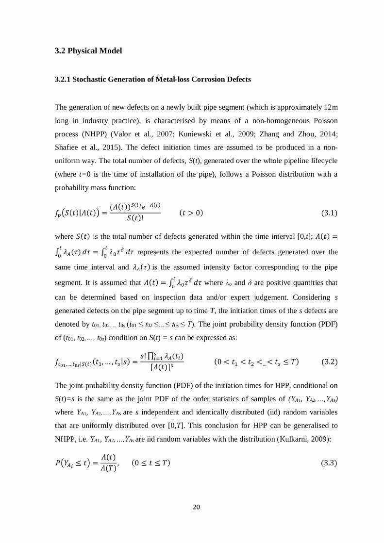
20
3.2 Physical Model
3.2.1 Stochastic Generation of Metal-loss Corrosion Defects
The generation of new defects on a newly built pipe segment (which is approximately 12m
long in industry practice), is characterised by means of a non-homogeneous Poisson
process (NHPP) (Valor et al., 2007; Kuniewski et al., 2009; Zhang and Zhou, 2014;
Shafiee et al., 2015). The defect initiation times are assumed to be produced in a non-
uniform way. The total number of defects, S(t), generated over the whole pipeline lifecycle
(where t=0 is the time of installation of the pipe), follows a Poisson distribution with a
probability mass function:
𝑓𝑝(𝑆(𝑡)|𝛬(𝑡)) =(𝛬(𝑡))𝑆(𝑡)𝑒−𝛬(𝑡)
𝑆(𝑡)! (𝑡 > 0) (3.1)
where 𝑆(𝑡) is the total number of defects generated within the time interval [0,t]; 𝛬(𝑡) =
∫ 𝜆𝐴(𝜏)𝑡
0𝑑𝜏 = ∫ 𝜆0𝜏
𝛿𝑡
0𝑑𝜏 represents the expected number of defects generated over the
same time interval and 𝜆𝐴(𝜏) is the assumed intensity factor corresponding to the pipe
segment. It is assumed that 𝛬(𝑡) = ∫ 𝜆0𝜏𝛿𝑡
0𝑑𝜏 where λo and δ are positive quantities that
can be determined based on inspection data and/or expert judgement. Considering s
generated defects on the pipe segment up to time T, the initiation times of the s defects are
denoted by t01, t02,…, t0s (t01 ≤ t02 ≤…≤ t0s ≤ T). The joint probability density function (PDF)
of (t01, t02,…, t0s) condition on S(t) = s can be expressed as:
𝑓𝑡01 ,…,𝑡0𝑠|𝑆(𝑡)(𝑡1, … , 𝑡𝑠|𝑠) =𝑠!∏ 𝜆𝐴(𝑡𝑖)
𝑠𝑖=1
[𝛬(𝑡)]𝑠 (0 < 𝑡1 < 𝑡2 <…< 𝑡𝑠 ≤ 𝑇) (3.2)
The joint probability density function (PDF) of the initiation times for HPP, conditional on
S(t)=s is the same as the joint PDF of the order statistics of samples of (YA1, YA2,…,YAs)
where YA1, YA2,…,YAs are s independent and identically distributed (iid) random variables
that are uniformly distributed over [0,T]. This conclusion for HPP can be generalised to
NHPP, i.e. YA1, YA2,…,YAs are iid random variables with the distribution (Kulkarni, 2009):
𝑃(𝑌𝐴𝑖 ≤ 𝑡) =𝛬(𝑡)
𝛬(𝑇), (0 ≤ 𝑡 ≤ 𝑇) (3.3)
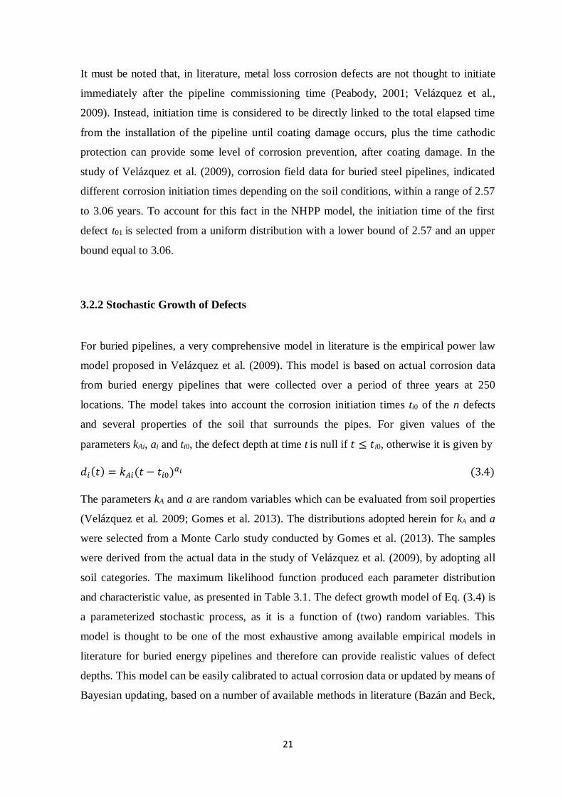
21
It must be noted that, in literature, metal loss corrosion defects are not thought to initiate
immediately after the pipeline commissioning time (Peabody, 2001; Velázquez et al.,
2009). Instead, initiation time is considered to be directly linked to the total elapsed time
from the installation of the pipeline until coating damage occurs, plus the time cathodic
protection can provide some level of corrosion prevention, after coating damage. In the
study of Velázquez et al. (2009), corrosion field data for buried steel pipelines, indicated
different corrosion initiation times depending on the soil conditions, within a range of 2.57
to 3.06 years. To account for this fact in the NHPP model, the initiation time of the first
defect t01 is selected from a uniform distribution with a lower bound of 2.57 and an upper
bound equal to 3.06.
3.2.2 Stochastic Growth of Defects
For buried pipelines, a very comprehensive model in literature is the empirical power law
model proposed in Velázquez et al. (2009). This model is based on actual corrosion data
from buried energy pipelines that were collected over a period of three years at 250
locations. The model takes into account the corrosion initiation times ti0 of the n defects
and several properties of the soil that surrounds the pipes. For given values of the
parameters kAi, ai and ti0, the defect depth at time t is null if 𝑡 ≤ 𝑡i0, otherwise it is given by
𝑑𝑖(𝑡) = 𝑘𝐴𝑖(𝑡 − 𝑡𝑖0)𝑎𝑖 (3.4)
The parameters kA and a are random variables which can be evaluated from soil properties
(Velázquez et al. 2009; Gomes et al. 2013). The distributions adopted herein for kA and a
were selected from a Monte Carlo study conducted by Gomes et al. (2013). The samples
were derived from the actual data in the study of Velázquez et al. (2009), by adopting all
soil categories. The maximum likelihood function produced each parameter distribution
and characteristic value, as presented in Table 3.1. The defect growth model of Eq. (3.4) is
a parameterized stochastic process, as it is a function of (two) random variables. This
model is thought to be one of the most exhaustive among available empirical models in
literature for buried energy pipelines and therefore can provide realistic values of defect
depths. This model can be easily calibrated to actual corrosion data or updated by means of
Bayesian updating, based on a number of available methods in literature (Bazán and Beck,
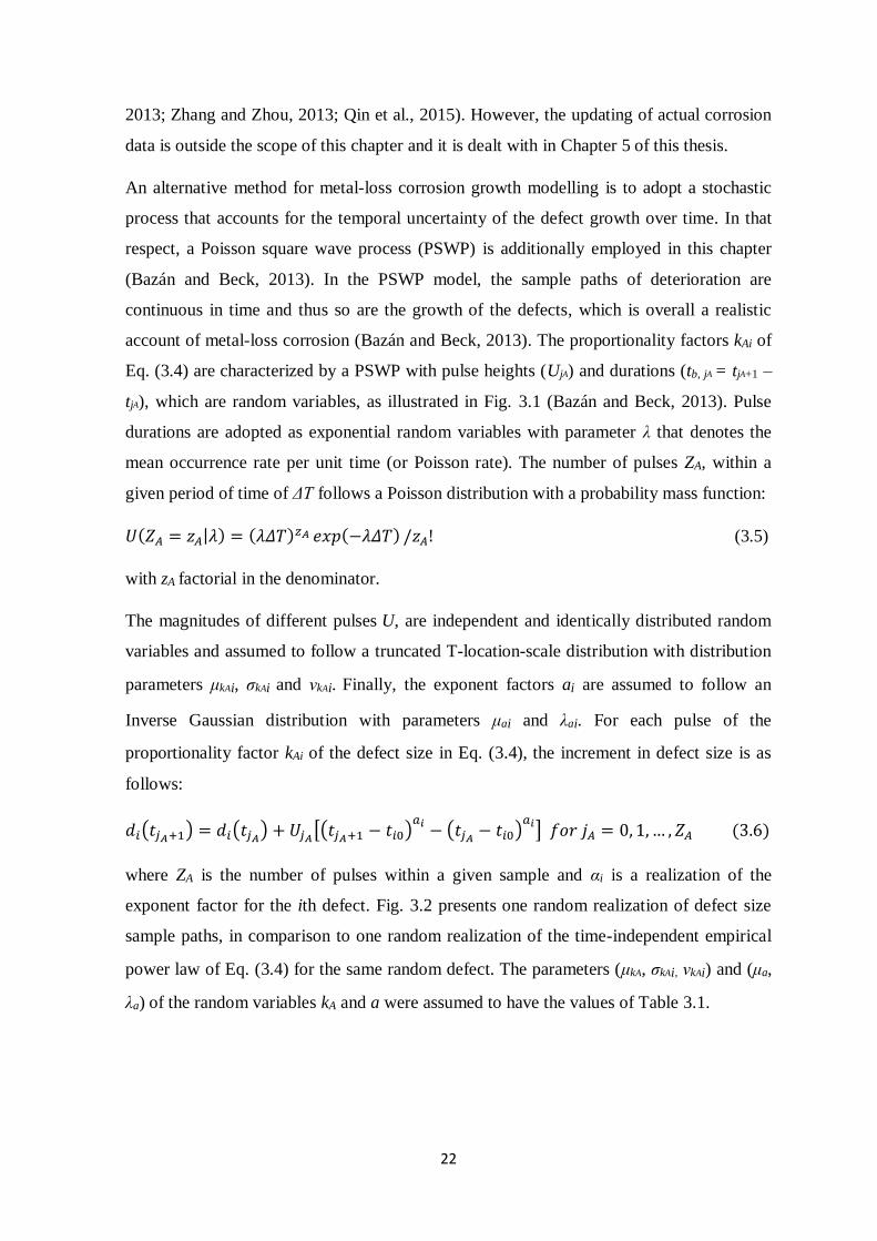
22
2013; Zhang and Zhou, 2013; Qin et al., 2015). However, the updating of actual corrosion
data is outside the scope of this chapter and it is dealt with in Chapter 5 of this thesis.
An alternative method for metal-loss corrosion growth modelling is to adopt a stochastic
process that accounts for the temporal uncertainty of the defect growth over time. In that
respect, a Poisson square wave process (PSWP) is additionally employed in this chapter
(Bazán and Beck, 2013). In the PSWP model, the sample paths of deterioration are
continuous in time and thus so are the growth of the defects, which is overall a realistic
account of metal-loss corrosion (Bazán and Beck, 2013). The proportionality factors kAi of
Eq. (3.4) are characterized by a PSWP with pulse heights (UjA) and durations (tb, jA = tjA+1 –
tjA), which are random variables, as illustrated in Fig. 3.1 (Bazán and Beck, 2013). Pulse
durations are adopted as exponential random variables with parameter λ that denotes the
mean occurrence rate per unit time (or Poisson rate). The number of pulses ZA, within a
given period of time of ΔT follows a Poisson distribution with a probability mass function:
𝑈(𝑍𝐴 = 𝑧𝐴|𝜆) = (𝜆𝛥𝑇)𝑧𝐴 𝑒𝑥𝑝(−𝜆𝛥𝑇) /𝑧𝐴! (3.5)
with zA factorial in the denominator.
The magnitudes of different pulses U, are independent and identically distributed random
variables and assumed to follow a truncated T-location-scale distribution with distribution
parameters μkAi, σkAi and νkAi. Finally, the exponent factors ai are assumed to follow an
Inverse Gaussian distribution with parameters μai and λai. For each pulse of the
proportionality factor kAi of the defect size in Eq. (3.4), the increment in defect size is as
follows:
𝑑𝑖(𝑡𝑗𝐴+1) = 𝑑𝑖(𝑡𝑗𝐴) + 𝑈𝑗𝐴[(𝑡𝑗𝐴+1 − 𝑡𝑖0)𝑎𝑖− (𝑡𝑗𝐴 − 𝑡𝑖0)
𝑎𝑖] 𝑓𝑜𝑟 𝑗𝐴 = 0, 1,… , 𝑍𝐴 (3.6)
where ZA is the number of pulses within a given sample and αi is a realization of the
exponent factor for the ith defect. Fig. 3.2 presents one random realization of defect size
sample paths, in comparison to one random realization of the time-independent empirical
power law of Eq. (3.4) for the same random defect. The parameters (μkA, σkAi, νkAi) and (μa,
λa) of the random variables kA and a were assumed to have the values of Table 3.1.
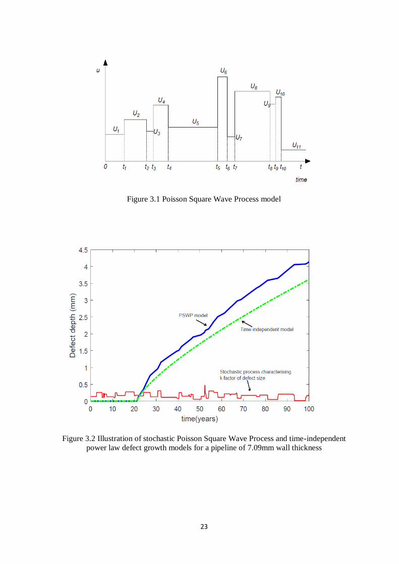
23
Figure 3.1 Poisson Square Wave Process model
Figure 3.2 Illustration of stochastic Poisson Square Wave Process and time-independent
power law defect growth models for a pipeline of 7.09mm wall thickness
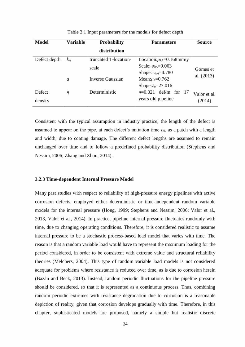
24
Table 3.1 Input parameters for the models for defect depth
Model Variable Probability
distribution
Parameters Source
Defect depth kA truncated Τ-location-
scale
Location:μkA=0.168mm/y
Scale: σkA=0.063
Shape: νkA=4.780 Gomes et
al. (2013) a Inverse Gaussian Mean:μa=0.762
Shape:λa=27.016
Defect
density
η Deterministic η=0.321 def/m for 17
years old pipeline Valor et al.
(2014)
Consistent with the typical assumption in industry practice, the length of the defect is
assumed to appear on the pipe, at each defect’s initiation time ti0, as a patch with a length
and width, due to coating damage. The different defect lengths are assumed to remain
unchanged over time and to follow a predefined probability distribution (Stephens and
Nessim, 2006; Zhang and Zhou, 2014).
3.2.3 Time-dependent Internal Pressure Model
Many past studies with respect to reliability of high-pressure energy pipelines with active
corrosion defects, employed either deterministic or time-independent random variable
models for the internal pressure (Hong, 1999; Stephens and Nessim, 2006; Valor et al.,
2013, Valor et al., 2014). In practice, pipeline internal pressure fluctuates randomly with
time, due to changing operating conditions. Therefore, it is considered realistic to assume
internal pressure to be a stochastic process-based load model that varies with time. The
reason is that a random variable load would have to represent the maximum loading for the
period considered, in order to be consistent with extreme value and structural reliability
theories (Melchers, 2004). This type of random variable load models is not considered
adequate for problems where resistance is reduced over time, as is due to corrosion herein
(Bazán and Beck, 2013). Instead, random periodic fluctuations for the pipeline pressure
should be considered, so that it is represented as a continuous process. Thus, combining
random periodic extremes with resistance degradation due to corrosion is a reasonable
depiction of reality, given that corrosion develops gradually with time. Therefore, in this
chapter, sophisticated models are proposed, namely a simple but realistic discrete
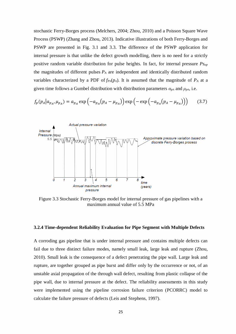
25
stochastic Ferry-Borges process (Melchers, 2004; Zhou, 2010) and a Poisson Square Wave
Process (PSWP) (Zhang and Zhou, 2013). Indicative illustrations of both Ferry-Borges and
PSWP are presented in Fig. 3.1 and 3.3. The difference of the PSWP application for
internal pressure is that unlike the defect growth modelling, there is no need for a strictly
positive random variable distribution for pulse heights. In fact, for internal pressure Psop
the magnitudes of different pulses PA are independent and identically distributed random
variables characterized by a PDF of fPA(pA). It is assumed that the magnitude of PA at a
given time follows a Gumbel distribution with distribution parameters αpA and μpA, i.e.
𝑓𝑝(𝑝𝐴|𝑎𝑝𝐴 , 𝜇𝑝𝐴) = 𝑎𝑝𝐴 exp (−𝑎𝑝𝐴(𝑝𝐴 − 𝜇𝑝𝐴)) exp (−exp (−𝑎𝑝𝐴(𝑝𝐴 − 𝜇𝑝𝐴))) (3.7)
Figure 3.3 Stochastic Ferry-Borges model for internal pressure of gas pipelines with a
maximum annual value of 5.5 MPa
3.2.4 Time-dependent Reliability Evaluation for Pipe Segment with Multiple Defects
A corroding gas pipeline that is under internal pressure and contains multiple defects can
fail due to three distinct failure modes, namely small leak, large leak and rupture (Zhou,
2010). Small leak is the consequence of a defect penetrating the pipe wall. Large leak and
rupture, are together grouped as pipe burst and differ only by the occurrence or not, of an
unstable axial propagation of the through wall defect, resulting from plastic collapse of the
pipe wall, due to internal pressure at the defect. The reliability assessments in this study
were implemented using the pipeline corrosion failure criterion (PCORRC) model to
calculate the failure pressure of defects (Leis and Stephens, 1997).
(Mpa) 5.5
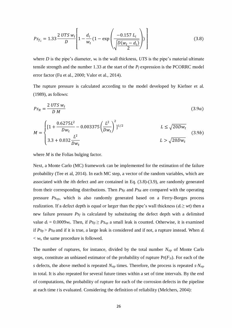
26
𝑃𝑠𝑓𝑖 = 1.332 𝑈𝑇𝑆 𝑤𝑡
𝐷
[
1 −𝑑𝑖
𝑤𝑡(1 − exp
(
−0.157 𝐿𝑖
√𝐷(𝑤𝑡 − 𝑑𝑖)2 )
)
]
(3.8)
where D is the pipe’s diameter, wt is the wall thickness, UTS is the pipe’s material ultimate
tensile strength and the number 1.33 at the start of the Pf expression is the PCORRC model
error factor (Fu et al., 2000; Valor et al., 2014).
The rupture pressure is calculated according to the model developed by Kiefner et al.
(1989), as follows:
𝑃𝑠𝑅 =2 𝑈𝑇𝑆 𝑤𝑡𝐷 𝑀
(3.9𝑎)
𝑀 =
{
[1 +
0.6275𝐿2
𝐷𝑤𝑡− 0.003375(
𝐿2
𝐷𝑤𝑡)
2
]1/2 𝐿 ≤ √20𝐷𝑤𝑡
3.3 + 0.032𝐿2
𝐷𝑤𝑡 𝐿 > √20𝐷𝑤𝑡
(3.9𝑏)
where M is the Folias bulging factor.
Next, a Monte Carlo (MC) framework can be implemented for the estimation of the failure
probability (Tee et al, 2014). In each MC step, a vector of the random variables, which are
associated with the ith defect and are contained in Eq. (3.8)-(3.9), are randomly generated
from their corresponding distributions. Then Psfi and PsR are compared with the operating
pressure Psop, which is also randomly generated based on a Ferry-Borges process
realization. If a defect depth is equal or larger than the pipe’s wall thickness (di ≥ wt) then a
new failure pressure Psf is calculated by substituting the defect depth with a delimited
value di = 0.0009wt. Then, if Psfi ≥ Psop a small leak is counted. Otherwise, it is examined
if Psft > PsR and if it is true, a large leak is considered and if not, a rupture instead. When di
< wt, the same procedure is followed.
The number of ruptures, for instance, divided by the total number Nstp of Monte Carlo
steps, constitute an unbiased estimator of the probability of rupture Pr(F3i). For each of the
s defects, the above method is repeated Nstp times. Therefore, the process is repeated s∙Nstp
in total. It is also repeated for several future times within a set of time intervals. By the end
of computations, the probability of rupture for each of the corrosion defects in the pipeline
at each time t is evaluated. Considering the definition of reliability (Melchers, 2004):
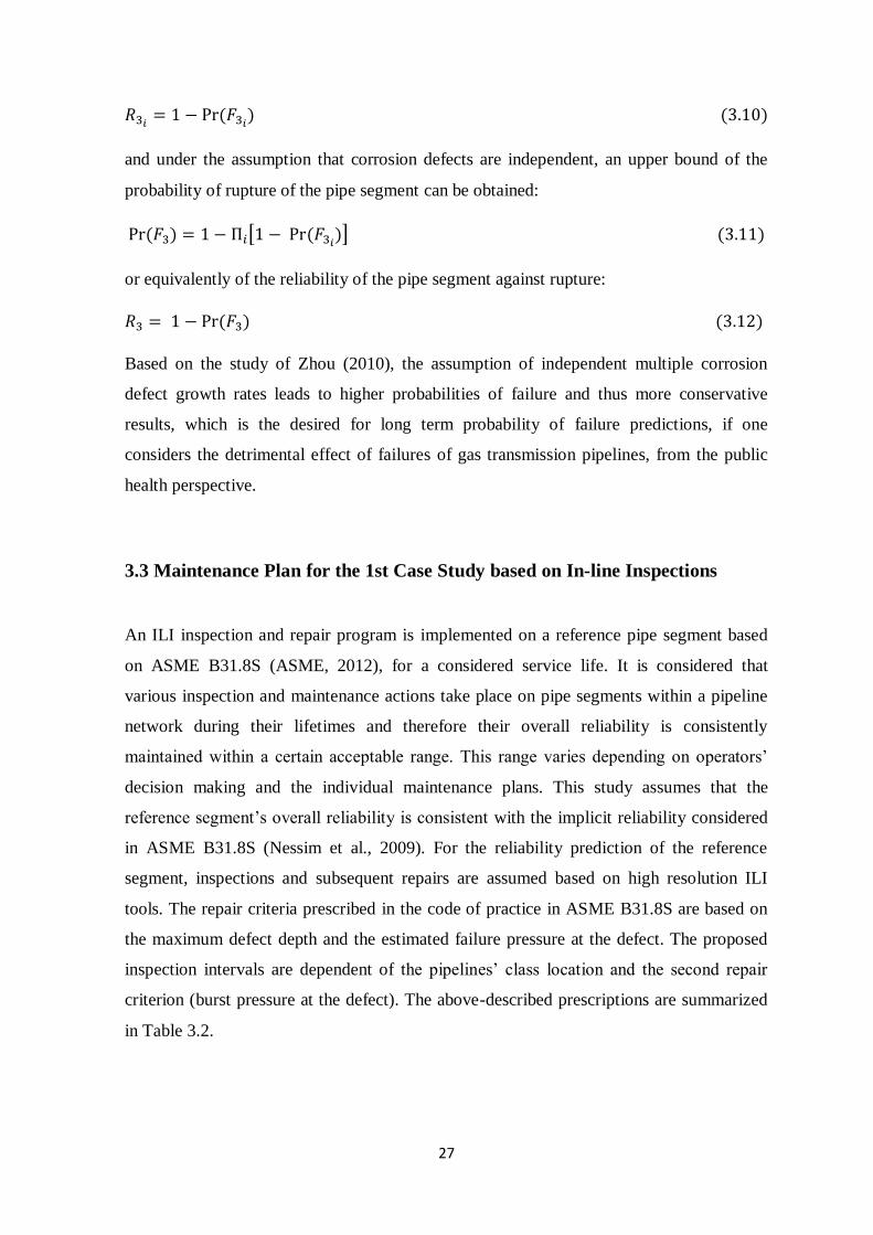
27
𝑅3𝑖 = 1 − Pr(𝐹3𝑖) (3.10)
and under the assumption that corrosion defects are independent, an upper bound of the
probability of rupture of the pipe segment can be obtained:
Pr (𝐹3) = 1 − Π𝑖[1 − Pr(𝐹3𝑖)] (3.11)
or equivalently of the reliability of the pipe segment against rupture:
𝑅3 = 1 − Pr (𝐹3) (3.12)
Based on the study of Zhou (2010), the assumption of independent multiple corrosion
defect growth rates leads to higher probabilities of failure and thus more conservative
results, which is the desired for long term probability of failure predictions, if one
considers the detrimental effect of failures of gas transmission pipelines, from the public
health perspective.
3.3 Maintenance Plan for the 1st Case Study based on In-line Inspections
An ILI inspection and repair program is implemented on a reference pipe segment based
on ASME B31.8S (ASME, 2012), for a considered service life. It is considered that
various inspection and maintenance actions take place on pipe segments within a pipeline
network during their lifetimes and therefore their overall reliability is consistently
maintained within a certain acceptable range. This range varies depending on operators’
decision making and the individual maintenance plans. This study assumes that the
reference segment’s overall reliability is consistent with the implicit reliability considered
in ASME B31.8S (Nessim et al., 2009). For the reliability prediction of the reference
segment, inspections and subsequent repairs are assumed based on high resolution ILI
tools. The repair criteria prescribed in the code of practice in ASME B31.8S are based on
the maximum defect depth and the estimated failure pressure at the defect. The proposed
inspection intervals are dependent of the pipelines’ class location and the second repair
criterion (burst pressure at the defect). The above-described prescriptions are summarized
in Table 3.2.
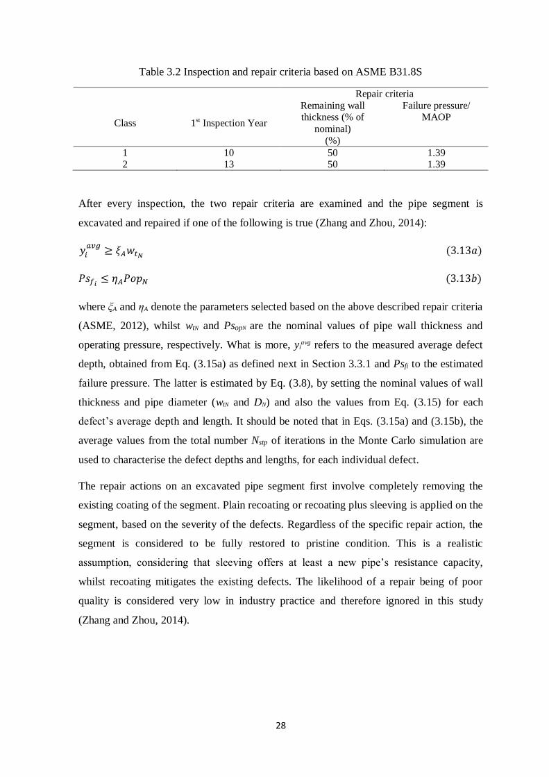
28
Table 3.2 Inspection and repair criteria based on ASME B31.8S
Repair criteria
Class 1st Inspection Year
Remaining wall thickness (% of
nominal)
(%)
Failure pressure/ MAOP
1 10 50 1.39 2 13 50 1.39
After every inspection, the two repair criteria are examined and the pipe segment is
excavated and repaired if one of the following is true (Zhang and Zhou, 2014):
𝑦𝑖𝑎𝑣𝑔
≥ 𝜉𝐴𝑤𝑡𝑁 (3.13𝑎)
𝑃𝑠𝑓𝑖 ≤ 휂𝐴𝑃𝑜𝑝𝑁 (3.13𝑏)
where ξA and ηA denote the parameters selected based on the above described repair criteria
(ASME, 2012), whilst wtN and PsopN are the nominal values of pipe wall thickness and
operating pressure, respectively. What is more, yiavg refers to the measured average defect
depth, obtained from Eq. (3.15a) as defined next in Section 3.3.1 and Psfi to the estimated
failure pressure. The latter is estimated by Eq. (3.8), by setting the nominal values of wall
thickness and pipe diameter (wtN and DN) and also the values from Eq. (3.15) for each
defect’s average depth and length. It should be noted that in Eqs. (3.15a) and (3.15b), the
average values from the total number Nstp of iterations in the Monte Carlo simulation are
used to characterise the defect depths and lengths, for each individual defect.
The repair actions on an excavated pipe segment first involve completely removing the
existing coating of the segment. Plain recoating or recoating plus sleeving is applied on the
segment, based on the severity of the defects. Regardless of the specific repair action, the
segment is considered to be fully restored to pristine condition. This is a realistic
assumption, considering that sleeving offers at least a new pipe’s resistance capacity,
whilst recoating mitigates the existing defects. The likelihood of a repair being of poor
quality is considered very low in industry practice and therefore ignored in this study
(Zhang and Zhou, 2014).
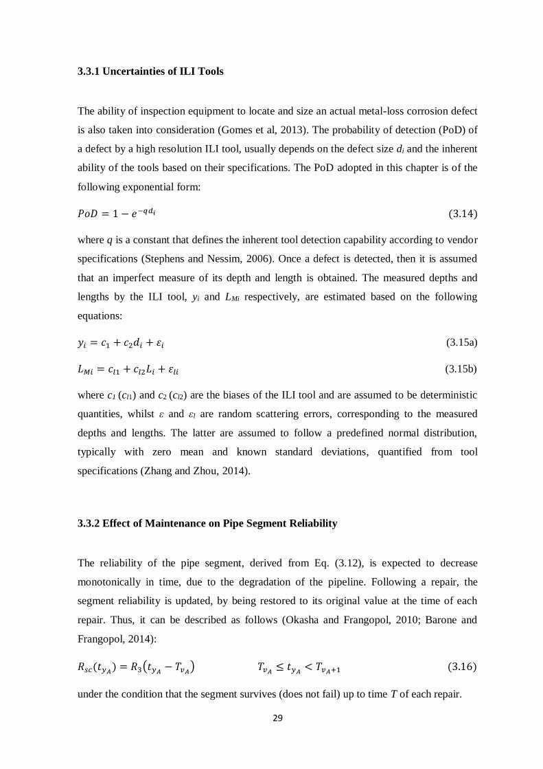
29
3.3.1 Uncertainties of ILI Tools
The ability of inspection equipment to locate and size an actual metal-loss corrosion defect
is also taken into consideration (Gomes et al, 2013). The probability of detection (PoD) of
a defect by a high resolution ILI tool, usually depends on the defect size di and the inherent
ability of the tools based on their specifications. The PoD adopted in this chapter is of the
following exponential form:
𝑃𝑜𝐷 = 1 − 𝑒−𝑞𝑑𝑖 (3.14)
where q is a constant that defines the inherent tool detection capability according to vendor
specifications (Stephens and Nessim, 2006). Once a defect is detected, then it is assumed
that an imperfect measure of its depth and length is obtained. The measured depths and
lengths by the ILI tool, yi and LMi respectively, are estimated based on the following
equations:
𝑦𝑖 = 𝑐1 + 𝑐2𝑑𝑖 + 휀𝑖 (3.15a)
𝐿𝑀𝑖 = 𝑐𝑙1 + 𝑐𝑙2𝐿𝑖 + 휀𝑙𝑖 (3.15b)
where c1 (cl1) and c2 (cl2) are the biases of the ILI tool and are assumed to be deterministic
quantities, whilst ε and εl are random scattering errors, corresponding to the measured
depths and lengths. The latter are assumed to follow a predefined normal distribution,
typically with zero mean and known standard deviations, quantified from tool
specifications (Zhang and Zhou, 2014).
3.3.2 Effect of Maintenance on Pipe Segment Reliability
The reliability of the pipe segment, derived from Eq. (3.12), is expected to decrease
monotonically in time, due to the degradation of the pipeline. Following a repair, the
segment reliability is updated, by being restored to its original value at the time of each
repair. Thus, it can be described as follows (Okasha and Frangopol, 2010; Barone and
Frangopol, 2014):
𝑅𝑠𝑐(𝑡𝑦𝐴) = 𝑅3(𝑡𝑦𝐴 − 𝑇𝑣𝐴) 𝑇𝑣𝐴 ≤ 𝑡𝑦𝐴 < 𝑇𝑣𝐴+1 (3.16)
under the condition that the segment survives (does not fail) up to time T of each repair.
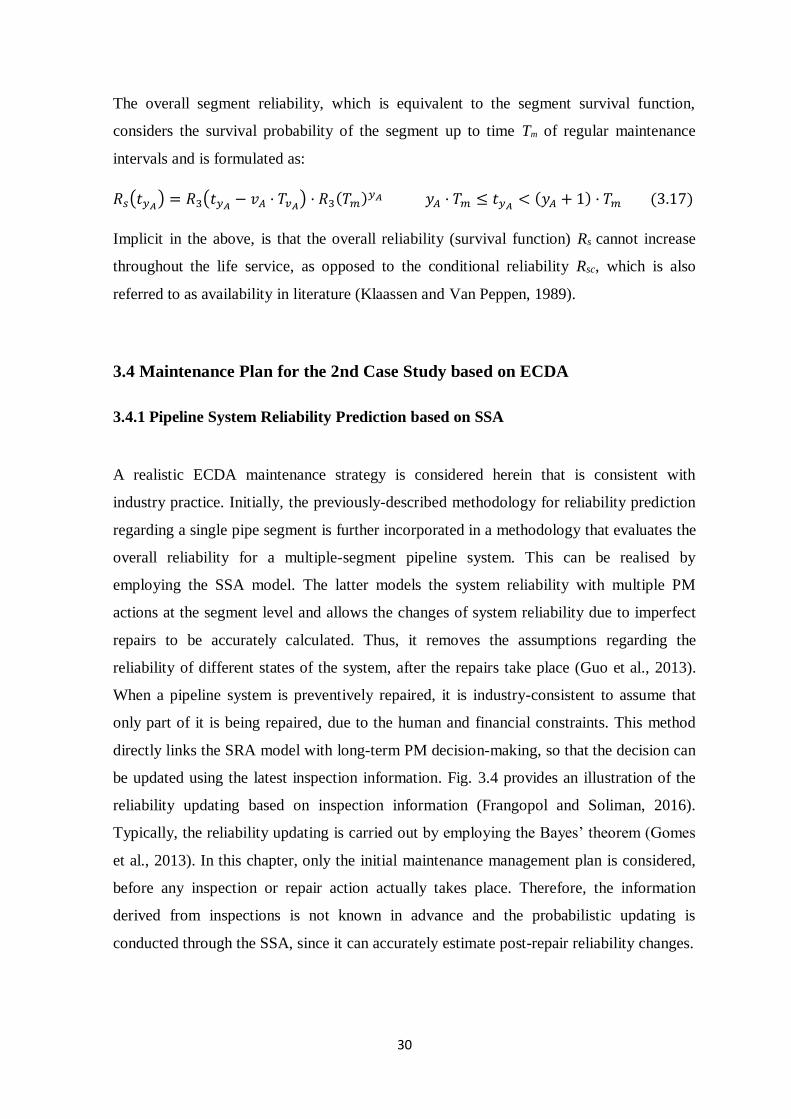
30
The overall segment reliability, which is equivalent to the segment survival function,
considers the survival probability of the segment up to time Tm of regular maintenance
intervals and is formulated as:
𝑅𝑠(𝑡𝑦𝐴) = 𝑅3(𝑡𝑦𝐴 − 𝑣𝐴 · 𝑇𝑣𝐴) · 𝑅3(𝑇𝑚)𝑦𝐴 𝑦𝐴 · 𝑇𝑚 ≤ 𝑡𝑦𝐴 < (𝑦𝐴 + 1) · 𝑇𝑚 (3.17)
Implicit in the above, is that the overall reliability (survival function) Rs cannot increase
throughout the life service, as opposed to the conditional reliability Rsc, which is also
referred to as availability in literature (Klaassen and Van Peppen, 1989).
3.4 Maintenance Plan for the 2nd Case Study based on ECDA
3.4.1 Pipeline System Reliability Prediction based on SSA
A realistic ECDA maintenance strategy is considered herein that is consistent with
industry practice. Initially, the previously-described methodology for reliability prediction
regarding a single pipe segment is further incorporated in a methodology that evaluates the
overall reliability for a multiple-segment pipeline system. This can be realised by
employing the SSA model. The latter models the system reliability with multiple PM
actions at the segment level and allows the changes of system reliability due to imperfect
repairs to be accurately calculated. Thus, it removes the assumptions regarding the
reliability of different states of the system, after the repairs take place (Guo et al., 2013).
When a pipeline system is preventively repaired, it is industry-consistent to assume that
only part of it is being repaired, due to the human and financial constraints. This method
directly links the SRA model with long-term PM decision-making, so that the decision can
be updated using the latest inspection information. Fig. 3.4 provides an illustration of the
reliability updating based on inspection information (Frangopol and Soliman, 2016).
Typically, the reliability updating is carried out by employing the Bayes’ theorem (Gomes
et al., 2013). In this chapter, only the initial maintenance management plan is considered,
before any inspection or repair action actually takes place. Therefore, the information
derived from inspections is not known in advance and the probabilistic updating is
conducted through the SSA, since it can accurately estimate post-repair reliability changes.
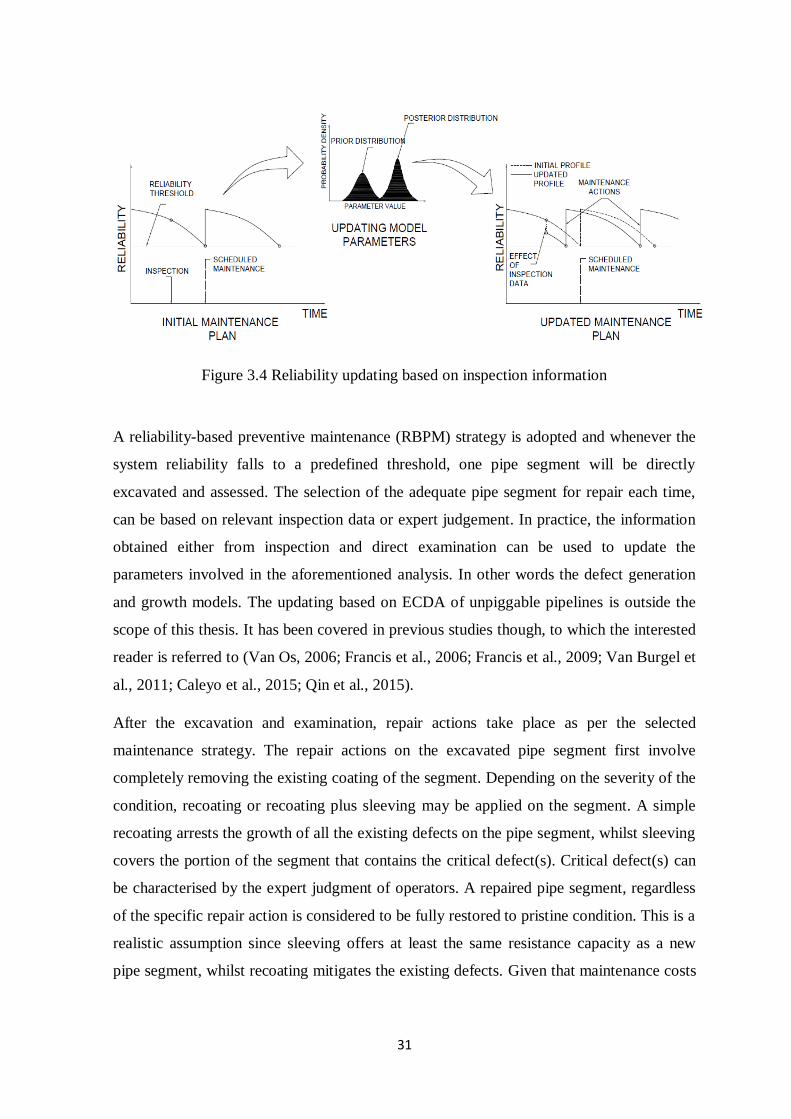
31
Figure 3.4 Reliability updating based on inspection information
A reliability-based preventive maintenance (RBPM) strategy is adopted and whenever the
system reliability falls to a predefined threshold, one pipe segment will be directly
excavated and assessed. The selection of the adequate pipe segment for repair each time,
can be based on relevant inspection data or expert judgement. In practice, the information
obtained either from inspection and direct examination can be used to update the
parameters involved in the aforementioned analysis. In other words the defect generation
and growth models. The updating based on ECDA of unpiggable pipelines is outside the
scope of this thesis. It has been covered in previous studies though, to which the interested
reader is referred to (Van Os, 2006; Francis et al., 2006; Francis et al., 2009; Van Burgel et
al., 2011; Caleyo et al., 2015; Qin et al., 2015).
After the excavation and examination, repair actions take place as per the selected
maintenance strategy. The repair actions on the excavated pipe segment first involve
completely removing the existing coating of the segment. Depending on the severity of the
condition, recoating or recoating plus sleeving may be applied on the segment. A simple
recoating arrests the growth of all the existing defects on the pipe segment, whilst sleeving
covers the portion of the segment that contains the critical defect(s). Critical defect(s) can
be characterised by the expert judgment of operators. A repaired pipe segment, regardless
of the specific repair action is considered to be fully restored to pristine condition. This is a
realistic assumption since sleeving offers at least the same resistance capacity as a new
pipe segment, whilst recoating mitigates the existing defects. Given that maintenance costs
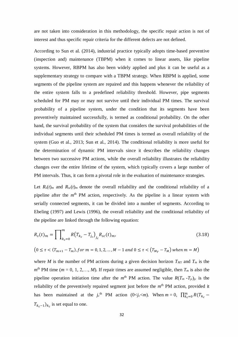
32
are not taken into consideration in this methodology, the specific repair action is not of
interest and thus specific repair criteria for the different defects are not defined.
According to Sun et al. (2014), industrial practice typically adopts time-based preventive
(inspection and) maintenance (TBPM) when it comes to linear assets, like pipeline
systems. However, RBPM has also been widely applied and plus it can be useful as a
supplementary strategy to compare with a TBPM strategy. When RBPM is applied, some
segments of the pipeline system are repaired and this happens whenever the reliability of
the entire system falls to a predefined reliability threshold. However, pipe segments
scheduled for PM may or may not survive until their individual PM times. The survival
probability of a pipeline system, under the condition that its segments have been
preventively maintained successfully, is termed as conditional probability. On the other
hand, the survival probability of the system that considers the survival probabilities of the
individual segments until their scheduled PM times is termed as overall reliability of the
system (Guo et al., 2013; Sun et al., 2014). The conditional reliability is more useful for
the determination of dynamic PM intervals since it describes the reliability changes
between two successive PM actions, while the overall reliability illustrates the reliability
changes over the entire lifetime of the system, which typically covers a large number of
PM intervals. Thus, it can form a pivotal role in the evaluation of maintenance strategies.
Let Rs(t)m and Rsc(t)m denote the overall reliability and the conditional reliability of a
pipeline after the mth PM action, respectively. As the pipeline is a linear system with
serially connected segments, it can be divided into a number of segments. According to
Ebeling (1997) and Lewis (1996), the overall reliability and the conditional reliability of
the pipeline are linked through the following equation:
𝑅𝑠(𝑡)𝑚 =∏ 𝑅(𝑇𝑘𝑐 − 𝑇𝑗𝑐)𝑗𝑐𝑅𝑠𝑐(𝑡)𝑚 ,
𝑚
𝑘𝑐=0 (3.18)
(0 ≤ 𝜏 < (𝑇𝑚+1 − 𝑇𝑚), 𝑓𝑜𝑟 𝑚 = 0, 1, 2, … ,𝑀 − 1 𝑎𝑛𝑑 0 ≤ 𝜏 < (𝑇𝑀𝑇− 𝑇𝑀) 𝑤ℎ𝑒𝑛 𝑚 = 𝑀)
where M is the number of PM actions during a given decision horizon TMT and Tm is the
mth PM time (m = 0, 1, 2,…, M). If repair times are assumed negligible, then Tm is also the
pipeline operation initiation time after the mth PM action. The value R(Tm -Tjc)jc is the
reliability of the preventively repaired segment just before the mth PM action, provided it
has been maintained at the jcth PM action (0<jc<m). When m = 0, ∏ 𝑅(𝑇𝑘𝑐 −
𝑚𝑘𝑐=0
𝑇𝑘𝑐−1)𝑘𝑐 is set equal to one.
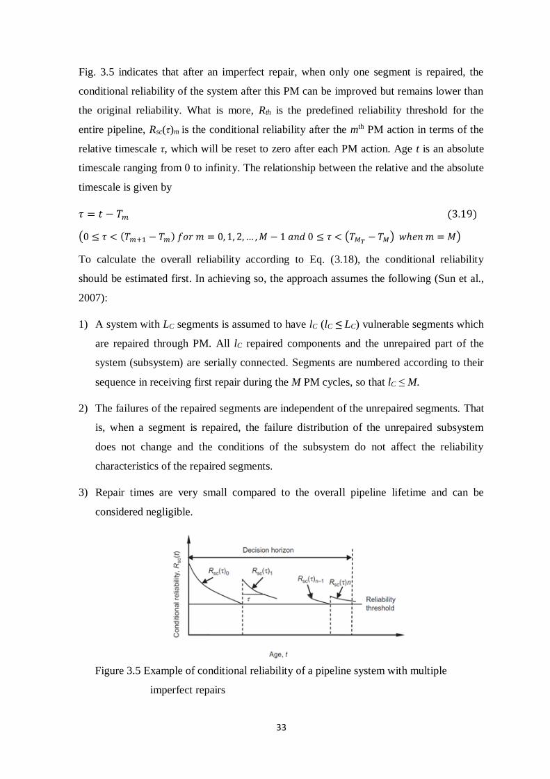
33
Fig. 3.5 indicates that after an imperfect repair, when only one segment is repaired, the
conditional reliability of the system after this PM can be improved but remains lower than
the original reliability. What is more, Rth is the predefined reliability threshold for the
entire pipeline, Rsc(τ)m is the conditional reliability after the mth PM action in terms of the
relative timescale τ, which will be reset to zero after each PM action. Age t is an absolute
timescale ranging from 0 to infinity. The relationship between the relative and the absolute
timescale is given by
𝜏 = 𝑡 − 𝑇𝑚 (3.19)
(0 ≤ 𝜏 < (𝑇𝑚+1 − 𝑇𝑚) 𝑓𝑜𝑟 𝑚 = 0, 1, 2, … ,𝑀 − 1 𝑎𝑛𝑑 0 ≤ 𝜏 < (𝑇𝑀𝑇− 𝑇𝑀) 𝑤ℎ𝑒𝑛 𝑚 = 𝑀)
To calculate the overall reliability according to Eq. (3.18), the conditional reliability
should be estimated first. In achieving so, the approach assumes the following (Sun et al.,
2007):
1) A system with LC segments is assumed to have lC (lC ≤ LC) vulnerable segments which
are repaired through PM. All lC repaired components and the unrepaired part of the
system (subsystem) are serially connected. Segments are numbered according to their
sequence in receiving first repair during the M PM cycles, so that lC ≤ M.
2) The failures of the repaired segments are independent of the unrepaired segments. That
is, when a segment is repaired, the failure distribution of the unrepaired subsystem
does not change and the conditions of the subsystem do not affect the reliability
characteristics of the repaired segments.
3) Repair times are very small compared to the overall pipeline lifetime and can be
considered negligible.
Figure 3.5 Example of conditional reliability of a pipeline system with multiple
imperfect repairs
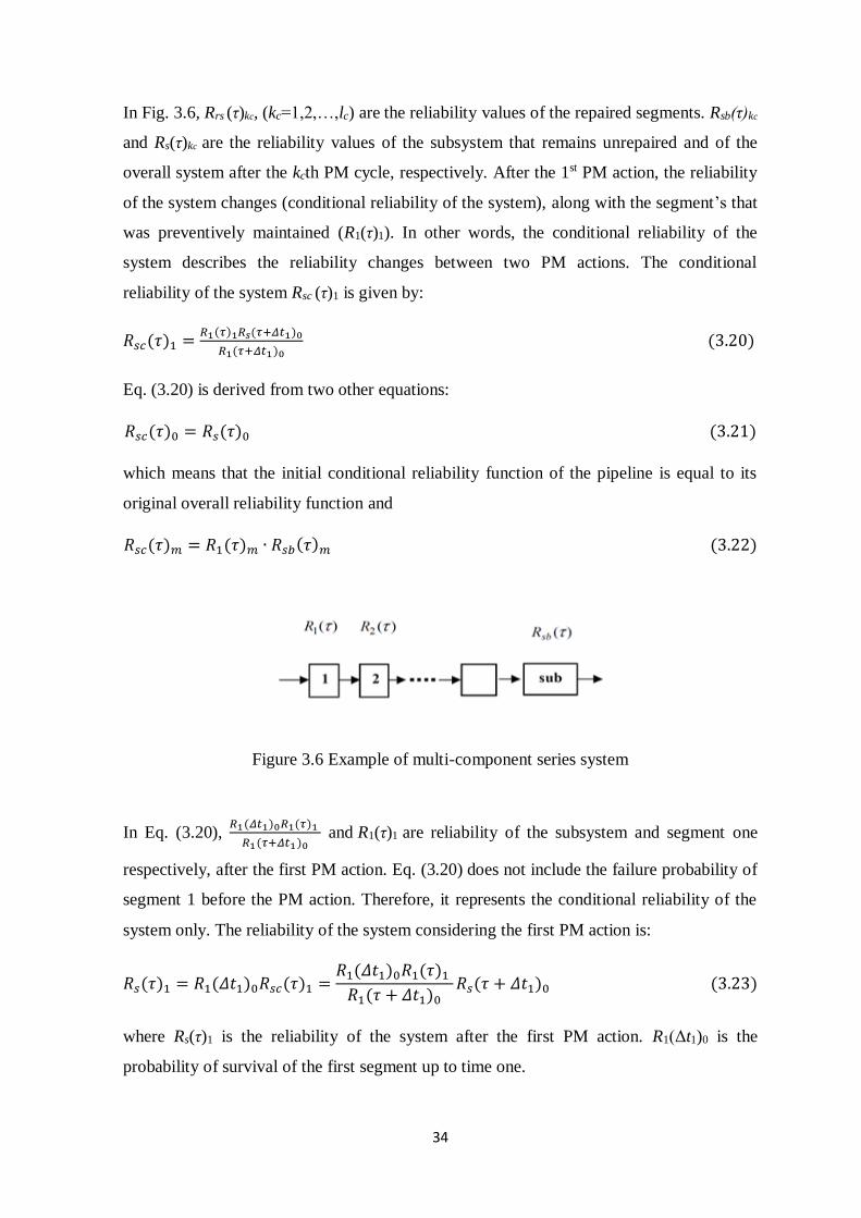
34
In Fig. 3.6, Rrs (τ)kc, (kc=1,2,…,lc) are the reliability values of the repaired segments. Rsb(τ)kc
and Rs(τ)kc are the reliability values of the subsystem that remains unrepaired and of the
overall system after the kcth PM cycle, respectively. After the 1st PM action, the reliability
of the system changes (conditional reliability of the system), along with the segment’s that
was preventively maintained (R1(τ)1). In other words, the conditional reliability of the
system describes the reliability changes between two PM actions. The conditional
reliability of the system Rsc (τ)1 is given by:
𝑅𝑠𝑐(𝜏)1 =𝑅1(𝜏)1𝑅𝑠(𝜏+𝛥𝑡1)0
𝑅1(𝜏+𝛥𝑡1)0 (3.20)
Eq. (3.20) is derived from two other equations:
𝑅𝑠𝑐(𝜏)0 = 𝑅𝑠(𝜏)0 (3.21)
which means that the initial conditional reliability function of the pipeline is equal to its
original overall reliability function and
𝑅𝑠𝑐(𝜏)𝑚 = 𝑅1(𝜏)𝑚 ∙ 𝑅𝑠𝑏(𝜏)𝑚 (3.22)
Figure 3.6 Example of multi-component series system
In Eq. (3.20), 𝑅1(𝛥𝑡1)0𝑅1(𝜏)1
𝑅1(𝜏+𝛥𝑡1)0 and R1(τ)1 are reliability of the subsystem and segment one
respectively, after the first PM action. Eq. (3.20) does not include the failure probability of
segment 1 before the PM action. Therefore, it represents the conditional reliability of the
system only. The reliability of the system considering the first PM action is:
𝑅𝑠(𝜏)1 = 𝑅1(𝛥𝑡1)0𝑅𝑠𝑐(𝜏)1 =𝑅1(𝛥𝑡1)0𝑅1(𝜏)1
𝑅1(𝜏 + 𝛥𝑡1)0𝑅𝑠(𝜏 + 𝛥𝑡1)0 (3.23)
where Rs(τ)1 is the reliability of the system after the first PM action. R1(Δt1)0 is the
probability of survival of the first segment up to time one.
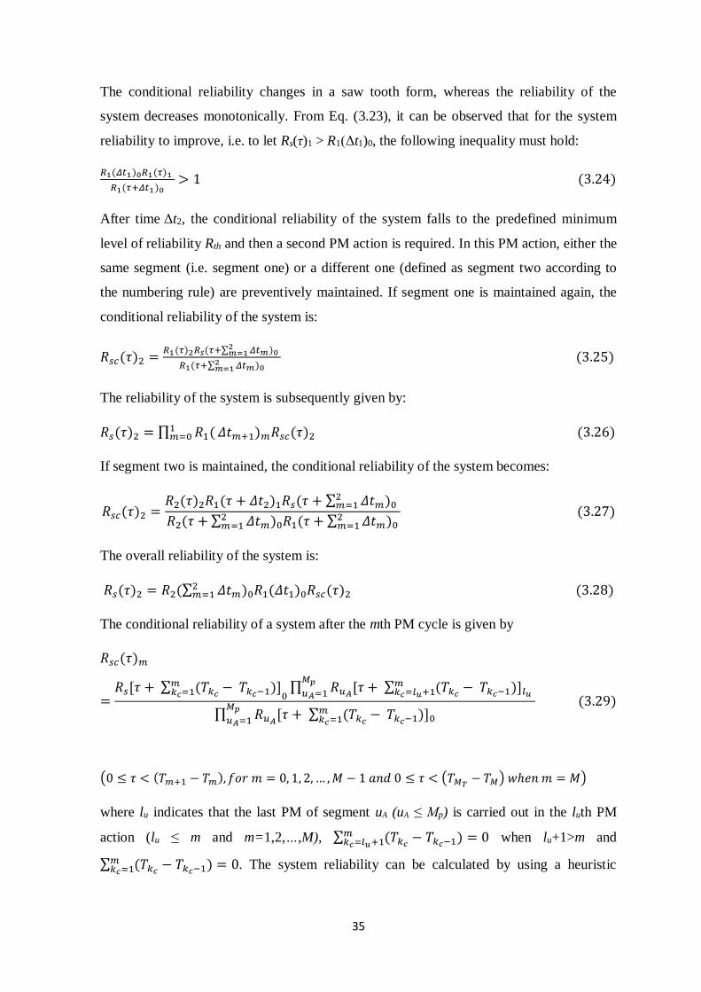
35
The conditional reliability changes in a saw tooth form, whereas the reliability of the
system decreases monotonically. From Eq. (3.23), it can be observed that for the system
reliability to improve, i.e. to let Rs(τ)1 > R1(Δt1)0, the following inequality must hold:
𝑅1(𝛥𝑡1)0𝑅1(𝜏)1
𝑅1(𝜏+𝛥𝑡1)0> 1 (3.24)
After time Δt2, the conditional reliability of the system falls to the predefined minimum
level of reliability Rth and then a second PM action is required. In this PM action, either the
same segment (i.e. segment one) or a different one (defined as segment two according to
the numbering rule) are preventively maintained. If segment one is maintained again, the
conditional reliability of the system is:
𝑅𝑠𝑐(𝜏)2 =𝑅1(𝜏)2𝑅𝑠(𝜏+∑ 𝛥𝑡𝑚
2𝑚=1 )0
𝑅1(𝜏+∑ 𝛥𝑡𝑚2𝑚=1 )0
(3.25)
The reliability of the system is subsequently given by:
𝑅𝑠(𝜏)2 = ∏ 𝑅1(1𝑚=0 𝛥𝑡𝑚+1)𝑚𝑅𝑠𝑐(𝜏)2 (3.26)
If segment two is maintained, the conditional reliability of the system becomes:
𝑅𝑠𝑐(𝜏)2 =𝑅2(𝜏)2𝑅1(𝜏 + 𝛥𝑡2)1𝑅𝑠(𝜏 + ∑ 𝛥𝑡𝑚
2𝑚=1 )0
𝑅2(𝜏 + ∑ 𝛥𝑡𝑚2𝑚=1 )0𝑅1(𝜏 + ∑ 𝛥𝑡𝑚
2𝑚=1 )0
(3.27)
The overall reliability of the system is:
𝑅𝑠(𝜏)2 = 𝑅2(∑ 𝛥𝑡𝑚2𝑚=1 )0𝑅1(𝛥𝑡1)0𝑅𝑠𝑐(𝜏)2 (3.28)
The conditional reliability of a system after the mth PM cycle is given by
𝑅𝑠𝑐(𝜏)𝑚
=𝑅𝑠[𝜏 + ∑ (𝑇𝑘𝑐 − 𝑇𝑘𝑐−1)]
𝑚𝑘𝑐=1 0
∏ 𝑅𝑢𝐴[𝜏 + ∑ (𝑇𝑘𝑐 − 𝑇𝑘𝑐−1)]𝑙𝑢𝑚𝑘𝑐=𝑙𝑢+1
𝑀𝑝𝑢𝐴=1
∏ 𝑅𝑢𝐴[𝜏 + ∑ (𝑇𝑘𝑐 − 𝑇𝑘𝑐−1)]0𝑚𝑘𝑐=1
𝑀𝑝𝑢𝐴=1
(3.29)
(0 ≤ 𝜏 < (𝑇𝑚+1 − 𝑇𝑚), 𝑓𝑜𝑟 𝑚 = 0, 1, 2, … ,𝑀 − 1 𝑎𝑛𝑑 0 ≤ 𝜏 < (𝑇𝑀𝑇− 𝑇𝑀) 𝑤ℎ𝑒𝑛 𝑚 = 𝑀)
where lu indicates that the last PM of segment uA (uA ≤ Mp) is carried out in the luth PM
action (lu ≤ m and m=1,2,…,M), ∑ (𝑇𝑘𝑐 − 𝑇𝑘𝑐−1𝑚𝑘𝑐=𝑙𝑢+1
) = 0 when lu+1>m and
∑ (𝑇𝑘𝑐 − 𝑇𝑘𝑐−1𝑚𝑘𝑐=1
) = 0. The system reliability can be calculated by using a heuristic
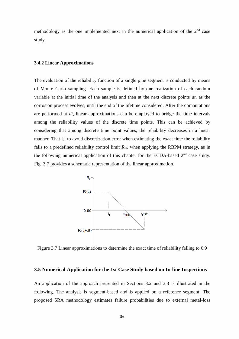
36
methodology as the one implemented next in the numerical application of the 2nd case
study.
3.4.2 Linear Approximations
The evaluation of the reliability function of a single pipe segment is conducted by means
of Monte Carlo sampling. Each sample is defined by one realization of each random
variable at the initial time of the analysis and then at the next discrete points dt, as the
corrosion process evolves, until the end of the lifetime considered. After the computations
are performed at dt, linear approximations can be employed to bridge the time intervals
among the reliability values of the discrete time points. This can be achieved by
considering that among discrete time point values, the reliability decreases in a linear
manner. That is, to avoid discretization error when estimating the exact time the reliability
falls to a predefined reliability control limit Rth, when applying the RBPM strategy, as in
the following numerical application of this chapter for the ECDA-based 2nd case study.
Fig. 3.7 provides a schematic representation of the linear approximation.
Figure 3.7 Linear approximations to determine the exact time of reliability falling to 0.9
3.5 Numerical Application for the 1st Case Study based on In-line Inspections
An application of the approach presented in Sections 3.2 and 3.3 is illustrated in the
following. The analysis is segment-based and is applied on a reference segment. The
proposed SRA methodology estimates failure probabilities due to external metal-loss
37
corrosion. Therefore, reported rupture incidents due to external metal-loss corrosion were
gathered for the period 2002-2014 from the PHMSA database and a reference pipeline was
built based upon the characteristics of the ruptured pipelines. In specific, the reference
segment’s random variables D, wt, UTS, Psop were defined by mean values equal to the
average of the corresponding actual values of the 52 ruptured segments and with suitable
corresponding probability distributions and standard deviations from the literature (Zhang
and Zhou, 2014; Zhou and Zhang, 2015). It is noted that only external metal-loss corrosion
incidents, as opposed to stress corrosion cracking, were taken into account. Moreover,
average data from the literature, which are based on extensive field studies on buried
onshore energy pipelines, were adopted to characterise the defect density and defect
growth rate (Velázquez et al., 2009; Gomes et al., 2013; Valor et al., 2014). All the
aforementioned values are summarized in Tables 3.1 and 3.3.
The service life considered for reliability prediction is 100 years. The number of defects on
the reference segment is characterised by Eq. (3.1), where λo and δ are set to 0.0278 and
unity respectively, i.e. S(t)=0.0139t2 , so that the expected number of defects over the first
17 years is 0.321 per metre, according to the assumed average defect density herein (Valor,
2014). The initiation time of the first defect is obtained from a uniform distribution with a
lower bound of 2.57 and an upper bound equal to 3.06. The growth of each defect is
realised by means of the PSWP model defined through Eq. (3.6), by adopting the
probabilistic characteristics presented in Table 3.1, as per Section 3.2.2. Average values
from literature, are adopted for the characterisation of the defect length; that is assumed to
have a mean value of 80mm and a COV of 130% (Nessim and Stephens, 2006; Zhang and
Zhou, 2014; Zhou and Zhang, 2015). Finally, the segment diameter (D), wall thickness
(wt) and ultimate tensile strength (UTS) are invariant within the pipe segment.
The ILI measured defect depths and lengths, are assumed to be unbiased and therefore the
parameters from Eqs. (3.15a) and (3.15b) are set equal to c1=cl1 = 0 and c2 = cl2 = 1. The
random scattering errors εi and εli are defined as 7.8%wt and 7.8mm respectively,
according to standard tool specifications (Zhou and Zhang, 2015). The PoD associated
with the ILI tool is estimated from Eq. (3.14) with q = 3.262 (mm-1), i.e. the PoD is equal
to 90% for a defect depth of 10%wt. Out of the 52 external corrosion rupture incidents
found in the PHMSA, 43 belong to Class 1 and the rest to Class 2; thus the safety
parameters ξA and ηA of Eq. (3.13a) and (3.13b) are equal to 0.5 and 1.39 respectively,
according to Table 3.2. Since the majority belongs to Class 1 pipelines, the initial
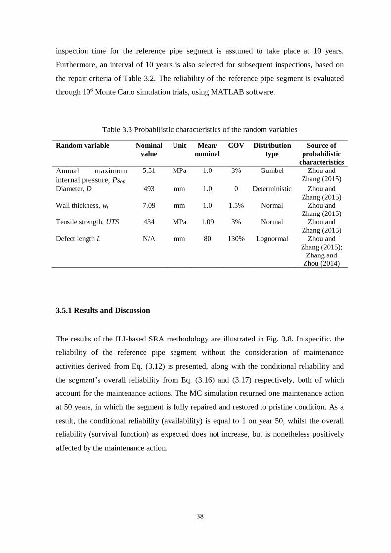
38
inspection time for the reference pipe segment is assumed to take place at 10 years.
Furthermore, an interval of 10 years is also selected for subsequent inspections, based on
the repair criteria of Table 3.2. The reliability of the reference pipe segment is evaluated
through 106 Monte Carlo simulation trials, using MATLAB software.
Table 3.3 Probabilistic characteristics of the random variables
Random variable Nominal
value
Unit Mean/
nominal
COV Distribution
type
Source of
probabilistic
characteristics
Annual maximum
internal pressure, Psop
5.51 MPa 1.0 3% Gumbel Zhou and
Zhang (2015)
Diameter, D 493 mm 1.0 0 Deterministic Zhou and
Zhang (2015) Wall thickness, wt 7.09 mm 1.0 1.5% Normal Zhou and
Zhang (2015)
Tensile strength, UTS 434 MPa 1.09 3% Normal Zhou and
Zhang (2015) Defect length L N/A mm 80 130% Lognormal Zhou and
Zhang (2015);
Zhang and Zhou (2014)
3.5.1 Results and Discussion
The results of the ILI-based SRA methodology are illustrated in Fig. 3.8. In specific, the
reliability of the reference pipe segment without the consideration of maintenance
activities derived from Eq. (3.12) is presented, along with the conditional reliability and
the segment’s overall reliability from Eq. (3.16) and (3.17) respectively, both of which
account for the maintenance actions. The MC simulation returned one maintenance action
at 50 years, in which the segment is fully repaired and restored to pristine condition. As a
result, the conditional reliability (availability) is equal to 1 on year 50, whilst the overall
reliability (survival function) as expected does not increase, but is nonetheless positively
affected by the maintenance action.
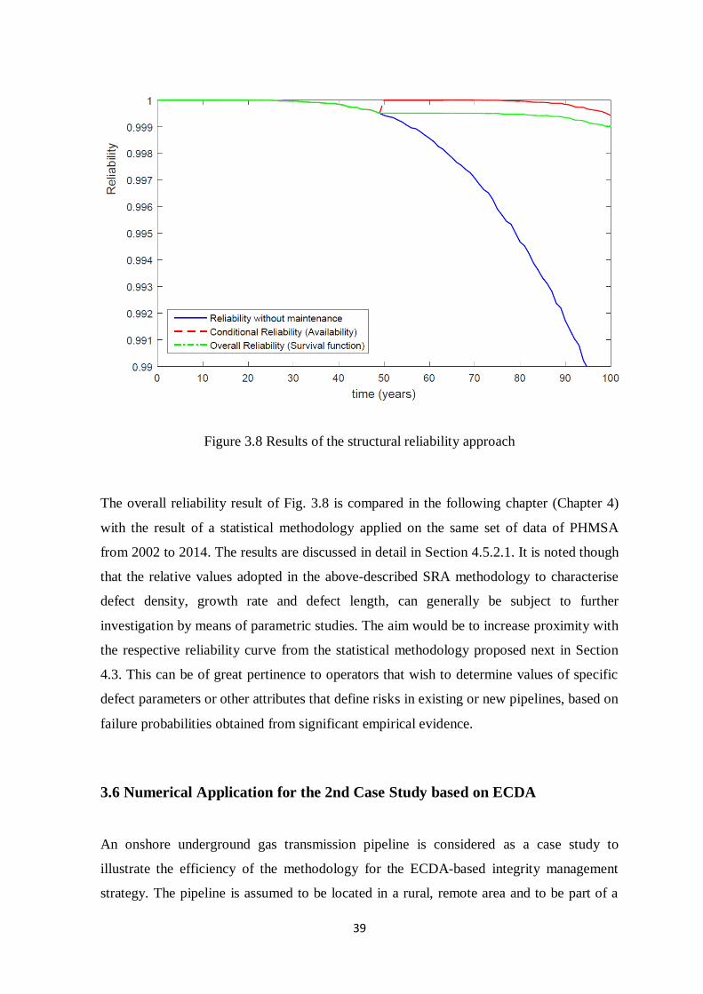
39
Figure 3.8 Results of the structural reliability approach
The overall reliability result of Fig. 3.8 is compared in the following chapter (Chapter 4)
with the result of a statistical methodology applied on the same set of data of PHMSA
from 2002 to 2014. The results are discussed in detail in Section 4.5.2.1. It is noted though
that the relative values adopted in the above-described SRA methodology to characterise
defect density, growth rate and defect length, can generally be subject to further
investigation by means of parametric studies. The aim would be to increase proximity with
the respective reliability curve from the statistical methodology proposed next in Section
4.3. This can be of great pertinence to operators that wish to determine values of specific
defect parameters or other attributes that define risks in existing or new pipelines, based on
failure probabilities obtained from significant empirical evidence.
3.6 Numerical Application for the 2nd Case Study based on ECDA
An onshore underground gas transmission pipeline is considered as a case study to
illustrate the efficiency of the methodology for the ECDA-based integrity management
strategy. The pipeline is assumed to be located in a rural, remote area and to be part of a
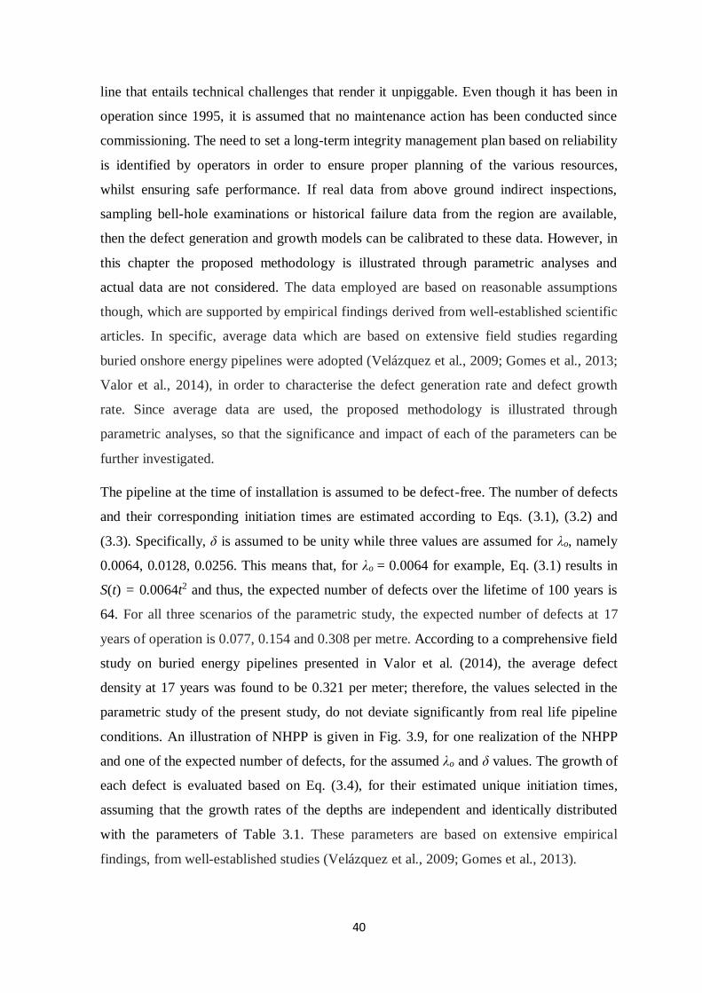
40
line that entails technical challenges that render it unpiggable. Even though it has been in
operation since 1995, it is assumed that no maintenance action has been conducted since
commissioning. The need to set a long-term integrity management plan based on reliability
is identified by operators in order to ensure proper planning of the various resources,
whilst ensuring safe performance. If real data from above ground indirect inspections,
sampling bell-hole examinations or historical failure data from the region are available,
then the defect generation and growth models can be calibrated to these data. However, in
this chapter the proposed methodology is illustrated through parametric analyses and
actual data are not considered. The data employed are based on reasonable assumptions
though, which are supported by empirical findings derived from well-established scientific
articles. In specific, average data which are based on extensive field studies regarding
buried onshore energy pipelines were adopted (Velázquez et al., 2009; Gomes et al., 2013;
Valor et al., 2014), in order to characterise the defect generation rate and defect growth
rate. Since average data are used, the proposed methodology is illustrated through
parametric analyses, so that the significance and impact of each of the parameters can be
further investigated.
The pipeline at the time of installation is assumed to be defect-free. The number of defects
and their corresponding initiation times are estimated according to Eqs. (3.1), (3.2) and
(3.3). Specifically, δ is assumed to be unity while three values are assumed for λo, namely
0.0064, 0.0128, 0.0256. This means that, for λo = 0.0064 for example, Eq. (3.1) results in
S(t) = 0.0064t2 and thus, the expected number of defects over the lifetime of 100 years is
64. For all three scenarios of the parametric study, the expected number of defects at 17
years of operation is 0.077, 0.154 and 0.308 per metre. According to a comprehensive field
study on buried energy pipelines presented in Valor et al. (2014), the average defect
density at 17 years was found to be 0.321 per meter; therefore, the values selected in the
parametric study of the present study, do not deviate significantly from real life pipeline
conditions. An illustration of NHPP is given in Fig. 3.9, for one realization of the NHPP
and one of the expected number of defects, for the assumed λo and δ values. The growth of
each defect is evaluated based on Eq. (3.4), for their estimated unique initiation times,
assuming that the growth rates of the depths are independent and identically distributed
with the parameters of Table 3.1. These parameters are based on extensive empirical
findings, from well-established studies (Velázquez et al., 2009; Gomes et al., 2013).
41
The defect length characteristics are presented in Table 3.4. Specifically, the length is
assumed to be static and follow a lognormal distribution with a mean of 105 mm and a
COV of 130%, while the wall thickness (wt) and yield strength (σy) are assumed to be
invariant within the pipe segment. The PCORRC model is adopted to evaluate the capacity
of the pipeline against burst (either large leak or rupture). Finally, the internal pressure is
assumed to be time-dependent according to a PSWP model, as presented in Section 3.2.3.
A parametric analysis is conducted, in order to characterise the generation rate λ of the
model. Three values are assumed, namely 0.75, 1.00, and 1.50. The probability distribution
of the magnitude of the internal pressure is presented in Table 3.4. The simulated time-
dependent internal pressure curves corresponding to λ = 0.75, λ = 1.00 and λ = 1.50 are
presented in Fig. 3.10 for a period of 100 years. All the pipeline probabilistic
characteristics are summarised in Tables 3.4 and 3.5.
Table 3.4 Probabilistic characteristics of the random variables
Random variable Nominal
value
Unit Mean/
nominal
COV Distribution type
Annual maximum internal pressure,
Psop
10.34 MPa 1.05 2% Gumbel
Diameter, D 762 mm 1.0 0 Deterministic
Wall thickness, t 8.96 mm 1.0 1.5% Normal
Yield strength, σy 550 MPa 1.08 3% Normal
Defect length L N/A mm 105 130% Lognormal
A pipeline system of three identical pipe segments is selected for the implementation of
the methodology. The adopted pipe segment characteristics are from the study of Zhang
and Zhou (2014). The nominal outside diameter of the pipeline is 762 mm and the
operating pressure is 10.34 MPa. The material is made from API 5L Grade X80 steel, with
a specified minimum yield and tensile strength of 550 MPa and 625 MPa respectively.
Finally, the pipeline has a nominal wall thickness of 8.96 mm. Each segment is 12m long
and the reliability of the single segment is estimated based on the limit state function for
burst. The Monte Carlo approach provides the calculation of the segment reliability. This
corresponds to a single realisation, for one generation of the total number of s defects and
104 iterations of random variable samples. However, in order to achieve more stable
results that more accurately depict the reliability prediction, 100∙104 iterations are chosen.
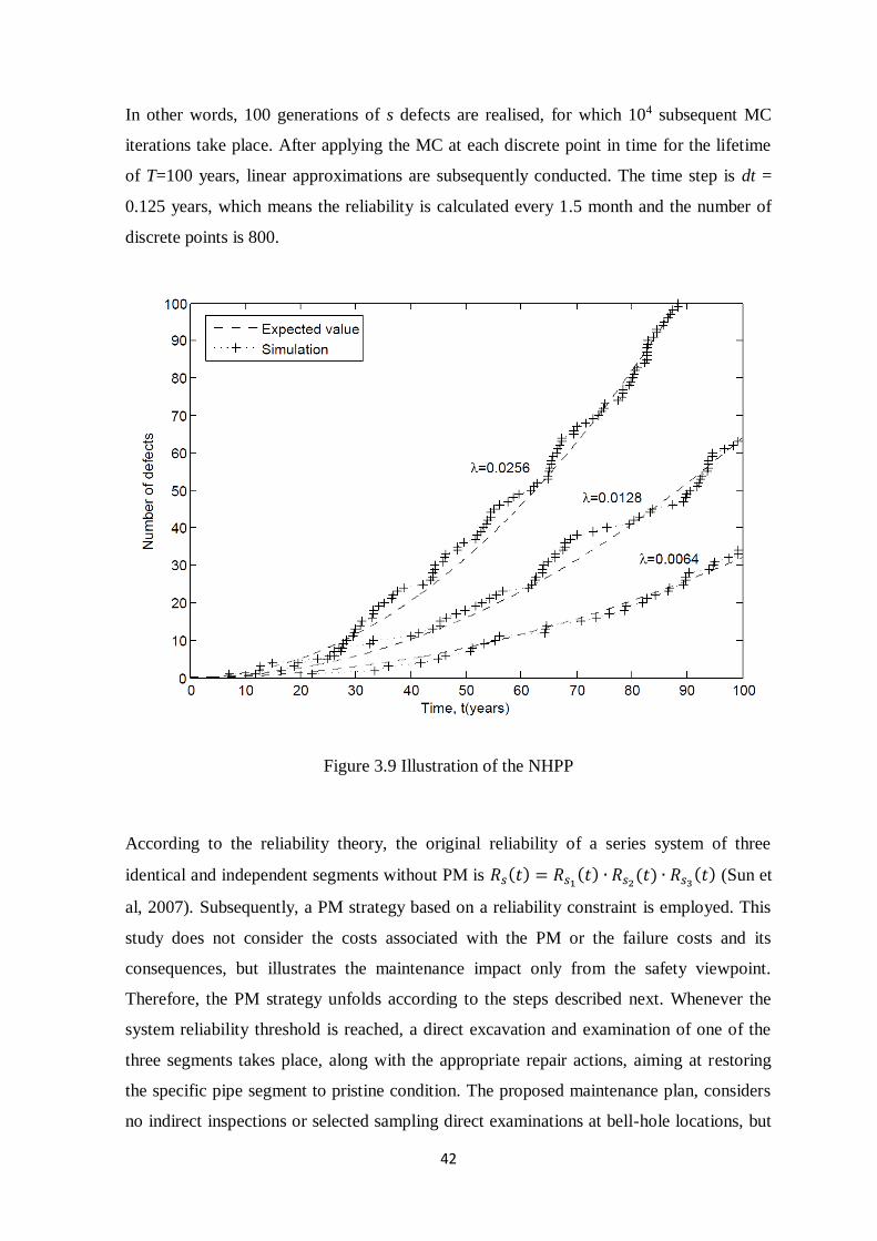
42
In other words, 100 generations of s defects are realised, for which 104 subsequent MC
iterations take place. After applying the MC at each discrete point in time for the lifetime
of T=100 years, linear approximations are subsequently conducted. The time step is dt =
0.125 years, which means the reliability is calculated every 1.5 month and the number of
discrete points is 800.
Figure 3.9 Illustration of the NHPP
According to the reliability theory, the original reliability of a series system of three
identical and independent segments without PM is 𝑅𝑠(𝑡) = 𝑅𝑠1(𝑡) ∙ 𝑅𝑠2(𝑡) ∙ 𝑅𝑠3(𝑡) (Sun et
al, 2007). Subsequently, a PM strategy based on a reliability constraint is employed. This
study does not consider the costs associated with the PM or the failure costs and its
consequences, but illustrates the maintenance impact only from the safety viewpoint.
Therefore, the PM strategy unfolds according to the steps described next. Whenever the
system reliability threshold is reached, a direct excavation and examination of one of the
three segments takes place, along with the appropriate repair actions, aiming at restoring
the specific pipe segment to pristine condition. The proposed maintenance plan, considers
no indirect inspections or selected sampling direct examinations at bell-hole locations, but
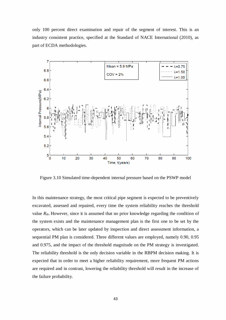
43
only 100 percent direct examination and repair of the segment of interest. This is an
industry consistent practice, specified at the Standard of NACE International (2010), as
part of ECDA methodologies.
Figure 3.10 Simulated time-dependent internal pressure based on the PSWP model
In this maintenance strategy, the most critical pipe segment is expected to be preventively
excavated, assessed and repaired, every time the system reliability reaches the threshold
value Rth. However, since it is assumed that no prior knowledge regarding the condition of
the system exists and the maintenance management plan is the first one to be set by the
operators, which can be later updated by inspection and direct assessment information, a
sequential PM plan is considered. Three different values are employed, namely 0.90, 0.95
and 0.975, and the impact of the threshold magnitude on the PM strategy is investigated.
The reliability threshold is the only decision variable in the RBPM decision making. It is
expected that in order to meet a higher reliability requirement, more frequent PM actions
are required and in contrast, lowering the reliability threshold will result in the increase of
the failure probability.
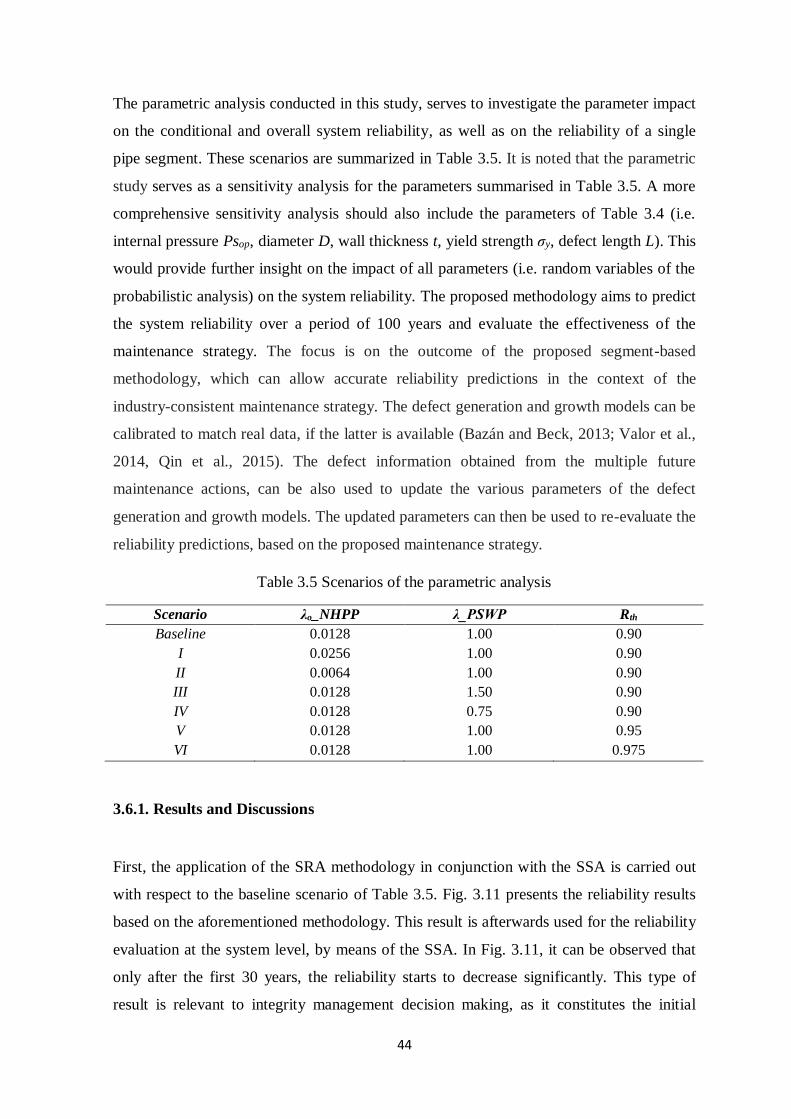
44
The parametric analysis conducted in this study, serves to investigate the parameter impact
on the conditional and overall system reliability, as well as on the reliability of a single
pipe segment. These scenarios are summarized in Table 3.5. It is noted that the parametric
study serves as a sensitivity analysis for the parameters summarised in Table 3.5. A more
comprehensive sensitivity analysis should also include the parameters of Table 3.4 (i.e.
internal pressure Psop, diameter D, wall thickness t, yield strength σy, defect length L). This
would provide further insight on the impact of all parameters (i.e. random variables of the
probabilistic analysis) on the system reliability. The proposed methodology aims to predict
the system reliability over a period of 100 years and evaluate the effectiveness of the
maintenance strategy. The focus is on the outcome of the proposed segment-based
methodology, which can allow accurate reliability predictions in the context of the
industry-consistent maintenance strategy. The defect generation and growth models can be
calibrated to match real data, if the latter is available (Bazán and Beck, 2013; Valor et al.,
2014, Qin et al., 2015). The defect information obtained from the multiple future
maintenance actions, can be also used to update the various parameters of the defect
generation and growth models. The updated parameters can then be used to re-evaluate the
reliability predictions, based on the proposed maintenance strategy.
Table 3.5 Scenarios of the parametric analysis
Scenario λo_NHPP λ_PSWP Rth
Baseline 0.0128 1.00 0.90
I 0.0256 1.00 0.90
II 0.0064 1.00 0.90
III 0.0128 1.50 0.90
IV 0.0128 0.75 0.90
V 0.0128 1.00 0.95
VI 0.0128 1.00 0.975
3.6.1. Results and Discussions
First, the application of the SRA methodology in conjunction with the SSA is carried out
with respect to the baseline scenario of Table 3.5. Fig. 3.11 presents the reliability results
based on the aforementioned methodology. This result is afterwards used for the reliability
evaluation at the system level, by means of the SSA. In Fig. 3.11, it can be observed that
only after the first 30 years, the reliability starts to decrease significantly. This type of
result is relevant to integrity management decision making, as it constitutes the initial
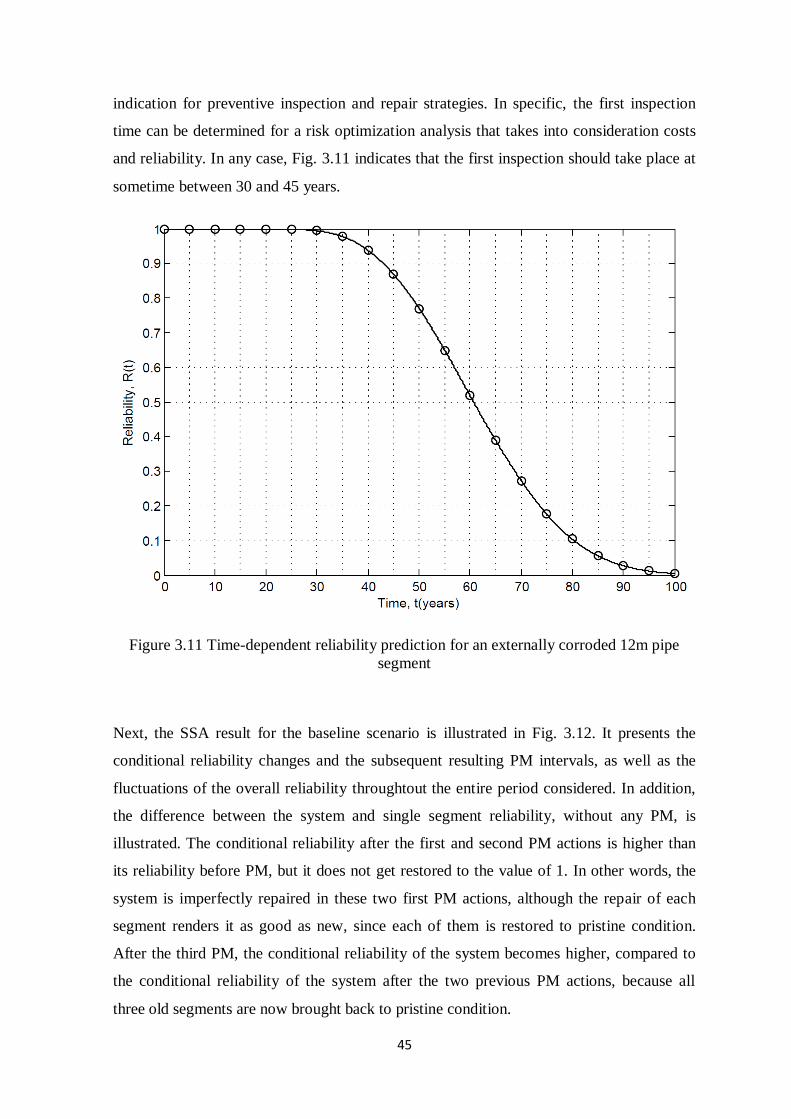
45
indication for preventive inspection and repair strategies. In specific, the first inspection
time can be determined for a risk optimization analysis that takes into consideration costs
and reliability. In any case, Fig. 3.11 indicates that the first inspection should take place at
sometime between 30 and 45 years.
Figure 3.11 Time-dependent reliability prediction for an externally corroded 12m pipe
segment
Next, the SSA result for the baseline scenario is illustrated in Fig. 3.12. It presents the
conditional reliability changes and the subsequent resulting PM intervals, as well as the
fluctuations of the overall reliability throughtout the entire period considered. In addition,
the difference between the system and single segment reliability, without any PM, is
illustrated. The conditional reliability after the first and second PM actions is higher than
its reliability before PM, but it does not get restored to the value of 1. In other words, the
system is imperfectly repaired in these two first PM actions, although the repair of each
segment renders it as good as new, since each of them is restored to pristine condition.
After the third PM, the conditional reliability of the system becomes higher, compared to
the conditional reliability of the system after the two previous PM actions, because all
three old segments are now brought back to pristine condition.
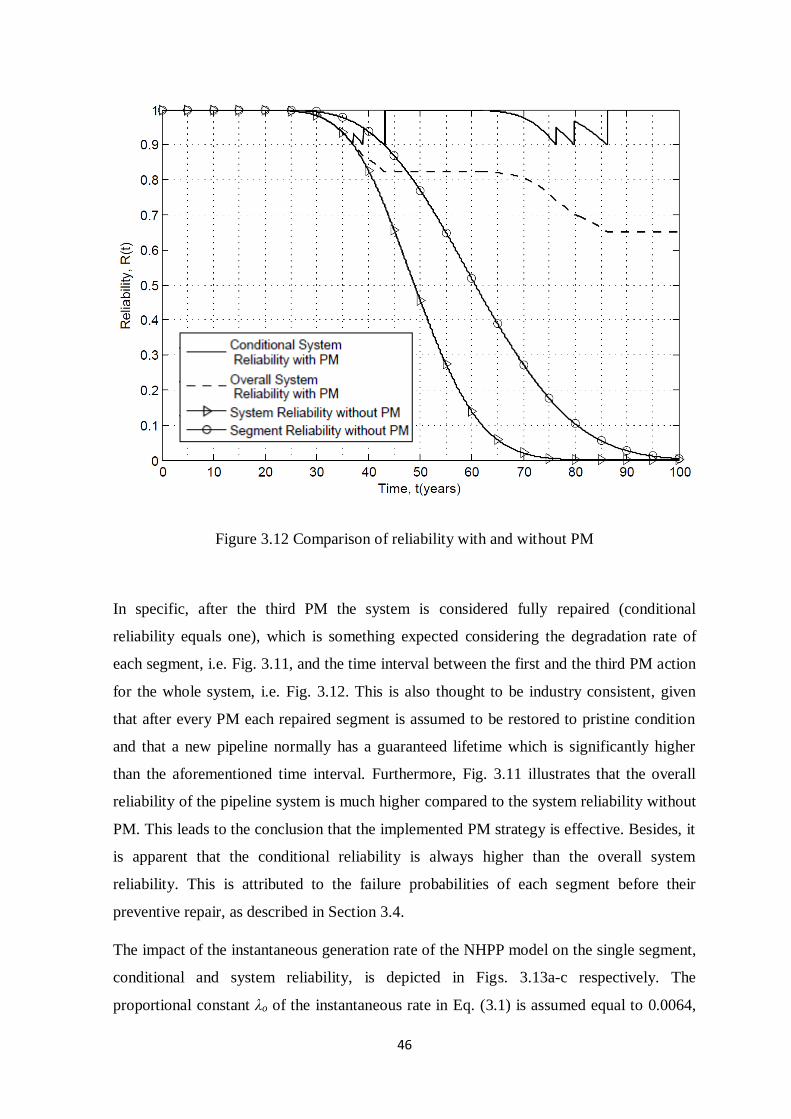
46
Figure 3.12 Comparison of reliability with and without PM
In specific, after the third PM the system is considered fully repaired (conditional
reliability equals one), which is something expected considering the degradation rate of
each segment, i.e. Fig. 3.11, and the time interval between the first and the third PM action
for the whole system, i.e. Fig. 3.12. This is also thought to be industry consistent, given
that after every PM each repaired segment is assumed to be restored to pristine condition
and that a new pipeline normally has a guaranteed lifetime which is significantly higher
than the aforementioned time interval. Furthermore, Fig. 3.11 illustrates that the overall
reliability of the pipeline system is much higher compared to the system reliability without
PM. This leads to the conclusion that the implemented PM strategy is effective. Besides, it
is apparent that the conditional reliability is always higher than the overall system
reliability. This is attributed to the failure probabilities of each segment before their
preventive repair, as described in Section 3.4.
The impact of the instantaneous generation rate of the NHPP model on the single segment,
conditional and system reliability, is depicted in Figs. 3.13a-c respectively. The
proportional constant λo of the instantaneous rate in Eq. (3.1) is assumed equal to 0.0064,
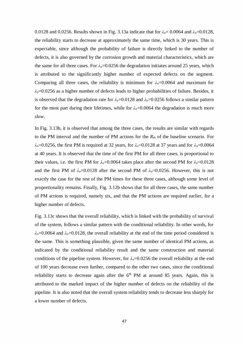
47
0.0128 and 0.0256. Results shown in Fig. 3.13a indicate that for λo= 0.0064 and λo=0.0128,
the reliability starts to decrease at approximately the same time, which is 30 years. This is
expectable, since although the probability of failure is directly linked to the number of
defects, it is also governed by the corrosion growth and material characteristics, which are
the same for all three cases. For λo=0.0256 the degradation initiates around 25 years, which
is attributed to the significantly higher number of expected defects on the segment.
Comparing all three cases, the reliability is minimum for λo=0.0064 and maximum for
λo=0.0256 as a higher number of defects leads to higher probabilities of failure. Besides, it
is observed that the degradation rate for λo=0.0128 and λo=0.0256 follows a similar pattern
for the most part during their lifetimes, while for λo=0.0064 the degradation is much more
slow.
In Fig. 3.13b, it is observed that among the three cases, the results are similar with regards
to the PM interval and the number of PM actions for the Rth of the baseline scenario. For
λo=0.0256, the first PM is required at 32 years, for λo=0.0128 at 37 years and for λo=0.0064
at 40 years. It is observed that the time of the first PM for all three cases, is proportional to
their values, i.e. the first PM for λo=0.0064 takes place after the second PM for λo=0.0128
and the first PM of λo=0.0128 after the second PM of λo=0.0256. However, this is not
exactly the case for the rest of the PM times for these three cases, although some level of
proportionality remains. Finally, Fig. 3.12b shows that for all three cases, the same number
of PM actions is required, namely six, and that the PM actions are required earlier, for a
higher number of defects.
Fig. 3.13c shows that the overall reliability, which is linked with the probability of survival
of the system, follows a similar pattern with the conditional reliability. In other words, for
λo=0.0064 and λo=0.0128, the overall reliability at the end of the time period considered is
the same. This is something plausible, given the same number of identical PM actions, as
indicated by the conditional reliability result and the same construction and material
conditions of the pipeline system. However, for λo=0.0256 the overall reliability at the end
of 100 years decrease even further, compared to the other two cases, since the conditional
reliability starts to decrease again after the 6th PM at around 85 years. Again, this is
attributed to the marked impact of the higher number of defects on the reliability of the
pipeline. It is also noted that the overall system reliability tends to decrease less sharply for
a lower number of defects.
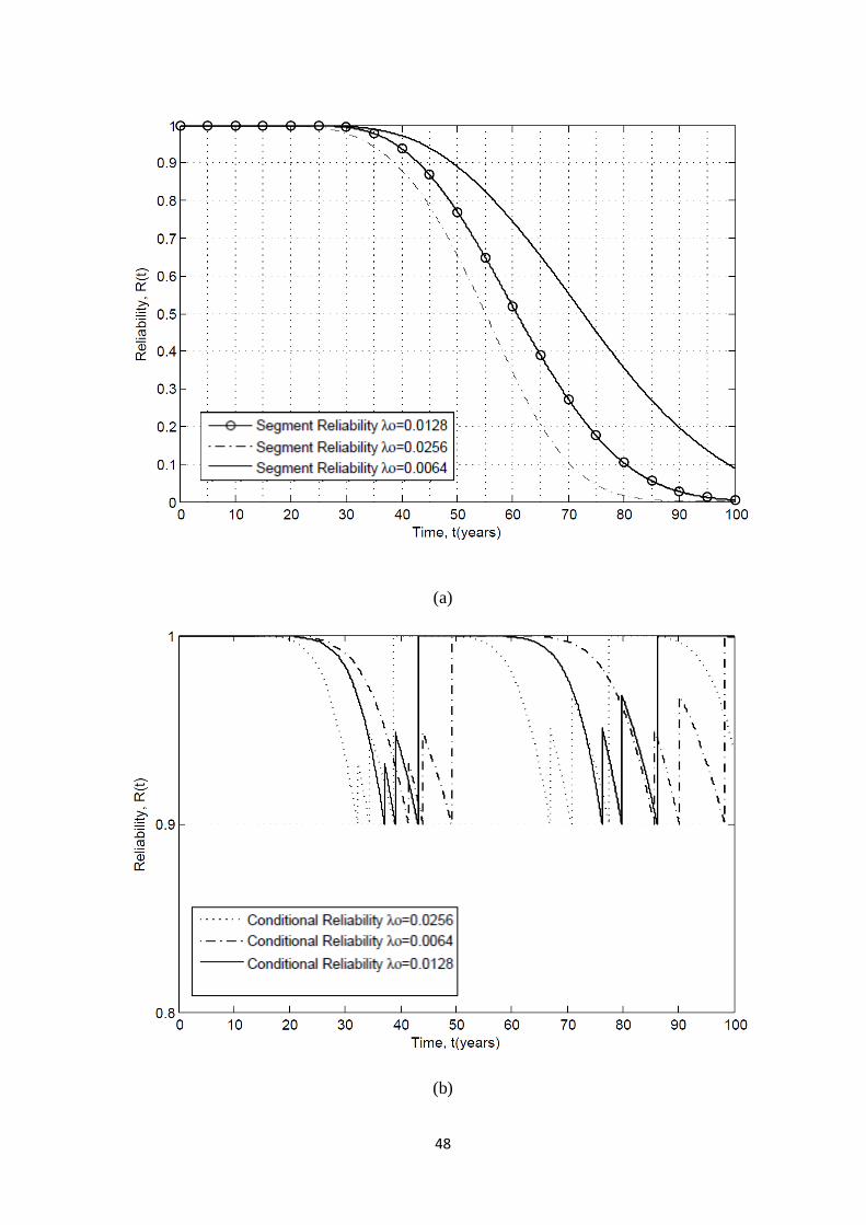
48
(a)
(b)
49
(c)
Figure 3.13 (a-c) Comparison of reliability predictions in terms of the proportional
constant λο of the defect generation model
The predictions for the single segment, conditional and system reliability are next realised
for the three parametric scenarios regarding the generation rate λ of the PSWP model and
are illustrated in Fig. 3.14a-c. Three values are assumed, namely 0.75, 1.00, and 1.50. It is
observed that the different values of λ have a relatively uniform impact on reliability,
proportional to the magnitude of λ. Therefore, single segment reliability in Fig. 3.14a
increases more significantly for a higher value of λ (1.50), while the difference among the
other two cases (0.75 and 1.00) is marginal. In specific, the reliability for λ=0.75 starts to
decrease slightly earlier compared to the one for λ=1.00, while both reach the reliability
control limit of Rth=0.90 simultaneously. Although for λ=0.75 the reliability remains
higher during the majority of the lifetime considered, at the end both become exactly
equal. This slight deviation can be attributed to the stochastic nature of the PSWP model
and the marginal difference among the λ values. A similar impact is shown in Fig. 3.14b,
with the conditional reliability curves indicating a shorter first PM interval for λ=1.50, then
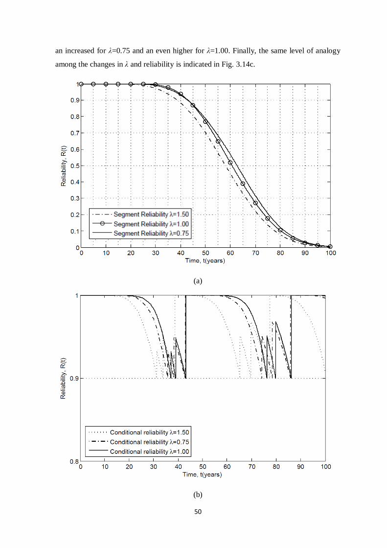
50
an increased for λ=0.75 and an even higher for λ=1.00. Finally, the same level of analogy
among the changes in λ and reliability is indicated in Fig. 3.14c.
(a)
(b)
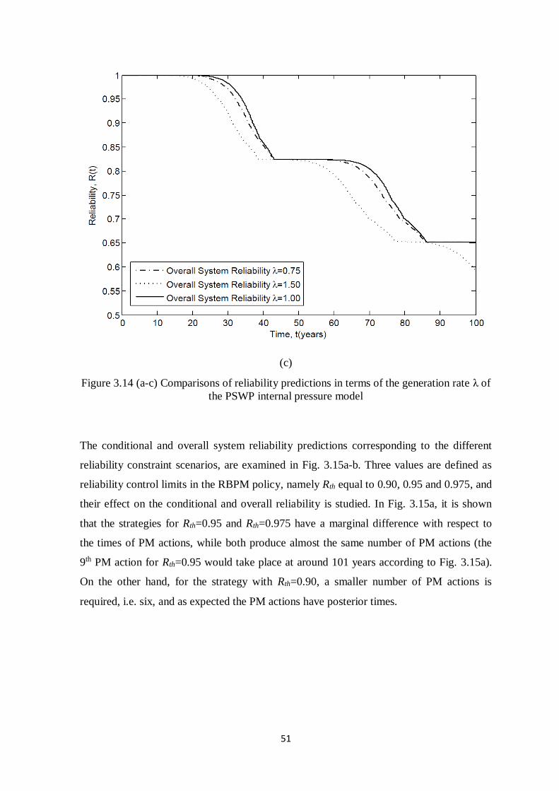
51
(c)
Figure 3.14 (a-c) Comparisons of reliability predictions in terms of the generation rate λ of
the PSWP internal pressure model
The conditional and overall system reliability predictions corresponding to the different
reliability constraint scenarios, are examined in Fig. 3.15a-b. Three values are defined as
reliability control limits in the RBPM policy, namely Rth equal to 0.90, 0.95 and 0.975, and
their effect on the conditional and overall reliability is studied. In Fig. 3.15a, it is shown
that the strategies for Rth=0.95 and Rth=0.975 have a marginal difference with respect to
the times of PM actions, while both produce almost the same number of PM actions (the
9th PM action for Rth=0.95 would take place at around 101 years according to Fig. 3.15a).
On the other hand, for the strategy with Rth=0.90, a smaller number of PM actions is
required, i.e. six, and as expected the PM actions have posterior times.
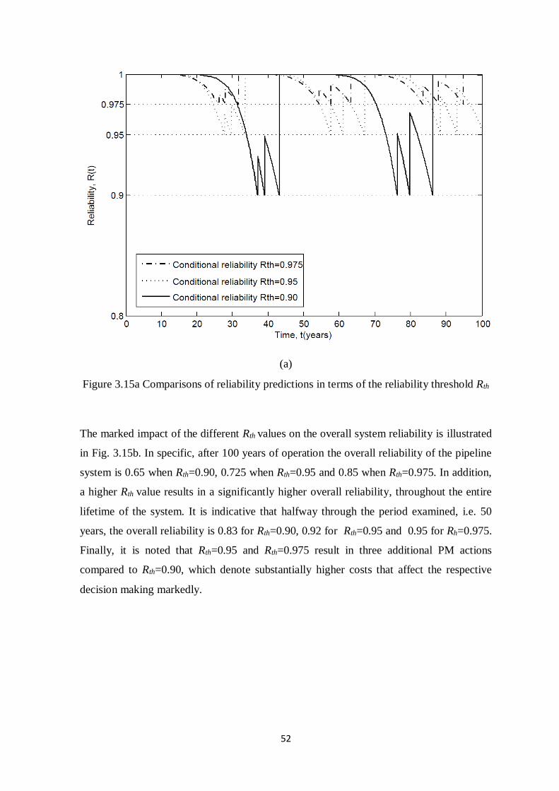
52
(a)
Figure 3.15a Comparisons of reliability predictions in terms of the reliability threshold Rth
The marked impact of the different Rth values on the overall system reliability is illustrated
in Fig. 3.15b. In specific, after 100 years of operation the overall reliability of the pipeline
system is 0.65 when Rth=0.90, 0.725 when Rth=0.95 and 0.85 when Rth=0.975. In addition,
a higher Rth value results in a significantly higher overall reliability, throughout the entire
lifetime of the system. It is indicative that halfway through the period examined, i.e. 50
years, the overall reliability is 0.83 for Rth=0.90, 0.92 for Rth=0.95 and 0.95 for Rh=0.975.
Finally, it is noted that Rth=0.95 and Rth=0.975 result in three additional PM actions
compared to Rth=0.90, which denote substantially higher costs that affect the respective
decision making markedly.
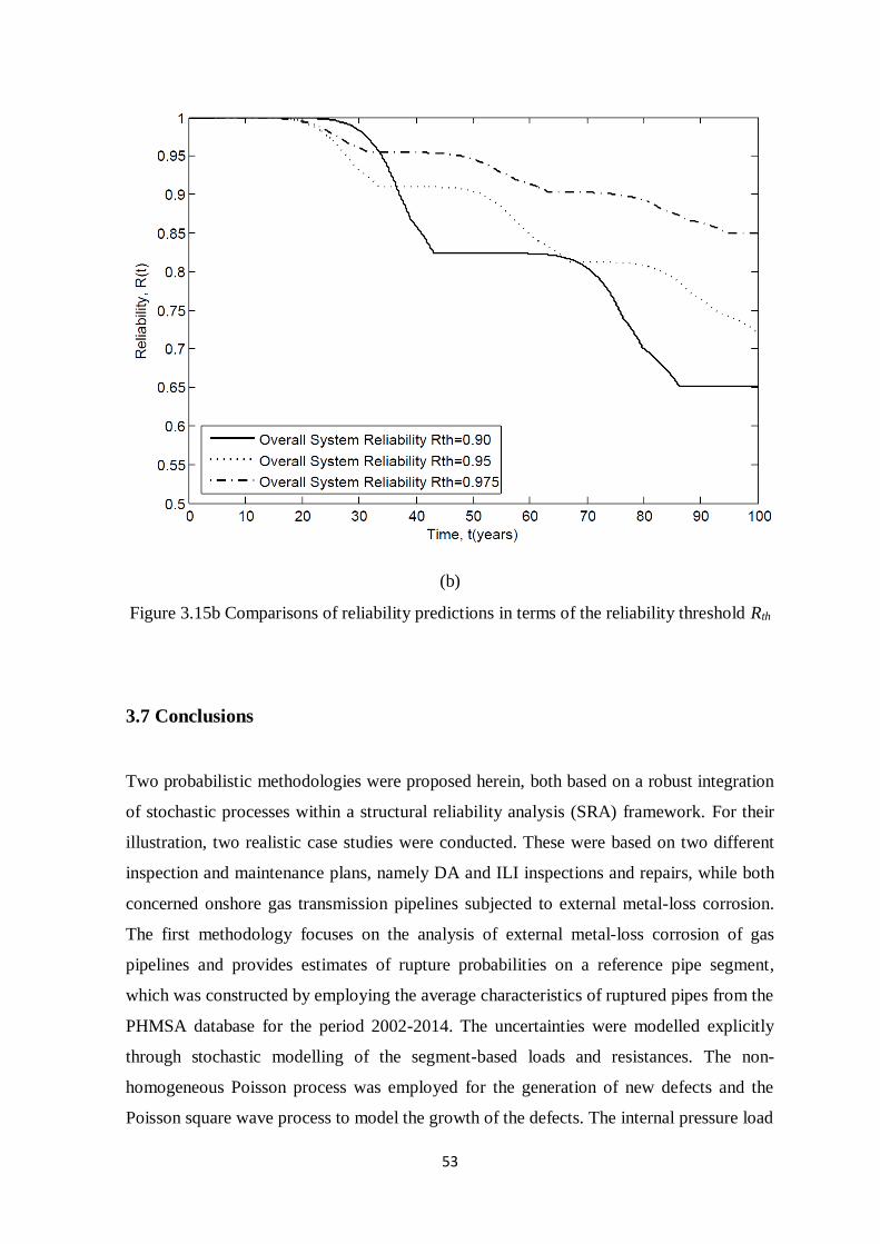
53
(b)
Figure 3.15b Comparisons of reliability predictions in terms of the reliability threshold Rth
3.7 Conclusions
Two probabilistic methodologies were proposed herein, both based on a robust integration
of stochastic processes within a structural reliability analysis (SRA) framework. For their
illustration, two realistic case studies were conducted. These were based on two different
inspection and maintenance plans, namely DA and ILI inspections and repairs, while both
concerned onshore gas transmission pipelines subjected to external metal-loss corrosion.
The first methodology focuses on the analysis of external metal-loss corrosion of gas
pipelines and provides estimates of rupture probabilities on a reference pipe segment,
which was constructed by employing the average characteristics of ruptured pipes from the
PHMSA database for the period 2002-2014. The uncertainties were modelled explicitly
through stochastic modelling of the segment-based loads and resistances. The non-
homogeneous Poisson process was employed for the generation of new defects and the
Poisson square wave process to model the growth of the defects. The internal pressure load
54
was modelled through a discrete Ferry-Borges stochastic process. An implicit ILI
inspection and maintenance plan was incorporated thereafter, based on standardised codes
of practice along with the corresponding uncertainties of the inspection procedure.
Considering the use of realistic characteristics from the PHMSA database, it can be
inferred that this model provides additional knowledge on the state of the PHMSA onshore
gas transmission network in 2002-2014, a period rather representative of the up-to-date
techniques and strategies for pipeline operation and rehabilitation in the industry,
amplifying the relevance of the results to reliability analyses of new or existing pipelines.
The second probabilistic methodology can accurately predict the time-dependent reliability
for unpiggable pipeline systems subjected to external metal-loss corrosion. The application
of the proposed methodology on an example pipeline system was conducted by
considering a direct excavation, assessment and repair strategy that is preventive in nature.
The non-homogeneous Poisson process was again employed for the generation of
corrosion defects over time and an empirical power law model for the defect growth, with
respect to a single pipe segment of 12m. A Poisson square wave process model was
adopted for the the internal pressure loading. The reliability of the corroding pipe segment
was evaluated by means of a Monte Carlo simulation technique against the failure mode of
burst. Next, a SSA, which is a heuristic method, was employed in order to update the
reliability corresponding to a linear system composed of a series of pipe segments. The
estimated single segment reliability, which is directly associated with the failure mode of
burst, was used in the SSA analysis, instead of the hazard function associated with the time
to failure. The pipeline system was assumed to be imperfectly repaired in every future PM
action. This is considered industry consistent due to human and financial constraints. The
SSA method can accurately quantify changes in reliability due to the imperfect repairs.
The type of maintenance strategy illustrated in the numerical application can be useful to
decision-making for reliability prediction of pipeline systems, both as a realistic ECDA
strategy and for comparison with other strategies, such as the ILI-based ones. The results
indicate the efficiency of the methodology in predicting reliability of pipeline systems over
time, while incorporating the effects of failure probabilities of repaired and unrepaired
segments.
Furthermore, the impact of certain parameters on the reliability predictions were examined
through a parametric study. The instantaneous generation rate λο of the defect generation
model had a significant impact on the single segment and overall system reliability, as well
55
as on the conditional reliability. A higher number of λο led to a proportionally higher
number of defects generated by the NHPP model and a respective proportional decrease of
pipeline reliability. The generation rate λ of the PSWP model had a marginal impact on the
different types of reliability examined, compared to λo. Also, the reliability constraint Rth
affected significantly the number and times of PM actions. It was found that even
relatively little changes in the magnitude of Rth can have a marked impact on the overall
system reliability after the PM actions. For instance, the parametric study showed that even
though Rth=0.95 and Rth=0.975 resulted in almost the same number of PM actions and
relatively similar PM times, the latter presented a significantly higher reliability during the
entire lifetime and especially at the end of it. The probabilistic methodologies proposed in
this chapter can assist pipeline operators in selecting efficient preventive ECDA and repair
strategies for unpiggable pipelines, as well as ILI and repair strategies for piggable ones. In
fact, for piggable pipelines, the two methodologies can be compared and then the optimal
one can be derived from an analysis that integrates failure risks and maintenance costs.
The methodologies of this chapter can therefore assist operators in making informed
maintenance decisions, based on reliability and risk.
56
4. Statistical Analyses for Reliability Predictions in Energy Pipelines
4.1 Introduction
When it comes to statistical analyses of failures in literature, pipelines are typically
examined as repairable systems. In other words, following a failure the system is assumed
to return to operation by repairing or even replacing some parts of it, instead of replacing
the entire system. The corresponding failure rate refers to a sequence of failure times
within a time interval, as opposed to a single time to failure distribution. In this chapter,
the times to failure of gas transmission pipelines are grouped and a non-repairable system
approach is implemented. There is often confusion among the two analyses, which can
lead to unsuitable analysis and wrong conclusions, since the failure rates derived from the
two methods are fundamentally different. An excellent discussion about the discrimination
between the two can be found in Ascher and Feingold (1984). The Pipeline and Hazardous
Material Safety Administration (PHMSA) database provides information on the
installation date of each pipeline for which an incident has been reported, as opposed to
other established databases that do not report raw data. As a result, inductive inferences
can be derived from the pipeline time to failure.
It is assumed that ruptured pipes are non-repairable segments functioning within a
repairable system, which is the entire pipeline network. This is thought to be a realistic
assumption since a pipe segment is discarded post rupture and replaced by a new one,
considering the typically detrimental effect of rupture. Even if a pipe segment has been
repaired or even restored to pristine condition before the rupture as part of a maintenance
and repair plan, when it eventually ruptures it becomes non-functional. In other words,
with regard to rupture, the lifetime of a pipe segment is a random variable defined by a
single time to failure. For a group of identical segments, the lifetimes are assumed to be
independent and identically distributed. The lifetimes of ruptured segments are arranged
by magnitude, whereas their individual rupture year is not of interest (Ascher and
Feingold, 1984; Leemis, 1995). Then, their reliability against rupture can be investigated
for a range of possible and competing failure causes.
Two distinct statistical methodologies are proposed in this chapter that account for
multiple integrity threats. In both of them, a non-repairable system approach is considered
57
and actual incidents derived from the PHMSA database are used for their numerical
application. In the first methodology, a well-established approach from reliability and
survival analysis is employed, known as nonparametric predictive inference (NPI). NPI
provides interval probabilities, also known as imprecise probabilities, which are quantified
via upper and lower bounds. The focus is on the rupture of a future pipe segment due to a
specific integrity threat, among a range of competing risks. The second statistical
methodology proposes a parametric hybrid empirical hazard model, in conjunction with a
robust data processing technique known as the non-linear quantile regression, for
reliability analysis and prediction. It provides inferences on the complete lifecycle
reliability of the average pipe segment of a region.
The content of this chapter is structured as follows. The specific analysis of the rupture
incident data from the PHMSA database, along with the basics of the NPI for different
failure causes are described in Section 4.2. The hybrid empirical hazard model and the
non-linear quantile regression methodology are presented in section 4.3. In Sections 4.4
and 4.5, the case studies are carried out for the NPI and hybrid parametric methodologies,
respectively. Finally, some concluding remarks are presented in Section 4.6, based on the
outcomes of the case studies.
4.2 Competing Risks Analysis of Failures based on the NPI Approach
4.2.1 General
The NPI statistical model deals efficiently with competing risks, as suggested in Coolen et
al. (2002) and Maturi et al. (2010). It provides insights into reliability of a pipeline
population under study, when little information is available and also when several failure
causes coexist. NPI enables statistical inference on future observations based on past ones
and assumes that failure causes are independent. The method is based on Hill’s assumption
𝐴(𝑥) (Hill 1988; 1993) which gives a direct conditional probability for a future observable
random quantity, conditioned on observed values of related random quantities and the
mathematical concept of exchangeability. Furthermore, it provides interval probabilities,
which are also referred to in literature as imprecise probabilities. In other words, this
means that uncertainty is quantified via lower and upper probabilities. Thus, survival
functions are estimated in bounds too. The NPI method enables inferences with regard to
58
the actual failure time of an exchangeable future unit and also deals with right-censoring
data, providing consequently inferences on each separate failure cause or competing risk.
The use of the NPI is tailored to the specifications of energy pipeline reliability analysis
and real world inferences for a complete pipeline lifecycle are derived, based on historical
failure records.
The aim of the first statistical methodology thus, is to apply the competing risks theory by
means of the NPI on the dataset of rupture incidents, in order to obtain realistic
probabilities of rupture, broken down by specific causes. This kind of information is
pivotal for fully understanding risks and their time-dependent implications. It is illustrated
how the NPI method can be applied on the PHMSA data to derive an evaluation of the
survival function of onshore gas transmission pipelines against rupture failures. The
application corresponds to only a population of ruptured components and not the entire
pipeline network. As a result, inferences concern a future segment that will rupture due to
a specific failure cause and lower and upper probabilities for this event are obtained. The
survival functions obtained represent the complementary probability of rupture for this
future segment, at a given time instant. Detailed mathematical justifications of the
aforementioned definitions should be sought in the references of this study and most
specifically in Maturi et al. (2010).
4.2.2 PHMSA Rupture Incidents from 2002-2014
The PHMSA database is updated on an annual basis. At the time of this study, the PHMSA
database for onshore gas transmission pipelines included the incident data from 1970 to
2015 and the mileage data from 1970 to 2014. In brief, pipeline operators report incidents
to PHMSA on a standardised form, which was subject to major changes on 1984 and 2002.
This study utilised the incident data from 2002 up to the end of 2014. The pre-2002 data is
excluded from the study because it is significantly less detailed and the description of most
data fields is very different compared to the post-2002 ones. Therefore, it is very difficult
to combine the data of those periods. Furthermore, the incident data between 2002 and
until 2014 is considered reasonably representative of the current state of onshore gas
transmission pipelines in the US, as well as the up-to-date inspection and maintenance
techniques. The history of in-line inspection tools shows that these were not fully
developed and applied in industry practice prior to 1980. Also, high-resolution tools were
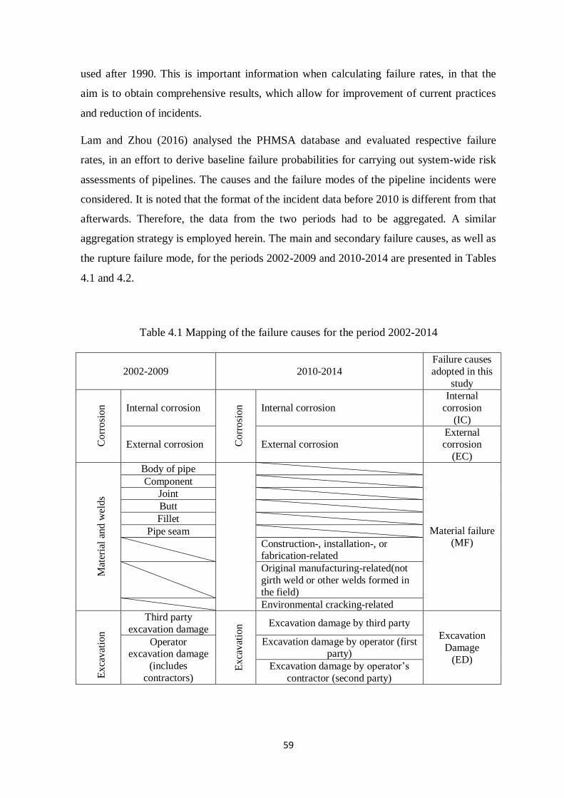
59
used after 1990. This is important information when calculating failure rates, in that the
aim is to obtain comprehensive results, which allow for improvement of current practices
and reduction of incidents.
Lam and Zhou (2016) analysed the PHMSA database and evaluated respective failure
rates, in an effort to derive baseline failure probabilities for carrying out system-wide risk
assessments of pipelines. The causes and the failure modes of the pipeline incidents were
considered. It is noted that the format of the incident data before 2010 is different from that
afterwards. Therefore, the data from the two periods had to be aggregated. A similar
aggregation strategy is employed herein. The main and secondary failure causes, as well as
the rupture failure mode, for the periods 2002-2009 and 2010-2014 are presented in Tables
4.1 and 4.2.
Table 4.1 Mapping of the failure causes for the period 2002-2014
2002-2009 2010-2014
Failure causes
adopted in this
study
Corr
osi
on
Internal corrosion
Corr
osi
on
Internal corrosion
Internal
corrosion
(IC)
External corrosion External corrosion External corrosion
(EC)
Mat
eria
l an
d w
elds
Body of pipe
Material failure (MF)
Component
Joint
Butt
Fillet
Pipe seam
Construction-, installation-, or fabrication-related
Original manufacturing-related(not
girth weld or other welds formed in the field)
Environmental cracking-related
Ex
cav
atio
n
Third party
excavation damage
Ex
cav
atio
n Excavation damage by third party
Excavation
Damage
(ED)
Operator excavation damage
(includes
contractors)
Excavation damage by operator (first party)
Excavation damage by operator’s
contractor (second party)
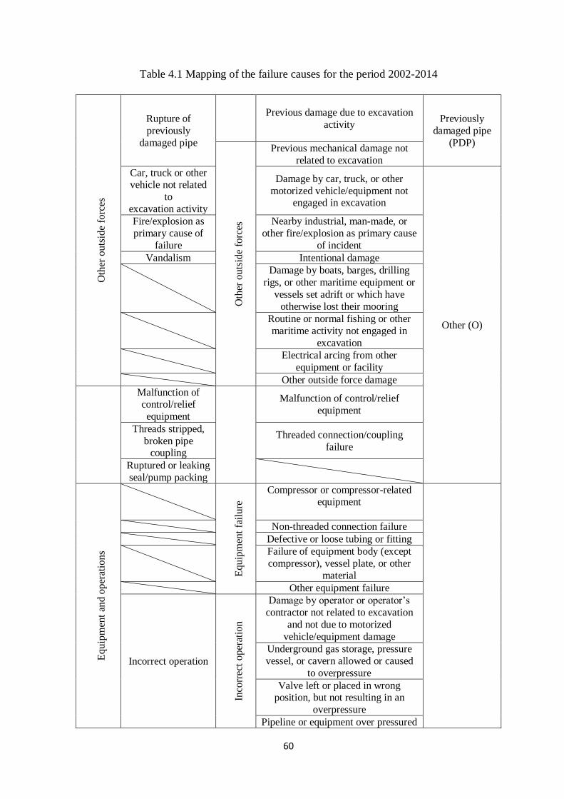
60
Table 4.1 Mapping of the failure causes for the period 2002-2014
Oth
er o
uts
ide
forc
es
Rupture of
previously
damaged pipe
Previous damage due to excavation
activity Previously
damaged pipe
(PDP)
Oth
er o
uts
ide
forc
es
Previous mechanical damage not
related to excavation
Car, truck or other vehicle not related
to
excavation activity
Damage by car, truck, or other
motorized vehicle/equipment not engaged in excavation
Other (O)
Fire/explosion as
primary cause of
failure
Nearby industrial, man-made, or
other fire/explosion as primary cause
of incident
Vandalism Intentional damage
Damage by boats, barges, drilling
rigs, or other maritime equipment or
vessels set adrift or which have
otherwise lost their mooring
Routine or normal fishing or other
maritime activity not engaged in
excavation
Electrical arcing from other
equipment or facility
Other outside force damage
Malfunction of control/relief
equipment
Malfunction of control/relief
equipment
Threads stripped,
broken pipe coupling
Threaded connection/coupling
failure
Ruptured or leaking
seal/pump packing
Eq
uip
men
t an
d o
per
atio
ns
Eq
uip
men
t fa
ilure
Compressor or compressor-related equipment
Non-threaded connection failure
Defective or loose tubing or fitting
Failure of equipment body (except
compressor), vessel plate, or other
material
Other equipment failure
Incorrect operation
Inco
rrect
op
erat
ion
Damage by operator or operator’s
contractor not related to excavation
and not due to motorized
vehicle/equipment damage
Underground gas storage, pressure
vessel, or cavern allowed or caused
to overpressure
Valve left or placed in wrong position, but not resulting in an
overpressure
Pipeline or equipment over pressured
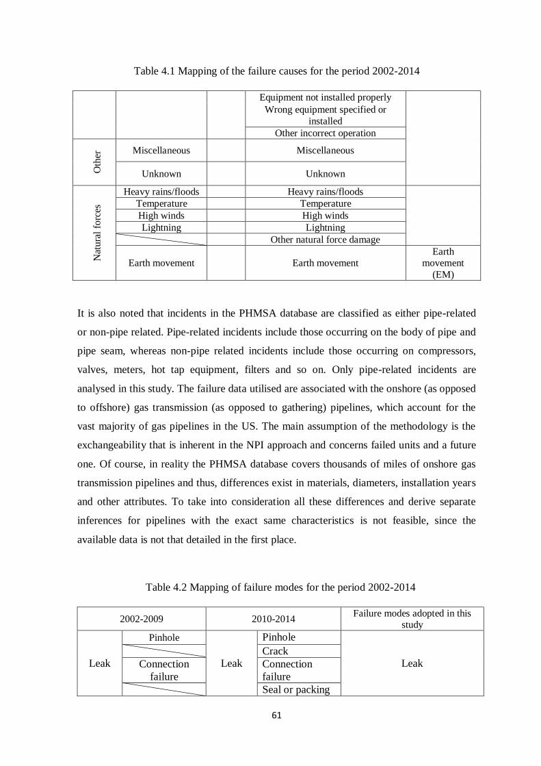
61
Table 4.1 Mapping of the failure causes for the period 2002-2014
Equipment not installed properly
Wrong equipment specified or
installed
Other incorrect operation
Oth
er Miscellaneous
Miscellaneous
Unknown
Unknown
Nat
ura
l fo
rces
Heavy rains/floods Heavy rains/floods
Temperature Temperature
High winds High winds
Lightning Lightning
Other natural force damage
Earth movement
Earth movement Earth
movement
(EM)
It is also noted that incidents in the PHMSA database are classified as either pipe-related
or non-pipe related. Pipe-related incidents include those occurring on the body of pipe and
pipe seam, whereas non-pipe related incidents include those occurring on compressors,
valves, meters, hot tap equipment, filters and so on. Only pipe-related incidents are
analysed in this study. The failure data utilised are associated with the onshore (as opposed
to offshore) gas transmission (as opposed to gathering) pipelines, which account for the
vast majority of gas pipelines in the US. The main assumption of the methodology is the
exchangeability that is inherent in the NPI approach and concerns failed units and a future
one. Of course, in reality the PHMSA database covers thousands of miles of onshore gas
transmission pipelines and thus, differences exist in materials, diameters, installation years
and other attributes. To take into consideration all these differences and derive separate
inferences for pipelines with the exact same characteristics is not feasible, since the
available data is not that detailed in the first place.
Table 4.2 Mapping of failure modes for the period 2002-2014
2002-2009 2010-2014 Failure modes adopted in this
study
Leak
Pinhole
Leak
Pinhole
Leak Crack
Connection
failure
Connection
failure
Seal or packing
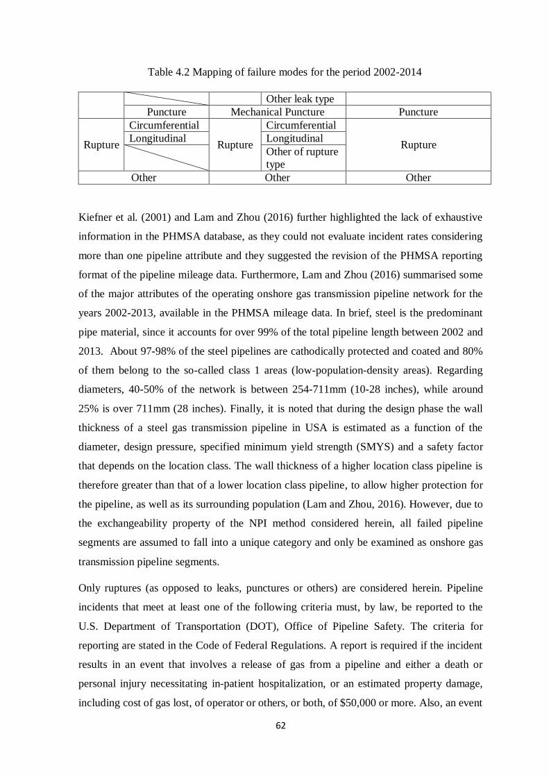
62
Table 4.2 Mapping of failure modes for the period 2002-2014
Other leak type
Puncture Mechanical Puncture Puncture
Rupture
Circumferential
Rupture
Circumferential
Rupture Longitudinal Longitudinal
Other of rupture
type
Other Other Other
Kiefner et al. (2001) and Lam and Zhou (2016) further highlighted the lack of exhaustive
information in the PHMSA database, as they could not evaluate incident rates considering
more than one pipeline attribute and they suggested the revision of the PHMSA reporting
format of the pipeline mileage data. Furthermore, Lam and Zhou (2016) summarised some
of the major attributes of the operating onshore gas transmission pipeline network for the
years 2002-2013, available in the PHMSA mileage data. In brief, steel is the predominant
pipe material, since it accounts for over 99% of the total pipeline length between 2002 and
2013. About 97-98% of the steel pipelines are cathodically protected and coated and 80%
of them belong to the so-called class 1 areas (low-population-density areas). Regarding
diameters, 40-50% of the network is between 254-711mm (10-28 inches), while around
25% is over 711mm (28 inches). Finally, it is noted that during the design phase the wall
thickness of a steel gas transmission pipeline in USA is estimated as a function of the
diameter, design pressure, specified minimum yield strength (SMYS) and a safety factor
that depends on the location class. The wall thickness of a higher location class pipeline is
therefore greater than that of a lower location class pipeline, to allow higher protection for
the pipeline, as well as its surrounding population (Lam and Zhou, 2016). However, due to
the exchangeability property of the NPI method considered herein, all failed pipeline
segments are assumed to fall into a unique category and only be examined as onshore gas
transmission pipeline segments.
Only ruptures (as opposed to leaks, punctures or others) are considered herein. Pipeline
incidents that meet at least one of the following criteria must, by law, be reported to the
U.S. Department of Transportation (DOT), Office of Pipeline Safety. The criteria for
reporting are stated in the Code of Federal Regulations. A report is required if the incident
results in an event that involves a release of gas from a pipeline and either a death or
personal injury necessitating in-patient hospitalization, or an estimated property damage,
including cost of gas lost, of operator or others, or both, of $50,000 or more. Also, an event
63
that is significant in the judgment of the operator, even though it did not meet the two
abovementioned can also be reported (Bolt et al., 2006). Given the aforementioned
reporting criteria and the implications of a typical rupture incident, it can be assumed that
most, if not all, of the actual ruptures were reported to PHMSA. On the other hand, the real
number of leaks or punctures that did not meet the reporting criteria may be significant,
compared to the number of reported leaks and punctures. Therefore, the rupture rate
evaluated using the PHMSA database is thought to be representative of the actual rupture
rate. Moreover, the consequences associated with ruptures are far more severe than those
associated with leaks and punctures. This is evident if one considers that most leaks (about
97%) and punctures (about 90%) did not result in ignition, while the majority of fatalities
and injuries (75% and 83% respectively) were due to ruptures. Therefore, the rupture
incidents are thought to be much more critical for analysis from the risk perspective,
compared to the leak and puncture rates (Lam and Zhou, 2016).
4.2.3 NPI for Competing Failure Causes
Competing risks theory constitutes a credible way of obtaining real world probabilities,
where a pipe segment is not only at risk of rupturing from a specific cause, but also from
any other rupture cause (Hinchliffe and Lambert, 2013). Competing risks theory allows for
breaking down probabilities of failure, to give operators a clearer indication of the risks
they face with each decision they make. This decision-making can regard selection of
maintenance plan, how to optimally allocate resources and finally understanding the
longer-term implications of failure mechanisms.
In this section, an overview of NPI for competing risks is realised, following Coolen and
Yan (2004) and Maturi et al. (2010). According to Hill (1988), 𝐴(𝑥) is a Bayesian, fiducial
and a confidence/tolerance procedure. It is simple, coherent and plausible, whilst at the
same time it is supported by all the serious approaches for statistical inference. According
to Hill (1988), 𝐴(𝑥) constitutes the fundamental solution to the problem of induction. Let
𝑌𝐵1, … , 𝑌𝐵𝑥 , 𝑌𝐵𝑥+1 be continuous and exchangeable random quantities. The values
𝑌𝐵1, … , 𝑌𝐵𝑥 are assumed to be observed and the corresponding ordered values are denoted
by -∞<yB1<…<yBx<∞ (yB0=-∞). It is assumed that no ties occur among the observed values
and if they do, the tied observations differ by trivial amounts (Maturi et al., 2010).
64
For 𝑌𝐵𝑥+1, which represents a future observable random quantity conditional on x
observations, 𝐴(𝑥) is (Hill, 1988):
𝑃(𝑌𝐵𝑥+1 ∈ (𝑦𝐵𝜔−1 , 𝑦𝜔)) = 1
𝑥+1, 𝜔 = 1,… , 𝑥, and
𝑃(𝑌𝐵𝑥+1 ∈ (𝑦𝐵𝑥 ,∞)) = 1
𝑥+1 (4.1)
NPI is a statistical method based on Hill’s assumption 𝐴(𝑥), which can be interpreted as a
post-data assumption, related to exchangeability (Coolen et al., 2002; Maturi et al., 2010).
Inferences based on 𝐴(𝑥) are predictive and nonparametric and are particularly suitable
when there is no additional information, or one does not wish to use such information, for
instance to study effects of additional assumptions underlying other statistical methods.
Such inferences are exactly calibrated (Lawless and Fredette, 2005), which strongly
justifies their use from the frequentist statistics perspective. Instead, 𝐴(𝑥) does not provide
precise probabilities for the events of interest but bounds for probabilities with strong
consistency properties in the theory of interval probability (Walley, 1991; Weichselberger,
2000).
Coolen and Yan (2004) generalised 𝐴(𝑥) into right-censoring 𝐴(𝑥) or rc- 𝐴(𝑥), to take into
account the effect of right-censoring for data, on event times that it is only known that the
event has not yet taken place, in specific terms. The rc- 𝐴(𝑥) uses the additional assumption
that the residual lifetime of a right-censored unit is exchangeable with the residual
lifetimes of all other units that have not yet failed or been censored, at the time of
censoring. To derive the required form of rc- 𝐴(𝑥) for NPI for competing risks, notation is
required for probability mass assigned to intervals, without further restrictions on the
spread within the intervals. The partial specification of probability distributions is called an
M-function and the notation is introduced next.
A probability mass assigned within an interval (aB, bB) in the above described way is
denoted by MYB(aB, bB) and referred to as M-function value for YB on (aB, bB). Since all M-
function values for YB on all intervals should sum up to one, each M-function value should
be in [0,1] and 𝐴(𝑥) can be expressed as 𝑀𝑌𝐵𝑥+1(𝑥𝜔, 𝑥𝜔+1) =1/(x+1), for ω=0,…,x-1 and
𝑀𝑌𝐵𝑥+1(𝑦𝐵𝑥 ,∞) =1/(x+1). The assumption ‘right-censoring 𝐴(𝑥)’ or rc- 𝐴(𝑥), partially
specifies the NPI-based probability distribution for a nonnegative random quantity Xx+1,
65
based on uB event times and vB right censoring times. In specific, it is partially specified by
(ω=0,…, uB; and kB = 1, …,lBω, with t0 = 0 and tuB+1 = ∞):
𝑀𝑋𝑥+1(𝑡𝜔, 𝑡𝜔+1) =1
𝑥+1 ∏
�̃�𝑐𝑟𝐵+1
�̃�𝑐𝑟𝐵{𝑟𝐵:𝑐𝑟𝐵 <𝑡𝜔}
(4.2)
𝑀𝑋𝑥+1(𝑐𝑘𝐵𝜔 , 𝑡𝜔+1) =
1
(𝑥+1)�̃�𝑐𝑘𝐵𝜔
∏�̃�𝑐𝑟𝐵
+1
�̃�𝑐𝑟𝐵{𝑟𝐵 :𝑐𝑟𝐵 <𝑐𝑘𝐵
𝜔 } (4.3)
The product terms are defined as one, if the product is taken over an empty set. This
implicitly assumes non-informative censoring, as a post-data assumption related to
exchangeability, for all items known to be at risk at any time t. If there are no censorings,
then rc- 𝐴(𝑥) is identical to 𝐴(𝑥) (Coolen et al., 2002; Coolen and Yan 2004; Maturi et al.,
2010). The terms �̃�𝑐𝑟𝐵 and �̃�𝑐𝑘𝐵𝜔 describe the number of units in the risk set prior to time
𝑐𝑟𝐵 and 𝑐𝑘𝐵𝜔 , respectively. The definition �̃�0 = 𝑥+1 is used throughout this chapter.
Summing up all M-function values assigned to intervals of this form (which have positive
M-function values and sum up to one over all these intervals) and having the same xω+1 as
right endpoint, gives the probability as follows:
𝑃(𝑋𝑥+1 ∈ (𝑥𝜔, 𝑥𝜔+1)) = 1
𝑥+1 ∏
�̃�𝑐𝑟𝐵+1
�̃�𝑐𝑟𝐵{𝑟𝐵 :𝑐𝑟𝐵 <𝑥𝜔+1}
(4.4)
where 𝑥𝜔, 𝑥𝜔+1 are two sequential failure times.
4.2.3.1 NPI Probabilities for Competing Risks
This study examines the case where a number of kB distinct failure causes (competing
risks) can cause a unit or segment to fail. The unit is assumed to be failing due to the first
occurrence of a cause and then withdrawn from further use and observation. It is assumed
that such failure observations are obtained for x units and that the cause leading to a failure
is known with certainty. For each unit, kB random quantities are considered and Tζ is then
defined for ζ=1,…, kB, where Tζ represents the unit’s time to failure, under the condition
that failure occurs due to cause ζ. These Tζ are considered to be independent continuous
random quantities, which in other words means that the failure causes are assumed to
occur independently and the failure time of the unit is the minimum among kB.
Furthermore, Tζ is assumed to be unique and known with certainty for each unit, while for
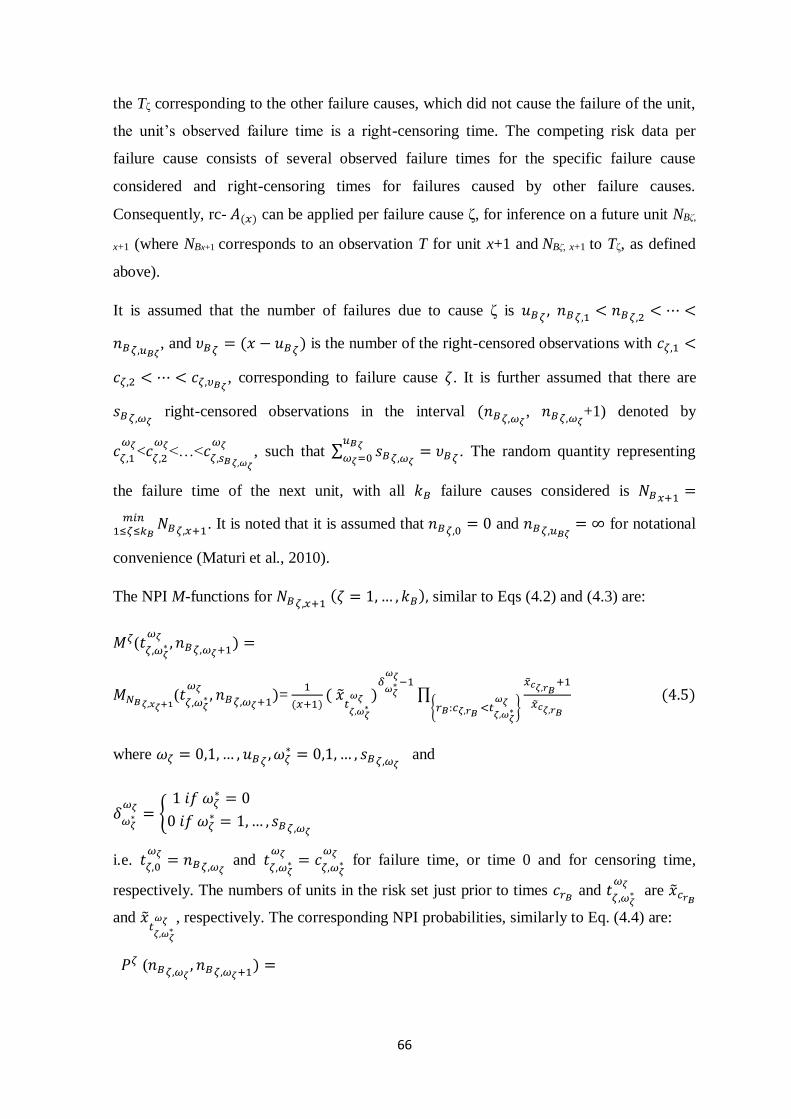
66
the Tζ corresponding to the other failure causes, which did not cause the failure of the unit,
the unit’s observed failure time is a right-censoring time. The competing risk data per
failure cause consists of several observed failure times for the specific failure cause
considered and right-censoring times for failures caused by other failure causes.
Consequently, rc- 𝐴(𝑥) can be applied per failure cause ζ, for inference on a future unit NBζ,
x+1 (where NBx+1 corresponds to an observation T for unit x+1 and NBζ, x+1 to Tζ, as defined
above).
It is assumed that the number of failures due to cause ζ is 𝑢𝐵𝜁 , 𝑛𝐵𝜁,1 < 𝑛𝐵𝜁,2 < ⋯ <
𝑛𝐵𝜁,𝑢𝐵𝜁, and 𝜐𝐵𝜁 = (𝑥 − 𝑢𝐵𝜁) is the number of the right-censored observations with 𝑐𝜁,1 <
𝑐𝜁,2 < ⋯ < 𝑐𝜁,𝜐𝐵𝜁 , corresponding to failure cause 휁. It is further assumed that there are
𝑠𝐵𝜁,𝜔𝜁 right-censored observations in the interval (𝑛𝐵𝜁,𝜔𝜁
, 𝑛𝐵𝜁,𝜔𝜁+1) denoted by
𝑐𝜁,1
𝜔𝜁<𝑐
𝜁,2
𝜔𝜁<…<𝑐
𝜁,𝑠𝐵𝜁,𝜔𝜁
𝜔𝜁, such that ∑ 𝑠𝐵𝜁,𝜔𝜁
𝑢𝐵𝜁𝜔𝜁=0
= 𝜐𝐵𝜁 . The random quantity representing
the failure time of the next unit, with all 𝑘𝐵 failure causes considered is 𝑁𝐵𝑥+1 =
𝑚𝑖𝑛1≤𝜁≤𝑘𝐵
𝑁𝐵𝜁,𝑥+1. It is noted that it is assumed that 𝑛𝐵𝜁,0 = 0 and 𝑛𝐵𝜁,𝑢𝐵𝜁= ∞ for notational
convenience (Maturi et al., 2010).
The NPI M-functions for 𝑁𝐵𝜁,𝑥+1 (휁 = 1, … , 𝑘𝐵), similar to Eqs (4.2) and (4.3) are:
𝑀𝜁(𝑡𝜁,𝜔𝜁
∗
𝜔𝜁 , 𝑛𝐵𝜁,𝜔𝜁+1) =
𝑀𝑁𝐵𝜁,𝑥𝜁+1(𝑡𝜁,𝜔𝜁
∗
𝜔𝜁 , 𝑛𝐵𝜁,𝜔𝜁+1)=
1
(𝑥+1)( �̃�
𝑡𝜁,𝜔𝜁
∗
𝜔𝜁 )𝛿𝜔𝜁∗
𝜔𝜁−1∏
𝑥𝑐𝜁,𝑟𝐵+1
�̃�𝑐𝜁,𝑟𝐵{𝑟𝐵:𝑐𝜁,𝑟𝐵 <𝑡𝜁,𝜔𝜁∗
𝜔𝜁}
(4.5)
where 𝜔𝜁 = 0,1,… , 𝑢𝐵𝜁 ,𝜔𝜁∗ = 0,1,… , 𝑠𝐵𝜁,𝜔𝜁
and
𝛿𝜔𝜁∗
𝜔𝜁 = {1 𝑖𝑓 𝜔𝜁
∗ = 0
0 𝑖𝑓 𝜔𝜁∗ = 1,… , 𝑠𝐵𝜁,𝜔𝜁
i.e. 𝑡𝜁,0
𝜔𝜁 = 𝑛𝐵𝜁,𝜔𝜁 and 𝑡
𝜁,𝜔𝜁∗
𝜔𝜁 = 𝑐𝜁,𝜔𝜁
∗
𝜔𝜁 for failure time, or time 0 and for censoring time,
respectively. The numbers of units in the risk set just prior to times 𝑐𝑟𝐵 and 𝑡𝜁,𝜔𝜁
∗
𝜔𝜁 are �̃�𝑐𝑟𝐵
and �̃�𝑡𝜁,𝜔𝜁
∗
𝜔𝜁 , respectively. The corresponding NPI probabilities, similarly to Eq. (4.4) are:
𝑃𝜁 (𝑛𝐵𝜁,𝜔𝜁, 𝑛𝐵𝜁,𝜔𝜁+1
) =
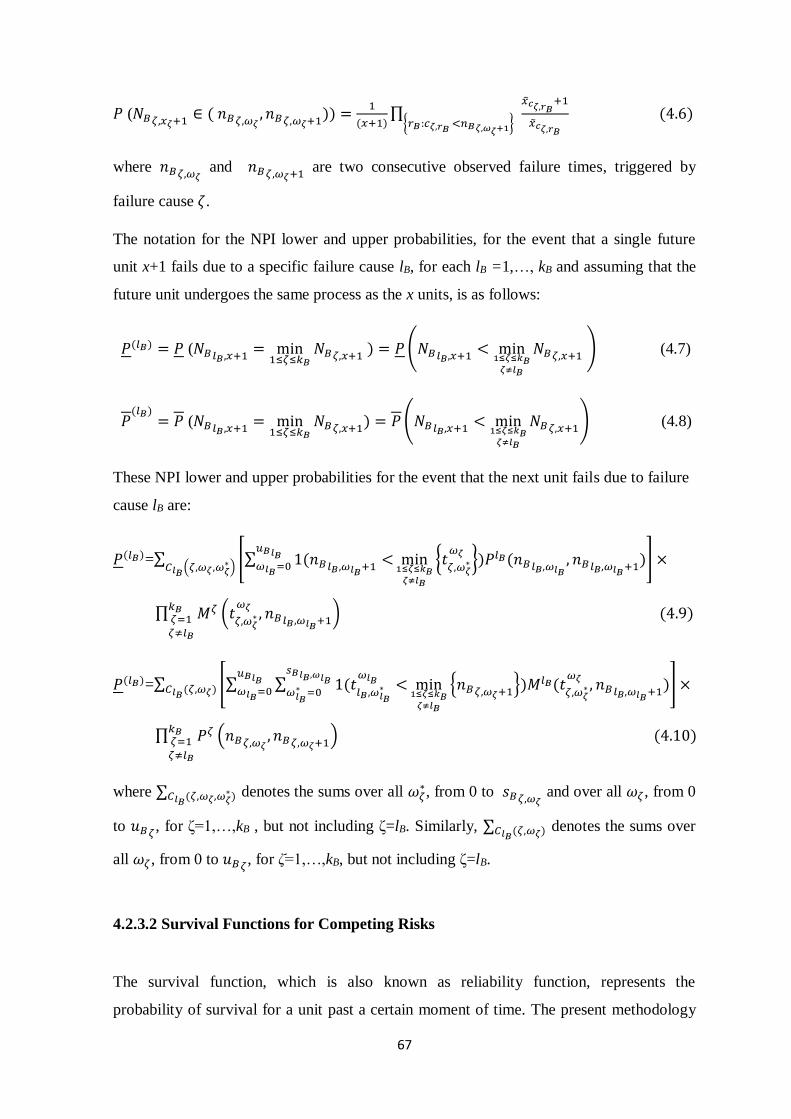
67
𝑃 (𝑁𝐵𝜁,𝑥𝜁+1∈ ( 𝑛𝐵𝜁,𝜔𝜁
, 𝑛𝐵𝜁,𝜔𝜁+1)) =
1
(𝑥+1)∏
�̃�𝑐𝜁,𝑟𝐵+1
𝑥𝑐𝜁,𝑟𝐵
(4.6){𝑟𝐵 :𝑐𝜁,𝑟𝐵 <𝑛𝐵𝜁,𝜔𝜁+1
}
where 𝑛𝐵𝜁,𝜔𝜁 and 𝑛𝐵𝜁,𝜔𝜁+1
are two consecutive observed failure times, triggered by
failure cause 휁.
The notation for the NPI lower and upper probabilities, for the event that a single future
unit x+1 fails due to a specific failure cause lB, for each lB =1,…, kB and assuming that the
future unit undergoes the same process as the x units, is as follows:
𝑃(𝑙𝐵) = 𝑃 (𝑁𝐵𝑙𝐵,𝑥+1 = min1≤𝜁≤𝑘𝐵
𝑁𝐵𝜁,𝑥+1 ) = 𝑃 (𝑁𝐵𝑙𝐵,𝑥+1 < min1≤𝜁≤𝑘𝐵𝜁≠𝑙𝐵
𝑁𝐵𝜁,𝑥+1 ) (4.7)
𝑃(𝑙𝐵)
= 𝑃 (𝑁𝐵𝑙𝐵,𝑥+1 = min1≤𝜁≤𝑘𝐵
𝑁𝐵𝜁,𝑥+1) = 𝑃(𝑁𝐵𝑙𝐵,𝑥+1 < min1≤𝜁≤𝑘𝐵𝜁≠𝑙𝐵
𝑁𝐵𝜁,𝑥+1) (4.8)
These NPI lower and upper probabilities for the event that the next unit fails due to failure
cause lB are:
𝑃(𝑙𝐵)=∑ [∑ 1(𝑛𝐵𝑙𝐵,𝜔𝑙𝐵+1<
𝑢𝐵𝑙𝐵𝜔𝑙𝐵=0
min1≤𝜁≤𝑘𝐵𝜁≠𝑙𝐵
{𝑡𝜁,𝜔𝜁
∗
𝜔𝜁 })𝑃𝑙𝐵(𝑛𝐵𝑙𝐵,𝜔𝑙𝐵, 𝑛𝐵𝑙𝐵,𝜔𝑙𝐵+1
)]𝐶𝑙𝐵(𝜁,𝜔𝜁 ,𝜔𝜁
∗)×
∏ 𝑀𝜁𝑘𝐵𝜁=1𝜁≠𝑙𝐵
(𝑡𝜁,𝜔𝜁
∗
𝜔𝜁, 𝑛𝐵𝑙𝐵 ,𝜔𝑙𝐵+1
) (4.9)
𝑃(𝑙𝐵)=∑ [∑ ∑ 1(𝑡𝑙𝐵,𝜔𝑙𝐵
∗
𝜔𝑙𝐵 <𝑠𝐵𝑙𝐵,𝜔𝑙𝐵𝜔𝑙𝐵∗ =0
𝑢𝐵𝑙𝐵𝜔𝑙𝐵=0
min1≤𝜁≤𝑘𝐵𝜁≠𝑙𝐵
{𝑛𝐵𝜁,𝜔𝜁+1})𝑀𝑙𝐵(𝑡
𝜁,𝜔𝜁∗
𝜔𝜁 , 𝑛𝐵𝑙𝐵,𝜔𝑙𝐵+1)]𝐶𝑙𝐵(𝜁,𝜔𝜁)×
∏ 𝑃𝜁𝑘𝐵𝜁=1𝜁≠𝑙𝐵
(𝑛𝐵𝜁,𝜔𝜁, 𝑛𝐵𝜁,𝜔𝜁+1
) (4.10)
where ∑𝐶𝑙𝐵(𝜁,𝜔𝜁,𝜔𝜁∗) denotes the sums over all 𝜔𝜁
∗, from 0 to 𝑠𝐵𝜁,𝜔𝜁 and over all 𝜔𝜁, from 0
to 𝑢𝐵𝜁, for ζ=1,…,kB , but not including ζ=lB. Similarly, ∑𝐶𝑙𝐵(𝜁,𝜔𝜁) denotes the sums over
all 𝜔𝜁, from 0 to 𝑢𝐵𝜁, for ζ=1,…,kB, but not including ζ=lB.
4.2.3.2 Survival Functions for Competing Risks
The survival function, which is also known as reliability function, represents the
probability of survival for a unit past a certain moment of time. The present methodology
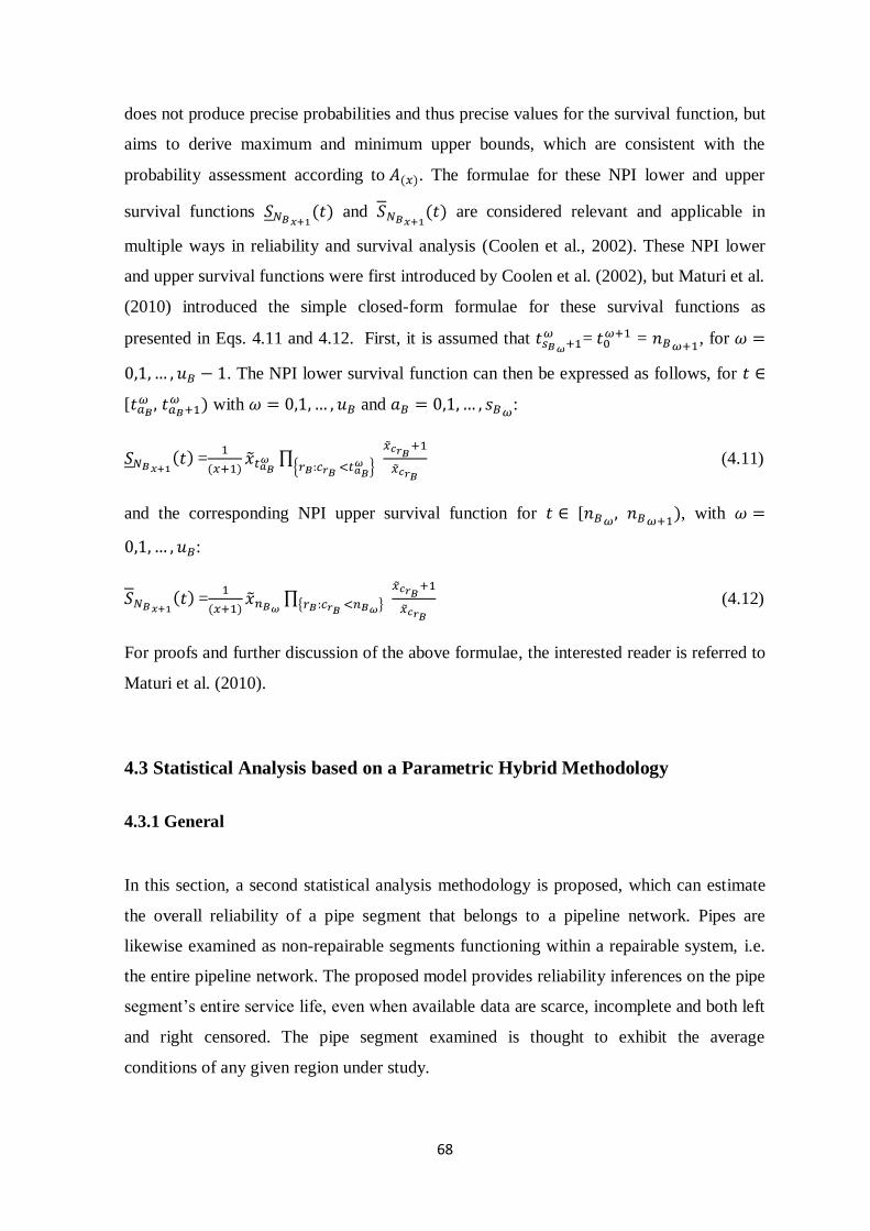
68
does not produce precise probabilities and thus precise values for the survival function, but
aims to derive maximum and minimum upper bounds, which are consistent with the
probability assessment according to 𝐴(𝑥). The formulae for these NPI lower and upper
survival functions 𝑆𝑁𝐵𝑥+1(𝑡) and 𝑆𝑁𝐵𝑥+1(𝑡) are considered relevant and applicable in
multiple ways in reliability and survival analysis (Coolen et al., 2002). These NPI lower
and upper survival functions were first introduced by Coolen et al. (2002), but Maturi et al.
(2010) introduced the simple closed-form formulae for these survival functions as
presented in Eqs. 4.11 and 4.12. First, it is assumed that 𝑡𝑠𝐵𝜔+1𝜔 = 𝑡0
𝜔+1 = 𝑛𝐵𝜔+1, for 𝜔 =
0,1,… , 𝑢𝐵 − 1. The NPI lower survival function can then be expressed as follows, for 𝑡 ∈
[𝑡𝑎𝐵𝜔 , 𝑡𝑎𝐵+1
𝜔 ) with 𝜔 = 0,1,… , 𝑢𝐵 and 𝑎𝐵 = 0,1,… , 𝑠𝐵𝜔:
𝑆𝑁𝐵𝑥+1(𝑡) =
1
(𝑥+1)�̃�𝑡𝑎𝐵
𝜔 ∏�̃�𝑐𝑟𝐵
+1
𝑥𝑐𝑟𝐵{𝑟𝐵:𝑐𝑟𝐵 <𝑡𝑎𝐵
𝜔 } (4.11)
and the corresponding NPI upper survival function for 𝑡 ∈ [𝑛𝐵𝜔, 𝑛𝐵𝜔+1), with 𝜔 =
0,1,… , 𝑢𝐵:
𝑆𝑁𝐵𝑥+1(𝑡) =
1
(𝑥+1)�̃�𝑛𝐵𝜔
∏�̃�𝑐𝑟𝐵
+1
𝑥𝑐𝑟𝐵{𝑟𝐵 :𝑐𝑟𝐵 <𝑛𝐵𝜔}
(4.12)
For proofs and further discussion of the above formulae, the interested reader is referred to
Maturi et al. (2010).
4.3 Statistical Analysis based on a Parametric Hybrid Methodology
4.3.1 General
In this section, a second statistical analysis methodology is proposed, which can estimate
the overall reliability of a pipe segment that belongs to a pipeline network. Pipes are
likewise examined as non-repairable segments functioning within a repairable system, i.e.
the entire pipeline network. The proposed model provides reliability inferences on the pipe
segment’s entire service life, even when available data are scarce, incomplete and both left
and right censored. The pipe segment examined is thought to exhibit the average
conditions of any given region under study.
69
To illustrate the proposed model, the data of Section 4.2.2, i.e. from the PHMSA database
for the period 2002-2014, are employed, with regard to rupture incidents of onshore gas
transmission pipelines. The incident data for the period 2002-2014 are considered fairly
representative of the current state and rehabilitation applications in regards to onshore gas
transmission pipelines. Undoubtedly, PHMSA database covers thousands of miles of
onshore gas transmission pipelines and thus differences exist in materials, diameters, soil
conditions and many other attributes. Furthermore, there is discrepancy among the annual
report database (that contains the pipeline details and mileage information) and the
incident database, which further hinders credible statistical analyses. These uncertainties,
associated with the statistical analysis of the PHMSA database, are taken into
consideration by adopting a hybrid empirical hazard model in liaison with a robust data
processing technique, known as the non-linear quantile regression. This proposed
combined model is thought to produce a credible expectation range of reliability
performance of the infrastructure under consideration, for a complete service life of 100
years, as opposed to the ROCOF approach that can produce average annual failure rates
only for the time period under study, i.e. 13 years for the period 2002-2014.
4.3.2 Hazard Functions and Corresponding Reliability
Gas pipelines, like a lot of the typical large-scale engineering structures, are considered to
follow some similar patterns when it comes to their failure or hazard rate. One of the most
commonly adopted hazard patterns in literature for large-scale engineering structures is the
bath-tub pattern (Sun et al., 2011; Shafiee et al., 2011). This one is adopted in this study
and is assumed to cover the whole lifecycle of gas transmission pipelines, consisting of
three phases as shown in Fig. 4.1. Phase 1 represents the incipient failure phase or ‘infant
mortality’ and the failure rate decreases with time. Phase 2 represents random failures and
the probability of failure is constant. Phase 3 is called the wear-out or degradation phase,
where the number of failures, and thus the failure rate, increase with time. Many models
can be successfully employed to describe these mixed distributions. In this study, the
exponential failure distribution with a constant failure rate λB is employed for phase 2 and
mixed exponential and Weibull distributions for phase 3. These are presented in Eq. (4.13)
and (4.14).

70
Figure 4.1 Bath-tub failure pattern
Phase 1 can be neglected for gas transmission pipelines and is not taken into consideration
herein. It is thought to regard failures at the initial operation years that are mainly caused
by construction and/or manufacturing defects, human errors, as well as random reasons.
However, since gas pipelines are generally large cross-country infrastructure with long
lifetimes, this first phase can be regarded trivial in terms of both duration and magnitude.
As a result, the hazard pattern considered includes only phase 2 and 3, as presented in Fig.
4.2.
ℎ(𝑡) = 𝜆𝐵 for 𝑘1 ≤ 𝑡 ≤ 𝑘2 (4.13)
ℎ(𝑡) = 𝜆𝐵 + (𝛽2𝛼2)(𝑡 − 𝑘2𝛼2
)𝛽2−1 𝑓𝑜𝑟 𝑡 ≥ 𝑘2, 𝛼2 > 0,𝛽2 > 1 (4.14)
where h(t) is the hazard function and t is the age of the pipeline under consideration.
Parameter λB is a constant failure rate and α2, β2 are the scale and shape parameters of the
Weibull distribution. Parameters k1 and k2 refer to the start and the end of phase 2,
respectively.
Once the hazard functions are obtained, the reliability functions can be derived from them.
Eq. (4.15) and (4.16) give continuous reliability curves that correspond to continuous
hazard curves. The reliability functions corresponding to Eq. (4.13) and (4.14) are:
𝑅𝑠1(𝑡) = 𝑒−𝜆𝐵𝑡 𝑓𝑜𝑟 𝑘1 ≤ 𝑡 ≤ 𝑘2 (4.15)
𝑅𝑠2(𝑡) = 𝑒−𝜆𝐵𝑡 + 𝑒
−(𝑡−𝑘2𝛼2
)𝛽2 𝑓𝑜𝑟 𝑡 ≥ 𝑘2, 𝛼2 > 0, 𝛽2 > 1 (4.16)
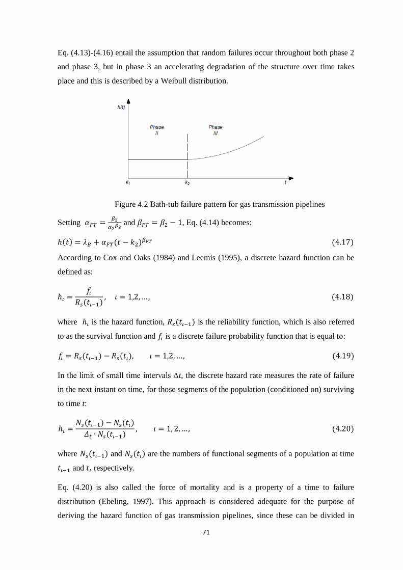
71
Eq. (4.13)-(4.16) entail the assumption that random failures occur throughout both phase 2
and phase 3, but in phase 3 an accelerating degradation of the structure over time takes
place and this is described by a Weibull distribution.
Figure 4.2 Bath-tub failure pattern for gas transmission pipelines
Setting 𝛼𝐹𝑇 =𝛽2
𝛼2𝛽2
and 𝛽𝐹𝑇 = 𝛽2 − 1, Εq. (4.14) becomes:
ℎ(𝑡) = 𝜆𝐵 + 𝛼𝐹𝑇(𝑡 − 𝑘2)𝛽𝐹𝑇 (4.17)
According to Cox and Oaks (1984) and Leemis (1995), a discrete hazard function can be
defined as:
ℎ𝜄 =𝑓𝜄
𝑅𝑠(𝑡𝜄−1), 𝜄 = 1,2,…, (4.18)
where ℎ𝜄 is the hazard function, 𝑅𝑠(𝑡𝜄−1) is the reliability function, which is also referred
to as the survival function and 𝑓𝜄 is a discrete failure probability function that is equal to:
𝑓𝜄 = 𝑅𝑠(𝑡𝜄−1) − 𝑅𝑠(𝑡𝜄), 𝜄 = 1,2,…, (4.19)
In the limit of small time intervals Δt, the discrete hazard rate measures the rate of failure
in the next instant on time, for those segments of the population (conditioned on) surviving
to time t:
ℎ𝜄 =𝛮𝑠(𝑡𝜄−1) − 𝑁𝑠(𝑡𝜄)
𝛥𝑡 ∙ 𝑁𝑠(𝑡𝜄−1), 𝜄 = 1, 2,…, (4.20)
where 𝛮𝑠(𝑡𝜄−1) and 𝑁𝑠(𝑡𝜄) are the numbers of functional segments of a population at time
𝑡𝜄−1 and 𝑡𝜄 respectively.
Eq. (4.20) is also called the force of mortality and is a property of a time to failure
distribution (Ebeling, 1997). This approach is considered adequate for the purpose of
deriving the hazard function of gas transmission pipelines, since these can be divided in
72
segments of same or similar characteristics, as described in the following example of
section 4.5. Also, this approach can efficiently deal with scarce, left or right-censored data,
by estimating discrete hazards solely at times that failure data are available (Sun et al.,
2011).
Once the hazard function has been derived, parameters of Eq. (4.17) should be then
estimated. The adopted approach for parameter estimation is comprised of two parts. The
first part is a heuristic method proposed elsewhere (Sun et al., 2011) and regards
parameters λΒ and k2. In specific, parameter k2 can be determined by the discrete hazard bar
chart that is produced from Eq. (4.20). Parameter k2 is thought to be easily attainable in the
presence of complete and consistent data, but due to statistical uncertainties and
fluctuations, this is not always the case and expert opinion is usually necessary.
Furthermore, λΒ is a constant rate of the exponential failure distribution and represents the
random failure phase. The value of λΒ can be obtained as the average of discrete hazard
values that belong to this phase, i.e. phase 2. It can be defined as:
𝜆𝛣 =1
𝑁𝑘∑ ℎ𝜄
1<𝜄≤𝑁𝑘
(4.21)
where k=k2-k1
Finally, parameters αFT and βFT need to be estimated from the wear-out phase, i.e. phase 3,
by means of the robust graphical method described in the next section.
4.3.3 Non-linear Quantile Regression
The most commonly adopted methods in literature for parameter estimation of
probabilistic models are the maximum likelihood method and the linear (or non-linear)
least-squares regression method (Rigdon and Basu, 2000; Basile et al. 2004; Caleyo et al.
2008; Tee et al., 2013; Morrison and Spencer, 2014). Maximum likelihood method has the
limitation that requires sufficient failure data to produce credible results. Least-squares
regression has often been applied to derive the mean response of the dependent variable
(hazard function herein), as a function of the independent variable (time herein). However,
both of these are thought to have difficulty in describing scarce and censored data and also
fail to yield a complete picture of the variables’ relationships. This is especially the case
73
for heteroscedastic data, data with non-Gaussian error distributions and data derived from
sample selections. Also, they are sensitive to extreme outliers that can distort the results
significantly. Furthermore, many times the researcher aims to obtain an upper bound of the
relationship such that the final result is conservative. This is especially the case in
applications such as gas pipelines, where extremes are important and upper quantiles of
rupture incident levels are critical from a public health perspective. This can be achieved
by the quantile regression, since it can estimate multiple rates of change, i.e. slopes, from
the minimum to maximum response (Cade and Noon, 2003; Chen, 2005).
Non-linear quantile regression is considered to be able to deal with the aforementioned
challenges and is employed for the data analysis and estimation of the parameters αFT and
βFT, contained in Eq. (4.17). It is a quantifiable, repeatable and non-biased statistical
methodology that provides estimates for a given quantile or, equivalently, a given
probability of exceedance. The greatest quantile that can be calculated by the method,
depends on the number of data points available in the dataset. For datasets with small
numbers of data, for instance less than 20 data points, it is likely that the quantile
regression lines for quantiles τq = {0.95, 0.98, and 0.99}, might be represented by the same
line. The existence of various slope estimates for different quantiles, constitutes an indirect
confirmation of the heteroscedasticity of the dataset (Morrison and Spencer, 2014). Errors
are assumed to be independent and identically distributed (iid) in this study.
Typically a response variable yB is some function of predictor variables xB, so that 𝑦𝐵 =
𝑓(𝑥𝐵). To this end, Eq. (4.17) is rearranged and set as follows:
𝑄𝑦𝐵 = ℎ(𝑡) − 𝜆𝛣 and 𝑥𝐵 = 𝑡 − 𝑘2, so that the following non-linear relationship can be
defined:
𝑄𝑦𝐵 = 𝛼𝐹𝑇 ∙ 𝑥𝐵𝛽𝐹𝑇 (4.22)
The conditional quantiles denoted by 𝑄𝑦𝐵(𝜏𝑞|𝑥𝐵) are the inverse of the conditional
cumulative distribution function of the response variable 𝐹𝑦𝐵−1(𝜏𝑞|𝑥𝐵), where τq ϵ [0,1]
denotes the quantiles (Koenker and Machado, 1999). For example, for τq =0.90,
𝑄𝑦𝐵(0.90|𝑥𝐵) is the 90th percentile of the distribution of yB conditional on the values of xB,
i.e. 90% of the values of yB are less than or equal to the specified function of xB. In contrast
to the mean regression technique, which employs the least-squares procedure, parameters
from the quantile regression are obtained by minimizing (Cao and Dean, 2015):
74
𝑆𝑄 = ∑ 𝜏𝑞[𝑄𝑦𝐵𝜄≥�̂�𝑦𝐵𝜄
𝑄𝑦𝐵𝜄 − �̂�𝑦𝐵𝜄] +∑ (1 − 𝜏𝑞) [𝑄𝑦𝐵𝜄 − �̂�𝑦𝐵𝜄] (4.23)𝑄𝑦𝐵𝜄
<�̂�𝑦𝐵𝜄
The non-linear iid quantile regression problem is solved using an interior point algorithm.
It is analytically described in Koenker and Park (1996). More references to the
methodology and code of non-linear regression are provided herein. The non-linear
quantile regression method is part of the quantile regression package quantreg in R
software, which was used for the respective estimations herein (Koenker, 2012). The
method directly generates quantiles at a specified exceedance level, removing the
requirement for subjectively processing the data and therefore results in a method that
produces a unique answer (Morrison and Spencer, 2014; Cao and Wang, 2015).
4.4 Case Study based on the NPI methodology
4.4.1 General
The purpose of this case study is to numerically apply the NPI for competing risks in the
aforementioned PHMSA dataset and then derive lower and upper probabilities, as well as
survival functions for different competing failure causes, for the future onshore gas
transmission pipe segment that will fail due to rupture. Only ruptured pipes are of interest
in this study. Given that only a tiny fraction of the overall number of pipes fails in the
entire US gas transmission pipeline network, applying the competing risks theory on the
entire network would be unfruitful, since the impact of incidents is trivial and the same
results are produced, either for realistic competing risks’ probabilities or for net
probabilities. A net survival probability is for instance one that describes the probability of
surviving external corrosion in the hypothetical world where a pipeline cannot rupture
from any other cause. Relative survival and cause-specific survival attempt to estimate
this, under specific assumptions. The second methodology proposed in this chapter covers
such an analysis, one that takes into account the entire US gas transmission pipeline
network. The focus thus herein, is to analyse the rupture incidents, so that realistic
marginal expectations of the interdependency among failure causes can be derived and a
cumulative rupture function of pipe segment ruptures can be defined in a comprehensive
way.
75
The main assumption of the methodology is that the future pipe segment undergoes the
same process and conditions, as the ones that have reportedly failed thus far. Taking into
consideration that only a very specific category of pipelines, i.e. onshore gas transmission,
is examined, it is reasonable to assume that similar behaviour is expected from this type of
pipelines. Besides, as described in Section 4.2, there are certain attributes that are common
for the majority of onshore gas transmission pipelines that operated between 2002-2014
(class location 1, carbon steel material of construction and cathodic and coating
protection). The future pipe segment that is examined against rupture is assumed to be a
typical 12m long pipe segment. For the sake of exchangeability which is inherent in the
NPI approach, each one of the 179 reported ruptures is assumed to originate from one or a
number of defects confined to the 12m pipe segment, irrespective of the propagation
length, post rupture initiation. The rupture lengths reported by pipeline operators in the
database besides, were found to be on average around 10m, which corroborates this
assumption.
Next, from the different types of failure that stem from different (thus competing) failure
causes, only rupture is examined. In the period 2002-2014, 189 pipe-related rupture
incidents were found in the database. The time to failure is of interest in the methodology
and as a result the installation dates of the pipelines that failed due to rupture were listed.
However, 10 rupture incidents concerned pipelines whose installation dates were unknown
(had not been reported to PHMSA). These 10 rupture incidents were not taken into
consideration, without significantly distorting the analysis. In Tables 4.3 and 4.4 a
breakdown of the numbers and percentages of the different failure causes for the 189 and
the 179 rupture cases is presented. It can be observed that ignoring the incidents with
unknown installation dates (and thus times to failure), does not impact rupture frequencies
due to different failure causes significantly. The time to failure is estimated by subtracting
the year of installation from the year of failure, for each rupture incident.
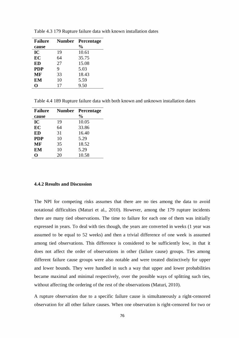
76
Table 4.3 179 Rupture failure data with known installation dates
Failure
cause
Number Percentage
%
IC 19 10.61
EC 64 35.75
ED 27 15.08
PDP 9 5.03
MF 33 18.43
EM 10 5.59
O 17 9.50
Table 4.4 189 Rupture failure data with both known and unknown installation dates
Failure
cause
Number Percentage
%
IC 19 10.05
EC 64 33.86
ED 31 16.40
PDP 10 5.29
MF 35 18.52
EM 10 5.29
O 20 10.58
4.4.2 Results and Discussion
The NPI for competing risks assumes that there are no ties among the data to avoid
notational difficulties (Maturi et al., 2010). However, among the 179 rupture incidents
there are many tied observations. The time to failure for each one of them was initially
expressed in years. To deal with ties though, the years are converted in weeks (1 year was
assumed to be equal to 52 weeks) and then a trivial difference of one week is assumed
among tied observations. This difference is considered to be sufficiently low, in that it
does not affect the order of observations in other (failure cause) groups. Ties among
different failure cause groups were also notable and were treated distinctively for upper
and lower bounds. They were handled in such a way that upper and lower probabilities
became maximal and minimal respectively, over the possible ways of splitting such ties,
without affecting the ordering of the rest of the observations (Maturi, 2010).
A rupture observation due to a specific failure cause is simultaneously a right-censored
observation for all other failure causes. When one observation is right-censored for two or
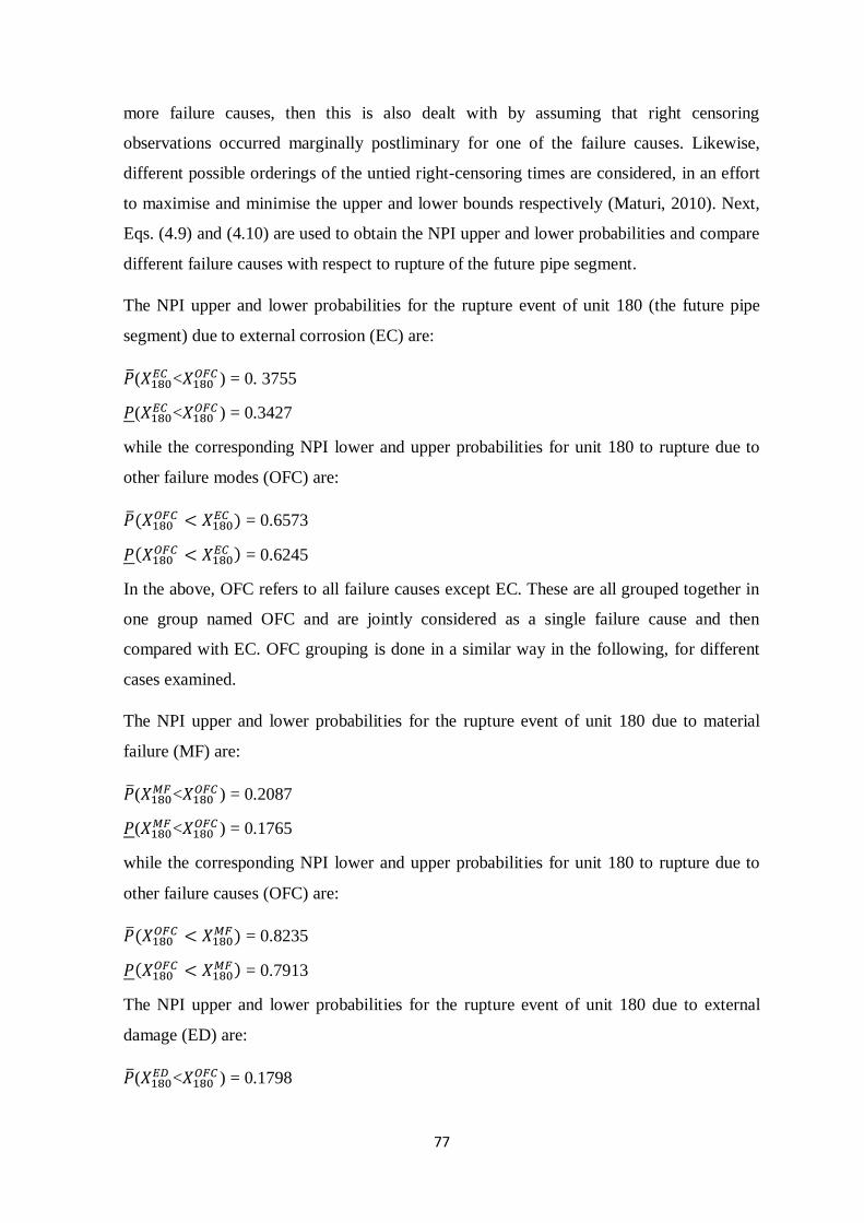
77
more failure causes, then this is also dealt with by assuming that right censoring
observations occurred marginally postliminary for one of the failure causes. Likewise,
different possible orderings of the untied right-censoring times are considered, in an effort
to maximise and minimise the upper and lower bounds respectively (Maturi, 2010). Next,
Eqs. (4.9) and (4.10) are used to obtain the NPI upper and lower probabilities and compare
different failure causes with respect to rupture of the future pipe segment.
The NPI upper and lower probabilities for the rupture event of unit 180 (the future pipe
segment) due to external corrosion (EC) are:
�̅�(𝑋180𝐸𝐶 <𝑋180
𝑂𝐹𝐶 ) = 0. 3755
𝑃(𝑋180𝐸𝐶 <𝑋180
𝑂𝐹𝐶 ) = 0.3427
while the corresponding NPI lower and upper probabilities for unit 180 to rupture due to
other failure modes (OFC) are:
�̅�(𝑋180𝑂𝐹𝐶 < 𝑋180
𝐸𝐶 ) = 0.6573
𝑃(𝑋180𝑂𝐹𝐶 < 𝑋180
𝐸𝐶 ) = 0.6245
In the above, OFC refers to all failure causes except EC. These are all grouped together in
one group named OFC and are jointly considered as a single failure cause and then
compared with EC. OFC grouping is done in a similar way in the following, for different
cases examined.
The NPI upper and lower probabilities for the rupture event of unit 180 due to material
failure (MF) are:
�̅�(𝑋180𝑀𝐹<𝑋180
𝑂𝐹𝐶 ) = 0.2087
𝑃(𝑋180𝑀𝐹<𝑋180
𝑂𝐹𝐶 ) = 0.1765
while the corresponding NPI lower and upper probabilities for unit 180 to rupture due to
other failure causes (OFC) are:
�̅�(𝑋180𝑂𝐹𝐶 < 𝑋180
𝑀𝐹) = 0.8235
𝑃(𝑋180𝑂𝐹𝐶 < 𝑋180
𝑀𝐹) = 0.7913
The NPI upper and lower probabilities for the rupture event of unit 180 due to external
damage (ED) are:
�̅�(𝑋180𝐸𝐷 <𝑋180
𝑂𝐹𝐶 ) = 0.1798

78
𝑃(𝑋180𝐸𝐷 <𝑋180
𝑂𝐹𝐶 ) = 0.1474
while the corresponding NPI lower and upper probabilities for unit 180 to rupture due to
other failure causes (OFC) are:
�̅�(𝑋180𝑂𝐹𝐶 < 𝑋180
𝐸𝐷 ) = 0.8526
𝑃(𝑋180𝑂𝐹𝐶 < 𝑋180
𝐸𝐷 ) = 0.8202
It is observed that for each one of the above three pairs of failure causes (EC and OFC, MF
and OFC, ED and OFC) examined, the lower and upper probabilities satisfy the conjugacy
property (Coolen, 1996). This is due to the fact that implicit in this method is the
assumption that the future segment eventually ruptures and this is assumed to happen with
certainty. When comparing one failure cause group with another group (or more than one
group as shown next), the resulting NPI upper and lower probabilities can provide either a
weak or a strong indication about the future unit’s failure (Maturi et al., 2010). For
example, the NPI lower and upper probabilities presented above, contain a strong
indication that the future segment will rupture due to another failure cause (OFC) when all
the other failure causes are grouped together, instead of when EC, MF and ED failure
causes are separate. This holds because:
𝑃(𝑋180𝑂𝐹𝐶 < 𝑋180
𝐸𝐶 ) > �̅�(𝑋180𝐸𝐶 <𝑋180
𝑂𝐹𝐶 ) and likewise for MF and ED.
In the next example, the weak indication term is also discussed. A different grouping of the
same time to failure data is illustrated. In specific, groups with three failure causes are
considered each time and inferences in the form of weak and strong indications are derived
in a similar manner to the case of two groups.
The NPI upper and lower probabilities for the event that unit 180 will rupture due to either
EC, MF or OFC are as follows:
�̅�(𝑋180𝐸𝐶 < min {𝑋180
𝑀𝐹 , 𝑋180𝑂𝐹𝐶}) = 0.3755
𝑃(𝑋180𝐸𝐶 < min{𝑋180
𝑀𝐹 , 𝑋180𝑂𝐹𝐶}) = 0.3321
�̅�(𝑋180𝑂𝐹𝐶 < min {𝑋180
𝑀𝐹 , 𝑋180𝐸𝐶 }) = 0.4806
𝑃(𝑋180𝑂𝐹𝐶 < min{𝑋180
𝑀𝐹 , 𝑋180𝐸𝐶 }) = 0.4407
�̅�(𝑋180𝑀𝐹 < min {𝑋180
𝐸𝐶 , 𝑋180𝑂𝐹𝐶}) = 0.2087

79
𝑃(𝑋180𝑀𝐹 < min {𝑋180
𝐸𝐶 , 𝑋180𝑂𝐹𝐶}) = 0.1707
The fact that 𝑃(𝑋180𝐸𝐶 < min{𝑋180
𝑀𝐹 , 𝑋180𝑂𝐹𝐶}) > �̅�(𝑋180
𝑀𝐹 < min {𝑋180𝐸𝐶 , 𝑋180
𝑂𝐹𝐶}) provides a strong
indication that EC is more likely than MF to cause a rupture, with all other failure causes
grouped together as OFC.
The NPI upper and lower probabilities for the event that unit 180 will rupture due to either
EC, excavation damage (ED) or OFC are as follows:
�̅�(𝑋180𝐸𝐶 < min {𝑋180
𝐸𝐷 , 𝑋180𝑂𝐹𝐶}) = 0.3755
𝑃(𝑋180𝐸𝐶 < min{𝑋180
𝐸𝐷 , 𝑋180𝑂𝐹𝐶}) = 0.3321
�̅�(𝑋180𝑂𝐹𝐶 < min {𝑋180
𝐸𝐷 , 𝑋180𝐸𝐶 }) = 0.5097
𝑃(𝑋180𝑂𝐹𝐶 < min{𝑋180
𝐸𝐷 , 𝑋180𝐸𝐶 }) = 0.4667
�̅�(𝑋180𝐸𝐷 < min {𝑋180
𝐸𝐶 , 𝑋180𝑂𝐹𝐶}) = 0.1798
𝑃(𝑋180𝐸𝐷 < min {𝑋180
𝐸𝐶 , 𝑋180𝑂𝐹𝐶}) = 0.1449
The NPI upper and lower probabilities for the event that unit 180 will rupture due to either
MF, ED or OFC are as follows:
�̅�(𝑋180𝐸𝐷 < min {𝑋180
𝑀𝐹 , 𝑋180𝑂𝐹𝐶}) = 0.1798
𝑃(𝑋180𝐸𝐷 < min{𝑋180
𝑀𝐹 , 𝑋180𝑂𝐹𝐶}) = 0.1449
�̅�(𝑋180𝑀𝐹 < min {𝑋180
𝐸𝐷 , 𝑋180𝑂𝐹𝐶}) = 0.2087
𝑃(𝑋180𝑀𝐹 < min{𝑋180
𝐸𝐷 , 𝑋180𝑂𝐹𝐶}) = 0.1707
�̅�(𝑋180𝑂𝐹𝐶 < min {𝑋180
𝐸𝐷 , 𝑋180𝑀𝐹}) = 0.6761
𝑃(𝑋180𝑂𝐹𝐶 < min {𝑋180
𝐸𝐷 , 𝑋180𝑀𝐹}) = 0.6284
In a similar manner, these NPI lower and upper probabilities can also provide weak
indications, for the event that the future segment ruptures due to a specific failure cause.
For example, the future rupture event due to ED is slightly less likely compared to rupture
due to MF, with all other failure causes grouped together (OFC). This is because:
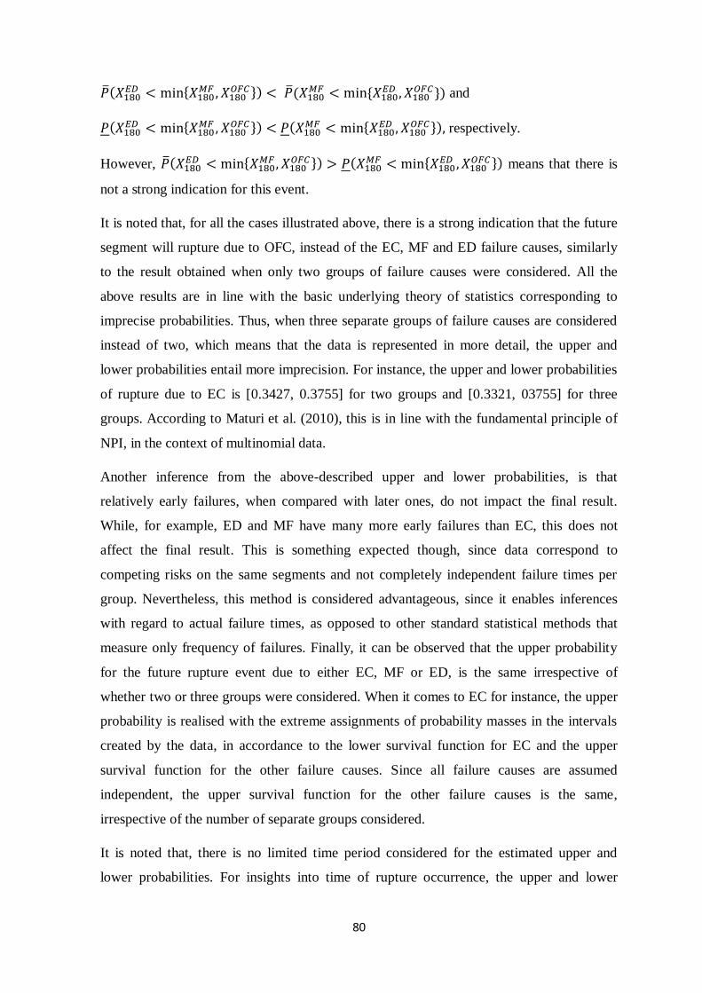
80
�̅�(𝑋180𝐸𝐷 < min{𝑋180
𝑀𝐹 , 𝑋180𝑂𝐹𝐶}) < �̅�(𝑋180
𝑀𝐹 < min {𝑋180𝐸𝐷 , 𝑋180
𝑂𝐹𝐶}) and
𝑃(𝑋180𝐸𝐷 < min{𝑋180
𝑀𝐹 , 𝑋180𝑂𝐹𝐶}) < 𝑃(𝑋180
𝑀𝐹 < min{𝑋180𝐸𝐷 , 𝑋180
𝑂𝐹𝐶}), respectively.
However, �̅�(𝑋180𝐸𝐷 < min{𝑋180
𝑀𝐹 , 𝑋180𝑂𝐹𝐶}) > 𝑃(𝑋180
𝑀𝐹 < min{𝑋180𝐸𝐷 , 𝑋180
𝑂𝐹𝐶}) means that there is
not a strong indication for this event.
It is noted that, for all the cases illustrated above, there is a strong indication that the future
segment will rupture due to OFC, instead of the EC, MF and ED failure causes, similarly
to the result obtained when only two groups of failure causes were considered. All the
above results are in line with the basic underlying theory of statistics corresponding to
imprecise probabilities. Thus, when three separate groups of failure causes are considered
instead of two, which means that the data is represented in more detail, the upper and
lower probabilities entail more imprecision. For instance, the upper and lower probabilities
of rupture due to EC is [0.3427, 0.3755] for two groups and [0.3321, 03755] for three
groups. According to Maturi et al. (2010), this is in line with the fundamental principle of
NPI, in the context of multinomial data.
Another inference from the above-described upper and lower probabilities, is that
relatively early failures, when compared with later ones, do not impact the final result.
While, for example, ED and MF have many more early failures than EC, this does not
affect the final result. This is something expected though, since data correspond to
competing risks on the same segments and not completely independent failure times per
group. Nevertheless, this method is considered advantageous, since it enables inferences
with regard to actual failure times, as opposed to other standard statistical methods that
measure only frequency of failures. Finally, it can be observed that the upper probability
for the future rupture event due to either EC, MF or ED, is the same irrespective of
whether two or three groups were considered. When it comes to EC for instance, the upper
probability is realised with the extreme assignments of probability masses in the intervals
created by the data, in accordance to the lower survival function for EC and the upper
survival function for the other failure causes. Since all failure causes are assumed
independent, the upper survival function for the other failure causes is the same,
irrespective of the number of separate groups considered.
It is noted that, there is no limited time period considered for the estimated upper and
lower probabilities. For insights into time of rupture occurrence, the upper and lower
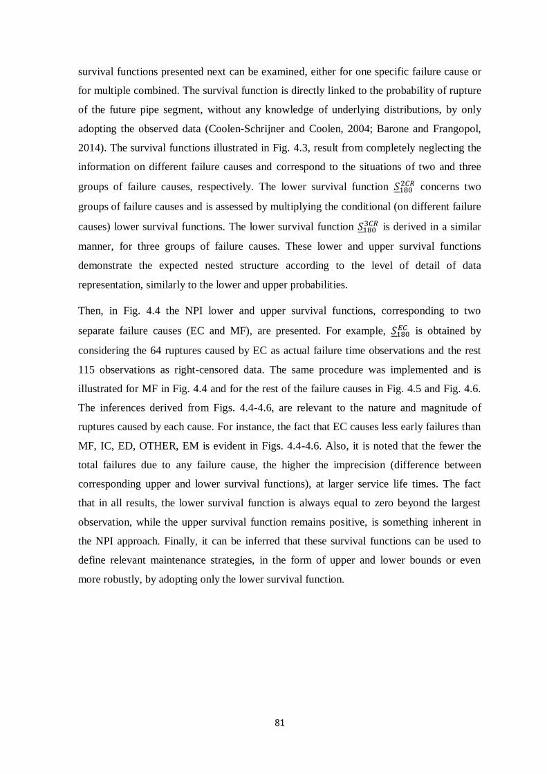
81
survival functions presented next can be examined, either for one specific failure cause or
for multiple combined. The survival function is directly linked to the probability of rupture
of the future pipe segment, without any knowledge of underlying distributions, by only
adopting the observed data (Coolen-Schrijner and Coolen, 2004; Barone and Frangopol,
2014). The survival functions illustrated in Fig. 4.3, result from completely neglecting the
information on different failure causes and correspond to the situations of two and three
groups of failure causes, respectively. The lower survival function 𝑆1802𝐶𝑅 concerns two
groups of failure causes and is assessed by multiplying the conditional (on different failure
causes) lower survival functions. The lower survival function 𝑆1803𝐶𝑅 is derived in a similar
manner, for three groups of failure causes. These lower and upper survival functions
demonstrate the expected nested structure according to the level of detail of data
representation, similarly to the lower and upper probabilities.
Then, in Fig. 4.4 the NPI lower and upper survival functions, corresponding to two
separate failure causes (EC and MF), are presented. For example, 𝑆180𝐸𝐶 is obtained by
considering the 64 ruptures caused by EC as actual failure time observations and the rest
115 observations as right-censored data. The same procedure was implemented and is
illustrated for MF in Fig. 4.4 and for the rest of the failure causes in Fig. 4.5 and Fig. 4.6.
The inferences derived from Figs. 4.4-4.6, are relevant to the nature and magnitude of
ruptures caused by each cause. For instance, the fact that EC causes less early failures than
MF, IC, ED, OTHER, EM is evident in Figs. 4.4-4.6. Also, it is noted that the fewer the
total failures due to any failure cause, the higher the imprecision (difference between
corresponding upper and lower survival functions), at larger service life times. The fact
that in all results, the lower survival function is always equal to zero beyond the largest
observation, while the upper survival function remains positive, is something inherent in
the NPI approach. Finally, it can be inferred that these survival functions can be used to
define relevant maintenance strategies, in the form of upper and lower bounds or even
more robustly, by adopting only the lower survival function.
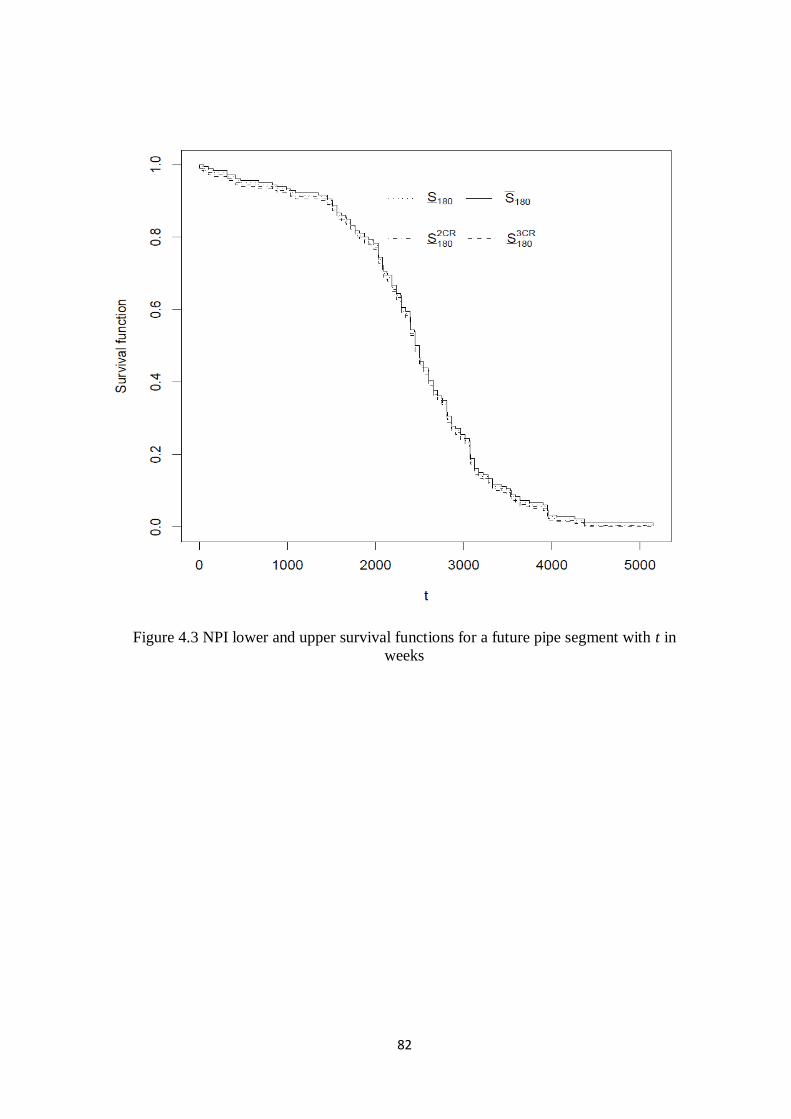
82
Figure 4.3 NPI lower and upper survival functions for a future pipe segment with t in
weeks
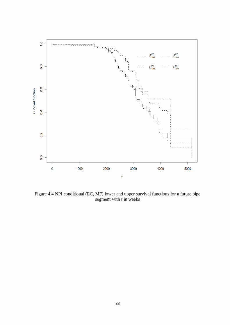
83
Figure 4.4 NPI conditional (EC, MF) lower and upper survival functions for a future pipe
segment with t in weeks
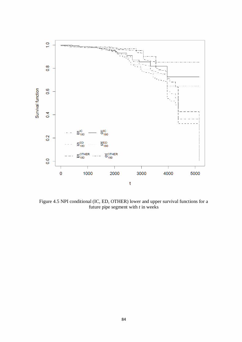
84
Figure 4.5 NPI conditional (IC, ED, OTHER) lower and upper survival functions for a
future pipe segment with t in weeks
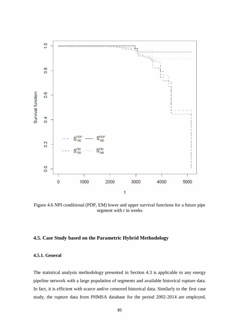
85
Figure 4.6 NPI conditional (PDP, EM) lower and upper survival functions for a future pipe
segment with t in weeks
4.5. Case Study based on the Parametric Hybrid Methodology
4.5.1. General
The statistical analysis methodology presented in Section 4.3 is applicable to any energy
pipeline network with a large population of segments and available historical rupture data.
In fact, it is efficient with scarce and/or censored historical data. Similarly to the first case
study, the rupture data from PHMSA database for the period 2002-2014 are employed,
86
with respect to onshore gas transmission pipelines. Moreover, the installation dates of
pipes are used, in order to derive the respective hazard and reliability functions. Upon
rupture, the pipe segment is assumed to be discarded and replaced by a new one,
considering the segments as non-repairable. The proposed statistical analysis methodology,
assumes that the network under consideration, can be divided into a number of similar pipe
segments, based on an adequate segmentation length. The resulting population of segments
is considered to operate under similar conditions. This is also assumed for those pipe
segments that have reportedly failed. This assumption certainly entails some level of
approximation but, as already analysed in Section 4.3, only one category of pipelines
(onshore gas transmission) is examined and thus, it is considered reasonable to expect, at a
significant extent, similar behaviour from this specific type of pipelines.
The segmentation length is assumed to be 12.5m, which is approximately the typical
length of a newly-constructed pipe segment in industry. Also, rupture incidents are
assumed to be confined to the 12.5m pipe segment. The rupture lengths of the 189
incidents, which are reported by pipeline operators in the database for the period 2002-
2014, was found to be around this magnitude (on average around 10m). As a result, the
assumption that a pipe segment of 12.5m is discarded after rupture and replaced by a new
one is considered fairly representative of real industry practice. Thus, the gas transmission
pipelines are assumed to form a statistically-related population of 12.5m long segments,
performing a similar function in a similar location. As mentioned already, 189 pipe-related
rupture incidents were reported in PHMSA, in the period 2002-2014. The time to rupture
is of interest and as a result the installation dates of the ruptured pipes are considered.
However, 10 rupture incidents concerned pipes whose installation dates are unknown (not
reported in the PHMSA). These 10 rupture incidents are not taken into consideration,
adding extra uncertainty when all failure cause rupture incidents are examined. However,
this uncertainty is thought to be counterbalanced at a significant extent, by the fact that a
percentage of approximately 2% of the total mileage on an annual basis is of unknown age
(installation date) as well and thus neglected in the analysis.
Furthermore, the lack of detailed information in the PHMSA mileage database, with
respect to the age of the operating network, necessitates the estimation of average values.
For every year between 2002 and 2014, the installation dates are available per decade. As a
result, different age groups of operating pipelines can be inferred for every year between
2002 and 2014. A careful examination of the yearly changes of pipeline lengths for each
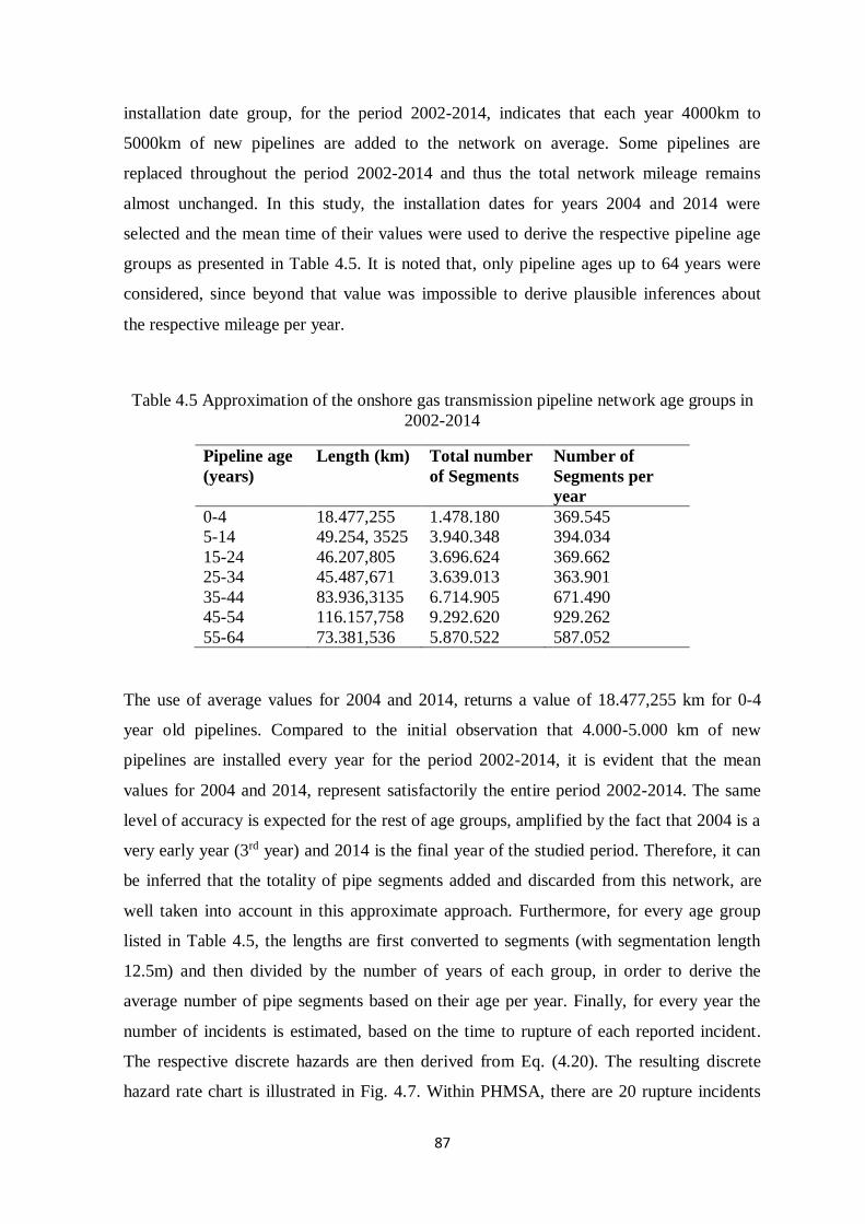
87
installation date group, for the period 2002-2014, indicates that each year 4000km to
5000km of new pipelines are added to the network on average. Some pipelines are
replaced throughout the period 2002-2014 and thus the total network mileage remains
almost unchanged. In this study, the installation dates for years 2004 and 2014 were
selected and the mean time of their values were used to derive the respective pipeline age
groups as presented in Table 4.5. It is noted that, only pipeline ages up to 64 years were
considered, since beyond that value was impossible to derive plausible inferences about
the respective mileage per year.
Table 4.5 Approximation of the onshore gas transmission pipeline network age groups in
2002-2014
Pipeline age
(years)
Length (km) Total number
of Segments
Number of
Segments per
year
0-4 18.477,255 1.478.180 369.545
5-14 49.254, 3525 3.940.348 394.034
15-24 46.207,805 3.696.624 369.662
25-34 45.487,671 3.639.013 363.901
35-44 83.936,3135 6.714.905 671.490
45-54 116.157,758 9.292.620 929.262
55-64 73.381,536 5.870.522 587.052
The use of average values for 2004 and 2014, returns a value of 18.477,255 km for 0-4
year old pipelines. Compared to the initial observation that 4.000-5.000 km of new
pipelines are installed every year for the period 2002-2014, it is evident that the mean
values for 2004 and 2014, represent satisfactorily the entire period 2002-2014. The same
level of accuracy is expected for the rest of age groups, amplified by the fact that 2004 is a
very early year (3rd year) and 2014 is the final year of the studied period. Therefore, it can
be inferred that the totality of pipe segments added and discarded from this network, are
well taken into account in this approximate approach. Furthermore, for every age group
listed in Table 4.5, the lengths are first converted to segments (with segmentation length
12.5m) and then divided by the number of years of each group, in order to derive the
average number of pipe segments based on their age per year. Finally, for every year the
number of incidents is estimated, based on the time to rupture of each reported incident.
The respective discrete hazards are then derived from Eq. (4.20). The resulting discrete
hazard rate chart is illustrated in Fig. 4.7. Within PHMSA, there are 20 rupture incidents
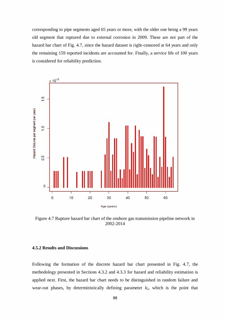
88
corresponding to pipe segments aged 65 years or more, with the older one being a 99 years
old segment that ruptured due to external corrosion in 2009. These are not part of the
hazard bar chart of Fig. 4.7, since the hazard dataset is right-censored at 64 years and only
the remaining 159 reported incidents are accounted for. Finally, a service life of 100 years
is considered for reliability prediction.
Figure 4.7 Rupture hazard bar chart of the onshore gas transmission pipeline network in
2002-2014
4.5.2 Results and Discussions
Following the formation of the discrete hazard bar chart presented in Fig. 4.7, the
methodology presented in Sections 4.3.2 and 4.3.3 for hazard and reliability estimation is
applied next. First, the hazard bar chart needs to be distinguished in random failure and
wear-out phases, by deterministically defining parameter k2, which is the point that
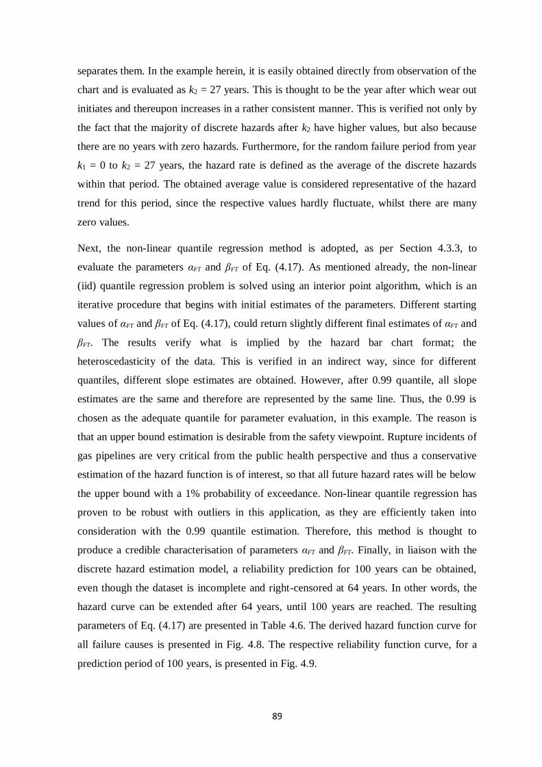
89
separates them. In the example herein, it is easily obtained directly from observation of the
chart and is evaluated as k2 = 27 years. This is thought to be the year after which wear out
initiates and thereupon increases in a rather consistent manner. This is verified not only by
the fact that the majority of discrete hazards after k2 have higher values, but also because
there are no years with zero hazards. Furthermore, for the random failure period from year
k1 = 0 to k2 = 27 years, the hazard rate is defined as the average of the discrete hazards
within that period. The obtained average value is considered representative of the hazard
trend for this period, since the respective values hardly fluctuate, whilst there are many
zero values.
Next, the non-linear quantile regression method is adopted, as per Section 4.3.3, to
evaluate the parameters αFT and βFT of Eq. (4.17). As mentioned already, the non-linear
(iid) quantile regression problem is solved using an interior point algorithm, which is an
iterative procedure that begins with initial estimates of the parameters. Different starting
values of αFT and βFT of Eq. (4.17), could return slightly different final estimates of αFT and
βFT. The results verify what is implied by the hazard bar chart format; the
heteroscedasticity of the data. This is verified in an indirect way, since for different
quantiles, different slope estimates are obtained. However, after 0.99 quantile, all slope
estimates are the same and therefore are represented by the same line. Thus, the 0.99 is
chosen as the adequate quantile for parameter evaluation, in this example. The reason is
that an upper bound estimation is desirable from the safety viewpoint. Rupture incidents of
gas pipelines are very critical from the public health perspective and thus a conservative
estimation of the hazard function is of interest, so that all future hazard rates will be below
the upper bound with a 1% probability of exceedance. Non-linear quantile regression has
proven to be robust with outliers in this application, as they are efficiently taken into
consideration with the 0.99 quantile estimation. Therefore, this method is thought to
produce a credible characterisation of parameters αFT and βFT. Finally, in liaison with the
discrete hazard estimation model, a reliability prediction for 100 years can be obtained,
even though the dataset is incomplete and right-censored at 64 years. In other words, the
hazard curve can be extended after 64 years, until 100 years are reached. The resulting
parameters of Eq. (4.17) are presented in Table 4.6. The derived hazard function curve for
all failure causes is presented in Fig. 4.8. The respective reliability function curve, for a
prediction period of 100 years, is presented in Fig. 4.9.
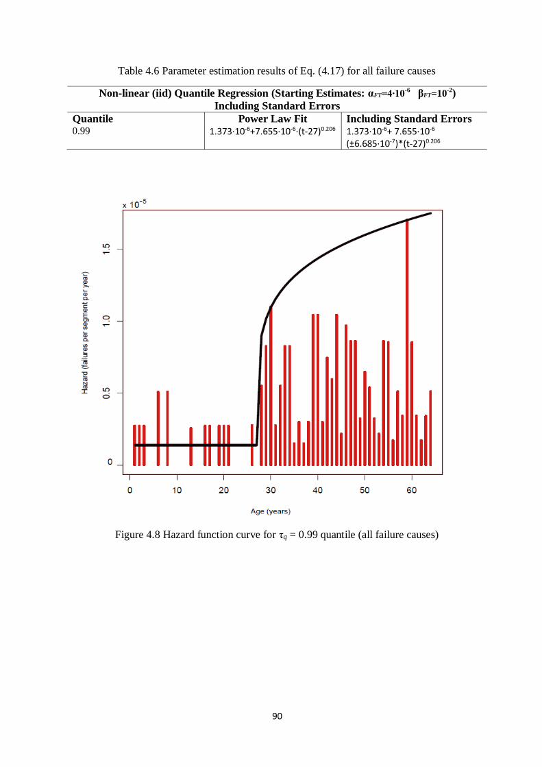
90
Table 4.6 Parameter estimation results of Eq. (4.17) for all failure causes
Non-linear (iid) Quantile Regression (Starting Estimates: αFT=4∙10-6
βFT=10-2)
Including Standard Errors Quantile Power Law Fit Including Standard Errors 0.99 1.373·10-6+7.655·10-6·(t-27)0.206 1.373·10-6+ 7.655·10-6
(±6.685·10-7)*(t-27)0.206
Figure 4.8 Hazard function curve for τq = 0.99 quantile (all failure causes)
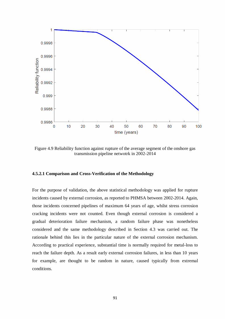
91
Figure 4.9 Reliability function against rupture of the average segment of the onshore gas
transmission pipeline netwotrk in 2002-2014
4.5.2.1 Comparison and Cross-Verification of the Methodology
For the purpose of validation, the above statistical methodology was applied for rupture
incidents caused by external corrosion, as reported to PHMSA between 2002-2014. Again,
those incidents concerned pipelines of maximum 64 years of age, whilst stress corrosion
cracking incidents were not counted. Even though external corrosion is considered a
gradual deterioration failure mechanism, a random failure phase was nonetheless
considered and the same methodology described in Section 4.3 was carried out. The
rationale behind this lies in the particular nature of the external corrosion mechanism.
According to practical experience, substantial time is normally required for metal-loss to
reach the failure depth. As a result early external corrosion failures, in less than 10 years
for example, are thought to be random in nature, caused typically from extremal
conditions.
92
Figure 4.10 Hazard bar chart for rupture due to external metal-loss corrosion
Table 4.7 Parameter estimation results of Eq. (4.17) for external corrosion incidents
Non-linear (iid) Quantile Regression (Starting Estimates: αFT=10-6
βFT=10-1)
Including Standard Errors Quantile Power Law Fit Including Standard Errors 0.99 2.228·10-7+1.958·10-6·(t-37)0.418 2.228·10-7+ 1.958·10-6
(±1.302·10-7)·(t-37)0.418
Following this, the end point of the random failure phase for external corrosion ruptures
was evaluated to be k2 = 37 years by the respective hazard bar chart and then the upper
bound for the wear out phase was estimated, based on the 0.99 quantile. It is noted that the
end point of the random failure phase was not set as 30 years, even if the hazard rate
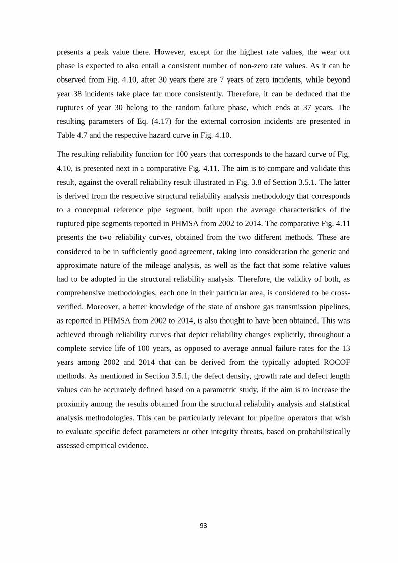
93
presents a peak value there. However, except for the highest rate values, the wear out
phase is expected to also entail a consistent number of non-zero rate values. As it can be
observed from Fig. 4.10, after 30 years there are 7 years of zero incidents, while beyond
year 38 incidents take place far more consistently. Therefore, it can be deduced that the
ruptures of year 30 belong to the random failure phase, which ends at 37 years. The
resulting parameters of Eq. (4.17) for the external corrosion incidents are presented in
Table 4.7 and the respective hazard curve in Fig. 4.10.
The resulting reliability function for 100 years that corresponds to the hazard curve of Fig.
4.10, is presented next in a comparative Fig. 4.11. The aim is to compare and validate this
result, against the overall reliability result illustrated in Fig. 3.8 of Section 3.5.1. The latter
is derived from the respective structural reliability analysis methodology that corresponds
to a conceptual reference pipe segment, built upon the average characteristics of the
ruptured pipe segments reported in PHMSA from 2002 to 2014. The comparative Fig. 4.11
presents the two reliability curves, obtained from the two different methods. These are
considered to be in sufficiently good agreement, taking into consideration the generic and
approximate nature of the mileage analysis, as well as the fact that some relative values
had to be adopted in the structural reliability analysis. Therefore, the validity of both, as
comprehensive methodologies, each one in their particular area, is considered to be cross-
verified. Moreover, a better knowledge of the state of onshore gas transmission pipelines,
as reported in PHMSA from 2002 to 2014, is also thought to have been obtained. This was
achieved through reliability curves that depict reliability changes explicitly, throughout a
complete service life of 100 years, as opposed to average annual failure rates for the 13
years among 2002 and 2014 that can be derived from the typically adopted ROCOF
methods. As mentioned in Section 3.5.1, the defect density, growth rate and defect length
values can be accurately defined based on a parametric study, if the aim is to increase the
proximity among the results obtained from the structural reliability analysis and statistical
analysis methodologies. This can be particularly relevant for pipeline operators that wish
to evaluate specific defect parameters or other integrity threats, based on probabilistically
assessed empirical evidence.
94
Figure 4.11 Comparison of the reliability function curves of the two different
methodologies
4.6 Conclusions
The first methodology of this chapter employed the NPI approach in an attempt to derive
inductive inferences from the lifetimes of a set of ruptured pipelines. This approach was
applied in a PHMSA dataset of rupture incidents of onshore gas transmission pipelines for
the period 2002-2014. The NPI method analysed the rupture incidents from a non-
repairable systems perspective, based on the time to rupture of the pipe segments. It was
shown that NPI is advantageous in deriving inferences for the future pipe segment that
ruptures due to a specific failure cause, by providing imprecise probabilities and survival
functions for this event, based on historical failure data. The results indicated external
corrosion as the predominant rupture cause for the aforementioned database under
consideration, with ruptures taking place mainly after 30 years. The predicted imprecise
probabilities and survival functions, can be used to examine and implement maintenance
strategies based on relative risk prioritization.
The second methodology was based on the PHMSA data for the period 2002-2014 as well.
An empirical discrete hazard model was adopted in conjunction with a non-subjective
parameter estimation technique, namely non-linear quantile regression, to evaluate the
hazard and reliability functions. The model provided inferences on the reliability of a
95
region’s reference pipe segment for its complete lifecycle, even in the case of scarce,
incomplete and censored data, as opposed to the commonly adopted ROCOF methods in
literature that only account for the limited time period under study. Furthermore, non-
linear quantile regression is thought to have yielded a complete picture regarding the
hazard dataset. Thus, it is considered that the generic nature of the historical data was
reasonably accounted for and the resulting reliability lies within a credible expectation
range. The results of the second statistical methodology were also compared with these of
the structural reliability model of Section 3.5.1, which was based on the same set of
PHMSA data. The results demonstrated reasonable proximity, which constitutes an
inherent validation of the soundness of both methodologies and their estimations. The
second statistical methodology can thus help pipeline operators to derive plausible
expectations for the performance of either new or existing pipelines. These expectations
can also be linked to specific parameters by means of parametric studies. The results of
both methodologies are thought to provide additional knowledge on the state of the
PHMSA onshore gas transmission network among 2002-2014 with respect to rupture, as
opposed to results from the ROCOF-based approaches typically employed in literature. In
addition, this period is considered representative of the most current operation and
rehabilitation techniques and practices in industry, corroborating the significance of the
results for new or existing pipelines. The methodologies of this chapter can therefore assist
pipeline operators in making informed maintenance decisions, based on reliability and risk.
96
5. Bayesian Analysis of Pipeline Reliability Based on Imperfect
Inspection Data
5.1 Introduction
Apart from metal-loss corrosion, environmental defects stemming from stress corrosion
cracking (SCC) are also major threats to the safe operation and structural integrity of
energy pipelines. A typical industry mitigation response to both of these, includes high-
resolution in-line inspections (ILI) to measure defects on the pipeline body and estimate
failure probabilities based on the inspection results. This chapter focuses on cases where
ILI data is available on the model response, where Bayesian analysis serves the
requirement to inversely determine the probabilistic input parameters given output data.
The analytical estimation of the high-dimensional integrals involved in the Bayesian
updating is impractical in pipeline problems and typically Markov Chain Monte Carlo
(MCMC) sampling techniques are adopted to numerically perform the task (Al-Amin and
Zhou, 2014).
The limitations of MCMC include the uncertainty around ensuring that the final samples
have reached the posterior distribution and also the difficulty in ultimately quantifying
small probabilities of rare failure incidents (Straub et al., 2016); particularly rupture due to
metal-loss corrosion in the setting of energy pipelines (Zhang and Zhou, 2013). An
alternative method to MCMC is Bayesian Updating with structural reliability methods
(BUS), which sets an analogy between Bayesian updating and a reliability problem (Straub
and Papaioannou, 2014a). This formulation enables the use of established Structural
Reliability methods for the Bayesian updating. The Structural Reliability method adopted
herein is Subset Simulation (SuS). The whole methodology is referred to as BUS-SuS and
is considered to be an improved reinterpretation of the classical rejection sampling
approach, to Bayesian analysis with subset simulation. BUS-SuS facilitates the estimation
of small posterior failure probabilities directly within the same analysis framework,
without the requirement of either explicit knowledge or approximation of the posterior
joint probability distribution of the random variables (Straub et al., 2016).
In the present chapter, two case studies involving existing gas pipelines are used to
illustrate and validate the proposed methodology. In the first case study, BUS-SuS is
applied in an existing gas pipeline containing metal-loss corrosion defects. The pipeline is
97
subjected to high-pressure internal loading and BUS-SuS is validated against field data.
The growth of multiple active metal-loss corrosion defects is characterised through
adopting the gamma stochastic process and incorporating it into an hierarchical Bayesian
framework based on multiple ILI data, along with a comprehensive consideration of
associated measurement errors. A Ferry-Borges stochastic process is employed to model
the internal process in the subsequent reliability analysis. The system reliability of the
pipeline is evaluated in terms of three distinctive failure modes, namely small leak, large
leak and rupture.
In the second case study, Bayesian updating is conducted by using BUS-SuS in conjuction
with a data augmentation (DA) technique. Simulated data corresponding to an existing gas
pipeline with high-pH SCC features and subjected to static internal pressure loading were
used to illustrate and validate the proposed methodology. The growth of multiple active
SCC features is characterised through adopting a non-homogeneous gamma process
(NHGP) model and incorporating it into the Bayesian framework based on multiple ILI
data, with the associated measurement errors comprehensively accounted for. Furthermore,
the dependence among the growths of different crack features is considered in the analysis,
using the Gaussian copula. The growth modeling focuses on the crack depth, as this is the
most critical crack dimension for high-pH SCC under constant loading (Song et al., 2011).
At the end, the system reliability is evaluated by means of the Battelle model (Yan et al.,
2014) and the sensitivity of both the growth model and system reliability to different
dependence scenarios is investigated.
The content of this chapter is organised as follows. Section 5.2 defines the uncertainties
involved in the ILI data. The formulations of the stochastic models for the crack generation
and growth are presented in Section 5.3. The Bayesian method for updating the model
parameters by means of BUS-SuS and DA are described in section 5.4. The system
reliability derivation is described in Section 5.5, for both metal-loss corrosion defects and
SCC cracks. In Section 5.6, a numerical application is presented based on an real gas
pipeline containing multiple active metal-loss corrosion defects. In Section 5.7, a case
study involving simulated ILI data that correspond to another existing in-service gas
pipeline that has presented high-pH SCC in the past is implemented, in order to illustrate
and validate the proposed methodology. Finally, some concluding remarks are presented in
section 5.8, on the basis of the outcomes of the study.
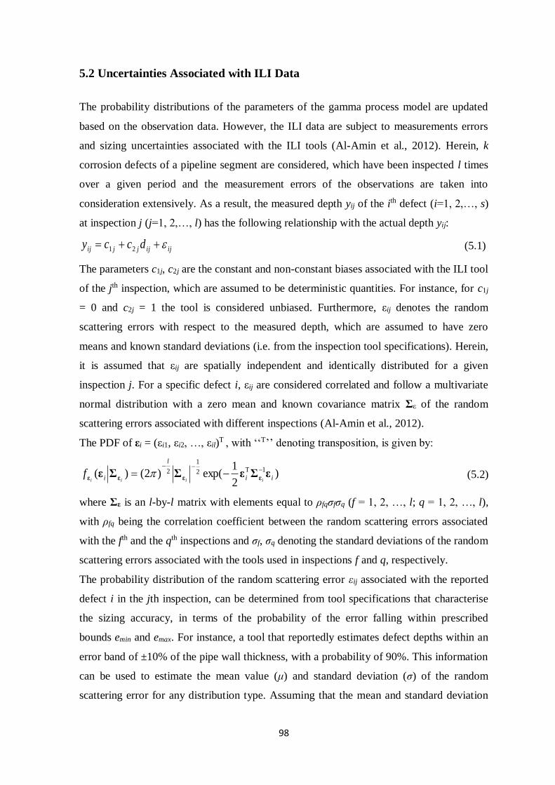
98
5.2 Uncertainties Associated with ILI Data
The probability distributions of the parameters of the gamma process model are updated
based on the observation data. However, the ILI data are subject to measurements errors
and sizing uncertainties associated with the ILI tools (Al-Amin et al., 2012). Herein, k
corrosion defects of a pipeline segment are considered, which have been inspected l times
over a given period and the measurement errors of the observations are taken into
consideration extensively. As a result, the measured depth yij of the ith defect (i=1, 2,…, s)
at inspection j (j=1, 2,…, l) has the following relationship with the actual depth yij:
ijijjjij dccy 21 (5.1)
The parameters c1j, c2j are the constant and non-constant biases associated with the ILI tool
of the jth inspection, which are assumed to be deterministic quantities. For instance, for c1j
= 0 and c2j = 1 the tool is considered unbiased. Furthermore, εij denotes the random
scattering errors with respect to the measured depth, which are assumed to have zero
means and known standard deviations (i.e. from the inspection tool specifications). Herein,
it is assumed that εij are spatially independent and identically distributed for a given
inspection j. For a specific defect i, εij are considered correlated and follow a multivariate
normal distribution with a zero mean and known covariance matrix Σε of the random
scattering errors associated with different inspections (Al-Amin et al., 2012).
The PDF of εi = (εi1, εi2, …, εil)Τ , with ‘‘T’’ denoting transposition, is given by:
)2
1exp()2()( 12
1
2ii
l
i iiiif εΣεΣΣε εεεε
(5.2)
where Σε is an l-by-l matrix with elements equal to ρfqσfσq (f = 1, 2, …, l; q = 1, 2, …, l),
with ρfq being the correlation coefficient between the random scattering errors associated
with the fth and the qth inspections and σf, σq denoting the standard deviations of the random
scattering errors associated with the tools used in inspections f and q, respectively.
The probability distribution of the random scattering error εij associated with the reported
defect i in the jth inspection, can be determined from tool specifications that characterise
the sizing accuracy, in terms of the probability of the error falling within prescribed
bounds emin and emax. For instance, a tool that reportedly estimates defect depths within an
error band of ±10% of the pipe wall thickness, with a probability of 90%. This information
can be used to estimate the mean value (μ) and standard deviation (σ) of the random
scattering error for any distribution type. Assuming that the mean and standard deviation
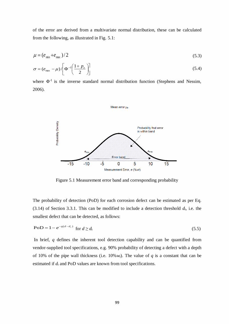
99
of the error are derived from a multivariate normal distribution, these can be calculated
from the following, as illustrated in Fig. 5.1:
2/)( maxmin ee (5.3)
2
1/)( 1
maxep
e (5.4)
where Φ-1 is the inverse standard normal distribution function (Stephens and Nessim,
2006).
Figure 5.1 Measurement error band and corresponding probability
The probability of detection (PoD) for each corrosion defect can be estimated as per Eq.
(3.14) of Section 3.3.1. This can be modified to include a detection threshold dt, i.e. the
smallest defect that can be detected, as follows:
)(1PoD tddq
e
for d ≥ dt (5.5)
In brief, q defines the inherent tool detection capability and can be quantified from
vendor-supplied tool specifications, e.g. 90% probability of detecting a defect with a depth
of 10% of the pipe wall thickness (i.e. 10%wt). The value of q is a constant that can be
estimated if dt and PoD values are known from tool specifications.
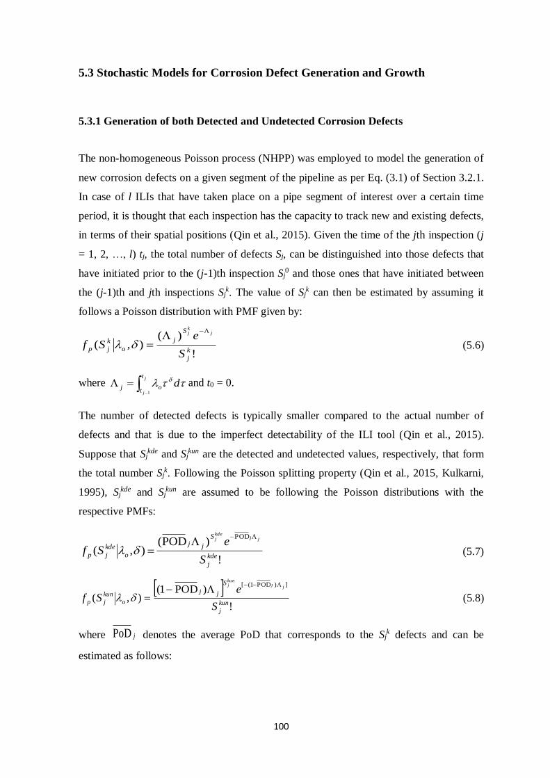
100
5.3 Stochastic Models for Corrosion Defect Generation and Growth
5.3.1 Generation of both Detected and Undetected Corrosion Defects
The non-homogeneous Poisson process (NHPP) was employed to model the generation of
new corrosion defects on a given segment of the pipeline as per Eq. (3.1) of Section 3.2.1.
In case of l ILIs that have taken place on a pipe segment of interest over a certain time
period, it is thought that each inspection has the capacity to track new and existing defects,
in terms of their spatial positions (Qin et al., 2015). Given the time of the jth inspection (j
= 1, 2, …, l) tj, the total number of defects Sj, can be distinguished into those defects that
have initiated prior to the (j-1)th inspection Sj0 and those ones that have initiated between
the (j-1)th and jth inspections Sjk. The value of Sj
k can then be estimated by assuming it
follows a Poisson distribution with PMF given by:
!
)(),(
k
j
S
j
o
k
jpS
eSf
jkj
(5.6)
where
j
j
t
toj d
1
and t0 = 0.
The number of detected defects is typically smaller compared to the actual number of
defects and that is due to the imperfect detectability of the ILI tool (Qin et al., 2015).
Suppose that Sjkde and Sj
kun are the detected and undetected values, respectively, that form
the total number Sjk. Following the Poisson splitting property (Qin et al., 2015, Kulkarni,
1995), Sjkde and Sj
kun are assumed to be following the Poisson distributions with the
respective PMFs:
!
)POD(),(
POD
kde
j
S
jj
o
kde
jpS
eSf
jjkdej
(5.7)
!
)POD1(),(
])POD1([
kun
j
S
jj
o
kun
jpS
eSf
jJkunj
(5.8)
where jPoD denotes the average PoD that corresponds to the Sjk defects and can be
estimated as follows:
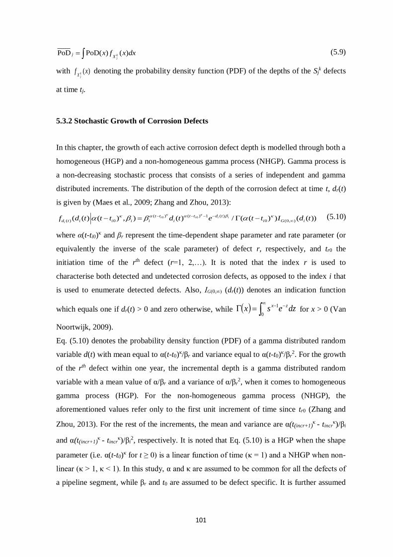
101
dxxfx kjX
j )()(PoDPoD (5.9)
with )(xf kjX
denoting the probability density function (PDF) of the depths of the Sjk defects
at time tj.
5.3.2 Stochastic Growth of Corrosion Defects
In this chapter, the growth of each active corrosion defect depth is modelled through both a
homogeneous (HGP) and a non-homogeneous gamma process (NHGP). Gamma process is
a non-decreasing stochastic process that consists of a series of independent and gamma
distributed increments. The distribution of the depth of the corrosion defect at time t, dr(t)
is given by (Maes et al., 2009; Zhang and Zhou, 2013):
0 0( ) ( ) 1 ( )
( ) 0 0 (0, )( ( ) ( ) , ) ( ) / ( ( ) ) ( ( ))i i i i
i
t t t t d t
d t i i i i i i G if d t t t d t e t t I d t
(5.10)
where α(t-ti0)κ and βr represent the time-dependent shape parameter and rate parameter (or
equivalently the inverse of the scale parameter) of defect r, respectively, and tr0 the
initiation time of the rth defect (r=1, 2,…). It is noted that the index r is used to
characterise both detected and undetected corrosion defects, as opposed to the index i that
is used to enumerate detected defects. Also, ΙG(0,∞) (dr(t)) denotes an indication function
which equals one if dr(t) > 0 and zero otherwise, while
0
1 dzesx zx for x > 0 (Van
Noortwijk, 2009).
Eq. (5.10) denotes the probability density function (PDF) of a gamma distributed random
variable d(t) with mean equal to α(t-t0)κ/βr and variance equal to α(t-t0)
κ/βr2. For the growth
of the rth defect within one year, the incremental depth is a gamma distributed random
variable with a mean value of α/βr and a variance of α/βr2, when it comes to homogeneous
gamma process (HGP). For the non-homogeneous gamma process (NHGP), the
aforementioned values refer only to the first unit increment of time since tr0 (Zhang and
Zhou, 2013). For the rest of the increments, the mean and variance are α(t(incr+1)κ - tincr
κ)/βi
and α(t(incr+1)κ - tincr
κ)/βi2, respectively. It is noted that Eq. (5.10) is a HGP when the shape
parameter (i.e. α(t-t0)κ for t ≥ 0) is a linear function of time (κ = 1) and a NHGP when non-
linear (κ > 1, κ < 1). In this study, α and κ are assumed to be common for all the defects of
a pipeline segment, while βr and t0 are assumed to be defect specific. It is further assumed
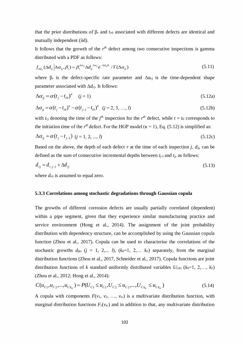
102
that the prior distributions of βr and tr0 associated with different defects are identical and
mutually independent (iid).
It follows that the growth of the rth defect among two consecutive inspections is gamma
distributed with a PDF as follows:
( , ) / ( )ij ij ij i
ij
d
d ij ij i i ij ijf d d e
(5.11)
where βr is the defect-specific rate parameter and Δαrj is the time-dependent shape
parameter associated with Δdrj. It follows:
0( )ij j it t (j = 1) (5.12a)
0 1 0( ) ( )ij j i j it t t t (j = 2, 3, …, l) (5.12b)
with trj denoting the time of the jth inspection for the rth defect, while t = t0 corresponds to
the initiation time of the rth defect. For the HGP model (κ = 1), Eq. (5.12) is simplified as:
1( )ij j jt t (j = 1, 2, ..., l) (5.12c)
Based on the above, the depth of each defect r at the time of each inspection j, dij, can be
defined as the sum of consecutive incremental depths between tj-1 and tj, as follows:
rjjrrj ddd 1, (5.13)
where dr0 is assumed to equal zero.
5.3.3 Correlations among stochastic degradations through Gaussian copula
The growths of different corrosion defects are usually partially correlated (dependent)
within a pipe segment, given that they experience similar manufacturing practice and
service environment (Hong et al., 2014). The assignment of the joint probability
distribution with dependency structure, can be accomplished by using the Gaussian copula
function (Zhou et al., 2017). Copula can be used to characterise the correlations of the
stochastic growths djk0 (j = 1, 2,... l), (k0=1, 2,… kF) separately, from the marginal
distribution functions (Zhou et al., 2017, Schneider et al., 2017). Copula functions are joint
distribution functions of k standard uniformly distributed variables UCk0 (k0=1, 2,…, kF)
(Zhou et al., 2012; Hong et al., 2014):
),...,,(),...,,(221121 FFF kCkCCCCCkCCC uUuUuUPuuuC (5.14)
A copula with components F(v1, v2, …, vkF) is a multivariate distribution function, with
marginal distribution functions Fr(vkF) and in addition to that, any multivariate distribution
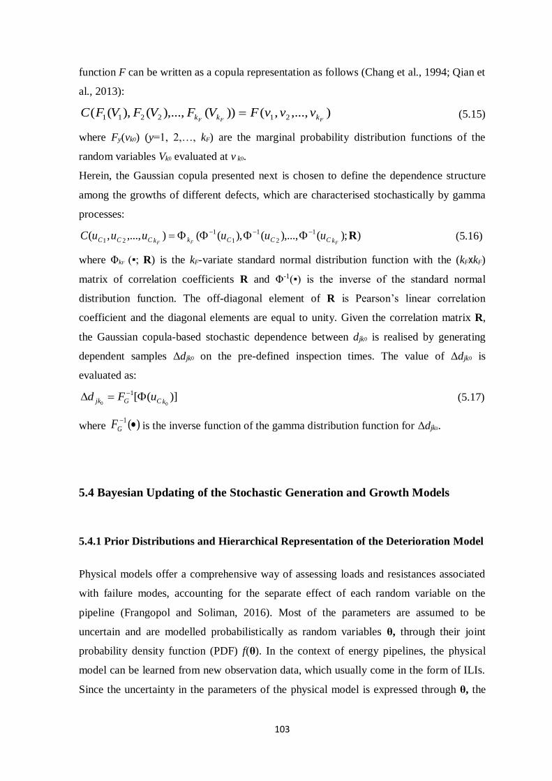
103
function F can be written as a copula representation as follows (Chang et al., 1994; Qian et
al., 2013):
),...,,())(),...,(),(( 212211 FFF kkk vvvFVFVFVFC (5.15)
where Fy(vk0) (y=1, 2,…, kF) are the marginal probability distribution functions of the
random variables Vk0 evaluated at v k0.
Herein, the Gaussian copula presented next is chosen to define the dependence structure
among the growths of different defects, which are characterised stochastically by gamma
processes:
));(),...,(),((),...,,( 1
2
1
1
1
21R
FFF kCCCkkCCC uuuuuuC (5.16)
where ΦkF (▪; R) is the kF-variate standard normal distribution function with the (kFxkF)
matrix of correlation coefficients R and Φ-1(▪) is the inverse of the standard normal
distribution function. The off-diagonal element of R is Pearson’s linear correlation
coefficient and the diagonal elements are equal to unity. Given the correlation matrix R,
the Gaussian copula-based stochastic dependence between djk0 is realised by generating
dependent samples Δdjk0 on the pre-defined inspection times. The value of Δdjk0 is
evaluated as:
)]([00
1
kCGjk uFd (5.17)
where )(1
GF is the inverse function of the gamma distribution function for Δdjk0.
5.4 Bayesian Updating of the Stochastic Generation and Growth Models
5.4.1 Prior Distributions and Hierarchical Representation of the Deterioration Model
Physical models offer a comprehensive way of assessing loads and resistances associated
with failure modes, accounting for the separate effect of each random variable on the
pipeline (Frangopol and Soliman, 2016). Most of the parameters are assumed to be
uncertain and are modelled probabilistically as random variables θ, through their joint
probability density function (PDF) f(θ). In the context of energy pipelines, the physical
model can be learned from new observation data, which usually come in the form of ILIs.
Since the uncertainty in the parameters of the physical model is expressed through θ, the
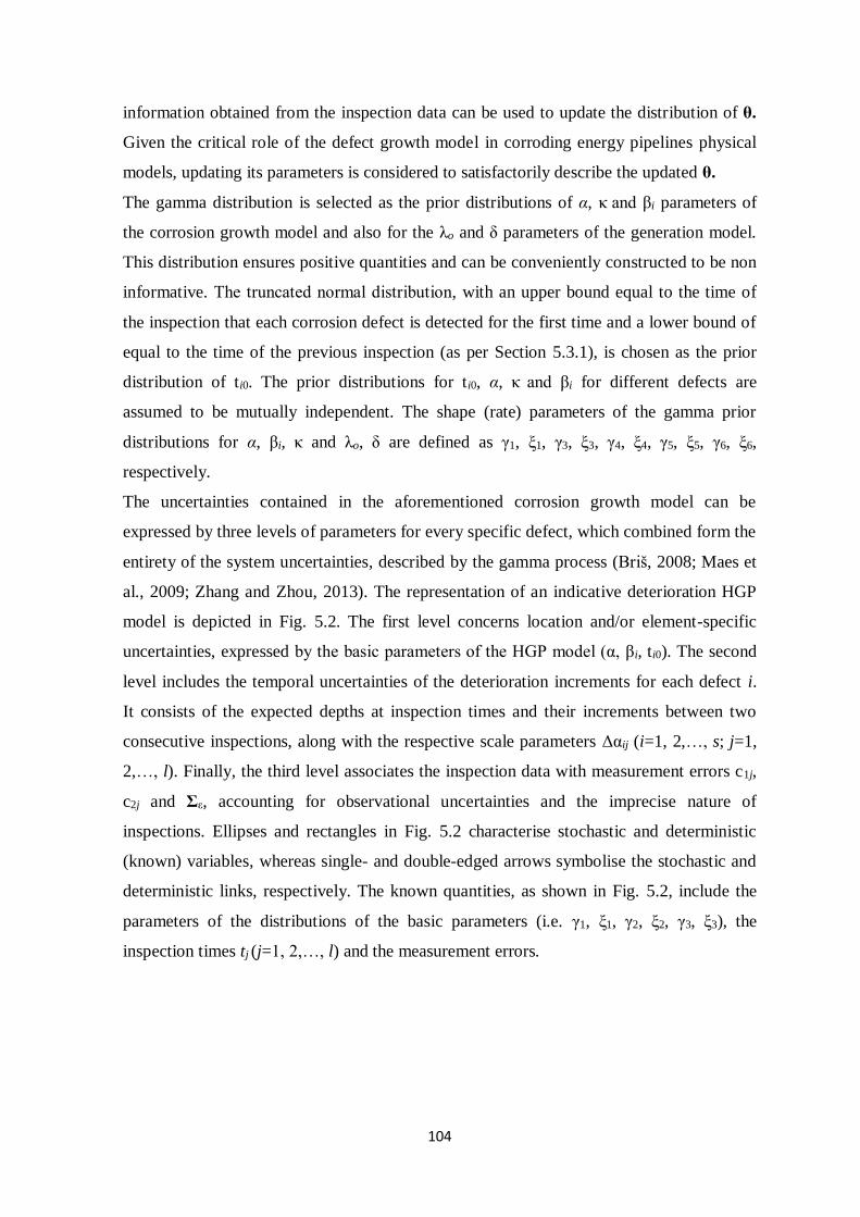
104
information obtained from the inspection data can be used to update the distribution of θ.
Given the critical role of the defect growth model in corroding energy pipelines physical
models, updating its parameters is considered to satisfactorily describe the updated θ.
The gamma distribution is selected as the prior distributions of α, κ and βi parameters of
the corrosion growth model and also for the λo and δ parameters of the generation model.
This distribution ensures positive quantities and can be conveniently constructed to be non
informative. Τhe truncated normal distribution, with an upper bound equal to the time of
the inspection that each corrosion defect is detected for the first time and a lower bound of
equal to the time of the previous inspection (as per Section 5.3.1), is chosen as the prior
distribution of ti0. The prior distributions for ti0, α, κ and βi for different defects are
assumed to be mutually independent. The shape (rate) parameters of the gamma prior
distributions for α, βi, κ and λo, δ are defined as γ1, ξ1, γ3, ξ3, γ4, ξ4, γ5, ξ5, γ6, ξ6,
respectively.
The uncertainties contained in the aforementioned corrosion growth model can be
expressed by three levels of parameters for every specific defect, which combined form the
entirety of the system uncertainties, described by the gamma process (Briš, 2008; Maes et
al., 2009; Zhang and Zhou, 2013). The representation of an indicative deterioration HGP
model is depicted in Fig. 5.2. The first level concerns location and/or element-specific
uncertainties, expressed by the basic parameters of the HGP model (α, βi, ti0). The second
level includes the temporal uncertainties of the deterioration increments for each defect i.
It consists of the expected depths at inspection times and their increments between two
consecutive inspections, along with the respective scale parameters Δαij (i=1, 2,…, s; j=1,
2,…, l). Finally, the third level associates the inspection data with measurement errors c1j,
c2j and Σε, accounting for observational uncertainties and the imprecise nature of
inspections. Ellipses and rectangles in Fig. 5.2 characterise stochastic and deterministic
(known) variables, whereas single- and double-edged arrows symbolise the stochastic and
deterministic links, respectively. The known quantities, as shown in Fig. 5.2, include the
parameters of the distributions of the basic parameters (i.e. γ1, ξ1, γ2, ξ2, γ3, ξ3), the
inspection times tj (j=1, 2,…, l) and the measurement errors.
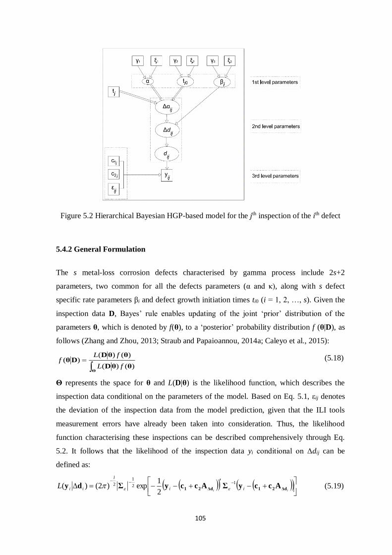
105
Figure 5.2 Hierarchical Bayesian HGP-based model for the jth inspection of the ith defect
5.4.2 General Formulation
The s metal-loss corrosion defects characterised by gamma process include 2s+2
parameters, two common for all the defects parameters (α and κ), along with s defect
specific rate parameters βi and defect growth initiation times ti0 (i = 1, 2, …, s). Given the
inspection data D, Bayes’ rule enables updating of the joint ‘prior’ distribution of the
parameters θ, which is denoted by f(θ), to a ‘posterior’ probability distribution f (θ|D), as
follows (Zhang and Zhou, 2013; Straub and Papaioannou, 2014a; Caleyo et al., 2015):
ΘθθD
θθDDθ
)()(
)()()(
fL
fLf (5.18)
Θ represents the space for θ and L(D|θ) is the likelihood function, which describes the
inspection data conditional on the parameters of the model. Based on Eq. 5.1, εij denotes
the deviation of the inspection data from the model prediction, given that the ILI tools
measurement errors have already been taken into consideration. Thus, the likelihood
function characterising these inspections can be described comprehensively through Eq.
5.2. It follows that the likelihood of the inspection data yi conditional on Δdij can be
defined as:
ii ii
l
iiL Δd21Δd21 AccyΣAccyΣdy1
2
1
2
2
1exp)2()( (5.19)
106
where AΔdi is an l x 1 vector with the jth element equal to
j
w iwd1
.
For the evaluation of Eq. 5.18, simulation techniques such as MCMC can be employed to
generate samples of the posterior distribution. Furthermore, when the computation of the
probability of failure conditional on the posterior distribution is of interest, a reliability
analysis can be performed as a post-processing step after the Bayesian analysis. Typically,
a crude Monte Carlo simulation is adopted to carry out this reliability analysis (Zhou,
2010; Zhang and Zhou, 2013; Valor et al., 2014). However, crude Monte Carlo cannot
efficiently estimate rare event probabilities (e.g. <10-6), such as rupture of energy pipelines
(Zhang and Zhou, 2013; Al-Amin and Zhou, 2014; Lam and Zhou, 2016). Thus, a
structural reliability method that can efficiently estimate small posterior probabilities is
necessary. Such a method would require an explicit knowledge of the joint posterior
distribution, which must thus be approximated from the posterior samples. This can lead to
considerable errors, especially in the tails of the distributions. In this study a new
methodology, which was proposed in Straub and Papaioannou (2014a) and Straub et al.
(2016) as an extension of the classical rejection sampling approach to Bayesian analysis, is
applied for sampling from the posterior distribution. In addition to that, it enables the
computation of the small posterior failure probabilities, directly within the same single
framework.
BUS-SuS can be interpreted as an extension of the classical rejection sampling approach to
Bayesian analysis. Details of the connection between the classical rejection sampling
approach and BUS-SuS can be found in Straub and Papaioannou (2014a). The simple
rejection sampling algorithm however, is thought to be inefficient, especially in the
presence of increasing amount of inspection data, such as often is the case with corroding
energy pipelines. This is also particularly aggravated when non-informative priors are
present. However, an advantage of the rejection sampling algorithm over MCMC is its
simplicity and the fact that ensures accurate and uncorrelated samples of the posterior.
BUS-SuS developed for corroding pipelines herein, maintains partly the advantages of the
simple rejection sampling algorithm, while it is highly efficient by employing Subset
simulation which is capable of computing very small probabilities (Au and Beck, 2001;
Tee et al, 2014).
Considering the augmented outcome space [θ; p] is the first step of the analysis. Then, by
defining the domain Ζ = {p ≤ cL(θ)}, the posterior distribution )( Dθf can be obtained by
censoring the joint distribution of p and θ to Z and marginalizing θ:
107
1
0)()],([)( dpfpIf Z θθDθ (5.20)
where IZ is an indicator function which takes value one if {p ≤ cL(θ)}and zero otherwise,
and p is a standard uniform random variable. Furthermore, c is defined as a positive
constant that ensures cL(θ) ≤ 1 for all θ. The selection of c is discussed in section 5.4.3. In
the structural reliability convention, the domain Z describes an observation event (in terms
of the Bayesian updating) through a limit state function rA, such that it corresponds to a
respective domain {rA(p,θ) ≤ 0}:
)(),( θθ cLpprA (5.21)
The probability of the observation event Pr(Z) is equal to the acceptance rate of the simple
rejection sampling algorithm which typically is too small for Monte Carlo simulation to be
efficient. Therefore, SuS is employed to explore the domain Z and compute Pr(Z). It is
advantageous to apply SuS in the standard Normal space (Papaioannou et al., 2015; Straub
et al., 2016), thus the outcome space of the original random variables p and θ is
transformed to a space with independent standard Normal random variables V. Moreover,
p and θ are a-priori independent, as a result they can be transformed separately. The
corresponding limit-state function expressed through the underlying standard Normal
random variables can be described in terms of a function RΑ:
)))((()( 1
0 vΤv cLvRA
(5.22)
where Φ is the standard Normal cumulative distribution function (CDF). The
transfomation T can be either performed by means of the Rosenblatt transformation or the
marginal transformation based on the Nataf model. Next, BUS-SuS can generate samples
from the transformed observation domain (Straub and Papaioannou, 2014a). SuS evaluates
the probability Pr(Z) associated with a limit state function RA(v), defined in the respective
domain {RA(v) ≤ 0}. This is realised by expressing the event Z as an intersection of M
nested intermediate events, such that cM...10
. The probability Pr(Z) can
be defined as:
ccMM
1
11
ZZPrZPr)ZPr(
(5.23)
where Z0 corresponds to the certain event (Au and Beck, 2001). The final probability is
expressed through larger conditional probabilities of the intermediate events Zχ = {RΑ(v) ≤
bχ}, with b1 > b2 > ... > bMc = 0 and χ > 0. The values of bχ are chosen adaptively, so that
the estimates of the conditional probabilities correspond to a specific value p0, which is
108
usually selected to be in the range of [0.1~0.3] (Au and Beck, 2001; Straub and
Papaioannou, 2014a). Towards this, H samples are simulated from V, conditional on each
intermediate event Zχ-1 and then the respective limit state function RS(v) value is
estimated. Based on this evaluation, the samples are placed in increasing order of
magnitude, whereas the threshold bχ is set to the p0-percentile of the ordered samples. The
process is repeated until bMc = 0, whilst b1 is estimated through unconditional samples of V
based on a crude Monte Carlo. Consecutively, the samples of V conditional on Zχ for χ =
1, ... , Mc - 1 are generated from Markov chains through MCMC sampling, with seeds the
samples conditional on Zχ-1 for which RA(v) ≤ bχ. Then, Pr(Z) is estimated as follows:
cM
Mpp c 1
0)Pr(
(5.24)
where cMp corresponds to the conditional probability )Pr( 1cc MM as follows:
GM
RM
c
c
ccI
Gp
1
1)(
1
ν (5.25)
where IRΑ is an indication function of the observation event and Hc
Mc
c,...,1,
1
v are
samples of V conditional on ZMc-1.
In Bayesian updating, apart from Pr(Z) one is interested in obtaining samples that fall into
the domain Z, thus a final step should be defined. That is an extra step, where W additional
samples conditional on Z are produced, so that a total number of (at least) H samples from
the posterior distribution can be obtained.
5.4.3 Constant c
The required choice of constant c in BUS-SuS should ensure 1)( θcL for all θ. Choosing
the constant c too low might undermine the efficiency of the method significantly, since
the acceptance probability is linearly related to c. Contrarily, if it is chosen too large, this
might lead to samples that do not follow the posterior distribution (Betz et al., 2014). An
optimal choice of c can be approximated based on (Straub and Papaioannou, 2014a):
)(sup
1
θLc (5.26)
For a given defect i that has been inspected and sized by multiple inspections, supL(θ) is
equal to the maximum of the PDF of the random scattering error εij with respect to the
measured defect depth (Straub and Papaioannou, 2014b). This is correlated, following a
109
multivariate normal distribution with a zero mean and known covariance matrix Σε
associated with the total number of different inspections l. supL(θ) occurs at the location of
the maximum likelihood and thus it is possible to evaluate it by employing an optimization
algorithm such that supL(θ) = L(θMLE), where θMLE denotes the maximum likelihood
estimator (Straub and Papaioannou, 2014a). In case of a relatively small number of
individual inspections (e.g <5), an alternative choice is thought to produce equally accurate
results, that is:
])([sup
1
1
l
j jLc
θ (5.27)
It should be mentioned that alternative methods of selecting the constant c when using SuS
have been described in Betz et al. (2014), DiazDelaO et al. (2017) and Betz et al. (2018).
5.4.4 Likelihood Function for the Growth Model of Detected Corrosion Defects
Suppose that a number of defects have been detected in a total of l inspections and a defect
i is first detected in the jth (j = 1, 2,… or l) inspection. Furthermore, yi = (yji, yj+1,i,… ,
yj+g,i,.. , yli)′ and di = (dji, dj+1,i,… , dj+g,i,... , dli)′ denote the vector of the ILI-reported
depths for defect i and the vector of the corresponding actual depths of defect i,
respectively. Given the measurement error described in Section 5.2, the likelihood of yi
conditional on di can be defined as follows:
)]()(2
1exp[)2()( 21
1
212
1
2
)1(
iiii
jl
ii iiL dbbyΣdbbyΣdy EE
(5.28)
where b1 = (bj, bj+1,…,bl)′ and b2 is an l-j+1 x l-j+1 diagonal matrix with the gth element
equal to b2j+g. Inherent in this formulation is the assumption that once a defect is detected,
it will be detected in the following inspections as well. This assumption can be relaxed via
the use of the multiple imputation technique (Qin et al., 2015; Rubin, 2004). In other
words, a feature that has been detected once by the ILI tool, might not be detected in a
later inspection and will be dealt as missing data, by means of the multiple imputation
technique.
110
5.4.5 Likelihood Function for the Generation Model of Corrosion Defects
Likewise the likelihood function of the growth model, the updating of the number of
detected defects inherently contains the possibility that some of the newly detected defects
in the jth inspection, might have actually been generated prior to the exactly previous
inspection, i.e. (j-1)th, but remain undetected until then. However, in order to simplify the
likelihood functions for NHHP, it is assumed that the newly detected defects in the jth
inspection have initiated between the (j-1)th and jth inspections. That is a conservative
approach, since it finally leads to overestimation of the instantaneous rate of defect
generation (Qin et al., 2015). Thus, the likelihood function for the number of newly
detected defects in l inspections, Sjkde (j = 1, 2, …, l), is defined as follows:
l
j
jjjkde
j
S
jjjkde
j ttS
ttSL
kdej
1
10
10
0 )(PoDexp)(PoD
),(
(5.29)
where jPoD includes both detected and undetected defects in the jth inspection. The
undetected defects are treated as the missing data and the data augmentation (DA)
technique is employed to incorporate these in the Bayesian analysis (Tanner and Wong,
1987). This technique is described in more detail in Section 5.5.3. In this methodology
thus, the jPoD serves as a link in the Bayesian updating, between the NHHP and NHGP
models.
5.5 Time-dependent Reliability Analysis
5.5.1 Limit State Functions for Metal-Corrosion Defects
The reliability assessments herein are implemented using the PCORRC model to calculate
the failure pressure of defects in Pa or kPa or MPa, as per Eq. (3.8) of section 3.2.4. In
addition, the rupture pressure is calculated according to Eqs. (3.9a-b) from the same
section.
At a given corrosion defect, the limit state function for small leak is defined as:
g1 = Psfi - Psop (5.30)
111
where Psfi is the failure pressure calculated from Eq. (3.8) of section 3.2.4, by substituting
d = 0.0009wt. It corresponds to the case where the depth of the defect is equal to the pipe
wall thickness, i.e. where the defect penetrates the pipe (Valor et al., 2014). It is noted that
Psop is the time dependent internal pressure of the pipe segment under examination.
The limit state function for plastic collapse due to internal pressure at the defect (large
leak) is given by:
g2 = Psfi - Psop (5.31)
where Psfi is the failure pressure calculated from Eq. (3.8) of section 3.2.4, without
changing the defect depth generated from the stochastic growth model (when d < wt). It
denotes the burst pressure on a part through wall corrosion defect (Zhang and Zhou, 2013).
The limit state function for unstable defect extension in the axial direction due to internal
pressure (rupture) is given by:
g3 = PsR - Psop (5.32)
where PsR is the pressure resistance of the pipe that contains a through wall defect, which
results from the burst at the corrosion defect and is defined by Eq. (3.9a) of section 3.2.4.
The discrimination between small leak, large leak and rupture based on g1, g2 and g3
follows the scheme described next (Valor et al., 2014). When a defect depth is equal to the
pipe wall thickness (di ≥ wt), then a failure pressure Psfi is calculated from Eq. (3.8) of
section 3.2.4, by substituting the defect depth with the delimited value di = 0.0009wt
(Valor et al., 2014). Then, if Psfi ≥ Psop, a small leak is counted. Otherwise if it holds Psfi <
Psop, it is examined if Psfi > PsR and if it is the case, a large leak is considered, whereas if
not a rupture instead. When di < wt the same procedure is repeated, by considering that if
Psfi ≥ 0 the pipeline is safe (instead of counting a small leak failure).
5.5.2 Limit State Functions for High-pH SCC Defects
The Battelle model, also known as the log secant approach or NG–18 Equation, is a semi
empirical model developed at the Battelle Memorial Institute to predict the burst pressure
of pipes that are subjected solely to internal pressure and contain longitudinally oriented
surface cracks (Yan et al., 2014). The model assumes a rectangular crack profile in the
through wall thickness direction, defined by the maximum crack depth and length and
112
estimates the burst pressure by adopting two criteria; the flow stress- and fracture
toughness- based criteria. The former addresses the plastic collapse failure mode, whilst
the latter addresses the fracture failure mode. According to the Battelle model, the burst
pressure Rb1 can be defined as follows:
2
2
18
exparccos
1
14
,
1
12
minf
mat
t
ij
t
ij
ft
t
ij
t
ij
f
bL
K
Mw
d
w
d
D
w
Mw
d
w
d
D
tR
(5.33)
where D is the outside diameter of the pipe, wt is the wall thickness, σf is the pipe’s
material flow stress and equals UTS + 68.95 MPa, with UTS representing the yield strength
of the pipe material. Furthermore, dij denotes the crack depth in the through pipe wall
thickness direction, for the ith crack in the jth inspection, and L is the length of the defect
in the longitudinal direction of the pipeline. Finally, Kmat refers to the fracture toughness of
pipe steel in terms of the stress intensity factor and M is the Folias factor, evaluated as
follows:
𝑀 =
{
[1 +
0.6275(2𝐿)2
𝐷𝑤𝑡− 0.003375(
(𝐿)2
𝐷𝑤𝑡)
2
]1/2 𝐿 ≤ √20𝐷𝑤𝑡
3.3 + 0.032𝐿2
𝐷𝑤𝑡 𝐿 > √20𝐷𝑤𝑡
(5.34)
The fracture toughness Kmat is evaluated by an empirical equation, i.e. Kmat = (CvE/Ac)0.5,
with Cv, Ac and E referring to the upper shelf Charpy V-notch (CVN) impact energy, net
cross-sectional area of the Charpy impact specimen and Young modulus of steel,
respectively.
5.5.3 System Reliability Analysis
The methodology for system reliability analysis of a pipe segment that contains multiple
corrosion defects and has been subjected to multiple ILIs, has the core consideration that
the pipe segment is a series system. This means that failure at any of the defects can yield
the failure of the whole system (Zhang and Zhou, 2013). Nonetheless, only the probability
distribution of the maximum depth is not sufficient. The reason is that failure probabilities
corresponding to large leak and rupture are affected by the defect length as well. In
addition, the maximum depth and length do not necessarily coincide at the same defect. In
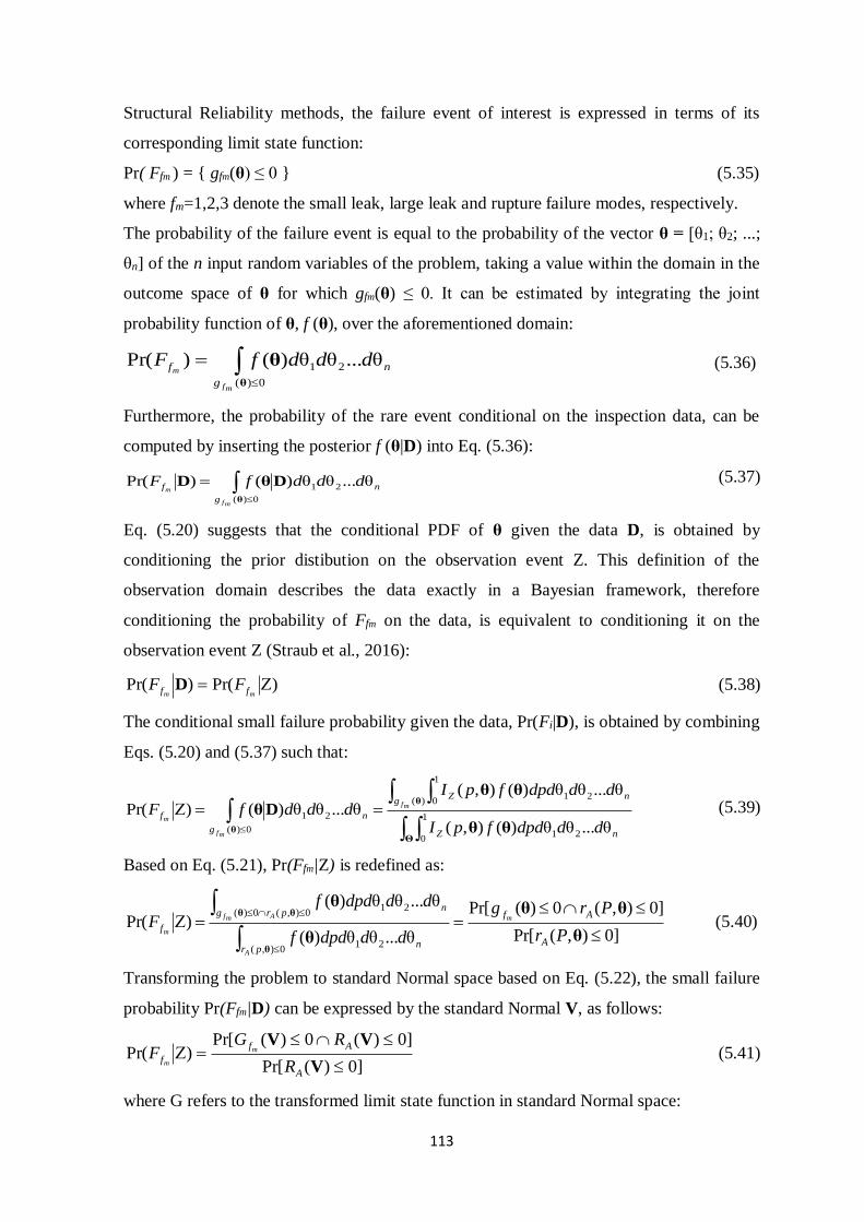
113
Structural Reliability methods, the failure event of interest is expressed in terms of its
corresponding limit state function:
Pr( Ffm ) = { gfm(θ) ≤ 0 } (5.35)
where fm=1,2,3 denote the small leak, large leak and rupture failure modes, respectively.
The probability of the failure event is equal to the probability of the vector θ = [θ1; θ2; ...;
θn] of the n input random variables of the problem, taking a value within the domain in the
outcome space of θ for which gfm(θ) ≤ 0. It can be estimated by integrating the joint
probability function of θ, f (θ), over the aforementioned domain:
0)(
21 θ...θθ)()Pr(θ
θ
mf
m
g
nf dddfF (5.36)
Furthermore, the probability of the rare event conditional on the inspection data, can be
computed by inserting the posterior f (θ|D) into Eq. (5.36):
0)(
21 θ...θθ)()Pr(θ
DθD
mf
m
g
nf dddfF (5.37)
Eq. (5.20) suggests that the conditional PDF of θ given the data D, is obtained by
conditioning the prior distibution on the observation event Z. This definition of the
observation domain describes the data exactly in a Bayesian framework, therefore
conditioning the probability of Ffm on the data, is equivalent to conditioning it on the
observation event Z (Straub et al., 2016):
)Pr()Pr( mm ff FF D (5.38)
The conditional small failure probability given the data, Pr(Fi|D), is obtained by combining
Eqs. (5.20) and (5.37) such that:
Θ
θ
θ θθ
θθ
Dθ1
021
)(
1
021
0)(
21
θ...θθ)(),(
θ...θθ)(),(
θ...θθ)()Pr(
nZ
gnZ
g
nf
dddpdfpI
dddpdfpI
dddfF mf
mf
m
(5.39)
Based on Eq. (5.21), Pr(Ffm|Z) is redefined as:
]0),(Pr[
]0),(0)(Pr[
θ...θθ)(
θ...θθ)(
)Pr(
0),(21
0),(0)(21
θ
θθ
θ
θ
θ
θθ
Pr
Prg
dddpdf
dddpdf
FA
Af
prn
prgn
fm
A
Amf
m (5.40)
Transforming the problem to standard Normal space based on Eq. (5.22), the small failure
probability Pr(Ffm|D) can be expressed by the standard Normal V, as follows:
]0)(Pr[
]0)(0)(Pr[)Pr(
V
VV
A
Af
fR
RGF m
m (5.41)
where G refers to the transformed limit state function in standard Normal space:
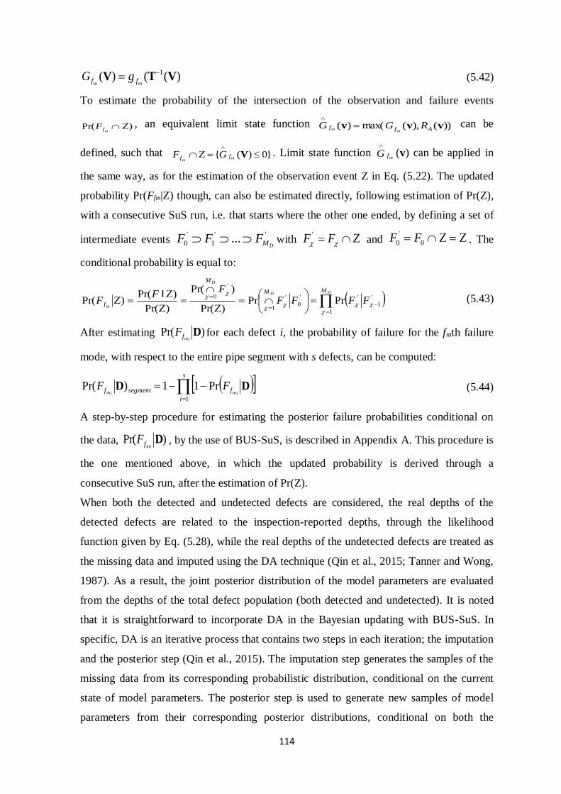
114
)(()( 1VTV
mm ff gG (5.42)
To estimate the probability of the intersection of the observation and failure events
)Pr( mf
F , an equivalent limit state function ))(),(max()( vvv Aff RGGmm
can be
defined, such that }0)({
Vmm
ff GF . Limit state function mfG
(v) can be applied in
the same way, as for the estimation of the observation event Z in Eq. (5.22). The updated
probability Pr(Ffm|Z) though, can also be estimated directly, following estimation of Pr(Z),
with a consecutive SuS run, i.e. that starts where the other one ended, by defining a set of
intermediate events ''
1
'
0 ...DMFFF with FF '
and 0
'
0 FF . The
conditional probability is equal to:
DD
D
m
MM
M
f FFFFF
FF
1
'
1
''
0
'
1
'
0PrPr
)Pr(
)Pr(
)Pr(
)Pr()Pr(
I (5.43)
After estimating )Pr( Dimf
F for each defect i, the probability of failure for the fmth failure
mode, with respect to the entire pipe segment with s defects, can be computed:
s
i
fsegmentfimim
FF1
Pr11)Pr( DD (5.44)
A step-by-step procedure for estimating the posterior failure probabilities conditional on
the data, )Pr( DmifF , by the use of BUS-SuS, is described in Appendix A. This procedure is
the one mentioned above, in which the updated probability is derived through a
consecutive SuS run, after the estimation of Pr(Z).
When both the detected and undetected defects are considered, the real depths of the
detected defects are related to the inspection-reported depths, through the likelihood
function given by Eq. (5.28), while the real depths of the undetected defects are treated as
the missing data and imputed using the DA technique (Qin et al., 2015; Tanner and Wong,
1987). As a result, the joint posterior distribution of the model parameters are evaluated
from the depths of the total defect population (both detected and undetected). It is noted
that it is straightforward to incorporate DA in the Bayesian updating with BUS-SuS. In
specific, DA is an iterative process that contains two steps in each iteration; the imputation
and the posterior step (Qin et al., 2015). The imputation step generates the samples of the
missing data from its corresponding probabilistic distribution, conditional on the current
state of model parameters. The posterior step is used to generate new samples of model
parameters from their corresponding posterior distributions, conditional on both the
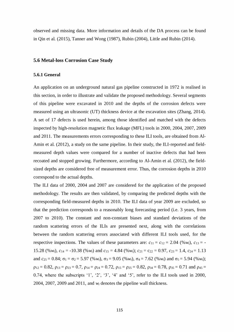
115
observed and missing data. More information and details of the DA process can be found
in Qin et al. (2015), Tanner and Wong (1987), Rubin (2004), Little and Rubin (2014).
5.6 Metal-loss Corrosion Case Study
5.6.1 General
An application on an underground natural gas pipeline constructed in 1972 is realised in
this section, in order to illustrate and validate the proposed methodology. Several segments
of this pipeline were excavated in 2010 and the depths of the corrosion defects were
measured using an ultrasonic (UT) thickness device at the excavation sites (Zhang, 2014).
A set of 17 defects is used herein, among those identified and matched with the defects
inspected by high-resolution magnetic flux leakage (MFL) tools in 2000, 2004, 2007, 2009
and 2011. The measurements errors corresponding to these ILI tools, are obtained from Al-
Amin et al. (2012), a study on the same pipeline. In their study, the ILI-reported and field-
measured depth values were compared for a number of inactive defects that had been
recoated and stopped growing. Furthermore, according to Al-Amin et al. (2012), the field-
sized depths are considered free of measurement error. Thus, the corrosion depths in 2010
correspond to the actual depths.
The ILI data of 2000, 2004 and 2007 are considered for the application of the proposed
methodology. The results are then validated, by comparing the predicted depths with the
corresponding field-measured depths in 2010. The ILI data of year 2009 are excluded, so
that the prediction corresponds to a reasonably long forecasting period (i.e. 3 years, from
2007 to 2010). The constant and non-constant biases and standard deviations of the
random scattering errors of the ILIs are presented next, along with the correlations
between the random scattering errors associated with different ILI tools used, for the
respective inspections. The values of these parameters are: c11 = c12 = 2.04 (%wt), c13 = -
15.28 (%wt), c14 = -10.38 (%wt) and c15 = 4.84 (%wt); c21 = c22 = 0.97, c23 = 1.4, c24 = 1.13
and c25 = 0.84; σ1 = σ2 = 5.97 (%wt), σ3 = 9.05 (%wt), σ4 = 7.62 (%wt) and σ5 = 5.94 (%wt);
ρ12 = 0.82, ρ13 = ρ23 = 0.7, ρ14 = ρ24 = 0.72, ρ15 = ρ25 = 0.82, ρ34 = 0.78, ρ35 = 0.71 and ρ45 =
0.74, where the subscripts ‘1’, ‘2’, ‘3’, ‘4’ and ‘5’, refer to the ILI tools used in 2000,
2004, 2007, 2009 and 2011, and wt denotes the pipeline wall thickness.
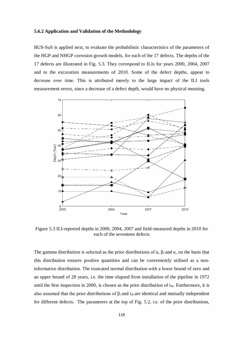
116
5.6.2 Application and Validation of the Methodology
BUS-SuS is applied next, to evaluate the probabilistic characteristics of the parameters of
the HGP and NHGP corrosion growth models, for each of the 17 defects. The depths of the
17 defects are illustrated in Fig. 5.3. They correspond to ILIs for years 2000, 2004, 2007
and to the excavation measurements of 2010. Some of the defect depths, appear to
decrease over time. This is attributed merely to the large impact of the ILI tools
measurement errors, since a decrease of a defect depth, would have no physical meaning.
Figure 5.3 ILI-reported depths in 2000, 2004, 2007 and field-measured depths in 2010 for
each of the seventeen defects
The gamma distribution is selected as the prior distributions of α, βi and κ, on the basis that
this distribution ensures positive quantities and can be conveniently utilised as a non-
informative distribution. Τhe truncated normal distribution with a lower bound of zero and
an upper bound of 28 years, i.e. the time elapsed from installation of the pipeline in 1972
until the first inspection in 2000, is chosen as the prior distribution of ti0. Furthermore, it is
also assumed that the prior distributions of βi and ti0 are identical and mutually independent
for different defects. The parameters at the top of Fig. 5.2, i.e. of the prior distributions,
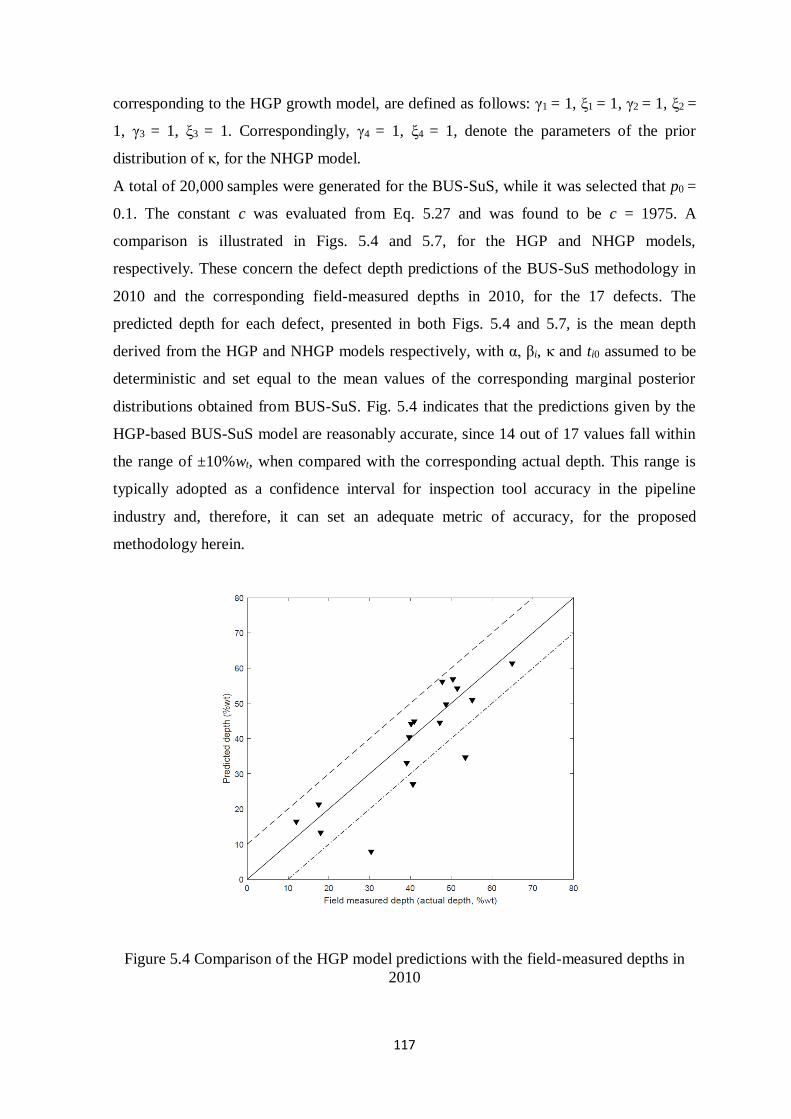
117
corresponding to the HGP growth model, are defined as follows: γ1 = 1, ξ1 = 1, γ2 = 1, ξ2 =
1, γ3 = 1, ξ3 = 1. Correspondingly, γ4 = 1, ξ4 = 1, denote the parameters of the prior
distribution of κ, for the NHGP model.
A total of 20,000 samples were generated for the BUS-SuS, while it was selected that p0 =
0.1. The constant c was evaluated from Eq. 5.27 and was found to be c = 1975. A
comparison is illustrated in Figs. 5.4 and 5.7, for the HGP and NHGP models,
respectively. These concern the defect depth predictions of the BUS-SuS methodology in
2010 and the corresponding field-measured depths in 2010, for the 17 defects. The
predicted depth for each defect, presented in both Figs. 5.4 and 5.7, is the mean depth
derived from the HGP and NHGP models respectively, with α, βi, κ and ti0 assumed to be
deterministic and set equal to the mean values of the corresponding marginal posterior
distributions obtained from BUS-SuS. Fig. 5.4 indicates that the predictions given by the
HGP-based BUS-SuS model are reasonably accurate, since 14 out of 17 values fall within
the range of ±10%wt, when compared with the corresponding actual depth. This range is
typically adopted as a confidence interval for inspection tool accuracy in the pipeline
industry and, therefore, it can set an adequate metric of accuracy, for the proposed
methodology herein.
Figure 5.4 Comparison of the HGP model predictions with the field-measured depths in
2010
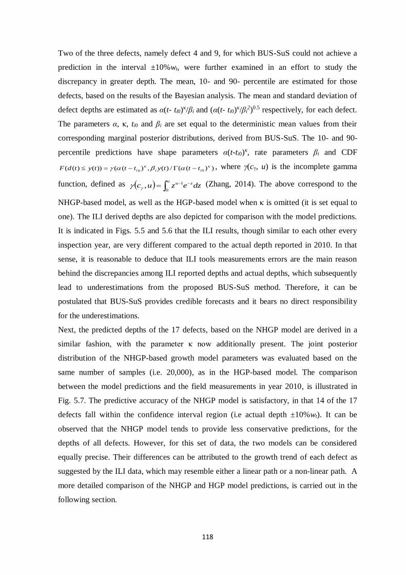
118
Two of the three defects, namely defect 4 and 9, for which BUS-SuS could not achieve a
prediction in the interval ±10%wt, were further examined in an effort to study the
discrepancy in greater depth. The mean, 10- and 90- percentile are estimated for those
defects, based on the results of the Bayesian analysis. The mean and standard deviation of
defect depths are estimated as α(t- ti0)κ/βi and (α(t- ti0)
κ/βi2)0.5 respectively, for each defect.
The parameters α, κ, ti0 and βi are set equal to the deterministic mean values from their
corresponding marginal posterior distributions, derived from BUS-SuS. The 10- and 90-
percentile predictions have shape parameters α(t-ti0)κ, rate parameters βi and CDF
))((/)(,)(())()(( 00
iii tttytttytdF , where γ(cγ, u) is the incomplete gamma
function, defined as
uzu dzezuc
0
1, (Zhang, 2014). The above correspond to the
NHGP-based model, as well as the HGP-based model when κ is omitted (it is set equal to
one). The ILI derived depths are also depicted for comparison with the model predictions.
It is indicated in Figs. 5.5 and 5.6 that the ILI results, though similar to each other every
inspection year, are very different compared to the actual depth reported in 2010. In that
sense, it is reasonable to deduce that ILI tools measurements errors are the main reason
behind the discrepancies among ILI reported depths and actual depths, which subsequently
lead to underestimations from the proposed BUS-SuS method. Therefore, it can be
postulated that BUS-SuS provides credible forecasts and it bears no direct responsibility
for the underestimations.
Next, the predicted depths of the 17 defects, based on the NHGP model are derived in a
similar fashion, with the parameter κ now additionally present. The joint posterior
distribution of the NHGP-based growth model parameters was evaluated based on the
same number of samples (i.e. 20,000), as in the HGP-based model. The comparison
between the model predictions and the field measurements in year 2010, is illustrated in
Fig. 5.7. The predictive accuracy of the NHGP model is satisfactory, in that 14 of the 17
defects fall within the confidence interval region (i.e actual depth ±10%wt). It can be
observed that the NHGP model tends to provide less conservative predictions, for the
depths of all defects. However, for this set of data, the two models can be considered
equally precise. Their differences can be attributed to the growth trend of each defect as
suggested by the ILI data, which may resemble either a linear path or a non-linear path. A
more detailed comparison of the NHGP and HGP model predictions, is carried out in the
following section.
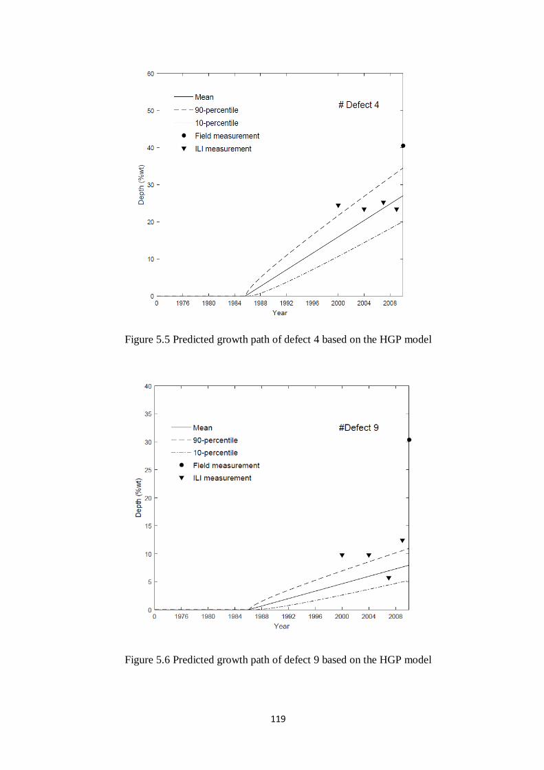
119
Figure 5.5 Predicted growth path of defect 4 based on the HGP model
Figure 5.6 Predicted growth path of defect 9 based on the HGP model
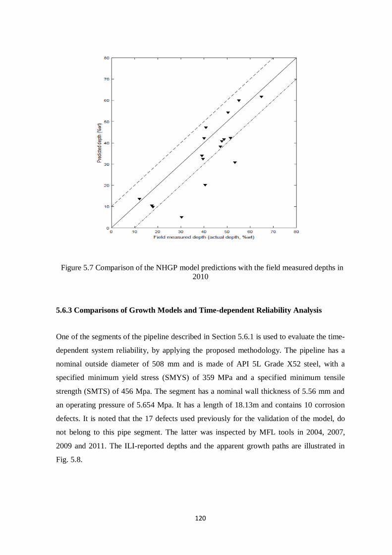
120
Figure 5.7 Comparison of the NHGP model predictions with the field measured depths in
2010
5.6.3 Comparisons of Growth Models and Time-dependent Reliability Analysis
One of the segments of the pipeline described in Section 5.6.1 is used to evaluate the time-
dependent system reliability, by applying the proposed methodology. The pipeline has a
nominal outside diameter of 508 mm and is made of API 5L Grade X52 steel, with a
specified minimum yield stress (SMYS) of 359 MPa and a specified minimum tensile
strength (SMTS) of 456 Mpa. The segment has a nominal wall thickness of 5.56 mm and
an operating pressure of 5.654 Mpa. It has a length of 18.13m and contains 10 corrosion
defects. It is noted that the 17 defects used previously for the validation of the model, do
not belong to this pipe segment. The latter was inspected by MFL tools in 2004, 2007,
2009 and 2011. The ILI-reported depths and the apparent growth paths are illustrated in
Fig. 5.8.
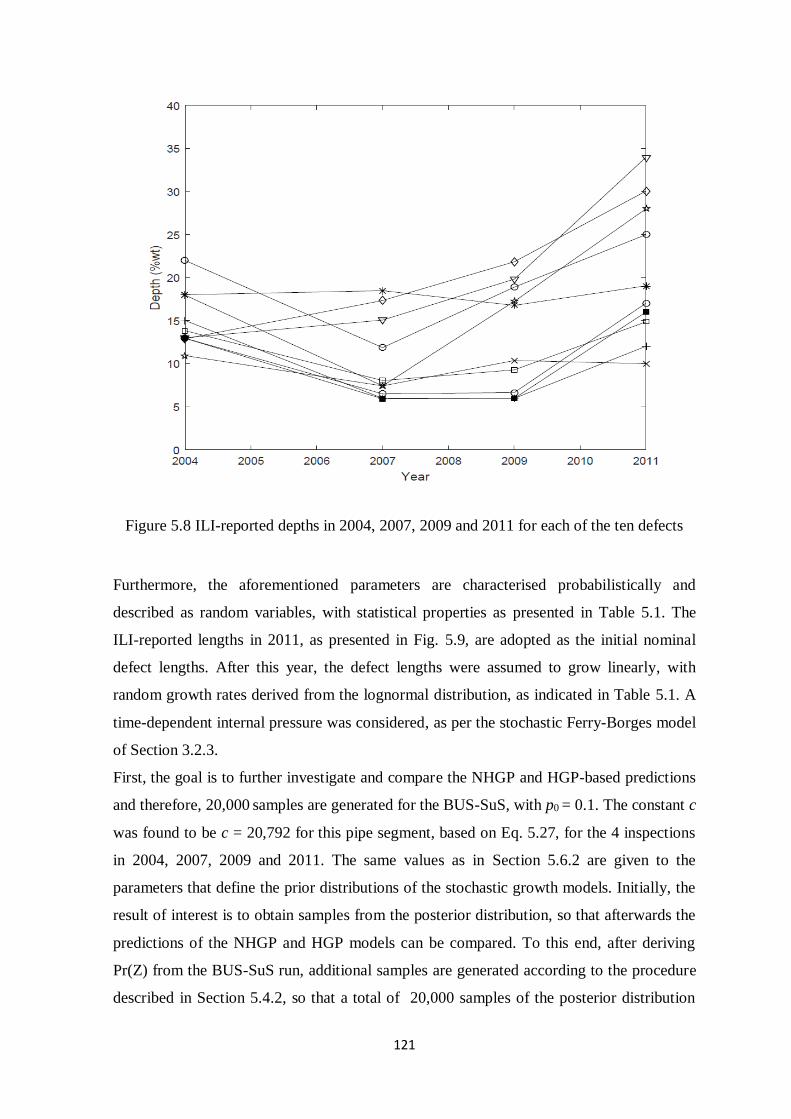
121
Figure 5.8 ILI-reported depths in 2004, 2007, 2009 and 2011 for each of the ten defects
Furthermore, the aforementioned parameters are characterised probabilistically and
described as random variables, with statistical properties as presented in Table 5.1. The
ILI-reported lengths in 2011, as presented in Fig. 5.9, are adopted as the initial nominal
defect lengths. After this year, the defect lengths were assumed to grow linearly, with
random growth rates derived from the lognormal distribution, as indicated in Table 5.1. A
time-dependent internal pressure was considered, as per the stochastic Ferry-Borges model
of Section 3.2.3.
First, the goal is to further investigate and compare the NHGP and HGP-based predictions
and therefore, 20,000 samples are generated for the BUS-SuS, with p0 = 0.1. The constant c
was found to be c = 20,792 for this pipe segment, based on Eq. 5.27, for the 4 inspections
in 2004, 2007, 2009 and 2011. The same values as in Section 5.6.2 are given to the
parameters that define the prior distributions of the stochastic growth models. Initially, the
result of interest is to obtain samples from the posterior distribution, so that afterwards the
predictions of the NHGP and HGP models can be compared. To this end, after deriving
Pr(Z) from the BUS-SuS run, additional samples are generated according to the procedure
described in Section 5.4.2, so that a total of 20,000 samples of the posterior distribution
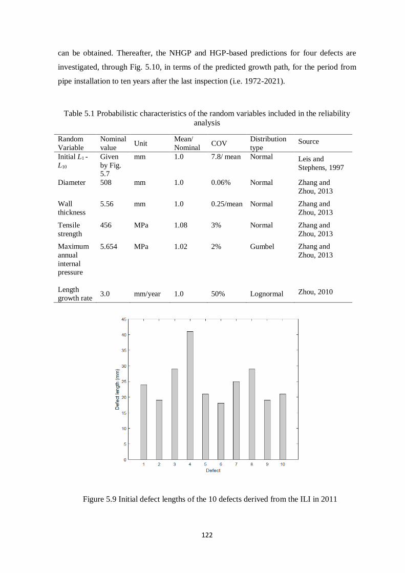
122
can be obtained. Thereafter, the NHGP and HGP-based predictions for four defects are
investigated, through Fig. 5.10, in terms of the predicted growth path, for the period from
pipe installation to ten years after the last inspection (i.e. 1972-2021).
Table 5.1 Probabilistic characteristics of the random variables included in the reliability
analysis
Random
Variable
Nominal
value Unit
Mean/
Nominal COV
Distribution
type Source
Initial L1 -
L10
Given
by Fig. 5.7
mm 1.0 7.8/ mean Normal Leis and
Stephens, 1997
Diameter 508 mm 1.0 0.06% Normal Zhang and
Zhou, 2013
Wall
thickness 5.56 mm 1.0 0.25/mean Normal Zhang and
Zhou, 2013
Tensile
strength
456 MPa 1.08 3% Normal Zhang and
Zhou, 2013
Maximum
annual
internal pressure
5.654 MPa 1.02 2% Gumbel Zhang and
Zhou, 2013
Length growth rate
3.0
mm/year
1.0
50%
Lognormal
Zhou, 2010
Figure 5.9 Initial defect lengths of the 10 defects derived from the ILI in 2011
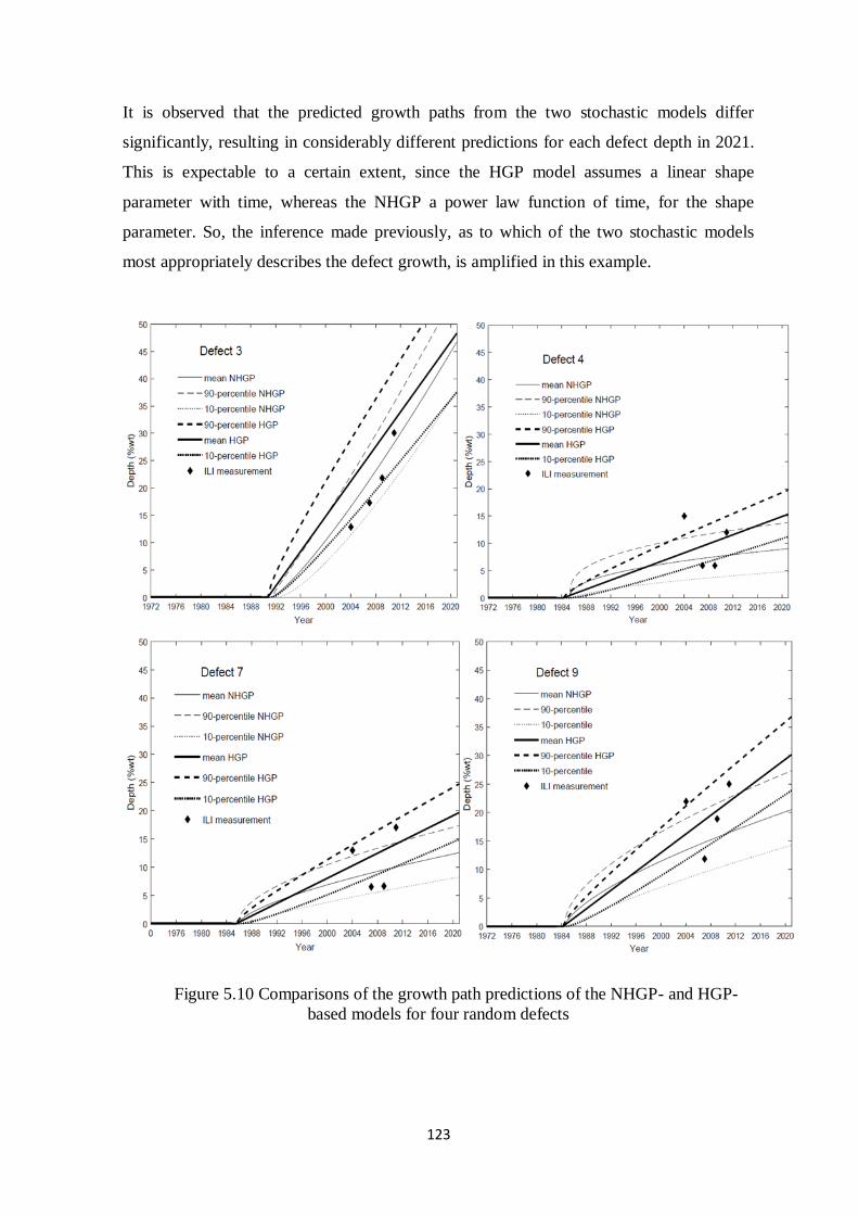
123
It is observed that the predicted growth paths from the two stochastic models differ
significantly, resulting in considerably different predictions for each defect depth in 2021.
This is expectable to a certain extent, since the HGP model assumes a linear shape
parameter with time, whereas the NHGP a power law function of time, for the shape
parameter. So, the inference made previously, as to which of the two stochastic models
most appropriately describes the defect growth, is amplified in this example.
Figure 5.10 Comparisons of the growth path predictions of the NHGP- and HGP-
based models for four random defects
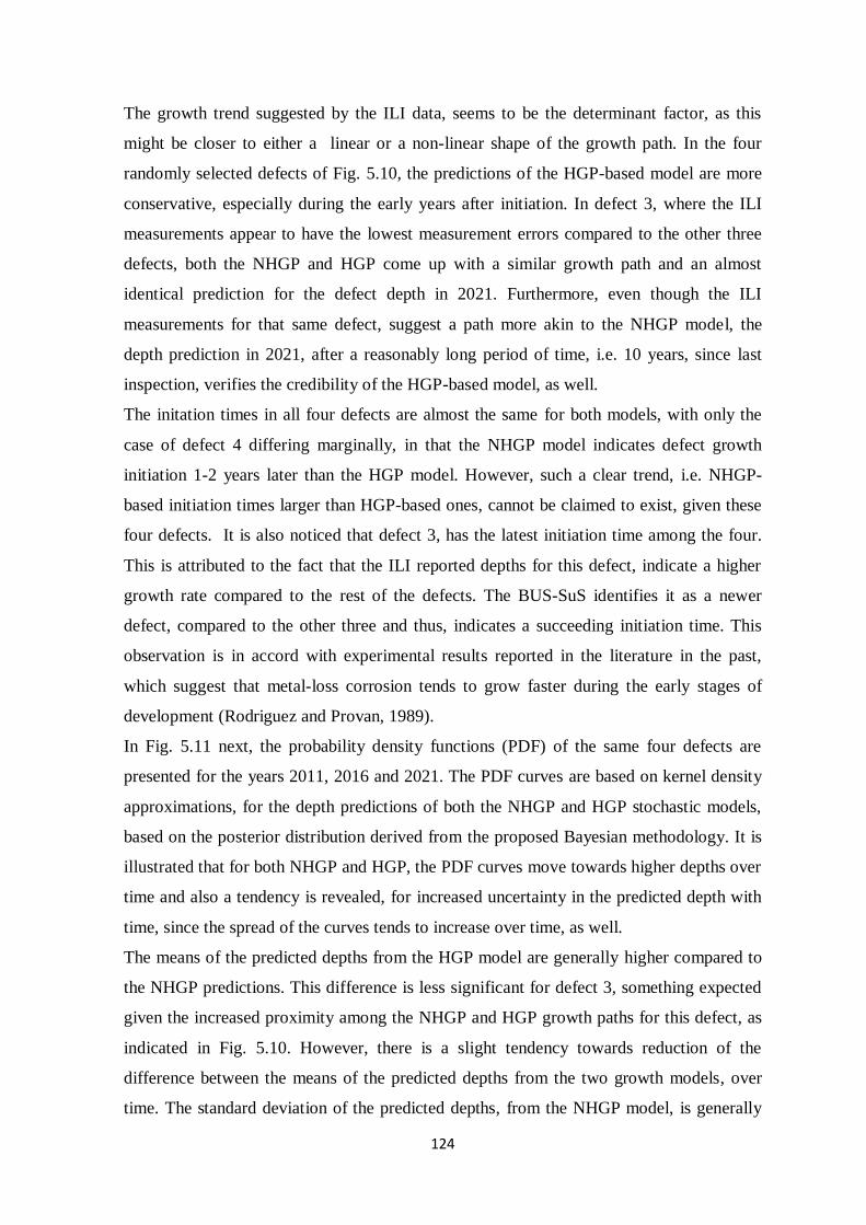
124
The growth trend suggested by the ILI data, seems to be the determinant factor, as this
might be closer to either a linear or a non-linear shape of the growth path. In the four
randomly selected defects of Fig. 5.10, the predictions of the HGP-based model are more
conservative, especially during the early years after initiation. In defect 3, where the ILI
measurements appear to have the lowest measurement errors compared to the other three
defects, both the NHGP and HGP come up with a similar growth path and an almost
identical prediction for the defect depth in 2021. Furthermore, even though the ILI
measurements for that same defect, suggest a path more akin to the NHGP model, the
depth prediction in 2021, after a reasonably long period of time, i.e. 10 years, since last
inspection, verifies the credibility of the HGP-based model, as well.
The initation times in all four defects are almost the same for both models, with only the
case of defect 4 differing marginally, in that the NHGP model indicates defect growth
initiation 1-2 years later than the HGP model. However, such a clear trend, i.e. NHGP-
based initiation times larger than HGP-based ones, cannot be claimed to exist, given these
four defects. It is also noticed that defect 3, has the latest initiation time among the four.
This is attributed to the fact that the ILI reported depths for this defect, indicate a higher
growth rate compared to the rest of the defects. The BUS-SuS identifies it as a newer
defect, compared to the other three and thus, indicates a succeeding initiation time. This
observation is in accord with experimental results reported in the literature in the past,
which suggest that metal-loss corrosion tends to grow faster during the early stages of
development (Rodriguez and Provan, 1989).
In Fig. 5.11 next, the probability density functions (PDF) of the same four defects are
presented for the years 2011, 2016 and 2021. The PDF curves are based on kernel density
approximations, for the depth predictions of both the NHGP and HGP stochastic models,
based on the posterior distribution derived from the proposed Bayesian methodology. It is
illustrated that for both NHGP and HGP, the PDF curves move towards higher depths over
time and also a tendency is revealed, for increased uncertainty in the predicted depth with
time, since the spread of the curves tends to increase over time, as well.
The means of the predicted depths from the HGP model are generally higher compared to
the NHGP predictions. This difference is less significant for defect 3, something expected
given the increased proximity among the NHGP and HGP growth paths for this defect, as
indicated in Fig. 5.10. However, there is a slight tendency towards reduction of the
difference between the means of the predicted depths from the two growth models, over
time. The standard deviation of the predicted depths, from the NHGP model, is generally
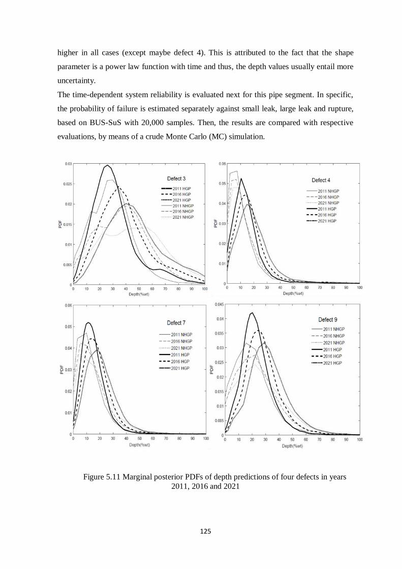
125
higher in all cases (except maybe defect 4). This is attributed to the fact that the shape
parameter is a power law function with time and thus, the depth values usually entail more
uncertainty.
The time-dependent system reliability is evaluated next for this pipe segment. In specific,
the probability of failure is estimated separately against small leak, large leak and rupture,
based on BUS-SuS with 20,000 samples. Then, the results are compared with respective
evaluations, by means of a crude Monte Carlo (MC) simulation.
Figure 5.11 Marginal posterior PDFs of depth predictions of four defects in years
2011, 2016 and 2021
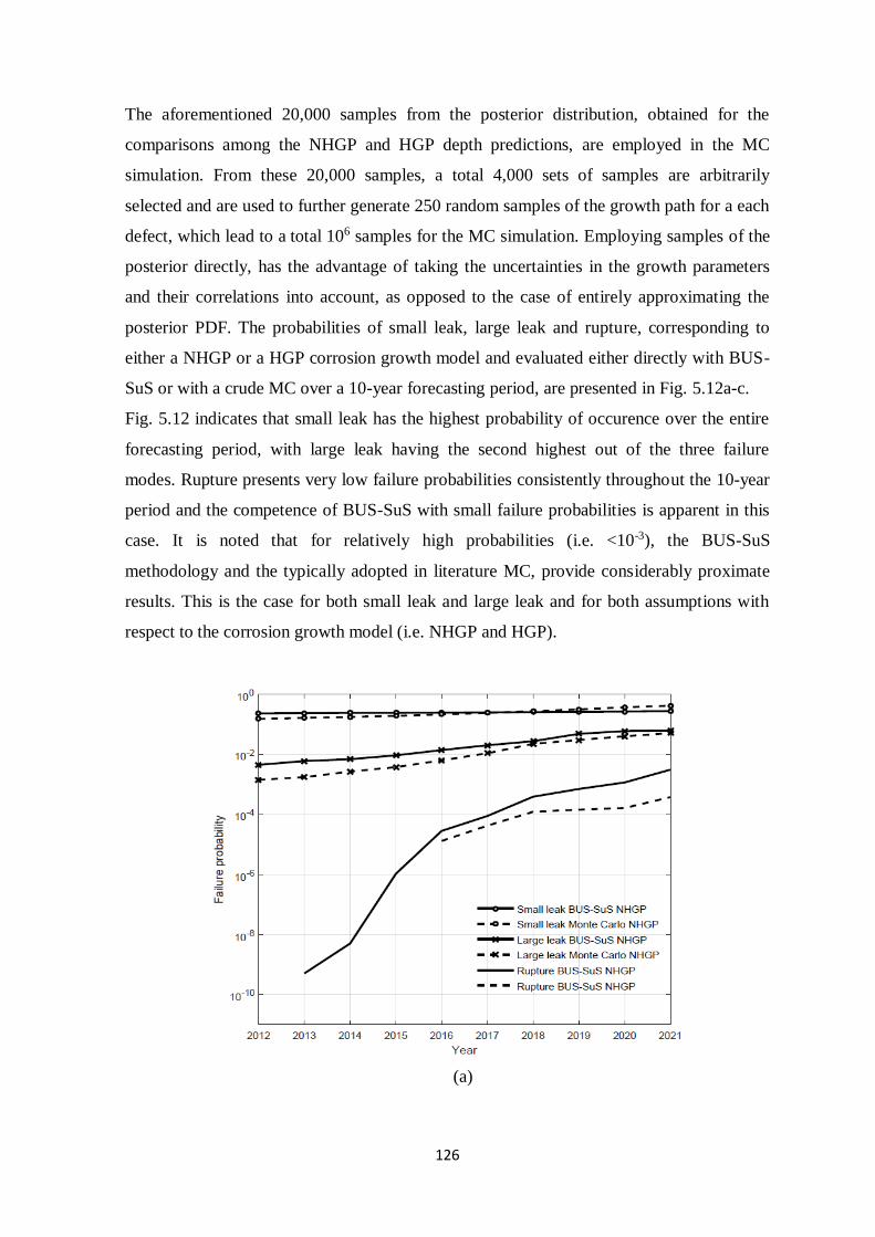
126
The aforementioned 20,000 samples from the posterior distribution, obtained for the
comparisons among the NHGP and HGP depth predictions, are employed in the MC
simulation. From these 20,000 samples, a total 4,000 sets of samples are arbitrarily
selected and are used to further generate 250 random samples of the growth path for a each
defect, which lead to a total 106 samples for the MC simulation. Employing samples of the
posterior directly, has the advantage of taking the uncertainties in the growth parameters
and their correlations into account, as opposed to the case of entirely approximating the
posterior PDF. The probabilities of small leak, large leak and rupture, corresponding to
either a NHGP or a HGP corrosion growth model and evaluated either directly with BUS-
SuS or with a crude MC over a 10-year forecasting period, are presented in Fig. 5.12a-c.
Fig. 5.12 indicates that small leak has the highest probability of occurence over the entire
forecasting period, with large leak having the second highest out of the three failure
modes. Rupture presents very low failure probabilities consistently throughout the 10-year
period and the competence of BUS-SuS with small failure probabilities is apparent in this
case. It is noted that for relatively high probabilities (i.e. <10-3), the BUS-SuS
methodology and the typically adopted in literature MC, provide considerably proximate
results. This is the case for both small leak and large leak and for both assumptions with
respect to the corrosion growth model (i.e. NHGP and HGP).
(a)
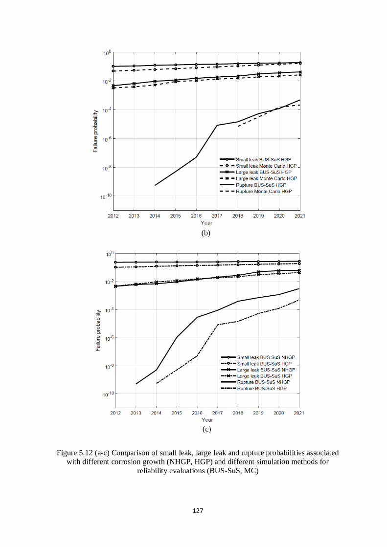
127
(b)
(c)
Figure 5.12 (a-c) Comparison of small leak, large leak and rupture probabilities associated
with different corrosion growth (NHGP, HGP) and different simulation methods for
reliability evaluations (BUS-SuS, MC)
128
Furthermore, Fig. 5.12a indicates that in the case of NHGP, small leak probability when
evaluated from BUS-SuS, is marginally higher in the first six years, i.e. 2012-2017, while
afterwards it is slightly less than the respective MC estimation. For large leak, BUS-SuS
consistently provides a more conservative estimation compared to MC, except for the last
year of the forecast, where the values seem to match. The same underestimation from the
MC is apparent in the rupture failure mode as well.
The discrepancies among the MC and BUS-SuS method are attributed to the approximate
nature of the MC simulation method. This specific above-described MC method, accounts
for the uncertainties of the growth parameters and their correlations only to certain extent,
since the additionally generated samples equate to an approximate posterior distribution.
On the other hand, in BUS-SuS such an approximation is not necessary. Next, the capacity
of BUS-SuS for small probabilities (i.e. <10-6), can also be observed in Fig. 5.12a. In
specific, the MC estimation can be realised only beyond 2016, since before that the
probability is too small for MC to produce credible (if any) results. On the contrary, BUS-
SuS can provide the complete picture of the failure probabilities. Its evaluations initiate
from the second year of the forecast period, i.e. 2013, and are in the order of 10-10. The
same features appear in Fig. 5.12b, which concern the HGP growth model. Minor
differences with the aforementioned are identified in specific aspects, as for example the
fact that the small leak probability curve from BUS-SuS, appears consistently higher than
the respective MC one and also that the large leak curves are coherently more akin. When
it comes to rupture, MC again presents limited capacity, in that it provides evaluations
only in the last 4 years, i.e. from 2018 onwards, in contrast to BUS-SuS that provides
predictions from the third year, starting again from a magnitude of 10-10.
The HGP probabilities are lower than the respective NHGP ones over the entire 10-year
period, especially the small ones, i.e. <10-3. This is evident in Fig. 5.12c, where the NHGP
rupture probability evaluations appear to be significantly more conservative compared to
the HGP ones, almost one order of magnitude higher. The same is the case for small leak
probabilities, but at a much smaller degree (almost one and half times higher), whereas
large leak probability curves, intersect twice and differ marginally overall. The
discrepancy is mainly attributed to the higher level of uncertainty involved in the NHGP
model, as discussed previously for Fig. 5.11. In other words, the larger spread in the depth
values generated from the NHGP model, due to the shape parameter being a power law
function with time, is thought to produce more failure events in the reliability analysis.
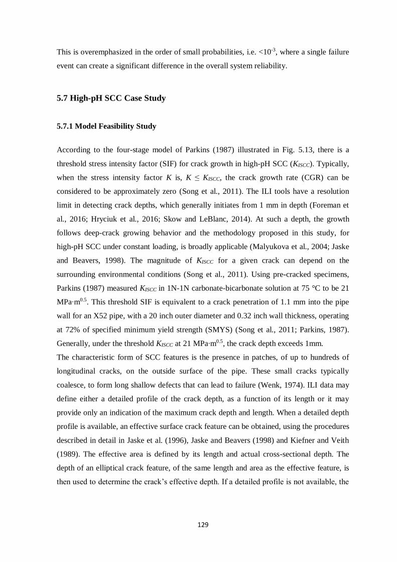
129
This is overemphasized in the order of small probabilities, i.e. <10-3, where a single failure
event can create a significant difference in the overall system reliability.
5.7 High-pH SCC Case Study
5.7.1 Model Feasibility Study
According to the four-stage model of Parkins (1987) illustrated in Fig. 5.13, there is a
threshold stress intensity factor (SIF) for crack growth in high-pH SCC (KISCC). Typically,
when the stress intensity factor K is, K ≤ KISCC, the crack growth rate (CGR) can be
considered to be approximately zero (Song et al., 2011). The ILI tools have a resolution
limit in detecting crack depths, which generally initiates from 1 mm in depth (Foreman et
al., 2016; Hryciuk et al., 2016; Skow and LeBlanc, 2014). At such a depth, the growth
follows deep-crack growing behavior and the methodology proposed in this study, for
high-pH SCC under constant loading, is broadly applicable (Malyukova et al., 2004; Jaske
and Beavers, 1998). The magnitude of KISCC for a given crack can depend on the
surrounding environmental conditions (Song et al., 2011). Using pre-cracked specimens,
Parkins (1987) measured KISCC in 1N-1N carbonate-bicarbonate solution at 75 °C to be 21
MPa∙m0.5. This threshold SIF is equivalent to a crack penetration of 1.1 mm into the pipe
wall for an X52 pipe, with a 20 inch outer diameter and 0.32 inch wall thickness, operating
at 72% of specified minimum yield strength (SMYS) (Song et al., 2011; Parkins, 1987).
Generally, under the threshold KISCC at 21 MPa∙m0.5, the crack depth exceeds 1mm.
The characteristic form of SCC features is the presence in patches, of up to hundreds of
longitudinal cracks, on the outside surface of the pipe. These small cracks typically
coalesce, to form long shallow defects that can lead to failure (Wenk, 1974). ILI data may
define either a detailed profile of the crack depth, as a function of its length or it may
provide only an indication of the maximum crack depth and length. When a detailed depth
profile is available, an effective surface crack feature can be obtained, using the procedures
described in detail in Jaske et al. (1996), Jaske and Beavers (1998) and Kiefner and Veith
(1989). The effective area is defined by its length and actual cross-sectional depth. The
depth of an elliptical crack feature, of the same length and area as the effective feature, is
then used to determine the crack’s effective depth. If a detailed profile is not available, the
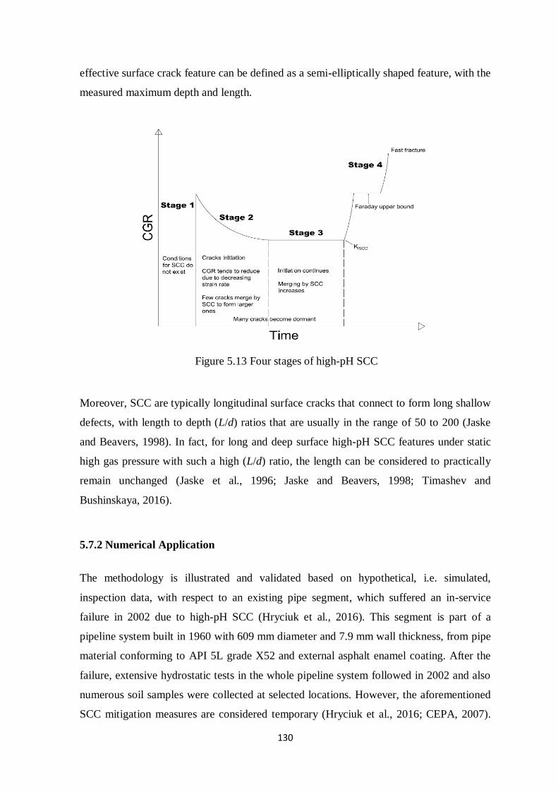
130
effective surface crack feature can be defined as a semi-elliptically shaped feature, with the
measured maximum depth and length.
Figure 5.13 Four stages of high-pH SCC
Moreover, SCC are typically longitudinal surface cracks that connect to form long shallow
defects, with length to depth (L/d) ratios that are usually in the range of 50 to 200 (Jaske
and Beavers, 1998). In fact, for long and deep surface high-pH SCC features under static
high gas pressure with such a high (L/d) ratio, the length can be considered to practically
remain unchanged (Jaske et al., 1996; Jaske and Beavers, 1998; Timashev and
Bushinskaya, 2016).
5.7.2 Numerical Application
The methodology is illustrated and validated based on hypothetical, i.e. simulated,
inspection data, with respect to an existing pipe segment, which suffered an in-service
failure in 2002 due to high-pH SCC (Hryciuk et al., 2016). This segment is part of a
pipeline system built in 1960 with 609 mm diameter and 7.9 mm wall thickness, from pipe
material conforming to API 5L grade X52 and external asphalt enamel coating. After the
failure, extensive hydrostatic tests in the whole pipeline system followed in 2002 and also
numerous soil samples were collected at selected locations. However, the aforementioned
SCC mitigation measures are considered temporary (Hryciuk et al., 2016; CEPA, 2007).
131
On pipeline material samples removed from lines that were hydrostatically tested, further
tests on SCC cracks that survived the pressure developed during the test (typically 110%
of SMYS), indicated growth rates of 0.29 mm/year to 0.5 mm/year. Furthermore, it was
decided to extensively perform remediation works of more permanent nature, i.e. the
replacement of the original degraded coating by a new one.
SCC is a particular class of corrosion, the development process of which stops, when the
contact between the steel surface and the ground is prevented. Thus, by replacing the
coating, the growth of existing cracks is also arrested. Accordingly, a 100% solids liquid
epoxy coating was applied to the pipeline system in 2003, including the susceptible part
nearby the rupture location of 2002. An ILI inspection in 2014 revealed the remanence of
five sub-critical SCC features in the susceptible part, whose growth had been arrested by
the recoating and thus, were considered fit for service. Subsequently, the part containing
verified SCC was cut out, in order to perform a full scale burst test. Material tests showed
a minimum tensile strength of 428 MPa and minimum Charpy Energy at 0 C of 18 J, in a
subsize specimen of 5 x 10 x 55 mm, equivalent to 36 J full size specimen (Hryciuk et al.,
2016). These values are above the API X52 minimum requirements of 460 Mpa tensile
strength and 27 J Charpy absorbed energy and actually met the requirements of API 5L
X52 (Hryciuk et al., 2016; API Standard, 2007).
Based on the above-described information, a hypothetical case study was considered in an
attempt to illustrate and validate the proposed methodology of this chapter. In specific, five
future ILIs are assumed to take place after 2014. It is assumed that due to local degradation
of the coating applied in 2003, SCC features start to generate and grow after 2014 and are
detected in the five future ILIs. To that end, SCC features are assumed to initiate based on
the NHHP model, by deterministically setting the parameters λo=0.5 and δ=1.0. In
addition, these are assumed to grow with a unique random rate that follows a uniform
distribution, with a lower bound of 0.29 mm/year and an upper bound of 0.50 mm/year, as
per the previously gathered actual data from the same pipeline system.
The results of the extensive study, presented in Foreman et al. (2016), were adopted to
quantify the measurement error and PoD for the five future inspections considered. The
study in Foreman et al. (2016), is based on significant populations of infield inspection
results from a variety of pipeline sections of different diameters. The aim of their study,
was to develop an absolute depth size specification, for ILI-based crack integrity
management of pipelines. A depth detection threshold of >1mm is defined herein, along
with a PoD of 98.3%, as per the aforementioned study. Furthermore, the measurement
132
error is assumed to fall within the bounds of ±1mm with 90% probability, as per the
respective absolute sizing model for cracks, from Foreman et al. (2016). Therefore, it is
estimated that q=4.0785 in Eq. (5.5) and also that the measurement error follows a
multivariate normal distribution, with mean zero and standard deviation σ=7.29%wt. For
simplicity, the constant and non-constant biases included in the measurement errors given
by Eq. (5.1), are assumed to be equal to zero and unity for all inspections respectively.
Finally, the random scattering errors associated with different inspections are defined as
mutually independent, with the same standard deviation of unity.
Individual crack features, are assumed to result from the coalescence of multiple
longitudinal surface cracks that have already merged, to form the final detected length to
depth (L/d) profile that follows a deep-crack growing behaviour. Their spatial dependence
due to similar manufacture and operation environment is accounted for, through the
correlation of their growths, based on the Copula method. Furthermore, it is considered
that during the deep crack growing stage, individual features cannot further merge. Deep
crack growing behaviour, apart from the studies already mentioned (i.e. Song et al., 2011;
Malyukova et al., 2004; Jaske and Beavers, 1998; Wenk, 1974), is supported by the actual
infield SCC cracks detected in 2014 on this very pipeline system (Hryciuk et al., 2016).
For the inspection data, only the critical dimension, i.e. depth, was generated in the
simulation and the length was evaluated according to the assumed ratio L/d = 50/1,
throughout the time interval under examination (Jaske et al., 1996; Jaske and Beavers,
1998; Timashev and Bushinskaya, 2016). This is also above the absolute detection
threshold, reported in Foreman et al. (2016) for crack lengths. The simulated inspection
data are illustrated in Table 5.2.
5.7.3 Validation of Bayesian Formulation
The Bayesian updating was carried out for both the NHPP and NHGP models, based on
the inspection data. The shape and scale parameters of the gamma prior distributions, for
the parameters of the models α, κ, βi and λo, δ, were all set to unity, and the newly detected
cracks in the jth inspection were assumed to initiate between the (j-1)th and jth inspections.
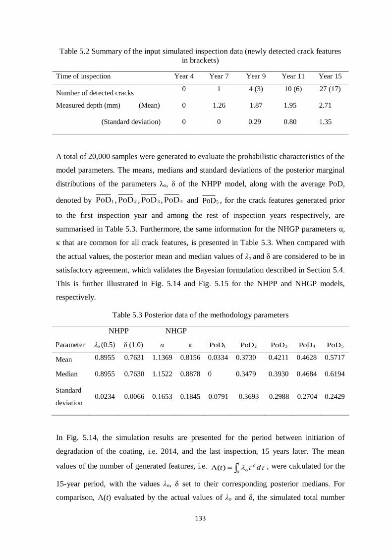
133
Table 5.2 Summary of the input simulated inspection data (newly detected crack features
in brackets)
Time of inspection Year 4 Year 7 Year 9 Year 11 Year 15
Number of detected cracks 0 1 4 (3) 10 (6) 27 (17)
Measured depth (mm) (Mean) 0 1.26 1.87 1.95 2.71
(Standard deviation) 0 0 0.29 0.80 1.35
A total of 20,000 samples were generated to evaluate the probabilistic characteristics of the
model parameters. The means, medians and standard deviations of the posterior marginal
distributions of the parameters λo, δ of the NHPP model, along with the average PoD,
denoted by 4321 PoD,PoD,PoD,PoD and 5PoD , for the crack features generated prior
to the first inspection year and among the rest of inspection years respectively, are
summarised in Table 5.3. Furthermore, the same information for the NHGP parameters α,
κ that are common for all crack features, is presented in Table 5.3. When compared with
the actual values, the posterior mean and median values of λo and δ are considered to be in
satisfactory agreement, which validates the Bayesian formulation described in Section 5.4.
This is further illustrated in Fig. 5.14 and Fig. 5.15 for the NHPP and NHGP models,
respectively.
Table 5.3 Posterior data of the methodology parameters
NHPP NHGP
Parameter λo (0.5) δ (1.0) α κ 1PoD 2PoD 3PoD 4PoD 5PoD
Mean 0.8955 0.7631 1.1369 0.8156 0.0334 0.3730 0.4211 0.4628 0.5717
Median 0.8955 0.7630 1.1522 0.8878 0 0.3479 0.3930 0.4684 0.6194
Standard
deviation 0.0234 0.0066 0.1653 0.1845 0.0791 0.3693 0.2988 0.2704 0.2429
In Fig. 5.14, the simulation results are presented for the period between initiation of
degradation of the coating, i.e. 2014, and the last inspection, 15 years later. The mean
values of the number of generated features, i.e. t
o dt0
)( , were calculated for the
15-year period, with the values λo, δ set to their corresponding posterior medians. For
comparison, Λ(t) evaluated by the actual values of λo and δ, the simulated total number
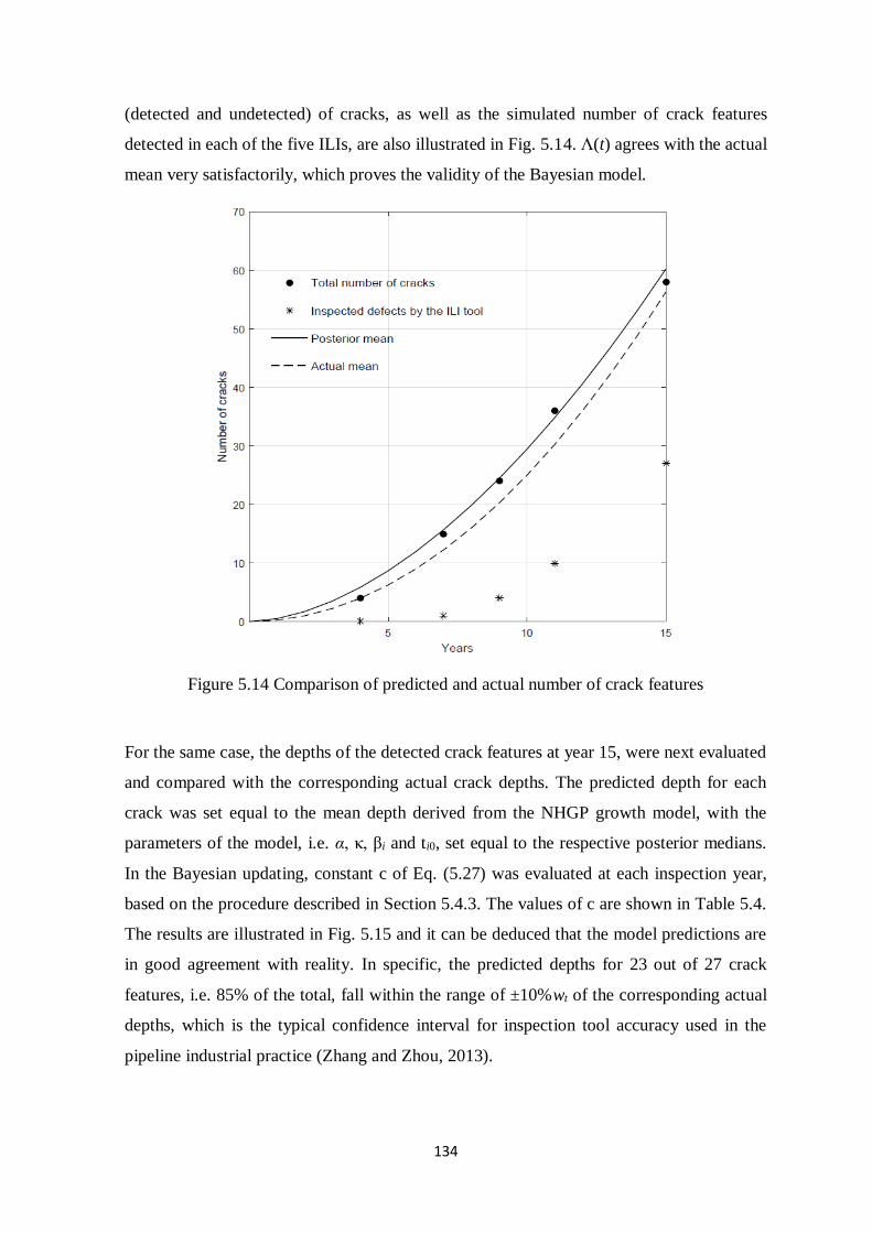
134
(detected and undetected) of cracks, as well as the simulated number of crack features
detected in each of the five ILIs, are also illustrated in Fig. 5.14. Λ(t) agrees with the actual
mean very satisfactorily, which proves the validity of the Bayesian model.
Figure 5.14 Comparison of predicted and actual number of crack features
For the same case, the depths of the detected crack features at year 15, were next evaluated
and compared with the corresponding actual crack depths. The predicted depth for each
crack was set equal to the mean depth derived from the NHGP growth model, with the
parameters of the model, i.e. α, κ, βi and ti0, set equal to the respective posterior medians.
In the Bayesian updating, constant c of Eq. (5.27) was evaluated at each inspection year,
based on the procedure described in Section 5.4.3. The values of c are shown in Table 5.4.
The results are illustrated in Fig. 5.15 and it can be deduced that the model predictions are
in good agreement with reality. In specific, the predicted depths for 23 out of 27 crack
features, i.e. 85% of the total, fall within the range of ±10%wt of the corresponding actual
depths, which is the typical confidence interval for inspection tool accuracy used in the
pipeline industrial practice (Zhang and Zhou, 2013).
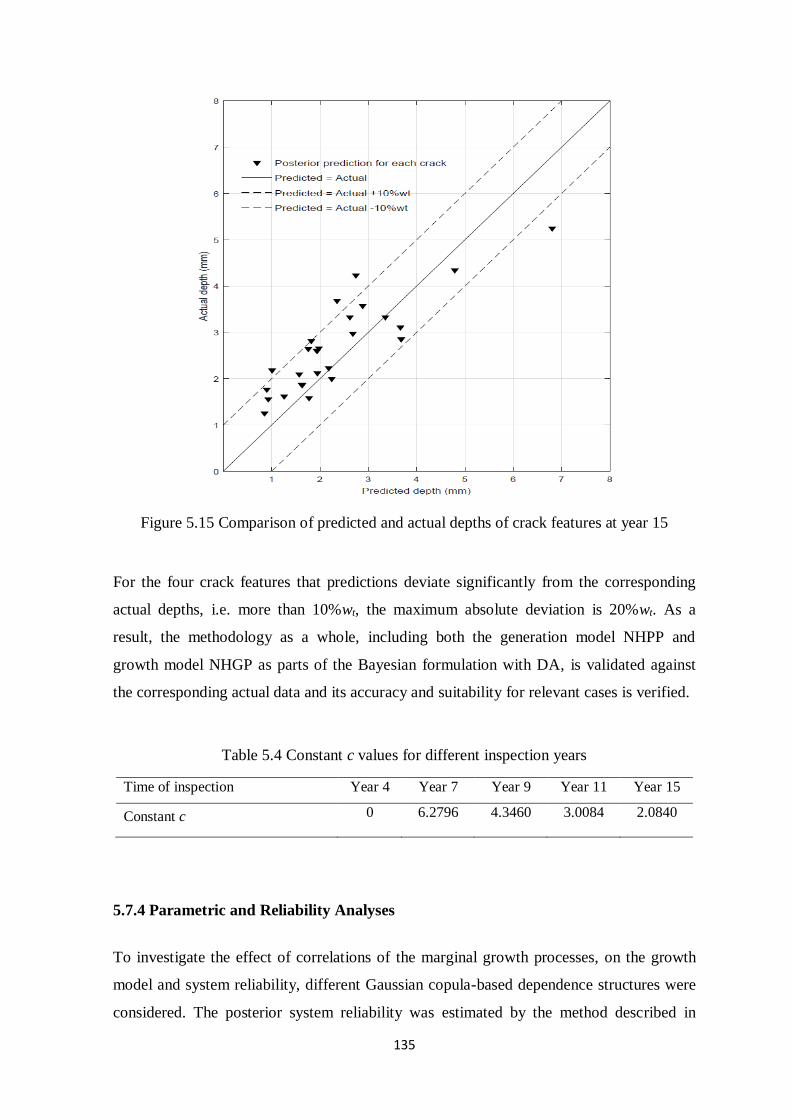
135
Figure 5.15 Comparison of predicted and actual depths of crack features at year 15
For the four crack features that predictions deviate significantly from the corresponding
actual depths, i.e. more than 10%wt, the maximum absolute deviation is 20%wt. As a
result, the methodology as a whole, including both the generation model NHPP and
growth model NHGP as parts of the Bayesian formulation with DA, is validated against
the corresponding actual data and its accuracy and suitability for relevant cases is verified.
Table 5.4 Constant c values for different inspection years
Time of inspection Year 4 Year 7 Year 9 Year 11 Year 15
Constant c 0 6.2796 4.3460 3.0084 2.0840
5.7.4 Parametric and Reliability Analyses
To investigate the effect of correlations of the marginal growth processes, on the growth
model and system reliability, different Gaussian copula-based dependence structures were
considered. The posterior system reliability was estimated by the method described in
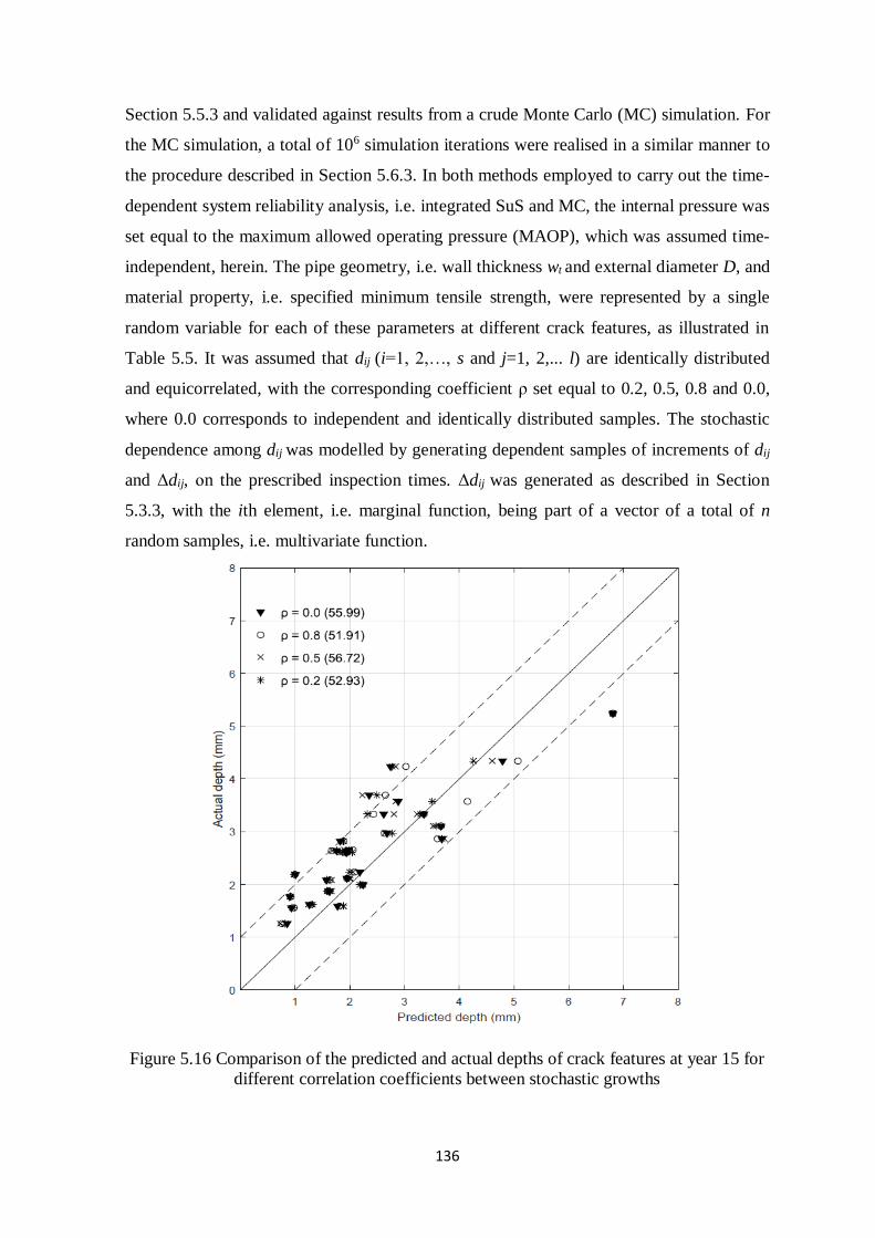
136
Section 5.5.3 and validated against results from a crude Monte Carlo (MC) simulation. For
the MC simulation, a total of 106 simulation iterations were realised in a similar manner to
the procedure described in Section 5.6.3. In both methods employed to carry out the time-
dependent system reliability analysis, i.e. integrated SuS and MC, the internal pressure was
set equal to the maximum allowed operating pressure (MAOP), which was assumed time-
independent, herein. The pipe geometry, i.e. wall thickness wt and external diameter D, and
material property, i.e. specified minimum tensile strength, were represented by a single
random variable for each of these parameters at different crack features, as illustrated in
Table 5.5. It was assumed that dij (i=1, 2,…, s and j=1, 2,... l) are identically distributed
and equicorrelated, with the corresponding coefficient ρ set equal to 0.2, 0.5, 0.8 and 0.0,
where 0.0 corresponds to independent and identically distributed samples. The stochastic
dependence among dij was modelled by generating dependent samples of increments of dij
and Δdij, οn the prescribed inspection times. Δdij was generated as described in Section
5.3.3, with the ith element, i.e. marginal function, being part of a vector of a total of n
random samples, i.e. multivariate function.
Figure 5.16 Comparison of the predicted and actual depths of crack features at year 15 for
different correlation coefficients between stochastic growths
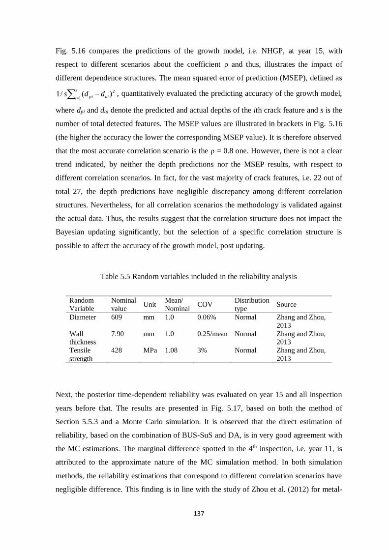
137
Fig. 5.16 compares the predictions of the growth model, i.e. NHGP, at year 15, with
respect to different scenarios about the coefficient ρ and thus, illustrates the impact of
different dependence structures. The mean squared error of prediction (MSEP), defined as
s
i aipi dds1
2)(/1 , quantitatively evaluated the predicting accuracy of the growth model,
where dpi and dai denote the predicted and actual depths of the ith crack feature and s is the
number of total detected features. The MSEP values are illustrated in brackets in Fig. 5.16
(the higher the accuracy the lower the corresponding MSEP value). It is therefore observed
that the most accurate correlation scenario is the ρ = 0.8 one. However, there is not a clear
trend indicated, by neither the depth predictions nor the MSEP results, with respect to
different correlation scenarios. In fact, for the vast majority of crack features, i.e. 22 out of
total 27, the depth predictions have negligible discrepancy among different correlation
structures. Nevertheless, for all correlation scenarios the methodology is validated against
the actual data. Thus, the results suggest that the correlation structure does not impact the
Bayesian updating significantly, but the selection of a specific correlation structure is
possible to affect the accuracy of the growth model, post updating.
Table 5.5 Random variables included in the reliability analysis
Random Variable
Nominal value
Unit Mean/ Nominal
COV Distribution type
Source
Diameter 609 mm 1.0 0.06% Normal Zhang and Zhou,
2013
Wall thickness
7.90 mm 1.0 0.25/mean Normal Zhang and Zhou, 2013
Tensile
strength
428 MPa 1.08 3% Normal Zhang and Zhou,
2013
Next, the posterior time-dependent reliability was evaluated on year 15 and all inspection
years before that. The results are presented in Fig. 5.17, based on both the method of
Section 5.5.3 and a Monte Carlo simulation. It is observed that the direct estimation of
reliability, based on the combination of BUS-SuS and DA, is in very good agreement with
the MC estimations. The marginal difference spotted in the 4th inspection, i.e. year 11, is
attributed to the approximate nature of the MC simulation method. In both simulation
methods, the reliability estimations that correspond to different correlation scenarios have
negligible difference. This finding is in line with the study of Zhou et al. (2012) for metal-
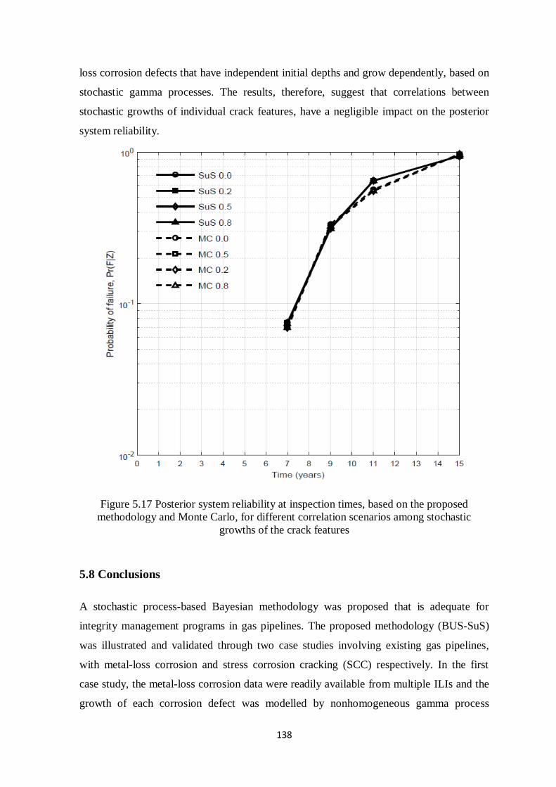
138
loss corrosion defects that have independent initial depths and grow dependently, based on
stochastic gamma processes. The results, therefore, suggest that correlations between
stochastic growths of individual crack features, have a negligible impact on the posterior
system reliability.
Figure 5.17 Posterior system reliability at inspection times, based on the proposed
methodology and Monte Carlo, for different correlation scenarios among stochastic
growths of the crack features
5.8 Conclusions
A stochastic process-based Bayesian methodology was proposed that is adequate for
integrity management programs in gas pipelines. The proposed methodology (BUS-SuS)
was illustrated and validated through two case studies involving existing gas pipelines,
with metal-loss corrosion and stress corrosion cracking (SCC) respectively. In the first
case study, the metal-loss corrosion data were readily available from multiple ILIs and the
growth of each corrosion defect was modelled by nonhomogeneous gamma process
139
(NHGP)- and homogeneous gamma process (HGP)- based models. The numerical
application consisted of initially applying the growth models on 17 external corrosion
defects, based on three ILIs that took place before a subsequent field measurement in
2010, while considering the measurement errors of inspections. The model predictions
were compared with the corresponding actual field measurements. The validation of the
model was satisfactory for 14 of the 17 defects in the range of ±10%wt, for the absolute
differences among the proposed methodology’s predictions and field measurements.
Further analysis of the results, indicated that the underestimations of the proposed
methodology, are due to large measurement errors in ILIs. Therefore, it proves to be a
reliable method in the setting of a real pipeline application, demonstrating at the same time
additional efficiency compared to MCMC techniques, which are typically adopted in
literature.
Furthermore, the time-dependent system reliability analysis was evaluated for a pipe
segment that contains 10 corrosion defects. Internal pressure was modelled by a Ferry
Borges stochastic process. Both the NHGP and HGP models were employed. It was shown
that the proposed methodology facilitates the estimation of small posterior failure
probabilities directly, without the requirement of either explicit knowledge or
approximation of the posterior joint probability distribution of the random variables. The
estimations were compared with results from crude Monte Carlo (MC) simulations and the
aforementioned assumptions were verified. Reliability estimations from the proposed
methodology, but also from MC at a lower extent, appear to give more conservative results
when the NHGP growth model is employed. This is mainly attributed to the higher
uncertainty contained in the NHGP model, due to the fact that the shape parameter is a
power law function and, thus, it produces corrosion depth values of higher uncertainty.
In the second case study, Bayesian updating was conducted by using BUS-SuS in
conjuction with the data augmentation (DA) technique. Simulated data were used,
corresponding to an existing gas pipeline with high-pH SCC defects, to illustrate and
validate the proposed methodology. The crack generation was characterised by the non-
homogeneous Poisson process (NHPP) and the growth, in terms of the crack depth, by the
non-homogeneous gamma process (NHGP), with a time-dependent shape parameter and a
time-independent scale parameter. Furthermore, the Gaussian copula method was adopted
to model the dependence among the stochastic growths of individual crack features. The
model parameters were all uncertain variables evaluated from the proposed updating
140
methodology, based on imperfect data from multiple ILIs. The Bayesian framework
accounted for the imperfect detectability of the ILI tool, as defined by the PoD, and also
for the measurement errors associated with the ILI data. The Bayesian updating was
performed together with the data augmentation algorithm, to account for undetected crack
features. The posterior time-dependent system reliability was evaluated through coupling
the updated crack growth model, with a probabilistic structural reliability model. The
underlying high-dimensional issues, were solved using subset simulation, in a similar
fashion to the first case study.
Different scenarios were considered with respect to the correlations of stochastic growths
of crack features, in an effort to examine their impact on the posterior growth model and
the system reliability. Stochastic growths of individual crack features were assumed
identically distributed and equicorrelated, with the coefficient ρ equal to 0.2, 0.5, 0.8 and
0.0. The results from the Bayesian updating of the generation and growth models, indicate
that the predicted overall crack population corresponding to the base case, i.e. ρ = 0.0, is in
satisfactory agreement with the actual crack population, which validates the proposed
methodology. The other three correlation scenarios also lead to predictions in good
agreement with the actual data and therefore the Bayesian methodology is validated as a
whole, irrespective of the correlation scenario. However, there were some discrepancies,
identified through the MSEP, in the accuracy of predictions among the different scenarios.
The most accurate was the one with ρ equal to 0.8. The evaluations of the posterior time-
dependent system reliability, based on both the direct coupled SuS methodology and the
crude Monte Carlo simulation, led to similar results, which verify the correctness of the
proposed methodology. Finally, for different dependence structures, the results from both
simulation models were found to have a negligible impact on the posterior system
reliability. Overall, the Bayesian framework proposed in this chapter, proves to be
particularly advantageous for energy pipelines, which typically involve multiple random
variables and particularly rare failure probabilities, which are often in the order of 10-6 or
less.
141
6. Conclusions, Research Achievements and Future Works
6.1 General Conclusions
The work reported in this thesis focused on certain critical aspects of the engineering
challenges included in reliability-based integrity management of energy pipelines. In
specific, stochastic modelling within a structural reliability framework was carried out,
along with statistical modelling for reliability predictions based on historical failures and
the results were cross-verified. In addition, robust methodologies for estimation of small
posterior failure probabilities were proposed, based on in-line inspection data. Conclusions
obtained from the research, along with contributions to knowledge and future works are
presented in the following.
6.1.1 Structural Reliability Analyses for Predictions in Energy Pipelines
Two probabilistic methodologies were proposed for onshore gas transmission pipelines
subjected to external metal-loss corrosion, based on a robust integration of stochastic
processes within a structural reliability analysis (SRA) framework. They were illustrated
through two realistic case studies and were based on two different inspection and
maintenance plans, i.e. DA and ILI inspections and repairs. The first methodology
investigated a predominant failure mechanism, i.e. external metal-loss corrosion, and
evaluated rupture probabilities regarding a reference pipe segment. The latter was
constructed by employing the average characteristics of ruptured pipes, from PHMSA
database of the United States Department of Transportation, for the period 2002-2014. The
uncertainties were modelled comprehensively, through stochastic modelling of the
segment-based loading and capacity. The non-homogeneous Poisson process was
employed for the generation of new defects and the Poisson square wave process to model
the growth of the defects. The internal pressure load was modelled through a discrete
Ferry-Borges stochastic process. An implicit ILI inspection and maintenance plan was
incorporated subsequently, based on standardised codes of practice, along with the
corresponding uncertainties of the inspection procedure. Considering the use of realistic
characteristics from the PHMSA database, it can be inferred that this model provides
142
additional knowledge on the state of the PHMSA onshore gas transmission network among
2002-2014, a representative period of the up-to-date techniques and strategies for
operation and rehabilitation in the industry, amplifying the relevance of the results to
reliability analyses for new or existing pipelines.
The second probabilistic methodology provided an accurate prediction of the time-
dependent reliability for unpiggable pipeline systems, subjected to external metal-loss
corrosion. The application of the proposed methodology on an example pipeline system
was realised by considering a preventive direct excavation, assessment and repair strategy.
The non-homogeneous Poisson process was employed for the generation of corrosion
defects over time and a parameterized stochastic process, i.e. non-linear function of two
random variables, for the defect growth, with respect to a single pipe segment of 12m. A
Poisson square wave process model was adopted for the internal pressure loading. The
reliability of the corroding pipe segment was evaluated by means of a Monte Carlo
simulation, against the failure mode of burst. Next, a heuristic method, i.e. SSA, was
employed, in order to update the corresponding reliability of a linear pipeline system,
composed of a series of segments. The estimated reliability of the single segment, which is
directly associated with the failure mode of burst, was used in the SSA analysis, instead of
the hazard function associated with the time to failure. The pipeline system was assumed
to be imperfectly repaired in every PM action, which is industry-consistent, due to human
and financial constraints. The SSA method accurately quantified changes in reliability, due
to the imperfect repairs. The results demonstrated the efficiency of the methodology in
accurately quantifying pipeline system reliability, by incorporating the effects of failure
probabilities of both repaired and unrepaired segments over time.
The probabilistic methodologies proposed in this chapter can assist operators in selecting
efficient preventive ECDA and repair strategies for unpiggable pipelines, as well as ILI
and repair strategies for piggable ones. In fact, for piggable pipelines, the two
methodologies can be compared and the optimal one can be identified, from an analysis
that conjointly considers failure probabilities and maintenance costs. The methodologies of
this chapter can therefore assist operators in making informed maintenance decisions,
based on reliability and risk.
143
6.1.2 Statistical Analyses for Reliability Predictions in Energy Pipelines
In the first case study of this chapter, the NPI established approach was employed, in an
attempt to derive inductive inferences from the lifetimes of a set of ruptured onshore gas
transmission pipelines, as reported in the PHMSA database in the period 2002-2014. The
NPI method analysed the rupture incidents from a non-repairable systems perspective,
based on the time to failure of the ruptured pipe segments. The analysis showed that NPI is
an advantageous method for derivation of inferences for a future pipe segment that
ruptures due to a specific failure cause, by providing imprecise probabilities and survival
functions for this event, based on historical failure data. The results, among others,
indicated external corrosion as the predominant rupture cause for the aforementioned
period under consideration in the USA, with ruptures taking place mainly after 30 years of
pipeline operation. The second case study was based on historical incident data from the
PHMSA database, for the period 2002-2014 as well. An empirical discrete hazard model
was adopted, in conjunction with a non-subjective parameter estimation technique, i.e.
non-linear quantile regression, to evaluate hazard and reliability functions. The model
provided inferences on the reliability of a region’s reference pipe segment for its complete
lifecycle, even in case of scarce, incomplete and censored data, as opposed to ROCOF
methods that only account for the limited time period under study. Furthermore, non-linear
quantile regression depicted accurately the hazard dataset. Thus, it is considered that the
generic nature of the historical data was sufficiently accounted for and that the resulting
reliability lies within a credible expectation range. The numerical application of the second
case study on the PHMSA database for the period 2002-2014, concerned rupture incidents
of onshore gas transmission pipelines.
The results of the second statistical methodology were compared with these of the first
case study of the previous chapter (Section 3.5), which was based on the same PHMSA
2002-2014 set of data. The results demonstrated reasonable proximity, which constitutes
an inherent validation of the soundness of both methodologies and their estimations. The
second statistical methodology therefore, can help pipeline operators to derive plausible
expectations for the performance of either new or existing pipelines. Those evaluations can
also correspond separately to specific parameters, like defect growth rates or defect density
or other pipeline attributes that define risk, by means of parametric studies. Furthermore,
the numerical application results of the second case study, are thought to provide further
144
information about the PHMSA onshore gas transmission network among 2002-2014 with
respect to rupture, which is more advantageous compared to the ROCOF-based approaches
typically employed in literature. The methodologies of this chapter can therefore assist
operators in making informed maintenance decisions based on reliability and risk.
6.1.3 Bayesian Analysis of Pipeline Reliability based on Imperfect Inspection Data
A stochastic process-based Bayesian methodology was proposed in this chapter, adequate
for corrosion management programs regarding gas pipelines. The proposed methodology
(BUS-SuS) was illustrated and validated through two case studies, involving existing gas
pipelines with metal-loss corrosion and stress corrosion cracking (SCC), respectively. In
the first case study, metal-loss corrosion data were available from multiple in-line
inspections (ILIs) and the growth of each corrosion defect was modelled by both
nonhomogeneous gamma process (NHGP)- and homogeneous gamma process (HGP)-
based models. The numerical application consisted of initially applying the growth models
on 17 external corrosion defects, based on three ILIs that took place before a subsequent
field measurement in 2010, while considering the measurement errors of inspections. The
model predictions were compared with the corresponding actual measurements from the
field. The validation of the model was satisfactory for 14 out of 17 defects, in the range of
±10%wt for the absolute differences among the methodology predictions and field
measurements. Further analysis of the results, indicated that the reasons for the
underestimations from the proposed methodology, were large measurement errors in ILIs.
Therefore, it proved to be a reliable method in the setting of a real pipeline application,
demonstrating at the same time additional efficiency compared to MCMC tecniques,
which are typically adopted in literature.
Furthermore, the time-dependent system reliability analysis was evaluated for a pipe
segment that contains 10 corrosion defects. Internal pressure was modelled by a Ferry-
Borges stochastic process. Both NHGP and HGP models were employed. It was shown
that the proposed methodology facilitates the estimation of small posterior failure
probabilities directly, without the requirement of either explicit knowledge or
approximation of the posterior joint probability distribution of the random variables. The
estimations were compared with results from crude Monte Carlo (MC) simulations and the
145
aforementioned assumptions were verified. Reliability estimations from the proposed
methodology, but also from MC at a lower extent, gave more conservative results when
the NHGP growth model was employed. This is mainly attributed to the higher uncertainty
contained in the NHGP model, due to the fact that the shape parameter is a power law
function with time and, thus, more uncertain corrosion depth values are produced.
In the second case study, Bayesian updating was carried out by using BUS-SuS, in
conjuction with a data augmentation (DA) technique. Simulated data corresponding to an
existing gas pipeline with high-pH SCC defects were used to illustrate and validate the
proposed methodology. The crack generation was characterised by the non-homogeneous
Poisson process and the growth, in terms of the crack depth, by the non-homogeneous
gamma process, with a time-dependent shape parameter and a time-independent scale
parameter. Furthermore, the Gaussian copula method was used to model the dependence
among stochastic growths of individual crack features. The model parameters were all
uncertain variables and were evaluated based on imperfect data obtained from multiple
ILIs. The Bayesian framework accounted for the imperfect detectability of the ILI tool, as
defined by the PoD, and also for the measurement errors associated with the ILI data. The
Bayesian updating was performed together with the data augmentation algorithm for the
undetected crack features, in order to obtain the posterior distributions of the model
parameters. The updated time-dependent system reliability was subsequently evaluated,
through coupling the updated crack growth model with a probabilistic structural model.
The underlying high-dimensional structural reliability problems were solved using SuS, in
a similar fashion to the first case study for small failure probabilities (< 10-6).
Different scenarios were considered with respect to correlations of the stochastic growths
of crack features, in an effort to examine their impact on the posterior growth model and
the system reliability. Stochastic growths of individual crack features were assumed
identically distributed and equicorrelated, with the coefficient ρ equal to 0.2, 0.5, 0.8 and
0.0. The results from the Bayesian updating of the generation and growth models,
indicated that the predicted overall crack population corresponding to the base case, i.e. ρ
= 0.0, was in satisfactory agreement with the actual crack population, which validates the
proposed Bayesian methodology. The other three correlation scenarios also led to
predictions of acceptable agreement with the actual data and therefore the Bayesian
methodology was validated, for all correlation scenarios. However, there were some
discrepancies in the accuracy of predictions among different scenarios, which were
146
identified through the mean squared error of prediction (MSEP). The most accurate among
all four scenarios, was the one with ρ equal to 0.8. The evaluations of the posterior time-
dependent system reliability on every inspection year, based on the direct BUS-SuS
methodology and the crude Monte Carlo, led to almost identical results, which verifies the
soundness of the proposed methodology. The results for different dependence structures,
based on both reliability models, i.e. BUS-SuS and Monte Carlo, was found to have a
negligible impact on the posterior system reliability. Overall, BUS-SuS proved to be
particularly advantageous for underground energy pipelines, which contain many random
variables and involve rare failure probabilities, especially rupture probabilities, which are
often in the order of 10-6 and less.
6.2 Research Achievements
The main contributions to knowledge from the research presented in this thesis, can be
summarized in the following. To begin with, in Chapter 3 a novel SRA methodology was
proposed that can predict time-dependent reliability for unpiggable corroding energy
pipelines on the system level, while taking into consideration imperfect repairs. This was
accomplished by linking the results of structural reliability analysis (SRA) to long-term
preventive maintenance (PM) planning, for multi-segment pipeline systems. The Split
System Approach (SSA) was adopted to achieve this. To the author’s best knowledge,
SSA had never been applied to a corroding energy pipeline system before with the
reliability estimated by a SRA, as opposed to the hazard function associated with the time
to failure (lifetime distribution) employed in previous SSA studies. Furthermore, the
results can be conveniently updated in the presence of new inspection and health
monitoring information. The model was proposed in the context of a realistic maintenance
strategy that is consistent with typical industry practice, namely External Corrosion Direct
Assessment. Therefore the developed methodology is directly applicable in real industry
practice. The optimal strategy can be subsequently determined, from a straightforward
incorporation of maintenance costs.
The contributions to knowledge derived from the research presented in Chapter 4, is first
the application of the theory of competing risks on energy pipelines. Competing risks arise
when a failure can result from one of several causes and one cause precludes the others. As
a result, the occurrence of one failure affects the probability of failure of the rest and
147
should be taken into account in reliability studies. This theory has been widely applied in
many fields like engineering and medical science, with applications in reliability, public
health and demography among others. To the best of the author’s knowledge, this was an
existing gap in reliability studies concerning energy pipelines. Next, a robust combination
of an empirical hazard model, with the non-linear quantile regression technique was
proposed, which can provide a credible range of expected lifecycle performance for gas
transmission pipelines on the segment level, even in the case of scarce and censored data.
This statistical method was validated against the SRA methodology proposed in the first
case study of Chapter 3. The cross-verification of SRA and statistical analyses has always
been a practical challenge in pipeline studies, due to the failure data being scarce and
generic. However, this was dealt with efficiently herein, by properly taking into account
the uncertainties associated with both methodologies. The numerical applications of the
aforementioned methodologies (including the SRA methodology proposed in the first case
study of Chapter 3) on the PHMSA database for onshore gas transmission pipeline rupture
incidents during the period 2002-2014, provide novel insights on the reliability against
rupture of pipes of this network, by considering the time to rupture of pipe segments,
instead of the ROCOF failure rate which is typically examined in literature.
The contributions from Chapter 5 include first the validation of BUS-SuS against an
industry application, with subsequent insights on its efficiency and second the computation
of small (<10-6) posterior failure probabilities conditional on inspection data, for the first
time in pipeline studies. Second, another novelty is the development of a probabilistic
model for high-pH SCC in gas pipelines, based on imperfect ILI data. A robust hybrid
Bayesian framework was proposed, based on BUS-SuS and a DA technique, which
eliminates the uncertainty regarding ensuring that the final samples have reached the
posterior distribution. Finally, the spatial correlation among the growth of different crack
features was quantified based on inspection data and was readily available for both the
development of the growth model and the evaluation of the system reliability, something
covered for the first time in the reliability-based corrosion management literature, to the
best of the author’s knowledge.
148
6.3 Recommendations for future study
Although the research has reached its aims, there are some unavoidable limitations, mainly
due to time and data constraints, which are listed below in the form of recommendations
for future research.
First, the spatial variability at different defects across the pipeline, can be exhaustively
taken into consideration. That is, local covariates such as pipe material, coating type, soil
condition, if known, can be accurately depicted in the growth model, to yield the complete
picture of the pipeline degradation, due to corrosion.
Second, multiple integrity threats can be considered in the structural reliability analysis
methodologies, for comparison with the respective reliability results from statistical
analyses. In specific, along with gradual deterioration models due to metal-loss corrosion
or stress corrosion cracking, external shocks due to mechanical damage from external third
party interference, can be modelled as well.
Third, multi-objective optimal maintenance management strategies for energy pipelines
facing multiple integrity threats can be developed and implemented, because an integrity
plan that minimizes the maintenance cost and maximizes the pipeline reliability, while
accounting for multiple potential failure causes, would be comprehensive and
advantageous to decision making.
Finally, the outcome, i.e. defect information, of any planned inspection can be used to
update the various parameters (e.g. probability of detection, inspection tool errors, defect
generation and growth models) employed in the analysis when conducting a multi-
objective optimization approach. The updated parameters can be subsequently used to re-
evaluate the optimal inspection interval in the subsequent years.
149
REFERENCES
Abdalla Filho, J.E., Machado, R.D., Bertin, R.J. and Valentini, M.D., 2014. On the failure
pressure of pipelines containing wall reduction and isolated pit corrosion defects.
Computers & Structures, 132, pp.22–33.
AER, 2013. Report 2013-B: Pipeline Performance in Alberta, 1990–2012. Alberta Energy
Regulator.
Ahammed, M., 1998. Probabilistic estimation of remaining life of a pipeline in the
presence of active corrosion defects. International Journal of Pressure Vessels and Piping,
75(4), pp.321–329.
Al-Amin, M., Zhou, W., Zhang S., Kariyawasam, S. and Wang, H., 2012. Bayesian model
for calibration of ILI tools. In: 2012 9th International Pipeline Conference. American
Society of Mechanical Engineers, pp.201–208.
Al-Amin, M. and Zhou, W., 2014. Evaluating the system reliability of corroding pipelines
based on inspection data. Structure and Infrastructure Engineering, 10(9), pp.1161–1175.
Allaoui, H. and Artiba, A., 2004. Integrating simulation and optimization to schedule a
hybrid flow shop with maintenance constraints, Computers & Industrial Engineering,
47(4), pp. 431–450.
Alrabghi, A. and Tiwari, A., 2015. State of the art in simulation-based optimisation for
maintenance systems, Computers & Industrial Engineering, 82, pp. 167–182.
Andersen, P.K., Geskus, R.B., de Witte, T., and Putter, H., 2012. Competing risks in
epidemiology: possibilities and pitfalls. International journal of epidemiology, 41(3),
pp.861–870.
Animah, I., Shafiee, M., Simms, N., Erkoyuncu, J. A. and Maiti, J., 2018. Selection of the
most suitable life extension strategy for ageing offshore assets using a life-cycle cost-
benefit analysis approach. Journal of Quality in Maintenance Engineering, 24(3), 311-330.
API Standard, 2007. 579-1/ASME FFS-1 Fitness for Service. Houston, TX: American
Petroleum Institute.
Asadi, Z.S. and Melchers, R.E., 2017. Extreme value statistics for pitting corrosion of old
underground cast iron pipes. Reliability Engineering & System Safety, 162, pp.64-71.
150
Ascher, H. and Feingold, H., 1984. Repairable systems reliability: modeling, inference,
misconceptions and their causes (p. 232). New York: M. Dekker.
ASME, 2012. ASME B31.8S-2004 - Managing System Integrity of Gas Pipelines:
Supplemental to ASME B31.8, New York.
Au, S.-K. and Beck, J.L., 2001. Estimation of small failure probabilities in high
dimensions by subset simulation. Probabilistic Engineering Mechanics, 16(4), pp.263–
277.
Baker Jr, M., 2004. Stress corrosion cracking study. Michael Baker Jr., Inc, OPS TT08.
Baker, M., 2008. Pipeline corrosion. Final report submitted to the US department of
transportation pipeline and hazardous materials safety administration. Washington, DC,
USA.
Banczek, E. P., Zarpelon, L. M. C., Faria, R. N. and Costa, I., 2009. Corrosion resistance
and microstructure characterization of rare-earth-transition metal–aluminum–magnesium
alloys, Journal of Alloys and Compounds, 479(1), pp. 342–347.
Barone, G. and Frangopol, D.M., 2014. Reliability, risk and lifetime distributions as
performance indicators for life-cycle maintenance of deteriorating structures. Reliability
Engineering & System Safety, 123, pp.21–37.
Basile, O., Dehombreux, P. and Riane, F., 2004. Identification of reliability models for non
repairable and repairable systems with small samples. In: Proceedings of IMS2004
Conference on Advances in maintenance and modeling, simulation and intelligent
monitoring of degradation, Arles (pp.1–8).
Bazán, F.A.V. and Beck, A.T., 2013. Stochastic process corrosion growth models for
pipeline reliability. Corrosion Science, 74, pp.50–58.
Beck, A. T. and de Santana Gomes, W. J., 2012. A comparison of deterministic, reliability-
based and risk-based structural optimization under uncertainty, Probabilistic Engineering
Mechanics, 28, pp. 18–29.
Beck, A. T. and Verzenhassi, C. C., 2008. Risk optimization of a steel frame
communications tower subject to tornado winds, Latin American Journal of Solids and
Structures, 5(3), pp. 187–203.
151
Benjamin, A.C. and Andrade, E.Q., 2003. Modified method for the assessment of the
remaining strength of corroded pipelines. In: Rio Pipeline Conference.
Betz, W., Beck, J. L., Papaioannou, I. and Straub, D. 2018. Bayesian inference with
reliability methods without knowing the maximum of the likelihood
function. Probabilistic Engineering Mechanics, 53, 14-22.
Betz, W., Papaioannou I. and Straub, D., 2014. Adaptive variant of the BUS approach to
Bayesian updating. In Proceedings of the 9th international conference on structural
dynamics (EURODYN). Porto, Portugal (pp. 3021-3028).
Betz, W., Papaioannou, I., Beck, J. L. and Straub D., 2018. Bayesian inference with subset
simulation: strategies and improvements. Computer Methods in Applied Mechanics and
Engineering, 331, 72-93.
Bolt, R., Hilgenstock, G.A., Ruhrgas, E.O.N., Vega, D.V., ENAGAS, S.A.A., Gas, S.R.,
Rasmussen, O. and Gassco, A.S., 2006. Using or Creating Incident Databases for Natural
Gas Transmission pipelines. In: 23rd World Gas Conference June. pp.1–5.
Briš, R., 2008. Parallel simulation algorithm for maintenance optimization based on
directed Acyclic Graph, Reliability Engineering & System Safety, 93(6), pp. 874–884.
Brongers, M. P. H., Beavers, J. A., Jaske, C. E. and Delanty, B. S., 2000. Effect of
hydrostatic testing on ductile tearing of X-65 line pipe steel with stress corrosion cracks,
Corrosion, 56(10), pp. 1050–1058.
Bucher, C. and Frangopol, D. M., 2006. Optimization of lifetime maintenance strategies
for deteriorating structures considering probabilities of violating safety, condition, and cost
thresholds, Probabilistic Engineering Mechanics, 21(1), pp. 1–8.
Cade, B.S. and Noon, B.R., 2003. A gentle introduction to quantile regression for
ecologists. Frontiers in Ecology and the Environment, 1(8), pp.412–420.
Caleyo, F., Alfonso, L., Alcántara, J., and Hallen, J.M., 2008. On the estimation of failure
rates of multiple pipeline systems. Journal of Pressure Vessel Technology, 130(2),
p.21704.
Caleyo, F., Gonzalez, J.L., and Hallen, J.M., 2002. A study on the reliability assessment
methodology for pipelines with active corrosion defects. International Journal of Pressure
Vessels and Piping, 79(1), pp.77–86.
152
Caleyo, F., Valor, A., Alfonso, L., Vidal, J., Perez-Baruch, E. and Hallen, J.M., 2015.
Bayesian analysis of external corrosion data of non-piggable underground pipelines.
Corrosion Science, 90, pp.33–45.
Caleyo, F., Velázquez, J.C., Valor, A., and Hallen, J.M., 2009. Markov chain modelling of
pitting corrosion in underground pipelines. Corrosion Science, 51(9), pp.2197–2207.
Cao, Q.V. and Dean, T.J., 2015. Using non-linear quantile regression to estimate the self-
thinning boundary curve. In Southern Silvicultural Research Conference (p. 349).
Cao, Q.V. and Wang, J., 2015. Evaluation of methods for calibrating a tree taper equation.
Forest Science, 61(2), pp.213-219.
CEPA, 2007. Stress corrosion cracking recommended practices. Canadian Energy
Pipeline Association, Alberta.
Chang, C.-H., Tung, Y.K. and Yang, J.C., 1994. Monte Carlo simulation for correlated
variables with marginal distributions. Journal of Hydraulic Engineering, 120(3), pp.313–
331.
Chaves, I. A., Melchers, R. E., Peng, L., and Stewart, M. G., 2016. Probabilistic remaining
life estimation for deteriorating steel marine infrastructure under global warming and
nutrient pollution. Ocean Engineering, 126, 129-137.
Chebaro, M.R. and Zhou, W., 2010, January. A limit state function for pipelines
containing long corrosion defects. In 2010 8th International Pipeline Conference (pp. 511-
517). American Society of Mechanical Engineers.
Chen, C., 2005. An introduction to quantile regression and the QUANTREG procedure. In
Proceedings of the Thirtieth Annual SAS Users Group International Conference. Cary,
NC: SAS Institute Inc.
Cheng, G., Xu, L. and Jiang, L., 2006. A sequential approximate programming strategy for
reliability-based structural optimization, Computers & structures, 84(21), pp. 1353–1367.
Ching, J. and Hsu, W.-C., 2008. Transforming reliability limit-state constraints into
deterministic limit-state constraints, Structural Safety, 30(1), pp. 11–33.
153
Choi, Y.-S., Shim, J.-J. and Kim, J.-G., 2005. Effects of Cr, Cu, Ni and Ca on the
corrosion behavior of low carbon steel in synthetic tap water, Journal of alloys and
compounds, 391(1), pp. 162–169.
CONCAWE, 2015. Performance of European cross-country oil pipelines: statistical
summary of reported spillages in 2013 and since 1971. Brussels, Belgium: Report no 4/15.
Corder, I., 1995. The application of risk techniques to the design and operation of
pipelines, In IMECHE Conference Transactions, Mechanical Engineering Publications,
pp. 113–126.
Corder, I. and Chatain, P., 1995. EPRG Recommendations for the Assessment of the
Resistance of Pipelines to External Damage, In Proceedings of the EPRG/PRC 10th
Biennial Joint Technical Meeting On Line Pipe Research, Cambridge, UK.
Cosham, A. and Hopkins, P., 2001. A New Industry Document Detailing Best Practices In
Pipeline Defect Assessment, In Fifth International Onshore Pipeline Conference
Amsterdam, The Netherlands.
Coolen, F.P.A., 1996. Comparing two populations based on low stochastic structure
assumptions. Statistics & Probability Letters, 29(4), pp.297–305.
Coolen, F.P.A., Coolen-Schrijner, P. and Yan, K.J., 2002. Nonparametric predictive
inference in reliability. Reliability Engineering & System Safety, 78(2), pp.185–193.
Coolen, F.P.A. and Yan, K.J., 2004. Nonparametric predictive inference with right-
censored data. Journal of Statistical Planning and Inference, 126(1), pp.25–54.
Coolen‐Schrijner, P. and Coolen, F.P.A., 2004. Non‐parametric Predictive Inference for
Age Replacement with a Renewal Argument. Quality and Reliability Engineering
International, 20(3), pp.203–215.
Cox, D.R. and Oakes, D., 1984. Analysis of survival data. CRC Press.
Dann, M. R. and Huyse, L., 2018. The effect of inspection sizing uncertainty on the
maximum corrosion growth in pipelines. Structural Safety, 70, 71-81.
Dann, M. R. and Maes, M. A., 2018. Stochastic corrosion growth modeling for pipelines
using mass inspection data. Reliability Engineering & System Safety, 180, 245-254.
154
De Leon, D., and Macías, O.F., 2005. Effect of spatial correlation on the failure probability
of pipelines under corrosion. International journal of pressure vessels and piping, 82(2),
pp.123–128.
DiazDelaO, F. A., Garbuno-Inigo, A., Au, S. K. and Yoshida, I., 2017. Bayesian updating
and model class selection with Subset Simulation. Computer Methods in Applied
Mechanics and Engineering, 317, pp. 1102-1121.
Dong, C. F., Li, X. G., Liu, Z. Y. and Zhang, Y. R., 2009. Hydrogen-induced cracking and
healing behaviour of X70 steel, Journal of alloys and compounds, 484(1), pp. 966–972.
Ebeling, C.E., 2004. An introduction to reliability and maintainability engineering. Tata
McGraw-Hill Education.
EGIG, 2015. 9th EGIG report 1970-2013: gas pipeline incidents, Groningen, MA,
Netherlands: European Gas Pipeline Incident Data Group.
El-Abbasy, M.S., Senouci, A., Zayed, T., Mirahadi, F., and Parvizsedghy, L., 2014.
Condition prediction models for oil and gas pipelines using regression analysis. Journal of
Construction Engineering and Management, 140(6), p.4014013.
Engelhardt, G. R., Macdonald, D. D. and Urquidi-Macdonald, M., 1999. Development of
fast algorithms for estimating stress corrosion crack growth rate, Corrosion Science,
41(12), pp. 2267–2302.
Fan, L., Liu, Z.-Y., Guo, W.-M., Hou, J., Du, C.-W., and Li, X.-G., 2015. A New
Understanding of Stress Corrosion Cracking Mechanism of X80 Pipeline Steel at Passive
Potential in High-pH Solutions. Acta Metallurgica Sinica (English Letters), 28(7), pp.866–
875.
Fang, Y., Xiong, J., and Tee, K.F., 2015. Time-variant structural fuzzy reliability analysis
under stochastic loads applied several times. Structural Engineering and Mechanics, 55(3),
pp.525-534.
Finkelstein, M. and Shafiee, M., 2017. Preventive maintenance for systems with repairable
minor failures. Proceedings of the Institution of Mechanical Engineers, Part O: Journal of
Risk and Reliability, 231(2), pp.101-108.
Foreman, G., Bott, S., Sutherland, J. and Tappert, S., 2016. The Development and Use of
an Absolute Depth Size Specification in ILI-Based Crack Integrity Management of
155
Pipelines. In: 2016 11th International Pipeline Conference. American Society of
Mechanical Engineers.
Francis, A., McCallum, M., Van Os, M.T., and Van Mastrigt, P., 2006. A New
Probabilistic Methodology for Undertaking External Corrosion Direct Assessment. In:
2006 International Pipeline Conference. American Society of Mechanical Engineers,
pp.937–950.
Francis, A., McCallum, M., and Jandu, C., 2009. Pipeline life extension and integrity
management based on optimized use of above ground survey data and inline inspection
results. Strength of materials, 41(5), pp.478–492.
Frangopol, D.M. and Soliman, M., 2016. Life-cycle of structural systems: recent
achievements and future directions. Structure and Infrastructure Engineering, 12(1), pp.1–
20.
Fu, B., Stephens, D., Ritchie, D. and Jones, C.L., 2000. Methods for assessing corroded
pipeline–review, validation and recommendations. Report GRTC, 3281.
Goodfellow, G. D., Haswell, J. V, McConnell, R. and Jackson, N. W., 2008. Development
of risk assessment code supplements for the UK pipeline codes IGE/TD/1 and PD 8010, In
2008 7th International Pipeline Conference, American Society of Mechanical Engineers,
pp. 461–471.
Gomes, W.J.S., Beck, A.T. and Haukaas, T., 2013. Optimal inspection planning for
onshore pipelines subject to external corrosion. Reliability Engineering & System Safety,
118, pp.18–27.
Golub, E., Dresnack, R., FH (Bud) Griffis and Pignataro, L.J., 1996. Pipeline accident
effects for natural gas transmission pipelines. Institute of Transportation, New Jersey
Institute of Technology.
Gong, C. and Zhou, W., 2018. Multi-objective maintenance strategy for in-service
corroding pipelines using genetic algorithms. Structure and Infrastructure Engineering, 1-
11.
Guo, B., Song, S. and Ghalambor, A., 2013. Offshore pipelines: design, installation, and
maintenance. Gulf Professional Publishing.
156
Gupta, A. and Lawsirirat, C., 2006. Strategically optimum maintenance of monitoring-
enabled multi-component systems using continuous-time jump deterioration models,
Journal of Quality in Maintenance Engineering, 12(3), pp. 306–329.
Haladuick, S. and Dann, M. R., 2018. Decision Making for Long-Term Pipeline System
Repair or Replacement. ASCE-ASME Journal of Risk and Uncertainty in Engineering
Systems, Part A: Civil Engineering, 4(2), 04018009.
Haladuick, S. and Dann, M. R., 2018. Value of information-based decision analysis of the
optimal next inspection type for deteriorating structural systems. Structure and
Infrastructure Engineering, 1-10.
Hill, B.M., 1988. De Finetti’s Theorem, Induction, and A (n) or Bayesian nonparametric
predictive inference (with discussion). Bayesian statistics, 3, pp.211–241.
Hill, B.M., 1993. Parametric models for A sub n: splitting processes and mixtures. Journal
of the Royal Statistical Society. Series B (Methodological), pp.423–433.
Hinchliffe, S.R. and Lambert, P.C., 2013. Flexible parametric modelling of cause-specific
hazards to estimate cumulative incidence functions. BMC medical research methodology,
13(1), pp.1-13.
Hohenbichler M. and Rackwitz R., 1983. First-order concepts in system reliability.
Structural Safety, 1(3), pp.177–88.
Hohl, G. and Knauf, G., 1999. Field Hydrotesting and its Significance to Modern
Pipelines, Proceedings EPRG/PRCI, 12.
Hong, H.P., 1999. Inspection and maintenance planning of pipeline under external
corrosion considering generation of new defects. Structural Safety, 21(3), pp.203–222.
Hong, H.P., Zhou, W., Zhang, S., and Ye, W., 2014. Optimal condition-based maintenance
decisions for systems with dependent stochastic degradation of components. Reliability
Engineering & System Safety, 121, pp.276–288.
Hryciuk, P.M., Carzoglio, E., Minellono, J.A., Martinetto, L., Guillen, P.M. and
Grillenberger, J., 2016. The Use of Hydrotesting and EMAT Inline Inspection Technology
for the Integrity Management of Stress Corrosion Cracking (SCC) in Gas Pipelines. In:
2016 11th International Pipeline Conference. American Society of Mechanical Engineers.
157
Hu, J., Tian, Y., Teng, H., Yu, L. and Zheng, M., 2014. The probabilistic life time
prediction model of oil pipeline due to local corrosion crack, Theoretical and applied
fracture mechanics, 70, pp. 10–18.
IGEM, 2008. IGEM/TD/1 Edition 5: Steel pipelines for high pressure gas transmission.
Loughborough: The Institution of Gas Engineers and Managers.
Jaske, C.E. and Beavers, J.A., 1998. Review and proposed improvement of a failure model
for SCC of pipelines. In 1998 2nd International Pipeline Conference (pp. 439-445).
American Society of Mechanical Engineers.
Jaske, C.E. and Beavers, J.A., 1998. Predicting the failure and remaining life of gas
pipelines subject to stress corrosion cracking. In: International Gas Research Conference.
Government Institutes Inc, pp.281–290.
Jaske, C.E., Beavers, J.A. and Harle, B.A., 1996. Effect of stress corrosion cracking on
integrity and remaining life of natural gas pipelines (No. CONF-960389--). NACE
International, Houston, TX (United States).
Kiefner, J.F. and Vieth, P.H., 1989. A modified criterion for evaluating the remaining
strength of corroded pipe (No. PR-3-805). Battelle Columbus Div., OH (USA).
Kiefner, J.F., Mesloh, R.E. and Kiefner, B.A., 2001. Analysis of DOT Reportable
incidents for gas transmission and gathering system pipelines, 1985 through 1997. Pipeline
Research Council International, Inc., Catalogue, (L51830e).
Kiefner, J.F. and Rosenfeld, M.J., 2012. The role of pipeline age in pipeline
safety. INGAA, Oct.
Kishawy, H.A., and Gabbar, H.A., 2010. Review of pipeline integrity management
practices. International Journal of Pressure Vessels and Piping, 87(7), pp.373–380.
Klaassen, K.B. and Van Peppen, J.C.L., 1989. System reliability. Edward Arnold.
Koenker, R. and Machado, J.A.F., 1999. Goodness of fit and related inference processes
for quantile regression. Journal of the American Statistical Association, 94(448), pp.1296–
1310.
Koenker, R. and Park, B.J., 1996. An interior point algorithm for non-linear quantile
regression. Journal of Econometrics, 71(1), pp.265–283.
158
Koenker, R., 2012. quantreg: Quantile Regression. R package version 4.98. Available at ht
tp://CRAN. R-project. org/package= quantreg (accessed 10 February 2016).
Kulkarni, VG., 1995. Modeling and analysis of stochastic systems. Chapman & Hall, Ltd.,
London, UK, UK.
Kulkarni, V.G., 2009. Modeling and analysis of stochastic systems. CRC Press.
Kuniewski, S.P., Van der Weide, J.A.M. and Van Noortwijk, J.M., 2009. Sampling
inspection for the evaluation of time-dependent reliability of deteriorating systems under
imperfect defect detection. Reliability Engineering & System Safety, 94(9), pp.1480–1490.
Lam, C. and Zhou, W., 2016. Statistical analyses of incidents on onshore gas transmission
pipelines based on PHMSA database, International Journal of Pressure Vessels and
Piping, 145, pp.29-40.
Lau, B., Cole, S.R., and Gange, S.J., 2009. Competing risk regression models for
epidemiologic data. American journal of epidemiology, 170, pp.244-256.
Lawless, J.F. and Fredette M., 2005. Frequentist prediction intervals and predictive
distributions, Biometrika, 92, pp. 529–542.
Lecchi, M., 2011. Evaluation of predictive assessment reliability on corroded transmission
pipelines. Journal of Natural Gas Science and Engineering, 3(5), pp.633–641.
Leemis, L.M., 1995. Reliability: probabilistic models and statistical methods. Prentice-
Hall, Inc.
Leewis, K., 2012. The Australian Pipeliner. [Online] [Accessed September 2015].
Leis, B.N., and Stephens, D.R., 1997. An alternative approach to assess the integrity of
corroded line pipe-part I: current status. In: The Seventh International Offshore and Polar
Engineering Conference. International Society of Offshore and Polar Engineers.
Lewis, E., 1996. Reliability Engineering, 2nd edition. New York.
Li, S.-X., Yu, S.-R., Zeng, H.-L., Li, J.-H., and Liang, R., 2009. Predicting corrosion
remaining life of underground pipelines with a mechanically-based probabilistic model.
Journal of Petroleum Science and Engineering, 65(3), pp.162–166.
Little, R.J.A. and Rubin, D.B., 2014. Statistical analysis with missing data. John Wiley &
Sons.
159
Macdonald, K. A. and Cosham, A., 2005. Best practice for the assessment of defects in
pipelines–gouges and dents, Engineering Failure Analysis, Elsevier, 12(5), pp. 720–745.
Maes, M.A., Faber, M.H. and Dann, M.R., 2009. Hierarchical modeling of pipeline defect
growth subject to ILI uncertainty. In: ASME 2009 28th International Conference on
Ocean, Offshore and Arctic Engineering. American Society of Mechanical Engineers,
pp.375–384.
Malyukova, M.G., Timashev, S.A. and Maltsev, I.L., 2004, January. Practical Method of
Updating Stochastic Remaining Life of Pipelines Using ILI Data. In 2004 International
Pipeline Conference (pp. 2487-2492). American Society of Mechanical Engineers.
Manfredi, C., and Otegui, J.L., 2002. Failures by SCC in buried pipelines. Engineering
Failure Analysis, 9(5), pp.495–509.
Maturi, T.A., Coolen-Schrijner, P. and Coolen, F.P.A., 2010. Nonparametric predictive
inference for competing risks. Proceedings of the Institution of Mechanical Engineers, Part
O: Journal of Risk and Reliability, 224(1), pp.11–26.
Maturi, T., 2010. Nonparametric predictive inference for multiple comparisons (Doctoral
dissertation, Durham University).
Melchers, R., 2004. Structural Reliability Analysis and Prediction, 2nd Edition. Wiley.
Melchers, R.E., 2016. Developing realistic deterioration models. In Life-Cycle of
Engineering Systems: Emphasis on Sustainable Civil Infrastructure: Proceedings of the
Fifth International Symposium on Life-Cycle Civil Engineering (IALCCE 2016), 16-19
October 2016, Delft, The Netherlands (p. 28). CRC Press.
Melchers, R. E., and Ahammed, M., 2016. Pitting corrosion of offshore water injection
steel pipelines. In The 26th International Ocean and Polar Engineering Conference.
International Society of Offshore and Polar Engineers.
Morrison, T. and Spencer, P., 2014. Quantile Regression-A Statisticians Approach to the
Local Ice Pressure-Area Relationship. In: OTC Arctic Technology Conference. Offshore
Technology Conference.
Morrison, T. B. and Worthingham, R. G., 1992. Reliability of high pressure line pipe
under external corrosion, In Proceedings of the International Conference on Offshore
Mechanics and Arctic Engineering, American Society of Mechanical Engineers, p. 401.
160
NACE International, 2010. Standard Recommended Practice: Pipeline External Corrosion
Direct Assessment Methodology. NACE International.
Nelsen, R.B., 2006. An introduction to copulas, ser. Lecture Notes in Statistics. New York:
Springer.
Nessim, M., Zhou, W., Zhou, J. and Rothwell, B., 2009. Target reliability levels for design
and assessment of onshore natural gas pipelines. Journal of Pressure Vessel Technology,
131(6), p.61701.
Nessim, M. and Zhou, W., 2011. Guidelines for Reliability Based Design and Assessment
of Onshore Natural Gas Pipelines. Submitted to Pipeline Research Council
International. Inc. CFER Report L, 177.
NTSB, 2015. Integrity Management of Gas Transmission Pipelines in High Consequence
Areas, NTSB SS-15/01.
Okasha, N.M. and Frangopol, D.M., 2010. Redundancy of structural systems with and
without maintenance: An approach based on lifetime functions. Reliability Engineering &
System Safety, 95(5), pp.520–533.
Opeyemi, D.A., Patelli, E., Beer, M. and Timashev, S.A., 2015. Comparative studies on
assessment of corrosion rates in pipelines as semi-probabilistic and fully stochastic values.
In 12th International Conference on Applications of Statistics and Probability in Civil
Engineering, ICASP12, July 12-15, Vancouver, Canada.
Pandey, M.D., 1998. Probabilistic models for condition assessment of oil and gas
pipelines. NDT & E International, 31(5), pp.349–358.
Pandey, M.D., and Lu, D., 2013. Estimation of parameters of degradation growth rate
distribution from noisy measurement data. Structural Safety, 43, pp.60–69.
Papaioannou, I., Betz, W., Zwirglmaier, K. and Straub, D., 2015. MCMC algorithms for
subset simulation. Probabilistic Engineering Mechanics, 41, 89-103.
Parkins, R.N., 1987. Factors Influencing Stress Corrosion Crack Growth Kinetics.
Corrosion. Vol. 43. pp. 130-138.
161
Payten, W. M., Wei, T., Snowden, K. U., Bendeich, P., Law, M. and Charman, D., 2011.
Crack initiation and crack growth assessment of a high pressure steam chest, International
Journal of Pressure Vessels and Piping, 88(1), pp. 34–44.
Peabody, A.W., 2001. Control of Pipeline Corrosion, ed. R. Bianchetti (Houston, TX:
NACE International, 2001).
Peng, X., Hang, P. and Chen, L., 2009. Long-distance oil/gas pipeline failure rate
prediction based on fuzzy neural network model. In: Computer Science and Information
Engineering, 2009 WRI World Congress on. IEEE, pp.651–655.
PHMSA, 2015. phmsa.dot.gov. [Online] Available at: http://phmsa.dot.gov[Accessed
September 2015].
Qian, G., Niffenegger, M., Zhou, W. and Li, S., 2013. Effect of correlated input
parameters on the failure probability of pipelines with corrosion defects by using FITNET
FFS procedure. International Journal of Pressure Vessels and Piping, 105, pp.19–27.
Qin, H., Zhou, W. and Zhang, S., 2015. Bayesian inferences of generation and growth of
corrosion defects on energy pipelines based on imperfect inspection data. Reliability
Engineering & System Safety, 144, pp.334–342.
Papadakis, G. A., 2000. Assessment of requirements on safety management systems in EU
regulations for the control of major hazard pipelines. Journal of hazardous
materials, 78(1-3), 63-89.
Rigdon, S.E. and Basu, A.P., 2000. Statistical methods for the reliability of repairable
systems. Wiley New York.
Rodriguez, E. S., and Provan, J. W., 1989. Part II: development of a general failure control
system for estimating the reliability of deteriorating structures, Corrosion, 45(3), pp. 193–
206.
Rubin, D.B., 2004. Multiple imputation for nonresponse in surveys. John Wiley & Sons.
Schneider, R., Thöns, S. and Straub, D., 2017. Reliability analysis and updating of
deteriorating systems with subset simulation. Structural Safety, 64, pp.20–36.
162
Senouci, A., Elabbasy, M., Elwakil, E., Abdrabou, B., and Zayed, T., 2014. A model for
predicting failure of oil pipelines. Structure and Infrastructure Engineering, 10(3), 375-
387.
Shafiee, M. and Ayudiani, P.S., 2015. Development of a risk-based integrity model for
offshore energy infrastructures-application to oil and gas pipelines. International Journal
of Process Systems Engineering, 3(4), pp.211-231.
Shafiee, M., Finkelstein, M. and Chukova, S., 2011. Burn-in and imperfect preventive
maintenance strategies for warranted products. Proceedings of the Institution of
Mechanical Engineers, Part O: Journal of Risk and Reliability, 225(2), pp.211-218.
Shafiee, M. and Finkelstein, M., 2015. An optimal age-based group maintenance policy for
multi-unit degrading systems. Reliability Engineering & System Safety, 134, pp.230-238.
Shafiee, M., Finkelstein, M. and Bérenguer, C., 2015. An opportunistic condition-based
maintenance policy for offshore wind turbine blades subjected to degradation and
environmental shocks. Reliability Engineering & System Safety, 142, pp.463-471.
Skow, J. and LeBlanc, L., 2014. In-line inspection tool performance evaluation using field
excavation data. In: Proceedings of the ASME 2014 10th international pipeline conference,
IPC.
Song, F. M., 2009. Predicting the mechanisms and crack growth rates of pipelines
undergoing stress corrosion cracking at high pH, Corrosion science, 51(11), pp. 2657–
2674.
Song, F., Lu, B., Gao, M. and Elboujdaini, M., 2011. Development of a commercial model
to predict stress corrosion cracking growth rates in operating pipelines (No. 20.14080).
Stephens, D.R. and Leis, B.N., 2000, October. Development of an alternative criterion for
residual strength of corrosion defects in moderate-to high-toughness pipe. In 2000 3rd
International Pipeline Conference (pp. 012-021). American Society of Mechanical
Engineers.
Stephens, M. and Nessim, M., 2006. A comprehensive approach to corrosion management
based on structural reliability methods. In: 2006 International Pipeline Conference.
American Society of Mechanical Engineers, pp.695–704.
163
Straub, D. and Faber, M.H., 2005. Risk based inspection planning for structural systems.
Structural Safety, 27(4), pp.335–355.
Straub, D. and Papaioannou, I., 2014a. Bayesian updating with structural reliability
methods. Journal of Engineering Mechanics, 141(3), p.4014134.
Straub, D. and Papaioannou, I., 2014b. Bayesian analysis for learning and updating
geotechnical parameters and models with measurements. Chapter 5, pp.221–264.
Straub, D., Papaioannou, I. and Betz, W., 2016. Bayesian analysis of rare events. Journal
of Computational Physics, 314, pp.538–556.
Streicher, H., and Rackwitz, R., 2004. Time-variant reliability-oriented structural
optimization and a renewal model for life-cycle costing, Probabilistic Engineering
Mechanics, 19(1), pp. 171–183.
Sun, Y., Fidge, C. and Ma, L., 2014. Optimizing Preventive Maintenance Strategies for
Linear Assets. In Engineering Asset Management 2011: Proceedings of the Sixth World
Congress on Engineering Asset Management. London: Springer-Verlag London.
Sun, Y., Fidge, C. and Ma, L., 2011. Reliability prediction of long-lived linear assets with
incomplete failure data. In: Quality, Reliability, Risk, Maintenance, and Safety
Engineering (ICQR2MSE), 2011 International Conference on. IEEE, pp.143–147.
Sun, Y., Ma, L. and Mathew, J., 2007. Prediction of system reliability for multiple
component repairs. In: Industrial Engineering and Engineering Management, 2007 IEEE
International Conference on. IEEE, pp.1186–1190.
Sun, Y., Ma, L. and Morris, J., 2009. A practical approach for reliability prediction of
pipeline systems. European Journal of Operational Research, 198(1), pp.210–214.
Taflanidis, A. A. and Beck, J. L., 2008. Stochastic subset optimization for optimal
reliability problems, Probabilistic Engineering Mechanics, 23(2), pp. 324–338.
Tanner, M.A. and Wong, W.H., 1987. The calculation of posterior distributions by data
augmentation. Journal of the American statistical Association, 82(398), pp.528–540.
Tee, K.F., Cai, Y. and Chen, H.-P., 2013. Structural damage detection using quantile
regression. Journal of Civil Structural Health Monitoring, 3(1), pp.19–31.
164
Tee, K.F., Khan, L.R. and Li, H.S., 2014. Application of subset simulation in reliability
estimation for underground pipelines. Reliability Engineering and System Safety, 130,
pp.125-131.
Teixeira, A.P., Soares, C.G., Netto, T.A. and Estefen, S.F., 2008. Reliability of pipelines
with corrosion defects. International Journal of Pressure Vessels and Piping, 85(4),
pp.228–237.
Timashev, S.A., Malyukova, M.G., Poluian, L.V. and Bushinskaya, A.V., 2008, January.
Markov description of corrosion defects growth and its application to reliability based
inspection and maintenance of pipelines. In 2008 7th International Pipeline
Conference (pp. 525-533). American Society of Mechanical Engineers.
Timashev, S.A. and Bushinskaya, A.V., 2016. Diagnostics and Reliability of Pipeline
Systems. Springer.
UKOPA, 2014. Pipeline Product Loss Incidents and Faults Report (1962-2013),
Ambergate, UK: UKOPA.
Valdebenito, M.A. and Schuëller, G.I., 2010. A survey on approaches for reliability-based
optimization. Structural and Multidisciplinary Optimization, 42(5), pp.645-663.
Valentin, T., Andrei, I., Tarean, C. and Toma, N., 2014. Maintenance of the Romanian
National Transportation System of Crude Oil and Natural Gas, Procedia Engineering, 69,
pp. 980–985.
Valor, A., Caleyo, F., Alfonso, L., Rivas, D. and Hallen, J.M., 2007. Stochastic modeling
of pitting corrosion: a new model for initiation and growth of multiple corrosion pits.
Corrosion science, 49(2), pp.559–579.
Valor, A., Caleyo, F., Alfonso, L., Vidal, J. and Hallen, J.M., 2014. Statistical analysis of
pitting corrosion field data and their use for realistic reliability estimations in non-piggable
pipeline systems. Corrosion, 70(11), pp.1090–1100.
Valor, A., Caleyo, F., Hallen, J.M. and Velázquez, J.C., 2013. Reliability assessment of
buried pipelines based on different corrosion rate models. Corrosion Science, 66, pp.78–
87.

165
Van Burgel, M., De Wacht, M. and Van Os, M.T., 2011. A complete and integrated
approach for the assessment of non-piggable pipelines. In: Proc. of the International Gas
Union Research Conference pp.1689–1703.
Van Noortwijk, J.M., 2009. A survey of the application of gamma processes in
maintenance. Reliability Engineering & System Safety, 94(1), pp.2–21.
Van Os, M.T. and Van Mastrigt, P., 2006. A direct assessment module for pipeline
integrity management at Gasunie. In: 23rd World Gas Conference.
Velázquez, J.C., Caleyo, F., Valor, A. and Hallen, J.M., 2009. Predictive model for pitting
corrosion in buried oil and gas pipelines. Corrosion, 65(5), pp.332–342.
Walley, P., 1991. Statistical reasoning with imprecise probabilities. Peter Walley.
Weichselberger, K., 2000. The theory of interval-probability as a unifying concept for
uncertainty. International Journal of Approximate Reasoning, 24(2), pp.149–170.
Wenk, R.L., 1974. Field investigation of stress corrosion cracking. In: 5th Symposium on
Line Pipe Research, American Gas Association, Inc., Catalog. No L30174.
Witek, M., 2018. Validation of in-line inspection data quality and impact on steel pipeline
diagnostic intervals. Journal of Natural Gas Science and Engineering.
Witek, M., Batura, A., Orynyak, I. and Borodii, M., 2018. An integrated risk assessment of
onshore gas transmission pipelines based on defect population. Engineering
Structures, 173, 150-165.
Yan, Z., Zhang, S. and Zhou, W., 2014. Model error assessment of burst capacity models
for energy pipelines containing surface cracks. International Journal of Pressure Vessels
and Piping, 120, pp.80–92.
Zhang, S., 2014. Development of Probabilistic Corrosion Growth Models with
Applications in Integrity Management of Pipelines. Doctoral dissertation, The University
of Western Ontario.
Zhang, S. and Zhou, W., 2013. System reliability of corroding pipelines considering
stochastic process-based models for defect growth and internal pressure. International
Journal of Pressure Vessels and Piping, 111, pp.120–130.
166
Zhang, S. and Zhou, W., 2014. Cost-based optimal maintenance decisions for corroding
natural gas pipelines based on stochastic degradation models. Engineering Structures, 74,
pp.74–85.
Zhang, S., Zhou, W., Al-Amin, M., Kariyawasam, S. and Wang, H., 2012. Time-
dependent corrosion growth modeling using multiple ILI data. In 2012 9th International
Pipeline Conference (pp. 693-702). American Society of Mechanical Engineers.
Zhou, W., 2010. System reliability of corroding pipelines. International Journal of
Pressure Vessels and Piping, 87(10), pp.587–595.
Zhou, W., 2011. Reliability evaluation of corroding pipelines considering multiple failure
modes and time-dependent internal pressure. Journal of Infrastructure Systems, ASCE,
17(4), pp.216–224.
Zhou, W., Hong, H.P. and Zhang, S., 2012. Impact of dependent stochastic defect growth
on system reliability of corroding pipelines. International Journal of Pressure Vessels and
Piping, Vol. 96-97, pp. 68-77.
Zhou, W., Xiang, W. and Hong, H.P., 2017. Sensitivity of system reliability of corroding
pipelines to modeling of stochastic growth of corrosion defects. Reliability Engineering &
System Safety, 167, pp.428–438.
Zhou, W. and Zhang, S., 2015. Impact of model errors of burst capacity models on the
reliability evaluation of corroding pipelines. Journal of Pipeline Systems Engineering and
Practice, 7(1), p.4015011.
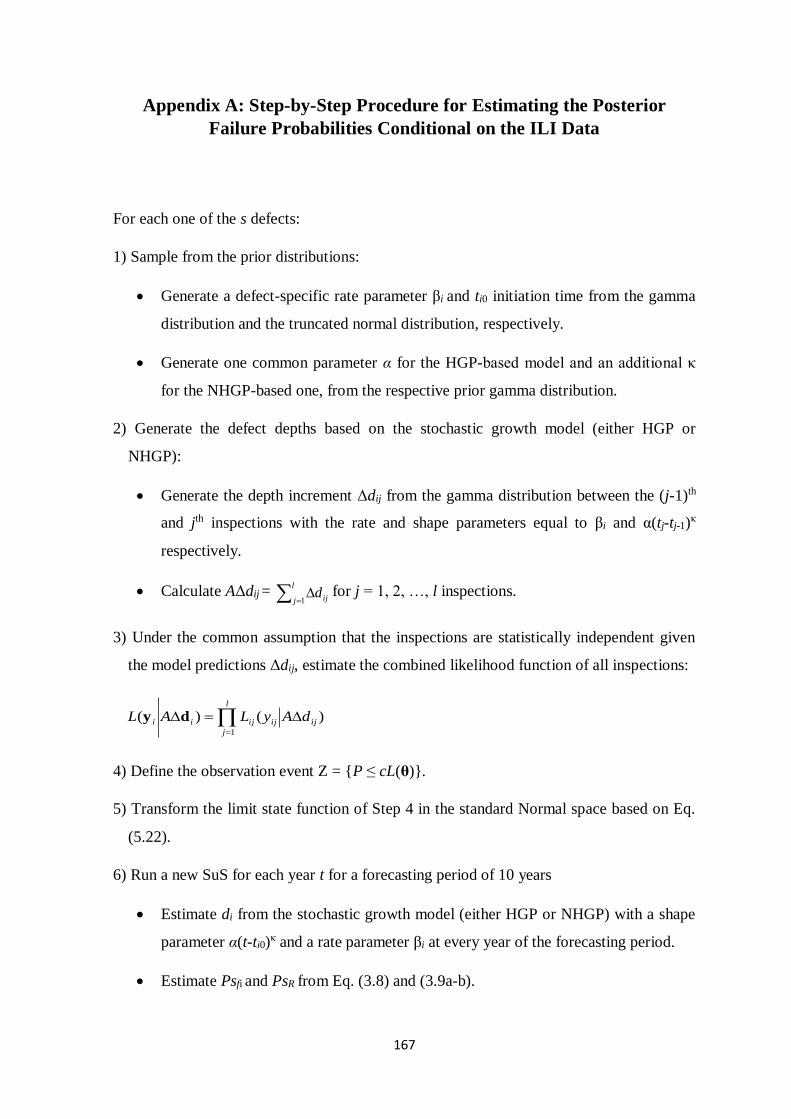
167
Appendix A: Step-by-Step Procedure for Estimating the Posterior
Failure Probabilities Conditional on the ILI Data
For each one of the s defects:
1) Sample from the prior distributions:
Generate a defect-specific rate parameter βi and ti0 initiation time from the gamma
distribution and the truncated normal distribution, respectively.
Generate one common parameter α for the HGP-based model and an additional κ
for the NHGP-based one, from the respective prior gamma distribution.
2) Generate the defect depths based on the stochastic growth model (either HGP or
NHGP):
Generate the depth increment Δdij from the gamma distribution between the (j-1)th
and jth inspections with the rate and shape parameters equal to βi and α(tj-tj-1)κ
respectively.
Calculate AΔdij =
l
j ijd1
for j = 1, 2, …, l inspections.
3) Under the common assumption that the inspections are statistically independent given
the model predictions Δdij, estimate the combined likelihood function of all inspections:
l
j
ijijijii dAyLAL1
)()( dy
4) Define the observation event Z = {P ≤ cL(θ)}.
5) Transform the limit state function of Step 4 in the standard Normal space based on Eq.
(5.22).
6) Run a new SuS for each year t for a forecasting period of 10 years
Estimate di from the stochastic growth model (either HGP or NHGP) with a shape
parameter α(t-ti0)κ and a rate parameter βi at every year of the forecasting period.
Estimate Psfi and PsR from Eq. (3.8) and (3.9a-b).
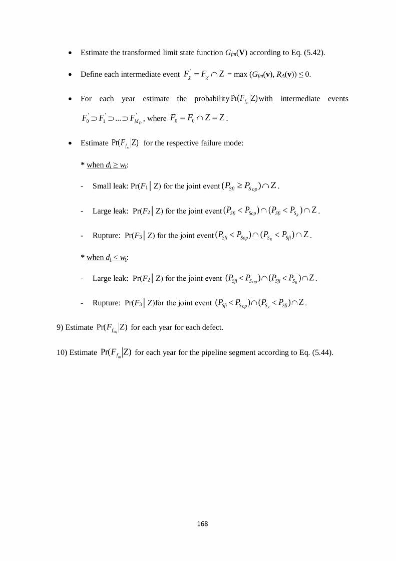
168
Estimate the transformed limit state function Gfm(V) according to Eq. (5.42).
Define each intermediate event FF ' = max (Gfm(v), RA(v)) ≤ 0.
For each year estimate the probability )Pr( mf
F with intermediate events
''
1
'
0 ...DMFFF , where 0
'
0 FF .
Estimate )Pr( mf
F for the respective failure mode:
* when di ≥ wt:
- Small leak: Pr(F1│Z) for the joint event )(opSSfi PP .
- Large leak: Pr(F2│Z) for the joint event )()(RSSfiSopSfi PPPP .
- Rupture: Pr(F3│Z) for the joint event )()( SfiSSopSfi PPPPR
.
* when di < wt:
- Large leak: Pr(F2│Z) for the joint event )()(RSSfiopSSfi PPPP .
- Rupture: Pr(F3│Z)for the joint event )()( SfiSopSSfi PPPPR
.
9) Estimate )Pr( imf
F for each year for each defect.
10) Estimate )Pr( mf
F for each year for the pipeline segment according to Eq. (5.44).
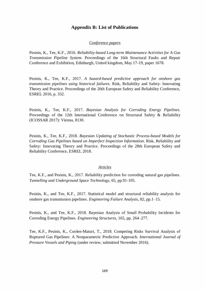
169
Appendix B: List of Publications
Conference papers
Pesinis, K., Tee, K.F., 2016. Reliability-based Long-term Maintenance Activities for A Gas
Transmission Pipeline System. Proceedings of the 16th Structural Faults and Repair
Conference and Exhibition, Edinburgh, United kingdom, May 17-19, paper 1678.
Pesinis, K., Tee, K.F., 2017. A hazard-based predictive approach for onshore gas
transmission pipelines using historical failures. Risk, Reliability and Safety: Innovating
Theory and Practice. Proceedings of the 26th European Safety and Reliability Conference,
ESREL 2016, p. 332.
Pesinis, K., Tee, K.F., 2017. Bayesian Analysis for Corroding Energy Pipelines.
Proceedings of the 12th International Conference on Structural Safety & Reliability
(ICOSSAR 2017): Vienna, 8130.
Pesinis, K., Tee, K.F., 2018. Bayesian Updating of Stochastic Process-based Models for
Corroding Gas Pipelines based on Imperfect Inspection Information. Risk, Reliability and
Safety: Innovating Theory and Practice. Proceedings of the 28th European Safety and
Reliability Conference, ESREL 2018.
Articles
Tee, K.F., and Pesinis, K., 2017. Reliability prediction for corroding natural gas pipelines.
Tunnelling and Underground Space Technology, 65, pp.91-105.
Pesinis, K., and Tee, K.F., 2017. Statistical model and structural reliability analysis for
onshore gas transmission pipelines. Engineering Failure Analysis, 82, pp.1–15.
Pesinis, K., and Tee, K.F., 2018. Bayesian Analysis of Small Probability Incidents for
Corroding Energy Pipelines. Engineering Structures, 165, pp. 264–277.
Tee, K.F., Pesinis, K., Coolen-Maturi, T., 2018. Competing Risks Survival Analysis of
Ruptured Gas Pipelines: A Nonparametric Predictive Approach. International Journal of
Pressure Vessels and Piping (under review, submitted November 2016).

170
Pesinis, K., and Tee, K.F., 2018. : Bayesian Updating and Reliability Analysis for High-
pH Stress Corrosion Cracking in Gas Pipelines. Journal of Engineering Mechanics ASCE
(under review, submitted in May 2018).