UNIVERSITY OF GENOA

FACULTY OF ENGINEERING

MASTER THESIS

In

Mechanical Aeronautical Engineering

”DEVELOPMENT OF A TOOL FOR THE

PREDICTION OF TRANSITION TO TURBULENCE

OVER SMALL AIRCRAFT WINGS”

Advisor: Prof. Jan Pralits

Co-Advisor: Ing. Christophe Favre

Co-Advisor: Prof. Alessandro Bottaro

Candidate: Marina Bruzzone

Academic Year 2012-2013

2

Index

1 INTRODUCTION ................................................................................................ 4

2 DRAG PREDICTION AND DESIGN ...................................................................... 6

3 TRANSITION PREDICTION ................................................................................. 8

3.1 THE PHYSICS ....................................................................................................................... 8

3.1.1 NATURAL” TRANSITION ............................................................................................ 10

3.1.2 RECEPTIVITY ............................................................................................................. 11

3.1.3 TYPES OF INSTABILITIES ........................................................................................... 12

3.1.4 METHOD ............................................................................................................. 16

3.2 MODELLING APPROACH ................................................................................................... 24

4 GOVERNING EQUATIONS ............................................................................... 26

4.1 INVISCID PART (EULER’S EQUATIONS) ............................................................................. 26

4.2 VISCOUS PART (BOUNDARY-LAYER EQUATIONS) ............................................................ 27

4.2.1 COMPRESSIBLE CASE ................................................................................................ 30

4.3 STABILITY ANALYSIS ......................................................................................................... 35

4.3.1 LINEAR STABILITY ..................................................................................................... 35

4.3.2 LINEAR STABILITY THEORY (Eigenvalue problem) .................................................... 38

4.3.3 POISEUILLE FLOW ..................................................................................................... 42

4.3.4 ANALYSIS FOR A SEMI-INFINITE DOMAIN ................................................................ 48

5 IMPLEMENTATION IN INDUSTRIAL CODES...................................................... 64

5.1 PROCEDURE ...................................................................................................................... 64

5.2 DETAILED DESCRIPTION OF EACH PASSAGE .................................................................... 67

5.2.1 GEOMETRY ............................................................................................................... 67

5.2.2 MESH GENERATION ................................................................................................. 73

3

5.2.3 CALCULATION OF PRESSURE DISTRIBUTION ............................................................ 75

5.2.4 CALCULATION OF THE BOUNDARY LAYER FLOW ..................................................... 85

5.2.5 LINEAR STABILITY ANALYSIS ..................................................................................... 88

5.2.6 POST-PROCESSING ................................................................................................... 93

6 TEST CASES..................................................................................................... 94

6.1 NLF0416 PROFILE ............................................................................................................ 94

6.2 NACA0012 PROFILE ......................................................................................................... 97

6.3 SST-TRANSITION MODEL ................................................................................................ 105

6.4 SPHEROID 1:6 ................................................................................................................. 109

7 CONCLUSIONS AND FUTURE WORK ............................................................. 120

4

1 INTRODUCTION

In the modern society the transport system is continuously developing. This allows more

people to travel but also poses questions regarding our environment since also pollution

increases. In today's world, technology is continuing to evolve. Concerning air transports,

we can move easily and quickly flying everywhere on the planet. To make this possible, it

is necessary to ensure the safety and reduce fuel consumption, topics which aeronautical

engineers deal with. In particular, fuel consumption is related to the drag forces caused by

the presence of air; reducing the drag means to have advantages in terms of performances

and fuel consumption. The requirements in aviation are high, competition is part of this

industry and innovations play an important role. The aeronautical companies seek

constantly improvements in the performance of the aircraft. A small drag reduction can

mean huge savings on a large scale in the case of airlines, but also a motivation for the

private client to purchase an aircraft. Daher-Socata is a French company, capable of

manufacturing its own aircraft from A to Z, a 5/6-seaters airplane, aimed for private

customers. In a context of this type, the need to invest in research to stay ahead of the other

companies is a fact. The design of a wing requires a thorough study on the behavior of the

fluid that evolves around it. It is important to make an estimation of lift and drag,

determine where the flow is laminar and where it becomes turbulent. Drag is one of the

most difficult quantities to evaluate in the study of the flow around a body. There are

indeed two contributions which participate in different ways depending on the speed: the

pressure drag, linked to flow separation, and the skin friction, linked to the viscosity of the

fluid. The second is more difficult to assess, since its value changes depending on the flow

5

regime. A laminar boundary layer in fact has a lower viscous drag than a turbulent

boundary layer. It is therefore in our interest to design wings to obtain laminar flow on the

largest possible area. The point where we have the passage from a laminar to a turbulent

flow is called "transition location", and to determine accurately its position is the subject of

this thesis. The technique usually employed is to study the flow using computational fluid

dynamics software (CFD), or other approaches in order to estimate the resistance caused

by a fully turbulent boundary layer. Conceptually, the origin of the transition is due to

infinitesimal perturbations, which grow inside the boundary layer, as they propagate

downstream. This is the concept on which the research developed in the following work is

based, in other words, the study of the stability of the perturbations within the boundary

layer, with the purpose of understanding where the flow transition from laminar to

turbulent flow. The stability analysis will be carried out through an innovative code

(Nolot), created specifically to calculate the growth of these perturbations. Another

analysis will be carried out in parallel with the software Fluent, and later these two results

will be compared with experimental data. At first will be addressed a study on two-

dimensional known airfoils (NACA0012 and NLF0416) and, subsequently, the same

methodology is applied to a three-dimensional case (a spheroid). Nolot can be used for

quasi three-dimensional flow, such the case of an infinite swept wing, which therefore does

not consider the three-dimensional effects. After establishing several assumptions, it is

then discussed how the code works for three-dimensional geometries, and its related

applications and future developments.

6

2 DRAG PREDICTION AND DESIGN

The Importance of Computational Fluid Dynamics has grown rapidly in recent years. The

development of computational tools allows by now to solve problems of high complexity

level.

The analytical solution of Navier Stokes equations can be done only in simple cases with

laminar flows and simple geometries, while the solution of real cases, in which turbulent

flows occur frequently, require necessarily a numerical approach.

Typically, the difficulty of the analysis is due to the presence of turbulence in the flow,

since it requires computational high-performances. The differences between the various

applications arise from the typology of the flow, such as free jets, flows in the vicinity of

solid walls, two-dimensional or three-dimensional configurations, and the nature of the

fluid, for example if it is Newtonian, incompressible, compressible, with solid particles or

with chemical reactions.

There are different ways to simulate a turbulent flow. On one hand, you may be interested

in solving the detailed dynamics of all scales of the flow. This is known as Direct

Numerical Simulation, DNS. This approach, which is the most expensive from the

computational viewpoint, is typically used for basic research and it is confined to turbulent

flows with low values of the Reynolds number.

In many cases, you may be interested exclusively in the dynamics of larger fluid structures

(large-scale vortices). The most appropriate formulation in this case is the Large Eddy

Simulation, LES. The computational cost is considerably reduced compared to the

previous case, and you can accomplish simulations at medium-high Reynolds numbers.

7

This approach is used in the industrial field, for sophisticated applications at moderate

Reynolds number (eg. fluid dynamic study of the combustion chambers).

In other cases you may be interested only in an estimate of the average values of the

variables. We resort, then, to the Reynolds Averaged Navier-Stokes Equations, RANS,

which present among the three approaches, the lower level of computational complexity.

Today there are many commercial software in the field of fluid dynamics. Among the best

known we find CFX, Fluent, PHOENICS, STAR-CD, STAR-CCM +, CFD + +, Floworks

and other open source as Code Saturne and OpenFOAM.

In the following work, the study of turbulence will be approached from another point of

view. In particular, we study the initial shape of transition from laminar to turbulent flow.

This is related, this time, to the growth of the perturbations within the boundary layer. An

analysis on its stability will then be made, by introducing a new code, Nolot, which will

enable us to calculate the exact point at which the transition occurs. In other words, it is

able to find the location where the perturbations will be grown to the point to change the

shape of the boundary layer. The main advantage of Nolot is precisely to consider the

stability analysis (what the normal CFD does not deal), to which is added the high speed

calculation and the lightness from the computational viewpoint.

It is important to know the transition location since it is determinant for the evaluation of

skin friction.

In fact, for high Reynolds numbers and thin shapes like the wings, the pressure drag

becomes always less important compared to the skin fiction. Therefore it is important to

focus on this part of the drag, with the aim of reducing as much as possible its amount.

The purpose of this work is to validate a transition prediction process on 2D wing profiles.

Later this will be extended to a 3D geometry to see in which limits and with which

precautions the methodology works.

Afterwards the results obtained with the linear stability analysis will be confronted with the

results obtained with the classical CFD analysis, considering which of the two approaches

is the most accurate in relation to the experimental data.

8

3 TRANSITION PREDICTION

3.1 THE PHYSICS

Prediction of transition is of great importance in the study of fluid mechanics problems,

since it controls aerodynamic quantities such as drag and heat transfer. For high-subsonic

speed aircraft, laminar flow on the wings reduces the drag and hence the fuel consumption.

Transition mechanisms can also generate noise.

Transition is the result of a sequence of complex phenomena which depend on many

parameters , such as flow quality, vibrations, roughness, vorticity, etc. When transition

results from the amplification of unstable waves, the linear stability theory can be used to

determine the characteristics of these disturbances and also to estimate the transition

location. This theory is called “ method”.

9

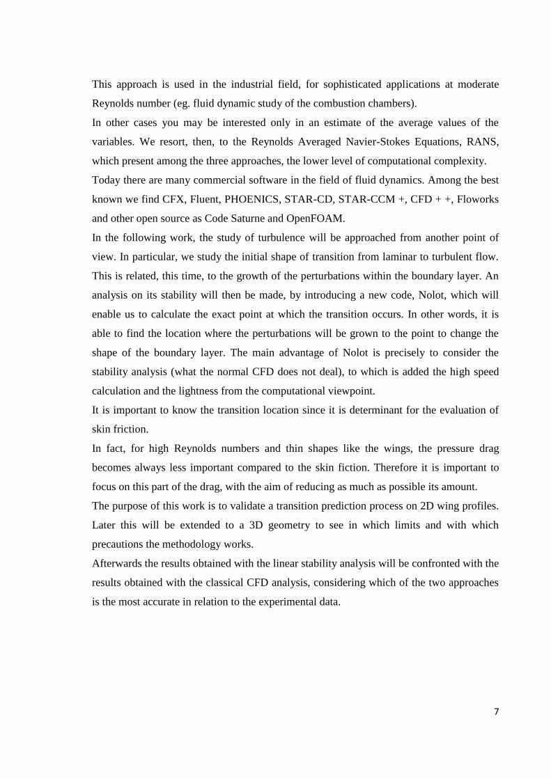
Figure 1 - Boundary layer along a flat plate: laminarity, transition and turbulence

A laminar flow developing along a given body is strongly affected by various type of

forced disturbances generated by the model itself or existing in the free stream. The first

stage of the transition process is described by receptivity; the theory that describes the

means by which the forced disturbances enter into the laminar boundary layer. We can

roughly make a difference between two transition scenarios:

Infinitesimal amplitude of the forced disturbances: regular oscillations start to

develop downstream a certain critical point where transition occurs (natural

transition). The first stage of the wave evolution can be described by linear theory.

Finite amplitude of the forced disturbances: if, for example, there are large isolated

roughness elements, then non linear phenomena will cause transition (bypass).

10

3.1.1 NATURAL” TRANSITION

If we consider two-dimensional flows, the amplitude of so called Tollmien-Schlichting

waves exhibits at first an exponential growth which can be computed by the linear stability

theory. Further downstream, the disturbances reach a finite amplitude, so that their

development begins to deviate from that predicted by the linear theory. Further

downstream, three dimensional and non linear effects become more and more important.

The non linear development of the disturbances terminates with the “breakdown”

phenomenon. The fluctuations finally take a random character and form a turbulent spot.

The onset of transition is defined as the location where the first spots appear and where

then the skin friction starts to exceed its laminar value. The turblent spots then develop

before the flow becomes fully turbulent.

For three-dimensional mean flows, the basic phenomena are qualitatively the same in the

linear regime, but considering that unstable waves now develop in all propagation

directions. The linear stability theory shows that the most unstable propagation direction

strongly depends if the flow is accelerated or decelerated.

Generally speaking, the transition process is an almost unknown field, hard to be

understood, due to the variety of influences such as freestream turbulence, surface

roughness, noise, etc. Disturbances in the freestream enter the boundary layer as unsteady

fluctuations of the basic state. This part of the process is called receptivity and it

establishes the initial conditions of disturbance amplitude, frequency and phase for the

breakdown of the laminar flow. When transition results from the amplification of unstable

waves, the linear stability theory can be used to determine the characteristics of these

disturbances and also to estimate the transition location.

In the following figures the typical evolution of the skin friction coefficient in laminar,

transitional and turbulent flow is shown.

11

Figure 2 - Skin friction coefficient trend and representation of the evolution of

boundary layer flow over a flat plate

The reason for which the laminarity is so sought by researchers is that the skin friction

decreases for increasingly large Reynolds numbers. But at the same time, if Re increases,

the flow changes its form becoming turbulent. In this way the skin friction assumes the

values of the turbulent flow.

Transition is the region where flow changes its status and where the skin friction goes from

the lower to the higher value.

3.1.2 RECEPTIVITY

A laminar flow developing along a given body is strongly affected by various types of

forced disturbances generated by the model itself or perturbations existing in the free

stream. The first stage of transition process is described by receptivity, the theory that

studies the means by which the forced disturbances enter the laminar boundary layer. The

linear stability behavior can be predicted, since it follows the principles of the linear theory

12

and its streamwise extent is comparable to the nonlinear region. At the same time,

especially for the 3D flows, non linear distortions of the base flow can occur early because

of the action of the primary instabilities; the nonlinear evolution of the disturbances leads

early to a saturation of the fundamental disturbance, bringing to a strong amplification of

high frequency instabilities and then to the breakdown.

Receptivity is also the study of the development of unstable waves which grow in the

boundary layer. For two-dimensional flow, receptivity process occurs in region of the

boundary layer where the mean flow exhibits rapid changes in the streamwise direction.

Figure 3 - Representation of various kinds of disturbances

3.1.3 TYPES OF INSTABILITIES

For what concerns two dimensional flows the instability leading to transition starts with the

development of wave-like disturbances, as the so-called Tollmien-Schlichting waves.

13

They experience at first an exponential growth, which can be computed by the linear

stability theory. After this first stage the disturbances begin to deviate from what is

predicted by the linear theory reaching a finite amplitude.

TS waves are initially of “peaks and valleys” periodic form, then they take a random

character because of the three dimensional and nonlinear effects.

Figure 4 - Tollmien-Schlichting waves. Transitional flow along a flat plate without

longitudinal pressure gradient.

Tollmien-Schlichting waves are sometimes called streamwise instabilities.

In three dimensional flow, for instance on a swept wing, the basic phenomena are

qualitatively the same but the unstable waves propagates in a very wide range of

directions. Cross-flow instabilities appear as co-rotating vortices and are thus commonly

referred to as cross-flow vortices.

14

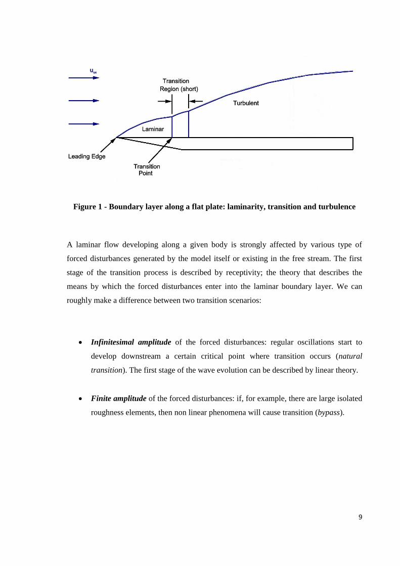
Figure 5 - Cross-flow waves in swept-wing boundary layers

Each instability identified in swept wing boundary layers is found in specific regions,

where the boundary layer is governed by effects such as surface curvature or acceleration.

The two most important types are explained:

1. Crossflow disturbances are instabilities of inviscid type. They appear as boundary

layer streaks closely aligned with the external streamline.

2. Tollmien-Schlichting waves represent viscous instabilities. The wave vector and

the direction of propagation are closely aligned with the streamline direction.

Both instability mechanisms have a respective characteristic region on a swept wing.

For instance negative pressure gradients stabilize TS-waves while positive pressure

gradients have a destabilizing effect. On the other hand CF instabilities arise where the

pressure gradient is negative.

Since the base flow in the spanwise direction tends to zero in the free-stream its profile

exhibits an inflection point. According to Rayleigh theory (1880) the existence of this point

is a necessary condition for inviscid instabilities to arise.

15

Linear stability theory studies the response of a laminar flow to a disturbance of small or

moderate amplitude. If the disturbance grow enough to change the flow from a laminar to a

turbulent status, we call the flow “unstable”. On the other hand, if the flow returns to its

original state we define the flow as “stable”.

More concretely, from a mathematical point of view, linear stability analysis introduces

small sinusoidal disturbances into the Navier-Stokes equations in order to study their

evolution in time or in space. The idea is to superpose disturbances on a laminar base flow:

as the disturbance grows above a few percent of the base flow, nonlinear effects become

important and the linear equations no longer accurately predict the disturbance evolution.

Even if linear equations have a limited region of validity they are important in detecting

physical growth mechanisms and identifying dominant disturbance types.

The fluctuating quantities involved are the velocity, the pressure, the density and the

temperature. Hence we will consider the variables composed by a base flow part and a

fluctuating one, as shown for the velocity perturbation field in Eqs.(1)-(2)-(3):

(1)

(2)

(3)

Where α is the streamwise wave number (x–direction), β is the spanwise wave number (z–

direction) and ω is the angular frequency. Depending on the choice of these parameters, we

can deal with two different kind of analysis, the temporal and the spatial problems. In the

case of spatial analysis, which is the one we are interested in, solving the continuity and the

momentum equations according to this approach, let us to compute the rate of

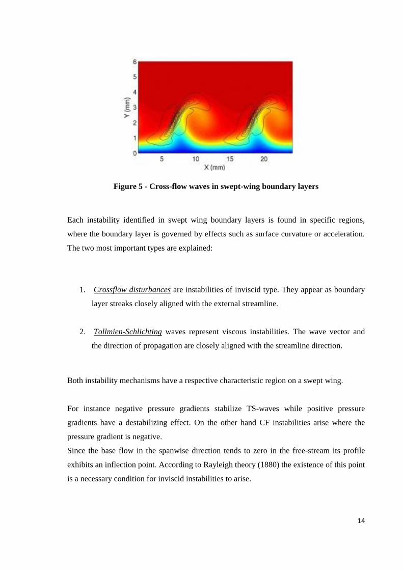
amplification for each couple of ω-β. The envelope of all these curves has to be intersected

with N-factor values from 8 to 10 along the ordinate. In fact for these values, from

experiments, we know that transition begins to occur. Therefore, the intersection gives us

the exact location in the x-direction where the flow start to become unstable, see Fig.6.

16

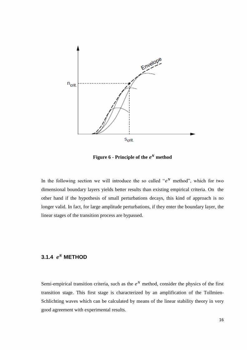
Figure 6 - Principle of the method

In the following section we will introduce the so called “ method”, which for two

dimensional boundary layers yields better results than existing empirical criteria. On the

other hand if the hypothesis of small perturbations decays, this kind of approach is no

longer valid. In fact, for large amplitude perturbations, if they enter the boundary layer, the

linear stages of the transition process are bypassed.

3.1.4 METHOD

Semi-empirical transition criteria, such as the method, consider the physics of the first

transition stage. This first stage is characterized by an amplification of the Tollmien-

Schlichting waves which can be calculated by means of the linear stability theory in very

good agreement with experimental results.

17

The advantage of the employ of the envelope method is the drastic reduction of the

computational effort.

The method is based on linear theory only, so that many fundamental aspects of the

transition process are not accounted for. The assumptions of small disturbances, local

parallelism and the neglection of nonlinear effects are further simplifications which we

have to take in account in the study.

Only in the case of two-dimensional waves (β=0), the disturbances are amplified or

damped according to the sign of the spatial growth rate.

For a given meanflow it is possible to compute a stability diagram showing the range of

unstable frequencies ω as a function of Re (streamwise distance x).

Let’s consider a wave of a fixed frequency, see Fig.7:

1. stable region (damped up to )

2. unstable region (amplified up to )

3. stable region (damped downstream of )

At a given station x, the total amplification rate of a spatially growing wave can be defined

as:

(4)

Where A is the wave amplitude and the index 0 refers to amplification of the perturbation

corresponding to the spanwise position where the wave becomes unstable.

The envelope of the total amplification curves is:

(5)

Then, it is the maximum of the whole amplifications calculated for every value of the

frequency.

18

Figure 7- Stability curve and corresponding

envelope curve for a chosen frequency

In Fig. 8 is shown the neutral curve in the F − Re plane. It defines the intersection between

the regions where these disturbances are damped and amplified, according to the sign of

the growth rate .

19

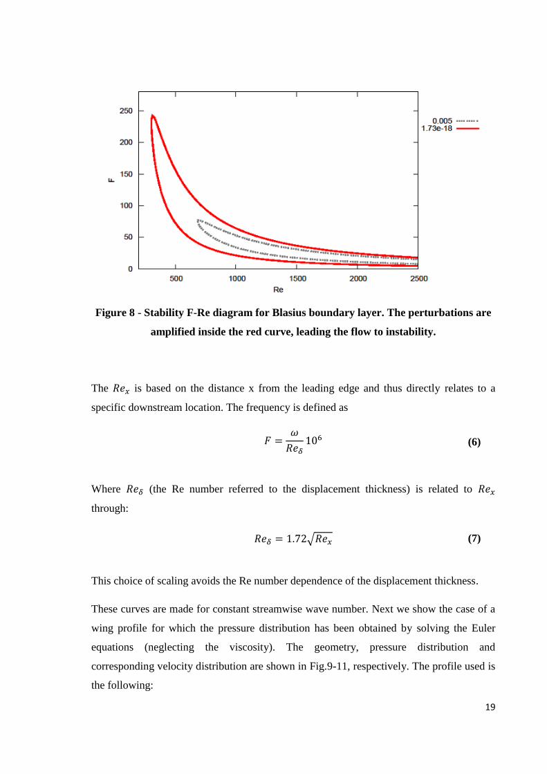
Figure 8 - Stability F-Re diagram for Blasius boundary layer. The perturbations are

amplified inside the red curve, leading the flow to instability.

The is based on the distance x from the leading edge and thus directly relates to a

specific downstream location. The frequency is defined as

(6)

Where (the Re number referred to the displacement thickness) is related to

through:

(7)

This choice of scaling avoids the Re number dependence of the displacement thickness.

These curves are made for constant streamwise wave number. Next we show the case of a

wing profile for which the pressure distribution has been obtained by solving the Euler

equations (neglecting the viscosity). The geometry, pressure distribution and

corresponding velocity distribution are shown in Fig.9-11, respectively. The profile used is

the following:

20

Figure 9 - Geometry of the test case profile

Figure 10 - Cp distribution on the test case profile

21

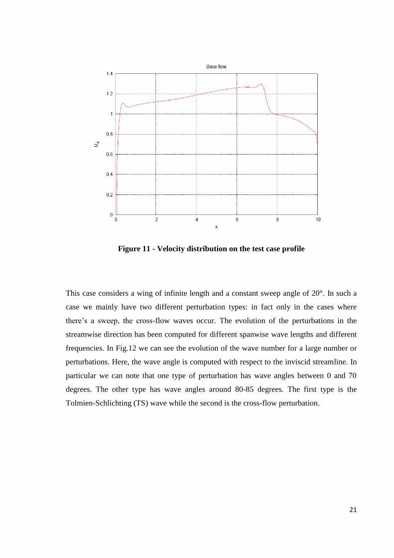
Figure 11 - Velocity distribution on the test case profile

This case considers a wing of infinite length and a constant sweep angle of 20°. In such a

case we mainly have two different perturbation types: in fact only in the cases where

there’s a sweep, the cross-flow waves occur. The evolution of the perturbations in the

streamwise direction has been computed for different spanwise wave lengths and different

frequencies. In Fig.12 we can see the evolution of the wave number for a large number or

perturbations. Here, the wave angle is computed with respect to the inviscid streamline. In

particular we can note that one type of perturbation has wave angles between 0 and 70

degrees. The other type has wave angles around 80-85 degrees. The first type is the

Tolmien-Schlichting (TS) wave while the second is the cross-flow perturbation.

22

Figure 12 - Wave angle of the perturbations

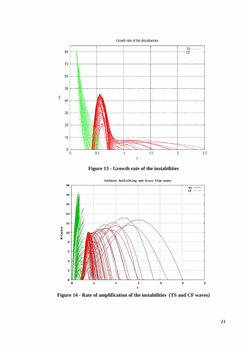
In Fig.13 and in Fig.14 we show the growth rates and N-factors of the same case. We can

note that the cross-flow waves grow that close to the leading edge while the TS waves

grow further downstream. It is clear that the cross-flow vortices reach N-factors above 8-

10 (upstream) the TS waves.

23

Figure 13 - Growth rate of the instabilities

Figure 14 - Rate of amplification of the instabilities (TS and CF waves)

24

We can therefore conclude that this case is cross-flow dominated, which is a characteristic

of swept wings.

3.2 MODELLING APPROACH

The Navier-Stokes equations are the governing equations, together with the continuity

equation and the energy equation, which describe a general flow. Passing through the

dimensional analysis, as will be seen later, in the hypothesis of very high Reynolds

numbers, some terms of the equations system are negligible compared with other terms. In

case one wants to study the flow around wings, considering the high speed of the aircraft,

we can assume a Reynolds number of approximately 10 ^ 6. With these premises, around

an airfoil, the Navier-Stokes equations reach a significant level of complexity due to the

presence of the viscous term. Assumptions are usually made to simplify the problem by

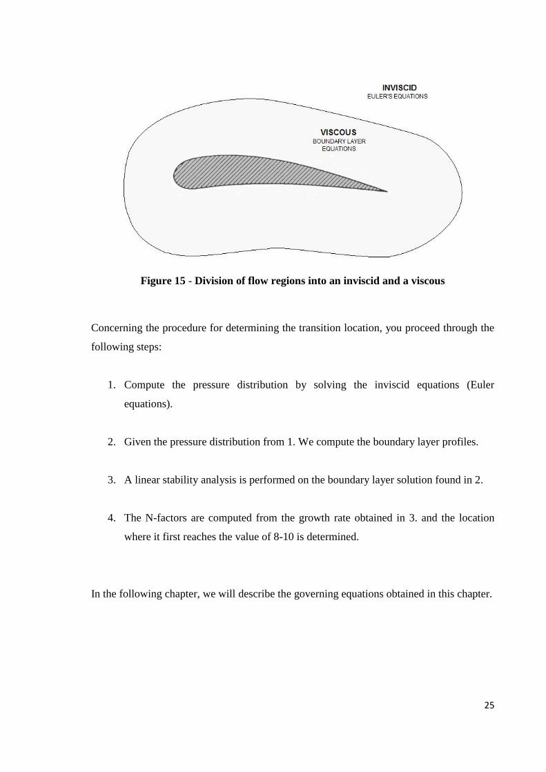
dividing the flow into two regions, see Fig.15:

1. An undisturbed region, away from the airfoil, where Euler’s equations

are valid. The fluid is then treated as inviscid and a slip condition is

assumed on the airfoil surface.

2. A region very close to the profile in which the viscosity plays an

important role. In this region the boundary layer equation are valid and

solved given the pressure distribution obtained from the solution of the

Euler equations.

25

Figure 15 - Division of flow regions into an inviscid and a viscous

Concerning the procedure for determining the transition location, you proceed through the

following steps:

1. Compute the pressure distribution by solving the inviscid equations (Euler

equations).

2. Given the pressure distribution from 1. We compute the boundary layer profiles.

3. A linear stability analysis is performed on the boundary layer solution found in 2.

4. The N-factors are computed from the growth rate obtained in 3. and the location

where it first reaches the value of 8-10 is determined.

In the following chapter, we will describe the governing equations obtained in this chapter.

26

4 GOVERNING EQUATIONS

4.1 INVISCID PART (EULER’S EQUATIONS)

The governing equations for incompressible viscous flows are written:

(8)

(9)

Where Eq.(8) is the continuity and the Eq.(9) is the Navier-Stokes equation. Boundary

conditions are set as:

at solid walls

And

, and in the freestream

Inviscid regions of the flow are regions where net viscous forces are very small compared

to inertial and pressure forces. In that case we assume this hypothesis , which implies that

the viscous term is negligible. Then in the Navier Stokes equations we will neglect the

27

viscous term. According to nondimensionalized analysis, this term is negligible only if

1/Re is small, and thus inviscid regions of flow are regions of high Reynolds number. The

Reynolds number is associated to a characteristic length L, for example the length of the

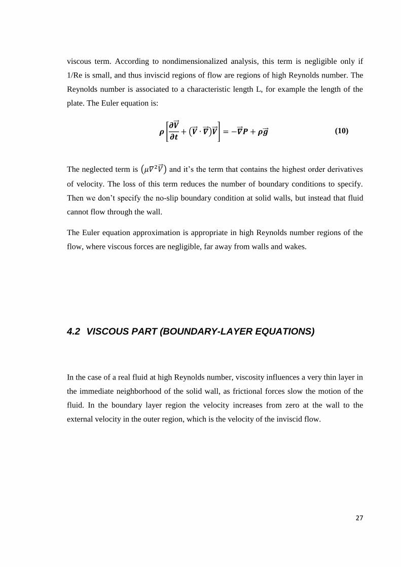
plate. The Euler equation is:

(10)

The neglected term is and it’s the term that contains the highest order derivatives

of velocity. The loss of this term reduces the number of boundary conditions to specify.

Then we don’t specify the no-slip boundary condition at solid walls, but instead that fluid

cannot flow through the wall.

The Euler equation approximation is appropriate in high Reynolds number regions of the

flow, where viscous forces are negligible, far away from walls and wakes.

4.2 VISCOUS PART (BOUNDARY-LAYER EQUATIONS)

In the case of a real fluid at high Reynolds number, viscosity influences a very thin layer in

the immediate neighborhood of the solid wall, as frictional forces slow the motion of the

fluid. In the boundary layer region the velocity increases from zero at the wall to the

external velocity in the outer region, which is the velocity of the inviscid flow.

28

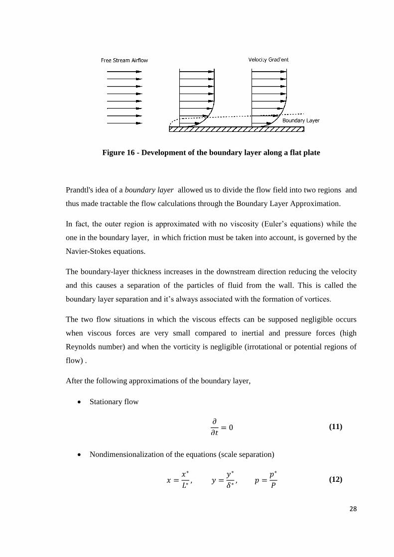
Figure 16 - Development of the boundary layer along a flat plate

Prandtl's idea of a boundary layer allowed us to divide the flow field into two regions and

thus made tractable the flow calculations through the Boundary Layer Approximation.

In fact, the outer region is approximated with no viscosity (Euler’s equations) while the

one in the boundary layer, in which friction must be taken into account, is governed by the

Navier-Stokes equations.

The boundary-layer thickness increases in the downstream direction reducing the velocity

and this causes a separation of the particles of fluid from the wall. This is called the

boundary layer separation and it’s always associated with the formation of vortices.

The two flow situations in which the viscous effects can be supposed negligible occurs

when viscous forces are very small compared to inertial and pressure forces (high

Reynolds number) and when the vorticity is negligible (irrotational or potential regions of

flow) .

After the following approximations of the boundary layer,

Stationary flow

(11)

Nondimensionalization of the equations (scale separation)

(12)

29

leads to neglect the less important terms according to the fact that

No variation of the quatities in the third direction z (Infinite swept)

(13)

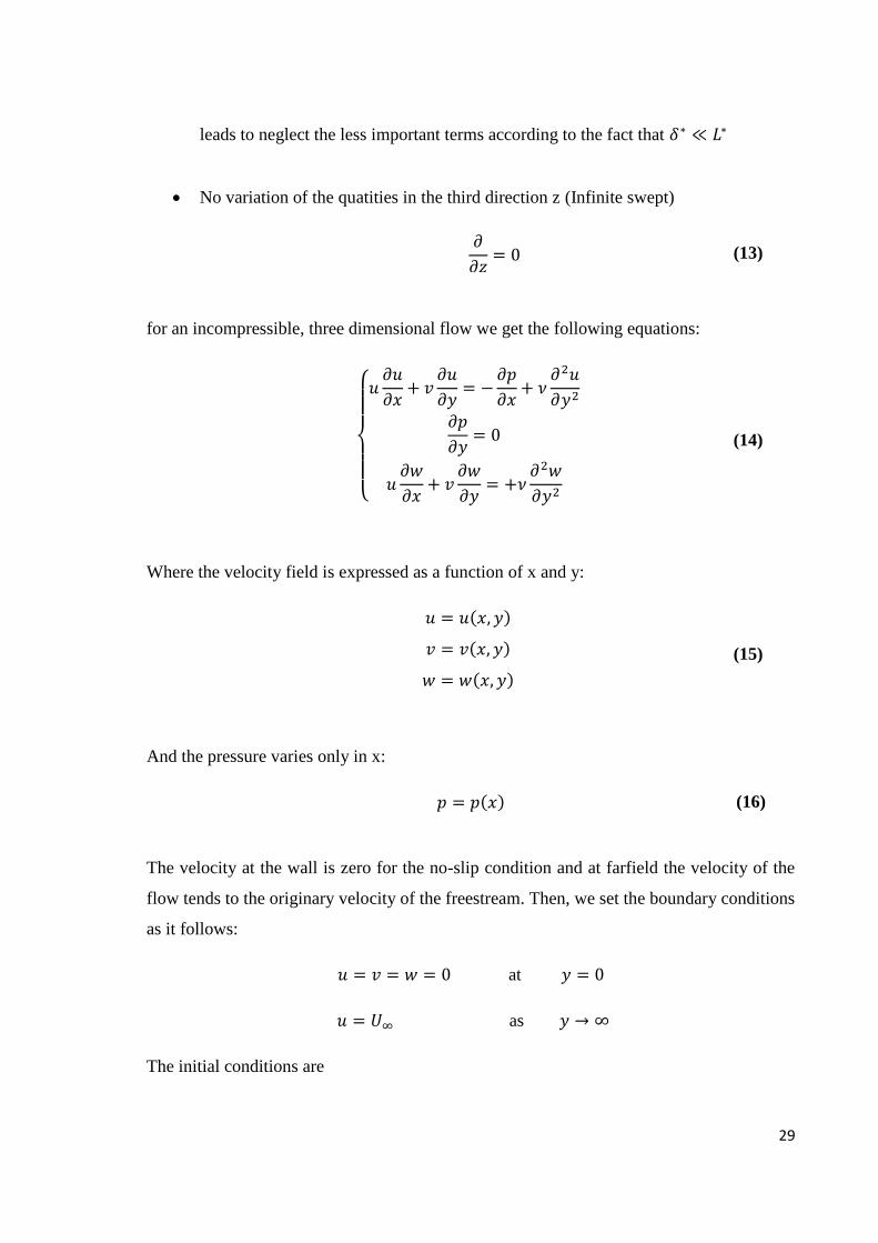
for an incompressible, three dimensional flow we get the following equations:

(14)

Where the velocity field is expressed as a function of x and y:

(15)

And the pressure varies only in x:

(16)

The velocity at the wall is zero for the no-slip condition and at farfield the velocity of the

flow tends to the originary velocity of the freestream. Then, we set the boundary conditions

as it follows:

at

as

The initial conditions are

30

4.2.1 COMPRESSIBLE CASE

In order to study flow at high Mach numbers (0.8) it is necessary to deal with the case of

compressible flow and then we introduce a new system of equations with the addition of

the conservation energy equation and the ideal gas law:

(17)

Where represent the dissipation function:

(18)

The last equation necessary to close the system is the ideal gas law:

(19)

31

So now we rewrite the equations of continuity, momentum and energy for the compressible

case:

(20)

The dimensional analysis yields to:

(21)

Where is the velocity scale, is the length scale, is the time scale and is the

pressure scale. Remembering that the variables are functions of the x-y coordinates and

simplifying:

(22)

The non-dimensional Navier-Stokes equations, respectively in x, y and z-directions are:

(23)

32

(24)

(25)

Since we deal with high Reynolds numbers we can make an approximation of the

boundary layer equations by stating that is a very small number compared to the

other terms in the equation; the term multiplied by is about of order 1:

(26)

(27)

33

(28)

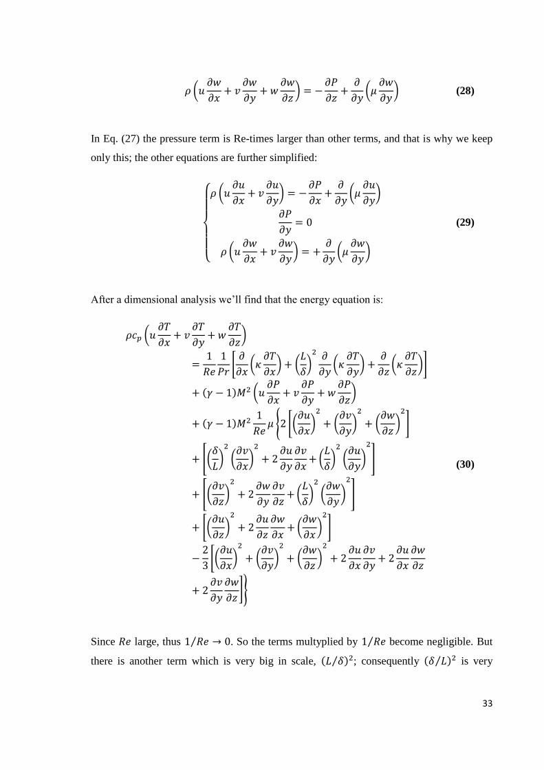
In Eq. (27) the pressure term is Re-times larger than other terms, and that is why we keep

only this; the other equations are further simplified:

(29)

After a dimensional analysis we’ll find that the energy equation is:

(30)

Since large, thus . So the terms multyplied by become negligible. But

there is another term which is very big in scale, ; consequently is very

34

small. Taking this into account, the terms multyplied by

become unitary. Therfore

we can simplify the equation seeing which are the terms that predominate on the others and

neglecting those not significant.

(31)

And after simplification due to the fact that velocity depends only on the x-y coordinates

and pressure only on x:

(32)

The boundary conditions are

at (33)

as (34)

The adiabatic wall leads to:

(35)

While the initial condition is

at (36)

35

4.3 STABILITY ANALYSIS

4.3.1 LINEAR STABILITY

In the linear stability analysis we assume infinitesimal perturbations superposed to the

basic flow.

For a parallel bidimensional incompressible flow, the Navier-Stokes equations for

infinitesimal disturbances can be found by substituting the velocity field and

the pressure field in the system formed by the continuity equation and the

Navier-Stokes equations:

(37)

(38)

In the case of parallel flow, the base flow depends only on coordinate while the pressure

only on the .

Then the base flow and the perturbations are:

(39)

(40)

Introducing the above flow decomposition into the governing equations yields:

36

(41)

The fluctuating quantities are assumed infinitesimal, so the quadratic terms (non linear

terms) of the disturbances can be neglected in the Navier-Stokes equations. Subtracting the

terms of the base flow, the system becomes:

(42)

(43)

Perturbations at the wall are zero and in far from the plate the perturbations tends to zero as

well. So we can write the boundary conditions:

at (44)

as (45)

The above system with four equations and four unknowns, can be further simplified as

shown here. Taking the divergence of the momentum equations and using the continuity

equation,

37

(46)

We find an expression for the perturbation pressure:

(47)

Taking the laplacian of the momentum-equation in the y-coordinate and substituting the

equation just found:

(48)

And after some manipulation, the equation yields:

(49)

The third dimension is accounted for by defining a new variable, the vorticity:

(50)

The governing equation for is obtained by subtracting the derivative in z of the

momentum equation along x (38.a) to the derivative in x of momentum equation along z

(38.c):

(51)

38

After manipulating Eq.(51) we find:

(52)

Equations (49) and (52) are denoted as the Orr-Sommerfeld and Squire equations. The

corresponding boundary conditions are:

(53)

at the wall, and

(54)

at the infinite.

4.3.2 LINEAR STABILITY THEORY (Eigenvalue problem)

The choice of the parameters α and ω determines if the growth of two dimensional

harmonic disturbance waves is in time or in space, or both. In general, α and ω are

complex and the growth evolves in time and space. If ω is introduced as a complex and α

as a real quantity, only the time-dependent growth is considered. On the other hand, spatial

amplification is determined with a real frequency ω and a complex α. In the last case, the

real part represents the wavenumber and its imaginary part the amplification rate.

Negative values of indicate a spatial amplification, whereas positive values mean decay

of the perturbation wave amplitude.

We can distinguish then two kinds of problems:

39

The choice of complex frequency and real wave numbers is known as the temporal

problem where the spatial structure of the wavelike perturbation is unchanged and

the amplitude of the wave grows or decays as time progresses.

Figure 17 - Evolution of disturbances in shear flows. Temporal evolution of a global

periodic disturbance

In the spatial problem the streamwise wave number is complex while the spanwise

one and frequency are real; the amplitude of the perturbation grows in space and

the frequency of the wave is constant.

Figure 18 - Evolution of disturbances in shear flows. Spatial evolution of a

disturbance created by an oscillatory source

4.3.2.1 Temporal analysis (complex ω, real α and β)

The evolution in time of wave-like perturbations can be studied by assuming the following

solution of the disturbances:

(55)

(56)

40

Where and are the real-valued streamwise and the spanwise wave numbers

respectively in and directions and the complex-valued frequency. Knowing that

and expressing the derivative in as , the equation for becomes:

(57)

The equation for the vorticity becomes:

(58)

And for :

(59)

The final system can be written:

41

(60)

This is a system of homogeneous, ordinary differential equations for the amplitude

functions and .

For the incompressible flow there are four equations (42)-(43) and for a compressible flow

the equations are six (continuity, - momentum equations, energy equation and the

equation of state).

For the simplest case of a two-dimensional, low speed flow with , the equation for ,

which is the one we’re interested in, doesn’t depend on the equation. So the Orr-

Sommerfeld equation becomes:

(61)

The boundary conditions are set in order to make the velocity disturbances vanish at the

wall and in the free stream:

At the wall: (62)

At infinite: (63)

Since the boundary conditions are homogeneous, this is an eigenvalue problem. Once the

mean flow is specified, non trivial solutions exist for certain combinations of the

parameters and . This constitute the dispersion relation.

The stability of the perturbations is found by the value of the imaginary part of . If

then the flow is unstable, if then the flow is stable. Neutral

solutions are found for .

42

4.3.3 POISEUILLE FLOW

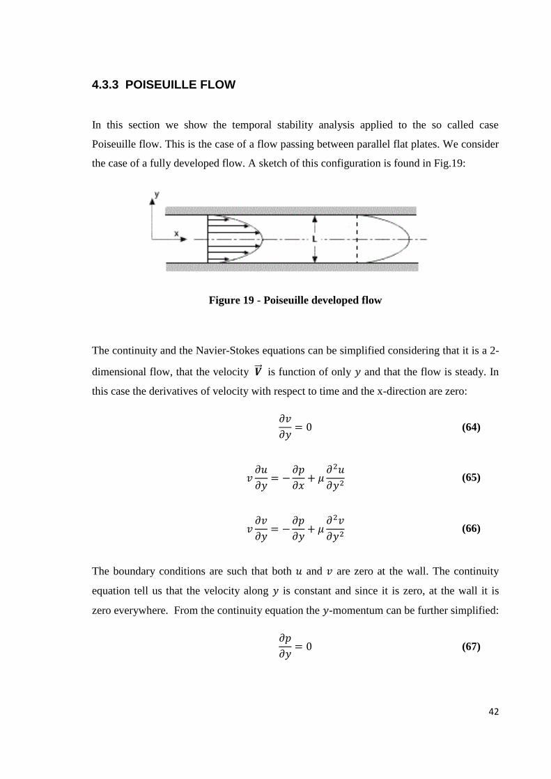
In this section we show the temporal stability analysis applied to the so called case

Poiseuille flow. This is the case of a flow passing between parallel flat plates. We consider

the case of a fully developed flow. A sketch of this configuration is found in Fig.19:

Figure 19 - Poiseuille developed flow

The continuity and the Navier-Stokes equations can be simplified considering that it is a 2-

dimensional flow, that the velocity is function of only and that the flow is steady. In

this case the derivatives of velocity with respect to time and the x-direction are zero:

(64)

(65)

(66)

The boundary conditions are such that both and are zero at the wall. The continuity

equation tell us that the velocity along is constant and since it is zero, at the wall it is

zero everywhere. From the continuity equation the -momentum can be further simplified:

(67)

43

Knowing that the velocity is zero the -momentum equation becomes:

(68)

Integration yealds to:

(69)

The boundary conditions let us to know the expression for :

(70)

(71)

Where

.

The Orr-Sommerfeld equations are solved for the Poiseuille flow, which is a two-

dimensional, incompressible, steady flow.

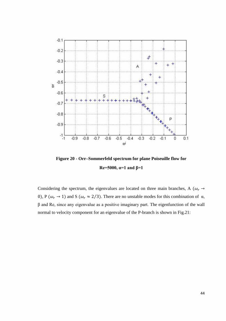
The Orr-Sommerfeld spectrum of plane Poiseuille flow for Re=5000 is shown in Fig.20.

Here the Reynolds number is defined as .

44

Figure 20 - Orr–Sommerfeld spectrum for plane Poiseuille flow for

Re=5000, α=1 and β=1

Considering the spectrum, the eigenvalues are located on three main branches, A

, P and S . There are no unstable modes for this combination of α,

β and Re, since any eigenvalue as a positive imaginary part. The eigenfunction of the wall

normal to velocity component for an eigenvalue of the P-branch is shown in Fig.21:

45

Figure 21 - Orr- Sommerfeld v-eigenfuction for plane Poiseuille flow. The P-branch

is represented, with Re=5000, α=1 and β=1.

The black line represents the magnitude of normal velocity or vorticity; the blue and the

red lines are the real and the imaginary parts. The corresponding eigenfunction for the

wall-normal vorticity is shown in Fig.22:

46

Figure 22 - Orr- Sommerfeld η -eigenfuction for plane Poiseuille flow. The P-branch

is represented, with Re=5000, α=1 and β=1.

In order to demonstrate the validity of the Squire theorem, which says that the most

unstable modes occur for the two dimensional flows (β=0), in Fig.23 is shown how

varies in function of the streamwise number for different values of . In this picture it is

evident that the greater values of can be obtained by setting and, as it increases,

becomes smaller.

47

Figure 23 - Imaginary part of frequency as function of α varying with β

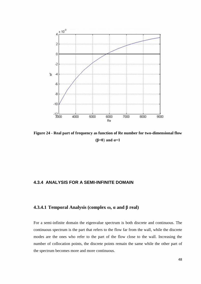
The critical Reynolds number, the value of Re at which an unstable solution is first found,

is shown in Fig.20. In Schmid P.J., Henningson D.S. Stability and Transition in Shear

Flows (2001), the critical Reynolds number for Poiseuille flow is about Re = 5772, as it

can be seen in Fig.24.

48

Figure 24 - Real part of frequency as function of Re number for two-dimensional flow

(β=0 and α=1

4.3.4 ANALYSIS FOR A SEMI-INFINITE DOMAIN

4.3.4.1 Temporal Analysis (complex ω, α and β real)

For a semi-infinite domain the eigenvalue spectrum is both discrete and continuous. The

continuous spectrum is the part that refers to the flow far from the wall, while the discrete

modes are the ones who refer to the part of the flow close to the wall. Increasing the

number of collocation points, the discrete points remain the same while the other part of

the spectrum becomes more and more continuous.

49

In the case of temporal analysis the eigenvalues found are plotted in Fig.25; on the x-axis

the real part is plotted and on the y-axis we find the imaginary part.

It is possible to represent the continuous spectrum with a function obtained by solving

analytically the Orr-Sommerfeld equation. It’s a fourth order differential equation with

constant coefficients.

The fundamental solutions of the equation can be written as:

(72)

(73)

(74)

The first two solutions are referred to as the viscous solutions or the vorticity modes

whereas the last two are called the inviscid solutions or the pressure modes.

The boundary layer has at most one unstable mode, also denoted a Tollmien-Schlichting

wave. It is stable for the parameter combination chosen here.

50

Figure 25 - Orr-Sommerfeld spectrum for Blasius boundary layer flow

Eigenfunctions for Blasius boundary layer flow are plotted in Fig.26-28. These plots are

referred to the most unstable value of the discrete spectrum.

The streamwise perturbation velocity is the following . Here

Reynolds number is defined as

, where is the displacement thickness.

51

Figure 26-– Eigenfunctions of the discrete spectrum for Blasius boundary layer flow.

Streamwise perturbation velocity (u), with Re=1000, α=0.3 and β=0.

The red line represents the magnitude of u or v perturbation velocity while the green and

blue dashed lines are the real and the imaginary parts respectively.

The vertical velocity component :

52

Figure 27 - Eigenfunctions of the discrete spectrum for Blasius boundary layer flow.

Vertical perturbation velocity (v), with Re=1000, α=0.3 and β=0.

The , and eigenfunctions normalized with :

53

Figure 28 - u,v-perturbation velocity and p-perturbation pressure for Blasius

boundary layer

It can be seen that is approximately times .

The curve that defines the boundary between areas where exponentially growing solutions

exist and where they do not, is called neutral curve. The neutral curve ( ) for Blasius

boundary layer is shown in Fig.29:

54

Figure 29 - Neutral curve for Blasius boundary layer flow in temporal analysis.

Contours of constant growth rate

The left-most tip of this region defines the lowest Reynolds number for which an

exponentially unstable eigenvalue exists. The corresponding Reynolds number is called the

critical Reynolds number. From Fig.29 we can obtain its value, which is , and

the critical phase velocity . They both compare well with values found in P.J.

Schimd, D. S. Henningson, “Stability and Transition in Shear Flows”. The figure presents

a contour plot of constant frequency omega. The neutral curve is the blue one.

55

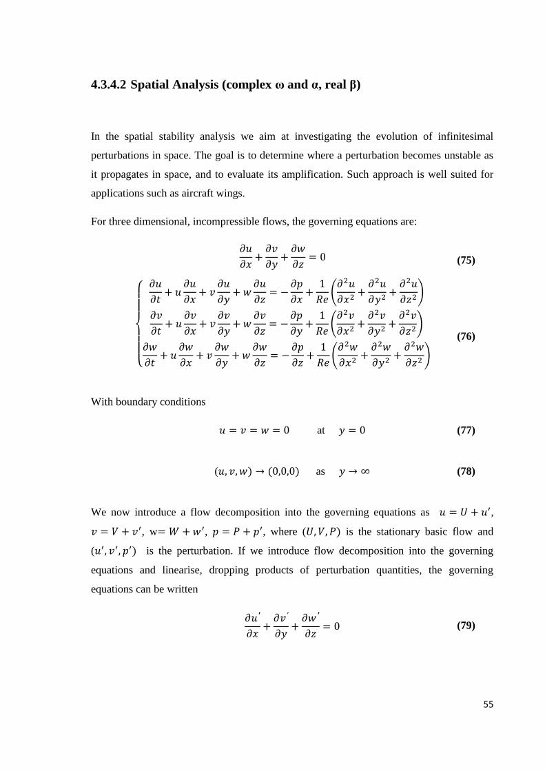
4.3.4.2 Spatial Analysis (complex ω and α, real β)

In the spatial stability analysis we aim at investigating the evolution of infinitesimal

perturbations in space. The goal is to determine where a perturbation becomes unstable as

it propagates in space, and to evaluate its amplification. Such approach is well suited for

applications such as aircraft wings.

For three dimensional, incompressible flows, the governing equations are:

(75)

(76)

With boundary conditions

at (77)

( as (78)

We now introduce a flow decomposition into the governing equations as ,

, w , , where ( is the stationary basic flow and

( is the perturbation. If we introduce flow decomposition into the governing

equations and linearise, dropping products of perturbation quantities, the governing

equations can be written

(79)

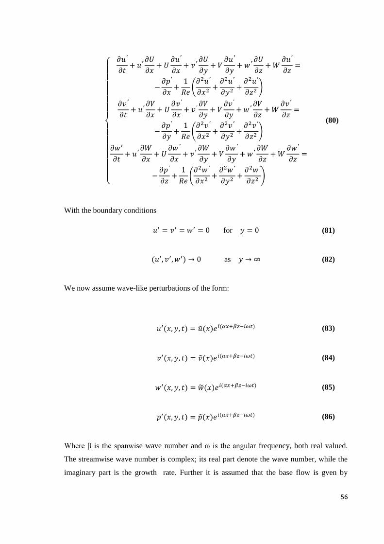
56

(80)

With the boundary conditions

for (81)

as (82)

We now assume wave-like perturbations of the form:

(83)

(84)

(85)

(86)

Where β is the spanwise wave number and ω is the angular frequency, both real valued.

The streamwise wave number is complex; its real part denote the wave number, while the

imaginary part is the growth rate. Further it is assumed that the base flow is gven by

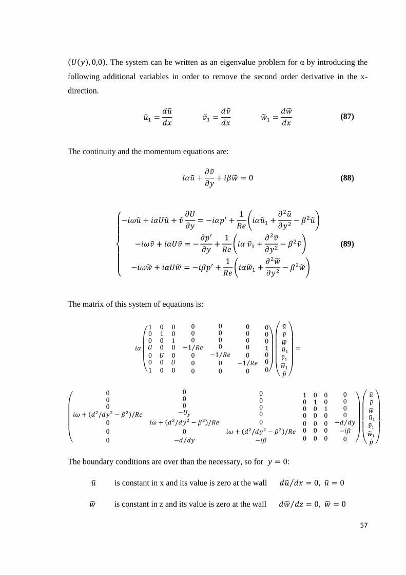
57

. The system can be written as an eigenvalue problem for α by introducing the

following additional variables in order to remove the second order derivative in the x-

direction.

(87)

The continuity and the momentum equations are:

(88)

(89)

The matrix of this system of equations is:

The boundary conditions are over than the necessary, so for :

is constant in x and its value is zero at the wall

is constant in z and its value is zero at the wall

58

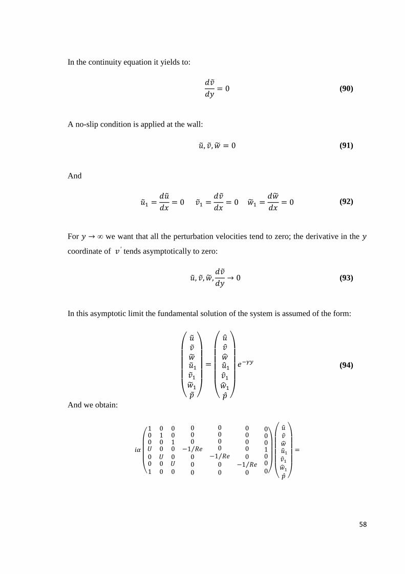
In the continuity equation it yields to:

(90)

A no-slip condition is applied at the wall:

(91)

And

(92)

For we want that all the perturbation velocities tend to zero; the derivative in the

coordinate of tends asymptotically to zero:

(93)

In this asymptotic limit the fundamental solution of the system is assumed of the form:

(94)

And we obtain:

59

Which can be written as:

(95)

(96)

The determinant of the matrix gives the possible solutions for the boundary conditions at

. For this boundary condition the derivative in of tends to zero; we set also

as it has been adimensionalized with the external velocity.

The solutions are:

(97)

(98)

(99)

Where .

An alternative way to solve the same problem is made by resolving the original system of

four equations and four unknowns:

(100)

60

(101)

We set and for the assumption at , the derivative

tends to zero:

(102)

(103)

In the matrix form it is:

We call . The determinant of the matrix is:

(104)

(105)

(106)

61

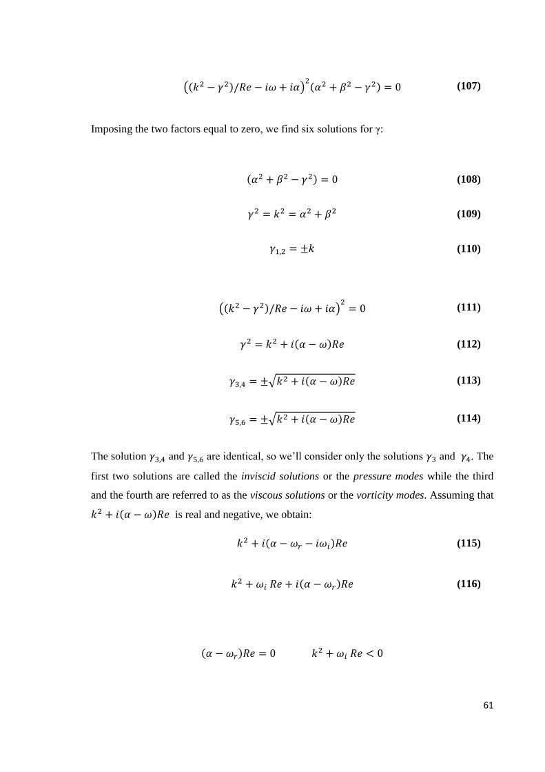
(107)

Imposing the two factors equal to zero, we find six solutions for γ:

(108)

(109)

(110)

(111)

(112)

(113)

(114)

The solution and are identical, so we’ll consider only the solutions and . The

first two solutions are called the inviscid solutions or the pressure modes while the third

and the fourth are referred to as the viscous solutions or the vorticity modes. Assuming that

is real and negative, we obtain:

(115)

(116)

62

The second expression can be rewritten as

(117)

Where is a small positive quantity. The spectrum is given as:

(118)

This is the analytical expression for the continuous spectrum.

Fig.30 shows neutral curves for Blasius boundary layer flow, according to spatial analyis.

The frequency is then a real number and the contours refer to constant values of the

streamwise wave number α.

Figure 30 - Neutral curve for Blasius boundary layer flow in spatial analysis.

Contours of constant growth rate

63

The neutral curve is the the red one, while the others are level curves. Inside the red curve,

the grey zone, the imaginary part of α is negative, so the flow is unstable. We find positive

values of in the outer region, where the flow is stable.

Figure 31 - Neutral curves as function of the spanwise wave number β

As a further demonstration of the Squire theorem, which says that the most unstable modes

occur for the two-dimensional flows, then for β =0 (red line), in Fig.31 the dependence of

the neutral curve from the spanwise wave number β is shown. It is evident that the most

wide area, is occupied by the zone confined by the neutral curve for beta = 0, so that

explains why the two dimensional flow is the most unstable. The other curves are the

neutral curves for higher values of beta.

64

5 IMPLEMENTATION IN INDUSTRIAL CODES

The objective of this analysis is to understand how and when turbulence occurs in a flow,

in order to prevent it as far as it’s possible. In fact reducing drag on a wing profile means

to reduce the fuel consumption. The way to reduce drag is strictly linked to the extent of

the laminar area on the wing. Different tools and ways of proceeding are used on three test

cases to find the transition point. In the following section it will be presented a

development of a methodology to find the transition location and where separation occurs.

5.1 PROCEDURE

We start for instance by explaining which are the passages of this methodology and the

tools used. The first step is to create the geometry of the wing profile and of the far field

(Design Modeler code). Between these two elements there is the domain where the stream

flows, so where the flow has to be analyzed. Then the mesh has to be generated inside

these two boundaries (Workbench). The mesh can be of two types, according to the kind of

study we deal with. If we proceed with a viscous calculation (Fluent) the mesh has to be

fine, especially in the boundary layer zone, to describe it the more precisely. The mesh

with inflation occupies a bigger memory than the one without inflation. The inviscid

65

calculation (Fluent), as the word says, analyze the flow without considering the viscosity

of the fluid. The mesh has not to be fine, since the absence of viscosity doesn’t produce the

boundary layer zone. This type of calculation is necessary to evaluate the pressure

distribution over a wing. The pressure coefficient distribution is the starting point to

proceed with the analysis of the boundary layer through a different code that will be

introduced (bl3D). This code calculates the boundary layer just only having the pressure

distribution along the profile and other quantities which define the conditions of the flow

(temperature at the infinite, Reynolds number, Mach number, the sweep angle, the

geometry of the profile and the chord length). The code stops to run when it finds the

separation location; but the most important data that it provides is the shape of the

boundary layer. We need to know it because with (autoinit code) it will be possible to find

the unstable modes characteristic of the boundary layer under study. Afterwards Nolot

code calculates the growth of these unstable modes (found by autoinit), allowing us to

identify the transition location through the method. Here after, all the steps of the

methodology will be explained in a detailed way.

Geometry

1. Take the geometry profile to be analyzed and write it as a readable file by Design

Modeler.

2. Create the geometry of the far field (or upload the new geometry profile in an old

file containing the farfield).

Mesh generation

3. Import the geometry created in Design Modeler to Workbench an set the right

options to create the mesh.

66

4. The mesh can be created in two ways: with and without inflation. The mesh with

the inflation is used to run the viscous calculations in Fluent while the mesh

without inflation is used to run Fluent when the fluid is considered inviscid. That is

because the viscous calculations are supposed to have a regular distribution of

quadrilaterals (convex polygons) in the boundary layer in order to obtain more

precise results.

Calculation of pressure distribution

5. Enter in Fluent and read the mesh. Create a journal file where all the settings (Re,

Ma, T, p, transition model, inviscid model) are written and ready to be executed

when one run the calculation. Set the boundary conditions. Run iterations, look at

the residuals and estimate if the results are acceptable and finally save them.

6. Extract the Cp distribution in the inviscid calculations and the skin friction

coefficient in the viscous one. Extract all the pictures of the variation of pressure or

Mach number around the airfoil.

Calculation of the boundary layer flow

7. Take the Cp distribution and use the code in Python, developed to create a

geo.dat_0000 file.

8. Run bl3D in Linux in the same folder of the geo.dat_0000 file. The parameters of

the boundary layer, such as the velocity profile, , momentum thickness, etc. are

then computed.

Linear stability analysis

9. Set in the auto.in_0000 file the range of β-angle, frequency, etc. one wants to use.

67

10. Run autoinit and copy the obtained file modes.in_0000 in modes.in, to make Nolot

read the file (since it reads only the modes.in files).

11. Run Nolot with the command nolot2 and plot the euro.dat_0000 file with Gnuplot

to see the trends of the growth rate, the N-factor and the angle of the perturbations

with respect to the x axis or to the streamline.

12. After plotting the 1st and the 8th columns to see the growth rate, check for which x

the envelope of these curves reach the N-factor equal to 8 or to 10. This process has

been automated by Python.

Post processing

13. Create an Excel file where the results of the skin friction (from viscous calculation),

the results from Nolot transition location and the experimental results (in literature)

are plotted.

5.2 DETAILED DESCRIPTION OF EACH PASSAGE

5.2.1 GEOMETRY

Design Modeler

Design Modeler is the code we have used to create the geometry of the domain. It needs to

be a closed area because otherwise it is not possible to create the mesh. The two elements

that have to be created are the far field and the geometry profile. Once the far field has

68

been created, one can enter the geometry of the profile, subtracting it to the area of the

region of the far field.

1) In order to make the wing profile readable for Design Modeler it’s necessary

to write it as a text file in the following way:

Figure 32 - Wing profile text file for Design Modeler

The first column is the number of the group, the second is the numeration of

the points for each group, and the other three columns are the x, y and z

coordinates of the profile.

69

Since the trailing edge of the airfoil is too sharp to be treated in the right way

by Design Modeler, the airfoil has been divided into two parts. The first part

is the airfoil it-self and the other part is a small segment which is needed in

order to avoid having a sharp tip.

Next, we open Workbench in Linux, from the front node by typing qsh from

the terminal. The command is

> runwb214

The ANSYS window is the following:

Figure 33 - Ansys window of a new project

Create the two parts:

1. Geometry

70

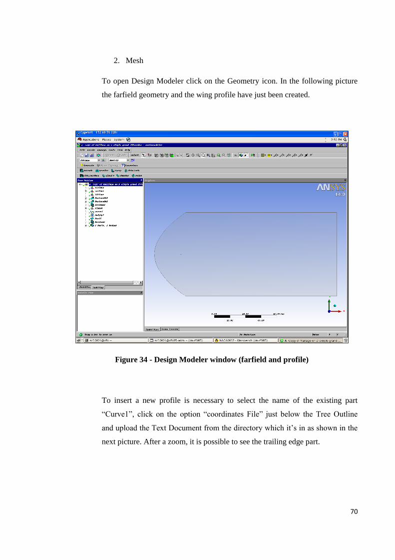
2. Mesh

To open Design Modeler click on the Geometry icon. In the following picture

the farfield geometry and the wing profile have just been created.

Figure 34 - Design Modeler window (farfield and profile)

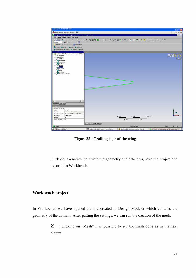
To insert a new profile is necessary to select the name of the existing part

“Curve1”, click on the option “coordinates File” just below the Tree Outline

and upload the Text Document from the directory which it’s in as shown in the

next picture. After a zoom, it is possible to see the trailing edge part.

71

Figure 35 - Trailing edge of the wing

Click on “Generate” to create the geometry and after this, save the project and

export it to Workbench.

Workbench project

In Workbench we have opened the file created in Design Modeler which contains the

geometry of the domain. After putting the settings, we can run the creation of the mesh.

2) Clicking on “Mesh” it is possible to see the mesh done as in the next

picture:

72

Figure 36 - Workbench mesh on the NACA0012 profile

This mesh has the inflation, a very regular distribution of quadrilaterals (the

polygonal elements of the mesh) around the profile. After having set all the

parameters click on Update to create the mesh. Then, save and place it in the

folder where the Fluent calculations have to be run.

To have a mesh with no inflation, which is very light in terms of memory

occupied and quicker in the Fluent calculations, is only necessary to remove the

option and regenerate the mesh.

73

5.2.2 MESH GENERATION

3) The reason why it is necessary to have two different meshes is because of the

different type of calculation that we want to run. With the hypothesis of inviscid

fluid, the equations are less and simpler and the calculation consequently. Thus

we do not need a very fine mesh, because it would be useless and expensive in

terms of memory and time, see Fig.37.

Figure 37 - Mesh without inflation for inviscid calculation

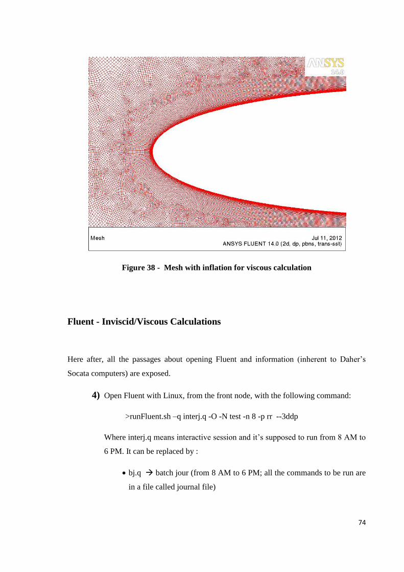
On the contrary for a viscous fluid the approach in terms of equations and

solution models is totally different. This time we need a very fine and tidy

mesh, with a regular distribution of quads in the boundary layer (as in Fig. 38 is

shown), since the solution is very sensitive to the distribution of the elements.

74

Figure 38 - Mesh with inflation for viscous calculation

Fluent - Inviscid/Viscous Calculations

Here after, all the passages about opening Fluent and information (inherent to Daher’s

Socata computers) are exposed.

4) Open Fluent with Linux, from the front node, with the following command:

>runFluent.sh –q interj.q -O -N test -n 8 -p rr --3ddp

Where interj.q means interactive session and it’s supposed to run from 8 AM to

6 PM. It can be replaced by :

bj.q batch jour (from 8 AM to 6 PM; all the commands to be run are

in a file called journal file)

75

nuit.q and after “–n 32” is to run the calculations during the night

(from 6 PM to 5 AM) using the new machine

nuit.q and after “-n24” is to run the calculations during the night

(from 6 PM to 5 AM) using the old machine

“-O” stands for “old machine”

“-N test” is the command to call “test” the job that is running. It is possible to

see it typing >qs from the terminal. In this way all the jobs that have been

started from other users are visible as well.

“-n 8” indicates the CPUs that you’re about to use.

In “-p rr” the “p” stands for node reservation rule and double “r” refers to

“round robin”. To use the old machine “-p 8” can be typed.

“--3ddp” is used when you want to open Fluent in three dimensions with double

precision, and it has to be in the last position of the command, while the other

commands are not required to respect any order.

Another example is:

>runFluent.sh –q nuit.q –n 24 -N jobname -i filename.jou --2ddp

The calculation can be executed at any time but it starts at 6PM, it uses 24

CPUs, the jobname.jou file is used to run all the commands written in it.

When Fluent is open import the mesh clicking on “File” “Read” “Mesh”

and select the mesh file from the folder where all the Fluent results are

supposed to be placed.

5.2.3 CALCULATION OF PRESSURE DISTRIBUTION

Fluent calculations are not simple to deal with. For this reason we proceed with the

creation of a file that serves to make ordered and systematic calculations.

76

5) After the reading of the mesh the settings can be chosen by hand or

automatically. The automatic way is recommended since it permits us not to

forget anything and to check every time we need all the parameters and settings

we have used for that precise calculation. The journal file is a particular file

where all the commands to be executed are written and to run it, it is necessary

to follow this path:

“File” “Read” “Journal” for an interactive session

Insert the journal file name in the command to run Fluent, preceded by “-i”.

The commands in the journal file used in the case of a NACA0012 airfoil, in

2D, for an inviscid calculation are:

;JOURNAL: CALCUL DE LE Cp du profil NACA0012 - INVISCID - NO INFLATION ;

(define (deg2rad angle) (/ (* angle 3.14159) 180)) CONVERTS FROM DEGREES

TO RADIANS

;CONDITIONS DU CALCUL =====================

(rp-var-define 'temperature 288.15 'real #f) DEFINE THE TEMPERATURE

(rp-var-define 'pressure 101325 'real #f) DEFINE THE PRESSURE

(rp-var-define 'M 0.12877562 'real #f) DEFINE THE MACH NUMBER

(rp-var-define 'Re_objectif 3000000 'real #f) DEFINE THE REYNOLDS NUMBER

; ==========================================

(define aoa 0.0) DEFINE THE ANGLE OF ATTACK

; Calcul de la vitesse

(define vitesse (* (** (* 1.4 287.053 (rpgetvar 'temperature #f)) 0.5) (rpgetvar 'M)))

; Calcul du Reynolds

(define rho (/ (rpgetvar 'pressure #f) (* 287.053 (rpgetvar 'temperature #f))))

(define mu (/ (* 0.0000014536846 (** (rpgetvar 'temperature #f) 1.5))(+ (rpgetvar

'temperature #f) 110.4)))

(define nu (/ mu rho))

(define Reynolds (/ vitesse nu))

77

(display Reynolds)

; Calcul de la corde

(define corde (/ (rpgetvar 'Re_objectif #f) Reynolds)) CALCULATE THE CHORD

TO REALISE Re

(display corde)

;===========================================

Choice of the right model (Viscous or Inviscid):

Settings of the parameters for inviscid calculation.

rc NACA0012noINFL.msh LOAD THE MESH

/mesh/scale corde corde SCALE THE MESH WITH THE CHORD

; MEP Modeles

;

/define/models/energy? n DON’T USE ENERGY EQUATION

;

/define/models/viscous/inviscid y DEFINITION OF INVISCID MODEL

/define/materials/change air air y constant 1.225 n n n n DEFINE AIR PROPERTIES

;

;------------------------------------------------------------------------------------

Settings of the parameters for viscous calculation.

In the case of a viscous calculation some settings have to be changed:

/define/models/energy? y y n CONSIDER THE ENERGY EQUATION

78

;

/define/materials/change air air y ideal-gas n n y sutherland three-coefficient-method

1.716e-05 288.15 110.56 n n n

DEFINE FLUID MODEL

;

/define/models/viscous/transition-sst? y SET SST–TRANSITION MODEL

Boundary conditions for inviscid calculation.

/mesh/modify-zone/zone-type outlet-bords velocity-inlet MESH SETTINGS ON

FARFIELD GEOM

/define/boundary-conditions/velocity-inlet inlet n y y n 0 n vitesse n 0 SET B.C. AS

VELOCITY INLET

/define/boundary-conditions/velocity-inlet outlet-bords n y y n 0 n vitesse n 0

;--------------------------------------------------------------------------------------

Boundary conditions for viscous calculation.

/mesh/modify-zone/zone-type inlet pressure-far-field MESH SET ON

PRESSURE-FARFIELD

/mesh/modify-zone/zone-type outlet-bords pressure-far-field

/mesh/modify-zone/zone-type outlet-aval pressure-far-field

/define/boundary-conditions/pressure-far-field inlet n 0 n (rpgetvar 'M #f) n (rpgetvar

'temperature #f) n (cos(deg2rad aoa)) n (sin(deg2rad aoa)) n n y n 1 0.1 10

SET BOUNDARY CONDITIONS

/define/boundary-conditions/pressure-far-field outlet-bords n 0 n (rpgetvar 'M #f) n

(rpgetvar 'temperature #f) n (cos(deg2rad aoa)) n (sin(deg2rad aoa)) n n y n 1 0.1 10

/define/boundary-conditions/pressure-far-field outlet-aval n 0 n (rpgetvar 'M #f) n

(rpgetvar 'temperature #f) n (cos(deg2rad aoa)) n (sin(deg2rad aoa)) n n y n 1 0.1 10

79

Mesh parameters in inviscid calculation.

;Setup Valeurs de references

/report/reference-values/compute/velocity-inlet inlet CALCULATE REFERENCE

VALUES FROM “INLET”

/report/reference-values/length corde SET REFERENCE LENGTH

/report/reference-values/area corde SET REFERENCE AREA ( DEPTH = 1)

;--------------------------------------------------------------------------------------

; Setup Couplage P-V

/solve/set/gradient-scheme y SET SOLUTION METHOD

/solve/set p-v-coupling 20 SET SCHEME SIMPLE (CORRESPONDS TO 20)

;-------------------------------------------------------------------------------------

/solve/set/under-relaxation mom 0.5 SET SOLUTION CONTROLS

/solve/set/under-relaxation pressure 0.5

/solve/set/under-relaxation body-force 1

/solve/set/under-relaxation density 0.95

;-------------------------------------------------------------------------------------

/solve/monitors/residual/convergence-criteria 0.000001 0.000001 0.000001

SET CONVERGENCE LIMITS

/solve/monitors/residual/plot? n DON’T SHOW THE RESIDUAL PLOT

DURING THE CALCULATION

Mesh parameters in viscous calculation.

/solve/set p-v-coupling 24 SET SCHEME COUPLED

/solve/set p-v-controls 10 0.4 0.4 SET CFL NUMBER

80

;

/solve/set/under-relaxation body-force 1 SET SOLUTION CONTROLS

/solve/set/under-relaxation density 0.95

/solve/set/under-relaxation k 0.6

/solve/set/under-relaxation omega 0.6

/solve/set/under-relaxation turb-viscosity 0.6

/solve/set/under-relaxation temperature 0.85

/solve/set/under-relaxation intermit 0.75

/solve/set/under-relaxation retheta 0.75

;

/solve/initialize/compute-defaults pressure-far-field inlet INITIALIZATION

/solve/initialize/initialize-flow

/solve/set/multi-grid-amg 20 2 0 1 30 "gauss-seidel" 20 8 0 4 30 "ilu" 30 50 0

/solve/initialize/set-fmg-initialization 5 0.001 10 0.001 50 0.001 100 0.001 500 0.001 500

0.5 no

/solve/initialize/fmg-initialization y

Way of proceeding for different angles of attack: run iterations, have a look at the residuals

and finally save the results.

Settings of angle of attack, iterations, and saving data.

;########################################################################

##############

; CALCUL A ALPHA=0°

;

(define aoa 0.0) DEFINE THE ANGLE OF ATTACK

;

/solve/initialize/compute-defaults velocity-inlet inlet INITIALIZATION OF THE

FLOW

81

/solve/initialize/initialize-flow

;

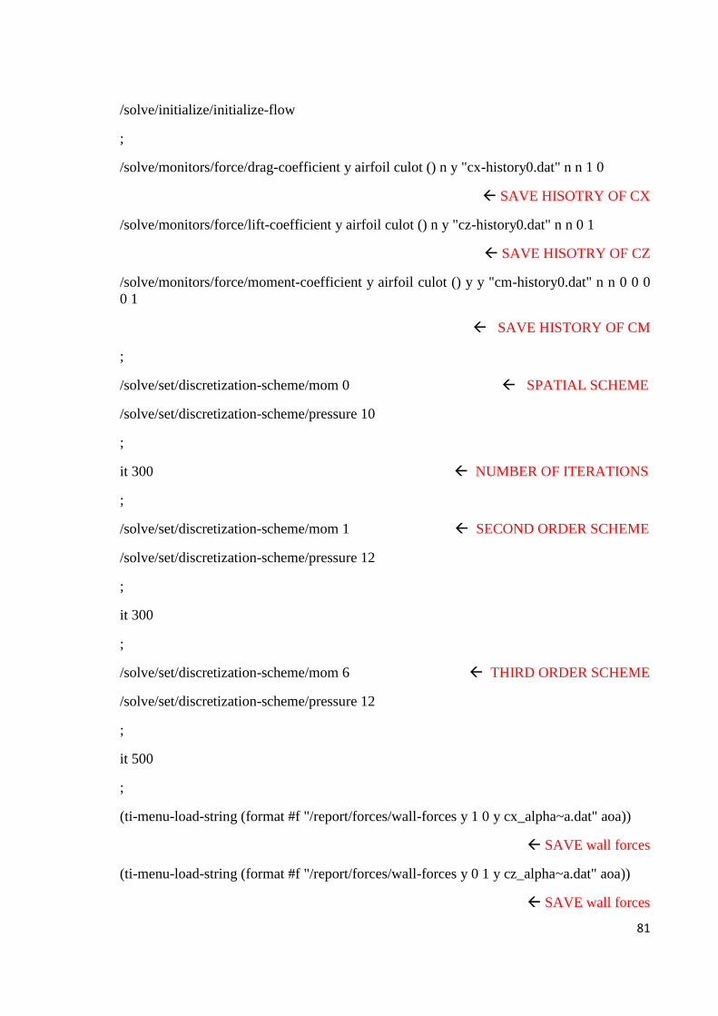
/solve/monitors/force/drag-coefficient y airfoil culot () n y "cx-history0.dat" n n 1 0

SAVE HISOTRY OF CX

/solve/monitors/force/lift-coefficient y airfoil culot () n y "cz-history0.dat" n n 0 1

SAVE HISOTRY OF CZ

/solve/monitors/force/moment-coefficient y airfoil culot () y y "cm-history0.dat" n n 0 0 0

0 1

SAVE HISTORY OF CM

;

/solve/set/discretization-scheme/mom 0 SPATIAL SCHEME

/solve/set/discretization-scheme/pressure 10

;

it 300 NUMBER OF ITERATIONS

;

/solve/set/discretization-scheme/mom 1 SECOND ORDER SCHEME

/solve/set/discretization-scheme/pressure 12

;

it 300

;

/solve/set/discretization-scheme/mom 6 THIRD ORDER SCHEME

/solve/set/discretization-scheme/pressure 12

;

it 500

;

(ti-menu-load-string (format #f "/report/forces/wall-forces y 1 0 y cx_alpha~a.dat" aoa))

SAVE wall forces

(ti-menu-load-string (format #f "/report/forces/wall-forces y 0 1 y cz_alpha~a.dat" aoa))

SAVE wall forces

82

(ti-menu-load-string (format #f "/report/forces/wall-moments y 0 0 0 0 1 y

cm_alpha~a.dat" aoa))

;

(rp-var-define 'name "NACA0012" 'char #f) DEFINE THE STRING NACA0012

;

(ti-menu-load-string (format #f "wc ~a-alpha~a-Re~a-M~a.cas.gz" (rpgetvar 'name #f) aoa

(/ (rpgetvar 'Re_objectif #f) 1000000) (rpgetvar 'M #f)))

DEFINE THE FILE NAME AND SAVE .CAS FILE

(ti-menu-load-string (format #f "wd ~a-alpha~a-Re~a-M~a.dat.gz" (rpgetvar 'name #f) aoa

(/ (rpgetvar 'Re_objectif #f) 1000000) (rpgetvar 'M #f)))

DEFINE THE FILE NAME AND SAVE .DAT FILE

;########################################################################

; CALCUL A ALPHA=1°

;

(define aoa 1.0) DEFINE THE ANGLE OF ATTACK

;

/define/boundary-conditions/velocity-inlet inlet n y y n 0 n (* vitesse (cos(deg2rad aoa)))

n (* vitesse (sin(deg2rad aoa)))

SET BOUNDARY CONDITIONS DEPENDING ON THE ANGLE OF ATTACK

/define/boundary-conditions/velocity-inlet outlet-bords n y y n 0 n (* vitesse (cos(deg2rad

aoa))) n (* vitesse (sin(deg2rad aoa)))

SET BOUNDARY CONDITIONS DEPENDING ON THE ANGLE OF ATTACK

;

(ti-menu-load-string (format #f "/solve/monitors/force/drag-coefficient y airfoil culot () n y

cx-history~a.dat n n ~a ~a" aoa (cos(deg2rad aoa)) (sin(deg2rad aoa))))

SAVE HISTORY OF CX

(ti-menu-load-string (format #f "/solve/monito rs/force/lift-coefficient y airfoil culot () n y

cz-history~a.dat n n ~a ~a" aoa (-(sin(deg2rad aoa))) (cos(deg2rad aoa))))

SAVE HISTORY OF CZ

(ti-menu-load-string (format #f "/solve/monitors/force/moment-coefficient y airfoil culot

() y y cm-history~a.dat n n 0 0 0 0 1" aoa))

SAVE HISTORY OF CM

83

;

/solve/set/discretization-scheme/mom 0

/solve/set/discretization-scheme/pressure 10

it 300

/solve/set/discretization-scheme/mom 1

/solve/set/discretization-scheme/pressure 12

it 300

/solve/set/discretization-scheme/mom 6

/solve/set/discretization-scheme/pressure 12

it 500

;

(ti-menu-load-string (format #f "/report/forces/wall-forces y ~a ~a y cx_alpha~a.dat"

(cos(deg2rad aoa)) (sin(deg2rad aoa)) aoa)) SAVE WALL FORCES

(ti-menu-load-string (format #f "/report/forces/wall-forces y ~a ~a y cz_alpha~a.dat" (-

(sin(deg2rad aoa))) (cos(deg2rad aoa)) aoa)) SAVE WALL FORCES

(ti-menu-load-string (format #f "/report/forces/wall-moments y 0 0 0 0 1 y

cm_alpha~a.dat" aoa))

;

(ti-menu-load-string (format #f "wc ~a-alpha~a-Re~a-M~a.cas.gz" (rpgetvar 'name #f) aoa

(/ (rpgetvar 'Re_objectif #f) 1000000) (rpgetvar 'M #f)))

SAVE .CAS FILE WITH THE PROPER AoA

(ti-menu-load-string (format #f "wd ~a-alpha~a-Re~a-M~a.dat.gz" (rpgetvar 'name #f) aoa

(/ (rpgetvar 'Re_objectif #f) 1000000) (rpgetvar 'M #f)))

SAVE .DAT FILE WITH THE PROPER AoA

;########################################################################

The use of scheme commands allows to parameterize file names, flow

quantities, etc.

The .cas and the .dat files are the files that contain all the data of the calculation

made and all the information. It’s important to save these files because if we

realize after that we need to check something, or if we need to extract a picture,

84

or if we want to restart a new calculation basing it on the first one (for example

changing the angle of attack), we don’t need to restart all the job from the

beginning.

6) When all the data for every angle of attack in the inviscid case are saved in the

“.cas “and “.dat “files, we need to get the Cp distribution from these files. To

get a Cp distribution with ordered x-coordinate it’s necessary to open Fluent

running on only one CPU. In fact if we open the “.cas” file from Fluent running

on several CPUs and save the Cp distribution from it, the data extracted are

taken from different CPUs, and the result is that even if we get all the points of

the Cp distribution, they will not be in the right sequence, they are practically

taken in a random way so that we cannot use them for the following analysis.

The command to run Fluent on one CPU is the next and it has to be launched

from the front node (>qsh):

>runFluent14

Clicking on “File””Read””Case&Data” it’s possible to load the case from

which you want to extract the Cp distribution.

It’s recommended to have a look at the residuals before considering the case a

good case.

After that the Cp distribution can be extracted from “Display” “Plots”

“XYPlot” “Set Up”, choosing “Pressure” “Pressure Coefficient” and

“Write to File”. The same thing can be done in the viscous calculation to extract

the “Skin Friction Coefficient”, since it indicates when the transition occurs.

This is because the skin friction coefficient changes its value due to the fact that

the fluid changes its status. In the case of inviscid Cp it’s necessary to extract

the Y-coordinate as well, since we will need to create a file that is called

geo.dat_id for the stability Nolot code.

85

To extract pictures, in order to have an idea of how the pressure, the Mach

number and other values vary around the airfoil click on “Display”

”Graphics and Animations” ”Contours” ”Set Up”.

5.2.4 CALCULATION OF THE BOUNDARY LAYER FLOW

Once the Fluent calculation has finished we need to post-process the results. In the case of

viscous calculation we only need to extract the friction coefficient to know where

transition occurs. In the case of inviscid analysis, we have to extract the pressure

coefficient distribution, in order to find the unstable modes responsible of the transition.

Since the process of transforming data from Fluent to data readable for bl3D is very long

and one can easily make mistakes, a code that do this work automatically has been created.

7) A Python code has been developed to take all the information we need from the

XCp and the XY files to create the geo.dat_myid in a readable form for Nolot.

The geo.dat_myid file is the file where the coordinates of the geometry of the

profile and the pressure distribution are written, and they are necessary to bl3D

to calculate the boundary layer. The Python script is called “Cp2geo.py” and it

is shown in Fig.39:

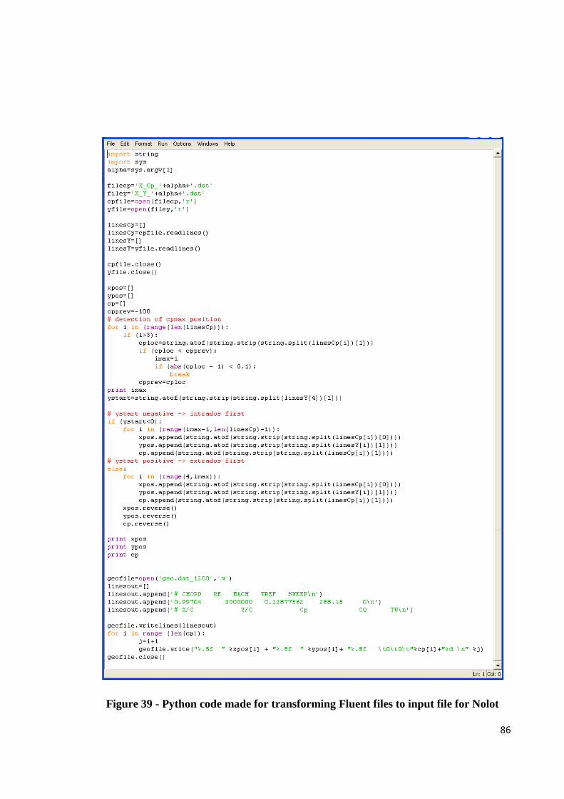
86

Figure 39 - Python code made for transforming Fluent files to input file for Nolot

87

In the case of 3D geometry, like in the case of the spheroid, taking the Cp along

the slices is not very easy. So it is necessary to display the Fluent results on

Tecplot or on Paraview. The procedure is the following:

Open Fluent and load the .cas file:

Tecplot

o Export Solution Data File Type (select Tecplot)

o Select the surfaces and the quantities (pressure coefficient and velocity in

x,y,z)

o Save and drag the file in the Tecplot window

Paraview

o Export Solution Data File Type (select EnSight Case Gold)

o Select interior-solid and the quantities (pressure coefficient and velocity in

x,y,z)

o Save and change the extension of the file “.encas” in to “.case”

o Open Paraview and open the file “.case”

8) To run the bl3D code it is necessary to use Linux. A software that links Linux

to Windows is Cygwin. Open it and, in the same folder of the geo.dat_0000

file, run bl3D from the terminal inserting the myid, or rather the identification

number of the file. It is necessary to have in the same folder with geo.dat_0000,

88

the bl.in_0000 file, which establishes the details of the calculation such as the

resolution in the normal direction, the domain of the calculation, Prandtl

number, the characteristic of the air, etc. Running the bl3D file, the parameters

of the boundary layer appear on the screen, such as the boundary layer

thickness and , the momentum thickness . All these data are saved in the

edge.dat_0000 file, in the blchar.dat_0000 file and in the meanflow.dat_0000.

The last point that bl3D writes on the screen is the point where the boundary

layer separates because of the pressure gradient. The transition can occur before

the separation of the boundary layer and be the cause of the transition because

of the growth of the unstable modes; on the contrary the transition can occur as

well when the separation is caused by the pressure gradient and not because of

the growth of the unstable waves.

In order to make a good plot of the final results is useful to take the separation x

point for each angle of attack and plot it on a Excel file, next to the transition

curve.

5.2.5 LINEAR STABILITY ANALYSIS

In agreement with the linear stability theory, the aim is to find the unstable modes which

provoke the transition of the boundary layer. The settings to put in the files are explained:

9) Open the auto.in_0000 file and set the parameters as the frequency range (ω),

the spanwise wave number range (β), the range of points on the profile, the

angle where perturbations develop, to look for which range of these variables

there are the more interesting unstable modes.

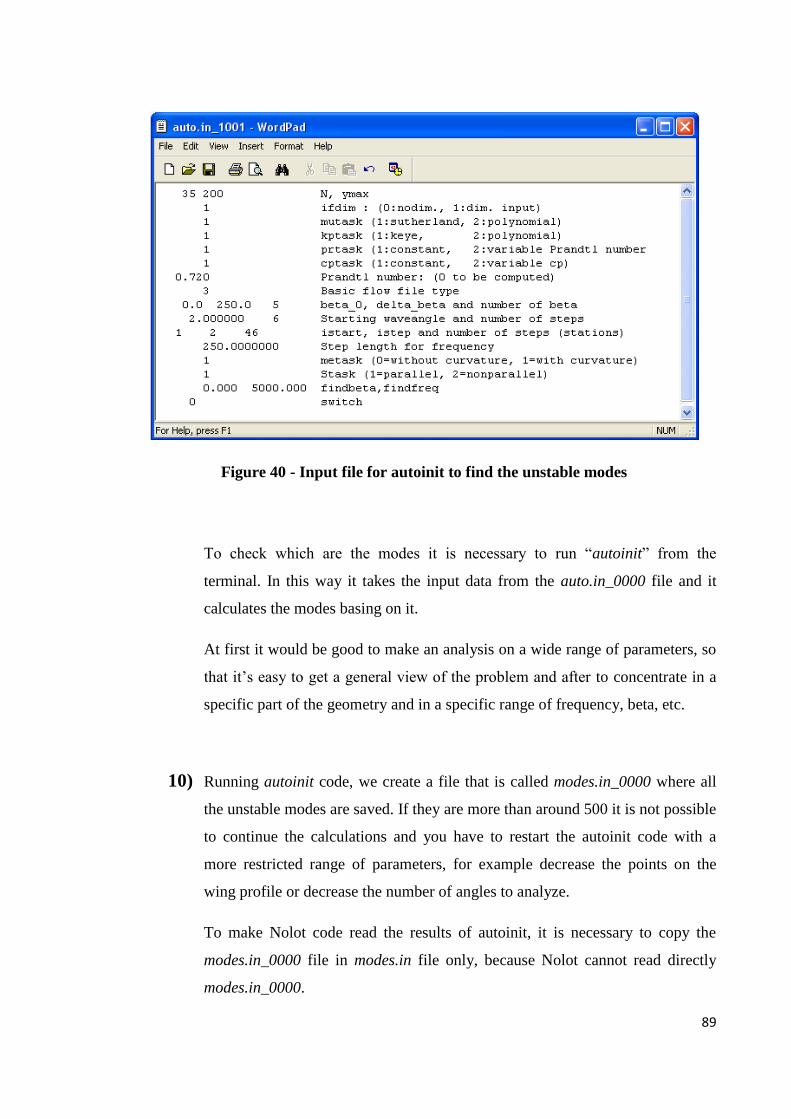
89

Figure 40 - Input file for autoinit to find the unstable modes

To check which are the modes it is necessary to run “autoinit” from the

terminal. In this way it takes the input data from the auto.in_0000 file and it

calculates the modes basing on it.

At first it would be good to make an analysis on a wide range of parameters, so

that it’s easy to get a general view of the problem and after to concentrate in a

specific part of the geometry and in a specific range of frequency, beta, etc.

10) Running autoinit code, we create a file that is called modes.in_0000 where all

the unstable modes are saved. If they are more than around 500 it is not possible

to continue the calculations and you have to restart the autoinit code with a

more restricted range of parameters, for example decrease the points on the

wing profile or decrease the number of angles to analyze.

To make Nolot code read the results of autoinit, it is necessary to copy the

modes.in_0000 file in modes.in file only, because Nolot cannot read directly

modes.in_0000.

90

After having checked where the unstable modes are, it remains to check the

behavior of the growth of the instabilities.

Nolot code

Nolot is a specific code developed at the Swedish Defense Research Agency (FOI) able to

find the transition point of a wing profile, relying only on the distribution of pressure, and

on data such as temperature, the Reynolds number, the geometry of the profile, the sweep

angle, the Mach number and the chord. As explained below it is a code that works only for

2D geometries, or even for 3D but constant in the third direction, in terms of geometry and

direction of the flow. Here after, are explained all the steps needed to learn to use it.

11) Run the Nolot code and plot the resulting file euro.dat_0000 with Gnuplot. If

you open the file you can find different columns which are for the x and s

coordinates (x is the direction of abscissa and s is the local geometry of the

profile), frequency, spanwise wave number, local sweep angle, growth rate and

N factor, respectively.

12) To plot these values type this after having opened Gnuplot:

>plot “euro.dat_0000” u 1:8 w l

This command plots the first column as abscissa and the column 8th

as ordinate.

The first column corresponds to the x coordinate and the 8th

to the Nfactor. It’s

possible to check other variables, such as the growth rate or the angles linked to

each perturbation type.

91

For example if in the auto.in_0000 file I check only the perturbations which

have an angle between 80° and 90°, if I find some unstable modes, I am sure

that these modes belong to the cross flow type of instabilities. To see it it’s

necessary to write as it follows:

(80.0 10 Starting waveangle and number of steps)

In this way the angles of the perturbation that are analyzed are the ones starting

from 80° up to 90°, divided in 10 parts.

After having run in Gnuplot the first and the eight columns of the

euro.dat_0000 file, a plot of the instability waves appears. It remains to check

where the curves intersect the N-factor chosen value for the case under study.

To make the job faster, it has been created a dedicated code that does it

automatically.

A Python code has been developed to take the right most value of the N-factor

envelope of curves, for a decided N-factor value. It reads the file

“euro.dat_0000” which is the file where all the results of the calculations are

saved, and checks for every block of results (every curve), if the x coordinate

that corresponds to the chosen N-factor is bigger or smaller than the previous.

In the case it is smaller, it saves this number as the right-most value found until

that moment. The code does this for every block and the last found is the x

transition point.

If you choose a N-factor=8, the code make an interpolation between the two

numbers before and after the N-factor chosen. The same for the x coordinate.

The code is shown in Fig.41:

92

Figure 41 - Python code crated to find automatically the transition location from the

amplification curve

93

It prints every time the x minimum value corresponding to the chosen N-factor.

5.2.6 POST-PROCESSING

13) Take all the transition location from the Python results and put them in the

Excel file created for the boundary layer separation. After that put results of the

skin friction (from viscous calculation), and finally the experimental results

found in the article you’re validating the case. Create an Excel file where the

results of the skin friction (from viscous calculation), the results from Nolot

transition location and the experimental results (article) are plotted.

94

6 TEST CASES

6.1 NLF0416 PROFILE

The first case analyzed was the case of NLF0416 profile which is shown in Fig.42:

Figure 42 - NLF0416 geometry profile

Based on the article “Transition-Flow-Occurrence-Estimation “A New Method” by Paul-

Dan Silisteanu and Ruxandra M. Botez, we’ve done the entire analysis choosing Mach =

0.1 and Re = 4 x 10^6. Fig.43 is from the article and it shows the transition locations on the

upper and lower side of the profile varying with the angle of attack.

95

Figure 43 - Article’s figure plotting the transition locations

The analysis has been done for different angles of attack and according with the two types

of analysis explained in the previous chapter. In Fig.44 are shown the two different type of

mesh, the first without inflation and the second with inflation.

Figure 44 - Mesh without inflation of the NLF0416 profile

The Fluent calculations lead to the following picture, which shows the pressure coefficient

around the airfoil, see Fig.45:

96

Figure 45 - Cp distribution on the NLF0416 profile.

Inviscid calculation made with Fluent

In Fig.46 are shown the boundary layer separation, the transition locations for an N-factor

of 8 and one another for 10, and finally the curve of the previous picture.

97

Figure 46 - Transition and separation location found with Nolot for NLF0416

From Fig.46 we can understand that the transition location made by Silisteanu and Botez is

indeed the separation location, since they roughly match.

6.2 NACA0012 PROFILE

Here we show the case of the most famous and known wing profile, the NACA0012. We

have done this choice because the history about this case is very well documented.

NACA0012 profile is symmetric and it is shown in Fig.47:

Experimental and Theoretical Transition Location

0

0.05

0.1

0.15

0.2

0.25

0.3

0.35

0.4

0.45

0 2 4 6 8 10 12

Angle of attack

Tra

nsit

ion

Lo

cati

on

Transition Location Note-Paul

Nolot - N=10

Nolot - N=8

B.L.Separation

98

Figure 47 - NACA0012 geometry profile

We referred to “Low-Speed Aerodynamic Characteristics of NACA 0012 Aerofoil Section,

including the Effects of Upper-Surface Roughness Simulating Hoar Frost, By N.

GREGORY and C. L. O'REILLY, January, 1970” article, so we set the fluid conditions as

it follows:

Mach = 0.128

Temperature = 288.15 K

Pressure = 101325 Pa

Re = 3 * 10^6

The mesh has been created in the two cases, with inflation and without. In Fig.48 is

presented the mesh with inflation on the leading edge of the profile. The advantage of

using the methodology with Nolot code is that we do not need to create a mesh with

inflation (which demands time and a powerful processor) while the inviscid calculations

with Fluent are rapid and not expensive in terms of memory used. In the case of the

NACA0012 mesh in fact, the one with inflation employs 528963 cells while the one

without inflation only 36886, which is 14 times smaller.

99

Figure 48 - Mesh with inflation of NACA0012 profile

In Fig.49 and in Fig.50 we show the pressure coefficient for the 0° and 4° angles of attack

obtained with the inviscid calculations by Fluent:

Figure 49 - NACA0012 inviscid calculation at AoA = 0°

100

Figure 50 - NACA0012 inviscid calculation at AoA = 4°

The maximum Cp is approximately 1 as expected. Before, even if the case was inviscid we

have obtained a wrong cp distribution, due to the fact that we have considered the option of

the energy equation. The maximum pressure coefficient distributions were around 1.6 to

1.8 and for an inviscid case it is impossible to have so high values unless you add a source

of energy in the flow.

The analogous plot but in the wrong case is shown in Fig.51:

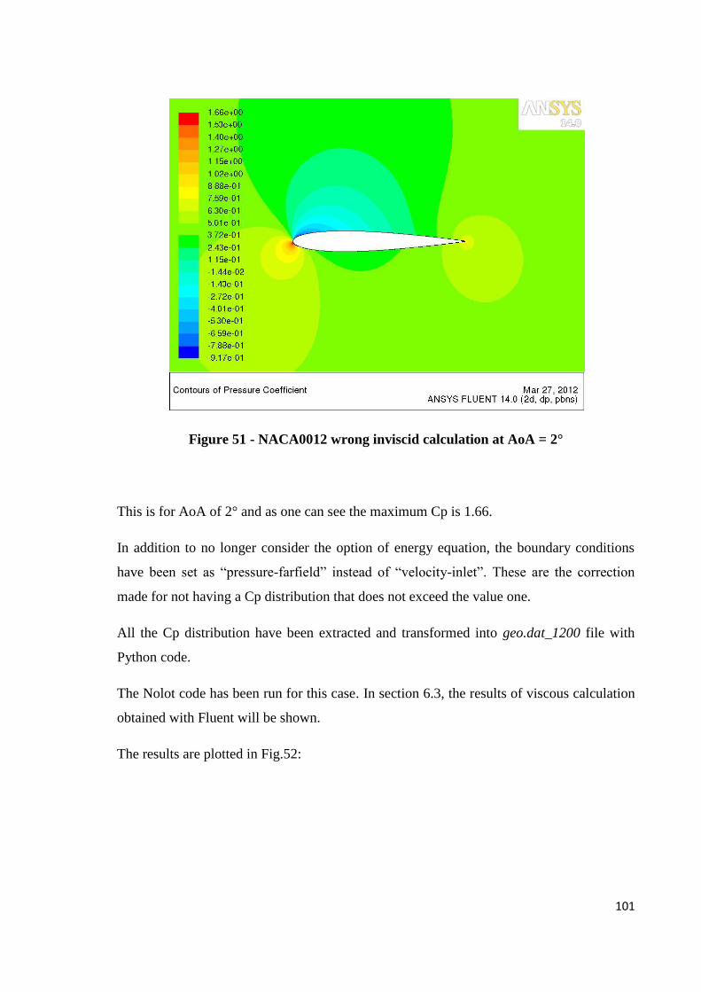
101

Figure 51 - NACA0012 wrong inviscid calculation at AoA = 2°

This is for AoA of 2° and as one can see the maximum Cp is 1.66.

In addition to no longer consider the option of energy equation, the boundary conditions

have been set as “pressure-farfield” instead of “velocity-inlet”. These are the correction

made for not having a Cp distribution that does not exceed the value one.

All the Cp distribution have been extracted and transformed into geo.dat_1200 file with

Python code.

The Nolot code has been run for this case. In section 6.3, the results of viscous calculation

obtained with Fluent will be shown.

The results are plotted in Fig.52:

102

Figure 52 - Nolot and experiments transition locations for NACA0012

The curves obtained with Nolot are 3% up to 10% difference close to the transition curves

of N. Gregory and C.L. O’Reilly’s article (Low-Speed Aerodynamic Characteristic of

NACA0012 Aerofoil Section, including the Effects of Upper-Surface Roughness

Simulating Hoar Frost - 1973). The plot of the transition points according to the article is

shown in Fig.53:

Transition location - Nolot - Experiments

0

0.1

0.2

0.3

0.4

0.5

0.6

-2 0 2 4 6 8 10 12

AoA

X/C

Transition Location O'Reilly

Nolot - Nfactor = 10

Nolot - Nfactor = 8

103

Figure 53 - Gregory O’Reilly graphic of transition location

The computed N-factor curves, for different frequencies, for 0 Aoa and in the case of

Re=3*10^6 Ma=0.128 are shown in Fig.54:

104

Figure 54 - Amplification rate for NACA0012 with AoA = 0°

From the data shown in Fig.54we can extract the transition locations based on the criteria

that it occurs at N-factor values of 8 and 10. We can see that for N-factor =10, the

transition location occurs at x ≈ 0.41. It is easy to see in Fig.52 that the first value

(Aoa=0°) of the curve for N-factor equal to 10, is 0.41.

105

6.3 SST-TRANSITION MODEL

In this section the SST-Transition Model in Fluent is discussed. One issue was related to

the setting of the turbulence intensity. In fact if we set it at the far field it decays with the

distance, until it arrives at the leading edge with a certain value. The decay is shown in

Fig.55.

Figure 55 - Decay of turbulence intensity with the distance

It was desired to have a turbulence intensity of 0.1% at the leading edge, which according

to the Mack’s law corresponds to a N-factor of 8. So we had to set the turbulence intensity

at the far field equal to 0.18%. We also made a calculation with a turbulence intensity at

the far field of 0.1%, so that at the leading edge it was equal to 0%. The two different Cp

distribution we obtained shown in Fig. 56:

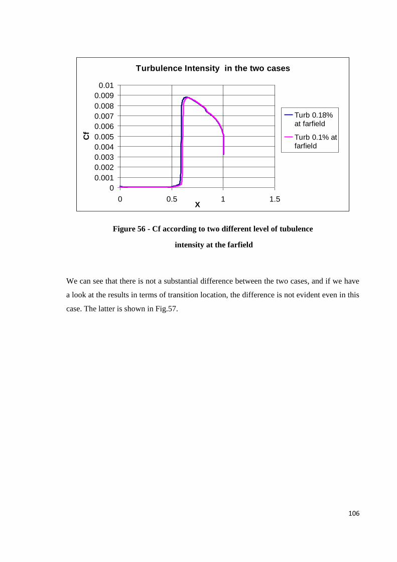
106

Figure 56 - Cf according to two different level of tubulence

intensity at the farfield

We can see that there is not a substantial difference between the two cases, and if we have

a look at the results in terms of transition location, the difference is not evident even in this

case. The latter is shown in Fig.57.

Turbulence Intensity in the two cases

0

0.001

0.002

0.003

0.004

0.005

0.006

0.007

0.008

0.009

0.01

0 0.5 1 1.5X

Cf

Turb 0.18%at farfield

Turb 0.1% atfarfield

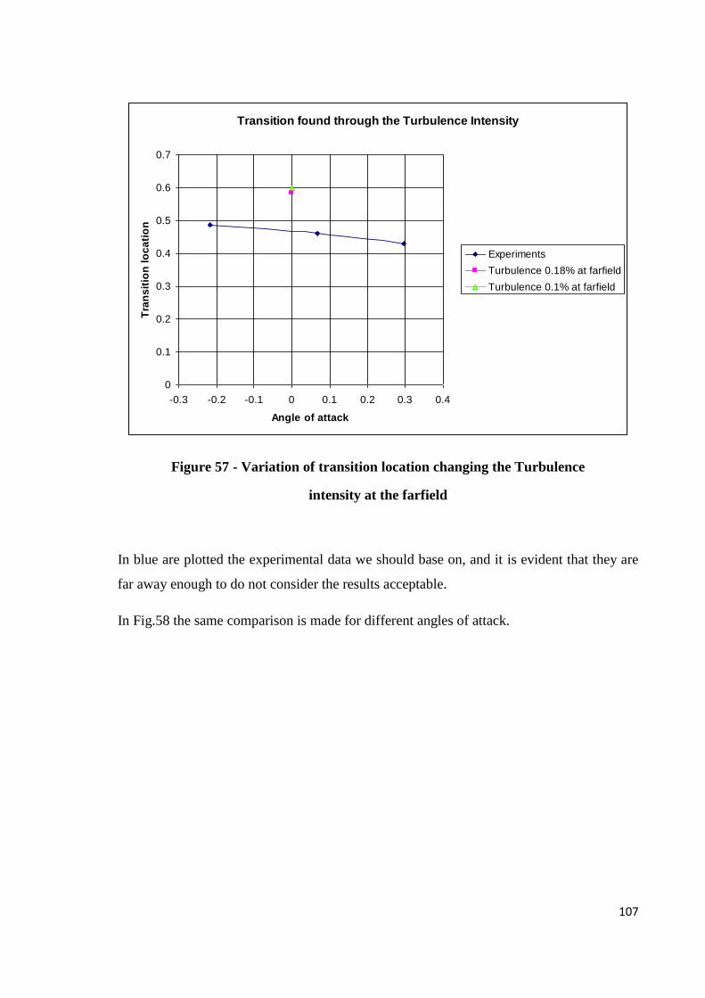
107

Figure 57 - Variation of transition location changing the Turbulence

intensity at the farfield

In blue are plotted the experimental data we should base on, and it is evident that they are

far away enough to do not consider the results acceptable.

In Fig.58 the same comparison is made for different angles of attack.

Transition found through the Turbulence Intensity

0

0.1

0.2

0.3

0.4

0.5

0.6

0.7

-0.3 -0.2 -0.1 0 0.1 0.2 0.3 0.4

Angle of attack

Tra

ns

itio

n l

oc

ati

on

Experiments

Turbulence 0.18% at farfield

Turbulence 0.1% at farfield

108

Figure 58 - SST –Transition calculation for NACA0012 compared

with experiments

To obtain the transition curve computed with Fluent we have extracted the points where

the skin friction coefficient underwent an abrupt change.

In conclusion we can say that there is a good agreement between the N-factor curve and

the experiments in the article. For the Fluent SST-Transition model the estimation of the

transition location is very far compared to the experimental one. It is true that the model

does not take into account the instabilities internal to the boundary layer but only the

pressure gradient. We can suppose then that it corresponds to the separation of the

boundary layer. In fact the curve obtained with bl3D code shows us that the separation

occurs near the curve obtained with Fluent SST-Transition model. This is valid for low

angles of attack. For high values of the angle of attack, the SST-Transition curve

approaches the experiments, but this is because the flow has a disordered configuration

around the profile and consequently the transition and the separation occur in a very

restricted space. It is also easy to notice that the Nolot calculations stop at angle of attack

because at this angle the separation of the boundary layer occurs before the transition.

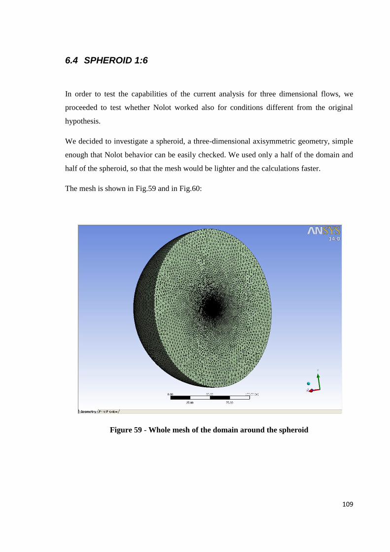
109

6.4 SPHEROID 1:6

In order to test the capabilities of the current analysis for three dimensional flows, we

proceeded to test whether Nolot worked also for conditions different from the original

hypothesis.

We decided to investigate a spheroid, a three-dimensional axisymmetric geometry, simple

enough that Nolot behavior can be easily checked. We used only a half of the domain and

half of the spheroid, so that the mesh would be lighter and the calculations faster.

The mesh is shown in Fig.59 and in Fig.60:

Figure 59 - Whole mesh of the domain around the spheroid

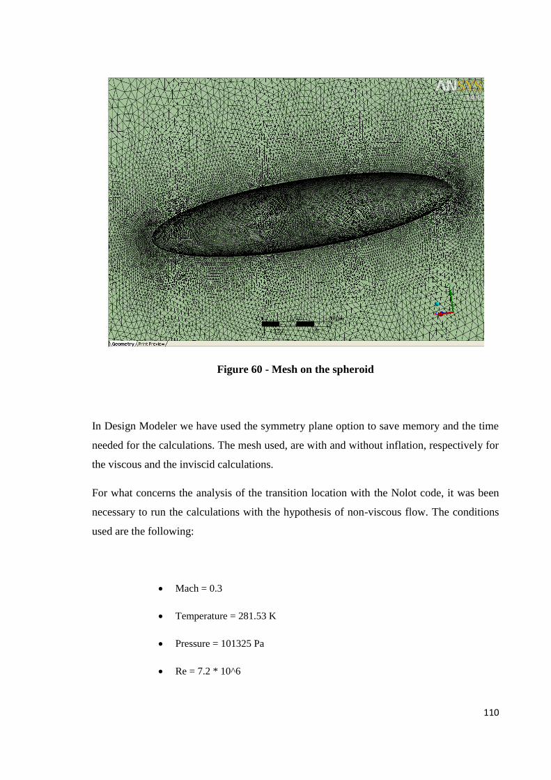
110

Figure 60 - Mesh on the spheroid

In Design Modeler we have used the symmetry plane option to save memory and the time

needed for the calculations. The mesh used, are with and without inflation, respectively for

the viscous and the inviscid calculations.

For what concerns the analysis of the transition location with the Nolot code, it was been

necessary to run the calculations with the hypothesis of non-viscous flow. The conditions

used are the following:

Mach = 0.3

Temperature = 281.53 K

Pressure = 101325 Pa

Re = 7.2 * 10^6

111

Air density set constant

Mesh setup: velocity inlet on the outlet bords, symmetry on the symmetry

plane (wall-solid) and wall on the spheroid

Boundary conditions: velocity inlet on the outlet bords

Calculation repeated for 0, 5 and 10 angles of attack

The mesh with the inflation has 9.848.487 cells and it needs a number of iterations equal to

1900. For the inviscid calculation, the mesh does not need the inflation, so we used

5.124.919 cells and 1100 iterations.

The Cp distribution on the symmetry plane of the spheroid for AoA=0°, is shown in

Fig.61:

Figure 61 - Mesh on the symmmetry plane of the spheroid for AoA = 0°

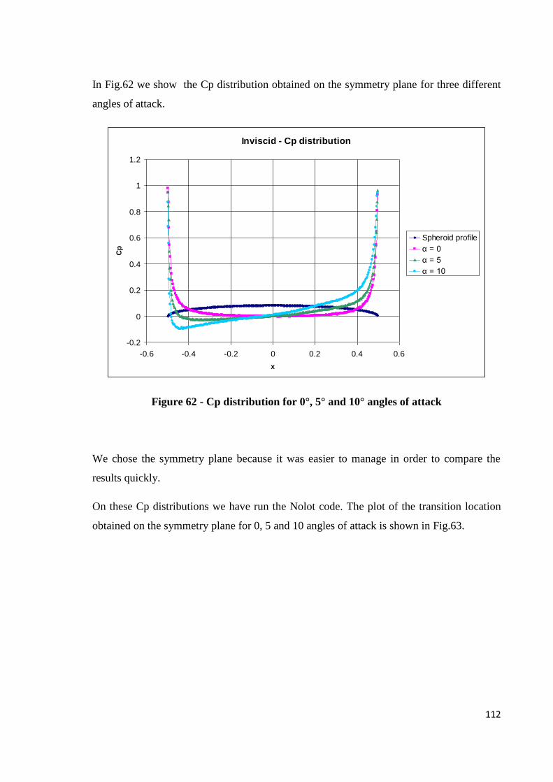
112

In Fig.62 we show the Cp distribution obtained on the symmetry plane for three different

angles of attack.

Figure 62 - Cp distribution for 0°, 5° and 10° angles of attack

We chose the symmetry plane because it was easier to manage in order to compare the

results quickly.

On these Cp distributions we have run the Nolot code. The plot of the transition location

obtained on the symmetry plane for 0, 5 and 10 angles of attack is shown in Fig.63.

Inviscid - Cp distribution

-0.2

0

0.2

0.4

0.6

0.8

1

1.2

-0.6 -0.4 -0.2 0 0.2 0.4 0.6

x

Cp

Spheroid profile

α = 0

α = 5

α = 10

113

Figure 63 - Transition locations of the sheroid for AoA=0°, 5° and 10°

In the experiments by the “Transitions Prediction for 2D and 3D Flows using the TAU-

Code and N-Factor Methods” article, the N-factors used are N=5, N=7.2; for this reason,

we took Nolot results referring to these values.

The results seem to match up only for zero angle of attack. This is probably due to the 3D

effects. In fact when the AoA=0, the flow over the spheroid has an axisymmetric shape.

This does not happen when the angle of attack is different from zero, since the flow

follows different paths along the spheroid.

The Nolot code that studies the properties of a 2D flow, almost is written for an infinite

wing with constant section. This does noy allow us to study flows where there is a

crossflow component in.

Spheroid - Ma = 0.3 - Re = 7200000

0

0.1

0.2

0.3

0.4

0.5

0.6

0.7

0 2 4 6 8 10

AoA

X/C

- T

ran

sit

ion

N=7.2

N=5

Article N=7.2

Article N=5

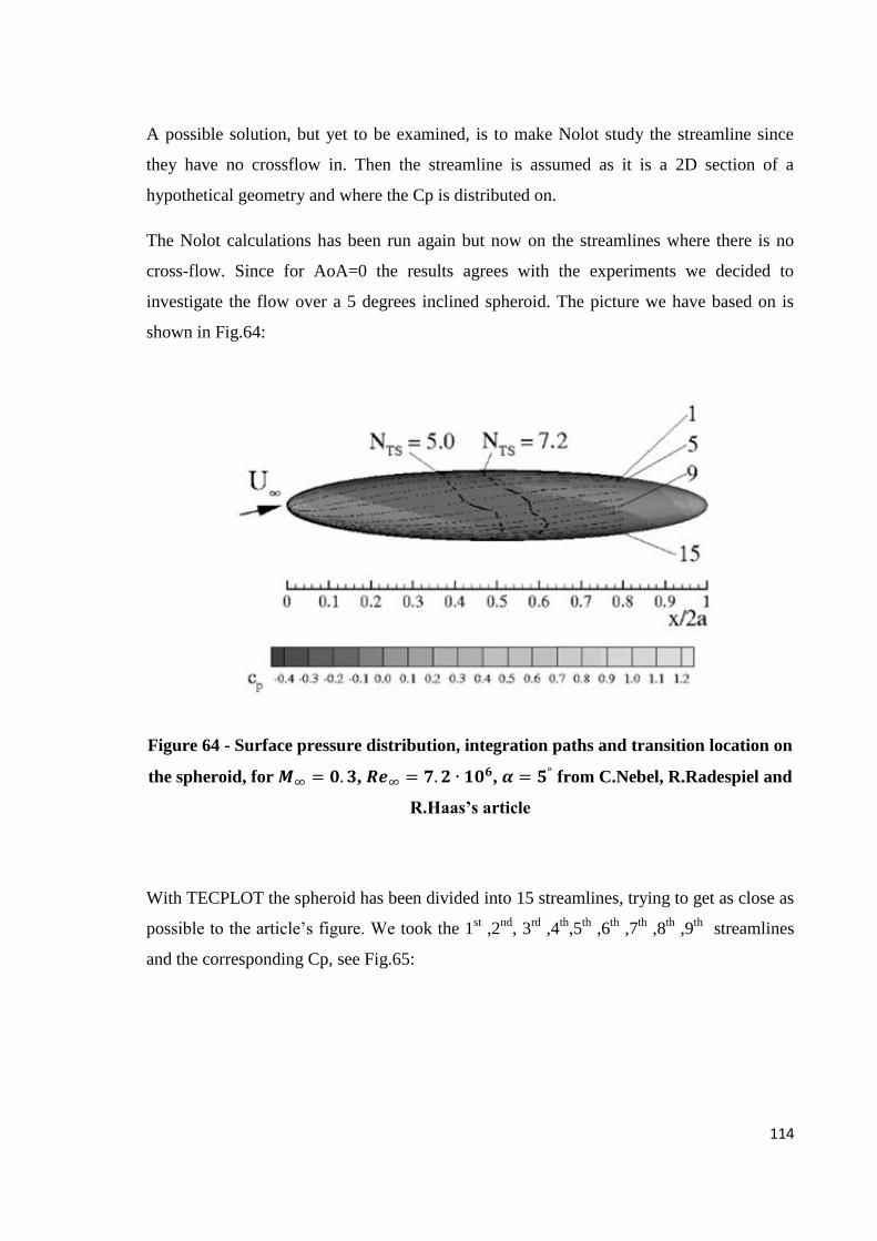
114

A possible solution, but yet to be examined, is to make Nolot study the streamline since

they have no crossflow in. Then the streamline is assumed as it is a 2D section of a

hypothetical geometry and where the Cp is distributed on.

The Nolot calculations has been run again but now on the streamlines where there is no

cross-flow. Since for AoA=0 the results agrees with the experiments we decided to

investigate the flow over a 5 degrees inclined spheroid. The picture we have based on is

shown in Fig.64:

Figure 64 - Surface pressure distribution, integration paths and transition location on

the spheroid, for , , from C.Nebel, R.Radespiel and

R.Haas’s article

With TECPLOT the spheroid has been divided into 15 streamlines, trying to get as close as

possible to the article’s figure. We took the 1st ,2

nd, 3

rd ,4

th,5

th ,6

th ,7

th ,8

th ,9

th streamlines

and the corresponding Cp, see Fig.65:

115

Figure 65 - The fifteen streamlines on the spheroid (inviscid calculation)

Since the Cp distribution is along a curved line the old coordinates have to be changed. In

the geo.dat_1001 file, the first and the second columns which refers to the x and y

coordinates of the geometry profile have been replaced by the real length of the streamline

(the s coordinate) and the local radius of the streamline (from the symmetry axis) for every

x point. In this way we no longer consider the geometry as the elliptic section of the

spheroid but as the streamline shape.

After running Nolot and finding the transition location, it has been written in the previous

coordinates, the spheroid axis.

The results are shown in Fig.66:

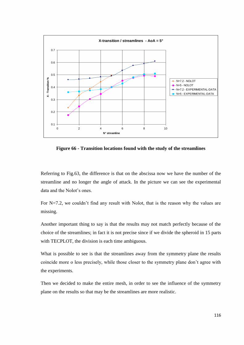
116

Figure 66 - Transition locations found with the study of the streamlines

Referring to Fig.63, the difference is that on the abscissa now we have the number of the

streamline and no longer the angle of attack. In the picture we can see the experimental

data and the Nolot’s ones.

For N=7.2, we couldn’t find any result with Nolot, that is the reason why the values are

missing.

Another important thing to say is that the results may not match perfectly because of the

choice of the streamlines; in fact it is not precise since if we divide the spheroid in 15 parts

with TECPLOT, the division is each time ambiguous.

What is possible to see is that the streamlines away from the symmetry plane the results

coincide more o less precisely, while those closer to the symmetry plane don’t agree with

the experiments.

Then we decided to make the entire mesh, in order to see the influence of the symmetry

plane on the results so that may be the streamlines are more realistic.

X-transition / streamlines - AoA = 5°

0.1

0.2

0.3

0.4

0.5

0.6

0.7

0 2 4 6 8 10

N° streamline

X -

Tra

nsit

ion

%

N=7.2 - NOLOT

N=5 - NOLOT

N=7.2 - EXPERIMENTAL-DATA

N=5 - EXPERIMENTAL-DATA

117

In parallel a mesh with the inflation has been done for the viscous case. This can be seen in

Fig.67.

Figure 67 - Inflation on the spheroid where the boundary layer is supposed to be

In Fig.68 is shown the trend of the pressure coefficient on the spheroid for the SST-

transition model.

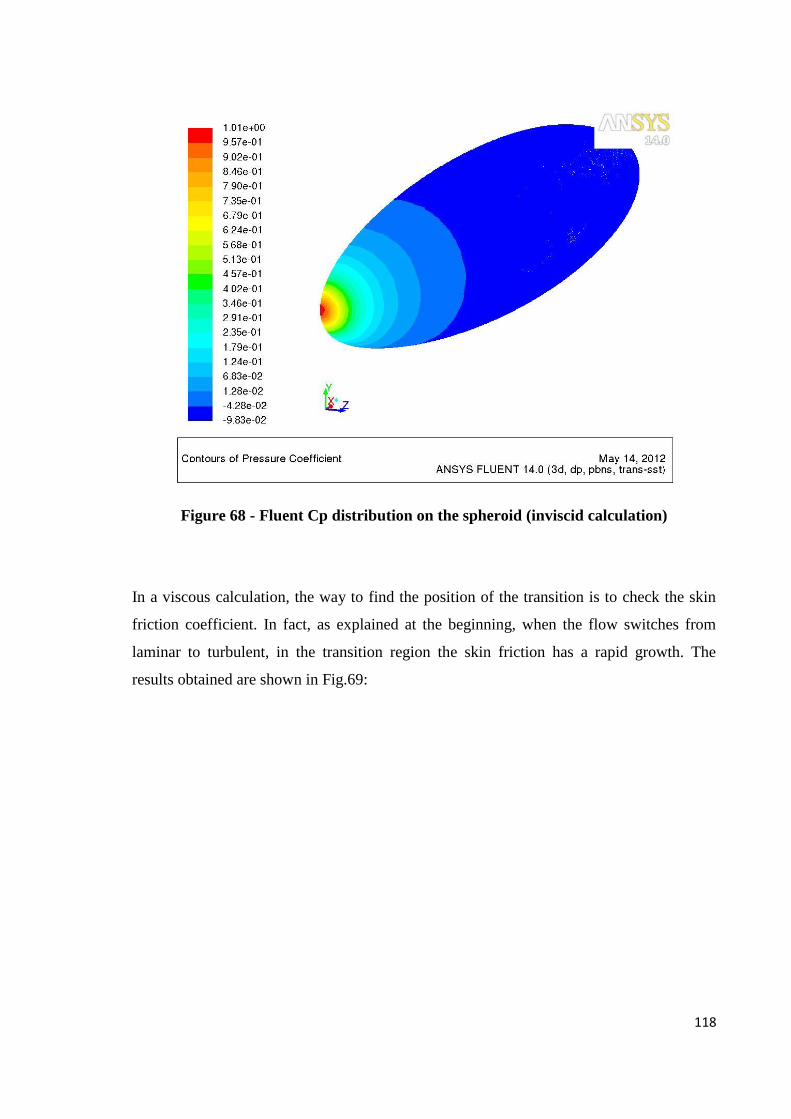
118

Figure 68 - Fluent Cp distribution on the spheroid (inviscid calculation)

In a viscous calculation, the way to find the position of the transition is to check the skin

friction coefficient. In fact, as explained at the beginning, when the flow switches from

laminar to turbulent, in the transition region the skin friction has a rapid growth. The

results obtained are shown in Fig.69:

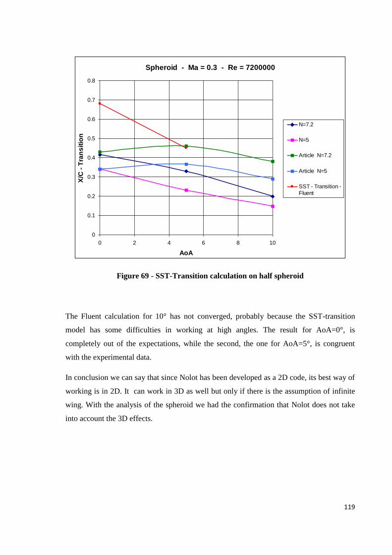
119

Figure 69 - SST-Transition calculation on half spheroid

The Fluent calculation for 10° has not converged, probably because the SST-transition

model has some difficulties in working at high angles. The result for AoA=0°, is

completely out of the expectations, while the second, the one for AoA=5°, is congruent

with the experimental data.

In conclusion we can say that since Nolot has been developed as a 2D code, its best way of

working is in 2D. It can work in 3D as well but only if there is the assumption of infinite

wing. With the analysis of the spheroid we had the confirmation that Nolot does not take

into account the 3D effects.

Spheroid - Ma = 0.3 - Re = 7200000

0

0.1

0.2

0.3

0.4

0.5

0.6

0.7

0.8

0 2 4 6 8 10

AoA

X/C

- T

ran

sit

ion

N=7.2

N=5

Article N=7.2

Article N=5

SST - Transition -

Fluent

120

7 CONCLUSIONS AND FUTURE WORK

A new methodology developed for searching the transition locations on a wing profile

has been created. The validation was successful for two dimensional profiles, as

NACA0012. For the NLF0416 profile we cannot be sure of the results since the

literature provide us only the boundary layer separation. The validation for the three

dimensional geometries is more complicated because we need to take into account the

3D effects. They can be avoided by applying the same methodology but along the

streamlines, since as the theory says, they are instantaneously tangent to the velocity

vector of the flow. For the moment Nolot code works only on simple geometries like a

spheroid (axisymmetric).

An interesting objective one wants to reach is manage the entire methodology with the

aim to make it faster and more efficient, accelerating the various processes with

dedicated programs. At the same time it is important to improve the Fluent calculations

(mesh, journal file, etc.) to get more accurate results. In fact, since the Nolot study

depends on the Fluent results, if we do not have good ones it is completely useless to

post process the data.

Another interesting continuation is to make a study of the entire spheroid to see how

much the symmetry plane influences the flow close to it.

Improving the Nolot code in order to use it along the streamlines is an attractive

objective since it allows to extend the methodology from two dimensional to three

121

dimensional geometries. Anyway it needs to be treated with caution and to be tested for

several geometry configurations, with the aim to make it applicable for the different

parts of the airplane.

122

Acknowledgements

I wish to thank all those who helped me in the realization of my thesis. I first thank

Professor Jan Pralits, who has always supported and advised me with infinite patience and

dedication, Eng. Christophe Favre, who taught me so much in only 6 months, devoting me

time and explanations, and Professor Alessandro Bottaro, who made this project possible

and for his special ability to transmit enthusiasm to students: without their support and

their wise guidance this thesis would not exist.

A special thank goes to my classmates with whom I studied and learned, Dany, Mattè,

Roby, Tibo and Teo. I would like to dedicate this work also to friends who have

encouraged and supported me during these years of studies (especially at the end), Iole

with your constant presence and your countless attentions, and Marta for your

encouragement from afar.

I would also like to thank the nearest and dearest people to me: my parents for moral and

economic support, and finally Bj for your love, patience and understanding.

123

Bibliography

[1] Y. A. Çengel, J. M. Cimbala, “Fluid Mechanics,”. Ed. New York: McGraw-Hill, 2006.

[2] P.J. Schimd, D. S. Henningson, “Stability and Transition in Shear Flows”. Ed: New

York, Springer-Verlag, 2001.

[3] Dr. Hermann Schlichting, “Boundary-Layer Theory”, Ed. McGraw-Hill, 1979.

[4] J. D. Anderson, “Fundamentals of Aerodynamics”. Ed: Singapore: McGraw-Hill, 2007.

[5] D. Tempelmann, “Receptivity of crossflow-dominated boundary layers”. Doctoral

Thesis in Mechanics, Ed. Stockholm, Sweden: KTH, 2011.

[6] D. Arnal, “Transition Prediction in Industrial Applications”, ONERA CERT DMAE,

Toulouse Cedex, France.

[7] H. L. Reed and W. Saric, “CFD Validation Issues for Boundary-Layer Stability and

Transition”, Mechanical and Aerospace Engineering, Arizona State University, 2003.

[8] C. Nebel, R. Radespiel, R. Haas, ”Transition Prediction for 2D and 3D Flows using the

TAU-Code and N-Factor Methods”. Braunschweig Technical University, Germany.

[9] J. Perraud, D. Arnal, G. Casalis, J-P. Archambaud, ONERA, Toulouse, France, and R.

Donelli, CIRA – Italian Aerospace Research Center, Capua, Italy, “Automatic Transition

predictions using Simplified Methods”.

[10] F.P. Bertolotti, Th Herbert and P.R Spalart, “Linear and nonlinear stability if the

Blasius boundary layer”, Great Britain, 1990

[11] “Boundary-Layer Transition Results From the F-16XL-2 Supersonic Laminar Flow

Control Experiment”, National Aeronautics and Space Administration, Edwards,

California,1999.

[12] R.E. Spall, M.R. Malik, “Linear Stability Theory And Three-Dimensional Boundary

Layer Transition”, High Technology Corporation Hampton, VA

[13] William S. Saric1, Helen L. Reed1, and Edward J. Kerschen, “BOUNDARY-LAYER

RECEPTIVITY TO FREESTREAM DISTURBANCES”, Arizona State University,

Tempe, Arizona, 2002.

[14] William S. Saric1, Helen L. Reed1, and Edward B.White, “STABILITY AND

TRANSITION OF THREE-DIMENSIONAL BOUNDARY LAYERS”, Arizona State

University, Tempe, Arizona 2003.

124

[15] Thorwald Herbert, “PARABOLIZED STABILITY EQUATIONS”, The Ohio State

University, Columbus, Ohio, 1997.

[15] Th. Lutz and S. Wagner, “NUMERICAL SHAPE OPTIMIZATION OF NATURAL

LAMINAR FLOW BODIES”, Institute of Aerodynamics and Gasdynamics, University of

Stuttgart, Germany.

[16] J.L. van Ingen, “The eN method for transition prediction. Historical review of work at

TU Delft”, Faculty of Aerospace Engineering, TU Delft, the Netherland, 2008.

[17] Th. Lutz, S. Wagnery “DRAG REDUCTION AND SHAPE OPTIMIZATION OF

AIRSHIP BODIES, Institute for Aerodynamics and Gas Dynamics, University of Stuttgart,

Germany.

[18] Paul-Dan Silisteanu and Ruxandra M. Botez, “Transition-Flow-Occurrence-

Estimation: A New Method”, March 2010.

[19] N. Gregory and C. L. O'Reilly “Low-Speed Aerodynamic Characteristics of NACA

0012 Aerofoil Section, including the Effects of Upper-Surface Roughness Simulating Hoar

Frost, January, 1970”

[19] C.Nebel, R.Radespiel and R.Haas “Transition Predictionfor 2D and 3D Flows using

the TAU-Code and N-Factor Methods”, Institute of Fluid Mechanics, Braunschweig,

Germany, 2005

125

Figures Index

Figure 1 - Boundary layer along a flat plate: laminarity, transition and turbulence.......................... 9

Figure 2 - Skin friction coefficient trend and representation of the evolution of boundary layer

flow over a flat plate ........................................................................................................................ 11

Figure 3 - Representation of various kinds of disturbances............................................................. 12

Figure 4 - Tollmien-Schlichting waves. Transitional flow along a flat plate without longitudinal

pressure gradient. ............................................................................................................................ 13

Figure 5 - Cross-flow waves in swept-wing boundary layers ........................................................... 14

Figure 6 - Principle of the method ............................................................................................. 16

Figure 7- Stability curve and corresponding .................................................................................... 18

Figure 8 - Stability F-Re diagram for Blasius boundary layer. The perturbations are amplified inside

the red curve, leading the flow to instability. .................................................................................. 19

Figure 9 - Geometry of the test case profile .................................................................................... 20

Figure 10 - Cp distribution on the test case profile ......................................................................... 20

Figure 11 - Velocity distribution on the test case profile ................................................................. 21

Figure 12 - Wave angle of the perturbations ................................................................................... 22

Figure 13 - Growth rate of the instabilities ...................................................................................... 23

Figure 14 - Rate of amplification of the instabilities (TS and CF waves) ......................................... 23

Figure 15 - Division of flow regions into an inviscid and a viscous .................................................. 25

Figure 16 - Development of the boundary layer along a flat plate .................................................. 28

Figure 17 - Evolution of disturbances in shear flows. Temporal evolution of a global periodic

disturbance ...................................................................................................................................... 39

Figure 18 - Evolution of disturbances in shear flows. Spatial evolution of a disturbance created by

an oscillatory source ........................................................................................................................ 39

Figure 19 - Poiseuille developed flow .............................................................................................. 42

Figure 20 - Orr–Sommerfeld spectrum for plane Poiseuille flow for............................................... 44

126

Figure 21 - Orr- Sommerfeld v-eigenfuction for plane Poiseuille flow. The P-branch is represented,

with Re=5000, α=1 and β=1. ............................................................................................................ 45

Figure 22 - Orr- Sommerfeld η -eigenfuction for plane Poiseuille flow. The P-branch is

represented, with Re=5000, α=1 and β=1. ...................................................................................... 46

Figure 23 - Imaginary part of frequency as function of α varying with β ........................................ 47

Figure 24 - Real part of frequency as function of Re number for two-dimensional flow (β=0 and

α=1 ................................................................................................................................................... 48

Figure 25 - Orr-Sommerfeld spectrum for Blasius boundary layer flow .......................................... 50

Figure 26-– Eigenfunctions of the discrete spectrum for Blasius boundary layer flow. Streamwise

perturbation velocity (u), with Re=1000, α=0.3 and β=0................................................................. 51

Figure 27 - Eigenfunctions of the discrete spectrum for Blasius boundary layer flow. Vertical

perturbation velocity (v), with Re=1000, α=0.3 and β=0. ................................................................ 52

Figure 28 - u,v-perturbation velocity and p-perturbation pressure for Blasius boundary layer ..... 53

Figure 29 - Neutral curve for Blasius boundary layer flow in temporal analysis. Contours of

constant growth rate .................................................................................................................. 54

Figure 30 - Neutral curve for Blasius boundary layer flow in spatial analysis. Contours of constant

growth rate ................................................................................................................................. 62

Figure 31 - Neutral curves as function of the spanwise wave number β ........................................ 63

Figure 32 - Wing profile text file for Design Modeler ...................................................................... 68

Figure 33 - Ansys window of a new project ..................................................................................... 69

Figure 34 - Design Modeler window (farfield and profile) ............................................................... 70

Figure 35 - Trailing edge of the wing ................................................................................................ 71

Figure 36 - Workbench mesh on the NACA0012 profile .................................................................. 72

Figure 37 - Mesh without inflation for inviscid calculation ............................................................. 73

Figure 38 - Mesh with inflation for viscous calculation .................................................................. 74

Figure 39 - Python code made for transforming Fluent files to input file for Nolot ........................ 86

Figure 40 - Input file for autoinit to find the unstable modes ......................................................... 89

Figure 41 - Python code crated to find automatically the transition location from the amplification

curve ................................................................................................................................................. 92

Figure 42 - NLF0416 geometry profile ............................................................................................. 94

127

Figure 43 - Article’s figure plotting the transition locations ............................................................ 95

Figure 44 - Mesh without inflation of the NLF0416 profile ............................................................. 95

Figure 45 - Cp distribution on the NLF0416 profile. ......................................................................... 96

Figure 46 - Transition and separation location found with Nolot for NLF0416 ............................... 97

Figure 47 - NACA0012 geometry profile .......................................................................................... 98

Figure 48 - Mesh with inflation of NACA0012 profile ...................................................................... 99

Figure 49 - NACA0012 inviscid calculation at AoA = 0° .................................................................... 99

Figure 50 - NACA0012 inviscid calculation at AoA = 4° .................................................................. 100

Figure 51 - NACA0012 wrong inviscid calculation at AoA = 2° ....................................................... 101

Figure 52 - Nolot and experiments transition locations for NACA0012 ........................................ 102

Figure 53 - Gregory O’Reilly graphic of transition location ............................................................ 103

Figure 54 - Amplification rate for NACA0012 with AoA = 0° .......................................................... 104

Figure 55 - Decay of turbulence intensity with the distance ......................................................... 105

Figure 56 - Cf according to two different level of tubulence ......................................................... 106

Figure 57 - Variation of transition location changing the Turbulence ........................................... 107

Figure 58 - SST –Transition calculation for NACA0012 compared ................................................. 108

Figure 59 - Whole mesh of the domain around the spheroid ....................................................... 109

Figure 60 - Mesh on the spheroid .................................................................................................. 110

Figure 61 - Mesh on the symmmetry plane of the spheroid for AoA = 0° ..................................... 111

Figure 62 - Cp distribution for 0°, 5° and 10° angles of attack ....................................................... 112

Figure 63 - Transition locations of the sheroid for AoA=0°, 5° and 10° ......................................... 113

Figure 64 - Surface pressure distribution, integration paths and transition location on the

spheroid, for , , from C.Nebel, R.Radespiel and R.Haas’s

article ............................................................................................................................................. 114

Figure 65 - The fifteen streamlines on the spheroid (inviscid calculation) .................................... 115

Figure 66 - Transition locations found with the study of the streamlines ..................................... 116

Figure 67 - Inflation on the spheroid where the boundary layer is supposed to be ..................... 117

128

Figure 68 - Fluent Cp distribution on the spheroid (inviscid calculation) ...................................... 118

Figure 69 - SST-Transition calculation on half spheroid ................................................................. 119