Development of a Series Elastic Actuator and a DistributedComputational Platform for Robotics

Gonçalo Patrício Luís

Thesis to obtain the Master of Science Degree in

Mechanical Engineering

Supervisor: Prof. Jorge Manuel Mateus Martins

Examination Committee

Chairperson: Prof. João Rogério Caldas PintoSupervisor: Prof. Jorge Manuel Mateus Martins

Member of the Committee: Prof. Carlos Baptista Cardeira

November 2015

i

ii

To my Parents

iii

iv

Acknowledgments

I would like to thank Professor Jorge Martins for believing in my ideas on building a new computational

platform from scratch in detriment of using the old platform. The first task he gave me was to play

arround with the old platform until I felt confortable with it, not all teachers believe in loosing time on

learning things that are supposed to work and should only be used instead of studied. In the end the

freedom he gave me turned into finding gross mistakes in the old platform and ultimately building a new,

more capable one.

I would like to thank Professor Carlos Cardeira for clearing some questions I had about electronics

regarding the circuit board for voltage conversion.

I would also like to thank Professor Paulo Oliveira and Professor Alexandra Moutinho for showing me

the power and beauty of control systems engineering in the lecture I had with them on that topic. Their

practical and clear explanations ultimately made me choose Systems as my Masters area, a choice I

couldn’t be happier about.

I am also deeply grateful to all the other teachers on the systems department and Eng. Camilo for

creating and maintaining a friendly environment during classes and at the laboratory.

I want to thank Sara, for being the best part of my life since we’ve met. Thank you also for being an

always available helping hand, without Sara’s support this project would have been very different.

Last but not least, I want to thank my parents for supporting me in this challenge during the last

years, which is also the biggest investment in my professional and moral education I will have.

Thank You.

v

vi

Resumo

A robotica e uma area extremamente transversal quanto as areas que envolve. Desde a electronica ate

ao controlo e a inteligencia artificial, passando pela mecanica, a robotica e o culminar do melhor que

ha nestas areas. O projecto em que esta tese se insere tem como objectivo explorar e implementar

algoritmos de controlo avancados para controlo de robos bipede, seja para andar, correr, saltar, ou

qualquer outra tarefa, nao so em simulacoes computacionais mas tambem num pequeno robo real.

Esta tese desenvolve a plataforma computacional onde o sistema de controlo sera implementado. A

plataforma desenvolvida usa tecnicas de programacao paralela e distribuida para alcancar a melhor

performance e assim dar mais possibilidades a quem implementar os algoritmos de controlo. Nesta

tese tambem e desenvolvido um actuator elastico em serie para actuacao em forca, baseado num

servo AX-12 Dynamixel da Robotis.

Palavras-chave: Actuador elastico em serie, controlo de forca, plataforma computacional

para robotica, controlo distribuido

vii

viii

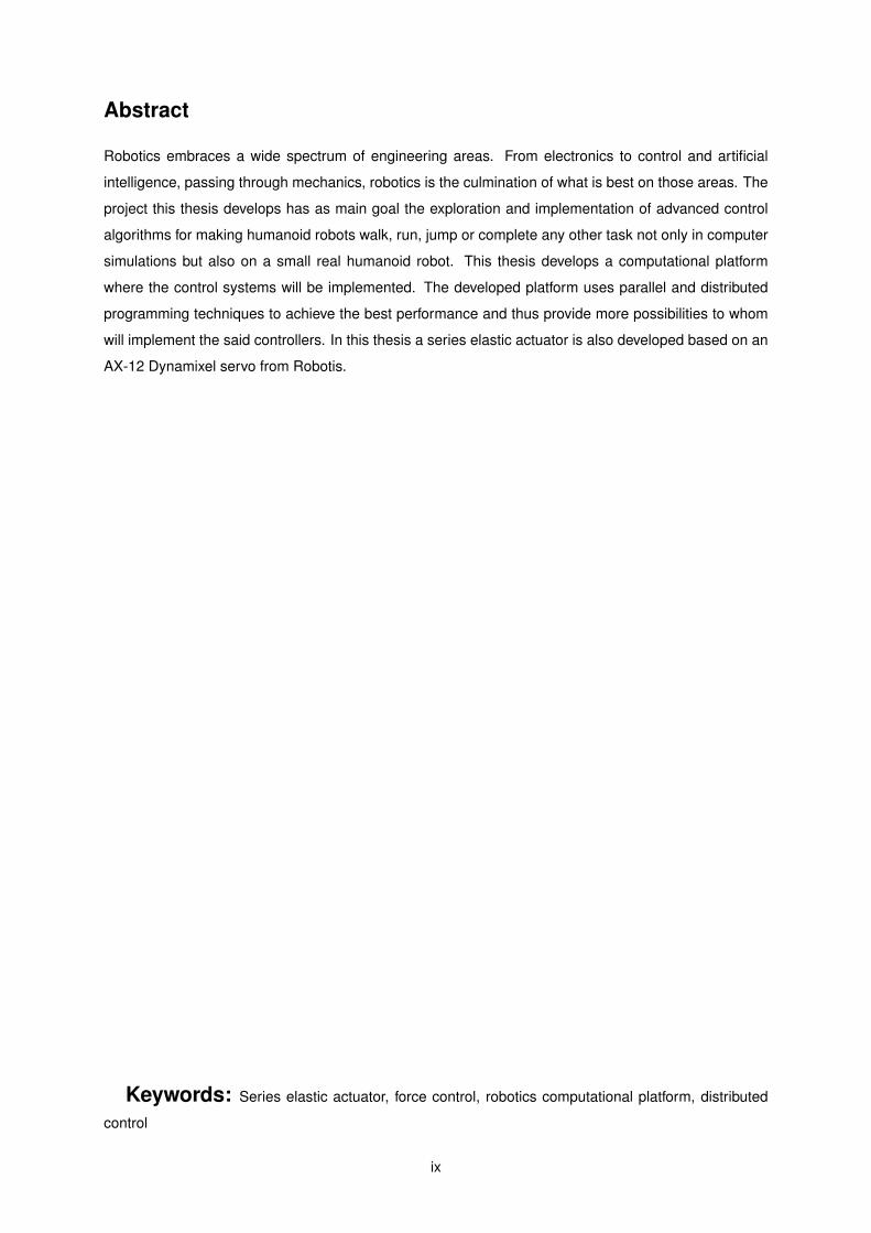
Abstract

Robotics embraces a wide spectrum of engineering areas. From electronics to control and artificial

intelligence, passing through mechanics, robotics is the culmination of what is best on those areas. The

project this thesis develops has as main goal the exploration and implementation of advanced control

algorithms for making humanoid robots walk, run, jump or complete any other task not only in computer

simulations but also on a small real humanoid robot. This thesis develops a computational platform

where the control systems will be implemented. The developed platform uses parallel and distributed

programming techniques to achieve the best performance and thus provide more possibilities to whom

will implement the said controllers. In this thesis a series elastic actuator is also developed based on an

AX-12 Dynamixel servo from Robotis.

Keywords: Series elastic actuator, force control, robotics computational platform, distributed

control

ix

x

Contents

Acknowledgments . . . . . . . . . . . . . . . . . . . . . . . . . . . . . . . . . . . . . . . . . . . v

Resumo . . . . . . . . . . . . . . . . . . . . . . . . . . . . . . . . . . . . . . . . . . . . . . . . . vii

Abstract . . . . . . . . . . . . . . . . . . . . . . . . . . . . . . . . . . . . . . . . . . . . . . . . . ix

List of Tables . . . . . . . . . . . . . . . . . . . . . . . . . . . . . . . . . . . . . . . . . . . . . . xiii

List of Figures . . . . . . . . . . . . . . . . . . . . . . . . . . . . . . . . . . . . . . . . . . . . . xvi

Nomenclature . . . . . . . . . . . . . . . . . . . . . . . . . . . . . . . . . . . . . . . . . . . . . . 1

Glossary . . . . . . . . . . . . . . . . . . . . . . . . . . . . . . . . . . . . . . . . . . . . . . . . 1

1 Introduction 1

1.1 Motivation . . . . . . . . . . . . . . . . . . . . . . . . . . . . . . . . . . . . . . . . . . . . . 1

1.2 State-of-the-art . . . . . . . . . . . . . . . . . . . . . . . . . . . . . . . . . . . . . . . . . . 2

1.3 Robot Platform . . . . . . . . . . . . . . . . . . . . . . . . . . . . . . . . . . . . . . . . . . 2

1.4 Outline of this thesis . . . . . . . . . . . . . . . . . . . . . . . . . . . . . . . . . . . . . . . 3

2 Previous Hardware and Low Level Software 5

2.1 Hardware . . . . . . . . . . . . . . . . . . . . . . . . . . . . . . . . . . . . . . . . . . . . . 5

2.1.1 Problems with the old platform . . . . . . . . . . . . . . . . . . . . . . . . . . . . . 5

2.1.2 New platform for High Level Control . . . . . . . . . . . . . . . . . . . . . . . . . . 7

2.1.3 Actuator Hardware . . . . . . . . . . . . . . . . . . . . . . . . . . . . . . . . . . . . 9

2.1.4 Communication Between the Odroid and the AX-12’s . . . . . . . . . . . . . . . . 13

2.2 Software . . . . . . . . . . . . . . . . . . . . . . . . . . . . . . . . . . . . . . . . . . . . . . 15

2.2.1 Problems with the old software . . . . . . . . . . . . . . . . . . . . . . . . . . . . . 15

2.2.2 Linux UART Driver . . . . . . . . . . . . . . . . . . . . . . . . . . . . . . . . . . . . 19

2.2.3 Pipelined Distributed High Level Controller Software . . . . . . . . . . . . . . . . . 19

2.2.4 Low Level Actuator Software . . . . . . . . . . . . . . . . . . . . . . . . . . . . . . 23

2.2.5 System Timer . . . . . . . . . . . . . . . . . . . . . . . . . . . . . . . . . . . . . . . 24

3 Force Actuator 28

3.1 Introduction to Force Control . . . . . . . . . . . . . . . . . . . . . . . . . . . . . . . . . . 28

3.1.1 Adding Compliance . . . . . . . . . . . . . . . . . . . . . . . . . . . . . . . . . . . 30

3.2 Series Elastic Actuators . . . . . . . . . . . . . . . . . . . . . . . . . . . . . . . . . . . . . 31

3.2.1 Introduction . . . . . . . . . . . . . . . . . . . . . . . . . . . . . . . . . . . . . . . . 31

xi

3.2.2 Open Loop Model . . . . . . . . . . . . . . . . . . . . . . . . . . . . . . . . . . . . 32

3.2.3 Motor and Gearbox Mathematical Model . . . . . . . . . . . . . . . . . . . . . . . . 33

3.2.4 Closed Loop: Constrained Position . . . . . . . . . . . . . . . . . . . . . . . . . . . 34

3.2.5 Closed Loop: Inertial Load . . . . . . . . . . . . . . . . . . . . . . . . . . . . . . . 38

3.2.6 Analysis with the real motor & hardware . . . . . . . . . . . . . . . . . . . . . . . . 39

3.2.7 Digital control system . . . . . . . . . . . . . . . . . . . . . . . . . . . . . . . . . . 46

3.2.8 Conclusions . . . . . . . . . . . . . . . . . . . . . . . . . . . . . . . . . . . . . . . . 46

3.3 Servo Platform . . . . . . . . . . . . . . . . . . . . . . . . . . . . . . . . . . . . . . . . . . 47

4 Conclusions 55

4.1 Future Work . . . . . . . . . . . . . . . . . . . . . . . . . . . . . . . . . . . . . . . . . . . . 55

Bibliography 58

A Work done on the previous platform 59

B Technical Drawing of the new shaft 60

xii

List of Tables

2.1 Comparison of the top 10 boards on the Linux.com and LinuxGizmos.com survey . . . . . 9

2.2 ATMega8(A) Specifications . . . . . . . . . . . . . . . . . . . . . . . . . . . . . . . . . . . 10

xiii

xiv

List of Figures

1.1 Robotis Bioloid . . . . . . . . . . . . . . . . . . . . . . . . . . . . . . . . . . . . . . . . . . 3

2.1 Previous robot infrastructure . . . . . . . . . . . . . . . . . . . . . . . . . . . . . . . . . . . 7

2.2 The top 10 Linux and Android SBCs in 2015, according to a Linux.com and LinuxGiz-

mos.com reader survey . . . . . . . . . . . . . . . . . . . . . . . . . . . . . . . . . . . . . 8

2.3 Odroid U3 and its Wi-fi dongle . . . . . . . . . . . . . . . . . . . . . . . . . . . . . . . . . 9

2.4 The Murata SV01A103 potentiometer used on the AX-12 Dynamixel servos . . . . . . . . 10

2.5 Controller schematic of the AX-12 Dynamixel servos . . . . . . . . . . . . . . . . . . . . . 12

2.6 Quad-buffer/line driver functional diagram . . . . . . . . . . . . . . . . . . . . . . . . . . . 13

2.7 Real IC wiring diagram . . . . . . . . . . . . . . . . . . . . . . . . . . . . . . . . . . . . . . 14

2.8 Voltage converter wiring diagram . . . . . . . . . . . . . . . . . . . . . . . . . . . . . . . . 14

2.9 Sparkfun bi-directional logic level converter . . . . . . . . . . . . . . . . . . . . . . . . . . 14

2.10 Quad-buffer/line driver and voltage level converter for the Odroid . . . . . . . . . . . . . . 15

2.11 Communication flow . . . . . . . . . . . . . . . . . . . . . . . . . . . . . . . . . . . . . . . 16

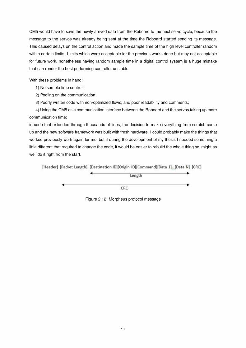
2.12 Morpheus protocol message . . . . . . . . . . . . . . . . . . . . . . . . . . . . . . . . . . 17

2.13 Control function of the morpheus firmware . . . . . . . . . . . . . . . . . . . . . . . . . . . 18

2.14 Odroid CPUs and communication ports . . . . . . . . . . . . . . . . . . . . . . . . . . . . 21

2.15 ATMega communication ports . . . . . . . . . . . . . . . . . . . . . . . . . . . . . . . . . . 21

2.16 High level controller scheduling . . . . . . . . . . . . . . . . . . . . . . . . . . . . . . . . . 23

2.17 Read and send processes overlap . . . . . . . . . . . . . . . . . . . . . . . . . . . . . . . 23

2.18 High level controller tasks . . . . . . . . . . . . . . . . . . . . . . . . . . . . . . . . . . . . 23

2.19 Tasks in serial(2 time-steps) . . . . . . . . . . . . . . . . . . . . . . . . . . . . . . . . . . . 24

2.20 Tasks in pipeline . . . . . . . . . . . . . . . . . . . . . . . . . . . . . . . . . . . . . . . . . 24

2.21 Low level controller scheduling . . . . . . . . . . . . . . . . . . . . . . . . . . . . . . . . . 24

2.22 Multiple servo scheduling . . . . . . . . . . . . . . . . . . . . . . . . . . . . . . . . . . . . 25

2.23 Final system scheduling . . . . . . . . . . . . . . . . . . . . . . . . . . . . . . . . . . . . . 25

3.1 Long and tight vs short and loose gearboxes . . . . . . . . . . . . . . . . . . . . . . . . . 29

3.2 Disassembled AX-12 Dynamixel gearbox . . . . . . . . . . . . . . . . . . . . . . . . . . . 29

3.3 Ideal actuator . . . . . . . . . . . . . . . . . . . . . . . . . . . . . . . . . . . . . . . . . . . 30

3.4 Regular actuator schematic . . . . . . . . . . . . . . . . . . . . . . . . . . . . . . . . . . . 31

xv

3.5 Force control using a high impedance force sensor . . . . . . . . . . . . . . . . . . . . . . 31

3.6 Series elastic actuator schematic . . . . . . . . . . . . . . . . . . . . . . . . . . . . . . . . 31

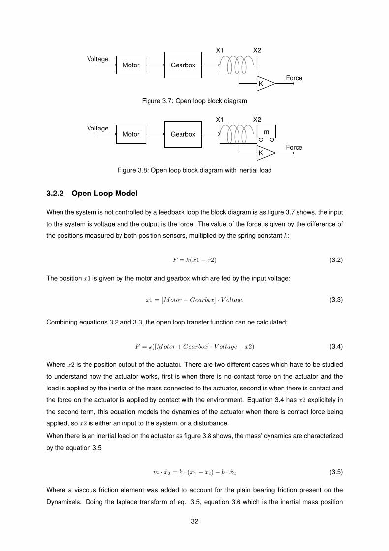
3.7 Open loop block diagram . . . . . . . . . . . . . . . . . . . . . . . . . . . . . . . . . . . . 32

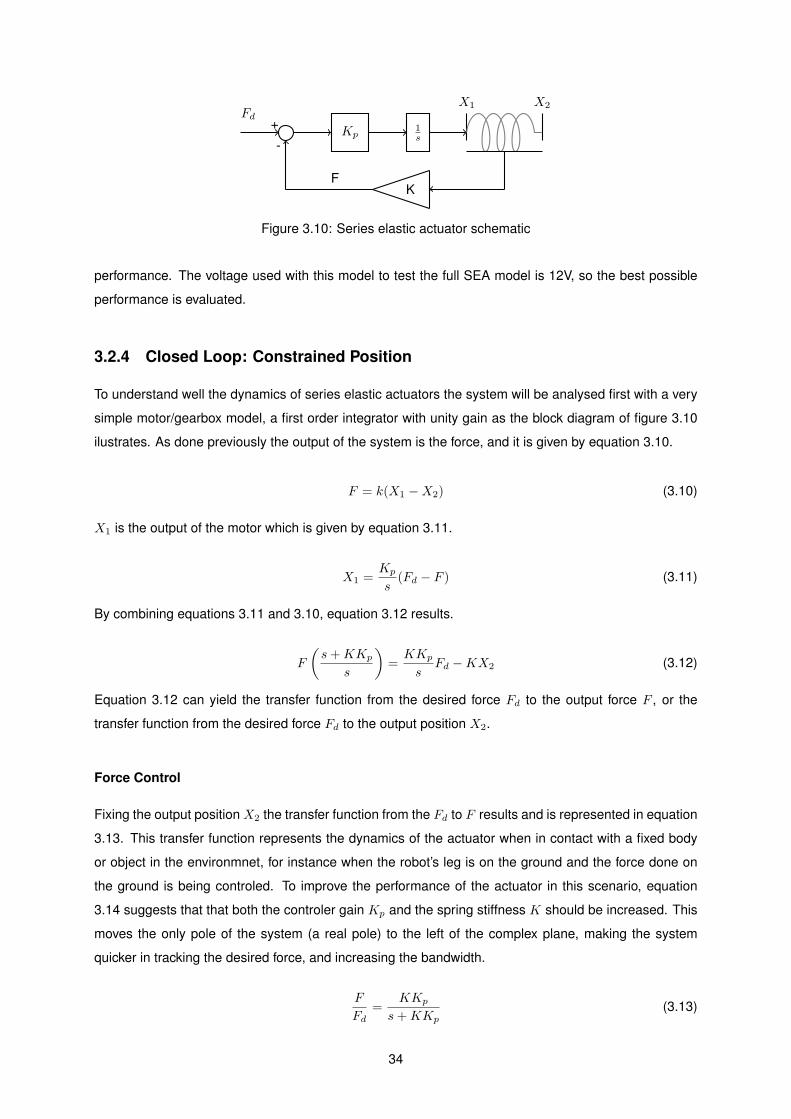
3.8 Open loop block diagram with inertial load . . . . . . . . . . . . . . . . . . . . . . . . . . . 32

3.9 Validation results of the dynamixel identification by Tiago Rato . . . . . . . . . . . . . . . 33

3.10 Series elastic actuator schematic . . . . . . . . . . . . . . . . . . . . . . . . . . . . . . . . 34

3.11 Impedance transfer function bode diagram. [blue:K = 1 and Kp = 1 . . . . . . . . . . . . 35

3.12 Comparison of different amplitude sine waves . . . . . . . . . . . . . . . . . . . . . . . . . 36

3.13 Frequency vs amplitude . . . . . . . . . . . . . . . . . . . . . . . . . . . . . . . . . . . . . 37

3.14 Position control block diagram . . . . . . . . . . . . . . . . . . . . . . . . . . . . . . . . . . 38

3.15 Trade off when selecting spring stiffness . . . . . . . . . . . . . . . . . . . . . . . . . . . . 40

3.16 Force control block diagram . . . . . . . . . . . . . . . . . . . . . . . . . . . . . . . . . . . 41

3.17 Comparison of saturated vs non-saturated actuators due to different spring stiffness . . . 41

3.18 Control action of saturated vs non-saturated actuators due to different spring stiffness . . 42

3.19 Position control block diagram . . . . . . . . . . . . . . . . . . . . . . . . . . . . . . . . . . 42

3.20 Comparison of soft and stiff springs in position tracking . . . . . . . . . . . . . . . . . . . 43

3.21 Frequency response of soft and stiff springs in position tracking . . . . . . . . . . . . . . . 43

3.22 Comparison of output impedance response of systems with different spring stiffness . . . 44

3.23 Input used to compare output impedance . . . . . . . . . . . . . . . . . . . . . . . . . . . 44

3.24 Output impedance block diagram . . . . . . . . . . . . . . . . . . . . . . . . . . . . . . . . 45

3.25 Comparison of the forces generated on impact of systems with different spring stiffnesses 45

3.26 Impact tolerance block diagram . . . . . . . . . . . . . . . . . . . . . . . . . . . . . . . . . 46

3.27 Impact tolerance simulation . . . . . . . . . . . . . . . . . . . . . . . . . . . . . . . . . . . 46

3.28 Dynamixel servo with the elastic element on the outside . . . . . . . . . . . . . . . . . . . 47

3.29 Inside the AX-12 Dynamixel servo . . . . . . . . . . . . . . . . . . . . . . . . . . . . . . . 47

3.30 Modified axle fitted with conductive foam . . . . . . . . . . . . . . . . . . . . . . . . . . . . 49

3.31 Wire installation . . . . . . . . . . . . . . . . . . . . . . . . . . . . . . . . . . . . . . . . . . 49

3.32 AX-12 with an elastic shaft and position sensor . . . . . . . . . . . . . . . . . . . . . . . . 50

3.33 Parts of the prototype shaft with position sensor . . . . . . . . . . . . . . . . . . . . . . . . 51

3.34 Assembled prototype shaft . . . . . . . . . . . . . . . . . . . . . . . . . . . . . . . . . . . 51

3.35 FEM analysis of the production shaft . . . . . . . . . . . . . . . . . . . . . . . . . . . . . . 52

A.1 Modified windows program to work with force control . . . . . . . . . . . . . . . . . . . . . 59

xvi

Chapter 1

Introduction

Every day in current times we face our selfs with technology, technology that is/was mainly created

not by the work of a single man or result of a single idea, but by stacking up decades of ideas and

solutions, each that make everything do something more or work a bit better. Those ideas and solutions

may come by from need, curiosity, or even by accident, but they most certainly will contribute latter to

make something bigger, different, or avoid catastrophic mistakes. Weather we build something useful or

learn something unknown before, we can thank our seemingly infinite curiosity for evolution. The natural

human urge to show every other man the success of our experiments is at the heart of knowledge

passing through times. Science can be seen as the biggest system that will ever exist.

Robotics is a culmination of this system, and by itself it relates disciplines all the way from electronics,

math and computation to mechanics, physics and control. This thesis is just another try at giving another

step towards better technology and ultimately a better society.

This thesis’ goal is twofold, to create a reliable and scalable embedded robotics computational frame-

work, and to develop a force actuator to be implemented in a humanoid robot.

1.1 Motivation

The project that this thesis develops is not new, Since 2007 that MSc students have been working on a

cheap, walking, running and jumping humanoid robot. It started with Pedro Teodoro’s Thesis ”Develop-

ment of a simulation environment of an entertainment humanoid robot” [23], then Tiago Rato’s ”Actuated

Character - Humanoid robots for videogames interaction” [19], and Francisco Ferreira’s ”Development

of a human walking model comprising springs and positive force feedback to generate stable gait” [11].

This thesis work was developed on top of those just mentioned, and the primary goal was to modify

the robot’s actuators that work in position feedback and are high impedance, to compliant force actuators.

Having force control in a humanoid robot opens the door to inumerous theoretical experiments that have

been successful in computer simulations but never made it to real robots. I find there are two main

reasons for that 1) because force actuators are usually only found on very expensive robotic arms; and

2)force sensors/actuators are bulky, expensive and not easy to implement in a humanoid robot. As many

1

articles verify [17] [7] [13] [4] [12], force control is the ultimate way to control a robot that walks, interacts

with humans, or handles delicate environments.

The need for new computational hardware exists because newer platforms allow more computational

speed, faster communication between boards, and better compatibility with new harware and operating

systems, which results in a broader range of control systems that can be implemented. For instance,

if we want to control the heel strike to toe strike movement of a humanoid robot via a feedback control

system, the sample time needs to be in the order of 2ms for a human sized robot. This wasn’t imaginable

with the previous hardware architecture but is very close reality with the new hardware. The low level

software had to be re-done because there were issues in the previous version, it had serious time

keeping problems and the code was generaly written in a way that is far from optimal for control systems.

1.2 State-of-the-art

In today’s robotics it’s undeniable that Petman, Bigdog and Cheetah from Boston Dynamics are probably

the most advanced robots in terms of physical capabilities. Walking, running and jumping were once

dominated by robots like Asimo from Honda that relied on position controlled actuators, today those

tasks are finely performed on the aforementioned robots with force controlled actuators in a much more

natural and robust way. The robot walking algorithms are evolving fast and there is an unprecedented

need for force actuators to test these algorithms in real robots.

The technology of electric position actuators has benefit from decades of use in the industry, home

apliances, cars, disk drives or even toys, they are widely available and there’s now almost a standard on

how to build good position actuators. While this is true for position actuators, force actuators aren’t new

but their small application spectrum has stopped them from evolving as much has position actuators.

There are several methods to build a force actuator but none has become a standard whether because

of the price or because the different methods offer very different specifications. For the MIT Cheetah, a

new force actuator was developed [5], it has low impedance and allows torque estimation by measuring

the current drawn by the motor. While this actuator offers very good specifications, it’s not possible to

implement on the robot of this thesis because of its size.

Series elastic actuators aren’t new and while there were many articles written on them, the need

for force control in robots is pushing scientists and engineers to analyse this form of force actuator

further, and numerous articles have been written on them on the last 5 years. These articles analyse

their compliance, optimizing their performance, controller stability, spring selection, and other topics and

promising results have been shown. This type of actuator can be built inexpensively and very compact,

which is why it was selected for this thesis.

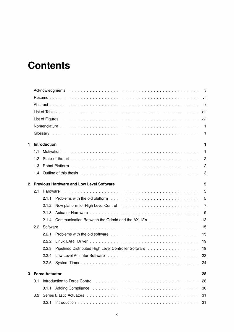
1.3 Robot Platform

The robot used on this thesis is the Robotis Bioloid. This robot is a very good platform for universities

to implement and test new algorithms because it’s inexpensive compared to other solutions and offers

2

decent performance. It’s a humanoid robot with 18 degrees of freedom powered by Dynamixel AX-12

servo motors.

Figure 1.1: Robotis Bioloid

1.4 Outline of this thesis

This thesis is structured in the following way.

Chapter 2 addresses the hardware and software problems of the previous computational platform

and describes the new platform.

In chapter 3 series elastic actuators are analysed, mathematical models are developed, and conclu-

sions are made about the selection of the spring stiffness for the Dynamixel SEA modification. Several

application tentatives are described and analysed and a final production axle is presented.

In chapter 4 conclusions are presented and suggestions for future work and continuation of the

project are given.

3

4

Chapter 2

Previous Hardware and Low Level

Software

2.1 Hardware

Originally the Bioloid’s control system runs on a controller board called CM5 that comes with the robot,

and on the Dynamixel servos. While the ATMega 8’s on the servos’ chips are more than capable of

running the requested tasks of a low level controller (usually a PID type controller), the CM5 has an

ATMega 128 which can easily become the bottleneck of projects like this. The reasons range from the

poor calculation capability when compared to a full ARM or x86 processor, which can become a problem

if later we need to implement a very complex control system (e.g. an adaptive neural network controller

coupled with computer vision algorithms), to the cumbersome and time consuming tasks needed to get

updated code in the MCU vs compiling directly under Linux, for instance. Another advantage of having

a processor running an OS, instead of an MCU, is the ability to easily log on to the robot’s computer via

wi-fi and be able to monitor and/or control the robot’s tasks directly ”as superuser”.

In this section, the motivations to aquire a new embedded computer platform are discussed, the

new platform is presented as well as the microcontroller present on the Dynamixel servos. These two

platforms’ UART ports work at different voltage levels and only one wire is used to send and receive data

on the servo’s MCU, the hardware solution is also presented.

2.1.1 Problems with the old platform

To be able to develop the control system from Matlab, in 2010 an embedded computer was implemented,

it was a Roboard. The original idea was to implement the Roboard as a standalone high level control

platform that communicated directly with the servos exchanging new control actions with sensor values,

but problems maintaining a fixed sample time appeared. The problem was that the linux version sup-

ported by the Roboard is very dated and doesn’t have good support for real-time tasks (if any), running

deterministic tasks in linux was in it’s infancy by that versions’ year, and altough a few scripts to fix this

5

existed, none of them was a trustworthy option to serve as the main clock for the robot’s control system.

Basically what those pieces of software do is make the control program the highest priority task in the

system, but the kernel itself typically isn’t preemptible in linux systems (only if RT Patch or Xenomai are

used), and kernel tasks may take up to more than 10ms [3], a latency value that is unaceptable in cer-

tain moments of the walking gait for instance. The team that implemented the Roboard also found out

that the system wasn’t capable of real-time because they had problems with the communication, they

were using an FTDI chip to make the conversion from the USB port of the Roboart to the servo’s UART

protocol. The problem is that all FTDI chips have a lantency associated with the conversion from one

protocol to the other of arround 1ms for each byte. The following quote from an official FTDI application

note [1] is put explicitly here to emphasize and clarify the issue:

”USB data transfer is prone to delays that do not normally appear in systems that have

been used to transferring data using interrupts. The original COM ports of a PC were directly

connected to the motherboard and were interrupt driven. When a character was transmitted

or received (depending if FIFO’s are used) the CPU would be interrupted and go to a routine

to handle the data. This meant that a user could be reasonably certain that, given a particular

baud rate and data rate, the transfer of data could be achieved without any real need for flow

control. The hardware interrupt ensured that the request would get serviced. Therefore data

could be transferred without using handshaking and still arrive into the PC without data loss.

USB does not transfer data using interrupts. It uses a scheduled system and as a result,

there can be periods when the USB request does not get scheduled and, if handshaking

is not used, data loss will occur. An example of scheduling delays can be seen if an open

application is dragged around using the mouse. For a USB device, data transfer is done in

packets. If data is to be sent from the PC, then a packet of data is built up by the device

driver and sent to the USB scheduler. This scheduler puts the request onto the list of tasks

for the USB host controller to perform. This will typically take at least 1 millisecond to execute

because it will not pick up the new request until the next ’USB Frame’ (the frame period is 1

millisecond). Therefore there is a sizable overhead (depending on your required throughput)

associated with moving the data from the application to the USB device. If data were sent ’a

byte at a time’ by an application, this would severely limit the overall throughput of the system

as a whole.”

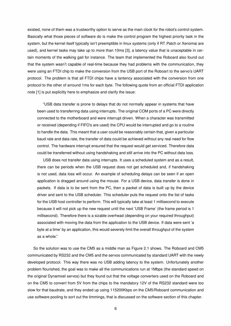
So the solution was to use the CM5 as a middle man as Figure 2.1 shows. The Roboard and CM5

communicated by RS232 and the CM5 and the servos communicated by standard UART with the newly

developed protocol. This way there was no USB adding latency to the system. Unfortunately another

problem flourished, the goal was to make all the communications run at 1Mbps (the standard speed on

the original Dynamixel servos) but they found out that the voltage converters used on the Roboard and

on the CM5 to convert from 5V from the chips to the mandatory 12V of the RS232 standard were too

slow for that baudrate, and they ended up using 115200Kbps on the CM5/Roboard communication and

use software pooling to sort out the timmings, that is discussed on the software section of this chapter.

6

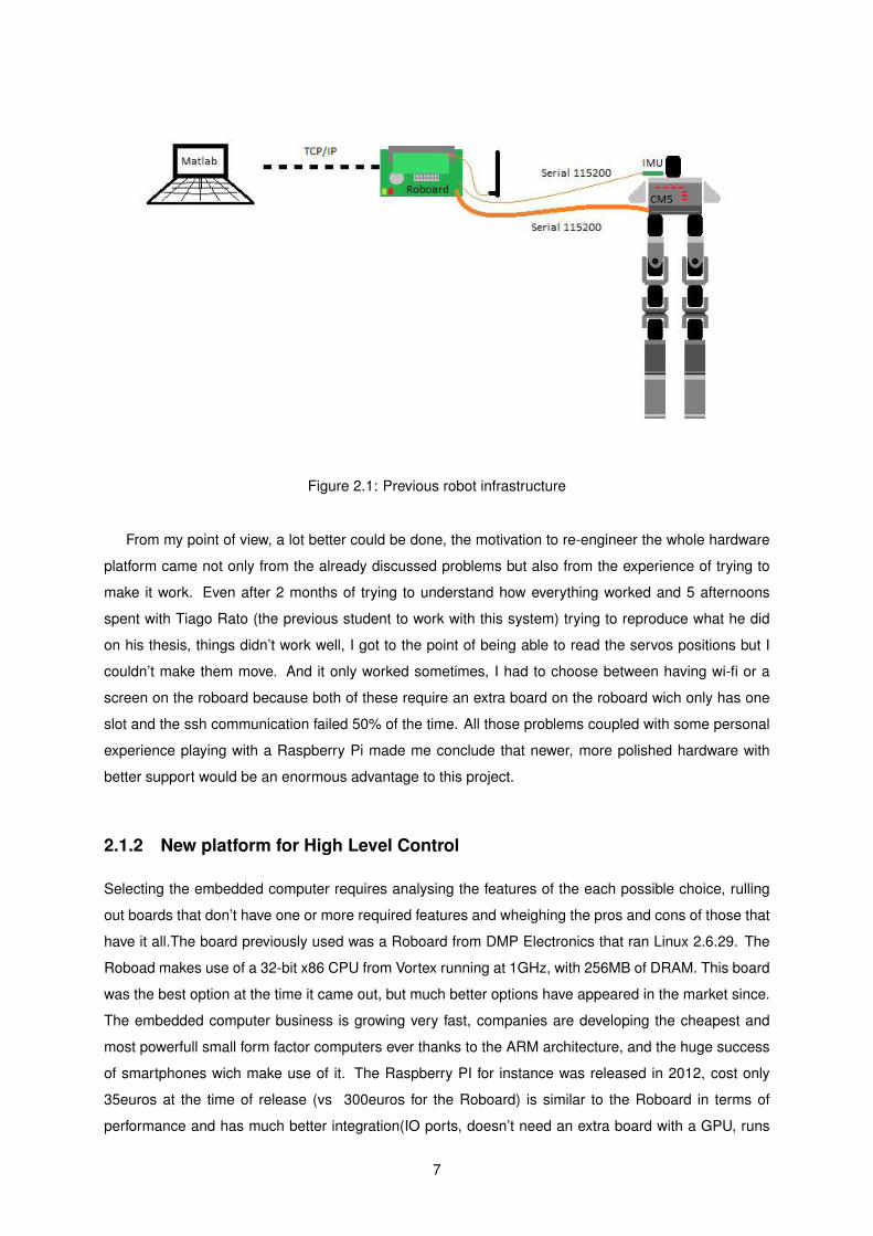
Figure 2.1: Previous robot infrastructure

From my point of view, a lot better could be done, the motivation to re-engineer the whole hardware

platform came not only from the already discussed problems but also from the experience of trying to

make it work. Even after 2 months of trying to understand how everything worked and 5 afternoons

spent with Tiago Rato (the previous student to work with this system) trying to reproduce what he did

on his thesis, things didn’t work well, I got to the point of being able to read the servos positions but I

couldn’t make them move. And it only worked sometimes, I had to choose between having wi-fi or a

screen on the roboard because both of these require an extra board on the roboard wich only has one

slot and the ssh communication failed 50% of the time. All those problems coupled with some personal

experience playing with a Raspberry Pi made me conclude that newer, more polished hardware with

better support would be an enormous advantage to this project.

2.1.2 New platform for High Level Control

Selecting the embedded computer requires analysing the features of the each possible choice, rulling

out boards that don’t have one or more required features and wheighing the pros and cons of those that

have it all.The board previously used was a Roboard from DMP Electronics that ran Linux 2.6.29. The

Roboad makes use of a 32-bit x86 CPU from Vortex running at 1GHz, with 256MB of DRAM. This board

was the best option at the time it came out, but much better options have appeared in the market since.

The embedded computer business is growing very fast, companies are developing the cheapest and

most powerfull small form factor computers ever thanks to the ARM architecture, and the huge success

of smartphones wich make use of it. The Raspberry PI for instance was released in 2012, cost only

35euros at the time of release (vs 300euros for the Roboard) is similar to the Roboard in terms of

performance and has much better integration(IO ports, doesn’t need an extra board with a GPU, runs

7

from a usb cable, etc). The Raspberry Pi became a standard thanks to the electronics hobyist market

(or maker market), and other companies followed the model and improved the concept.

From the enormous amout of possibilities, choosing a the best board is not easy, specially taking

into account that all these products are development boards without much support and advertized as

non finished products. The problem with this is that we can’t trust a board maker simply because they

sell the one with best features, because if there aren’t any serial port drivers we can’t do anything with

it on this project. So the ”trick” is to select the board with best features from the most popular boards.

The mandatory feature was to have support for high speed UART communication (more than 1Mbps) to

allow direct communication with the servos thus removing the need for the CM5. The selected platform

was the Odroid U3 from Hardkernel. It makes use of a Samsung Exynos 4412, a quad-core ARM SOC

running at 1.7GHz that costs around 60 euros. The platform was selected in May 2014, figure 2.2 is the

result of a survey released by Linux.com and LinuxGizmos.com in june 2015 on open spec single board

computers [6]. As can be seen, the Odroid U3 is made it to the top 10 so the Odroid is a popular board

in a universe of 53 boards, as sugested the popularity and comunity activity of the board in the SOC (or

SBC) market is very important to have decent support available. Table 2.1 shows a comparison of the

features of the top 10 boards on the survey. The second column indicates if the board was available

in the market at the time the Odroid U3 was bought. The Odroid U3 is clearly the winner in terms of

features from the available boards, and still competes with the majority of latter boards.

Since this is a research project and students from this department are more familiar with Matlab than

any other language or developing environment, having hardware that is supported by Matlab is a big

bonus. The Raspberry Pi was supported to some extent by Matlab, and some tests were done with it

but Matlab lacked communication through the UART support, that together with the slow communication

speeds put the Raspberry Pi B+ behind the Odroid U3.

Figure 2.2: Points for each board at the top 10 Linux and Android SBCs in 2015, according to aLinux.com and LinuxGizmos.com reader survey.

8

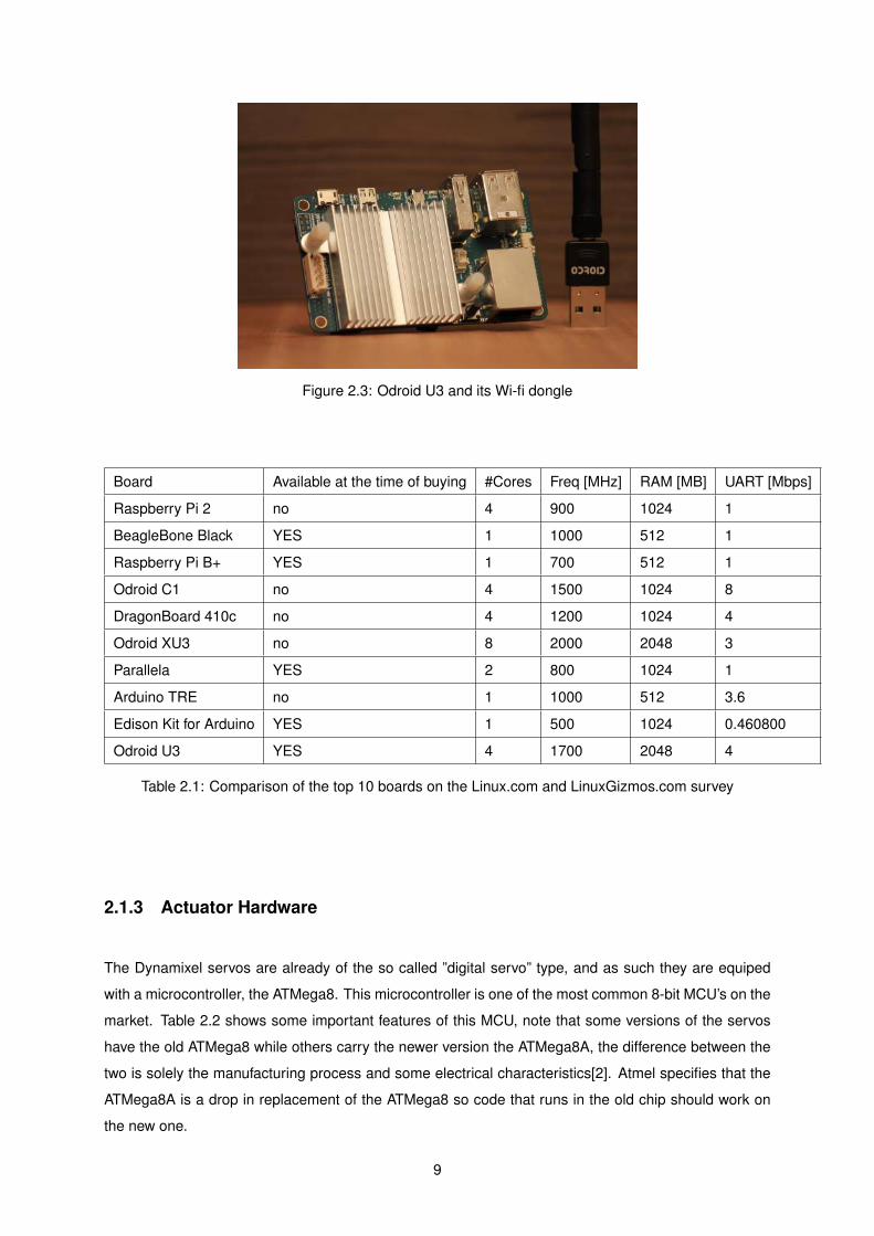
Figure 2.3: Odroid U3 and its Wi-fi dongle

Board Available at the time of buying #Cores Freq [MHz] RAM [MB] UART [Mbps]

Raspberry Pi 2 no 4 900 1024 1

BeagleBone Black YES 1 1000 512 1

Raspberry Pi B+ YES 1 700 512 1

Odroid C1 no 4 1500 1024 8

DragonBoard 410c no 4 1200 1024 4

Odroid XU3 no 8 2000 2048 3

Parallela YES 2 800 1024 1

Arduino TRE no 1 1000 512 3.6

Edison Kit for Arduino YES 1 500 1024 0.460800

Odroid U3 YES 4 1700 2048 4

Table 2.1: Comparison of the top 10 boards on the Linux.com and LinuxGizmos.com survey

2.1.3 Actuator Hardware

The Dynamixel servos are already of the so called ”digital servo” type, and as such they are equiped

with a microcontroller, the ATMega8. This microcontroller is one of the most common 8-bit MCU’s on the

market. Table 2.2 shows some important features of this MCU, note that some versions of the servos

have the old ATMega8 while others carry the newer version the ATMega8A, the difference between the

two is solely the manufacturing process and some electrical characteristics[2]. Atmel specifies that the

ATMega8A is a drop in replacement of the ATMega8 so code that runs in the old chip should work on

the new one.

9

ATMEGA8

CPU Freq. 16MHz - -

Memory

Flash 8KB -

SRAM 1KB -

EEPROM 512B -

Interfaces

SPI 4 MHz1 1 Ch

I2C 400 kHz 1 Ch

UART 2 Mbps 1 Ch

Analog ADC 10 bit 8 Ch

Table 2.2: ATMega8(A) Specifications

To make a series elastic actuator we need to have two position sensors, one on each side of the

elastic member on the shaft. As Figure 2.5 shows, the dynamixels use pin 23(ADC0) to read the value

of the position for feedback control. The sensor used is the analog potentiometer in figure 2.4. The

schematic on the AX-12’s allowed us to connect a second sensor in pin 24, the second sensor was

taken from a burned donor servo. Originally the idea was to use the AX-12’s as guinea pig to study the

implementation possibilities and then implement the force actuation on better servos from the Dynamixel

MX line, there are advantages in that across the board, they’re faster, stronger and more precise. Al-

though time didn’t allow for that, the second sensor to be implemented on those servos was chosen to

be an iC-MU from IC Haus. Using a sensor from a donor MX servo isn’t possible because they use

top mounted encoders instead of hollow shaft potentiometers. The implementation of this sensor would

be more complex because a PCB had to be developed and the communication protocol between the

ATMega and the enconder chip would have to be taken care of.

Figure 2.4: The Murata SV01A103 potentiometer used on the AX-12 Dynamixel servos

Note that the potentiometer used on the AX-12 servos is only capable of reading 300 degrees of

rotation, so when implementing the second sensor care has to be taken to avoid increasing the force

sensing deadzone by intersecting the deadzone of one sensor with the sensible zone of the other, in

other words the potentiometers should be aligned.

Altough the ATMega8 has a regular UART port with TX and RX lines, those aren’t readily available

on the servo connector. In the bottom of the servo schematic in figure 2.5 we see that the TX and RX

lines are connected to a 3 state quad buffer/line driver (the 74HC126D), wich then connects to the servo

1When the ATMega8 is running at 16MHz

10

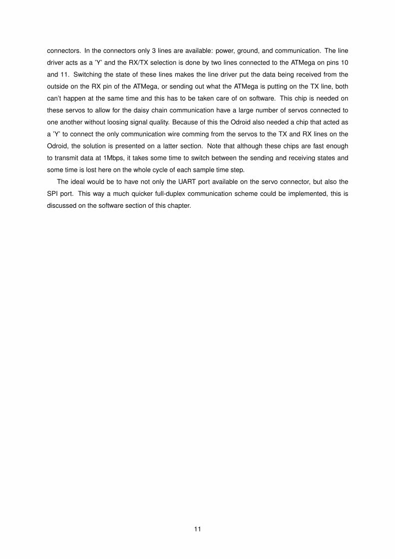
connectors. In the connectors only 3 lines are available: power, ground, and communication. The line

driver acts as a ’Y’ and the RX/TX selection is done by two lines connected to the ATMega on pins 10

and 11. Switching the state of these lines makes the line driver put the data being received from the

outside on the RX pin of the ATMega, or sending out what the ATMega is putting on the TX line, both

can’t happen at the same time and this has to be taken care of on software. This chip is needed on

these servos to allow for the daisy chain communication have a large number of servos connected to

one another without loosing signal quality. Because of this the Odroid also needed a chip that acted as

a ’Y’ to connect the only communication wire comming from the servos to the TX and RX lines on the

Odroid, the solution is presented on a latter section. Note that although these chips are fast enough

to transmit data at 1Mbps, it takes some time to switch between the sending and receiving states and

some time is lost here on the whole cycle of each sample time step.

The ideal would be to have not only the UART port available on the servo connector, but also the

SPI port. This way a much quicker full-duplex communication scheme could be implemented, this is

discussed on the software section of this chapter.

11

Figure 2.5: Controller schematic of the AX-12 Dynamixel servos

12

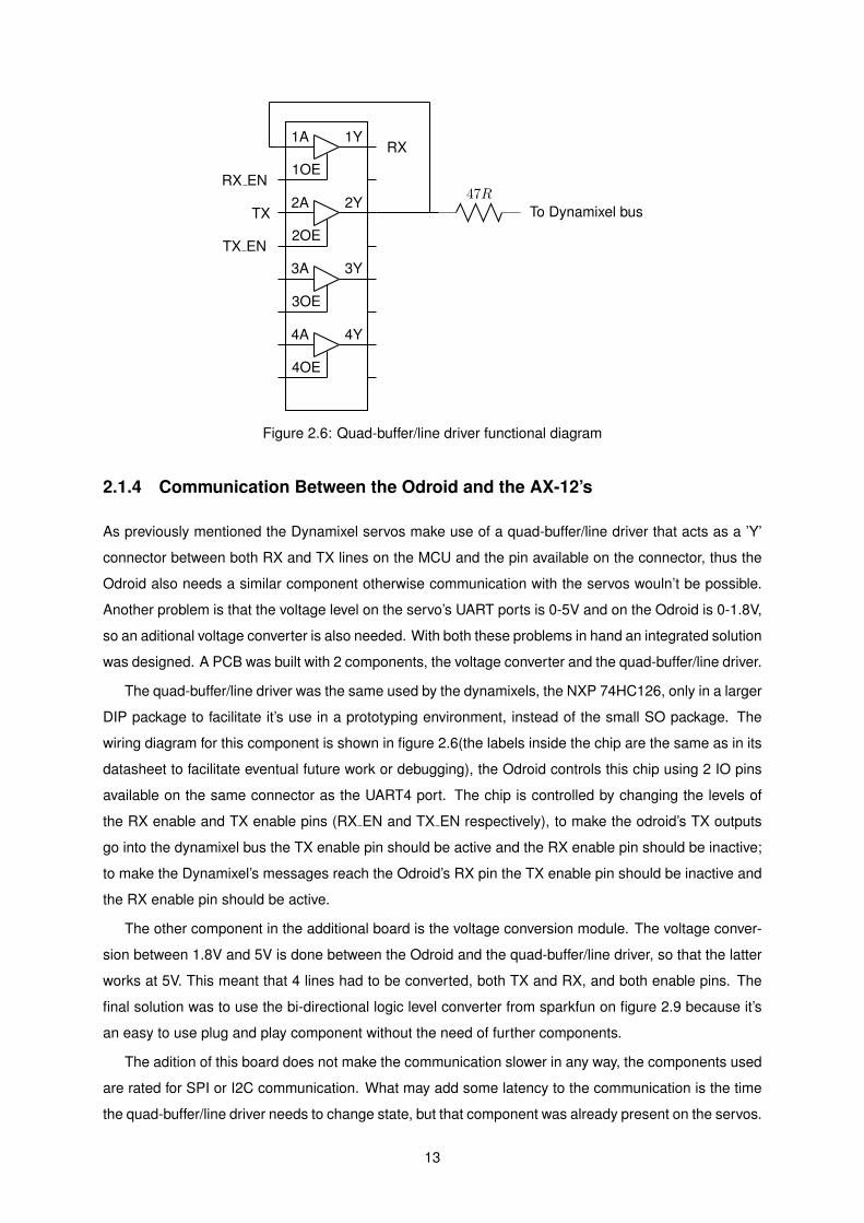
1A

2A

3A

4A

1OE

2OE

3OE

4OE

1Y

2Y

3Y

4Y

RX EN

TX

TX EN

RX

47R

To Dynamixel bus

Figure 2.6: Quad-buffer/line driver functional diagram

2.1.4 Communication Between the Odroid and the AX-12’s

As previously mentioned the Dynamixel servos make use of a quad-buffer/line driver that acts as a ’Y’

connector between both RX and TX lines on the MCU and the pin available on the connector, thus the

Odroid also needs a similar component otherwise communication with the servos wouln’t be possible.

Another problem is that the voltage level on the servo’s UART ports is 0-5V and on the Odroid is 0-1.8V,

so an aditional voltage converter is also needed. With both these problems in hand an integrated solution

was designed. A PCB was built with 2 components, the voltage converter and the quad-buffer/line driver.

The quad-buffer/line driver was the same used by the dynamixels, the NXP 74HC126, only in a larger

DIP package to facilitate it’s use in a prototyping environment, instead of the small SO package. The

wiring diagram for this component is shown in figure 2.6(the labels inside the chip are the same as in its

datasheet to facilitate eventual future work or debugging), the Odroid controls this chip using 2 IO pins

available on the same connector as the UART4 port. The chip is controlled by changing the levels of

the RX enable and TX enable pins (RX EN and TX EN respectively), to make the odroid’s TX outputs

go into the dynamixel bus the TX enable pin should be active and the RX enable pin should be inactive;

to make the Dynamixel’s messages reach the Odroid’s RX pin the TX enable pin should be inactive and

the RX enable pin should be active.

The other component in the additional board is the voltage conversion module. The voltage conver-

sion between 1.8V and 5V is done between the Odroid and the quad-buffer/line driver, so that the latter

works at 5V. This meant that 4 lines had to be converted, both TX and RX, and both enable pins. The

final solution was to use the bi-directional logic level converter from sparkfun on figure 2.9 because it’s

an easy to use plug and play component without the need of further components.

The adition of this board does not make the communication slower in any way, the components used

are rated for SPI or I2C communication. What may add some latency to the communication is the time

the quad-buffer/line driver needs to change state, but that component was already present on the servos.

13

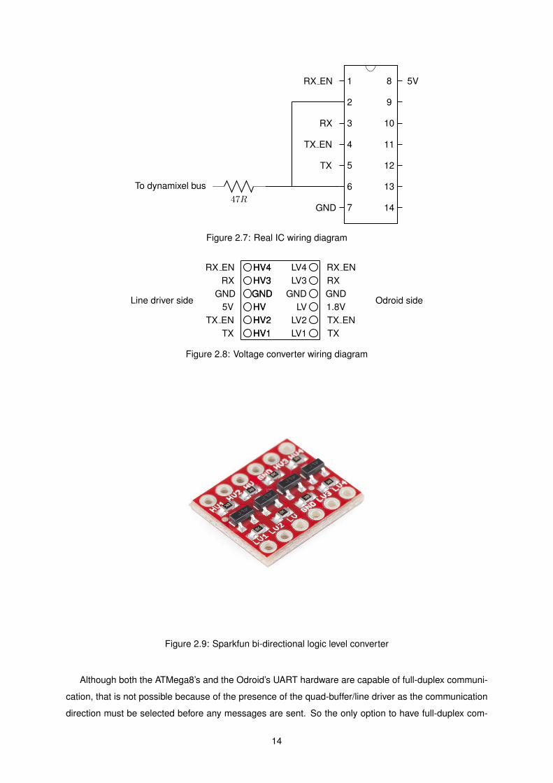
RX EN

RX

TX EN

TX

GND

5V

47R

To dynamixel bus

1

2

3

4

5

6

7

8

9

10

11

12

13

14

Figure 2.7: Real IC wiring diagram

HV1HV2HVGNDHV3HV4

LV1LV2

LVGND

LV3LV4

HV1HV2HVGNDHV3HV4

TXTX EN1.8VGNDRXRX EN

TXTX EN

5VGND

RXRX EN

Odroid sideLine driver side

Figure 2.8: Voltage converter wiring diagram

Figure 2.9: Sparkfun bi-directional logic level converter

Although both the ATMega8’s and the Odroid’s UART hardware are capable of full-duplex communi-

cation, that is not possible because of the presence of the quad-buffer/line driver as the communication

direction must be selected before any messages are sent. So the only option to have full-duplex com-

14

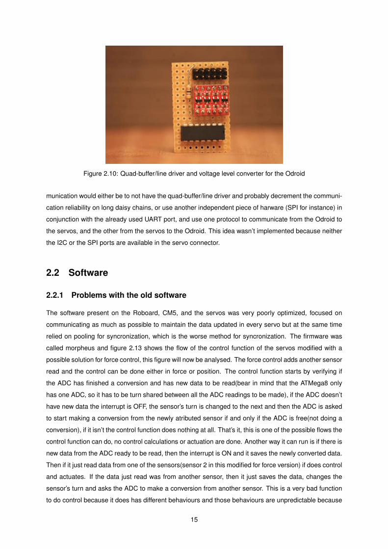
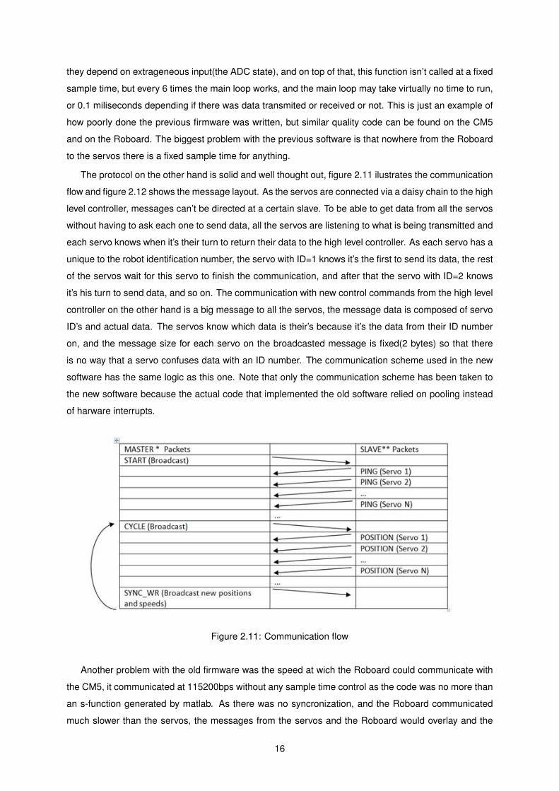
Figure 2.10: Quad-buffer/line driver and voltage level converter for the Odroid

munication would either be to not have the quad-buffer/line driver and probably decrement the communi-

cation reliability on long daisy chains, or use another independent piece of harware (SPI for instance) in

conjunction with the already used UART port, and use one protocol to communicate from the Odroid to

the servos, and the other from the servos to the Odroid. This idea wasn’t implemented because neither

the I2C or the SPI ports are available in the servo connector.

2.2 Software

2.2.1 Problems with the old software

The software present on the Roboard, CM5, and the servos was very poorly optimized, focused on

communicating as much as possible to maintain the data updated in every servo but at the same time

relied on pooling for syncronization, which is the worse method for syncronization. The firmware was

called morpheus and figure 2.13 shows the flow of the control function of the servos modified with a

possible solution for force control, this figure will now be analysed. The force control adds another sensor

read and the control can be done either in force or position. The control function starts by verifying if

the ADC has finished a conversion and has new data to be read(bear in mind that the ATMega8 only

has one ADC, so it has to be turn shared between all the ADC readings to be made), if the ADC doesn’t

have new data the interrupt is OFF, the sensor’s turn is changed to the next and then the ADC is asked

to start making a conversion from the newly atributed sensor if and only if the ADC is free(not doing a

conversion), if it isn’t the control function does nothing at all. That’s it, this is one of the possible flows the

control function can do, no control calculations or actuation are done. Another way it can run is if there is

new data from the ADC ready to be read, then the interrupt is ON and it saves the newly converted data.

Then if it just read data from one of the sensors(sensor 2 in this modified for force version) if does control

and actuates. If the data just read was from another sensor, then it just saves the data, changes the

sensor’s turn and asks the ADC to make a conversion from another sensor. This is a very bad function

to do control because it does has different behaviours and those behaviours are unpredictable because

15

they depend on extrageneous input(the ADC state), and on top of that, this function isn’t called at a fixed

sample time, but every 6 times the main loop works, and the main loop may take virtually no time to run,

or 0.1 miliseconds depending if there was data transmited or received or not. This is just an example of

how poorly done the previous firmware was written, but similar quality code can be found on the CM5

and on the Roboard. The biggest problem with the previous software is that nowhere from the Roboard

to the servos there is a fixed sample time for anything.

The protocol on the other hand is solid and well thought out, figure 2.11 ilustrates the communication

flow and figure 2.12 shows the message layout. As the servos are connected via a daisy chain to the high

level controller, messages can’t be directed at a certain slave. To be able to get data from all the servos

without having to ask each one to send data, all the servos are listening to what is being transmitted and

each servo knows when it’s their turn to return their data to the high level controller. As each servo has a

unique to the robot identification number, the servo with ID=1 knows it’s the first to send its data, the rest

of the servos wait for this servo to finish the communication, and after that the servo with ID=2 knows

it’s his turn to send data, and so on. The communication with new control commands from the high level

controller on the other hand is a big message to all the servos, the message data is composed of servo

ID’s and actual data. The servos know which data is their’s because it’s the data from their ID number

on, and the message size for each servo on the broadcasted message is fixed(2 bytes) so that there

is no way that a servo confuses data with an ID number. The communication scheme used in the new

software has the same logic as this one. Note that only the communication scheme has been taken to

the new software because the actual code that implemented the old software relied on pooling instead

of harware interrupts.

Figure 2.11: Communication flow

Another problem with the old firmware was the speed at wich the Roboard could communicate with

the CM5, it communicated at 115200bps without any sample time control as the code was no more than

an s-function generated by matlab. As there was no syncronization, and the Roboard communicated

much slower than the servos, the messages from the servos and the Roboard would overlay and the

16

CM5 would have to save the newly arrived data from the Roboard to the next servo cycle, because the

message to the servos was already being sent at the time the Roboard started sending its message.

This caused delays on the control action and made the sample time of the high level controller random

within certain limits. Limits which were acceptable for the previous works done but may not acceptable

for future work, nonetheless having random sample time in a digital control system is a huge mistake

that can render the best performing controller unstable.

With these problems in hand:

1) No sample time control;

2) Pooling on the communication;

3) Poorly written code with non-optimized flows, and poor readability and comments;

4) Using the CM5 as a communication interface between the Roboard and the servos taking up more

communication time;

in code that extended through thousands of lines, the decision to make everything from scratch came

up and the new software framework was built with fresh hardware. I could probably make the things that

worked previously work again for me, but if during the development of my thesis I needed something a

little different that required to change the code, it would be easier to rebuild the whole thing so, might as

well do it right from the start.

Figure 2.12: Morpheus protocol message

17

Figu

re2.

13:

Con

trolf

unct

ion

ofth

em

orph

eus

firm

war

e

18

2.2.2 Linux UART Driver

Although the Odroid U3 is capable of driving the UART port at 4Mbps, the stock linux driver in the

Odroid U3 port limits the communication speed 921600Kbps. Note that this is not the same as 1Mbps,

and as the servo’s UART driver can’t communicate at that speed, the next compatible speed with both

systems is 500Kbps, this is the max baudrate the Odroid can communicate with the servos with the stock

UART driver. As one of the primary goals when choosing the Odroid was to have fast communication

speeds, the driver needed to be modified in order to allow up to 2Mbps(the fastest the ATMega8’s

can communicate through UART). Reading the kernel source code on github we can find that in the

linux/drivers/tty/serial/samsung.c file, the function uart get baud rate has as last argument 8*115200

which equals 921600, this argument to the function is the max baud the function will allow communication

to occour. Although this was discovered and modified to allow faster communication speeds the Odroid’s

baudrate stayed capped at 921600 and the problem wasn’t solved.

Nevertheless even at 500Kbps the whole communication takes less time than the previous because

the communication is direct to the servos at 500Kbps, instead of at 115200bps to the CM5 and then at

1Mbps to the servos. Communication at 500000Kbps is more than 4 times faster than at 115200.

2.2.3 Pipelined Distributed High Level Controller Software

In digital control systems, maintaining a controlled sample-time with a minimum frequency is fundamen-

tal [9]. The Nyquist criterion (eq. 2.1) states that the minimum sample period should be less than or

equal to half of the minimum period on the system, conversely the minimum sample frequency should be

at least twice the maximum frequency the system achieves(the system’s bandwidth). In the real world, a

more conservative rule should be applied to avoid aliasing the signals on higher frequencies. Equation

2.2 suggests a lower frequency limit of 10 times the maximum system frequency and an upper limit of

20 times the maximum system frequency, which helps reducing erroneus high frequency noise from the

sensors.

T ≤ Tmin

2or F ≥ 2Fmax (2.1)

10F ≤ Fmax ≤ 20F (2.2)

Walking is a very complex task, humans have evolved in non trivial ways to be able to attain efficient

and stable walking patterns[8] [24]. Some periods on the walking cycle require feedback control of force

at very high rates. What nature did to allow controlling force at those high rates, for instance in the period

between heel strike and toe strike, was distribute the control scheme along the nervous system and use

”pre-programmed” patterns that don’t require real-time processing and are activated by certain triggers

throughout the gait cycle[10], that’s why we need to learn how to walk, and why we fall if we miss a

step. In robotics this can also be done to allow robots to have human like reactions, but in this thesis a

more modest control scheme was aproached, with simple real-time feedback control for walking. With

19

this kind of controller, every movement needs to be calculated and syncronized between all the joints

of the robot, this requires a very fast control platform that will allow the implementation of the controller

and be able to deliver the minimum sample time needed to control the robot. Having this requirement,

the possibilities to materialize such a system were studied, and a pipelined parallel control scheme was

developed.

Analisys of the control system

The system to be controlled is a robot with up to 18 DOF’s(12 for both legs and 6 for the arms), each

DOF’s control action will most certainly deppend on the control actions of other DOF’s not only in the

forward or inverse kinematics fashion but also because inertial forces generated for instance in the arm

of the robot will influence the force done on the foot. Also walking methodologies like the ZMP [18]

method require coupled calculation of the control actions for all the joints. This part of the control system

requires data from all the sensors and the calculations can’t be parallelized. But normally these central

control systems only calculate the trajectory of the joints, leaving the control of the actuator out. The

control of the actuator is responsible for generating the required control action on the actuator itself such

that the high level control order is followed, normally a PID is used for this, and contrary to the trajectory

planning control, this control system is independend for each actuator. This means that the low level

control of the actuators can be parallelized. With this in hand the layout of the computational platform

for the control system can be developed.

As analysed in the previous section, in humanoid robots increasing the sample rate gives more

possibilities. The MIT Cheetah [22] makes use of a highly optimized computational platform to allow the

required sample time to make the robot run(4000Hz). There are no specific requirements for the robot in

this thesis, so no required sample-time can be calculated, but having the fastest possible platform from

the start is a good way to start, and when the limit of this platform is achieved, a whole new platform

with faster hardware should be developed, or even a more serious robot. This is preferred to building an

”enough for now” platform that may be rendered useless in less than a year. With this perspective, the

fastest possible controller platform was developed.

Analysis of the hardware

The selected platform, the Odroid has four cores in its CPU, and the microcontrollers on the servos also

have computational capability. The layout of the Odroid is shown in figure 2.14, the use of USB has

been rulled out because of inherent delay issue so there are two ways the Odroid can communicate

reliably with the servos: UART and I2C. The servos’ communication ports are shown in figure 2.15,

although the microcontroller has SPI and I2C communication capability, only the UART port is available

in the servo’s connectors. With this we have a dedicated CPU for each actuator(in the servos), 4 general

purpose CPUs(on the Odroid) and way of communicating between all of them(UART). This immediatly

suggests implementing the high level dependent control on the Odroid and the low level independent

control on the servos’ microcontroller.

20

CPU1 CPU2 CPU3 CPU4

Samsung Exynos 4412

USB UART I2C

All ports are accessible on the Odroid U3 board

Figure 2.14: Odroid CPUs and communication ports

ATMega8

CPU

SPI UART I2C

Only the UART port is available in the connector of the dynamixel PCB

Figure 2.15: ATMega8 communication ports

21

Paralelizing tasks

The required tasks for such a system to work are:

-The low level controllers read the sensors;

-The low level controllers send data to the high level controller;

-The high level controller reads data from the low level controllers;

-The high level controller calculates the next high level control action;

-The high level controller sends the high level control action to all the low level controllers;

-The low level controllers read data from the high level controller;

-The low level controllers calculate the next low level control action;

-The low level controllers act;

Since we have multiple cores at our disposal and some of the required tasks don’t need to be done

serially, parallel processing can be implemented [22] to increase the max sampling frequency the system

can achieve. On the Odroid side paralelization can only be implemented in a pipeline fashion because

the tasks of the high level controller are all dependent and thus need to be acomplished serialy. Because

control calculations can only be done after the data from the servos is received, and sending data to the

servos is only possible after the calculations have completed. Nonetheless these tasks are separable

and uncoupled, and while the control calculations from sample moment t are being done, the Odroid can

be receiving data from sample moment t+1, so that when the calculations from moment t are complete,

data for the next calculations is ready.

Figure 2.18 shows the tasks of the high level controller in the order they have to be done. If a regular

single worker method is implemented, that is a single program does everything in loop, the workflow in

figure 2.19 is achieved. If on the other hand a multiworker method is implemented the workflow of figure

2.20 is achieved. The pipeline method has decreased the time needed to acomplish two time steps by

a third, supposing that all the tasks take the same time to complete. Comparing figure 2.19 and 2.20

we can verify that the pipelined solution doesn’t increase the sample-time but increases the sample-

rate. The throughput is augmented, 3 tasks are running simultaneously all the time, thus this method is

computationally more efficient because at no point there is an idling pipeline stage. Note that altough

this is possible to acomplish in some systems, it isn’t possible in the system of this thesis because as

was seen previously, the servos only have the UART port available in the connector and because of the

quad-buffer/line driver, full-duplex communication isn’t possible although the UART hardware both on

the Odroid and on the ATMega8s is capable of full-duplex communication. This leaves just one option,

to not paralelize the communication as figure 2.16 shows. In this scheme there is no aparent reason

to have separate processes for reading and writing on the communication bus, but as the messages

need to be assembled before they are sent and also need to be interpreted when they arrive there would

be some time lost if these tasks weren’t parallel. Figure 2.17 illustrates how these processes overlap.

The parallelism isn’t working at the communication port level, but only at the processing tasks level of

these processes. As the reading process finishes receiving a message from the servos, it still needs to

deconstruct the message, save the data to appropriate variables and pass it to the controller. Having

the read process separate to the send process allows to have the send process start sending as soon

22

Read Data

Send Data

Control Calc.

Read Data

Send Data

Control Calc.

CPU 1

CPU 2

CPU 3

Figure 2.16: High level controller scheduling

Read Data

Send Data

Figure 2.17: Read and send processes overlap

as the messages from the servos finish, without having to wait for the message that just arrived to be

interpreted.

2.2.4 Low Level Actuator Software

The easiest tasks to parallelize are the independent ones, in this case everything that happens in the

servos: sensor reading, actuation, low level control calculations and communication. So instead of

having each servo act in it’s own time window, all servos can be commanded to act simultaneously since

all the servos have the same tasks and they all take the same time to complete.

One important aspect of distributed control systems is syncronization between all the sensors and

actuators. The high level controller must receive the data from all the sensors from the same sam-

pling moment, if not the control system can become unstable. Conversely the actuation must also be

syncronized, servos actuation must be simultaneous from the same control action. To achieve this an

independent clock was implemented that syncronizes all systems in the control infrastructure, that is

analysed in the next section.

The tasks of the low level control system are:

-Impose the control action;

-Read the current state;

-Do control calculations;

-Communicate with the high level controller exchanging the next control value with the sensor values;

The first task is to choose the order at which the tasks are going to execute. As previously stated, the

actuation must be syncronized between all the servos, and since some tasks may have jitter, it’s best to

do the actuation at the begining of the time step, another reason for this is reducing the delay between

Read data Control calc. Send data

time

Figure 2.18: High level controller tasks

23

Read data Control calc. Send data Read data Control calc. Send data

time

Figure 2.19: Tasks in serial(2 time-steps)

Read data Control calc. Send data

Read data Control calc. Send data

time

Figure 2.20: Tasks in pipeline

reading the sensors and acting. The other task that has time requirements is reading the sensors, so it

was put after the actuation. The tasks with most jitter are the communication and the control calculations,

so those were left for last, as for their order, if the communication is done before doing control, the control

calculations benefit from freshly arrived data, so the final task scheduling for the low level controllers is

as figure 2.21 ilustrates. The software that implements this is controlled by interrupts to ensure the

time requirements. The scheduling of figure 2.21 suggests after data is sent to the high level controller

and the high level controller responds immediatly. Note that all the servos are running this schedule in

parallel and the communication line is unique, so to allow this each servo knows when it’s time to send

its data from its identification number. The first servo to send is servo with ID=1, this servo doesn’t wait,

as soon as it finishes reading the ADC it sends data to the high level controller. Meanwhile the other

servos are actually listening on the line, and only after servo n has completed its communication, will

servo n + 1 start its communication, as figure 2.22 ilustrates. Note that although the communication

scheduling is the same as implemented before and shown in figure 2.11, the old software scheduling did

one communication per sample time(although there was no fixed sample time, I am calling sample time

the time between two consecutive actuations of the low level software), so in practice if 12 servos were

implemented, 12 time steps were needed for all the servos to send their data to the high level controller,

while with this software only one time step is needed. Although this system still works as a master/slave

system, the master controller has the same bandwidth as the the slave controllers.

2.2.5 System Timer

The system timer was implemented in an ATMega8 from a dynamixel servo. The timer is a program

that uses a hardware clock to generate pulses, those pulses are fed to an output pin of the chip and

fed into the interrupt input pins of all the servos. This way the sample time can’t drift from servo to

PWM Read ADC Send data Read data Control calc.

time

Figure 2.21: Low level controller scheduling

24

PWM Read ADC Send data Wait Wait Read Data Control Calc.

PWM Read ADC Wait Send Data Wait Read Data Control Calc.

PWM Read ADC Wait Wait Send Data Read Data Control Calc.

time

Servo 1

Servo 2

Servo 3

Figure 2.22: Multiple servo scheduling

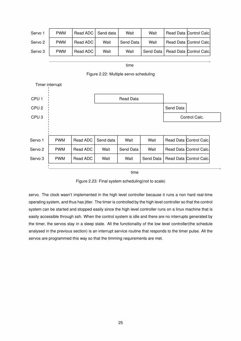
Timer interrupt

Read Data

Send Data

Control Calc.

CPU 1

CPU 2

CPU 3

PWM Read ADC Send data Wait Wait Read Data Control Calc.

PWM Read ADC Wait Send Data Wait Read Data Control Calc.

PWM Read ADC Wait Wait Send Data Read Data Control Calc.

time

Servo 1

Servo 2

Servo 3

Figure 2.23: Final system scheduling(not to scale)

servo. The clock wasn’t implemented in the high level controller because it runs a non hard real-time

operating system, and thus has jitter. The timer is controlled by the high level controller so that the control

system can be started and stopped easily since the high level controller runs on a linux machine that is

easily accessible through ssh. When the control system is idle and there are no interrupts generated by

the timer, the servos stay in a sleep state. All the functionality of the low level controller(the schedule

analysed in the previous section) is an interrupt service routine that responds to the timer pulse. All the

servos are programmed this way so that the timming requirements are met.

25

26

27

Chapter 3

Force Actuator

3.1 Introduction to Force Control

Robot actuators are still generally position controlled, this control method is very good for precise repet-

itive tasks like painting a car or spot welding. But if a robot is to be in contact with new environments

or different tasks are required, position precision is not very helpful. One good example (for people who

drive cars at least) is what happens when we use the gearbox of a car we’re driving for the first time,

although we know the gear lever is there(we can see it) the feel can be very different, the throw can

be different, we need may need to apply more force or it may take more time for gears to engage, we

can feel it because we know the ammount of force we’re doing, we use force feedback to feel what’s

happening and learn the behaviour of the new gearbox. If we program a robotic arm to shift gears of

a car by position feedback, it will be able to use that specific gearbox or very similar ones only. For

instance if the gearbox we programmed it for is the one in figure 3.1 on the left and we put the robot in

a car with the gearbox on the right then it will very likely damage the gearbox or itself, at least in the

long run because without force feedback the position controllers will force the joints to move although

the movement is constrained by the shorter throw of the gear lever. If on the other hand the robot knew

that to engage first gear it needed to apply 20N max to the left and stop if the force increased without

further movement and then another 20N max to the front until no more movement was possible without

increasing force drasticaly, then the robot could put any car in first gear, just like we do.

Force control is also required for safe use of robots that interact with people, the ability to limit the

applied force is very important to keep the robots safe in delicate environments [7]. The ability to pick up

objects without damaging or dropping them is another task that requires force control [13] [4]. Last but

most important for this thesis, force control is important to make robots walk, or at least very helpfull and

brings numerous advantages [12] [17]. It’s been shown that humans change the impedance of the legs

deppending on the walking speed and the floor surface type [14]. This brings up the concept of variable

impedance.

Impedance is a measure of how much something resists motion when subjected to a force. Con-

versely, compliance is how much something accepts motion when subjected to an external force. Human

28

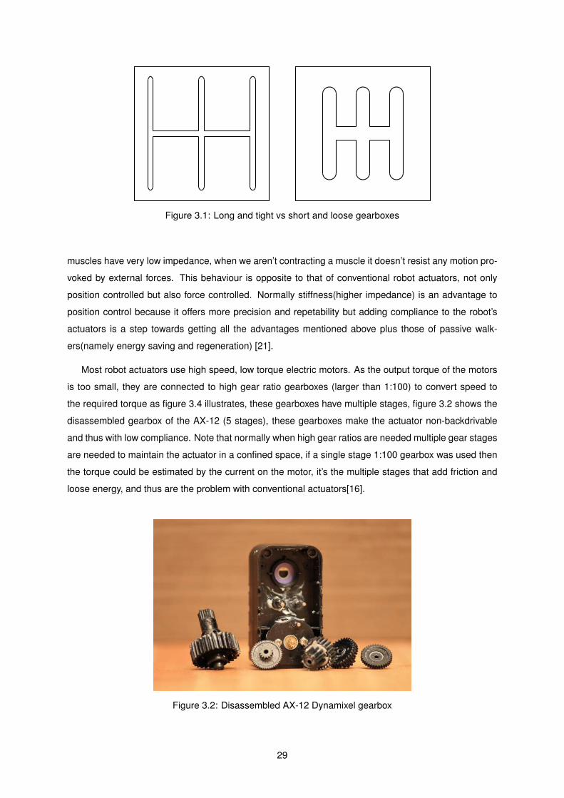
Figure 3.1: Long and tight vs short and loose gearboxes

muscles have very low impedance, when we aren’t contracting a muscle it doesn’t resist any motion pro-

voked by external forces. This behaviour is opposite to that of conventional robot actuators, not only

position controlled but also force controlled. Normally stiffness(higher impedance) is an advantage to

position control because it offers more precision and repetability but adding compliance to the robot’s

actuators is a step towards getting all the advantages mentioned above plus those of passive walk-

ers(namely energy saving and regeneration) [21].

Most robot actuators use high speed, low torque electric motors. As the output torque of the motors

is too small, they are connected to high gear ratio gearboxes (larger than 1:100) to convert speed to

the required torque as figure 3.4 illustrates, these gearboxes have multiple stages, figure 3.2 shows the

disassembled gearbox of the AX-12 (5 stages), these gearboxes make the actuator non-backdrivable

and thus with low compliance. Note that normally when high gear ratios are needed multiple gear stages

are needed to maintain the actuator in a confined space, if a single stage 1:100 gearbox was used then

the torque could be estimated by the current on the motor, it’s the multiple stages that add friction and

loose energy, and thus are the problem with conventional actuators[16].

Figure 3.2: Disassembled AX-12 Dynamixel gearbox

29

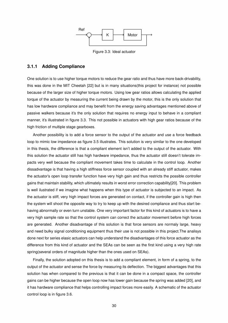
K MotorRef

Figure 3.3: Ideal actuator

3.1.1 Adding Compliance

One solution is to use higher torque motors to reduce the gear ratio and thus have more back-drivability,

this was done in the MIT Cheetah [22] but is in many situations(this project for instance) not possible

because of the larger size of higher torque motors. Using low gear ratios allows calculating the applied

torque of the actuator by measuring the current being drawn by the motor, this is the only solution that

has low hardware compliance and may benefit from the energy saving advantages mentioned above of

passive walkers because it’s the only solution that requires no energy input to behave in a compliant

manner, it’s illustrated in figure 3.3. This not possible in actuators with high gear ratios because of the

high friction of multiple stage gearboxes.

Another possibility is to add a force sensor to the output of the actuator and use a force feedback

loop to mimic low impedance as figure 3.5 illustrates. This solution is very similar to the one developed

in this thesis, the difference is that a compliant element isn’t added to the output of the actuator. With

this solution the actuator still has high hardware impedance, thus the actuator still doesn’t tolerate im-

pacts very well because the compliant movement takes time to calculate in the control loop. Another

dissadvantage is that having a high stiffness force sensor coupled with an already stiff actuator, makes

the actuator’s open loop transfer function have very high gain and thus restricts the possible controller

gains that maintain stability, which ultimately results in worst error correction capability[20]. This problem

is well ilustrated if we imagine what happens when this type of actuator is subjected to an impact. As

the actuator is stiff, very high impact forces are generated on contact, if the controller gain is high then

the system will shoot the opposite way to try to keep up with the desired compliance and thus start be-

having abnormally or even turn unstable. One very important factor for this kind of actuators is to have a

very high sample rate so that the control system can correct the actuator movement before high forces

are generated. Another disadvantage of this solution is that force sensors are normaly large, heavy

and need bulky signal conditioning equipment thus their use is not possible in this project.The analisys

done next for series elasic actuators can help understand the disadvantages of this force actuator as the

difference from this kind of actuator and the SEAs can be seen as the first kind using a very high rate

spring(several orders of magnitude higher than the ones used on SEAs).

Finally, the solution adopted on this thesis is to add a compliant element, in form of a spring, to the

output of the actuator and sense the force by measuring its deflection. The biggest advantages that this

solution has when compared to the previous is that it can be done in a compact space, the controller

gains can be higher because the open loop now has lower gain because the spring was added [20], and

it has hardware compliance that helps controlling impact forces more easily. A schematic of the actuator

control loop is in figure 3.6.

30

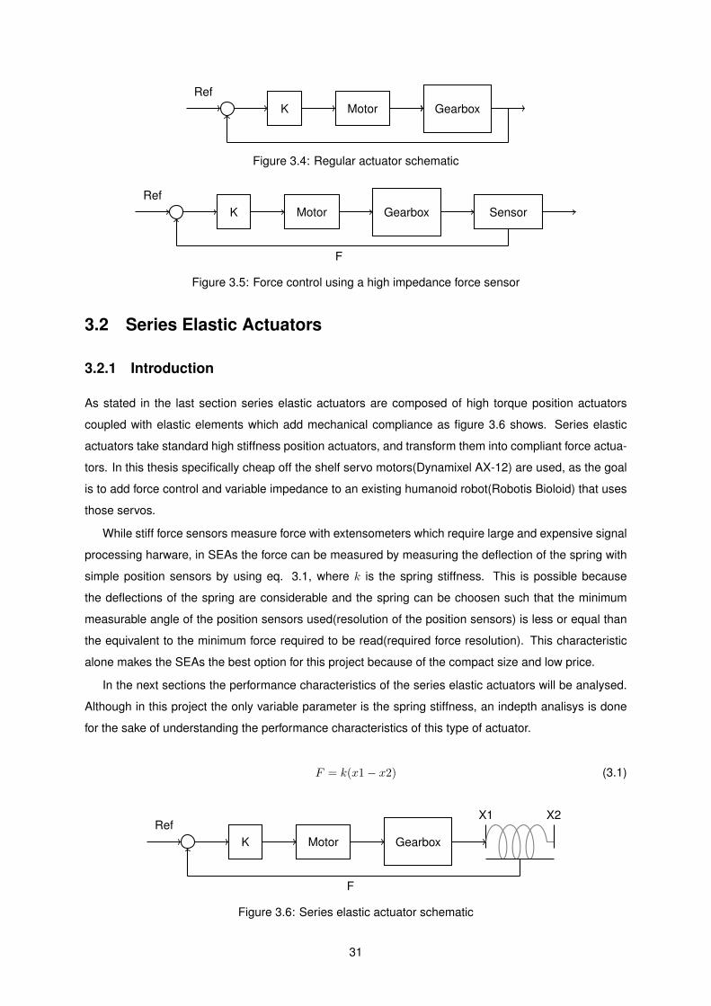
K Motor GearboxRef

Figure 3.4: Regular actuator schematic

K Motor Gearbox Sensor

F

Ref

Figure 3.5: Force control using a high impedance force sensor

3.2 Series Elastic Actuators

3.2.1 Introduction

As stated in the last section series elastic actuators are composed of high torque position actuators

coupled with elastic elements which add mechanical compliance as figure 3.6 shows. Series elastic

actuators take standard high stiffness position actuators, and transform them into compliant force actua-

tors. In this thesis specifically cheap off the shelf servo motors(Dynamixel AX-12) are used, as the goal

is to add force control and variable impedance to an existing humanoid robot(Robotis Bioloid) that uses

those servos.

While stiff force sensors measure force with extensometers which require large and expensive signal

processing harware, in SEAs the force can be measured by measuring the deflection of the spring with

simple position sensors by using eq. 3.1, where k is the spring stiffness. This is possible because

the deflections of the spring are considerable and the spring can be choosen such that the minimum

measurable angle of the position sensors used(resolution of the position sensors) is less or equal than

the equivalent to the minimum force required to be read(required force resolution). This characteristic

alone makes the SEAs the best option for this project because of the compact size and low price.

In the next sections the performance characteristics of the series elastic actuators will be analysed.

Although in this project the only variable parameter is the spring stiffness, an indepth analisys is done

for the sake of understanding the performance characteristics of this type of actuator.

F = k(x1− x2) (3.1)

K Motor Gearbox

X1 X2

F

Ref

Figure 3.6: Series elastic actuator schematic

31

Motor Gearbox

KForce

X1 X2Voltage

Figure 3.7: Open loop block diagram

Motor Gearbox m

KForce

X1 X2Voltage

Figure 3.8: Open loop block diagram with inertial load

3.2.2 Open Loop Model

When the system is not controlled by a feedback loop the block diagram is as figure 3.7 shows, the input

to the system is voltage and the output is the force. The value of the force is given by the difference of

the positions measured by both position sensors, multiplied by the spring constant k:

F = k(x1− x2) (3.2)

The position x1 is given by the motor and gearbox which are fed by the input voltage:

x1 = [Motor +Gearbox] · V oltage (3.3)

Combining equations 3.2 and 3.3, the open loop transfer function can be calculated:

F = k([Motor +Gearbox] · V oltage− x2) (3.4)

Where x2 is the position output of the actuator. There are two different cases which have to be studied

to understand how the actuator works, first is when there is no contact force on the actuator and the

load is applied by the inertia of the mass connected to the actuator, second is when there is contact and

the force on the actuator is applied by contact with the environment. Equation 3.4 has x2 explicitely in

the second term, this equation models the dynamics of the actuator when there is contact force being

applied, so x2 is either an input to the system, or a disturbance.

When there is an inertial load on the actuator as figure 3.8 shows, the mass’ dynamics are characterized

by the equation 3.5

m · x2 = k · (x1 − x2)− b · x2 (3.5)

Where a viscous friction element was added to account for the plain bearing friction present on the

Dynamixels. Doing the laplace transform of eq. 3.5, equation 3.6 which is the inertial mass position

32

transfer function is obtained.

X2

X1=

k

ms2 + bs+ k(3.6)

The open loop transfer function of the system when there is an inertial load connected to the output of

the actuator can be determined by combining equations 3.4 and 3.6, equation 3.7 is the result.

F

V oltage= [Motor +Gearbox]

(k − k2

ms2 + bs+ k

)(3.7)

3.2.3 Motor and Gearbox Mathematical Model

The dynamics of the motor and gearbox limit the capabilities of series elastic actuators, as such a real

model is used. The parametric model was obtained by Tiago Rato [19] in his thesis and it includes the

dynamics of the motor and the gearbox, from the input voltage to the output angle on the servo. The

parametric equation used was that of equation 3.8, where V is voltage, L is inductance, R is resistance,

J is the gearbox inertia, b is the viscous friction, and K is a constant that relates torque with current.

The identified values yield the transfer function of equation 3.9. Figure 3.9 is the result of a simulation,

in blue is the input voltage to the motor, in red is the simulated output in radians and in green is the real

output also in radians. This is included to prove the validity of the used model.

θ

V=

K

JLs3 + (Lb+ JR)s2 + (Rb+K2)s(3.8)

θ

V=

0.0071

9.09× 10−7s3 + 9.09× 10−4s2 + 0.013s(3.9)

Figure 3.9: Validation results of the dynamixel identification by Tiago Rato

The voltage used on the AX-12s is 9.8V but it can go up to 12V, so depending on the voltages used,

the dynamics of the series elastic actuator will differ, so that a higher voltage will always deliver better

33

Kp1s

X1 X2

K

Fd

F

+

-

Figure 3.10: Series elastic actuator schematic

performance. The voltage used with this model to test the full SEA model is 12V, so the best possible

performance is evaluated.

3.2.4 Closed Loop: Constrained Position

To understand well the dynamics of series elastic actuators the system will be analysed first with a very

simple motor/gearbox model, a first order integrator with unity gain as the block diagram of figure 3.10

ilustrates. As done previously the output of the system is the force, and it is given by equation 3.10.

F = k(X1 −X2) (3.10)

X1 is the output of the motor which is given by equation 3.11.

X1 =Kp

s(Fd − F ) (3.11)

By combining equations 3.11 and 3.10, equation 3.12 results.

F

(s+KKp

s

)=KKp

sFd −KX2 (3.12)

Equation 3.12 can yield the transfer function from the desired force Fd to the output force F , or the

transfer function from the desired force Fd to the output position X2.

Force Control

Fixing the output position X2 the transfer function from the Fd to F results and is represented in equation

3.13. This transfer function represents the dynamics of the actuator when in contact with a fixed body

or object in the environmnet, for instance when the robot’s leg is on the ground and the force done on

the ground is being controled. To improve the performance of the actuator in this scenario, equation

3.14 suggests that that both the controler gain Kp and the spring stiffness K should be increased. This

moves the only pole of the system (a real pole) to the left of the complex plane, making the system

quicker in tracking the desired force, and increasing the bandwidth.

F

Fd=

KKp

s+KKp(3.13)

34

Output Impedance

Now fixing the desired force Fd and letting X2 vary, equation 3.14 results. This expression can be seen

as the output impedance if we take X2 as an extrageneous disturbance that affects the desired force

tracking. The goal in this type of actuators is to haveX2 affect F the least possible so that output position

disturbances are well attenuated. To acomplish this, the spring stiffness K should be decreased and the

controler gain Kp should be increased, by doing this the overall impedance of the actuator is lowered.

F

X2=

−Kss+KKp

(3.14)

Analysing the bode diagram of equation 3.14, we can see the influence of K and Kp in the frequency

response. The response in blue is obtained when K = 1 and Kp = 1, by increasing both K and Kp to

10 the response in green in obtained. If K is decreased and Kp is increased as suggested in the last

paragraph to 5 and 500 respectively the response in red is obtained. As can be seen, to decrease the

influence of X2 in F , K should be decreased and Kp should be increased for frequency response to

attenuate the maximum possible, the widest spectrum of frequencies.

Figure 3.11: [green:K = 10 and Kp = 10] [red: K = 5 and Kp = 500]]Impedance transfer function bode diagram for

various K and Kp values

35

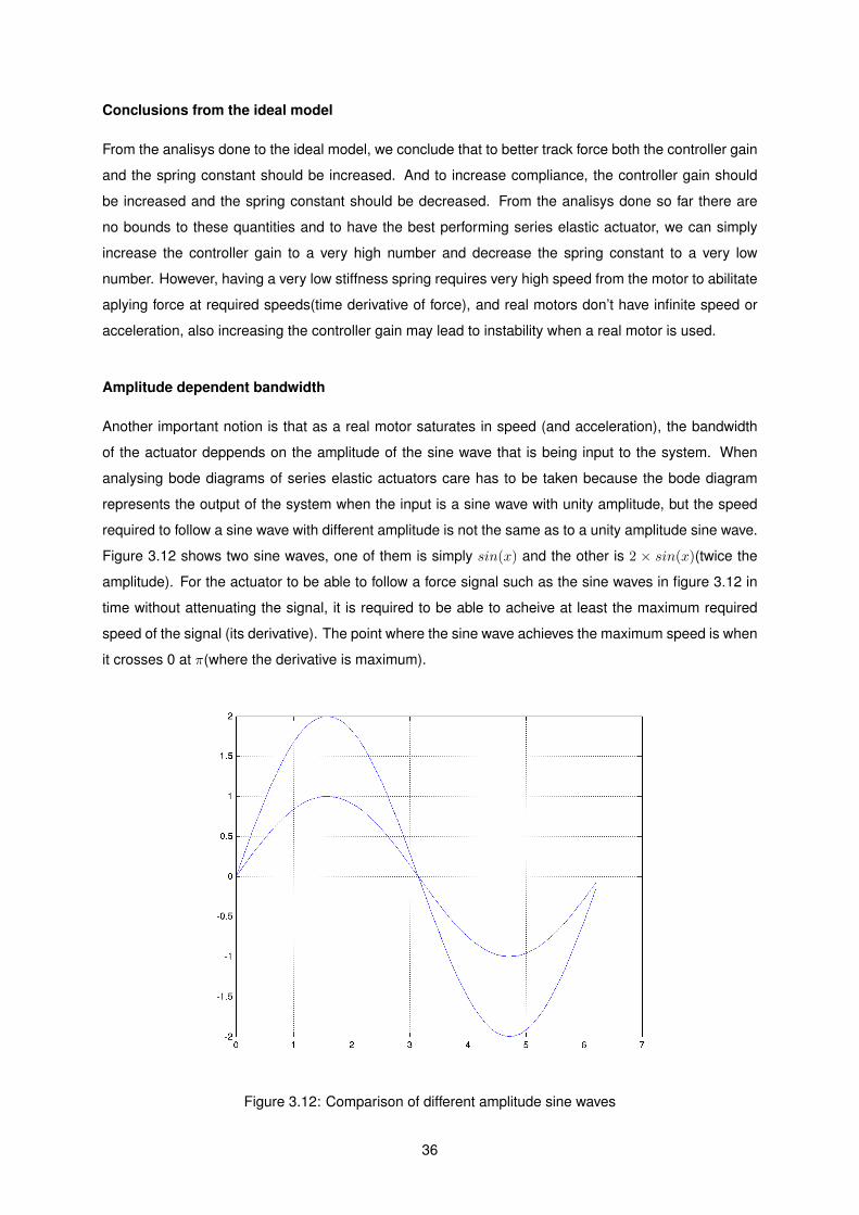
Conclusions from the ideal model

From the analisys done to the ideal model, we conclude that to better track force both the controller gain

and the spring constant should be increased. And to increase compliance, the controller gain should

be increased and the spring constant should be decreased. From the analisys done so far there are

no bounds to these quantities and to have the best performing series elastic actuator, we can simply

increase the controller gain to a very high number and decrease the spring constant to a very low

number. However, having a very low stiffness spring requires very high speed from the motor to abilitate

aplying force at required speeds(time derivative of force), and real motors don’t have infinite speed or

acceleration, also increasing the controller gain may lead to instability when a real motor is used.

Amplitude dependent bandwidth

Another important notion is that as a real motor saturates in speed (and acceleration), the bandwidth

of the actuator deppends on the amplitude of the sine wave that is being input to the system. When

analysing bode diagrams of series elastic actuators care has to be taken because the bode diagram

represents the output of the system when the input is a sine wave with unity amplitude, but the speed

required to follow a sine wave with different amplitude is not the same as to a unity amplitude sine wave.

Figure 3.12 shows two sine waves, one of them is simply sin(x) and the other is 2 × sin(x)(twice the

amplitude). For the actuator to be able to follow a force signal such as the sine waves in figure 3.12 in

time without attenuating the signal, it is required to be able to acheive at least the maximum required

speed of the signal (its derivative). The point where the sine wave achieves the maximum speed is when

it crosses 0 at π(where the derivative is maximum).

Figure 3.12: Comparison of different amplitude sine waves

36

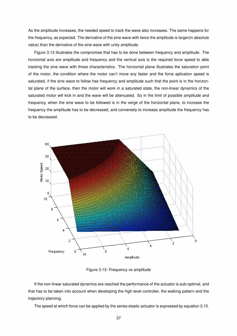
As the amplitude increases, the needed speed to track the wave also increases. The same happens for

the frequency, as expected. The derivative of the sine wave with twice the amplitude is larger(in absolute

value) than the derivative of the sine wave with unity amplitude.

Figure 3.13 illustrates the compromise that has to be done between frequency and amplitude. The

horizontal axis are amplitude and frequency and the vertical axis is the required force speed to able

tracking the sine wave with those characteristics. The horizontal plane illustrates the saturation point

of the motor, the condition where the motor can’t move any faster and the force aplication speed is

saturated, if the sine wave to follow has frequency and amplitude such that the point is in the horizon-

tal plane of the surface, then the motor will work in a saturated state, the non-linear dynamics of the

saturated motor will kick in and the wave will be attenuated. So in the limit of possible amplitude and

frequency, when the sine wave to be followed is in the verge of the horizontal plane, to increase the

frequency the amplitude has to be decreased, and conversely to increase amplitude the frequency has

to be decreased.

Figure 3.13: Frequency vs amplitude

If the non-linear saturated dynamics are reached the performance of the actuator is sub-optimal, and

that has to be taken into account when developing the high level controller, the walking pattern and the

trajectory planning.

The speed at which force can be applied by the series elastic actuator is expressed by equation 3.15.

37

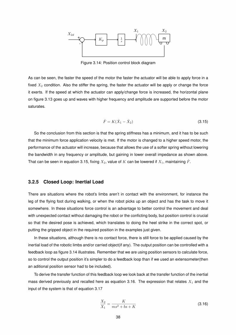
Kp1s

X1 X2X2d

+

-m

Figure 3.14: Position control block diagram

As can be seen, the faster the speed of the motor the faster the actuator will be able to apply force in a

fixed X2 condition. Also the stiffer the spring, the faster the actuator will be apply or change the force

it exerts. If the speed at which the actuator can apply/change force is increased, the horizontal plane

on figure 3.13 goes up and waves with higher frequency and amplitude are supported before the motor

saturates.

F = K(X1 − X2) (3.15)

So the conclusion from this section is that the spring stiffness has a minimum, and it has to be such

that the minimum force application velocity is met. If the motor is changed to a higher speed motor, the

performance of the actuator will increase, because that allows the use of a softer spring without lowering

the bandwidth in any frequency or amplitude, but gaining in lower overall impedance as shown above.

That can be seen in equation 3.15, fixing X2, value of K can be lowered if X1, maintaining F .

3.2.5 Closed Loop: Inertial Load

There are situations where the robot’s limbs aren’t in contact with the environment, for instance the

leg of the flying foot during walking, or when the robot picks up an object and has the task to move it

somewhere. In these situations force control is an advantage to better control the movement and deal

with unexpected contact without damaging the robot or the conficting body, but position control is crucial

so that the desired pose is achieved, which translates to doing the heel strike in the correct spot, or

putting the gripped object in the required position in the examples just given.

In these situations, although there is no contact force, there is still force to be applied caused by the

inertial load of the robotic limbs and/or carried object(if any). The output position can be controlled with a

feedback loop as figure 3.14 illustrates. Remember that we are using position sensors to calculate force,

so to control the output position it’s simpler to do a feedback loop than if we used an extensometer(then

an aditional position sensor had to be included).

To derive the transfer function of this feedback loop we look back at the transfer function of the inertial

mass derived previously and recalled here as equation 3.16. The expression that relates X1 and the

input of the system is that of equation 3.17

X2

X1=

K

ms2 + bs+K(3.16)

38

X1 =Kp

s(X2d −X2) (3.17)

Combining equations 3.6 and 3.17 the transfer function of the closed loop position control system

results which is expressed in equation 3.18. As expected it’s a third degree system, with two poles from

the mass and one pole from the ideal motor model.

X2

X2d=

KKp

ms3 + bs2 +Ks+KKp(3.18)

In the limit when the spring constant is set to infinity, the system reduces to a simple first order

position control system which is represented in equation 3.19.

X2

X2d=

Kp

s+Kp(3.19)

In this case, it’s always best to have the highest possible spring constant because the stiffer the

spring, the faster the system will be able to respond and settle to new position references and deviations

without major oscillations. A compromise has to be made so that position control is reasonable but the

actuator still has good impact tolerance, because although pure position control is possible in series

elastic actuators, the primary goal of SEAs is to have high compliance in case of impact even when

doing pure position control. SEAs are better than stiff force actuators doing force control in terms of

impact tolerance, but a lot worse doing position control than regular stiff actuators. To be able to control

position and still have good impact tolerance, the control software has to check the force in every time

step, because as the compliance is in part virtual(acomplished by the control system), to attenuate the

force of an impact, the control scheme has to change when an impact is sensed or at least the control

action has to take into account and limit the applied force(deppending on the situation).

3.2.6 Analysis with the real motor & hardware

The real motor has more complex dynamics than the model used so far, and analysing the actuator

with the real motor dynamics is fundamental to understand the capabilities of the SEA built arround

the AX-12 platform. The variables that affect the performance of the SEA the most are motor perfor-

mance(maximum speed, torque, and acceleration), the sample rate, and the spring stiffness. Stepping

back and looking at these variables from a systemic point of view, in this project the stock motor is used

so increasing the performance of the motor in the servos isn’t an option in this thesis, the hardware and

software of the controllers has been optimized and is now performance capped by the hardware used

and the communication protocol speed, the spring stiffness is ajustable but also has limits. The spring

stiffness on the real case is bounded, the spring can’t be too stiff has to not allow the position sensor to

read the minimum force that has to be read, and it can’t be too soft so that the force application speed

is too slow as analysed before. The analysis from here on will be done for rotational SEA’s as is the

practical case of this thesis.

The position value read by the ATMega8 has resolution of 0.29◦, so if the required minimum force

39

Kmin Kmax

Better impact tolerance Better position tracking

Figure 3.15: Trade off when selecting spring stiffness

reading(force resolution) is mT , the maximum spring stiffness Kmax can be calculated using Hooke’s

law (3.20 on the left), plugging the position resolution and the force resolution expression 3.20 (right)

results.

T = K · θ Kmax =mT

0.29(3.20)

This gives an upper bound for the spring stiffness. A lower bound can also be calculated by knowing

the maximum speed at which force has to be applied. The force aplication speed for SEA’s in the

contact force case(fixed output position) can be expressed as the first time derivative of Hooke’s law,

with θ1 being the output position of the motor, this is expressed in equation 3.21 on the left. If Tmin is

the minimum force application speed and θ1max is the maximum speed of the motor, then the minimum

spring stiffness Kmin can be calculated, and is expressed in equation3.21 on the right.

T = K · θ1 Kmin =Tmin

θ1max

(3.21)

As expected the same analysis can be done for the force acceleration and jerk, and should be done

if such critical requirements are to be met. Further analisys of the motor dynamics and a deeper study in

motor speed and acceleration capabilities would be advisable as these quantities are derivatives of the

position which is what Tiago based his analisys on, and although his model has acceptable behaviour

in position tracking, errors increase when analysing velocity, acceleration and jerk tracking.

So the spring stiffness must be selected between these two values, the exact value in that accept-

able spectrum has to be selected according to the desired impact impedance and position tracking

capabilities. A stiffer spring will be better for position tracking and a softer spring will make the actuator

more compliant in case of impact as figure 3.15 illustrates. The influence of the spring stiffness on the

performance of the actuator on those situations will be now analysed.

Force Tracking

When in pure force control, the block diagram is as figure 3.16 shows, here the Motor block is the real

motor dynamics of section 3.2.3 which also encompasses the gearbox. The transfer function of the

system is thus equation 3.22. In this equation the spring stiffness K and the proportional term of the

PID controller are interchangeable, this means that we can select any spring and adjust the controller to

have good performance, in fact systems with different springs can have the same exact transfer function.

The difference is that with a softer spring the motor has to move at higher speeds to achieve the same

force in the same amount of time, and it will saturate in situations the same system with stiffer spring

wouldn’t. So the difference is that the non linearity will kick in more easily the softer the spring is. Figure

40

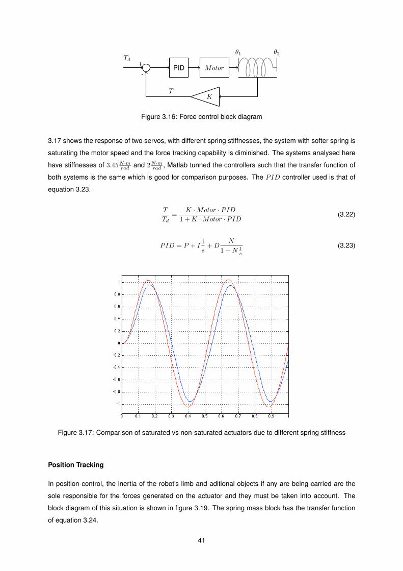
PID Motor

θ1 θ2

K

Td

T

+

-

Figure 3.16: Force control block diagram

3.17 shows the response of two servos, with different spring stiffnesses, the system with softer spring is

saturating the motor speed and the force tracking capability is diminished. The systems analysed here

have stiffnesses of 3.45N ·mrad and 2N ·m

rad , Matlab tunned the controllers such that the transfer function of

both systems is the same which is good for comparison purposes. The PID controller used is that of

equation 3.23.

T

Td=

K ·Motor · PID1 +K ·Motor · PID

(3.22)

PID = P + I1

s+D

N

1 +N 1s

(3.23)

Figure 3.17: Comparison of saturated vs non-saturated actuators due to different spring stiffness

Position Tracking

In position control, the inertia of the robot’s limb and aditional objects if any are being carried are the

sole responsible for the forces generated on the actuator and they must be taken into account. The

block diagram of this situation is shown in figure 3.19. The spring mass block has the transfer function

of equation 3.24.

41

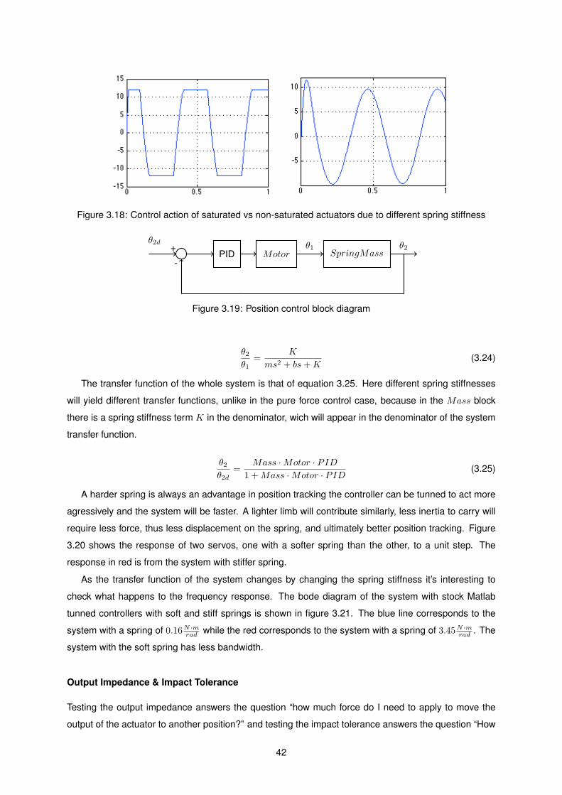
Figure 3.18: Control action of saturated vs non-saturated actuators due to different spring stiffness

PID Motorθ1 θ2

SpringMass

θ2d+

-

Figure 3.19: Position control block diagram

θ2θ1

=K

ms2 + bs+K(3.24)

The transfer function of the whole system is that of equation 3.25. Here different spring stiffnesses

will yield different transfer functions, unlike in the pure force control case, because in the Mass block

there is a spring stiffness term K in the denominator, wich will appear in the denominator of the system

transfer function.

θ2θ2d

=Mass ·Motor · PID

1 +Mass ·Motor · PID(3.25)

A harder spring is always an advantage in position tracking the controller can be tunned to act more

agressively and the system will be faster. A lighter limb will contribute similarly, less inertia to carry will

require less force, thus less displacement on the spring, and ultimately better position tracking. Figure

3.20 shows the response of two servos, one with a softer spring than the other, to a unit step. The

response in red is from the system with stiffer spring.

As the transfer function of the system changes by changing the spring stiffness it’s interesting to

check what happens to the frequency response. The bode diagram of the system with stock Matlab

tunned controllers with soft and stiff springs is shown in figure 3.21. The blue line corresponds to the

system with a spring of 0.16N ·mrad while the red corresponds to the system with a spring of 3.45N ·m

rad . The

system with the soft spring has less bandwidth.

Output Impedance & Impact Tolerance

Testing the output impedance answers the question “how much force do I need to apply to move the

output of the actuator to another position?” and testing the impact tolerance answers the question “How

42

Figure 3.20: Comparison of soft and stiff springs in position tracking

Figure 3.21: Frequency response of soft and stiff springs in position tracking

does the system react when subjected to an impact of certain energy?”.

The output impedance block diagram is that of figure 3.24 and the transfer function is in equation

3.26. It’s easy to see that lowering the spring stiffness K will lower the effect of the output position in the

torque, the effect can be seen in figure 3.22 which is response of two systems, one with stiffer spring

than the other, to the same input. The input function used to do this test is shown in figure 3.23. A stiffer

spring will also cause the motor to saturate with less abrupt position inputs than with a softer spring.

43

Figure 3.22: Comparison of output impedance response of systems with different spring stiffness

Figure 3.23: Input used to compare output impedance

T

θ2=

−K1 +K ·Motor · PID

(3.26)

The impact tolerance was tested by subjecting the system to an impact of an object at a determined

speed. To do that a simulation was done with a certain mass attached to an hipotetical arm of a certain

lenght, with non-zero initial velocity, figure 3.27 illustrates the situation. The block diagram is shown on

figure 3.26 and the transfer function of this system is that of equation 3.31. The force applied by the

actuator on the mass is expressed by equation 3.27 where T is the actuator torque that is expressed by

equation 3.28. Although the mass moves in a straight line, I’ve assummed that the mass is attached to

the arm of the robot and it moves as one with it, but to ease the calculations the component of inertia

parallel to the robotic arm wasn’t considered. Doing the sum of all forces applied on the mass under

these conditions equation 3.30 arrises, and doing the laplace transform we get the transfer function of

the SpringMass block.

44

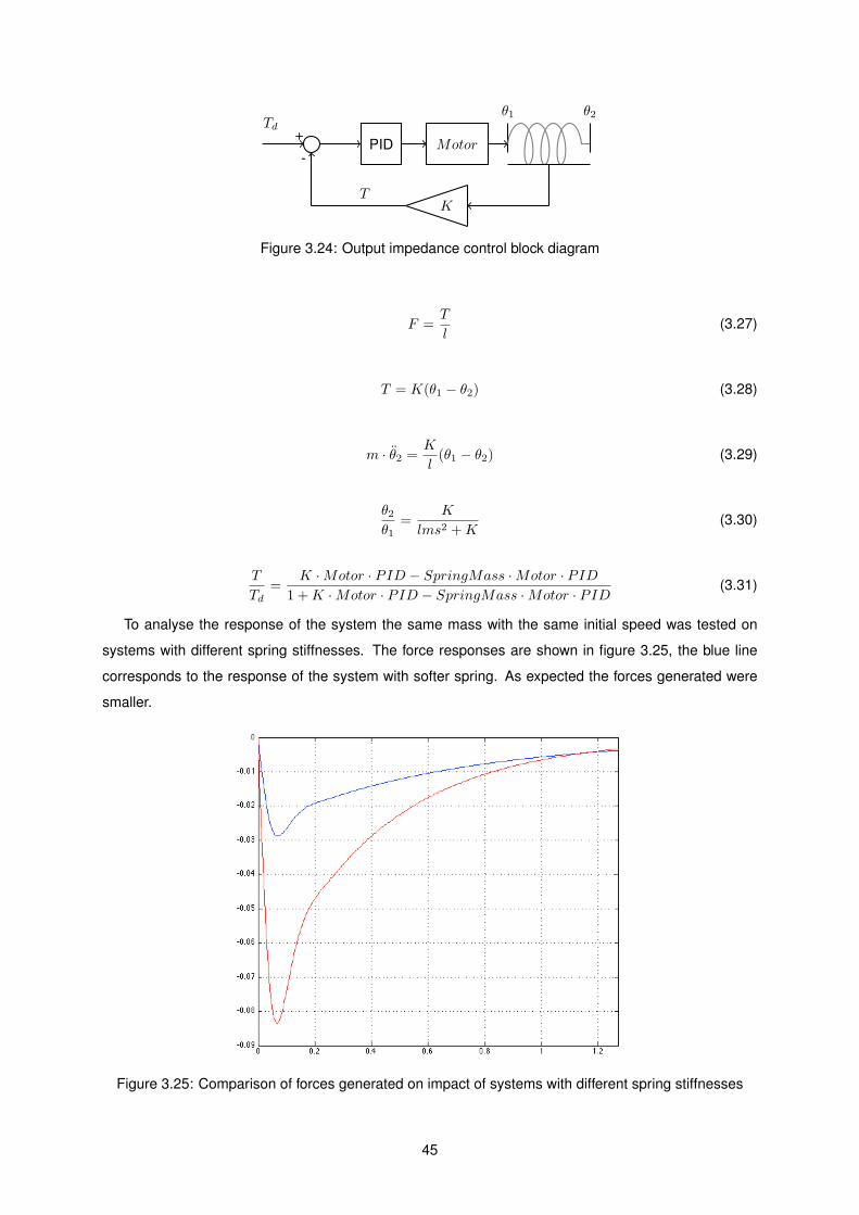
PID Motor

θ1 θ2

K

Td

T

+

-

Figure 3.24: Output impedance control block diagram

F =T

l(3.27)

T = K(θ1 − θ2) (3.28)

m · θ2 =K

l(θ1 − θ2) (3.29)

θ2θ1

=K

lms2 +K(3.30)

T

Td=

K ·Motor · PID − SpringMass ·Motor · PID1 +K ·Motor · PID − SpringMass ·Motor · PID

(3.31)

To analyse the response of the system the same mass with the same initial speed was tested on

systems with different spring stiffnesses. The force responses are shown in figure 3.25, the blue line

corresponds to the response of the system with softer spring. As expected the forces generated were

smaller.

Figure 3.25: Comparison of forces generated on impact of systems with different spring stiffnesses

45

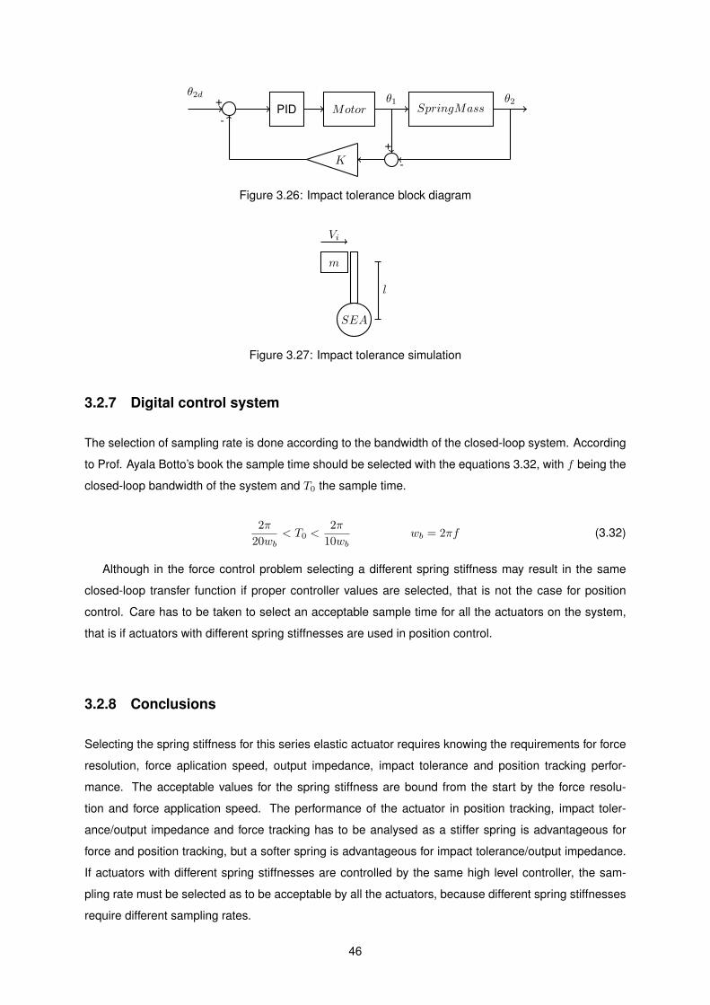
PID Motorθ1 θ2

SpringMass

θ2d

K

+

-

+

-

Figure 3.26: Impact tolerance block diagram

m

SEA

Vi

l

Figure 3.27: Impact tolerance simulation

3.2.7 Digital control system

The selection of sampling rate is done according to the bandwidth of the closed-loop system. According

to Prof. Ayala Botto’s book the sample time should be selected with the equations 3.32, with f being the

closed-loop bandwidth of the system and T0 the sample time.

2π

20wb< T0 <

2π

10wbwb = 2πf (3.32)

Although in the force control problem selecting a different spring stiffness may result in the same

closed-loop transfer function if proper controller values are selected, that is not the case for position

control. Care has to be taken to select an acceptable sample time for all the actuators on the system,

that is if actuators with different spring stiffnesses are used in position control.

3.2.8 Conclusions

Selecting the spring stiffness for this series elastic actuator requires knowing the requirements for force

resolution, force aplication speed, output impedance, impact tolerance and position tracking perfor-

mance. The acceptable values for the spring stiffness are bound from the start by the force resolu-

tion and force application speed. The performance of the actuator in position tracking, impact toler-

ance/output impedance and force tracking has to be analysed as a stiffer spring is advantageous for

force and position tracking, but a softer spring is advantageous for impact tolerance/output impedance.

If actuators with different spring stiffnesses are controlled by the same high level controller, the sam-

pling rate must be selected as to be acceptable by all the actuators, because different spring stiffnesses

require different sampling rates.

46

3.3 Servo Platform

To introduce elasticity in the servo shaft several possibilities were studied, the most important aspect of

the servo modification process was that the servos couldn’t change on the outside so that they would

fit and work on the robot just like they did before. For instance the work done by L.T.Martins et.al [15]

shown on figure 3.28 is not an option.

Figure 3.28: Dynamixel servo with the elastic element on the outside

The inside of a regular hobby servo or the dynamixel servos (figure 3.29) is already somewhat packet

and little space is left to work with, so a compact solution was required to be able to fit in the small

available space. The various options for adding elasticity to the output shaft of the servo were analysed

and will now be presented.

Figure 3.29: Inside the AX-12 Dynamixel servo

47

Using conductive foam

The output shaft of the servo is made “plastic” as described by robotis, plastic materials generally have

some elasticity to them although their mechanical behaviour under tension isn’t perfectly elastic. One of

the ideas was to weaken the shaft to reduce its cross sectional area so that it would deform the minimum

considerable ammount to make the SEA. This way the original shaft could be used and the stiffness

could be controlled by the ammount of material taken from the shaft. To measure the deformation of

the shaft a position sensor taken from another servo couldn’t be used because it wouldn’t be possible

to mount. The only way to mount a potentiometer from another servo is to cut the shaft an mount the

sensor in the middle because it’s a hollow shaft sensor and it’s inside diameter is smaller than that

of the gears at the end of the shaft, and after cutting the shaft it’s very difficult or even impossible

to rebuild it using only it’s own material. A larger hollow shaft sensor was considered but the only

one found that would fit was an iC-MU from iCHaus, this sensor is a chip that reads the position of a

magnetized track with integrated Hall sensors, the track this sensor reads is mountable on the dynamixel

shaft without destroying it. To implement this sensor a greatter effort would be needed because as just

stated, this sensor is a chip and it would require designing and manufacturing a circuit board to hold

it. Furthermore a communication protocol between the sensor and the ATMega microcontroller would

have to be developed. These reasons made the idea of implementing this sensor difficult and not easily

accomplishable during this thesis, and the fact that the material used has a far from linear tension-strain

behaviour and the results wouldn’t be readily usefull made this idea go back in the idea box to remain

just an idea.

Another way to measure the deformation of the shaft is using extensometers, but those need rela-

tively large signal conditioning hardware packages that for their size can’t be considered for this project.

Remember that each servo would have one extensometer, thus for the 12 servos of the legs 12 signal

conditioning boxes would have to be embedded on the robot.

A unconventional approach was tried, that was to use the conductive foam usually found on DIP

packaged chip boxes. The DIP package chips are to be installed on through hole PCBs so they have

considerable feet that need to be protected during shipment. Conductive foam protects the feet from

impact damage and static discharge by grounding all pins of the IC. Several times pressure sensors

were made by the academia and maker community because it’s a very cheap way to sense deformation.

Conductive foam changes it’s conductivity as it deforms, it’s a porous material so when it’s compressed

the density of the material increases and it’s conductivity decreases, the opposite happens when it’s

stretched. To measure the varying conductivity two conductive wires can be pierced into the material,

the deformation can then be measured by measuring the resistance across those wires.

To measure the deformation of the servo shaft with conductive foam the foam needs to be installed

such that deforming the shaft will always provoke measurable deformation on the foam. Since the shaft

had to be weakened, it could have a through cut where the foam could be installed, this way twisting

the shaft would make the foam twist aswell. But to abilitate distinguishing clockwise deformation from

counter-clockwise deformation the cut had to be done in an angle such that the foam is compressed

when the shaft is deformed to one side and stretched when the shaft is deformed to the other. The shaft

48

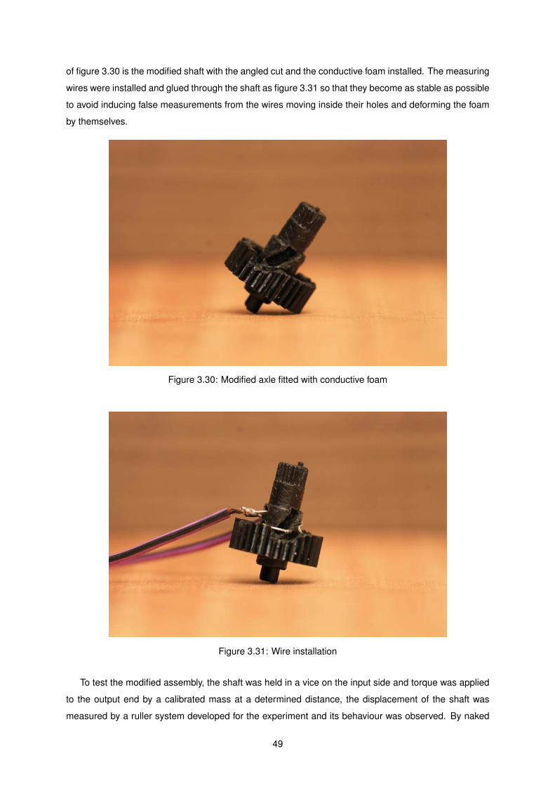
of figure 3.30 is the modified shaft with the angled cut and the conductive foam installed. The measuring

wires were installed and glued through the shaft as figure 3.31 so that they become as stable as possible

to avoid inducing false measurements from the wires moving inside their holes and deforming the foam

by themselves.

Figure 3.30: Modified axle fitted with conductive foam

Figure 3.31: Wire installation

To test the modified assembly, the shaft was held in a vice on the input side and torque was applied

to the output end by a calibrated mass at a determined distance, the displacement of the shaft was

measured by a ruller system developed for the experiment and its behaviour was observed. By naked

49

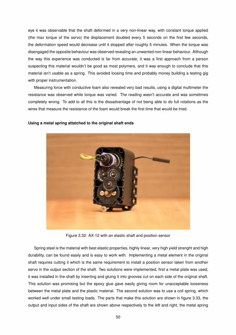
eye it was observable that the shaft deformed in a very non-linear way, with constant torque applied

(the max torque of the servo) the displacement doubled every 5 seconds on the first few seconds,

the deformation speed would decrease until it stopped after roughly 5 minutes. When the torque was

disengaged the opposite behaviour was observed revealing an unwanted non-linear behaviour. Although

the way this experience was conducted is far from accurate, it was a first approach from a person

suspecting this material wouldn’t be good as most polymers, and it was enough to conclude that this

material isn’t usable as a spring. This avoided loosing time and probably money building a testing gig

with proper instrumentation.

Measuring force with conductive foam also revealed very bad results, using a digital multimeter the

resistance was observed while torque was varied. The reading wasn’t accurate and was sometimes

completely wrong. To add to all this is the dissadvantage of not being able to do full rotations as the

wires that measure the resistance of the foam would break the first time that would be tried.

Using a metal spring attatched to the original shaft ends

Figure 3.32: AX-12 with an elastic shaft and position sensor

Spring steel is the material with best elastic properties, highly linear, very high yield strenght and high

durability, can be found easily and is easy to work with. Implementing a metal element in the original

shaft requires cutting it which is the same requirement to install a position sensor taken from another

servo in the output section of the shaft. Two solutions were implemented, first a metal plate was used,

it was installed in the shaft by inserting and gluing it into grooves cut on each side of the original shaft.

This solution was promising but the epoxy glue gave easily giving room for unacceptable looseness

between the metal plate and the plastic material. The second solution was to use a coil spring, which

worked well under small testing loads. The parts that make this solution are shown in figure 3.33, the

output and input sides of the shaft are shown above respectively to the left and right, the metal spring

50

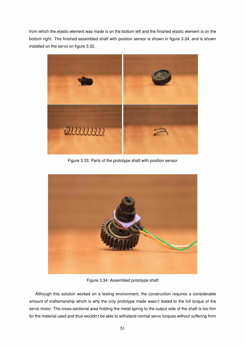
from which the elastic element was made is on the bottom left and the finished elastic element is on the

bottom right. The finished assembled shaft with position sensor is shown in figure 3.34, and is shown

installed on the servo on figure 3.32.

Figure 3.33: Parts of the prototype shaft with position sensor

Figure 3.34: Assembled prototype shaft

Although this solution worked on a testing environment, the construction requires a considerable

amount of craftsmanship which is why the only prototype made wasn’t tested to the full torque of the

servo motor. The cross-sectional area holding the metal spring to the output side of the shaft is too thin

for the material used and thus wouldn’t be able to withstand normal servo torques without suffering from

51

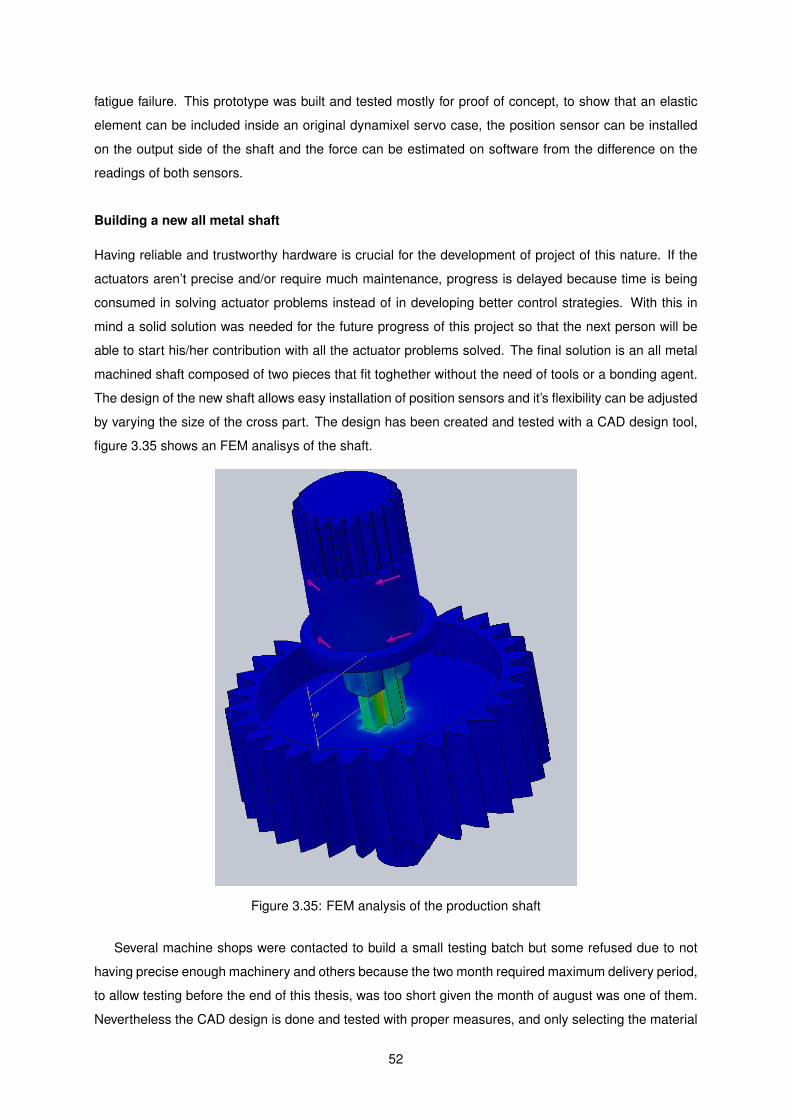
fatigue failure. This prototype was built and tested mostly for proof of concept, to show that an elastic

element can be included inside an original dynamixel servo case, the position sensor can be installed

on the output side of the shaft and the force can be estimated on software from the difference on the

readings of both sensors.

Building a new all metal shaft

Having reliable and trustworthy hardware is crucial for the development of project of this nature. If the

actuators aren’t precise and/or require much maintenance, progress is delayed because time is being

consumed in solving actuator problems instead of in developing better control strategies. With this in

mind a solid solution was needed for the future progress of this project so that the next person will be

able to start his/her contribution with all the actuator problems solved. The final solution is an all metal

machined shaft composed of two pieces that fit toghether without the need of tools or a bonding agent.

The design of the new shaft allows easy installation of position sensors and it’s flexibility can be adjusted

by varying the size of the cross part. The design has been created and tested with a CAD design tool,

figure 3.35 shows an FEM analisys of the shaft.

Figure 3.35: FEM analysis of the production shaft

Several machine shops were contacted to build a small testing batch but some refused due to not

having precise enough machinery and others because the two month required maximum delivery period,

to allow testing before the end of this thesis, was too short given the month of august was one of them.

Nevertheless the CAD design is done and tested with proper measures, and only selecting the material

52

and the size of the cross section of the shaft is left to do before ordering a batch. The material selection

wasn’t done because the availability of good steels for the elastic part may be limited and expensive as

the selected steel would have to be adequate for a spring. Not every shop has the availability to make

parts like this, a specific material may be hard to find at a good price and some materials are harder

to work with than others which would result in different prices at the machine shop. Thus the material

selection was left to be done when machine shops and steel retailers are contacted and the material

that offers the highest quality/price ratio is found. Then the size of the elastic part of the shaft can be

ajusted to get the right spring stiffness. The focus on choosing the steel can be reduced to choosing

a steel that fulfills the spring part requirements, good fatigue strenght specially, because the rest of the

shaft is replacing a part that was made of a weak polymeric material that withstood the stresses without

any problem.

53

54

Chapter 4

Conclusions

In this thesis a whole new robot control framework was developed, it makes use of parallel processing

and acheives high performance by distributing the tasks throughout various computational agents. The

distribution of the tasks was done such that the data flow and sample-rate of the control system are

optimized. By using of the shelf and already in house hardware components the architecture of the

system was moulded by the capabilities of the components but still allowing to achieve much better

performance than anything previously in this project. A deterministic hard real-time control system with

consistent sample time was achieved with variable sampling frequency of up to 200Hz.

The voltage converter and quad-buffer/line driver was designed, built and tested by me, and revealed

to be reliable with zero failures or faulty data transactions observed. This piece of hardware was needed

because the Dynamixel servos use these chips but they don’t add latency to the communication.

An all new servo software was developed from scratch to replace the old cumbersome software.

The new software relies on internal and external interrupts to time and syncronize the tasks, achieving

deterministic time response from the servos.

The possibilities to modify the AX-12 dynamixel servos to series elastic actuators were exploited and

evaluated. Several options were analysed and the best revealed to be to build an all new metal shaft with

the elastic element built into itself. The performance of the SEA was evaluated and the choice of spring

stiffness was explored, the allowed spring stiffness value is restricted by the precision of the position

sensor and the speed at which force needs to be applied. In between those values a stiffer spring will

give a faster actuator and a softer spring will give a more compliant actuator, the selection must be done

according to the application case after simulations of the working system are done and the requirements

for the actuator are determined.

4.1 Future Work

Left out of this thesis was the testing with the final metal shaft/elastic element without which made it

impossible to test the real performance of the series elastic actuator. The full project for the shaft is

done and ready to be built so that is the next step.

55

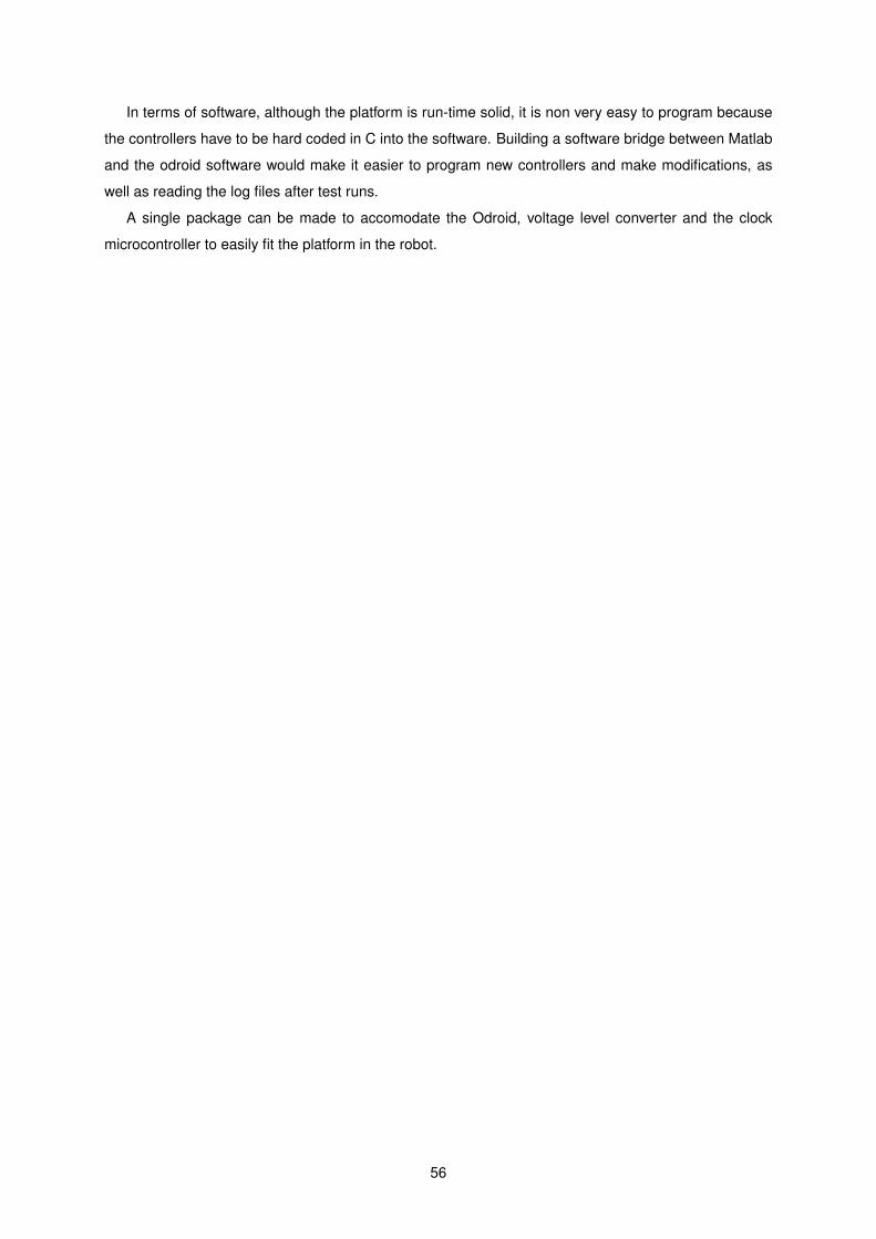
In terms of software, although the platform is run-time solid, it is non very easy to program because

the controllers have to be hard coded in C into the software. Building a software bridge between Matlab

and the odroid software would make it easier to program new controllers and make modifications, as

well as reading the log files after test runs.

A single package can be made to accomodate the Odroid, voltage level converter and the clock

microcontroller to easily fit the platform in the robot.

56

Bibliography

[1] An232b-04 data throughput, latency and handshaking, 2006.

www.ftdichip.com/Support/Documents/AppNotes/AN232B-04 DataLatencyFlow.pdf.

[2] Avr523: Migration from atmega8 to atmega8a, 2009. http://www.atmel.com/Images/AVR523.pdf.

[3] Rt patch wiki, 2012. rt.wiki.kernel.org/index.php/Main Page.

[4] The biotac from syntouch, 2015. http://www.syntouchllc.com/Products/BioTac/.

[5] Optimal actuator, 2015. https://biomimetics.mit.edu/research/optimal-actuator.

[6] Top 10 linux and android hacker sbcs of 2015, 2015. www.linux.com/news/embedded-

mobile/mobile-linux/834861-top-10-linux-and-android-based-hacker-sbcs-of-2015.

[7] B. Siciliano L. Villani A. De Santis, V. Lippiello. Advances in Control Theory and Applications,

Lecture Notes in Control and Information Sciences, chapter Human-robot interaction control using

force and vision.

[8] A.J.Ijspeert and J. Kodjabachian. Evolution and development of a central pattern generator for the

swimming of a lamprey. Department of Artificial Intelligence, University of Endinburgh, 1998.

[9] Miguel Ayala Botto. Controlo de Sistemas. IST Press, 2009.

[10] R. Muller et.al. Preparing the leg for ground contact in running: The contribution of feedforward and

visual feedback. The Journal of Experimental Biology, 2015.

[11] Francisco Ferreira. Development of a human walking model comprising springs and positive force

feedback to generate stable gait. Master’s thesis, Instituto Superior Tecnico, 2013.

[12] G.A.Pratt. Low impedance walking robots. Oxford Integrative and Comparative Biology, 2002.

[13] K.Althoefer H.Yousefa, M.Boukallela. Tactile sensing for dexterous in-hand manipulation in robotics

- a review. Sensors and Actuators A: Physical, 2011.

[14] H.Herr J.A.Blaya. Adaptive control of a variable-impedance ankle-foot orthosis to assist drop-foot

gait. IEEE Transactions on Neural Systems and Rehabilitation Engineering, 2004.

[15] Leandro Tome Martins, Roberta de Mendonca Pretto, Reinhard Gerndt, and Rodrigo

da Silva Guerra. Design of a modular series elastic upgrade to a robotics actuator. 2014.

57

[16] T.Siedel M.Hild and T.Geppert. Design of a passive, bidirectional overrunning clutch for rotary joints

of autonomous robots. Intelligent Robotics and Applications: 4th International Conference,ICIRA

2011, 2011.

[17] M.Laffranchi D.G.Caldwell Nikos G.Tsagarakis, B.Vanderborght. The mechanical design of the new

lower body for the child humanoid robot ’icub’. Intelligent Robots and Systems, 2009.

[18] P.Sardain and G.Bessonnet. Forces acting on a biped robot. center of pressure - zero moment

point. IEEE Transactions on Systems, Man and Cybernetics, 2004.

[19] Tiago Rato. Actuated character - humanoid robots for videogames interaction. Master’s thesis,

Instituto Superior Tecnico, 2012.

[20] David William Robinson. Design and Analysis of Series Elasticity in Closed-loop Actuator Force

Control. PhD thesis, Massachusetts Institute of Technology, 2000.

[21] R.Tedrake M.Wisse S.Collins, A.Ruina. Efficient bipedal robots based on passive-dynamic walkers.

Science Magazine, 2005.

[22] Sangok Seok. Highly Parallelized Control Programming Methodologies using Multicore CPU and

FPGA for Highly Dynamic Multi-DoF Mobile Robots, Applied to the MIT Cheetah. PhD thesis,

Massachusetts Institute of Technology, 2014.

[23] Pedro Teodoro. Humanoid robot - development of a simulation environment of an entertainment

humanoid robot. Master’s thesis, Instituto Superior Tecnico, 2007.

[24] M.Panne T.Geijtenbeek and A.F.Stappen. Flexible muscle-based locomotion for bipedal creatures.

ACM Transactions on Graphics, 2013.

58

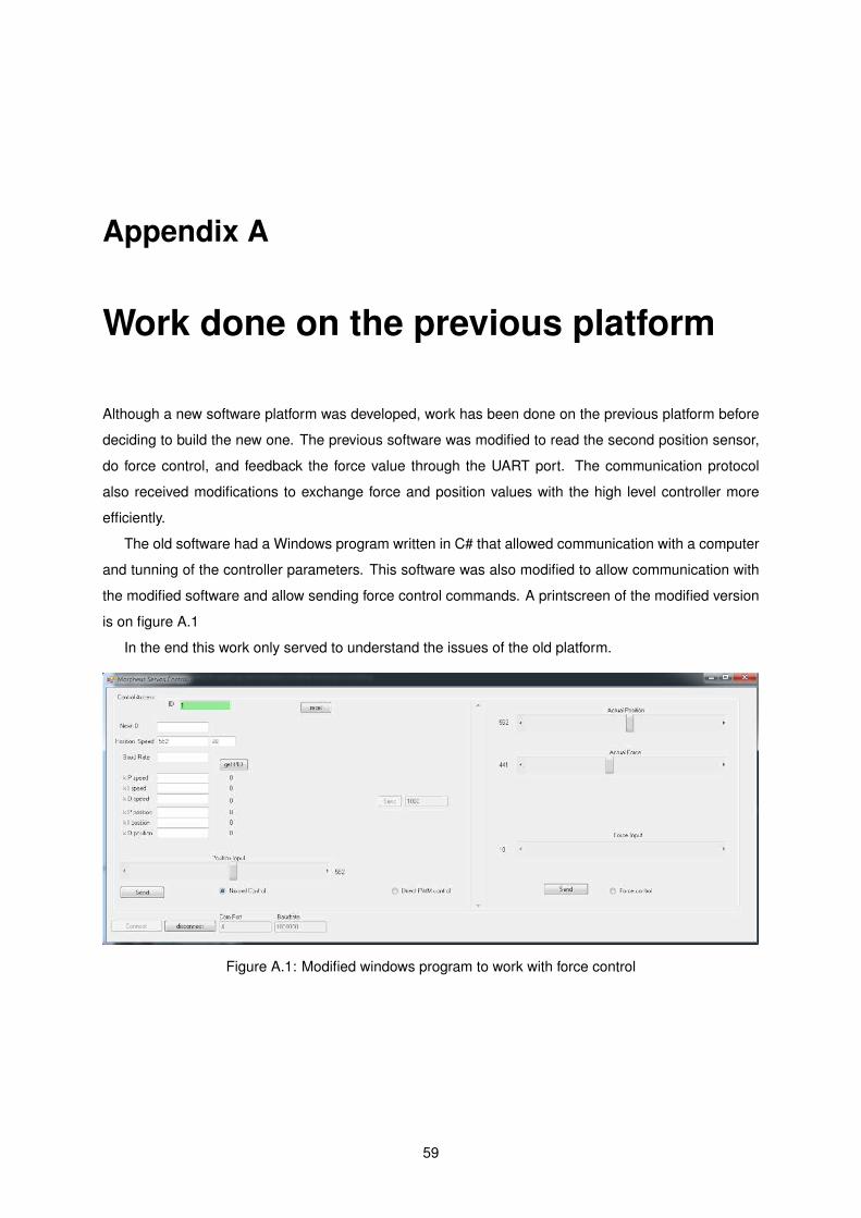
Appendix A

Work done on the previous platform

Although a new software platform was developed, work has been done on the previous platform before

deciding to build the new one. The previous software was modified to read the second position sensor,

do force control, and feedback the force value through the UART port. The communication protocol

also received modifications to exchange force and position values with the high level controller more

efficiently.

The old software had a Windows program written in C# that allowed communication with a computer

and tunning of the controller parameters. This software was also modified to allow communication with

the modified software and allow sending force control commands. A printscreen of the modified version

is on figure A.1

In the end this work only served to understand the issues of the old platform.

Figure A.1: Modified windows program to work with force control

59

Appendix B

Technical Drawing of the new shaft

60

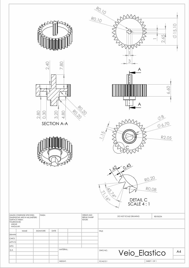
6,6

0

A

A

15

,10

2,6

5

1

1

3

R0,10 R0,10

6,70 8

R2,05 1,1

5

C

7,8

0

2,4

0

2,8

0 0

,30

4,8

0

3,2

0

R0,20 R0,20

SECTION A-A

45,74°

71,16°

R0,08

R0,20 1,62 0,45

DETAIL C SCALE 4 : 1

Veio_ElasticoWEIGHT:

A4

SHEET 1 OF 1SCALE:2:1

DWG NO.

TITLE:

REVISIONDO NOT SCALE DRAWING

MATERIAL:

DATESIGNATURENAME

DEBUR AND BREAK SHARP EDGES

FINISH:UNLESS OTHERWISE SPECIFIED:DIMENSIONS ARE IN MILLIMETERSSURFACE FINISH:TOLERANCES: LINEAR: ANGULAR:

Q.A

MFG

APPV'D

CHK'D

DRAWN

8,

40

8

6,

80

92°

5,

60 3,40

R2,90 R0,05

0,2

0 R0,20 0

,80

4,9

0

4,2

0 40°

R0,10

0,1

0

R2

8,

40

1

1

R0,10

R0,10 1,1

5

Veio_SaidaWEIGHT:

A4

SHEET 1 OF 1SCALE:5:1

DWG NO.

TITLE:

REVISIONDO NOT SCALE DRAWING

MATERIAL:

DATESIGNATURENAME

DEBUR AND BREAK SHARP EDGES

FINISH:UNLESS OTHERWISE SPECIFIED:DIMENSIONS ARE IN MILLIMETERSSURFACE FINISH:TOLERANCES: LINEAR: ANGULAR:

Q.A

MFG

APPV'D

CHK'D

DRAWN