ANNUAL TRANSACTIONS OF THE NORDIC RHEOLOGY SOCIETY, VOL. 17, 2009

ABSTRACT The present article describes analy-tically the feasibility of a capillary system that performs direct measurements of pressure in the capillary. Different alternatives are described and the system limitations are given. This article precedes an experimental article that shows the application of the new rheometer measuring liver paste. INTRODUCTION In capillary rheometry a large pressure drop is commonly associated with the flow in the die entrance (major) and exit (minor) regions1. Today, pressure in capillary rheometers using cylindrical die holes is measured in the reservoir above the capillary die, entrance and exit pressure corrections must be performed to estimate the “true” pressure drop along the capillary die (i.e. Bagley procedure). By measuring the pressure drop (ΔP) between two points in the capillary, it is possible to directly calculate the shear stress at the wall (τw) that is a requisite to determine rheological properties. Consequently pressure entry and exit corrections would no longer be required. The Bagley procedure requires a number of tests that uses different length to diameter (L/D) ratios at different shear rates. This results in a large number of

experiments that are required to determine the rheological properties of a fluid (e.g. flow behaviour index (n) and consistency index (K)). Once n is estimated, the shear rate at the wall ( ) can be calculated. Sombatsompop and Intawong2 describes a number of researchers finding such corrections as very difficult to use because: (i) the extension of the imaginary length of the dies (N) and pressure values vary with shear rate, (ii) non-linearity of the correction curve, (iii) N depends on the ratio barrel to die diameter, (iv) negative N values and (v) the method to determine N value is experimental, and thus difficult to utilize the process for calculations. The present article describes two alternative measurement principles to directly measure ΔP and hence τw. In addition, the system limitations are given and CFD calculations are performed to see whether the insertions of sensors in the capillary will affect the flow conditions or not. This article precedes a comparative analysis using direct measurements of ΔP in the capillary and pressure drop corrections using different L/D ratios. Commercial liver paste was the process fluid3. DESIGN FEATURES The capillary rheometer shown on Fig. 1, is designed to be connected to a Lloyd LR50KPlus 50 KN texture analyzer (Lloyd

Development of a New Capillary Rheometer that uses

Direct Pressure Measurements in the Capillary Carlos Salas-Bringas1, Odd-Ivar Lekang1, Elling Olav Rukke2, and Reidar Barfod Schüller2

1 Dep. Of Mathematical Sciences and Technology, Norwegian University of Life Sciences, P.O. Box 5003, N-1432 Ås, Norway

2 Dep. Of Chemistry, Biotechnology and Food Science, Norwegian University of Life Sciences, P.O. Box 5003, N-1432 Ås, Norway

w

.γ

Instruments Ltd, Meerbusch, Germany) by the RAM (1) and a connector (7). Assemblies into other texture analyzers can be done by customizing the mentioned connectors; items (1) and (7).

Figure 1. General description of the

capillary rheometer. Items are indicated by numbers: (1) RAM, (2) piston, (3) barrel, (4)

capillary die, (5) feed collector, (6) load cell, (7) bottom connector, (8), (9) and (11) are the location of pressure measurements

and (10) entry zone.

The rheometer uses a piston (2) to compress and force semi-solid materials to flow through a capillary die. Estimations of pressure in the barrel (3) are possible by measuring the force on the piston in relation to its compressing surface (1.948·10-3 m3). In addition, a pressure sensor (Dynisco PT467E-1/2/5C-10/18, Franklin MA, USA) is flush mounted in the location of item (11) on Fig. 1. The volumetric flow rate of material can be estimated in two ways; through the displacement in the piston by neglecting any leakage in the clearance between piston (2) and barrel (3), or by mass flow rate measurements through a load cell (6) (Tedea Huntleigh 1042, Chatsworth Ca, USA). The density of the fluid must be previously

determined to obtain the true volumetric flow rate. Details from the capillary die are given on Fig. 2 where: item (8) and (9) indicates the location of the pressure measurements. One of the alternatives to obtain τw is to use sub-miniature pressure sensors (e.g. EPI-B0, Entran Ltd, Northants, Eng.). Another solution is to use a differential pressure sensor (e.g. Fuji FCX-CII) that could be either connected through a nozzle–pin configuration (see Fig. 3) or through a membrane as similarly used by the sub-miniature pressure sensors shown in Fig. 2 (item 12). This system can use an incompressible Newtonian fluid to transfer the pressure to the differential sensor’s membrane.

Figure 2. Detailed view of die section. Items

are indicated by numbers: (8) and (9) location pressure sensors, (12) membrane

pressure sensors and (13) capillary channel. Dimensions are in millimetres.

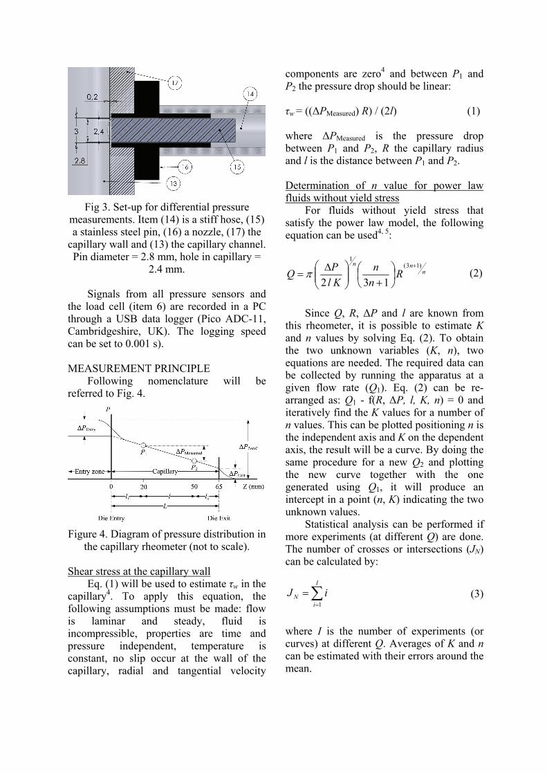
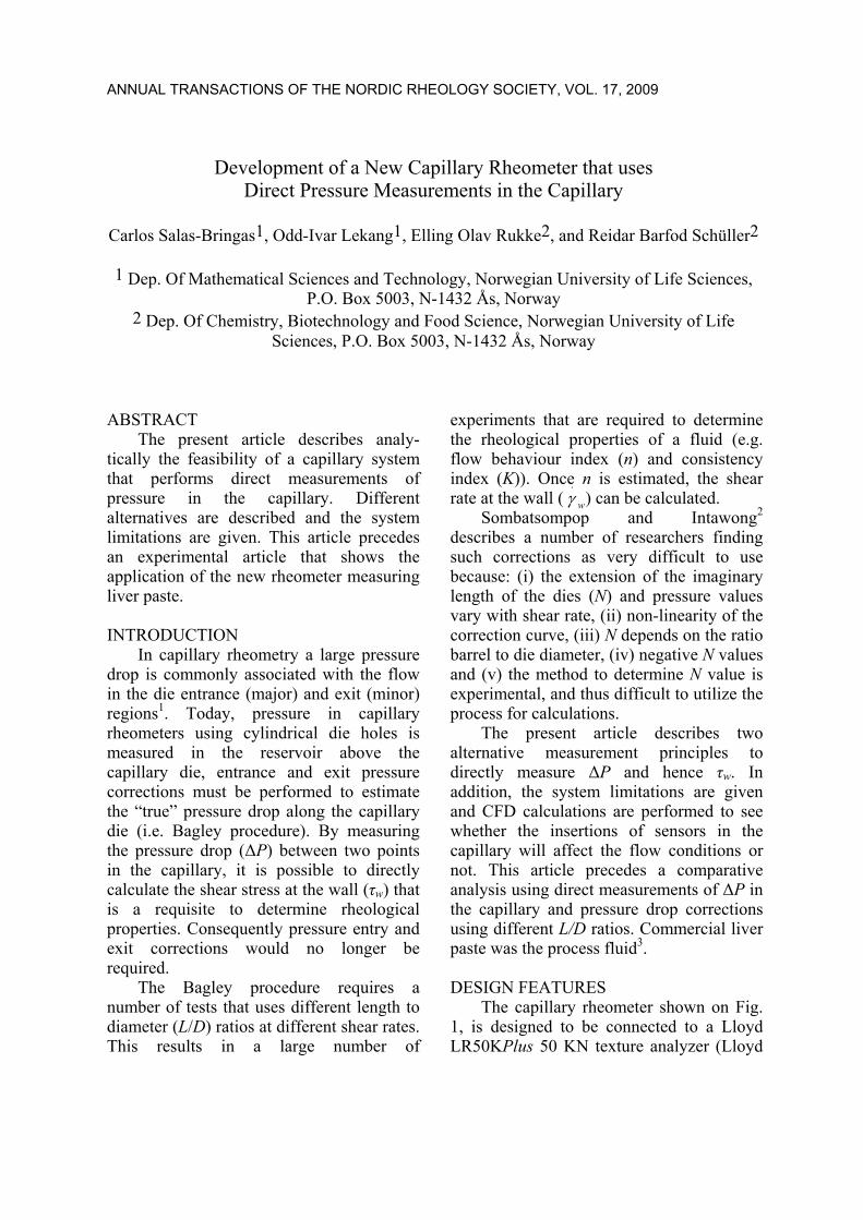
Fig 3. Set-up for differential pressure measurements. Item (14) is a stiff hose, (15) a stainless steel pin, (16) a nozzle, (17) the

capillary wall and (13) the capillary channel. Pin diameter = 2.8 mm, hole in capillary =

2.4 mm. Signals from all pressure sensors and the load cell (item 6) are recorded in a PC through a USB data logger (Pico ADC-11, Cambridgeshire, UK). The logging speed can be set to 0.001 s). MEASUREMENT PRINCIPLE Following nomenclature will be referred to Fig. 4.

Figure 4. Diagram of pressure distribution in the capillary rheometer (not to scale).

Shear stress at the capillary wall Eq. (1) will be used to estimate τw in the capillary4. To apply this equation, the following assumptions must be made: flow is laminar and steady, fluid is incompressible, properties are time and pressure independent, temperature is constant, no slip occur at the wall of the capillary, radial and tangential velocity

components are zero4 and between P1 and P2 the pressure drop should be linear: τw = ((ΔPMeasured) R) / (2l) (1) where ΔPMeasured is the pressure drop between P1 and P2, R the capillary radius and l is the distance between P1 and P2. Determination of n value for power law fluids without yield stress For fluids without yield stress that satisfy the power law model, the following equation can be used4, 5:

nnn

Rnn

KlPQ

)13(1

132

+

⎟⎠⎞

⎜⎝⎛

+⎟⎟⎠

⎞⎜⎜⎝

⎛ Δ= π (2)

Since Q, R, ΔP and l are known from

this rheometer, it is possible to estimate K and n values by solving Eq. (2). To obtain the two unknown variables (K, n), two equations are needed. The required data can be collected by running the apparatus at a given flow rate (Q1). Eq. (2) can be re-arranged as: Q1 - f(R, ΔP, l, K, n) = 0 and iteratively find the K values for a number of n values. This can be plotted positioning n is the independent axis and K on the dependent axis, the result will be a curve. By doing the same procedure for a new Q2 and plotting the new curve together with the one generated using Q1, it will produce an intercept in a point (n, K) indicating the two unknown values. Statistical analysis can be performed if more experiments (at different Q) are done. The number of crosses or intersections (JN) can be calculated by:

∑=

=I

iN iJ

1 (3)

where I is the number of experiments (or curves) at different Q. Averages of K and n can be estimated with their errors around the mean.

Yield stress determination The yield stress (τ0) can be determined by a stress relaxation test. This test requires compressing the material and forcing it to flow through the die. Once this occurs it is possible to stop the piston (ref. item (2) on Fig. 1) and to record the pressure difference from the measuring points (8, 9 ref. Fig. 1) when a minimum value ΔPmin is reached. The yield stress is calculated from a force balance on the fluid as4:

LRP

2min

0Δ

=τ (4)

Bingham plastic fluids For these fluids, the Buckingham-Reiner equation for flows in a pipe can be used4:

⎥⎥⎦

⎤

⎢⎢⎣

⎡⎟⎟⎠

⎞⎜⎜⎝

⎛⎟⎠⎞

⎜⎝⎛+⎟⎟

⎠

⎞⎜⎜⎝

⎛⎟⎠⎞

⎜⎝⎛−

⎟⎟⎠

⎞⎜⎜⎝

⎛ Δ=

4

00

4

31

341

8)(

ww

pl lQPR

ττ

ττ

πμ

(5)

where µpl is the plastic viscosity and τ0 yield stress. By determining Q, R, ΔP, l, τ0 and τw, is possible to obtain µpl by performing one experiment at a selected flow rate. Herschel-Bulkley fluids Different equations to estimate the volumetric flow rate of a laminar flow of a Herschel-Bulkley fluid in a circular pipe are given on different literature (Eq. (6)5, Eq. (7)6 and Eq. (8)4) where:

⎥⎥⎥⎥

⎦

⎤

⎢⎢⎢⎢

⎣

⎡

+

⎟⎠⎞⎜

⎝⎛

++

⎟⎠⎞⎜

⎝⎛ −⎟⎠⎞⎜

⎝⎛

++

⎟⎠⎞⎜

⎝⎛ −

⎟⎟⎠

⎞⎜⎜⎝

⎛−⎟

⎠⎞

⎜⎝⎛=

+

112

12

13

1

1

2000

20

1

0

13

nnn

KnRQ

wwww

nn

w

nw

ττ

ττ

ττ

ττ

τττπ

(6)

( )⎥⎥⎦

⎤

⎢⎢⎣

⎡⎥⎦

⎤⎢⎣

⎡⎟⎟⎠

⎞⎜⎜⎝

⎛+⎟⎟

⎠

⎞⎜⎜⎝

⎛+

++

−

⎟⎟⎠

⎞⎜⎜⎝

⎛−⎟

⎠⎞

⎜⎝⎛⎟⎠⎞

⎜⎝⎛

+⎟⎟⎠

⎞⎜⎜⎝

⎛=

ww

w

n

w

nw

nn

nn

KnnRQ

ττ

ττττ

τττπ

000

1

013

11

2112

1

113

4256 (8)

The unknown variables in this system are K and n. K and n can be determined following the same procedure described to solve Eq. (2). A plot using this method can be found in Rukke et al.3 Diameter of the plug for fluids with yield stress A plug can be formed in the centre of the capillary when the shear stress τ is smaller than the yield stress, τ0. Determining τ0 and τw, the diameter of the plug (Dp) in the centre of the capillary can be easily estimated as follows5:

wp

RDττ 02

= (9)

RANGE OF OPERATION The range of operation can be seen in Fig. 5, which is made using Eq. (1) for shear stress and for shear rate = (4Q)/(πR3) when n = 1 (Newtonian fluids). The plot presents different values for a capillary of radius 0.003 m.

Figure 5. Differential pressure at different viscosities (Newtonian fluid) and shear

rates. Distance between sensors is set to 30 mm). (7)

( )

⎥⎥⎦

⎤

⎢⎢⎣

⎡

++

+⎟⎠⎞

⎜⎝⎛ −

Δ+

+⎟⎠⎞

⎜⎝⎛ −

Δ

⎟⎠⎞

⎜⎝⎛ −

Δ⎟⎠⎞

⎜⎝⎛ Δ

=+−

−

11222

132

22

2000

2

0

1

0

313

nn

nn

lPR

nn

lPR

lPR

lPRKRQ

nn

n

ττττ

τπ

w

.γ

w

.γ

SENSOR INSTALLATION AND SOURCES OF ERROR A number of sources of error are given in literature for tube viscoemeters4, they are analyzed for our system from die entry to exit. Additionally CFD calculations are performed to see the magnitude of the flow disturbance given by the pressure measurements in the capillary. Entry angle and elongational flow The die entry was designed to have a gradual (curved) reduction of the entry angle (clearly seen on Fig. 2). Consequently, a small entry angle is made in the last entry section to facilitate the velocity development of the fluid, since the fluid should be fully developed when reaches the first pressure sensor in the capillary (P1 in Fig. 4). Mitsoulis and Hatzikiriakos1 found that excess pressure loss decreases for the same apparent shear rate with increasing contraction angle from 10° to about 45°, and consequently slightly increases from 45° up to contraction angles of 150°. They discovered that shear is the dominant factor controlling the overall pressure drop in flows through small contraction angles. At higher contraction angles (> 45°) elongation becomes important1. Excess pressure loss and elongation are intended to be avoided with our die setup. As seen in Fig. 6, contraction angles 2α < 43.87° are present from 20 mm above the capillary entry. This can be estimated by the equation of a tangent line at the point (x1, y1) to a circle of radius r cantered at the origin where:

θtan1

1 =−

=yx

xdyd (10)

Figure 6. Entry angle. Dimensions are in millimetres.

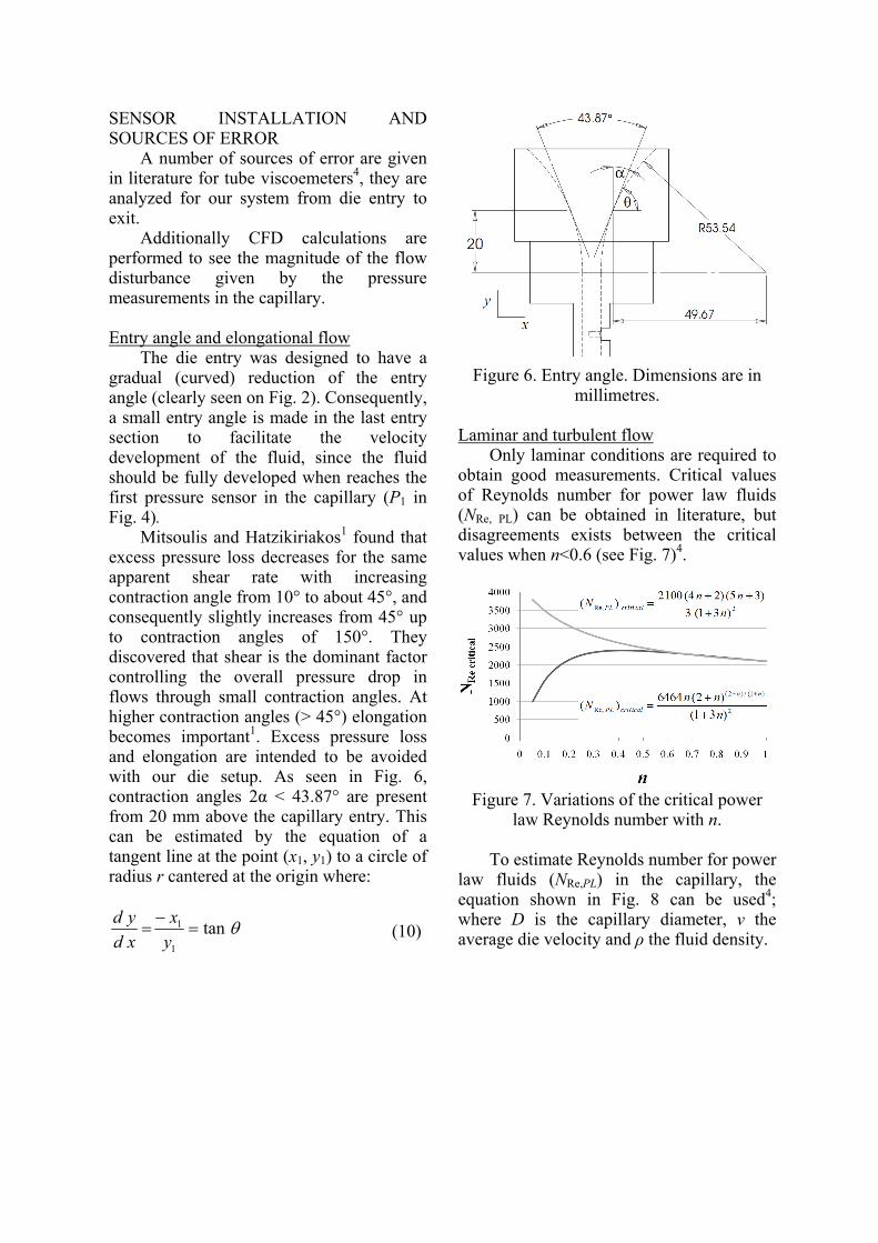
Laminar and turbulent flow Only laminar conditions are required to obtain good measurements. Critical values of Reynolds number for power law fluids (NRe, PL) can be obtained in literature, but disagreements exists between the critical values when n<0.6 (see Fig. 7)4.

Figure 7. Variations of the critical power law Reynolds number with n.

To estimate Reynolds number for power law fluids (NRe,PL) in the capillary, the equation shown in Fig. 8 can be used4; where D is the capillary diameter, v the average die velocity and ρ the fluid density.

Figure 8. Variation of Reynolds number for different power law, times the consistency

index (K) divided by the density (ρ) at different die velocities (mm/s). The plot

considers D = 0.006 m.

Entry length Measurement problems due to the loss

of effective pressure at the entry (ref. Fig. 4, ΔPEntry), can be avoided by inserting the pressure sensors (P1 and P2) far from the entry (l1), in the region where pressure decreases linearly.

It is mandatory that the flow at P1 is fully developed, thus the velocity of the fluid in the center of the capillary should be constant between P1 and P2. Today it is possible to find a relatively large number of equations that estimates entry lengths for inelastic Non-Newtonian liquids7-14. Recently in 2007, Pooley and Ridley15, developed a model based on an extensive analysis of entry lengths for inelastic non-Newtonian flows using previous models7-14, their model is only valid for power law indices 0.4<n<1.5. This model is presented in Eq. (11) and plotted on Fig. 9.

( )( )

6.1/1

6.1Re,

6.121

0567.0

03.1675.0246.0

⎥⎥⎦

⎤

⎢⎢⎣

⎡ ++−=

PLN

nnDl

(11)

It was decided to use an entry length (Le or l1) of 20 mm (l1/D = 3.33) which requires NRe,PL < 53.2 for n = 0.4 and NRe,PL < 56.5 for n = 1.5 (ref. Eq. (11)).

Figure 9. Entry length for different die diameters, n values and Reynolds numbers

for inelastic power law fluids. One of the inevitable sources of error in capillary rheometers, occur when strongly elastic behaviours are present in the fluid. Consequently, a full relaxation will not occur in the transit through the capillary. One way of assessing the extension of the elastic behaviour in our system is by performing the stress relaxation test that was previously described. Exit effects By keeping a distance of P2 from the die exit (l2), it is possible to avoid the effects of the energy losses caused by the viscous or elastic behavior. It was decided to use l2 = 15 mm to asses P2 which is expected to be far from the exit effects. Exit effects are considered to be smaller than entry effects1. Pressure estimation from force on the piston It is likely to obtain over estimations of pressure by calculating pressure from the piston force16. The main problem is caused by the friction generated by the material that is located in the clearance piston-barrel. The present piston has two flights with sharp edges ((17) and (18) in Fig. 10) to reduce the friction area to a minimum ((19) in Fig. 3).

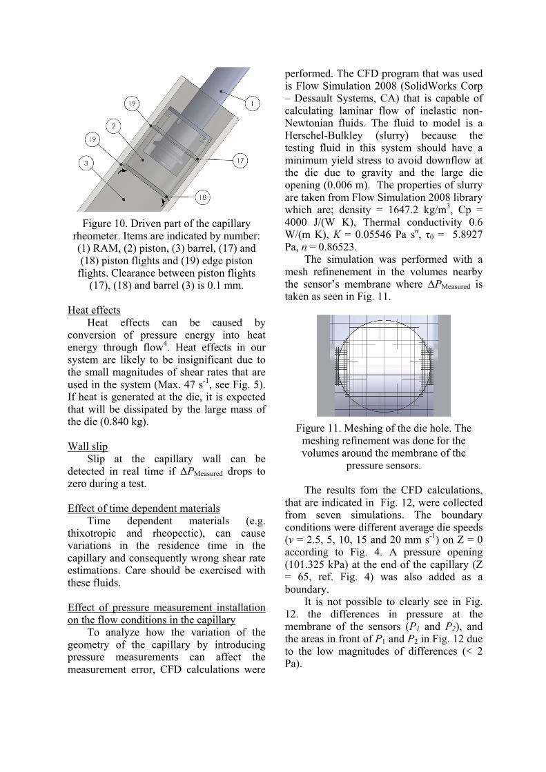
Figure 10. Driven part of the capillary rheometer. Items are indicated by number: (1) RAM, (2) piston, (3) barrel, (17) and (18) piston flights and (19) edge piston

flights. Clearance between piston flights (17), (18) and barrel (3) is 0.1 mm.

Heat effects Heat effects can be caused by conversion of pressure energy into heat energy through flow4. Heat effects in our system are likely to be insignificant due to the small magnitudes of shear rates that are used in the system (Max. 47 s-1, see Fig. 5). If heat is generated at the die, it is expected that will be dissipated by the large mass of the die (0.840 kg). Wall slip Slip at the capillary wall can be detected in real time if ΔPMeasured drops to zero during a test. Effect of time dependent materials Time dependent materials (e.g. thixotropic and rheopectic), can cause variations in the residence time in the capillary and consequently wrong shear rate estimations. Care should be exercised with these fluids. Effect of pressure measurement installation on the flow conditions in the capillary To analyze how the variation of the geometry of the capillary by introducing pressure measurements can affect the measurement error, CFD calculations were

performed. The CFD program that was used is Flow Simulation 2008 (SolidWorks Corp – Dessault Systems, CA) that is capable of calculating laminar flow of inelastic non-Newtonian fluids. The fluid to model is a Herschel-Bulkley (slurry) because the testing fluid in this system should have a minimum yield stress to avoid downflow at the die due to gravity and the large die opening (0.006 m). The properties of slurry are taken from Flow Simulation 2008 library which are; density = 1647.2 kg/m3, Cp = 4000 J/(W K), Thermal conductivity 0.6 W/(m K), K = 0.05546 Pa sn, τ0 = 5.8927 Pa, n = 0.86523. The simulation was performed with a mesh refinenement in the volumes nearby the sensor’s membrane where ΔPMeasured is taken as seen in Fig. 11.

Figure 11. Meshing of the die hole. The meshing refinement was done for the volumes around the membrane of the

pressure sensors. The results fom the CFD calculations, that are indicated in Fig. 12, were collected from seven simulations. The boundary conditions were different average die speeds (v = 2.5, 5, 10, 15 and 20 mm s-1) on Z = 0 according to Fig. 4. A pressure opening (101.325 kPa) at the end of the capillary (Z = 65, ref. Fig. 4) was also added as a boundary. It is not possible to clearly see in Fig. 12. the differences in pressure at the membrane of the sensors (P1 and P2), and the areas in front of P1 and P2 in Fig. 12 due to the low magnitudes of differences (< 2 Pa).

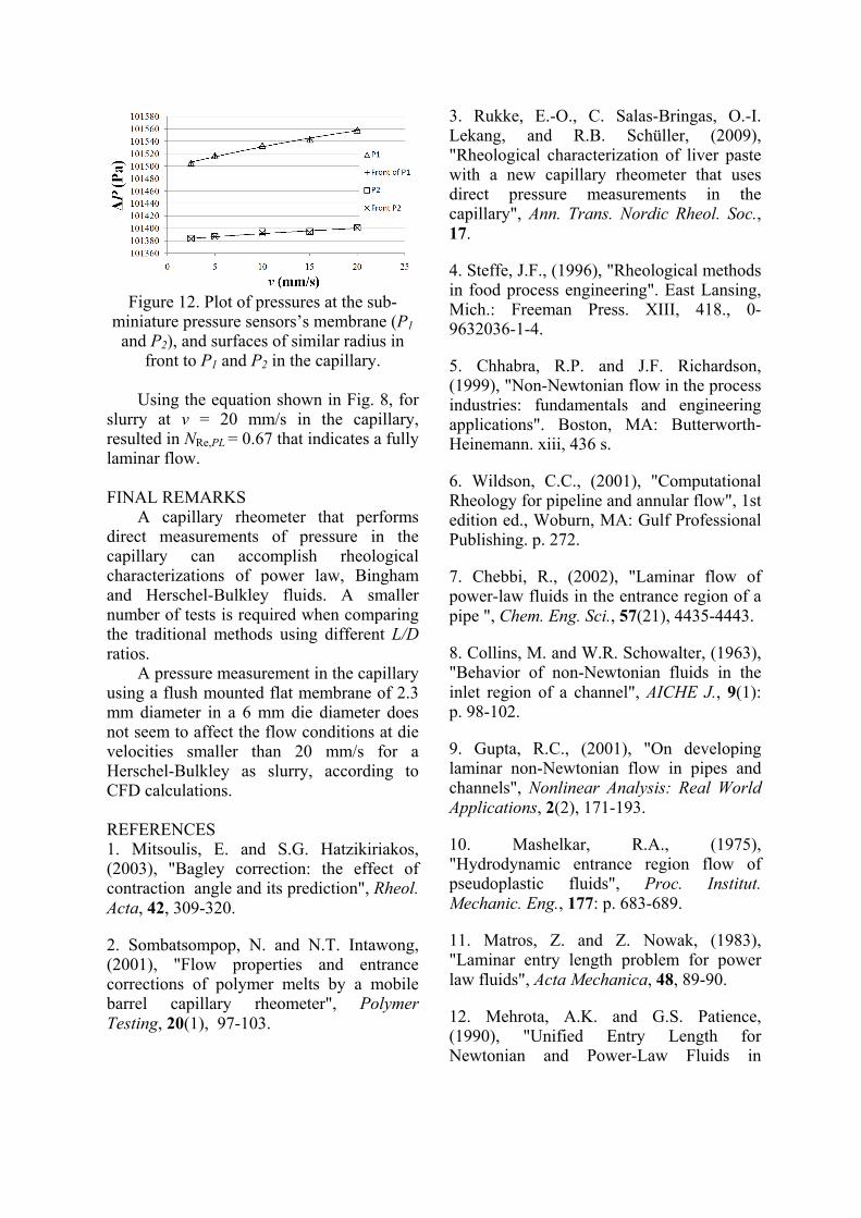
Figure 12. Plot of pressures at the sub-

miniature pressure sensors’s membrane (P1 and P2), and surfaces of similar radius in

front to P1 and P2 in the capillary.

Using the equation shown in Fig. 8, for slurry at v = 20 mm/s in the capillary, resulted in NRe,PL = 0.67 that indicates a fully laminar flow. FINAL REMARKS

A capillary rheometer that performs direct measurements of pressure in the capillary can accomplish rheological characterizations of power law, Bingham and Herschel-Bulkley fluids. A smaller number of tests is required when comparing the traditional methods using different L/D ratios.

A pressure measurement in the capillary using a flush mounted flat membrane of 2.3 mm diameter in a 6 mm die diameter does not seem to affect the flow conditions at die velocities smaller than 20 mm/s for a Herschel-Bulkley as slurry, according to CFD calculations. REFERENCES 1. Mitsoulis, E. and S.G. Hatzikiriakos, (2003), "Bagley correction: the effect of contraction angle and its prediction", Rheol. Acta, 42, 309-320.

2. Sombatsompop, N. and N.T. Intawong, (2001), "Flow properties and entrance corrections of polymer melts by a mobile barrel capillary rheometer", Polymer Testing, 20(1), 97-103.

3. Rukke, E.-O., C. Salas-Bringas, O.-I. Lekang, and R.B. Schüller, (2009), "Rheological characterization of liver paste with a new capillary rheometer that uses direct pressure measurements in the capillary", Ann. Trans. Nordic Rheol. Soc., 17.

4. Steffe, J.F., (1996), "Rheological methods in food process engineering". East Lansing, Mich.: Freeman Press. XIII, 418., 0-9632036-1-4.

5. Chhabra, R.P. and J.F. Richardson, (1999), "Non-Newtonian flow in the process industries: fundamentals and engineering applications". Boston, MA: Butterworth-Heinemann. xiii, 436 s.

6. Wildson, C.C., (2001), "Computational Rheology for pipeline and annular flow", 1st edition ed., Woburn, MA: Gulf Professional Publishing. p. 272.

7. Chebbi, R., (2002), "Laminar flow of power-law fluids in the entrance region of a pipe ", Chem. Eng. Sci., 57(21), 4435-4443.

8. Collins, M. and W.R. Schowalter, (1963), "Behavior of non-Newtonian fluids in the inlet region of a channel", AICHE J., 9(1): p. 98-102.

9. Gupta, R.C., (2001), "On developing laminar non-Newtonian flow in pipes and channels", Nonlinear Analysis: Real World Applications, 2(2), 171-193.

10. Mashelkar, R.A., (1975), "Hydrodynamic entrance region flow of pseudoplastic fluids", Proc. Institut. Mechanic. Eng., 177: p. 683-689.

11. Matros, Z. and Z. Nowak, (1983), "Laminar entry length problem for power law fluids", Acta Mechanica, 48, 89-90.

12. Mehrota, A.K. and G.S. Patience, (1990), "Unified Entry Length for Newtonian and Power-Law Fluids in

Laminar Pipe Flow ", Can. J. Chem. Eng., 68, 529-533.

13. Ookawara, S., K. Ogawa, N. Dombrowski, E. Amooie-Foumeny, and A. Riza, (2000), "Unified Entry Length Correlation for Newtonian, Power Law and Bingham Fluids in Laminar Pipe Flow at Low Reynolds Number", J. Chem. Eng. Japan, 33, 675-678.

14. Soto, R.J. and V.L. Shah, (1976), "Entrance flow of a yield-power law fluid ", Appl. Sci. Res., 32(1), 73-85.

15. Poole, R.J. and B.S. Ridley, (2007), "Development-Length Requirements for Fully Developed Laminar Pipe Flow of Inelastic Non-Newtonian Liquids", J. Fluids Eng., 129(10), 1281-1287.

16. Alfani, R., N. Grizzuti, G.L. Guerrini, and G. Lezzi, (2007), "The use of the capillary rheometer for the rheological evaluation of extrudable cement-based materials", Rheol. Acta, 46, 703-709.