DEVELOPMENT OF A MULTI-DIRECTIONAL DIRECT SIMPLE ...
210
DEVELOPMENT OF A MULTI-DIRECTIONAL DIRECT SIMPLE SHEAR TESTING DEVICE FOR CHARACTERIZATION OF THE CYCLIC SHEAR RESPONSE OF MARINE CLAYS A Dissertation by CASSANDRA JANEL RUTHERFORD Submitted to the Office of Graduate Studies of Texas A&M University in partial fulfillment of the requirements for the degree of DOCTOR OF PHILOSOPHY May 2012 Major Subject: Civil Engineering
Transcript of DEVELOPMENT OF A MULTI-DIRECTIONAL DIRECT SIMPLE ...

DEVELOPMENT OF A MULTI-DIRECTIONAL DIRECT SIMPLE SHEAR
TESTING DEVICE FOR CHARACTERIZATION OF THE CYCLIC SHEAR
RESPONSE OF MARINE CLAYS
A Dissertation
by
CASSANDRA JANEL RUTHERFORD
Submitted to the Office of Graduate Studies of Texas A&M University
in partial fulfillment of the requirements for the degree of
DOCTOR OF PHILOSOPHY
May 2012
Major Subject: Civil Engineering

Development of a Multi-directional Direct Simple Shear Testing Device for
Characterization of the Cyclic Shear Response of Marine Clays
Copyright 2012 Cassandra Janel Rutherford

DEVELOPMENT OF A MULTI-DIRECTIONAL DIRECT SIMPLE SHEAR
TESTING DEVICE FOR CHARACTERIZATION OF THE CYCLIC SHEAR
RESPONSE OF MARINE CLAYS
A Dissertation
by
CASSANDRA JANEL RUTHERFORD
Submitted to the Office of Graduate Studies of Texas A&M University
in partial fulfillment of the requirements for the degree of
DOCTOR OF PHILOSOPHY
Approved by:
Chair of Committee, Giovanna Biscontin Committee Members, Charles Aubeny Marcelo Sanchez William Bryant Head of Department, John Niedzwecki
May 2012
Major Subject: Civil Engineering

iii
ABSTRACT
Development of a Multi-directional Direct Simple Shear Testing Device for
Characterization of the Cyclic Shear Response of Marine Clays. (May 2012)
Cassandra Janel Rutherford B.S., Texas A&M University;
M.S., Texas A&M University
Chair of Advisory Committee: Dr. Giovanna Biscontin
This dissertation describes the development of a new multi-directional direct
simple shear testing device, the Texas A&M Multi-directional Direct Simple Shear
(TAMU-MDSS), for testing marine soil samples under conditions, which simulate, at the
element level, the state of stress acting within a submarine slope under dynamic loading.
Prototype testing and an experimental program to characterize the response of marine
clays to complex loading conditions are presented.
The work is divided into four major components: 1) Equipment Development:
Design and construction of a prototype multi-directional direct simple shear testing
device (TAMU-MDSS) that addresses the limitations of previous devices. 2) Support
systems: selection of control software, development of data acquisition system and
design of back pressure systems for direct pore pressure measurements. 3) Prototype
Testing: performance of the TAMU MDSS system and testing of strain-control and
stress-control capabilities. 4) Experimental Testing: characterize the response of marine
clays to monotonic, dynamic and random loads.

iv
The two-directional monotonic, cyclic, circular and figure-8 tests demonstrated the
undrained shear strength increases with increasing initial shear stress, τc (i.e, slope), for
shearing in the same direction (equivalent to downhill). The strength decreases for
shearing in the direction opposite to the initial stress (shearing uphill). The response is as
brittle for shearing in the same direction as the shear stress applied during consolidation
(τc) and ductile for shearing opposite to τc. These findings have important implications
for the stability of the slope, predicting that forces acting downward in the slope
direction will need to mobilize less strain to reach peak strength and initiate failure.
This information provides insight into the behavior of marine soils under complex
loading conditions, and provides high quality laboratory data for use in constitutive and
finite element model development for analysis of submarine slopes.

v
DEDICATION
This dissertation is dedicated to my family and husband who have supported me
through times of frustration, exhaustion, and exhilaration.

vi
ACKNOWLEDGEMENTS
I would like to gratefully thank my advisor, Dr. Giovanna Biscontin, for all her
support and help completing this work. I would also like to thank the members of my
dissertation committee, Dr. Charles Aubeny, Dr. Marcelo Sanchez and Dr. Bill Bryant,
for their advice and recommendations during the course of my doctoral work. I am also
thankful for the conversations and mentorship of Dr. Niall Slowey. Thank you to Dr. Jim
Brooks and Dr. Bernie Bernard of TDI-Brooks International for the opportunities they
have provided me for working offshore and managing the onshore geotechnical lab.
I would also like to thank Vishal Dantal and Dr. Youjeng Deng for their help
with the x-ray diffraction analyses, and Maddy Madhuri for conducting the TEM
imaging. Without the technical and mechanical expertise of Mike Linger and Charles
Pivonka, the TAMU-MDSS would have never have worked. I also want to express my
gratitude to all geotech graduate students, specifically Michelle Bernhardt, for helping
me relax after many frustrating days and nights in the lab. I thank all of them.
To my family, Jay and Sandra Rutherford, Jayson and Christy Rutherford and my
nephew, Britain, thank you for encouraging me to continue to work towards my goals
and enjoy life. Finally, to my husband, Josh Peschel, thank you for taking this journey
with me. I could have never done it without you.
The TAMU-MDSS was designed and machined by James Cox and Sons, Inc. of
Colfax, CA. The Gulf of Mexico cores were donated by TDI-Brooks Intl. This research
was supported by the National Science Foundation CAREER Award CMMI-0449021.

vii
NOMENCLATURE
α angle of orientation of consolidation shear stress (τc/σ′p)
av coefficient of compressibility
b pore water pressure parameter (∆u/∆σ) for undrained isotropic loading
Cα coefficient of secondary compression
Cc compression index
CKα consolidation under shear stress at angle α
CKo consolidation under Ko conditions
Cr recompression index
CSR cyclic stress ratio, normalized amplitude cyclic shear stress (τcyc/σ′p)
CSRmax maximum cyclic stress ratio
cv coefficient of consolidation
δ angle between the direction of shearing and zero degrees
∆u excess pore water pressure
e void ratio eo initial void ratio εv vertical strain εvol volumetric strain γ engineering shear strain, magnitude of displacement normalized
by height of sample (∆h/ho)

viii
γavg average shear strain
γc consolidation shear strain
γcyc cyclic shear strain
γT total unit weight
γw unit weight of water
γx, γy shear strain magnitude in x or y direction
GOM Gulf of Mexico
Gmax maximum shear modulus Gs specific gravity k permeability
Kα stress conditions simulating sloping ground
Ko coefficient of lateral earth pressure at rest for normally consolidated soils, stress conditions simulating level ground
LVDT linear variable differential transducer
mv coefficient of volume change
NGI Norwegian Geotechnical Institute
OCR overconsolidation ratio
psi pounds per square inch
ru normalized pore water pressure (∆u/σ′p)
σ′p preconsolidation pressure σ′n effective normal stress

ix
σ′vc effective vertical stress, confining stress at which the sample has been consolidation prior to shearing
σ′vo initial effective vertical stress SHANSEP Stress History and Normalized Soil Engineering Properties su undrained shear strength t time TAMU-MDSS Texas A&M University Multi-directional Direct Simple Shear τc initial shear stress τcyc cyclic shear stress τf shear stress at failure τx, τy shear stress in x or y direction τx max, τy max maximum shear stress in x or y direction ν Poisson’s ratio w water content wL liquid limit wP plastic limit

x
TABLE OF CONTENTS
Page
ABSTRACT .............................................................................................................. iii
DEDICATION .......................................................................................................... v
ACKNOWLEDGEMENTS ...................................................................................... vi
NOMENCLATURE .................................................................................................. vii
TABLE OF CONTENTS .......................................................................................... x
LIST OF FIGURES ................................................................................................... xiii
LIST OF TABLES .................................................................................................... xx
1. INTRODUCTION ............................................................................................... 1
1.1 Scope of Work ...................................................................................... 4 1.2 Research Objectives ............................................................................. 4 1.3 Dissertation Outline .............................................................................. 6 2. BACKGROUND ................................................................................................. 8
2.1 Submarine Slopes ................................................................................. 8 2.2 Simple Shear Testing ........................................................................... 15 2.3 Previous Multi-directional Simple Shear Testing Devices .................. 18 2.4 Measured Soil Response ...................................................................... 24 2.5 Conclusions .......................................................................................... 27 3. DESCRIPTION OF TAMU-MDSS ................................................................... 28
3.1 Overview of TAMU-MDSS Simple Shear Equipment ........................ 28 3.1.1 Backpressure and Cell Pressure Systems ................................... 33 3.1.2 Specimen .................................................................................... 35 3.1.3 Multi-axis Load Cell .................................................................. 36 3.2 Hydraulic Power Supply ...................................................................... 37 3.3 Computer Control and Data Acquisition .............................................. 38 3.4 Conclusions .......................................................................................... 43

xi
Page
4. EXPERIMENTAL EVALUATION OF THE TAMU-MDSS ........................... 44
4.1 Friction and Cross-coupling of Loading Tables ................................... 44 4.2 Constant Stress Testing of Vertical and Horizontal Loads .................. 55 4.3 TAMU-MDSS Loading Path Evaluation ............................................. 58 4.4 Comparison of Multi-axis Load Cell and Measurements of Torque ... 69 4.5 Evaluation of the Backpressure System and Chamber ......................... 75 4.6 Conclusions .......................................................................................... 76 5. GULF OF MEXICO CLAYS ............................................................................. 78 5.1 Sampling of Gulf of Mexico Clay ........................................................ 79 5.2 Geology of Gulf of Mexico Clay ........................................................ 82 5.3 Multi-sensor Core Logger Profiles ....................................................... 82 5.4 Geotechnical Engineering Properties of Gulf of Mexico Clay ........... 86 5.4.1 Natural Water Content and Index Classification ........................ 86 5.4.2 Miniature Vane Shear Strength .................................................. 88 5.4.3 Grain Size Distribution and Specific Gravity ............................ 88 5.5 Clay Mineralogy ................................................................................... 91 5.6 Transmitting Electron Microscopy (TEM)........................................... 94 5.7 Constant Rate of Strain Consolidation ................................................. 101 5.8 Triaxial Testing .................................................................................... 105 5.9 Previous Testing on Gulf of Mexico Marine Clay ............................... 108 6. MULTI-DIRECTIONAL DIRECT SIMPLE SHEAR BEHAVIOR OF GULF OF MEXICO CLAYS ............................................................................. 110 6.1 Testing Procedures ............................................................................... 110 6.2 Consolidation ...................................................................................... 112 6.3 Undrained Shear Tests ......................................................................... 114 6.3.1 Monotonic Tests ......................................................................... 115 6.3.2 Cyclic Tests ................................................................................ 118 6.3.3 Circular Tests ............................................................................. 121 6.3.4 Figure-8 Tests ............................................................................. 125 6.4 Conclusions .......................................................................................... 128 7. SUMMARY AND CONCLUSIONS .................................................................. 129
7.1 Summary .............................................................................................. 129 7.2 Recommendations for Future Work ..................................................... 130 7.2.1 TAMU-MDSS Device ................................................................ 130

xii
Page
7.2.2 Multi-directional Testing of Gulf of Mexico Clays ................... 130 REFERENCES .......................................................................................................... 132
APPENDIX A SIMPLE SHEAR TESTING OF CLAYS ........................................ 138
APPENDIX B TAMU-MDSS DEVICE TEST PROCEDURES ............................. 146
APPENDIX C GULF OF MEXICO MARINE CLAY TEST RESULTS ................ 156
APPENDIX D MATLAB DATA REDUCTION AND PROCESSING CODE ...... 176
VITA ......................................................................................................................... 189

xiii
LIST OF FIGURES
FIGURE Page
1.1 Complex loading paths (Modified from Kammerer, 2001) ....................... 2 2.1 Possible triggering mechanisms of submarine slope failures
(After http://www.ngi.no/en/Geohazards/Research/ Offshore-Geohazards/) ............................................................................... 11 2.2 Submarine slumps identified on the Sigsbee Escarpment
(After Young et al., 2003a) ........................................................................ 13 2.3 Static and cyclic loading conditions for level and sloping ground ............ 13 2.4 Stress conditions related to direction of slope
(After Boulanger and Seed, 1995) .............................................................. 14 2.5 Cambridge DSS device and NGI direct simple shear device
(After Franke et al., 1979) .......................................................................... 16 2.6 Comparisons of stress conditions in (a) triaxial and (b) simple shear test (After Kammerer, 2001) ............................................................................. 17 2.7 Examples of tests that can be used to determine strength along different
sections of a failure surface for embankments and shallow foundations (After Lacasse et al., 1988) ........................................................................ 19
2.8 Gyratory simple shear apparatus (After Casagrande, 1976) ...................... 20 2.9 Two-directional simple shear apparatus
(After Ishihara and Yamazaki, 1980) ......................................................... 21 2.10 MIT Multi-directional simple shear device (After DeGroot, 1989) ........... 22
2.11 University of California, Berkeley bidirectional cyclic simple shear device (UCS-2D) (After Boulanger and Seed, 1995) ................................ 23
2.12 Photograph of the University of California, Berkeley bidirectional cyclic
simple shear device (After Kammerer et al., 1999) ................................... 23 2.13 Digitally-controlled simple shear (DC-SS) (After Duku et al., 2007) ....... 25

xiv
FIGURE Page
2.14 Photographs of DC-SS showing (a) overview of device, (b) close-up view of tri-post frame, and (c) sample with top and bottom cap
(After Duku et al., 2007) ............................................................................ 25 3.1 Photograph and schematic of TAMU-MDSS device ................................. 30
3.2 Mounting of sample in TAMU-MDSS ...................................................... 30
3.3 Horizontal tables and horizontal load cells ................................................ 32
3.4 Plan view showing TAMU-MDSS coordinate axes .................................. 32
3.5 Idealized schematic of backpressure system .............................................. 33
3.6 Photographs of backpressure system (a) side view of backpressure system (b) Top view of backpressure system ............................................. 34
3.7 Schematic and photos of multi-axis load cell ............................................ 36
3.8 Hydraulic power supply ............................................................................. 37
3.9 Layout for control system components of TAMU-MDSS device ............. 39
3.10 Data acquisition boards .............................................................................. 40
4.1 Frictional resistance on the horizontal tables for monotonic tests for a rate of (a) 5%/hr and (b) 50%/hr ....................................................................... 46
4.2 (a) Stroke and (b) frictional resistance for cyclic tests in the x-direction
at frequencies of 0.1 Hz and 1 Hz .............................................................. 48 4.3 (a) Stroke and (b) frictional resistance for cyclic tests in the y-direction
at frequencies of 0.1 Hz and 1 Hz .............................................................. 49 4.4 (a) Stroke and (b) frictional resistance for circular tests at frequencies
of 0.1 Hz and 1 Hz ..................................................................................... 50 4.5 (a)Stroke and (b) frictional resistance for figure-8 tests at frequencies
of 0.2 Hz and 1 Hz in x-direction ............................................................... 51

xv
FIGURE Page
4.6 Cross-coupling of horizontal tables in (a) x-direction at 1 Hz, (b) x- direction at 0.1Hz, (c) y-direction at 1 Hz, and
(d) y-direction at 0.1 Hz ............................................................................. 54 4.7 Rubber sample installed in TAMU-MDSS ................................................ 55 4.8 (a) Horizontal load in x-direction, (b) vertical load in during x-direction
constant test ................................................................................................ 56 4.9 (a) Horizontal load in y-direction, (b) vertical load during y-direction
constant load test ........................................................................................ 57 4.10 Plots of monotonic tests on rubber sample in x-direction at
(a) 5%/hr and (b) 50%/hr ........................................................................... 61 4.11 Plots of monotonic tests on rubber sample in y-direction at
(a) 5%/hr and (b) 50%/hr ........................................................................... 62 4.12 Plots of cyclic tests on rubber sample in x-direction at
(a) 0.1 Hz and (b) 1 Hz ............................................................................... 64 4.13 Plots of cyclic tests on rubber sample in y-direction at
(a) 0.1 Hz and (b) 1 Hz ............................................................................... 65 4.14 Plots of circular tests on rubber sample at (a) 0.1 Hz and (b) 1 Hz ........... 66 4.15 Plots of figure-8 tests on rubber sample in x-direction at
(a) 0.1 Hz and (b) 1 Hz ............................................................................... 67 4.16 Plots of figure-8 tests on rubber sample in y-direction at
(a) 0.1 Hz and (b) 1 Hz ............................................................................... 68 4.17 Torque measurements for monotonic tests in (a) x-direction and (b) y-direction ............................................................................................. 70 4.18 Torque measurements for (a) CKo and (b) CKα cyclic tests in
x-direction .................................................................................................. 71 4.19 Gap formed between cap and rubber sample ............................................. 72

xvi
FIGURE Page
4.20 Torque measurements for circular tests (a) CKα horizontal load in positive x-direction and (b) CKα horizontal load in negative x-direction and positive y-direction .............................................................................. 73 4.21 Torque measurements for figure-8 tests (a) CKα horizontal load in
positive x-direction and (b) CKα horizontal load in negative x- direction ...................................................................................................... 74 4.22 Chamber pressure lag time ......................................................................... 76 5.1 R/V Brooks McCall .................................................................................... 79 5.2 TDI-Brooks International jumbo piston coring system
(After www.tdi-bi.com) .............................................................................. 80 5.3 (a) Jumbo piston core rig ready for deployment (b) Jumbo piston core
rig in deployment ....................................................................................... 81 5.4 Locations of jumbo piston cores from Gulf of Mexico
(Madhuri, 2011) ......................................................................................... 83 5.5 Photograph of multi-sensor core logger ..................................................... 84 5.6 MSCL profiles of bulk density, compressional velocity and porosity
from GOM-core1 (Madhuri, 2011) ............................................................ 85 5.7 Natural water content with depth for GOM-core1 (Madhuri, 2011) .......... 87 5.8 Atterberg limits for GOM-core1 samples plotted on Casagrande’s
plasticity chart ............................................................................................ 89 5.9 Miniature vane shear strengths with depth for GOM-core1
(Madhuri, 2011) ......................................................................................... 90 5.10 Hydrometer analysis from four sections of GOM-core1
(Madhuri, 2011) ......................................................................................... 91 5.11 Bulk XRD analysis comparisons of sample 1 and sample 2 ...................... 93 5.12 XRD analysis magnesium and potassium saturation - sample 1 ................ 95 5.13 XRD analysis magnesium and potassium saturation - sample 2 ................ 96

xvii
FIGURE Page 5.14 TEM micrograph showing halloysite in the center of chlorite ................... 99 5.15 TEM micrograph showing chlorite interspersed with folded
smectite layers ............................................................................................ 99 5.16 TEM micrograph showing dispersion of the clay plates ............................ 100 5.17 TEM micrograph showing moire fringes on muscovite mineral or mica .. 100 5.18 Casagrande’s graphical method to determine pre-consolidation pressure
(Madhuri, 2011) ......................................................................................... 102 5.19 CRS plot of effective stress vs strain ......................................................... 103 5.20 CRS plot of effective stress vs void ratio ................................................... 104 5.21 Normalized effective stress paths from CKoU-C/E testing
(Madhuri, 2011) ........................................................................................ 106 5.22 Normalized effective stress paths from CIU-C/E testing (Madhuri, 2011) ......................................................................................... 107 5.23 Results of consolidated undrained direct simple shear tests
(After Young et al., 2003b) ........................................................................ 109 6.1 CKα consolidation loading scheme. ........................................................... 113 6.2 Complex loading paths used in experimental testing program .................. 115 6.3 Monotonic test results (a) stress paths, (b) stress-strain curves, and
(c) pore pressure ratio ................................................................................. 117 6.4 GOM-5 CKo cyclic test results (a) stress path, (b) stress-strain curve, (c) pore pressure ratio, and (d) shear strain with cycles ............................. 119 6.5 Cyclic tests (a) development of pore pressures, (b) accumulation of plastic
strains ......................................................................................................... 120 6.6 GOM-10 CKo circular test results (a) shear stress pattern, (b) shear strain in x and y-directions, (c) pore pressure ratio, and (d) shear strain with cycles .................................................................................................. 123

xviii
FIGURE Page 6.7 Circular tests (a) development of pore pressures, (b) accumulation of plastic strains x-direction, (c) accumulation of plastic strain y-direction .. 124 6.8 GOM-13 CKo figure-8 test results (a) shear stress pattern, (b) shear strain in x and y-directions, (c) pore pressure ratio, and (d) shear strain with cycles .................................................................................................. 126 6.9 Figure-8 tests (a) development of pore pressures, (b) accumulation of plastic strains in x-direction, and (c) accumulation of plastic strain in y-direction .................................................................................................. 127 A.1 (a) General strain state; (b) Simple shear strain state (After Biscontin, 2001) .............................................................................. 138 A.2 Schematic distribution of non-uniform distribution (a) of shear stresses from absence of complementary shear stress on the ends of the sample; (b) of normal stresses on the top and bottom faces of a sample in the simple shear device (After Airey et al., 1985) ........................................... 140 A.3 Stress distribution on the principal third for a constant volume test on kaolin in the Cambridge simple shear device (a) Principal third load cells; (b) Normal and (c) shear stresses (α is the shear distortion γxy) (after Airey and Wood, 1987). ................................................................... 142 A.4 Comparison constant volume and undrained test results (After Dyvik et al., 1987) ................................................................................................. 144 A.5 Comparison of specimens using different saturation conditions (After
Kammerer et al., 1999) ............................................................................... 145 C.1 Results for all CKo consolidated tests ........................................................ 159 C.2 Results for all CKα consolidated tests ........................................................ 159 C.3 GOM-1 CKo monotonic x-direction 5%/hr δ = 0° ..................................... 160 C.4 GOM-2 CKα monotonic x-direction 50%/hr δ = 0° ................................... 161 C.5 GOM-3 CKα monotonic x-direction 5%/hr hr δ = 0° ................................ 162 C.6 GOM-4 CKα monotonic x-direction 5%/hr δ = 180° ................................ 163
xix
FIGURE Page C.7 GOM-5 CKo cyclic x-direction, 0.1 Hz, τcyc/σ′p = 0.2, δ = 0° ................. 164 C.8 GOM-6 CKα cyclic x-direction, 0.1 Hz, τcyc/σ′p = 0.2, δ = 0° ................ 165 C.9 GOM-7 CKα cyclic x-direction , 0.1 Hz, τcyc/σ′p = 0.15, δ = 0° .............. 166 C.10 GOM-8 CKα cyclic x-direction, 0.1 Hz, τcyc/σ′p = 0.2, δ = 90° ................. 167 C.11 GOM-9 CKα cyclic x-direction, 0.1 Hz, τcyc/σ′p = 0.15, δ = 90°. ............. 168 C.12 GOM-10 CKo circular 0.1Hz, τcyc/σ′p = 0.2 ............................................... 169 C.13 GOM-11 CKα circular 0.1Hz, , τcyc/σ′p = 0.2 ............................................ 170 C.14 GOM-12 CKα circular 0.1Hz, τcyc/σ′p = 0.15 ............................................. 171 C.15 GOM-13 CKα figure-8, 0.1 Hz x-direction, τcyc/σ′p = 0.2, δ = 0°.............. 172 C.16 GOM-14 CK o figure-8, 0.1 Hz x-direction, τcyc/σ′p = 0.2, δ = 0° ............. 173 C.17 GOM-15 CKα figure-8, 0.1 Hz x-direction, τcyc/σ′p = 0.15, δ = 0°............ 174 C.18 GOM-16 CKα figure-8, 0.1 Hz x-direction, τcyc/σ′p = 0.2, δ = 90°............ 175

xx
LIST OF TABLES
TABLE Page 2.1 Summary of published submarine slides
(After Edgers and Karlsrud, 1982) ............................................................. 10 3.1 Data acquisition used in TAMU-MDSS .................................................... 41 3.2 List of TAMU-MDSS transducers ............................................................. 42
4.1 Summary of table tests for frictional resistance ......................................... 53
4.2 Summary of rubber testing. ........................................................................ 59
5.1 Summary of representative sample testing ................................................. 90
5.2 Summary of constant rate of strain consolidation tests. ............................. 101
6.1 Summary of GOM samples tested in TAMU-MDSS. ............................... 111
6.2 CKα consolidation loading schedule .......................................................... 114
C.1 Summary of Gulf of Mexico specimens .................................................... 157
C.2 Consolidation information for all tests on Gulf of Mexico clays ............... 158

1
1. INTRODUCTION
Today, approximately 3 billion people, about half of the world's population, live
within 120 miles of a coastline. By 2025, this figure is predicted to double. In many
coastal regions, geohazards are a major threat costing lives, disrupting infrastructure and
destroying livelihoods. Coastal communities can be impacted directly by geohazards,
such as submarine slope failures, through retrogressive failures, or by tsunamis
generated by the failed mass movements.
Due to the world’s growing oil and natural gas consumption, companies are
venturing farther into deepwater, drilling deeper than ever in their quest for energy. As
exploration and production moves off the shelf to the continental slope, there is an
increased concern over submarine slope failures leading to possible damage to offshore
structures, pipelines, anchoring systems, and telecommunication lines. An important
aspect of risk assessment for offshore structures and submarine infrastructure is an
evaluation of nearby submarine slope stability.
Most experimental results in the literature for fine grained soils concentrate on
one-dimensional response, both for monotonic and cyclic tests. Although the traditional
direct simple shear device has been used to investigate cyclic loading effects on marine
clay, it does not allow for complex loading conditions, which often contribute to the
failure on submarine slopes. Analysis and modeling of submarine slope stability require
____________
This dissertation follows the style of Journal of Geotechnical and Geoenvironmental Engineering.

2
knowledge of numerous soil parameters and relies on the selection of appropriate shear
strength values. Understanding the interaction between the initial shear stress,
representing the slope, and the multi-directional shaking due to earthquake or storm
loading has only been recognized as an important factor in the last few years (DeGroot,
1989; Boulanger and Seed, 1995; Biscontin, 2001; Kammerer, 2001). The initial static
driving force on the slope (Figure 1.1) is combined with the dynamic loading by storms
and earthquakes to create complex loading paths. Therefore, the ability to apply complex
stress or strain paths is important to fully study the shear response of marine clays on
submarine slopes.
Fig. 1.1. Complex loading paths (Modified from Kammerer, 2001).

3
Very few multi-directional simple shear devices have been developed
(Casagrande and Rendon, 1978; Ishihara and Yamazaki, 1980; Boulanger et al., 1993;
DeGroot et al., 1996; Duku et al., 2007). However, these devices have limitations
including top-bottom cap rocking, sample size restrictions, no backpressure control
systems, limited testing amplitude and frequencies, and measurable friction between the
horizontal loading tables. A discussion of each device is presented in Section 2.3. A new
multi-directional simple shear device (TAMU-MDSS) was developed to provide high
quality experimental test data at a wide range of amplitudes and cyclic frequencies for
characterizing soil response more fully and for use in constitutive and finite element
model development for analysis of submarine slopes.
One of the primary challenges in studying submarine landslides is the lack of
information about the properties of these soils. Because offshore soil sampling is
expensive, published experimental information on marine clays from offshore is limited.
Most marine clay testing in the research literature is conducted on marine deposits that
are now onshore and easily accessible such as Boston Blue Clay (BBC) and San
Francisco Young Bay Mud (YBM). However, due to the depositional environment and
mechanisms, the stress history for these soils differs from that of offshore marine
sediments.
The characterization of actual offshore marine deposits is important since the
depositional environment, depositional mechanics, and stress history strongly influence
the structure of the deposit and consequently their mechanical response. Limited multi-
directional monotonic and cyclic testing has been conducted on BBC (DeGroot, 1989;

4
Torkornoo, 1991) and YBM samples (Biscontin, 2001). No multi-directional simple
shear testing on actual offshore marine clays is available in the literature.
1.1 Scope of Work
This dissertation describes the development of a new multi-directional direct
simple shear testing device, the Texas A&M Multi-directional Direct Simple Shear
(TAMU-MDSS), for testing marine soil samples under conditions, which simulate, at the
element level, the state of stress acting within a submarine slope under dynamic loading.
Prototype testing and an experimental program to characterize the response of marine
clays to complex loading conditions is presented.
1.2 Research Objectives
The two main objectives of this research are 1) to design and develop a shear
testing device with the capabilities to test marine clays in stress conditions as applied on
submarine slopes, and 2) to conduct an experimental program with the device on Gulf of
Mexico marine clays to investigate the undrained shear response of level versus sloping
ground conditions.
The research consists of four major components: 1) equipment design and
construction; 2) development of support systems; 3) extensive testing of capabilities of
new device; and 4) analysis and synthesis of the results of an experimental testing
program.
1. Equipment Development: Design and construction of a prototype multi-
directional direct simple shear testing device (TAMU-MDSS) that will
address the limitations including: top-bottom cap rocking; sample size

5
flexibility; control of back pressure system; reproduce sinusoidal and
broadband command signals across a wide range of frequencies; and
amplitude and decrease friction between horizontal tables.
2. Support systems: Selection of control software that allows for high
frequency control and high precision for small displacements; development
of data acquisition system for high accuracy; and connection for multiple
transducers; design of back pressure systems for direct pore pressure
measurements; control of cell pressure and installation of a multi-directional
load cell.
3. Prototype Testing: The performance of the TAMU MDSS system will be
evaluated using both monotonic and cyclic input motions and testing of
strain-control and stress-control capabilities.
4. Experimental Testing: Sampling of marine samples; characterize the
response of marine clays to monotonic, cyclic, circular and figure-8 strain
and load paths; evaluate the effect of strain rate and study pore pressure
generation during multi-directional loading.
The development of a new multi-directional direct simple shear testing device
allows for the investigation of the response of marine clays to two dimensional loading
paths. This information provides insight into the behavior of marine soils under complex
loading conditions and high quality laboratory data for use in constitutive and finite
element model development for analysis of submarine slopes.

6
1.3 Dissertation Outline
The research outlined above is presented in seven sections. Section 2 describes
the importance of analysis of submarine slope stability and the loading associated with
submarine slopes. The relevance of simple shear testing for the characterization of
marine clays to dynamic loading and measured soil response is discussed. A review of
existing direct simple shear devices and their limitations is presented. A discussion of
the important issues related to simple shear testing is provided in Appendix A.
The design and development of the Texas A&M University Multi-directional
Direct Simple Shear device (TAMU-MDSS) is described in Section 3. This section
includes the description of the backpressure system, chamber, and the measurement of
forces and strains. The section also covers the control and data acquisition equipment
and reduction and processing of the data. Detailed information on the procedures is
located in Appendix B.
Section 4 describes the methods and procedures for evaluation of the capabilities
of the TAMU-MDSS. Results from tests on rubber samples, cross-coupling analysis and
harmonic testing are included.
The sampling procedures and basic geotechnical engineering properties of the
Gulf of Mexico clay samples are presented in Section 5. Results from two preliminary
testing studies are also presented. Eight constant rate of strain consolidation tests were
conducted at various depths and varying strain rates. Eighteen Ko and isotropic triaxial
tests were also conducted on the Gulf of Mexico samples (Madhuri 2011). X-ray
diffraction results and transmitting electron microscopy images are presented.

7
The results from the TAMU-MDSS experimental program on Gulf of Mexico
marine clay are presented in Section 6. The experimental program was conducted to
provide information on the behavior of marine clays under stress conditions
representative of soils within submarine slopes. In particular, the difference in the
response of level versus sloping ground conditions was investigated. Monotonic and
cyclic tests to study the effect of consolidation stress history and direction of anisotropy
were conducted. Complex load patterns such as circular and figure-8 were also carried
out at different shear stress ratios. Detailed information from the tests is located in
Appendix C.
Section 7 presents a synthesis of the results of the experimental program. The
section concludes with recommendations for future work with the TAMU-MDSS. The
code for data reduction is provided in Appendix D.

8
2. BACKGROUND
With the increase in the demand of oil and natural gas, exploration and
production has continued to move deeper from the easily accessible continental shelf to
deepwater reservoirs off the continental slope. With these advances come additional
risks due to possibility of submarine slope failures damaging pipelines, offshore
structures, anchoring systems and telecommunications cables. Analysis and modeling of
nearby submarine slope stability has become an important aspect of the risk analysis for
offshore structures and seabed infrastructure. The characterization of the undrained shear
response of these soils to complex loading is required for the constitutive modeling and
finite element analysis of the submarine slopes.
2.1 Submarine Slopes
Submarine slope failures, also known as submarine landslides, are soil mass
movements that can result in sediment transport across the continental shelf and into the
deep ocean. A submarine landslide is initiated when the downwards driving stress
exceeds the resisting stress of the seafloor slope material. Two main characteristics
differentiate submarine from aerial slope failures: 1) their large size and volume of
sediment carried, and, 2) the extremely shallow slopes of the failures. Evidence has
shown that failures have occurred on slopes as low as 1-4 degrees (Lewis, 1971). Edgers
and Karlsrud (1982) provide information on known submarine slides summarized in
Table 2.1.

9
The evaluation of submarine slope stability can be complex due to the large
number of possible triggering mechanisms and difficulty in collecting information
regarding the mass movements (Figure 2.1). Some hypothesized causes of submarine
slope failures include: 1) presence of weak geological layers; 2) oversteepening of the
slope due to erosion; 3) overpressure due to rapid accumulation of sedimentary deposits
on the slope; 4) high pore pressure and groundwater seepage; 5) volcanic island growth;
6) glacial loading; 7) earthquakes; 8) storm wave loading and dynamic loading from
hurricanes; and 9) gas hydrate dissociation (Hampton et al., 1996).
Dynamic loading such as earthquakes and storm wave loading have been
identified as causes of large slope failures. One of the largest submarine slope failures
historically recorded was triggered by an earthquake on the Grand Banks, Newfoundland
in 1929 creating a submarine landslide that severed trans-Atlantic communication cables
almost 600 km away (Heezen and Ewing, 1952; Hampton et al., 1996) and resulted in a
tsunami which killed 28 people (Fine et al., 2005). A submarine landslide triggered by
an earthquake offshore Papua New Guinea in 1998 created a tsunami killing about 2000
people (Tappin et al., 2001). In 1969, offshore platforms in the Gulf of Mexico were
damaged due to slope failures caused by twenty-meter high waves associated with
Hurricane Camille (Bea, 1971).
Large-scale submarine slope failures have been observed near the Mississippi
Delta in the Gulf of Mexico (Coleman and Garrison, 1977) and along the Sigsbee
Escarpment. Prior and Coleman (1978) reported slide failures on the Mississippi Delta
front on slopes with an average inclination of 0.5 degrees. For submarine slopes near

Tab
le 2
.1. S
umm
ary
of p
ublis
hed
subm
arin
e sl
ides
(Afte
r Edg
ers a
nd K
arls
rud,
198
2).
Slid
e Y
ear
V (m
3)
L (k
m)
H (m
) L/
H
Soil
Type
Tr
igge
ring
mec
hani
sms
Ref
eren
ces
1. B
asse
in
Anc
ient
70
0-90
0 x
10
215
2200
98
S, E
Q
Moo
re e
t al.,
197
6 2.
Sto
regg
a A
ncie
nt
800
x 10
>1
60
1700
94
EQ ?
B
ugge
et a
l., 1
979
3. G
rand
Ban
ks
1929
76
0 x
10
>750
50
00
152
Sand
/silt
EQ
H
eeze
n an
d Ew
ing,
195
2 4.
Spa
nish
Sah
ara
Anc
ient
60
0 x
10
700
3100
22
6 G
rav.
cl.
sand
S
Embl
ey, 1
976
5. R
ocka
ll A
ncie
nt
296
x 10
5
700
>19.
3
S R
ober
ts, 1
972
6. W
alvi
s Bay
S.W
. Afr
ica
Anc
ient
90
x 1
0 25
0 21
00
119
Emer
y et
al.,
197
5 7.
Mes
sina
19
08
>> 1
04 >2
20
3200
>6
9 Sa
nd/s
ilt
EQ
Rya
n an
d H
eeze
n, 1
965
8. O
rlean
svill
e 19
54
>> 1
04
100
2600
38
EQ
Hee
zen
and
Ewin
g, 1
955
9. Ic
e B
ay/M
alas
pina
A
ncie
nt
32 x
10
12
80
150
Cla
yey
silt
EQ
Car
lson
, 197
8 10
. Coo
per R
iver
A
ncie
nt
24 x
109
8
45
94
Silt/
sand
S
Car
lson
and
Mol
nia,
197
7 11
. Ran
ger
Anc
ient
20
x 1
09
37
800
46
Cla
yey
and
sand
y si
lt S
(EQ
) N
orm
ark,
197
4
12. M
id. A
lb. B
ank
Anc
ient
19
x 1
09
5.3
600
9 Si
lty c
lay
EQ, S
H
amot
on e
t al.,
197
8 13
. Wil.
Can
yon
Anc
ient
11
x 1
0 60
28
00
21.4
Si
lty c
lay
and
silt
S M
cGre
gor a
nd B
enne
t, 19
77
14. K
idna
pper
s A
ncie
nt
8 x
10
11
200
55
Sand
y si
lt
EQ (?
) Le
wis
,197
1 15
. Kay
ak
Anc
ient
5.
9 x
10
18
150
120
Cla
yey
silt
S, E
Q
Car
lson
and
Mol
nia,
197
7 16
. Pao
anui
A
ncie
nt
1 x
109
7 20
0 35
Si
lt/sa
nd
EQ (?
) Le
wis
, 197
1 17
. Mid
. Atl.
Con
t. Sl
ope
Anc
ient
4
x 10
9 3.
5 30
0 11
.7
Silty
cla
y S
Kne
bel a
nd C
arso
n, 1
979
18. M
agda
lena
R.
1935
3
x 10
8 24
14
00
17
S
Hee
zen,
195
6, M
enar
d,
1964
19
. Cal
iforn
ia
Anc
ient
2.
5 x
3.
5 15
0 23
C
laye
y an
d sa
ndy
silt
EQ (?
) Ed
war
ds e
t al.,
198
0
20. S
uva,
Fiji
19
53
1.5
x 10
11
0 18
00
61
Sand
EQ
H
outz
and
Wel
lman
, 19
62
21. V
alde
z 19
64
7.5
x 10
1.
28
168
7.6
Gra
velly
silty
sa
nd
EQ
Cou
lter a
nd M
iglia
ccio
, 19
66
22. O
rkda
lsfjo
rd
1930
2.
5 x
107
22.5
50
0 45
Sa
nd/s
ilt
M
Bje
rrum
, 197
1 23
. Sok
kelv
ik
1959
10
6-10
7 >5
10
0 >5
0 Q
uick
cla
y sa
nd?
B
raen
d, 1
961
24. S
andn
esjo
en
1967
10
5-10
6 1.
2 18
0 7
M
K
arls
rud,
197
9 25
. Hel
sink
i har
bor
1936
6
x 10
3 0.
4 11
13
Sa
nd/s
ilt
M
And
rese
n an
d B
jerr
um,
1967
10

11
Fig. 2.1. Possible triggering mechanisms of submarine slope failures (After http://www.ngi.no/en/Geohazards/Research/Offshore-Geohazards/).
river deltas, the deposition rate is faster than the rate of consolidation and the new
material can trigger localized gravity failures in the weak, unconsolidated sediments. On
the continental shelf, the deposition rate is low, the sediments are usually fine silts and
clays and are allowed to gain sufficient strength. Theoretically the slopes are stable
under gravity loads; however, submarine slope failures have been observed on the
Sigsbee Escarpment over the last 25,000 years and have been attributed to seismic
loading (Frydman et al., 1988) or wave loading (Schapery and Dunlap, 1978). A
variety of mass movement features such as translational slides, rotational slumps, and
debris flows have been identified (Figure. 2.2). The complex topography of the seafloor
in this region is caused mainly by salt dynamics that has resulted in the formation of
large salt domes, basins, and canyons (Bryant et al., 1990; Bryant et al., 1991). The walls

12
of these features are steep slopes, and in some cases, the inter-basin and inter-canyon
slopes exceed 25 degrees (Young et al. 2003a).
Slope instability is a direct potential threat to subsea infrastructure, pipelines and
anchor system s on the slope and is, therefore, a key concern in most geohazard studies.
Recent advances have been made in understanding the nature and processes of
submarine landslides through the use seafloor mapping technology. Hazard maps of the
continental slopes offshore Oregon, California, the Texas/Louisiana Gulf Coast, and
New Jersey/Maryland have been created (McAdoo and Watts, 2004). Understanding the
response of the soil and the submarine slope to dynamic loading is an important aspect to
accurate hazard maps.
Soils on sloping ground surfaces are subjected to initial static driving shear
stresses, which the soil must resist in order to maintain stability of the slope (Figure 2.3).
For level ground conditions, there are no driving shear stresses and, consequently, there
are no initial static shear stresses acting on horizontal planes within the ground. The
earthquake shaking of a slope produces multi-directional components of dynamic
loading generally assumed as upward propagating horizontal shear waves (Figure 2.4).
The horizontal shear waves can be subdivided into two orthogonal components which
act in the transverse (parallel to the dip direction of the slope) and longitudinal
(perpendicular to the dip direction of the slope). The static stresses prior to seismic
loading on the slope are the vertical effective stress (σ′vc) and the shear stress (τs) in the
direction of the slope. During seismic loading, an additional cyclic shear stress (τcyc) is

13
Fig. 2.2. Submarine slumps identified on the Sigsbee Escarpment (After Young et al., 2003a).
Fig. 2.3. Static and cyclic loading conditions for level and sloping ground.

14
Fig. 2.4. Stress conditions related to direction of slope (After Boulanger and Seed, 1995).

15
applied to the slope in the direction parallel and perpendicular to the dip direction on the
slope.
The undrained shear strength is an important parameter required for analysis and
modeling of slope stability. Because shear strength varies according to the state of stress
associated with the soil’s failure mechanism and the strain rate, the selection of the
appropriate experimental laboratory tests is imperative. Given the large size of
submarine landslides, the failure surface of a submarine slope can be realistically
described by simple shear conditions along a large portion of length (Bjerrum and
Landva, 1966).
2.2 Simple Shear Testing
The direct simple shear (DSS) apparatus, developed in 1936 by Royal Swedish
Geotechnical Institute, was the first device capable of deforming a soil specimen in
simple shear (Kjellman, 1951). Two types of DSS devices have evolved from the
original 1936 apparatus (Figure 2.5): the Cambridge device designed by Roscoe (1953)
and the Norwegian Geotechnical Institute (NGI) device created by Bjerrum and Landva
(1966). Extensive comparisons and reviews of the advantages and limitations of each
device are available in the literature (Lucks et al., 1972; Shen et al., 1978; Saada et al.,
1982; Vucetic and Lacasse,1982; Budhu,1985; Amer et al., 1987; Airey and Wood,
1987; Budhu and Britto, 1987; Boulanger et al., 1993).
Historically, DSS devices have been used to study embankments, design pile
shafts, study liquefaction of sand and assess the cyclic behavior of pile foundations. One
advantage of the DSS test over the triaxial test is that it allows the principal stresses to

16
rotate during shearing, while the specimen is kept in a plane strain condition (Figure
2.6). Criticisms of the DSS apparatus are mainly due to its inability to impose uniform
normal and shear stresses to a test specimen. A discussion of the important issues related
to simple shear testing such as state of stress at failure, failure conditions, and constant
volume versus constant height testing is provided in Appendix A.
Numerous analytical, numerical and experimental studies (Finn et al. 1971; Lucks et
al. 1972; Prevost and Hoeg, 1976; Saada and Townsend, 1981; Finn et al., 1982) have
been conducted to determine the importance of the stress non-uniformity on the
measured soil response. However, as shown by Shen et al. (1978), the uniformity of the
shear stress distribution in a sample improves as the specimen height–diameter ratio
Fig. 2.5. Cambridge DSS device and NGI direct simple shear device (After Franke et al., 1979).

17
Fig. 2.6. Comparisons of stress conditions in (a) triaxial and (b) simple shear test
(After Kammerer, 2001).

18
decreases, percent of wire-reinforcement increases, elastic modulus of the soil decreases,
Poisson’s ratio of the soil decreases and applied horizontal displacement increases. Even
with the limitations of the DSS to implement ideal simple shear boundary conditions, the
uniformity of stresses and strains is better in the DSS than in a standard triaxial appartus
due to the considerable bulging of the sample that may occur as the test approaches
failure (Airey and Wood, 1987). Although the traditional DSS device has been used to
investigate cyclic loading effects on marine clay (Andersen et al., 1980; Azzouz et al.,
1989; McCarron et al., 1995), it does not allow for complex loading conditions, which
often contribute to the failure on submarine slopes (Figure 2.7).
2.3 Previous Multi-directional Simple Shear Testing Devices
Cyclic loading tests in DSS were limited to single axis shear loading until
Casagrande and Rendon (1978) and Ishihara and Yamazaki (1980) developed multi-
directional direct simple shear apparatuses. Both devices were developed to study the
liquefaction behavior of sands and, although they provde unique abilities, both have their
own limitations. Liquefaction studies use DSS testing since earthquakes waves can be
simplified as vertically propagating horizontal shear waves.
The gyratory simple shear apparatus (Figure 2.8) designed by Casagrande and
Rendon (1978) can conduct uni-directional cyclic direct shear tests and gyratory shear
test in which the top of the sample rotates through 360 degrees. However, this device is
only able to apply one horizontal shear force which could not be varied during a test.
This limitation would prevent the ability to conduct undrained shear tests at a constant
rate of strain.

19
Fig. 2.7. Examples of tests that can be used to determine strength along different sections of a failure surface for embankments and shallow foundations
(After Lacasse et al., 1988).

20
Fig. 2.8. Gyratory simple shear apparatus (After Casagrande, 1976).
The two-directional simple shear apparatus (Figure 2.9) developed at the
University of Tokyo by Ishihara and Yamazaki (1980) is capable of applying two
horizontal cyclic shear forces to the top of circular samples in two mutually
perpendicular directions. The device can conduct multi-directional loading but the
horizontal forces must act perpendicular to one another. Therefore, only angles of 0, 90
and 180 degrees between the horizontal shear forces can be applied. Both circular and
elliptic loading is possible.
Other multi-directional simple shear devices have been developed to overcome
limitations of the gyratory and two-directional simple shear apparatuses. DeGroot (1989)
Sample
to pore pressure transducer
Vertical load
Gyratory arm
Displacement transducer

21
Fig. 2.9. Two-directional simple shear apparatus (After Ishihara and Yamazaki, 1980).
developed a new multidirectional direct simple shear (MDSS) testing device for testing
soil samples under conditions which simulate, at the element level, the state of stress
acting within the foundation soil of an offshore Arctic gravity structure (Figure 2.10).
Although providing the ability to apply both a vertical stress and a horizontal shear stress
to the sample during consolidation, the MDSS created new limitations. Corrections for
frictional resistance between horizontal shear force plates and rotation of the top cap
during application of applied horizontal shear force were issues. The MDSS also has
limited angles in which the horizontal shear forces can be applied and can only change
directions of loading between phases of test.
Pneumatic loader
Displacement transducer
Upper and lower loaders
Sample

22
The University of California, Berkeley bidirectional cyclic simple shear device
(UCS-2D) described Boulanger et al. (1993) significantly reduced mechanical
compliance issues that caused relative top-base cap rocking in earlier devices and
provided chamber pressure control which allows back pressure saturation (Figures 2.11
and 2.12). However, due to the pneumatic loading systems the UCS-2D is unable to
apply earthquake-like broadband loading at rapid displacement rates.
Fig. 2.10. MIT Multi-directional simple shear device (After DeGroot, 1989).
Vertical stress pneumatic cylinder
Sample
Horizontal stress pneumatic cylinder
Plexiglass water bath

23
Fig. 2.11. University of California, Berkeley bidirectional cyclic simple shear device (UCS-2D) (After Boulanger and Seed, 1995).
Fig. 2.12. Photograph of the University of California, Berkeley bidirectional cyclic simple shear device (After Kammerer et al., 1999).
Sample
Load cells
Horizontal actuator
Vertical actuator
Acrylic chamber

24
The digitally-controlled simple shear (DC-SS) (Duku et al., 2007) incorporated a
servo-hydraulic actuation and true digital control to overcome control limitations of
previous multi-directional simple shear devices (Figures 2.13 and 2.14). The DC-SS is
able to reproduce sinusoidal and broadband command signals across a wide range of
frequencies and amplitudes, however has limited control for small displacements.
Although each of the existing multi-directional simple shear devices was
developed to overcome some previous limitations they retain a number of limitations
including top-bottom cap rocking, no back pressure control systems, limited testing
amplitude and frequencies, and measurable friction between the horizontal loading
tables. The TAMU-MDSS is necessary to provide high quality experimental test data at
a wide range of amplitudes and frequencies for use in constitutive and finite element
model development for analysis of submarine slope.
2.4 Measured Soil Response
One of the primary challenges in studying submarine landslides is the lack of
information about the properties of these soils in situ. Because offshore soil sampling is
expensive, published experimental information on marine clays from offshore is limited.
Most marine clay testing in the research literature is conducted on marine deposits that
are now onshore and easily accessible such as Boston Blue Clay (BBC) and San
Francisco Young Bay Mud (YBM). However, due to the depositional environment and
mechanisms, the stress history for these samples differs from offshore marine sediments.
A very limited number of two-directional monotonic and cyclic tests on clays are
available and the results are sometimes contradictory (Biscontin, 2001; DeGroot et. al.,

25
Fig. 2.13. Digitally-controlled simple shear (DC-SS) (After Duku et al., 2007).
Fig. 2.14. Photographs of DC-SS showing (a) overview of device, (b) close-up view of tri-post frame, and (c) sample with top and bottom cap
(After Duku et al., 2007).
Sample
Vertical load cell
Vertical load air cylinder
Lower table Upper table
Top spacer adapter
cap
Bottom cap
adapter spacer
(a) (b) (c)

26
1996). Results from simple shear testing on BBC (Ladd and Edgers, 1972; Malek, 1987;
DeGroot, 1989) and YBM (Rau, 1999; Biscontin, 2001) have demonstrated the
undrained shear strength increases with increasing initial shear stress, τc (i.e, slope), for
shearing in the same direction (equivalent to downhill). The strength decreases for
shearing in the direction opposite to the initial stress (shearing uphill). The response is
brittle for shearing in the same direction as the shear stress applied during consolidation
(τc) and ductile for shearing opposite to τc.
These findings have important implications for the stability of the slope,
predicting that forces acting downward in the slope direction will need to mobilize less
strain to reach peak strength and initiate failure. During cyclic stress controlled tests with
no initial shear stress (τc = 0) simulating level ground, the cyclic strains are
symmetrically centered around the zero strain axis, with full reversal at each cycle.
When τc ≠ 0 (simulating a slope) an average shear strain accumulates during the tests
and the maximum and minimum shear strains are not centered around the zero strain
axis.
The characterization of actual offshore marine deposits is important since the
depositional environment, depositional mechanics and stress history strongly influence
the structure of the deposit and consequently their mechanical response. Limited multi-
directional montonic and cyclic testing has been conducted on BBC (DeGroot, 1989;
Torkornoo, 1991) and YBM samples (Biscontin, 2001). No multi-directional simple
shear testing on actual offshore marine clays is available in the literature.

27
2.5 Conclusions
Analysis and modeling of submarine stability slopes require knowledge of
numerous soil parameters and relies on the selection of appropriate shear strength values.
However, most experimental results in the literature for fine grained soils concentrate on
one-dimensional response, both for monotonic and cyclic tests. Although the traditional
direct simple shear device has been used to investigate cyclic loading effects on marine
clay, it does not allow for complex loading conditions, which often contribute to the
failure on submarine slopes.
Understanding the interaction between the initial shear stress, representing the
slope, and the multi-directional shaking due to earthquakes or storm loading has only
been recognized as an important factor in the last few years (DeGroot, 1989; Boulanger
and Seed, 1995; Biscontin, 2001; Kammerer, 2001). Very few multi-directional simple
shear devices have been developed (Casagrande and Rendon, 1978; Ishihara and
Yamazaki, 1980; Boulanger et al., 1993; DeGroot et al., 1996; Duku et al., 2007).
However, these devices have reported issues such as top-bottom cap rocking, sample
size restrictions, no back pressure control systems, limited testing amplitude and
frequencies, and measurable friction between the horizontal loading tables.

28
3. DESCRIPTION OF TAMU-MDSS
The Texas A&M Multi-directional Simple Shear (TAMU-MDSS) device was
developed to experimentally simulate, at the element level, the stress conditions within a
submarine slope subjected to cyclic loading. The new device allows for the investigation
of the response of marine clays to shear rate effects, frequencies, and multi-directional
loading paths. This prototype provides the ability to apply a large range of shear stresses
and complex loading paths, such as figure-8 and circular patterns, to a cylindrical soil
sample confined by a wire-reinforced membrane. The load and torque experienced by
the sample is directly measured by a multi-axis load cell installed above the sample.
Backpressure saturation of the sample is possible due to the ability to apply pressure in
the chamber and backpressure to the water lines. The TAMU-MDSS system consists of
three components: the direct simple shear testing equipment, the computer and data
acquisition console and the hydraulic power supply (Figure 3.1).
3.1 Overview of TAMU-MDSS Simple Shear Equipment
The testing equipment allows loading along three independent axes, two
perpendicular horizontal directions (X-axis and Y-axis) to allow any stress or strain
paths in the horizontal plane, and a third in the vertical direction (Z-axis). Special care
was taken with the design of the support for the top assembly to minimize compliance
and increase stiffness in order to eliminate the rocking motion observed for other types
of multi-directional simple shear testing devices. Instead of a tri-post frame used in the
DC-SS, the TAMU-MDSS design incorporates a four column support frame. The top

29
assembly is mounted on the four column support frame using low friction bearing
sleeves.
Loads are applied to the top assembly by a hydraulic actuator mounted at the top
of the device. The TAMU-MDSS can also apply cyclic loading in the z-axis, allowing
the device to be used as a cyclic triaxial testing device with some modification to the
sample caps and attachments. The vertical loads are transmitted to the sample through
the top assembly attached to a vertical load cell (Figure 3.2). The maximum vertical
capacity of the vertical load cell is ± 1.1 kN (250 lbf) with ± 0.04% static error band and
hysteresis.
Vertical confinement is provided by end caps with embedded porous stones
allowing drainage. The fine porous stones are recessed into the cap with a tight fit but
can be removed for cleaning. The stones can be saturated for undrained tests. Drainage
lines are connected to both caps leading to the backpressure system. The caps are held
tightly in position by the top and bottom assembly adapters. The top cap is attached to
the top assembly using a circular clamp. The bottom cap is secured to the bottom
assembly by tightening two bolts in the “t” shaped bracket which allows a measure of
movement before tightening. This feature is provided to avoid shearing the specimen if
caps are slightly misaligned. Once the specimen is secured, the LVDTs record the initial
position. Step by step procedures for sample installation are provided in Appendix B.

30
Fig. 3.1. Photograph and schematic of TAMU-MDSS device.
Fig. 3.2. Mounting of sample in TAMU-MDSS.

31
Horizontal shear loads are applied to the bottom assembly by two independently
controlled horizontal tables (Figure 3.3). The horizontal loads are applied by actuators
and recorded by two load cells. The maximum horizontal capacity for each load cell is ±
1.1 kN (250 lbf) for both x and y directions. The maximum actuator stroke in the x and y
direction is ± 5.0 cm (1.97 in). The bottom of the sample can move in any direction as a
result of a custom-built layered system consisting of two track and table elements
aligned perpendicularly to each other (Figure 3.3). The top horizontal table (x-direction)
is mounted using low- friction track bearings directly on lower table (y-direction). The
lower table also moves on the low-friction track bearings attached to the base of the
device. This design allows for independent control of each horizontal table allowing for
the creation of any strain and stress-controlled loading path. An evaluation of possible
cross-coupling of the two horizontal tables is discussed in section 4. The coordinate
axes, as shown in Figure 3.4, are used for reference in describing the direction of the
displacements and applied forces.
In the TAMU-MDSS, the sample can deform vertically and in any horizontal
direction. The horizontal deformation takes place with the bottom of the sample moving
relative to the top. The top assembly and top cap are held fixed against horizontal
displacement. Deformations are monitored with linear variable distance transformers
(LVDTs) mounted on the load frame and horizontal tables. The vertical displacement
transducer is a Macrosensor AC model PR 812-2000 LVDT with a range of ±50 mm.
The two horizontal displacement transducers mounted to the horizontal tables are
Solartron AC LVDT’s gage type stroke ± 10.0 mm.
32
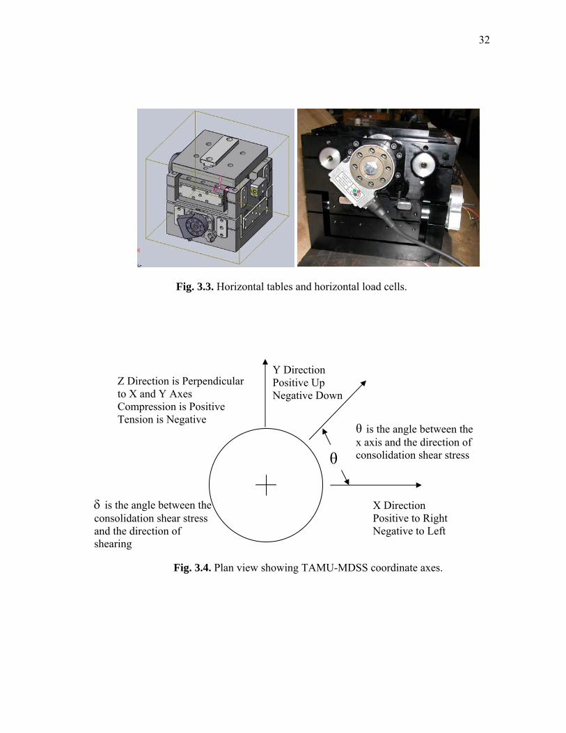
Fig. 3.3. Horizontal tables and horizontal load cells.
Fig. 3.4. Plan view showing TAMU-MDSS coordinate axes.
Y Direction Positive Up Negative Down
X Direction Positive to Right Negative to Left
Z Direction is Perpendicular to X and Y Axes Compression is Positive Tension is Negative
θ
θ is the angle between the x axis and the direction of consolidation shear stress
δ is the angle between the consolidation shear stress and the direction of shearing

33
3.1.1 Backpressure and Cell Pressure Systems
Most simple shear devices are unable to perform truly undrained testing with
direct measurement of pore pressure because they do not allow full saturation of the
sample. In the TAMU MDSS, both backpressure and cell pressure can be independently
measured and controlled. The pressure chamber is rated for a maximum air pressure of
861.8 kPa (125 psi). The chamber pressure transducer is a Honeywell model FP2000
transducer with a range of 50psi and an accuracy of ±0.10% FS.
Two differential pressure transducers are used in the backpressure system to
measure the excess pore pressure and volume change of sample (Figures 3.5 and 3.6).
The excess pore pressure transducer referred as the “effective transducer” is a
Honeywell model FP2000 wet/wet pressure transducer with a range of 50 psi and an
accuracy of ±0.10% FS. The volume change transducer is a Honeywell model FP2000
wet/dry pressure transducer with a range of 10 inch water and an accuracy of ±0.10%.
Fig. 3.5. Idealized schematic of backpressure system.

34
Fig. 3.6. Photographs of backpressure system (a) side view of backpressure system (b) top view of backpressure system.
Volume pipette
Air pressure supply
Water supply
Cell pressure
Backpressure regulator
Volume transducer
“Effective” transducer
(a)
(b)

35
3.1.2 Specimen
The device can accommodate specimens up to a diameter of 100 mm (4 in),
larger than the more typical size of 70 mm (2.8 in) and resulting in more uniform stress
distribution (Vucetic and Lacasee, 1982; Finn et al., 1982). Larger samples up to 150
mm (6 in) can be tested with minor modifications to the sample mounting brackets.
Similar to the NGI simple shear device, the samples are circular and maintain constant
cross-sectional area by using a wire-reinforced membrane.
As discussed in Section 2.3, the diameter to height ratio was selected as 4 to
minimize the effects of non-uniform stress distribution along the top and bottom of the
sample due to the lack of complementary shear stress on the lateral boundaries of the
sample.
The wire-reinforce latex membrane is manufactured by Geonor for the NGI shear
device. The standard sized membrane with a specimen area of 50 cm2 is used. A wire-
stiffness of c = 1.0 is used in an effort to match the average stiffness properties of the
soil. The reinforcement in these membranes is constant wire with a diameter of 0.015
cm, a Young’s modulus of 1.55 x 10⁶ kg/cm2, and a tensile strength of 5800 kg/cm2
(Dyvik, 1981). The wire is wound at 20 turns per centimeter of membrane height (0.05
cm center to center spacing). A chamber pressure lower than the anticipated lateral
pressure in the samples is applied to minimize the load carried by the wires in the
reinforced membrane. The use of the reinforced membrane prevents direct measurement
of the lateral confining pressure because the amount of stress that the wire carries is
unknown. The membrane is assumed to have negligible lateral deformation and

36
therefore the samples are consolidated under Ko conditions. Cell pressure can also be
used to enforce Ko conditions following procedures outline in Boulanger et al. (1993).
Backpressure procedures are described in more detail in Appendix B.
3.1.3 Multi-axis Load Cell
One of the main improvements of the TAMU-MDSS over similar devices is the
multi-axis load cell installed directly above the sample to increase accuracy and reduce
the influence of compliance (Figure 3.7). The transducer has a sensing range of ± 2 kN
(450 lbf) in the vertical axis and ±0.67 kN (150 lbf) in the horizontal axes. The torque
applied to the specimen can be measured within a range of ± 0.068 kN-m (600 lbf-in) in
all three directions. The data acquisition system for the multi-axis load cell is through a
separate laptop using Labview software. Six channels, three forces and three torques, are
recorded with time.
Fig. 3.7. Schematic and photos of multi-axis load cell

37
3.2 Hydraulic Power Supply
A servo-hydraulic control system (Figure 3.8) is used to allow for frequencies up
to 20 Hz and more reliable control. The hydraulic power supply (Model CS7580-D)
system was designed specifically for laboratory use. Standard hydraulic power supplies
using fixed or variable displacement piston pumps run at a constant rotations per minute
(RPM). The noise level and heat generated remains virtually constant. However, the
CS7580-D system varies the pump RPM in relation to demand. When variable lower
flow rates are required, the motor speed slows to the minimum rotation required to
maintain the programmed pressure. This concept reduces energy cost up to 50%, lowers
operating temperatures and runs 30-40% quieter than other hydraulic units. For
additional noise reduction, the pumping system is enclosed in an acoustically dampened
outer cabinet.
Fig.3.8. Hydraulic power supply.

38
3.3 Computer Control and Data Acquisition
The Automated Testing System (ATS) software package (Sousa and Chan, 1991)
was chosen for control of the closed-loop system. ATS provides control signals to servo-
valve drivers for the hydraulic actuators and the chamber pressure controller (Figure
3.9). Voltage from the LVDTs, load cells and pressure transducers are acquired from the
data acquisition board by ATS through a data acquisition board (National Instruments
PCI-6703).
The 16-bit board allows high sampling resolution and analog-to-digital and
digital-to-analog processing allowing the system to record data and control servo-valves.
ATS can sample all 16 input channels (Figure 3.10 and Table 3.1) and then update the
output commands sent to the selected servos at a rate selected by the user of either 500,
1000 or 2000 times per second. All components of the data acquisition system are
summarized in Table 3.2. The control system uses a PD (Proportional-Derivative)
control algorithm. Gains for the PD control system are determined by manual tuning.
ATS allows for either manual or automatic control of each output channel using any
input channel as the feedback to be controlled.
A number of pre-programmed control signals, called tests, are available on ATS.
Ramp tests are used to change feedback channel from one value to another at a specified
constant rate of change. Cyclic tests are used to produce a sinusoidal wave of specified
amplitude, frequency and mean value, while wave tests are used to reproduce a wave
form which the user specifies by providing a digitized data file describing one cycle of
the wave. Each test can be applied to a specific feedback channel and multiple tests can

39
be combined to control different channels simultaneously. Tests using all three servos
valves can be conducted in parallel allowing complex loading patterns such as circular
and figure-8. The ability to specify the feedback channel allows versatility in running
either strain or stress controlled tests.
Fig. 3.9. Layout for control system components of TAMU-MDSS device.

40
Fig. 3.10. Data acquisition boards.

41
Table 3.1 Data acquisition used in TAMU-MDSS.
Channel No. Channel Name Instrument
0 Zstroke Vertical LVDT 1 Zload Vertical load cell
2 Xstroke X direction LVDT
3 Xload X direction load cell
4 Ystroke Y direction LVDT
5 Yload Y direction load cell
6 “Effective” Differential pressure transducer
7 Cell Pressure transducer
8 Empty -
9 Volume Differential pressure transducer
10 Empty -
11 Signal conditioning -
12 Empty -
13 SV2 Servo y direction
14 SV1 Servo x direction
15 SVO Servo z direction

42
Table 3.2 List of TAMU-MDSS transducers. Transducer Measured Quantity Model and Sensitivity
Vertical LVDT Axial deformation
Macrosensors General Purpose AC-Operated LVDT Position Sensor Model PR812-2000 Range ±50.0 mm ±0.25% FS
Vertical load cell Vertical load
Interface Model 1010 Fatigue rated load cell Capacity: 250 lbf ±0.03% FS
X direction Horizontal LVDT Shear deformation x-direction
Solartron AC LVDT gage type Range: ± 10.0 mm ±0.2% FS
X direction Load cell Load in x-direction
Straincert Universal Load Cell. Capacity: 250 lbf Nonlinearity ±0.10% FS
Y direction Horizontal LVDT Shear deformation y-direction
Solartron AC LVDT gage type Range: ± 10.0 mm ±0.2% FS
Y direction Load cell Load in y-direction
Straincert Universal Load Cell. Capacity: 250 lbf Nonlinearity ±0.10% FS
Differential pressure transducer
Difference between volume and cell pressure
Honeywell FP2000 range : 50psi Accuracy ±0.10%
Pressure transducer Chamber pressure Honeywell FP2000 range : 50psi Accuracy ±0.10%
Differential pressure transducer Volume (inches of water)
Honeywell FP2000 range: 10 inch water, Accuracy ±0.10%

43
3.4 Conclusions
An overview of the development and capabilities of the new Texas A&M multi-
directional simple shear device has been presented. The TAMU-MDSS applies both
vertical and horizontal loads to a cylindrical sample confined in a wire-reinforced
membrane. The device is capable of shearing the sample in monotonic, cyclic and
complex patterns under both stress and strain-control. Chamber pressure and
backpressure can be applied to allow for sample saturation. Pore pressure generation
during undrained shearing can be directly measured. The forces and torques applied to
the sample are measured by the multi-axis load cell installed immediately above the
sample. The capabilities of the TAMU-MDSS will be demonstrated in section 4 through
the testing of a rubber sample.

44
4. EXPERIMENTAL EVALUATION OF THE TAMU-MDSS
An experimental evaluation of the TAMU-MDSS was performed to determine
the full capabilities of the device. Initially, each strain-controlled test was carried out
using only the horizontal tables. These tests were used to determine the friction between
the tables and if the direction of the test and rate influenced the friction. Secondly, a
rubber sample with dimensions similar to those of the marine clay specimens in the
experimental study was used to evaluate the capabilities of the device and the
repeatability of the tests. The device evaluation program has two main objectives:
1. Evaluate the kinematics of the device to ensure the TAMU-MDSS is capable of
conducting strain and stress-controlled monotonic, cyclic, circular and figure-8
test patterns.
2. Verify the sample set-up procedures and data acquisition systems are working
properly and produce repeatable results.
The performance of the TAMU-MDSS system was evaluated using harmonic input
motions and the resulting feedback signal was recorded. To evaluate each axis
independently, uni-directional tests were conducted. Cross-coupling effects between the
axes were analyzed by conducting bi-directional testing and varying the signal
frequencies to each horizontal table.
4.1 Friction and Cross-coupling of Loading Tables
The loads applied to the sample by the three actuators (two horizontal and one
vertical) are measured by load cells mounted inside the chamber between the actuators

45
and the loading tables. Thus, the load cells measure both frictional and inertial loads
which may not be transferred to the sample. The magnitude of the loads developed by
“device friction” between the horizontal tables needs to be determined.
First, each axis of motion was evaluated on its own. A ramp monotonic
command signal was sent to one of the actuators and the load and displacement of each
table was recorded to access friction between the tables. Two different strain rates were
conducted to determine if the friction in the system was rate dependent.
Figure 4.1 shows plots of frictional resistance for monotonic tests in the x and y-
directions at strain rates of 5%/hr and 50%/hr. In monotonic loading at a rate of 5%/hr
(1 mm/hr), the recorded force due to friction in the x-direction was measured to be a
maximum of ±0.017 kN (4 lbf), which corresponds to less than 3.6 kPa (0.5 psi) over a
79.75 mm (3.14 in) diameter sample. The friction in the y-direction was measured to be
a maximum of ± 0.017 kN (4 lbf), which corresponds to less than 3.6 kPa (0.5 psi) for
the samples. For a rate of 50%/hr (10 mm/hr), a maximum force of ±0.022 kN (5 lbf) or
4.5 kPa (0.7 psi) was measured. Based on the measured loads in each direction and
different strain rates, the frictional resistance is smaller in magnitude in the x-direction.
The monotonic tests also indicate friction of the tables is mostly is independent of rate
for the rates which will be used in the testing program.

46
Fig. 4.1. Frictional resistance on the horizontal tables for monotonic tests for a rate of (a) 5%/hr and (b) 50%/hr.
(a)
(b)

47
Sinusoidal command signals were also sent to each axis to determine the
frictional resistance for cyclic, circular and figure-8 strain controlled tests. Two
amplitudes (0.1 mm and 3 mm) and two frequencies (0.1 Hz and 1 Hz) were used.
Figure 4.2 and Figure 4.3 shows plots for cyclic tests in the x-direction and y-direction,
respectively. For cyclic loading at both frequencies and amplitudes, the friction in the x-
direction was measured to be less than 0.007 kN (1.5 lbf), which corresponds to less than
1.3 kPa (0.19 psi). The friction in the y-direction was measured to be less than
±0.178 kN (4 lbf) or 3.6 kPa (0.5 psi). As indicated in the plots, the frictional resistance
is directly related to the amplitude of the cyclic loading. As the amplitude increased from
0.1 mm to 3 mm, the load in the corresponding direction increased from 0.002 kN
(0.5 lbf) to 0.004 kN (1 lbf). Increased frequency does not seem to create additional
frictional resistance in cyclic loading.
Circular tests were conducted at frequencies of 0.1 Hz and 1 Hz with full strain
amplitudes of 0.1 mm and 3 mm. Figure 4.4 shows plots for circular tests. The load due
to friction in the x-direction was measured to be less than 0.004 kN (1 lbf) or 0.89 kPa
(0.1 psi). The frictional resistance in the y-direction was measured to be less than
0.013 kN (3 lbf), which corresponds to less than 0.3 psi (2.67 kPa).
Figure-8 tests were conducted at frequencies of 0.1 Hz and 1 Hz with full strain
amplitudes in the major axis of 0.2 mm and 6 mm. Figure 4.5 shows plots for figure-8
tests. The x-direction and y-direction load cells measured the friction to be less than
0.004 kN (1 lbf) or 0.89 kPa (0.1 psi). The frictional resistance measured in the y-
direction was less than ±0.178 kN (4 lbf) or 3.6 kPa (0.5 psi).

48
Fig. 4.2. (a) Stroke and (b) frictional resistance for cyclic tests in the x-direction at frequencies of 0.1 Hz and 1 Hz.
(a)
(b)

49
Fig. 4.3. (a) Stroke and (b) frictional resistance for cyclic tests in the y-direction at frequencies of 0.1 Hz and 1 Hz.
(a)
(b)

50
Fig. 4.4. (a) Stroke and (b) frictional resistance for circular tests at frequencies of 0.1 Hz and 1 Hz.
(a)
(b)

51
Fig. 4.5. (a)Stroke and (b) frictional resistance for figure-8 tests at frequencies of 0.2 Hz and 1 Hz in x-direction.
(a)
(b)

52
Table 4.1 summarizes the measured forces due to friction for each axis and type
of table test. Lubrication prior to each test minimizes the magnitude of friction along the
track bearings. The magnitude of the frictional resistance is important for the stress-
controlled tests in which the horizontal table load cells measure the feedback for the
control loop. However, the shear response of the sample is also measured by the multi-
directional load cell installed directly above the sample.
Once each axis had been tested individually, cross-coupling effects were
examined by providing a harmonic command signal to one of the tables while recording
the movement of the stationary table. Cross coupling would be indicated if there is a
significant movement of the stationary table when the other table is moving at different
strain amplitudes and frequencies. A sine wave of strain amplitudes 0.1 mm and 3 mm at
frequencies of 0.1 Hz and 1 Hz was applied to each axis. As shown in Figure 4.6, for
each case, negligible movement of the stationary table was measured indicating limited
cross-coupling between the horizontal tables during cyclic loading.

53
Table 4.1. Summary of table tests for frictional resistance.
No. Test Stroke (mm) Rate
Max. force due to friction x-direction
(lbf)
Max. force due to friction y-direction
(lbf) 1 MONO 3 5%/hr or 1 mm/hr 4 4 2 MONO 3 -5%/hr or -1 mm/hr 4 4 3 MONO 3 50%/hr or 10 mm/hr 5 5 4 MONO 3 -50%/hr or –10 mm/hr 5 5 5 CYC 0.1 0.1 Hz 0.5 1.5 6 CYC 3 0.1 Hz 1.5 4 7 CYC 0.1 1 Hz 0.5 1.5 8 CYC 3 1 Hz 1 3 9 CIRR 0.1 0.1 Hz 1 1
10 CIRR 3 0.1 Hz 1 3
11 CIRR 0.1 1 Hz 0.5 0.5
12 CIRR 3 1 Hz 0.5 1
13 FIG8 0.2 x-dir 0.1 y-dir
0.2 Hz x-dir/ 0.1 Hz y-dir 0.5 1
14 FIG8 6 x-dir 3 y-dir
1 Hz x-dir/ 0.5 Hz y-dir 1 4
15 FIG8 0.2 x-dir 0.1 y-dir
0.2 Hz x-dir/ 0.1 Hz y-dir 0.5 1
16 FIG8 6 x-dir 3 y-dir
1 Hz x-dir/ 0.5 Hz y-dir 1 3

54
Fig. 4.6. Cross-coupling of horizontal tables in (a) x-direction at 1 Hz, (b) x-direction at 0.1Hz, (c) y-direction at 1 Hz, and (d) y-direction at 0.1 Hz.
(a) (b)
(c) (d)

55
4.2 Constant Stress Testing of Vertical and Horizontal Loads
To ensure the TAMU-MDSS could maintain constant stress in the vertical and
horizontal loads, an elastic rubber sample (Figure 4.7) was subjected to each of the
following: 1) a vertical load of 0.444kN (100 lbf) over 12 hours, 2) a vertical load of
0.444 kN (100 lbf) and a horizontal load in the x-direction of 0.089 kN (20 lbf) for
12 hours, and 3) a vertical load of 0.444 kN (100 lbf) and a horizontal load in the y-
direction of 0.089 kN (20 lbf) for 12 hours. The results of each test are plotted in Figures
4.8 and 4.9. As shown in the plots, the vertical load fluctuates approximately 0.013 kN
(3 lbf) during horizontal loading in the x and y-directions. The horizontal load fluctuates
approximately 0.002 kN (0.4 lbf) in the x-direction and 0.004 kN (1 lbf) in the y-
direction. These fluctuations may be due to the inherent behavior of the rubber sample
to vertical and horizontal loading and not the system controls.
Fig. 4.7. Rubber sample installed in TAMU-MDSS.

56
Fig. 4.8. (a) Horizontal load in x-direction, (b) vertical load in during x-direction constant test.
(a)
(b)

57
Fig. 4.9. (a) Horizontal load in y-direction, (b) vertical load during y-direction constant load test.
(a)
(b)

58
4.3 TAMU-MDSS Loading Path Evaluation
Fifty-eight tests were conducted on a rubber sample to access the performance of
the TAMU-MDSS. The rubber sample was subjected to the same stresses and
deformations under which the marine clay specimens were tested in the experimental
plan. Table 4.2 gives a summary of the tests conducted in the TAMU-MDSS on a
rubber sample. In all the tests, the rubber sample was subjected to a vertical load of
0.444 kN (100 lbf). For CKα type tests, a horizontal load of 0.089 kN (20 lbf) was
applied. The angle, θ, is the angle between the positive x-axes and the direction of the
applied horizontal consolidation shear stress. Shearing for each case occurred at an
angle, δ, which is the angle between the consolidation shear stress and the direction of
shearing. Twenty-nine tests were at the same rate used for the clay samples. The
loading path capabilities are shown in Table 4.2. Additional tests were performed at
different rates to evaluate the device at higher monotonic rates and cyclic frequencies.
Eight monotonic tests were carried out at a rate of 50%/hr and twenty cyclic and multi-
directional tests were conducted at a frequency of 1 Hz.
The monotonic tests were conducted to simulate both CKo and CKα
consolidation and subsequent shearing in each direction indicated by δ in Table 4.2. In
CKo consolidation of the clay specimens only a vertical load is applie, while CKα
consolidation also requires a horizontal load (as indicated by dashed line), in addition to
the vertical. In both cases, lateral constraint is applied by the wire-reinforced membrane.
During the evaluation with the rubber specimen, no lateral constraint is applied, but the

59
Table 4.2. Summary of rubber testing.
Plan View Test Path Test Name Consolidation δ (degrees) 1-D linear path x-direction
MONOXR-1 MONOXR-2 MONOXRa-3 MONOXRa-4 MONOXRa-5
CKo CKo CKα CKα CKα
- - 0 90
180 1-D linear path y-direction
MONOYR-6 MONOYRa-7 MONOYRa-8 MONOYRa-9
CKo CKα CKα CKα
- 270 0 90
2-D cyclic path x-direction
CYCXR-10 CYCRa-11 CYCRa-12 CYCRa-13
CKo CKα CKα CKα
- 0 90
180
2-D cyclic path y-direction
CYCYR-14 CYCYRa-15 CYCYRa-16 CYCYRa-17
CKo CKα CKα CKα
- 270 90
180
Circular path
CIRR-18 CIRRa-19 CIRRa-20 CIRRa-21
CKo CKα CKα CKα
- 0 90
180
Figure-8 path x-direction
FIG8XR-22 FIGXRa-23 FIGXRa-24 FIGXRa-25
CKo CKα CKα CKα
- 0 90
180
Figure-8 path y-direction
FIGYR-26 FIGYRa-27 FIGYRa-28 FIGYRa-29
CKo CKα CKα CKα
- 270 0 90

60
loading pattern – vertical load only for Ko and vertical and horizontal load for Kα –
remains the same. Due to the addition of the horizontal load, there is an initial
displacement in the x-direction or y-direction as illustrated in Figures 4.10 and 4.11.
The first two tests (MONOXR-1 and MONOXR-2) were CKo type and sheared
at a rate of 5%/hr to 3 mm displacement. The tests were compared to determine if the
device was able to repeat the same strain controlled test. As shown in Figure 4.9, the plot
of the x-stroke with time for each test is the same. CKα type tests (MONOXRa-3,
MONOXRa-4, MONOXRa-5) were simulated by applying a horizontal shear stress in
the positive x-direction (θ = 0°). For monotonic tests, both downhill (δ = 0°), across the
slope (δ = 90°), and uphill (δ = 180°) shearing directions were tested.
The following examples are used to illustrate the definitions of shearing
downhill, across the slope and uphill. For example, MONOXRa-3 had a horizontal load
of 0.089 kN (20 lbf) applied in the x-direction (θ = 0°) and then monotonically sheared
in the same direction (δ = 0°), which simulates a downhill monotonic shearing test. For
MONOXRa-4, the rubber sample was similarly subjected to a horizontal load of 0.089
kN (20 lbf) in the x-direction (θ = 0°), however, was sheared monotonically in the
positive y-direction (δ = 90°) simulating across the slope shearing. As shown in each
plot, the x-stroke has a positive offset for CKα tests due to the application of a horizontal
load in the x-direction.
The tests were repeated at a rate of 50%/hr. MONOXRa-3B was stopped early to
prevent overloading to the fine load cell due to the large horizontal load in the x-

61
Fig. 4.10. Plots of monotonic tests on rubber sample in x-direction at (a) 5%/hr and (b) 50%/hr.
(a)
(b)

62
Fig. 4.11. Plots of monotonic tests on rubber sample in y-direction at (a) 5%/hr and (b) 50%/hr.
(a)
(b)

63
direction. Monotonic tests (MONOY-6, MONOYRa-7, MONOYRa-8, MONOYRa-9) at
5%/hr and 50%/hr were also conducted in the y-direction (Figure 4.10). MONOYRa-9
was stopped early due to large horizontal load in the y-direction. Similar results in both
directions indicate that monotonic testing in both directions is equivalent.
An evaluation of each axis using stress-controlled cyclic loading was also
conducted with the rubber sample. Cyclic tests at frequencies of 0.1 Hz and 1 Hz were
carried out in both directions with a horizontal load of 20 lbf. Both CKo and CKα type
tests were simulated as discussed previously. Comparisons of the results are shown in
Figures 4.12 and 4.13. These tests indicate that the TAMU-MDSS is able to conduct
stress-controlled tests at various frequencies. The testing software is also able to start the
shearing portion of the test with no drift of the load from the consolidation shear stress.
This is shown in the tests with δ = 0, 90 and 180 degrees. As indicated in the figures,
when shearing is applied in the perpendicular direction ( δ = 90°), the load measured in
the axis in which the horizontal load is applied remains constant.
Circular and figue-8 stress controlled loading patterns were tested at both 0.1 Hz
and 1 Hz. It was critical to evaluate if the device could conduct these complex load
patterns for both CKo and CKα consolidation. Figures 4.14 – 4.16 show the results of the
multi-directional shearing patterns. As illustrated in the plots, the higher frequency
results have larger noise, which may be due to the inherent material properties of the
rubber samples, increased friction between the tables as determined earlier by the
frictional resistance testing or less accurate controls at higher frequencies.

64
Fig. 4.12. Plots of cyclic tests on rubber sample in x-direction at (a) 0.1 Hz and (b) 1 Hz.
(a)
(b)

65
Fig. 4.13. Plots of cyclic tests on rubber sample in y-direction at (a) 0.1 Hz and (b) 1 Hz.
(a)
(b)

66
Fig. 4.14. Plots of circular tests on rubber sample at (a) 0.1 Hz and (b) 1 Hz.
(a)
(b)

67
Fig. 4.15. Plots of figure-8 tests on rubber sample in x-direction at (a) 0.1 Hz and (b) 1 Hz.
(a)
(b)

68
Fig. 4.16. Plots of figure-8 tests on rubber sample in y-direction at (a) 0.1 Hz and (b) 1 Hz.
(a)
(b)

69
4.4 Comparison of Multi-axis Load Cell and Measurements of Torque
The multi-axis load cell is installed directed above the sample and measures the
forces and torques applied to the sample. The TAMU-MDSS vertical load cell and the
multi-axis load cell were directly calibrated to each other through the use a of specially
designed aluminum cylinder. The measured torques applied to the top cap can provide
insight to the degree of rocking the sample is experiencing. Plots of torque compared to
the load applied to the sample over time are presented in Figures 4.17 and 4.18 for the
monotonic and cyclic tests. The stiffness of the rubber sample creates a large torque in
the opposite direction of the loading. As the horizontal table moves monotonically, a gap
is formed between the rubber sample and the sample cap along the trailing edge (Figure
4.19). The rubber sample also tilts during loading in the perpendicular direction as
illustrated in the plots by the increase of torque in the perpendicular axes. Some slight
rotation occurs shown by the small change in torque in the z-direction. Similar results
are shown in Figure 4.20 and Figure 4.21 for circular and figure-8 tests.

70
Fig. 4.17. Torque measurements for monotonic tests in (a) x-direction and (b) y-direction.
(a)
(b)

71
Fig. 4.18. Torque measurements for (a) CKo and (b) CKα cyclic tests in x-direction.
(a)
(b)

72
Fig. 4.19. Gap formed between cap and rubber sample.

73
Fig. 4.20. Torque measurements for circular tests (a) CKα horizontal load in positive
x-direction and (b) CKα horizontal load in negative x-direction and positive y-direction.
(a)
(b)

74
Fig. 4.21. Torque measurements for figure-8 tests (a) CKα horizontal load in positive
x-direction and (b) CKα horizontal load in negative x-direction.
(a)
(b)

75
4.5 Evaluation of the Backpressure System and Chamber
Tests were conducted to evaluate possible leakage through valves, line
connections and the connection through the chamber. The first test accessed the
backpressure system and sample drainage lines. The sample water lines were capped
creating a closed system. A pressure of 20 psi was applied through the backpressure
system. The valve to the volume pipette was closed to prevent drainage and the change
in pressure over time was recorded. The system has a small change in pressure over
time, however, with constant application of backpressure to the volume pipette minimal
pressure change occurs.
The second tests evaluated the chamber and cell pressure regulator system. A
constant chamber pressure was maintained for 36 hours at a pressure of 20 psi to
determine the amount of cell pressure dissipation over time. The chamber maintains a
constant pressure and does not leak. A third tests was conducted to evaluate the time it
takes the chamber to fill to the same pressure set by the regulator. The backpressure
regulator was fully open and set to zero psi. The cell pressure was increased by 5 psi
every 5 minutes. The chamber pressure was recorded by the cell pressure transducer
over the duration of the test. As indicated in Figure 4.22, there is a lag between
application of the cell pressure and the measurement of the chamber pressure by the
pressure transducer installed in the top of the chamber. However, with small incremental
chamber pressure increases during back saturation, the lag does not directly affect the
specimen.

76
Fig. 4.22. Chamber pressure lag time.
4.6 Conclusions
An experimental evaluation of the TAMU-MDSS was conducted to determine
the full capabilities and limitations of the device. Strain-controlled tests were used to
determine the force due to friction between the horizontal tables. It was determined that
the friction depended on both rate and direction. A majority of the experimental plan
tests for Gulf of Mexico marine clays will be conducted in the x-direction since this axis
had a lower amount of friction in comparison with the y-direction.

77
Rubber sample tests were used to verify the TAMU-MDSS testing software and
device were able to apply both strain and stress-controlled monotonic, cyclic, circular
and figure-8 test patterns. The device is capable of performing tests at various
frequencies, however, it shows evidence of increased noise either due to friction or
control issues at higher frequencies. Therefore, the initial cyclic and multi-directional
tests will be performed at a frequency of 0.1 Hz. Forces and torque measurements from
the multi-axis load cell showed the rubber sample tilted and rotated during shearing,
however, this may be due to the material properties of the rubber sample. The influence
of tilt and twist was studied when conducting the Gulf of Mexico marine clay tests
(Section 6).
Finally, the backpressure system was shown to be capable of maintaining
pressure during the duration of the test. Some fluctuations from the house pressure can
be an issue for maintaining the chamber and backpressure higher than 20 psi, however,
at 20 psi, the fluctuations are minimal.

78
5. GULF OF MEXICO CLAYS
This section presents the sampling and results from basic and advanced
characterizations of the Gulf of Mexico marine clay samples. Geotechnical engineering
properties are of critical importance for the analysis and design of seafloor processes and
operations such as evaulation of slope stability and the design of anchors and
foundations. One of the primary challenges in studying submarine landslides is the lack
of information about the properties of these soils in situ. Because offshore soil sampling
is expensive, published experimental information on marine clays from offshore is
limited. Most marine clay testing in the research literature is conducted on marine
deposits that are now onshore and easily accessible such as Boston Blue Clay (BBC) and
San Francisco Young Bay Mud (YBM). However, due to the depositional environment
and mechanisms, the stress history for these samples differs from that of offshore marine
sediments.
Marine clays on the continental shelf and slope differ from traditionally tested
fine grained sediments in three important aspects: depositional environment,
depositional mechanisms, and stress history. Because the structure of the deposits and
the mechanical response to loading can be influenced by these factors, the samples used
in the experimental plan are undisturbed marine soils. However, not only is collecting
offshore samples expensive and requires specialized equipment, high quality undisturbed
samples require great expertise.

79
5.1 Sampling of Gulf of Mexico Clay
The Gulf of Mexico samples were collected in and around the Green Canyon
near the Sigsbee Escarpment in October 2007 on the Research Vessel Brooks-McCall
operated by TDI-Brooks International (Figure 5.1). The 100 mm (4 in) diameter cores
were taken using the jumbo piston core system at approximately 1000-1300 meters of
water depth. Approximately 30 sites were sampled on varying degrees of slope.
Fig. 5.1. R/V Brooks McCall.
A jumbo piston corer uses the "free fall" of the coring rig to achieve a greater
initial force on impact than gravity coring (Figure 5.2). A sliding piston inside the core
barrel is used to reduce inside wall friction with the sediment and to assist in the
evacuation of displaced water from the top of the core. TDI-BI vessels are equipped with
30 meter 4" Jumbo Piston cores (JPC) that can be collected at depths in excess of 4,000
meters. The JPC utilizes a cantilevered deployment platform over the stern of the vessel

80
Fig. 5.2. TDI-Brooks International jumbo piston coring system (After www.tdi-bi.com).
with a rail and capture bucket assembly placed on the deck of the vessel directly beneath
the stern A-frame (Figure 5.3). The JPC consists of a 4,000 lbf weight stand, a 4" core
barrel, a mechanical trigger, standard schedule 40 PVC liner, a cutting shoe, and a foil
core catcher.
The cores were cut into 1 meter long sections, labeled, wax sealed, capped and
stored vertically. Some cores were tested with a laboratory miniature vane on the vessel
and the top 7-8 cm (3 in) were bagged for additional geotechnical testing onshore.

81
Fig. 5.3. (a) Jumbo piston core rig ready for deployment (b) Jumbo piston core rig in deployment
(a)
(b)

82
Processed core sections were stored in an air conditioned room on the vessel pending
their careful offload at the next port call. These sections were then transported by
enclosed truck to on-shore laboratories for further geotechnical testing.
5.2 Geology of Gulf of Mexico Clay
The Southern Green Canyon (Figure 5.4) lies along the Sigsbee Escarpment in
the Gulf of Mexico. Al-Khafaji et al. (2003) describe the geology of the lower
continental slope as consisting of uniform surficial deposits of highly plastic Holocene
clays overlying older, stiffer, less plastic, Pleistocene clays. The Sigsbee Escarpment
consists of stiff clays that have been exposed by slides and slumps. These sediments
have also experienced uplift by the underlying salt and erosion caused by bottom
currents. The upper continental rise consists of uniform deposits of highly plastic clays
with a thin drape of Holocene clays (Jeanjean et al, 2003; Slowey et al, 2003).
5.3 Multi-sensor Core Logger Profiles
The core samples were scanned using a GEOTEK Multi-sensor core logger
(MSCL) (Figure 5.5). A conveyor system moves the sensor array, which scans the core
as it passes. The conveyor is driven by a stepper motor which can position a core to an
accuracy of better than 0.5 mm. The computer controlling the conveyor also controls the
sensors, so that all data are automatically correlated. The computer also measures the
length of each core section and can automatically subtract the thickness of the end caps,
allowing the sections to follow sequentially, producing an unbroken stream of data.
The MSCL can handle core sections up to 1.5 m long and 15 cm in diameter, and
can sample at 1-mm intervals. The logger is equipped with a 137-Cs gamma source in a

83
Fig.
5.4
. Loc
atio
ns o
f jum
bo p
isto
n co
res f
rom
Gul
f of M
exic
o (M
adhu
ri, 2
011)
.

84
Fig. 5.5. Photograph of multi-sensor core logger.
lead shield for determining bulk density, with a resolution of 1%. The logger is also
equipped with 250-500 kHz piezo-electric ceramic transducers for measuring P-wave
velocity, which are spring-loaded against the sample and accurate to 0.2%. Core
diameter measurements are taken using rectilinear displacement transducers, with a
resolution of 0.05 mm (sleeved core). Data recorded includes p-wave velocity, bulk
density, porosity and moisture content.
Figure 5.6 shows the MSCL data for GOM-core1 which was used in the
experimental testing program. GOM-core1 was sampled from a water depth of 1,310 m
beneath mean sea level. The core had a total length of 13.46 m. The p-wave velocity was
used to locate samples within the core liner with a minimal amount of disturbance. The
end of the core sections were not used because of possible disturbance due to storage,
transportation, oxidation and changes in water content. The p-wave velocities measured

85
Fig
5.6.
MSC
L pr
ofile
s of b
ulk
dens
ity, c
ompr
essi
onal
vel
ocity
and
por
osity
from
GO
M-c
ore1
(Mad
huri,
201
1).

86
within the soil were approximately 1050 m/s. Larger p-wave measurements indicate
gaps in the core at location in which the core was sub-sampled for remold miniature
vane tests and index testing. Locations of constant density and porosity indicate
homogenous material.
5.4 Geotechnical Engineering Properties of Gulf of Mexico Clay
Classification and index testing was conducted on samples throughout GOM-
corel. The natural water content and miniature vane strengths were determined from the
top of each section. Atterberg limits, grain size analysis and specific gravity tests were
performed on representative samples along the length of the core. Constant rate of strain
consolidation and triaxial tests were also conducted on limited sections of GOM-core1.
5.4.1 Natural Water Content and Index Classification
The natural water content was measured at the top of each section of the core.
Figure 5.7 presents the water content with core depth from the mudline. As illustrated in
the plot, the top 4 m of sediment has a water content higher than 100%. The water
content slowly decreases from 100% to 60% between a depth of 4 m to 7 m. Below 7 m,
the water content remains constant between 60%-80%. Consolidation, triaxial and direct
simple shear tests were conducted on samples below 7 m because the shallower samples
were too soft to trim without considerable disturbance,
As indicated in Figure 5.7, liquid and plastic limits were determiined at the same
locations as the natural water content. The liquid limit gradually decreases in the top 4
m from 100 to 60 and ranges from 60 to 80 below depths of 7 m. The natual water
content is greater than liquid limit until approximately 6 m. The plastic limit is

87
Fig. 5.7. Natural water content with depth for GOM-core1 (Madhuri, 2011).

88
approximatly 36 for the first 4 m of the core and then decreases to 29 . Results of
classification tests are plotted in Figure 5.8. As is typical with marine clays, the results
are close to the A-line and classify the clay sample is either MH or CH.
5.4.2 Miniature Vane Shear Strength
Laboratory miniature vane shear strength tests were conducted offshore on the
tops of each section and the bottom of the last section. Figure 5.9 shows the shear
strength increases gradually with depth with a maximum shear strength of 22 kPa.
Samples for advanced geotechnical testing were chosen in the lower sections of the core
with shear strengths of approximately 20 kPa.
5.4.3 Grain Size Distribution and Specific Gravity
Grain size analysis and specific gravity tests were conducted on samples within
the sections used for advanced geotechnical testing (Table 5.1). Hydrometer analyses
were performed in accordance with ASTM D422-63(2007). As illustrated in Figure 5.10,
the four hydrometer tests are consistent for the lower sections of the core. The soil
consists of 84-99% fine particles of which 51-72% are clay size. Specific gravity tests
were carried out in accordance with ASTM D854. The results indicate consistent
material in sections 11,12, 13 and 15.

89
Fig. 5.8. Atterberg limits for GOM-core1 samples plotted on Casagrande’s plasticity chart.

90
Fig. 5. 9. Miniature vane shear strengths with depth for GOM-core1 (Madhuri, 2011).
Table 5.1. Summary of representative sample testing. Section Depth (m) Specific gravity Soil Type
11 9.0 - 9.7 2.74 MH 12 9.7 - 10.6 2.76 CH 13 10.6 - 11.5 2.76 CH 15 12.2 - 13.5 2.76 CH

91
Fig. 5.10. Hydrometer analysis from four sections of GOM-core1 (Madhuri, 2011).
5.5 Clay Mineralogy
X-ray diffraction (XRD) analysis was used to determine the mineralogy of two
clay samples. The subsamples were taken from the trimmings from the first and last clay
samples. A bulk XRD analysis was conducted as an initial x-ray survey of the bulk
sample before a detailed investigation of the fine clay minerals was carried out. Bulk
XRD analysis allows for determination of the mineralogy of the whole sample before the
sample is subjected to different treatments to create an oriented particle sample. The

92
sample preparation required an air dry sample to be ground with a mortar and pestle
using soft pressure. The sample was then passed through a 140 mesh sieve (0.104 mm)
to obtain a uniform particle size of the minerals in the sample. A front loading mount
method was used to prepare the sample for bulk XRD analysis. Figure 5.11 shows the
bulk XRD for both samples. As indicated in the plots, the mineral composition of the
two samples is similar. The samples are a mixture of seven main minerals, clinochlore
(chlorite), muscovite (mica), quartz, feldspar albite, magnesium calcite, dolomite and
halite. The minerals present suggest that the sample consists mainly of fine-grained
sediments and does not require fractionation for the fine clay fraction.
To perform a detailed investigation of clay size Phyllosilicate minerals, different
techniques such as cation exchange, organic salvation and heat treatments were uaed,
oriented specimens dried on a flat support for XRD analysis. The two samples were then
prepared using two different treatments to concentrate some mineral components and
enhance the x-ray signal response. The first treatment was magnesium saturation.
Magnesium was used because it highly hydrates and its presence in the interlayer of the
clay minerals results in a stable complex with two water layer between each 2:1 layer of
clay (Deng et al., 2009). The cation saturation is required because the d-spacings for
smectite and vermiculite are highly variable without a known exchange cation. The
following procedures were used for preparation of the sample using the magnesium
saturation treatment. 50 mg of air-dired clay was transferred into a centrifuge tube.
Approximately 2 mL of MgCl2 was added to the tube and mixed using a vortex mixer to
suspend the particles. 0.5 M MgCl2 solution was then added to increase the volume

93
Fig. 5.11. Bulk XRD analysis comparisons of sample 1 and sample 2.
Lin
(Cps
)
Sample 1
Sample 2
Qua
rtz
Clin
ochl
ore
- Chl
orite
Mag
nesi
um c
alci
te
Mus
covi
te -
Mic
a
Dol
omite
Feld
spar
Alb
ite
Hal
ite

94
of solution to 15 mL in the centrifuge tube. The sample was shaken for 20 minutes on a
shake table and then centrifuged at 2000 rpm for 10 minutes. The supernatant of the
sample was removed using a pipette and then entire process was repeated two more
times. The magnesium saturated clay was washed using deionized water, vortexed, and
centrifuged for a total of three times. The clear fluid was removed for a final time and
the remaining clay solution was pipetted onto a glass disc for analysis.
The same procedures were used for the second treatment of potassium saturation
with 1 M KCl solution. The potassium is used because the large size of the cation allows
the cation to migrate into interlayer in smectites and vermiculites in an unhydrated state
(Deng et al., 2009). Since the samples are heat treated at 330o C and 550 o C, two K-
saturated discs are created for each clay sample. Any difference between the XRD
patterns for the two different treatments reveal the presence of swelling components in
the sample (Deng et al., 2009). Figures 5.12 and 5.13 shows the XRD of the fine clay for
each sample. As shown in the plots, the XRD pattern reveals the presence of chlorite,
mica, kaolinite, smecitie, quartz, feldspar albite, and dolomite in both samples.
5.6 Transmitting Electron Microscopy (TEM)
Transmission electron microscpy (TEM) was used to study dispersions of
individual particles. TEM can be used for morphology and chemical analysis; however,
its main advantage is the sub-micron particle viewing. Analysis can be conducted on
minerals that include selected area electron diffraction (SAED), lattice fringes, and
moire fringes. The electron microscope used was the JEOL 2010, where the image was
projected on a fluorescent viewing screen with a digital CCD camera (Gatan ORIUS
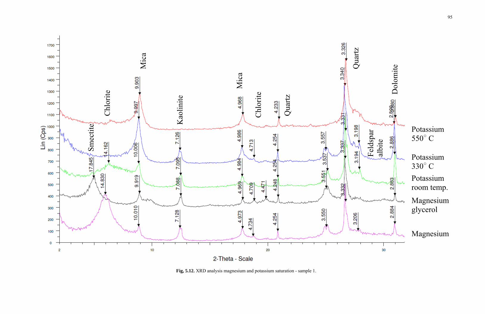
95
Fig, 5.12. XRD analysis magnesium and potassium saturation - sample 1.
Magnesium
Potassium room temp.
Kao
linite
Chl
orite
Mic
a
Dol
omite
Mic
a
Qua
rtz
Magnesium glycerol
Potassium 330○ C
Potassium 550○ C
Feld
spar
al
bite
Qua
rtz
Chl
orite
Smec
tite

96
Fig. 5.13. XRD analysis magnesium and potassium saturation - sample 2.
Magnesium
Potassium room temp.
Kao
linite
Chl
orite
Mic
a
Dol
omite
Mic
a
Qua
rtz
Magnesium glycerol
Potassium 330○ C
Potassium 550○ C
Feld
spar
al
bite
Qua
rtz
Chl
orite
Smec
tite
Feld
spar
al
bite
2 Theta -Scale

97
CCD camera) beneath it and on a computer monitor. The source of the electron
illumination is a small heated tungsten filament at the top of the evacuated column.
Vacuum pressures on the order of 10-5 Torr are employed. The sample must be dry and
the dissipation of heat from the concentrated electron beam is by conduction through the
sample and grid.
The sample clay used for TEM was prepared or dispersed in two ways. First,
distilled, deionized water was used to disperse the clay, secondly, one clay sample was
prepared with alcohol and water to observe the difference in the sample dispersion. An
aliquot of the saturated clay sample (about 5 mg of clay) was dispersed in 10 ml of
distilled, deionized water and another aliquot where 5 mg of the clay was dispersed in 10
ml of ethyl alcohol in labeled test tubes.
The diluted clay was dispersed by vigorous manual agitation of the test tubes.
The test tubes were placed in an ultrasonic generator and sonicated for 3-4 min. The
frequency of the ultrasonic field should be checked as very high frequencies of 106 Hz or
higher can produce particle degeneration. The time allowed for sonication is also
important as longer agitation times can produce heating.
After dispersion, 100 µl of the water suspension was removed from mid-depth
with a disposable pipette and placed in a smaller test tube. Using another pipette, 500 µl
of distilled deionized water was added to the suspension to dilute it. Another sample was
prepared by adding 100 µl of the suspension to 1000 µl of water. Similarly, 100 µl of the
clay suspension in ethanol was removed from mid-depth and diluted using 500 µl and
1000 µl of ethanol.

98
These four smaller test tubes with different concentrations were then placed in
the ultrasonic generator and agitated for 3-4 min. 400 mesh holey carbon grids were used
to mount the clay. The carbon film was first rendered hydrophilic by ion bombardment
from a glow discharge source. A droplet from each of the four small test tubes was
placed onto four hydrophilic carbon support films using a light microscope. The four
carbon grids were then left to dry and then placed in labeled containers ready to be used
in the microscope.
Figure 5.14 shows the presence of halloysite (long tubular structure clay particle)
in the center surrounded by chlorite in the background. Figure 5.15 shows chlorite
interspersed with folded smectite layers or as complex interstratified grains of silica
mineral in between particles of chlorite. The results of the X-ray diffraction show
presence of both smectite and quartz, making the minerals shown in the image difficult
to identify. Figure 5.16 shows the dispersion of the clay plates. Although the image is
not entirely clear and lacks contrast, the different clay platelets can be discerned. Figure
5.17 shows moire fringes on muscovite mineral or mica.

99
Fig. 5.14. TEM micrograph showing halloysite in the center of chlorite.
Fig. 5.15. TEM micrograph showing chlorite interspersed with folded smectite layers.

100
Fig. 5.16. TEM micrograph showing dispersion of the clay plates.
Fig. 5.17. TEM micrograph showing moire fringes on muscovite mineral or mica.

101
5.7 Constant Rate of Strain Consolidation
Constant rate of strain consolidation tests were conducted on eight samples at
various depths and strain rates (Table 5.2). As shown in Figure 5.18, Casagrande’s
graphical method was used to obtain the value of pre-consolidation pressure (σ′p ). For a
depth of 11.5 m, the pre-consolidation pressure was calculated to be 72 kPa. Figure 5.19
presents results of effective stress vs strain and Figure 5.20 presents results of void ratio
changing over effective stress. Results indicate a compression index (Cc) of 0.55 and a
recompression index (Cr) of 0.07 for all the curves.
Table 5.2. Summary of constant rate of strain consolidation tests.
Test Name Depth (m) Strain Rate CRS-GOM1 13.14 7 CRS-GOM2 13.18 5 CRS-GOM3 13.23 3 CRS-GOM4 11.81 1 CRS-GOM7 11.96 2 CRS-GOM6 12.10 1.5 CRS-GOM7 12.13 1.5 CRS-GOM8 10.01 1.5

102
Fig. 5.18. Casagrande’s graphical method to determine pre-consolidation pressure (Madhuri, 2011).

103
Fig. 5.19. CRS plot of effective stress vs strain.

104
Fig. 5.20. CRS plot of effective stress vs void ratio.

105
5.8 Triaxial Testing
A comprehensive series of CKoU compression and tension and CIU compression
and extension triaxial tests were performed on the Gulf of Mexico sample (Madhuri,
2011). Figure 5.21 presents the normalized effective stress paths for CKoU compression
and extension testing. For the compression tests, the effective stress envelope at critical
state is represented by a perfectly straight line at a of 25:5°. For the extension tests, the
effective stress shear envelope at critical state is not as clear as for compression. It is
best represented by a line which passes through the points of maximum shear stress with
an of 26:5°. The friction angle (φ) for the compression failure envelope was found to be
28° and - for the extension failure envelope was found to be 29.5°.
Figure 5.22 presents the normalized effective stress paths for CIU compression
and extension testing. For compression tests, the effective shear stress envelope at
critical state is at an angle of 24°. The effective shear stress envelope for the extension
tests was 25°. The friction angles for the compression and extension tests were found to
be 26.4° and 27.7°.
Comparing the strengths between the CKoU-C/E tests and the CIU-C/E tests, it
can be seen that the isotropic tests tend to fail at slightly lower strengths than the Ko
consolidated tests. Additionally, the angle for the isotropic tests in both compression and
extension is less than the angles obtained from the CKoU-C/E tests.

106
Fig. 5.21. Normalized effective stress paths from CKoU-C/E testing (Madhuri 2011).

107
Fig. 5.22. Normalized effective stress paths from CIU-C/E testing (Madhuri 2011).

108
5.9 Previous Testing on Gulf of Mexico Marine Clay
Limited monotonic direct simple shear tests results of Gulf of Mexico clays are
available in the literature. Young et al. (2003b) conducted consolidated undrained direct
simple shear monotonic tests on Gulf of Mexico samples from the northern Garden
Banks and northern Green Canyon regions. Normalized shear behavior was observed at
consolidation pressures of about 2.5 times the effective consolidation pressure, σ’vu. The
ratio of peak shear strength to the effective consolidation pressure, Su/ σ’vu ranged from
0.221 to 0.273 (Figure 5.23).

109
Fig. 5.23. Results of consolidated undrained direct simple shear tests (After Young et al., 2003b).

110
6. MULTI-DIRECTIONAL DIRECT SIMPLE SHEAR BEHAVIOR OF GULF
OF MEXICO CLAYS
An experimental test program was conducted on Gulf of Mexico clay with the
objective of simulating the stress conditions within a submarine slope. Specimens were
anisotropically consolidated under a vertical normal stress and horizontal shear stress
and subsequently sheared undrained by application of an additional horizontal shear
stress acting at an angle, δ, relative to the consolidation shear stress. Monotonic, cyclic,
circular, and figure-8 tests were conducted to simulate various loading patterns on a
submarine slope subjected to dynamic loading. Table 6.1 summarizes the Gulf of
Mexico specimens tested in the TAMU-MDSS.
6.1 Testing Procedures
The MSCL data was used to locate specimens within the core liner with a
minimum amount of disturbance. Both ends of core sections were discarded because of
possible disturbance, possible oxidation and change in water content during the storage
period. The cores were stored in the humidity room until testing. The location of each
sample was determined and the depth was recorded. The liner of the core was marked
with the depth, specimen name and an arrow indicting the orientation. The height of
each specimen was approximately 20 cm. A PVC cutter was used to cut the PVC liner
above and below the specimen. A wire was used to cut the soil and was then extruded
using a jack or allowed to extrude due to self weight. The porous stones were saturated
and filter paper was cut for both the top and bottom caps. The weight of the caps,

111
Table 6.1. Summary of GOM specimens tested in TAMU-MDSS.
Specimen Test type Consolidation Rate Cyclic
shear stress ratio (CRS)
Direction of shearing
δ (degrees) GOM-1 MONO CKo 5%/hr - 0
GOM-2 MONO CKo 50%/hr - 0
GOM-3 MONO CKα 5%/hr - 0
GOM-4 MONO CKα 5%/hr - 180
GOM-5 CYCLIC CKo 0.1 Hz 0.20 0
GOM-6 CYCLIC CKα 0.1 Hz 0.20 0
GOM-7 CYCLIC CKα 0.1 Hz 0.15 0
GOM-8 CYCLIC CKα 0.1 Hz 0.20 90
GOM-9 CYCLIC CKα 0.1 Hz 0.15 90
GOM-10 CIRCULAR CKo 0.1 Hz 0.20 -
GOM-11 CIRCULAR CKα 0.1 Hz 0.20 -
GOM-12 CIRCULAR CKα 0.1 Hz 0.15 -
GOM-13 FIGURE-8 CKo 0.1 Hz x-dir 0.2 Hz y-dir 0.20 0
GOM-14 FIGURE-8 CKα 0.1 Hz x-dir 0.2 Hz y-dir 0.20 0
GOM-15 FIGURE-8 CKα 0.1 Hz x-dir 0.2 Hz y-dir 0.15 0
GOM-16 FIGURE-8 CKα 0.1 Hz x-dir 0.2 Hz y-dir 0.20 90
GOM-17 FIGURE-8 CKα 0.1 Hz x-dir 0.2 Hz y-dir 0.15 90

112
saturated porous stones, filter paper, o-rings and membrane was recorded. The specimen
was then placed on the bottom cap and transferred to the trimmer. A wire saw was used
to trim the specimen to the specified diameter of approximately 79.8 mm (3.14 in) for a
diameter to height ratio of 4:1. The water content and Atterberg limits were determined
from trimmings. The specimen was laterally confined by a wire-reinforced membrane.
O-rings and hose clamps were installed on the top and bottom cap to prevent the o-rings
from moving during shearing and causing water to leak decreasing the excess pore
pressure. A summary of the depth, initial and final water contents, and unit weight for
each specimen is provided in Appendix C.
6.2 Consolidation
Consolidation of the specimens is used to minimize the effects of sampling
disturbance and load the specimen to a normally consolidated state. The wire-reinforced
membrane was used to provide lateral restraint and ensure Ko conditions (Bjerrum and
Landva, 1966). Back saturation of the specimen was conducted following procedures
similar to those used in triaxial testing. The chamber pressure and backpressure are
increases gradually keeping the difference between the two at a small value that will
minimize the effective stress applied to the specimen. The specimens were backpressure
saturated to a minimum B-value of 0.95. The consolidation effective stress (σ′vc) was
selected as 83.6 kPa so that all specimens would be normally consolidated to a stress at
least 1.5 times the estimated maximum past pressure. The effect of a slope was
simulated by reproducing the consolidation stress history by subjecting the specimen to a
consolidation shear stress (τc).

113
For CKo consolidated tests, the loading increment was applied in a single step
and the specimen was allowed to consolidate for 12 hours. For CKα tests, the vertical
load increments were applied in three stages, with two shear load increments for each
vertical (Figure 6.1). After the last increment, the specimens were allowed to
consolidate for 12 hours. Table 6.2 summarizes the loading schedule.
Fig. 6.1. CKα consolidation loading scheme.

114
Table 6.2. CKα consolidation loading schedule. Time (min) Vertical stress (kPa) Horizontal stress (kPa)
0 29.9 0 10 29.9 4.19 20 29.9 8.37 60 59.8 8.37 70 59.8 11.96 80 59.8 16.15 120 83.6 16.15 130 83.6 20.33 140 83.6 23.92
6.3 Undrained Shear Tests
The testing program was aimed at characterizing the response of marine clay
deposits in simple shear. The first part of the testing concentrated on establishing the
response to one-dimensional monotonic and cyclic shearing of CKo consolidated
specimens, simulating level ground conditions. Results were compared with other clay
tests specifically Boston Blue Clay (DeGroot, 1989) and San Francisco Young Bay Mud
(Biscontin, 2011) published in the literature. The effect of the slope (simulated by CKα
consolidation conditions) was investigated on monotonic and cyclic tests under varying
stress amplitude as well as orientation on the horizontal plane (angle δ between slope
direction and loading axis). Multi-directional loading patterns such as circles and figure-
8 (hourglass shape) were used to simulate simplified earthquake loading. Figure 6. 2
illustrates the stress paths used in the experimental testing program.

115
Fig. 6.2. Complex loading paths used in experimental testing program (Modified from Kammerer, 2001).
6.3.1 Monotonic Tests
Four specimens were monotonically sheared to investigate the influence of an
initial shear stress (τc) on the overall behavior of the soil. Test GOM-1 was performed at
τc = 0 (CKo consolidation) at the standard rate of 5% strain per hour and constitutes the
baseline of monotonic response for level ground. Test GOM-2 was performed at CKo
consolidation at a rate of 50%/hr for comparison of the rate effects on the shear behavior
of the soil. Test GOM-3 was CKα consolidated at τc/σ′vc = 0.2, which is equivalent to a
slope of 11.3° and then sheared at 5%/hr along the same direction as the applied
consolidation shear stress simulating shearing downslope (δ = 0°). Test GOM-4 was

116
also CKα consolidated at τc/σ′vc = 0.2 and then sheared at 5%/hr in the opposite
direction (δ = 180°), or upslope. The tests results are summarized in Figure 6.3.
Tests GOM-1 and GOM-3 reach approximately the same condition in the stress
path space, for a stress ratio τc/σ′vc = ψ of 23.7°, however, neither GOM-2 or GOM-4
reach the failure envelope. A normalized shear stress at large strains ranging from 0.20
to 0.38. Biscontin (2001) reported a failure envelope at ψ = 25° and a normalized shear
stress values approximately 0.27 for San Francisco Young Bay Mud Ko consolidated
monotonically sheared at 5%/hr. Young et al. (2003b) reported consolidated undrained
direct simple shear monotonic tests with normalized shear stress ratios ranging from
0.221 to 0.273 for Gulf of Mexico clays.
The complete state of stress during the tests is unknown because lack of
horizontal stress measurements due to the use of the wire reinforced membrane to
maintain Ko conditions during consolidation. An assumption related to the orientation of
the principal stresses has to be made for the construction of the Mohr’s circle. Appendix
A presents the most common hypotheses for failure conditions in simple shear testing.
For this work, failure criterion 1 in which the maximum horizontal shear stress is also
the shear strength of the soil (su) will be used.
For CKα consolidated monotonic tests (GOM-1 and GOM-2), both tests show a
continuous increase in shear stress until large strains are reached. Test GOM-3, in which
the specimen was strained in the same direction (downslope) as the consolidation shear
stress, has a larger shear strength than the other tests and once the shear stress has
reached the failure envelope continues down the failure envelope with continued shear

117
Fig. 6.3. Monotonic test results (a) stress paths, (b) stress-strain curves,
and (c) pore pressure ratio
(a)
(b)
(c)

118
strain. For the upslope shearing case, GOM-4, the shear strength shows a ductile
behavior and does not reach the failure envelope. Additional shear strain may be
required for the shear stress to continue to the failure envelope.
6.3.2 Cyclic Tests
Five specimens were consolidated and subjected to uniform cycles of shear
loading at a frequency of 0.1 Hz. Test GOM-5 was CKo consolidated and sheared at an
amplitude of τcyc/σ′vc of 0.2. This test represents the baseline for level ground conditions
in terms of the cyclic response of Gulf of Mexico clay. Figure 6.4 shows results for
GOM-5.
Four specimens were CKα consolidated at τc/σ′vc = 0.2, which is equivalent to a
slope of 11.3°. Two different cyclic stress ratios (CSR = τcyc/σ′vc) of 0.15 and 0.2 were
investigated. GOM-6 was CKα consolidated and sheared at a frequency of 0.1 Hz and
τcyc/σ′vc = 0.2 in the same direction as the consolidation shear stress (δ = 0°). Similarly,
GOM-7 was CKα consolidated and sheared at a frequency of 0.1 Hz at δ = 0°, however,
the cyclic shear stress ratio was 0.15. GOM-8 and GOM-9 were CKα consolidated and
sheared at a frequency of 0.1 Hz, however, were sheared in the perpendicular direction
(δ = 90°) of the consolidation shear stress equivalent to shearing across the slope.
The fundamental soil behavior during cyclic shearing is the development of
excess pore pressure with accumulation of plastic strains as the number of cycles
increases. The excess pore pressure versus the number of cycles for the two cyclic shear
stress ratios (CRS) is plotted in Figure 6.5. The accumulation of plastic strains with

119
Fig.
6.4
. GO
M-5
CK
o cyc
lic te
st re
sults
(a) s
tress
pat
h, (
b) st
ress
-stra
in c
urve
, (c
) por
e pr
essu
re ra
tio, a
nd (d
) she
ar st
rain
with
cyc
les
(a)
(b)
(c)
(d)

120
Fig. 6.5. Cyclic tests (a) development of pore pressures, (b) accumulation of plastic strains
(a)
(b)

121
progressing cycles is also plotted. The value of CRS and the application to an initial
static driving stress directly influences the generation of pore pressure during the test.
For CKα consolidated tests (GOM-6, GOM-7, GOM-8 and GOM-9), excess pore
pressure generation was significantly decreased in comparison with GOM-5 simulating
level ground. Test GOM-5 reached a pore pressure ratio (∆uexcess/σp) of approximately
0.75 while the other tests accumulated permanent strains in the downhill direction very
quickly thus limiting the generation of excess pore pressure.
For tests GOM-8 and GOM-9 in which undrained shearing was performed
perpendicular to the direction of the consolidation shear stress (δ = 90°), the specimen
also failed in the downhill direction. Because the stresses are loading the specimen in the
same direction at the point of the test where the material is the softest, permanent
displacements accumulate in the direction of the consolidation shear stress, in this case,
the x-direction.
As the cyclic stress ratio increased from 0.15 to 0.20, as illustrated in tests GOM-
6 and GOM-7, the rate of the accumulation of permanent strains increased and the
generation of excess pore pressures also increased. Test GOM-6 at a CRS value of 0.2
accumulated shear strains over 15% in 5 cycles, whereas test GOM-7, in which the CRS
value was 0.15, did not accumulated shear strains over 15% until 26 cycles.
6.3.3 Circular Tests
Due to the complexity of earthquake loading, circular load patterns were used to
simplify the multi-directional shearing of the specimen. Three specimens were subjected
to a circular stress loading pattern at a frequency of 0.1 Hz. GOM- 10 was CKo

122
consolidated and sheared at a cyclic shear stress ratio, τcyc/σ′vc = 0.2 (Figure 6.6). This
test was used as the baseline for circular shearing on level ground. Figure 6.7 compares
the generation of excess pore pressure and accumulation of plastic strains with cycles for
the circular tests.
Results for test GOM-10 show failure of the specimen occurs at approximately
13 cycles and moves in a positive x-direction. The pore pressure ratio was approximately
0.5. GOM-11 and GOM-12 were CKα consolidated and sheared at CRS of 0.15 and 0.2,
respectively. Both tests accumulated permanent strains in the direction of the
consolidation shear stress and generated approximately the same excess pore pressure,
however, tests GOM-11 failed in 7 cycles whereas tests GOM-12 failure in 27 cycles.
Due to the symmetry of the circular tests, the shear stress values do not approach
zero at any point in the tests unlike cyclic and figure-8 tests. The excess pore pressure
generation for the circular tests on sloping ground are similar to the magnitudes in the
CKα cyclic tests, however, accumulate permanent strains at a lower number of cycles.

123
Fig.
6.6
. GO
M-1
0 C
Ko c
ircul
ar te
st re
sults
(a) s
hear
stre
ss p
atte
rn, (
b) sh
ear s
train
in
x a
nd y
-dire
ctio
ns, (
c) p
ore
pres
sure
ratio
, and
(d) s
hear
stra
in w
ith c
ycle
s

124
Fig. 6.7. Circular tests (a) development of pore pressures, (b) accumulation of plastic strains x-direction, (c) accumulation of plastic strain y-direction
(a)
(b)
(c)

125
6.3.4 Figure-8 Tests
Figure-8 tests were used as simplified earthquake loading patterns. Five figure-8
tests were conducted at a frequency of 0.1 Hz in the x-direction and simultaneously a
frequency of 0.2 Hz in y-direction. GOM-13 was CKo consolidated and sheared at a
cyclic shear stress ratio, τcyc/σ′vc = 0.2 (Figure 6.8). This tests will be used the figure-8
baseline for level ground. Four tests (GOM-14, GOM-15, GOM-16 and GOM-17) were
CKα consolidated and subjected to a figure-8 stress loading pattern at two cyclic stress
ratios and in two different directions. GOM-14 and GOM-15 were sheared in the same
direction as the consolidation shear stress (δ = 0°) while GOM-16 and GOM-17 where
sheared perpendicular to the consolidation shear stress (δ = 90°). GOM-14 and GOM-16
were sheared with a cyclic stress ratio of 0.2 while GOM-15 and GOM-17 were sheared
with τcyc/σ′vc = 0.15. Figure 6.9 compares the generation of excess pore pressure and
accumulation of plastic strains with cycles for the circular tests.
Test GOM-13 simulating level ground generates the largest pore pressure ratio of
approximately 0.75 which is the same magnitude as the pore pressure generation by the
cyclic CKo test GOM-5. As the CRS was decreased, the number of cycles during
accumulation of permanent strains increased from 3 cycles to 11 cycles. The excess pore
pressure generation for the tests simulating sloping ground generate approximately the
same excess pore pressure ratios. Tests performed perpendicular to the consolidation
shear stress generate more excess pore pressure than the other CKa tests, however,
accumulated permanent strains in the downhill direction regardless of the cyclic shear
stress ratio.

126
Fig.
6.8
. GO
M-1
3 C
Ko f
igur
e-8
test
resu
lts (a
) she
ar st
ress
pat
tern
, (b)
shea
r stra
in
in x
and
y-d
irect
ions
, (c)
por
e pr
essu
re ra
tio, a
nd (d
) she
ar st
rain
with
cyc
les

127
Fig. 6.9. Figure-8 tests (a) development of pore pressures, (b) accumulation of plastic strains in x-direction, and (c) accumulation of plastic strain in y-direction
(a)
(b)
(c)

128
6.4 Conclusions
Results of CKo consolidation cyclic and multi-directional tests (GOM-5, GOM-
10, and GOM-13) indicate that the largest generation of excess pore pressures occurs for
specimens subjected to full stress reversals. Because of the different geometries of the
stress paths, pore pressure generation is affected in different ways by the inclusion of an
initial driving shear stress even if the nominal amount of stress reversal is the same.
Figure-8 tests accumulated permanent deformations in less cycles than both
cyclic and circular tests due to the combination of the horizontal shear stress rotation and
complete shear stress removal and reversal during loading. For tests incorporating an
initial horizontal shear stress, the strains migrated in the downhill direction regardless of
the orientation of the cyclic loading.
These findings have important implications for the stability of the slope,
predicting that forces acting downward in the slope direction will need to mobilize less
strain to reach peak strength and initiate failure. During cyclic tests with no initial shear
stress (τc = 0) simulating level ground, the cyclic strains are symmetrically centered
around the zero strain axis, with full reversal at each cycle. When τc ≠ 0 (simulating a
slope) an average shear strain accumulates during the tests and the maximum and
minimum shear strains are not centered around the zero strain axis.

129
7. SUMMARY AND CONCLUSIONS
7.1 Summary
This dissertation describes the development of a new multi-directional direct
simple shear testing device, the Texas A&M Multi-directional Direct Simple Shear
(TAMU-MDSS), for testing marine soil samples under conditions, which simulate, at the
element level, the state of stress acting within a submarine slope under dynamic loading.
Prototype testing and an experimental program to characterize the response of marine
clays to complex loading conditions is presented.
The work is divided into four major components: 1) Equipment Development:
Design and construction of a prototype multi-directional direct simple shear testing
device (TAMU-MDSS) that addresses the limitations of previous devices. 2) Support
systems: selection of control software, development of data acquisition system and
design of back pressure systems for direct pore pressure measurements. 3) Prototype
Testing: performance of the TAMU MDSS system and testing of strain-control and
stress-control capabilities. 4) Experimental Testing: characterize the response of marine
clays to monotonic, dynamic and random loads.
The two-directional monotonic, cyclic, circular and figure-8 tests demonstrated the
undrained shear strength increases with increasing initial shear stress, τc (i.e, slope), for
shearing in the same direction (equivalent to downhill). The strength decreases for
shearing in the direction opposite to the initial stress (shearing uphill). The response is
brittle for shearing in the same direction as the shear stress applied during consolidation

130
(τc) and ductile for shearing opposite to τc. These findings have important implications
for the stability of the slope predicting that forces acting downward in the slope direction
will need to mobilize less strain to reach peak strength and initiate failure.This
information provides insight into the behavior of marine soils under complex loading
conditions and provides high quality laboratory data for use in constitutive and finite
element model development for analysis of submarine slopes.
7.2 Recommendations for Future Work 7.2.1 TAMU-MDSS Device
Like other devices of its type, the TAMU-MDSS has some measureable
frictional resistance between the horizontal loading plates during strain-controlled
motions. An additional evaluation of the “device friction” should be conducted to
determine the extent in which application of vertical load to the horizontal plates effects
the measured frictional resistance. Control of the TAMU-MDSS using ATS has some
limitation specifically related to the PID controls. A sensitivity analysis of the gains to
specific material stiffness is required. Currently, the multi-axis load cell data acquisition
is recorded on a separate system. Incorporation of all sensor measurements into one data
acquisition system would be beneficial. The backpressure and cell pressure system could
be automated using flow pumps and an air pressure controller to facilitate the
backpressure portion of the testing.
7.2.2. Multi-directional Testing of Gulf of Mexico Clays
An experimental testing program using reconstituted samples could be conducted
to compare the results with undisturbed tests conducted in this research. Specimens

131
could also be consolidated at different OCR to determine influence of over consolidation
on behavior. The tests conducted in this experimental study focused on a single slope
angle, however, testing should be carried out to determine to what extent different slope
angles effect the behavior. Additionally, tests at varying cyclic frequencies and different
cyclic stress ratios could be conducted to provide more insight into the multi-directional
undrained shear behavior of Gulf of Mexico clays subjected to complex load patterns.
132
REFERENCES
Airey, D., M. Budhu, and D. Wood (1985). “Some aspects of the behavior of soils in simple shear.” Developments in Soil Mechanics and Foundation Engineering, Stress-Strain Modeling of Soils, Elsevier, London, U.K., Chapter 6, 185-213. Airey, D. and Wood, D. (1987). “An evaluation of direct simple shear tests on clay.” Geotechnique, 37(1), 25-35. Al-Khafaji, Z. A., Young, A. G., DeGroff, W. and Humphrey, G. D. (2003). “Geotechnical properties of the Sigsbee Escarpment from deep soil borings.” 2003 Offshore Technology Conference, Houston, TX, U.S.A., 5-8 May 2003. paper no. OTC 15158. Amer, M. I., Kovacs, W. D., and Aggour, M.S. (1987). “Cyclic simple shear size effects.” J. of Geotech. Engrg. 113(7), 693-707. Andersen, K., Pool, J., Brown, S., and Rosenbrand, W. (1980). “Cyclic and static laboratory tests on Drammen clay.” J. of Geotech.l Engrg. Div., 106(GT5), 499-529. Azzouz, A., Malek, A., and M. Baligh (1989). “Cyclic behavior of clays in undrained simple shear.” J. of Geotech. Eng. 115(5), 637-657. Bea, R. G. (1971). “How sea floor slides affect offshore structures.” Oil and Gas J., 69, 88-91. Biscontin, G. (2001). “Modeling the dynamic behavior of lightly overconsolidated soil deposits on submerged slopes.” Ph.D. Dissertation, University of California, Berkeley. Bjerrum, L. (1954). Theoretical and experimental investigations on the shear strength of soils. Norwegian Geotechnical Institute, Oslo, Norway. Bjerrum, L., and Landva, A. (1966). “Direct simple-shear test on a Norwegian quick clay.” Geotechnique, 16(1), 1-20. Boulanger, R.W. (1990). “Liquefaction behavior of saturated cohesionless soils subjected to unidirectional and bidirectional static and cyclic simple shear stresses.” Ph.D. Dissertation, University of California, Berkeley. Boulanger, R. W. and Seed, R. B. (1995). “Liquefaction of sand under bidirectional monotonic and cyclic loading.” J. Geotech. Engrg., 121(12), 870-878.

133
Boulanger, R.W., Chan, C. K., Seed, H. B., Seed, R.B., and Sousa, J. (1993). “A low-compliance bi-directional cyclic simple shear apparatus.” Geotech. Test. J., 16(1), 36-45. Bryant, W. R., Bryant, J. R., Feeley, M.H., and Simmons, G.R. (1990). “Physiographic and bathymetric characteristics of the continental slope, northwest Gulf of Mexico.” Geo. Mar. Letters., 10, 182-199. Bryant, W.R., Simmons, G.R., and Grin, P. (1991). “The morphology and evolution of basins on the continental slope, northwest Gulf of Mexico.” Gulf Coast Association of Geological Societies Transactions, 41, 73-82. Budhu, M. (1985). “Lateral stresses observed in the simple shear apparatus.” J. of Geotech. Eng., 111(6), 698-711. Budhu, M. and Britto, A. (1987). “Numerical analysis of soils in simple shear devices.” Soils Found., 29(2), 31-41. Casagrande, A. (1976). "Liquefaction and cyclic deformation of sands - A critical review." Harvard Soil Mechanics Series No. 88, Harvard University, Cambridge, MA., January. Casagrande, A. and Rendon, F. (1978). “Gyratory shear apparatus: Design, testing procedures.” Technical Report S-78-15, Corps of Engineers Waterway Experiment Station, Vicksburg, MS. Coleman, J. and L. Garrison (1977). “Geological aaspects of marine slope stability, northwestern Gulf of Mexico.” Marine Geotechnology 2, 9-44. Deng, Y., White, G. N., and Dixon. J. B., (2009). “Soil mineralogy laboratory manual.” 11th edition. Published by the authors, Department of Soil and Crop Sciences, Texas A&M University, College Station, TX 77843-2474. DeGroot, D. J. (1989). “The multidirectional direct simple shear apparatus with application to design of offshore arctic structures.” Ph.D. Dissertation, Massachusetts Institute of Technology, Cambridge. DeGroot, D.J., Ladd, C.C., and Germaine, J.T. (1996). “Undrained multidirectional direct simple shear behavior of cohesive soil,” J. Geotech. Engrg., 122(2), 91-98. Duku, P.M., Stewart, J. P, Whang, D. H, and Venugopal, R. (2007). “Digitally controlled simple shear apparatus for dynamic soil testing,” Geotech. Test. J., 30(5), 1-10.

134
Dyvik, R.(1981). “Strain and pore pressure behavior of fine grained soils subjected to cyclic shear loading,” Ph.D. Dissertation, Reneesleaer Polytechnic Institute, Troy. Dyvik, R., Berre, T., Lacasse, S., and Raadim, B. (1987). “Comparison of truly undrained and constant volume direct simple shear tests.” Geotechnique, 37(1), 3-10. Edgers, L. and Karlsrud, K. (1982). “Soil flows generated by submarine slides- case studies and consequences.” In Proc. 3rd Int. Cong. On the Behavior of Off-Shore Structures, Cambridge, MA. 2, 425-437. Fine, I.V., Rabinovichb, A.B., Bornholdd, B.D., Thomsonb, R.E. and Kulikovb, E.A. (2005). “The Grand Banks landslide-generated tsunami of November 18, 1929: preliminary analysis and numerical modeling.” Mar. Geol., 215, 45-57. Finn, L. W. D., Pickering, D. J., and Bransby, P. L. (1971). “Sand liquefaction in triaxial and simple shear tests.” J. Soil Mech. and Found. Div., 97(SM4). 639-659. Finn, L. W. D., Bhatia, D. K., and Pickering, D. J. (1982). “The cyclic simple shear test.” Soil mechanics – Transient and cyclic loads, G. N. Pande and O. C. Zienkiewicz, eds., John Wiley & Sons, New York, NY, book chapter 21, 583-607. Franke, E., Kiekbusch, M., and Schuppener, B. (1979). “A new direct simple shear device.” Geotech. Test. J ., 2(4), 190-199. Frydman, S., Talesnick, M., Almagor, G., and Wiseman, G. (1988). “Simple shear testing for the study of the earthquake response of clay from the Israeli continental slope.” Mar. Geotech., 7, 143-171. Hampton, M. A., Lee, H.J. and Locat, J. (1996). “Submarine landslides.” Reviews of Geophysics, 34, 33-59. Heezen, B.C. and Ewing, M. (1952). “Turbidity currents and submarine slumps, and the 1929 Grand Banks earthquake.” American Journal of Science, 250, 849-873. International Centre for Geohazards. (2010). “Offshore Geohazards.”< http://www.ngi.no/en/Geohazards/Research/Offshore-Geohazards/> (Dec. 16, 2011). Ishihara, K. and Yamazaki, F., (1980). “Cyclic simple shear tests on saturated sand in multi-directional loading.” Soil Found., 20(1), 45-59. Jeanjean, P., Hill, A., Taylor, S. (2003). “The challenges of siting facilities along the Sigsbee Escarpment in the southern Green Canyon area of the Gulf of Mexico: Framework for Integrated Studies.” Offshore Technology Conference, OTCX 15156.

135
Kammerer, A. (2001). “Undrained response of cohesionless soils under multidirectional cyclic simple shear conditions.” Ph.D. Dissertation, University of California, Berkeley. Kammerer, A. M., Hunt, C. E., and Riemer, M. (1999). “UC Berkeley geotechnical testing for the East Bay crossing of the San Francisco-Ooakland Bay Bridge.” Report No. UCB/GT/99-18, Department of Civil and Environmental Engineering. University of California, Berkeley. Kjellman, W. (1951). “Testing the shear strength of clay in Sweden.” Geotechnique, 2(3), 225-235. Lacasse, S., Dyvik, R., and Hoeg, K. (1988). “Discussion on the behavior of normally consolidated clay as observed in undrained direct shear tests by Wroth (1987).” Geotechnique, 38(1), 144-146. Ladd, C. C. and Edgers, L. (1972). “Consolidated-undrained direct-simple shear tests on saturated clays.” Report No. 16, Department of Civil Engineering, Massachusetts Institute of Technology, Cambridge. Lewis, K. (1971). “Slumping on a continental shelf inclined at 1 to 4.” Sedimentology, 16, 97-110. Lucks, A., Christian, J., Brandow, G., and Hoeg, K. (1972). “Stress conditions in NGI simple shear test.” J. of the Soil Mechanics and Found. Div. 98 (SM1), 155-160. Madhuri, M. (2011). “ Characterization of Gulf of Mexico clay using automated triaxial testing.” M.S. Thesis, Texas A&M University, College Station. Malek, A. M. (1987). “Cyclic behavior of clay in undrained simple shearing and application to offshore tension piles.” Ph.D. Dissertation, Massachusetts Institute of Technology, Cambridge. McAdoo, B. G. and Watts, P. (2004). “Tsunami hazard from submarine landslides on the Oregon continental slope.” Mar. Geol., 203, 235-245. McCarron, W. O., Lawrence, J. C., Werner, R. J., Germaine, J. T., and Cauble, D. F. (1995). “Cyclic direct simple shear testing of Beaufort Sea clay.” Can. Geotech. J., 32(4), 584–600. Prevost, J. and Hoeg. K. (1976). “Reanalysis of simple shear soil testing.” Canadian Geotech. J. 13(4), 418-429. Prior, D. and J. Coleman (1978). “Disintegrating retrogressive landslide on very-low-angle subaqueous slopes, Mississippi delta.” Marine Geotechnology, 3(1), 37-60.
136
Rau, G. A. (1999). “Evaluation of strength degradation in seismic loading of holocene bay mud from Marin County, California.” Ph.D. Dissertation, University of California, Berkeley. Roscoe, K. (1953). “An apparatus for the application of simple shear to soil samples.” Proc. of the 3rd Int. Conf. In Soil Mechanics and Foundation Engineering, Zurich, Switzerland, 1, 186-191. Saada, A. and Townsend, F. (1981). “State of the art: Laboratory strength testing of soils.” Laboratory shear strength of soil, R. N. Yong and F. C. Townsend (Eds.), American Society of Testing and Materials, Philadelphia, PA, 7-77. Saada , A. S., Fries, G., and Ker, C. C., (1982). “An evaluation of laboratory testing techniques in soil mechanics.” J. of Geotech. Engrgr., 123(3), 379-398. Schapery, R. and Dunlap, W. (1978). “Prediction of storm induced sea bottom movement and platform forces.” Offshore Technology Conference, Houston TX, 1789-1796. Shen, C.K., Sadigh, K., and Herrmann, L. R., (1978), “An analysis of NGI simple shear apparatus for cyclic load testing.” Dynamic Geotechnical Testing, ASTM STP 654, ASTM International, West Conshohocken, PA, 148-162. Slowey, N. C., Bryant, W. R., Bean, D.A., Young, A.G., and Gartner, S. (2003). “Sedimentation in the vicinity of the Sigsbee Escarpment during the last 25,000 years.” Proc. 19th Int’l OMAE Conference, paper no. 5045. Sousa, J. B. and Chan, C. K. (1991). “Computer applications in the geotechnical laboratories of the University of California at Berkeley.” Geotechnical Engineering Congress, Geotechnical Engineering Division of ASCE. Tappin, D., Watts, P., McMurty, G., Lafoy, Y., and Matsumoto, T. (2001). “Prediction of slump generated tsumanis: the July 17, 1998 Papua New Guinea tsunami.” Prediction of underwater landslide hazards, P. Watts, C.E. Synolakis, and J.-P. Bardet (Eds.), Balekema, The Netherlands. TDI-Brooks International. “Welcome to TDI-Brooks International.” <www.tdi-bi.com> (Dec. 16, 2011). Torkornoo, R. (1991). “Multidirectional simple shear behavior of an overconsolidated clay.” Master Thesis, University of Massachusetts, Amherst.

137
Vucetic, M. and Lacasee, S. (1982). “Specimen size effect in simple shear test.” J. of the Geotech. Engrg Div., 108(GT12), 1567-1585. Young, A.G., Bryant, W.R., Slowey, N.C., Brand, J.R., and Garnter, S. (2003a). “Age dating of past slope failures of the Sigsbee Escarpment within Atlantis and Mad Dog developments.” Offshore Technology Conference, Houston TX, OTC 15204. Young, A.G., Honganen, C.D., Silva, A.J., and Bryant, W.R. (2003b). “Comparison of geotechnical properties from large-diameter long cores and borings in deep water Gulf of Mexico.” Offshore Technology Conference, Houston TX, OTC 12089.

138
APPENDIX A
SIMPLE SHEAR TESTING OF CLAYS
A.1. Stresses in the Simple Shear Device
Simple shear conditions refers to the plane strain condition in which only the shear
strain γyx and the vertical strain, εyy, are non-zero. The strain, εzz, and engineering strains,
γyx and γzx are equal to zero. For constant volume tests, no vertical displacement occurs
and εyy is also zero. However, implementation of these conditions is difficult to attain in
laboratory testing devices as illustrated in Figure A.1.
Fig. A.1. (a) General strain state; (b) Simple shear strain state (After Biscontin, 2001).

139
The idealized in-situ boundary conditions in the field require four main
assumptions for direct simple shear testing. The assumption of the constant volume of
the sample implies no drainage of pore pressure redistribution during loading. This
assumption also implies that any shear loading imposed occurs so rapidly that drainage
of the soil cannot occur. The application of a constant vertical load to the sample implies
that the overburden remains constant during shearing. Assuming no lateral strain of the
specimen presumes the deposit is of large horizontal extent that lateral stresses
throughout the layer are such that lateral strains do not occur. Finally, the maintenance
of a constant height of the sample is assumed because if the volume is constant and no
lateral strains occur then the height must be also be constant.
A wire-reinforced membrane is used to maintain the boundary conditions of
constant volume and no lateral strain, although, one drawback is that lateral stresses
cannot be easily measured. Stacked rings have been used in some direct simple shear
testing devices, however, in this research stacked rings are not used because of possible
inherent mechanical restraint against multi-directional loading. By using a device with
chamber pressure and direct measurements of pore pressure, constant load can be
maintained during tests. Constant height is assumed since the sample has completed the
consolidation phase of the testing and drainage is prevented during shearing.
A criticism of direct simple shearing testing is mainly due to the inability to
impose uniform normal and shear stresses to a test specimen. Non-uniform stresses
conditions (Figure A.2) in simple shear tests specimens may develop due to (Boulanger,
1990):

140
1) The lack of complimentary shear stresses on the lateral boundaries
2) Corner and edge effects
3) Non-rigid boundaries which allows stress redistribution
4) Pinching effects which may result from any relative rocking motions between
the sample’s cap and base
5) Consolidation which is not truly one-dimensional which in combination with
the rigid top and bottom boundaries results in non-uniform radial shear
stresses
Fig. A.2. Schematic distribution of non-uniform distribution (a) of shear stresses from absence of complementary shear stress on the ends of the sample; (b) of normal stresses on the top and bottom faces of a sample in the simple shear device (After Airey et al., 1985).

141
The influence of the lack of complementary shear stresses along the
lateral boundaries of circular test specimens has been investigated both
experimentally (Finn et al., 1971, Finn et al., 1982, Vucetic and Lacasse, 1982,
Budhu, 1985, Airey and Wood, 1984) and numerically (Roscoe, 1953. Lucks et
al, 1972). Budhu (1985) presented measurements of radial normal stresses
obtained by instrumented wire wrapped membranes and compared with the
measurements of two orthogonal lateral normal stresses that developed at the
rigid lateral boundaries of an instruments Cambridge device (cuboidal sample).
Airey and Wood (1984, 1987) showed that the uniformity of stresses improves as
the plasticity of the material tested increases. Typical normal and shear stress
distributions measured on the center of the sample during constant volume tests
are shown in Figure A.3. Analytical and numerical test results suggest that for
D/H values of 4 or greater the lack of complementary shear stress affects a
relatively small portion of the sample such that the average shear stresses applied
to the sample are reasonably representative of the shear stresses acting over the
center portion of the sample.

142
Fig. A.3. Stress distribution on the principal third for a constant volume test on kaolin in the Cambridge simple shear device (a) Principal third load cells; (b) Normal and (c) shear stresses (α is the shear distortion γxy) (after Airey and
Wood, 1987).
A.2. Undrained vs. Constant Volume Testing
Casagrande (1976) deviated from the traditional NGI method by placing the
sample in a pressure cell allowing back pressure to be applied to ensure full saturation of
the specimen and the direct measurement of the pore water pressure during the
undrained shear test. This approach allowed for an alternative to the historical “constant
volume” approach which had been introduced early on with the NGI apparatus (Taylor,
1953; Bjerrum, 1954). Constant volume of the specimen is ensured by maintaining a
143
constant height of the sample by changing the vertical load. The excess pore pressure is
then assumed equal to the change in vertical stress.
Few existing simple shear devices have been designed to impose a chamber
pressure allowing for the full saturation of the sample. Comparing direct measurements
with “constant volume” results, monotonic tests by Dyvik et al. (1987) and Kammerer et
al. (1999) show that the assumption that constant volume tests are equal to excess pore
pressure measurements for saturated soils (Figure A.4 and A.5). No comparisons of the
two methods are available in the literature for cyclic tests on saturated clays.

144
Fig. A.4. Comparison of constant volume and undrained tests results (Dyvik et al., 1987).

145
Fig. A.5. Comparison of specimens using different saturation conditions (After Kammerer et al., 1999).

146
APPENDIX B
TAMU-MDSS DEVICE TEST PROCEDURES
1 - Saturation of the caps (Need: caps, porous stones, de-aired water, vacuum chambers)
• De-air vacuum chamber with vacuum pump • Pour de-aired water from the vacuum chamber into the reservoir or bowl • Hook up the drain lines of the caps to the lines from the vacuum chamber and
submerge the caps in the water (keep valve to lines closed) • Apply house vacuum to vacuum chamber and open valve to one cap. Switch to
the other cap to pull all the air out • Take lines off from the connection closer to the caps • Let the caps soak completely submerged
1a – Saturation of the caps (from dry condition) • De-air water in the vacuum chamber and connect the lines • Let water flow into the caps slowly through capillary suction • Switch frequently
2- Preparing the sample (Need: core section, cm ruler, marker, pipe cutter, thin wire, glass plate, extruder, caps, o-rings, filter paper, spacer, dial gage, scale, water content cups, test information sheet, pen)
• Measure 20 mm on liner • Use pipe cutter to cut liner • Use wire to cut through soil • Extrude soil from sampler (about 20 mm thick) • Measure the caps with a spacer • Weigh caps with membrane, clamps and 4 o-rings • Weigh 2 water content cups (1 for trimmings and 1 for sample)
3 – Trimming the sample (Need: sample, caps, filter paper, trimming jig, wire saw, paper towels, wet rag, ziplok bag, moisture cup, level, scale, oven, test information sheet)
• Place sample on the filter paper and bottom cap • Place bottom cap and sample on the trimming jig • Position the bottom cap correctly for trimming • Trim sample to desired diameter • Use one trimming piece for moisture content • Weigh trimming and cup and place in oven • Place trimmings in labeled ziplok bag and place in moisture room

147
4 – Placing the membrane (Need: sample, caps, membrane, o-rings, square, level, dial gage, pi tape, vacuum chambers, vacuum source, test information)
• Remove sample and bottom cap from trimming jig • Place filter paper and top cap • Flip sample upside down to top cap • Remove bottom cap • Pull the wet membrane on the sample • Use o-ring extender to stretch and place two o-rings on bottom cap • Stretch two o-rings over extender for top cap and place around sample • Replace top cap • Check alignment with square and level • Install 2-orings on top cap • Fix o-ring location, sacrificial membranes and hose clamps • Weigh the assembly • Measure the height of the assembly • Measure the diameter with pi tape • Connect drain lines from vacuum chamber to caps • Attach line to house vacuum • Apply slight vacuum to top cap(about 1.5 in Hg) making sure bottom cap
vacuum chamber is open • Measure the height of the assembly • Measure the diameter with pi tape • Check if visible bubbles are coming out
5 – Seating the sample in the device (Need: assembled sample, vacuum chambers, socket wrench)
• Zero x and y axis strokes (control -> transducers -> zero units) • Put sample into the device • Move the sample still connected to the vacuum chamber to the device • Little by little lower the top of the device toward the sample until there is just a
small space left • Load sample to 10lbs in vertical axis using stroke control • Disconnect vacuum chamber from vacuum lines • Connect water lines by wet connection (slight pressure on back pressure lines to
cause constant dripping, 0.2 is enough) • Change Z-axis from stroke control to load control and immediately manually
lower the load back to 10lbs (changing to load control causes slight rise in piston)
• Check to make sure P gain is set to 100 for the remainder of the test • Install top clamp around sample cap and fine loadcell, tighten by hand until you
can no longer turn it

148
• Use ratchet with hexhead to tighten bottom sample cap to bar on lower plate, tighten each side equally while monitoring x and y loads to ensure they remain close to 0.0
• Record all initial readings • Continue to backpressure steps
6 – Getting rid of the bubbles still in the sample (Need: cloth towel, vacuum chamber, house pressure, test information sheet)
• Flush the lines so that any bubbles are pushed out. Remember to use a towel to protect the device from the water
• Take line that is open to vacuum chamber (but no vacuum on it) and connect to one of the drainage line of the device). Make sure it is a “wet connection
• Repeat with the second line • Select which line to get bubbles out • Move vacuum chambers to top of chamber • Discount lines and attach vacuum chambers • Make sure that each vacuum chamber valve is open • Using vacuum chamber attached to top and apply slight vacuum (2-5). Let stay
until all bubbles make it out. • Switch to the other vacuum chamber • Close valves to samples • Disconnect vacuum chambers • Slightly increase back pressure just enough to push air out of drainage lines to
the elevation of the top of the chamber • Make a wet connection from drainage lines to valves • Turn off pressure • Open valves to samples • Take LVDT measurements and initial volume measurements • Close the chamber
7 – B value checks (Need: B-value check file, test information sheet, house pressure, back pressure calculation excel spreadsheet)
• Close A valve • Close cell release valve under chamber (opened to allow oil in chamber to drain) • Verify that nothing is in the path of the chamber as it is lowered • Lower chamber by pushing chamber down button on the computer console • Once chamber is completely lowered, switch metal toggle switch to on to prevent
chamber from rising during test • Increase cell pressure to 2psi and maintain the 10lbs load in the vertical direction
(manually move back and forth increasing each incrementally to desired values) differential pressure goes down during this step

149
• Record vertical load, chamber pressure and effective stress (as indicated in the test sheet)
• Close the b-valve and open the a-valve • Increase the differential pressure to 0.1 • Open the b-valve • Slightly increase the back pressure to approximately 0.2 and hold for 30 min to
1hour • Bring cell pressure up (~ 5 psi) until effective stress is about 10-12 kPa (1.45 –
1.75 psi) while keeping the vertical load constant (by increasing it slowly) • Wait until equilibrium is reached • Read measurements • Close B valve and open A valve • Increase backpressure until effective stress is back to slightly less than zero (~-
0.2) • Open B valve, open A valve • Calculate B value check • Wait 10 minutes or more depending on how low B valve is • Close A valve • Check if effective stress is going up (suction: still need more time to get pore
pressure down). Open A and let stand a little while. • Repeat B value check until you get a value over 0.95 • Maximum house pressure is 29 psi
8 – Starting the consolidation (Need: Consolidation ATS file, test information sheet,
• When the B value check is right, let stand until re-equilibrated for the last time • Open ATS consolidation test file • Select vertical load needed to consolidated to the desired value of stress • Keep A valve open • Take LVDT readings and initial volume • Start data test • Reset column of water by opening and closing pipette/reservoir valve • Record ending consolidation test information on test sheet
9 – Starting shearing test (Need: Shear ATS file, test information sheet) • Record information on test sheet • Make sure A valve is closed • Open ATS shear test file • Select shearing rate or shearing load needed for test • Take LVDT readings and initial volume • Start data test • Record ending shear test information on test sheet

150
10 – Removing sample from MDSS (Need: House pressure, assembled sample, scale, dial gage, pi tape, sample moisture content cup, test information sheet, oven)
• Open A valve • Slowly decrease both cell pressure and back pressure maintaining a low effective
stress difference (-.2 and -1.5 psi) also decreasing the total load on sample back to seating pressure of 5 lbs
• Once both cell pressure and back pressure are close to 1 psi turn off house pressure supply
• Remove line from house pressure supply • Open chamber • Switch Z axis to stroke control • Loosen bottom clamps and top clamps • Slowly rise Z_stroke until able to remove sample • Remove drainage lines and attach to t-valve • Weigh sample • Measure height and diameter • Remove top cap and membrane • Place sample in sample moisture content cup • Weight sample and cup • Place sample and cup in oven over night • Take dry weights of trimmings and sample after 24 hours

151
MULTI-DIRECTIONAL SIMPLE SHEAR TESTING DATA SHEET AND PROCEDURE CHECKLIST Sample: _________________________________________________ Date: _______________ Soil Depth: ___________________________ Water Depth: ___________ Soil Type: ___________________________________________ NC OC Ratio: ______ ? In-situ vertical effective stress:____________ In-situ vertical total stress:__________________ Ko assumed:_______ In-situ horiz. eff. stress:________Membrane Reinforced C:____ Regular
INITIAL PREPARATION
Dial gauge reading Membrane Trimmer O-Rings Saturated Caps with ___mm spacer:_______(a) Moisture tins Ziplok for trimmings Filter paper circles
INITIAL MEASUREMENTS & CONDITIONS (CLAYS) TARES: Wt w.c. cup ________ No____ Trimmings Wt saturatedcaps+membrane+orings+filter paper________
Wt w.c. cup ___________ No______ Sample WEIGHTS & CALCS: Before Test: Wet Wt sample+saturatedcaps+membrane+orings+filterpaper : ____________ Wet Wt. trimmings & cup: _____________ Dry Wt trim & cup:_________________ After Test: Wet Wt.sample+csaturatedaps+membrane+oring+filterpaper: ________ Dry Wt sample & cup:_________ INITIAL SAMPLE READINGS: Dial gauge (w/o suction):___________ range (w/o suction)______ Diameter (wo/suction) ____________ Applied suction ________________ Dial gauge (w/suction):_____________(c ) Range:____________ Membrane thickness1:____________(e) Diameter w/membranes:___________(f)Area2:____________(g)
1 Typically 0.012” or 0.305 mm 2 Area=(π (f-2e)2/4)

152
SAMPLE SEATING CHECKLIST Horizontal LVDT centered X-axis Y-axis Top cap secured Bottom cap secured Horizontal load cell at 0 load X-axis Y-axis Z-stroke LVDT Readings: ___________________
____________________@ ________________ vertical load
(Z-load)
____________________
Initial X-stroke LVDT reading:__________________
Initial Y-stroke LVDT reading: __________________
BACK PRESSURE SATURATION
Valve open Max. Effective Stress:___________Min. Effective Stress:________ X-stroke LVDT Reading (before saturation):________ Y-stroke LVDT Reading: __________
Z-stroke LVDT Readings: ________________ _________________ ________________
Volume Reading: ________________ X-axis Load _____________ Y-axis Load __________
Date/Time started
A Closed Vertical
load
1 Initial Cell 2 Initial Eff 3 Final Cell 4 Final Eff 5 ∆Cell (3-1) 6 ∆u (3-1)-(4-2) B-Value
(6/5)
Values Reset and Valve A Open
A B C D E X-stroke LVDT Reading (after saturation):________ Y-stroke LVDT Reading: ___________
Z-stroke LVDT Reading ____________ ________________ _________________
Volume ______________ X-axis Load _________________ Y-axis Load ______________

153
CONSOLIDATION Time/date started:________________________________ HLC zero Z-load Vert load Initial ________ Z-load Vert. load Final ______ Volume Initial ______________ X-stroke LVDTInitial ________Final _________Y-stroke LVDTInitial __________Final _________
Z-stroke LVDTInitial __________ _______ ______ Final __________ __________ ________
Cell pressure _________________
One-Step Consolidation Final Stress _______ Data File ____________
Sequenced Consolidation Data File: ________________________
Time Cell (σ3v) Z-load (σv) X-stoke X-load Y-stroke Y-load

154
CYCLIC/ CIRCULAR/ FIGURE8 TESTING Time/date performed: ___________________
Horizontal switched to load or displacement control A-valve CLOSED Gain Set
Initial Readings: Cell____________Effective_____________ Volume________________ Test file name:_____________________Data file name:___________________________ Horizontal Cut-off: Displacement: __________________ Stress:________________ Frequency: _____Hz No cycles:_________
Sampling Rate ________________ Horizontal Control: Stress Full amplitude load:________ Equiv. Stress: _________ Strain Full amplitude disp:________ Equiv. strain: _________ Initial readings: Vertical LVDT____________ ______________ _________________
Horizontal LVDT_____________ Cell________________
Effective____________ Volume____________ Diameter____________ Vertical : Constant load Dev. Load Setting:__________ Deviator stress:_____________
Total Stress: __________________ ` Constant height Final readings: Vertical LVDT____________ ______________ _________________
Horizontal LVDT_____________ Cell________________
Effective____________ Volume____________ Diameter____________
NOTES ON TEST:

155
MONOTONIC TESTING Time/date performed: ___________________
Horizontal switched to load or displacement control
A-valve CLOSED Gain Set
Initial Readings: Cell____________Effective__________Volume___________________ Test file name:______________________Data file name:___________________________ Sampling rate _________________________ Horizontal Control: Strain Stress
Full amp. Disp:_________________ Full amp. Load:_________________ Starting value:_________________ Starting Value:____________________
Strain Rate : ___________________ Stress Rate: _______________________ Displacement Rate:______________ Load Rate: ____________________
Length of test: _________________ Length of test: _________________ Vertical Control: Constant load Dev. Load Setting:_______ Deviator stress:________ Total Stress: __________________
Constant height Final readings: Vertical LVDT____________ ______________ _________________
Horizontal LVDT_____________ Cell________________
Effective____________ Volume____________ Diameter____________ NOTES ON TEST:

156
APPENDIX C
GULF OF MEXCIO MARINE CLAY TEST RESULTS
Data for the individual tests are presented in this section. Table C.1 summarizes data
for each Gulf of Mexico specimen. Table C.2. contains the values of stresses and strains
at the end of consolidation for each test. Figures C.1 and C.2 show plots of the Ko and
Kα consolidation phase of the test. Figures C.3 through C.18 provide plots for each
individual undrained shearing test.

157
Table C.1. Summary of Gulf of Mexico specimens.
Test Depth (m)
Initial Water Content (%)
Final Water Content (%)
Initial Unit Weight
(kN/m3) GOM-1 10.59 36.92 35.71 15.3
GOM-2 10.92 38.21 14.6
GOM-3 10.47 39.36 36.68 14.2
GOM-4 10.61 36.98 35.01 14.6
GOM-5 10.45 39.17 36.76 14.8
GOM-6 10.63 37.74 37.68 15.8
GOM-7 10.65 38.37 36.87 15.9
GOM-8 10.86 37.36 36.07 14.6
GOM-9 10.92 38.85 15.1
GOM-10 10.51 38.92 35.85 16.1
GOM-11 10.55 29.13 28.51 16.0
GOM-12 10.67 39.01 38.33 14.3
GOM-13 10.53 35.28 34.92 15.7
GOM-14 10.57 30.37 28.75 15.7
GOM-15 10.88 38.04 37.64 14.2
GOM-16 10.90 39.85 36.81 16.2

158
Table C.2. Consolidation information for all tests on Gulf of Mexico clays.
Test Final
Height (mm)
Vertical Stress (kPa)
End of Consolidation Stress Ratio (kPa)
End of Consolidation Strains (%)
τx/σ′p τy/ σ′p γx γy εv GOM-1 19.027 83.6 -0.017 0.004 -0.006 0.007 11.1
GOM-2 18.203 83.9 -0.019 0.012 -0.016 0.210 16.5
GOM-3 19.876 83.7 -0.204 0.002 -13.445 0.010 14.2
GOM-4 17.406 91.4 -0.181 -0.002 -9.362 -0.011 14.5
GOM-5 19.788 83.0 -0.013 0.025 0.011 -0.010 14.9
GOM-6 21.944 82.9 -0.209 0.017 -13.871 0.009 13.5
GOM-7 17.968 84.4 -0.206 -0.012 -20.372 0.017 17.3
GOM-8 18.794 84.7 -0.202 -0.015 -22.751 0.002 24.8
GOM-9 20.145 83.9 -0.019 0.012 -0.016 0.216 13.5
GOM-10 17.753 85.4 0.000 -0.003 0.019 0.011 12.2
GOM-11 20.590 81.0 -0.218 0.051 -9.692 0.017 8.7
GOM-12 15.934 83.2 -0.208 0.007 -12.375 0.002 21.9
GOM-13 18.056 81.3 -0.018 0.020 -0.029 0.007 11.2
GOM-14 17.823 83.9 -0.206 0.005 -15.87 0.026 14.3
GOM-15 15.448 88.6 -0.194 0.004 -11.14 0.016 17.1
GOM-16 16.028 83.4 -0.205 0.013 -18.90 0.004 13.2

159
Fig. C.1. Results for all CKo consolidated tests.
Fig. C.2. Results for all CKα consolidated tests.

160
Fig.
C.3
. GO
M-1
CK
o mon
oton
ic x
-dire
ctio
n 5%
/hr δ
= 0
°.

161
Fig.
C.4
. GO
M-2
CK
0 m
onot
onic
x-d
irect
ion
50%
/hr δ
= 0
°.

162
Fig.
C.5
. GO
M-3
CK
α m
onot
onic
x-d
irect
ion
5%/h
r δ =
0°.

163
=
Fig.
C.6
. GO
M-4
CK
α m
onot
onic
x-d
irect
ion
5%/h
r δ =
180
°.

164
Fig.
C.7
. GO
M-5
CK
ο cyc
lic x
-dire
ctio
n, 0
.1 H
z, τ
cyc/σ
′ p =
0.2,
δ
= 0°
.

165
Fig.
C.8
. GO
M-6
CK
α c
yclic
x-d
irect
ion,
0.1
Hz,
τcy
c/σ′ p
= 0.
2, δ
= 0
°.

166
Fig.
C.9
. GO
M-7
CK
α c
yclic
x-d
irect
ion
, 0.1
Hz,
τcy
c/σ′ p
= 0.
15, δ
= 0
°.

167
Fig.
C.1
0. G
OM
-8 C
Kα c
yclic
x-d
irect
ion,
0.1
Hz,
τcy
c/σ′ p
= 0.
2, δ
= 9
0°.

168
Fig.
C.1
1. G
OM
-9 C
Kα c
yclic
x-d
irect
ion,
0.1
Hz,
τcy
c/σ′ p
= 0.
15, δ
= 9
0°.

169
Fig.
C.1
2. G
OM
-10
CK
ο circ
ular
0.1
Hz,
τcy
c/σ′ p
= 0.
2.

170
Fig.
C.1
3. G
OM
-11
CK
α c
ircul
ar 0
.1H
z, τ
cyc/σ
′ p =
0.2.

171
Fig.
C.1
4. G
OM
-12
CK
α c
ircul
ar 0
.1H
z, τ
cyc/σ
′ p =
0.15
.

172
Fig.
C.1
5. G
OM
-13
CK
ο fig
ure-
8, 0
.1 H
z x-
dire
ctio
n, τ
cyc/σ
′ p =
0.2,
δ =
0°.

173
Fig.
C.1
6. G
OM
-14
CK
α fi
gure
-8, 0
.1 H
z x-
dire
ctio
n, τ
cyc/σ
′ p =
0.2,
δ =
0°.

174
Fig.
C.1
7. G
OM
-15
CK
α fi
gure
-8, 0
.1 H
z x-
dire
ctio
n, τ
cyc/σ
′ p =
0.15
, δ =
0°.

175
Fig.
C.1
8. G
OM
-16
CK
α fi
gure
-8, 0
.1 H
z x-
dire
ctio
n, τ
cyc/σ
′ p =
0.2,
δ =
90°
.

176
APPENDIX D
MATLAB DATA REDUCTION AND PROCESSING CODE
The data files were processed using the Matlab code below. Three files were used: 1)
consol.m for the consolidation phase of the test, 2) mono.m for monotonic undrained
shear tests, and 3) cyclic.m for the cyclic, circular and figure-8 undrained shear tests.
D.1. Consolidation Program consol.m
%%% consolidation processing file %%% last modified November 27, 2011 %%% Cassie Rutherford clear all clc %%%%% User enters ats data file with extension atsfile=input('Enter ATS filename with extension:','s'); atsdata= load (atsfile);% raw data from ats file rtime = atsdata(:,1); % time in seconds rStroke_Z=atsdata(:,2); % stroke in z direction in mm rLoad_Z=atsdata(:,3)* .00444822; % load in z direction converted from lbs to kilonewtons rStroke_Y=atsdata(:,4); % stroke in y direction in mm rLoad_Y=atsdata(:,5)* .00444822; % load in y direction converted from lbs to kilonewtons rStroke_X=atsdata(:,6); %stroke in x direction in mm rLoad_X=atsdata(:,7)* .00444822; % load in x direction converted from lbs to kilonewtons rDiff_press=atsdata(:,8)* 6.89475729; % differential pressure between cell and backpressure converted from psi to kPa rCell_press=atsdata(:,9)* 6.89475729; % cell pressure converted from psi to kPa rVolume=atsdata(:,10); % volume in pipet in cm3 [r,s]=size(atsdata);% size of atsdata matrix length=length(rtime);% length of time vector %%%%% sample data user inputs diameter and initial height diameter=input('Enter diameter in mm:'); % entered by user area=pi*diameter.^2/4*.000001; % in m^2 hi = input('Enter initial height in mm:'); % entered by user height(1,1)=hi; % height vector

177
%%% calculations for height change and pore pressure changeStroke_Z(:,1)=rStroke_Z(1)-rStroke_Z;% change in stroke in z direction height= hi-changeStroke_Z; % initial height minus change in stroke in z direction changeStroke_X(:,1)=rStroke_X(1)-rStroke_X; % change in x-direction changeStroke_Y(:,1)=rStroke_Y(1)-rStroke_Y; % change in y dh=-1*changeStroke_Z/hi*100; % delta height in percent % Change in height in mm from the volume (cm3 to mm3 mult by 1000) and area % (m2 to mm2 mult by 1x10^6) hvol=hi-((rVolume-rVolume(1))*1000)/(area*1000000); % pore pressure calculation from differential pore pressure transducer u(1,1)=rDiff_press(1,1); u = rDiff_press-rDiff_press(1); % kPa % stress calculations stress_X=rLoad_X/area; % kPa stress_Y=rLoad_Y/area; % kPa verticalpressure=rLoad_Z/area - rDiff_press; % kPa % strain calculations strain_X=changeStroke_X./hi*100; % in percent strain_Y=changeStroke_Y./hi*100; % in percent strain_Z=changeStroke_Z./hi*100; % in percent %%%%% Plots %%%%% % consolidation plots and data save for Kaleidagraph file format semilogx(rtime,height) xlabel('time (seconds)','FontSize', 20) ylabel('height (mm)','FontSize', 20) set(gca,'FontSize',18) saveas(gcf,'16log_time_height.jpg') semilogx(rtime,dh) xlabel('time (seconds)','FontSize', 20) ylabel('height (mm)','FontSize', 20) set(gca,'FontSize',18) saveas(gcf,'15log_time_dheight.jpg') semilogx(rtime,hvol) xlabel('time (s)','FontSize', 20) ylabel('height from volume (mm)','FontSize', 20);

178
set(gca,'FontSize',18) saveas(gcf,'13log_time_changeheight.jpg') plot(strain_X,stress_X) xlabel('X Shear strain %') ylabel('X Shear stress (kPa)') set(gca,'FontSize',18) saveas(gcf, '13-Strain_xShearStress_X.jpg') plot(strain_Y,stress_Y) xlabel('Transverse strain %');ylabel('Transverse Stress (kPa)'); set(gca,'FontSize',18) saveas(gcf, '14-Strain_yShearStress_Y.jpg') % Write data file to ,txt file that will be opened in Kaleidagraph fid=fopen('consolidation.txt','wt'); fprintf(fid,'%s\n','sec sv(kPa) h(mm) hvol(mm) dh(%) u(kPa) tx(kPa) gx(%) ty(kPa) gy(%)\n'); kaleido=[rtime,verticalpressure,height,hvol,dh,u,stress_X, strain_X,stress_Y,strain_Y]; fprintf(fid,'%-6.1f %4.5f %4.5f %4.5f %4.5f %4.5f %4.5f %4.5f %4.5f %4.5f\n', kaleido'); st=fclose(fid); % write final height after consolidation to screen to record on % datasheet hf = height(length,1) %%%%%%%END%%%%%%%%%
D.2. Monotonic Program mono.m
%%%%%% monotonic processing file %%%%%% last modified November 27, 2011 %%%%%% Cassie Rutherford clear all clc %%%%% User enters ats data file with extension atsfile=input('Enter ATS filename with extension:','s'); atsdata= load (atsfile);% raw data from ats file rtime = atsdata(:,1); % time in seconds rStroke_Z=atsdata(:,2); % stroke in z direction in mm

179
rLoad_Z=atsdata(:,3)* .00444822; % load in z direction converted from lbs to kilonewtons rStroke_Y=atsdata(:,4); % stroke in y direction in mm rLoad_Y=atsdata(:,5)* -.00444822; % load in y direction converted from lbs to kilonewtons rStroke_X=atsdata(:,6); % stroke in x direction in mm rLoad_X=atsdata(:,7)* -.00444822; % load in x direction converted from lbs to kilonewtons rDiff_press=atsdata(:,8)* 6.89475729; % differential pressure between cell and backpressure converted from psi to kPa rCell_press=atsdata(:,9)* 6.89475729; % cell pressure converted from psi to kPa rVolume=atsdata(:,10); % volume in pipet in cm3 [r,s]=size(atsdata);%size of atsdata matrix length=length(rtime);% length of time vector %%%%% ATI files atifile=input('Enter ATI filename with extension:','s'); atidata= load (atifile); atitime = atidata(:,1); % time in sec atiLoad_Y=atidata(:,3)* -.00444822; % convert from lbs to kilonewtons atiLoad_X=atidata(:,2)* -.00444822; % convert from lbs to kilonewtons atiLoad_Z=atidata(:,4)* .00444822; % convert from lbs to kilonewtons atiTorque_Y=atidata(:,5); atiTorque_X=atidata(:,6); atiTorque_Z=atidata(:,7); [rati,sati]=size(atidata); count=0; %%% zero ATI x and y load cells atiLoad_Xzero=atiLoad_X-atiLoad_X(1); atiLoad_Yzero=atiLoad_Y-atiLoad_Y(1); %%%%% sample data user inputs diameter and initial height diameter=input('Enter diameter in mm:'); %entered by user area=pi*diameter.^2/4*.000001; % in m^2 hi = input('Enter initial height in mm:'); %entered by user height(1,1)=hi; %height vector %%% calculations for height change and pore pressure changeStroke_Z(:,1)=rStroke_Z(1)-rStroke_Z;% change in stroke in z direction height= hi-changeStroke_Z; % initial height minus change in stroke in z direction changeStroke_X(:,1)=rStroke_X-rStroke_X(1); % change in x-direction changeStroke_Y(:,1)=rStroke_Y-rStroke_Y(1); % change in y
180
% Change in height in mm from the volume (cm3 to mm3 mult by 1000) and area % (m2 to mm2 mult by 1x10^6) hvol=hi-((rVolume-rVolume(1))*1000)/(area*1000000); % pore pressure calculation from differential pore pressure transducer u(1,1)=rDiff_press(1,1); u = rDiff_press-rDiff_press(1); % kPa % stress calculations stress_X=rLoad_X/area; % kPa stress_Y=rLoad_Y/area; % kPa finestress_X=atiLoad_Xzero/area; % kPa finestress_Y=atiLoad_Yzero/area; % kPa verticalpressure=rLoad_Z/area - rDiff_press; % kPa fineverticalpressure=atiLoad_Z/area - rDiff_press; % kPa % strain calculations strain_X=changeStroke_X./hi*100; % in percent strain_Y=changeStroke_Y./hi*100; % in percent strain_Z=changeStroke_Z./hi*100; % in percent % initial normalized parameters for initial test init_vertical_press=verticalpressure(1); fine_init_vertical_press=fineverticalpressure(1); finetcx=finestress_X./fine_init_vertical_press; finesv=fineverticalpressure/fine_init_vertical_press; finetcy=finestress_Y./fine_init_vertical_press; tcx=stress_X./init_vertical_press; sv=verticalpressure/init_vertical_press; tcy=stress_Y./init_vertical_press; gtotal=sqrt(strain_X.^2+strain_Y.^2); tc=sqrt(tcx.^2+tcy.^2); Ru = u/init_vertical_press; %%%%%%% Plots monotonic tests plot(rtime, rStroke_X) xlabel('Time (seconds)', 'FontSize', 20) ylabel('Stroke_X (mm)','FontSize', 20) set(gca,'FontSize',18) saveas(gcf, '1-time_Stroke_x.jpg') plot(rtime, rLoad_X) xlabel('Time (seconds)','FontSize', 20) ylabel('Load_X (kN)','FontSize', 20) set(gca,'FontSize',18)

181
saveas(gcf, '2-time_Load_x.jpg') plot(rtime, atiLoad_Xzero) xlabel('Time (seconds)','FontSize', 20) ylabel('fine Load_X (kN)','FontSize', 20) set(gca,'FontSize',18) saveas(gcf, '2a-time_fineLoad_x.jpg') plot(sv, tcx) xlabel('norm. vertical pressure (sn/sp)','FontSize', 20) ylabel('norm. shear stress in x-direction (tx/sp)','FontSize', 20) set(gca,'FontSize',18) saveas(gcf, '3-vert_stress_xnormshearstress.jpg') plot(finesv, finetcx) xlabel('fine norm. vertical pressure (sn/sp)','FontSize', 20) ylabel('fine norm. shear stress in x-direction (tx/sp)','FontSize', 20) set(gca,'FontSize',18) saveas(gcf, '3a-finevert_stress_xnormshearstress.jpg') plot (strain_X, tcx) xlabel('Strain in the x-direction','FontSize', 20) ylabel('norm. shear stress in x-direction (tx/sp)','FontSize', 20) set(gca,'FontSize',18) saveas(gcf, '4-xstrain_normshearstress.jpg') plot (strain_X, finetcx) xlabel('Strain in the x-direction','FontSize', 20) ylabel('norm. shear stress in x-direction (tx/sp)','FontSize', 20) set(gca,'FontSize',18) saveas(gcf, '4a-xstrain_finenormshearstress.jpg') plot(strain_X, stress_X) xlabel('Shear strain in x-direction %','FontSize', 20) ylabel('Shear stress in x-direction tx (kPa)','FontSize', 20) set(gca,'FontSize',18) saveas(gcf, '5-xstrain_xstress.jpg') plot(strain_X, finestress_X) xlabel('Shear strain in x-direction %','FontSize', 20) ylabel('Shear stress in x-direction tx(kPa)','FontSize', 20) set(gca,'FontSize',18) saveas(gcf, '5a-xstrain_finexstress.jpg') plot(rtime, rStroke_Y) xlabel('Time (seconds)','FontSize', 20) ylabel('Stroke_Y (mm)','FontSize', 20) set(gca,'FontSize',18) saveas(gcf, '6-time_Stroke_y.jpg') plot(rtime, rLoad_Y) xlabel('Time (seconds)','FontSize', 20)

182
ylabel('Load_Y (kN)','FontSize', 20) set(gca,'FontSize',18) saveas(gcf, '7-time_Load_y.jpg') plot(rtime, atiLoad_Y) xlabel('Time (seconds)','FontSize', 20) ylabel('Load_Y (kN)','FontSize', 20) set(gca,'FontSize',18) saveas(gcf, '7a-time_fineLoad_y.jpg') plot(sv,tcy) xlabel('norm. vert. pressure (sn/sp)','FontSize', 20) ylabel('norm. shear stress in y-direction (ty/sp)','FontSize', 20) set(gca,'FontSize',18) saveas(gcf, '8-vert_stress_ynormshearstress.jpg') plot(finesv,finetcy) xlabel('norm. fine vertical pressure (sn/sp)','FontSize', 20) ylabel('fine norm. shear stress in y-direction (ty/sp)','FontSize', 20) set(gca,'FontSize',18) saveas(gcf, '8a-finevert_stress_ynormshearstress.jpg') plot(strain_Y, tcy) xlabel('Strain in the y-direction','FontSize', 20) ylabel('norm. shear stress','FontSize', 20) set(gca,'FontSize',18) saveas(gcf, '9-ystrain_normshearstress.jpg') plot(strain_Y, finetcy) xlabel('Strain in the y-direction','FontSize', 20) ylabel('norm. shear stress','FontSize', 20) set(gca,'FontSize',18) saveas(gcf, '9a-ystrain_finenormshearstress.jpg') plot (strain_Y, stress_Y) xlabel('Shear strain in y-direction %','FontSize', 20) ylabel('Shear stress in y-direction(kPa)','FontSize', 20) set(gca,'FontSize',18) saveas(gcf, '10-ystrain_ystress.jpg') plot (strain_Y, finestress_Y) xlabel('Shear strain in y-direction %','FontSize', 20) ylabel('Shear stress in y-direction(kPa)','FontSize', 20) set(gca,'FontSize',18) saveas(gcf, '10a-ystrain_fineystress.jpg') plot(Ru, strain_X) xlabel('Ru','FontSize', 20) ylabel('X Strain %','FontSize', 20) set(gca,'FontSize',18) saveas(gcf, '11-Ru_xstrain.jpg')

183
plot(Ru, strain_Y) xlabel('Ru','FontSize', 20) ylabel('Y Strain %','FontSize', 20) set(gca,'FontSize',18) saveas(gcf, '12-Ru_ystrain.jpg') % Write data file to Kaleidagraph format file fid=fopen('monotonic.txt','wt'); fprintf(fid,'%s\n','sec sv(kPa) t(kPa) sv/sp tx/sp gx(%) u(kPa) ru ty(kPa) ty/sp gy(%) fineLoadx fineLoady fineLoadz finestressX finestressY finesv finetcx finetcy'); kaleido=[rtime,verticalpressure,stress_X, sv, tcx, strain_X, u, Ru, stress_Y, tcy, strain_Y, atiLoad_X, atiLoad_Y, atiLoad_Z, finestress_X, finestress_Y, finesv, finetcx, finetcy]; fprintf(fid,'%-6.1f %4.5f %4.5f %4.5f %4.5f %4.5f %4.5f %4.5f %4.5f %4.5f %4.5f %4.5f %4.5f %4.5f %4.5f %4.5f %4.5f %4.5f %4.5f\n', kaleido'); st=fclose(fid); %%%%%% END %%%%%%%%
D.3. Cyclic program cyclic.m
%%%%%% cyclic processing file %%%%%% last modified November 27, 2011 %%%%%% Cassie Rutherford clear all clc %%% User enters ats data file with extension atsfile=input('Enter ATS filename with extension:','s'); atsdata= load (atsfile);%raw data from ats file rtime = atsdata(:,1); % time in seconds rStroke_Z=atsdata(:,3); % stroke in z direction in mm rLoad_Z=atsdata(:,4)* .00444822; % load in z direction converted from lbs to kilonewtons rStroke_Y=atsdata(:,5); % stroke in y direction in mm rLoad_Y=atsdata(:,6)* -.00444822; % load in y direction converted from lbs to kilonewtons rStroke_X=atsdata(:,7); %stroke in x direction in mm rLoad_X=atsdata(:,8)* -.00444822; % load in x direction converted from lbs to kilonewtons rDiff_press=atsdata(:,9)* 6.89475729; % differential pressure between cell and backpressure converted from psi to kPa rCell_press=atsdata(:,10)* 6.89475729; % cell pressure converted from psi to kPa rVolume=atsdata(:,11); % volume in pipet in cm3

184
[r,s]=size(atsdata);%size of atsdata matrix length=length(rtime);% length of time vector %%% zero stroke data rStroke_Yzero=rStroke_Y-rStroke_Y(1); rStroke_Xzero=rStroke_X-rStroke_X(1); % ATI files atifile=input('Enter ATI filename with extension:','s'); ratidata= load (atifile); %subsample ati data to same length and time interval as ats data for k=1:length; atidata(k,:)=ratidata(2*k-1,:); end atitime = atidata(:,1); % time in sec atiLoad_Y=atidata(:,3)* -.00444822; % convert from lbs to kilonewtons atiLoad_X=atidata(:,2)* -.00444822; % convert from lbs to kilonewtons atiLoad_Z=atidata(:,4)* .00444822; % convert from lbs to kilonewtons atiTorque_Y=atidata(:,5); atiTorque_X=atidata(:,6); atiTorque_Z=atidata(:,7); [rati,sati]=size(atidata); %%%%% sample data user inputs diameter and initial height diameter=input('Enter diameter in mm:'); %entered by user area=pi*diameter.^2/4*.000001; % in m^2 hi = input('Enter initial height in mm:'); %entered by user height(1,1)=hi; %height vector freq = input('Enter frequency:'); % entered by user rnocycles = rtime*freq; %number of cycles %%% calucations for height change and pore pressure changeStroke_Z(:,1)=rStroke_Z(1)-rStroke_Z;% change in stroke in z direction height= hi-changeStroke_Z; % initial height minus change in stroke in z direction changeStroke_X(:,1)=rStroke_Xzero; % change in x-direction changeStroke_Y(:,1)=rStroke_Yzero; % change in y % Change in height in mm from the volume (cm3 to mm3 mult by 1000) and area % (m2 to mm2 mult by 1x10^6) hvol=hi-((rVolume-rVolume(1))*1000)/(area*1000000); % pore pressure calculation from differential pore pressure transducer

185
u(1,1)=rDiff_press(1,1); u = rDiff_press-rDiff_press(1); % kPa % stress calculations stress_X=rLoad_X/area; % kPa stress_Y=rLoad_Y/area; % kPa finestress_X=atiLoad_X/area; % kPa finestress_Y=atiLoad_Y/area; % kPa verticalpressure=rLoad_Z/area - rDiff_press; % kPa fineverticalpressure=atiLoad_Z/area - rDiff_press; % kPa % strain calculations strain_X=changeStroke_X./hi*100; % in percent strain_Y=changeStroke_Y./hi*100; % in percent strain_Z=changeStroke_Z./hi*100; % in percent % initial normalized parameters for initial test init_vertical_press=verticalpressure(1); % kPa fine_init_vertical_press=fineverticalpressure(1); % kPa finetcx=finestress_X./fine_init_vertical_press; %norm. fine load cell in x-direction finesv=fineverticalpressure/fine_init_vertical_press; %norm. fine load cell in z-direction finetcy=finestress_Y./fine_init_vertical_press; %norm. fine load cell in y-direction tcx=stress_X./init_vertical_press; %norm. xload load cell in x-direction sv=verticalpressure/init_vertical_press; %norm. load cell in z-direction tcy=stress_Y./init_vertical_press; %norm. fine load cell in y-direction gtotal=sqrt(strain_X.^2+strain_Y.^2); tctotal=sqrt(tcx.^2+tcy.^2); Ru = u/init_vertical_press; % Plots cyclic tests plot(rtime, rStroke_Xzero) xlabel('Time (seconds)', 'FontSize', 20) ylabel('Stroke_X (mm)','FontSize', 20) set(gca,'FontSize',18) saveas(gcf, '1-time_Stroke_x.jpg') plot(rtime, rLoad_X) xlabel('Time (seconds)','FontSize', 20) ylabel('Load_X (kN)','FontSize', 20) set(gca,'FontSize',18) saveas(gcf, '2-time_Load_x.jpg')

186
plot(rtime, atiLoad_X) xlabel('Time (seconds)','FontSize', 20) ylabel('fine Load_X (kN)','FontSize', 20) set(gca,'FontSize',18) saveas(gcf, '2a-time_fineLoad_x.jpg') plot(sv, tcx) xlabel('norm. vertical pressure (sn/sp)','FontSize', 20) ylabel('norm. shear stress in x-direction (tx/sp)','FontSize', 20) set(gca,'FontSize',18) saveas(gcf, '3-vert_stress_xnormshearstress.jpg') plot(finesv, finetcx) xlabel('fine norm. vertical pressure (sn/sp)','FontSize', 20) ylabel('fine norm. shear stress in x-direction (tx/sp)','FontSize', 20) set(gca,'FontSize',18) saveas(gcf, '3a-finevert_stress_xnormshearstress.jpg') plot (strain_X, tcx) xlabel('Strain in the x-direction','FontSize', 20) ylabel('norm. shear stress in x-direction (tx/sp)','FontSize', 20) set(gca,'FontSize',18) saveas(gcf, '4-xstrain_normshearstress.jpg') plot (strain_X, finetcx) xlabel('Strain in the x-direction','FontSize', 20) ylabel('norm. shear stress in x-direction (tx/sp)','FontSize', 20) set(gca,'FontSize',18) saveas(gcf, '4a-xstrain_finenormshearstress.jpg') plot(strain_X, stress_X) xlabel('Shear strain in x-direction %','FontSize', 20) ylabel('Shear stress in x-direction tx (kPa)','FontSize', 20) set(gca,'FontSize',18) saveas(gcf, '5-xstrain_xstress.jpg') plot(strain_X, finestress_X) xlabel('Shear strain in x-direction %','FontSize', 20) ylabel('Shear stress in x-direction tx(kPa)','FontSize', 20) set(gca,'FontSize',18) saveas(gcf, '5a-xstrain_finexstress.jpg') plot(rtime, rStroke_Y) xlabel('Time (seconds)','FontSize', 20) ylabel('Stroke_Y (mm)','FontSize', 20) set(gca,'FontSize',18) saveas(gcf, '6-time_Stroke_y.jpg') plot(rtime, rLoad_Y) xlabel('Time (seconds)','FontSize', 20) ylabel('Load_Y (kN)','FontSize', 20) set(gca,'FontSize',18)

187
saveas(gcf, '7-time_Load_y.jpg') plot(rtime, atiLoad_Y) xlabel('Time (seconds)','FontSize', 20) ylabel('Load_Y (kN)','FontSize', 20) set(gca,'FontSize',18) saveas(gcf, '7a-time_fineLoad_y.jpg') plot(sv,tcy) xlabel('norm. vert. pressure (sn/sp)','FontSize', 20) ylabel('norm. shear stress in y-direction (ty/sp)','FontSize', 20) set(gca,'FontSize',18) saveas(gcf, '8-vert_stress_ynormshearstress.jpg') plot(finesv,finetcy) xlabel('norm. fine vertical pressure (sn/sp)','FontSize', 20) ylabel('fine norm. shear stress in y-direction (ty/sp)','FontSize', 20) set(gca,'FontSize',18) saveas(gcf, '8a-finevert_stress_ynormshearstress.jpg') plot(strain_Y, tcy) xlabel('Strain in the y-direction','FontSize', 20) ylabel('norm. shear stress','FontSize', 20) set(gca,'FontSize',18) saveas(gcf, '9-ystrain_normshearstress.jpg') plot(strain_Y, finetcy) xlabel('Strain in the y-direction','FontSize', 20) ylabel('norm. shear stress','FontSize', 20) set(gca,'FontSize',18) saveas(gcf, '9a-ystrain_finenormshearstress.jpg') plot (strain_Y, stress_Y) xlabel('Shear strain in y-direction %','FontSize', 20) ylabel('Shear stress in y-direction(kPa)','FontSize', 20) set(gca,'FontSize',18) saveas(gcf, '10-ystrain_ystress.jpg') plot (strain_Y, finestress_Y) xlabel('Shear strain in y-direction %','FontSize', 20) ylabel('Shear stress in y-direction(kPa)','FontSize', 20) set(gca,'FontSize',18) saveas(gcf, '10a-ystrain_fineystress.jpg') plot(Ru, strain_X) xlabel('Ru','FontSize', 20) ylabel('X Strain %','FontSize', 20) set(gca,'FontSize',18) saveas(gcf, '11-Ru_xstrain.jpg') plot(Ru, strain_Y) xlabel('Ru','FontSize', 20)

188
ylabel('Y Strain %','FontSize', 20) set(gca,'FontSize',18) saveas(gcf, '12-Ru_ystrain.jpg') plot(Ru,rnocycles) xlabel('Ru','FontSize', 20) ylabel('Number of Cycles','FontSize', 20) set(gca,'FontSize',18) saveas(gcf, '13-Ru_cycles.jpg') % Write data file to Kaleidagraph format file fid=fopen('cyclic.txt','wt'); fprintf(fid,'%s\n','sec nocy sv(kPa) t(kPa) sv/sp tx/sp gx(%) u(kPa) ru ty(kPa) ty/sp gy(%) gtotal tctotal finestressX finestressY finesv finetcx finetcy'); kaleido=[rtime,rnocycles, verticalpressure,stress_X, sv, tcx, strain_X, u, Ru, stress_Y, tcy, strain_Y, gtotal, tctotal, finestress_X, finestress_Y, finesv, finetcx, finetcy]; fprintf(fid,'%-6.1f %4.5f %4.5f %4.5f %4.5f %4.5f %4.5f %4.5f %4.5f %4.5f %4.5f %4.5f %4.5f %4.5f %4.5f %4.5f %4.5f %4.5f %4.5f\n', kaleido'); st=fclose(fid); %%%%%%%END%%%%%%%%%%

189
VITA
Cassandra Janel Rutherford received her Bachelor of Science degree in civil
engineering from Texas A&M University in 2002. She continued her studies at the
graduate level, earning a Master of Science in civil engineering with a specialty in
geotechnical engineering from Texas A&M University in 2004. During the pursuit of her
doctoral degree, she taught Introductory to Geotechnical Engineering and guest lectured
for many undergraduate and graduate level geotechnical engineering courses. Cassandra
received her Ph.D. in 2012.
Cassandra’s graduate study has been supported by the National Science
Foundation through Dr. Giovanna Biscontin’s project titled NSF CAREER:
Characterization and modeling of marine clays for slope stability. She has also received
financial support from the J. Malon Southerland ’65 Aggie Leader Scholarship, Zachry
Department of Civil Engineering Graduate Fellowship and Foster Graduate Fellowship.
Cassandra has accepted a position as an Assistant Professor at the University of
Illinois in Champaign-Urbana and will start in January 2012.
Cassandra Rutherford can be contacted at [email protected] or at 601
W. Green St., Champaign, IL 61820.