DEVELOPMENT OF A LIFE-CYCLE ASSESSMENT TOOL FOR …

DEVELOPMENT OF A LIFE-CYCLE ASSESSMENT TOOL FOR FLEXIBLE PAVEMENT

IN-PLACE RECYCLING TECHNIQUES AND CONVENTIONAL METHODS

BY

MOUNA KRAMI SENHAJI

THESIS

Submitted in partial fulfillment of the requirements

for the degree of Master of Science in Civil Engineering

in the Graduate College of the

University of Illinois at Urbana-Champaign, 2017

Urbana, Illinois

Advisers:

Professor Imad L. Al-Qadi

Dr. Hasan Ozer

ii

ABSTRACT

The worldwide interest in using recycled materials in flexible pavements as an alternative

to virgin materials has increased significantly over the past few decades. Therefore, recycling has

been utilized in the pavement maintenance and rehabilitation activities. Three types of in-place

recycling technologies have been introduced since the late 70’s: hot-in-place recycling (HIR),

cold-in-place recycling (CIR), and full-depth reclamation (FDR). The use of in-place recycling

(IPR) have been evolving using new equipment trains, mix design specifications, and use of

additives (e.g., engineered emulsion, lime, and cement). The advantages of using these evolving

techniques include conservation of virgin materials, reduction of energy use and environmental

impacts, reduction of construction time and traffic flow disruptions, reduction of number of

hauling trucks, and improvement of pavement condition. The main objectives of this thesis are to

develop a framework and a life-cycle assessment (LCA) methodology to evaluate maintenance

and rehabilitation treatments, specifically in-place recycling and conventional paving methods;

provide a fuel usage analysis of in-place recycling techniques during the construction stage; and

develop a LCA tool utilizing Visual Basic for Applications (VBA) to help local and state

highway agencies to evaluate environmental benefits and tradeoffs of in-place recycling

techniques as compared to conventional rehabilitation methods at each life-cycle stage from the

material extraction and production to the end of life. The ultimate outcome of this study is the

development of a framework and a user-friendly LCA tool assesses the environmental impact of

a wide range of pavement treatments, including in-place recycling, conventional methods, and

surface treatments. The tool utilizes data, simulation, and models through all the stages of the

IPR stages for the pavement LCA, including materials, construction, maintenance/rehabilitation,

use, and end of life stages. The developed tool provides pavement industry practitioners,

consultants and agencies the opportunity to complement their projects economic and social

iii

assessment with the environmental impacts quantification. In addition, the tool presents the main

factors that impact produced emissions and energy consumed at every stage of the pavement life

cycle due to pavement treatment. The tool provides detailed information such as fuel usage

analysis of in-place recycling techniques based on field data. It shows that fuel usage is affected

by pavement hardness, pavement width, air temperature, and horsepower of the equipment used.

iv

ACKNOWLEDGEMENTS

I would first thank my advisor Imad Al-Qadi for his outstanding support and for the great

opportunity of joining his research group at the University of Illinois at Urbana-Champaign and

of learning from his expertise. Professor Imad Al-Qadi inspired me as a person, as a scholar and

as a leader.

I was marked during my research work by Dr. Hasan Ozer ’s passion and dedication. I

would like to express my sincere gratitude for his suggestions that guided my work.

In addition, this project wouldn’t have been possible without the support of Federal

Highway Administration. I was privileged to collaborate with them and with Professor John

Harvey and Arash Saboori from University of California Davis and Professor Hao Wang from

Rutgers University.

I also would like to acknowledge Illinois Center for Transportation personnel and

students. I would specially thank Rebekah Yang, Seunggu Kang and Qingwen Zhou for their

collaboration.

Finally, I would specially thank my wonderful mother Amina Benmamoun and my

brother Oussama for their infinite love, support and confidence in me that always retained my

strength and encouraged me to do my best.

v

TABLE OF CONTENTS

LIST OF ACRONYMS AND ABBREVIATIONS ................................................................... vi

CHAPTER 1: INTRODUCTION ................................................................................................ 1

CHAPTER 2: REVIEW OF IN-PLACE RECYCLING TECHNIQUES ............................... 5

CHAPTER 3: DEVELOPMENT OF THE LCA TOOL METHODOLOGY ...................... 15

CHAPTER 4: PAVEMENT PERFORMANCE MODELING .............................................. 52

CHAPTER 5: ANALYSIS AND INTERPRETATION .......................................................... 61

CHAPTER 6: DECISION MAKING TOOL DEVELOPMENT ........................................... 69

CHAPTER 7: SUMMARY, FINDINGS, CONCLUSIONS, AND RECOMMENDATIONS

....................................................................................................................................................... 84

REFERENCES ............................................................................................................................ 86

APPENDIX A: AGENCY QUESTIONNAIRE SURVEY SUMMARY ............................... 90

APPENDIX B: MAJOR UNIT PROCESSES MODELED .................................................... 94

APPENDIX C: DECISION MATRIX ...................................................................................... 96

APPENDIX D: HMA QUANTITY CALCULATION .......................................................... 104

vi

LIST OF ACRONYMS AND ABBREVIATIONS

General Terms

AADT Annual Average Daily Traffic

AC Asphalt Concrete

ADP Acidification Potential

CH4 Methane

CIR Cold In-place Recycling

CO Carbon Monoxide

CO2 Carbon Dioxide

CTUs Comparative Toxicity Units

CY Cubic Yard

DOT Department of Transportation

eGRID Emissions and Generation Resource Integrated Database

EIA Energy Information Administration

EOL End of Life

EPA Environmental Protection Agency

ESAL Equivalent Single Axle Load

FDR Full-Depth Reclamation

FHWA Federal Highway Administration

GWP Global Warming Potential

HIR Hot In-place Recycling

HMA Hot Mix Asphalt

HP Horsepower

IRI International Roughness Index

ISO International Organization of Standardization

LCA Life-Cycle Assessment

LCCA Life-Cycle Cost Analysis

LCIA Life-Cycle Impact Assessment

vii

M&R Maintenance and Rehabilitation

MOVES Motor Vehicle Emission Simulator

MPD Mean Profile Depth

MSDS Material Specification Data Sheet

NMHC Non-Methane Hydrocarbons

NMVOC Non-Methane Volatile Organic Compounds

NOx Nitrogen Oxides

PADD Petroleum Administration for Defense Districts

PCI Pavement Condition Index

PCS Pavement Condition Survey

PM Particulate Matter

PMS Pavement Management System

RAP Recycled Asphalt Pavement

RSI Roughness-Speed Impact Model

SO2 Sulfur Dioxide

SY Square Yard

TRACI

Tool for Reduction and Assessment of Chemical and other environmental Impacts

VBA Visual Basic Applications

1

CHAPTER 1: INTRODUCTION

In-place recycling (IPR) techniques, including hot-in-place recycling (HIR) and cold in-place

recycling (CIR) methods, which have been used by local and state roadway agencies, are part of

the preservation and rehabilitation techniques. The environmental impacts of IPR takes into

consideration a large number of possible factors, including equipment operation, fuel

consumption, transportation, materials production and handling, reusability of reclaimed

aggregates, and expected longevity/durability of the pavement. The research approach followed

in this work is based on the concepts of life-cycle assessment (LCA), and it includes the

following interconnected deliverables:

• LCA framework/methodology.

• LCA decision-making tool.

• LCA comparative study.

The organizational structure of the goal and scope definition is based on “Chapter 3: Goal and

Scope Definition of the Pavement Life-Cycle Framework” initiated by the FHWA (Harvey et al.,

2016),which is consistent with the International Standards Organization (ISO) 14040:2006 for

“Environmental Management – Life-Cycle Assessment – Principles and Framework” and the

ISO14044:2006 for “Environmental Management – Life-Cycle Assessment – Requirements and

Guidelines.” (ISO, 2006)

MOTIVATION

Roadway construction is a capital-intensive operation in which a vast amount of materials and

various sets of equipment are used. The pavement industry is continually looking for more

sustainable construction practices that can save costs and reduce environmental impacts. Since

the increase of crude oil price in the 1970s, worldwide interest in using recycled materials in

flexible pavements as an alternative to virgin materials has increased (IMF, 2000).

A plurality of design procedures and material selection frameworks were developed in the 1970s

and 1980s primarily to reduce costs of construction and also improve sustainability. Such

construction processes and material selection frameworks were tailed to the use of recycled

asphalt concrete (AC) pavements (RAP) or IPR of the existing AC pavement. Therefore,

recycling has played a significant role in pavement maintenance and rehabilitation activities.

There are different types of recycling technologies: CIR, HIR, and hot in-plant recycling (HIPR).

This report focuses on the three IPR techniques and their energy consumption and environmental

impacts as categorized below:

• Cold in-place recycling (CIR)

• Full-depth reclamation (FDR)

• Hot-in-place recycling (HIR)

o Surface recycling

o Remixing

2

o Repaving

In-place recycling methods have been evolving through the use of new equipment trains, mix

design specifications, and use of additives (e.g., emulsion, lime, and cement). The advantages of

using these evolving techniques reside in the following: (Stroup Gardiner, 2011)

• Conservation of virgin materials.

• Reduction of energy use and environmental impacts.

• Reduction of construction time and traffic flow disruptions.

• Reduction of number of hauling trucks.

• Improvement of pavement surface condition and sometimes structural capacity.

According to the online survey conducted by National Cooperative Highway Research Program

(NCHRP), a total of 34 states reported having experience with IPR (Stroup Gardiner, 2011).

Contractors reported in this survey that one of the factors limiting the use of IPR is the lack of

project selection criteria. In addition, the increasing trend of using this technology raises questions

about the level of efficiency of these technologies versus traditional conventional methods.

Therefore, there is a need to develop a generalized methodology for IPR project selection through

performance and environmental assessment.

This comparative study is the first to systematically apply LCA framework/methodology to

compare IPR to conventional techniques. Figure 1.1 and 1.2 show, respectively, typical

equipment set used for CIR and conventional mill and fill. The cases in the study cover a range

of traffic, climatic, and structural conditions as well as pavement life expectancies and

construction practices in various U.S. regions to develop a broad baseline assessment. Future

users of the LCA framework/methodology and tool will be able to refer to this baseline when

conducting their own environmental assessments.

Figure 1.1 (right). Photo. CIR equipment train.

3

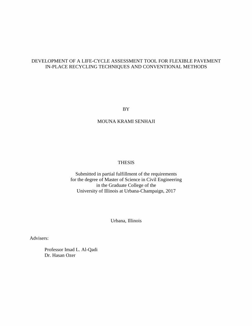
Figure 1.2 (left). Photo. Conventional mill and fill train (Wirtgen Group)

OBJECTIVES

The main objectives of this study are to (1) develop a framework and a life-cycle assessment

methodology to evaluate maintenance and rehabilitation treatments; specifically IPR and

conventional paving methods; (2) provide a comprehensive fuel usage analysis of IPR techniques

during the construction stage; and (3) develop a LCA tool utilizing Visual Basic for Applications

(VBA) to help local and state highway agencies to evaluate environmental benefits and tradeoffs

of IPR techniques as compared to conventional rehabilitation methods at each life-cycle stage

from the material extraction and production to the end of life.

METHODOLOGY

The LCA methodology followed conforms to ISO 14044 standards as illustrated in Figure 1.3.

The goal and scope focused on developing a LCA methodology to compare IPR and

conventional methods along the life cycle of a project during the same analysis period that is

defined based on FHWA LCA framework (Harvey et al, 2016). The inventory database covers

materials and equipment used for the construction of IPR and conventional methods. Finally, the

impact assessment is performed to compile the unit environmental emission and energy produced

by each inventory item. The impacts are calculated using commercial and governmental software

tools such as SimaPro and MOVES (EPA), respectively. The interpretation phase analyzes the

final results of all phases and identifies the most significant factors and items though a sensitivity

analysis.

4

Figure 1.3. LCA methodology (ISO, 2006)

5

CHAPTER 2: REVIEW OF IN-PLACE RECYCLING TECHNIQUES

IN-PLACE RECYCLING TECHNIQUES

The chapter provides a synthesis of the literature surrounding the application and evaluation of

CIR and HIR. The structure of this report is divided into two main sections for the two categories

of IPR. Each section addresses the following nine topics for CIR and HIR: 1) construction

process and materials, 2) applications in the U.S. and elsewhere, 3) project selection, 4) design

and material characterization, 5) performance history and models, 6) consideration in pavement

management systems (PMS), 7) cost effectiveness, 8) energy and emissions, and 9) life cycle

assessment (LCA) studies.

Hot In-Place Recycling

Hot In-Place Recycling (HIR) is a sustainable pavement preservation/rehabilitation technique

that is becoming more widely used in North America. It is a technique used to correct AC

pavement surface distresses by “softening the existing surface with heat, mechanically removing

the pavement surface, mixing it with asphalt binder, possibly adding virgin aggregate, and

replacing the recycled material on the pavement without removing it from the original pavement

site.” There are three types of HIR: surface recycling (or heater scarification), repaving, and

remixing.

The Asphalt Recycling and Reclamation Association (ARRA) defines surface recycling as a

process that restores cracked, brittle, and irregular pavement in preparation for a final thin

wearing course; this method has a scarification depth of up to 2 in, but typical thicknesses are ¾

to 1 in (FHWA, 1997).This method was originally developed by a contractor in Utah in the

1930s and the technology was advanced in the 1970s into a more complex system (Terrel et al.,

1997). The repaving method is similar to the surface recycling method, but is combined with

simultaneous AC overlay. It is expected to correct pavement distresses in the upper 1 to 2 in of

an existing AC pavement (FHWA, 1997). This method is often referred to as the Cutler process,

named after its inventor in the 1950s (FHWA, 1997). The third type of HIR technique is

remixing, which consists of heating the surface to a depth of 1½ to 2 in, scarification and

collection into a windrow, mixing with virgin aggregate, recycling agents and/or new AC in a

pugmill, and laying the recycled mix (FHWA, 1997).

Construction Process and Materials

Chapter 9 of FHWA reference book describes the typical construction processes of HIR in four

steps: (1) softening of asphalt pavement surface with heat, (2) scarification and mechanical

removal of the surface material, (3) mixing with recycling agent, asphalt binder, or new mix, and

(4) laydown and paving of the recycled mix. The three types of HIR (surface recycling, repaving,

and remixing) use different sets of equipment (FHWA, 1997); typical sequence of construction

equipment for each type of HIR is shown in Figure 2.1 to Figure 2.3.

6

Figure 2.1 Typical sequence of equipment for HIR surface recycling

Figure 2.2. Typical sequence of equipment for HIR repaving

Figure 2.3. Typical sequence of equipment for HIR remixing

Energy Use and Emissions

Few studies document the energy and emissions associated specifically with the HIR processes.

However, the energy and emissions associated with the production of virgin binder and

aggregates as well as conventional AC plant operations are more readily available. The first

study to estimate the energy required for HIR techniques is recorded in NCHRP report 214-19.

Energy estimates for the production of pavement materials as well as for the operation of

construction equipment were compiled in order to calculate the energy requirements for various

initial roadway construction, maintenance, and rehabilitation techniques. For HIR treatments

with a ¾ in thickness, the study reported energy consumption of 10,000–20,000 Btu/yd2, with the

range depending on the type of stabilization agent used (if any) (Epps et al., 1980).

In 2003, Colas Group released a study comparing energy and greenhouse gasses (GHGs) for

various road construction techniques, including rehabilitation practices.The energy consumption

and GHG emissions reported by the Colas Group for HIR are presented in Table 2.1 (Chappat;

Bilal, 2003).

7

Table 2.1. Energy and GHG emissions for HIR (after Colas Group) (Chappat; Bilal, 2003)

Material Amount

(kg/ton)

Energy

(MJ/ton)

GHG

(kg/ton) Data Source

Asphalt Binder 100 98 6 Eurobitume

Aggregates 200 4 1.0 Athena, IVL

Transportation -- 12 0.8 IVL

Laying -- 456 34.2 Colas Group

Total 1000 570 42 --

Cold In-Place Recycling

Cold in-place recycling (CIR) is an in-place rehabilitation technique that pulverizes the surface

of the pavement, mixes the recycled material with new materials, compacts it, and places an

overlay as a wearing surface. CIR starts with milling and pulverizing the surface of the

distressed pavement to a predetermined depth. The pulverized materials are then mixed with or

without additives and are graded, placed, and compacted back in place providing an improved

base layer and a wearing hot mix asphalt (HMA) overlay or a surface treatment is typically

added on top. There are two types of CIR practice: partial IPR which only pulverizes the

materials in the HMA layer of the previous section and does not go through the layers

underneath, and full depth reclamation (FDR) in which all of the HMA and at least 2 in of the

base/sub-base materials are pulverized.

The benefits of IPR according to a study conducted by NCHRP in 2011 are as follows (Stroup-

Gardiner, 2011):

• Reduction in use of natural resources

• Elimination of materials generated for disposal or landfilling

• Reduction in fuel consumption primarily due to reduction in transport of new materials

• Reduction in Greenhouse Gas (GHG) emissions between 50% to 85%

• Reduction in lane closure times

• Safety improvement by increasing friction, widening lanes, and eliminating overlay edge

drop-off

• Reduction in costs of preservation, maintenance, and rehabilitation

• Improving base support with minimum overlay thickness

This section discusses cold in-place recycling in detail starting with the construction processes

and the materials and additives that are used, then continues with examples of applications in the

U.S. and other parts of the world. Project selection criteria are discussed afterwards, explaining

suitable candidates for each cold in-place technique. The document then focuses on energy

consumption and emission data collected from previous projects followed by a summary of

performance evaluations for each technique and a discussion on cost effectiveness of the

treatments. The section is wrapped up with a review and summary of available life cycle

assessment (LCA) studies on CIR.

ARRA recommends that the equipment used for CIR be capable of the following: (ARRA, 2014)

8

• Milling of the existing roadway

• Sizing the resulting RAP

• Mixing the RAP with the additives designated in the mix design

• Meeting the required gradation and sizing with either the milling process or with

additional sizing equipment

• Producing a homogenous and uniformly coated mixture (if emulsions) by mixing RAP

and additives in the milling machine or in an additional mixing chamber

• Placement and compaction according to the specifications

These requirements can be achieved through a set of equipment consisting of (not all the

equipment may be needed for every project):

• Pavement cold planer (milling machine) with a minimum 12.5 ft cutter and a means for

controlling the depth of milling and the cross-slope or pulverization machine

• Crushing and sizing equipment

• Mixing and proportioning equipment

• Cement and asphalt emulsion or foamed asphalt storage and supply equipment

• Mixing and spreading equipment for dry cement

• Mixing and spreading equipment for corrective aggregate

• Paving equipment

• Water truck

• Compaction equipment

• Fog sealing and sand spreading equipment

The construction process starts with roadway preparation in which the contractor should identify

the location of all utilities within the project site, clean and remove any dirt or obstacle, reference

the profile and cross-slope, cold mill along cross walks and gutters to prepare for the final

overlay, and correct all areas known to have soft or yielding subgrades.

CIR construction is recommended only when the existing pavement temperature is above 50°F

and the previous overnight temperature is above 35°F. A control strip with a minimum length of

1000 ft should be constructed on the first day of the project to show that the construction process

meets the specifications. The optimal rates of additives (if any) and the rolling pattern to achieve

the optimum field density should be identified from the control strip.

The existing pavement should be milled to the depth required by the plan or the specifications

and the recycled materials should be crushed and sized to the maximum particle size specified.

Typical depths are 2 to 4 in. The incorporation of recycling additive or stabilizing agent can be in

the form of applying mechanical, chemical, or bituminous additives or a combination of all

(ARRA, 2014). Mechanical stabilization in the form of compaction is used for all treatments, and

the addition of imported granular materials is used if the existing in-place materials do not

provide a satisfactory gradation (Van Dam, et al. 2015). Chemical stabilization is achieved by

adding one or a combination of Portland cement, fly ash, calcium chloride, magnesium chloride,

and lime. Bituminous stabilization consists of adding asphalt emulsion or foamed asphalt. The

common practice in many states is to use a combination of bituminous stabilization and chemical

9

stabilization for partial-depth recycling. Cement or lime slurry may be directly added to the

mixing chamber or sprayer over the cutting teeth of the milling machine (Van Dam et al., 2015).

If dry cement or corrective aggregate is needed, it can be spread on the existing surface before

milling. The CIR milling and mixing process can be accomplished with a single-unit machine or

a multi-unit train (Van Dam et al., 2015).

The placement of the recycled materials is conducted either with conventional asphalt pavers or

cold mix pavers followed by compaction. The time between material placement and start of

compaction is determined by the contractor. Compaction (initial/breakdown, intermediate, and

final compaction) is one of the main factors affecting the future performance of the section. The

type and number of compactors depend on many factors such as the degree of compaction

required, material properties of the pulverized mix, support capabilities of the underlying layers,

and the needed productivity. In general, the characteristics of the recycled mix determine the

type of roller needed and the thickness of the layer and the required compaction dictates the

weight, amplitude, and frequency of the compactors (Van Dam et al., 2015).

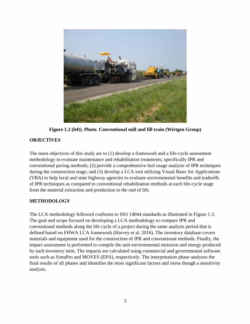
For materials stabilized by some chemical and/bituminous materials, in a process similar to that

shown in Figures 2.4 and 2.5, curing is a critical step and is needed to assure achieving adequate

strengths before opening to traffic, prevent raveling, and facilitate placement of the final wearing

course. The curing rate depends on multiple factors such as the nature of the stabilization

particularly if asphalt emulsions are used, temperature, humidity, moisture content of the mix,

compaction level, and drainage characteristics of the section.

ARRA requires CIR to cure for a minimum of three days and the moisture content to be less than

3% before proceeding to secondary compaction or opening to traffic. ARRA recommends

secondary compaction if the recycling agent is emulsified asphalt. If secondary compaction is

planned, a separate rolling pattern should be established during the control strip and the density

of the recycled materials after secondary compaction should be checked to verify compliance

(ARRA, 2014). ARRA suggests that secondary compaction be done with pneumatic and double

drum vibratory at temperatures above 80 °F. As materials are better understood and contractors

gain more experience, local governments in several locations with light vehicles moving at slow

speeds often open within hours of construction and follow with re-compaction and overlay

several days later.

In the final step, a wearing course is usually laid on top. For low-traffic roads, a single or double

chip seal might be sufficient, but in sections with higher traffic levels, an AC overlay might be

needed. The minimum recommended thickness for AC overlays is 1 in, depending on the

specifics of the project, agency policies, anticipated traffic, climate, economics, stabilizing agent,

and structural requirements. For AC or warm mix asphalt (WMA) overlays, ARRA recommends

applying a tack coat of either CSS-1h or SS-1h emulsified asphalt at minimum rate of 0.05

gal/yd2 before applying the wearing course.

The construction of CIR should always include field adjustments because these processes are

variable in nature due to changes in the materials being recycled along the roadway, changes in

the speed of the equipment and, therefore, the RAP gradation from milling, and changes in the

10

ambient temperature and humidity conditions. Field observations and adjustments are, thus,

needed to assure good coating of the materials and workability of the AC mixture and quality

construction even though the optimum moisture, additive type and content, and other factors are

determined through laboratory tests and are stated in the job mix formula. These modifications

and adjustments should be conducted by experienced field personnel who are continuously

engaged in observing the material being placed behind the recycling train. Table 2.2 lists some of

the common early problems that are observed in sections with CIR and recommended mitigation

for them.

Figure 2.4. Diagram of CIR process. (Van Dam et al., 2015)

Figure 2.5. Diagram of CIR equipment (Wirtgen America Inc.)

11

Table 2.2 CIR early damage and mitigation (ARRA, 2014)

Full-Depth Reclamation

The FDR construction process is similar to CIR, the only difference as stated earlier is that the

whole thickness of the existing AC layer and a predetermined thickness of the underlying layer

for at least 2 in are pulverized and mixed together (with water and with or without additives) into

a homogenous mixture, as shown in Figures 2.6 and 2.7.

Figure 2.6. Diagram of FDR process (Van Dam et al., 2015)

Distress Mitigation

Isolated areas of minor raveling or scuffing. Sweep and monitor. Determine if fog sealing or re-fog sealing is

necessary to protect.

Isolated areas of major raveling, scuffing or

tearing.

Maintain better traffic restrictions in areas that are not cured.

Sweep and monitor. Determine if fog sealing or re-fog sealing is

necessary to protect. Fill or remove and replace deep damaged

areas with AC mixture (cold mix, recycled mix, WMA, or

traditional AC) prior to surface course.

Large scale areas of raveling, scuffing or

tearing in straight traffic areas.

Re-recycle or remove and replace with asphalt mixture (cold

mix, recycled mix, WMA, or AC).

Dimpling due to parked vehicles or

equipment.

Fill with AC mixture (cold mix, recycled mix, WMA, or

traditional AC) prior to surface course.

Permanent deformation within wheel path

areas due to secondary compaction by traffic.

If pavement temperatures permit, apply secondary compaction.

Fill with AC mixture (cold mix, recycled mix, WMA, or

traditional AC) or micro surfacing in the low areas or cold mill

to provide a smooth surface.

Permanent deformation and shoving due to

unstable mix.

Investigate pavement structure in conjunction with mix design

lab. Depending on investigation, remove and replace affected

areas with AC mixture (cold mix, recycled mix, WMA, or

traditional AC) or re-recycle supplementing with uncoated

coarse aggregate, additives and/or recycling agent as necessary.

12

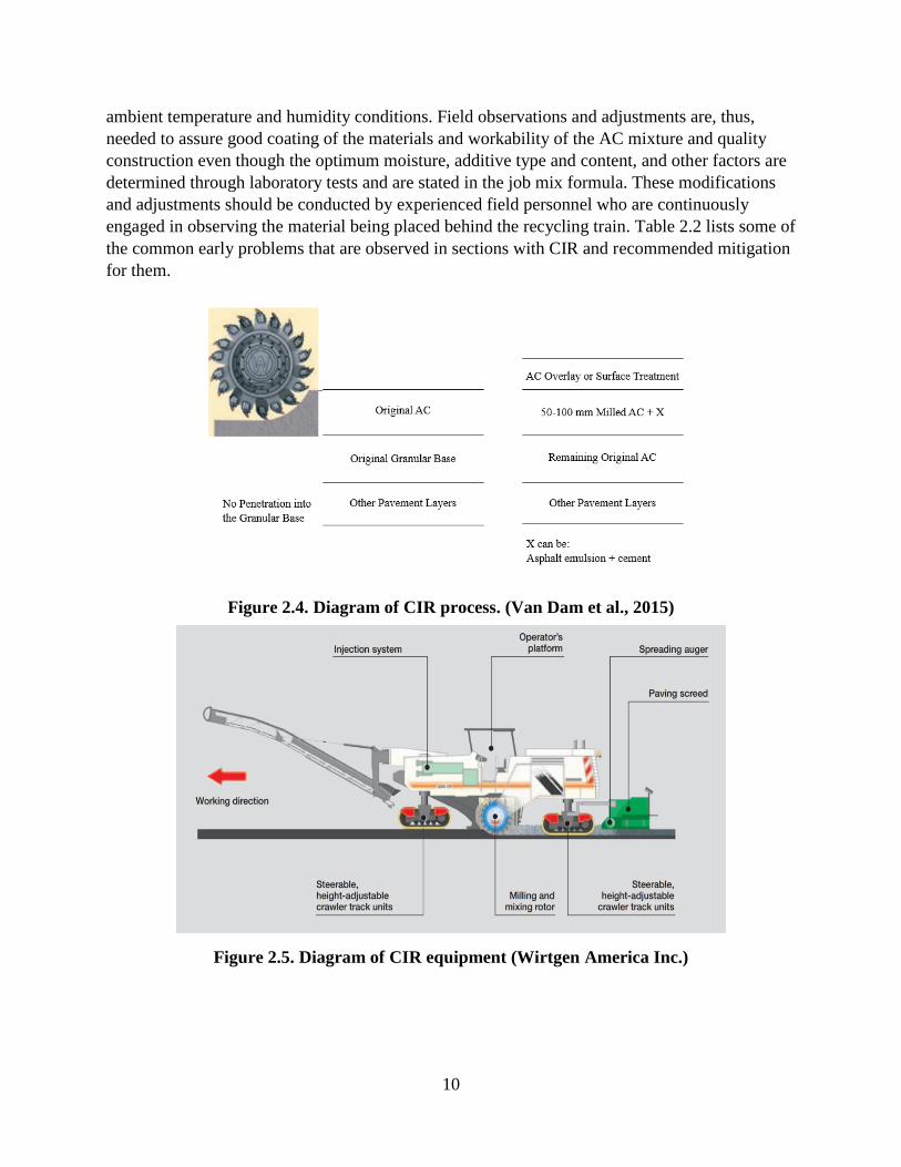
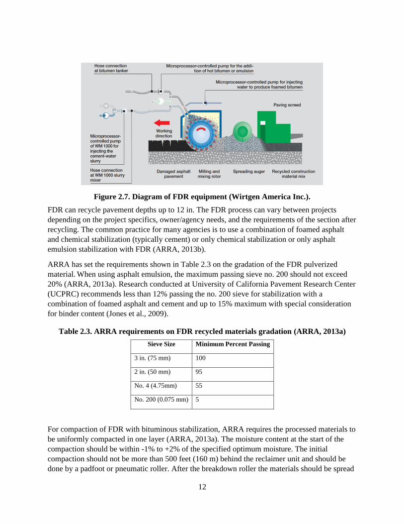
Figure 2.7. Diagram of FDR equipment (Wirtgen America Inc.).

FDR can recycle pavement depths up to 12 in. The FDR process can vary between projects

depending on the project specifics, owner/agency needs, and the requirements of the section after

recycling. The common practice for many agencies is to use a combination of foamed asphalt

and chemical stabilization (typically cement) or only chemical stabilization or only asphalt

emulsion stabilization with FDR (ARRA, 2013b).

ARRA has set the requirements shown in Table 2.3 on the gradation of the FDR pulverized

material. When using asphalt emulsion, the maximum passing sieve no. 200 should not exceed

20% (ARRA, 2013a). Research conducted at University of California Pavement Research Center

(UCPRC) recommends less than 12% passing the no. 200 sieve for stabilization with a

combination of foamed asphalt and cement and up to 15% maximum with special consideration

for binder content (Jones et al., 2009).

Table 2.3. ARRA requirements on FDR recycled materials gradation (ARRA, 2013a)

Sieve Size Minimum Percent Passing

3 in. (75 mm) 100

2 in. (50 mm) 95

No. 4 (4.75mm) 55

No. 200 (0.075 mm) 5

For compaction of FDR with bituminous stabilization, ARRA requires the processed materials to

be uniformly compacted in one layer (ARRA, 2013a). The moisture content at the start of the

compaction should be within -1% to +2% of the specified optimum moisture. The initial

compaction should not be more than 500 feet (160 m) behind the reclaimer unit and should be

done by a padfoot or pneumatic roller. After the breakdown roller the materials should be spread

13

using a motor grader until the desired shape and slope are achieved. After blading, a vibratory

double drum steel roller and pneumatic roller should be used for intermediate and final

compaction of the layer. Completed portions can be immediately opened to low speed local

traffic. The overlay should follow within several days to protect the recycled layer from traffic

wear.

For stabilization with cement, ARRA recommends that no more than 60 min pass between the

first contact of cementitious stabilizer with water and application on the subgrade, and the time

span between placement of the stabilizer and start of mixing not exceed 30 min. Compaction

should begin no more than 20 min after mixing and all compaction operations should be

completed within two hrs from start of the mixing process. There should be no grading or

blading of the material after compaction has been completed. Curing is done by application of a

bituminous or other approved sealing membrane or by using water spray to keep the section

moist for three to five days. To help limit shrinkage cracking, micro-cracking can be done

(optional) by using a 12 ton steel wheel vibratory roller. Completed portions of the section can

be immediately opened to low speed local traffic (ARRA, 2013b).

The key for quality FDR construction as identified by a UCPRC report on guidelines for IPR is

the following: (Jones et al., 2009)

• Contractor experience

• Traffic accommodation

• Pre-milling in cases where the asphalt layer is too thick (typically more than 10 in) or

when precise surface levels need to be maintained

• Importing new material in case additional materials are needed to correct grades, increase

layer thickness, and/or improve the bearing capacity of the section

• Equipment inventory

• Recycling train crew responsibilities

• Recycling train setup

• Test strip to check processes and determine compaction rolling pattern necessary to

achieve specified density

• Ambient and pavement temperatures for asphalt emulsion additives (it is recommended

to start the recycling when the ambient temperature is over 50 ºF and the temperatures of

the road surface and pre-spread active filler are both equal of above 60 ºF)

• Recycling plan

• Recycling additive content and application rate

• Recycling depth and recycled material consistency

• Lateral joints

• Compaction moisture

• Initial compaction, final grades, and final compaction

• Curing

• Trafficking

• Surfacing

• Drainage

14

• Quality control

The FHWA has published checklists for CIR and FDR in collaboration with the ARRA and the

National Center for Pavement Preservation. The checklists are comprehensive and include items

for document review, project review, materials checks, preconstruction inspection

responsibilities (preconstruction meeting, surface preparation, and equipment inspection),

weather requirements, mix design, traffic control, project inspection responsibilities (milling,

crushing, mixing, pickup machine and paver, rolling procedure, and quality assurance), opening

to traffic, curing, and surface course (FHWA, 2013c; FHWA, 2013d) .

Energy Use and Emissions

There are a few studies that have tried to estimate energy consumption and emissions of IPR

techniques. Although the number of studies is limited, they all result in the same conclusion that

CIR not only reduces consumption of virgin materials but also results in significant savings in

energy consumption and emission compared to conventional methods of rehabilitation.

Thenoux compared the energy consumption during construction for three different structural

pavement rehabilitation alternatives which included AC overlay, reconstruction and FDR-

foamed asphalt. It was determined that the FDR technique is the least energy consuming in all

the scenarios, resulting in energy savings between 20% to 50% compared to AC overlay and up

to 244% compared to reconstruction (Thenoux et al., 2007).

Robinette and Epps conducted a literature survey for estimating energy consumption and

emissions of IPR practices (Robinette, 2010). The results are presented in Table 2.4 and Table

2.5.

Table 2.4. Energy consumption (Btu/yd2-in) for CIR processes (Robinette, 2010)

Operation NCHRP 214 Colas Group PaLATE Granite

Construction

Representative

Range

CIPR—partial depth -- 6,400 24,600 3,100 3,000–24,000

CIPR—full depth 15,000–20,000 6,200 34,700 1,300–11,100 1,300–15,000

Table 2.5. GHG emissions (CO2-eq. lb/yd2-in) of different CIR processes (Robinette, 2010)

Operation Colas Group Granite Construction Representative Range

Cold milling asphalt pavement 0.084 3.377 0.08-3.500

CIPR-partial depth – 0.71 –

CIPR-full depth 1.082 0.932-4.017 0.900-4.100

15

CHAPTER 3: DEVELOPMENT OF THE LCA TOOL METHODOLOGY

In this chapter, the LCA methodology developed to analyze each life cycle phase is presented.

This discussion includes goal and scope, life cycle inventory and life cycle phases modeling and

GOAL AND SCOPE

The goal of this study is to develop a LCA methodology to assess the environmental impacts and

energy use of transportation projects that involve maintenance and rehabilitation treatments

using IPR and conventional paving methods.

This study is related to a project sponsored by FHWA that aims to develop a life cycle

assessment decision making tool for IPR techniques. The pavement LCA framework and tool

developed in this thesis can be applied to various agencies and national roadway practitioners.

The scoping elements include the methodological choices required at the Goal and Scope phase

of LCA according to the ISO 14044 (ISO, 2006) and FHWA Pavement LCA Framework

(Harvey et al., 2016).

System Boundary

The product systems included in the study are IPR methods recognized by federal and state

transportation agencies in the U.S which will be compared with conventional hot mix asphalt

(HMA) overlays. The LCA includes the following life-cycle stages: material production,

construction, maintenance, use, and end of life. The material production and construction life

cycles of the systems considered in this LCA are related to IPR or conventional mill/fill

processes. Thus, any processes related to the production and construction of the initial pavement

is not included. The system boundary for the product system is shown as the dashed line in

Figure 1.3.

Figure 3.1. Life-cycle phases and system boundary of the LCA scope.

16

Functional Unit

The functional unit used in this LCA study is a one lane-mile over the analysis period. The

analysis period depends on the treatments under comparison. The lane width is assumed to be

equal to 12 ft.

Analysis Period

The analysis period is calculated following the method highlighted in the FHWA pavement LCA

framework (Harvey et al., 2016). This method compares the life expectancy of treatments under

study, defines the alternative treatment with the longest life expectancy, and adds it to the

estimated life of the subsequent maintenance of the longest living treatment, as illustrated in

Figure 3.2. It is important to assign a common analysis period in order to compare the pavement

rehabilitation alternatives and to quantify the impacts of the use stage.

Figure 3.2. Analysis period strategy illustrating the first treatment’s lifetime to be analyzed

by the tool and subsequent overlays.

Allocation Method

The adopted allocation method is the cut-off or also known as recycled content methodology.

The boundary of the analysis conducted is limited to the pavement system during the analysis

period without accounting for the quantity of resources used in a subsequent system (Nicholson,

2009). The substitution allocation method is analyzed in the interpretation step of the LCA

methodology to compare its effect to the cut-off method.

0 10 20 30 40 50 60

1

2

3

4

5

Years

Mai

nte

nan

ce o

r re

hab

iluta

oti

on a

lter

nat

ives

Rehabilitation

AC Overlay 1

AC Overlay 2

AC Overlay 3

Analysis period

17

LIFE CYCLE INVENTORY

Data collection phase of the study included collecting primary and secondary data from various

sources. Primary data refers to specific data collected for some of the IPR techniques from the

contractors whereas secondary data refer to average and background data for processes like fuel

and electricity production, emission due to equipment use. Data sources included agency and

contractor questionnaires and interviews, commercial inventory databases, and publicly available

data sources.

Primary Data

The primary data are the information collected from field projects and used for quantification of

life-cycle inventory (LCI) impacts. Questionnaires have been distributed to contractors

throughout the nation in 2016-2017. Data collection was undertaken at an early stage of the

project in order to collect information and data about IPR techniques and construction methods.

The project information and data were analyzed to assess the fuel usage of IPR techniques,

especially CIR and FDR. Follow-up interviews were conducted with some of the contractors to

collect additional data.

Figure 3.3 represents the distribution of agencies and contractors that responded to

questionnaires and shared their IPR data from field projects.

Figure 3.3. Representative map of contractors and agencies contacted in the three main US

regions.

Appendix A contains information collected from agencies regarding the HIR and CIR/FDR

practices. The main conclusions extracted from the data collected are that IPR techniques are

applied under specific project conditions. The selection of any IPR type requires a good

understanding of the dynamic parameters (traffic level, truck percent, lane closures and

openings, and climate) and static characteristics (road geometry, structural capacity, and existing

18

pavement condition). It was found that HIR and CIR are commonly used at low traffic volume

pavements, under a truck percent that varies from 5% to 10% for a pavement length of 100 lane-

mi per year. According to agencies responses, CIR extends existing pavement service life to

more than 11 years, whereas HIR is reported to extend service life from five to ten years. The

difference in performance between CIR/FDR and HIR is due to the fact that CIR/FDR is a

rehabilitation technique that enhances the structural capacity and treats a wide range of surface

and deep distresses. On the other hand, HIR is classified as a maintenance treatment applied to a

limited number of functional distresses.

Secondary Data

The secondary data complements the inventory items missing in the primary data collected.

Various sources were used to compile a comprehensive inventory list which are (1) Commercial

LCI databases (e.g. Ecoinvent 2.2/3.0 (Frischknecht, 2004; Wernet et al., 2016)), US-Ecoinvent

2.2 (EarthShift, 2013)), (2) software (e.g. EPA MOVES 2014 (EPA, 2015), eGRID 2010

(eGRID, 2015)), (3) governmental databases, (4) governmental reports, (5) material safety data

sheets, and (6) equipment manufacturer specifications.

Other Data Collected from Questionnaires (States)

Apart from primary data collected from contractors, a set of questionnaire surveys was

distributed to state/local transportation agencies (via online survey). There were two sets of

questionnaire surveys: one for HIR, and the other for CIR. Each set contains similar questions

inquiring agency experience in IPR, pavement management, construction details, performance,

and specifications. A sample questionnaire survey and the detailed results of questionnaire

surveys are attached in Appendix A. Some survey result highlights are summarized in Table 3.1

for HIR and CIR.

This information was also used to support the development of the decision matrix for the

pavement performance estimation qualitative approach. Agencies were asked about the

following information:

• Major items associated with the IPR practice.

• Most sensitive specification requirements pertaining to IPR.

• Safety concerns.

• Lane closure and opening strategies.

• Existing regulations regarding emissions associated with the construction practices

such as dust, dirt, or smoke.

• Factors affecting the success of CIR/FDR project.

• Traffic condition.

• Pavement performance indicators used by the agency.

• Cost per square yard.

19

Table 3.1. Survey highlights for HIR and CIR.

Questionnaire

Contents Agencies Common Practices in HIR Agencies Common Practices in CIR

IPR use Less than 100 lane-mi/year Less than 100 lane-mi/year

Traffic Low volume roads below 10,000 AADT Low volume roads below 10,000 AADT

Truck percent Varies between 5 and 10% Varies between 5 and 10%

Condition index PCI, PDI, or in-house index PCI, PDI, other in-house index (i.e.,

distresses)

What triggers? The selected index The selected index and others (i.e., IRI,

distresses, etc.)

Index after IPR > 50% improvement > 26% improvement

Expected life Varies but between 5 and 10 years Varies but between 3 and 7 years

Cost Varies between $4 and $7 per sq yd Varies between $3 and $6 for CIR; $9 and $12

per sq yd

Lane closure Mostly partial closure Majority partial closures

Opening time 1 – 4 hours after treatment 1 – 4 hours after treatment

As seen in Table 3.1, the application of IPR is still limited to low-volume roads with relatively

low traffic levels (less than 10,000 AADT). The condition index used varies greatly; among

different indices, pavement condition index (PCI), pavement distress index (PDI), pavement

quality index (PQI), and international roughness index (IRI) are the most commonly used ones.

Most agencies trigger treatment based on the condition index in use. Upon the application of

IPR, it is reported that the index improves more than 50% for HIR and more than 26% for CIR

INVENTORY ANALYSIS AND IMPACT CATEGORIZATION

Inventory database is compiled from primary and secondary sources with regionalized data

collected from agencies and contractors from the three main US regions. Life cycle inventory

analysis is performed using regionalized models for fuel and electricity.

The impact characterization is performed using TRACI categories. Four quantitative outcomes

from the LCA study are:

• Global warming potential,

• Energy,

• Total energy with feedstock,

• Single score.

20

Global Warming Potential

“Global warming is an average increase in the temperature of the atmosphere near the Earth’s

surface and in the troposphere, which can contribute to changes in global climate patterns.

Global warming can occur from a variety of causes, both natural and human induced. In common

usage, “global warming” often refers to the warming that can occur as a result of increased

emissions of greenhouse gases from human activities” (EPA, 2008). This impact is given in units

of kg carbon dioxide equivalence (CO2e). The 100-year GWP is calculated using the EPA’s Tool

for Reduction and Assessment of Chemicals and Other Environmental Impacts (TRACI) 2.1.

Single Score

Other environmental impacts were reported in a condensed format though calculation of a unit-

less parameter calculated based on the normalization and weighting for TRACI impacts using the

coefficients presented in Table 3.2 (Lautier et al.,2010; Bare et al., 2006). This parameter is

referred to as the Single Score, which is reported in “points.” It must be noted that the weighting

given to the Single Score is subjective, though the weighting values developed by National

Institute of Standards and Technology (NIST) are specific to the context of the U.S.

Table 3.2. TRACI Impacts with Normalization and Weighting Factors

Impact category Unit Normalization Weighting

Ozone depletion kg CFC-11 eq 6.20 0.024

Smog kg O3 eq 0.000718 0.048

Acidification kg SO2 eq 0.0110 0.036

Fossil fuel depletion MJ surplus 0.0000579 0.121

Eutrophication kg N eq 0.0463 0.072

Respiratory effects kg PM2.5 eq 0.0412 0.108

Non carcinogenics CTUh 952 0.060

Carcinogenics CTUh 19,706 0.096

Ecotoxicity CTUe 0.0000905 0.084

Global warming kg CO2 eq 0.0000413 0.349

Energy Indicators

Two energy consumption indicators are included in the impact assessment: energy and total

energy with feedstock. Energy refers to combusted or expended energy as fuel. Total energy with

feedstock includes energy that is embodied as a fuel (e.g. diesel, natural gas) and energy that is

21

embodied as a material (e.g. plastics, asphalt binder). As FHWA Pavement LCA guidelines

recommend, two types of energy are reported to provide a more complete view of energy

consumption over the life cycle (Harvey et al., 2016). For example, accounting feedstock energy

for asphalt agents results in higher energy for asphalt concrete pavement life cycle due to the

energy retained in the asphalt binder.

DATA QUALITY ASSESSMENT

Data Quality Requirements

Data quality assessment was conducted following ISO 14044 recommendations (ISO, 2006) and

FHWA pavement LCA framework (Harvey et al., 2016). High-quality data is important to ensure

an accurate LCA study and reliable results to use at the decision-making stage (Weidema;

Wesnaes, 1996). Table 3.3 shows the quality goals description assessed in this study.

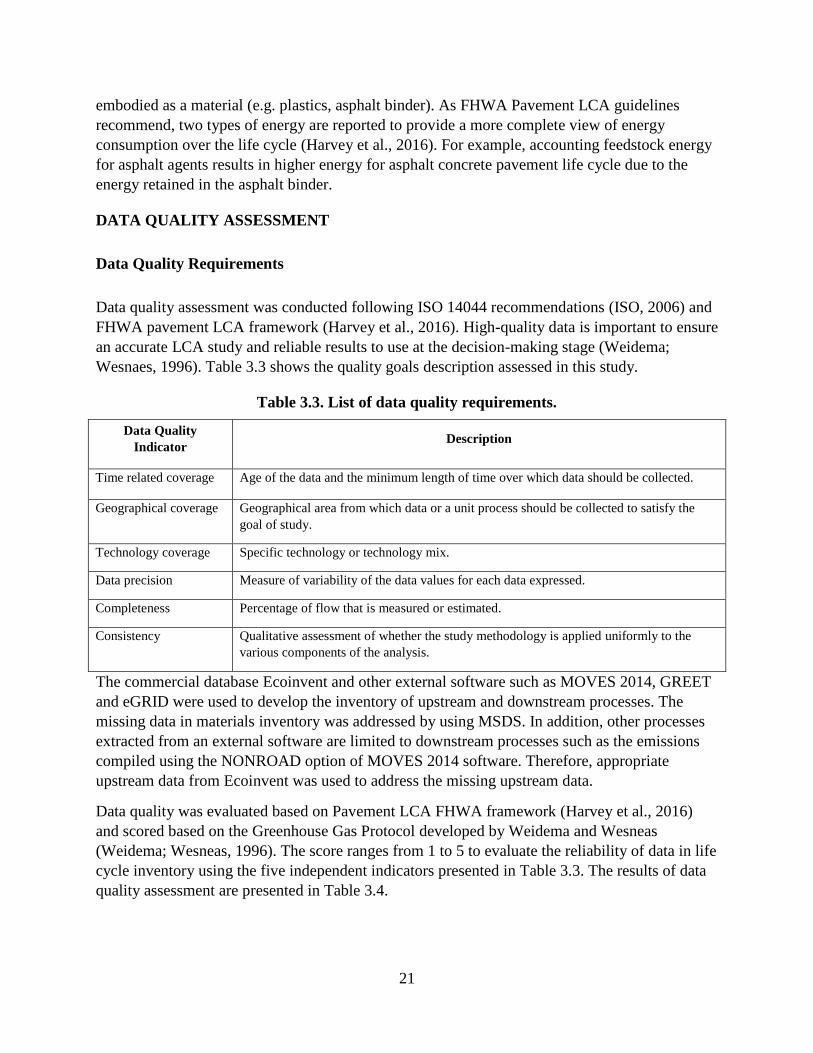
Table 3.3. List of data quality requirements.

Data Quality

Indicator Description

Time related coverage Age of the data and the minimum length of time over which data should be collected.

Geographical coverage Geographical area from which data or a unit process should be collected to satisfy the

goal of study.

Technology coverage Specific technology or technology mix.

Data precision Measure of variability of the data values for each data expressed.

Completeness Percentage of flow that is measured or estimated.

Consistency Qualitative assessment of whether the study methodology is applied uniformly to the

various components of the analysis.

The commercial database Ecoinvent and other external software such as MOVES 2014, GREET

and eGRID were used to develop the inventory of upstream and downstream processes. The

missing data in materials inventory was addressed by using MSDS. In addition, other processes

extracted from an external software are limited to downstream processes such as the emissions

compiled using the NONROAD option of MOVES 2014 software. Therefore, appropriate

upstream data from Ecoinvent was used to address the missing upstream data.

Data quality was evaluated based on Pavement LCA FHWA framework (Harvey et al., 2016)

and scored based on the Greenhouse Gas Protocol developed by Weidema and Wesneas

(Weidema; Wesneas, 1996). The score ranges from 1 to 5 to evaluate the reliability of data in life

cycle inventory using the five independent indicators presented in Table 3.3. The results of data

quality assessment are presented in Table 3.4.

22

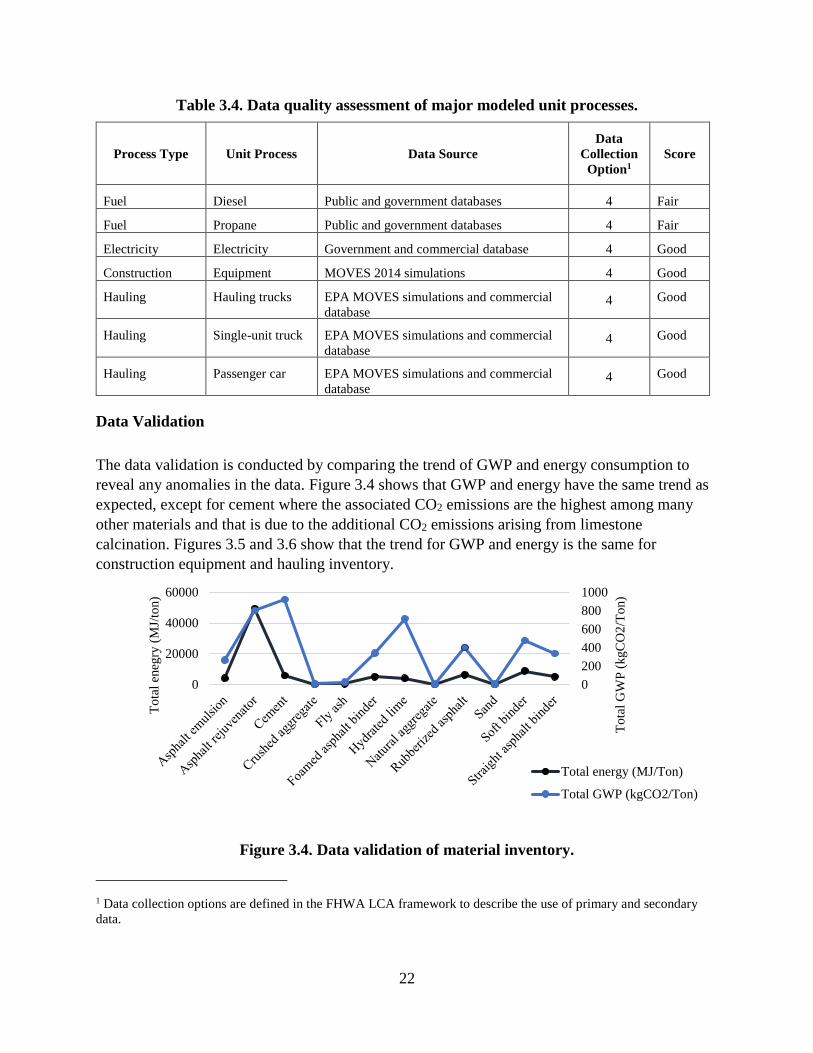
Table 3.4. Data quality assessment of major modeled unit processes.

Process Type Unit Process Data Source

Data

Collection

Option1

Score

Fuel Diesel Public and government databases 4 Fair

Fuel Propane Public and government databases 4 Fair

Electricity Electricity Government and commercial database 4 Good

Construction Equipment MOVES 2014 simulations 4 Good

Hauling Hauling trucks EPA MOVES simulations and commercial

database 4 Good

Hauling Single-unit truck EPA MOVES simulations and commercial

database 4 Good

Hauling Passenger car EPA MOVES simulations and commercial

database 4 Good

Data Validation

The data validation is conducted by comparing the trend of GWP and energy consumption to

reveal any anomalies in the data. Figure 3.4 shows that GWP and energy have the same trend as

expected, except for cement where the associated CO2 emissions are the highest among many

other materials and that is due to the additional CO2 emissions arising from limestone

calcination. Figures 3.5 and 3.6 show that the trend for GWP and energy is the same for

construction equipment and hauling inventory.

Figure 3.4. Data validation of material inventory.

1 Data collection options are defined in the FHWA LCA framework to describe the use of primary and secondary

data.

0

200

400

600

800

1000

0

20000

40000

60000

To

tal

GW

P (

kgC

O2

/To

n)

To

tal

eneg

ry (

MJ/

ton)

Total energy (MJ/Ton)

Total GWP (kgCO2/Ton)

23

Figure 3.5. Data validation of equipment inventory.

Figure 3.6 Data validation of hauling inventory.

0

20

40

60

80

100

120

140

160

0

500

1000

1500

2000

2500

To

tal

GW

P (

kgC

O2

/gal

)

To

tal

ener

gy (

MJ/

gal

)

Total energy Total GWP

0

1

2

3

4

5

6

-6 -5 -4 -3 -2 -1 0 1 2 3 4 5 6 8

0

0.05

0.1

0.15

0.2

0.25

0.3

0.35

0.4

0.45

To

tal

ener

gy (

MJ/

ton-m

i)

Grade (%)

To

tal

GW

P (

kgC

O2

/to

n-m

i)

Total GWP - RH = 60 - T = 70 F Total energy - RH = 60 - T = 70 F

24

MATERIAL PRODUCTION AND HAULING PHASE

This section discusses the regional models developed to assess the impacts of materials’

production and hauling to site. A list of materials used for construction of pavement maintenance

and rehabilitation was developed to allow running materials phase analysis.

Modeling procedure

Fuel and Electricity

The fuel and electricity inventory database was regionalized based on the Petroleum

Administration for Defense Districts (PADD) and eGRID regions. The IPR tool is intended to be

applied on a national scale. Therefore, fuel and electricity production unit processes inventory

database was developed to cover all U.S. states. These processes are used to assess the impacts

of materials production.

Figure 3.7 highlights the five PADD regions based on the U.S Energy Information

Administration that help in analyzing open source data of regional petroleum product supplies

(EIA, 2010a). A study by Yang et al. compiled life-cycle impact processes of crude oil

production including extraction, flaring, and transportation (Yang et al., 2016). The results of this

work allowed assessing the environmental impacts and energy use of asphalt binder production

in the five PADDs. It was assumed that the same quantity of 1tn.sh of a processed crude oil is

necessary to produce 1tn.sh of asphalt binder. Figures 3.8 and 3.9 shows the energy of asphalt

products production in all PADDs.

Figure 3.7. PADDs map from U.S. Energy Information Administration (EIA, 2010a)

25

Figure 3.8 (left). Energy of different asphaltic materials production in the five PADD

regions without feedstock. (Yang et al., 2016)

Figure 3.9 (right). Energy of different asphaltic materials production in the five PADD

regions with feedstock. (Yang et al., 2016)

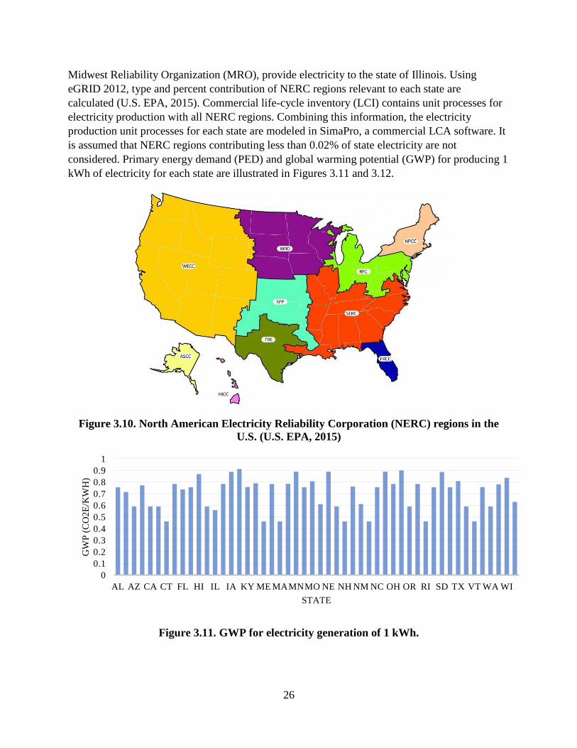
There are ten North American Electricity Reliability Corporation (NERC) regions in the U.S. as

illustrated in Figure 3.10.Unlike PADDs district, NERC regions do not have clear boundaries

because the region that electricity providers cover is not strictly divided by state (U.S. EPA,

2015). This implies that a state may belong to multiple NERC regions. For example, three NERC

regions, Reliability First Corporation (RFC), Southeastern Reliability Council (SERC), and

0

10000

20000

30000

40000

50000

Ener

gy (

MJ/

To

n)

PADD5

PADD4

PADD3

PADD2

PADD1

0

50000

100000

150000

200000

250000

To

tal

ener

gy w

ith f

eed

sto

ck (

MJ/

To

n)

PADD5

PADD4

PADD3

PADD2

PADD1

26

Midwest Reliability Organization (MRO), provide electricity to the state of Illinois. Using

eGRID 2012, type and percent contribution of NERC regions relevant to each state are

calculated (U.S. EPA, 2015). Commercial life-cycle inventory (LCI) contains unit processes for

electricity production with all NERC regions. Combining this information, the electricity

production unit processes for each state are modeled in SimaPro, a commercial LCA software. It

is assumed that NERC regions contributing less than 0.02% of state electricity are not

considered. Primary energy demand (PED) and global warming potential (GWP) for producing 1

kWh of electricity for each state are illustrated in Figures 3.11 and 3.12.

Figure 3.10. North American Electricity Reliability Corporation (NERC) regions in the

U.S. (U.S. EPA, 2015)

Figure 3.11. GWP for electricity generation of 1 kWh.

0

0.1

0.2

0.3

0.4

0.5

0.6

0.7

0.8

0.9

1

AL AZ CA CT FL HI IL IA KY ME MAMNMO NE NH NM NC OH OR RI SD TX VT WA WI

GW

P (

CO

2E

/KW

H)

STATE

27

Figure 3.12. Primary Energy Demand (PED) for electricity generation of 1 kWh.

Construction Materials

As IPR techniques are used on AC pavement, mineral aggregate, asphaltic materials, other (i.e.,

rejuvenating and stabilizing) materials, and plant operation are considered. The mineral

aggregates considered include natural aggregate, crushed aggregate, and sand. Impacts

associated with producing these materials are calculated using relevant unit processes in the U.S.

Ecoinvent (US-EI) 2.2 database (EarthShift, 2013). Aggregate unit processes are then modified

by replacing default electricity models with state electricity models developed to improve its

regional proximity.

The production of asphaltic materials follows similar procedures as petroleum fuel production in

the previous section because asphalt binder is a co-product obtained during petroleum refining

processes. Therefore, the impacts of asphalt binder vary with regions (i.e., five PADDs) (Yang et

al., 2016).Taking the asphalt binder model as the base, other asphaltic materials such as

emulsion, ground tire rubber (GTR) binder, polymer modified binder, and foam asphalt are

modeled in SimaPro (Simapro, 2014) . Additional information about material composition and

fuel/electricity use is summarized in Appendix B.

Asphalt rejuvenator is a paraffinic material used during IPR techniques to restore binder

properties. This material consists predominantly of aromatic hydrocarbon with carbon numbers

in the range of C20 to C50 [paraffin wax] with 5% of C4 to C6 numbered aromatic hydrocarbons

[benzene]. Impacts associated with these materials are obtained from US-EI 2.2 database.

Hydrated lime can be used for stabilizing subgrade and the impact of producing hydrated lime is

obtained from US-EI 2.2 database (U.S. EPA, 2017; NIH, 2016).

Asphalt plant operation involves various processes. The sources of fuel consumption include the

use of electricity to operate mixing drums and conveyor belts, the use of fuel (i.e., natural gas) to

dry aggregate and heat asphalt binder, and the use of diesel to operate loaders for in-plant

transportation. Combining these processes based on data collected from questionnaires,

commercial database (Kang et al., 2014), and literature, a base AC plant model is developed

0

2

4

6

8

10

12

14

16

AL AZ CA CT FL HI IL IA KY ME MAMNMO NE NH NM NC OH OR RI SD TX VT WA WI

PE

D (

MJ/

KW

H)

STATE

28

(Young, 2007). By adopting different electricity models, the environmental impact associated

with operating AC plants is computed for each state.

Hauling

One of the advantages of using IPR techniques over conventional rehabilitation methods is the

significant reduction in material hauling. Mill and inlay is the most widely used rehabilitation

technique in AC pavements. Deteriorated AC surface is milled to a certain depth and transported

for recycling (mainly) or to a landfill; and new AC materials are transported to the site for the

new surface course. IPR techniques typically do not require much new materials because

scarified in-situ pavement materials are re-used on-site. Hence, material hauling is minimized;

this is manifested by capturing environmental benefits when IPR techniques are used.

Environmental Protection Agency (EPA)’s Motor Vehicle Emission Simulator is used to

compute the environmental impacts of hauling operations (U.S. EPA, 2016). Based on

preliminary simulations, it is found that six parameters including truck speed, road grade,

payload, year, temperature, and relative humidity affect emissions of heavy truck operations.

Through numerous simulations, variable impact transportation (ICT-VIT) model was developed

to compute the environmental impacts and energy associated with hauling activities (Franzese,

2011). Types and values of variables considered are summarized in Table 3.5. The results of

preliminary simulations are illustrated in Figure 3.13 through Figure 3.16.

Table 3.5. Types and ranges of variables considered in MOVES simulations.

2.715

2.718

2.721

2.724

2.727

2.730

20 70 120

GW

P (

kg C

O2e/t

ruck-m

i)

Relative Humidity (%)

Variable Quantity

Vehicle speed (mph) Idling, 1, 2.5, 5, 10, 20, 30, 40, 50, 55, 60, 70

Vehicle weight (tn.sh) 9.07, 15.3, 24.6, 30.1, 33.4, 36.3

Road grade (%) 0, ±1, ±2, ±3, ±4, ±5, ±6, ±8

Temperature (°F) 0 - 110

Relative humidity (%) 30 - 100

Year 2015 - 2050

29

Figure 3.13 (top left). Effect of relative humidity on global warming potential (GWP)

(T=temperature, RH=relative humidity, G=grade, M=payload).

Figure 3.14 (top right). Effect of temperature on global warming potential (GWP)

(Temp=temperature, RH=relative humidity, G=grade, M=payload).

Figure 3.15 (bottom left). Effect of grade on global warming potential (GWP)

(T=temperature, RH=relative humidity, M=payload).

Figure 3.16 (bottom right). Effect of payload on global warming potential (GWP)

(T=temperature, RH=relative humidity, G=grade).

2.64

2.68

2.72

2.76

2.80

2.84

50 70 90 110 130G

WP

(kg C

O2e/t

ruck-m

i)Temperature (°F)

0

2

4

6

8

10

12

14

-10 -5 0 5 10

GW

P (

kg C

O2e/t

ruck-m

i)

Grade (%)

2.690

2.700

2.710

2.720

2.730

18.1 (full) 9.05 (half full) 0 (empty)

GW

P (

kg C

O2e/t

ruck-m

i)

Payload (tn.sh)

30

CONSTRUCTION STAGE

The impacts resulting from the construction stage are associated to fuel usage of on-site

equipment and additional emissions due to traffic delay. Construction equipment data was

collected from contractors and agencies experienced with use of IPR techniques. Therefore, fuel

usage models were modeled. Also, procedure was developed to assess the impacts of

construction stage. The use of the existing pavement during the construction phase is governed

by the work zone traffic control which is assessed based on the user traffic management strategy.

Fuel Usage Models for IPR Techniques

This section presents the various construction practices of IPR treatments and their energy

analysis during the construction stage of life-cycle. In the construction stage, the processes are

mainly associated with fuel usage of equipment used in construction. The main factors that affect

energy use are discussed, evaluated, and quantified to measure their impact on the construction

stage of each treatment. The construction processes modeled represent specific construction

projects. The IPR techniques are introduced and discussed separately.

Hot In-Place Recycling

General HIR Process

In this study, the milling depth during HIR construction processes is assumed 1.5-1.75 in for

resurfacing and 1-3 in for remixing and repaving. The construction information of the HIR

treatments was based on data collected from projects in various locations. The total propane

consumption ranges from 118.17 to 253.46 gal/hr for resurfacing and from 138.55 gal/hr to

1030.73 gal/hr for remixing and repaving. The equipment propane consumption was based on an

average train speed of 18.5 ft/min. Figure 3.17 shows that most of the HIR projects consumed

approximately 323 gal/hr of propane fuel.

Figure 3.17. Graph. Histogram of HIR projects propane consumption.

0 5 10 15 20 25 30 35 40

118.2

323.0

527.7

732.5

937.3

1142.1

1346.8

More

Frequency

To

tal

HIR

to

tal

pro

pa

ne

con

sum

pti

on

(g

al/

hr)

31

According to the results in Table 3.6, the energy consumption of HIR resurfacing, HIR remixing,

and HIR repaving construction operations were found to be 95.95GJ/lane-mi, 242.56GJ/lane-mi,

250.56 GJ/lane-mi, respectively.

Table 3.6. Details for the environmental assessment of HIR construction processes.

Activity Equipment Type Fuel Type HP

Hourly Fuel

Consumption

(Gal/hr)

Speed

(ft/min)

Total

Energy

(GJ/Lane

-mi) HIR Surface

Recycling

Preheater Diesel 99 3 18.5 95.95

HIR Surface

Recycling

Heater/Scarifier Unit Diesel 321 3 18.5 –

HIR Surface

Recycling

Preheater Propane 99 106 18.5 –

HIR Surface

Recycling

Heater/Scarifier Unit Propane 321 71 18.5 –

HIR Surface

Recycling

Vibratory Roller Diesel 150 8.1 25 –

HIR Remixing Preheater Diesel 99 3 18.5 242.56

HIR Remixing Heater/Mixer Unit Diesel 321 3 18.5 –

HIR Remixing Preheater Propane 99 286 18.5 –

HIR Remixing Heater/Mixer Unit Propane 321 190 18.5 –

HIR Remixing Vibratory Roller Diesel 150 8.1 25 –

HIR Repaving Preheater Diesel 99 3 18.5 250.65

HIR Repaving Heater/Scarifier or

Mixer Unit

Diesel 321 3 18.5 –

HIR Repaving Preheater Propane 99 286 18.5 –

HIR Repaving Heater/Scarifier Unit Propane 321 190 18.5 –

HIR Repaving Vibratory Roller Diesel 150 8.1 25 –

HIR Repaving Paver Diesel 250 10.6 18.5 –

32

The energy use results calculated for each HIR treatment are shown in Figure 3.18 separated by

fuel type and equipment type. Repaving has the highest amount of energy use among all HIR

treatments since it has an additional paving activity of an asphalt overlay. The equipment used to

heat the pavement surface (preheater, heater/scarifier unit, and heater/mixer unit) contributes the

most to energy consumption due to their high propane consumption. The heating machines

contribute 90.45%, 96.22%, and 93.12% to overall energy consumption for resurfacing, remixing

and repaving, respectively.

Figure 3.18. Construction energy consumption of HIR methods.

Effect of Air Temperature

The HIR projects analyzed were constructed in air temperature that ranges from 34°F to 87°F.

The data analysis within this range showed that air temperature does not have any effect on

propane consumption of the heating machines as it did not show any consistent trend. However,

it was clear that the highest propane consumption rates were localized in the range between 68°F

and 87°F which falls in the range of the construction season temperatures that usually start in

April and end in October (Figure 3.19).

0

20

40

60

80

100

120

140

Vib

rato

ry R

oll

er

Pre

hea

ter

Hea

ter/

Mix

er U

nit

Vib

rato

ry R

oll

er

Pav

er

Pre

hea

ter

Hea

ter/

Mix

er U

nit

Vib

rato

ry R

oll

er

Pre

hea

ter

Hea

ter/

Sca

rifi

er U

nit

HIR Remixing HIR Repaving HIR Surface

Recycling

To

tal

Ener

gy(G

J/la

ne-m

i)

Propane Fuel

Diesel Fuel

33

Figure 3.19. The HIR total propane consumption versus air temperature for different U.S.

states.

Effect of Construction Year

According to the results presented in Figure 3.20, the data collected from contractors between

2012 and 2014 show that the average propane consumption of the projects analyzed decreases

over the years. That decrease might be due to the use of a lower number of equipment units or

change in the operation of trains. Propane consumption decreased 44.75% from 2012 to 2013

and 49.05% from 2013 to 2014.

Figure 3.20. Total HIR propane consumption versus year of construction.

0

100

200

300

400

500

600

700

50 57 58 65 70 75 78 79 80 82 83 85 87

To

tal

pro

pa

ne

con

sum

pti

on

(g

al/

hr)

Average air temperature (ºF)

Illinois

New Jersey

Tennessee

Wisconson

California

Construction Season

IL

NJ

TN

WI

CA

0

200

400

600

800

2012 2013 2014

To

tal

pro

pan

e co

nsu

mp

tio

n (

gal

/hr)

Construction year

34

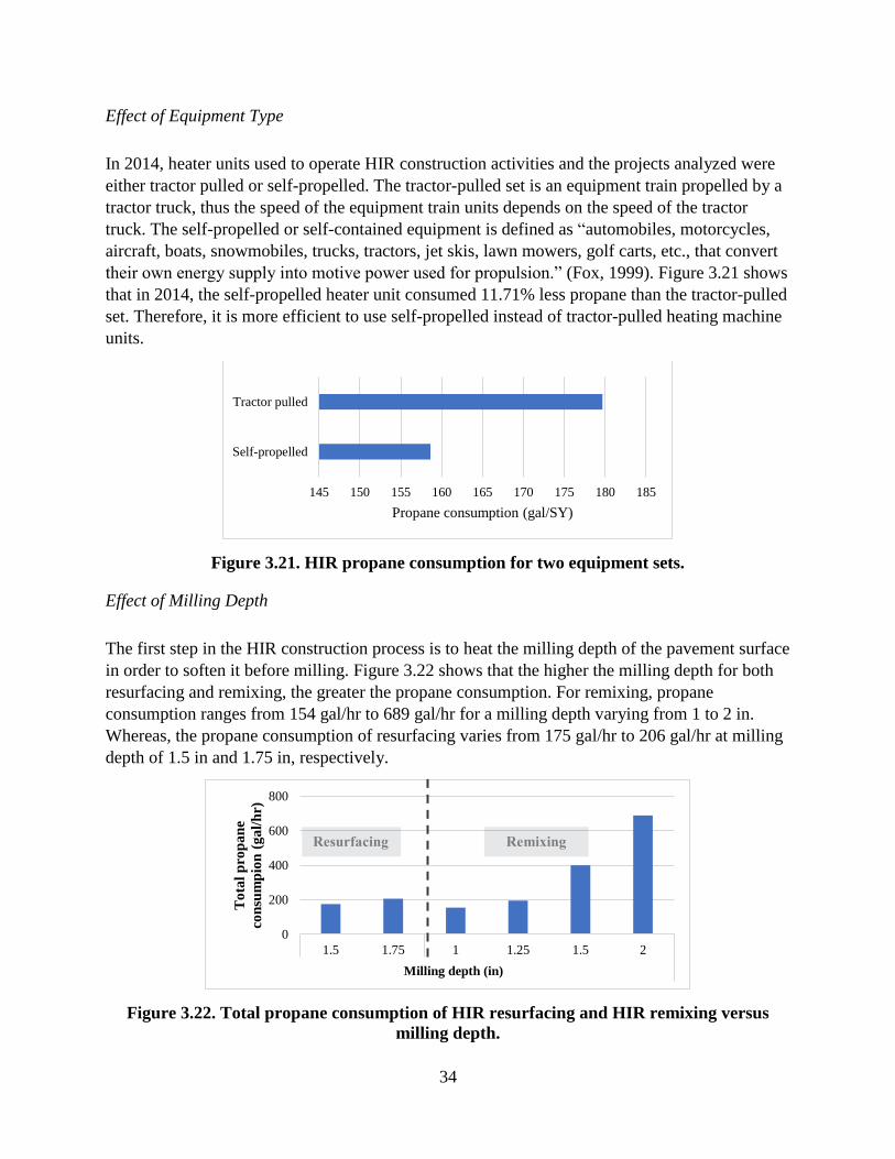
Effect of Equipment Type

In 2014, heater units used to operate HIR construction activities and the projects analyzed were

either tractor pulled or self-propelled. The tractor-pulled set is an equipment train propelled by a

tractor truck, thus the speed of the equipment train units depends on the speed of the tractor

truck. The self-propelled or self-contained equipment is defined as “automobiles, motorcycles,

aircraft, boats, snowmobiles, trucks, tractors, jet skis, lawn mowers, golf carts, etc., that convert

their own energy supply into motive power used for propulsion.” (Fox, 1999). Figure 3.21 shows

that in 2014, the self-propelled heater unit consumed 11.71% less propane than the tractor-pulled

set. Therefore, it is more efficient to use self-propelled instead of tractor-pulled heating machine

units.

Figure 3.21. HIR propane consumption for two equipment sets.

Effect of Milling Depth

The first step in the HIR construction process is to heat the milling depth of the pavement surface

in order to soften it before milling. Figure 3.22 shows that the higher the milling depth for both

resurfacing and remixing, the greater the propane consumption. For remixing, propane

consumption ranges from 154 gal/hr to 689 gal/hr for a milling depth varying from 1 to 2 in.

Whereas, the propane consumption of resurfacing varies from 175 gal/hr to 206 gal/hr at milling

depth of 1.5 in and 1.75 in, respectively.

Figure 3.22. Total propane consumption of HIR resurfacing and HIR remixing versus

milling depth.

145 150 155 160 165 170 175 180 185

Self-propelled

Tractor pulled

Propane consumption (gal/SY)

0

200

400

600

800

1.5 1.75 1 1.25 1.5 2

Resurfacing Remixing

To

tal

pro

pa

ne

con

sum

pio

n (

ga

l/h

r)

Milling depth (in)

35

Effect of Pavement Aggregate Hardness

Pavement aggregate hardness is one of the main factors that influence propane and diesel fuel

consumption. This study considers the impact of pavement hardness on propane consumption

because the propane usage has the highest contribution to the overall energy use. The impact of

pavement hardness is mostly seen during the scarification or grinding of the existing HMA

surface. Hardness can be attributed to aggregate type, temperature during heating, and asphalt

binder type used in the surface layers. The project-specific data collected from the contractors

were used to evaluate the effect of hardness with an intent to develop a model that is capable of

predicting the relative hardness of the pavement based on project location.

Available data show propane consumption during the remixing process in different job locations

in Georgia, Illinois, Massachusetts, New Jersey, Tennessee, and Wisconsin. In order to

characterize the aggregate hardness at these locations, the average Moh’s hardness (0-10) was

defined for each state based on the predominant aggregate types found in these states according

to a U.S. Geological Survey (USGS) study illustrated in Figure 3.23 (Langer, 2011). For

instance, the predominant rock type in Illinois and Tennessee is limestone, so the average Moh’s

hardness associated to their job locations is 3.5. Granite and Limestone are the predominant

rocks in Wisconsin and Georgia, so their associated average Moh’s hardness is 5.5. Granite and

sandstone are the predominant rocks in New Jersey and Massachusetts, and their average Moh’s

hardness is 6.5. Based on the primary data collected about HIR remixing job locations, the

average propane consumption in Illinois, Tennessee, Wisconsin, Georgia, New Jersey and

Massachusetts are 0.15 gal/SY, 0.16 gal/SY, 0.47 gal/SY, 0.56 gal/SY, 0.58 gal/SY and 0.86

gal/SY, respectively. The results summarized in Table 3.7 show that pavements containing

harder aggregates result in higher propane consumption during the remixing process.

Figure 3.23. Generalized locations of aggregate resources (Langer, 2011)

36

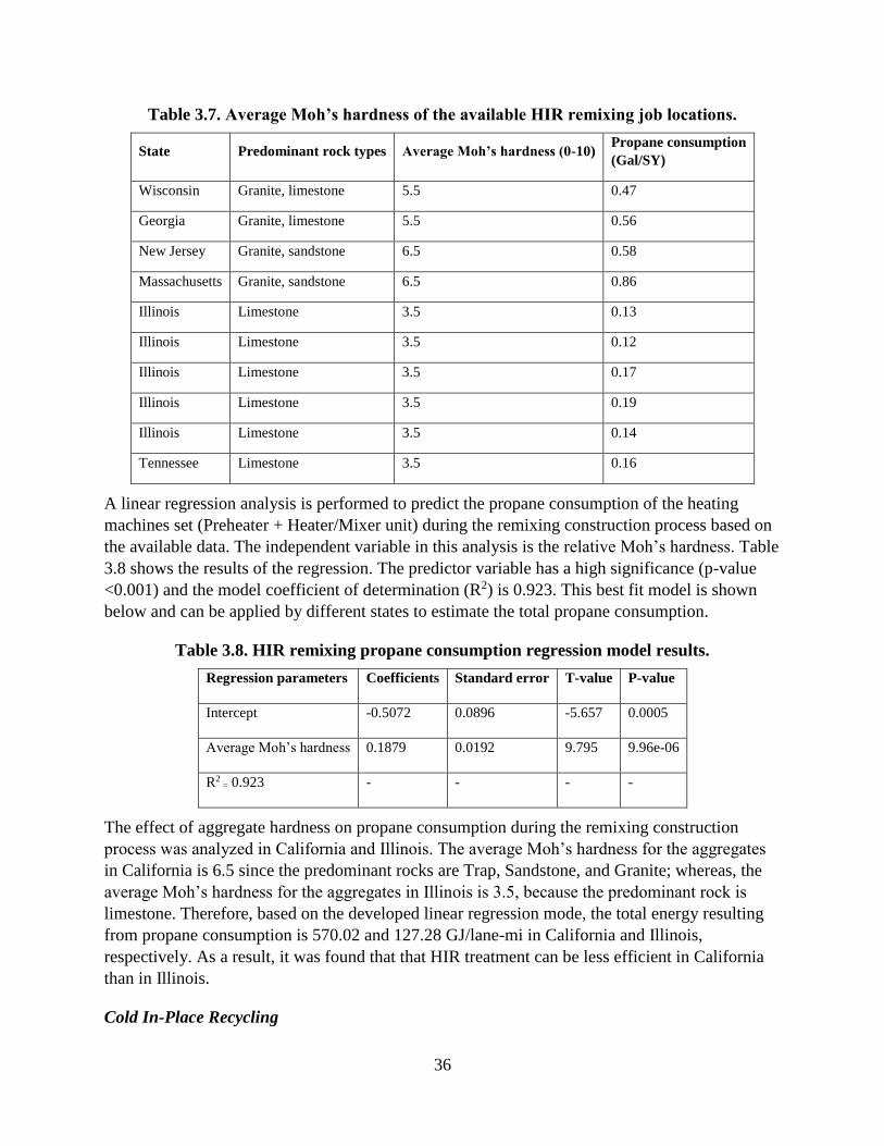
Table 3.7. Average Moh’s hardness of the available HIR remixing job locations.

State Predominant rock types Average Moh’s hardness (0-10) Propane consumption

(Gal/SY)

Wisconsin Granite, limestone 5.5 0.47

Georgia Granite, limestone 5.5 0.56

New Jersey Granite, sandstone 6.5 0.58

Massachusetts Granite, sandstone 6.5 0.86

Illinois Limestone 3.5 0.13





Tennessee Limestone 3.5 0.16

A linear regression analysis is performed to predict the propane consumption of the heating

machines set (Preheater + Heater/Mixer unit) during the remixing construction process based on

the available data. The independent variable in this analysis is the relative Moh’s hardness. Table

3.8 shows the results of the regression. The predictor variable has a high significance (p-value

<0.001) and the model coefficient of determination (R2) is 0.923. This best fit model is shown

below and can be applied by different states to estimate the total propane consumption.

Table 3.8. HIR remixing propane consumption regression model results.

Regression parameters Coefficients Standard error T-value P-value

Intercept -0.5072 0.0896 -5.657 0.0005

Average Moh’s hardness 0.1879 0.0192 9.795 9.96e-06

R2 = 0.923 - - - -

The effect of aggregate hardness on propane consumption during the remixing construction

process was analyzed in California and Illinois. The average Moh’s hardness for the aggregates

in California is 6.5 since the predominant rocks are Trap, Sandstone, and Granite; whereas, the

average Moh’s hardness for the aggregates in Illinois is 3.5, because the predominant rock is

limestone. Therefore, based on the developed linear regression mode, the total energy resulting

from propane consumption is 570.02 and 127.28 GJ/lane-mi in California and Illinois,

respectively. As a result, it was found that that HIR treatment can be less efficient in California

than in Illinois.

Cold In-Place Recycling

37

General CIR Process

According to the information collected from contractors in 2015. Two different construction

methods are commonly used for CIR, namely, single machine and the single-pass equipment

train.

The single machine method breaks, pulverizes, and adds recycling agents in a single pass. The

advantages of a single machine include high production capacity and simplicity of operation. On

the other hand, the single-pass equipment train consists of a cold milling machine, a portable

crusher, a travel-plant mixer, and a laydown machine (FHWA, 2015). It provides better process

control, more uniformity, and higher production rates (often more than two miles per day)

(FHWA, 2015).

An environmental impact assessment is conducted for CIR operations. In this study, the milling

depth during CIR construction processes ranges from 3 to 4 in. The construction information of

CIR was based on the data collected from 24 projects located in Illinois, Indiana, Iowa,

Massachusetts, and Nebraska, that used the single-pass equipment train method. The equipment

fuel consumption was based on an average train speed of 22 ft/min. The fuel consumption of the

equipment used in CIR processes is presented in Table 3.9. The milling operation contributes the

most in the total energy of the CIR construction process with approximately 82.32%.

Figure 3.24 shows that most of the CIR projects consumed approximately 0.04 gal/SY of diesel,

which also matches the total fuel consumption calculated for the CIR single-pass equipment train

0.036 gal/SY in Table 3.9, thus resulting in a total of 58.628 GJ/lane-mi energy use.

Table 3.9. Details for the Environmental Assessment of CIR.

Equipment type HP Average fuel

consumption

(Gal/SY)

CIR energy

(GJ/Lane-mi) Milling machine 860 0.01966 48.260

Crusher/pugmill 375 0.00488 4.792

Oil pump 5 0.00005 0.002

Paver 150 0.00204 2.000

Pickup machine 90 0.00126 1.238

Skid steer 70 0.00019 0.186

Double steel drum roller 115 0.00128 1.255

Rubber tire roller 150 0.00081 0.802

Water truck 425 0.00027 0.011

Pickup truck 300 0.00448 0.061

Service truck 300 0.00154 0.021

Total - 0.03646 58.628

38

Figure 3.24. Graph. Histogram of CIR projects total diesel consumption.

Effect of Air Temperature

The University of Leeds conducted a study on the “impact of ambient temperatures on exhaust

thermal characteristics during cold start.” (Li et al., 2005). The study showed that ambient

temperatures have an impact on fuel consumption and that 1.4% more fuel was consumed in cold

winter (28.4°F) compared with hot summer (87.8°F) because of the higher heat losses caused by

increased mechanical frictions in the vehicle engine. A study investigated the relationship of

combustion efficiency of direct injection diesel engine as function of time cold and warm

conditions. It was found that for warm start of the engine, the efficiency was over 98%; whereas,

the efficiency did not exceed 95% at cold start (Bielaczyc et al., 2001). Figure 3.25 shows that

the diesel consumption of the CIR projects analyzed has a decreasing trend with higher air

temperatures. In addition, the cutting speed during the milling operation increases under warmer

temperatures.

Figure 3.25. Effect of air temperature on diesel consumption and cutting speed during

milling operation

0 2 4 6 8 10 12 14

0.02

0.04

0.06

More

Frequency

To

tal

CIR

die

sel

con

sum

pti

on

(g

al/

SY

)

0

5

10

15

20

25

30

0

0.01

0.02

0.03

0.04

0.05

0.06

62 68 71 77 79 84 87 89 Aver

age

cut

spee

d (

ft/m

in)

Aver

age

die

sel

consu

mp

tio

n

(gal

/SY

)

Average air temperature (ºF)

Fuel consumption Cut speed

Linear (Fuel consumption) Linear (Cut speed)

39

Effect of Pavement Width

During the follow-up interviews with the contractors, it was found that pavement width is

another factor affecting fuel consumption during the milling operation. The CIR contractors

typically used a half-lane milling machine model characterized by a cut width of 12.5 ft. Figure

3.26 shows that the wider the pavement lane, the more diesel is consumed by the milling

machine and the higher is the number of teeth per 100 ton used in the milling operation. In fact,

the contractor needs to change the number of installed cutting teeth for different widths.

Figure 3.26. Total CIR fuel consumption versus width.

A multiple regression analysis was performed to predict the diesel consumption of the milling

machines set (milling machine + crusher) during CIR construction process based on available

data. The independent variables in this model are pavement width and the number of teeth per

100 tons. The predictor variable has a high significance (p-value <0.001) and the model R2 is

0.81. The best fit model obtained is given in Table 3.10 and can be used to estimate the fuel

consumption during the milling operation of CIR.

Table 3.10. CIR milling operation fuel consumption regression model.

Regression Parameters Coefficients Standard Error T-Value P-Value

Intercept -0.0343 0.0482 -0.711 0.4949

Width 0.0039 0.0047 0.950 0.3668

Teeth per 100 tons 0.0017 0.0003 6.005 0.0002

R2 = 0.8063 - - - -

0

1

2

3

4

5

6

7

8

0

0.005

0.01

0.015

0.02

0.025

0.03

11 12 13

Num

ber

of

too

th p

er t

on

Aver

age

mil

ling d

iese

l co

nsu

mp

tio

n

(gal

/SY

)

Pavement width (ft)

Milling fuel consumption Number of tooth per 100 ton

40

Effect of Milling Depth

The effect of milling depth on fuel consumption has been investigated. Figure 3.27 shows that

the total fuel consumption increases with higher milling depth. However, there is no clear trend

of crushing and milling fuel consumption rates with increasing milling depth. In the range from

3.5 to 5 in cut depth, the milling fuel consumption is clearly increasing, but the crushing

contribution stays at approximately a constant rate from 3 to 5 in.

Figure 3.27. CIR Diesel consumption versus milling depth.

Effect of Equipment Technology

Higher horsepower results in higher fuel consumption (Suman, 2010). The CIR contractor used

two types of equipment trains that differ in their milling machine horsepower (HP) (FHWA,

2015). Train 1 has a milling machine of HP equal to 800 and train 2 is characterized by a milling

machine of HP equal to 860. Table 3.11 shows that HP of 860 results in a fuel consumption

higher than HP of 800 with a difference of 4%.

Table 3.11. Summary of HP effect on fuel efficiency.

Train type Train 1 (Milling machine, HP= 800) Train 2 (Milling machine, HP= 860)

Diesel consumption (gal/SY) 0.0197 0.0205

Fuel Use for Conventional Overlay Methods

The fuel usage data for conventional overlays was extracted from Tollway pay items (Yang et

al., 2017). According to results of Figure 3.28, HMA full-depth projects construction total

0

0.005

0.01

0.015

0.02

0.025

0.03

0.035

0.04

0.045

0.05

3 3.5 4 5

Aver

age

die

sel

consu

mp

tio

n (

gal

/SY

)

Milling depth (in)

Total fuel consumption Milling fuel consumption Crushing fuel consumption

41

consumption is higher than the HMA surface and base courses. In Figure 3.29, the contribution

of equipment unit used in a HMA full depth of 12 in thickness was assessed and it was found

that that the milling machine contributes the most to the overall construction processes fuel

consumption followed by paver and then the different roller types.

Figure 3.28. Fuel consumption of conventional overlay projects.

Figure 3.29. HMA full depth 12-in overlay equipment use contribution.

Modeling Procedure

EPA MOVES 2014 (NONROAD)

The equipment unit processes are compiled using the NONROAD 2008 model incorporated in

MOVES 2014 software. NONROAD equipment are used to perform and help to operate

construction activities on-site. Air pollution emission inventories are combined with TRACI

impact assessment methodology to estimate the unit emission quantities per gallon of fuel

consumed. TRACI 2.1 provides characterization factors for life-cycle impact categories rates:

ozone depletion, GWP, acidification, eutrophication, smog formation, human health impacts,

ecotoxicity, and fossil fuel depletion for fuel combustion (Bare, 2011). Figure 3.30 shows the

0

0.05

0.1

0.15

0.2

0.25

HMA (full

depth), 12 in

HMA (full

depth), 15 in

HMA base

course, 4 in

HMA surface

course, 3 in

Aver

age

fuel

co

nsu

mp

tio

n

(gal

/SY

)

50%

14%

13%

13%

10%Milling Machine

Paver

Single Drum Roller

Tandem Drum Roller

Pneumatic Roller

42

methodology used to calculate TRACI impact categories rates from eight pollutant types

included in MOVES 2014.

Figure 3.30. TRACI impacts rates calculation from pollutants emissions included in

MOVES 2014.

NONROAD Model Development

Simulations have been performed using MOVES 2014 from 2015 to 2050 to allow for running

LCIA of equipment for future projects, as shown in Figure 3.31.

The simulations run on MOVES 2014 software allowed developing a NONROAD model to

assess the environmental impacts of on-site equipment. For a single equipment type, the unit

emission of a substance depends on three main variables which are tier category, HP bin (range),

and year of construction. NONROAD model inputs are geographic bound, time spans,

NONROAD vehicle equipment type and pollutants/processes types. The outputs are the rates of

the pollutants selected. These rates are then used to calculate the US-EI 2.2 unit processes of

diesel combustion. The TRACI characterization of fuel production is used to quantify the unit

processes of diesel upstream production.

The total per-gallon inventory quantities of diesel combustion and production shares represent

the NONROAD equipment impact as illustrated in Figure 3.32.

Figure 3.33 shows GWP results of various types of equipment in three different counties:

Champaign (Illinois), Yolo (California), and Middlesex (New Jersey). It was found that the

environmental impacts of on-site equipment are not sensitive to the geographic location. Since

results are not sensitive to location, Champaign County was used to run simulations.

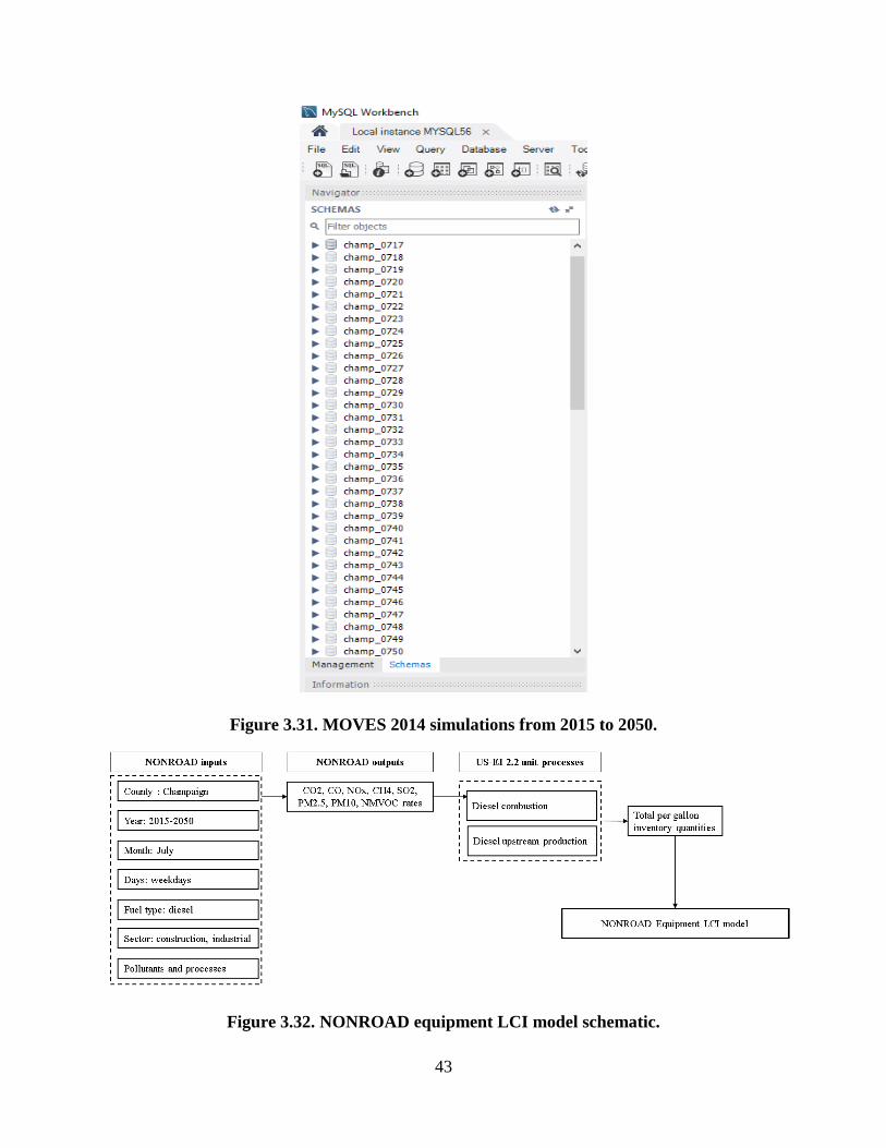
43

Figure 3.31. MOVES 2014 simulations from 2015 to 2050.

Figure 3.32. NONROAD equipment LCI model schematic.

44

Figure 3.33. Sensitivity analysis of equipment GWP results to the geographic location.

The model accounts for four tier categories, which are the federal emission standards for

compression ignition engines (diesel engines) used in most construction vehicles, resulting from

five regulations as follows:

• “Determination of Significance for Nonroad Sources and Emission Standards for

New Nonroad Compression Ignition Engines at or above 37 Kilowatts.” This rule

establishes “Tier 1” standards for compression ignition (CI) engines at or above 50 hp

(37 kW). (EPA, 1994)

• “Control of Emissions from Nonroad Diesel Engines”. This rule lists “Tier 1” and

“Tier 2” standards for CI engines below 50 hp, and “Tier 2” and “Tier 3 ” standards

for engines of 50 hp and greater. (EPA, 1998)

• “Control of Emissions from Nonroad Large Spark-Ignition (SI) Engines and

Recreational Engines (Marine and Land-Based).” This rule establishes “Tier 2”

equivalent standards for recreational marine diesel engines over 50 hp. (EPA, 2002)

• “Control of Emissions from Nonroad Diesel Engines and Fuel.” This rule establishes

“Tier 4” standards for CI engines covering all hp categories and regulates diesel fuel

sulfur content. (EPA, 2004)

• “Control of Emissions of Air Pollution from Locomotive Engines and Marine

Compression Ignition Engines Less Than 30 Liters per Cylinder; Republication.” This

rule establishes “Tier 3” standards for recreational marine diesel engines. (EPA,

2008)

The objective of these regulations is to reduce NOx, NMHC, PM pollutant. Therefore, the impact

categories such as smog, acidification, eutrophication, and respiratory effects will decrease over

time. Figure 3.34 shows that respiratory effects impact decreases with the years and with the

development of engine technologies through regulations mentioned above.

11.69

11.691

11.692

11.693

11.694

11.695

GW

P (

kgC

O2

/gal

)

Champaign

Middlesex

Yolo

45

Figure 3.34. Respiratory effects variation and tier progression of pavers (100<HP<=175)

over the years.

Contractors’ data were collected for Tier 2 equipment. Using the NONROAD model, other tier

categories were evaluated to compare their impact on the environmental emissions. It was found

that using a Tier 4 (T4) instead of Tier 2 (T2) for the CIR single-pass equipment train results in a

reduction of 37% of the total respiratory effects as shown in Figure 3.35.

Figure 3.35. Comparison of total respiratory effects of a CIR single-pass equipment train

Tier 2 versus Tier 4.

0

0.005

0.01

0.015

0.02

0.025

0.03

0.035

0.04

Res

pir

ato

ry E

ffec

ts (

CT

Uh

/gal

)

Years

T4N

T4

T3

T2

T1

0 0.05 0.1 0.15 0.2 0.25 0.3

T2

T4

Total respiratory effects (PM2.5/lane-mi)

Tie

r

Diesel Fuel - 2017 - CIR (single-pass equipment train)

37% reduction

46

Work zone modeling

Many studies investigated methods to model work zone strategies. Governmental agencies and

FHWA developed software tools (e.g., Construction Analysis for Pavement Rehabilitation

Strategies (CA4PRS) (Rister; Graves, 2002), Kentucky user cost program (KyUCP) (Lee; Ibbs,

2005)) to select strategies for traffic delay management during the construction stage. A good

traffic management plan prior to construction is important to provide a contractor with an

optimal construction window and ensure a better flow of traffic through the work zone. The

developed tool assumes that user has already set a traffic management plan and parameters to

model the work zone. These parameters are represented in Table 3.12.

Table 3.12. Work zone parameters used for impact calculation.

Work Zone Parameters

Queue length (mi)

Work zone length (mi)

Queue speed (mi)

Work zone speed (mph)

Normal traffic speed (mph)

Passenger car (%)

Small truck (%)

Medium truck (%)

Large truck (%)

Virginia Department of Transportation (DOT) applied CIR and FDR on 3.66 mi of southbound I-

81 in August County and monitored the road section performance for three-year service period.

The results of the study showed that the IPR techniques were successfully constructed

(Diefenderfer,2014). The traffic management plan of the project consisted of reducing two lanes

to one lane for the entire length. A closure window was decided based on traffic data which

reflected times when highest volumes occurred.

USE STAGE

The use stage is analyzed using roughness and texture related rolling resistance progression over

the analysis period. This stage is the most significant among all life cycle stages and includes

other components such as albedo and lighting (Santero et al., 2011) which are considered out of

scope. During use phase, agencies tend to apply maintenance and rehabilitation activities in order

to maintain the pavement in a good condition.

Impact of roughness on rolling resistance

The Roughness-Speed Impact Model (RSI) by Ziyadi et al. was used to calculate the

environmental impacts and energy consumption of use stage (Ziyadi et al., 2017). The general

form of the RSI model depends on the vehicle speed and IRI progression as equation 3.1 shows.

A regression analysis was then conducted using MOVES simulations to define the model

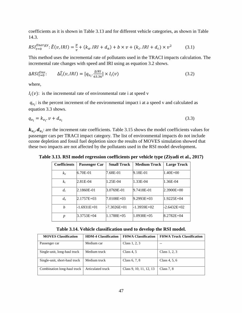
47

coefficients as it is shown in Table 3.13 and for different vehicle categories, as shown in Table

14.3.

𝑅𝑆𝐼𝑡=0𝐸𝑛𝑒𝑟𝑔𝑦

: �̂�(𝑣, 𝐼𝑅𝐼) =𝑝

𝑣+ (𝑘𝑎. 𝐼𝑅𝐼 + 𝑑𝑎) + 𝑏 × 𝑣 + (𝑘𝑐. 𝐼𝑅𝐼 + 𝑑𝑐) × 𝑣2 (3.1)

This method uses the incremental rate of pollutants used in the TRACI impacts calculation. The

incremental rate changes with speed and IRI using as equation 3.2 shows.

∆𝑅𝑆𝐼𝑡=0𝐸𝑛𝑣: ∆𝐼�̂�(𝑣, 𝐼𝑅𝐼) = [𝑞𝑣𝑖

.∆𝐼𝑅𝐼

63.36] × 𝐼𝑖(𝑣) (3.2)

where,

𝐼𝑖(𝑣): is the incremental rate of environmental rate i at speed v

𝑞𝑣𝑖: is the percent increment of the environmental impact i at a speed v and calculated as

equation 3.3 shows.

𝑞𝑣𝑖= 𝑘𝑣𝑖

. 𝑣 + 𝑑𝑣𝑖 (3.3)

𝒌𝒗𝒊, 𝒅𝒗𝒊

: are the increment rate coefficients. Table 3.15 shows the model coefficients values for

passenger cars per TRACI impact category. The list of environmental impacts do not include

ozone depletion and fossil fuel depletion since the results of MOVES simulation showed that

these two impacts are not affected by the pollutants used in the RSI model development.

Table 3.13. RSI model regression coefficients per vehicle type (Ziyadi et al., 2017)

Coefficients Passenger Car Small Truck Medium Truck Large Truck

ka 6.70E-01 7.68E-01 9.18E-01 1.40E+00

kc 2.81E-04 1.25E-04 1.33E-04 1.36E-04

dc 2.1860E-01 3.0769E-01 9.7418E-01 2.3900E+00

da 2.1757E+03 7.0108E+03 9.2993E+03 1.9225E+04

b -1.6931E+01 -7.3026E+01 -1.3959E+02 -2.6432E+02

p 3.3753E+04 1.1788E+05 1.0938E+05 8.2782E+04

Table 3.14. Vehicle classification used to develop the RSI model.

MOVES Classification HDM-4 Classification FHWA Classification FHWA Truck Classification

Passenger car Medium car Class 1, 2, 3 --

Single-unit, long-haul truck Medium truck Class 4, 5 Class 1, 2, 3

Single-unit, short-haul truck Medium truck Class 6, 7, 8 Class 4, 5, 6

Combination long-haul truck Articulated truck Class 9, 10, 11, 12, 13 Class 7, 8

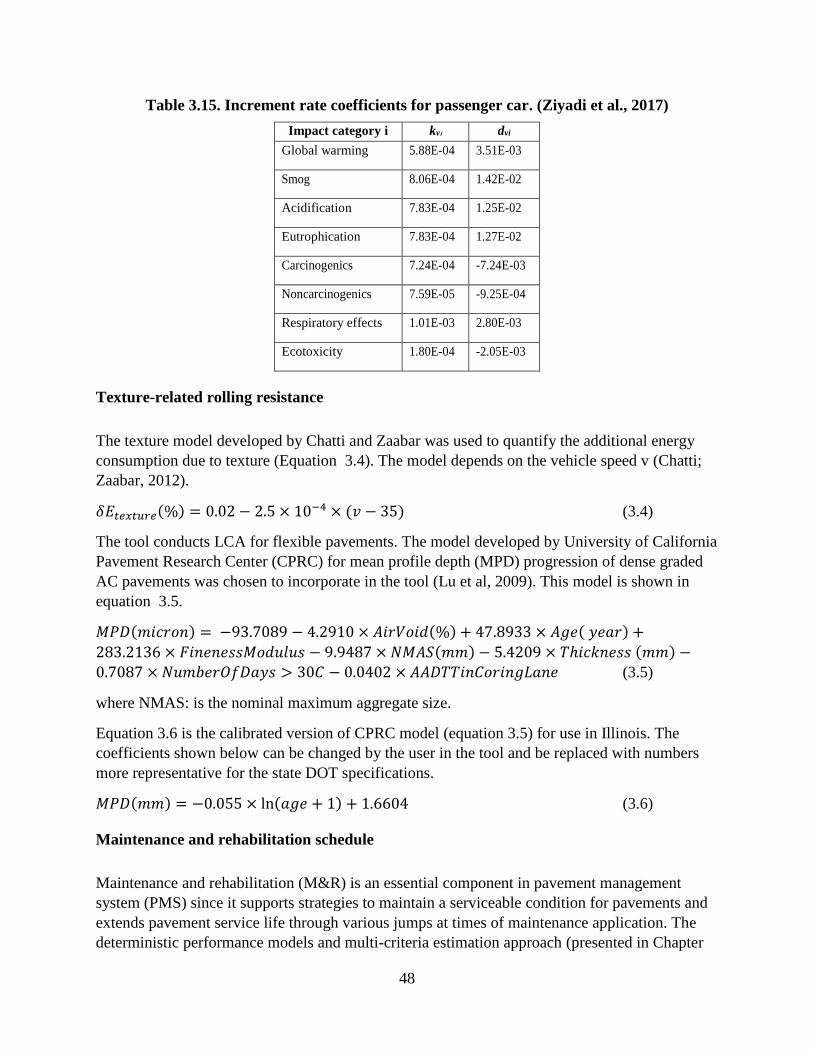
48

Table 3.15. Increment rate coefficients for passenger car. (Ziyadi et al., 2017)

Impact category i kvi dvi

Global warming 5.88E-04 3.51E-03

Smog 8.06E-04 1.42E-02

Acidification 7.83E-04 1.25E-02

Eutrophication 7.83E-04 1.27E-02

Carcinogenics 7.24E-04 -7.24E-03

Noncarcinogenics 7.59E-05 -9.25E-04

Respiratory effects 1.01E-03 2.80E-03

Ecotoxicity 1.80E-04 -2.05E-03

Texture-related rolling resistance

The texture model developed by Chatti and Zaabar was used to quantify the additional energy

consumption due to texture (Equation 3.4). The model depends on the vehicle speed v (Chatti;

Zaabar, 2012).

𝛿𝐸𝑡𝑒𝑥𝑡𝑢𝑟𝑒(%) = 0.02 − 2.5 × 10−4 × (𝑣 − 35) (3.4)

The tool conducts LCA for flexible pavements. The model developed by University of California

Pavement Research Center (CPRC) for mean profile depth (MPD) progression of dense graded

AC pavements was chosen to incorporate in the tool (Lu et al, 2009). This model is shown in

equation 3.5.

𝑀𝑃𝐷(𝑚𝑖𝑐𝑟𝑜𝑛) = −93.7089 − 4.2910 × 𝐴𝑖𝑟𝑉𝑜𝑖𝑑(%) + 47.8933 × 𝐴𝑔𝑒( 𝑦𝑒𝑎𝑟) +

283.2136 × 𝐹𝑖𝑛𝑒𝑛𝑒𝑠𝑠𝑀𝑜𝑑𝑢𝑙𝑢𝑠 − 9.9487 × 𝑁𝑀𝐴𝑆(𝑚𝑚) − 5.4209 × 𝑇ℎ𝑖𝑐𝑘𝑛𝑒𝑠𝑠 (𝑚𝑚) −0.7087 × 𝑁𝑢𝑚𝑏𝑒𝑟𝑂𝑓𝐷𝑎𝑦𝑠 > 30𝐶 − 0.0402 × 𝐴𝐴𝐷𝑇𝑇𝑖𝑛𝐶𝑜𝑟𝑖𝑛𝑔𝐿𝑎𝑛𝑒 (3.5)

where NMAS: is the nominal maximum aggregate size.

Equation 3.6 is the calibrated version of CPRC model (equation 3.5) for use in Illinois. The

coefficients shown below can be changed by the user in the tool and be replaced with numbers

more representative for the state DOT specifications.

𝑀𝑃𝐷(𝑚𝑚) = −0.055 × ln(𝑎𝑔𝑒 + 1) + 1.6604 (3.6)

Maintenance and rehabilitation schedule

Maintenance and rehabilitation (M&R) is an essential component in pavement management

system (PMS) since it supports strategies to maintain a serviceable condition for pavements and

extends pavement service life through various jumps at times of maintenance application. The

deterministic performance models and multi-criteria estimation approach (presented in Chapter

49

4) were used to build M&R schedule that extends over the analysis period calculated based on

the alternatives selected by the user. More information about the M&R schedule construction

methods are presented in Chapter 6: Decision making Tool Development

The developed tool assumes thin AC overlay to be a default maintenance activity applied every

time it is optimum to take an action to maintain the pavement in a good condition. However, in

case IRI progression is triggered by cracking threshold then CIR with overlay is applied to

enhance structural capacity of the pavement.

END OF LIFE STAGE

The end of life analysis depends on the approach used by the user to allocate the system

resources. Figure 3.36 shows the chain of material life cycle from System 1 (original system) to

System 2 (subsequent system) (Ekvall; Tillman, 1997). Nicholson showed that environmental

impacts and energy resulting from materials production stage is sensitive to the allocation

method choice. A 100% cut-off allocation was chosen to manage end of life burdens in this LCA

study as illustrated in Figure 3.37. In fact, pavement construction materials (e.g., AC) may be

recycled at the end of life. Therefore, the recycled materials can be either accounted as a burden

when using cut-off or as a benefit to the original system using substitution.

Figure 3.36. Cascade of System 1 and System 2 material life cycles (T = material

transportation) (Ekvall; Tillman, 1997)

50

Figure 3.37. Cut-off allocation method system boundary.

Cut-Off Method

In the cut-off method, the recycling processing R1 is not included in the impacts resulting from

system 1 and is considered as a burden on System 2. The overall emissions resulting from

System 1 materials life cycle is the summation of emissions due virgin material input

V1 production and hauling, disposal and hauling of waste to a landfill facility at the end of life of

System 1 as equation 3.7 shows.

𝐸𝑇𝑜𝑡 = 𝑋1𝐸𝑣1+ (1 − 𝑋1 )𝐸𝑅0

+ 𝑊1𝐸𝑊1 (3.7)

where,

X1: proportion of material in the virgin input of System 1

R0: proportion of material in the recycled input of System 0

V1: proportion of material in the virgin input of System 1

W1: proportion of waste material at the end of life of System 1

EV1: emission arising from material in the virgin input of System 1

ER0: emission arising from material in the recycled material of System 0

EW1: emission arising from disposal of waste/landfill material of System 1

Substitution (Closed Loop Approximation)

The substitution method gives a credit to original system for producing RAP for the future

system as a substitute for virgin materials. The impacts calculation for this method is shown in

equation 3.8.

𝐸𝑇𝑜𝑡 = (1 − 𝑅1)𝐸𝑉1+ 𝑅1𝐸𝑅1

+ (1 − 𝑅1)𝐸𝑊1 (3.8)

51

where,

R1: proportion of material in the product recycled at the end of life of System 1

ER1: emission arising from material in the recycled input of System 1

52

CHAPTER 4: PAVEMENT PERFORMANCE MODELING

OVERVIEW OF METHODS

The performance and lifetime estimation play a critical role in evaluating life-cycle benefits of

IPR treatments as compared with conventional treatments. The methodology to incorporate

performance and lifetime estimation into the life-cycle comparative tool is introduced and a two-

pronged approach is presented: Multi-criteria performance estimation and deterministic

performance models. When deterministic models are not available for the selected treatments, a

multi-criteria performance estimation approach is proposed to evaluate the selected treatments to

make predictions.

• Deterministic performance models – The models in the tool were developed by

University of California Davis using network level condition survey data from the

California Department of Transportation and are used to predict the international

roughness index (IRI) progression and wheelpath cracking performance over the life of

pavement. The outputs from these models are estimates of the performance of

conventional AC overlays, CIR, and FDR pavements in terms of wheelpath cracking

(fatigue cracking) and IRI, which can be used to estimate the time to the next treatment.

Similar models can be developed using information from other agencies.

• Multi-criteria performance estimation –This approach utilizes existing information in the

literature (e.g., decision-making recommendations from various agencies, treatment lives,

guidelines, best practices, expert opinion) to estimate the performance of a treatment

considering specific on-site conditions. This approach relies on a process that calculates a

“performance score” on a 1 to 5 scale indicating the level of risk of a selected treatment

based on available on-site condition information regarding traffic, climate, existing

pavement conditions, soil properties and material characteristics. The process then

compares the performance score with on-site conditions and estimates a treatment life

based on the recommendations and other information reported in the literature, which can

be modified by the user. This approach also selects an estimated roughness progression

rate based on the available information. This approach is used when deterministic

performance models do not exist or those available are not considered applicable.

The two approaches determine IRI progression starting from the treatment application time at a

trigger IRI value to an IRI threshold value input by the user. This enables the user to visualize

the IRI progression and decide the timing of the next treatment. Figure 4.1 presents the IRI

progression for two different treatments A and B that start, respectively, from 𝐼𝑅𝐼𝑎 and 𝐼𝑅𝐼𝑏 and

reach the corresponding thresholds 𝐼𝑅𝐼𝑡ℎ𝑟𝑒𝑠ℎ𝑜𝑙𝑑.Both performance prediction approaches are

utilized in the developed tool. Once the project input parameters are entered, the user would be

provided with a list of treatment alternatives. The user would have the option to select one or

more IPR treatments and compare them to one or more conventional AC overlay treatments. The

selected treatments are initially screened for their applicability for the project conditions. If there

are obvious and clear barriers against application of the selected treatment (e.g., geometric

features impeding application of using a long IPR train), the user would be warned. After this,

53

the user can decide to use either one of the performance modeling approaches to evaluate the

selected treatments and calculate treatment lifetime and develop IRI progression curves. In the

following schematic (Figure 4.2), a flowchart of the developed tool illustrates the performance

estimation process integration to the overall flow of data and input flow.

Figure 4.1. A schematic of IRI progression curves with significant model parameters

obtained by the performance estimating methods.

Figure 4.2. Flowchart of the treatments selection, evaluation, and life-cycle analysis.

54

MULTI-CRITERIA PERFORMANCE ESTIMATION APPROACH

Concept

When there is no performance model available, the multi-criteria performance estimation

approach could be used. The multi-criteria performance estimation process is used to estimate

treatment life by collecting information related to various site-specific conditions and evaluating

this information through a rating system to determine an expected treatment performance. This

approach provides an estimate of treatment life based on reported lifespans in the literature or

observed by the user in the region of interest adjusted for site-specific conditions. The

relationship of various site-specific factors to expected performance is compiled from multiple

sources. These include existing literature for best practices and experimental data, agency and

contractor surveys, decision trees adopted by local and state highway agencies, and expert

opinions.

The performance estimation process is based on five major categories of information: climate,

traffic, existing pavement condition, soil properties, and pavement material properties. The

process of integrating these into the performance score calculation, treatment suitability and

performance estimation process is as follows:

• Collect site-specific condition information for each major category for a given treatment

candidate from the user (traffic, including average daily traffic (ADT), % truck, and road

type, existing pavement condition, including overall condition index and distress level of

severity, soil properties, climate type, and materials properties, including mix design if

performed)

• Score the site-specific condition under each major category as a risk of poor performance

rating score from 1 to 5. The interpretation of each rating score of a treatment under a

certain condition is as follows:

1: High risk; 2: Medium-high risk; 3: Medium risk; 4: Medium-Low risk; 5: Low or no

risk.

• For example, a HIR resurfacing treatment followed by a thin overlay of 2 in or less. If a

high traffic level of >30,000 AADT is used, a score of 1 is assigned; the literature widely

agrees that this treatment type is not suitable for high traffic levels. Assigning a rating of

“1” in this case means that there is a high risk that the selected design may perform

poorly.

• Evaluate score for each category and determine the final rating score for the application.

• Based on the rating score, calculate expected treatment life based on lifetime estimates

compiled from the literature and surveys.

The treatment overall performance score (PS) is calculated based on the following formulation

(equation 4.1). It is assumed that all the factors are independent:

55

𝑃𝑆 = ∑ 𝐶𝑖

𝑁𝑐𝑖=1 +∑ 𝑇𝑖

𝑁𝑇𝑖=1

+∑ 𝑆𝑖𝑁𝑆𝑖=1

+∑ 𝐸𝑖+∑ 𝐷𝑖𝑁𝐷𝑖=1

𝑁𝐸𝑖=1

𝑁𝐶+𝑁𝑇+𝑁𝑆+𝑁𝐸+𝑁𝐷 (4.1)

where,

𝑇𝑖 : rating for each traffic related factor i

𝐶𝑖 : rating for each climate condition i

𝑆𝑖 : rating for each soil property i

𝐸𝑖 : rating for each existing pavement condition related factor i

𝐷𝑖 : rating for material properties condition related factor i

NC : number of climate condition related factors

NT : number of traffic related factors

NS : number of soil properties related factors

NE : number of existing conditions related factors

ND : number of structural design properties related factors

The interpretation of PS and resulting impact on treatment life is explained as follows:

• 4 or 5: Ideal on-site conditions for treatment; indicating very low risk for performance.

Treatment life can be expected to be at the highest range.

• 2 or 3: Conditions are fair carrying medium risk for the performance of treatment.

Treatment life can be expected to be at medium range of expectations.

• 1: On-site conditions are not appropriate for the treatment with very high risk. Treatment

life may be predicted at lower range of expected values.

Development of Performance Estimation

Population of the Treatments List

The first step of the development process is to populate a list of anticipated in-place,

conventional, and surface treatments. The list of treatments considered in the tool were classified

into five categories with their associated expected life range as shown in Table 4.1. Tables 4.2 to

4.6 show the expected service life of treatments under each category. The information reported is

based on the literature review and surveys collected from contractors and agencies for IPR

treatments application. Agencies questionnaire feedback reflects the percent of agencies that

applied various IPR treatments under different life ranges.

Table 4.1. Treatment categories expected life range.

Treatment Category Type Expected Life Range (year)

Category 1 3-5

Category 2 4-10

Category 3 7-15

Category 4 12-20

Category 5 15-25

56

Table 4.2. Compiled list of treatment life estimates obtained of category 1 from various

literature sources.

Treatment Type Expected life range (year) Literature Data Source

Fog seal 1-3 (Peshkin, 2011)

Sand seal 3-4 (Peshkin, 2011)

Slurry seal 3-6 (Peshkin, 2011)

Microsurfacing Single course 3-6 (Peshkin, 2011)

Chip seal Single course 3-7 (Peshkin, 2011)

Table 4.3. Compiled list of treatment life estimates obtained of Category 2 from various

literature sources and surveys.

Treatment Type Expected life

range (year)

Literature Data

Source Agency Questionnaire Feedback

Cape seal 4-7 years (Peshkin, 2011) –

Microsurfacing Double course 4-7 years (Peshkin, 2011) –

Chip seal Double course 5-10 years (Peshkin, 2011) –

HIR resurfacing 6-10 years (ARRA, 2015) 3-5 years (17%), 5-8 years (50%), 8-

10 years (33%)

Thin HMA overlay (2 in or less) 6-12 years (Peshkin, 2011) –

HIR remixing 3-15 years – 3-5 years (17%), 5-8 years (50%), 8-

10 years (33%)




range (year)

Literature

Data Source Agency Questionnaire Feedback

CIR 6-10 years (ARRA,

2015)

1-5 years (7%), 6-10 years (29%), 11-15 years

(36%), 16-20 years (21%), >25 years (7%)

CIR + cape seal 6-10 years (ARRA,

2015)


(36%), 16-20 years (21%), >25 years (7%)

CIR + chip seal 6-10 years (ARRA,

2015)


(36%), 16-20 years (21%), >25 years (7%)

HIR remixing + thin

overlay (2in or less) 7-20 years

(ARRA,

2015) 3-5 years (17%), 5-8 years (50%), 8-10 years (33%)

HIR remixing + medium

overlay (between 2 and 4

in)

7-20 years (ARRA,


HIR remixing + thick

overlay (over 4 in) 7-20 years

(ARRA,


HIR repaving 7-20 years (ARRA,


CIR + thin overlay (2 in

or less) 7-20 years

(ARRA,

2015)


(36%), 16-20 years (21%), >25 years (7%)

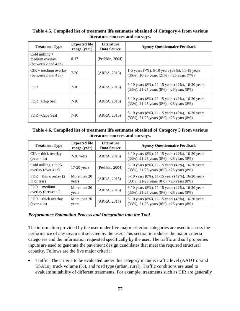
57




range (year)

Literature


Cold milling +

medium overlay

(between 2 and 4 in)

6-17 (Peshkin, 2004) –

CIR + medium overlay

(between 2 and 4 in) 7-20 (ARRA, 2015)


(36%), 16-20 years (21%), >25 years (7%)

FDR 7-10 (ARRA, 2015) 6-10 years (8%), 11-15 years (42%), 16-20 years

(33%), 21-25 years (8%), >25 years (8%)

FDR +Chip Seal 7-10 (ARRA, 2015) 6-10 years (8%), 11-15 years (42%), 16-20 years

(33%), 21-25 years (8%), >25 years (8%)

FDR +Cape Seal 7-10 (ARRA, 2015) 6-10 years (8%), 11-15 years (42%), 16-20 years

(33%), 21-25 years (8%), >25 years (8%)




range (year)

Literature


CIR + thick overlay

(over 4 in) 7-20 years (ARRA, 2015)


(33%), 21-25 years (8%), >25 years (8%)

Cold milling + thick

overlay (over 4 in) 17-30 years (Peshkin, 2004)


(33%), 21-25 years (8%), >25 years (8%)

FDR + thin overlay (2

in or less)

More than 20

years (ARRA, 2015)


(33%), 21-25 years (8%), >25 years (8%)

FDR + medium

overlay (between 2

and 4 in)

More than 20

years (ARRA, 2015)


(33%), 21-25 years (8%), >25 years (8%)

FDR + thick overlay

(over 4 in)

More than 20

years (ARRA, 2015)


(33%), 21-25 years (8%), >25 years (8%)

Performance Estimation Process and Integration into the Tool

The information provided by the user under five major criterion categories are used to assess the

performance of any treatment selected by the user. This section introduces the major criteria

categories and the information requested specifically by the user. The traffic and soil properties

inputs are used to generate the pavement design candidates that meet the required structural

capacity. Follows are the five major criteria:

• Traffic: The criteria to be evaluated under this category include: traffic level (AADT or/and

ESALs), truck volume (%), and road type (urban, rural). Traffic conditions are used to

evaluate suitability of different treatments. For example, treatments such as CIR are generally

58

used and recommended for lower volume roads whereas FDR can be designed to serve

adequately for higher volume roads.

• Existing pavement conditions: This category is evaluated by criteria related to drainage

adequacy, ride quality, and either overall pavement condition index or composition of critical

distresses present in the pavement. The existing conditions of a pavement are vital for

evaluating the relevance of treatment types. For example, the severity and type of distresses

may limit the usefulness of some treatments (e.g., HIR surface recycling) which cannot

address structural distresses.

• Soil properties: Characterization of the structure and soil type helps in determining which

designs are more likely to satisfy structural capacity requirements. The user is asked to input

a value of the California Bearing Ratio (CBR) to evaluate the support of pavement. This

input is also used in the pavement design criteria that is introduced later.

• Material properties: The tool evaluates mix designs as part of this approach if provided. It is

assumed that the use of a mix design reduces risks and accounts for the use of additives and

their dosages that affect pavement performance.

• Climate: The climate may have an impact on the performance of some of the treatments.

Normally, one should expect that the designs should be adjusted according to the climate

conditions. However, (4) there may be some treatments performing favorably under certain

climatic conditions such as micro-surfacing under warmer climates. Another factor is the

curing time required when additives are used along with IPR techniques. Therefore, the

different climate conditions considered in this study are cold/wet, cold/dry, hot/dry, and

hot/wet.

The overall performance score value defines the risk factor that should be applied on the

treatment. This process is applied on all the treatments selected by the user and directly

influences the treatment life expectancy. The major category criteria are scored for each

treatment considered in the tool using previous studies (e.g., (Peshkin, 2011), (ARRA, 2015),

(Stroup-Gardiner, 2011), (IDOT, 2012), (Wu et al., 2010), and (Hicks et al., 1999)) where

decision matrices were developed to help in decision making at the network level. Appendix C

shows the “IPR Decision Matrix” for rehabilitation and preservation treatments selection and

evaluation matrix.

Some of the limitations of this approach include the fact that rating of on-site conditions

classified under five categories relies on information available in the literature and expert

opinion without supporting data. Therefore, a validation step was conducted to support the

design lives estimated by this approach. The validation step includes case studies with

performance data available and vetting by internal and external experts. Case studies were

chosen primarily from the following sources:

• Local and state highway pavement management databases (CalTrans, IDOT, and others)

NCHRP study 09-51.

59

• LCA studies conducted to assess the environmental impacts and to evaluate the

performance of preventive maintenance treatments.

• INDOT Study that show models to measure short and long effectiveness of Highway

pavement maintenance.

Table 4.7 shows the five main criterion categories and conditions considered under each category

in the decision matrix. The selected treatment score points ranges from 1 to 5 for each one of

these conditions. These values are used to assess the treatments overall performance.

Table 4.7. List of main components of the performance evaluation categories.

Criteria Category Conditions (Subcategories) Possible Values/Ranges

Traffic Traffic level (AADT and/or ESALs) Low, Medium, High

Traffic % Truck volume <10% or >=10%

Traffic Road type Rural, Urban

Existing pavement conditions PCI or an Equivalent Overall Condition Index Good, Satisfactory, Fair, Poor

Existing pavement conditions Raveling Low, Medium, High

Existing pavement conditions Potholes Low, Medium, High

Existing pavement conditions Bleeding Yes/No

Existing pavement conditions Low Skid Resistance Yes/No

Existing pavement conditions Shoulder Drop-Off Yes/No

Existing pavement conditions Rutting-Wear Low, Medium, High

Existing pavement conditions Corrugations Low, Medium, High

Existing pavement conditions Shoving Low, Medium, High

Existing pavement conditions Fatigue Cracking Low, Medium, High

Existing pavement conditions Edge Cracking Low, Medium, High

Existing pavement conditions Slippage Low, Medium, High

Existing pavement conditions Block Cracking Low, Medium, High

Existing pavement conditions Longitudinal Cracking Low, Medium, High

Existing pavement conditions Transverse Cracking Low, Medium, High

Existing pavement conditions Rough Ride Quality Yes/No

Existing pavement conditions Drainage Adequacy Yes/No

Soil properties CBR Good (CBR >=10), Fair (3<CBR<10),

Poor (CBR>=3)

Structural design Pavement design performed Yes/No

Climate Type Dry/Cold (-20F/14F), Wet/Cold (14F-

50F),Wet/Hot (50F/64F), Dry/Hot

(>64F)

Example: Case study

Suppose the user selects CIR with thin AC overlay and inputs the criteria in Table 4.8. In the

performance score calculation, either the rating of existing pavement conditions is calculated

through PCI or by considering the average of rating scores of all the structural and non-structural

distresses. This distinction comes from the fact that PCI calculation considers the extent of

distresses and level of severity. Therefore, if PCI is considered in the existing pavement

60

condition evaluation, PS would be equal to 3, as shown in equation 4.2 which comprises the

rating for traffic conditions, PCI, soil properties, material properties, and climate type.

𝑃𝑆 = (!+1+5)+(5)+(1)+(5)+(5)

7= 3.29 ~3 (4.2)

Otherwise, if the rating of the different distresses is considered, then PS calculation is shown in

equation 4.3.

𝑃𝑆 = (1+1+5)+(

5+5+3+5+5+4+5+5+5+4+5+5+3+5+5

15)+(1)+(5)+(5)

7= 3.23 ~ 3 (4.3)

The conditions are fair, indicating medium risk for the performance of the treatment.

Treatment life can be expected to be at medium range of expectations which is 6 to 10 years

(Peshkin, 2011).

Table 4.8. Example of PS criteria.

Criteria category Conditions Possible values/ranges PS

Traffic Traffic level AADT 40000 1

Traffic % Truck Volume 20% 1

Traffic Road type Rural 5

Existing pavement conditions PCI Good 5

Existing pavement conditions Raveling High 5

Existing pavement conditions Potholes Low 5

Existing pavement conditions Bleeding Yes 3

Existing pavement conditions Skid Resistance Low 5

Existing pavement conditions Shoulder Drop-off No 5

Existing pavement conditions Rutting-Wear Low 4

Existing pavement conditions Corrugations High 5

Existing pavement conditions Fatigue cracking Low 5

Existing pavement conditions Edge cracking Low 5

Existing pavement conditions Slippage Medium 4

Existing pavement conditions Block cracking Low 5

Existing pavement conditions Longitudinal cracking Low 5

Existing pavement conditions Transverse cracking Low 3

Existing pavement conditions Rough ride quality Yes 5

Existing pavement conditions Drainage adequacy Yes 5

Soil properties CBR (%) 7 1

Structural design Pavement design performed Yes 5

Climate Climate condition Wet/Hot 5

61

CHAPTER 5: ANALYSIS AND INTERPRETATION

The developed tool allows comparing energy use and emissions arising during various

maintenance and rehabilitation treatments life cycle. Additionally, the performance progression

over the analysis period is provided. In this chapter, a sensitivity analysis is conducted for

various project-level factors.

SENSITIVITY ANALYSIS

Each life-cycle stage is assessed through analyzing the sensitivity of LCIA over the analysis

period, considering allocation method, end of life scenarios, hauling distance, and pavement

hardness.

Analysis Period

The analysis period is calculated following the approach explained in the pavement LCA

framework as the duration from the longest living first major rehabilitation to the end of its

subsequent rehabilitation application (Harvey et al., 2016).

The study is applied on a pavement in a good condition. The sensitivity of the M&R schedule to

rehabilitation and maintenance alternatives selection is conducted through two rehabilitation

alternatives which are conventional mill and fill (12 years) and CIR (15 years) and three

maintenance scenarios:

• Scenario 1: P1, thin overlay (8 years) (from 3 to 13 years when IRI is used). (Labi; Sinha,

2005)

• Scenario 2: P2, bituminous surface treatment (BST) (7 years). (Braun Intelec

Incorporation, 2016)

• Scenario 3: P1P2, thin overlay + BST.

The goal of this study is to show the impact of the analysis period on the use stage energy for the

traffic characteristics presented in Table 5.1. Table 5.2 shows the analysis period calculation for

the M&R scenarios considered. Since CIR service life is longer compared to mill and fill, AP

calculation is based on the time of its subsequent rehabilitation; it is assumed same as the first

major rehabilitation.

Figure 5.1 shows the M&R schedule, involving more maintenance applications, results in greater

annualized energy and higher analysis period at low and high traffic. Furthermore, it is clear that

the use energy is more sensitive to ADT than to analysis period value.

Table 5.1. Traffic assumptions.

ADT Truck

Percent

(%)

Small

Truck

(%)

Medium

Truck

(%)

Large

Truck

(%)

Growth

Factor (%)

Average

Speed (mph)

2000/8000 10 35 40 25 2 55

62

Table 5.2. Analysis period sensitivity analysis scenarios.

M&R Scenario Analysis Period (years)

RP1R 15+8+15 = 38

RP2R 15+7+15 = 37 s

RP1P2R 15+8+7+15 = 45

Figure 5.1 Annualized energy at use stage and analysis period for various M&R schedules.

End of Life

This section assesses the sensitivity of life-cycle total impacts to allocation method selection, to

the recycling rate at end of life, to hauling road type, and to end of life recycling scenario. The

analysis was applied on CIR/OL which is a combination of CIR and 2.5-in AC overlay treatment

for an existing pavement surface of 4 in. The impacts of each life-cycle stage of the CIR/OL

project are assessed and Table 5.3 presents the processes involved at each stage. The traffic

information and AC materials quantities are presented in Tables 5.4 and 5.5, respectively. The

analysis schematic is depicted in Figure 5.2.

Finally, an end-of-life comparative study of two equivalent IPR and conventional method

designs was conducted to study the effect of end of life factors on different treatment types for

the same pavement structure.

It was assumed that AC materials are all virgin and do not contain any RAP content and that the

only recyclable materials are AC materials and be used as RAP for the future system.

0

5

10

15

20

25

30

35

40

45

50

0

2000

4000

6000

8000

10000

12000

14000

16000

RP1P2R RP1R RP2R RP1P2R RP1R RP2R

ADT = 2000 ADT = 8000

Anay

lsis

per

iod

(yea

rs)

Annual

ized

use

ener

gy (

GJ/

lane-m

i)

Annualized use energy Analysis period

63

Table 5.3. Life-cycle processes of CIR/OL treatment.

Material

Production/Hauling

Construction Use Maintenance

• Asphalt straight binder

• Crushed aggregate

• Natural aggregate

• AC operation

• Cement

• Asphalt emulsion

• Milling machine

• Crusher/ pugmill

• Paver

• Pneumatic roller

• Vibratory roller

• Grader

• Water truck

• Service truck

• Dump truck

• Pickup machine

• Work zone

• Roughness

• Texture

• Asphalt straight binder

production

• Crushed aggregate

production

• Natural aggregate

production

• Hauling AC raw

material to plant

• Hauling AC, cement,

asphalt emulsion to

site

• Milling machine

• Paver

• Sweeper

• Vibratory roller

Table 5.4. Traffic assumptions.

ADT IRI

Threshold

(in/mi)

Passenger

Car (%)

Small

Truck

(%)

Medium

Truck (%)

Large

Truck

(%)

Growth

Factor (%)

Average

Speed (mph)

2000 300 80 4 1 15 4 70

Table 5.5. Asphalt concrete overlay material quantities.

Material Type Quantities (ton)

Asphalt binder 57.2

Crushed aggregate 705.5

Natural aggregate 213.2

AC 985.1

Figure 5.2. EOL sensitivity analysis schematic.

64

EOL Allocation Methods

Cut-off and substitution methods were evaluated to assess the impact of allocation method

selection in an urban area where all material hauling distances are assumed to be 10 mi and

where the pavement is totally recycled on plant at the end of life. Figures 5.3 and 5.4 shows that

using 100% cut-off results in higher energy and GWP compared to 100% substitution. The total

life-cycle energy and GWP show 8.3% and 3.5% reduction, respectively, when using substitution

versus cut-off since cut-off allocates all burden of the pavement at end of life to the original

pavement; whereas, substitution rewards the original system for producing recyclable materials

for the future system.

Figure 5.3. Total life-cycle energy for using 100% substitution versus 100% cut-off (at CPR

= central plant recycling).

Figure 5.4. Total life-cycle GWP for using 100% substitution versus 100% cut-off (at CPR

= central plant recycling).

7.6E+06

7.8E+06

8.0E+06

8.2E+06

8.4E+06

8.6E+06

8.8E+06

100% Cut-off 100% Substitution

To

tal

life

cy

cle

ener

gy

(M

J/l

an

e-m

i)

Allocation method

1.14E+06

1.15E+06

1.16E+06

1.17E+06

1.18E+06

1.19E+06

1.20E+06

1.21E+06

100% Cut-off 100%

Substitution

To

tal

life

cy

cle

GW

P (

kg

CO

2/l

an

e-

mi)

Allocation method

65

Recycling Rate

At the end of life, the recycling rate decision has effect on the total life-cycle impacts. The higher

the recycling rate, the more reward is allocated to the original system and the lower the impacts.

Figure 5.5 shows a lower recycling rate at the end of life results in higher environmental impacts

when using both cut-off and substitution. However, the cut-off method is less sensitive to the

end-of-life recycling rate than substitution since the difference percent of using recycling rates of

80% and 60% versus 100% are 1.0% and 2.1%, respectively. However, substitution impacts at

recycling rates of 80% and 60% versus 100% increase by 5.0% and 10.0%, respectively.

Therefore, it is recommended to use the substitution method when part of the pavement is

recycled. The cut-off method considers the pavement at the end of life as an isolated system

responsible for all the burden generated during the life cycle.

Figure 5.5. Total life-cycle energy and GWP versus different 100% substitution recycling

rates.

Recycling EOL Scenarios

Three scenarios are usually considered at the end of life to manage the use of pavement

materials: CPR, IPR, and landfilling. For a case presented herein, a pavement is located in an

urban area and is totally recycled at end of life. When using the substitution method, Figure 5.6

shows that using IPR reduces end-of-life energy by 74.5%; however, it is 10.6% when allocating

resources using the cut-off method. Therefore, cut-off is less sensitive to recycling EOL

scenarios selection.

7.4E+06

7.6E+06

7.8E+06

8.0E+06

8.2E+06

8.4E+06

8.6E+06

8.8E+06

9.0E+06

60% 80% 100%

To

tal

life

cy

cle

ener

gy

(M

J/l

an

e-m

i)

Recycling rate


66

Figure 5.6. Total EOL energy using IPR versus CPR at 100% substitution and cut-off

criteria.

Road Type

The effect of road type is assessed by calculating the impacts of hauling materials on an urban

road (10 mi) versus a rural road (50 mi) when the pavement is recycled at different rates 60%,

80% and 100% using the CPR scenario. Figure 5.7 shows that the longer the hauling distance,

the larger the impacts. At a hauling distance of 50 mi, the life-cycle energy calculated using

substitution is higher than the one calculated with the cut-off method at 60% and 80% recycling

rates. In addition, cut-off method is less sensitive to hauling distances from pavement location to

central plant and landfill facilities; whereas, substitution is more sensitive to the road type since

it accounts for hauling of virgin materials of the original system and hauling of RAP or waste to

future systems.

Figure 5.7. Sensitivity of energy to cut-off and substitution methods for different road

types.

0

200000

400000

600000

800000

1000000

CPR IPR

To

tal

EO

L e

ner

gy

(M

J/l

an

e-m

i)

EOL scenario

100% Cut-off

100% Substitution

7.0E+06

7.5E+06

8.0E+06

8.5E+06

9.0E+06

9.5E+06

1.0E+07

Urban road Rural road Urban road Rural road Urban road Rural road

60% 80% 100%

To

tal

life

cy

cle

ener

gy

(M

J/l

an

e-

mi)


𝑹𝟐 = 𝟔𝟎% 𝑹𝟐 = 𝟖𝟎% 𝑹𝟐 = 𝟏𝟎𝟎%

67

Comparative Study

The following case study was employed to make a comparative energy assessment between the

use of CIR/OL and conventional mill and fill (MF). Major factors affecting the comparative energy

consumption such as pavement hardness, pavement width, AC hauling distance and hauling road

grade were changed to perform a sensitivity analysis. When all major factors are considered for

realistic CIR and overlay designs, such sensitivity analysis would allow for evaluation of the range

of energy savings.

The existing structure consists of 4 in AC, 8 in crushed aggregate base coarse layer, and 4 in

crushed granular material on top of a subgrade soil having a California Bearing Ratio (CBR) value

of 6%. Both designs were conducted based on Chapter 46 of Illinois Department of Transportation

Bureau of Local Roads and Streets (IDOT BLRS) manual for pavement rehabilitation. The design

procedure for both alternatives assumes typical values of structural coefficients for each material

and calculates a remaining structural number (SNR) and a final structural number (SNF) for each

layer, which are calculated based on inputs for traffic levels, subgrade strength, and existing layer

thicknesses. The required thickness of the overlay is then calculated based on the difference

between the two structural numbers (IDOT, 2012).

The design was used for a low-volume road with a traffic factor of 0.65, equivalent to an average

daily traffic of 2041 vehicles/day with 7.5% single-unit trucks and 2.5% multiple unit trucks. For

the CIR with an overlay design alternative, the existing 4 in AC was recycled. The SNR and SNF

were calculated to be 2.24 and 3.25, respectively, which requires an additional overlay thickness

of 2.5 in on top of the recycled AC. For the mill and fill design alternative, on the other hand, the

top 2 in of AC was milled, thus resulting in calculated values of 1.84 and 3.25 for SNR and SNF,

respectively, and an additional overlay thickness of 4 in.

Figure 5.8 shows that MF produces higher life-cycle energy compared with CIR/OL:

Approximately 19.2 million MJ/lane-mi using a 100% cut-off and 18.01 million MJ/lane-mi using

100% substitution. CIR/OL method results in 54.3% and 55.4% less energy than MF when cut-off

and substitution were used, respectively. Hence, allocation methods are independent if in-place

and conventional designs.

Figure 5.8. Comparison of CIR and MF life-cycle energy at 100% cut-off and 100%

substitution methods.

0.0E+00

5.0E+06

1.0E+07

1.5E+07

2.0E+07

CIR/OL MF

To

tal

life

cy

cle

ener

gy

(MJ

/la

ne-m

i)

Treatment type

100% Cut-off

100% Substitution

68

MAJOR ASSUMPTIONS AND LIMITATIONS

The followings are limitations of the tool:

• More M&R realistic schedule is needed to better trigger performance over the analysis

period.

• LCCA is not considered in the study.

• Deterministic models are limited to one region.

• The tool generates results that have embedded uncertainties. Therefore, a quantitative

uncertainty should be considered.

• Use stage is limited to roughness and texture; hence, albedo and pavement deflection

should be considered.

• The equipment inventory should be updated regularly.

69

CHAPTER 6: DECISION MAKING TOOL DEVELOPMENT

PROGRAMMING PLATFORM

The IPR tool is developed using visual basic applications (VBA) in Microsoft® excel. VBA is an

event-driven programming language from Microsoft. The VBA allows the use of the tool by all

transportation project stakeholders and access inventory databases and performance models. The

developed tool is a series of linked user forms operated by macros (programmed instructions to

automate a task) that allow modeling the environmental impacts and performance of projects

selected through databases built in the tool excel file worksheets. The user form is a user-friendly

interactive platform to enter data required to compile the final outputs. The tool key terms as

they are used in this report are defined in Table 6.1.

Table 6.1. Tool key terms definition.

Key

Term

Definition

Worksheet A MS excel worksheet or sheet is a single page in a MS excel workbook.

Table A MS table is a special object available in MS excel that contains column headers and

advanced properties.

Form controls A MS excel form control is an interactive button, checkbox or other visual control that is

directly implemented on a worksheet.

Command

button

A user-form control used to run a macro.

Checkbox A user-form control used to indicate a Boolean choice.

Combobox A user-form control to create a dropdown list.

Page A control existing on user-forms that contain different sections associated to different project

aspects.

Default button Form control that is clicked to generate data extracted from primary data collected.

The features that highlight the user-friendly quality of the developed tool are listed below:

• Worksheets are used as a platform to report data and review results.

• The worksheet interfaces include form controls to guide the user in the project analysis.

• Invalid user inputs or questionable user choices are checked by displaying an error

message.

• Projects results reports can be downloaded in pdf format.

MODULES

The tool includes five modules which are materials, construction, work zone, use and end of life.

The user can select up to five maintenance or rehabilitation treatments candidates, from the list

reported in Table 6.2, as alternatives for analyses.

70

Table 6.2. List of maintenance and rehabilitation treatments considered for project

selection.

Maintenance Treatments Rehabilitation Treatments

Cape seal CIR

Chip seal double course CIR + cape seal

Chip seal single course CIR + chip seal

Fog seal CIR + medium overlay (between 2 and 4 in)

HIR remixing CIR + thick overlay (over 4 in)

HIR remixing + medium overlay (between 2 and 4 in) CIR + thin overlay (2 in or less)

HIR remixing + thick overlay (over 4 in) Cold milling + medium overlay (between 2 and 4 in)

HIR remixing + thin overlay (2in or less) Cold milling + thick overlay (over 4 in)

HIR repaving Cold milling + thin overlay (2 in or less)

HIR resurfacing FDR

HIR resurfacing + medium overlay (between 2 and 4 in) FDR + medium overlay (between 2 and 4 in)

HIR resurfacing + thick overlay (over 4 in) FDR + thick overlay (over 4 in)

HIR resurfacing + thin overlay (2 in or less) FDR + thin overlay (2 in or less)

Microsurfacing double course FDR + Chip Seal

Microsurfacing single course FDR + Chip Seal

Sand seal

Slurry seal

Thin AC overlay (2 in or less)

Ultra-thin bonded wearing course

The user inputs required data in the five modules for environmental impacts and energy use

calculation, which are summarized in a worksheet and a breakdown chart as shown in Figure 6.1.

Figure 6.1. Projects selection process schematic (M/R = maintenance or rehabilitation).

71

General Inputs

The "Main Inputs" user form has key items to perform life-cycle analysis as illustrated in Figure

6.2. These inputs are entered in user form presented in Figure 6.3 before the treatment selection.

All general inputs entered by the user are automatically reported in “Main Inputs” spreadsheet

shown in Figure 6.4.

Figure 6.2. Impact assessment and project main inputs dependencies

Figure 6.3. “Main Inputs” user form pages.

72

Figure 6.4. "Main Inputs" spreadsheet.

Treatment Selection

The treatment selection follows entering a project main inputs. Figure 6.5 shows an example of

“CIR + Medium Overlay (between 2 to 4 in)” selection from the list of treatments displayed in

“Treatment Selection” user form. The number of treatments selected can be up to five and listed

in “Treatments for Analysis” user form with their corresponding performance score and risk

level on performance as illustrated in Figure 6.6.

Figure 6.5. Example of a selected treatment in the “Treatment Selection” user form.

73

Figure 6.6. “Treatment for Analysis” user form.

Pavement Performance

The pavement performance analysis is important to present the expected life of the treatment and

expected change in condition after applying a rehabilitation or a maintenance treatment over the

analysis period. There are various descriptors that can be used to assess pavement performance

such as IRI, wheel path cracking percent, pavement condition index, etc. In the tool, the

performance models used in California were utilized. Since the tool is designed to be applied on

a national scale, two options were provided to the user to estimate life expectancy of the

treatment selected. First, the life expectancy range [Lmin, Lmax] of all treatments considered in the

scope the project is estimated using data from literature. Performance score (PS) is evaluated

using multi-criteria performance estimation approach and then used to estimate the treatment life

expectancy as follows:

1. PS is 4 or 5: ideal on-site conditions for selected treatment; indicating very low

risk for performance. Treatment life can be expected to be at the highest range,

Lmax.

2. PS is 2 or 3: conditions are fair carrying medium risk for the performance of

selected treatment. Treatment life can be expected to be at medium range of

expectations, (Lmax + Lmin)/2.

3. PS is 1. on-site conditions are not appropriate for the selected treatment with very

high risk. Treatment life may be predicted at lower range of expected values, Lmin.

The estimated service life using the first approach is used to produce a default M&R schedule

that the user visualizes on the “Life Expectancy” user form, as shown in Figure 6.7.

74

Figure 6.7. Life expectancy estimation approaches flowchart.

The second option is using deterministic performance models to predict the performance

progression. The service life is triggered by default IRI threshold; if cracking model is selected,

the performance is further triggered by cracking threshold. The cracking model is a good option

to trigger the performance when the pavement has severe structural problems.

Figure 6.8. “Life Expectancy” user form.

The pavement management plan of a project requires building a M&R schedule to model the

timings when maintenance or rehabilitation actions are applied on the pavement during the

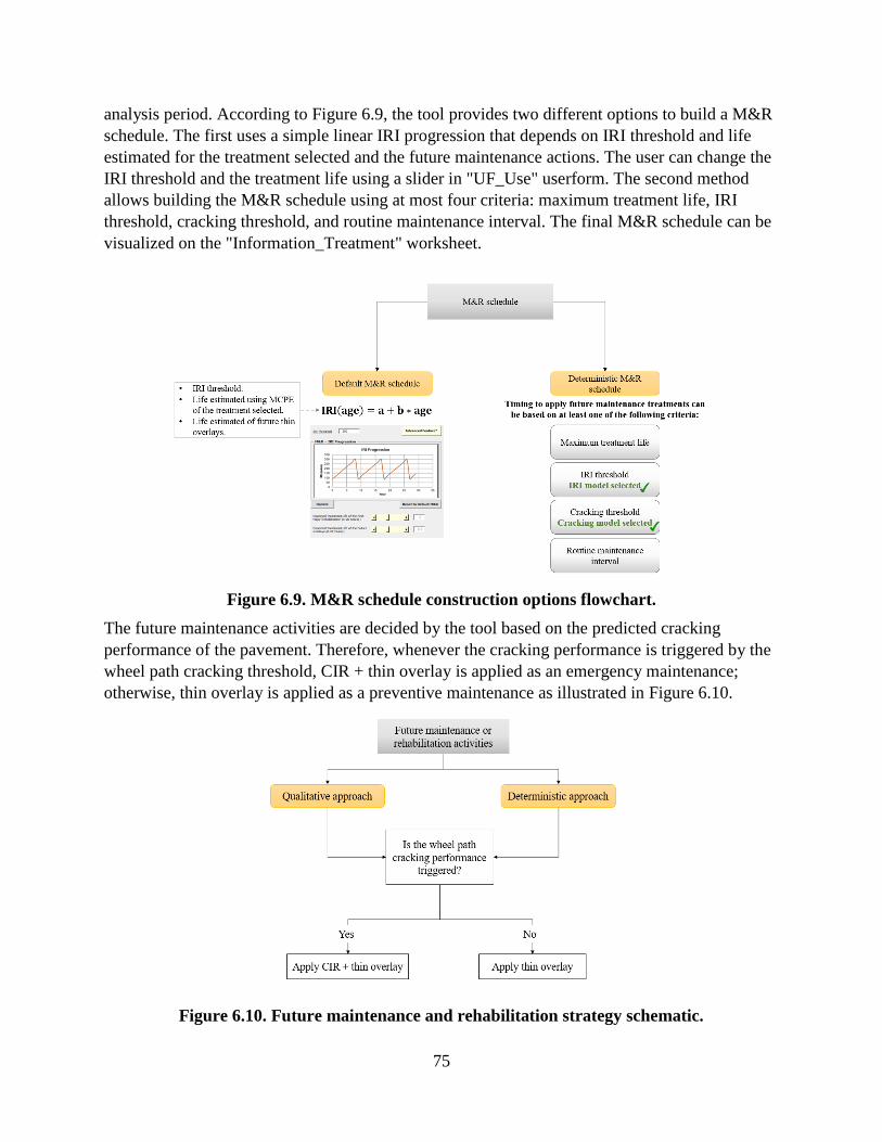
75

analysis period. According to Figure 6.9, the tool provides two different options to build a M&R

schedule. The first uses a simple linear IRI progression that depends on IRI threshold and life

estimated for the treatment selected and the future maintenance actions. The user can change the

IRI threshold and the treatment life using a slider in "UF_Use" userform. The second method

allows building the M&R schedule using at most four criteria: maximum treatment life, IRI

threshold, cracking threshold, and routine maintenance interval. The final M&R schedule can be

visualized on the "Information_Treatment" worksheet.

Figure 6.9. M&R schedule construction options flowchart.

The future maintenance activities are decided by the tool based on the predicted cracking

performance of the pavement. Therefore, whenever the cracking performance is triggered by the

wheel path cracking threshold, CIR + thin overlay is applied as an emergency maintenance;

otherwise, thin overlay is applied as a preventive maintenance as illustrated in Figure 6.10.

Figure 6.10. Future maintenance and rehabilitation strategy schematic.

76

Materials Extraction, Production and Hauling Stage

The user is shown the “Materials” page of “Life-Cycle Inventory” user form (Figure 6.11) upon

clicking “Open LCIA Module” command button. In this page, the user either selects materials

and enters the corresponding quantities or uses default materials list and quantities upon clicking

“Default” command button.

Figure 6.11. “Life-Cycle Inventory” user form, “Materials” page.

In addition, the user can specify pavement design materials by clicking “OR Checking Your

Custom Layer Design” as illustrated in Figure 6.11 and then the user is shown the “Pavement

Design” page, shown in Figure 6.12. For example, if the user selects a combination of a major

rehabilitation and microsurfacing or slurry seal, then “Microsurfacing and Slurry Seal” frame is

enabled and it is required to input the thickness of aggregate or sand application as well as the

application rate (by weight% of aggregate) of asphalt products (e.g., asphalt binder, emulsion).

Whereas, if fog seal, sand seal or chip seal is selected, then “Fog Seal, Sand Seal and Chip Seal”

frame is enabled and it is required to input the application rate of each material for the surface

treatment by lbs/sq.yd unit. Finally, if cape seal is selected, both “Microsurfacing and Slurry

Seal” and “Fog Seal, Sand Seal and Chip Seal” framed are enabled since cape seal is a

combination of slurry seal or microsurfacing and chip seal.

In addition, the user is asked to input material information necessary for the construction of the

treated pavement layers. If any of the IPR treatments is selected then the user need to input the

pavement recycled thickness. Furthermore, if AC operation is selected in one of the materials

list, then “Edit AC design” command button to enter mix design characteristics and mix

materials types and proportions, as Figure 6.13 shows.

77

Figure 6.12. “Life-Cycle Inventory” user form, “Pavement Design” page.

Figure 6.13. “Life-Cycle Inventory” user form, “Mix Design” page.

The final stage in the “Materials” page should be filling hauling distances for the selected

materials, as shown in Figure 6.11. The hauling distance can be either to plant or to site. If the

user selects the customization option then AC raw materials hauling distances to plant are

entered in “Mix Design” page, as shown in Figure 6.13, while the AC hauling to site is entered in

the “Materials” page, shown in Figure 6.11.

Construction Stage

At the construction stage, the user should select the equipment used to operate the construction

activities in the “Equipment” page of “Life-Cycle Inventory” user form, which is visible upon

78

clicking “Open LCIA Module” command button, shown in Figure 6.14. The inputs required to

enter are fuel type, equipment type, HP bin, tier category, fuel efficiency, speed and number of

passes. These inputs can also be generated upon clicking “Default” command button. The default

equipment units represent the equipment data collected from contractors.

Figure 6.14. “Life-Cycle Inventory” user form, “Equipment” page.

The construction stage accounts for the work zone as well. The user enters work zone inputs in

“Work Zone” user form, shown in Figure 6.15 upon clicking “Open Work Zone Module”

command button.

Figure 6.15. “Work Zone” user form.

79

Maintenance and Rehabilitation Stage

The ultimate outcome from “Life Expectancy” user form is to obtain a M&R schedule. M&R

schedule is necessary to compile use and maintenance stages’ impacts. Figure 6.8 shows

example of a default M&R schedule for a threshold of 300 in/mi and service life estimated to be

20 years, and a deterministic M&R schedule that shows when IRI progression is triggered by

rehabilitation interval (Figure 6.16 and 6.17). The deterministic M&R schedule is obtained using

up to five criteria and displayed in “Create Schedule” user form, shown in Figure 6.18.

Figure 6.16. Deterministic M&R schedule.

Figure 6.17. M&R built using deterministic models.

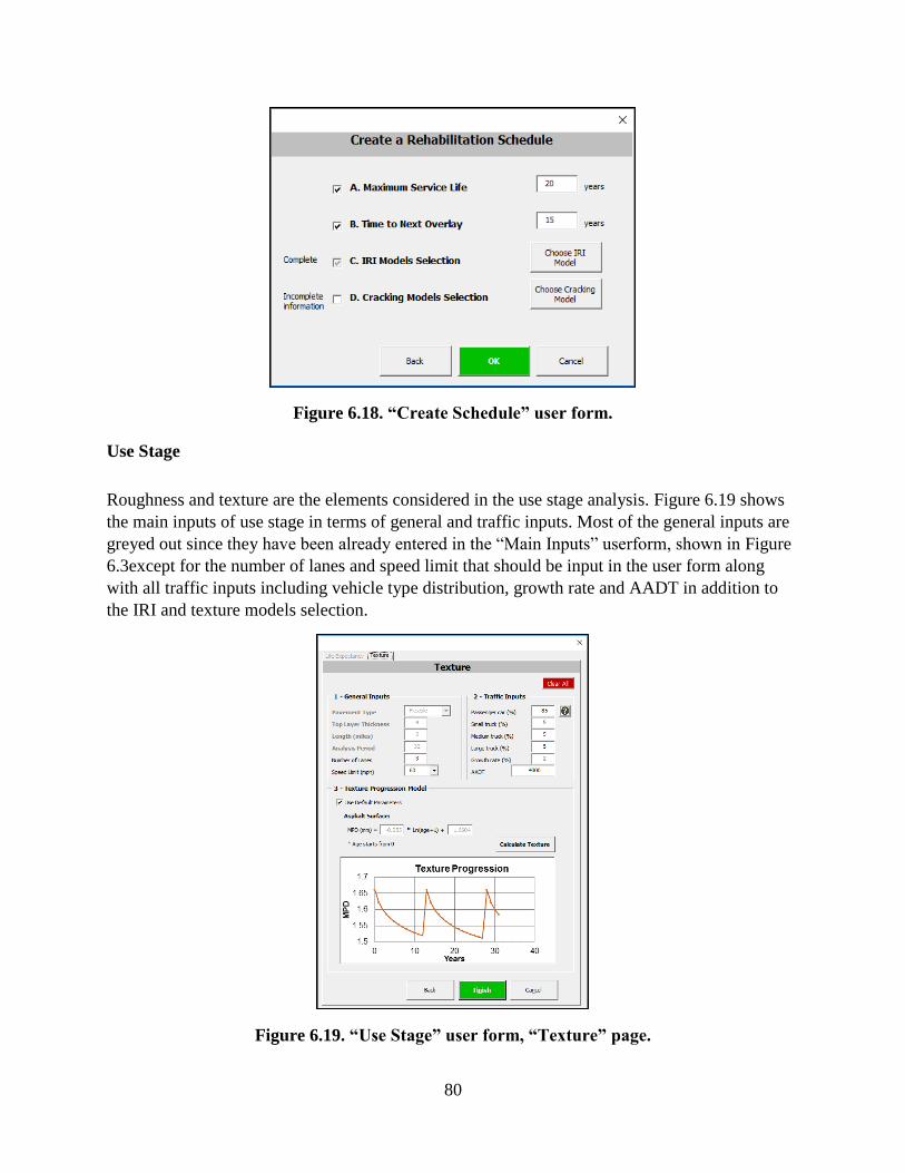
80

Figure 6.18. “Create Schedule” user form.

Use Stage

Roughness and texture are the elements considered in the use stage analysis. Figure 6.19 shows

the main inputs of use stage in terms of general and traffic inputs. Most of the general inputs are

greyed out since they have been already entered in the “Main Inputs” userform, shown in Figure

6.3except for the number of lanes and speed limit that should be input in the user form along

with all traffic inputs including vehicle type distribution, growth rate and AADT in addition to

the IRI and texture models selection.

Figure 6.19. “Use Stage” user form, “Texture” page.

81

End of Life Stage

At the end of life stage, various scenarios can be considered namely landfilling, recycling on-

and off-site. The user is shown “End of Life” user form, shown in Figure 6.20, upon clicking

“Open End of Life Module” where the percent of application of each end of life scenario is

entered, as well as the hauling distances to landfill facility and central plant recycling.

Figure 6.20. “End of Life” user form.

Review and Results

The results can be reviewed upon completing all requirements of the tool modules in “Modules

Analysis” user form, as shown in Figure 6.21. Then, the “Treatments for Analysis” user form is

shown (Figure 6.22) where the user clicks “Finish/ Go to Review Page” to visualize the results of

the energy or emission selected by the user from a dropdown list in the “Review Results”

spreadsheet (Figure 6.23). In the interpretation step of the LCA study, the user can check

aggregate results of items involved in each stage in “Chart” spreadsheet (Figure 6.24).

Figure 6.21. Requirements completed before reviewing final results.

82

Figure 6.22. Completed analysis prior to clicking Finish/Go to Review Page button.

Figure 6.23. Review of total results of each life-cycle stage.

83

Figure 6.24. Breakdown chart of final results for CIR + Medium Overlay (between 2 to 4

in).

84

CHAPTER 7: SUMMARY, FINDINGS, CONCLUSIONS, AND RECOMMENDATIONS

SUMMARY

The thesis aims to develop a new LCA methodology to evaluate maintenance and rehabilitation

treatments, conduct a fuel usage analysis of in-place recycling techniques during the construction

stage, and develop a tool to help highway agencies in comparing the environmental impacts of

pavement maintenance and rehabilitation treatments. Construction data about IPR projects were

collected from contractors and agencies to support the user selection during construction stage

and to conduct fuel usage analysis of IPR techniques.

This study develops a LCA tool for pavement IPR that provides pavement industry practitioners,

consultants and agencies the opportunity to complement their projects economic and social

assessment with the environmental impacts quantification.

FINDINGS

The followings are findings of this study:

• Propane and diesel consumption are sensitive to project-level factors such as pavement

hardness, pavement width, air temperature, and horsepower of the equipment used during

pavement M&R treatments’ construction activities and specifically for in-place recycling

techniques.

• Analysis period is shown to be sensitive to the number of maintenance applications

applied on the pavement system. The more maintenance activities involved, the longer is

the analysis period and thus the higher is the energy consumed during the pavement life

cycle.

• End of life stage is found to be sensitive to the allocation method selected. Substitution

method resulted in reduced environmental impacts compared to the cut-off method. Also,

the higher the recycling rate at the end of life, the less is the energy resulting from the

system under analysis.

• In-place recycling techniques are found to be a more optimal alternative to use at the end

of life stage compared to the central plant recycling scenario.

• Operating end of life stage activities in a rural road resulted in higher environmental

impacts since hauling distances are higher compared to an urban area.

CONCLUSIONS

The followings are the conclusions of this study:

• An equipment inventory model was developed to evaluate the impacts of pavement M&R

treatments during the construction stage.

• Regional fuel usage models for in place recycling techniques was developed based on

regional factors such as average Moh’s Hardness, to predict the fuel efficiency under

various project level conditions.

85

• A decision matrix was built to estimate pavement performance based on multiple criteria

(traffic, climate, pavement condition, structural design, and soil capacity). The

performance estimation is important since it helps in building a M&R schedule and to

quantify use stage impacts.

• A LCA tool, using VBA, was developed and intended for public use to assess the

environmental impacts of pavement maintenance and rehabilitation alternatives for

highway pavements including IPR techniques. The developed tool utilizes data,

simulation, and models through all the LCA stages of the pavement IPR, including

materials, construction, maintenance/rehabilitation, use, and end of life.

RECOMMENDATIONS

A future work can combine the environmental assessment with socio-economic impact

assessment and pavement design in order to provide agencies with a comprehensive evaluation

of pavement projects’ alternatives.

86

REFERENCES

1. Harvey, J.T., Meijer, J., Ozer, H., Al-Qadi, I.L., Saboori, A., and Kendall, A. Pavement

Life-Cycle Assessment Framework. No. FHWA-HIF-16-014. 2016.

2. ISO, EN. "Environmental Management Life Cycle Assessment Principles and

Framework (ISO 14040: 2006)." (2006).

3. International Monetary Fund, http://www.imf.org/external/pubs/ft/oil/2000/

4. Stroup-Gardiner, M. Recycling and reclamation of asphalt pavements using in-place

methods. No. Project 20-05 (Topic 40-13). 2011.

5. Wirtgen Group, http://media.wirtgen-

group.com/media/02_wirtgen/news_and_press_releases_1/2013_cold_milling/bauma_W

210_street_880x0.jpg

6. Federal Highway Administration (FHWA) (1997). “Chapter 9. Hot In-Place Recycling

(Construction Methods and Equipment)” Washington, D.C.

7. Terrel, R., and Lee, S. "Hot In-place Recycling of Asphalt Pavements." In Arab Urban

Development Institute Symposium. Al-Ain, United Arab Emirates. 1997.

8. Epps, Jon A., and Finn, F.N. Energy Requirements Associated with Pavement

Construction, Rehabilitation, and Maintenance. Texas Transportation Institute, 1980.

9. Chappat, M., and Bilal, J. "The Environmental Road of the Future: Life Cycle

Analysis." Colas SA, Paris 9 (2003): 1-34.

10. Manual, Basic Asphalt Recycling. "Asphalt Recycling and Reclaiming Association."

Annapolis, Maryland (2014).

11. Van Dam, T.J., Harvey, J.T., Muench, S.T., Smith, K.D., Snyder, M.B., Al-Qadi, I.L.,

Ozer, H, et al. "Towards Sustainable Pavement Systems: A Reference

Document." Urbana 51 (2015): 61801.

12. Asphalt Recycling and Reclaiming Association (ARRA) (2013a). “Recommended

Construction Guidelines For Full Depth Reclamation (FDR) Using Bituminous

Stabilization.” Asphalt Recycling and Reclaiming Association, Annapolis, MD.

13. Jones, D., Pengcheng, F., and Harvey, J.T. Full-Depth Pavement Reclamation with

Foamed Asphalt in California: Guidelines for Project Selection, Design, and

Construction. No. UCPRC-GL-2008-01. 2009.

14. Asphalt Recycling and Reclaiming Association (ARRA) (2013b). “Recommended

Construction Guidelines For Full Depth Reclamation (FDR) Using Cementitious

Stabilization.” Asphalt Recycling and Reclaiming Association, Annapolis, MD.

15. FHWA, Cold In-Place Asphalt Recycling Application Checklist (2013c)

https://www.fhwa.dot.gov/pavement/preservation/ppcl12.pdf

16. FHWA, Full Depth Reclamation Application Checklist (2013d)

https://www.fhwa.dot.gov/pavement/pubs/hif13036.pdf

17. Thenoux, G., Gonzalez, A., and Dowling, R. "Energy Consumption Comparison for

Different Asphalt Pavements Rehabilitation Techniques Used in Chile." Resources,

Conservation and Recycling 49, no. 4 (2007): 325-339.

18. Robinette, C., and Epps, J. "Energy, Emissions, Material Conservation, and Prices

Associated with Construction, Rehabilitation, and Material Alternatives for Flexible

Pavement." Transportation Research Record: Journal of the Transportation Research

Board 2179 (2010): 10-22.

http://media.wirtgen-group.com/media/02_wirtgen/news_and_press_releases_1/2013_cold_milling/bauma_W210_street_880x0.jpg



https://www.fhwa.dot.gov/pavement/preservation/ppcl12.pdf

87

19. Nicholson, A.L., Olivetti, E.A., Gregory, J.R., Field, F.R., and Kirchain, R.E. "End-of-

life LCA Allocation Methods: Open Loop Recycling Impacts on Robustness of Material

Selection Decisions." In Sustainable Systems and Technology, 2009. ISSST'09. IEEE

International Symposium on, pp. 1-6. IEEE, 2009.

20. Frischknecht, R. "ecoinvent Data v1. 1 (2004): From Heterogenous Databases to Unified

and Transparent LCI Data." The International Journal of Life Cycle Assessment 10, no. 1

(2005): 1-2.

21. Wernet, G., Bauer, C., Steubing, B., Reinhard, J., Moreno-Ruiz, E., and Weidema, B.

"The ecoinvent Database Version 3 (Part I): Overview and Methodology." The

International Journal of Life Cycle Assessment 21, no. 9 (2016): 1218-1230.

22. EarthShift (2013). US-Ecoinvent Database. Version 2.2. [Database]. Swiss Center for

Life-Cycle Inventories, St-Gallen, Switzerland.

23. U.S. Environmental Protection Agency (U.S. EPA). Motor Vehicle Emission Simulator

(MOVES) 2014 [software]. Washington, D.C. (2015a).

24. U.S. Environmental Protection Agency (U.S. EPA) (2015b). Emissions and Generation

Resource Integrated Database (eGRID). Retrieved from

https://www.epa.gov/energy/emissions-generation-resource-integrated-database-egrid

25. US Environmental Protection Agency (2008) Climate Change: Basic Information

[online]. http://epa.gov/climatechange/basicinfo.html [accessed June 9, 2008

26. Lautier, A., Rosenbaum, R. K., Margini, M., Bare, J.C., Pierre-Olivier, R., Deschenes, L.

(2010). Development of normalization factors for Canada and the United States and

comparison with European factors. Science of the Total Environment, 409: 33-42.

27. Bare, J., Gloria, T., and Norris, G. (2006). Development of the Method and U.S.

Normalization Database for Life Cycle Impact Assessment and Sustainability Metrics.

Environmental Science and Technology, 40(16): 5108-5115.

28. Weidema, B.P., and Wesnaes, M.S. "Data Quality Management for Life Cycle

Inventories—An Example of Using Data Quality Indicators." Journal of cleaner

production 4, no. 3-4 (1996): 167-174.

29. U.S. Energy Information Administration (EIA) (2010a). Coal Data (2008-2011) [Online

Database]. Retrieved from http://www.eia.gov/coal/data.cfm

30. Yang, R., Ozer, H., and Al-Qadi., I.L. "Regional upstream life-cycle impacts of

petroleum products in the United States." Journal of Cleaner Production 139 (2016):

1138-1149

31. SimaPro (2014). Version 8.0.4. PRé Consultants. [Software], Amersfoort, Netherlands.

32. U.S. Environmental Protection Agency (U.S. EPA) (2017). Heavy paraffinic distillate

solvent petroleum extracts. Retrieved from

https://iaspub.epa.gov/sor_internet/registry/substreg/searchandretrieve/advancedsearch/ex

ternalSearch.do?p_type=CASNO&p_value=64742-04-7#

33. National Institutes of Health (2016). Haz-Map. Paraffin Waxes (petroleum), clay-treated.

Retrieved from https://hazmap.nlm.nih.gov/category-

details?table=copytblagents&id=10724

34. Kang, S., Yang, R., Ozer, H., Al-Qadi, I.L. (2014). Life-Cycle Greenhouse Gases and

Energy Consumption for the Material and Construction Phases of Pavement with Traffic

Delay. In: Transportation Research Record: Journal of Transportation Research Record,

No. 2428. Transportation Research Board of the National Academies, Washington, DC,

pp. 24–27.

https://www.epa.gov/energy/emissions-generation-resource-integrated-database-egrid

http://www.eia.gov/coal/data.cfm

https://iaspub.epa.gov/sor_internet/registry/substreg/searchandretrieve/advancedsearch/externalSearch.do?p_type=CASNO&p_value=64742-04-7

https://iaspub.epa.gov/sor_internet/registry/substreg/searchandretrieve/advancedsearch/externalSearch.do?p_type=CASNO&p_value=64742-04-7

https://hazmap.nlm.nih.gov/category-details?table=copytblagents&id=10724

https://hazmap.nlm.nih.gov/category-details?table=copytblagents&id=10724

88

35. Young, T.J. (2007). Energy Conservation in Hot-Mix Asphalt Production. National

Asphalt Pavement Association, Lanham, MD.

36. U.S. Environmental Protection Agency (U.S. EPA) (2016). Motor Vehicle Emission

Simulator (MOVES) 2014a. [Software], Office of Transportation and Air Quality,

Washington, D.C.

37. Franzese, O. (2011). Effect of Weight and Roadway Grade on the Fuel Economy of

Class-8 Freight Trucks. Oak Ridge National Laboratory, Tennessee.

38. Fox, M.A. "Self-Propelled Vehicles." In Glossary for the Worldwide Transportation of

Dangerous Goods and Hazardous Materials, pp. 219-220. Springer Berlin Heidelberg,

1999.

39. Langer, W.H. Aggregate Resource Availability in the Conterminous United States,

Including Suggestions for Addressing Shortages, Quality, and Environmental Concerns.

No. 2011-1119. US Geological Survey, 2011.

40. Federal Highway Administration (FHWA) (2015). Chapter 13. Cold In-Place Recycling

(Construction Methods and Equipment). Retrieved

fromhttp://www.fhwa.dot.gov/pavement/recycling/98042/13.cfm

41. Li, H., Andrews, G.E., Zhu, G., Daham, B.K., Bell, M.C., Tate, J.E., and Ropkins, K.

"Impact of Ambient Temperatures on Exhaust Thermal Characteristics during Cold Start

for Real World SI Car Urban Driving Tests." In SAE Proceedings: Powertrain and Fluid

Systems Conference and Exhibition. Society of Automotive Engineers, 2005.

42. Bielaczyc, P., Merkisz, J., and Pielecha, J. Investigation of Exhaust Emissions from di

Diesel Engine during Cold and Warm Start. No. 2001-01-1260. SAE Technical Paper,

2001.

43. Suman, G. "What Factors Affect Average Fuel Economy of US Passenger Vehicles?."

(2010).

44. Yang, R., Yoo, W., Ozer, H., and Al-Qadi, I.L. Development and Application of a

Roadway/Roadside Life-Cycle Assessment Software for the Illinois Tollway. No. 17-

06079. 2017.

45. Bare, J. "TRACI 2.0: the tool for the reduction and assessment of chemical and other

environmental impacts 2.0." Clean Technologies and Environmental Policy 13, no. 5

(2011): 687-696.

46. EPA, “Control of Air Pollution; Determination of Significance for Nonroad Sources and

Emission Standards for New Nonroad Compression Ignition Engines At or Above 37

Kilowatts,” 59 FR 31306, June 17, 1994.

47. EPA, “ Control of Emissions of Air Pollution From Nonroad Diesel Engines,” 63 FR

56967, October 23, 1998.

48. EPA, “Control of Emissions From Nonroad Large Spark-Ignition Engines and

Recreational Engines (Marine and Land-Based); Final Rule,” 67 FR 68241, November 8,

2002.

49. EPA, “Control of Emissions of Air Pollution From Nonroad Diesel Engines and Fuel;

Final Rule,” 69 FR 38958, June 29, 2004.

50. EPA, “Control of Emissions of Air Pollution From Locomotive Engines and Marine

Compression-Ignition Engines Less Than 30 Liters per Cylinder; Republication,” (Final

Rule), 73 FR 37096, June 30, 2008.

51. EPA, “Exhaust and Crankcase Emission Factors for Nonroad Engine Modeling,

Compression-Ignition”

http://www.fhwa.dot.gov/pavement/recycling/98042/13.cfm

89

52. Rister, B., and Graves, C. "The Cost of Construction Delays and Traffic Control for Life-

Cycle Cost Analysis of Pavements." (2002).

53. Lee, E.B., and Ibbs, C.W. "Computer Simulation Model: Construction Analysis for

Pavement Rehabilitation Strategies." Journal of Construction Engineering and

management 131, no. 4 (2005): 449-458.

54. Diefenderfer, B.K., and Apeagyei, A.K. I-81 In-Place Pavement Recycling Project. No.

FHWA/VCTIR 15-R1. 2014.

55. Santero, Nicholas J., Eric Masanet, and Arpad Horvath. "Life-cycle assessment of

pavements. Part I: Critical review." Resources, Conservation and Recycling 55, no. 9

(2011): 801-809.

56. Ziyadi, M., Ozer. H., Lu, L., Kang, S., and Al-Qadi, I.L. "Vehicle Energy Consumption

and Environmental Impact Calculation Model for Transportation Systems" Journal of

Cleaner Production, (submitted).

57. Chatti, K., and Zaabar, I. Estimating the Effects of Pavement Condition on Vehicle

Operating Costs. Vol. 720. Transportation Research Board, 2012.

58. Lu, Q., Kohler, E.R., Harvey, J.T., and Ongel, A. "Investigation of Noise and Durability

Performance Trends For Asphaltic Pavement Surface Types: Three-Year

Results." Institute of Transportation Studies (2009).

59. Ekvall, T., and Tillman, A.M. "Open-loop Recycling: Criteria for Allocation

Procedures." The international journal of life cycle assessment 2, no. 3 (1997): 155-162.

60. Peshkin, D. G. Guidelines for the preservation of high-traffic-volume roadways.

Transportation Research Board, 2011.

61. Manual, Basic Asphalt Recycling. "Asphalt recycling and reclaiming Association."

Annapolis, Maryland (2015).

62. Peshkin, D.G., Hoerner, T.E., and Zimmerman, K.A. Optimal timing of pavement

preventive maintenance treatment applications. Vol. 523. Transportation Research

Board, 2004.

63. Illinois Department of Transportation (IDOT). 2012. Pavement Rehabilitation. In Bureau

of Local Roads and Streets Manual, IDOT, Springfield, IL.

64. Wu, Z., Groeger, J.L., Simpson, A.L., and Hicks, R.G. "Performance evaluation of

various rehabilitation and preservation treatments." (2010).

65. Hicks, R., Moulthrop, J., and Daleiden, J. "Selecting a preventive maintenance treatment

for flexible pavements." Transportation Research Record: Journal of the Transportation

Research Board 1680 (1999): 1-12.

66. Labi, S., and Sinha, K.C. "Life-cycle Evaluation of Flexible Pavement Preventive

Maintenance." Journal of Transportation Engineering131, no. 10 (2005): 744-751.

67. Braun Interlec Incorporation. Alternatives to Seal Coats. Minnesota: Local Road

Research Board. Accessed February 2016.

http://www.dot.state.mn.us/research/TRS/2016/TRS1602.pdf

.

http://www.dot.state.mn.us/research/TRS/2016/TRS1602.pdf

90

APPENDIX A: AGENCY QUESTIONNAIRE SURVEY SUMMARY

Figure A.1 (left). Agency experience with hot in-place recycling (HIR).

Figure A.2 (right). Agency experience with cold in-place recycling (CIR).

Figure A.3. (left). Agency experience with hot in-place recycling (HIR) by region.

Figure A.4. (right). Agency experience with cold in-place recycling (CIR) by region.

Figure A.5. (left). Types of hot in-place recycling (HIR) that agency experienced.

Figure A.6. (right). Types of cold in-place recycling (CIR) that agency experienced.

91

Figure A.7. (left). State of application of hot in-place recycling (HIR) by agency.

Figure A.8. (right). State of application of cold in-place recycling (CIR) by agency.

Figure A.9. (left). Traffic levels of pavement in which hot in-place recycling (HIR) is

applied.

Figure A.10. (right). Traffic levels of pavement in which cold in-place recycling (CIR) is

applied.

Figure A.11. (left). Truck percent of pavement in which hot in-place recycling (HIR) is

applied.

Figure A.12. (right). Truck percent of pavement in which cold in-place recycling (CIR) is

applied.

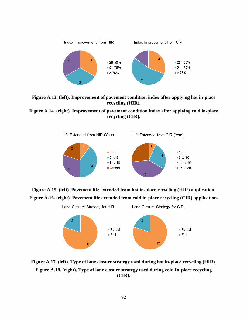
92

Figure A.13. (left). Improvement of pavement condition index after applying hot in-place

recycling (HIR).

Figure A.14. (right). Improvement of pavement condition index after applying cold in-place

recycling (CIR).

Figure A.15. (left). Pavement life extended from hot in-place recycling (HIR) application.

Figure A.16. (right). Pavement life extended from cold in-place recycling (CIR) application.

Figure A.17. (left). Type of lane closure strategy used during hot in-place recycling (HIR).

Figure A.18. (right). Type of lane closure strategy used during cold In-place recycling

(CIR).

93

Figure A.19. (left). Opening time (in hour) after hot in-place recycling (HIR) application.

Figure A.20. (right). Opening time (in hour) after cold in-place recycling (CIR) application.

Figure A.21. (left). Reduction in lane closure time for hot in-place recycling (HIR)

compared with conventional rehabilitation.

Figure A.22. (right). Reduction in lane closure time for cold in-place recycling (CIR)

compared with conventional rehabilitation.

Figure A.23. (left). Cost per yd2 of hot in-place recycling (HIR) application.

Figure A.24. (right). Cost per yd2 of cold in-place recycling (CIR) application.

94

APPENDIX B: MAJOR UNIT PROCESSES MODELED

Table B.1. Type and percent contribution of NERC regions for each state (eGRID, 2015)

State NERC Region

Contribution

(%) State NERC Region

Contribution

(%)

AK ASCC 100 NC SERC 100

AL SERC 100 ND MRO 100

AR SERC 89.6585 NE MRO 100

AR SPP 10.3415 NH NPCC 99.9959

AZ WECC 100 NJ NPCC 6.93202

CA WECC 100 NJ RFC 93.068

CO WECC 100 NM SPP 6.64509

CT NPCC 100 NM WECC 93.3549

DC RFC 100 NV WECC 100

DE RFC 100 NY NPCC 100

FL FRCC 95.5426 OH RFC 99.4508

FL SERC 4.45744 OH TRE 0.549153

GA SERC 100 OK SERC 4.15301

HI HICC 100 OK SPP 90.226

IA MRO 99.1633 OK TRE 5.621

IA RFC 0.836656 OR WECC 100

ID WECC 100 PA RFC 100

IL MRO 0.0255141 RI NPCC 100

IL RFC 65.7789 SC SERC 100

IL SERC 34.1956 SD MRO 99.0926

IN RFC 100 SD WECC 0.907452

KS SPP 100 TN SERC 99.9592

KY RFC 6.77734 TN WECC 0.0408408

KY SERC 93.2227 TX SERC 5.98278

LA SERC 78.1378 TX SPP 10.7096

LA SPP 21.8622 TX TRE 82.6485

MA NPCC 100 TX WECC 0.659124

MD RFC 100 UT WECC 100

ME NPCC 100 VA RFC 2.73803

MI MRO 0.976683 VA SERC 97.262

MI RFC 99.0233 VT NPCC 100

MN MRO 99.9999 WA WECC 100

MO MRO 0.394321 WI MRO 49.9817

MO SERC 66.9628 WI RFC 50.0183

MO SPP 32.6429 WV RFC 88.3757

MS SERC 100 WV SERC 11.6243

MT MRO 6.83667 WY MRO 13.6308

MT WECC 93.1633 WY WECC 86.3692

95

Table B.2. Unit processes adopted from US-EI 2.2 in material stage.

Materials Unit Processes from US-EI 2.2

Crushed aggregate Gravel, crushed, at mine/US* US-EI U

Natural aggregate Gravel, round, at mine/US* US-EI U

Sand Sand, at mine/US* US-EI U

Asphalt rejuvenator Paraffin, at plant/US- US-EI U, Benzene, at plant/US- US-EI U

Hydrated lime Lime, hydrated, loose, at plant/US* US-EI U

Table B.3. Unit processes information of asphalt binder products used in the materials

database.

Asphalt Binder Product Unit Processes

Emulsion • 65% binder, transported 200 mi by rail

• 1.5% hydrochloric acid, transported 200 mi by truck

• 0.2% emulsifier (ethylene diamine), transported 200 mi by truck

• 33 kWh (65.32 + 53.5 MJ) electricity

• 83.1 gal water

GTR binder • 85% binder, transported 200 mi by rail

• 15% GTR, transported 200 mi by train

• 15.9 kWh electricity

• 6.29E5 KJ heat, light fuel oil, at industrial furnace, US-EI

SBS polymer modified binder • 96.5% binder, transported 200 mi by rail

• 3.5% Styrene butadiene rubber, transported 200 mi by truck

• 35.45 ft3 natural gas, combusted in industrial equipment

• 0.0936 gal diesel, combusted in industrial boiler

• 0.0021 tn.sh coal, combusted in industrial boiler

• 54 kWh electricity Foamed asphalt • 97.5% binder, transported 200 mi by rail

• 2.5% water

96

APPENDIX C: DECISION MATRIX

Table C.1. Decision matrix (1/4)

Tre

atm

ent

Ty

pe

AA

DT

< 5

00

0

AA

DT

50

00

-300

00

AA

DT

>3

00

00

AA

DT

Un

kn

ow

n

R

ura

l R

oa

d

Urb

an

Ro

ad

Ro

ad

Ty

pe

Un

kn

ow

n

Tru

ck <

10

%

T

ruck

>1

0%

Tru

ck V

olu

me

Un

kn

ow

n

PC

I 8

6 t

o 1

00

PC

I 7

1 t

o 8

5

P

CI

56

to

70

PC

I <

56

PC

I U

nk

no

wn

Lo

w R

av

elin

g

M

ediu

m R

av

elin

g

Hig

h R

av

elin

g

Ra

vel

ing

Un

kn

ow

n

Cape seal 5 5 5 1 5 5 1 5 5 1 5 5 1 1 1 5 5 5 1

Chip seal double course 5 5 1 1 5 5 1 5 5 1 5 5 1 1 1 5 5 5 1

Chip seal single course 0 0 0 1 5 5 1 5 5 1 5 5 1 1 1 5 5 5 1

CIR 5 5 1 1 5 5 1 5 1 1 5 5 5 1 1 5 5 5 1

CIR + cape seal 5 5 1 1 5 5 1 5 1 1 5 5 5 1 1 5 5 5 1

CIR + chip seal 5 5 1 1 5 5 1 5 1 1 5 5 5 1 1 5 5 5 1

CIR + thin overlay (2 in or less) 5 5 1 1 5 5 1 5 1 1 5 5 5 1 1 5 5 5 1

CIR + medium overlay ( between 2 and 4 in) 5 5 1 1 5 5 1 5 1 1 5 5 5 1 1 5 5 5 1

CIR + thick overlay (over 4 in) 5 5 1 1 5 5 1 5 1 1 5 5 5 1 1 5 5 5 1

FDR 5 5 5 1 5 5 1 5 5 1 5 5 5 5 1 5 5 5 1

FDR + cape seal 5 5 5 1 5 5 1 5 5 1 5 5 5 5 1 5 5 5 1

FDR + chip seal 5 5 5 1 5 5 1 5 5 1 5 5 5 5 1 5 5 5 1

FDR + thin overlay (2 in or less) 5 5 5 1 5 5 1 5 5 1 5 5 5 5 1 5 5 5 1

FDR + medium overlay (between 2 and 4 in) 5 5 5 1 5 5 1 5 5 1 5 5 5 5 1 5 5 5 1

FDR + thick overlay (over 4 in) 5 5 5 1 5 5 1 5 5 1 5 5 5 5 1 5 5 5 1

Fog seal 5 5 1 1 5 5 1 5 3 1 5 5 1 1 1 5 5 5 1

HIR remixing 5 5 5 1 5 5 1 5 1 1 5 5 5 1 1 5 5 5 1

HIR remixing + thin overlay (2 in or less) 5 5 5 1 5 5 1 5 1 1 5 5 5 1 1 5 5 5 1

97

Table C.1. Decision matrix (1/4) (cont)

HIR remixing + medium overlay (between 2 and 4

in) 5 5 5 1 5 5 1 5 1 1 5 5 5 1 1 5 5 5 1

HIR remixing + thick overlay (over 4 in) 5 5 5 1 5 5 1 5 1 1 5 5 5 1 1 5 5 5 1

HIR repaving 5 5 5 1 5 5 1 5 1 1 5 5 5 1 1 5 5 5 1

HIR resurfacing 5 5 1 1 5 5 1 5 1 1 5 5 5 1 1 5 5 5 1

HIR resurfacing + thin overlay (2 in or less) 5 5 1 1 5 5 1 5 1 1 5 5 5 1 1 5 5 5 1

HIR resurfacing + medium overlay (between 2 and 4

in) 5 5 1 1 5 5 1 5 1 1 5 5 5 1 1 5 5 5 1

HIR resurfacing + thick overlay (over 4 in) 5 5 1 1 5 5 1 5 1 1 5 5 5 1 1 5 5 5 1

Microsurfacing double course 0 0 0 1 5 5 1 5 5 1 5 5 1 1 1 5 5 5 1

Microsurfacing single course 5 5 5 1 5 5 1 5 5 1 5 5 1 1 1 5 5 5 1

Cold Milling + Thin Overlay (2 in or less) 5 5 5 1 5 5 1 5 5 1 5 5 5 1 1 5 5 5 1

Cold Milling + Medium Overlay (between 2 and 4

in) 5 5 5 1 5 5 1 5 5 1 5 5 5 1 1 5 5 5 1

Cold Milling + Thick Overlay (over 4 in) 5 5 5 1 5 5 1 5 5 1 5 5 5 5 1 5 5 5 1

Sand seal 5 5 1 1 5 3 1 5 3 1 5 5 1 1 1 5 5 5 1

Slurry seal 5 5 5 1 1 5 1 5 3 1 5 5 1 1 1 5 5 5 1

Thin HMA Overlay (2 in or less) 5 5 5 1 5 5 1 5 5 1 5 5 5 1 1 5 5 5 1

Ultra thin bonded wearing course 5 5 5 1 5 5 1 5 5 1 5 5 5 1 1 5 5 5 1

Table C.2. Decision matrix (2/4).

Tre

atm

ent

Ty

pe

Lo

w P

oth

ole

s

Med

ium

Po

tho

les

Hig

h P

oth

ole

s

Po

tho

les

Un

kn

ow

n

Ble

edin

g

No

Ble

edin

g

Ble

edin

g U

nk

no

wn

Lo

w S

kid

Res

ista

nce

Hig

h S

kid

Resi

sta

nce

Sk

id R

esi

sta

nce

Un

kn

ow

n

Sh

ou

lder

Dro

p-O

ff

No

Sh

ou

lder

Dro

p-O

ff

Sh

ou

lder

Dro

p-o

ff U

nk

no

wn

Lo

w R

utt

ing

Med

ium

Ru

ttin

g

Hig

h R

utt

ing

Ru

ttin

g U

nk

no

wn

Lo

w C

orr

ug

ati

on

s

Med

ium

Co

rru

ga

tio

ns

Hig

h C

orr

ug

ati

on

s

Co

rru

ga

tio

ns

Un

kn

ow

n

Lo

w F

ati

gu

e

Med

ium

Fa

tig

ue

Hig

h F

ati

gu

e

Fa

tig

ue

Un

kn

ow

n

Cape seal 5 3 3 1 1 5 1 5 5 1 1 5 1 4 3 1 1 3 3 1 1 3 3 1 1

98


Chip seal double course 5 3 1 1 1 5 1 5 5 1 1 5 1 4 3 1 1 3 3 1 1 3 3 1 1

Chip seal single course 5 3 1 1 1 5 1 5 5 1 1 5 1 4 1 1 1 4 3 1 1 3 3 1 1

CIR 5 5 5 1 3 5 1 5 5 1 1 5 1 4 5 5 1 4 5 5 1 5 4 4 1

CIR + cape seal 5 5 5 1 3 5 1 5 5 1 1 5 1 4 5 5 1 4 5 5 1 5 4 4 1

CIR + chip seal 5 5 5 1 3 5 1 5 5 1 1 5 1 4 5 5 1 4 5 5 1 5 4 4 1

CIR + thin overlay (2 in

or less) 5 5 5 1 3 5 1 5 5 1 1 5 1 4 5 5 1 4 5 5 1 5 4 4 1

CIR + medium overlay (

between 2 and 4 in) 5 5 5 1 3 5 1 5 5 1 1 5 1 4 5 5 1 4 5 5 1 5 4 4 1

CIR + thick overlay (over

4 in) 5 5 5 1 3 5 1 5 5 1 1 5 1 4 5 5 1 4 5 5 1 5 4 4 1

FDR 5 5 5 1 5 5 1 5 5 1 1 5 1 5 5 5 1 5 5 5 1 5 5 5 1

FDR + cape seal 5 5 5 1 5 5 1 5 5 1 1 5 1 5 5 5 1 5 5 5 1 5 5 5 1

FDR + chip seal 5 5 5 1 5 5 1 5 5 1 1 5 1 5 5 5 1 5 5 5 1 5 5 5 1

FDR + thin overlay (2 in

or less) 5 5 5 1 5 5 1 5 5 1 1 5 1 5 5 5 1 5 5 5 1 5 5 5 1

FDR + medium overlay

(between 2 and 4 in) 5 5 5 1 5 5 1 5 5 1 1 5 1 5 5 5 1 5 5 5 1 5 5 5 1

FDR + thick overlay

(over 4 in) 5 5 5 1 5 5 1 5 5 1 1 5 1 5 5 5 1 5 5 5 1 5 5 5 1

Fog seal 1 1 1 1 1 5 1 1 5 1 1 5 1 1 1 1 1 1 1 1 1 1 1 1 1

HIR remixing 5 5 3 1 3 5 1 5 5 1 1 5 1 0 0 0 1 4 5 5 1 5 4 4 1

HIR remixing + thin

overlay (2 in or less) 5 5 3 1 3 5 1 5 5 1 1 5 1 4 5 5 1 4 5 5 1 5 4 4 1

99


HIR remixing + medium


in)

5 5 3 1 3 5 1 5 5 1 1 5 1 4 5 5 1 4 5 5 1 5 4 4 1

HIR remixing + thick

overlay (over 4 in) 5 5 3 1 3 5 1 5 5 1 1 5 1 4 5 5 1 4 5 5 1 5 4 4 1

HIR repaving 5 5 3 1 3 5 1 5 5 1 1 5 1 4 5 5 1 4 5 5 1 5 4 4 1

HIR resurfacing 5 5 3 1 3 5 1 5 5 1 1 5 1 4 5 5 1 4 4 3 1 4 4 3 1

HIR resurfacing + thin

overlay (2 in or less) 5 5 3 1 3 5 1 5 5 1 1 5 1 4 5 5 1 5 4 3 1 4 4 3 1

HIR resurfacing + medium


in)

5 5 3 1 3 5 1 5 5 1 1 5 1 4 5 5 1 5 4 3 1 4 4 3 1

HIR resurfacing + thick

overlay (over 4 in) 5 5 3 1 3 5 1 5 5 1 1 5 1 4 5 5 1 5 4 3 1 4 4 3 1

Microsurfacing double

course 5 3 3 1 1 5 1 5 5 1 1 5 1 5 4 3 1 3 3 1 1 3 3 1 1

Microsurfacing single

course 5 3 3 1 1 5 1 5 5 1 1 5 1 4 3 1 1 3 1 1 1 3 3 1 1

Cold Milling + Thin

Overlay (2 in or less) 5 5 5 1 3 5 1 5 5 1 1 5 1 4 5 4 1 5 5 5 1 4 4 3 1

Cold Milling + Medium

Overlay (between 2 and 4

in)

5 5 5 1 3 5 1 5 5 1 1 5 1 5 5 5 1 5 5 5 1 4 4 4 1

Cold Milling + Thick

Overlay (over 4 in) 5 5 5 1 3 5 1 5 5 1 1 5 1 5 5 5 1 5 5 5 1 4 4 4 1

Sand seal 5 3 1 1 0 0 1 5 5 1 1 5 1 1 1 1 1 1 1 1 1 1 1 1 1

Slurry seal 5 3 3 1 1 5 1 5 5 1 1 5 1 3 1 1 1 1 1 1 1 1 1 1 1

Thin HMA Overlay (2 in

or less) 5 5 5 1 3 5 1 5 5 1 1 5 1 4 5 4 1 5 4 3 1 5 5 3 1

Ultra thin bonded wearing

course 5 1 1 1 1 5 1 5 5 1 1 5 1 4 3 1 1 4 3 1 1 3 3 1 1

100

Table C.3. Decision matrix (3/4).

Tre

atm

ent

Ty

pe

Lo

w E

dg

e C

rack

ing

Med

ium

Ed

ge

Cra

ckin

g

H

igh

Ed

ge

Cra

ckin

g

Ed

ge

Cra

ckin

g

Lo

w S

lip

pa

ge

Med

ium

Sli

pp

ag

e

H

igh

Sli

pp

ag

e

Sli

pp

ag

e U

nk

no

wn

Lo

w B

lock

Cra

ckin

g

Med

ium

Blo

ck C

rack

ing

H

igh

Blo

ck C

rack

ing

Blo

ck C

rack

ing

Un

kn

ow

n

Lo

w L

on

git

ud

ina

l C

rack

ing

Med

ium

Lo

ng

itu

din

al

Cra

ck

ing

H

igh

Lo

ng

itu

din

al

Cra

ckin

g

Lo

ng

itu

din

al

Cra

ckin

g U

nk

no

wn

Lo

w T

ran

sver

se C

rack

ing

Med

ium

Tra

nsv

erse

Cra

ckin

g

H

igh

Tra

nsv

erse

Cra

ckin

g

Tra

nsv

erse

Cra

ckin

g U

nk

no

wn

Cape seal 3 3 1 1 3 3 1 1 5 3 1 1 3 3 1 1 5 3 1 1

Chip seal double course 4 4 3 1 3 3 1 1 5 4 3 1 4 4 3 1 5 4 3 1

Chip seal single course 5 4 4 1 3 3 1 1 5 4 4 1 5 4 4 1 5 4 4 1

CIR 5 3 1 1 5 4 4 1 5 5 4 1 5 3 1 1 3 3 1 1

CIR + cape seal 5 3 1 1 5 4 4 1 5 5 4 1 5 3 1 1 3 3 1 1

CIR + chip seal 5 3 1 1 5 4 4 1 5 5 4 1 5 3 1 1 3 3 1 1

CIR + thin overlay (2 in or less) 5 3 1 1 5 4 4 1 5 5 4 1 5 3 1 1 3 3 1 1

CIR + medium overlay ( between 2 and 4

in) 5 3 1 1 5 4 4 1 5 5 4 1 5 3 1 1 3 3 1 1

CIR + thick overlay (over 4 in) 5 3 1 1 5 4 4 1 5 5 4 1 5 3 1 1 3 3 1 1

FDR 5 5 5 1 5 5 5 1 5 5 5 1 5 5 5 1 5 5 5 1

FDR + cape seal 5 5 5 1 5 5 5 1 5 5 5 1 5 5 5 1 5 5 5 1

FDR + chip seal 5 5 5 1 5 5 5 1 5 5 5 1 5 5 5 1 5 5 5 1

FDR + thin overlay (2 in or less) 5 5 5 1 5 5 5 1 5 5 5 1 5 5 5 1 5 5 5 1

FDR + medium overlay (between 2 and 4

in) 5 5 5 1 5 5 5 1 5 5 5 1 5 5 5 1 5 5 5 1

FDR + thick overlay (over 4 in) 5 5 5 1 5 5 5 1 5 5 5 1 5 5 5 1 5 5 5 1

Fog seal 3 1 1 1 1 1 1 1 3 1 1 1 3 1 1 1 3 1 1 1

HIR remixing 5 3 1 1 5 4 4 1 5 4 4 1 5 3 1 1 3 3 1 1

HIR remixing + thin overlay (2 in or less) 5 3 1 1 5 4 4 1 5 4 4 1 5 3 1 1 3 3 1 1

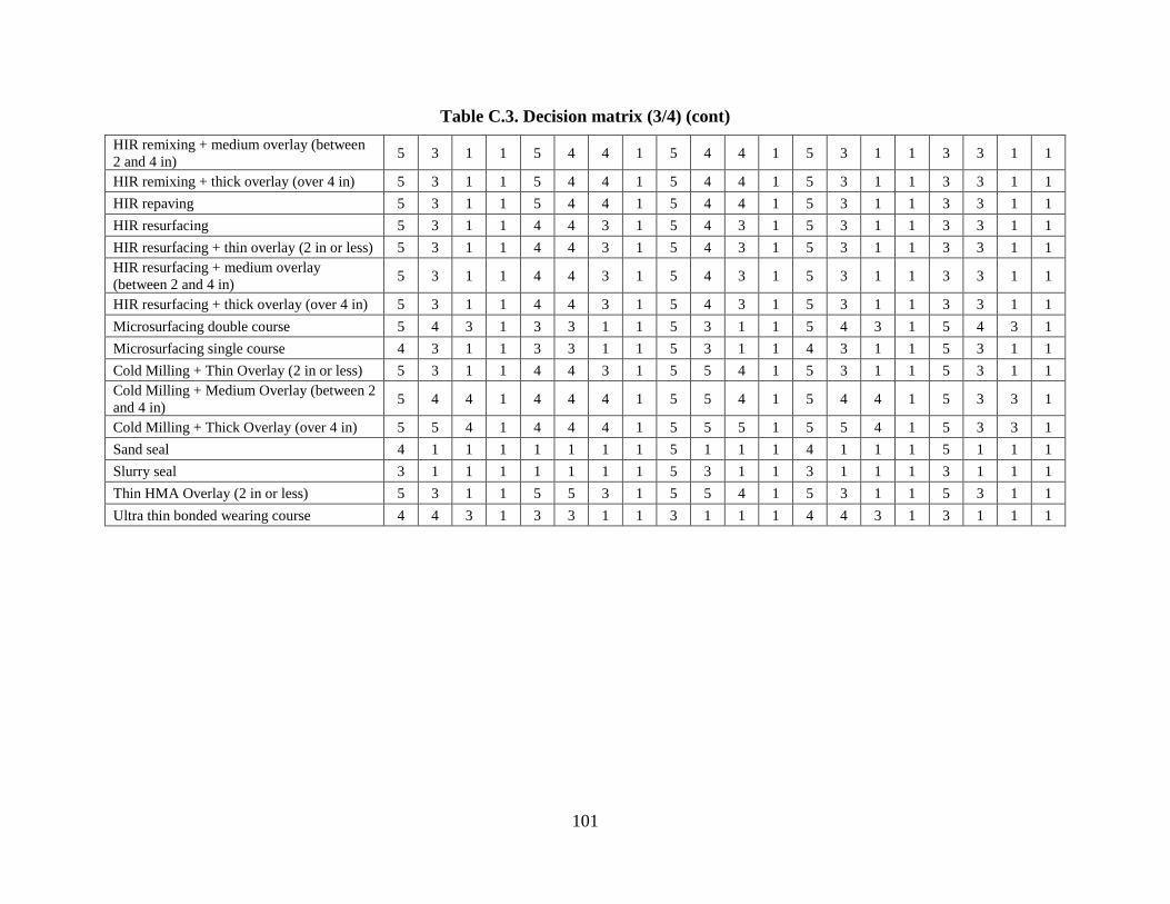
101


HIR remixing + medium overlay (between

2 and 4 in) 5 3 1 1 5 4 4 1 5 4 4 1 5 3 1 1 3 3 1 1

HIR remixing + thick overlay (over 4 in) 5 3 1 1 5 4 4 1 5 4 4 1 5 3 1 1 3 3 1 1

HIR repaving 5 3 1 1 5 4 4 1 5 4 4 1 5 3 1 1 3 3 1 1

HIR resurfacing 5 3 1 1 4 4 3 1 5 4 3 1 5 3 1 1 3 3 1 1

HIR resurfacing + thin overlay (2 in or less) 5 3 1 1 4 4 3 1 5 4 3 1 5 3 1 1 3 3 1 1

HIR resurfacing + medium overlay

(between 2 and 4 in) 5 3 1 1 4 4 3 1 5 4 3 1 5 3 1 1 3 3 1 1

HIR resurfacing + thick overlay (over 4 in) 5 3 1 1 4 4 3 1 5 4 3 1 5 3 1 1 3 3 1 1

Microsurfacing double course 5 4 3 1 3 3 1 1 5 3 1 1 5 4 3 1 5 4 3 1

Microsurfacing single course 4 3 1 1 3 3 1 1 5 3 1 1 4 3 1 1 5 3 1 1

Cold Milling + Thin Overlay (2 in or less) 5 3 1 1 4 4 3 1 5 5 4 1 5 3 1 1 5 3 1 1

Cold Milling + Medium Overlay (between 2

and 4 in) 5 4 4 1 4 4 4 1 5 5 4 1 5 4 4 1 5 3 3 1

Cold Milling + Thick Overlay (over 4 in) 5 5 4 1 4 4 4 1 5 5 5 1 5 5 4 1 5 3 3 1

Sand seal 4 1 1 1 1 1 1 1 5 1 1 1 4 1 1 1 5 1 1 1

Slurry seal 3 1 1 1 1 1 1 1 5 3 1 1 3 1 1 1 3 1 1 1

Thin HMA Overlay (2 in or less) 5 3 1 1 5 5 3 1 5 5 4 1 5 3 1 1 5 3 1 1

Ultra thin bonded wearing course 4 4 3 1 3 3 1 1 3 1 1 1 4 4 3 1 3 1 1 1

102

Table C.4. Decision matrix (4.4)

Tre

atm

ent

Ty

pe

Ro

ug

h R

ide

Qu

ali

ty

No

t R

ou

gh

Rid

e Q

ua

lity

Ro

ug

h R

ide

Qu

ali

ty U

nk

no

wn

Ad

equ

ate

Dra

ina

ge

N

ot

Ad

equ

ate

Dra

ina

ge

Dra

ina

ge

Un

kn

ow

n

CB

R<

3

CB

R 3

-10

C

BR

>1

0

CB

R U

nk

no

wn

Mix

Des

ign

Per

form

ed

Mix

Des

ign

No

t P

erfo

rmed

M

ix D

esig

n U

nk

no

wn

Dry

-Co

ld C

lim

ate

Wet

-Co

ld C

lim

ate

Wet

-Ho

t C

lim

ate

Wet

-Ho

t C

lim

ate

Dry

-Ho

t C

lim

ate

Cli

ma

te U

nk

no

wn

Cli

ma

te U

nk

no

wn

Cape seal 3 5 1 5 1 1 1 1 5 1 5 1 1 0 0 0 0 0

Chip seal double course 3 5 1 5 1 1 1 1 5 1 5 1 1 5 5 5 5 1

Chip seal single course 3 5 1 5 1 1 1 1 5 1 5 1 1 5 3 3 3 1

CIR 5 5 1 5 1 1 1 1 5 1 5 1 1 5 3 3 5 1

CIR + cape seal 5 5 1 5 1 1 1 1 5 1 5 1 1 5 3 3 5 1

CIR + chip seal 5 5 1 5 1 1 1 1 5 1 5 1 1 5 3 3 5 1

CIR + thin overlay (2 in or less) 5 5 1 5 1 1 1 1 5 1 5 1 1 5 3 3 5 1

CIR + medium overlay ( between 2 and 4 in) 5 5 1 5 1 1 1 1 5 1 5 1 1 5 3 3 5 1

CIR + thick overlay (over 4 in) 5 5 1 5 1 1 1 1 5 1 5 1 1 5 3 3 5 1

FDR 5 5 1 5 1 1 5 5 5 1 5 1 1 5 5 5 5 1

FDR + cape seal 5 5 1 5 1 1 5 5 5 1 5 1 1 5 5 5 5 1

FDR + chip seal 5 5 1 5 1 1 5 5 5 1 5 1 1 5 5 5 5 1

FDR + thin overlay (2 in or less) 5 5 1 5 1 1 5 5 5 1 5 1 1 5 5 5 5 1

FDR + medium overlay (between 2 and 4 in) 5 5 1 5 1 1 5 5 5 1 5 1 1 5 5 5 5 1

FDR + thick overlay (over 4 in) 5 5 1 5 1 1 5 5 5 1 5 1 1 5 5 5 5 1

Fog seal 1 5 1 5 1 1 1 1 5 1 5 1 1 0 0 0 0 1

HIR remixing 5 5 1 5 1 1 1 1 5 1 5 1 1 3 5 5 3 1

HIR remixing + thin overlay (2 in or less) 5 5 1 5 1 1 1 1 5 1 5 1 1 3 5 5 3 1

103


HIR remixing + medium overlay (between 2 and

4 in) 5 5 1 5 1 1 1 1 5 1 5 1 1 3 5 5 3 1

HIR remixing + thick overlay (over 4 in) 5 5 1 5 1 1 1 1 5 1 5 1 1 3 5 5 3 1

HIR repaving 5 5 1 5 1 1 1 1 5 1 5 1 1 3 5 5 3 1

HIR resurfacing 5 5 1 5 1 1 1 1 5 1 5 1 1 3 5 5 3 1

HIR resurfacing + thin overlay (2 in or less) 5 5 1 5 1 1 1 1 5 1 5 1 1 3 5 5 3 1

HIR resurfacing + medium overlay (between 2

and 4 in) 5 5 1 5 1 1 1 1 5 1 5 1 1 3 5 5 3 1

HIR resurfacing + thick overlay (over 4 in) 5 5 1 5 1 1 1 1 5 1 5 1 1 3 5 5 3 1

Microsurfacing double course 3 5 1 5 1 1 1 1 5 1 5 1 1 5 5 5 3 1

Microsurfacing single course 3 5 1 5 1 1 1 1 5 1 5 1 1 5 5 5 5 1

Cold Milling + Thin Overlay (2 in or less) 5 5 1 5 1 1 1 1 5 1 5 1 1 5 5 5 5 1

Cold Milling + Medium Overlay (between 2 and

4 in) 5 5 1 5 1 1 1 1 5 1 5 1 1 5 5 5 5 1

Cold Milling + Thick Overlay (over 4 in) 5 5 1 5 1 1 1 1 5 1 5 1 1 5 5 5 5 1

Sand seal 1 5 1 5 1 1 1 1 5 1 5 1 1 0 0 0 0 1

Slurry seal 5 5 1 5 1 1 1 1 5 1 5 1 1 5 5 5 5 1

Thin HMA Overlay (2 in or less) 5 5 1 5 1 1 1 1 5 1 5 1 1 5 5 5 5 1

Ultra thin bonded wearing course 5 5 1 5 1 1 1 1 5 1 5 1 1 5 5 5 3 1

104

APPENDIX D: HMA QUANTITY CALCULATION

Assuming that all the aggregate types (including RAP) selected in the design are put in a batch,

the amount of aggregate type 𝑖 (𝑄𝑎𝑔𝑔,𝑖, ) by the total weight of a batch (𝑄𝐵𝑎𝑡𝑐ℎ) should verify the

equation shown in equations D.1 and D.2.

𝑃𝑖,𝐵𝑎𝑡𝑐ℎ(%) = 𝑄𝑎𝑔𝑔,𝑖

𝑄𝐵𝑎𝑡𝑐ℎ× 100 (D.1)

∑ 𝑃𝑖,𝐵𝑎𝑡𝑐ℎ = 100 (D.2)

When RAP is used, the amount of recycled binder in the batch depends on the amount of

recycled binder in aggregate type 𝑖 (𝑄𝑟𝑒𝑐𝑦𝑐𝑙𝑒𝑑 𝑏𝑖𝑛𝑑𝑒𝑟,𝑖) as shown in equation D.3; 𝛿𝑖,𝐵𝑎𝑡𝑐ℎ=0 when

aggregate type 𝑖 is virgin aggregate. Therefore, the recycled binder in the batch is calculated as

follows:

𝐵𝑖𝑛𝑑𝑒𝑟𝐵𝑎𝑡𝑐ℎ𝑟𝑒𝑐𝑦𝑐𝑙𝑒𝑑(%) = ∑

𝛿𝑖,𝐵𝑎𝑡𝑐ℎ

100×

𝑃𝑖,𝐵𝑎𝑡𝑐ℎ

100× 100 (D.3)

The aggregate content 𝑄𝑎𝑔𝑔, 𝑛𝑜 𝑏𝑖𝑛𝑑𝑒𝑟 (does not include the weight of recycled binder in the

batch) is calculated using the formula shown in equation D.4.

𝐴𝑔𝑔𝐵𝑎𝑡𝑐ℎ(%) = 100 − ∑𝛿𝑖,𝐵𝑎𝑡𝑐ℎ

100×

𝑃𝑖,𝐵𝑎𝑡𝑐ℎ

100× 100 (D.4)

Since asphalt content (%) of the AC mix (it includes the virgin binder and recycled binder

contained in RAP) is known, the aggregate content in the AC mix is (equation D.5):

𝐴𝑔𝑔𝐴𝐶(%) = 𝑄𝑎𝑔𝑔,𝑛𝑜 𝑏𝑖𝑛𝑑𝑒𝑟

𝑄𝐴𝐶× 100 =

𝑄𝐴𝐶−𝑄𝑡𝑜𝑡𝑎𝑙 𝑏𝑖𝑛𝑑𝑒𝑟

𝑄𝐴𝐶× 100 = 100 − 𝐴𝑠𝑝ℎ𝑎𝑙𝑡 𝑐𝑜𝑛𝑡𝑒𝑛𝑡 (%)

(D.5)

The percent of AC by the weight of batch should be (equation D.6):

𝐴𝐶𝐵𝑎𝑡𝑐ℎ(%) = 𝑄𝐴𝐶

𝑄𝐵𝑎𝑡𝑐ℎ× 100 =

𝐴𝑔𝑔𝐵𝑎𝑡𝑐ℎ(%)

1−𝐴𝑠𝑝ℎ𝑎𝑙𝑡 𝑐𝑜𝑛𝑡𝑒𝑛𝑡 (%)

100

(D.6)

And the amount of virgin binder by the weight of AC is calculated as follows (equation D.7):

𝐵𝑖𝑛𝑑𝑒𝑟𝐴𝐶𝑣𝑖𝑟𝑔𝑖𝑛(%) = 𝐴𝑠𝑝ℎ𝑎𝑙𝑡 𝑐𝑜𝑛𝑡𝑒𝑛𝑡 (%) −

𝐵𝑖𝑛𝑑𝑒𝑟𝐵𝑎𝑡𝑐ℎ𝑟𝑒𝑐𝑦𝑐𝑙𝑒𝑑

(%)

𝐴𝐶𝐵𝑎𝑡𝑐ℎ(%)× 100 (D.7)

The amount of aggregate type 𝑖 by the weight of AC is (equation D.8)

𝐴𝑔𝑔𝑖,𝐴𝐶(%) = 𝑃𝑖,𝐵𝑎𝑡𝑐ℎ

𝐴𝐶𝐵𝑎𝑡𝑐ℎ(%)× 100 (D.8)

The bulk specific gravity (Gsb (g/cm2) is used in AC quantity calculation and is expressed as follows

(equation D.9):

𝐺𝑠𝑏 = (1 −𝐴𝑖𝑟 𝑣𝑜𝑖𝑑𝑠

100) × 𝐺𝑚𝑚 (D.9)

DEVELOPMENT OF A LIFE-CYCLE ASSESSMENT TOOL FOR …

Documents

Transcript of DEVELOPMENT OF A LIFE-CYCLE ASSESSMENT TOOL FOR …