DEVELOPMENT OF A DYNAMIC BALLOON VOLUME SENSOR SYSTEM FOR USE

IN PULSATING BALLOON CATHETERS WITH CHANGING HELIUM

CONCENTRATIONS

by

Timothy David Campbell Nolan

B.S. in Bioengineering, University of Pittsburgh, 2000

Submitted to the Graduate Faculty of

the School of Engineering in partial fulfillment

of the requirements for the degree of

Masters of Science

University of Pittsburgh

2005

UNIVERSITY OF PITTSBURGH

SCHOOL OF ENGINEERING

This thesis was presented

by

Timothy David Campbell Nolan

It was defended on

November 14, 2003

and approved by

William J. Federspiel, PhD, Associate Professor

George D. Stetten, MD PhD, Associate Professor

James F. Antaki, PhD, Adjunct Associate Professor

Thesis Advisor: William J. Federspiel, PhD, Associate Professor

ii

DEVELOPMENT OF A DYNAMIC BALLOON VOLUME SENSOR SYSTEM FOR USE

IN CHANGING HELIUM CONCENTRATIONS

Timothy David Campbell Nolan, M.S.

University of Pittsburgh, 2005

A dynamic balloon volume sensor system (DBVSS) was designed for use with

the intra-aortic balloon pump (IABP), a therapeutic device to assist heart recovery after

cardiac dysfunction or cardiac trauma, and the Pittsburgh respiratory support catheter

(RSC), an internally deployed gas exchange device which augments lung function. The

DBVSS was designed to detect the degree of inflation of the balloons incorporated into

each device as they pulse within a patient. Both devices require full inflation for optimal

performance, and both will under-inflate during normal operation. The sensor system

requirements were to measure volumes within 10% of the actual across the range of

expected pulsation frequencies as well as in changing concentrations of helium.

The DBVSS employed a hot wire anemometer to detect the flow entering the

balloon, combined with a computer algorithm to integrate the flow to find volume. The

system compensated for the flow reading changes resulting from changing helium

concentration by measuring gas properties during zero gas flow between pulsations,

and used this data to correct the flow profile at each helium concentration. The volume

from the DBVSS was compared to the volume standard as measured by water

displacement in a plethysmograph.

iii

The system was able to accurately measure delivered balloon volume under

changing gas composition as well as detected volume loss from the balloon across

helium concentrations. The DBVSS measured the volume within 10% across these

tests, as well as under compression of the balloon, high resistance in the driveline and

across frequencies up to 480 beats per minute. The DBVSS was proved to be within the

design requirements for helium concentration and inflation methods for both the devices

considered.

iv

TABLE OF CONTENTS

ABSTRACT……………………………………………………………………….. iii

TABLE OF CONTENTS ……………………………………………...………… v

LIST OF FIGURES …………………………………………………..………….. viii

NOMENCLATURE ………………………………..…………………………… xi

ACKNOWLEDGMENTS………………………………………………………… xv

1.0 INTRODUCTION……………………………………………….…………… 1

1.1 STATEMENT OF PURPOSE ……………………………………… 9

2.0 BACKGROUND……………………………………………………………… 11

2.1 SELECTION OF FLOW METER…………………………………… 12

2.2 HOT WIRE ANEMOMETRY………………………………………… 14

2.3 KING’S LAW………………………………………………….……. 17

2.4 USE OF HWA IN VOLUME MEASUREMENT…………….…….. 22

2.5 OBJECTIVES, CHALLENGES AND RESEARCH PLAN…….… 23

3.0 HWA CALIBRATION AND STEADY FLOW TESTS ………………….. 26

3.1 APPARATUS……………………………………………….……..... 26

3.2 PROCEDURE……………………………………………….………. 28

3.3 DATA ANALYSIS…………………………………………….……… 29

3.4 RESULTS…………………………………………………….…….. 30

3.5 DISCUSSION ……………………………………………….……… 30

4.0 EMIN DEPENDENCE ON HELIUM CONCENTRATION ……………… 32

v

4.1 APPARATUS AND PROCEDURE………………………………. 32

4.2 RESULTS AND DISCUSSION ……………………………………. 33

5.0 DEVELOPMENT OF A VOLUME MEASURE FROM FLOW DATA… 35

5.1 APPARATUS………………………………………………….…… 38

5.2 PROCEDURE……………………………………………….……… 38

5.3 DATA ANALYSIS…………………………………………….…….. 39

5.4 RESULTS………………………………………………….………. 39

6.0 DBVSS DEVELOPMENT………………………………………………… 40

6.1 SETUP, SENSORS AND DATA ACQUISITION …………….. 40

6.2 VOLUME STANDARD……………………………………….……. 43

6.3 DATA ANALYSIS…………………………………………….….. 43

7.0 INITIAL TESTING OF DBVSS………………………………………… 50

7.1 HELIUM PULSATION TESTS…………………………………….. 50

7.2 DATA ANALYSIS………………………………………….…….. 50

7.3 RESULTS AND DISCUSSION…………………………….…….…. 51

8.0 DEVELOPMENT OF HELIUM COMPENSATION ALGORITHMS……. 53

8.1 DBVSS METHOD…………………………………………….…….. 58

8.2 DETERMINATION OF KING’S LAW COEFFICIENTS………… 59

8.3 CALIBRATION TESTS……………………………………….…….. 60

8.4 TESTING OF EQUATIONS………………………………………… 61

8.5 RESULTS AND DISCUSSION……………………………….…… 61

9.0 FUNCTIONAL TESTING OF THE DBVSS……………………………… 64

9.1 DILUTION TESTS……………………………………………….…. 64

vi

9.2 VARIABLE VOLUME TESTS……………………………………….. 65

9.3 BALLOON CONSTRICTION TESTS……………………………… 68

9.4 DRIVELINE RESISTANCE TESTS…………………….…………… 70

9.5 TESTING ACROSS PULSATION FREQUENCIES……………… 72

10.0 CONCLUSIONS…………………………………………………………. 75

11.0 FUTURE DIRECTIONS………………………………………………… 80

APPENDIX A: DATA ACQUISITION, LABVIEW FRONT PANEL………… 82

APPENDIX B: DBVSS PROGRAM, LABVIEW FRONT PANEL…………… 83

APPENDIX C: DBVSS PROGRAM, LABVIEW BACK PANEL……………. 84

APPENDIX D: DBVSS PROGRAM, MATLAB CODE ……………………. 85

BIBLIOGRAPHY……………………………………………………………… 89

vii

LIST OF FIGURES

Figure 1. Inflation and Deflation of IABP catheter, which shows the balloon filling the aorta during diastole (left) and deflated in the aorta during systole (right). 3

Figure 2. Schematic of Respiratory Support Catheter (RSC), showing the gas flow path and the integral pulsating balloon placed within the mat of hollow fiber membranes Figure 3 Decrease of balloon pulsation volume with increase of balloon frequency, showing different performance with duty cycle (D) at three levels, 36%, 40% and 50%. Arrows mark the frequencies corresponding to maximum balloon generated flow at each duty cycle. Figure 4. Effect of balloon volume on balloon generated flow shown at three duty cycles (D); 36%, 40% and 50%. The peaks of these graphs demonstrate the loss of balloon generated flow both higher and lower than the frequency of maximum balloon filling Figure 5. Difference in carbon dioxide transfer between the partially filled respiratory support catheter and the fully filled device above 0 BPM [9] Figure 6. Circuit diagram for standard constant temperature hot wire anemometer (HWA), showing the balanced Wheatstone bridge and amplified voltage output. Figure 7. Ideal King’s Law Voltage output vs. Flow velocity in a hot wire anemometer, showing zero velocity voltage offset, Emin

Figure 8. Hot wire anemometer steady state heat loss from wire due to resistive heating of wire (I2R), showing fluid flow, heat balance and Nusselt number relations. Figure 9. Expected voltage response flow for a HWA in pulsatile flow, showing Emin at zero flow and the variability of the voltage signal in backward flow. Figure 10. Hot wire anemometer calibration setup for steady flow, with the gas supply drawn under vacuum pressure through the volume standard and anemometer Figure 11. Non linear fits from helium, air and mixed gas calibrations of the hot wire anemometer, showing increasing y-intercepts and flow coefficients with increased helium concentration. Figure 12. The change in Emin with changing helium concentration, illustrating the upper limit of 2.38 volts in helium, and the lower limit of 0.5 volts in air.

viii

Figure 13. Example flow for a HWA in pulsatile flow, shown for two gas concentrations in the same flow meter. Figure 14. Setup for injection of known volumes through anemometer, with stopcocks to ensure zero gas flow between tests Figure 15. Results of using numerical integration on known 40cc air injections Figure 16. Setup for testing the DBVSS against the Plethysmograph standard, showing gas driveline from pump to balloon as well as sensor and data acquisition setup Figure 17. Example flow voltage from the hot wire anemometer, as it is taken into the DBVSS for processing (sampling rate reduced for clarity) Figure 18. Example flow voltage from Figure 17 converted to flow using King’s Law, as performed in DBVSS program (sampling rate reduced for clarity) Figure 19. Flow signal from above demarcated by the marker points for the beginning of each flow pulse, as determined by the DBVSS analysis program. Figure 20. Flow data from the DBVSS program, showing the marked integration regions, and the integrating of every other pulse to evaluate the positive flow. Figure 21. Resulting volumes from numerical integration of flow pulses marked in Figure 20. Figure 22. Example results for integrating dynamic helium flow using steady flow helium calibrations Figure 23 Ideal voltage response to flow, showing the Ψ ratio at differing flow rates Figure 24. Psi Function prediction of mixed gas flow, plotted against actual steady gas flowto show divergence from the actual voltage output at higher flows Figure 25. The correlation between actual volume and measured volume as n changes Figure 26. The change in b with a change in Emin, n=0.65 and the linear fit relationship between them Figure 27. Dilution results showing the DBVSS correction under changing helium concentrations Figure 28. DBVSS performance across changing volumes and differing concentrations Figure 29. DBVSS function under constriction of the balloon, showing the consistent agreement of actual balloon volume and DBVSS measured volume

ix

Figure 30. DBVSS function with increased driveline resistance, showing less than 7% divergence between the actual and measured volume Figure 31. DBVSS performance across frequency at 90% helium Figure 32. DBVSS performance across frequency at 65% helium, showing divergence of DBVSS and Actual volume above 420 BPM Figure 33. Scanning electron micrograph of a microfabricated hot wire anemometer, University of Louisville MicroTechnology Center 22

x

NOMENCLATURE

AW – Contact area between hot wire and surrounding fluid

a - Coefficient of conductive heat transfer in King’s Law

a’ - Coefficient of conductive heat transfer in Nusselt number

aa – Coefficient of conductive heat transfer for air in King’s Law

am – Coefficient of conductive heat transfer for air-helium mixture in King’s Law

ah – Coefficient of conductive heat transfer for helium in King’s Law

b - Coefficient of fluid flow convective heat transfer in King’s Law

b’ - Coefficient of fluid velocity convective heat transfer in King’s Law

b’’ – Coefficient of convective heat transfer in Nusselt number

ba – Coefficient of convective heat transfer for air in King’s Law

bm – Coefficient of convective heat transfer for air-helium mixture in King’s Law

bh – Coefficient of convective heat transfer for helium in King’s Law

BPM – Beats per minute

D – Duty Cyle, the ratio of time of flow into the balloon to time of flow out of the

balloon over a flow pulse

Dt - Internal tube diameter of hot wire anemometer at wire

Dw – Characteristic diameter of wire

DBVSS – Dynamic Balloon Volume Sensor System

E – Voltage output of hot wire anemometer

Ea – Hot wire anemometer voltage output in air flow

xi

Eh – Hot wire anemometer voltage output in helium flow

Em – Hot wire anemometer voltage output in mixed gas flow

Emin – Zero flow voltage of hot wire anemometer

Et – Voltage output of sensor at time t

EKG – Electrocardiogram

h – Heat transfer coefficient from hot wire anemometer to fluid

∆H – Heat transfer from hot wire anemometer

Hconv – Heat lost from hot wire anemometer due to convection in fluid stream

Hcond – Heat lost from hot wire anemometer due to conduction to fluid stream

Hrad – Heat lost from hot wire anemometer due to radiation from wire

HA - Difference between average squared voltage in helium and in air

[He] – Helium gas concentration

HWA – Hot wire anemometer

I – Current through hot wire

IABP – Intra-aortic balloon pulsation

k – Thermal conductivity of fluid

LPM – Liters per minute

MA - Difference between average squared voltage in air-helium mix and in air

n – Exponent of fluid flow in King’s Law

Nu – Nusselt number

P - Plethysmograph pressure

P0 - Plethysmograph pressure at zero balloon filling

Q – Fluid flow through hot wire anemometer

xii

Qa – Expired air flow

R – Wire resistance

R(T) – Varying resistance in hot wire portion of Wheatstone bridge

R0 – Wheatstone bridge resistor in series with hot wire

R1 – Wheatstone bridge resistor balanced to hot wire

R2 – Fourth Wheatstone bridge resistor

Rc2- Statistical coefficient of determination

Re – Reynolds number

RSC – Respiratory support catheter

TW – Hot wire temperature

TF– Fluid temperature

t - Time

∆t - Time per sample, inverse sampling rate

U – Fluid velocity

V0 – Volume of plethysmograph air column at zero balloon inflation

Vb – Balloon Volume

Vbr – Breath Volume

Vbact – Actual balloon volume

VbDBVSS – Balloon volume as measured by the DBVSS

VbPL – Displaced volume in plethysmograph

VbUC – Volume calculations resulting from assuming 100% helium

vCO2 – Volume of CO2 transferred by respiratory support catheter per minute

γ – Adiabatic expansion constant for air

xiii

µ – Fluid viscosity

ρ – Fluid density

σ − Stefan-Boltzmann constant, equal to 5.67x10-12 W cm-2 K-4

τ − Time of positive flow pulse, length of integration interval

Ψ − The ratio of voltage differences between mixed air and the pure gases

composing the mixture in hot wire anemometry steady flows

xiv

ACKNOWLEDGEMENTS

My Advisor, Dr. Federspiel, for the years of research in his lab, in which I learned far

more than is covered in this paper, and especially for lighting the fire when necessary.

Committee member Dr. Stetten for the guidance in electronics and the experience as

his TA in systems and signals

Committee member Dr. Antaki for his help in developing research methods and flow

sensor applications.

The Bioengineering Department of the University of Pittsburgh, especially Department

Chair Dr. Borovetz and Undergraduate program chairman Dr. Redfern.

The staff and students of the Artificial Lung Lab, all of whom have helped me at every

step, and many who I now call friend.

My two families, the Nolans and the Funyaks, who have both supported me and given

me guidance through my years of research.

My wife Rachel, who means more to me than the entire world, and to whom this whole

work, my past and future, are dedicated.

This work was supported by the U.S. Army Medical Research, Development,

Acquisition, and Logistics command under prior Contract No. DAMD17-94-C-052 and

current Grant No. DAMD17-98-1-8638.

xv

1.0 INTRODUCTION

Several medical devices use pumping balloons inserted within the cardiovascular

system of a patient. One such balloon system is the intra-aortic balloon pump (IABP),

which is used on patients recovering from cardiac dysfunction or cardiac trauma.

Cardiac trauma can come from multiple sources including cardiogenic shock, cardiac

contusions, and unstable angina or following cardiac procedures such as angioplasty

and stent insertion. IABP is also used as a bridge to either transplant or mechanical

assist devices.1,2,3 It remains difficult to estimate how often IABP is used, but use after

cardiac surgery and after cardiac arrest amounts to tens of thousands of insertions per

year.2

The IABP device consists of a balloon inserted percutaneously (via a large gauge

needle) into the femoral artery, through the abdominal and thoracic aorta and into the

aortic arch. The balloon pulsates in counter synchrony to the heart, as shown in Figure

1, timed to an external EKG measurement. 2, 3

IABP treatment aids healing of the heart in two ways. The balloon inflation during

diastole encourages coronary and periphery perfusion, which increases oxygenation

and recovery of heart tissues. The balloon deflation during systole reduces the stroke

load on the heart and increases ventricular ejection, reducing the strain on injured heart

muscle during recovery.

1

Inflated balloon

Deflated balloon

a

Figure 1. Inflation and Deflatiothe aorta during diastole (left)

Greatest patient benefit occurs when

the heart. 1,2 However, under-filled ba

pressure even during operation desig

catheter reduces peripheral perfusion

diminishing the benefit of the pulsatio

Pulsating balloons have also b

catheter (RSC), illustrated in Figure 2

designed for temporary use within the

respiratory failure from injury, smoke

or other factors. 5,6,7 The catheter is c

small porous tubes that carry oxygen

fibers, oxygen in delivered and carbo

patient. The integral balloon of the RS

fiber membranes, which enhances ga

Thoracic Aort

n of IABP catheter, which shows the balloon filling and deflated in the aorta during systole (right). 3

the balloon volume matches the stroke volume of

lloons can occur due to variations in the aortic

ned to maintain full inflation. 1,4 An under-inflated

and increased the work performed by the heart,

n therapy.

een incorporated into a novel respiratory support

. The RSC is a hollow fiber membrane oxygenator

vena cava of patients in order to treat acute

inhalation, acute emphysema, chemical inhalation

onstructed of multiple hollow fiber membranes,

in their lumens. As the blood flows around the

n dioxide is removed from the bloodstream of the

C is pulsed to mix blood through the mat of hollow

s transfer in the patient, 150% or more over the

2

non-pulsing device. 7 The pulsation also reduces the load on the patient’s heart caused

by the resistance of the device to blood flow in the vena cava.

O2 INPROXIMAL MANIFOLD

DISTAL MANIFOLD

HOLLOW FIBER MEMBRANES

EXIT MANIFOLD

PNEUMATIC DELIVERY SHAFT

PULSATING (HE) BALLOON

HE

O2/CO2 OUT

O2 INPROXIMAL MANIFOLD

DISTAL MANIFOLD

HOLLOW FIBER MEMBRANES

EXIT MANIFOLD

PNEUMATIC DELIVERY SHAFT

PULSATING (HE) BALLOON

HE

O2/CO2 OUT

Figure 2. Schematic of Respiratory Support Catheter (RSC), showing the gas flow path and the integral pulsating balloon placed within the mat of hollow fiber membranes

The RSC is designed to supplement the current treatment of lung dysfunction,

mechanical ventilation, where high-pressure gas is forced into the lungs to maintain

oxygenation of the blood and remove carbon dioxide from the patient. Mechanical

ventilation has a survival rate of approximately 50%, as the therapy can cause more

damage through barotrauma or volutrauma and slow or prevent recovery. 7 The

respiratory support catheter would enable reduced pressures and volumes in the

mechanical ventilator by reducing the gas exchange demand of the ventilator and

therefore improve patient recovery. 7

Both the volume of the balloon and the frequency of pulsation control the gas

exchange in the respiratory catheter. 5,6,7 Increasing the pulsation rate increases the gas

3

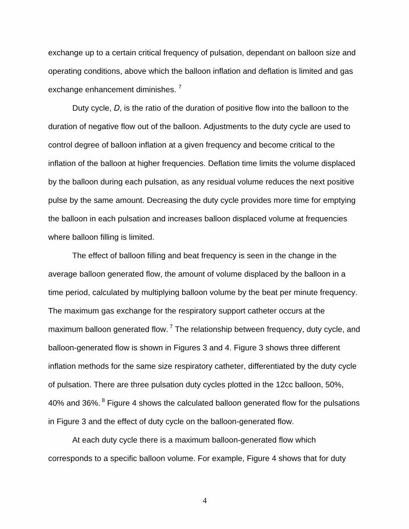
exchange up to a certain critical frequency of pulsation, dependant on balloon size and

operating conditions, above which the balloon inflation and deflation is limited and gas

exchange enhancement diminishes. 7

Duty cycle, D, is the ratio of the duration of positive flow into the balloon to the

duration of negative flow out of the balloon. Adjustments to the duty cycle are used to

control degree of balloon inflation at a given frequency and become critical to the

inflation of the balloon at higher frequencies. Deflation time limits the volume displaced

by the balloon during each pulsation, as any residual volume reduces the next positive

pulse by the same amount. Decreasing the duty cycle provides more time for emptying

the balloon in each pulsation and increases balloon displaced volume at frequencies

where balloon filling is limited.

The effect of balloon filling and beat frequency is seen in the change in the

average balloon generated flow, the amount of volume displaced by the balloon in a

time period, calculated by multiplying balloon volume by the beat per minute frequency.

The maximum gas exchange for the respiratory support catheter occurs at the

maximum balloon generated flow. 7 The relationship between frequency, duty cycle, and

balloon-generated flow is shown in Figures 3 and 4. Figure 3 shows three different

inflation methods for the same size respiratory catheter, differentiated by the duty cycle

of pulsation. There are three pulsation duty cycles plotted in the 12cc balloon, 50%,

40% and 36%. 8 Figure 4 shows the calculated balloon generated flow for the pulsations

in Figure 3 and the effect of duty cycle on the balloon-generated flow.

At each duty cycle there is a maximum balloon-generated flow which

corresponds to a specific balloon volume. For example, Figure 4 shows that for duty

4

cycle of 36 the maximum gas exchange is at 420 BPM, which corresponds to 11ml, 80-

90% of the maximum balloon volume. Lower pulsation rates fully inflate, and higher

pulsation rates have lower filling volume, but in the 420 beats per minute region the

volume and rate are balanced at the greatest balloon delivered volume as the loss in

volume is balanced by the gain from frequency of pulsation.

Loss of total drive gas in the system can also reduce gas exchange. A partially

inflated balloon leads to greatly lowered gas exchange in the RSC, as shown in Figure

4. 9 The Figure data shows that at zero beat rate the balloon filling has no effect, but

with increasing frequency the under filling reduces blood gas transfer as the drive gas is

unavailable to displace and mix the blood. Even with the most ideal pulsation frequency

and duty cycle, reduced system gas volume would limit the catheter gas transfer.

5

0

2

4

6

8

10

12

14

0 60 120 180 240 300 360 420 480 540 600 660Frequency (BPM)

Volu

me

(cc)

D = 36%

D = 40%

D = 50%

0

2

4

6

8

10

12

14

0 60 120 180 240 300 360 420 480 540 600 660Frequency (BPM)

Volu

me

(cc)

D = 36%

D = 40%

D = 50%

Figure 3 Decrease of balloon pulsation volume with increase of balloon frequency, showing different performance with duty cycle (D) at three levels, 36%, 40% and 50%. Arrows mark the frequencies corresponding to maximum balloon generated flow at each duty cycle 8

6

0

2

3

5

6

8

9

0 60 120 180 240 300 360 420 480 540 600 660Frequency (BPM)

Gen

erat

ed fl

ow (l

pm)

D = 36%

D = 40%

D = 50%

0

2

3

5

6

8

9

0 60 120 180 240 300 360 420 480 540 600 660Frequency (BPM)

Gen

erat

ed fl

ow (l

pm)

D = 36%

D = 40%

D = 50%

Figure 4. Effect of balloon volume on balloon generated flow shown at three duty cycles (D); 36%, 40% and 50%. The peaks of these graphs demonstrate the loss of balloon generated flow both higher and lower than the frequency of maximum balloon filling 8

7

0.0

50.0

100.0

150.0

200.0

250.0

300.0

0 100 200 300 400Balloon Pulsation Rate (BPM)

vCO

2 /m2

(ml/m

in/m

2 )

Fully Filled 40cc RSC

Partially Filled 40cc RSC

0.0

50.0

100.0

150.0

200.0

250.0

300.0

0 100 200 300 400Balloon Pulsation Rate (BPM)

vCO

2 /m2

(ml/m

in/m

2 )

Fully Filled 40cc RSC

Partially Filled 40cc RSC

Figure 5. Difference in carbon dioxide transfer between the partially filled respiratory support catheter and the fully filled device above 0 BPM 9

8

Maintaining correct balloon volume in both IABP and the respiratory support

catheter is necessary for the devices to achieve their maximum level of performance.

An improperly inflated IABP system causes a weakened heart to work more than

necessary, decreases peripheral perfusion and leads to reduced patient recovery. 1,2

The current system for monitoring IABP filling volume depends on the backpressure of

the system, which requires training to interpret and remains qualitative. Direct volume

readout from a measurement system would provide a quantitative, easily read number

to supplement the pressure monitoring method.

An under-inflated respiratory support catheter has a limited balloon-generated

flow and reduced mixing of blood, which therefore limits oxygen transfer to and carbon

dioxide removal from the patient. 5,6,7 The RSC has yet to have an in vivo volume

measurement, and would benefit from a volume measurement system as the delivered

therapy in the RSC can often change in both beat frequency and duty cycle. Best

patient treatment can be obtained by finding and maintaining optimal inflation through

use of a volume sensor.

1.1 STATEMENT OF PURPOSE

This research developed a system capable of measuring the volume of helium

delivered to a pulsating balloon in a clinical situation, a dynamic balloon volume sensor

system (DBVSS), with the goal of measuring volumes within 10% of the actual balloon

volume. The aim of volume measurement was to maintain the two discussed balloon

catheters at their optimal filling volume, through monitoring the degree of inflation. The

9

system was designed to operate in the catheter drive gas, across a number of balloon

volumes, pulsation frequencies and expected clinical variations to the inflation methods.

10

2.0 BACKGROUND

Measurement of the balloon volumes in IABP and RSC catheters is a challenging

task, as the catheter placement within a patient makes the balloon inaccessible to most

measurement techniques. Flow into the balloon can still be measured at the entrance

point of the catheter tubing, and so flow is a logical method of monitoring catheter

inflation. The flow signal can be used to calculate the volume delivered to the balloon,

similar to spirography, a technique that measures both lung volume and breath tidal

volume in respiration. 10 One method of spirography is to integrate the expired airflow,

Qa, to determine the breath volume, Vbr, using:

∫+

=τt

tabr dttQV )( (1)

Where the period of one breath is the flow signal from time t to t+τ.

The flow meter to be used in the DBVSS had a number of constraints based on

the drive system properties. Typical pulsating balloon catheters use helium as the drive

gas, due to the low inertial load and low internal friction of the gas. Helium

concentrations of the drive gas for both IABP and the respiratory support catheter drive

systems can change over time due to small leaks in the driveline and helium diffusion

through the plastic components of the system. The leak rate of helium can be up to

1cc/hour in IABP balloons, 1 and similar leak rates have also been observed for the

respiratory support catheter. The leak causes room air to be a greater component of the

11

drive gas mixture as pulsation continues. This shift in concentration complicates flow

measurement, as the flow meter must measure gas flow in which the physical

properties change with time.

The helium oscillates at high rates up to 600 beats per minute in some tests,

which with a 40cc balloon is an average of 24 liters per minute, with expected

maximums of 40 liters per minute. The system requires a flow meter with a time

response fast enough to measure the flow pulses, which at 600 BPM has a flow pulse

lasting only 50 milliseconds.

A final constraint is the placement of the catheters in the patients themselves,

which limits the geometry and location of any accessory volume measurement devices.

The Dynamic Balloon Volume Sensor System would need to be an accessory to current

therapeutic treatments (such as IABP), which demands the ability to add on to the

system with minimal interference in the normal function of the devices.

2.1 SELECTION OF FLOW METER

The changing gas concentration during pulsing has an adverse affect upon flow

meters intended to measure the gas flow. Loss of helium causes an increase in the fluid

density, viscosity and momentum as well as a decrease in thermal conductivity. The

gain in density and momentum complicates the conversion between mass and

volumetric flow, as well as interfering with the function of rotameters, Pitot tubes,

pneumotachometers, vortex shedding flow meters, and Venturi tubes. Rotameters

suspend a float at a certain height in a vertically moving column of fluid, where the float

has a potential energy equal to the momentum imparted by the fluid. The fluid

12

momentum in rotameters is a property of viscosity and density that would cause the

rotameter to read incorrectly higher flow in lower concentrations of helium. Pitot tubes

would also read higher flow, as they determine the weight of a column of gas stagnated

by flow against a nozzle. The measured height would be then be higher, and seem to

be a higher flow rate. Pneumotachometers depend on a known resistance to flow, which

would increase as the viscosity of the fluid increased, contributing to erroneously higher

flows. The vortex shedding flow meter would also be affected by change in viscosity, as

the higher viscosity would lead to longer times between release of the vortex, which

would result in lower flows read in lower concentrations of helium. A Venturi tube is

calibrated for a certain flow profile and pressure drop that requires a known viscosity

and density for the fluid, the changing helium concentration would render this calibration

useless.

Heat capacity and heat transfer would also change with gas concentration. The

higher heat capacity and lower heat transfer coefficient would interfere with the

operation of thermal flow meters such as capillary mass flow meters, and hot film or hot

wire anemometers. A reduced heat loss in these devices may not be due to reduced

flow, but instead due to lower helium concentration in the drive gas.

As helium leaks and gas concentration changes in the driveline, all these flow

meters all have potential for error in measuring flow, and therefore balloon volume. A

compensation method for helium leakage is a requirement for these flow meters to be

used in a balloon volume sensor, while some flow meters must be excluded due to their

slow time response, such as bubble flow meters, capillary flow meters and rotameters.

11

13

There also remain flow meters that are unaffected by gas concentration changes,

but would not be feasibly implemented in this application. Bubble flow meters are very

accurate and independent of gas concentration, but they require non-oscillating, one-

way flow and they are used mostly for steady flow, as the average flow over the transit

time of the bubble. Doppler flow meters would require some sort of particulate or bubble

to be in the system, which is not possible in the medical catheters under study. Turbine

flow meters are insensitive to gas composition, temperature or humidity, but have

inertial effects from the turbine that would interfere with their ability to measure high

speed oscillating flow. 11

Among the flow meters that may possibly be used in the volume sensor, the hot

wire and hot film anemometers have the most potential, as they both have performance

properties that will allow them to function, with compensation, in changing gas flow. The

anemometers have a zero-flow response that is due to the composition of the measured

fluid, which allows information regarding the fluid properties to be gathered at a known

flow rate. Hot wire anemometers (HWA) also have a response time around 1-10 ms,

which makes them fast enough for our fluid flow measurements. 12

2.2 HOT WIRE ANEMOMETRY

Hot wire anemometry can be used in gas flows and has a faster flow rate than

hot film anemometers, 12,13 and therefore is the flow meter of choice for this experiment.

A hot wire anemometer uses the principles of heat transfer to measure the flow of a gas

or other fluid. The specific type of HWA in this research was a constant temperature

anemometer. The constant temperature sensor suspends a very thin, high aspect ratio

14

wire into the fluid stream to be measured. This wire is heated to high temperatures (250

Celsius in this case) by the electric current though the wire. Flow past the wire causes

heat transfer to the flowing fluid, and the wire cools.

The temperature is maintained by measuring the resistance of the wire. The wire

forms a quarter of a balanced Wheatstone bridge, an electrical circuit made of four

resistors designed to measure small changes in resistance by comparing one resistor

with the set of three other resistors. The bridge starts out with balanced resistance

values, which produces equal current flowing through each half of the bridge. The

resistance of the hot wire increases with the decrease of wire temperature and the

balance of current through the bridge changes, which results in a potential difference

across the bridge between points 1 and 2. 12-15

The bridge output is connected to an operational amplifier feedback circuit that

supplies additional voltage, and thereby current, across the bridge to return the wire

temperature to the balance point of the bridge. This added voltage is measured as the

voltage output of the sensor. The output voltage is related to the amount of heat lost by

the wire into the fluid, and to the fluid flow by King’s Law. 12,13

15

2 1

Figure 6. Circuit diagram for standard constant temperature hot wire anemometer (HWA), showing the balanced Wheatstone bridge and amplified voltage output.

The same principles are used in hot film anemometry, where a plate is heated on

the side of the fluid flow path and the fluid flows across the top surface of the plate. Hot

film anemometers are more robust for use in liquid flows, but hot wire anemometry was

cheaper to implement and had a faster response time for this application. 11, 13

16

2.3 KING’S LAW

Hot wire anemometry measures the heat lost into a moving fluid stream in order

to calculate the velocity and flow of the fluid. The general relation between the output of

the sensor (voltage, E) and the movement of fluid through the sensor is King’s Law:

nUbaE ′+=2 (2)

King’s Law is composed of two components: a, the zero-flow heat loss term and a

constant for a specific gas concentration and b’Un, the heat loss due to fluid motion,

made up of the sensor constant n, the fluid velocity U and the convective constant b’,

determined by gas properties. The theoretical output graph is Figure 7, an exponential

curve with a definite zero flow offset a, equal to the squared voltage at zero-flow Emin2.

12,13,14,16

The heat loss in high aspect ratio wires is governed by the equations for heat

loss from a cylinder in a moving fluid. The assumptions used in this analysis are: 12,13,14

• The temperature of the wire is held constant and is constant along its entire length

• All heat lost from the wire is transferred to the fluid, with minimal conduction to other

parts of the sensor and minimal loss from radiation

• Fluid velocity is uniform over the length of the wire and is small compared to sonic

speed

• The heat transfer is governed by the Nusselt number, Nu.

17

0

1

2

3

4

5

6

0 2 4 6 8 10Fluid velocity U (m/s)

Vol

tage

E2 v

olts

2

E2 = a + bUc

Emin2

0

1

2

3

4

5

6

0 2 4 6 8 10Fluid velocity U (m/s)

Vol

tage

E2 v

olts

2

E2 = a + bUc

Emin2

Figure 7. Ideal King’s Law Voltage output vs. Flow velocity in a hot wire anemometer, showing zero velocity voltage offset, Emin

18

Gas Flow

( )nradcondconv

baNu

HHHRI

Re

2

′+′=

++=

T=Tw

T=TF

wire

Gas Flow

( )nradcondconv

baNu

HHHRI

Re

2

′+′=

++=

T=Tw

T=TF

wire

Figure 8. Hot wire anemometer steady state heat loss from wire due to resistive heating of wire (I2R), showing fluid flow, heat balance and Nusselt number relations.

We may also assume that in a constant temperature wire that there is no

change in the heat stored in the wire and the heat input equals the heat output of the

wire. The power loss from current in the wire is completely transmitted as heat to the

environment, which results in the power balance:

radcondconv HHHRI ++=2 (3)

The resistive heating of the wire is I2R, where I is current and R is wire resistance.

Some heat is lost through conduction to the supports, Hcond , but this heat loss is

considered to be negligible as most anemometers are constructed of low conductive

materials for this very reason. 12,13 The radiative heat loss, Hrad, is equal to (1)σ (TW4 –

TF4). The view number is 1, as the wire is completely surrounded by the lumen of the

flow meter, and the heat lost to radiation is therefore 0.66 Watts per square centimeter.

When combined with the extremely small surface area of the wire, the radiative heat

loss can be considered negligible. 12,13 Therefore all heat loss is transferred to the fluid,

as Hcond and Hrad go to zero Equation 3 becomes:

19

( )FWW TThARI −=2 (4)

where h is the heat transfer coefficient from the wire to the fluid, Aw is the contact area

of the wire to the fluid, Tw is the wire temperature, and TF is the fluid temperature.12,14

The specific Nusselt number for a cylinder in cross flow is in equation (5).

( )k

hDbaNu wn =′′+′= Re (5)

Where k is the thermal conductivity of the fluid and Dw is the diameter of the wire.

Solving for h and inserting into Equation 4, we obtain:

( )[ ]( ) wFWn

wATTbaD

kRI −′′+′⎟⎠⎞⎜

⎝⎛= Re2

(6)

Rewriting the Reynolds number in terms of fluid density (ρ), viscosity (µ), velocity (U),

and tube diameter (Dt) and multiplying both sides by the wire resistance (to obtain

voltage squared) yields:

( ) RATTUDbaDkE wFW

nt

w−⎥

⎦

⎤⎢⎣

⎡⎟⎠⎞⎜

⎝⎛′′+′⎟

⎠⎞⎜

⎝⎛= µ

ρ2 (7)

Equation 7 can be simplified by incorporating all the constant terms into the two

coeffiecients, a and b, 11, which returns us to Equation 2, King’s Law:

nUbaE ′+=2 (2)

where:

( )

( ) RATTDD

kbb

RATTDkaa

wFW

nt

w

wFWw

−⎟⎟⎠

⎞⎜⎜⎝

⎛⎟⎠⎞⎜

⎝⎛′′=′

−⎟⎠⎞⎜

⎝⎛′=

µρ

20

The coefficient a can be replaced by the term Emin, or minimum voltage, as the minimum

voltage will occur when U=0 (seen in Figure 9), and the heat transfer is governed by

conduction to the static fluid. In flow through constant cross section, the velocity is equal

to the flow divided by area. The inverse flow lumen area incorporated into b allows a

reformulation of Equation 2: 12,13,14,16

nbQEE += 2min

2 (8)

King’s Law is necessarily a general formula, as it describes behavior of all hot

wire anemometers. Specific applications, such as in the DBVSS, require assignment of

the variables Emin, b, and n. These variables change based on properties of the fluid

measured as well as the specific geometry and composition of the hot wire

anemometer.

Many hot wire anemometers have an n of approximately 0.5, and many

theoretical solutions use this value of n as the standard. But experimental results have

shown that n can vary between 0.4 and 0.7 and should be separately calculated for

each anemometer during calibration.12,13

21

0

2

4

6

8

10

12

0 200 400 600Time (ms)

Out

put V

olta

ge (V

)

Emin

Positive Flow

Negative Flow

Figure 9. Expected voltage response flow for a HWA in pulsatile flow, showing Emin at zero flow and the variability of the voltage signal in backward flow.

2.4 USE OF HWA IN VOLUME MEASUREMENT

Hot wire anemometry is well established for measuring oscillatory volumes in the

spirography of respiration where the flow meter can be calibrated to known exhalation

pressures and gas concentrations. Scalfaro et. al. and Plakk et. al. measured

exhalation flow on patients on a ventilator. 17,18 They showed that integration of the flow

does give repeatable and accurate volume measures of respiration volume and that

22

HWA has low resistance to flow. While the HWA will be affected by changes in gas

concentrations, as with other flow meters, this change can be compensated for due to

the predictable response of the HWA sensor. In areas where the constant flow is

known, HWA can also be used to measure changes in gas concentration, specifically

helium, where the flow rate in known 19,20 so an application that measures both

changing flow and changing volume can readily be developed from this collection of

research.

Plakk et. al.16 did present a method for compensating for concentration changes

between inspired and expired air during spirometry. While a compensation method was

developed, the errors cause by the difference between inspired and expired air were

minor (approximately 1%) because the reduced oxygen and increased carbon dioxide in

the expired air did not significantly change the gas thermal properties. Thus the

compensation method was not really needed in this case nor was it validated under

conditions of more substantive differences in gas composition. In helium pulsed balloon

catheters, the thermal conductivity of helium can be up to 16 times that of air, 21,22 and

so even small changes in gas composition greatly affect gas thermal properties and

require compensating for gas composition in the flow measurement used to monitor

balloon volume.

2.5 OBJECTIVES, CHALLENGES AND RESEARCH PLAN

The dynamic balloon volume sensor system (DBVSS) combines techniques of

spirography with an algorithm to compensate for helium loss. This paper describes the

development of this unique system as a tool to measure the volume of pulsating

catheters. The development of the flow relations from theory, the development of the

23

sensor response to changing helium concentrations, and the combination of these

elements into a fully functional flow sensor are shown. The DBVSS was validated using

techniques of spirography to measure pulsating balloon catheters, as well as

demonstrating a robust method to compensate a hot wire anemometer for changing gas

concentrations.

The practical application of the hot wire anemometer was a challenge in these

complex inflation systems. Certain steps were necessary to first verify the actual

function of the HWA as a volume measure in the pulsing drive gas. The first step was to

examine the flow meter response in the expected different flow and gas regimes in the

DBVSS operation. The sensor needed to be tested in steady and dynamic flow against

a flow standard, to confirm the previous authors’ work on HWA. Flow testing could then

be followed by exploration of the sensor response to changing gas concentration. These

two independant verifications of the sensor response could then lead to operating the

sensor in combined dynamic flow and changing gas concentrations.

The combined operation would entail adding functionality to either the sensor or

the data analysis system, as there will be two unknowns in the system, concentration

and flow, and only the sensor voltage output with which to measure them. The usable

flow meter could measure the correct flow regardless of gas concentration, which

allowed the flow to be used to measure volume delivered. The spirographic technique

could be employed, using known volumes to check to applicability of integrating the

measured flow. Volume measurements could be automated after the spirographic

technique is shown to be effective, and the system would detect and measure flow

pulses out of a set of pulsation data during experiments. This last step marks the

24

formation of the actual dynamic balloon volume sensor system, a system which can

measure flow, correct for helium concentration, detect the flow pulses, and integrate

them to find the delivered volumes. The DBVSS could then be tested across the full

range of expected variations in pulsation, such as simulated helium loss, volume loss or

change in frequency as well as constrictions and interference with balloon inflation.

25

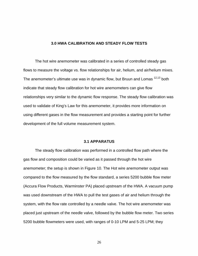
3.0 HWA CALIBRATION AND STEADY FLOW TESTS

The hot wire anemometer was calibrated in a series of controlled steady gas

flows to measure the voltage vs. flow relationships for air, helium, and air/helium mixes.

The anemometer’s ultimate use was in dynamic flow, but Bruun and Lomas 12,13 both

indicate that steady flow calibration for hot wire anemometers can give flow

relationships very similar to the dynamic flow response. The steady flow calibration was

used to validate of King’s Law for this anemometer, it provides more information on

using different gases in the flow measurement and provides a starting point for further

development of the full volume measurement system.

3.1 APPARATUS

The steady flow calibration was performed in a controlled flow path where the

gas flow and composition could be varied as it passed through the hot wire

anemometer; the setup is shown in Figure 10. The Hot wire anemometer output was

compared to the flow measured by the flow standard, a series 5200 bubble flow meter

(Accura Flow Products, Warminster PA) placed upstream of the HWA. A vacuum pump

was used downstream of the HWA to pull the test gases of air and helium through the

system, with the flow rate controlled by a needle valve. The hot wire anemometer was

placed just upstream of the needle valve, followed by the bubble flow meter. Two series

5200 bubble flowmeters were used, with ranges of 0-10 LPM and 5-25 LPM; they

26

allowed flow calibration over a range of 0 to 25 LPM. The gases entered the bubble flow

meter through a pair of mixing rotameters (Cole-Parmer inc, Vernon Hills IL) that

controlled the ratio of room air to helium entering the flow path. The rotameters each

had an integral needle valve, which could control and measure the relative contribution

each gas made to the total gas flow in the system. The air was room air, and the helium

was supplied from a 99.95% medical grade helium tank. The helium supply line had a

Y-junction connected to the surrounding atmosphere, which maintained the helium at

atmospheric pressure, the same as the air supply. The bubble flowmeters had ANSI

traceable flow calibration, and were used to check the rotameters.

Bubble Flowmeter

Mixing Rota meter s

Air

Helium HWA

Flowmeter Vacuum

Pump

Needle Valve

Figure 10. Hot wire anemometer calibration setup for steady flow, with the gas supply drawn under vacuum pressure through the volume standard and anemometer

27

3.2 PROCEDURE

The hot wire anemometer was tested in three gases: air, helium and an

air/helium mixture. Air was tested first, pulled through the air rotameter by the vacuum,

which produced 360 mmHg absolute pressure, 400 mmHg below atmospheric, with the

needle valve fully open. The voltage of the HWA was read with a voltmeter (Tektronics

inc., Beaverton, OR) and recorded, and the bubble meter provided a flow output on a

digital display, which was recorded for three successive bubble measurements and

arithmetically averaged. The needle valve was adjusted to vary the flow rate from 0 to 9

LPM while using the 0-10 LPM bubble flow meter, and the flow and voltages recorded.

Zero flow was measured by clamping off the entrance and exit tubing to the HWA after

flushing the system with gas of interest for one minute. The 0-10 LPM bubble flow meter

was replaced with the 5-25 LPM bubble flow meter to measure flows of 6-12 LPM. The

meter had the ability to measure flows above 12 LPM, but the pressure difference

during air flow in this system caused excessive bubbling that precluded use of the

bubble flow meter at higher flows.

Pure helium tests followed, with the air rotameter closed and the helium

rotameter opened to the Y-junction and on to the supply tank. The tests were then

repeated, measuring voltage and flow across 0-9 LPM, then from 6-25 LPM with the two

bubble flow meters, as the helium allowed full range use of the bubble flow meter. Three

additional zero-flow measurements were taken during helium testing to confirm helium

concentration across the tests, the first after the 1 LPM test, the second after the 9 LPM

test on the first flow meter, and the third after the 25 LPM test.

28

The pure helium test was followed by a mixed air/helium calibration, where the

two mixing rotameters were opened partially to allow a constant 3 to 7 volume ratio of

air flow to helium flow across the range of calibration flows. The mixed gas was

measured over a range of 0-9 LPM, then 6-18 LPM. The bubble flow meter was able to

measure flow over a larger range than with air, but smaller range than with helium.

3.3 DATA ANALYSIS

Each bubble flow meter reading was arithmetically averaged across the three

recorded flows, and matched with the corresponding voltage output of the hot wire

anemometer. These paired values were entered into the Matlab mathematical language

program (The MathWorks inc., Natick MA ) as three

‘n x 2’ matrices, one for each test gas. The Matlab non-linear fit function, “nlinfit.m”, was

used to calculate the constants b and n for the equations relating flow to voltage, of the

King’s Law form E2 = Emin +bQn (Equation 9). The variable Emin is the zero flow voltage,

directly measured. The exponent n was constrained to be equal across all gases, and

each gas’s flow equation was regressed to its own value of b.

29

3.4 RESULTS

Figure 12 shows the steady flow calibrations hot wire anemometer calibrations, in

all three gases. The flow exponent for all three gases was n=0.63, above the typical

assumed exponent of n=0.5 but within the cited 0.4 to 0.7 range. 12,13 The helium

response is the top curve, showing the higher heat transfer of helium compared to the

lower curve of the air flow data, and the mixed gas response lies between the other two

curves. The air calibration regressed to E2= 0.25+0.3510*Q0.63, 70% helium to

E2=3.7425+0.7867*Q0.63 and 100% helium to E2=5.3453+0.8365*Q0.63. With increasing

helium concentration, the zero flow voltage increased, as well as the rate at which

voltage changed with flow.

3.5 DISCUSSION

The steady flow tests did confirm King’s Law operation in the HWA and the dependence

of b and Emin on gas composition, but the direct application of the steady flow

calibrations in oscillatory flow application required further refinement. Bruun 12 did find

similar dynamic and steady flow responses in hot wire anemometers, but it became

important to optimize the DBVSS volume determination for the pulsating balloon

systems. Accordingly, experiments were undertaken to refine the King’s Law

calibrations determined from steady flow, which used oscillatory flow representative of

the applications of interest.

30

0

2

4

6

8

10

12

0 5 10 15 20 25

Steady Gas Flow (LPM)

Volta

ge S

quar

ed (E

2 )100% He: E2= 5.3453 +0.8365*Q0.63

70% He: E2= 3.7425 +0.7867*Q0.63

100% Air: E2= 0.25 +0.3510*Q0.63

Figure 11. Non linear fits from helium, air and mixed gas calibrations of the hot wire anemometer, showing increasing y-intercepts and flow coefficients with increased helium concentration.

31

4.0 EMIN DEPENDENCE ON HELIUM CONCENTRATION

The steady flow results in Figure 12 illustrate the differing flow responses in

lowered helium concentrations. The exact effect may be complicated to determine, as

the derivation of King’s Law demonstrates that there are concentration dependant terms

that make up both Emin and b (Equations 7,8 and 2a). However, it is possible to explore

the Emin term alone to illustrate what effect helium concentration has at zero flow.

Examination of the relationship of helium concentration to these zero-flow values can

provide insight into how the dynamic voltage response will change with reduced helium

concentration.

4.1 APPARATUS AND PROCEDURE

Confirming how Emin changes with respect to the helium concentration required a

change in the testing setup from the steady flow. The hot wire anemometer was fitted

with stopcocks to enable filling the sensor with volumetric mixtures of helium and air.

The voltage output was connected to the Tektronics multimeter to read the zero flow

voltage. The gas mixtures were 100%, 90%, 80%, 70% and 0% helium, mixed in 50cc

amounts (e.g. 70% helium was 35cc of helium and 15cc of air). The inner lumen volume

was approximately 30ml, the bolus size was chosen to fill and sweep the entire lumen.

Medical grade helium flushed the inside of the sensor lumen before each test, and then

the 50cc gas bolus was pushed into the open sensor. Zero flow was guaranteed by

32

sealing both ends of the sensor with the stopcocks after the mixture filled the sensor

lumen, and the resulting voltage output was measured using the Tektronics multimeter.

Each test was performed three times at the same gas concentration.

4.2 RESULTS AND DISCUSSION

The expected result from King’s Law was confirmed, as Figure 17 shows Emin

lowering with lowered helium concentration. The voltage response is bracketed on

either side by the pure gas results in this binary gas system, by 100% helium on the

high side and by 100% air (or 0% helium) on the low side. The linear fit through the

averaged voltages had a y-intercept equal to the measured zero flow in air, 0.5 volts.

The standard deviation between tests is shown on the graph, which demonstrates the

low variance between tests as well as the linear relationship between the percent

helium and Emin.

33

0

0.5

1

1.5

2

2.5

0% 20% 40% 60% 80% 100%

Percent Helium [He]

Zero

Flo

w V

olta

ge (E

min

)Pure Helium Emin = 2.38

Pure Air Emin = 0.5 V

Emin = 1.7866 [He] + 0.5009

0

0.5

1

1.5

2

2.5

0

0.5

1

1.5

2

2.5

0% 20% 40% 60% 80% 100%

Percent Helium [He]

Zero

Flo

w V

olta

ge (E

min

)Pure Helium Emin = 2.38

Pure Air Emin

Emin = 1.7866 [He] + 0.5009

= 0.5 V

Figure 12. The change in Emin with changing helium concentration, illustrating the upper limit of 2.38 volts in helium, and the lower limit of 0.5 volts in air.

34

5.0 DEVELOPMENT OF A VOLUME MEASURE FROM FLOW DATA

Steady flow measurements and the zero flow response are useful for

understanding the sensor properties, but development of the full volume measurement

system requires examination of the flow pulses in dynamic conditions. A main challenge

lies in the fact that a flow standard for the dynamic flow is not available, due to the

inapplicability of most flow methods described in section 2.2. The sensor must therefore

be used to measure volume, and be compared to a volume standard, a calibrated

plethysmograph.

Spirography can use a flow pulse to measure the delivered volume over a time

period τ. The steady flow voltage vs. flow relationship allows the hot wire anemometer

voltage output during pulsation (Figure 14) to be converted to flow. The flow is related to

balloon filling volume, Vb, through Equation 1:

∫+

=τt

tb dttQV )( (1)

Q is the flow past the sensor, t is time, and τ is the time period corresponding to the

positive flow into the balloon, seen in Figures 6 and 14. Equation 1 then becomes more

useful with flow as the independent variable:

n

bEE

Q1

2min

2

⎟⎟⎠

⎞⎜⎜⎝

⎛ −= (10)

35

0

0.5

1

1.5

2

2.5

3

3.5

4

4.5

5

0 100 200 300 400 500Time (ms)

HW

A o

utpu

t (Vo

lts)

Forward Flow Backward Flow

Emin

100% He70% He

τ

0

0.5

1

1.5

2

2.5

3

3.5

4

4.5

5

0 100 200 300 400 500Time (ms)

HW

A o

utpu

t (Vo

lts)

Forward Flow Backward Flow

Emin

100% He70% He

τ

Figure 13. Example flow for a HWA in pulsatile flow, shown for two gas concentrations in the same flow meter.

36

Integrating the full flow signal requires some method of recording the full flow

signal, and to refine instantaneous flow Q into flow which varies with time Q(t). Digitally

sampling provides a series of discrete flow values across time points, which lends itself

well to numerical integration of the flow signal. The trapezoidal rule for numerical

integration was used to integrate the flow, defined as:

∑ ∆++

= ttQtQVb 2)1()(

(11)

The combination of Equation 11 with Equation12 combines the theoretical flow

response with the sampling method to allow numerical processing of the signal. The

practical application of this equation requires the King’s law equation, with b, Emin and n

defined for a specific gas. The solution for the steady flow voltage vs. flow relationship

in the hot wire anemometer in air provides values for these variables in 100% helium

70% helium and 100% air. The steady flow equation for 100% air allows the test of the

spirographic technique on air pulses, to see the applicability to the hot wire

anemometer. Flow in 100% air prevents any change in gas composition, as the drive

gas and atmospheric gas are the same composition, which simplifies the conversion of

flow signals. Integrating a flow signal would then produce an accurate measure of the

volume that flowed through the sensor.

37

5.1 APPARATUS

The hot wire anemometer was set up to allow the injection of an air bolus through

the lumen of the flow meter, as shown in Figure 14. The downstream end of the HWA

was open to atmosphere, and the upstream end was connected to a stopcock and then

to a 60cc syringe filled with 40cc of air. The flow and temperature voltages were

connected as differential inputs to a AT-MIO-16E data acquisition card (National

Instruments, Austin TX).

HWA

40cc Syringe

Stopcock Stopcock

Voltage OutHWA

40cc Syringe

Stopcock Stopcock

Voltage Out

Figure 14. Setup for injection of known volumes through anemometer, with stopcocks to ensure zero gas flow between tests

5.2 PROCEDURE

The tests measured a series of air injections through the hot wire anemometer.

The syringe was filled with air and the two channels of data were recorded into a “.dat”

file, sampled at 100 Hz, using a National Instruments LabVIEW data acquisition

program. The stopcock was opened and the air bolus injected through the system. The

38

data acquisition was stopped 3-5 seconds after each injection, after the flow voltage

returned to the minimum, no-flow level. The injection test was performed six times with

the 40cc bolus.

5.3 DATA ANALYSIS

The data files were opened in Microsoft Excel. The hot wire anemometer

voltages were converted to flow data using the equation fit to the steady flow data

(Figure12), where Emin=0.25, b=0.3510, and n=0.63. Equation 12 was used to calculate

the trapezoidal numerical integration of adjoining flow data points, which were summed

starting at the first non-zero flow value and ending at the last non-zero flow value in the

flow pulse.

5.4 RESULTS

The integrated injection volumes across the series are plotted in order of the

tests, Figure 13. The results show that the calculated volumes were at most 7% off of

the injected volume of 40cc, and had a mean value of 39.78cc, which was only 0.5%

below the actual volume. These tests indicate the integration of flow provides volumes

near the actual flow values, and also shows there is some amount of variability between

integrations even when similar flow conditions are repeated. The ability to measure and

record flow signals was now demonstrated, and the next step towards a full volume

sensor was to analyze pulsating flow.

39

0

5

10

15

20

25

30

35

40

45

0 1 2 3 4 5 6 7Injection Number

Volu

me

(ml)

Mean = 39.78Std. Dev. = 1.19

Figure 15. Results of using numerical integration on known 40cc air injections

40

6.0 DBVSS DEVELOPMENT

The flow integration hypothesis for the DBVSS was confirmed in the air injection

tests, which enabled the expansion into testing oscillatory flow. Several steps were

necessary to construct the full volume measurement system. First a volume standard

had to be established for comparison to the measured pulsatile flow. Next the data

acquisition system to gather data had to be assembled and connected to all the

required sensors for flow and volume measurement. Finally the computational system

had to be built that could analyze the recorded data from pulsation and calculate the

balloon volumes.

6.1 SETUP, SENSORS AND DATA ACQUISITION

The full DBVSS consists of the hot wire anemometer, pressure sensors, data

acquisition system and the computer program to analyze the data. The DBVSS was to

be evaluated by comparing its volume output, VbDBVSS, to the water displaced by the

pumping of a Datascope 40cc Intra-Aortic Balloon Catheter (Datascope, Fairfield, NJ),

Vbact. The setup can be seen in Figure 14. The balloon was placed underwater in a

sealed plethysmograph, and the drive tubing ran through the hot wire anemometer and

on to the drive system, so the HWA could measure all flow into the balloon. The helium

line, 1/4 inch Tygon tubing (Cole-Parmer inc, Vernon Hills IL) ultimately terminated in a

safety chamber (Datascope), the source for the pulsing helium flow. Two Sensym 921

41

A, 0-780 mmHg pressure transducers (Sensym, Milpitas CA) were connected to the

plethysmograph (P2) and the driveline (P1).

Four channels of data (temperature, plethysmograph pressure, driveline pressure

and flow) and one control voltage were recorded through a National Instruments AT-

MIO-16E-10 data acquisition board using a custom LabVIEW (National Instruments,

Austin TX) data acquisition program. Sampling rate in each pulsation test was 1000Hz,

and each data set was 15 seconds long. Signal conditioning consisted of a 10 Hz

Butterworth low pass filter on the plethysmograph pressure transducer box (P2) and a

control voltage, which grounded the unused channels.

Data Acquisition

Q T

Balloon PumpHot Wire

Anemometer

P1P2

PlethysmographBalloon

LabVIEWData

Acquisition

Q T

Balloon PumpHot Wire

Anemometer

P1P2

PlethysmographBalloon

Data Acquisition

Q T

Balloon PumpHot Wire

Anemometer

P1P2

PlethysmographBalloon

LabVIEW

Figure 16. Setup for testing the DBVSS against the Plethysmograph standard, showing gas driveline from pump to balloon as well as sensor and data acquisition setup

42

6.2 VOLUME STANDARD

Actual displaced balloon volume, Vbact, was determined from the pressure signal

of the plethysmograph by using the model for adiabatic compression of air and the

following relationship:

0

01P

VPV act

b∗

=γ (12)

where γ is the adiabatic constant for air, P is the absolute plethysmograph pressure at

full balloon inflation, P0 is the plethysmograph pressure at balloon deflation (also

atmospheric pressure), and V0 is the volume of air in the plethysmograph at balloon

deflation. As the balloon inflates, the water level rises, compressing the air trapped at

the top of the plethysmograph, V0, which increases the pressure, P.

The plethysmograph is calibrated to the accurate V0 through injections of known

water volumes, which can be measured using isothermal expansion of gas. Isothermal

volume is found by setting γ =1 in equation 12. The system is sealed, and atmospheric

pressure is measured. A series of 1cc water injections are injected into the

plethysmograph, up to 20cc. Using these volumes as Vbact in the isothermal case of

equation 12, it is possible to solve for V0, which in this case is 2286cc.

6.3 DATA ANALYSIS

The recorded data was analyzed using a custom LabVIEW program, Appendices

B,C, and D. This program built upon the established integration methods of spirography

by combining the integration techniques with the data acquisition system, as well as the

development of algorithms that can detect and automatically mark and integrate the

43

positive flow pulses. The data analysis portion of the DBVSS was very systematic in the

processing of the flow voltages and the step by step methods follow.

The program opened the data files using LabVIEW, and passed the flow and

pressure voltages into a Matlab subroutine for analysis. The subroutine converted the

HWA voltage signal to a flow signal, using King’s Law of the form E2=Emin +bQ0.63. The

minimum flow voltage, Emin, was measured as the minimum voltage measured in the

first 1000 data points (1 second at 1000Hz), and n=0.63. The final coefficient, b, was

taken from the steady flow solution for 100% helium. Example voltage and flow are

shown in Figure 17 and Figure 18, with reduced number of data points to better

illustrate the data processing.

The program then analyzed the voltage signal to detect the beginnings of each

flow region. The mathematical method to detect peaks was multifold. A threshold for

examining flow pulses was determined by looking only at those points at least 10%

above Emin. The data was tested to find three rising points in a row, and which marked

any the flow section longer than 20 points long, in order to exclude small artifact pulse-

like flows. The beginning points of the flow pulses were marked in separate matrix, an

example of which can be seen superimposed over the flow signal in Figure 19.

44

0

2

4

6

8

10

12

0 500 1000 1500Time

Volta

ge S

quar

ed

Figure 17. Example flow voltage from the hot wire anemometer, as it is taken into the DBVSS for processing (sampling rate reduced for clarity)

45

0

2

4

6

8

10

12

0 500 1000 1500Time

Flow

(LPM

)

Figure 18. Example flow voltage from Figure 17 converted to flow using King’s Law, as performed in DBVSS program (sampling rate reduced for clarity)

46

0

2

4

6

8

10

12

0 500 1000 1500Time

Flow

(LPM

)

Figure 19. Flow signal from above demarcated by the marker points for the beginning of each flow pulse, as determined by the DBVSS analysis program.

The next program step was to numerically integrate the positive flow pulses. This

step did require user input to select the first positive flow pulse, using the displayed flow

and pressure data. The program then used the beginning points marked in ‘ipoint’ to

numerically integrate every other pulse from the flow signal data, using Equation 11.

This integration turns the flow pulses into discrete volumes, as graphed in Figures 20

and 21.

47

0

2

4

6

8

10

12

0 500 1000 1500Time

Flow

(LPM

)

Σ Σ

Figure 20. Flow data from the DBVSS program, showing the marked integration regions, and the integrating of every other pulse to evaluate the positive flow.

48

0

5

10

15

20

25

30

35

1 2 3 4 5Pulse number

Volu

me

(ml)

. . . n

. . .

Figure 21. Resulting volumes from numerical integration of flow pulses marked in Figure 20.

The DBVSS also measures the displaced volume on each pulsation, as

measured in the plethysmograph above. The maximum and minimum pressure voltage

was measured and the difference converted to the difference in pressure, using the

calibration for the pressure transducer. This actual volume, Vbact, was plotted against

the measured volume from the flow meter VbDBVSS. This series of steps establishes the

testing protocol through which we can compare the DBVSS measured volume to the

actual volume of the balloon. More data processing was necessary to create

compensation methods for changes in the concentration of the pulsating helium, but the

basic methods of testing were now established.

49

7.0 INITIAL TESTING OF DBVSS

The volume measurement method described above now allows the test of the

steady flow King’s Law equations found in Chapter 3. The King’s Law coefficients

solved in Figure 12 can allow us to examine air and helium flow in the full DBVSS

system. Beginning with 100% helium, as the device is expected to be after inflation, we

can test the ability to measure volumes in the pulsating balloon.

7.1 HELIUM PULSATION TESTS

The helium pulsation tests used the same test setup developed for the air

pulsation tests, Figure 16. The system was filled with helium and the balloon pulsated

for 5 minutes, after which the balloon pump was halted in the inflated position, with the

balloon fully inflated under the water level in the plethysmograph. The entire system

was evacuated by pulling a vacuum four times with a 60cc syringe. The system was

then filled with 120cc of helium, refilling the submerged balloon in the plethysmograph.

The system was then pulsed at 120 BPM, recording the four data channels described

above (Flow voltage, Temperature Voltage, plethysmograph pressure voltage and line

pressure voltage) for 10 seconds at 1000Hz.

7.2 DATA ANALYSIS

The collected data was analyzed following the pulsation, using the DBVSS

program described in section 6 above. The value of b was taken from the steady flow

50

tests, b=0.8365, and Emin was measured from the hot wire anemometer flow voltage.

Twenty pulsations from the data set were analyzed to find the average DBVSS volume

and the plethysmograph volume (actual volume).

7.3 RESULTS AND DISCUSSION

The volume measurements seen in Figure 16 show the DBVSS volumes (the

lower, square data points) are consistently below the upper triangular volume data from

the plethysmograph. This difference between the actual volume and the DBVSS volume

can be attributed to two factors. First, there was an expected difference in steady flow

and dynamic flow response, but the actual contribution of this cannot be measured.

Second, the gas from the above test was diluted to a certain degree with air, due to

imperfect filling methods, here measured as approximately 95% helium, where the

King’s Law coefficients were measured in near-100% helium. The effects of the lowered

helium on Emin were demonstrated in Chapter 4, but the effects upon b must be

examined before a dynamic voltage vs. flow relationship can be found.

The combination of these two factors demonstrates that the dynamic calibration

of the sensor needs to test both the dynamic response to flow, as well as the change in

the coefficients of King’s Law with respect to changing helium concentrations. The lack

of a dynamic flow standard limits the testing methods used to develop the DBVSS

further, but use of a volume standard will allow progress in the helium compensation

portion of the DBVSS.

51

05

10152025303540

0 5 10 15 20Pulsation Number

Vol

ume

(ml)

Plethys. VolumeDBVSS Volume

Figure 22. Example results for integrating dynamic helium flow using steady flow helium calibrations

52

8.0 DEVELOPMENT OF HELIUM COMPENSATION ALGORITHMS

The heat transfer theory of King’s Law combined with empirical testing of the hot

wire anemometer allows us to define a voltage vs. flow relationship for any helium

concentration. Using repeated measurements and regression could have produced a

relationship from empirical testing alone, but exploring the theory before applying the

empirical iterations allowed a more detailed examination of the flow response.

Heat loss, and thereby voltage output, from the hot wire sensor is governed by

the difference in gas temperature and wire temperature: (TW -TF), the flow past the

sensor: Q, the gas properties: k, ρ, and µ, and the coefficients a’ and b’’. The wire

temperature is held constant by the HWA feedback circuit, and the bulk gas

temperature remains equal to the atmospheric temperature during pulsation, so the

temperature difference essentially remains constant during operation. The coefficients

a’ and b’’ also remain constant, and are components of the King’s Law coefficients a

and b. The items of interest for changing voltage response are therefore the flow and

gas concentration, which influences the thermal conductivity, density and viscosity of

the fluid.

A ratio method is discussed in Lomas 12, to be applied in changing gas

concentration in order to find the calibration at different gas concentrations. We can

expand King’s law to be specific to a certain gas, such as Equation set 14. The

53

subscripts a, m, and h refer to response in air, mixed gas and helium, respectively. The

coefficients a and b are thus a function of the gas concentration.

nhhh

nmmm

naaa

UbaE

UbaE

UbaE

+=

+=

+=

2

2

2

(13)

From these equations can be developed a normalized quantity to measure the

effect of the concentration on voltage output, which gives the Psi equation:

HAMA

EE

EE

ah

am =−

−=Ψ 22

22

(14)

which was shown to be independent of velocity up to 20 m/s in steady flow. This

equation is best shown in the idealized flow plotted in Figure 23, which shows that for

any given flow, the squared voltage difference of the gas mixture to the air value and

the difference between the helium and the air value is a constant ratio. 19

2

2

1

1

HAMA

HAMA

==Ψ (15)

This equation seems to indicate that with a steady flow calibration in air to find the value

of n, we can extrapolate the voltage vs. flow curve for any concentration of helium by

using the known gas properties.

The Psi ratio formula was developed for steady, fully developed flow conditions,

and therefore uses average voltage as opposed to the near-instantaneous flow voltage

from dynamic flow through the hot wire anemometer. However tests at different

velocities showed that the ratio was independent of velocity for steady flow, so the

equations could possibly be adapted for mixed gas flow in the DBVSS.

54

0

1

2

3

4

5

6

7

8

9

10

0 1 2 3 4 5 6 7 8 9 10Flow (LPM)

Vol

tage

Squ

ared

(V2 )

Helium

Mixed

Air

MAMA

HA

HA

1

1

2

2

2

2

1

1

HAMA

HAMA

==Ψ

Figure 23 Ideal voltage response to flow, showing the Ψ ratio at differing flow rates

55

Figure 23 should then be the ideal version of the steady flow results in Figure 11,

which can be readily checked. We could measure HA and calculate ME across the flow

range, leading to Figure 24, in which we can see the limitations of the Psi function for

this research. The plotted function for the mixed gas diverges greatly from the actual

gas flows measured. Further, by merely measuring the Psi functions in the Figure 11,

we can see that they are inconsistent across the measured flow range. The ratio at 0

LPM is 0.685, the ratio at 5 LPM is 0.729 and at 10 LPM it is 0.746. The difference in

calculated and observed ratio would result in a four liter-per-minute error in the flow

measurement at the point indicated on the graph. This steady increase in the error of

the ratios suggested that the Psi method is not usable in this DBVSS application, and

that a method based on the observed changes in the hot wire anemometer output would

be more useful. Better results could come from a focus on the King’s Law equation itself

and how b and Emin would change with lowered helium concentration.

56

0

2

4

6

8

10

12

0 5 10 15Flow (LPM)

Vol

tage

(E2 )

100% Helium70% Helium0% HeliumPsi Prediction

Voltage Divergence

Figure 24. Psi function prediction of mixed gas flow, plotted against actual steady gas flow to show divergence from the actual voltage output at higher flows.

57

8.1 DBVSS METHOD

The coefficients for King’s Law can be calculated in steady flow calibration for a

given temperature and fluid. Equation 7 indicates that a change in fluid properties will

result in a different voltage output for the same fluid velocity. The fluid composition

changes in our tests as helium is diluted with room air, which alters the values of ρ, µ,

and k. The above theory indicates that n is a property of the sensor and will stay the

same in changing fluids, but a and b will change as the helium concentration changes.

Equation 7 also shows that a will change as a function of k, while b changes as a

function of ρn, µn, and k, their other components remaining constant.

Pulsation of the balloon in the plethysmograph allows us to measure actual

volume, and the King’s Law relationship in the DBVSS can be built from our known

value of n=0.63, and a measured Emin. The value of b can then be regressed until the

DBVSS volumes match the actual volumes. The proper formulation of King’s law

should transform the flow voltage signals of the same balloon pulsation measured at

two separate concentrations (such as in Figure 13) into flow signals that integrate to the

same volume. The flow signals themselves will not be identical, even under ideal

measurement, as the differing gas concentrations will also have different viscosity and

density.

The value of a can be directly measured, as it is the square of the zero-flow

(conductive) heat loss from the sensor, Emin. The hypothesis for creating a

concentration compensation algorithm was that a relationship could be determined

between the change in Emin and the change in b for the equation. The gas properties

58

that contribute to the voltage vs. flow coefficients are shown in Equation 2a, and can be

used to approximate the relative changes in King’s Law.

The heat transfer coefficient between the wire and helium is sixteen times that of

air. 21 The viscosities and densities of the gases have similar differences, as the

viscosity of air is 107% of the viscosity of helium, and the density of helium 62% of the

density of air. 22 Changes in b should be dominated by k, with small contributions from

the changes in viscosity and density. Emin is controlled by the same gas property, k, and

so is Emin and b should change at a similar rate in changing gas concentrations. This

relationship would enable generation of reliable E2 vs. Q relationships for any helium

concentration.

8.2 DETERMINATION OF KING’S LAW COEFFICIENTS

A procedure needed to be built to develop the helium compensation algorithm,

one based on the nature of the King’s Law equation:

nbQEE += 2min

2 (8)

The algorithm needed to produce the coefficients for this equation at any gas

concentration. The data available is the voltage signal, E2, and the minimum voltage,

Emin. The coefficient b and the exponent n can be chosen to make up correct voltage

vs. flow relationship. “Correct” in this instance is the equation that converts the voltage

signal to a flow signal that can be integrated to find a balloon volume, VbDBVSS, which

matches the actual volume Vbact. If one of these terms can be determined, then the

other can be regressed until the two volumes match. Therefore, the first step was to

59

determine the correct value of n. Steady flow tests had developed a value for n, but

testing in dynamic flow suggested further refinement of the King’s Law equation.

8.3 CALIBRATION TESTS

A range of n values were examined, n=[0.45, 0.55,0.6, 0.63,0.65, 0.7], which

included the typical literature value 0.45, the steady flow value 0.63, and a series of

values up to the expected max from previous HWA testing, 0.7. 12,14 A series of

pulsation data sets was gathered using the plethysmograph volume testing apparatus,

Figure 16, and this data was used to evaluate all the n values. The balloon was filled to

40cc and pulsed at 120BPM, while recording 10 seconds of the same data channels

described above. The recording was then repeated as the balloon volume was reduced

to 30cc and 20cc. The balloon was returned to 40cc and the pulsation was recorded as

the balloon was diluted with room air six times down to 70% helium. At 70% helium the

volume was again reduced to 30cc and 20cc. The same recording of 10 sec of data

occurred at each change in volume or concentration.

These tests provided a range of volumes and concentrations, paired with the flow

voltage signal from the hot wire anemometer. It was then possible to iterate the n value

to find the equation which best fit this full range of expected inflation values. Choosing

one n value, it was possible to use the DBVSS integration algorithm to keep regressing

b until the volumes for one specific test matched the actual volumes. Each regressed

value of b provided a new point in a Emin vs. b plot, which could then be fitted to a Emin

vs. b equation, one equation for each value of n.

60

8.4 TESTING OF EQUATIONS

Each Emin vs. b equation was then used to predict the b values and therefore the flow

equation for the entire data set. The aim was to find which n value equation gave the

greatest correlation across the greatest number of tests, which was measured using the

statistical coefficient of determination, Rc2, the ratio of the regression sum of squares to the

total sum of squares: 23

( )

( )2

1

2

12

ˆ

∑

∑

=

=

−

−=

n

ii

n

ii

C

VV

VVR (16)

where V is the mean balloon volume, is the particular balloon volume, and is the

calculated volume from the regression equation. The coefficient of determination is

designed to test how well as regression equation fits the data.

iV iV̂

8.5 RESULTS AND DISCUSSION

Figure 25 shows how the Rc2 values change over the range in n, from 0.85 at n=0.45

to the maximum 0.965 at n=0.65. This maximum is near the steady flow regressed value of

n=0.63, with both above the 0.45 or 0.5 often quoted in HWA literature. 12-14 The data also

demonstrates the local maximum, with n values higher and lower than 0.65 having lower

Rc2 correlation. This value of n has a repeatable b vs. Emin relationship that was used for the

remainder of the tests in this project, Figure 26. Using Equation 10 and substituting for b

from Figure 19, we arrive at the general flow vs. voltage relationship for the hot wire

anemometer in dynamic flow:

65.01

min2min

2 )]*3655.01963.0/()[( EEEQ t +−= (17)

61

0.84

0.86

0.88

0.9

0.92

0.94

0.96

0.98

0.4 0.5 0.6 0.7 0.8

'n' value

Coe

ffici

ent o

f Det

erm

inat

ion

R2

0.65

Figure 25. The correlation between actual volume and measured volume as n changes

62

0.6

0.65

0.7

0.75

0.8

0.85

0.9

0.95

1

1.05

1.1

1.8 1.9 2 2.1 2.2 2.3 2.4Vmin (volts)

b (N

*Ohm

s)

b= 0.1963 + 0.3655 Vmin

Figure 26. The change in b with a change in Emin, n=0.65 and the linear fit relationship between them

63

9.0 FUNCTIONAL TESTING OF THE DBVSS

The complete DBVSS has now combined the proper form of King’s Law, a

usable compensation algorithm for gas, a flow integration method and a data collection

and analysis program to result in a usable volume measurement for pulsating balloon

catheters. The DBVSS no longer requires user input to define the components of King’s

Law, and so may function ‘automatically’ for the subsequent tests. The individual

development of the separate DBVSS functions suggests that further testing of the full

system be undertaken. A testing regime is necessary that can measure the

performance of the full DBVSS across the expected range of clinical conditions,

especially including those not covered during development of the theory of operation.

9.1 DILUTION TESTS

The b vs. Emin relationship was tested with the drive gas at several

concentrations of helium. The gas was pulsated in the same experimental setup shown

in Figure 14, with the only change occurring in the program code, which had been

amended to include the flow vs. voltage relationship enumerated in Equation 16. The

balloon system was filled with helium and pulsated at 120 BPM, with the data recorded

by the DBVSS. The drive gas was then diluted by a 5ml injection of room air, mixed,

and then 5ml of the mixed air was removed. The 120 BPM pulsation and measurement

were repeated in the diluted gas, and measured again by the DBVSS. The 5ml dilution

64

was performed 8 times, for a total of 9 tests, diluting the test gas from 92 to 65% helium.

The data was processed using the DBVSS algorithm above.

The results can be seen in Figure 27, which shows the dilutions from left to right,

and the three volume measurements Vbact, Vb

DBVSS and VbUC calculated at each dilution.

The uncorrected volume was 14% below the actual volume at the highest concentration

of helium, and VbUC decreased to 30% below Vb

act as the helium concentration lowered

to 65%. The DBVSS volume VbDBVSS was within 6% of Vb

act across all the dilutions, and

was within 1% at the lower concentrations of helium.

9.2 VARIABLE VOLUME TESTS

The DBVSS was next tested for ability to measure volume loss from the balloon.

These tests continued with the same volume measurement setup as detailed in Figure

9, with the test balloon pulsating at 120 BPM underwater in the plethysmograph. The

system was purged with helium and the balloon was fully filled before the first pulsation.

Data was collected for 20 seconds of pulsation and analyzed with the DBVSS as

detailed in Chapter 6; using equation 16 to convert voltage to flow and integrating the

flow pulses. Subsequent tests each had five-milliliter volumes of drive gas removed,

reducing the balloon inflation volumes across six experiments, as the balloon was again

pulsated and measured after each removal. The full series of six volume removals were

then repeated at concentrations of 80% and 70% helium.

65

60708090100Percent Helium

Volu

me

(ml)

Actual VolumeDBVS VolumeUncorrected Volume

Helium Dilution

10

20

30

40

5

15

25

35

DBVSS Volume

Figure 27. Results of volume measurement across helium dilutions. The DBVSS volume remains within 6% of the actual across all concentrations, while the uncorrected volume varies from 14% to 30% below the actual.

66

Total results of the variable volume tests are shown in Figure 28, with the three

graphs representing the three helium concentrations of 90%, 80% and 70% left to right.

The dark line on each graph is the actual volume, measured by the plethysmograph.

The squares represent the DBVSS measured volume, while the triangles show the

uncorrected volume measurements. The results show the ability of the DBVSS to

measure across many different volumes, as the DBVSS volume results stay within 10%

of the actual volume across the tests, and again the uncorrected volume 20% below the

actual volume or lower, especially at the lower helium concentrations.

0

5

10

15

20

25

30

35

Volu

me

(ml)

0

5

10

15

20

25

30

35

0

5

10

15

20

25

30

3590% H e 80% H e 70% H e

U ncorrected V olum e

A ctual V olum e

D B V SS V olum e

V olum e Rem oval

V olum e Rem oval

V olum e Rem oval

0

5

10

15

20

25

30

35

Volu

me

(ml)

0

5

10

15

20

25

30

35

0

5

10

15

20

25

30

35

0

5

10

15

20

25

30

35

Volu

me

(ml)

0

5

10

15

20

25

30

35

0

5

10

15

20

25

30

3590% H e 80% H e 70% H e

U ncorrected V olum e

A ctual V olum e

D B V SS V olum e

V olum e Rem oval

V olum e Rem oval

V olum e Rem oval

90% H e 80% H e 70% H e

U ncorrected V olum e

A ctual V olum e

D B V SS V olum e

V olum e Rem oval

V olum e Rem oval

V olum e Rem oval

Figure 28. DBVSS performance across changing volumes and differing concentrations

67

9.3 BALLOON CONSTRICTION TESTS

The testing of the DBVSS went beyond those deviations suggested by King’s

Law theory, into possibilities of malfunctioning catheters. For example, the catheters

have the possibility of a clinical insertion into a tortuous or constrictive anatomical

region, which could limit balloon inflation volumes. Device constriction could also be

caused clinically by improper deployment of the balloon or another insertion difficulty.

The DBVSS must read correct volumes even when the insertion location limits balloon

inflation or increases the backpressure on the system. This is especially important in a

system designed to detect improper inflation.

This next test uses the same experimental setup as had been employed, but with

a slight modification to the balloon location in the plethysmograph. The intra-aortic

balloon was inserted into a constricting half-inch rubber tube to simulate a tight vascular

insertion and limit the balloon maximum filling volume, but with open ends to allow the

balloon to still displace water. The balloon was tested at three levels of constriction:

outside the tube, then inserted to half its length, and finally completely inserted into the

tube, followed by a repeated test outside the tube. This set of tests was conducted at

120 BPM and at two gas concentrations; the system filled with helium and with the

system diluted with room air to approximately 80% helium, for a total of eight data sets.

Each test was 15 seconds and followed the same data acquisition procedure as the

previous tests.

Figure 29 shows the results of the balloon constriction tests - eight data points,

four at 92% helium and four at 82% helium. The graph again shows the three volume

68

measures, actual volume, DBVSS volume and uncorrected volume. The data point

shows the volume measurements of the unconstricted balloon. The filling volumes are

reduced as the balloon is inserted into the tubing in the second and third data points,

and the volumes return when the balloon is removed from the tubing before the fourth

data point. The next four data points show the performance at the lowered helium

concentration, 82%. The measured volumes are fairly repeatable between

concentrations, but with the expected divergence of uncorrected volumes from the

actual in the lower helium case.

The uncorrected volume VbUC was 15% below the actual volume in 92% helium,

while VbDBVSS was within 5% of Vb

act at this higher concentration of helium. The volume

difference 82% helium was much greater, as the uncorrected volumes were more that

25% below the actual volumes. The DBVSS was able to remain within 5% of the actual

volume across both concentrations, and was within 3% for many of the tests.

69

0

5

10

15

20

25

30

35

40Vo

lum

e (m

l)

Actual Volume DBVSS Volume

92% Helium 82% Helium

(*) Unconstricted

(**) 50% Constricted

(***) 100% Constricted

* * * *

** **

*** ***

0

5

10

15

20

25

30

35

40Vo

lum

e (m

l)92% Helium 82% Helium

0

5

10

15

20

25

30

35

40Vo

lum

e (m

l)92% Helium 82% Helium

(*) Unconstricted

(**) 50% Constricted

(***) 100% Constricted

* * * *

** **

*** ***

0

5

10

15

20

25

30

35

40Vo

lum

e (m

l)92% Helium 82% Helium

0

5

10

15

20

25

30

35

40Vo

lum

e (m

l)92% Helium 82% Helium

(*) Unconstricted

(**) 50% Constricted

(***) 100% Constricted

* * * *

** **

*** ***

0

5

10

15

20

25

30

35

40Vo

lum

e (m

l)92% Helium 82% Helium

0

5

10

15

20

25

30

35

40Vo

lum

e (m

l)92% Helium 82% Helium

(*) Unconstricted

(**) 50% Constricted

(***) 100% Constricted

* * * *

** **

*** ***

(*) Unconstricted

(**) 50% Constricted

(***) 100% Constricted

* * * *

** **

*** ***

Actual VolumeActual VolumeActual VolumeActual VolumeActual VolumeActual VolumeDBVSS VolumeUncorrected Volume

0

5

10

15

20

25

30

35

40Vo

lum

e (m

l)

Actual Volume DBVSS Volume

92% Helium 82% Helium

0

5

10

15

20

25

30

35

40Vo

lum

e (m

l)

Actual Volume DBVSS Volume

92% Helium 82% Helium

(*) Unconstricted

(**) 50% Constricted

(***) 100% Constricted

* * * *

** **

*** ***

0

5

10

15

20

25

30

35

40Vo

lum

e (m

l)92% Helium 82% Helium

0

5

10

15

20

25

30

35

40Vo

lum

e (m

l)92% Helium 82% Helium

(*) Unconstricted

(**) 50% Constricted

(***) 100% Constricted

* * * *

** **

*** ***

(*) Unconstricted

(**) 50% Constricted

(***) 100% Constricted

* * * *

** **

*** ***

0

5

10

15

20

25

30

35

40Vo

lum

e (m

l)92% Helium 82% Helium

0

5

10

15

20

25

30

35

40Vo

lum

e (m

l)92% Helium 82% Helium

(*) Unconstricted

(**) 50% Constricted

(***) 100% Constricted

* * * *

** **

*** ***

0

5

10

15

20

25

30

35

40Vo

lum

e (m

l)92% Helium 82% Helium

0

5

10

15

20

25

30

35

40Vo

lum

e (m

l)92% Helium 82% Helium

(*) Unconstricted

(**) 50% Constricted

(***) 100% Constricted

* * * *

** **

*** ***

(*) Unconstricted

(**) 50% Constricted

(***) 100% Constricted

* * * *

** **

*** ***

(*) Unconstricted

(**) 50% Constricted

(***) 100% Constricted

* * * *

** **

*** ***

(*) Unconstricted

(**) 50% Constricted

(***) 100% Constricted

* * * *

** **

*** ***

Actual VolumeActual VolumeActual VolumeActual VolumeActual VolumeActual VolumeDBVSS VolumeUncorrected Volume

Actual VolumeActual VolumeActual VolumeActual VolumeActual VolumeActual VolumeDBVSS VolumeUncorrected Volume

Progression of tests0

5

10

15

20

25

30

35

40Vo

lum

e (m

l)

Actual Volume DBVSS Volume

92% Helium 82% Helium

(*) Unconstricted

(**) 50% Constricted

(***) 100% Constricted

* * * *

** **

*** ***

0

5

10

15

20

25

30

35

40Vo

lum

e (m

l)92% Helium 82% Helium

0

5

10

15

20

25

30

35

40Vo

lum

e (m

l)92% Helium 82% Helium

(*) Unconstricted

(**) 50% Constricted

(***) 100% Constricted

* * * *

** **

*** ***

0

5

10

15

20

25

30

35

40Vo

lum

e (m

l)92% Helium 82% Helium

0

5

10

15

20

25

30

35

40Vo

lum

e (m

l)92% Helium 82% Helium

(*) Unconstricted

(**) 50% Constricted

(***) 100% Constricted

* * * *

** **

*** ***

0

5

10

15

20

25

30

35

40Vo

lum

e (m

l)92% Helium 82% Helium

0

5

10

15

20

25

30

35

40Vo

lum

e (m

l)92% Helium 82% Helium

(*) Unconstricted

(**) 50% Constricted

(***) 100% Constricted

* * * *

** **

*** ***

(*) Unconstricted

(**) 50% Constricted

(***) 100% Constricted

* * * *

** **

*** ***

Actual VolumeActual VolumeActual VolumeActual VolumeActual VolumeActual VolumeDBVSS VolumeUncorrected Volume

0

5

10

15

20

25

30

35

40Vo

lum

e (m

l)

Actual Volume DBVSS Volume

92% Helium 82% Helium

0

5

10

15

20

25

30

35

40Vo

lum

e (m

l)

Actual Volume DBVSS Volume

92% Helium 82% Helium

(*) Unconstricted

(**) 50% Constricted

(***) 100% Constricted

* * * *

** **

*** ***

0

5

10

15

20

25

30

35

40Vo

lum

e (m

l)92% Helium 82% Helium

0

5

10

15

20

25

30

35

40Vo

lum

e (m

l)92% Helium 82% Helium

(*) Unconstricted

(**) 50% Constricted

(***) 100% Constricted

* * * *

** **

*** ***

(*) Unconstricted

(**) 50% Constricted

(***) 100% Constricted

* * * *

** **

*** ***

0

5

10

15

20

25

30

35

40Vo

lum

e (m

l)92% Helium 82% Helium

0

5

10

15

20

25

30

35

40Vo

lum

e (m

l)92% Helium 82% Helium

(*) Unconstricted

(**) 50% Constricted

(***) 100% Constricted

* * * *

** **

*** ***

0

5

10

15

20

25

30

35

40Vo

lum

e (m

l)92% Helium 82% Helium

0

5

10

15

20

25

30

35

40Vo

lum

e (m

l)92% Helium 82% Helium

(*) Unconstricted

(**) 50% Constricted

(***) 100% Constricted

* * * *

** **

*** ***

(*) Unconstricted

(**) 50% Constricted

(***) 100% Constricted

* * * *

** **

*** ***

(*) Unconstricted

(**) 50% Constricted

(***) 100% Constricted

* * * *

** **

*** ***

(*) Unconstricted

(**) 50% Constricted

(***) 100% Constricted

* * * *

** **

*** ***

Actual VolumeActual VolumeActual VolumeActual VolumeActual VolumeActual VolumeDBVSS VolumeUncorrected Volume

Actual VolumeActual VolumeActual VolumeActual VolumeActual VolumeActual VolumeDBVSS VolumeUncorrected Volume

Progression of tests

Figure 29. DBVSS function under constriction of the balloon, showing the consistent agreement of actual balloon volume and DBVSS measured volume.

9.4 DRIVELINE RESISTANCE TESTS

Driveline constriction is another event that could limit the filling ability of the

balloon catheters, as it would alter the flow pattern and the amount of gas delivered to

the balloon. Change in flow could also cause erroneous integration if the program is not

able to adapt to flow patterns outside standard operation, or if the flow exceeds the high

or low measurement limit of the sensor. The effects of a constricted driveline were

tested by running pulsation tests at different resistances of the tubing.

The same measurement and drive system setup was used for the resistance

tests as in previous tests, Figure 16. A needle valve was inserted between the DBVSS

and the balloon to increase the line resistance and simulate driveline crimping. The

needle valve was left open for the first test, but the fully open valve had an increase in

70

resistance over the open Tygon tube. The needle valve was tightened and the line

resistance increased across the next two tests, reducing the delivered volume with each

increase in resistance. The final test repeated the first, with the valve completely open.

These four tests were performed at maximum helium concentration (approximately 95%

helium).

The changing volumes in Figure 30 correspond to the tightening of the needle

valve placed in the driveline during the driveline constriction tests, and the final data

point shows the recovery of the system after the needle valve is reopened. The DBVSS

did accurately read the volumes delivered, and across all data points in Figure 20 the

agreement of VbDBVSS to Vb

act was within 7% across all data points. These results show

that different flow patterns still result in accurate volume measurement by the DBVSS.

0

510

15

20

2530

35

40

Volu

me

(ml)

Actual Volume

DBVSS Volume

Increasing Resistance

Valve Released

0

510

15

20

2530

35

40

Volu

me

(ml)

Actual Volume

DBVSS Volume

Increasing Resistance

Valve Released

Figure 30. DBVSS function with increased driveline resistance, showing less than 7% divergence between the actual and measured volume.

71

9.5 TESTING ACROSS PULSATION FREQUENCIES.

The range of frequencies tested covers the expected pulsation rates for both IABP

and the respiratory catheter. 2-7 Fifteen seconds of data were recorded at each pulsation

rate, from 120 to 480 beats per minute (BPM) with intervals of 60 BPM. Two sets of data

were recorded: one in ascending and one in descending order of frequency. A second

experiment tested the effect of frequency on the DBVSS in a lowered helium concentration.

The system was tested again from 120 to 480 beats per minute but in a system diluted with

20cc of room air to approximately 65% helium. Two sets of data were recorded: one

ascending in frequency and one descending.

The DBVSS calculated the volumes, both VbUC and Vb

DBVSS, from the data gathered

in the above tests, and the plethysmograph provided the control volumes, Vbact. Figures 31

and 32 compare these three volumes across frequencies. The effect of frequency can be

seen as the volumes decrease with increased frequency, as the balloon has less time to fill.

The three volume readings at 90% helium (Figure 31) maintain a rather constant separation

across frequencies, with the uncorrected volumes consistently reading about 13% below

Vbact. Vb

DBVSS is also below the actual, but is within the 10% goal of the research, and has

about half the deviation of the uncorrected volumes.

The tests in 65% helium, Figure 32, show extremely good agreement (<5%) between

VbDBVSS and Vb

act, up to 420 beats per minute. Figure 31 shows that VbDBVSS diverges from

the values of Vbact when measuring above 420, with the DBVSS volumes and uncorrected

volumes both reading above the volume standard. This deviation is important, as it seems

to indicate an upper frequency limit for the current DBVSS program.

72

0

5

10

15

20

25

30

35

40

0 100 200 300 400 500 600Frequency (BPM)

Volu

me

(ml)

Actual Volume

DBVSS Volume

Uncorrected Volume

90% Helium

0

5

10

15

20

25

30

35

40

0 100 200 300 400 500 600Frequency (BPM)

Volu

me

(ml)

0

5

10

15

20

25

30

35

40

0 100 200 300 400 500 600Frequency (BPM)

Volu

me

(ml)

Actual Volume

DBVSS Volume

Uncorrected Volume

90% Helium

Figure 31. DBVSS performance across frequency at 90% helium

73

0

5

10

15

20

25

30

35

0 200 400 600Frequency (BPM)

Volu

me

(ml)

Actual Volume

DBVSS Volume

Uncorrected Volume

65% Helium

Figure 32. DBVSS performance across frequency at 65% helium, showing divergence of DBVSS and Actual volume above 420 BPM

74

10.0 CONCLUSIONS

The project goal was to develop a volume measurement system for helium-

pulsed balloon catheters, which could measure the delivered volumes to the balloon.

This research had the extra requirement of maintaining accurate measurement as the

drive gas, helium, leaked from the system and was replaced by room air. The data has

shown the functionality of the system and has confirmed that our theory on flow

measurement was developed into an accurate volume measurement system. This final

system was able to meet our goal of measuring balloon volume within 10% of the actual

volume, Vact.

Development of the DBVSS has built upon previous work in the field of

spirography, 10,17,18 and of the basic science of hot wire anemometry. 12,13,16,17,18 HWA

was previously limited to situations where the flow rate or the gas compensation was

known or measured by a second sensor. This work has expanded the use of a single

hot wire sensor in flow measurement. Likewise, spirography can benefit from our sensor

and does not need to rely on assumptions of gas composition or on calculations from

outside variables. Plakk et al 18 did touch upon this development, but that equation

required the measurement of both gas density and viscosity and was ultimately not

used in the study. Our method simplifies the equations from Plakk et al into one easily

measurable independent variable and provides a repeatable and robust method for

applying HWA theory to volume measurement. The compensation method in our paper

75

requires only one measurement, which is taken from the sensor data already gathered

in the flow signal. This reduction in the total sensors, in addition to the compensation

algorithm for helium concentration, is what greatly adds to the functionality of hot wire

anemometers.

Full clinical applicability of the DBVSS would require testing across other

changing variables that would also occur in its use. The main concern at higher

frequencies will be the measurement of the minimum voltage, Emin, when the shuttle gas

has limited zero-flow time between pulsations. A certain amount of this higher frequency

limit was seen in the Figure 24 results. The measurement difficulty only represents a

problem in the initial prototype, as further improvement of precision and sampling speed

would greatly reduce this error. Also, the rate of helium loss is slow enough that Emin

only needs to be checked infrequently. A DBVSS integrated with the drive system could

pause the pulsations for half a second at intervals of 15 minutes (or other determined

time). Both balloon catheters discussed in this paper have regular pauses in their

functions, and these zero flow pauses could be so short and infrequent as to not affect

patient treatment.

The volume limit of the system also has yet to be determined, both on the high

and low end. We did confirm that the system was functional in the range of IABP

balloons that would be used clinically, and the theory suggests that there should be no

problems measuring different volume ranges. Low volumes could be difficult to measure

with the current flow meter when the resolution of the hot wire anemometer is reached.

However, the design of the system is such that it would be possible to select a specific

flow meter of the appropriate flow to eliminate this problem. Again, specific application

76

devices using our technology would have much better function over certain ranges than

our general-purpose prototype.

Helium-air mixture effects were examined in this paper, but other binary gas

systems might also be analyzed with the DBVSS. Hot wire anemometry theory indicates

that other mixtures can be used, but a new b vs. Emin relationship would have to be

found for each pair of gases. This adaptation is probably only necessary between gases

of disparate thermal conductivities, and the margin of error can be determined for each

case using the appropriate portions of the equations.

The Emin vs. b relationship is useful shorthand for the actual gas changes

occurring in the system. Re-examining the derivation of King’s law we see that Emin and

b are functions of many variables, including gas properties, fluid flow geometry, and

sensor properties. The variables changing as the gas concentration changes are k, ρ

and µ, with Emin a function of k and b a function of kn, ρn, and µn.

This set of experiments has shown only one realm into which our DBVSS can be

applied; the theory of hot wire anemometry we have developed can be applied in many

situations beyond medical catheters. The reduction of mixed gas properties to a single

measurement within the flow signal can have many applications for the simplification

and reduction of hot wire anemometer measurement systems, with the equations

independent of flow range or gas mixture. The expansion of spirography, and single hot

wire anemometer flow meters, can be applied to many fields of flow research, including

nanotechnology and MEMS, where anemometry is a valuable method on measuring

minute flows.

77

In the process of validating a specific volume system, this data has also

expanded the theory of flow measurement using hot wire anemometry and so affects all

the application areas in which that flow measure is used.

In conclusion, this work expands upon previous work on measurement of spirography to

measure oscillating volume. The ability to measure dynamic flow under changing helium

concentrations is a valuable expansion of the abilities of hot wire anemometry and

spirography in general. Our system is also adaptable to different flow patterns, shown

by the functionality across different volume pulsations, and further work should readily

confirm the readiness of the DBVSS for several pulsating catheter applications.

78

Figure 33. Scanning electron micrograph of a microfabricated hot wire anemometer, University of Louisville MicroTechnology Center 24

79

11.0 FUTURE DIRECTIONS

The DBVSS has been shown to be an accurate method for measuring balloon

volume in changing gas concentrations, but it needs refinement before becoming a

useful research tool. First, the system is not real time, as it requires tow steps: data

collection and then data analysis. The added step takes only a matter of minutes to

execute, but a real time device would be best for use in a clinical setting.

The limitation is in the setup of the data collection and thresholding of the data

that is currently performed. The actual processing and data analysis takes only 15

seconds on a 266 MHz Pentium II processor, which could probably be shortened with

further refinement of the data processing algorithms.

A requirement for real-time operation would be a refinement of the low peak

detecting that separates the forward and reverse flow signals. Currently, the operator

has to select the positive flow signal based on the driveling pressure, but this selection

could readily be automated. The thresholding of where to divide the flow signal is also

an issue. The algorithm sometimes selects smaller, artifact peaks as flow peaks, which

causes erroneous volume measures.

Second, the flow meter used in the DBVSS was not ideal. The HWA flow meter

was designed for use in 0-300 LPM air or oxygen flow. Errors from low resolution of the

flow meter in the lower flow range were not detected during testing, but a device with a

larger voltage change over the studied flow range would make data acquisition and

analysis easier, as it would boost the signal to noise ratio. This is of special concern at

80

the higher frequencies where the algorithm had higher occurrences of false positives

and false negatives in the volume detection.

The theoretical applications of this research are in the relationships between the

voltage vs. flow graphs at different helium concentrations. While a method for finding

the equation has been demonstrated, the correlation of these equations to changes in

the actual gas properties is theoretically possible. The equations exist, and the theory of

mixed gases is well established.

81

APPENDIX A

DATA ACQUISITION PROGRAM, LABVIEW FRONT PANEL

1Device

qtsi, ttsi, control, plethys, lineChannels

STOP

8

-1

0

1

2

3

4

5

6

7

1-1 0

q ts i

t ts i

c o n tro l

p le th ys

lin e

LOGGED DATA

1 0 0 0 .0 0

S a m p le s p e r se c o n d

1 5 0 0 0

n u m b e r o f sa m p le s / b lo c k

n e w f ile p a th (N o t A P a th if c a n c e lle d )file path (d ia lo g if e m p ty )

82

APPENDIX B

DBVSS DATA ACQUISITION PROGRAM, LABVIEW FRONT PANEL

APPENDIX C

DBVSS DATA ACQUISITION PROGRAM, LABVIEW BACK

PANEL

D riv e lin e P M a x

S td e v P le th ys

O u tp u t

In p u t

L e n g th

0 .1 9 6 3

0 .3 6 5 5

V m in F it

1 .0 5 8 8

H e C a lib .

1 0 0 .0 0

T e m p

V m insc a le

M e a n V o l P le th ys

1 0 .8 9 7

6 .4 6 5

S td e v

M e a n V o lu m e T S I

% H e liu m

V o lu m e s

s ta rt D a ta

L a s t F ile P a thn e w f ile p a th

V o lta g e In p u t

1 0 0 0 .0 0sa m p lin g ra te (H z)

P T B

V 0

P a tm in H g

% d o c u m e n ta t io n is in v b a r7 .mte m p = ts i(:,2 );te m p = te m p '; p re ss= ts i(: ,4 ); p re ss= p re ss '; t f lo w = ts i(: ,1 );tf lo w = tf lo w ';%p lin e = ts i(: ,5 );%p lin e _ lo w = p lin e ';%p lin e = p lin e _ lo w -p tb 0 ;

a te m p = (.8 0 7 7 .* te m p .^ 2 ) - 2 1 .3 3 5 .* te m p + 7 3 .4 2 ;te m p 1 = m e a n (a te m p );

%c o e ff ic ie n ts a re V ^ 2 = A + B Q ^ C

v s td = tf lo w ;v s td (1 )= 2 .3 6 ;v s td 2 = v s td .^ 2 ;v m in 2 = m in (v s td 2 (4 0 0 0 :8 0 0 0 ));%v m in 2 = 1 .9 5 6 ^ 2 ;

if v m in 2 > (2 .3 8 ^ 2 ); v m in 2 = (2 .3 8 ^ 2 );e n dv m in = v m in 2 ^ .5 ;

a = v m in 2 ;b = sc l;c = .6 5 ;

lin e m a x

p s td

a m o u n t

te m p 1

v m in

sc l

p m e a n

sa m p le

ts td

tm e a n

h e liu m

v c yc le 2

in t

ip o in t

na te m p

p v o l

q ts i

p re ss

te m p

ts i

t f lo w

d e la y

p tb

p 0

p a tm

MATLAB Script

84

85

APPENDIX D

DBVSS DATA ACQUISITION PROGRAM, MATLAB CODE %-------------------------------------------------------------- % DBVSS analysis code % Tim Nolan %-------------------------------------------------------------- % input temperature voltage from column 2 of data file temp=tsi(:,2); temp=temp'; %input plethysmograph pressure transducer voltage from column 4 of %data file press=tsi(:,4); press=press'; % input flow voltage from column 1 of data file tflow=tsi(:,1); tflow=tflow'; %use thermister equation from TSI to calculate average temperature atemp=(.8077.*temp.^2) - 21.335.*temp + 73.42; temp1=mean(atemp); %coefficients are V^2=A +BQ^C vstd=tflow; vstd(1)=2.36; vstd2=vstd.^2; %vmin2 is the minimum voltage over a 4 second period vmin2=min(vstd2(4000:8000)); %vmin2 is bounded on the high side by the value of 100% helium zero-%flow if vmin2>(2.38^2); vmin2=(2.38^2); end vmin=vmin2^.5;

86

a=vmin2; % scl is user input from LabVIEW program, changed to regress values or % calculated by program and delivered to user b=scl; %c was found through dynamic volume measurement c=.65; %King’s law solved for flow as the independent variable %voltage data converted to flow data qtsi =(((vstd2 - a)./b).^(1/c)); %anemometer cannot measure negative flow qtsi =abs(qtsi); %converts atmospheric pressure from inHg to mmHg patm=25.4*patm; % Calculate isothermal expansion coefficient isothermal=patm/2287; % Use adiabatic constant for air to calculate adiabatic expansion %coefficient adiabatic=1.401*isothermal; %Finding pressure change by subtracting minimum pressure press1=press-p0; %convert pressure voltages to pressures using PTB calibration press2=press1.*ptb; %calculate volume change from pressure change pvol=press2./adiabatic; %set up empty matrix to hold time data on pulsations len=length(vstd); x=1:len; ipoint=zeros(size(vstd)); %set minimum length of flow pulsation smp=round((sample/100)*7); % calculate helium concentration helium=(vmin-.5072)/1.8788; % begin detection algorithm for flow pulsations % set region of examination to the interval over which vmin was %determined, beginning point ‘n’ set by user. for i=n:len-4; %set threshold over zero flow voltage detect positive flow if vstd(i)<(1.15*vmin);

87

%is point in question the bottom of a ‘valley’ or the transition from steady %flow to increasing flow? mark as a ‘1’ in [ipoint] if vstd(i-1)>=vstd(i) & vstd(i+1)>=vstd(i); if vstd(i-3)>=vstd(i) & vstd(i+3)>=vstd(i) & ipoint(i-1)==0; ipoint(i)=1; for t=1:smp; ipoint(i-t)=0; end end end end end %Make the ipoint vector more visible on the display ipoint=80.*ipoint; count=0; %no loops integrated tag=-1; %will toggle on at start s=n; %set counter to start index %none integrated yet sum5=0; c1=0; loops=qtsi; while count<=amount; if ipoint(s)==80; tag=tag*(-1); %turns on or off at inflections c1=c1+1; end if tag==1 & ipoint(s)==80 if count>0; int5(count)=sum5; %move integral to vector if count==1; st=1; else st=int5i(count-1)-40; end interval=pvol(st:(s+40)); %interval2=pline(st:(s+40)); vcycle(count)=max(interval) -min(interval); int5i(count)=s; sum5=0; %reset integral end count=count+1 %increments count per loop end if tag==1; %positive flow sum5=sum5 + (qtsi(s) + qtsi(s+1))*(delay/(2*60*1000)); end s=s+1; end

88

vcycle2=abs(vcycle.*((patm + linemax)/(patm))); int=abs(int5.*1000); tmean=mean(int5)*1000; tstd=std(int5)*1000; pmean=mean(vcycle2);

pstd=std(vcycle2)

89

http://www.arrowintl.com/products/critical_care/faqs2/

BIBLIOGRAPHY

1. Quaal SJ: Comprehensive Intraaortic Balloon Counterpulsation. St. Louis, Mosby-Year Book, 1993.

2. Troubleshooting Beyond the Basics, Arrow Intra-Aortic Balloon Pump, Arrow

International, part number IAT-01002, Revision 2/98 Arrow International: Reading, PA.

3. Arrow International, 2003, Cardiac Assist FAQs and Educational Materials,

Online, accessed 12/15/03.

4. Sakamoto T, Akamatsu H, Swartz MT, Shoji Y., Kazama S, Kujiyoshi K,

Hashiguci Y, Suzuki A, Miyahita M, Arai H, Suzuki A: ”Changes of Intraaortic Balloon Volume During Pumping in a Mock Circulation Sytem,” Artif Organs 20(3): 275-277,1996.

5. Golob JF, Federspiel WJ, Merrill TL, Frankowski BJ, Litwak K, Russian H, Hattler

BG, “Acute in vivo testing of an intravascular respiratory support Catheter,” ASAIO J 47:432-437, 2001.

6. Hewitt TJ, Hattler BG, Federspiel WJ, “Experimental Evaluation of a Model for

Oxygen Exchange in a Pulsating Intravascular Artificial Lung,” Ann Biomed Eng 28: 160-167, 2000.

7. Hattler BG, Federspiel WJ. “Gas exchange in the venous system: Support for

the failing lung”; in Vaslef SN, Anderson RN (eds), The Artificial Lung, Landes Bioscience Georgetown, TX, 133-174, 2002.

8. Garcia MY, Graduate Researcher, Artificial Lung Laboratory, University of

Pittsburgh. Personal Correspondence. 9. Henchir K, Graduate Researcher, Artificial Lung Laboratory, University of

Pittsburgh. Personal Correspondence. 10. Spirometry expert, online, accessed 5/25/04

http://www.spirxpert.com/technical.htm

90

http://www.dantecmt.dk/CTA/Princip/Index.html

11. Dally JW, Riley WF, McConnell KG, “Fluid Flow Measurements”; in Instrumentation for Engineering Measurements, John Wiley & Sons, Inc, Hoboken NJ, 1993

12. Bruun HH: Hot-Wire Anemometry – Principles and Signal Analysis Oxford

University Press, Oxford, UK, 1995 13. Lomas CG, 1987, “Fundamentals of Hot Wire Anemometry” Cambridge

University Press, Oxford, UK, 1987 14. Dantec Measurement Technology, 2001, CTA Measurement Principles, Online

15. Introduction to sensors, online, accessed 5/20/04

http://newton.ex.ac.uk/teaching/CDHW/Sensors/ 16. Benjamin SF, Roberts CA, “Measuring flow velocity at elevated temperature with

a hot wire anemometer calibrated to cold flow,” Int J Heat Mass Trans 45: 703-706, 2002.

17. Scalfaro P, Pillow JJ, Sly PD, Cotting J: Reliable tidal volume estimates at the

airway opening with an infant monitor during high-frequency oscillatory ventilation. Crit Care Med 29(10): 1925-1930, 2001

18. Plakk P, Liik P, Kingisepp P-H, 1998, “Hot-wire anemometer for spirography,”

Med Biol Eng Comp 36 17-21,1998. 19. Kuroda C, Ogawa K, Inoue I, 1987, “Measurement of the fluctuations in the

concentration of helium in a turbulent stream of air,” Int Chem Eng, v.27, n.4, Oct 1987, pp 694-700

20. Pfeffer JD, Tompkins WJ, Bathe D, Tham R, 1991,”A Study of Multi-Sensor Flow

Measurements of Unknown Gas Compositions,” Annual International Conference of the IEEE Engineering in Medicine and Biology Society, Vol.13, No.4 pp. 1668-1669

21. NIST website: table of gas properties online, accessed 6/10/04

ftp://ftp.boulder.nist.gov/pub/fluids/NIST_Data/Hot-Wire/NISTIR3961.txt 22. “Thermophysical Properties of Fluids,” “ Viscosity of Fluids” in Lide DR (ed.),

CRC Handbook of Chemistry and Physics, CRC Press, Boca Raton FL, 6-16, 6-168, 1998-1999

23. Hogg RV, Laedolter J. “Inferences in the Regression model”; in Applied Statistics

for Engineers and Physical Scientists, Macmillan Publishing Company, New York, NY, 355-358, 1992.

91

http://mitghmr.spd.louisville.edu/research/jason_sems.html24. University of Louisville MicroTechnology Center, online, accessed 6/10/04