Development of a Demand Response Programme for the Coal ...

Development of a Demand Response

Programme for the Coal Mining Industry

by

Coenraad Benjamin Pretorius

Thesis presented in the partial fulfilment of the requirements for the degree of

Master of Science in Engineering at Stellenbosch University

Supervisor: Prof. H.J. Vermeulen

Faculty of Engineering

Department of Electrical and Electronic Engineering

December 2016

i

DECLARATION

By submitting this thesis electronically, I declare that the entirety of the work contained therein

is my own, original work, that I am the sole author thereof (save to the extent explicitly

otherwise stated), that reproduction and publication thereof by Stellenbosch University will not

infringe any third party rights and that I have not previously in its entirety or in part submitted

it for obtaining any qualification.

December 2016

Copyright © 2016 Stellenbosch University

All rights reserved

Stellenbosch University https://scholar.sun.ac.za

ii

ABSTRACT

Power grids are facing significant challenges today. Their primary purpose is to provide energy

that is reliable, affordable, environmentally friendly and available at the push of a button. The

historical power grid based on large, fossil fuel based, centralised power stations is shifting

towards a smart grid based on distributed, low carbon power stations. The smart grid of the

future is required to be able to adapt and optimise itself in real-time. Demand response is

expected to play a major role in balancing supply and demand in future, especially for systems

with high penetration of renewable energy. It is important that consumers take an active role in

managing their energy consumption and performance.

This project focusses on evaluating the potential for demand response in the coal mining

industry. The high-level mining processes are reviewed with the view to identify viable demand

response assets, i.e. electrical load components that can respond significantly to a demand

response event. A detailed analysis of operating parameters and electrical energy consumption

profiles of the various mining processes are conducted for six mines, representing both open-

pit operations and underground operations. The results indicate that the coal processing plants,

draglines and the underground sections represent viable demand response assets.

Historical, current and potential demand response events were analysed to characterise the

frequency and durations of typical demand response events. These events include pricing based

events, voluntary participation programmes, emergency load curtailment and extreme load

curtailment. These scenarios were considered both with and without a solar photovoltaic plant

on the consumer side of the grid.

Regression models, which allow energy consumption to be predicted based on production

throughput, were developed for each of the demand response assets. Simulations were

conducted to determine the hourly production plan for the demand response assets, with the

objective to minimise energy costs. The simulations were limited by the historic operational

constraints and the energy constraints, based on the four typical demand response scenarios.

The simulations were done for both the MegaFlex and critical peak day tariffs. The results of

the simulations indicate that the demand response scenarios could be theoretically

accommodated by adjusting production planning while meeting the monthly production


iii

throughput. In many cases, potential energy costs savings and production increases may be

realised.

The need for demand response in the future power grid is clear. It will require changes from

governments, utilities and consumers as a crucial first step. The solution is driven by people,

behaviour and processes rather than technology. Demand response is, however, further enabled

by the advances in smart grids, data analytics, processing power of modern computers and

distributed energy resources. The time is apt to develop a clear demand response strategy for

South Africa as part of the introduction of smart grid concepts.


iv

OPSOMMING

Kragstelsels ondergaan tans groot uitdagings. Hul hoofdoel is om energie te voorsien wat

betroubaar, bekostigbaar, omgewingsvriendelik en beskikbaar is met die druk van 'n knoppie.

Die historiese kragstelsel wat gebaseer is op groot, fossiel brandstof, gesentraliseerde

kragstasies is besig om verskuif na ‘n slim netwerk, gebaseer op verspreide, lae koolstof

kragstasies. Die slim netwerk van die toekoms sal homself in reële tyd kan aanpas en optimeer.

Daar word verwag dat vraagrespons 'n belangrike rol gaan speel in die balans van voorsiening

en aanvraag in die toekoms, veral vir stelsels met ‘n hoë penetrasie van hernubare energie. Dit

is belangrik dat verbruikers 'n aktiewe rol neem in die bestuur van hul energieverbruik en

prestasie.

Hierdie projek fokus op evaluering van die potensiaal van vraagrespons in die steenkool

mynbedryf. Die hoë-vlak mynbou prosesse word hersien met die doel om lewensvatbare

vraagrespons bates te identifiseer, m.a.w. die bates wat beduidend kan reageer op 'n

vraagrespons gebeurtenis. 'n Gedetailleerde ontleding van bedryfstelsel parameters en

elektriese energieverbruik profiele van die verskillende myn prosesse word uitgevoer vir ses

myne, wat beide oop groef en ondergrondse operasies behels. Die resultate dui daarop dat die

steenkool verwerkingsaanlegte, draglines en die ondergrondse seksies lewensvatbare

vraagrespons bates verteenwoordig.

Historiese, huidige en potensiële vraagrespons gebeure is ontleed ten einde frekwensie en

duurtes van tipiese vraagrespons gebeurtenisse te bepaal. Hierdie gebeurtenisse sluit prys

gebaseerde gebeure, vrywillige deelname programme, nood las inperking en uiterste las

beperking in. Hierdie scenario’s is oorweeg beide met, en sonder 'n sonkrag fotovoltaïese aanleg

aan die verbruiker kant van die netwerk.

Regressie modelle, wat toelaat dat die energieverbruik voorspel kan word gebaseer op die

produksie deurset, is vir elk van die vraagrespons bates ontwikkel. Simulasies is uitgevoer om

die uurlikse produksie plan vir die vraagrespons bates te bepaal, met die doel om die koste van

energie te minimaliseer. Die simulasies is beperk deur die historiese operasionele beperkings

en die energie beperkings, gebaseer op die vier tipiese vraagrespons scenario’s. Die simulasies

is vir beide die MegaFlex en kritiese piek dagtariewe gedoen. Die resultate van die simulasies

toon aan dat die vraagrespons scenario’s teoreties geakkommodeer kan word deur produksie


v

beplanning aan te pas, terwyl die maandelikse produksie deurset gehandhaaf kan word. In baie

gevalle kan potensiële energie koste besparings en produksie toenames verwesenlik word.

Die behoefte vir vraagrespons in die toekomstige kragnetwerk is duidelik. Dit sal veranderinge

vereis van regerings, kragvoorsieners en verbruikers as 'n belangrike eerste stap. Die oplossing

word deur mense, gedrag en prosesse eerder as deur tegnologie gedryf. Vraagrespons word

nietemin verder bevorder deur die vooruitgang in slim netwerke, data analise, die verwerkings

vermoë van moderne rekenaars en verspreide energiebronne. Daar bestaan tans ‘n goeie

geleentheid om ‘n duidelike strategie te ontwikkel vir vraagrespons wat deel vorm van die

bekendstelling van slim netwerk konsepte in Suid-Afrika.


vi

ACKNOWLEDGEMENT

I would like to thank Anglo American for the opportunity to use some of their mines as real-

life examples and for their contribution to this thesis. I would like to thank Prof. HJ Vermeulen,

Department of Electrical and Electronic Engineering at Stellenbosch University, for his

contribution to this thesis. Special thanks to Dr. Vince Micali for his assistance and support

with the statistical analysis in this thesis.

I would like to express my deepest gratitude to my family and friends for their invaluable

motivation and support.


vii

CONTENTS

LIST OF FIGURES .............................................................................................................. ix

LIST OF TABLES ............................................................................................................... xv

LIST OF ABBREVIATIONS ..............................................................................................xvi

1. Project motivation and description ...................................................................................1

1.1. Introduction ..............................................................................................................1

1.2. Project motivation ....................................................................................................1

1.3. Project description ....................................................................................................8

1.4. Overview of thesis document .................................................................................. 10

2. Literature review ........................................................................................................... 12

2.1. Overview of the chapter.......................................................................................... 12

2.2. Basic economics of electricity pricing .................................................................... 12

2.3. Demand response overview .................................................................................... 13

2.4. Demand response interlinkages............................................................................... 19

2.5. Demand response in the global context ................................................................... 20

2.6. Demand response in the South African context ....................................................... 25

2.7. Measurement and verification of demand response programmes ............................. 31

2.8. Demand response challenges and opportunities ...................................................... 33

2.9. Data analysis, modelling and optimisation methods ................................................ 37

2.10. Software tools ..................................................................................................... 45

3. Methodology to develop a demand response programme and the definition of typical

demand response scenarios ................................................................................................... 47

3.1. Methodology to develop a DR programme ............................................................. 47

3.2. Analysis of the typical national load profiles .......................................................... 47

3.3. Define demand response scenarios ......................................................................... 50

4. Electricity consumption and characterisation in the coal mining industry ....................... 57


viii

4.1. Coal mining process ............................................................................................... 57

4.2. Energy risks in the coal mining industry ................................................................. 60

4.3. Electricity consumption analysis............................................................................. 61

4.4. Electricity costs for the mines ................................................................................. 79

4.5. Demand response initiatives in the coal mining industry ......................................... 80

5. Develop regression models for demand response assets ................................................. 83

5.1. Methodology used for the regression analysis ......................................................... 83

5.2. Model used for the regression analysis ................................................................... 85

5.3. Regression analysis for the plants ........................................................................... 85

5.4. Regression analysis for the draglines ...................................................................... 93

5.5. Regression analysis for the underground sections ................................................. 100

5.6. Recommendations for improving the regression models ....................................... 105

6. Develop and simulate a scheduling program ................................................................ 106

6.1. Purpose of the scheduling program ....................................................................... 106

6.2. Setting up a linear programming model ................................................................ 107

6.3. Simulations .......................................................................................................... 112

6.4. Summary of simulation results ............................................................................. 137

7. Conclusion and recommendation ................................................................................. 142

7.1. Overview .............................................................................................................. 142

7.2. Recommendation .................................................................................................. 144

7.3. Further research .................................................................................................... 145

8. References ................................................................................................................... 146

APPENDIX A. Regression diagnostic plots ........................................................................ 152

A.1. Final regression plots ............................................................................................ 152


ix

LIST OF FIGURES

Figure 1-1. Emergency load curtailment events from 2013 to 2015. ........................................7

Figure 2-1. Equilibrium price and quantity in a perfectly competitive market [25]. ............... 13

Figure 2-2. Changes in demand and supply of electricity [25]. .............................................. 13

Figure 2-3. The typical components of DR [30]. ................................................................... 15

Figure 2-4. Average daily load profiles for the weekdays of 2015, based on one-minute interval

data. The summer period is for the low demand season, September to May, and the winter

period is for the high demand season, June to August [44]. ................................................... 26

Figure 2-5. Distribution feeder modelled after the duck curve indicating the impact of solar PV

with and without solar integrated storage (SIS) [45].............................................................. 27

Figure 2-6. Heat map of the TOU periods for 2015, based on the MegaFlex tariff. ................ 28

Figure 2-7. An example of how load curtailment will be measured against a scaled Consumer

Baseline (CBL) in accordance with NRS048 part 9 [48]. ...................................................... 30

Figure 3-1. Flow diagram indicating the process to develop a DR programme. ..................... 47

Figure 3-2. Load duration curves for summer and winter for 2015 [44]. ................................ 48

Figure 3-3. Histogram plots of summer and winter profiles for 2015 [44]. ............................ 48

Figure 3-4. Zoomed in view of the average winter profile during evening peak for 2015 [44].

............................................................................................................................................. 49

Figure 3-5. Histograms showing the duration of load curtailment events from 2013 to 2015. 53

Figure 3-6. Bar plots showing the duration of load curtailment events by day of the week and

time of day. .......................................................................................................................... 54

Figure 3-7. Grid-connected solar PV power generation during a solar eclipse. ...................... 56

Figure 4-1. A graphical representation of the open-pit mining process [85]. .......................... 58

Figure 4-2. A graphical representation of the underground mining process [85]. ................... 59

Figure 4-3. A graphical representation of the Grootegeluk coal beneficiation plant [86]. ....... 60

Figure 4-4. Schematic representation of the mines included in this project including the

individual DRAs. The greyed out sections are excluded from the scope. ............................... 62


x

Figure 4-5. Average weekly load profile of Plant 4.2 for 2015. ............................................. 63

Figure 4-6. The average weekly load profile of Dragline 1.1 for 2015. .................................. 64

Figure 4-7. The average weekly load profile of Mine 6, including UG sections 6.1 for 2015. 64

Figure 4-8. Histograms for Plant 4.2 (weekdays only) for 2015. ........................................... 65

Figure 4-9. Histogram of demand for all the plants (weekdays only) for 2015. ...................... 66

Figure 4-10. Histograms for Dragline 1.1 (full week) for 2015.............................................. 67

Figure 4-11. Histogram of demand for all the draglines (full week) for 2015. ....................... 67

Figure 4-12. Histogram of demand for all the mines (full week) for 2015. ............................ 68

Figure 4-13. Heat map of solar energy generated by Solar plant 5.1, for 2015. ...................... 69

Figure 4-14. Solar power generated on 7, 10, 12 and 20 January 2015. ................................. 70

Figure 4-15. Solar power generated on 17 and 29 June 2015. ................................................ 71

Figure 4-16. Graph indicating the cost sequence of the v-fold cross-validation algorithm to

determine the optimal number of clusters.............................................................................. 72

Figure 4-17. The sequence of the various cluster groupings for each day in 2015. ................. 72

Figure 4-18. The average solar generation per cluster is shown in black together with the actual

daily solar generation curves that belong to that cluster. ....................................................... 73

Figure 4-19. Frequency per cluster of days in 2015. .............................................................. 74

Figure 4-20. Average demand per mine for the 2015 period. ................................................. 75

Figure 4-21. Average weekday load profiles for each mine for 2015. .................................... 76

Figure 4-22. Total demand for all six mines for 2015 represented in a heat map. .................. 77

Figure 4-23. Total critical load demand for all six mines for 2015 represented in a heat map.

............................................................................................................................................. 78

Figure 4-24. Average weekday load profile for the six mines including the critical loads. ..... 78

Figure 4-25. Average annual historic and forecasted electricity pricing. ................................ 80

Figure 4-26. The normalised cost of electricity versus consumption for 2015 with the high

demand season highlighted. .................................................................................................. 81


xi

Figure 4-27. Energy cost saving estimation for responding to the DR pricing signal for Plant

4.2 during the high demand season in 2015. .......................................................................... 81

Figure 4-28. Heat map of load curtailment events for 2015. .................................................. 82

Figure 5-1. Data preparation flow diagram to prepare raw data for regression analysis. ........ 83

Figure 5-2. Regression analysis flow diagram that is used for modelling of DRAs. ............... 84

Figure 5-3. Initial scatter plot analysis for Plant 4.1 identifying possible outliers based on the

loess model. .......................................................................................................................... 86

Figure 5-4. Initial scatter plot analysis for Plants 1.1, 2.1, 3.1 and 4.2 identifying possible

outliers based on the loess model. ......................................................................................... 86

Figure 5-5. Initial standardised residual plots for the plants identifying possible outliers based

on the loess model. ............................................................................................................... 87

Figure 5-6. Histograms of energy consumption for the plants, grouped into non-productive and

productive data sets. ............................................................................................................. 89

Figure 5-7. First regression diagnostic plots for Plant 4.1. ..................................................... 90

Figure 5-8. Final regression diagnostic plots for Plant 4.1. .................................................... 91

Figure 5-9. Final regression models after removal of outliers for the plants. .......................... 92

Figure 5-10. Initial scatter plot analysis for the draglines identifying possible outliers based on

the loess model. .................................................................................................................... 94

Figure 5-11. Initial standardised residual plots for the draglines identifying possible outliers

based on the loess model. ..................................................................................................... 95

Figure 5-12. Histograms of energy consumption for the draglines, grouped into non-productive

and productive data sets. ....................................................................................................... 96

Figure 5-13. First regression diagnostic plots for Dragline 1.1. ............................................. 97

Figure 5-14. Final regression diagnostic plots for Dragline 1.1. ............................................ 98

Figure 5-15. Final regression models after removal of outliers for the draglines. ................... 99

Figure 5-16. Initial scatter plot analysis for the underground sections 5.1 and 6.1 identifying

possible outliers based on the loess model. ......................................................................... 100


xii

Figure 5-17. Initial standardised residual plots for underground sections 5.1 and 6.1 identifying

possible outliers based on the loess model. ......................................................................... 101

Figure 5-18. Histograms of energy consumption for the underground sections, grouped into

non-productive and productive data sets. ............................................................................ 102

Figure 5-19. First regression diagnostic plots for the underground sections 6.1. .................. 103

Figure 5-20. Final regression diagnostic plots for the underground sections 6.1. ................. 104

Figure 5-21. Final regression models after removal of outliers for the underground sections 5.1

and 6.1................................................................................................................................ 104

Figure 6-1. Flow diagram describing how the objective functions were defined. ................. 107

Figure 6-2. Flow diagram describing how the operational constraints were defined. ........... 110

Figure 6-3. Flow diagram describing how the energy constraints were defined. .................. 112

Figure 6-4. Flow diagram describing the linear programming optimisation process. ........... 113

Figure 6-5. Diagram of the various DR simulations that were performed. ........................... 113

Figure 6-6. The demand response required, i.e. change in MW, for the base case simulation,

measured against the actual hourly demand of 2015. ........................................................... 114

Figure 6-7. Base case simulation load profiles for MegaFlex and CPD. .............................. 115

Figure 6-8. The demand response required, i.e. change in MW, for the optimised base case

simulation, measured against the actual hourly demand of 2015. ........................................ 115

Figure 6-9. Optimised base case simulation load profiles for MegaFlex and CPD. .............. 116

Figure 6-10. Simulation results for the change in the demand compared to the base case for

MegaFlex and CPD, for the optimised base case simulation. ............................................... 117

Figure 6-11. Difference in the scaled-up power generation for the various clusters based on the

average generation of clusters 1 and 2, which are almost perfect bell curves. ...................... 118

Figure 6-12. Heat map of the integrated solar plant DR requirement for simulations S3.x. .. 118

Figure 6-13. The demand response required, i.e. change in MW, for the fixed demand


Figure 6-14. Fixed demand simulation load profiles for MegaFlex and CPD. ...................... 120


xiii


MegaFlex and CPD, for the fixed demand simulation. ........................................................ 121

Figure 6-16. The demand response required, i.e. change in MW, for the voluntary participation


Figure 6-17. Voluntary participation simulation load profiles for MegaFlex and CPD......... 123


MegaFlex and CPD, for the voluntary DR participation simulation. .................................... 124

Figure 6-19. Simulated demand response during voluntary DR participation together with the

cumulative incentive that may be realised. .......................................................................... 125

Figure 6-20. The demand response required, i.e. change in MW, for the emergency load

curtailment simulation, measured against the actual hourly demand of 2015. ...................... 126

Figure 6-21. Emergency load curtailment simulation load profiles for MegaFlex and CPD. 127


MegaFlex and CPD, for the emergency load curtailment simulation. .................................. 128

Figure 6-23. The demand response required, i.e. change in MW, for the extreme load

curtailment simulation, measured against the actual hourly demand of 2015. ...................... 129

Figure 6-24. Extreme load curtailment simulation load profiles for MegaFlex and CPD. .... 130


MegaFlex and CPD, for the extreme load curtailment simulation. ....................................... 131

Figure 6-26. The potential production losses due to the extreme load curtailment events. ... 132

Figure 6-27. The range of estimated demand response rates for the selected mines. The lower

range is to cover to operating unit costs while the higher range is the rate to cover loss of income.

........................................................................................................................................... 133

Figure 6-28. The demand response required, i.e. change in MW, for the combined simulation,

measured against the actual hourly demand of 2015. ........................................................... 134

Figure 6-29. Combined simulation load profiles for MegaFlex and CPD. ........................... 135


MegaFlex and CPD, for the combined simulation. .............................................................. 136


xiv


cumulative incentive that may be realised. .......................................................................... 137

Figure A-1. Final regression diagnostic plots for Plant 1.1. ................................................. 152





Figure A-6. Final regression diagnostic plots for Dragline 1.1. ........................................... 154




Figure A-10. Final regression diagnostic plots for UG sections 5.1. .................................... 156

Figure A-11. Final regression diagnostic plots for UG sections 6.1. .................................... 157


xv

LIST OF TABLES

Table 2-1. The benefits of demand response [25]. ................................................................. 18

Table 2-2. MegaFlex TOU periods per season [46]. .............................................................. 28

Table 2-3. National load reduction requirements under system emergencies [48]. ................. 29

Table 2-4. Pros and cons of various baseline methodologies for DR [30]. ............................. 33

Table 2-5. R packages used for the analysis and simulations in this project. .......................... 46

Table 3-1. Summary of the utilities’ DR programmes [83]. ................................................... 51

Table 4-1. Full curtailable load of each DRA. ....................................................................... 69

Table 5-1. Regression model parameters for the productive period for the plants. ................. 93

Table 5-2. Regression model parameters for the non-productive period for the plants. .......... 93

Table 5-3. Regression model parameters for the productive period for the draglines. ............ 99

Table 5-4. Regression model parameters for the non-productive period for the draglines. ... 100

Table 5-5. Regression model parameters for the productive period for the underground sections.

........................................................................................................................................... 105

Table 5-6. Regression model parameters for the non-productive period for the underground

sections. ............................................................................................................................. 105

Table 6-1. List of symbols and descriptions for linear programming equations. .................. 108

Table 6-2. Estimated maximum average hourly production rates. ....................................... 110

Table 6-3. Summary of simulation results for the MegaFlex tariff. ..................................... 138

Table 6-4. Summary of simulation results for the CPD tariff. .............................................. 139

Table 6-5. Summary of simulation results, comparing the MegaFlex and CPD tariffs. ........ 140


xvi

LIST OF ABBREVIATIONS

CBL Curtailment Baseline

CPD Critical Peak Day

DER Distributed Energy Resource

DG Distributed Generation

DMP Demand Market Participation

DR Demand Response

DRA Demand Response Asset

DSM Demand Side Management

GHG Greenhouse Gas

IPP Independent Power Producers

IRP Integrated Resource Plan

ISO Independent System Operator

KIC Key Industrial Customers

M&V Measurement & Verification

OCGT Open Cycle Gas Turbines

PPA Power Purchase Agreements

ROM Run-of-mine

SO System Operator

TOU Time-of-use

UG Underground

VPS Virtual Power Station


1

1. Project motivation and description

1.1. Introduction

“Machinery that gives abundance has left us in want [1]”. In the last couple of centuries, we

have become reliant and accustomed to having abundant and cheap electricity at the push of a

button. The historical model of having large centralised power stations and a linear power flow

is becoming outdated in favour of smaller, decentralised, low carbon microgrids [2]. To enable

this transition, it is necessary to implement new approaches to power systems operations,

particularly regarding concepts such as power flow, voltage control, system stability, power

dispatch and energy consumption behaviour [3].

South Africa’s power system has come under significant pressure in these past few years and

is faced with significant challenges. These range from generation capacity constraints, a huge

maintenance backlog, increasing operating costs, lack of financial resources, integration of

large renewable plants, regulations relating to carbon tax and air quality emissions as well as a

leadership and a skills vacuum. Constraints in generation and transmission capacities, in

particular, have given rise to recurring load reduction events in the recent past.

1.2. Project motivation

In order the understand the motivation for the project, the current and future challenges of the

power system are discussed. The potential role of demand response to address these challenges

is then discussed, together with the demand response initiatives in the coal mining industry.

1.2.1. Current challenges faced by the power system

1.2.1.1. Generation constraints and maintenance backlogs

Various classes of power stations are required to supply the daily energy requirement of the

country. Baseload power stations normally run at full rated capacity to supply the minimum

constant load requirement while mid-merit power stations are typically required to supply the

additional daytime load. Peaking power stations cater for peak period, such as morning and

evening peak periods, and runs only for a short duration at a more expensive energy rate.

Renewables power plants, with the exception of hybrid power stations with dispatchable energy


2

storage such as concentrated solar plants, are typically non-dispatching or self-dispatching

generators that deliver power to the grid when it becomes available [4].

The local utility, Eskom, added the majority of its capacity between 1952 to 1996 [5], where

after 11 years passed before any new capacity was added. In 2007 the utility commissioned

various open-cycle gas turbines (OCGT) designed to run as peaking stations for eight hours per

day [6]. Two new coal-fired stations, namely Medupi and Kusile rated at 4 800 MW each, are

currently under construction. The first baseload coal generation unit from Medupi was added

in 2015 after about a five-year delay. It is expected that Medupi and Kusile will be fully

commissioned by 2021 [7], adding 9 564 MW to the grid. Ingula, a peaking pumped storage

plant rated at 1 332 MW, is planned to be commissioned in 2016. An additional 1 600 MW

(installed capacity) was also added to the national grid at the end of 2014 [8] through the

Renewable Energy Independent Power Producer Procurement Programme (REIPPPP) with

another 3 600 MW planned [9]. Request for proposals was issued in 2015 to secure both coal

and gas generation from Independent Power Producers (IPPs).

Although new generation capacity has been and is planned to be added to reduce the medium-

term supply constraints, the decisions for new capacity required for the longer term, as outlined

in the Integrated Resource Plan (IRP), has been significantly delayed. The IRP aims to achieve

the right balance between energy security, energy costs, carbon emission reductions, water

usage, job creation and regional developments [10]. The majority of the existing coal power

plants will be retiring from 2030 to 2050 [10] and thus the decisions in the IRP are critical for

long-term energy security, at a reasonable cost. It is estimated that the cost for Medupi will be

in the region of US$ 2 600 /kW while the planned nuclear build is expected to be

US$ 8 000 /kW, thus requiring significant future tariff increases.

The policy to “keep the lights on” on at all cost led to an increase in the power station

maintenance backlog due to the deferral of maintenance activities [11]. This led to more

frequent breakdowns and longer maintenance outages. Due to the limited time available for

maintenance and repairs, partial load losses also increased and units were operated at reduced

capacity. The utility planned to increase its planned maintenance from 7% to 15%, however, it

can only reach about 10% due to the constraints of resources such as manpower, spares,

finances and a narrow reserve margin [12].


3

1.2.1.2. Emergency load reductions

Load reduction is achieved by either load curtailment and/or load shedding. Load curtailment

requires large electricity consumers that are supplied directly by the utility, to reduce their

electrical load on request by a fixed percentage, compared to their average daytime load. Load

shedding is the disconnection of consumers from the grid altogether. These consumers may be

supplied directly by the utility or by a redistributor such as municipalities.

The first power system emergency since 2008 was declared in November 2013, due to the loss

of additional generating units and extensive use of emergency reserves. Key Industrial

Customers (KICs) were requested to curtail their electrical load by a minimum of 10% in

accordance with NRS048-9. Various emergencies followed on an ad-hoc basis in November

2013 and in February and March 2014. The first load shedding event since 2008, which affected

the wider public, occurred on 6 March 2014 and KICs were also requested to curtail load by

20%. The reasons for the emergency was a multiple unit trip at Kendal power station, reduced

output from Duvha power station following a conveyor fire in December 2013, depletion of dry

coal stockpiles which led to reduced output from some units due to wet coal, low water levels

at the pumped storage schemes and loss of imports from Zimbabwe [13]. Load reductions

became more frequent towards the latter part of 2014 due to an increase in unplanned outages

and the collapse of the main coal silo at Majuba power station in November 2014.

An electricity war room was established in December 2014 to address the electricity challenges

in the country. The war room was tasked to implement a five-point plan which entails

implementing the utilities’ maintenance and capacity improvement programme, introducing

new generation capacity through coal, entering into cogeneration contracts with the private

sector, introducing power generation from gas and accelerating demand side management [14].

Four of the five points in the war room plan focusses on the supply side options and rightly so.

An enormous amount of pressure is placed on supply side management, i.e. on the utility and

the government, to reduce maintenance backlogs and add new generation capacity to the grid.

However, these options require substantial additional funds to build new power stations,

contract labour and fuel costs for running OCGTs as mid-merit stations. Given the delays

experienced with the construction of the current new power stations, it is clear that it takes

several years longer than planned. This translates into higher electricity tariffs for consumers.


4

The last point on the war room plan focussed on accelerating demand side management (DSM).

This is the least cost option, with shorter time periods to realise the intended benefits. Various

DSM projects were implemented over the years, with funding mostly provided by the utility.

These projects focussed on load shifting and energy efficiency with savings of over

47 000 GWh [15]. More can and needs to be done, however, to ensure the benefits of these

projects are sustained and new projects are implemented to continually improve electrical

demand management.

While some energy efficiency projects do reduce the demand on the grid, energy efficiency

interventions do not imply that power demand will be lower or better managed at various times

of the day. The power demand and supply balance is dynamic and is not necessarily considered

by energy efficiency interventions implemented by individual consumers, with the possible

exception of not exceeding the notified maximum demand.

1.2.1.3. Rising energy costs

Electricity prices in South Africa have soared from 2008 with an average annual increase of

20% per annum, from 2008 to 2013, compared to an average of 5% per annum between 2000

to 2007 [16]. One of the significant drivers of the price increases is the extensive use of OCGTs,

which are being utilised not as peaking stations but more as mid-merit stations due to lack of

adequate generation capacity. The average fuel cost of running the OCGTs is about R 3 /kWh

compared to the average utility selling price of R 0.74 /kWh [17]. The expected levelised cost

for the Medupi, Kusile, and Ingula power stations are expected to be around R 1 /kWh [18].

The renewable energy generated from the REIPPPP have resulted in a significant reduction in

diesel and coal costs in 2014. This reduction is in the region of R 3.64 billion due to displacing

2.2 TWh with wind and solar energy. Based on the cost of unserved energy, an additional saving

of R 1.67 billion was achieved through avoided load reductions [19].

1.2.2. Future challenges faced by the power system

1.2.2.1. Implementation of carbon tax

Many economists and other stakeholders around the world believe that there is only one way to

combat climate change and that is through the implementation of carbon tax [20]. Imposing this

additional cost on fossil fuel based energy is to be the primary driver to reduce carbon emissions.


5

Many countries have set ambitious renewable energy targets to further decarbonize their power

systems [2]. If carbon tax is implemented in South Africa and the utility is eligible for this

taxation, this cost is expected to be passed through to the consumer. It is estimated to

R 0.05 c/kWh to the electricity tariff in the first year, after which it escalates at 10% per annum

until 2020.

For various deep level mines, the price of electricity represents more than 20% of total

production costs [21]. Adding the additional cost of carbon tax is making utility electricity

supply unaffordable, especially due to low commodity prices [21]. Supplemental and

alternative energy generation solutions are available for large consumers, but most do not have

the capital to invest in these. Furthermore, signing long-term Power Purchase Agreements

(PPA) may not be viable or too risky in the current environment.

1.2.2.2. Increased penetration of renewables

The rapid developments in renewable energy technologies and reduction in costs to install these

power plants, make them competitive with utility-supplied grid power for certain consumers.

For several municipal supplied consumers, the price is at grid parity or even below the utility

price. For large consumers, directly supplied by the utility, grid parity is not yet reached, but

these investments do offer some electricity price certainty for the next 15 to 20 years.

The intermitted nature of renewables causes some problems on the existing grid including

power quality issues, bi-directional power flow and rapid changes in generation capacity. The

existing grid was not designed for such dynamic and distributed power plants. Extreme weather

events, such as periods of extended rain across the country, and natural phenomenon, such as

solar eclipses, has a significant impact on solar energy generation. This implies that the existing

grid will need to be modernised to ensure the reliability of energy supply under normal and

abnormal conditions.

The challenges described above, if not adequately addressed, cause negative reactions from

consumers. It creates uncertainty, especially for business, concerning aspects around energy

security, energy prices and ultimately survival. To an extent, most of these challenges are not

new but have evolved in scope and urgency. It follows that focused actions, along with

consistent leadership and transparent communication are required to address them.


6

1.2.3. The potential role of demand response to mitigate power system challenges

Predicted disrupting technologies may cut out the traditional utilities and allow Independent

Power Producers (IPPs) or even consumers to offer decentralised generation and dispatchable

demand, enabled through a digital smart grid [22]. Providing adequate supply at all times,

especially with increasing penetration of renewable energy technologies, has given rise to huge

annual electricity tariff increases. Regarding energy management, a systems optimisation

approach is taken, starting with the end-use requirement as it is the primary driver. This

approach typically identifies low-cost initiatives with a significant upstream impact. In the

context of power system optimisation, the least cost option to ensure a balanced grid starts with

managing the consumer's demand.

Demand Response (DR) represents a viable DSM strategy in the above context. DR is defined

by the Federal Energy Regulatory Commission, as the “changes in electric usage by end-use

customers from their normal consumption patterns in response to changes in the price of

electricity over time, or to incentive payments designed to induce lower electricity use at times

of high wholesale market prices or when system reliability is jeopardized” [23].

DR aims to manage the total demand on the power system in such a way as to reduce load

during critical periods, typically system peak periods, and possibly increasing load in non-

critical periods. Thereby it addresses the cost of unserved energy, unlocks energy savings and

carbon emission reductions [2]. In the decentralised power system, DR does not only includes

changes in consumer’s electrical loads but also includes energy storage and generation behind

the consumer meter [2]. These are important to include, especially as the power system becomes

more decentralised with higher renewable energy penetration to balance the grid. The purpose

of DR is to optimise electricity use on the demand side so that it aids the supply side network

to meet the required demand in the most efficient manner, both technically and economically.

Effective DR leads to reduced operating costs for utilities and results in reasonable electricity

tariff increases for consumers.

1.2.3.1. Demand response in the coal mining industry

In the coal mining industry, various initiatives have been implemented to reduce energy

consumption, reduce demand, reduce carbon emissions and ultimately deliver operational cost

reductions. Mines are participating in various utility DSM initiatives including projects


7

targeting lighting, ventilation systems, compressors, and pumps. DR activities triggered by peak

tariff periods remain a largely untapped resource in the coal mining industry as the value of

saleable production generally, make up for higher electricity prices in the end. However, recent

declines in commodity prices have triggered large cost reduction plans. It follows that electricity

tariffs and annual increases now have a more significant impact on operations.

Another form of DR is when the utility experiences capacity constraints and request load

curtailment from KICs to keep the grid stable. In 2015, KICs experienced 59 load curtailments

events totalling 532 hours, as indicated in Figure 1-1. During these events, large equipment

and/or plants were stopped to reduce electrical demand by 10% or 20% of normal demand.

Figure 1-1. Emergency load curtailment events from 2013 to 2015.

1.2.3.2. Influencing consumer behaviour

Electricity usage behaviour is influenced by various factors, which include low electricity prices

(especially in the past), heavily subsidised domestic consumers, a mindset that electricity is the

only source of energy for the home, a political policy that everyone is entitled to have electricity

and massive non-payment and theft [24]. This all leads to inefficient usage of electricity by all

sectors of consumers.

The prevailing culture to strive for abundance in electricity supply is steering the industry in

the wrong direction. In this mindset it is easier to add new capacity, in whatever form, to meet

demand needs. A more holistic approach is to follow a system optimisation approach involving

3 events

3 events0

9 events

8 events1 event

59 events51 events

8 events

0

100

200

300

400

500

600

700

2013Total

10% 20% 2014Total

10% 20% 2015Total

10% 20%

Dura

tion

[hou

rs]

Classification of events

Emergency load curtailment events


8

the entire system, i.e. the end-use requirement (demand side), the distribution system (the grid)

and then the generation side (supply side power generation) [2].

A huge change in mindset is required to address these challenges through the implementation

of various DR measures, which may include changing processes, adjusting maintenance times

and working hours, generating supplemental electricity on-site and fuel switching. Energy

usage needs to become more integrated into the day-to-day operations and will need to include

DR activities [2]. The best way to achieve this change is through smaller incremental changes.

This will unfortunately take time, but needs to be done sooner rather than later. A proper DR

programme needs to cater for both the utility and the consumer needs. It needs to be supported

by secure, reliable systems and infrastructure, which can provide real-time data and information

processing.

1.3. Project description

The research objectives and research methodology for the project are described below.

1.3.1. Research objectives

The project motivation described in sections 1.1 and 1.2 give rise to the following research

objectives:

Develop a DR programme for the coal mining industry that will supplement the current

energy efficiency strategies to inform mine planning and enable dynamic demand

changes.

Develop models, optimisation methods, and appropriate software systems to implement

and operate the above DR strategy.

Evaluate and analyse the DR programmes’ performance in terms of achieving the

required load reduction and satisfying the business objectives.

1.3.2. Research methodology

The project objectives give rise to the following key research questions:

What opportunities does the coal mining industry have to make demand agiler and what

changes are required to enable DR?


9

How can operational activities be optimised to allow for the lowest cost impact on mining

operations and what incentives are necessary to allow DR to be successful?

What mindset changes are needed to make DR part of everyday life?

The research objectives define the fundamental elements of the project. To achieve the

objectives listed in the previous section, the following research methodology will be used:

Conduct a literature review:

– Review the several DR programmes that are implemented around the world with the

view to assessing their impacts together with their successes and challenges.

– Review previous utility DSM and DR initiatives and their implementation in the coal

mining industry.

– Review South African load reduction methodologies and load profiles.

– Review electricity load forecasting models and methods.

– Review optimisation methods that may be implemented to perform DR prioritisation.

– Review the requirements and challenges surrounding technology to enable DR

involving smart metering.

– Review the various methodologies used for measurement and verification (M&V) of

DR activities as well as their application, as there may be different approaches needed

for different consumers or processes.

Review the various mining processes:

Mining processes vary not only for the different commodities but also for the same

commodity. An open-pit operation, for example, has different equipment, challenges, and

products compared to an underground operation. It is, therefore, important to understand

the process flow, constraints, commodity, product and electrical demand associated with

the individual cases.

Model current electrical demand and develop forecasting models:

Based on the mining process review and use of available historic data, the electrical

demand can be modelled and used for forecasting demand based on certain inputs, which

will typically include production plans and maintenance activities.


10

Simulate various DR events using historic data using various optimisation methods:

Various simulations can be conducted on past load curtailment events to quantify demand,

energy reductions, and the associated cost savings. Using forecasting data from the utility,

it is possible to highlight typical constraints for particular periods in the future and

simulate what the benefits will be if DR is triggered for such periods. It is important also

to quantify the impact on the business if it is opting for DR on that day compared with a

normal production day. This will give an indication of the possible incentives that may

be required to allow for a wider adoption of DR in the operations.

1.4. Overview of thesis document

This thesis is structured into seven chapters.

Chapter 1 presented the project overview, motivation, and description along with the

research objectives of the study.

Chapter 2 presents a literature review on the main components of this study, namely:

– basic economics of power systems and the drivers for DR;

– concepts and interlinkages of DR;

– DR in the global context and the South African context;

– M&V methodologies;

– challenges and opportunities relating to DR;

– data analysis, modelling and optimisation techniques; and

– software platforms that are available to be used.

Chapter 3 describes the national load profiles for summer and winter and defines the four

typical demand response scenarios that should be catered for. Detailed analysis of the

various scenarios is performed to determine the frequency and duration of DR events.

Chapter 4 gives an overview of the mining process for both underground and open-pit

operations. It further describes the general risks related to electricity and defines the scope

and boundaries for this project. A detailed study is made on the load profile of the

operations included and the DR assets are identified.

In Chapter 5, a detailed data analysis is performed on the identified DR assets, from

Chapter 4. The primary driver for the electricity consumption was found to be production

and a regression model was built for each DR asset.


11

Chapter 6 combines all the components into a production scheduling simulation. Using

the regression models from chapter 5, the demand for each DR asset can be estimated

based on the production. The various DR scenarios are used as constraints in the model.

The simulations determine whether the DR constraints can be accommodated while still

achieving the business objectives. The impacts on electricity costs, production volumes,

and DR incentives are quantified.

Chapter 7 contains the conclusion and recommendation for further work.


12

2. Literature review

2.1. Overview of the chapter

This literature review focuses on the drivers, concepts, interlinkages and requirements of DR

programmes. The following aspects are discussed:

basic economics of electricity pricing;

DR drivers, concepts, and interlinkages;

DR programmes in the global context;

DR programmes in the South African context;

the challenges and opportunities associated with DR programmes;

the software requirements associated with a DR programme; and

statistical analysis and optimisation methods used in a DR programme.

2.2. Basic economics of electricity pricing

In markets with perfect competition, economic theory says that there is an efficient allocation

of resources when the marginal utility of consumption equals the marginal costs of supply, i.e.

p* and q* as shown in Figure 2-1 [25]. The supply curve is constructed by ranking generators

from lowest to highest marginal operating costs [25]. As the curve moves more toward the limit

of the available capacity, the cost of electrical energy tends to increase as a result of the use of

higher cost peaking power stations. The demand curve slopes downward as the marginal value

of additional consumption are declining with additional consumption [25]. The pricing curves

represent a snapshot for a given period. Thus, utilities may have a forecast for the day-ahead

but also use an updated hourly curve based on the current system status.


13

Figure 2-1. Equilibrium price and quantity in a perfectly competitive market [25].

The changes in how consumers demand power and at what time of day vary per sector.

Therefore, the demand curve may shift left or right, affecting the quantities consumed and

pricing, as shown in Figure 2-2. The availability of generation units and/or the transmission

network, shifts the supply curve up or down. If there is a high penetration of renewables, the

supply curve may change rapidly over short periods.

Figure 2-2. Changes in demand and supply of electricity [25].

2.3. Demand response overview

2.3.1. Drivers for demand response

In recent years, energy infrastructure has struggled to keep up with rapidly increasing demand,

especially during the system peak times. In a power system, the supply must match the demand

in real-time. This means adequate generation should always be available. It, however, is not


14

possible to store large quantities of electricity economically. The cost of generation also varies

significantly depending on the technology employed and fuel source used.

Peak periods last for short intervals but can lead to supply capacity constraints. Other than the

peak times, general increases in demand in certain areas may cause localised or national

interruptions. There may not be enough generation capacity available in that area and/or the

transmission or distribution network is not able the handle the demand. Capital investments to

construct peaking power stations are huge and they are only utilised for short durations. The

fuel costs associated with these peaking power stations may be expensive as well. If consumers

reduce demand on the system during constrained periods, however, the utility does not need to

construct and operate more peaking power stations.

Looking ahead, especially with higher penetration of renewable energy that is fuelled by

aggressive carbon emission reduction goals [26], the need for DR is set to become a critical

factor to ensure grid stability [2][27]. As the penetration of renewables increase, the grid needs

to respond quickly to changes in daily conditions but also need to be able to ride out longer

weather systems that can last several days and natural phenomena such as solar eclipses. It is

estimated that the costs to manage the UK’s balancing services are set to double within five

years due to an increase of renewable generation, which is eventually passed the consumer [28].

In essence, DR allows the existing grid to be optimised by controlling the electrical demand in

real-time and in this way it acts as electricity storage and/or a virtual peak power station [2][26].

DR does not require extensive capital investments, can be implemented quickly and has zero

carbon emissions.

2.3.2. Defining demand response

DR, according to the Federal Energy Regulatory Commission (as in Chapter 1), is defined as

the “changes in electric usage by end-use customers from their normal consumption patterns

in response to changes in the price of electricity over time, or to incentive payments designed

to induce lower electricity use at times of high wholesale market prices or when system

reliability is jeopardized” [23]. Nordel similarly defines DR as a voluntary, temporary

adjustment of electricity demand in response to a price signal or a reliability-based action [29].

It includes the following [29]:


15

short-term (capacity) or medium-term (energy) constraints;

a price signal that comes from the power market, regulating power market after a call

from the System Operator (SO), balancing markets, ancillary services markets or from

tariffs;

reliability-based actions from the SO or distribution companies and can be activated

manually or automatically; and

distributed generation in consumption areas.

The typical components of DR can be diagrammatically summarised as shown in Figure 2-3

[30]. It can be classified into dispatchable and non-dispatchable DR. The non-dispatchable leg

is made of pricing signals, i.e. time-of-use (TOU), critical peak and real-time pricing. The

dispatchable leg is made up of components relating the power system reliability, e.g. load

control and generation, and economics, e.g. bidding in energy markets and incentives for load

buy-backs. Critical peak pricing is seen as both dispatchable and non-dispatchable as the SO

determines when critical peak days are declared [30].

Figure 2-3. The typical components of DR [30].


16

2.3.3. Typical criteria for demand response success

There are typically four high-level criteria for successful DR:

there should be a willing consumer;

the load should be available to be reduced;

reliable and accurate interval metering data should be available in real-time; and

there should be a benefit to the consumer.

The first criteria in DR are to have consumers that are willing to participate in DR programmes.

Most programmes are based on voluntary participation [27], which generally works best in

practice. Under certain conditions, however, this participation may become mandatory to

ensure grid stability. Load reductions are one of the most common forms of DR [2]. Consumers

with flexible loads who are subjected to TOU tariffs, mostly participate in DR programmes by

responding to higher pricing during peak periods to lower electricity costs [2].

The second criteria are that the load should be available or operational for it to be curtailed

when needed. The loads identified for DR are referred to as DR assets (DRA) [31]. The typical

DRA usage hours are from 20 to 100 hours per year. The DRAs typically consists of non-

essential loads that can be curtailed, loads that can be shifted to other times during the day

and/or distributed generation [27]. The DRAs may be an aggregation of various metered loads.

Consumers may participate by either manually reducing load or by using automated systems.

Automated systems are preferred by utilities as more consumers participate [2]. It requires less

effort on both sides and provides more precise and predictable load reductions [2].

The third criteria are to have reliable and accurate metering and communications in place for

the identified DRAs [26]. The utility usually requires interval data to be available in real-time

to measure the reduction. The use of revenue-quality meters is preferred, but non-revenue class

meters may be accepted if they meet the minimal accuracy levels [26][31]. This concept is

important, as the participant will receive payment based on the metering data.

The fourth criteria are to define the benefit for the participating consumer. Other than

responding to pricing signals on tariffs, participating consumers may be paid on an incentive

basis [27]. The incentive involves a fixed charge to be on standby throughout the year and an

additional payment on each DR event. Participants can earn from 5% to 25% back on their

annual electricity costs [26].


17

2.3.4. General demand response activation process

The utility will decide based on the current system status and forecasted demand if a load

change, generally a reduction, is required. This is typically done a day-ahead basis and in real-

time [27]. If a load reduction is required, it is requested from the participating consumers. The

participants either would have been offered a price for a reduction in the day-ahead or real-time

markets or would be participating at an agreed fixed incentive rate [31].

The participating consumers will receive a notification from the utility to reduce the load. A

participant will consider the current load and operating schedules and then either accept or reject

the request if a voluntary arrangement applies [31]. This highlights two current challenges for

effective DR, namely that there is not automated feedback to the utility and that operating

schedules are relatively static [26]. If rejected, the participant will notify the utility of the

decision and may be penalised depending on the agreement in place [31]. If the request is

accepted, load control activities will be initiated, either manually or automated, for the required

duration after which normal operations may resume [26][31].

This process allows for DR to be implemented if the constraints are known ahead of time. For

example, in California, the SO implements DR during the hottest summer days between 12:00

to 18:00 due to the increased usage of air conditioning units [2]. Weather forecasts may assist

for heating and cooling loads, however, this does not cater for real-time constraints on the

system.

2.3.5. Benefits of demand response programmes

The value-creating benefits of DR are summarised in Table 2-1. The three elements are market

efficiency, system reliability and volatility of prices and quantities [25]. The advances made in

terms of computing power, modelling and communication infrastructure makes DR more

attractive to optimise electrical networks [2].


18

Table 2-1. The benefits of demand response [25].

Stakeholders Short-term Long-term

Consumer Expression of preferences Lower prices Lower price volatility

Risk management Customer services Security of supply (price)

Producer/Investors Lower volatility Insurance values Lower hedging costs

System Operator System reliability Grid stability Security of supply

Society Market functionality Market power mitigation

Resource exploitation Option value Security of supply (level) Externalities

One of the operational benefits of DR is that it can provide energy security by controlling the

demand in real-time [2][26]. Certain loads, such as heating and cooling loads, may be switched

off for short periods with no immediate impacts on processes or human comfort [2]. This

reduces the requirement for generating units to run at part load conditions to cater for variations,

leading to reduced costs and fewer operating cycles [2].

Adding new generating capacity to the electrical network is a costly and timely process [7] and

does not address the power system inefficiencies. This may lead to periods where generating

units may only be required for short periods and idling the rest of the time as spinning reserves,

in the case of baseload power generation units [2]. Alternatively, it may lead to running flexible,

but expensive, peaking power stations for extended periods [2]. With DR, only the required

baseload capacity will be added and peaking power generation units will be utilised as a last

resort. With the reduction of inefficient fossil fuel based power generation, a further benefit is

a reduction in carbon emissions [2][27].

DR has considerable economic benefits, not only for utilities but also for consumers. As

mentioned above, deferring the capital investment of new power generation capacity and

reducing cycling, leads to significant benefits for both parties [2]. This implies lower electricity

tariff increases for the consumer. Enabling real-time pricing for consumers, especially those on

flat rate tariffs, will further increase the economic benefits for them [2].


19

2.4. Demand response interlinkages

There are several interlinked concepts that are part of DR. The two most relevant links, i.e. the

smart grid and distributed generation, are discussed below.

2.4.1. The link with the smart grid

The purpose of the smart grid is to develop a self-optimising grid that enables effective and

automated DR [26]. In a smart grid, digital technologies are applied to the grid to enable real-

time, two-way communications between utilities, consumers and distributed generation [23]. It

further enables implementation of real-time pricing, availability of real-time data to consumers

and utilities, improving grid reliability and reducing costs [27]. DR is certainly a major driver

to implement the smart grid.

The smart grid allows for consumers to better manage their electricity usage through real-time

data being available and being able to receive and respond to a DR signal [27], whether it be

pricing or capacity related. By implementing real-time tariffs, it allows the utility to offer cost

reflective tariffs to consumers. It thereby ensures that the costs for generating units, that at

dispatched at that specific time, are catered for. This is of particular interest in the South African

context to recover costs quicker and avoid tariff increases that recover these costs years later.

2.4.2. The link with distributed generation

Distributed generation (DG) are smaller scale generation units, referred to as distributed energy

resources (DER), that are located near loads that consume power [3]. DERs can include small

gas or coal generation units, solar PV, wind, fuel cells and storage devices [3]. DERs can be

located anywhere in the generation, transmission and distribution networks. This requires bi-

directional energy flows and various grid interconnections to ensure the power system can be

balanced [26].

The advantages of DERs is that there are minimal transmission losses, it improves power

system reliability and reduces carbon emissions of the power system, depending on the

technology and fuel source [3]. The DERs, in many cases, are located behind the consumer’s

meter and is used for backup purposes [26]. They are also used to respond to tariff pricing

signals if the cost of running the DERs is less than that of the current tariff price. The main

disadvantage of DERs is the intermittency associated with the renewables plants and the


20

potential higher cost of electricity as compared to the grid supply [3]. DR will have a major role

to play to maintain stability in microgrids, which integrate the various DERs [3], particularly

when there is a high penetration of renewables [26][27].

2.5. Demand response in the global context

DR has been in operation around the world for several years [2], perhaps under different names

and for different reasons. DR programmes historically focussed on the needs of the utilities and

not the consumers. There appears to be renewed interest in DR mostly due to rising growth,

especially in consumer electronics, low-cost power electronics and information technology

infrastructure [32]. This, together with penetration of renewables and its intermittent nature, is

leading to narrower reserve margins on existing power systems as a capital investment into

large new power stations are deferred and/or smaller power stations cannot keep up with

demand. DR can make a tremendous contribution to achieving energy savings, carbon emission

reductions, and consumer cost savings. DR is a consumer-centred programme and may provide

an alternative revenue stream for consumers, over and above the previously mentioned benefits.

As an example, a total of US $2.2 billion was earned by US businesses and households that

participated in their DR programmes [33].

2.5.1. Demand response in the United States

A brief overview of DR in the United States is given and two case studies are discussed.

2.5.1.1. Overview

In the United States, the Federal Energy Regulatory Commission was required to develop a

National Action Plan on Demand Response [23]. The three objectives of the plan, published in

2010, was to identify the technical assistance that the various states needed to enable them to

maximise the amount of DR resources, design and identify the requirement for a national

communication programme, including customer education on DR, and to develop or identify

analytical tools, information, model contracts and other supporting information that may be

needed [23].

To provide technical assistance to the various states, a panel of experts was assembled to inform

them of products, technologies, incentives and the costs and benefits of such programmes [23].

The various practical aspects of DR implementation were to be addressed through conducting


21

or sponsoring research [23]. National and regional forums were established to provide

information to the various stakeholders [23]. A multifaceted research-based communications

programme was established to communicate directly to large industrial and commercial

consumers, a local strategy targeted at commercial and residential consumers and direct

outreaches to states, policymakers, and partners [23].

For development, enhancement and dissemination of tools and materials, a web-based

clearinghouse was developed with the latest research, information, and analysis on DR [23].

Existing analytical tools and methods were used and developed to expand current programmes

[34]. It was also used to aid the creation of new programmes, advance DR to support operations

of consumers and enable consumers to participate better in the programmes [34].

Part of the FERC’s mandate is to provide an annual report on DR and advanced metering [23].

In the 2015 report, it was noted that penetration of advanced meters continues to increase,

starting at 4.7% in 2007 to 36.3% in 2014 [35]. It was found that the amount of potential peak

reduction varies across years, states and customer classes and that classification of DR loads

need to be defined properly, certified and monitored continually [35].

A study from the South-Central Partnership for Energy Efficiency as a Resource group found

that the state of Texas in the United States could have saved US$ 200 million in five days in

2012 and 2013 if it had implemented DR on those specific days [36]. The savings were based

on the available supply curves for those days and modelling DR in 500 MW blocks, ranging

from US$ 300 to US$ 1 000 per MWh (the energy market cap was US$ 9 000 per MWh in

2015). The current system has a US$ 50 million cap on its current DR programme, called

emergency response service. It is clear that DR is used as an emergency measure and that the

full potential is not yet realised.

2.5.1.2. Salt River Project case study

The Salt River Project (SRP) operates or participates in 11 major power plants and it has been

a pioneer in terms of time-based pricing and prepayment since 1980 [37]. It ensures consumer

satisfaction by embedding choices into its culture and programmes [37]. Smart meters are

further expanding the potential for both established and new programmes, having reached a

smart meter penetration of 86% in May 2012 [37]. The top five lessons learnt by the SRP, in

terms of DR, can be summarised as follows [37]:


22

make the programmes easy, simple and voluntary and allow participants to change their

contribution or opt out at any point;

pricing programmes should help people to develop new daily habits and routines;

offer prepayment to all consumers to allow them to manage their cash flow;

assist consumers to decide which programmes fits their specific situation and address

their concerns; and

deployment of smart metering can expand existing programmes and allow new

programmes to be developed.

SRP had a load cycling programme in the 90’s where consumer equipment was cycled on and

off for short periods [37]. However, consumers prefer to be in control and rather respond to the

pricing signal [37]. With advancements in technologies that will allow for remote cycling, there

may be potential to re-evaluate the programme [37]. Many of the pricing DR pilot programmes

have indicated that consumers respond to price signals, especially when enabled by automation

[37].

2.5.1.3. ISO New England case study

Independent System Operator (ISO) New England was established in 1997 after the energy

market was deregulated in 1996 [38]. The purpose of ISO New England is to operate the

regional power system, administer the wholesale markets and plan for the future power system

to meet the demand for the next ten years [38]. In 2014, ISO New England had a total generating

capacity of 31 000 MW consisting of 44% natural gas, 34% nuclear and a 9% renewable

contribution, with a maximum all-time winter peak demand of 22 818 MW recorded on 15

January 2004 [38]. ISO New England launched their first demand response programme in 2001

[27] and had a 100 MW signed up by 2003. This increased to 500 MW by 2005 [38]. In 2014,

DR contributed 700 MW of capacity while energy efficiency initiatives provided 1 400 MW of

capacity [39].

One of the main challenges faced by ISO New England relates to the penetration of renewable

energy sources [40]. The remote location of wind generators, in particular, poses a challenge in

the sense that the network in these areas is not adequate sized to deal with the large power

generation [40]. Solar PV plants that are installed behind the consumer’s meter, provide a

challenge to system planning and response, as these are not dispatchable by the ISO or

sometimes the ISO is not even aware of these plants [40]. These challenges will continue to


23

increase as renewable energy prices continue to fall and pressure increases to decarbonise the

grid [41].

The ISO offers a day-ahead and real-time DR programmes. The consumer may register DRAs

which can reduce demand from 8:00 to 18:00 on weekdays, is at least capable of a 100 kW

demand reduction and has the required metering and communication equipment in place [31].

The DRAs may be an aggregation of metered consumers and may include DERs [31]. Data

needs to be sent to the ISO in real-time at 5-minute intervals [31]. The meter can be the same

meter that the distribution company uses for billing. i.e. a revenue class meter with an accuracy

of +/- 0.5% [31]. If it is not the same meter used for billing, then either a revenue class meter

or a non-revenue class meter with an accuracy of +/-2%, certified by the manufacturer, is

required [31]. Regular testing and calibration of meters need to be done at the cost of the

consumer, including an annual independent certification of the accuracy and precision of both

the meter and the meter communication systems [31]. The ISO may periodically audit the

facility to check the metering, communication system, records and witness demand reduction

activities [31].

Participants must submit a DR offer in terms of a single price in $/MWh, capped at

$1 000 /MWh, and a single demand reduction amount in MW to the nearest 0.1 MW [31].

Participants may submit a single offer for each of their DRAs for the real-time market [31]. For

day-ahead offers, the participants must submit an offer before the deadline the previous day and

may not change the DR offer after that [31]. Each participant is required to establish a DR

baseline prior to submitting a DR offer [31].

2.5.2. Demand response in Europe

A brief overview of DR in Europe is given and a case study is discussed.

2.5.2.1. Overview

Reviewing the DR experiences in Europe, it was found that the two biggest obstacles were

demand inelasticity due to lack of policy in designing TOU tariffs to influence demand use and

limited participation due to slow roll-out of technical infrastructure, such as smart meters, that

will facilitate better participation [32]. The study derived four major observations, namely that

the total amount of DR was rather low in recent years, load management forecasts increased


24

during recent years, most existing DR initiatives consisted of interruptible programmes and that

a significant number of countries did not consider DR in the system and network planning [32].

In a report published in 2014, Smart Energy Demand Coalition defined ten guidelines for

enabling DR participation and categorised those in four criteria: involve consumers, create

products, develop M&V requirements and ensure fair payment [33].

In Europe, the main barrier to involving consumers is the legislative process where demand is

not accepted as a resource or the legislative process that does not allow direct access to

consumers [33]. From a South African perspective, this may not be a problem for consumers

supplied by the utility directly, with the proper agreements in place, but may be a barrier for

consumers supplied via municipalities as this affects their revenue stream. This highlights the

need for consumers to understand the bigger picture of DR [2] and see it as an additional

revenue stream.

One of the other significant challenges for DR is enabling two-way communication between

the utility and the consumer [33]. The smart grid is seen as one of the requirements to enable

the full potential of DR. Smart metering devices, however, tend to be costly, especially when

deployed on a large scale. It is estimated that at least 80% of European consumers will be

equipped with smart meters by 2020 [42]. In the European context, M&V does not exist yet for

several countries and no transparent and standardised methodology is used [33]. Proper M&V

methodologies are essential to ensure that demand reductions are measured objectively for each

consumer, while also catering to their specific needs.

Managing fair payment and risk is where many DR programmes tend to get derailed. In the

European study, it was noted that the penalties for non-compliance are adequate and fair, but

that payment for DR is less than the cost of generation, compared MW to MW [33].

2.5.2.2. Sweden

The Swedish SO, Svenska kraftnät (SvK), according to local law, is responsible for ensuring

that there is enough reserve capacity, referred to as the strategic reserve, available in situations

where there is a constrained supply and is referred to as the strategic reserve [43]. In 2014/2015

SvK procured 1 346 MW of strategic reserves, consisting of a 720 MW generation component

and a 626 MW as DRA components [43].


25

For participation in the demand side portion of the strategic reserve, the participant must be

connected to the Swedish grid and have a minimum DRA of 5 MW in a given area [43]. The

DRA must be able to be activated in 30 minutes or less, with a duration of at least 2 hours and

the time to restart the DRA cannot exceed 24 hours [43]. The participant must continually offer

bids of at least 5 MW on the balancing market [43]. The DRA may consist of a group of

different loads that need to be in the same area or zone [43]. The participants must report to the

state of the DRA on a regular basis and inform the SO should it become unavailable [43]. There

remains a significant potential for various industries to participate in the DR programme. Areas

for improvement are to educate industrial consumers to understand the opportunities better,

simplifying administration and improving the administration process [43].

2.6. Demand response in the South African context

An overview is given on the typical national load profiles for South Africa, together with a

discussion of current DR initiatives, i.e. tariff signals, emergency load reductions and voluntary

DR programmes.

2.6.1. Overview of the national load profiles

The typical winter and summer load profiles for the local grid are shown in Figure 2-4. The off-

peak times, i.e. 22:00 to 5:00, have a similar profile for winter and summer and demand ranges

between 23 to 25 GW. The summer profile is a flatter curve during the day. The summer

evening peak is about 1.5 GW higher than the average daily consumption and occurs around

20:00. Although the flatter profile is relatively constant, it presents a challenge in the sense that

when the power system is constrained, it is typically for the entire day. This implies load

curtailment and/or shedding for the whole day.


26

Figure 2-4. Average daily load profiles for the weekdays of 2015, based on one-minute interval

data. The summer period is for the low demand season, September to May, and the winter

period is for the high demand season, June to August [44].

The winter profile has two distinct peaks, i.e. the morning peak and the significantly larger

evening peak. The morning peak is generally manageable, but the evening peak presents a big

challenge for the utility as the load increases by 3 GW from 17:00 to 18:00, reaching a peak

that is about 4 GW higher that the daily average. This implies the possibility of load curtailment

and/or shedding from 16:00 to 22:00 in the winter period when the power system is constrained.

In winter, the utility generally implements load shedding first and if further reductions are

required, call on KICs for load curtailment. Another challenge is to maintain grid stability

during stage 3 and 4 load shedding and/or curtailment, when large sections of power are shifted

on a rotational basis.

The steep increase in consumption, especially during winter, will be further impacted by the

penetration of grid-connected solar PV plants. These solar PV installations aid in power

generation during the day and thereby mitigating diesel usage by OCGTs, if there are power

system capacity constraints. As the sun sets, however, it leaves a gap in capacity that must be

met by other generation sources. Not only is there a gap, but it also requires a rapid increase in

generation over a short period. This is referred to as the duck curve [45]. In this situation, solar

integrated storage (SIS) can play a role to reduce the rate of change and flatten out his transition

as shown in Figure 2-5 [45].


27

Figure 2-5. Distribution feeder modelled after the duck curve indicating the impact of solar PV

with and without solar integrated storage (SIS) [45].

Integration of grids connected solar PV, without integrated storage, on the demand side does

not lead to an increase in evening peak demand, however, the utility will see and will need to

respond to the rapid increase in load. As a DR measure, a benefit for KICs would be to move

evening load to midday or to store solar energy during the day and discharge the energy during

the evening peak period, when the peak electricity pricing applies.

2.6.2. Electricity tariffs as a demand response signal

A brief overview is given of the utilities’ existing TOU MegaFlex tariff and the proposed

critical peak day tariff.

2.6.2.1. Existing MegaFlex tariff

There are various TOU tariffs on offer from the utility for different sized consumers [46]. The

majority of large consumers are on a TOU tariff called MegaFlex. MegaFlex comprises of three

TOU periods, namely peak, standard and off-peak [46]. There is also a seasonal component for

the high and low demand seasons, as per Table 2-2 [46]. The energy price for the high demand

season peak periods is about 280% more expensive than the average cost. This is used as a DR

pricing signal for large consumers to reduce consumption [46]. This peak period aligns with the

national profile peak times in winter, as shown in Figure 2-4 [46]. It has been moved one hour

earlier from 2015, for the high demand season, to better align with the system peak demand

period [46].


28

Table 2-2. MegaFlex TOU periods per season [46].

Day of the week TOU period Low Demand Season Hours High Demand Season Hours

Weekdays (excluding public

holidays)

Off-peak 00:00 to 06:00 00:00 to 06:00

Standard 06:00 to 07:00 -

Peak (morning) 07:00 to 10:00 06:00 to 09:00

Standard 10:00 to 18:00 09:00 to 17:00

Peak (evening) 18:00 to 20:00 17:00 to 19:00

Standard 20:00 to 22:00 19:00 to 22:00

Off-peak 22:00 to 24:00 22:00 to 24:00

Saturdays

Off-peak 00:00 to 07:00 00:00 to 07:00

Standard 07:00 to 12:00 07:00 to 12:00

Off-peak 12:00 to 18:00 12:00 to 18:00

Standard 18:00 to 20:00 18:00 to 20:00

Sundays Off-peak 00:00 to 24:00 00:00 to 24:00

The different TOU periods can also be presented graphically in a heat map, as per Figure 2-6.

The shift in the peak periods during the high demand season can be observed as well as the

applicable periods for weekdays, Saturdays, Sundays and public holidays.

Figure 2-6. Heat map of the TOU periods for 2015, based on the MegaFlex tariff.


29

2.6.2.2. Proposed critical peak day pricing

The utility has been piloting a Critical Peak Day (CPD) tariff based on the MegaFlex TOU tariff

[47]. Such tariffs have been proven internationally to reduce the load on the declared CPDs,

when the power system is extremely constrained [27][47]. It is achieved by significantly

increasing electricity pricing on CPDs, i.e. 20 days a year from 06:00 to 22:00. The tariff offers

reduced pricing on normal days, i.e. the remaining 345 days of a year. The lower tariff prices

for normal days are expected to yield an energy cost saving of between 17% to 23% [47]. The

days are predetermined by the utility and consumers are notified at least a day ahead [47]. The

tariff is said to be designed to be revenue neutral for the average consumer, implying that if no

DR activities are initiated on CPDs, the annual cost would be almost similar to an average cost

of that consumer on a MegaFlex tariff [47]. No penalties are charged if consumers do not

respond on a CPD.

2.6.3. Load reduction practices during system emergencies

Following the load shedding in 2008, which the country, in general, was unprepared for, the

NRS048 part 9 standard was developed to address load reduction practices, system restoration

practices, and the management of critical load and essential load requirements under a variety

of system emergencies [48]. These emergencies range from extreme weather events, sabotage

and vandalism, failure of networks or generating units, limited supply capacity and unforeseen

events [48]. For these emergencies, NRS048-9 defines four stages of load reduction

requirements, as summarised in Table 2-3 [48].

Table 2-3. National load reduction requirements under system emergencies [48].

Stage Reduction required for load shedding customers

Reduction required for load curtailment customers

1 1 000 MW (typically 5% of national demand) 10% reduction in normal demand profile

2 2 000 MW (typically 10% of national demand)




30

In the 2010 version of NRS048-9, there were some gaps, one of them being that the normal

demand profile for KICs as not properly defined. This led to confusion in certain situations,

especially if operations were already operating below their normal demand usage and they were

requested to reduce further. In the 2016 revision, the normal demand profile for a KIC and how

curtailment will be measured are better defined [48]. A half-hourly curtailment baseline (CBL)

profile will be established for every day of the week based on historic usage [48]. It will be

scaled up or down to match the actual load based on the average of two half hours, a half hour

before the event [48]. This reference point may be moved up to three hours back as indicated

in Figure 2-7 [48].

Figure 2-7. An example of how load curtailment will be measured against a scaled Consumer

Baseline (CBL) in accordance with NRS048 part 9 [48].

While NRS048-9 provides an essential lever to manage demand in emergencies, it was not

meant to be implemented for sustained periods. By integrating these emergency situations in a

DR programme, it will allow informed decision-making and ensure equal participation across

operations with the lowest cost impact from a consumer’s perspective.

2.6.4. Utility demand response programmes

The utility has had various DR programmes in the past; the best known is Demand Market

Participation (DMP). DMP was initially aimed at large industrial customers, with load

reductions in the order of 10 to 30 MW, to voluntary reduce load to balance the supply when

0

20

40

60

80

100

120

140

160

12:0

0

12:3

0

13:0

0

13:3

0

14:0

0

14:3

0

15:0

0

15:3

0

16:0

0

16:3

0

17:0

0

17:3

0

18:0

0

18:3

0

19:0

0

19:3

0

20:0

0

Dem

and

[MW

]

Time of day [hour]

Load curtailment example

CBLScaled CBLActual Load

X(z)-6 -5 -4 -3 -2 -1


31

required [49]. The programme had both a standby payment and a dispatched payment based on

a measured load reduction. To manage these various interruptible loads, the utility established

a Virtual Power Station (VPS), which allows these loads to be dispatched in a similar fashion

as its own generating capacity and exceeded 800 MW at the end of 2011 [50].

More recently, the utility launched initiatives under the DR name, one of which included a hard-

wired DR programme in which, participating consumers would reduce load between 17:00 and

20:00 during every evening winter peak in 2013 and 2014, paid at a rate of R 1.20 and

R 1.25 /kWh, respectively. This programme ended in 2014 as the TOU periods for winter

months were moved one hour earlier in 2015 to align with system peak demand. The peak

period tariff was seen as an appropriate DR signal.

A DR aggregation pilot study was done in 2011/2012 focussed on aggregating loads from

smaller industrial and commercial consumers [49]. The pilot study was targeting 500 MW by

the winter of 2012, with a total estimated potential to reach 2 500 MW [49].

2.7. Measurement and verification of demand response programmes

A brief overview of measurement and verification methodologies are discussed in this section.

2.7.1. FERC guideline on measurement and verification

In the FERC guideline, M&V is addressed in two contexts, settlement and impact estimation

[51]. The settlement relates to the demand reduction an individual or group of programmes

achieve and the determination of the financial payment to be received or penalties to be claimed

[51]. Impact estimation relates to the total demand reduction that has been achieved or projected

to be achieved for an entire programme, used for planning purposes [51]. The M&V process is

essential to design cost-effective DR programmes. It provides accurate payment to consumers

for participation, enhances the ability to predict the impact of DR and provides fairness and

transparency [51].

As with energy efficiency, it is not possible to directly meter load reductions. Instead, the actual

load needs to be compared to a theoretical load that would have been present if there was no

DR signal. It is recommended that the baseline be adjusted or scaled to improve accuracy and

reduce bias by matching the load a few hours before a DR event [51]. The baselining method

should be based on a load simulation to determine the estimation of the error [51]. This


32

estimation error is critical to ensure conservative financial payments are made [51]. The

baseline should contain all normal operating conditions of a particular consumer and there

should be a distinction between dispatched and non-dispatched days [51]. For highly variable

loads the predictability element should be explored, typically with the aid of additional

information from the consumer and using regression analysis [51].

To estimate the impact on a wider basis, various other tools may be employed, such as

individual or pooled regression analysis, matching non-event days to the current event day,

using additional consumer data and experimental design simulations [51]. To limit

manipulation of the baseline by consumers, M&V methodologies should include data from

similar days during a similar operational profile [51]. Random checks are also performed and

perverse patterns are investigated [51]. Advance notice of scheduled shutdowns is important to

ensure the availability of DRAs [51].

2.7.2. AEIC white paper on measurement and verification

The Association of Edison Illuminating Companies (AEIC) published a white paper on DR

M&V, listing methodologies to be used for both individual impact estimation as well as mass

market impact estimation [30]. For individual impact estimation, four baseline methodologies

were considered, namely: comparison to the previous day, average daily usage, using a proxy

day and using a regression model [30]. Additionally, more complex engineering algorithms can

also be used [30]. Each one of these methodologies come with their own advantages and

disadvantages as listed in Table 2-4 [30]. Various methodologies exist to answer the question

“what would a consumers’ load have been”, however, it depends highly on the consumers’ load

profile, i.e. the consumers’ internal processes [30].


33

Table 2-4. Pros and cons of various baseline methodologies for DR [30].

Methodology Advantages Disadvantages

Previous Day

Most likely the same usage pattern as the event day. Easy method for a customer to understand.

Does not take into account the effects of weather or other drivers on load. The need for a baseline adjustment.

Average Daily Usage

Easy method for a customer to understand. Averaging takes out the variability in load for the days used to create the average day.

An average load shape created from multiple day load shapes will not totally capture the usage pattern for an event day. The need for a baseline adjustment.

Proxy Day Matches a day based on defined variables uniform with event day.

Finding a day based on the defined variables. The need for a baseline adjustment. There might not be a day to use as the proxy day.

Regression Model The concept of variable relationship is easy to understand.

Customer understanding of the process used. Selecting the correct variables to use in the model.

2.7.3. Consumer considerations for measurement and verification

It is important to analyse the consumer’s load profiles and determine the best method to

establish a baseline. A few key questions should be asked, namely:

Should the baseline be static and dynamically scaled?

What is the operating profile i.e. daily, seven-day or monthly and seasonal variations?

What are the main drivers for the process and how can they change?

How are unplanned maintenance, breakdowns, weather and reduced demand handled?

2.8. Demand response challenges and opportunities

The challenges and opportunities relating to effective DR are discussed. They include:

production process constraints;

cybersecurity concerns;

consumer education and engagement;

modelling assumptions; and

the use of appropriate DR standards.


34

2.8.1. Production process constraints

DR is seen as competing with business objectives that result in a loss of production and income.

Certain production processes take time to start and stop and production costs may increase if

processes start and stop frequently. Restarting a process or equipment after a stoppage may

present a risk in terms of reliability, especially in older processes. Certain processes are linked

and may have a delayed impact, days, weeks or even months later [29].

There may be industries with high load factors, which consist of a large number of baseload

loads. The majority of these loads are critical for safety, such as in the deep level mines, which

may limit participation. There may be limited stockpile or buffer capacity available in the

production process, which may limit participation or the duration thereof. The price of

electricity compared to total operating cost may present another challenge. If the electricity cost

is low compared to other components, it may not be worthwhile to participate due to the low

value to be gained [2]. Another aspect to consider is the impact on personnel during a DR event,

especially if it affects production. Labour costs are typically fixed in most cases. Personnel

should be able to do productive work; such as carry out maintenance or attend training.

DR events may occur at irregular intervals which make planning for production and

maintenance a challenge. Sometimes a DR may occur at an inconvenient time during the

production schedule which may have a larger impact on the business. It remains a challenge to

motivate production personnel, that are being measured against production, to participate in DR.

2.8.2. Cybersecurity concerns

With the advances in the smart grid comes the added threat of cyber security concerns. The five

most important challenges are [52]:

the large amount of sensitive customer data that is transmitted;

a greater number of remotely controllable devices;

poor physical security of a big portion of these devices;

the use of the Internet Protocol as a communication standard; and

a greater number of stakeholders that the grid will rely on for smooth operation.

The successful implementation of the smart grid, and therefore DR, depends on open and secure

infrastructure [52]. It also brings together various stakeholders from different disciplines to

ensure smooth operation [52]. The legislative framework needs to support the development of


35

the smart grid to ensure the roles and responsibilities are allocated to the relevant parties in

terms of ownership, possession and access to data [52].

2.8.3. Consumer education and engagement

Consumer engagement is essential to ensure that smart grids are economical and sustainable in

the long term [52]. Most consumers do not understand the need for DR and in many cases, are

not even aware of how much electricity they consume [2]. To ensure DR is successful,

consumers must understand the benefits to them and trust in the reliability and security of the

smart grid [52]. That will make them more willing to change their habits and pay for products

and services [52].

Tied to smart metering is the implementation of TOU or real-time tariffs for commercial and

residential consumers. With the greater availability of data of the various sectors of consumers,

better products and services can be tailored to suit both the consumer and the utility [52].

Studies have shown that increasing consumer awareness around their energy consumption, even

on a flat rate, can realise a 7% to 14% reduction in consumption [2]. On the other hand, for

certain smaller consumers, the cost of electricity is small compared to other operating costs and

may lead to no change in consumption [2]. This is especially true for residential consumers,

where there are many competing priorities. A study of 400 households in New Zealand found

that even with TOU tariffs, consumer’s heating loads were still present during peak periods [2].

In certain cases, some consumers showed an asymmetric response, with little reduction in peak

periods and a significant increase in off-peak periods [2].

Even if consumers do participate, it may not be every event or the same amount of load. It is

also unrealistic to expect consumers to track real-time pricing continuously [27]. Thus,

responding to TOU or real-time pricing does not guarantee an adequate DR, which makes a

case for automated DR [2]. This enables a more reliable and predictable DR [2], however, this

comes at a cost. It will require more metering and control equipment to be installed and

maintained, as well as more data to process. The consumer still cannot be removed at this level.

The consumer is still required to be engaged to ensure the equipment or appliance is switched

on for a DR to be achieved [2].


36

2.8.4. Modelling assumptions

A significant challenge for DR is the lack of experience in the full potential application thereof

as well as modelling assumptions that are made [2]. The first assumption is based on the

economics of DR. Looking at the various studies [2] and from experiences within South Africa,

it is clear that not all consumers respond to TOU pricing. There are many other driving factors

for consumers to take into account, other than just considering electricity costs.

The grouping together of various DRAs presents another challenge as they are typically diverse

[2]. It may include curtailable production, weather driven loads, renewables and energy storage

units. Each of these has different characteristics and constraints that are typically not catered

for, implying that the models used may be flawed or misleading [2][53]. Detailed models are

needed to model the characteristics of the various DRAs more accurately. To ensure an

appropriate DR, these models also need to be continuously updated and information fed back

to the utility or SO [26]. The amount and duration of the DR can then be better estimated before

the event, rather than relying on having a predefined DR which can only be verified after the

event [26].

2.8.5. Use of appropriate demand response standards

Most of the technical and computing challenges have been addressed and solutions are available.

The lack of proper standards and common systems that integrate DRAs is now the greater

challenge [2]. OpenADR, a US-based alliance initiative, is an open and standardised way for

utilities and SOs to communicate DR signals with each other as well as their consumers using

a common language over any existing IP-based network [26][54]. Their mission is to foster the

development, adoption and compliance of OpenADR standards through education, training,

testing and certification [54]. Various states in the US use the OpenADR standard, with

California utilities having enrolled over 250MW of automated DR [26].

An implementation guide has been released for OpenADR 2.0 to guide utilities to deploy DR

programmes that utilise it [55]. It allows for communicating DR related messages between

utilities and consumers and assist manufacturers of equipment to incorporate this standard to

enable this exchange [26][55]. The guide contains templates for the following DR programmes

[55]:


37

critical peak pricing;

capacity bidding programme;

thermostat programme or direct load control;

fast DR dispatch or ancillary services programme;

electric vehicle DR programme; and

distributed energy resources programme.

With all these challenges mentioned above, it makes it difficult to build a proper business case

for DR programmes, as there are many uncertainties that are not yet clarified. DR programmes

need to be designed and adapted to the target consumers and will be a combination of forecasted

programmes, e.g. day-ahead, and real-time programmes [27].

2.9. Data analysis, modelling and optimisation methods

In this study, both descriptive and inferential statistics were used for data analysis. Descriptive

statistics refers to methods for summarising data in graphs and numbers, while inferential

statistics are methods used for decisions and predictions [56].

2.9.1. Descriptive statistics using histograms

A histogram is one of the preferred methods to visualise a quantitative variable by displaying

the frequencies or relative frequencies (density) of the possible outcomes to form a distribution

[56]. Typically, when using continuous variables, the values need to be grouped into intervals

or bins to form the bars, which are of the same size [56]. The size of the intervals is important

as one may lose detail if the intervals are too big or have too much detail when the intervals are

too small [56]. There is no right way to define these intervals, but it should be suitable to provide

enough detail for the specific analysis at hand [56].

Numerical summaries are used to describe the centre of the distribution, using the mean, median

and/or mode as well as the variability of the distribution [56]. The shape of the distribution of

data in the histogram affects these numerical summaries and is essential to interpret the results

correctly [56]. The interquartile range is used as a measure of variability and as a means to

detect potential outliers [56]. This is best visualised with a box-and-whisker plot, which lacks

some detail compared to a histogram [56]. It is also useful to compare different groups of data

to each other [56].


38

2.9.2. Inferential statistics

Probability is the key method for conducting inferential statistics and making conclusions about

populations based on sample data [56]. A function can be fitted to the distribution of data in a

histogram called the probability density function (PDF) and it is used to predict the probability

that a certain value will lie within a certain confidence interval [56]. The standard deviation of

a probability distribution is the variability from the mean value [56].

2.9.3. Linear regression

Regression analysis is used to determine the association between a dependent variable and an

independent variable (or many variables) and to predict the dependent value based on the

independent variable [57]. This is visualised using a scatter plot where various data points are

used and the independent variable is plotted on the x-axis and the dependent variable is plotted

on the y-axis. A straight-line approximation of the relationship between the dependent and

independent variable is assumed together with some implicit random error [57] and is defined

by the regression model:

𝑦𝑦 = 𝛽𝛽0 + 𝛽𝛽1𝑥𝑥 + 𝜀𝜀 (2.1)

where y is the dependent variable, x is the independent variable, β0 is the intercept, β1 is the

slope of the line and ε is the random error. Estimates for the intercept and slope are found from

a representative sample of data that contains data for all or most operating conditions. The

regression estimates for a predicted value (y-hat) is given as:

𝑦𝑦� = 𝑏𝑏0 + 𝑏𝑏1𝑥𝑥 (2.2)

where b0 is an estimate of β0 and b1 is an estimate of β1 based on sampled data. The error is

then:

𝑒𝑒 = 𝑦𝑦 − 𝑦𝑦� (2.3)

The coefficients of the regression line may have a range of values, however, the line that is

chosen will minimise the sum of square errors and is referred to as least-squares regression [57].

A regression model assumes that the errors are independent, the errors are normally distributed,

the errors have a mean of zero and the errors have a constant variance [57]. Thus, the residual

error is evaluated using residual diagnostic plots. A residual versus fitted plot is used to inspect


39

the residuals, which should be randomly spread with no apparent patterns forming [58]. If the

residuals do follow a pattern, then the error changes with the predicted y value and is called

heteroscedasticity [58]. This violates the assumption of the regression analysis being performed.

A normal Q-Q plot is used to plot the standardised residuals to check for normality [58].

These plots are also useful for identifying possible outliers where certain residuals have much

larger values, both positive and negative, than the majority of the residuals. A residual versus

leverage plot is used to determine the leverage or influence of outliers on the regression line

using Cook’s distance [58]. The higher the residual, leverage (more than 2 × number of

coefficients (k) / number of observations (n)) and Cook’s distance (larger than 1), the more

influential an observation is on the regression line [58].

There are six key statistics to determine the precision and reliability of the regression model

[59]. They are [59]:

precision measured by the standard error of the estimate;

goodness of fit using the R2;

statistical reliability using the F-statistic;

statistical reliability of each independent variable using the t-value;

reliability of precision, meaning constant variance; and

non-independence of the errors using the Durbin-Watson statistic.

To calculate the coefficients, the sum of squares for x, y and x × y needs to be determined as

follows [60]:

𝑆𝑆𝑆𝑆𝑥𝑥𝑥𝑥 = Σ(𝑥𝑥 − �̅�𝑥)2 (2.4)

𝑆𝑆𝑆𝑆𝑦𝑦𝑦𝑦 = Σ(𝑦𝑦 − 𝑦𝑦�)2 (2.5)

𝑆𝑆𝑆𝑆𝑥𝑥𝑦𝑦 = Σ(𝑥𝑥 − �̅�𝑥)(𝑦𝑦 − 𝑦𝑦�) (2.6)

where n is the number of observations, x-bar is the mean of the x values and y-bar is the mean

of the y values. The slope (b1) and the intercept (b0) can then be calculated using:

𝑏𝑏1 =𝑆𝑆𝑆𝑆𝑥𝑥𝑦𝑦𝑆𝑆𝑆𝑆𝑥𝑥𝑥𝑥

(2.7)

𝑏𝑏0 = 𝑦𝑦� − 𝑏𝑏1. �̅�𝑥 (2.8)


40

The significance of each coefficient b0 and b1 needs to be determined to ensure that they are

different from zero using the t-tests [58]. The t-values of each coefficient is calculated as:

𝑡𝑡0 = 𝑏𝑏0 − 0𝑆𝑆𝑆𝑆𝑏𝑏0

𝑎𝑎𝑎𝑎𝑎𝑎 𝑡𝑡1 = 𝑏𝑏1 − 0𝑆𝑆𝑆𝑆𝑏𝑏1

(2.9)

where 𝑆𝑆𝑆𝑆𝑏𝑏0 = � 𝑆𝑆𝑆𝑆𝑆𝑆 𝑎𝑎 − 𝑘𝑘 − 1 .�

1𝑎𝑎 +

�̅�𝑥2

𝑆𝑆𝑆𝑆𝑥𝑥𝑥𝑥 𝑎𝑎𝑎𝑎𝑎𝑎 𝑆𝑆𝑆𝑆𝑏𝑏1 = �

𝑆𝑆𝑆𝑆𝑦𝑦𝑦𝑦𝑆𝑆𝑆𝑆𝑥𝑥𝑥𝑥� − 𝑏𝑏12

𝑎𝑎 − 𝑘𝑘 − 1 (2.10)

where SEb0 and SEb1 are the standard errors for the coefficients. Thus, if the p-value is less than

the required significance level, it indicates high significance. The significance test for t0 is often

meaningless as there is no natural interpretation of the intercept, except to consider an intercept

of zero [58].

The goodness of fit of the model needs to be determined as well as the confidence level. As a

starting point, the sum of squares total (SST) is used which measures the total variability in y

about the mean [57]. The sum of squares error (SSE) measures the variability in y about the

regression line and then the sum of squares due to regression (SSR) indicated how much of the

total variability in y is explained by the regression model [57]. The equations are as follows:

𝑆𝑆𝑆𝑆𝑆𝑆 = Σ(𝑦𝑦 − 𝑦𝑦�)2 (2.11)

𝑆𝑆𝑆𝑆𝑆𝑆 = Σ𝑒𝑒2 = Σ(𝑦𝑦 − 𝑦𝑦�)2 (2.12)

𝑆𝑆𝑆𝑆𝑆𝑆 = Σ(𝑦𝑦� − 𝑦𝑦�)2 (2.13)

𝑆𝑆𝑆𝑆𝑆𝑆 = 𝑆𝑆𝑆𝑆𝑆𝑆 + 𝑆𝑆𝑆𝑆𝑆𝑆 (2.14)

The coefficient of determination (R2) is the proportion of variability in y that is explained by

the regression line [57]. It ranges from a value of 0 to 1 and is defined as:

𝑆𝑆2 =𝑆𝑆𝑆𝑆𝑆𝑆𝑆𝑆𝑆𝑆𝑆𝑆 = 1 −

𝑆𝑆𝑆𝑆𝑆𝑆𝑆𝑆𝑆𝑆𝑆𝑆 (2.15)

The correlation summarises the direction, being a positive or negative slope. It measures the

strength of a linear trend with a value between -1 to +1 [56]. It is worth to note that the data

must be graphed in a scatter plot to verify the results of the correlation value, as certain cases

may give a high correlation but may not be representative of the data [56].


41

The error variance is not known but can be estimated by sample data using the mean squared

error (MSE):

𝑠𝑠2 = 𝑀𝑀𝑆𝑆𝑆𝑆 = 𝑆𝑆𝑆𝑆𝑆𝑆

𝑎𝑎 − 𝑘𝑘 − 1 (2.16)

where n is the number of observations in the sample and k in the number of independent

variables. From the variance, the standard error of the estimate can be determined which is used

to find interval estimates for both y and the prediction coefficients [56].

𝑠𝑠 = √𝑀𝑀𝑆𝑆𝑆𝑆 (2.17)

A hypothesis test is performed, using the F-statistic, to determine if there is a linear relationship

between the independent variable (x) and the dependent variable (y) [57]. The null hypothesis

is that there is no linear relationship, i.e. β1 = 0. The alternate hypothesis is that there is a linear

relationship, i.e. β1 ≠ 0 [57]. The F-statistic is based on the MSE and the mean squared

regression (MSR) and is described by the F-distribution with degrees of freedom from the

numerator (df1 = k) and denominator (df2 = n – k -1) [57].

𝑀𝑀𝑆𝑆𝑆𝑆 = 𝑆𝑆𝑆𝑆𝑆𝑆𝑘𝑘 (2.18)

𝐹𝐹 = 𝑀𝑀𝑆𝑆𝑆𝑆𝑀𝑀𝑆𝑆𝑆𝑆 (2.19)

Thus, if Fcalculated > Fα,df1,df2 , the null hypothesis is rejected, implying that there is a linear

relationship between y and x. When the calculated F-value is large, it implies that the

significance level, i.e. the p-value, will be low indicating that it is unlikely that this would have

occurred by chance [57].

The regression model is constructed on a sample set of data, based on certain conditions. These

conditions need to be quantified to enable accurate predictions. Confidence intervals provide a

way of assessing the quality of such predictions. The first is a confidence interval estimate for

the mean value of a single future value of y corresponding to a chosen value of x [60]. The need

for a confidence interval is that the predicted value of y may be a range of values for a single

value of x as is visible on a scatter plot. This confidence interval estimate is defined with a

confidence level of 1 – α as:


42

𝑦𝑦� ± 𝑠𝑠 . 𝑡𝑡𝑛𝑛−2,∝/2 .�1𝑎𝑎 +

(𝑥𝑥 − �̅�𝑥)2

𝑆𝑆𝑆𝑆𝑥𝑥𝑥𝑥 (2.20)

The second is a confidence interval estimate for a single point on the regression line also

referred to as the prediction interval [60]. The new value of y will be subject to random

variations and thus the results will always be more uncertain than the mean response [60]. The

prediction interval can also be used to identify any outliers in the data [60]. The prediction

interval is defined with a confidence level of 1 – α as:

𝑦𝑦� ± 𝑠𝑠 . 𝑡𝑡𝑛𝑛−2,∝/2 .�1 +1𝑎𝑎 +

(𝑥𝑥 − �̅�𝑥)2

𝑆𝑆𝑆𝑆𝑥𝑥𝑥𝑥 (2.21)

The third is a confidence region based on the whole regression line. This allows confidence

statements to be made about the predicted y values based on a range of x values [60]. It is

defined as:

𝑦𝑦� ± 𝑠𝑠 . 2 .𝐹𝐹𝑑𝑑𝑑𝑑1,𝑑𝑑𝑑𝑑2,∝ .�1𝑎𝑎 +

(𝑥𝑥 − �̅�𝑥)2

𝑆𝑆𝑥𝑥𝑥𝑥 (2.22)

A precision interval can also be defined as per equation (2.23) which established the limits of

which P percent of a large number of measured y values will be, with respect to predicted values

for a given x value [61].

𝑦𝑦� ± 𝑡𝑡𝑛𝑛−2,∝/2. 𝑠𝑠 (2.23)

There are some important aspects to consider when analysing associations between variables.

The first is to avoid extrapolation of data beyond the observed range of x values that was used

in the model. The model may not be applicable for values outside the observed range [56]. The

second is to consider the impact of influential outliers. The purpose is to identify values that are

regression outliers, i.e. values that impact the R-squared value and thus the regression model

[56]. The third is that correlation does not imply causation as there may be some other

explanation for the association [56].

Standardised residuals larger than two, larger than three for large data sets, are referred to as

outliers and may indicate a model failure at that point [62]. This is typically visualised with


43

residual plots. After fitting an initial model, a proper diagnostics need to be performed to

determine if the fit is not overly determined by a few observations. Influential points are points

that if omitted from the data set, it would result in a different regression model [62]. One method

for measuring influence is using Cook’s distance. Cook’s distance measure the difference

between the fitted values obtained from the full data and the fitted values obtained by deleting

the i-th observation [62], as per:

𝐶𝐶𝐶𝐶 = ∑ �𝑦𝑦�𝑗𝑗 − 𝑦𝑦�𝑗𝑗(𝑖𝑖)�

2𝑛𝑛𝑗𝑗=1

𝜎𝜎�2(𝑝𝑝 + 1) , 𝐶𝐶 = 1, 2, …𝑎𝑎 (2.24)

2.9.4. Non-linear regression

Many times the simple linear regression in equation (2.2) does not describe the best fit for the

data provided. In those cases, other models would need to be explored. For a start, a loess

smoother (locally weighted scatterplot smoother also known as lowess) curve can be applied to

the data. The loess smoother does the following [63]:

a smoothing parameter, f, ranging from zero to one is selected;

the smoothing parameter is multiplied by the sample size (n) to find the f times n nearest

neighbours for xi;

the weighted least squares regression is computed with the points closer to xi having a

higher weight;

the fitted value is then returned at xi, and the steps above repeated for all values of xi; and

finally, the points are joined to form a smooth curve.

A good starting point is to fit both the linear model and loess smoother curve to the scatterplot.

By examining the loess smoother compared with the linear line, a determination can be made

if a linear model is a good fit. In some cases, the regression line may be presented better by

another non-linear model, such as a polynomial model. A second order polynomial model can

be described as:

𝑦𝑦 = 𝑏𝑏0 + 𝑏𝑏1𝑥𝑥 + 𝑏𝑏2𝑥𝑥2 (2.25)

Various other models can be used depending on the data and variables, but these do tend to

increase the complexity. It becomes useful as the model better describes the sample data,


44

however, the meaning of the coefficients may not be easy to interpret [58]. To simplify the

regression fitting process and use the simple linear regression methods, the various non-linear

equations can be transformed into linear equations [58]. The quadratic model in equation (2.25)

can be represented as a multivariate linear regression model [64]:

𝑦𝑦 = 𝑏𝑏0 + 𝑏𝑏1𝑥𝑥 + 𝑏𝑏2𝑥𝑥1 (2.26)

where 𝑥𝑥1 = 𝑥𝑥2 (2.27)

After the regression has been performed, it can be back-transformed to a quadratic equation

(2.25).

2.9.5. Linear programming

Linear programming is a mathematical technique used to help people plan and make decisions

about resource allocation [57]. The purpose of linear programming is to either maximise or

minimise an objective function based on one or more constraints that limit the objective

function and based on various alternative options that can be chosen from [57]. The objective

function and constraints are all expressed as linear equations or inequalities [57].

It is assumed that numbers in the objective function and constraints are known and do not

change during the period, referred to as certainty [57]. Furthermore, it is assumed that the

solution result is divisible, i.e. does not need to be whole numbers, and that the solution is non-

negative, i.e. one cannot produce a negative production [57]. The specific problem at hand

needs to be understood in detail together with the associated constraints and other practicalities

[57]. In certain cases, however, this solution may affect another part of the business, either up

or downstream, and thus appropriate stakeholder engagement should be a priority.

A linear programming problem may produce two or more optimal solutions in certain cases

[57]. This allows management with flexibility regarding allocation of resources. Linear

programming assumes certainty, however, in the real world, there are changes that may occur

that influence the objective function and/or constraints [57]. This calls for a sensitivity analysis

to be performed to address the “what-if” questions in the solutions [57].


45

2.9.6. Cluster analysis

Cluster analysis is a tool to help classify data into certain groups and reveal the relationship

between the groups [58][65]. It has several applications in various disciplines, including pattern

recognition, image processing and information retrieval [66]. It is typically used to discover

energy consumption patterns [65].

K-means clustering is a numeric, non-deterministic and iterative method to find clusters [67].

The algorithm followings the following steps [67]:

1. A k number of clusters are chosen which represents the initial centroids.

2. Each of the data points is assigned to the nearest centroid.

3. The position of k centroids is recalculated after all the data points have been assigned.

4. Step 2 and 3 are reiterated until no other distinguished centroid can be found. This

implies that the intracluster distance is minimised and the intercluster distance is

maximised.

The advantages of k-means clustering are that it is computationally fast [65] and it is a simple

and understandable algorithm [67]. The disadvantages are that it is difficult to determine the

initial clusters and therefore the k clusters are chosen at the beginning, and the final patterns

depend on the initial patterns [67]. In order to determine an optimal number of clusters, a v-fold

cross validation algorithm can be used [68]. The algorithm draws repeated random v samples

from the data which are used the calculate the predicted classifications, using the predictive

method [68]. Summary indices are computed to determine the accuracy of the prediction for

each sample [68].

2.10. Software tools

A brief overview is given of the software tools used for this project.

2.10.1. Statistical programming using R

R is a statistical, open source, programming language used for computational statistics,

visualisation and data science [69]. It has arguably become the most popular language used for

data science globally because of its ease of use, extensibility and graphical techniques [69]. R

is the main statistical package that is used to analyse data, develop models and optimise


46

solutions. Table 2-5 lists the R packages that were used for the analysis and simulations in this

project.

Table 2-5. R packages used for the analysis and simulations in this project.

Package Package Package

base [70] ggplot2 [71] gridExtra [72]

ggExtra [73] stargazer [74] car [75]

nlstools [76] scales [77] Rsymphony [78]

lpSolve [79] lpSolveAPI [80]

To produce the graphical output, the base package [70] was used as well as ggplot2 [71],

gridExtra [72], ggExtra [73] and scales [77]. The reason for using the additional graphing

packages was to make several visualisations using the same data and to quickly produce good

looking visualisations. In addition to the base regression packages, the car [75] and nlstools

[76] packages were used to provide more tools to evaluate the regression models and provide

tools for non-linear regression. The regression output was processed with the stargazer [74]

package which provided a well formatted output. For linear programming, the Rsymphony [78],

lpSolve [79] and lpSolveAPI [80] packages were used to implement the simulations and to

confirm similar results.

2.10.2. Self-service business intelligence using Tableau

Tableau is described as a package to help people see and understand data [81]. It is a self-service

business intelligence tool that is fast, flexible, easy to use and aimed at the end user compared

to traditional business intelligence tools, which relied on specialists setting up reports and the

user getting a standard fixed report [81]. Tableau is used for some quick data visualisations and

displaying data to end users. It also integrates with R.


47

3. Methodology to develop a demand response programme and the

definition of typical demand response scenarios

The purpose of this chapter is to propose a methodology to develop a DR programme, perform

analysis on the national load profiles and past emergency load curtailment events, and to define

typical DR scenarios that need to be considered.

3.1. Methodology to develop a DR programme

The flow diagram in Figure 3-1 defines the high-level methodology to develop a DR

programme. Firstly, the typical DR scenarios are defined. The DRAs are then modelled,

typically using regression analysis to enable prediction of energy consumption based on

production. These two processes are then combined to define and run several linear

programming simulations to optimise electrical consumption while satisfying the business

objectives, i.e. production volumes. The results are discussed and the next steps are

recommended.

Figure 3-1. Flow diagram indicating the process to develop a DR programme.

The rest of this chapter will focus on defining the typical demand response scenarios that will

need to be catered for on a day-to-day basis. To understand the current main driver for the

existing DR programmes, a high-level analysis of the national load profiles is needed.

3.2. Analysis of the typical national load profiles

The national load profiles for 2015 are presented in Figure 2-4 where the data is shown in one-

minute intervals. By analysing the data further, load duration curves for the summer and winter

profiles were constructed, as indicated in Figure 3-2 [44]. The load duration curves for both

winter and summer appears to follow a similar pattern. The peak demand for the average day

is only present for a short period in both cases. There is a difference in peak demand of

2.125 GW when comparing winter and summer.

START

END

Define typical demand response scenarios

Develop models for demand

response assets

Define and run demand response

simulations

Analyse electrical consumption

patterns

Discuss results and recommend

next steps


48

Figure 3-2. Load duration curves for summer and winter for 2015 [44].

Histograms were constructed, as shown in Figure 3-3, of the average load profiles and it gives

a better insight into the demand of the country [44]. Most the time, for summer, the demand is

28.5 GW, which makes sense as the load profile is relatively flat throughout a typical summers

day. The other peak is at 23 GW, which is mostly the off-peak demand during the late and early

evening.

Figure 3-3. Histogram plots of summer and winter profiles for 2015 [44].


49

A similar off-peak demand is present for a typical winter day, but it is slightly less than the

summer off-peak. The winter peak is significantly more than the summer, as one would expect.

The range of the peak demand, for winter, is larger than summer and has two distinct modes.

This can be attributed to the morning and evening peaks. In both cases, the maximum demand

is only present for short durations. In summer, the maximum demand is about 2.5 GW more

than the mode and in winter, it is about 3.5 GW more than the second highest mode. Thus,

typically the utility needs about 2.5 to 3.5 GW of peak reserves. The current OCGTs have a

capacity of just over 2 GW, which leaves a gap of 0.5 to 1.5 GW, assuming that they have a

capacity up until the mode of each distribution.

The winter demand profile shows the DR impact of the TOU pricing signal during the peak

hours. Figure 3-4 indicates the fall and rise at the start and end of the evening peak time,

respectively [44]. The winter load profile shows the evening peak response well, but the

morning peak is not that noticeable. Large industrial customers typically reduce load in winter

in response to the pricing signal. Residential customers contribute towards the peak reduction

as well through the Power Alert programme. The Power Alert programme was able to realise

an average demand reduction of 339 MW during April and June 2014 during evening peak [82].

Figure 3-4. Zoomed in view of the average winter profile during evening peak for 2015 [44].

The demand starts to decrease just before 17:00 as mainly industrial customers start to curtail

load, however, residential customers start to increase load. The demand increases dramatically

from 17:00 to 18:00 by about 2.5 GW. The blip at 18:00 may be attributable to the activation


50

of the instantaneous DR participants. As the peak starts to reduce towards 19:00, the end of the

peak tariff period, there is an increase in demand of 0.429 GW as industrial customers ramp up

the curtailed loads. The residential load is declining during this period as well, thus the increase

in demand may be more that the indicated 0.429 GW.

3.3. Define demand response scenarios

Based on the research from the literature study and high-level analysis of the national load

profiles, four DR scenarios can be defined. These are:

tariff pricing signals;

voluntary participation programmes;

emergency load curtailment; and

extreme load curtailment.

The integration of renewables on the consumer side, specifically solar PV, can be considered a

fifth scenario. However, some consumers may decide to integrate solar PV on their side of the

grid where as others may choose another option such as wheeling. For this reason, the

integration of a large solar PV plant was considered separately for each of the scenarios above.

3.3.1. Tariff pricing signals

The high demand season always runs from June to August and the peak hours are fixed. This is

easier to model as it is known, however the production for the entire year needs to be scheduled

around these three months, which is not always practical. The challenge is even greater when

production is behind plan before the high demand season starts, which influences the

opportunity to reduce load.

The CPD tariff is expected to be simpler to manage since there are only 20 CPDs. The 20 days

are only communicated a day ahead, which makes planning for them and scheduling of

production a challenge.

3.3.2. Voluntary demand response programmes

For the utility, DR fulfils an important role in terms of energy security and has proven to be a

cost-effective programme [83]. The utility had 1 249 MW of DR loads signed up as at the end

of April 2016 [83], however, this does vary according to market conditions that affect


51

consumers. The utility offers four demand response programmes or products, as summarised in

Table 3-1. These are mainly focussed on large industrial customers [83].

Table 3-1. Summary of the utilities’ DR programmes [83].

Instantaneous Self-generation Supplemental Day-ahead*

Load > 10 MW > 1 MW > 500 kW or 10%

of average load (greatest)

> 500 kW or 10% of average load

(greatest)

Duration 2x 10 minute events /day

2 – 4 hour event per day



Frequency Average 200 events /annum

100 events /annum

150 events /annum

150 events /annum

Notice period Day-ahead before 15:00

Day-ahead before 15:00



Dispatch period < 6 seconds 30 minutes 30 minutes Day-ahead before 15:00

Standby capacity incentive R 22.42 /MW/h

R 29.12 /MW/h (peak) and

R 12.22 /MW/h (off-peak)

R 0 /MW/h

Energy reduction incentive R 0 /MWh R 3 000 /MWh R 1 364 /MWh R 1 091 /MWh

Performance measurement

Dynamic customer baseline

(CBL)


(CBL)


(CBL)


(CBL) * Pilot programme in 2016

The first DR programme is the instantaneous product. This is used for large consumer loads

that can respond within six seconds for a maximum of two 10 minute periods per day. The

purpose is to temporarily stabilise the power system while other measures are implemented to

fully stabilise the power system. The second DR programme is the standby generator product

where consumers are compensated for supplying themselves with electricity, on request from

the utility [84]. For this programme, the standby generation should be at least 1 MW and should

be able to operate for at least two hours [84]. Consumers will receive a standby payment and a

further energy payment up to a maximum of R 3 /kWh, on utilisation [84]. The energy rate

depends on the fuel source that is to be used, e.g. gas, diesel, coal, etc. [84].


52

The third DR programme is the supplemental product for industrial and commercial consumers

that can reduce their demand by 500 kW or 10% of their average demand, whichever is greater

[84]. The duration is typically two to four hours a day and the events are limited to a maximum

of 150 events per year [84]. Notification is given a day-ahead to be on standby for DR the next

day and the dispatch to reduce load will be 30 minutes prior to the event [84]. The fourth DR

programme is the day-ahead product which is at the pilot stage. It is similar to the supplemental

product in terms of DR load, however, consumers are notified and dispatched a day-ahead,

typically before 15:00 [83]. There is no capacity payment and the energy payment is 80% of

the supplemental product rate [83]. It is expected that this product will increase consumer

participation in DR and enable other consumers to patriciate that could not do so previously

[83].

For these DR programmes, the utility will schedule a time to visit the premises for discussion,

inspection and verification [84]. If satisfied, consumers will be required to sign a legal

agreement with the utility, register as a vendor to receive payments and allow the utility to

install and maintain remote metering equipment [84].

For the mines included in this project, only the fourth programme will be considered as a DR

scenario. The DRAs do not qualify for the instantaneous product, both in terms of minimum

load and dispatch time. The mines do have standby diesel generators for emergencies to run

critical loads during outages. Some modification will be required if the generators are to

participate in the standby generator product, as the generators are not currently able to

synchronise with the grid. They are interlocked to run independently from the grid when the

main utility supply is isolated. The supplemental product dispatch period may be too short for

some DRAs to respond in time. The incentive that is being offered may also provide a barrier

as the incentive may be too low to make it feasible for the mines. The incentive for standby

generator is expected to cover the costs of running the unit but perhaps not cover the

maintenance of the units. The supplemental and day-ahead incentives are insufficient to cover

the loss of revenue, the fixed operating costs or the lost opportunity cost.

3.3.3. Emergency load curtailment events

The load curtailment events in this analysis are all the official load curtailment requests that

were accompanied by the SO declaring a system emergency in terms of NRS048-9. It does not


53

include voluntary reduction requests. The histograms of the frequency of the duration of load

curtailment events are shown in Figure 3-5, for the last three years. There were only three events

in 2013 and nine events in 2014, which does not mean much on their own. The majority of the

events occurred in 2015, up until October.

Figure 3-5. Histograms showing the duration of load curtailment events from 2013 to 2015.

Various patterns start emerging when comparing the load curtailment histograms. The majority

of the events lasted between four and six hours, while another local mode of the distribution

indicates that the second most prevalent duration of events lasted between 12 and 14 hours. The

first mode can be attributed to load curtailment events that were required to cater for the evening

peak, while the second mode was more related to baseload capacity constraints. This is

confirmed by looking at the start time of these events as shown in Figure 3-6. The bar width

represents the number of events and the height represents the total duration of events that started

at that particular time. The majority of events started at 17:00 followed by 8:00, which are

typically whole day constraints.


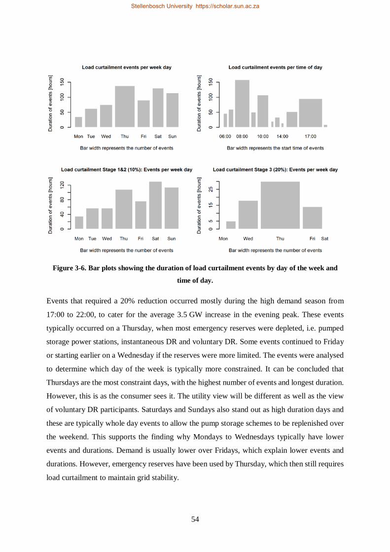
54

Figure 3-6. Bar plots showing the duration of load curtailment events by day of the week and

time of day.

Events that required a 20% reduction occurred mostly during the high demand season from

17:00 to 22:00, to cater for the average 3.5 GW increase in the evening peak. These events

typically occurred on a Thursday, when most emergency reserves were depleted, i.e. pumped

storage power stations, instantaneous DR and voluntary DR. Some events continued to Friday

or starting earlier on a Wednesday if the reserves were more limited. The events were analysed

to determine which day of the week is typically more constrained. It can be concluded that

Thursdays are the most constraint days, with the highest number of events and longest duration.

However, this is as the consumer sees it. The utility view will be different as well as the view

of voluntary DR participants. Saturdays and Sundays also stand out as high duration days and

these are typically whole day events to allow the pump storage schemes to be replenished over

the weekend. This supports the finding why Mondays to Wednesdays typically have lower

events and durations. Demand is usually lower over Fridays, which explain lower events and

durations. However, emergency reserves have been used by Thursday, which then still requires

load curtailment to maintain grid stability.


55

From this analysis, it can be said that the most load curtailment events typically occurred on

Thursdays, from 17:00 to 22:00. The other typical events took place on Saturdays and Sundays,

from 08:00 to 20:00. The majority of the events required a 10% load reduction. This scenario

makes it difficult to model due to the random nature of these events. The event may be a once

off or may last various sequential days.

3.3.4. Extreme load curtailment

This is an alternative scenario to emergency load curtailment. Instead of declaring an

emergency and requesting all consumers to curtail load, this scenario considers extreme load

curtailment from willing consumers to bare minimum load at a negotiated rate. This rate is not

to be compared with running peaking power stations, such as the OCGTs, but rather the cost of

unserved energy. This will prompt the particular consumer to negotiate a rate that will reflect

the cost of unserved energy specifically for their business. This will allow the utility to maintain

power system stability, reduce negative impacts on the economy, avoid negatively affecting

small businesses and residential consumers and maintain a good public image.

These events are expected to be for short periods, i.e. one to three days, about four times per

annum and would be events that potentially affect the entire country. It may be requested as a

result of a multiple unit trip at a power station or in future when large weather systems move

over the country that affects renewable energy generation. Another typical application will be

during natural phenomena events, such as a solar eclipse, which affect generation output for a

few hours. The effect of such an event, which occurred on 1 September 2016, on solar PV

power generation is shown in Figure 3-7. The solar eclipse affected the solar PV generation

from about 9:00 to 13:00 as compared to the previous day which was a clear sunny day.


56

Figure 3-7. Grid-connected solar PV power generation during a solar eclipse.

3.3.5. Integration of solar PV on the consumer side

Each of the above scenarios excluded the impact of integrated solar PV on the consumer side.

Higher penetration of grid-connected solar PV at a mine site creates a localised challenge for

both the mine and the utility. Thus, each scenario will be considered without and with integrated

solar PV on the consumer side.

Sudden changes in solar PV output requires the local grid to be stiff enough to supply,

potentially, enormous amounts of power in a short period. Some form of short-term storage will

be beneficial to smooth out this rapid transition, however, the power will still need to be

supplied by the grid. Electrical faults, solar PV module damage, rain and overcast days for

prolonged periods, imply that the mine will depend more on the grid to supply power, especially

if large solar PV plants are installed. This may be a challenge if the mine has expanded with the

supplemental generation provided by solar PV and now they may exceed their notified

maximum demand and incur penalties or cause an electrical trip. It implies that an additional

DR measure is needed to ensure that the internal mine grid remains balanced, as the solar

generation various across different times of the day. Thus, the utility will see the same load

profile as before as the mine has internally balanced to supply and demand.


57

4. Electricity consumption and characterisation in the coal mining industry

This chapter describes the open-pit and underground coal mining processes and identifies the

potential DRAs. Each DRA’s electrical usage is characterised as well as the resulting load

profiles for each mine, for the total grouped by the type of mining operation and for the total

sample of mines selected. An analysis is also performed on a grid connected solar PV plant that

is on the mine’s side of the grid.

4.1. Coal mining process

The environmental context for this project is focussed on the coal mining process, including

beneficiation. The mining process starts with a geological model that is based on extensive

exploration drilling data. The geological exploration data culminates in the production of a

strategic mine plan. Dependent mainly of the depth of the coal, it is decided to use the open-pit

mining method for coal that is closer to the surface or the underground mining method for coal

that is uneconomical to mine from the surface. The blocks are then prioritised based on various

factors and then scheduled for mining.

4.1.1. Open-pit mining process

The typical open-pit mining process is graphically represented in Figure 4-1. The activities

commence with the removal of topsoil (mineral-rich layer for rehabilitation) and subsoil

(weathered material), followed by pre-stripping to prepare the area for the drilling rig. This is

achieved through the use of diesel vehicles.


58

Figure 4-1. A graphical representation of the open-pit mining process [85].

Holes are then drilled to the top of coal and blasted to loosen the overburden material. The

overburden material is mechanically excavated by the dragline (electrically driven) to expose

the coal, where after the coal is drilled and blasted. The coal referred to as run-of-mine (ROM)

coal, is loaded onto trucks (diesel driven) by shovels (electric and/or diesel driven) and

transported to the plant via conveyors.

4.1.2. Underground mining process

The typical underground mining process is graphically represented in Figure 4-2. Development

typically involves sinking shafts for access and ventilation, developing the initial mining panels

and installing infrastructure and services. Large ventilation fans are installed to provide fresh

air for personnel underground, dilute flammable and noxious gases and control the temperature.


59

Figure 4-2. A graphical representation of the underground mining process [85].

The mining activities commence with the continuous miner (CM) cutting the coalface with a

rotating drum. The coal is then loaded into the back of the CM to a shuttle car or battery hauler,

which transports the coal to a feeder. The feeder roughly sizes the coal and loads it onto the

underground conveyors. The underground conveyor network transports the ROM coal out via

a shaft conveyor, typically into a surface silo. From the silo, it is then transported to the plant

via overland conveyors for processing.

4.1.3. Coal washing process

A typical coal washing plant is graphically represented in Figure 4-3. Depending on the specific

mine, the plant may or may not have a stockpile to store or stack ROM coal before it is

processed. When the coal is ready to be processed, it is reclaimed from the ROM stockpile and

fed into the plant via a series of conveyor belts. The plant typically consists of various modules

running in parallel. The ROM coal goes through washing module that contains a series of sizing

screens to separate the coal from the fine material. It then undergoes dense medium separation,

which removes contaminants, such as stones and soils, from the coal to produce a refined

saleable product. The saleable product is stacked out on a stockpile that is later reclaimed and


60

sent via conveyors to the load-out station. From here, it is loaded onto trains and/or trucks to be

dispatched to customers.

Figure 4-3. A graphical representation of the Grootegeluk coal beneficiation plant [86].

4.2. Energy risks in the coal mining industry

There are five major risks to the industry from an energy perspective, namely energy security,

the rising cost of energy, carbon tax, legal compliance and reputation. They can be summarised

as follows:

Energy security: It relates to the inability of the utility to supply electricity reliably at all

times. Possible diesel shortages, which may affect OCGTs and internal diesel emergency

generators and equipment, are also considered.

The rising cost of energy: Diesel prices are linked to the international price of oil and can

be volatile. Electricity prices have increased significantly and are set to continue to

increase above inflation for the next decade.

Carbon tax: Carbon tax is planned to be introduced in 2017. This will add additional costs

to fossil fuels based energy sources, both coal and diesel. When considering constructing

fossil fuel based DERs, this needs to be accounted for.


61

Legal compliance: Future requirements include submission of five-year energy

management and Greenhouse Gas (GHG) management plans with annual progress reports.

This includes reporting of verified energy consumption and savings as well as GHG

emissions data.

Reputation: Organisations are under more pressure, from both internal and external

stakeholders, to ensure they adequately address sustainability issues, particularly relating

to climate change. Investors are also applying pressure to see the real impacts of

sustainability projects.

4.3. Electricity consumption analysis

In this section, the scope and boundaries of the project are defined within the coal mining

industry. The DRAs characteristics together with the resulting load profiles for the mines are

discussed in detail.

4.3.1. Scope and boundaries

The boundaries for this project include six coal mining operations in the Mpumalanga province,

consisting of three open-pit mines and three underground mines. Only the direct mining

activities are included in the analysis and loads, such as villages, are excluded. The equipment,

systems or processes that contribute significantly toward power consumption are of interest for

DR activities, i.e. DRAs. A schematic representation of the included mines and DRAs are

shown in Figure 4-4. Open-pit mines are numbered from one to three, while the underground

mines are numbered from four to six. The DRAs for each mine are numbered by starting with

the mine number as the first identifier, e.g. Plant 2.1 is the plant associated with Mine 2.


62

Figure 4-4. Schematic representation of the mines included in this project including the

individual DRAs. The greyed out sections are excluded from the scope.

In open-pit mining, the DRAs are the draglines and the plants. The draglines are at the beginning

of the mining process that exposes the coal and any issue affecting the draglines may impact

the rest of the process, depending on the duration. The draglines have the advantage that they

can be stopped and started quickly.

For underground mining, the DRAs are the plants, underground (UG) sections and the

ventilation fans. The ventilation fans are critical for safety, run 24 hours a day, seven days a

week and is governed by strict regulations. The ventilation fans are not considered a curtailable

load in the coal mining context. Even on maintenance days the mines still need ventilation to

prevent the build-up of flammable gases. The underground sections are literally at the coalface,

thus any issue that causes them to stop may affect the rest of the process. UG sections 4.1 are

excluded due to their small overall impact and distributed locations.

The plants, in most instances, have some form of stockpile or buffer capacity that can be utilised,

however, the start-up and shutdown times tend to be around 30 minutes to two hours. The silos

in the process may also add some buffer capacity but not for long durations. Mine 5 has a small

integrated solar PV plant, Solar plant 5.1, that was analysed and scaled up for simulation

purposes.

4.3.2. Electrical load profiles and characterisation of consumption for the demand response assets

The initial starting point was to analyse each of the individual DRAs for each mine. The focus

is this section was on the plants, draglines and UG sections. Plant capacity does vary across the


63

mines, but the process and equipment are similar, with newer plants being more energy efficient.

The draglines are of similar capacity as well as the UG sections, only varying in the number of

sections included.

The average weekly load profile for Plant 4.2 is shown in Figure 4-5. On Mondays, Tuesdays

and Thursdays, the plant is not producing at full capacity which implies either maintenance is

being carried out on the plant modules or it is stopped due to low ROM stockpiles. The plant

completely stops on Sundays, thus resulting in a much lower baseload compared to when the

plant is not producing at full capacity. The 10th and 90th percentile graphs were overlaid on

Figure 4-5 to indicate the variation in load and it is a significant variation. There is always a

baseload present on the plant.

Figure 4-5. Average weekly load profile of Plant 4.2 for 2015.

A similar analysis was done for Dragline 1.1 as shown in Figure 4-6. The dragline operates

mostly at full load when moving overburden. It operates slightly below full load when

relocating, or walking. When maintenance is being carried out, or it is idling for short periods,

consumption ranges from 0 to 0.6 MW. The 10th and 90th percentile lines are overlaid as well

to indicate the variation. It indicated that these is a baseload when operating, but no baseload

when completely on stop.


64

Figure 4-6. The average weekly load profile of Dragline 1.1 for 2015.

The average load profile for Mine 6, including UG sections 6.1, is shown in Figure 4-8. From

the load profile, is can be shown that the mine does not produce on Sundays and morning

maintenance activities are carried out on Tuesdays and Thursdays. The baseload and most of

the load in the 10th percentile can be attributed to the main ventilation fans, Fans 6.1, that run

continually.

Figure 4-7. The average weekly load profile of Mine 6, including UG sections 6.1 for 2015.

The average load profiles provide some good information about how the plants, draglines and

UG sections typically operate. For DR, the real-time demand per hour is of greater importance


65

for the purpose of reducing demand. By analysing the demand with the aid of histograms, a

better estimate of the real-time demand can be gained.

The histogram for Plant 4.2 is shown in Figure 4-10. From this analysis, it is shown that the

average demand understates the real-time demand, which is closer to 6.25 MW, i.e. the first

mode. The histogram excludes the data for Saturdays and Sundays because the plant winds

down from Saturday afternoon. The second mode of 1.75 MW, indicates that the plant stops

regularly, mainly due to maintenance activities or low ROM stockpiles. The demand, however,

never gets to zero except for the odd electrical outage. It can also be seen from the dip in the

middle that the plant does not completely stop for maintenance. Typically, one module at a time

is stopped and the rest of the plant continues to operate. Thus, a short-term demand reduction

can realise 3 MW while a long-term demand reduction can realise 4.5 MW. Figure 4-9 shows

the histograms for all the other plants and similar bimodal distribution can be observed.

Figure 4-8. Histograms for Plant 4.2 (weekdays only) for 2015.


66

Figure 4-9. Histogram of demand for all the plants (weekdays only) for 2015.

For Dragline 1.1, the average demand again understates the real-time demand, which is closer

to 2.75 MW, as shown in Figure 4-10. The histogram indicates that there are times when the

dragline is completely switched off. Thus, the short- and long-term demand reduction for the

dragline that can be realised is 2.75 MW.


67

Figure 4-10. Histograms for Dragline 1.1 (full week) for 2015.

Only Dragline 1.1 is metered separately and it differs from Draglines 2.1, 2.2 and 2.3. For this

reason, data was analysed for draglines that are of a similar capacity to Draglines 2.1, 2.2 and

2.3 and that will be used to estimate the curtailable load, similarly to that of Dragline 1.1 above.

The results are shown in Figure 4-11 and indicate similar distributions to Dragline 1.1, with the

higher capacity draglines, Dragline 2.1 and 2.2, having a higher demand.

Figure 4-11. Histogram of demand for all the draglines (full week) for 2015.

The histograms for Mine 5 and Mine 6 are shown in Figure 4-12. It can be observed that they

have bi-modal distributions, similar to the plants. The first and the highest mode is an indication

of the baseload that is due maintenance activities. Mine 5 operates full time, with a rotating

maintenance shift compared to Mine 6 which does not produce on Sundays and does


68

maintenance at the same time. This explains the significant difference in the first mode. The

second mode occurs at maximum production for all shifts. It is important to note that these

includes the ventilations which explain the constant baseload.

Figure 4-12. Histogram of demand for all the mines (full week) for 2015.

By using the various histograms for the plants, draglines and mines, an accurate estimate can

be made of the potential demand contribution that each of the DRAs are able to provide. For

the plants and the mines, this will typically be the difference between the modes, while for the

draglines it will be the highest mode, excluding zero. Table 4-1 lists the DRAs for each mine

and indicates the estimated load that can be curtailed for each DRA. The total potential

curtailable load is 31.75 MW.


69

Table 4-1. Full curtailable load of each DRA.

Mine DRA Curtailable Load [MW] Comments

Mine 1 Plant 1.1 2.50 Individually metered. Dragline 1.1 2.75 Individually metered.

Mine 2 Plant 2.1 1.50 Individually metered. Dragline 2.1 3.00 Metered on pit feeder. Dragline 2.2 3.00 Metered on pit feeder. Dragline 2.3 2.50 Metered on pit feeder.

Mine 3 Plant 3.1 0.75 Individually metered. Mine 4 Plant 4.1 2.25 Metered with a portion of the underground workings.

Plant 4.2 4.50 Individually metered. Mine 5 UG sections 5.1 3.50 Plant is linked to underground with no buffer capacity. Mine 6 UG sections 6.1 5.50 Only underground sections with a storage silo on surface.

TOTAL 31.75

4.3.3. Electrical load profiles and characterisation of consumption for the integrated solar PV plant

Mine 5 has a 90 kWp grid connected, fixed solar PV plant, Solar plant 5.1. The solar plant feeds

in solar energy into the internal mine electrical grid to supply power to the office block. The

heat map in Figure 4-13 shows the solar energy generated in 2015. Data loss can be clearly

identified by clear green lines, e.g. during February.

Figure 4-13. Heat map of solar energy generated by Solar plant 5.1, for 2015.


70

The longer daylight hours during summer is clearly visible as well as the contraction in the

middle of the graph for winter months. During the winter months, the output is more stable,

indicated by the smoother transitions in colour, as there are clearer skies in winter. The outputs

in some of the winter days are affected by fog in the Mpumalanga area, as can be seen with

green bars for part of the morning. For the summer months, the abrupt changes in output are

also visible, as there are not many smooth transitions of colour. This is highlighted in Figure

4-14, which shows the erratic nature of solar power generated for a couple of days in January

2015. The main cause is cloud cover, generally more in the afternoons.

Figure 4-14. Solar power generated on 7, 10, 12 and 20 January 2015.

As larger solar plants get integrated into the internal mine grid, this erratic nature may present

a problem depending on the local grid availability and stability [27]. The graphs show the

integrated hourly values, which does smooth out some of the intermittency. Some form of short-

term energy storage would be preferred, especially for large systems, to reduce the spikes and

have smoother transitions. However, this kind of storage will typically be measured in minutes

to be cost effective. This may solve potential power quality problems; however significant

power output changes will still need to be addressed. The solar plant is small in comparison

with the total power requirement of the mine and thus does not have a major impact in terms of

energy reduction and maximum demand. It does, however, provide useful data on how a larger

plant will typically operate in a similar geographic location.


71

Looking closer at two days of winter solar generation, illustrated in Figure 4-15, it can be seen

that on a clear day, with clean panels, an almost perfect bell curve is generated, as is the case

on 17 June 2015. A couple of days later on 29 June 2015, the peak output is lower and the shape

is deformed. The lower out may be explained either by the solar irradiance or the cleanliness of

the panels. The deformation of the shape, from 7:00 to 11:00, is due to heavy fog on that

particular day that reflects the sun’s light. As soon as the fog lifts, the panels get the full sunlight

and start generating more energy. This is important from a DR perspective as this loss in power

will need to be catered for when the plants become larger and there are other network

constraints. The different daily output needs to be considered in terms of impact on the overall

power consumption as well as the impact of fog in winter.

Figure 4-15. Solar power generated on 17 and 29 June 2015.

Some specific examples were highlighted that need to be accounted for in future DR

programmes. To better account for these events on various days, a cluster analysis was

performed on the daily data for 2015, using the Statistica data mining software. The purpose of

the cluster analysis is to group similar energy generation days together to get a better

understanding of the pattern of generation and define typical DR events that need to be catered

for in future. The data was split into the individual days, as cases, and the hours from 5:30 to

19:30 was used as the variables. The k-means algorithm was chosen and Euclidean distances

were used. To determine the optimum number of clusters, the v-fold cross-validation algorithm

[68] was used with 50 folds, a minimum number of clusters of two, a maximum number of


72

clusters of 25 and classification error rate change of less than 1%. The optimal number of

clusters were found to be seven, as indicated in the results in Figure 4-16.

Figure 4-16. Graph indicating the cost sequence of the v-fold cross-validation algorithm to

determine the optimal number of clusters.

The sequence in which these clusters occur during the year provides some context to describe

the average generation profiles over the period. The sequence of the clusters is shown in Figure

4-17. It indicates a strong seasonal trend, with clusters 3, 5 and 7 mainly in autumn, winter and

spring and clusters 1, 2, 4 and 6 occurring in summer, autumn and spring.

Figure 4-17. The sequence of the various cluster groupings for each day in 2015.


73

The average solar generation per cluster is shown in Figure 4-18 together with the actual daily

solar generation power curves which belong to those clusters.

Figure 4-18. The average solar generation per cluster is shown in black together with the actual

daily solar generation curves that belong to that cluster.

Clusters 2 and 3 are almost perfect bell shapes with similar peak generation, however, the tails

do differ. Cluster 3 starts generating a little later and stops a little sooner than cluster 2,


74

suggesting that it is more likely generation during the winter periods. This is confirmed in

Figure 4-17 where it typically occurs in the winter but also extends towards some parts of

autumn and spring. Cluster 1 is more related to full day rain and cloud cover in the summer,

while cluster 6 is related to afternoon rain and/or cloud cover that is typically observed. Cluster

7 represents more the winter period with the narrower bell curve as well as the effect of morning

fog. The lower output may also suggest that the PV panels were perhaps covered with dust, due

to the dry winter period.

The average clustered generation profiles give valuable information on the changes that will be

required in terms of demand, while the sequence gives an indication of when the demand will

be reduced. The other factor to consider is the frequency that these clusters occur. In Figure

4-19 the frequency of days included in each cluster is presented in the bar graph. Clusters 1, 4,

5 and 7 are the most important as their lower generation will have a bigger impact on the

demand of the mine. The reduced output occurs for 156 days of the year, however, cluster 7,

which counts for 87 days, is a 16% reduction from a clear day. Clusters 1 and 5 is about a 60%

reduction in generation compared to a clear day.

Figure 4-19. Frequency per cluster of days in 2015.

4.3.4. The resulting electrical load profiles and characterisation of consumption for mines

The average demand of each mine for 2015 is shown in Figure 4-20, along with the critical

loads, i.e. the ventilation fans and a water treatment plant. It is worth to note that the general

trend is that the older the mine is, the higher the power consumption will be. This is because

when mining starts, the plants are nearby and there are short conveyors and electrical

reticulation. As mining progresses over time, the distance becomes greater and more ventilation


75

and infrastructure is required to produce similar tonnes. The overall average is just over 56 MW,

but the averages can be misleading, especially if low load factors are involved. The critical

loads run at a fairly fixed load, at 7.7 MW, thus the rest of the load is mainly variable.

Figure 4-20. Average demand per mine for the 2015 period.

Analysis of the individual average weekly load profiles of each mine, as shown in Figure 4-21,

allows characterisation of each mine. Mine 1, 2 and 3 operate 24/7 while mine 4, 5 and 6 start

to wind down on Saturday afternoons and do not produce on Sundays. This highlights the

danger of use averages, especially with low load factor mines that do not operate the entire

week. Some clear patterns emerge that highlights daily morning maintenance for the

underground mines, which is a couple of hours in duration. There are also longer maintenance

periods, which lasts until the afternoon and can generally be attributed to the plants. Most of

the maintenance occurs on Thursdays, followed closely by Tuesdays.


76

Figure 4-21. Average weekday load profiles for each mine for 2015.

4.3.5. The resulting electrical load profiles and characterisation of consumption for all the mines

The load profiles for each of the six mines were combined to produce a heat map as shown in

Figure 4-22. The heat map allows the visualisation of the hourly data for 2015 in one view. The

colour range is from green to red, which represents the total demand from low to high. The

lowest value is 17 099 kW, which indicates the minimum baseload of all the mines combined

and a maximum demand of 83 163 kW. The biggest portion of the baseload is the ventilation

fans for the three underground mines. The combined peak demand occurs mostly in the off-

peak period between 20:00 and 06:00, as indicated by the red blocks.


77

Figure 4-22. Total demand for all six mines for 2015 represented in a heat map.

The green stripes that stand out indicate the days when the demand was at baseload levels.

These are mostly on public holidays, as is the case at the beginning of January and during April.

In October, there is a band of green for 10 days and this was due to industrial action that affected

all the mines. This indicates the baseload requirement in terms of health and safety due to

ventilating underground mines, pumping water and general lighting.

There appears to be a general pattern that emerges. Demand is high from 00:00 to 06:00, then

there is a reduction between 06:00 and 09:00. The demand appears to pick-up from 09:00, but

not reaching maximum levels in most cases. After 20:00, the demand is mostly at maximum

until 23:00. The 06:00 to 09:00 period is typically maintenance time for most mines, which

explains the significantly lower demand. The maximum demand, indicated by the bright red

colour, appears to have reduced slightly from the end of March. The rest of the year’s maximum

demand is less than it was in the first quarter of 2015, indicated by the dimmer red colour April

onwards. This was mainly due to slightly lower production volumes from most of the mines.

The critical loads for the six mines are mostly ventilation fans as well as a water treatment plant

that runs the whole year. From the heat map in Figure 4-23, it can be seen that the critical loads

consume a fixed amount of baseload power, due to the fairly constant red colour. Critical loads

are just over 9 MW. From Figure 4-22, the baseload was about 17 MW of which 9 MW can be

attributed to metered critical loads. That leaves another baseload component of about 8 MW.

This is expected to consist of loads such as pumping, auxiliary fans, lighting and office blocks.


78

Figure 4-23. Total critical load demand for all six mines for 2015 represented in a heat map.

The average weekly load profile for 2015 is shown in Figure 4-24, together with the critical

loads. The 10th and 90th percentile lines are also overlaid to give an indication of the variation

in load.

Figure 4-24. Average weekday load profile for the six mines including the critical loads.


79

The low load factor for the coal mines is in contrast with the deep level gold and platinum mines,

which usually have a high load factor due to high baseload equipment. This implies that a

significant portion of the electricity usage is linked to production as the main driver. Seeing that

there are not any refrigeration plants or heat involved in the processes, the temperature will not

be a significant driver of electricity usage.

A weekday pattern emerges which varies in intensity. As from the heat map in Figure 4-22, the

change in demand can be observed when the morning maintenance period commences, with

changes of 10 to 20 MW during this period. After the maintenance period, there is a gradual

increase in demand throughout the day. Demand tapers down on Saturday and appears relatively

constant on Sundays, which is due to the shift patterns at some of the mines, as mentioned.

4.4. Electricity costs for the mines

An important aspect of DR is the current and projected electricity prices. This will impact

voluntary participation programmes, tariff based signals as well as if one wishes to implement

DERs on-site to counter the current electricity price. However, from a business aspect, the other

costs in the business also need to be considered, such as labour and raw materials. That may

mean that a mine will rather produce in a peak tariff period than reduce demand if the overall

benefit favours that scenario.

The average electricity costs per year for the six mines was analysed and compared with the

mining industry average [16] and shown in Figure 4-25. The historic costs indicate that the

cost for the six mines is 25.5% higher than the mining industry average. This is probably due

to their lower load factors, their demand ramping up through the evening peak, as evident in

the load profiles, and minimal load shifting initiatives as compared to deep-level mines.

Forecasted prices are based on industry projections, the growth of the economy and the need to

get to cost reflective tariffs within five years. The future projections provide a view to helping

structure DR incentives and assist in compiling a cost-benefit analysis.


80

Figure 4-25. Average annual historic and forecasted electricity pricing.

4.5. Demand response initiatives in the coal mining industry

The current DR initiatives that are implemented for the six mines are discussed in this section.

4.5.1. Tariff based demand response initiatives

The “beat the peak” initiative aims to reduce the cost of the winter peak tariff rates, i.e. the high

demand season based on a tariff pricing signal. The mines are on the utilities’ MegaFlex tariff.

The tariff rate in the high demand season peak is about 2.8 times more than low season. Figure

4-26 indicates that the average normalised cost for electricity is 47% more in the high demand

season. The energy consumption is relatively constant, with the impact of the holidays in

January, April and December being visible as well as the industrial action in October. The

energy consumption is higher during the high demand season. From an open-pit mine

perspective, there is no or minimal rain that effects operations in the pit during winter and from

an underground perspective, there are no or minimal lightning events during winter. It may also

be an indication of an organisational cycle, which is a consequence of production pressure, to

ensure annual business plan production volumes can be met. It can be stated that the mines

minimally respond to the DR tariff signal and does not reduce peak demand significantly.


81

Figure 4-26. The normalised cost of electricity versus consumption for 2015 with the high

demand season highlighted.

Mine 4 has responded to the DR tariff signal in 2015 with the aim to reduce electricity costs.

Plant 4.2, in particular, managed to save 14.6% in 2015 by running the plant optimally. Figure

4-27 breaks down the various components of the saving of that plant. It included an energy

saving intervention as well as a DR initiative.

Figure 4-27. Energy cost saving estimation for responding to the DR pricing signal for Plant 4.2

during the high demand season in 2015.

The cost associated with DR was conservatively estimated to be 4.5% for the three months. The

plant’s capacity exceeded the ROM coal coming from the underground sections. A decision


82

was made to stop the plant and build the ROM stockpile. The plant would run as soon as a

significant ROM stockpile was available to ensure the plant can operate at full capacity for an

extended period and avoided the peak periods when possible.

4.5.2. Emergency load curtailment

The load curtailment events are visualised in Figure 4-28, which excludes load shedding events,

although they do overlap most of the time. A clear pattern emerges that is tied back to the typical

national load profiles in Figure 2-4. During the summer months, the event period matched

closely with the flatter profile and during winter the event period was matched to the high

evening peak.

Figure 4-28. Heat map of load curtailment events for 2015.

0% 10% 20%


83

5. Develop regression models for demand response assets

The purpose of this chapter is to develop regression models for the DRAs to predict their

electrical demand based on their production. This enables the characterisation of these DRAs

by building more detailed models [2]. Only daily production values and the direct operating

hours are available. This will be used to calculate an average tonne per hour value for each day

and then matched to the hourly electricity consumption.

5.1. Methodology used for the regression analysis

The initial step in the regression analysis process is to prepare the raw data for analysis. The

data preparation process is shown in Figure 5-1. The electricity data is captured at half-hourly

intervals, aligned with the utilities’ billing intervals, while the production data is captured daily.

The electricity half hours needed to be rolled up into daily values, taking into consideration

when the daily production values are captured. That is, some mines measure production from

21:00 the previous day to 21:00 the current day. The data was also combined in one file from

two SQL server databases.

Figure 5-1. Data preparation flow diagram to prepare raw data for regression analysis.

The statistical software, R, was used to perform the regression analysis. The regression analysis

flow diagram is in Figure 5-2, as adapted from [62], describes the process flow for the

regression analysis R script.

START

Load electricity

data

Define production days

30 minute electricity data for SQL server

END

Roll up electricity data to daily

values

Load production

data

Daily production data from SQL

server

Combine data

Store data to file

Store data in CSV file


84

Figure 5-2. Regression analysis flow diagram that is used for modelling of DRAs.

The methodology used to in the regression analysis is summarised as follows:

Step 1. The objective for each regression is stated and relevant variables are identified. The

available data is collected and placed into comma separated files for analysis in R, as shown in

Figure 5-1.

Step 2. An initial scatter plot analysis is performed on the data set. A loess model plot is fitted

together with a linear model for reference. A 2D-contour plot is overlaid to show the density of

the data points. Possible outliers are identified based on standardised residuals greater than the

absolute number of two and the standardised residuals are plotted.

Step 3. The possible outliers are investigated and omitted if there is a sound reason to do so.

The reasons for removal of outliers is recorded in the data file. Another scatterplot analysis is

performed with both loess and linear methods. A histogram is produced if the 2D-contour plots

START

Load prepared

data

Define variables and functions

Prepared data from CSV file

Store model parameters


END

Initial scatter plot analysis

Initial standardised residual plot

Investigate and remove outliers

Split data into respective groupings

Store residuals

output

Store output in CSV file

Record reasons for

outliers

Revised scatter plot analysisHistogram of data

Normal distribution?

Perform scatter plot analysis

Fit appropriate model

Review diagnostic plots

Acceptable diagnostics?

NO

YES

YES NO


85

show distinct groupings. Further data analysis is performed to identify the different factors if

the distribution is not normal.

Step 4. Once the data analysis is complete, an appropriate model is then fitted, informed by the

loess model, and the parameters recorded. The R2 values are checked as well as the Significance

of F, for the regression model. The p-values for the independent variables are checked to be

significant. The model uncertainty is quantified and recorded. A full set of diagnostic plots is

generated which include residuals versus fitted values, normal Q-Q, scale location and residuals

versus fitted.

Step 5. Based on the diagnostic plots from step 4, the models are accepted if it satisfies the

requirements. If there are data points that do not fall within the requirements, they are further

investigated and removed if appropriate. The final scatter plots are then generated, along with

their diagnostics plots, and the final parameters recorded.

5.2. Model used for the regression analysis

For all the regression models that will follow, a second order polynomial was found to provide

the best fit for the data sets. The rationale will be discussed in the sections that will follow. It is

important to note that the model is only representative within the bounds of the sampled data

set. The generalised regression equation is:

𝑦𝑦 = 𝑎𝑎 + 𝑏𝑏.𝑥𝑥 + 𝑐𝑐.𝑥𝑥2 (5.1)

where y is the predicted energy consumption in kWh, x the production tonnes and a, b and c the

regression coefficients.

5.3. Regression analysis for the plants

Following the methodology in section 5.1, the initial scatter plots were constructed for the plants,

as indicated in Figure 5-3 and Figure 5-4. From this initial analysis, it can be seen that linear

models, the blue lines, do not describe the relationship between energy consumption and

production adequately. The loess models, the red lines, tend not to be close to a linear line. The

2D-contour plots indicate the density of the data points while the red points indicate possible

outliers, based on the loess models.


86

Figure 5-3. Initial scatter plot analysis for Plant 4.1 identifying possible outliers based on the

loess model.

Figure 5-4. Initial scatter plot analysis for Plants 1.1, 2.1, 3.1 and 4.2 identifying possible outliers

based on the loess model.

The standardised residuals for each plant are shown in Figure 5-5, based on the loess model.

All residuals greater than +2 or -2 were highlighted to indicate that these may be possible


87

outliers that need to be investigated. Some of the other possible outliers were not picked up in

the residual plots. One such example is when there are zero production and zero energy

consumption. This cannot be as there is always a baseload present for the plants, which is

typically at least lighting loads, offices and the control room, as indicated in the histograms in

Figure 4-9. The only way for electricity consumption to be zero is if there is a power outage for

the whole day or if metering data is missing.

Figure 5-5. Initial standardised residual plots for the plants identifying possible outliers based on

the loess model.

Another example is the two outliers in Figure 5-4 for Plant 2.1, which are almost double the

maximum production. They were not picked up by the residual plot as the loess model was


88

fitted through those points. On closer inspection, is was found that the production data for those

two days were captured twice, in different fields. When the data was retrieved, the sum of the

two was taken, where normally only one field is used to capture production data.

The other possible outliers were investigated and the majority of them were confirmed to be

outliers. One common cause was that production data for certain days was not captured, leading

to high energy consumption with zero production, as shown in Figure 5-4 for Plant 4.2 and

Plant 2.1. The second most common cause was metering errors, mainly for Plant 3.1 in Figure

5-4, where abnormally high energy consumption was recorded for a couple of consecutive days.

The cause was a change at the substation when new current transformers were installed.

Another minor cause was missing metering data, either for the whole day or a significant part

of the day.

After the possible outliers had been investigated, they were either removed or corrected as

appropriate. Another scatter plot analysis was performed to confirm the use of non-linear

models. On visual inspection, there are more outliers that were not corrected or removed from

the previous analysis. There also still exist two distinct groupings based on the 2D-contour

diagrams. There appear to be two different populations in the data set, one for the non-

productive period, i.e. when there is zero production, and the productive period which

represents the entire range of production. The data was split into these two groupings and

histograms were constructed, as shown in Figure 5-6.

The histogram plots in Figure 5-6, matches with the bi-modal distribution observed in Figure

4-9. The data can now be separated into the two distinct groupings for further analysis. These

simple histogram plots reveal various opportunities for improvement in operational control,

which will lead to improvement in energy performance. The non-productive period indicates a

relatively wide distribution of energy consumption when there is no production, which would

be good to investigate to reduce demand and energy consumption during these periods. For the

productive period, the operating range for each plant can be observed. From a production and

energy efficiency point of view, the productive period histogram should resemble more closely

to that of Plant 4.1, 1.1 and 3.1, i.e. negatively skewed distributions. That will maximise

production and ensure the plant is run at its best efficiency point, i.e. rated capacity. Several

factors may influence this requirement of a negatively skewed distribution and may result in a

more normal distribution such as Plant 4.2 and 2.1. For example, if there is not enough


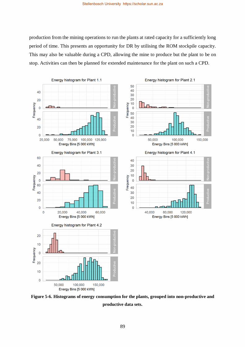
89

production from the mining operations to run the plants at rated capacity for a sufficiently long

period of time. This presents an opportunity for DR by utilising the ROM stockpile capacity.

This may also be valuable during a CPD, allowing the mine to produce but the plant to be on

stop. Activities can then be planned for extended maintenance for the plant on such a CPD.

Figure 5-6. Histograms of energy consumption for the plants, grouped into non-productive and

productive data sets.


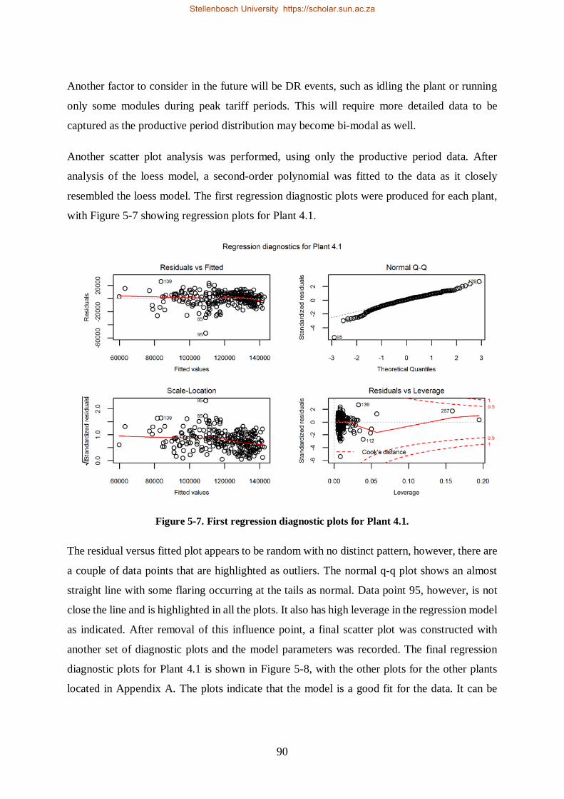
90

Another factor to consider in the future will be DR events, such as idling the plant or running

only some modules during peak tariff periods. This will require more detailed data to be

captured as the productive period distribution may become bi-modal as well.

Another scatter plot analysis was performed, using only the productive period data. After

analysis of the loess model, a second-order polynomial was fitted to the data as it closely

resembled the loess model. The first regression diagnostic plots were produced for each plant,

with Figure 5-7 showing regression plots for Plant 4.1.

Figure 5-7. First regression diagnostic plots for Plant 4.1.

The residual versus fitted plot appears to be random with no distinct pattern, however, there are

a couple of data points that are highlighted as outliers. The normal q-q plot shows an almost

straight line with some flaring occurring at the tails as normal. Data point 95, however, is not

close the line and is highlighted in all the plots. It also has high leverage in the regression model

as indicated. After removal of this influence point, a final scatter plot was constructed with

another set of diagnostic plots and the model parameters was recorded. The final regression

diagnostic plots for Plant 4.1 is shown in Figure 5-8, with the other plots for the other plants

located in Appendix A. The plots indicate that the model is a good fit for the data. It can be


91

further improved by gathering more detailed data, however, it will make the model more

complicated. For this analysis, it is deemed sufficient.

Figure 5-8. Final regression diagnostic plots for Plant 4.1.

The final scatter plots are shown in Figure 5-9, with the blue lines indicating the linear model,

the red lines the loess model and the green lines the fitted model.


92

Figure 5-9. Final regression models after removal of outliers for the plants.

The model parameters are shown in Table 5-1 for the productive period for plants and all

coefficients were found to be significant, i.e. all coefficients had a p-value < 0.01. The

parameters for the non-productive period is shown in Table 5-2.


93

Table 5-1. Regression model parameters for the productive period for the plants.

Parameters Plant 1.1 Plant 2.1 Plant 3.1 Plant 4.1 Plant 4.2

a 52 406.52*** 57 476.86*** 23 094.08*** 51 906.08*** 53 715.87***

b 5.64*** 6.05*** 3.05*** 6.58*** 8.92***

c -0.000110*** -0.000150*** -0.000066*** -0.000107*** -0.000193***

Observations 342 291 272 270 272

R-square 0.78 0.57 0.83 0.74 0.83

Residual Standard Error

7 385.53 10 640.30 4 153.49 9 225.60 9 292.91

F Statistic 599.55*** 192.25*** 637.82*** 375.96*** 667.46***

Note: Significance at p = 0.1, p = 0.05 and p = 0.01 are denoted by '*', '**' and '***' respectively.

Table 5-2. Regression model parameters for the non-productive period for the plants.

Parameters Plant 1.1 Plant 2.1 Plant 3.1 Plant 4.1 Plant 4.2

Mean 37 816.04 39 273.05 20 111.87 27 524.84 38 421.03

Median 36 595.00 30 713.75 20 669.00 25 802.00 38 667.50

Mode 49 161.50 26 303.00 5 553.00 18 699.50 42 912.50

Observations 13 50 62 64 77

Standard Error 5 714.32 17 513.55 6 585.43 6 118.36 7 390.18

5.4. Regression analysis for the draglines

The analysis for the draglines, shown in Figure 5-10, shows similarly to the plants that a linear

model, the blue lines, do not describe the relationship between energy consumption and

production adequately. Note that the analysis for Dragline 2.1 is identical to Dragline 2.2, as

they use the same data set, but it is included for completeness. The scatter plots indicate a wide

range of variation around the regression line.


94

Figure 5-10. Initial scatter plot analysis for the draglines identifying possible outliers based on

the loess model.

The standardised residuals for each dragline are shown in Figure 5-11, based on the loess model.


outliers that need to be investigated. It was a bit of a challenge to determine outliers for the

draglines as they do tend to “walk” or relocate from time to time, which implies that energy

consumption may be more than normal for a particular production volume. Data for the

relocation activities were not readably available. However, the major factor will be based on

production volumes.

An example of possible outliers are when there is zero production, the energy consumption

ranges from zero to a significant amount of energy consumption. When the dragline is switched

off, it can consume zero energy, however, if it is idling there may be a small amount of energy

being consumed. The larger values may indicate longer relocation activities or days when the

production tonnages were not recorded. The possible outliers were investigated and the

minority of them could be confirmed to be outliers. These were mainly confirmed metering

errors and days when the production was not captured correctly.


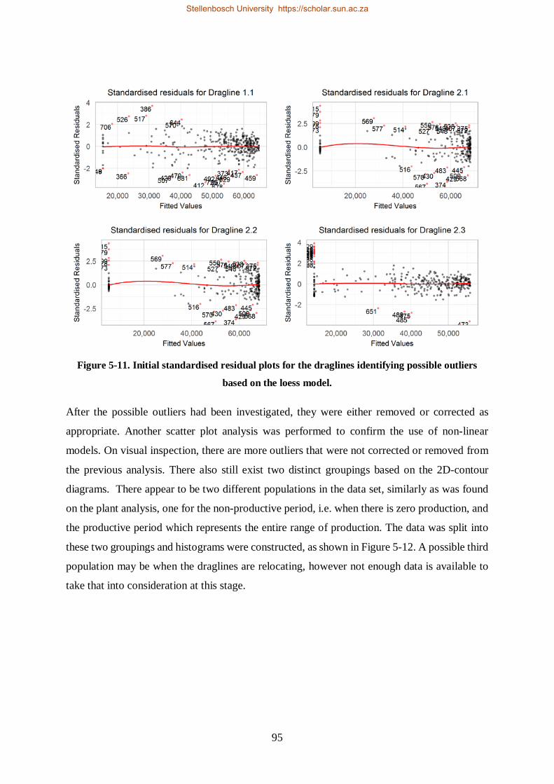
95

Figure 5-11. Initial standardised residual plots for the draglines identifying possible outliers

based on the loess model.





diagrams. There appear to be two different populations in the data set, similarly as was found

on the plant analysis, one for the non-productive period, i.e. when there is zero production, and

the productive period which represents the entire range of production. The data was split into

these two groupings and histograms were constructed, as shown in Figure 5-12. A possible third

population may be when the draglines are relocating, however not enough data is available to

take that into consideration at this stage.


96

Figure 5-12. Histograms of energy consumption for the draglines, grouped into non-productive

and productive data sets.

The histogram plots in Figure 5-12, matches with the bi-modal distribution observed in Figure

4-11. The data can now be separated into the two distinct groupings for further analysis. These

simple histogram plots reveal various opportunities for improvement in operational control,

which will lead to improvement in energy performance. Particularly the non-productive period

of Dragline 2.1, indicates a relatively high energy consumption in the second bin. This may be

due to the dragline idling for extended periods or excessive relocations, but will need the be

investigated further. For the productive period, a negatively skewed distribution is preferred to

maximise efficiency, such as is the case for Dragline 1.1. The wider distributions for Draglines

2.1, 2.2 and 2.3 probably include more relocation activities.

The opportunity for DR is relatively limited as the draglines can either be on or off, however,

this has a direct impact on the production process as the draglines remove the overburden before

the coal can be mined. This may be useful to exploit on a CPD depending on production


97

planning, but load shifting during the TOU peak periods may be more viable as they are for

shorter durations.

Another scatter plot analysis was performed, using only the productive period data. After

analysis of the loess model, a second-order polynomial was fitted to the data as it closely

resembled the loess model. The first regression diagnostic plots were produced for each dragline,

with Figure 5-13 showing regression plots for Dragline 1.1.

Figure 5-13. First regression diagnostic plots for Dragline 1.1.


a couple of data points that are highlighted as outliers. The normal q-q plot shows an almost

straight line with some flaring occurring at the tails as normal. However, the low tail does vary

significantly from the straight line. Most of the data points that were identified are related to

the lower tail. After removal of some of the justified influence points, a final scatter plot was

constructed with another set of diagnostic plots and the model parameters was recorded. The

final regression diagnostic plots for Dragline 1.1 is shown in Figure 5-14, with the other plots

for the other draglines located in Appendix A. The plots indicate that the model is a fairly good

fit for the data, except for the lower tail indicated in the normal q-q plot. For this analysis, it is

deemed sufficient.


98

Figure 5-14. Final regression diagnostic plots for Dragline 1.1.




99

Figure 5-15. Final regression models after removal of outliers for the draglines.




Table 5-3. Regression model parameters for the productive period for the draglines.

Parameters Dragline 1.1 Dragline 2.1 Dragline 2.2 Dragline 2.3

a 14 276.06*** -979.78 -979.78 12 160.19***

b 1.79*** 3.04*** 3.04*** 1.30***

c -0.000016*** -0.000033*** -0.000033*** -0.000010***

Observations 350 204 204 293

R-square 0.63 0.47 0.47 0.74

Residual Std. Error 7 431.70 8 712.64 8 712.64 7 492.72

F Statistic 301.29*** 88.85*** 88.85*** 420.13***



100

Table 5-4. Regression model parameters for the non-productive period for the draglines.

Parameters Dragline 1.1 Dragline 2.1 Dragline 2.2 Dragline 2.3

Mean 13 252.21 5 064.00 5 064.00 4 763.19

Median 16 344.75 4 275.00 4 275.00 2 002.50

Mode - 4 044.00 4 044.00 17 936.50

Observations 12 156 156 50

Standard Error 8 357.43 4 684.51 4 684.51 7 429.13

5.5. Regression analysis for the underground sections

For the analysis of the two mines’ underground sections, the total energy consumed versus total

production was used as detailed sub-metering was not available per section. The process flow

for these mines also allowed for it, as they have no significant storage or stockpiles between the

mining and plant activities. The scatter plot analysis for the two underground sections is shown

in Figure 5-16 and it shows that a linear model, the blue lines, appears to almost describe the

relationship between energy consumption and production adequately. However, when

compared with the loess models, the red lines, the ends tend to change the model to be non-

linear.

Figure 5-16. Initial scatter plot analysis for the underground sections 5.1 and 6.1 identifying

possible outliers based on the loess model.

The standardised residuals for each mine are shown in Figure 5-17, based on the loess model.


outliers that need to be investigated. Again, some of the outliers at zero production may have

been missed as the ventilation fans run continuously and do consume a significant amount of

baseload energy. This typically indicates days were metering data was missing.


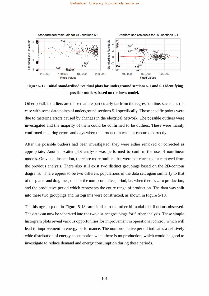
101

Figure 5-17. Initial standardised residual plots for underground sections 5.1 and 6.1 identifying

possible outliers based on the loess model.

Other possible outliers are those that are particularly far from the regression line, such as is the

case with some data points of underground sections 5.1 specifically. Those specific points were

due to metering errors caused by changes in the electrical network. The possible outliers were

investigated and the majority of them could be confirmed to be outliers. These were mainly

confirmed metering errors and days when the production was not captured correctly.





diagrams. There appear to be two different populations in the data set, again similarly to that

of the plants and draglines, one for the non-productive period, i.e. when there is zero production,

and the productive period which represents the entire range of production. The data was split

into these two groupings and histograms were constructed, as shown in Figure 5-18.

The histogram plots in Figure 5-18, are similar to the other bi-modal distributions observed.

The data can now be separated into the two distinct groupings for further analysis. These simple

histogram plots reveal various opportunities for improvement in operational control, which will

lead to improvement in energy performance. The non-productive period indicates a relatively

wide distribution of energy consumption when there is no production, which would be good to

investigate to reduce demand and energy consumption during these periods.


102

Figure 5-18. Histograms of energy consumption for the underground sections, grouped into non-

productive and productive data sets.

For the productive period, the operating range for each mine can be observed. From a

production and energy efficiency point of view, the productive period histogram should

resemble a more negatively skewed distribution, rather than the almost normal distributions

observed. Various factors may influence this requirement of a negatively skewed distribution.

For example, these two mines have various underground sections which contribute to the

overall production and energy consumption and thus, describes the normal distributions that are

observed. Never the less, this may be a significant opportunity.

This presents an opportunity for DR as well, as some sections can be stopped to reduce demand,

however, this has a direct impact on the production process. The first buffer capacity is the silo

on the surface, but this is limited in terms of capacity. This will not be useful to exploit on a

CPD, but rather for load shifting during the TOU peak periods. Another scatter plot analysis

was performed, using only the productive period data. After analysis of the loess model, a

second-order polynomial was fitted to the data as it closely resembled the loess model. The first

regression diagnostic plots were produced for each mine, with Figure 5-19 showing regression

plots for underground sections 6.1.


103

Figure 5-19. First regression diagnostic plots for the underground sections 6.1.


a couple of data points that are highlighted. The normal q-q plot shows an almost straight line

with some flaring occurring at the tails as normal. The data point with the highest leverage was

the day that record production was recorded. This point was not removed as it forms part of the

data set.

The final scatter plot was constructed with another set of diagnostic plots and the model

parameters were recorded. The final regression diagnostic plots for underground sections 6.1 is

shown in Figure 5-20, with the other plots for the other mine is located in Appendix A. The

plots indicate that the model is a good fit for the data. It can be further improved by gathering

more detailed data, however, it will make the model more complicated. For this analysis, it is

deemed sufficient.


104

Figure 5-20. Final regression diagnostic plots for the underground sections 6.1.



Figure 5-21. Final regression models after removal of outliers for the underground sections 5.1

and 6.1.





105

Table 5-5. Regression model parameters for the productive period for the underground

sections.

Parameters UG sections 5.1 UG sections 6.1

a 127 191.84*** 97 177.28***

b 5.76*** 4.59***

c -0.000117*** -0.000028***

Observations 283 266

R-square 0.52 0.85

Residual Std. Error 11 715.17 9 378.61

F Statistic 150.70*** 744.81***


Table 5-6. Regression model parameters for the non-productive period for the

underground sections.

Parameters UG sections 5.1 UG sections 6.1

Mean 136 405.78 76 201.24

Median 139 759.42 76 768.00

Mode 100 914.36 61 626.00

Observations 59 83

Standard Error 17 571.92 8 532.51

5.6. Recommendations for improving the regression models

In this chapter, regression models were developed to predict daily energy consumption, given

a specific level of production, for the five plants, four draglines and two underground sections.

To further improve the accuracy of all the regression models, hourly data should be used to

develop the models. For the draglines, more data needs to be collected about the relocation

activities and included as an additional relevant variable. For the underground sections, sub-

metering is recommended to isolate those DRAs for analysis.


106

6. Develop and simulate a scheduling program

The purpose of this chapter is to develop a scheduling simulation program for production. The

various DR scenarios, from chapter 3, are used as constraints to production scheduling, first

individually and then combined. The regression models, from chapter 5, are used to estimate

the electrical load based on production. The estimated electrical load profile is then compared

with the base case load profile to determine the DR impact. The energy costs, production

volumes and incentives are quantified for each simulation.

6.1. Purpose of the scheduling program

A linear programming approach was taken to schedule production. The benefits of linear

programming lie in the scalability and efficiency in finding optimal solutions, which enables it

to be used for online applications [26]. Linear programming was applied to a surface coal mine

in China to maximise profits by optimising production [87]. Most of the factors for coal

production can be based on linear models or can be transformed into linear models [87].

Linear programming is similarly applied for the scheduling program to produce an hourly

production plan for each of the DRAs that satisfies the objective function to reduce electricity

costs as well as taking into consideration various operational and energy constraints. A similar

optimisation problem was simulated to model DR and distributed generation, but from the point

of view to minimise the costs on the distribution side [53]. Once the production volumes have

been established, these are plugged into the regression models to predict the estimated energy

(or power) consumption for that hour. These, in turn, gets plugged into the TOU costing model

to determine the predicted energy costs.

The scheduling program produces an hourly production schedule, on a monthly basis, i.e. a

defined time horizon. The schedule is flexible as the model can be re-run, however practically,

the time horizon may be fixed from one to two weeks to allow scheduling of business resources

[53]. There is also a risk that production targets may not be met for the month if significant

operational or energy constraints are included. The statistical software, R, was used to

implement the scheduling program.


107

6.2. Setting up a linear programming model

The sections that follow describe the definition of the linear programming problem including

the objective functions, operating constraints and energy constraints.

6.2.1. Defining the objective functions

The purpose of this DR programme is to ensure production targets are met, electricity costs are

kept as low as possible and other constraints can be accommodated. The objective function for

this optimisation problem is to minimise the cost of electrical energy for all the DRAs. Thus,

the TOU unit electricity cost, for each hour, forms part of the objective function taking into

account the low and high seasons, weekends and public holidays. A TOU model was developed

for 2015 to address all the requirements mentioned and only considers energy-related costs, e.g.

TOU rates and subsidies. An alternative objective function is based on the CPD pricing of

electricity. The 20 CPDs were selected based on the days in the year with the highest electricity

for simulation purposes.

The process to define the objective functions are shown in the flow diagram in Figure 6-1. The

dates and times were split into their components to allow them to be matched with the lookup

tables for the various components. Public holidays were classified either as Saturdays or Sunday,

according to the utility tariff guide for 2015.

Figure 6-1. Flow diagram describing how the objective functions were defined.

Define hourly date and times

Separate date and time fields into components

Add lookup table for tariff period

Write data to file


START

END

Add lookup table for seasonality

Add lookup table for public holidays

Add lookup table for TOU periods

for MegaFlex

Add lookup table for TOU costs for MegaFlex


for CPD


for CPD

Define 20 CPDs


108

The objective functions are mathematically described in this section and the operational and

energy constraints in the following two sections. The symbols and description used in the

equations are listed in Table 6-1 with the corresponding units.

Table 6-1. List of symbols and descriptions for linear programming equations.

Symbol Description Symbol Description

ECM Energy Cost for MegaFlex [ZAR] j DRA

ECC Energy Cost for CPD [ZAR] n number of DRAs

TM TOU rate for MegaFlex [ZAR/kWh] PM Monthly production target [tonnes]

TC TOU rate for CPD [ZAR/kWh] EL Energy Limit [kWh]

ER Energy Rate of DRA [kWh/tonne] i hours

PR Production Rate [tonne/hour] mh hours in the month

To include all 11 DRAs in the optimisation problem, the objective functions needed to be

serialised for the month. That means the first set of hourly production rates (𝑃𝑃𝑆𝑆𝑖𝑖+(𝑗𝑗−1)×𝑚𝑚ℎ) are

related to the energy consumption rate (𝑆𝑆𝑆𝑆𝑗𝑗) of the first DRA (j=1), at the TOU pricing for

MegaFlex (𝑆𝑆𝑀𝑀𝑖𝑖) for that hour (i). The second set of hourly production rates (𝑃𝑃𝑆𝑆𝑖𝑖+(𝑗𝑗−1)×𝑚𝑚ℎ), in

the same equation, are related to energy consumption rate (𝑆𝑆𝑆𝑆𝑗𝑗) of the second DRA (j=2), but

at the same TOU pricing rate for MegaFlex (𝑆𝑆𝑀𝑀𝑖𝑖 ) for that hour (i). Mathematically, the

objective function for the MegaFlex tariff can be defined as:

𝑚𝑚𝐶𝐶𝑎𝑎𝐶𝐶𝑚𝑚𝐶𝐶𝑠𝑠𝑒𝑒 𝑆𝑆𝐶𝐶𝑀𝑀 = ��𝑆𝑆𝑀𝑀𝑖𝑖 ×𝑆𝑆𝑆𝑆𝑗𝑗 ×𝑃𝑃𝑆𝑆𝑖𝑖+(𝑗𝑗−1)×𝑚𝑚ℎ

𝑚𝑚ℎ

𝑖𝑖=1

� 𝑛𝑛

𝑗𝑗=1

(6.1)

The objective function for the CPD tariff is similarly defined, only changing the applicable

TOU pricing rate (𝑆𝑆𝐶𝐶𝑖𝑖) for CPDs and non-CPDs, as follows:

𝑚𝑚𝐶𝐶𝑎𝑎𝐶𝐶𝑚𝑚𝐶𝐶𝑠𝑠𝑒𝑒 𝑆𝑆𝐶𝐶𝐶𝐶 = ��𝑆𝑆𝐶𝐶𝑖𝑖 ×𝑆𝑆𝑆𝑆𝑗𝑗 ×𝑃𝑃𝑆𝑆𝑖𝑖+(𝑗𝑗−1)×𝑚𝑚ℎ

𝑚𝑚ℎ

𝑖𝑖=1

� 𝑛𝑛

𝑗𝑗=1

(6.2)


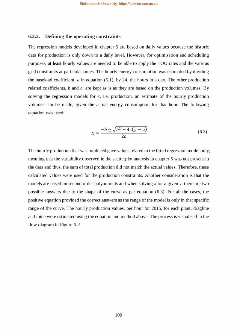
109

6.2.2. Defining the operating constraints

The regression models developed in chapter 5 are based on daily values because the historic

data for production is only down to a daily level. However, for optimisation and scheduling

purposes, at least hourly values are needed to be able to apply the TOU rates and the various

grid constraints at particular times. The hourly energy consumption was estimated by dividing

the baseload coefficient, a in equation (5.1), by 24, the hours in a day. The other production

related coefficients, b and c, are kept as is as they are based on the production volumes. By

solving the regression models for x, i.e. production, an estimate of the hourly production

volumes can be made, given the actual energy consumption for that hour. The following

equation was used:

𝑥𝑥 =−𝑏𝑏 ± �𝑏𝑏2 + 4𝑐𝑐(𝑦𝑦 − 𝑎𝑎)

2𝑐𝑐 (6.3)

The hourly production that was produced gave values related to the fitted regression model only,

meaning that the variability observed in the scatterplot analysis in chapter 5 was not present in

the data and thus, the sum of total production did not match the actual values. Therefore, these

calculated values were used for the production constraints. Another consideration is that the

models are based on second order polynomials and when solving x for a given y, there are two

possible answers due to the shape of the curve as per equation (6.3). For all the cases, the

positive equation provided the correct answers as the range of the model is only in that specific

range of the curve. The hourly production values, per hour for 2015, for each plant, dragline

and mine were estimated using the equation and method above. The process is visualised in the

flow diagram in Figure 6-2.


110

Figure 6-2. Flow diagram describing how the operational constraints were defined.

The output was used to estimate the hourly production profile to determine the maximum

average hourly production rate. The average of the largest 300 data points, for each of the DRAs,

were used and is indicated in Table 6-2. This maximum hourly production rate was the first

operating constraint to be included as the DRAs cannot produce more than this rate of

production in a given hour. It is set up as an integer constraint with values from zero to the

maximum hourly production rate for that particular DRA.

Table 6-2. Estimated maximum average hourly production rates.

DRA Maximum production rate [tonnes/hour] DRA Maximum production rate

[tonnes/hour]

Plant 1.1 585 Dragline 1.1 1 457




Plant 4.2 476 UG sections 5.1 1 022

UG sections 6.1 975 Additionally, the running hours of each DRA were also determined for 2015. The times the

DRAs were not producing include times such as maintenance, breakdowns and holidays. This

data is used as a simple binary constraint, which indicates if production is possible for that

Load raw electricity

data

30 minute data in SQL server

Add separate date and time fields

Roll up data to hourly demand

values

Apply formula to estimate hourly

production

Is production > 0?

Set production value zero

Write data to file


START

END

Set production value estimate

YES

NO

Set binary value for production

hours


111

particular hour (1) or if no production is possible for that hour (0). The final operating constraint

is a sum total of production per DRA that needs to be greater or equal to the total production of

2015. The purpose is the ensure that at least the same amount of production is achieved in each

month. It can be slightly greater but needs to remain within the production plan. This was also

limited by the objective functions, which aimed to minimise electricity costs and thus opted to

produce the minimum production volumes. In future, the budgeted production figures for the

year can be used.

The monthly operational constraints are defined as the sum of each of the hourly production

rates for the month (𝑃𝑃𝑆𝑆𝑖𝑖+(𝑗𝑗−1)×𝑚𝑚ℎ), for a particular DRA (j), that must be greater or equal to

the monthly production volumes (𝑃𝑃𝑀𝑀𝑗𝑗). In is described mathematically as:

��𝑃𝑃𝑆𝑆𝑖𝑖+(𝑗𝑗−1)×𝑚𝑚ℎ

𝑚𝑚ℎ

𝑖𝑖=1

� 𝑛𝑛

𝑗𝑗=1

≥ 𝑃𝑃𝑀𝑀𝑗𝑗 (6.4)

6.2.3. Defining the energy constraints

The various energy constraints are based on the DR scenarios from chapter 3. The DR pricing

signals are built into the objective functions to ensure minimum energy costs are incurred. The

actual energy consumption for 2015 was used as a reference. The baseload was subtracted from

the actual consumption to leave only the variable component, i.e. the productive period, and is

profile is defined as S0. For each of the scenarios, the required demand response was subtracted

from S0, thereby limiting the energy that can be consumed in that hour. The process is

visualised in Figure 6-3. The energy constraints are discussed in more detail below, under each

of the simulation scenarios.


112

Figure 6-3. Flow diagram describing how the energy constraints were defined.

To define the energy constraints for each hour in the month (mh), the hourly production rate

(𝑃𝑃𝑆𝑆𝑖𝑖+(𝑗𝑗−1)×𝑚𝑚ℎ) for that particular hour (i), for each DRA (j), was multiplied by the energy rate

for those DRAs (𝑆𝑆𝑆𝑆𝑗𝑗). The sum of these values, for each DRA for a particular hour (i), was

constrained to the energy limit (𝑆𝑆𝐸𝐸𝑚𝑚ℎ) for that particular hour (i). The energy limits (𝑆𝑆𝐸𝐸𝑚𝑚ℎ),

for that hour (i), were based on the load profiles that were developed using the DR scenarios.

The hourly energy constraints can be mathematically described as follows:

��𝑆𝑆𝑆𝑆𝑗𝑗 ×𝑃𝑃𝑆𝑆𝑖𝑖+(𝑗𝑗−1)×𝑚𝑚ℎ

𝑛𝑛

𝑗𝑗=1

�𝑚𝑚ℎ

𝑖𝑖=1

≤ 𝑆𝑆𝐸𝐸𝑚𝑚ℎ (6.5)

6.3. Simulations

The linear programming optimisation simulation scenarios were defined and the simulations

ran. The process flow diagram for running the simulations are shown in Figure 6-4. The

prepared data, production schedules, production volumes and energy constraints were loaded

and the variables defined. The objective functions, operational constraints and energy

constraints were constructed and loaded into the optimisation algorithm. The simulations were

run and checked if optimal solutions were found. The user was informed of the outcome. If an

optimal solution was found, the results were recorded in a file.

Load raw electricity

data

30 minute data in SQL server

Add separate date and time fields

Roll up data to hourly demand

values

Remove baseload component from

actual data

Write data to file


START

END

Store data for base case [S0]

Subtract data for scenario X from

S0

Store data for scenario

X [SX]

Repeat X times


113

Figure 6-4. Flow diagram describing the linear programming optimisation process.

Twelve different scenarios were devised for the optimisation simulations, as shown in Figure

6-5. The simulations were conducted without an integrated consumer side solar plant (S2.x)

and with an integrated consumer side solar plant (S3.x). More detail on each scenario is

described in the following sub-sections.

Figure 6-5. Diagram of the various DR simulations that were performed.

START

Load prepared

data

Define variables and functions

Prepared data from CSV file

Build linear optimisation model

Run linear optimisation

algorithmOptimal solution found?

Store optimal solution


END

Display error

message

Display success message

YES NO

Define objective function

Define operational constraints

Define energy constraints


114

6.3.1. The base case simulation (S0)

The base case is based on the actual historic performance of 2015 to serve as a reference point.

Both the standard MegaFlex tariff was used as well as the CPD tariff. For the CPD tariff, the

20 days with the total highest energy consumption between 6:00 and 22:00 was chosen as CPDs

to present the worst case scenario. These CPDs were fixed on these selected days for all the

other simulation scenarios. The required DR is shown in Figure 6-6, which for the base case is

zero.

Figure 6-6. The demand response required, i.e. change in MW, for the base case simulation,

measured against the actual hourly demand of 2015.

The resulting load profiles from the simulation, for both the MegaFlex and CPD tariffs, are

shown in Figure 6-7. The base case simulation does describe the actual operating and energy

constraints as expected, with the October industrial action period clearly visible. The CPDs are

also visible in the first part of the year, deviating significantly from the MegaFlex profile. The

simulation results do differ from the actual load profiles and costs due to modelling errors and

the optimisation. However, the behaviour of the base case scenario does respond correctly and

thus, is deemed adequate to serve as a basis for comparison for all the other scenarios.


115

Figure 6-7. Base case simulation load profiles for MegaFlex and CPD.

6.3.2. Optimised base case simulation (S1)

The optimised base case is based only on the operating constraints of 2015 with the objective

to minimise electricity costs. No energy constraints were considered in this simulation.

Figure 6-8. The demand response required, i.e. change in MW, for the optimised base case

simulation, measured against the actual hourly demand of 2015.

The simulation results indicate that when the DRAs operate at maximum production, their

combined demand is just over 120 MW, as shown in Figure 6-9. The energy costs are

significantly lower for both tariffs in this simulation. However, it should be noted that the


116

simulation only considers energy pricing, which typically accounts for 75% of the utility

account. The demand pricing, which accounts for around 20% of the utility account are not

considered.

Figure 6-9. Optimised base case simulation load profiles for MegaFlex and CPD.

The other caution with this scenario is that the DRAs are assumed to be able to stop and start

for short intervals. In many cases, this is not practical, efficient or economical. The optimisation

opportunity still exists, but it is expected to be somewhere between the optimised base case and

the base case.

Figure 6-10 shows heat maps of the change in the load profile compared to the base case for

both the MegaFlex and CPD tariffs. The red colour (the positive values) indicate the DR, i.e. a

reduction in the load profile compared to the base case. Production is scheduled mainly out of

the TOU peak periods and out of CPDs. The heat maps also indicate that during these periods,

all production is stopped, which ties in with the caution above that this may not be practical.


117


MegaFlex and CPD, for the optimised base case simulation.

6.3.3. Simulations with and without solar PV

The last energy constraint is based on the 2015 historic performance of the Solar plant 5.1 and

the results of the cluster analysis from Chapter 4. For these simulations, the solar plant was

scaled up to a 9 MW plant and only the changes in generation output, between 8:00 and 16:00

were considered in the simulations. The average of clusters 1 and 2 was used as a reference and

the remaining clusters were subtracted to determine the amount of DR required for the scaled

up solar plant, as shown in Figure 6-11. The frequency of these DR changes was based on

historic data, as indicated in Figure 4-19. The required DR is indicated on the heat map in Figure

6-12.


118

Figure 6-11. Difference in the scaled-up power generation for the various clusters based on the

average generation of clusters 1 and 2, which are almost perfect bell curves.

Figure 6-12. Heat map of the integrated solar plant DR requirement for simulations S3.x.

6.3.4. Fixed demand simulation (S2.1 and S3.1)

In this scenario, the demand limit was fixed so that the total demand of the combined DRAs do

not exceed 100 MW. The purpose is to simulate a smoother operating profile for the year,

thereby limiting the peaks and troughs in the load profile. The required DR is shown in the heat

maps in Figure 6-13. As indicated, significant production changes need to be made during the

year to accommodate the fixed demand limit.

0.0

0.5

1.0

1.5

2.0

2.5

3.0

3.5

4.0

4.5

8:00 9:00 10:00 11:00 12:00 13:00 14:00 15:00 16:00

Pow

er G

ener

atio

n [M

W]

Time of day [hours]

Difference between clusters of solar PV generation

Cluster 1 differenceCluster 4 differenceCluster 5 differenceCluster 6 differenceCluster 7 difference


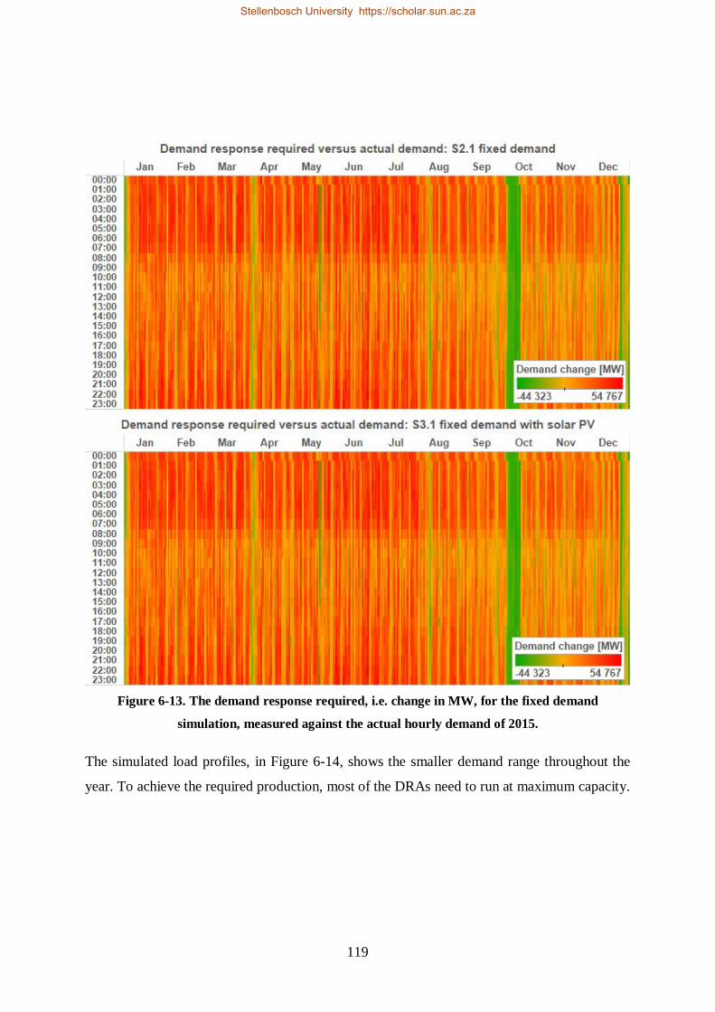
119

Figure 6-13. The demand response required, i.e. change in MW, for the fixed demand


The simulated load profiles, in Figure 6-14, shows the smaller demand range throughout the

year. To achieve the required production, most of the DRAs need to run at maximum capacity.


120

Figure 6-14. Fixed demand simulation load profiles for MegaFlex and CPD.

Figure 6-15 shows heat maps of the change in the load profiles compared to the base case for


reduction in the load profile compared to the base case. As expected, the TOU peak tariff

periods are avoided as well as the CPDs. However, due to the duration of the CPDs, not all of

them can be adequately responded to as they are constrained by the operating hours and

production volumes. It also appears that there is more flexibility towards the second half of the

year to better initiate a DR.


121


MegaFlex and CPD, for the fixed demand simulation.

6.3.5. Voluntary demand response participation simulation (S2.2 and S3.2)

This simulation used the same operating constraints as the base case, with the addition that the

energy constraints included voluntary DR participation. 150 weekdays, from Monday to


122

Thursday, were randomly selected and the two hours was aligned to the evening peak hours.

The total energy consumption for those periods was be limited to 10% below the actual load

profile, as indicated in Figure 6-16.

Figure 6-16. The demand response required, i.e. change in MW, for the voluntary participation


The simulation load profiles, as shown in Figure 6-17, do indicate the rapid responses to the

DR participation events, but is somewhat lost in the noise due to the load factor. The results

indicate a slightly lower energy costs in all cases, but also a slight drop in production compared


123

the base case. The slight savings in energy cost may not be worth the loss of profit from the

additional production volumes if there is adequate demand for the coal.

Figure 6-17. Voluntary participation simulation load profiles for MegaFlex and CPD.



reduction in the load profile compared to the base case. The two-hour voluntary participation

can be clearly identified in all cases. However, for the MegaFlex tariff, there is a lesser response

in the first part of the year which is limited by the operational constraints. The DR for the CPDs

is also limited by the operational constraints.


124


MegaFlex and CPD, for the voluntary DR participation simulation.

The simulated DR values are shown in Figure 6-19 together with the running total of the

expected DR incentive. The results indicate that a total DR incentive of around R 1.3 million


125

and R 2 million may be realised for the MegaFlex and CPD tariff options, respectively. When

including the integrated solar plant, the incentive amounts are slightly higher.


cumulative incentive that may be realised.

6.3.6. Emergency load curtailment event simulation (S2.3 and S3.3)

Constraints for load curtailment events was limited to a random selection of 25 Thursdays of

which 20 days were for a 10% reduction for 6 hours and 5 days were for a 20% reduction for 4

hours, below the actual total demand. The other constraints were for 5 weekends, Saturday and

Sunday, for a 10% reduction for 12 hours, below the actual total demand. These are visually

indicated in the heat maps in Figure 6-20.


126

Figure 6-20. The demand response required, i.e. change in MW, for the emergency load

curtailment simulation, measured against the actual hourly demand of 2015.

The simulation results, shown in Figure 6-21, indicate a slight decrease in energy cost for the

MegaFlex tariff while the CPD also significantly impacted. However, in both tariffs periods,

production is much higher than the base case with the integrated solar plant.


127

Figure 6-21. Emergency load curtailment simulation load profiles for MegaFlex and CPD.

The main reason for the increase in the MegaFlex tariff is related to the increased production

during other peak times to achieve the required production volumes. The CPD tariff is neutral

due to response on CPDs and lower energy costs during other periods. Figure 6-22 shows heat

maps of the change in the load profiles compared to the base case for both the MegaFlex and

CPD tariffs. The red colour (the positive values) indicate the DR, i.e. a reduction in the load

profile compared to the base case. It indicates that the events are responded to, however, the

production is shifted to adjacent day TOU peak and CPD periods to achieve the production

requirements.


128


MegaFlex and CPD, for the emergency load curtailment simulation.

6.3.7. Extreme load curtailment simulation (S2.4 and S3.4)

The extreme load curtailment simulation consisted of the following events, occurring from 5:00

to 22:00 each day:


129

two one-day events;

one two-day event; and

one three-day event.

These events were defined using the cluster analysis of Solar plant 5.1 and selecting the four

worst solar generation events in the year. The required DR is visually represented in the heat

maps in Figure 6-23.

Figure 6-23. The demand response required, i.e. change in MW, for the extreme load

curtailment simulation, measured against the actual hourly demand of 2015.


130

The simulation results, shown in Figure 6-24, indicate a slight increase in energy cost for the

MegaFlex tariff while the CPD is not significantly impacted. However, in both tariffs periods,

production is slightly lower than the base case.

Figure 6-24. Extreme load curtailment simulation load profiles for MegaFlex and CPD.



reduction in the load profile compared to the base case. It indicates that the extreme events are

responded to, however, it resulted in a significant production change for January. The DR for

November is not as severe as anticipated, mainly due to possible additional production capacity.


131


MegaFlex and CPD, for the extreme load curtailment simulation.

The simulated production losses were calculated for these four events and are shown in Figure

6-26. This, however, includes total tonnes from all the DRAs. Analysis of these tonnes revealed

that 60.7% were tonnes associated with the draglines, i.e. overburden material, and 39.3% were


132

related to ROM tonnes for the plants and UG sections. Factoring in a conservative 50% yield,

i.e. saleable coal, only 19.6% of the tonnes shown in Figure 6-26 can be classified as a loss.

The simulation indicates that this can be accommodated without production loss, due to other

factors in a real case, this is potentially the lost saleable coal or at least the opportunity loss.

Figure 6-26. The potential production losses due to the extreme load curtailment events.

When such events are requested in future from the utility, without declaring an official

emergency, it is expected that the consumer may bid in a DR offer. This bid depends on several

factors including were the DRAs scheduled for production, how long these events are in

duration and the potential income loss to the organisation or at least, the fixed operating cost

for the organisation that would be incurred. The reduction in energy cost is not considered as a

benefit, as the energy needs to be used at another stage to make up the production volumes.

From several annual reports of various coal mining companies, it was found that the average

export thermal coal price for 2015 was US$ 55 /tonne and the average unit costs were

US$ 39 /tonne. These values were converted to ZAR using an exchange rate or R 13.15 /US$.

The energy (kWh) that was avoided during these events were calculated by comparing the

required load profile with the actual load profile (S0), this taking into account, general activities

such as maintenance. A high-level calculation was then conducted to determine a range of

possible DR bids for the six coal mines in this project. The highest bid amount was estimated,

based on loss of income, using the following equation:


133

𝐷𝐷𝑆𝑆𝐷𝐷𝑖𝑖𝑛𝑛𝑖𝑖𝑖𝑖𝑚𝑚𝑖𝑖 =𝑆𝑆𝑎𝑎𝑆𝑆𝑒𝑒𝑎𝑎𝑏𝑏𝑆𝑆𝑒𝑒 𝑐𝑐𝑐𝑐𝑎𝑎𝑆𝑆 𝑆𝑆𝑐𝑐𝑠𝑠𝑡𝑡 (𝑡𝑡𝑐𝑐𝑎𝑎𝑎𝑎𝑒𝑒𝑠𝑠) ×𝑆𝑆𝑥𝑥𝑝𝑝𝑐𝑐𝐸𝐸𝑡𝑡 𝑐𝑐𝑐𝑐𝑎𝑎𝑆𝑆 𝑝𝑝𝐸𝐸𝐶𝐶𝑐𝑐𝑒𝑒 (𝑍𝑍𝑍𝑍𝑆𝑆)

𝑆𝑆𝑎𝑎𝑒𝑒𝐸𝐸𝐸𝐸𝑦𝑦 𝑎𝑎𝑎𝑎𝑐𝑐𝐶𝐶𝑎𝑎𝑒𝑒𝑎𝑎 (𝑘𝑘𝑘𝑘ℎ) (𝑍𝑍𝑍𝑍𝑆𝑆𝑘𝑘𝑘𝑘ℎ

) (6.6)

The lower bid was based to cover unit cost, using the following equation:

𝐷𝐷𝑆𝑆𝐷𝐷𝑢𝑢𝑛𝑛𝑖𝑖𝑢𝑢 𝑖𝑖𝑖𝑖𝑐𝑐𝑢𝑢 =𝑆𝑆𝑎𝑎𝑆𝑆𝑒𝑒𝑎𝑎𝑏𝑏𝑆𝑆𝑒𝑒 𝑐𝑐𝑐𝑐𝑎𝑎𝑆𝑆 𝑆𝑆𝑐𝑐𝑠𝑠𝑡𝑡 (𝑡𝑡𝑐𝑐𝑎𝑎𝑎𝑎𝑒𝑒𝑠𝑠)×𝑈𝑈𝑎𝑎𝐶𝐶𝑡𝑡 𝑐𝑐𝑐𝑐𝑠𝑠𝑡𝑡 (𝑍𝑍𝑍𝑍𝑆𝑆)

𝑆𝑆𝑎𝑎𝑒𝑒𝐸𝐸𝐸𝐸𝑦𝑦 𝑎𝑎𝑎𝑎𝑐𝑐𝐶𝐶𝑎𝑎𝑒𝑒𝑎𝑎 (𝑘𝑘𝑘𝑘ℎ) (𝑍𝑍𝑍𝑍𝑆𝑆𝑘𝑘𝑘𝑘ℎ

) (6.7)

The potential bid offer may be even lower, depending on what just the fixed costs are for the

DRAs. The potential DR bid offers were calculated for each event day and shown in Figure

6-27. The bids range from R 3.80 /kWh to R 6.55 /kWh, with not much difference between the

MegaFlex and CPD tariffs. These bids are only high-level estimations and depend on external

factors such is the export thermal coal price, the exchange rate and energy avoided.

Figure 6-27. The range of estimated demand response rates for the selected mines. The lower

range is to cover to operating unit costs while the higher range is the rate to cover loss of income.

6.3.8. Combined demand response simulation (S2.5 and S3.5)

The combined DR simulation consists of the following:

voluntary DR participation (as in subsection 6.3.5);

only the 20% reductions for load curtailment (as in subsection 6.3.6) as the voluntary

participation in DR above negates the requirement to reduce load by 10%; and

the extreme load curtailment events (as in sub-section 6.3.7).


134

The resulting DR heat maps are shown in Figure 6-28. It is clear that the evening peak voluntary

DR and 20% load curtailment events are separated from the integrated solar PV plant.

Figure 6-28. The demand response required, i.e. change in MW, for the combined simulation,

measured against the actual hourly demand of 2015.

The simulated load profiles are indicated in Figure 6-29. The results indicate, that for both

tariffs, the energy cost is slightly lower than the base case scenario, while the production is

significantly impacted. The production impact is mainly due to the load curtailment events and

voluntary DR participation.


135

Figure 6-29. Combined simulation load profiles for MegaFlex and CPD.



reduction in the load profile compared to the base case. The 10% DRs is clearly visible during

the evening TOU peak periods, but the integrated solar PV is less visible due to the variation in

the change. The green stripes indicate that more energy needs to be used adjacent to the CPDs

to achieve production requirements.


136


MegaFlex and CPD, for the combined simulation.

The simulated DR values are shown in Figure 6-31 together with the running total of the

expected DR incentive. The results indicate that a total DR incentive of around R 1.3 million


137

and R 2.5 million may be realised for the MegaFlex and CPD tariffs, respectively. The

incentives are slightly higher with the integrated solar plant.


cumulative incentive that may be realised.

6.4. Summary of simulation results

The results of the simulations are summarised in Table 6-3 for the MegaFlex tariff and in Table

6-4 for the CPD tariff. The tables indicate both the energy cost and total production volumes as

well as the percentage change of each scenario with respect to the base case scenario.


138

Table 6-3. Summary of simulation results for the MegaFlex tariff.

Simulation Energy Cost [ZAR]

% change in energy cost

Production [tonnes]

% change in production

S0 Base case R 457 329 096 0.0% 55 051 118 0.0%

S1 Optimised base case R 432 233 475 -5.5% 59 750 182 8.5%

S2.1 Fixed demand R 444 717 580 -2.8% 59 750 182 8.5%

S3.1 Fixed demand with solar PV R 456 325 710 -0.2% 54 902 348 -0.3%

S2.2 Voluntary participation R 458 541 715 0.3% 55 018 882 -0.1%

S3.2 Voluntary participation with solar PV R 454 754 538 -0.6% 54 314 985 -1.3%

S2.3 Load curtailment R 454 074 757 -0.7% 54 168 888 -1.6%

S3.3 Load curtailment with solar PV R 444 768 216 -2.7% 59 750 182 8.5%

S2.4 Extreme load reductions R 456 302 582 -0.2% 54 902 175 -0.3%

S3.4 Extreme load reductions with solar PV R 458 526 277 0.3% 55 018 709 -0.1%

S2.5 Combined simulation R 454 777 091 -0.6% 54 314 836 -1.3%

S3.5 Combined simulation with solar PV R 454 022 960 -0.7% 54 168 739 -1.6%

For the MegaFlex tariff, energy costs did not increase significantly in any of the simulations,

while the optimised base case (S1), fixed demand without solar PV (S2.1) and load curtailment

with integrated solar PV (S3.3) showed significant savings against the base case (S0). For the

integrated solar PV scenarios, it is worth to note that the energy costs exclude the generated

solar energy that offsets the energy from the utility, which may influence the benefit either way

and it also excludes potential carbon taxation on grid electricity.

Production decreased in the voluntary DR participation with solar PV (S3.2), load curtailment

(S2.3) and both combined scenarios (S2.5 and S3.5), which may negate the energy cost saving

if the product could have been sold. However, the additional DR incentive payments will also

need to be considered. The fixed demand and optimised base case indicate potential synergies

where energy cost can be reduced while increasing production output.


139

Table 6-4. Summary of simulation results for the CPD tariff.

Simulation Energy Cost [ZAR]


Production [tonnes]

% change in production

S0 Base case R 465 742 422 0.0% 55 051 118 0.0%

S1 Optimised base case R 432 233 475 -7.2% 59 750 182 8.5%

S2.1 Fixed demand R 452 234 464 -2.9% 59 750 182 8.5%

S3.1 Fixed demand with solar PV R 463 816 774 -0.4% 54 902 348 -0.3%

S2.2 Voluntary participation R 465 570 641 0.0% 55 018 882 -0.1%

S3.2 Voluntary participation with solar PV R 463 091 331 -0.6% 54 314 985 -1.3%

S2.3 Load curtailment R 461 081 737 -1.0% 54 168 888 -1.6%

S3.3 Load curtailment with solar PV R 452 244 515 -2.9% 59 750 182 8.5%

S2.4 Extreme load reductions R 463 906 669 -0.4% 54 902 175 -0.3%

S3.4 Extreme load reductions with solar PV R 465 597 595 0.0% 55 018 709 -0.1%

S2.5 Combined simulation R 463 132 283 -0.6% 54 314 836 -1.3%

S3.5 Combined simulation with solar PV R 461 088 556 -1.0% 54 168 739 -1.6%

For the CPD tariff, energy costs did not increase significantly for any of the simulations, while

the optimised base case (S1), fixed demand without solar PV (S2.1), load curtailment with and

without integrated solar PV (S2.3 and S3.3) and the combined simulation with solar PV (S3.5)

showed significant savings against the base case (S0). The production was similarly affected as

in the MegaFlex tariff.

Table 6-5 compares the total energy cost for both the MegaFlex and CPD tariffs for all scenarios.

The results indicate that the CPD tariff results in an average increase in energy cost of 1.7%,

with the exception of the optimised base case simulation (S1), which shows no significant

change. The optimised base case only had operating constraints and the simulation was able to

shift more energy out of the peak and critical periods.


140

Table 6-5. Summary of simulation results, comparing the MegaFlex and CPD tariffs.

Simulation MegaFlex Energy Cost [ZAR]

CPD Energy Cost [ZAR]


S0 Base case R 457 329 096 R 465 742 422 1.8%

S1 Optimised base case R 432 233 475 R 432 233 475 0.0%

S2.1 Fixed demand R 444 717 580 R 452 234 464 1.7%

S3.1 Fixed demand with solar PV R 456 325 710 R 463 816 774 1.6%

S2.2 Voluntary participation R 458 541 715 R 465 570 641 1.5%

S3.2 Voluntary participation with solar PV R 454 754 538 R 463 091 331 1.8%

S2.3 Load curtailment R 454 074 757 R 461 081 737 1.5%

S3.3 Load curtailment with solar PV R 444 768 216 R 452 244 515 1.7%

S2.4 Extreme load reductions R 456 302 582 R 463 906 669 1.7%

S3.4 Extreme load reductions with solar PV R 458 526 277 R 465 597 595 1.5%

S2.5 Combined simulation R 454 777 091 R 463 132 283 1.8%

S3.5 Combined simulation with solar PV R 454 022 960 R 461 088 556 1.6%

From the various simulations, it can be concluded that the MegaFlex tariff is the better tariff to

remain on, based on the current operating methodologies. It consistently resulted in the lower

energy costs when compared to the CPD tariff. The CPDs are not fixed as in the simulations,

which makes them unpredictable and a challenge to plan.

Secondly, the optimised base case and fixed demand simulations have the biggest potential in

terms of energy cost reduction and production output, however, does include very limited DR.

These also are theoretical numbers, which mean that operating methodologies need to change

significantly. The full potential may not be practical to realise, but it is a good indication of the

range of the improvement opportunity.

Finally, in all the simulations, the operating constraints ensured that monthly production

volumes met the required targets, at least theoretically. The slight changes in production

indicate the difference from the base case. Thus, production should not be used as a limiting


141

factor not to consider the DR scenarios presented. The additional income for DR incentives and

savings from integrated solar plants can further strengthen the business base for DR. At the very

least, the DR incentive should cover the premium of integrated solar PV generation costs, as it

is not yet at grid parity on the MegaFlex tariff. This results in lower carbon emissions which

imply that less carbon tax will be paid, once it is implemented.


142

7. Conclusion and recommendation

This chapter provides an overview of this project, makes recommendations and suggests further

research areas.

7.1. Overview

DR is playing a big part in utilities around the world and is set to become even bigger, enabled

by the smart grid and the increase in penetration of DERs. South Africa has already started on

this journey and has several DR programmes running in the industrial sector, mainly the larger

consumers. The smaller industrial, commercial and residential sectors remain largely untapped

but have great potential. The stability of the national grid will depend on larger integration of

DR into all sectors.

The benefits of DR are improved energy security, cost-reflective tariffs and more integration of

DERs, including renewable energy sources. DR is required to drive the transition from a

centralised power system to a decentralised, low carbon power system. Technology, data

analytics and computing enable the smart grid, opening the door for effective and automated

DR. There are however some significant challenges that need to be addressed and lessons to be

learnt to realise the full potential of DR.

Various mines in the coal mining industry were used to quantify the potential for DR in the

sector and included a mix of both open-pit and underground mines. Each of the typical process

flows was discussed as well as a thorough analysis of their electrical energy usage and costs.

This led to the identification of DRAs as well as a discussion around the typical operating

characteristics of each and current DR initiatives.

Four typical DR scenarios were constructed, namely tariff pricing signals, voluntary DR

initiatives, emergency load curtailment events as well as extreme load curtailment events, each

considered on their own and with the integration of a grid connected solar PV plant. A detailed

analysis of each of the scenarios resulted in identifying characteristics of typical DR events and

what to expect from these events in terms of the number of events and the duration thereof.

Detailed regression models for each of the DRAs was developed to enable accurate prediction

of energy consumption based on their given production rates and volumes. The exploratory data


143

analysis also highlighted the fact that a good understanding of the process is crucial as well as

good data management practices.

Finally, all of the elements were combined into a scheduling simulation where hourly

production was planned for the entire year. The simulations were based on the 2015 operating

hours and the energy constraints from the various DR scenarios. The objective was to minimise

energy costs, based on both the MegaFlex and CPD tariffs.

The simulation results showed that the appropriate DR objectives can be achieved, while still

achieving the required production volumes. In many cases, the total energy costs can also be

reduced slightly. While this may not be seen as significant, the ability to respond to DR events

and still meet production targets and energy budgets is significant. Not to mention other benefits

related to carbon tax when using low carbon DERs.

The MegaFlex tariff provided the lowest energy costs when compared to the CPD tariff and

thus, is still the preferred tariff, based on the 2015 operating conditions. The results also showed

a potential of reduced energy cost and increased production, using the optimised base case.

While this is theoretical, at least some of this potential can be unlocked with operational control

and thus, typically requires no or little capital investment. The extreme load curtailment event

scenario was also highlighted as a future alternative to emergency load shedding and

curtailment. These short-term events, such as multiple unit trips, extreme weather and natural

phenomena, can potentially be accommodated and the utility or SO may ask consumers to offer

a DR bid. The potential bid ranges were estimated to give an indication of the cost that may be

involved and this is business specific.

The results highlighted the need for a change in mindset, behaviour and technology. To achieve

optimal DR and minimise energy costs, a review of the operating methodology is required as

well as the time when production is scheduled. The operating methodologies should holistically

include not only safety, production and costs, but also energy security, energy performance and

carbon emission reductions.

Technology also has a major role to play. After a review of the operating methodologies, the

case can be made to include proper automation systems to respond to DR events and the

inclusion of DERs. Secondly, the use of the correct data analytics and optimisation techniques,


144

for planning and scheduling, are crucial to ensure that operations are running optimally and

meet the required business objectives, which now includes energy and carbon emission

requirements.

7.2. Recommendation

From the simulation results, it is clear that there is a potential for DR in the coal mining industry.

The recommendation is to design and implement a pilot DR programme in a working mine.

The first step would be to gain commitment from management to ensure that DR is aligned with

their business objectives and that they will drive the implementation by allocating the required

resources. Next, a more detailed review of the identified DRAs need to be conducted with

operating and maintenance personnel. The scope and boundaries need to be defined and linked

to the measurement plan as well as data quality assurance. The regression models need to be

redone based on hourly production values and hourly energy consumption to give more accurate

predictions. A central scheduling module needs to be designed with an easy user interface where

the actual hourly data will be fed into as well as provide the facility to enter the operating and

energy constraints and support monitoring of activities.

Looking outside of the coal mining industry, opening up the grid to various IPPs would provide

an excellent opportunity to secure energy and run a more efficient power system. However,

with limited DR and insufficient processes in place, it presents a greater risk to energy security.

The landscape is changing fast and it needs to be embraced by putting the required processes

in place. A good starting point, to enable widespread effective DR in South Africa, would be to

form a technical committee with stakeholders from all sectors. A standard for DR needs to be

developed and/or adopted to allow interoperability of various DR systems. This will also need

to be aligned with the requirements of the smart grid and cyber security.

There is a vast amount of data that is generated on a daily basis by the local utility and industry.

Making non-sensitive data openly available, opens the doors for many researchers, specialists

and amateur data scientists to provide insight into how to make the power system more efficient.

Unemployment is a major issue in South Africa. The decentralisation of the grid will provide

an opportunity for local employment, not only for construction but more importantly operation

and maintenance of infrastructure. This enables communities to service their own microgrids.

The skills development needs should form part of the overall DR strategy.


145

7.3. Further research

To enable an efficient and stable power system, it would be useful to understand, in more detail,

the difficulties utilities face to maintain grid stability and how they are responding to the rapid

change in the power generation and distribution sectors. This research is essential to enable the

transition for the utilities to ensure they can meet their objectives and are not left behind with

stranded assets.

It would also be beneficial to understand how various other sectors operate and how they can

contribute towards DR. Each sector has some common requirements and constraints, but often

the specific constraints linked to an individual operation may have a bigger impact on how it

can respond to DR. In this project, production was the primary relevant variable affecting

energy consumption but in other processes, weather and other variables may come into play. It

is essential to look outside of the operational boundaries and determine what synergies with

other local stakeholders can be beneficial for both parties and the greater community of South

Africa.


146

8. References

[1] C. Chaplin, The Great Dictator. USA, 1940.

[2] N. O׳Connell, P. Pinson, H. Madsen, M. O׳Malley, N. Oconnell, P. Pinson, H. Madsen, and M. Omalley, “Benefits and challenges of electrical demand response: A critical review,” Renew. Sustain. Energy Rev., vol. 39, pp. 686–699, 2014 [Online]. Available: http://linkinghub.elsevier.com/retrieve/pii/S1364032114005504

[3] H. A. Rahman, S. Majid, A. R. Jordehi, C. Kim, M. Yusri, and S. O. Fadhl, “Operation and control strategies of integrated distributed energy resources : A review,” vol. 51, pp. 1412–1420, 2015.

[4] G. The, S. African, S. African, S. Africa, and EngineeringNews, “The case for mid-merit power generation,” 2015. [Online]. Available: http://www.engineeringnews.co.za/article/the-case-for-mid-merit-power-generation-2013-08-09. [Accessed: 30-May-2015]

[5] MyBroadband, “How Eskom handles power crises: 1950s, 70s, and now.” [Online]. Available: http://mybroadband.co.za/news/energy/124633-how-eskom-handles-power-crises-1950s-70s-and-now.html. [Accessed: 30-May-2015]

[6] Eskom, “Ankerlig and gourikwa gas turbine power stations fact sheet,” no. September 2007, pp. 1–3, 2014 [Online]. Available: http://www.eskom.co.za/AboutElectricity/FactsFigures/Pages/Facts_Figures.aspx

[7] EWN, “Medupi, Kusile to be completed by 2021.” [Online]. Available: http://ewn.co.za/2015/04/22/Medupi-Khusile-to-be-completed-by-2021. [Accessed: 30-May-2015]

[8] Africa Energy, “South Africa renewables: Industry reveals its benefits,” no. 293, 2015 [Online]. Available: http://www.sapvia.co.za/wp-content/uploads/2015/02/AE-293-SA-renewables.pdf

[9] SeeNews, “South Africa to add 6.3 GW to future green tenders.” [Online]. Available: http://renewables.seenews.com/news/south-africa-to-add-6-3-gw-to-future-green-tenders-472852#. [Accessed: 30-May-2015]

[10] Department of Minerals and Energy, “Integrated Resource Plan (IRP) 2010 - 2030,” 2011.

[11] News24, “Eskom vows to keep the lights on ‘at all costs.’” [Online]. Available: http://www.news24.com/Archives/City-Press/Eskom-vows-to-keep-the-lights-on-at-all-costs-20150429. [Accessed: 30-May-2015]

[12] EngineeringNews, “Does Eskom have a maintenance plan?,” pp. 1–4, 2015 [Online]. Available: http://www.engineeringnews.co.za/article/does-eskom-have-a-maintenance-plan-2015-05-26. [Accessed: 30-May-2015]

[13] D. Daws, “Major business disruptions as SA has first load-shedding relapse since 2008,” 2015. [Online]. Available: http://www.engineeringnews.co.za/article/major-business-disruptions-as-sa-has-first-load-shedding-relapse-since-2008-2014-03-06. [Accessed: 30-May-2015]

[14] SA News, “Electricity war room focused on keeping the lights on,” 2015. [Online]. Available: http://www.sanews.gov.za/south-africa/electricity-war-room-focused-keeping-lights. [Accessed: 30-May-2015]

[15] T. Creamer, “Eskom targeting 975 MW in savings as it restarts DSM schemes,” pp. 25–27, 2015 [Online]. Available: http://www.miningweekly.com/article/eskom-targeting-975-mw-in-savings-as-it-restarts-dsm-schemes-2015-03-25. [Accessed: 30-May-2015]


147

[16] Eskom, “Tariff history.” [Online]. Available: http://www.eskom.co.za/CustomerCare/TariffsAndCharges/Pages/Tariff_History.aspx. [Accessed: 30-May-2015]

[17] FinancialMail, “Open Cycle Gas Trubines: Between a rock and a hard place.” [Online]. Available: http://www.financialmail.co.za/coverstory/2015/01/29/open-gas-cycle-turbines-between-a-rock-and-a-hard-place. [Accessed: 30-May-2015]

[18] Fin24, “Unanswered questions on Eskom’s price hike application,” 2015. [Online]. Available: http://www.fin24.com/Economy/Eskom/Unanswered-questions-on-Eskoms-price-hike-application-20150529. [Accessed: 30-May-2015]

[19] T. Bischof-Niemz, “Financial Costs and Benefits of Renewables in South Africa in 2014,” 2015 [Online]. Available: http://www.csir.co.za/media_releases/docs/Financial_benefits_Wind_PV_2014_CSIR_10Feb2015_report.pdf

[20] D. Kestenbaum, “Economists Have A One-Page Solution To Climate Change,” 2015. [Online]. Available: http://www.npr.org/sections/money/2013/06/28/196355493/economists-have-a-one-page-solution-to-climate-change. [Accessed: 30-May-2015]

[21] R. Baxter, P. Turner, and A. Parsons, “Presentation of Chamber Position on Carbon Tax to the Davis Tax Committee.” 2015 [Online]. Available: http://www.taxcom.org.za/docs/New_Folder2/Chamber of Mines carbon tax presentation to DTC.pdf

[22] S. Nyquist, “Peering into energy’s crystal ball,” McKinsey Q., 2015.

[23] The Federal Energy Regulatory Commission Staff and The Federal Energy Regulatory Comission Staff, “National Action Plan on Demand Response,” Response, vol. 63, pp. 1–9, 2010 [Online]. Available: http://www.ferc.gov/legal/staff-reports/06-17-10-demand-response.pdf

[24] Department of Minerals and Energy, Government Gazette: Electricity Pricing Policy of the South African Electricity Supply Industry, vol. 522, no. 31741. 2008, pp. 1–56 [Online]. Available: http://www.greengazette.co.za/pages/national-gazette-37230-of-17-january-2014-vol-583_20140117-GGN-37230-003

[25] F. M. Andersen, S. G. Jensen, H. V Larsen, P. Meibom, H. Ravn, K. Skytte, and M. Togeby, Analyses of Demand Response in Denmark, vol. 1565, no. October. 2006.

[26] G. Ghatikar, S. Mashayekh, M. Stadler, R. Yin, and Z. Liu, “Distributed energy systems integration and demand optimization for autonomous operations and electric grid transactions,” Appl. Energy, vol. 167, pp. 432–448, 2016 [Online]. Available: http://dx.doi.org/10.1016/j.apenergy.2015.10.117

[27] F. Shariatzadeh, P. Mandal, and A. K. Srivastava, “Demand response for sustainable energy systems : A review , application and implementation strategy,” Renew. Sustain. Energy Rev., vol. 45, pp. 343–350, 2015 [Online]. Available: http://dx.doi.org/10.1016/j.rser.2015.01.062

[28] Telegraph, “Balancing demand ‘could cost National Grid £ 2bn,’” pp. 1–2, 2016.

[29] NORDEL, “Enhancement of Demand Response,” 2006.

[30] Association of Edison Illuminating Companies, “Demand Response Measurement & Verification: Applications for Load Research,” no. March, 2009 [Online]. Available: http://www.aeic.org/load_research/AEIC-MV-Whitepaper-030409.pdf

[31] ISO-NE, “Market Rule 1 Appendix E - Demand Response,” 2015.


148

[32] J. Torriti, M. G. Hassan, and M. Leach, “Demand response experience in Europe: Policies, programmes and implementation,” Energy, vol. 35, no. 4, pp. 1575–1583, 2010 [Online]. Available: http://dx.doi.org/10.1016/j.energy.2009.05.021

[33] SEDC, Smart Energy Demand Coalition, and SEDC, “Mapping Demand Response in Europe Today,” SEDC. Smart Energy Demand Coalit., no. April, p. 92, 2014 [Online]. Available: http://www.febeliec.be/web/infosession strategic demand reserve _ 16_5_2014/1011306087/list1187970122/f1.html\nhttp://sedc-coalition.eu/wp-content/uploads/2014/04/SEDC-Mapping_DR_In_Europe-2014-04111.pdf

[34] A. Satchwell, C. Goldman, H. Hossein, and M. Lesiw, “An Assessment of Analytical Capabilities, Services, and Tools for Demand Response,” 2013 [Online]. Available: http://emp.lbl.gov/sites/all/files/napdr-assessment-of-analytical-capabilities_0.pdf\npapers2://publication/uuid/B2B45A0A-0D50-4DE1-BA2D-CCD59DCE91D2

[35] FERC, “Assessment of Demand Response & Advanced Metering,” Eff. Br. mindfulness Interv. acute pain Exp. An Exam. Individ. Differ., vol. December, pp. 1689–1699, 2015 [Online]. Available: https://www.ferc.gov/legal/staff-reports/2015/demand-response.pdf

[36] K. Tweed, “Demand Response Could Have Saved Texans $85M in One Day.” [Online]. Available: http://www.greentechmedia.com/articles/read/demand-response-could-have-saved-texans-85m-in-one-day?utm_source=SmartGrid&utm_medium=Headline&utm_campaign=GTMDaily. [Accessed: 05-Jun-2015]

[37] J. Schwartz, “Case Study : Salt River Project — The Persistence of Consumer Choice National Forum of the National Action Plan on Demand Response.”

[38] ISO New England, “Our History.” [Online]. Available: http://www.iso-ne.com/about/what-we-do/history. [Accessed: 04-Feb-2016]

[39] N. E. Power and I. N. England, “New England Power Grid 2014–2015 Profile,” 2015.

[40] ISO-NE, “ISO New England 2015 Regional Electricity Outlook 2015,” 2015.

[41] ISO-NE, “The Challenge Of Keeping The Lights On In New England: A Conversation With ISO-NE’s CEO,” pp. 1–7, 2016 [Online]. Available: http://www.forbes.com/sites/peterdetwiler/2016/06/14/the-challenge-of-keeping-the-lights-on-in-new-england-a-conversation-with-iso-nes-ceo/#5cf243e6f800. [Accessed: 15-Jun-2016]

[42] C. D. E. Jonghe and C. De Jonghe, “Short-term demand response in electricity generation planning and scheduling,” KU Leuven, 2011 [Online]. Available: http://www.esat.kuleuven.be/electa-projects/publications/fulltexts/pub_2231.pdf

[43] U. Hammarstedt and M. Nilsson, “Demand response in the strategic reserve - The case of Sweden,” 2014.

[44] Eskom, “Eskom System Status Overview - 26 January 2016,” 2016 [Online]. Available: http://www.eskom.co.za/OurCompany/MediaRoom/Pages/Media_Room.aspx

[45] K. Munson, “Integrated Energy Storage: An Answer to Addressing the Duck Curve?,” 2015. [Online]. Available: http://www.renewableenergyworld.com/rea/news/article/2015/04/integrated-energy-storage-an-answer-to-addressing-the-duck-curve?cmpid=StorageNL-Thursday-April9-2015. [Accessed: 10-Apr-2015]

[46] Eskom, “Eskom Tariffs & Charges 2015/16,” no. April 2015, p. 26, 2016.


149

[47] Eskom, “Critical Peak Day Pricing (Pilot tariff).” [Online]. Available: http://www.eskom.co.za/CustomerCare/TariffsAndCharges/WhatsNew/Pages/CriticalPeakDay.aspx. [Accessed: 30-May-2015]

[48] “Electricity Supply - Part 9: Load reduction practices, system restoration practices, and critical load and essential load requirements under system emergencies.” NRS048-9, 2010.

[49] Eskom, “Demand market participation.” [Online]. Available: http://www.eskom.co.za/Whatweredoing/ElectricityGeneration/LoadManagement/Pages/Demand_Market_Participation.aspx. [Accessed: 15-Jun-2016]

[50] R. Surtees and D. Blane, “SA’s Virtual Power Station 800MW’s ...and counting,” in 23rd AMEU Technical Convention, 2011, pp. 1–5.

[51] M. L. Goldberg and G. Kennedy Agnew, “Measurement and Verification for Demand Response,” Prep. Natl. Forum Natl. Action Plan Demand Response Meas. Verif. Work. Group. U.S. Dep. Energy Fed. Energy Regul. Comm., p. 123, 2013 [Online]. Available: file:///C:/Users/SATELLITE/Google Drive/Referencias Doctorado//Goldberg, Kennedy Agnew - 2013 - Measurement and Verification for Demand Response.pdf

[52] V. Giordano, F. Gangale, G. F. Jrc-ie, M. Sánchez, J. Dg, I. Onyeji, A. Colta, I. Papaioannou, A. Mengolini, C. Alecu, T. Ojala, and I. Maschio, “Smart Grid projects in Europe : lessons learned and current developments,” Europe, vol. 2011, pp. 1–118, 2011.

[53] P. Faria, Z. Vale, and J. Baptista, “Constrained consumption shifting management in the distributed energy resources scheduling considering demand response,” Energy Convers. Manag., vol. 93, pp. 309–320, 2015 [Online]. Available: http://dx.doi.org/10.1016/j.enconman.2015.01.028

[54] OpenADR, “About OpenADR.” [Online]. Available: http://www.openadr.org/overview. [Accessed: 07-Feb-2016]

[55] OpenADR, “Demand Response Program Implementation Guide,” 2014.

[56] A. Agresti and C. Franklin, Statistics - The art and science of learning from data, Third Edit. 2013.

[57] B. Render, R. M. Stair, and M. E. Hanna, Quantitative Analysis For Management, 11th ed. 2012.

[58] M. Acevedo, Data analysis and statistics for Geography, Environmental Science and Engineering. CRC Press, 2013.

[59] McGraw Hill, “Regression Analysis Supplement,” no. 3, pp. 2–7 [Online]. Available: http://highered.mheducation.com/sites/dl/free/0078025532/966295/ch08_online_appendix.pdf

[60] H. Arsham, “Time Series Analysis for Business Forecasting.” [Online]. Available: http://home.ubalt.edu/ntsbarsh/business-stat/stat-data/forecast.htm. [Accessed: 20-Feb-2016]

[61] P. F. Dunn, Measurement, Data Analysis, and Sensor Fundamentals for Engineering and Science. 2010.

[62] S. Chatterjee and A. S. Hadi, Regression Analysis by Example, Fourth Edi. Wiley, 2015 [Online]. Available: https://books.google.com/books?hl=en&lr=&id=zyjWBgAAQBAJ&pgis=1

[63] D. Cook and S. Weisberg, Applied Regression including computing and graphics. Wiley, 1999.

[64] StatTrek, “Transformations to Achieve Linearity.” [Online]. Available: http://stattrek.com/regression/linear-transformation.aspx. [Accessed: 28-Jul-2016]

[65] S. Aghabozorgi, A. Seyed Shirkhorshidi, and T. Ying Wah, “Time-series clustering - A decade review,” Inf. Syst., vol. 53, pp. 16–38, 2015 [Online]. Available: http://dx.doi.org/10.1016/j.is.2015.04.007


150

[66] K. L. Lo, Z. Zakaria, and M. H. Sohod, “Determination of Consumers’ Load Profiles based on Two-stage Fuzzy C-Means,” Proc. 5th WSEAS Int. Conf. Power Syst. Electromagn. Compat., vol. 2005, pp. 212–217, 2005.

[67] M. Namratha, T. Prajwala, I. Journal, and C. Engineering, “A Comprehensive Overview of Clustering Algorithms in Pattern Recognition,” vol. 4, no. 6, pp. 23–30, 2012.

[68] Statsoft, “How To Group Objects Into Similar Categories, Cluster Analysis.” [Online]. Available: http://www.statsoft.com/Textbook/Cluster-Analysis. [Accessed: 26-May-2016]

[69] “What is R?” [Online]. Available: http://www.revolutionanalytics.com/what-r. [Accessed: 29-Jan-2016]

[70] R Core Team, “R: A Language and Environment for Statistical Computing.” Vienna, Austria, 2016 [Online]. Available: https://www.r-project.org/

[71] H. Wickham, ggplot2: Elegant Graphics for Data Analysis. Springer-Verlag New York, 2009 [Online]. Available: http://ggplot2.org

[72] B. Auguie, “gridExtra: Miscellaneous Functions for ‘Grid’ Graphics.” 2016 [Online]. Available: https://cran.r-project.org/package=gridExtra

[73] D. Attali, “ggExtra: Add Marginal Histograms to ‘ggplot2’, and More ‘ggplot2’ Enhancements.” 2016 [Online]. Available: https://cran.r-project.org/package=ggExtra

[74] M. Hlavac, “stargazer: Well-Formatted Regression and Summary Statistics Tables.” Cambridge, USA, 2015 [Online]. Available: http://cran.r-project.org/package=stargazer

[75] J. Fox and S. Weisberg, An {R} Companion to Applied Regression, Second. Thousand Oaks {CA}: Sage, 2011 [Online]. Available: http://socserv.socsci.mcmaster.ca/jfox/Books/Companion

[76] F. Baty, C. Ritz, S. Charles, M. Brutsche, J.-P. Flandrois, and M.-L. Delignette-Muller, “A Toolbox for Nonlinear Regression in {R}: The Package {nlstools},” J. Stat. Softw., vol. 66, no. 5, pp. 1–21, 2015 [Online]. Available: http://www.jstatsoft.org/v66/i05/

[77] H. Wickham, “scales: Scale Functions for Visualization.” 2016 [Online]. Available: https://cran.r-project.org/package=scales

[78] R. Harter, K. Hornik, and S. Theussl, “Rsymphony: SYMPHONY in R.” 2016 [Online]. Available: https://cran.r-project.org/package=Rsymphony

[79] M. Berkelaar and others, “lpSolve: Interface to ‘Lp_solve’ v. 5.5 to Solve Linear/Integer Programs.” 2015 [Online]. Available: https://cran.r-project.org/package=lpSolve

[80] lp_solve and K. Konis., “lpSolveAPI: R Interface to ‘lp_solve’ Version 5.5.2.0.” 2016 [Online]. Available: https://cran.r-project.org/package=lpSolveAPI

[81] Tableau, “About Tableau.” [Online]. Available: http://www.tableau.com/about. [Accessed: 14-Jun-2016]

[82] Eskom, “Eskom Integrated Report 2015 - Presentation,” no. August, 2015 [Online]. Available: http://www.eskom.co.za/IR2015/Documents/IRpresentation_2015.pdf

[83] Eskom, “Demand Response Product - Day-ahead pilot,” 2016. [Online]. Available: http://www.eskom.co.za/sites/idm/ManageYourConsumption/Pages/Demandresponsedayahead.aspx. [Accessed: 25-Aug-2016]

[84] Eskom, “Demand Response Programmes.” [Online]. Available: http://www.eskom.co.za/sites/idm/ManageYourConsumption/Pages/DemandResponse.aspx. [Accessed: 13-Mar-2016]


151

[85] United States Securities and Exchange Commission, “Annual report pursuant to section 13 or 15(d) of the Securities Exchange Act of 1934.” [Online]. Available: http://www.sec.gov/Archives/edgar/data/1037676/000095012310019343/c55409e10vk.htm. [Accessed: 09-Apr-2016]

[86] J. Gillllandt, “The planning and establishment of the coal-beneficiation plant at Grootegeluk,” no. December, 1982.

[87] Z. Sun, Y. Zhao, Z. Li, Z. Cao, S. Zhenming, Z. Yiqing, L. Zhongxue, and C. Zhiguo, “A coal mine production scheduling optimization system and its application,” 2011 Seventh Int. Conf. Nat. Comput., pp. 1889–1892, 2011 [Online]. Available: http://ieeexplore.ieee.org/lpdocs/epic03/wrapper.htm?arnumber=6022568


152

APPENDIX A. Regression diagnostic plots

A.1. Final regression plots

Figure A-1. Final regression diagnostic plots for Plant 1.1.



153




154


Figure A-6. Final regression diagnostic plots for Dragline 1.1.


155




156


Figure A-10. Final regression diagnostic plots for UG sections 5.1.


157

Figure A-11. Final regression diagnostic plots for UG sections 6.1.


Development of a Demand Response Programme for the Coal ...

Documents

Transcript of Development of a Demand Response Programme for the Coal ...