Development of a Database for Surface Energy of Aggregates and

1. Report No. FHWA/TX-09/5-4524-01-1

2. Government Accession No.

3. Recipient's Catalog No. 5. Report Date January 2009 Published: July 2009

4. Title and Subtitle DEVELOPMENT OF A DATABASE FOR SURFACE ENERGY OF AGGREGATES AND ASPHALT BINDERS

6. Performing Organization Code

7. Author(s) Jonathan Howson, Amit Bhasin, Eyad Masad, Robert Lytton and Dallas Little

8. Performing Organization Report No. Report 5-4524-01-1

10. Work Unit No. (TRAIS)

9. Performing Organization Name and Address Texas Transportation Institute The Texas A&M University System College Station, Texas 77843-3135

11. Contract or Grant No. Project 5-4524-01 13. Type of Report and Period Covered Technical Report: September 2007-August 2008

12. Sponsoring Agency Name and Address Texas Department of Transportation Research and Technology Implementation Office P. O. Box 5080 Austin, Texas 78763-5080

14. Sponsoring Agency Code

15. Supplementary Notes Project performed in cooperation with the Texas Department of Transportation and the Federal Highway Administration. Project Title: Pilot Implementation of Surface Energy Measurements to Predict Moisture Susceptibility of HMA URL: http://tti.tamu.edu/documents/5-4524-01-1.pdf 16. Abstract TxDOT project 0-4524 evaluated the influence of surface energy of aggregates and binders on the resistance of asphalt mixtures to moisture damage. The results from this research lead to the development of a three-tier approach to assess the moisture damage resistance of asphalt mixtures. This approach is based on testing and evaluating the physical and/or mechanical properties of the constituent materials, the fine aggregate mixture, and full asphalt mixture. In the first tier, an energy-based parameter termed the energy ratio (ER) is calculated using the surface energy measurements. This parameter is used as a screening tool to select binders and aggregates that have good resistance to moisture damage. The second and third tiers rely on measuring the mechanical properties of the fine aggregate mixture and full asphalt mixture, respectively. This report documents the results of an implementation project of the testing methods and analysis approaches of the 0-4524 project. This implementation project included (a) providing training on the developed experimental and analysis methods, (b) conducting measurements of the surface energy of binders, additives, and aggregates, and (c) developing a database of surface energy measurements. This database will be useful as a diagnostic tool for finding the cause of poor moisture damage resistance in mixes and to suggest remedies through modification with anti-strip agents, lime, polymers, other additives, or through a change of materials in extreme cases. 17. Key Words Surface Energy, Asphalt, Aggregate, Database, DMA

18. Distribution Statement No restrictions. This document is available to the public through NTIS: National Technical Information Service Springfield, Virginia 22161 http://www.ntis.gov

19. Security Classif. (of this report) Unclassified

20. Security Classif. (of this page) Unclassified

21. No. of Pages 76

22. Price

http://tti.tamu.edu/documents/5-4524-01-1.pdf

http://www.ntis.gov

DEVELOPMENT OF A DATABASE FOR SURFACE ENERGY OF AGGREGATES AND ASPHALT BINDERS

by

Jonathan Howson Graduate Assistant Research

Texas Transportation Institute

Amit Bhasin Assistant Professor University of Texas

Eyad Masad

Associate Research Scientist Texas Transportation Institute

Robert Lytton

Research Engineer Texas Transportation Institute

and

Dallas Little

Senior Research Fellow Texas Transportation Institute

Report 5-4524-01-1 Project 0-4524-01

Project Title: Pilot Implementation of Surface Energy Measurements to Predict Moisture Susceptibility of HMA

Performed in cooperation with the

Texas Department of Transportation and the

Federal Highway Administration

January 2009 Published: July 2009

TEXAS TRANSPORTATION INSTITUTE

The Texas A&M University System College Station, Texas 77843-3135

v

DISCLAIMER

The contents of this report reflect the views of the authors, who are responsible

for the facts and the accuracy of the data presented herein. The contents do not

necessarily reflect the official view or policies of the Texas Department of Transportation

and/or the Federal Highway Administration. This report does not constitute a standard,

specification, or regulation. The engineer in charge of the project was Eyad Masad, Texas

P.E. #96368.

.

vi

ACKNOWLEDGMENTS

The authors wish to express their appreciation to the Texas Department of

Transportation personnel for their support throughout this project, as well as the Federal

Highway Administration. We would also like to thank the project director Jerry Peterson

and the members of the project monitoring committee, for their valuable technical

comments during this project.

vii

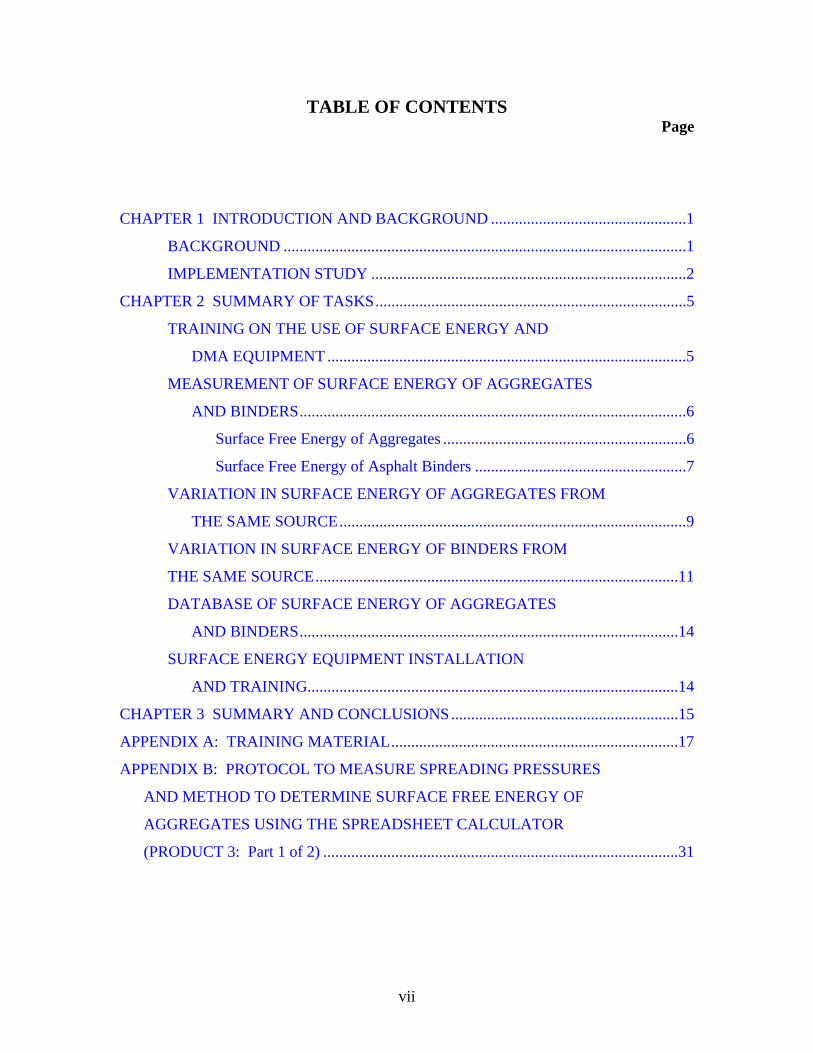
TABLE OF CONTENTS Page

CHAPTER 1 INTRODUCTION AND BACKGROUND .................................................1

BACKGROUND .....................................................................................................1

IMPLEMENTATION STUDY ...............................................................................2

CHAPTER 2 SUMMARY OF TASKS..............................................................................5

TRAINING ON THE USE OF SURFACE ENERGY AND

DMA EQUIPMENT ..........................................................................................5

MEASUREMENT OF SURFACE ENERGY OF AGGREGATES

AND BINDERS.................................................................................................6

Surface Free Energy of Aggregates .............................................................6

Surface Free Energy of Asphalt Binders .....................................................7

VARIATION IN SURFACE ENERGY OF AGGREGATES FROM

THE SAME SOURCE.......................................................................................9

VARIATION IN SURFACE ENERGY OF BINDERS FROM

THE SAME SOURCE...........................................................................................11

DATABASE OF SURFACE ENERGY OF AGGREGATES

AND BINDERS...............................................................................................14

SURFACE ENERGY EQUIPMENT INSTALLATION

AND TRAINING.............................................................................................14

CHAPTER 3 SUMMARY AND CONCLUSIONS.........................................................15

APPENDIX A: TRAINING MATERIAL........................................................................17

APPENDIX B: PROTOCOL TO MEASURE SPREADING PRESSURES

AND METHOD TO DETERMINE SURFACE FREE ENERGY OF

AGGREGATES USING THE SPREADSHEET CALCULATOR

(PRODUCT 3: Part 1 of 2) .........................................................................................31

viii

TABLE OF CONTENTS Page

APPENDIX C: PROTOCOL TO MEASURE CONTACT ANGLE

AND METHOD TO DETERMINE SURFACE FREE ENERGY OF

ASPHALT BINDERS USING THE SPREADSHEET CALCULATOR

(PRODUCT 3: PART 2 OF 2)....................................................................................45

APPENDIX D: PROCEDURE TO USE AND POPULATE THE DATABASE

OF SURFACE FREE ENERGIES IN SPREADSHEET FORMAT...........................59

ix

LIST OF FIGURES Figure Page

B.1. Auto Centering Module in SEMS Software ....................................................37

B.2. Degassing Module in SEMS Software ............................................................38

B.3. Adsorption Test Module in SEMS Software ...................................................39

B.4. Results Reported by SEMS Software ..............................................................41

B.5. Worksheets Contained in SPREADING PRESSURE TO SE.........................42

B.6. Aggregate Input Sheet Layout .........................................................................43

B.7. Managing SSA.................................................................................................44

B.8. Summarized USD Results................................................................................44

C.1. Schematic of the Wilhelmy Plate Device ........................................................49

C.2. Glass Slide Coated with Asphalt Binder for Testing with the

Wilhelmy Plate Device ..............................................................................52

C.3. Asphalt Binder Sample Suspended from Micro Balance for

Immersion in Probe Liquid ........................................................................53

C.4. Selection of Representative Area to Determine Advancing

and Receding Contact Angles....................................................................55

C.5. Entering Contact Angle Information to Compute Surface Energy..................56

C.6. Computing Surface Energy Components.........................................................57

C.7. Summary Table of Results...............................................................................57

D.1. User Interface...................................................................................................61

D.2. Asphalt-Aggregate Selection Screen ...............................................................62

D.3. Combinations of Asphalt-Aggregate Chosen by User.....................................62

D.4. Results from Asphalt-Aggregate Combination................................................64

D.5. Results Worksheet ...........................................................................................64

D.6. Asphalt Input Sheets ........................................................................................65

D.7. Aggregate Input Sheet......................................................................................65

x

LIST OF TABLES Table Page

1 List of Aggregates Used for Surface Energy Measurement .......................................7

2 List of Asphalt Binders Used for Surface Energy Measurement................................8

3 Z-Statistic for Change in Spreading Pressure of Various Probe Liquids

with Aggregate Samples Obtained at Different Times ...........................................10

4 Kendall Tau Correlation Coefficient for Aggregate Spreading Pressures.................11

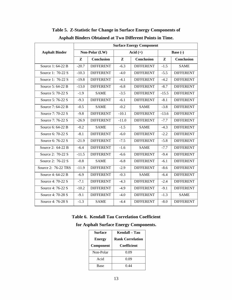
5 Z-Statistic for Change in Surface Energy Components of Asphalt Binders

Obtained at Two Different Points in Time .............................................................13

6 Kendall Tau Correlation Coefficient for Asphalt Surface Energy Components.......13

1

CHAPTER 1. INTRODUCTION AND BACKGROUND 1.1 BACKGROUND

Moisture damage is a major form of pavement distress resulting in high

maintenance costs of state and federal highways. Moisture damage can be defined as loss

of strength and durability due to the presence of moisture at the binder-aggregate

interface (adhesive failure) or within the binder (cohesive failure). Current laboratory

procedures for assessing moisture sensitivity of an hot mix asphalt (HMA) rely on

comparing mechanical properties of unconditioned specimens with moisture conditioned

specimens. Although this approach is helpful in comparative analysis of the moisture

susceptibility of various mixes, it does not focus on measuring the fundamental material

properties related to the mechanisms described above. As such, the results cannot be

used to explain causes for poor or good performance and do not provide feedback into the

process of redesigning better performing mixes. It is therefore necessary to supplement

the mechanical properties normally measured with fundamental properties that affect

physical adhesion between the asphalt and aggregate and the propensity to lose this bond

in the presence of water.

As part of the TxDOT 0-4524 project, the researchers developed a three-tier

approach to assess the moisture damage resistance of asphalt mixtures. The three tiers

are based on testing and evaluating the physical and/or mechanical properties of the

constituent materials, the sand-asphalt mixture, and full asphalt mixture. In the first tier,

an energy-based parameter termed the energy ratio (ER) is calculated using the surface

energy measurements. This parameter is used as a screening tool to select binders and

aggregates that have good resistance to moisture damage. In the second tier, the dynamic

mechanical analysis (DMA) of fine aggregate matrix specimens consisting of asphalt

binder and fine portion of aggregates is used to evaluate moisture susceptibility. Finally,

in the third tier the moisture susceptibility of the full mixture is evaluated. The testing at

the second and third tiers yields a crack growth index that is a function of fundamental

material properties. The DMA is useful to evaluate moisture susceptibility of the

materials without being influenced by mixture design and internal structure distribution.

2

The evaluation of the full mixture is necessary, however, in order to verify that

the mixture design and internal structure distribution are optimized to improve the

resistance to moisture damage. At the end of the 0-4524 project, researchers

recommended a tentative range of values for the parameters determined at each of the

three steps.

1.2 IMPLEMENTATION STUDY

It was decided to implement the findings from the 0-4524 project, starting with

the first tier. This implementation project was developed in order to transfer the

know-how on test and analytical methods that are used to characterize the fundamental

properties of aggregate and binder that influence the resistance to moisture damage. The

objectives of this implementation project were to:

• Provide training on the developed experimental and analysis methods.

• Measure surface energy of binders, additives, and aggregates. These

measurements will be used to more completely analyze surface energies of typical

materials; to evaluate the effects of additives and modifiers on the surface

energies of commonly used asphalts; and to evaluate the changes in aggregate and

asphalt surface energies due to changes in refinery processes and geological strata

over time.

• Incorporate surface energy measurements from the previous work and from this

implementation project into a database. This database will be useful as a

diagnostic tool to determine the cause of poor moisture damage resistance in

mixes and to suggest remedies through modification with anti-strip agents, lime,

polymers, other additives, or through a change of materials in extreme cases.

The aforementioned objectives were achieved by accomplishing the following

tasks in this project.

Task 1: Training on the use of Wilhelmy plate device, Universal Sorption Device, and

Dynamic Mechanical Analyzer testing protocols and analysis methods.

3

Task 2: Measurements of the surface energy of aggregates and binders that are typically

used in the State of Texas.

Task 3: Analysis of changes in surface energies of aggregate samples from the same

source. This task is aimed at determining the variability in aggregate surface energy over

time and due to changes in the geological strata within a given source.

Task 4: Analysis of changes in surface energies of binder samples from the same

supplier. This task is aimed at determining the variability in binder surface energy due to

changes in the binder source and modification process.

Task 5: Development of an updated database of aggregate and binder surface energies.

This database will be valuable for the selection of aggregate and binder combinations

with very good resistance to moisture damage. Also, it will be used later to verify the

analysis methods developed in project 0-4524 through comparison between the predicted

resistance to moisture damage and field performance.

Task 6: Purchase equipment to measure surface energy on aggregates and asphalt binders

for installation at CST Central laboratory, and provide training and technical assistance

on the operation of the equipment.

Chapter 2 presents a summary on the aforementioned tasks in seriatim.

5

CHAPTER 2. SUMMARY OF TASKS This chapter presents a brief summary on each of the tasks accomplished in this

implementation project.

2.1 TRAINING ON THE USE OF SURFACE ENERGY AND DMA EQUIPMENT

Measurement of surface free energy of materials and mechanical properties of the

fine aggregate matrix (FAM) are the first two steps in the three-tier approach to mixture

characterization and design. This task was designed to provide hands on training to

TxDOT personnel who may want to run these tests at the CST laboratory. The first

training was provided to six TxDOT personnel on March 8, 2007, at the Texas

Transportation Institute laboratory in College Station. The training included the

following three tests:

1. Dynamic mechanical analysis (DMA) to evaluate the mechanical properties of the

FAM.

2. Test method to determine the surface free energy of asphalt binders using the

Wilhelmy plate device.

3. Test method to determine the surface free energy of aggregates using the

Universal Sorption Device (USD).

The one-day training included a theory session that included a background on

each of the test methods, a detailed explanation of the test procedure, and demonstration

of the analytical techniques to interpret results from each of these test methods.

Appendix A of this report includes the training material. The theory session was

followed by hands on training with each one of the test methods.

6

2.2 MEASUREMENT OF SURFACE ENERGY OF AGGREGATES AND

BINDERS

2.2.1 Surface Free Energy of Aggregates

The Universal Sorption Device (USD) was used to determine the surface free

energy of aggregates. The surface free energy values for a total of 16 different types of

aggregates were compiled in this research. Of these 16 different types of aggregates, the

surface free energy components of five different types of aggregates were determined by

obtaining samples from the same source at two different points in time. This resulted in a

total testing of 21 aggregates. The objective of this exercise was to evaluate changes in

the surface free energy characteristics amongst different batches of aggregates obtained

from the same source. Section 2.3 presents more details on this objective that was

accomplished in Task 3.

At least three different replicates for each aggregate type were tested with each

one of the three probe liquids. All tests were conducted in accordance with the draft

protocol that was developed following the NCHRP 9-37 project and TxDOT 0-4524

project. The draft protocols are included in Appendix B of this report. This appendix

also includes guidelines to use the spreadsheet to compute the surface free energy

components using the spreading pressures determined using the USD test method.

Table 1 enumerates the list of aggregates that were included in Tasks 2 and 3. The results

from these tests are included in the database of surface energy values. Section 2.5

presents further details regarding this database.

7

Table 1. List of Aggregates Used for Surface Energy Measurement.

Number Mineralogy Quarry Procurement Date

1a Granite Snyder, OK May-04

1b Granite Snyder, OK Jun-07

2 Quartzite Jones Mill, AK May-04

3a Sandstone Sawyer, OK May-04

3b Sandstone Sawyer, OK Jun-07

4 Silcious River Gravel Prescott, AK May-04

5 Limestone Bridgeport, TX May-04

6 Limestone Spore "Bucyrus" OH May-04

7 River Gravel Melco, OH May-04

8a Crushed River Gravel Murphy, TX Oct-03

8b Crushed River Gravel Murphy, TX Jun-07

9a Crushed Limestone Brownwood, TX May-04

9b Crushed Limestone Brownwood, TX Jun-07

10a Crushed Traprock Knippa, TX Apr-04

10b Crushed Traprock Knippa, TX Jun-07

11 Sandstone Sawyer, OK Feb-06

12 Limestone New Braunfels, TX Jul-06

13 Sandstone Brownlee, TX May-06

14 Limestone Hunter, TX May-06

15 Limestone Odessa, TX Unknown

16 Granite Herndon, VA Jun-02

17 Limestone

Material Reference

Library (MRL) Oct-07

18 Granite

Material Reference

Library (MRL) Oct-07

Note: Aggregate with alpha-numerical numbering such as 1a and 1b indicate that the aggregates were

sampled from the same source at two different times for surface energy measurement.

2.2.2 Surface Free Energy of Asphalt Binders

The Wilhelmy plate device was used to determine the surface free energy of

asphalt binders. The surface free energy values for a total of 44 different types of neat

and modified asphalt binders were compiled in this project. Of these, 24 binders were

obtained from seven different manufacturers and included base as well as polymer

8

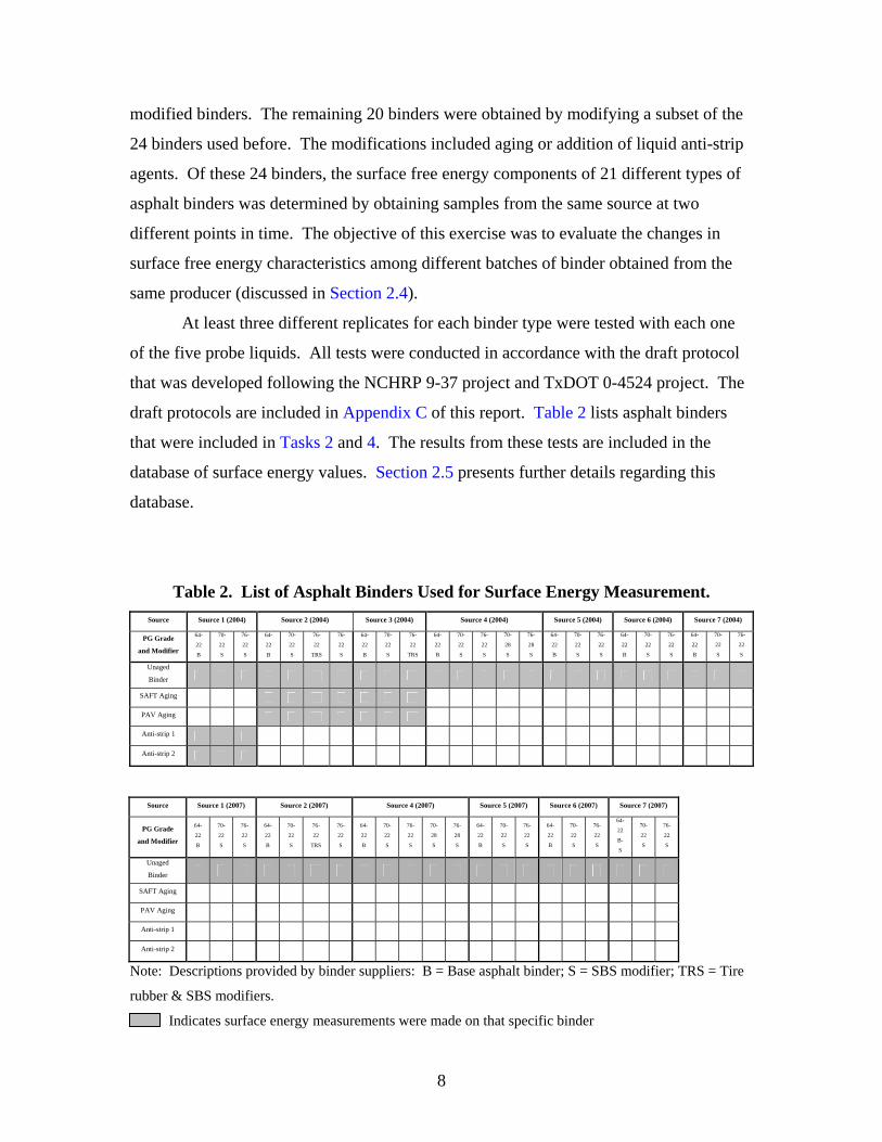
modified binders. The remaining 20 binders were obtained by modifying a subset of the

24 binders used before. The modifications included aging or addition of liquid anti-strip

agents. Of these 24 binders, the surface free energy components of 21 different types of

asphalt binders was determined by obtaining samples from the same source at two

different points in time. The objective of this exercise was to evaluate the changes in

surface free energy characteristics among different batches of binder obtained from the

same producer (discussed in Section 2.4).

At least three different replicates for each binder type were tested with each one

of the five probe liquids. All tests were conducted in accordance with the draft protocol

that was developed following the NCHRP 9-37 project and TxDOT 0-4524 project. The

draft protocols are included in Appendix C of this report. Table 2 lists asphalt binders

that were included in Tasks 2 and 4. The results from these tests are included in the

database of surface energy values. Section 2.5 presents further details regarding this

database.

Table 2. List of Asphalt Binders Used for Surface Energy Measurement. Source Source 1 (2004) Source 2 (2004) Source 3 (2004) Source 4 (2004) Source 5 (2004) Source 6 (2004) Source 7 (2004)

PG Grade

and Modifier

64-

22

B

70-

22

S

76-

22

S

64-

22

B

70-

22

S

76-

22

TRS

76-

22

S

64-

22

B

70-

22

S

76-

22

TRS

64-

22

B

70-

22

S

76-

22

S

70-

28

S

76-

28

S

64-

22

B

70-

22

S

76-

22

S

64-

22

B

70-

22

S

76-

22

S

64-

22

B

70-

22

S

76-

22

S

Unaged

Binder

SAFT Aging

PAV Aging

Anti-strip 1

Anti-strip 2

Source Source 1 (2007) Source 2 (2007) Source 4 (2007) Source 5 (2007) Source 6 (2007) Source 7 (2007)

PG Grade

and Modifier

64-

22

B

70-

22

S

76-

22

S

64-

22

B

70-

22

S

76-

22

TRS

76-

22

S

64-

22

B

70-

22

S

76-

22

S

70-

28

S

76-

28

S

64-

22

B

70-

22

S

76-

22

S

64-

22

B

70-

22

S

76-

22

S

64-

22

B-

S

70-

22

S

76-

22

S

Unaged

Binder

SAFT Aging

PAV Aging

Anti-strip 1

Anti-strip 2

Note: Descriptions provided by binder suppliers: B = Base asphalt binder; S = SBS modifier; TRS = Tire

rubber & SBS modifiers.

Indicates surface energy measurements were made on that specific binder

9

2.3 VARIATION IN SURFACE ENERGY OF AGGREGATES FROM THE

SAME SOURCE

A database of any material property is valid and meaningful for future use only as

long as the subject material property does not change over time. The objective of Task 3

was to determine the change in surface free energy of an aggregate obtained from the

same source but mined and produced at different points in time. In other words, the

objective of this task was to determine whether the surface free energy of aggregates

changed significantly due to differences in the geologic location over time during the

quarrying operations. Five different aggregates were selected for this task (Table 1).

These aggregates represented different lithology including granite, limestone, sandstone,

river gravel, and traprock. Two samples of each of these aggregates were obtained from

the same location with a minimum interval of two years between each of the two

samples. The surface energy components of the aggregates were determined using the

procedures described before.

Variation in the surface characteristics of aggregates over time was determined

based on the spreading pressure of three different probe liquids. The comparison was not

made directly based on the surface energy components for the following two reasons.

First, the error propagation model to determine standard deviations in the computed

surface free energy components based on the standard deviations in the measured

spreading pressures is not well established. Second, the exact same numbers of replicates

were not used with different probe vapors tested with the same aggregate. A z-test was

conducted to determine whether or not the average spreading pressure changed between

two aggregate samples collected at different points in time. The null hypothesis in this

case is H 0 : μ 1 = μ 2. Table 3 lists the z-statistic for different aggregates and whether

the spreading pressure was the same over time (accept null hypothesis) or whether it was

different (reject null hypothesis) at significance of α of 0.05.

10

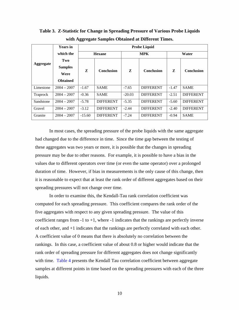
Table 3. Z-Statistic for Change in Spreading Pressure of Various Probe Liquids

with Aggregate Samples Obtained at Different Times. Probe Liquid

Hexane MPK Water

Aggregate

Years in

which the

Two

Samples

Were

Obtained

Z Conclusion Z Conclusion Z Conclusion

Limestone 2004 – 2007 -1.67 SAME -7.65 DIFFERENT -1.47 SAME

Traprock 2004 – 2007 -0.36 SAME -20.03 DIFFERENT -2.51 DIFFERENT

Sandstone 2004 – 2007 -5.78 DIFFERENT -5.35 DIFFERENT -5.60 DIFFERENT

Gravel 2004 – 2007 -3.12 DIFFERENT -2.44 DIFFERENT -2.40 DIFFERENT

Granite 2004 – 2007 -15.60 DIFFERENT -7.24 DIFFERENT -0.94 SAME

In most cases, the spreading pressure of the probe liquids with the same aggregate

had changed due to the difference in time. Since the time gap between the testing of

these aggregates was two years or more, it is possible that the changes in spreading

pressure may be due to other reasons. For example, it is possible to have a bias in the

values due to different operators over time (or even the same operator) over a prolonged

duration of time. However, if bias in measurements is the only cause of this change, then

it is reasonable to expect that at least the rank order of different aggregates based on their

spreading pressures will not change over time.

In order to examine this, the Kendall-Tau rank correlation coefficient was

computed for each spreading pressure. This coefficient compares the rank order of the

five aggregates with respect to any given spreading pressure. The value of this

coefficient ranges from -1 to +1, where -1 indicates that the rankings are perfectly inverse

of each other, and +1 indicates that the rankings are perfectly correlated with each other.

A coefficient value of 0 means that there is absolutely no correlation between the

rankings. In this case, a coefficient value of about 0.8 or higher would indicate that the

rank order of spreading pressure for different aggregates does not change significantly

with time. Table 4 presents the Kendall Tau correlation coefficient between aggregate

samples at different points in time based on the spreading pressures with each of the three

liquids.

11

Table 4. Kendall Tau Correlation Coefficient

for Aggregate Spreading Pressures. Probe

Liquid

Kendall – Tau

Rank Correlation

Coefficient

Hexane 0.6

MPK 0.8

Water 0.8

From Tables 3 and 4, it is evident that the surface properties of aggregates

obtained from the same source are changing over time. However, the ranking of these

aggregates based on their polar components (reflected by spreading pressures) did not

change significantly. It is important to reiterate here that the polar components of the

aggregate are the most significant contributors to determining the moisture damage

potential for any different pair of aggregate and asphalt binder. Therefore, the surface

energy components of the aggregates available from a database may be used for future

materials selection with some caution. It is also recommended that the surface energy of

the aggregates be measured and monitored based on samples collected more frequently

than two to three years.

2.1 VARIATION IN SURFACE ENERGY OF BINDERS FROM THE SAME

SOURCE

The objective of Task 4 was to determine the change in surface free energy of an

asphalt binder obtained from the same manufacturer, with same PG grade, and similar

modification if any, but produced at a different point in time or batch. Twenty-one

different asphalt binders were selected for this task (Table 2). Two samples of each

binder were obtained in 2004 and 2007, respectively. After obtaining the samples the

binders were stored in air tight containers at low temperatures to ensure that any

permanent change to the asphalt binder due to oxidation was minimal. The surface

energy components of the binders were determined using the procedures described

before.

12

Unlike aggregates, there is a well-defined error propagation model to determine

the standard deviation in each component based on the standard deviation in the

measured contact angles with different probe liquids. Variations in the surface free

energy of the binders were determined based on the average value and standard deviation

of each surface energy components. A z-test was conducted to determine whether or not

the average surface energy components changed between two otherwise similar asphalt

binder samples collected at different points in time. The null hypothesis in this case is

. Table 5 lists the z-statistic for different asphalt binders and whether the

surface energy components were similar over time (accept null hypothesis) or different

(reject null hypothesis) at significance of α of 0.05.

In all cases, at least one of the three surface free energy components changed due

to changes in the batch used for the test sample. As in the case of aggregates, it is

possible that the change in surface energy of the binder may be due to a bias in the

measurements. As before a rank correlation coefficient was used to estimate whether the

rank order of different binders based on their surface energy components were preserved

over time despite the changes in the absolute values. Table 6 presents the Kendall Tau

correlation coefficient between asphalt binders sampled at two different points in time

based in their surface energy components.

H 0 : μ 1 = μ 2

13

Table 5. Z-Statistic for Change in Surface Energy Components of

Asphalt Binders Obtained at Two Different Points in Time.

Asphalt Binder

Surface Energy Component

Non-Polar (LW) Acid (+) Base (-)

Z Conclusion Z Conclusion Z Conclusion

Source 1: 64-22 B -20.7 DIFFERENT -6.3 DIFFERENT -1.5 SAME

Source 1: 70-22 S -10.3 DIFFERENT -4.0 DIFFERENT -5.5 DIFFERENT


Source 5: 64-22 B -13.0 DIFFERENT -6.8 DIFFERENT -8.7 DIFFERENT

Source 5: 70-22 S -1.9 SAME -3.5 DIFFERENT -15.5 DIFFERENT


Source 7: 64-22 B -0.5 SAME -0.2 SAME -3.8 DIFFERENT



Source 6: 64-22 B -0.2 SAME -1.5 SAME -4.3 DIFFERENT



Source 2: 64-22 B -6.4 DIFFERENT -1.6 SAME -7.7 DIFFERENT



Source 2: 76-22 TRS -11.9 DIFFERENT -2.9 DIFFERENT -8.6 DIFFERENT

Source 4: 64-22 B -6.9 DIFFERENT -0.3 SAME -6.4 DIFFERENT



Source 4: 70-28 S -9.1 DIFFERENT -4.0 DIFFERENT -1.3 SAME


Table 6. Kendall Tau Correlation Coefficient

for Asphalt Surface Energy Components. Surface

Energy

Component

Kendall – Tau

Rank Correlation

Coefficient

Non-Polar 0.09

Acid 0.09

Base 0.44

14

From Tables 5 and 6 it is evident that the surface energy components of similar

asphalt binders from the same source were significantly different from one batch to

another. Unlike the polar components of the aggregates, the rank correlation coefficient

for asphalt binders based on their polar components was very poor. This indicates that

the surface free energy and concomitant ranking of asphalt binders are both susceptible to

significant changes when samples are obtained from different batches. It is

recommended that the surface energy of the asphalt binder be measured much more

frequently than the aggregates.

2.5 DATABASE OF SURFACE ENERGY OF AGGREGATES AND BINDERS

A database of surface energy values for all the materials tested in Tables 1 and 2

was prepared. The database was in the form of a Microsoft Excel® spreadsheet and

includes several user-friendly features such as determination of the energy parameters for

materials selection. Appendix D provides more details on using this spread sheet to add /

delete information and interpret results from existing data. The electronic database with

the complete data from this project will accompany this report as product P1.

2.6 SURFACE ENERGY EQUIPMENT INSTALLATION AND TRAINING

A Wilhelmy plate device was purchased and installed at the TxDOT CST

laboratory in Cedar Park campus in August 2008. A second round of training was

provided to the project coordinator and laboratory personnel at the TxDOT facility. The

training included specimen preparation and testing using the Wilhelmy plate device. The

device to measure surface free energy of aggregates was not purchased per the

instructions from TxDOT.

15

CHAPTER 3. SUMMARY AND CONCLUSIONS A total of 21 aggregates and 44 different types of asphalt binders were included in

this implementation project. The three surface energy components of these materials

were determined and included in a user-friendly electronic database. The electronic

database allows the user to add/modify/delete surface free energy properties of

aggregates and asphalt binders. The database also computes the adhesion characteristics

for different combinations of asphalt binders and aggregates that can be selected by the

user.

The surface energy components of two samples of five different aggregates were

determined in this project. The two samples were obtained from the same aggregate

source but at least two years apart. Results indicate that although the surface free energy

components of the aggregates from the same source may change over time, the rank order

of the aggregates based on their polar components did not change significantly.

The surface energy components of two samples for each of the 21 different

asphalt binders were determined in this project. The two samples were obtained from the

same manufacturer but from different batches of production. Results indicate that the

surface free energy components of the asphalt binder are likely to change significantly

with changes in the batch of production. Also, the rank order of the asphalt binders based

on their surface energy components changed significantly over time.

It is recommended that the surface energy components of asphalt binders and

aggregates be measured and monitored over time. Surface energy of asphalt binders must

be measured and incorporated into the database more frequently than the aggregate.

17

APPENDIX A:

TRAINING MATERIAL

This appendix presents the training material that was used during the

demonstration and training on the use of DMA and surface energy equipment.

Dynamic Mechanical Analyzer

Training as a part of the Implementation Program

OUTLINE

• Mix Design (FAM – Fine Aggregate Matrix)

• Sample Preparation• Test Method • Data Analysis

MIX DESIGN

F/A – filler and binder proportion by volumeA/A – binder plus filler and fine aggregates proportion in massExample

MIX DESIGN• Alternative and simpler FAM design procedure being

developed.

• More representative of the mastic in the mixture

• Requires fewer assumptions

• Lab trials in progress to determine any adjustments if required to make specimen compactible in SGC

SAMPLE PREPARATIONCONVENTIONAL 6” SGC SAMPLE PREPARATION

12

3 4

5 67 8

150mm

At least 3min of mixingis usually necessary

2h short term aging atcompaction temperature

2

3

Wait around 10min beforeremove the sample from the mold

8

SAMPLE PREPARATION

SAWING PROCESS

CORING PROCESS

50mm

19

SAMPLE PREPARATION

Gmb DETERMINATION

GLUING PROCESS

WEIGHT IN WATER

TEST METHODBOHLIN RHEOMETER

• CREEP / CREEP RECOVERY• VISCOMETRY• OSCILLATION• RELAXATION

Controller System• f 10-6 to 150 Hz• T 0.1μNm to

200mNm• Torsional Load• Static or Dynamic

SamplesΦ - 10 to 25 mmh – 40 to 100 mm

Temperature Control Unit-150°C to 550°C


• START UP OF RHEOMETER SYSTEM

• SELECT THE CORRECT MEASURING SYSTEM

• INSTALLING THE MEASURING SYSTEM


• SETTING THE CORRECT GAP

• SAMPLE LOADING



20


LOW STRAIN – 0.0065% ( LinearViscoelastic Properties)

HIGH STRAIN – 0.2% (Non LinearViscoelastic Properties and Damage)




Low % StrainLinear Viscoelastic Properties

High % StrainNon Linear Viscoelastic Properties and Damage

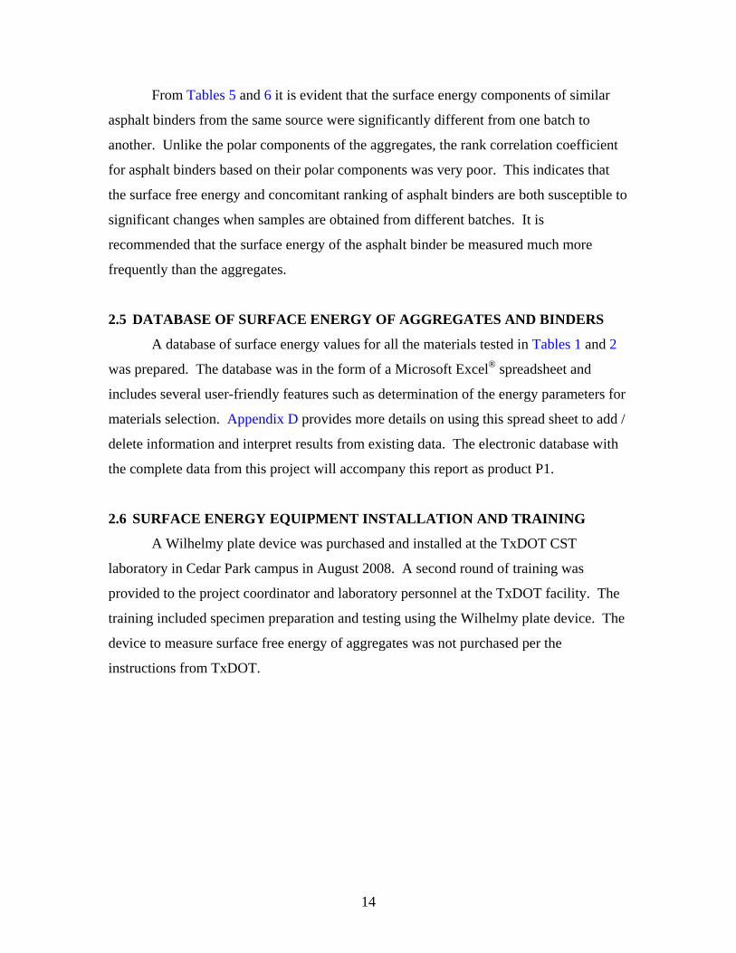
Data Analysis

Two types:• Direct estimation of fatigue life in terms of number of

cycles to failure– Straightforward and simple– Higher variability– Gross measure of FAM performance

• Estimation of crack growth index– Based on fracture mechanics– Lower variability– Accounts for different material properties

Fatigue Life

• Obtain summary raw data file from DMA

• Plot G* vs. time or number of load cycles

• Plot φ vs. time or number of load cycles

• Plot NxG*(N)/G*(1) vs. number of load cycles

• Obtain fatigue life

21

Fatigue Life

0

0.2

0.4

0.6

0.8

1

1.2

0 20000 40000 60000 80000 100000 120000 140000

Cycles

G*/G

0

0

10

20

30

40

50

60

70

Phas

e A

ngle

FATIGUE LIFE ANALYSIS

Fatigue Life

0

5000

10000

15000

20000

25000

30000

35000

40000

45000

0 20000 40000 60000 80000 100000 120000 140000

Cycles

N*G

*/G0

0

0.2

0.4

0.6

0.8

1

1.2

G*/G

0

FATIGUE LIFE ANALYSIS

PARA-METERS

Dynamic Mechanical Analyzer (DMA)

Relaxation Test

Cyclic load - low strain

Cyclic load - high strain

Wilhelmy Plate

U S D

Surface energy of asphalt binder

TEST DEVICE

Surface energy of aggregate

b(from

DPSE vs. N curve)

GR(Undamaged reference modulus)

E1 & m(Relaxation

test parameters)

TEST TYPE

ΔGf(work of cohesion / adhesion)

ΔR(N) – Crack growth index

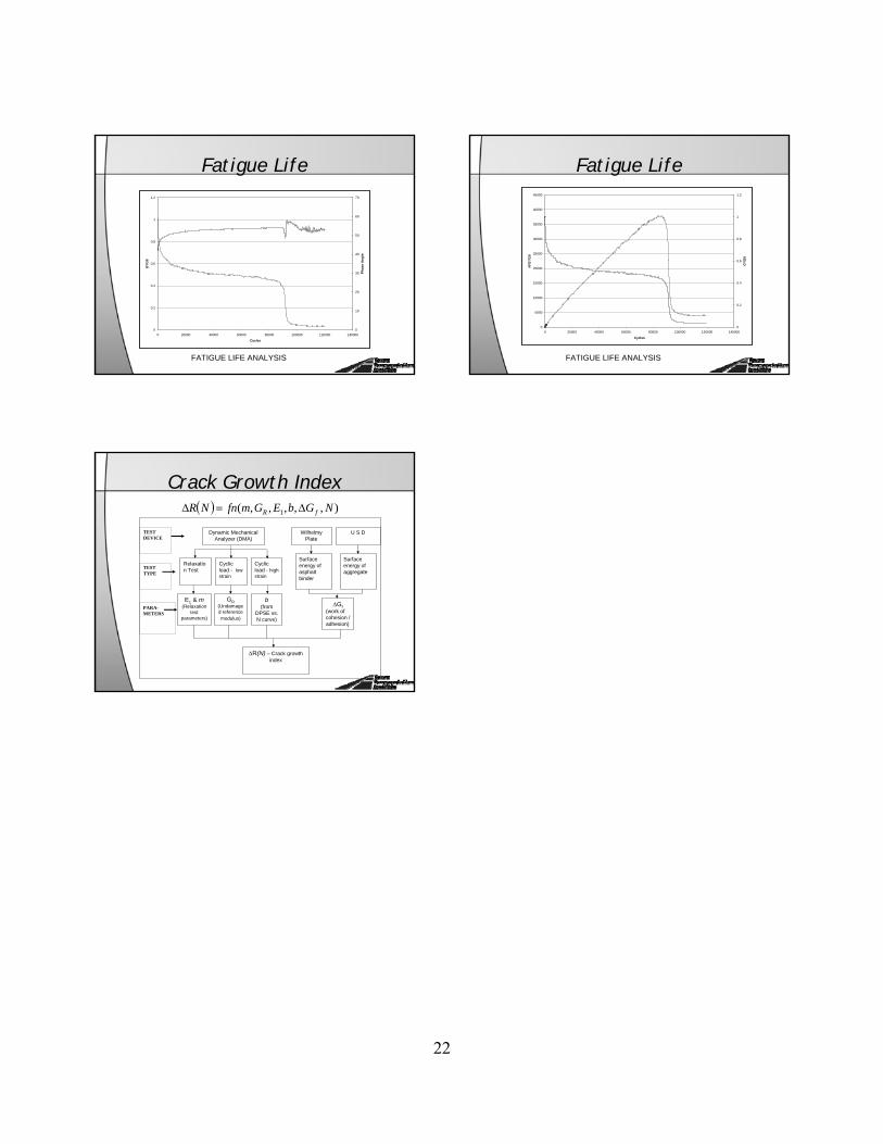
( ) ),,,,,( 1 NGbEGmfnNR fR Δ=Δ

Crack Growth Index

22

Surface Energy

Bulk molecule -uniform forces

Surface molecule –subject to inward forces

DefinitionEnergy required to form a unit area of new surface

NoteInterface is a special type of a surface

Adhesion

→Surface energy of Interface = γAS

→Work done for ‘da’ of material A = γA da

→Work done for ‘da’ of material S = γS da

→‘da’ of interface A-S lost = γAS da

→ Adhesive bond energy ΔGAS = γA + γS – γAS

Greater magnitude of ΔGAS → stronger the bond between the two materials

Surface Energy

dada

Moisture Damage

SA = lost aggregate-asphalt interface (-γSA)WS = new water-aggregate interface (γWS)WA = new water-asphalt interface (γWA)

Total energy used ΔGWAS = γWA + γWS – γSA

≤ 0 !! (Typically)

Lesser magnitude of ΔGWAS → greater work required by external loads to drive water to strip bitumen from aggregate → lesser moisture sensitivity

Surface Energy

SA

WA

WS

Conditions favorable to resist moisture damage:

(i) High value of adhesive bond energy ΔGAS

(ii) Low value of reduction in free energy of the system |ΔGWAS|

Combining the above two statements:

Surface Energy

ERGG

WAS

AS =ΔΔ

∝ damage moisture to Resistance

fn(surface energy components of A, S, & W)

Surface Energy

Asphalt:

Contact Angle Method

Aggregate:

Vapor Adsorption Method

Surface Energy

Wilhelmy Plate Test Adsorption Test (USD)

Output: Contact angles Output: Adsorption isotherm

Analysis: Work of adhesion with probe liquids

Analysis: Work of adhesion with probe vapors

Result: Three surface energy components

Result: Three surface energy components

Performance related parameters:(1) ΔGAS (2) ΔGWAS

Moisture Sensitivity of Mixes:Field / Laboratory Performance

23

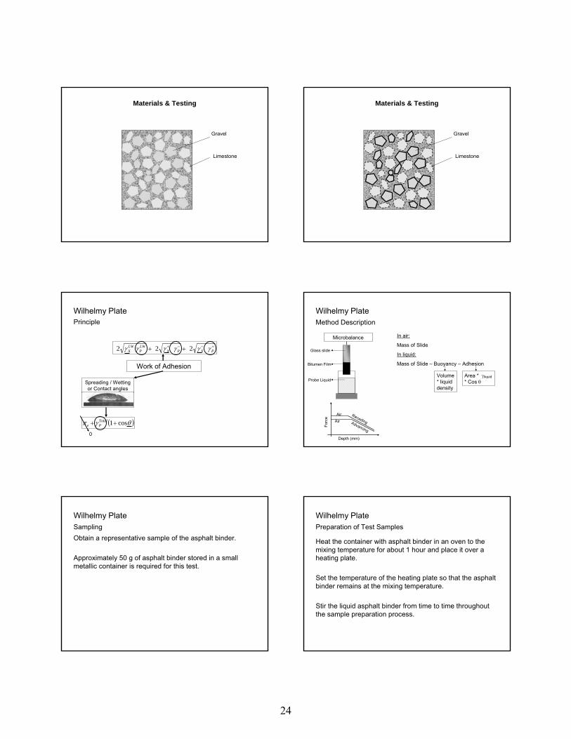
Gravel

Limestone

Materials & Testing

Gravel

Limestone

Materials & Testing

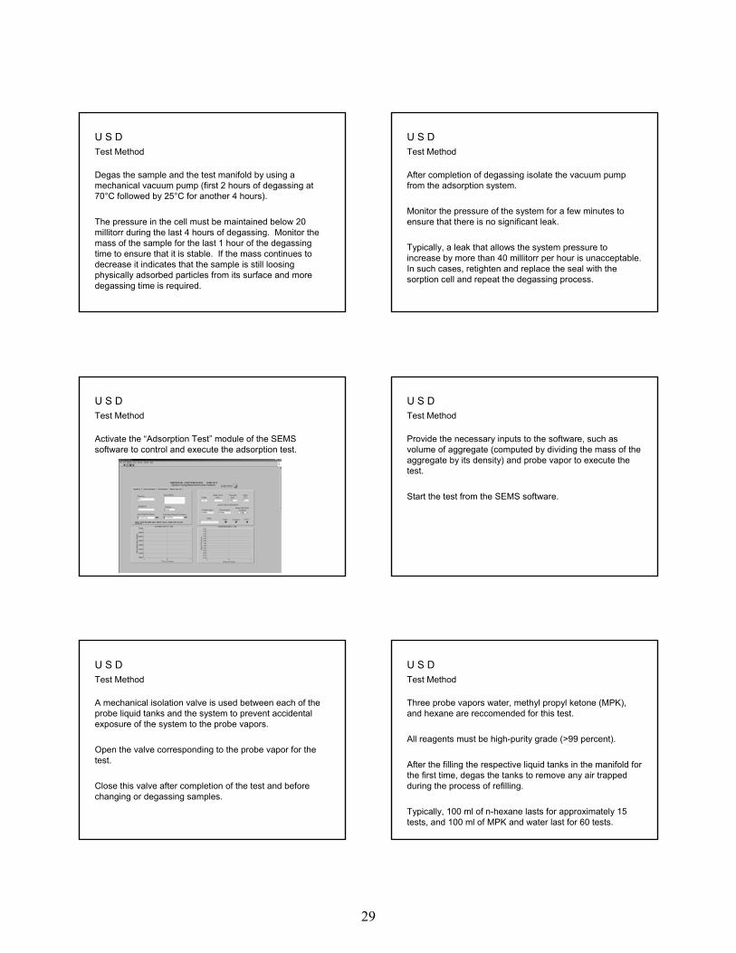
Wilhelmy PlatePrinciple

+−−+ ++ PXPXLWP

LWX γγγγγγ 222

Work of Adhesion

( )θγπ cos1++ TotalPe

Spreading / Wetting or Contact angles

0

Microbalance In air:

Mass of Slide

In liquid:

Mass of Slide – Buoyancy – Adhesion

Volume * liquid density

Area * γliquid* Cos θ

Air Advancing

Receding

Air

Depth (mm)

Forc

e

Glass slide

Bitumen Film

Probe Liquid

Method Description Wilhelmy Plate

Obtain a representative sample of the asphalt binder.

Approximately 50 g of asphalt binder stored in a small metallic container is required for this test.

SamplingWilhelmy Plate

Heat the container with asphalt binder in an oven to the mixing temperature for about 1 hour and place it over a heating plate.

Set the temperature of the heating plate so that the asphalt binder remains at the mixing temperature.

Stir the liquid asphalt binder from time to time throughout the sample preparation process.

Preparation of Test SamplesWilhelmy Plate

24

Pass the end of the glass slide intended for coating six times on each side through the blue flame of a propane torch to remove any moisture.


Dip the slide into the molten bitumen to a depth of approximately 15 mm.


Drain excess binder is allowed to drain from the plate until a very thin (0.18 to 0.35 mm) and uniform layer at least 10 mm thick remains on the plate.

A thin coating is required to reduce variability of the results.


A thin coating is required to reduce variability of the results.Turn the plate with the uncoated side downward and carefully place it in the slotted slide holder.


If necessary, the heat-resistant slide holder with all the coated slides is placed in the oven after coating for 15 to 30 seconds to obtain the desired smoothness.

Place the binder-coated plates in a desiccator overnight.


Ensure that the microbalance is calibrated in accordance with the manufacturer specifications prior to the start of test.

Remove one asphalt binder coated slide from the desiccator at a time.

Measure the width and thickness of the asphalt binder slide to an accuracy of 0.01 mm to calculate its perimeter. The measurements must be made just beyond 8 mm from the edge of the slide to avoid contamination of the portion of coating that will be immersed in the probe liquid.

Test MethodWilhelmy Plate

25

Suspend the glass slide coated with asphalt binder from the microbalance using a crocodile clip.

Ensure that the slide is horizontal with respect to the base of the balance.

Fill a clean glass beaker with the probe liquid to a depth of at least 10 mm and place it on the balance stage.


Raise the stage manually to bring the top of the probe liquid in proximity to the bottom edge of the slide


During the test, the stage is raised or lowered at the desired rate via a stepper motor controlled by the accompanying software.

A rate of 40 microns per second is recommended to achieve the quasi-static equilibrium conditions for contact angle measurement.

The depth to which the sample is immersed in the probe liquid is set to 8 mm.


Five probe liquids are recommended for use with this test. These are water, ethylene glycol, methylene iodide (diiodomethane), glycerol, and formamide.

All reagents must be high-purity grade (>99%). Contact angles must be measured for at least three replicates with each probe liquid for each asphalt binder.

Since methylene iodide is a light-sensitive material, cover the beaker containing methylene iodide with black tape to reduce the effect of light.


Dispose the probe liquid in the beaker after testing with three asphalt binder slides, and use a fresh sample of the probe liquid for each different type of binder. Store all probe liquids in air tight containers and dot not use after prolonged exposure to air in open-mouthed beakers.

Tests must be completed within 24 to 36 hours from the time of preparation of the slides.


Select a representative area of the line for regression analysis. The software reports the advancing & receding contact angles based on the area selected using the aforementioned equation.

Results Wilhelmy Plate

26

Report force measurements that are not smooth, i.e., if sawtooth-like force measurements are observed due to slip-stick behavior between the probe liquid and the asphalt binder

The typical standard deviation of the measured contact angle for each pair of liquid and asphalt binder based on measurements with three replicate slides is less than 2°.


The contact angle of each replicate and probe liquid is used with the surface energy analysis workbook that conducts the required analysis to determine the three surface energy components of the asphalt binder and the standard deviations of these components.

This workbook also verifies the accuracy and consistency of the measured contact angles and integrates data from other test methods such as the surface energy components of aggregates to determine various parameters of interest that are related to the performance of asphalt mixes.


+−−+ ++ PXPXLWP

LWX γγγγγγ 222

Work of Adhesion

( )θγπ cos1++ TotalPe

Spreading / Wetting or Contact angles

1

Principle U S D

Microbalance

Sorption Cell

Aggregate

p1

p2

p3

Time

Adso

rbed

Mas

s

Method Description U S D

m1

m2

m3

Partial Vapor Pressure

Adso

rbed

M

ass

(p1,m1)(p2,m2)

(p3,m3)

Method Description U S D

nHexaneIsotherm

MPK Isotherm Water Isotherm

SSA from nHexaneadsorption using BET method

Equilibrium spreading

pressure for each vapor

Work of Adhesion +

GVOC Theory

Surface Energy Components

Sieve the sample to obtain about 100 g of aggregates passing a 4.75 mm sieve (#4) and retained on a 2.36 mm sieve (#8)

Sampling U S D

27

Thoroughly wash about 25 g of the aggregate in a 2.36 mm sieve with deionized or distilled water.

The quality of water used for cleaning of aggregates must be comparable to the quality of water used for gas chromatography.

Place the clean aggregate sample in an oven at 150°C for 8 hours, and thereafter transfer it to a desiccator at room temperature for at least 8 hours before testing.

Preparation of Samples U S D

The samples are held in a wire mesh basket during the test.

Rinse the basket with acetone and air dry.

Test Method U S D

Transfer the aggregate sample to the basket and suspend the basket from the hook underneath the suspension balance.

Test Method U S D

Seal the sorption cell with the coupling with the suspension balance using a viton O-ring. A metal jacket connected to a water bath is used around the sorption cell to maintain temperature.

Test Method U S D

Activate and deactivate the magnetic suspension coupling repeatedly until stable and consistent readings are observed. This can also be automatically executed with the “Horizontal Centering” module of the SEMS software.

Test Method U S D

The temperature and degassing times can be controlled manually or automatically using the “Degassing” module of the SEMS software.

Test Method U S D

28

Degas the sample and the test manifold by using a mechanical vacuum pump (first 2 hours of degassing at 70°C followed by 25°C for another 4 hours).

The pressure in the cell must be maintained below 20 millitorr during the last 4 hours of degassing. Monitor the mass of the sample for the last 1 hour of the degassing time to ensure that it is stable. If the mass continues to decrease it indicates that the sample is still loosing physically adsorbed particles from its surface and more degassing time is required.

Test Method U S D

After completion of degassing isolate the vacuum pump from the adsorption system.

Monitor the pressure of the system for a few minutes to ensure that there is no significant leak.

Typically, a leak that allows the system pressure to increase by more than 40 millitorr per hour is unacceptable. In such cases, retighten and replace the seal with the sorption cell and repeat the degassing process.

Test Method U S D

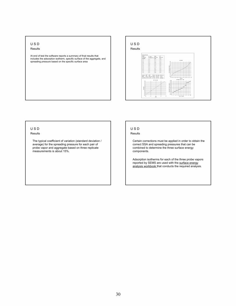
Activate the “Adsorption Test” module of the SEMS software to control and execute the adsorption test.

Test Method U S D

Provide the necessary inputs to the software, such as volume of aggregate (computed by dividing the mass of the aggregate by its density) and probe vapor to execute the test.

Start the test from the SEMS software.

Test Method U S D

A mechanical isolation valve is used between each of the probe liquid tanks and the system to prevent accidental exposure of the system to the probe vapors.

Open the valve corresponding to the probe vapor for the test.

Close this valve after completion of the test and before changing or degassing samples.

Test Method U S D

Three probe vapors water, methyl propyl ketone (MPK), and hexane are reccomended for this test.

All reagents must be high-purity grade (>99 percent).

After the filling the respective liquid tanks in the manifold for the first time, degas the tanks to remove any air trapped during the process of refilling.

Typically, 100 ml of n-hexane lasts for approximately 15 tests, and 100 ml of MPK and water last for 60 tests.

Test Method U S D

29

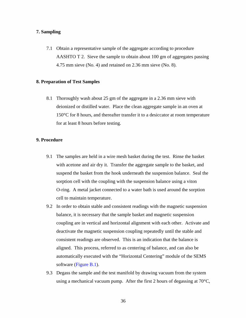
At end of test the software reports a summary of final results that includes the adsorption isotherm, specific surface of the aggregate, and spreading pressure based on the specific surface area

Results U S D

Results U S D

The typical coefficient of variation (standard deviation / average) for the spreading pressure for each pair of probe vapor and aggregate based on three replicate measurements is about 15%.

Results U S D

Certain corrections must be applied in order to obtain the correct SSA and spreading pressures that can be combined to determine the three surface energy components.

Adsorption isotherms for each of the three probe vapors reported by SEMS are used with the surface energy analysis workbook that conducts the required analysis.

Results U S D

30

31

APPENDIX B:

PROTOCOL TO MEASURE SPREADING PRESSURES

AND METHOD TO DETERMINE SURFACE FREE ENERGY

OF AGGREGATES USING THE SPREADSHEET CALCULATOR

(PRODUCT 3: PART 1 OF 2)

33

This appendix includes a draft protocol to determine the surface free energy of

aggregates using the USD. The draft protocol is in AASHTO format and was originally

developed during the NCHRP 9-37 project. The appendix also includes a guide to use

Microsoft Excel® spreadsheets to compute the surface free energy components of the

aggregates from the data generated using the USD software.

1. Scope

1.1 This test method covers the procedures for preparing samples and measuring

adsorption isotherms using a sorption device with an integrated Surface Energy

Measurement System (SEMS) to determine the three surface energy

components of asphalt binders.

1.2 This standard is applicable to aggregates that pass through 4.75 mm sieve

(No. 4) and are retained on a 2.36 mm sieve (No. 8).

1.3 This method must be used in conjunction with the manual for mathematical

analysis to determine surface energy components from spreading pressures or

the computerized spreadsheets that were developed to carry out this analysis.

1.4 This standard may involve hazardous material, operations, and equipment.

This standard is not intended to address all safety problems associated with its

use. It is the responsibility of the user of this procedure to establish

appropriate safety and health practices and to determine the applicability of

regulatory limitations prior to its use.

2. Referenced Documents

2.1 AASHTO Standards T 2 Practice for sampling aggregates

34

3. Definitions

3.1 Surface Energy- γ , or surface free energy of a material is the amount of work

required to create unit area of the material in vacuum. The total surface energy

of a material is divided into three components namely the Lifhsitz-van der

Waals component, the acid component, and the base component.

3.2 Equilibrium spreading pressure - eπ , is the reduction in surface energy of the

solid due to adsorption of vapors at its saturation vapor pressure on the surface

of the solid.

3.3 Probe Vapor, within the context of this test, refers to vapors from any of the

pure, homogeneous liquids that do not chemically react or dissolve with

aggregates and is used to measure the spreading pressure with the aggregate.

The three surface energy components of the probe vapor must be known at the

test temperature from the literature.

3.4 Relative Vapor Pressure, within the context of this test, refers to the ratio of

the pressure of the vapor to its saturation vapor pressure and can vary from 0

(complete vacuum) to 1 (saturation vapor pressure).

3.5 Adsorption Isotherm, of a vapor with an aggregate, is the relationship between

the equilibrium mass of vapor adsorbed per unit mass of the aggregate and the

relative vapor pressure of the vapors at a constant temperature.

4. Summary of Method

4.1 Clean aggregate samples are degassed under high temperature and vacuum in

an airtight sorption cell. Vapors of probe liquids are introduced into the

sorption cell in controlled and gradually incremental quantities to achieve

different relative pressures. The equilibrium mass of the vapor adsorbed to the

solid surface is recorded for each relative pressure to obtain the adsorption

isotherm. The adsorption isotherm is used to compute the equilibrium

spreading pressure of the probe vapor with the aggregate.

35

4.2 Equilibrium spreading pressure with different probe vapors are used with

equations of work of adhesion to determine the three surface energy

components of the aggregate.

5. Significance and Use

5.1 Surface energy components of aggregates is an important material property

that is related to the performance of hot mix asphalt. Surface energy

components of aggregates can be combined with the surface energy

components of asphalt binders to quantify the work of adhesion between these

two materials and the propensity for water to displace the asphalt binder from

the asphalt binder-aggregate interface. These two quantities are related to

adhesive fracture properties and moisture sensitivity of the asphalt mix.

6. Apparatus

6.1 A sorption device integrated with the SEMS comprising of an air tight

adsorption cell, a magnetic suspension balance that measures the mass the

sample in the sorption cell in non-contact mode, a manifold with vacuum

pump, temperature control, probe liquid containers with appropriate valves and

controls to regulate the flow of vapors into the sorption cell, and associated

software for test control and analysis. The micro balance must have a least

count of 10 μgm with a capacity to weight at least 50 gm.

6.2 Temperature of the sorption cell, piping that carry vapors, and the buffer tank

are maintained using a water bath that is automatically controlled by the SEMS

software.

6.3 An oven capable to heating up to 150°C is required to prepare aggregate

samples before testing.

36

7. Sampling

7.1 Obtain a representative sample of the aggregate according to procedure

AASHTO T 2. Sieve the sample to obtain about 100 gm of aggregates passing

4.75 mm sieve (No. 4) and retained on 2.36 mm sieve (No. 8).

8. Preparation of Test Samples

8.1 Thoroughly wash about 25 gm of the aggregate in a 2.36 mm sieve with

deionized or distilled water. Place the clean aggregate sample in an oven at

150°C for 8 hours, and thereafter transfer it to a desiccator at room temperature

for at least 8 hours before testing.

9. Procedure

9.1 The samples are held in a wire mesh basket during the test. Rinse the basket

with acetone and air dry it. Transfer the aggregate sample to the basket, and

suspend the basket from the hook underneath the suspension balance. Seal the

sorption cell with the coupling with the suspension balance using a viton

O-ring. A metal jacket connected to a water bath is used around the sorption

cell to maintain temperature.

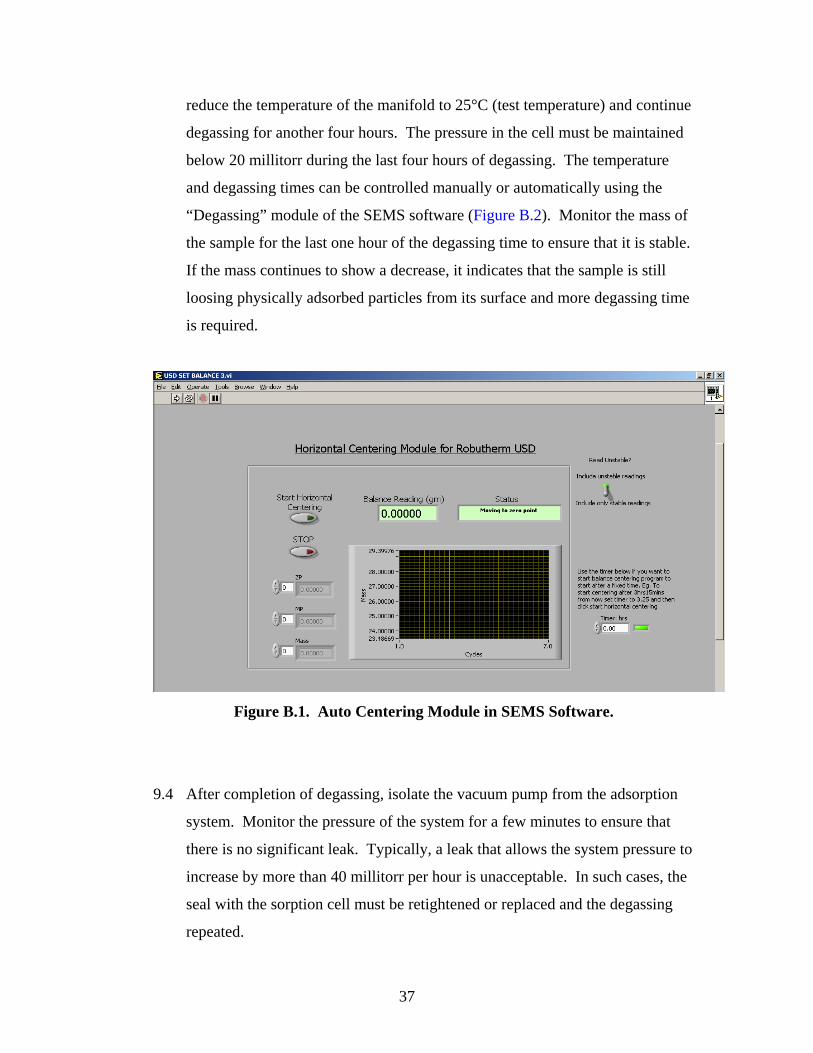
9.2 In order to obtain stable and consistent readings with the magnetic suspension

balance, it is necessary that the sample basket and magnetic suspension

coupling are in vertical and horizontal alignment with each other. Activate and

deactivate the magnetic suspension coupling repeatedly until the stable and

consistent readings are observed. This is an indication that the balance is

aligned. This process, referred to as centering of balance, and can also be

automatically executed with the “Horizontal Centering” module of the SEMS

software (Figure B.1).

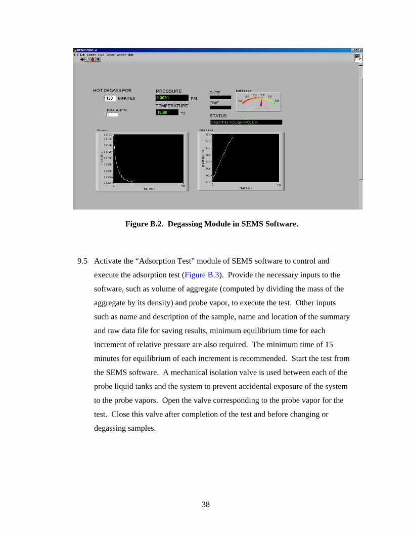
9.3 Degass the sample and the test manifold by drawing vacuum from the system

using a mechanical vacuum pump. After the first 2 hours of degassing at 70°C,

37

reduce the temperature of the manifold to 25°C (test temperature) and continue

degassing for another four hours. The pressure in the cell must be maintained

below 20 millitorr during the last four hours of degassing. The temperature

and degassing times can be controlled manually or automatically using the

“Degassing” module of the SEMS software (Figure B.2). Monitor the mass of

the sample for the last one hour of the degassing time to ensure that it is stable.

If the mass continues to show a decrease, it indicates that the sample is still

loosing physically adsorbed particles from its surface and more degassing time

is required.

Figure B.1. Auto Centering Module in SEMS Software.

9.4 After completion of degassing, isolate the vacuum pump from the adsorption

system. Monitor the pressure of the system for a few minutes to ensure that

there is no significant leak. Typically, a leak that allows the system pressure to

increase by more than 40 millitorr per hour is unacceptable. In such cases, the

seal with the sorption cell must be retightened or replaced and the degassing

repeated.

38

Figure B.2. Degassing Module in SEMS Software.

9.5 Activate the “Adsorption Test” module of SEMS software to control and

execute the adsorption test (Figure B.3). Provide the necessary inputs to the

software, such as volume of aggregate (computed by dividing the mass of the

aggregate by its density) and probe vapor, to execute the test. Other inputs

such as name and description of the sample, name and location of the summary

and raw data file for saving results, minimum equilibrium time for each

increment of relative pressure are also required. The minimum time of 15

minutes for equilibrium of each increment is recommended. Start the test from

the SEMS software. A mechanical isolation valve is used between each of the

probe liquid tanks and the system to prevent accidental exposure of the system

to the probe vapors. Open the valve corresponding to the probe vapor for the

test. Close this valve after completion of the test and before changing or

degassing samples.

39

Figure B.3. Adsorption Test Module in SEMS Software.

9.6 The test is controlled, and data are acquired using the SEMS software. The

software regulates valves to dose probe vapors into the system in ten steps to

achieve an increment of 0.1 in the relative pressure with each step. The mass

of the sample is continuously acquired during this process by the SEMS

software. The software computes the mass of vapor adsorbed in real time as

the difference in the mass of sample at any time with the mass of the sample in

vacuum after applying for corrections due to buoyancy. The software also

corrects for any drift in the measurements due to the magnetic suspension

coupling. Each increment of relative pressure is applied by the software after

the mass of the sample comes into equilibrium due to adsorption of vapors

from the previous increment or after the minimum time for equilibrium is

achieved, which ever is later. The test is complete after the saturation vapor

40

pressure of the probe liquid is achieved in ten increments, and the equilibrium

mass of vapor adsorbed is recorded for each increment.

9.7 Three probe vapors are recommended for this test. These are water, methyl

propyl ketone (MPK), and hexane. All reagents must be high purity grade

(>99 percent). After the liquids are filled in their respective tanks in the

manifold for the first time, the liquid tanks must be degassed to remove any

trapped air during the process of refilling. Typically, 100 ml of n-Hexane lasts

for approximately 15 tests, and 100 ml of MPK and water last for 60 tests.

10. Calculations

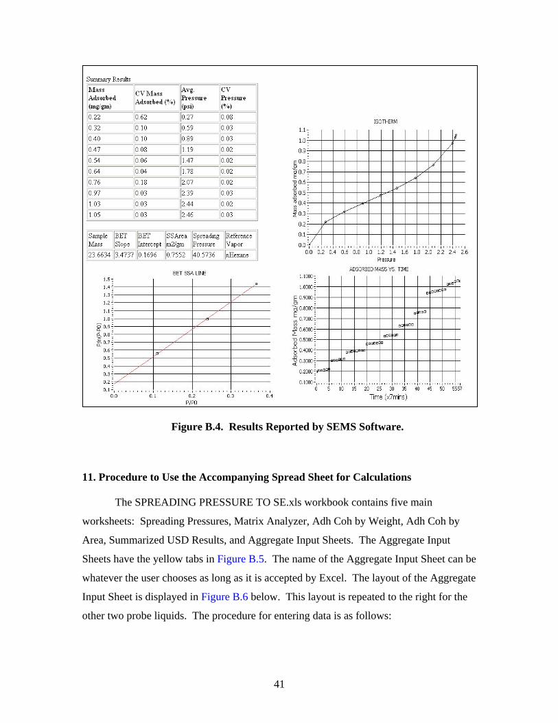
10.1 After completion of all ten increments in vapor pressure, the software reports a

summary of final results that include the adsorption isotherm, specific surface

of the aggregate with BET equations, and spreading pressure based on the

specific surface area and the adsorption isotherm (Figure B.4).

10.2 Although the SEMS software reports specific surface areas and spreading

pressures for each test, certain corrections must be applied in order to obtain

the correct specific surface area and spreading pressures that can be combined

to determine the three surface energy components. Therefore, the adsorption

isotherms with each of the three probe vapors reported by SEMS are used with

the surface energy analysis workbook that conducts the required analysis to

determine the specific surface area and the three surface energy components of

the aggregate and the standard deviations of these components. This

user-friendly workbook also integrates data from other tests such as the surface

energy components of asphalt binders to determine various parameters of

interest that are related to the performance of asphalt mixes.

41

Figure B.4. Results Reported by SEMS Software. 11. Procedure to Use the Accompanying Spread Sheet for Calculations The SPREADING PRESSURE TO SE.xls workbook contains five main

worksheets: Spreading Pressures, Matrix Analyzer, Adh Coh by Weight, Adh Coh by

Area, Summarized USD Results, and Aggregate Input Sheets. The Aggregate Input

Sheets have the yellow tabs in Figure B.5. The name of the Aggregate Input Sheet can be

whatever the user chooses as long as it is accepted by Excel. The layout of the Aggregate

Input Sheet is displayed in Figure B.6 below. This layout is repeated to the right for the

other two probe liquids. The procedure for entering data is as follows:

42

Figure B.5. Worksheets Contained in SPREADING PRESSURE TO SE.

1. Click on the Aggregate Input Sheet that data will be entered in. If none are

available, right click on one of the Aggregate Input Sheets, select “Move or

Copy…”, check the “Create a copy” box and choose the location for the sheet.

Once the new sheet has been created, it can be renamed as needed.

2. Click on “Import MPK #1” or the respective button for the data needing to be

input.

3. An “Open” window will appear. Choose the appropriate data file to open. The

software on the USD outputs the test data in .html format; therefore, the

programming in this spreadsheet only recognizes that file type.

4. Open all files for the aggregate.

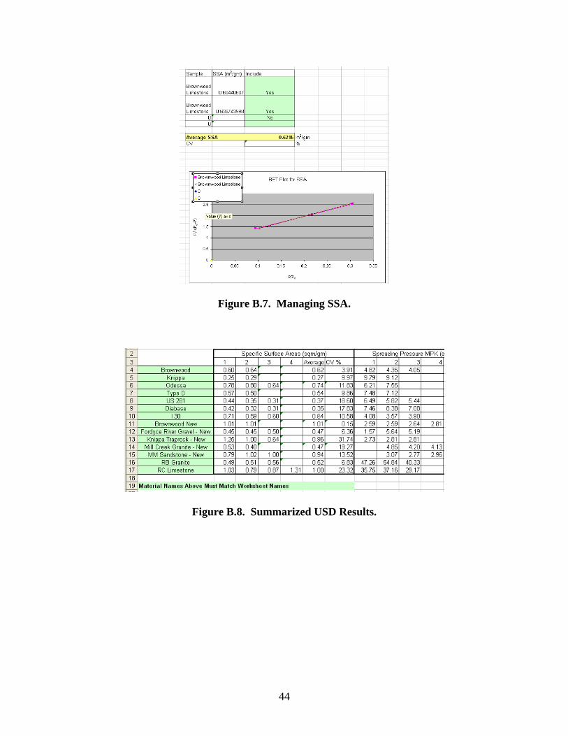
5. Once all files have been opened, it is time to check the calculation for specific

surface area (SSA) of the aggregate. The SSA of the aggregate is based off the

information from the probe liquid n-Hexane. Figure B.7 illustrates the setup of

the SSA information in the worksheet. The SSA for each replicate is displayed in

the table at the top. If one of the replicates has a large variation from the others it

can be removed by selecting “No” instead of “Yes” under the Include column.

6. All the data have been entered.

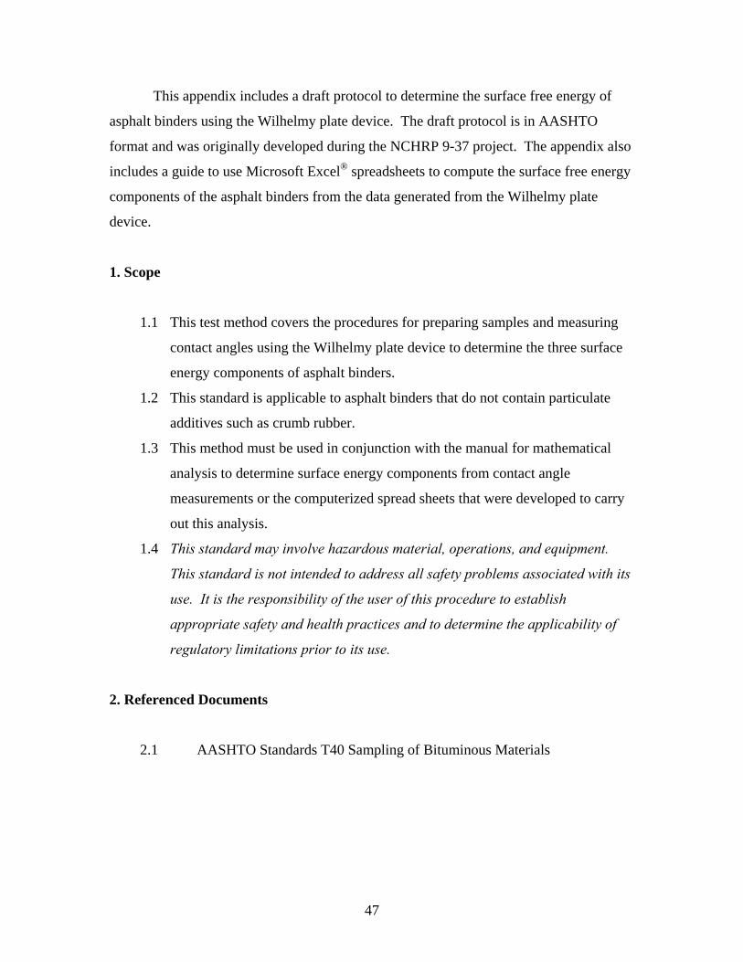
7. Click on the “Summarized USD Results” tab.

8. On the left-hand side of the screen is a column of green cells as shown in

Figure B.8 below. Enter the name of the Aggregate Input Sheet in one of the

green cells. It must be labeled identical or the spreadsheet will not recognize it.

If there are no available spaces, copy as many rows as necessary and paste it right

below the main table. All the surface energy information will appear as soon as

the name of the Aggregate Input Sheet is entered.

43

Figure B.6. Aggregate Input Sheet Layout.

44

Figure B.7. Managing SSA.

Figure B.8. Summarized USD Results.

45

APPENDIX C:

PROTOCOL TO MEASURE CONTACT ANGLE AND METHOD

TO DETERMINE SURFACE FREE ENERGY OF ASPHALT

BINDERS USING THE SPREADSHEET CALCULATOR

(PRODUCT 3: PART 2 OF 2)

47

This appendix includes a draft protocol to determine the surface free energy of

asphalt binders using the Wilhelmy plate device. The draft protocol is in AASHTO

format and was originally developed during the NCHRP 9-37 project. The appendix also

includes a guide to use Microsoft Excel® spreadsheets to compute the surface free energy

components of the asphalt binders from the data generated from the Wilhelmy plate

device.

1. Scope

1.1 This test method covers the procedures for preparing samples and measuring

contact angles using the Wilhelmy plate device to determine the three surface

energy components of asphalt binders.

1.2 This standard is applicable to asphalt binders that do not contain particulate

additives such as crumb rubber.

1.3 This method must be used in conjunction with the manual for mathematical

analysis to determine surface energy components from contact angle

measurements or the computerized spread sheets that were developed to carry

out this analysis.

1.4 This standard may involve hazardous material, operations, and equipment.

This standard is not intended to address all safety problems associated with its

use. It is the responsibility of the user of this procedure to establish

appropriate safety and health practices and to determine the applicability of

regulatory limitations prior to its use.

2. Referenced Documents

2.1 AASHTO Standards T40 Sampling of Bituminous Materials

48

3. Definitions

3.1 Surface Energy- γ , or surface free energy of a material, is the amount of work

required to create unit area of the material in vacuum. The total surface energy

of a material is divided into three components namely the Lifhsitz-van der

Waals component, the acid component, and the base component.

3.2 Contact Angle - θ , refers to the equilibrium contact angle of a liquid on a solid

surface measured at the point of contact of the liquid-vapor interface with the

solid.

3.3 Advancing Contact Angle, within the context of this test, refers to the contact

angle of a liquid with the solid surface as the solid surface is being immersed

into the liquid.

3.4 Receding Contact Angle, within the context of this test, refers to the contact

angle of a liquid with the solid surface as the solid surface is being withdrawn

from the liquid.

3.5 Probe Liquid, within the context of this test, refers to any of the pure,

homogeneous liquids that does not react chemically or dissolve with asphalt

binders and is used to measure the contact angles with the binder. The three

surface energy components of the probe liquid must be known at the test

temperature from the literature.

3.6 Mixing Temperature, within the context of this test, refers to the temperature at

which the viscosity of the asphalt binder is approximately 0.170 Pas, or any

other temperature that is prescribed or determined by the user for use as the

mixing temperature with aggregates to prepare hot mix asphalt.

4. Summary of Method

4.1 A glass slide coated with the asphalt binder and suspended from a

micro balance is immersed in a probe liquid. From simple force equilibrium

conditions the contact angle of the probe liquid with the surface of the asphalt

49

binder can be determined. The analysis to obtain the contact angle is carried

out using a software accompanying the device.

4.2 Contact angles measured with different probe liquids are used with equations

of work of adhesion to determine the three surface energy components of the

asphalt binder.

4.3 Figure C.1 presents a schematic of the Wilhelmy plate device.

Figure C.1. Schematic of the Wilhelmy Plate Device.

5. Significance and Use

5.1 Surface energy components of asphalt binders is an important material

property that is related to the performance of hot mix asphalt. Surface energy

components of asphalt binders can be used to determine the total surface

energy and cohesive bond strength of this material. The cohesive bond

strength of asphalt binders is related to the work required for micro cracks to

propagate within the asphalt binder in an asphalt mix, which is related to the

fatigue cracking characteristics of the mix.

Meniscus formation

Glass slide coated with bitumen

Probe liquid

Micro balance

50

5.2 Surface energy components of asphalt binders can also be combined with the

surface energy components of aggregates to compute the work of adhesion

between these two materials and the propensity for water to displace the

asphalt binder from the asphalt binder-aggregate interface. These two

quantities are related to the moisture sensitivity of the asphalt mix.

6. Apparatus

6.1 Wilhelmy plate device – This device comprises of a micro balance with a

motor controlled stage that can be raised or lowered at desired speed to

immerse a slide with asphalt binder in the probe liquid in advancing mode and

to withdraw the slide from the probe liquid in receding mode.

6.2 A data acquisition and analysis software to collect the data and determine the

contact angles.

6.3 An oven capable of heating up to 150°C is required to heat asphalt binders for

sample preparation. Microscope glass slides (24 mm x 60 mm No. 1.5) are

required to serve as substrates for the asphalt binder and a vernier calipers to

measure the dimensions of the slide. A heating plate with temperature control

is required for maintaining the temperature of the asphalt binder during the

sample preparation process.

6.4 The tests are conducted at 25°C. If the room temperature is significantly

different from the test temperature, then an appropriate environmental chamber

may be required to house the apparatus.

6.5 A slotted slide holder is required to hold the finished asphalt binder slides.

7. Sampling

7.1 Obtain a representative sample of the asphalt binder according to procedure

AASHTO T 40. Approximately 50 gm of asphalt binder stored in a small

metallic container will be required for this test.

51

8. Preparation of Test Samples

8.1 Heat the container with asphalt binder in an oven to the mixing temperature for

about one hour and place it over a heating plate. Set the temperature of the

heating plate so that the asphalt binder remains at the mixing temperature. The

liquid asphalt binder is stirred from time to time throughout the sample

preparation process.

8.2 Pass the end of the glass slide intended for coating six times on each side

through the blue flame of a propane torch to remove any moisture. Dip the

slide into the molten bitumen to a depth of approximately 15 mm. Excess

bitumen is allowed to drain from the plate until a very thin (0.18 to 0.35 mm)

and uniform layer of at least 10 mm remains on the plate. A thin coating is

required to reduce variability of the results. Turn the plate with the uncoated

side downwards (Figure C.2) and carefully place it in the slotted slide holder.

If necessary, the heat-resistant slide holder, with all the coated slides is placed

in the oven after coating for 15 to 30 seconds to obtain the desired smoothness.

Place the bitumen-coated plates in a desiccator overnight.

9. Procedure

9.1 The user must ensure that the micro balance is calibrated in accordance with

the manufacturers specifications prior to the start of test.

9.2 One bitumen-coated slide is removed from the desiccator at a time. Measure

the width and thickness of the asphalt binder slide to an accuracy of 0.01 mm

to calculate its perimeter. The measurements must be made just beyond 8 mm

from the edge of the slide to avoid contamination of the portion of coating that

will be immersed in the probe liquid.

52

Figure C.2. Glass Slide Coated with Asphalt Binder for Testing

with the Wilhelmy Plate Device.

9.3 Suspend the glass slide coated with asphalt binder the micro balance using a

crocodile clip. Ensure that the slide is horizontal with respect to the base of the

balance. Fill a clean glass beaker with the probe liquid to a depth of at least

10 mm and place it on the balance stage. Raise the stage manually to bring the

top of the probe liquid in proximity to the bottom edge of the slide

(Figure C.3).

9.4 During the test, the stage is raised or lowered at the desired rate via a stepper

motor controlled by the accompanying software. A rate of 40 microns per

second is recommended to achieve the quasi-static equilibrium conditions for

contact angle measurement. Set the depth to which the sample is immersed in

the probe liquid is set to 8 mm. Larger depths up to 15 mm may be used if the

thickness of asphalt coating on the slide is uniform. The weight of the slide

measured by the micro balance is recorded continuously during the advancing

(stage is raised to dip the slide) and receding (stage is lowered to retract the

slide from the liquid) process.

9.5 Five probe liquids are recommended for this test. These are water, ethylene

glycol, methylene iodide (diiodomethane), glycerol, and formamide. All

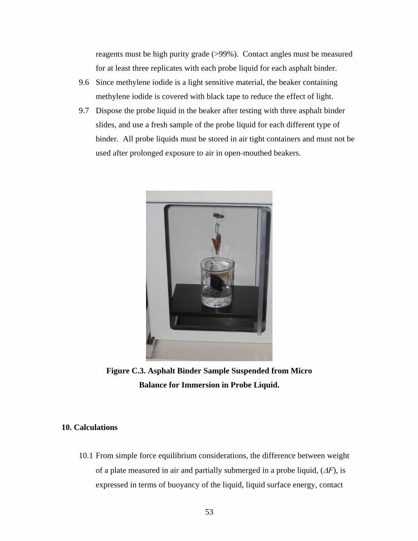
53

reagents must be high purity grade (>99%). Contact angles must be measured

for at least three replicates with each probe liquid for each asphalt binder.

9.6 Since methylene iodide is a light sensitive material, the beaker containing

methylene iodide is covered with black tape to reduce the effect of light.

9.7 Dispose the probe liquid in the beaker after testing with three asphalt binder

slides, and use a fresh sample of the probe liquid for each different type of

binder. All probe liquids must be stored in air tight containers and must not be

used after prolonged exposure to air in open-mouthed beakers.

Figure C.3. Asphalt Binder Sample Suspended from Micro

Balance for Immersion in Probe Liquid.

10. Calculations

10.1 From simple force equilibrium considerations, the difference between weight

of a plate measured in air and partially submerged in a probe liquid, (ΔF), is

expressed in terms of buoyancy of the liquid, liquid surface energy, contact

54

angle, and geometry of the plate. The contact angle between the liquid and

surface of the plate is calculated from this equilibrium as:

( )TotLt

airLim

PgVF

γρρ

θ−+Δ

=cos

where Pt is the perimeter of the bitumen coated plate, TotLγ is the total surface

energy of the liquid, θ is the dynamic contact angle between the bitumen and

the liquid, Vim is the volume immersed in the liquid, ρL is the density of the

liquid, ρair is the air density, and g the local acceleration due to gravitation.

The accompanying software requires the density of the liquid, total surface

tension of the liquid, dimensions of the sample, and local acceleration due to

gravity as inputs to compute the contact angle using the force measurements

from the micro balance.

10.2 Buoyancy correction based on slide dimensions and liquid density can

introduce unwanted variability into the resulting contact angles. To eliminate

these effects, the accompanying software performs a regression analysis of the

buoyancy line and extrapolates the force to zero depth. The user must select a

representative area of the line for regression analysis (Figure C.4). The

software reports the advancing and receding contact angles based on the area

selected using the aforementioned equation.

10.3 If the force measurements are not smooth, i.e., if saw tooth like force

measurements are observed due to slip-stick behavior between the probe liquid

and the asphalt binder, then report this along with the advancing and receding

contact angles.

10.4 The contact angle of each replicate and probe liquid is used with the surface

energy analysis workbook that conducts the required analysis to determine the

three surface energy components of the asphalt binder and the standard

deviations in these components. This workbook also verifies the accuracy and

consistency of the measured contact angles and integrates data from other test

methods such as the surface energy components of aggregates to determine

various parameters of interest that are related to the performance of asphalt

mixes.

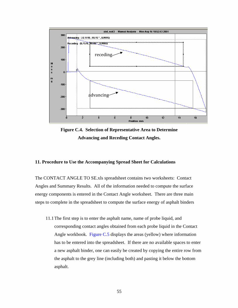
55

Figure C.4. Selection of Representative Area to Determine

Advancing and Receding Contact Angles.

11. Procedure to Use the Accompanying Spread Sheet for Calculations

The CONTACT ANGLE TO SE.xls spreadsheet contains two worksheets: Contact

Angles and Summary Results. All of the information needed to compute the surface

energy components is entered in the Contact Angle worksheet. There are three main

steps to complete in the spreadsheet to compute the surface energy of asphalt binders

11.1 The first step is to enter the asphalt name, name of probe liquid, and

corresponding contact angles obtained from each probe liquid in the Contact

Angle workbook. Figure C.5 displays the areas (yellow) where information

has to be entered into the spreadsheet. If there are no available spaces to enter

a new asphalt binder, one can easily be created by copying the entire row from

the asphalt to the grey line (including both) and pasting it below the bottom

asphalt.

advancing

receding

56

11.1.1 The name of the asphalt binder is entered into the top left-hand yellow

highlighted cell. Do not number the asphalt in this cell, only label.

11.1.2. The probe liquids are located in the cells below the asphalt name.

Every cell contains a drop-down list of all available probe liquids,

which is linked to their corresponding material properties. Select the

probe liquids used during the test and choose “None” for the remaining

liquid cells.

11.1.3. The contact angles obtained from the Wilhelmy Plate are entered into

the yellow cells in columns G, H, I, and J and on the row corresponding

to the probe liquid used. Looking at Figure C.5, three replicates were

run using formamide with resulting contact angles of 85.64, 86.43, and

86.09. Columns K and M display the average contact angle and

standard deviation, respectively.

Figure C.5. Entering Contact Angle Information to Compute Surface Energy.

11.2 The second step is computing the surface energy components. Once all the

contact angle information has been entered, the surface energy can easily be

computed. The sample number is located in column A of the spreadsheet as

displayed in Figure C.5 above. This number is entered in the yellow cell in

column AO as shown in Figure C.6. To the right of this is a button labeled

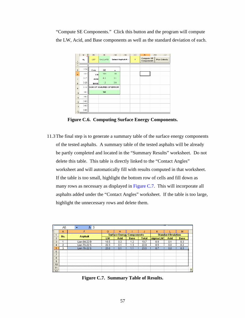
57

“Compute SE Components.” Click this button and the program will compute

the LW, Acid, and Base components as well as the standard deviation of each.

Figure C.6. Computing Surface Energy Components.

11.3 The final step is to generate a summary table of the surface energy components

of the tested asphalts. A summary table of the tested asphalts will be already

be partly completed and located in the “Summary Results” worksheet. Do not

delete this table. This table is directly linked to the “Contact Angles”

worksheet and will automatically fill with results computed in that worksheet.

If the table is too small, highlight the bottom row of cells and fill down as

many rows as necessary as displayed in Figure C.7. This will incorporate all

asphalts added under the “Contact Angles” worksheet. If the table is too large,

highlight the unnecessary rows and delete them.

Figure C.7. Summary Table of Results.

59

APPENDIX D:

PROCEDURE TO USE AND POPULATE

THE DATABASE OF SURFACE FREE ENERGIES

IN SPREADSHEET FORMAT

61

The database created for TxDOT was designed to be very user friendly and easily

updatable. When the program is started the user is greeted by the screen shown in

Figure D.1. At this point the user can:

• Analyze existing materials in the database;

• Add new asphalt or aggregate information into the database;

• Delete an existing asphalt or aggregate out of the database; and

• Exit the user interface and navigate the spreadsheet.

Figure D.1. User Interface.

Analyze Available Aggregate-Asphalt Combinations

This option will allow the user to select as many combinations of asphalt-

aggregate as are contained in the database. Figure D.2. below illustrates the selection

screen. All asphalts and aggregates are displayed in this screen and disappear once they

have been selected.

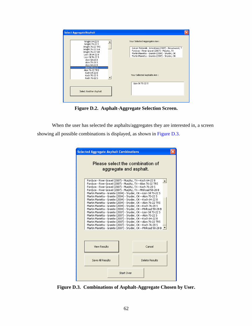
62

Figure D.2. Asphalt-Aggregate Selection Screen.

When the user has selected the asphalts/aggregates they are interested in, a screen

showing all possible combinations is displayed, as shown in Figure D.3.

Figure D.3. Combinations of Asphalt-Aggregate Chosen by User.

63

The user now has the options of:

• Viewing the results of any asphalt-aggregate combination;

• Saving the results of all combinations in the “Results” worksheet;

• Exiting the user interface mode;

• Deleting results from the “Results” worksheet; and

• Starting back over from the beginning screen shown in Figure D.3.

If the “View Results” button is clicked, a screen showing the results for the selected

asphalt-aggregate combination is displayed; an example is shown in Figure D.4. These

individual results can be saved in the “Results” worksheet, or the user can return to the

previous screen.

Clicking the “Save All Results” or “Delete Results” will either save the current

information into the “Results” worksheet or allow the user to delete any or all the

information out of the “Results” worksheet, respectively.

The “Results” worksheet, shown in Figure D.4. below, organizes the results seen

in Figure D.5. in a tabular form. The user also has the option of printing the results,

saving the results in a separate workbook without the program, or restarting the user

interface.

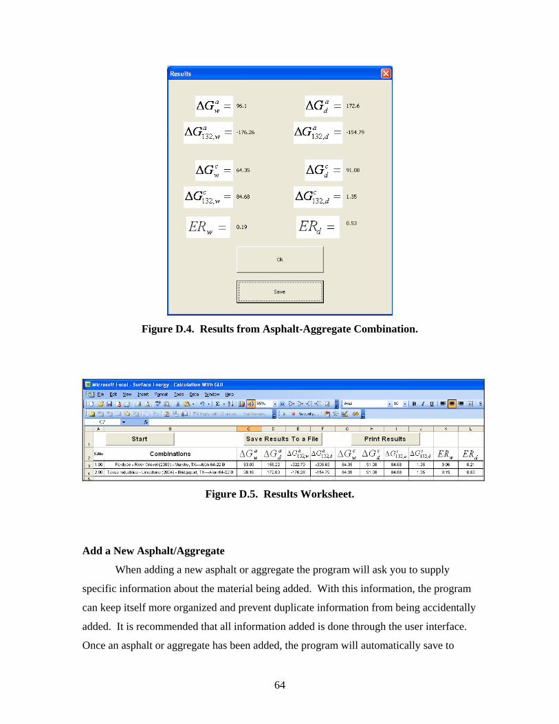
64

Figure D.4. Results from Asphalt-Aggregate Combination.

Figure D.5. Results Worksheet.

Add a New Asphalt/Aggregate

When adding a new asphalt or aggregate the program will ask you to supply

specific information about the material being added. With this information, the program

can keep itself more organized and prevent duplicate information from being accidentally

added. It is recommended that all information added is done through the user interface.

Once an asphalt or aggregate has been added, the program will automatically save to

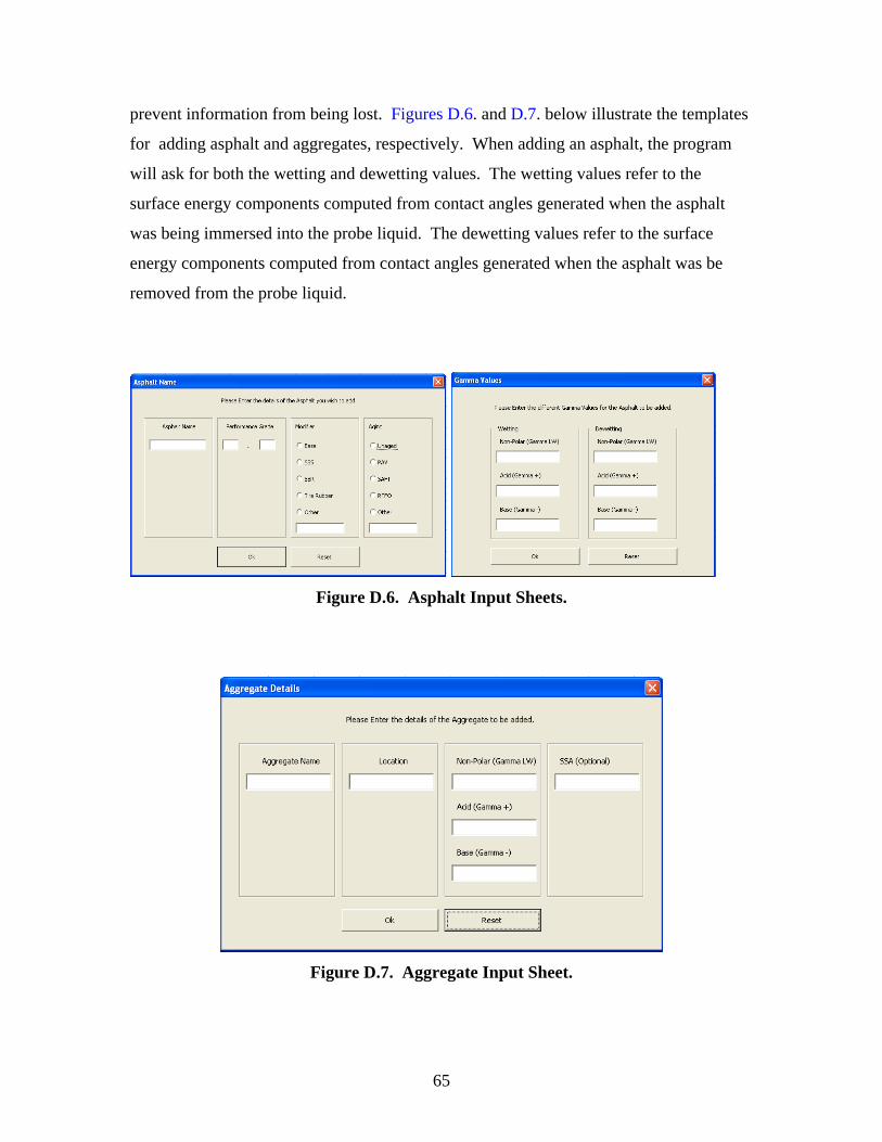
65

prevent information from being lost. Figures D.6. and D.7. below illustrate the templates

for adding asphalt and aggregates, respectively. When adding an asphalt, the program

will ask for both the wetting and dewetting values. The wetting values refer to the

surface energy components computed from contact angles generated when the asphalt

was being immersed into the probe liquid. The dewetting values refer to the surface

energy components computed from contact angles generated when the asphalt was be

removed from the probe liquid.

Figure D.6. Asphalt Input Sheets.

Figure D.7. Aggregate Input Sheet.

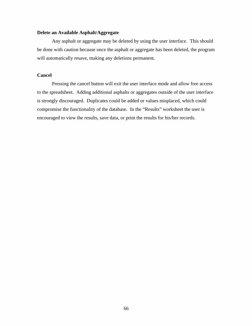
66

Delete an Available Asphalt/Aggregate

Any asphalt or aggregate may be deleted by using the user interface. This should

be done with caution because once the asphalt or aggregate has been deleted, the program

will automatically resave, making any deletions permanent.

Cancel

Pressing the cancel button will exit the user interface mode and allow free access

to the spreadsheet. Adding additional asphalts or aggregates outside of the user interface

is strongly discouraged. Duplicates could be added or values misplaced, which could

compromise the functionality of the database. In the “Results” worksheet the user is

encouraged to view the results, save data, or print the results for his/her records.

Development of a Database for Surface Energy of Aggregates and

Documents

Transcript of Development of a Database for Surface Energy of Aggregates and