Development of a Customized Autopilot for Unmanned Helicopter Model Using Genetic Algorithm via the...

Paper: ASAT-14-008-US 14th International Conference on AEROSPACE SCIENCES & AVIATION TECHNOLOGY, ASAT - 14 – May 24 - 26, 2011, Email: [email protected] Military Technical College, Kobry Elkobbah, Cairo, Egypt Tel: +(202) 24025292 –24036138, Fax: +(202) 22621908

1

Development of a Customized Autopilot for Unmanned Helicopter Model Using Genetic Algorithm via the Application of Different

Guidance Strategies

A. Hosny*, M. Hosny†, and H. Ez-Eldeen‡

Abstract: The objective of this paper is to develop a customized autopilot system that enables a helicopter model to carry out an autonomous flight using on-board microcontroller. The main goal of this project is to provide a comprehensive controller design methodology, Modeling, simulation, guidance and verification for an unmanned helicopter model. The autopilot system was designed to demonstrate autonomous maneuvers such as flying over the planned waypoints with constant forward speed and considerable steep maneuvers. For the controller design, the nonlinear dynamic model of the Remote Control helicopter was built by employing Lumped Parameter approach comprising of four different subsystems such as actuator dynamics, rotary wing dynamics, force and moment generation process and rigid body dynamics. The nonlinear helicopter mathematical model was then linearized using small perturbation theory for stability analysis and linear feedback control system design. The linear state feedback for the stabilization and control of the helicopter was derived using Pole Placement Method. The overall dynamic system control with output feedback was computed using Genetic Algorithm. Series of Matlab-Simulink models and guidance algorithms were presented in this work to simulate and verify the autopilot system performance. The proposed autopilot has shown acceptable capability of stabilizing and controlling the helicopter during tracking the desired waypoints. This paper is presenting a detailed comparison study for two different guidance strategies. The first strategy is concerning the difference between the desired heading or elevation referred to the next waypoint and the actual heading or elevation of the unmanned helicopter model. The second strategy is concerning the relative distance between the actual and the desired trajectories. In other words the first method is tracking the waypoints while the second one is tracking the trajectory. In this work a comparison study was conducted through the mentioned strategies simulation to show the significant differences in the output performance. Some performance indexes were presented to evaluate the system performance errors and the control effort needed for both strategies using the same desired trajectory and the same waypoints. Keywords: UAH unmanned aerial helicopter, RC Remote Control, PPM Pole Placement Method, GA Genetic Algorithm, DTCS Desired Trajectory Current Segment, WPTM Waypoint Tracking Method. TTM Trajectory Tracking Method, WPTM Waypoint Tracking Method, Jerk, FFR Fixed Frame of Reference, BFR Body Frame of Reference.

* Egyptian Armed Forces, Egypt, [email protected] † Egyptian Armed Forces, Egypt, [email protected] ‡ Egyptian Armed Forces, Egypt, [email protected]

mailto:[email protected]�

mailto:[email protected]�

Paper: ASAT-14-008-US

2

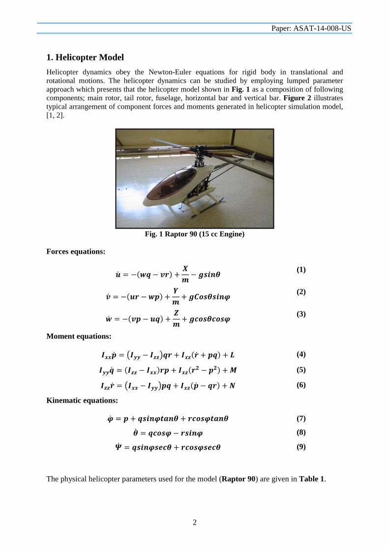
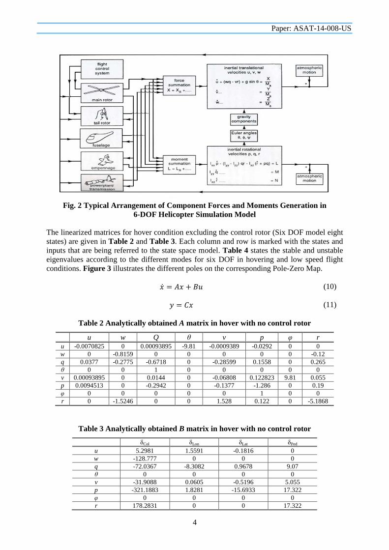
1. Helicopter Model Helicopter dynamics obey the Newton-Euler equations for rigid body in translational and rotational motions. The helicopter dynamics can be studied by employing lumped parameter approach which presents that the helicopter model shown in Fig. 1 as a composition of following components; main rotor, tail rotor, fuselage, horizontal bar and vertical bar. Figure 2 illustrates typical arrangement of component forces and moments generated in helicopter simulation model, [1, 2].

Fig. 1 Raptor 90 (15 cc Engine)

Forces equations:

�̇�𝒖 = −(𝒘𝒘𝒘𝒘− 𝒗𝒗𝒗𝒗) +𝑿𝑿𝒎𝒎− 𝒈𝒈𝒈𝒈𝒈𝒈𝒈𝒈𝒈𝒈 (1)

�̇�𝒗 = −(𝒖𝒖𝒗𝒗 − 𝒘𝒘𝒘𝒘) +𝒀𝒀𝒎𝒎

+ 𝒈𝒈𝒈𝒈𝒈𝒈𝒈𝒈𝒈𝒈𝒈𝒈𝒈𝒈𝒈𝒈𝒈𝒈 (2)

�̇�𝒘 = −(𝒗𝒗𝒘𝒘 − 𝒖𝒖𝒘𝒘) +𝒁𝒁𝒎𝒎

+ 𝒈𝒈𝒈𝒈𝒈𝒈𝒈𝒈𝒈𝒈𝒈𝒈𝒈𝒈𝒈𝒈𝒈𝒈 (3)

Moment equations:

𝑰𝑰𝒙𝒙𝒙𝒙�̇�𝒘 = �𝑰𝑰𝒚𝒚𝒚𝒚 − 𝑰𝑰𝒛𝒛𝒛𝒛�𝒘𝒘𝒗𝒗 + 𝑰𝑰𝒙𝒙𝒛𝒛(�̇�𝒗 + 𝒘𝒘𝒘𝒘) + 𝑳𝑳 (4)

𝑰𝑰𝒚𝒚𝒚𝒚�̇�𝒘 = (𝑰𝑰𝒛𝒛𝒛𝒛 − 𝑰𝑰𝒙𝒙𝒙𝒙)𝒗𝒗𝒘𝒘 + 𝑰𝑰𝒙𝒙𝒛𝒛(𝒗𝒗𝟐𝟐 − 𝒘𝒘𝟐𝟐) + 𝑴𝑴 (5)

𝑰𝑰𝒛𝒛𝒛𝒛�̇�𝒗 = �𝑰𝑰𝒙𝒙𝒙𝒙 − 𝑰𝑰𝒚𝒚𝒚𝒚�𝒘𝒘𝒘𝒘 + 𝑰𝑰𝒙𝒙𝒛𝒛(�̇�𝒘 − 𝒘𝒘𝒗𝒗) + 𝑵𝑵 (6)

Kinematic equations:

�̇�𝒈 = 𝒘𝒘 + 𝒘𝒘𝒈𝒈𝒈𝒈𝒈𝒈𝒈𝒈𝒒𝒒𝒒𝒒𝒈𝒈𝒈𝒈 + 𝒗𝒗𝒈𝒈𝒈𝒈𝒈𝒈𝒈𝒈𝒒𝒒𝒒𝒒𝒈𝒈𝒈𝒈 (7)

�̇�𝒈 = 𝒘𝒘𝒈𝒈𝒈𝒈𝒈𝒈𝒈𝒈 − 𝒗𝒗𝒈𝒈𝒈𝒈𝒈𝒈𝒈𝒈 (8)

�̇�𝜳 = 𝒘𝒘𝒈𝒈𝒈𝒈𝒈𝒈𝒈𝒈𝒈𝒈𝒒𝒒𝒈𝒈𝒈𝒈 + 𝒗𝒗𝒈𝒈𝒈𝒈𝒈𝒈𝒈𝒈𝒈𝒈𝒒𝒒𝒈𝒈𝒈𝒈 (9)

The physical helicopter parameters used for the model (Raptor 90) are given in Table 1.


3

Table 1 Parameters of Raptor 90 helicopter for simulation model

Parameter Description ρ = 1.225 kg/m3 Atmosphere density m = 7.70 kg Helicopter mass Ixx = 0.192 kg m2 Rolling moment of inertia Iyy = 0.34 kg m2 Pitching moment of inertia Izz = 0.280 kg m2 Yawing moment of inertia Ωnom = 162 rad/s Nominal main rotor speed RM = 0.775 m Main rotor radius RCR = 0.370 m Stabilizer bar radius CM = 0.058 m Main rotor chord CCR = 0.06 m Stabilizer bar chord aM = 5.5 rad-1 Main rotor blade lift curve slope 𝐶𝐶𝐷𝐷𝐷𝐷𝑀𝑀 =0.024 Main rotor blade zero lift drag coefficient 𝒈𝒈𝑻𝑻𝒎𝒎𝒒𝒒𝒙𝒙𝑴𝑴 =0.00168 Main rotor max thrust coefficient Iβ = 0.038 kg m2 Main rotor blade flapping inertia RT = 0.13 m Tail rotor radius CT = 0.029 m Tail rotor chord aT = 5.0 rad-1 Tail rotor blade lift curve slope 𝒈𝒈𝑫𝑫𝒈𝒈𝑻𝑻 =0.024 Tail rotor blade zero lift drag coefficient 𝒈𝒈𝑻𝑻𝒎𝒎𝒒𝒒𝒙𝒙𝑻𝑻 =0.0922 Tail rotor max thrust coefficient nT = 4.66 Gear ratio of tail rotor to main rotor nes = 9.0 Gear ratio of engine shaft to main rotor 𝜹𝜹𝑻𝑻𝒒𝒒𝒗𝒗𝒈𝒈𝒎𝒎= 0.1 rad Tail rotor pitch trim offset SV= 0.012 m2 Effective vertical fin area SH =0.01 m2 Effective horizontal fin area 𝐶𝐶𝐿𝐿∝𝑉𝑉 = 2.0 rad-1 Vertical fin lift curve slope 𝐶𝐶𝐿𝐿∝𝐻𝐻 = 3.0 rad-1 Horizontal tail lift curve slope 𝑆𝑆𝑥𝑥𝐹𝐹 = 0.1 m2 Frontal fuselage drag area 𝑺𝑺𝒚𝒚𝑭𝑭= 0.22 m2 Side fuselage drag area 𝑆𝑆𝑧𝑧𝐹𝐹 = 0.15 m2 Vertical fuselage drag area hM = 0.235 m Main rotor hub height above CG lM = 0.015 m Main rotor hub behind CG lT = 0.91 m Tail rotor hub location behind CG hT = 0.08 m Tail rotor height above CG lH= 0.71 m Stabilizer location behind CG kMR =0.3333 Amount of commanded swash plate tilt

kCR =1.1429 Geometry coefficient of the mechanical linkage of control rotor and swash plate


4

Fig. 2 Typical Arrangement of Component Forces and Moments Generation in

6-DOF Helicopter Simulation Model The linearized matrices for hover condition excluding the control rotor (Six DOF model eight states) are given in Table 2 and Table 3. Each column and row is marked with the states and inputs that are being referred to the state space model. Table 4 states the stable and unstable eigenvalues according to the different modes for six DOF in hovering and low speed flight conditions. Figure 3 illustrates the different poles on the corresponding Pole-Zero Map.

�̇�𝑥 = 𝐴𝐴𝑥𝑥 + 𝐵𝐵𝐵𝐵 (10)

𝑦𝑦 = 𝐶𝐶𝑥𝑥 (11)

Table 2 Analytically obtained A matrix in hover with no control rotor

u w Q θ v p φ r u -0.0070825 0 0.00093895 -9.81 -0.0009389 -0.0292 0 0 w 0 -0.8159 0 0 0 0 0 -0.12 q 0.0377 -0.2775 -0.6718 0 -0.28599 0.1558 0 0.265 θ 0 0 1 0 0 0 0 0 v 0.00093895 0 0.0144 0 -0.06808 0.122823 9.81 0.055 p 0.0094513 0 -0.2942 0 -0.1377 -1.286 0 0.19 φ 0 0 0 0 0 1 0 0 r 0 -1.5246 0 0 1.528 0.122 0 -5.1868

Table 3 Analytically obtained B matrix in hover with no control rotor

δCol δLon δLat δPed u 5.2981 1.5591 -0.1816 0 w -128.777 0 0 0 q -72.0367 -8.3082 0.9678 9.07 θ 0 0 0 0 v -31.9088 0.0605 -0.5196 5.055 p -321.1883 1.8281 -15.6933 17.322 φ 0 0 0 0 r 178.2831 0 0 17.322


5

Table 4 Eigenvalues and modes for 6-DOF in Hovering/Low Speed Flight Condition

Mode Eigenvalues Damping Frequency (rad/s) Longitudinal Oscillation 0.169 ± 0.392i -0.395 0.427 Lateral Oscillation -0.0279 ± 0.765i 0.0365 0.765 Heave -0.68 ± 0.142i 0.979 0.695 Roll Subsidence -1.68 1 1.68 Yaw -5.28 1 5.28

Fig. 3 Poles of Coupled Longitudinal and Lateral Motion for

6-DOF with no Control Rotor 2. Application of Pole Placement Method to 6-DOF (8 States Linear Model) The objective of applying Pole Placement Method (PPM) to 6-DOF model is to shift the unstable Poles (the above marked ones) to the Left region of the root Locus (stable region). Consequently an initial stable reference model is established and ready to be tuned by applying GA functions to optimize the net performance index. The default poles will be placed in new position as the following (-0.8±1.095i, -0.85±1.096i, -57, -10, -15, -10) according to the stated flying qualities in Fig. 4, [5]:


6

Fig. 4 Limits on pitch (roll) oscillations – hover and low speed according to

Aeronautical Design Standard for military helicopter (ADS-33C) (US Army Aviation Systems Command, 1989)

2. Application of GA Functions to optimize the PID Controller Parameters The main objective of the proposed GA procedure is to optimize (minimize) the output performance index (maximize fitness function) of the whole integrated control system used in Fig. 5. An application of GA code combined with SIMULINK control model for the proposed Helicopter model is implemented to minimize the performance index (J), [3]. The equation describing the net output performance (J) is stated below:

∫∞

⋅⋅+⋅⋅+⋅⋅+⋅⋅=0

4

2

3

2

2

2

1

2 ])_()_()_()_([ dtsimresimesimwesimueJ WtWtWtWt ϕ (12)

where e(u_sim) is the forward speed error e(w_sim) is the normal speed error e(𝜑𝜑_sim) is the bank angle error e(r_sim) is the yaw rate error W1,W2, W3 and W4 are the performance weights that depend on the required performance priority. The previous index can be obtained from the nonlinear simulation of the pitch control model consequently GA can use it as the fitness function.

2.1 Optimizing PID Parameters

2.1.1 Using binary system coding Coding: using 10-bit binary genes to express DIP KKK ,, . For example (KP) from bit 1

(0)0000000000 , to bit 10 is (1023)1111111111 .Then string DIP KKK ,, to 30-bit binary cluster. 0000100010 1 110111000 0000110111:x expresses a chromosome，the former 10-bit express KP, the second portion express KI and the third one express the KD. Decoding: Cut one string of 30-bit binary string to three 10-bit binary string，then converts them to decimal system values y1, y2 and y3, [3, 4].


7

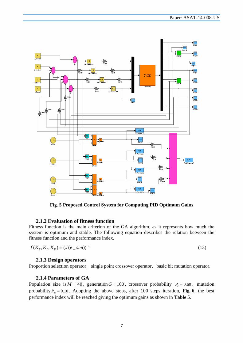
Fig. 5 Proposed Control System for Computing PID Optimum Gains

2.1.2 Evaluation of fitness function Fitness function is the main criterion of the GA algorithm, as it represents how much the system is optimum and stable. The following equation describes the relation between the fitness function and the performance index.

1))_((),,( −= simeJKKKf DIP (13)

2.1.3 Design operators Proportion selection operator，single point crossover operator，basic bit mutation operator.

2.1.4 Parameters of GA Population size is 04=M , generation 100=G , crossover probability 0.60c =P ，mutation probability 0.10m =P . Adopting the above steps, after 100 steps iteration, Fig. 6, the best performance index will be reached giving the optimum gains as shown in Table 5.


8

Fig. 6 Performance Index J after 100 iterations

Table 5 PID Optimum Gains for the Integrated Control System

k1 k2 k3 k4 kp0 kd0 ki0 kp1

-0.7634 -0.1711 -0.9081 -0.9902 0.0190 0 -1.8034 4.6676 kd1 ki1 kp2 kd2 ki2 kp3 kd3 Ki3 0 4.6774 4.9022 0 2.9062 2.9120 0 3.0459

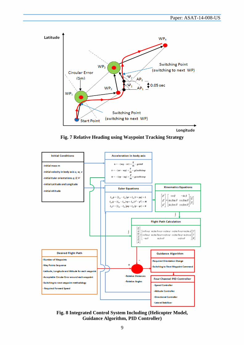
3. Integrated Control System Building up the PID controller using the previous optimum gains stated in Table 5 (inner loop controller). Then a proposed guidance algorithm is established and fed with the flying model position from the GPS and the waypoints data (number of waypoints, locations and sequence). Applying vector analysis with mathematical aids, the relative heading and elevation with respect to the next waypoint will be calculated. Consequently the required change in heading and elevation will be fed to the PID controller (outer loop) after applying manual tuning to the out loop gains. Figure 7 demonstrates the current and the relative heading with respect to the next waypoint in the sequence. The guidance algorithm maintains the actual flight path not to fly in continuous loops around a definite waypoint by using some switching limiters such as acceptable circular error around the proposed waypoints and switching orthogonal liners. Figure 8 shows the integrated control system including (Helicopter Model, Guidance Algorithm and PID Controller) with the input commands and the output performance. The guidance algorithm was implemented using Matlab code, and all the simulation results were conducted using Simulink. 4. Guidance Approach

4.1 TTM Trajectory Tracking Method This approach is concerning the relative distances such as the lateral and the vertical distances with respect to the desired trajectory current segment DTCS body axis Fig. 9. In this method (in case of lateral control) inner and outer loops will be required, the inner loop will control the yaw rate and the outer loop will be fed by the lateral relative distance with respect to the desired trajectory current segment DTCS body axis while the feedback signal will represent the change in the heading as the absolute heading is not useful in this case. Both the inner and the out loop gains will be tuned by several trials after system integration. This approach leads to minimize the relative distances between the actual flight path and the desired trajectory.


9

Fig. 7 Relative Heading using Waypoint Tracking Strategy

Fig. 8 Integrated Control System Including (Helicopter Model, Guidance Algorithm, PID Controller)


10

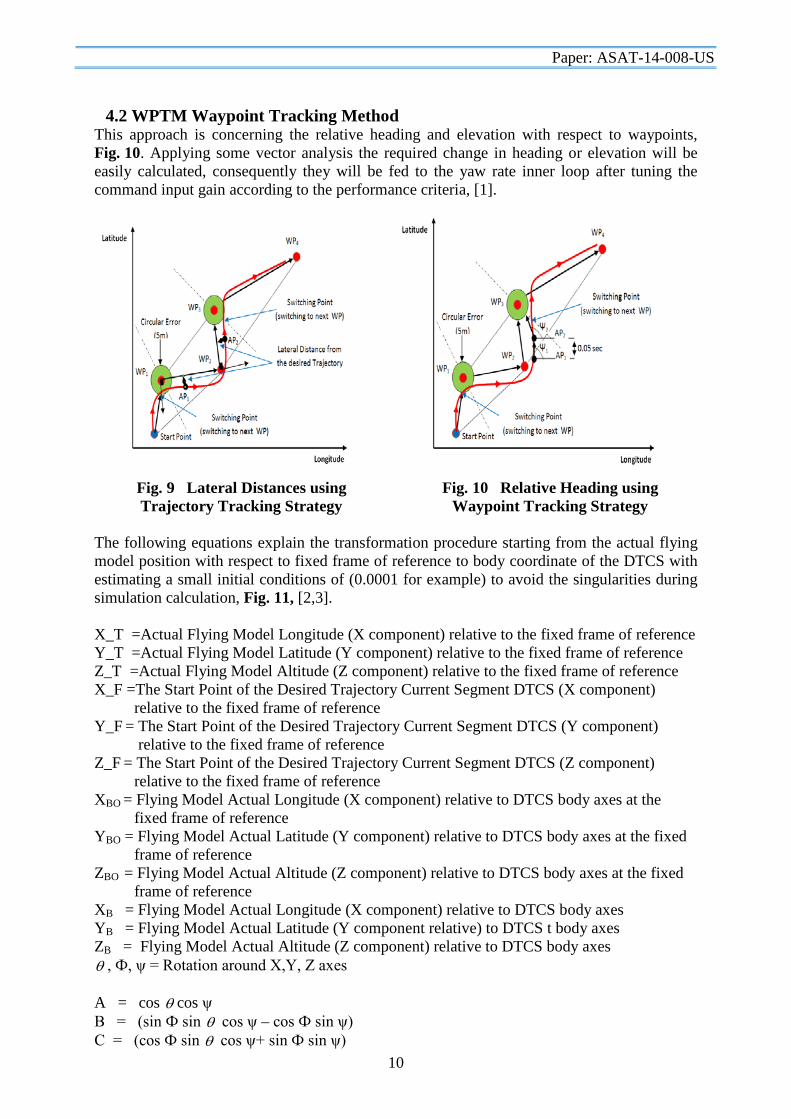
4.2 WPTM Waypoint Tracking Method This approach is concerning the relative heading and elevation with respect to waypoints, Fig. 10. Applying some vector analysis the required change in heading or elevation will be easily calculated, consequently they will be fed to the yaw rate inner loop after tuning the command input gain according to the performance criteria, [1].

Fig. 9 Lateral Distances using Trajectory Tracking Strategy

Fig. 10 Relative Heading using Waypoint Tracking Strategy

The following equations explain the transformation procedure starting from the actual flying model position with respect to fixed frame of reference to body coordinate of the DTCS with estimating a small initial conditions of (0.0001 for example) to avoid the singularities during simulation calculation, Fig. 11, [2,3]. X_T =Actual Flying Model Longitude (X component) relative to the fixed frame of reference Y_T =Actual Flying Model Latitude (Y component) relative to the fixed frame of reference Z_T =Actual Flying Model Altitude (Z component) relative to the fixed frame of reference X_F =The Start Point of the Desired Trajectory Current Segment DTCS (X component) relative to the fixed frame of reference Y_F = The Start Point of the Desired Trajectory Current Segment DTCS (Y component) relative to the fixed frame of reference Z_F = The Start Point of the Desired Trajectory Current Segment DTCS (Z component) relative to the fixed frame of reference XBO = Flying Model Actual Longitude (X component) relative to DTCS body axes at the fixed frame of reference YBO = Flying Model Actual Latitude (Y component) relative to DTCS body axes at the fixed frame of reference ZBO = Flying Model Actual Altitude (Z component) relative to DTCS body axes at the fixed frame of reference XB = Flying Model Actual Longitude (X component) relative to DTCS body axes YB = Flying Model Actual Latitude (Y component relative) to DTCS t body axes ZB = Flying Model Actual Altitude (Z component) relative to DTCS body axes θ , Ф, ψ = Rotation around X,Y, Z axes A = cos θ cos ψ B = (sin Ф sin θ cos ψ – cos Ф sin ψ) C = (cos Ф sin θ cos ψ+ sin Ф sin ψ)


11

D = cos θ sin ψ E = (sin Ф sin θ sin ψ + cos Ф cos ψ) F = (cos Ф sin θ sin ψ – sin Ф cos ψ) G = – sin θ M = sin Ф cos θ N = cos Ф cos θ

)])(())([()])(())([(

BDEANACGMABGCDFABDEAZAXGMABGXDYAZ BO −−−−−

−−−−−= (14)

)()]()[(

BDEACDFAZXDYAY BO

BO −−−−

= (15)

ACZBYX

X BOBOBO

)( −−= (16)

)])(())([()])(())([(

BDEANACGMABGCDFABDEAAZGXMABGDXAYZ FFFF

SHIFT −−−−−−−−−−

= (17)

)()]()[(

BDEACDFAZDXAYY SHIFTFF

SHIFT −−−−

= (18)

ACZBYX

X SHIFTSHIFTFSHIFT

)( −−= (19)

XB = XBO – X shift (20) YB = YBO – Y shift (21) ZB = ZBO – Z shift (22)

Fig. 11 Calculating the Flying Model Relative Distances with Respect to DTCS Body Axis


12

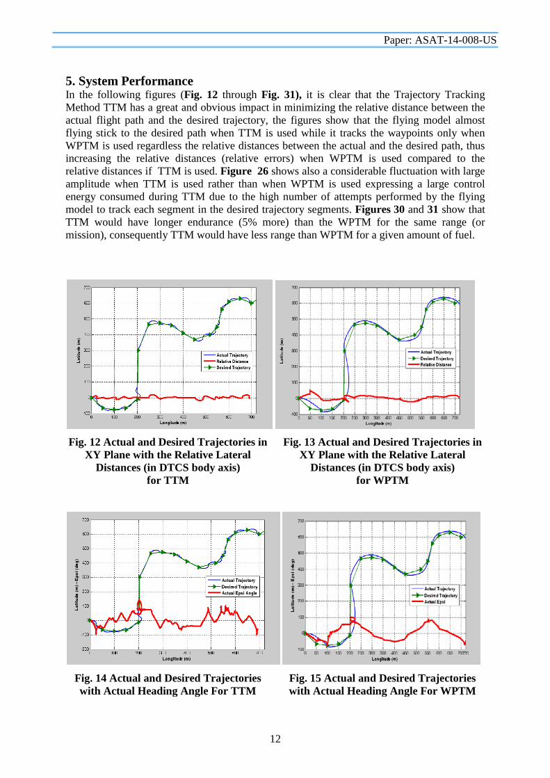
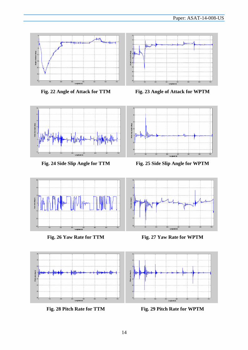
5. System Performance In the following figures (Fig. 12 through Fig. 31), it is clear that the Trajectory Tracking Method TTM has a great and obvious impact in minimizing the relative distance between the actual flight path and the desired trajectory, the figures show that the flying model almost flying stick to the desired path when TTM is used while it tracks the waypoints only when WPTM is used regardless the relative distances between the actual and the desired path, thus increasing the relative distances (relative errors) when WPTM is used compared to the relative distances if TTM is used. Figure 26 shows also a considerable fluctuation with large amplitude when TTM is used rather than when WPTM is used expressing a large control energy consumed during TTM due to the high number of attempts performed by the flying model to track each segment in the desired trajectory segments. Figures 30 and 31 show that TTM would have longer endurance (5% more) than the WPTM for the same range (or mission), consequently TTM would have less range than WPTM for a given amount of fuel.

Fig. 12 Actual and Desired Trajectories in XY Plane with the Relative Lateral

Distances (in DTCS body axis) for TTM

Fig. 13 Actual and Desired Trajectories in XY Plane with the Relative Lateral

Distances (in DTCS body axis) for WPTM

Fig. 14 Actual and Desired Trajectories with Actual Heading Angle For TTM

Fig. 15 Actual and Desired Trajectories with Actual Heading Angle For WPTM


13

Fig. 16 Actual and Desired Trajectories in XZ Plane with the Relative Vertical

Distances (in DTCS body axis) for TTM

Fig. 17 Actual and Desired Trajectories in XZ Plane with the Relative Vertical

Distances (in DTCS body axis) for WPTM

Fig. 18 Actual and Desired Trajectories in XZ Plane with Actual Elevation

for TTM

Fig. 19 Actual and Desired Trajectories in XZ Plane with Actual Elevation

for WPTM

Fig. 20 Actual and Desired Forward Speed for TTM

Fig. 21 Actual and Desired Forward Speed for WPTM


14

Fig. 22 Angle of Attack for TTM

Fig. 23 Angle of Attack for WPTM

Fig. 24 Side Slip Angle for TTM

Fig. 25 Side Slip Angle for WPTM

Fig. 26 Yaw Rate for TTM

Fig. 27 Yaw Rate for WPTM

Fig. 28 Pitch Rate for TTM

Fig. 29 Pitch Rate for WPTM


15

Fig. 30 Range and Endurance for TTM

Fig. 31 Range and Endurance for WPTM 6. Control System Performance Figures 32 through 39 illustrate the control efforts done by each servo to perform the maneuvers required for the desired flight path for both TTM and WPTM. Figure 38 indicates an obvious fluctuation with large amplitude that would need a considerable amount of electric energy. This number of fluctuations would reduce the servos life time, and decrease the mean time between failures.

Fig. 32 Lateral Control Effort for TTM

Fig. 33 Lateral Control Effort for WPTM

Fig. 34 Pitch Control Effort for TTM

Fig. 35 Pitch Control Effort for WPTM

Fig. 36 Collective Control Effort for TTM

Fig. 37 Collective Control Effort for WPTM


16

Fig. 38 Rudder Control Effort for TTM

Fig. 39 Rudder Control Effort for WPTM 7. System Evaluation The absolute relative distance integral in both (X, Y) directions (in DTCS body axis) was chosen to be the evaluation criteria (Performance Index PI) in this work. Figures 40 and 41 show that the Trajectory Tracking Method TTM has less (Performance Index PI) when it is compared with Waypoint Tracking Method WPTM though the (Performance Index PI) using WPTM is slightly less than when using TTM in Z direction (with respect to DTCS body axis). As the global performance index for both directions Y, Z (with respect to DTCS body axis) using TTM is much less when compared with the WPTM. On the other hand when applying the same performance index to both methods (TTM, WPTM) for yaw rate, yaw acceleration and yaw jerk, it is clear that the TTM energy consumption during the tracking maneuvers is much more than the energy consumed by the WPTM as it is shown in Figs. 42, 43 and 44, [4,5].

Fig. 40 Performance Index in (Z) Directions for TTM and WPTM

Fig. 41 Performance Index in (Y) Directions for TTM and WPTM


17

Fig. 42 Absolute Yaw Rate Integral for both TTM and WPTM

Fig. 43 Absolute Yaw Angular Acceleration Integral for both TTM and WPTM

Fig. 44 Absolute Yaw Angular Jerk Integral for both TTM and WPTM


18

8. Conclusion This paper has presented a customized autopilot using PID controller combined with a guidance algorithm. Genetic algorithm was used in this work to tune the proposed stable state space model after applying pole placement method PPM. The proposed stable poles satisfy the flying qualities criteria. The illustrated results show an adequate system performance with a reasonable relative distances with respect to the desired trajectory. The forward speed was maintained constant during the whole flight according the desired speed. The servos control efforts are satisfying the band width limits, and also the minimum and maximum limits. It is concluded from the system performance that it is recommended to use TTM in case when the unmanned flying model is required to track a planned trajectory with less relative errors, while the WPTM is recommended when the precision in tracking the planned trajectory is not an objective. However the control energy consumed by TTM is obviously more than WPTM for the same planned trajectory (Flight Path), thus the control servos using TTM would require more batteries than they would require when using WPTM. The application of hybrid system that utilizes both methods advantages is strongly recommended in this case. Using both methods will allow applying TTM during loitering when the tracking precision is required, while applying WPTM when it is only required to pass the waypoints without tracking the flight path passing those waypoints (when covering distances only is required during flight). 9. References [1] Shamsudin S. S., “The Development of Autopilot System for an Unmanned Aerial

Vehicle (UAV) Helicopter Model”, M. Sc. thesis, Universiti Teknologi, Malaysia, Faculty of Mechanical Engineering. 2007, pp. 1-147.

[2] Hosny A. M., Chao H., “Development of Fuzzy Logic LQR Control Integration for Aerial Refueling Autopilot”, " Proceedings of the 12th International Conference on Aerospace Sciences and Aviation Technology, ASAT-12," , MTC, Cairo, Egypt, May 29-31, 2007.

[3] Hosny A. M., Chao H., “Fuzzy Logic Controller Tuning Via Adaptive Genetic Algorithm Applied to Aircraft Longitudinal Motion”, " Proceedings of the 12th International Conference on Aerospace Sciences and Aviation Technology, ASAT-12," MTC, Cairo, Egypt, May 29-31, 2007.

[4] Goldberg, D., Genetic Algorithms in Search, Optimization & Machine Learning,1st. ed., Vol. 1, Addison Wesley Longman, 1989.

[5] Flying Qualities of Aeronautical Design Standard for Military Helicopter (ADS-33C) (US Army Aviation Systems Command, 1989).

Development of a Customized Autopilot for Unmanned Helicopter Model Using Genetic Algorithm via the...

Design

Transcript of Development of a Customized Autopilot for Unmanned Helicopter Model Using Genetic Algorithm via the...