DEVELOPMENT OF A COMPUTER CONTROLLED UNDERBODY PLOW

IOWA HIGHWAY RESEARCH BOARD PROJECT TR 412

FINAL REPORT

Wilfrid A Nixon, George Kochumman, Carrie Novotny, and Anton Kruger

IIHR Technical Report No. 448

IIHR—Hydroscience & Engineering College of Engineering The University of Iowa Iowa City IA 52242

January 2006

ACKNOWLEDGEMENTS

This project was made possible by funding from the Iowa Highway Research

Board, Project Number TR 412. This support is gratefully acknowledged, as is the

assistance of Mr. Mark Dunn in bringing this project to completion.

The support of the Directors of IIHR Hydroscience and Engineering during the

execution of this project, Dr. V.C. Patel and Dr. L.J. Weber, enabled this study to

proceed. The computer support staff at IIHR, led by Mr. Mark Wilson and assisted by

Mr. Brian Miller, made the development of the computer model possible. Their

assistance with program installation and troubleshooting was particularly invaluable. The

drafting work of Mr. Mike Kundert was very helpful.

The opinions, findings, and conclusions expressed in this publication are those of

the authors, and not necessarily those of the Iowa Highway Research Board.

i

ABSTRACT

Underbody plows can be very useful tools in winter maintenance, especially when

compacted snow or hard ice must be removed from the roadway. By the application of

significant down-force, and the use of an appropriate cutting edge angle, compacted snow

and ice can be removed very effectively by such plows, with much greater efficiency than

any other tool under those circumstances.

However, the successful operation of an underbody plow requires considerable

skill. If too little down pressure is applied to the plow, then it will not cut the ice or

compacted snow. However, if too much force is applied, then either the cutting edge may

gouge the road surface, causing significant damage often to both the road surface and the

plow, or the plow may ride up on the cutting edge so that it is no longer controllable by

the operator. Spinning of the truck in such situations is easily accomplished. Further,

excessive down force will result in rapid wear of the cutting edge.

Given this need for a high level of operator skill, the operation of an underbody

plow is a candidate for automation. In order to successfully automate the operation of an

underbody plow, a control system must be developed that follows a set of rules that

represent appropriate operation of such a plow. These rules have been developed, based

upon earlier work in which operational underbody plows were instrumented to determine

the loading upon them (both vertical and horizontal) and the angle at which the blade was

operating.

These rules have been successfully coded into two different computer programs,

both using the MatLab® software. In the first program, various load and angle inputs are

analyzed to determine when, whether, and how they violate the rules of operation. This

program is essentially deterministic in nature. In the second program, the Simulink®

package in the MatLab® software system was used to implement these rules using fuzzy

logic. Fuzzy logic essentially replaces a fixed and constant rule with one that varies in

such a way as to improve operational control. The development of the fuzzy logic in this

simulation was achieved simply by using appropriate routines in the computer software,

rather than being developed directly.

The results of the computer testing and simulation indicate that a fully automated,

computer controlled underbody plow is indeed possible. The issue of whether the next

ii

steps toward full automation should be taken (and by whom) has also been considered,

and the possibility of some sort of joint venture between a Department of Transportation

and a vendor has been suggested.

iii

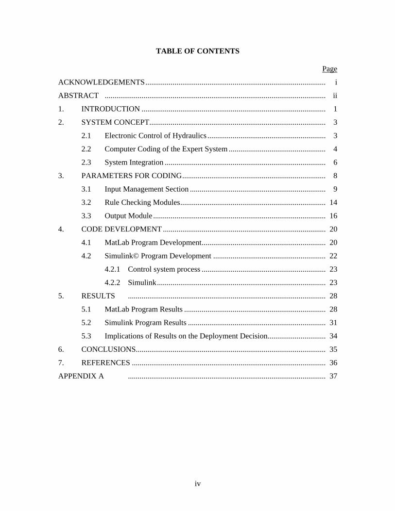
TABLE OF CONTENTS

Page

ACKNOWLEDGEMENTS............................................................................................. i

ABSTRACT .................................................................................................................. ii

1. INTRODUCTION ............................................................................................... 1

2. SYSTEM CONCEPT........................................................................................... 3

2.1 Electronic Control of Hydraulics ............................................................. 3

2.2 Computer Coding of the Expert System .................................................. 4

2.3 System Integration ................................................................................... 6

3. PARAMETERS FOR CODING.......................................................................... 8

3.1 Input Management Section ...................................................................... 9

3.2 Rule Checking Modules........................................................................... 14

3.3 Output Module ......................................................................................... 16

4. CODE DEVELOPMENT .................................................................................... 20

4.1 MatLab Program Development................................................................ 20

4.2 Simulink© Program Development .......................................................... 22

4.2.1 Control system process ................................................................ 23

4.2.2 Simulink....................................................................................... 23

5. RESULTS ...................................................................................................... 28

5.1 MatLab Program Results ......................................................................... 28

5.2 Simulink Program Results ....................................................................... 31

5.3 Implications of Results on the Deployment Decision.............................. 34

6. CONCLUSIONS.................................................................................................. 35

7. REFERENCES .................................................................................................... 36

APPENDIX A ...................................................................................................... 37

iv

LIST OF FIGURES

Figure Page

2.1 Schematic of the Hydraulic System..................................................................... 4

2.2 Concept of Fuzzy Relationships versus Deterministic Relationships.................. 5

3.1 Typical Horizontal and Vertical Force Data for an Underbody Plow ................. 10

3.2 Typical Blade Angle and Force Angle Data for an Underbody Plow ................. 11

3.3 Vertical Force Data Set A to Test Rules 2 and 4 ................................................. 13

3.4 Vertical Force Data Set B to Test Rule 5............................................................. 14

3.5 Blade Angle Data Set C to Test Rules 6 and 7 .................................................... 15

3.6 Blade Angle Data Set D to Test Rules 6 and 7 .................................................... 16

3.7 Force Angle Data Set E to Test Rule 8 ................................................................ 17

3.8 Horizontal Force Data Set F to Test Rule 9......................................................... 18

4.1 Smoothing Process............................................................................................... 21

4.2 The Rule Checking Module ................................................................................. 22

4.3 Simulink model.................................................................................................... 24

4.4 Simulink model with force and displacement as variables.................................. 25

4.5 Parameters of the force function .......................................................................... 26

4.6 Parameters of the displacement function ............................................................. 26

5.1 Smoothed input data ............................................................................................ 30

5.2 The Output Vertical Force in Response to a Force Violation.............................. 31

5.3 Force function ...................................................................................................... 32

5.4 Displacement function ......................................................................................... 33

v

LIST OF TABLES

Table Page

2.1 Preliminary Listing of Expert System Rules ....................................................... 6

3.1 Conditions to be tested......................................................................................... 12

3.2 Data Sets used for Condition Testing .................................................................. 13

5.1 Results of tests of data sets that violate operational rules.................................... 29

vi

1. INTRODUCTION Underbody plows are used in winter maintenance activities to remove ice and

compacted snow from the road surface. Typically, such plows are only used when

conditions are very severe, such as during an ice storm or after heavy snow fall, when

snow on the roadway has been compacted by vehicle traffic. Underbody plows are

typically mounted to tandem axle trucks. Sometimes, motor graders are used for snow

removal, and the blade operation in these cases is similar to that for an underbody

mounted on a truck.

Effective operation of an underbody plow is not a simple task. If too little down

pressure is applied to the underbody plow, then it will not cut the ice or compacted snow.

However, if too much force is applied, then one of two bad outcomes may occur. The

cutting edge may gouge the road surface, causing significant damage often to both the

road surface and the plow. Alternatively, the plow may ride up on the cutting edge so that

it is no longer controllable by the operator. Spinning of the truck in such situations is

easily accomplished. Further, excessive down force will result in rapid wear of the

cutting edge. Anecdotal reports indicate that the whole edge may get worn away in a

matter of minutes, which event is rapidly followed by the wearing and eventual

destruction of the underbody mold board. In short, effective operation of an underbody

plow in winter maintenance is a skilled art.

It is precisely because the operation of an underbody plow requires such skill that

such operation is a good candidate for automation. As skilled truck operators retire, it

becomes harder to replace them with new labor of equal skills. Training in underbody use

thus becomes a harder task, and both plow effectiveness and operator safety may suffer

as a result. In cases in which the skill pool is shrinking, the use of so called “expert

systems” presents a way in which these skills may be effectively preserved.

The benefits of using an expert system to control an underbody plow during snow

and ice removal operations are twofold. First, provided a suitable expert system is

developed, the plow will operate at a very high level of effectiveness, since the

parameters for its operation will be developed from data taken from plowing conducted

by highly experienced and skilled operators. Thus the plow will give good performance

1

regardless of the skill level of the operator. Second, by allowing the operator to

concentrate on driving the truck (essentially by making the plow operation a “hands free”

process) plowing safety should also be improved. Thus the use of an expert system to

control the underbody should benefit both safety and efficiency in winter maintenance

operations.

The purpose of this study is to examine whether the development of a computer

controlled underbody plow is feasible. The initial plan was to implement such a system

on a plow, and test it in the field, but a revision in funding level limited the investigation

to a bench test of the software required for the automation. Thus this study presents the

three steps that would be needed to implement such a system (electronic control of

hydraulics, computer coding of the expert system, and system integration) in concept, and

then details the computer coding and the testing of that coding. The issue of whether the

next steps toward full automation should be taken (and by whom) is also considered.

2

2. SYSTEM CONCEPT

The system to operate an underbody plow automatically and autonomously can be

broken into three parts. These parts, the electronic control of hydraulics, the computer

coding of the expert system, and system integration, are each considered in more detail

below.

2.1 Electronic Control of Hydraulics

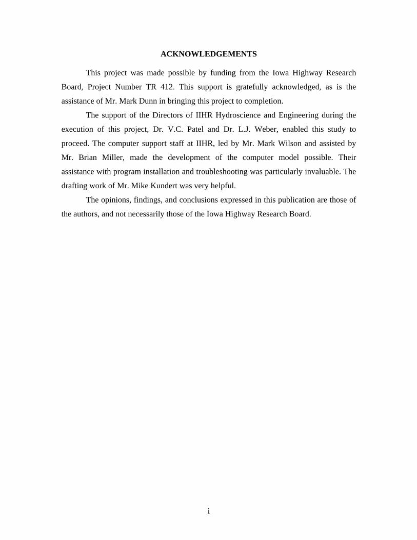
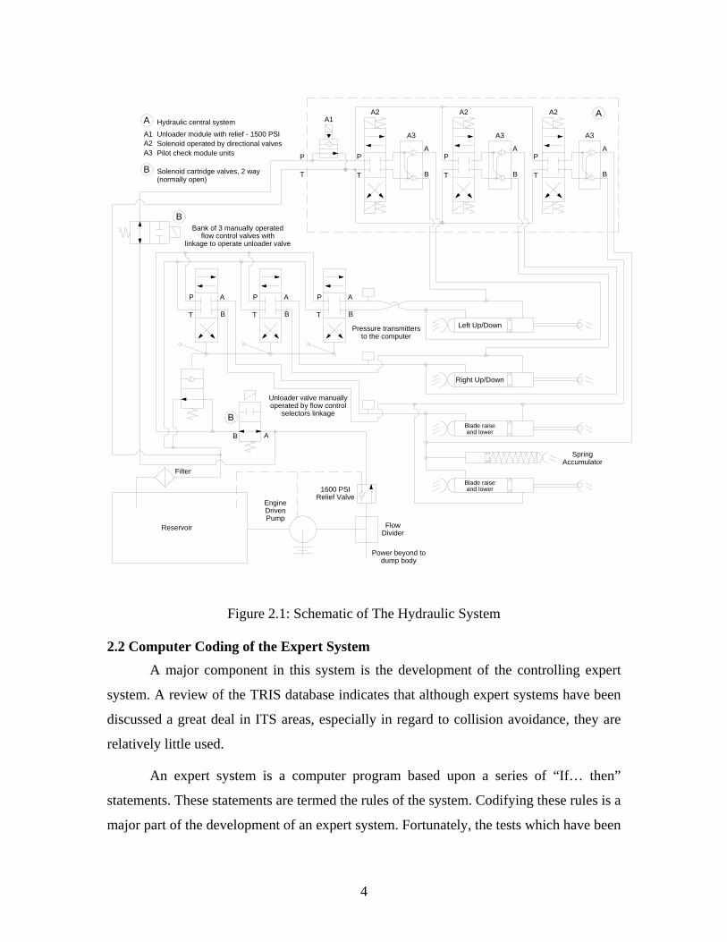
In order to control the underbody plow with a computer, a first step is to ensure

that the hydraulic system that operates the plow can be electronically controlled. One

such system is shown in Figure 2.1. In this system, the plow can be operated both

electronically and manually. In a fully deployed system, the manually operated actuators

could be removed.

In an electronically controlled system, a first level of implementation replaces

manual control (via levers) with electronic control that is still human-initiated. That is,

rather than adjust the plow position and force by manually operating levers the operator

will be entering commands on a keypad. Such a system could provide a full range of

possible plow positions and force levels, but is clearly somewhat less wieldy in that

regard than a traditional system. Rather, a significant benefit could be obtained from such

a system if the keypad presented the operator with a limited number of pre-set actuator

conditions.

The use of pre-sets in this manner would serve as an interim to a full computer

controlled deployment. Clearly, if the pre-sets were well chosen, then even an unskilled

operator would be able to achieve adequate system performance. However, the drawback

of this interim system is that it cannot adapt to changing positions on the road. This lack

of flexibility might, under certain conditions, lead to circumstances in which blade or

pavement damage was all but assured. The approach proposed herein avoids this

potential drawback by using the force levels measured in the plow itself as a feedback

signal to control the plow forces. Thus, provided the feedback algorithm is appropriate,

the danger of damaging plow or road is mitigated.

3

P

T

P

T

P

T

A

B

A

B

A

B

P

T

A

B

P

T

A

B

P

T

A

BLeft Up/Down

Bank of 3 manually operatedflow control valves with

Pressure transmittersto the computer

Unloader valve manually

linkage to operate unloader valve

operated by flow controlselectors linkage

P

T

Right Up/Down

Blade raiseand lower

A

B

Unloader module with relief - 1500 PSISolenoid operated by directional valvesPilot check module units

Solenoid cartridge valves, 2 way

Hydraulic central systemAA1A2A3

B

B

SpringAccumulator

B A

A2

A3

A2

A3

A2

A3

Blade raiseand lower

Filter

Reservoir

Engine

FlowDivider

DrivenPump

Power beyond todump body

1600 PSIRelief Valve

A1

(normally open)

Figure 2.1: Schematic of The Hydraulic System

2.2 Computer Coding of the Expert System A major component in this system is the development of the controlling expert

system. A review of the TRIS database indicates that although expert systems have been

discussed a great deal in ITS areas, especially in regard to collision avoidance, they are

relatively little used.

An expert system is a computer program based upon a series of “If… then”

statements. These statements are termed the rules of the system. Codifying these rules is a

major part of the development of an expert system. Fortunately, the tests which have been

4

conducted both in closed road testing of underbody plows and in field-deployed testing of

Iowa Department of Transportation trucks at the Oakdale garage provide an excellent

database from which such a rule set can be derived (Nixon and Potter, 1997).

However, such a series of rules would, if implemented strictly, lead to an over-

constrained system. Thus, in general, a process is applied to the rules, sometimes termed

“fuzzy logic” or “fuzzy engineering.” This area of systems control is considered in

greater detail by Kosko (1997). The basis of this approach is to transform a curve into a

series of “fuzzy” regions (see Figure 2.2). This fuzziness represents the reality that the

“If…then” rules are only imperfectly known. Fuzzy engineering has been used in a

number of computer controlled engineering applications.

Figure 2.2: Concept of Fuzzy Relationships versus Deterministic Relationships

A critical part of the expert system is the rules that will be used to build the

system. In the initial phase of system development the rules can be written as simple

linguistic statements, and as noted by Cox (1994) some of the rules may appear

contradictory. A preliminary set of rules for the underbody plow system is shown in

Table 2.1. These do not all appear in the form of “If…then” statements, although

ultimately they must be transformed into such statements for the purpose of computer

coding. The “then” part of such statements may be thought of as being the consequences

of a rule violation.

5

Table 2.1 Preliminary Listing of Expert System Rules

Rule Number Rule Description

Rule 1 When the plow is “on” it should be scraping

Rule 2 The operator should be able to control the truck

Rule 3 If the panic button is pushed, then the plow should disengage

quickly and safely

Rule 4 The down force should not be too high

Rule 5 The down force should not be too low

Rule 6 The blade should operate close to the vertical

Rule 7 The blade should be at an angle between 0 and 30 degrees

Rule 8 The ratio of horizontal to vertical force should be high

Rule 9 The horizontal force should be high

The numerical values (in for example, rule 4) will be obtained from Nixon and

Potter (1997). The expert system will be tested using a computer driven simulated plow

that produces output in response to the controlling system input. The output will be

somewhat randomized (or “fuzzed”), yet based on actual data gathered by Nixon and

Potter from in-service plowing experiments.

2.3 System Integration

The first two parts of this project (as outlined in sections 2.1 and 2.2 above) will

produce a system capable in theory of providing computer control of an underbody plow.

However, the final stage of system integration is unlikely to be straightforward. A major

issue in this regard is response time of the hydraulic system. The computer control

system will provide signals to drive the actuators that are based on immediate or very

rapid response to the signals by the system. In reality, there is some lag between the

signal and a change in the loading observed by the computer system. If the feedback

process is not damped or detuned, the system will be unstable, over-correcting the input

signal, because no output response has yet been observed. While some approximations of

the extent of de-tuning or damping can be made, the actual parameters will have to be

6

determined in-situ. This is not a simple process, and while beyond the scope of this

project, would clearly need to be considered in any implementation of the system.

A further consideration is the human factors aspect of this project. The goal of the

project is to take the control of the underbody plow away from the operator and give it to

a computer. This is likely to bring about a certain level of discomfort among operators.

The system integration must be conducted in such a way that operators are quite clear

that they have the ability to over-ride the system. Further, operators will need to be

convinced that the system can operate safely on its own. Again, this topic lies beyond the

scope of this study, yet it too is a critical step to be considered in the implementation of

the system.

7

3. PARAMETERS FOR CODING

In developing the code for this project, the goal was to ensure that, insofar as

possible, the bench test model was similar to that which would be used in real life.

However, a number of inevitable differences existed. In a deployed version of the system,

the computing would be handled by some sort of programmable logic controller or PLC.

In the bench test, all computing was done on a desktop PC machine. The program code

for PLCs varies from system to system, but in the prototype testing, the programming

language of MatLab was used, because this includes an extensive library of subroutines

that relates to fuzzy logic systems.

In addition to testing with the standard version of MatLab, a simulation program

termed Simulink © (which is an extension of the algorithm development capabilities of

MatLab) was also used to test some of the feedback aspects of this project. This approach

is described more completely in Chapter 4.

Another obvious difference between the bench test and the full scale deployment

was that the input and output data would come from and be written to data files in the

bench test, whereas in the full scale, these would come directly from and go to the

electronic interface with the hydraulic system. The input data set was developed from

data recorded in previous field studies of underbody plow performance (Nixon and

Potter, 1997) and comprised vertical force, horizontal force, and plow blade angle. These

three parameters would be the ones used to control the fully automated system, and thus,

while much other data were available, only these three have been used in the program

development.

The input data set was manipulated somewhat to ensure that sufficient variation in

force levels and blade angles were included in the data set to test the full range of output

options. Some situations that need to be modeled were not measured in the field tests

conducted earlier (Nixon and Potter, 1997) so for those situations, appropriate data were

developed to provide as full a test as possible of the proposed system.

The code was developed and tested in a modular manner. At the highest level, the

program can be considered to consist of three parts: input; rule checking; and output. The

8

coding approach (or pseudo-code as it is sometimes termed) in each of these three areas

is presented below.

3.1 Input Management Section

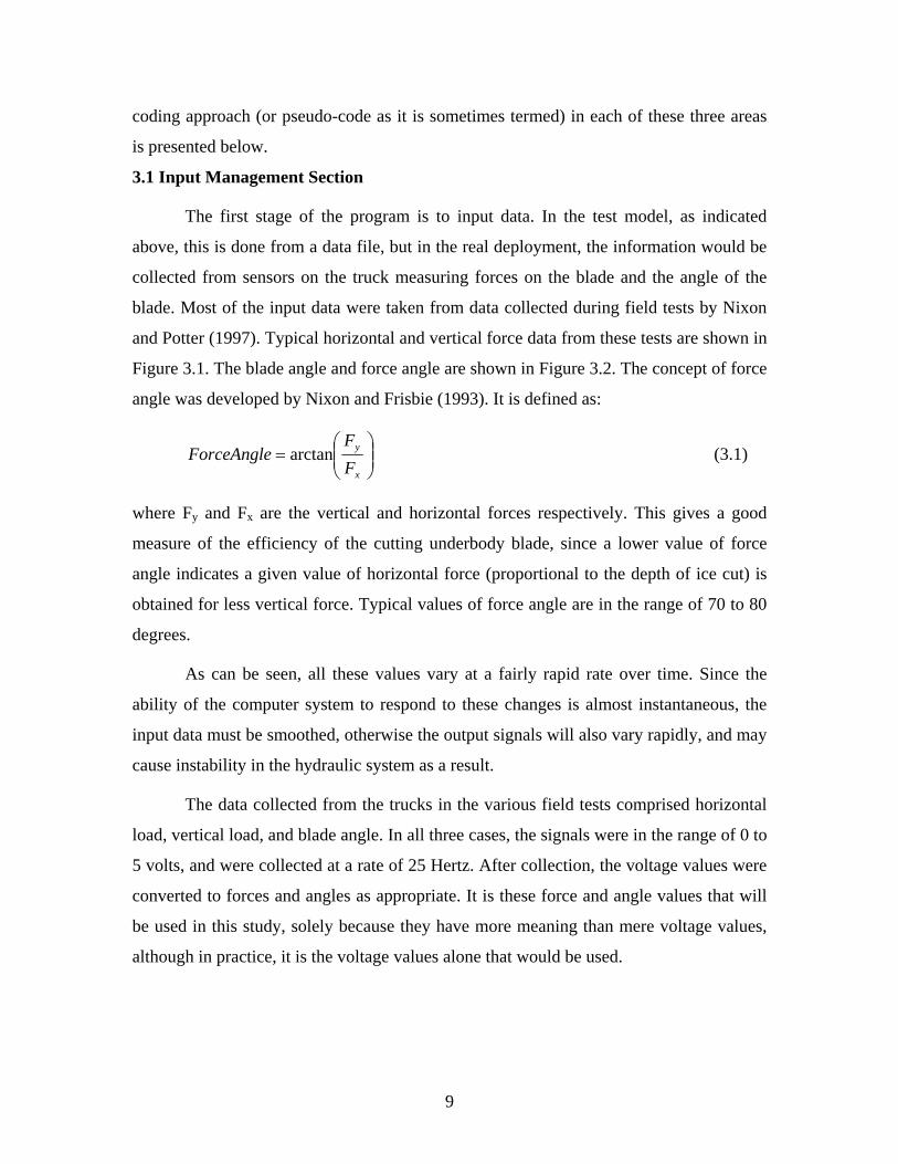
The first stage of the program is to input data. In the test model, as indicated

above, this is done from a data file, but in the real deployment, the information would be

collected from sensors on the truck measuring forces on the blade and the angle of the

blade. Most of the input data were taken from data collected during field tests by Nixon

and Potter (1997). Typical horizontal and vertical force data from these tests are shown in

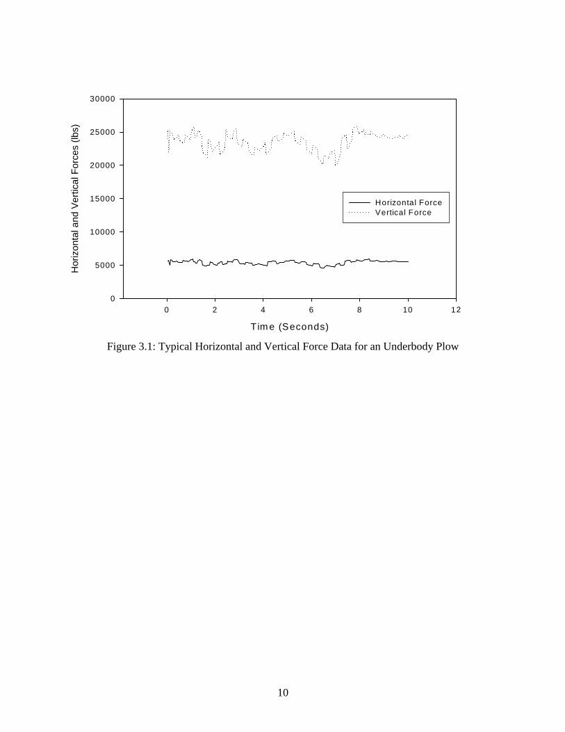
Figure 3.1. The blade angle and force angle are shown in Figure 3.2. The concept of force

angle was developed by Nixon and Frisbie (1993). It is defined as:

⎟⎟⎠

⎞⎜⎜⎝

⎛=

x

y

FF

ForceAngle arctan (3.1)

where Fy and Fx are the vertical and horizontal forces respectively. This gives a good

measure of the efficiency of the cutting underbody blade, since a lower value of force

angle indicates a given value of horizontal force (proportional to the depth of ice cut) is

obtained for less vertical force. Typical values of force angle are in the range of 70 to 80

degrees.

As can be seen, all these values vary at a fairly rapid rate over time. Since the

ability of the computer system to respond to these changes is almost instantaneous, the

input data must be smoothed, otherwise the output signals will also vary rapidly, and may

cause instability in the hydraulic system as a result.

The data collected from the trucks in the various field tests comprised horizontal

load, vertical load, and blade angle. In all three cases, the signals were in the range of 0 to

5 volts, and were collected at a rate of 25 Hertz. After collection, the voltage values were

converted to forces and angles as appropriate. It is these force and angle values that will

be used in this study, solely because they have more meaning than mere voltage values,

although in practice, it is the voltage values alone that would be used.

9

Tim e (Seconds)

0 2 4 6 8 10 1

Hor

izon

tal a

nd V

ertic

al F

orce

s (lb

s)

0

5000

10000

15000

20000

25000

30000

Horizontal ForceVertical Force

2

Figure 3.1: Typical Horizontal and Vertical Force Data for an Underbody Plow

10

Time (Seconds)

0 2 4 6 8 10 12

Bla

de a

nd F

orce

Ang

les

(Deg

rees

)

20

30

40

50

60

70

80

90

Blade AngleForce Angle

Figure 3.2: Typical Blade Angle and Force Angle Data for an Underbody Plow

In order to smooth the data it was decided to calculate a ten point moving average

for all the input data. Of course, the data could be averaged over any number of points

and the choice of ten rather than say five, twenty or one hundred is arbitrary. However,

while it is clear that some smoothing will be needed, it is not clear how much, and this

cannot be determined until the responsiveness of the hydraulic system to the feedback

signal has been observed. Thus the final data smoothing may well be different from that

used here, but the selection of a ten point moving average allows for the concept of

smoothing to be tested and evaluated. Smoothed data are shown in Chapter 5.

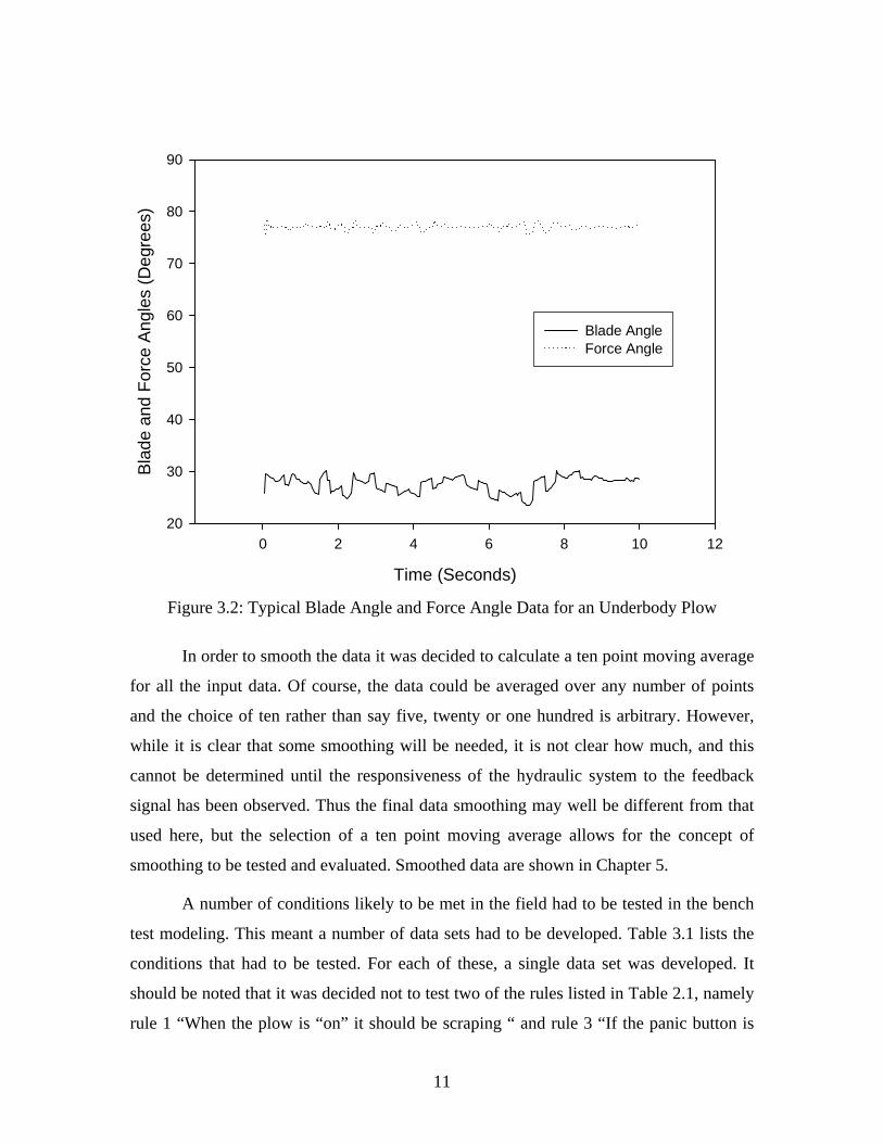
A number of conditions likely to be met in the field had to be tested in the bench

test modeling. This meant a number of data sets had to be developed. Table 3.1 lists the

conditions that had to be tested. For each of these, a single data set was developed. It

should be noted that it was decided not to test two of the rules listed in Table 2.1, namely

rule 1 “When the plow is “on” it should be scraping “ and rule 3 “If the panic button is

11

pushed, then the plow should disengage quickly and safely.” All these require in practice

is in the first instance a check that the forces are non-zero, and in the second an extra data

channel that is either off or on. When the latter is on, it should result in the blade

disengaging, all hydraulic levels being reduced to zero as rapidly as possible, and the

blade being raised to an angle of 90 degrees (or as close to horizontal as feasible for the

truck). The programming of this is trivial but the deployment of such a system poses a

number of issues that come under the area of system integration. As such, this part of the

development was not considered in this study.

Table 3.1: Conditions to be tested

Rule # Condition Data to test

1 When the plow is “on” it should be scraping Not tested

2 The operator should be able to control the truck Fy less than 29,000 lbs

3 If the panic button is pushed, then the plow

should disengage quickly and safely

Not tested

4 The down force should not be too high See rule 2

5 The down force should not be too low Fy greater than 20,000 lbs

6 The blade should operate close to the vertical See rule 7

7 The blade should be at an angle between 0 and

30 degrees

Blade angle is the measure

8 The ratio of horizontal to vertical force should

be high

Force angle less than 80

degrees

9 The horizontal force should be high Fx greater than 2000 lbs

However, for each of the conditions to be tested, an appropriate data set was

required. In some cases, a single data set could be used to test a number of the conditions.

However, a total of 5 different data sets (in addition to the base data set described above)

were developed. Table 3.2 shows which data sets (labeled A through F) were used for

which conditions. Figures 3.3 through 3.8 show the input data sets A through F

respectively.

12

Table 3.2: Data Sets used for Condition Testing

Rule(s) to be tested Data set description

2, 4 Vertical force moves above 29,000 lbs during test period (A)

5 Vertical force moves below 20,000 lbs during test period (B)

6, 7 Two data sets. In one, the blade angle exceeds 30 degrees at some

points. In the other, it goes below 0 degrees at some points (C, D)

8 The force angle moves above 80 degrees during test period (E)

9 Horizontal force goes below 2,000 lbs during test period (F)

Time (Seconds)

0 2 4 6 8 10 12

Mod

ified

Ver

tical

For

ce (l

bs)

[Rul

es 2

and

4]

22000

24000

26000

28000

30000

32000

Vertical Force

Figure 3.3: Vertical Force Data Set A to Test Rules 2 and 4

13

Time (Seconds)

0 2 4 6 8 10 12

Mod

ified

Ver

tical

For

ce (l

bs)

[Rul

e 5]

18000

19000

20000

21000

22000

23000

24000

25000

26000

Vertical Force (lbs)

Figure 3.4: Vertical Force Data Set B to Test Rule 5

The pseudo-code for the input module is straightforward. Data must be read from

an input file into arrays within the program. Each set of values (horizontal force, vertical

force, and blade angle) is then smoothed using a ten point moving average, and the result

stored in a new array. This array must then be made available to the next module, for rule

testing.

3.2 Rule Checking Modules Each of the data values must be checked against the rules that have been

expressed in tables 2.1 and 3.1. It will be noted that in some cases, the ratio of horizontal

force to vertical force must be used, and so a first step in this series of modules is to

calculate this ratio value (using smoothed values for both horizontal and vertical forces)

and store it in an array. Then a series of modules compare the values with the limits

expressed by the rules.

14

Time (Seconds)

0 2 4 6 8 10 12

Mod

ified

Bla

de A

ngle

[Dat

a S

et C

]

24

25

26

27

28

29

30

31

32

Blade Angle (degrees)

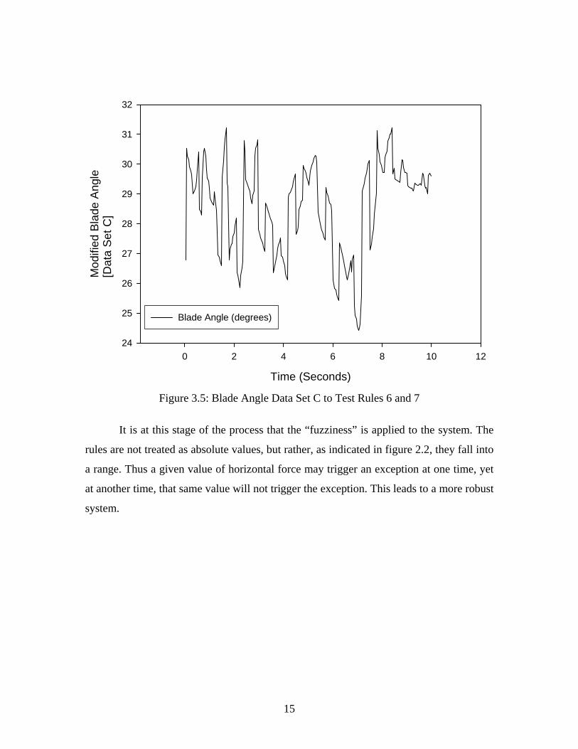
Figure 3.5: Blade Angle Data Set C to Test Rules 6 and 7

It is at this stage of the process that the “fuzziness” is applied to the system. The

rules are not treated as absolute values, but rather, as indicated in figure 2.2, they fall into

a range. Thus a given value of horizontal force may trigger an exception at one time, yet

at another time, that same value will not trigger the exception. This leads to a more robust

system.

15

Time (Seconds)

0 2 4 6 8 10 12

Mod

ified

Bla

de A

ngle

[Dat

a S

et D

]

-2

-1

0

1

2

3

4

5

6

Blade Angle (degrees)

Figure 3.6: Blade Angle Data Set D to Test Rules 6 and 7

The approach taken in the rule setting part of the program is to develop a series of

evaluative statements, which test whether or not a given data value has exceeded the

fuzzy limit set for it by the rule being tested. The results of this test will be a zero if the

rule has not been violated, or 1 if the rule has been violated. These values will be placed

into a results matrix which is then passed to the third part of the program, the output.

3.3 Output Module

The purpose of the output module is to take the results of the rule checking

modules and use those results to develop commands that would be sent to the hydraulic

control system to modify the behavior of the system.

16

Time (Seconds)

0 2 4 6 8 10 12

Mod

ified

For

ce A

ngle

[Dat

a S

et E

]

77

78

79

80

81

82

Force Angle (degrees)

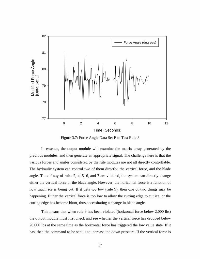
Figure 3.7: Force Angle Data Set E to Test Rule 8

In essence, the output module will examine the matrix array generated by the

previous modules, and then generate an appropriate signal. The challenge here is that the

various forces and angles considered by the rule modules are not all directly controllable.

The hydraulic system can control two of them directly: the vertical force, and the blade

angle. Thus if any of rules 2, 4, 5, 6, and 7 are violated, the system can directly change

either the vertical force or the blade angle. However, the horizontal force is a function of

how much ice is being cut. If it gets too low (rule 9), then one of two things may be

happening. Either the vertical force is too low to allow the cutting edge to cut ice, or the

cutting edge has become blunt, thus necessitating a change in blade angle.

This means that when rule 9 has been violated (horizontal force below 2,000 lbs)

the output module must first check and see whether the vertical force has dropped below

20,000 lbs at the same time as the horizontal force has triggered the low value state. If it

has, then the command to be sent is to increase the down pressure. If the vertical force is

17

not below the 20,000 lb level, then the system must adjust the blade angle from either 30

to 15 degrees or from 15 to 30 degrees, because the blade has most likely worn blunt and

needs a change in blade angle to sharpen itself again (common practice among

experienced underbody plow operators, as noted by Nixon and Potter, 1997). Thus in this

circumstance, the output module must adjust the blade angle, and not change the vertical

force.

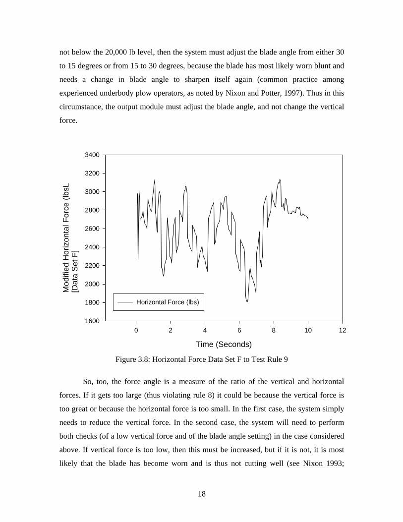
Figure 3.8: Horizontal Force Data Set F to Test Rule 9

So, too, the force angle is a measure of the ratio of the vertical and horizontal

forces.

Time (Seconds)

0 2 4 6 8 10 12

Mod

ified

Hor

izon

tal F

orce

(lbs

L[D

ata

Set

F]

1600

1800

2000

2200

2400

2600

2800

3000

3200

3400

Horizontal Force (lbs)

If it gets too large (thus violating rule 8) it could be because the vertical force is

too great or because the horizontal force is too small. In the first case, the system simply

needs to reduce the vertical force. In the second case, the system will need to perform

both checks (of a low vertical force and of the blade angle setting) in the case considered

above. If vertical force is too low, then this must be increased, but if it is not, it is most

likely that the blade has become worn and is thus not cutting well (see Nixon 1993;

18

Nixon and Chung, 1992; Nixon et al., 1996). In this case the blade angle must be adjusted

as indicated above.

19

4. CODE DEVELOPMENT

In this chapter the coding approach is discussed in greater detail. The chapter first

presents the information on how the standard MatLab coding was done, and then

discusses the use of the Simulink© program.

4.1 MatLab Program Development

As indicated above, there are three main phases to the MatLab programming:

input, rule checking, and output. The input module essential reads data from an input file,

calculates a ten point moving average for each data set, and then outputs those data to

another file for use in the rule checking module. Figure 4.1 illustrates this schematically.

This part of the process is very straightforward.

In the rule checking module, the various rules to be checked are considered at

each time step. A number of sequences can be used for this, but it is in general best to

start with the simplest steps and then move to greater complexity. Accordingly, the

module checks blade angle first. If it exceeds 30 degrees, it is set to 29 degrees. If it falls

below zero degrees it is set to 16 degrees. If either of these two conditions is violated, the

program moves to the next time step.

The next stage is to check the horizontal force. As noted in chapter 3, the

horizontal force is not directly controlled by the hydraulics. Thus, if the horizontal force

has fallen below 2,000 lbs, first the vertical force is checked. If this is less than 20,000

lbs, it is increased to 25,000 lbs ( the mid-part of the vertical force operating range). If the

vertical force is at an appropriate level, the blade angle is changed (the assumption being

that the horizontal force is low because the blade has become blunt and is thus not cutting

ice). First, the blade angle is checked to see if it is greater than 22.5 degrees (the mid-

point of the operating range). If it is greater than this, it is set to 15 degrees. If it is less

than 22.5 degrees, it is increased to 29 degrees. If the horizontal force is too low, then the

program, having issued corrective measures, moves to the next time step.

20

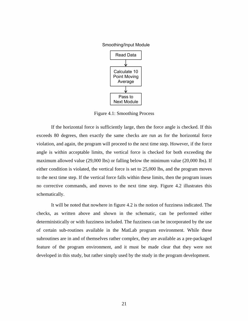
Figure 4.1: Smoothing Process

If the horizontal force is sufficiently large, then the force angle is checked. If this

exceeds 80 degrees, then exactly the same checks are run as for the horizontal force

violation, and again, the program will proceed to the next time step. However, if the force

angle is within acceptable limits, the vertical force is checked for both exceeding the

maximum allowed value (29,000 lbs) or falling below the minimum value (20,000 lbs). If

either condition is violated, the vertical force is set to 25,000 lbs, and the program moves

to the next time step. If the vertical force falls within these limits, then the program issues

no corrective commands, and moves to the next time step. Figure 4.2 illustrates this

schematically.

It will be noted that nowhere in figure 4.2 is the notion of fuzziness indicated. The

checks, as written above and shown in the schematic, can be performed either

deterministically or with fuzziness included. The fuzziness can be incorporated by the use

of certain sub-routines available in the MatLab program environment. While these

subroutines are in and of themselves rather complex, they are available as a pre-packaged

feature of the program environment, and it must be made clear that they were not

developed in this study, but rather simply used by the study in the program development.

21

Figure 4.2: The Rule Checking Module

The output module simply takes the results of the rule checking and turns these

into particular commands that would be issued to the hydraulic control system. In

essence, this is already included in figure 4.2. To make the steps more explicit, whenever

one of the rules is violated, a value in an array, corresponding both to the time step where

the violation occurred and to the nature of the violation is changed from zero to one. In

the output module, this array is read and the indications of particular violations are turned

into specific commands issued to the control system.

4.2 Simulink© Program Development

In developing the simulation of the system, some simplifying assumptions were

required to make the program development tractable. A number of these concerned the

22

way in which the system responds to input commands from operators. To that end, it is

assumed that the automated system, at first, lowers the blade to touch the road surface.

The road surface, in turn, gives a reaction that is measured by the automated system. It is

by this reaction that the system can determine the correct down force to apply, which in

turn determines the depth for the blade. The final down force is determined after a series

of actions involving lowering and raising the blade. As noted in the previous studies, it is

critical that a clearance angle is maintained on the cutting edge. Experienced underbody

plow operators maintain this clearance (as the blade wears) by periodically adjusting the

angle of curl of the blade. It is such expertise that the computer controlled system must

capture.

4.2.1 Control system process

From the above, it is clear that the system will use a series of trials (adjusting

down force and thus raising and lowering the blade) to decide on the optimal blade depth

and vertical force. The force exerted by the road surface on the blade is used in this

simulation as the controlling factor. This can be used as a feedback in a classical control

system process.

4.2.2 Simulink

Simulink is a software package that enables us to model, simulate and analyze

systems whose outputs change over time. These systems are dynamic and simulating

them is a two-step process. First, a graphical model of the system to be simulated is

developed, using Simulink’s model editor. The model depicts the time-dependent

mathematical relationships among the system inputs, states and outputs. Then Simulink is

used to simulate the behavior of the system over the specified time-span.

23

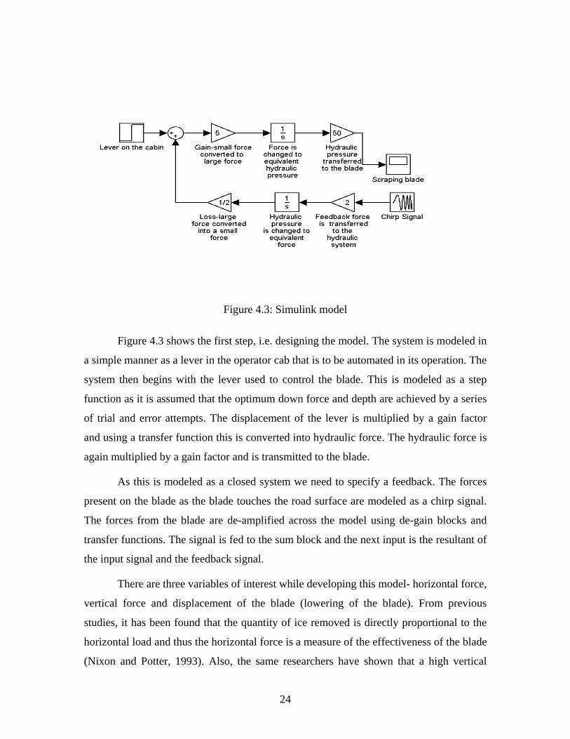
Figure 4.3: Simulink model

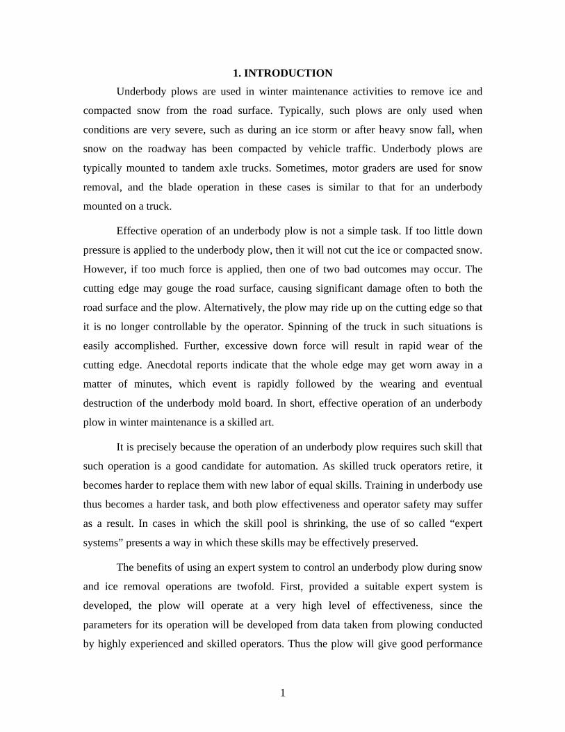
Figure 4.3 shows the first step, i.e. designing the model. The system is modeled in

a simple manner as a lever in the operator cab that is to be automated in its operation. The

system then begins with the lever used to control the blade. This is modeled as a step

function as it is assumed that the optimum down force and depth are achieved by a series

of trial and error attempts. The displacement of the lever is multiplied by a gain factor

and using a transfer function this is converted into hydraulic force. The hydraulic force is

again multiplied by a gain factor and is transmitted to the blade.

As this is modeled as a closed system we need to specify a feedback. The forces

present on the blade as the blade touches the road surface are modeled as a chirp signal.

The forces from the blade are de-amplified across the model using de-gain blocks and

transfer functions. The signal is fed to the sum block and the next input is the resultant of

the input signal and the feedback signal.

There are three variables of interest while developing this model- horizontal force,

vertical force and displacement of the blade (lowering of the blade). From previous

studies, it has been found that the quantity of ice removed is directly proportional to the

horizontal load and thus the horizontal force is a measure of the effectiveness of the blade

(Nixon and Potter, 1993). Also, the same researchers have shown that a high vertical

24

download is a cause of concern because it removes traction from the trucks axles and

makes the truck rest predominantly on the cutting edge.

-10

InitialDisplacement

of blade

[15]

IC Initial Force

Force exerted on the blade

s

1

Force function

-0.8

Displacementof bladeDisplay

s

1

Displacementfunction

Figure 4.4: Simulink model with force and displacement as variables

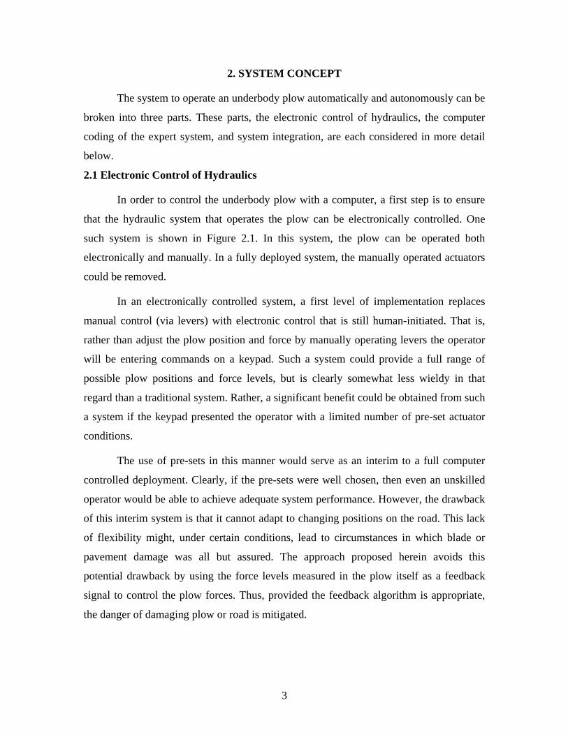
Figure 4.4 shows the model with force applied on the blade and displacement of

the blade as the major variables. Force and displacement functions have been integrated

with respect to time. The lower and upper limits of force function integration range from

negative to positive infinity. The parameters of the force and displacement functions are

shown in figures 4.5 and 4.6. The outputs of both functions are obtained by the scope

variables, shown at the right hand corner of figure 4.4. The results of this simulation are

presented in Chapter 5.

25

Figure 4.5: Parameters of the force function

Figure 4.6: Parameters of the displacement function

26

5. RESULTS

This chapter presents the results from the programming described previously, and

discusses, where appropriate, those results. The chapter is presented in two parts: results

from basic MatLab programming, and then results from the Simulink© program.

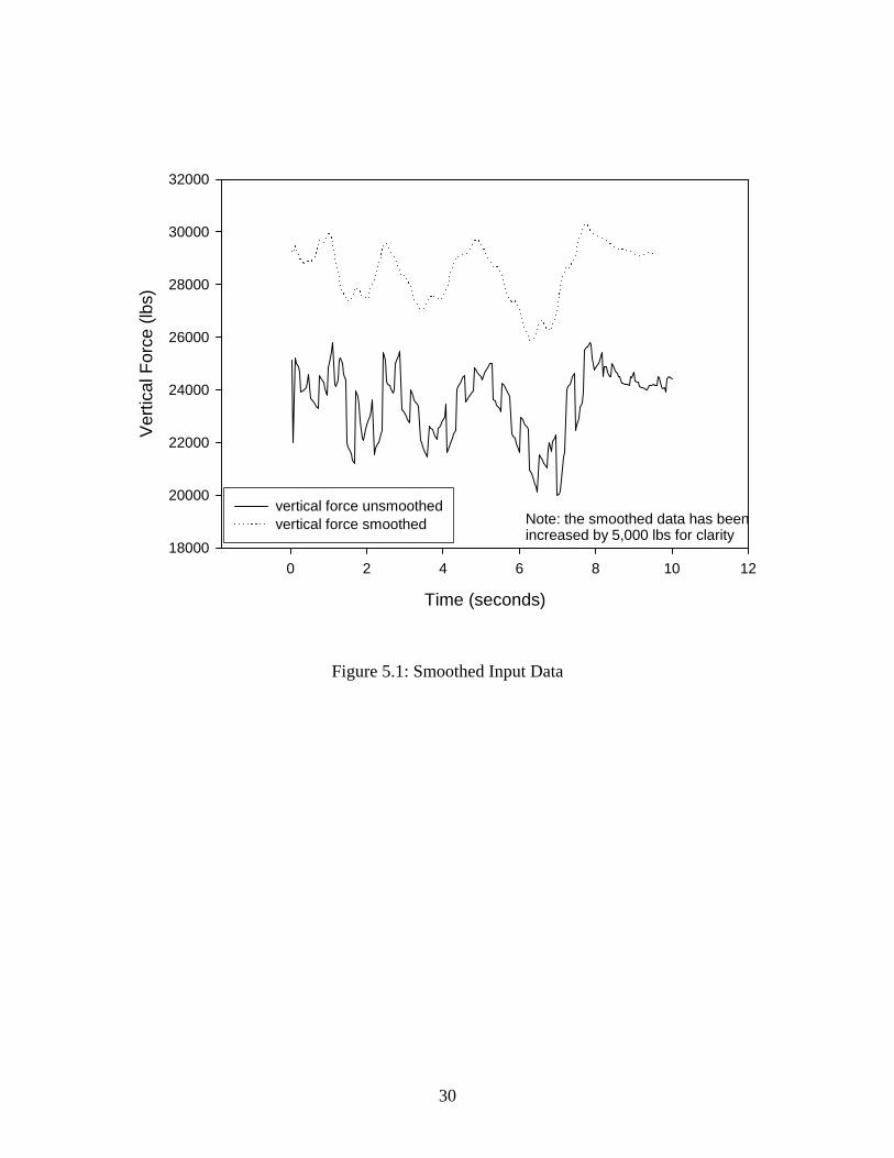
5.1 MatLab Program Results

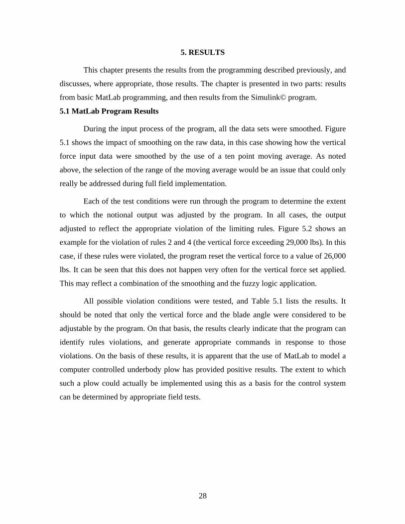
During the input process of the program, all the data sets were smoothed. Figure

5.1 shows the impact of smoothing on the raw data, in this case showing how the vertical

force input data were smoothed by the use of a ten point moving average. As noted

above, the selection of the range of the moving average would be an issue that could only

really be addressed during full field implementation.

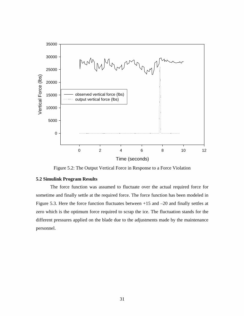
Each of the test conditions were run through the program to determine the extent

to which the notional output was adjusted by the program. In all cases, the output

adjusted to reflect the appropriate violation of the limiting rules. Figure 5.2 shows an

example for the violation of rules 2 and 4 (the vertical force exceeding 29,000 lbs). In this

case, if these rules were violated, the program reset the vertical force to a value of 26,000

lbs. It can be seen that this does not happen very often for the vertical force set applied.

This may reflect a combination of the smoothing and the fuzzy logic application.

All possible violation conditions were tested, and Table 5.1 lists the results. It

should be noted that only the vertical force and the blade angle were considered to be

adjustable by the program. On that basis, the results clearly indicate that the program can

identify rules violations, and generate appropriate commands in response to those

violations. On the basis of these results, it is apparent that the use of MatLab to model a

computer controlled underbody plow has provided positive results. The extent to which

such a plow could actually be implemented using this as a basis for the control system

can be determined by appropriate field tests.

28

Table 5.1: Results of tests of data sets that violate operational rules

Condition Output Value of Blade

Angle (degrees)

Output Value of Vertical

Force (lbs)

Blade angle exceeds 30º 29º Not changed Blade angle less than 0º 16º Not changed Fx less than 2,00lbs and Fy less than 20,000 lbs

Not changed 25,000 lbs

Fx less than 2,000 lbs, Fy greater than 20,000 lbs and blade angle greater than 22.5º

15º Not changed

Fx less than 2,000 lbs, Fy greater than 20,000 lbs and blade angle less than 22.5º

28º Not changed

Force angle greater than 80º and Fy less than 20,000 lbs

Not changed 25,000 lbs

Force angle greater than 80º, Fy greater than 20,000 lbs and blade angle greater than 22.5º

15º Not changed

Force angle greater than 80º, Fy greater than 20,000 lbs and blade angle less than 22.5º

28º Not changed

Fy greater than 29,000 lbs Not changed 26,000 lbs Fy less than 20,000 lbs Not changed 24,000 lbs

29

Time (seconds)

0 2 4 6 8 10 12

Ver

tical

For

ce (l

bs)

18000

20000

22000

24000

26000

28000

30000

32000

vertical force unsmoothedvertical force smoothed Note: the smoothed data has been

increased by 5,000 lbs for clarity

Figure 5.1: Smoothed Input Data

30

Time (seconds)

0 2 4 6 8 10 12

Ver

tical

For

ce (l

bs)

0

5000

10000

15000

20000

25000

30000

35000

observed vertical force (lbs)output vertical force (lbs)

Figure 5.2: The Output Vertical Force in Response to a Force Violation

5.2 Simulink Program Results The force function was assumed to fluctuate over the actual required force for

sometime and finally settle at the required force. The force function has been modeled in

Figure 5.3. Here the force function fluctuates between +15 and –20 and finally settles at

zero which is the optimum force required to scrap the ice. The fluctuation stands for the

different pressures applied on the blade due to the adjustments made by the maintenance

personnel.

31

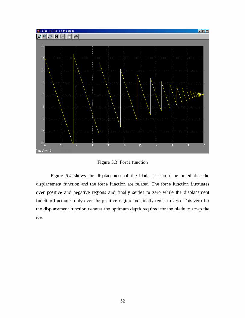
Figure 5.3: Force function

Figure 5.4 shows the displacement of the blade. It should be noted that the

displacement function and the force function are related. The force function fluctuates

over positive and negative regions and finally settles to zero while the displacement

function fluctuates only over the positive region and finally tends to zero. This zero for

the displacement function denotes the optimum depth required for the blade to scrap the

ice.

32

Figure 5.4: Displacement function

The real life example of scraping ice using an underbody plow has been modeled

here using a simulation tool, Simulink. Two functions while scraping ice, i.e, force

exerted on the blade to scrap ice and displacement of the blade are considered in this

simulation. These functions have been found to be the most important while simulating

the scraping of ice using an underbody plow.

The outputs have been displayed as graphical outputs, one as a force function and

the other as a displacement function. The force function tends to fluctuate within a

positive and negative range before settling to zero, which is the required optimum force.

The displacement function, on the other hand, tends to fall from a positive range and

settles to zero, which is the optimum displacement.

33

5.3 Implications of Results on the Deployment Decision

The results of the two simulations presented in this chapter make it clear that it

would be possible to develop an automated system that would control an underbody

plow, and provide a level of operational skill that would likely be competent if not

brilliant. The tests conducted and reported herein do not allow for an evaluation of the

skill of the automated system, since that would depend significantly on the

implementation and integration of the automated system. Nonetheless it is clear that

automation is possible and feasible.

The next issue is then to consider whether implementation of an automated

underbody plow is desirable. Two arguments can be made in favor of such a system. The

first is that an automated system would likely provide an acceptable skill level for

underbody plowing. That is, while the plow performance would likely not be optimal at

all times, it would be safe, and reasonably effective, without causing undue wear on the

equipment. This argument has particular relevance for any organization that expects to

lose through retirement or job changes the most skilled group among its snow plow

operators. The extent to which such a situation might be relevant in Iowa or in other

organizations is beyond the scope of this work.

The second argument in favor of an automated underbody plow system is one of

safety. The snow plow cab is becoming an increasingly complex place, with multiple

equipment requiring operation often under extremely stressful and hazardous conditions.

The automation of one such piece of equipment would reduce the operational burden on

the snow plow driver, and would thus tend to increase safety. However, it should be

noted that while such a result seems likely, the human factors aspects of operating an

automated versus a regular underbody plow were not considered in this study.

Two arguments can also be made against the development and implementation of

an automated underbody plow system. The first relates to safety. If the plow

automatically adjusts the loads and angles of the underbody plow this will likely impact

the dynamic performance of the snow plow. Under certain, extreme, conditions it is

possible that such automated changes might render the truck temporarily out of control

(although this is unlikely). The use of such an automated system should thus only be

34

considered if prototype operation indicates clearly that such unexpected losses of stability

have been themselves controlled and rendered extremely unlikely or impossible.

The second concern with using such a system is likely to be cost. No such system

currently exists, and thus it would need to be developed. Such new technology is likely to

be expensive to purchase, although the price may in essence be recovered over time by

improved performance resulting in a higher level of service to the traveling public.

This second concern raises the question of who should develop such a system. If

it is developed by a Department of Transportation, then significant costs would be sunk

into the development and all the risk would be taken by the Department. If, instead, the

task is taken on by a private vendor, the challenge of the competitive bid process may

make it difficult to recover the vendor’s investment. Perhaps, if such a system is deemed

worthy of further exploration, it would be a candidate for some sort of joint venture

between a Department and a vendor. Such agreements are relatively common in Europe

(Smithson, 2005, personal communication) but are very rare in the United States.

6. CONCLUSIONS

The purpose of this study has been to examine whether the development of a

computer controlled underbody plow is feasible. The study has presented the three steps

that would be needed to implement such a system (electronic control of hydraulics,

computer coding of the expert system, and system integration) in concept. The computer

control concept has been tested in two ways, using both MatLab and the Simulink

simulation environment. Details of the coding have been provided. The results of the

computer testing and simulation indicate that a fully automated, computer controlled

underbody plow is indeed possible. The issue of whether the next steps toward full

automation should be taken (and by whom) has also been considered, and the possibility

of some sort of joint venture between a Department of Transportation and a vendor has

been suggested.

35

7. REFERENCES Cox, E. (1994). “The Fuzzy Systems Handbook,” AP Professional, Chestnut Hill, MA, U.S.A. Kosko, B. (1997). “Fuzzy Engineering,” Prentice Hall, Upper Saddle River, NJ, U.S.A. Nixon, W. A., “Improved Cutting Edges for Ice Removal,” National Research Council, SHRP Report, SHRP-H-346, 1993, 98 pages. Nixon, W. A. and C.-H. Chung, “Development of a New Test Apparatus to Determine Scraping Loads for Ice Removal from Pavements,” Proc. 11th IAHR Ice Symposium, vol. 1, pp. 116-127, Banff, 1992. Nixon, W.A., and Frisbie, T.R. (1993). “Field Measurements of Plow Loads during Ice Removal; Operations: Iowa Department of Transportation Project HR 334,” IIHR Technical Report # 365, November 1993, 126 pages. Nixon, W. A., T. J. Gawronski, and A. E. Whelan, “Development of a Model for the Ice Scraping Process: Iowa Department of Transportation Project HR361,” IIHR Technical Report # 383, October 1996, 57 pages. Nixon, W. A., and J.D. Potter (1997). “Measurement of Ice Scraping Forces on Snow-Plow Underbody Blades: Iowa Department of Transportation Project HR 372,” IIHR Technical Report # 385, February 1997, 70 pages.

36

APPENDIX A: PROGRAM LISTINGS The following section includes listing of all MatLab programs used in this study.

A.1: Program to test violation of Vertical Force Rules (2 and 4). In this case, the vertical force exceeds 29,000 lbs. Lines that begin with a % symbol are comment lines.

%first enter the input data clear uinput =[0.04 5661.087866 28876.5 25.78577406 77.29499484; 0.08 5778.451883 25311.5 29.53472803 75.28968236; 0.12 5065.062762 28991.5 29.27698745 78.63967673; 0.16 5801.464435 28738.5 29.15983264 76.9302156; 0.2 5750.83682 28623.5 28.91380753 76.99010557; 0.24 5502.301255 28382 28.76150628 77.43169377; 0.28 5511.506276 27496.5 28.64435146 77.01945815; 0.32 5520.711297 27542.5 28.01171548 77.01949313; 0.36 5546.025105 27588.5 28.05857741 76.98300154; 0.4 5592.050209 27715 28.10543933 76.93653087; 0.44 5536.820084 27945 28.23430962 77.16414121; 0.48 5472.384937 28290 28.46861925 77.45850126; 0.52 5449.372385 27232 28.82008368 77.04040507; 0.56 5437.866109 27174.5 29.41757322 77.04040507; 0.6 5426.359833 27117 27.48451883 77.04040507; 0.64 5398.74477 26979 27.40251046 77.04040507; 0.68 5727.824268 26898.5 27.28535565 76.23999831; 0.72 5679.497908 26783.5 28.53891213 76.29533753; 0.76 5649.58159 28232.5 29.41757322 77.04040507; 0.8 5626.569038 28117.5 29.53472803 77.04040507; 0.84 5603.556485 28002.5 29.27698745 77.04040507; 0.88 5587.447699 27922 28.8083682 77.04040507; 0.92 5610.460251 27669 28.52719665 76.87397217; 0.96 5718.619247 27347 28.44518828 76.47825438; 1 5803.76569 28577.5 28.1874477 76.85409979; 1.04 5863.598326 29003 27.85941423 76.91137858; 1.08 5937.238494 29302 27.74225941 76.88324157; 1.12 5571.338912 29670 27.68368201 77.81446693; 1.16 5548.32636 27841.5 27.6251046 77.09213857; 1.2 5382.635983 27726.5 28.08200837 77.4149107; 1.24 5359.623431 28014 27.84769874 77.59163153; 1.28 5605.857741 28876.5 27.44937238 77.41497916; 1.32 5778.451883 28991.5 26.74644351 77.09008606; 1.36 5801.464435 28738.5 25.94979079 76.9302156; 1.4 5750.83682 28278.5 25.87949791 76.83687858; 1.44 5658.786611 28037 25.7623431 76.9325915; 1.48 4982.217573 25288.5 25.58661088 77.23416607;

37

1.52 4966.108787 25116 28.5623431 77.18956643; 1.56 4910.878661 24897.5 29.11297071 77.21983369; 1.6 4880.962343 24817 29.54644351 77.25528675; 1.64 4961.506276 24541 29.85104603 76.91137858; 1.68 5012.133891 24391.5 30.22594142 76.70434333; 1.72 5053.556485 27565.5 28.36317992 78.09476998; 1.76 5065.062762 27335.5 28.2460251 77.97096013; 1.8 5516.108787 26944.5 25.78577406 76.75214058; 1.84 5470.083682 26254.5 26.13723849 76.52590158; 1.88 5391.841004 25472.5 26.30125523 76.31891667; 1.92 5253.76569 25403.5 26.33640167 76.62163692; 1.96 5097.280335 25852 26.5707113 77.22436083; 2 5083.472803 26082 26.68786611 77.36657907; 2.04 5060.460251 26197 26.93389121 77.47541548; 2.08 5025.941423 26438.5 27.1916318 77.66833609; 2.12 5290.585774 26691.5 25.36401674 77.15915422; 2.16 5341.213389 27151.5 25.28200837 77.25273377; 2.2 5433.263598 24794 25.00083682 75.85559768; 2.24 5493.096234 25047 24.84853556 75.84473633; 2.28 5520.711297 25254 25.25857741 75.88836607; 2.32 5134.100418 25311.5 25.51631799 76.86984445; 2.36 5166.317992 25656.5 25.72719665 76.9618512; 2.4 5173.221757 25817.5 29.8041841 77.02367291; 2.44 5219.246862 29256 29.4292887 78.40612732; 2.48 5242.259414 28888 28.49205021 78.2122; 2.52 5596.65272 27968 28.3748954 77.04040507; 2.56 5573.640167 27853 28.29288703 77.04040507; 2.6 5557.531381 27772.5 28.15230126 77.04040507; 2.64 5529.916318 27634.5 28.10543933 77.04040507; 2.68 5520.711297 27450.5 27.85941423 76.97746963; 2.72 5472.384937 27588.5 27.66025105 77.15006709; 2.76 5750.83682 28738.5 27.96485356 77.04040507; 2.8 5801.464435 28991.5 28.10543933 77.04040507; 2.84 5824.476987 29106.5 29.27698745 77.04040507; 2.88 5858.995816 29279 29.53472803 77.04040507; 2.92 5854.393305 26737.5 29.65188285 75.86663157; 2.96 5780.753138 26668.5 29.82761506 76.00270587; 3 5295.188285 26553.5 26.8167364 77.08379792; 3.04 5267.573222 26461.5 26.65271967 77.10572638; 3.08 5235.355649 26323.5 26.52384937 77.11701624; 3.12 5210.041841 26162.5 26.39497908 77.1009661; 3.16 5184.728033 27588.5 26.34811715 77.80477688; 3.2 5175.523013 27347 26.21924686 77.72151999; 3.24 5150.209205 27174.5 26.07866109 77.70454608; 3.28 5437.866109 27071 27.68368201 76.99253888; 3.32 5417.154812 26979 27.57824268 76.99771136;

38

3.36 5398.74477 26898.5 27.48451883 77.00293549; 3.4 5382.635983 25403.5 27.40251046 76.30569369; 3.44 5350.41841 25288.5 27.23849372 76.3250042; 3.48 5336.610879 25116 27.16820084 76.26882094; 3.52 5313.598326 24863 27.05104603 76.19195992; 3.56 4979.916318 24771 26.95732218 76.98228459; 3.6 5025.941423 24656 25.35230126 76.80700448; 3.64 5051.25523 26036 25.58661088 77.42262111; 3.68 5097.280335 25909.5 25.71548117 77.25178584; 3.72 5141.004184 25863.5 25.94979079 77.12395069; 3.76 5164.016736 25737 26.17238494 77.00683834; 3.8 5187.029289 25599 26.28953975 76.88299461; 3.84 5210.041841 25449.5 26.40669456 76.75216226; 3.88 5122.594142 25921 26.52384937 77.19605573; 3.92 5092.677824 26036 25.92635983 77.32280139; 3.96 5083.472803 26151 25.87949791 77.39884675; 4 5060.460251 26266 25.7623431 77.50728298; 4.04 5025.941423 26404 25.58661088 77.65271722; 4.08 4975.313808 26979 25.32887029 78.02632115; 4.12 4956.903766 24886 25.23514644 77.09828394; 4.16 4933.891213 25116 25.11799163 77.26995742; 4.2 5511.506276 25242.5 27.89456067 75.90479455; 4.24 5525.313808 25472.5 28 75.99342835; 4.28 5548.32636 25691 28.05857741 76.05231538; 4.32 5582.845188 25806 28.12887029 76.02903067; 4.36 5601.25523 27611.5 28.2460251 76.86841759; 4.4 5633.472803 27726.5 28.42175732 76.84838604; 4.44 5651.882845 27899 28.51548117 76.88565322; 4.48 5667.991632 27991 28.67949791 76.89129989; 4.52 5688.702929 28152 26.64100418 76.91770028; 4.56 5233.054393 28244 26.758159 77.97173358; 4.6 5256.066946 27094 26.89874477 77.42366661; 4.64 5283.682008 27232 27.48451883 77.42172149; 4.68 5398.74477 27289.5 27.60167364 77.18296262; 4.72 5421.757322 27381.5 27.74225941 77.17195352; 4.76 5449.372385 27485 27.80083682 77.15572431; 4.8 5460.878661 27542.5 28.97238494 77.15548345; 4.84 5479.288703 28543 28.85523013 77.55099744; 4.88 5500 28439.5 28.76150628 77.46138011; 4.92 5691.004184 28324.5 28.69121339 76.9895747; 4.96 5667.991632 28232.5 28.5623431 76.99960662; 5 5649.58159 28163.5 28.42175732 77.00973002; 5.04 5635.774059 28037 28.29288703 76.9839196; 5.08 5610.460251 28324.5 28.77322176 77.16757169; 5.12 5714.016736 28428 28.85523013 76.98469633; 5.16 5737.029289 28554.5 28.96066946 76.98998405;

39

5.2 5755.439331 28669.5 29.08953975 77.0002284; 5.24 5750.83682 28761.5 29.20669456 77.05041914; 5.28 5711.715481 28738.5 29.30041841 77.12561838; 5.32 5440.167364 27186 29.27698745 77.04040507; 5.36 5428.661088 27128.5 29.07782427 77.04040507; 5.4 5387.238494 26921.5 27.39079498 77.04040507; 5.44 5380.334728 26887 27.26192469 77.04040507; 5.48 5355.020921 26760.5 27.12133891 77.04040507; 5.52 5327.405858 26622.5 26.88702929 77.04040507; 5.56 5582.845188 27899 26.78158996 77.04040507; 5.6 5557.531381 27772.5 26.66443515 77.04040507; 5.64 5543.723849 27703.5 26.54728033 77.04040507; 5.68 5509.205021 27531 26.46527197 77.04040507; 5.72 5488.493724 27427.5 28.22259414 77.04040507; 5.76 5465.481172 27312.5 28.04686192 77.04040507; 5.8 5122.594142 25702.5 27.94142259 77.09083976; 5.84 5104.1841 25599 27.82426778 77.08541618; 5.88 5055.857741 25507 27.69539749 77.1590203; 5.92 5028.242678 25265.5 27.63682008 77.10881936; 5.96 4979.916318 25127.5 27.42594142 77.16081261; 6 4954.60251 24886 25.11799163 77.1040733; 6.04 4933.891213 26392.5 24.97740586 77.86697598; 6.08 5281.380753 26289 24.83682008 76.99111532; 6.12 5260.669456 26174 24.77824268 76.98539932; 6.16 5237.656904 26059 24.6376569 76.98515663; 6.2 5214.644351 25978.5 24.54393305 77.00160875; 6.24 5198.535565 25863.5 24.41506276 76.98473911; 6.28 5175.523013 24092.5 26.34811715 76.12339642; 6.32 5143.305439 23966 26.18410042 76.13646444; 6.36 4676.150628 23816.5 26.07866109 77.27643662; 6.4 4630.125523 23483 25.98493724 77.22450835; 6.44 4602.51046 23368 25.73891213 77.23775871; 6.48 4614.016736 23138 25.59832636 77.08397857; 6.52 4643.933054 24759.5 25.35230126 77.82801398; 6.56 4830.334728 24656 25.22343096 77.30350447; 6.6 4936.192469 24518 25.12970711 76.96407438; 6.64 4975.313808 24380 25.32887029 76.79257462; 6.68 4906.276151 24322.5 25.48117155 76.93979556; 6.72 4878.661088 24184.5 25.7623431 76.9392217; 6.76 4867.154812 25012.5 25.37573222 77.38631749; 6.8 4839.539749 25288.5 25.80920502 77.58825783; 6.84 4821.129707 24909 25.96150628 77.45154106; 6.88 4795.8159 25334.5 24.26276151 77.71862435; 6.92 4765.899582 25484 23.92301255 77.86241395; 6.96 4699.16318 25633.5 23.80585774 78.09526617; 7 5129.497908 23000 23.57154812 75.61513039;

40

7.04 5166.317992 23057.5 23.43096234 75.55080822; 7.08 5216.945607 23207 23.48953975 75.50520883; 7.12 5272.175732 24138.5 23.641841 75.90037963; 7.16 5366.527197 24667.5 24.59079498 75.95363258; 7.2 5005.230126 24863 28.10543933 76.96513323; 7.24 5060.460251 27588.5 28.25774059 78.08862536; 7.28 4984.518828 27738 28.3748954 78.32390272; 7.32 5069.665272 27853 28.52719665 78.1776891; 7.36 5099.58159 28002.5 28.69121339 78.17159135; 7.4 5635.774059 28163.5 28.84351464 77.04040507; 7.44 5665.690377 28313 29.00753138 77.04040507; 7.48 5697.90795 25817.5 29.12468619 75.75878893; 7.52 5720.920502 26070.5 26.11380753 75.83675508; 7.56 5741.631799 26346.5 26.30125523 75.93049801; 7.6 5757.740586 26818 26.55899582 76.13097148; 7.64 5412.552301 27048 26.84016736 77.04040507; 7.68 5504.60251 27508 27.32050209 77.04040507; 7.72 5520.711297 29348 27.55481172 77.79336824; 7.76 5550.627615 29463 28.02343096 77.77567277; 7.8 5573.640167 29451.5 30.12050209 77.7218776; 7.84 5603.556485 29670 29.53472803 77.74612459; 7.88 5801.464435 29566.5 29.31213389 77.28416751; 7.92 5757.740586 28991.5 29.07782427 77.13481583; 7.96 5711.715481 28474 28.96066946 77.01006448; 8 5688.702929 28589 28.84351464 77.11094357; 8.04 5665.690377 28692.5 28.72635983 77.20613756; 8.08 5642.677824 28773 28.71464435 77.29089665; 8.12 5640.376569 28888 29.23012552 77.34485321; 8.16 5780.753138 29233 29.31213389 77.18827473; 8.2 5849.790795 28163.5 29.4292887 76.56580038; 8.24 5872.803347 28612 29.78075314 76.71871326; 8.28 5895.8159 28600.5 29.89790795 76.66335635; 8.32 5893.514644 28359 30.01506276 76.55894959; 8.36 5937.238494 28198 30.00334728 76.38846377; 8.4 5916.527197 28186.5 30.22594142 76.42885809; 8.44 5640.376569 28773 28.67949791 77.29591156; 8.48 5635.774059 28543 28.87866109 77.2070062; 8.52 5633.472803 28428 28.50376569 77.16203788; 8.56 5672.594142 28313 28.48033473 77.02514759; 8.6 5598.953975 28198 28.45690377 77.13747361; 8.64 5635.774059 28186.5 28.4334728 77.05062343; 8.68 5725.523013 27910.5 28.41004184 76.72607674; 8.72 5723.221757 27887.5 28.38661088 76.72066739; 8.76 5674.895397 27864.5 28.69121339 76.81838007; 8.8 5642.677824 27841.5 29.14811715 76.88016813; 8.84 5566.736402 27818.5 29.13640167 77.04040507;

41

8.88 5562.133891 27795.5 28.89037657 77.04040507; 8.92 5557.531381 28163.5 28.72635983 77.21437277; 8.96 5559.832636 28152 28.71464435 77.20419963; 9 5564.435146 28347.5 28.69121339 77.27939058; 9.04 5566.736402 27979.5 28.30460251 77.11248061; 9.08 5594.351464 27956.5 28.2460251 77.04040507; 9.12 5589.748954 27933.5 28.22259414 77.04040507; 9.16 5585.146444 27726.5 28.19916318 76.9573332; 9.2 5580.543933 27703.5 28.1874477 76.95726425; 9.24 5575.941423 27680.5 28.12887029 76.95719519; 9.28 5571.338912 27669 28.10543933 76.96236176; 9.32 5624.267782 27611.5 28.36317992 76.81634754; 9.36 5635.774059 27588.5 28.33974895 76.77969475; 9.4 5628.870293 27772.5 28.31631799 76.87977029; 9.44 5619.665272 27784 28.29288703 76.90572074; 9.48 5635.774059 27807 28.30460251 76.87996946; 9.52 5628.870293 27818.5 28.32803347 76.90071686; 9.56 5555.230126 27772.5 28.33974895 77.04559031; 9.6 5536.820084 27784 28.29288703 77.09224565; 9.64 5541.422594 28163.5 28.69121339 77.25021954; 9.68 5557.531381 28129 28.65606695 77.19920764; 9.72 5559.832636 27761 28.28117155 77.03003096; 9.76 5548.32636 27669 28.1874477 77.01438519; 9.8 5543.723849 27692 28.21087866 77.03520498; 9.84 5539.121339 27485 28 76.95136781; 9.88 5536.820084 28106 28.63263598 77.23525352; 9.92 5525.313808 28163.5 28.69121339 77.28607646; 9.96 5520.711297 28129 28.65606695 77.28124874; 10 5500 28083 28.60920502 77.30733445 ]; %now, smooth the data for horizontal force, vertical force, and blade angle for k=1:240 smoothfx(k)=(uinput(k,3)+uinput(k+1,2)+uinput(k+2,2)+uinput(k+3,2)+uinput(k+4,2)+uinput(k+5,2)+uinput(k+6,2)+uinput(k+7,2)+uinput(k+8,2)+uinput(k+9,2))/10.0; smoothfy(k)=(uinput(k,3)+uinput(k+1,3)+uinput(k+2,3)+uinput(k+3,3)+uinput(k+4,3)+uinput(k+5,3)+uinput(k+6,3)+uinput(k+7,3)+uinput(k+8,3)+uinput(k+9,3))/10.0; smoothba(k)=(uinput(k,3)+uinput(k+1,4)+uinput(k+2,4)+uinput(k+3,4)+uinput(k+4,4)+uinput(k+5,4)+uinput(k+6,4)+uinput(k+7,4)+uinput(k+8,4)+uinput(k+9,4))/1000.0; end; smoothfx=smoothfx'; smoothfy=smoothfy'; smoothba=smoothba'; %now determine the force angle from the smoothed horizontal and vertical

42

%force data for k=1:240 rat=smoothfy(k)/smoothfx(k); smoothfa(k)=(atan(rat))*(180/3.14159); end; smoothfa=smoothfa'; %now perform the various checks for k=1:240 baout(k)=0.0; fyout(k)=0.0; if smoothba(k)>30.0 baout(k)=29.0; elseif smoothba(k)<0.0 baout(k)=16.0; elseif smoothfx(k)<2000.0 if smoothfy(k)<20000.0 fyout(k)=25000.0; elseif smoothba(k)>22.5 baout(k)=15.0; else baout(k)=28.0; end elseif smoothfa(k)>80.0 if smoothfy(k)<20000.0 fyout(k)=25000; elseif smoothba(k)>22.5 baout(k)=15.0; else baout(k)=28.0; end elseif smoothfy(k)>29000.0 fyout(k)=26000.0; elseif smoothfy(k)<20000.0 fyout(k)=24000.0; end end; %now report on the values of baout and fyout as set by the program %different values indicate different violations of the rules baout=baout'; fyout=fyout';

43