Development of a Carbon Fibre Swingarm Bevan Ian Smith
146
Development of a Carbon Fibre Swingarm Bevan Ian Smith A research report submitted to the Faculty of Engineering and the Built Environment, of the University of the Witwatersrand, in partial fulfilment of the requirements for the degree of Master of Science in Engineering. Johannesburg 2013
Transcript of Development of a Carbon Fibre Swingarm Bevan Ian Smith

Development of a Carbon Fibre Swingarm
Bevan Ian Smith
A research report submitted to the Faculty of Engineering and the Built Environment, of
the University of the Witwatersrand, in partial fulfilment of the requirements for the
degree of Master of Science in Engineering.
Johannesburg 2013

i
DECLARATION
I declare that this research report is my own unaided work. It is being submitted to the
Degree of Master of Science to the University of the Witwatersrand, Johannesburg. It
has not been submitted before for any degree or examination to any other University.
……………………………………………………………………………
(Signature of Candidate)
……….. day of …………….., ……………
(day) (month) (year)

ii
ABSTRACT
Carbon fibre has not been extensively used in the development of motorcycle
swingarms. This study investigates the development of a carbon fibre swingarm with
an emphasis on the structural integrity and on developing a finite element model
(FEM).
The motorcycle swingarm is a critical component in the rear part of the motorcycle.
The literature shows that swingarms need to be strong enough to handle various loads
experienced in the field, stiff enough to increase motorcycle response and stability,
and light enough to improve motorcycle performance and reduce the rear unsprung
mass. To this end carbon fibre was used in the design of a swingarm for a Ducati
1098 motorcycle due to its high stiffness and strength to weight ratios. The current
research presents the first step in the design process of a single-sided carbon fibre
swingarm.
A test rig was developed for testing the stiffness and strength of swingarms. Vertical,
lateral and torsional stiffness values of 500 kN/m, 445 kN/m and 550 Nm/deg
respectively, were determined from deflection measurements. The lateral and
torsional stiffness values are on the lower spectrum of stiffness values when compared
with swingarms measured in the literature which suggests the swingarm will exhibit a
sluggish response and reduced weave mode stability at medium to high speeds. To
determine the strength, strains were measured on the swingarm. Maximum strain
values of 1100 µε were measured which are considerably lower than the ultimate
strain of 8000 µε for the material which indicates the swingarm is strong enough.
Furthermore, a finite element (FE) model was developed so that later design iterations
could be completed more quickly and cheaply. The FE model showed good
correlation with the vertical displacement results (difference ≈ 4%); the torsional
deflection difference was approximately 28% and the lateral deflection difference,
50%. The experimental lateral loading used was 133 N, resulting in a displacement of
0.3 mm as compared to the experimental vertical loading used which was 8000 N,
resulting in a displacement of 16.5 mm. The error due to lash and bedding in which is
plausibly in the region of 0.15 mm is likely the cause of the poor correlation between

iii
the measured and FE lateral deflection results. The strains calculated by the FE model
showed both good (less than 10% difference) and poor (larger than 100% difference)
correlation. Plausible reasons for the poor correlation results were determined to be
largely due to the influence of ply overlap and to a lesser extent, gauge misalignment
and gauge placement accuracy. The first iteration of the prototype carbon fibre
swingarm is 1.5 kg lighter than the original aluminium swingarm. Future work will
look to improve the stiffness of future swingarm designs using the FE model.

iv
ACKNOWLEDGEMENTS
I would like to thank Dr Frank Kienhöfer for his supervising this project. He was
always available to see me when I needed guidance. He also did his utmost to provide
me with all the necessary tools to complete this project.
Thank you to Mr Jarryd Deiss for greatly assisting me in the setup of the swingarm
for testing.
To my wife Lanie, thank you for always believing in me.
And to those gentlemen who choose to remain anonymous, thank you for your
immense help.
Thank You Lord Jesus for everything and all things.

v
TABLE OF CONTENTS
DECLARATION ............................................................................................................ i
ABSTRACT ................................................................................................................... ii
ACKNOWLEDGEMENTS .......................................................................................... iv
LIST OF FIGURES ....................................................................................................viii
LIST OF TABLES ...................................................................................................... xiv
LIST OF SYMBOLS ................................................................................................... xv
LIST OF ACRONYMS .............................................................................................. xvi
1. INTRODUCTION ................................................................................................. 1
1.1 Background ..................................................................................................... 1
1.2 The Motorcycle Swingarm .............................................................................. 2
1.3 Composite Materials ....................................................................................... 5
1.4 Project Overview ............................................................................................. 7
2. LITERATURE REVIEW .................................................................................... 10
2.1 Automotive Test Rig Development ............................................................... 10
2.2 Swingarm Development ................................................................................ 12
2.3 Leyni Durability Test .................................................................................... 18
2.4 Experimental Strain Measurements on Composites ...................................... 18
2.5 Finite Element Analysis on Composites ....................................................... 20
3. OBJECTIVES ...................................................................................................... 21
4. METHODOLOGY .............................................................................................. 22
4.1 Experimental Equipment and Instrumentation .............................................. 22
4.2 Experimental Rig Setup and Loading – Vertical Testing ............................. 27
4.3 Experimental Rig Setup and Loading – Torsional Testing ........................... 27
4.4 Experimental Rig Setup and Loading – Lateral Testing ............................... 32
4.5 Development of the Finite Element Model ................................................... 33

vi
4.5.1 Software ................................................................................................. 34
4.5.2 Assumptions ........................................................................................... 34
4.5.3 Model Preparation and Mesh Generation .............................................. 36
4.5.4 Creation of the Layups ........................................................................... 36
4.5.5 FE Model Boundary Conditions ............................................................ 40
4.6 Finite Element Analysis –Vertical Testing ................................................... 43
4.7 Finite Element Analysis –Torsional Testing ................................................. 44
4.8 Finite Element Analysis –Lateral Testing ..................................................... 45
5. RESULTS AND DISCUSSIONS ........................................................................ 46
5.1 Swingarm Deflection ..................................................................................... 46
5.2 Strain Analysis .............................................................................................. 56
5.2.1 Strain Gauge Validation ......................................................................... 56
5.2.2 Strain Gauge Transverse Sensitivity ...................................................... 56
5.2.3 Strain Measurements .............................................................................. 58
5.3 Finite Element Analysis ................................................................................ 69
5.3.1 Finite Element Analysis: Deflections .................................................... 69
5.3.2 Finite Element Analysis: Strains ............................................................ 72
5.3.3 Effect of Ply Thickness on FE Model Accuracy ................................... 94
5.3.4 Finite Element Model – Conclusion ...................................................... 95
6. CONCLUSION AND RECOMMENDATIONS ................................................ 97
6.1 Conclusions ................................................................................................... 97
6.2 Recommendations ....................................................................................... 100
7. REFERENCES .................................................................................................. 102
Appendix A Strain Gauge Validation ................................................................... 106
Appendix B Load Cell Calibration ....................................................................... 110
Appendix C Ply Overlap ....................................................................................... 113
Appendix D Strain Gauge Positions and NI Data Acquisition System ................ 114

vii
Appendix E Test Rig Modification Calculations and Drawings .......................... 124
Appendix F Mesh Dependency ............................................................................ 128

viii
LIST OF FIGURES
Figure 1. Example showing the main components of a motorcycle. [4] ...................... 2
Figure 2. Example of the rear part of a motorcycle showing the swingarm. [4] .......... 3
Figure 3. A double-sided swingarm [6]. ....................................................................... 3
Figure 4. A single-sided swingarm [7]. ........................................................................ 4
Figure 5. Sample carbon fibre composite sheets. [11] .................................................. 5
Figure 6. Example of carbon fibre composite sketch showing different layers
orientated in different directions. [17] ........................................................................... 6
Figure 7. Single-sided carbon fibre swingarm for a Ducati 1098 motorcycle [19]. ..... 8
Figure 8. Swingarm test rig developed to test the carbon fibre swingarm. .................. 8
Figure 9. Durability test rig for motorcycle handlebars. [23] ..................................... 10
Figure 10. Durability test rig for suspension system. [25] .......................................... 11
Figure 11. Example of multi-body simulation using ADAMS® simulation software.
...................................................................................................................................... 11
Figure 12. Loads acting on the swingarm during cornering assuming thin wheels [8].
...................................................................................................................................... 13
Figure 13. Loads acting on the swingarm during cornering assuming thick wheels [8].
...................................................................................................................................... 13
Figure 14. Lateral loading of the double-sided aluminium swingarm using spacer and
spindle to simulate real loading conditions [8]. ........................................................... 14
Figure 15. Torsional loading of the double-sided swingarm without using a spacer
and spindle. .................................................................................................................. 14
Figure 16. Torque-angle curves for three swingarms [5] ........................................... 16
Figure 17. Test rig showing various components. ...................................................... 23
Figure 18. Test rig showing various components. ...................................................... 23
Figure 19. Connection from swingarm to rocker-arm. ............................................... 24
Figure 20. Rosette strain gauge. .................................................................................. 25
Figure 21. Strain gauge measurement positions. ........................................................ 26
Figure 22. Strain gauge measurement positions. ........................................................ 26
Figure 23. Swingarm test rig to apply vertical load. ................................................... 27
Figure 24. Rig setup to apply a torsional load on swingarm. ..................................... 28
Figure 25. Test rig showing the steel arm used in the torsional test. .......................... 29
Figure 26. Schematic of deflection of steel arm during torsional loading. ................. 31

ix
Figure 27. Rig setup for applying lateral loads in the global z-direction. .................. 32
Figure 28. Position of dial gauge during lateral loading test measuring the lateral
deflection. ..................................................................................................................... 33
Figure 29. ANSYS Workbench Project Schematic showing the three parts of the
simulation. .................................................................................................................... 34
Figure 30. Swingarm showing the aluminium inserts. ............................................... 35
Figure 31. Finite element mesh on the swingarm ....................................................... 36
Figure 32. Outer zone of the top arm. ......................................................................... 37
Figure 33. Top zone of the top arm. ............................................................................ 37
Figure 34. Inside zone of the top arm. ........................................................................ 38
Figure 35. Zone underneath the top arm. .................................................................... 38
Figure 36. Zone on outside of bottom arm. ................................................................ 39
Figure 37. Top zone of the bottom arm. ..................................................................... 39
Figure 38. Inside zone of the bottom arm. .................................................................. 40
Figure 39. Underside zone of the bottom arm. ........................................................... 40
Figure 40. Positions of loading and constraints on the swingarm. ............................. 41
Figure 41. Rocker arm assembly. ............................................................................... 42
Figure 42. Rocker arm assembly. ............................................................................... 42
Figure 43. Finite element model of swingarm showing the rocker arm. The red dots
indicate the positions of the revolute joints. ................................................................ 43
Figure 44. FE model showing constraints applied during vertical loading. ............... 44
Figure 45. FE model subjected to a moment about the longitudinal x-axis and a force
in the motorcycle vertical direction. ............................................................................ 45
Figure 46. FE model subjected to a load in the motorcycle lateral direction. ............ 45
Figure 47. Vertical deflection of swingarm showing the vertical stiffness coefficient
of 500 kN/m. ................................................................................................................ 46
Figure 48. Schematic showing the rear spring and the swingarm as springs in series
between the chassis and the wheel. .............................................................................. 47
Figure 49. Deflection during loading and unloading of the swingarm ....................... 48
Figure 50. Deflection during loading and unloading near the zero load mark. .......... 49
Figure 51. Torsional deflection of the swingarm. ....................................................... 50
Figure 52. Torsional deflection of the swingarm showing the torsional stiffness
coefficient of 550 Nm/deg. .......................................................................................... 50

x
Figure 53. Torsional deflection of swingarm during loading and unloading during two
torsional tests. .............................................................................................................. 52
Figure 54. Torsional deflection during loading and unloading near the zero mark. ... 53
Figure 55. Lateral deflection of the swingarm. ........................................................... 54
Figure 56. Lateral deflection of the swingarm showing the lateral stiffness coefficient
of 445 kN/m. ................................................................................................................ 54
Figure 57. Strain Gauge measurement positions ........................................................ 58
Figure 58. Strain gauge measurement positions. ........................................................ 59
Figure 59. Longitudinal strain measured at positions 3 through 8. ............................ 60
Figure 60. Transverse strain measured at positions 1 through 7. ................................ 61
Figure 61. Maximum longitudinal and transverse strain at Position 3 during vertical
loading. ......................................................................................................................... 62
Figure 62. Maximum longitudinal and transverse strain at Positions 4 and 5 during
vertical loading. ............................................................................................................ 62
Figure 63. Maximum longitudinal and transverse strain occurring at Positions 6
during vertical loading. ................................................................................................ 63
Figure 64. Schematic of the vertical and rotational translation of the swingarm during
vertical loading. ............................................................................................................ 64
Figure 65. Normalized strain on the top arm of the swingarm due to vertical loading.
...................................................................................................................................... 64
Figure 66. Longitudinal strain due to the torsional loading. Strain gauge positions are
shown on the figure. ..................................................................................................... 66
Figure 67. Strain in the transverse direction due to torsional loading. ....................... 66
Figure 68. Maximum longitudinal and transverse strain at Position 3 during torsional
loading. ......................................................................................................................... 67
Figure 69. Maximum longitudinal and transverse strain at Positions 4 and 5 during
torsional loading. .......................................................................................................... 67
Figure 70. Maximum longitudinal and transverse strain at Position 6 during torsional
loading. ......................................................................................................................... 68
Figure 71. Normalized strain occurring on the top arm of the swingarm due to
torsional loading. .......................................................................................................... 69
Figure 72. Vertical deflection at 8000N. .................................................................... 70
Figure 73. Deflection measured during maximum torsional loading of 2000 N and
680 Nm. ........................................................................................................................ 71
xi
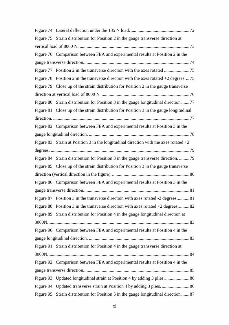
Figure 74. Lateral deflection under the 135 N load. ................................................... 72
Figure 75. Strain distribution for Position 2 in the gauge transverse direction at
vertical load of 8000 N. ............................................................................................... 73
Figure 76. Comparison between FEA and experimental results at Position 2 in the
gauge transverse direction. ........................................................................................... 74
Figure 77. Position 2 in the transverse direction with the axes rotated ...................... 75
Figure 78. Position 2 in the transverse direction with the axes rotated +2 degrees. ... 75
Figure 79. Close up of the strain distribution for Position 2 in the gauge transverse
direction at vertical load of 8000 N ............................................................................. 76
Figure 80. Strain distribution for Position 3 in the gauge longitudinal direction. ...... 77
Figure 81. Close up of the strain distribution for Position 3 in the gauge longitudinal
direction. ...................................................................................................................... 77
Figure 82. Comparison between FEA and experimental results at Position 3 in the
gauge longitudinal direction. ....................................................................................... 78
Figure 83. Strain at Position 3 in the longitudinal direction with the axes rotated +2
degrees. ........................................................................................................................ 79
Figure 84. Strain distribution for Position 3 in the gauge transverse direction. ......... 79
Figure 85. Close up of the strain distribution for Position 3 in the gauge transverse
direction (vertical direction in the figure). ................................................................... 80
Figure 86. Comparison between FEA and experimental results at Position 3 in the
gauge transverse direction. ........................................................................................... 81
Figure 87. Position 3 in the transverse direction with axes rotated -2 degrees. .......... 81
Figure 88. Position 3 in the transverse direction with axes rotated +2 degrees. ......... 82
Figure 89. Strain distribution for Position 4 in the gauge longitudinal direction at
8000N. .......................................................................................................................... 83
Figure 90. Comparison between FEA and experimental results at Position 4 in the
gauge longitudinal direction. ....................................................................................... 83
Figure 91. Strain distribution for Position 4 in the gauge transverse direction at
8000N. .......................................................................................................................... 84
Figure 92. Comparison between FEA and experimental results at Position 4 in the
gauge transverse direction. ........................................................................................... 85
Figure 93. Updated longitudinal strain at Position 4 by adding 3 plies. ..................... 86
Figure 94. Updated transverse strain at Position 4 by adding 3 plies. ........................ 86
Figure 95. Strain distribution for Position 5 in the gauge longitudinal direction. ...... 87

xii
Figure 96. Comparison between FEA and experimental results at Position 5 in the
gauge longitudinal direction. ....................................................................................... 88
Figure 97. Strain distribution for Position 5 in the gauge transverse direction. ......... 88
Figure 98. Comparison between FEA and experimental results at Position 5 in the
gauge transverse direction. ........................................................................................... 89
Figure 99. Strain distribution for Position 6 in the gauge longitudinal direction. ...... 90
Figure 100. Comparison between FEA and experimental results at Position 6 in the
gauge longitudinal direction. ....................................................................................... 91
Figure 101. Longitudinal strain at Position 6 after adding three ±45° plies. .............. 92
Figure 102. Strain distribution near Position 6 in the gauge transverse direction. ..... 92
Figure 103. Comparison between FEA and experimental results at Position 6 in the
gauge transverse direction. ........................................................................................... 93
Figure 104. Strain distribution for Position 6 in the gauge transverse direction with
the addition of 3 ±45° plies. ......................................................................................... 94
Figure 105. Rig setup for testing the carbon fibre plate. .......................................... 106
Figure 106. Axial strain gauge applied near the fixed end of the plate. ................... 107
Figure 107. Constraints applied to the carbon fibre plate created in Ansys Composite.
.................................................................................................................................... 108
Figure 108. Graphical FEA results for the cantilever plate. ..................................... 108
Figure 109. Longitudinal strain of 499 µε obtained from Ansys Composite. .......... 109
Figure 110. Top part of the load cell calibration rig showing the load cell attached to
the portable crane via a steel chain. ........................................................................... 110
Figure 111. Basket carrying weights applying a load to the load cell. ..................... 111
Figure 112. Calibration curve for the 50kN load cell. .............................................. 112
Figure 113. Schematic of plies overlapping each other. ........................................... 113
Figure 114. Adjacent plies without ply overlap. ....................................................... 113
Figure 115. Strain Gauge 1 ....................................................................................... 114
Figure 116. Strain Gauge 1. ...................................................................................... 114
Figure 117. Strain Gauge 2. ...................................................................................... 115
Figure 118. Strain Gauge 2. ...................................................................................... 115
Figure 119. Strain Gauge 3. ...................................................................................... 116
Figure 120. Strain Gauge 3. ...................................................................................... 116
Figure 121. Strain Gauge 4. ...................................................................................... 117

xiii
Figure 122. Strain Gauge 4. ...................................................................................... 118
Figure 123. Strain Gauge 5. ...................................................................................... 119
Figure 124. Strain Gauge 5. ...................................................................................... 119
Figure 125. Strain Gauge 6. ...................................................................................... 120
Figure 126. Strain Gauge 6. ...................................................................................... 120
Figure 127. Strain Gauges 7 & 8. ............................................................................. 121
Figure 128. Strain Gauge 7. ...................................................................................... 121
Figure 129. Strain Gauge 8. ...................................................................................... 122
Figure 130. NI data acquisition system connected to the strain gauges on the
swingarm. ................................................................................................................... 123
Figure 131. Isometric view of the top part of the steel shaft. ................................... 125
Figure 132. Top part of the steel shaft. ..................................................................... 126
Figure 133. Bottom part of steel shaft. ..................................................................... 127
Figure 134. Position 4 with element size of 5 mm. .................................................. 128
Figure 135. Position 4 with element size of 3 mm. .................................................. 128
Figure 136. Position 4 with element size of 1 mm. .................................................. 129

xiv
LIST OF TABLES
Table 1. Equipment and instrumentation used in the test rig. ..................................... 22
Table 2. Forces and moments applied during torsional test. ....................................... 30
Table 3. Loads applied during lateral test. .................................................................. 33
Table 4. Material properties of the carbon fibre plies used in the FE model. ............. 35
Table 5. Comparison of torsional stiffness values obtained from the literature. ........ 51
Table 6. Comparison lateral stiffness values. ............................................................. 55
Table 7. Measured strain in the longitudinal and transverse directions at maximum
load of 8000 N at Positions 3-6. ................................................................................... 57
Table 8. Strain correction at Positions 3-6 using Kt = +5% (0.05). ............................ 57
Table 9. Strain correction at Positions 3-6 using Kt = -5% (-0.05). ............................ 57
Table 10. Comparison between experimental and FEA vertical deflection at the wheel
mount. .......................................................................................................................... 70
Table 11. Comparison between experimental and FEA rotation at the wheel mount. 71
Table 12. Comparison between experimental and FEA lateral deflections at the wheel
mount. .......................................................................................................................... 72
Table 13. Effect of change in thickness of plies at Position 4. ................................... 94
Table 14. Comparison of experimental and FE strain results. .................................... 99
Table 15. Load applied to cantilever plate and the resultant axial strain from
experimental setup. .................................................................................................... 107
Table 16. Comparison between the measured strain and the strain calculated by
ANSYS. ..................................................................................................................... 109
Table 17. Calibration values for the 50kN load cell. ................................................ 111
Table 18. Mesh sensitivity. ....................................................................................... 129

xv
LIST OF SYMBOLS
d Length of moment arm [m]
F Applied force [N]
I Second moment of area [m4]
Kt Transverse sensitivity factor
kt Torsional stiffness coefficient [Nm/deg] or [Nm/rad]
ksp Stiffness coefficient of spring [kN/m]
ksw Vertical stiffness of swingarm [kN/m]
M Moment [Nm]
r Radius [m]
s Deflection [m]
s1 Deflection at top of arm [m]
s2 Deflection at wheel mount [m]
y Distance from the neutral axis [m]
εx Actual strain in the gauge 0° direction [µε]
εy Actual strain in the gauge 90° direction [µε]
εmx Measured strain in the gauge 0° direction [µε]
εmy Measured strain in the gauge 90° direction [µε]
θ Angle of rotation [rad]
υ0 Poisson’s ratio for steel
σ Stress [Pa]

xvi
LIST OF ACRONYMS
APDL ANSYS Parametric Design Language
CAE Computer Aided Engineering
CFRP Carbon Fibre Reinforced Plastic
CLT Classical Laminate Theory
FE Finite Element
FEA Finite Element Analysis
FEM Finite Element Model
FRP Fibre Reinforced Plastic
GFRP Glass Fibre Reinforced Plastic
MBS Multi-Body Simulation
RVE Representative Volume Element
SPATE Stress Pattern Analysis by Thermal Emission

1
1. INTRODUCTION
1.1 Background
Carbon fibre has not been extensively used in the development of motorcycle
swingarms. This study investigates the development of a carbon fibre swingarm with
an emphasis on the structural integrity and on developing a finite element model
(FEM). The motorcycle swingarm plays an important role in the rear part of the
motorcycle. The literature shows that strength, stiffness and weight are important
factors in motorcycle swingarm design. The swingarm should be strong enough to
handle typical loads experienced in the field and stiff enough to increase the response
and stability of the motorcycle. The weight of the swingarm should also be reduced
to improve motorcycle performance and increase the road holding of the rear wheel.
Most motorcycles use materials such as steel, aluminium and magnesium in their
swingarm design. Carbon fibre however, offers benefits such as low weight while
maintaining high stiffness and strength characteristics [1] and being able to tailor the
material characteristics for specific applications [2]. The current research presents the
initial phase in the design and manufacture of a carbon fibre swingarm for a Ducati
1098 motorcycle using preliminary laminates. Essentially, a swingarm was
manufactured using an initial design of the carbon fibre laminates and this study
proceeded to investigate the swingarm from a structural integrity point of view. The
literature further shows that the development of a finite element (FE) model is
important in the continued improvement of the swingarm design. To these two ends,
a test rig was developed for measuring deflection (to determine stiffness) and strain
(to determine strength) of swingarms and the results were used in developing an FE
model. The results provided insight into further possible areas of improvement in the
design of a carbon fibre swingarm. As indicated above, this research report does not
present information regarding the design of the carbon fibre laminates but presents the
testing of the swingarm (to determine the stiffness and strain characteristics) and the
development of a FE model. Once the stiffness characteristics were obtained, it was
then possible to see which areas of design (including the laminate) might need
improvement.

2
1.2 The Motorcycle Swingarm
The motorcycle structure is made up of three main components, namely the front fork,
the main frame and the swingarm [3] (Figure 1).
Figure 1. Example showing the main components of a motorcycle. [4]
The swingarm is the main component of the rear suspension of a motorcycle and
functions to connect the rear wheel to the chassis and to regulate the rear wheel-road
interaction via the spring and shock absorber [5]. Figure 2 presents an example of a
rear part of a motorcycle and its swingarm.
Front fork
Main frame Swingarm

3
Figure 2. Example of the rear part of a motorcycle showing the swingarm. [4]
There are two basic swingarm designs, namely the double-sided, shown in Figure 3
and the single-sided, shown in Figure 4.
Figure 3. A double-sided swingarm [6].
Attached to
shock absorber
Attached to main
frame
Attached to axle
Swingarm
Connects to frame
via bearings
Connects to rear wheel axle
Connects to spring and shock
absorber

4
Figure 4. A single-sided swingarm [7].
A benefit of the single-sided swingarm is that it allows for easier removal of the rear
wheel during racing [2]. A twisting moment acts in the single-sided swingarm which
does not exist in conventional double-sided designs [2], and to maintain torsional
rigidity similar to that of a double-sided swingarm, extra material may need to be
added which increases the unsprung mass. This may be a disadvantage because in
general a higher unsprung mass decreases the roadholding of the rear wheel. This
presents the need to reduce the weight of the swingarm.
The swingarm lateral and torsional stiffness is shown to be important in swingarm
design [3] [8] because they affect the side to side movement (weave mode) of the
motorcycle. In general, it is desirable to maximise the swingarm stiffness to reduce
the weave mode instability [9]. The vertical stiffness also plays an important role in
the motorcycle setup. The swingarm and the rear suspension spring form two springs
in series between the main chassis and the wheel. If not stiff enough vertically, the
swingarm can change the motorcycle setup and produce unpredictable behaviour.
Although each motorcycle will require different values for swingarm rigidity,
Cossalter [10] states that typical values for lateral swingarm stiffness are 800 kN/m –
1600 kN/m and 1 kNm/deg – 2 kNm/deg for torsional stiffness. No literature was
found documenting typical values for vertical stiffness.
Connects to rear wheel
axle
Connects to frame
via bearings
5
It should be noted that no standards were found that govern swingarm design. The
literature essentially shows that the swingarm should be strong enough to handle the
various loads, light enough to reduce the unsprung mass, and be designed to limit the
dynamic instability of the motorcycle. More detail will be presented in Section 2.2 on
swingarm development.
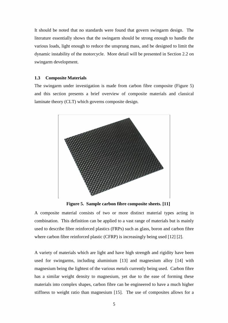
1.3 Composite Materials
The swingarm under investigation is made from carbon fibre composite (Figure 5)
and this section presents a brief overview of composite materials and classical
laminate theory (CLT) which governs composite design.
Figure 5. Sample carbon fibre composite sheets. [11]
A composite material consists of two or more distinct material types acting in
combination. This definition can be applied to a vast range of materials but is mainly
used to describe fibre reinforced plastics (FRPs) such as glass, boron and carbon fibre
where carbon fibre reinforced plastic (CFRP) is increasingly being used [12] [2].
A variety of materials which are light and have high strength and rigidity have been
used for swingarms, including aluminium [13] and magnesium alloy [14] with
magnesium being the lightest of the various metals currently being used. Carbon fibre
has a similar weight density to magnesium, yet due to the ease of forming these
materials into complex shapes, carbon fibre can be engineered to have a much higher
stiffness to weight ratio than magnesium [15]. The use of composites allows for a

6
range of benefits such as being able to modify the material characteristics and
structural stiffness [2], and having high strength and stiffness to weight ratios [1]. In
the automotive industry, composites have been used in chassis, car doors, drive shafts
and leaf springs.
Although the benefits of carbon fibre over metals are well documented, developments
in the application of carbon fibre reinforced plastic has not been as fast as expected
[12] and in motorcycle design there has not been widespread use [13]. Reasons
include high carbon fibre price, complex motorcycle shapes and general industrial
challenges which indicate the supporting carbon fibre industry is not yet mature
enough for mass production [13] [16].
A difficulty arises when designing a component using composite material since not
only must a design of the component be carried out, but due to the anisotropic nature
of composite material, the material itself must also be designed. Anisotropic
materials have properties that change according to direction due to their non-
homogeneous nature and differences in properties between fibres and the matrix [12].
Classical laminate theory (CLT) is used to predict the properties and behaviour of a
laminate which consists of laminae (plies) orientated in different directions (Figure 6).
Figure 6. Example of carbon fibre composite sketch showing different layers orientated in different directions. [17]
When applying this method, the following assumptions are made [12]:
• Each lamina is macroscopically homogeneous and linearly elastic
• The plies are perfectly bonded to each other when forming the laminate
• The laminate has infinite through thickness shear stiffness. The through
thickness direction is normal to the lamina surface.

7
• The plane sections remain plane when the laminate is bent or extended.
CLT provides a method of calculating strains and curvatures in the laminate if the
forces and moments acting on the laminate are known. Conversely, if the strains and
curvature are known, then the forces and moments can be calculated.
FEA is the most popular numerical technique for analysing composite structures
according to Wood [18] and the finite element package ANSYS (ANSYS® Academic
Research, Release 14.5, Composite PrepPost, ANSYS, Inc.) used in this study, bases
its composite software on CLT. Difficulties arise when trying to obtain material
properties and failure strengths for composite materials.
1.4 Project Overview
This study begins by reviewing literature to establish what research has been carried
out in the following areas:
• The development of test rigs (both experimental and virtual) for the testing of
automotive components.
• The design and testing of motorcycle swingarms.
• The application of finite element analysis (FEA) to composite materials.
Based on the literature review, a few points will be seen. The first is that a need exists
to develop automotive components from composite materials due to their lightweight
and high strength and stiffness properties. This was carried out using an initial
laminate design and this study investigates this design. A single-sided carbon fibre
swingarm shown in Figure 7 was developed for a Ducati 1098 motorcycle.

8
Figure 7. Single-sided carbon fibre swingarm for a Ducati 1098 motorcycle [19].
The second is the importance of determining the stiffness characteristics of swingarms
because of their effect on the stability of the motorcycle. For fatigue and static testing
of the swingarm, a durability test rig was developed (Figure 8).
Figure 8. Swingarm test rig developed to test the carbon fibre swingarm.
The vertical, lateral and torsional stiffness characteristics of the swingarm as well as
strains at various positions were determined from the experimental tests.

9
Lastly, there is the need to develop a finite element model of the swingarm which will
facilitate cost-effective design optimisations. This research report presents a study of
the stiffness characteristics and strain distribution of the swingarm as well as the
development of a finite element model of a carbon fibre swingarm.

10
2. LITERATURE REVIEW
2.1 Automotive Test Rig Development
A considerable amount of research has been carried out in the development of test rigs
for automotive component design. Product development is no longer confined to
experimental testing but now also includes testing in the virtual (computer simulated)
environment. Advantages of virtual testing include being able to evaluate the design
early in the development process before the prototype is available and also allows for
data to be obtained to help with setting up experimental testing [20]. Virtual models
are best at delivering an understanding of system behaviour, interactions and
sensitivity, whilst physical tests are good at identifying absolute levels of performance
and the response of complex systems [21].
Durability tests have been used extensively in automotive component design. Servo-
hydraulic rigs (used for durability testing) are one of the main experimental methods
used in automotive design [22]. Durability test rigs have been built to test the fatigue
life of motorcycle handlebars (Figure 9) [23], vehicle suspensions (Figure 10) [20]
and motorcycle frames [24] to name a few. During testing, results are generally
obtained by measuring strain on the component and then calculating the
corresponding stresses.
Figure 9. Durability test rig for motorcycle handlebars. [23]

11
Figure 10. Durability test rig for suspension system. [25]
The literature indicates that there is an increasing need to develop virtual tests that can
simulate the experiments. Multi-body simulation (MBS) has been used to simulate
suspension test rigs and thereby calculate accelerations, bending moments and forces
in motorcycle frames (Figure 11) [20]. Forces calculated in MBS may then be used in
the FEA of the component to calculate stresses and strains. In certain cases, FEA is
carried out to first obtain an indication of the stress and strain distribution which then
allows for more strategic strain measurements to be carried out during experimental
testing [22] [23].
Figure 11. Example of multi-body simulation using ADAMS® simulation software.

12
From this discussion on test rigs, it is clear that for the successful design and testing
of automotive components, there is the need to combine virtual (FEA) and
experimental methods.
2.2 Swingarm Development
A survey of the literature shows that there has been limited research into the design
and testing of motorcycle swingarms and even less into the development of composite
swingarms. Armentani, Fusco and Pirozzi [8] determined lateral and torsional
stiffness values of three double-sided aluminium swingarms by carrying out
experimental tests and FEA. They claimed that the main difficulty in designing the
swingarm is to obtain the right balance between the flexional and torsional stiffness,
although no indication is given of what the right balance is. They initially defined the
loads acting on the rear wheel during cornering. When viewed from the rear of the
motorcycle (Figure 12) along the longitudinal axis, the moment caused by the
centrifugal force (that tends to restore the motorcycle to the vertical position) is
balanced by the moment caused by the weight of the motorcycle and rider (that tends
to cause the motorcycle to fall over). Assuming that the wheels are thin, the resultant
of these two forces is balanced by a resultant reaction and friction force at the wheel-
road contact point that acts along the plane of the wheel.

13
Figure 12. Loads acting on the swingarm during cornering assuming thin wheels [8].
In reality however, due to the thickness of the tyres, the resultant force does not act in
the plane of the wheel but along the line connecting the centre of mass and the tyre
contact point (Figure 13). This actual resultant force (Rs) has components acting
parallel and perpendicular to the wheel plane. The perpendicular component will
generate both a lateral force and a moment about the longitudinal axis.
Figure 13. Loads acting on the swingarm during cornering assuming thick wheels [8].
Weight
Lateral force
Normal force
Centrifugal force Centre of mass
14
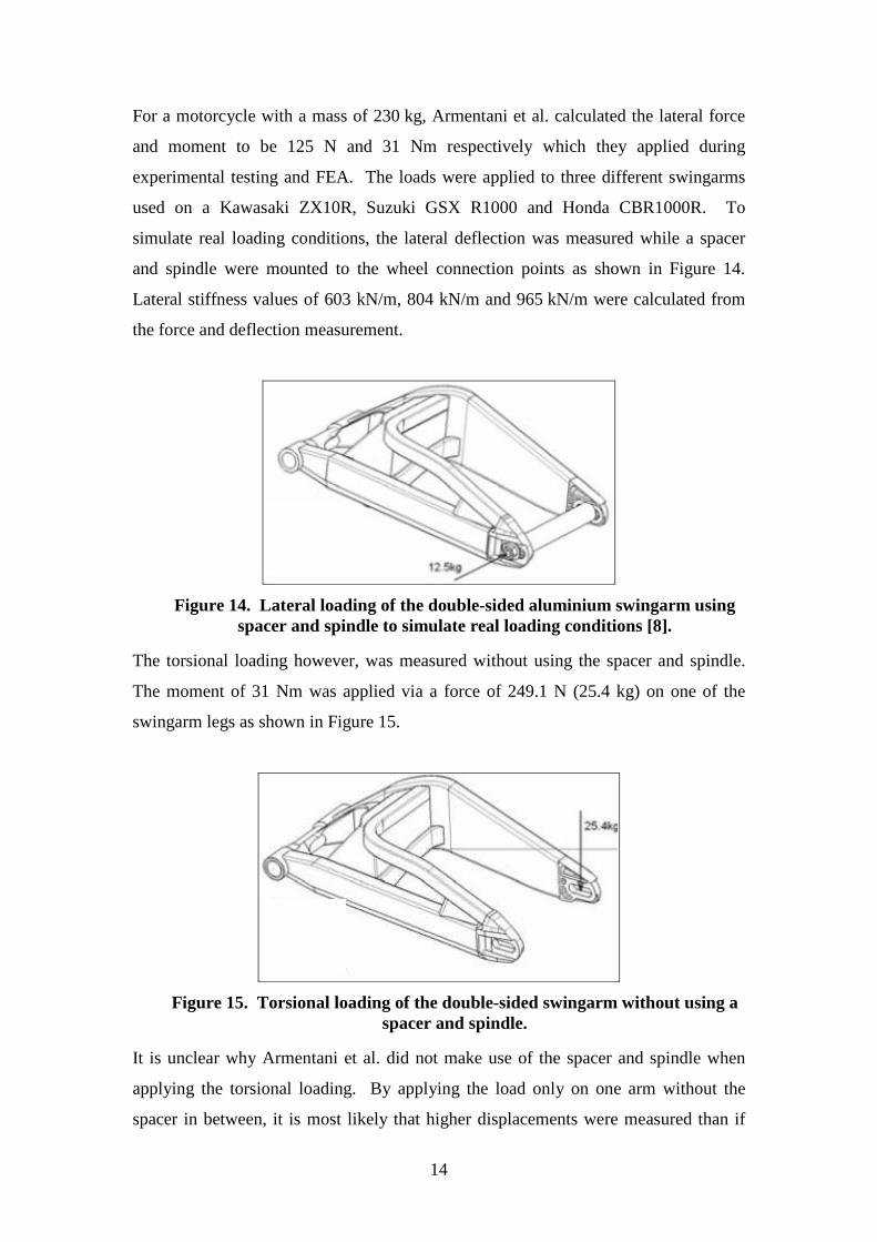
For a motorcycle with a mass of 230 kg, Armentani et al. calculated the lateral force
and moment to be 125 N and 31 Nm respectively which they applied during
experimental testing and FEA. The loads were applied to three different swingarms
used on a Kawasaki ZX10R, Suzuki GSX R1000 and Honda CBR1000R. To
simulate real loading conditions, the lateral deflection was measured while a spacer
and spindle were mounted to the wheel connection points as shown in Figure 14.
Lateral stiffness values of 603 kN/m, 804 kN/m and 965 kN/m were calculated from
the force and deflection measurement.
Figure 14. Lateral loading of the double-sided aluminium swingarm using spacer and spindle to simulate real loading conditions [8].
The torsional loading however, was measured without using the spacer and spindle.
The moment of 31 Nm was applied via a force of 249.1 N (25.4 kg) on one of the
swingarm legs as shown in Figure 15.
Figure 15. Torsional loading of the double-sided swingarm without using a spacer and spindle.
It is unclear why Armentani et al. did not make use of the spacer and spindle when
applying the torsional loading. By applying the load only on one arm without the
spacer in between, it is most likely that higher displacements were measured than if

15
the spacer and spindle were inserted to simulate real life conditions. By applying the
load without spacer and spindle, torsional stiffness values of 5896 Nm/rad
(102.9 Nm/deg), 8068 Nm/rad (140.8 Nm/deg) and 8068 Nm/rad (140.8 Nm/deg)
were calculated for the Kawasaki ZX10R, Suzuki GSX R1000 and Honda CBR1000R
swingarms respectively. The torsional stiffness values are therefore assumed to be
less stiff than what would be measured while simulating real life conditions. It will be
seen later that these torsional stiffness values are indeed much lower than other values
measured in the literature.
Dragoni and Foresti [26] aimed to improve a magnesium swingarm design by using
carbon-epoxy composite material. They claimed that the structural behaviour of
magnesium is satisfactory but sought to reduce the mass of the arm while maintaining
a similar stiffness. Before investigating the composite design, an FE model of the
original magnesium model was verified by simulating the torsional response and
comparing it with experimental values. They state that the torsional response is the
single most important feature of the swingarm from a structural point of view. The
finite element package ALGOR was used to build the FE model of the composite
design because it supports anisotropic plate elements suited for laminate structures.
Three models were built based on three designs. A pure-torsional load was applied to
each of them, and the laminate thickness was adjusted to obtain similar stiffness
values to the magnesium design. No detail is provided as to the magnitudes of the
loads. Normalised results show that the final composite design had an increased
torsional stiffness of 10%, a reduced mass of 30% and a reduced mass moment of
inertia of 40%.
Risitano, Scappaticci, Grimaldi and Mariani [5] aimed to link objective data such as
swingarm stiffness and natural frequencies with subjective information such as
handling and comfort perceived by riders. They claimed that to characterize the
swingarm, it is important to look at the torsional stiffness. The less stiff the swingarm
is, the heavier the motorcycle feels to the driver and the more difficult manoeuvring
becomes. The stiffer the swingarm, the quicker the response is during cornering.
Risitano et al. tested the torsional rigidity and symmetrical behaviour of three double-
sided aluminium swingarms. A rig was built that could apply a purely torsional load
to the swingarm and measure the twist angle about the longitudinal axis. This was

16
done in both clockwise and counterclockwise directions. No explanation was given
for how the magnitudes of the torsional loads (between 0 and 400 Nm) were derived,
and it is assumed that the loading was applied simply to obtain the stiffness
characterization. The loads were applied by hydraulic jacks and deflections were
measured via potentiometers. From the tests, torsional stiffness values of
670 Nm/deg, 890 Nm/deg and 1330 Nm/deg were found for the three swingarms
(Figure 16).
Figure 16. Torque-angle curves for three swingarms [5]
An FE model was built in ANSYS Workbench and similar tests were simulated. The
average difference between the FE and experimental results was under 4%.
Cossalter, Lot and Massaro [27] studied the effect the swingarm has on the weave
mode stability of a 150 cc scooter. The weave mode describes the side to side
oscillation of the motorcycle which is due to yaw and roll effects of the motorcycle.
Cossalter et al. showed that from 0 m/s to 18 m/s (65 km/h), the degree of torsional
and lateral rigidity has negligible effect on the weave mode stability. However, as the
torsional stiffness increases, the weave mode stability increases at speeds higher than
18 m/s. The weave mode stability also increases as the lateral stiffness increases, but
only up until 36 m/s (130 km/h). At speeds above 130 km/h an increase in lateral
stiffness shows a decrease in weave mode stability. Therefore at speeds greater than
670 Nm/deg
890 Nm/deg
1330 Nm/deg

17
130 km/h, the torsional and lateral stiffness affects the weave mode stability in a
contradictory manner.
Lake, Thomas and Williams [28] summarized work carried out by various researchers
on the effect that swingarm stiffness has on the motorcycle weave mode and found
conclusions that matched Cossalter et al. [27] above. Lake et al. state that it is
obvious that the increase in torsional stiffness increases the weave mode stability but
asked what are acceptable values of swingarm torsional stiffness? They showed that
Sharp [29] claimed that a torsional stiffness value of 209 Nm/deg would approach an
absolutely rigid swingarm. However recent designs have significantly higher
swingarm stiffness values. For example, Cossalter [10] stated that modern swingarms
have stiffness values of between 1000 Nm/deg and 2000 Nm/deg as discussed earlier.
Risitano et al. [5], also discussed above, determined values of 670 Nm/deg and higher.
The values calculated by Armentani et al [8] (discussed earlier) of between 102.9
Nm/deg and 140.8 Nm/deg, appear to be unusually low for swingarms and even lower
than what was suggested by Sharp [29] and the possible reasons for their low stiffness
values were discussed earlier. Lake et al. [28] conclude their study on torsional
stiffness by saying that the reported torsional stiffness on contemporary swingarm
designs is not consistent.
Iwasaki, Mizuta, Hasegawa and Yoshitake [14] developed a magnesium swingarm
due to the growing concern over improving fuel efficiency in motorcycles. Four finite
element models of the swingarm were built using MSc–Nastran. The first was a
conventional aluminium design and the other three designs were of magnesium. The
torsional rigidity of the designs was analysed using finite element models and a test
rig. The redesigned swingarms were 10% lighter and 60% more torsionally rigid.
Dragoni (discussed above) [26], Airoldi & Bertolie [2] and O’Dea [13] carried out
designs of swingarms using composite materials. The latter two investigated methods
of designing the swingarm by optimising the stacking sequence of the laminates in the
composite. Airoldi et al. carried out a redesign of a single-sided swingarm using
carbon fibre composite. The goal was to compare a composite swingarm design with
an existing aluminium design. They aimed to minimize the torsional, lateral and
vertical deflections as well as the mass by investigating the stacking sequences of the

18
plies. Genetic algorithms were used to identify a lamination sequence that gave the
desired stiffness properties. FEA was only carried out on the original aluminium
design and not on the composite arm which was designed using an optimisation
algorithm (implemented in Matlab). O’Dea redesigned and manufactured a double-
sided swingarm from a Honda CRF450 using carbon fibre epoxy composite moulded
in metal inserts. The method of design was carried out using the Composite Modeler
ply modelling and fibre simulation software developed by Simulayt Ltd [30].
Composite Modeler allows the user to specify the design of the plies and then
simulate the manufacturing process to highlight any possible manufacturing problems.
2.3 Leyni Durability Test
Thus far the literature has focussed on determining lateral and torsional stiffness of
swingarms. The only literature found that looked at vertical loading of swingarms
was the Leyni Durability Test used by Gaiani [31] that carried out fatigue tests on an
aluminium single-sided swingarm in the vertical direction. The Leyni Test rig
consists of a drum with a 300 mm high step on it and turns with a speed of 20 km/h
and rotational frequency of 3.7 Hz. The rear wheel of a motorcycle is mounted on the
drum and as the drum rotates it applies an impulse load to the wheel every time the
step passes. During the cyclic loading, the initial static load due to the driver and
passenger was 1960 N and a maximum applied loading of 5900 N occurred when the
step impacted the wheel. Therefore although the current research is based on static
loading, the magnitude of the vertical loads applied in the Leyni Test were taken into
account.
2.4 Experimental Strain Measurements on Composites
Due to the swingarm being made from carbon fibre it was necessary to study literature
discussing measuring strain on orthotropic1 materials. Tuttle and Brinson [32] studied
strain gauge transverse-sensitivity effects and errors due to gauge misalignment when
measuring strain on orthotropic materials. The transverse-sensitivity refers to a strain
gauge responding to a strain field that is perpendicular to the gauge’s major axis. This
response is undesirable because the reading obtained is not the actual strain in that
direction but a combination of axial and transverse strain. The effect of transverse
1 A material whose properties differ in the x-,y- and z-directions.

19
sensitivity should always be considered when strain is being measured in a biaxial
stress field and if the error due to this phenomenon is significant, then correction
should be made. A full discussion on correcting for transverse sensitivity can be seen
in [33] but the basic equations for correcting transverse sensitivity are presented in
Equations 2-1 and 2-2 which can be used when a rosette strain gauge is applied to
measure strain.
= 1 − − (2-1)
= 1 − − (2-2)
Where εmx, εmy = Strains measured along the x and y axes,
Kt = Transverse sensitivity factor calculated by dividing the
transverse gauge factor by the axial gauge factor, normally
between -0.05 and +0.05,
εx, εy = Corrected or true strains in the x- and y-directions, and
υ = Poisson’s ratio of the material on which the manufacturer’s
gauge factor was measured, normally 0.285.
Concerning gauge misalignment, due to the orthotropic nature of carbon fibre
composites, the principal strain direction does not always coincide with the principal
stress directions. Therefore if a gauge is intended to measure strain along a specific
direction and there is slight misalignment, errors may occur which are larger than that
for an isotropic2 material. The error is dependent on the following:
• misalignment of the gauge with the intended direction of measurement, and
• angle between the fibre direction and the measurement direction.
Tuttle and Brinson [32] looked at the effect of gauge misalignment at plus and minus
2 and 4 degrees with reference to the intended axis of measurement on a
unidirectional graphite epoxy composite. It was found that the largest errors occurred
when the angle between the gauge direction and the fibre direction was 8°. Errors of
15% and 30% occurred for the 2° and 4° misalignment. Therefore when comparing
2 A material whose properties are the same in all directions.

20
the FE results with the experimental values in Section 5.3.2, the effect of gauge
alignment is discussed.
2.5 Finite Element Analysis on Composites
As presented in Section 2.2, only a few papers were found that directly investigated
composite swingarms. It was necessary therefore to briefly look at literature
focussing on the use of FEA for general composite applications.
Ali [34] studied the performance of FE techniques by analyzing structures where the
theoretical solutions were available. These structures included an axially loaded plate
and a simply supported plate and beam. A fundamental difficulty with FE systems is
their inability to accurately define the orientation of composite materials which are
anisotropic. Stresses are discontinuous at the interface of two plies. The stress-strain
relationship for a laminate can be synthesized from the properties of all the plies
making up the laminate. The entire stack of plies can therefore be modelled with a
single shell finite element because the material properties of the laminate are
completely reflected in the elastic moduli matrices for the element. These matrices
can be calculated if the thickness, material properties and relative orientation is known
for each ply in the laminate.
Yinhuan and Zhigao [35] analysed the mechanical characteristics of a glass fibre leaf
spring using ANSYS software. Glass fibre reinforced plastics (GFRP) are orthotropic
materials and the SOLID 46 laminated element was used in the finite element model.
This element allows for up to 250 layers where the material properties, thicknesses
and orientations can be specified for each layer.
Mian, Wang and Dar Zhang [36] investigated the proper fibre orientation and
laminate thickness for three composites, namely S-glass/epoxy, Kevlar/epoxy and
Carbon/epoxy used in pressure vessel design. The ANSYS Parametric Design
Language (APDL) and Design Optimization module was used in the analysis and the
numerical results were verified using Matlab code based on classical lamination
theory and Tsai-Wu failure criteria. Tsai-Wu failure criteria were used to predict first
ply failure of a composite laminate.

21
3. OBJECTIVES
This study took the initial step in the design of a carbon fibre swingarm. The
following objectives were set:
1. Determine the vertical, lateral and torsional stiffness and strain characteristics
of a prototype swingarm through experimental testing.
2. Develop an FE model of prototype carbon fibre swingarm which would be
validated using the strains and displacements measured during experimental
testing. The loads used during experimental testing were applied to the FE
model during validation.

22
4. METHODOLOGY
A carbon fibre swingarm was developed using an initial laminate design. To
determine which areas on the swingarm are inadequate from a design point of view, it
was necessary to determine stiffness and strain characteristics from deflection and
strain measurements and also to develop a FE model. This section describes the
following:
1. The setup of the test rigs
2. The experimental tests
3. The development of the FE model
4. The FE simulations carried out on the swingarm
4.1 Experimental Equipment and Instrumentation
This section presents the equipment and instrumentation used in the vertical, lateral
and torsional tests. The torsional and lateral tests have slight variations which are
discussed in Sections 4.3 and 4.4. Table 1 presents the equipment and
instrumentation used during testing and the figures that they appear in. The design
and manufacture of the test rig was presented by Chacko [37].
Table 1. Equipment and instrumentation used in the test rig.
Component Figures
Hydraulic jack for applying loads 17
Three brackets for rigidly mounting the swingarm 17 & 18
Two plummer block bearings 18
Chain for transmitting the load between the hydraulic jack and the load
cell and swingarm
17
Load cell (50 kN) that provided the load readings. For the load cell
calibration, see Appendix B.
17
Rosette strain gauges (120 Ω) for measuring strain in the 0°, 45°, and 90°
directions
20 and 115
to 129
NI data acquisition hardware 130
LabView software for reading and recording strain measurements -
Computer -
Dial gauges for measuring deflection 17

23
Figure 17. Test rig showing various components.
Figure 18. Test rig showing various components.
Hydraulic jack
Load cell
Dial gauge
Swingarm
Plummer blocks
Chain
Bracket
Brackets
y
z
x
Bracket
Strain gauges
Rocker arm

24
Figure 19. Connection from swingarm to rocker-arm.
The positioning of strain gauges is often based on the strain distribution obtained from
FEA. In general, gauges are placed in areas showing a uniform and high strain field.
In this case, due to the complexity of building an FE model of the swingarm, this
approach was not taken. This was because it was not known if the FE model would
present accurate enough results on which to base the positioning of the strain gauges.
Therefore the gauge positioning was based on the following:
• Comparing the strain at the aluminium inserts with the strain in the middle of
the swingarm.
• Looking at the type (tensile or compressive) and magnitude of the strain at the
lower and upper arms of the swingarm.
• Assuming that the highest strains would generally occur on the top arm which
is potentially the furthest distance from the neutral axis.
Rocker arm
assembly
25
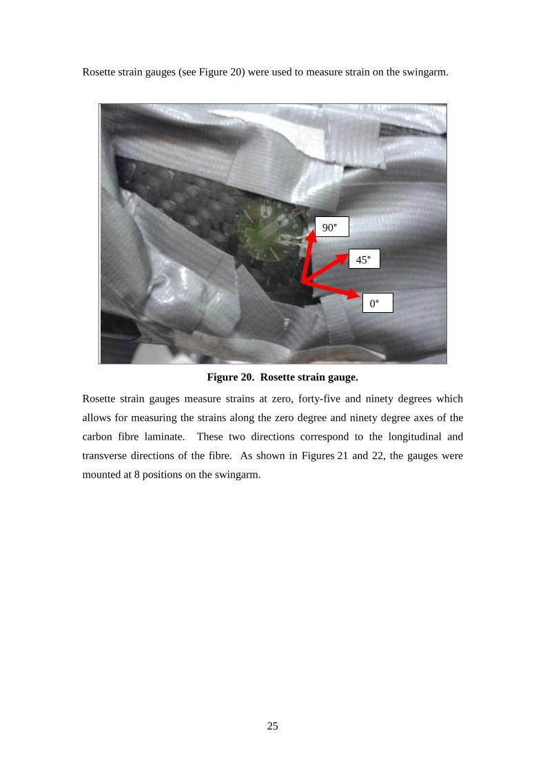
Rosette strain gauges (see Figure 20) were used to measure strain on the swingarm.
Figure 20. Rosette strain gauge.
Rosette strain gauges measure strains at zero, forty-five and ninety degrees which
allows for measuring the strains along the zero degree and ninety degree axes of the
carbon fibre laminate. These two directions correspond to the longitudinal and
transverse directions of the fibre. As shown in Figures 21 and 22, the gauges were
mounted at 8 positions on the swingarm.
0°
45°
90°

26
Figure 21. Strain gauge measurement positions.
Figure 22. Strain gauge measurement positions.
Each strain gauge had its own local coordinate system. The zero degree (longitudinal)
direction for each gauge was lined up with the global x-axis which corresponds to the
longitudinal axis of the swingarm (Figure 22). The ninety degree (transverse)
direction was aligned perpendicular to the longitudinal gauge direction and parallel to
the surface on which the gauge was placed. The positioning of the strain gauges can
be seen in more detail in Appendix D.
1
2
3
6
7
8
4
5
Global x-axis

27
4.2 Experimental Rig Setup and Loading – Vertical Testing
This section describes the set-up of the test rig that applied loading to the swingarm in
the swingarm vertical plane. The test rig is shown in Figure 23. Although it shows
the loads being applied to the swingarm in the horizontal plane via the hydraulic jack,
it actually simulates the vertical swingarm loads because the swingarm is rotated
through 90° on the test rig.
Figure 23. Swingarm test rig to apply vertical load.
More detail with respect to the manner in which the swingarm was attached to the rig
is discussed under Section 4.5.5 when describing the constraints for the FE model. In
the vertical test, loads of between 0 N and 8000 N were applied in increments of
1000 N. The aim was to include the range of loads in the Leyni Test and also to apply
a wider range of vertical loads on the swingarm to determine the stiffness
characteristics.
4.3 Experimental Rig Setup and Loading – Torsional Testing
This section describes the setup of the rig during torsional loading of the swingarm
(see Figure 24). The aim of this test was to apply a torsional load to the swingarm in
order to calculate the torsional stiffness and to measure strain. The equipment,
instrumentation and positions of the strain gauges are the same as that used during the
Swingarm Hydraulic jack
Direction of load

28
vertical loading. The difference here is that a vertical steel shaft3 was attached to the
wheel mount and the hydraulic jack was elevated in order to apply the loads at a
distance from the longitudinal axis. This resulted in a moment about the longitudinal
axis of the swingarm. From the reader’s perspective, the longitudinal axis goes into
the page.
Figure 24. Rig setup to apply a torsional load on swingarm.
The torsional loading was based on the work carried out by Risitano et al. [5] and the
aim of these tests was to determine the torsional stiffness of the swingarm by applying
a moment and calculating the angle of rotation. Risitano et al. applied loads of
between 0 and 400 Nm and measured the deflection angle for each load application.
The loads applied during the current test included this range but went up to 680 Nm.
Figure 25 shows that due to a single force being applied at a perpendicular distance
from the longitudinal axis, a force and couple moment act at the wheel mount [38].
3 For more detail on the design of the vertical steel shaft, see Appendix E.
Vertical steel
shaft
Raised hydraulic jack
Wheel mount
Load

29
Figure 25. Test rig showing the steel arm used in the torsional test.
The length of the moment arm was 340 mm and the range of forces was between 0 N
and 2000 N in increments of 100 N. Equation 4-1 presents a sample equation
showing how the moment was calculated using a force of 100 N.
Applied
force
Resultant moment
340mm
Resultant force
Dial gauge 2
Dial gauge 1

30
=
= 100 × 0.34
= 34 Nm
(4-1)
Where: M = Moment [Nm],
F = Load applied on the vertical steel arm [N], and
d = Length of moment arm [m].
Therefore based on the methodology above, Table 2 presents the range of forces and
moments that were applied.
Table 2. Forces and moments applied during torsional test.
Force [N] Moment [Nm] Force [N] Moment [Nm]
100 34 1100 374
200 68 1200 408
300 102 1300 442
400 136 1400 476
500 170 1500 510
600 204 1600 544
700 238 1700 578
800 272 1800 612
900 306 1900 646
1000 340 2000 680
As discussed earlier, due to the applied force not being a couple4, a resultant force
occurs at the wheel mount. Therefore a deflection not only occurs at the top of the
arm but also at the wheel mount. When measuring the angle of rotation, the
deflection at the top of the steel arm and the deflection at the wheel mount were both
taken into account (hence the need for two dial-gauges shown in Figure 25). To
present the method of calculating the angle of rotation, a schematic is presented in
Figure 26. During loading, both the top of the steel arm and the wheel mount deflect
4 A couple is defined as two parallel forces that have the same magnitude but opposite directions and
are separated by a perpendicular distance [34].

31
to the left. In order to obtain the net deflection at the top of the arm, the deflection s1
at the wheel mount, was subtracted from the deflection s2 at the top of the arm. The
two dial-gauges were used to measure deflection at the bottom and at the top.
Figure 26. Schematic of deflection of steel arm during torsional loading.
The resultant deflection was divided by the radius 0.34 m as shown in Equation 4-2 to
calculate the angle of rotation.
=
−
(4-2)
Where: θ = Angle of rotation [rad],
s1 = Deflection measured at wheel mount [m],
s2 = Deflection measured at top of steel arm [m], and
r = Radius [m].
The torsional stiffness was then calculated using Equation 4-3
=
(4-3)
Where: kt = Torsional stiffness [Nm/rad],
M = Moment [Nm], and
θ = Angle of rotation according to Equation 4-2 [rad].
θ
s
Top of steel arm
Wheel mount
s2
s1
r =0.34 m

32
The units of the the torsional stiffness were converted to Nm/deg by multiplying by
π [rad]/180 [deg].
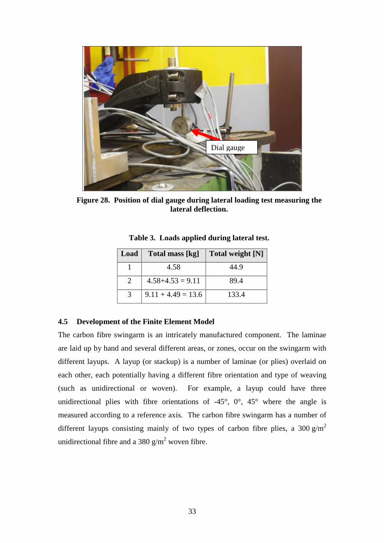
4.4 Experimental Rig Setup and Loading – Lateral Testing
Due to the swingarm being rotated 90° about the longitudinal axis, in order to
simulate a lateral load, a vertical load was applied at the wheel mount. As shown in
Figure 27, the hydraulic jack was disconnected and weights were simply placed on the
wheel mount which would apply a load vertically downwards.
Figure 27. Rig setup for applying lateral loads in the global z-direction.
The range of loads was based on work carried out by Armentani et al. [8] who
calculated a maximum lateral load of 125 N. In the current test, a load of up to
133.4 N was applied. Three mass pieces of 4.58 kg, 4.53 kg and 4.49 kg were used to
apply increasing loads as shown in Table 3. The deflection was measured at each
load increment using a dial gauge positioned at the bottom of the wheel mount as
shown in Figure 28.
Load
33
Figure 28. Position of dial gauge during lateral loading test measuring the lateral deflection.
Table 3. Loads applied during lateral test.
Load Total mass [kg] Total weight [N]
1 4.58 44.9
2 4.58+4.53 = 9.11 89.4
3 9.11 + 4.49 = 13.6 133.4
4.5 Development of the Finite Element Model
The carbon fibre swingarm is an intricately manufactured component. The laminae
are laid up by hand and several different areas, or zones, occur on the swingarm with
different layups. A layup (or stackup) is a number of laminae (or plies) overlaid on
each other, each potentially having a different fibre orientation and type of weaving
(such as unidirectional or woven). For example, a layup could have three
unidirectional plies with fibre orientations of -45°, 0°, 45° where the angle is
measured according to a reference axis. The carbon fibre swingarm has a number of
different layups consisting mainly of two types of carbon fibre plies, a 300 g/m2
unidirectional fibre and a 380 g/m2 woven fibre.
Dial gauge

34
4.5.1 Software
ANSYS Composite PrepPost together with ANSYS Static Structural was used in the
FEA (Figure 29). ACP (Pre) was used for pre-processing (creating the composite
layups) and ANSYS Static Structural was used to apply the mesh and boundary
conditions, to solve the simulations, and also to view the deflection and strain results.
Figure 29. ANSYS Workbench Project Schematic showing the three parts of the simulation.
4.5.2 Assumptions
To develop the finite element model, it was necessary to first determine the various
zones on the swingarm and the type of layup that made up each zone. Once that
information was obtained, various initial assumptions were made:
• Only the most significant zones with their layups were modelled. Due to the
complex shape of the swingarm and the large number of zones, to simplify the
modelling, the smaller zones (which had slight differences in layup to the
larger more significant zones) were modelled with the same layup as the larger
zones.
• Lamina overlap was not modelled due to its complexity. Plies were modelled
essentially assuming butt joints. For more discussion on ply overlap, see
Appendix C.
• The aluminium inserts (shown in Figure 30) were not modelled. The aim of
the simulation was to get an overall impression of the effects of the loadings
and the aim of leaving out the inserts was to simplify the FE model.

35
Figure 30. Swingarm showing the aluminium inserts.
Furthermore, the supplier supplied limited information on the material properties and
therefore standard properties for both the unidirectional and woven plies were
assumed which are presented in Table 4. The approximate thickness of each ply is
also given.
Table 4. Material properties of the carbon fibre plies used in the FE model.
Material E1
[GPa]
E2
[GPa]
G12
[GPa]
υ Thickness
[mm]
Unidirectional (300 g/m2) 135 10 5 0.3 0.3
Woven (380 g/m2) 70 70 10 0.1 0.38
Aluminium inserts

36
4.5.3 Model Preparation and Mesh Generation
ANSYS DesignModeler was used for modifying and preparing the swingarm solid
model for FEA in ANSYS. First the solid model was transformed into a surface
model to allow for later modelling of shell elements. Further preparation included
repairing holes, sharp angles and edges which allowed for a better FE mesh to be
created. The model was also sectioned for modelling the various layups and applying
the various loads using the Named Selection function in ANSYS. After model
preparation, the mesh was generated as shown in Figure 31. The mesh consisted of
triangular and quadrilateral shell elements with 51,694 nodes and 52,295 elements.
Figure 31. Finite element mesh on the swingarm
The element type used in the mesh was a SHELL181 which is a 4-node structural
shell suitable for analyzing thin to moderately thick shell structures. It has six degrees
of freedom at each node: translation in the x-, y- and z-directions, and rotations about
the x-, y- and z-axes. The element is used for layered applications for modelling
composite shells.
4.5.4 Creation of the Layups
The various zones made it possible to create the carbon fibre layups in ANSYS ACP
(Pre). Before creating the layups, the types of material used in the layups, namely the
380 g/m2 woven fibre and 300 g/m2 unidirectional fibre, were defined with their
material properties. Thereafter a specific layup for each zone was created based on
the number of plies used, the type of plies and each ply’s orientation. The main zones

37
covering the top and bottom arms5 of the swingarm are presented in Figures 32
through 39. As discussed earlier, the smaller zones with their layups were included in
these larger more significant zones with their layups shown in these figures.
Figure 32. Outer zone of the top arm.
Figure 33. Top zone of the top arm.
5 Not all the zones are shown here. The aim is to give the reader an indication of the method of zoning
to create layups in those areas.

38
Figure 34. Inside zone of the top arm.
Figure 35. Zone underneath the top arm.

39
Figure 36. Zone on outside of bottom arm.
Figure 37. Top zone of the bottom arm.

40
Figure 38. Inside zone of the bottom arm.
Figure 39. Underside zone of the bottom arm.
4.5.5 FE Model Boundary Conditions
Figure 40 shows a solid model of the test rig assembly with the aim being to present
the constraints on the swingarm and how they were applied in the FE model. The rig

41
was built to simulate how the swingarm is mounted to the motorcycle. Point A shows
the wheel mount position where the vertical, lateral or torsional loads were applied
Figure 40. Positions of loading and constraints on the swingarm.
Points D and E represent where the swingarm is mounted to the main motorcycle
chassis via bushes. These constraints were modelled in the FE model as cylindrical
supports which only allow rotation about the pivot axis and no translation in any
direction. The pivot axis here is essentially from Point D to E which is the axis about
which the swingarm pivots. Points B and C indicate where the swingarm was
connected to the rocker arm assembly via revolute joints. Figures 41 and 42 show
close-ups of the rocker arm assembly which consists of two rigid aluminium links
connected to an aluminium cross member.
A
B
C
D
E
Rocker arm
assembly

42
Figure 41. Rocker arm assembly.
Figure 42. Rocker arm assembly.
It is important to note that the centre of the cross member also acts as a pivot point
where only rotation about the axis coming out of the page is free. Every other rotation
and translation is fixed.
The rocker arm was modelled using line bodies and each line body was designated a
certain length, material and cross section to simulate the aluminium links in the rocker
Rigid links
Cross member
Rigid links Revolute joint
Revolute joint
Revolute joint
Cross member

43
arm assembly. Figure 43 shows the FE model with the line bodies representing the
rocker arm assembly. The parallel rocker arm links were attached to the main
swingarm using revolute joints which allow the links to rotate about an axis parallel to
the swingarm pivot axis. The parallel arms were attached to the cross member also
with revolute joints allowing rotation about the pivot axis. The cross member was
then attached to ground also via a revolute joint at its centre. The revolute joint
allows for rotation about the axis parallel to the pivot axis and is constrained in every
other translational and rotational direction. The figure presents the revolute joints as
red dots and the centre of the cross member is attached to ground.
Figure 43. Finite element model of swingarm showing the rocker arm. The red dots indicate the positions of the revolute joints.
4.6 Finite Element Analysis –Vertical Testing
During the vertical loading simulations, due to being linear, the FE model was
subjected to the maximum load of 8000 N in the vertical plane as shown in Figure 44
and deflection and strains were determined. The results were compared with the
deflection and strain measurements obtained during experimental testing.
Pivot axis
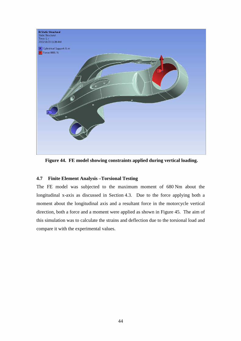
44
Figure 44. FE model showing constraints applied during vertical loading.
4.7 Finite Element Analysis –Torsional Testing
The FE model was subjected to the maximum moment of 680 Nm about the
longitudinal x-axis as discussed in Section 4.3. Due to the force applying both a
moment about the longitudinal axis and a resultant force in the motorcycle vertical
direction, both a force and a moment were applied as shown in Figure 45. The aim of
this simulation was to calculate the strains and deflection due to the torsional load and
compare it with the experimental values.

45
Figure 45. FE model subjected to a moment about the longitudinal x-axis and a force in the motorcycle vertical direction.
4.8 Finite Element Analysis –Lateral Testing
The maximum lateral force of 133.4 N was applied to the FE model to simulate the
maximum load applied in Section 4.4. The FE model is shown in Figure 46. The aim
of this simulation was to compare the lateral deflection with the experimentally
measured lateral deflection.
Figure 46. FE model subjected to a load in the motorcycle lateral direction.
Force
Moment
Longitudinal axis

46
5. RESULTS AND DISCUSSIONS
This section presents and discusses first the results from the experimental deflection
and strain measurements. Thereafter the results from the FEA are discussed and
compared with the experimental results.
5.1 Swingarm Deflection
The vertical deflection of the swingarm is shown in Figure 47 and is based on the
experimental set-up discussed in Section 4.2. The first observation is that the
swingarm exhibits a linear relationship between force and deflection within the range
of loads applied. A maximum deflection of 15.85 mm was measured at the maximum
load of 8000 N. Furthermore, Figure 47 shows the slope of the curve to be
approximately 500 N/mm or 500 kN/m which represents the stiffness coefficient of
the swingarm in the vertical direction.
Figure 47. Vertical deflection of swingarm showing the vertical stiffness coefficient of 500 kN/m.
As discussed earlier, the swingarm and the spring of the rear suspension form two
springs in series between the chassis and the wheel. The swingarm must therefore be
rigid enough to not negatively affect the effective stiffness between the chassis and
0 2 4 6 8 10 12 14 160
1000
2000
3000
4000
5000
6000
7000
8000
Deflection [mm]
For
ce [
N]
Vertical deflection
y = 5e+002*x + 39
500 kN/m
15.85 mm

47
the wheel. Consider two springs in series as shown in Figure 48, where ksp, ksw and
keff represent the stiffness coefficients of the rear spring, swingarm and effective
stiffness between the chassis and wheel, respectively. Typical values for rear springs
on the Ducati are between 50 kN/m and 100 kN/m. Assuming a rear spring value of
50 kN/m the equation calculating the effective stiffness is as follows: 1/ksp + 1/ksw =
1/keff. The effective stiffness is calculated as 45 kN/m. The swingarm therefore needs
to have vertical rigidity considerably higher than that of the rear spring, in the region
of ten times higher. Therefore it can be safely assumed that the effect that the carbon
fibre swingarm will have on the effective stiffness between the chassis and the wheel
will be minimal. This indicates that the larger the difference in the vertical stiffness
between the rear spring and the swingarm, the closer the effective stiffness will be to
that of the rear spring. Essentially the lower spring stiffness dominates the effective
stiffness. It is concluded therefore that the swingarm has a sufficiently high rigidity to
not negatively affect the rear spring.
Figure 48. Schematic showing the rear spring and the swingarm as springs in series between the chassis and the wheel.
The vertical deflection of the swingarm was also measured during unloading, i.e. once
the maximum load of 8000 N was reached, the load was decreased by 1000 N
increments and the corresponding deflections were recorded. Figure 49 shows the
vertical deflection during loading and unloading for two sets of tests that were carried
out.
Chassis
Wheel
ksp = 50 kN/m
ksw = 500 kN/m
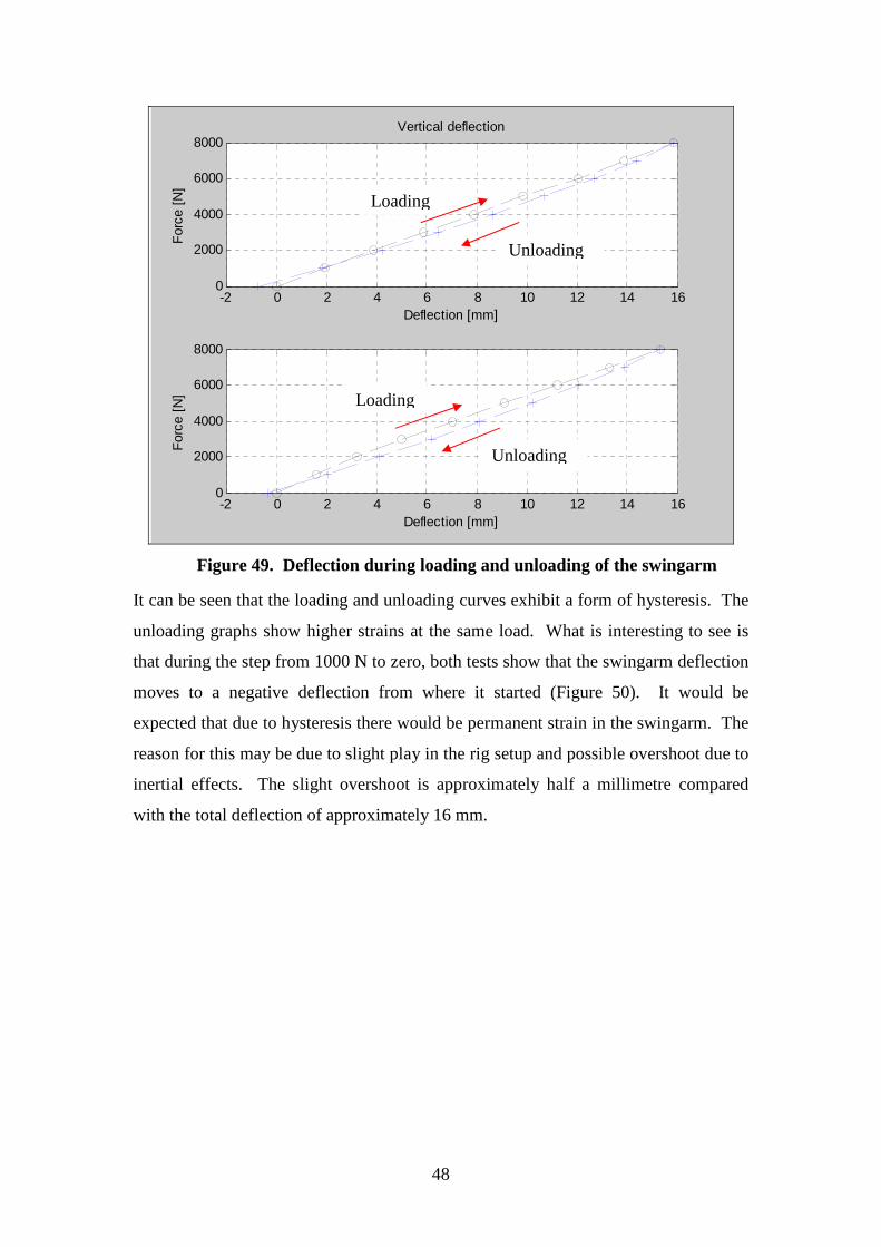
48
Figure 49. Deflection during loading and unloading of the swingarm
It can be seen that the loading and unloading curves exhibit a form of hysteresis. The
unloading graphs show higher strains at the same load. What is interesting to see is
that during the step from 1000 N to zero, both tests show that the swingarm deflection
moves to a negative deflection from where it started (Figure 50). It would be
expected that due to hysteresis there would be permanent strain in the swingarm. The
reason for this may be due to slight play in the rig setup and possible overshoot due to
inertial effects. The slight overshoot is approximately half a millimetre compared
with the total deflection of approximately 16 mm.
-2 0 2 4 6 8 10 12 14 160
2000
4000
6000
8000
Deflection [mm]
For
ce [
N]
Vertical deflection
-2 0 2 4 6 8 10 12 14 160
2000
4000
6000
8000
Deflection [mm]
For
ce [
N]
Loading
Unloading
Unloading
Loading
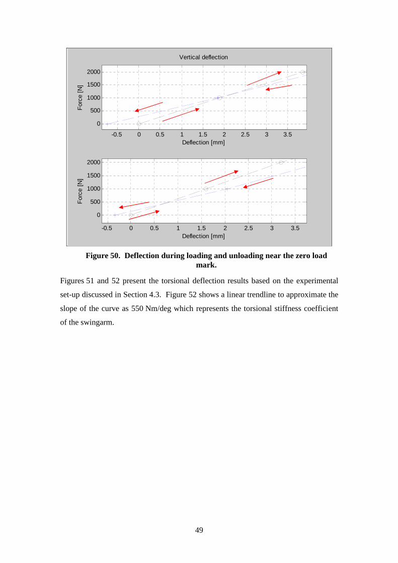
49
Figure 50. Deflection during loading and unloading near the zero load mark.
Figures 51 and 52 present the torsional deflection results based on the experimental
set-up discussed in Section 4.3. Figure 52 shows a linear trendline to approximate the
slope of the curve as 550 Nm/deg which represents the torsional stiffness coefficient
of the swingarm.
-0.5 0 0.5 1 1.5 2 2.5 3 3.5
0
500
1000
1500
2000
Deflection [mm]
For
ce [
N]
Vertical deflection
-0.5 0 0.5 1 1.5 2 2.5 3 3.5
0
500
1000
1500
2000
Deflection [mm]
For
ce [
N]

50
Figure 51. Torsional deflection of the swingarm.
Figure 52. Torsional deflection of the swingarm showing the torsional stiffness coefficient of 550 Nm/deg.
This value appears to be approximately in the middle of the spectrum of values found
in the literature (see Table 5).
0 0.2 0.4 0.6 0.8 1 1.2 1.40
100
200
300
400
500
600
700
Angle [deg]
Mom
ent
[N.m
]
Torsional deflection
0 0.2 0.4 0.6 0.8 1 1.2 1.40
100
200
300
400
500
600
700
Angle [deg]
Mom
ent
[N.m
]
Torsional deflection
y = 5.5e+002*x + 5.2
Experimental results
Linear trendline
550 Nm/deg

51
Table 5. Comparison of torsional stiffness values obtained from the literature.
Designation Torsional stiffness [Nm/deg]
Kawasaki ZX10R (Armentani et al.) 102.9
Suzuki GSX R1000 (Armentani et al.) 140.8
Honda CBR 1000R (Armentani et al.) 140.8
Sharp 209
Ducati Carbon Fibre 550
S2008 (Risitano et al.) 670
SM 2008 (Risitano et al.) 890
BNG 2008 (Risitano et al.) 1330
Cossalter 1000 - 2000
The 550 Nm/deg is higher than the 102.9 Nm/deg and 140.8 Nm/deg determined by
Armentani et al. [8] and the 209 Nm/deg suggested by Sharp [29]. It is lower than
those obtained by Risitano et al. [5] of 670 Nm/deg, 890 Nm/deg and 1330 Nm/deg
and also lower than the typical values presented by Cossalter et al. of between
1000 Nm/deg and 2000 Nm/deg [10]. As discussed in Section 2.2, the values
calculated by Armentani et al. were calculated without using a spacer and spindle to
simulate real conditions. It was felt that the deflections calculated by Armentani et al.
were higher than if real life conditions were simulated which means their stiffness
values were lower. Due to the uncertainty of the torsional stiffness values calculated
by Armentani et al., the carbon fibre swingarm was rather compared with the value of
209 Nm/deg by Sharp and the higher stiffness values mentioned above. This
uncertainty shows the need to develop a standard method of testing both single-sided
and double-sided swingarms to determine the stiffness characteristics.
Based on the value suggested by Sharp, the carbon fibre swingarm is stiff enough.
However, when compared with the higher values determined by Risitano et al. and
Cossalter, the rider may experience a “heavier” ride due to the lower torsional
stiffness. Furthermore, as was discussed by Cossalter et al., lower torsional rigidity
reduces weave mode stability at higher speeds. Therefore the results suggest the

52
carbon fibre swingarm may cause the motorcycle to experience lower stability in the
weave mode at higher speeds than the other motorcycles.
Figures 53and 54 show the torsional loading and unloading for two different tests.
Hysteresis is shown to occur in the swingarm which could add to the torsional
damping.
Figure 53. Torsional deflection of swingarm during loading and unloading during two torsional tests.
0 0.2 0.4 0.6 0.8 1 1.2 1.40
200
400
600
800
Angle [deg]
Mom
ent
[N.m
]
Torsional deflection
0 0.2 0.4 0.6 0.8 1 1.2 1.40
200
400
600
800
Angle [deg]
Mom
ent
[N.m
]
Loading
Loading
Unloading
Unloading

53
Figure 54. Torsional deflection during loading and unloading near the zero mark.
The lateral deflection (based on Section 4.4) of the swingarm is presented in
Figures 55 and 56 with Figure 56 adding a linear trendline approximating the slope of
the curve. The slope of the curve represents the lateral stiffness coefficient equal to
approximately 445 N/mm (445 kN/m).
0 0.05 0.1 0.15 0.2 0.25 0.3 0.35
0
100
200
Angle [deg]
Mom
ent
[N.m
]
Torsional deflection
0 0.02 0.04 0.06 0.08 0.1 0.12 0.14 0.16 0.18
-50
0
50
100
150
Angle [deg]
Mom
ent
[N.m
]Loading
Loading
Unloading
Unloading

54
Figure 55. Lateral deflection of the swingarm.
Figure 56. Lateral deflection of the swingarm showing the lateral stiffness coefficient of 445 kN/m.
0 0.05 0.1 0.15 0.2 0.25 0.3 0.350
20
40
60
80
100
120
140
Deflection [mm]
Late
ral l
oad
[N]
Lateral deflection of swingarm
0 0.05 0.1 0.15 0.2 0.25 0.3 0.350
20
40
60
80
100
120
140
Deflection [mm]
Late
ral l
oad
[N]
Lateral deflection of swingarm
y = 445*x + 0.232
Experimental results
Linear trendline
445 kN/m

55
Comparing this result to those obtained by Armentani et al. [8] and typical values
stated by Cossalter [10] (Table 6), it can be seen that the swingarm lateral stiffness of
445 kN/m is on the lower end of the spectrum. In a similar manner to the torsional
rigidity, the lower lateral stiffness may cause the rider to experience a “heavier” ride
due to the slower response time. The lower stiffness (compared with other values)
may also reduce weave mode stability at medium to higher speeds. However as
shown by Cossalter et al. [27], the lower lateral stiffness may increase the weave
mode stability at high speeds.
Table 6. Comparison lateral stiffness values.
Designation Torsional stiffness [kN/m]
Ducati Carbon Fibre 445
Kawasaki ZX10R (Armentani et al.) 603
Suzuki GSX R1000 (Armentani et al.) 804
Honda CBR 1000R (Armentani et al.) 965
Cossalter 800-1600
Although the results show the torsional and lateral stiffness values of the carbon fibre
swingarm to be generally lower than other swingarm stiffness values, it is difficult to
state whether the swingarm will certainly affect the cornering response time and
weave mode stability as suggested. In comparing swingarms, a few points should be
noted. First, the affect that swingarm stiffness has on weave mode was studied on a
150 cc scooter (Cossalter et al. [27]). The question to ask here is, can the results from
a scooter be compared with that of a much larger racing motorcycle? Second, which
follows on from the first, is it appropriate to directly compare swingarm stiffness
values of different motorcycles with one another? Each motorcycle consists of a
number of different components such as wheels, frame and suspensions, each with a
certain mass, stiffness and damping. Each motorcycle potentially has a different
overall dynamic system. A direct comparison of stiffness values may not provide the
overall picture of how the swingarm affects the system as a whole.
The discussion suggests that it is better to compare swingarms that have motorcycles
with similar overall dynamic systems. To determine the actual effect that the carbon

56
fibre swingarm stiffness would have on the motorcycle would require firstly a
comparison with the stiffness values of a standard aluminium Ducati 1098 swingarm.
Furthermore, it is recommended to carry out experimental acceleration and strain
measurements on both the original aluminium swingarm and the carbon fibre
swingarm while the motorcycle is being operated through typical driving conditions at
increasing speeds. Only then could more conclusive statements be made regarding
the effect that the swingarm has on the motorcycle. This study however, has
successfully characterized the stiffness of the carbon fibre swingarm.
5.2 Strain Analysis
The results and discussions of strain measurements on the swingarm are presented
next.
5.2.1 Strain Gauge Validation
Before the strain gauges were mounted on the swingarm and measurements were
made, an axial strain gauge was mounted on a cantilever rectangular plate and loads
were applied. The strain was measured and compared with the FEA carried out on the
plate (Appendix A). The aim of this exercise was to validate the strain measurements
with classical laminate theory used in the FEA. Differences of less than 2% were
found between the FEA and strain gauge readings showing that the measured values
corresponds well with the results obtained using FEA.
5.2.2 Strain Gauge Transverse Sensitivity
Strain gauge transverse sensitivity was discussed in Section 2.4 where equations were
presented that calculate the actual strain along a gauge axis based on the strain
measured axially and perpendicular to gauge axis. These equations were applied to
the measured strain in the 0° and 90° axes where the x-direction corresponds to 0° and
the y-direction corresponds to 90°. Table 7 shows the measured strains εmx and εmy at
the maximum vertical load of 8000 N. Furthermore, only Positions 3 through 6 were
taken into account because the data acquisition system only captured both the x- and
y-direction strains needed to calculate the error due to transverse sensitivity at Gauges
3-6. Tables 8 and 9 show the actual strain (εx and εy ) using transverse sensitivity

57
factors of Kt = +5% (0.05) and -5% (-0.05) respectively. The Poisson’s ratio υ0 for
steel was taken as 0.285 [39].
Table 7. Measured strain in the longitudinal and transverse directions at maximum load of 8000 N at Positions 3-6.
Position εmx [µε] εmy [µε]
3 -592 831
4 -1090 660
5 1050 -884
6 725 -394
Table 8. Strain correction at Positions 3-6 using Kt = +5% (0.05).
Position εx [µε] % error
x-direction
εy [µε] % error
y-direction
3 -625 -5.5 848 -2
4 -1109 -1.7 702 -6.4
5 1077 -2.6 -923 -4.4
6 734 -1.2 -424 -7.6
Table 9. Strain correction at Positions 3-6 using Kt = -5% (-0.05).
Position εx [µε] % error
x-direction
εy [µε] % error
y-direction
3 -558 5.7 813 2.1
4 -1072 1.7 614 6.9
5 1020 2.9 -843 4.6
6 715 1.4 -363 7.9
The maximum error due to transverse gauge sensitivity was approximately -7.6% and
+7.9% for Strain Gauge 6 in the y-direction. Based on these results, it was assumed
that the errors were small enough to ignore when presenting the experimental results
in this section. It should be noted that the aim in this section was to obtain an
indication of the type and magnitude of the strains and therefore errors of less than 8%
were considered small enough to ignore. However, when comparing experimental

58
and FE results in Section 5.3.2, the errors due to transverse sensitivity were taken into
account when attempting to minimize the error between the FE and experimental
results. The following section presents the strain results as measured.
5.2.3 Strain Measurements
For the sake of clarity, the strain gauge measurement positions on the swingarm are
presented again in Figures 57 and 58. The lower arm refers to the part of the
swingarm that contains Positions 2 and 3; the top arm refers to the region where
Positions 4, 5 and 6 are situated; Position 1 is on the wheel mount and Positions 7 and
8 are on the pivot points.
Figure 57. Strain Gauge measurement positions
1
2
3
6
7
8

59
Figure 58. Strain gauge measurement positions.
Before proceeding, it should be noted that during the vertical loading tests, two
channels measuring the longitudinal strain in Gauges 1 and 2 did not function.
Therefore out of the possible eight longitudinal strain measurements, only six were
measured.
Figure 59 presents the longitudinal strain measurements at Positions 3 through 8
during the vertical loading. The strain on the top arm at Positions 4, 5 and 6 measured
the highest strains. At the maximum load of 8000 N, Gauges 4 and 5 measured
approximately 1100 µε (compressive) and 1100 µε (tensile) respectively and Gauge 6
measured approximately 750 µε (tensile). Therefore based on the positions measured,
when designing the swingarm, it is important to know that the highest longitudinal
strains in both tension and compression occur on the top arm during vertical loading.
4
5

60
Figure 59. Longitudinal strain measured at positions 3 through 8.
Normal strain due to bending in a beam is given by the equation ε = My/EI where M
is the bending moment acting at the measurement point, y is the distance from the
neutral axis, E is the modulus of elasticity and I is the second moment of area. It is
difficult to discuss the strain results with respect to the distance from the neutral axis
because it is uncertain where the neutral axis of the swingarm lies. However, the
higher strain on the top arm may be due to a lower second moment of area in the top
arm compared with that in the bottom arm. Also, the lowest strains occur at the pivot
point at Positions 7 and 8. This is due to the aluminium inserts being mounted at
those positions which increase the rigidity of those positions substantially.
The transverse strain due to vertical loading is shown in Figure 60. Positions 3 and 4
experience the highest tensile strains of approximately 800 µε and 650 µε respectively
and Position 5 experiences the highest compressive strain of approximately 900 µε.
Typical ultimate strain values for a woven carbon fibre ply are approximately 8000 µε
for both the axial and transverse directions. For a unidirectional ply the ultimate
strain is approximately 10000 µε and 5000 µε for the axial and transverse directions
respectively. The measured strains were considerably lower than the maximum
allowable strains which indicates the laminate design is strong enough to handle the
0 1000 2000 3000 4000 5000 6000 7000 8000-1500
-1000
-500
0
500
1000
1500
Str
ain
[ µε]
Vertical load [N]
Longitudinal strain due to vertical force
3
4
5
6
7
8

61
vertical loading. Furthermore, the ultimate strains are typical values for single plies.
In the case of the swingarm, the laminates consist of a number of plies bonded
together which increases the strength. It is also important to know that during vertical
loading that causes bending in the swingarm, longitudinal as well as transverse strains
occur on the swingarm. This is due to the nature of the layup design.
Figure 60. Transverse strain measured at positions 1 through 7.
Figures 61 to 63 show the magnitude and direction of strain (due to vertical loading)
occurring at the positions on the bottom and top arms. The reason only the bottom
and top arms were looked at was to determine how the loading affects the middle part
of the swingarm. In the figures, the arrows pointing away from each other specify
tensile strain and the arrows pointing toward each other specify compressive strain
along that direction.
Position 3 experiences compression in the gauge longitudinal direction and tension in
the transverse direction.
0 1000 2000 3000 4000 5000 6000 7000 8000-1000
-800
-600
-400
-200
0
200
400
600
800
1000
Vertical force [N]
Str
ain
[ µε]
Transverse strain due to vertical force
4
6
5
2
7
3
1

62
Figure 61. Maximum longitudinal and transverse strain at Position 3 during vertical loading.
During vertical loading the bottom (Position 6) and the side (Position 5) of the top
arm experienced tension in the longitudinal direction and the top of the arm (Position
4) experienced compression in the longitudinal direction.
Figure 62. Maximum longitudinal and transverse strain at Positions 4 and 5 during vertical loading.
4: 1100 µε
5: 1100 µε
550 µε
850 µε
4: 700 µε
5: 900 µε

63
Figure 63. Maximum longitudinal and transverse strain occurring at Positions 6 during vertical loading.
The fact that the top part of the arm is in compression and the bottom part is in tension
in the longitudinal direction is expected. The top arm can be considered to be a beam
with a bending moment applied to it which causes the compression at the top and the
tension at the bottom. The side of the top arm, Position 5, also experiences tension in
the longitudinal direction. This may indicate, due to the asymmetric design of the
swingarm and the shape of the top arm that as the swingarm is loaded vertically
upward, a slight rotation about the longitudinal axis also develops as shown in Figure
64. This may also be the reason why in the transverse direction, there is a stretch on
top and compression on the side and bottom of the top arm. This suggests that
coupling exists between vertical and torsional direction. That is, as a load is applied
in the vertical direction, not only are vertical deflections seen but also torsional
deflections.
6: 750 µε
6: 400 µε

64
Figure 64. Schematic of the vertical and rotational translation of the swingarm during vertical loading.
To establish the relationship between the strains on the top arm as the vertical load is
increased, the strains were normalized (Figure 65) based on the maximum strain of
1100 µε. The numbers on each column refer to the gauge position, and the letters L
and T refer to longitudinal and transverse directions respectively.
Figure 65. Normalized strain on the top arm of the swingarm due to vertical loading.

65
As the vertical load is applied, Positions 4 and 5 experience the same magnitude of
longitudinal strain but with Position 4 in compression and 5 in tension. The
longitudinal strain at Position 6 is approximately 0.7 time as large as the maximum
strain. Therefore the areas which will govern the design are Positions 4 and 5 in the
longitudinal direction and Position 5 in the transverse direction. If a linear strain is
assumed, then these positions will experience failure first under vertical loading
conditions.
Figures 66 and 67 present the longitudinal and transverse strain occurring during
torsional loading. During the testing, the data acquisition system did not capture
Strain Gauge 2 in its longitudinal direction and Strain Gauge 8 in its transverse
direction. Also, it appeared that the data from Strain Gauge 7 in its transverse
direction did not present proper results and was therefore not included.
At the maximum torsional loading of 680 Nm, Position 6 experienced the highest
longitudinal strain of approximately 380 µε. The longitudinal strain was highest on
the top and underside of the top arm (Positions 4 and 6). In terms of the positions
away from the aluminium inserts, Positions 4, 5 and 6 experience tension and
Position 3 experiences compression in the longitudinal direction.

66
Figure 66. Longitudinal strain due to the torsional loading. Strain gauge positions are shown on the figure.
The highest transverse strain due to torsional loading, was measured at Positions 5
and 6 of approximately 250 µε (compression). Positions 3, 4, 5 and 6 all experience
compression in their respective transverse directions during torsional loading.
Figure 67. Strain in the transverse direction due to torsional loading.
0 100 200 300 400 500 600 700-200
-100
0
100
200
300
400
Moment [N.m]
Str
ain
[[µ
Str
ain]
Longitudinal strain due to torsional loading
0 100 200 300 400 500 600 700-250
-200
-150
-100
-50
0
50
100
Moment [N.m]
Str
ain
[µS
trai
n]
Transverse strain due to torsional loading
1
3
4
5
6
8
1
2
3 (red)
4
5
6
7

67
Figures 68 to 70 present graphically the strains occurring at the positions in the central
part of the swingarm.
Figure 68. Maximum longitudinal and transverse strain at Position 3 during torsional loading.
Figure 69. Maximum longitudinal and transverse strain at Positions 4 and 5 during torsional loading.
3: 120 µε
4: 150 µε
5: 80 µε
3: 10 µε
4: 80 µε
5: 250 µε
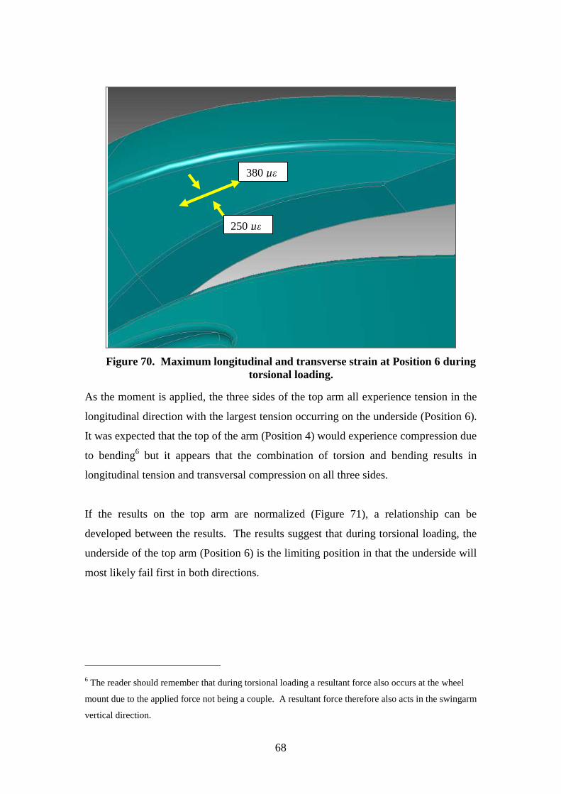
68
Figure 70. Maximum longitudinal and transverse strain at Position 6 during torsional loading.
As the moment is applied, the three sides of the top arm all experience tension in the
longitudinal direction with the largest tension occurring on the underside (Position 6).
It was expected that the top of the arm (Position 4) would experience compression due
to bending6 but it appears that the combination of torsion and bending results in
longitudinal tension and transversal compression on all three sides.
If the results on the top arm are normalized (Figure 71), a relationship can be
developed between the results. The results suggest that during torsional loading, the
underside of the top arm (Position 6) is the limiting position in that the underside will
most likely fail first in both directions.
6 The reader should remember that during torsional loading a resultant force also occurs at the wheel
mount due to the applied force not being a couple. A resultant force therefore also acts in the swingarm
vertical direction.
380 µε
250 µε

69
Figure 71. Normalized strain occurring on the top arm of the swingarm due to torsional loading.
5.3 Finite Element Analysis
This section presents the results obtained from the FEA. The assumptions for
modelling the FE model are briefly presented again:
• Only the layup at the major zones were modelled with the smaller zones
included in the larger more significant zones.
• Ply overlap was not modelled due to the complexity of the swingarm design.
• The aluminium inserts were not modelled.
Therefore when viewing the results, the reader should keep in mind the assumptions
that were made to model the highly complex swingarm.
5.3.1 Finite Element Analysis: Deflections
The deflections of the swingarm were compared with the experimental results. Figure
72 shows the vertical deflection of the swingarm due to the maximum 8000 N vertical
load.
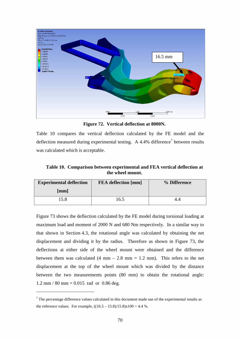
70
Figure 72. Vertical deflection at 8000N.
Table 10 compares the vertical deflection calculated by the FE model and the
deflection measured during experimental testing. A 4.4% difference7 between results
was calculated which is acceptable.
Table 10. Comparison between experimental and FEA vertical deflection at the wheel mount.
Experimental deflection
[mm]
FEA deflection [mm] % Difference
15.8 16.5 4.4
Figure 73 shows the deflection calculated by the FE model during torsional loading at
maximum load and moment of 2000 N and 680 Nm respectively. In a similar way to
that shown in Section 4.3, the rotational angle was calculated by obtaining the net
displacement and dividing it by the radius. Therefore as shown in Figure 73, the
deflections at either side of the wheel mount were obtained and the difference
between them was calculated (4 mm – 2.8 mm = 1.2 mm). This refers to the net
displacement at the top of the wheel mount which was divided by the distance
between the two measurements points (80 mm) to obtain the rotational angle:
1.2 mm / 80 mm = 0.015 rad or 0.86 deg.
7 The percentage difference values calculated in this document made use of the experimental results as
the reference values. For example, ((16.5 – 15.8)/15.8)x100 = 4.4 %.
16.5 mm

71
Figure 73. Deflection measured during maximum torsional loading of 2000 N and 680 Nm.
The maximum angle measured during experimental testing was approximately
1.2 deg. A comparison between the experimental and FEA angles of rotation is
presented in Table 11 which gave a difference of 28%.
Table 11. Comparison between experimental and FEA rotation at the wheel mount.
Experimental rotation
[deg]
FEA rotation [deg] % Difference
1.2 0.86 28
The FEA lateral deflection was calculated as approximately 0.15 mm at the maximum
lateral load of 135 N as shown in Figure 74. The deflection measured during
experimental loading was 0.3 mm, twice as large as that calculated by the FEA. A
difference of 50% was calculated between FEA and experimental lateral deflection
(Table 12).
Top deflection = 4 mm
Bottom deflection = 2.8 mm
Distance between
points = 80 mm

72
Figure 74. Lateral deflection under the 135 N load.
Table 12. Comparison between experimental and FEA lateral deflections at the wheel mount.
Experimental rotation
[mm]
FEA rotation [mm] % Difference
0.3 0.15 50
An initial reason for the large difference could be due to very low deflections
(0.3 mm) in the lateral direction. At low deflections large differences occur in relative
terms because the errors due to lash and bedding have a more significant effect. At
larger loads and deflections a higher degree of correlation will result. For future
testing, more accurate results may be obtained if much larger loads are applied in the
lateral direction.
5.3.2 Finite Element Analysis: Strains
The strains calculated by the FE model were also compared with the measured strains.
It should be noted that only the strains situated away from the aluminium inserts were
analyzed. Due to not accurately modelling the region at the aluminium inserts, the
results obtained by the FEA at those positions were not trusted and were therefore
ignored. Only Positions 2 to 6 were analyzed and compared with experimental
values. Furthermore, as was seen in Section 5.2, the data acquisition system did not

73
record proper results for Gauge 2 in the longitudinal direction and therefore only the
results from Gauge 2 in its transverse direction were compared with the FE results.
All the following results shown in the FEA figures are based on the maximum vertical
load of 8000 N. Due to the linearity of the FE model, at zero load there is zero strain
and at the maximum load of 8000 N the swingarm experiences the maximum
magnitude of strain.
The underside of the swingarm, which includes Position 2, is shown in Figure 75.
The transverse strain calculated by the FEA at this point was approximately -230 µε.
The measured strain at the same load was -450 µε and a comparison between
experimental and simulated strain over the entire 0 N - 8000 N range is presented in
Figure 76.
Figure 75. Strain distribution for Position 2 in the gauge transverse direction at vertical load of 8000 N.
Position 2 (T) = -230 µε
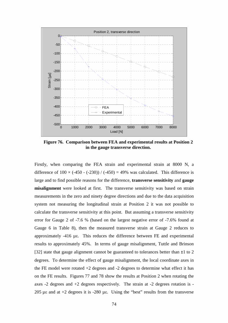
74
Figure 76. Comparison between FEA and experimental results at Position 2 in the gauge transverse direction.
Firstly, when comparing the FEA strain and experimental strain at 8000 N, a
difference of 100 × (-450 - (-230)) / (-450) = 49% was calculated. This difference is
large and to find possible reasons for the difference, transverse sensitivity and gauge
misalignment were looked at first. The transverse sensitivity was based on strain
measurements in the zero and ninety degree directions and due to the data acquisition
system not measuring the longitudinal strain at Position 2 it was not possible to
calculate the transverse sensitivity at this point. But assuming a transverse sensitivity
error for Gauge 2 of -7.6 % (based on the largest negative error of -7.6% found at
Gauge 6 in Table 8), then the measured transverse strain at Gauge 2 reduces to
approximately -416 µε. This reduces the difference between FE and experimental
results to approximately 45%. In terms of gauge misalignment, Tuttle and Brinson
[32] state that gauge alignment cannot be guaranteed to tolerances better than ±1 to 2
degrees. To determine the effect of gauge misalignment, the local coordinate axes in
the FE model were rotated +2 degrees and -2 degrees to determine what effect it has
on the FE results. Figures 77 and 78 show the results at Position 2 when rotating the
axes -2 degrees and +2 degrees respectively. The strain at -2 degrees rotation is -
205 µε and at +2 degrees it is -280 µε. Using the “best” results from the transverse
0 1000 2000 3000 4000 5000 6000 7000 8000-500
-450
-400
-350
-300
-250
-200
-150
-100
-50
0
Load [N]
Str
ain
[ µε]
Position 2, transverse direction
FEA
Experimental

75
sensitivity (-416 µε) and the gauge misalignment (-280 µε), a difference of
approximately 33% was calculated which shows a reduced difference.
Figure 77. Position 2 in the transverse direction with the axes rotated
-2 degrees.
Figure 78. Position 2 in the transverse direction with the axes rotated +2 degrees.
Looking at further potential reasons for the large difference, Figure 79 shows that
Position 2 in the transverse direction, is in the middle of a high strain gradient, i.e. the
strain is changing rapidly in this area.
-205µε
-280 µε

76
Figure 79. Close up of the strain distribution for Position 2 in the gauge transverse direction at vertical load of 8000 N
If the results on the FE model are viewed approximately 20 mm to the right, a value
of -450 µε is obtained. Also, moving approximately 10 mm and 20 mm to the top
left, it can be seen that the strain on the FE model becomes 107 µε and 368 µε
respectively. Therefore the position chosen to mount the 90° (transverse) strain gauge
is near a region that changes from tensile to compressive strain and it is possible that
the strain gauge readings in the transverse direction would not yield accurate results
due to small changes resulting in high strain differences. Even though this is the case,
simply by moving approximately 20 mm to the right on the FE model, strains very
near to the measured values were found. Therefore based on the above discussions,
transverse sensitivity, gauge misalignment and a high strain field gradient may all
plausibly explain in part the difference in the FEA and measured strains.
The strain field for Position 3 in the longitudinal direction (horizontal direction in the
figure) at 8000 N is shown in Figures 80 and 81. At Position 3, a longitudinal strain
of -43 µε was found on the FE model. Once again it can be seen that Strain Gauge 3
in the longitudinal direction was placed in the region of a high strain gradient.
Position 2 (T) = -230 µε
-450 µε 107 µε
368 µε

77
Figure 80. Strain distribution for Position 3 in the gauge longitudinal direction.
Figure 81. Close up of the strain distribution for Position 3 in the gauge longitudinal direction.
The comparison with the experimental results is shown in Figure 82. The
experimental longitudinal strain measured at this position was -592 µε and the
difference was calculated as 100 × (-592 - (-43)) / (-592) = 93%. Once again, this
difference is large and is likely due to the high strain gradient surrounding the
measurement point. For example, studying Figure 81, it can be seen that moving
Position 3 (L) = -43 µε
Position 3 (L) = -43 µε
13 µε
28 µε
22 µε

78
approximately 20 mm below Position 3, a positive strain of 28 µε was found and
moving similar distances above the measurement point, values in the region of 13 µε
to 22 µε are found on the FE model. This means that both above and below the
measurement point the strain changes rapidly from negative to positive. As discussed
with Position 2, it is possible that a strain gauge placed in a region such as this will
not yield accurate results.
Figure 82. Comparison between FEA and experimental results at Position 3 in the gauge longitudinal direction.
The strain gauge transverse sensitivity error calculation reduces the measured strain to
approximately -557 µε. Rotating the axes through +2 degrees, a strain of -78 µε is
obtained shown in Figure 83. Therefore it can be concluded that the transverse
sensitivity and the gauge misalignment do not play a significant role in the large
difference obtained and that the difference is most likely due to the high strain
gradient. Further strain gauge testing needs to be carried out in this area.
0 1000 2000 3000 4000 5000 6000 7000 8000-600
-500
-400
-300
-200
-100
0
100
Load [N]
Str
ain
[ µε]
Position 3, longitudinal direction
FEA
Experimental

79
Figure 83. Strain at Position 3 in the longitudinal direction with the axes rotated +2 degrees.
The strain field around Position 3 in the gauge transverse direction (vertical direction
in the figures) is shown in Figures 84 and 85 as approximately 430 µε.
Figure 84. Strain distribution for Position 3 in the gauge transverse direction.
Position 3 (T) = 430 µε
-78µε

80
Figure 85. Close up of the strain distribution for Position 3 in the gauge transverse direction (vertical direction in the figure).
The experimental strain measured at 8000 N was approximately 850 µε and a
comparison between experimental and FE results over the range of loads is presented
in Figure 86. The calculated difference in the FE and measured strains is 100 × (850 -
430)/830 = 49%. As can be seen in Figure 85 a strain of 850 µε is found
approximately 15 mm below the measurement point. This shows that although the
exact point does not give the correct results, good correlation occurs nearby. Due to
ply overlap, slightly different load paths exist in the real swingarm as compared to the
model which plausibly explains the difference in the FE and measured strains.
Position 3 (T) = 430 µε
850 µε

81
Figure 86. Comparison between FEA and experimental results at Position 3 in the gauge transverse direction.
Rotating the axes through -2 and +2 degrees does not significantly change the result in
as shown in Figures 87 and 88. Also, the error due to transverse sensitivity was
approximately 2% which would not significantly change the results. The large
difference is then most likely due to ply overlap altering the load paths in that region.
Figure 87. Position 3 in the transverse direction with axes rotated -2 degrees.
0 1000 2000 3000 4000 5000 6000 7000 8000-100
0
100
200
300
400
500
600
700
800
900
Load [N]
Str
ain
[ µε]
Position 3, transverse direction
FEA
Experimental
434 µε
803 µε

82
Figure 88. Position 3 in the transverse direction with axes rotated +2 degrees.
The strain in the longitudinal direction on the top side of the top arm (Position 4) was
found to give very good results. Figure 89 shows the FE longitudinal strain
distribution on the top arm with a value of -1100 µε at Position 4. The measured
strain was -1090 µε and Figure 90 shows the comparison between experimental and
FEA results for Position 4. An error of approximately 100 × (-1100 - (-1090)) / (-
1100) = 0.9% was calculated. Therefore this result shows that the FE model
corresponds well with the experimental results at certain positions.
853 µε
453 µε

83
Figure 89. Strain distribution for Position 4 in the gauge longitudinal direction at 8000N.
Figure 90. Comparison between FEA and experimental results at Position 4 in the gauge longitudinal direction.
When the axes were rotated through +2 and -2 degrees, longitudinal strains at
Position 4 of -1122 µε and -1055 µε were obtained which do not significantly change
the results. Error due to transverse sensitivity was calculated to be less than 1.7% (see
Section 5.2) and therefore would not significantly affect the results either.
0 1000 2000 3000 4000 5000 6000 7000 8000-1200
-1000
-800
-600
-400
-200
0
Load [N]
Str
ain
[ µε]
Position 4, longitudinal direction
FEA
Experimental
Position 4 (L) = -1100 µε

84
The strain on the top side of the top arm in transverse direction is shown in Figure 91
with the strain at Position 4 in the transverse direction being approximately +1700 µε.
Figure 91. Strain distribution for Position 4 in the gauge transverse direction at 8000N.
The experimental result at 8000 N was approximately 660 µε (see Figure 92), and a
difference between the experimental and FE results of 157% was calculated which is
exceedingly high.
Position 4 (T) = 1700 µε

85
Figure 92. Comparison between FEA and experimental results at Position 4 in the gauge transverse direction.
Rotating the axes through +2 and – 2 degrees give values FE strain of 1820 µε and
1690 µε respectively and does not decrease the error significantly. Applying gauge
transverse sensitivity effects, a measured strain of 702 µε was calculated as shown in
Table 8. Therefore it can be concluded that the differences are not due to sensitivity
factors or gauge misalignment. Once again, the reader needs to be reminded that the
swingarm and the layup of the swingarm is very complex. Not modelling the ply
overlap due to the complexity of the swingarm was one of the major assumptions and
to accurately model the overlap would present great difficulty. The layup on the top
part of the top arm consisted mainly of ±45° woven plies with the fibre reference
direction being along the longitudinal direction of the swingarm. In an attempt to
simulate the overlap on the top arm, extra ±45° woven plies were added in this region
because during layup the overlap consisted mainly of these types of plies. After
adding three plies on the top, new longitudinal and transverse strains were calculated
by the FEA and shown in Figures 93 and 94 respectively.
0 1000 2000 3000 4000 5000 6000 7000 80000
200
400
600
800
1000
1200
1400
1600
1800
Load [N]
Str
ain
[ µε]
Position 4, transverse direction
FEA
Experimental
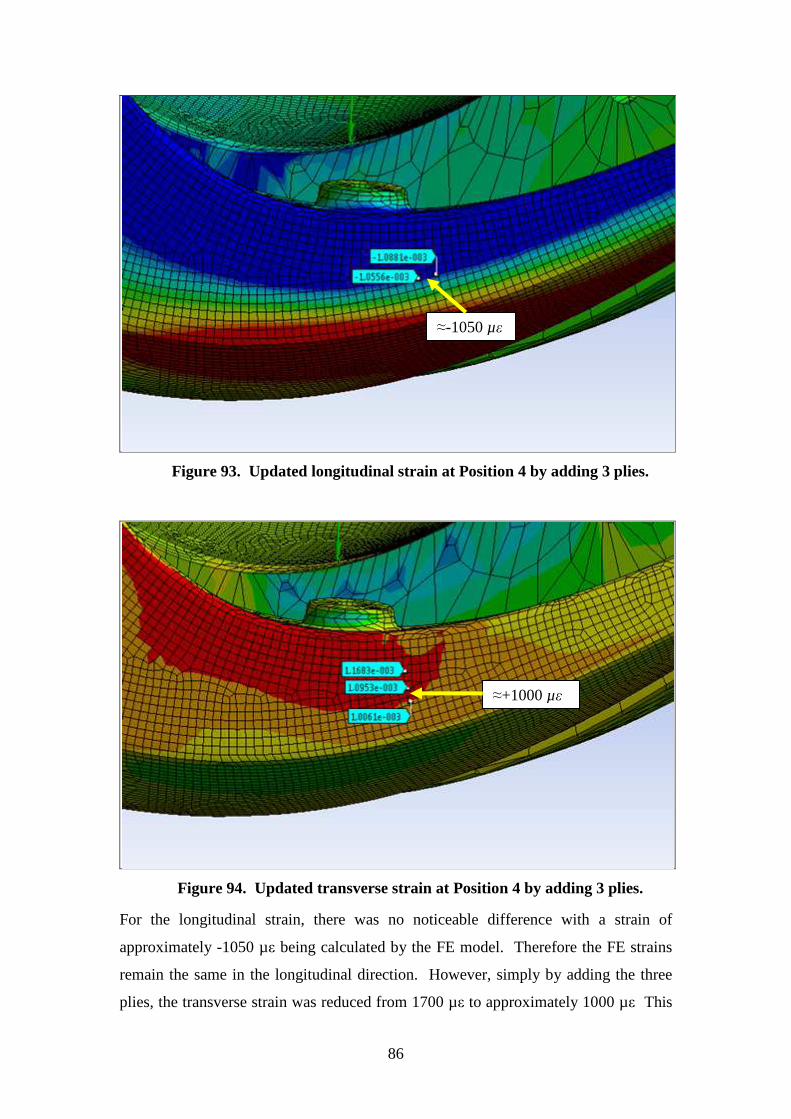
86
Figure 93. Updated longitudinal strain at Position 4 by adding 3 plies.
Figure 94. Updated transverse strain at Position 4 by adding 3 plies.
For the longitudinal strain, there was no noticeable difference with a strain of
approximately -1050 µε being calculated by the FE model. Therefore the FE strains
remain the same in the longitudinal direction. However, simply by adding the three
plies, the transverse strain was reduced from 1700 µε to approximately 1000 µε This
≈-1050 µε
≈+1000 µε

87
presents a reduction of about 40% and a new difference of just below 40% when
compared with the experimental value of 725 µε at 8000 N. This exercise shows that
by simply adding three plies to simulate some degree of overlap in that area, the
transverse strain becomes more accurate and the longitudinal strain remains almost
the same. The overlap plays a huge role in obtaining accurate transverse FE strain
results but does not appear to affect the longitudinal strain results in this region. This
may be due to high Poisson’s ratio effects based on the ±45° plies. It is concluded
therefore that if highly accurate results are to be obtained at Position 4 in the
transverse direction, a method would need to be developed to accurately model the
overlap.
The longitudinal strain calculated by the FE model at Position 5 (on the side of the top
arm) is shown in Figure 95. Strain of approximately 1100 µε was calculated by the
FE model and the experimental value was 1050 µε. The comparison between the
experimental and FE results (Figure 96) show good correlation at this position
(difference of 5%). Once again, good results have been found along the longitudinal
direction and no significant difference was found when looking at transverse
sensitivity and gauge misalignment.
Figure 95. Strain distribution for Position 5 in the gauge longitudinal direction.
Position 5 (L) = 1100 µε

88
Figure 96. Comparison between FEA and experimental results at Position 5 in the gauge longitudinal direction.
Figure 97 shows the transverse strain distribution on the side of the top arm near
Position 5. A strain of approximately -1200 µε at Position 5 was found from the FEA.
The experimental result was approximately -870 µε which gives a difference of 38%
(see comparison in Figure 98).
Figure 97. Strain distribution for Position 5 in the gauge transverse direction.
0 1000 2000 3000 4000 5000 6000 7000 8000-200
0
200
400
600
800
1000
1200
Load [N]
Str
ain
[ µε]
Position 5, longitudinal direction
FEA
Experimental
Position 5 (T) = -1200 µε
-840 µε

89
Figure 98. Comparison between FEA and experimental results at Position 5 in the gauge transverse direction.
Rotating the axes -2 degrees reduced the FE strain to -1188 µε which is not a
significant change. The change in measured strain due to transverse sensitivity
(-923 µε from Table 8) reduced the difference to approximately 30% which is a
significant difference. Once again, the difference is most likely due to the overlap not
being modelled which causes different load paths. If the results are viewed
approximately 10 mm above Position 5, then strains of approximately -840 µε are
found on the FE model which are very close to the measured value of -870 µε. This
shows that the FE load paths are slightly different to the actual load path due to
different rigidity in the transverse direction. This position is therefore relatively
accurate.
Figure 99 presents the strain distribution under the top arm (Position 6) in the
longitudinal direction. It can be seen that the strain distribution is highly uniform and
the longitudinal strain calculated by the FEA at Position 6 was approximately
1000 µε. A strain of 725 µε was measured during testing which results in a difference
of approximately 38%. Figure 100 shows the comparison between experimental and
FE results over the range of loads. A possible reason for this error could be due to the
0 1000 2000 3000 4000 5000 6000 7000 8000-1200
-1000
-800
-600
-400
-200
0
Load [N]
Str
ain
[ µε]
Position 5, transverse direction
FEA
Experimental

90
narrowing of the arm and curve of the arm at this position. It was concluded earlier
with respect to Position 4, that the increase in the ±45° plies does not play a role in
changing the longitudinal strain. But in this case, because of the narrowing and
curvature it is possible that the lack of overlap affects the longitudinal strain more.
However, by moving up 10 mm (see Figure 99) a strain of approximately 730 µε was
found which is very close to the measured strain. This could again indicate that the
inaccuracy is due to not modelling ply overlap which cause the load paths to be
slightly different.
Figure 99. Strain distribution for Position 6 in the gauge longitudinal direction.
Position 6 (L) ≈ 1000 µε
730 µε
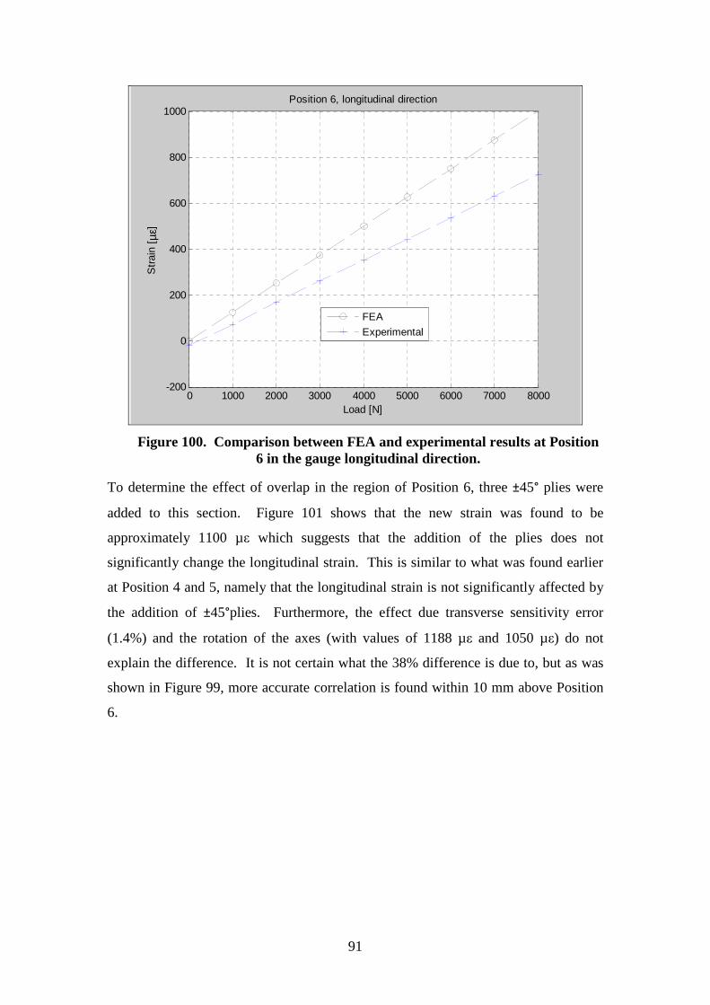
91
Figure 100. Comparison between FEA and experimental results at Position 6 in the gauge longitudinal direction.
To determine the effect of overlap in the region of Position 6, three ±45° plies were
added to this section. Figure 101 shows that the new strain was found to be
approximately 1100 µε which suggests that the addition of the plies does not
significantly change the longitudinal strain. This is similar to what was found earlier
at Position 4 and 5, namely that the longitudinal strain is not significantly affected by
the addition of ±45°plies. Furthermore, the effect due transverse sensitivity error
(1.4%) and the rotation of the axes (with values of 1188 µε and 1050 µε) do not
explain the difference. It is not certain what the 38% difference is due to, but as was
shown in Figure 99, more accurate correlation is found within 10 mm above Position
6.
0 1000 2000 3000 4000 5000 6000 7000 8000-200
0
200
400
600
800
1000
Load [N]
Str
ain
[ µε]
Position 6, longitudinal direction
FEA
Experimental

92
Figure 101. Longitudinal strain at Position 6 after adding three ±45° plies.
In terms of the transverse strain at Position 6, a value of approximately -830 µε was
found as shown in Figure 102. The comparison between experimental and FE results
is shown in Figure 103. Comparing the FE result (-830 µε) with the measured strain
(-394 µε) gives a difference of approximately 110% which is very large. Before
looking at possible reasons for the difference, Figure 102 shows that simply by
moving 10 mm below Position 6, strain of approximately -400 µε is found which is
very close to the measured result (less than 2% difference).
Figure 102. Strain distribution near Position 6 in the gauge transverse direction.
≈1100 µε
Position 6 (T) = -830 µε
≈-400 µε
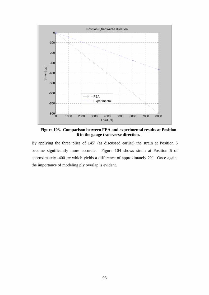
93
Figure 103. Comparison between FEA and experimental results at Position 6 in the gauge transverse direction.
By applying the three plies of ±45° (as discussed earlier) the strain at Position 6
become significantly more accurate. Figure 104 shows strain at Position 6 of
approximately -400 µε which yields a difference of approximately 2%. Once again,
the importance of modeling ply overlap is evident.
0 1000 2000 3000 4000 5000 6000 7000 8000-800
-700
-600
-500
-400
-300
-200
-100
0
Load [N]
Str
ain
[ µε]
Position 6,transverse direction
FEA
Experimental
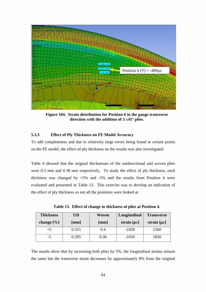
94
Figure 104. Strain distribution for Position 6 in the gauge transverse direction with the addition of 3 ±45° plies.
5.3.3 Effect of Ply Thickness on FE Model Accuracy
To add completeness and due to relatively large errors being found at certain points
on the FE model, the effect of ply thickness on the results was also investigated.
Table 4 showed that the original thicknesses of the unidirectional and woven plies
were 0.3 mm and 0.38 mm respectively. To study the effect of ply thickness, each
thickness was changed by +5% and -5% and the results from Position 4 were
evaluated and presented in Table 13. This exercise was to develop an indication of
the effect of ply thickness so not all the positions were looked at.
Table 13. Effect of change in thickness of plies at Position 4.
Thickness
change [%]
UD
[mm]
Woven
[mm]
Longitudinal
strain [µε]
Transverse
strain [µε]
+5 0.315 0.4 -1050 1560
-5 0.285 0.36 -1050 1850
The results show that by increasing both plies by 5%, the longitudinal strains remain
the same but the transverse strain decreases by approximately 8% from the original
Position 6 (T) ≈ -400µε

95
1700 µε. The transverse strain is increased by about 9% when the thicknesses are
decreased by 5%. Although not very large, the change in thickness of the plies
definitely plays a role in the results obtained in the transverse direction. Therefore
any slight error in the thickness could add to the reasons why differences were
obtained.
5.3.4 Finite Element Model – Conclusion
The finite element model shows areas of satisfactory (less than 10%) and poor
(>100%) correlation with the experimental results. The reader may consider some of
these values to be highly unacceptable and generally this opinion would be valid.
There is the need therefore for further discussion to justify the work.
It was briefly mentioned earlier that a strain gauge validation test was carried out
before testing the swingarm (see Appendix A). The aim of the validation test was to
determine if the readings obtained from the strain gauge measurement were closely
matched by the calculations carried out using classical lamination theory. As
discussed in Appendix A, the strain gauge results were compared with classical
laminate theory results using FEA in ANSYS. It was shown there that differences of
less than 2% were found for three separate tests. This is mentioned because for a very
simple carbon fibre structure it is possible to get highly accurate results. The structure
was a simple rectangular beam consisting of a number of plies at various orientations.
But when a very complex structure such as the swingarm is modelled, it seems very
challenging to obtain a finite element model of the swingarm to correlate with strain
gauge measurements. The reasons for the differences in the results have been
discussed above. These differences seem to be primarily due to ply overlap but can
also be attributed to gauge misalignment, gauge transverse sensitivity and ply
thickness. If the swingarm was made of an isotropic material, then most likely a
much higher degree of correlation would be found.
A question then could be asked: is building a finite element model the best method for
determining stress and strain distribution for such a complex composite structure?
Most analysts would say it is and for simple structures it is easy to be convinced that it
is the best method. But for a complex structure such as the carbon fibre swingarm,
unless a method is found to model the numerous overlaps occurring over the

96
swingarm, it may not be possible to obtain accurate correlation. To obtain accurate
results in certain areas of the swingarm may require the analyst to focus on a certain
section and only model that section. The strains there would need to be determined
by experimental measurement and then the forces and moments acting at that point
could be reconstructed on the FE model. Therefore instead of modelling the entire
swingarm in a more general way, a specific section could be modelled in a more
accurate way.

97
6. CONCLUSION AND RECOMMENDATIONS
6.1 Conclusions
Carbon fibre has not been extensively used in the development of motorcycle
components due to high costs and manufacturing constraints. Carbon fibre has a
higher strength/stiffness to weight ratio than materials such as steel, aluminium and
magnesium and therefore can provide better structural characteristics at lower weight.
This research report presented the first step in the design process of a carbon fibre
swingarm for a Ducati 1098 motorcycle. Using preliminary carbon fibre laminate
designs, the aim was to develop a swingarm that exhibited satisfactory strength under
typical loading conditions with reduced weight.
The literature showed that it is important to characterize the stiffness of the swingarm
for two reasons. The first is that the degree of rigidity of the swingarm affects the
response time of the motorcycle when cornering. The second is the effect that the
stiffness (specifically lateral and torsional) has on the weave mode stability of the
motorcycle. Therefore the stiffness coefficients were calculated by measuring
deflections in the vertical, lateral and torsional directions while the swingarm was
subjected to typical loads experienced in the field. Lateral and torsional stiffness
values of 445 kN/m and 550 Nm/deg respectively, were determined from the
deflection measurements. Both values are on the lower end of the spectrum when
compared with other stiffness values found in the literature. The lower lateral and
torsional stiffness values may negatively affect the weave mode stability of the
motorcycle at medium to high speeds and also cause the motorcycle to have a
sluggish response when turning. The vertical stiffness coefficient was calculated to be
500 kN/m and was deemed sufficiently rigid to not negatively affect the effective
stiffness between the chassis and wheel.
Results from the strain measurements were found to be considerably lower than the
ultimate strains for the type of laminates employed in the design. Longitudinal and
transverse strain was measured at eight positions on the swingarm. Even at high
vertical loads of 8000 N and moments about the longitudinal axis of 680 Nm (applied
separately), the measured strain did not exceed values of 1100 µε in tension or
compression. These values were well under the ultimate strain for typical

98
unidirectional and woven plies of between 5000 µε and 8000 µε. It is concluded that
the swingarm is sufficiently strong at the positions that were measured. Furthermore,
the strain measurements show that during vertical loading, there is a coupling between
vertical and torsional loading. This means that due to the asymmetric design of the
swingarm, as a vertical load is applied, there is also a twisting of the swingarm.
Results also suggest that during vertical loading, the limiting position is the side of the
top arm, Position 5. This means that during increased vertical loading, Position 5
measures the highest strain in both the longitudinal and transverse direction and will
therefore most likely fail first. Similarly, Position 6 (underside of the top arm) is the
limiting factor during torsional loading.
In terms of weight, the carbon fibre swingarm was measured to be 1.5 kg less than the
original aluminium swingarm which satisfies the requirement for a reduction in
weight.
A finite element model of the composite swingarm was developed based on the
following assumptions: not modelling ply overlap and the aluminium inserts and
simplifying the modelling to model only the major zones. In terms of deflection,
good correlation was found for the vertical deflection (less than 5%). Less accurate
results were obtained for the torsional (28%) and lateral (50%) deflection. Reasons
for the large difference in lateral deflection are most likely due to the very low
deflection measurements of less than 1 mm and not modelling ply overlap. To obtain
a higher degree of accuracy, it may be necessary to apply loads of an order of
magnitude higher for the lateral deflection.
When comparing the FE strain results with the experimental strain gauge values in
order to further validate the model, a range of differences between 0.9% and 157%
were initially found. Two areas were focused on in terms of FEA strains, namely the
bottom and top arms of the swingarm. On the lower arm two positions were
measured in the longitudinal and transverse directions. Results showed differences of
between 49% and 93% which are significantly large. This can be attributed to the
strain gauge measurements being placed in a rapidly changing strain field. For two
out of the three positions on the lower arm, accurate results (less than 10% difference)
were found within 10 mm to 20 mm from the measurement position on the FE model.
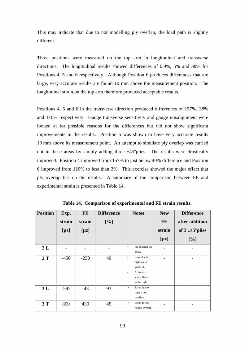
99
This may indicate that due to not modelling ply overlap, the load path is slightly
different.
Three positions were measured on the top arm in longitudinal and transverse
directions. The longitudinal results showed differences of 0.9%, 5% and 38% for
Positions 4, 5 and 6 respectively. Although Position 6 produces differences that are
large, very accurate results are found 10 mm above the measurement position. The
longitudinal strain on the top arm therefore produced acceptable results.
Positions 4, 5 and 6 in the transverse direction produced differences of 157%, 38%
and 110% respectively. Gauge transverse sensitivity and gauge misalignment were
looked at for possible reasons for the differences but did not show significant
improvements in the results. Position 5 was shown to have very accurate results
10 mm above its measurement point. An attempt to simulate ply overlap was carried
out in these areas by simply adding three ±45°plies. The results were drastically
improved. Position 4 improved from 157% to just below 40% difference and Position
6 improved from 110% to less than 2%. This exercise showed the major effect that
ply overlap has on the results. A summary of the comparison between FE and
experimental strain is presented in Table 14.
Table 14. Comparison of experimental and FE strain results.
Position Exp.
strain
[µε]
FE
strain
[µε]
Difference
[%]
Notes New
FE
strain
[µε]
Difference
after addition
of 3 ±45°plies
[%]
2 L - - - • No reading on
DAQ - -
2 T -450 -230 49 • Error due to
high strain
gradient,
• Accurate
strain 10mm
to the right
- -
3 L -592 -43 93 • Error due to
high strain
gradient
- -
3 T 850 430 49 • Error due to
no ply overlap - -

100
• Accurate
strain 15mm
below
4 L -1090 -1100 0.9 - - -
4 T 660 1700 157 • Error due to
no ply overlap
• Add 3 plies to
simulate
overlap
1000 40
5 L 1050 1100 5 - - -
5 T -870 -1200 38 • Error due to
no ply overlap
• Accurate
strain 10mm
above
- -
6 L 725 1000 38 • Error due to
no ply overlap
• Accurate
strain 10mm
above
• Add 3 plies to
simulate
overlap
- -
6 T -394 -830 110 • Error due to
no ply overlap
• Accurate
strain 10mm
above
• Add 3 plies to
simulate
overlap
400 2
6.2 Recommendations
The stiffness values of the original aluminium swingarm were not known and
although the stiffness results suggest the motorcycle will exhibit slow response and
lower stability, a clearer picture will be obtained if a direct comparison is made with
the original aluminium swingarm. Furthermore, to determine the actual response and
stability of the swingarm, there would be the need to carry out experimental testing
during motorcycle operating conditions.
With regard to the FE model, it is of vital importance that a method is devised to
accurately model ply overlap for future research. Both the torsional and lateral
deflections and the transverse strains depend highly on ply overlap. Furthermore, if

101
highly accurate results are required then it may necessitate only modelling a specific
part of the swingarm and focussing the analysis on that part alone.

102
7. REFERENCES
[1] H. Sol and W. de Wilde, “Identification of elastic properties of composite materials using resonant
frequencies,” Computational Mechanics Publications, pp. 273-280, 1988.
[2] A. Airoldi, S. Bertoli, L. Lanzi, M. Sirna and G. Sala, “Design of a motorcycle composite swing-
arm by means of multi-objective optimisation,” Appl Compos Mater, vol. 19, pp. 599-618, 2012.
[3] T. Foale, Motorcycle handling and chassis design, Spain: Tony Foale Designs, 2006.
[4] B. Madson, “Motorcycle-USA.com,” 14 August 2009. [Online]. Available:
http://www.motorcycle-usa.com/363/4336/Motorcycle-Article/2010-Sachs-MadAss-125-First-
Look.aspx?WT.i_e_dcsvid=1464738270. [Accessed 25 March 2013].
[5] G. Risitano, L. Scappaticci, C. Grimaldi and F. Mariani, “Analysis of the structural behavior of
racing motorcycle swingarms,” SAE Technical Paper 2012-01-0207, 2012.
[6] K. H. C. C. Ltd, “DIY Trade,” 23 November 2009. [Online]. Available:
http://www.diytrade.com/china/pd/6169920/alloy_swing_arm.html#normal_img. [Accessed 25
March 2013].
[7] T. Carrithers, “Motor Cyclist,” June 2011. [Online]. Available:
http://www.motorcyclistonline.com/howto/answers/122_1106_dangerous_helmets_swingarms_an
d_valve_stem_cap_questions/. [Accessed 20 February 2013 ].
[8] E. Armentani, S. Fusco and M. Pirozzi, “Numerical evaluation and experimental tests for a road
bike swingarm,” in Science and Motor Vehicles JUMV International Automotive Conference with
Exhibition, Beograd, Serbia, 2007.
[9] S. Cassani and A. Mancuso, “Shape Optimization of a High Performance Motorbike Single Sided
Swingarm,” SAE International, 2005.
[10] V. Cossalter, Motorcycle Dynamics, 2006.
[11] Unknown, “www.mindsetsonline.co.uk,” Mind Sets, 2013. [Online]. Available:
http://www.mindsetsonline.co.uk/Catalogue/ProductDetail/genuine-carbon-fibre-
sheet?productID=a00ac9d6-b444-425a-b52e-b4b6167f8181&catalogueLevelItemID=4d561b21-
7a62-4ba3-896c-cd0b2ff19840. [Accessed 19 May 2014].
[12] W. University, “Mechanics of Composite Materials, MECN 4003 Notes,” South Africa, University
of the Witwatersrand.
[13] N. O'Dea, “Motorcycle swingarm redesigned in carbon composite,” Reinforced Plastics, vol. 55,

103
no. 6, pp. 38-41, 2011.
[14] H. Iwasaki, A. Mizuta, T. Hasegawa and H. Yoshitake, “Development of a magnesium swing arm
for motorcycles,” SAE Technical Paper2004-32-0048, 2004.
[15] J. S. Hoksbergen, M. Ramalu, P. Reinhall and T. M. Briggs, “A Comparison of the vibration
characteristics of carbon fiber reinforced plastic plates with those of magnesium plates,” Appl
Compos Mater, vol. 16, pp. 263-283, 2009.
[16] R. Sullivan, “Automotive carbon fiber: opportunities and challenges,” JOM, 2006.
[17] Unknown, “www.firehole.com,” Firehole Composites Analysis Software & Services, July 2011.
[Online]. Available: http://www.firehole.com/news/quarter_02_2011/fpf.aspx. [Accessed 19 May
2014].
[18] J. Wood, “Finite element analysis of composite structures,” Composite Structures, vol. 29, pp. 219-
230, 1994.
[19] B. S. Arms, “OPP Racing,” 2013. [Online]. Available:
http://www.oppracing.com/image_display.php?image=54619&id=32189. [Accessed 25 March
2013].
[20] R. Kharul, S. Balakrishnan and D. Karedla, “Virtual testing and correlation for a motorcycle
design,” SAE Technical Paper2010-01-0925, 2010.
[21] P. Wilkinson, “The changing role of physical testing in vehicle development programmes,”
Journal of Terramechanics, vol. 44, p. 15, 2007.
[22] K. Dressler, M. Speckert and G. Bitsch, “Virtual durability test rigs for automotive engineering,”
Vehicle System Dynamics: International Journal of Vehicle Mechanics and Mobility, vol. 47, no. 4,
pp. 387-401, 2009.
[23] K. Lin, J. Chang, J. Wu, C. Chang, S. Chang, J. Hwang and C. Fung, “Durability assessments of
motorcycle handlebars,” SAE International, no. 2005-01-0801, 2005.
[24] R. Ide, T. Ogushi, Y. Sunayama, Y. Kishita and S. Watanabe, “Estimating of motorcycle frame
strength by virtual durability test,” SAE International, no. 2009-32-0143, 2009.
[25] Mira, “www.mira.co.uk,” 2014. [Online]. Available: http://www.mira.co.uk/facilities. [Accessed
21 May 2014].
[26] E. Dragoni and F. Foresti, “Design of a single-sided composite swing arm for racing motorcycles,”
Int. J. of Materials and Product Technology, vol. 13, no. 3-6, pp. 411-420, 1998.
[27] V. Cossalter, R. Lot and M. Massaro, “The influence of frame compliance and rider mobility on
104
the scooter stability,” Vehicle System Dynamics: International Journal of Vehicle Mechanics and
Mobility, vol. 45, no. 4, pp. 313-326, 2007.
[28] K. Lake, R. Thomas and O. Williams, “The influence of compliant chassis components on
motorcycle dynamics: an historical overview and the potential future impact of carbon fibre,”
Vehicle System Dynamics: International Journal of Vehicle Mechanics and Mobility, vol. 50, no. 7,
pp. 1043-1052, 2012.
[29] R. Sharp, “Research Note: The influence of frame flexibility on the lateral stability of
motorcycles,” J. Mech. Eng. Sci, vol. 16, no. 2, pp. 117-120, 1974.
[30] D. Systemes, “plmmarketplace.com,” Dassault Systemes, 2002-2013. [Online]. Available:
http://www.plmmarketplace.com/blog/CategoryView,category,Simulayt.aspx. [Accessed 21 May
2014].
[31] C. Stan, Development trends of motorcycles II, Germany: Expert Verlag, 2005.
[32] M. Tuttle and H. Brinson, “Resistance-foil strain-gage technology as applied to composite
materials,” Experimental Mechanics, vol. 24, no. 1, pp. 54-65, 1984.
[33] “Errors due to transverse sensitivity in strain gages,” M-M Tech. Note TN-509, Micro-
Measurements Division, Measurement Group, Inc., Raleigh, NC, 1982.
[34] R. Ali, “Use of finite element technique for the analysis of composite structures,” Computers &
Structures, vol. 58, no. 5, pp. 1015-1023, 1996.
[35] Z. Yinhuan, X. Ka and H. Zhigao, “Finite element analysis of composite leaf spring,” in The 6th
Internatonal Conference on Computer Science & Education, Singapore, 2011.
[36] H. Mian, G. Wang, U. Dar and W. Zhang, “Optimization of composite material system and lay-up
to achieve minimum weight pressure vessel,” Appl Compos Mat, 2012.
[37] R. Chacko, “Design and experimental validation of a carbon fibre swing arm test rig.,” University
of the Witwatersrand, Johannesburg, 2013.
[38] R. Hibbeler, “Simplification of a force and couple system,” in Engineering mechanics statics
twelfth edition in SI units, Singapore, Prentice Hall, 2010, p. 160.
[39] P. Benham, R. Crawford and C. Armstrong, Mechanics of Engineering Materials, Singapore:
Pearson Education Limited, 1996.
[40] M. Pinfold and G. Calvert, “Experimental analysis of a composite automotive suspension arm,”
Composites, vol. 25, no. 1, pp. 59-63, 1994.
[41] P. Beardmore, “Composite structures for automobiles,” Compos. Struct., vol. 5, pp. 163-176, 1986.

105
[42] G. Smith, “Design and production of composites in the automotive industries,” Compos. Manuf,
vol. 1, no. 2, pp. 112-116, 1990.
[43] K. Edwards, “Strategic substitution of new materials for old: applications in automotive product
development,” Materials and Design, vol. 25, no. 6, pp. 529-533, 2004.
[44] T. Foale, Motorcycle handling and chassis design, Tony Foale Designs, 2006.

106
Appendix A Strain Gauge Validation
Prior to applying strain gauges to the swingarm, it was necessary to compare results
from a basic strain gauge application with results using classical laminate theory. A
carbon fibre plate consisting of a number of plies of various types and orientations
was fixed at one end and a load was applied at the other end as shown in Figure 105.
Figure 105. Rig setup for testing the carbon fibre plate.
The plate that was used, closely resembled one of the main layups used in the
swingarm but the details are withheld here.
A load was applied toward the end of the beam which would cause a maximum
bending moment near the fixed side (as well as a constant shear force along the plate).
An axial strain gauge (see Figure 106) was mounted near the fixed end of the plate
and the strain along the length of the plate was measured.
Load
Plate
Fixed end

107
Figure 106. Axial strain gauge applied near the fixed end of the plate.
The length, width and height of the plate were 200 mm, 50 mm and 5 mm
respectively. As a further validation test, it was decided to use ANSYS Composite
PrepPost to calculate the strain based on classical laminate theory and at the same
time determine the accuracy of ANSYS Composite.. Three tests were carried out with
increasing load applied at the end of the beam. The load and the measured strain are
presented in Table 15.
Table 15. Load applied to cantilever plate and the resultant axial strain from experimental setup.
Load [N] Measured strain [µε]
34.8 509
79 1117
123 1732
Thereafter, the carbon fibre plate was built in ANSYS Composite PrepPost and the
same constraints and loads were applied to the model. Figure 107 shows the plate
with the applied force at one end and a fixed support at the other end.
Axial strain gauge

108
Figure 107. Constraints applied to the carbon fibre plate created in Ansys Composite.
Figure 108 presents the strain along the plate in graphical form after the first load of
35 N was applied.
Figure 108. Graphical FEA results for the cantilever plate.
Figure 109 shows the strain of 499 µε calculated at the same position as the strain
gauge.

109
Figure 109. Longitudinal strain of 499 µε obtained from Ansys Composite.
Table 16 shows that the FEA which utilizes classical laminate theory, calculated
results within 2% of the measured strain. The remaining two measurement values
were also compared and both had differences of less than 2%
Table 16. Comparison between the measured strain and the strain calculated by ANSYS.
Measured strain [µε] FEA [µε] % difference
509 499 2
1117 1125 1
1732 1757 1.5
The experimental strain results very closely match the classical laminate theory results
and this exercise also shows a degree of confidence in the results calculated by
ANSYS Composite. It was therefore felt that the results were validated.

110
Appendix B Load Cell Calibration
A 50kN load cell was used during the testing to read the applied loads. The following
presents the calibration of the load cell unit. The load cell was attached to a crane via
a steel chain as shown in Figure 110.
Figure 110. Top part of the load cell calibration rig showing the load cell attached to the portable crane via a steel chain.
A basket was hung from the load cell via a belt as shown in Figure 111. Known
weights were placed inside the basket to apply the loads and the value shown on the
load cell display was read. Table 17 presents the total mass applied to the load cell
and also the load cell readings.
50 kN load cell
Steel chain
Crane

111
Figure 111. Basket carrying weights applying a load to the load cell.
Table 17. Calibration values for the 50kN load cell.
Description Total mass [kg] Load cell reading [kg]
Basket + belt 3.91 4
31.3 35.2 34
31.25 66.5 68
31.3 97.8 100
31.4 129.2 131
31.4 160.6 162
31.4 192 193
31.4 223.4 225
31.5 254.9 255
31.4 286.3 288
Figure 112 shows the calibration graph together with a linear trendline. The trendline
indicates what the load cell will display if a given mass is applied.
Load cell
Belt
Basket
Weights
Load cell
display

112
Figure 112. Calibration curve for the 50kN load cell.
More importantly, to know what the actual force is when a value is read off the load
cell display, the axes were simply inverted and the equation y = 0.995x – 0.33 was
obtained. This means that if the load cell reads 100kg for example, then the actual
load will be y = 0.995(100) – 0.33 = 99.17kg. This allows for adjusting the load until
the correct loading is applied.
y = 1.0046x + 0.345
0
50
100
150
200
250
300
350
-50 0 50 100 150 200 250 300 350
Loa
d c
ell
re
ad
ing
[k
g]
Applied force [kg)

113
Appendix C Ply Overlap
Ply overlap occurs when two adjacent plies are mounted on each other as shown in
Figure 113.
Figure 113. Schematic of plies overlapping each other.
This method was not used when creating the finite element model in ANSYS
Composite due to the difficulty of modelling the overlap. Therefore in the areas
where ply overlap exist, the method used was to model the adjacent plies as shown in
Figure 114.
Figure 114. Adjacent plies without ply overlap.
Overlap

114
Appendix D Strain Gauge Positions and NI Data
Acquisition System
The following figures show the positioning of the strain gauges.
Figure 115. Strain Gauge 1
Figure 116. Strain Gauge 1.
Strain gauge 1
Longitudinal
Transverse

115
Figure 117. Strain Gauge 2.
Figure 118. Strain Gauge 2.
Strain Gauge 2
Longitudinal
Transverse

116
Figure 119. Strain Gauge 3.
Figure 120. Strain Gauge 3.
Strain Gauge 3
Longitudinal
Transverse

117
Figure 121. Strain Gauge 4.
Strain Gauge 4

118
Figure 122. Strain Gauge 4.
Transverse
Longitudinal

119
Figure 123. Strain Gauge 5.
Figure 124. Strain Gauge 5.
Strain Gauge 5
Longitudinal
Transverse

120
Figure 125. Strain Gauge 6.
Figure 126. Strain Gauge 6.
Longitudinal
Transverse
Strain Gauge 6

121
Figure 127. Strain Gauges 7 & 8.
Figure 128. Strain Gauge 7.
Gauge 7
Gauge 8
Transverse
Longitudinal

122
Figure 129. Strain Gauge 8.
Longitudinal
Transverse

123
Figure 130. NI data acquisition system connected to the strain gauges on the swingarm.

124
Appendix E Test Rig Modification Calculations and
Drawings
The design and manufacture of the test rig can be seen in Chacko [37]. However
modifications were made to the rig in order to apply torsional loading. A steel shaft
was designed that would act as a moment arm to apply a moment to the wheel mount
of the swingarm. The arm would be subjected to a maximum load of 2000 N at the
top end. The length of the arm from the load application point to the top of the wheel
mount is approximately 250 mm. Therefore the maximum moment calculated at the
wheel mount is given in Equation A.1
=
= 2000 × 0.25
= 500!"
(A.1)
The maximum bending stress in the shaft is calculated in Equation A.2.
# =
$
%
=$
&'
64
=(500)(0.3)
&(0.6)'
64
= 235.7*+
(A.2)
Where: σ = Stress due to bending [MPa]
y = Maximum distance from neutral axis [m]
I = Second moment of area of shaft [m4]
d = Diameter of shaft [m]
The maximum stress of 235.7 MPa is below the yield strength of 250 MPa for steel
therefore the shaft is thick enough. The design drawings of the shaft is shown in
Figures 131 to 133.

125
Figure 131. Isometric view of the top part of the steel shaft.

126
Figure 132. Top part of the steel shaft.

127
Figure 133. Bottom part of steel shaft.

128
Appendix F Mesh Dependency
The effect that the mesh has on the results is presented in this section. Figures 134 to
136 present the strain at Position 4 on the finite element model at decreasing element
sizes. Figure 134 shows a strain of -1164 µε using element sizes of 5 mm.
Figure 134. Position 4 with element size of 5 mm.
Figure 135 shows strain of -1164 µε at Position 4 using element sizes of 3 mm.
Figure 135. Position 4 with element size of 3 mm.
-1162 µε
-1164 µε

129
Figure 136 shows strain at Position 4 of -1162 µε with an element size of 1 mm.
Figure 136. Position 4 with element size of 1 mm.
It can be seen that as the mesh is refined, the results do not significantly change
(Table 18). The percentage difference between the strain using element sizes of 5 mm
and 3 mm is ((1162-1164)/1162) x 100 = -0.172 % which is negligible. The
percentage strain difference between the 3 mm and 1 mm element size mesh is
((11640-11626)/1164) x 100 = 0.12 % which also is negligible. This exercise shows
the results are mesh independent.
Table 18. Mesh sensitivity.
Element size [mm] 5 3 1
Strain [µε] 1162.0 1164.0 1162.6
-1162 µε