Development, Modeling And Control of A Humanoid Robot Masters Thesis upload.pdf · This master’s...
298
Master’s Thesis Jens Christensen - Jesper Lundgaard Nielsen Mads Sølver Svendsen - Peter Falkesgaard Ørts Aalborg University 2007 Development, Modeling And Control of A Humanoid Robot
Transcript of Development, Modeling And Control of A Humanoid Robot Masters Thesis upload.pdf · This master’s...

Master’s ThesisJens Christensen - Jesper Lundgaard Nielsen
Mads Sølver Svendsen - Peter Falkesgaard ØrtsAalborg University 2007
Development, Modeling And Control of
A Humanoid Robot

AALBORG UNIVERSITY
DEPARTMENT OF ELECTRONIC SYSTEMS
SECTION OF AUTOMATION AND CONTROL
DEVELOPMENT, MODELING AND CONTROL OF
A HUMANOID ROBOT
INTELLIGENT AUTONOMOUS SYSTEMS
GROUP 1033
MASTER’S THESIS - SPRING 2007
JENS CHRISTENSEN - JESPER LUNDGAARD NIELSEN
MADS SØLVER SVENDSEN - PETER FALKESGAARD ØRTS


Department of Electronic SystemsFredrik Bajers Vej 7 A19220 Aalborg, DenmarkPhone: +45 96358600Web: http://es.aau.dk/
TITLE: Development, Modeling and
Control of a Humanoid Robot
PROJECT SEMESTER:
9th and 10th semester, 4th
September 2006 - 7th June
2007
PROJECT GROUP:
1033
GROUP MEMBERS:
Jens Christensen
Jesper L. Nielsen
Mads S. Svendsen
Peter F. Ørts
SUPERVISORS:
Jan Helbo
Dan D. V. Bhanderi
NUMBER OF COPIES:
14
NUMBER OF PAGES THESIS:
164
TOTAL NUMBER OF PAGES:
277
APPENDED DOCUMENTS:
1 CD-ROM
FINISHED:
7th June 2007
ABSTRACT:
This master’s thesis concerns the development,
modeling and control of a humanoid robot,
which enables human-like walk.
As the focus is to obtain human-like walk, the
robot is designed to resemble human propor-
tions and a special joint has been developed to
resemble the hip joint of humans, and thereby
enabling walking in curved paths. Further-
more the hardware necessary to obtain a fully
autonomous system is developed and imple-
mented. The result of the design phase is a
humanoid robot, called ”Roberto”, measuring
58 cm and with 21 actuated degrees of freedom.
A complete dynamical model describing the
system has been developed. The model is a hy-
brid model which enables simulation of com-
plete walking cycles. A novel solution of the
dynamics of the robot during double support
phase has been given.
To enable human-like walk a set of trajectories
has been developed, based on the zero-moment
point and dynamical simulations. The trajecto-
ries are simulated, and human-like walk is ob-
tain on the model. To maintain stability dur-
ing walk with the real robot, two controllers
have been developed, a posture controller and
a zero-moment point controller. It was found
that the controllers were able to track a zero-
moment point reference and a inclination refer-
ence given to the system.
Human-like walk was not obtained on the real
system, due to system limitations. If a new in-
terface to the DC-motors in the servos was de-
veloped, and a faster on-board computer was
chosen, human-like walk should be possible.


Institut for Electroniske SystemerFredrik Bajers Vej 7 A19220 Aalborg ØTlf: +45 96358600Web: http://es.aau.dk/
TITEL: Development, Modeling and
Control of a Humanoid Robot
PROJEKTPERIODE:
9. og 10. semester,
4. september 2006 - 7. juni
2007
PROJEKTGRUPPE:
1033
GRUPPE MEDLEMMER:
Jens Christensen
Jesper L. Nielsen
Mads S. Svendsen
Peter F. Ørts
VEJLEDERE:
Jan Helbo
Dan D. V. Bhanderi
ANTAL KOPIER:
14
SIDER I HOVEDRAPPORT:
164
SIDER IALT:
277
BILAG:
1 CD-ROM
AFSLUTTET:
7. juni 2007
SYNOPSIS:
Dette speciale omhandler udvikling, modeller-
ing og kontrol af en menneskelignende robot,
hvorpa menneskelignende gang ønskes imple-
menteret.
Der er i dette speciale fokuseret pa at opna men-
neskelig gang og robotten er derfor designet
med menneskelige proportioner. Dertil er et
specielt led blevet konstrueret, der ligner den
menneskelige hofteskal og giver robotten mu-
lighed for at dreje under gang. Der er yder-
mere udviklet og implementeret hardware, der
gør robotten fuldt ud autonom. Resultatet er en
menneskelignende robot, kaldet ”Roberto”, der
er 58 cm høj og har 21 aktuerede frihedsgrader.
Der er blevet udviklet en komplet dynamisk
model, som beskriver alle input og output af
systemet. Modellen en hybrid model, der
muliggører simulering af en komplette gang
cykler. En ny løsning er blevet foreslaet, der
beskriver dynamikken af robotten, nar den har
begge ben pa jorden.
Et sæt af menneskelignende gangtrajektorier er
blevet udviklet, som er baseret pa zero-moment
point og dynamiske simuleringer. Disse trajek-
torier er blevet simuleret og menneskelig gang
blev opnaet pa modellen. For at opretholde sta-
bilitet under gang, med den udviklede robot,
er to regulatorer blevet designet. Disse kon-
trollerer kropsholdningen samt positionen af
zero-moment point. Regulatorerne var i stand
til at følge en reference, bade et zero-moment
point og en given orientering.
Menneskelig gang blev ikke opnaet pa den
rigtige robot, grundet begrænsninger i systemet.
Det blev vurderet, at hvis der blev konstrueret
et nyt interface print til DC-motoren inde i ser-
voerne, ville dette give bedre resultater. Yder-
mere blev det anbefalet at implementere en hur-
tigere computer pa robotten. Med disse op-
graderinger skulle det være muligt at opna men-
neskelig gang med robotten.


PREFACE
This master’s thesis is written at the Department of Electronic Systems at the Section
of Automation and Control at Aalborg University, under the Master’s program ”Intel-
ligent Autonomous Systems”.
It is the documentation of the work performed by the group members in their 9th and
10th semester. A part of the project was to construct a humanoid robot. This new hu-
manoid robot was named ”Roberto”. In order to investigate the area of biped robotics,
the group members have been on a study trip to Tokyo. This included, among others,
a visit to the University of Tokyo and a visit to their robotic laboratory.
Throughout this project, MATLAB has been used for capturing, processing and rep-
resentation of data, specifically MATLAB version 7.3, R2006b. Simulink version 6.5,
R2006b has been used for building the model and for making an interface to the robot.
SolidWorks 2006, SP0.0 has been used to design the mechanical parts of the robot,
and to retrieve all kinematic information. The mechanical design can be found on the
enclosed CD-ROM. Maple 10, has been used for large algebraic computations and for
optimization of the equations used in the model.
References to literature will be done using the Harvard method. Throughout the thesis
figures, tables and equations are numbered consecutively inside each chapter. When-
ever an illustration can be made more expressive, a red colour is used to represents the
left side and a green colour for the right side, as used in maritime navigation.
On the last page, a CD-ROM is enclosed, which contains literature, model files, draw-
ings of the robot etc. A complete description of the contents on the CD-ROM can be
found in Appendix O on page 277. Furthermore a list of the acronyms used throughout
this thesis can be found in Appendix N on Page 275.
Aalborg University, 2007
Jens Christensen Jesper L. Nielsen
Mads S. Svendsen Peter F. Ørts
Group 1033 VII


TABLE OF CONTENTS
List of Figures XVII
List of Tables XIX
1 Introduction 1
1.1 Background 1
1.2 Thesis Outline 3
2 Conceptual Knowledge 5
2.1 Representation 6
2.2 Humanoid Robots Locomotion 6
2.3 Stability 7
3 Analysis of Human Gait 13
3.1 Human Gait 14
3.2 Posture During Straight Gait 16
3.3 Curved Gait 18
3.4 Thesis Objectives 20
4 Mechanics 21
4.1 Introduction to Mechanical Design 22
4.2 Description of the Human Body 22
4.3 Multi Degree of Freedom Joint 24
4.4 Torso 26
4.5 Dimensioning the Limbs 27
4.6 Partial Conclusion to Mechanical Design 32
5 Hardware 33
5.1 Hardware Overview 34
5.2 Sensor Determination 35
5.3 Actuators 36
5.4 Choosing an On-board Computer 40
5.5 Description of the Interface print 41
5.6 Battery Pack and Voltage Monitor Circuit 43
5.7 Partial Conclusion to Hardware 44
Group 1033 IX
TABLE OF CONTENTS
6 Software 47
6.1 System Overview 48
6.2 I/O Drivers 49
6.3 High Level Interfacing 56
6.4 Partial Conclusion to Software 60
7 Modeling 61
7.1 Introduction to Modeling 63
7.2 Servo Motor Model 67
7.3 Kinematic Model 71
7.4 Dynamical Model 79
7.5 Phase Estimator 86
7.6 Foot Model 92
7.7 Head Model 96
7.8 Partial Conclusion to Modeling 99
8 Inverse Kinematics 101
8.1 Closed Form Solution to the Inverse Kinematic Problem 103
8.2 Partial Conclusion to Inverse Kinematics 108
9 Trajectory Generation 109
9.1 Trajectory Generation Methods 110
9.2 Establishing the Trajectories 114
9.3 Simulation of Trajectories 122
9.4 Resulting Trajectories 125
9.5 Conclusion on Trajectory Generation 128
10 Controlling the Biped Robot 133
10.1 Control Design Approach 135
10.2 Estimation of Control Input 135
10.3 Inverse ZMP Controller 146
10.4 ZMP Controller 148
10.5 Hybrid Posture Controller 152
10.6 Partial Conclusion to Control 156
11 Epilogue 159
11.1 Discussion 160
11.2 Conclusion 163
Bibliography 165
X Aalborg University 2007
TABLE OF CONTENTS
Appendix 171
A Servo Controller Board 173
B Feedback from Servo Motors 175
C Hardware Wiring Description 185
D Strain Gauges Print 191
E Motivating Examples for Model 195
F Modeling Verification 203
G Numerical Solution to Inverse Kinematics 233
H Verification of the Inverse Kinematic Model 237
I Trajectories 243
J Verification of the ZMP Estimators 255
K Controller Simulation and Verification 261
L Joint Limitations 271
M Drawing of Complete Robot 273
N Acronyms 275
O CD Contents 277
Group 1033 XI

LIST OF FIGURES
Figure 1.1 Three different biped robots. . . . . . . . . . . . . . . . . . . 1
Figure 1.2 A picture of the group members at the University of Tokyo. . . 2
Figure 1.3 Exploded view of the developed humanoid. . . . . . . . . . . . 3
Figure 2.1 Global reference frame and planes of motion. . . . . . . . . . 6
Figure 2.2 The PoS is the convex hull of all contact points. . . . . . . . . 8
Figure 2.3 Top view of the foot. . . . . . . . . . . . . . . . . . . . . . . . 11
Figure 3.1 The human motion control division. . . . . . . . . . . . . . . 14
Figure 3.2 The human motion cycle. . . . . . . . . . . . . . . . . . . . . 15
Figure 3.3 Sagittal view of a gait cycle. . . . . . . . . . . . . . . . . . . . 18
Figure 3.4 Frontal view of a gait cycle. . . . . . . . . . . . . . . . . . . . 18
Figure 3.5 Walking along a curved path. . . . . . . . . . . . . . . . . . . 19
Figure 4.1 Leonardo da Vinci’s Vitruvian Man . . . . . . . . . . . . . . . 22
Figure 4.2 Multi DoF joint placement . . . . . . . . . . . . . . . . . . . 24
Figure 4.3 Three different joint designs . . . . . . . . . . . . . . . . . . . 24
Figure 4.4 Mechanical levers principle . . . . . . . . . . . . . . . . . . . 25
Figure 4.5 Torso placement . . . . . . . . . . . . . . . . . . . . . . . . . 26
Figure 4.6 Exploded view of torso . . . . . . . . . . . . . . . . . . . . . 26
Figure 4.7 Close up of shaft in torso . . . . . . . . . . . . . . . . . . . . 27
Figure 4.8 Connection of the limbs . . . . . . . . . . . . . . . . . . . . . 28
Figure 4.9 Drawing of the leg . . . . . . . . . . . . . . . . . . . . . . . . 29
Figure 4.10 Drawing of the arm . . . . . . . . . . . . . . . . . . . . . . . 30
Figure 4.11 Exploded view of the foot . . . . . . . . . . . . . . . . . . . 31
Figure 5.1 Hardware overview, showing the entire system. . . . . . . . . 34
Figure 5.2 Picture of the right foot with strain gauge print. . . . . . . . . 36
Figure 5.3 Picture of the head with the IMU. . . . . . . . . . . . . . . . . 37
Figure 5.4 The control signal to the servo motors. . . . . . . . . . . . . . 38
Figure 5.5 Measurement from the potentiometer. . . . . . . . . . . . . . . 39
Figure 5.6 The realization of the Sallen and Key filter. . . . . . . . . . . . 40
Figure 5.7 Picture of the on-board computer and the interface print. . . . . 41
Figure 5.8 LiPo battery recharging setup. . . . . . . . . . . . . . . . . . . 44
Figure 6.1 Description of the system. . . . . . . . . . . . . . . . . . . . . 48
Figure 6.2 The routines that run when using the system. . . . . . . . . . . 50
Figure 6.3 The different parts of the software system layer. . . . . . . . . 51
Figure 6.4 Connection of multiplexers to the on-board computer. . . . . . 52
Figure 6.5 The sequence called for reading all the sensors. . . . . . . . . 53
Figure 6.6 The flow of the functions used to update the servos. . . . . . . 57
Figure 6.7 Parallel execution. . . . . . . . . . . . . . . . . . . . . . . . . 57
Group 1033 XIII

LIST OF FIGURES
Figure 7.1 Open chain robot in sagittal plan . . . . . . . . . . . . . . . . 63
Figure 7.2 Closed chain robot in sagittal plan . . . . . . . . . . . . . . . 63
Figure 7.3 Complete model I/O . . . . . . . . . . . . . . . . . . . . . . . 66
Figure 7.4 Complete model I/O - extended . . . . . . . . . . . . . . . . . 66
Figure 7.5 I/O Servo motor model . . . . . . . . . . . . . . . . . . . . . 68
Figure 7.6 State space servo motor model . . . . . . . . . . . . . . . . . 68
Figure 7.7 Servo motor parameter estimation . . . . . . . . . . . . . . . . 70
Figure 7.8 Torque and maximum velocity relationship . . . . . . . . . . . 70
Figure 7.9 Results for servo motor test . . . . . . . . . . . . . . . . . . . 71
Figure 7.10 Kinematic model I/O . . . . . . . . . . . . . . . . . . . . . . 72
Figure 7.11 Kinematic definitions . . . . . . . . . . . . . . . . . . . . . 73
Figure 7.12 Definition of angles . . . . . . . . . . . . . . . . . . . . . . 75
Figure 7.13 Frame representation in SSP-R . . . . . . . . . . . . . . . . 76
Figure 7.14 Result of the kinematic test of the left hand . . . . . . . . . . 79
Figure 7.15 Dynamic Model I/O . . . . . . . . . . . . . . . . . . . . . . 80
Figure 7.16 Forces acting on the robot in DSP . . . . . . . . . . . . . . . 85
Figure 7.17 Results dynamical leg model test - Strain gauges right . . . . 87
Figure 7.18 Phase estimator I/O . . . . . . . . . . . . . . . . . . . . . . . 87
Figure 7.19 Kinematic interpretation in SSP-R and SSP-L . . . . . . . . . 88
Figure 7.20 Calculating weight distribution . . . . . . . . . . . . . . . . 91
Figure 7.21 Isometric view of foot . . . . . . . . . . . . . . . . . . . . . 92
Figure 7.22 Foot model I/O . . . . . . . . . . . . . . . . . . . . . . . . . 92
Figure 7.23 Placement of CoM in foot . . . . . . . . . . . . . . . . . . . 93
Figure 7.24 Placement of frame 1 in foot . . . . . . . . . . . . . . . . 93
Figure 7.25 Frontal view of foot . . . . . . . . . . . . . . . . . . . . . . 94
Figure 7.26 Sagittal view of the foot . . . . . . . . . . . . . . . . . . . . 94
Figure 7.27 Verification foot model results . . . . . . . . . . . . . . . . . 96
Figure 7.28 Head model I/O . . . . . . . . . . . . . . . . . . . . . . . . 96
Figure 7.29 Placement of IMU in head . . . . . . . . . . . . . . . . . . . 97
Figure 7.30 Results head model verification . . . . . . . . . . . . . . . . 98
Figure 7.31 Effect of movement of coordinate origin . . . . . . . . . . . . 99
Figure 8.1 Inputs and output relations of the inverse kinematic model. . . 102
Figure 8.2 Position vectors in the inverse kinemeatics. . . . . . . . . . . . 103
Figure 8.3 Position vectors in the inverse kinematics. . . . . . . . . . . . 104
Figure 9.1 Principle of using an inverted pendulum to generate trajectories. 112
Figure 9.2 Stable region and ZMP. . . . . . . . . . . . . . . . . . . . . . 115
Figure 9.3 Stability measure. . . . . . . . . . . . . . . . . . . . . . . . . 116
Figure 9.4 Illustration of the walking cycle in the sagittal plane. . . . . . . 117
Figure 9.5 Illustration of the walking cycle in the frontal plane. . . . . . . 120
Figure 9.6 Plot of the stability index. . . . . . . . . . . . . . . . . . . . . 123
Figure 9.7 Power consumption, PoS and ZMP, in sagittal plane. . . . . . . 124
Figure 9.8 The stability index for torso in frontal plane. . . . . . . . . . . 124
Figure 9.9 Power consumption, PoS and ZMP, in frontal plane. . . . . . . 125
XIV Aalborg University 2007
LIST OF FIGURES
Figure 9.10 Trajectories for the right and left foot. . . . . . . . . . . . . . 126
Figure 9.11 Trajectories for the right and left foot in sagittal plane. . . . . 126
Figure 9.12 Trajectories for the torso. . . . . . . . . . . . . . . . . . . . . 127
Figure 9.13 Trajectory for the torso shown in the three planes. . . . . . . 129
Figure 9.14 Behavior of ZMP with 40 Hz. . . . . . . . . . . . . . . . . . 129
Figure 9.15 Behavior of the ZMP with four different frequencies. . . . . . 130
Figure 9.16 Slower walking trajectories, joint three. . . . . . . . . . . . . 131
Figure 10.1 Overview of the control strategy used in the project. . . . . . 135
Figure 10.2 Overview of the estimators used in the project. . . . . . . . . 136
Figure 10.3 Input and output of the phase estimator. . . . . . . . . . . . . 136
Figure 10.4 Input/output relation of the ZMP estimator. . . . . . . . . . . 137
Figure 10.5 Simplified ZMP estimated comparred with real ZMP. . . . . . 138
Figure 10.6 Estimating the ZMP using position and acceleration of torso. . 138
Figure 10.7 Inputs and output of attitude estimator. . . . . . . . . . . . . 140
Figure 10.8 Test setup for recording data from the IMU. . . . . . . . . . . 142
Figure 10.9 Signal from the gyro used to estimate the inclination. . . . . . 143
Figure 10.10 Rotation about the x-axis estimated using the accelerometer. 143
Figure 10.11 Implemented filter, used for the inclination estimator. . . . . 145
Figure 10.12 Estimated and actual inclination using sensor fusion. . . . . 146
Figure 10.13 Concept of the ZMP controller. . . . . . . . . . . . . . . . . 148
Figure 10.14 A standard PI-controller. . . . . . . . . . . . . . . . . . . . 149
Figure 10.15 Implementation of two PI-controllers for ZMP control. . . . 149
Figure 10.16 ZMP controller simulation in DSP along the y-axis. . . . . . 151
Figure 10.17 Overview of the posture controller. . . . . . . . . . . . . . . 152
Figure 10.18 Biped with backlash problem in SSP. . . . . . . . . . . . . . 154
Figure 10.19 Posture controller used for SSP. . . . . . . . . . . . . . . . 154
Figure 11.1 Wobbling effect of the foot. . . . . . . . . . . . . . . . . . . 161
Figure A.1 The Pololu Micro Serial Servo Controller. . . . . . . . . . . . 174
Figure B.1 Access to potentiometers inside servo. . . . . . . . . . . . . . 176
Figure B.2 Measurement from the potentiometer. . . . . . . . . . . . . . 177
Figure B.3 Measurement test circuit for the servo motor. . . . . . . . . . 177
Figure B.4 FFT of servo signal. . . . . . . . . . . . . . . . . . . . . . . . 178
Figure B.5 Bode plot of servo filter. . . . . . . . . . . . . . . . . . . . . 179
Figure B.6 Before and after applying the filter implemented in MATLAB . 180
Figure B.7 A low-pass Sallen and Key Filter. . . . . . . . . . . . . . . . . 181
Figure B.8 Before and after filter realization in hardware. . . . . . . . . . 182
Figure B.9 An FFT on the unfiltered and the filtered measurement. . . . . 183
Figure B.10 The realization of the Sallen and Key filter. . . . . . . . . . . 183
Figure C.1 Schematic showing the wiring of the main power cords. . . . . 185
Figure C.2 Placement of DC-connectors and main switches. . . . . . . . . 186
Figure C.3 Definition of servo names, where S is short servo. . . . . . . . 188
Group 1033 XV
LIST OF FIGURES
Figure C.4 Silk screen of the PCB showing the placement of connectors . 190
Figure D.1 Strain gauge print. . . . . . . . . . . . . . . . . . . . . . . . . 191
Figure D.2 The middle strain plate on the foot. . . . . . . . . . . . . . . . 193
Figure D.3 The measured data from the FDSS along with the fitted line. . 193
Figure E.1 Motivating example definitions . . . . . . . . . . . . . . . . . 195
Figure E.2 Motivating example virtual links . . . . . . . . . . . . . . . . 198
Figure E.3 Motivating example ground reaction force . . . . . . . . . . . 200
Figure F.1 Order of model verification . . . . . . . . . . . . . . . . . . . 204
Figure F.2 Servo motor model I/O . . . . . . . . . . . . . . . . . . . . . 205
Figure F.3 Results servo test - HSR-5995TG . . . . . . . . . . . . . . . . 206
Figure F.4 Results servo test - HS-645MG . . . . . . . . . . . . . . . . . 207
Figure F.5 Foot model I/O . . . . . . . . . . . . . . . . . . . . . . . . . . 207
Figure F.6 Foot model test setup . . . . . . . . . . . . . . . . . . . . . . 208
Figure F.7 Input to the foot model test . . . . . . . . . . . . . . . . . . . 209
Figure F.8 Numeration of the strain gauges . . . . . . . . . . . . . . . . . 209
Figure F.9 Foot model test result . . . . . . . . . . . . . . . . . . . . . . 210
Figure F.10 Effect of movement of coordinate origin . . . . . . . . . . . . 211
Figure F.11 Kinematic model I/O . . . . . . . . . . . . . . . . . . . . . . 212
Figure F.12 Kinematic chains . . . . . . . . . . . . . . . . . . . . . . . . 213
Figure F.13 Animation used in the kinematic leg test . . . . . . . . . . . . 213
Figure F.14 Animation used in the kinematic arm test . . . . . . . . . . . 214
Figure F.15 Positioning of accelerometers in the kinematic test . . . . . . 215
Figure F.16 Result of the kinematic test of the left hand . . . . . . . . . . 215
Figure F.17 Result of the kinematic test of the right hand . . . . . . . . . 216
Figure F.18 Result of the kinematic test of the left leg . . . . . . . . . . . 217
Figure F.19 Result of the kinematic test of the right leg . . . . . . . . . . 217
Figure F.20 I/O head model . . . . . . . . . . . . . . . . . . . . . . . . . 218
Figure F.21 Animation of movements in head model test . . . . . . . . . 219
Figure F.22 Acceleration results head model test . . . . . . . . . . . . . . 220
Figure F.23 Angular velocity results head model test . . . . . . . . . . . . 220
Figure F.24 I/O dynamical model . . . . . . . . . . . . . . . . . . . . . . 221
Figure F.25 Movements used in dynamical leg test . . . . . . . . . . . . . 222
Figure F.26 Movements in dynamical arm test . . . . . . . . . . . . . . . 222
Figure F.27 Results dynamical leg model test - Strain gauges right . . . . 223
Figure F.28 Results dynamical leg model test - Strain gauges left . . . . . 223
Figure F.29 Results dynamical arm model test - Strain gauges right . . . . 224
Figure F.30 Results dynamical arm model test - Strain gauges left . . . . . 225
Figure F.31 Complete model I/O . . . . . . . . . . . . . . . . . . . . . . 226
Figure F.32 Movements used in the complete model test . . . . . . . . . . 226
Figure F.33 Complete model test results - Servo 1..6 . . . . . . . . . . . . 227
Figure F.34 Complete model test results - Servo 7..12 . . . . . . . . . . . 228
Figure F.35 Results complete model test - Strain gauges right foot . . . . 229
Figure F.36 Results complete model test - Strain gauges left foot . . . . . 229
XVI Aalborg University 2007

LIST OF FIGURES
Figure F.37 Results complete model test - IMU rotation . . . . . . . . . . 230
Figure F.38 Results complete model test - IMU acceleration . . . . . . . . 231
Figure G.1 Input for numerical solution for inverse kinematics. . . . . . . 234
Figure G.2 The squared error for 100 iteration. . . . . . . . . . . . . . . . 236
Figure H.1 I/O inverse kinematic model . . . . . . . . . . . . . . . . . . 237
Figure H.2 Test setup inverse kinematic model test . . . . . . . . . . . . 238
Figure H.3 Movements used in the inverse kinematic test . . . . . . . . . 238
Figure H.4 Results inverse kinematic test - Torso Position . . . . . . . . . 239
Figure H.5 Results inverse kinematic test - Right hand position . . . . . . 240
Figure H.6 Results inverse kinematic test - Left hand position . . . . . . . 240
Figure H.7 Results inverse kinematic test - Torso orientation . . . . . . . 241
Figure I.1 Illustration of the start-up phase. . . . . . . . . . . . . . . . . . 244
Figure I.2 Stability and xZMP for start-up. . . . . . . . . . . . . . . . . . 245
Figure I.3 Stability and yZMP for start-up. . . . . . . . . . . . . . . . . . . 246
Figure I.4 Illustration of the stop phase. . . . . . . . . . . . . . . . . . . 247
Figure I.5 Stability and xZMP for stop phase. . . . . . . . . . . . . . . . . 247
Figure I.6 Stability and yZMP for stop phase. . . . . . . . . . . . . . . . . 248
Figure I.7 Implementation of the trajectories. . . . . . . . . . . . . . . . 250
Figure I.8 Slow trajectories for the feet. . . . . . . . . . . . . . . . . . . 252
Figure I.9 Slow trajectories for the torso. . . . . . . . . . . . . . . . . . . 253
Figure J.1 Movements of the robot in sagittal plane. . . . . . . . . . . . . 256
Figure J.2 Movements of the robot in sagittal plane. . . . . . . . . . . . . 256
Figure J.3 ZMP estimate using the accelerometer in test 1. . . . . . . . . 257
Figure J.4 ZMP estimate using the accelerometer in test 2. . . . . . . . . 258
Figure J.5 Measured angles from the servo motors. . . . . . . . . . . . . 258
Figure J.6 ZMP estimate using the pressure sensors in test 1. . . . . . . . 259
Figure J.7 ZMP estimate using the pressure sensors in test 2. . . . . . . . 259
Figure K.1 ZMP controller simulation in DSP along the x-axis. . . . . . . 262
Figure K.2 ZMP controller simulation in DSP along the y-axis. . . . . . . 262
Figure K.3 ZMP controller simulation in SSP along the x-axis. . . . . . . 263
Figure K.4 ZMP controller simulation in SSP along the y-axis. . . . . . . 263
Figure K.5 ZMP controller verification in DSP along the x-axis. . . . . . 264
Figure K.6 ZMP controller simulation in DSP along the y-axis. . . . . . . 265
Figure K.7 Posture controller simulation in DSP, about the x-axis. . . . . 266
Figure K.8 Posture controller simulation in DSP, about the y-axis. . . . . 267
Figure K.9 Posture controller simulation in SSP, about the x-axis. . . . . . 267
Figure K.10 Posture controller simulation in SSP, about the y-axis. . . . . 268
Figure K.11 Posture controller verification in DSP, about the x-axis. . . . 269
Figure K.12 Posture controller verification in DSP, about the y-axis. . . . 270
Group 1033 XVII


LIST OF TABLES
Table 3.1 Duration of the different phases during straight walk. . . . . . . 17
Table 3.2 Data for the timing of the phases. . . . . . . . . . . . . . . . . 17
Table 4.1 Human body segment ratio . . . . . . . . . . . . . . . . . . . . 23
Table 4.2 Foot dimensions of group members . . . . . . . . . . . . . . . 31
Table 5.1 Servo motor parameters. . . . . . . . . . . . . . . . . . . . . . 38
Table 6.1 Register values and ADC. . . . . . . . . . . . . . . . . . . . . 52
Table 7.1 Robot leg parameters . . . . . . . . . . . . . . . . . . . . . . . 72
Table 7.2 Parameters for the torso and head of the robot. . . . . . . . . . 74
Table 7.3 Parameters for the arms of the robot. . . . . . . . . . . . . . . . 74
Table 7.4 Link-frame axis of rotation . . . . . . . . . . . . . . . . . . . . 76
Table 9.1 Parameters down scaled from human to robot. . . . . . . . . . . 122
Table 10.1 Error when the accelerometer is used to estimate the attitude. . 144
Table 10.2 Performance of the sensor fusion filter. . . . . . . . . . . . . . 146
Table 10.3 Controller gains used in the ZMP controller. . . . . . . . . . . 150
Table 10.4 Controller gains used in the posture controller. . . . . . . . . . 153
Table 10.5 Controller gains used in the posture controller. . . . . . . . . . 153
Table C.1 Table showing all the switch combinations on the robot. . . . . 187
Table C.2 Connection of the 21 servos to the three servo controllers. . . . 187
Table C.3 The three servo controllers connection to the interface print. . . 187
Table C.4 Connections between potentiometers and interface print. . . . . 189
Table C.5 Connections between strain gauges and strain gauge prints. . . 189
Table C.6 Connections between strain gauge prints and interface print. . . 189
Table C.7 Connections between IMU and interface print. . . . . . . . . . 189
Table C.8 What the connectors on the interface print are connected to. . . 190
Table F.1 R2-value of servo motor test . . . . . . . . . . . . . . . . . . . 207
Table F.2 Calculated R2-value of the foot model test. . . . . . . . . . . . 210
Table F.3 Position of accelerometers in kinematic test . . . . . . . . . . . 214
Table F.4 Calculated R2-value - Kinematic test . . . . . . . . . . . . . . 216
Table F.5 Calculated R2-values of the head model test. . . . . . . . . . . 219
Table F.6 R2-value of servo motor output in complete model test . . . . . 227
Table H.1 R2-values of the inverse kinematic test . . . . . . . . . . . . . 239
Table L.1 The joint limitations. . . . . . . . . . . . . . . . . . . . . . . . 271
Group 1033 XIX


1INTRODUCTION
1.1 BackgroundConventional robot manipulators have been studied for many years, and are greatly
utilized in the industry to improve the output of the production and ease the heavy
workload previously imposed on humans. In the medical world robots have also been
used to aid in surgeries that require high accuracy. Furthermore traditional wheeled
robots have been used to perform tasks where movement of the robot is necessary.
However in the recent years more and more interest has been given toward humanoid or
biped robots. The advantage of these two-legged robots is, that they are often capable
of performing more versatile and demanding tasks, than the traditional robots.
(a) ASIMO (130 cm) (b) PINO(70 cm) (c) UT-µ (58 cm)
Figure 1.1: Three different biped robots. ASIMO has been developed by Honda, PINO has been
developed by ZMP Inc. and UT-µ has been developed by students at the University of Tokyo.
The height of the biped is given belov each picture.
Biped robots could be used to assist humans in carrying heavy materials around, en-
tering high risk areas such as an atomic power plant, aid in the household, etc. An
advantage of the biped robots, compared to the wheeled, is the ability to move around
in human environments, where different obstacles or stairs should be surmounted. A
Group 1033 1

Section 1.1: Background
human sized robot is at the moment under development at Aalborg University. The
goal of this robot is to be able to investigate different types of prothetic legs before
they are used on humans. It is expected that within the coming years, the need for two
legged robots will increase, and as the knowledge in the area is expanded, the number
of different tasks that can be solved by robots will increase rapidly.
The number of successfully developed biped robots is relatively small, but several com-
panies have invested large amounts of money and research into developing such robots.
For instance Hondas ASIMO, which can be seen in Figure 1.1(a), is one of the most
advanced in the field. Also the Japanese company ZMP Inc. has developed a humanoid
called PINO, which is shown in Figure 1.1(b). Several universities have also joined the
race in developing humanoid robots. The Technical University of Munich has devel-
oped the robot Johnnie, and at the University of Tokyo students have developed the
small UT-µ, seen in Figure 1.1(c). They have also developed the human sized robot
UT-θ, which is seen in Figure 1.2.
Figure 1.2: A picture of the group members and UT-θ, taken at the University of Tokyo during astudy trip in February 2007. UT-θ is 150 cm high.
The task of making a humanoid robot walk is however not trivial, since the system is
a highly complex dynamical system often with a large number of degrees of freedoms.
This is also what makes the area very interesting, and properly why a large number of
researchers have dedicated themselves to solve these challenging problems.
To the best of our knowledge, no one has obtained real human-like walk on a biped
robot. This master’s thesis will therefore focus on developing a humanoid robot and
obtaining human-like walk. The development is realized in a number of steps:
- Development of a fully autonomous robot platform.
- Development of a complete dynamical model of the biped robot.
- Creation of dynamic human-like walking trajectories based on human gait anal-
ysis.
- Implementation of controllers to suppress external disturbances and model un-
certainties.
The following will give an outline on how the above has been achieved.
2 Aalborg University 2007

Chapter 1: Introduction
1.2 Thesis OutlineThis thesis is a documentation of the development, modeling and control of a humanoid
robot. An illustration of the platform is shown in Figure 1.3.
Mechanics Hardware Software
Figure 1.3: Exploded view of the developed humanoid.
This platform also gives an outline of the thesis:
Analysis: First some conceptual knowledge is given in Chapter 2 in order to equip the
reader with a basic understanding of the area. In Chapter 3 an analysis of the
human gait is given to determine key parameters in human locomotion.
Development: The development of the biped robot is documented through three chap-
ters. Chapter 4 gives a description of the mechanics. This includes the design
of all joints and the torso on which the hardware is mounted. The limbs are
designed to match human proportions. Next, the hardware, on-board computer,
power supply, actuators and sensors, is explained in Chapter 5. The operating
system and drivers are then described in Chapter 6 along with the developed
software.
Modeling: Having given a description of the physical platform, a model of the system
is then derived. This model is a complete input to output model of the system,
and is described in Chapter 7. The next chapter, Chapter 8, is a description of
the inverse kinematic model for the robot. This is necessary in order to create a
usable control input for the robot.
Control: Then the control for the robot is explained, starting in Chapter 9 with a
derivation of the walking trajectories used for making the robot perform dynamic
Group 1033 3

Section 1.2: Thesis Outline
walk. Next, the controllers used to maintain balance and suppress external dis-
turbances are explained in Chapter 10.
Epilogue: In Chapter 11, an epilogue, with discussion and conclusions of the obtained
results, is given.
4 Aalborg University 2007
2CONCEPTUAL
KNOWLEDGE
Chapter contents2.1 Representation 6
2.2 Humanoid Robots Locomotion 6
2.3 Stability 7
2.3.1 The Zero-Moment Point 8
2.3.2 The Fictitious Zero-Moment Point 10
2.3.3 The Centre of Pressure 10
IN THIS CHAPTER some of the basic notions and terms used in the area humanoid
robotics will be presented. Especially those terms used throughout this thesis will be
covered. This is done to build up a common understanding of the terms that are used.
First some basic information on the representation of kinematic of the biped robot is
examined in Section 2.1. Then, in Section 2.2, different terms attached to the locomo-
tion of humanoid robots will be covered. Afterward some terms concerning the stability
of a humanoid robot will be examined, which is done in Section 2.3, at the end of the
chapter. Both the zero-moment point is examined and the centre of pressure will be
covered. The zero-moment point is the measure of stability in the field of humanoid
robotics.
Group 1033 5

Section 2.1: Representation
2.1 RepresentationIt is necessary to define how the coordinates are represented, unless otherwise specified
positions are given in the global reference frame. The global reference frame is a right-
handed XYZ-coordinate system, that is place in the right foot. The coordinate system
is illustrated in Figure 2.1(a), and is orientated with the x-axis pointing forward, the
y-axis pointing to the left, and the z-axis pointing upward intersecting the ankle joint.
This means that the x-direction is the walking direction.
(a) Reference frame (b) Planes
Figure 2.1: 2.1(a) shows the position and orientation of the global reference frame. 2.1(b)
shows the three planes of motion. 1. is frontal plane, 2. is horizontal plane and 3. is sagittal
plane.
Further more, when talking about motion of a humanoid, it is often desired to address
motion in certain planes. For this reason three planes perpendicular planes are speci-
fied:
1. Frontal plane
2. Horizontal plane
3. Sagittal plane
where the numbers refer to Figure 2.1(b), where the three planes are illustrated.
2.2 Humanoid Robots LocomotionThis section will mainly rely on [Vukobratovic et al., 2006] and [Azevedo et al., 2005]
who have made a contribution toward a unification in the area of humanoid robots.
6 Aalborg University 2007

Chapter 2: Conceptual Knowledge
Walk In the area of humanoid locomotion walk is defined as: Movement by putting
forward each foot in turn, not having both feet off the ground at once [Vukobra-
tovic et al., 2006].
Gait The term gait and walk is not the same, gait refers to the manner of walking.
Hence when a humanoids walk, the can have different gaits. If a vector, θ(t) is
defined to contain all the joint angles, then a time history of θ(t) represents the
specific gait.
Step A step is defined as: in the direction of motion, during the contact with the
ground, the leg from the front position with respect to the trunk comes to the rear
position, then it is deployed from the ground and in the transfer phase moves
to the front position, to make again contact with the ground, and the cycle is
repeated [Vukobratovic et al., 2006]. Note that the duration of a step runs from
the foot has a certain position until it reaches that position again.
Support Phases A step can be divided into a large number of phases but must at least
contain the following two: a single support phase (SSP) where only one foot is
in contact with ground, and a double support phase (DSP) where both feet are in
contact with ground. The SSP can be divided into two different phases, namely
the left single support phase (SSP-L), where the left leg is the supporting leg, and
the right single support phase, where the right leg is the supporting leg. SSP-L
and SSP-R can be further divided into the lift-off phase and the impact phase.
The impact phase starts when the heel of the rear foot leaves the ground and ends
when the toe leaves the ground, afterwhich the SSP starts. The impact phase is
when the heel of the front foot hits the ground.
Periodic Gait A gait is periodic if the same step is repeated identically, thus θ(t) =θ(t + T ), where T is the duration of one step.
Symmetric Gait A gait is symmetric if the step can be divided into two equal time
periods, and the right leg in one period behaves as left leg in the other period.
Thus θright(t) = θleft(t + T/2) where θright are the joint angles on the right leg,
and θleft are the corresponding joint angles on the left leg.
2.3 StabilityAs Section 2.2 this section will mainly build on [Vukobratovic et al., 2006] and [Azevedo
et al., 2005], but also [Bachar, 2004] will be used as a source of inspiration.
In biped robotics, different types of stability during gait have been developed and these
types are divided in two different categories.
Static stable gait Which is characterized by its ability to maintain stability at all in-
stances of the walk, due to the fact that system dynamics is neglected because
of slow movements. This means that when the gait is static stable, it is actually
possible to interrupt the biped robot, and it will maintain its current position,
until the the walk is resumed. One of the disadvantages of this type of walk is
that the motion has to be slow, otherwise the system dynamics can not be ne-
glected. Further, the CoM of the robot must remain within the support area at
all time, and depending on the size of the feet, the support area can be relatively
Group 1033 7

Section 2.3: Stability
small. Trying to keep the CoM inside this little area can make the walk appear
duck-like. Therefore a disadvantage is that the walking does not resemble human
walk very well, as humans emphasize the dynamics of the walk, to minimize the
energy usage while walking [Collins et al., 2001]. In [Christensen et al., 2006]
statical stable walk has successfully been implemented on a 21 DoF biped robot.
Dynamic Stable Gait This is more difficult to define, but the gait is defined as dy-
namical stable, when dynamical balance is maintained. The rest of this section
is devoted to investigate when the biped robot can be designated as dynamical
stable.
The term dynamic stability is difficult to define in the case of a biped robot, though
it has a very precise definition in the area of system control, biped locomotion cannot
be classified as stable in the sense of a classical dynamical system. In [Vukobratovic
et al., 2006] the dynamical balance of a human or humanoid is formulated as: if there
is no rotation of the supporting foot (or feet) about its (or their common) edge during
walking.
A common way, in the area of robotics, to investigate if this criteria is fulfilled, is
to calculate the ZMP. The ZMP was introduced by [Vukobratovic and Juricic, 1969].
ZMP is the point on ground, where the moments around any axis, passing through this
point and being tangential to the ground, is equal to zero. This can be expressed as:
∑
Mx = 0 and∑
My = 0 (2.1)
where Mx and My are the moments around the x-axis and the y-axis, respectively. Now
if this point is kept within the convex hull of all contact points between the biped robot
and the ground, dynamical stability is ensured. The convex hull of all contact points is
named the polygon of support PoS, and is illustrated in Figure 2.2, where Figure 2.2(a)
shows the PoS in SSP, and Figure 2.2(b) shows the larger PoS that is obtained in DSP.
PoS(a) Single support phase
PoS(b) Double support phase
Figure 2.2: The PoS is the convex hull of all contact points. If the ZMP is located inside PoS,
dynamical stability is ensured. The gray area represents the foot soles.
2.3.1 The Zero-Moment Point
The ZMP concept was introduced in [Vukobratovic and Juricic, 1969], and has since
been widely use as a measure of stability of biped robots. In the literature different
definitions of the ZMP can be found, and it is therefore chosen to explain the concept.
8 Aalborg University 2007

Chapter 2: Conceptual Knowledge
The ZMP is defined in the horizontal plane, and is the point at which all moments are
zero, hence the name. From [Bachar, 2004], it is given that the ZMP must apply the
following two equations:
n∑
i=1
(mi (ri − p)× (ri + g) + Iiωi + ωi × Iiωi) = M (2.2)
M × g = 0 (2.3)
where:
n :is number of links
mi :is the mass of link i
ri ≡ [xi yi zi]T
:is the position of CoM of link i
p ≡ [xZMP yZMP zZMP]T
:is the position of ZMP
g ≡ [gx gy gz]T
:is the gravity acceleration
Ii ≡ diag(Iix, Iiy, Iiz) :is the inertia tensor of link i
ωi ≡ [ωix ωiy ωiz]T
:is the angular velocity of link i
M ≡ [Mx My Mz]T
:is the moment around ZMP
Now from [Bachar, 2004], it is given that Equation (2.2) and (2.3) can be combined
into one equation:
n∑
i=1
(mi(ri − p)× ri + Iiωi + ωi × Iiωi −mi(ri − p)× g) = [0 0 ∗]T (2.4)
In [Huang et al., 2001] and in [Peng et al., 2005] the solution to the two scalars repre-
senting the ZMP is given as:
xZMP =
n∑
i=1
mi (xi(zi + gz)− xizi)− Iiyωiy
n∑
i=1
mi(zi + gz)
(2.5)
yZMP =
n∑
i=1
mi (yi(zi + gz)− yizi)− Iixωix
n∑
i=1
mi(zi + gz)
(2.6)
where the height of the ground is set to zero. In [Erbatur et al., 2002] and [Bachar,
2004] a more simple method to calculate the ZMP was proposed; assuming that the
mass of link i is uniformly distributed about the centre of mass the inertia can be
Group 1033 9
Section 2.3: Stability
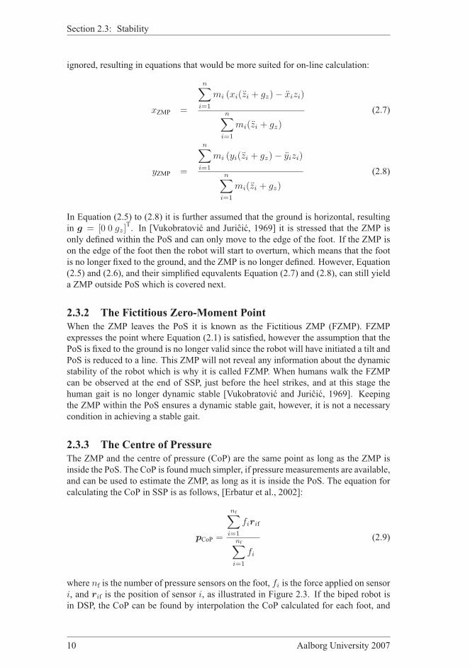
ignored, resulting in equations that would be more suited for on-line calculation:
xZMP =
n∑
i=1
mi (xi(zi + gz)− xizi)
n∑
i=1
mi(zi + gz)
(2.7)
yZMP =
n∑
i=1
mi (yi(zi + gz)− yizi)
n∑
i=1
mi(zi + gz)
(2.8)
In Equation (2.5) to (2.8) it is further assumed that the ground is horizontal, resulting
in g = [0 0 gz]T. In [Vukobratovic and Juricic, 1969] it is stressed that the ZMP is
only defined within the PoS and can only move to the edge of the foot. If the ZMP is
on the edge of the foot then the robot will start to overturn, which means that the foot
is no longer fixed to the ground, and the ZMP is no longer defined. However, Equation
(2.5) and (2.6), and their simplified equvalents Equation (2.7) and (2.8), can still yield
a ZMP outside PoS which is covered next.
2.3.2 The Fictitious Zero-Moment Point
When the ZMP leaves the PoS it is known as the Fictitious ZMP (FZMP). FZMP
expresses the point where Equation (2.1) is satisfied, however the assumption that the
PoS is fixed to the ground is no longer valid since the robot will have initiated a tilt and
PoS is reduced to a line. This ZMP will not reveal any information about the dynamic
stability of the robot which is why it is called FZMP. When humans walk the FZMP
can be observed at the end of SSP, just before the heel strikes, and at this stage the
human gait is no longer dynamic stable [Vukobratovic and Juricic, 1969]. Keeping
the ZMP within the PoS ensures a dynamic stable gait, however, it is not a necessary
condition in achieving a stable gait.
2.3.3 The Centre of Pressure
The ZMP and the centre of pressure (CoP) are the same point as long as the ZMP is
inside the PoS. The CoP is found much simpler, if pressure measurements are available,
and can be used to estimate the ZMP, as long as it is inside the PoS. The equation for
calculating the CoP in SSP is as follows, [Erbatur et al., 2002]:
pCoP =
nf∑
i=1
firif
nf∑
i=1
fi
(2.9)
where nf is the number of pressure sensors on the foot, fi is the force applied on sensor
i, and rif is the position of sensor i, as illustrated in Figure 2.3. If the biped robot is
in DSP, the CoP can be found by interpolation the CoP calculated for each foot, and
10 Aalborg University 2007

Chapter 2: Conceptual Knowledge
weighing by the total force applied to all the sensors:
pCoP =
nfr∑
i=1
firrir +
nfl∑
i=1
filril
nfl∑
i=1
fil +
nfr∑
i=1
fir
(2.10)
where nir and nil are the total number of sensor on right and left foot respectively, fir
and fil are the forces applied to sensor i on right and left foot respectively and rir and
ril are the positions of the the sensors on the right and left foot respectively.
x
r1
r2
r3yf3
f2
f1
Figure 2.3: Top view of the foot. ri is the position of sensor i given in the global reference
frame, fi is the measured force of sensor i.
Group 1033 11


3ANALYSIS OF
HUMAN GAIT
Chapter contents3.1 Human Gait 14
3.2 Posture During Straight Gait 16
3.2.1 Determination of Phase Transitions 16
3.2.2 Straight Walking Strategy 17
3.3 Curved Gait 18
3.4 Thesis Objectives 20
T HE PREVIOUS chapter gave an understanding of some of the important aspects
used in humanoid robotics and expressed an objective for this master thesis. In
this chapter an analysis of the posture of the human body, both during gait in a straight
line and during gait that follows a curved path is given. The analysis is performed
to reveal some basic information on how human-like walk should be obtain with a
humanoid robot. The analysis emphasizes how commands are given to each limb,
which can be utilized in the control of the system. Further the analysis directs attention
to some important issues when designing the mechanics of the humanoid robot. The
purpose of this is to further analyze the objective to elaborate it.
Group 1033 13
Section 3.1: Human Gait
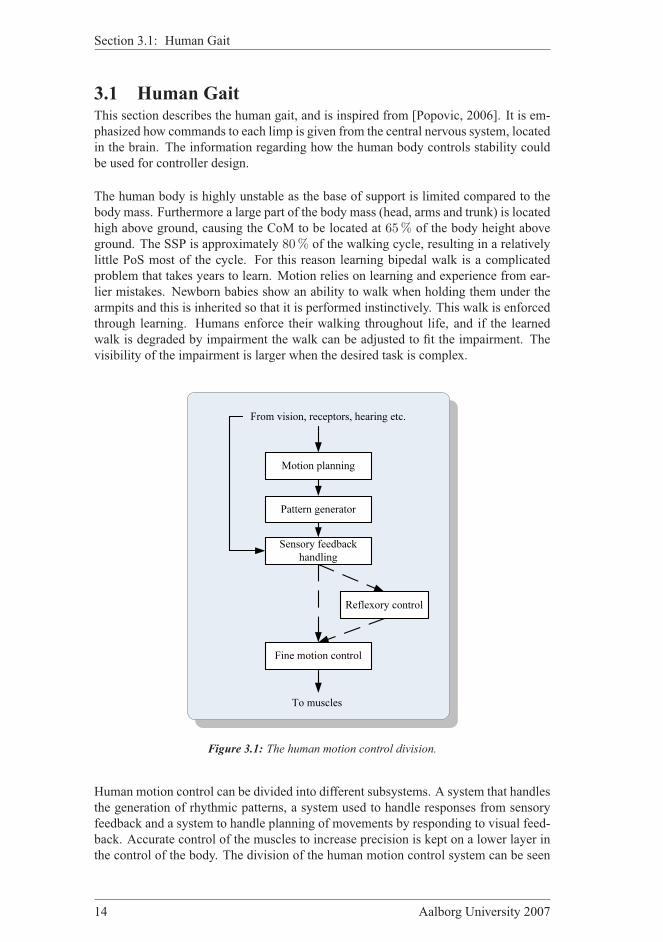
3.1 Human GaitThis section describes the human gait, and is inspired from [Popovic, 2006]. It is em-
phasized how commands to each limp is given from the central nervous system, located
in the brain. The information regarding how the human body controls stability could
be used for controller design.
The human body is highly unstable as the base of support is limited compared to the
body mass. Furthermore a large part of the body mass (head, arms and trunk) is located
high above ground, causing the CoM to be located at 65% of the body height above
ground. The SSP is approximately 80% of the walking cycle, resulting in a relatively
little PoS most of the cycle. For this reason learning bipedal walk is a complicated
problem that takes years to learn. Motion relies on learning and experience from ear-
lier mistakes. Newborn babies show an ability to walk when holding them under the
armpits and this is inherited so that it is performed instinctively. This walk is enforced
through learning. Humans enforce their walking throughout life, and if the learned
walk is degraded by impairment the walk can be adjusted to fit the impairment. The
visibility of the impairment is larger when the desired task is complex.
Pattern generator
Fine motion control
Motion planning
From vision, receptors, hearing etc.
To muscles
Sensory feedback handling
Reflexory control
Figure 3.1: The human motion control division.
Human motion control can be divided into different subsystems. A system that handles
the generation of rhythmic patterns, a system used to handle responses from sensory
feedback and a system to handle planning of movements by responding to visual feed-
back. Accurate control of the muscles to increase precision is kept on a lower layer in
the control of the body. The division of the human motion control system can be seen
14 Aalborg University 2007

Chapter 3: Analysis of Human Gait
from Figure 3.1. Human reflexes are not used in ordinary mode, but are an underlaying
structure which is ready to take over if the normal procedures does not fit the condi-
tions, which is also shown in Figure 3.1.
The stand of a human or biped robot is the posture where the net torque and force
generated by gravity and muscles are zero, and thus the balance is concentrated around
keeping an upright equilibrium position. Walking is caused by a desire to move the
body from one point in space to another, which means that all movements, but reflec-
tive movements, are planned before they are initiated, this is also seen from Figure 3.1.
Walking initiates when the stance equilibrium is disrupted by internal forces of muscle
activity. The torques move the CoM out of the stable stance region and thereby initiates
a fall. This is the beginning of walk. The gravity is used to bring forward the CoM,
and to prevent a fall the counter leg is used to support the falling body. The counter
leg takes over support of the body and regains stability using the momentum gained by
the gravity. Then upright double support position is regained. This cycle is repeated,
and thus walking is characterized by cyclic repetition of movements. Locomotion is
established by cooperation of the entire body. The arms are used to gain or remove
energy from the moving body, and to maintain stability. When walking, the body has a
certain momentum, and by forcing the arms back this momentum can be decreased by
moving the CoM.
a) b) c)Figure 3.2: The human motion cycle. a) The cycle is initiated by internal muscle activity, and
the upper body moves forward in a free fall. b) The direction of the fall is controlled by the
stance leg, and the swing leg is moved forward to support the body. c) The stance leg is shifted
and initial position is regained by moving the new swing leg.
When walking, the human tries at all time to benefit from the gravity, thereby minimiz-
ing the energy used to move the body. According to [Popovic, 2006] human walk can
be described using an inverted multi-link pendulum, moving the CoM in the direction
of the movement. The movement of the swing leg can be seen as a normal pendulum,
and is used to prevent falling. The inverted pendulum motion is repeated when the
swing leg contacts the ground. At normal speed the muscles exhibit low activity in the
swing phase, they only burst during the initiation or end of a swing. When walking,
there are three different phases. DSP, SSP-L and SSP-R, as explained in Section 2.2.
Between these phases is the impact/switch phase, where the foot, not supporting the
Group 1033 15
Section 3.2: Posture During Straight Gait
weight, impacts the ground. During DSP the muscles are active and used to establish
initial conditions of the upcoming SSP. Simultaneous control of both internal and ex-
ternal forces are used, meaning that the muscles are controlled and at the same time the
dynamics given by the movement in a gravity field is exploited. The most important
feature when walking is to keep a vertical posture of the upper body, using one or two
legs.
As earlier explained, a central pattern generator is used to generate the cyclic motion.
The pattern generator can be activated with signals from the brain. The pattern gener-
ator activates the muscles at the appropriate time so the cyclic motion is kept, called
time keeping, and furthermore it generates the appropriate patterns to the muscles for
the desired task. Phase division can be applied to many of the patterns generated, e.g.
a swing phase and a stance phase for a leg. When an obstacle is detected, the initiated
pattern is disrupted, and a decision to avoid it must be taken. Four major possibili-
ties are available in this situation. These are lifting the leg over the obstacle, slowing
down the pace by taking smaller steps, regulate the sideways step width or completely
change direction by initiating a rotated movement on the supporting leg. The last op-
tion requires the most energy.
The human sensor system is altered to fit the current condition. This means that when
walking, the sensors are mainly used to sensor stable walk and obstacles, and are not
used for other purposes.
Humans adjust the walk to fit the terrain, load and unexpected events. Main sensors
used to control the walk is pressure feedback from the sensory system located in the
skin, balance input from sensors located in the brain used to adjust the posture of the
body and the last main sensor is the visual input which is among others used to detect
obstacles and thereby give a reflectory movement of the body, see [Kuo, 1997].
3.2 Posture During Straight GaitThe previous section gave a description of the human gait. In this section the posture of
a human body during walk will be analyzed from test results. The basis for this analysis
will be the results of a test conducted at the Center of SMI (Sensory-Motor Interaction)
at Aalborg University, previously described in [Christensen et al., 2006]. These results
comprise 14 joint trajectories of a normal human walking a straight line measured in
three dimensional space, henceforth referred to as straight human gait. In this section
it is emphasized how the body posture is, seen from a human control/balance point of
view.
3.2.1 Determination of Phase Transitions
In [Christensen et al., 2006] different phase transitions for the straight walk was found,
the date is listed in Table 3.1.
What is worth noticing in Table 3.1, is that during straight human walk, the SSP is long
compared to the full cycle. The test subject is in SSP 92% of the cycle. In Section 3.1
it was stated that the human body minimizes the use of energy while in SSP and en-
ables the muscles while in DSP. Since the DSP only last 8% of the full cycle, which
16 Aalborg University 2007
Chapter 3: Analysis of Human Gait
Duration Percentage
SSP-L 0.59 s 49%DSP 0.10 s 8%SSP-R 0.51 s 43%Total phase 1.20 s 100%
Table 3.1: Duration of the different phases during straight walk. The results are found for three
steps for one test subject, which is why there is an asymmetric difference from left and right
stride.
means that the muscles only have a short time interval to guide the body in the right
direction. The planning of the motion therefore needs to be precise. It also indicates
that the CoM is located outside the stable region of support in most of the walking
cycle.
In order to get a more valid data set, it has been chosen to use data from [Borghese
et al., 1996], where a number of walking experiments performed on several subjects
has been documented. In Table 3.2, the data from the test subject is shown. It should
however be noted that, the data of Table 9.1 can not be found directly in [Borghese
et al., 1996], but can be derived from the presented data.
Duration Percentage
DSP 0.24 s 20%SSP 0.97 s 80%Total phase 1.21 s 100%
Table 3.2: Data for the timing of the phases found in [Borghese et al., 1996].
Note that the there is only one time for the SSP in Table 3.2, which is because the two
SSP’s are of equal length. What is also worth noting is that the duration of the cycle
for the test object in Table 3.1 and the test subject in 3.2 are the same.
3.2.2 Straight Walking Strategy
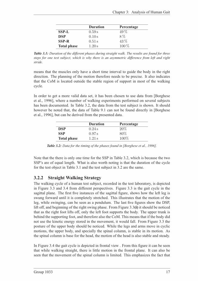
The walking cycle of a human test subject, recorded in the test laboratory, is depicted
in Figure 3.3 and 3.4 from different perspectives. Figure 3.3 is the gait cycle in the
sagittal plane. The first five instances of the sagittal figure, shows how the left leg is
swung forward until it is completely stretched. This illustrates that the motion of the
leg, while swinging, can be seen as a pendulum. The last five figures show the DSP,
lift off, and beginning of the right swing phase. From Figure 3.3(i) it should be noticed
that as the right foot lifts off, only the left foot supports the body. The upper trunk is
behind the supporting foot, and therefore also the CoM. This means that if the body did
not use the kinetic energy stored in the movement, it would fall. From Figure 3.3 the
posture of the upper body should be noticed. While the legs and arms move in cyclic
motions, the upper body, and specially the spinal column, is stable in its motion. As
the spinal column is base for the head, the motion of the head is also stable and steady.
In Figure 3.4 the gait cycle is depicted in frontal view . From this figure it can be seen
that while walking straight, there is little motion in the frontal plane. It can also be
seen that the movement of the spinal column is limited. This emphasizes the fact that
Group 1033 17
Section 3.3: Curved Gait
(a) (b) (c) (d) (e)
(f) (g) (h) (i) (j)
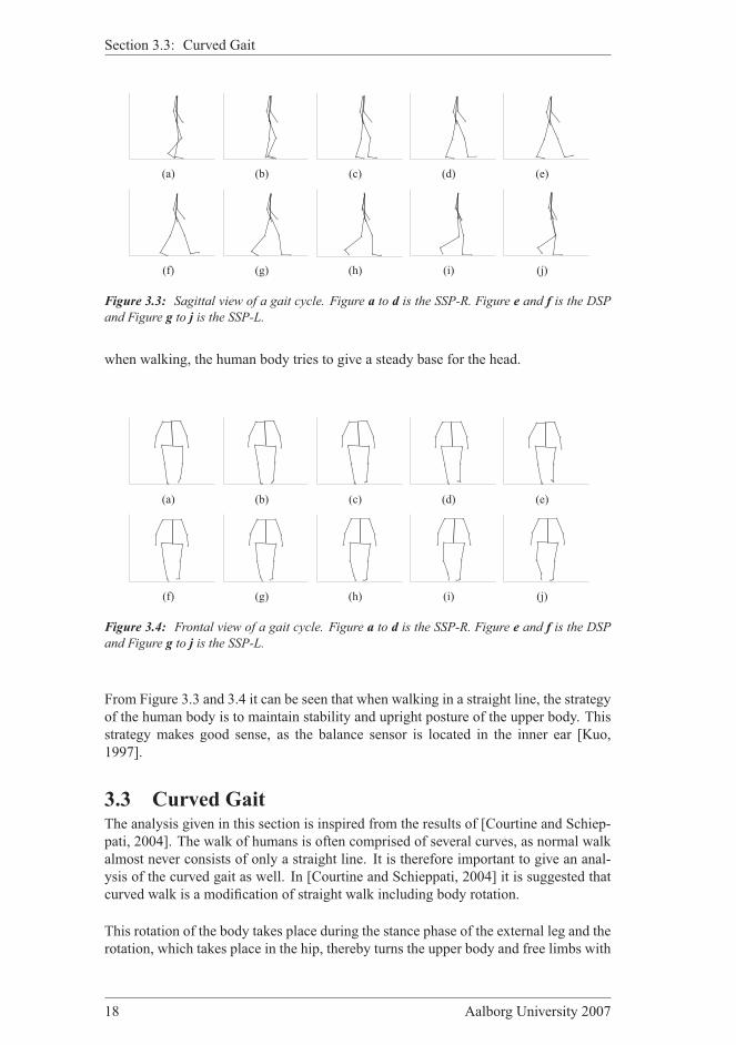
Figure 3.3: Sagittal view of a gait cycle. Figure a to d is the SSP-R. Figure e and f is the DSP
and Figure g to j is the SSP-L.
when walking, the human body tries to give a steady base for the head.
(a) (b) (c) (d) (e)
(f) (g) (h) (i) (j)
Figure 3.4: Frontal view of a gait cycle. Figure a to d is the SSP-R. Figure e and f is the DSP
and Figure g to j is the SSP-L.
From Figure 3.3 and 3.4 it can be seen that when walking in a straight line, the strategy
of the human body is to maintain stability and upright posture of the upper body. This
strategy makes good sense, as the balance sensor is located in the inner ear [Kuo,
1997].
3.3 Curved GaitThe analysis given in this section is inspired from the results of [Courtine and Schiep-
pati, 2004]. The walk of humans is often comprised of several curves, as normal walk
almost never consists of only a straight line. It is therefore important to give an anal-
ysis of the curved gait as well. In [Courtine and Schieppati, 2004] it is suggested that
curved walk is a modification of straight walk including body rotation.
This rotation of the body takes place during the stance phase of the external leg and the
rotation, which takes place in the hip, thereby turns the upper body and free limbs with
18 Aalborg University 2007

Chapter 3: Analysis of Human Gait
Centrifugal force
Rotation direction
Walking path
Figure 3.5: Body rotation results in a centripetal force, when walking along a curved path.
Humans segmentalize the curve to ease the turning. The external stride is longer than that of the
internal stride. The black crosses is the step where the actual turn is taken place, where gray
crosses is a normal straight step.
regards to the stance leg. When turning on the external stride, the energy added to the
system by the centrifugal force is transfered to the rotation of the upper body. Had this
rotation taken place on the internal stride, the energy would not be transferred to the
rotation of the upper body. Rotation of the body takes place during the toe-off phase,
and the rotation of the body results in a rotation of the foot as well. The rotation of the
body is larger than the rotation of the foot. Turning the body results in a centrifugal
force, and thereby in movement of the body CoM toward the inner foot as the body
is leaned inward to counteract the centrifugal force, shown in Figure 3.5. When the
velocity of the turn increases, so does the angular momentum of the trunk.
Obviously the stride length of the internal and external foot differ, the internal being
the smallest, which is depicted in Figure 3.5. The external stride length does not differ
significantly from the stride length at straight walk. When walking a planned curved
path, humans mostly change the direction at the beginning of the curve. The body ve-
locity decreases at the beginning of the curved path until reaching a velocity fit for the
turning radius of the curve. The larger the turning radius of the curve the smaller the
velocity of the body.
If the curved path has a sharp turn, humans tend to divide the path up in segmented
pieces, and thus not walk in a continuous path. This results in small jerks in body
direction when walking curved paths, and thus also fast changes in the angular accel-
eration of the body.
As it is suggested that the curved gait is similar to that of straight gait modified with
angular rotation, the body posture must be somewhat similar to that of the straight walk.
But as the velocity and turning ratio increases so does the tilt of body, as the CoM is
moved toward the center of rotation to counteract the centrifugal force. Therefore it
is assessed that when walking in a curved path it is both important to keep a straight
and steady posture of the upper body, but at the same time it is also important to adjust
Group 1033 19
Section 3.4: Thesis Objectives
the tilt of the posture to follow the centripetal force. This means that the posture not
necessarily needs to be upright as well.
3.4 Thesis ObjectivesIn Section 3.1 the overall objective of this thesis was found to be:
Develop a humanoid platform and through this investigate how human-
like walk can be implemented on this platform.
In the analyze given in this chapter, the human walking properties for straight and
curved walk were given. It was stated that human-like walk exploits the gravity in its
dynamic movements. Humans fall out of the SSP, and the walk can therefore be cate-
gorized as unstable, but still they walk in a stable manner, as the fall is caught by the
swing leg.
The overall objective is now outlined:
- As the walk should resemble human walk, the proportions of the robot platform
should resemble human proportions, thus a humanoid robot must be developed
- The robot platform should be independent of external power supply and external
processing power
- The architecture of the robot platform should resemble that of Figure 3.1, mean-
ing that:
– A trajectory planning and pattern generator should be generated
– The planned trajectories should exploit the dynamics, but still ensure that
the robot walks in a stable manner
– Sensor feedback in the manner of humans should be provided
– Control, based sensor feedback, should be used to maintain stability
The above outlines the main objectives of this thesis, and the following will be a doc-
umentation of how these objectives are achieved.
20 Aalborg University 2007

4MECHANICS
Chapter contents4.1 Introduction to Mechanical Design 22
4.2 Description of the Human Body 22
4.3 Multi Degree of Freedom Joint 24
4.4 Torso 26
4.5 Dimensioning the Limbs 27
4.5.1 The legs 28
4.5.2 The Arms 29
4.5.3 The feet 30
4.6 Partial Conclusion to Mechanical Design 32
IN THIS CHAPTER the design of the mechanics is described. The robot is designed
to match human proportions, to make it possible to resemble human walk. The
chapter therefore starts out with a description of the human body, which can be found
in Section 4.2. In Section 4.3 the design og the special multi-DoF joint is explained.
The torso is designed such that on-board computer, servo motors and batteries can be
mounted, this is explained in Section 4.4. Next, in Section 4.5 the design of the arms and
legs is explained, and last Section 4.5.3 holds a description of the special foot design,
that is constructed such that the force distribution can be measured. SolidWorks is used
to create a 3D-representation of the robot.
Group 1033 21

Section 4.1: Introduction to Mechanical Design
r
g
e
f q
o nm
p
d
c ba
lki
jh
Figure 4.1: The human proportions depicted in Leonardo da Vinci’s Vitruvian Man [Gielo-
Perczak, 2001]. When a human stretches out the arms, the body makes a square consisting of
the legs, arms and head. The distance from the navel to the feet, makes the radius of the circle
which encircle the body.
4.1 Introduction to Mechanical DesignAs it was stated in Section 3.4 on page 20 on of the thesis objectives was to construct
a humanoid robot, on which the architecture of Figure 3.1 on page 14 could be imple-
mented. On this humanoid robot it should be possible to implement human-like walk-
ing patterns, and the robot should therefore be constructed with human proportions.
This chapter describes the construction of the mechanics for this humanoid robot, and
first is an introduction to the human proportions given.
4.2 Description of the Human BodyThis section is inspired by [Popovic, 2006] and [Gielo-Perczak, 2001], and will serve
as a base for the design of the biped robot. When designing a robot that should re-
semble human walk, an analysis of the human body must be made. This section gives
a description of the human proportions. The human proportions is used to design the
mechanical parts of the biped robot, as described later in this chapter. Leonardo da
Vinci’s Vitruvian man, depicts the human proportions, as shown in Figure 4.1. He dis-
covered that there was a connection between the proportions of different limps of the
human body and the number phi:
ϕ =1
ϕ=
1
1.618= 0.618 (4.1)
If a circle is drawn with center in the naval of the body, and a radius going from the
naval to the feet, this circle encircles the entire body. A square, consisting of the span
of the arms and the full body height (which is equal), is drawn. Then the ratio between
the radius of the circle and the length of a side in the square equals ϕ. These propor-tions are depicted in Figure 4.1.
22 Aalborg University 2007

Chapter 4: Mechanics
Body segments (A:B) A [cm] B [cm] [A:B] ǫ [%]a:b 11.9 19.9 0.596 3.24b:c 19.9 29.8 0.668 8.09c:d 29.8 39.8 0.749 21.2d:e 39.8 69.6 0.572 7.44e:f 69.6 105.5 0.660 6.8f:g 105.5 175 0.603 2.43h:i 20.1 25.9 0.776 25.57i:j 25.9 45.8 0.566 8.41k:j 29.8 45.8 0.651 5.34j:l 45.8 73.6 0.622 0.65m:n 21.9 37.8 0.579 6.31n:o 37.8 59.7 0.633 2.43p:o 41.8 59.7 0.700 13.27o:q 59.7 95.5 0.625 1.13
Table 4.1: The ratio between body segments. ǫ is the percentage deviation from ϕ = 0.618[Gielo-Perczak, 2001].
In [Gielo-Perczak, 2001] the proportions shown in Figure 4.1, has been analyzed sta-
tistically. The results are shown in Table 4.2, and it it seen that there is a close statistic
relation between ϕ and the ratio of different body segments.
One of the goals of the project is to design a biped robot that is able to perform dynamic
walk, resembling humans as much as possible. In doing so the efficiency of bipedal lo-
comotion can be very high as shown by [Collins et al., 2001] where a three dimensional
passive dynamic walker with human leg proportions was constructed. Human-like sta-
ble gait with low power consumption was achived.
In order to achieve this the following key points have been determined and should be
emphasized in the design:
- Resemble the proportions of a human, that is, the length of the limbs should
follow the ratios found in humans
The factor ϕ in Equation (4.1) describes the proportions found in humans.
- Joints on humans with more than one degree of freedom (DoF) in the same
plane should be designed as such on the robot
To compare the robot and a human the joints should be alike thereby making it
possible to directly compare trajectories.
- Under own power carry batteries and electronics
The robot has to be designed to house the batteries and electronics somewhere
in the body such that the robot can be autonomous.
The following will describe how the biped robot has been designed. The parts in the
design will not undergo a stress analysis to determine if they are strong enough under
the applied load. Instead it is intuitively assessed if a part is strong enough. First is the
design of the ankle and hip joint constructed.
Group 1033 23

Section 4.3: Multi Degree of Freedom Joint
Figure 4.2: Placement of the multi DoF joint in the complete construction.
4.3 Multi Degree of Freedom JointThis section gives a description of the design of the multi degree of freedom (DoF)
joint. This joint fits into the complete construction as seen on Figure 4.2, where it is
the part which is not transparent.
In a human the joint in the hip and ankle have more than one degree of freedom in the
same plane. The joint in this section can be used both in the ankle and hip implement-
ing movement in the x and y-direction. It has been chosen to use standard-sized (4 cm× 2 cm × 3.6 cm) servomotors as it is assessed that they have a good size to torque
ratio.
One approach could be to design brackets that place the shafts of two servo motors in
the same plane as shown on Figure 4.3(a). However, this design is asymmetric and
wide which to some extent clashes with the desire to make the robot human-like.
(a) Joint design1 (b) Joint design 2 (c) Joint design 3
Figure 4.3: Three different joint designs
24 Aalborg University 2007
Chapter 4: Mechanics
F1
L1
L2
l2
l11τ
2τ
1θ
2θ
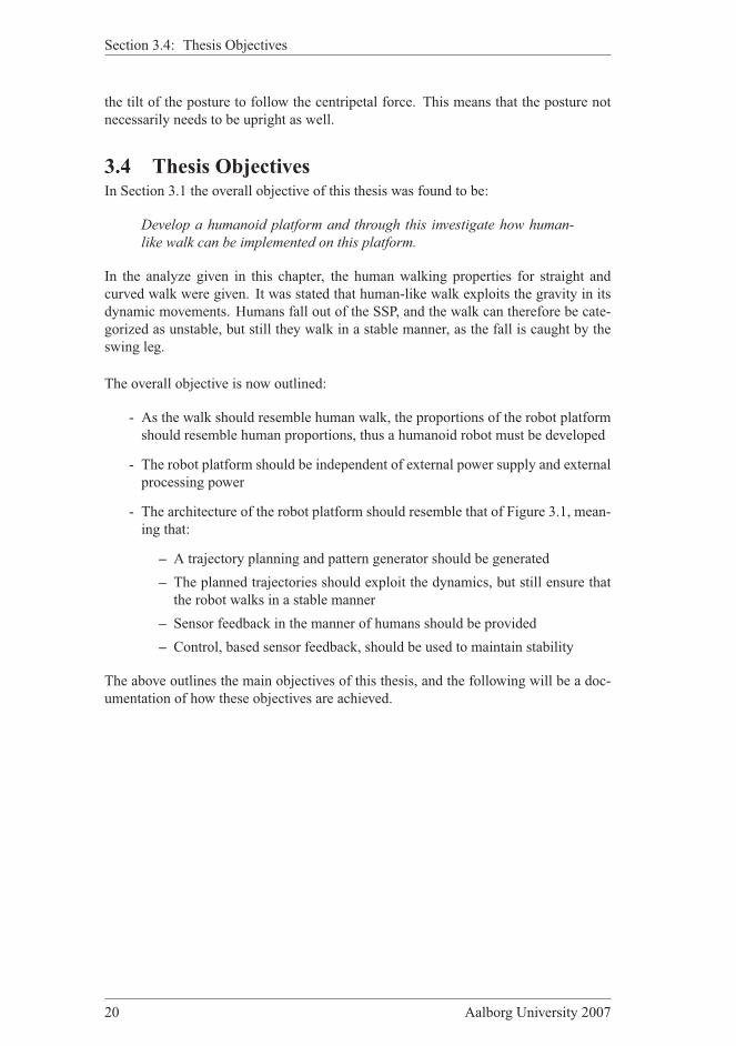
Figure 4.4: One of the levers of joint design 3. Used to determine the transmission ratio of the
torque.
To make the joint symmetric gears can be used as shown in Figure 4.3(b). However,
this design is fairly complex and more prone to backlash, introduces by the gears, than
the previous design. Figure 4.3(c) shows the design that was used in the biped robot.
The design is rather compact, making it ideal for implementation on the robot, and any
additional backlash added to the joint is limited to the axis driven by the levers. By
using two levers the strain on the horn will be symmetric about the shaft thereby not
adding additional strain lengthwise to the shaft which would have been the case if only
one lever was used.
To show that using the design of Figure 4.3 the energy lost in the transfer using the
levers, can be considered zero, a small example is given. This principle is shown in
Figure 4.4 where the force acting on servo horn one is τ1.
To determine τ2 the force F1 has to be determined:
F1 =τ1l1
(4.2)
Where l1 is equal to cos(θ1)L1 because only the vertical component of the force is
considered. Because of this the torque τ2 can be determined using F1:
τ2 = F1L2 cos(θ2) (4.3)
τ2 = τ1L2 cos(θ2)
L1 cos(θ1)(4.4)
As the arms connected to the levers are the same length in both ends Equation (4.4)
reduces to:
τ2 = τ1 (4.5)
Thereby Equation (4.5) states that there is a one-to-one transmission of the torque, ne-
glecting the loss due to friction in the bearings on the levers.
Group 1033 25
Section 4.4: Torso
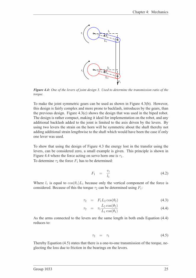
Figure 4.5: Placement of the torso in the complete construction.
Figure 4.6: An exploded view of the torso showing the interconnection of the parts.
It is therefore selected that the multi DoF joint depicted in Figure 4.3c should be used
as the ankle and hip joint. Next is the design of the torso given.
4.4 TorsoThe design of the torso is the base of the robot. It connects all limbs and further holds
the on-board computer and batteries. The placement of the torso as connection joint is
seen from Figure 4.5 as the part which is not transparent.
The torso needs five servo motors to drive the limbs, one for each leg and arm plus
rotation of the head. This puts a lower limit on how small the torso can be. Therefore
the torso is designed first and the limbs are designed to match the size of the torso, so
that all match the human proportions given in Section 4.2.
The torso has a single aluminum part, which the servo motors and the on-board elec-
tronics are attached to. This aluminum part is seen from the exploded view of the torso
depicted in Figure 4.6.
26 Aalborg University 2007
Chapter 4: Mechanics
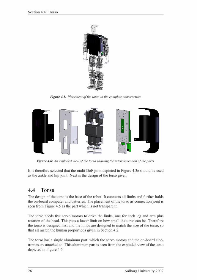
Figure 4.7: A close up on the additional shaft located in the torso.
Two of the servo motors in the torso implement the leg motion in the z-direction, butthe leg can not be connected directly to the shaft as this would be to weak. Instead an
additional shaft is implemented in the torso that offloads the shaft of the servo motor.
This is depicted on Figure 4.7.
It has been chosen to enclose the battery inside the torso. As the battery is one of the
heavier parts of the biped robot it can also have a great influence on the centre of mass
of the torso. Therefore placing it outside the torso gives an asymmetric distribution
of the CoM on the finished biped robot. To enclose the battery and stiffen the torso,
an aluminum plate is designed which fits the holes on the ball bearing sockets and
distance pieces that are connected at the shoulders. At the top and sides of the frontal
torso plate, pieces of the aluminum plate is bend in a 90 deg angle. The piece to the
right closes the battery compartment in one end and the piece on the left side is shorter
so the battery can be inserted in the compartment. The pieces on the top of the plate
closes the shoulders. The large extruded cuts of frontal and back plate reduces the
weight and eases the routing of cables. On the back plate the on-board electronics
is mounted. As it is considered inevitable that the biped robot falls the electronics
is placed behind a plastic shield to avoid damage. This shield is a prototype made
using a selective laser sintering (SLS) technique, and should therefore be stronger than
ordinary plastic constructions. To give the biped robot a more appealing appearance
a shield, covering the chest, is also designed. This also gives the possibility to house
even more electronics if this is necessary on future revisions of the biped robot. All the
parts of the torso can be seen from Figure 4.6.
4.5 Dimensioning the LimbsAs the design of the torso has been completed, the dimensions found can be used to
design the additional limbs of the robot. These are seen from Figure 4.8 including the
Group 1033 27
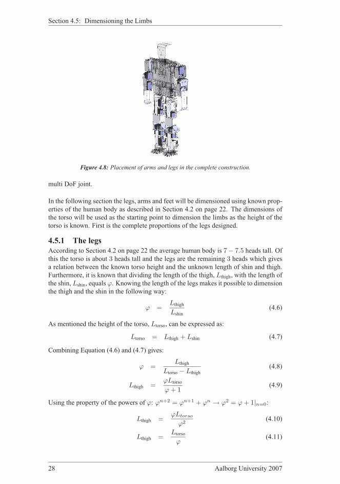
Section 4.5: Dimensioning the Limbs
Figure 4.8: Placement of arms and legs in the complete construction.
multi DoF joint.
In the following section the legs, arms and feet will be dimensioned using known prop-
erties of the human body as described in Section 4.2 on page 22. The dimensions of
the torso will be used as the starting point to dimension the limbs as the height of the
torso is known. First is the complete proportions of the legs designed.
4.5.1 The legs
According to Section 4.2 on page 22 the average human body is 7− 7.5 heads tall. Ofthis the torso is about 3 heads tall and the legs are the remaining 3 heads which gives
a relation between the known torso height and the unknown length of shin and thigh.
Furthermore, it is known that dividing the length of the thigh, Lthigh, with the length of
the shin, Lshin, equals ϕ. Knowing the length of the legs makes it possible to dimensionthe thigh and the shin in the following way:
ϕ =Lthigh
Lshin
(4.6)
As mentioned the height of the torso, Ltorso, can be expressed as:
Ltorso = Lthigh + Lshin (4.7)
Combining Equation (4.6) and (4.7) gives:
ϕ =Lthigh
Ltorso − Lthigh
(4.8)
Lthigh =ϕLtorso
ϕ + 1(4.9)
Using the property of the powers of ϕ: ϕn+2 = ϕn+1 + ϕn → ϕ2 = ϕ + 1|n=0:
Lthigh =ϕLtorso
ϕ2(4.10)
Lthigh =Ltorso
ϕ(4.11)
28 Aalborg University 2007
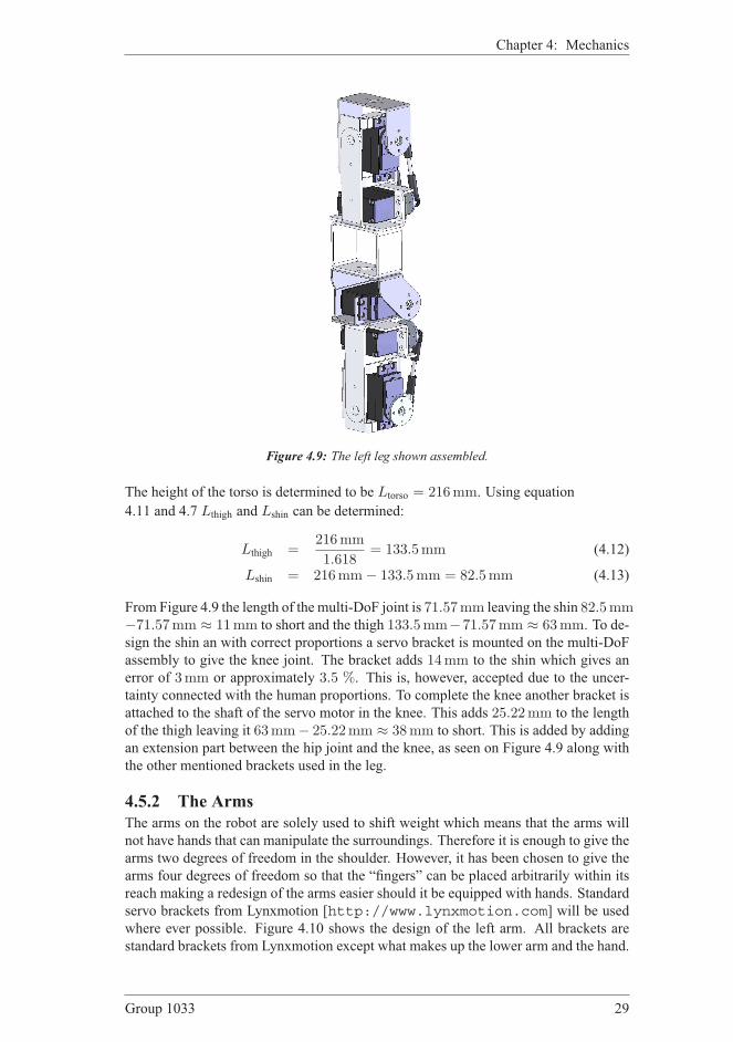
Chapter 4: Mechanics
Figure 4.9: The left leg shown assembled.
The height of the torso is determined to be Ltorso = 216mm. Using equation
4.11 and 4.7 Lthigh and Lshin can be determined:
Lthigh =216mm
1.618= 133.5mm (4.12)
Lshin = 216mm− 133.5mm = 82.5mm (4.13)
From Figure 4.9 the length of the multi-DoF joint is 71.57mm leaving the shin 82.5mm−71.57mm ≈ 11mm to short and the thigh 133.5mm−71.57mm ≈ 63mm. To de-
sign the shin an with correct proportions a servo bracket is mounted on the multi-DoF
assembly to give the knee joint. The bracket adds 14mm to the shin which gives an
error of 3mm or approximately 3.5 %. This is, however, accepted due to the uncer-
tainty connected with the human proportions. To complete the knee another bracket is
attached to the shaft of the servo motor in the knee. This adds 25.22mm to the length
of the thigh leaving it 63mm− 25.22mm ≈ 38mm to short. This is added by adding
an extension part between the hip joint and the knee, as seen on Figure 4.9 along with
the other mentioned brackets used in the leg.
4.5.2 The Arms
The arms on the robot are solely used to shift weight which means that the arms will
not have hands that can manipulate the surroundings. Therefore it is enough to give the
arms two degrees of freedom in the shoulder. However, it has been chosen to give the
arms four degrees of freedom so that the “fingers” can be placed arbitrarily within its
reach making a redesign of the arms easier should it be equipped with hands. Standard
servo brackets from Lynxmotion [http://www.lynxmotion.com] will be used
where ever possible. Figure 4.10 shows the design of the left arm. All brackets are
standard brackets from Lynxmotion except what makes up the lower arm and the hand.
Group 1033 29

Section 4.5: Dimensioning the Limbs
Figure 4.10: The arm shown assembled
This part has been fitted with additional holes where weights can be mounted in order
to increase the momentum of the arm.
4.5.3 The feet
The feet can either be passive or active. An active foot is able to bend its toes actively
meaning that the toe joint is actuated. A passive foot is not actuated in the toe joint,
and it is therefore not possible to control the bending of the toe. An active foot more
closely mimics the human foot but becomes heavier and bigger, because of the added
servo motor. Because the toes are used actively during human locomotion the foot
should be active.
However, making the foot active also clashes with the design goals as it would make
it larger than what is considered acceptable in regards to the human proportions. This
has given the following compromise in the design; the foot is passive however the toes
are always bend. This shortens the foot making the task of keeping the balance of the
biped robot harder when standing still because the polygon of support is reduced. Fig-
ure 4.11 shows an exploded view of the foot including the base of the foot where the
toes are bend in a curve.
This enables the robot to “roll” onto the toes instead of bending them. To determine
the correct size of the feet the members of the project group have measured their feet.
The length from the heel to approximately the middle of the first joint of the big toe
on the right foot is measured. This is used as the length of the foot. To determine the
width of the foot the widest part of the foot is measured. The length and width are both
divided by the test subjects height to give ratios that can be used in the design of the
feet. The measurements are shown in Table 4.2.
The width and length of the robots feet can now determined using the height of the
robot which from Solid Works is determined to be 58 cm. This yields:
30 Aalborg University 2007

Chapter 4: Mechanics
Figure 4.11: Exploded view of the foot, including all the part which it consists of.
Height(H)[cm] Width(W)[cm] Length(L)[cm] W/H L/H
173 9.1 16.5 0.0526 0.0954
175 8.5 17.4 0.0486 0.0994
186 9.7 18.8 0.0522 0.101
172 8.4 17.6 0.0488 0.102
Average: 0.05055 0.09945
Table 4.2: Length, without the toes, and width of the right foot of the group members.
lfoot = 580mm · 0.09945 = 57.681mm ≈ 58mm (4.14)
wfoot = 580mm · 0.05055 = 29.319mm ≈ 30mm (4.15)
In order to uniquely determine the centre of pressure (CoP) three pressure points has
to be measured. Figure 4.11 shows the foot where three plates, called strain plates, are
attached, on which the strain will be measured. In order to distribute the forced applied
to the entire foot to the strain plates a solid plate, the top plate, has to be mounted to
the strain plates. An ideal strain gauge is only sensitive to strain in the direction it is
designed to measure. However the strain gauges will be influenced by strain perpen-
dicular to the direction that is to be measured. If pressure is placed on one strain plate
the other strain plates are twisted which is referred to as mechanical cross talk. In order
to minimize cross talk the top plate is mounted to the strain plates through a membrane
which is similar to the feet discussed in [Loffler et al., 2004]. The membrane also
functions as a spring/damper system which reduces the nonlinearities associated with
the impact phase as suggested by [Buschmann et al., 2006] and [Collins et al., 2001].
The dimensions of the strain plates has been determined with the exception of the
thickness and the material. A feasible choice for the material is steel and aluminum as
these are available. It has been chosen to use spring steel due to a higher elasticity than
aluminum and ordinary steel. The spring steel is able to bend and then return to the
initial position without any memory of the bend.
It should, as a minimum, be possible to measure the weight of the robot. The robot
weighs mrobot = 3.7 kg or 36.3N. However, the robot could have accelerations thatmakes it necessary to measure above 36.3N. Therefore the minimum measurable
Group 1033 31
Section 4.6: Partial Conclusion to Mechanical Design
weight has been set to 2mrobot = 7.4 kg. Each strain plate should therefore be able
to measure mmin,meas137.4 kg ≈ 2.5 kg. The system that measures the force is designed
and tested in Appendix D on page 191.
This completes the design of the foot and thereby the design of the robot.
4.6 Partial Conclusion to Mechanical DesignIn this chapter a complete mechanical solution for a biped robot with human propor-
tions was given. Several mechanical parts were custom designed, while some relied on
available design from external manufactures. A multi DoF joint was designed which
enabled three axis rotation in one point. This multi DoF joint was similar to that of the
human hip, thus enabling movements in all directions. Thereby it was possible to make
the robot turn as well. Furthermore a custom made foot was designed with possibility
to measure the weight distribution. The design also made sure that an on-board hard-
ware solution could be implemented, including a power supply. A SolidWorks drawing
of the complete humanoid robot can be seen from Appendix M.
32 Aalborg University 2007

5HARDWARE
Chapter contents5.1 Hardware Overview 34
5.2 Sensor Determination 35
5.2.1 Strain Gauges Mounted on the Feet 35
5.2.2 Potentiometer Signals 35
5.2.3 Inertia Measurement Unit 36
5.3 Actuators 36
5.3.1 Servo Motors 37
5.3.2 Servo Controllers 37
5.3.3 Feedback from Servo Motors 38
5.4 Choosing an On-board Computer 40
5.5 Description of the Interface print 41
5.5.1 Description of Multiplexer 42
5.6 Battery Pack and Voltage Monitor Circuit 43
5.7 Partial Conclusion to Hardware 44
T HIS CHAPTER gives a description of the entire hardware system. To realize a
wireless, fully controllable and autonomous robot, an on-board computer needs
to be mounted on the robot. To retrieve information from the servo motors and other
sensors located on the robot, an interface print is developed. This interface print gath-
ers all sensor signals, and sends them to the on-board computer. This chapter starts
out with an overall system description, and will then describe the chosen sensors. Af-
terward the actuators will be described. This chapter will also include a description of
how the system is powered.
Group 1033 33

Section 5.1: Hardware Overview
5.1 Hardware OverviewThis section gives a description of the entire hardware system, located on the robot.
Each hardware module will be given a short description and a reference will be given
to the specific section describing that module more detailed. Figure 5.1 shows the en-
tire system, and is used as reference figure in this section.
Servo MotorPotentiometers
IMU
Strain Gauges
Analog multiplexer
#1
Push-buttons
Dip-switch
Analog multiplexer
#2
Pressure[6]
Button state[3]
Acc. &Ang. Velocity
[6]
Positions[12]
Switch state[4]
Multiplexed signals[1]
Address signals[4]
Multiplexed signals[1]
Address signals[4]
Interruptbutton Interrupt signal
[1]
Analog Input
Digital Output
Analog Input
Digital Output
Digital Input
On-board Computer
Servos Pololu boardsPositions[21]
Servo positions/velocities[3]
Reset signal[1]
Battery voltage monitor
Battery voltage[2]
UART
Digital Output
Analog Input
Interface print
Debug LED’s On/Off signal[4] Digital Output
Figure 5.1: Hardware overview, showing the entire system. The number in the brackets refers to
the number of signal wires. The on-board computer is shown in the right side of the figure, and
marked with a green box. The interface print is marked with a blue box and is shown in the left
side of the figure. Boxes that are located outside the interface print and the on-board computer
are connected to the interface print using a number of connectors. As seen all external hardware
is connected to the interface print, even if the signal should just be routed unchanged to/from the
on-board computer.
To collect information on the state of the system, a number of sensors is placed on the
robot. As seen in Figure 5.1 the sensors are strain gauges, IMU, and servo potentiome-
ters. These will be described in Section 5.2. Further more, to move the robot a number
of actuators must be inserted which is explained in Section 5.3. The system consists of
an on-board computer that controls the whole system, this is described more detailed
in Section 5.4. The on-board computer is connected to the interface print using a 40
34 Aalborg University 2007
Chapter 5: Hardware
pin connector cable. The interface print contains several electronic circuits used to
gather measurements from the large number of sensors and actuators, providing com-
munication between the on-board computer and the surroundings. The interface print
is described in Section 5.5.
5.2 Sensor DeterminationFor the purpose of getting feedback from the biped robot, and therefrom generating
control signals, several sensors are available. In this project, the choice of sensors is
based on experience from [Christensen et al., 2006] and studies of human gait, de-
scribed in Section 3.1. In [Christensen et al., 2006], it was chosen to use accelerome-
ters and force sensing resistors (FSR). The accelerometers were used for fault detection
purpose, to determine if the robot was about to fall. The FSR’s were used to determine
the weight distribution on the feet. This weight distribution was used as control input
for a fuzzy logic controller.
5.2.1 Strain Gauges Mounted on the Feet
Humans use signals from the receptors under the foot sole to control their stability, and
based on this it is chosen that the robot should provide some kind of feedback on the
force distribution under the feet. In [Christensen et al., 2006] they implemented FSR to
obtain the feedback, experience with FSR’s as the only control input however showed
two major problems. These problems were:
- Drift in signals: When exposing the sensors to a static load, i.e. a solid mass,
the output from the sensors drifted, meaning that the measurement could not be
used to determine the exact load over time. The output started to drift immedi-
ately after the mass had been placed on the sensor and more than a minute passed
before a steady-state was reached.
- Poor repeatability: If the same load was applied to the FSR several times, the
output deviates significantly compared to each other. Hence, the reliability of
the sensors was not as good as expected, and not suitable for the purpose.
Based on these experiences, it has been concluded that FSR’s are not applicable in
this project. Load cells are not considered an option due to their high price and large
physical size. It could be a problem to mount several load cells on such small feet
as those used in this project. This narrows the choice down to strain gauges. These
have been chosen due to their high precision, low price and high reliability. In order
to retrieve the information by measuring the change in resistance, a strain gauge print
has been developed. This print consists of three Wheatstone bridges, that converts the
resistance change into a voltage signal. This signal is amplified an filtered, and then
led to the interface print. A strain gauge print is mounted on each foot, to reduce the
amount of noise on the signals. Figure 5.2 shows a picture of the foot with the strain
gauge print mounted on top of it. A more detailed description of the development of
this print can be found in Appendix D on page 191.
5.2.2 Potentiometer Signals
To obtain further feedback from the robot, it has been chosen to modify the servo
motors in the legs, to provide the internal potentiometer signal. This modification is
Group 1033 35

Section 5.3: Actuators
Figure 5.2: Picture of the right foot. On top of the foot, the strain gauge print can be seen.
described in Appendix B on page 175. The potentiometer signal provides the actual po-
sition of the servo motor shaft and is used for internal feedback inside each servo motor.
It has been chosen to use this signal as control signal due to experience from [Chris-
tensen et al., 2006] where the load from the robot made the servo motors change their
position. It was concluded that the internal controller is a P-type controller, meaning
that the servo motors not necessarily reached the correct position when being exposed
to a load. The potentiometer signals from the arms have not been extracted, due to the
fact that the load in the arm joints is small compared to the load in the leg joints.
5.2.3 Inertia Measurement Unit
When a human walks, the stability is controlled by using signals gathered from the
inner ear, as explained in Section 3.2.2 on page 17. The goal of this project is to obtain
human-like walk. To resemble the human perception, it has therefore been decided to
place a five DoF inertia measurement unit (IMU) in the head of the robot. In Figure
5.3 a picture shows the location of the IMU.
The IMU consists of a small printed circuit board (PCB), where an IDG300 dual-axis
gyroscope [InvenSense Inc, 2006] and an ADXL330 three-axis accelerometer [De-
vices, 2006] are mounted. The output from the IMU is three analogue signals describ-
ing the acceleration of the unit in all three axis, and two analogue signals describing
the angular velocity of the unit in terms of the roll and pitch. The analogue signals are
routed directly to the interface print, where they are routed to the analogue multiplexer.
5.3 ActuatorsAs actuators for the biped robot it has been chosen to use two different servo motors.
The legs are exposed to high torques since they will be carrying the body during walk.
The servos in the knees will be exposed to a load during stance, due to the design of the
knee. However the servo motors in the arms only have to move their own weight, as
this project focuses on the walk of the biped and the arms are only used as stabilizing
factor by moving masses.
36 Aalborg University 2007

Chapter 5: Hardware
Figure 5.3: A picture of the head of the robot. Below the mouth, the IMU is seen.
5.3.1 Servo Motors
The servo motors where chosen based on experience gained from [Christensen et al.,
2006]. In [Christensen et al., 2006, pp. 206] applying the designed walking patterns
showed that some of the servo motors where unable to deliver the required torque in all
phases. This biped robot was 30 cm high and weighed 1.7 kg and the maximum torque
required was found to be 1.1Nm. The biped robot designed in this project is 58 cmhigh and weighs 3.6 kg, which means that the servo motors have to be even stronger.In [Santos and Silva, 2005] a biped robot was developed that weighed 5 kg and was
60 cm high. The model of this biped showed a maximum torque of 2.6Nm. With the
above mentioned in mind, it is chosen to equip the legs with the HSR-5995TG from
Hitec which has a maximum torque of 2.9Nm. Additionally the HSR-5995TG uses
titanium gears which makes it more durable, compared to steel gears. The simulated
walking pattern in [Christensen et al., 2006, pp. 207] showed that the required torque in
the arms never exceeded 0.04Nm. The arms on the biped robot related to this project
are longer but lighter, they are, however, designed so that the weight can be increased,
should this be necessary. So to ensure that added weight can be moved satisfactory
the HS-645MG servo motor from Hitec, which has a maximum torque of 0.92Nm, is
placed in the arms. The specifications for the two servo motors are shown in Table 5.1.
5.3.2 Servo Controllers
This section seeks to describe the interface to the servo motors, and explains how the
servo controller boards work. It defines the protocol used to control the servos. The
source of information is the data sheets for the servo motors [HiTec, 2005] and [HiTec,
2006], as well as the manual for the servo controller board [Robotics and Electronics,
2005].
Group 1033 37

Section 5.3: Actuators
HSR-5995TG HS-645MG
Operating voltage 7.4V 6VRunning current 380mA 450mAStall current 5.2A N/A
Standing torque 2.9Nm 0.92NmStall torque 3.8Nm N/A
Pulse rate 90 deg.400 µs
45 deg.400 µs
Pulse range ±90deg. 1100µs− 1900µs 700 µs− 2300µsNeutral 1500µs 1500 µsDead band width 2µs 8 µsSpeed (No load) 8.73 rad/s 5.22 rad/sClock wise direction Increase pulse period Increase pulse period
Gear Titanium Steel/nylon
Weight 62 g 55.2 g
Table 5.1: Specifications for HSR-5995TG and HS-645MG. Values indicated are maximum rat-
ings from [HiTec, 2005] and [HiTec, 2006].
Motor Interface Description
The position of each servo motor is determined from the width of the pulse given to
the servo motor. A pulse of 1500µs sets the middle position. For the HS-645MG the
range is 800µs to each side, which corresponds to ±90 deg.. The HSR-5995TG uses
a pulse at half the time, to set a similar position. The servo control signal is updated
with 50Hz, i.e. every 20ms.
This section describes the control of a HS-645MG. Same description goes for the HSR-
5995TG if the pulse widths are divided by two. On Figure 5.4 the servo control signal
for the HS-645MG is depicted. The working range of the motor is illustrated with
the dashed lines at 700µs and 2300µs, corresponding to ±90 deg. respectively. Themaximal turning rate, at 6V supply, is 5.24 rad/s. To create these control signals, a
Voltage [V]
Time [ms]201 5 10
5
Figure 5.4: The control signal to the servo motors. The solid line corresponds to a position of
0 deg.. The dashed lines show the pulse widths corresponding to a position of ±90 deg..
Pololu servo controller board is used. The board is very small in size, only 23mm ×23mm, and capable of controlling up to 8 servo motors. A further description of the
servo controllers and the motor interface is given in Appendix A on page 173.
5.3.3 Feedback from Servo Motors
This section will concern the extraction of the position measurement from potentiome-
ters inside the servo motor. It was determined in Section 5.2.2 on page 35 that these
38 Aalborg University 2007
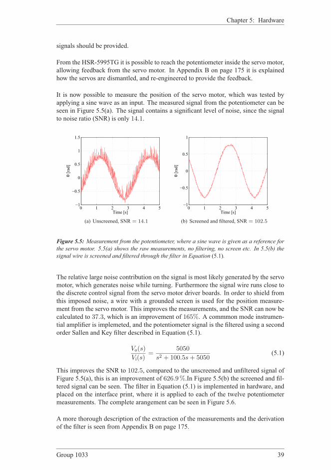
Chapter 5: Hardware
signals should be provided.
From the HSR-5995TG it is possible to reach the potentiometer inside the servo motor,
allowing feedback from the servo motor. In Appendix B on page 175 it is explained
how the servos are dismantled, and re-engineered to provide the feedback.
It is now possible to measure the position of the servo motor, which was tested by
applying a sine wave as an input. The measured signal from the potentiometer can be
seen in Figure 5.5(a). The signal contains a significant level of noise, since the signal
to noise ratio (SNR) is only 14.1.
0 1 2 3 4 5−1
−0.5
0
0.5
1
1.5
θ [rad]
Time [s]
(a) Unscreened, SNR = 14.1
0 1 2 3 4 5−1
−0.5
0
0.5
1
θ [rad]
Time [s]
(b) Screened and filtered, SNR = 102.5
Figure 5.5: Measurement from the potentiometer, where a sine wave is given as a reference for
the servo motor. 5.5(a) shows the raw measurements, no filtering, no screen etc. In 5.5(b) the
signal wire is screened and filtered through the filter in Equation (5.1).
The relative large noise contribution on the signal is most likely generated by the servo
motor, which generates noise while turning. Furthermore the signal wire runs close to
the discrete control signal from the servo motor driver boards. In order to shield from
this imposed noise, a wire with a grounded screen is used for the position measure-
ment from the servo motor. This improves the measurements, and the SNR can now be
calculated to 37.3, which is an improvement of 165%. A commmon mode instrumen-
tial amplifier is implemeted, and the potentiometer signal is the filtered using a second
order Sallen and Key filter described in Equation (5.1).
Vo(s)
Vi(s)=
5050
s2 + 100.5s + 5050(5.1)
This improves the SNR to 102.5, compared to the unscreened and unfiltered signal ofFigure 5.5(a), this is an improvement of 626.9%.In Figure 5.5(b) the screened and fil-
tered signal can be seen. The filter in Equation (5.1) is implemented in hardware, and
placed on the interface print, where it is applied to each of the twelve potentiometer
measurements. The complete arangement can be seen in Figure 5.6.
A more thorough description of the extraction of the measurements and the derivation
of the filter is seen from Appendix B on page 175.
Group 1033 39
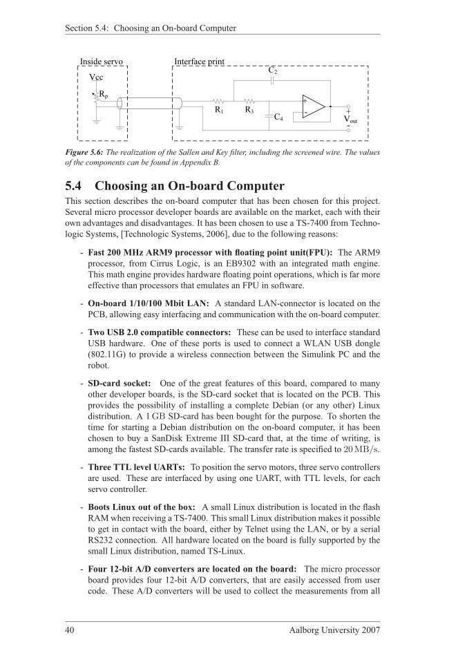
Section 5.4: Choosing an On-board Computer
R3 VoutR1
-+C4
C2
Rp
VccInside servo
+-
Interface print
Figure 5.6: The realization of the Sallen and Key filter, including the screened wire. The values
of the components can be found in Appendix B.
5.4 Choosing an On-board ComputerThis section describes the on-board computer that has been chosen for this project.
Several micro processor developer boards are available on the market, each with their
own advantages and disadvantages. It has been chosen to use a TS-7400 from Techno-
logic Systems, [Technologic Systems, 2006], due to the following reasons:
- Fast 200 MHz ARM9 processor with floating point unit(FPU): The ARM9
processor, from Cirrus Logic, is an EB9302 with an integrated math engine.
This math engine provides hardware floating point operations, which is far more
effective than processors that emulates an FPU in software.
- On-board 1/10/100 Mbit LAN: A standard LAN-connector is located on the
PCB, allowing easy interfacing and communication with the on-board computer.
- Two USB 2.0 compatible connectors: These can be used to interface standard
USB hardware. One of these ports is used to connect a WLAN USB dongle
(802.11G) to provide a wireless connection between the Simulink PC and the
robot.
- SD-card socket: One of the great features of this board, compared to many
other developer boards, is the SD-card socket that is located on the PCB. This
provides the possibility of installing a complete Debian (or any other) Linux
distribution. A 1GB SD-card has been bought for the purpose. To shorten the
time for starting a Debian distribution on the on-board computer, it has been
chosen to buy a SanDisk Extreme III SD-card that, at the time of writing, is
among the fastest SD-cards available. The transfer rate is specified to 20MB/s.
- Three TTL level UARTs: To position the servo motors, three servo controllers
are used. These are interfaced by using one UART, with TTL levels, for each
servo controller.
- Boots Linux out of the box: A small Linux distribution is located in the flash
RAMwhen receiving a TS-7400. This small Linux distribution makes it possible
to get in contact with the board, either by Telnet using the LAN, or by a serial
RS232 connection. All hardware located on the board is fully supported by the
small Linux distribution, named TS-Linux.
- Four 12-bit A/D converters are located on the board: The micro processor
board provides four 12-bit A/D converters, that are easily accessed from user
code. These A/D converters will be used to collect the measurements from all
40 Aalborg University 2007

Chapter 5: Hardware
Figure 5.7: Picture of the on-board computer in the top, and the interface print in the bottom.
The two boards are connected with a 40-pin cable, seen in the middle.
the sensors on the robot, meaning the potentiometer signals, strain gauge mea-
surements, IMU data and battery voltage.
- 20 digital I/O: The board provides 20 digital input/output that can be accessed
directly through the 40-pin connector.
- Small size: The board only measures 7.4 cm × 12 cm, making it suitable for
the robot.
To interface the on-board computer, the 40-pin connector is used. The interface print
is equipped with a similar connector, making it possible to connect the two boards by
a single cable. The on-board computer provides a 5V supply as well as 3.3V supply
in the 40-pin connector, which is used to supply all external prints, both the interface
print, the strain gauge prints and the Pololu boards. A picture of the on-board computer
along with the interface print can be seen in Figure 5.7.
Besides from the key features mentioned in the list, Technologic System provides a
wide range of code examples, test programs, Linux distributions and well documented
manuals, which ease the development of the robot platform.
5.5 Description of the Interface printThe interface print can be seen in Figure 5.1 and consist of the following components:
- twelve low-pass filters for the potentiometer signals: The signals from the
potentiometers, located inside the servo motors, are noisy and should be filtered
before the signals are usable in a control system. To ease the on-board computer,
Group 1033 41

Section 5.5: Description of the Interface print
these filters are implemented in hardware. Section B.2 on page 178 describes the
design of the filters in details. It has been chosen to use a second order Sallen
and Key filter. On the interface print, 12 identical filters for the potentiometer
signals are placed.
- two 16-channel analogue multiplexers: To make it possible to read all ana-
logue signals with only four analogue inputs available on the on-board computer,
two 16-channel analogue multiplexers are used. Section 5.5.1 gives a descrip-
tion of the chosen multiplexers. The analogue multiplexers reduce the number
of needed analogue inputs from 31 down to 2, for the sensors.
- one 4-bit dip-switch: To make it possible to set some parameters permanently
externally, a dip-switch with four on/off switches is inserted. The dip-switch is
connected to one of the multiplexers.
- three pushbuttons: When developing code, it is preferable if it is possible to
change some parameters, break code, initiate function calls, etc. by externally
pushing some buttons. To realize this, three pushbuttons have been mounted on
the interface print. These buttons are connected directly to one of the multiplex-
ers.
- one interrupt button: If the code should end up ind a dead-lock, an interrupt
switch have been mounted on the interface print. This is connected directly to a
digital input on the on-board computer, that can be used as external interrupt.
- four light emitting diodes (LED’s): For debugging purpose, four LED’s has
been place on the interface print. The state of the LED’s can be changed inde-
pendently of each other.
- Connectors for external modules: The strain gauges and the IMU are con-
nected to the interface print by using the corresponding connectors. On each
foot, an amplifier circuit to the strain gauges measurements is located. This cir-
cuit is described in Section 5.2.1 on page 35. Further more the interface print
contains connectors for the Pololu boards and the battery voltage monitor, these
signal are just routed unchanged to the on-board computer.
5.5.1 Description of Multiplexer
To reduce the total number of analogue signals going to the on-board computer, two
analogue multiplexers are used. These two multiplexers, reduces 31 analogue signals
down to 2. It has been chosen to use a MAX396, see [Maxim Integrated Products,
2006], from Maxim Semiconductors, due to following properties:
- Single-supply operation with wide voltage supply range (2.7V−16V) : The
possibility for using single-supply voltage supply is preferable since no negative
voltage supply is located on the on-board computer.
- Low power consumption (< 10µW): Because of a power consumption less
than 10µW, it can be neglected compared to the power consumption of the other
components located on the robot.
- Maximum analogue input voltage same as the supply voltage: This ensures
that no other hardware is needed to convert the levels of the signals before the
they are multiplexed.
42 Aalborg University 2007
Chapter 5: Hardware
- Low cross talk between channels (−92dB) : The low cross talk between the
channels in the multiplexer ensures that one specific measurement will not be
affected by any of the other measurements.
- High speed operation (Transition time less than 250ns) : The multiplexer isfast enough to allow sampling all 16 input channels with a frequency of 250 kHz.The specifications for the ARM9 processor, states that the internal A/D-converter
is limited to 3750 samples per second [Cirrus Logic, 2004]. This means that the
MAX396 is 67 times faster than the internal A/D-converter located inside the
ARM9, which means that the multiplexer is fast enough for this purpose.
To retrieve the 32 signals, four address wires are used, to address the specific analogue
signals. The same address signals are being used for both multiplexers, as the same
sample rate is wanted for all sensors. Using the same address signals, simplifies the
interface to the multiplexers. 32 signals plus the two signals from the voltage monitor
circuit have to be sampled. The ADC in the on-board computer can, as mentioned,
sample the signals with a frequency of 3750Hz, the delay between the first measure-ment and the last measurement can then be found to tdelay = 34−1
3750Hz = 8.8ms. Thisdelay is found acceptable.
A picture of the interface print can be seen in Figure 5.7, where it is placed below the
on-board computer.
5.6 Battery Pack and Voltage Monitor CircuitIn this project, one of the goals is to construct a robot capable of walking without any
cables attached. To realize this, the robot needs a battery pack that is capable of provid-
ing the power that is needed by motors and on-board computer. The batteries should
have a high capacity to provide a reasonable running time of the robot. It is therefore
chosen to use two Lithium Polymer (LiPo) batteries, each with two cells and a capac-
ity of 3700mAh. Each cell has an output voltage of 3.7V, they are coupled in seriesto achieve an output voltage of 7.4V. The batteries can provide 70A of peak cur-
rent, which is more than sufficient for this project. Setting the two batteries in parallel
will result in one battery, with an output voltage of 7.4V and a capacity of 7400mAhcapable of providing 140A peak current. The batteries should, however, be charged
individually. To provide this possibility, the batteries are not soldered directly together
in parallel, but is set in parallel by a switch instead. This is described in Section C.1
on page 185. To reduce the total size of the two batteries, consisting of four LiPo cells,
the batteries have been disassembled, and then combined into one single battery pack.
The output from this battery, is two 7.4V outputs and a common ground.
The voltage of each cell in the battery should never drop below 3.2V, therefore thebattery voltage has to be monitored. Should the voltage drop below 3.2V, the capacityof the battery will be reduced, as well as the battery life time. It can even be difficult
to recharge the batteries, as the internal safety circuits of some LiPo chargers do not
allow such low voltage. To monitor the battery voltage, two identical voltage divider
circuits have been designed to divide the battery voltage to a level that is acceptable
for the A/D converter located on the on-board computer. Because the maximum input
voltage to the on-board computer is 3.3V, it is chosen to divide the voltage by three.
Group 1033 43

Section 5.7: Partial Conclusion to Hardware
Choosing R1 = 6.8 kΩ, R2 is calculated to R2 = 3.3 kΩ in a voltage divider circuit.
This results in an output voltage on approximately one third of the battery voltage.
The battery voltage should be monitored by the main program, and should provide the
user with some alarm-signal if the voltage is close to the limit. Automatic shut down
is not possible due to the hardware design.
When the batteries has to be recharged, the robot should be set into charging mode by
setting the switches in the correct combination. Table C.1 on page 187 shows the com-
binations of the two main switches. After the robot has been set into charging mode,
the two batteries should be recharged by using a prober LiPo charger and a compatible
balancing circuit. The balancing circuit ensures that the voltage difference between the
two cells in a battery never exceeds 5mV.
Battery(Hyperion LVX3700 2S)
Balancer(Hyperion EOS LBA10)
Main
powe
r cord
s
Balan
cer ca
ble
Charger(Hyperion EOS 5i-DP)
Power cords
Data cable
PSU15 V, 4 A
Powe
r cord
s
Figure 5.8: LiPo battery recharging setup.
The setup shown in Figure 5.8 controls the recharging process, and stops when both
cells in the battery has been recharged. It is important that both batteries are balanced
and has the same voltage before they are put in parallel by the main switch.
5.7 Partial Conclusion to HardwareThe preceding sections have described the hardware that is required on the robot. In
order to implement it, Orcad has been used to create a print layout that implements the
filters, multiplexers, connectors etc. on a single PCB, called the interface print. It is
designed such that it can be mounted on the back of the robot. The interface print is
the link between the chosen sensors/actuators and the on-board computer. Figure 5.7
shows a picture of the interface print and the on-board computer, placed on the back of
44 Aalborg University 2007

Chapter 5: Hardware
the torso. It has been chosen to actuate the robot with 21 servo motors, and to equip it
with accelerometer, gyroscope, potentiometers and strain gauges for sensor feedback.
In Appendix C on page 185 is a description of the hardware wiring and the connectors
implemented on the robot given. In this appendix a silk screen of the interface print
can be seen, where the placement of the connectors is also seen.
Group 1033 45


6SOFTWARE
Chapter contents6.1 System Overview 48
6.2 I/O Drivers 49
6.2.1 Low Level Input Drivers 51
6.2.2 Low Level Output Drivers 55
6.3 High Level Interfacing 56
6.3.1 Interfacing the Servo Motors 56
6.3.2 Interfacing the Sensors 59
6.4 Partial Conclusion to Software 60
T HIS CHAPTER describes the software located on the robot and on the Simulink
PC. The chapter starts out with an overall system description, and will then
proceed with driver design and development. These drivers are interfaced from the
Simulink PC to provide a simple interface to the actuators and sensors located on the
robot.
Group 1033 47
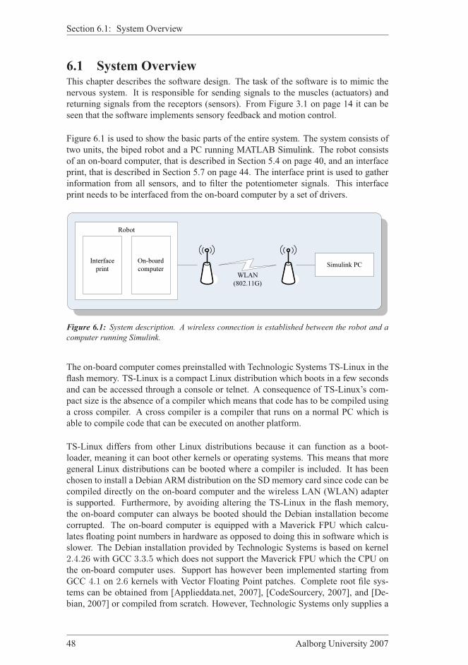
Section 6.1: System Overview
6.1 System OverviewThis chapter describes the software design. The task of the software is to mimic the
nervous system. It is responsible for sending signals to the muscles (actuators) and
returning signals from the receptors (sensors). From Figure 3.1 on page 14 it can be
seen that the software implements sensory feedback and motion control.
Figure 6.1 is used to show the basic parts of the entire system. The system consists of
two units, the biped robot and a PC running MATLAB Simulink. The robot consists
of an on-board computer, that is described in Section 5.4 on page 40, and an interface
print, that is described in Section 5.7 on page 44. The interface print is used to gather
information from all sensors, and to filter the potentiometer signals. This interface
print needs to be interfaced from the on-board computer by a set of drivers.
Simulink PCWLAN
(802.11G)
On-board computer
Interface print
Robot
Figure 6.1: System description. A wireless connection is established between the robot and a
computer running Simulink.
The on-board computer comes preinstalled with Technologic Systems TS-Linux in the
flash memory. TS-Linux is a compact Linux distribution which boots in a few seconds
and can be accessed through a console or telnet. A consequence of TS-Linux’s com-
pact size is the absence of a compiler which means that code has to be compiled using
a cross compiler. A cross compiler is a compiler that runs on a normal PC which is
able to compile code that can be executed on another platform.
TS-Linux differs from other Linux distributions because it can function as a boot-
loader, meaning it can boot other kernels or operating systems. This means that more
general Linux distributions can be booted where a compiler is included. It has been
chosen to install a Debian ARM distribution on the SD memory card since code can be
compiled directly on the on-board computer and the wireless LAN (WLAN) adapter
is supported. Furthermore, by avoiding altering the TS-Linux in the flash memory,
the on-board computer can always be booted should the Debian installation become
corrupted. The on-board computer is equipped with a Maverick FPU which calcu-
lates floating point numbers in hardware as opposed to doing this in software which is
slower. The Debian installation provided by Technologic Systems is based on kernel
2.4.26 with GCC 3.3.5 which does not support the Maverick FPU which the CPU on
the on-board computer uses. Support has however been implemented starting from
GCC 4.1 on 2.6 kernels with Vector Floating Point patches. Complete root file sys-
tems can be obtained from [Applieddata.net, 2007], [CodeSourcery, 2007], and [De-
bian, 2007] or compiled from scratch. However, Technologic Systems only supplies a
48 Aalborg University 2007

Chapter 6: Software
object file for the UART which can not be linked with object files compiled with GCC
4.1. Since the UART is essential for the robot to function it is necessary to forgo the
possibility of using the FPU by compiling the code with GCC 4.1. Another way of
using the FPU is by assembler instructions, however converting all operations involv-
ing floating point calculations to assembler would be very time consuming and a rather
cumbersome task. It is therefore chosen to use the Debian distribution provided by
Technologic Systems.
To ease the implementation of controllers and filters Real-Time Workshop (RTW)for
MATLAB Simulink is used. RTW discretizes a Simulink model and generates C-code
that encapsulates the model. In order for RTW to support linux the soft real-time linux
target LNX [Bhanderi, 2006] is used which executes the model at the frequency speci-
fied in the Simulink model.
Figure 6.1 shows the robot and the Simulink computer connected through the wireless
connection. The idea is that a set of drivers are developed as S-functions in a Simulink
environment. These drivers provide a simple interface to the actuators on the robot as
well as all the sensor signals. The code, along with a automatically generated make-
file, is then uploaded to the robot through the wireless connection. In order to compile
the uploaded code an ssh connection is established to the robot and the make-file is
executed using make. After the code has been compiled, a stand-alone program is
available on the robot, that is executed using the ssh connection and the task speci-
fied in the Simulink model is carried out. After the code has been generated, only the
make-file and the generated code is needed on the on-board computer. The work flow
for executing a command specified by Simulink is seen from Figure 6.2. This figure
also shows that it is possible to download the data measured on the sensors.
To exploit the full potential of the 200MHz ARM9 processor located on the on-
board computer, a high level interface has been developed which implements a multi-
threading system. So the software layers consists of a Debian Linux distribution, the
LNX RTW Target controlling the soft real-time requirements, the developed Simulink
model, the high level interface drivers ensuring multi-threading and the low level in-
put/output drivers where the communication protocol to interface sensors and servo
motors is implemented. The layering of the implemented software is depicted in Fig-
ure 6.3.
Next a description of the low level I/O drivers is given, after which a description of the
high level interface drivers is given. All the code that the drivers consist of will not be
shown here. Instead the reader is encouraged to read the source code located on the
enclosed CD-ROM under software/drivers.
6.2 I/O DriversThe drivers can be divided into input drivers and output drivers. The drivers will in the
following be described as such. Technologic System supplies code that shows how the
interfacing of the I/O is done. This code has been utilized in the development of the
drivers.
Group 1033 49
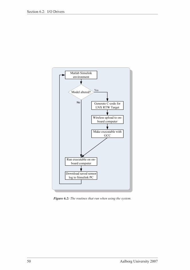
Section 6.2: I/O Drivers
Matlab Simulinkenvironment
Generate C-code for LNX RTW Target
Wireless upload to on-board computer
Make executable with GCC
Download saved sensor log to Simulink PC
Run executable on on-board computer
Model altered? Yes
No
Figure 6.2: The routines that run when using the system.
50 Aalborg University 2007

Chapter 6: Software
Linux Debian OS
LNX RTW Target
Simulink Model
High Level Interface Drivers
Low Level Input Drivers
Low Level Output Drivers
Figure 6.3: The different parts of the software system layer.
6.2.1 Low Level Input Drivers
As described in Section 5.5.1 on page 42, 32 sensor input signals have to be read
through two external multiplexers which are each connected to another multiplexer
located internally in the on-board computer. Furthermore the voltage levels on the bat-
teries have to be read as well. Figure 6.4 shows how the multiplexers and the batteries
are connected to the on-board computer. As can be seen on the figure the four address
pins (AD0-3) on the multiplexers share the same four general purpose input output
(GPIO) pins on the on-board computer. This means that changing the levels of the
GPIO pins sets a new address on both multiplexers. ADC0-3 on Figure 6.4 refers to
the analogue-to-digital converters on the on-board computer.
The address pins are not connected to the GPIO’s in an incrementing order because
this would have complicated the layout of the interface print. This has to be handled in
the driver so the correct sensors are addressed. Changing the levels of the GPIO’s are
controlled by a single 8 bit register where a high bit corresponds to a high level. Table
6.1 shows which input on the multiplexer is connected to the ADC at the given register
values.
The task of reading a sensor is thereby twofold, the correct value has to be written to
the register and afterwards the ADC0 and ADC1 has to be read. An intuitive approach
would be to read both ADC0 and ADC1 before changing the address on the external
multiplexer. However, because the on-board computer does not have four dedicated
ADC channels and instead uses a multiplexer that connects four inputs to a single
ADC, it is faster to read all 16 channels on one of the external multiplexers and then
change to the next ADC. This is because the multiplexer on the on-board computer
is slower than the one used on the interface print. The sequence for reading all the
sensors is seen from Figure 6.5.
Group 1033 51

Section 6.2: I/O Drivers
ADC0
ADC1ADC2ADC3
GPIO0
GPIO2GPIO4
GPIO3
AD0AD1AD2AD3
Sensors
1x16
1x16External multiplexers
On-board computer
Battery 1Battery 2
Internal multipexerADC
Figure 6.4: The figure shows how the multiplexers and the batteries are connected to the on-
board computer.
Input Register value ADC0 ADC1
1 0 θ7 IMU gyro X
2 1 θ9 IMU gyro Y
3 4 θ8 IMU reference voltage
4 5 θ10 IMU acc. X
5 16 θ11 IMU acc. Y
6 17 θ12 IMU acc. Z
7 20 θ6 Right foot force 1
8 21 θ4 Ground
9 8 DIP switch 3 Right foot force 2
10 9 DIP switch 4 Right foot force 3
11 12 DIP switch 1 Left foot force 1
12 13 DIP switch 2 Left foot force 2
13 24 θ5 Left foot force 3
14 25 θ3 Push button 1
15 28 θ2 Push button 2
16 29 θ1 Push button 3
Table 6.1: The register value corresponds to the input that is connected to the ADC.
52 Aalborg University 2007

Chapter 6: Software
1. Read ADC0 to switch internal multiplexer to ADC0
2. Discard the value and wait for the internal multiplexer to settle
on the input for ADC0
3. Read and save all 16 channels
4. Repeat step 1 to 3 for ADC1
6. Read and save the value on ADC2
5. Repeat step 1 to 2 for ADC2
7. Repeat step 5 to 6 for ADC3
Figure 6.5: The sequence called for reading all the sensors.
Group 1033 53

Section 6.2: I/O Drivers
The ADC is read using the function read channel which was supplied by Techno-
logic Systems.
read channel:Arguments: unsigned long adc page, unsigned short channelReturns: intExplanation: The function returns the value recorded by the ADC channel specified by the argument channel. The
argument adc page is the memory page of the ADC.
The virtual address space is divided into two areas. One area is the kernel space which
is restricted to access from the kernel only. The second area is the user space where in
the compiled Simulink model runs. As the ADC stores the read values in kernel space,
these can not be accessed from the compiled code in user space by simply assigning
the address of the register to a pointer. Doing so would lead to a segmentation fault.
Instead the system call mmap is used to access kernel space from user space.
mmap:Arguments: void *start, size t length, int prot, int flags, int fd, off t offsetReturns: void *Explanation: Is a function that can map devices in to memory. mmap asks to map length in to memory from the file
descriptor fd starting at offset preferably mapped to start. prot tells what kind of protection should be on the mapping, eg.read only or write only. flags specifies if the map should be private to the process or shared.
The value returned from the ADC is not a linear representation of the voltage which
is explained in the data sheet [Cirrus Logic, 2004, pp. 34]. If the voltage is between
0V and 1.65V the ADC will return a value from 40, 536 to 65, 535 where 40, 536represents 0V. If the voltage is between 1.65V and 3.3V the ADC will return a value
from 0 to 25, 000. The returned value from the ADC is normalized by the function
adcNorm to a value between 0 and 50, 000.
adcNorm:Arguments: int adcValReturns: intExplanation: The function converts adcVal, which is the value returned by read channel, to a value between 0 and
50, 000.
Conve¡rting the normalized ADC value to a voltage can be done using Equation (6.1)
VADC =3.3nADC
50, 000(6.1)
where nADC is the normalized value from the function adcNorm. The complete driver
can be found in Software/Drivers/ADC/sensor_thread.c on the enclosed
CD-ROM.
Known driver issues
As described in the previous section mmap is used to access kernel space where the
ADC registers are situated. The LNX RTW Target uses the function mlockall to
avoid that the address space, used by the process, is paged to the swap area, i.e., the
memory card which is slower to read from than RAM.
mlockall:Arguments: const void *addr, size t lenReturns: intExplanation: The function locks the virtual address space starting from addr to len bytes for the calling process.
This is done to increase the performance, however, in kernel 2.4 which is supported byTechnologic System the same process can not use both mmap and mlockall. Doing
54 Aalborg University 2007

Chapter 6: Software
so makes the kernel crash and the system needs to be rebooted. mlockall is therefore
not used. As a consequence the model stops with an alarm clock until it has been called
4-5 times. The reason why the program then starts after some attempts is most likely
because the kernel recognizes the model as a frequently called program and keeps the
memory page in RAM which results in faster startup of the model.
6.2.2 Low Level Output Drivers
The task of the output driver is to control the servo motors. To do this the driver must
support the communication protocol specified in Section A. However not the entire
protocol will be implemented as it is only necessary to control the position and the
velocity. The servo controllers uses a standard UART for the communication. Be-
cause of the Debian Linux running on the on-board computer the UARTs have to be
utilized through the kernel which is done using open. open returns a file descriptor
that can be used with write, which writes a string on the UART. However before
write is used the UART has to be configured with the correct settings which is done
using a struct named adc. The entries in termios dictates the baud rate, synchronous or
non-synchronous operation etc. These settings are given in Appendix A on page 173
concerning the setup of the protocol used for communication with the Pololu boards.
open and termios are used in initSerPort.
initSerPort:Arguments: char *deviceReturns: intExplanation: Returns a file descriptor to the UART pointed to by *device. *device is a string which gives the path to theserial port, eg. /dev/ttyAM0.
After the serial port has been initialized by initSerPort the Pololu boards can be
accessed. Controlling the position of the servo motors can be done using command 4
of the Pololu protocol which is explained in Appendix A on page 173. This is imple-
mented in the function sendPos.
sendPos:Arguments: unsigned short int pos, unsigned char servoNumber, int fdReturns: intExplanation: Implements command 4 of the Pololu protocol. pos is a value between 500 and 5500 specifying the desiredposition of the servo motor connected to output servoNumber on the serial port pointed to by the file descriptor fd. Inorder to update the position of a servo motor it is necessary to send a packet of 6 bytes.
Controlling the velocity of the servo motors can be done using command 1 of the
Pololu protocol which is implemented in the function sendVel.
sendVel:Arguments:unsigned var vel, unsigned char servoNumber, int fd)Returns: intExplanation: Implements command 1 of the Pololu protocol. vel is the velocity at which the servo motor should move.This can be between 0 and 127. 0makes the servo motor change to the desired position as fast as possible. servoNumberis the output port on the Pololu board pointed to by the file descriptor fd. In order to set the velocity of a servo motor it isnecessary to send a packet of 5 bytes.
From the functions sendPos and sendVel it can be seen that a total of ∆d = 11Bhas to be sent to each servo motor if position and velocity are to be controlled. Each
servo controller board has a dedicated UART as described in Section 5.4 on page 40
where it is possible to connect 8 servo motors. The servo controllers can not operate
at a baud rate higher than 38, 400 baud. To translate this to bytes per second it has to
be determined how many bits that are needed to transmit a byte. The servo controller
Group 1033 55

Section 6.3: High Level Interfacing
board specifies that 8 bit should be sent at a time, including no parity and one stop
bit. If one byte has to be transmitted a start bit and stop bit have to be sent along
with the 8 bit giving a total of 10 bit. However using 10 bits assumes that there is nodelay between sending two bytes. The data sheet [Cirrus Logic, 2004] for the on-board
computer does not mention how long this delay is. Therefore it has been chosen to
assume that a byte, that is to be transmitted requires 11 bits. Converting the baud rateto a data rate can thereby be done in the following way:
smax =38400 baud
11 bit= 3490
B
s(6.2)
As the maximum data rate has been determined it is now possible to determine the
maximum update frequency. This is done in a worst case sense meaning that it is
assumed that 8 servo motors are connected to the servo controller board:
fmax =smax
nservos∆d(6.3)
=3490 B
s
8 · 11B(6.4)
= 39.7Hz (6.5)
However a better approach would be to connect 7 servo motors to each servo controllerboard reducing nservos to 7, and thereby increasing fmax to 45.3Hz. It can also be men-tioned that if the velocity input is omitted then the maximum update frequency, fmax,can be increased to 83.0Hz.
The source code for the low level output functions can be found on the enclosed CD-
ROM in Software/Drivers/Serial driver/serial_driver.c.
In the next section the high level interface of the drivers is described.
6.3 High Level InterfacingThe following section describes the interface between the Simulink model and the low
level drivers. This interface isolates the low level drivers from Simulink such that only
two functions are needed by Simulink for each task; an initialization function and a
function for the task. The tasks here are to update the servo motors and collect sensor
data.
6.3.1 Interfacing the Servo Motors
The flow of the functions used to update the servo motors is depicted in Figure 6.6.
Updating the servo motors is a rather slow process due to the low baud rate that can
be communicated with the Pololu boards. In Equation (6.5) the maximum update fre-
quency, fmax, was determined to 39.7Hz. This frequency is without any execution ofcode on the robot, which means that the frequency has to be lowered to give time to
executing code. A better approach would be to update the servo motors in parallel with
56 Aalborg University 2007
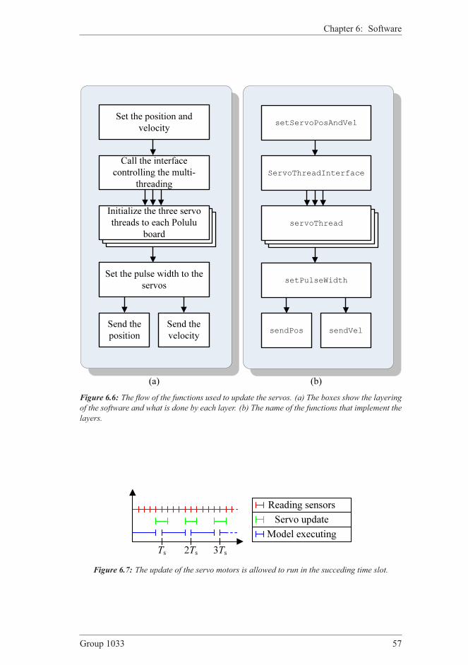
Chapter 6: Software
Set the position and velocity
Call the interface controlling the multi-
threading
Initialize the three servo threads to each Polulu
board
Set the pulse width to the servos
Send the position
Send the velocity
setServoPosAndVel
ServoThreadInterface
servoThread
setPulseWidth
sendPos sendVel
(a) (b)Figure 6.6: The flow of the functions used to update the servos. (a) The boxes show the layering
of the software and what is done by each layer. (b) The name of the functions that implement the
layers.
Ts 2Ts 3Ts
Model executingServo update
Reading sensors
Figure 6.7: The update of the servo motors is allowed to run in the succeding time slot.
Group 1033 57

Section 6.3: High Level Interfacing
the executing code.
In Figure 6.7 the principle of parallel execution is depicted, where Ts is the sample
time. Here the update sequence of the servo motors can continue in the next timeslot
as long as fmax > 1/Ts. To accomplish this each Pololu board is controlled by a
thread. A shared memory area, called a critical section, is created between the Simulink
model and the threads. This critical section is protected by a mutual exclusion (mutex)
to avoid concurrent access. A library exists in Linux which implements the POSIX
thread standard called pthreads. Mutex support is directly implemented in pthreads.
But before the thread can be designed it is necesarry to have a way of representing
the Pololu boards and the servo motors. In order to describe each servo motor the
following struct is used:
s t r u c t s e r voMo to rshor t i n t servoNumber ;
shor t i n t outputNumber ;
shor t i n t se rvoType ;
double uppe rL im i t ;
double l owe rL im i t
double pos ;
double v e l ;
In the struct servoMotor the variable servoNumber is the number of the servo motor
as described by Figure C.3 on page 188. outputNumber is the connector on the Pololu
board which the servo motor is connected to. servoType is the type of servo motor,
either a HS645 or a 5995TG. upperLimit and lowerLimit are the limits, in degress, in
which the servo motor is allowed to operate. pos is the postion of the servo motor
shaft in degrees and vel is the velocity at which the servo motor should move to a
new position. Each Pololu board can have up to 8 servo motors connected. This is
encapsulated in the following struct:
s t r u c t s e r voBoa rdshor t i n t boardNumber ;
shor t i n t numberOfServos ;
shor t i n t d a t a ;
p t h r e a d mu t e x t ∗newData ;char s e r i a l P o r t [ 2 5 ] ;
s t r u c t s e r voMo to r s e rvoMoto r s [ 8 ] ;
In the struct servoBoard the variable boardNumber is the number given to the Pololu
board as described in Table C.3 on page 187. numberOfServos is the number of servo
motors that are connected to the Pololu board. The mutex newData is used to avoid
concurrent access to the servoBoard struct. serialPort[25] is a string which gives the
path to the serial port, e.g., /dev/ttyAM0, which the Pololu board is connected to.
In order to update the positions contained in the servoBoard struct the function set-
PulseWidth is used.
setPulseWidth:Arguments: struct servoBoard *servoBoard, int fdReturns: voidExplanation: The function traverses the array servoMotors in *servoBoard and updates the position and velocity of eachservoMotor struct. fd is a file descriptor of the serial port which the Pololu board is connected to. The upper and
lower limits of the servo motors are checked and the output is limited if necessary. If the limit is exceeded a warning
is printed in the console telling which servo motor was limited. setPulseWidth uses sendPos and sendVel,described in Section 6.2.2 on page 55, to update position and velocity of the servo motors.
58 Aalborg University 2007

Chapter 6: Software
The task of the thread, called servoThread, is now to take a pointer to a
servoBoard struct and call setPulseWidth with this struct.
servoThread:Arguments: void *servoBoardReturns: void *Explanation: When the thread is called it first calls initSerPort with the path to the serial port given in *servoBoard-¿serialPort. The thread waits for *servoBoard-¿data to become true indicating that there are new positions and velocities
that should be updated. To avoid that the thread uses its complete time slot, checking to see if data becomes true,
sleep(0) is called each time *servoBoard-¿data is checked and it is false. sleep(0) releases the CPU so other
processes or threads may run instead.
Since there are three Pololu boards three servoThread threads have to be started
each with their own servoBoard struct. The three servoBoard structs have to be
stored some where in the memory which also allow the Simulink model to access
them. This is done using the function servoThreadInterface.
servoThreadInterface:Arguments: int task, double *positions, char *velocitiesReturns: voidExplanation: The argument task can either be SEND or INIT. If task is INIT the function initializes three static
servoBoard structs with the appropriate limits, serial port, servo number etc. If task is SEND then the values pointed
to by posistions and velocities are inserted in the servoMotor structs and the threads sends the new values to the servo
motors.
To enable the Simulink model to update the positions and velocities of the servo motors
the function setServoPosAndVel is used.
setServoPosAndVel:Arguments: double *servoPos, signed char *velReturns: intExplanation: The function updates the positions and the velocities of the servo motors given in *servoPos and *vel.
The positions *servoPos and velocities *vel, in the function setServoPosAndVel,
must be ordered incrementally. That is, the position and velocity of servo motor
1, abbrivated as S1 in Figure C.3 on page 188, must be in posistions[0] and ve-
locities[0], position and velocity of servo motor 2 must be in posistions[1] and ve-
locities[1] etc. servoThreadInterface is called with task set to SEND, the
pointer *positions set to *servoPos, and the pointer *velocities set to *vel. Before
setServoPosAndVel can be called by the Simulink model the threads have to ini-
tialized. This is done by calling the function initServos.
initServos:Arguments: voidReturns: voidExplanation: The function initializes the threads that update the servo motors. initServos must be called before
setServoPosAndVel can be used.
The source code for the low level output functions can be found on the enclosed CD-
ROM in software/drivers/serial_driver.c.
6.3.2 Interfacing the Sensors
Using the same approach as described in Section 6.3.1, and depicted in Figure 6.7, thesensors are read by a thread. The readings are stored in the struct acq.
s t r u c t acqp t h r e a d mu t e x t ∗ r e ad ing sMutex ;
double ∗ r e a d i n g s ;
Group 1033 59
Section 6.4: Partial Conclusion to Software
The thread, readSensorsThread, implements the approach described in Section
6.2.1 for reading the sensors.
readSensorsThread:Arguments: void *pReturns: voidExplanation: The thread continously reads the sensors and stores them in * acq-¿readings. The mutex readingsMutex islocked with every update of * acq-¿readings.
The thread continously reads the sensors as fast as possible. Everytime a sensor is
read the mutex readingsMutex is locked and when the sensor value has been aqcuired
the mutex is unlocked and the thread pauses until the multiplexer has settled on a new
sensor. In this pause the sensor readings can be extracted and used in Simulink. This
requires some shared memory that can accessed both by the thread and Simulink. The
interface between the thread and Simulink is implemented by the function
readSensorsInterface.
readSensorsInterface:Arguments: struct acq *acq, double *readings, int taskReturns: voidExplanation: The function either copies the contents of *readings to *acq-¿readings or copies *acq-¿readings to *read-ings depending on the value of task.
When the thread is started it calls readSensorsInterface with task set to INIT
and a pointer to a acq struct where the sensor readings are stored. The thread can
then put readings in the shared memory by writing to the pointer readings. When
Simulink needs the readings it calls readSensors from an S-function with a pointer
to a local double array that can hold 34 values.
readSensors:Arguments: double *readingsReturns: voidExplanation: The function copies the sensor readings to *readings.
readSensors calls readSensorsInterface with task set to GETDATA and
the pointer readings, which lock the mutex and copies the data to the pointer. Before
readSensors can be used the function initSensors has to called which initial-
izes the thread readSensorsThread.
6.4 Partial Conclusion to SoftwareThis chapter gave a description of the implemented software. The solution given en-
abled the robot to be completely autonomous. A Debian distribution was installed on
the SD card on the on-board computer. A real-time target for RTW was installed en-
abling the use of Simulink for the design of the controllers. The developed drivers were
designed to run in a multi-treaded environment in order to optimize the acquisition of
sensor readings. Futhermore Simulink was isolated from the low level drivers by only
having to initialize the threads by calling initServos and initSensors and af-
terwards using setServoPosAndVel to update the servo motors and
readSensors to read the sensors.
60 Aalborg University 2007

7MODELING
Chapter contents7.1 Introduction to Modeling 63
7.1.1 System Description 63
7.1.2 Previous Work 64
7.1.3 Modeling Approach 66
7.2 Servo Motor Model 67
7.2.1 Implementation of the Servo Motor Model 68
7.2.2 Determination of Servo Motor Parameters 69
7.2.3 Verification of Servo Motor Model 71
7.3 Kinematic Model 71
7.3.1 Representation of the Mechanical Structure 72
7.3.2 Attacing Frames 74
7.3.3 The Generalized Coordinates 77
7.3.4 Verification of the Kinematic Model 78
7.4 Dynamical Model 79
7.4.1 Dynamical Modeling Approach 80
7.4.2 Single Support Phase Modeling 82
7.4.3 Double Support Phase Modeling 83
7.4.4 Verification of the Dynamical Model 86
7.5 Phase Estimator 86
7.5.1 The Hybrid Model 88
7.5.2 Finding the Phase of the System 90
7.5.3 Calculation of the Weight Distribution 90
7.6 Foot Model 92
7.6.1 Forces Acting on the Foot 93
7.6.2 Summing the Forces 95
7.6.3 Verification of the Foot Model 95
7.7 Head Model 96
7.7.1 Angular Velocity of the Head 96
7.7.2 Linear Acceleration of the Head 97
7.7.3 Verification of the Head Model 98
7.8 Partial Conclusion to Modeling 99
Group 1033 61

I N THIS CHAPTER a model for biped robot system i developed. The purpose of
model is to give an insight into the system and thereby obtain a model which can be
used for testing and simulation of controllers. In the following an introduction is given
to the general system of biped robots, afterward a look at the approaches in the existing
literature will be given. Then, as a last point before describing the development of the
actual model, an explanation of the approach taken in this project is given.
62 Aalborg University 2007
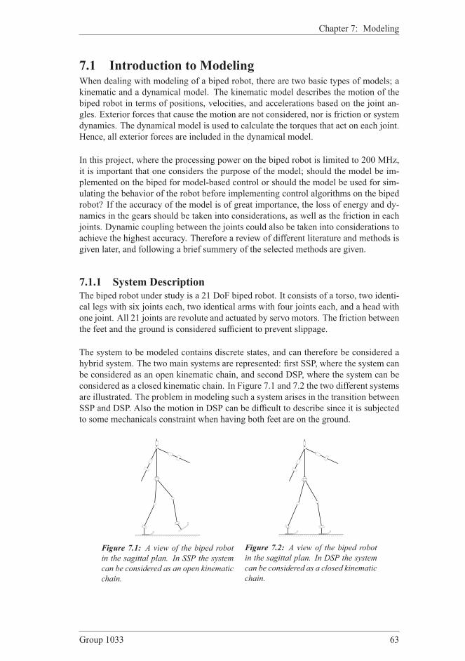
Chapter 7: Modeling
7.1 Introduction to ModelingWhen dealing with modeling of a biped robot, there are two basic types of models; a
kinematic and a dynamical model. The kinematic model describes the motion of the
biped robot in terms of positions, velocities, and accelerations based on the joint an-
gles. Exterior forces that cause the motion are not considered, nor is friction or system
dynamics. The dynamical model is used to calculate the torques that act on each joint.
Hence, all exterior forces are included in the dynamical model.
In this project, where the processing power on the biped robot is limited to 200 MHz,
it is important that one considers the purpose of the model; should the model be im-
plemented on the biped for model-based control or should the model be used for sim-
ulating the behavior of the robot before implementing control algorithms on the biped
robot? If the accuracy of the model is of great importance, the loss of energy and dy-
namics in the gears should be taken into considerations, as well as the friction in each
joints. Dynamic coupling between the joints could also be taken into considerations to
achieve the highest accuracy. Therefore a review of different literature and methods is
given later, and following a brief summery of the selected methods are given.
7.1.1 System Description
The biped robot under study is a 21 DoF biped robot. It consists of a torso, two identi-
cal legs with six joints each, two identical arms with four joints each, and a head with
one joint. All 21 joints are revolute and actuated by servo motors. The friction between
the feet and the ground is considered sufficient to prevent slippage.
The system to be modeled contains discrete states, and can therefore be considered a
hybrid system. The two main systems are represented: first SSP, where the system can
be considered as an open kinematic chain, and second DSP, where the system can be
considered as a closed kinematic chain. In Figure 7.1 and 7.2 the two different systems
are illustrated. The problem in modeling such a system arises in the transition between
SSP and DSP. Also the motion in DSP can be difficult to describe since it is subjected
to some mechanicals constraint when having both feet are on the ground.
Figure 7.1: A view of the biped robot
in the sagittal plan. In SSP the system
can be considered as an open kinematic
chain.
Figure 7.2: A view of the biped robot
in the sagittal plan. In DSP the system
can be considered as a closed kinematic
chain.
Group 1033 63

Section 7.1: Introduction to Modeling
7.1.2 Previous Work
Different attempts have been made to set up models for biped locomotion. In some of
the many available papers the approaches are varying. A large number of prevailing
papers only cover the SSP [Shih, 1996], and some only the DSP [Zhao et al., 1997].
Some neglects the impact phase [Mu and Wu, 2004] while others claim that this phase
is the most important phase in the description of biped locomotion [Bruneau et al.,
2001]. Some include a very thorough actuator model, while other completely disre-
gard the actuators.
Many of the papers also have some similarities, they rarely includes the arms in the
model, many consider robots with low degree of freedom, usually 4-6 DoF’s and in
most papers the model only describes the biped robot in the sagittal plane. Further-
more rotation about the z-axis in the hip is almost never included. All these points
simplify the modeling much.
In this project, it is desired to develop a complete model, describing a biped robot with
21 DoF’s and human proportions. Furthermore it is desired to describe movement in
both the sagittal and frontal plane, while switching between SSP and DSP. To develop
this model, it is necessary to combine ideas presented in many different papers. The
following will be a description of some of the approaches taken in the available litera-
ture. The description is divided into some of the main topics within modeling of biped
robots.
Kinematic Representation To be able to describe the position and orientation of the
links on the biped robot, a frame is attached to each of them. The kinematic
model developed in [Mu and Wu, 2004] considers the biped robot as an open-
loop serial-chain from the supporting foot to the free ends. This frame attach-
ment is intuitive, since all positions are found relative to a frame fixed to the
ground. However, some problems can arise during the DSP, where both feet are
placed on the ground. Furthermore some consideration should be given toward
the fact that the biped robot will shift the supporting foot during a walking cycle.
In [Yamaguchi et al., 1999] the position of all links are given relative to a frame
attached in the hip. Using this configuration there is no need for moving the base
frame around. A consequence of having the frame fixed to the hip, is however
that all positions are found relative to a frame that moves with respect to the
ground. In [Li et al., 1993] the model is developed with respect to a ground fixed
frame and a moving frame placed in the waist of the robot.
Dynamic Representation The dynamics of the biped robot can be described using
two different approaches; the Newtonian and the Lagrangian. The Newtonian
approach is based on Newtons laws while the Lagrangian approach builds on
energy considerations.
In [Craig, 1989] a very thorough description of the Newtonian approach is given.
Though the application is manipulators, the ideas can be applied on a biped
robot. In [Christensen et al., 2006] a Newtonian model, based on [Craig, 1989],
describing a 21 DoF biped robot in SSP has been implemented. Furthermore
[Christensen et al., 2006] has implemented a model of a 10 DoF biped robot in
SSP based on the lagrangian approach, and compared the two approaches. The
64 Aalborg University 2007

Chapter 7: Modeling
main result of this comparison was that the Newtonian approach was more intu-
itive, but had shortcomings when the DSP should be modeled. However [Chris-
tensen et al., 2006] gives a proposal for a DSP model using the Lagrangian ap-
proach. The Newtonian model is recursively defined and therefore the calcula-
tion time increases significantly with the number of DoF. One way of optimizing
the Newton Euler algorithm is by reducing the DoF. To do that, the reduced DoF
must be taken into account by adding constraints to the kinematic, dynamical
and inverse kinematic model. In the swing phase, it is possible to lock some of
the joints, and thereby merging two or more joints to a single joint. Similar, in
DSP it is also possible to merge some of the joints to achieve a reduced model,
which has been used in [Hardt et al., 1999]. It is clear that the effect of the
optimization is limited due to the fact that even though the number of DoF is
reduced, the algorithm is still time consuming and with a high number of DoF,
the possibilities for implementing such model on a small-scale computer is im-
possible [Chaillet et al., 1994].
The Lagrangian approach is very time demanding in the derivation phase, but
when the model is derived first time, the simulation time is low compared to the
Newtonian approach, for large DoF. This is due to the fact that the Lagrangian
approach will result in a number of analytic equations compared with the recur-
sive algorithms of the Newton Euler approach.
Constraints in DSP Many papers treat the difficult issues that arise when the biped
robot is in DSP and the system is imposed to different constraints. In [Mu
and Wu, 2003] and [Mu and Wu, 2004] a complete dynamical model for a
five link biped robot is outlined, the model is based on D’Alembert’s princi-
ple (Lagrangian). The constraints imposed on the system are implemented as
Lagrangian multipliers, which is also described in [Wisniewski, 2006]. In [Ud-
wadia and Kalaba, 2001] and [Udwadia and Kalaba, 2002] they obtain the equa-
tions of motion for systems where the principle of D’Alembert’s does not hold,
which is the case when sliding friction is present. In [Christensen et al., 2006] an
approach is suggested where the DSP model is based on a combination of SSP
models. The latter seems optimal since the SSP models can be used for both SSP
and DSP. No specific model for the DSP model needs to be derived.
Impact phase The switch phase in a normal gait-cycle has a very strong influence on
the system dynamics. In [Buschmann et al., 2006] the importance of deriving
a model for the foot if this contains damping or any other shock absorber is
mentioned. In the case of the biped robot for this project, the foot could be
modeled as a spring and a damper in parallel. This model can be used as a
transition between the SSP and the DSP model. The same method is used in
[Buschmann et al., 2006] where the feet on Johnnie are modeled as a spring and
a damper in parallel. Other articles mention that the need for deriving a model
of the feet is limited due to the fact that the duration of the impact is very short.
So by saying that the time is infinite short, there is no need to model the impact
phase. These, however, do not use any shock-absorber and often model their
robots as having single-point contact with the surface [Doi et al., ]. A model
describing the system in the impact phase rather than a model of the foot, is
given in [Hurmuzlu, 2001]. Here it is found that if the impact phase is included
Group 1033 65

Section 7.1: Introduction to Modeling
in the model, it will result in smooth walk, as the biped robot is able to minimize
to impact.
7.1.3 Modeling Approach
CompleteModelrefθθθθ
feetf
heada
headωωωω
legsθθθθ
Figure 7.3: The model of the biped robot, with the same input and output as the physical system.
The final model of the biped robot should describe the relationship between the input
applied to the physical system and the output measured at the physical system. This is
illustrated in Figure 7.3.
refθθθθ
feetf
heada
headωωωω
legsθθθθ
Servo Motor Model
Kinematic Model , ,q q qɺ ɺɺ, ,θ θ θθ θ θθ θ θθ θ θɺ ɺɺ
ττττ
Foot Modelf
Head Model
Model
refθθθθɺ
wPhase Estimator
Dynamical Model
ρ
Figure 7.4: An extended illustration of the model, describing the interfaces and division be-
tween/of sub models.
In order to clarify the modeling of the entire biped robot, it is divided into several sub
models. These sub models can be seen in Figure 7.4, where the interface between the
models is also illustrated. The model is divided into five sub models, which are:
Servo motor model As seen in Figure 7.4 the input to the model are the angular po-
sition references, θref. In the physical system these references are given to each
servo motor, whose internal controller ensures that the motor shaft obtains this
66 Aalborg University 2007

Chapter 7: Modeling
position. Therefore the first sub model is a model of the servo motors. This
model should describe the relationship between the input reference angle and
the actual position, θ, velocity, θ, and acceleration, θ, of the motor shaft. This
motion is however also dependent on the load of the servo motor, therefore the
servo model is extended with an additional input, providing the torque on the
motor shaft. This torque is calculated in the dynamical model, and provided as
feedback to the servo motor. From the output of the servo motor model, it is
possible to retrieve the actual position of the twelve servos in the legs, θlegs. The
deviation of the servo motor model is explained in Section 7.2.
Kinematic model At this point the exact motion of the biped robot is given in joint
space using θ, θ, and θ. A kinematic model transforms from joint coordinates
into generalized coordinates, q, q, and q. This makes the motion of the biped
robot be given in both joint coordinates and Cartesian coordinates. The deviation
of the kinematic model is explained in Section 7.3.
Dynamical model With the generalized coordinates as input, a dynamical model is
found. This dynamical model describes the torque that each servo motor is sub-
jected to, given the motion. This torque is fed back to the servo motors. The
dynamical model describes both the SSP-R, SSP-L and the DSP. As described in
Section 7.1.1 the SSP and DSP are two different systems, therefore the dynam-
ical model will be a hybrid model, capable of describing both types of system.
The dynamical model will be developed using Lagrangian formulation. The de-
viation of the dynamical model is explained in Section 7.4.
Phase estimator Both the dynamical and the kinematic model are dependent of the
phase of the hybrid system, that is if the biped robot is in SSP-R, SSP-L or DSP.
A phase estimator is designed in order to determine the phase. Further the phase
estimator calculates the weight distribution between the feet, since the dynamics
of the system is dependent on this distribution.
Foot model In order to determine the six forces exerted on the feet it is necessary to
have a model of the foot. This model takes the forces and torques exerted in
the ankle joint, and returns the forces exerted on the left and right foot. The
deviation of the foot model is explained in Section 7.6.
Head model The output from the kinematic model can be transformed using the head
model, to give the output of the IMU, namely the linear acceleration and angular
velocity. The deviation of the head model is explained in Section 7.7.
In the following the development of each of the five models will be described, starting
with the servo motor model.
7.2 Servo Motor ModelThe servo motor can be controlled by a position reference,θref, and according to this
reference, and the load, τ , the shaft is moved with a certain velocity and acceleration.
The servo motor model is illustrated in Figure 7.5. The block contains 21 servo motor
models, each having τi and θrefi as input, and θi, θi and θi as output. Note that there are
two different servo motors 12 of the type HSR-5995TG and 9 of the type HS-645MG.
The specifications of the two servo motors can be found in Table 5.1 on page 38.
Group 1033 67

Section 7.2: Servo Motor Model
Servo motor model θθθθɺɺ
θθθθɺθθθθ
refθθθθ
ττττ
Figure 7.5: The I/O of the servo motor model.
7.2.1 Implementation of the Servo Motor Model
The model is based on a discrete state space system and is build up using the structure
seen from Figure .
ΣB C
A
1z
+
+
refθθθθ , , θ θ θθ θ θθ θ θθ θ θɺ ɺɺ
Figure 7.6: State space structure of the servo motor model.
The velocity is used to control the other states, and can be calculated as:
θk+1 = c(θref − θk) = cθref − cθk , θmin(τ) ≤ θk+1 ≤ θmax(τ) (7.1)
where c is a constant controlling the first order behavior when θ is close to θref. As
seen, the maximum and minimum velocity depends on τ . This relationship has to
be found from measurements, which is done in Section 7.2.2. The velocity is imple-
mented as a dynamic saturation which depend on the load τ .
The position is calculated from the velocity:
θk+1 = θk + Tsθk (7.2)
where Ts is the sampling time. The acceleration can be calculated by saving the ve-
locity state one step back in time and calculate the difference between the new and old
velocity divided by the sampling time:
θk+1 =θk − θk−1
Ts, −θmax ≤ θk+1 ≤ θmax (7.3)
Since it is the velocity state that is being controlled, the maximum acceleration is im-
posed on the velocity as a rate limiter. Thus Equation (7.1) is also limited by:
− θmax ≤θk − θk−1
Ts
≤ θmax (7.4)
68 Aalborg University 2007
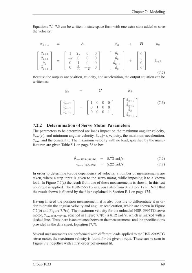
Chapter 7: Modeling
Equations 7.1-7.3 can be written in state space form with one extra state added to save
the velocity:
xk+1 = A xk + B uk
θk+1
θk+1
θk
θk+1
=
1 Ts 0 0−c 0 0 00 1 0 00 1
Ts− 1
Ts0
θk
θk
θk−1
θk
+
0c00
θref
(7.5)
Because the outputs are position, velocity, and acceleration, the output equation can be
written as:
yk = C xk
θk+1
θk+1
θk+1
=
1 0 0 00 1 0 00 0 0 1
θk+1
θk+1
θk
θk+1
(7.6)
7.2.2 Determination of Servo Motor Parameters
The parameters to be determined are loads impact on the maximum angular velocity,
θmax(τ), and minimum angular velocity, θmin(τ), velocity, the maximum acceleration,
θmax, and the constant c. The maximum velocity with no load, specified by the manu-
facturer, are given Table 5.1 on page 38 to be:
θmax,HSR-5995TG = 8.73 rad/s (7.7)
θmax,HS-645MG = 5.22 rad/s (7.8)
In order to determine torque dependency of velocity, a number of measurements are
taken, where a step input is given to the servo motor, while imposing it to a known
load. In Figure 7.7(a) the result from one of these measurements is shown. In this test
no torque is applied. The HSR-5995TG is given a step from 0 rad to 2.1 rad. Note thatthe result shown is filtered by the filter explained in Section B.1 on page 175.
Having filtered the position measurement, it is also possible to differentiate it in or-
der to obtain the angular velocity and angular acceleration, which are shown in Figure
7.7(b) and Figure 7.7(c). The maximum velocity for the unloaded HSR-5995TG servo
motor, θmax,HSR-5995TG, reached in Figure 7.7(b) is 8.12 rad/s, which is marked with adashed line. Thus there is accordance between the measurements and the specifications
provided in the data sheet, Equation (7.7).
Several measurements are performed with different loads applied to the HSR-5995TG
servo motor, the maximum velocity is found for the given torque. These can be seen in
Figure 7.8, together with a first order polynomial fit.
Group 1033 69

Section 7.2: Servo Motor Model
0 0.1 0.2 0.3 0.4 0.5 0.6 0.7 0.8−2
0
2
4
θ[rad]
Time [s]
(a) Position
0 0.1 0.2 0.3 0.4 0.5 0.6 0.7 0.8−5
0
5
10
θ[rad/s]
Time [s]
(b) Angular velocity
0 0.1 0.2 0.3 0.4 0.5 0.6 0.7 0.8−200
0
200
θ[rad/s2
]
Time [s]
(c) Angular acceleration
Figure 7.7: Measurement taken from the servo potentiometer and differentiated to obtain veloc-
ity and acceleration. No load is applied.
−1 −0.8 −0.6 −0.4 −0.2 0 0.2 0.4 0.6 0.8 14
6
8
10
12
θ max
[rad
/s]
Torque [Nm]
Figure 7.8: The relationship between the torque and the maximum velocity. * marks the point
found from the measurements, and the straight line is the fit.
70 Aalborg University 2007
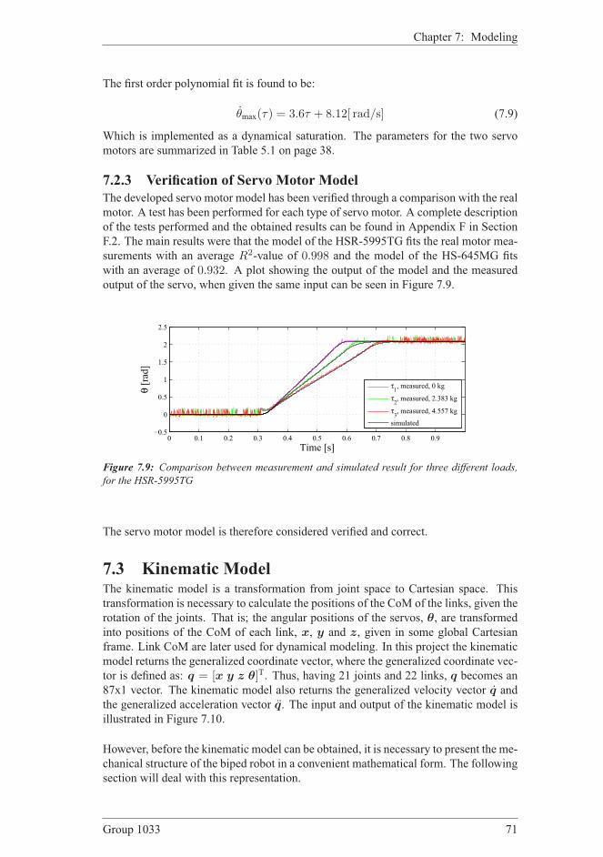
Chapter 7: Modeling
The first order polynomial fit is found to be:
θmax(τ) = 3.6τ + 8.12[ rad/s] (7.9)
Which is implemented as a dynamical saturation. The parameters for the two servo
motors are summarized in Table 5.1 on page 38.
7.2.3 Verification of Servo Motor Model
The developed servo motor model has been verified through a comparison with the real
motor. A test has been performed for each type of servo motor. A complete description
of the tests performed and the obtained results can be found in Appendix F in Section
F.2. The main results were that the model of the HSR-5995TG fits the real motor mea-
surements with an average R2-value of 0.998 and the model of the HS-645MG fits
with an average of 0.932. A plot showing the output of the model and the measured
output of the servo, when given the same input can be seen in Figure 7.9.
0 0.1 0.2 0.3 0.4 0.5 0.6 0.7 0.8 0.9−0.5
0
0.5
1
1.5
2
2.5
θ [rad]
Time [s]
τ1, measured, 0 kg
τ2, measured, 2.383 kg
τ3, measured, 4.557 kg
simulated
Figure 7.9: Comparison between measurement and simulated result for three different loads,
for the HSR-5995TG
The servo motor model is therefore considered verified and correct.
7.3 Kinematic ModelThe kinematic model is a transformation from joint space to Cartesian space. This
transformation is necessary to calculate the positions of the CoM of the links, given the
rotation of the joints. That is; the angular positions of the servos, θ, are transformed
into positions of the CoM of each link, x, y and z, given in some global Cartesian
frame. Link CoM are later used for dynamical modeling. In this project the kinematic
model returns the generalized coordinate vector, where the generalized coordinate vec-
tor is defined as: q = [x y z θ]T. Thus, having 21 joints and 22 links, q becomes an
87x1 vector. The kinematic model also returns the generalized velocity vector q and
the generalized acceleration vector q. The input and output of the kinematic model is
illustrated in Figure 7.10.
However, before the kinematic model can be obtained, it is necessary to present the me-
chanical structure of the biped robot in a convenient mathematical form. The following
section will deal with this representation.
Group 1033 71

Section 7.3: Kinematic Model
Kinematic model
q
θθθθɺɺθθθθɺθθθθ
qɺɺ
qɺ
Figure 7.10: The kinematic model is a transformation from joint coordinates to generalized
coordinates.
7.3.1 Representation of the Mechanical Structure
The biped robot can be considered a collection of links and joints collected in a unique
structure. All the names are assigned with basis in a situation where the biped robot
is in SSP-R, thus the mechanical structure is seen as a kinematic chain starting from a
reference frame placed on the sole of the right foot. The kinematic model developed
in this section will be a model describing the kinematics when in SSP-R. With few
changes the model can be extended to include the DSP and SSP-L. This will be ex-
plained at the end of this section.
In Figure 7.11(a) the names of all the joints are illustrated. The joints are named in ac-
cordance with the name of the actuator in the specific joint. The name of the actuators
can be seen in Figure C.3 on page 188. Now joint i has a unique reference name, ji.
All joints are actuated revolute joints, controlled by a servo motor. In Figure 7.11(b)
the link vectors are illustrated, the link vector ai is the vector ji−1 to ji. Thus link i isthe link connecting joint ji−1 and ji. A joint with n DoF, will in this model be threated
as n joints with 1 DoF, placed in the same point, [Craig, 1989]. Therefore not all link
vectors are illustrated in Figure 7.11(b), since the lengths are zero. Following joints
have multiple DoF; the ankle joints (j1− j2 and j11− j12); the hip joints (j4− j5− j6)and j7 − j8 − j9); the shoulder joints (j13 − j14 and j17 − j18) and the elbow joints
(j15 − j16 and j19 − j20).
Link vectors CoM vectors Masses Moments of inertia
[mm] [mm] [g] [kg/mm2]
a1 = [0 0 45]T b1 = [9.2 0 13]T m1 = 43.4 I1 = [0 0 0]T
a2 = [0 0 0]T b2 = [3.5 0 6.6]T m2 = 137 I2 = [47 51 34]T
a3 = [−10.6 0 86.4]T b3 = [0 0 61.7]T m3 = 195.3 I3 = [872 876 56]T
a4 = [10.6 0 139.1]T b4 = [14.9 0 71.4]T m4 = 209.6 I4 = [1299 1320 124]T
a5 = [0 0 0]T b5 = [3.5 0 − 6.6]T m5 = 137 I5 = [47 52 34]T
a6 = [0 0 0]T b6 = [0 0 27.4]T m6 = 18.2 I6 = [25 20 6]T
a8 = [0 0 0]T b8 = [0 0 27.4]T m8 = 18.2 I8 = [25 20 6]T
a9 = [0 0 0]T b9 = [3.5 0 − 6.6]T m9 = 137 I9 = [47 52 34]T
a10 = [−10.6 0 139.1]T b10 = [0 0 − 67.3]T m10 = 209.6 I10 = [1182 1158 79]T
a11 = [10.6 0 − 86.4]T b11 = [11.4 0 − 24.2]T m11 = 195.3 I11 = [243 270 80]T
a12 = [0 0 0]T b12 = [3.5 0 6.6]T m12 = 137 I12 = [48 52 35]T
a13 = [0 − 63 192.7]T b13 = [9.2 0 − 32]T m13 = 43.4 I13 = [14 21 22]T
Table 7.1: Parameters for the legs of the biped robot. These have been calculated in SolidWorks.
In Figure 7.11(c) the CoM vectors are illustrated. A CoM vector is a vector, bi, speci-
fying the CoM of link i relative to ji−1. In Figure 7.11(c) the mass of the link i, calledmi, is also specified. In Table 7.1, Table 7.2 and Table 7.3 the sizes of all the parame-
72 Aalborg University 2007
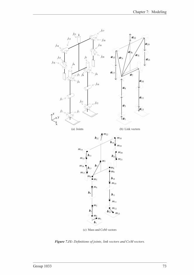
Chapter 7: Modeling
j1j2
j3
j4
j5
j6j7
j8 j9
j10
j11 j12
j21j13
j17
j18j19
j20
j14
j15j16
yz
x(a) Joints
a1
a3
a4
a7
a10
a11
a19
a7la7h
a7ra15
a13
a21
a17
a22
(b) Link vectors
m1m2
m3
m13
m4
m11
m5m6
m7
m10
m9
m8
m22m18
m19
m21
m14
m15
m17
m20
m16
b1
b3
b4
b7
b10
b11
b13
b21
b19b22
b15
b17
m12
(c) Mass and CoM vectors
Figure 7.11: Definitions of joints, link vectors and CoM vectors.
Group 1033 73

Section 7.3: Kinematic Model
ters illustrated in Figure 7.11 are given along with the principal moment of inertia for
each link. All parameters are found from measurement of the robot, while moments of
inertia is found from a model of the biped robot drawn in SolidWorks.
Link vectors CoM vectors Masses Moments of inertia
[mm] [mm] [g] [kg/mm2]
a7 = [0 82 0]T b7 = [1.5 41 130.8]T m7 = 1213.6 I7 = [6799 2832 4526]T
a7r = [0 − 63 192.7]T
a7l = [0 145 192.7]T
a7h = [0 41 219.4]T
a22 = [0 0 84.5]T b22 = [15.2 0 48]T m22 = 15.6 I22 = [14 14 4]T
Table 7.2: Parameters for the torso and head of the robot.
It should be noted that the masses and principal moments of inertia given in this section
are of no interest in relation to the kinematic model, since it only describes the motion
of the system, with no consideration of forces that cause this motion. These parameters
will be used in Section 7.4 where the derivation of the dynamical model of the biped
robot is described.
Link vectors CoM vectors Masses Moments of inertia
[mm] [mm] [g] [kg/mm2]
a14 = [0 0 0]T b14 = [−3 0 − 6.4]T m14 = 62.7 I14 = [13 15 6]T
a15 = [0 0 − 114.8]T b15 = [0 0 − 17]T m15 = 11.3 I15 = [6 12 8]T
a16 = [0 0 0]T b16 = [8.5 0 43]T m16 = 78.2 I16 = [17 29 18]T
a17 = [0 0 107.1]T b17 = [7 0 − 21.2]T m17 = 83.3 I17 = [76 77 11]T
a18 = [0 0 0]T b18 = [−3 0 − 6.4]T m18 = 62.7 I18 = [13 15 6]T
a19 = [0 0 − 114.8]T b19 = [0 0 − 17]T m19 = 11.3 I19 = [6 12 8]T
a20 = [0 0 0]T b20 = [8.5 0 43]T m20 = 78.2 I20 = [17 29 18]T
a21 = [0 0 107.1]T b21 = [7 0 − 21.2]T m21 = 83.3 I21 = [76 77 11]T
Table 7.3: Parameters for the arms of the robot.
In Figure 7.12(a) the zero-position and the direction of rotation is defined for all ro-
tations around the x-axis, in Figure 7.12(b) for the rotations around the y-axis, and inFigure 7.12(c) for the yaw movements (joints rotating around the z-axis). The dashedlines indicates the ankle each link should be positioned in, in order to assume zero-
position.
7.3.2 Attacing Frames
In Figure 7.11 the constant parameters of the biped robot are defined and in Figure
7.12 the variable parameters of the biped robot are defined. Next a representation of
the positions of all links relative to a global reference frame is given. As mentioned
in Section 7.1.2, the choice of reference frame varies in the literature. It is chosen
to consider the biped robot as an open loop serial chain from the supporting foot as
in [Mu and Wu, 2004]. In DSP both right and left foot are individually chosen as the
supporting foot, and a combination of these two makes the DSP model. This means
that whenever the right foot is on the ground (in SSP-R) the generalized positions, q,
are given with respect to frame 0, and when in SSP-L, q are given in frame 13.When in DSP, both models are used. In Figure 7.13 the biped robot is shown in SSP-R
and frame 0 is attached to the sole of the right foot.
74 Aalborg University 2007

Chapter 7: Modeling
2θ
4θ
9θ
11θ
18θ
14θ
20θ
16θ
y
z
x
(a) Frontal view
1θ3θ
5θ
8θ
10θ
12θ
17θ
13θ
y
z
x
(b) Sagittal view
y
z x
6θ
7θ
15θ
19θ
21θ
(c) Horizontal view
Figure 7.12: Definition of the angles in the three planes.
Group 1033 75

Section 7.3: Kinematic Model
yz
x 0
yz
x G
p0
Figure 7.13: In SSP-R the biped robot is represented in frame 0. The position of frame 0 isgiven in a floor fixed global reference frame G.
To keep track of the global position a floor fixed global reference frame, frame G, isintroduced. The position of frame G is assigned as the initial position of frame 0.To describe the orientation of the links, a link-frame is attached to each link, with its
origin placed in the joints. Thus frame i is placed with its origin in ji and attached
to link i + 1. In [Craig, 1989] and in [Christensen et al., 2006] the link-frames are
oriented such that they rotate around the z-axis. In this project it is chosen to orientthe link-frames, such that they are aligned with the reference frame when all angles
are zero (θ = 0), meaning that the robot is in zero-position. The advantage is, that therotation between two succeeding link-frames is solely described by the joint angle. In
Table 7.4 the axis of rotation is stated for each link-frame.
Frame Axis of rotation
2, 4, 9, 11, 14, 16, 18, 20 x
1, 3, 5, 8, 10, 12, 13, 17 y
6, 7, 15, 19, 21 z
Table 7.4: Axis of rotation for the link-frames.
The rotation matrix:
i−1i R =
[i−1xi
i−1yii−1zi
](7.10)
describes the orientation of the axis of frame i relative to frame i− 1. i−1i R is an
Euler rotation of θi and for rotation around the x-axis it is defined as [Craig, 1989]:
i−1i Rx(θi) =
1 0 00 cos θi − sin θi
0 sin θi cos θi
(7.11)
about the y-axis:
76 Aalborg University 2007

Chapter 7: Modeling
i−1i Ry(θi) =
cos θi 0 sin θi
0 1 0− sin θi 0 cos θi
(7.12)
and around the z-axis:
i−1i Rz(θi) =
cos θi − sin θi 0sin θi cos θi 0
0 0 1
(7.13)
From the above definitions of rotation matrices, it is also possible to find the orientation
of frame i + n relative to frame i. This is given as:
ii+nR(θi+1, θi+2, ..., θi+n) = i
i+1R(θi+1)i+1i+2R(θi+2) ... i+n−1
i+n R(θi+n) (7.14)
The kinematics of the robot is dependent on the phase of the system, if the phase is
SSP-R, θ1 is the first joint angle in the chain, but if the phase is SSP-L, then θ12 is
the first joint angle in the chain. As a consequence, when the notation i−1i R is used, i
does not refer to the name of the link, but the location in the kinematic chain. When in
SSP-R there are the following four kinematic chains:
[1 2 3 4 5 6 7 8 9 10 11 12] , for i ≤ 12[1 2 3 4 5 6 13 14 15 16] , for 13 ≤ i ≤ 16[1 2 3 4 5 6 17 18 19 20] , for 17 ≤ i ≤ 20[1 2 3 4 5 6 21] , for i = 21
(7.15)
and when the phase is SSP-L the following four chains are represented:
[12 11 10 9 8 7 6 5 4 3 2 1] , for i ≤ 12[12 11 10 9 8 7 13 14 15 16] , for 13 ≤ i ≤ 16[12 11 10 9 8 7 17 18 19 20] , for 17 ≤ i ≤ 20[12 11 10 9 8 7 21] , for i = 21
(7.16)
Thus if the phase is SSP-R and i = 13, the i−1i R means 6
13R (the rotation matrix from
the right hip to the right shoulder).
To get the right output of the kinematic model, it is necessary to know the phase of the
system, and thereby know if the supporting foot is the right foot or the left foot. The
will be handled in Section 7.5, where a phase estimator is designed.
7.3.3 The Generalized Coordinates
The output of the kinematic model is the generalized coordinates, which is chosen to
be the positions of all CoM’s and all joint angles. The generalized position vector, q,
is defined to:
q 87×1 ≡
x
y
z
θ
(7.17)
Group 1033 77

Section 7.3: Kinematic Model
where
x = [x1 x2 ... x22]T , y = [y1 y2 ... y22]
T , z = [z1 z2 ... z22]T (7.18)
contains the x-, y- and z-coordinates of all CoM’s, and:
θ = [θ1 θ2 ... θ21]T
(7.19)
contains all the joint angles.
With reference to Figure 7.11 on page 73 the generalized coordinate vector can now
be determined. The iterative equation for pi+1 (the position of CoM of link i + 1) isdefined as:
pi+1 =
xi+1
yi+1
zi+1
= 0i Rbi + pji
(7.20)
where pjiis the position of joint i defined as:
pji=
xji
yjizji
= 0i−1Rai + pji−1
(7.21)
From Equation (7.20) and Equation (7.21) the generalized position vector defined in
Equation (7.17) can now be found.
From Figure 7.10 it can be seen that the kinematic model also returns the generalized
velocity vector, q, and the generalized acceleration vector, q. These are defined as
follows:
q ≡ ∂q
∂t, q ≡ ∂2q
∂t2(7.22)
Now the theoretical basis for the kinematic model is established. In Appendix E on
page 195 the kinematic model will be derived for a simple 4 DoF biped robot with 3
links. Its purpose is to clarify the derivation of the complete model.
7.3.4 Verification of the Kinematic Model
A test have been performed in order to verify the kinematic model developed above.
The complete description of the test and a review of the results can be found in Ap-
pendix F in Section F.4 on page 212. To verify the model four different tests have been
performed, and sensors have been mounted temporary on the robot for test purpose
only. The result from one of these tests can be seen from Figure 7.14.
The main result is that the kinematic model fits the measured output of the real system
with a average R2-value of 0.702, where 1 is the best. Considering the noise on the
measurements along with all the uncertainties in a test like this, the kinematic model is
considered verified.
78 Aalborg University 2007
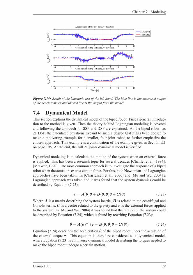
Chapter 7: Modeling
0 1 2 3 4 5 6 7 8 9 10−20
−10
0
10Acceleration of the left hand,x−direction
a x,lh [m/s2]
0 1 2 3 4 5 6 7 8 9 10−10
0
10Acceleration of the left hand, y−direction
a y,lh [m/s2]
0 1 2 3 4 5 6 7 8 9 10−10
0
10
20Acceleration of the left hand, z−direction
a z,lh [m/s2]
Time [s]
Measured
Simulated
Figure 7.14: Result of the kinematic test of the left hand. The blue line is the measured output
of the accelerometer and the red line is the output from the model.
7.4 Dynamical ModelThis section explains the dynamical model of the biped robot. First a general introduc-tion to the method is given. Then the theory behind Lagrangian modeling is coveredand following the approach for SSP and DSP are explained. As the biped robot has21 DoF, the calculated equations expand to such a degree that it has been chosen tomake a motivating example for a smaller, four joint robot, to further emphasize thechosen approach. This example is a continuation of the example given in Section E.1on page 195. At the end, the full 21 joints dynamical model is verified.
Dynamical modeling is to calculate the motion of the system when an external forceis applied. This has been a research topic for several decades [Chaillet et al., 1994],[McGeer, 1990]. The most common approach is to investigate the response of a bipedrobot when the actuators exert a certain force. For this, both Newtonian and Lagrangianapproaches have been taken. In [Christensen et al., 2006] and [Mu and Wu, 2004] aLagrangian approach was taken and it was found that the system dynamics could bedescribed by Equation (7.23):
τ = A(θ)θ + B(θ, θ)θ + C(θ) (7.23)
Where A is a matrix describing the system inertia, B is related to the centrifugal andCoriolis terms, C is a vector related to the gravity and τ is the external forces appliedto the system. In [Mu and Wu, 2004] it was found that the motion of the system couldbe described by Equation (7.24), which is found by rewriting Equation (7.23):
θ = A(θ)−1(τ −B(θ, θ)θ −C(θ)) (7.24)
Equation (7.24) describes the acceleration θ of the biped robot under the actuation ofthe external torque τ . This equation is therefore considered as a dynamical model,where Equation (7.23) is an inverse dynamical model describing the torques needed tomake the biped robot undergo a certain motion.
Group 1033 79

Section 7.4: Dynamical Model
As the purpose of the model is to give a description of the robot system, usable foroff-line testing of controllers and off-line trajectory generation, it is chosen to developan inverse dynamic model of the biped robot and the input/output relation of the dy-namical system can then be seen from Figure 7.15.
Dynamical model
q
qɺɺ
qɺττττ
f
Figure 7.15: Input/output relation of the dynamical model
But as the biped robot system can be seen as a hybrid system with three phases (SSP-L, SSP-R and DSP) and the inverse dynamical model only describes the biped robotsystem when in SSP, another solution has to be found to described the forces acting onthe system when in DSP. If a dynamic model was to be found, a common approach isto introduce a constraint on the system resulting in an altered motion because of theconstraint force acting on the system. In [Christensen et al., 2006] and [Mu and Wu,2004] this was investigated and it was found that by using Lagrangian multipliers themotion of the system could be described by:
θ = A(θ)−1((τ + JT(θ)λ)−B(θ, θ)θ −C(θ)) (7.25)
Where JT(θ)λ is the contribution from the constraint force, λ is the Lagrangian mul-tiplier and JT(θ) is the Jacobian matrix of the constraints with respect to θ. Theproblem with using the Lagrangian multipliers is that this approach can be rather cum-bersome, as the multiplier has to be solved for and then inserted into the Equation(7.25). Another approach is to use Udwadia-Kalaba equations to describing motion ofa dynamic system under constrains, which follows the same approach as with the La-grangian multipliers by introducing a force of constraints [Udwadia and Kalaba, 2001].
But with this approach it is not necessary to compute the Lagrangian multiplier, andthe approach is therefore more straight forward. But the problem with both of the ap-proaches is that they can only be used for the dynamical model, and are non-invertible.An approach valid for estimating the external forces in the DSP has not been found inthe literature and therefore a solution, to solve this problem, has to be found.
7.4.1 Dynamical Modeling Approach
As earlier explained it is chosen to use Lagrangian modeling to describe the dynamicalsystem. In this section an introduction to the Lagrangian approach is given basedon [Wisniewski, 2006]. Lagrange modeling is based on Hamilton’s principle. Theprinciple states that the integrated difference between the kinetic energy, K, minuspotential energy, P , is always minimal. The motion of a mechanical system from timea to b can be expressed by:
80 Aalborg University 2007

Chapter 7: Modeling
I(t, q, q) =
∫ b
a
L(t, q, q)dt (7.26)
L is called the Lagrangian and is defined as the energy difference of the mechanicalsystem (Kinetic energy (K) minus potential energy (P )) and q is the generalized co-ordinate. Hamilton’s principle describes the path used to come from a to b, such thatthe difference in energy is minimal. Thus, I(t, q, q) has to be at a critical point (a pointwhere the derivative is zero), and the derivative, i.e. a small change of path, is zero forthe true path (the path the system undergoes). A small change of path can be describedas:
I(t, q + ǫη, q + ǫη) , ǫ→ 0 (7.27)
for any arbitrary path η.
The derivative of Equation (7.27) is then given as:
d
dǫI(t, q + ǫη, q + ǫη) = 0 , ǫ→ 0 (7.28)
Substituting Equation (7.26) into Equation (7.28) and performing the differentiation,the following expression, which applies to all the generalized co-ordinates qi, can beobtained:
∫ b
a
(∂L
∂qi− d
dt
∂L
∂qi
)
ηdt = 0 (7.29)
Now the Fundamental Lemma of Calculus of Variations is applied to Equation (7.29).This lemma basically states that if the expression is true, then the expression in thebrackets has to be zero as well:
∂L
∂qi− d
dt
∂L
∂qi= 0 (7.30)
This applies to all the generalized co-ordinates. The expression can be rewritten asa vector equation describing the motion of a mechanical system with n generalizedcoordinates under influence of no external force.
∂L∂q1
− ddt
∂L∂q1
∂L∂q2
− ddt
∂L∂q2
...∂L∂qn− d
dt∂L∂qn
=
00...0
(7.31)
If the mechanical system is influenced by external forces the Lagrange-d’Alembertprinciple can be applied. The principle states that the external force field, Q, can betaken into account as follows:
I(t, q, q) =
∫ b
a
L(t, q, q)dt +
∫ b
a
Q(t, q, q)dt (7.32)
The force field in Equation (7.32) can be interpreted as the displacement from theminimal energy state in the motion of the system, done by the work of the externalforceQ. Using the same method as for the system under influence of no external force,
Group 1033 81

Section 7.4: Dynamical Model
Equation (7.32) leads to the following equation describing the motion of a mechanicalsystem under influence of an external force:
∂L
∂qi− d
dt
∂L
∂qi= Qi (7.33)
In the case of a robot with joint angles as generalized co-ordinates, the external forceis the torque applied to each servo, and hence Equation (7.33) can be rewritten intovector equation describing the motion of the robot:
∂L∂q1
− ddt
∂L∂q1
∂L∂q2
− ddt
∂L∂q2
...∂L∂qn− d
dt∂L∂qn
=
τ1
τ2
...τn
(7.34)
where τi is the torque provided by the servo motor controlling the i’th link.
As the model of the biped robot in DSP is a combination of SSP-L and SSP-R, a modelof the biped robot in SSP has to be derived first. Hence the following section will useEquation (7.34) to develop a model of the biped robot in single support phase.
7.4.2 Single Support Phase Modeling
In this section an overview of the approach used in the SSP modeling will be given.This model has two different phases, namely when in SSP-L and SSP-R. Only the ap-proach for the SSP-R phase will be given, as the approach for each phase is similar.
When using Lagrangian modeling it is the energy in the system that is considered, andthereby the model is derived from energy equations. As a biped robot is seen as amulti linked body connected by joints, the energy has to be considered for each link.From Figure 7.11 it is possible to see the different joints which connect the links of therobot. As earlier explained the Lagrangian can be found as the kinetic energy minusthe potential energy. The kinetic energy of the i’th link can be calculated as in [Craig,1989, p. 207], where all coordinates are given in Cartesian coordinates:
ki = 12 mi vT
i vi + 12 ωT
i Ii ωi = 12 mi (x2
i + y2i + z2
i ) + 12 ωT
i Ii ωi (7.35)
The matrix, Ii, is the inertia tensor of the i’th link, vi is the linear velocity and ωi isthe angular velocity vector of the link. The angular velocity can be found as [Craig,1989, p. 207]:
ωi+1 = ωi + i+10 Rθiζ (7.36)
Where i+10 R is the rotation from the base frame to frame i + 1, found from Equa-
tion 7.14 on page 77 and ζ is a vector denoting the axis which θi rotates about. The
kinetic energy of all links can be found as K =
22∑
i=1
ki
82 Aalborg University 2007

Chapter 7: Modeling
The potential energy of link i is calculated as:
pi = mi g zi (7.37)
The potential energy of all links is P =
22∑
i=1
pi, and the Lagrangian is calculated as
L = K −P . To calculate the external forces given by Equation (7.33), the Lagrangianis first differentiated with respect to the generalized coordinates as:
∂L
∂q1×87 =
[∂L∂x
∂L∂y
∂L∂z
∂L∂θ
]
(7.38)
Notice that the Lagrangian differentiated with respect to the generalized coordinatesbecomes a 1 × 87. Now the derivate of the Lagrangian with respect to the velocity ofthe generalized coordinates are found. This is then differentiated with respect to timeand yields:
∂
∂t
∂L
∂q1×87 =
[∂∂t
∂L∂x
∂∂t
∂L∂y
∂∂t
∂L∂z
∂∂t
∂L
∂θ
]
(7.39)
Substracting Equation (7.38) with Equation (7.39) yields Equation (7.33). Now theexternal forces acting on the system in SSP are found. As this is given in the Cartesiancoordinate system it corresponds to the linear force, f , the robot needs to be influencesby to move the CoM’s for each link in the desired motion. But as the external forcesacting on the biped robot is the torque actuated by the servo motor, given in the jointspace, a transformation from linear forces in Cartesian coordinates to torques in jointcoordinates has to be performed. For this mapping the Jacobian can be used and theactuator torque can be found as [Wisniewski, 2006]:
Q = τθ =
(dq
dθ
)T
f (7.40)
where q is the Cartesian coordinates and θ is the joint coordinates.(
dqdθ
)
is the Jaco-
bian of q denoted J(q), and describes the transformation from Cartesian coordinatesto joint coordinates given by the calculations described in Section 7.3.3 on page 77:
dq
dθ= J(q) =
∂q1
∂θ1. . . ∂q1
∂θ21...
. . ....
∂q87
∂θ1. . . ∂q87
∂θ21
(7.41)
f¯is the Cartesian force field and Q is the joint space force field. This yields the model
for the biped robot in the SSP-R phase. To construct the model for the SSP-L phase, allthe previous steps need to be repeated with the left foot as base frame. This has beenperformed and implemented for the final model but will not be presented here.
7.4.3 Double Support Phase Modeling
As explained in the introduction to Section 7.4, obtaining a model for the torque givena motion of the biped robot system in DSP, has not been described in the searched
Group 1033 83
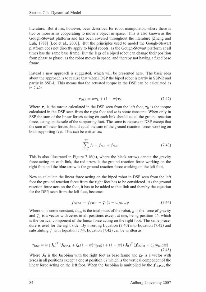
Section 7.4: Dynamical Model
literature. But it has, however, been described for robot manipulator, where there istwo or more arms cooperating to move a object in space. This is also known as theGough-Stewart platform and has been covered throughout the literature [Zheng andLuh, 1988] [Lee et al., 2003]. But the principles used to model the Gough-Stewartplatform does not directly apply to biped robots, as the Gough-Stewart platform at alltimes has the same base frame. But the legs of a biped robot can change their positionfrom phase to phase, as the robot moves in space, and thereby not having a fixed baseframe.
Instead a new approach is suggested, which will be presented here. The basic ideaabout the approach is to realize that when i DSP the biped robot is partly in SSP-R andpartly in SSP-L. This means that the actuated torque in the DSP can be calculated asin 7.42:
τDSP = wτL + (1− w)τR (7.42)
Where τL is the torque calculated in the DSP seen from the left foot, τR is the torquecalculated in the DSP seen from the right foot and w is some constant. When only inSSP the sum of the linear forces acting on each link should equal the ground reactionforce, acting on the sole of the supporting foot. The same is the case in DSP, except thatthe sum of linear forces should equal the sum of the ground reaction forces working onboth supporting feet. This can be written as:
22∑
i=1
fi = fN-L + fN-R (7.43)
This is also illustrated in Figure 7.16(a), where the black arrows denote the gravityforce acting on each link, the red arrow is the ground reaction force working on theright foot and the blue arrow is the ground reaction force working on the left foot.
Now to calculate the linear force acting on the biped robot in DSP seen from the leftfoot the ground reaction force from the right foot has to be considered. As the groundreaction force acts on the foot, it has to be added to that link and thereby the equationfor the DSP, seen from the left foot, becomes:
fDSP-L = fSSP-L + ζL(1− w)mtotg (7.44)
Where w is come constant, mtot is the total mass of the robot, g is the force of gravityand ζL is a vector with zeros in all positions except at one, being position 45, whichis the vertical component of the linear force acting on the right foot. The same proce-dure is used for the right side. By inserting Equation (7.40) into Equation (7.42) andsubstituting f with Equation 7.44, Equation (7.42) can be written as:
τDSP = w (JL)T(fSSP-L + ζL(1− w)mtotg) + (1− w) (JR)
T(fSSP-R + ζRmtotgw)
(7.45)
Where JR is the Jacobian with the right foot as base frame and ζR is a vector withzeros in all positions except a one at position 57 which is the vertical component of thelinear force acting on the left foot. When the Jacobian is multiplied by the fDSP-R, the
84 Aalborg University 2007

Chapter 7: Modeling
y
z
x
fN-R fN-Lρ
(a) Forces in the DSP
ρ
(b) Distribution of forces in DSPseen from the right foot
ρ
(c) Distribution of forces in DSPseen from the left foot
Figure 7.16: Forces acting on the biped robot when in DSP. a) Red arrow is the normal force
acting on the right foot. Blue arrow is the normal force acting on the left foot. Black arrows is
the gravity force acting on each link CoM. b) Green is the forces from gravity acting on the right
foot. Blue is the normal force acting on the right foot and which has been distributed to the rest
of the links. c) Gray is the forces from the gravity acting on the left foot. Red is the normal force
acting on the left foot and which has been distributed to the rest of the links.
Group 1033 85
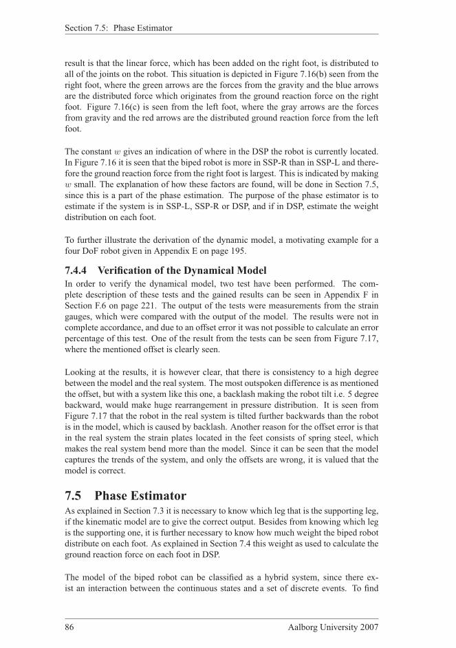
Section 7.5: Phase Estimator
result is that the linear force, which has been added on the right foot, is distributed toall of the joints on the robot. This situation is depicted in Figure 7.16(b) seen from theright foot, where the green arrows are the forces from the gravity and the blue arrowsare the distributed force which originates from the ground reaction force on the rightfoot. Figure 7.16(c) is seen from the left foot, where the gray arrows are the forcesfrom gravity and the red arrows are the distributed ground reaction force from the leftfoot.
The constant w gives an indication of where in the DSP the robot is currently located.In Figure 7.16 it is seen that the biped robot is more in SSP-R than in SSP-L and there-fore the ground reaction force from the right foot is largest. This is indicated by makingw small. The explanation of how these factors are found, will be done in Section 7.5,since this is a part of the phase estimation. The purpose of the phase estimator is toestimate if the system is in SSP-L, SSP-R or DSP, and if in DSP, estimate the weightdistribution on each foot.
To further illustrate the derivation of the dynamic model, a motivating example for afour DoF robot given in Appendix E on page 195.
7.4.4 Verification of the Dynamical Model
In order to verify the dynamical model, two test have been performed. The com-plete description of these tests and the gained results can be seen in Appendix F inSection F.6 on page 221. The output of the tests were measurements from the straingauges, which were compared with the output of the model. The results were not incomplete accordance, and due to an offset error it was not possible to calculate an errorpercentage of this test. One of the result from the tests can be seen from Figure 7.17,where the mentioned offset is clearly seen.
Looking at the results, it is however clear, that there is consistency to a high degreebetween the model and the real system. The most outspoken difference is as mentionedthe offset, but with a system like this one, a backlash making the robot tilt i.e. 5 degreebackward, would make huge rearrangement in pressure distribution. It is seen fromFigure 7.17 that the robot in the real system is tilted further backwards than the robotis in the model, which is caused by backlash. Another reason for the offset error is thatin the real system the strain plates located in the feet consists of spring steel, whichmakes the real system bend more than the model. Since it can be seen that the modelcaptures the trends of the system, and only the offsets are wrong, it is valued that themodel is correct.
7.5 Phase EstimatorAs explained in Section 7.3 it is necessary to know which leg that is the supporting leg,if the kinematic model are to give the correct output. Besides from knowing which legis the supporting one, it is further necessary to know how much weight the biped robotdistribute on each foot. As explained in Section 7.4 this weight as used to calculate theground reaction force on each foot in DSP.
The model of the biped robot can be classified as a hybrid system, since there ex-ist an interaction between the continuous states and a set of discrete events. To find
86 Aalborg University 2007
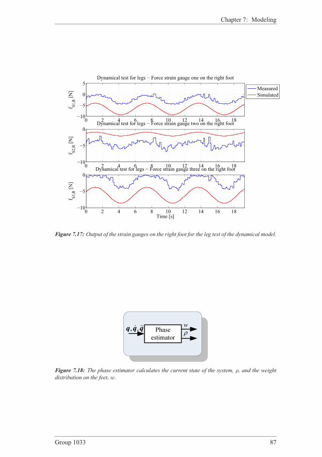
Chapter 7: Modeling
0 2 4 6 8 10 12 14 16 18−10
−5
0
5Dynamical test for legs − Force strain gauge one on the right foot
f S1,R [N]
0 2 4 6 8 10 12 14 16 18−10
−5
0Dynamical test for legs − Force strain gauge two on the right foot
f S2,R [N]
0 2 4 6 8 10 12 14 16 18−10
−5
0Dynamical test for legs − Force strain gauge three on the right foot
Time [s]
f S3,R [N]
Measured
Simulated
Figure 7.17: Output of the strain gauges on the right foot for the leg test of the dynamical model.
, ,ɺ ɺɺq q qw
Phase estimator
ρ
Figure 7.18: The phase estimator calculates the current state of the system, ρ, and the weight
distribution on the feet, w.
Group 1033 87

Section 7.5: Phase Estimator
these two values a phase estimator is used. The phase estimator is illustrated in Figure7.18, where it can be seen that it takes the generalized coordinate vector as an input,and returns the current state of the system, ρ, and the weight distribution on the feet, w.
The necessity of the phase estimator can easily be shown by the example in Figure7.19, where the biped robot is shown in two completely different situations. But in thetwo cases the exact same input vector, θ, is given. This illustrates that from the inputsolely it is not possible to determine the state of the system.
y
z
x
(a) SSP-R
y
z
x
(b) SSP-L
Figure 7.19: The biped robot seen in SSP-R and SSP-L. In both cases the the same input vector,
θ, is given.
7.5.1 The Hybrid Model
The dynamics of a biped robot can be divided into three phases, only two blocks aredependent on the phase, the dynamical model and the kinematic model. The dynamicalmodel is found using Lagrangian formulation, from which the force vector, f , is found.The torque on the motor shaft is calculated as follows:
τ =
JT1 f1 if P = ρ1
(1− w)JT1 f1 + wJT
2 f2 if P = ρ2
JT2 f2 if P = ρ3
(7.46)
where f1 = fSSP-L + ζL (1− w) mtotg and f2 = fSSP-R + ζRmtotgw, J1 and J2 are
the Jacobians of SSP-R and SSP-L (size 21 × 87), f1 and f2 are the force vectors of
SSP-R and SSP-L (size 1×87), and w is a weight factor denoting how much the biped
robot is in SSP-L. Where the following holds for w:
DSP: 0 < w < 1
SSP-R: w = 0 (7.47)
SSP-L: w = 1
88 Aalborg University 2007

Chapter 7: Modeling
P and ρi links to the current state of the system, and will be described more thorough
in the follow, where the whole system is formulated as a hybrid automaton, which is
the common way to express a hybrid system.
Hybrid Automaton
In [Bak and Izadi-Zamanabadi, 2006, pp. 11] a hybrid automaton, H , is given as:
H = (P,X, Init, f,Dom, E,G,R)
Note that in [Bak and Izadi-Zamanabadi, 2006] the phase of the system, P , is denotedwith Q, but since q is the generalized coordinate vector, in this project, the phase is
denoted P .
In this project the elements of H is given as follows:
P is the discrete state/phase of the system.
P = ρ1, ρ2, ρ3 = SSP-R,DSP,SSP-L
X is the continuous variables, is this case the joint angles.
X = θ1, θ2, ..., θ21 , X ∈ ℜ21
Init is the initial conditions, the biped robot always starts up in zero position, and DSP.
Init = θ1 = 0, θ2 = 0, ..., θ21 = 0,P = DSP
f is a vector field.
f (ρ1,X) = fSSP-R (X)
f (ρ2,X) = fDSP (X)
f (ρ3,X) = fSSP-L (X)
Dom is the domain, assigned to each discrete state.
dom(ρ1) = x ∈ X : zleft,foot(X) > zright,foot(X)dom(ρ2) = x ∈ X : zleft,foot(X) = zright,foot(X)dom(ρ3) = x ∈ X : zleft,foot(X) < zright,foot(X)
E is a collection of discrete transitions.
E = (ρ1, ρ2), (ρ2, ρ1), (ρ3, ρ2), (ρ2, ρ3)
G are the guards, assigned to each discrete transition.
G(ρ1, ρ2) = x ∈X : zleft,foot(X) = zright,foot(X)G(ρ2, ρ1) = x ∈X : zleft,foot(X) > zright,foot(X)G(ρ3, ρ2) = x ∈X : zleft,foot(X) = zright,foot(X)G(ρ2, ρ3) = x ∈X : zleft,foot(X) < zright,foot(X)
R are the reset relations.
R(ρ1, ρ2, x) = R(ρ2, ρ1, x) = R(ρ3, ρ2, x) = R(ρ2, ρ3, x) = x
Group 1033 89

Section 7.5: Phase Estimator
7.5.2 Finding the Phase of the System
As mentioned, the dynamics of a biped robot can be divided into three phases, P . Theswitch between the different phases is called a transition, E, and are governed by the
guards, G.
Transitions are evoked when the height of the feet are changing. When the height is
equal both feet are on the ground and the biped must be in DSP. In SSP the foot that
is on the ground determines which phase the biped robot is in. These constraints are
therefore used as guards to determine the transitions between the phases, and the de-
sign of the phase location estimation will depend on these transitions.
In practice it is not possible to implement the phase estimator precisely as described
above, since the feet will never have exactly the same height, and the system will never
reach DSP. It is therefore chosen to insert a small limit, δDSP, and the guards are thengiven as:
G(ρ1, ρ2) = x ∈X : zleft,foot(X) < zright,foot(X) + δDSPG(ρ2, ρ1) = x ∈X : zleft,foot(X) > zright,foot(X) + δDSPG(ρ3, ρ2) = x ∈X : zleft,foot(X) > zright,foot(X)− δDSPG(ρ2, ρ3) = x ∈X : zleft,foot(X) < zright,foot(X)− δDSP
The value of this limit is set to δDSP = 5mm.
7.5.3 Calculation of the Weight Distribution
The phase estimator should also return the weight distribution on the feet w. In thethree phases w is given in Equation (7.47). As seen w is easily found in SSP, where
all the weight is on one foot. In DSP it is however a little more difficult. In DSP w is
calculated from the ZMP, which was introduced in Section 2.3 on page 7 and given as:
xZMP =
22∑
i=1
mi ((zi − gz) xixizi)
22∑
i=1
mi (zi − gz)
(7.48)
The ZMP in the frontal plane is given by:
yZMP =
22∑
i=1
mi ((zi − gz) yi − yizi)
22∑
i=1
mi (zi − gz)
(7.49)
The problem with the calculation of the ZMP from Equation (7.48) and Equation (7.49)
is that if the denominator equals zero the result will go to infinity. Instead a new way
of calculation the ZMP is given in Equation (7.50) and Equation (7.51), where the
denominator consists of a constants factor. This ZMP calculation is given in [You
et al., 2004]:
90 Aalborg University 2007

Chapter 7: Modeling
xZMP,m =
22∑
i=1
mi (gzxi − xizi)
22∑
i=1
migz
(7.50)
Where the added subscript “,m” is short for “modified”. For the y-direction, the ZMP
is calculated as follows:
yZMP,m =
22∑
i=1
mi (gzyi − yizi)
22∑
i=1
migz
(7.51)
Now to calculate w the ZMP and the distance between the feet are used. This is illus-
trated in Figure 7.20:
Right foot
Left foot
∆yf
∆xf
(xzmp,m,yzmp,m)
y zx
Figure 7.20: The ZMP and distances ∆xf and ∆yf used for calculation of the weight distribu-
tion, w.
Now w can be calculated as:
w =xZMP,m
∆xf + ∆yf+
yZMP,m
∆xf + ∆yf(7.52)
where only ZMP values between the feet are used, thus:
xZMP,m ∈ [0;∆xf] (7.53)
yZMP,m ∈ [0;∆yf] (7.54)
w now serves as a weight factors that indicates where in the DSP, the dynamical system
currently is located in. The closer the ZMP is to the left foot, the more the model is in
SSP-L and the model for this phase gets the most influence. Now the collected torque
in the DSP can be calculated using Equation (7.45).
Group 1033 91

Section 7.6: Foot Model
7.6 Foot ModelIn Section 4.5.3 on page 30 the foot is designed, and it can be seen that it consists of
an upper part, which is placed on three bendable levers, called strain plates. On the
three plates a strain gauge is placed on each side. These three levers are mounted on
the lower part of the foot which consist of the sole.
yz
x
CoM
fg
ff2 f3 f1
τ
p2 p3 p1
Figure 7.21: Isometric view of the foot. Showing the forces acting on the upper part of the foot.
In Figure 7.21 the upper part of the right foot is illustrated. The model of the foot will
yield the three forces, ffoot = [f1z , f2z , f3z ]T (the vertical components of f1, f2 and
f3), acting on the connection point of each of these plates. The measurement model of
the strain gauge sensors, described in Appendix D on page 191, also yields this value.
The foot model describes the three forces imposed on the strain gauges plates, given
the torque in the ankle. This is illustrated in Figure 7.22.
footfττττ
Foot modelf
Figure 7.22: The foot model is a transformation from the torques and forces in the ankle joint
to the three forces measured by the strain gauges.
The developed model, described in this section, builds on principals presented in
[Ito and Kawasaki, 2005] and [Ito et al., 2004], where similar models are derived,
though only for two dimensions. All general equations and laws of physics are found
in [Serway and Beichner, 2000]. Also the approach taken in [Christensen et al., 2006]
is considered, where a similar model for three dimensions is developed.
92 Aalborg University 2007

Chapter 7: Modeling
7.6.1 Forces Acting on the Foot
In order to make an expression of the ground reaction force, it is necessary to identify
all the forces acting on the foot. In Figure 7.21 it can be seen that the foot is influenced
by the gravity force, fg, acting on the CoM of the upper part of the foot, a linear force,
f , imposed by the next link, a torque, τ , imposed by the next link and the ground
reaction forces, f1, f2 and f3. Since it is only wanted to find the vertical components
of the ground reaction force it is only necessary to consider the vertical component
of f , called fz, and the two components of the torque situated on the x-axis and they-axis, called τx and τy, see Figure 7.25 and Figure 7.26.
CoMz
x
p1
p3
p2 ylc2
lc3lc1
Figure 7.23: Horizontal view of the foot
seen from above. Showing placement of
CoM.
z x
p1
p3
p2 ylf2
lf3lf1
l2
l1
l3
Figure 7.24: Horizontal view of the foot
seen from above. Showing placement of
frame 1.
Gravity, fg
First the effect from the gravity is considered. The total effect from the gravity is mg,
where m is the mass of the upper part of the foot. The mass m should now be ”dis-
tributed” among the three contact points, p1, p2 and p3. Figure 7.23 is an illustration
of the foot in the horizontal plane, illustrating the placement of CoM.
The part of the mass m introduce the following force at pi:
fgi = cmlcili
mg (7.55)
where cm is a constant ensuring that the resulting mass on the three contact points
equals m, lci is the distance from the CoM to the sides of the triangle and li is the
heights of the triangle, illustrated in Figure 7.24. cm is given as:
cm =
(3∑
i=1
lcili
)−1
(7.56)
Linear force, fzFigure 7.24 shows the placement of frame 1, which is the point where the force fz isapplied. The same considerations as for the gravity, can be done for the force fz. Thisforce has the following influence on the contact point pi:
Group 1033 93
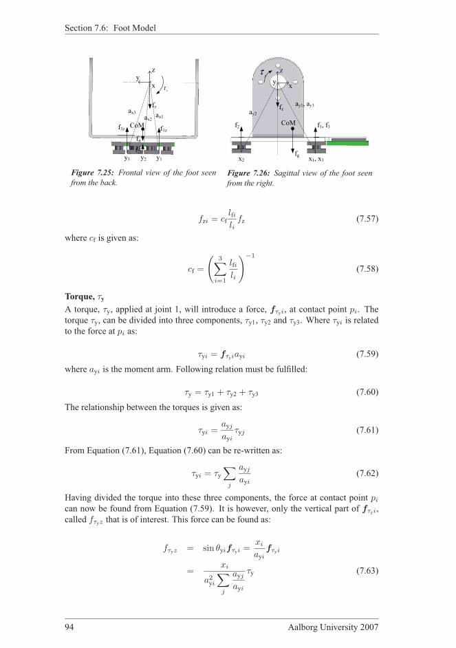
Section 7.6: Foot Model
yzx
CoMax3 ax2 ax1
y3 y2 y1
xτ
fz
fgf3z
f2z
f1z
Figure 7.25: Frontal view of the foot seen
from the back.
yz
x
CoMay2
yτ
ay1, ay3
x1, x3x2
fz
fg
f2 f1, f3
Figure 7.26: Sagittal view of the foot seen
from the right.
fzi = cflfili
fz (7.57)
where cf is given as:
cf =
(3∑
i=1
lfili
)−1
(7.58)
Torque, τy
A torque, τy, applied at joint 1, will introduce a force, fτyi, at contact point pi. The
torque τy, can be divided into three components, τy1, τy2 and τy3. Where τyi is relatedto the force at pi as:
τyi = fτyiayi (7.59)
where ayi is the moment arm. Following relation must be fulfilled:
τy = τy1 + τy2 + τy3 (7.60)
The relationship between the torques is given as:
τyi =ayjayi
τyj (7.61)
From Equation (7.61), Equation (7.60) can be re-written as:
τyi = τy∑
j
ayjayi
(7.62)
Having divided the torque into these three components, the force at contact point pi
can now be found from Equation (7.59). It is however, only the vertical part of fτyi,
called fτyz that is of interest. This force can be found as:
fτyz = sin θyifτyi =xi
ayifτyi
=xi
a2yi
∑
j
ayjayi
τy (7.63)
94 Aalborg University 2007

Chapter 7: Modeling
Note that p1 and p3 in the sagittal plane are placed equal, thus fτy1 = fτy3.
Torque, τxWith reference to Figure 7.25, the same calculations can be performed in the frontal
plane, and the force at contact point pi is given as:
fτxi = − yi
a2xi
∑
j
axjaxi
τx (7.64)
7.6.2 Summing the Forces
Gathering the contribution from the gravity force, the linear force, and the two torques,
given in Equation (7.55), (7.57), (7.63) and (7.64) respectively, the resulting force
applied at the three contact points can be found as:
fi = fgi + fzi + fτyi + fτxi (7.65)
which can be written as:
ffoot =
f1f2f3
= A
1fz(t)τy(t)τx(t)
(7.66)
where A is found, by inserting all know values, to be:
A =
cmlc1l1
mg cflf1l1
x1
a2y1+ay1ay2+ay1ay3
− y1a2x1+ax1ax2+ax1ax3
cmlc2l2
mg cflf2l2
x2
ay1ay2+a2y2+ay2ay3
− y2ax1ax2+a2
x2+ax2ax3
cmlc3l3
mg cflf3l3
x1
ay1ay3+ay2ay3+a2y3
− y1ax1ax3+ax2ax3+a2
x3
(7.67)
Note that the foot model described in this section is for the right foot, however the
same approach holds for the left foot. The foot shown in Figure 7.21 is the right foot,
the left foot is exactly the same, only the location of the contact point changes. Thus if
all the constants are changed according to the coordinate system placed in the joint 12,the same model can be used for the left foot.
7.6.3 Verification of the Foot Model
In order to verify the model of the foot, one of the feet has been dismounted from the
robot, such that known torques and forces could be applied. The complete description
of the performed tests and the obtained results is placed in Appendix F in Section F.3
on page 207. The main result is, that the foot model fits the real foot with a average
R2-value of 0.622. The relatively low fit percentage is mostly due to noise in the
measurements. A plot of the results can be seen in Figure 7.27, where it can be seen
that the model estimates the trend in the output. Therefore it is concluded that the foot
model is correct.
Group 1033 95
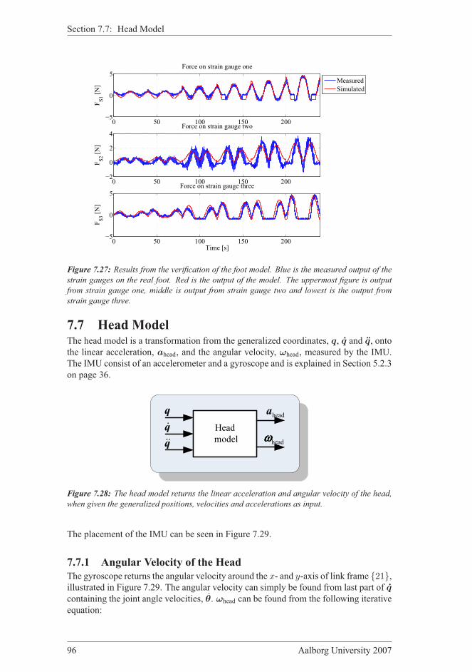
Section 7.7: Head Model
0 50 100 150 200−5
0
5Force on strain gauge one
FS1 [N]
0 50 100 150 200−2
0
2
4Force on strain gauge two
FS2 [N]
0 50 100 150 200−5
0
5Force on strain gauge three
Time [s]
FS3 [N]
Measured
Simulated
Figure 7.27: Results from the verification of the foot model. Blue is the measured output of the
strain gauges on the real foot. Red is the output of the model. The uppermost figure is output
from strain gauge one, middle is output from strain gauge two and lowest is the output from
strain gauge three.
7.7 Head ModelThe head model is a transformation from the generalized coordinates, q, q and q, onto
the linear acceleration, ahead, and the angular velocity, ωhead, measured by the IMU.
The IMU consist of an accelerometer and a gyroscope and is explained in Section 5.2.3
on page 36.
Head model
q
qɺɺ
qɺ
headωωωω
heada
Figure 7.28: The head model returns the linear acceleration and angular velocity of the head,
when given the generalized positions, velocities and accelerations as input.
The placement of the IMU can be seen in Figure 7.29.
7.7.1 Angular Velocity of the Head
The gyroscope returns the angular velocity around the x- and y-axis of link frame 21,illustrated in Figure 7.29. The angular velocity can simply be found from last part of q
containing the joint angle velocities, θ. ωhead can be found from the following iterative
equation:
96 Aalborg University 2007

Chapter 7: Modeling
p22
21
IMU
pIMU
z
xy
Figure 7.29: The placement of the IMU. p22 is the CoM of the head, frame 21 is the link
frame attached to the head.
iωi = ii−1R
i−1ωi−1 + ζiθi (7.68)
where ζi is a vector denoting the axis which θi rotates about. From Equation (7.68)
the angular velocity of the head can be found:
ωhead = 21ω21 (7.69)
7.7.2 Linear Acceleration of the Head
From q the linear acceleration of the CoM of the head can be found. The head is
link 22, thus a22 = [x22, y22, z22]T. a22 is the actual acceleration of link 22, the
accelerometer however also measures the acceleration due to the gravity force. As
the model should give the same output as sensors, the contribution from the force of
gravity is added:
Ga22 =
x22
y22
z22
+
00g
(7.70)
As indicated by the leading superscript,G, the acceleration is given in the global frame,
the accelerometer however measures the acceleration in its own frame, which is aligned
with frame 21. Therefore Ga22 has to be transformed to this frame, which is done
by premultiplying with the rotation matrix defined in Equation (7.14) on page 77:
21a22 = 210 R Ga22 (7.71)
Equation (7.71) gives the acceleration of the CoM of the head, this should instead be
the acceleration of the IMU. Having the linear acceleration of one point in a rigid body,
it can be moved to another point of the body with Equation (7.72) [Craig, 1989]:
ahead = ω21 × pIMU + ωhead × (ωhead × pIMU) + 21a22 (7.72)
Group 1033 97
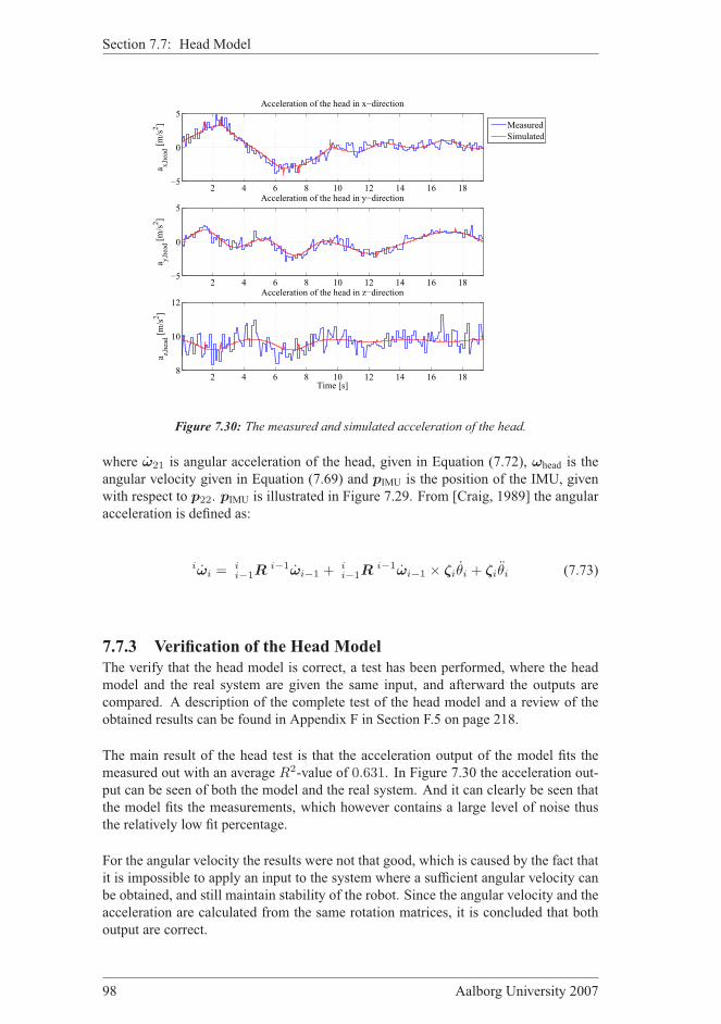
Section 7.7: Head Model
2 4 6 8 10 12 14 16 18−5
0
5Acceleration of the head in x−direction
a x,head [m/s2]
2 4 6 8 10 12 14 16 18−5
0
5Acceleration of the head in y−direction
a y,head [m/s2]
2 4 6 8 10 12 14 16 188
10
12Acceleration of the head in z−direction
Time [s]
a z,head [m/s2]
Measured
Simulated
Figure 7.30: The measured and simulated acceleration of the head.
where ω21 is angular acceleration of the head, given in Equation (7.72), ωhead is the
angular velocity given in Equation (7.69) and pIMU is the position of the IMU, given
with respect to p22. pIMU is illustrated in Figure 7.29. From [Craig, 1989] the angular
acceleration is defined as:
iωi = ii−1R
i−1ωi−1 + ii−1R
i−1ωi−1 × ζiθi + ζiθi (7.73)
7.7.3 Verification of the Head Model
The verify that the head model is correct, a test has been performed, where the head
model and the real system are given the same input, and afterward the outputs are
compared. A description of the complete test of the head model and a review of the
obtained results can be found in Appendix F in Section F.5 on page 218.
The main result of the head test is that the acceleration output of the model fits the
measured out with an average R2-value of 0.631. In Figure 7.30 the acceleration out-put can be seen of both the model and the real system. And it can clearly be seen that
the model fits the measurements, which however contains a large level of noise thus
the relatively low fit percentage.
For the angular velocity the results were not that good, which is caused by the fact that
it is impossible to apply an input to the system where a sufficient angular velocity can
be obtained, and still maintain stability of the robot. Since the angular velocity and the
acceleration are calculated from the same rotation matrices, it is concluded that both
output are correct.
98 Aalborg University 2007

Chapter 7: Modeling
0 50 100 150 200−5
0
5
10Force on strain gauge one
FS1 [N]
0 50 100 150 200−2
0
2
4Force on strain gauge two
FS2 [N]
0 50 100 150 200−5
0
5Force on strain gauge three
Time [s]
FS3 [N]
0 mm
2 mm Right
4 mm Right
2 mm Left
4 mm Left
Figure 7.31: The coordinate system located in the foot was moved to the left and right in the
y-axis. It is seen that his has a large impact on the model, specially on strain gauge two which
is located right above the origin.
7.8 Partial Conclusion to ModelingIn this chapter the model of the robot was developed. The model was designed to be
an input to output description of the real system, enabling the possibility to used the
model for simulation purpose. Both kinetics and dynamics were included in the model.
The model was constructed for both SSP and DSP which thereby made the model a
hybrid system. The dynamics during the DSP was calculated using a novel solution,
combining the two SSP in one. A phase estimator was designed and implemented to
switch between models.
A verification of the complete model is conducted, where the model and the robot are
given the same input and afterward the output is compared. The complete description
of the performed test can be seen in Appendix F in Section F.7. The main result of the
test was, that the developed model fits the real system to a certain degree. That is, the
same fluctuations changes in signals can be observed, but several of the outputs have an
offset error, which was also observed in the verification of the dynamical model. The
main reason for the divergens between the model output and the system is the bendable
spring steel plates in the feet. Because of these plates the robot starts wobbling, which
have a huge impact on the output. Furthermore the backlash in the system makes the
robot tilt, which also influences the measurements greatly.
A test was conducted to see how much an error in the location of the origin in the foot,
had on the foot model. This is seen from Figure 7.31, where the origin was moved in
the y-axis. From this figure it is seen that moving the origin has a large impact on the
model, which would be the same in the real system. If the real origin is located different
than that of the model, this would lead to a difference in the output of the strain gauges.
Group 1033 99

Section 7.8: Partial Conclusion to Modeling
Based on the fact that all sub-models have been verified individually and based on the
fact that the model clearly estimates the trends of the measure output, it is concluded
that the complete model is correct. However a more precise model can be obtained if
the plates in the feet and the backlash in the system are included in the model.
100 Aalborg University 2007

8INVERSE KINEMAT-
ICS
Chapter contents8.1 Closed Form Solution to the Inverse Kinematic Problem 103
8.1.1 Inverse Kinematics for the Legs 104
8.1.2 Inverse Kinematics for the Arms 107
8.2 Partial Conclusion to Inverse Kinematics 108
I N SECTION 7.3 on page 71, a kinematic model for the biped robot was derived.
This model can be used to calculate the position and orientation of the CoM of all
links, given the joint angles. In this chapter, the inverse kinematic model is derived,
which can be used to calculate the joint angles, if the orientation and position of the
torso, swing foot and the hands are given. Two solutions are given to solve the inverse
kinematic problem of the robot; a closed form solution and a numerical solution. The
former, which is utilized in this project, is explained in this chapter, whereas the latter,
which is not utilized, is explained in Appendix G on page 233.
Group 1033 101
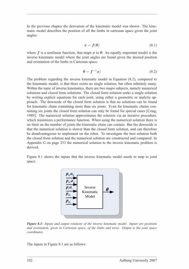
In the previous chapter the derivation of the kinematic model was shown. The kine-
matic model describes the position of all the limbs in cartesian space given the joint
angles:
x = f(θ) (8.1)
where f is a nonlinear function, that maps x to θ. An equally important model is the
inverse kinematic model where the joint angles are found given the desired position
and orientation of the limbs in Cartesian space:
θ = f−1x) (8.2)
The problem regarding the inverse kinematic model in Equation (8.2), compared to
the kinematic model, is that there exists no single solution, but often infinitely many.
Within the topic of inverse kinematics, there are two major subjects, namely numerical
solutions and closed form solutions. The closed form solution seeks a single solution
by writing explicit equations for each joint, using either a geometric or analytic ap-
proach. The downside of the closed form solution is that no solutions can be found
for kinematic chain containing more than six joints. Even for kinematic chains con-
taining six joints the closed form solution can only be found for special cases [Craig,
1989]. The numerical solution approximates the solution via an iterative procedure,
which minimizes a performance function. When using the numerical solution there is
no limit on the number of joints the kinematic chain can contain. But the downside is
that the numerical solution is slower than the closed form solution, and can therefore
be disadvantageous to implement on the robot. To investigate the best solution both
the closed form solution and the numerical solution are constructed and compared. In
Appendix G on page 233 the numerical solution to the inverse kinematic problem is
derived.
Figure 8.1 shows the inputs that the inverse kinematic model needs to map to joint
space.
Inverse Kinematic
Modelθθθθ
lf lfp o
f rfrp o
t tp o
rhp
lhp
Figure 8.1: Inputs and output relations of the inverse kinematic model. Inputs are positions
and orientation, given in Cartesian space, of the limbs and torso. Output is the joint space
coordinates.
The inputs in Figure 8.1 are as follows:
102 Aalborg University 2007

Chapter 8: Inverse Kinematics
plf The position vector of the left foot
olf The orientation vector of the left foot
prf The position vector of the right foot
orf The orientation vector of the right foot
pt The position vector of the torso
ot The orientation vector of the torso
prh The position vector of the right hand
plh The position vector of the left hand
Using the above inputs it is possible to place and orient the limbs of the robot. Figure
8.2 shows how the above position vectors are placed on the robot with regards to a
common frame.
rhp
tp
lfp
rfp
lhp
tp6
Figure 8.2: Position vectors in the inverse kinemeatics.
The following will describe the derivation of the closed form inverse kinematic model.
8.1 Closed Form Solution to the Inverse Kinematic Prob-
lemIn this section a closed form solution for the inverse kinematic problem for legs and
arms is given.
Group 1033 103
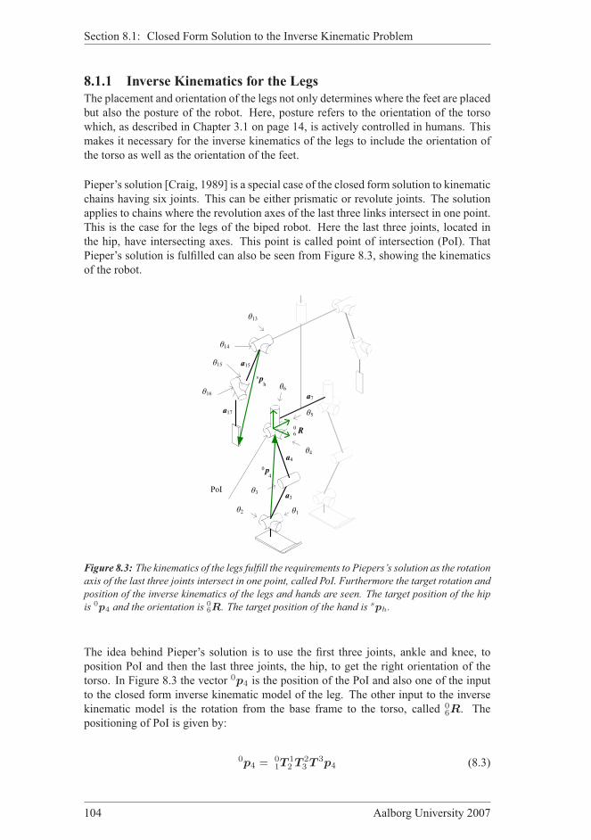
Section 8.1: Closed Form Solution to the Inverse Kinematic Problem
8.1.1 Inverse Kinematics for the Legs
The placement and orientation of the legs not only determines where the feet are placed
but also the posture of the robot. Here, posture refers to the orientation of the torso
which, as described in Chapter 3.1 on page 14, is actively controlled in humans. This
makes it necessary for the inverse kinematics of the legs to include the orientation of
the torso as well as the orientation of the feet.
Pieper’s solution [Craig, 1989] is a special case of the closed form solution to kinematic
chains having six joints. This can be either prismatic or revolute joints. The solution
applies to chains where the revolution axes of the last three links intersect in one point.
This is the case for the legs of the biped robot. Here the last three joints, located in
the hip, have intersecting axes. This point is called point of intersection (PoI). That
Pieper’s solution is fulfilled can also be seen from Figure 8.3, showing the kinematics
of the robot.
θ1θ2
θ3
θ4
θ5
θ6
PoI
θ13
θ14
θ16
θ15
a3
a4
a17
a15
hps
R06
04p
a7
Figure 8.3: The kinematics of the legs fulfill the requirements to Piepers’s solution as the rotation
axis of the last three joints intersect in one point, called PoI. Furthermore the target rotation and
position of the inverse kinematics of the legs and hands are seen. The target position of the hip
is 0p4 and the orientation is 06R. The target position of the hand is sph.
The idea behind Pieper’s solution is to use the first three joints, ankle and knee, to
position PoI and then the last three joints, the hip, to get the right orientation of the
torso. In Figure 8.3 the vector 0p4 is the position of the PoI and also one of the input
to the closed form inverse kinematic model of the leg. The other input to the inverse
kinematic model is the rotation from the base frame to the torso, called 06R. The
positioning of PoI is given by:
0p4 = 01T
12 T 2
3 T 3p4 (8.3)
104 Aalborg University 2007

Chapter 8: Inverse Kinematics
where 01T describes the position and orientation of frame 1 relative to frame 0. 0
1T
is a transformation matrix, that maps a point 1p 7→ 0p. If the mapping to be performed
is 0p 7→ 1p this can be obtained by using 10T = 0
1T−1. The transformation matrix
can be computed as:
01T =
01R
0p1org
0 0 0 1
(8.4)
where 01R is the rotation matrix that describes the orientation of frame 1 relative to
frame 0 and 0p1org is the position vector, that describes the origin of frame 1 rel-ative to 0. A more thorough description of the rotation matrices and their properties
can be found in Section 7.3 on page 71.
Pieper’s solution states that Equation (8.3) can be written as:
3p4 = 01T
12 T
f1(θ3)f2(θ3)f3(θ3)
1
(8.5)
where fi is a function describing PoI in frame 2. It is noticed that the function fi
only contains θ3 as a variable. Note that:
0p4 = a4 =
a4x
a4y
a4z
1
(8.6)
With 23T and 3
4p given, fi can be written as:
f1 = c3a4x + s3a4z − a3x (8.7)
f2 = 0 (8.8)
f3 = −s3a4x + c3a4z + a3z (8.9)
The magnitude squared of 04p is calculated as:
r2 = f21 + f2
2 + f23 (8.10)
For the type of kinematic composition used for the biped robot, the magnitude squared
of 04p can also be written as:
r2 = c32a4x
2 − 2c3a3xa4x + s32a4z
2 − 2s3a4za3x + a3x2 + s3
2a4x2 (8.11)
−2s3a4xa3z + c32a4z
2 + 2c3a4za3z + a3z2
According to Pieper the solution of the magnitude squared of 0p4 can contain other
variables than θ3. Finding θ3 from Equation (8.11) would then have been more cum-
bersome. But because of the construction of the biped robot, the magnitude squared of
Group 1033 105
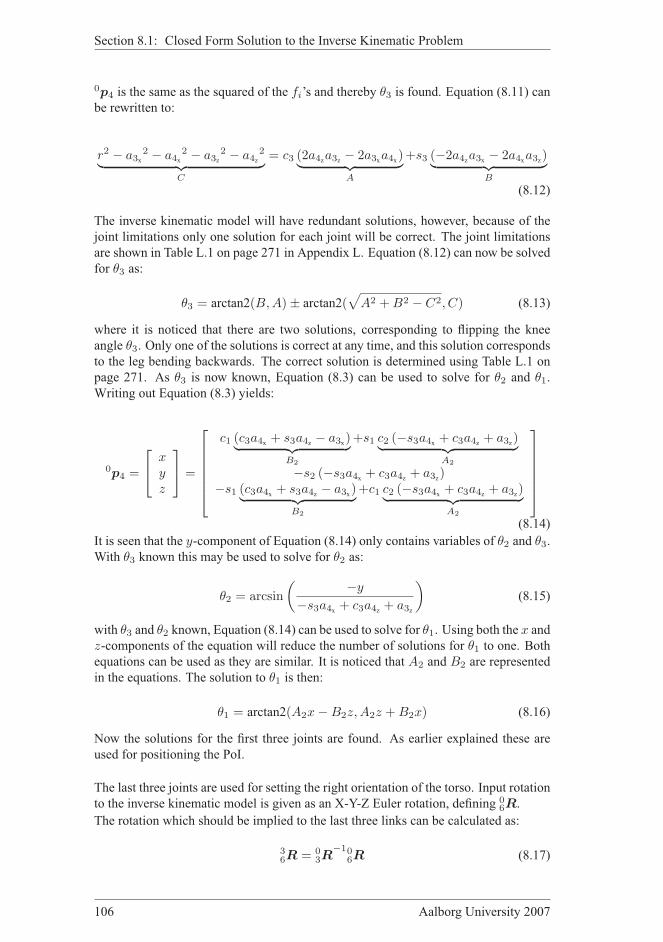
Section 8.1: Closed Form Solution to the Inverse Kinematic Problem
0p4 is the same as the squared of the fi’s and thereby θ3 is found. Equation (8.11) can
be rewritten to:
r2 − a3x2 − a4x
2 − a3z2 − a4z
2
︸ ︷︷ ︸
C
= c3 (2a4za3z − 2a3xa4x)︸ ︷︷ ︸
A
+s3 (−2a4za3x − 2a4xa3z)︸ ︷︷ ︸
B
(8.12)
The inverse kinematic model will have redundant solutions, however, because of the
joint limitations only one solution for each joint will be correct. The joint limitations
are shown in Table L.1 on page 271 in Appendix L. Equation (8.12) can now be solved
for θ3 as:
θ3 = arctan2(B,A)± arctan2(√
A2 + B2 − C2, C) (8.13)
where it is noticed that there are two solutions, corresponding to flipping the knee
angle θ3. Only one of the solutions is correct at any time, and this solution corresponds
to the leg bending backwards. The correct solution is determined using Table L.1 on
page 271. As θ3 is now known, Equation (8.3) can be used to solve for θ2 and θ1.
Writing out Equation (8.3) yields:
0p4 =
xyz
=
c1 (c3a4x + s3a4z − a3x)︸ ︷︷ ︸
B2
+s1 c2 (−s3a4x + c3a4z + a3z)︸ ︷︷ ︸
A2
−s2 (−s3a4x + c3a4z + a3z)−s1 (c3a4x + s3a4z − a3x)
︸ ︷︷ ︸
B2
+c1 c2 (−s3a4x + c3a4z + a3z)︸ ︷︷ ︸
A2
(8.14)
It is seen that the y-component of Equation (8.14) only contains variables of θ2 and θ3.
With θ3 known this may be used to solve for θ2 as:
θ2 = arcsin
( −y
−s3a4x + c3a4z + a3z
)
(8.15)
with θ3 and θ2 known, Equation (8.14) can be used to solve for θ1. Using both the x andz-components of the equation will reduce the number of solutions for θ1 to one. Both
equations can be used as they are similar. It is noticed that A2 and B2 are represented
in the equations. The solution to θ1 is then:
θ1 = arctan2(A2x−B2z,A2z + B2x) (8.16)
Now the solutions for the first three joints are found. As earlier explained these are
used for positioning the PoI.
The last three joints are used for setting the right orientation of the torso. Input rotation
to the inverse kinematic model is given as an X-Y-Z Euler rotation, defining 06R.
The rotation which should be implied to the last three links can be calculated as:
36R = 0
3R−10
6R (8.17)
106 Aalborg University 2007

Chapter 8: Inverse Kinematics
It is known that the rotation of the last three links is an X-Y-Z rotation about θ4, θ5,
and θ6, and thereby can Equation (8.17) be re-written as:
c5c6 −c5s6 s5
s4s5c6 + c4s6 −s4s5s6 + c4c6 −s4c5
−c4s5c6 + s4s6 c4s5s6 + s4c6 c4c5
=
r1,1 r1,2 r1,3
r2,1 r2,2 r2,3
r3,1 r3,2 r3,3
(8.18)
The right side of Equation (8.18) can be found using θ1 . . . θ3 to calculate03R, and the
target rotation is used to find 06R. From Equation (8.18) it is seen that θ5 can be found
as:
θ5 = arcsin(r1,3) (8.19)
There are two solutions to (8.19), and again the Table L.1 on page 271 used to deter-
mine the correct solution. With θ5 known, Equation (8.18) may be solved for θ6:
θ6 = arctan2
(r1,2
− cos(θ5),
r1,1
cos(θ5)
)
(8.20)
θ4 is now found as:
θ4 = arctan2
(r2,3
− cos(θ5),
r3,3
cos(θ5)
)
(8.21)
The described solution determines θ1 . . . θ6 for the right leg. The approach for finding
θ7 . . . θ12 is the same, differing only in signs. This completes the inverse kinematics
for both the right and left leg. Now the inverse kinematics for the arms will be solved.
8.1.2 Inverse Kinematics for the Arms
Solving the inverse kinematics for the arms takes on the same problem as for the legs.
As it is valued that the arms will only be used for stability purposes, it is chosen to
solve the problem for three links only. Thereby the same method as the lower three
links of the leg can be used, namely Pieper’s method. Using only three joints have the
advantage that the goal can be specified using only position and not orientation. It has
been chosen not to include joint 15 and 19 in the inverse kinematic solution and this
can then later be used for rotation purposes. The rotation of the arms is then given by
an Y-X-X rotation and the target position is given from:
sph = s13T
1314T
1416T
16ph (8.22)
where sph is the position of the hand with respect to frame s placed in the shoulder.sph is the input to the inverse kinematic solution of the arms and is also seen from
Figure 8.3. The fi function is found from16ph and
1416T . Using the magnitude squared
of the fi functions θ16 is found to be:
θ16 = arctan2(
Q16,±√
1−Q16
)
(8.23)
where Q16 =r2−a15z
2−a17z2
2a15za17z. Writing out Equation (8.22) yields:
Group 1033 107
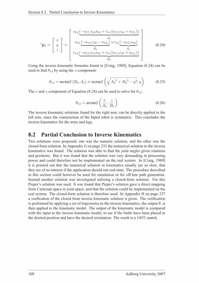
Section 8.2: Partial Conclusion to Inverse Kinematics
sph =
xyz
=
s13 (−a17zs14s16 + c14 (a17zc16 + a15z))︸ ︷︷ ︸
A5
s14 (−a17zc16 − a15z)︸ ︷︷ ︸
B4
+c14 (−a17zs16)︸ ︷︷ ︸
A4
c13 (−a17zs14s16 + c14 (a17zc16 + a15z))︸ ︷︷ ︸
B5
(8.24)
Using the inverse kinematic formulas found in [Craig, 1989], Equation (8.24) can be
used to find θ14 by using the x-component:
θ14 = arctan2 (B4, A4)± arctan2
(√
A42 + B4
2 − y2, y
)
(8.25)
The x and z-component of Equation (8.24) can be used to solve for θ13:
θ13 = arctan2
(x
A5,
z
B5
)
(8.26)
The inverse kinematic solutions found for the right arm, can be directly applied to the
left arm, since the construction of the biped robot is symmetric. This concludes the
inverse kinematics for the arms and legs.
8.2 Partial Conclusion to Inverse KinematicsTwo solutions were proposed, one was the numeric solution, and the other was the
closed form solution. In Appendix G on page 233 the numerical solution to the inverse
kinematics was found. The solution was able to find the joint angles given rotations
and positions. But it was found that the solution was very demanding in processing
power and could therefore not be implemented on the real system. In [Craig, 1989]
it is pointed out that the numerical solution to kinematics usually are so slow, that
they are of no interest if the application should run real-time. The procedure described
in this section could however be used for simulation or for off-line path generation.
Instead another solution was investigated utilizing a closed-form solution. For this
Pieper’s solution was used. It was found that Pieper’s solution gave a direct mapping
from Cartesian space to joint space, and that the solution could be implemented on the
real system. The closed-form solution is therefore used. In Appendix H on page 237
a verification of the closed from inverse kinematic solution is given. The verification
is performed by applying a set of trajectories to the inverse kinematics, the output θ, isthen applied to the kinematic model. The output of the kinematic model is compared
with the input to the inverse kinematic model, to see if the limbs have been placed in
the desired position and have the desired orientation. The result is a 100% match.
108 Aalborg University 2007

9TRAJECTORY
GENERATION
Chapter contents9.1 Trajectory Generation Methods 110
9.1.1 On-line and Off-line Trajectory Generation 110
9.1.2 Methods for Generating Walking Trajectories 111
9.2 Establishing the Trajectories 114
9.2.1 ZMP-stability 114
9.2.2 Foot Trajectories 117
9.2.3 Torso Trajectory 119
9.2.4 Start-Up and Stop Phase 121
9.2.5 Scaling Parameters from Human Walk 121
9.2.6 Cubic Splines 122
9.3 Simulation of Trajectories 122
9.3.1 Finding Parameters for Sagittal Movement 123
9.3.2 Finding Parameters for Frontal Movement 124
9.4 Resulting Trajectories 125
9.4.1 Polynomials for Feet 125
9.4.2 Polynomials for Torso 125
9.5 Conclusion on Trajectory Generation 128
T HIS CHAPTER describes the derivation of the walking trajectories. First some
methods that are frequently used for generating walking trajectories, will be de-
scribed. The prospects and considerations for each of the different types will be em-
phasized, which is done in Section 9.1. The chosen method will be given a detailed
description. Both the steady-state walk, the start-up phase and the stop phase will be
considered. This leads to estimation of the parameters that should be used to generate
walking trajectories. All this is described in Section 9.2. Section 9.3 describes a simu-
lation on the developed model, and the resulting trajectories are presented in Section
9.4.
Group 1033 109

Section 9.1: Trajectory Generation Methods
9.1 Trajectory Generation MethodsAs stated in Section 3.4 on page 20, and as depicted in Figure 3.1 on page 14, a tra-
jectory generator has to be developed. This section describes the methods often used
for generating walking trajectories. The section will begin with a description of the
two overall methods; on-line and off-line trajectory generation. Here after a number
of different methods, which are most frequently used for generating on-line or off-line
trajectories will be described.
9.1.1 On-line and Off-line Trajectory Generation
There are two overall methods used for trajectory generation, which is investigated
in this thesis; on-line and off-line trajectory generation. An introduction to these two
methods will be given in this section, and their prospects and considerations will be
described.
On-line Trajectory Generation
When using on-line trajectory generation, walking trajectories are calculated on-the-
fly as the robot walk. This makes the robot capable of changing its walking patterns if
changes in the surroundings should occur. Changes in the surroundings could be pre-
sented as a tilted surface, uneven surface, obstacles in the walking path, etc. On-line
trajectory generation can be enhanced by using self-learning algorithms. This is seen
in [Capi et al., 2003]. A disadvantage of this type of trajectory generation is the fact
that it is very demanding with regards to processing power. Most projects regarding
on-line trajectory generation is limited to simulation due to the high demand of pro-
cessing power and complex implementation, as in [Kondak and Hommel, 2003].
In [Kondak and Hommel, 2003] they propose a method where a biped robot is per-
forming stable walk without any precomputed trajectories. The trajectory generation
is made on-line, along with model-based control of the robot. The downside of the
results in [Kondak and Hommel, 2003] is however, that the algorithms are only imple-
mented on a model in simulation. This is the most widespread approach taken in the
literature, when on-line trajectory generation is the subject.
Off-line Trajectory Generation
When using off-line trajectory generation, walking trajectories are calculated before-
hand. Trajectories could be calculated using an external computer and then imple-
mented on the robot as a look-up table or as functions describing the trajectories. The
advantage of calculating the trajectories off-line is that the new reference positions are
found faster, making it easier to fulfill the real-time demands. Hence, it is possible to
calculate trajectories, using the dynamical model to ensure energy efficiency, if this is
a matter of interest, and then implement the trajectories when these have been calcu-
lated. This method is very applicable in systems where the processing power is very
limited.
Due to the limited processing power in this project, being a 200MHz ARM9 proces-
sor, it has been chosen to use off-line trajectory generation. Different methods that can
be used to generate the trajectories are described in the following section. A disad-
vantage of using off-line trajectory generation is that the possibility of changing the
walking patterns on-the-fly is limited to the number of trajectories stored on the robot.
110 Aalborg University 2007
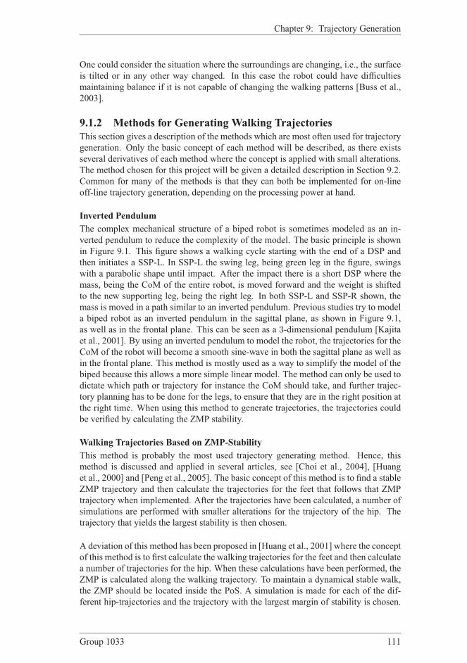
Chapter 9: Trajectory Generation
One could consider the situation where the surroundings are changing, i.e., the surface
is tilted or in any other way changed. In this case the robot could have difficulties
maintaining balance if it is not capable of changing the walking patterns [Buss et al.,
2003].
9.1.2 Methods for Generating Walking Trajectories
This section gives a description of the methods which are most often used for trajectory
generation. Only the basic concept of each method will be described, as there exists
several derivatives of each method where the concept is applied with small alterations.
The method chosen for this project will be given a detailed description in Section 9.2.
Common for many of the methods is that they can both be implemented for on-line
off-line trajectory generation, depending on the processing power at hand.
Inverted Pendulum
The complex mechanical structure of a biped robot is sometimes modeled as an in-
verted pendulum to reduce the complexity of the model. The basic principle is shown
in Figure 9.1. This figure shows a walking cycle starting with the end of a DSP and
then initiates a SSP-L. In SSP-L the swing leg, being green leg in the figure, swings
with a parabolic shape until impact. After the impact there is a short DSP where the
mass, being the CoM of the entire robot, is moved forward and the weight is shifted
to the new supporting leg, being the right leg. In both SSP-L and SSP-R shown, the
mass is moved in a path similar to an inverted pendulum. Previous studies try to model
a biped robot as an inverted pendulum in the sagittal plane, as shown in Figure 9.1,
as well as in the frontal plane. This can be seen as a 3-dimensional pendulum [Kajita
et al., 2001]. By using an inverted pendulum to model the robot, the trajectories for the
CoM of the robot will become a smooth sine-wave in both the sagittal plane as well as
in the frontal plane. This method is mostly used as a way to simplify the model of the
biped because this allows a more simple linear model. The method can only be used to
dictate which path or trajectory for instance the CoM should take, and further trajec-
tory planning has to be done for the legs, to ensure that they are in the right position at
the right time. When using this method to generate trajectories, the trajectories could
be verified by calculating the ZMP stability.
Walking Trajectories Based on ZMP-Stability
This method is probably the most used trajectory generating method. Hence, this
method is discussed and applied in several articles, see [Choi et al., 2004], [Huang
et al., 2000] and [Peng et al., 2005]. The basic concept of this method is to find a stable
ZMP trajectory and then calculate the trajectories for the feet that follows that ZMP
trajectory when implemented. After the trajectories have been calculated, a number of
simulations are performed with smaller alterations for the trajectory of the hip. The
trajectory that yields the largest stability is then chosen.
A deviation of this method has been proposed in [Huang et al., 2001] where the concept
of this method is to first calculate the walking trajectories for the feet and then calculate
a number of trajectories for the hip. When these calculations have been performed, the
ZMP is calculated along the walking trajectory. To maintain a dynamical stable walk,
the ZMP should be located inside the PoS. A simulation is made for each of the dif-
ferent hip-trajectories and the trajectory with the largest margin of stability is chosen.
Group 1033 111

Section 9.1: Trajectory Generation Methods
SSP-L SSP-RDSP
xWalking direction
zHe
ight
Figure 9.1: The basic principle of using an inverted pendulum to generate trajectories. Two
steps in the sagittal plane is illustrated. The green line is the right leg and the red line is the left
leg. The circle illustrates the CoM of the entire robot.
The appealing property of using this method is that human-like walking patterns could
be realized by analyzing human walk and then set the desired step length, foot angle,
etc. according to this. The trajectory of the hip should also be fitted to human walking
trajectories but several hip trajectories should be generated with small alterations. Af-
ter having simulated all the trajectories, the trajectory with the best stability properties
should be chosen. A downside of this method is however, that the energy in the move-
ments is not exploited in a sufficient degree, as for instance with the inverted pendulum
method. This could result in an unnecessary load exposed on the actuators.
CoMMethod
Another popular method is the centre of mass method, which has been studied and
previously used in [Christensen et al., 2006]. This method relies on calculations of the
CoM, and keeping this point within the PoS. It was discovered that this type of gait
generation resulted in a stable walk of the robot. But the walk was not dynamical, only
static. As the requirements to the CoM being within the PoS, given by the supporting
foot/feet, results in shifting of the weight from foot to foot. This results in a ”duck-
like” walk, which does not resemble human walk. The upside of this method, is that it
is relatively simple, and the trajectories can easily be calculated off-line. It should be
noted that the CoMmethod differs significantly from the ZMPmethod, as the dynamics
of the movement is not included in the CoM method, but only the static location of the
CoM is considered.
Cyclic Motion Generator
Cyclic motion generation is often mentioned as being the method that humans use
to generate walking trajectories, see [Borghese et al., 1996], [Ogino et al., 2003]
and [Nielsen, 2003]. When humans walk, the cyclic walking patterns are generated
in a nerve center in the spinal cord. This is often referred to as the spinal central pat-
tern generator, called central pattern generator (CPG). When CPG is used to achieve
human-like motion, a cyclic motion generator is implemented, generating the cyclic
trajectories that characterize human walk. The energy efficiency should be optimal
when using CPG, see [Ogino et al., 2003], since CPG seeks to copy human walking
patterns that are said to be optimal with regards to energy efficiency [Popovic, 2006].
112 Aalborg University 2007
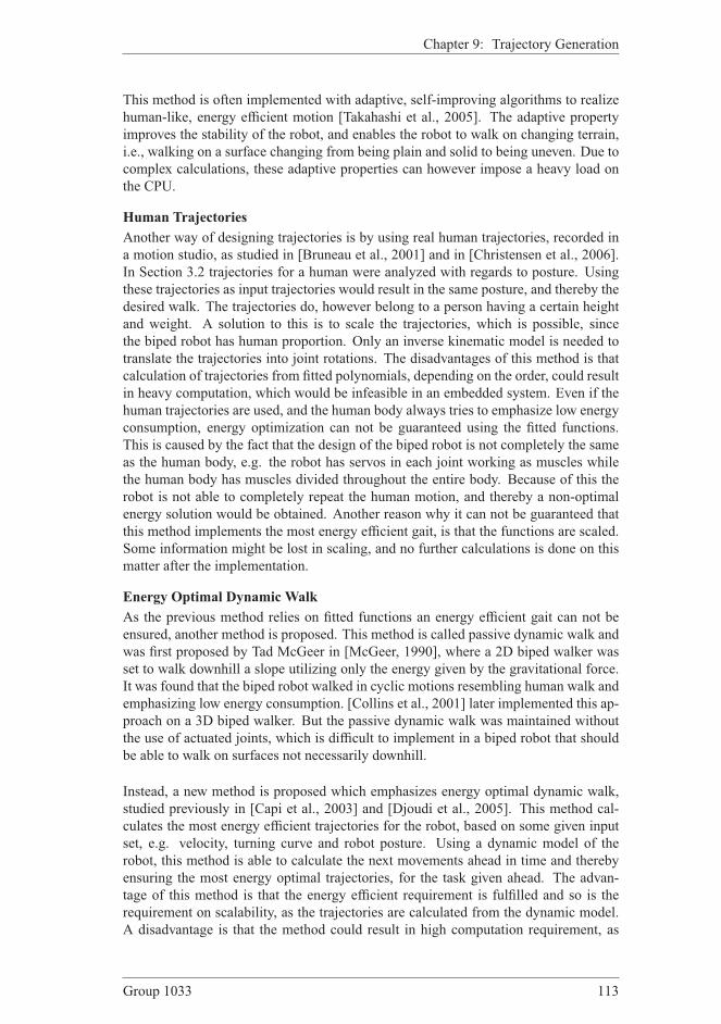
Chapter 9: Trajectory Generation
This method is often implemented with adaptive, self-improving algorithms to realize
human-like, energy efficient motion [Takahashi et al., 2005]. The adaptive property
improves the stability of the robot, and enables the robot to walk on changing terrain,
i.e., walking on a surface changing from being plain and solid to being uneven. Due to
complex calculations, these adaptive properties can however impose a heavy load on
the CPU.
Human Trajectories
Another way of designing trajectories is by using real human trajectories, recorded in
a motion studio, as studied in [Bruneau et al., 2001] and in [Christensen et al., 2006].
In Section 3.2 trajectories for a human were analyzed with regards to posture. Using
these trajectories as input trajectories would result in the same posture, and thereby the
desired walk. The trajectories do, however belong to a person having a certain height
and weight. A solution to this is to scale the trajectories, which is possible, since
the biped robot has human proportion. Only an inverse kinematic model is needed to
translate the trajectories into joint rotations. The disadvantages of this method is that
calculation of trajectories from fitted polynomials, depending on the order, could result
in heavy computation, which would be infeasible in an embedded system. Even if the
human trajectories are used, and the human body always tries to emphasize low energy
consumption, energy optimization can not be guaranteed using the fitted functions.
This is caused by the fact that the design of the biped robot is not completely the same
as the human body, e.g. the robot has servos in each joint working as muscles while
the human body has muscles divided throughout the entire body. Because of this the
robot is not able to completely repeat the human motion, and thereby a non-optimal
energy solution would be obtained. Another reason why it can not be guaranteed that
this method implements the most energy efficient gait, is that the functions are scaled.
Some information might be lost in scaling, and no further calculations is done on this
matter after the implementation.
Energy Optimal Dynamic Walk
As the previous method relies on fitted functions an energy efficient gait can not be
ensured, another method is proposed. This method is called passive dynamic walk and
was first proposed by Tad McGeer in [McGeer, 1990], where a 2D biped walker was
set to walk downhill a slope utilizing only the energy given by the gravitational force.
It was found that the biped robot walked in cyclic motions resembling human walk and
emphasizing low energy consumption. [Collins et al., 2001] later implemented this ap-
proach on a 3D biped walker. But the passive dynamic walk was maintained without
the use of actuated joints, which is difficult to implement in a biped robot that should
be able to walk on surfaces not necessarily downhill.
Instead, a new method is proposed which emphasizes energy optimal dynamic walk,
studied previously in [Capi et al., 2003] and [Djoudi et al., 2005]. This method cal-
culates the most energy efficient trajectories for the robot, based on some given input
set, e.g. velocity, turning curve and robot posture. Using a dynamic model of the
robot, this method is able to calculate the next movements ahead in time and thereby
ensuring the most energy optimal trajectories, for the task given ahead. The advan-
tage of this method is that the energy efficient requirement is fulfilled and so is the
requirement on scalability, as the trajectories are calculated from the dynamic model.
A disadvantage is that the method could result in high computation requirement, as
Group 1033 113
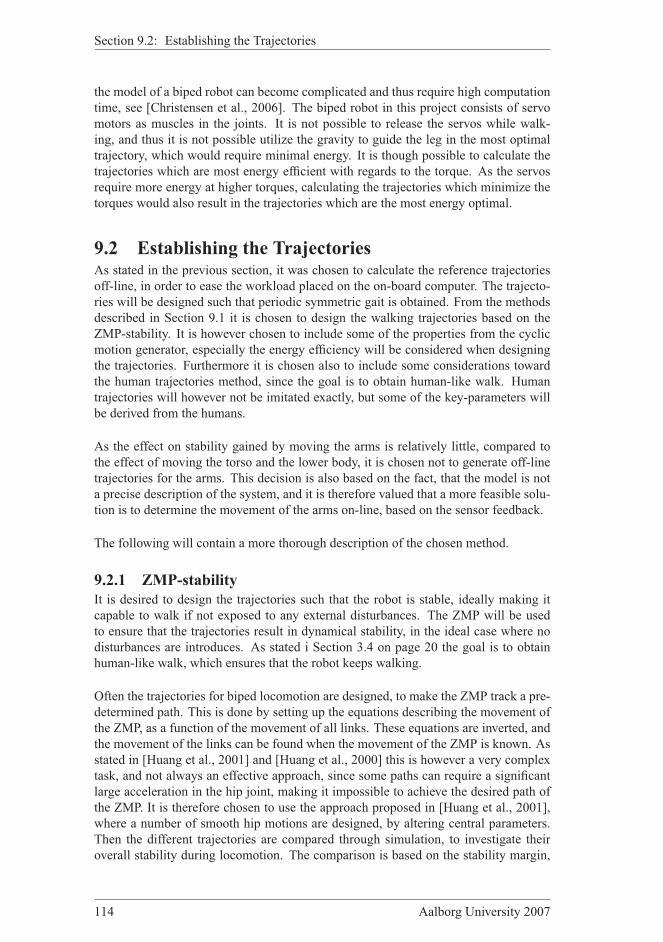
Section 9.2: Establishing the Trajectories
the model of a biped robot can become complicated and thus require high computation
time, see [Christensen et al., 2006]. The biped robot in this project consists of servo
motors as muscles in the joints. It is not possible to release the servos while walk-
ing, and thus it is not possible utilize the gravity to guide the leg in the most optimal
trajectory, which would require minimal energy. It is though possible to calculate the
trajectories which are most energy efficient with regards to the torque. As the servos
require more energy at higher torques, calculating the trajectories which minimize the
torques would also result in the trajectories which are the most energy optimal.
9.2 Establishing the TrajectoriesAs stated in the previous section, it was chosen to calculate the reference trajectories
off-line, in order to ease the workload placed on the on-board computer. The trajecto-
ries will be designed such that periodic symmetric gait is obtained. From the methods
described in Section 9.1 it is chosen to design the walking trajectories based on the
ZMP-stability. It is however chosen to include some of the properties from the cyclic
motion generator, especially the energy efficiency will be considered when designing
the trajectories. Furthermore it is chosen also to include some considerations toward
the human trajectories method, since the goal is to obtain human-like walk. Human
trajectories will however not be imitated exactly, but some of the key-parameters will
be derived from the humans.
As the effect on stability gained by moving the arms is relatively little, compared to
the effect of moving the torso and the lower body, it is chosen not to generate off-line
trajectories for the arms. This decision is also based on the fact, that the model is not
a precise description of the system, and it is therefore valued that a more feasible solu-
tion is to determine the movement of the arms on-line, based on the sensor feedback.
The following will contain a more thorough description of the chosen method.
9.2.1 ZMP-stability
It is desired to design the trajectories such that the robot is stable, ideally making it
capable to walk if not exposed to any external disturbances. The ZMP will be used
to ensure that the trajectories result in dynamical stability, in the ideal case where no
disturbances are introduces. As stated i Section 3.4 on page 20 the goal is to obtain
human-like walk, which ensures that the robot keeps walking.
Often the trajectories for biped locomotion are designed, to make the ZMP track a pre-
determined path. This is done by setting up the equations describing the movement of
the ZMP, as a function of the movement of all links. These equations are inverted, and
the movement of the links can be found when the movement of the ZMP is known. As
stated in [Huang et al., 2001] and [Huang et al., 2000] this is however a very complex
task, and not always an effective approach, since some paths can require a significant
large acceleration in the hip joint, making it impossible to achieve the desired path of
the ZMP. It is therefore chosen to use the approach proposed in [Huang et al., 2001],
where a number of smooth hip motions are designed, by altering central parameters.
Then the different trajectories are compared through simulation, to investigate their
overall stability during locomotion. The comparison is based on the stability margin,
114 Aalborg University 2007
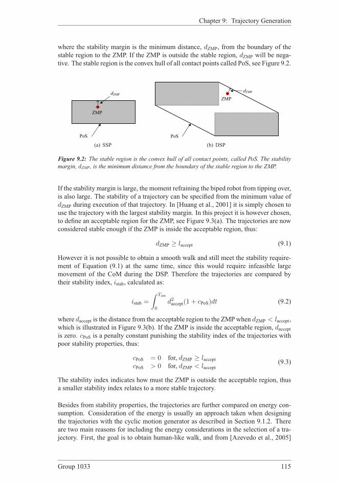
Chapter 9: Trajectory Generation
where the stability margin is the minimum distance, dZMP, from the boundary of the
stable region to the ZMP. If the ZMP is outside the stable region, dZMP will be nega-
tive. The stable region is the convex hull of all contact points called PoS, see Figure 9.2.
ZMP
dZMP
PoS
(a) SSP
ZMPdZMP
PoS
(b) DSP
Figure 9.2: The stable region is the convex hull of all contact points, called PoS. The stability
margin, dZMP, is the minimum distance from the boundary of the stable region to the ZMP.
If the stability margin is large, the moment refraining the biped robot from tipping over,
is also large. The stability of a trajectory can be specified from the minimum value of
dZMP during execution of that trajectory. In [Huang et al., 2001] it is simply chosen to
use the trajectory with the largest stability margin. In this project it is however chosen,
to define an acceptable region for the ZMP, see Figure 9.3(a). The trajectories are now
considered stable enough if the ZMP is inside the acceptable region, thus:
dZMP ≥ laccept (9.1)
However it is not possible to obtain a smooth walk and still meet the stability require-
ment of Equation (9.1) at the same time, since this would require infeasible large
movement of the CoM during the DSP. Therefore the trajectories are compared by
their stability index, istab, calculated as:
istab =
∫ Tsim
0
d2accept(1 + cPoS)dt (9.2)
where daccept is the distance from the acceptable region to the ZMPwhen dZMP < laccept,which is illustrated in Figure 9.3(b). If the ZMP is inside the acceptable region, dacceptis zero. cPoS is a penalty constant punishing the stability index of the trajectories withpoor stability properties, thus:
cPoS = 0 for, dZMP ≥ lacceptcPoS > 0 for, dZMP < laccept
(9.3)
The stability index indicates how must the ZMP is outside the acceptable region, thus
a smaller stability index relates to a more stable trajectory.
Besides from stability properties, the trajectories are further compared on energy con-
sumption. Consideration of the energy is usually an approach taken when designing
the trajectories with the cyclic motion generator as described in Section 9.1.2. There
are two main reasons for including the energy considerations in the selection of a tra-
jectory. First, the goal is to obtain human-like walk, and from [Azevedo et al., 2005]
Group 1033 115
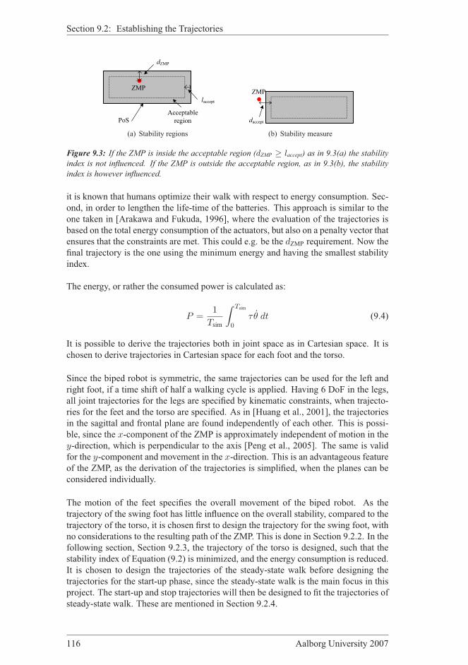
Section 9.2: Establishing the Trajectories
PoS
ZMP
Acceptable region
laccept
dZMP
(a) Stability regions
ZMP
Stable region
daccept
Stable region(b) Stability measure
Figure 9.3: If the ZMP is inside the acceptable region (dZMP ≥ laccept) as in 9.3(a) the stability
index is not influenced. If the ZMP is outside the acceptable region, as in 9.3(b), the stability
index is however influenced.
it is known that humans optimize their walk with respect to energy consumption. Sec-
ond, in order to lengthen the life-time of the batteries. This approach is similar to the
one taken in [Arakawa and Fukuda, 1996], where the evaluation of the trajectories is
based on the total energy consumption of the actuators, but also on a penalty vector that
ensures that the constraints are met. This could e.g. be the dZMP requirement. Now the
final trajectory is the one using the minimum energy and having the smallest stability
index.
The energy, or rather the consumed power is calculated as:
P =1
Tsim
∫ Tsim
0
τ θ dt (9.4)
It is possible to derive the trajectories both in joint space as in Cartesian space. It is
chosen to derive trajectories in Cartesian space for each foot and the torso.
Since the biped robot is symmetric, the same trajectories can be used for the left and
right foot, if a time shift of half a walking cycle is applied. Having 6 DoF in the legs,
all joint trajectories for the legs are specified by kinematic constraints, when trajecto-
ries for the feet and the torso are specified. As in [Huang et al., 2001], the trajectories
in the sagittal and frontal plane are found independently of each other. This is possi-
ble, since the x-component of the ZMP is approximately independent of motion in the
y-direction, which is perpendicular to the axis [Peng et al., 2005]. The same is validfor the y-component and movement in the x-direction. This is an advantageous featureof the ZMP, as the derivation of the trajectories is simplified, when the planes can be
considered individually.
The motion of the feet specifies the overall movement of the biped robot. As the
trajectory of the swing foot has little influence on the overall stability, compared to the
trajectory of the torso, it is chosen first to design the trajectory for the swing foot, with
no considerations to the resulting path of the ZMP. This is done in Section 9.2.2. In the
following section, Section 9.2.3, the trajectory of the torso is designed, such that the
stability index of Equation (9.2) is minimized, and the energy consumption is reduced.
It is chosen to design the trajectories of the steady-state walk before designing the
trajectories for the start-up phase, since the steady-state walk is the main focus in this
project. The start-up and stop trajectories will then be designed to fit the trajectories of
steady-state walk. These are mentioned in Section 9.2.4.
116 Aalborg University 2007

Chapter 9: Trajectory Generation
9.2.2 Foot Trajectories
The trajectories for the ankles will be designed in this section. Given these and the
orientation of the feet, the trajectories of the feet can be found from kinematic con-
straints. It is the trajectories of the feet that determine the velocity and the direction of
the biped robot across ground. Therefore it is necessary to specify the desired walking
speed, vwalking, and the desired step length, lstep. Then the time period for one step canbe found as:
Tstep =lstep
vwalking(9.5)
Note that the cycle time is Tcycle = 2Tstep.
yzx ht,min
a1z(a) DSP: t1 = (k − 1)Tstep
loθ
yzx xt,b
ltoe
(b) Lift off: t2 = kTstep − TSSP
yzx
ha,maxla,max
ht,max
(c) Middle of SSP: t3 = (k − 1)Tstep +Tmax
yzx
lstep lstep
xt,e
(d) Impact: t4 = kTstep
Figure 9.4: Illustration of the walking cycle in the sagittal plane, the green colour represents
right-side limbs and the red represents the left-side. 9.4(a) shows the middle of the DSP, where
the supporting leg is shifted, in 9.4(b) the SSP is initiated with the rear foot leaving the ground,
in 9.4(c) the ankle reaches its maximum height and in 9.4(d) the SSP is terminated with the
impact. The blue lines illustrates the trajectory taken by the torso and the right foot.
Foot Movement in the Sagittal Plane
The foot trajectory for the k’th step is illustrated in Figure 9.4. It is defined to startin the DSP when the heel of the rear foot leaves the ground, at time t1, as depicted in
Group 1033 117

Section 9.2: Establishing the Trajectories
Figure 9.4(a). The k’th step ends when the heel of the other foot in Figure 9.4(d) leavesthe ground at time t4. The SSP starts at time t2, with the toe of the rear foot leavingthe ground, this is illustrated in Figure 9.4(b). Then at time t3 the ankle of the swingleg, passes through its maximum point, (x, z) = (la,max, ha,max), as illustrated in Figure9.4(c). And finally the SSP is terminated when the swing leg impacts the ground at
time t4, shown in Figure 9.4(d). It is chosen to impact the ground with a flat foot, sincethe foot is not design for impact and tipping on heel. The time instants are given as
follows:
t1 = (k − 1)Tstep
t2 = kTstep − TSSP
t3 = (k − 1)Tstep + Tmax (9.6)
t4 = kTstep
where TSSP is the duration of the SSP and Tmax is the duration from the cycle starts
until the swing foot reaches it maximum height.
From the above, a number of constraints on the trajectory can be found:
xa(t) =
(k − 1)lstep , t = t1(k − 1)lstep + a1z sin(θlo) + ltoe (1− cos(θlo)) , t = t2(k − 1)lstep + la,max , t = t3klstep , t = t4
(9.7)
za(t) =
a1z , t = t1a1z cos(θlo) + ltoe sin(θlo) , t = t2ha,max , t = t3a1z , t = t4
(9.8)
where xa(t) and za(t) are the position of the ankle in the sagittal plane at time t, asdepicted in Figure 9.4, a1z is the height of the ankle and ltoe is the length from the ankle
to the toe, both shown in Figure 9.4, θlo is the angle of the foot at lift off. Furthermoresome constraints on the orientation of the foot can be found:
of(t) =
[0 0 0]T
, t = t1[0 − θlo 0]
T, t = t2
[0 0 0]T
, t = t3[0 0 0]
T, t = t4
(9.9)
where of(t) is the orientation of the foot, given as XYZ Euler angles fixed to the initial
frame, as described in Chapter 8 on page 101. Some constraints can also be attached
to the velocity of the ankle. It is known that the foot is placed flat on the ground at time
t1, thus the following constraints can be applied:
xa(t1) = 0
za(t1) = 0 (9.10)
of(t1) = [0 0 0]T
Furthermore the velocity trajectories, xa(t),za(t) and of(t), have to be differentiableand continuous for all t and their derivative, xa(t), za(t) and of(t), has to be continuousfor all t. Note that this should also apply in the breakpoints, where t = kTstep. These
requirements ensure smooth trajectories with no sudden accelerations.
118 Aalborg University 2007
Chapter 9: Trajectory Generation
Foot Movement in the Frontal Plane
If straight walk is the only goal, no movement of the feet in the frontal plane is neces-
sary, thus:
ya(t) = 0 (9.11)
This is because the movement in the frontal plane is performed by the torso.
9.2.3 Torso Trajectory
As explained earlier in this chapter, the trajectory of the torso will be designed such that
the locomotion of the biped robot fulfills the stability requirement, including consid-
erations on the energy efficiency. The stability requirement is that the ZMP should be
inside the acceptable region, as illustrated in Figure 9.3(a). In Section 3.2 on page 16 it
was decided, that the posture of the torso should always be maintained upright. Which
results in the following constraints:
ot(t) = [0 0 θt,z]T
(9.12)
where ot(t) is the orientation of the torso, and θt,z is the rotation around the z-axis. Asfor the design of the foot trajectories, this design is also divided into a part concerning
the trajectories of sagittal movement and of frontal movement. When considering the
stability, the stability margin, dZMP, is divided into two parts, xZMP and yZMP, which
denotes the stability margin in the sagittal and frontal direction, respectively.
Torso Movement in the Sagittal Plane
The torso of a human moves relatively little up and down during walk. Based on these
observations, it is chosen that the trajectory of the torso in the z-direction should havea simple appearance, where it reaches maximum at time t = t3, as shown in Figure9.4(c), and reaches minimum in the middle of DSP at time t = t1, as illustrated in
Figure 9.4(a). These constraints can be formulated as:
zt(t) =
ht,min , t = t1ht,max , t = t3
(9.13)
The values of ht,min and ht,max are derived from human walk, this is described in Sec-
tion 9.2.5.
For the trajectories to be cyclic zt(t1) = zt(t4), zt(t1) = zt(t4) and zt(t1) = zt(t4).Furthermore the constrains in Equation (9.13) are global maximum and minimum, thus
zt(t1) = zt(t3) = 0.
As earlier mentioned, it is difficult to track a predefined path of the ZMP, and there it
is difficult to make the walk appear human-like. Therefore a series of hip motions in
the sagittal plane are designed, and one is selected based on its stability and energy
properties. In [Huang et al., 2001] trajectories for the torso are made by varying two
parameters. The first is the distance in the x-direction from the hip to the ankle of the
supporting foot at the beginning of SSP, xt,b, and the second is the distance from the
hip to the same point at the end of SSP, xt,e, as depicted in Figure 9.4(b) and 9.4(d)
respectively. This approach is also used in this project, and the two parameters are set
to vary within a range of:
0.2lstep ≤ xt,b ≤ 0.5lstep0.3lstep ≤ xt,e ≤ 0.7lstep
(9.14)
Group 1033 119
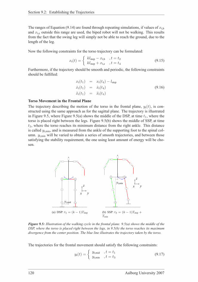
Section 9.2: Establishing the Trajectories
The ranges of Equation (9.14) are found through repeating simulations, if values of xt,b
and xt,e outside this range are used, the biped robot will not be walking. This results
from the fact that the swing leg will simply not be able to reach the ground, due to the
length of the leg.
Now the following constraints for the torso trajectory can be formulated:
xt(t) =
klstep − xt,b , t = t2klstep + xt,e , t = t4
(9.15)
Furthermore, if the trajectory should be smooth and periodic, the following constraints
should be fulfilled:
xt(t1) = xt(t4)− lstep
xt(t1) = xt(t4) (9.16)
xt(t1) = xt(t4)
Torso Movement in the Frontal Plane
The trajectory describing the motion of the torso in the frontal plane, yt(t), is con-structed using the same approach as for the sagittal plane. The trajectory is illustrated
in Figure 9.5, where Figure 9.5(a) shows the middle of the DSP, at time t1, where thetorso is placed right between the legs. Figure 9.5(b) shows the middle of SSP, at time
t3, where the torso reaches its minimum distance from the right ankle. This distance
is called yt,min, and is measured from the ankle of the supporting foot to the spinal col-
umn. yt,min will be varied to obtain a series of smooth trajectories, and between thosesatisfying the stability requirement, the one using least amount of energy will be cho-
sen.
yt,mid
y
z
x
(a) DSP: t1 = (k − 1)Tstep
yt,miny
z
x
(b) SSP: t3 = (k − 1)Tstep +Tmin
Figure 9.5: Illustration of the walking cycle in the frontal plane. 9.5(a) shows the middle of the
DSP, where the torso is placed right between the legs, in 9.5(b) the torso reaches its maximum
divergence from the center position. The blue line illustrates the trajectory taken by the torso.
The trajectories for the frontal movement should satisfy the following constraints:
yt(t) =
yt,mid , t = t1yt,min , t = t3
(9.17)
120 Aalborg University 2007

Chapter 9: Trajectory Generation
where yt,min is set to vary within a fixed range of:
− 0.2yt,mid ≤ yt,min ≤ 0.4yt,mid (9.18)
The ranges specified in Equation (9.18) are found through presimulations. Further-
more, as the motion should be cyclic, following constraints should be fulfilled:
yt(t1) = yt(t4)
yt(t1) = −yt(t4) (9.19)
yt(t1) = yt(t4)
and since yt(t) = yt,min should be the maximum deviation from center, the following
constraint must be satisfied:
yt(t3) = 0 (9.20)
9.2.4 Start-Up and Stop Phase
The establishment of the trajectories for the start-up and stop phase is almost identical
to the steady-state walk. The only difference is, that the start-up phase trajectories are
responsible for moving the robot from initial position and into the steady state walk.
The trajectories of the stop phase are responsible for taking the robot from steady state
walk into initial position. In order to minimize the redundancy, the establishment of
the trajectories for the start-up and stop phase are placed in Appendix I on page 243.
9.2.5 Scaling Parameters from Human Walk
In Section 3.2.2 on page 17 some parameters describing the human walk were found
in [Borghese et al., 1996]. It has been chosen to use data from [Borghese et al., 1996]
to create the trajectories, but more detailed data than those found in Section 3.2.2 has to
be found. In Table 9.1, the data from the human test subject is listed. It should however
be noted that, the data of Table 9.1 can not be found directly in [Borghese et al., 1996],
but can be derived from the presented data. To scale the human walking parameters,
the height of the test subject compared to the robot is used. This is calculated to be:
ρh,r =htest subject
hrobot
=1.69m
0.58m= 2.914 (9.21)
The data has been extracted from human walk, where a human test subject walked the
same path, at approximately the same speed six times (maximum deviation in walking
speed was 0.027m/s).
The scaled parameters can however not be applied directly on the robot, since the max-
imum velocity of the actuators introduces constraints. The scaled walking velocity
of 0.374m/s can not be obtained, as a result it is necessary to change this parame-
ter, and through repeating simulation on the model of the biped robot, it is found that
the maximum possible walking velocity is approximately half the scaled value, thus
vwalking = 0.187m/s. Furthermore it is not possible to walk with a step length of
0.226m, as it should be possible to vary the parameters xt,b, xt,e and yt,min within theranges specified by Equation (9.14) and (9.18). The walking speed is reduced, which
supports an reduction in the step length. It is therefore chosen to reduce the step length
with 30% since this will permit the intended variations, thus lstep = 0.158m. Only
vwalking and lstep have been changed, compared to the scaled values.
Group 1033 121

Section 9.3: Simulation of Trajectories
Parameter Human Scaled
vwalking 1.084m/s 0.374m/slstep 0.658m 0.226mha,max 0.112m 0.039mla,max 1.48lstep 1.48lstepht,max 0.702m 0.270mht,min 0.590m 0.240mθlo 1.40 rad 1.40 radTSSP 0.8Tstep 0.8Tstep
Tmax 0.48Tstep 0.48Tstep
Table 9.1: Parameters used to generate the trajectories. The scaled parameters are obtained
from the parameters derived from human walk, by using the ρh,r of Equation (9.21). Note that
vwalking and lstep are modified, in order to adapt the parameters to the actuators. Tstep is found
from Equation (9.5).
9.2.6 Cubic Splines
One polynomial for each trajectory, fulfilling all the requirements on position, veloc-
ity and acceleration, would have a very high order, and therefore not be efficient for
implementation. For this reason it is chosen to use cubic splines, which are widely
used to create the trajectories in joint space in the area of robotics. Cubic splines con-
sist of interpolated third-order polynomials, and can assure continuity of velocity and
acceleration [Guan et al., 2005]. It also has been investigated if it is possible to use
MATLAB’s polyfit, this is however very important that the trajectories have the same
velocity in the end of a cycle, as in the beginning, otherwise the trajectories are not
cyclic. Polyfit does not offer the possibility of specifying velocities in certain points,
as the cubic spline method does, and it is therefore not possible to use polyfit to create
the trajectories.
9.3 Simulation of TrajectoriesIn order to find the best trajectory a number of simulations are performed on the com-
plete model of the biped robot. The derivation of the model is described in Chapter 7.
The simulation is divided into several parts, first a number of simulations are per-
formed to find the values of xt,b and xt,e that provide the largest stability index. Those
providing an acceptable stability index, are compared on energy efficiency, and the fi-
nal values of xt,b and xt,e are chosen to be those using the least amount of energy, which
is described in Section 9.3.1. Next step, described in Section 9.3.2, is to find the value
of yt,max providing the largest stability index and using the least amount of energy, thisis conducted using the same approach as for the x-direction. Next a number of simula-tion are performed to find the values of xt,max, yt,max,up and Ty,max,up which describes the
start-up phase, the simulation of the start-up phase is placed in Section I.1 on page 243.
These parameters will be chosen solely on their stability properties, with no consider-
ations to energy consumption. As a last step the parameters for the stop phase are
determined, this is done exactly like for the start-up phase, and the description of the
parameter determination can be found in Section I.2 on page 246.
122 Aalborg University 2007
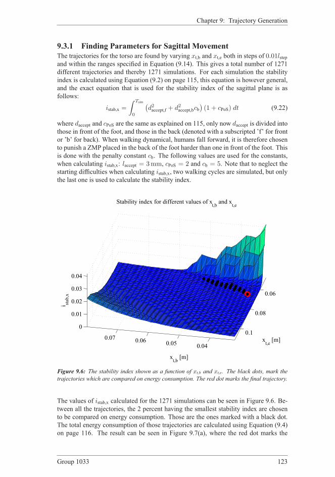
Chapter 9: Trajectory Generation
9.3.1 Finding Parameters for Sagittal Movement
The trajectories for the torso are found by varying xt,b and xt,e both in steps of 0.01lstepand within the ranges specified in Equation (9.14). This gives a total number of 1271
different trajectories and thereby 1271 simulations. For each simulation the stability
index is calculated using Equation (9.2) on page 115, this equation is however general,
and the exact equation that is used for the stability index of the sagittal plane is as
follows:
istab,x =
∫ Tsim
0
(
d2accept,f + d2
accept,bcb)
(1 + cPoS) dt (9.22)
where daccept and cPoS are the same as explained on 115, only now daccept is divided intothose in front of the foot, and those in the back (denoted with a subscripted ’f’ for front
or ’b’ for back). When walking dynamical, humans fall forward, it is therefore chosen
to punish a ZMP placed in the back of the foot harder than one in front of the foot. This
is done with the penalty constant cb. The following values are used for the constants,when calculating istab,x: laccept = 3mm, cPoS = 2 and cb = 5. Note that to neglect thestarting difficulties when calculating istab,x, two walking cycles are simulated, but onlythe last one is used to calculate the stability index.
0.040.050.060.07
0.06
0.08
0.10
0.01
0.02
0.03
0.04
xt,e [m]
xt,b [m]
Stability index for different values of xt,b and x
t,e
i stab,x
Figure 9.6: The stability index shown as a function of xt,b and xt,e. The black dots, mark the
trajectories which are compared on energy consumption. The red dot marks the final trajectory.
The values of istab,x calculated for the 1271 simulations can be seen in Figure 9.6. Be-tween all the trajectories, the 2 percent having the smallest stability index are chosen
to be compared on energy consumption. Those are the ones marked with a black dot.
The total energy consumption of those trajectories are calculated using Equation (9.4)
on page 116. The result can be seen in Figure 9.7(a), where the red dot marks the
Group 1033 123

Section 9.3: Simulation of Trajectories
trajectory which uses the least amount of energy, thus it is the final trajectory of torso
in the sagittal plane.
5 10 15 20 2514
16
18
20Power for the most stable trajectories
Power [Watt]
k
(a) Power consumption
0 1 2 3
−0.2
0
0.2
0.4
PoS vs. xZMP
−trajectory
Time [s]
x [m]
xZMP
PoS
(b) PoS and xZMP
Figure 9.7: 9.7(a) shows the power consumption of the trajectories having the best stability.
The red dot marks the one using the least amount of power. 9.7(b) shows the trajectory of xZMP
during two walking cycles, this is plotted together with the PoS during the two cycles.
In Figure 9.7(b) the PoS in the x-direction is plotted together with the trajectory of
xZMP. This is the result of the simulation where the final trajectories were used. It can
be seen that the ZMP is inside the PoS at all times, except at initial value. The spikes
that can be seen in Figure 9.7(b) result from phase shifts in the model. The final values
of the varied parameters are:
xt,b = 35.2mmxt,e = 65.5mm
(9.23)
9.3.2 Finding Parameters for Frontal Movement
The same procedure as for sagittal movement is applied for the frontal. The parameter
yt,max is varied within the ranges specified in Equation (9.18) on page 121, in steps of0.01yt,mid. This makes a total of 61 simulations.
−0.005 0 0.005 0.01 0.0150
5e−005
0.0001
Stability index for different values of yt,max
i stab,y
yt,max
[m]
Figure 9.8: The stability index shown as a function of yt,max. The black dots, mark the trajectories
which are compared on energy consumption. The red dot marks the final trajectory.
For each simulation the stability index, istab,y, is calculated as in Equation (9.2) on
page 115, the result is shown in Figure 9.8. The 20 % having the smallest stability
index, those marked with a black dot, are compared on power consumption, which is
done using Equation (9.4). The 20 % is chosen to get a sufficient representation of
124 Aalborg University 2007
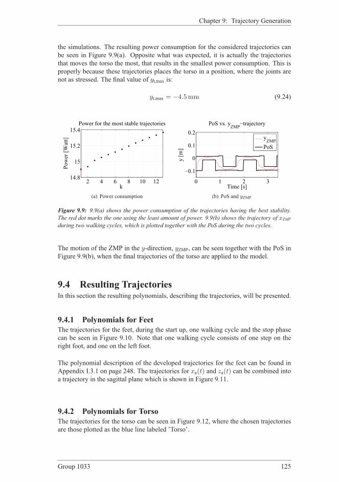
Chapter 9: Trajectory Generation
the simulations. The resulting power consumption for the considered trajectories can
be seen in Figure 9.9(a). Opposite what was expected, it is actually the trajectories
that moves the torso the most, that results in the smallest power consumption. This is
properly because these trajectories places the torso in a position, where the joints are
not as stressed. The final value of yt,max is:
yt,max = −4.5mm (9.24)
2 4 6 8 10 1214.8
15
15.2
15.4Power for the most stable trajectories
Power [Watt]
k
(a) Power consumption
0 1 2 3
−0.1
0
0.1
0.2
PoS vs. yZMP
−trajectory
Time [s]y [m]
yZMP
PoS
(b) PoS and yZMP
Figure 9.9: 9.9(a) shows the power consumption of the trajectories having the best stability.
The red dot marks the one using the least amount of power. 9.9(b) shows the trajectory of xZMP
during two walking cycles, which is plotted together with the PoS during the two cycles.
The motion of the ZMP in the y-direction, yZMP, can be seen together with the PoS in
Figure 9.9(b), when the final trajectories of the torso are applied to the model.
9.4 Resulting TrajectoriesIn this section the resulting polynomials, describing the trajectories, will be presented.
9.4.1 Polynomials for Feet
The trajectories for the feet, during the start up, one walking cycle and the stop phase
can be seen in Figure 9.10. Note that one walking cycle consists of one step on the
right foot, and one on the left foot.
The polynomial description of the developed trajectories for the feet can be found in
Appendix I.3.1 on page 248. The trajectories for xa(t) and za(t) can be combined intoa trajectory in the sagittal plane which is shown in Figure 9.11.
9.4.2 Polynomials for Torso
The trajectories for the torso can be seen in Figure 9.12, where the chosen trajectories
are those plotted as the blue line labeled ’Torso’.
Group 1033 125
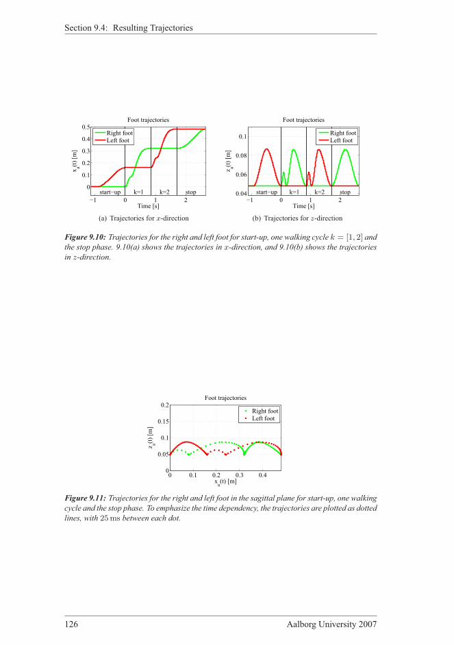
Section 9.4: Resulting Trajectories
−1 0 1 2
0
0.1
0.2
0.3
0.4
0.5
Time [s]
xa(t) [m]
Foot trajectories
start−up k=1 k=2 stop
Right foot
Left foot
(a) Trajectories for x-direction
−1 0 1 20.04
0.06
0.08
0.1
Time [s]
z a(t) [m]
Foot trajectories
start−up k=1 k=2 stop
Right foot
Left foot
(b) Trajectories for z-direction
Figure 9.10: Trajectories for the right and left foot for start-up, one walking cycle k = [1, 2] andthe stop phase. 9.10(a) shows the trajectories in x-direction, and 9.10(b) shows the trajectories
in z-direction.
0 0.1 0.2 0.3 0.40
0.05
0.1
0.15
0.2
xa(t) [m]
z a(t) [m]
Foot trajectories
Right foot
Left foot
Figure 9.11: Trajectories for the right and left foot in the sagittal plane for start-up, one walking
cycle and the stop phase. To emphasize the time dependency, the trajectories are plotted as dotted
lines, with 25ms between each dot.
126 Aalborg University 2007

Chapter 9: Trajectory Generation
0 0.2 0.4 0.6 0.8 1 1.2 1.4 1.60.05
0.1
0.15
0.2
0.25
0.3
0.35
0.4
0.45
Time [s]
xt(t) [m]
Torso trajectory
k=1 k=2
Torso 1x
Torso 2x
Torso 3x
Torso 4x
Torso
(a) Trajectory for x-direction
−1 −0.5 0 0.5 1 1.5 2 2.5
−0.02
0
0.02
0.04
0.06
0.08
0.1
0.12
0.14
Time [s]
yt(t) [m]
Torso trajectory
start−up k=1 k=2 stop
Torso 1y
Torso 2y
Torso up1y
Torso up2y
Torso up3y
Torso up4y
Torso
Torso st1y
Torso st2y
(b) Trajectory for y-direction
−1 0 1 2
0
0.1
0.2
0.3
0.4
0.5
Time [s]
xt(t) [m]
Torso trajectory
start−up k=1 k=2 stop
Torso up1x
Torso up2x
Torso
Torso st1x
Torso st2x
(c) Trajectory for x-direction
−1 0 1 20.23
0.24
0.25
0.26
0.27
0.28
Time [s]
z t(t) [m]
Torso trajectory
start−up k=1 k=2 stop
Torso
(d) Trajectory for z-direction
Figure 9.12: Trajectories for the torso, for the start-up phase, the following walking cycle k =[1, 2], and the stop phase. 9.12(a) shows the trajectory in the x-direction, for different valuesof xt,b and xt,e. 9.12(b) shows the trajectory in y-direction, for different values of yt,max, yt,up,
Ty,up and yt,stop. 9.12(c) shows the trajectories in x-direction for different values of the start-up
parameter xt,up and the stop parameter xt,stop. 9.12(d) shows the trajectory in z-direction, zt(t).In all figures, the wider blue line represents the chosen trajectory.
Group 1033 127

Section 9.5: Conclusion on Trajectory Generation
Additionally Figure 9.12(a) shows some of the tested trajectories for the exterior values
of xt,b and xt,e. Specifically:
Torso 1x : xt,b = 0.2lstep , xt,e = 0.3lstepTorso 2x : xt,b = 0.2lstep , xt,e = 0.7lstepTorso 3x : xt,b = 0.5lstep , xt,e = 0.3lstepTorso 4x : xt,b = 0.5lstep , xt,e = 0.7lstep
Figure 9.12(b) also includes some of the tested trajectories, specifically for the exterior
values of yt,max, yt,up, Ty,up and yt,stop:
Torso 1y : yt,max = −0.2yt,midTorso 2y : yt,max = 0.4yt,midTorso up1y : yt,up = −0.2yt,mid , Ty,up = 0.3Tinit
Torso up2y : yt,up = −0.2yt,mid , Ty,up = 0.7Tinit
Torso up3y : yt,up = 0.4yt,mid , Ty,up = 0.3Tinit
Torso up4y : yt,up = 0.4yt,mid , Ty,up = 0.7Tinit
Torso st1y : yt,stop = 1.6yt,midTorso st2y : yt,stop = 2.2yt,mid
And finally Figure 9.12(c) shows the trajectories for the exterior values of xt,up and
xt,stop, specifically:
Torso up1x : xt,up = 0Torso up2x : xt,up = 0.6(xt,e − lstep)Torso st1x : xt,stop = 0.65lstepTorso st2x : xt,stop = 0.95lstep
The polynomial description of the torso trajectories can be found in Appendix I.3.2 on
page 249. The trajectories for xt(t), zt(t) and yt(t) can be combined into a trajectoriesin the sagittal, frontal and horizontal plane which are shown in Figure 9.13(a), 9.13(b)
and 9.13(c) respectively.
9.5 Conclusion on Trajectory GenerationThe trajectories described in the this chapter are tested on the real system. As expected
the robot was not able to maintain balance, when only given these trajectories in a feed
forward manner, and with no sensor feedback. However during the test another crucial
property of the system was observed. The joints were moving in steps; they quickly
moved to the reference given to them, and then stopped until the next reference was
given. This unwanted behavior resulted in very large accelerations/decelerations mak-
ing the ZMP jumping back and forth. This is due to the relative low update frequency
of the system of 40Hz. This observation can be supported by a simulation of the sys-tem, where the trajectories are clocked in with a frequency of 40Hz, the resulting ZMP
can be seen in Figure 9.14.
There is a number of possible solutions for this problem;
128 Aalborg University 2007

Chapter 9: Trajectory Generation
0.1 0.15 0.2 0.25 0.3 0.35
0.2
0.25
0.3
xt(t) [m]
z t(t) [m]
Torso trajectory
Torso
(a) Sagittal plane
0 0.02 0.04 0.06 0.080.23
0.24
0.25
0.26
0.27
0.28
yt(t) [m]
z t(t) [m]
Torso trajectory
Torso
(b) Frontal plane
0.1 0.15 0.2 0.25 0.3 0.35−0.05
0
0.05
0.1
xt(t) [m]
yt(t) [m]
Torso trajectory
Torso
(c) Horizontal plane
Figure 9.13: Trajectory for the torso shown in the three planes, for one walking cycle k = [1, 2].To emphasize the time dependency, the trajectory is plotted as a dotted line, with 25 ms betweeneach dot.
0.5 1 1.5 2 2.5
−0.2
0
0.2
0.4
0.6
Time [s]
x [m]
PoS vs. xZMP
−trajectory
xZMP
PoS
Figure 9.14: The figure shows how the xZMP behaves, when the trajectories are clocked in with
a frequency of 40Hz.
Group 1033 129

Section 9.5: Conclusion on Trajectory Generation
Increase the update frequency of the system: Increasing the update frequency of the
system would however not remove this problem, since the servo motors are con-
trolled with a standard input, as described in Section 5.3.2, that only allows one
to control them with a position reference given every 20ms. Hence it is onlypossible to control the servo motors with a maximum frequency of 50Hz, and afaster system would therefore not remove this problem.
Change trajectories: The trajectories can be changed such that the distance between
the reference points are smaller. This way the influence on the stability due to
this unwanted feature of the actuators can be minimized.
Acquire new actuators: The only way to completely remove the problem is to ac-
quire new actuators, that provides the possibility of velocity control. Such that
they can be controlled more smooth. This solution is however not considered an
option, since new actuators are very expensive, and since implementation of for
instance DC-motors with a velocity controller would be very time demanding.
Modify the actuators: The given actuators could be modified, by either removing
the internal print and create a new or by reprogramming the controller already
placed in the servo. This way the communication standard could be changed,
and a faster control could be achieved. In order to find out how fast the control
should be, a simulation has been performed, where the control frequency has
been changed. The result of this simulation is seen in Figure 9.15, where it is
seen that the control frequency should be around 250Hz.
0 1 2 3
−0.2
0
0.2
0.4
0.6
time [s]
x [m]
xZMP
PoS
(a) 50 Hz
0 1 2 3
−0.2
0
0.2
0.4
0.6
time [s]
x [m]
xZMP
PoS
(b) 62.5 Hz
0 1 2 3
−0.2
0
0.2
0.4
0.6
time [s]
x [m]
xZMP
PoS
(c) 125 Hz
0 1 2 3
−0.2
0
0.2
0.4
0.6
time [s]
x [m]
xZMP
PoS
(d) 250 Hz
Figure 9.15: The figures show the ZMP, with four different control frequencies of the servo motor
model.
130 Aalborg University 2007
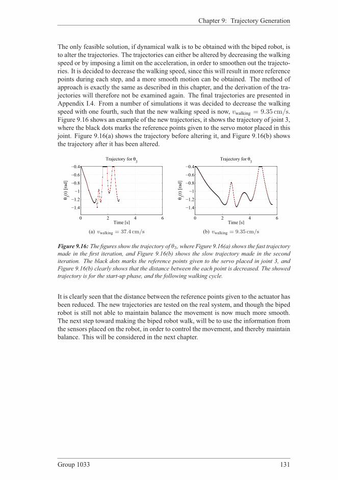
Chapter 9: Trajectory Generation
The only feasible solution, if dynamical walk is to be obtained with the biped robot, is
to alter the trajectories. The trajectories can either be altered by decreasing the walking
speed or by imposing a limit on the acceleration, in order to smoothen out the trajecto-
ries. It is decided to decrease the walking speed, since this will result in more reference
points during each step, and a more smooth motion can be obtained. The method of
approach is exactly the same as described in this chapter, and the derivation of the tra-
jectories will therefore not be examined again. The final trajectories are presented in
Appendix I.4. From a number of simulations it was decided to decrease the walking
speed with one fourth, such that the new walking speed is now, vwalking = 9.35 cm/s.Figure 9.16 shows an example of the new trajectories, it shows the trajectory of joint 3,
where the black dots marks the reference points given to the servo motor placed in this
joint. Figure 9.16(a) shows the trajectory before altering it, and Figure 9.16(b) shows
the trajectory after it has been altered.
0 2 4 6
−1.4
−1.2
−1
−0.8
−0.6
−0.4
Trajectory for θ3
Time [s]
θ3(t) [rad]
(a) vwalking = 37.4 cm/s
0 2 4 6
−1.4
−1.2
−1
−0.8
−0.6
−0.4
Trajectory for θ3
Time [s]
θ3(t) [rad]
(b) vwalking = 9.35 cm/s
Figure 9.16: The figures show the trajectory of θ3, where Figure 9.16(a) shows the fast trajectory
made in the first iteration, and Figure 9.16(b) shows the slow trajectory made in the second
iteration. The black dots marks the reference points given to the servo placed in joint 3, and
Figure 9.16(b) clearly shows that the distance between the each point is decreased. The showed
trajectory is for the start-up phase, and the following walking cycle.
It is clearly seen that the distance between the reference points given to the actuator has
been reduced. The new trajectories are tested on the real system, and though the biped
robot is still not able to maintain balance the movement is now much more smooth.
The next step toward making the biped robot walk, will be to use the information from
the sensors placed on the robot, in order to control the movement, and thereby maintain
balance. This will be considered in the next chapter.
Group 1033 131


10CONTROLLING THE
BIPED ROBOT
Chapter contents10.1 Control Design Approach 135
10.2 Estimation of Control Input 135
10.2.1 Phase Estimation 136
10.2.2 ZMP Estimation 137
10.2.3 Attitude Estimation 140
10.3 Inverse ZMP Controller 146
10.4 ZMP Controller 148
10.4.1 Designing the ZMP Controller 148
10.4.2 Simulating the ZMP Controller Performance 150
10.4.3 Implementation and Verification 151
10.5 Hybrid Posture Controller 152
10.5.1 Designing the Posture Controller 152
10.5.2 Simulating the Posture Controller Performance 155
10.5.3 Implementation and Verification 155
10.6 Partial Conclusion to Control 156
THIS CHAPTER describes the development and implementation of two controllers
for the biped robot. Two controllers are designed and implemented, each with a
specific purpose. A hybrid posture controller controls the attitude of the torso and a
ZMP controller controls the position of the ZMP. The design of a third controller, the
inverse ZMP controller is proposed and the method is discussed.
Group 1033 133

So far, a complete model and an inverse kinematic model has been derived. The model
was used to calculate dynamical walking trajectories based on human gait data. The
walking trajectories were improved using the ZMP stability, that is a measure of how
stable the gait is along the walking path. Due to backlash, model uncertainties and
external disturbances, it will not be possible to perform dynamic walk by feeding the
trajectories directly to the inverse kinematic model and then to the robot, hence a con-
troller must be implemented.
When studying control of biped robots, several different approaches are seen. In
[Christensen et al., 2006] a simple fuzzy controller is implemented on a 21 DoF robot
in order to maintain balance if the robot is exposed to smaller disturbances. This fuzzy
controller made it possible to set up a simple, but large, set of control rules, enabling
smaller disturbances to be suppressed, even though the control input was unreliable.
A large disturbance controller, that was capable of avoiding a fall by taking a step in
the correct direction, was also implemented and tested. Only static walk was achieved
in [Christensen et al., 2006].
In [Takahashi et al., 2005] two controllers are implemented on a 5 DoF biped robot
in order to achieve dynamic walk by using CPG. To ensure a correct angle of all the
joints, a PD controller that controls the torque in each joint is implemented. A CPG
controller is implemented to control the leg movements in order to maintain balance.
The CPG controller, that also generates the walking trajectories, also uses the torque
in each joint as control variable. In systems where the torque can be measured, torque
control has an advantage if energy efficient walk is desired, since the torque in each
joint can be converted directly to energy.
Another control approach is to use the angular acceleration as control input and by
using an inverse dynamics model convert this to a torque in each joint. This approach
is seen in [Kondak and Hommel, 2003], where a 5 DoF biped robot is simulated. Here,
two controller types are implemented. Three inner PD controllers are used to maintain
the correct position of the servos. The inputs to these controllers are the desired po-
sition of the joints and the output is the angular acceleration. A second controller, a
non-linear controller, ensures that the movements stay within the stability region. This
controller converts the angular acceleration to joint torques and apply these to each
motor. The output of the system is the angular velocity and position, which is used for
the inner control loops as feedback.
An interesting control approach is seen in [Bachar, 2004] where the inverse Jacobian,
describing the change of the ZMP based on the change of the generalized coordinates,
is calculated for the model of a 22 DoF biped robot. This inverse Jacobian, can then
be used to move the ZMP in a desired direction. The thesis describes how a ZMP
counter balance controller is calculated and used to regain balance, if exposed to an
external disturbance. This method seems very applicable since it would be possible to
ensure stability if the reference ZMP is set to be inside the PoS. Unfortunately only
simulations are carried out in the mentioned thesis.
134 Aalborg University 2007
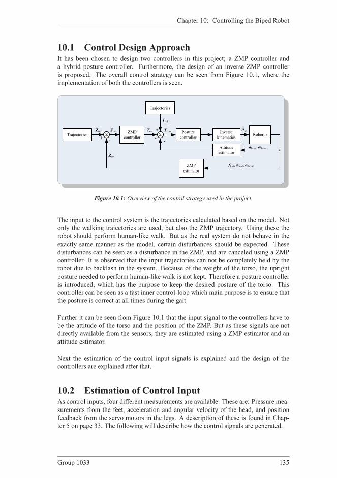
Chapter 10: Controlling the Biped Robot
10.1 Control Design ApproachIt has been chosen to design two controllers in this project; a ZMP controller and
a hybrid posture controller. Furthermore, the design of an inverse ZMP controller
is proposed. The overall control strategy can be seen from Figure 10.1, where the
implementation of both the controllers is seen.
ZMPcontroller Roberto
ZMP estimator
Σ ΣZref Terr
ffeet, ahead,ωhead
Tcorr
Tref
Inverse kinematics
θrefZerr
Zest
Posturecontroller
Trajectories
Attitudeestimator
+ - -
+
-ahead,ωhead
Trajectories
Figure 10.1: Overview of the control strategy used in the project.
The input to the control system is the trajectories calculated based on the model. Not
only the walking trajectories are used, but also the ZMP trajectory. Using these the
robot should perform human-like walk. But as the real system do not behave in the
exactly same manner as the model, certain disturbances should be expected. These
disturbances can be seen as a disturbance in the ZMP, and are canceled using a ZMP
controller. It is observed that the input trajectories can not be completely held by the
robot due to backlash in the system. Because of the weight of the torso, the upright
posture needed to perform human-like walk is not kept. Therefore a posture controller
is introduced, which has the purpose to keep the desired posture of the torso. This
controller can be seen as a fast inner control-loop which main purpose is to ensure that
the posture is correct at all times during the gait.
Further it can be seen from Figure 10.1 that the input signal to the controllers have to
be the attitude of the torso and the position of the ZMP. But as these signals are not
directly available from the sensors, they are estimated using a ZMP estimator and an
attitude estimator.
Next the estimation of the control input signals is explained and the design of the
controllers are explained after that.
10.2 Estimation of Control InputAs control inputs, four different measurements are available. These are: Pressure mea-
surements from the feet, acceleration and angular velocity of the head, and position
feedback from the servo motors in the legs. A description of these is found in Chap-
ter 5 on page 33. The following will describe how the control signals are generated.
Group 1033 135
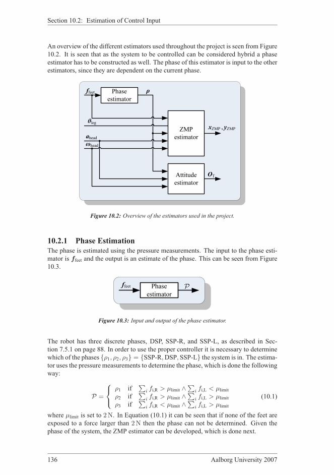
Section 10.2: Estimation of Control Input
An overview of the different estimators used throughout the project is seen from Figure
10.2. It is seen that as the system to be controlled can be considered hybrid a phase
estimator has to be constructed as well. The phase of this estimator is input to the other
estimators, since they are dependent on the current phase.
Phase estimator
ZMP estimator
Attitude estimator
ffeet
ahead
θleg
ωhead
ρ
OT
xZMP , yZMP
Figure 10.2: Overview of the estimators used in the project.
10.2.1 Phase Estimation
The phase is estimated using the pressure measurements. The input to the phase esti-
mator is ffeet and the output is an estimate of the phase. This can be seen from Figure
10.3.
Phase estimator
ffeet
Figure 10.3: Input and output of the phase estimator.
The robot has three discrete phases, DSP, SSP-R, and SSP-L, as described in Sec-
tion 7.5.1 on page 88. In order to use the proper controller it is necessary to determine
which of the phases ρ1, ρ2, ρ3 = SSP-R,DSP,SSP-L the system is in. The estima-
tor uses the pressure measurements to determine the phase, which is done the following
way:
P =
ρ1 if∑
i fi,R > µlimit ∧∑
i fi,L < µlimit
ρ2 if∑
i fi,R > µlimit ∧∑
i fi,L > µlimit
ρ3 if∑
i fi,R < µlimit ∧∑
i fi,L > µlimit
(10.1)
where µlimit is set to 2N. In Equation (10.1) it can be seen that if none of the feet areexposed to a force larger than 2N then the phase can not be determined. Given the
phase of the system, the ZMP estimator can be developed, which is done next.
136 Aalborg University 2007

Chapter 10: Controlling the Biped Robot
10.2.2 ZMP Estimation
The inputs and outputs of the ZMP estimator are seen from Figure 10.4. Given the
available sensor measurements on the system two methods for estimating the ZMP are
investigated.
ZMP estimator
ffeet
ahead
θleg
ωhead
ρ xZMP , yZMP
Figure 10.4: Input/output relation of the ZMP estimator.
The first method estimates the ZMP using the output from the IMU, namely the ac-
celeration and the angular velocity. Another method investigated is estimation of the
ZMP using the pressure measurements.
ZMP Estimation Using the IMU
In the developed model the ZMP is determined using Equation (2.5) and (2.6) on page
9. This approach is not feasible on the robot since the linear and the angular accelera-
tion of all links have to be determined. The developed model could be used to estimate
the accelerations, but it is however not feasible to implement the developed model on
the real system due to the relatively low processing power. Instead another property of
the robot is exploited. The weight of the robot is 3.7 kg in total and of this, the torso
weighs 1.2 kg, that is, 32.4% of the total weight is in the torso meaning the ZMP is
mostly determined by the torso. This has resulted in the assumptions seen in Equation
(10.3) to (10.5).
xZMP,m ≈ xZMP,t (10.2)
22∑
i=1
migzxi −22∑
i=1
mixizi
22∑
i=1
migz
≈ gzxt − xztgz
(10.3)
yZMP,m ≈ yZMP,t (10.4)
22∑
i=1
migzyi −22∑
i=1
miyizi
22∑
i=1
migz
≈ gzyt − yztgz
(10.5)
To verify if these assumptions are valid the walking trajectories, developed in Chapter 9
on page 109, are used as input to the complete model where the simplified ZMP from
Equation (10.3) and (10.5) is implemented. The result can be seen in Figure 10.5.
Group 1033 137

Section 10.2: Estimation of Control Input
0 0.5 1 1.5 2−0.1
0
0.1
0.2
0.3
0.4
xZMP
−trajectory
Time [s]
x [m]
xZMP,t
xZMP
Figure 10.5: Simplified ZMP estimated comparred with real ZMP.
j1j2
j3
j4j5j6
yz
x
m7
IMU ay
ax
ytxt
b7
pt
yθ&
xθ&
Figure 10.6: The ZMP is determined using only the position and the acceleration of the torso
CoM.
138 Aalborg University 2007

Chapter 10: Controlling the Biped Robot
As it can be seen from the figure, the simplified ZMP only differs slightly from the true
ZMP. It therefore seems reasonable to use the simplified ZMP on the robot. Inspecting
Equation (10.3) and (10.5) it is seen that the positions xt, yt, and zt have to be deter-mined along with the accelerations xt and yt. The accelerations that are measured bythe IMU have to be related to the acceleration of the CoM of the torso, m7. Figure 10.6
shows the direction of the accelerations of m7, xt and yt, along with the direction ofthe accelerations that can be measured by the IMU, ax and ay. From the figure it can
be seen that the orientation of the IMU is required to transfer ax and ay to xt and yt.First the gravity acceleration that is present in the measurement is removed based on
the orientation of the IMU:
xt = ax − g sin(θy) (10.6)
yt = ay − g sin(θx) (10.7)
Now the acceleration given in the IMU is rotated, such that the accelerations are given
with respect to the base frame using Equation (10.8):
at =
xt
ytzt
= 06R
6at , for ρ = ρ1, ρ2 (10.8)
And for the SSP-L it is given by Equation (10.9):
at =
xt
ytzt
= 127 R 7at , for ρ = ρ3 (10.9)
What remains from Equation (10.3) and (10.5) is to determine the positions xt, yt, andzt. From Figure 10.6 it can be seen that these can be determined by the kinematic chain
for the supporting leg described by Equation (10.10):
[pt
1
]
=
xt
ytzt1
=06 T
[6b7
1
]
, for ρ = ρ1, ρ2 (10.10)
Equation (10.10) is only valid in SSP-R and in DSP. In SSP-L the kinematic chain for
the left leg is used:
[pt
1
]
=
xt
ytzt1
=127 T
[7b7
1
]
, for ρ = ρ3 (10.11)
Since the phase, P , is required to determine if the ZMP, the estimator becomes a hybrid
estimator.
Group 1033 139
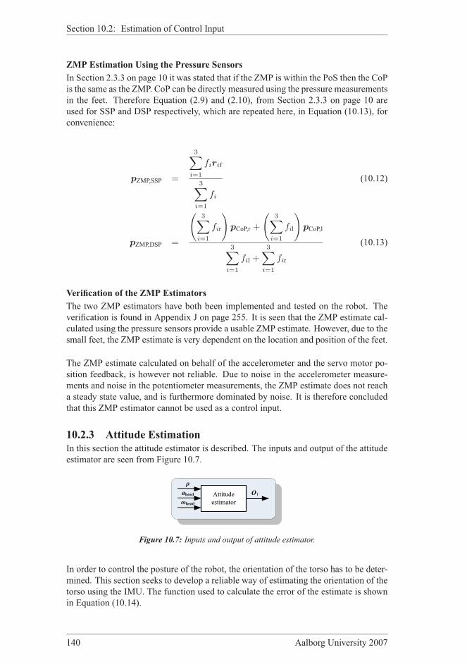
Section 10.2: Estimation of Control Input
ZMP Estimation Using the Pressure Sensors
In Section 2.3.3 on page 10 it was stated that if the ZMP is within the PoS then the CoP
is the same as the ZMP. CoP can be directly measured using the pressure measurements
in the feet. Therefore Equation (2.9) and (2.10), from Section 2.3.3 on page 10 are
used for SSP and DSP respectively, which are repeated here, in Equation (10.13), for
convenience:
pZMP,SSP =
3∑
i=1
firif
3∑
i=1
fi
(10.12)
pZMP,DSP =
(3∑
i=1
fir
)
pCoP,r +
(3∑
i=1
fil
)
pCoP,l
3∑
i=1
fil +3∑
i=1
fir
(10.13)
Verification of the ZMP Estimators
The two ZMP estimators have both been implemented and tested on the robot. The
verification is found in Appendix J on page 255. It is seen that the ZMP estimate cal-
culated using the pressure sensors provide a usable ZMP estimate. However, due to the
small feet, the ZMP estimate is very dependent on the location and position of the feet.
The ZMP estimate calculated on behalf of the accelerometer and the servo motor po-
sition feedback, is however not reliable. Due to noise in the accelerometer measure-
ments and noise in the potentiometer measurements, the ZMP estimate does not reach
a steady state value, and is furthermore dominated by noise. It is therefore concluded
that this ZMP estimator cannot be used as a control input.
10.2.3 Attitude Estimation
In this section the attitude estimator is described. The inputs and output of the attitude
estimator are seen from Figure 10.7.
Attitude estimator
aheadωhead
ρOT
Figure 10.7: Inputs and output of attitude estimator.
In order to control the posture of the robot, the orientation of the torso has to be deter-
mined. This section seeks to develop a reliable way of estimating the orientation of the
torso using the IMU. The function used to calculate the error of the estimate is shown
in Equation (10.14).
140 Aalborg University 2007
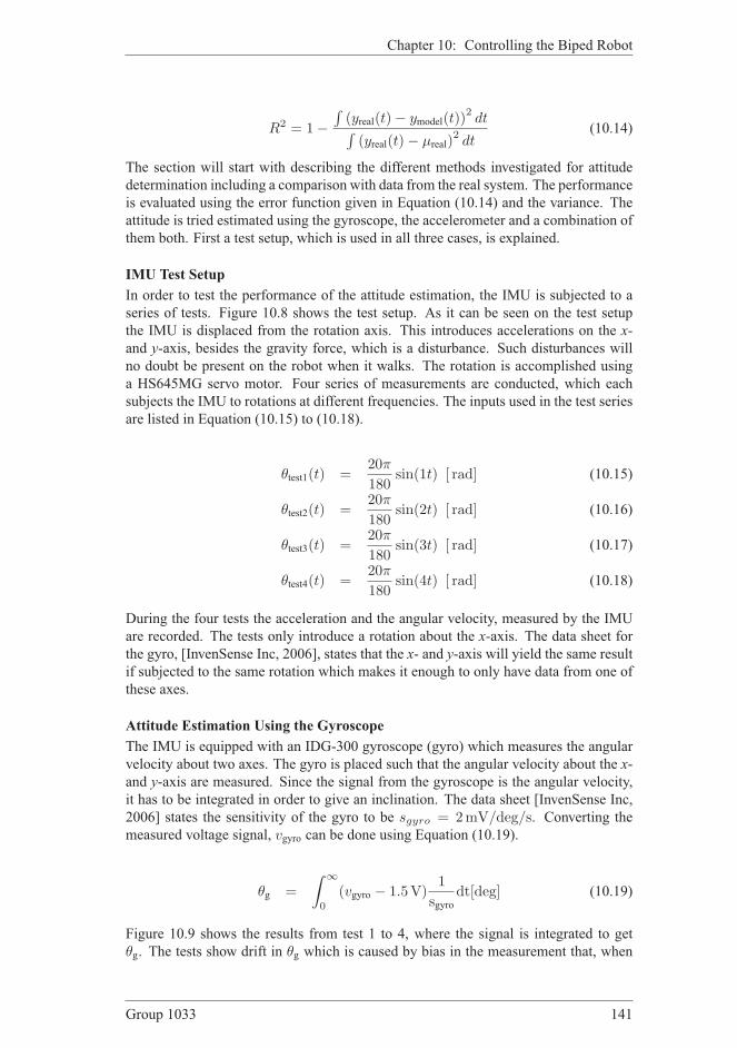
Chapter 10: Controlling the Biped Robot
R2 = 1−∫
(yreal(t)− ymodel(t))2dt
∫(yreal(t)− µreal)
2dt
(10.14)
The section will start with describing the different methods investigated for attitude
determination including a comparison with data from the real system. The performance
is evaluated using the error function given in Equation (10.14) and the variance. The
attitude is tried estimated using the gyroscope, the accelerometer and a combination of
them both. First a test setup, which is used in all three cases, is explained.
IMU Test Setup
In order to test the performance of the attitude estimation, the IMU is subjected to a
series of tests. Figure 10.8 shows the test setup. As it can be seen on the test setup
the IMU is displaced from the rotation axis. This introduces accelerations on the x-
and y-axis, besides the gravity force, which is a disturbance. Such disturbances will
no doubt be present on the robot when it walks. The rotation is accomplished using
a HS645MG servo motor. Four series of measurements are conducted, which each
subjects the IMU to rotations at different frequencies. The inputs used in the test series
are listed in Equation (10.15) to (10.18).
θtest1(t) =20π
180sin(1t) [ rad] (10.15)
θtest2(t) =20π
180sin(2t) [ rad] (10.16)
θtest3(t) =20π
180sin(3t) [ rad] (10.17)
θtest4(t) =20π
180sin(4t) [ rad] (10.18)
During the four tests the acceleration and the angular velocity, measured by the IMU
are recorded. The tests only introduce a rotation about the x-axis. The data sheet for
the gyro, [InvenSense Inc, 2006], states that the x- and y-axis will yield the same result
if subjected to the same rotation which makes it enough to only have data from one of
these axes.
Attitude Estimation Using the Gyroscope
The IMU is equipped with an IDG-300 gyroscope (gyro) which measures the angular
velocity about two axes. The gyro is placed such that the angular velocity about the x-
and y-axis are measured. Since the signal from the gyroscope is the angular velocity,
it has to be integrated in order to give an inclination. The data sheet [InvenSense Inc,
2006] states the sensitivity of the gyro to be sgyro = 2mV/deg/s. Converting the
measured voltage signal, vgyro can be done using Equation (10.19).
θg =
∫ ∞
0
(vgyro − 1.5V)1
sgyrodt[deg] (10.19)
Figure 10.9 shows the results from test 1 to 4, where the signal is integrated to get
θg. The tests show drift in θg which is caused by bias in the measurement that, when
Group 1033 141
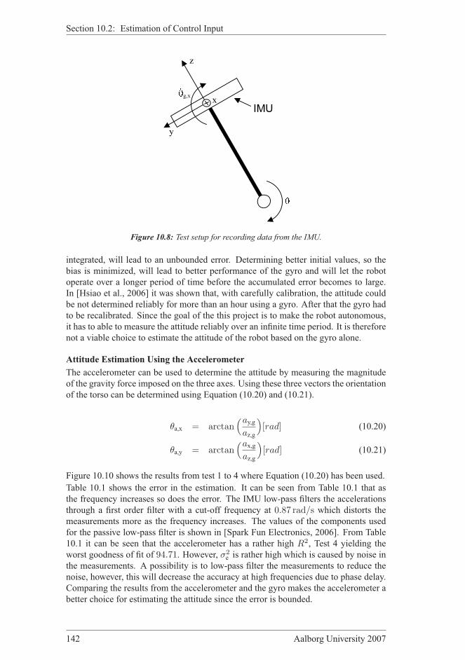
Section 10.2: Estimation of Control Input
IMU
y
z
xg,x
Figure 10.8: Test setup for recording data from the IMU.
integrated, will lead to an unbounded error. Determining better initial values, so the
bias is minimized, will lead to better performance of the gyro and will let the robot
operate over a longer period of time before the accumulated error becomes to large.
In [Hsiao et al., 2006] it was shown that, with carefully calibration, the attitude could
be not determined reliably for more than an hour using a gyro. After that the gyro had
to be recalibrated. Since the goal of the this project is to make the robot autonomous,
it has to able to measure the attitude reliably over an infinite time period. It is therefore
not a viable choice to estimate the attitude of the robot based on the gyro alone.
Attitude Estimation Using the Accelerometer
The accelerometer can be used to determine the attitude by measuring the magnitude
of the gravity force imposed on the three axes. Using these three vectors the orientation
of the torso can be determined using Equation (10.20) and (10.21).
θa,x = arctan(ay,g
az,g
)
[rad] (10.20)
θa,y = arctan(ax,g
az,g
)
[rad] (10.21)
Figure 10.10 shows the results from test 1 to 4 where Equation (10.20) has been used.
Table 10.1 shows the error in the estimation. It can be seen from Table 10.1 that as
the frequency increases so does the error. The IMU low-pass filters the accelerations
through a first order filter with a cut-off frequency at 0.87 rad/s which distorts the
measurements more as the frequency increases. The values of the components used
for the passive low-pass filter is shown in [Spark Fun Electronics, 2006]. From Table
10.1 it can be seen that the accelerometer has a rather high R2, Test 4 yielding the
worst goodness of fit of 94.71. However, σ2e is rather high which is caused by noise in
the measurements. A possibility is to low-pass filter the measurements to reduce the
noise, however, this will decrease the accuracy at high frequencies due to phase delay.
Comparing the results from the accelerometer and the gyro makes the accelerometer a
better choice for estimating the attitude since the error is bounded.
142 Aalborg University 2007
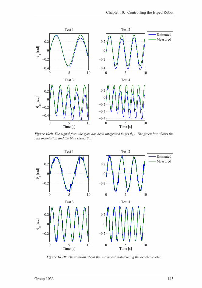
Chapter 10: Controlling the Biped Robot
0 5 10
−0.4
−0.2
0
0.2
Test 1
θg [rad]
0 5 10
−0.4
−0.2
0
0.2
Test 2
Estimated
Measured
0 5 10
−0.4
−0.2
0
0.2
Test 3
Time [s]
θg [rad]
0 5 10
−0.6
−0.4
−0.2
0
0.2
Test 4
Time [s]
Figure 10.9: The signal from the gyro has been integrated to get θg,x. The green line shows the
real orientation and the blue shows θg,x.
0 5 10
−0.2
0
0.2
Test 1
θa [rad]
0 5 10
−0.2
0
0.2
Test 2
Estimated
Measured
0 5 10
−0.2
0
0.2
Test 3
Time [s]
θa [rad]
0 5 10
−0.2
0
0.2
Test 4
Time [s]
Figure 10.10: The rotation about the x-axis estimated using the accelerometer.
Group 1033 143

Section 10.2: Estimation of Control Input
R2[%] σ2e
Test 1 98.06 % 3.41
Test 2 96.45 % 6.87
Test 3 96.85 % 6.22
Test 4 94.71 % 10.57
Mean 96.52 % 6.77
Table 10.1: Error when the accelerometer is used to estimate the attitude of the robot.
Attitude Estimation Using Sensor Fusion
Extensive research has been conducted in fusing gyroscopes, accelerometers, and incli-
nometers to give a good estimate of the attitude of autonomous systems. In [Rehbinder
and Hu, 2001] the measurements from a gyro and an accelerometer were fused using
a modified Kalman filter. The approach made use of two models which were switched
between based on the magnitude of the acceleration. During high acceleration the
gyro was used and during low acceleration the accelerometer was used. The algorithm
showed errors no greater than 0.6 deg when the accelerometer was used, however whenthe gyro was used the algorithm still showed drift in the estimation. Like [Rehbinder
and Hu, 2001] other authors have shown in [Foxlin, 1996], [Rehbinder and Hu, 2000],
and [Vaganay et al., 1993] various ways of combining measurements about the attitude
using Kalman filters.
In [Baerveldt and Klang, 1997] the authors developed an attitude estimation system for
an autonomous helicopter which fused an inclinometer and a gyro through a comple-
mentary filter. This approach showed an error of about 2 deg without drift. This ap-
proach was implemented succesfully in [Loffler et al., 2004] on a biped robot. In [Hsiao
et al., 2006] the same approach was used but, instead of an inclinometer, an accelerom-
eter was used. Since the computational power on the robot is limited it is decided to use
the approach in [Hsiao et al., 2006]. Here in it was suggested that the measurements
from the accelerometer and the gyro should only be used in the frequency domains
where it can be considered ideal:
- The accelerometer uses the gravity force to determine the angle which means
that accelerations caused by movement decreases the accuracy. Therefore the
accelerometer should be considered ideal at low frequencies.
- Integrating the signal from the gyroscope will lead to unbounded drift due to
bias in the signal. Therefore the gyroscope should be considered ideal at high
frequencies.
To achieve the above [Baerveldt and Klang, 1997] suggested the use of a complemen-
tary filter with the following property:
Ha(s)Ga(s) + sHg(s)Gg(s) = 1 (10.22)
Here Ha(s) and Hg(s) are the sensor dynamics of the accelerometer and gyroscope
respectively. Ga(s) is a low-pass filter for the measurement from the accelerometer
and Gg(s) is a high-pass filter for the measurements from the gyro. The sensors are
considered ideal, thus Hg(s) = Ha(s) = 1. Figure 10.11 shows the implemented
144 Aalborg University 2007

Chapter 10: Controlling the Biped Robot
filter. [Baerveldt and Klang, 1997] suggested that Ga(s) be a first order low-pass filterin series with a lead filter and Gg(s) be a second order high-pass filter:
Ga(s)
Gg(s)
a
g
Figure 10.11: Implemented filter, used for the inclination estimator.
Ga(s) =2τs + 1
(τs + 1)2(10.23)
Gg(s) =τ2s
(τs + 1)2(10.24)
Which gives the following filter for the estimator:
θ(s) =2τs + 1
(τs + 1)2+ s
τ2s
(τs + 1)2(10.25)
The complementary filter in Equation (10.22) only has a single design parameter, τ .τ should be chosen low enough to effectively remove the offset in the gyro and high
enough not to filter, and thereby distort, the measurements from the accelerometer.
The performance of the filter is evaluated using the R2 performance function given in
Equation (10.14) on page 141.
τ should be chosen so that Equation (10.14) is minimized which is done using the
steepest descent method. It is assumed that Equation (10.14) has a global maximum.
A value of τ that minimizes the error for test 1 to 4 is determined. τi is the value of τthat minimizes the error in test i. Table 10.2 shows the value of τi that minimizes theerror in each of the tests along with the error and variance.
From Table 10.2 it can be seen that in order to minimize the error at high frequencies τhas to be smaller than at low frequencies. This means that that at high frequencies the
gyro is trusted the most and at low frequencies the accelerometer is trusted the most.
This supports the assumptions about where the accelerometer and the gyro should be
considered ideal.
Group 1033 145

Section 10.3: Inverse ZMP Controller
τ1 = 0.525 τ2 = 0.491 τ3 = 0.362 τ4 = 0.296R2[%] σ2
e R2[%] σ2e R2[%] σ2
e R2[%] σ2e
Test 1 99.60 0.706 99.59 0.712 99.54 0.817 99.47 0.919
Test 2 99.39 1.187 99.40 1.160 99.21 1.526 98.96 2.019
Test 3 99.02 1.957 99.15 1.684 99.41 1.175 99.30 1.376
Test 4 97.41 5.228 97.65 4.708 98.42 3.149 98.59 2.823
Mean 98.85 2.269 98.94 2.067 99.14 1.667 99.08 1.784
Table 10.2: Performance of the filter where the τ that minimizes R2 has been determined using
steepest descent. τi is the τ that minimizes R2 in test i.
The choice of τ can either be to minimize the error at a certain frequency or minimize
the error over the frequency range recorded. If the latter, then τ should be 0.362 wherethe mean of R2 is 99.14% and the variance 1.667 as can be seen in Table 10.2. This ischosen, since it is expected that the input will consist of a wide range of frequencies.
Figure 10.12 shows the estimated inclination along with the actual inclination.
0 5 10
−0.2
0
0.2
Test 1
θf [rad]
0 5 10
−0.2
0
0.2
Test 2
Estimated
Measured
0 5 10
−0.2
0
0.2
Test 3
Time [s]
θf [rad]
0 5 10
−0.2
0
0.2
Test 4
Time [s]
Figure 10.12: Actual and estimated inclination using sensor fusion. Estimated inclination is
shown as blue and the actual inclination is shown as green.
10.3 Inverse ZMP ControllerThe inverse ZMP controller could seem like the most optimal controller for this ap-
plication. The basic idea of the inverse ZMP controller is to calculate how much the
torso should be moved, in order to obtain the desired position of the ZMP. This is done
by first calculating the Jacobian, being the matrix describing the rate of change of the
146 Aalborg University 2007

Chapter 10: Controlling the Biped Robot
ZMP location with respect to a change of the generalized position, as given in Equation
(10.26).
JZMP ≡∂pzmp
∂q(10.26)
Then, by calculating the inverse Jacobian, it is possible to calculate how the generalized
positions should be changed, in order to achieve a desired ZMP displacement:
∆q = ∆pZMPJ−1ZMP (10.27)
Note that (10.27) only holds for small ∆pZMP. However, differentiating the ZMP with
respect to the position of each links CoM would be a cumbersome task. To simplify
the calculations, only the position and acceleration of the torso could be used. This
simplification is possible, with minor deviation compared to the complete model of the
robot, since most of the mass is located in the torso, as were seen in Figure 10.5. The
displacement of the torso, when given a desired displacement in the ZMP, can now be
found to be:
∆ptorso = ∆pZMPJ−1ZMP,t (10.28)
Where the Jacobian, JZMP,t can be calculated as:
JZMP,t ≡∂pzmp
∂ptorso
=
∂
[xZMP,t
yZMP,t
]
∂
[xtorso
ytorso
] =
[∂xZMP,t
∂xtorso
∂yZMP,t
∂xtorso∂xZMP,t
∂ytorso
∂yZMP,t
∂ytorso
]
(10.29)
Equation (10.3) and (10.5) shows how the ZMP is calculated. Since yZMP is inde-
pendent by changes of movement along the x-axis and since xZMP is independent by
movements along the y-axis, Equation (10.29) can then be simplified to:
JZMP,t =
[∂xZMP,t
∂xtorso0
0 ∂yZMP,t
∂ytorso
]
(10.30)
Now, when calculating∂xZMP,t
∂xtorsoa problem arises. When calculating this, it is necessary
to find the triple derivative of xtorso. This is seen in Equation (10.31).
∂xZMP,t
∂xtorso
= 1− ztgz
∂xtorso
∂xtorso
= 1− ztgz
∂xtorso
∂t
∂t
∂xtorso
= 1− ztgz
...x torsox
−1torso (10.31)
The same procedure is used for calculating∂yZMP,t
∂ytorsoand is therefore not shown. Due to
noise in the measurement data, taking the derivative of the acceleration will not yield
any useful information. The inverse ZMP controller will therefore not be implemented
on the robot in this project.
Group 1033 147

Section 10.4: ZMP Controller
10.4 ZMP ControllerIn Chapter 9 on page 109 where the walking trajectories were calculated, a number of
different trajectories were found, and a specific walking path was chosen based on the
ZMP stability. To calculate the ZMP stability, the position of the ZMP was calculated
along the walking path which was stable, if the ZMP trajectory was within PoS. The
trajectory which had the largest stability margin was chosen. This ZMP trajectory is
used as a reference input to the ZMP controller that is designed in this section.
The basic control concept is shown in Figure 10.13. In this figure the actual ZMP is
estimated using the ZMP estimator explained in Section 10.2.2 on page 137. The ZMP
estimate is subtracted from the ZMP reference trajectory which result in a position er-
ror of the ZMP, named Zerr. This signal is fed into the ZMP controller, and the output,
which is a correction of the reference trajectory, is converted into a displacement and
inclination of the torso.
Roberto
ZMP estimator
Σ ΣZMPtrajectories
Zref
ffeet, θhead, ωhead
Inverse kinematics
Zerr
Zest
Trajectories
+ - +
+ZMP controller
Tcorr
Tref.
Terr. θref
Figure 10.13: Concept of the ZMP controller.
The displacement and inclination of the torso is added to the actual reference trajec-
tories before they are fed into the inverse kinematic model. The actual controller is
a PI-controller, that is tuned using simulations and actual measurement data gathered
during experiments. The ZMP controller is designed in the following section.
10.4.1 Designing the ZMP Controller
As mentioned in the previous section, the ZMP controller consists of a PI-controller.
The basic structure of the PI-controller is shown in Figure 10.14.
Two PI-controllers have been implemented in the ZMP controller; one controlling the
position of the torso along the y-axis, and one controlling the inclination around they-axis. The first mentioned controller is capable of moving the ZMP along the y-axisand the last mentioned is capable of moving the ZMP along the x-axis. The implemen-tation of the two is seen in Figure 10.15.
148 Aalborg University 2007
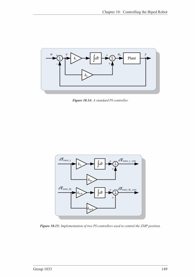
Chapter 10: Controlling the Biped Robot
Σ ki ∫dt Σ
kp
Plantu e yuc
+
++
-
Figure 10.14: A standard PI-controller.
dTtorso_y
dTtorso_θy
kiy ∫dt Σ
kpy
+
+
∫dt Σ+
+kiyθ
kpyθ
dTtorso_y_corr
dTtorso_θy_corr
Figure 10.15: Implementation of two PI-controllers used to control the ZMP position.
Group 1033 149

Section 10.4: ZMP Controller
The main subject of this design is how to determine the controller gains, these be-
ing the proportional gains and the integral gains. No general rise-time, overshoot nor
other control parameters can be calculated, meaning that no traditional controller tun-
ing methods can be applied. Similar, it is not possible to analyze the stability of the
controller using standardized methods since the system is a non-linear hybrid system.
Due to this, it has been necessary to tune the ZMP controller by hand. This was done
in the model to realize a starting point for fine-tuning of the controller on the robot. By
using the model, the gains shown in Table 10.3 was found.
kiy kpy kiyθ kpyθ
Tuned using model 0.050 0.050 0.010 0.005Fine-tuned using robot 0.050 0.170 0.005 0.100
Table 10.3: Controller gains used in the ZMP controller.
After implementation of the controller, the gains were fine-tuned in order to achieve a
better result. The new gains are also found in this table. Surprisingly, it was possible to
increase the controller gains, and hereby achieve a better performance than simulated.
Unfortunately, it was not possible to simulate the controller performance with the new
parameters since these made the system unstable. The simulation of the controller
is described in the following section. It is seen that the values for the proportional
gains are rather small. This is due to the fact that larger values will result in large
accelerations that will make the ZMP move in the opposite direction. This can be seen
from Equation (2.8), where the basic equations used for ZMP calculation is found.
10.4.2 Simulating the ZMP Controller Performance
To test the ZMP controller, four tests were carried out. First, the controller was tested
while standing in zero-position, meaning that the robot was in DSP. Next, the controller
was tested in SSP. In both DSP and SSP, steps in the ZMP reference are applied along
both the x- and y-axis.
Simulation data and comments for all simulations and tests are found in Appendix K
on page 261. The results from the simulations and tests are summarized in this chapter.
ZMP Controller Simulation in DSP
The controller was implemented and simulated on the complete model, and two exper-
iments were conducted. First a 1 cm step in the ZMP reference is applied along the
x-axis. Next, a 2 cm step was applied along the y-axis. The simulated performance ofthe controller is seen in Figure K.1 on page 262 and K.2 on page 262.
The reason for using a larger step along the y-axis is that the PoS is greater than alongthe x-axis. Overshoot has to be avoided since this will make the robot fall. The cost ofthis is a slower controller.
ZMP Controller Simulation in SSP
To test the ZMP controller in SSP, the robot was positioned in SSP and then the right
leg was lifted 2 cm above the ground. After the robot movements had settled, a 1 cm
150 Aalborg University 2007

Chapter 10: Controlling the Biped Robot
step was applied along the x-axis. Next, a 0.5 cm step was applied along the y-axis.The response of the system is shown in Figure K.3 on page 263 and K.4 on page 263.
It must be concluded that a sampling frequency of 40Hz is too slow for applications
like a walking biped robot. It is doubtable that ZMP controller would work if imple-
mented on a walking biped robot due to the slow response times that can be seen from
the figures. The ZMP controller was, however, capable of moving the ZMP to the
correct position, so the method must be considered applicable.
10.4.3 Implementation and Verification
The ZMP controller was implemented on the actual system and with minor changes
to the controller gains ZMP control was realized. The controller was implemented as
shown in Figure 10.13. To test the controller, steps were given to the reference position
of the ZMP.
Testing ZMP Controller in x-direction
In this test, a step of 2.5 cm on the reference to the ZMP is applied in the x-direction.The corresponding position of the ZMP can be seen in Figure K.5 on page 264. It is
seen that the ZMP controller manages to move the position of the ZMP to the desired
location within 10 seconds which is too slow if the controller should be used while the
robot is walking.
Testing ZMP Controller in y-direction
In this test, a step was applied to the position of the ZMP in the y-direction. The stepis applied with a magnitude of 2.5 cm compared to the starting position. The corre-
sponding position of the ZMP can be seen in Figure 10.16.
0 5 10 15 200.01
0.02
0.03
0.04
0.05
0.06
0.07ZMP estimate when given a step input in the y−direction
Time [s]
yZMP [m]
yZMP
estimate
yZMP
reference
Figure 10.16: Testing the ZMP controller on the real system in DSP by applying a step in the
y-direction.
It is seen that the ZMP controller is faster in the y-direction than in the x-direction,and that it reaches the reference position after one second. This is mainly due to the
Group 1033 151

Section 10.5: Hybrid Posture Controller
controller gains, that are larger than those for the controller in the x-direction.
To summarize, the slow response of the ZMP controller is not as pronounced on the
actual system due to the possibility of using larger controller gains. The controller
is capable of moving the ZMP to a desired location and it must be concluded that
this method is applicable for use on a walking biped robot if faster sampling time and
controller update frequency is possible.
10.5 Hybrid Posture ControllerA hybrid posture controller is implemented in order to maintain the correct attitude of
the torso at all times. This controller is necessary due to backlash in the joints. The
basic structure of the controller is shown in Figure 10.17.
Roberto
Inclination estimator
ΣTrajectoriesTref Inverse
kinematicsTerr
θest
+-
Posture controller
Tcorr θref
ωhead, ahead
Figure 10.17: Overview of the posture controller.
The basic concept of this controller is as follows. Using the inclination estimator, de-
scribed in Section 10.2.3 on page 140, the inclination of the torso around the x- andy-axis is estimated. This estimate is subtracted from the torso inclination reference
(found in Tref). The result is the walking trajectories, with the torso inclination error.
These trajectories are then fed into the controller which control output goes to the in-
verse kinematic model.
Due to pronounced backlash in SSP, this controller has to be a hybrid controller, capa-
ble of switching between three different controllers based on the current phase; SSP-L,
SSP-R or DSP. The following section describes the development of the three con-
trollers. The specific controller is chosen by using the phase estimate described in
Section 10.2.1.
10.5.1 Designing the Posture Controller
The hybrid posture controller consists of three different PI-controllers. This section
describes the development of the DSP controller, as well as the two SSP controller.
DSP Posture Controller Design
In DSP, the backlash around the x-axis is limited, hence no further backlash compen-sation other than the controller it self is necessary. The structure of this controller
152 Aalborg University 2007
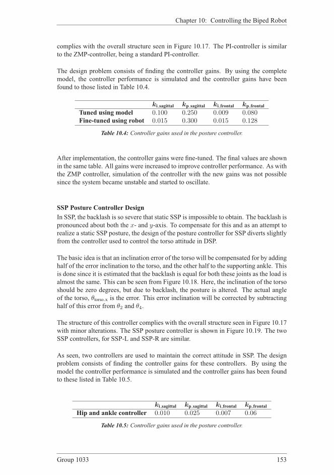
Chapter 10: Controlling the Biped Robot
complies with the overall structure seen in Figure 10.17. The PI-controller is similar
to the ZMP-controller, being a standard PI-controller.
The design problem consists of finding the controller gains. By using the complete
model, the controller performance is simulated and the controller gains have been
found to those listed in Table 10.4.
ki sagittal kp sagittal ki frontal kp frontal
Tuned using model 0.100 0.250 0.009 0.080Fine-tuned using robot 0.015 0.300 0.015 0.128
Table 10.4: Controller gains used in the posture controller.
After implementation, the controller gains were fine-tuned. The final values are shown
in the same table. All gains were increased to improve controller performance. As with
the ZMP controller, simulation of the controller with the new gains was not possible
since the system became unstable and started to oscillate.
SSP Posture Controller Design
In SSP, the backlash is so severe that static SSP is impossible to obtain. The backlash is
pronounced about both the x- and y-axis. To compensate for this and as an attempt torealize a static SSP posture, the design of the posture controller for SSP diverts slightly
from the controller used to control the torso attitude in DSP.
The basic idea is that an inclination error of the torso will be compensated for by adding
half of the error inclination to the torso, and the other half to the supporting ankle. This
is done since it is estimated that the backlash is equal for both these joints as the load is
almost the same. This can be seen from Figure 10.18. Here, the inclination of the torso
should be zero degrees, but due to backlash, the posture is altered. The actual angle
of the torso, θtorso x is the error. This error inclination will be corrected by subtracting
half of this error from θ2 and θ4.
The structure of this controller complies with the overall structure seen in Figure 10.17
with minor alterations. The SSP posture controller is shown in Figure 10.19. The two
SSP controllers, for SSP-L and SSP-R are similar.
As seen, two controllers are used to maintain the correct attitude in SSP. The design
problem consists of finding the controller gains for these controllers. By using the
model the controller performance is simulated and the controller gains has been found
to these listed in Table 10.5.
ki sagittal kp sagittal ki frontal kp frontal
Hip and ankle controller 0.010 0.025 0.007 0.06
Table 10.5: Controller gains used in the posture controller.
Group 1033 153
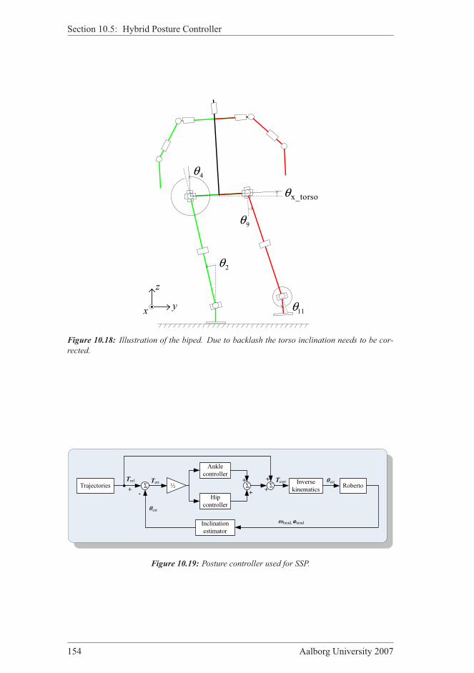
Section 10.5: Hybrid Posture Controller
2θ
4θ
9θ
11θy
z
x
x_torsoθ
Figure 10.18: Illustration of the biped. Due to backlash the torso inclination needs to be cor-
rected.
Roberto
Inclination estimator
ΣTrajectoriesTref Inverse
kinematicsTerr
+-
Ankle controller
Hip controller
Σ++
θest
ωhead, ahead
Tcorr θest½ Σ+
+
Figure 10.19: Posture controller used for SSP.
154 Aalborg University 2007
Chapter 10: Controlling the Biped Robot
In previous design sections, the controllers were implemented and the controller gains
were fine-tuned in order to achieve better performance. This was however not possible
in SSP.
10.5.2 Simulating the Posture Controller Performance
The performance of the hybrid posture controller was tested in both DSP and SSP.
First, the controller was tested in DSP and steps were given to the inclination of the
torso around the x-axis and around the y-axis in two different tests. Next, the posturecontroller was tested in SSP. To verify that the controller is capable of suppressing
disturbances caused by backlash, 0.087 rad is subtracted from the inclination instead
of giving a step with the reference. This will simulate of effect caused by backlash.
This substitution will only be applied in SSP in around the x-axis, as backlash is mostpronounced around this axis.
Posture Controller Simulation in DSP
In this test, a a step of 0.09 rad was applied about the x-axis. Next, a step of 0.09 radwas applied about the y-axis. The robot was set in zero-position before the tests werecarried out. The responses are seen in Figure K.7 on page 266 and K.8 on page 267.
It can be seen that the controllers work as intended but the settling times are too slow.
This is mainly due to the slow sampling rate of the system, that puts a limit on the
gains.
Posture Controller Simulation in SSP
This test differs from the test conducted in DSP, but only for the test regarding step-
input about the x-axis. Instead of giving an inclination step input, 0.087 rad is sub-
tracted from the inclination estimate. This simulates the behavior of backlash in the
system. The posture controller will then suppress this disturbance by increasing the
inclination in both the ankle and the torso as described in the design section. The re-
sponse is seen in Figure K.9 on page 267.
Finally, a step on 0.087 rad was applied about the y-axis. The response of the systemis shown in Figure K.10 on page 268.
Only the controller for SSP-L is tested, since the controller for the right leg is similar,
the simulation is not shown.
10.5.3 Implementation and Verification
This section describes the implementation of the DSP posture controller. The controller
will be tested by two experiments, where a step in the inclination is given, in both the
sagittal and the frontal plane individually. It was not possible to verify the performance
of the SSP controller due to backlash and wobbling. This will be described more
detailed in the following.
Testing the DSP Posture Controller About the x-axis
To test the posture controller, the robot was positioned in zero position. A 0.09 rad stepwas then given on the inclination reference about the x-axis. The measured inclination,θx,ref, and reference input is seen in Figure K.11 on page 269. In this figure, it is seen
Group 1033 155
Section 10.6: Partial Conclusion to Control
that there is a 0.03 rad overshoot but that the controller otherwise settles at the correct
inclination.
Testing the DSP Posture Controller About the y-axis
To test the posture controller about the y-axis, a 0.09 rad step was given. The biped
was placed in zero position with zero inclination. After 15 seconds the step was ap-
plied. The resulting inclination is seen in Figure K.12 on page 270.
Similar to the posture controller around the x-axis it must be concluded that this con-troller is too slow to realize posture control while performing dynamic walk. Once
again, backlash, wobbling in the joints and a slow inclination estimator is the main
reason for this.
10.6 Partial Conclusion to ControlIn this chapter, control signals have been generated by using all the sensors available
on the robot. The sensors; being an accelerometer, a gyroscope, pressure sensors, and
position feedback all have advantages and disadvantages.
To provide control input for the hybrid posture controller, an inclination estimator has
been developed. Through tests, it has been concluded that the inclination estimator,
described in Section 7.3 is too slow to provide a descent control input for the posture
controller. The rate of change of the signal is too slow to allow real-time posture con-
trol. A faster inclination estimator must be implemented in order to design a posture
controller, working in an inner control loop.
The ZMP estimate provided by the accelerometer and position feedback from the ser-
vos is also unreliable due to the high noise contribution on position measurements
when heavily loaded. Also the accelerometer measurements had large noise contribu-
tions in the signal. It has therefore been chosen not to use this estimate for control
purpose.
The ZMP estimate, calculated on behalf of the pressure measurements, provided a con-
trol signal, that was not dominated by noise, and made it possible to implement a ZMP
controller. Implementing a Kalman-filter, using input from the model, it would be pos-
sible to achieve a better ZMP estimate if the accelerometer and position feedback was
included in the estimate. This seems plausible since the estimate contains some level
of information. It has, however, not been verified due to the limited processing power
available on the robot.
Even though the output from the ZMP estimate is usable, there is one major problem
with the pressure sensors. Due to the small feet, the sensor output highly depends on
the positioning of the feet. If the feet are moved as little as 1mm the ZMP estimate
tends to change dramatically. Because of this, the position of the feet had to be cali-
brated before each controller test, by measuring the load on each pressure sensors. The
feet were then repositioned until descent pressure measurements were achieved. This
is not a feasible solution, and it must therefore be concluded that the pressure sensors
alone do not provide a sufficient ZMP estimate.
156 Aalborg University 2007
Chapter 10: Controlling the Biped Robot
The ZMP controller was simulated and implemented with a successful result for DSP
only, and successful simulated for SSP. This controller only used the ZMP estimate
provided by the feet as control input. By changing the position of the feet until a de-
scent ZMP estimate was achieved, it was clear that the ZMP position was moved to
the desired location. It has only been possible to implement the controller for use in
DSP while standing still. This is mainly due to the slow controller frequency. Only a
40Hz update frequency could be achieved on the system due to the limited process-
ing power. This results in jerky movements of the robot and noise dominated estimates.
The posture controller was simulated in both DSP and SSP and implemented for DSP.
Due to backlash, SSP is not possible when standing still and it has there for only been
tested using simulations.
Group 1033 157


11EPILOGUE
Chapter contents11.1 Discussion 160
11.1.1 Mechanical Design 160
11.1.2 Hardware Design 161
11.1.3 Software Design 161
11.1.4 Modeling 162
11.1.5 Trajectory Design 162
11.1.6 Control Design 163
11.2 Conclusion 163
THIS CHAPTER CONTAINS the epilogue of this master’s thesis. It will start with
a discussion of some of the main problems experienced throughout the project. All
the main areas such as mechanical design, hardware design, software design, model-
ing, trajectory generation and control will be discussed. Afterward a conclusion on the
entire master’s thesis will be given.
Group 1033 159
Section 11.1: Discussion
11.1 DiscussionThis section will discuss some of the areas covered in this master’s thesis. Mainly areas
that have been problematic in some sense will be accentuated and discussed.
11.1.1 Mechanical Design
A complete mechanical solution was given for a humanoid robot, which should be able
to resemble human walk. It was emphasized that the solution should build on avail-
able mechanical solutions, but first and foremost it should result in a robot with human
proportions. Therefore some of the mechanical parts have been custom-made for this
project. An entire humanoid platform was constructed, which using the multi DoF
joint created enables straight and curved walk.
An issue regarding the mechanical solution was an observed backlash in the system,
especially outspoken in the legs. At the design stage, this was sought minimized by
using custom-made solutions, such as the multi DoF joint used in the hip. These have
been satisfactory for the single joint, but in such a complex mechanical construction,
backlash is difficult to avoid entirely. Therefore, when building up a kinematical chain,
with a large number of joints, the backlash becomes more significant. A consequence
was that when the robot was positioned in zero position, it could not be guaranteed
that it was in the exact same position every time. The weight distribution on the feet
therefore changed from time to time and the measurements of the strain gauges were
not always reliable. A solution to this problem could be to measure the backlash by
mounting a potentiometer directly on the joint. The position feedback provided by the
internal potentiometers does not measure backlash, and it is therefore not possible to
control the backlash of the mechanics.
Custom-made feet were constructed which made it possible to measure the force dis-
tribution of the robot on the feet. The feet were made as a bendable construction of
spring steel plates, making it possible to measure the strain on the plates when exposed
to a force. Cross-talk was minimized using dampers inserted. To minimize the oscil-
lating effect, caused by the spring steel plate, the dampers should have been designed
especially for this. As the feet were designed to have humanoid proportions they were
small in size, with only 15mm between the inner and outer strain plate. This results in
a very small PoS. The oscillating effect of the spring steel plates had the observed effect
that the robot would sway some degrees forward and backwards in the y-direction, ex-erting a limit-cycle behavior, and the whole system would wobbling. The effect could
be observed both in frontal and sagittal plane, but was most outspoken in the sagittal
plane when standing in DSP. When the robot should stand in SSP, the PoS was further
minimized in the y-direction as there was only one strain plate to give support at theheel. While the strain plates, at the left and right side of each foot, should give support
by minimizing the pressure on the middle strain gauge plate, they rather amplified the
oscillations due to the spring effect. The stability of the robot in SSP could then be
compared to a pivoted beam, as the weight would keep shifting from side to side. This
problem is also illustrated in Figure 11.1. A solution to this problem could be to design
a mechanical solution which would utilize the entire foot as support, rather than only
these three points, and a construction that is more solid than the bendable spring steel.
Thereby the introduced oscillations could be minimized.
160 Aalborg University 2007
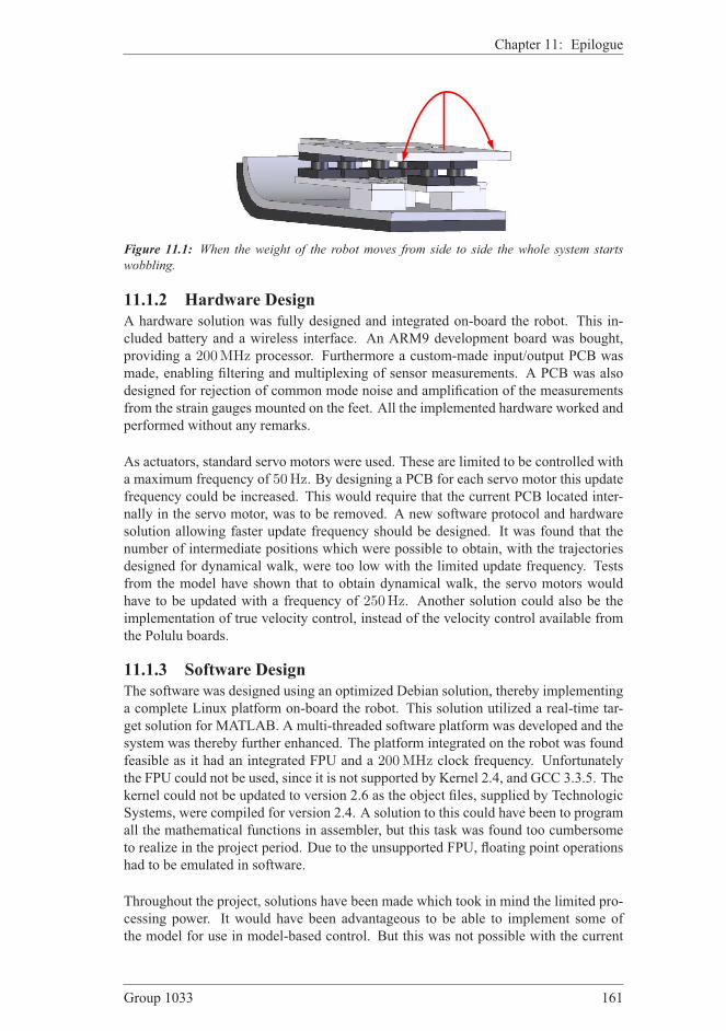
Chapter 11: Epilogue
Figure 11.1: When the weight of the robot moves from side to side the whole system starts
wobbling.
11.1.2 Hardware Design
A hardware solution was fully designed and integrated on-board the robot. This in-
cluded battery and a wireless interface. An ARM9 development board was bought,
providing a 200MHz processor. Furthermore a custom-made input/output PCB was
made, enabling filtering and multiplexing of sensor measurements. A PCB was also
designed for rejection of common mode noise and amplification of the measurements
from the strain gauges mounted on the feet. All the implemented hardware worked and
performed without any remarks.
As actuators, standard servo motors were used. These are limited to be controlled with
a maximum frequency of 50Hz. By designing a PCB for each servo motor this update
frequency could be increased. This would require that the current PCB located inter-
nally in the servo motor, was to be removed. A new software protocol and hardware
solution allowing faster update frequency should be designed. It was found that the
number of intermediate positions which were possible to obtain, with the trajectories
designed for dynamical walk, were too low with the limited update frequency. Tests
from the model have shown that to obtain dynamical walk, the servo motors would
have to be updated with a frequency of 250Hz. Another solution could also be the
implementation of true velocity control, instead of the velocity control available from
the Polulu boards.
11.1.3 Software Design
The software was designed using an optimized Debian solution, thereby implementing
a complete Linux platform on-board the robot. This solution utilized a real-time tar-
get solution for MATLAB. A multi-threaded software platform was developed and the
system was thereby further enhanced. The platform integrated on the robot was found
feasible as it had an integrated FPU and a 200MHz clock frequency. Unfortunatelythe FPU could not be used, since it is not supported by Kernel 2.4, and GCC 3.3.5. The
kernel could not be updated to version 2.6 as the object files, supplied by Technologic
Systems, were compiled for version 2.4. A solution to this could have been to program
all the mathematical functions in assembler, but this task was found too cumbersome
to realize in the project period. Due to the unsupported FPU, floating point operations
had to be emulated in software.
Throughout the project, solutions have been made which took in mind the limited pro-
cessing power. It would have been advantageous to be able to implement some of
the model for use in model-based control. But this was not possible with the current
Group 1033 161

Section 11.1: Discussion
processor. Experiments showed that a 10 s simulation of the model was conducted in42.6 s, which is approximately 1/4 real-time, on a computer with an Intel P4 2.8GHzprocessor and 512MB ram running Windows XP. A feasible solution would be to im-
plement the needed states of the model on an Intel P4 2GHz processor with a fullysupported FPU. It is evaluated that this would be sufficient to implement the most im-
portant parts of the model.
11.1.4 Modeling
A complete model was developed which gave a full description of the system, giving a
complete input to output model of the actual system. Tests showed that the model was
able to give a good estimate of the real system. But some of the issues the test revealed
were that some unmodeled effects in the real system had a high impact on the results,
which resulted in an offset error between the output from the model and the measured
output on the real system. Especially the spring effect of the strain plates mounted on
the feet, causing an amplified bend of the plates, should be modeled if a more precise
description of the real system is wanted. The spring effect further caused oscillations
in the real system, while this was not the case for the model.
The model gave a description of the ZMP, but if the ZMP was to move outside the PoS
the robot did not fall. This effect could be added by modeling the tip of the foot as an
extra DoF, which would limit the model to fall forward but still give a better indication
of the dynamics during walk.
As the model also included all the internal states of the system, it was a good base for
learning the dynamics of the system and for development and testing of the controllers.
The trajectories used in the project were created using the model and the controllers
were developed and tested using the model as well.
11.1.5 Trajectory Design
A complete set of dynamic walking trajectories were created, including both the start-
up and the stop phase. These trajectories were generated off-line and optimized toward
keeping the ZMP inside the PoS at all times. Furthermore the trajectories were de-
signed to minimize the energy consumption. It was found that the designed dynamical
trajectories for the model kept the ZMP inside the PoS, but for the real robot the ZMP
was not kept inside the PoS. Further it was found that because of the control frequency
of the servos and backlash in the joints, it was not possible to implement the designed
trajectories. Some new and slower trajectories were designed, and performed better
than the first set of trajectories, but the problems with backlash were still too signifi-
cant to obtain walk.
As the trajectories were designed using the model, these could have been optimized
further, if the model was able to roll on the front of the feet. This could have aided the
design of the trajectories in such a way that a more human-like walk could have been
achieved.
162 Aalborg University 2007

Chapter 11: Epilogue
11.1.6 Control Design
In the control design, several individually estimators and controllers were developed.
These controllers aimed at controlling the position of the ZMP and the posture of the
robot. This was found advantageous as the ZMP was also used to design the trajec-
tories. Simulations showed that the controllers were able to minimize the error in the
position of the ZMP during DSP and SSP. In DSP, the ZMP was tested with a success-
ful result. Similar, the posture controller was tested in DSP and SSP, and verified in
DSP. It was concluded that both controllers was too slow to control a walking biped
robot.
As an important factor in human walk is to foresee what happens next, it would be
beneficial to use model-based control to make the system more adaptive. Thereby the
position of the ZMP could have been predicted some steps ahead, which would have
been important for correct control of the robot during walk.
11.2 ConclusionThe main goal of this project was to develop a humanoid robot and make it perform
dynamic walk. The first part, concerning the development was achieved by designing
a 21 DoF biped robot from scratch. The developed robot possesses human proportions,
i.e., the correct relationship between length of limbs and the height of the robot. Fur-
thermore a special joint was developed to imitate the ankle and the hip joints in human
beings, where several degrees of freedom are located in one joint. The feet were also
designed to fit the size of a human, making the support area on ground very small. A
big advantage of the robot-design is the possibility to walk in a curved path, using the
multi DoF joint which has been designed.
To control this mechanical structure, 21 servo motors were inserted, such that each
DoF became actuated. The servo motors enable a simple interface to control the posi-
tion of each joint. Furthermore a hardware platform has been developed that enables
the humanoid robot to be completely autonomous. An on-board computer was placed
on the robot in order to control all actuators and to process the inputs from the large
number of sensors located on the system. Furthermore the system was equipped with
batteries, making it possible to run for around one and a half hour without recharg-
ing. A complete software platform was constructed, including an interface to the robot
which enables easy testing of controllers. The software was designed as multi-threaded
real-time system, and was verified working.
Before any controllers for the system were developed, a model was derived. The model
is a complete mathematical description of the complex non-linear dynamical system.
Using this model it was possible to simulate complete walking cycles and extract in-
formation on stability properties of the walk, information on how forces and torques
worked in different joints during the walk. The most challenging part of the modeling
was the dynamical part of the system, especially in DSP where a closed kinematical
chain made the modeling a complex task. The problems were however solved, using a
novel solution proposed in this thesis, and a complete dynamical model, taking all 21
DoF and all three dimensions into consideration, has been developed. The model was
verified through a series of tests performed on the sub-models, and finally a test that
verified the complete model. The result of the tests were, that the model is valid, but
Group 1033 163

Section 11.2: Conclusion
if a more precise description of the system is essential, it is necessary to expand the
model to include the bendable plates in the feet as well as the backlash that is present
in the system. It is concluded that the accuracy of the model is sufficient for the scope
of this project.
In order to obtain dynamical walk, a set of dynamical walking trajectories were de-
veloped, which were optimized toward improving the stability properties and lowering
the energy consumption. The trajectories gave a satisfying result when simulated, but
due to some drawbacks on the real system, it was not possible to obtain dynamical
walk. The main reason for this, is that the control frequency of the servo motors is
only 50Hz, resulting in a rough set of position references to the servo motors, whichcaused a shaking of the entire system. This was sought solved by creating slower tra-
jectories, but could not be removed completely. Another decisive reason for not being
able to perform dynamical walk, was the backlash in the system.
The reliability of the control input is also an essential problem in the system. Due to
the small feet, the ZMP estimate is very dependent on the orientation of the feet.
To maintain stability of the system two controllers were developed; a hybrid posture
controller and a ZMP controller. In order to minimize the effect of backlash, a posture
controller was implemented. It was concluded that the posture controller worked as
intended in DSP, both in sagittal and in frontal plane. A test of the controller in SSP
could not be performed due to backlash. It was however concluded that the controller
was too slow to be implemented on a walking robot, due to the low sample frequency
of the system.
The ZMP controller worked as intended both in sagittal and frontal plane. As with the
posture controller, it was not fast enough to be implemented on a walking robot. It was
not possible to test the ZMP controller on the actual system in SSP, but simulations
documents the performance in this phase.
To summarize the conclusion; a humanoid robot platform was developed, capable of
performing dynamic walk and even curved gait. This consists of a complete mechani-
cal solution designed from scratch, an on-board computer and a layered software plat-
form with a wireless interface that supports easy implementation of controllers and
trajectories. A complete dynamical model has been derived, and verified, with the
same inputs and outputs as the real system. Using the model, dynamic stable walking
trajectories have been designed. Controllers, which increase stability of the robot, have
been designed and tested. To conclude; this thesis gives a solution to the development,
modeling and control of a humanoid robot.
164 Aalborg University 2007
BIBLIOGRAPHY
[Analog Devices, 2000] Analog Devices (2000). Precision Single Supply Instrumen-
tation Amplifier, AMP04. [CD-ROM, 2007, literature/datasheets/amp04.pdf].
[Applieddata.net, 2007] Applieddata.net (2007). Applied data’s
root filesystem with support for the maverick engine.
http://armel.applieddata.net/developers/linux/eabi/
armel-root-fs.tar.bz2.
[Arakawa and Fukuda, 1996] Arakawa, T. and Fukuda, T. (1996). Natural mo-
tion trajectory generation of biped locomotion robot using genetic algo-
rithm through energy optimization. IEEE International Conference on Systems,
Man, and Cybernetics. [CD-ROM, 2007, literature/trajectory generation/natu-
ral motion trajectory generation energy optimization.pdf].
[Azevedo et al., 2005] Azevedo, C., Espiau, B., Amblard, B., and Assaiante,
C. (2005). Bipedal locomotion: toward unified concepts in robotics and
neuroscience. Biological Cybernetrics. [CD-ROM, 2007, literature/gener-
al/bipedal locomotion toward unified.pdf].
[Bachar, 2004] Bachar, Y. (2004). Developing controllers for biped humanoid loco-
motion. Technical report, University of Edinburgh, School of Informatics. [CD-
ROM, 2007, literature/control/developing controllers for biped.pdf].
[Baerveldt and Klang, 1997] Baerveldt, A.-J. and Klang, R. (1997). A
low-cost and low-weight attitude estimation system for an au-
tonomous helicopter. Proc. of the IEEE Int. Conf. on Intel-
ligent Engineering Systems. [CD-ROM, 2007, literature/sen-
sor fusion/attitude estimation system for an autonomous helicopter.pdf].
[Bak and Izadi-Zamanabadi, 2006] Bak, T. and Izadi-Zamanabadi, R. (2006). Lecture
notes - hybrid systems. Technical report, Aalborg University. [CD-ROM, 2007,
literature/hybrid systems/hs.pdf].
[Bhanderi, 2006] Bhanderi, D. (2006). Linux soft real-time target v2.3.
http://www.control.aau.dk/˜danji/downloads.
[Borghese et al., 1996] Borghese, N. A., Bianchi, L., and Lacquaniti, F.
(1996). Kinematic determinants of human locomotion. Journal of
Physiology. [CD-ROM, 2007, literature/trajectory generation/kine-
matic determinants of human locomotion.pdf].
[Bruneau et al., 2001] Bruneau, O., Ouezdou, F. B., and Fontaine, J.-G. (2001).
Dynamic walk of a bipedal robot having flexible feet. International Confer-
ence on Intelligent Robots and Systems. [CD-ROM, 2007, literature/gait/dy-
namic walk flex feet.pdf].
[Buschmann et al., 2006] Buschmann, T., Lohmeier, S., Ulbrich, H., and Pfeif-
fer, F. (2006). Dynamics simulation for a biped robot: Modeling and
experimental verification. Proceedings of the 2006 IEEE International
Conference on Robotics and Automation Orlando, Florida - May 2006. [CD-
ROM, 2007, literature/modeling/Dynamics Simulation for a Biped Robot-
Modeling and Experimental Verification.pdf].
Group 1033 165

BIBLIOGRAPHY
[Buss et al., 2003] Buss, M., Hardt, M., Kiener, J., Sobotka, M., Stelzer, M., von
Stryk, O., , and Wollherr, D. (2003). Towards an autonomous, humanoid, and
dynamically walking robot: Modeling, optimal trajectory planning, hardware
architecture, and experiments. Proceedings of the 3rd International Conference
on Humanoid Robots 2003, Karlsruhe, Germany. [CD-ROM, 2007, literature/-
control/towards an autonomous.pdf].
[Capi et al., 2003] Capi, G., Nasu, Y., Barolli, L., and Mitobe, K. (2003). Real time
gait generation for autonomous humanoid robots: A case study for walk-
ing. Robotics and Autonomous Systems, vol. 42. [CD-ROM, 2007, literature/-
gait/real time gait generation.pdf].
[CD-ROM, 2007] CD-ROM (2007). The enclosed CD-ROM.
[Chaillet et al., 1994] Chaillet, N., Abba, G., and Ostertag, E. (1994). Double dynamic
modelling and computed-torque control of a biped robot. [CD-ROM, 2007, lit-
erature/modeling/double dynamic model.pdf].
[Choi et al., 2004] Choi, Y., You, B.-J., and Oh, S.-R. (2004). On the stability of indi-
rect zmp controller for biped robot systems. [CD-ROM, 2007, literature/trajec-
tory generation/on the stability of indirect zmp.pdf].
[Christensen et al., 2006] Christensen, J., Nielsen, J. L., Svendsen, M. S., Sven-
strup, M. S., Winter, K., and Ørts, P. F. (2006). Modelling and control of a
biped robot. Technical report, Aalborg University, Institute of electronic sys-
tems, Department of Control Engineering. [CD-ROM, 2007, literature/model-
ing/p8 report.pdf].
[Cirrus Logic, 2004] Cirrus Logic (2004). High Speed ARM9 System-on-
Chip Processor with MaverickCrunch, EP9302. [CD-ROM, 2007,
literature/datasheets/EP9302-arm9.pdf].
[CodeSourcery, 2007] CodeSourcery (2007). Gnu toolchain for arm eabi.
http://www.codesourcery.com/gnu toolchains/arm/download.html.
[Collins et al., 2001] Collins, S. H., Wisse, M., and Ruina, A. (2001). A three-
dimensional passive-dynamics walking robot with two legs and kness. The In-
ternational Journal of Robotics Research Vol. 20, No. 7, July 2001, pp. 607-
615. [CD-ROM, 2007, literature/modeling/3d passive dynamic.pdf].
[Courtine and Schieppati, 2004] Courtine, G. and Schieppati, M. (2004). Human
walking along a curved path: Body trajectory, segment orientation and the effect
of vision. European Journal of Neuroscience, vol. 18. [CD-ROM, 2007, litera-
ture/gait/human walk curved path 1.pdf].
[Craig, 1989] Craig, J. J. (1989). Introduction to Robotics - Mechanics and Control,
Second Edition. Addison Wesley.
[Debian, 2007] Debian (2007). Debian arm eabi port.
http://wiki.debian.org/ArmEabiPort.
[Deo and Walker, 1997] Deo, A. S. and Walker, I. D. (1997). Minimum ef-
fort inverse kinematics for redundant manipulators. IEEE Transactions on
Robotics and Automation, vol. 13, no. 5,. [CD-ROM, 2007, literature/model-
ing/min effort inverse kinematics.pdf].
166 Aalborg University 2007

BIBLIOGRAPHY
[Devices, 2006] Devices, A. (2006). ADXL: Small, Low Power, 3-Axis +/-
3 g, iMEMS Accelerometer. [CD-ROM, 2007, literature/datasheet-
s/ADXL330 0 imu accelerometer.pdf].
[Djoudi et al., 2005] Djoudi, D., Chevallereau, C., and Aoustin, Y. (2005). Op-
timal reference motions for walking of a biped robot. International con-
ference on robotics and automation. [CD-ROM, 2007, literature/gait/opti-
mal reference motions.pdf].
[Doi et al., ] Doi, M., Hasegawa, Y., and Fukuda, T. Realization of 3-dimensional dy-
namic walking based on the assumption of point-contact. International Confer-
ence on Robotics and Automation, Barcelona, Spain, April 2005.
[Erbatur et al., 2002] Erbatur, K., Okazaki, A., Obiya, K., Takahashi, T., and Kawa-
mura, A. (2002). A study on the zero moment point measurement for biped
walking robots. 7th International Workshop on Advanced Motion Control,
IEEE. [CD-ROM, 2007, literature/modeling/zmp measure.pdf].
[Foxlin, 1996] Foxlin, E. (1996). Inertial head-tracker sensor fusion by a complemen-
tary separate-bias kalman filter. Proceedings of the IEEE 1996 virtual reality
annual international symposium, Santa Clara, CA. [CD-ROM, 2007, litera-
ture/sensor fusion/intertial head tracker sensor fusion.pdf].
[Gielo-Perczak, 2001] Gielo-Perczak, K. (2001). The golden section as a harmoniz-
ing feature of human dimensions and workplace design. Theoretical Issues in
Ergonomics Science. [CD-ROM, 2007, literature/gait/human proportions.pdf].
[Goldenberg et al., 1985] Goldenberg, A. A., Benhabib, B., and Fenton, R. G. (1985).
A complete generalized solution to the inverse kinematics of robots. IEEE Jour-
nal of Robotics and Automation, vol. ra-1, no. 1. [CD-ROM, 2007, literature/-
modeling/A Complete Generalized Solution to the Inverse Kinematics.pdf].
[Guan et al., 2005] Guan, Y., Yokoi, K., Stasse, O., and Khed-
dar, A. (2005). On robotic trajectory planning using polyno-
mial interpolations. IEEE International Conference on Robotics
and Biomimetrics. [CD-ROM, 2007, literature/trajectory genera-
tion/on robotic trajectory planning using polynomial interpolations.pdf].
[Hardt et al., 1999] Hardt, M., Kreutz-Delgado, K., and Helton, J. W. (1999). Optimal
biped walking with a complete dynamical model. [CD-ROM, 2007, literature/-
modeling/optimal walk complete dynamical model.pdf].
[HiTec, 2005] HiTec (2005). Announced specification of HS-645MG standard
deluxe high torque servo. [CD-ROM, 2007, literature/datasheets/HS-
645MG servomotor.pdf].
[HiTec, 2006] HiTec (2006). Announced specification of HSR-5995TG standard
deluxe high torque servo. [CD-ROM, 2007, literature/datasheets/HSR-
5995TG spec.pdf].
[Hsiao et al., 2006] Hsiao, F.-B., Liu, T.-L., Chien, Y.-H., and Lee, M.-
T. (2006). The development of a target-lock-on optical remote sens-
ing system. Aeronautical Journal. [CD-ROM, 2007, literature/sen-
sor fusion/The development of a target lock.pdf].
[Huang et al., 2000] Huang, Q., Kaneko, K., Yokoi, K., Kajita, S., Ko-
toku, T., Koyachi, N., Arai, H., Imamura, N., Komoriya, K., and
Group 1033 167

BIBLIOGRAPHY
Tanie, K. (2000). Balance control of a biped robot combining off-line
pattern with real-time modification. IEEE International Conference on
Robotics & Automation. [CD-ROM, 2007, literature/trajectory generation/bal-
ance control of a biped robot combining offline pattern with realtime modi-
fication.pdf].
[Huang et al., 2001] Huang, Q., Yokoi, K., Kajita, S., Kaneko, K., Arai, H., Koyachi,
N., and Tanie, K. (2001). Planning walking patterns for a biped robot. IEEE
Transactions on Robotics and Automation. [CD-ROM, 2007, literature/trajec-
tory generation/planning walking patterns for a biped robot.pdf].
[Huelsman, 1993] Huelsman, L. P. (1993). Active and Passive Analog Filter Design,
an introduction. McGraw-Hill, Inc.
[Hurmuzlu, 2001] Hurmuzlu, Y. (2001). Dynamics of bipedal gait part i: Objective
functions and the contact event of a planar five-link biped. [CD-ROM, 2007,
literature/modeling/impact phase/Impact phase.pdf].
[InvenSense Inc, 2006] InvenSense Inc (2006). Integrated Dual-Axis
Gyro, IDG-300. [CD-ROM, 2007, literature/datasheets/IDG-
300 Datasheet imu gyroscope.pdf].
[Ito and Kawasaki, 2005] Ito, S. and Kawasaki, H. (2005). Regularity in an
environment produces an internal torque pattern for biped balance
control. Biological Cybernetrics. [CD-ROM, 2007, literature/model-
ing/biped balance control periodic disturbance.pdf].
[Ito et al., 2004] Ito, S., Saka, Y., and Kawasaki, H. (2004). Where center of
pressure should be controlled in biped upright posture. System and com-
puters in Japan, vol. 35, no. 5. [CD-ROM, 2007, literature/modeling/cen-
ter of presure model 3.pdf].
[Kajita et al., 2001] Kajita, S., Kanehiro, F., Kaneko, K., Yokoi, K., and Hirukawa,
H. (2001). The 3d linear inverted pendulum mode: A simple modeling for
a biped walking pattern generation. International Conference on Intelligent
Robots and Systems. Proceedings of the 2001. [CD-ROM, 2007, literature/mod-
elling/the 3d linear inverted pendulum mode].
[Kondak and Hommel, 2003] Kondak, K. and Hommel, G. (2003). Control and on-
line computation of stable movement for biped robots. Proceedings of the 2003
IEEE/RSJ international Conference on Intelligent Robots and Systems. [CD-
ROM, 2007, literature/control/control and online computation.pdf].
[Kuo, 1997] Kuo, A. D. (1997). An optimal control model of human balance: Can it
provide theoretical insight to neural control of movement? American Control
Conference, 1997. Proceedings of the 1997. [CD-ROM, 2007, literature/bal-
ance/optimal control model human balance.pdf].
[Lee et al., 2003] Lee, S., Song, J., Choi, W., and Hong, D. (2003). Position con-
trol of a stewart platform using inverse dynamics control with approximate
dynamics. Mechatronics vol. 13. [CD-ROM, 2007, literature/modeling/stew-
art platform.pdf].
[Loffler et al., 2004] Loffler, K., Gienger, M., Pfeiffer, F., and Ulbrich, H. (2004).
Sensors and control concept of a biped robot. IEEE transactions on indus-
trial electronics, vol. 51, no. 5, October 2004. [CD-ROM, 2007, literature/sen-
sor fusion/sensor control of johnny.pdf].
168 Aalborg University 2007

BIBLIOGRAPHY
[Li et al., 1993] Li, Q., Takanishi, A., and Kato, I. (1993). Learning control for a biped
walking robot with a trunk. International Conference on Intelligent Robots &
Systems, IEEE. [CD-ROM, 2007, literature/control/learning control.pdf].
[Maxim Integrated Products, 2006] Maxim Integrated Products (2006). MAX396 -
Precision, 16 channel, Low-Voltage, CMOS Analog Multiplexer. [CD-ROM,
2007, literature/datasheets/MAX396 multiplexer.pdf].
[McGeer, 1990] McGeer, T. (1990). Passive walking with knees. IEEE international
Conference on Robotics and Automation. [CD-ROM, 2007, literature/gait/-
tad mcgeer passive walking.pdf].
[Mu and Wu, 2003] Mu, X. and Wu, Q. (2003). A complete dynamic model of five-
link bipedal walking. Proceedings of the American Control Conference. [CD-
ROM, 2007, literature/modeling/complete dynamic model.pdf].
[Mu and Wu, 2004] Mu, X. and Wu, Q. (2004). Development of a complete dynamic
model of a planar five-link biped and sliding mode control of its locomotion
during the double support phase. International Journal of Control. [CD-ROM,
2007, literature/modeling/dynamic model biped mu wu.pdf].
[Nielsen, 2003] Nielsen, J. B. (2003). How we walk: Central control of muscle ac-
tivity during human walking. Neuroscientist 2003. [CD-ROM, 2007, literature/-
gait/how we walk.pdf].
[Ogino et al., 2003] Ogino, M., Hosoda, K., and Asada3, M. (2003). Learn-
ing energy efficient walking based on ballistics. SICE -ANNUAL
CONFERENCE-. [CD-ROM, 2007, literature/trajectory generation/learn-
ing energy efficielt walking based on ballistics.pdf].
[Peng et al., 2005] Peng, Z., Huang, Q., Zhang, L., Jafri, A. R., Zhang, W.,
and Li, K. (2005). Humanoid on-line pattern generation based on param-
eters of off-line typical walk patterns. IEEE International Conference on
Robotics and Automation. [CD-ROM, 2007, literature/trajectory generation/hu-
manoid online pattern genration.pdf].
[Popovic, 2006] Popovic, D. B. (2006). Control of walking in humans. [CD-ROM,
2007, literature/gait/popovic control of walking in humans.pdf].
[Rehbinder and Hu, 2000] Rehbinder, H. and Hu, X. (2000). Nonlinear pitch and roll
estimation for walking robots. Proceedings of the 2000 IEEE international con-
ference on robotics and automation, Vol. 3, San Francisco, CA, USA. [CD-ROM,
2007, literature/sensor fusion/nonlinear pitch and roll estimation.pdf].
[Rehbinder and Hu, 2001] Rehbinder, H. and Hu, X. (2001). Drift-free attitude esti-
mation for accelerated rigid bodies. Proceedings of the 2001 IEEE Interna-
tional Conference on Robotics and Automation. [CD-ROM, 2007, literature/sen-
sor fusion/Drift free attitude estimation for accelerated rigid bodies.pdf].
[Robotics and Electronics, 2005] Robotics, P. and Electronics (2005). Micro Se-
rial Servo Controller, User’s Guide. [CD-ROM, 2007, literature/datasheet-
s/pololu servo controller.pdf].
[Santos and Silva, 2005] Santos, V. M. F. and Silva, F. M. T. (2005). Engineering so-
lutions to build an inexpensive humanoid robot based on a distributed control
architecture -. 5th IEEE-RAS International Conference on Humanoid Robots.
[CD-ROM, 2007, literature/feet/straingauge biped2.pdf].
Group 1033 169
BIBLIOGRAPHY
[Sciavicco and Siliano, 1988] Sciavicco, L. and Siliano, B. (1988). A solution algo-
rithm to the inverse kinematic problem for redundant manipulators. IEEE Jour-
nal of Robotics and Automation, vol. 4, no. 4,. [CD-ROM, 2007, literature/mod-
eling/inverse kinematic obstacle avoid.pdf].
[Serway and Beichner, 2000] Serway, R. A. and Beichner, R. J. (2000). Physics For
Scientists and Engineers with Modern Physics, Fifth Edition. Saunders College
Publishing.
[Shanmugan and Breipohl, 1988] Shanmugan, K. S. and Breipohl, A. (1988). Random
Signals: Detectiobn, Estimation and Data Analysis. John Wiley and Sons, Inc.
[Shih, 1996] Shih, C.-L. (1996). Analysis of the dynamics of a biped
robot with seven degrees of freedom. International Conference on
Robotics and Automation, IEEE. [CD-ROM, 2007, literature/model-
ing/biped dynamics single support.pdf].
[Spark Fun Electronics, 2006] Spark Fun Electronics (2006). Spark Fun Electronics.
http://www.sparkfun.com.
[Takahashi et al., 2005] Takahashi, M., Narukawa, T., Miyakawa, K., and Yoshida,
K. (2005). Combined control of cpg and torso attitude control for biped
locomotion. Intelligent Robots and Systems, 2005. (IROS 2005). 2005
IEEE/RSJ International Conference. [CD-ROM, 2007, literature/control/com-
bined control of CPG and torso attitude control.pdf].
[Technologic Systems, 2006] Technologic Systems (2006). TS-7400 Data sheet -
System on Module with 1.1s Ultra-Fast Bootup to Linux. [CD-ROM, 2007,
literature/datasheets/ts-7400-datasheet.pdf].
[Udwadia and Kalaba, 2001] Udwadia, F. E. and Kalaba, R. E. (2001). Ex-
plicit equations of motion for mechanical systems with nonideal con-
straints. Transaction of the ASME. [CD-ROM, 2007, literature/modeling/non-
ideal constraints udwadia.pdf].
[Udwadia and Kalaba, 2002] Udwadia, F. E. and Kalaba, R. E. (2002). On the foun-
dations of analytical dynamics. International Journal of Non-Linear Mechan-
ics. [CD-ROM, 2007, literature/modeling/analytical dynamics udwadia.pdf].
[Vaganay et al., 1993] Vaganay, J., Aldon, M. J., and Fournier, A. (1993). Mobile
robot attitude estimation by fusion of inertial data. Proceedings of the 1993
IEEE international conference on robotics and automation, Vol. 1. [CD-ROM,
2007, literature/sensor fusion/mobile robot attitude estimation.pdf].
[Vukobratovic et al., 2006] Vukobratovic, M., Borovac, B., and Potkonjak, V. (2006).
Towards a unified understanding of basic notions and terms in humanoid
robotics. Robotica, Cambridge University Press. [CD-ROM, 2007, literature/-
general/Towards a unified understanding of basic notions.pdf].
[Vukobratovic and Juricic, 1969] Vukobratovic, M. and Juricic, D. (1969). Contribu-
tion to the synthesis of biped gait. Proceedings of the IFAC Symposium on Tech-
nical and Biological Problem of Control. Available from the Library.
[Wisniewski, 2006] Wisniewski, R. (2006). Mechanical systems ii - lagrange mechan-
ics. Technical report, Aalborg University. Lecture notes from lecture three of the
course Modelling of Mechanical Systems II. [CD-ROM, 2007, literature/mod-
eling/MechanicalSystemsSection3.pdf].
170 Aalborg University 2007
BIBLIOGRAPHY
[Yamaguchi et al., 1999] Yamaguchi, J., Soga, E., Inoue, S., and Takanishi, A.
(1999). Development of a bipedal humanoid robot - control method of
whole body cooperative dynamic biped walking -. International Conference
on Robotics & Automation, IEEE. [CD-ROM, 2007, literature/control/W-
hole body cooperative.pdf].
[You et al., 2004] You, B.-J., Oh, S.-R., and Choi, Y. (2004). On the stability of indi-
rect zmp controller for biped robot systems. IEEE/RSJ International Conference
on Intelligent Robots and Systems, vol. 2. [CD-ROM, 2007, literature/model-
ing/zmp calc2.pdf].
[Zhao et al., 1997] Zhao, W., Wu, G., and III, H. J. S. (1997). Closed-form kinemat-
ics for a spartial closed-chain mechanism modeling biped stance. Mechanical
Machine Theory Vol. 33 No. 4, Elsevier. [CD-ROM, 2007, literature/model-
ing/biped dynamics doubble support.pdf].
[Zheng and Luh, 1988] Zheng, Y. F. and Luh, J. (1988). Optimal load distribution for
two industrial robots handling a single object. IEEE International Conference
on Robotics and Automation & Systems, IEEE. [CD-ROM, 2007, literature/-
modeling/load distribution of two arms.pdf].
Group 1033 171


ASERVO CONTROLLER
BOARD
The control signal is generated by a servo driver board, Pololu Micro Serial Servo
Controller [Robotics and Electronics, 2005], acquired from Pololu Robotics and Elec-
tronics. It is possible to connect up to eight servo motors to one servo board. To
increase the possible update rate, it has been chosen to use a separate serial line for
each of the three servo controller boards. The input to the servo board is a serial bit-
stream with TTL levels. Up to 16 servo boards can be connected to the same serial
input signal, enabling the user to control up to 128 servo motors with only one serial
line. Thus, three servo boards are sufficient for controlling all 21 servos on the biped
robot. Each board has a size of only 23mm × 23mm, which makes them well suited
for this project because of the limited space for hardware.
The supply voltage should be within 5V and 16V, and the current consumption forone board is 5mA in average. A picture of the board is shown in Figure A.1.
A.1 Setup of the Servo BoardThe boards operate in two different modes: Mini SSC II mode and Pololu mode. In
this configuration Pololu mode is used, as this supports a baud rate up to 38, 400 baud,whereas Mini SSC II mode only supports a baud rate of 2, 400 baud or 9, 600 baud.Pololu mode also enables some more advanced features, e.g. setting the turning rate,
altering the neutral position as well as the turning direction of the servos. The Pololu
mode is set by removing the jumper in the top left corner of the picture in Figure A.1.
The power supply to the servos is connected through a common supply connector on
the board, which is separate from the power supply to the board itself. Depending
on the load of the servos, the current consumption will vary from around 200mA to
around 5A. If several servos are stalling simultaneously, the current consumption canexceed 10A, and measures should be taken to avoid this.´
Group 1033 173

Section A.2: Controlling the Servo Motors
Figure A.1: The Pololu Micro Serial Servo Controller. The connectors for the eight servo motors
are placed on the right side. The jumper in the top left corner should be removed to set the board
to “Pololu mode”.
A.2 Controlling the Servo MotorsTo control the servo motors, the following protocol is used. A string of five or six bytesis transmitted to the boards:
<startbyte> <device ID> <command> <servo number> <data 1> <data 2>
- <startbyte>: Always 128.
- <device ID>: 1 for the Pololu Micro Serial Servo Controller.
- <command>: One of six different commands to send. An integer between 0 and5, both included. With this byte different parameters can be set e.g. if the servo
should be velocity or position controlled, the turning rate, the size of the input,
change of neutral position etc. For specific information consult the manual for
the servo controller board
[Robotics and Electronics, 2005].
- <servo number>: The number of the servo motor to control - in this case an
integer between 0 and 20, both included.
- <data 1>: First data byte. An integer between 0 and 127, both included. Therange does not go from 0 to 255 due to the reason that the first bit always should
be set to zero. This means that only 7 bits can be used to set the value of the
byte.
- <data 2>: Second data byte (not used for <command> = 0, 1, and 2). An
integer between 0 and 127, both included.
An elaboration of how to retrieve the potentiometer measurements from the servo mo-
tors can be seen in Appendix B.
174 Aalborg University 2007

BFEEDBACK FROM
SERVO MOTORS
This appendix will concern the extraction of the position measurement from poten-
tiometers inside the servo motor. First it is explained how the measurement is phys-
ically extracted from the servo motor, next the measurement circuit, including a low-
pass filtering, is designed.
B.1 Extracting the Potentiometer MeasurementOne great advantage of the HSR-5995TG servo motor is that it is possible to reach
the potentiometer inside the servo motor, allowing feedback from the servo motor. By
removing the back plate, as seen in Figure B.1(a), the PCB (Printed Circuit Board)
containing the internal control circuit of the servo motor can be reached. If the three
solderings marked in the figure are removed, the PCB can be lifted, providing direct ac-
cess to the potentiometer as seen in Figure B.1(b). A wire is soldered to the wiper and
lead out of the servo motor case, and position feedback of the servo motor is now pro-
vided. This procedure is carried out for all 12 servo motors of the type HSR-5995TG,
placed in the legs.
It is now possible to measure the position of the servo motor, which was tested by
applying a sine wave as an input. The measured signal from the potentiometer can be
seen in Figure B.2(a). The signal contains a significant level of noise, and in order
to get a measurement of this noise the signal-to-noise power ratio (SNR) is calculated
from [Shanmugan and Breipohl, 1988][p. 330]:
SNR =ES2(t)EN2(t) (B.1)
where S(t) is the input signal, and N(t) is the noise superimposed on the signal S(t).In practice Equation (B.1) is implemented like:
Group 1033 175

Section B.1: Extracting the Potentiometer Measurement
(a) Solderings (b) Potentiometer
Figure B.1: When the back plate of the HSR-5995TG servo motor is moved the printed circuit
board can be reached. The three solderings marked in (a) are connected to the motor. If the
PCB is moved, there is direct access to the potentiometer, providing the position feedback to the
internal control circuit in the servo motor. The potentiometer is marked in (b) with a red circle.
SNR =
N∑
k=1
(S[k])2
N∑
k=1
(M [k]− S[k])2
(B.2)
where M[k] is the measured signal, N is the number of samples, in this case 2000.
From Equation (B.2) the SNR of the measurement illustrated in Figure B.2(a) is calcu-
lated to be 14.1. In this section the SNR will not be used as a value itself, but instead
as a benchmark.
The relative large noise contribution on the signal is most likely generated by the servo
motor, which generates noise while turning. Furthermore the signal wire runs close to
the discrete control signal from the servo motor driver boards. In order to shield from
this imposed noise, a wire with a grounded screen is used for the position measurement
from the servo motor. This improves the measurements, as seen in Figure B.2(b), and
the SNR can now be calculated to 37.3, which is an improvement of 165%.
To further remove some of the noise, the circuit in Figure B.3 is used. The circuit is
a common mode rejection filter, designed to remove noise which is imposed on both
signals. As seen in the figure, the signal is measured relative to a virtual ground. This
virtual ground is constructed by inserting voltage divider, R1 and R2, inside the servo
motor case. The resistors are chosen so that R1 = R2 and R1 + R2 = Rp. Meeting the
last requirement ensures that the same current runs in the two branches, and thereby
the surrounding noise should have approximately the same influence. This is impor-
176 Aalborg University 2007

Appendix B: Feedback from Servo Motors
0 1 2 3 4 5−1
−0.5
0
0.5
1
1.5
θ [rad]
Time [s]
(a) Unscreened, SNR = 14.1
0 1 2 3 4 5−1
−0.5
0
0.5
1
1.5
θ [rad]
Time [s]
(b) Screened, SNR = 37.3
Figure B.2: Measurement from the potentiometer, where a sine wave is given as a reference for
the servo motor. (a) shows the raw measurements, no filtering, no screen etc. In (b) the signal
wire is screened.
tant since the AMP04 [Analog Devices, 2000] is an instrumental amplifier, specially
designed to remove the noise which exist on both channels, as it has a high common
mode rejection.
AMP04
R1
R2
Rp
Vcc RGAIN
+
-
+-
Vcc
Vout
Inside servo
Voffset
Roff
Figure B.3: The measurement test circuit for the servo motor potentiometer.
The virtual ground and the measured signal is led into the two input terminals of the
instrumentation amplifier, AMP04. The gain of the AMP04 is set with RGAIN. Since
the amplitude of the signal is sufficient, unit gain is utilized. It is desired to represent
both negative and positive values with a unipolar signal at the output, since the input
range on the A/D converter of the on-board computer is 0V − 3.3V [Cirrus Logic,
2004]. This can be obtained by using the offset input, Voffset, on the AMP04. Now the
output, Vout, is given as:
Vout = Vin+ − Vin- + Voffset (B.3)
where Voffset is chosen to12Vcc. The advantage of this circuit is that Vout is found rela-
tive to a virtual ground that is imposed by the same noise as the signal itself. Thus in
Group 1033 177
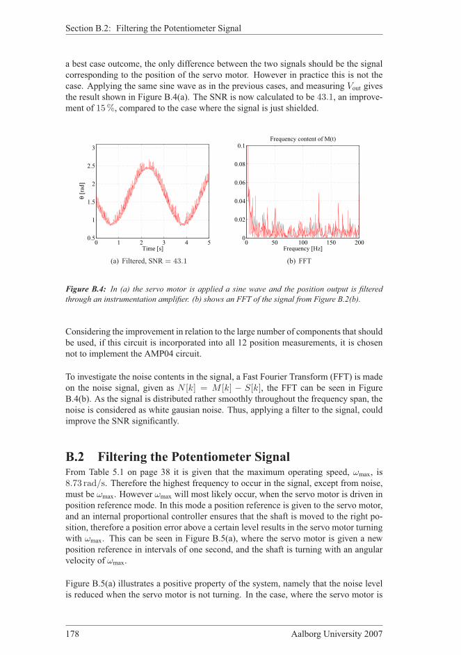
Section B.2: Filtering the Potentiometer Signal
a best case outcome, the only difference between the two signals should be the signal
corresponding to the position of the servo motor. However in practice this is not the
case. Applying the same sine wave as in the previous cases, and measuring Vout gives
the result shown in Figure B.4(a). The SNR is now calculated to be 43.1, an improve-ment of 15%, compared to the case where the signal is just shielded.
0 1 2 3 4 50.5
1
1.5
2
2.5
3
θ [
rad]
Time [s]
(a) Filtered, SNR = 43.1
0 50 100 150 2000
0.02
0.04
0.06
0.08
0.1Frequency content of M(t)
Frequency [Hz]
(b) FFT
Figure B.4: In (a) the servo motor is applied a sine wave and the position output is filtered
through an instrumentation amplifier. (b) shows an FFT of the signal from Figure B.2(b).
Considering the improvement in relation to the large number of components that should
be used, if this circuit is incorporated into all 12 position measurements, it is chosen
not to implement the AMP04 circuit.
To investigate the noise contents in the signal, a Fast Fourier Transform (FFT) is made
on the noise signal, given as N [k] = M [k] − S[k], the FFT can be seen in Figure
B.4(b). As the signal is distributed rather smoothly throughout the frequency span, the
noise is considered as white gausian noise. Thus, applying a filter to the signal, could
improve the SNR significantly.
B.2 Filtering the Potentiometer SignalFrom Table 5.1 on page 38 it is given that the maximum operating speed, ωmax, is
8.73 rad/s. Therefore the highest frequency to occur in the signal, except from noise,
must be ωmax. However ωmax will most likely occur, when the servo motor is driven in
position reference mode. In this mode a position reference is given to the servo motor,
and an internal proportional controller ensures that the shaft is moved to the right po-
sition, therefore a position error above a certain level results in the servo motor turning
with ωmax. This can be seen in Figure B.5(a), where the servo motor is given a new
position reference in intervals of one second, and the shaft is turning with an angular
velocity of ωmax.
Figure B.5(a) illustrates a positive property of the system, namely that the noise level
is reduced when the servo motor is not turning. In the case, where the servo motor is
178 Aalborg University 2007
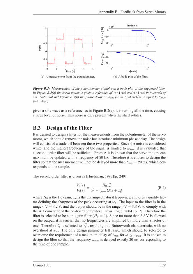
Appendix B: Feedback from Servo Motors
0 1 2 3 4 5−1
−0.5
0
0.5
1
1.5
θ [
rad]
Time [s]
(a) A measurement from the potentiometer.
100
101
−20
−10
0
x 10−3
Mag
nit
ude
[dB
]
Bode plot
100
101
−20
−10
0
Phas
e [d
eg]
ω [rad/s]
(b) A bode plot of the filter.
Figure B.5: Measurement of the potentiometer signal and a bode plot of the suggested filter.
In Figure B.5(a) the servo motor is given a reference of -π/4 rad and π/4 rad in intervals of
1 s. Note that ind Figure B.5(b) the phase delay at ωmax (ω = 8.73 rad/s) is equal to θdelay(−10 deg.).
given a sine wave as a reference, as in Figure B.2(a), it is turning all the time, causing
a large level of noise. This noise is only present when the shaft rotates.
B.3 Design of the FilterIt is desired to design a filter for the measurements from the potentiometer of the servo
motor, which should remove the noise but introduce minimum phase delay. The design
will consist of a trade off between these two properties. Since the noise is considered
white, and the highest frequency of the signal is limited to ωmax, it is evaluated that
a second order filter will be sufficient. From A it is known that the servo motors can
maximum be updated with a frequency of 50Hz. Therefore it is chosen to design the
filter so that the measurement will not be delayed more than tmax = 20ms, which cor-
responds to one sample.
The second order filter is given as [Huelsman, 1993][p. 249]:
Vo(s)
Vi(s)=
H0ω2n
s2 + (ωn/Q)s + ω2n
(B.4)
where H0 is the DC-gain, ωn is the undamped natural frequency, and Q is a quality fac-
tor defining the sharpness of the peak occurring at ωn. The input to the filter is in the
range 0V − 3.2V, and the output should be in the range 0V − 3.3V, to comply with
the AD converter of the on-board computer [Cirrus Logic, 2004][p. 7]. Therefore the
filter is selected to be a unit gain filter (H0 = 1). Since no more than 3.3V is allowed
on the output, it is crucial that no frequencies are amplified by more than a factor of
one. Therefore Q is selected to√
22 , resulting in a Butterworth characteristic, with no
overshoot at ωn. The only design parameter left is ωn, which should be selected to
overcome the requirement of a maximum delay of tmax for ω ≤ ωmax. It is chosen to
design the filter so that the frequency ωmax is delayed exactly 20ms corresponding to
the time of one sample.
Group 1033 179

Section B.3: Design of the Filter
A time delay for a certain frequency can be translated into a phase delay, θdelay:
θdelay = ωmaxtmax = 8.73 rad/s 20ms = 0.1746 rad (B.5)
which is approximately 10 deg. Substituting s = jω in Equation (B.4) gives:
Vo(jω)
Vi(jω)=
H0ω2n
(jω)2 + (ωn/Q)(jω) + ω2n
=H0ω
2n
ω2n − ω2 + j(ωn/Q)ω
(B.6)
inserting ω = ωmax and separating the real and imaginary part gives:
Vo(jω)
Vi(jω)=
H0ω2n (ω2
n − ωmax)
(ω2n − ω2
max)2 − ω2
maxω2n /Q2
− jH0ω
3n ωmax/Q
(ω2n − ω2
max)2 − ω2
maxω2n /Q2
(B.7)
and the phase delay of the filter at ω = ωmax can now be found as:
θdelay = arctan
(−H0ω
3n ωmax/Q
(ω2n−ω2
max)2−ω2
maxω2n /Q2
)
(H0ω2
n (ω2n−ωmax)
(ω2n−ω2
max)2−ω2
maxω2n /Q2
)
= atan
(−ωmaxωn/Q
ω2n − ω2
max
)
(B.8)
Which can be rewritten to:
0 = Q tan(θdelay)ω2n + ωmaxωn − ω2
maxQtan(θdelay) (B.9)
Solving this second order equation results in a natural undamped frequency of:
ωn = 71.06 rad/s (B.10)
Setting H0 = 1, Q =√
22 and ωn = 71.06 rad/s results in following filter:
Vo(s)
Vi(s)=
5050
s2 + 100.5s + 5050(B.11)
A bode plot of the filter can be seen in Figure B.5(b). Note that the phase delay at ωmax
is 10 deg.
0 1 2 3 4 5−1
−0.5
0
0.5
1
1.5
θ [
rad
]
Time [s]
Unfiltered signal
Filtered signal
Figure B.6: The measured signal before and after applying the filter implemented in MATLAB,
SNR = 146.9.
180 Aalborg University 2007

Appendix B: Feedback from Servo Motors
The filter is implemented in MATLAB, and the measured signal, illustrated in Figure
B.2(b), is passed through the filter. The result from this simulation can be seen in
Figure B.6, and as seen the filter removes a significant proportion of the noise. The
SNR is now found to be 146.9, which is a theoretical improvement of 294%. It could
be chosen to use this MATLAB implementation of the filter, and run it on the on-board
computer. It is however chosen to realize the filter in hardware, in order to ease the
burden on the computer. The next section will concern the realization of the filter.
B.4 Realization of the FilterIt is chosen to realize the filter as a Sallen and Key low-pass filter shown in Figure
B.7 [Huelsman, 1993][p. 252]. The filter in Equation (B.4) can be written as:
V2(s)
V1(s)=
KR1R3C2C4
s2 + s(
1R3C4
+ 1R1C2
+ 1R3C2
− KR3C4
)
+ 1R1R3C2C4
(B.12)
R3
V2
R1
V1
-
+
-
+K
C4
C2
Figure B.7: A low-pass Sallen and Key Filter.
Comparing Equation (B.4) and Equation (B.12) gives the following:
ωn =1√
R1R3C2C4
(B.13)
1
Q=
√
R3C4
R1C2
+
√R1C4
R3C2
+ (1−K)
√R1C2
R3C4
(B.14)
H0 = K (B.15)
As stated earlier the filter should be a unity gain filter, thus K = 1. Furthermore
two parameters are defined for the ratios of the resistor values and capacitor values
respectively:
n =R3
R1
, m =C4
C2
(B.16)
now Equation (B.13) and (B.14) becomes:
ωn =1√
mnR1C2
(B.17)
1
Q= (n + 1)
√m
n(B.18)
Group 1033 181

Section B.5: Conclusion on the Servo Motor Feedback
An expression for n can now be found to be [Huelsman, 1993][p. 254]:
n =
(1
2mQ2− 1
)
± 1
2mQ2
√
1− 4mQ2 (B.19)
From Equation (B.19) it can be seen that m ≤ 14Q2 . It is chosen to use m = 1
4Q2 ,
thus having a ratio of the capacitor values of m = 0.5. Inserting Q and m in Equation
(B.19), gives n = 1. Consequently the ratio of the resistor values is 1 (R1 = R2).
0 1 2 3 4 5−1
−0.5
0
0.5
1
1.5
θ [
rad]
Time [s]
Unfiltered signal
Filtered signal
(a) Sine wave input
0 1 2 3 4 5−1
−0.5
0
0.5
1
1.5
2
θ [
rad]
Time [s]
Unfiltered signal
Filtered signal
(b) Square wave input, SNR = 102.5
Figure B.8: Signal before and after the filter realized in hardware. In Figure B.8(a) a sine wave
is introduced, and in B.8(b) the input is the square wave signal introduced in Section B.2.
It is chosen that C2 = 0.1µF, since m = 0.5, C4 = 50nF. Inserting this in Equation
(B.17) together with the natural undamped frequency, ωn = 71.06 rad/s from Equation
(B.10), gives:
R1 = R3 =1√
mnωnC2
≈ 200 kΩ (B.20)
Now the circuit in Figure B.7 is realized and tested. The result from this test can be
seen in Figure B.8(a).
B.5 Conclusion on the Servo Motor FeedbackEven though the filter implemented in hardware is not as good as the filter tested in
MATLAB (Figure B.6), it still improves the signal. Compared to the unfiltered, the
SNR is improved from 37.3 to 102.5, an improvement of 175%. The implemented
filter is furthermore tested on the square wave signal, the result from this test kan be
seen in Figure B.8(b). Since there is less noise on this signal, the improvement is not
as distinct as for the sine wave. It can however be seen that the filter reduces some the
lager spikes. Particularly the spikes orcurring right after the reference goes high (at
time = 0.8 s, 2.8 s, 4.8 s) are removed.
To further emphasize the improvement an FFT is made on the filtered sine wave signal
and plotted in Figure B.9 together with the FFT on the unfiltered signal from Figure
182 Aalborg University 2007

Appendix B: Feedback from Servo Motors
0 50 100 150 2000
0.02
0.04
0.06
0.08
0.1Frequency content of M(t)
Frequency [Hz]
Unfiltered signal
Filtered signal
Figure B.9: An FFT on the unfiltered and the filtered measurement.
B.4(b). As seen the high frequency noise has been reduced significantly.
R3 VoutR1
-+C4
C2
Rp
VccInside servo
+-
Interface print
Figure B.10: The realization of the Sallen and Key filter, including the screened wire.
The total improvement made to the raw measurements, those of Figure B.2(a), is a
change of the SNR from 14.1 to 102.5 which is an improvement of 626.9%. The
final implementation of the Sallen and Key filter can be seen in Figure B.10, where it
is stressed out which part that is placed inside the servo motor, and which part on the
interface print. This circuit is applied for all 12 servo motors of the type HSR-5995TG.
Group 1033 183


CHARDWARE WIRING
DESCRIPTION
This appendix describes the wiring of the biped robot. This includes sensors, servo
motors, control signals and power wiring. The section is divided into three sections.
The first section describes the wiring of the two main switches located on the robot.
The second section concerns the wiring of the 21 servo motors located on the biped.
The third section concerns the wiring of the pressure sensors, the five DoF IMU, and
the 12 potentiometer feedback signals.
C.1 Wiring of the Main SwitchesTo be able to choose between being powered from an external PSU or from the battery
supply, two switches have been mounted on the robot. These switches also provide
the possibility of charging the two batteries located inside the robot by using the same
DC-connector that is used when running from the PSU. The placement of the DC-
connector can be seen in Figure C.2(a). A schematic showing the wiring of the main
Servo voltage supply
Battery 1
Battery 2
SW1
Charger/PSU
1
2
3
4
1
2
3
4
SW2a
SW2b
7A fuse
7A fuse
Onboard computer+ sensors 1.5A
fuse
1
1
2
2
Figure C.1: Schematic showing the wiring of the main power cords on the biped robot.
power cords can be seen in Figure C.1. Table C.1 shows the combination of the two
Group 1033 185

Section C.1: Wiring of the Main Switches
main switches; SW1 and SW2.
(a) DC-connectors (b) Main switches
Figure C.2: C.2(a) shows the placement of the DC-connector on the robot. This connector
is used to recharge the batteries located inside the robot, and is used as a connector for an
external power supply. C.2(a) shows the placement of the two main switches on the robot. The
on/off switch is referred to as SW2, and the circular switch is referred to as SW1.
It is important to note that a PSU never should be connected when the robot is in charg-
ing mode as this could damage the batteries and robot. The two switches SW2a and
SW2b, seen in Figure C.1, consist of a dual bipolar switch, meaning that SW2a and
SW2b are located in the same switch. Figure C.2 shows where the two switches are
mounted and where the positions of the switches are located.
To protect the batteries and other electronics located on the biped robot, three fuses
have been inserted. One fuse is inserted at each battery to protect these, and one has
been inserted to protect the on-board computer and the hardware interfacing the sen-
sors. Each battery is protected by a 7A fuse, and a 1.5A fuse is mounted to protect
the electronics. To identify the two batteries, these have been colour coded inside the
robot. The wire, marked with a green label is connected to battery one. This battery is
located closest to the front of the robot. The wire marked with a yellow label is battery
two. This battery is located closest to the back of the robot.
186 Aalborg University 2007

Appendix C: Hardware Wiring Description
SW1 SW2 Robot state
1 1 Robot OFF (Battery 1 ‖ battery 2)1 2 Robot ON -Running on battery (1 ‖ 2)2 1 Robot OFF
2 2 Robot ON -Running on PSU
3 1 Robot OFF -Charging battery 1
3 2 Robot ON -Running on battery 1
4 1 Robot OFF - Charging battery 2
4 2 Robot ON -Running on battery 2
Table C.1: Table showing all the switch combinations on the robot.
This concludes the description of the wiring of the main power cords inside the robot.
The following two sections describe the wiring of the servo motors and sensors located
on the robot.
C.2 Wiring of the 21 Servo MotorsThe 21 servo motors are controlled using three Pololu servo controllers
[Robotics and Electronics, 2005] as explained in Section 5.3.2 on page 37. Each of
the servo controllers are connected to their own serial port on the on-board computer.
Table C.2 shows how the 21 servos are connected to the three servo controllers.
Servo controller 1 Servo controller 2 Servo controller 3
Connector 0 Servo 7 Servo 13 Servo 6
Connector 1 Servo 8 Servo 14 Servo 5
Connector 2 Servo 9 Servo 15 Servo 4
Connector 3 Servo 10 Servo 16 Servo 3
Connector 4 Servo 11 Servo 17 Servo 2
Connector 5 Servo 12 Servo 18 Servo 1
Connector 6 Servo 21 Servo 19 N/C
Connector 7 N/C Servo 20 N/C
Table C.2: Connection of the 21 servos to the three servo controllers.
The servo controllers are located side by side in the order 1, 2, 3 from left to right.
To see where the servo motors are located on the robot, refer to Figure C.3. This
figure presents the naming convention for each servo motor. The servo controllers
are connected to the interface print as listed in Table C.3. The label J9 refers to the
specific connector located on the interface print, and pin refers to the specific pin in
that connector. See Figure C.4 on page 190 where the silk-layer for the interface print
can be found.
Servo Controller Logic level serial input Reset pin
1 (left) UART 1 (J9, Pin 3) J9, Pin 4
2 (middle) UART 2 (J9, Pin 2) J9, Pin 4
3 (right) UART 3 (J9, Pin 1) J9, Pin 4
Table C.3: The three servo controllers connection to the interface print.
Group 1033 187

Section C.3: Wiring of Sensors
s1s2
s3
s4
s5
s6
s7
s8 s9
s10
s11 s12
s21s13
s17
s18s19
s20
s14
s15s16
Figure C.3: Definition of servo names, where S is short servo.
The logic level serial input on the servo controller board is used to avoid having to
implement a level converter circuit. The reset pins are all connected to the same con-
nector on the interface print, to make it possible to reset all servo controllers at once.
Each servo controller is connected to their own serial port to increase the update rate
of each servo. In [Christensen et al., 2006] it was concluded that the maximum update
rate for each servo, when having 21, was limited to 37Hz due to the limited baud rateon the servo controller. By using three serial ports, it is possible to update the servo
position with a frequency of 50Hz, which is the internal update frequency of the servocontroller board.
C.3 Wiring of SensorsThis section describes how the following sensors are connected on the biped robot:
- 12 potentiometers; one from each servo in the legs.
- 6 strain gauges; three on each foot.
- 1 IMU with five DoF.
- 2 battery voltage monitors.
C.3.1 Potentiometer Signals
Inside the 12 servo motors in the legs, the potentiometer signal is taken directly and
then sent into an active low-pass filter. The filter is described in detail in Section B.2
on page 178. Table C.4 shows where each potentiometer signal is connected on the
interface print.
188 Aalborg University 2007
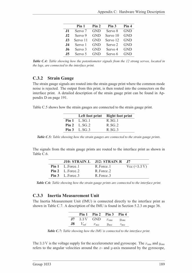
Appendix C: Hardware Wiring Description
Pin 1 Pin 2 Pin 3 Pin 4
J1 Servo 7 GND Servo 8 GND
J2 Servo 9 GND Servo 10 GND
J3 Servo 11 GND Servo 12 GND
J4 Servo 1 GND Servo 2 GND
J6 Servo 3 GND Servo 4 GND
J5 Servo 5 GND Servo 6 GND
Table C.4: Table showing how the potentiometer signals from the 12 strong servos, located in
the legs, are connected to the interface print.
C.3.2 Strain Gauge
The strain gauge signals are routed into the strain gauge print where the common mode
noise is rejected. The output from this print, is then routed into the connectors on the
interface print. A detailed description of the strain gauge print can be found in Ap-
pendix D on page 191.
Table C.5 shows how the strain gauges are connected to the strain gauge print.
Left foot print Right foot print
Pin 1 L SG 1 R SG 1
Pin 2 L SG 2 R SG 2
Pin 3 L SG 3 R SG 3
Table C.5: Table showing how the strain gauges are connected to the strain gauge prints.
The signals from the strain gauge prints are routed to the interface print as shown in
Table C.6.
J10: STRAIN L J12: STRAIN R J7
Pin 1 L Force 1 R Force 1 Vcc (+3.3V)Pin 2 L Force 2 R Force 2
Pin 3 L Force 3 R Force 3
Table C.6: Table showing how the strain gauge prints are connected to the interface print.
C.3.3 Inertia Measurement Unit
The Inertia Measurement Unit (IMU) is connected directly to the interface print as
shown in Table C.7. A description of the IMU is found in Section 5.2.3 on page 36.
Pin 1 Pin 2 Pin 3 Pin 4
J7 3.3V GND xrate yrateJ8 Vref xacc yacc zacc
Table C.7: Table showing how the IMU is connected to the interface print.
The 3.3V is the voltage supply for the accelerometer and gyroscope. The xrate and yraterefers to the angular velocities around the x- and y-axis measured by the gyroscope,
Group 1033 189
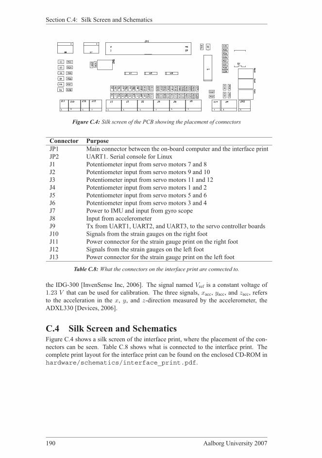
Section C.4: Silk Screen and Schematics
Figure C.4: Silk screen of the PCB showing the placement of connectors
Connector Purpose
JP1 Main connector between the on-board computer and the interface print
JP2 UART1. Serial console for Linux
J1 Potentiometer input from servo motors 7 and 8
J2 Potentiometer input from servo motors 9 and 10
J3 Potentiometer input from servo motors 11 and 12
J4 Potentiometer input from servo motors 1 and 2
J5 Potentiometer input from servo motors 5 and 6
J6 Potentiometer input from servo motors 3 and 4
J7 Power to IMU and input from gyro scope
J8 Input from accelerometer
J9 Tx from UART1, UART2, and UART3, to the servo controller boards
J10 Signals from the strain gauges on the right foot
J11 Power connector for the strain gauge print on the right foot
J12 Signals from the strain gauges on the left foot
J13 Power connector for the strain gauge print on the left foot
Table C.8: What the connectors on the interface print are connected to.
the IDG-300 [InvenSense Inc, 2006]. The signal named Vref is a constant voltage of
1.23 V that can be used for calibration. The three signals, xacc, yacc, and zacc, refersto the acceleration in the x, y, and z-direction measured by the accelerometer, the
ADXL330 [Devices, 2006].
C.4 Silk Screen and SchematicsFigure C.4 shows a silk screen of the interface print, where the placement of the con-
nectors can be seen. Table C.8 shows what is connected to the interface print. The
complete print layout for the interface print can be found on the enclosed CD-ROM in
hardware/schematics/interface_print.pdf.
190 Aalborg University 2007
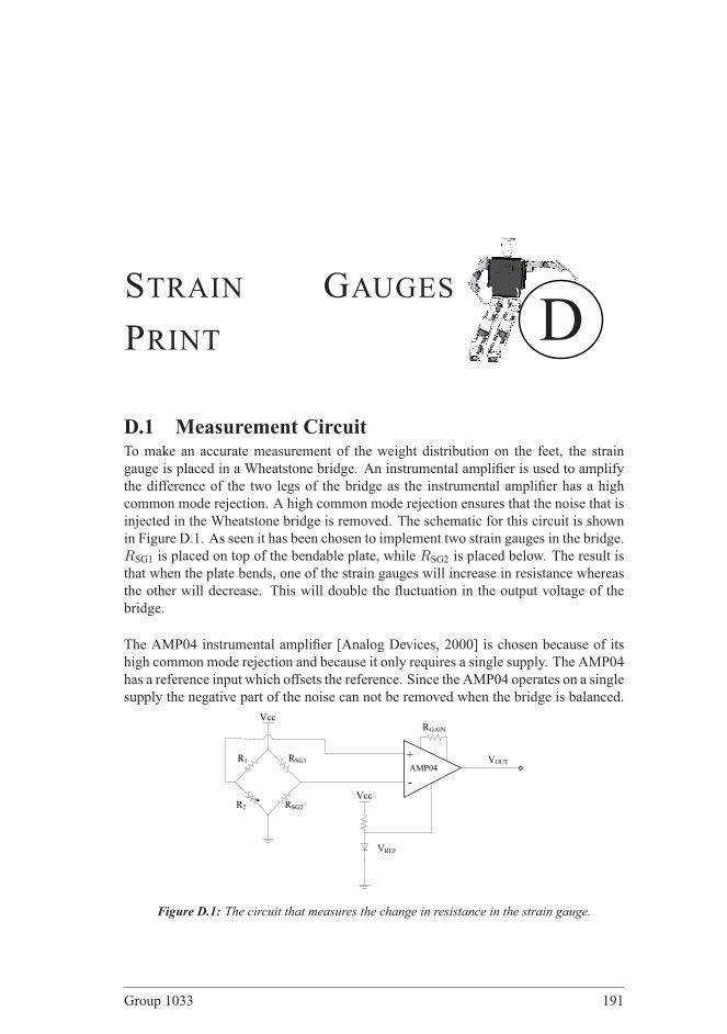
DSTRAIN GAUGES
D.1 Measurement CircuitTo make an accurate measurement of the weight distribution on the feet, the strain
gauge is placed in a Wheatstone bridge. An instrumental amplifier is used to amplify
the difference of the two legs of the bridge as the instrumental amplifier has a high
common mode rejection. A high common mode rejection ensures that the noise that is
injected in the Wheatstone bridge is removed. The schematic for this circuit is shown
in Figure D.1. As seen it has been chosen to implement two strain gauges in the bridge.
RSG1 is placed on top of the bendable plate, while RSG2 is placed below. The result is
that when the plate bends, one of the strain gauges will increase in resistance whereas
the other will decrease. This will double the fluctuation in the output voltage of the
bridge.
The AMP04 instrumental amplifier [Analog Devices, 2000] is chosen because of its
high common mode rejection and because it only requires a single supply. The AMP04
has a reference input which offsets the reference. Since the AMP04 operates on a single
supply the negative part of the noise can not be removed when the bridge is balanced.
R2
R1 RSG1AMP04
RGAIN
+
-
VREF
Vcc
VOUT
Vcc
RSG2
Figure D.1: The circuit that measures the change in resistance in the strain gauge.
Group 1033 191

Section D.1: Measurement Circuit
To avoid this the reference input is used. Using a diode the reference is set to 0.7Vwhich is considered to be enough to cover injected noise.
The strain gauges, that will be used in the force distribution sensing system (FDSS),
have a nominal resistance of 120 Ω and in order to balance the bridgeR1 andR2 are set
to 120 Ω. However it can not be guaranteed that the strain gauges keep their nominalresistance after they have been attached to a strain plate. To remedy this, R2 is made
adjustable so the bridge can be balanced after assembly of the foot. Supplying the
bridge with 5V, like with the on-board computer, it will draw approximately 42mA.Each foot will have three off these circuits, and the task of determining the force exerted
on one foot therefore requires a minimum 126mA. This is considered too much and thebridge and AMP04 is instead supplied with 3.3 V and the required current is reduced to
3(3.3V/120Ω) = 82.5mA for each foot. Decreasing the current flowing through the
bridge also decreases the sensitivity, as the voltage difference between the two sides
of the bridge is proportional to the current. This can be remedied by increasing the
amplification in the AMP04. Determining the amplification requires that the mass
to voltage change is known, which means determining the change in resistance of
the strain gauges when a mass is placed on the strain plate. Figure D.2 shows the
dimensions of the strain plate, on which a test is carried out. In the test a piece of
spring steel, 1mm thick, with the same dimensions as shown in Figure D.2 is mounted
such that it is able to bend freely. A strain gauge is attached to the plate and a mass
is placed on the pressure point and the change in resistance is recorded. In the test a
weight of 0.5 kg was placed on the pressure point which gave a change in resistance of∆R0.5 kg = 0.073Ω. The slope ∆Ω/∆mload is considered constant and determining
the maximum change in resistance can be found to:
∆Ωmax =mmin,meas
0.5 kgR0.5 kg = 0.38 Ω (D.1)
where mmin,meas is the maximum weight that the strain plate should be exposed to,
which was determined in Section 4.5 on page 27 to be 2.5 kg. Equation (D.2) stemsfrom [Serway and Beichner, 2000, pp. 889] and can be used to determine the voltage
difference of the Wheatstone bridge when ∆Ωmax is present in the circuit.
∆Vmax =( RSG1
RSG2 + RSG1− R2
R1 + R2
)
Vs (D.2)
∆Vmax =( 119.62 Ω
119.62 Ω + 120.38 Ω− 120 Ω
120 Ω + 120 Ω
)
3.3V = −5.19mV
(D.3)
As it is the difference that is amplified the output of the AMP04 can not exceed what is
the largest difference between the legs of the bridge which is Vmax = Vs−Vref = 2.6V.This means that the gain that should be used in the AMP04 can be determined to:
G =∣∣∣
Vmax
∆Vmax
∣∣∣ ≈ 500 (D.4)
From the data sheet [Analog Devices, 2000] for the AMP04 the gain can be set by the
following relation:
G =100 kΩ
RGAIN
(D.5)
From the above equation RGAIN is determined to 200 Ω.
192 Aalborg University 2007

Appendix D: Strain Gauges Print
Strain gauge
Line at whichthe plate bends
Pressure point20mm
Figure D.2: The middle strain plate on the foot.
0 0.2 0.4 0.6 0.8 1 1.20
0.2
0.4
0.6
0.8
1
Weight [kg]
Voltage [V]
y = 1.011 x − 0.079
MeasurementsFitted line
Figure D.3: The measured data from the FDSS along with the fitted line.
D.2 Testing the FDSSThe FDSS is subjected to a series of different masses in order to determine the transfer
function. Figure D.3 shows the measured data, the line that has been fitted to the data
and the transfer function which has be estimated.
The maximum weight that can be measured can be determined to:
mmax,meas =Vmax
1.0112= 2.57 kg (D.6)
mmax,meas is larger than the required minimum, mmin,meas, that the FDSS was designed
to measure. In the previous section the gain for the AMP04 was determined using a
test setup where a strain gauge was attached to 1mm spring steel. The strain gauges
have been attached manually meaning that the strain gauges will not have the same
characteristics after assembly. This is properly the cause of the deviation.
D.3 Implementing the FDSSA circuit was designed which implements the FDSS. The circuit is small enough to fit
on the foot and the signal can sampled directly by the ADC on the on-board computer.
Tests showed that when the FDSS was not mounted on the robot the noise never ex-
ceeded ±25mV and additional filtering of the signal was deemed unnecessary. How-
Group 1033 193

Section D.3: Implementing the FDSS
ever when the FDSS was implemented on the robot the noise reached ±275mV at a
frequency of 91 kHz. This is most likely caused by the power electronics in the servomotors since the signal wires from the FDSS run alongside the servo motors in the
legs. Implementing a filter should therefore be considered.
194 Aalborg University 2007
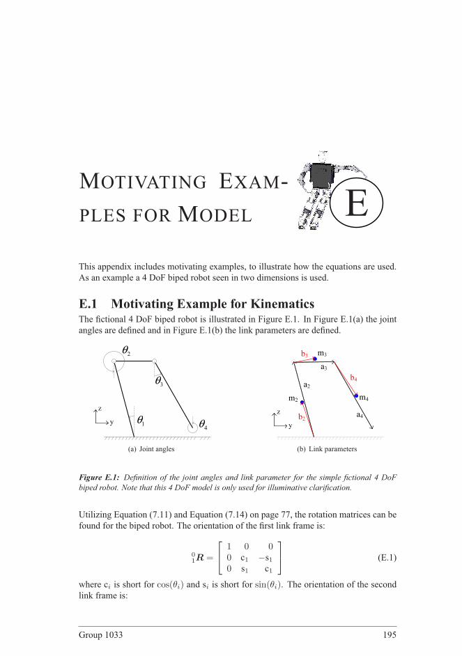
EMOTIVATING EXAM-
PLES FOR MODEL
This appendix includes motivating examples, to illustrate how the equations are used.
As an example a 4 DoF biped robot seen in two dimensions is used.
E.1 Motivating Example for KinematicsThe fictional 4 DoF biped robot is illustrated in Figure E.1. In Figure E.1(a) the joint
angles are defined and in Figure E.1(b) the link parameters are defined.
1θ
2θ
3θ
4θy
z
(a) Joint angles
y
z
a2
a3
a4b2
b3
b4
m4m2
m3
(b) Link parameters
Figure E.1: Definition of the joint angles and link parameter for the simple fictional 4 DoF
biped robot. Note that this 4 DoF model is only used for illuminative clarification.
Utilizing Equation (7.11) and Equation (7.14) on page 77, the rotation matrices can be
found for the biped robot. The orientation of the first link frame is:
01R =
1 0 00 c1 −s10 s1 c1
(E.1)
where ci is short for cos(θi) and si is short for sin(θi). The orientation of the secondlink frame is:
Group 1033 195

Section E.1: Motivating Example for Kinematics
02R =
1 0 00 c1c2 − s1s2 −c1s2 − s1c2
0 s1c2 − c1s2 −s1s2 + c1c2
(E.2)
and of orientation of the third link frame is:
0
3R =
1 0 00 (c1c2 − s1s2)c3 − (c1s2 + s1c2)s3 (s1s2 − c1c2)s3 − (c1s2 + s1c2)c3
0 (s1c2 − c1s2)c3 − (s1s2 − c1c2)s3 (c1s2 − s1c2)s3 − (s1s2 − c1c2)c3
(E.3)
The generalized position vector can now be found if the rotation matrices and link
parameters are combined as stated in Equation (7.20) and Equation (7.21). Since no
movement in the x-direction is present in the motivating example no contribution inthis direction is included in q,q and q:
q =
c1b2y − s1b2z−s1a2z + c1+2b3y − s1+2b3z
−s1a2z + c1+2a3y + c1+2+3b4y − s1+2+3b4zs1b2y + c1b2z
c1a2z + s1+2b3y + c1+2b3zc1a2z + s1+2a3y + s1+2+3b4y + c1+2+3b4z
θ1
θ2
θ3
θ4
(E.4)
where there has be further simplifications in form of c1+2 which is equal to cosθ1+θ2.
This simplification will be used in this example where necessary. Now the generalized
velocity can be found from Equation (7.22):
q =
−s1θ1b2y − c1θ1b2z
−c1θ1a2z − s1+2b3y θ1 − s1+2b3y θ2 − c1+2b3z θ1 − c1+2b3z θ2
−c1θ1a2z − s1+2a3y θ1 − s1+2a3y θ2 − s1+2+3b4y θ1 − s1+2+3b4y θ2
−s1+2+3b4y θ3 − c1+2+3b4z θ1 − c1+2+3b4z θ2 − c1+2+3b4z θ3
c1θ1b2y − s1θ1b2z
−s1θ1a2z + c1+2b3y θ1 + c1+2b3y θ2 − s1+2b3z θ1 − s1+2b3z θ2
−s1θ1a2z + c1+2a3y θ1 + c1+2a3y θ2 + c1+2+3b4y θ1 + c1+2+3b4y θ2
+c1+2+3b4y θ3 − s1+2+3b4z θ1 − s1+2+3b4z θ2 − s1+2+3b4z θ3
θ1
θ2
θ3
θ4
(E.5)
Also the generalized acceleration can be found from Equation (7.22):
196 Aalborg University 2007

Appendix E: Motivating Examples for Model
q =
−c1θ21b2y − s1θ1b2y + s1θ2
1b2z − c1θ1b2z
s1θ21a2z − c1θ1a2z − b3y θ
21c1+2 − b3y θ1s1+2 − 2 b3y θ1θ2c1+2 − b3y θ
22c1+2
−b3y θ2s1+2 + b3z θ21s1+2 − b3z θ1c1+2 + 2 b3z θ1θ2s1+2 + b3z θ
22s1+2 − b3z θ2c1+2
−b4y θ21c1+2+3 − b4y θ1s1+2+3 − b4y θ
22c1+2+3 − b4y θ2s1+2+3
−b4y θ3s1+2+3 − b4y θ23c1+2+3 − a3y θ
21c1+2 − a3y θ1s1+2 − a3y θ
22c1+2 − a3y θ2s1+2
−2 a3y θ1θ2c1+2 + 2 b4z θ3θ2s1+2+3 + 2 b4z θ3θ1s1+2+3 + 2 b4z θ1θ2s1+2+3
+b4z θ22s1+2+3 + b4z θ
21s1+2+3 − b4z θ1c1+2+3 − b4z θ2c1+2+3
+b4z θ23s1+2+3 − 2 b4y θ1θ2c1+2+3 − 2 b4y θ3θ2c1+2+3 − 2 b4y θ3θ1c1+2+3
−b4z θ3c1+2+3 + s1θ21a2z − c1θ1a2z
−s1θ21b2y + c1θ1b2y − c1θ2
1b2z − s1θ1b2z
−c1θ21a2z − s1θ1a2z − b3y θ
21s1+2 + b3y θ1c1+2 − 2 b3y θ1θ2s1+2 − b3y θ
22s1+2
+b3y θ2c1+2 − b3z θ21c1+2 − b3z θ1s1+2 − 2 b3z θ1θ2c1+2 − b3z θ
22c1+2 − b3z θ2s1+2
−2 b4y θ3θ1s1+2+3 − 2 b4y θ1θ2s1+2+3 − b4y θ22s1+2+3
−b4y θ21s1+2+3 − 2 b4y θ3θ2s1+2+3 − b4y θ
23s1+2+3 + b4y θ2c1+2+3 + b4y θ1c1+2+3
+b4y θ3c1+2+3 − 2 b4z θ1θ2c1+2+3 − 2 b4z θ3θ1c1+2+3 − b4z θ1s1+2+3
−b4z θ22c1+2+3 − 2 a3y θ1θ2s1+2 − b4z θ2s1+2+3 − b4z θ3s1+2+3 − b4z θ
23c1+2+3
−2 b4z θ3θ2c1+2+3 − c1θ21a2z − s1θ1a2z − a3y θ
21s1+2 + a3y θ1c1+2
−a3y θ22s1+2 + a3y θ2c1+2 − b4z θ
21c1+2+3
θ1
θ2
θ3
θ4
(E.6)
As seen in Equation (E.4), (E.5) and (E.6) the expressions quickly becomes very large,
even for this simple example-robot with 3 links. Because of this rapidly expansion it
was chosen to show the derivation of the kinematic model, with this example, while it
also has be conducted for the real model.
The deviation of q, q and q is done in Maple. Afterward Maple can generate MATLAB
code, and write to a m-file.
E.2 Motivating Example for DynamicsTo illustrate the approach used to calculate the dynamical model for the 21 joint bipedrobot, a motivating example is given, using a simple 3 link and 4 joint robot previouslyexplained in Section E.1 on page 195. The example is calculated with right foot as base
frame and thereby the torque τR is calculated. The calculations for τL are not shown.
As the motivating example from Section E.1 on page 195 does not contain any foot
links, the linear force, described in Section 7.4.3 on page 83, which needs to be added
in the DSP has no link to be attached to. Therefore a virtual foot link is attached to the
4 DoF biped robot example. This virtual link has zero mass, zero length and therefore
zero inertia. The position of the virtual foot links are shown in Figure E.2.
Because of the two extra links, q changes dimensions from 1 × 10 to 1 × 14 thereby
making the biped robot a 5 link 4 joint robot. Now the calculations for the example can
be initiated and first the energy of the 4 DoF biped robot has to be calculated to derive
the Lagrangian. The kinetic energy is given by Equation (7.35) using the CoM of
each link (found in the motivating example in Section E.1 on page 195)and the angular
Group 1033 197

Section E.2: Motivating Example for Dynamics
yz
m1=0
m2
m3
m4
m5=0
Figure E.2: Virtual links of the simple 4 DoF biped robot.
velocity given by Equation (7.36). The calculated kinetic energy is see from Equation
(E.7):
KR =1
2m2
(
y2
2 + z2
2
)
+1
2θ2
1 I2x +1
2m3
(
y2
3 + z2
3
)
+1
2
(
θ1 + θ2
)2
I3x (E.7)
+1
2
(
y2
4 + z2
4
)
m4 +1
2
(
θ1 + θ2 + θ3
)2
I4x
Now the potential energy P is calculated using Equation (7.37).
PR = −m2gz2 −m3gz3 −m4gz4 (E.8)
The Lagrangian is calculated as LR = KR−PR. The Lagrangian is differentiated with
respect to the generalized coordinates q = [y,z,θ]T and this yields:
∂LR
∂q=
000000
−m2g
−m3g
−m4g
00000
(E.9)
To get the second term of Equation (7.33) the Lagrangian is differentiated with respect
to the generalized velocities q = [y, z, θ]T, which yields:
∂LR
∂q=
00
m2y2
m3y3
m4y4
00
m2z2
m3z3
m4z4
0
θ1I2x +(
θ1 + θ2
)
I3x +(
θ1 + θ2 + θ3
)
I4x(
θ1 + θ2
)
I3x +(
θ1 + θ2 + θ3
)
I4x(
θ1 + θ2 + θ3
)
I4x
0
(E.10)
198 Aalborg University 2007

Appendix E: Motivating Examples for Model
Then the derivative of the Lagrangian with respect to the generalized velocities is dif-
ferentiated with respect to time, which yields:
∂
∂t
∂LR
∂q=
0m2y2
m3y3
m4y4
00
m2z2
m3z3
m4z4
0
θ1I2x +(
θ1 + θ2
)
I3x +(
θ1 + θ2 + θ3
)
I4x(
θ1 + θ2
)
I3x +(
θ1 + θ2 + θ3
)
I4x(
θ1 + θ2 + θ3
)
I4x
0
(E.11)
Now the generalized forces in Cartesian coordinates can be calculated by taking Equa-
tion (E.9) and then subtract Equation (E.11). This yields:
FR =
0−m2y2
−m3y3
−m4y4
00
−m2g−m2z2
−m3g−m3z3
−m4g−m4z4
0
−θ1I2x −(
θ1 + θ2
)
I3x −(
θ1 + θ2 + θ3
)
I4x
−(
θ1 + θ2
)
I3x −(
θ1 + θ2 + θ3
)
I4x
−(
θ1 + θ2 + θ3
)
I4x
0
(E.12)
To map the generalized forces to joint space, the Jacobian has to be calculated. By
using Equation (7.41) the Jacobian can be calculated, and this yields:
JR = [JR1,JR2] (E.13)
Where JR1 and JR2 are the components of JR, which has been split.
JR1 =
0 00 0
−s1b2y − c1b2z 0−c1a2z − s1+2b3y − c1+2b3z −s1+2b3y − c1+2b3z
−c1a2z − s1+2a3y − s1+2+3b4y − c1+2+3b4z −s1+2a3y − s1+2+3b4y − c1+2+3b4z−c1a2z − s1+2a3y − c1+2+3a4z −s1+2a3y − c1+2+3a4z
0 0c1b2y − s1b2z 0
−s1a2z + c1+2b3y − s1+2b3z c1+2b3y − s1+2b3z−s1a2z + c1+2a3y + c1+2+3b4y − s1+2+3b4z c1+2a3y + c1+2+3b4y − s1+2+3b4z
−s1a2z + c1+2a3y − s1+2+3a4z c1+2a3y − s1+2+3a4z
1 00 10 00 0
(E.14)
Group 1033 199

Section E.2: Motivating Example for Dynamics
JR2 =
0 00 00 00 0
−s1+2+3b4y − c1+2+3b4z 0−c1+2+3a4z 0
0 00 00 0
c1+2+3b4y − s1+2+3b4z 0−s1+2+3a4z 0
0 00 01 00 1
(E.15)
The torque in joint space is now calculated using Equation (7.40) and this yields:
τR =
−I3x θ1 − I3x θ2 − I4x θ2 − I4x θ3 − I4x θ1 + m4y4s1+2a3y −m3c1+2b3yg+m3y3s1+2b3y + m3y3c1+2b3z + m2y2s1b2y + m2y2c1b2z + m3y3c1a2z
+m4y4c1a2z − c1b2ym2g− θ1I2x −m4c1+2+3b4yg−m4c1+2+3b4y z4 + m4s1+2+3b4zg+m4s1+2+3b4z z4 + m4y4s1+2+3b4y + m4y4c1+2+3b4z −m3c1+2b3y z3 + m3s1+2b3zg+m3s1+2b3z z3 −m4c1+2a3yg−m4c1+2a3y z4 − c1b2ym2z2 + s1b2zm2g + s1b2zm2z2
+s1a2zm3g + s1a2zm3z3 + s1a2zm4g + s1a2zm4z4
−I3x θ1 − I3x θ2 − I4x θ2 − I4x θ3 − I4x θ1 + m4y4s1+2a3y −m3c1+2b3yg+m3y3s1+2b3y + m3y3c1+2b3z −m4c1+2+3b4yg−m4c1+2+3b4y z4 + m4s1+2+3b4zg+m4s1+2+3b4z z4 + m4y4s1+2+3b4y + m4y4c1+2+3b4z −m3c1+2b3y z3 + m3s1+2b3zg
+m3s1+2b3z z3 −m4c1+2a3yg−m4c1+2a3y z4
m4y4s1+2+3b4y + m4y4c1+2+3b4z −m4c1+2+3b4yg−m4c1+2+3b4y z4
+m4s1+2+3b4zg + m4s1+2+3b4z z4 − I4x θ1 − I4x θ2 − I4x θ3
0
(E.16)
Notice in Equation (E.16), which is only valid in SSP-R, that the torque on the fourth
joint is always zero. This is an effect of the virtual joint added, which has no mass.
Now the model for the SSP-R is given by Equation (E.16), and the model for the DSP
phase is calculated. For simplification only the term ρRJTR (fSSP-R + ζRρRmtotg) of
Equation (7.45) is calculated as the calculations for when the left foot is base frame is
identical.
y
z
fN-L
f2
f3
f4
Figure E.3: Ground reaction force added to the virtual link.
First the force fN-L, depicted in Figure E.3, needs to be calculated. This yields:
fN-L = ρRmtotg = ρRg (m2 + m3 + m4) (E.17)
Now ρL is calculated using Equation (7.52). The distance ∆yf between the feet inthe frontal direction can be calculated using the generalized positions calculated in the
200 Aalborg University 2007
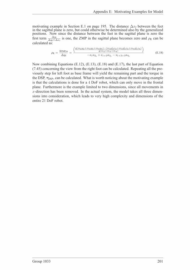
Appendix E: Motivating Examples for Model
motivating example in Section E.1 on page 195. The distance ∆xf between the feetin the sagittal plane is zero, but could otherwise be determined also by the generalizedpositions. Now since the distance between the feet in the sagittal plane is zero the
first term ∆yf∆yf+∆xf
is one, the ZMP in the sagittal plane becomes zero and ρR can be
calculated as:
ρR =yZMP,m
∆yf=
(g(m2y2+m3y3+m4y4)−(m2y2z2+m3y3z3+m4y4z4)
g(m2+m3+m4)
)
−s1a2z + c1+2a3y − s1+2+3a4z
(E.18)
Now combining Equations (E.12), (E.13), (E.18) and (E.17), the last part of Equation
(7.45) concerning the view from the right foot can be calculated. Repeating all the pre-
viously step for left foot as base frame will yield the remaining part and the torque in
the DSP, τDSP, can be calculated. What is worth noticing about the motivating example
is that the calculations is done for a 4 DoF robot, which can only move in the frontal
plane. Furthermore is the example limited to two dimensions, since all movements in
x-direction has been removed. In the actual system, the model takes all three dimen-sions into consideration, which leads to very high complexity and dimensions of the
entire 21 DoF robot.
Group 1033 201


FMODELING
VERIFICATION
F.1 Introduction to Model VerificationIn this section the verification of all sub-models is described. First a short introduc-
tion to the approach used to verify the models is given. Then each model is verified
individually and last a verification of the complete model is given.
F.1.1 Model Verification Approach
The goal of the model verification is to verify the complete model, consisting of a
number of sub-models. In order to do so, each sub-model has to be verified individu-
ally. To conduct a verification of a model, real data must be available for comparison.
As the inputs and outputs of all sub-models can not be measured in the real system,
some models are used in the verification of other sub-model. This way inputs that can
be applied to the systems and outputs that can be measured are achieved. The model
dependency is seen from Figure F.1, where the order of verification is also seen. Next
a short introduction to the different verification steps is given.
First the verification of the servo motor model is conducted. This is done by apply-
ing different loads to a real servo motor, introducing a step on the input and then by
reading the potentiometer output, giving the position of the servo. This measurement
can then be compared with the servo motor model when applying equal load and input
reference. A more thorough description of the test is given in Section F.2 on page 205,
where the results of the test also can be seen.
Next the foot model is verified. This is done in a test setup were different weights can
be mounted on the actual foot. Then the position of the weights is altered to apply dif-
ferent torques and forces to the foot. The output of the strain gauges is then measured.
Applying the same torques and forces to the foot model, should then give the same
output. This test can be seen in Section F.3 on page 207.
Group 1033 203

Section F.1: Introduction to Model Verification
Foot Model Kinematic Model
Dynamical Model
Head Model
Complete Model
Servo Motor Model
Figure F.1: The verification of some models depend on others, which is illustrated in this figure
together with the order of the test verification.
Afterward the kinematic model is verified. To do so, extra test output from the real
system has to be constructed. These are achieved by mounting an extra accelerometer
in each foot, which are only used for test purpose. Now an input to the robot is given,
such that each leg by turn moves the foot up and away from zero position. The input is
constructed in such a way that the influence from the dynamics of the system is mini-
mized. The acceleration in all three axis is then measured. The same input is given to
the model, and the output acceleration from the model is compared to the output of the
accelerometers from the robot. As the acceleration is the double differentiated of the
position, the kinematic model is considered verified if the accelerations are consistent.
A further description of the test and the results can be seen in Section F.4 on page 212.
As the kinematic model can be considered verified at this stage, this can be used to
verify the model of the head. An input with the same characteristics as used for the
kinematic model verification is constructed, and thereby minimizing the dynamical in-
fluence on the system. Then the angular velocity and acceleration of the IMU located
in the head are measured and compared with the output of the head model. This can be
seen in Section F.5 on page 218.
The last sub-model to be verified is the dynamical model. This test is conducted last
as it relies on the verification of the servo motor model, the foot model and the kine-
matic model. The test is divided into two parts, one verifying the dynamics of the legs
and one verifying the dynamics of the upper body including the arms. For the first
test, concerning the legs, an input is constructed which emphasize the dynamics of the
systems. Even though this input should reveal the system dynamics it must still be
constructed in such a way that it can be applied to the real system and still maintain
a stable position. As the real system is most stable in DSP, this phase is used to test
204 Aalborg University 2007
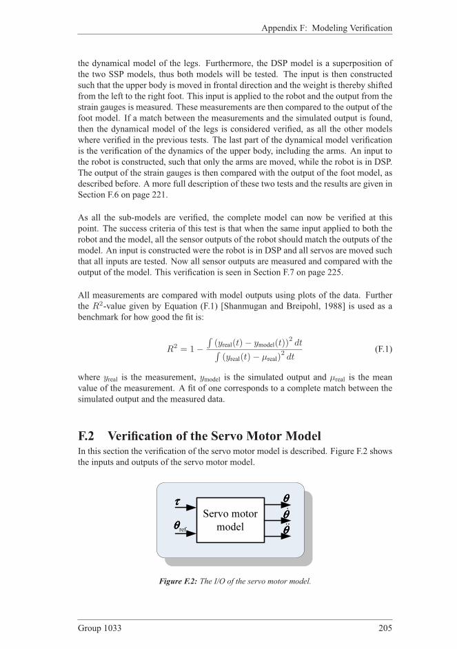
Appendix F: Modeling Verification
the dynamical model of the legs. Furthermore, the DSP model is a superposition of
the two SSP models, thus both models will be tested. The input is then constructed
such that the upper body is moved in frontal direction and the weight is thereby shifted
from the left to the right foot. This input is applied to the robot and the output from the
strain gauges is measured. These measurements are then compared to the output of the
foot model. If a match between the measurements and the simulated output is found,
then the dynamical model of the legs is considered verified, as all the other models
where verified in the previous tests. The last part of the dynamical model verification
is the verification of the dynamics of the upper body, including the arms. An input to
the robot is constructed, such that only the arms are moved, while the robot is in DSP.
The output of the strain gauges is then compared with the output of the foot model, as
described before. A more full description of these two tests and the results are given in
Section F.6 on page 221.
As all the sub-models are verified, the complete model can now be verified at this
point. The success criteria of this test is that when the same input applied to both the
robot and the model, all the sensor outputs of the robot should match the outputs of the
model. An input is constructed were the robot is in DSP and all servos are moved such
that all inputs are tested. Now all sensor outputs are measured and compared with the
output of the model. This verification is seen in Section F.7 on page 225.
All measurements are compared with model outputs using plots of the data. Further
the R2-value given by Equation (F.1) [Shanmugan and Breipohl, 1988] is used as a
benchmark for how good the fit is:
R2 = 1−∫
(yreal(t)− ymodel(t))2dt
∫(yreal(t)− µreal)
2dt
(F.1)
where yreal is the measurement, ymodel is the simulated output and µreal is the mean
value of the measurement. A fit of one corresponds to a complete match between the
simulated output and the measured data.
F.2 Verification of the Servo Motor ModelIn this section the verification of the servo motor model is described. Figure F.2 shows
the inputs and outputs of the servo motor model.
Servo motor model θθθθɺɺ
θθθθɺθθθθ
refθθθθ
ττττ
Figure F.2: The I/O of the servo motor model.
Group 1033 205

Section F.2: Verification of the Servo Motor Model
As seen the servo motor model takes a vector containing references to all servos, θref,
and a vector denoting the load torque on each servo, τ , as input. It returns the angular
position, θ, angular velocity, θ, and angular acceleration θ of each servo.
F.2.1 Servo Motor Model Test Setup
To verify the model, a number of test is performed. The servo motor is exposed to step
from 0 rad to 2.1 rad, and is exposed to a load given as:
τi = mi g l cos (θi − 1.05) (F.2)
where l is the length of the arm, which is 19.5mm, θi is the angle of the servo motor,
mi is a mass suspended in a wire in the end of the arm, and g is the gravity acceleration.Three tests are performed, where different masses are chosen m1 = 0, m2 = 2.383 kgand m3 = 4.557 kg. This corresponds to a load torque of:
τ1 = 0Nm (F.3)
τ2 = 0.456 sin(θi − 1.05)Nm (F.4)
τ3 = 0.873 sin(θi − 1.05)Nm (F.5)
It should be noted that two different type of servo’s are located on the robot, and a
model is derived for both of them. Therefore, this test will include a verification of
both models.
F.2.2 Servo Motor Model Test Results
In Figure F.3 the raw measurements from these three tests are plotted.
0 0.1 0.2 0.3 0.4 0.5 0.6 0.7 0.8 0.9−0.5
0
0.5
1
1.5
2
2.5
θ [rad]
Time [s]
τ1, measured, 0 kg
τ2, measured, 2.383 kg
τ3, measured, 4.557 kg
simulated
Figure F.3: Comparison between measurements and simulated data for three different loads, on
the HSR-5995TG
Furthermore a simulation is performed on the implemented servo motor model, which
is exposed to the same three loads. The result of this simulation can be seen in Figure
F.3 as the three black lines. The same procedure is taken for the HS-645MG servo
motor, and similar result are obtained which can be seen in Figure F.4.
The normed error can be seen in Table F.1.
F.2.3 Servo Motor Model Test Discussion
It can be seen that the output of the simulation fits the measured data, with a 0.924to 0.999 fit of the R2-value, for both servos. The measurement in Figure F.4 is more
206 Aalborg University 2007

Appendix F: Modeling Verification
0 0.1 0.2 0.3 0.4 0.5 0.6 0.7 0.8 0.9−0.5
0
0.5
1
1.5
2
2.5
θ [rad]
Time [s]
τ1, measured, 0 kg
τ2, measured, 2.383 kg
τ3, measured, 4.557 kg
simulated
Figure F.4: Comparison between measurements and simulated data for three different loads, on
the HS-645MG.
R2τ1
R2τ2
R2τ3
HSR-5995TG 0.999 0.998 0.997HS-645MG 0.936 0.937 0.924
Table F.1: Calculated R2-value of the servo motor model test.
noisy than that of Figure F.3, this is because the HS-645MG is weaker, and τ3 is close
to the maximum load for this servo.
F.2.4 Servo Motor Model Test Conclusion
Due to a model fit lying between 0.924 and 0.937 for the HS-645MG and between
0.997 and 0.999 for the HSR-5995TG, it is concluded that both models are sufficientlyaccurate for the purpose of this thesis. The models are now considered verified.
F.3 Verification of the Foot ModelIn this section the verification of the foot model documented. The derivation of the
model is explained in Section 7.6.
footfττττ
Foot modelf
Figure F.5: Inputs and output of the foot model. Input is the force and torques acting on the foot
from the last joint of the leg. Output is the force acting on the strain gauges.
As it can be seen from Figure F.5 the inputs to the foot model are the torques, τ , and
force, f , acting in the ankle joint. The output is the forces measured by the three
strain gauges, ffoot = [fS1 fS2 fS3]T As the torques and force applied to the foot cannot
be measured on the robot, a construction has to made which applies different known
torques and forces to the foot.
Group 1033 207

Section F.3: Verification of the Foot Model
F.3.1 Foot Model Test Setup
As the foot consists of three different spring steel plates mounted in such a way that
the foot forces can be measured in different positions, the test setup is made such that
different forces and torques can be applied. The test setup is seen from Figure F.6. It
is seen that a rod is connected to a servo motor mounted in a servo bracket. Different
weights can be applied with variable distance to the center of rotation of the rod. When
the servo motor starts rotating, the position of the weight changes, thereby making dif-
ferent forces and torques acting in the ankle.
Test one
Test two
x
y
z
(a) Top view
Weights are applied here
x y
z
(b) Seen the left
Figure F.6: F.6(a) shows the movement seen from the top, F.6(b) shows the placement of the
weights from the left.
The strain gauges are initially calibrated to zero, when the test setup is mounted, with-
out any weights. This ensures that only the forces and torques from the weight is
included in the measurements. Using Newtons second law, the force acting on the foot
can be calculated. Knowing the force and the position of the weight, the torque in the
frontal and sagittal direction can be calculated. Next is a description of the different
tests conducted to verify the foot model:
1. Place a 60 g weight at the outer-most position of the rod, namely 55mm. Then
rotate the rod, using the servo motor, 360 deg clockwise until reaching initial
position. Then turn the rod counter clockwise 360 deg until initial position is
reached again. This test is repeated for 160 g and 260 g weights.
2. The first test are repeated changing only the position of the weight to 41mm.
The input to the model is the torque around the x and y-axis, τx and τy , and the force inz-direction, fz. These are calculated from the weights and the position of the weights,
and is shown in Figure F.7.
The numeration of the strain gauges located on the foot is as shown in Figure F.8.
Next the results from the foot model test is described.
F.3.2 Foot Model Test Results
Output of the model and the measured data can be seen from Figure F.9.
208 Aalborg University 2007

Appendix F: Modeling Verification
0 50 100 150 200−0.2
0
0.2Input torque around the x−direction to the foot model test
τ x [Nm]
0 50 100 150 200−0.2
0
0.2Input torque around the y−direction to the foot model test
τ x [Nm]
0 50 100 150 2000
1
2
3Input force in z−direction to the foot model test
Fz [N]
Time [s]
Figure F.7: Input used in the foot model test.
Figure F.8: Numeration of the strain gauges on the foot.
Group 1033 209

Section F.3: Verification of the Foot Model
0 50 100 150 200−5
0
5Force on strain gauge one
FS1 [N]
0 50 100 150 200−2
0
2
4Force on strain gauge two
FS2 [N]
0 50 100 150 200−5
0
5Force on strain gauge three
Time [s]
FS3 [N]
Measured
Simulated
Figure F.9: Results from the verification of the foot model. The blue lines are the measured
output of the strain gauges on the real foot. The red lines are the output of the model. The
uppermost figure is the output from strain gauge one, the middle is the output from strain gauge
two and the lowest is the output from strain gauge three.
R2S1 R2
S2 R2S3
0.782 0.432 0.652
Table F.2: Calculated R2-value of the foot model test.
The calculated R2-value, using Equation (F.1), can be seen in Table F.2
F.3.3 Foot Model Test Discussion
As it can be seen from Table F.2 the calculated error percentage reveals a mismatch
between the model and the measured data. The calculated error is the largest on strain
gauge two. The main reason for the relatively large deviation of the modeling of strain
gauge two is the the phase lag between the model and measurements. This phase lag
is also seen from the error measured on strain gauge three, but is not as distinct on the
error measured on strain gauge one.
From Figure F.9 it is seen that there are several discontinuities in both the measure-
ments and in the output from the model. These discontinuities are caused by the way
the inputs are fused together, e.g. when there is a sudden change in the weight applied
the force acting on the system change abrupt. This phenomenon is also seen from the
created input shown in Figure F.7.
In Figure F.9 it looks like the model do not reach the same amplitudes as the real sys-
tem. This is because the point where the force and torques are applied is directly above
the point where strain gauge two is positioned, in the y-direction. Thereby τx has noeffect on this strain gauge. This can however never be the case in the real world, since
it is not possible to place the point exactly. A problem like this can be amplified fur-
210 Aalborg University 2007
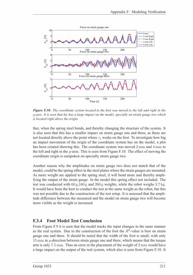
Appendix F: Modeling Verification
0 50 100 150 200−5
0
5
10Force on strain gauge one
FS1 [N]
0 50 100 150 200−2
0
2
4Force on strain gauge two
FS2 [N]
0 50 100 150 200−5
0
5Force on strain gauge three
Time [s]
FS3 [N]
0 mm
2 mm Right
4 mm Right
2 mm Left
4 mm Left
Figure F.10: The coordinate system located in the foot was moved to the left and right in the
y-axis. It is seen that his has a large impact on the model, specially on strain gauge two which
is located right above the origin.
ther, when the spring steel bends, and thereby changing the structure of the system. It
is also seen that this has a smaller impact on strain gauge one and three, as these are
not located directly above the point where τy works on the foot. To investigate how big
an impact movement of the origin of the coordinate system has on the model, a plot
has been created showing this. The coordinate system was moved 2mm and 4mm to
the left and right in the y-axis. This is seen from Figure F.10. The effect of moving the
coordinate origin is outspoken on specially strain gauge two.
Another reason why the amplitudes on strain gauge two does not match that of the
model, could be the spring effect in the steel plates where the strain gauges are mounted.
As more weight are applied to the spring steel, it will bend more and thereby ampli-
fying the output of the strain gauge. In the model this spring effect not included. The
test was conducted with 60 g,160 g and 260 g weights, while the robot weighs 3.7 kg.It would have been the best to conduct the test at the same weight as the robot, but this
was not possible due to the construction of the test setup. It is assessed that the ampli-
tude difference between the measured and the model on strain gauge two will become
more visible as the weight is increased.
F.3.4 Foot Model Test Conclusion
From Figure F.9 it is seen that the model tracks the input changes in the same manner
as the real system. Due to the construction of the foot the R2-value is best on strain
gauge one and three. It should be noted that the width of the foot is small, with only
15mm in y-direction between strain gauge one and three, which means that the torquearm is only 7.5mm. Thus an error in the placement of the weight of 2mm would have
a large impact on the output of the real system, which also is seen from Figure F.10. It
Group 1033 211
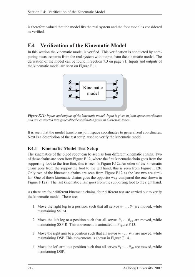
Section F.4: Verification of the Kinematic Model
is therefore valued that the model fits the real system and the foot model is considered
as verified.
F.4 Verification of the Kinematic ModelIn this section the kinematic model is verified. This verification is conducted by com-
paring measurements from the real system with output from the kinematic model. The
derivation of the model can be found in Section 7.3 on page 71. Inputs and outputs of
the kinematic model are seen on Figure F.11.
Kinematic model
q
θθθθɺɺθθθθɺθθθθ
qɺɺ
qɺ
Figure F.11: Inputs and outputs of the kinematic model. Input is given in joint space coordinates
and are converted into generalized coordinates given in Cartesian space.
It is seen that the model transforms joint space coordinates to generalized coordinates.
Next is a description of the test setup, used to verify the kinematic model.
F.4.1 Kinematic Model Test Setup
The kinematics of the biped robot can be seen as four different kinematic chains. Two
of these chains are seen from Figure F.12, where the first kinematic chain goes from the
supporting foot to the free foot, this is seen in Figure F.12a.An other of the kinematic
chain goes from the supporting foot to the left hand, this is seen from Figure F.12b.
Only two of the kinematic chains are seen from Figure F.12 as the last two are simi-
lar. One of these kinematic chains goes the opposite way compared the one shown in
Figure F.12a). The last kinematic chain goes from the supporting foot to the right hand.
As there are four different kinematic chains, four different test are carried out to verify
the kinematic model. These are:
1. Move the right leg to a position such that all servos θ1 . . . θ6 are moved, while
maintaining SSP-L.
2. Move the left leg to a position such that all servos θ7 . . . θ12 are moved, while
maintaining SSP-R. This movement is animated in Figure F.13.
3. Move the right arm to a position such that all servos θ13 . . . θ16 are moved, while
maintaining DSP. This movements is shown in Figure F.14.
4. Move the left arm to a position such that all servos θ17 . . . θ20 are moved, while
maintaining DSP.
212 Aalborg University 2007

Appendix F: Modeling Verification
yz
xb)a)
Figure F.12: Two of the four kinematic chains are seen from this figure. a) The kinematic chain
of the legs and the positioning of the extra accelerometer mounted on the feet. b) The kinematic
chain of the arms and the positioning of the accelerometer mounted in the hands.
Figure F.13: Animation of the movements of the left leg used in the verification of the kinematic
model. The five figures above show the movements in the sagittal plane, while the five figures
below show the movements in the frontal plane. The span of the test is 10 s
Group 1033 213
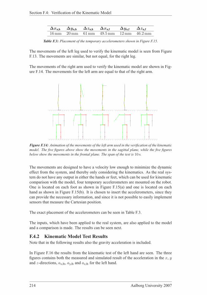
Section F.4: Verification of the Kinematic Model
∆xa,h ∆ya,h ∆za,h ∆xa,f ∆ya,f ∆za,f16mm 20mm 61mm 49.5mm 12mm 46.2mm
Table F.3: Placement of the temporary accelerometers shown in Figure F.15.
The movements of the left leg used to verify the kinematic model is seen from Figure
F.13. The movements are similar, but not equal, for the right leg.
The movements of the right arm used to verify the kinematic model are shown in Fig-
ure F.14. The movements for the left arm are equal to that of the right arm.
Figure F.14: Animation of the movements of the left arm used in the verification of the kinematic
model. The five figures above show the movements in the sagittal plane, while the five figures
below show the movements in the frontal plane. The span of the test is 10 s.
The movements are designed to have a velocity low enough to minimize the dynamic
effect from the system, and thereby only considering the kinematics. As the real sys-
tem do not have any output in either the hands or feet, which can be used for kinematic
comparison with the model, four temporary accelerometers are mounted on the robot.
One is located on each foot as shown in Figure F.15(a) and one is located on each
hand as shown in Figure F.15(b). It is chosen to insert the accelerometers, since they
can provide the necessary information, and since it is not possible to easily implement
sensors that measure the Cartesian position.
The exact placement of the accelerometers can be seen in Table F.3.
The inputs, which have been applied to the real system, are also applied to the model
and a comparison is made. The results can be seen next.
F.4.2 Kinematic Model Test Results
Note that in the following results also the gravity acceleration is included.
In Figure F.16 the results from the kinematic test of the left hand are seen. The three
figures contains both the measured and simulated result of the acceleration in the x, yand z-directions, ax,lh, ay,lh and az,lh for the left hand.
214 Aalborg University 2007

Appendix F: Modeling Verification
faz ,∆
fax ,∆
fay ,∆
y
z
x
y
zx
(a) Top view
y
z
x x y
z
hax ,∆
haz ,∆
hay ,∆
(b) Seen the left
Figure F.15: Positioning of the temporary mounted accelerometers. F.15(a) Position on the left
foot. Right foot is the same, where the accelerometer is positioned on the outer right side on the
foot. F.15(b) Position of the accelerometer mounted on the right arm. The position of the left
arm is similar.
0 1 2 3 4 5 6 7 8 9 10−20
−10
0
10Acceleration of the left hand,x−direction
a x,lh [m/s2]
0 1 2 3 4 5 6 7 8 9 10−10
0
10Acceleration of the left hand, y−direction
a y,lh [m/s2]
0 1 2 3 4 5 6 7 8 9 10−10
0
10
20Acceleration of the left hand, z−direction
a z,lh [m/s2]
Time [s]
Measured
Simulated
Figure F.16: Result of the kinematic test of the left hand. The blue line is the measured output
of the accelerometer and the red line is the output from the model.
Group 1033 215

Section F.4: Verification of the Kinematic Model
0 1 2 3 4 5 6 7 8 9 10−20
−10
0
10Acceleration of the right hand, x−direction
a x,rh [m/s2]
0 1 2 3 4 5 6 7 8 9 10−10
0
10Acceleration of the right hand, y−direction
a y,rh [m/s2]
0 1 2 3 4 5 6 7 8 9 10−10
0
10
20Acceleration of the right hand, z−direction
Time [s]
a z,rh [m/s2]
Measured
Simulated
Figure F.17: Result of the kinematic test of the right hand. The blue line is the measured output
of the accelerometer and the red line is the output from the model.
R2ax
R2ay
R2az
Left hand 0.924 0.816 0.864Right hand 0.916 0.762 0.903Left foot 0.136 0.821 0.559Right foot 0.170 0.879 0.672
Table F.4: Calculated R2-value of the kinematic model test.
In Figure F.17 the results from the kinematic test of the right hand are seen. The threefigures contains both the measured and simulated result of the acceleration in the x, yand z-directions, ax,rh, ay,rh and az,rh for the right hand.
In Figure F.18 the results from the kinematic test of the left foot are seen. The threefigures contains both the measured and simulated result of the acceleration in the x, yand z-directions, ax,lf, ay,lf and az,lf for the left foot.
In Figure F.19 the results from the kinematic test of the right foot are seen. The threefigures contains both the measured and simulated result of the acceleration in the x, yand z-directions, ax,rf, ay,rf and az,rf for the right foot.
F.4.3 Kinematic Model Test Discussion
From Table F.4 it can be seen that the calculated R2 values of the test reveal a good fitbetween the simulated outputs and the measurements. Only R2
ax,lfand R2
ax,rf, are some-
what smaller than the rest of the calculated fits. The error is however not caused tobad fit, but rather to a bad selection of the input. This is evident from the top graphin Figures F.18 and F.19, where it can be seen that the measured ax,lf and ax,lf havesmaller amplitudes. The R2 values tends to be small, if the deflection from the meanis small. This is the case in the mentioned situations.
216 Aalborg University 2007

Appendix F: Modeling Verification
3 4 5 6 7 8 9 10 11 12 13−5
0
5
10Acceleration of the left leg, x−direction
a x,lf [m/s2]
3 4 5 6 7 8 9 10 11 12 13−5
0
5
10Acceleration of the left leg, y−direction
a y,lf [m/s2]
3 4 5 6 7 8 9 10 11 12 130
10
20Acceleration of the left leg, z−direction
Time [s]
a z,lf [m/s2]
Measured
Simulated
Figure F.18: Result of the kinematic test of the left foot. The blue line is the measured output of
the accelerometer and the red line is the output from the model.
0 1 2 3 4 5 6 7 8 9 10−20
0
20Acceleration of the right leg, x−direction
a x,rf [m/s2]
0 1 2 3 4 5 6 7 8 9 10−10
0
10
20Acceleration of the right leg, y−direction
a y,rf [m/s2]
0 1 2 3 4 5 6 7 8 9 10−20
0
20
40Acceleration of the right leg, z−direction
Time [s]
a z,rf [m/s2]
Measured
Simulated
Figure F.19: Result of the kinematic test of the right foot. The blue line is the measured output
of the accelerometer and the red line is the output from the model.
Group 1033 217

Section F.5: Verification of the Head Model
Furthermore, it is seen from Figure F.16, F.17, F.18 and F.19 that all measurementshave relatively large noise contributions in periods. This is most significant duringmovement, where the movements of the servo motors is to fast which introduces largeaccelerations, which is not presented in the model. As the internal controller only con-tains a proportional gain, there is no integration of the error which makes the controlof the position imprecise. This is a general problem of the servos and is more evidentthe heavier they are loaded.
What should be noticed is that the tests shows the acceleration of the limbs, rather thanshowing the actual position. For two reasons it is assessed that the error in acceler-ation would be somewhat larger than the actual error in position. The first reason isthat the acceleration is the double differentiated of the position, and this differentiationwould give errors from measuring the actual position. The second reason is that sincethe accelerometer measures the acceleration from gravity, a small initial tilt in the po-sitioning of the accelerometer would result in an offset error when the limbs reachesfinal position. Such an offset error has a large influence on the calculated R2 values.
F.4.4 Kinematic Model Test Conclusion
From Figure F.16, F.17, F.18, F.19 and the calculated R2 values shown in Table F.4 itis seen that the kinematic model gives a good estimate of the actual accelerations ofthe limps of the robot. As it gives a good acceleration fit it can be concluded that theposition estimate would be good as well. It can thereby be concluded that the kinematicmodel estimates the positions and accelerations of the limbs of the robot.
F.5 Verification of the Head ModelIn this section the verification of the head model is given. The head model was earlierderived in Section 7.7. This model gives an estimate of the output of the IMU sensorlocated in the head of the robot. The inputs and outputs of the head model are seenfrom Figure F.20
Head model
q
qɺɺ
qɺ
headωωωω
heada
Figure F.20: Inputs and outputs of the head model.
The head model returns the linear acceleration, ahead, and angular velocity,ωhead, of thehead, when given the generalized position vector, q, the generalized velocity vector,q, and the generalized acceleration vector, q, as input. As the generalized positions,velocities and accelerations are output from the kinematic model, this model is used toverify the head model.
218 Aalborg University 2007
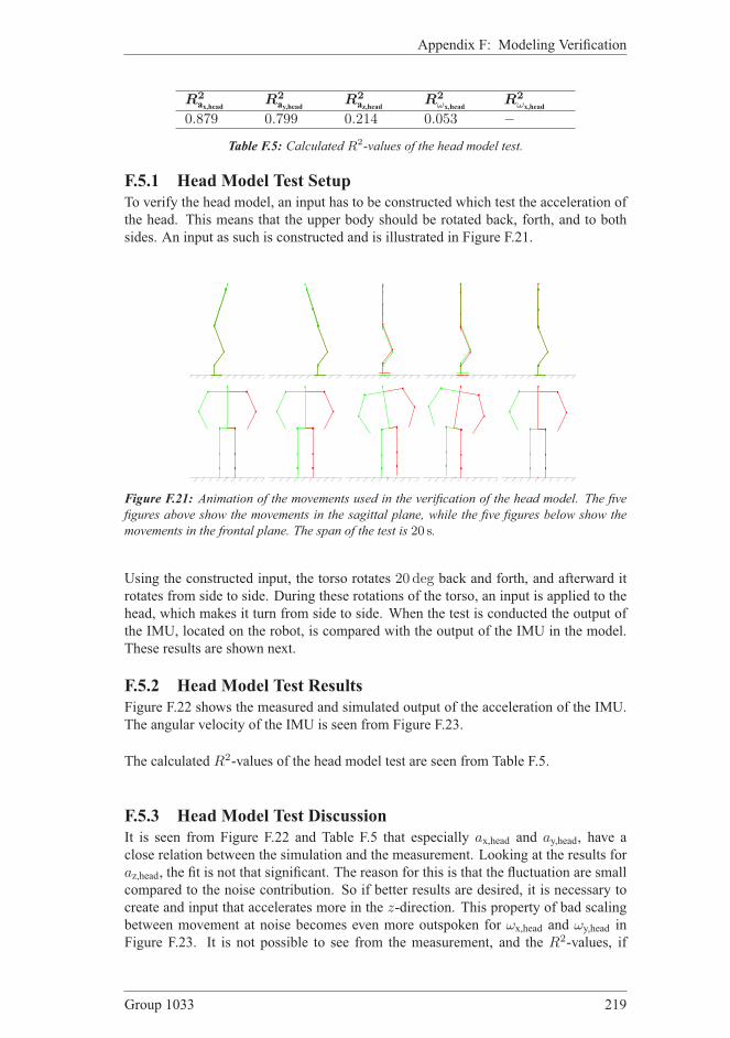
Appendix F: Modeling Verification
R2ax,head
R2ay,head
R2az,head
R2ωx,head
R2ωx,head
0.879 0.799 0.214 0.053 −Table F.5: Calculated R2-values of the head model test.
F.5.1 Head Model Test Setup
To verify the head model, an input has to be constructed which test the acceleration ofthe head. This means that the upper body should be rotated back, forth, and to bothsides. An input as such is constructed and is illustrated in Figure F.21.
Figure F.21: Animation of the movements used in the verification of the head model. The five
figures above show the movements in the sagittal plane, while the five figures below show the
movements in the frontal plane. The span of the test is 20 s.
Using the constructed input, the torso rotates 20 deg back and forth, and afterward itrotates from side to side. During these rotations of the torso, an input is applied to thehead, which makes it turn from side to side. When the test is conducted the output ofthe IMU, located on the robot, is compared with the output of the IMU in the model.These results are shown next.
F.5.2 Head Model Test Results
Figure F.22 shows the measured and simulated output of the acceleration of the IMU.The angular velocity of the IMU is seen from Figure F.23.
The calculated R2-values of the head model test are seen from Table F.5.
F.5.3 Head Model Test Discussion
It is seen from Figure F.22 and Table F.5 that especially ax,head and ay,head, have aclose relation between the simulation and the measurement. Looking at the results foraz,head, the fit is not that significant. The reason for this is that the fluctuation are smallcompared to the noise contribution. So if better results are desired, it is necessary tocreate and input that accelerates more in the z-direction. This property of bad scalingbetween movement at noise becomes even more outspoken for ωx,head and ωy,head inFigure F.23. It is not possible to see from the measurement, and the R2-values, if
Group 1033 219

Section F.5: Verification of the Head Model
2 4 6 8 10 12 14 16 18−5
0
5Acceleration of the head in x−direction
a x,head [m/s2]
2 4 6 8 10 12 14 16 18−5
0
5Acceleration of the head in y−direction
a y,head [m/s2]
2 4 6 8 10 12 14 16 188
10
12Acceleration of the head in z−direction
Time [s]
a z,head [m/s2]
Measured
Simulated
Figure F.22: The measured and simulated acceleration of the head.
2 4 6 8 10 12 14 16 18−1
−0.5
0
0.5
1Angular velocity of the head around the x−axis
ωx,head [rad/s]
2 4 6 8 10 12 14 16 18−1
−0.5
0
0.5Angular velocity of the head around the y−axis
Time [s]
ωy,head [rad/s]
Measured
Simulated
Figure F.23: The measured and simulated angular velocity of the head.
220 Aalborg University 2007

Appendix F: Modeling Verification
the model is correct. The problem with the low signal values is a trade-off, since itis desired to apply mush faster input to the robot, to really stimulate the dynamics ofthe system. But if this done, the robot would not be able to maintain stability withouthuman interference.
F.5.4 Head Model Test Conclusion
Based on the test results, it is concluded that the head model is correct. This is entirelybased on the output of the accelerometer, since it is not possible to conclude anythingbased on the measurements of the angular velocity. The low R2-values of the angu-lar velocity is however, assigned a bad input rather than a bad model. Based on theknowledge that ahead and ωhead are calculated from the the same rotation matrices, it isvalued that the entire model is correct. The head model is now considered verified.
F.6 Verification of the Dynamical ModelIn this section, the dynamical model is verified. The description of the derivation of themodel can be found in Section 7.4 on page 79. The inputs and outputs of the dynamicmodel is seen from Figure F.24.
Dynamical model
q
qɺɺ
qɺττττ
f
Figure F.24: Input/output relation of the dynamical model
As it can be seen,the input to the dynamical model is the generalized coordinate vector,q, velocity vector, q, and acceleration vector, q, while the outputs are the torques, τ ,and forces, f , working in each joint. These forces and torques can not be measureddirectly on the robot, and the dynamical model therefore has to be validated throughother models. As the forces acting on the feet are measured through the strain gauges,these can be used to verify the dynamical properties of the system. Therefore thefoot model is included in the verification of the dynamical model. As the input to thedynamical model is the generalized coordinates the kinematic model is included in theverification to transform the joint coordinates. The servo motor model is also includedin the test of the dynamical model, since the calculated torque is used for feedback tothe servo motors, and thereby having an effect on the dynamical properties.
F.6.1 Dynamical Model Test Setup
The test is divided into two sub-tests, as it is assessed that the dynamical movement ofall limbs at one time can be difficult to see on the output of the strain gauges. Thereforethe dynamical properties of the arms and of the legs are tested separately. When testingthe legs, an input must be constructed in such a way, that the system maintain stabilityduring the test. To obtain the best stability the robot must be in DSP. An input is then
Group 1033 221

Section F.6: Verification of the Dynamical Model
constructed which shifts the weight from left to right foot. The test input is illustratedin Figure F.25. The input is applied to both the model and the real system. Output fromthe strain gauges is compared.
Figure F.25: Animation of the movements used in the verification of the dynamical model of
the legs. The five figures above show the movements in the sagittal plane, while the five figures
below show the movements in the frontal plane. The span of the test is 20 s.
Another input is created, which should verify the dynamical changes in the arms. Thisinput is illustrated in Figure F.26. As for the leg test, the output of the strain gauges iscompared for the dynamical test of the arms.
Figure F.26: Animation of the movements used in the verification of the dynamical model of
the arms. The five figures above show the movements in the sagittal plane, while the five figures
below show the movements in the frontal plane. The span of the test is 10 s.
Next the results of the test is given.
F.6.2 Dynamical Model Test Results
Figure F.27 and F.28 show the output of the strain gauges for the dynamical test of thelegs.
222 Aalborg University 2007
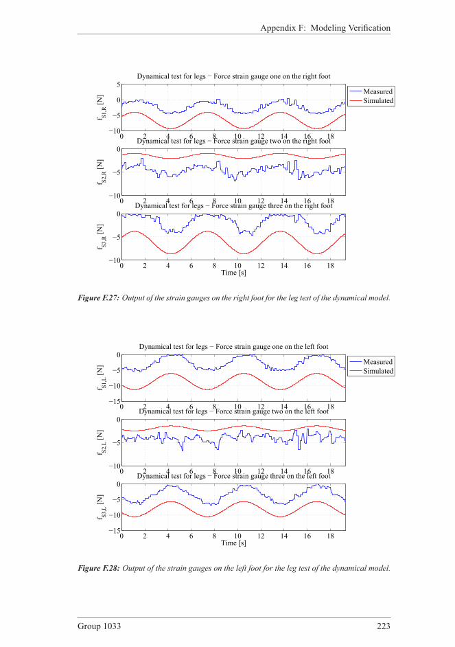
Appendix F: Modeling Verification
0 2 4 6 8 10 12 14 16 18−10
−5
0
5Dynamical test for legs − Force strain gauge one on the right foot
f S1,R [N]
0 2 4 6 8 10 12 14 16 18−10
−5
0Dynamical test for legs − Force strain gauge two on the right foot
f S2,R [N]
0 2 4 6 8 10 12 14 16 18−10
−5
0Dynamical test for legs − Force strain gauge three on the right foot
Time [s]
f S3,R [N]
Measured
Simulated
Figure F.27: Output of the strain gauges on the right foot for the leg test of the dynamical model.
0 2 4 6 8 10 12 14 16 18−15
−10
−5
0Dynamical test for legs − Force strain gauge one on the left foot
f S1,L [N]
0 2 4 6 8 10 12 14 16 18−10
−5
0Dynamical test for legs − Force strain gauge two on the left foot
f S2,L [N]
0 2 4 6 8 10 12 14 16 18−15
−10
−5
0Dynamical test for legs − Force strain gauge three on the left foot
f S3,L [N]
Time [s]
Measured
Simulated
Figure F.28: Output of the strain gauges on the left foot for the leg test of the dynamical model.
Group 1033 223

Section F.6: Verification of the Dynamical Model
In Figure F.29 and F.30 the output of the strain gauges is shown for the dynamical testof the arms.
0 2 4 6 8 10 12 14 16 18−10
−5
0
Dynamical test for arms − Force strain gauge one on the right foot
f S1,R [N]
0 2 4 6 8 10 12 14 16 18−10
−5
0
Dynamical test for arms − Force strain gauge two on the right foot
f S2,R [N]
0 2 4 6 8 10 12 14 16 18−10
−5
0
Dynamical test for arms − Force strain gauge three on the right foot
Time [s]
f S3,R [N]
Measured
Simulated
Figure F.29: Output of the strain gauges on the right foot for the arm test of the dynamical
model.
F.6.3 Dynamical Model Test Discussion
As can be seen in Figure F.29, F.30, F.27 and F.28 the results from the two tests of thedynamical model are not very good. There are some trends which match between themodel and the measurements, but generally there is not very good consistency. Thereare several reasons for this, the first thing to notice is that on some of the measurementsthere are higher amplitudes than on the output from the model. This larger amplitudeis caused by the bending of the spring steel, on which the strain gauges are mounted.As the arms move forward the weight of the robot makes the spring steel bend further,and thereby amplifying the output of the strain gauges. This property was also seen inthe test of the foot model described in Section F.3.
Furthermore large ripples are presented throughout the measured signals. The reasonfor this, is that when moving the robot, the servos get heavier loaded and thereforehave a harder time keeping the right position. This is seen as shaking of the robotwhen moving and have a large impact on the output of the strain gauges, as the shakingis amplified by the spring effect of the strain gauge plates. The levels, or the meansvalues, of the measurements and the model does not fit either, this partly caused bythe backlash, which makes the robot turn forward, and thereby completely changingthe pressure distribution under the feet. An other reason is the small feet, because thepressure distribution is highly dependent on the placement of the feet. When haven
224 Aalborg University 2007

Appendix F: Modeling Verification
0 2 4 6 8 10 12 14 16 18−10
−5
0
Dynamical test for arms − Force strain gauge one on the left foot
f S1,L [N]
0 2 4 6 8 10 12 14 16 18−10
−5
0
Dynamical test for arms − Force strain gauge two on the left foot
f S2,L [N]
0 2 4 6 8 10 12 14 16 18−10
−5
0
Dynamical test for arms − Force strain gauge three on the left foot
Time [s]
f S3,L [N]
Measured
Simulated
Figure F.30: Output of the strain gauges of the left foot for the arm test of the dynamical model.
these dissimilarities in the levels, it makes no sense to calculate the error percentage.
Even though the levels and the fluctuations does not match, it is clearly seen that thatthere is a relationship between the output of the model and the measurements, theyhave the same characteristics.
F.6.4 Dynamic Model Test Conclusion
The results of the dynamic model test are varying in success. However having theseunmodeled bendable plates under the feet, it is impossible to obtain better results.Based on the fact that the dynamical model is verified through three other models withtheir own limitations, and taking all the uncertainties into consideration, the dynamicalmodel is considered good for the purpose and scope of this project. But if a exactdescription of the system is desired, it is clear from this test, that it is necessary toinclude the bendable plates under the feet in the model.
F.7 Verification of the Complete ModelIn this section the complete model is verified. This is done by comparing the outputof the complete model with the sensor output of the real system, given the same input.The model contains all sub-models and the input and outputs are as shown i FigureF.31.
Input to the system and model for this test is the positions joint angle vector, θ, and theoutput are the positions of the servos in the legs, θleg, the acceleration and rotation ofthe head, ahead and ωhead, and the force acting on the strain gauges, ffeet. Next the testsetup is described.
Group 1033 225

Section F.7: Verification of the Complete Model
CompleteModelrefθθθθ
feetf
heada
headωωωω
legsθθθθ
Figure F.31: Input and outputs of the complete model.
F.7.1 Complete Model Test Setup
To verify the complete model an input must be created, which ensures that a noticeablefluctuation is seen on all measured output of both the model and the real system. At thesame time, the input must be created in such way that the real robot is stable withouthuman interference. This last requirement limits the possible input trajectories to onlyinclude those in DSP. Movements in forward direction are limited, as this would causethe robot to fall. Therefore an input is created which moves the torso in the sagittalplane. Further more the arms are moved in all directions while the head is turned fromside to side. Thereby are all servos actuated. The test is conducted for 30 s, but the first5 s is discarded as settle time. The movements of the robot are illustrated in Figure F.32.
Figure F.32: Animation of the movements of the robot used in the verification of the complete
model. The five figures above show the movements in the sagittal plane, while the five figures
below show the movements in the frontal plane. The span of the test is 20 s, but here is shownthe movements of the first 10 s as these are repeated in the last 10 s.
Next the results of the complete test are shown.
F.7.2 Complete Model Test Results
There are four outputs from the complete test. These are the servo motor positions, theoutput of the strain gauges, the acceleration of the head and the angular velocity. The
226 Aalborg University 2007
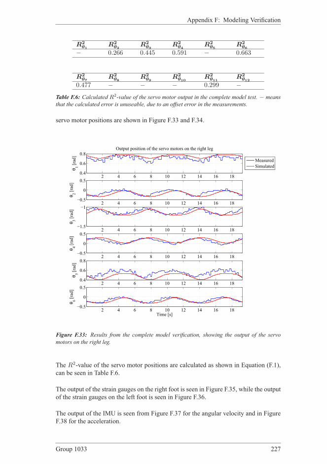
Appendix F: Modeling Verification
R2θ1
R2θ2
R2θ3
R2θ4
R2θ5
R2θ6
− 0.266 0.445 0.591 − 0.663
R2θ7
R2θ8
R2θ9
R2θ10
R2θ11
R2θ12
0.477 − − − 0.299 −Table F.6: Calculated R2-value of the servo motor output in the complete model test. − means
that the calculated error is unuseable, due to an offset error in the measurements.
servo motor positions are shown in Figure F.33 and F.34.
2 4 6 8 10 12 14 16 180.4
0.6
0.8Output position of the servo motors on the right leg
θ1 [rad]
2 4 6 8 10 12 14 16 18−0.5
0
0.5
θ2 [rad]
2 4 6 8 10 12 14 16 18−1.5
−1
θ3 [rad]
2 4 6 8 10 12 14 16 18−0.5
0
0.5
θ4 [rad]
2 4 6 8 10 12 14 16 180.4
0.6
0.8
θ5 [rad]
2 4 6 8 10 12 14 16 18−0.5
0
0.5
θ6 [rad]
Time [s]
Measured
Simulated
Figure F.33: Results from the complete model verification, showing the output of the servo
motors on the right leg.
The R2-value of the servo motor positions are calculated as shown in Equation (F.1),can be seen in Table F.6.
The output of the strain gauges on the right foot is seen in Figure F.35, while the outputof the strain gauges on the left foot is seen in Figure F.36.
The output of the IMU is seen from Figure F.37 for the angular velocity and in FigureF.38 for the acceleration.
Group 1033 227

Section F.7: Verification of the Complete Model
2 4 6 8 10 12 14 16 180.4
0.6
0.8Output position of the servo motors on the right leg
θ1 [rad]
2 4 6 8 10 12 14 16 18−0.5
0
0.5
θ2 [rad]
2 4 6 8 10 12 14 16 18−1.5
−1
θ3 [rad]
2 4 6 8 10 12 14 16 18−0.5
0
0.5
θ4 [rad]
2 4 6 8 10 12 14 16 180.4
0.6
0.8
θ5 [rad]
2 4 6 8 10 12 14 16 18−0.5
0
0.5
θ6 [rad]
Time [s]
Measured
Simulated
Figure F.34: Results from the complete model verification, showing the output of the servo
motors on the left leg.
228 Aalborg University 2007

Appendix F: Modeling Verification
2 4 6 8 10 12 14 16 18−10
−5
0Force on strain gauge one, on the right foot
f S1,R [N]
2 4 6 8 10 12 14 16 18−10
−5
0Force on strain gauge two, on the right foot
f S2,R [N]
2 4 6 8 10 12 14 16 18−10
−5
0Force on strain gauge three, on the right foot
Time [s]
f S3,R [N]
Measured
Simulated
Figure F.35: Output of the strain gauges on the right foot for the complete model test.
2 4 6 8 10 12 14 16 18−15
−10
−5
0Force on strain gauge one, on the left foot
f S1,L [N]
2 4 6 8 10 12 14 16 18−15
−10
−5
0
Force on strain gauge two, on the left foot
f S2,L [N]
2 4 6 8 10 12 14 16 18−15
−10
−5
0Force on strain gauge three, on the left foot
Time [s]
f S3,L [N]
Measured
Simulated
Figure F.36: Output of the strain gauges on the left foot for the complete model test.
Group 1033 229

Section F.7: Verification of the Complete Model
2 4 6 8 10 12 14 16 18 20−1
−0.5
0
0.5Angular velocity around the x−axis for the head
ωx [rad/s]
2 4 6 8 10 12 14 16 18 20−1
−0.5
0
0.5Angular velocity around the y−axis for the head
Time [s]
ωy [rad/s]
Measured
Simulated
Figure F.37: Angular velocity output of the IMU in the complete model test.
F.7.3 Complete Model Test Discussion
It is seen from Figure F.33 and F.34 that the output of the model of the servo motorsestimates the real system good, though a little delayed, but the fluctuations and ampli-tudes in the signals are seen to match.
Looking at the output from the strain gauges in Figure F.35 and F.36, it is seen that themodel output and the measurements does not well. This was however expected, basedon the results from the verification on the complete model, where it was found that if aprecise output of the strain gauges is wanted, it is necessary to include the strain platesin the model. It is however seen, that the strain gauges estimates the trends of the sig-nal. Especially fS2,R, fS1,L and fS3,L track the signal very well, though with an offseterror. This is caused by the small feet, since the measurements are very dependent onthe placement of these. Due to the offset errors it makes no sense to calculate the errorpercentages.
Looking at Figure F.37 it is seen that the model and the measurements are equal inlevel, but with the given input the fluctuations in the signal very small compared to thenoise. If this output should be evaluated, it is necessary to give a different input, wherethe angular velocity in the frontal and sagittal plane is much larger. This is howevernot possible, since the robot is not able to maintain balance if so.
In Figure F.38 the acceleration can be seen, and for ay,head, it can be seen that the modeltracks the signal very well, but a significant level of noise is however presented on thesignal. For ax,head and az,head the fluctuations in the signal are to small to be seen, but it
230 Aalborg University 2007

Appendix F: Modeling Verification
2 4 6 8 10 12 14 16 18 20−4
−2
0
2Acceleration of the head in x−direction
a x,head [m/s2]
2 4 6 8 10 12 14 16 18 20−2
0
2Acceleration of the head in y−direction
a y,head [m/s2]
2 4 6 8 10 12 14 16 18 208
10
12
14Acceleration of the head in z−direction
a z,head [m/s2]
Time [s]
Measured
Simulated
Figure F.38: Acceleration output of the IMU in the complete model test.
can however be seen that the level match.
It should be noted that the measured data is raw, unfiltered information. If the signalswere filtered it is possible to get a better result in many of the cases. Only the servomotor positions are filtered through the filter implemented in hardware.
F.7.4 Complete Model Test Conclusion
It is not completely clear from the results of this test if the complete model is correct. Itis however seen that the model gives the same trends as the system. But it is also clear,that it is necessary to include the bending of the strain plates in the model, if a moreprecise description is desired. This will however not be done, since a better solutionwould be to design other feet for the robot, and thereby remove the limit cycles of thesystem.
Furthermore it is necessary to include the backlash in the model if a precise model iswanted. It is however valued that the model is precise enough for the scope of thisproject.
Based on the fact that all sub-models have been verified individually, it is concludedthat the developed model is correct, and no further modeling will be done.
F.8 Partial Conclusion to Modeling VerificationIn this section was the model verified. All the sub-models was verified individually andthe complete model was then verified using the sub-models. The tests showed that the
Group 1033 231

Section F.8: Partial Conclusion to Modeling Verification
model overall gave a good estimation of the real system. It was found that the modelcould be further enhanced by including un-modeled effects such as the spring effect ofthe strain plates in the foot, as well as backlash in the system.
232 Aalborg University 2007

GNUMERICAL SOLU-
TION TO INVERSE
KINEMATICS
G.1 Conceptual KnowledgeAs stated in Chapter 8 on page 101 the solution to the inverse kinematic is given as:
θ = f−1(x) (G.1)
Due to the complexity and nonlinearity of f , a closed form solution can often be diffi-cult to establish. In [Goldenberg et al., 1985], [Sciavicco and Siliano, 1988] and [Deoand Walker, 1997] the inverse kinematic model is found from the Jacobian matrix,expressing the following relationship:
x = J ˙(θ) (G.2)
where J(θ) ≡ ∂f∂θ. Thus the Jacobian describes the relationship between changes in
joint space and the corresponding changes in Cartesian space.
If a robot arm has redundant DoF, the inverse kinematic problem can be divided intosub-problems, where an iterative procedure can be used to determine some of the jointvariables, and the rest can be determined to minimize some performance function.
The aim of the inverse kinematic model is to transform a desired position, pT, andorientation, RT, of the torso, into joint coordinates. Furthermore to transform a de-sired position, pF, and orientation, RF, of the swing foot relative to the torso into jointvariables. These position and rotation vectors can be seen from Figure G.1. In thethree-dimensional space a robot arm must have at least 6 DoF in order to position theend-effector in an arbitrary position and orientation [Goldenberg et al., 1985] [Craig,1989]. Thus the mechanical structure of the leg leaves no redundant joints for opti-mization.
Group 1033 233

Section G.1: Conceptual Knowledge
yz
x
RT
RF
pF
pT
Figure G.1: The position and rotation vectors used in the numerical solution of the inverse
kinematics.
The desired position of the torso is given as pT = [xT yT zT]T, and the orientation
as RT = [ nT oT aT ]. Where nT oT aT are the three column vectors of the rotationmatrix, 6
0R, explained in Section 7.3.2. 60R is the rotation matrix from frame 0 to
frame 6, thus it describes the orientation of the torso relative to the right foot.
Now a residual vector, r(θ) ∈ R6, can be defined:
r =
rxryrzrα
rβ
rγ
=
na · (pT − pa)oa · (pT − pa)aa · (pT − pa)
12 (aa · oT − aT · oa)12 (na · aT − nT · aa)12 (oa · nT − oT · na)
(G.3)
where Ra = [na oa aa ] is the actual orientation of the torso, and pa = [xa ya za]Tis
the actual position of the torso. The squared error can now be calculated as:
G = rT r (G.4)
The Jacobian that relates the changes in joint coordinates to changes in the residualvector, is defined as:
Jres ≡∂r
∂θ=
∂rx∂θ1
· · · ∂rx∂θ6
∂ry∂θ1
· · · ∂ry∂θ6
∂rz∂θ1
· · · ∂rz∂θ6
∂rα
∂θ1· · · ∂rα
∂θ6∂rβ
∂θ1· · · ∂rβ
∂θ6∂rγ
∂θ1· · · ∂rγ
∂θ6
(G.5)
Applying the chain rule to Equation (G.5) gives following relationship:
r = Jresθ (G.6)
234 Aalborg University 2007

Appendix G: Numerical Solution to Inverse Kinematics
An expression for the changes in joint variables for corresponding errors can now beformulated as:
θ = J+resr (G.7)
where J+res is the pseudo-inverse. The following section describes the developed it-
erative procedure that, by means of the pseudoinverse Jacobian matrix, transforms adesired position and orientation of the torso into joint variables.
G.2 Iterative ProcedureThe main steps of the numerical iterative procedure are produced with inspiration from[Goldenberg et al., 1985], and are as follows (k is the iteration):
1. Initialization:
k = 1 , θk = θ
2. Determine the error:
(a) Find the residual vector, r(θk), from Equation (G.3).
(b) Find the squared error, Gk , from Equation (G.4).
3. Calculate the next step:
(a) Find the Jacobian matrix, Jres(θk), from Equation (G.5)
(b) Find the pseudoinverse Jacobian matrix, J+res(θk)
(c) Calculate the changes in joint variables corresponding to the error:
δk = J+
res(θk)r(θk)
4. Step size control, λ = 1:
(a) Calculate r(θk + λδk), from Equation (G.3)
(b) Calculate Gk+1, from Equation (G.4).
(c) Check if the error is reduced Gk+1 < Gk . If not, reduce step size by:
λ =1
2λ
and return to step 4a.
5. Update joint variables: θk+1 = θk + λδk
6. Check if the squared error is less than a given threshold value, ǫ:
- if Gk+1 < ǫ,
then θ = θk+1 and terminate the procedure
- else,
k = k + 1 and return to step 3
The numerical procedure described above has been implemented in MATLAB as a
function that takes the desired position, pT, and orientation, RT, of the torso as an
input, and returns the corresponding joint variables, θ. Above procedure can also be
used for the left leg.
Group 1033 235
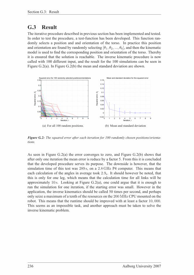
Section G.3: Result
G.3 ResultThe iterative procedure described in previous section has been implemented and tested.
In order to test the procedure, a test-function has been developed. This function ran-
domly selects a position and and orientation of the torso. In practice this position
and orientation are found by randomly selecting [θ1, θ2, ..., θ6], and then the kinematicmodel is used to find the corresponding position and orientation of the torso. Thereby
it is ensured that the solution is reachable. The inverse kinematic procedure is now
called with 100 different input, and the result for the 100 simulations can be seen in
Figure G.2(a). In Figure G.2(b) the mean and standard deviation are shown.
0 1 2 3 4 5 6 7 8 90
0.05
0.1
0.15
0.2
0.25
0.3
0.35
Iteration, i
Sq
ua
red
err
or,
Gi
Squared error for 100 randomly selected positions/orientations
(a) For all 100 random positions.
0 1 2 3 4 5 6 7 8 9−0.02
0
0.02
0.04
0.06
0.08
0.1
0.12
0.14
0.16
Iteration, i
Sq
ua
red
err
or,
Gi
Mean and standard deviation for the squared error
(b) Mean and standard deviation
Figure G.2: The squared error after each iteration for 100 randomly chosen positions/orienta-
tions.
As seen in Figure G.2(a) the error converges to zero, and Figure G.2(b) shows that
after only one iteration the mean error is reduce by a factor 5. From this it is concluded
that the developed procedure serves its purpose. The downside is however, that the
simulation time of this test was 289 s, on a 2.8GHz P4 computer. This means that
each calculation of the angles in average took 2.9s. It should however be noted, thatthis is only for one leg, which means that the calculation time for all links will be
approximately 10 s. Looking at Figure G.2(a), one could argue that it is enough to
run the simulation for one iteration, if the starting error was small. However in the
application, the inverse kinematics should be called 50 times per second, and perhaps
only seize a maximum of a tenth of the resources on the 200MHz CPUmounted on the
robot. This means that the runtime should be improved with at least a factor 10, 000.This seems as an impossible task, and another approach must be taken to solve the
inverse kinematic problem.
236 Aalborg University 2007

HVERIFICATION
OF THE INVERSE
KINEMATIC MODEL
In this appendix the inverse kinematic model is verified. The inverse kinematic model
gives a coordinate transformation from generalized coordinates of the end of each limb
and of the torso, to joint space. The input and output of the inverse kinematic model
can be seen from Figure H.1.
Inverse Kinematic
Modelθθθθ
lf lfp o
f rfrp o
t tp o
rhp
lhp
Figure H.1: Inputs and output relations of the inverse kinematic model. Inputs are positions
and orientation, given in Cartesian space, of the limbs and torso. Output is the joint space
coordinates. plf is the position of the left foot. prf is the position of the right foot. pt is the
position of the torso. prh is the position of the right hand and plh is the position of the left hand.
As the joint coordinates are only measurable for the leg joints, it is not sufficient to
test the inverse kinematic model using these. Instead the inverse kinematic model
is verified through the kinematic model. As the kinematic model has been verified,
this can be used to verify other models. The verification of the kinematic model can
be seen in Appendix F in Section F.4. By connecting the inverse kinematic model
with the kinematic model a transformation of coordinates can be made from Cartesian
Group 1033 237

Section H.1: Inverse Kinematic Model Test Setup
space to joint space and then back to Cartesian space. By comparing the positions
and orientations before and after the transformation to joint coordinates it can be seen
whether the inverse kinematic model is correct. This connection can be seen from
Figure H.2. The kinematic model gives the generalized coordinates as output, in which
the position of all links can be found, but it can also be modified to give the orientation
of the limbs. This information is inside the model, and is therefore accessible.
Kinematic model
qInverse Kinematic
Model
θ
lflf op
rfrf op
ttop
rhp
lhp
o
Figure H.2: The positions and orientations of the limbs are transformed to joint space coordi-
nates and then back to generalized coordinates.
H.1 Inverse Kinematic Model Test SetupFor this test no physical test setup is used. Instead the test is conducted through the
kinematic model, as shown in Figure H.2. An input is constructed which lies inside
the reachable space of the kinematics. This input is then transformed to joint space
through the inverse kinematic model. Joint coordinates are transformed via the kine-
matic model, which returns the generalized coordinates of all joints and links. Now
the input is compared to the output. An animation of the input used to test the inverse
kinematic model is shown in Figure H.3.
Figure H.3: Animation of the movements used in the verification of the inverse kinematic model.
The five figures above show the movements in the sagittal plane, while the five figures below
show the movements in the frontal plane. The span of the test is 10 s.
Next the results of the inverse kinematic test are given.
238 Aalborg University 2007
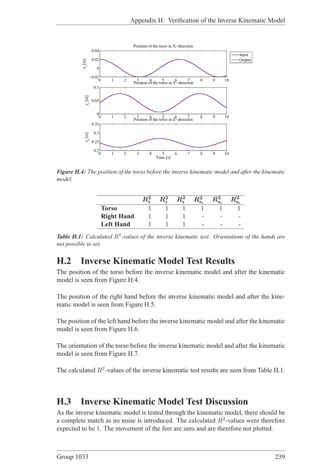
Appendix H: Verification of the Inverse Kinematic Model
0 1 2 3 4 5 6 7 8 9 10−0.02
0
0.02
0.04Position of the torso in X−direction
xt [m]
0 1 2 3 4 5 6 7 8 9 100
0.05
0.1Position of the torso in Y−direction
yt [m]
0 1 2 3 4 5 6 7 8 9 100.2
0.25
0.3
0.35Position of the torso in Z−direction
Time [s]
z t [m]
Input
Output
Figure H.4: The position of the torso before the inverse kinematic model and after the kinematic
model.
R2x R2
y R2z R2
oxR2
oyR2
oz
Torso 1 1 1 1 1 1Right Hand 1 1 1 - - -
Left Hand 1 1 1 - - -
Table H.1: Calculated R2-values of the inverse kinematic test. Orientations of the hands are
not possible to set.
H.2 Inverse Kinematic Model Test ResultsThe position of the torso before the inverse kinematic model and after the kinematic
model is seen from Figure H.4.
The position of the right hand before the inverse kinematic model and after the kine-
matic model is seen from Figure H.5.
The position of the left hand before the inverse kinematic model and after the kinematic
model is seen from Figure H.6.
The orientation of the torso before the inverse kinematic model and after the kinematic
model is seen from Figure H.7.
The calculated R2-values of the inverse kinematic test results are seen from Table H.1.
H.3 Inverse Kinematic Model Test DiscussionAs the inverse kinematic model is tested through the kinematic model, there should be
a complete match as no noise is introduced. The calculated R2-values were therefore
expected to be 1. The movement of the feet are zero and are therefore not plotted.
Group 1033 239
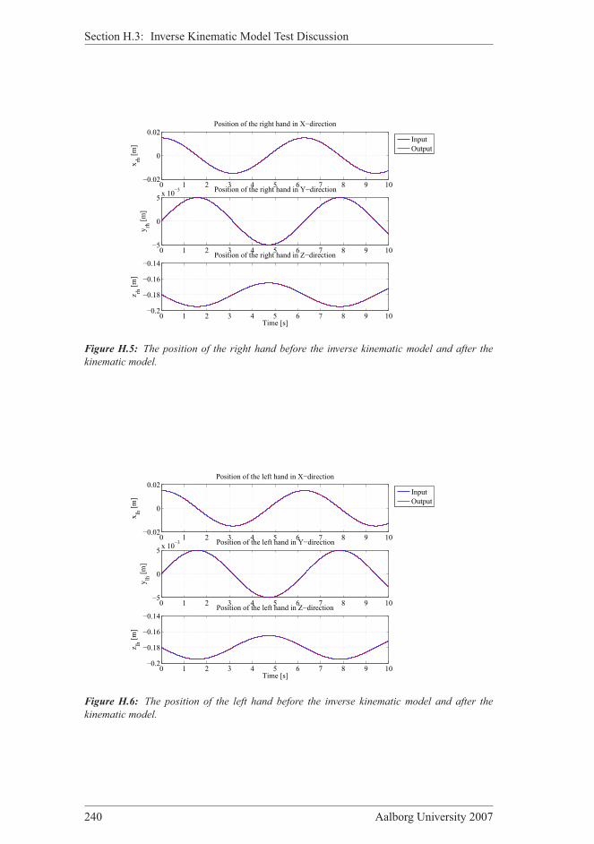
Section H.3: Inverse Kinematic Model Test Discussion
0 1 2 3 4 5 6 7 8 9 10−0.02
0
0.02Position of the right hand in X−direction
xrh [m]
0 1 2 3 4 5 6 7 8 9 10−5
0
5x 10
−3 Position of the right hand in Y−direction
yrh [m]
0 1 2 3 4 5 6 7 8 9 10−0.2
−0.18
−0.16
−0.14Position of the right hand in Z−direction
Time [s]
z rh [m]
Input
Output
Figure H.5: The position of the right hand before the inverse kinematic model and after the
kinematic model.
0 1 2 3 4 5 6 7 8 9 10−0.02
0
0.02Position of the left hand in X−direction
xlh [m]
0 1 2 3 4 5 6 7 8 9 10−5
0
5x 10
−3 Position of the left hand in Y−direction
ylh [m]
0 1 2 3 4 5 6 7 8 9 10−0.2
−0.18
−0.16
−0.14Position of the left hand in Z−direction
z lh [m]
Time [s]
Input
Output
Figure H.6: The position of the left hand before the inverse kinematic model and after the
kinematic model.
240 Aalborg University 2007

Appendix H: Verification of the Inverse Kinematic Model
0 1 2 3 4 5 6 7 8 9 10−0.2
0
0.2Orientation of the torso around the X−axis
ot,x [rad]
0 1 2 3 4 5 6 7 8 9 10−0.2
0
0.2Orientation of the torso around the Y−axis
ot,y [rad]
0 1 2 3 4 5 6 7 8 9 10−0.2
0
0.2Orientation of the torso around the Z−axis
ot,z [rad]
Time [s]
Input
Output
Figure H.7: The orientation of the torso before the inverse kinematic model and after the kine-
matic model.
H.4 Inverse Kinematic Model Test ConclusionIt can be seen from Figure H.4, H.5 and H.6 that there is a complete match in the
positioning before the inverse kinematic model and after the kinematic model. This
is also the case for the orientation for the torso, as seen in Figure H.7. This is further
strengthen by the R2-values shown in Table H.1. On basis of this, it is concluded that
the inverse kinematic model is able to transform desired positions and orientations into
joint space coordinates. The inverse kinematic model is therefore considered verified.
Group 1033 241

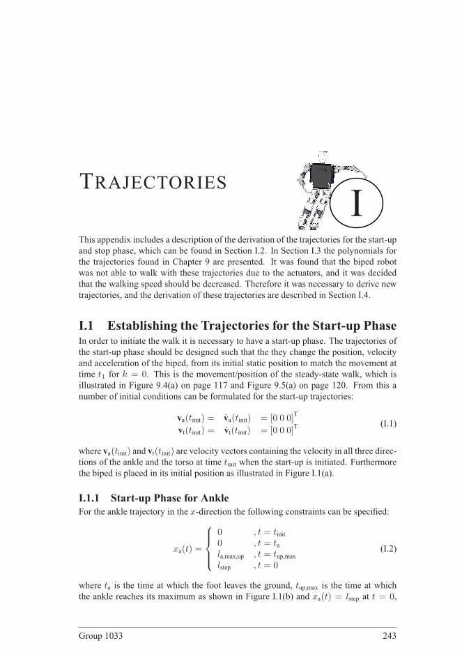
ITRAJECTORIES
This appendix includes a description of the derivation of the trajectories for the start-up
and stop phase, which can be found in Section I.2. In Section I.3 the polynomials for
the trajectories found in Chapter 9 are presented. It was found that the biped robot
was not able to walk with these trajectories due to the actuators, and it was decided
that the walking speed should be decreased. Therefore it was necessary to derive new
trajectories, and the derivation of these trajectories are described in Section I.4.
I.1 Establishing the Trajectories for the Start-up PhaseIn order to initiate the walk it is necessary to have a start-up phase. The trajectories of
the start-up phase should be designed such that the they change the position, velocity
and acceleration of the biped, from its initial static position to match the movement at
time t1 for k = 0. This is the movement/position of the steady-state walk, which isillustrated in Figure 9.4(a) on page 117 and Figure 9.5(a) on page 120. From this a
number of initial conditions can be formulated for the start-up trajectories:
va(tinit) = va(tinit) = [0 0 0]T
vt(tinit) = vt(tinit) = [0 0 0]T (I.1)
where va(tinit) and vt(tinit) are velocity vectors containing the velocity in all three direc-tions of the ankle and the torso at time tinit when the start-up is initiated. Furthermorethe biped is placed in its initial position as illustrated in Figure I.1(a).
I.1.1 Start-up Phase for Ankle
For the ankle trajectory in the x-direction the following constraints can be specified:
xa(t) =
0 , t = tinit0 , t = tala,max,up , t = tup,maxlstep , t = 0
(I.2)
where ta is the time at which the foot leaves the ground, tup,max is the time at whichthe ankle reaches its maximum as shown in Figure I.1(b) and xa(t) = lstep at t = 0,
Group 1033 243

Section I.1: Establishing the Trajectories for the Start-up Phase
y
z
x
(a) Inital: t = tinit
yzx
lstep ha,max
la,max,up
xt,max
(b) SSP: t = tup,max
yt,max,up
y
z
x
(c) SSP: t = ty,max,up
Figure I.1: Illustration of the start-up phase. I.1(a) initial position, in I.1(b) the ankle reaches
its maximum point and the torso reaches xt,max. I.1(c) shows biped robot at the instant where it
reaches its maximum deviation to the right during the start-up phase.
is the same position as the leading foot of Figure 9.4(a) where the steady-state walk is
initiated. For the z-direction following must be fulfilled:
za(t) =
a1 , t = tinita1 , t = taha,max , t = tup,maxa1 , t = 0
(I.3)
Note that the foot does not leave the ground until after time ta, the reason for that isthat the CoM has to be moved over the supporting foot prior to initiating a SSP. As for
the steady state walk, there is no other requirements to the movement of the foot in the
y-direction, than:ya(t) = 0 (I.4)
I.1.2 Start-Up Phase for Torso
The trajectories for the torso is designed such that the stability index is minimized.
The procedure is all most identical with the one used to obtain the trajectories for the
steady-state walk. A number of constraints is formulated to ensure that the torso passes
through the wanted positions. For the x-direction the constraints are:
xt(t) =
0 , t = tinitxt,max , t = tup,maxxt(t) , t = 0
(I.5)
where xt,max is the parameter that is varied in order to minimize the stability index and
xt(0) is the position of the torso at the moment where the steady-state walk is initiated,this value can be found from the trajectories of the torso presented in Section 9.4 on
page 125, to be xt(0) = xt,e − lstep. xt,max is varied in the range of:
0 ≤ xt,max ≤ 0.6xt(0) (I.6)
The trajectories in the y-direction should satisfy the following constraints:
yt(t) =
yt,mid , t = tinityt,max,up , t = ty,max,upyt,mid , t = 0
(I.7)
244 Aalborg University 2007

Appendix I: Trajectories
where yt,mid is the middle position of the torso as illustrated in Figure 9.5(a), yt,max,up isthe maximum deviation to the right of the torso during the start-up phase, as illustrated
in Figure I.1(c) which happens at time ty,max,up. For the y-direction it is chosen to varyon two parameters, namely the value of yt,max,up and the time at which this point is
reached, ty,max,up. The first parameter is varied within the ranges specified i Equation(9.18) on page 121, the second parameter will be varied within:
0.3tinit ≤ ty,max,up ≤ 0.7tinit (I.8)
The movement of the torso in the z-direction during the start-up phase is designed
exactly like for the steady-state walk.
I.1.3 Finding Parameters for the Start-up Phase
The first parameter to find that describes the start-up phase is xt,max which is varied
within the ranges specified in Equation (I.6) in steps of 0.01(xte − lstep), giving a totalof 61 simulations. The stability index is calculated using Equation (9.22), and the result
of the simulations can be seen in Figure I.2(a), where the red dot marks the most stable
trajectory. The value of xt,max is found to be:
xt,max = 14.4mm (I.9)
The ZMP trajectory for this simulation, where the start-up phase and the first step cycle
is simulated, is plotted in Figure I.2(b) together with the PoS. It can be seen the ZMP
is inside the PoS during the entire start-up phase.
0 0.01 0.02 0.030
5e−005
0.0001
Stability index for different values of Xt,max
i stab,x
Xt,max
[m]
(a) Stability
−1 −0.5 0 0.5
0
0.2
0.4
PoS vs. xZMP
−trajectory
time [s]
x [m]
PoS
xZMP
(b) PoS and xZMP
Figure I.2: I.2(a) shows the stability index, istab,x, for the start-up phase. The red dot marks the
most stable trajectory. I.2(b) shows the trajectory of xZMP during the start-up phase and the first
step cycle, this is plotted together with the PoS.
Next the values of yt,max,up and ty,max,up are found through simulations. The two valuesare varied within the ranges specified in Equation (9.18) on page 121 and (I.8). yt,max,upis varied in steps of 0.025yt,mid and ty,max,up in steps of 0.025tinit, making a total of 425simulations. The resulting stability index, istab,y, of these simulations can be seen inFigure I.3(a), where the red dot marks the trajectory having the smallest stability index,
thus the best stability properties. The stability index is calculated using Equation (9.2)
on page 115. The values of yt,max,up and ty,max,up are found to be:
yt,max,up = 4.1mmty,max,up = −0.635 s
(I.10)
Group 1033 245

Section I.2: Establishing the Trajectories for the Stop Phase
−0.010
0.010.02
−1
−0.5
00
0.5
1
1.5
x 10−4
Yt,max,up
[m]Ty,max,up
[m]
i stab,y
(a) Stability
−1 −0.5 0 0.5
0
0.1
0.2
PoS vs. yZMP
−trajectory
time [s]
y [m]
PoS
yZMP
(b) PoS and yZMP
Figure I.3: I.3(a) shows the stability index, istab,y, for the start-up phase. The red dot marks the
most stable. I.3(b) shows the trajectory of yZMP during the start-up phase and the the first step
cycle, this is plotted together with the PoS.
In Figure I.3(b) the ZMP trajectory is plotted together with the PoS, and it can be seen
that the ZMP is inside the PoS during the entire start-up phase. At t = 0, a largespike can be observed, this spike occurs because there is a phase shift model, where
the supporting foot is changed, and is therefore not a spike that will occur in the real
system, since there is no sudden phase shifts.
I.2 Establishing the Trajectories for the Stop PhaseThe purpose of the stop phase is to bring the robot from the steady state walk to the
initial posture, when it is desired to stop walking. The approach is exactly the same as
for the start-up phase, a number of parameters describing the trajectories are altered,
and a simulation is performed with each value of the parameter, to finally select the
value given the best stability. As for the start-up phase, there will be no considera-
tions toward energy consumption, since it is desired to use the trajectories providing
the largest stability margin.
The movement in the sagittal plane during the stop phase is illustrated in Figure I.4(a)
and I.4(c), where the last one illustrates the goal position, namely the biped robot
placed at rest in its initial posture. Figure I.4(b) illustrates the movement in the frontal
plane, where the torso reaches its maximum deviation to the left, yt,stop. As seen thetorso passes through the point (x, y) = (xt,stop, yt,stop) at time tstop,max, and these are thetwo values that are changed in order to obtain the most stable motion during the stop
phase. The two values are changed within the ranges:
0.65lstep ≤ xt,stop ≤ 0.95lstep (I.11)
1.6yt,mid ≤ yt,stop ≤ 2.2yt,mid (I.12)
I.2.1 Finding Parameters for the Stop Phase
The stop phase is described by two parameters, the one is xt,stop which is varied within
the ranges specified in Equation (I.11) in steps of 0.01lstep, giving a total of 31 simu-lations. The stability index is calculated using Equation (9.22) on page 123, and the
246 Aalborg University 2007

Appendix I: Trajectories
yzx
ha,max
la,stop
xt,stop
(a) SSP: t = tstop,max
yt,stopy
z
x
(b) SSP: t = tstop,max
y
z
x
(c) Initial posture: t =tstop
Figure I.4: Illustration of the stop phase. The biped robot should be moved from steady state
walk to the position shown in I.1(b) the ankle reaches its maximum point, ha,max, and the torso
reaches xt,stop. At the same time the torso reaches its maximum deviation to the left, yt,stop, as
shown in I.4(b). Finally the biped robot reaches its initial posture as shown in I.4(c).
result of the simulations can be seen in Figure I.5(a), where the red dot marks the most
stable trajectory. The value of xt,stop is found to be:
xt,stop = 151.8mm (I.13)
The simulation consisted of a start-up phase, one walking cycle and a stop phase.
Note that only the data from the last step and the stop phase is used, when calculating
the stability index for the stop phase. This ZMP-trajectory is plotted in Figure I.5(b)
together with the PoS.
0.1 0.12 0.14 0.160
0.02
0.04
0.06
Stability index for values of xt,stop
i stab,x
xt,stop
[m]
(a) Stability
1 1.5 2 2.5
0.2
0.4
PoS vs. xZMP
−trajectory
Time [s]
x [m]
PoS
xZMP
(b) PoS and xZMP
Figure I.5: I.5(a) shows the stability index, istab,x, for the stop phase. The red dot marks the moststable. I.5(b) shows the trajectory of xZMP during the stop phase and the preceding step, this is
plotted together with the PoS.
Next the value of yt,stop is found through simulations. yt,stop is varied within the rangesspecified in Equation (I.12). yt,stop is varied in steps of 0.01yt,mid, making a total of 61simulations. The resulting stability index, istab,y, of these simulations can be seen inFigure I.3(a), where the red dot marks the trajectory having the smallest stability index,
thus the best stability properties. istab,y is calculated using Equation (9.2) on page 115.
Group 1033 247

Section I.3: Polynomials from first Iteration
0.02 0.03 0.04 0.050.0002
0.00025
0.0003
0.00035
Stability index for values of yt,stop
i stab,y
yt,stop
[m]
(a) Stability
1 1.5 2 2.5
0
0.1
0.2
0.3
PoS vs. yZMP
−trajectory
Time [s]
y [m]
PoS
yZMP
(b) PoS and yZMP
Figure I.6: I.6(a) shows the stability index, istab,y, for the start-up phase. The red dot marks the
most stable. I.6(b) shows the trajectory of yZMP during the start-up phase and the the first step
cycle, this is plotted together with the PoS.
The value of yt,stop is found to be:
yt,stop = 90.2mm (I.14)
In Figure I.6(b) the ZMP trajectory is plotted together with the PoS.
I.3 Polynomials from first IterationIn Section 9.3 on page 122 the steady-state walking trajectories for the torso and the
feet are found. In Section I.1 they are found for the start-up phase, and in Section
I.2 they are found for the stop phase. In this section the polynomial description of the
trajectories of the biped robot is presented. It is organized such that all the polynomials
for the feet will be presented first, and then the all the polynomials for the torso will be
presented.
I.3.1 Polynomials for the Feet
Steady State Walk
The polynomials describing the orientation of the foot are given as:
θa,y(t) =
−560.806t3 + 143.776t2 , t ∈ [t1, t2]204.375t3 − 73.355t2 + 1.400 , t ∈ [t2, t3]0 , t ∈ [t3, Tcycle]
(I.15)
and the polynomials describing the trajectories of Figure 9.10 are:
xa(t) =
a1 sin(θa,y(t)) + ltoe sin(θa,y(t)) , t ∈ [t1, t2]−8.753t3 + 4.600t2 + 0.080 , t ∈ [t2, t3]1.348t3 − 1.684t2 + 0.698t + 0.224 , t ∈ [t3, t4]2lstep , t ∈ [t4, Tcycle]
(I.16)
za(t) =
a1 cos(θa,y(t)) + ltoe(1− cos(θa,y(t))) , t ∈ [t1, t2]−5.646t3 + 2.027t2 + 0.048 , t ∈ [t2, t3]0.880t3 − 0.586t2 + 0.086 , t ∈ [t3, t4]a1 , t ∈ [t4, Tcycle]
(I.17)
It should be noted that the polynomials in Equation (I.15), (I.16) and (I.17) are for the
right foot, but can be applied on the left foot by time shifting them one step cycle, Tstep.
248 Aalborg University 2007

Appendix I: Trajectories
The reason that the number of polynomials are not the same in Equation (I.15), (I.16)
and (I.17) is that the number of requirements are different.
Start-up Phase
The orientation of the foot is not altered during the start-up, thus:
θa,y(t) = 0 , t ∈ [tstart, 0] (I.18)
and the polynomials describing the position of the ankle are:
xa(t) =
0 , t ∈ [tstart, tup]−0.365t3 + 0.530t2 , t ∈ [tup, tupmax]−0.398t3 + 0.080t2 + 0.250t + 0.064 , t ∈ [tupmax, 0]
(I.19)
za(t) =
a1 , t ∈ [tstart, tup]−0.929t3 + 0.611t2 + 0.048 , t ∈ [tup, tupmax]0.633t3 − 0.533t2 + 0.032t + 0.086 , t ∈ [tupmax, 0]
(I.20)
Note that Equation (I.18), (I.19) and (I.20) are for the left foot, since the walking cycle
is always initiated by moving the left foot. Note that the time index for the start-up
phase is negative, this is because the steady-state walking cycle is defined to start at
t = 0.
Stop Phase
The orientation of the foot is not altered during the stop phase, thus:
θa,y(t) = 0 , t ∈ [Tcycle, tstop] (I.21)
and the polynomials describing the position of the ankle are:
xa(t) =
−0.077t3 + 0.326t2 , t ∈ [Tcycle, tstop,max]−0.693t3 + 0.217t2 + 0.255t + 0.0639 , t ∈ [tstop,max, tstop]
(I.22)
za(t) =
−0.744t3 + 0.524t2 + 0.048 , t ∈ [Tcycle, tstop,max]0.744t3 − 0.524t2 + 0.086 , t ∈ [tstop,max, tstop]
(I.23)
Note that Equation (I.21), (I.22) and (I.23) are for the right foot, since the walking
cycle is always ended with moving the right foot, such that the biped robot will stop in
initial posture.
I.3.2 Polynomials for the Torso
The polynomials describing the movement of the torso will be presented below.
Steady State Walk
The polynomials describing the chosen trajectories of the torso are given as:
xt(t) =
−4.761t3 + 0.698t2 + 0.366t + 0.225 , t ∈ [t1, t2]0.553t3 − 0.436t2 + 0.187t + 0.125 , t ∈ [t2, t4]
(I.24)
yt(t) =−0.250t2 + 0.213t + 0.041 , t ∈ [t1, t4] (I.25)
zt(t) =
−0.869t3 + 0.535t2 + 0.240 , t ∈ [t1, t3]0.684t3 − 0.456t2 + 0.270 , t ∈ [t3, t4]
(I.26)
Group 1033 249

Section I.3: Polynomials from first Iteration
Start-up Phase
The polynomials for the torso during the start-up phase are as follows:
xt(t) =
−0.178t3 + 0.147t2 , t ∈ [tstart, tstop,max]0.673t3 − 0.173t2 − 0.016t + 0.014 , t ∈ [tstop,max, 0]
(I.27)
yt(t) =
0.597t3 − 0.442t2 + 0.041 , t ∈ [tstart, tstop,max]0.248t3 − 0.068t2 + 0.005 , t ∈ [tstop,max, 0]
(I.28)
zt(t) =
0.046t3 − 0.078t2 + 0.273 , t ∈ [tstart, 0] (I.29)
Stop Phase
The polynomials for the torso during the stop phase are as follows:
xt(t) =
0.170t3 − 0.435t2 + 0.368t + 0.058 , t ∈ [Tcycle, tstop,max]0.169t3 − 0.195t2 + 0.071t + 0.152 , t ∈ [tstop,max, tstop]
(I.30)
yt(t) =
−0.233t3 − 0.116t2 + 0.211t + 0.041 , t ∈ [Tcycle, tstop,max]0.709t3 − 0.444t2 − 0.053t + 0.090 , t ∈ [tstop,max, tstop]
(I.31)
zt(t) =−0.080t3 + 0.113t2 + 0.240 , t ∈ [Tcycle, tstop] (I.32)
I.3.3 Implementation of Trajectories
To ease the workload on the on-board computer, the trajectories are not implemented
like the polynomials described above, but are implemented as a look-up table. The
values in the look-up table are calculated from the polynomials. The implementation
is illustrated in Figure I.7, where it can be seen that when the walk is initiated the data
for the start-up phase is executed, then the data for the steady state walk is executed
cyclic, until it is chosen to terminate the walk, and then the data for the stop phase is
executed.
Start-up phase
Steady state walk
Stop phase
Init
Stop?
yes
no
Figure I.7: The trajectories are implemented as look-up tables, where the data for the start-up
phase is executed when the walk is initiated, the data for the steady state walk is used in a cyclic
manner, until the it is chosen to stop walking, and at this time the data for the stop phase is used.
250 Aalborg University 2007

Appendix I: Trajectories
Figure I.7 illustrates why it is important that the trajectories for the start-up phase and
the stop phase are designed to fit the steady state walk, and why it is important that the
trajectories for the steady state walk are cyclic.
I.4 Derivation of Slower TrajectoriesAs found in Section 9.5 on page 128 the developed trajectories are not suitable for
obtaining dynamical walk, with the given actuators. It is therefore chosen to develop a
new set of trajectories, that are more adapted to the servo motors at hand. It is chosen
to decrease the walking speed, and in response to this also the step length. Through
simulations it is found that the new walking speed and the new step length are:
vwalking = 9.35 cm/s (I.33)
lstep = 8 cm (I.34)
The establishment of the new trajectories are exactly the same as for the first iteration,
the same parameters are varied, the same simulations are performed, the same criteria
are used to single out the best values of the parameters. Only one change has been
made, the reference to the servo motor model are given with a frequency of 40Hz as onthe real system. This way the unfavourable property is taken into consideration when
the parameters are determined. Since the approach is the same as for the first iteration,
it will not be examined once again, but only the result will be presented below.
I.4.1 Polynomials for the Feet
Steady State Walk
The polynomials describing the trajectories of the foot are given as:
xa(t) =
0 , t ∈ [t1, t2]−0.732t3 + 0.769t2 , t ∈ [t2, t3]0.113t3 − 0.282t2 + 0.233t + 0.096 , t ∈ [t3, t4]2lstep , t ∈ [t4, Tcycle]
(I.35)
za(t) =
a1 , t ∈ [t1, t2]−0.704t3 + 0.506t2 + 0.048 , t ∈ [t2, t3]0.110t3 − 0.147t2 + 0.086 , t ∈ [t3, t4]a1 , t ∈ [t4, Tcycle]
(I.36)
Start-up Phase
The orientation of the foot is not altered during the start-up, thus:
θa,y(t) = 0 , t ∈ [tstart, 0] (I.37)
and the polynomials describing the position of the ankle are:
xa(t) =
0 , t ∈ [tstart, tup]0.025t3 + 0.003t2 , t ∈ [tup, tupmax]−0.058t3 + 0.065t2 + 0.056t + 0.016 , t ∈ [tupmax, 0]
(I.38)
za(t) =
a1 , t ∈ [tstart, tup]−0.116t3 + 0.153t2 + 0.048 , t ∈ [tup, tupmax]0.079t3 − 0.133t2 + 0.016t + 0.086 , t ∈ [tupmax, 0]
(I.39)
Group 1033 251

Section I.4: Derivation of Slower Trajectories
Stop Phase
The polynomials describing the position of the ankle are:
xa(t) =
0.034t3 − 0.014t2 , t ∈ [Tcycle, tstop,max]−0.082t3 + 0.081t2 + 0.064t + 0.016 , t ∈ [tstop,max, tstop]
(I.40)
za(t) =
−0.093t3 + 0.131t2 + 0.048 , t ∈ [Tcycle, tstop,max]0.093t3 − 0.131t2 + 0.086 , t ∈ [tstop,max, tstop]
(I.41)
The new trajectories for the feet can be seen i Figure I.8.
−2 0 2 4
0
0.1
0.2
0.3
0.4
0.5
Time [s]
xa(t) [m]
Foot trajectories
start−up k=1 k=2 stop
Right foot
Left foot
(a) Trajectories for x-direction
−2 0 2 40.04
0.06
0.08
0.1
Time [s]
z a(t) [m]
Foot trajectories
start−up k=1 k=2 stop
Right foot
Left foot
(b) Trajectories for z-direction
Figure I.8: Trajectories for the right and left foot for start-up, one walking cycle k = [1, 2] andthe stop phase. I.8(a) shows the trajectories in the x-direction, and I.8(b) shows the trajectoriesin the z-direction.
I.4.2 Polynomials for the Torso
The polynomials describing the movement of the torso will be presented below.
Steady State Walk
The polynomials describing the chosen trajectories of the torso are given as:
xt(t) =
0.061t3 − 0.096t2 + 0.047t + 0.064 , t ∈ [t1, t2]−0.525t3 + 0.154t2 + 0.126t + 0.104 , t ∈ [t2, t4]
(I.42)
yt(t) =−0.062t2 + 0.106t + 0.041 , t ∈ [t1, t4] (I.43)
zt(t) =
−0.109t3 + 0.134t2 + 0.240 , t ∈ [t1, t3]0.086t3 − 0.114t2 + 0.270 , t ∈ [t3, t4]
(I.44)
Start-up Phase
The polynomials for the torso during the start-up phase are as follows:
xt(t) =
−0.022t3 + 0.032t2 , t ∈ [tstart, tstop,max]0.071t3 − 0.046t2 − 0.017t + 0.084 , t ∈ [tstop,max, 0]
(I.45)
yt(t) =
0.020t3 − 0.052t2 + 0.041 , t ∈ [tstart, tstop,max]−0.217t3 + 0.277t2 − 0.008 , t ∈ [tstop,max, 0]
(I.46)
zt(t) =
0.006t3 − 0.020t2 + 0.273 , t ∈ [tstart, 0] (I.47)
252 Aalborg University 2007

Appendix I: Trajectories
Stop Phase
The polynomials for the torso during the stop phase are as follows:
xt(t) =
0.073t3 − 0.163t2 + 0.126t + 0.024 , t ∈ [Tcycle, tstop,max]−0.035t3 + 0.043t2 + 0.013t + 0.059 , t ∈ [tstop,max, tstop]
(I.48)
yt(t) =
0.030t3 − 0.112t2 + 0.105t + 0.041 , t ∈ [Tcycle, tstop,max]0.030t3 − 0.028t2 − 0.026t + 0.066 , t ∈ [tstop,max, tstop]
(I.49)
zt(t) =−0.010t3 + 0.028t2 + 0.240 , t ∈ [Tcycle, tstop] (I.50)
The new trajectories for the torso can be seen in Figure I.9.
−2 0 2 4
0
0.1
0.2
0.3
0.4
0.5
Time [s]
xt(t) [m]
Torso trajectory
start−up k=1 k=2 stop
Torso
(a) Trajectory for x-direction
−2 0 2 4
0
0.05
0.1
Time [s]
yt(t) [m]
Torso trajectory
start−up k=1 k=2 stop
Torso
(b) Trajectory for y-direction
−2 0 2 40.23
0.24
0.25
0.26
0.27
0.28
Time [s]
z t(t) [m]
Torso trajectory
start−up k=1 k=2 stop
Torso
(c) Trajectory for z-direction
Figure I.9: Trajectories for the torso, for start-up phase, the following walking cycle k = [1, 2],and stop phase. I.9(a) shows the trajectory in the x-direction. I.9(b) shows the trajectory in the
y-direction. I.9(c) shows the trajectory in the z-direction.
Comparing the trajectories of this second iteration with those of the first iteration, it
can be seen that most of the movement of the torso is performed during the DSP. This
is a result from clocking in the trajectories with a frequency of 40Hz, which makes theZMP jump back and forth. The largest stability is obtained if the largest movements
are made in the DSP.
Group 1033 253

JVERIFICATION
OF THE ZMP
ESTIMATORS
This appendix supports Section 10.2 on page 135 and contains verification of the de-
veloped ZMP estimator.
In order to verify the developed ZMP estimators, the model of the robot is used to
determine a reference ZMP trajectory that can be compared with the output of the
estimator. The test scenario will consist of moving the torso along the x- and y-axis.The test will only be done when in DSP since it was not possible to make the robot
balance on one leg. The test has been divided into two sub test:
- Verification scenario one: The first scenario moves the torso in the sagittal
direction and can be is seen from Figure J.1.
- Verification scenario two: The second scenario moves the torso in the frontal
direction, which is seen from Figure J.2.
The verification trajectory can be found on the enclosed CD in Simulink/Test-
Trajectories. When the inputs were chosen it was noted, that even though an
input given to the model kept the ZMP within the PoS the same input did not give a
stable posture of the real robot. This was caused by backlash, mainly in the hips. The
backlash made the actual robot lean its torso further backward than in the model which
made it unable to stand. Therefore the inputs were altered such that the robot was able
to stand by leaning the torso forward and afterward these inputs were used in a simu-
lation to determine the ZMP trajectory.
Verification scenario one and scenario two are shown in Figure J.3 and J.4 respectively
where the estimation of the ZMP is done using the accelerometer. The figures show
that the estimate is unreliable. This can not be contributed to the backlash alone. The
estimator is sligthly better at estimating a static ZMP, however when trying to estimate
Group 1033 255

Figure J.1: Animation of the movements of the robot used in the verification of the ZMP esti-
mator in the sagittal direction. The five figures above show the movements in the sagittal plane,
while the five figures below show the movements in the frontal plane.
Figure J.2: Animation of the movements of the robot used in the verification of the ZMP esti-
mator in the frontal direction. The five figures above show the movements in the sagittal plane,
while the five figures below show the movements in the frontal plane.
256 Aalborg University 2007

Appendix J: Verification of the ZMP Estimators
a moving ZMP the estimator shows a very poor result. The estimator shows better
results when used in a simulation of the robot as shown in Figure 10.6, suggesting that
the problem does not lie in the approach but in the inputs. Figure J.5 shows the mea-
sured angles from the servo motors which are used in Equation (10.10) to calculate the
position of the CoM of the torso.
Because of Equation (10.10) the noise becomes highly correlated in the position lead-
ing to the poor results seen in Figures J.3 and J.4.
0 2 4 6 8 10 12 14−0.02
−0.01
0
0.01
0.02
0.03
ZMP estimation using the accelerometer, test 1
Time [s]
xZMP [m]
0 2 4 6 8 10 12 140.02
0.04
0.06
0.08
0.1
Time [s]
yZMP [m]
Figure J.3: The ZMP estimate using the accelerometer in test 1. The green line shows the
simulated ZMP and the blue line shows the estimated ZMP.
Figure J.6 and J.7 show verification scenario one and scenario two where the pressure
sensors are used. As expected the ZMP estimator does not yield the same result as the
model. The ZMP in the x-axis shows that the estimated ZMP lies approximately 2 cmbehind the simulated ZMP. In the y-axis the estimated ZMP lies about 5mm to the
left of what was simulated. It should however be noted that the amplitude of the ZMP
estimate is almost identical to the simulated ZMP. Since the ZMP estimator uses the
pressure measurements from the feet, this estimate will yield the actual position of the
ZMP. Therefore the ZMP estimator can be considered accurate and able to detect the
deviation between the ZMP from the model and the real ZMP on the robot. The devi-
ation consists in the fact that backlash and bending of the strain plates is not included
in the dynamical model.
The ZMP estimator that uses the pressure sensors is only able to measure the ZMP
within the PoS and measuring FZMP is therefore not possible. However the ZMP
Group 1033 257

0 2 4 6 8 10 12 14−0.04
−0.02
0
0.02
0.04
ZMP estimation using the accelerometer, test 2
Time [s]
xZMP [m]
0 2 4 6 8 10 12 140.02
0.04
0.06
0.08
0.1
Time [s]
yZMP [m]
Figure J.4: The ZMP estimate using the accelerometer in test 2. The green line shows the
simulated ZMP and the blue line shows the estimated ZMP.
0 2 4 6 8 10 12 14−0.4
−0.3
−0.2
−0.1
0
0.1
0.2
0.3
0.4
0.5
Measured angles from the servo motors
Time [s]
θi [rad]
θ1
θ2
θ3
θ4
θ5
θ6
Figure J.5: The measured angles from the servo motors that are used to estimate the ZMP.
258 Aalborg University 2007

Appendix J: Verification of the ZMP Estimators
0 2 4 6 8 10 12 14 16 18 20−0.015
−0.01
−0.005
0
0.005
0.01
0.015
0.02
ZMP estimation using the pressure sensor, test 1
Time [s]
xZMP [m]
0 2 4 6 8 10 12 14 16 18 200.04
0.042
0.044
0.046
0.048
Time [s]
yZMP [m]
Figure J.6: The ZMP estimate using the pressure sensors in test 1. The green line line shows
the simulated ZMP and the blue line shows the estimated ZMP.
0 2 4 6 8 10 12 14 16 18 20−0.01
−0.005
0
0.005
0.01
0.015
0.02
ZMP estimation using the pressure sensor, test 2
Time [s]
xZMP [m]
0 2 4 6 8 10 12 14 16 18 200.03
0.035
0.04
0.045
0.05
0.055
Time [s]
yZMP [m]
Figure J.7: The ZMP estimate using the pressure sensors in test 2. The green line line shows
the simulated ZMP and the blue line shows the estimated ZMP.
Group 1033 259

estimator that uses the accelerometer is able to measure FZMP and it would be advan-
tageous to fuse the two estimates. Because of the reliablity issues regarding the FZMP
estimate it is chosen to only use the ZMP estimator that uses the pressure sensors.
260 Aalborg University 2007

KCONTROLLER SIMU-
LATION AND VERIFI-
CATION
This Appendix supports Chapter 10 on page 133 where the ZMP controller and hy-
brid posture controller is designed and implemented. The simulations and tests are
described, and the resulting system response is commented after each simulation or
test.
K.1 ZMP Controller Simulation in DSPThe controller was implemented in the complete model of the system, and two exper-
iments were conducted. First a 1 cm step in the ZMP reference is applied along the
x-axis. The simulated performance of the controller is seen in Figure K.1.
Next, a 2 cm step was applied along the y-axis. The response of the system is shown in
Figure K.2. The reason for using a larger step along the y-axis is that the PoS is greaterthan along the x-axis. Overshoot has to be avoided since this will make the robot fall.The cost of this is a slower controller. As it can be seen in Figure K.1 and K.2, the
ZMP starts out by moving in the wrong direction. This is caused by the acceleration,
and is therefore unavoidable, since it is not possible to move a body, at rest, without
acceleration it. However, with the small gains, the effect can be kept to a minimum.
The controller gains were adjusted to minimize the effect of the ZMP going the wrong
way the first few samples. When doing this, the stability is increased, but the controller
performs much slower.
K.1.1 ZMP Controller Simulation in SSP
To test the ZMP controller in SSP, the robot was positioned in SSP and then the right
leg was lifted 2 cm above the ground. After the robot movements had settled, a step
was applied along the x-axis. The same method was used to test the ZMP controller
Group 1033 261

Section K.1: ZMP Controller Simulation in DSP
0 2 4 6 8 10 12−0.01
−0.005
0
0.005
0.01
0.015
0.02
0.025
0.03Simulated ZMP controller performance in DSP, along the x−axis
Time [s]
xZMP [m]
xZMP
xZMP
reference
Figure K.1: Simulating the ZMP controller in DSP by applying a step in x-direction.
0 2 4 6 8 10 120.01
0.015
0.02
0.025
0.03
0.035
0.04
0.045
0.05Simulated ZMP controller performance in DSP, along the y−axis
Time [s]
yZMP [m]
yZMP
yZMP
reference
Figure K.2: Simulating the ZMP controller in DSP by applying a step in y-direction.
262 Aalborg University 2007

Appendix K: Controller Simulation and Verification
along the y-axis.
First, a 1 cm step was applied on the reference of the ZMP in the x-axis. The responseof the system is shown in Figure K.3. Due to the acceleration, the position of the ZMP
0 2 4 6 8 10 12−0.01
−0.005
0
0.005
0.01
0.015
0.02Simulated ZMP controller performance in SSP, along the x−axis
Time [s]
xZMP [m]
xZMP
xZMP
reference
Figure K.3: Simulating the ZMP controller in SSP by applying a step in x-direction.
is moved in the opposite direction at first. Then the ZMP is moved in place within two
seconds. Overshoot is not wanted for the ZMP controller as this would make the robot
fall. At the cost of this, the controller performs slowly.
Next, a 0.5 cm step was applied along the y-axis. The reason for choosing a smallerstep along the y-axis is due to the smaller PoS in SSP. The response of the system
is shown in Figure K.4. Once again, overshoot has to be avoided to ensure that the
0 2 4 6 8 10 12−0.01
−0.005
0
0.005
0.01
0.015
0.02Simulated ZMP controller performance in SSP, along the y−axis
Time [s]
yZMP [m]
yZMP
yZMP
reference
Figure K.4: Simulating the ZMP controller in SSP by applying a step in y-direction.
controller does not make the robot fall. The controller gains were increased as much
Group 1033 263

Section K.2: Implementation and Verification
as possible to gain the fastest response times. It must however be concluded that a
sampling frequency of 40Hz is too slow for applications like a walking biped robot. It
is doubtable that these SSP controllers would work if implemented on a walking biped
robot due to their slow response times.
K.2 Implementation and VerificationThe ZMP controller was implemented on the actual system and with minor changes
to the controller gains ZMP control was realized. The controller was implemented as
shown in Figure 10.13. To test the controller, steps were given to the reference position
of the ZMP. Two steps were given in two different experiments. First, the desired ZMP
position was moved in the x-direction by giving a step in the x-direction. Next, thecontroller was tested by applying a step in the y-direction.
K.2.1 Testing ZMP Controller in x-direction
In this test, a step of 2.5 cm on the reference to the ZMP is applied in the x-direction.The corresponding position of the ZMP can be seen in Figure K.5.
0 5 10 15 20−0.02
−0.01
0
0.01
0.02
0.03
0.04ZMP estimate when given a step input in the x−direction
Time [s]
xZMP [m]
xZMP
estimate
xZMP
reference
Figure K.5: Testing the ZMP controller in DSP by applying a step in x-direction.
It is seen that the ZMP controller manages to move the position of the ZMP to the
desired location within 10 s which is too slow if the controller should be used while the
robot is walking. One could argue that by increasing the gains, the controller would
perform faster. This is also the case, but due to the limited PoS in the x-direction,the robot tends to fall if the ZMP is moved any faster than shown in Figure K.5. The
2.5 cm step is the largest step that can be applied to the robot if the robot should main-
tain balance.
When the step is applied, it is seen that the position of the ZMP jumps approximately
1.5 cm this is due to backlash in the joints. When the robot is at initial position, the
robot can tilt freely around 5 deg so a sudden jump in the position of the ZMP is
to be expected since the starting point of the robot was zero-position. The position
of the ZMP is slowly changed, but the position also vary with a higher frequency at
264 Aalborg University 2007

Appendix K: Controller Simulation and Verification
approximately 1Hz. This frequency is the natural frequency of the robot and occur dueto wobbling and backlash in the joints as well as the strain plates in the feet that acts like
three steel plate springs. The internal controller in the servo motors also contributes
to this swinging of the robot. It has not been possible to retrieve any information
regarding the internal controllers from the developing company.
K.2.2 Testing ZMP Controller in y-direction
In this test, a step was applied to the position of the ZMP in the y-direction. The
step is applied with a magnitude of 2.5 cm compared to the starting position. The
corresponding position of the ZMP can be seen in Figure K.6.
0 5 10 15 200.01
0.02
0.03
0.04
0.05
0.06
0.07ZMP estimate when given a step input in the y−direction
Time [s]
yZMP [m]
yZMP
estimate
yZMP
reference
Figure K.6: Testing the ZMP controller in DSP by applying two steps in y-direction.
It is seen that the ZMP controller is faster in the y-direction than in the x-direction,and that it reaches the reference position after one second. This is mainly due to the
controller gains that are larger than the controller gains used for the controller in the
x-direction. This is possible since the PoS is much larger in the frontal plane than in
the sagittal plane, when the robot is in DSP. As it can be seen in Table 10.3 the integral
gain, is larger than kiy for the other controller, and the proportional gain is likewise
increased. It is due to the larger stability in the y-direction that these increased gainscan be used.
K.3 Simulating the Posture Controller PerformanceThe performance of the hybrid posture controller was tested in both DSP and SSP.
First, the controller was tested in DSP and steps were given to the inclination of the
torso around the x-axis and around the y-axis in two different tests. Next, the posturecontroller was tested in SSP. To verify that the controller is capable of suppressing
disturbances causes by backlash, 0.087 rad is subtracted from the inclination instead
of giving a step with the reference. This will simulate of effect caused by backlash.
This substitution will only be applied in SSP in around the x-axis, as backlash is mostpronounced around this axis.
Group 1033 265

Section K.3: Simulating the Posture Controller Performance
In all the simulations, it can be seen that the estimated inclination has a spike going the
opposite direction than the reference inclination. This happens since the inclination is
estimated using the accelerometer data. When accelerating in the opposite direction
than the gravity vector, the estimated inclination will have this characteristics. This is
not represented in the actual inclination of the torso, but only in the estimated inclina-
tion.
K.3.1 Posture Controller Simulation in DSP
In this test, a 0.09 rad step was first applied about the x-axis. This corresponds to ap-proximately 5 deg. The robot was set in zero-position before the test was carried out.
The response is seen in Figure K.7.
0 2 4 6 8 10 12−0.05
0
0.05
0.1Simulated posture controller performance in DSP, about the x−axis
Time [s]
θx [rad]
θx
θx reference
Figure K.7: Simulating the posture controller in DSP by applying a step about the x-axis.
It is seen that the robot reaches the reference inclination after one second with a slight
overshoot. When tuning the controller, it is a trade-off between having a slight over-
shoot or a slow controller. It has been decided that the overshoot is acceptable at this
level. Next, a 0.09 rad step was applied about the y-axis. In this test, the robot wasalso set in zero-position before the test was carried out. The response of the system
is shown in Figure K.8. The characteristics of the response to this test are similar to
the previous. Once again a minor overshoot is detected, but this is considered to be
acceptable.
K.3.2 Posture Controller Simulation in SSP
This test differs from the test conducted in DSP, but only for the test regarding step-
input about the x-axis. Instead of giving an inclination step input, 0.087 rad is sub-
tracted from the inclination estimate. This simulates the behavior of backlash in the
system. The posture controller will then suppress this disturbance by increasing the
inclination in both the ankle and the torso as described in the design section. The re-
sponse is seen in Figure K.9.
266 Aalborg University 2007

Appendix K: Controller Simulation and Verification
0 2 4 6 8 10 12−0.05
0
0.05
0.1Simulated posture controller performance in DSP, about the y−axis
Time [s]
θy [rad]
θy
θy reference
Figure K.8: Simulating the posture controller in DSP by applying a step about the y-axis.
0 2 4 6 8 10 12−0.05
0
0.05
0.1Simulated posture controller performance in SSP, about the x−axis
Time [s]
θx [rad]
θx
θx reference
Figure K.9: Simulating the posture controller in SSP by subtracting 0.087 rad from the inclina-
tion estimate.
Group 1033 267

Section K.4: Implementation and Verification
First, it is seen that the measured inclination increase, event though the error-inclination
is subtracted. This is due to the sudden acceleration that occurs when the inclination
of the torso is changed rapidly. This acceleration of the torso yields an error in the
inclination estimate that is shown in the figure. Next, the inclination is estimated cor-
rectly and the controller begins to minimize the error. Once again it has been chosen
to accept a minor overshoot to realize a faster settle time.
Finally, a step on 0.087 rad was applied about the y-axis. The response of the systemis shown in Figure K.10.
0 2 4 6 8 10 12−0.05
0
0.05
0.1Simulated posture controller performance in SSP, about the y−axis
Time [s]
θy [rad]
θy
θy reference
Figure K.10: Simulating the posture controller in SSP by applying a step about the y-axis.
This concludes that the posture controller is capable of controlling the model of the
biped robot while standing in SSP. Only the controller for SSP-L is tested, since the
controller for the right leg is similar, the simulation is not shown.
K.4 Implementation and VerificationThis section describes the implementation of the DSP posture controller. The controller
will be tested by two experiments, where a step in the inclination is given, in both the
sagittal and the frontal plane individually. It was not possible to verify the performance
of the SSP controller due to backlash and wobbling. This will be described more
detailed in the following.
K.4.1 Testing the DSP Posture Controller About the x-axis
To test the posture controller, the robot was positioned in zero position. A 0.09 rad
step was then given on the inclination reference about the x-axis. The measured
inclination,θx,ref, and reference input is seen in Figure K.11.
In this figure, it is seen that there is a 0.03 rad overshoot. This is primarily due to
backlash and wobbling in the joints. It was however also noticed, that the spring plates
located in the feet were bended when the torso was tilted, which contributes to the
268 Aalborg University 2007

Appendix K: Controller Simulation and Verification
0 5 10 15 20 25 30 35 40 45
−0.02
0
0.02
0.04
0.06
0.08
0.1
0.12
Inclination estimate when given a step input around the x−axis
Time [s]
θx [rad]
θx estimate
θx reference
Figure K.11: A 0.09 rad step input around x-axis is given after 15 seconds.
overshoot. By adjusting the controller gains, it was not possible to achieve better per-
formance than shown in the figure. If the controller gains were raised the movements
became too rapid, and the robot could not maintain its balance. The settling time of the
controller is too slow, to realize posture control while the robot is performing dynamic
walk and is therefore not suitable for this application. This is mainly due to the slow
control signal given by the inclination estimator. The data provided by the accelerom-
eter is dominated by noise resulting in the need of a low-pass filter with a very low
cut-off frequency. See Section 10.2.3 on page 140 for details regarding the inclination
estimator.
K.4.2 Testing the DSP Posture Controller About the y-axis
To test the posture controller about the y-axis, a 0.09 rad step was given. The biped
was placed in zero position with zero inclination. After 15 sec the step was applied.
The resulting inclination is seen in Figure K.12.
Similar to the posture controller test around the y-axis, overshoot was seen. The over-shoot is measured to 0.015 rad. The overshoot was attempted minimized by decreasingthe controller gains with a slower controller at the cost. Similar to the posture controller
around the x-axis it must be concluded that this controller is too slow to realize posture
control while performing dynamic walk. Once again, backlash, wobbling in the joints
and a slow inclination estimator is the main source for these problems.
Group 1033 269

Section K.4: Implementation and Verification
0 5 10 15 20 25 30 35 40 45
−0.02
0
0.02
0.04
0.06
0.08
0.1
0.12
Inclination estimate when given a step input around the y−axis
Time [s]
θy [rad]
θy estimate
θy reference
Figure K.12: A 0.09 rad step input around y-axis is given after 15.
270 Aalborg University 2007

LJOINT LIMITATIONS
Table L.1 shows the joint limitations. The limitations are chosen such that the robot
does not harm itself.
Joint limitations
−1.05 ≤ θ1 ≤ 1.22−0.52 ≤ θ2 ≤ 0.61−1.57 ≤ θ3 ≤ 0.09−0.35 ≤ θ4 ≤ 0.79−1.48 ≤ θ5 ≤ 1.48−0.52 ≤ θ6 ≤ 0.78−0.79 ≤ θ7 ≤ 0.35−1.05 ≤ θ8 ≤ 1.40−0.61 ≤ θ9 ≤ 0.35−0.09 ≤ θ10 ≤ 3.4−0.7 ≤ θ11 ≤ 0.52−1.13 ≤ θ12 ≤ 0.79−1.57 ≤ θ13 ≤ 0.52−1.39 ≤ θ14 ≤ 1.57−1.48 ≤ θ15 ≤ 1.48
0.17 ≤ θ16 ≤ 1.66−1.48 ≤ θ17 ≤ 1.48−1.55 ≤ θ18 ≤ 1.40−1.40 ≤ θ19 ≤ 1.40
0.17 ≤ θ16 ≤ 1.66−0.79 ≤ θ21 ≤ 0.79
Table L.1: The joint limitations given in radians.
Group 1033 271


MDRAWING OF COM-
PLETE ROBOT
Group 1033 273


NACRONYMS
Acronym Description
ADC Analogue to Digital Converter
ASM Assembler
CoM Centre of Mass
CoP Centre of Pressure
CPU Central Processing Unit
CPG Central Pattern Generator
DC Direct Current
DoF Degrees of Freedom
DSP Double Support Phase
FDSS Force Distribution Sensing System
FFT Fast Fourier Transform
FPU Floating Point Unit
FSR Force Sensing Resistor
GCC GNU Compiler Collection
GPIO General Purpose Input/Output
IMU Inertia Measurement Unit
LAN Local Area Network
LiPo Lithium Polymer
PCB Printed Circuit Board
PoI Point of Intersection
PSU Power Supply Unit
SNR Signal to Noise Ratio
SSH Secure SHell
SSP Single Support Phase
SSP-L Left Single Support Phase
SSP-R Right Single Support Phase
TTL Transistor-Transistor Logic
UART Universal Asynchronous Receiver-Transmitter
USB Universal Serial Bus
WLAN Wireless Local Area Network
ZMP Zero-Moment Point
Group 1033 275


OCD CONTENTS
Literature Literature, articles and data sheets used in the project. The actual location
in the folder can be seen in the Bibliography
Mechanical Design 3D drawings and blueprints from SolidWorks
Electrical Design Drawings, schematics and component lists used for construction of
the hardware. Mainly from Orcad
Schematics Hardware schematics
Simulink Simulink files
Models Simulink files for the models
Test Trajectories Simulink files of the test trajectories
Controllers Simulink files of the controllers
Interface Simulink interface for the real system. Including xPC
Maple Maple files
Matlab MATLAB files
Models Files used for modeling
Sensor Fusion Files used for estimation and sensor fusion
Trajectories Files used to find trajectories
Measurement Data Measurement data from the test
Reports The thesis, the report from the study trip and a handout of the project
Videos and Pictures Videos and pictures from the project
Software Software files
Drivers Drivers for the hardware
Data logger Files for logging of data in Simulink
Group 1033 277