Development and Applications of Quantitative X-ray Photoelectron
92
Development and Applications of Quantitative X-ray Photoelectron Spectroscopy PhD Thesis Miklós Mohai Institute of Materials and Environmental Chemistry Chemical Research Center Hungarian Academy of Sciences 2005
Transcript of Development and Applications of Quantitative X-ray Photoelectron

Development and Applications of Quantitative
X-ray Photoelectron Spectroscopy
PhD Thesis
Miklós Mohai
Institute of Materials and Environmental Chemistry Chemical Research Center
Hungarian Academy of Sciences
2005

Content 1. Abstract 4
2. Glossary 5
3. Introduction 6 3.1. Basic Principles of X-Ray Photoelectron Spectroscopy 7
3.1.1. The Photo-Ionisation Process 7 3.1.2. The Auger Process 8
3.2. Quantification of Photoelectron Spectra 9 3.2.1. Homogeneous Samples 9 3.2.2. Planar Samples Covered by Overlayers 11
3.3. Fundamental Parameters of Quantification 12 3.3.1. Intensity Measurement 12 3.3.2. Relative Sensitivity Factors 13 3.3.3. Cross Sections 14 3.3.4. Anisotropy of Photoelectrons 14 3.3.5. Inelastic Mean Free Path 15
3.4. Overview of XPS Software Packages 19 3.4.1. Commercial XPS Data Processing Programs 19 3.4.2. Common Data Processing System 19 3.4.3. Unifit 19 3.4.4. XPS Multiline Analysis 19 3.4.5. QUASES 20 3.4.6. Spectral Data Processor 20 3.4.7. CasaXPS 20 3.4.8. Comparison of Programs 20
3.5. Conclusions and Purpose of the Work 22
4. Experimental 23 4.1. XPS Measurements 23
4.1.1. Analysis Conditions 23 4.1.2. Charge Referencing 23 4.1.3. Data Processing 23 4.1.4. Quantification 23 4.1.5. Ion Bombardment 24
4.2. Sample Characteristics and Preparation 24 4.2.1. Contamination Studies on Sodium Chloride and Silicon Dioxide 24 4.2.2. Silicon Nitride Nanopowders 24 4.2.3. Aluminium Foil 24 4.2.4. Silylated Glass 24 4.2.5. Zinc Hydroxystannate-Coated Hydrated Fillers 25 4.2.6. Langmuir-Blodgett Type Arachidate Films 25 4.2.7. Zinc Ferrite Nanopowders 25
5. Results in Development of Quantitative Evaluation 26 5.1. Correction for Surface Contaminations 26
5.1.1. Determination of Correction Factors 26 5.1.2. Testing of the Method 28 5.1.3. Conclusions 29
2

5.2. Calculation of Overlayer Thickness on Curved Surfaces 30 5.2.1. Quantification Models 30 5.2.2. Spherical Samples 30 5.2.3. Cylindrical Samples 33 5.2.4. Experimental Testing of the Proposed Calculations 34 5.2.5. Conclusions 36
5.3. The XPS MultiQuant Program 37 5.3.1. Reasons of Development 37 5.3.2. Phases of Development: Predecessors of XPS MultiQuant 37 5.3.3. Characteristics of XPS MultiQuant 39 5.3.4. Relationship with Other Programs 48 5.3.5. Application Examples 49 5.3.6. Conclusions 51
6. Results in Applications of Quantitative X-ray Photoelectron Spectroscopy 53 6.1. Surface Composition of Glasses: Modifications Induced by
Chemical and Thermal Treatments 54 6.1.1. Acidic and Heat Treatments 54 6.1.2. The Effect of Silylation 57 6.1.3. Conclusions 59
6.2. XPS Analysis of Zinc Hydroxystannate-Coated Hydrated Fillers 60 6.2.1. Surface Composition 60 6.2.2. Quantification Model 61 6.2.3. Conclusions 67
6.3. Preparation and Characterisation of Langmuir-Blodgett Type Arachidate Films 68
6.3.1. Chemical Composition of the LB-films 68 6.3.2. Quantification Model 69 6.3.3. Thickness of the Pb- and Cd-arachidate Layers 70 6.3.4. X-ray Induced Changes in the Pb-arachidate layer 72 6.3.5. Conclusions 73
6.4. Surface Investigation of Zinc Ferrite Nanopowders Synthesised in Thermal Plasma 74
6.4.1. Phase Composition 74 6.4.2. Surface Study 75 6.4.3. Conclusions 76
7. Summary 78
8. References 80 8.1. General References 80 8.2. References Related to the Present Dissertation 85
8.2.1. Papers 85 8.2.2. Conference Presentations 86
8.3. References on Application of Quantitative XPS by the Author 87
9. Theses 91
10. Acknowledgement 92
3
1. Abstract Development and Applications of Quantitative X-ray Photoelectron Spectroscopy X-ray Photoelectron Spectroscopy is one of the most powerful surface analytical techniques capable to provide accurate qualitative, quantitative and, chemical state information on the outermost layers of solids (condensed materials). To enhance and extend the capabilities of the quantitative evaluation of photoelectron spectra, in the present work, a new surface contamination correction method was developed, where the correction factor is dynamic, being proportional to the concentration of the adventitious carbon, which allows the correction in wide range of contamination level; new quantification geometry models were developed to calculate the thickness of overlayers on spherical (powder) and cylindrical (fibrous) sample surfaces. Application of the common planar model to these surfaces leads to overestimated layer thickness values.
In order to perform the conventional and the sophisticated quantitative evaluation of photoelectron spectra conveniently, a complex program was written. XPS MultiQuant serves as a practical and universal tool for the surface scientist. The program can handle both the homogeneous quantification model to calculate surface chemical composition as well as the structured quantification models to calculate thickness of overlayers. Wide range of built-in methods and library of basic data are offered together with several independently controllable correction features providing accurate results.
Applications of quantitative X-ray photoelectron spectroscopy are described in details to emphasise the benefit of the complex evaluation. Examples of applications include chemically and heat-treated glass surface, multilayered Langmuir-Blodgett type films, surface coated inorganic powders and nanopowders synthesised in RF plasma.
4

2. Glossary AES Auger Electron Spectroscopy AL Attenuation Length ARXPS Angle Resolved X-ray Photoelectron Spectroscopy ATH Aluminium Trihydroxide BE Binding Energy CAE Constant Analyser Energy CRR Constant Retard Ratio DOS Disk Operating System ED Escape Depth EELS Electron Energy Loss Spectroscopy EPES Elastic Peak Electron Spectroscopy ESCA Electron Spectroscopy for Chemical Analysis or Applications FAT Fixed Analyser Transmission FRR Fixed Retard Ratio FWHM Full Width at Half Maximum G-1 Gries (formula) GUI Graphical User Interface ICP-AES Inductively Coupled Plasma Atomic Emission Spectroscopy ID Information Depth IMFP Inelastic Mean Free Path IR Infrared (spectroscopy) ISS Ion Scattering Spectroscopy KE Kinetic Energy LB Langmuir–Blodgett film LEIS Low Energy Ion Scattering MH Magnesium Hydroxide ML Monolayer RF Radio Frequency SEM Scanning Electron Microscopy SIMS Secondary Ion Mass Spectroscopy TEM Transmission Electron Microscopy TPP-2M Tanuma–Powell–Penn (formula) UPS Ultra-violet Photoelectron Spectroscopy UV Ultraviolet (spectroscopy) VAMAS Versailles Project on Advanced Materials and Standards XAES X-ray excited Auger Electron Spectroscopy XMQ XPS MultiQuant (program) XPS X-ray Photoelectron Spectroscopy XRD X-ray Diffraction ZHS Zinc Hydroxystannate
5

3. Introduction The information on the upper atomic layers of solid materials is gaining ever-growing importance not only from scientific point of view but also for technical applications.
The influence of the environment on materials systems is transmitted by their surface. In the majority of cases, the service life of structural or functional materials, machines and constructions depends on or is defined by their surface properties. Numerous trivial examples clearly demonstrate the decisive role of the surface even for bulky structural materials because, in addition to load bearing, they are to resist other types of outside influence. Among those are thermal, corrosion and erosion resistance, low coefficient of friction, etc. The functional properties of the surface play exceptional role in heterogeneous catalysts, solid-state electronic devices and sensors.
X-ray Photoelectron Spectroscopy (XPS) is one of the most powerful surface analytical techniques capable to provide accurate qualitative elemental analysis (for all elements but hydrogen and helium), quantitative composition and, at the same time, determination of the chemical state (binding and oxidation) is also straightforward. The information is originated from the top ~10 nm surface layer (with the customary excitation energies). The applied soft X-ray excitation, in most of the cases, is not destructive for the surface. The achievable moderate lateral resolution (3–4 mm2) of the earlier instruments was the only limitation in certain applications; nowadays the modern devices provide local analysis below to 1 µm lateral dimensions.
Determination of the chemical state of elements on the surface is of great theoretical and practical interest. The chemical shifts of the binding energy values of the core electron lines represent the most easily accessible and interpretable information on the changes in the chemical state. However, information on the chemical state together with the quantitative surface chemical composition enables one to get a deeper insight into chemical and physical (electronic) characteristics of the material surfaces studied. Simultaneous application of the quantification and the chemical state determination (chemical shift, peak decomposition, etc.) will enhance the reliability of the results and help creating consistent results for the surface of the investigated material system.
6

3.1. Basic Principles of X-Ray Photoelectron Spectroscopy The X-ray Photoelectron Spectroscopy (XPS) was invented by Prof. Kai Siegbahn (Nobel laureate in 1981). ESCA (originally Electron Spectroscopy for Chemical Analysis (Siegbahn), later Electron Spectroscopy for Chemical Applications (IUPAC) [1]) is often used as synonym of XPS, although ESCA includes X-ray excited Auger-electron (XAES) and also ultra-violet radiation excited spectroscopy (UPS).
3.1.1. The Photo-Ionisation Process The XPS is based on the photoelectric effect (discovered by Hertz in 1887) in which the interaction of an X-ray photon of sufficient energy with a solid resulted in the emission of an electron from its surface. The usually applied X-ray radiation (1–15 keV) is capable to induce electrons not only from the outer shells but also from core levels of all elements of the periodic table.
The energy balance of the process is described as follows:
spΦν ++= kFi EEh (1)
where, Ek is the kinetic energy of the emitted electron, EiF is the ionisation energy
related to the Fermi level and Φsp is the work function of the spectrometer. EiF is called
in the literature as binding energy (B.E. or BE), although it is known, that Equation (1) describes the energy of the ionisation process. Emission of an electron from a core level induces severe perturbation of the electron cloud around the atom, which relaxes to a lower ground-state energy than was the original orbital energy level in the un-ionised atom.
The ionisation process is illustrated in Fig. 1 (left). Here we consider an electric contact to exists between the conductive sample and the spectrometer allowing the Fermi level coupling equalizing between them. This is why the Φsp (and not Φ sample) is included in Equation (1). In the case of low conductivity or insulating samples, a positive charge (Φch) will build up on the sample due to the emission of electrons. Thus, the emitted electrons will have lower kinetic energy. This is taken into account in Equation (2), together with the introduction of binding energy (Ei) instead of Ei
F.
chspkFii EhEE ΦΦν −−−=≡ (2)
In order to identify correctly the spectral lines and to evaluate the chemical state by the energy shifts of the lines, it is necessary to determine their energy with ±0.1–0.2 eV accuracy. For this reason the linearity of the energy scale must be calibrated and the correction for the Φsp and Φch components must be done with similar accuracy.
7

hν
K
L1
L2,3
M
EF
EV-s
Sp
K
L1
L2,3
M
EF
EV-s
Sp
EiF
Ek EA
ΦSp
EFL
EV-Sp
2,3hν
K
L1
L2,3
M
EF
EV-s
Sp
K
L1
L2,3
M
EF
EV-s
Sp
EiF
Ek EA
ΦSp
EFL
EV-Sp
hν
K
L1
L2,3
M
EF
EV-s
Sp
K
L1
L2,3
M
EF
EV-s
Sp
K
L1
L2,3
M
EF
EV-s
Sp
K
L1
L2,3
M
EF
EV-s
Sp
EiF
Ek EA
ΦSp
EFL
EV-Sp
2,3
Figure 1. Energetics of the photoionisation and the Auger processes. EF is the Fermi level, EV-s and EV-Sp are the vacuum level of the sample and the
spectrometer, Ek and EA are the kinetic energy of the photo and Auger electrons, Φsp is the work function of the spectrometer.
3.1.2. The Auger Process When an electron (Ei(K)) is leaving an atom according to the scheme given in Fig. 1 (left), a highly energetic unstable state is created. The core hole is then filled by transition of an electron from an outer level of the atom (Ei(L1)). The energy gained in this transition may be either transferred to another electron (Ei(L2,3)) as represented by the scheme in Fig. 1 (right) or may be converted to an X-ray photon. This latter electron is ejected with a kinetic energy EkA according to the energy balance of Equation (3).
( ) chsp)i(L)i(Li(K)kA 2,31EEEE ΦΦ −−+−= (3)
Such process was first observed by Pierre Auger in 1925, and after him, these ejected electrons are called Auger electrons. As seen, the EkA depends only on the energy separations of the levels involved, but independent from the energy spent for the creation of the core hole. The Auger electrons recorded simultaneously with the X-ray excited electron peaks contain valuable additional information especially for the determination of the chemical state of the atoms involved.
The basic principles and practical applications of the XPS technique are described in more details in a series of early and recent monographs, e.g., [2-11].
8

3.2. Quantification of Photoelectron Spectra The integrated intensity of a photoelectron line is proportional to the density of atoms of the measured sample. Historically in the past only the simplest, and recently more sophisticated evaluation methods are being used. The latter provide data with enhanced accuracy.
3.2.1. Homogeneous Samples When the chemical composition of the surface is required, usually the “infinitely thick homogeneous sample” model is used.
The intensity of the photoelectron line excited from the infinitesimally thin layer of an infinitely thick homogeneous sample is described by Equation (4):
( dxx/-NkdI θcosλexpσΦ= ) (4)
where I is the intensity, Φ is the X-ray flux, σ is the photoionisation cross section of the given line, N is the number of atoms per unit volume, k is a factor characteristic to the instrument performance, λ is the inelastic mean free path (IMFP), θ is the angle between the escaping electrons and the surface normal and x is the distance from the sample surface [3,11].
The exponential character of this expression reflects the decrease of contribution in depth to the integral intensity, i.e., the lower probability of escaping electrons ionised in deeper layers. This is why even inhomogeneities in the atomic scale of the topmost surface layers (which is a general case), will alter significantly the intensity.
0
x
∞
e-
hνπ/2 - θφ
0
x
∞
e-
hνπ/2 - θ
0
x
∞
e-
hν
0
x
∞
0
x
∞
e-e-
hνhνπ/2 - θφ
Figure 2. An electron emitted from the infinitesimally thin layer of an infinitely thick homogeneous sample.
In case of homogeneous samples, integrating the above expression by x from 0 to infinity, the total intensity can be determined as:
θλσΦ cosNkI =∞ (5)
9

If the sample is covered with an overlayer of d thickness, e.g., surface contamination; Equation (4) must be integrated from 0 to d and from d to infinity to get the intensity from the surface layer (6) and the bulk (7):
( )[ ]θλθλσΦ cosexpcos sss d/1NkI −−= (6)
( θλθλσΦ cosexpcos sbb d/NkI −= ) (7)
where λs and λb are the inelastic mean free path of the surface layer and the bulk, respectively. In the practice, instead of absolute intensity, intensity ratios are used thus the constant, i.e., energy independent parts of the equations (Φkcosθ) can be neglected. The measured intensity should also be corrected by the transmission function of the analyser (and also detector sensitivity), by the differential photoionisation cross section (which accounts for electrons exited into every directions, i.e., 4π sr solid angle) and for the angle of detection.
Thus, the relative concentration of atom i in an infinitely thick homogeneous sample covered by surface contamination can be calculated from the total intensity by the following equations:
i
ii F
IN = (8)
( ) ( iiiii λcλβφσ −⋅⋅⋅⋅= exp, ii TLF ) (9)
where Ii is the measured integral intensity of the line of element i and Fi is the relative sensitivity factor which consist of the following terms: σi is the relative subshell photoionisation cross section (function of photoelectron transition), L(φ,βi) is the angular correction factor (function of the asymmetry parameter, β and the angle between the incident X-ray and the analyser, φ), λi is the IMFP (function of the material and kinetic energy), Ti the transmission correction (function of the kinetic energy) and c is the correction for surface contamination (proportional to the layer thickness).
The described quantification gives relative concentrations thus the results should be normalised to atomic percent or atomic ratio, by one of the formulae given below.
100N
NR
jj
iai
% ⋅=∑
(atomic %) (10)
where Ni is the relative concentration of element i (from Equation (8)) and Ri is the normalised relative concentration. The j index is varied from 1 to the number of elements.
bb
iai n
NNR R ⋅= (atomic ratio) (11)
where Nb is the relative concentration and nb is the number of atoms of a selected ‘base’ element. This mode supplies the coefficients of the stoichiometric formula.
10

3.2.2. Planar Samples Covered by Overlayers Flat samples with overlayers on the top surface occur frequently in the practice. Examples may include microelectronic devices, surface modified machine parts, sensors, etc.
When the surface of the sample is covered by one or more thin overlayers (the whole structure should be thinner than the information depth of the XPS measurement) and the compositions (stoichiometry) of these layers are known, the thickness of the layers can be calculated from the photoelectron intensity.
0
d1
d1+d2
∞
S1
S2
Bi
j
k0
d1
d1+d2
∞
0
d1
d1+d2
∞
0
d1
d1+d2
∞
S1
S2
Bi
j
k
Figure 3. Electrons emitted from an infinitely thick planar sample covered with two thin overlayers.
The photoelectron intensity emitted from a flat, infinitely thick sample, covered with overlayers of d1, d2, … thickness, can be calculated by equations similar to (4)-(7).
For example, intensity of elements i, j and k from a flat bulk sample (B) covered by two overlayers (S1 and S2) are expressed by:
( )( )[ ]θλ1θλ
θλ
11
1
1
1
1
0
cosexpcos
cosexp
Sk
Skk
Skk
dSk
dN
dxxNI
−−=
=−= ∫ (12)
( )( ) ( )[ ]θλ1θλθλ
θλ
cosexpcosexpcos
cosexp
212
2
21
1
2
Sj2
Sj1
Sjj
Sjj
dd
d
Sj
ddN
dxxNI
−−−=
=−= ∫+
(13)
( )
( ) ( )θλθλθλ
θλ
cosexpcosexpcos
cosexp
12
21
Si1
Si2
Bii
Bii
dd
Bi
ddN
dxxNI
−−=
=−= ∫+
∞
(14)
11

where I is the photoelectron intensity, N is the number of atoms per unit volume, λ is the inelastic mean free path, d is the layer thickness and θ is the detection angle. The S1, S2 and B indexes denote the surface layers and the bulk, respectively; while i, j, k refer to chemical elements, selected independently for each layer.
In the simplest cases, the layer thickness (d) can be expressed analytically from the above equations. When a metal surface is covered with a single and uniform layer of its native oxide, and the intensity of the photoelectron peaks of the metallic (Im) and oxidic (Io) chemical states of the metal can be resolved, the intensity ratio can be written as:
( )( )θλ
θλλλ
cos/expcos/exp
o
o
oo
mm
o
m
d1d
NN
II
−−−⋅= (15)
Solving the Equation (15) the layer thickness can be directly calculated [12,13]:
⎟⎟⎠
⎞⎜⎜⎝
⎛+⋅= 1
II
NNd
m
o
oo
mmo λ
λθλ lncos (16)
In other cases, Equations (12)-(14) should be solved numerically, usually by non-linear parameter fitting procedures.
3.3. Fundamental Parameters of Quantification
3.3.1. Intensity Measurement Prior the quantitative evaluation, proper determination of the intensity of the photoelectron lines is essential. In XPS either peak height or peak area may be taken as intensity. Peak heights are rarely used due to resolution variations, line shape changes, peak broadening by chemical state variations and statistical effects.
The generated photoelectrons of a characteristic peak will undergo different inelastic interactions with the electrons in the solid sample producing a continuous background at the lower kinetic energy side of each photoelectron line. In addition, due to the successive electronic excitations induced by the photoelectrons (secondary electrons), the intensity of the continuous background can be very high at the low kinetic energy part (usually below 100 eV) of the spectrum.
The area of a photoelectron peak can be determined after a suitable inelastic background subtraction. For some peaks it is easy to measure but with others shake-up, shake-off and multiplet splitting can lead to features appearing and extending over a wide energy range, so the measurement of the peak area involves some decision about the precise background to use [4]. The choice may be of a simple linear background, an integral or Shirley background [14], or a Tougaard background [15].
The linear, straight-line method is simple thus it is popular; but it gives correct result only when little change in background occurs, i.e., the change in the background intensity is not very large.
An alternative to this method is that of Shirley [14] in which the background intensity at a point is determined by an iterative analysis, to be proportional to the intensity of the total peak area above the background towards higher binding energy. This background
12

gives adequate accuracy in cases where there is a stepwise change in background intensity on the high binding energy side of the peak, but the background shape is nearly horizontal. It is often found that the background slopes behind the peak, in which case the Shirley expression is not satisfactory.
The method of Tougaard [15] extracts the ‘true’ electron spectrum (the primary excitation function, F(E)) from the measured spectrum j(E), after correcting for instrumental effects, taking into account inelastic electron scattering in a realistic manner. An important outcome of application of this type of background is that the necessary spectral region extends to ~50 eV towards the high binding energy side of the peak, which contains significant contribution from primary electrons. This intensity is not included in the linear or Shirley background methods, which consequently underestimates the true intensity.
Thus, the linear background is simple but physically not justified. The Tougaard background is physically realistic but it requires a rather large range on the lower kinetic energy side of the peak and may not work very well in practice with complex specimens containing many elements. The Shirley background is widely used, although it is neither physically totally correct nor particularly simple [11].
3.3.2. Relative Sensitivity Factors When the quantitative composition of a sample is calculated by Equation (8) using the integral intensity, the relative sensitivity factors are applied. These factors can be established either experimentally or theoretically, calculated from basic data by Equation (9).
The advantage of the experimental sensitivity factors is, that it contains the contribution of small features (shake-up satellites, loss peaks, etc.), which cannot be covered by theory. On the other hand, the experimental data may suffer from problems related to statistical uncertainties, the purity of material and the nature of any surface treatment, the effect of contamination, and sensitivity variation of different spectrometers. For these reasons, experimental sensitivity factors should not be applied directly unless instruments with identical characteristics are used; and the application of theoretical sensitivity factors has been popular.
Data sets of experimental sensitivity factors were published by several research groups (e.g., Jørgensen et al. [16,17], Castle et al. [18], Szajman et al. [19], Yabe et al. [20]) but the data sets correlating reasonable well with theoretical data [24] were presented by Wagner et al. [21] and by Nefedov et al. [22,23].
The data of Wagner et al. [21,3,4], relative to F1s = 1, were measured with Mg Kα and Al Kα excitation, fixed analyser transmission mode (FAT, CAE), at 84° analyser-excitation angle (and also with cylindrical mirror analyser). The published values are average for Mg and Al radiation; the strongest lines are insensitive to the excitation energy while the secondary lines should be corrected: the sensitivity factors are multiplied by 0.9 for Mg Kα and by 1.1 for Al Kα excitation.
The data of Nefedov et al. [22,23], relative to Na1s = 1, were recorded with Al Kα radiation, fixed analyser transmission mode (FAT, CAE).
Attempts were also made to apply sensitivity factors based on peak heights instead of peak areas [16,17,21] for simplicity. However, heights factors proved to be more
13

unreliable because of the variability of the line width due to multiple chemical states and differential charging.
3.3.3. Cross Sections To calculate the relative sensitivity factors theoretically, knowledge of the relative differential subshell photoionisation cross sections is essential. These important parameters can be also obtained either experimentally or theoretically.
The data of Scofield [26] are theoretically calculated cross sections (using relativistic single-potential Hartree-Slater atomic model). The cross sections were calculated using transition matrix elements with the electrons in the initial and final state treated as moving in the Hartree-Slater potential. The potential was determined self consistently for the neutral-atom occupations of the subshells with the potential introduced by Slater [25] used to approximate the effect of exchange. The relativistic formulation of the calculation was used with the calculated binding energies applied for ionisation energies and the coefficients of the exchange potential given by Slater [25]. The total and subshell cross sections were presented relative to the calculated values for the ionisation of the 1s state of carbon of 22,000 barns at 1254.6 eV and 13,600 barns at 1486.6 eV.
The data of differential subshell photoionisation cross sections of Evans et al. [27], relative to F1s = 1, were derived from XPS peak intensity measurements on a wide range of compounds. The data covered selected elements from lithium to uranium. An interpolation procedure yielded the experimentally based relative cross sections (values agree with previous work to ± 12 % on average) for at least one reasonably intense core-level signal for every element between these limits. Data were measured with Mg Kα radiation, fixed retard ratio (FRR, CRR) analyser mode and at 90° analyser-excitation angle. Cross sections were calculated using ∝ E1/2 for inelastic mean free path dependency and ∝ E for transmission.
The angular dependency of Evans’ experimental cross section data was not eliminated. To correct it to the 4π sr solid angle before calculating sensitivity factors for angles other than 90°, Equation (17) must be applied,
⎟⎠⎞
⎜⎝⎛ +=
411
E
βσ
σ (17)
where σ is the total relative subshell photoionisation cross section, σE is Evans’ cross section and β is the asymmetry parameter.
Comparing the theoretical [26] and experimental values revealed a mean discrepancy of ≈ 20 %, well in excess of the experimental error. Some of the errors may be due to experimental factors but a substantial part apparently results from approximations inherent in the theoretical treatment.
3.3.4. Anisotropy of Photoelectrons The energy of a photoelectron line does not depend on the angle of detection of the electron but the relative intensity, however, does. To interpret the relative intensity in terms of photoionisation cross sections, knowledge of the angular distribution is necessary.
14

The angular distribution of photoelectrons ionised by unpolarised photons from the nl subshell is given by Equation (18) [28].
( ) ( ) ( ) ( ⎥⎦⎤
⎢⎣⎡ −= φβ
πσ
Ωσ cos2
nlnlnl P2E1
4E
dEd ) (18)
where E is the photoelectron energy, σnl(E) is the photoionisation cross section of subshell nl, φ is the angle between the photon and photoelectron direction, P2(x) = (3x2-1)/2 and βnl(E) is the asymmetry parameter. Equation (18) depends only upon the photoabsorption going via an electric dipole process, not upon the details of the wave function employed. The asymmetry parameter, however, does. βnl(E) can be calculated using Hartree-Slater [29] wave functions in a formulation given by Manson [30]. Calculations for Mg Kα and Al Kα excitations were done by Reilman et al. [31].
The asymmetry parameter is 2 for the s subshells and varies from –1 to 2 for the others. The relative intensity of the photoelectron lines can be calculated using the angular correction factor calculated by Equation (19):
⎥⎦
⎤⎢⎣
⎡⎟⎠⎞
⎜⎝⎛ −−=
21
23
21
41L 2 φβπ
cos (19)
The tabulated values of the asymmetry parameters published in Reference [31] are widely accepted [24] and applied in XPS analysis.
The effect of elastic scattering can be taken into consideration by using a modified asymmetry parameter, as described in References [32,33].
3.3.5. Inelastic Mean Free Path The probability that the photoelectrons leave the solid with their original energy is determined in part by inelastic scattering processes. A number of terms for describing the effects of inelastic electron scattering are encountered in the literature: the inelastic mean free path (IMFP), the escape depth (ED), the attenuation length (AL) and the information depth (ID) [34].
The inelastic mean free path is the average distance that an electron with a given energy travels between successive inelastic collisions.
The escape depth is the distance normal to the surface at which the probability of an electron escaping without significant energy loss due to inelastic scattering process dropped to 1/e (36.8 %) of its original value.
The attenuation length, in general, describes reduction of intensity of any radiation with distances traversed in matter; depending on experimental geometry. This term should be used to refer to the reduction of intensity of parallel beams of particles or radiation. The AL can be applied at calculation of layer structures, when the elastic scattering is taken into account.
The information depth is the distance, normal to the surface, from which a specified percentage of the detected electrons originates.
For determination of surface composition by XPS, application of the inelastic mean free path is recommended [34]. The IMFP values are one of the most important parameters
15

of the quantitative XPS calculations thus the data should be selected very carefully, using reliable sources.
The application of the IMFP values is slightly different for calculations of the homogeneous and the structured models. For the homogeneous model, when the relative composition of the sample is calculated, instead of the absolute IMFP values, numbers proportional to the IMFP can be used. Consequently, several straightforward approximations are available, like the simple exponential approach (function of kinetic energy with exponent being usually between 0.5 and 0.9) or the method of Jablonski [35], with pre-set exponents for three material classes (0.7283, 0.7234 and 0.7665 for elements, inorganic materials and polymers, respectively). Obviously, the actual IMFP values can also be used. Conversely, for the structured models, when the thickness of the overlayers is calculated, using of the actual IMFP values is essential.
3.3.5.1. Experimental Determination of IMFP Overlayer-Film Method. In this case, a film is deposited in layers of increasing thickness on a substrate; and the peak intensities of Auger electron or photoelectron lines of the substrate and overlayer measured as a function of film thickness or emission angle. The IMFP values are readily determined from the measured dependency of the intensity ratios of the overlayer and the underlying infinitely thick bulk materials.
This method has affected by several principal problems. There are numerous sources of experimental uncertainty, like lack of film uniformity, the effects of surface excitations, the effects of interferences between so-called intrinsic excitations occurring during electron transport, atomic reconstructions at the surface and interface. Another problem is that elastic-electron scattering is neglected at the calculation and the electrons were considered to move straight-line trajectories from the point of emission to the surface. The effects of elastic scattering are particularly pronounced in XPS because the anisotropy of photoionisation [36]. Although the method is not favoured nowadays, measurements with a modified overlayer-film method are still published [37].
Elastic-Peak Electron Spectroscopy (EPES) Method. IMFP values can be determined from measurements of the intensity of electrons elastically backscattered from a given solid, at various energies, relative to the intensity of the incident beam. It is necessary, however, to make use of a model for describing elastic scattering of electrons into the acceptance angle of the electron energy analyser [36,38].
From an approximate analysis of elastic-electron backscattering, Gergely [39] found that the elastic-backscattered intensity was proportional to the IMFP. First determinations of IMFP from EPES spectra were performed using a simple model of elastic backscattering [40,41].
In the EPES experiment a standard sample with known IMFP and the unknown sample are measured at identical experimental conditions. The backscattered electron intensity from both samples is calculated, varying the IMFP. Comparing the calculated intensity ratio to the measured one, the IMFP can be determined. The major development in the theoretical description of elastic backscattering was the application of the Monte Carlo method to simulate the measurements. The Monte Carlo program constructs an electron trajectory in the solid. The trajectory is followed until either the electron leaves the solid or it becomes too long to contribute significantly to the backscattered intensity [41].
16

Measurement of IMFP by EPES has many advantages: it can be made with the spectrometers typically used for surface analysis; it is not necessary to prepare thin films; the method is non destructive and can be applied locally. The formalism can be extended also to multicomponent solids. This is why the number of papers publishing IMFP data measured by EPES is increasing continuously (e.g., [42-47]).
3.3.5.2. Calculation of IMFP by Predictive Formulae Beside the experimentally measured data, several methods for calculating IMFP values were published. They are partially based on the large number of published experimental data.
Seah and Dench [48] calculate the IMFP for the three material classes using Equations (20)-(22) for elements, inorganic materials and polymers, respectively.
( ) 21
2 aE410E538 ⋅+= .λ [monolayers] (20)
( ) 21
2 aE720E
2170 ⋅+= .λ [monolayers] (21)
21
2 E110E49 ⋅+= .λ [mg·m-2] (22)
where E is the kinetic energy (eV) and a is the average monolayer thickness in nm calculated by Equation (23).
3ρ 602
Ma ⋅
= (23)
where M is the mean molecular weight and ρ is the density in g·cm-3 unit. The numerical factor is derived from Avogadro's constant.
Tanuma, Powell and Penn [49,50] proposed the following equations for calculating the IMFP as a function of electron kinetic energy and various material parameters. Equations (24)-(30) are collectively known as TPP-2M formula.
][ )(D/E(C/E)E)(EE
p22 γβ
λ+−
=ln
(24)
where E is the kinetic energy (eV), Ep is the free-electron plasmon energy (eV) and
0.1212
g2p 0.069)E(E0.9440.10 ρβ +++−= (25)
0.500.191 −= ργ (26)
U0.911.97C −= (27)
U20.853.4D −= (28)
829.4EMNU 2pv == ρ (29)
17

( ) 21
vp MN28.8E ρ= (30)
where ρ is the density (g·cm-3), Nv is the number of the valence electrons per atom or molecule, M is the molecular weight, Eg is the bandgap energy (eV).
Gries [50,51] developed the following G-1 Equations (31)-(33) for the calculation of the IMFP:
( ) ( )2*
a1 kEEZVk10 −= logλ (31)
where Va is the atomic volume (cm3·mol-1), Z* is a parameter found empirically equal to Z1/2, Z is the atomic number, k1 and k2 are parameters. The terms Va and Z* are generalised to apply for compounds, ApBB
)q…Cr:
( ) ( rqpZrZqZpZ 1/2C
1/2B
1/2A
* ++++++= KK (32)
( ) ( )rqpMrMqMpV CBAa ++++++= KK ρ (33)
where p, q, … r are the stoichiometric coefficients of elements A, B, … C, respectively, M is the atomic weight, ρ is the density (g·cm-3). The values of the k parameters for the different material classes are listed in Table 1.
Table 1. Coefficients of the G-1 equation [50,51].
Material class k1 k2
Elements 3d (Ti–Cu) 0.0020 1.30 4d (Zr–Ag) 0.0019 1.35 5d (Hf–Au) 0.0019 1.45 other (and Y) 0.0014 1.10 Inorganic compounds 0.0019 1.30 Organic compounds 0.0018 1.00
The uncertainties of the IMFP values calculated by the two latter methods are discussed in Reference [50] and also in the references therein.
Varsányi [52] constructed a model to predict IMFP for the solid elements, where the inelastic collision have been treated as a reaction for which the theory of absolute reaction rates has been applied. The formula is shown by Equation (34):
( ) pEEAK exp=λ (34)
where K contains the excitation probability of electrons in solid, the molar concentration and parameters characterising the atomic size; A stands for the activation free energy of the inelastic collision, p is a parameter varying from 0.79 to 0.83 and E is the kinetic energy of the electron. The parameters were fitted to the IMFP data published by Tanuma et al. [53]. Values of K, A and p are tabulated for all solid elements in Reference [52].
18

3.4. Overview of XPS Software Packages The following enumeration cannot be complete and gives no classification; its aim is only to present an overview of the quantification capabilities of some XPS related software.
3.4.1. Commercial XPS Data Processing Programs The commercial systems from different spectrometer manufacturers (e.g., Kratos DS 300 [54], Kratos DS 800 [55], Kratos Vision [56], Kratos Vision 2 [57], VG VS5250 [58]) include the standard spectral processing capabilities, like charge shift correction, smoothing, background removal, peak fitting, etc.
Considering several systems, it can be concluded that the quantification software is usually the weakest part of them. Calculations are usually restricted to simple multiplication by a sensitivity factor (sometimes from unidentified sources) and normalisation to atomic percent.
3.4.2. Common Data Processing System A spectral data processing system is being constructed under the VAMAS (Versailles Project on Advanced Materials and Standards) project since 1989. Common Data Processing System (ComPro) is designed to be a program to convert an original spectral data file structure to ISO 14975 and 14976 formats, to assess the data processing procedures proposed by scientists, to calibrate energy and intensity scales, to check a spectrum, and to build both spectra and correction factor database. In this system, the spectral data acquired on different instruments or computers can be compared with one another. All usual spectrum processing tools are available.
Surface composition can be calculated from peak height or peak area. The system has two built-in and also user definable sensitivity factor sets. Results can be presented as atomic %. It also has advanced calibration features for intensity scale (i.e., analyser transmission) [59].
3.4.3. Unifit It is a complete spectral processing system, including the sensitivity factors of Wagner [21] and cross sections of Scofield [26]. Further sensitivity factor sets can be defined by the users. Results can be obtained in atomic percent [60,61]. A unique feature of the program is that the 2004 version provides detailed information on the uncertainties of the peak shape analysis [62].
3.4.4. XPS Multiline Analysis This is a stand-alone program [63], running under DOS, to quantify XPS data, based on homogeneous model. Main features include built-in theoretical cross section set [26], corrections for analyser transmission (exponential or polynomial), correction for IMFP and optionally for elastic scattering, spectrometer geometry and excitation source energy (Mg Kα or Al Kα). Composition is computed using the intensity data of several lines of the same element (multiline approach). Results are presented in atom and mass fractions and can be demonstrated graphically. Although it is not a complete spectrum processing system, background removal (linear or Shirley types) and peak integration can also be performed by the program.
19

3.4.5. QUASES This program family applies a unique approach; it is based on that the XPS peak shape depends on the surface structure of the solid on the nanometer depth scale. By analysis of the XPS peak shape, the quantitative composition of the surface region with nanometer depth resolution can be therefore readily determined. The method allows also studying the change in morphology of a surface nano-structure during surface treatment as, e.g., chemical reaction, annealing, etc.
The software has a menu driven graphical user interface, which allows the user to interactively perform the analysis of the spectrum by changing the choice of the surface structure. A graphical representation of the assumed in-depth composition profile as well as the resulting spectrum calculated for this profile are displayed simultaneously on the screen together with the measured spectrum.
The method gives results even when the structure of the surface is unknown, and when the intensity data supply insufficient information (e.g., single element islands on a single element substrate). This approach is exceptionally useful analysing thin film growth mechanisms, inter-diffusion depth profiles and surface nano-structures, etc. The major drawback of this program is that due to its complexity, the number of elements, used simultaneously in the calculation, is limited [64-66].
3.4.6. Spectral Data Processor This is a complete spectrum processing system with all of the usual data handling features. A large database of spectra is included with the program.
The library of the program includes the theoretical cross sections of Scofield [26] (separately for Mg Kα and Al Kα excitations), relative sensitivity factors of Wagner [21] for Mg Kα. and the CRR4 sensitivity factor set of the VG spectrometers. Corrections can be made for instruments effects and kinetic energy effects. Results are presented as atomic % [67].
3.4.7. CasaXPS CasaXPS (Computer Aided Surface Analysis for X-ray Photoelectron Spectroscopy) offers a compact, portable, efficient and user friendly processing system. Beside the widely applied spectrum processing procedures, the Principal Component Analysis and Target Factor Analysis are also available as an option. Spectra can be calibrated with respect to energy and intensity (transmission).
Relative sensitivity factors are included into the element library of the program. Results are presented in atomic % [68].
3.4.8. Comparison of Programs Table 2 collates the most important capabilities of the enumerated programs. Most of them are general-purpose XPS spectral processing programs and can perform only basic quantification for homogeneous samples, except QUASES and XPS Multiline Analysis. Results can usually be expressed as atomic percent. The explicit application of correction factors for the described fundamental parameters (e.g., IMFP, transmission function, etc.) is limited (see also Table 4 on page 37).
20

Table 2. Comparison of the XPS software packages.
Software Main purpose Quantification Special features Licence
Manufacturers’ packages
data acquisition spectral processing
homogeneous instrument control
commercial
ComPro spectral processing homogeneous cross-platform freeware Unifit spectral processing homogeneous calculating fit
uncertainties commercial
XPS Multiline Analysis
quantification homogeneous correction for elastic scattering, multiple lines
freeware
QUASES quantification overlayers, composition profile
background shape analysis
commercial
Spectral Data Processor
spectral processing homogeneous large spectral database
commercial
CasaXPS spectral processing homogeneous Principal Component and Target Factor Analysis
commercial
The software packages of the manufacturers are usually supplied with the spectrometers. They are essential because only they can control the particular instrument. These packages usually provide some simplified quantification program with a set of measured or imported sensitivity factors of unknown origin. However, general spectral processing and quantification programs can be selected without restrictions if they can interpret the recorded spectra.
The commercial programs are usually expensive due to the very limited number of potential users.
21

3.5. Conclusions and Purpose of the Work From the two decades of personal experiences in evaluation of X-ray photoelectron spectra and also from the presented survey it can be concluded that XPS users are lacking an efficient quantitative evaluation program capable of handling homogeneous as well as structured surfaces.
From Equations (4)-(7) and (12)-(19) it is obvious that the XPS line intensities are dependent on the take-off angle of emission. While this dependence is not important for truly homogeneous samples, it induces significant differences for inhomogeneous surfaces. Rough and geometrically structured surfaces consist of areas of significantly different emission angles. Unfortunately, this is the case for most of the ‘real’ samples.
As was stated above, the XPS intensity data always sensitively reflect also the sample geometry: implicitly or explicitly, a geometry model is applied. Two different kinds of quantitative calculations can be performed using the integrated XPS intensity data:
Homogeneous model. When the chemical composition of the surface is required, usually the “infinitely thick homogeneous sample” model is used. The applied sensitivity factor should account for corrections for the photoionisation cross section, the IMFP, angular distribution, analyser transmission and surface contamination. The results must also be normalised in different ways.
Structured models. When the surface of the sample is covered by one or more thin overlayers (the whole structure should be thinner than the information depth of the XPS measurement) and the compositions and arrangement of these layers are known, the thickness of the layers can be calculated from the photoelectron intensities. The well-known model for planar surfaces can be extended for calculating curved surfaces and also for surfaces with non-continuous layers (‘islands’). In these cases, the applied sensitivity factors should also correct for cross section, angular distribution and analyser transmission; handling of the IMFP and contamination is explicit.
The major purpose of this work was to enhance the quantitativeness of the evaluation of XP spectra first by developing correction for the ubiquitous carbonaceous surface contamination and primarily by developing a complex program package capable to handle not only the data of a single sample but also of measurement series, several overlayers on top of bulk samples, and also spherical and cylindrical shape samples (powders, fibres) and rough surfaces of such kind.
22

4. Experimental
4.1. XPS Measurements
4.1.1. Analysis Conditions Photoelectron spectra were recorded on a Kratos XSAM 800 spectrometer operated in fixed analyser transmission (FAT, pass energy 80 eV for wide scans and 40 eV for regions) or fixed retarding ratio (FRR, retard ratio 20) modes, using non-monochromatic Mg Kα1,2 (1253.6 eV) or Al Kα1,2 (1486.6 eV) excitation. The linearity of the energy scale was calibrated by the dual Al/Mg anode method setting a 233.0 eV kinetic energy difference between the two Ag3d5/2 lines. The pressure of the analysis chamber was lower than 10-7 Pa. At these conditions only a slow, but detectable build up of the O1s (adsorbed CO and H2O) and C1s (C-O and C-H type) signals could be detected on some ion-bombarded samples. Wide scan spectra were recorded by 0.5 eV steps in the 50–1300 eV kinetic energy range while the detailed spectra of the main constituent elements were recorded by 0.1 eV steps. The resolution at 40 eV pass energy, defined as the width of the Ag3d5/2 line at its half magnitude, was 1.27 eV. At this applied resolution, the line energy positions could be determined with an accuracy better than ±0.2 eV.
4.1.2. Charge Referencing Spectra were referenced to the C1s line of the hydrocarbon type carbon, set to 284.6 eV binding energy. The applicability of such referencing was proved using the gold decoration method by setting the Au4f7/2 line to 84.0 eV.
4.1.3. Data Processing Spectra were acquired and processed by the Kratos DS 300 [54], DS 800 [55], Vision [56] and Vision 2 [57] software packages. Peak area intensity data were obtained after Shirley type background subtraction. Peak decomposition of the complex lines was performed by the peak synthesis method using mixed Gaussian-Lorenzian peak shape. The T ∝ E1 and T ∝ E-0.8 analyser transmission functions were applied for the FRR and the FAT modes, respectively, according to the specification of the instrument manufacturer.
4.1.4. Quantification Quantitative analysis, based on integrated peak intensity, and layer thickness calculations were performed by the XPS MultiQuant (version 3.0) program [P1] using the experimentally determined relative differential subshell photo-ionisation cross section data of Evans et al. [27] and asymmetry parameters of Reilman et al. [31]. The inelastic mean free path values of the photoelectrons were calculated by the TPP-2M formula using the NIST Electron Inelastic-Mean-Free-Path Database (version 1.1) program [50]. The typical effective sampling depths for the concerned lines were in the range of 5–10 nm [3,4].
23

4.1.5. Ion Bombardment In some cases sample cleaning and depth profiling were required. Ion bombardments were performed by using a Kratos MacroBeam ion gun fed with high (5N5) purity Ar. The ion beam (spot size of about 2 mm, non mass-selected, incident at mean angle 55° to the surface normal) was rastered over the sample area of about 8×8 mm2. At 2.5 keV energy a typical current density of 1–10 μA/cm2 was measured as sample current.
4.2. Sample Characteristics and Preparation The samples presented in this work were selected either to give experimental evidence on the newly developed quantification methods, or to demonstrate in details the benefit of the application of the advanced quantification methods.
4.2.1. Contamination Studies on Sodium Chloride and Silicon Dioxide The following clean, i.e., practically carbon free samples of well-defined stoichiometry were prepared, which were intentionally contaminated to various degrees of adventitious carbon:
NaCl. Freshly cleaved sodium chloride single crystals were left in the preparation chamber to let the adventitious carbon to build up (samples denoted as NaCl). Another piece of NaCl was contaminated by exposure to vaporous and by immersion into liquid n-hexane (NaCl+hexane).
SiO2. Silicon wafers with thermally grown oxide layer were treated either in oxygen at 1400 °C for 12 hours or in low pressure oxygen plasma for 10 min. Samples were contaminated by the adventitious carbon in the vacuum system (SiO2) or hydrocarbon layer of increasing thickness was deposited by casting of polystyrene from benzene solution in three subsequent steps (SiO2 +polymer).
4.2.2. Silicon Nitride Nanopowders Silicon nitride nanodisperse powder was synthesised by vapour phase reaction in RF thermal plasma [69]. Bulk nitrogen content was determined by wet chemical analysis, while oxygen content by gas extraction method (LECO TC-436). The powder consisted of nearly spherical particles with 400 Å average diameter. Samples were aged in air of 80 % relative humidity for various lengths of times, up to 90 days.
4.2.3. Aluminium Foil Commercial, rolled aluminium foil with oxide layer and carbonaceous contamination was used at various geometry and spectrometer settings as given in Chapter 5.2.4.2 on page 35.
4.2.4. Silylated Glass A commercial cover glass for microscope slides was used as a model sample. The ‘untreated’ samples were analysed as received. Etching with 5 mol·l-1 hydrochloric acid was performed in a closed vessel at 410 K for 12 h followed by rinsing with distilled water and drying at room temperature.
24

For dehydration, a treatment for 2 h at 550 K in air was applied. Silylation was carried out with hexamethyl-disiloxane vapour in a sealed glass ampoule at 670 K for 12 h.
4.2.5. Zinc Hydroxystannate-Coated Hydrated Fillers ZHS-coated fillers were prepared according to the ‘standard’ route as follows. In a typical example, alumina trihydroxide filler (ATH, Alcan SF4, Alcan Chemicals, median particle size by sedimentation is 1.4 μm) were slurried in an aqueous solution of sodium hydroxystannate, then zinc chloride was added. The solid product was separated from the solution by centrifugation, washed and dried in air at 110 ºC. ZHS-coated magnesium hydroxide (MH, Magnifin H5, produced by Martinswerk GmbH, median particle size by laser diffraction is 1.35 μm) powders were prepared using a similar method.
4.2.6. Langmuir-Blodgett Type Arachidate Films Substrate: Silica glass slides (20×40 mm2, Menzel–Gläser, Germany) cleaned by cc. H2SO4 + H2O2, washed with water and dried in vacuum, were silylated by 5 % solution of trimethyl-chloro-silane (Sigma) in diethylether at room temperature. After rinsing with water, the samples were cured in an oven at 150 °C for 1 hour.
Langmuir–Blodgett films: 100 μg arachidic acid (Merck, > 99 % purity) dissolved in chloroform, was spread onto an aqueous solution of metal chloride (Cd or Pb), c = 5·10-4 mol·dm3, pH 5.7 in a Langmuir trough (Model 622D2, Nima Technology). Following the condensation of the layer due to metallic soap formation, transfer of monolayer from subphase to substrate was performed by film lifting at constant surface pressure (πc) controlled by a Wilhelmy-type surface tension sensor. Various πc values were chosen on that part of the isotherm where the surface pressure showed linear variation with the film area typical for condensed monolayers [69]. A 120 s waiting time was introduced between the subsequent immersion/emersion cycles during deposition.
4.2.7. Zinc Ferrite Nanopowders Precursors for the synthesis of ZnxFe3-xO4 (0 < x ≤ 1) were prepared by mixing of analytical grade Fe2O3 and ZnO powders or by precipitating hydroxides from salt solutions. The precursors were treated in a laboratory scale RF thermal plasma reactor (27 MHz, 1–7 kW) connected to an air-cooled, two-stage powder collector [71]. Argon was used as the central plasma gas (7 l·min-1) and as the sheath gas (19 l·min-1), as well. The powder was injected continuously into the plasma tail flame region by carrier gas (argon or air) passed through a fluidised and vibrated powder-bed. The oxide mixture and the co-precipitated hydroxides were calcined in air at 900 ºC for 6 h, to compare ferrites prepared in the plasma reactor with those obtained by the conventional ceramic processing.
The bulk chemical composition of dissolved samples was analysed by ICP-AES (Labtest PSX7521).
25

5. Results in Development of Quantitative Evaluation
5.1. Correction for Surface Contaminations Most of the samples subjected to XPS analysis suffer from some level of carbonaceous contamination, which may alter the result of the quantification, especially when spectral lines with different kinetic energy are involved.
Methods of various sophistications have been developed and used with varying success. Accuracy of the results is unfavourably affected by the lack of exact knowledge on surface geometry, IMFP values, densities of the surface contamination layers, etc. As the simplest approach the “infinitely thick homogeneous sample” model is frequently applied (and usually this is the only method built in manufacturers’ software). The presence of the adventitious carbon contamination, however, may severely influence the results even in this case.
To overcome this problem the “homogeneous sample with overlayer” model, can be used for flat samples as proposed and described in detail in several papers, e.g., [27,72,73]. Application of this model in the everyday practice, however, is still restricted.
In addition to the theoretical cross section correction values experimental reference data sets are also frequently used. From the three most reliable sets (compared in [4,24]), we applied the one compiled by Evans et al. [27]. These data were measured on powdered, i.e., contaminated samples thus corrections had to be done.
The correction method proposed [27] introduces an exp(-c/E0.5) factor where c (i.e., a value proportional to the layer thickness of the carbon contaminant) is an experimentally derived constant, fixed at 14.3. Such correction proved to be satisfactory for the majority of samples exposed to the ambient atmosphere. For clean, practically carbon free (e.g., cleaved, ion etched) samples or, on the contrary, for strongly contaminated ones this factor does not provide proper correction. In order to extend the applicability of the Evans’ method, I proposed and developed a novel enhanced correction method, replacing the constant c in the correction factor by a variable, being a function of the actual surface hydrocarbon contamination concentration [P2].
5.1.1. Determination of Correction Factors NaCl samples. The freshly cleaved NaCl single crystals remain practically carbon free (0–2 atomic %) with no traces of oxygen within the first series of spectrum acquisition (20–120 min). The composition, i.e., atomic ratios of various clean samples, evaluated by using the experimental cross section data of Evans without contamination correction fell between NaCl0.96 and NaCl1.06, i.e., about ±5 % around the 1:1 stoichiometry.
A well measurable build up of C (e.g., more than 5 atomic %) could be detected only after 10 hours. During this period, a small amount of oxygen (up to about 2 atomic %) was also built up.
26

SiO2 samples. The absolutely carbon free state of these samples could not be reached; with both cleaning processes, described in Experimental chapter, ≈ 6 % carbon remained on the surface. The composition of the O2 plasma treated sample was SiO2.01 while that of the thermally treated silicon was SiO1.84 without any correction.
After the step by step contamination of the samples the compositions were calculated using the original method of Evans, with the only exception that the c constant was varied to get back the stoichiometry of the clean samples. In order to get a normalized carbon intensity, the composition was also calculated with c = 0, i.e., with the “homogeneous” model.
The c factor values vs. the normalized carbon intensity on the various sets of samples are shown in Fig. 4. The data points can be fitted with a linear function (c = a·[Cat%] + b) with a correlation coefficient better than 0.95; where a = 0.7 and b = 0.
0
10
20
30
40
50
60
70
80
90
0 20 40 60 80
Normalised carbon intensity (%)
C fa
ctor
100
Figure 4. Experimentally obtained c factors vs. measured normalized carbon intensity ( SiO2 , SiO2+polymer, NaCl, NaCl+hexane)[P2].
The measured data were compared to calculated ones shown in Fig. 5. In this case c factors and normalized carbon intensities were calculated with the Evans’ formula given above and by varying the thickness of a (CHx)n type overlayer from 0.1 nm to 5 nm (with the estimated density of polystyrene 1 g/cm3) on an underlying homogeneous SiO2 substrate (with a bulk density of 2.32 g/cm3). Three sets of IMFP data extracted from [74,75] were applied. The results are represented in Fig. 5. Although the density of the adventitious carbon overlayer is only a rough estimate and the IMFP values represent a certain scatter, still a reasonable linear fit with a slope of 0.6 was obtained, which is only slightly different from the 0.7 value obtained for experimental data.
27

0
10
20
30
40
50
60
70
80
90
0 20 40 60 80
Normalised carbon intensity (%)
C fa
ctor
100
Figure 5. Calculated c factors vs. calculated normalized carbon intensity Solid line: calculated data, dashed line: experimental data;
IMFP values applied: calculated data [74,75], optical data for SiO2 [74], optical data for SiO2 and calculated ones for C1s [75] and for O1s [26].
5.1.2. Testing of the Method The applicability of the proposed correction method is demonstrated in Table 3. No correction means that the c factor in Evans’ formula is set to 0, with Evans correction c is 14.3, while in the proposed method [P2] the c factor is evaluated as 0.7·[Cat%]. This modified method is applicable even for carbon containing samples when the signal from constituent carbon (e.g., carbonate or carbide types) can be separated by decomposition from the CHx type contamination. Such correction cannot be applied, however, to samples containing hydrocarbon type constituents. The results presented demonstrate the applicability of the proposed correction procedure up to about 60 atomic % of hydrocarbon type contamination concentration within a well acceptable ±5 % error; enabling to determine the elemental composition of the sample beneath the carbon contamination overlayer.
28

Table 3. Comparison of the different contamination correction methods.
Sample Correction c factor Na Cl NaCl None 0 1.0 0.96 clean Evans 14.3 1.0 0.98 proposed method 0.0 1.0 0.96 NaCl None 0 1.0 0.90 highly Evans 14.3 1.0 0.92 contaminated proposed method 64.6 1.0 1.01 Sample Correction c factor Si O SiO2 None 0 1.0 2.01 clean Evans 14.3 1.0 2.25 proposed method 4.3 1.0 2.08 SiO2 None 0 1.0 1.31 highly Evans 14.3 1.0 1.46 contaminated proposed method 50.6 1.0 1.94
5.1.3. Conclusions The adventitious carbon contamination may severely influence the results of
quantification.
The correction method proposed by Evans is applicable only in case of intermediate level of contamination.
It was shown that the correction procedure proposed in this work, when the correction factor is proportional to the adventitious carbon concentration, can be applied in wide concentration range of surface contamination for variety of samples [P2].
29

5.2. Calculation of Overlayer Thickness on Curved Surfaces Precise knowledge of the surface chemistry of powdered and fibrous samples is of major importance for many applications. When the surface of the sample is covered by one or more thin overlayers, and the composition and arrangement of these layers are known, the thickness of the layers can be calculated, in principle, from the photoelectron intensity data.
Curved surfaces (spherical or cylindrical), covered by thin overlayers, frequently occur and are applied in the practice. Examples may include intentionally coated or contaminated powders like catalysts, paint fillers, ceramic precursors, etc. and wires, coated or surface treated fibres for reinforcement of composites, etc.
5.2.1. Quantification Models The equations to calculate theoretical XPS intensity data for a planar sample covered by thin layers are well known [4,11]. As an example, a two layers model can be calculated by the basic Equations (12)-(14) as shown in the previous chapter. The thicknesses of the layers are derived by fitting the measured and calculated intensity values for the selected lines of all constituent elements in both the layers and the underlying bulk. The validity of this model has been proven experimentally, among others, by measuring planar Langmuir-Blodgett films built from well-defined organic molecular chains [P3]. Applying this planar approach to curved surfaces, however, leads to overestimated layer thickness values.
When the measured sample is not planar, the effective thickness of the layers (the actual thickness seen from the direction of electron analyser) varies from point to point along the surface (Fig. 6), showing a steep increase at high angles of elevation (Fig. 8). The way of the calculation of photoelectron intensity emerging from curved surfaces covered by overlayers is similar to the calculation of planar samples, except that the areas with different effective layer thickness values should be calculated separately and should be weighted by a geometry correction factor, taking into account the projected areas corresponding to different thickness values.
5.2.2. Spherical Samples The intensity of the bulk emission integrated to a hemisphere:
( ) φααλα2π
0
π2
0
dddII0tt cosexpsin −= ∫ ∫ (35)
Where It is the total intensity emitted from the sphere, It0 is the total intensity emitted from planar surface, d is the layer thickness, λ is the inelastic mean free path, α is the angle of elevation and φ is the polar angle.
The integral describing the relative layer thickness of a hemisphere is hard to solve analytically, therefore here a numerical way is selected. The cross section of the solid body of the hemisphere is divided into segments (Fig. 6) [P4,P5]. For practical applications, using 9 segments of 10° is sufficient (in the figure only 3 segments are shown for clarity). Every segment is represented by its central angle (5°, 15°, 25°, etc.). The radius of the solid bodies should be much larger (R > 1000 d) than the layer
30

thickness otherwise this model cannot be applied because there is no ‘bulk-like’ material in the core. If the radius of the sphere is large enough, the effective thickness can be calculated by the following simplified equation, neglecting the curvature:
α=
cosieff
idd (36)
When the radius of the sphere is smaller (but still R >> 3λ) it cannot be neglected and di
eff is calculated by Equation (37).
( ) ⎟⎟⎠
⎞⎜⎜⎝
⎛−α−−−⎟⎟
⎠
⎞⎜⎜⎝
⎛−α= ∑∑
==
i
1jjii
2i
1jj
2effi dRR2dddRd coscos (37)
where R is the total radius (bulk plus layers) and the term R-Σdj stands for the radius of the core under the current layer.
deff
0 d1 d1+d2 R
G1 G2 G3
2α
3α
α
deff
0 d1 d1+d2 R
G1 G2 G3
2α
3α
α
0 d1 d1+d2 R
G1 G2 G3
2α
3α
α
0 d1 d1+d2 R
G1 G2 G3G1 G2 G3
2α
3α
α2α
3α
α
Figure 6. Cross section and top views of a sphere with two overlayers [P5].
The geometry correction factors (G1, G2, etc.; see Fig. 6) are proportional to the projected areas of the segments (annuli) of the sphere. The dependence of these factors for spherical surfaces is described by a maximum curve in the function of the angle of elevation (central angle), as in Fig. 8. After calculating the intensity values for every segment, according to equations similar to (12)-(14), they are weighted (multiplied) by the corresponding geometry correction factors and the intensities are summed.
31

These factors represent, however, only one row of spheres. In reality, the flattened surface of powder samples is similar to the closest packed plane of the hexagonal lattice. The specific feature of this layout is that small fractions of the second and third rows of spheres below the top one are also visible. For enhancing the accuracy of the calculations, the geometry correction factors should also include these contributions to describe the realistic samples (Fig. 8). This contribution is considerably high from the second row for low angle segments (5° to 25°) and from the third row for high angle segments (55° to 75°).
Figure 7. The surface of closest packed plane of the hexagonal lattice. Some parts of the second and third rows of spheres are also visible [P5]
0.0
0.1
0.2
0.3
0.4
0.5
0.6
0 10 20 30 40 50 60 70 80 90
Central angle of segments
Wei
ght f
acto
r
0
2
4
6
8
10
12
Rel
ativ
e la
yer t
hick
nes
0.0
0.1
0.2
0.3
0.4
0.5
0.6
0 10 20 30 40 50 60 70 80 90
Central angle of segments
Wei
ght f
acto
r
0
2
4
6
8
10
12
Rel
ativ
e la
yer t
hick
nes
Figure 8. The geometry correction factors of the segments as a function of the central angle of segments
spherical model without contribution of the lower rows of spheres spherical model with contribution of the lower rows of spheres (inset)
cylindrical model, the relative thickness of the layer [P5].
32

5.2.3. Cylindrical Samples The cross section of a cylinder is identical to that of a sphere but the shapes of the projected surface areas are rectangles instead of annuli (Fig. 9) and in closely packed arrangement the lower rows are not visible. Thus, the algorithm of the calculation for spheres and cylinders are similar but the values of the geometry correction factors are different (Fig. 8).
G1 G2 G3
2α
3α
α
0 d1 d1+d2 R
d1eff
G1 G2 G3
2α
3α
α
0 d1 d1+d2 R
G1 G2 G3
2α
3α
α
0 d1 d1+d2 R
G1 G2 G3G1 G2 G3
2α
3α
α2α
3α
α
0 d1 d1+d2 R0 d1 d1+d2 R
d1eff
Figure 9. Axial cross section and top views of a cylinder with two overlayers. The cross section (with the segments) is identical with the sphere but the
shapes and ratio of the projected areas are different [P5].
Theoretical intensities are calculated for two (or more) preselected thickness values of overlayers covering the bulk, for each chemical element present, by Equations (12)-(15). This must be performed separately for each segment using the effective layer thickness specific to that segment. Intensities of the segments are multiplied by the appropriate geometry correction factors then summed up.
The theoretical intensity data are fitted to the measured, normalised XPS intensity data (corrected by cross section, angular distribution and analyser transmission) by varying the layer thickness values either by manual interactive iteration or automatically, using a non-linear parameter fitting procedure, until reaching an optimum fit for all elements by minimising the sum of the squares of the differences between the measured and calculated relative intensity values. These treatments are included in the XPS MultiQuant program package providing a convenient way of calculation [P1,P6].
33

5.2.4. Experimental Testing of the Proposed Calculations Two examples are presented to give experimental verification. It is usually difficult to select or prepare a sample with spherical or cylindrical shape and covered by surface layers with known thickness.
5.2.4.1. Nanodisperse Silicon Nitride Powder The nanodisperse silicon nitride powder samples were measured after various times of ageing [69]. The powder consisted of nearly spherical particles, as illustrated in Fig. 10. The structure of the particles was assumed as follows: a core of Si3N4 is covered by a continuous SiO2 layer and a carbonaceous contaminant layer. The thickness of the layers were calculated by the spherical model using the intensities of the XPS measurements. The thickness of the SiO2 layers were also calculated from the bulk chemical composition data. The two sets of values are in relatively good agreement (Fig. 11). It is obvious from this figure that when the planar model is applied the layer thickness are overestimated by approx. 50 %.
Figure 10. Electron micrograph of the nanodisperse silicon nitride powder sample.
34

0
5
10
15
20
25
30
0 20 40 60 80
Ageing time (days)
Thic
knes
s of
SiO
2 la
yer
(Å)
35
100
CHx
SiO2
Si3N4
0
5
10
15
20
25
30
0 20 40 60 80
Ageing time (days)
Thic
knes
s of
SiO
2 la
yer
(Å)
35
100
CHx
SiO2
Si3N4
CHx
SiO2
Si3N4
CHx
SiO2
Si3N4
Figure 11. The thickness of the growing oxide layer on silicon nitride nanodisperse powder aged in air of 80 % relative humidity; calculated from
the XPS intensity by the spherical model ( ), from XPS intensity by the planar model ( ), from bulk chemical analysis data ( ) [P5].
5.2.4.2. Aluminium Foil A flat aluminium foil was measured at 0 and 60° take-off angles and the thickness of the oxide and contaminant layers were calculated by the regular planar model. Subsequently the same foil was spooled, to form tiny cylinders, while preserving the same thickness of the oxide layer (Fig. 12). Several of these cylinders were tightly assembled by sticking them to a flat sample holder and measured at 0° take-off angle with FAT and FRR spectrometer modes. The layer thickness was calculated by the cylindrical model, resulting the same thickness for the oxide layer as done by the planar model for the flat arrangement (Fig. 12). During the sample manipulation, the thickness of the contamination layer inevitably increased slightly but as it was taken into account, it has not altered the calculated thickness of the oxide layer.
The validity of the proposed calculation is approved by the excellent agreement of the thickness values of the oxide layers. Conversely, when the planar model was applied to the cylindrical samples, the thickness of the layer was overestimated by more than 15 %. This way of testing of the model is based on relative comparison and not perturbed by any uncertainties of other terms of the calculations, e.g., cross section, IMFP, analyser transmission, etc.
35

0
10
20
30
40
50
60
70
80
90
100
A B C D E
Laye
r thi
ckne
ss (Å
)CHx Al2O3CHx Al2O3CHx
Al2O3
Al
0
10
20
30
40
50
60
70
80
90
100
A B C D E
Laye
r thi
ckne
ss (Å
)CHx Al2O3CHx Al2O3CHx Al2O3CHx
Al2O3
Al
CHxAl2O3
Al
CHxAl2O3
Al
CHxAl2O3
Al
CHxAl2O3
Al
Figure 12. Calculated thickness of the Al-oxide layer on Al foil measured at various geometry and spectrometer settings. The flat aluminium foil was wound
up, forming cylinders, preserving the same thickness of the oxide layer. A Flat sample, planar model; B Flat sample (recorded at 60º take-off angle), planar model; C Cylinders, cylindrical model (FAT mode); D Cylinders (FRR
mode), cylindrical model; E Cylinders calculated by the planar model: overestimated layer thickness [P5].
5.2.5. Conclusions Application of the common planar model to spherical and cylindrical surfaces leads
to overestimated layer thickness values.
The geometry correction factors for spherical and cylindrical surfaces were derived by applying pure geometric considerations.
These types of calculations can be conveniently performed by XPS MultiQuant. The geometry correction factors, together with other necessary parameters, are included into the library of the program.
The applicability of the calculations is proved by two sets of experiments; videlicet on oxidised Si3N4 powder and on oxidised Al foil.
36

5.3. The XPS MultiQuant Program Quantitative evaluation of XP spectra is a major issue in surface characterisation. Numerous methods, models and data sets were developed and published but usually only the simplest ones are built into the data systems used for the daily work. The quantification capabilities of these programs are very limited; their supplied sensitivity factor sets do not take into account a number of factors affecting accurate quantification, like precise control of overlayer effect, variation of inelastic mean free path with the material of the sample, etc.
5.3.1. Reasons of Development Table 4 compares the quantification facilities of some XPS processing software. Programs A–G are provided by the instrument manufacturers so they are used routinely. In most of the cases, the quantification is limited to division by a sensitivity factor and normalisation. Results can be presented in one or two formats.
Table 4. Comparison of quantification capabilities of some XPS data processing packages.
Correction for Software package
Geometry models
Data sets *
IMFP Angle Trans. Cont. Result
formats
A 0 0 – – – – 0 B 2 1 ( ) – – – 3 C 1 1 – – – 2 D 1 1 – – – 2 E 1 2 – – 2 F 1 1 – – – 1 G 1 2 – – – 1
* Cross sections or sensitivity factors
The aim of developing the present XPS MultiQuant program was to give a practical tool to the surface chemist to produce reliable analytical results in most of the cases.
5.3.2. Phases of Development: Predecessors of XPS MultiQuant Prior the development of XPS MultiQuant, some other programs were also written by the author. They already owned some preliminary versions of the features of the final software.
5.3.2.1. QUANT-140 This quantification program could handle a simplified homogeneous model. It was an overlay program system, consisting of five programs (QUANT-140, WEIGHT-140, EDIT-140, FACTOR-140, ENERGY-140), written for a Texas Instruments TI-59 pocket calculator with magnetic card reader and printer. One experiment with 14 elements could be calculated; results could be expressed as atomic % or atomic ratio (Fig. 13).
37

Figure 13. Typical printout of the QUANT-140 program.
5.3.2.2. Layers It is a stand-alone program, written by the author for DOS, to calculate the intensity and intensity ratio of electrons excited from planar or spherical samples covered with overlayers. Three layers with 6 elements could be calculated. Comparison of the calculated and measured intensity (quantified separately) had to be done manually, outside of the program.
5.3.2.3. XPS MultiQuant for DOS This quantification program was written by the author for DOS (Fig. 14). It could calculate 33 experiments with 15 elements simultaneously; the results could be displayed as atomic %, atomi ratio, oxide ratio or mass %. Two label sets (Name and Time) could be assigned to the experiments. The dynamic contamination correction method [P2] was already implemented. A library with three cross section sets (Evans [27] and Scofield Mg Kα and Al Kα [26]) was also included.
The program could apply a few structured models (Layers-on-Plane and Layers-on-Sphere [P4]) with maximum three layers as well but only with interactive (manual) parameter fitting. It had no graphic capabilities and no help system was available.
38

Figure 14. Typical screen of the XPS MultiQuant for DOS program.
5.3.3. Characteristics of XPS MultiQuant The program requires only the input of the integrated intensity values of the measured XPS lines. All necessary basic data, like theoretical and experimental cross sections, asymmetry parameters, line energy data, etc., are provided by the attached library. One of the basic features of the program is that all terms of the sensitivity factors (cross section, angular correction, IMFP correction, analyser transmission and contamination correction) can be selected independently and can be overridden manually at any stage of the calculation. It serves as a ‘toolbox’ of different quantification methods where the user is responsible of applying and combining separate ‘tools’.
The program can handle all of the quantification models (homogeneous; layers with planar, spherical or cylindrical shape) described in the previous chapters (Fig. 15), extending the layered models with the ‘island’ features where some of the layers are not continuous.
The features of the program are summarised in Table 7 on page 52.
5.3.3.1. Basic Quantification Data Cross sections and sensitivity factors. Five sets of theoretical and experimental cross section and sensitivity factor data are included in the library [21-23,26,27]. Any data from other sources can also be applied. When sensitivity factors entered directly, all redundant correction features can be switched off. The applicability of the data sets is expanded by the option of splitting the cross section of the doublet lines into its components.
Angular correction. The theoretically calculated asymmetry parameters are given in [31] tabulated for the different transitions in five atomic number steps. Polynomials with order of 6 were fitted to every asymmetry parameter set and the coefficients
39

together with the transition names and the validity ranges (atomic numbers) are stored in the library. Separate data sets are available for Mg Kα and Al Kα excitation sources.
IMFP correction. The built-in IMFP correction methods are divided into two groups. The members of the first group (Exponential, Jablonski) supply numbers proportional to the IMFP, thus they can be used routinely for the homogeneous model calculations [35]. The members of the other group (Seah-Dench, Tanuma-Powell-Penn, Gries) supply the actual IMFP values, thus they can be used to calculate the IMFP data for using with the structured models [48-51].
Transmission correction. Beside the common predefined transmissions, like FAT or FRR, exponential and polynomial functions with separate coefficient sets for different kinetic energy ranges can be applied to describe any complicated analyser transmission. The applied transmission function can also be displayed graphically.
Contamination correction The factor for the contamination correction can be constant, as proposed by Evans [27], or function of the concentration of the carbonaceous contaminant, as proposed by the author [P2] (Chapter 5.1).
Layers-on-Plane Islands-on-Plane
Layers-on-Sphere
Layers-on-Cylinder
Islands-on-Sphere
Islands-on-Cylinder
Homogeneous (with contamination)
Layers-on-Plane Islands-on-Plane
Layers-on-Sphere
Layers-on-Cylinder
Islands-on-Sphere
Islands-on-Cylinder
Layers-on-Plane Islands-on-Plane
Layers-on-Sphere
Layers-on-Cylinder
Islands-on-Sphere
Islands-on-Cylinder
Homogeneous (with contamination)Homogeneous (with contamination)
Figure 15. Quantification models of the XPS MultiQuant program [P1].
40

5.3.3.2. Homogeneous Model The results can be presented for convenience in various normalised forms. Beside the conventionally applied atomic % and atomic ratio normalisation types, new results forms were introduced [P1,P6]: oxide molar %, oxide molar ratio, mass %, mass ratio, oxide mass %, oxide mass ratio, as defined by Equations (38)-(43):
100oN
oNR
jjj
iioi
% ⋅⋅
⋅=∑
(oxide molar %) (38)
bjb
iioi n
oNoNR R ⋅
⋅⋅= (oxide molar ratio) (39)
100wN
wNR
jjj
iimi
% ⋅⋅
⋅=∑
(mass %) (40)
bjb
iimi n
wNwNR R ⋅
⋅⋅= (mass ratio) (41)
100woN
woNR
jjjj
iiiomi
% ⋅⋅⋅
⋅⋅=∑
(oxide mass %) (42)
bjjb
iiiomi n
woNwoNR R ⋅
⋅⋅⋅⋅= (oxide mass ratio) (43)
where Ni is the relative concentration (from Equation (8)) and Ri is the normalised relative concentration, Nb is the relative concentration and nb is the number of atoms of the ‘base’ element, oi is the number of atoms in one mol of oxide, wi is the atomic weight. The i index denotes the actual element while the j index is varied from 1 to the number of elements.
When ‘percentage’ type results are selected, any of the elements can be omitted from the 100 % sum, which is useful for direct comparison of some selected elements or omitting the carbon of the total composition if it is only a contamination on the sample. Any of the elements can be selected as the base for the ‘ratio’ type results, which directly supplies the coefficients of the chemical formulae. When an ‘oxide’ type normalisation is selected, the oxygen balance is also calculated, which is the ratio of the measured and calculated (required by the specified chemical formula) oxygen concentration, indicating directly the relative oxygen deficiency (< 1) or surplus (> 1) [P1,P6]. Mass concentrations can also be calculated, which may be useful for industrial applications.
Elements of the sample being present in different chemical states can be calculated separately but can be summed up easily, as necessary (see the “Merge chemical states” checkbox in the Results subwindow in Fig. 16).
41

Figure 16. Main window of XPS MultiQuant at calculating homogeneous model for representing results of depth profiling vs. Ar+ ion sputtering time.
The program can handle up to 20 elements, including the different chemical states, which is satisfactory for most practical applications. Calculation of several samples or experimental data sets, up to 40 experiments (e.g., series of ion bombardments or heat treatments, etc.), can be performed simultaneously. Several types of labels can be assigned to the experiments to hold every necessary auxiliary data, like sample name, tilt angle, temperature, time, etc.
Data and results can be stored in files for further use, and exported to other programs. The set of experiments can be charted as a dependence plot of various parameters (labels), e.g., depth profiles (Fig. 16). The etching time scale of depth profiles can be easily converted to depth scale, if the sputter rate is known. Detailed reports can be printed with selectable data items and result formats (Fig. 17).
42

XPS MultiQuant 3.00 05 September, 2004 Cr-O-Si cermet film © 1999-2003 M. Mohai
Parameters Model: Homogeneous Excitation: Mg K (1253.6 eV) Cross sections: Evans IMFP correction: method: Exponential exponent: 0.5 Angular correction: method: Reilman analyser-excitation: 65.0 ° Transmission: type: FRR, CRR Contamination correction: Mohai
Elements Line State B. E. Cross s. Asymm. At. w. Val. Ox. O 1s 531.0 0.6240 2.0000 16.000 2 0 Cr 2p 574.0 2.3400 1.4590 52.000 3 3 C 1s 285.0 0.2250 2.0000 12.010 0 0 Si 2p 99.0 0.2300 1.1060 28.090 4 2
Intensity Time (s) O Cr C Si 1 0 837624 669910 41853 213533 2 10 467572 936964 20378 296118 3 20 436508 936100 21494 293938 4 30 422376 938868 15150 302254 5 40 424544 955776 16565 290347 6 50 417772 942724 13359 292522
Atomic % Time (s) O Cr C Si 1 0 65.2 14.7 20.2 2 10 42.7 24.1 33.2 3 20 41.2 24.8 34.0 4 30 39.9 24.9 35.2 5 40 40.4 25.6 34.0 6 50 40.0 25.4 34.6
Oxide molar ratio Time (s) O Cr2O3 C SiO2 O bal. 1 0 1.00 0.78 2.75 1.05 2 10 1.00 0.27 2.76 0.42 3 20 1.00 0.29 2.74 0.39 4 30 1.00 0.20 2.83 0.37 5 40 1.00 0.22 2.66 0.38 6 50 1.00 0.18 2.73 0.37
Figure 17. Report example of XPS MultiQuant: the Ar+ ion etched Cr-O-Si cermet film.
43

5.3.3.3. Structured Models Prior to the layer thickness calculation of the structured models, the sample structure must be defined by specifying the number and compositions of the layers and other important data, like molecular weight, density and IMFP (Fig. 18). The entered model data is thoroughly tested both for value ranges and for consistency. Calculation of the layer thickness (Fig. 19) is performed either manually, by interactive iterations; providing numeric and graphical aids for comparing the calculated and measured data, or automatically, by a non-linear parameter fitting procedure using a modified Levenberg-Marquardt algorithm [76]. Elements can be excluded from the automatic calculation, if necessary (see the “Omit” column in Fig. 18).
Figure 18. The layer model definition window of XPS MultiQuant for determining overlayer thickness.
There are some other characteristics to assist defining more complex models. If there is some ‘a priori’ knowledge on the relation of the various layers, thickness of the different layers may be declared to be equal (“Link to” row in Fig. 18). Furthermore, if there are repeated layers on the sample, it is enough to define the ‘unit’ and to set the number of the repetitions. The typical application of these features is the study of Langmuir-Blodgett type multilayered films, thin multilayer structures, etc.
If spectra of a planar sample are recorded at several take-off angles (angle dependent XPS, ‘ARXPS’), the thickness of the layers can be calculated using all of the experiments together. This technique increases the number of independent variables and allows calculation of systems, which is ill-defined when measured at one take-off angle only (typical example is single element islands on another type of single element substrate).
44

Figure 19. The main window of XPS MultiQuant at calculating layer thickness by the spherical model. The bar graph compares the measured and calculated
intensity. The layout of the current model can also be demonstrated.
5.3.3.4. The Built-in Library of XPS MultiQuant The library of the program, a specially designed binary file, includes all necessary basic data for the calculations (Table 5). The library is compiled from its data sources by a separate program (XPS MultiQuant Librarian), which is not part of the distributed system. During the compilation, some basic check of the data is performed and the mean scale factors are calculated.
Some built-in features of the program may help to extend the applicability of the library data. When the experimental cross section or sensitivity factors are used, some data may be missing from the data set. In these cases, for rough approximation, splitting and scaling of experimental data are implemented.
Cross section of the doublet lines of the experimental data can be split to its components, e.g., 3d to 3d3/2 and 3d5/2, using the corresponding theoretical ratio (Equation (44)) or by the nominal ratio values (1:2 for p lines, 2:3 for d lines, etc.).
th2
th1
thiex
sumexi
σσσσσ+
= (44)
45

where σiex is the (split) experimental cross section of either doublet component, σi
th is the theoretical cross section of the same doublet component and σ exsum the experimental cross section of the doublet line.
When the data for a required line is not included in the experimental data set, the available theoretical value may be scaled to the applied set. This can be done by the ratio of the closest line (Equation (45)) or by an average factor, which is the arithmetic mean of the ratio of all available corresponding photoelectron line pairs (Equation (46)).
thj
exjth
iexi
σσ
σσ = (45)
∑=j
thj
exjth
iexi j
σσ1σσ (46)
Although splitting usually provides reliable data, scaling is considered as a rough estimation only. It may be used only when there is no other possibility and usage must be restricted for minor components only. The ‘closest’ line may be as far as 1000 eV from the ‘base’ line.
Table 5. Specification of the library of XPS MultiQuant.
Library item Content Number of items
Element entries atomic number, symbol, name, atomic weight, density, valence, number of oxygen atoms in the oxide, number of valence electrons
103
Photoelectron line entries transition name, binding energy, cross section 446
Cross section and sensitivity factor sets
Scofield (Mg), Scofield (Al), Evans, Wagner, Nefedov 5
Cross section and sensitivity factor data items
1287
Asymmetry parameter coefficient sets
Mg Kα, Al Kα 2
Geometry correction factor sets
spherical model, cylindrical model 2
Mean scale factors Evans/Scofield, Wagner/Scofield, Nefedov/Scofield 3
5.3.3.5. Technical Details The program is as user friendly as possible. All data are re-usable, which means that the users are allowed to modify one or some of the input data to see the consequence of the changes, while all other previously entered data are retained. Any data extracted from the library can be overwritten manually at any stage of the calculation. All input data are
46

validated for scope (e.g., density cannot be greater than 22.5, atomic mass cannot be less than 1, coverage must be between 0 and 1, etc.) and consistency (e.g., presence of necessary IMFP values).
The XPS MultiQuant can run on 32-bit Windows operating systems. On advanced personal computers, the program is extremely fast; calculation with maximum number of input data (20 elements and 40 experiments) is usually done within one second. A few seconds are required to fit the parameters of the structured models calculations.
The hardware requirements are relatively low. It can run even on computers equipped with Pentium I processor. The resources are mainly consumed by the GUI of the operating system (except the parameter fitting procedure).
The XPS MultiQuant is distributed as a standard package (CAB file), including setup and uninstall programs, system runtime components, help files, library, data file examples, etc.
The program was written in Visual Basic. The length of the source code exceeds the 10,000 lines. The source of the non-linear parameter fitting procedure was taken from the public domain [76] and was rewritten from Fortran to Visual Basic by the author.
5.3.3.6. User Support A ‘wizard’ is available to guide unfamiliar users through the different phases of setting up a calculation by giving step-by-step instructions and also warning messages, if necessary (Fig. 20).
Figure 20. Two examples of the wizard window of XPS MultiQuant: a regular and a warning message.
47

The program is equipped with full text, searchable online help including brief description of the built-in methods and data with literature references. Sample data files with ample of comments are also included. A hundred pages comprehensive User’s Manual [P1] is available, extending the online help with detailed step-by-step instructions for some common tasks and application examples. The users can access the program’s homepage (http://www.chemres.hu/aki/XMQpages/XMQhome.htm), where supplementary application sheets, screen shots and program upgrades can be downloaded free of charge.
5.3.4. Relationship with Other Programs XPS MultiQuant is a standalone quantification program, which can be used routinely together with the photoelectron spectrum processing packages, to improve the flexibility and precision of the quantitative calculations. It can be applied for sophisticated calculation of layered samples (including its unique curved surface models) if the structure is known and the intensity data supply sufficient information. In lack of this information, a special approach is necessary, e.g., as performed by QUASES [64]; see chapter 3.4.5.
Direct comparison was done with XPS Multiline Analysis [63]. When entering the same experimental conditions and intensity data, it gives results equivalent with XPS MultiQuant within ≈ 0.5 % differences (Table 6).
Table 6. Comparison of results (atomic %) calculated by XPS Multiline Analysis [63] and XPS MultiQuant [P1], measured on molybdenum sulphide layer [A40], using cross sections of Scofield.
XPS Multiline Analysis
XPS MultiQuant
Relative difference %
Tilt angle 0 ° 60 ° 0 ° 60 ° 0 ° 60 °
C 24.7 44.1 24.7 44.1 0.00 0.00 O 21.2 19.3 21.2 19.2 0.00 0.52 S 26.8 19.0 26.9 19.1 -0.37 -0.52 Cu 1.0 0.6 1.0 0.6 0.00 0.00 Mo 26.3 17.0 26.3 17.0 0.00 0.00
48

5.3.5. Application Examples
5.3.5.1. Depth Profile — Handling of Multistep Series The XP spectra (Fig. 21) were recorded on a double layer electrical contact prepared by deposition of titanium and subsequently silver on top of a silicon wafer [A36]. The sample was heat-treated causing diffusion of the components. The upper layers were oxidised and the top surface was contaminated by carbon. Ion etch series were performed by 2 keV Ar+ ions in 2 min steps.
Figure 21. 3D plot of the regions of the ion etch series of the electric contact sample [A36].
The ion etch depth profile (Fig. 22) reflects the changes seen in the previous figure. Beside the intensity (height) changes of the lines, consider alterations in FWHM as well; this explains the shallower concentration differences visible in the Ti profile. The reduction of the system can be seen from not only the chemical shift changes but the decreasing oxygen balance, as well.
The depth profile figure (Fig. 22) was prepared from the exported data as described in the User’s Manual [P1] and demonstrated by the spreadsheet file including the distribution kit of the program.
49

0
10
20
30
40
50
60
70
80
90
100
0 10 20 30 40 50 60 70
Time (min)
Ato
mic
%
O
Ti
Ag
Si
Figure 22. Depth profile of the double layer electrical contact on Si [A36].
5.3.5.2. Oxygen Balance Cr-O-Si cermet films are widely applied in microelectronics devices. Such layers were prepared by RF-sputtering of a Cr:O:Si target with a nominal atomic ratio of 1:1:1 onto thermally oxidised silicon wafers.
XP spectra of the characteristic lines (Cr2p, Si2p, O1s, C1s) were recorded [A7,A9]. Ion bombardments were performed by 2 keV Ar+ ions. Composition, expressed in Oxide molar ratio, was calculated for assumed combinations: Cr2O3 + SiO2, Cr2O3 + Si and Cr + SiO. The Oxygen balance, the ratio of the measured and calculated (according to the assumed “stoichiometric” formula) oxygen concentrations, are depicted in Fig. 23 as a function of the bombardment time.
The chart revealed that the top surface is totally oxidised, i.e., Oobs/Ocal ≈ 1 for the assumed Cr2O3 + SiO2. After 10 min bombardment, the top layer is removed and the former composition gives unrealistic oxygen deficiency. The composition of the layer is close to either of the Cr2O3 + Si or Cr + SiO (or also CrO + Si) supposed structures. Further bombardment does not change the composition. Chemical shifts of the photoelectron lines will determine the correct chemical structure but this method can reduce the choice, discard unrealistic combinations and by this assists the peak decomposition procedure.
50

0.0
0.5
1.0
1.5
2.0
2.5
3.0
3.5
0 10 20 30 40 50 6
Ar+ ion bombardment time (min)
Oxy
gen
bala
nce
0
S1
S2
S3
Cr2O + Si
Cr2O3 + Si
Cr + SiO
0.0
0.5
1.0
1.5
2.0
2.5
3.0
3.5
0 10 20 30 40 50 6
Ar+ ion bombardment time (min)
Oxy
gen
bala
nce
0
S1
S2
S3
Cr2O + Si
Cr2O3 + Si
Cr + SiO
Cr2O + Si
Cr2O3 + Si
Cr + SiO
Figure 23. The oxygen balance values of the Ar+ ion etched Cr-O-Si cermet films calculated for three different supposed surface compositions [A7,A9].
5.3.6. Conclusions The XPS MultiQuant program is a fast and universal tool for the surface chemist from the daily routine analysis to the sophisticated research measurements. Wide range of built-in methods and library of basic data are offered together with several independently controllable correction features providing accurate results. The integral intensity values of the spectral lines are the only input required. Results can be presented in various forms.
When the capabilities of this program (7 geometry models, 5 data sets, 8 result formats, all correction features available) are compared to those presented in Table 4, the progress is obvious.
51

Table 7. Summary of the independently selectable features of the XPS MultiQuant program.
Feature Options References Remarks Quantification models
Homogeneous Layers-on-Plane Layers-on-Sphere Layers-on-Cylinder Islands-on-Plane Islands-on-Sphere Islands-on-Cylinder
4, 11 4, 11 P4, P5, P6P1, P5, P6P1 P1 P1
Excitation sources Mg Kα Al Kα Other 1
1 Excitation energy is supplied by the user.
Cross section or sensitivity factor sets
None 1 Scofield Evans Wagner Nefedov
26 27 21, 4 22, 23
1 Sensitivity factors or cross sections are supplied by the user.
IMFP correction None Explicit 1,2 Exponential 1 Seah-Dench 1,2 Jablonski 1 Tanuma-Powell-Penn 2 Gries 2
48, 4 35 49 51
1 For homogeneous model. 2 For structured models to
calculate explicit IMFP values.
Angular correction None Reilman
31
Elastic scattering correction
None Ebel
32, 33
Contamination correction 1
None Explicit Evans Mohai
27 P2
1 For structured models contamination correction can be implemented by defining an explicit contaminant layer.
Analyser transmission correction
None FRR (CAE) FAT (CRR) Exponential File 1
P1
1 Exponential or polynomial functions with separate coefficient sets for different kinetic energy ranges.
Result normalisation Atomic percent Atomic ratio Oxide molar percent 1 Oxide molar ratio 1 Mass percent Mass ratio Oxide mass percent 1 Oxide mass ratio 1
P1, P6 P1, P6 P1, P6 P1, P6
1 The ‘oxygen balance’ is calculated.
52

6. Results in Applications of Quantitative X-ray Photoelectron Spectroscopy
During the last two decades, the author has applied different kinds of quantitative evaluation methods of photoelectron spectra for a large number of material systems published in papers and technical reports. Examples, appeared in papers, include oxides [A1-A13], nitrides [A14-A22], metals [A23-A25], glasses [A26-A27], polymers [A28-A30], catalysts [A31-A35], various industrial [A36-A40], as well as archaeological samples [A41].
In this chapter, some selected examples of applications of quantitative X-ray photoelectron spectroscopy are described in detail to emphasise the benefit of the complex evaluation.
XPS investigations together with Ar+ ion depth profiling have been applied to follow compositional as well as structural changes of the outermost layers of soda glass surfaces. Silylated samples were tested and a surface model was proposed and verified by quantitative data. These results may help to elucidate problems concerning the preparation of ‘inert’ or ‘tailored’ glass surfaces for application in chromatographic glass capillary columns.
Aluminium hydroxide and magnesium hydroxide powder samples coated by zinc hydroxystannate (ZHS) to various extents have been studied by X-ray photoelectron spectroscopy. For quantification of the XPS results, a model was applied, in which the substrate was covered by islands of ZHS, and on top covered by a uniformly thin carbonaceous contamination overlayer. The surface coverage by ZHS and the thickness values of the carbonaceous and ZHS islands were determined by the XPS MultiQuant program.
Metal arachidate Langmuir-Blodgett (LB) films with Pb2+ and Cd2+ cations and varying number of monomolecular layers (2 and 4 monolayers) were deposited on silylated glass substrates. Both the extent of salt formation and the build-up of the LB layer were evaluated by quantitative XPS. The surface coverage of the glass substrate by the LB film was assessed by calculations based on a substrate-overlayer model using the XPS MultiQuant program.
Nanosized zinc ferrite spinel powders of various compositions were produced in RF thermal plasma. The products were characterised for bulk and surface chemical compositions (ICP-AES and XPS), and phase conditions (XRD). In spite of the short residence time of reagents in the plasma reactor a high degree of spinel formation was achieved. The surface Zn enrichment determined by quantitative XPS is attributed to a thin ZnO layer on the surface of the zinc ferrite particles and, in addition, to an inhomogeneous distribution of Zn inside the grains.
53

6.1. Surface Composition of Glasses: Modifications Induced by Chemical and Thermal Treatments
Detailed information on the chemical composition and structure of the surface and subsurface layers is of primary importance to assess durability and corrosion as well as other chemical properties of glasses [77-79]. Modification of surface chemical composition has become a common routine for numerous special purposes. Recent development in capillary gas chromatography is also based on suitable modification of the glass surface in order to achieve good wettability by the stationary phase and at the same time low adsorptivity towards polar solutes [80]. For this, chemical steps involving acid treatment [81] followed by silylation [82,83] are usually performed mainly at empirically optimised conditions. Recently developed surface analytical techniques such as XPS, AES, EELS, ISS, SIMS can detect even small chemical or structural changes on the glass surfaces enabling a better insight into fundamental chemical processes to be obtained [79].
In this chapter [P7,P8] X-ray photoelectron spectroscopy (XPS) is applied to follow surface chemical changes (on a soda glass sample) induced by high temperature acid treatment, by subsequent heat treatment and also by silylation processes for modelling steps applied in the preparation of glass capillary columns for gas chromatography.
6.1.1. Acidic and Heat Treatments Fig. 24 shows the wide scan spectrum of the untreated glass. As can be seen the major components detected on the surface are: O, Si, Al, Na and K. Other elements like Ca, Cl, S and C can be found in minor quantities. The latter are common additives of glasses. A depth profile of the major components can be seen in Fig. 25. The carbon concentration is rather high in the outermost surface layer but decreases rapidly in depth. The bulk composition calculated from XPS data obtained after the last etching step is, approximately, 81SiO2:6A12O3:10Na2O:2.5K2O. The surface composition does not differ considerably from that of the bulk. As is known the sodium tends to migrate to the surface leaving a silica rich layer behind [78].
A slight enrichment of Na and K on the surface can be concluded for our case also from the Na/Si and K/Si values being the highest in the top layer (Fig. 26). The large amount of surface carbon is of hydrocarbon origin as deduced from the C1s peak position at B.E.=284.6 eV. The amounts of sulphur and calcium were so small that these cannot be reliably quantified, thus they were omitted. The wide scan spectrum of the acid treated sample can be seen in Fig. 27. Comparing this with Fig. 24 a striking difference is seen: the surface has become depleted in most of the elements except Si, O and Cl. A depth profile of the acid-treated surface is shown in Fig. 28. One can see that the Na and K have been completely removed not only from the surface but also from the deeper lying layers. At the same time Al depletion is also observed, manifesting a vigorous destruction of the glass network. Along with this, the amount of chlorine and carbon increased considerably in this distorted layer when compared to the untreated sample (see Fig. 25). The parallel change of Al and Cl suggests that the built-in chlorine is connected to Al.
54

6000
4000
2000
01000 800 600 400 200 0
Binding energy (eV)
Inte
nsity
O K
LL
O 1
s
C 1
sN
a K
LL
Si 2
s Si 2
pA
l 2p
Na
2sCl 2
p
K 2
p
6000
4000
2000
01000 800 600 400 200 0
Binding energy (eV)
Inte
nsity
6000
4000
2000
01000 800 600 400 200 0
6000
4000
2000
0
6000
4000
2000
0
6000
4000
2000
01000 800 600 400 200 01000 800 600 400 200 0
Binding energy (eV)
Inte
nsity
Binding energy (eV)
Inte
nsity
O K
LL
O 1
s
C 1
sN
a K
LL
Si 2
s Si 2
pA
l 2p
Na
2sCl 2
p
K 2
p
Figure 24. Wide scan spectrum of the untreated glass [P7,P8].
0
10
20
30
40
50
60
70
0 100 200 300 400 500 600 700
Ion etch time (s)
Con
cent
ratio
n (a
tom
ic %
)
0.0
0.5
1.0
1.5
2.0
2.5
3.0
3.5(m
inor
com
pone
nts)
O
Al
K
Si
NaC
Cl
0
10
20
30
40
50
60
70
0 100 200 300 400 500 600 700
Ion etch time (s)
Con
cent
ratio
n (a
tom
ic %
)
0.0
0.5
1.0
1.5
2.0
2.5
3.0
3.5(m
inor
com
pone
nts)
O
Al
K
Si
NaC
Cl
O
Al
K
Si
NaC
Cl
Figure 25. Ar+ ion depth profile of the untreated glass [P7,P8].
55

0.0
0.1
0.2
0.3
0 100 200 300 400 500 600 700
Ion etch time (s)
Ato
mic
ratio
Na/Si
Al/Si
K/Si
0.0
0.1
0.2
0.3
0 100 200 300 400 500 600 700
Ion etch time (s)
Ato
mic
ratio
Na/Si
Al/Si
K/Si
Na/Si
Al/Si
K/Si
Figure 26. Ar+ ion depth profile of the untreated glass: relative concentration of Na, Al and K with depth [P7,P8].
1000 800 600 400 200 0Binding energy (eV)
6000
4000
2000
0
Inte
nsity
O K
LL
C 1
s
Si 2
s Si 2
p
Cl 2
p
O 1
s
1000 800 600 400 200 0Binding energy (eV)
6000
4000
2000
0
Inte
nsity
1000 800 600 400 200 0Binding energy (eV)
1000 800 600 400 200 0Binding energy (eV)
1000 800 600 400 200 01000 800 600 400 200 0Binding energy (eV)
6000
4000
2000
0
Inte
nsity
6000
4000
2000
0
6000
4000
2000
0
Inte
nsity
O K
LL
C 1
s
Si 2
s Si 2
p
Cl 2
p
O 1
s
Figure 27. Wide scan spectrum of the HCl etched glass.
56

0
10
20
30
40
50
60
0 200 400 600 800 1000 1200 1400
Ion etch time (s)
Con
cent
ratio
n (a
tom
ic %
)
0.0
0.5
1.0
1.5
2.0
2.5
3.0
(min
or c
ompo
nent
s)
O
Si
C
Al
70 3.5
Cl
0
10
20
30
40
50
60
0 200 400 600 800 1000 1200 1400
Ion etch time (s)
Con
cent
ratio
n (a
tom
ic %
)
0.0
0.5
1.0
1.5
2.0
2.5
3.0
(min
or c
ompo
nent
s)
O
Si
C
Al
70 3.5
Cl
O
Si
C
AlAl
ClCl
Figure 28. Ar+ ion depth profile of the HCl etched glass [P7,P8].
Heat treatment performed after acid etch leads to depth profile curves similar to those shown in Fig. 28. The only exception is the Cl-content, which is decreased to the original bulk value of about 1 %.
Trace amounts of surface Na (0.5 %) could be detected after 60 s ion etch by the appearance of the most intense Na(Kl L23L23) Auger line, but this line, due to the lack of suitable data, cannot be used for quantification in conjunction with photoelectron lines.
6.1.2. The Effect of Silylation The wide scan spectrum (not shown) of the silylated glass sample is similar to that shown in Fig. 27. By the appearance of the Na(KlL23L23) line and a more intense Cl2p line, we can conclude that the applied silylation condition (reaction time, temperature) was sufficient to achieve a detectable surface enrichment of Cl and Na from the bulk.
The O1s, C1s and Si2p lines of the detailed spectra (Fig. 29) could be decomposed into Gaussian components by the peak synthesis method. The results are summarized in Table 8. Two types of carbon atoms were found: the hydrocarbon type from the methyl groups and a H-C-O type contamination (the third C1s peak at 282.8 eV in Fig. 29 is contamination on the sample holder). Two types of oxygen and silicon could be distinguished. The smallest peaks can be identified as those originating from the supposed (CH3)3-Si-O type surface species, while the larger ones originate from the oxygen and silicon atoms of the glass surface network.
As it can be seen, the atomic % values for the (CH3)3SiO-group C:O:Si = 11.5:3.6:3.9 show an excellent consistency with the expected 3:1:1 ratio (Fig. 30). The binding energy values are in good accordance with the literature [84,85]. The ratio of the corresponding bulk Si and O atoms is also close to 2, which means that OH groups can hardly be found on the silylated surface.
57

100
50
0
100
50
0
100
50
0
536 534 532 530
290 285 280
110 105 100Binding energy (eV)
100
50
0
100
50
0
100
50
0
536 534 532 530
290 285 280
110 105 100
100
50
0
100
50
0
100
50
0
536 534 532 530
290 285 280
110 105 100
100
50
0
100
50
0
100
50
0
536 534 532 530
100
50
0
100
50
0
100
50
0
100
50
0
100
50
0
100
50
0
100
50
0
100
50
0
100
50
0
536 534 532 530536 534 532 530
290 285 280290 285 280
110 105 100110 105 100Binding energy (eV)
Figure 29. Detailed spectra of the silylated glass [P7,P8].
O
3
CH3CH3 Si
CH
SiO
SiO
SiOO
O
3
CH3CH3 Si
CH
SiO
O
3
CH3CH3 Si
CH
O
3
CH3CH3 Si
CH
SiO
SiO
SiO
SiOO
SiOO OO OO
Figure 30. Scheme of the silylated glass surface [P7,P8].
58

Table 8. Silylated glass surface: binding energy and peak width values for C1s, O1s and Si2p lines, and their contribution to the elemental composition.
Peak Binding energy
(eV)
FWHM (eV)
Surface composition (atomic %)
Origin
C1s 286.1 2.2 2.4 contamination 284.6 2.2 11.5 –CH3
O1s 533.2 2.1 46.7 Si–O–Si, Si–O–H 531.5 2.2 3.6 (CH3)3 Si–O– Si2p 103.8 2.4 27.2 Si–O–Si, Si–OH 102.2 2.4 3.9 (CH3)3 Si–
6.1.3. Conclusions Acid treatment performed under moderate conditions leads to the complete depletion
of Na, K, Ca and a partial depletion of Al to a depth far beyond the detection limit of XPS.
Heat treatment performed at 550 K does not stimulate reappearance of K and Ca in the surface layers to levels above the detection limit.
The amount of (CH3)3Si-groups built onto the surface can be quantitatively followed by the change of the Si2p peak component at 102.2 eV.
59
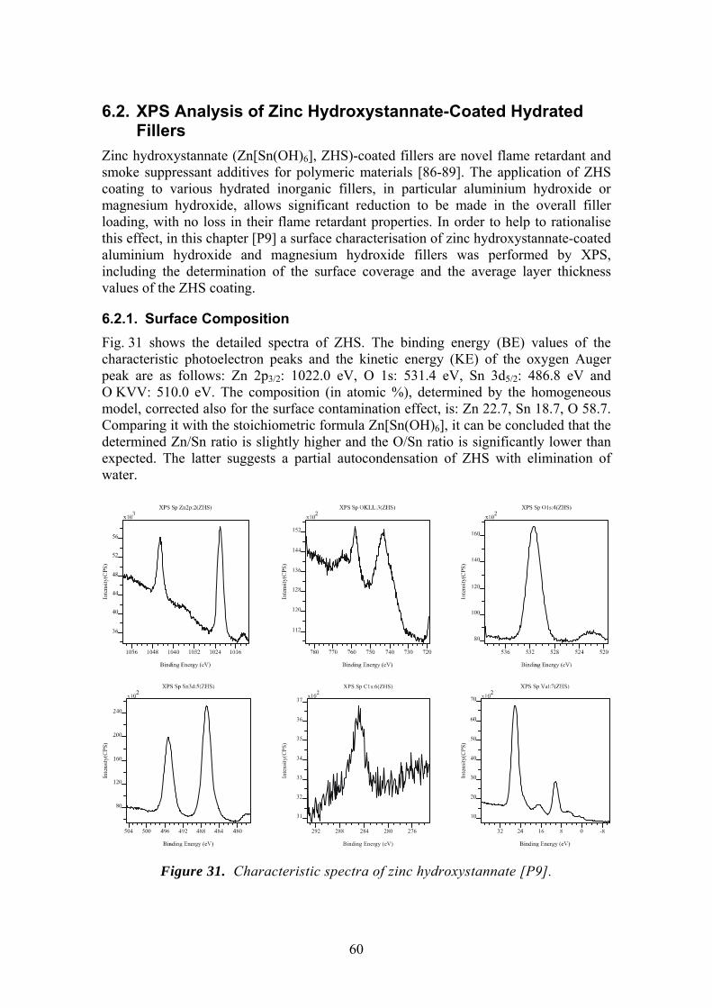
6.2. XPS Analysis of Zinc Hydroxystannate-Coated Hydrated Fillers
Zinc hydroxystannate (Zn[Sn(OH)6], ZHS)-coated fillers are novel flame retardant and smoke suppressant additives for polymeric materials [86-89]. The application of ZHS coating to various hydrated inorganic fillers, in particular aluminium hydroxide or magnesium hydroxide, allows significant reduction to be made in the overall filler loading, with no loss in their flame retardant properties. In order to help to rationalise this effect, in this chapter [P9] a surface characterisation of zinc hydroxystannate-coated aluminium hydroxide and magnesium hydroxide fillers was performed by XPS, including the determination of the surface coverage and the average layer thickness values of the ZHS coating.
6.2.1. Surface Composition Fig. 31 shows the detailed spectra of ZHS. The binding energy (BE) values of the characteristic photoelectron peaks and the kinetic energy (KE) of the oxygen Auger peak are as follows: Zn 2p3/2: 1022.0 eV, O 1s: 531.4 eV, Sn 3d5/2: 486.8 eV and O KVV: 510.0 eV. The composition (in atomic %), determined by the homogeneous model, corrected also for the surface contamination effect, is: Zn 22.7, Sn 18.7, O 58.7. Comparing it with the stoichiometric formula Zn[Sn(OH)6], it can be concluded that the determined Zn/Sn ratio is slightly higher and the O/Sn ratio is significantly lower than expected. The latter suggests a partial autocondensation of ZHS with elimination of water.
276280284288292
Binding Energy (eV)
x102
31
32
33
34
35
36
37
Inte
nsity
(CPS
)
XPS Sp C1s:6(ZHS)
Figure 31. Characteristic spectra of zinc hydroxystannate [P9].
60

The spectra of the ZHS-coated hydrated fillers contain peaks pertaining to both substrate and coating (see e.g. Fig. 32). A peculiar feature in the spectra of the ZHS-coated magnesium hydroxide (MH) samples is the presence of a small carbonate component in the C 1s region at 289.3 eV. Elapsed time-dependent spectra of the ZHS-coated MH samples performed with intervals of some months show a slow increase in the intensity of the carbonate component, which is probably due the incorporation of CO2 by MH from the ambient atmosphere.
02004006008001000
Binding Energy (eV)
x103
40
80
120
160
Inte
nsity
(CPS
)
O1s
Sn3d
Sn MNN
Zn LMM
O KLL
Al2s Al2p
Sn4p Sn4d
Zn2p
Sn3p
C1s
02004006008001000
Binding Energy (eV)
x103
40
80
120
160
Inte
nsity
(CPS
)
O1s
Sn3d
Sn MNN
Zn LMM
O KLL
Al2s Al2p
Sn4p Sn4d
Zn2p
Sn3p
C1s
Figure 32. Wide scan spectrum of aluminium trihydroxide (ATH; bottom) and ATH coated by 10 % of ZHS (top) [P9].
6.2.2. Quantification Model Based on the morphology determined previously (lamelliform particles, Fig. 33) by scanning electron microscopy [87,88], for quantification of the coated samples the ‘Islands-on-Plane’ model was applied. In particular, it is supposed that the planar substrate is covered by islands of ZHS, and this system is covered uniformly by the ubiquitous thin carbonaceous contamination layer, CHx (Fig. 34).
The mathematical equations applied in the calculation of the thickness values of the carbonaceous and of the ZHS layers and also of the surface coverage by ZHS are described elsewhere [P1,P6]. The results of this calculation are reported in Table 9.
61

Figure 33. The lamelliform particles of the ATH samples (dark gray) covered by zinc hydroxystannate (white).
CHZHS x
MH or ATH
CHZHS x
MH or ATHMH or ATH
Figure 34. The scheme of the “Islands-on-Plane” model applied for the quantification of the ZHS-coated MH and ATH samples [P9].
62

Table 9. Calculated layer thickness (h) and surface coverage (α) values for the uncoated and ZHS-coated MH and ATH samples.
Sample hCHx (nm) hZHS (nm) α
MH 1.59 0 0 10 % ZHS in MH 0.43 4.7 0.53 ATH 0.45 0 0 1 % ZHS in ATH 0.66 2.3 0.08 2 % ZHS in ATH 0.63 4.2 0.15 3 % ZHS in ATH 0.75 3.2 0.17 4 % ZHS in ATH 0.70 4.0 0.20 5 % ZHS in ATH 0.60 3.3 0.21 10 % ZHS in ATH 0.66 3.8 0.47 15 % ZHS in ATH 0.57 6.5 0.52
It can be seen that in the case of the ZHS-coated MH sample, characterised by 10 % bulk concentration of ZHS, the coverage value remains well below the complete one (α = 0.53), and the calculated thickness of the ZHS islands is surprisingly low (h = 4.7 nm). This statement is also valid for the ZHS-coated ATH samples studied, whose coverage values range between 0.08 and 0.52, and whose corresponding calculated thickness values range between 2.3 and 6.5 nm.
Fig. 35 shows the surface coverage of ATH by ZHS as a function of applied bulk concentration of ZHS. As expected, α increases monotonously with the concentration of ZHS.
Fig. 36 demonstrates the thickness of ZHS islands in relation to the applied bulk concentration of ZHS. The increasing trend is obvious also in this case, but the scatter is higher than that observed in the previous figure.
In Fig. 37 the layer thickness of ZHS versus surface coverage is depicted. When the bulk concentration of ZHS is higher than 10 % (α > about 0.5), the slope of the dependence seems to become very steep, suggesting that at high bulk concentrations of the ZHS coating, it is mainly the layer thickness, which tends to increase and not the degree of coverage. According to the ASTM cards, ZHS has a cubic cell with a lattice parameter a=0.772 nm (ASTM 33-1376) or 0.78 nm (ASTM 20-1455). In Fig. 37 multiples of the lattice parameter from 3a to 8a are also depicted. It seems that the measured layer thickness values correspond to multiples of the lattice parameter, implying that with the increase of coverage the number of monolayers increases from 3 to 8 in the experimental range studied.
63

0.0
0.2
0.4
0.6
0.8
1.0
0 5 10 15 20
Applied ZHS concentration (w %)
Cov
erag
e, α
Figure 35. Surface coverage (α) of ATH by ZHS versus applied bulk concentration of ZHS [P9].
0
1
2
3
4
5
6
7
0 5 10 15
Applied ZHS concentration (w % )
Thic
knes
s, h
(nm
)
Figure 36. Thickness (h) of ZHS islands as a function of its applied bulk concentration [P9].
64

0
1
2
3
4
5
6
0.0 0.1 0.2 0.3 0.4 0.5 0.6
Coverage, α
Thic
knes
s, h
(nm
)
3a
4a
5a
6a
7a
8a
7
0
1
2
3
4
5
6
0.0 0.1 0.2 0.3 0.4 0.5 0.6
Coverage, α
Thic
knes
s, h
(nm
)
3a
4a
5a
6a
7a
8a
3a
4a
5a
6a
7a
8a
7
Figure 37. Thickness (h) of ZHS islands as a function surface coverage (α) [P9]. Horizontal lines represent the multiples of lattice parameter (a) of ZHS.
In order to make a judgment about the consistency of the α and h values calculated above, the theoretical concentrations (c) of ZHS (in weight %), corresponding to the α and h values are calculated below, and then compared with the experimentally applied bulk concentrations.
The theoretical ratio of the mass of the coating, mc to the mass of the substrate, ms can be described by the following equation:
ραhAmm
s
c = (47)
where α is the coverage, h is the layer thickness, and A and ρ are the surface area of the substrate and the mass density of the coating, respectively.
The bulk weight concentration (c) of the coating is
( )sc
c
mmm100c+
= (48)
Rewriting Equation (48) and then combining it with (47) we get
( )ραhA
11mm1
mmsm
c100
c
s
c
c +=+=+= (49)
from which it follows that
( )ραhA11100c
+= (50)
65

The values of α and h are taken from Table 9, the surface area A for ATH determined by the BET nitrogen absorption technique is 6.2 m2/g, and according to the product specification sheet, ρ for ZHS is 3.3 g/cm3. The theoretical concentrations calculated by Equation (50) are shown in Table 10. From this table, it can be concluded that the applied bulk concentration values of ZHS and the corresponding values calculated from the α and h values are in reasonable agreement. These are of the same magnitude, although the former are higher by a factor ranging from 1.6 to 3.6. It is noteworthy that the relationship between the applied and calculated values is linear (Fig. 38). From the slope of the line, a mean difference factor of 2.3 can be calculated. This may be due to various reasons including the non-exact stoichiometry of the ZHS coating, or the possibility that the mass density of ZHS in the coating may not be necessarily equal to the mass density of ZHS in bulk. It is considered that the accuracy of the calculated coverage values is good, because the fitting parameters applied during the calculations (Qsum and Diff.%) [P1] are extremely sensitive even to small variations in α. However, the fitting parameters are less sensitive to the variation of the layer thickness. Furthermore, the thickness determined by XPS is expected to have an upper limit (hmax ≈ 3λ, where λ is the inelastic mean free path of the electrons), above which the fitting parameters should become insensitive to changes in the thickness value. At such high thickness values, however, the dependence depicted in Fig. 38 should deviate from linearity.
0
1
2
3
4
5
6
7
8
0 2 4 6 8 10 12 14
Applied ZHS concentration (%)
Cal
cula
ted
ZHS
conc
entra
tion
(%)
Figure 38. Calculated versus applied concentrations of ZHS [P9].
66

Table 10. Applied and calculated bulk concentrations for the ZHS-coated ATH samples.
Applied bulk concentration of ZHS
(weight %)
Calculated bulk concentration of ZHS
(weight %)
Factor of difference
1 0.38 2.6 2 1.27 1.6 3 1.11 2.7 4 1.61 2.5 5 1.40 3.6
10 3.53 2.8 15 6.47 2.3
6.2.3. Conclusions The suitability of the XPS MultiQuant program to determine layer thickness and coverage values for ZHS-coated inorganic fillers has been demonstrated. The results show that the thickness of ZHS coatings on MH and ATH fillers is of the order of several nanometres. Thus, the applied coating method of MH or ATH by ZHS — regarding the dimension of the thickness — is a nanoscale method leading to enhanced ZHS dispersion. This helps to rationalise the previously observed [87,89] high flame retardant and smoke suppressant efficacy of zinc hydroxystannate-coated fillers when applied in various polymeric formulations.
67

6.3. Preparation and Characterisation of Langmuir-Blodgett Type Arachidate Films
Langmuir-Blodgett (LB) films have been intensively studied in the last two decades. The reason for this is their nearly two-dimensional structure offering a broad spectrum of potential applications (in traditional areas like those of adhesive and anticorrosion layers, and in advanced areas like molecular electronics, non-linear optics, storage of optical information, piezoelectric organic films, waveguides, biomimetic membranes, etc.). To take advantage of the well-defined properties of LB-films, detailed information is needed on their thickness, orientation, structure, stability, and also on the dependence of these parameters on the conditions of preparation and characterization.
LB-films are frequently studied by various methods such as IR [90] and UV spectroscopy [91], XPS [92,93], neutron and X-ray scattering [94,95] as well as high performance imaging techniques [96,97]. Another novel method such as the surface sensitive mode of positron annihilation spectroscopy was also introduced into the characterisation of LB films [98,99]. XPS is one of the most powerful surface sensitive techniques for the investigation of the structure of the LB-films, because it provides chemical information on both composition and bonding.
In this work metal arachidate LB-films with Me = Cd2+ or Pb2+ and with varying number of monomolecular layers (MLs) were deposited on hydrophobic, trimethyl-silylated glass substrates and the films were studied by X-ray photoelectron spectroscopy.
6.3.1. Chemical Composition of the LB-films The metal (Cd, Pb) content of the arachidate LB-films measured for 2 and 4 MLs was about 1.3 and 1.7 atomic %, respectively.
The extent of the salt forming reaction between the dissolved metal ions and the arachidic acid in the Langmuir film was assessed from normalized intensity data measured for LB-films. The content of the actual metal atom was related to that of the carboxylic type carbon component with C1s BE at about 288.5 eV. The average of these values for 2 and 4 ML Cd- and Pb-arachidate films was ICd,Pb/ICOO = 0.45±0.05, which, within the experimental error, suggests a complete salt formation characterized by a value of 0.5. The ratio of intensity of the hydrocarbon type carbon component to that of the carboxylic type carbon component also provides information on the chemical composition of the LB-film. The obtained ICH/ICOO = 20.0±1.8 ratio is a quite reasonable value compared to the theoretical one of 19 for the arachidates.
The above parameters describing the chemical composition of the LB-films support the completeness of salt formation between arachidic acid and metal ions, and the transfer of this salt from the subphase to the substrate surface.
68

6.3.2. Quantification Model The quantification model for calculating the thickness of the arachidate layers from XPS intensity was constructed as follows: the arachidate monolayer was considered as two sublayers due to the dissimilar nature of the two parts of the molecule. The physical constants (molecular mass, density, IMFP) of the octadecane (C18H38) and the Cd or Pb acetate (Me(COOCH3)2) were used for the hydrocarbon chain and the hydrophilic part of the molecule, respectively. The contribution of the silyl groups was neglected.
In the XPS MultiQuant program a double arachidate layer of the Y-type structure was implemented by three sublayers, as shown in Fig. 39; and one, two or three of this double layers were applied for the calculation of the 2L, 4L and 6L samples, respectively. The measured XPS intensity data were corrected by cross section, angular distribution and analyser transmission and were normalised to a selected element.
1st LB layer
2nd LB layer
Sylilated glass substrate
(C18H37)2 hydrocarbon chains of the molecule
Pb(COOCH2)2 part of the molecule
1st LB layer
2nd LB layer
1st LB layer
2nd LB layer
Sylilated glass substrate
(C18H37)2 hydrocarbon chains of the molecule
Pb(COOCH2)2 part of the molecule
Figure 39. The model of the LB-film with Y-type structure used in the calculations [P3].
The thickness of the corresponding hydrocarbon and acetate layers were kept equal to each other during the calculation. Results were obtained by least squares fitting of the relative intensity data calculated by the model to the normalised measured intensity. The described model system was computed in two ways:
Full coverage of the surface was supposed and the layer thickness values were calculated. The reduced layer thickness was accepted for the tilt of the molecules. (Ya)
Partial coverage of the surface was supposed. The thickness of the layers was fixed to 28 Å (monolayer of perpendicular orientation) and the surface coverage was calculated. (Yb)
A model of the X-type structure (with alternating hydophobic-hydrophillic sublayers) was also examined for comparison.
69

6.3.3. Thickness of the Pb- and Cd-arachidate Layers The monolayer thickness values calculated by the Ya model from the XPS intensity data by the MultiQuant program for the LB-films composed of 2 or 4 MLs of Pb- or Cd-arachidate are displayed in Table 11.
Table 11. Thickness of monolayers in metal-arachidate LB-films calculated from XPS intensity, and the angle of tilt of the film-forming molecules to the
normal of the surface (model Ya) and coverage (model Yb) for the various LB-films prepared at various surface pressure (πc).
Sample
Cation Number of MLs
πc (mN/m)
Thickness of ML(Å)
Tilt angle (degree)
Coverage (%)
Pb2+ 2 35 28.8 0 100.0
Cd2+ 2 31 26.3 20 99.5
Cd2+ 4 31 26.5 19 97.0
Cd2+ 4 25 21.7 39 95.5
Comparing the length of the arachidate molecule (28 Å) to the experimentally determined ML thickness values, a good agreement can be found for the 2 MLs Pb-arachidate film prepared at πc=35 mN/m.
The other films deposited at lower surface pressures resulted in layers with lower thickness values although the molecular areas (calculated from the isotherm compression curves) in the corresponding LB films were only slightly varied (between 19.5 and 21.2 Å2) with the surface pressure (Fig. 40 a). It is known that arachidate molecules in such films may have an orientation significantly different from the normal one to the substrate surface (e.g., [100,101]; Fig. 40 d). Taking this into consideration, the tilt angles of the axis of the molecules were also calculated and presented in Table 11 for the various Cd-arachidate films. The tilt of the molecules in the MLs was about 20° for the LB-films prepared with the usually applied surface pressure of 30 mN/m. The largest modification in the orientation (39° from the normal) occurred in the 4 ML LB-film deposited at πc = 25 mN/m. Tilt angle of the molecules, calculated from the virtual thickness of the layers, show a strong correlation with the surface pressure (Fig. 41). Thus, the dependence of the film quality on the transfer pressure is clearly demonstrated by these data.
Alternatively, the deviations of the intensity ratio values from the expected ones could be interpreted by a partial coverage model as well (Yb; Fig. 40 c). The calculated values represent high surface coverage for all samples (Table 11 and Fig. 41). These values are almost independent of the surface pressure.
70

a b
c d
a b
c d
Figure 40. Possible reasons of the measured smaller monolayer thickness: a, the molecules are not stretched; b, the layer is X type; c, the layer is not
continuous; d, the molecules are not perpendicular to the substrate.
0
10
20
30
40
50
60
20 25 30 35 40
Surface pressure (mN/m)
Tilt
of m
olec
ules
(°)
0
20
40
60
80
100
120
Cov
erag
e (%
)
2
2
4
4
Pb
Cd
0
10
20
30
40
50
60
20 25 30 35 40
Surface pressure (mN/m)
Tilt
of m
olec
ules
(°)
0
20
40
60
80
100
120
Cov
erag
e (%
)
2
2
4
4
Pb
Cd
Figure 41. Correlation of the tilt angle of the molecules (left axis, ) or the surface coverage (right axis, ) with the surface pressure of the preparation
of the LB films. The digits show the number of monolayers [P3].
71

Although both interpretations seem to be realistic, the estimation of the tilt structure (Ya) is supported by the strong correlation between the tilt angle and the applied surface pressure, the mechanism of the film formation involving molecular interactions and the preparation conditions, i.e., layer-by-layer build up. Structures described by the combination of the two models, on the other hand, cannot be excluded, either.
In order to determine the molecular arrangement in the LB films beside the applied Y-type structure models, a model of the X-type structure was also fitted to the measured data. While a reasonable fit could be achieved, the thickness ratio of the acetate and hydrocarbon sublayers was unrealistic thus, the X-type structure could be excluded (Fig. 40 b).
It is shown that the XPS technique combined with the application of XPS MultiQuant quantification program is a suitable tool of monitoring the structure and orientation of the films on the preparation conditions.
6.3.4. X-ray Induced Changes in the Pb-arachidate layer The LB-film composed of 4 MLs of Pb-arachidate was exposed to a prolonged X-ray irradiation in the measuring chamber of the XPS instrument. The spectra were recorded for the as prepared sample (state 1) and after one and two exposure periods, each of 30 min (states 2 and state 3, respectively). A 60° of electron take-off angle was applied for state 3. The results are summarised in Table 12.
Table 12. Surface composition (atomic %) and the Pb to carboxyl composition ratio of 4 ML Pb-arachidate LB-film measured by XPS [P3]
(State 1: original sample; State 2: after 30 min of X-ray exposure; State 3: after 60 min of X-ray exposures, at 60° take-off angle).
State O C Pb total
Pb ionic Si I Pb
total
I COO
I Pb2+
I COO
I CHI COO
Relative thickness
% 1 14.2 79.5 1.72 1.72 4.66 0.43 0.43 17.2 100 2 16.7 74.9 1.95 1.74 6.45 0.58 0.52 19.0 84 3 6.51 89.9 1.63 1.23 1.96 0.68 0.51 33.8 70
It can be seen that the effect of X-ray exposure on the Pb-arachidate film is twofold. On the one hand, a substantial degradation of the LB-film was observed due to X-ray exposure. The increasing Si2p and O1s intensities measured for state 2, as compared to state 1, indicate a pronounced decrease in the nominal film thickness of the substrate. This could be well demonstrated quantitatively using the XPS MultiQuant program. The original nominal film thickness (100 %) virtually decreased to 84 % after the first X-ray exposure, and to 70 % after the second exposure period.
The other X-ray induced damage phenomenon concerns the chemical state of Pb. Apart from the doublet peak of ionic Pb detected at 138.7 and 143.5 eV, a new doublet of another Pb component appeared at lower BE for the X-ray beam-damaged states 2 and 3 (Fig. 42). According to the BE = 136.5 and 141.3 eV, this component can be assigned to Pb in reduced (Pb0) state. Following the first and second X-ray exposures, 11 and 25 %
72

of the total Pb content of the surface layer was transformed to this reduced, metallic state. The simultaneous alterations in the chemical composition also corroborated the above findings. Thus, the IPb
2+/ICOO intensity ratios (having values close to the stoichiometric one of 0.5) showed that the Pb2+ ions took part in the Pb-arachidate formation, while the reduced form of Pb was not coordinated to the arachidic acid resulting in unrealistic I Pb
total / I COO ratios.
132136140144148
Binding Energy (eV)
x102
40
60
80
100
Inte
nsity
(CPS
)
Pb 4f
Pb2+
138.7 eV
Pb0
136.5 eV
a b
132136140144148
Binding Energy (eV)
x102
40
60
80
100
Inte
nsity
(CPS
)
Pb 4f
Pb2+
138.7 eV
Pb0
136.5 eV
a b
Figure 42. Pb4f line of Pb-arachidate LB-film before (a) and after 60 min (b) X-ray irradiation [P3].
6.3.5. Conclusions In case of Cd- and Pb-arachidate the LB-layers were found to be composed of the
complete salt, MeA2.
The agreement between the measured photoelectron intensity values and the corresponding calculated values to the (Y-type) LB-layer model provides a proof for the development of Y-type structure.
The observed layer thickness and tilt angle values of the arachidate molecules depend on the applied surface pressure at the preparation of LB-films.
At prolonged X-ray exposure, reduction of Pb2+ to Pb0 was detected by XPS in the Pb-arachidate LB-films.
73

6.4. Surface Investigation of Zinc Ferrite Nanopowders Synthesised in Thermal Plasma
The spinel ferrites contain a close-packed cubic structure of oxygen ions in which tetrahedral (A) and octahedral (B) interstitial sites are occupied by cations [102]. Zinc ferrite belongs to the class of normal spinels, which presumably have a cation distribution of (Zn2+)A((Fe3+)2)B(O )B
2-4. It is paramagnetic at room temperature. However,
in special synthesis conditions (e.g., co-precipitation [ ], rapid quenching [ ] and mechanochemical activation [ ]) some Fe ions may occupy tetrahedral, as well as octahedral sites forming the inverse spinel structure. The strong superexchange among these sites results in an unusually high magnetisation as compared to normal spinels [ ]. A direct correlation was found between particle size and saturation magnetization: the finer the particles were, the more saturation magnetization could be measured [ , ]. The relatively high magnetization of pure Fe
103 104105 3+
104
106 107 3O4 can be further increased by Zn substitution and the highest saturation magnetisation ever found in spinel ferrites can be measured for zinc ferrous ferrites (ZnxFe3-xO4 where x ≤ 0.5) [ ]. 108
Radiofrequency thermal plasmas offer unique advantages for the synthesis of special ceramic powders due to the easily achievable high temperatures and energy densities. In addition, a high temperature gradient exists between the hot plasma flame and the surrounding gas phase. The resulting rapid quenching rate is favourable for producing fine particles with unstable structures in thermodynamic terms. In this chapter [P10] results on the thermal plasma synthesis of zinc ferrites and zinc ferrous ferrites are presented.
6.4.1. Phase Composition Sample preparation conditions and results of XRD analysis are collected in Table 13. The XRD patterns of the heat-treated oxide mixture (900 ºC, 6 h) show the formation of spinel phase. The calculated lattice parameter (a) is equal to that of ZnFe2O4 within the experimental error (Table 13, Sample 1). Contrary to the “conventional” synthesis, plasma treatment of the oxide mixture resulted in the formation of magnetite with the incorporation of a small amount of Zn only (Sample 2). The spinel composition was estimated by assuming the increase of lattice parameter due to Zn incorporation to be proportional with the Zn concentration. The calculated composition indicated the presence of about 0.1 mol of Zn in the spinel structure (Zn0.1Fe2.9O4). Particular ferrite probably formed through the condensation of oxide vapours. The small mean size of spinel grains (D = 34 nm) supports this assumption.
Treatment of the hydroxide-precursor in air at 900 °C for 6 h resulted in the formation of ZnFe2O4 phase (Table 2, Sample 3). The Fe:Zn molar ratio was 6:1 in the precursor powder. Hence, formation of Fe2O3 could be attributed to the excess of iron. The thermal plasma treatment of co-precipitated hydroxides in argon atmosphere resulted in a spinel phase with an estimated composition of Zn0.4Fe2.6O4 (Sample 4). The product contained some ZnO, as well. Spinel composition calculated from the cell parameter is very close to that of calculated from the Fe:Zn ratio of the precursor supposing a complete chemical transformation (Zn0.3Fe2.7O4).
74

Table 13. Methods of sample preparation and results of XRD measurements. Composition of spinel phase was estimated from the lattice parameter (a). The
mean grain size (D) was calculated from the FWHM of XRD profiles [P10].
Spinel phase Precursor
Fe:Zn molar ratio
Preparation method a (Å) Composition D (nm)
Other phases
1 oxides 2:1 900 °C, 6 h, air 8.439 ZnFe2O4 100 2 oxides 2:1 plasma / Ar 8.400 Zn0.1Fe2.9O4 34 Fe2O3, ZnO3 hydroxides 6:1 900 °C, 6 h, air 8.439 ZnFe2O4 65 Fe2O3
4 hydroxides 6:1 plasma / Ar 8.415 Zn0.4Fe2.6O4 42 ZnO, FeO 5 hydroxides 6:1 plasma / Ar+air 8.438
8.393 ZnFe2O4 Fe3O4
47 62
Fe2O3
SEM investigations showed similar mean grain sizes (D) to those calculated from the XRD profiles. Both Sample 3 (conventional technique) and Sample 4 (plasma treatment) consisted of fine particles that form agglomerates of 10-40 μm size. According to TEM micrographs, the particle size of plasma treated sample is in the range of 10-30 nm.
6.4.2. Surface Study Surface structure of zinc-substituted spinels was extensively studied by low-energy ion scattering (LEIS) previously [103,111]. It was suggested that octahedral sites were exposed at the surface. Anantharaman [103] reported much more zinc on the surface of a high surface area ZnFe2O4 sample as compared to a sample prepared by ceramic processing. Thus, he concluded that some zinc occupied octahedral sites in the sample prepared by co-precipitation. This finding was confirmed by Mössbauer spectroscopy, as well. XPS, which gives information from more than one atomic layer on the surface, is not suitable to identify the inverse spinel structure from the surface zinc enrichment. Nevertheless, a significant chemical shift was measured between tetrahedrally and octahedrally coordinated Zn ions by XPS [112].
Bulk and surface chemical compositions of our samples differed significantly (Table 14). The XPS results indicated some surface enrichment of ZnO even in the sample prepared by conventional ceramic processing (Table 14, Sample 1). However, a much higher surface enrichment of ZnO was measured on the surface of plasma treated samples. To remove the unreacted ZnO from Sample 4 it was washed with diluted HCl solution. After washing ZnO molar ratio decreased both in the bulk and on the surface, but the S:B ratio still was 4:1. No significant chemical shift of the Zn 2p doublet could be measured in the samples. To explain the surface enrichment of Zn, we assumed spherical particles of zinc ferrite covered by a ZnO layer. Composition and size of these spherical grains were obtained from the XRD analysis (Table 13). Composition and thickness of ZnO layer was calculated by the XPS MultiQuant program from the XPS intensities. For the plasma treated hydroxide precursor (Sample 4), the high Zn surplus could be explained by a relatively thin (1.2 nm) ZnO layer covering the zinc ferrite particles. This layer thickness is equal to about six molecular layers of ZnO. In the case of sample prepared by conventional technique and for the acid treated sample a ZnO
75

layer thickness of 0.15 nm was calculated being less than one molecular layer. In particular cases, we suppose an inhomogeneous distribution of Zn inside the grains rather than a partial surface coverage.
Table 14. Surface (S) and bulk (B) molar ratios of ZnO related to Fe2O3 and calculated layer thickness (d) of ZnO [P10].
ZnO (mol) Sample Fe2O3
(mol) S B S / B d
(nm)
1 1.00 2.01 0.99 2 0.15 2 1.00 9.17 0.42 20 4 1.00 4.45 0.35 13 1.20 4 * 1.00 0.96 0.22 4 0.15 * treated with a diluted HCl solution
Formation of inverse spinel structure due to special synthesis conditions is rather probably. However, other experimental techniques (e.g., magnetization measurements, Mössbauer spectroscopy) are needed to support this assumption.
100 nm
ZnO0.15 nm
ZnFe2O442 nm
ZnO1.2 nm
0.15 nm *
Zn0.4Fe2.6O4
100 nm
ZnO0.15 nm
ZnFe2O4
100 nm100 nm
ZnO0.15 nm
ZnFe2O442 nm
ZnO1.2 nm
0.15 nm *
Zn0.4Fe2.6O442 nm42 nm
ZnO1.2 nm
0.15 nm *
Zn0.4Fe2.6O4
Figure 43. The size and thickness of the ZnO layer of the zinc ferrite nanoparticles of samples 1 and 4 (* after washing with HCl).
6.4.3. Conclusions Nanosized spinel phases of various compositions can be synthesized in an RF thermal plasma reactor in spite of the very short residence time of reagents in the hot plasma region. Iron and zinc containing precursors probably first atomise then vaporize near to the plasma flame. Spinels are forming during the condensation. This mechanism is supported by the fine (10-30 nm) particle size of powders produced. Conversion of the precursors was not complete in the plasma reactor. The quantity of unreacted compounds was smaller in the case of co-precipitated precursors. It stresses the importance of the grain size of precursors. Partial pressure of oxygen can easily be adjusted in the plasma reactor. Thus, zinc ferrous ferrites can also be synthesized in these conditions.
76

XPS analysis indicated a high surface enrichment of Zn in all plasma prepared samples. This finding can be explained by two reasons: (i) condensation of ZnO vapours onto the surface of the spinel grains during quenching and (ii) inhomogeneous distribution of zinc in the spinel particles.
77

7. Summary X-ray Photoelectron Spectroscopy (XPS) is one of the most powerful surface analytical techniques capable to provide accurate qualitative, quantitative and chemical state information. Determination of the chemical state of elements on the surface is of great theoretical and practical interest. However, simultaneous application of the quantification and the chemical state determination will enhance the reliability of the results and help creating a consistent picture for the surface of the investigated material system.
Numerous quantification methods, models and data sets were published but usually only the simplest ones are built into the data systems used for routine work. The major purpose of this work was to enhance the quantitativeness of the evaluation of photoelectron spectra by developing a complex program package and to give a practical and universal tool to the surface scientist to produce reliable analytical results in most of the cases.
The XPS MultiQuant program was developed based on two-decade experience to perform sophisticated quantitative calculations. The program can handle the classic “infinitely thick homogeneous sample” model, to calculate surface chemical composition, as well as the structured models to calculate thickness of overlayers. The program requires only the input of the integrated intensity values of the measured XPS lines. All necessary basic data, like theoretical and experimental cross sections, asymmetry parameters, line energy data, etc., are provided by the attached library. One of the basic features of the program is that all terms of the sensitivity factors (cross section, angular correction, IMFP correction, analyser transmission and contamination correction) can be selected independently and can be overridden manually. Wide range of built-in methods is offered providing accurate results. Calculation of several experiments can be performed simultaneously. Data and results can be stored, printed, charted and exported to other programs. The program is equipped with user-friendly interface and furnished with ample help facilities (online help, wizard, user’s manual).
This work presents a set of newly developed methods to enhance and extend the capabilities of the quantitative evaluation of photoelectron spectra, which are integrated into the XPS MultiQuant program.
Most of the samples subjected to XPS analysis contain, unfortunately, some level of ubiquitous carbonaceous contamination, which affect the result of the quantification. A new correction method for surface contamination was developed where the correction factor is dynamic, being proportional to the concentration of the adventitious carbon. It was shown that the method can be applied in wide concentration range of surface contamination for variety of samples.
Precise knowledge of the surface chemistry of powdered and fibrous samples is of major importance for many applications. Curved surfaces (spherical or cylindrical), covered by thin overlayers, frequently occur and are applied in the practice. Examples may include intentionally coated or contaminated powders and wires, etc. (e.g., for synthesising composite materials). Applying the common planar model to these surfaces leads to overestimated layer thickness values. A new quantification
78

model was developed to calculate the thickness of overlayers on spherical and cylindrical surfaces. The geometry correction factors for spherical and cylindrical surfaces were derived by applying pure geometric considerations.
During the past years, the author has applied the different kinds of quantitative evaluation methods of photoelectron spectra for a large number of material systems, including oxides, nitrides, metals, glasses, polymers, catalysts, etc. Selected examples illustrate the different fields of application of the quantitative X-ray photoelectron spectroscopy to emphasise the benefit of the complex evaluation.
Application of the homogeneous model was illustrated by following the compositional as well as structural changes in the outermost layers of soda glass surfaces. The treated then silylated samples were tested and a surface model was proposed and verified by quantitative data. These results may contribute to elucidate problems concerning the preparation of ‘inert’ or ‘tailored’ glass surfaces for application in chromatographic glass capillary columns.
The applicability of the planar multilayer model was demonstrated on metal arachidate Langmuir-Blodgett (LB) films with Pb2+ and Cd2+ cations and varying number of monomolecular layers. Both the extent of salt formation and the build-up of the LB layer were evaluated by quantitative XPS. The surface coverage of the glass substrate by the LB film was assessed by calculations based on a substrate-overlayer model using the XPS MultiQuant program.
The planar layer model can be applied even in case of powder samples having lamelliform particles. As an example, aluminium hydroxide and magnesium hydroxide samples coated by zinc hydroxystannate (ZHS) have been studied by XPS. Analysis of data By XPS MultiQuant showed that the system can be described by a model, in which the substrate was covered by islands of ZHS, and on top covered by a uniformly thin carbonaceous contamination overlayer.
The model of spheres covered by overlayers was applied to study the nanosized zinc ferrite spinel powders, produced in RF thermal plasma. The products were characterised for both bulk and surface chemical compositions, and phase conditions. The surface Zn enrichment determined by quantitative XPS is attributed to a thin ZnO layer on the surface of the zinc ferrite particles and, in addition, to an inhomogeneous distribution of Zn inside the grains.
In general, the presented examples all emphasize the necessity of the proper quantitative evaluation of photoelectron spectra. The complex approach, the consistent application of the chemical state determination and quantification allow to get a deeper insight into the studied material system.
79

8. References
8.1. General References 1. J. Inczédy, T. Lengyel, A. M. Ure: Compendium of Analytical Nomenclature
(definitive rules 1997), 3rd edition, Blackwell Science, (1998); http://www.iupac.org/publications/analytical_compendium/Cha17sec212.pdf.
2. K. Siegbahn, C. Nordling, A. Fahlman, R. Nordberg, K. Hamrin, J. Hedman, G. Johansson, T. Bergmark, S. E. Karlson, B. Lindgren Lindberg: ESCA Atomic, Molecular and Solid State Structure Studied by Means of Electron Spectroscopy, Almquist Wiksells, Uppsala (l967).
3. D. Briggs, M. P. Seah (Eds.): Practical Surface Analysis by Auger and X-ray Photoelectron Spectroscopy, John Wiley & Sons, Chichester, NewYork, Brisbane, Toronto, Singapore (1983).
4. D. Briggs, M. P. Seah (Eds.): Practical Surface Analysis, 2nd ed., Vol. 1, John Wiley & Sons, Chichester-New York-Brisbane-Toronto-Singapore, Salle+Sauerländer, Aarau, Frankfurt am Main, Salzburg (1990).
5. D. Briggs: Handbook of X-Ray and Ultraviolet Photoelectron Spectroscopy, Heyden, London (l977).
6. Berényi D.: Az ESCA módszer alapjai és legújabb eredményei, A kémia újabb eredményei 35., Akadémiai Kiadó (1977).
7. Berényi D.: Fotoelektron-spektroszkópia : XPS, UPS, A Szilárdtestkutatás újabb eredményei 5., Akadémiai Kiadó (1979).
8. O. Brümmer, J. Heydenreich, K. H. Krebs, H. G. Schneider (Eds.): Szilárd testek vizsgálata elektronokkal, ionokkal és röntgensugárzással, Műszaki Könyvkiadó, Budapest (1984).
9. Varsányi G., Veszprémi T., Bertóti I.: Fotoelektronspektroszkópia, Budapesti Műszaki Egyetem, Mérnöki Továbbképző Intézet (l985).
10. T. L. Barr: Modern ESCA, CRC Press, Inc., Boca Raton - Ann Arbor - London - Tokyo (1994).
11. J. C. Rivière, S. Myhra (Eds.): Handbook of Surface and Interface Analysis Marcel Dekker, Inc., New York-Basel-Hong Kong (1998).
12. T. A. Carlson, Surf. Interface Anal. 4, 125 (1982).
13. B. R. Stohmeier, Surf. Interface Anal. 15, 51 (1990).
14. D. A. Shirley, Phys. Rev. B 5 4707 (1972).
15. S. Tougaard, Surf. Sci. 216, 343 (1989).
16. C. K. Jørgensen, H. Berthou, Discuss. Faraday Soc. 54, 269 (1973).
17. H. Berthou, C. K. Jørgensen, Anal. Chem. 47, 21 (1975).
18. J. E. Castle, R. H. West, J. Electron Spectrosc. Relat. Phenom. 19, 409 (1980).
80

19. J. Szajman, J. G. Jenkin, R. C. G. Leckey, J. Liesegang, J. Electron Spectrosc. Relat. Phenom. 19, 383 (1980).
20. K. Yabe, T. Yamashina, Appl. Surface Sci. 8, 387 (1981).
21. C. D. Wagner, L. E. Davis, M. V. Zeller, J. A. Taylor, R. H. Raymond, L. H. Gale, Surf. Interface Anal. 3, 211 (1981).
22. V. I. Nefedov, N. P. Sergushin, I. M. Band, M. B. Trzhaskovskaya, J. Electron Spectrosc. Relat. Phenom. 2, 383 (1973).
23. V. I. Nefedov, N. P. Sergushin, Y. V. Salyn, I. M. Band, M. B. Trzhaskovskaya, J. Electron Spectrosc. Relat. Phenom. 7, 175 (1975).
24. M. P. Seah, Surf. Interface Anal. 2, 222 (1980).
25. J. C. Slater, Phys. Rev. 81, 385 (1951).
26. J. H. Scofield, J. Electron Spectrosc. Relat. Phenom. 8, 129 (1976).
27. S. Evans, R. G. Pritchard, J. M. Thomas, J. Electron Spectrosc. Relat. Phenom. 14, 341 (1978).
28. D. J. Kennedy, S. T. Manson, Phys. Rev. A 5, 237 (1972).
29. F. Hermann, S. Skillman: Atomic Structure Calculations, Prentice-Hall, Englewood Cliffs, NJ (1963).
30. S. T. Manson, J. Electron Spectrosc. 1, 413 (1973).
31. R. F. Reilman, A. Msezane, S. T. Manson, J. Electron Spectrosc. Relat. Phenom. 8, 389 (1976).
32. H. Ebel, M. F. Ebel, A. Jablonski, J. Electron Spectrosc. Relat. Phenom. 35, 155 (1985).
33. W. Hanke, H. Ebel, M. F. Ebel, A. Jablonski, K. Hirokawa, J. Electron Spectrosc. Relat. Phenom. 40, 241 (1986).
34. A. Jablonski, C. J. Powell, Surf. Interface Anal. 20, 771 (1993).
35. A. Jablonski, Surf. Interface Anal. 20, 317 (1993).
36. C. J. Powell, A. Jablonski, J. Phys. Chem. Ref. Data 28, 19 (1999); and the references therein.
37. J. Zemek, S. Hucek, Fresenius J. Anal. Chem. 363, 156 (1999).
38. G. Gergely, Prog. Surf. Sci. 71. 31 (1999).
39. G. Gergely, Surf. Interface Anal. 3, 201 (1981).
40. A. Jablonski, P. Mrozek, G. Gergely, M. Menyhard, A. Sulyok, Surf. Interface Anal. 6, 291 (1984).
41. A. Jablonski, Surf. Sci. 151, 166 (1985).
42. P. Mrozek, A. Jablonski, A. Sulyok, Surf. Interface Anal. 11, 499 (1988).
43. G. Gergely, A. Konkol, M. Menyhard, B. Lesiak, A. Jablonski, D. Varga, J. Tóth, Vacuum 48, 621 (1997).
81

44. G. Gergely, A. Sulyok, M. Menyhard, J. Tóth, D. Varga, A. Jablonski, M. Krawczyk, B. Gruzza, L. Bideux, C. Robert, Appl. Surf. Sci. 144, 173 (1999).
45. W. S. M. Werner, C. Tomastik, T. Cabela, G. Richter, H. Störi, Surf. Sci. 470, 123 (2000).
46. S. Tougaard, M. Krawczyk, A. Jablonski, J. Pavluch, J. Tóth, D. Varga, G. Gergely, M. Menyhard, A. Sulyok, Surf. Interface Anal. 31, 1 (2001).
47. M. Krawczyk, A. Jablonski, L. Zommer, J. Tóth, D. Varga, L. Kövér, G. Gergely, M. Menyhard, A Sulyok, Zs. Benedek, B. Gruzza, C. Robert, Surf. Interface Anal. 33, 23 (2002).
48. M. P. Seah, W. A. Dench, Surf. Interface Anal. 1, 2 (1979).
49. S. Tanuma, C. J. Powell, D. R. Penn, Surf. Interface Anal. 21, 165 (1994).
50. C. J. Powell, A. Jablonski: NIST Electron Inelastic-Mean-Free-Path Database - Version 1.1, National Institute of Standards and Technology, Gaithersburg, MD (2000).
51. W. H. Gries, Surf. Interface Anal. 24, 38 (1996).
52. G. Varsányi, ACH Models Chem. 132, 949 (1995).
53. S. Tanuma, C. J. Powell, D. R. Penn, Surf. Interface Anal. 11, 577 (1988).
54. DS 300 for XSAM 800 User’s Guide, Kratos Analytical Ltd., Manchester (1981).
55. DS 800 Operator’s Guide, Kratos Analytical Ltd., Manchester.
56. Vision Reference Manual, Kratos Analytical Ltd., Manchester (1993).
57. AXIS HSi 165 and Ultra Operating Manual, Kratos Analytical Ltd., Manchester (2000).
58. VGS 5250 Data System Users Manual, VG Scientific, East Grinstead (1989).
59. K. Yoshihara, in ECASIA'99 Abstracts, (Eds. J. M. Sanz, J. P. Espinós). Sevilla, 179 (1999); http://www.sasj.jp.
60. R. Hesse, T. Chassé, R. Szargan, Fresenius J. Anal. Chem. 365, 48 (1999).
61. R. Hesse, T. Chassé, R. Szargan, Anal. Bioanal. Chem. 375, 856 (2003).
62. R. Hesse, T. Chassé, P. Sterubel, R. Szargan, in ECASIA’03 Book of Abstracts (Eds. W. E. S. Unger, I. Retzko, Th. Gross), Berlin, 87 (2003).
63. A. Jablonski, personal communication (1995).
64. S. Tougaard, J. Vacuum Science Technol. A 1, 1415 (1996).
65. S. Tougaard, Appl. Surf. Sci. 100/101, 1 (1996).
66. S. Tougaard, Surf. Interface Anal. 26, 249 (1998); http://www.quases.com.
67. B. V. Crist: Spectral Data Processor Operation Guide, XPS International LLC, Mountain View, CA (1994-2004); http://www.xpsdata.com
82

68. CasaXPS User’s Manual, Casa Software Ltd., Wilmslow, (2000); http://www.casaxps.cwc.net.
69. J. Szépvölgyi, I. Mohai, J. Gubicza, J. Mat. Chem. 11, 859 (2001).
70. M. Yazdanian, H. Yu, G. Zografi, Langmuir 6, 1093 (1990).
71. Z. Károly, J. Szépvölgyi, Zs. Farkas, Powder Technol. 110, 169 (2000).
72. T. Reich, V. I. Nefedov, J. Electron Spectrosc. Relat. Phenom. 56, 33 (1991).
73. T. J. Horr, J. R. Ralston, R. St. C. Smart, Colloids Surfaces A 92, 277 (1994).
74. S. Tanuma, C. J. Powell, D. R. Penn, Surf. Interface Anal. 17, 911 (1991).
75. S. Tanuma, C. J. Powell, D. R. Penn, Surf. Interface Anal. 21, 165 (1994).
76. B. S. Garbow, K. E. Hillstrom, J. J. More: MINPACK Project, Argonne National Laboratory, (1980); http://gams.nist.gov/serve.cgi/Module/MINPACK/LMDIF/8379/
77. L. L. Hench, J. Non-crystal. Solids 19, 27 (1975).
78. L. L. Hench, XIth Int. Conf. on Glass, Vol I, 343 (1977).
79. L. L. Hench, D. E. Clark, in Industrial Applications of Surface Analysis (Eds. L. A. Casper, C. J. Powell), ACS Symp. Ser. 199, 203 (1982).
80. G. Alexander, Chromatographia 13, 651 (1980).
81. K. Grob, G. Grob, J. Chromatogr. 125, 471 (1976).
82. Th. Welsch, W. Engewald, Ch. Klaudie, Chromatographia 10, 22 (1977).
83. K. Grob, G. Grob, K. Grob, Jr, J. High Res. Chrom. Chrom. Comm. 2, 31 (1979).
84. C. D. Wagner, D. E. Passoja, H. F. Hillery, T. G. Kinsky, H. A. Six, W. T. Jansen, J. A. Fayler, J. Vac. Sci. Technol. 21, 993 (1982).
85. C. D. Wagner, W. M. Riggs, L. E. Davis, J. F. Moulder, G. T. Muilenberg: Handbook of X Ray Photoelectron Spectroscopy, Perkin Elmer, Eden Prairie, MN (1979).
86. P. A. Cusack, B. Patel, M. S. Heer, R. G. Baggaley, Intern. Patent Appl. 1996; PCT/GB96/01475.
87. R. G. Baggaley, P. R. Hornsby, R. Yahya, P. A. Cusack, A. W. Monk, Fire and Mater. 21, 179 (1997).
88. P. A. Cusack, P. R. Hornsby, J. Vinyl Addit. Techn. 5, 21 (1999).
89. M. S. Cross, P. A. Cusack, P. R. Hornsby, Polym. Degrad. Stab. 79, 309 (2003).
90. M. Leonard, R. M. Morelis, P. R. Coulet, Thin Solid Films 260, 227 (1995).
91. G. G. Roberts, Advances in Physics 34, 475 (1985).
92. M. Sastry, S. Badrinarayanan, P. Ganguly, Phys. Rev. B 45, 9320 (1992).
93. M. Schreck, D. Schmeisser, W. Göpel, H. Schrier, H. U. Habermeier, S. Roth, L. Dulog, Thin Solid Films 175, 95 (1989).
83

94. S. Takeuchi, Y. Nogami, T. Ishiguro, H. Oyanagi, Thin Solid Films 250, 243 (1994).
95. A. Malik, M. K. Durbin, A. G. Richter, K. G. Huang, P. Dutta, Phys. Rev. B 52, R11654 (1995).
96. L. Bordieu, P. Silberzan, D. Chatenay, Phys. Rev. Lett. 67, 2029 (1991).
97. J. M. Solletti, M. Botreau, F. Sommer, W. L. Brunat, S. Kasa, Tran Minh Duc, M. R. Celio. Langmuir 12, 5379 (1996).
98. Cs. Szeles, A. Vértes, É. Kiss, S. Szpala, K. G. Lynn, J. Colloid Interface Sci. 176, 358 (1995).
99. T. Marek, Cs. Szeles, K. Süvegh, É. Kiss, A. Vértes, K. G. Lynn, Langmuir 15, 8189 (1999).
100. S. Garoff, H. W. Dechman, J. H. Dunsmuir, M. S. Alvarez, J. Physique 47, 701 (1986).
101. D. A. Outka, J. Stohr, J. P. Rabe, J. D. Swalen, H. H. Rotermund, Phys. Rev. Letters 59, 1321 (1987).
102. B. D. Cullity: Introduction to Magnetic Materials, Addison-Werley, Reading, MA (1972).
103. M. R. Anantharaman, S. Jagatheesan, K. A. Malini, S. Sindhu, A. Narayanasamy, C. N. Chinnasamy, J. P. Jacobs, S. Reine, K. Seshan, R. H. H. Smits, H. H. Brongersma, J. Magn. Magn. Mat. 189, 83 (1998).
104. K. Tanaka, M. Makita, Y. Shmizugawa, K. Hirao, N. Soga, J. Phys. Chem. Solids 59, 1611 (1998).
105. V. Šepelák, U. Steinike, D. Chr. Uecker, S. Wissmann, K. D. Becker, J. Solid State Chem. 135, 52 (1998).
106. T. Sato, K. Haneda, N. Seki, T. Iijima, Appl. Phys. A 50 13, (1990).
107. T. Kamiyama, K. Haneda, T. Sato, S. Ikeda, H. Asano, Solid State Commun. 81, 563 (1992).
108. V. A. M. Brabers, J. Phys. IV. Fr. 7, C1-223 (1997).
109. Z. Károly, J. Szépvölgyi, Zs. Farkas, Powder Technol. 110, 169 (2000).
110. H. P. Klug, L. E. Alexander: X-ray Diffraction Procedure for Polycrystalline and Amorphous Materials, John Wiley & Sons, New York (1974).
111. J. P. Jacobs, A. Maltha, J. G. H. Reintjes, J. Drimal, V. Ponec, H. H. Brongersma, J. Catal. 147, 294 (1994).
112. U. Steinike, P. Druska, B. Wallis, D. Chr. Uecker,V. Šepelák, Chem. Papers 52, 147 (1998).
84

8.2. References Related to the Present Dissertation
8.2.1. Papers P1. M. Mohai:
XPS MultiQuant for Windows User’s Manual. Budapest (1999, 2001, 2003); http://www.chemres.hu/aki/XMQpages/XMQhome.htm
P2. M. Mohai, I. Bertóti: Correction for Surface Contaminations in XPS: A Practical Approach. ECASIA 95 (Eds. H. J. Mathieu, B. Reihl, D. Briggs), John Willey & Sons, Chichester-New York-Brisbane-Toronto-Singapore (1995), ISBN 0 471 95899 9, pp. 675-678.
P3. M. Mohai, É. Kiss, A. Tóth, J. Szalma, I. Bertóti: Preparation and Characterisation of Langmuir-Blodgett Type Arachidate Films. Surf. Interface Anal. 34, 772-776 (2002).
P4. G. Varsányi, G. Mink, K. Rée, M. Mohai: Consideration of Twodimensional Surface Roughnesses in Quantitative XPS Analysis. Periodica Polytechnica 31(1-2), 3-17 (1987).
P5. M. Mohai, I. Bertóti: Calculation of Overlayer Thickness on Curved Surfaces Based on XPS Intensities. Surf. Interface Anal. 36, 805-808 (2004).
P6. M. Mohai: XPS MultiQuant: Multimodel XPS Quantification Software. Surf. Interface Anal. 36, 828-832 (2004).
P7. Mohai M., Bertóti I., Alexander G.: Módositott üvegfelületek ESCA vizsgálata. XXIX. Magyar Szinképelemző Vándorgyűlés és II. Magyar Molekulaspektroszkópiai Konferencia előadásai, Gépipari Tudományos Egyesület (1986), Keszthely, pp. 491.
P8. I. Bertóti, M. Mohai, M. Révész, G. Alexander: Surface Composition of Glasses: Modifications Induced by Chemical and Heat Treatments. Vacuum 37(1-2), 129-131 (1987).
P9. M. Mohai, A. Tóth, P. R. Hornsby, P. A. Cusack, M. Cross, G. Marosi: XPS Analysis of Zinc Hydroxystannate-Coated Hydrated Fillers. Surf. Interface Anal. 34, 735-739 (2002).
P10. I. Mohai, J. Szépvölgyi, I. Bertóti, M. Mohai, J. Gubicza, T. Ungár: Thermal Plasma Synthesis of Zinc Ferrit Nanopowders. Solid State Ionics 141-142, 163-168 (2001).
85

8.2.2. Conference Presentations C1. I. Bertóti, M. Mohai, M. Révész, G. Alexander: Surface Composition of Glasses:
Modifications Induced by Chemical and Heat Treatments. Hungarian-Austrian-Yugoslavian 3rd Joint Vacuum Conference, Debrecen, 7–9 October 1985.
C2. Mohai M., Bertóti I., Alexander G.: Módositott üvegfelületek ESCA vizsgálata. XXIX. Magyar Szinképelemző Vándorgyűlés – II. Magyar Molekulaspektroszkópiai Konferencia, Keszthely, 1986. június 17–20.
C3. G. Alexander, I. Bertóti, M. Mohai, T. Székely: Surface Studies on Variously Silylated Glasses Used for Capillary Column Preparation. 24th International Symposium on Advances in Chromatography, West Berlin, 8–10 September 1987.
C4. Bertóti I., Mohai M., Szépvölgy J., Tóth A.: Si3N4 porok felületkémiai minősítése. XXI. Szilikátkémiai Ankét és II. Különleges Aluminium-oxid Konferencia, Zamárdi, 1990 május 3–4.
C5. M. Mohai, I. Bertóti: Correction for Surface Contaminations in XPS: A Practical Approach. 6th European Conference on Application of Surface and Interface Analysis, Montreaux, Switzerland, 9–13 October 1995.
C6. I. Bertóti, A. Tóth, M. Mohai, R. Kelly, G. Marletta, M. Farkas-Jahnke: Nanoscale In-depth Modification of Cr-O-Si Layers. European Materials Research Society (E-MRS) 1996 Spring Meeting, Strasbourg, France, 4–7 June 1996.
C7. M. Mohai: XPS MultiQuant: a Practical Tool for XPS Quantification. 8th European Conference on Application of Surface and Interface Analysis, Sevilla, Spain, 4–8 October 1999.
C8. M. Mohai: Practical Application of IMFP: Quantification of Photoelectron Spectra by XPS MultiQuant. International Workshop on Inelastic Mean Free Path of Electrons, IMFP 2000, Budapest, Hungary 27–29 January 2000.
C9. I. Mohai, J. Szépvölgyi, I. Bertóti, M. Mohai, J. Gubicza, T. Ungár: Thermal Plasma Synthesis of Zinc Ferrite Nanopowders. XIVth Internatl. Symp. on the Reactivity of Solids, ISRS 2000, Budapest, Hungary 27–31 August 2000.
C10. M. Mohai, A. Tóth, P. R. Hornsby, P. A. Cusack, M. Cross: Surface Analysis of Zinc Hydroxystannate-Coated Hydrated Fillers. 9th European Conference on Applications of Surface and Interface Analysis, Avignon, France, 30 September – 5 October 2001.
C11. É. Kiss, M. Mohai, A. Tóth, J. Szalma, I. Bertóti: Preparation and Characterisation of Langmuir-Blodgett Type Arachidate Films. 9th European Conference on Applications of Surface and Interface Analysis, Avignon, France, 30 September – 5 October 2001.
86

C12. M. Mohai: XPS MultiQuant: a Practical Tool for XPS Quantification. 9th European Conference on Applications of Surface and Interface Analysis, Avignon, France, 30 September – 5 October 2001.
C13. M. Mohai, I. Bertóti: Calculation of Layer Thickness on Curved Surfaces by XPS MultiQuant. 34th Workshop of the International Union of Vacuum Science, Technique and Applications: XPS: From Spectra to Results —Towards an Expert System. Saint Malo, France, 21–26 April 2002.
C14. M. Mohai: XPS MultiQuant: Multimodel XPS Quantification Software. 10th European Conference on Applications of Surface and Interface Analysis Berlin, Germany, October 5–10, 2003.
C15. M. Mohai, I. Bertóti: Calculation of Layer Thickness on Curved Surfaces by XPS MultiQuant. 10th European Conference on Applications of Surface and Interface Analysis Berlin, Germany, October 5–10, 2003.
8.3. References on Application of Quantitative XPS by the Author
A1. Bertóti I., Mink Gy., Mohai M., Révész M., Réti F., Varsányi Gy.: Fotoelektronspekrtoszkópiai (ESCA) vizsgálatok oxidok (Al2O3, TiO2) felületén. XXIX. Magyar Szinképelemző Vándorgyűlés és II. Magyar Molekulaspektroszkópiai Konferencia előadásai, Gépipari Tudományos Egyesület (1986), Keszthely, pp. 514.
A2. G. Mink, I. Bertóti, I. S. Pap, M. Mohai, T. Székely: On the Role Potassium Additives in Chlorination of TiO2 by CCl4 and COCl2. Vacuum 37(1-2), 133-135 (1987).
A3. I. Bertóti, R. Kelly, M. Mohai, A. Tóth: A Possible Solution to the Problem of Composisional Change with Ion-Bombarded Oxides. IBM Research Report RC 17609 (#77505) 1/13/92, Materials Science, IBM Research Division, Almaden, T. J. Watson, Tokyo, Zürich, pp. 1-17.
A4. I. Bertóti, R. Kelly, M. Mohai, A. Tóth: A Possible Solution to the Problem of Compositional Change with Ion-bombarded Oxides. Surf. Interface Anal. 19, 291-297 (1992).
A5. I. Bertóti, R. Kelly, M. Mohai, A. Tóth: Response of Oxides to Ion Bombardment: The Difference between Chemically Inert and Reactive Ions. Nucl. Instrum. Methods B 80/81, 1219-1225 (1993).
A6. I. Bertóti, A. Tóth, M. Mohai, R. Kelly, G. Marletta: Effect of Ion Bombardment on Cr-Si-O Layers: An XPS Study. E-MRS Symposia Proceedings, vol. 41, Stimulated Deposition Processes and Materials Aspects of Ion Beam Synthesis (Eds. H. Freller, J. M. Martinez-Duart, Y. Pauleau, J. Dieleman, P. L. F. Hemment, J. A. Kilner), Elsevier, North-Holland, Amsterdam (1994), pp. 211-217.
87

A7. I. Bertóti, A. Tóth, M. Mohai, R. Kelly, G. Marletta: Effect of Ion Bombardment on Cr–O–Si Layers: an X-ray Photoelectron Specroscopic Study. Thin Solid Films 241-217, 211 (1994).
A8. I. Bertóti, A. Tóth, M. Mohai: Sputter-deposited Cr-Si-O Cermet Films by XPS. Surf. Sci. Spectra 3, 105-111 (1995).
A9. I. Bertóti, A. Tóth, M. Mohai, R. Kelly, G. Marletta: He+ and Ar+ Bombardment Induced Chemical Changes in Cr–O–Si Layers. Nucl. Instrum. Methods B 116, 200-206 (1996).
A10. I. Bertóti, A. Tóth, M. Mohai, R. Kelly, G. Marletta, M. Farkas-Jahnke: Nanoscale In-Depth Modification of Cr-O-Si Layers. Nucl. Instrum. Methods B 122, 510-513 (1997).
A11. I. Bertóti, A. Tóth, M. Mohai, R. Kelly, G. Marletta, M. Farkas-Jahnke: Nanoscale In-Depth Modification of Cr-O-Si Layers. E-MRS Symposia Proceedings, vol. 65, New Trends in Ion Beam Processing of Materials and Beam Induced Nanometric Phenomena (Eds. F. Priolo, J. K. N. Lindner, A. Nylandsted Larse, J. M. Poate, E. E. B. Camplbell, R. Kelly, G. Marletta, M. Toulemonde), Elsevier, Amsterdam-Lausanne-New York-Oxford-Shannon-Tokyo (1997), ISBN 0-444-20501-2, pp. 510-513
A12. I. Bertóti, M. Mohai, A. Tóth: Nanoscale In-Depth Modification of Metal Oxides and Nitrides by Low Energy Ion Beams — Chemical Aspects. NANOTECHNOLOGY: a dedicated tool for the future, (Eds. I. Mojzes and B. Kovács), MIL-ORG Ltd. & NETI, Budapest (1997), ISBN 963-85316 5 7, pp. 107-134.
A13. J. P. Espinós, A. R. González-Elipe, M. Mohai, I. Bertóti: Surface Chemical Effects of Low Energy N2
+ Ion Bombardment on Single Crystalline α-Al2O3. Surf. Interface Anal. 30, (2000) 90-94.
A14. Bertóti I., Mohai M., Szépvölgyi J., Tóth A.: A szilicium-nitrid porok felületkémiai minősitése XPS (ESCA) módszerrel. Épitőanyag 43, 42-47 (1991).
A15. F. Pavlyák, I. Bertóti, M. Mohai, I. Biczó, J. Giber: AES and XPS Characterization of SiNx Layers. Surf. Interface Anal. 20, 221-227 (1993).
A16. I. Bertóti, M. Mohai, J. L. Sullivan, S. O. Saied: Surface Chemical Changes in PVD TiN Layers Induced by Ion Bombardment. Surf. Interface Anal. 21, 467-473 (1994).
A17. I. Bertóti, M. Mohai, J. L. Sullivan, S. O. Saied: Surface Characterization of Plasma Nitrided Titanium: an XPS Study. Appl. Surf. Sci. 84 357-372, (1995).
A18. Mohai I., Szépvölgyi J., Bertóti I., Mohai M., Tóth M.: A szilícium-nitrid gázfázisú szintézisének optimálása termikus plazmában. Építőanyag 50, 98-104 (1998).
88

A19. I. Bertóti, M. Mohai, A. Tóth, B. Zelei: Effect of Ar+, N2+, He+ and H2
+ Bombardment on the Composition and Structure of CNx Layers. Nucl. Instrum. Methods B 148, 645-649 (1999).
A20. C. Blawert, B. L. Mordike, M. Mohai, I. Bertóti, A. Juhász: Investigation of Nitrided and Carburized Layers Produced by Plasma Immersion Ion Implantation of Aluminium at Elevated Temperatures. Proc. 7th Internatl. Seminar of IFHT: Heat Treatment and Surface Engineering of Light Alloys (Eds. J. Lendvai, T. Réti), Hung. Soc. Mechanical Eng. (1999), Budapest, pp. 51-60.
A21. T. Ujvári, A. Tóth, M. Mohai, J. Szépvölgyi, I. Bertóti: Composition and Chemical Structure Characteristics of CNx Layers Prepared by Different Plasma Assisted Techniques. Solid State Ionics 141-142, 63-69 (2001).
A22. I. Bertóti, M. Mohai, P. H. Mayrhofer, C. Mitterer: Surface Chemical Changes Induced by Low Energy Ion Bombardment in Chromium Nitride Layers. Surf. Interface Anal. 34, 740-743 (2002).
A23. I. Bertóti, M. Mohai, A. Csanády, P. B. Barna, H. Berek: XPS Studies on Intermetallic Phases Formed in Al-Ni and Al-Mn Thin Films. Surf. Interface Anal. 19, 457-463 (1992).
A24. M. Mohai, A. Tóth, I. Sajó, T. Ujvári, I. Bertóti: Plasma Surface Modification of Titanium and Ti-alloy. Surf. Interface Anal. 36, 1155-1158 (2004).
A25. A. Tóth, M. Mohai, T. Ujvári, T. Bell, H. Dong, I. Bertóti: Surface Chemical and Nanomechanical Aspects of Air PIII-Treated Ti and Ti-Alloy. Surf. Coat. Technol. 186, 248-254 (2004).
A26. Bertóti I., Mohai M., Révész M.: Az XPS elve és alkalmazása üvegfelületek vizsgálatára. Épitőanyag 43, 3-9 (1991).
A27. M. Mohai, I. Bertóti, M. Révész: XPS Study of the State of Oxygen on a Chemically Treated Glass Surface. Surf. Interface Anal. 15, 364-368 (1990).
A28. A. Tóth, I. Bertóti, T. Székely, M. Mohai: XPS Study of Ion-Induced Changes on the Surface of an Organosilicon Model Polymer. Surf. Interface Anal. 7, 282-288 (1985).
A29. A. Tóth, I. Bertóti, G. Marletta, G. G. Ferenczy, M. Mohai: Ion Beam Induced Chemical Effects in Organosilicon Polymers. Nucl. Instrum. Methods B 116, 299-304 (1996).
A30. A. Tóth, I. Bertóti, M. Mohai: Nanoscale In-Depth Modification of Organosilicon Polymers by Particle Beams. NANOTECHNOLOGY: a dedicated tool for the future, (Eds. I. Mojzes and B. Kovács), MIL-ORG Ltd. & NETI, Budapest (1997), ISBN 963-85316 5 7, pp. 135-152.
89

A31. G. Mink, I. Bertóti, L. Németh, G. Gáti, M. Mohai, T. Székely: Surface Characterization of the Deactivation of Alumina Catalysts Used for COS Synthesis. Surf. Interface Anal. 12, 262-268 (1988).
A32. Á. Molnár, M. Varga, G. Mulas, M. Mohai, I. Bertóti, A. Lovas, G. Cocco: Cu-Mg Powders and Ribbons; Characterization and Catalytic Tests Reactions. Mater. Sci. Eng. A 304-306, 1078-1082 (2001).
A33. G. Mulas, M. Varga, I. Bertóti, M. Mohai, Á. Molnár, G. Cocco: Characterization of Pd-Mg Catalyst Precursors Prepared by Ball Milling and Comparison with Cu-Mg. Mater. Sci. Forum 377, 57-62 (2001).
A34. M. Varga, Á. Molnár, G. Mulas, M. Mohai, I. Bertóti, G. Cocco: Cu-MgO Samples Prepared by Mechanochemistry for Catalytic Application. J. Catal. 206, 71-81 (2002).
A35. M. Varga, Á. Molnár, M. Mohai, I. Bertóti, M. Janik-Czachor, A. Szummer: Selective Hydrogenation of Pentynes over PdZr and PdCuZr Prepared from Amorphous Precursors. Appl. Catal. A 234, 167-178 (2002).
A36. Bertóti I., Tóth A., Mohai M.: Szilícium napelemeken kialakított fémkontaktusok XPS vizsgálata. Research report, (1984), unpublished.
A37. Csordás Tóth A., Bertóti I., Mohai M.: Különböző aluminium-hidroxid minták szennyezőinek vizsgálata felületfizikai módszerekkel. Szemelvények az aluminiumipari anyagvizsgálat köréből (Ed. Major G.) ALUTERV-FKI, Budapest, (1986) pp. 61-79.
A38. J. Szépvölgyi, I. Bertóti, I. Varga, M. Mohai, T. Székely, I. Párkányi: Studies on the Flotation of a Non-Ferrous Slag Minerals Engineering 1(2), 127-136 (1988).
A39. Szépvölgyi J., Bertóti I., Varga I., Mohai M., Székely T., Párkányi I., Csillag I., Farkas A., Fodor Gy.: Szinesfémtartalmú salak flotációs dúsitásának vizsgálata. BKL-Kohászat 122(2), 83-92 (1989).
A40. I. Bertóti, M. Mohai, N. M. Renevier, E. Szilágyi: XPS Investigation of Ion Beam Treated MoS2-Ti Composite Coatings. Surf. Coat. Technol. 125, 173-178 (2000).
A41. M. Tóth, I. Bertóti, M. Mohai, I. Fórizs, I. Vozil: Material Analysis of the Bronze Statuette of Imhotep. Bulletin du Musée Hongrois des Beaux-Arts, 95, 35-44 (2001).
90

9. Theses 1. A new surface contamination correction method was developed where the correction
factor is dynamic, being proportional to the concentration of the adventitious carbon. The method can be applied in wide concentration range of surface contamination for variety of samples.
2. A new quantification model was developed to calculate the thickness of overlayers on spherical and cylindrical surfaces. Applying the common planar model to these surfaces leads to overestimated layer thickness values. The geometry correction factors for spherical and cylindrical surfaces were derived by applying pure geometric considerations.
3. A complex program was developed to perform sophisticated quantitative evaluation of X-ray photoelectron spectra. The program can handle the classic “infinitely thick homogeneous sample” model as well as the structured models to calculate thickness of overlayers. Wide range of built-in methods and library of basic data are offered together with several independently controllable correction features providing accurate results. All newly developed features, like dynamic contamination correction, calculation of overlayer thickness on curved surfaces, presented in the dissertation are implemented.
4. Quantitative XPS measurements have confirmed that the acidic treatment of soda-lime glass leads to the complete depletion of alkali and alkali earth metals and also a partial depletion of Al to a depth far beyond the detection limit. The silylation of the etched surface can be quantitatively followed by the change of the chemical state of the constituents.
5. Quantitative XPS results show that the thickness of ZHS coatings on MH and ATH fillers is of the order of several nanometres. Thus, the applied coating method of MH or ATH by ZHS is a nanoscale method leading to enhanced ZHS dispersion. The suitability of the XPS MultiQuant program to determine layer thickness and coverage values for ZHS-coated inorganic fillers has been demonstrated.
6. Quantitative XPS measurements have verified that in case of Cd- and Pb-arachidate LB-layers the films were composed of the complete salt, MeA2. The applied sublayer model has provided a proof for the development of Y-type structure. The observed layer thickness and tilt angle values of the arachidate molecules depend on the applied surface pressure applied during the preparation of LB-films.
7. Quantitative XPS analysis of nanosized zinc ferrite particles has indicated a high surface enrichment of Zn in all plasma prepared samples. For the plasma treated hydroxide precursor the high Zn surplus could be explained by a relatively thin (1.2 nm) ZnO layer covering the zinc ferrite particles. This finding can be explained by two reasons: condensation of ZnO vapours onto the surface of the spinel grains during quenching, and inhomogeneous distribution of zinc in the spinel particles.
91

10. Acknowledgement The author is indebted to all of his colleagues who supported this work:
to Dr. Imre Bertóti and to Dr. András Tóth, the supervisors, for their valuable advices and remarks, and also for careful reading of the manuscript;
to Prof. György Varsányi for the initiation of the topic and the recurring fruitful discussions;
to Mr. László Gulyás for his technical assistance in XPS measurements;
to Dr. János Szépvölgyi and Dr. Ilona Mohai for the synthesis of nanosized powders;
to Dr. Éva Kiss for the preparation of Langmuir-Blodgett films;
to Dr. Gábor Alexander for the preparation of the silylated glass samples;
to all co-authors, not listed here, for their indispensable contribution to the papers.
Copyright © 2006 Miklós Mohai
The PhD degree was awarded by the University of Pannonia, Veszprém, Hungary.
This copy is slightly different from the ‘official’ one, deposited in the Library of the University. Minor corrections, suggested by the referees, are included; the foreign language abstracts and the Hungarian list of theses were omitted.
The XPS MultiQuant program described here is the version 3.0. Advanced versions are available at the homepage of the program.
92