Development and Application of a Land Use Model for Santiago de Chile
47
Development and Application of a Land Use Model for Santiago de Chile Universidad de Chile Francisco Martínez Francisco Martínez Universidad de Chile Universidad de Chile www.citilabs.com www.citilabs.com www.mussa.cl www.mussa.cl
-
Upload
constance-chavez -
Category
Documents
-
view
29 -
download
0
description
Universidad de Chile. www.mussa.cl. www.citilabs.com. Development and Application of a Land Use Model for Santiago de Chile. Francisco Martínez Universidad de Chile. Introduction. ASSESS URBAN POLICIES. Evaluation of Zone Regulation Plans Max or min lot sizes Building density - PowerPoint PPT Presentation
Transcript of Development and Application of a Land Use Model for Santiago de Chile

Development and Application of a Land Use Model for Santiago de Chile
Development and Application of a Land Use Model for Santiago de Chile
Universidad de Chile
Francisco MartínezFrancisco MartínezUniversidad de ChileUniversidad de Chile
www.citilabs.comwww.citilabs.comwww.mussa.clwww.mussa.cl

ASSESS URBAN POLICIESASSESS URBAN POLICIES
• Evaluation of Zone Regulation Plans– Max or min lot sizes– Building density – Land use banned (residential, indust.,
commercial)
– Max height of buildings
• Incentives: subsidies or taxes
• Sensitive to transport policies
• Optimal regulation plans
Introduction

APPLICATIONSAPPLICATIONS
• Equilibrium predictions– Create scenarios for transport studies– Evaluation of mega projects (Transatiago
BRT, Cerillos Airport, Central Ring)
• Optimal Location (subsidies)– Land use under externalities– Schools: minimum transport cost – Emissions: minimum emission and
tradable CO2 permits
Introduction

Model structure

Model inputs
• Growth: N° households and firms (Hh)
• Transport (acchi, atti)
• Regulations on supply and land use• Incentives or taxes for allocation of residential
and commercial activities
The Equilibrium Model

The model problem
Predict location, rents and supply with:
• Land Market: auction
• Agents (households and firms h ): rational, diverse tastes, competing for land, externalities.
• Space (zones i ): heterogeneous attributes, limited space and regulated.
• Real State Industry (v) variety of options, maximize profit
The Equilibrium Model

• Land use (Svi, qhvi)• Allocation (Hhvi)• Rents (rvi) • Consumers and producers
surpluses
Results and notation
The Equilibrium Model
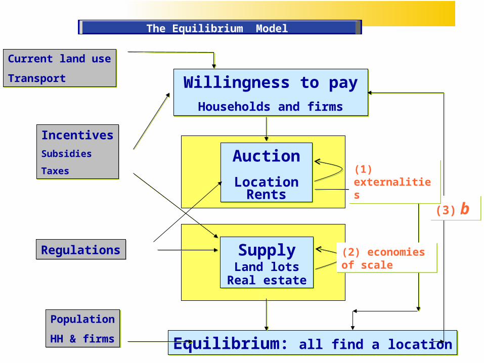
Auction
LocationRents
Auction
LocationRents
Equilibrium: all find a locationEquilibrium: all find a location
SupplyLand lots
Real estate
SupplyLand lots
Real estate
Willingness to pay
Households and firms
Willingness to pay
Households and firms
RegulationsRegulations
Incentives
Subsidies
Taxes
Incentives
Subsidies
Taxes
(3) b(3) b
(1) externalities(1) externalities
Population
HH & firms
Population
HH & firms
Current land use
Transport
Current land use
Transport
The Equilibrium Model
(2) economies of scale(2) economies of scale

Demand and Supply models
Mathematic Formulation

The Bid function
( , , )v hi iD acc att
( , ) ( , )vihvi h h hvi hvi i hvi v i hviB I b F X Z Sub B D Z
Subsidy or Tax:
To consumer type h for locationg at dewlling
type v in zone i
Consumer’s
utility level
Attributes
Dwelling
Accesibility,
Attractivenes.
Zonal (externalities)
Supply specific bid
Mathematic Formulation
hh
h
Ub
Consumer’s
income

Externalities
( , )i i i iZ Z S H h H v V
Location Externalities
Attribute defined by allocation of consumers
and supply in zone i
Endogenous Attributes
Example: h hvih HH v V
ihvi
h HH v V
I HI
H
Average income of residents
Mathematic Formulation
/( , ) ,hvi h i iB B S P h H v V
Bids depend on endogenous variables: land use and built environment

Allocation by auctions
//
/
exp( ( ))
exp( ( ) )
hvi vi hvi
h hvi hvi ih vi
g gvi gvi ig H
H S P
H B PP
H B P
Constraints
Income budget.Location bid:
Deterministic term
),,( SPbPP Auction fixed-pointAdjusts externalities
(1)
Hh: Number of agents in cluster h
Mathematic Formulation
Theoretical obs.Theoretical obs.: !max bidder implies max utility¡
Auction probability

Cut-off factors
K
k
Unki
Lnkini
1
11
11
n i
hi
n ii n
if C Z
if C Zexp Z C
Mathematic Formulation
0
0.2
0.4
0.6
0.8
1
1.2
Serie1
Serie2
nkbnka
kiZ
Lnki
Unki
Composite cut-off
0 1( , )
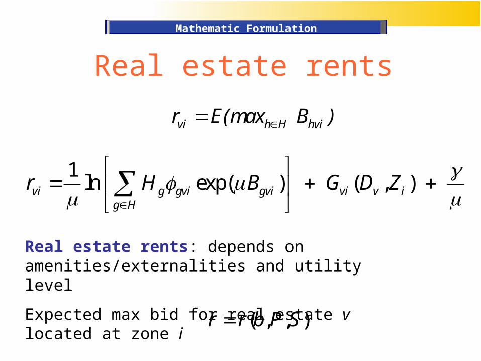
Real estate rents
1ln exp( ) ( , )vi g gvi gvi vi v i
g H
r H B G D Z
Real estate rents: depends on amenities/externalities and utility level
Expected max bid for real estate v located at zone i
vi h H hvir E(max B )
),,( SPbrr
Mathematic Formulation

(2)
Real estate supply
.
' ' ' ' . ' ' ' ' '' '
exp ( ( ) ( ))
exp ( ( ) ( ))vi vi i vi v vi
vi viv i v i i v i v v i
v i
r S s C SS HP H
r S s C S
Supply:
Total Nr of real estate units Regulations
Rents
Subsidies or taxes
SCrmaxargHS tvvivivi ,,
ProductionCost with
scale/scope economies
),,( SPbSS Supply MNL fixed-point
Mathematic Formulation

(3)
Equilibrium Condition: every agents is allocated
vi
hvihvi hHbPS )(/
Supply:
Nr of real estate type v available in zona i
Allocation probability:
Probability that consumidor type h is best bidder on real
estate type v in zone i
Nr agents type h to be allocated
),,( SPbbb Equilibrium logsum fixed-pointAdjusts utility levels
Mathematic Formulation

(1)
(2)
(3)
Resume of equilibrium equations
Allocation w/ externalities...Allocation w/ externalities...
Supply w/ econ. scale...................Supply w/ econ. scale...................
Equilibrium ...............................Equilibrium ...............................
),,,,( SPbSS
),,,,( SPbbb
),,,,( SPbPP
System of fixed point
Mathematic Formulation

Parameters Calibration
Calibration

Santiago supply model
Calibration supply

Data collectionSources of data:
– OD trips household survey 2001– Real estate rents– Household income
– Tax records– Supply by real estate type and zone– Real estate attributes
Calibration Supply

Residential land use (m2)
Data collectionCalibration supply

Total housing floor space (m2)
Data collectionCalibration supply

Total floor space of buildings (m2)
Data collectionCalibration supply

Average residents income
Data collectionCalibration supply
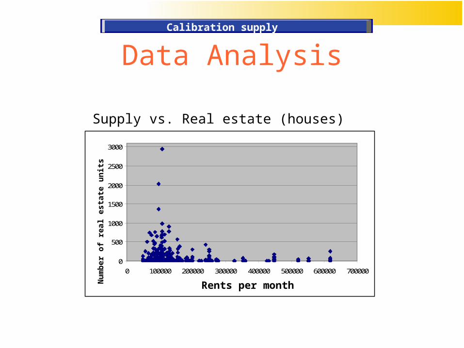
Supply vs. Real estate (houses)
Data Analysis
0
500
1000
1500
2000
2500
3000
0 100000 200000 300000 400000 500000 600000 700000
arriendo
ofe
rta
.
Rents per month
Nu
mb
er
of
rea
l e
sta
te u
nit
s
Calibration supply

Number of real estate (house) units vs. built houses floor space
0
500
1000
1500
2000
2500
3000
0.0 50.0 100.0 150.0 200.0 250.0 300.0 350.0 400.0
superficie construida
ofe
rta
.N
um
be
r o
f re
al
es
tate
un
its
Built floor space
Data AnalysisCalibration supply

0
500
1000
1500
2000
2500
3000
0.0 50.0 100.0 150.0 200.0 250.0
ingreso zonal (UF)
ofe
rta
.N
um
be
r o
f re
al
es
tate
un
its
Number of real estate (house) units vs. average residents’ income
Average income
Data AnalysisCalibration supply

Santiago supply model
cons terrvi v vi v vi v i vi v i v i ir q p q ing _ zon Q
Classic profit: rent minus direct costs (building and land)
Additional explaining variables
iviv
vinnvi HHS
,
00
)exp(
)exp(
Calibration supply

Resultados modelo Casa
Variable Parámetro estimado
Error Estándar Test-T
vir 0.069 0.019 3.739 consviq -0.004 0.002 -2.644
terrvii qp -0.006 0.002 -3.052
izoning _ 0.009 0.003 3.516
iQ -1.700 0.317 -5.365
Resultados modelo Depto
Variable Parámetro estimado
Error Estándar Test-T
vir 0.129 0.027 4.851 consviq -0.003 0.002 -1.470
terrvii qp -0.025 0.004 -6.934
izoning _ -0.006 0.003 -1.860
iQ -0.417 0.498 -0.837
Supply model calibration: by typeEstimatedparameter
Estimatedparameter
Standarderror
Standarderror
Houses
Departments buildings
Rents
Floor space
Land price x floor space
Residents Income
Available zone land
Rents
Floor space
Land price x floor space
Residents Income
Available zone land
Calibration supply

Santiago demand model
Calibration demand

HOUSEHOLDS CLUSTERSHOUSEHOLDS CLUSTERS
5 income levels
3 levels of car ownership
5 Levels of household size
Socioconomic segments:
MUSSA Santiago: 65 household types; 16 million inhabitants
Calibration demand
Typology

FIRMS FIRMS
Industry Retail
Service Education
Other
Segments by:
Commercial type
Business size
MUSSA Santiago: 5 types of firms
Calibration demand
Typology

REAL ESTATE SUPPLYREAL ESTATE SUPPLY
Types by:
700 Zones
12 Real estate building type
Calibration demand
MUSSA Santiago: 8.400 location options
Typology

Accessibility attributes
1. Use balancing factors Anpi: from trip distribution model, by agent n, time
period p and residential zone i:
2. Interpolate missing values: spatially for each agent type
3. Aggregate on periods
4. Normalize between 0-1
1npi npi
np
acc ln( A )
ni npi npp
acc acc * ( t )
ni
nj
njj
accacc'
max acc
Calibration demand

Calibration Methodology: BidsBid functions: linear-in-parameters multi-variate
functional form
k
hviknknhvi xB 0
Parameters per income level n
Examples of variables regarding their sub-index:
Household xh : Household Income
Zone xi : Residents average income, zone sevices
Household-zone xhi : accessibility
Real estate-zone xvi : Built floor space of real estate type v in zone i
Calibration demand

Maximum likelihood estimators of the parameters set
h/vihvih,v ,i
Máx d ln ( ) P
0 1
0hvi
if h is located at ( v,i )d
if not
Calibration demand
Calibration Methodology: Bids
With d obtained from the observed data:

Linear least squared regression
2
00
1vikvi vi k
,v ,i k
MIN r E( B ) x
rvi0 is the observed value of rents
E(B)vi is the expected maximum bid obtained as the logsum of bids
Calibration demand
Calibration Methodology: Rents

Residential Data• Data sources 2001:
– OD survey: residents location, socioeconomics, rents and trips
– Tax records: land use– Transport model ESTRAUS: trip balancing factors
• Variables collected• Household characteristics (size, income, car ownership, age
of household’s main adult)• Real estate attributes (type, land lot size, floor space, height)• Zone attributes (land use, average residents income, land
use densities, accessibility)
Calibration demand

Land use pattern
Average land use density by residents income level
(m2 of land use/zone area)
Income levelIndustry land use density
Retail land use density
Service land use density
Education land use density
1 0,014 0,014 0,009 0,007
2 0,013 0,017 0,015 0,007
3 0,015 0,025 0,023 0,010
4 0,017 0,036 0,039 0,012
5 0,006 0,032 0,040 0,011
Calibration demand
Data Analysis

Floor space pattern
Average floor space by income level and household size (m2)
Income level
Household size
1 2 3
1 62 53 49
2 67 59 53
3 71 65 60
4 89 84 79
5 115 123 150
Calibration demand
Data Analysis

Zone average of residents income
Average zone income compared with the household income in the same zone (Ch$ 2001)
0
500000
1000000
1500000
1 2 3 4 5
Calibration demand
Data Analysis

Accessibility
Average accessibility by income level and car ownership
Income level
Car ownership
0 1 2+
1 10,0 10,5 10,3
2 10,9 11,6 11,2
3 11,3 11,6 11,6
4 10,1 11,8 11,5
5 8,6 11,5 12,0
Calibration demand
Data Analysis

NON-Residential Data• Data sources 2001:
– Tax records: land use– Transport model ESTRAUS: trip balancing
factors
• Variables collected• Firms características (business type)• Real estate (type, land lot size, floor space, height)• Zone attributes (land use, zone average income,
density, attractiveness)
Calibration demand

Attributes by business type
Business category
Average land lot size (m2)
Average floor space (m2)
Attractiveness (tips attracted by
zone)
Average residents’
income by zone (Ch$ 2001)
Education 841 352 4.256 550.790
Industry 380 227 3.746 540.064
Services 191 152 11.118 733.262
Retail 181 121 5.820 572.514
Other 417 166 3.400 608.527
Calibration demand
NON-Residential Data

Parameter estimates
Residential BIDS Model
Income level
Constant ln(zone_income)
Accessib. Dummy apartm
ent
Industrydensity
Education density
ln(floor_space)
Houses
1-2 -9,284(-5,317)
2,642(2,678)
1,287(4,356)
35,366(13,343)
1,198(0,912) *
0,293(0,925) *
_
3 -15,984(-9,769)
0,758(2,420)
3,090(2,541)
12,821(1,454)
36,748(17,071)
2,750(2,056)
2,438(5,951)
4 -21,340(12,588)
3,769(2,323)
0,962(2,590)
-2,152(-5,867)
-6,093(-0,704) *
36,471(17,651)
4,732(3,347)
5 -35,475(-4,593)
36,746(13,727)
13,063(10,221)
-8,547(-6,627)
-1,015(-3,528)
_ 2,888(11,019)
Calibration demand

NON Residential BIDS Models
Business category
Constant ln(floor_space)
ln(land lot size)
ln(attractiveness)
ln(zone income)
Education_ 0,424
(1,549)0,570
(4,400)0,441
(5,348)0,116
(0,544) *
Industry3,321
(1,113)1,028
(3,917)0,170
(1,485)0,403
(1,894)0,422
(3,602)
Services-1,559
(-0,421)0,310
(1,462)_ 0,142
(1,252)_
Retail6,505
(1,769)_ 0,512
(5,087)0,163
(2,031)0,035
(0,379) *
Other3,128
(0,782) *0,500
(3,384)_ 0,044
(0,524) *0,337
(1,353)
Calibration demand
Parameter estimates

Residential RENTS ModelVariable Estimate Test T
Constant 3.847 0.148
Logsum 7.386 2.511
Land lot size (houses) 0.233 8.484
Floor space (houses) 0.274 3.115
Floor space (apartments) 1.117 8.305
Family size (houses) 21.922 4.690
Ln(Family size) (apartments) 44.906 6.230
Income (houses) 0.000 21.990
Income (apartments) 0.000 6.921
Floor Industry/ Nr of households -0.526 -2.799
Floor Education/ Nr of households 0.559 1.645
Calibration demand
Parameter estimates