Developing Robust Project Scheduling Methods for...

Amirkabir University of Technology

(Tehran Polytechnic)

Vol. 47, No. 1, spring 2015, pp. 21- 32

Amirkabir International Journal of Science & Research

(Modeling, Identification, Simulation & Control)

AIJ-MISC))

Corresponding Author, Email: [email protected]٭

Vol. 47 - No. 1 - Spring 2015 21

Developing Robust Project Scheduling Methods for

Uncertain Parameters

I. Bossaghzadeh1*

, S. R. Hejazi2, and Z. Pirmoradi

3

1- MSc of Industrial Engineering, Isfahan University of Technology, Isfahan, Iran

2- Professor of Industrial Engineering, Isfahan University of Technology, Isfahan, Iran

3- PhD of Product Design and Optimization Lab, Simon Fraser University, Surrey, Canada

ABSTRACT

A common problem arising in project management is the fact that the baseline schedule is often disrupted

during the project execution because of uncertain parameters. As a result, project managers are often unable

to meet the deadline time of the milestones. Robust project scheduling is an effective approach in case of

uncertainty. Upon adopting this approach, schedules are protected against possible disruptions that may

occur during project execution. In order to apply robust scheduling principles to real projects, one should

make assumptions close to the actual conditions of the project as much as possible. In this paper, in terms of

uncertainty in both activities duration and resources availability, some methods are proposed to construct the

robust schedules. In addition, various numerical experiments are applied to different problem types with the

aid of simulation. The main purpose of those is to assess the performance of robust scheduling methods

under different conditions. Finally, we formulate recommendations regarding the best method of robust

scheduling based on the results of these experiments.

KEYWORDS

Project Scheduling, Uncertainty Modeling, Robustness, Simulation.



(AIJ-MISC)

I. Bossaghzadeh, S. R. Hejazi, and Z. Pirmoradi

Vol. 47 - No. 1 - Spring 2015 22

1. INTRODUCTION

The vast majority of the research efforts in project

scheduling assume complete information about the

scheduling problem to be solved and a static deterministic

environment within which the pre-computed baseline

schedule will be executed. However, in the real world,

project parameters are subject to considerable uncertainty,

which is gradually resolved during project execution.

Herroelen and Leus [1] reviewed fundamental approaches

for scheduling under uncertainty: stochastic project

scheduling, fuzzy project scheduling, sensitivity analysis,

robust scheduling and reactive scheduling. Most efforts on

stochastic project scheduling concentrate on the so-called

stochastic resource-constrained project scheduling

problem. This problem aims at scheduling project

activities with uncertain durations in order to minimize the

expected project duration subject to zero-lag finish-start

precedence constraints and renewable resource constraints

[1]. The advocates of the fuzzy activity duration approach

argue that probability distributions for the activity

durations are unknown due to the lack of historical data.

As activity durations have to be estimated by human

experts, often in a non-repetitive or even unique setting,

project management is often confronted with judgmental

statements that are vague and imprecise [1]. The approach

sensitivity analysis addresses „„What if...?‟‟ types of

questions that arise from parameter changes. The

approach of robust scheduling is one of the recent

approaches to handle uncertainties of the project

parameters. Using this approach, the baseline schedule can

be constructed so that the parameter variations during a

project‟s execution cause the least possible disruption in

the schedule [1]. A schedule is called robust if variations

do not cause significant changes in the value of the

baseline schedule objective function [2]. Two types of

robust scheduling are of importance: quality robustness

and solution robustness [3]. Under quality robustness, the

baseline schedule can be constructed so that the parameter

variations cause the least delay in the realized completion

time of the project in comparison with the committed

deadline. The most common quality robustness objective

function is the expected project completion time

(makespan). One notable recent development in this field

is Critical Chain approach developed by Goldratt [4]. On

the other hand, solution robustness helps constructing

schedules in which the parameter variations cannot cause

significant delay in realized starting times of the activities

in comparison to the baseline starting times. The solution

robustness objective function measures sum of the

weighted deviations between the baseline schedule and the

expected realized schedule. Note that, this paper

concentrates on the solution robustness issue for project

scheduling. Another approach to handle uncertainties in

projects is reactive scheduling. The main role of this

approach is to correct the schedule after disruption [5]. If

disruption occurs during implementation of the project,

the current schedule might lose feasibility. Under such

condition, the managers should invoke in-time policies to

return the schedule to a feasible mode so that the new

value of the objective function deviates only little from the

baseline schedule.

Most of the recent articles recognize Goldratt`s

CC/BM1 approach as one of the most remarkable recent

improvements in the project management literature [6].

The main purpose of this approach is to construct a robust

schedule under the condition of uncertain activity

durations, and by using the quality robustness. In this

approach, a robust schedule is constructed based on the

chain and buffer concepts. Herroelen and Leus [6] studied

the merits and pitfalls of the CC/BM approach. Al-Fawzan

and Haouari [7] considered both the completion time and

robustness as the objectives of the RCPSP2 and used the

total free float of the activities as a surrogate function of

robustness. Danka [8] presented a primary-secondary-

criteria robust scheduling model for RCPSP with the

makespan as primary and the NPV3 as secondary criterion.

In this paper, financial issues is combined with robustness

concept in project scheduling. In the approach, it is

assumed that each activity duration and each cash flow

value is an uncertain-but-bounded parameter without any

probabilistic or possibilistic interpretation and

characterized by an optimistic and pessimistic estimations.

The evaluation of a given robust schedule is based on the

investigation of variability of the makespan as a primary

and the net present value as secondary criterion on the set

of randomly generated scenarios given by a sampling-on-

sampling-like process. Danka`s model can be classified as

a multi-objective RCPSP so that quality robustness is the

primary criteria. Note that, to formulate the primary

criterion, only activities duration assumed uncertain, while

cash flow as an uncertain parameter doesn`t have any role

in the primary criterion formulation. Once, all but one of

the parameters has been assumed deterministic.

One of the initial important references on project

scheduling with solution robustness is the Herroelen and

Leus‟s paper [9]. Basic assumptions of their research were

unbounded resource availability and “just in case”

scenarios for uncertain durations, which allow only one

1 Critical Chain/ Buffer Management

2 Resource Constrained Project Scheduling Problem

3 Net Present Value



(AIJ-MISC)

Interval Analysis of Controllable Workspace for Cable Robots

Vol. 47 - No. 1 - Spring 2015 23

activity duration to change during the project

implementation. Van de Vonder observed a trade-off

between the quality robustness and solution robustness

[3]. In their model, scheduling was performed without the

resource constraints and with recognition of the duration

uncertainty. Various tests have been conducted, based on

simulation. Van de Vonder also examined the trade-off

between quality and solution robustness, this time with

resource constraints [10]. he has also proposed heuristic

algorithms for constructing robust schedules under

duration uncertainty and with a solution robustness

objective [11]. Lambrechts‟s paper is the first source in

which resource availability rather than activity durations

contains the uncertainty; the author assumes that resources

can exhibit unexpected failures [12]. Their purpose was

the development of robust scheduling procedures with

solution robustness. Another paper from Lambrechts et al.

is also about consideration of the impact of unexpected

resource breakdowns on activity durations [13]. They

developed an approach for inserting explicit idle time into

the project schedule in order to protect it as well as

possible from disruptions caused by resource

unavailability. This strategy was compared to a traditional

simulation-based procedure and a heuristic developed for

the case of stochastic activity durations.

In practice, almost all of the project parameters have

an uncertain nature. In order to apply robust scheduling

principles to real projects, one should make assumptions

close to the actual conditions of the project as much as

possible. This paper aims to develop methods for the

solution robustness, which provide the most accordance

between the constructed schedules and the actual

condition of the project. Therefore, assuming uncertainty

in two project parameters in our research, the STC4

method is developed to construct robust schedules. The

structure of this paper is as follows: section 2 sets out the

proposed problem formulation. In section 3, we explore

developing the STC method. For assessing the

performance of the methods, several numerical tests are

performed by simulation. The applied tests and their

results are explained in section 4. Section 5 contains the

conclusion and finally, we suggest some issues for further

research in section 6.

2. PROBLEM STATEMENT

Two parameters are assumed uncertain in constructing

a robust schedule with solution robustness: the activity

duration and the resource availability. These parameters

4 Starting Time Criticality

are assumed to take probabilistic values and their

probability distribution functions are known. This problem

can be formulated as:

( ( ) )1N

Min Z w E S sj j j j (1)

RjijSiDiS ),(

(2)

1, 2, ..., , 1, 2, ...,

r Ai WIP ik ktt

t k K

(3)

NjjSjs ,...,2,1

(4)

sN

(5)

Relation (1) shows the objective function for a project

with N activities. Note that activities 1 and N are dummy

activities with a duration and a resource usage of 0.

Activity 1 indicates the start of the project whereas

activity N signals the end. Variables sj and Sj denote the

baseline starting time and the realized starting time of

activity j, respectively. Every activity j has a weight wj

that denotes the marginal cost of deviating Sj during

execution from sj. Uncertain parameters Dj and Akt are

stochastic variables that denote the realized duration of

activity j and the available units of renewable resource k at

time t, respectively. Relation (2) imposes the precedence

constraint to the model. In this relation, set R includes

couple activities (i,j) in which, activity i is predecessor for

activity j. Relation (3) is also necessary to assure

feasibility of the scheduling due to the renewable resource

constrainedness. In this relation, rik denotes the used units

of renewable resource k by activity i. In addition, WIPt is

the set of activities that are being implemented at time t.

One of the important aspects of solution robustness is the

so-called railway mentality according to which, no

activity is allowed to start earlier than its baseline starting

time [2]. The related constraint is shown in relation (4).

Relation (5) is also needed due to the presence of the

deadline. This constraint precludes the baseline

completion time to exceed . Our problem is classified as

))((|,~

,|~,1, sSEwdcpmavm [14]. The first field specifies

the resource characteristics: ( avm ~,1, ) refers to an arbitrary

number of renewable resource types, each with a

stochastic availability that varies over time. The second

field refers to the activities characteristics; cpm shows the

precedence constraints of a finish to start type with zero

time lags. Symbol d~

refers to the stochastic duration of

the activities. In addition, symbol δ represents existence of



(AIJ-MISC)


Vol. 47 - No. 1 - Spring 2015 24

the project deadline. At last, third field shows the

objective function.

Note that the parameter s is the only decision variable

of this model, while parameter S is a dependent variable.

The probability distribution function of S is not known

and it might be difficult or impossible to calculate,

because its value is dependent on 3 factors. It is firstly

dependent on the baseline schedule, because in ideal

condition each of the activities must start on its baseline

time. The second effective factor on S is the parameter`s

uncertainties; the reason is that the baseline starting times

may be affected by parameter`s variations. The last one is

a reactive scheduling procedure; when disruption occurs,

the corrective actions should be taken through reactive

scheduling procedures in order to retain the schedule

feasibility. Since RCPSP is NP-hard, the proposed

problem also has at least the same complexity, because the

RCPSP is a special case of our problem. As discussed

before, the baseline schedule is the first influential factor

on the realized starting time of the activities. On the other

hand, the realized starting times information is required

for solving the model. Due to this mutual relation and

because of the other dependences of variable S, no direct

solution is available for the model. That is why, in this

paper, a heuristic method is developed to construct a

baseline schedule.

3. DEVELOPING THE STC METHOD

STC method is known as one of the most effective

methods to allocate time buffers to the activities [11]. The

basic idea is to start from an initial unbuffered schedule

and iteratively create intermediate schedules by adding a

one-unit time buffer in front of that activity that needs it

the most in the current intermediate schedule, until adding

more safety would no longer improve stability. The

starting time criticality of an activity j is defined as:

jwjjwjsjSP

jstc

)(

(6)

where γj denotes the probability that activity j cannot be

started at its baseline starting time.

The iterative procedure runs as follows. At each

iteration step the buffer sizes of the current intermediate

schedule are updated. The activities are listed in

decreasing order of the stcj. The list is scanned and the

size of the buffer to be placed in front of the currently

selected activity from the list is augmented by one time

period such that the starting times of the activity itself and

of the direct and transitive successors of the activity are

increased by one time unit. If this new schedule has a

feasible project completion (sN ) and results in a lower

estimated cost ( jstc ), the schedule serves as the input

schedule for the next iteration step. If not, the next activity

in the list is considered. Whenever no feasible

improvement is found, a local optimum is obtained and

the method terminates. Regrettably, the probabilities γj are

not easy to compute. This value can be estimated only for

the case of uncertain durations [11]. In this method, lack

of attention to the uncertainty of other parameters is a

considerable weakness. Therefore, we try to find proper

estimations of γj assuming uncertainty in both activity

duration and resource availability.

A. Simulation

The analytic evaluation of the objective function is

very cumbersome, so that one usually relies on simulation

[12]. In this paper, we try to run the simulations close to

the condition of real projects. Note that in all of the

simulations, the railway mentality has been followed. The

first precondition of simulation is to determine the

probability distribution function of uncertain parameters.

It is assumed that activity`s durations follow the Beta

distribution. This parameter is assumed to follow the Beta

distribution in most of the related researches [11]. The

main reason for using this distribution is its compatibility

with real conditions of activities duration in which, Lower

bound, upper bound and average of the beta distribution

are equivalent to optimistic, pessimistic and most likely

duration of the activity, respectively. Since the failure rate

and the repair rate of the resources are the effective factors

on variation of the resources availability, MTTR5 and

MTBF6 are used for determining the distribution function

of resource availability. MTTR and MTBF are supposed

to follow exponential distributions for resources. The use

of the exponential distribution is supported by empirical

evidence as well as by mathematical arguments [12].

Using these properties and the queuing theory concepts,

determination of the distribution function for the resource

availability will be possible.

Since after occurrence of disruption, a corrective

scheduling procedure should be selected for simulating the

schedule, another precondition of simulation is to

determine a reactive scheduling procedure. The reactive

scheduling procedures used in this paper are based on the

activities priority list. This list shows the scheduling

priorities for project activities. The priorities are obtained

based on EBST7 rule (greatest lateness weight as

tiebreaker). This procedure is called EBST1 reactive

5 Mean Time To Repair

6 Mean Time Between Failures

7 Earliest Baseline Starting Time



(AIJ-MISC)


Vol. 47 - No. 1 - Spring 2015 25

scheduling. In EBST1, after occurrence of disruption, the

incomplete activities are ordered non-decreasingly based

on their starting time in the baseline schedule. Note that

the activities are scheduled based on SGS8 method and

according to the railway mentality. In SGS method, the

next unscheduled activity in the priority list is selected and

assigned the first possible starting time that satisfies the

precedence and resource constraints. In this method,

average value of the uncertain parameters can be used.

According to the LW rule, if there are activities with the

same baseline starting time, the activity with the greatest

lateness weight gets the highest priority. Note that the

sequence in the priority list should match the predecessor

relations of the activities. It is shown that EBST1

produces good results [5]. Moreover, for each schedule,

simulation is also done by a random reactive scheduling

procedure. In this procedure, after occurrence of

disruption, incomplete activities are scheduled randomly

under the constraint of feasibilities. This procedure can be

a proper benchmark for the EBST1 method.

Determination of the succession to implement the

activities after preemption is another precondition for the

simulation. Generally, the way an activity would be

implemented after preemption is one of the following

cases: preempt-resume, preempt-repeat, and preempt-

setup [6]. Preempt-resume implies that whenever an

activity is interrupted and preempted, it can be continued

from the point where execution was halted whenever the

reason for the interruption is removed. Preempt-repeat

implies that all the time and effort was invested in the

execution of that activity until the time of the interruption

is lost. This scenario is encountered in practice whenever

an activity must be executed without interruption. Of

course, both cases are often a simplification of reality. It

can be imagined that in practice a mixed form is more

likely. Usually, activities will not have to be restarted all

the way from zero after they were preempted but it will

probably also not be possible to carry on as if nothing

happened. The third possibility is therefore that whenever

an activity is preempted, a setup time has to be taken into

account when restarting this activity. Therefore, it has

called this variant preempt-setup. In this paper, the

implementing of the activities after preemption is assumed

to be the preempt-resume or preempt-repeat, and the

robust scheduling methods are discussed separately for

these types.

B. Methods

In this paper, a two-stage procedure is applied for

constructing the robust schedules. In the first stage, an

8 Schedule Generation Scheme

initial semi-active schedule is generated using the SGS

method. A semi-active schedule is a feasible schedule

where none of the activities can be locally left shifted

[15]. In such schedules, no idle-insert is allowed. In the

second stage, time buffers are allocated to the initial

schedule. The purpose of this stage is to protect the

baseline starting time of the activities against possible

parameters variations during the implementation of the

project. This two-stage procedure is illustrated in Fig. 1.

Fig. 1. Fig. 1. Two stages procedure of constructing robust

schedules

i. Initial scheduling

To construct the initial schedules, the only step is to

generate the activities priority list. The methods applied

for creating the priority list are explained below:

Solving the RCPSP

Allocation of time buffers to activities can increase

project completion time. Due to presence of the project

deadline constraint, time buffers can be added to the

schedule only if the project completion time does not

exceed the deadline. Therefore, if the project completion

time is shorter in a schedule, it is more possible to allocate

time buffers to that schedule. Since the objective of the

deterministic RCPSP is to minimize the project

completion time, the schedules constructed by solving the

RCPSP can be the proper initial schedules. In this model,

all of the parameters are assumed to have deterministic

nature and the average value of the uncertain parameters

can be used for them. In the schedules obtained by solving

the RCPSP, the activities will be placed in the priority list

based on non-decreasing order of their starting time.

Various algorithms can be used for solving the RCPSP. It

is shown that HGA9 is one of the most effective

algorithms for solving the RCPSP. For medium and large-

scale problems, this algorithm provides better results than

any other algorithms and for small problems, it compares

favorably to the best current algorithms [16]. That is why;

this meta-heuristic algorithm is used for solving the

RCPSP in the paper.

Using CIW10

Index

9 Hybrid Genetic Algorithm 10 Cumulative Instability Weight



(AIJ-MISC)


Vol. 47 - No. 1 - Spring 2015 26

In this method, a precedence feasible priority list is

constructed with the activities in non-increasing order of

their CIW

index (tie-breaker is the lowest activity

number). This index is defined in equation (7), where Suci

denotes the set of direct and indirect successors of activity

i [12]. In other words, for an activity, this index is defined

as sum of the lateness weights for that activity and all of

its successor activities. Because disruptions propagate

throughout the schedule, activities for which a change in

starting time would have a high impact on the objective

function value are now less likely to be severely disrupted

than activities with a lower impact since the former are

scheduled earlier in time and are thus less prone to

disruptions.

:CIW w w

j j Suci i ji

(7)

Solving a MADM11

Problem

Actually, this method is an extension of the CIW index

method for generating the priority list. In the CIW index,

only the cost of starting delay is considered and lack of

attention to uncertainty of the parameters is a considerable

weakness of this method. This weakness is handled and

removed in the index obtained by MADM. In this method,

three different attributes are used to generate the priority

list. Note that in most of the decision making problems, no

ideal alternative may be obtained with highest rank for all

of the defined attributes [17]. Here, by MADM

techniques, a final value is calculated for each activity and

then the activities are sorted based on the descending

values of this index. In order to solve this problem, a

decision matrix is generated for which, the project

activities are the problem alternatives. This decision

matrix is shown in Table 1.

TABLE 1. THE DECISION MATRIX FOR SOLVING THE

MADM PROBLEM

The ADU and RLU denote the activity duration

uncertainty and resource availability level uncertainty.

Moreover, the CIW is the disruption cost for each activity

that is calculated using the equation (7). The values of this

matrix also represent the attributes values for each activity

of the project. The activities with more uncertainty in

duration should be scheduled as late as possible in order to

11 Multi Attributes Decision Making

cause less disruption in the successor activities. Therefore,

variance of the activities duration is used as the ADU

value for the activities. Note that, higher ADU value

means lower priority for an activity. On the other hand,

resource failure can result in preemption. In order to

prevent delay in starting times of other activities, the

activities with a higher probability of facing resource

failure should be scheduled as late as possible. When the

resource consumption percentage is less than 100%, if one

unit of the resource fails, one available unit of that

resource type can replace the failed resource and therefore

preemption will not happen for that activity. Since the

priority list is being generated in this stage, no information

is available about the resources consumption percentage

per time unit. Therefore, it is not possible to exactly

determine the probability of preemption for activities. It is

obvious that if no failure occurs for the resources of an

activity, preemption will not happen for that activity.

According to this, the activity with less probability of

resource failure will have more chance for getting higher

place in the schedule. So, the probability of failure-free for

all related resources of an activity is used as RLU value

for that activity. Note that, higher RLU value means

higher priority for an activity.

Equation (8) shows the probability of failure-free for

all related resources of an activity with average duration d.

In this equation, Eikt denotes the event of failure-free for ith

unit of the resource type k in time t for the related activity.

Also the terms k and rk denote the number of resource

types and the consumption units of resource k for the

activity, respectively. Note that the distributions of

different resource types and also different units of a

particular resource are independent. This assumption is in

accordance with the conditions of real projects.

( )1 11

rdkK

RLU P Ei tk ikt

(8)

Now, the probability of failure-free for the unit ith

of the resource type k during the activity implementation can be calculated as equation (9) shows:

( )1

( ) ( | ) ( | , )1 2 1 3 1 2

... ( | , , ..., )1 2 1

dP E

t ikt

P E P E E P E E Eik ik ik ik ik ik

P E E E Eikd ik ik ikd

(9)

since time between two consequent failures follows the

exponential distribution, the equation (9) can be simplified

by using properties of the markovian processes. It means

that if the system state is known at time t-1, then the state

of that system at time t is independent of its state at times



(AIJ-MISC)


Vol. 47 - No. 1 - Spring 2015 27

before t-1. Using this property, the equation (9) will be

simplified into equation (10):

( )1

( ) ( | ) ( | )1 2 1 3 2

.... ( | )1

dP E

t ikt

P E P E E P E Eik ik ik ik ik

P E Eikd ikd

(10)

Now, the probability of failure-free for unit ith of the

resource type k in the first time unit is calculated as the

first term of the equation (10). This probability value can

be calculated using the birth-death processes. Assume that

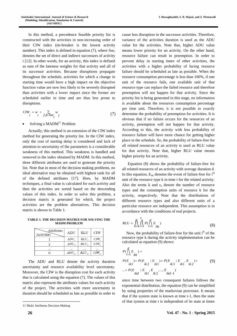
the diagram of Fig. 2 shows the availability rate of one

unit of resource; where, 0 and 1 denote being failure-free

and failure, respectively.

Fig. 2. Fig. 2. The availability rate to one unit of resource

In this figure, parameters λ and μ denote the failure

rate and the repair rate for the related resource. The failure

rates are assumed to be similar for all units of a resource

type, and so are the repair rates. Therefore, equation (11)

shows the probability of failure-free for each unit of

resource k in the first time unit of implementing the

related activity. This value is obtained by solving the

balance equations of the related birth-death process.

( )1

kP E

ikk k

(11)

Memory-less property of exponential distribution is

used for calculating the remaining terms of equation (10).

Equation (12) shows how these terms can be calculated.

This equation holds for all values of i.

keXPtXtXP

iktE

iktEP

)1()|1(

)1

|(

(12)

In this equation, X is an exponential random variable

with parameter λk which shows the remaining time before

failure of the related resource. Therefore, the equation (10)

can be shown in form of equation (13). Now, the RLU can

be simply calculated for all of the activities.

( 1)

( )1

dd kkP E e

t iktk k

(13)

After establishment of the decision matrix, TOPSIS

method is applied for prioritizing the activities, as one of

the current methods for solving the MADM problem. In

this method, higher priority is given to activity that is

closest to the ideal alternative and has the largest

difference with the negative ideal alternative [17]. It

should be noted that similar weights are assigned to all of

the three attributes. Fuzzy normalizing method is used for

normalizing the attributes. This method is adaptable to the

conditions of our problem.

ii. Time buffers allocation

By allocating time buffers, the initial schedule leaves

its semi-active property. Therefore, for describing such

schedules, it is necessary to use a buffer list in addition to

the priority list. Elements of the buffer list represent idle

inserts assigned to each activity. The buffer list is the main

output of time buffers allocation methods. It worth noting

that allocating time buffer to an activity provides float for

its predecessors. Three methods are proposed to allocate

time buffers: STC, SB-STC12

and SBM13

.

STC

STC method is shown to be one of the most effective

methods for allocating time buffers to the activities when

durations are uncertain [11]. The STC exploits

information about both the lateness weights and the

variance of the durations. The basic idea is to start from an

initial unbuffered schedule and iteratively create

intermediate schedules by adding a one-unit time buffer in

front of the activity that needs it the most in the current

intermediate schedule. The process is stopped when

allocation of time buffers cannot improve the objective

function value anymore. The starting time criticality of

each activity is defined as equation (14) where, γj denotes

the probability that activity j cannot be started at its

baseline starting time. Due to computational complexity,

no method is suggested for computing this probability

value. This value can be estimated according to equation

(14) as:

( )stc P S s w wj j j j j j

(14)

SB-STC

Due to the lack of a method to estimate the value of γ

under uncertainty of the resource availability, the SB-STC

method is used here to estimate these values. The main

difference of the SB-STC with the STC is the way of

calculating γ. In the SB-STC method, it is tried to find a

12

Simulation Based STC 13

Simulation Based Method



(AIJ-MISC)


Vol. 47 - No. 1 - Spring 2015 28

proper estimation of γ for the activities by simulating the

schedules in each step.

SBM

In this method, one unit of time buffer is temporarily

added to a project activity. Then, the schedule is updated.

By simulating the new schedule, the value of the objective

function is calculated and this process will be repeated for

all of the activities. At last, the activity will be selected

that adding time buffers to it, makes the largest

improvement in the objective function. Then, one unit of

time buffer will be permanently added to the selected

activity. On the same basis, the time buffers are also

allocated in next steps and this process will be continued

by the time that no more improvement can be obtained in

the objective function value.

4. COMPUTATION RESULTS

A. Experimental Setup

The algorithms for all of the above mentioned methods

have been coded by C++. Then, the problems are solved

by a Pentium IV PC with 3.2 GHz CPU. The problems

used for this study, were randomly selected, using

RANGEN II which is one of the most powerful softwares

in generating project scheduling problems [18]. In this

software, it is possible to assign values to several

parameters of the project. Some of these parameters are

related to the resources and the others are related to the

project network structure. The main parameters of this

software are the number of project activities, complexity

of predecessor relations, resource factor, and resource

constraint. Greater values for complexity of predecessor

relations show the existence of more relations among the

activities and therefore less possibility of simultaneous

implementation of the project activities. In addition,

greater values of the resource factor, indicates existence of

more resource types for the activities. On the other hand,

greater value of the resource constraint parameter shows

that the average consumption of each resource type is

higher for each of the activities.

In this paper, different values are assigned to each

parameter for performing the computational tests. The

assigned values are shown in Table 2.

The purpose of this procedure is to generate diverse

problems and project types with diverse structures. Since

three different values are supposed for each parameter, 81

problem types are produced by a combination of these

parameters. In this paper, 10 problems are randomly

produced for each of the problem types and therefore 810

problems have been considered and tested in whole. These

problems have been produced by 4 renewable resource

types and by 10 available units per time unit

TABLE 2. THE PROJECT PARAMETERS VALUES IN RANGEN II

High Medium Low Value

Parameter

120 60 30 No of activity

0.8 0.5 0.2 Complexity of

predecessor relations

1 0.75 0.5 resource factor

0.7 0.5 0.3 resource constraint

Using the discussed methods, three different priority

lists are generated for each of these problems. Another

priority list is also randomly generated. The main purpose

of using a random list is to examine if applying systematic

methods for generating a priority list will provide better

results than a random list. On the other hand, time buffers

are allocated to each initial schedule based on the three

methods introduced above. Since robustness of the

schedules generated by STC method is expected to be

poor, this method also can serve as a proper benchmark

for other methods of allocating time buffers.

After allocating time buffers, with the aid of

simulation, the objective function value for the solution

robustness is calculated for each schedule. Note that every

solution is simulated in two cases: preempt-repeat and

preempt-resume. As discussed before, the EBST1 and

random reactive scheduling procedures are used in this

paper for simulations. Since each problem is solved by 4

methods to generate the priority list and 3 methods to

allocate the time buffers, for each problem 12 different

solutions will be obtained. Then, 4 simulation types are

applied to each of the solutions. This process is illustrated

in Fig. 3.

Fig. 3. Fig. 3. The problem solving and simulation process

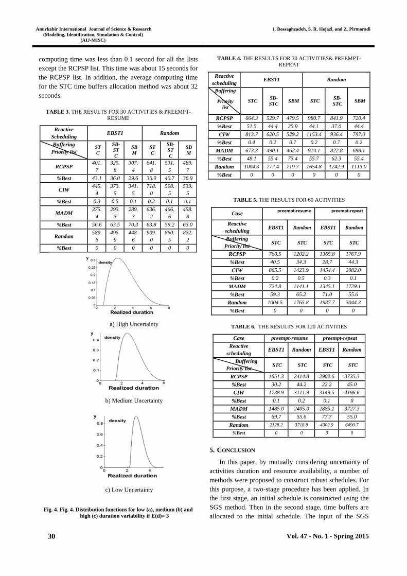
For each schedule, the simulation is run 100 times. In

these tests, the realized duration of activities follows a

discrete right-skewed beta-distribution with parameters 2

and 5. In addition, 3 levels of high, medium and low



(AIJ-MISC)


Vol. 47 - No. 1 - Spring 2015 29

uncertainty are considered. The activities duration

randomly match one of these levels. According to this, in

high level of uncertainty, for an activity with average

duration d, the lower bound and the upper bound of the

Beta distribution are 0.25d and 2.875d, respectively.

These bounds are 0.5d and 2.25d in medium level of

uncertainty and 0.75d and 1.625d in low level of

uncertainty, respectively [11]. Fig. 4 shows the

distribution functions from which the realized durations

are drawn for an activity with expected 3-period duration.

In these tests, for each resource, MTBF parameter

takes a random integer value from the range [0.5Cmax,

1.5Cmax] in which, Cmax is the minimum project duration.

This value is obtained through solving the deterministic

RCPSP for each problem. It is noted that this model is

solved by the HGA algorithm. Moreover, for each

resource, the MTTR parameter takes a random integer

value between 1 and 5 [12]. It should also be noted that

the deadline δ for each of the problems is equal to

[1.3Cmax] [10]. The lateness weights are drawn for each

non-dummy activity j from a discrete triangular

distribution with equation (15):

( ) (21 2 )% {1, 2, ...,10}P w q q qj (15)

This distribution results in a higher probability for low

weights and in an average weight wavg =3.85. The weight

wn of the dummy end activity denotes the marginal cost of

not making the baseline project completion and will be

fixed at [10wavg]=38 [11].

B. Analysis

In tables blow, the average value for the objective

function of the solution robustness is shown for different

types of problems. For each time buffer allocation

method, a value is calculated which is called “best

percentage” here. This value is the proportion of

simulations in which a priority list has provided better

results than other lists.

In the Table 3, the simulation results of problems with

30 activities in the preempt-resume case are shown for the

two reactive scheduling procedures.

Comparing the according values of the two types of

reactive scheduling given above shows that using a

systematic procedure for removing the schedule

disruptions (the reactive scheduling procedure), will result

in less disruption in the next times of the project. As can

be seen, the poorest values among time buffers allocation

methods is resulted from the STC method that can be due

to uncertainty of the resource availability parameter. Since

the random priority list has provided very poor results, it

can be concluded that for constructing robust schedules,

systematic methods generate better priority lists.

According to Table 3, most of the best values are obtained

by MADM and SBM methods. In some of the problems,

the best value is obtained by the MADM list and in some

others by the RCPSP list. Generally, the MADM list has

performed better than the RCPSP one. On the other hand,

the CIW list in most of the cases has provided poor results

compared to the MADM and RCPSP lists. It is remarkable

that in most of the problems for which the complexity of

predecessor relations was 0.8, the RCPSP list performed

better than the MADM list. Therefore, it can be concluded

that the effectiveness of the RCPSP list is higher for

problems with more complexity in predecessor relations,

and for other problems MADM list will provide better

results. In Table 4, the simulation results for problems of

30 activities in preempt-repeat case are shown for the two

reactive scheduling procedures.

For problems of 30 activities, the provided results in

the preempt-repeat case are almost the same as those of

the preempt-resume case. Of course, the corresponding

values in the preempt-repeat case are fairly higher than the

preempt-resume case. The reason may lie in the

probability of more disruption in the preempt-repeat case.

For problems of 30 activities, except the RCPSP list, the

average computing time (in two preemption cases) was

less than 0.1 second for generating the priority lists, while,

this time was about 1 second for the RCPSP list.

Moreover, the average computing time for STC, SB-STC,

and SBM time buffers allocation methods were about 2,

24, and 195 seconds, respectively. In Table 5, the results

for problems with 60 activities are presented in Table 5.

The values provided by the SB-STC and the SBM

time buffers allocation methods are not shown here. This

is due to the high computing time of these methods

resulted from large number of the project activities and

enormous simulations. In problems of 60 activities, the

average computing time was less than 0.1 second for

generating all the lists except the RCPSP one and about 3

seconds for the RCPSP list. The average computing time

for the STC was about 5 seconds. It is notable that for

problems of 60 activities, other methods of allocating time

buffers did not provide any result even after 1 hour of

processing. The results for problems of 120 activities are

presented in Table 6.

The provided results for the problems of 60 and 120

activities are almost similar to those of 30 activities. It is

obvious that if the project activities increase, the value of

the objective function for the solution robustness will

increase. In the 120 activities problems, again the average



(AIJ-MISC)


Vol. 47 - No. 1 - Spring 2015 30

computing time was less than 0.1 second for all the lists

except the RCPSP list. This time was about 15 seconds for

the RCPSP list. In addition, the average computing time

for the STC time buffers allocation method was about 32

seconds.

TABLE 3. THE RESULTS FOR 30 ACTIVITIES & PREEMPT-

RESUME

Random EBST1 Reactive

Scheduling

SB

M

SB-

ST

C

ST

C

SB

M

SB-

ST

C

ST

C

Buffering

Priority list

489.

7

531.

5

641.

8

307.

4

325.

8

401.

7 RCPSP

36.9 40.7 36.0 29.6 36.0 43.1 %Best

539.

5

598.

5

718.

0

341.

5

373.

5

445.

4 CIW

0.1 0.1 0.2 0.1 0.5 0.3 %Best

458.

8

466.

6

636.

2

289.

3

293.

3

375.

4 MADM

63.0 59.2 63.8 70.3 63.5 56.6 %Best

832.

2

860.

5

909.

0

448.

6

495.

9

589.

6 Random

0 0 0 0 0 0 %Best

Fig. 4. Fig. 4. Distribution functions for low (a), medium (b) and

high (c) duration variability if E(d)= 3

TABLE 4. THE RESULTS FOR 30 ACTIVITIES& PREEMPT-

REPEAT

Random EBST1 Reactive

scheduling

SBM SB-

STC STC SBM

SB-

STC STC

Buffering

Priority

list

720.4 841.9 980.7 479.5 529.7 664.3 RCPSP

44.4 37.0 44.1 25.9 44.4 51.5 %Best

797.0 936.4 1153.4 529.2 620.5 813.7 CIW

0.2 0.7 0.2 0.7 0.2 0.4 %Best

698.1 822.8 914.1 462.4 490.1 673.3 MADM

55.4 62.3 55.7 73.4 55.4 48.1 %Best

1113.0 1242.9 1654.8 719.7 777.4 1004.3 Random

0 0 0 0 0 0 %Best

TABLE 5. THE RESULTS FOR 60 ACTIVITIES

preempt-repeat preempt-resume Case

Random EBST1 Random EBST1 Reactive

scheduling

STC STC STC STC Buffering

Priority list

1767.9 1365.8 1202.2 760.5 RCPSP

44.3 28.7 34.3 40.5 %Best

2082.0 1454.4 1423.9 865.5 CIW

0.1 0.3 0.5 0.2 %Best

1729.1 1345.1 1141.1 724.8 MADM

55.6 71.0 65.2 59.3 %Best

3044.3 1987.7 1765.8 1004.5 Random

0 0 0 0 %Best

TABLE 6. THE RESULTS FOR 120 ACTIVITIES

preempt-repeat preempt-resume Case

Random EBST1 Random EBST1 Reactive

scheduling

STC STC STC STC Buffering

Priority list

3735.3 2902.6 2414.8 1651.3 RCPSP

45.0 22.2 44.2 30.2 %Best

4196.6 3149.5 3111.9 1738.9 CIW

0 0.1 0.2 0.1 %Best

3727.3 2885.1 2405.0 1485.0 MADM

55.0 77.7 55.6 69.7 %Best

6490.7 4302.9 3718.8 2128.2 Random

0 0 0 0 %Best

5. CONCLUSION

In this paper, by mutually considering uncertainty of

activities duration and resource availability, a number of

methods were proposed to construct robust schedules. For

this purpose, a two-stage procedure has been applied. In

the first stage, an initial schedule is constructed using the

SGS method. Then in the second stage, time buffers are

allocated to the initial schedule. The input of the SGS

a) High Uncertainty

b) Medium Uncertainty

c) Low Uncertainty



(AIJ-MISC)


Vol. 47 - No. 1 - Spring 2015 31

method is a priority list in which scheduling consequences

are determined for the activities. In this paper, some

methods are proposed for generating the priority list;

solving the RCPSP, CIW index, and solving a MADM

model. On the other hand, for allocating time buffers to

initial schedules, STC, SB-STC and SBM methods have

been applied. The set of problems tested in this study have

been generated by RANGEN II and various computational

tests have been performed on each of the generated

problems. The purpose of these tests was to assess

performance of different methods which are used to

generate priority lists, and different methods of allocating

time buffers. The tests have been performed with the aid

of simulation in two preemption cases: preempt-resume

and preempt-repeat. According to the obtained results, it

was observed that for each of the time buffers allocation

methods, the MADM list and then the RCPSP list have

better performance. In addition, for each of the priority

lists generating methods, the SBM method is superior to

other existing methods of time buffers allocation. Of

course, this method is applicable to only small problems

due to its long computing time.

6. SUGGESTIONS FOR FURTHER RESEARCH

Because of the time buffers allocating methods based

on the simulation takes too much processing time,

developing other efficient heuristic methods to allocate

time buffers with short computational time can be an

interesting issue for future study.

Furthermore, there is not any procedure to find an

optimum solution for the model with solution robustness

objective function as a NP-hard problem. Hence,

developing and considering surrogate functions for the

model is another interesting issue as a future research.

Note that, surrogate-based optimization is a methodology

to find the local or global optimal solution for a problem,

indirectly and quickly.

7. ACKNOWLEDGEMENTS

The authors would like to thank Professor Roel Leus

for his valuable suggestions that have led to several

improvements.

REFERENCES

[1] W. Herroelen, R. Leus, “Project scheduling under

uncertainty: Survey and research potentials: On the

merits and pitfalls of critical chain scheduling,”

European Journal of Operational Research, vol.

165, pp. 289-306, 2005.

[2] R. Leus, “The generation of stable project plans,”

Ph.D. dissertation, Department of applied

economics, Katholieke Universiteit Leuven,

Belgium, 2003.

[3] S. Van de Vonder, E. Demeulemeester, W.

Herroelen, R. Leus, “The use of buffers in project

management: The trade-off between stability and

Makespan,” International Journal of Production

Economics, vol. 97, pp. 227-240, 2005.

[4] E. M. Goldratt, “Critical chain,” The North River

Press Publishing Corporation, Great Barrington,

1997.

[5] S. Van de Vonder, F. Ballestin, E.

Demeulemeester, W. Herroelen, “Heuristic

procedures for reactive project scheduling,”

Computers & Industrial Engineering, vol. 52, pp.

11–28, 2007.

[6] W. Herroelen, R. Leus, “On the merits and pitfalls

of critical chain scheduling,” Journal of Operations

Management, vol. 19, pp. 559-577, 2001.

[7] M. A. Al-Fawzan, M. Haouari, “A bi-objective

model for robust resource constrained project

scheduling,” International Journal of Production

Economics, vol. 96, pp. 175-187, 2005.

[8] S. Danka, “Robust resource constrained project

scheduling with uncertain-but-bounded activity

duration and cash flows,” International Journal of

Optimization in Civil Engineering, vol. 3, no. 4,

pp. 527-542, 2013.

[9] W. Herroelen, R. Leus, “The construction of stable

baseline schedules,” European Journal of

Operational Research, vol. 156, pp. 550– 565,

2004.


Herroelen, R. Leus, “The trade-off between

stability and makespan in resource constrained

project scheduling,” International Journal of

Production Research, vol. 44, no. 2, pp. 215-236,

2006.


Herroelen, “Proactive heuristic procedures for

robust project scheduling: An experimental

analysis,” European Journal of Operational

Research, vol. 189, no. 3, pp. 723-733, 2008.

[12] O. Lambrechts, E. Demeulemeester, W. Herroelen,

“Proactive and reactive strategies for resource

constrained project scheduling with uncertain

resource availabilities,” Journal of scheduling, vol.

11, no. 2, pp. 121-136, 2008.

[13] O. Lambrechts, E. Demeulemeester, W. Herroelen,

“Time slack-based techniques for robust project

scheduling subject to resource uncertainty,” Annals

of Operations Research, vol. 186, no. 1, pp. 443-

464, 2010.



(AIJ-MISC)


Vol. 47 - No. 1 - Spring 2015 32

[14] W. Herroelen, B. De Reyck, E. Demeulemeester,

“A note on the paper „Resource-constrained project

scheduling: notation, classification, models and

methods‟ by Brucker et al,” European Journal of

Operational Research, vol. 128, pp. 679–688,

2001.

[15] A. Sprecher, R. Kolisch, A. Drexl, “Semi-active,

active, and non-delay schedules for the resource-

constrained project scheduling problem,” European

Journal of Operational Research, vol. 80, pp. 94–

102, 1995.

[16] V. Valls, F. Ballestin, S. Quintanilla, “A hybrid

genetic algorithm for the resource-constrained

project scheduling problem,” European Journal of

Operational Research, vol. 185, pp. 495–508,

2008.

[17] J. L. Ringuest, Multi objective optimization:

Behavioral and Computational Considerations,

Kluwer Academic publishers, 1992.

[18] M. Vanhoucke, J. Coelho, D. Debels, B.

Maenhout, L. V. Tavares, “An evaluation of the

adequacy of project network generators with

systematically sampled networks,” European

Journal of Operational Research, vol. 187, pp. 511-

524, 2008.

Developing Robust Project Scheduling Methods for...

Documents

Transcript of Developing Robust Project Scheduling Methods for...